Advanced Aerodynamic Analysis of the NASA High-Lift Trap

Advanced Aerodynamic Analysis of the NASA

High-Lift Trap Wing with a Moving Flap

Configuration

David M. Holman∗, Ruddy M. Brionnaud†, Francisco J. Martınez†

and Monica Mier-Torrecilla‡

Next Limit Technologies, Madrid, Spain

This paper presents the results of the CFD code XFlowTM for the test case proposedin the First High Lift Prediction Workshop and demonstrates some of the possibilities ofits particle-based kinetic solver based on the Lattice-Boltzmann Method. Traditional CFDsoftware requires a time consuming meshing process that is prone to errors and the meshquality can significantly affect the outcome of a simulation. Furthermore, the meshingprocess does not allow for an easy incorporation of moving parts in the simulations. Giventhis situation, the research presented in the second part of this paper will focus on movinggeometries: first we will present a polar sweep analysis of the NASA trapezoidal wing thatmimics wind tunnel studies; and second, we will study the flow patterns and aerodynamicloads during the stowing and un-stowing transitions of the flap and slat. This analysiswill allow us to highlight the effects of the transient evolution of the aircraft aerodynamicsduring real flight conditions, especially in landing and takeoff configurations.

I. Introduction

The 1st AIAA CFD High Lift Prediction Workshop1 (HiLiftPW-1), which took place in June 2010,provides a reference benchmark for the aeronautical industry. There, most of the CFD software packageson the market were tested and shown to accurately predict the aerodynamic loads and moments for a largerange of incidence angles, including the post-stall region. In spite of this, many other fields remain tobe investigated. Among them one can find the transition prediction, the effects of the tunnel walls, theeffects of the support brackets, the turbulence modeling, or even the effect of moving the flap and slatbetween the stowed and un-stowed configurations. This last topic is one of the most challenging, since onlya few CFD software packages allow to include moving geometries due to the limitations of the mesh-basedalgorithms. The interest of moving geometries applied to the High Lift Prediction research is multiple: topredict the polar curve with a continuously rotating geometry instead of running point-by-point independentsimulations, and to study the effects on the flow of transforming from un-stowed to stowed configuration inorder to investigate real landing and taking off conditions. These topics will be addressed in this paper usingXFlow.

XFlow is a CFD software specifically designed to simulate complex systems involving highly transientflows and even the presence of moving parts. These two areas have traditionally proven to be difficult to treatwith traditional mesh-based approaches. As shown in previous works,2 XFlow has already demonstrated itsability to handle external aerodynamic problems involving moving parts.

II. Numerical Methodology

Over the last few years schemes based on minimal kinetic models for the Boltzmann equation are becomingincreasingly popular as a reliable alternative over conventional CFD approaches.

∗Head of XFlow, Next Limit Technologies, Angel Cavero 2, 28043 Madrid, Spain.†XFlow Research and Development, Next Limit Technologies, Angel Cavero 2, 28043 Madrid, Spain.‡Abengoa Research, Seville, Spain

1 of 19

American Institute of Aeronautics and Astronautics

The Lattice Boltzmann method (LBM) was originally developed as an improved modification of theLattice Gas Automata to remove the statistical noise and to achieve better Galilean invariance.3,4 Due tothe flexibility afforded by its close connection to the kinetic theory, the LBM can be adapted to model severalphysical phenomena. Recent research has led to major improvements, including physically consistent modelsfor multiphase and multicomponent flow and fully compressible flow.5–7

II.A. Lattice Gas Automata

The Lattice Gas Automata (LGA) is a simple scheme to model the behavior of gases. The basic idea behindthe LGA is that particles with specific velocities (ei, i = 1, ..., b) propagate through a d-dimensional lattice,at discrete times t = 0, 1, 2, ... and collide according to specific rules designed to preserve the mass and thelinear momentum when different particles reach the same lattice position.

The simplest LGA model is the HPP approach, introduced by Hardy, Pomeau and de Pazzis, in whichparticles move in a two-dimensional square lattice and in four directions (d = 2, b = 4). The state of anelement of the lattice at instant t is given by the occupation number ni(r, t), with ni = 1 being presence andni = 0 absence of particles with velocity ei.

The stream-and-collide equation that governs the evolution of the system is

ni(r + ei, t+ dt) = ni(r, t) + Ωi(n1, ..., nb), i = 1, ..., b, (1)

where Ωi is the collision operator that computes a post-collision state conserving mass and linear momentum.If one were to assume Ωi = 0, only an streaming operation would be performed.

From a statistical point of view, the system is constituted by a large number of elements which aremacroscopically equivalent to the problem investigated. The macroscopic density and linear momentum canbe computed as:

ρ =1

b

b∑i=1

ni (2)

ρv =1

b

b∑i=1

niei (3)

II.B. Lattice Boltzmann method

While the LGA schemes use boolean logic to represent the occupation stage, the LBM method makes use ofstatistical distribution functions fi with real variables, preserving by construction the conservation of massand linear momentum.

The Boltzmann transport equation is defined as follows:

∂fi∂t

+ ei · ∇fi = Ωi, i = 1, ..., b, (4)

where fi is the particle distribution function in the direction i, ei the corresponding discrete velocity and Ωithe collision operator.

The stream-and-collide scheme of the LBM can be interpreted as a discrete approximation of the continu-ous Boltzmann equation. The streaming or propagation step models the advection of the particle distributionfunctions along discrete directions, while most of the physical phenomena are modeled by the collision oper-ator which also has a strong impact on the numerical stability of the scheme.

In the most common approach, a single-relaxation time (SRT) based on the Bhatnagar-Gross-Krook(BGK) approximation is used

ΩBGKi =

1

τ(f eqi − fi), (5)

where τ is the relaxation time parameter, related to the macroscopic viscosity as follows

ν = c2s(τ −1

2). (6)

2 of 19


f eqi is the local equilibrium function usually defined as

f eqi = ρwi

(1 +

eiαuαc2s

+uαuβ2c2s

(eiαeiβc2s

− δαβ))

. (7)

Here cs is the speed of sound, u the macroscopic velocity, δ the Kronecker delta and the wi are weightingconstants built to preserve the isotropy. The α and β subindexes denote the different spatial components ofthe vectors appearing in the equation and Einsteins summation convention over repeated indices has beenused.

By means of the Chapman-Enskog expansion the resulting scheme can be shown to reproduce the hy-drodynamic regime for low Mach numbers.7–9

The single-relaxation time approach is commonly used because of its simplicity, however it is not wellposed for high Mach number applications and it is prone to numerical instabilities. Some of the BGKlimitations are addressed with multiple-relaxation-time (MRT) collision operators where the collision processis carried out in moment space instead of the usual velocity space

ΩMRTi = M−1ij Sij(m

eqi −mi), (8)

where the collision matrix Sij is diagonal, meqi is the equilibrium value of the moment mi and Mij is the

transformation matrix.10,11

An alternative method that aims to overcome the limitations of the BGK approach is the entropic latticeBoltzmann (ELBM) scheme, which may rely on a single-relaxation-time where the attractors of the particledistribution functions are based on the minimization of a Lyapunov-type functional enforcing the H-theoremlocally in the collision step. However, this method is expensive from the computational point of view12 andthus not used on practical engineering applications.

The collision operator in XFlow is based on a multiple relaxation time scheme. However, as opposed tostandard MRT, the scattering operator is implemented in central moment space. The relaxation process isperformed in a moving reference frame by shifting the discrete particle velocities with the local macroscopicvelocity, naturally improving the Galilean invariance and the numerical stability for a given velocity set.13

Raw moments can be defined as

µxkylzm =

N∑i

fiekixe

liye

miz (9)

and the central moments as

µxkylzm =

N∑i

fi(eix − ux)k(eiy − uy)l(eiz − uz)m (10)

II.C. Turbulence modeling

The approach used for turbulence modeling is the Large Eddy Simulation (LES). This scheme introducesan additional viscosity, called turbulent eddy viscosity νt, in order to model the subgrid turbulence. TheLES scheme we have used is the Wall-Adapting Local Eddy viscosity model, that provides a consistent localeddy-viscosity and near wall behavior.14

The actual implementation is formulated as follows:

νt = ∆2f

(GdαβGdαβ)3/2

(SαβSαβ)5/2 + (GdαβGdαβ)5/4

(11)

Sαβ =gαβ + gβα

2(12)

Gdαβ =1

2(g2αβ + g2βα)− 1

3δαβg

2γγ (13)

gαβ =∂uα∂xβ

(14)

where ∆f = Cw∆x is the filter scale, S is the strain rate tensor of the resolved scales and the constant Cwis typically 0.325.

3 of 19


A generalized law of the wall that takes into account for the effect of adverse and favorable pressuregradients is used to model the boundary layer:15

U

uc=

U1 + U2

uc=uτuc

U1

uτ+upuc

U2

up(15)

=τwρu2τ

uτucf1

(y+

uτuc

)+

dpw/dx

|dpw/dx|upucf2

(y+

upuc

)(16)

y+ =ucy

ν(17)

uc = uτ + up (18)

uτ =√|τw| /ρ (19)

up =

(ν

ρ

∣∣∣∣dpwdx

∣∣∣∣)1/3

. (20)

Here, y is the normal distance from the wall, uτ is the skin friction velocity, τw is the turbulent wall shearstress, dpw/dx is the wall pressure gradient, up is a characteristic velocity of the adverse wall pressuregradient and U is the mean velocity at a given distance from the wall. The interpolating functions f1 andf2 given by Shih et al.15 are depicted in figure 1.

100 101 102

y+ uτ/uc

0

5

10

15

20

25

f 1

f1 (y+ uτ/uc )

100 101 102

y+ up /uc

0

5

10

15

20

25

30

35

40

45

f 2

f2 (y+ up /uc )

Figure 1. Unified laws of the wall

III. 1st High Lift Prediction Workshop Results

Before focusing on the main topic, namely the analysis of the polar sweep and the stowing and un-stowing that involve the presence of moving geometries, we discuss the results of the first benchmark caseHiLiftPW-1.1

We have run several simulations according to the following parameters:

• Trap wing ”Config 1” (slat 30, flap 25)

• Mach number = 0.2

• Reynolds number = 4.3E+6 based on mean aerodynamic chord (MAC)

• Mean aerodynamic chord = 1.0067 m

• No brackets

• Angles-of-attack: -4, 1, 6, 13, 21, 28, 32, 34 and 37 degrees.

The hardware used in all the computations is a single workstation with two Intel Xeon E5620 @ 2.4 GHzprocessors (8 cores) and 12GB of RAM.

4 of 19


III.A. Simulation setup

III.A.1. Virtual wind tunnel configuration

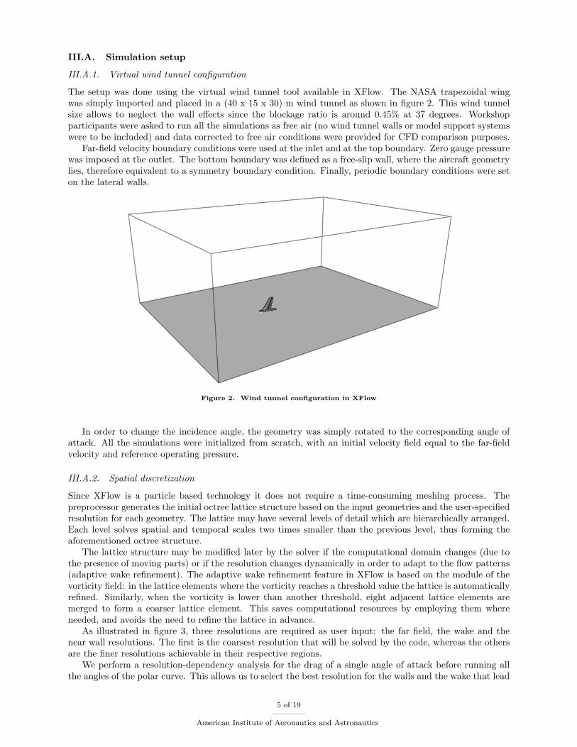
The setup was done using the virtual wind tunnel tool available in XFlow. The NASA trapezoidal wingwas simply imported and placed in a (40 x 15 x 30) m wind tunnel as shown in figure 2. This wind tunnelsize allows to neglect the wall effects since the blockage ratio is around 0.45% at 37 degrees. Workshopparticipants were asked to run all the simulations as free air (no wind tunnel walls or model support systemswere to be included) and data corrected to free air conditions were provided for CFD comparison purposes.

Far-field velocity boundary conditions were used at the inlet and at the top boundary. Zero gauge pressurewas imposed at the outlet. The bottom boundary was defined as a free-slip wall, where the aircraft geometrylies, therefore equivalent to a symmetry boundary condition. Finally, periodic boundary conditions were seton the lateral walls.

Figure 2. Wind tunnel configuration in XFlow

In order to change the incidence angle, the geometry was simply rotated to the corresponding angle ofattack. All the simulations were initialized from scratch, with an initial velocity field equal to the far-fieldvelocity and reference operating pressure.

III.A.2. Spatial discretization

Since XFlow is a particle based technology it does not require a time-consuming meshing process. Thepreprocessor generates the initial octree lattice structure based on the input geometries and the user-specifiedresolution for each geometry. The lattice may have several levels of detail which are hierarchically arranged.Each level solves spatial and temporal scales two times smaller than the previous level, thus forming theaforementioned octree structure.

The lattice structure may be modified later by the solver if the computational domain changes (due tothe presence of moving parts) or if the resolution changes dynamically in order to adapt to the flow patterns(adaptive wake refinement). The adaptive wake refinement feature in XFlow is based on the module of thevorticity field: in the lattice elements where the vorticity reaches a threshold value the lattice is automaticallyrefined. Similarly, when the vorticity is lower than another threshold, eight adjacent lattice elements aremerged to form a coarser lattice element. This saves computational resources by employing them whereneeded, and avoids the need to refine the lattice in advance.

As illustrated in figure 3, three resolutions are required as user input: the far field, the wake and thenear wall resolutions. The first is the coarsest resolution that will be solved by the code, whereas the othersare the finer resolutions achievable in their respective regions.

We perform a resolution-dependency analysis for the drag of a single angle of attack before running allthe angles of the polar curve. This allows us to select the best resolution for the walls and the wake that lead

5 of 19


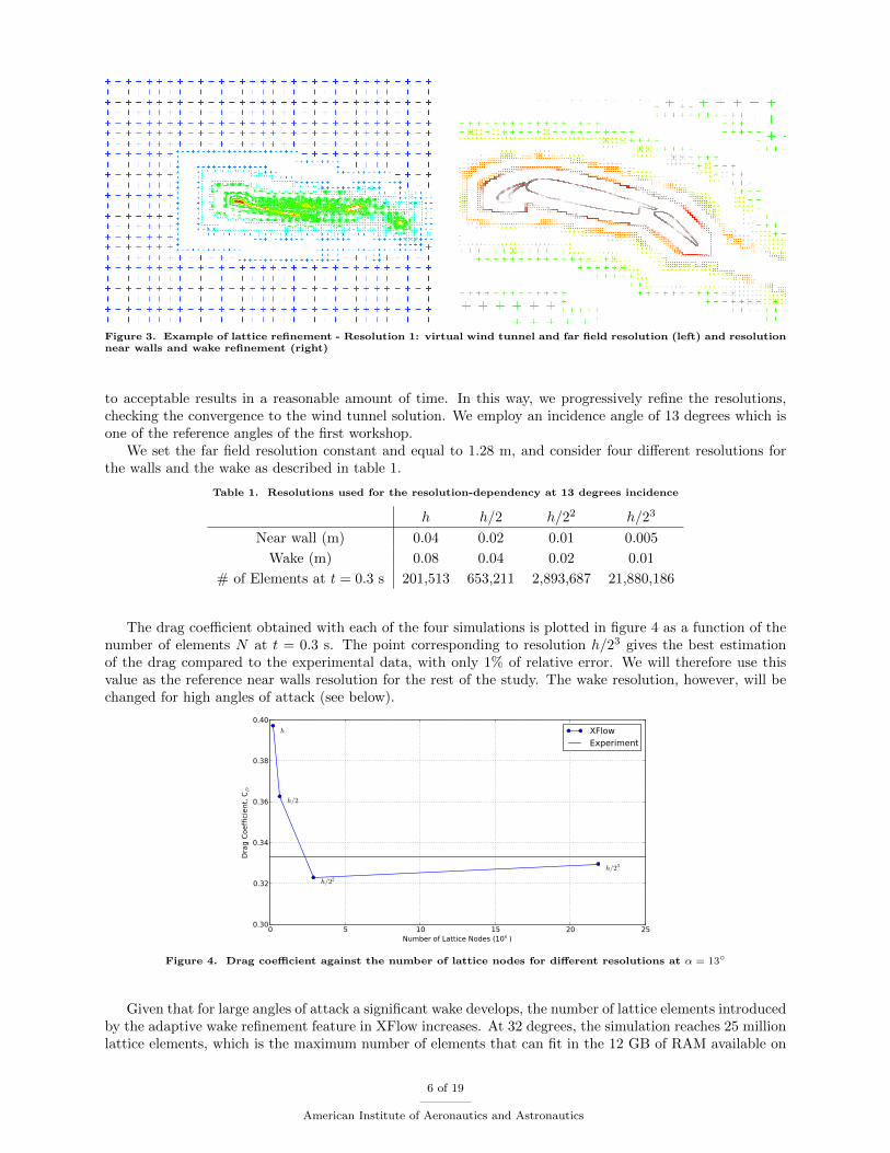
Figure 3. Example of lattice refinement - Resolution 1: virtual wind tunnel and far field resolution (left) and resolutionnear walls and wake refinement (right)

to acceptable results in a reasonable amount of time. In this way, we progressively refine the resolutions,checking the convergence to the wind tunnel solution. We employ an incidence angle of 13 degrees which isone of the reference angles of the first workshop.

We set the far field resolution constant and equal to 1.28 m, and consider four different resolutions forthe walls and the wake as described in table 1.

Table 1. Resolutions used for the resolution-dependency at 13 degrees incidence

h h/2 h/22 h/23

Near wall (m) 0.04 0.02 0.01 0.005

Wake (m) 0.08 0.04 0.02 0.01

# of Elements at t = 0.3 s 201,513 653,211 2,893,687 21,880,186

The drag coefficient obtained with each of the four simulations is plotted in figure 4 as a function of thenumber of elements N at t = 0.3 s. The point corresponding to resolution h/23 gives the best estimationof the drag compared to the experimental data, with only 1% of relative error. We will therefore use thisvalue as the reference near walls resolution for the rest of the study. The wake resolution, however, will bechanged for high angles of attack (see below).

0 5 10 15 20 25Number of Lattice Nodes (106 )

0.30

0.32

0.34

0.36

0.38

0.40

Dra

g Co

effic

ient

, CD

h/23

h/22

h/2

h XFlowExperiment

Figure 4. Drag coefficient against the number of lattice nodes for different resolutions at α = 13

Given that for large angles of attack a significant wake develops, the number of lattice elements introducedby the adaptive wake refinement feature in XFlow increases. At 32 degrees, the simulation reaches 25 millionlattice elements, which is the maximum number of elements that can fit in the 12 GB of RAM available on

6 of 19


the workstation. Special care is thus required in order to keep this number within the memory constraintsfor higher angles. Thus, we limit the resolution for the wake in those cases to the double of the normal value,(Resolution 2 in table 2).

Table 2. Resolutions used for the 1st High Lift Prediction Workshop

Walls (m) Wake (m) Far Field (m) Max. # of Particles Angles

Resolution 1 0.005 0.01 1.28 25× 106 [-4; 32]

Resolution 2 0.005 0.02 1.28 10× 106 [34; 37]

III.B. Numerical results

The experimental data were obtained in the 14x22 wind-tunnel at NASA Langley. Forces, moments, andpressure distributions have been provided with free transition16 and have been corrected for free air condi-tions. Data are provided as lower and upper values which are assumed to be the range of uncertainty in thewind tunnel measurements.

10 0 10 20 30 40α (deg)

0.0

0.2

0.4

0.6

0.8

1.0

Dra

g Co

effic

ient

, CD

(a)

ExperimentalExperimental LowerExperimental UpperXFlow

10 0 10 20 30 40α (deg)

0.0

0.5

1.0

1.5

2.0

2.5

3.0

3.5

Lift

Coef

ficie

nt, C

L

(b)

0.0 0.2 0.4 0.6 0.8 1.0Drag Coefficient, CD

0.0

0.5

1.0

1.5

2.0

2.5

3.0

3.5

Lift

Coef

ficie

nt, C

L

(c)

10 0 10 20 30 40α (deg)

0.5

0.4

0.3

0.2

0.1

0.0

Pitc

hing

Mom

ent,

C m

(d)

Figure 5. Drag (top left) and lift (top right) coefficient against the angle of attack, the polar curve (bottom left), andthe pitching moment coefficient (bottom right)

One can observe the drag and lift coefficients against the angle of attack α in panels (a) and (b) of figure5. The drag prediction computed by XFlow closely matches the experimental data along the whole range ofincidence angles, specifically the simulation results agree at extreme angles of attack.

XFlow results also show good agreement with the wind tunnel data for the lift coefficient for all attackangles. Within the range [1, 28] degrees, the code predicts accurately both the slope and the absolute valuesof the lift coefficient. XFlow is also able to predict the critical angle successfully: the wind tunnel dataindicate that the critical angle is reached at around 33 degrees, and it appears in the range between 32 and34 degrees in XFlow. From that point onwards, the lift drops due to a large bubble of separation on thewing, which is a characteristic feature of the post-stall region. The bubble of separation grows from the wingtip, as shown in figure 6, essentially on the main element of the wing. This is the expected behavior for the

7 of 19


Figure 6. Averaged Line Integral Convolution (LIC) at 37 degrees incidence

lift. More details of the flow structure for the whole range of angles of attack is shown in the Appendix,figure 15.

Since both drag and lift coefficients are quite well predicted, the polar curve in panel (c) of figure 5 alsomatches closely the experimental results, including the post-stall region.

The pitching moment coefficient is accurately estimated for the range [1, 32] degrees and lays betweenthe upper and lower limits of the experimental results, as shown in panel (d) of figure 5. At extreme angles itfollows the trend of the experimental data with slightly less accuracy, but showing a good overall prediction.

IV. Polar sweep

Once shown in section III that the results obtained with XFlow are satisfactory even in the post-stallregion, we focus on a slightly more advanced topic.

The first example presented in this section investigates the ability of XFlow to determine the polarcurve within a single simulation by means of a rotating geometry that sweeps an interval of angles. Themotivation to perform this kind of analysis is multiple, e.g. to improve the time-to-solution of the fullpolar curve, to minimize the engineering-time required for the setup, or to mimic experimental and inflightoperating conditions.

IV.A. Sweep motion setup

In order to perform the sweep motion analysis, two variables should be defined: the range of angles to sweepand the angular velocity. Since we are interested in investigating the flow around the stall point as well asthe linear part of the polar curve, we have selected an initial angle equal to the reference angle of 13 degrees,well within the linear range, and a final angle of 37 degrees which lays beyond the stall point.

Regarding the angular velocity, on the one hand, it must be slow enough so that the estimation of bothlift and drag remains comparable to the stationary cases. But on another hand, it must be quick enough sothat the simulation runs in a reasonable amount of time.

The characteristic velocity due to the rotation should be much lower than the far field velocity

vrotch = ωLch << v∞, (21)

8 of 19


where ω is the angular velocity and Lch is a characteristic length of the plane. The velocity inlet is v∞ = 68m/s and the plane length is ∼ 3 m. Setting ω = 24 deg/s fulfills the above condition.

The code allows the specification of angular laws using analytical expressions or tabular data as input,allowing to define complex motions with flexibility. The sweeping motion has been decomposed into threephases: constant at 13 degrees, a constant angular speed rotation, and constant at 37 degrees. The purposeof the first stage is to start the sweeping of the polar curve once the flow has converged from the initialconditions. From the study conducted in section III, we obtained that 0.2 s of simulation time is requiredbefore getting a fully converged drag and lift prediction, and consequently the angle increment starts att = 0.2 s. To achieve the sweeping from 13 degrees until 37 degrees at 24 deg/s, one second of simulationtime is required. The angle then remains constant at 37 degrees from t = 1.2 s (see figure 7). This last stageallows us to check that the forces are stable at the end of the simulation.

0.0 0.1 0.2 0.3 0.4 0.5 0.6 0.7 0.8 0.9 1.0 1.1 1.2 1.3 1.4 1.5Time (s)

0.20.10.00.10.20.30.40.50.60.70.80.91.01.11.2

Dis

plac

emen

t fra

ctio

n

Figure 7. The sweeping law.

IV.B. Selection of resolutions and optimization

In order to proceed further in the drag and lift sweeping prediction, one must assess carefully the resolutionused, since the computation requires more simulation time and includes moving parts. Each point of thepolar curve presented in figure 5 requires from 0.2 to 0.5 s of simulation time, depending on the incidenceangle, to obtain converged aerodynamic loads, whereas this simulation will require a minimum of 1.2 s toachieve the full sweeping.

In the resolution-dependency study conducted in section III, see figure 4, it can be noted that a resolutionof 0.01 m near the walls and 0.02 m (point h/22) within the wake still closely predicts the drag coefficientwith less computational effort. It is interesting to study the impact of the wake refinement resolution onthe solution at this wall resolution, in order to lower the wake resolution if possible. Hence, a small wake-dependency study has been conducted at 13 degrees incidence using a constant resolution of 1.28 m at thefar field, a near wall resolution of 0.01 m, and five different wake resolutions as described in table 3.

Table 3. Wake resolutions used for the wake-dependency at 13 degrees incidence

No Wake Ref. 23w 22w 2w w

Near wall (m) 0.01 0.01 0.01 0.01 0.01

Wake (m) - 0.08 0.04 0.02 0.01

# of Elements at t = 0.3 s 1,274,167 1,402,232 1,591,113 2,893,687 19,457,710

The results for the wake-dependency study are gathered in figure 8. It can be clearly seen that the point22w is the coarsest point that still gives an accurate prediction of the lift. With the finest wake resolutionw the variation in lift coefficient is only about 0.06%, and about 2% with no wake refinement.

9 of 19


0 5 10 15 20 25Number of Lattice Nodes (106 )

2.03

2.04

2.05

2.06

2.07

2.08

2.09

Lift

Coef

ficie

nt, C

L

w2w

22 w

23 w

No Wake RefinementXFlowExperiment

Figure 8. Lift coefficient against the number of elements for different wake resolutions at α = 13

While the above resolution may suffice for low angles of attack, it may not be fine enough for anglesnear the stall point, where the importance of the wake refinement is higher. As we discussed in table 2, aresolution of 0.005 m near walls and 0.02 m at the wake (Resolution 2) was selected for the highest angles ofattack, starting from 34 degrees. This set of resolutions has proven its reliability to predict the drop in thelift coefficient at the stall point (figure 5). However, it is not as fine as the Resolution 1 showed in table 2,and thus is able to sweep the full range of angles while keeping the memory requirements within the availablelimits. Therefore, we have designed it as the second resolution choice for the polar sweep.

To summarize, the two resolutions chosen for the polar sweep are listed in table 4.

Table 4. Resolutions used for the sweep polar simulation

Walls (m) Wake (m) Far Field (m)

Sweep Resolution Coarse 0.01 0.04 1.28

Sweep Resolution Fine 0.005 0.02 1.28

IV.C. Drag, lift and pitching moment sweep predictions

The results of the polar sweep simulation in terms of drag, lift and pitching moment are shown in figure9. In the linear range, between ∼ 13 and 25 degrees, both coarse and fine sweeps achieve results that arewithin the experimental limits. For higher angles (above ∼ 27 degrees), the coarse simulation proves unableto successfully predict the lift and drag, while the fine simulation is in better agreement with the wind tunneldata.

The fine simulation shows an overall better agreement with the experimental data. Indeed, the dragcurve is very close to the reference data until an angle of 35 degrees is reached. At this angle, the curveachieves a peak value which seems to be similar to the increase of drag present on the experimental data at∼ 37 degrees, but about 2 degrees earlier. A similar behavior happens with the pitching moment predictedby XFlow, which perfectly matches the wind tunnel results from 13 degrees to 35 degrees and then suddenlydrops. This discrepancy may be explained by considering dynamic effects, as a too quick angular velocityof the trap wing may amplify the separation bubbles forming around the critical angle. The lift coefficientis properly predicted for the whole range of angles. Albeit slight deviations appear for the highest angles ofattack, the lift curve shows a critical angle of 33 degrees, exactly as expected from the reference data.

The results of the polar sweep case are in good agreement with the wind tunnel data. An interestingapplication of the coarse simulation is to quickly predict an accurate curve slope of the drag and lift as well

10 of 19


10 0 10 20 30 40α (deg)

0.0

0.2

0.4

0.6

0.8

1.0

Dra

g Co

effic

ient

, CD

(a)

ExperimentalExperimental LowerExperimental UpperSweep Coarse Res.Sweep Fine Res.

10 0 10 20 30 40α (deg)

0.0

0.5

1.0

1.5

2.0

2.5

3.0

3.5

Lift

Coef

ficie

nt, C

L

(b)

10 0 10 20 30 40α (deg)

0.5

0.4

0.3

0.2

0.1

0.0

Pitc

hing

Mom

ent,

C m

(c)

Figure 9. Sweeping drag (top left) and lift (top right) and pitching moment (bottom) coefficient against angle of attack

as an exact estimation of their absolute values in the linear region. The fine resolution provides a greatimprovement over the first simulation, and can be regarded as complementary. It allows to explore withhigher detail the post-stall range of incidences for which the lift is correctly predicted by XFlow, and givesa more accurate prediction of the behavior of the flow around the critical angle.

V. Moving flap and slat transformation

As a second application involving moving geometries in the context of the High Lift Prediction Workshopresearch, we investigate the transformation from an un-stowed to a stowed configuration, and vice versa.These are typical operations for an aircraft while taking off and landing. As a proof of concept for thesekind of applications, a possible motion of interest consists in a first transformation from the un-stowedconfiguration to the stowed configuration, followed by a reverse transformation from the stowed to the un-stowed configuration. This proof of concept test is run for the reference angle of 13 degrees. For thesesimulations, we used a resolution of 1.28 m at the far field, 0.01 m at the wake and 0.02 m near the wallswhich were shown to be fairly accurate in table 1.

V.A. Geometry and transformation processing

In order to apply the desired transformation, the geometry has been separated into different components:the fuselage, the main wing, the slat and the flap. In order to avoid gaps between slat and the flap andthe fuselage through the transition, these surfaces have been extended. It should be noted that the lack offairing may increase the sensitivity of the flow to separation, specifically for the flap surface.

Different transformations are required for the slat and the flap in order to go from un-stowed to stowedconfigurations while the rest remains fixed. The description of such transformation is defined in.1 Bothconfigurations are shown in figure 10.

Once the position and orientation for both stowed and un-stowed configurations are known, we implementa transition function in XFlow in order to go from one to another. Two approaches have been devised in

11 of 19


Figure 10. Un-stowed (left) and stowed (right) configurations

order to approximate the transition: a simple piecewise-linear function and a piecewise-linear function withsmooth third-order polynomial transitions between the linear parts.

The first method is straightforward to implement and only requires to know how long the transition fromone configuration to another takes. We set a transition time of 0.4 s, in agreement with the usual times sucha maneuver takes on real aircraft scaled down accordingly to our model length.

The full transformation we specify for the piecewise-linear function includes five steps: fixed at un-stowedconfiguration, stowing, fixed at stowed position, un-stowing, and finally constant at stowed configuration.The duration of each stage is respectively: 0.1 s, 0.4 s, 0.1 s, 0.4 s and 0.5 s. The function is shown in figure11.

0.0 0.1 0.2 0.3 0.4 0.5 0.6 0.7 0.8 0.9 1.0 1.1 1.2 1.3 1.4 1.5Time (s)

0.0

0.1

0.2

0.3

0.4

0.5

0.6

0.7

0.8

0.9

1.0

1.1

Dis

plac

emen

t fra

ctio

n

Figure 11. Piecewise-linear function used for the motion

An alternative displacement function to the previous piecewise-linear approach can be devised by ensuringsmooth transitions between the linear parts using third order polynomials. The idea is to create a piecewisefunction which would be fully continuous and differentiable over the entire simulation time. Given two linearfunctions, a third order interpolating polynomial a3x

3+a2x2+a1x+a0 can be determined. The linear pieces

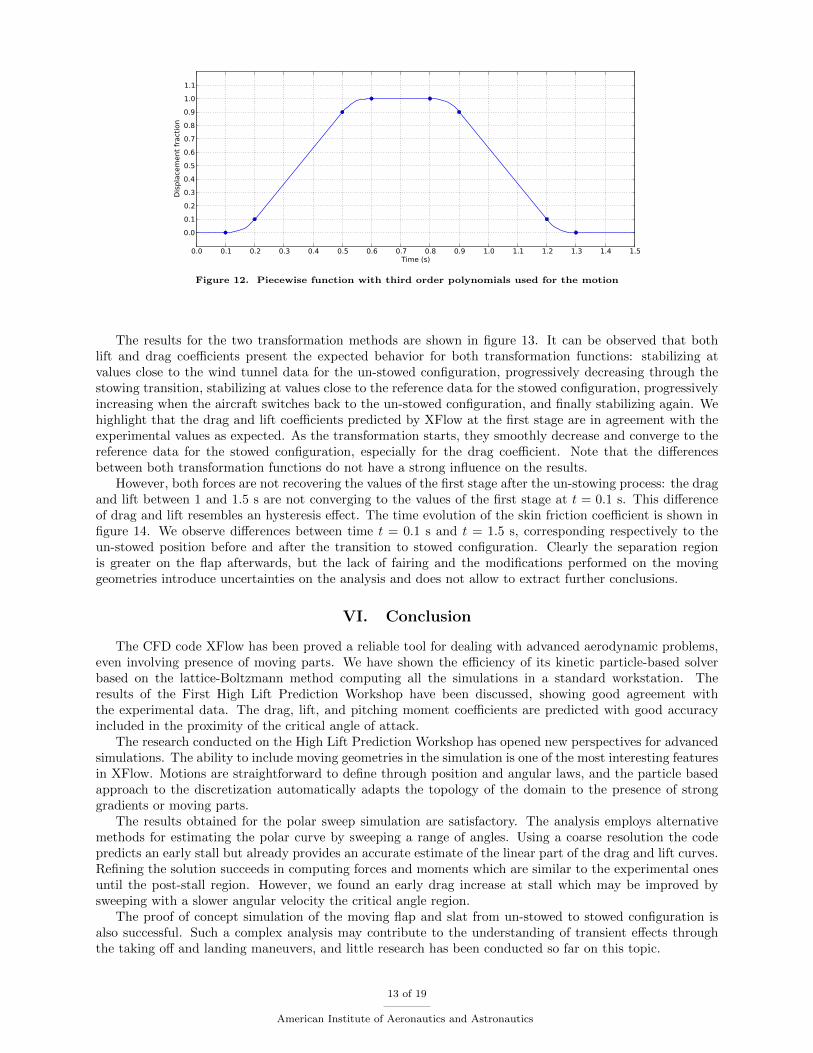
have been cut off at 10% and 90% of the transformation to be joined with the polynomial pieces. Each linearpiece lasts 0.3 s, and each polynomial piece lasts 0.1 s. The transformation function can be seen in figure 12.

V.B. Transformation analysis results

Since no wind tunnel data was available for the stowed configuration, a simulation of the trap wing onstowed configuration at a fixed angle of attack of 13 degrees is used as reference. The simulation convergedto a drag coefficient of 0.11 and a lift coefficient of 1.18. As expected, these values are lower than thosefor the un-stowed configuration. This is a good indicator of the lower bound expected for both drag andlift during the simulation of the complete transformation, and can be used to check the consistency of theresults obtained with moving parts.

12 of 19


0.0 0.1 0.2 0.3 0.4 0.5 0.6 0.7 0.8 0.9 1.0 1.1 1.2 1.3 1.4 1.5Time (s)

0.0

0.1

0.2

0.3

0.4

0.5

0.6

0.7

0.8

0.9

1.0

1.1

Dis

plac

emen

t fra

ctio

n

Figure 12. Piecewise function with third order polynomials used for the motion

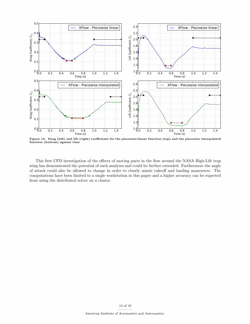
The results for the two transformation methods are shown in figure 13. It can be observed that bothlift and drag coefficients present the expected behavior for both transformation functions: stabilizing atvalues close to the wind tunnel data for the un-stowed configuration, progressively decreasing through thestowing transition, stabilizing at values close to the reference data for the stowed configuration, progressivelyincreasing when the aircraft switches back to the un-stowed configuration, and finally stabilizing again. Wehighlight that the drag and lift coefficients predicted by XFlow at the first stage are in agreement with theexperimental values as expected. As the transformation starts, they smoothly decrease and converge to thereference data for the stowed configuration, especially for the drag coefficient. Note that the differencesbetween both transformation functions do not have a strong influence on the results.

However, both forces are not recovering the values of the first stage after the un-stowing process: the dragand lift between 1 and 1.5 s are not converging to the values of the first stage at t = 0.1 s. This differenceof drag and lift resembles an hysteresis effect. The time evolution of the skin friction coefficient is shown infigure 14. We observe differences between time t = 0.1 s and t = 1.5 s, corresponding respectively to theun-stowed position before and after the transition to stowed configuration. Clearly the separation regionis greater on the flap afterwards, but the lack of fairing and the modifications performed on the movinggeometries introduce uncertainties on the analysis and does not allow to extract further conclusions.

VI. Conclusion

The CFD code XFlow has been proved a reliable tool for dealing with advanced aerodynamic problems,even involving presence of moving parts. We have shown the efficiency of its kinetic particle-based solverbased on the lattice-Boltzmann method computing all the simulations in a standard workstation. Theresults of the First High Lift Prediction Workshop have been discussed, showing good agreement withthe experimental data. The drag, lift, and pitching moment coefficients are predicted with good accuracyincluded in the proximity of the critical angle of attack.

The research conducted on the High Lift Prediction Workshop has opened new perspectives for advancedsimulations. The ability to include moving geometries in the simulation is one of the most interesting featuresin XFlow. Motions are straightforward to define through position and angular laws, and the particle basedapproach to the discretization automatically adapts the topology of the domain to the presence of stronggradients or moving parts.

The results obtained for the polar sweep simulation are satisfactory. The analysis employs alternativemethods for estimating the polar curve by sweeping a range of angles. Using a coarse resolution the codepredicts an early stall but already provides an accurate estimate of the linear part of the drag and lift curves.Refining the solution succeeds in computing forces and moments which are similar to the experimental onesuntil the post-stall region. However, we found an early drag increase at stall which may be improved bysweeping with a slower angular velocity the critical angle region.

The proof of concept simulation of the moving flap and slat from un-stowed to stowed configuration isalso successful. Such a complex analysis may contribute to the understanding of transient effects throughthe taking off and landing maneuvers, and little research has been conducted so far on this topic.

13 of 19


0.0 0.2 0.4 0.6 0.8 1.0 1.2 1.4Time (s)

0.0

0.1

0.2

0.3

0.4

0.5

Dra

g Co

effic

ient

, CD

XFlow - Piecewise interpolated

0.0 0.2 0.4 0.6 0.8 1.0 1.2 1.4Time (s)

0.0

0.1

0.2

0.3

0.4

0.5

Dra

g Co

effic

ient

, CD

XFlow - Piecewise linear

0.0 0.2 0.4 0.6 0.8 1.0 1.2 1.4Time (s)

1.0

1.2

1.4

1.6

1.8

2.0

2.2

2.4

Lift

Coef

ficie

nt, C

L

XFlow - Piecewise linear

0.0 0.2 0.4 0.6 0.8 1.0 1.2 1.4Time (s)

1.0

1.2

1.4

1.6

1.8

2.0

2.2

2.4

Lift

Coef

ficie

nt, C

L

XFlow - Piecewise interpolated

Figure 13. Drag (left) and lift (right) coefficients for the piecewise-linear function (top) and the piecewise interpolatedfunction (bottom) against time

This first CFD investigation of the effects of moving parts in the flow around the NASA High-Lift trapwing has demonstrated the potential of such analyses and could be further extended. Furthermore the angleof attack could also be allowed to change in order to closely mimic takeoff and landing maneuvers. Thecomputations have been limited to a single workstation in this paper and a higher accuracy can be expectedfrom using the distributed solver on a cluster.

14 of 19


Figure 14. Skin friction coefficient over the trap wing

15 of 19


Appendix

Figure 15 shows the different vorticity patterns that appear at the angles studied in figure 5.

16 of 19


17 of 19


Figure 15. Volume rendering of vorticity module for different angles

18 of 19


Acknowledgments

Thanks to Christopher Rumsey and Judith A. Hannon from the NASA Langley Research Center for theirsupport.

References

1Rumsey, C., “The 1st AIAA CFD High Lift Prediction Workshop,” June 2010.2Holman, D., Mier-Torrecilla, M., Drage, P., and Kussman, C., “Aerodynamic analysis involving moving parts with a

particle-based CFD solution,” NAFEMS Wolrd Congress, 2011.3Frisch, U., Hasslacher, B., and Pomeau, Y., “Lattice-gas automata for the Navier-Stokes equation,” Physical review

letters, Vol. 56, No. 14, 1986, pp. 1505–1508.4McNamara, G. R. and Zanetti, G., “Use of the Boltzmann equation to simulate lattice-gas automata,” Physical Review

Letters, Vol. 61, Nov. 1988, pp. 2332–2335.5Chen, S. and Doolen, G., “Lattice Boltzmann method for fluid flows,” Annual review of fluid mechanics, Vol. 30, No. 1,

1998, pp. 329–364.6Succi, S., “The lattice Boltzmann equation,” For Fluid Dynamics and Beyond , 2001.7Ran, Z. and Xu, Y., “Entropy and weak solutions in the thermal model for the compressible Euler equations,” Arxiv

preprint arXiv:0810.3477 , 2008.8Qian, Y. H., D’Humieres, D., and Lallemand, P., “Lattice BGK models for Navier-Stokes equation,” EPL (Europhysics

Letters), Vol. 17, Feb. 1992, pp. 479.9Higuera, F. J. and Jimenez, J., “Boltzmann approach to lattice gas simulations,” EPL (Europhysics Letters), Vol. 9,

Aug. 1989, pp. 663.10Shan, X. and Chen, H., “A general multiple-relaxation-time Boltzmann collision model,” International Journal of Modern

Physics C , Vol. 18, No. 4, 2007, pp. 635–643.11d’Humieres, D., “Multiple–relaxation–time lattice Boltzmann models in three dimensions,” Philosophical Transactions of

the Royal Society of London. Series A: Mathematical, Physical and Engineering Sciences, Vol. 360, No. 1792, 2002, pp. 437–451.12Asinari, P., “Entropic multiple-relaxation-time lattice Boltzmann models,” Tech. rep., Politecnico di Torino, Torino, Italy,

2008.13Premnath, K. and Banerjee, S., “On the Three-Dimensional Central Moment Lattice Boltzmann Method,” Journal of

Statistical Physics, 2011, pp. 1–48.14Ducros, F., Nicoud, F., and Poinsot, T., “Wall-adapting local eddy-viscosity models for simulations in complex geome-

tries,” Proceedings of 6th ICFD Conference on Numerical Methods for Fluid Dynamics, 1998, pp. 293–299.15Shih, T., Povinelli, L., Liu, N., Potapczuk, M., and Lumley, J., “A generalized wall function,” NASA Technical Report ,

July 1999.16McGinley, C., Jenkins, L., Watson, R., and Bertelrud, A., “3-D High-Lift Flow-Physics Experiment–Transition Measure-

ments,” AIAA Paper , Vol. 5148, 2005, pp. 2005.

19 of 19


Documents

Advanced Aerodynamic Analysis of the NASA High-Lift Trap