Adv Dynamics Notes

Advanced Dynamics Notes

Jed Rembold

September 24, 2009

2

Contents

1 Survey of Elementary Particles 51.1 Mechanics of a Particle . . . . . . . . . . . . . . . . . . . . . . . . . . . . . . . . . . . 51.2 Mechanics of a System of Particles . . . . . . . . . . . . . . . . . . . . . . . . . . . . 71.3 Constraints . . . . . . . . . . . . . . . . . . . . . . . . . . . . . . . . . . . . . . . . . 111.4 D’Alembert’s Principle and Lagrange’s Equations . . . . . . . . . . . . . . . . . . . . 131.5 Velocity Dependent Potentials and Dissipation Functions . . . . . . . . . . . . . . . 151.6 Simple Applications of Lagrangian Formalism . . . . . . . . . . . . . . . . . . . . . . 15

2 Variational Principles and Lagrange’s Equations 192.1 Hamilton’s Principle and Calculus of Variations . . . . . . . . . . . . . . . . . . . . . 192.2 The 3 Classic Problems of the Calculus of Variations . . . . . . . . . . . . . . . . . . 212.3 Calculus of Variations and Lagrange’s Equations . . . . . . . . . . . . . . . . . . . . 212.4 Non-Holonomic Systems and Lagrange Multipliers . . . . . . . . . . . . . . . . . . . 242.5 Conservation Theorems and Symmetry Properties . . . . . . . . . . . . . . . . . . . 29

2.5.1 Energy Conservation and Time Homogeneity . . . . . . . . . . . . . . . . . . 302.5.2 Momentum Conservation and Space Homogeneity . . . . . . . . . . . . . . . 312.5.3 Angular Momentum Conservation and Rotational Invariance . . . . . . . . . 32

3 The Central Force Problem 353.1 2 body to 1 body problem and Reduced Mass . . . . . . . . . . . . . . . . . . . . . . 35

3

4 CONTENTS

Chapter 1

Survey of Elementary Particles

1.1 Mechanics of a Particle

We begin with a review of common expressions. Recall that

r = position vector of a particle from a given origin

v = particle’s vector velocity

We thus know that

v =dr

dtand p = mv

where

p = linear momentum of a particle

m = the mass of a particle

F = total force exerted on the particle

The mechanics or motion of the particle are given by Newton’s 2nd Law of Motion:

F =dp

dt= p

For an inertial or Galilean reference frame, this can be expressed as

F =d

dt(mv)

For a particle with constant mass, this simplifies to:

F = ma = mdv

dt= m

d2r

dt2

where a is the particle’s acceleration. Now, if F = 0 = p, then p equals a constant, and thus wehave Conservation of Linear Momentum of the particle.

5

6 CHAPTER 1. SURVEY OF ELEMENTARY PARTICLES

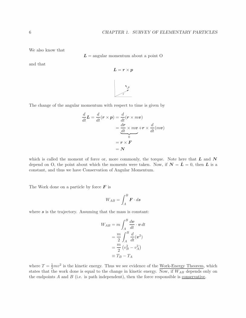
We also know that

L = angular momentum about a point O

and that

L = r × p

The change of the angular momentum with respect to time is given by

d

dtL =

d

dt(r × p) =

d

dt(r ×mv)

=dr

dt×mv

︸︷︷︸

0

+r ×d

dt(mv)

= r × F

= N

which is called the moment of force or, more commonly, the torque. Note here that L and N

depend on O, the point about which the moments were taken. Now, if N = L = 0, then L is aconstant, and thus we have Conservation of Angular Momentum.

The Work done on a particle by force F is

WAB =

∫ B

AF · ds

where s is the trajectory. Assuming that the mass is constant:

WAB = m

∫ B

A

dv

dt· v dt

=m

2

∫ B

A

d

dt(v2)

=m

2

(v2B − v2

A

)

≡ TB − TA

where T = 12mv2 is the kinetic energy. Thus we see evidence of the Work-Energy Theorem, which

states that the work done is equal to the change in kinetic energy. Now, if WAB depends only onthe endpoints A and B (i.e. is path independent), then the force responsible is conservative.

1.2. MECHANICS OF A SYSTEM OF PARTICLES 7

Thus we see that, in a conservative system, the work around a closed path is

∮

F · ds = 0

Remark 1: Dissipative forces such as friction are not conservative since

F · ds > 0

for work done by the particle.

For a conservative force (WAB path independent), we can write

F = −∇V (r)

where V is the potential or potential energy. Thus we have

F · ds = −dV ⇒ Fs = −dV

ds

Remark 2: Note that

F = −∇ (V (r) + constant) = −∇V (r)

and thus the zero of V (r) is arbitrary.

Remark 3: For a conservative system, WAB = VA − VB. Thus we have that

VA − VB = TB − TA ⇒ VA + TA = VB + TB

which is our expression for the Conservation of Total Energy!

1.2 Mechanics of a System of Particles

The goal here is to generalize Newton’s 2nd law to a system of particles. Starting with the equationof motion for the ith particle:

∑

j

Fji + F(e)i = pi


where

Fji = the internal force on particle i by particle j and

F(e)i = an external force

Now, assuming that Fij = −Fji (Newton’s 3rd Law, or the Weak Law of Action and Reaction),then

∑

i

Fi =d2

dt2

∑

i

miri =∑

i

F(e)i +

∑

i6=j

Fji

︸︷︷︸

0

We define R as:

R =

∑

i miri∑

i mi=

∑

i miri

M

where R is the center of mass and M is the total mass. Thus we have that

Md2

dt2R =

∑

i

F(e)i ≡ F (e)

Consequentally, purely internal forces (forces on particles from other particles) vanish by Newtons3rd law. The total linear momentum can thus be expressed as

P =∑

i

midri

dt= M

dR

dt

Thus total linear momentum is conserved when the total external forces are equal to zero.

The total angular momentum is written as

L =∑

i

Li =∑

i

ri × pi

Hence,

dL

dt= L =

∑

i

d

dt(ri × pi)

=∑

i

ri × pi

=∑

i

ri × F(e)i +

∑

i6=j

ri × Fji

but∑

i6=j

ri × Fji = 12

∑

i6=j

[ri × Fji + rj × Fij]

= 12

∑

i6=j

(ri − rj)× Fji

1.2. MECHANICS OF A SYSTEM OF PARTICLES 9

If we define

rij = ri − rj

then we can write∑

i6=j

ri × Fji = 12

∑

i6=j

rij × Fji

Note that if Fji is parallel to rij , then rij ×Fji = 0, which is called the Strong Law of Action andReaction. If this is true, then

dL

dt=∑

i

ri × F(e)i + 1

2

∑

i6=j

rij × F ji

︸︷︷︸

0

= N (e)

Thus, if the applied external torque, N (e), equals 0, then L is constant in time and we haveConservation of Angular Momentum.

Remark 1: The Strong Law of Action and Reaction requires the internal forces to be central.

We can also describe the particle position with respect to the center of mass:

So we have

ri = R + r′i

vi = V + v′i

where

V =dR

dt= velocity of center of mass

v′i =

dr′i

dt= velocity about the center of mass


Then

L =∑

i

ri × pi =∑

i

(R + r′

i

)×(miV + miv

′i

)

=∑

i

R×miV +∑

i

R×miv′i

︸︷︷︸

0

+∑

i

r′i ×miV︸︷︷︸

0

+∑

i

r′i ×miv

′i

= R×MV +∑

i

r′i ×miv

′i

So the total angular momentum is:

L = R×MV +∑

i

r′i ×miv

′i

= angular momentum of the CM + angular momentum about the CM

Now,

WAB =∑

i

∫ B

AFi · dsi =

∑

i

∫ B

AF

(e)i · dsi +

∑

i6=j

∫ B

AFji · si

=∑

i

∫ B

Amivi · vi dt

=∑

i

∫ B

Ad(

12miv

2i

)

= TB − TA

with total kinetic energy T = 12

∑

i miv2i . We can also write

T = 12

∑

i

miv2i = 1

2

∑

i

mi

(V + v′

i

)·(V + v′

i

)

= 12MV 2 +

∑

i

miv′i

︸︷︷︸

0

·V + 12

∑

i

miv′i2

= 12MV 2 + 1

2

∑

i

miv′i2

= KE of CM + KE about CM

We now go back to

WAB =∑

i

∫ B

AF

(e)i · dsi +

∑

i6=j

∫ B

AFji · si

For conservative external forces, we have that:

∑

i

∫ B

AF

(e)i · dsi = −

∑

i

∫ B

A∇iVi · dsi = −

∑

i

Vi

∣∣∣∣∣

B

A

1.3. CONSTRAINTS 11

For conservative internal forces:

Fji = −∇jVji

where Vji = Vji(|ri − rj |) to satisfy the Strong Law of Action and Reaction

= ∇iVij

= −Fij

where there is no implied sum over repeated indices above. Therefore

WAB = −∑

i

Vi

∣∣∣∣∣

B

A

+ 12

∑

i6=j

∫ B

A(Fji · dsi + Fij · dsj)

= −∑

i

Vi

∣∣∣∣∣

B

A

+ 12

∑

i6=j

∫ B

AFji · (dsi − dsj)

= −∑

i

Vi

∣∣∣∣∣

B

A

+ 12

∑

i6=j

∫ B

AFji · dsij

= −∑

i

Vi

∣∣∣∣∣

B

A

− 12

∑

i6=j

∫ B

A∇jiVji · dsij

= −∑

i

Vi

∣∣∣∣∣

B

A

− 12

∑

i6=j

Vji

∣∣∣∣∣∣

B

A

Thus the total potential energy is

V =∑

i

Vi −12

∑

i6=j

Vij

Remark 2: T + V is conserved for T, V the total kinetic and potential energy.

Remark 3: For a rigid body, internal potential energy is constant, and thus internal forces dueno work.

1.3 Constraints

Constraints limit the motion of a system: ie, beads on a string, ball on a circular track, or gasmolecules in a container.


Holonomic Constraints: A Holonomic constraint is one where the constraint can be expressedas an equation connecting the space and time coordinates of a particle with the form:

f(r1, r2, r3, . . . , rN , t) = 0

Examples include rigid bodies (which have equations of the form (ri − rj)2 −C2

ij = 0) andparticles constrained to move on a curve or surface.

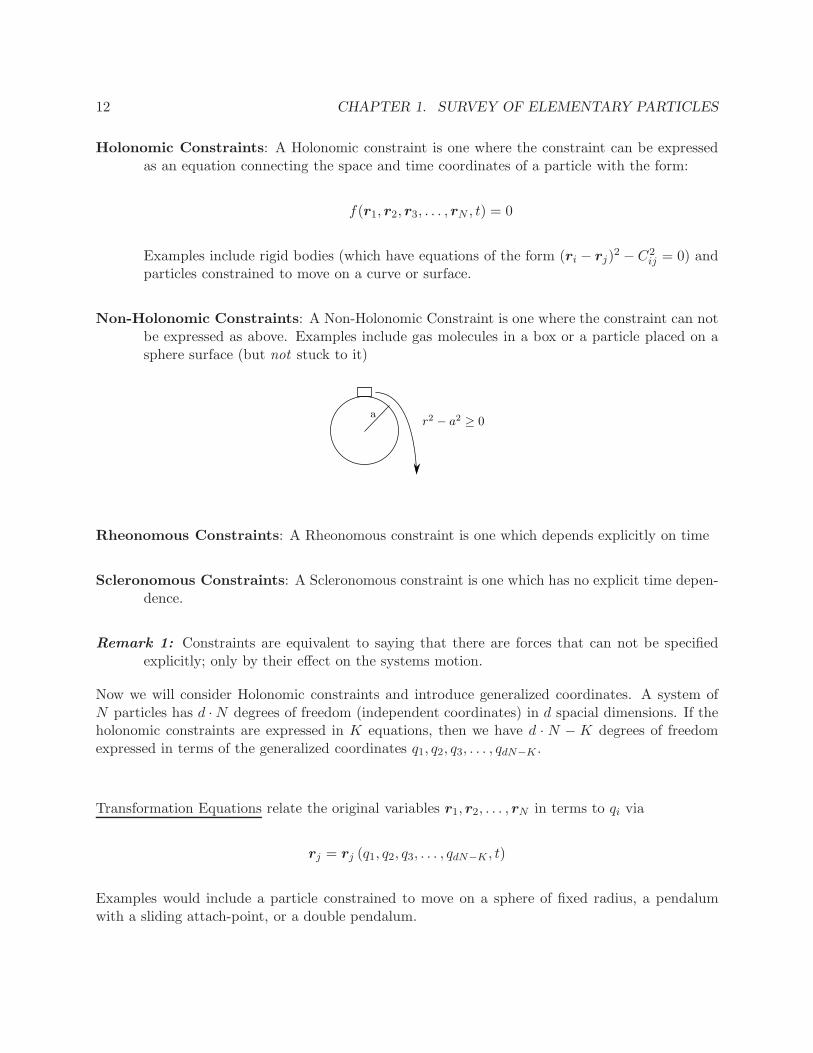
Non-Holonomic Constraints: A Non-Holonomic Constraint is one where the constraint can notbe expressed as above. Examples include gas molecules in a box or a particle placed on asphere surface (but not stuck to it)

Rheonomous Constraints: A Rheonomous constraint is one which depends explicitly on time

Scleronomous Constraints: A Scleronomous constraint is one which has no explicit time depen-dence.

Remark 1: Constraints are equivalent to saying that there are forces that can not be specifiedexplicitly; only by their effect on the systems motion.

Now we will consider Holonomic constraints and introduce generalized coordinates. A system ofN particles has d ·N degrees of freedom (independent coordinates) in d spacial dimensions. If theholonomic constraints are expressed in K equations, then we have d · N − K degrees of freedomexpressed in terms of the generalized coordinates q1, q2, q3, . . . , qdN−K .

Transformation Equations relate the original variables r1, r2, . . . , rN in terms to qi via

rj = rj (q1, q2, q3, . . . , qdN−K , t)

Examples would include a particle constrained to move on a sphere of fixed radius, a pendalumwith a sliding attach-point, or a double pendalum.

1.4. D’ALEMBERT’S PRINCIPLE AND LAGRANGE’S EQUATIONS 13

1.4 D’Alembert’s Principle and Lagrange’s Equations

Let

Fi︸︷︷︸

total forceon ith

particle

= F(a)i︸︷︷︸

appliedforces

+ fi︸︷︷︸

force ofconstraint

By Newton’s 2nd law:

Fi = pi ⇒ Fi − pi = 0

which gives

∑

i

(Fi − pi) · δri︸︷︷︸

infinitesimaldisplacement

= 0 =∑

i

(

F(a)i − pi

)

· δri +∑

i

(fi − pi) · δri

Consider the case where∑

i fi · δri = 0. This is akin to

i.e. the forces of constraint do no work. This leaves us with:

∑

i

(

F(a)i − pi

)

· δri = 0 ⇒ D’Alembert’s Principle (†)

Note that the above equation contains no constraints, so we’ll drop the “(a)” designation unam-biguously in the future.

For ri = ri (q1, q2, q3, . . . , qn, t), we will write (†) in terms of the generalized coordinates qi:

δri =∑

i

∂ri

∂qjδqj

⇒∑

i

Fi · δri =∑

i,j

Fi ·∂ri

∂qjδqj ≡

∑

j

Qj δqj

where

Qj =∑

i

Fi ·∂ri

∂qj= the generalized force


Working on the other half of the equation, we have:

⇒∑

i

pi · δri =∑

i,j

mivi ·∂ri

∂qjδqj

=∑

i,j

[d

dt

(

mivi ·∂ri

∂qj

)

−mivi ·d

dt

(∂ri

∂qj

)]

δqj

Using the fact that

vi =dri

dt=

∂

∂tri +

∑

k

qk∂ri

∂qkby chain rule

⇒∂vi

∂qj=

∂ri

∂qj

Thus:

∑

i

pi · δri =∑

i,j

[d

dt

(

mivi ·∂vi

∂qj

)

−mivi ·∂vi

∂qj

]

δqj

=∑

j

{

d

dt

[

∂

∂qj

(∑

i

12miv

2i

)]

−∂

∂qj

(∑

i

12miv

2i

)}

δqj

And D’Alembert’s principle becomes:

∑

i

(Fi − pi) · δri =∑

j

{

Qj −d

dt

∂T

∂qj+

∂T

∂qj

}

δqj = 0

with T =∑

i12miv

2i . Now if the system is Holonomic, then it is possible to find qj such that δqj is

independent of δqk for all j 6= k. Thus, the individual coefficients must vanish:

d

dt

∂T

∂qj−

∂T

∂qj= Qj

If Fi = −∇U (conservative force), then

Qj =∑

i

Fi ·∂ri

∂qj= −

∑

i

∇iU ·∂ri

∂qj= −

dU

dqj= −

dU

dqj+

d

dt

(dU

dqj

)

︸︷︷︸

0

where the last term is 0 since we are taking U to be velocity independent. Thus we have

d

dt

∂

∂qj(T − U)−

∂

∂qj(T − U) = 0

Define the Lagrangian to be L = T − U . Thus Lagrange’s equations become:

d

dt

∂L

∂qj−

∂L

∂qj= 0

Note that the Lagrangian is not unique! (See HW)

1.5. VELOCITY DEPENDENT POTENTIALS AND DISSIPATION FUNCTIONS 15

1.5 Velocity Dependent Potentials and Dissipation Functions

If U = U(qj , qj), then

Qj = −∂U

∂qj+

d

dt

(∂U

∂qj

)

and L = T − U

An example would be a charged particle in an EM field (See HW). If frictional forces are present,then we’ll have

d

dt

(∂L

∂qj

)

−∂L

∂qj= Qj = forces not arising from a potential

Example: Consider Rayleigh’s dissipation function:

F = 12

∑

i

(kxv2

ix + kyv2iy + kzv

2iz

)

And

Ffx = −∂F

∂vx; Ff = −∇vF

where Ffx is the x component of the frictional force and the sum over i is over all particles.Thus we have that Qj (the generalized force due to friction) is

Qj =∑

i

Ffi·∂ri

∂qj= −

∑

i

∇vF ·∂ri

∂qj

= −∑

i

∇vF ·∂vi

∂qj= −

∂F

∂qj

⇒d

dt

(∂L

∂qj

)

−∂L

∂qj+

∂F

∂qj= 0

1.6 Simple Applications of Lagrangian Formalism

Example 1: Consider a single free particle in space:

T = 12m(x2

1 + x22 + . . . + x2

d

)in d-dimensional space

U = 0

Qi =∑

j

Fj ·∂rj

∂qi


where, in cartesian coordinates,∂xj

∂qi= δij

L = T

d

dt

∂L

∂xi−

∂L

∂xi= 0

⇒ mxi = Fxi= 0

Example 2: Consider a particle constrained on a sphere. Using polar coordinates, we have

x1 = R sin θ cos φ

x2 = R sin θ sin φ

x3 = R cos θ

Calculate x1, x2, x3 and substitute into T it get the kinetic energy for the system whosenatural coordinates are spherical.

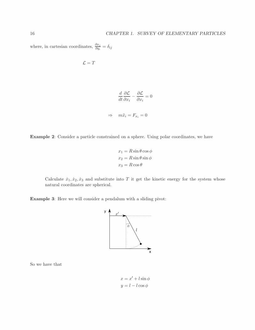
Example 3: Here we will consider a pendalum with a sliding pivot:

So we have that

x = x′ + l sin φ

y = l − l cos φ

1.6. SIMPLE APPLICATIONS OF LAGRANGIAN FORMALISM 17

Thus we have:

T = 12m(x2 + y2

)

= 12m

((

x′ + l cos φφ)2

+(

l sin φφ)2)

= 12m(

x′2+ 2l cos φx′φ + l2 cos2 φφ2 + l2 sin2 φφ2

)

= 12m(

x′2+ 2l cos φx′φ + l2φ2

)

U = mgy = mg (l − l cos φ)

L = 12m(

x′2+ 2l cos φx′φ + l2φ2

)

−mgl (1− cos φ)

Remark 1: Generalized coordinates are not necessarily orthogonal!

d

dt

∂L

∂qi−

∂L

∂qi

d

dt

∂L

∂x′−

∂L

∂x′=

d

dt

(

mx′ + ml cos φφ)

− 0 = 0

d

dt

∂L

∂φ−

∂L

∂φ=

d

dt

(

ml cos φx′ + ml2φ)

+ ml sin φx′φ + mgl sin φ = 0

To find the equilibrium points:U = mgl −mgl cos φ

∂U

∂φ= mgl sin φ = 0 ⇒ φ = 0, π

∂2U

∂φ2= mgl cos φ|φ=0,π =

{

mgl > 0, φ = 0

−mgl < 0, φ = π

So we have a stable equilibrium at φ = 0 and an unstable equilibrium at φ = π (as we’dexpect).


Chapter 2

Variational Principles and Lagrange’sEquations

2.1 Hamilton’s Principle and Calculus of Variations

Consider a system with n generalized coordinates: q1, q2, . . . , qn. These coordinates make up ann-dimensional configuration space with each q corresponding to an axis in the space.

1. t is a parameter of curve C with t ∈ [t−, t+] = interval

2. q− = q(t−), q+ = q(t+)

3. ddtq(t) ≡ q(t) is the tangent vector

4. If L(q(t), q(t), t) is a function of the q’s and their tangents, then we define a number thatcharacterizes the path:

S(C) =

t+∑

t−

L(q(t), q(t), t) dt

Note that this is more general than t = time and L = Lagrangian. The above is true of any

function of q, q and t.

5. S is called a functional (a functional is an animal that eats a function and spits out a number).

6. If C → C + δC, then S → S + δS continuously

19

20 CHAPTER 2. VARIATIONAL PRINCIPLES AND LAGRANGE’S EQUATIONS

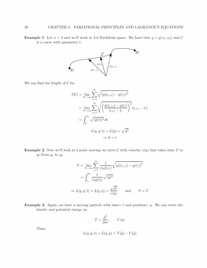
Example 1: Let n = 2 and we’ll work in 2-d Euclidean space. We have that q = q(x1, x2) and Cis a curve with parameter t.

We can find the length of C by:

l(C) = limN→∞

N∑

i=1

√

(q(ti+1)− q(ti))2

= limN→∞

N∑

i=1

√(

q(ti+1)− q(ti)

ti+1 − ti

)2

(ti+1 − ti)

=

∫ t2

t1

√

(q(t))2 dt

L(q, q, t) = L(q) =√

q2

⇒ S = l

Example 2: Now we’ll look at a point moving on curve C with velocity v(q) that takes time T togo from q1 to q2.

T = limN→∞

n∑

i=1

1

v(q(ti))

√

(q(ti+1)− q(ti))2

=

∫ t2

t1

1

v(q(t))

√

(q)2

⇒ L(q, q, t) = L(q, q) =

√

q2

v(q)and S = T

Example 3: Again, we have a moving particle with time= t and position= q. We can write thekinetic and potential energy as:

T =q2

2m, U(q)

Thus:L(q, q, t) = L(q, q) = T (q)− U(q)

2.2. THE 3 CLASSIC PROBLEMS OF THE CALCULUS OF VARIATIONS 21

S =

∫ t2

t1

L(q(t), q(t), t) dt

So S is the Action. Hamilton’s principle says that S has a stationary value for the actualpath of motion:

⇒ δS = δ

∫ t2

t1

L(q, q, t) dt = 0

2.2 The 3 Classic Problems of the Calculus of Variations

The Brachistochrone Problem: Brachistochrone means “short time”, so these type of problemsare attempting to minimize the time. A massive particle moves from A to B under the force

of gravity along path C. Which C gives the shortest travel time?

The Geodesics Problem: A ship is traveling from Portland, OR to Hawaii along the surface ofa sphere. Which route is the shortest?

The Isoperimetric Problem (Dido’s Problem): For a curve C with given length l, which formgives the maximum area?

2.3 Calculus of Variations, Hamilton’s Principle, and Lagrange’sEquations

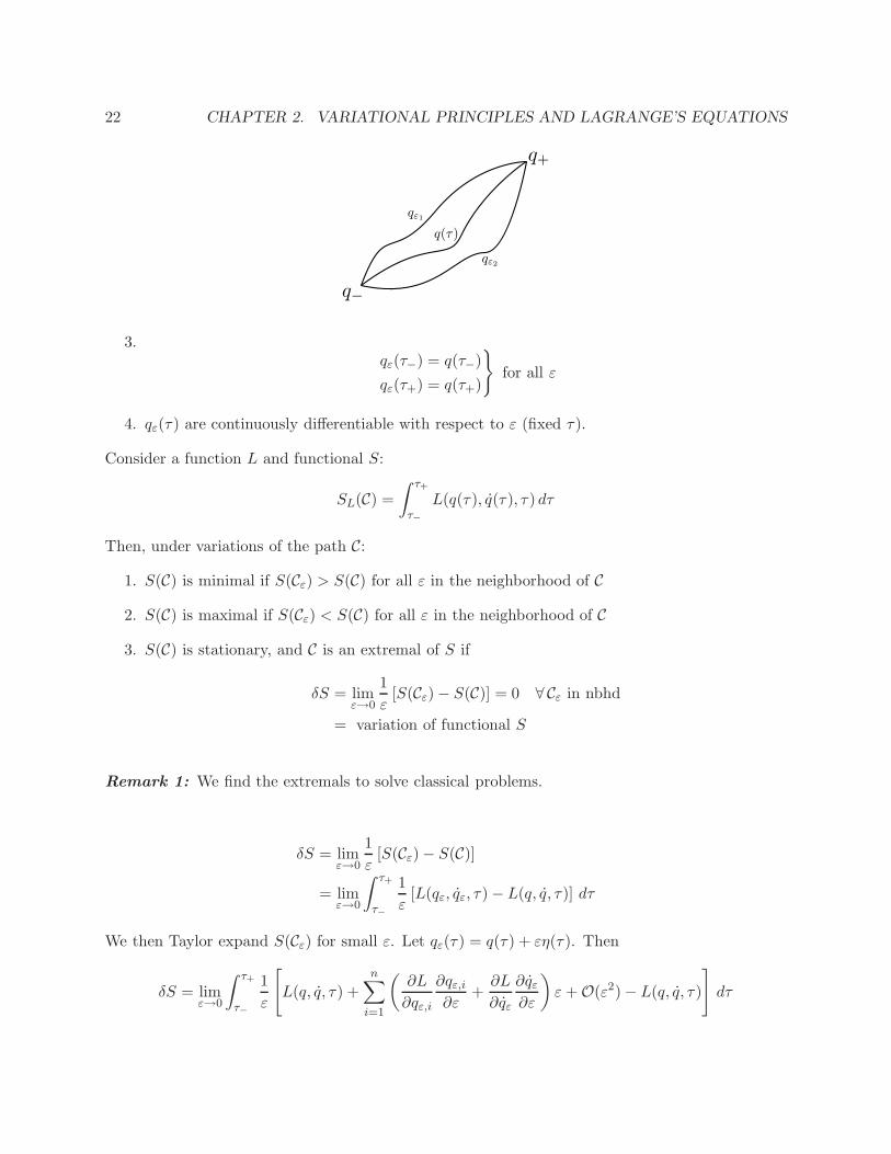
Consider a curve Cε in configuration space.

Cε : qε(τ) = qε (q1(τ, ε), . . . , qn(τ, ε))

Some things to note:

1. qε(τ) is a path for every fixed ε.

2. qε=0(τ) = q(τ)


3.qε(τ−) = q(τ−)

qε(τ+) = q(τ+)

}

for all ε

4. qε(τ) are continuously differentiable with respect to ε (fixed τ).

Consider a function L and functional S:

SL(C) =

∫ τ+

τ−

L(q(τ), q(τ), τ) dτ

Then, under variations of the path C:

1. S(C) is minimal if S(Cε) > S(C) for all ε in the neighborhood of C

2. S(C) is maximal if S(Cε) < S(C) for all ε in the neighborhood of C

3. S(C) is stationary, and C is an extremal of S if

δS = limε→0

1

ε[S(Cε)− S(C)] = 0 ∀ Cε in nbhd

= variation of functional S

Remark 1: We find the extremals to solve classical problems.

δS = limε→0

1

ε[S(Cε)− S(C)]

= limε→0

∫ τ+

τ−

1

ε[L(qε, qε, τ)− L(q, q, τ)] dτ

We then Taylor expand S(Cε) for small ε. Let qε(τ) = q(τ) + εη(τ). Then

δS = limε→0

∫ τ+

τ−

1

ε

[

L(q, q, τ) +

n∑

i=1

(∂L

∂qε,i

∂qε,i

∂ε+

∂L

∂qε

∂qε

∂ε

)

ε +O(ε2)− L(q, q, τ)

]

dτ

2.3. CALCULUS OF VARIATIONS AND LAGRANGE’S EQUATIONS 23

Note that, since qε(τ) = q(τ) + εη(τ), we have

∂qε

∂ε= η(τ)

⇒∂L

∂qε=

∂L

∂q

∂q

∂qε︸︷︷︸

1

=∂L

∂q

Thus

δS = limε→0

∫ τ+

τ−

1

ε

[n∑

i=1

(∂L

∂qiηi +

∂L

∂qiηi

)

ε +O(ε2)

]

dτ

=

∫ τ+

τ−

n∑

i=1

∂L

∂qiηi dτ +

n∑

i=1

∂L

∂qiηi

∣∣∣∣

τ+

τ−

︸︷︷︸

0

−

∫ τ+

τ−

ηid

dt

∂L

∂qidτ

=

∫ τ+

τ−

n∑

i=1

[∂L

∂qi−

d

dt

∂L

∂qi

]

ηi(τ) dτ

= 0 since S is stationary.

Now, applying the fundamental lemma of the calculus of variations:

Lemma: Let f(τ) be continuous for τ ∈ [τ−, τ+] and

∫ τ+

τ−

f(τ)η(τ) dτ = 0 ∀η

which are 2 times differentiable and obey

η(τ+) = η(τ−) = 0

Then

f(τ) = 0

since ηi(τ) is arbitrary and vanishes at the endpoints.

⇒∂L

∂qi−

d

dt

∂L

∂qi= 0 = Euler Equations (†)

Remark 2: When L = T − U in (†), these are the Euler-Lagrange equations.

Remark 3: The functional S =∫

L(q(τ), q(τ), τ) dτ is stationary only if the functional L obeysthe Euler-Lagrange equations.


Remark 4: (†) implies that

∂L

∂qi−∑

k

∂

∂qk

(∂L

∂qi

)

qk −∑

k

∂

∂qk

(∂L

∂qi

)

qk −∂

∂t

(∂L

∂qi

)

= 0

⇒∑

k

Lik qk =∂L

∂qi−

∂2L

∂qi∂τ−∑

k

(∂2L

∂qk∂qi

)

qi (‡)

and

Lik =∂2L

∂qi∂qk← symmetric n×n matrix

So the Euler-Lagrange equations (†) are equivalent to n-coupled ODE’s of second order for q(τ).Therefore, the initial point of q(τ−) and initial tangent q(τ−) completely determine the path.

Remark 5: (‡) has the structure of Newton’s Second Law.

Remark 6: Lagrange’s equations of motion follow naturally from Hamilton’s Principle.

Example: Geodesics in d-dimensional Euclidean space: Recall that the length of curve C isgiven by

l(C) =

∫ τ+

τi

√

(q(τ))2 dτ = L(q, q, τ) =√

q2 =

d∑

j=1

(qj(τ))2

1/2

(†) then implies that

d

dt

∂L

∂qi−

∂L

∂qi=

d

dt

(

1

2

1√

q2· 2qi

)

= 0 ∀i

⇒qi√

q2= constant

⇒ q = a = constant ⇒ q(τ) = aτ + b = straight lines

So the geodesics must run thru 2 points to specify a and b, implying that we require a 2-dcondition.

2.4 Extensions of Hamilton’s Principle to Non-Holonomic Sys-tems (Lagrange Multipliers)

δS = δ

∫ t+

t−

L(q, q, t) dt = 0 =

∫ τ+

τ−

∑

i

(∂

∂qi−

d

dt

∂L

∂qi

)

dτ δqi = 0

2.4. NON-HOLONOMIC SYSTEMS AND LAGRANGE MULTIPLIERS 25

Non-Holonomic constraints imply that the generalized coordinates are not independent. Thisimplies that displacements of the path may or may not satisfy the constraints. If displacementssatisfy constraints, then the constraints are holonomic. If the displacements do not satisfy theconstraints, then we want to eliminate the constraints by means of Lagrange Multipliers. Lagrangemultipliers work for “semi-holonomic” constraints, which can be put in the form:

fα (q1, . . . , qn, q1, . . . , qn) = 0 (†)

where α = 1, 2, . . . , n.

Remark 1: Semi-holonomic differs from holonomic in that the latter can be expressed in terms ofone constraint equation (function of generalized coordinates only), whereas the former conbe more than one (function of tangents as well).

Remark 2: In terms of path displacements, the semi-holonomic constraints can be expressed:∑

k

aik dqk + ait dt = 0 where i = 1, . . . ,m

This is more restrictive than (†).

Remark 3: (†) implies that:m∑

α=1

λαfα = 0

whereλα = λα (q1, . . . , qn, q1, . . . , qn, t)

are undetermined functions.

Recall Hamilton’s Principle:

δ

∫ t2

t1

L dt = 0

which implies∫ t2

t1

∑

k

(∂L

∂qk−

d

dt

∂L

∂qk

)

dt δqk = 0

And δqk are no longer independent (if we have non-holonomic constraints). But if the constraintsare semi-holonomic, then:

δ

∫ t2

t1

(

L+

m∑

α=1

λαfα

)

dt = 0

Changing notation slightly, let

L = L1,

m∑

α=1

λαfα = λL2

︸︷︷︸

⋆


where (⋆) in the piece that will make the δqk’s independent. Then

L3 = L1 + λL2

⇒ δ

∫ t2

t1

(L1 + λL2) dt = δ

∫ t2

t1

L3 dt = 0

⇒

∫ t2

t1

∑

k

(∂L3

∂qi−

d

dt

∂L3

∂qi

)

dt δqi = 0

And L3 obeys Lagrange’s equations:

d

dt

∂L3

∂qi−

∂L3

∂qi= 0

Also

d

dt

∂L3

∂qi−

∂L3

∂qi=

d

dt

∂

∂qi(L1 + λL2)−

∂

∂qi(L1 + λL2)

=d

dt

∂

∂qiL1 −

∂L1

∂qi+

d

dt

∂

∂qi(λL2)−

∂

∂qi(λL2)

= 0

Now,d

dt

∂L1

∂qi−

∂L1

∂qi=

∂

∂qi(λL2)−

d

dt

∂(λL2)

∂qi≡ Qi

⇒d

dt

∂L1

∂qi−

∂L1

∂qi= Qi = forces of constraint

with

Qi =∂

∂qi(λL2)−

d

dt

∂

∂qi(λL2)

Remark 4: Lagrange multipliers allow us to map a semi-holonomic system of n-generalized coor-dinates and m-constraints to a holonomic one with n + m generalized coordinates.

Example:L = 1

2m(x2 + y2

)− U(x, y) ≡ L1

Constraint: f(x, y, y) = xy + ky = 0 ≡ L2 where k = const (1)

⇒ L3 = L1 + λL2 andd

dt

∂L3

∂qi−

∂L3

∂qi= 0

⇒d

dt

∂L3

∂x−

∂L3

∂x=

d

dt(mx + λy) +

∂U

∂x= 0 (2)

d

dt

∂L3

∂y−

∂L3

∂y=

d

dt(my + λx) +

∂U

∂y− kλ = 0 (3)

2.4. NON-HOLONOMIC SYSTEMS AND LAGRANGE MULTIPLIERS 27

Thus we have 3 unknowns: x, y, λ, and 3 equations: (1), (2), (3).

Remark 5: Physically, the λ’s represent forces of constraints.

Remark 6: Forces of constraint do no work in (virtual) displacements (See §2.4 of Goldstein).

Remark 7: Lagrange multipliers can be used for holonomic constraints (α = 1) as well.

Example: Hoop Rolling without Slipping Down an Inclined Plane: We are using the

generalized coordinates x, θ. Our constraint in the rolling constraint:

rθ = x

⇒ rθ = x

⇒ rθ − x = 0 (3)

T = 12mx2 + 1

2mr2θ2

U = mg(l − x) sin φ

⇒ L1 = 12mx2 + 1

2mr2θ2 −mg(l − x) sin φ

L2 = rθ − x

L3 = L1 + λL2

= 12mx2 + 1

2mr2θ2 −mg(l − x) sin φ + λ(rθ − x)

⇒d

dt

∂L3

∂x−

∂L3

∂x= mx−mg sin φ + λ = 0 (1)

d

dt

∂L3

∂θ−

∂L3

∂θ= mr2θ − λr = 0 (2)

⇒ mx = mg sin φ− λ

= mg sin φ−mrθ from (2)

= mg sin φ−mx by (3)


⇒ 2mx = mg sin φ ⇒ x = 12g sinφ

So rolling has half the acceleration as the hoop sliding on a frictionless plane!

θ =g

2rsin φ

λ =mg

2sin φ→ “frictional force” of constraint

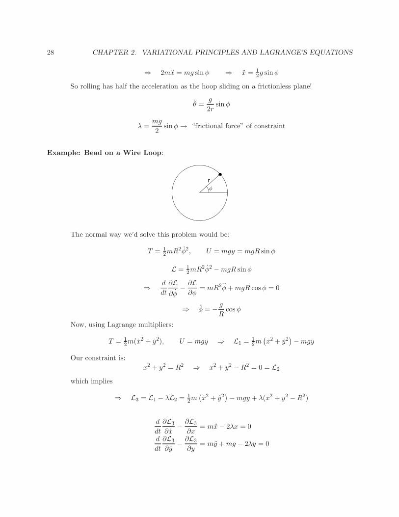
Example: Bead on a Wire Loop:

The normal way we’d solve this problem would be:

T = 12mR2φ2, U = mgy = mgR sin φ

L = 12mR2φ2 −mgR sinφ

⇒d

dt

∂L

∂φ−

∂L

∂φ= mR2φ + mgR cos φ = 0

⇒ φ = −g

Rcos φ

Now, using Lagrange multipliers:

T = 12m(x2 + y2), U = mgy ⇒ L1 = 1

2m(x2 + y2

)−mgy

Our constraint is:

x2 + y2 = R2 ⇒ x2 + y2 −R2 = 0 = L2

which implies

⇒ L3 = L1 − λL2 = 12m(x2 + y2

)−mgy + λ(x2 + y2 −R2)

d

dt

∂L3

∂x−

∂L3

∂x= mx− 2λx = 0

d

dt

∂L3

∂y−

∂L3

∂y= my + mg − 2λy = 0

2.5. CONSERVATION THEOREMS AND SYMMETRY PROPERTIES 29

So our 3 equations are:

mx = 2λx

my = −mg + 2λy

R2 = x2 + y2

Lettingx = R cos φ y = R sin φ

x = −R sin φφ y = R cos φφ

x = −R cos φφ2 −R sin φφ y = −R sin φφ2 + R cos φφ

Taking mx = 2λx and plugging in x implies:

m(

−R cos φφ2 −R sin φφ)

= 2λR cos φ

⇒ λ = −m

2φ2 −

m

2

sinφ

cos φφ

Taking my = −mg + 2λy:

⇒ m(

−R sinφφ2 + R cos φφ)

= −mg + 2(

−m

2φ2 −

m

2tan φφ

)

R sin φ

⇒ (mR cos φ + mR tan φ sin φ) φ = −mg

⇒ φ = −g

Rcos φ

2.5 Conservation Theorems and Symmetry Properties

Consider a function f(q, q, t). Ifd

dt(f(q, q, t)) = 0

thenf(q, q, t) = const (†)

where (†) is called the

• first integral of the equations of motion

• integrals of motion

• constant of motion

Remark 1: Conservation laws are an example of (†).

Nother’s Theorem: Symmetries in a system are related to conservation laws.


2.5.1 Energy Conservation and Time Homogeneity

Consider the Lagrangian:

L = L(q(τ), q(τ), τ)

Time homogeneity (time-translational invariance) means that L does not depend ex-plicitly on time.

⇒ L = L(q(τ), q(τ))

Thend

dtL =

∑

i

∂L

∂qiqi +

∑

i

∂L

∂qiqi +

∂L

∂t︸︷︷︸

0

Recall Lagrange’s equations of motion:

d

dt

∂L

∂qj=

∂L

∂qj

These imply

d

dtL =

∑

i

(d

dt

∂L

∂qj

)

qj +∑

i

∂L

∂qjqj

=∑

i

d

dt

(

qj∂L

∂qj

)

⇒d

dt

[∑

i

qj∂L

∂qj− L

]

= 0

⇒∑

i

qj∂L

∂qj− L ≡ H = E

Then H = E = const is the energy and energy is conserved in a system whoseLagrangian has no explicit time dependence.

Example:

L = T (q)− U(q), T = 12

∑

j

mj q2j

⇒ H =∑

i

qimiqi −12

∑

i

miq2i + U(q)

= 12

∑

i

miq2i + U(q) = T (q) + U(q) = total energy

Remark 1: Here we have assumed that U = U(q), so there does not exist dissipativeforces (which dissipate energy).


Remark 2: If L is an explicit function of time:

dH

dt= −

∂L

∂t

Remark 3: H is sometimes called the energy function, and it’s form coincides withthe Hamiltonian.

Remark 4: For frictional forces that are derivable from a dissipative function F :

From §1.5:d

dt

(∂L

∂qj

)

−∂L

∂qj+

∂F

∂qj= 0

Then

d

dtL =

∑

i

∂L

∂qiqi +

∑

i

∂L

∂qiqi +

∂L

∂t

=∑

i

qi

(d

dt

∂L

∂qi+

∂F

∂qi

)

+∑

i

∂L

∂qiqi +

∂L

∂t

=∑

i

d

dt

(

qi∂L

∂qi

)

+∑

i

qi∂F

∂qi︸︷︷︸

=2F by §1.5

+∂L

∂t

⇒dH

dt= −

∂L

∂t− 2F

for L = L(q, q) and H = E then this gives the dissipative rate.

2.5.2 Momentum Conservation and Space Homogeneity

This will correspond to space translational invariance. This implies that the La-grangian is invariant under ri → ri + ε (every particle moves by some same displace-ment). For now, we’ll only consider shifts in coordinates, not velocities.

δL =∑

i

∂L

∂riδri = 0 =

∑

i

∂L

∂qiδqi︸︷︷︸

⋆

where (⋆) is arbitrary, and only for holonomic constraints. This implies that

∂L

∂qi= 0 =

d

dt

∂L

∂qi

⇒∂L

∂qi= const


If U = U(q) only, then∂L

∂qi= mqi = pi

⇒ pi ≡∂L

∂qi= canonical (or conjugate) momentum

p also generalizes to include U = U(q, q). Now consider L = T (q)− U(q):

d

dt

∂T

∂qi+

∂U

∂qi= 0 ⇒

d

dt

∂T

∂qi= pi = −

∂U

∂qi≡ Qi

⇒ pi = Qi = generalized force

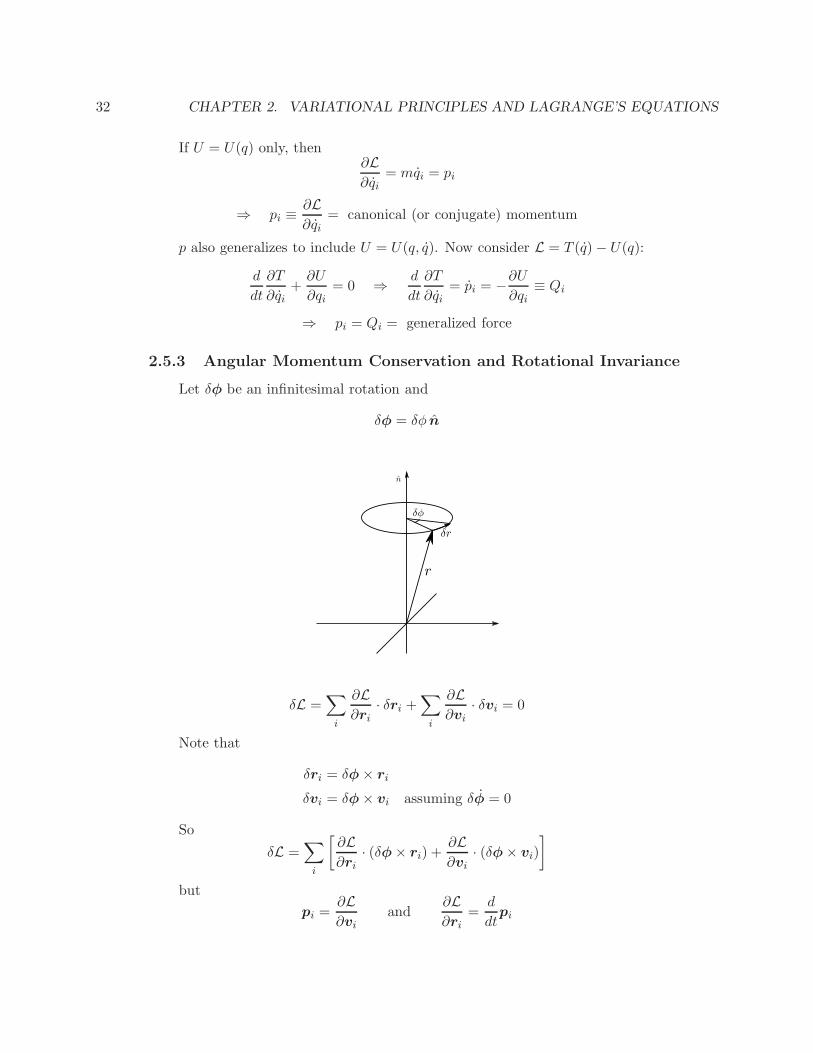
2.5.3 Angular Momentum Conservation and Rotational Invariance

Let δφ be an infinitesimal rotation and

δφ = δφ n

δL =∑

i

∂L

∂ri· δri +

∑

i

∂L

∂vi· δvi = 0

Note that

δri = δφ× ri

δvi = δφ× vi assuming δφ = 0

So

δL =∑

i

[∂L

∂ri· (δφ× ri) +

∂L

∂vi· (δφ× vi)

]

but

pi =∂L

∂viand

∂L

∂ri=

d

dtpi


⇒ δL =∑

i

[d

dtpi · (δφ× ri) + pi · (δφ× vi)

]

Now, recall that a · (b× c) = b · (c× a) = c · (a× b).

⇒ δL =∑

i

[δφ · (ri × pi) + δφ · (vi × pi)]

= δφ∑

i

d

dt(ri × pi) = 0

But δφ is arbitrary, so

d

dt

∑

i

(ri × pi) = 0

Now Mi = ri × pi = angular momentum, so we have that∑

i

Mi = const

Remark 1: The components of angular momentum along any axis (e.g. the z-axis)are given by

Mz =∑

i

∂L

∂φi

where φ = φ z

Example: We’ll take a look at how this works in cylindrical coordinates:

Mz =∑

i

(ri × pi)z =∑

i

mi (xiyi − yixi)

x = r cos φ x = r cos φ− r sin φ φ

y = r sin φ y = r sin φ + r cos φ φ

⇒Mz =∑

i

mi

[

ri cos φi

(

ri sinφi + ri cos φiφi

)

+ ri sin φi

(

ri cos φi − ri sin φiφi

)]

=∑

i

mir2i φi

Comparing with

∑

i

∂L

∂φi

=∑

i

∂

∂φi

[12mi

(

r2i + r2

i φ2i + z2

)

− U(ri, φ, z)]

=∑

i

mir2i φi


Chapter 3

The Central Force Problem

3.1 2 Body to 1 Body Problem and Reduced Mass

The two body problem:

35

Documents

Adv Dynamics Notes