Adoption and impact of climate-smart innovation on

Adoption and impact of climate-smart innovation on household productivity, food and nutritional

security in Benin: A Case study of Drought tolerant maize (DTM) varieties

1

Tchegoun Michel. Atchikpa

Plan

• Introduction

• Objectives of the study

• Data and methods

• Results and discussion

• Conclusion

• Recommandations and scope for nextstep

2

Introduction

• With the existence of very critical areas where hunger is rife, the foodsecurity status in the world is very worrying

(FAO and PAM, 2009).

• Indeed, over 39 countries surveyed in 2006 with high level of foodinsecurity in the world 25 of them come from Africa.

• Undertaking of micronutrient in consumption food than the required is oneof the largest health and socio-economic issues.

Horton et al., (2009)

• But the treatment of which is underestimated. Rising food prices haveserious consequences for inflation and the well-being of people around theworld and especially in developing countries.

(Golay, 2010)

3

Introduction

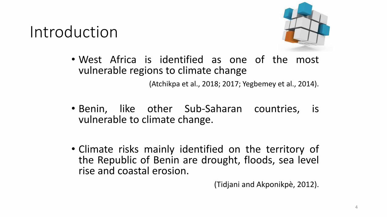
• West Africa is identified as one of the mostvulnerable regions to climate change

(Atchikpa et al., 2018; 2017; Yegbemey et al., 2014).

• Benin, like other Sub-Saharan countries, isvulnerable to climate change.

• Climate risks mainly identified on the territory ofthe Republic of Benin are drought, floods, sea levelrise and coastal erosion.

(Tidjani and Akponikpè, 2012).

4

Introduction

• In Benin, 1.1 million people were food insecure in 2013, comingfrom 11% of households with less than 1% severe food insecurityand 11% moderate food insecurity.

AGVSA, (2014)

• In recent years studies have shown the primal role of innovation inAfrica agricultural development in this context of climate change.

(Tambo and Wünscher, 2017; Wiggins, 2014)

• Indeed, it is commonly accepted that climate-smart innovationsare crucial to meeting the challenges of adaptation to climatechange to ensure food security and increase farmer’s income

(Campbell et al., 2014; Fieldsend, 2013; Long et al., 2016; Zongo et al., 2015)5

Introduction

• Dissemination or promotion seven varieties of DroughtTolerant Maize in Benin like in 12 others countries (DTMA,2009).

• But thing surprising despite of these multiple efforts only20 percent in Benin, 30 percent in Mali and 27 per cent inMozambique of farmers adopted the promoted varieties(CIMMYT-IITA, 2015).

• In the context of Benin, understanding the maindeterminants of DTM varieties adoption, in addition to theexpected returns from adoption, in order to designpolicies that could address the supply side constraints inWest Africa is consequently important.

6

Introduction

In addition:

• Generally empirical data on adoption of rates, on productivity andoutcome indicators related to well-being are few in the literature, butthere is practically no studies on the adoption of DTM varieties andbetter on their impact in Benin.

• Contradiction in some impact assessment study of adoption ofinnovations. (Omilola, 2009; Schneider and Gugerty, 2011; Suri,2011)

• Also, it is difficult to observe the impact of innovation since thebenefits are spread over several years and are distributed amongseveral producers.

• The adoption of technology may favour some people to thedetriment of others

7

Objectives of the study

The paper examine the adoption DTM varieties asclimate-smart innovations and evaluate it impact of onfood security and nutritional status of maize farminghouseholds in Benin.

• Bring out the probable impacts of adoption of DTmaize varieties at the household level in Benin thispaper offers a comprehensive ex-post assessment.

• Empirically contributes to the current adoptionliterature by examining the food security andnutritional status effects using a rigorous approachaccounting for both unobserved and observed variablesof heterogeneity between non-adopters and adopters

8

MunicipalitiesNumber ofvillages

VillagesSize ofsample

Kétou 5Adaplamè, Kpankou, Akpambahou, Achoubi,Idigny.

54

Savè 10Djaloumo, Ayedjoko, Gobé, Achakpa, Alafia,Ouoghi G, Djabata, Oké owo, Gogoro, Diho 1.

104

Bembèrèkè 8Guessou-Nord, Gando, Pèdarou, Gam-Oues,Wodora, INA 1, Wanrarou, Warakéru.

87

Kandi 9Padé, Tui, Sinanwon, Donwari, Pèdè, Sonsoro,Heboumey, Angaradébou, Kassakou.

94

Malanville 8SakawanT, Tomboutu, Boiffo, Degue D, Guené,Garou T, Galliel, Monkassa

84

Tanguiéta 8Finta , Sonta, Sépounga, Yarika, Mamoussa,Tchatingou, Douani, Kouayoti

95

Total 48 - 518

Data and methods

9

Data and methodsData collected:

• socio-economic and demographic characteristics

• perceptions of drought and the climate-smart innovations practicesdeveloped to reduce the effects of climate change;

• quantities of inputs and outputs;

• household consumption expenditure

• perception of household food security; Knowledge Aptitudes and Practicesin Food, Nutrition and Maternal and Child Health (Breastfeeding of theChild, Minimum Acceptable Diet, Eating Habits, household's DietaryDiversity)

• others information’s on the village and production systems

• Anthropometric data on children under 5 years old, as well as mortalitydata on all household members

Technic for data collection:• Investigations through structured and semi-structured interviews• Group discussions and participant observations

10

Data and methods: Conceptual framework

11

• Economic theory predicts that faced with a problem of choice, the rational economic

agent opts for the option that maximizes its utility (McFadden, 1975, Gourieroux, 1989).

• The utility is a measure of the welfare or satisfaction obtained by obtaining a good,

service or money (Mosnier, 2009).

• The economic principle of rationality and especially the maximization of utility

assumption form the basis for the analysis of choice (Bouatay and Mhenni, 2014;

Wooldridge, 2003).

• Although it is generally economical, this rationality can be ecological or sociocultural

(Rasmussen and Reenberg, 2012).

𝒀𝑱𝑨 = 𝑿𝒋𝜷𝑨 + 𝜺𝒋𝑨 𝒂𝒏𝒅 𝒀𝑱𝑵 = 𝑿𝒋𝜷𝑵 + 𝜺𝒋𝑵

• Where the factor prices, as well as farm and household characteristics, are represented by 𝑋𝑗,

휀𝑗𝐴 and 휀𝑗𝑁 are iids; βA and βN are vectors of parameters.

• Farm households will generally choose the technology if the profit derived by doing so are

higher than those obtained by not using the technology, that is, 𝑌𝐽𝐴 > 𝑌𝐽𝑁.

• Therefore, a farmer adopts technology only if the perceived profit is positive. Although the

preferences of the farmer, such as perceived profit of adoption are unknown to the researcher,

the characteristics of the farmer and the attributes of the technology are observed during the

survey period.

• Thus, the profit derived from innovation or technology adoption can be represented by a

latent variable 𝐿𝑗∗ , which is not observed but can be expressed as a function of the observed

attributes and characteristics denoted as Z in the latent variable model as follows:


12

• where 𝐿𝑗 is a binary variable that equals 1 for farmers that adopt the technology

and zero for farmers that do not adopt, with γ representing a vector of the

parameter to be estimated.

• The error term µj with mean zero and variance 𝛿𝜇2 captured measurement errors and

factors unobserved to the researcher but known to the farmer. Variables in Z

include factors affecting the adoption decision, such as farm-level, institutionnal

variables and household characteristics.

• Therefore, the equation is also known as the selection equation.

• The probability of technology or innovation adoption can then be expressed as:

𝑳𝒋∗ = 𝒁𝒚𝒋

∗ + 𝝁𝒋 𝑳 = 𝟏, 𝒊𝒇 𝑳𝒋∗ > 𝟎


13

• Where 𝑌𝐽𝐴 and 𝑌𝐽𝑁 represent the outcome indicators for adopters (maize

yield economic performances and welfare indicators) and for non-adoptersrespectively in regime 1 and 0;

• 휀𝑗𝐴 and 휀𝑗𝑁 represent the error term of the outcome variable respectively in

regime 1 and 0

• The variables X capture represents a vector of the exogenous variables thoughtto influence the outcome function like the farm inputs and characteristics socio-economic/demographics with all other variables.

• While βA and βN are parameters to be estimated, however, selection bias mayoccur if unobservable factors affecting the error terms in the section equationand the outcome equations thus, resulting in a correlation between the twoerror terms such that corr (ԑ, µ) = ρ different to 0

𝑹𝒆𝒈𝒊𝒎𝒆 𝟏 𝑨𝒅𝒐𝒑𝒕𝒆𝒓𝒔 𝒀𝑱𝑨 = 𝑿𝒋𝜷𝑨 + 𝜺𝒋𝑨 If L j = 1

𝑹𝒆𝒈𝒊𝒎𝒆 𝟎 𝑵𝒐𝒏 − 𝑨𝒅𝒐𝒑𝒕𝒆𝒓𝒔 𝒀𝑱𝑵= 𝑿𝒋𝜷𝑵 + 𝜺𝒋𝑵 𝐈𝐟 𝐋 𝐣 = 𝟎

Data and methods: Empirical framework

14

• According to Lee, (1982) and Rees and Maddala, (1985), in order toaccount for selection bias that may arise from observable andunobservable in farm and non-farm characteristics of the households onone other hand and estimate impact of DTM varieties adoption on theoutcomes of interest on the other hand, the Endogenous SwitchingRegression (ESR) model approach is employed.

• The outcome equations and the error terms of the selection, in the ESRmodel, are supposed having a trivariate normal distribution, with zeromean and non-singular covariance matrix stated as:

𝒄𝒐𝒗(𝝁𝒊, 𝜺𝟏, 𝜺𝟐) =

𝝈𝑨𝟐 𝝈𝑨𝑵 𝝈𝑨𝝁

𝝈𝑨𝑵 𝝈𝑵𝟐 𝝈𝑵𝝁

𝝈𝑨𝝁 𝝈𝑵𝝁 𝝈𝟐

Where 𝜎𝐴2 = 𝑣𝑎𝑟 휀1 ; 𝜎𝑁

2 = 𝑣𝑎𝑟 (휀2); 𝜎2 =

𝑣𝑎𝑟 (𝜇𝑖) ; 𝜎𝐴𝑁 = 𝑐𝑜𝑣 (휀1; 휀2); 𝜎𝐴𝜇 =

𝑐𝑜𝑣 (휀1; 𝜇𝑖) and 𝜎𝑁𝜇 = 𝑐𝑜𝑣 (휀2; 𝜇𝑖). 𝜎2 is stand

for the variance of the error term in the selection

equation and 𝜎𝐴2, 𝜎𝑁

2 represent the variance of the

error terms in the outcome equations


15

𝑬 Τ𝜺𝒋𝑨 𝑳𝒊 = 𝟎 = 𝑬 Τ𝜺𝒋𝑨 𝝁𝒊 > −𝒁𝒚𝒋′ = 𝝈𝑨𝝁

𝝋(𝒁𝒚𝒋′ ∕ 𝝈

𝝓(𝒁𝒚𝒋′ ∕ 𝝈

= 𝝈𝑨𝝁𝝀𝟏

𝑬 Τ𝜺𝒋𝑵 𝑳𝒊 = 𝟎 = 𝑬 Τ𝜺𝒋𝑵 𝝁𝒊 > −𝒁𝒚𝒋′ = 𝝈𝑵𝝁

𝝋(𝒁𝒚𝒋′ ∕𝝈

𝟏−𝝓(𝒁𝒚𝒋′ ∕𝝈

= 𝝈𝑵𝝁𝝀𝟐

Expected values ofthe truncated errorKotz, (1970):

Where and are the probability density and cumulative distribution functions of the standard normal distribution respectively.

The ratio of and represented by λ1 and λ2 in equations is referred to as the Inverse Mills Ratio (IMR) which denotes selection bias terms. Equations in (1) can then be written as follow:

𝑨𝒅𝒐𝒑𝒕𝒆𝒓𝒔: 𝒀𝑱𝑨 = 𝒁𝜷𝑱𝑨 + 𝝈𝑨𝝁𝝀𝟏 + 𝜺𝒋𝑨

𝑵𝒐𝒏 𝑨𝒅𝒐𝒑𝒕𝒆𝒓𝒔: 𝒀𝑱𝑵 = 𝒁𝜷𝑱𝑵 + 𝝈𝑵𝝁𝝀𝟐 + 𝜺𝒋𝑵


16

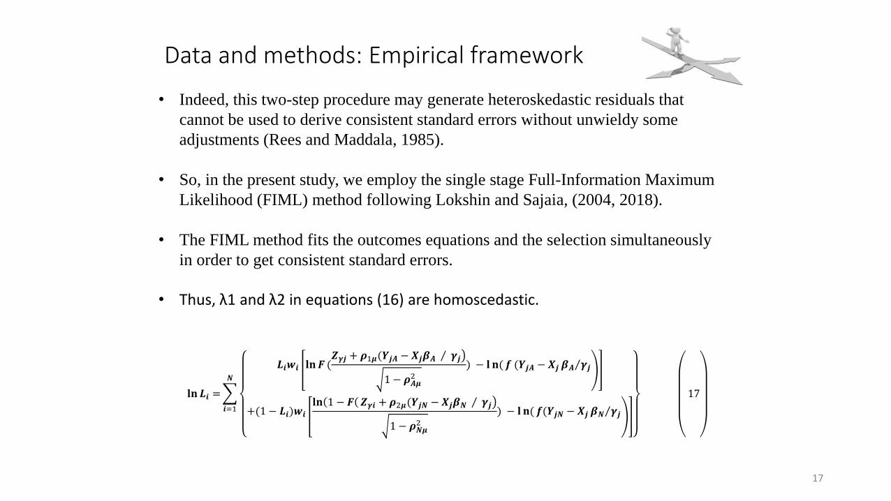
• Indeed, this two-step procedure may generate heteroskedastic residuals that

cannot be used to derive consistent standard errors without unwieldy some

adjustments (Rees and Maddala, 1985).

• So, in the present study, we employ the single stage Full-Information Maximum

Likelihood (FIML) method following Lokshin and Sajaia, (2004, 2018).

• The FIML method fits the outcomes equations and the selection simultaneously

in order to get consistent standard errors.

• Thus, λ1 and λ2 in equations (16) are homoscedastic.

𝐥𝐧 𝑳𝒊 =

𝒊=1

𝑵

𝑳𝒊𝒘𝒊 ቍ𝐥𝐧𝑭 (

൯𝒁𝜸𝒋 + 𝝆1𝝁(𝒀𝒋𝑨 − 𝑿𝒋𝜷𝑨 Τ 𝜸𝒋

1 − 𝝆𝑨𝝁2

) − 𝐥 𝐧( 𝒇 (𝒀𝒋𝑨 − 𝑿𝒋 Τ𝜷𝑨 𝜸𝒋

+(1 − 𝑳𝒊)𝒘𝒊 ቍ

൯𝐥𝐧 1 − 𝑭 𝒁𝜸𝒊 + 𝝆2𝝁(𝒀𝒋𝑵 − 𝑿𝒋𝜷𝑵 Τ 𝜸𝒋

1 − 𝝆𝑵𝝁2

) − 𝐥 𝐧( 𝒇(𝒀𝒋𝑵 − 𝑿𝒋 Τ𝜷𝑵 𝜸𝒋

17


17

Afterwards estimating the model’s parameters, theconditional expectations or expected outcomes and theAverage treatment effect on treated households (ATT) arecomputed as follows:

𝑨𝒅𝒐𝒑𝒕𝒆𝒓𝒔: 𝑬( 𝒀𝑱𝑨|𝑳𝒊 = 𝟏) = 𝒁𝜷𝑱𝑨 + 𝝈𝑨𝝁𝝀𝟏

𝑵𝒐𝒏 𝑨𝒅𝒐𝒑𝒕𝒆𝒓𝒔: 𝑬( 𝒀𝑱𝑵|𝑳𝒊 = 𝟏) = 𝒁𝜷𝑱𝑵 + 𝝈𝑵𝝁𝝀𝟏

(18)

𝑨𝑻𝑻 = 𝑬 𝒀𝒋𝑨 𝑳𝒊 = 𝟏 − 𝑬(𝒀𝑱𝑵|𝑳𝒊 = 𝟏)

𝑨𝑻𝑻 = 𝑬 𝒀𝑱𝑨 − 𝒀𝑱𝑵𝑳𝒊 = 𝟏 = 𝒁𝒋 𝜷𝑨 − 𝜷𝑵 + (𝝈𝑨𝝁 − 𝝈𝑵𝝁)𝝀𝟏

(19)


18

Results and Discussion

19

Table: Socio-economic characteristics of the respondents

Variable Name and descriptionMean in thefull sample(n=518)

Mean in theadopters’ group(n=314)

Mean in non-adopters’ group(n=204)

Age age of head of household (in years) 48,64 48,78 48,44

household sizeNumber of the people livingtogether in the same house andeating from one pot.

11,19 11,31 11

Total of land cultivated size total area planted (in ha) 8,16 7,83 8,67

Gender sex of the head of household (0 = Woman, 1= Man) 1,93 1,93 1,92

Education number of years of the head of household on the benches (years) 4.02 4,38 3.47

Religionreligion (1 = Christianity, 2 = Islam, 3 = Traditional religion(Animism), 4 = Other (No need to specify)

1,69 1,70 1,67

Wife Number of wives of the household 1,46 1,45 1,48

Farm income Household farm income in Euro 2231.681 2520.163 1787.645

Land ownershipIf the household is the owner of this maize producing land (1 = yesand 0 = no)

0.9324324 0.964 0.8823529

Level of formal educationThe highest level of school attended by the head of household (0=No formal education,1= Primary education,2= Secondaryeducation,3= University education)

0,66 0,71 0,57

Informal educationIf the head of household attend Informal education (0 = Non-formal education, 1 = Qur'anic education, 2 = Literacy, 3 = Other)

0,57 0,60 0,52

Side activity If the head household has a secondary activity (0 = No, 1 = Yes) 0,36 0,31 0,44

Experience in agricultureNumber of the year the head of the household started to farm ingeneral (in years)

24.22 24.14 24.35

MigrationIf the head of household migrated for agricultural purposes (0 =No, 1 = Yes)

0,05 0,04 0,05

Experience of growing maizeNumber of the year the head of household started to cultivatemaize in his farm (in years)

22,67 22,83 22,42

Maize size average total area planted in all for your maize crop (in ha) 4,16 3,87 4,62


20

Figure : Adoption rate of DTM varieties by the municipality

39.38%

34.04%

22.62%

50.57%

31.73%

48.15%

52.63%

60.04%

65.96%

77.38%

49.43%

68.27%

51.85%

47.37%

0.00%

10.00%

20.00%

30.00%

40.00%

50.00%

60.00%

70.00%

80.00%

90.00%

Whole sample Kandi Malanville Bembérékè Savè Kétou Tanguiéta

Non-Adopters Adopters


21

Table : Descriptive statistics of the food security indicators outcome used

Variable Definition MeanStd.Dev.

Min Max

Household Per capita FoodExpenditure

Household Per capita Food Expenditure 47701.3 72378.8 0.26667 1333333

Household Food Diversity ScoreNumber of food groups consumed within during theseven days preceding the survey by a household

2.65058 0.59941 1 3

Household food consumptionscores

Sum of the weighting of each food group multiple bythe number of days of consumption

2.57722 0.69317 1 3

Food insecurity severityexperienced by households

Sum of the score of the nine questions on foodinsecurity experience

5.93243 3.81553 1 10

VariableWhole Study area Non-Adopters Adopters

Underweight or WAZ -0.67 -0.74 -0.58

Stunting or HAZ -1.07 -1.17 -0.97

Wasting or WHZ -0.09 -0.08 -0.00

Table : Descriptive statistics of the nutritional indicators outcome used


22

Tableau : Determinants of productivity(Only significant variables are presented here)

VARIABLES

Maize productivity or yield

Non-Adopter Adopter Selection model

Age of head of household (in years 0.057* (0.032) 0.015 (0.037) -0.052 (0.082)

Square of the Age of the household head -0.001** (0.000) -0.000 (0.000) 0.001 (0.001)

emigration for agricultural purposes 0.235 (0.215) 0.540* (0.297) 0.002 (0.659)

Experience of growing maize (years) 0.005 (0.010) -0.029* (0.016) -0.049* (0.029)

Ownership of the land on which maize is produced 0.289* (0.152) -0.164 (0.330) 1.060** (0.472)

membership in an association or producer's cooperative 0.186 (0.115) 0.241* (0.134) -0.509* (0.280)

Number of poultry holding -0.000***(0.000) -0.000 (0.000) -0.000* (0.000)

Total of farm income 0.000** (0.000) -0.000 (0.000) 0.000*** (0.000)

Number of wagon holding 0.175** (0.087) 0.061 (0.154) -0.373 (0.278)

Maize farm size (ha) 0.027* (0.016) -0.098*** (0.034) 0.008 (0.044)

Use of fertilizer(NPK) 0.317** (0.137) -0.021 (0.209) -0.744* (0.412)

Quantity of fertilizer used (kg) 0.000* (0.000) 0.000*** (0.000) -0.000*** (0.000)

Total farm assets in the household -0.033** (0.014) 0.039** (0.017) -0.036 (0.030)

Distance from house to demonstration farm -0.565*** (0.080)

Distance from house to farm inputs magazine. 0.099*** (0.017)

Constant 4.809*** (0.900) 7.727*** (1.081) 1.581 (2.254)

Wald chi2 121.07***

Log likelihood -720.009

lns0, lns1 -0.501***(0.050) 0.008 (0.040)

r0, r1 -0.246 (0.208) -0.329 (0.218)

σ0, σ1 0.605*** (0.030) 1.008 (0.040)

ρ0, ρ1 -.241*** (0.196) -.318 (0.195)

LR test of indep. eqns. 3.79


23

Tableau : Determinants of household Per capita Food consumption expenditure per year in (US Dollars)(Only significant variables are presented here)

VARIABLEShousehold Per capita Food consumption expenditure per year

in (US Dollars)Non-adopter Adopter selection

Household’s total assets amount -0.00 (0.00) 0.00** (0.00) -0.00 (0.00)Gender 0.03 (0.16) 0.26** (0.11) 0.18 (0.33)Access to agricultural credits 0.20* (0.11) 0.03 (0.05) 0.30 (0.19)Awareness of climate change -0.20 (0.15) 0.13*(0.07) 0.83*** (0.26)Size of the household -0.05*** (0.01) -0.06*** (0.01) 0.04** (0.02)Experience in agriculture 0.01** (0.01) -0.00 (0.00) -0.02 (0.01)Quantity of maize consumed in the household 0.00*** (0.00) 0.00** (0.00) 0.00*** (0.00)Holding of a bank account 0.28** (0.12) 0.25*** (0.06) 0.26 (0.21)Amount of Own financial capital 0.00*** (0.00) 0.00*** (0.00) 0.00 (0.00)Use fertilizers 0.28** (0.12) 0.19***(0.07) -0.58** (0.24)Total maize farm size 0.03*** (0.01) 0.00 (0.01) -0.09*** (0.02)Existence of Health centre -0.20 (0.13) -0.12* (0.07) -0.01 (0.26)The distance of home to Demonstration fields -0.43*** (0.06)The distance of home to Farm inputs shop 0.07*** (0.01)Constant 11.08***(0.32) 11.85*** (0.21) 0.08 (0.74)Wald chi2 143.83***Log-likelihood -427.10008lns0, lns1 -0.636***,-0.878***r0, r1 0.004, 0.811**σ0, σ1 0.529, 0.415ρ0, ρ1 0.004, 0.670***LR test of indep. eqns. chi2(2) = 8.83 Prob > chi2 = 0.0121


24

Tableau : Determinants of Household food consumption score (HFCS)(Only significant variables are presented here)

VARIABLESHousehold food consumption score (HFCS)

Non-adopter Adopter selectTotal Amount of the household assets 0.00*** (0.00) 0.00 (0.00) -0.00 (0.00)Age of household head -0.03*** (0.18) 0.01(0.07) 0.01(0.20)Awareness of climate change -0.51** (0.23) -0.19** (0.08) 0.83*** (0.26)Participation in Migration -0.40 (0.32) 0.29* (0.16) -0.12 (0.44)Household size 0.04* (0.02) -0.00 (0.01) 0.05** (0.02)Number of children dropped from school -0.11*** (0.03) -0.02** (0.01) -0.04 (0.03)Experience in agriculture 0.03*** (0.01) -0.01* (0.00) -0.02* (0.01)Contact with extension services 0.50*** (0.16) 0.08 (0.07) -0.38* (0.20)Quantity of maize consumed in the household -0.00*** (0.00) -0.00 (0.00) 0.00** (0.00)Holding of a bank account -0.58*** (0.19) -0.00 (0.07) 0.39* (0.21)Amount of Own financial capital -0.00*** (0.00) -0.00 (0.00) 0.00 (0.00)Possession of a side activity 0.32** (0.16) 0.01 (0.07) -0.16 (0.19)Existence of Health centre 0.34* (0.20) 0.10 (0.08) 0.01 (0.27)Year of Education 0.03* (0.02) 0.00 (0.01) 0.03 (0.02)Participation in an informal education 0.07 (0.08) -0.10*** 0.04) 0.03 (0.11)Awareness of DTM varieties -0.05 (0.22) 0.15* (0.09) 0.78*** (0.24)The distance of home to Demonstration fields -0.47*** 0.05)The distance of home to Farm inputs shop 0.08*** (0.01)Constant 4.01*** (0.51) 3.84*** (0.26) 0.53 (0.74)Wald chi2 92.52***Log-likelihood -581.65748lns0, lns1 -0.151**,-0.690***r0, r1 -0.331**,0.147σ0, σ1 0.859, .501ρ0, ρ1 -0.319**,0.146LR test of indep. eqns. chi2(2) = 4.37 Prob > chi2 = 0.1127Observations 518


25

Tableau : Determinants of Household Food insecurity severity experienced (HFIES)(Only significant variables are presented here)

VARIABLESHousehold Food insecurity severity experienced (HFIES)

Non- adopter Adopter selection

Gender -0.19 (0.40) -0.61* (0.34) 0.11 (0.34)

Contact with extension services -0.27 (0.25) -0.33* (0.18) -0.39** (0.20)

Possession of a side activity 0.37 (0.25) 0.30* (0.18) -0.07 (0.19)

Year of Education -0.7*** (0.03) 0.02 (0.02) 0.03 (0.02)

Participation in an informal education 0.32** (0.13) 0.03 (0.10) 0.02 (0.11)

Awareness of DTM varieties -0.14 (0.35) 0.26 (0.23) 0.80*** (0.24)

The distance of home to Demonstration fields -0.47*** (0.05)

The distance of home to Farm inputs shop 0.08*** (0.01)

Constant 2.15*** (0.80) 2.24*** (0.68) 0.28 (0.75)

Wald chi2 21.78

Log-likelihood -921.12135

lns0, lns1 0.288***, 0.228***

r0, r1 -0.397**, -0.186

σ0, σ1 1.334, 1.256

ρ0, ρ1 -0.377**, -0.184

LR test of indep. eqns. chi2(2) = 4.86 Prob > chi2 = 0.0879

Observations 518


26

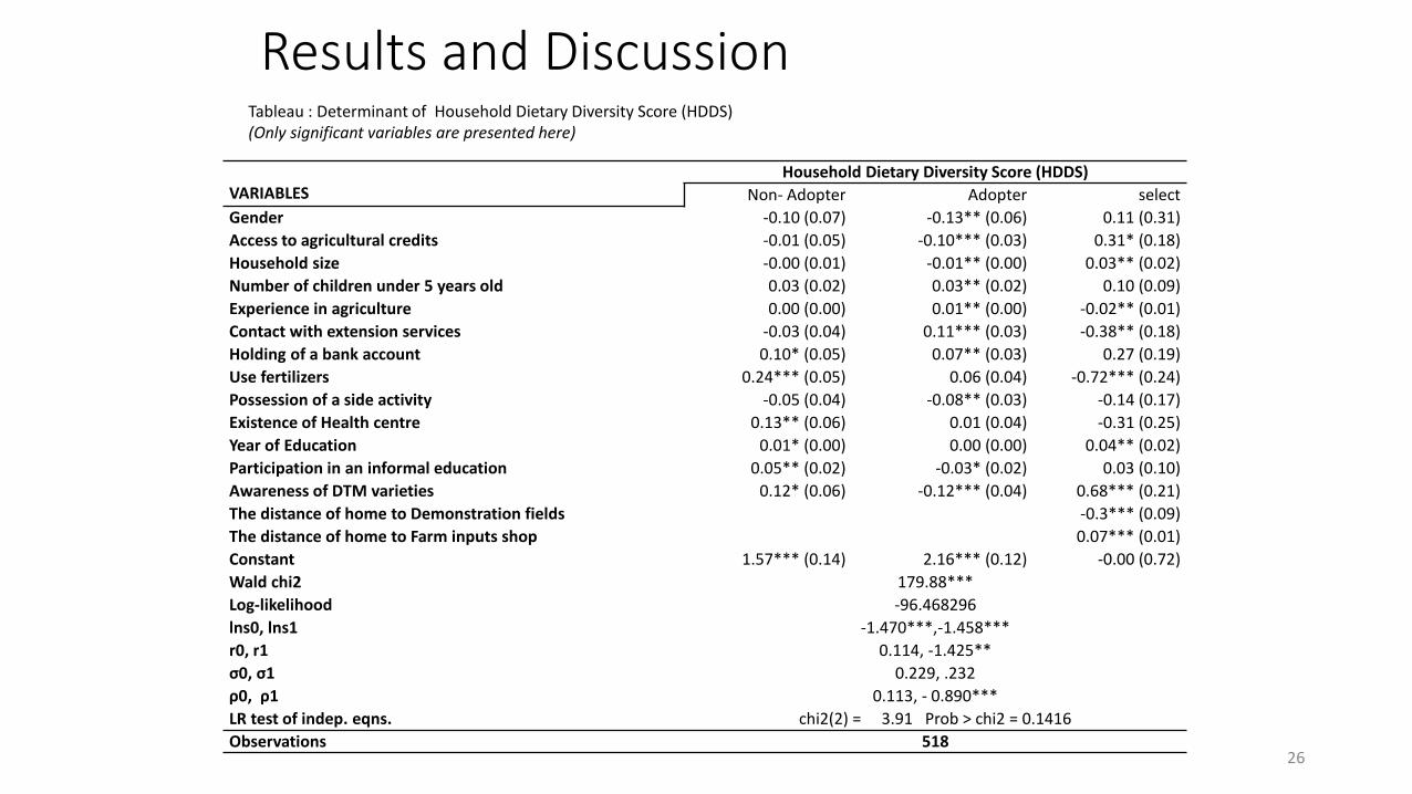
Tableau : Determinant of Household Dietary Diversity Score (HDDS) (Only significant variables are presented here)

VARIABLESHousehold Dietary Diversity Score (HDDS)

Non- Adopter Adopter select

Gender -0.10 (0.07) -0.13** (0.06) 0.11 (0.31)

Access to agricultural credits -0.01 (0.05) -0.10*** (0.03) 0.31* (0.18)

Household size -0.00 (0.01) -0.01** (0.00) 0.03** (0.02)

Number of children under 5 years old 0.03 (0.02) 0.03** (0.02) 0.10 (0.09)

Experience in agriculture 0.00 (0.00) 0.01** (0.00) -0.02** (0.01)

Contact with extension services -0.03 (0.04) 0.11*** (0.03) -0.38** (0.18)

Holding of a bank account 0.10* (0.05) 0.07** (0.03) 0.27 (0.19)

Use fertilizers 0.24*** (0.05) 0.06 (0.04) -0.72*** (0.24)

Possession of a side activity -0.05 (0.04) -0.08** (0.03) -0.14 (0.17)

Existence of Health centre 0.13** (0.06) 0.01 (0.04) -0.31 (0.25)

Year of Education 0.01* (0.00) 0.00 (0.00) 0.04** (0.02)

Participation in an informal education 0.05** (0.02) -0.03* (0.02) 0.03 (0.10)

Awareness of DTM varieties 0.12* (0.06) -0.12*** (0.04) 0.68*** (0.21)

The distance of home to Demonstration fields -0.3*** (0.09)

The distance of home to Farm inputs shop 0.07*** (0.01)

Constant 1.57*** (0.14) 2.16*** (0.12) -0.00 (0.72)

Wald chi2 179.88***

Log-likelihood -96.468296

lns0, lns1 -1.470***,-1.458***

r0, r1 0.114, -1.425**

σ0, σ1 0.229, .232

ρ0, ρ1 0.113, - 0.890***

LR test of indep. eqns. chi2(2) = 3.91 Prob > chi2 = 0.1416

Observations 518


27

Tableau : Determinant of body index (Only significant variables are presented here)

VARIABLES Children body index Adopter Non-Adopter selection

Age of children in the household -0.02(0.01) -0.03***(0.01) -0.02 (0.02)

Square of age of the household head 0.00(0.00) 0.00***(0.00) -0.00(0.00)

Access to agricultural credits 0.29(0.23) -0.90***(0.34) -0.12(0.40)

Contact with extension services 0.11(0.27) 1.49***(0.36) -0.75*(0.44)

Own financial capital 0.87**(0.38) 1.25***(0.36) 0.10(0.61)

Year of Education -0.04(0.03) 0.10***(0.04) 0.04(0.05)Total maize farm size -0.02(0.02) -0.14***(0.03) 0.01(0.04)Participation in maize market 0.29(0.26) 0.73**(0.31) -0.11(0.41)Awareness of DTM varieties -0.66*(0.36) -1.11**(0.45) 0.14(0.56)Awareness of climate change 0.61*(0.36) 2.40***(0.53) 0.97(0.62)Existence of Health centre 0.33(0.31) -1.42***(0.41) -0.30(0.52)

Household completed secondary school -0.04(0.41) 1.94***(0.58) -0.69(0.77)

The distance of home to Demonstration fields -0.60***(0.12)

The distance of home to Farm inputs shop 0.08***(0.03)

Constant -0.71(0.61) -2.47***(0.95) 2.78**(1.41)

Wald chi2 21.51*Log-likelihood -189.86072lns0, lns1 -0.3200635**, -0.0232575r0, r1 0.6784223 , 0.4055517σ0, σ1 0.7261029* , 0.9770109*ρ0, ρ1 0.5904928** , 0.3846892LR test of indep. eqns. chi2(1) = 4.26 Prob > chi2 = 0.0390Observations 122


28

Tableau : Impact of DTM adoption on the food security in farming household in Benin (Only significant variables are presented here)

Outcomes

Decision of Adoption of DTM varieties ATT ATT in %

To adopt To not adopt

Maize productivity (grain yield of maize). 6.92 6.89 0.04 0.52

Household Per capita expenditure 5.22 4.63 0.58*** 11.19

Household Food expenditure per capita 73.26 84.46 -11.2*** -15.29

Household Food Insecurity Access Scale 6.16 3.02 3.14 50.93

households Dietary Diversity score 2.78 2.46 0.32*** 11.55

Household Food Diversity Score 2.68 2.51 0.16*** 6.14

Children Body index 4.63 5.22 0.59*** 12.74

Conclusion• By conducting our study on the impact of Drought tolerant

maize (DTM) varieties adoption on household productivity,food security and Nutritional status in Benin, we contribute tothe existing literature on climate smart innovations.

• For this purpose, we have based our analysis on estimations ofthe Treatment Effect (ATT) method for adoption DTM varietieson productivity and household welfare indicators measured bytotal expenditure, consumption expenditure and food securityand nutritional status.

• To control selection bias, we have applied econometrictechniques on our data from a field survey of rural farmhouseholds in Benin

29

Conclusion

• Omitted the indicator of Household Food Insecurity AccessExperience score, the significant contribution to all the otherindicators of food security and household nutritional status inBenin of the adoption of DTM varieties,

• This suggested the need to undertake additional actions toensure that the positive effects on productivity translate intoan increase in the share of maize harvests reserved forconsumption likely to undergo agri-food processing for betterhousehold nutrition in the area of our study.

• Thus, it would be beneficial that beyond the availabilitydimension of food security, in our study area that policies toreduce food insecurity also focus on nutritional security

30

Recommandations and scope for next step• Even though our study has shown that poor rural farmers

with limited resources through the adoption of DTM varietiesthat generate benefits on household welfare, the adoption ofinnovation being a dynamic process.

• Envision that future research involving panel data to studythe long-term effects of innovations led by farmers.

• Finally, it would also be interesting to extend this research onthe impact of DTM varieties on the children intake energy inthe same study area also on the nutritional status on womenin the same household in Benin using innovative technologies

31

Thank you for your attention!

32

Documents

Adoption and impact of climate-smart innovation on