Embed Size (px)
Citation preview

ADJUSTMENT COMPUTATIONS
Adjustment Computations: Spatial Data Analysis, Fourth Edition. C. D. Ghilani and P. R. Wolf© 2006 John Wiley & Sons, Inc. ISBN: 978-0-471-69728-2
ADJUSTMENTCOMPUTATIONSSpatial Data Analysis
Fourth Edition
CHARLES D. GHILANI, Ph.D.Professor of EngineeringSurveying Engineering ProgramPennsylvania State University
PAUL R. WOLF, Ph.D.Professor EmeritusDepartment of Civil and Environmental EngineeringUniversity of Wisconsin–Madison
JOHN WILEY & SONS, INC.
This book is printed on acid-free paper. ��
Copyright � 2006 by John Wiley & Sons, Inc. All rights reserved.
Published by John Wiley & Sons, Inc., Hoboken, New JerseyPublished simultaneously in Canada.
No part of this publication may be reproduced, stored in a retrieval system, or transmitted inany form or by any means, electronic, mechanical, photocopying, recording, scanning, orotherwise, except as permitted under Section 107 or 108 of the 1976 United States CopyrightAct, without either the prior written permission of the Publisher, or authorization throughpayment of the appropriate per-copy fee to the Copyright Clearance Center, Inc., 222Rosewood Drive, Danvers, MA 01923, (978) 750-8400, fax (978) 750-4470, or on the web atwww.copyright.com. Requests to the Publisher for permission should be addressed to thePermissions Department, John Wiley & Sons, Inc., 111 River Street, Hoboken, NJ 07030, (201)748-6011, fax (201) 748-6008, or online at http: / /www.wiley.com/go /permission.
Limit of Liability /Disclaimer of Warranty: While the publisher and author have used their bestefforts in preparing this book, they make no representations or warranties with respect to theaccuracy or completeness of the contents of this book and specifically disclaim any impliedwarranties of merchantability or fitness for a particular purpose. No warranty may be created orextended by sales representatives or written sales materials. The advice and strategies containedherein may not be suitable for your situation. You should consult with a professional whereappropriate. Neither the publisher nor author shall be liable for any loss of profit or any othercommercial damages, including but not limited to special, incidental, consequential, or otherdamages.
For general information on our other products and services or for technical support, pleasecontact our Customer Care Department within the United States at (800) 762-2974, outside theUnited States at (317) 572-3993 or fax (317) 572-4002.
Wiley also publishes its books in a variety of electronic formats. Some content that appears inprint may not be available in electronic books. For more information about Wiley products,visit our web site at www.wiley.com.
Library of Congress Cataloging-in-Publication Data:Ghilani, Charles D.
Adjustment computations : spatial data analysis / Charles D. Ghilani, PaulR. Wolf.—4th ed.
p. cm.Prev. ed. entered under Wolf.ISBN-13 978-0-471-69728-2 (cloth)ISBN-10 0-471-69728-1 (cloth)
1. Surveying—Mathematics. 2. Spatial analysis (Statistics) I. Wolf, PaulR. II. Title.
TA556.M38W65 2006526.9—dc22
2005028948
Printed in the United States of America
10 9 8 7 6 5 4 3 2 1
v
CONTENTS
PREFACE xix
ACKNOWLEDGMENTS xxiii
1 INTRODUCTION 1
1.1 Introduction / 11.2 Direct and Indirect Measurements / 21.3 Measurement Error Sources / 21.4 Definitions / 31.5 Precision versus Accuracy / 41.6 Redundant Measurements in Surveying and Their
Adjustment / 71.7 Advantages of Least Squares Adjustment / 81.8 Overview of the Book / 10Problems / 10
2 OBSERVATIONS AND THEIR ANALYSIS 12
2.1 Introduction / 122.2 Sample versus Population / 122.3 Range and Median / 132.4 Graphical Representation of Data / 142.5 Numerical Methods of Describing Data / 172.6 Measures of Central Tendency / 172.7 Additional Definitions / 18
vi CONTENTS
2.8 Alternative Formula for Determining Variance / 212.9 Numerical Examples / 232.10 Derivation of the Sample Variance (Bessel’s
Correction) / 282.11 Programming / 29Problems / 30
3 RANDOM ERROR THEORY 33
3.1 Introduction / 333.2 Theory of Probability / 333.3 Properties of the Normal Distribution Curve / 363.4 Standard Normal Distribution Function / 383.5 Probability of the Standard Error / 41
3.5.1 50% Probable Error / 423.5.2 95% Probable Error / 423.5.3 Other Percent Probable Errors / 43
3.6 Uses for Percent Errors / 433.7 Practical Examples / 44Problems / 47
4 CONFIDENCE INTERVALS 50
4.1 Introduction / 504.2 Distributions Used in Sampling Theory / 52
4.2.1 �2 Distribution / 524.2.2 t (Student) Distribution / 544.2.3 F Distribution / 55
4.3 Confidence Interval for the Mean: t Statistic / 564.4 Testing the Validity of the Confidence Interval / 594.5 Selecting a Sample Size / 604.6 Confidence Interval for a Population Variance / 614.7 Confidence Interval for the Ratio of Two Population
Variances / 63Problems / 65
5 STATISTICAL TESTING 68
5.1 Hypothesis Testing / 685.2 Systematic Development of a Test / 715.3 Test of Hypothesis for the Population Mean / 725.4 Test of Hypothesis for the Population Variance / 74

CONTENTS vii
5.5 Test of Hypothesis for the Ratio of Two PopulationVariances / 77
Problems / 81
6 PROPAGATION OF RANDOM ERRORS IN INDIRECTLYMEASURED QUANTITIES 84
6.1 Basic Error Propagation Equation / 846.1.1 Generic Example / 88
6.2 Frequently Encountered Specific Functions / 886.2.1 Standard Deviation of a Sum / 886.2.2 Standard Deviation in a Series / 896.2.3 Standard Deviation of the Mean / 89
6.3 Numerical Examples / 896.4 Conclusions / 94Problems / 95
7 ERROR PROPAGATION IN ANGLE AND DISTANCEOBSERVATIONS 99
7.1 Introduction / 997.2 Error Sources in Horizontal Angles / 997.3 Reading Errors / 100
7.3.1 Angles Observed by the RepetitionMethod / 100
7.3.2 Angles Observed by the DirectionalMethod / 101
7.4 Pointing Errors / 1027.5 Estimated Pointing and Reading Errors with Total
Stations / 1037.6 Target Centering Errors / 1047.7 Instrument Centering Errors / 1067.8 Effects of Leveling Errors in Angle Observations / 1107.9 Numerical Example of Combined Error Propagation in
a Single Horizontal Angle / 1127.10 Use of Estimated Errors to Check Angular Misclosure
in a Traverse / 1147.11 Errors in Astronomical Observations for an
Azimuth / 1167.12 Errors in Electronic Distance Observations / 1217.13 Use of Computational Software / 123Problems / 123
viii CONTENTS
8 ERROR PROPAGATION IN TRAVERSE SURVEYS 127
8.1 Introduction / 1278.2 Derivation of Estimated Error in Latitude and
Departure / 1288.3 Derivation of Estimated Standard Errors in Course
Azimuths / 1298.4 Computing and Analyzing Polygon Traverse Misclosure
Errors / 1308.5 Computing and Analyzing Link Traverse Misclosure
Errors / 1358.6 Conclusions / 140Problems / 140
9 ERROR PROPAGATION IN ELEVATION DETERMINATION 144
9.1 Introduction / 1449.2 Systematic Errors in Differential Leveling / 144
9.2.1 Collimation Error / 1449.2.2 Earth Curvature and Refraction / 1469.2.3 Combined Effects of Systematic Errors on
Elevation Differences / 1479.3 Random Errors in Differential Leveling / 148
9.3.1 Reading Errors / 1489.3.2 Instrument Leveling Errors / 1489.3.3 Rod Plumbing Error / 1489.3.4 Estimated Errors in Differential
Leveling / 1509.4 Error Propagation in Trigonometric Leveling / 152Problems / 156
10 WEIGHTS OF OBSERVATIONS 159
10.1 Introduction / 15910.2 Weighted Mean / 16110.3 Relation between Weights and Standard Errors / 16310.4 Statistics of Weighted Observations / 164
10.4.1 Standard Deviation / 16410.4.2 Standard Error of Weight w and Standard
Error of the Weighted Mean / 16410.5 Weights in Angle Observations / 16510.6 Weights in Differential Leveling / 166

CONTENTS ix
10.7 Practical Examples / 167Problems / 170
11 PRINCIPLES OF LEAST SQUARES 173
11.1 Introduction / 17311.2 Fundamental Principle of Least Squares / 17411.3 Fundamental Principle of Weighted Least Squares / 17611.4 Stochastic Model / 17711.5 Functional Model / 17711.6 Observation Equations / 179
11.6.1 Elementary Example of Observation EquationAdjustment / 179
11.7 Systematic Formulation of the Normal Equations / 18111.7.1 Equal-Weight Case / 18111.7.2 Weighted Case / 18311.7.3 Advantages of the Systematic Approach / 184
11.8 Tabular Formation of the Normal Equations / 18411.9 Using Matrices to Form the Normal Equations / 185
11.9.1 Equal-Weight Case / 18511.9.2 Weighted Case / 187
11.10 Least Squares Solution of Nonlinear Systems / 18811.11 Least Squares Fit of Points to a Line or Curve / 191
11.11.1 Fitting Data to a Straight Line / 19211.11.2 Fitting Data to a Parabola / 194
11.12 Calibration of an EDM Instrument / 19511.13 Least Squares Adjustment Using Conditional
Equations / 19611.14 Example 11.5 Using Observation Equations / 198Problems / 200
12 ADJUSTMENT OF LEVEL NETS 205
12.1 Introduction / 20512.2 Observation Equation / 20512.3 Unweighted Example / 20612.4 Weighted Example / 20912.5 Reference Standard Deviation / 211
12.5.1 Unweighted Example / 21212.5.2 Weighted Example / 213
x CONTENTS
12.6 Another Weighted Adjustment / 213Problems / 216
13 PRECISION OF INDIRECTLY DETERMINED QUANTITIES 221
13.1 Introduction / 22113.2 Development of the Covariance Matrix / 22113.3 Numerical Examples / 22513.4 Standard Deviations of Computed Quantities / 226Problems / 229
14 ADJUSTMENT OF HORIZONTAL SURVEYS: TRILATERATION 233
14.1 Introduction / 23314.2 Distance Observation Equation / 23514.3 Trilateration Adjustment Example / 23714.4 Formulation of a Generalized Coefficient Matrix for a
More Complex Network / 24314.5 Computer Solution of a Trilaterated Quadrilateral / 24414.6 Iteration Termination / 248
14.6.1 Method of Maximum Iterations / 24914.6.2 Maximum Correction / 24914.6.3 Monitoring the Adjustment’s Reference
Variance / 249Problems / 250
15 ADJUSTMENT OF HORIZONTAL SURVEYS: TRIANGULATION 255
15.1 Introduction / 25515.2 Azimuth Observation Equation / 255
15.2.1 Linearization of the Azimuth ObservationEquation / 256
15.3 Angle Observation Equation / 25815.4 Adjustment of Intersections / 26015.5 Adjustment of Resections / 265
15.5.1 Computing Initial Approximations in theResection Problem / 266
15.6 Adjustment of Triangulated Quadrilaterals / 271Problems / 275
CONTENTS xi
16 ADJUSTMENT OF HORIZONTAL SURVEYS: TRAVERSESAND NETWORKS 283
16.1 Introduction to Traverse Adjustments / 28316.2 Observation Equations / 28316.3 Redundant Equations / 28416.4 Numerical Example / 28516.5 Minimum Amount of Control / 29116.6 Adjustment of Networks / 29116.7 �2 Test: Goodness of Fit / 300Problems / 301
17 ADJUSTMENT OF GPS NETWORKS 310
17.1 Introduction / 31017.2 GPS Observations / 31117.3 GPS Errors and the Need for Adjustment / 31417.4 Reference Coordinate Systems for GPS
Observations / 31417.5 Converting between the Terrestrial and Geodetic
Coordinate Systems / 31617.6 Application of Least Squares in Processing GPS
Data / 32117.7 Network Preadjustment Data Analysis / 322
17.7.1 Analysis of Fixed Baseline Measurements / 32217.7.2 Analysis of Repeat Baseline Measurements / 32417.7.3 Analysis of Loop Closures / 32517.7.4 Minimally Constrained Adjustment / 326
17.8 Least Squares Adjustment of GPS Networks / 327Problems / 332
18 COORDINATE TRANSFORMATIONS 345
18.1 Introduction / 34518.2 Two-Dimensional Conformal Coordinate
Transformation / 34518.3 Equation Development / 34618.4 Application of Least Squares / 34818.5 Two-Dimensional Affine Coordinate Transformation / 35018.6 Two-Dimensional Projective Coordinate
Transformation / 353
xii CONTENTS
18.7 Three-Dimensional Conformal CoordinateTransformation / 356
18.8 Statistically Valid Parameters / 362Problems / 364
19 ERROR ELLIPSE 369
19.1 Introduction / 36919.2 Computation of Ellipse Orientation and Semiaxes / 37119.3 Example Problem of Standard Error Ellipse
Calculations / 37619.3.1 Error Ellipse for Station Wisconsin / 37619.3.2 Error Ellipse for Station Campus / 37719.3.3 Drawing the Standard Error Ellipse / 378
19.4 Another Example Problem / 37819.5 Error Ellipse Confidence Level / 37919.6 Error Ellipse Advantages / 381
19.6.1 Survey Network Design / 38119.6.2 Example Network / 383
19.7 Other Measures of Station Uncertainty / 385Problems / 386
20 CONSTRAINT EQUATIONS 388
20.1 Introduction / 38820.2 Adjustment of Control Station Coordinates / 38820.3 Holding Control Station Coordinates and Directions of
Lines Fixed in a Trilateration Adjustment / 39420.3.1 Holding the Direction of a Line Fixed by
Elimination of Constraints / 39520.4 Helmert’s Method / 39820.5 Redundancies in a Constrained Adjustment / 40320.6 Enforcing Constraints through Weighting / 403Problems / 406
21 BLUNDER DETECTION IN HORIZONTAL NETWORKS 409
21.1 Introduction / 40921.2 A Priori Methods for Detecting Blunders in
Observations / 41021.2.1 Use of the K Matrix / 41021.2.2 Traverse Closure Checks / 411
CONTENTS xiii
21.3 A Posteriori Blunder Detection / 41221.4 Development of the Covariance Matrix for the
Residuals / 41421.5 Detection of Outliers in Observations / 41621.6 Techniques Used in Adjusting Control / 41821.7 Data Set with Blunders / 42021.8 Some Further Considerations / 428
21.8.1 Internal Reliability / 42921.8.2 External Reliability / 429
21.9 Survey Design / 430Problems / 432
22 GENERAL LEAST SQUARES METHOD AND ITS APPLICATIONTO CURVE FITTING AND COORDINATETRANSFORMATIONS 437
22.1 Introduction to General Least Squares / 43722.2 General Least Squares Equations for Fitting a Straight
Line / 43722.3 General Least Squares Solution / 43922.4 Two-Dimensional Coordinate Transformation by General
Least Squares / 44322.4.1 Two-Dimensional Conformal Coordinate
Transformation / 44422.4.2 Two-Dimensional Affine Coordinate
Transformation / 44722.4.3 Two-Dimensional Projective Transformation / 448
22.5 Three-Dimensional Conformal Coordinate Transformationby General Least Squares / 449
Problems / 451
23 THREE-DIMENSIONAL GEODETIC NETWORK ADJUSTMENT 454
23.1 Introduction / 45423.2 Linearization of Equations / 456
23.2.1 Slant Distance Observations / 45723.2.2 Azimuth Observations / 45723.2.3 Vertical Angle Observations / 45923.2.4 Horizontal Angle Observations / 45923.2.5 Differential Leveling Observations / 46023.2.6 Horizontal Distance Observations / 460
xiv CONTENTS
23.3 Minimum Number of Constraints / 46223.4 Example Adjustment / 462
23.4.1 Addition of Slant Distances / 46423.4.2 Addition of Horizontal Angles / 46523.4.3 Addition of Zenith Angles / 46623.4.4 Addition of Observed Azimuths / 46723.4.5 Addition of Elevation Differences / 46723.4.6 Adjustment of Control Stations / 46823.4.7 Results of Adjustment / 46923.4.8 Updating Geodetic Coordinates / 469
23.5 Building an Adjustment / 47123.6 Comments on Systematic Errors / 471Problems / 474
24 COMBINING GPS AND TERRESTRIAL OBSERVATIONS 478
24.1 Introduction / 47824.2 Helmert Transformation / 48024.3 Rotations between Coordinate Systems / 48424.4 Combining GPS Baseline Vectors with Traditional
Observations / 48424.5 Other Considerations / 489Problems / 489
25 ANALYSIS OF ADJUSTMENTS 492
25.1 Introduction / 49225.2 Basic Concepts, Residuals, and the Normal
Distribution / 49225.3 Goodness-of-Fit Test / 49625.4 Comparison of Residual Plots / 49925.5 Use of Statistical Blunder Detection / 501Problems / 502
26 COMPUTER OPTIMIZATION 504
26.1 Introduction / 50426.2 Storage Optimization / 50426.3 Direct Formation of the Normal Equations / 50726.4 Cholesky Decomposition / 50826.5 Forward and Back Solutions / 511
CONTENTS xv
26.6 Using the Cholesky Factor to Find the Inverse of theNormal Matrix / 512
26.7 Spareness and Optimization of the Normal Matrix / 513Problems / 518
APPENDIX A INTRODUCTION TO MATRICES 520
A.1 Introduction / 520A.2 Definition of a Matrix / 520A.3 Size or Dimensions of a Matrix / 521A.4 Types of Matrices / 522A.5 Matrix Equality / 523A.6 Addition or Subtraction of Matrices / 524A.7 Scalar Multiplication of a Matrix / 524A.8 Matrix Multiplication / 525A.9 Computer Algorithms for Matrix Operations / 528
A.9.1 Addition or Subtraction of TwoMatrices / 528
A.9.2 Matrix Multiplication / 529A.10 Use of the MATRIX Software / 531Problems / 531
APPENDIX B SOLUTION OF EQUATIONS BY MATRIX METHODS 534
B.1 Introduction / 534B.2 Inverse Matrix / 534B.3 Inverse of a 2 � 2 Matrix / 535B.4 Inverses by Adjoints / 537B.5 Inverses by Row Transformations / 538B.6 Example Problem / 542Problems / 543
APPENDIX C NONLINEAR EQUATIONS AND TAYLOR’STHEOREM 546
C.1 Introduction / 546C.2 Taylor Series Linearization of Nonlinear
Equations / 546C.3 Numerical Example / 547C.4 Using Matrices to Solve Nonlinear
Equations / 549
xvi CONTENTS
C.5 Simple Matrix Example / 550C.6 Practical Example / 551Problems / 554
APPENDIX D NORMAL ERROR DISTRIBUTION CURVE ANDOTHER STATISTICAL TABLES 556
D.1 Development of the Normal Distribution CurveEquation / 556
D.2 Other Statistical Tables / 564D.2.1 �2 Distribution / 564D.2.2 t Distribution / 566D.2.3 F Distribution / 568
APPENDIX E CONFIDENCE INTERVALS FOR THE MEAN 576
APPENDIX F MAP PROJECTION COORDINATE SYSTEMS 582
F.1 Introduction / 582F.2 Mathematics of the Lambert Conformal Conic
Map Projection / 583F.2.1 Zone Constants / 584F.2.2 Direct Problem / 585F.2.3 Inverse Problem / 585
F.3 Mathematics of the Transverse Mercator / 586F.3.1 Zone Constants / 587F.3.2 Direct Problem / 588F.3.3 Inverse Problem / 588
F.4 Reduction of Observations / 590F.4.1 Reduction of Distances / 590F.4.2 Reduction of Geodetic Azimuths / 593
APPENDIX G COMPANION CD 595
G.1 Introduction / 595G.2 File Formats and Memory Matters / 596G.3 Software / 596
G.3.1 ADJUST / 596G.3.2 STATS / 597G.3.3 MATRIX / 598G.3.4 Mathcad Worksheets / 598

CONTENTS xvii
G.4 Using the Software as an InstructionalAid / 599
BIBLIOGRAPHY 600
INDEX 603
xix
PREFACE
No measurement is ever exact. As a corollary, every measurement containserror. These statements are fundamental and universally accepted. It followslogically, therefore, that surveyors, who are measurement specialists, shouldhave a thorough understanding of errors. They must be familiar with thedifferent types of errors, their sources, and their expected magnitudes. Armedwith this knowledge they will be able to (1) adopt procedures for reducingerror sizes when making their measurements and (2) account rigorously forthe presence of errors as they analyze and adjust their measured data. Thisbook is devoted to creating a better understanding of these topics.
In recent years, the least squares method of adjusting spatial data has beenrapidly gaining popularity as the method used for analyzing and adjustingsurveying data. This should not be surprising, because the method is the mostrigorous adjustment procedure available. It is soundly based on the mathe-matical theory of probability; it allows for appropriate weighting of all ob-servations in accordance with their expected precisions; and it enablescomplete statistical analyses to be made following adjustments so that theexpected precisions of adjusted quantities can be determined. Procedures foremploying the method of least squares and then statistically analyzing theresults are major topics covered in this book.
In years past, least squares was seldom used for adjusting surveying databecause the time required to set up and solve the necessary equations wastoo great for hand methods. Now computers have eliminated that disadvan-tage. Besides advances in computer technology, some other recent develop-ments have also led to increased use of least squares. Prominent among theseare the global positioning system (GPS) and geographic information systemsand land information systems (GISs and LISs). These systems rely heavily
xx PREFACE
on rigorous adjustment of data and statistical analysis of the results. Butperhaps the most compelling of all reasons for the recent increased interestin least squares adjustment is that new accuracy standards for surveys arebeing developed that are based on quantities obtained from least squares ad-justments. Thus, surveyors of the future will not be able to test their mea-surements for compliance with these standards unless they adjust their datausing least squares. Clearly, modern surveyors must be able to apply themethod of least squares to adjust their measured data, and they must also beable to perform a statistical evaluation of the results after making theadjustments.
This book originated in 1968 as a set of lecture notes for a course taughtto a group of practicing surveyors in the San Francisco Bay area by ProfessorPaul R. Wolf. The notes were subsequently bound and used as the text forformal courses in adjustment computations taught at both the University ofCalifornia–Berkeley and the University of Wisconsin–Madison. In 1980, asecond edition was produced that incorporated many changes and suggestionsfrom students and others who had used the notes. The second edition, pub-lished by Landmark Enterprises, has been distributed widely to practicingsurveyors and has also been used as a textbook for adjustment computationscourses in several colleges and universities.
For the fourth edition, new chapters on the three-dimensional geodeticnetwork adjustments, combining GPS baseline vectors and terrestrial obser-vations in an adjustment, the Helmert transformation, analysis of adjustments,and state plane coordinate computations are added. These are in keeping withthe modern survey firm that collects data in three dimensions and needs toanalyze large data sets. Additionally, Chapter 4 of the third edition has beendivided into two new chapters on confidence intervals and statistical testing.This edition has greatly expanded and modified the number of problems foreach chapter to provide readers with ample practice problems. For instructorswho adopt this book in their classes, a Solutions Manual to Accompany Ad-justment Computations is also available from the publisher.
Two new appendixes have been added, including one on map projectioncoordinate systems and another on the companion CD. The software includedon the CD for this book has also been greatly expanded and updated. AMathcad electronic book added to the companion CD demonstrates the com-putations for many of the example problems in the text. To obtain a greaterunderstanding of the material contained in this text, these electronic work-sheets allow the reader to explore the intermediate computations in moredetail. For readers not having the Mathcad software package, hypertextmarkup language (html) files are included on the CD for browsing.
The software STATS, ADJUST, and MATRIX are now Windows-based andwill run on a PC-compatible computer. The first package, called STATS, per-forms basic statistical analyses. For any given set of measured data, it willcompute the mean, median, mode, and standard deviation, and develop andplot the histogram and normal distribution curve. The second package, called
PREFACE xxi
ADJUST, contains programs for performing specific least-squares adjust-ments. Level nets, horizontal surveys (trilateration, triangulation, traverses,and horizontal network surveys), GPS networks, and traditional three-dimensional surveys can be adjusted using software in this package. It alsocontains programs to compute the least-squares solution for a variety of co-ordinate transformations, and to determine the least squares fit of a line, pa-rabola, or circle to a set of data points. Each of these programs computesresiduals and standard deviations following the adjustment. The third programpackage, called MATRIX, performs a collection of basic matrix operations,such as addition, subtraction, transpose, multiplication, inverse, and more.Using this program, systems of simultaneous linear equations can be solvedquickly and conveniently, and the basic algorithm for doing least squaresadjustments can be solved in a stepwise fashion. For those who wish to de-velop their own software, the book provides several helpful computer algo-rithms in the languages of BASIC, C, FORTRAN, and PASCAL. Additionally,the Mathcad worksheets demonstrate the use of functions in developing mod-ular programs.
This current edition now consists of 26 chapters and several appendixes.The chapters are arranged in the order found most convenient in teachingcollege courses on adjustment computations. It is believed that this order alsobest facilitates practicing surveyors who use the book for self-study. In earlierchapters we define terms and introduce students to the fundamentals of errorsand methods for analyzing them. The next several chapters are devoted to thesubject of error propagation in the various types of traditional surveying mea-surements. Then chapters follow that describe observation weighting and in-troduce the least-squares method for adjusting observations. Application ofleast squares in adjusting basic types of surveys are then presented in separatechapters. Adjustment of level nets, trilateration, triangulation, traverses, andhorizontal networks, GPS networks, and traditional three-dimensional surveysare included. The subject of error ellipses is covered in a separate chapter.Procedures for applying least squares in curve fitting and in computing co-ordinate transformations are also presented. The more advanced topics ofblunder detection, the method of general least squares, and computer optim-ization are covered in the last chapters.
As with previous editions, matrix methods, which are so well adapted toadjustment computations, continue to be used in this edition. For those stu-dents who have never studied matrices, or those who wish to review thistopic, an introduction to matrix methods is given in Appendixes A and B.Those students who have already studied matrices can conveniently skip thissubject.
Least-squares adjustments often require the formation and solution of non-linear equations. Procedures for linearizing nonlinear equations by Taylor’stheorem are therefore important in adjustment computations, and this topic ispresented in Appendix C. Appendix D contains several statistical tables in-cluding the standard normal error distribution, the �2 distribution, Student’s t

xxii PREFACE
distribution, and a set of F-distribution tables. These tables are described atappropriate locations in the text, and their use is demonstrated with exampleproblems.
Basic courses in statistics and calculus are necessary prerequisites to un-derstanding some of the theoretical coverage and equation derivations givenherein. Nevertheless, those who do not have these courses as background butwho wish to learn how to apply least squares in adjusting surveying obser-vations can study Chapters 1 through 3, skip Chapters 4 through 8, and thenproceed with the remaining chapters.
Besides being appropriate for use as a textbook in college classes, thisbook will be of value to practicing surveyors and geospatial information man-agers. The authors hope that through the publication of this book, leastsquares adjustment and rigorous statistical analyses of surveying data willbecome more commonplace, as they should.
xxiii
ACKNOWLEDGMENTS
Through the years many people have contributed to the development of thisbook. As noted in the preface, the book has been used in continuing educationclasses taught to practicing surveyors as well as in classes taken by studentsat the University of California–Berkeley, the University of Wisconsin–Madison, and the Pennsylvania State University–Wilkes-Barre. The studentsin these classes have provided data for many of the example problems andhave supplied numerous helpful suggestions for improvements throughout thebook. The authors gratefully acknowledge their contributions.
Earlier editions of the book benefited specifically from the contributionsof Mr. Joseph Dracup of the National Geodetic Survey, Professor HaroldWelch of the University of Michigan, Professor Sandor Veress of the Uni-versity of Washington, Mr. Charles Schwarz of the National Geodetic Survey,Mr. Earl Burkholder of the New Mexico State University, Dr. Herbert Stough-ton of Metropolitan State College, Dr. Joshua Greenfeld of New Jersey In-stitute of Technology, Dr. Steve Johnson of Purdue University, Mr. BrianNaberezny of Pennsylvania State University, and Professor David Mezera ofthe University of Wisconsin–Madison. The suggestions and contributions ofthese people were extremely valuable and are very much appreciated.
To improve future editions, the author will gratefully accept any construc-tive criticisms of this edition and suggestions for its improvement.

1
CHAPTER 1
INTRODUCTION
1.1 INTRODUCTION
We currently live in what is often termed the information age. Aided by newand emerging technologies, data are being collected at unprecedented rates inall walks of life. For example, in the field of surveying, total station instru-ments, global positioning system (GPS) equipment, digital metric cameras,and satellite imaging systems are only some of the new instruments that arenow available for rapid generation of vast quantities of measured data.
Geographic Information Systems (GISs) have evolved concurrently withthe development of these new data acquisition instruments. GISs are nowused extensively for management, planning, and design. They are being ap-plied worldwide at all levels of government, in business and industry, bypublic utilities, and in private engineering and surveying offices. Implemen-tation of a GIS depends upon large quantities of data from a variety ofsources, many of them consisting of observations made with the new instru-ments, such as those noted above.
Before data can be utilized, however, whether for surveying and mappingprojects, for engineering design, or for use in a geographic information sys-tem, they must be processed. One of the most important aspects of this is toaccount for the fact that no measurements are exact. That is, they alwayscontain errors.
The steps involved in accounting for the existence of errors in measure-ments consist of (1) performing statistical analyses of the observations toassess the magnitudes of their errors and to study their distributions to deter-mine whether or not they are within acceptable tolerances; and if the obser-vations are acceptable, (2) adjusting them so that they conform to exact
Adjustment Computations: Spatial Data Analysis, Fourth Edition. C. D. Ghilani and P. R. Wolf© 2006 John Wiley & Sons, Inc. ISBN: 978-0-471-69728-2
2 INTRODUCTION
geometric conditions or other required constraints. Procedures for performingthese two steps in processing measured data are principal subjects of thisbook.
1.2 DIRECT AND INDIRECT MEASUREMENTS
Measurements are defined as observations made to determine unknown quan-tities. They may be classified as either direct or indirect. Direct measurementsare made by applying an instrument directly to the unknown quantity andobserving its value, usually by reading it directly from graduated scales onthe device. Determining the distance between two points by making a directmeasurement using a graduated tape, or measuring an angle by making adirect observation from the graduated circle of a theodolite or total stationinstrument, are examples of direct measurements.
Indirect measurements are obtained when it is not possible or practical tomake direct measurements. In such cases the quantity desired is determinedfrom its mathematical relationship to direct measurements. Surveyors may,for example, measure angles and lengths of lines between points directly anduse these measurements to compute station coordinates. From these coordi-nate values, other distances and angles that were not measured directly maybe derived indirectly by computation. During this procedure, the errors thatwere present in the original direct observations are propagated (distributed)by the computational process into the indirect values. Thus, the indirect mea-surements (computed station coordinates, distances, and angles) contain errorsthat are functions of the original errors. This distribution of errors is knownas error propagation. The analysis of how errors propagate is also a principaltopic of this book.
1.3 MEASUREMENT ERROR SOURCES
It can be stated unconditionally that (1) no measurement is exact, (2) everymeasurement contains errors, (3) the true value of a measurement is neverknown, and thus (4) the exact sizes of the errors present are always unknown.These facts can be illustrated by the following. If an angle is measured witha scale divided into degrees, its value can be read only to perhaps the nearesttenth of a degree. If a better scale graduated in minutes were available andread under magnification, however, the same angle might be estimated totenths of a minute. With a scale graduated in seconds, a reading to the nearesttenth of a second might be possible. From the foregoing it should be clearthat no matter how well the observation is taken, a better one may be possible.Obviously, in this example, observational accuracy depends on the divisionsize of the scale. But accuracy depends on many other factors, including theoverall reliability and refinement of the equipment used, environmental con-
1.4 DEFINITIONS 3
ditions that exist when the observations are taken, and human limitations (e.g.,the ability to estimate fractions of a scale division). As better equipment isdeveloped, environmental conditions improve, and observer ability increases,observations will approach their true values more closely, but they can neverbe exact.
By definition, an error is the difference between a measured value for anyquantity and its true value, or
ε � y � � (1.1)
where ε is the error in an observation, y the measured value, and � its truevalue.
As discussed above, errors stem from three sources, which are classifiedas instrumental, natural, and personal:
1. Instrumental errors. These errors are caused by imperfections in instru-ment construction or adjustment. For example, the divisions on atheodolite or total station instrument may not be spaced uniformly.These error sources are present whether the equipment is read manuallyor digitally.
2. Natural errors. These errors are caused by changing conditions in thesurrounding environment, including variations in atmospheric pressure,temperature, wind, gravitational fields, and magnetic fields.
3. Personal errors. These errors arise due to limitations in human senses,such as the ability to read a micrometer or to center a level bubble. Thesizes of these errors are affected by the personal ability to see and bymanual dexterity. These factors may be influenced further by tempera-ture, insects, and other physical conditions that cause humans to behavein a less precise manner than they would under ideal conditions.
1.4 DEFINITIONS
From the discussion thus far, it can be stated with absolute certainty that allmeasured values contain errors, whether due to lack of refinement in readings,instabilities in environmental conditions, instrumental imperfections, or hu-man limitations. Some of these errors result from physical conditions thatcause them to occur in a systematic way, whereas others occur with apparentrandomness. Accordingly, errors are classified as either systematic or random.But before defining systematic and random errors, it is helpful to definemistakes.
1. Mistakes. These are caused by confusion or by an observer’s careless-ness. They are not classified as errors and must be removed from any
4 INTRODUCTION
set of observations. Examples of mistakes include (a) forgetting to setthe proper parts per million (ppm) correction on an EDM instrument,or failure to read the correct air temperature, (b) mistakes in readinggraduated scales, and (c) blunders in recording (i.e., writing down 27.55for 25.75). Mistakes are also known as blunders or gross errors.
2. Systematic errors. These errors follow some physical law, and thus theseerrors can be predicted. Some systematic errors are removed by follow-ing correct measurement procedures (e.g., balancing backsight and fore-sight distances in differential leveling to compensate for Earth curvatureand refraction). Others are removed by deriving corrections based onthe physical conditions that were responsible for their creation (e.g.,applying a computed correction for Earth curvature and refraction on atrigonometric leveling observation). Additional examples of systematicerrors are (a) temperature not being standard while taping, (b) an indexerror of the vertical circle of a theodolite or total station instrument,and (c) use of a level rod that is not of standard length. Corrections forsystematic errors can be computed and applied to observations to elim-inate their effects. Systematic errors are also known as biases.
3. Random errors. These are the errors that remain after all mistakes andsystematic errors have been removed from the measured values. In gen-eral, they are the result of human and instrument imperfections. Theyare generally small and are as likely to be negative as positive. Theyusually do not follow any physical law and therefore must be dealt withaccording to the mathematical laws of probability. Examples of randomerrors are (a) imperfect centering over a point during distance measure-ment with an EDM instrument, (b) bubble not centered at the instant alevel rod is read, and (c) small errors in reading graduated scales. It isimpossible to avoid random errors in measurements entirely. Althoughthey are often called accidental errors, their occurrence should not beconsidered an accident.
1.5 PRECISION VERSUS ACCURACY
Due to errors, repeated observation of the same quantity will often yielddifferent values. A discrepancy is defined as the algebraic difference betweentwo observations of the same quantity. When small discrepancies exist be-tween repeated observations, it is generally believed that only small errorsexist. Thus, the tendency is to give higher credibility to such data and to callthe observations precise. However, precise values are not necessarily accuratevalues. To help understand the difference between precision and accuracy, thefollowing definitions are given:
1. Precision is the degree of consistency between observations based onthe sizes of the discrepancies in a data set. The degree of precision
1.5 PRECISION VERSUS ACCURACY 5
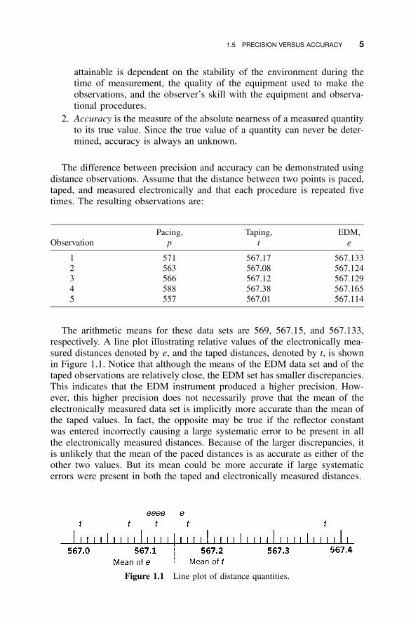
Figure 1.1 Line plot of distance quantities.
attainable is dependent on the stability of the environment during thetime of measurement, the quality of the equipment used to make theobservations, and the observer’s skill with the equipment and observa-tional procedures.
2. Accuracy is the measure of the absolute nearness of a measured quantityto its true value. Since the true value of a quantity can never be deter-mined, accuracy is always an unknown.
The difference between precision and accuracy can be demonstrated usingdistance observations. Assume that the distance between two points is paced,taped, and measured electronically and that each procedure is repeated fivetimes. The resulting observations are:
ObservationPacing,
pTaping,
tEDM,
e
1 571 567.17 567.1332 563 567.08 567.1243 566 567.12 567.1294 588 567.38 567.1655 557 567.01 567.114
The arithmetic means for these data sets are 569, 567.15, and 567.133,respectively. A line plot illustrating relative values of the electronically mea-sured distances denoted by e, and the taped distances, denoted by t, is shownin Figure 1.1. Notice that although the means of the EDM data set and of thetaped observations are relatively close, the EDM set has smaller discrepancies.This indicates that the EDM instrument produced a higher precision. How-ever, this higher precision does not necessarily prove that the mean of theelectronically measured data set is implicitly more accurate than the mean ofthe taped values. In fact, the opposite may be true if the reflector constantwas entered incorrectly causing a large systematic error to be present in allthe electronically measured distances. Because of the larger discrepancies, itis unlikely that the mean of the paced distances is as accurate as either of theother two values. But its mean could be more accurate if large systematicerrors were present in both the taped and electronically measured distances.

6 INTRODUCTION
Figure 1.2 Examples of precision versus accuracy.
Another illustration explaining differences between precision and accuracyinvolves target shooting, depicted in Figure 1.2. As shown, four situationscan occur. If accuracy is considered as closeness of shots to the center of atarget at which a marksman shoots, and precision as the closeness of the shotsto each other, (1) the data may be both precise and accurate, as shown inFigure 1.2(a); (2) the data may produce an accurate mean but not be precise,as shown in Figure 1.2(b); (3) the data may be precise but not accurate, asshown in Figure 1.2(c); or (4) the data may be neither precise nor accurate,as shown in Figure 1.2(d).
Figure 1.2(a) is the desired result when observing quantities. The othercases can be attributed to the following situations. The results shown in Figure1.2(b) occur when there is little refinement in the observational process.Someone skilled at pacing may achieve these results. Figure 1.2(c) generallyoccurs when systematic errors are present in the observational process. Forexample, this can occur in taping if corrections are not made for tape lengthand temperature, or with electronic distance measurements when using thewrong combined instrument–reflector constant. Figure 1.2(d) shows resultsobtained when the observations are not corrected for systematic errors andare taken carelessly by the observer (or the observer is unskilled at the par-ticular measurement procedure).
In general, when making measurements, data such as those shown in Figure1.2(b) and (d) are undesirable. Rather, results similar to those shown in Figure1.2(a) are preferred. However, in making measurements the results of Figure1.2(c) can be just as acceptable if proper steps are taken to correct for thepresence of systematic errors. (This correction would be equivalent to a

1.6 REDUNDANT MEASUREMENTS IN SURVEYING AND THEIR ADJUSTMENT 7
marksman realigning the sights after taking shots.) To make these corrections,(1) the specific types of systematic errors that have occurred in the observa-tions must be known, and (2) the procedures used in correcting them mustbe understood.
1.6 REDUNDANT MEASUREMENTS IN SURVEYING ANDTHEIR ADJUSTMENT
As noted earlier, errors exist in all observations. In surveying, the presenceof errors is obvious in many situations where the observations must meetcertain conditions. For example, in level loops that begin and close on thesame benchmark, the elevation difference for the loop must equal zero. How-ever, in practice, this is hardly ever the case, due to the presence of randomerrors. (For this discussion it is assumed that all mistakes have been elimi-nated from the observations and appropriate corrections have been applied toremove all systematic errors.) Other conditions that disclose errors in survey-ing observations are that (1) the three measured angles in a plane trianglemust total 180�, (2) the sum of the angles measured around the horizon atany point must equal 360�, and (3) the algebraic sum of the latitudes (anddepartures) must equal zero for closed polygon traverses that begin and endon the same station. Many other conditions could be cited; however, in anyof them, the observations rarely, if ever, meet the required conditions, due tothe presence of random errors.
The examples above not only demonstrate that errors are present in sur-veying observations but also the importance of redundant observations; thosemeasurements made that are in excess of the minimum number that areneeded to determine the unknowns. For example, two measurements of thelength of a line yield one redundant observation. The first observation wouldbe sufficient to determine the unknown length, and the second is redundant.However, this second observation is very valuable. First, by examining thediscrepancy between the two values, an assessment of the size of the error inthe observations can be made. If a large discrepancy exists, a blunder or largeerror is likely to have occurred. In that case, measurements of the line wouldbe repeated until two values having an acceptably small discrepancy wereobtained. Second, the redundant observation permits an adjustment to be madeto obtain a final value for the unknown line length, and that final adjustedvalue will be more precise statistically than either of the individual observa-tions. In this case, if the two observations were of equal precision, the adjustedvalue would be the simple mean.
Each of the specific conditions cited in the first paragraph of this sectioninvolves one redundant observation. For example, there is one redundant ob-servation when the three angles of a plane triangle are observed. This is truebecause with two observed angles, say A and B, the third could be computedas C � 180� � A � B, and thus observation of C is unnecessary. However,
8 INTRODUCTION
measuring angle C enables an assessment of the errors in the angles and alsomakes an adjustment possible to obtain final angles with statistically improvedprecisions. Assuming that the angles were of equal precision, the adjustmentwould enforce a 180� sum for the three angles by distributing the total dis-crepancy in equal parts to each angle.
Although the examples cited here are indeed simple, they help to defineredundant measurements and to illustrate their importance. In large surveyingnetworks, the number of redundant observations can become extremely large,and the adjustment process is somewhat more involved than it is for the simpleexamples given here.
Prudent surveyors always make redundant observations in their work, forthe two important reasons indicated above: (1) to make it possible to assesserrors and make decisions regarding acceptance or rejection of observations,and (2) to make possible an adjustment whereby final values with higherprecisions are determined for the unknowns.
1.7 ADVANTAGES OF LEAST SQUARES ADJUSTMENT
As indicated in Section 1.6, in surveying it is recommended that redundantobservations always be made and that adjustments of the observations alwaysbe performed. These adjustments account for the presence of errors in theobservations and increase the precision of the final values computed for theunknowns. When an adjustment is completed, all observations are correctedso that they are consistent throughout the survey network [i.e., the same valuesfor the unknowns are determined no matter which corrected observation(s)are used to compute them].
Many different methods have been derived for making adjustments in sur-veying; however, the method of least squares should be used because it hassignificant advantages over all other rule-of-thumb procedures. The advan-tages of least squares over other methods can be summarized with the fol-lowing four general statements: (1) it is the most rigorous of adjustments; (2)it can be applied with greater ease than other adjustments; (3) it enablesrigorous postadjustment analyses to be made; and (4) it can be used to per-form presurvey planning. These advantages are discussed further below.
Least squares adjustment is rigorously based on the theory of mathematicalprobability, whereas in general, the other methods do not have this rigorousbase. As described later in the book, in a least squares adjustment, the fol-lowing condition of mathematical probability is enforced: The sum of thesquares of the errors times their respective weights is minimized. By enforcingthis condition in any adjustment, the set of errors that is computed has thehighest probability of occurrence. Another aspect of least squares adjustmentthat adds to its rigor is that it permits all observations, regardless of theirnumber or type, to be entered into the adjustment and used simultaneouslyin the computations. Thus, an adjustment can combine distances, horizontal
1.7 ADVANTAGES OF LEAST SQUARES ADJUSTMENT 9
angles, azimuths, zenith or vertical angles, height differences, coordinates,and even GPS observations. One important additional asset of least squaresadjustment is that it enables ‘‘relative weights’’ to be applied to the obser-vations in accordance with their estimated relative reliabilities. These relia-bilities are based on estimated precisions. Thus, if distances were observedin the same survey by pacing, taping, and using an EDM instrument, theycould all be combined in an adjustment by assigning appropriate relativeweights.
Years ago, because of the comparatively heavy computational effort in-volved in least squares, nonrigorous or ‘‘rule-of-thumb’’ adjustments weremost often used. However, now because computers have eliminated the com-puting problem, the reverse is true and least squares adjustments are per-formed more easily than these rule-of-thumb techniques. Least squaresadjustments are less complicated because the same fundamental principles arefollowed regardless of the type of survey or the type of observations. Also,the same basic procedures are used regardless of the geometric figures in-volved (e.g., triangles, closed polygons, quadrilaterals, or more complicatednetworks). On the other hand, rules of thumb are not the same for all typesof surveys (e.g., level nets use one rule and traverses use another), and theyvary for different geometric shapes. Furthermore, the rule of thumb appliedfor a particular survey by one surveyor may be different from that applied byanother surveyor. A favorable characteristic of least squares adjustments isthat there is only one rigorous approach to the procedure, and thus no matterwho performs the adjustment for any particular survey, the same results willbe obtained.
Least squares has the advantage that after an adjustment has been finished,a complete statistical analysis can be made of the results. Based on the sizesand distribution of the errors, various tests can be conducted to determine ifa survey meets acceptable tolerances or whether the observations must berepeated. If blunders exist in the data, these can be detected and eliminated.Least squares enables precisions for the adjusted quantities to be determinedeasily and these precisions can be expressed in terms of error ellipses forclear and lucid depiction. Procedures for accomplishing these tasks are de-scribed in subsequent chapters.
Besides its advantages in adjusting survey data, least squares can be usedto plan surveys. In this application, prior to conducting a needed survey,simulated surveys can be run in a trial-and-error procedure. For any project,an initial trial geometric figure for the survey is selected. Based on the figure,trial observations are either computed or scaled. Relative weights are assignedto the observations in accordance with the precision that can be estimatedusing different combinations of equipment and field procedures. A leastsquares adjustment of this initial network is then performed and the resultsanalyzed. If goals have not been met, the geometry of the figure and theobservation precisions are varied and the adjustment performed again. In thisprocess different types of observations can be used, and observations can be
10 INTRODUCTION
added or deleted. These different combinations of geometric figures and ob-servations are varied until one is achieved that produces either optimum orsatisfactory results. The survey crew can then proceed to the field, confidentthat if the project is conducted according to the design, satisfactory resultswill be obtained. This technique of applying least squares in survey planningis discussed in later chapters.
1.8 OVERVIEW OF THE BOOK
In the remainder of the book the interrelationship between observational errorsand their adjustment is explored. In Chapters 2 through 5, methods used todetermine the reliability of observations are described. In these chapters, theways that errors of multiple observations tend to be distributed are illustrated,and techniques used to compare the quality of different sets of measuredvalues are examined. In Chapters 6 through 9 and in Chapter 13, methodsused to model error propagation in observed and computed quantities arediscussed. In particular, error sources present in traditional surveying tech-niques are examined, and the ways in which these errors propagate throughoutthe observational and computational processes are explained. In the remainderof the book, the principles of least squares are applied to adjust observationsin accordance with random error theory and techniques used to locate mis-takes in observations are examined.
PROBLEMS
1.1 Describe an example in which directly measured quantities are used toobtain an indirect measurement.
1.2 Identify the direct and indirect measurements used in computing trav-erse station coordinates.
1.3 Explain the difference between systematic and random errors.
1.4 List possible systematic and random errors when measuring:(a) a distance with a tape.(b) a distance with an EDM.(c) an angle with a total station.(d) the difference in elevation using an automatic level.
1.5 List three examples of mistakes that can be made when measuring anangle with total station instruments.
PROBLEMS 11
1.6 Identify each of the following errors as either systematic or random.(a) Reading a level rod.(b) Not holding a level rod plumb.(c) Leveling an automatic leveling instrument.(d) Using a level rod that has one foot removed from the bottom of
the rod.
1.7 In your own words, define the difference between precision andaccuracy.
1.8 Identify each of the following errors according to its source (natural,instrumental, personal):(a) Level rod length.(b) EDM–reflector constant.(c) Air temperature in an EDM observation.(d) Reading a graduation on a level rod.(e) Earth curvature in leveling observations.(f) Horizontal collimation error of an automatic level.
1.9 The calibrated length of a particular line is 400.012 m. A length of400.015 m is obtained using an EDM. What is the error in theobservation?
1.10 In Problem 1.9, if the length observed is 400.007 m, what is the errorin the observation?
1.11 Why do surveyors measure angles using both faces of a total station(i.e., direct and reversed)?
1.12 Give an example of compensating systematic errors in a vertical angleobservation when the angle is measured using both faces of theinstrument.
1.13 What systematic errors exist in taping the length of a line?
1.14 Discuss the importance of making redundant observations in surveying.
1.15 List the advantages of making adjustments by the method of leastsquares.
12
CHAPTER 2
OBSERVATIONS AND THEIR ANALYSIS
2.1 INTRODUCTION
Sets of data can be represented and analyzed using either graphical or nu-merical methods. Simple graphical analyses to depict trends commonly appearin newspapers and on television. A plot of the daily variation of the closingDow Jones industrial average over the past year is an example. A bar chartshowing daily high temperatures over the past month is another. Data canalso be presented in numerical form and be subjected to numerical analysis.As a simple example, instead of using a bar chart, the daily high temperaturescould be tabulated and the mean computed. In surveying, observational datacan also be represented and analyzed either graphically or numerically. Inthis chapter some rudimentary methods for doing so are explored.
2.2 SAMPLE VERSUS POPULATION
Due to time and financial constraints, generally only a small data sample iscollected from a much larger, possibly infinite population. For example, po-litical parties may wish to know the percentage of voters who support theircandidate. It would be prohibitively expensive to query the entire voting pop-ulation to obtain the desired information. Instead, polling agencies select asample subset of voters from the voting population. This is an example ofpopulation sampling.
As another example, suppose that an employer wishes to determine therelative measuring capabilities of two prospective new employees. The can-
Adjustment Computations: Spatial Data Analysis, Fourth Edition. C. D. Ghilani and P. R. Wolf© 2006 John Wiley & Sons, Inc. ISBN: 978-0-471-69728-2
2.3 RANGE AND MEDIAN 13
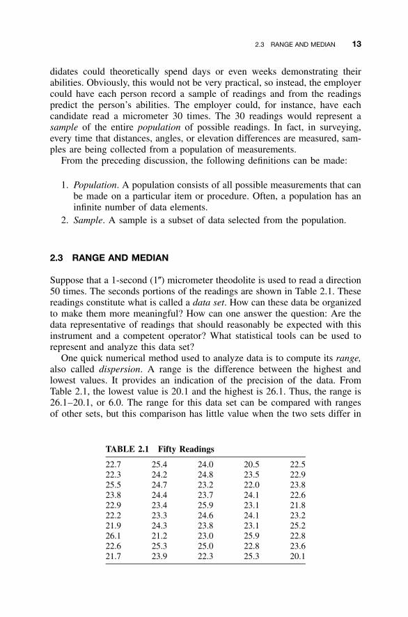
TABLE 2.1 Fifty Readings
22.7 25.4 24.0 20.5 22.522.3 24.2 24.8 23.5 22.925.5 24.7 23.2 22.0 23.823.8 24.4 23.7 24.1 22.622.9 23.4 25.9 23.1 21.822.2 23.3 24.6 24.1 23.221.9 24.3 23.8 23.1 25.226.1 21.2 23.0 25.9 22.822.6 25.3 25.0 22.8 23.621.7 23.9 22.3 25.3 20.1
didates could theoretically spend days or even weeks demonstrating theirabilities. Obviously, this would not be very practical, so instead, the employercould have each person record a sample of readings and from the readingspredict the person’s abilities. The employer could, for instance, have eachcandidate read a micrometer 30 times. The 30 readings would represent asample of the entire population of possible readings. In fact, in surveying,every time that distances, angles, or elevation differences are measured, sam-ples are being collected from a population of measurements.
From the preceding discussion, the following definitions can be made:
1. Population. A population consists of all possible measurements that canbe made on a particular item or procedure. Often, a population has aninfinite number of data elements.
2. Sample. A sample is a subset of data selected from the population.
2.3 RANGE AND MEDIAN
Suppose that a 1-second (1�) micrometer theodolite is used to read a direction50 times. The seconds portions of the readings are shown in Table 2.1. Thesereadings constitute what is called a data set. How can these data be organizedto make them more meaningful? How can one answer the question: Are thedata representative of readings that should reasonably be expected with thisinstrument and a competent operator? What statistical tools can be used torepresent and analyze this data set?
One quick numerical method used to analyze data is to compute its range,also called dispersion. A range is the difference between the highest andlowest values. It provides an indication of the precision of the data. FromTable 2.1, the lowest value is 20.1 and the highest is 26.1. Thus, the range is26.1–20.1, or 6.0. The range for this data set can be compared with rangesof other sets, but this comparison has little value when the two sets differ in
14 OBSERVATIONS AND THEIR ANALYSIS
TABLE 2.2 Arranged Data
20.1 20.5 21.2 21.7 21.821.9 22.0 22.2 22.3 22.322.5 22.6 22.6 22.7 22.822.8 22.9 22.9 23.0 23.123.1 23.2 23.2 23.3 23.423.5 23.6 23.7 23.8 23.823.8 23.9 24.0 24.1 24.124.2 24.3 24.4 24.6 24.724.8 25.0 25.2 25.3 25.325.4 25.5 25.9 25.9 26.1
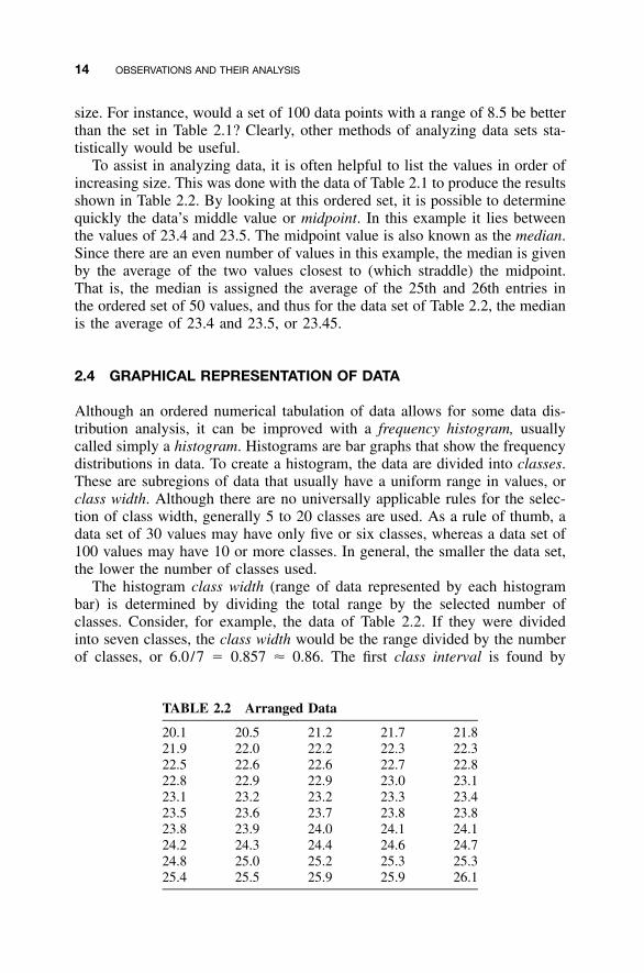
size. For instance, would a set of 100 data points with a range of 8.5 be betterthan the set in Table 2.1? Clearly, other methods of analyzing data sets sta-tistically would be useful.
To assist in analyzing data, it is often helpful to list the values in order ofincreasing size. This was done with the data of Table 2.1 to produce the resultsshown in Table 2.2. By looking at this ordered set, it is possible to determinequickly the data’s middle value or midpoint. In this example it lies betweenthe values of 23.4 and 23.5. The midpoint value is also known as the median.Since there are an even number of values in this example, the median is givenby the average of the two values closest to (which straddle) the midpoint.That is, the median is assigned the average of the 25th and 26th entries inthe ordered set of 50 values, and thus for the data set of Table 2.2, the medianis the average of 23.4 and 23.5, or 23.45.
2.4 GRAPHICAL REPRESENTATION OF DATA
Although an ordered numerical tabulation of data allows for some data dis-tribution analysis, it can be improved with a frequency histogram, usuallycalled simply a histogram. Histograms are bar graphs that show the frequencydistributions in data. To create a histogram, the data are divided into classes.These are subregions of data that usually have a uniform range in values, orclass width. Although there are no universally applicable rules for the selec-tion of class width, generally 5 to 20 classes are used. As a rule of thumb, adata set of 30 values may have only five or six classes, whereas a data set of100 values may have 10 or more classes. In general, the smaller the data set,the lower the number of classes used.
The histogram class width (range of data represented by each histogrambar) is determined by dividing the total range by the selected number ofclasses. Consider, for example, the data of Table 2.2. If they were dividedinto seven classes, the class width would be the range divided by the numberof classes, or 6.0/7 � 0.857 � 0.86. The first class interval is found by
2.4 GRAPHICAL REPRESENTATION OF DATA 15
TABLE 2.3 Frequency Count
(1)Class
Interval
(2)Class
Frequency
(3)Class Relative
Frequency
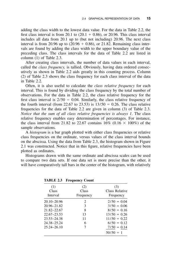
20.10–20.96 2 2/50 � 0.0420.96–21.82 3 3/50 � 0.0621.82–22.67 8 8/50 � 0.1622.67–23.53 13 13/50 � 0.2623.53–24.38 11 11/50 � 0.2224.38–25.24 6 6/50 � 0.1225.24–26.10 7 7/50 � 0.14
50/50 � 1
adding the class width to the lowest data value. For the data in Table 2.2, thefirst class interval is from 20.1 to (20.1 � 0.86), or 20.96. This class intervalincludes all data from 20.1 up to (but not including) 20.96. The next classinterval is from 20.96 up to (20.96 � 0.86), or 21.82. Remaining class inter-vals are found by adding the class width to the upper boundary value of thepreceding class. The class intervals for the data of Table 2.2 are listed incolumn (1) of Table 2.3.
After creating class intervals, the number of data values in each interval,called the class frequency, is tallied. Obviously, having data ordered consec-utively as shown in Table 2.2 aids greatly in this counting process. Column(2) of Table 2.3 shows the class frequency for each class interval of the datain Table 2.2.
Often, it is also useful to calculate the class relative frequency for eachinterval. This is found by dividing the class frequency by the total number ofobservations. For the data in Table 2.2, the class relative frequency for thefirst class interval is 2/50 � 0.04. Similarly, the class relative frequency ofthe fourth interval (from 22.67 to 23.53) is 13/50 � 0.26. The class relativefrequencies for the data of Table 2.2 are given in column (3) of Table 2.3.Notice that the sum of all class relative frequencies is always 1. The classrelative frequency enables easy determination of percentages. For instance,the class interval from 21.82 to 22.67 contains 16% (0.16 � 100%) of thesample observations.
A histogram is a bar graph plotted with either class frequencies or relativeclass frequencies on the ordinate, versus values of the class interval boundson the abscissa. Using the data from Table 2.3, the histogram shown in Figure2.1 was constructed. Notice that in this figure, relative frequencies have beenplotted as ordinates.
Histograms drawn with the same ordinate and abscissa scales can be usedto compare two data sets. If one data set is more precise than the other, itwill have comparatively tall bars in the center of the histogram, with relatively
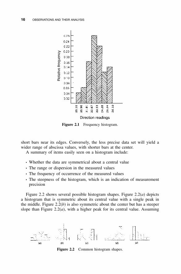
16 OBSERVATIONS AND THEIR ANALYSIS
Figure 2.1 Frequency histogram.
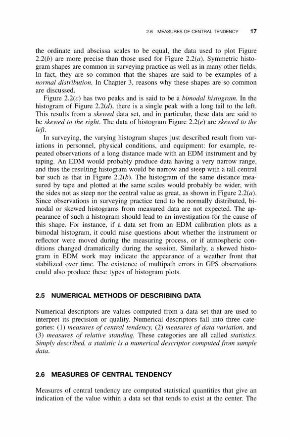
Figure 2.2 Common histogram shapes.
short bars near its edges. Conversely, the less precise data set will yield awider range of abscissa values, with shorter bars at the center.
A summary of items easily seen on a histogram include:
• Whether the data are symmetrical about a central value• The range or dispersion in the measured values• The frequency of occurrence of the measured values• The steepness of the histogram, which is an indication of measurement
precision
Figure 2.2 shows several possible histogram shapes. Figure 2.2(a) depictsa histogram that is symmetric about its central value with a single peak inthe middle. Figure 2.2(b) is also symmetric about the center but has a steeperslope than Figure 2.2(a), with a higher peak for its central value. Assuming
2.6 MEASURES OF CENTRAL TENDENCY 17
the ordinate and abscissa scales to be equal, the data used to plot Figure2.2(b) are more precise than those used for Figure 2.2(a). Symmetric histo-gram shapes are common in surveying practice as well as in many other fields.In fact, they are so common that the shapes are said to be examples of anormal distribution. In Chapter 3, reasons why these shapes are so commonare discussed.
Figure 2.2(c) has two peaks and is said to be a bimodal histogram. In thehistogram of Figure 2.2(d), there is a single peak with a long tail to the left.This results from a skewed data set, and in particular, these data are said tobe skewed to the right. The data of histogram Figure 2.2(e) are skewed to theleft.
In surveying, the varying histogram shapes just described result from var-iations in personnel, physical conditions, and equipment: for example, re-peated observations of a long distance made with an EDM instrument and bytaping. An EDM would probably produce data having a very narrow range,and thus the resulting histogram would be narrow and steep with a tall centralbar such as that in Figure 2.2(b). The histogram of the same distance mea-sured by tape and plotted at the same scales would probably be wider, withthe sides not as steep nor the central value as great, as shown in Figure 2.2(a).Since observations in surveying practice tend to be normally distributed, bi-modal or skewed histograms from measured data are not expected. The ap-pearance of such a histogram should lead to an investigation for the cause ofthis shape. For instance, if a data set from an EDM calibration plots as abimodal histogram, it could raise questions about whether the instrument orreflector were moved during the measuring process, or if atmospheric con-ditions changed dramatically during the session. Similarly, a skewed histo-gram in EDM work may indicate the appearance of a weather front thatstabilized over time. The existence of multipath errors in GPS observationscould also produce these types of histogram plots.
2.5 NUMERICAL METHODS OF DESCRIBING DATA
Numerical descriptors are values computed from a data set that are used tointerpret its precision or quality. Numerical descriptors fall into three cate-gories: (1) measures of central tendency, (2) measures of data variation, and(3) measures of relative standing. These categories are all called statistics.Simply described, a statistic is a numerical descriptor computed from sampledata.
2.6 MEASURES OF CENTRAL TENDENCY
Measures of central tendency are computed statistical quantities that give anindication of the value within a data set that tends to exist at the center. The
18 OBSERVATIONS AND THEIR ANALYSIS
arithmetic mean, the median, and the mode are three such measures. Theyare described as follows:
1. Arithmetic mean. For a set of n observations, y1, y2, . . . , yn, this is theaverage of the observations. Its value, is computed from the equationy,
n� yii�1y � (2.1)n
Typically, the symbol is used to represent a sample’s arithmetic meanyand the symbol � is used to represent the population mean. Otherwise,the same equation applies. Using Equation (2.1), the mean of the ob-servations in Table 2.2 is 23.5.
2. Median. As mentioned previously, this is the midpoint of a sample setwhen arranged in ascending or descending order. One-half of the dataare above the median and one-half are below it. When there are an oddnumber of quantities, only one such value satisfies this condition. Fora data set with an even number of quantities, the average of the twoobservations that straddle the midpoint is used to represent the median.
3. Mode. Within a sample of data, the mode is the most frequently occur-ring value. It is seldom used in surveying because of the relatively smallnumber of values observed in a typical set of observations. In smallsample sets, several different values may occur with the same frequency,and hence the mode can be meaningless as a measure of central ten-dency. The mode for the data in Table 2.2 is 23.8.
2.7 ADDITIONAL DEFINITIONS
Several other terms, which are pertinent to the study of observations and theiranalysis, are listed and defined below.
1. True value, �: a quantity’s theoretically correct or exact value. As notedin Section 1.3, the true value can never be determined.
2. Error, ε: the difference between a measured quantity and its true value.The true value is simply the population’s arithmetic mean. Since thetrue value of a measured quantity is indeterminate, errors are also in-determinate and are therefore only theoretical quantities. As given inEquation (1.1), repeated for convenience here, errors are expressed as
ε � y � � (2.2)i i
where yi is the individual observation associated with εi and � is thetrue value for that quantity.
2.7 ADDITIONAL DEFINITIONS 19
3. Most probable value, that value for a measured quantity which, basedy:on the observations, has the highest probability of occurrence. It isderived from a sample set of data rather than the population and issimply the mean if the repeated measurements have the same precision.
4. Residual, v: The difference between any individual measured quantityand the most probable value for that quantity. Residuals are the valuesthat are used in adjustment computations since most probable valuescan be determined. The term error is frequently used when residual ismeant, and although they are very similar and behave in the same man-ner, there is this theoretical distinction. The mathematical expression fora residual is
v � y � y (2.3)i i
where vi is the residual in the ith observation, yi, and is the mostyprobable value for the unknown.
5. Degrees of freedom: the number of observations that are in excess ofthe number necessary to solve for the unknowns. In other words, thenumber of degrees of freedom equals the number of redundant obser-vations (see Section 1.6). As an example, if a distance between twopoints is measured three times, one observation would determine theunknown distance and the other two would be redundant. These redun-dant observations reveal the discrepancies and inconsistencies in ob-served values. This, in turn, makes possible the practice of adjustmentcomputations for obtaining the most probable values based on the mea-sured quantities.
6. Variance, �2: a value by which the precision for a set of data is given.Population variance applies to a data set consisting of an entire popu-lation. It is the mean of the squares of the errors and is given by
n 2� εii�12� � (2.4)n
Sample variance applies to a sample set of data. It is an unbiasedestimate for the population variance given in Equation (2.4) and is cal-culated as
n 2� vii�12S � (2.5)n � 1
Note that Equations (2.4) and (2.5) are identical except that ε has beenchanged to v and n has been changed to n � 1 in Equation (2.5). The validityof these modifications is demonstrated in Section 2.10.
20 OBSERVATIONS AND THEIR ANALYSIS
It is important to note that the simple algebraic average of all errors in adata set cannot be used as a meaningful precision indicator. This is becauserandom errors are as likely to be positive as negative, and thus the algebraicaverage will equal zero. This fact is shown for a population of data in thefollowing simple proof. Summing Equation (2.2) for n samples gives
n n n n2ε � (y � �) � y � y � n� (a)� � � �i i i i
i�1 i�1 i�1 i�1
Then substituting Equation (2.1) into Equation (a) yields
nn n n n� yii�1ε � y � n � y � y � 0 (b)� � � �i i i ini�1 i�1 i�1 i�1
Similarly, it can be shown that the mean of all residuals of a sample data setequals zero.
7. Standard error, �: the square root of the population variance. FromEquation (2.4) and this definition, the following equation is written forthe standard error:
n 2� εii�1� � (2.6)� n
where n is the number of observations and is the sum of then 2� εii�1
squares of the errors. Note that both the population variance, �2, andthe standard error, �, are indeterminate because true values, and henceerrors, are indeterminate.
As explained in Section 3.5, 68.3% of all observations in a populationdata set lie within �� of the true value, �. Thus, the larger the standarderror, the more dispersed are the values in the data set and the lessprecise is the measurement.
8. Standard deviation, S: the square root of the sample variance. It iscalculated using the expression
n 2� vii�1S � (2.7)� n � 1
where S is the standard deviation, n � 1 the degrees of freedom ornumber of redundancies, and the sum of the squares of then 2� vii�1
residuals. Standard deviation is an estimate for the standard error of thepopulation. Since the standard error cannot be determined, the standarddeviation is a practical expression for the precision of a sample set of
2.8 ALTERNATIVE FORMULA FOR DETERMINING VARIANCE 21
data. Residuals are used rather than errors because they can be calcu-lated from most probable values, whereas errors cannot be determined.Again, as discussed in Section 3.5, for a sample data set, 68.3% of theobservations will theoretically lie between the most probable value plusand minus the standard deviation, S. The meaning of this statement willbe clarified in an example that follows.
9. Standard deviation of the mean: the error in the mean computed froma sample set of measured values that results because all measured valuescontain errors. The standard deviation of the mean is computed fromthe sample standard deviation according to the equation
SS � � (2.8)y �n
Notice that as n → �, then → 0. This illustrates that as the size ofSy
the sample set approaches the total population, the computed mean ywill approach the true mean �. This equation is derived in Chapter 4.
2.8 ALTERNATIVE FORMULA FOR DETERMINING VARIANCE
From the definition of residuals, Equation (2.5) is rewritten as
n 2� (y � y )ii�12S � (2.9)n � 1
Expanding Equation (2.9) yields
12 2 2 2S � [(y � y ) � (y � y ) � � � � � (y � y ) ] (c)1 2 nn � 1
Substituting Equation (2.1) for into Equation (c) and dropping the boundsyfor the summation yields
2 2 21 � y � y � yi i i2S � � y � � y � � � � � � y�� � � � � �1 2 nn � 1 n n n (d)
Expanding Equation (d) gives us
22 OBSERVATIONS AND THEIR ANALYSIS
2 21 � y � y � y � yi i i i2 2S � � 2y � y � � 2y�� � � �1 1 2n � 1 n n n n2� y � yi i2 2� y � � � � � � 2y � y (e)� � 2 n nn n
Rearranging Equation (e) and recognizing that (� yi /n)2 occurs n times inEquation (e) yields
21 � y � yi i2 2 2 2S � n � 2 (y � y � � � � � y ) � y � y � � � � � y� � � 1 2 n 1 2 nn � 1 n n
(ƒ)
Adding the summation symbol to Equation (ƒ) yields
2 21 � y 2i2 2S � n � y � y (g)� �� � � � � i in � 1 n n
Factoring and regrouping similar summations in Equation (g) produces
2 21 2 1 1 12 2 2S � y � � y � y � y� � � �� � �� � � � � i i i in � 1 n n n � 1 n
(h)
Multiplying the last term in Equation (h) by n /n yields
21 � yi2 2S � y � n (i)�� � � in � 1 n
Finally, by substituting Equation (2.1) in Equation (i), the following expres-sion for the variance results:
2 2� y � nyi2S � (2.10)n � 1
Using Equation (2.10), the variance of a sample data set can be computedby subtracting n times the square of the data’s mean from the summation ofthe squared individual observations. With this equation, the variance and thestandard deviation can be computed directly from the data. However, it shouldbe stated that with large numerical values, Equation (2.10) may overwhelma handheld calculator or a computer working in single precision. If this prob-lem should arise, the data should be centered or Equation (2.5) used. Cen-
2.9 NUMERICAL EXAMPLES 23
tering a data set involves subtracting a constant value (usually, the arithmeticmean) from all values in a data set. By doing this, the values are modified toa smaller, more manageable size.
2.9 NUMERICAL EXAMPLES
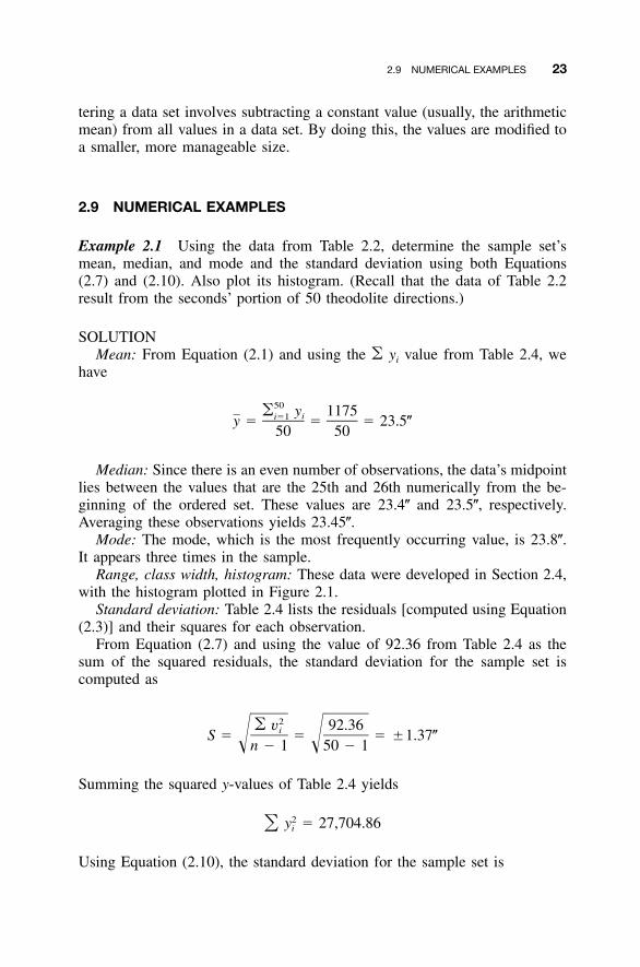
Example 2.1 Using the data from Table 2.2, determine the sample set’smean, median, and mode and the standard deviation using both Equations(2.7) and (2.10). Also plot its histogram. (Recall that the data of Table 2.2result from the seconds’ portion of 50 theodolite directions.)
SOLUTIONMean: From Equation (2.1) and using the � yi value from Table 2.4, we
have
50� y 1175ii�1y � � � 23.5�50 50
Median: Since there is an even number of observations, the data’s midpointlies between the values that are the 25th and 26th numerically from the be-ginning of the ordered set. These values are 23.4� and 23.5�, respectively.Averaging these observations yields 23.45�.
Mode: The mode, which is the most frequently occurring value, is 23.8�.It appears three times in the sample.
Range, class width, histogram: These data were developed in Section 2.4,with the histogram plotted in Figure 2.1.
Standard deviation: Table 2.4 lists the residuals [computed using Equation(2.3)] and their squares for each observation.
From Equation (2.7) and using the value of 92.36 from Table 2.4 as thesum of the squared residuals, the standard deviation for the sample set iscomputed as
2� v 92.36iS � � � �1.37�� �n � 1 50 � 1
Summing the squared y-values of Table 2.4 yields
2y � 27,704.86� i
Using Equation (2.10), the standard deviation for the sample set is
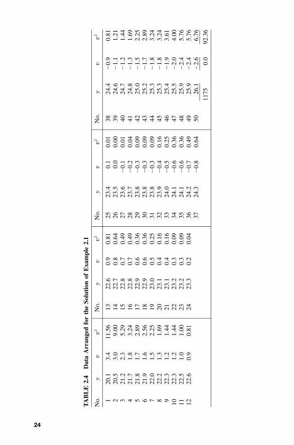
24
TA
BL
E2.
4D
ata
Arr
ange
dfo
rth
eSo
luti
onof
Exa
mpl
e2.
1
No.
yv
v2N
o.y
vv2
No.
yv
v2N
o.y
vv2
1 2 3 4 5 6 7 8 9 10 11 12
20.1
20.5
21.2
21.7
21.8
21.9
22.0
22.2
22.3
22.3
22.5
22.6
3.4
3.0
2.3
1.8
1.7
1.6
1.5
1.3
1.2
1.2
1.0
0.9
11.5
69.
005.
293.
242.
892.
562.
251.
691.
441.
441.
000.
81
13 14 15 16 17 18 19 20 21 22 23 24
22.6
22.7
22.8
22.8
22.9
22.9
23.0
23.1
23.1
23.2
23.2
23.3
0.9
0.8
0.7
0.7
0.6
0.6
0.5
0.4
0.4
0.3
0.3
0.2
0.81
0.64
0.49
0.49
0.36
0.36
0.25
0.16
0.16
0.09
0.09
0.04
25 26 27 28 29 30 31 32 33 34 35 36 37
23.4
23.5
23.6
23.7
23.8
23.8
23.8
23.9
24.0
24.1
24.1
24.2
24.3
0.1
0.0
�0.
1�
0.2
�0.
3�
0.3
�0.
3�
0.4
�0.
5�
0.6
�0.
6�
0.7
�0.
8
0.01
0.00
0.01
0.04
0.09
0.09
0.09
0.16
0.25
0.36
0.36
0.49
0.64
38 39 40 41 42 43 44 45 46 47 48 49 50
24.4
24.6
24.7
24.8
25.0
25.2
25.3
25.3
25.4
25.5
25.9
25.9
26.1
�0.
9�
1.1
�1.
2�
1.3
�1.
5�
1.7
�1.
8�
1.8
�1.
9�
2.0
�2.
4�
2.4
�2.
6
0.81
1.21
1.44
1.69
2.25
2.89
3.24
3.24
3.61
4.00
5.76
5.76
6.76
1175
0.0
92.3
6
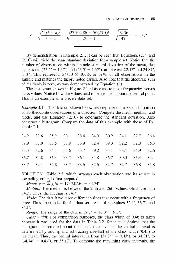
2.9 NUMERICAL EXAMPLES 25
2 2 2� y � ny 27,704.86 � 50(23.5) 92.36iS � � � � �1.37�� � �n � 1 50 � 1 49
By demonstration in Example 2.1, it can be seen that Equations (2.7) and(2.10) will yield the same standard deviation for a sample set. Notice that thenumber of observations within a single standard deviation of the mean, thatis, between (23.5� � 1.37�) and (23.5� � 1.37�), or between 22.13� and 24.87�,is 34. This represents 34/50 � 100%, or 68%, of all observations in thesample and matches the theory noted earlier. Also note that the algebraic sumof residuals is zero, as was demonstrated by Equation (b).
The histogram shown in Figure 2.1 plots class relative frequencies versusclass values. Notice how the values tend to be grouped about the central point.This is an example of a precise data set.
Example 2.2 The data set shown below also represents the seconds’ portionof 50 theodolite observations of a direction. Compute the mean, median, andmode, and use Equation (2.10) to determine the standard deviation. Alsoconstruct a histogram. Compare the data of this example with those of Ex-ample 2.1.
34.2 33.6 35.2 30.1 38.4 34.0 30.2 34.1 37.7 36.4
37.9 33.0 33.5 35.9 35.9 32.4 39.3 32.2 32.8 36.3
35.3 32.6 34.1 35.6 33.7 39.2 35.1 33.4 34.9 32.6
36.7 34.8 36.4 33.7 36.1 34.8 36.7 30.0 35.3 34.4
33.7 34.1 37.8 38.7 33.6 32.6 34.7 34.7 36.8 31.8
SOLUTION Table 2.5, which arranges each observation and its square inascending order, is first prepared.
Mean: � � yi /n � 1737.0/50 � 34.74�yMedian: The median is between the 25th and 26th values, which are both
34.7�. Thus, the median is 34.7�.Mode: The data have three different values that occur with a frequency of
three. Thus, the modes for the data set are the three values 32.6�, 33.7�, and34.1�.
Range: The range of the data is 39.3� � 30.0� � 9.3�.Class width: For comparison purposes, the class width of 0.86 is taken
because it was used for the data in Table 2.2. Since it is desired that thehistogram be centered about the data’s mean value, the central interval isdetermined by adding and subtracting one-half of the class width (0.43) tothe mean. Thus, the central interval is from (34.74� � 0.43�), or 34.31�, to(34.74� � 0.43�), or 35.17�. To compute the remaining class intervals, the
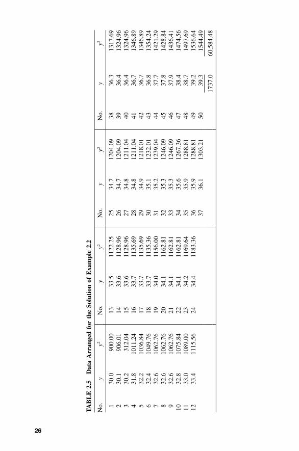
26
TA
BL
E2.
5D
ata
Arr
ange
dfo
rth
eSo
luti
onof
Exa
mpl
e2.
2
No.
yy2
No.
yy2
No.
yy2
No.
yy2
1 2 3 4 5 6 7 8 9 10 11 12
30.0
30.1
30.2
31.8
32.2
32.4
32.6
32.6
32.6
32.8
33.0
33.4
900.
0090
6.01
312.
0410
11.2
410
36.8
410
49.7
610
62.7
610
62.7
610
62.7
610
75.8
410
89.0
011
15.5
6
13 14 15 16 17 18 19 20 21 22 23 24
33.5
33.6
33.6
33.7
33.7
33.7
34.0
34.1
34.1
34.1
34.2
34.4
1122
.25
1128
.96
1128
.96
1135
.69
1135
.69
1135
.36
1156
.00
1162
.81
1162
.81
1162
.81
1169
.64
1183
.36
25 26 27 28 29 30 31 32 33 34 35 36 37
34.7
34.7
34.8
34.8
34.9
35.1
35.2
35.3
35.3
35.6
35.9
35.9
36.1
1204
.09
1204
.09
1211
.04
1211
.04
1218
.01
1232
.01
1239
.04
1246
.09
1246
.09
1267
.36
1288
.81
1288
.81
1303
.21
38 39 40 41 42 43 44 45 46 47 48 49 50
36.3
36.4
36.4
36.7
36.7
36.8
37.7
37.8
37.9
38.4
38.7
39.2
39.3
1317
.69
1324
.96
1324
.96
1346
.89
1346
.89
1354
.24
1421
.29
1428
.84
1436
.41
1474
.56
1497
.69
1536
.64
1544
.49
1737
.060
,584
.48
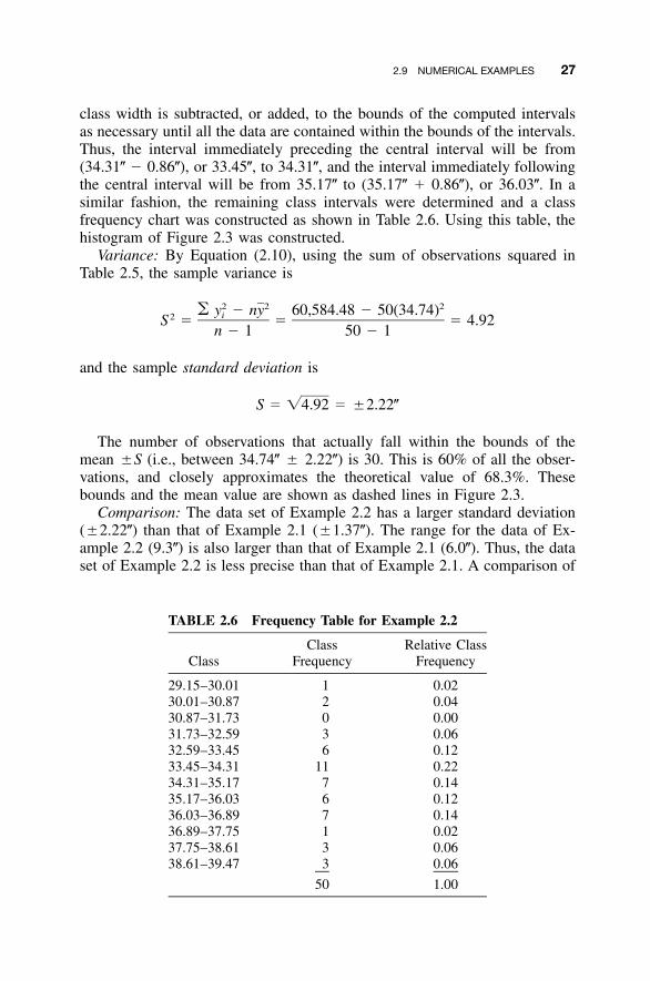
2.9 NUMERICAL EXAMPLES 27
TABLE 2.6 Frequency Table for Example 2.2
ClassClass
FrequencyRelative Class
Frequency
29.15–30.01 1 0.0230.01–30.87 2 0.0430.87–31.73 0 0.0031.73–32.59 3 0.0632.59–33.45 6 0.1233.45–34.31 11 0.2234.31–35.17 7 0.1435.17–36.03 6 0.1236.03–36.89 7 0.1436.89–37.75 1 0.0237.75–38.61 3 0.0638.61–39.47 3 0.06
50 1.00
class width is subtracted, or added, to the bounds of the computed intervalsas necessary until all the data are contained within the bounds of the intervals.Thus, the interval immediately preceding the central interval will be from(34.31� � 0.86�), or 33.45�, to 34.31�, and the interval immediately followingthe central interval will be from 35.17� to (35.17� � 0.86�), or 36.03�. In asimilar fashion, the remaining class intervals were determined and a classfrequency chart was constructed as shown in Table 2.6. Using this table, thehistogram of Figure 2.3 was constructed.
Variance: By Equation (2.10), using the sum of observations squared inTable 2.5, the sample variance is
2 2 2� y � ny 60,584.48 � 50(34.74)i2S � � � 4.92n � 1 50 � 1
and the sample standard deviation is
S � �4.92 � �2.22�
The number of observations that actually fall within the bounds of themean �S (i.e., between 34.74� � 2.22�) is 30. This is 60% of all the obser-vations, and closely approximates the theoretical value of 68.3%. Thesebounds and the mean value are shown as dashed lines in Figure 2.3.
Comparison: The data set of Example 2.2 has a larger standard deviation(�2.22�) than that of Example 2.1 (�1.37�). The range for the data of Ex-ample 2.2 (9.3�) is also larger than that of Example 2.1 (6.0�). Thus, the dataset of Example 2.2 is less precise than that of Example 2.1. A comparison of
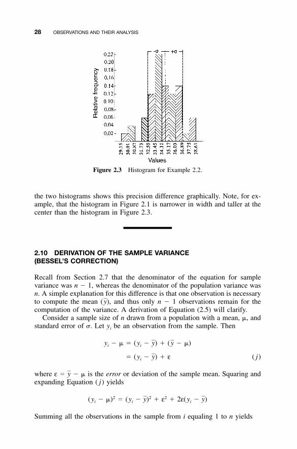
28 OBSERVATIONS AND THEIR ANALYSIS
Figure 2.3 Histogram for Example 2.2.
the two histograms shows this precision difference graphically. Note, for ex-ample, that the histogram in Figure 2.1 is narrower in width and taller at thecenter than the histogram in Figure 2.3.
2.10 DERIVATION OF THE SAMPLE VARIANCE(BESSEL’S CORRECTION)
Recall from Section 2.7 that the denominator of the equation for samplevariance was n � 1, whereas the denominator of the population variance wasn. A simple explanation for this difference is that one observation is necessaryto compute the mean and thus only n � 1 observations remain for the(y),computation of the variance. A derivation of Equation (2.5) will clarify.
Consider a sample size of n drawn from a population with a mean, �, andstandard error of �. Let yi be an observation from the sample. Then
y � � � (y � y) � (y � �)i i
� (y � y) � ε ( j)i
where ε � � � is the error or deviation of the sample mean. Squaring andyexpanding Equation ( j) yields
2 2 2(y � �) � (y � y) � ε � 2ε(y � y)i i i
Summing all the observations in the sample from i equaling 1 to n yields
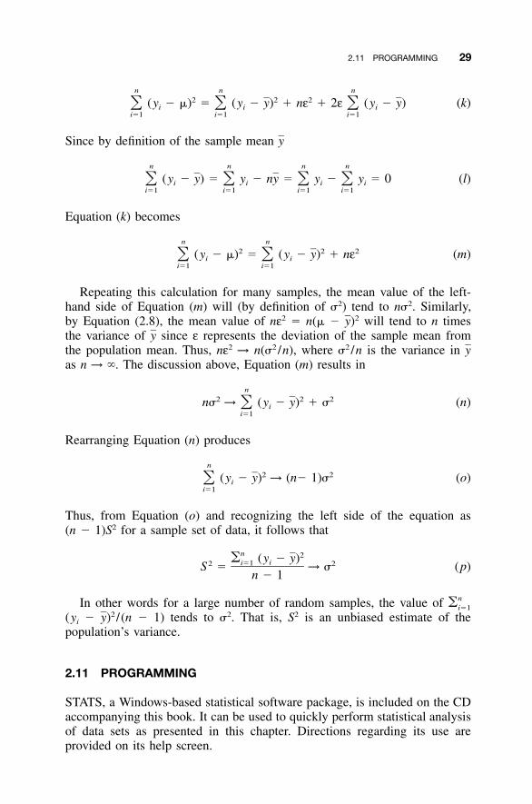
2.11 PROGRAMMING 29
n n n2 2 2(y � �) � (y � y) � nε � 2ε (y � y) (k)� � �i i i
i�1 i�1 i�1
Since by definition of the sample mean y
n n n n
(y � y) � y � ny � y � y � 0 (l)� � � �i i i ii�1 i�1 i�1 i�1
Equation (k) becomes
n n2 2 2(y � �) � (y � y) � nε (m)� �i i
i�1 i�1
Repeating this calculation for many samples, the mean value of the left-hand side of Equation (m) will (by definition of �2) tend to n�2. Similarly,by Equation (2.8), the mean value of nε2 � n(� � will tend to n times2y)the variance of since ε represents the deviation of the sample mean fromythe population mean. Thus, nε2 → n(�2 /n), where �2 /n is the variance in yas n → �. The discussion above, Equation (m) results in
n2 2 2n� → (y � y) � � (n)� i
i�1
Rearranging Equation (n) produces
n2 2(y � y) → (n� 1)� (o)� i
i�1
Thus, from Equation (o) and recognizing the left side of the equation as(n � 1)S2 for a sample set of data, it follows that
n 2� (y � y)ii�12 2S � → � (p)n � 1
In other words for a large number of random samples, the value of n�i�1
(yi � / (n � 1) tends to �2. That is, S2 is an unbiased estimate of the2y)population’s variance.
2.11 PROGRAMMING
STATS, a Windows-based statistical software package, is included on the CDaccompanying this book. It can be used to quickly perform statistical analysisof data sets as presented in this chapter. Directions regarding its use areprovided on its help screen.

30 OBSERVATIONS AND THEIR ANALYSIS
Additionally, an electronic book is provided on the CD accompanying thisbook. To view the electronic book interactively, Mathcad software is required.However, for those of you who do not have a copy of Mathcad, html files ofthe electronic book are included on the CD. The electronic book demonstratesmost of the numerical examples given in the book.
Many chapters include programming problems following the problem setsat the end of the chapters. The electronic book demonstrates the rudimentsof programming these problems. Other programs on the CD include MATRIXand ADJUST. MATRIX can be used to solve problems in the book that in-volve matrices. ADJUST has examples of working least squares adjustmentprograms. ADJUST can be used to check solutions to many of the examplesin the book.
When you select the desired installation options, the installation programprovided on the CD will load the files to your computer. The installationpackage will install each option as the option is selected. This software doesnot remove (uninstall) the packages. This can be done using the ‘‘Add/Re-move programs’’ options in your computer’s control panel.
PROBLEMS
2.1 The optical micrometer of a precise differential level is set and read10 times as 8.801, 8.803, 8.798, 8.801, 8.799, 8.802, 8.802, 8.804,8.800, and 8.802. What value would you assign to the operator’s abilityto set the micrometer on this instrument?
2.2 The seconds’ part of 50 pointings and readings for a particular directionmade using a 1� total station with a 0.1� display are
26.7, 26.4, 24.8, 27.4, 25.8, 27.0, 26.3, 27.8, 26.7, 26.0, 25.9, 25.4,
28.0, 27.2, 25.3, 27.2, 27.0, 27.7, 27.3, 24.8, 26.7, 25.3, 26.9, 25.5,
27.4, 25.4, 25.8, 25.5, 27.4, 27.2, 27.1, 27.4, 26.6, 26.2, 26.3, 25.3,
25.1, 27.3, 27.3, 28.1, 27.4, 27.2, 27.2, 26.4, 28.2, 25.5, 26.5, 25.9,
26.1, 26.3
(a) What is the mean of the data set?(b) Construct a frequency histogram of the data using seven uniform-
width class intervals.(c) What are the variance and standard deviation of the data?(d) What is the standard deviation of the mean?
2.3 An EDM instrument and reflector are set at the ends of a baseline thatis 400.781 m long. Its length is measured 24 times, with the followingresults:
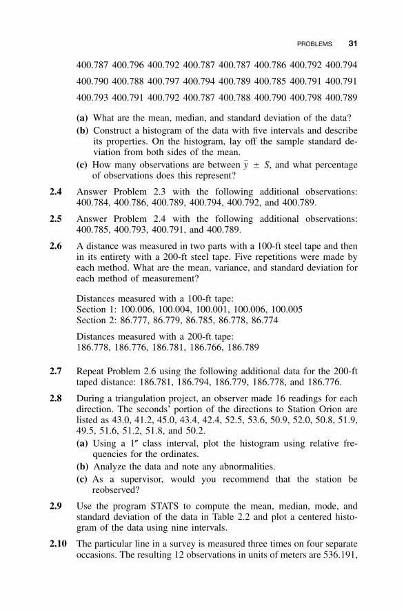
PROBLEMS 31
400.787 400.796 400.792 400.787 400.787 400.786 400.792 400.794
400.790 400.788 400.797 400.794 400.789 400.785 400.791 400.791
400.793 400.791 400.792 400.787 400.788 400.790 400.798 400.789
(a) What are the mean, median, and standard deviation of the data?(b) Construct a histogram of the data with five intervals and describe
its properties. On the histogram, lay off the sample standard de-viation from both sides of the mean.
(c) How many observations are between � S, and what percentageyof observations does this represent?
2.4 Answer Problem 2.3 with the following additional observations:400.784, 400.786, 400.789, 400.794, 400.792, and 400.789.
2.5 Answer Problem 2.4 with the following additional observations:400.785, 400.793, 400.791, and 400.789.
2.6 A distance was measured in two parts with a 100-ft steel tape and thenin its entirety with a 200-ft steel tape. Five repetitions were made byeach method. What are the mean, variance, and standard deviation foreach method of measurement?
Distances measured with a 100-ft tape:Section 1: 100.006, 100.004, 100.001, 100.006, 100.005Section 2: 86.777, 86.779, 86.785, 86.778, 86.774
Distances measured with a 200-ft tape:186.778, 186.776, 186.781, 186.766, 186.789
2.7 Repeat Problem 2.6 using the following additional data for the 200-fttaped distance: 186.781, 186.794, 186.779, 186.778, and 186.776.
2.8 During a triangulation project, an observer made 16 readings for eachdirection. The seconds’ portion of the directions to Station Orion arelisted as 43.0, 41.2, 45.0, 43.4, 42.4, 52.5, 53.6, 50.9, 52.0, 50.8, 51.9,49.5, 51.6, 51.2, 51.8, and 50.2.(a) Using a 1� class interval, plot the histogram using relative fre-
quencies for the ordinates.(b) Analyze the data and note any abnormalities.(c) As a supervisor, would you recommend that the station be
reobserved?
2.9 Use the program STATS to compute the mean, median, mode, andstandard deviation of the data in Table 2.2 and plot a centered histo-gram of the data using nine intervals.
2.10 The particular line in a survey is measured three times on four separateoccasions. The resulting 12 observations in units of meters are 536.191,
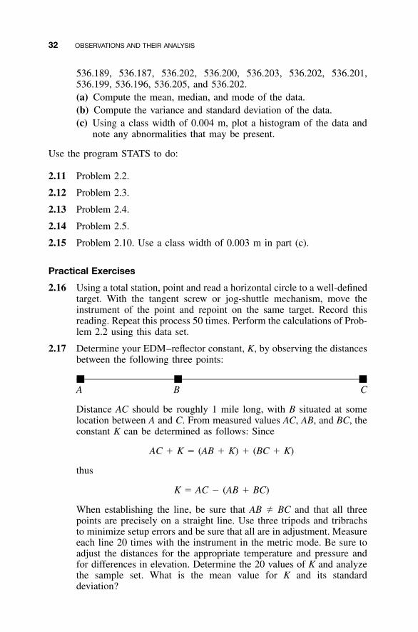
32 OBSERVATIONS AND THEIR ANALYSIS
536.189, 536.187, 536.202, 536.200, 536.203, 536.202, 536.201,536.199, 536.196, 536.205, and 536.202.(a) Compute the mean, median, and mode of the data.(b) Compute the variance and standard deviation of the data.(c) Using a class width of 0.004 m, plot a histogram of the data and
note any abnormalities that may be present.
Use the program STATS to do:
2.11 Problem 2.2.
2.12 Problem 2.3.
2.13 Problem 2.4.
2.14 Problem 2.5.
2.15 Problem 2.10. Use a class width of 0.003 m in part (c).
Practical Exercises
2.16 Using a total station, point and read a horizontal circle to a well-definedtarget. With the tangent screw or jog-shuttle mechanism, move theinstrument of the point and repoint on the same target. Record thisreading. Repeat this process 50 times. Perform the calculations of Prob-lem 2.2 using this data set.
2.17 Determine your EDM–reflector constant, K, by observing the distancesbetween the following three points:
� � �A B C
Distance AC should be roughly 1 mile long, with B situated at somelocation between A and C. From measured values AC, AB, and BC, theconstant K can be determined as follows: Since
AC � K � (AB � K) � (BC � K)
thus
K � AC � (AB � BC)
When establishing the line, be sure that AB � BC and that all threepoints are precisely on a straight line. Use three tripods and tribrachsto minimize setup errors and be sure that all are in adjustment. Measureeach line 20 times with the instrument in the metric mode. Be sure toadjust the distances for the appropriate temperature and pressure andfor differences in elevation. Determine the 20 values of K and analyzethe sample set. What is the mean value for K and its standarddeviation?
33
CHAPTER 3
RANDOM ERROR THEORY
3.1 INTRODUCTION
As noted earlier, the adjustment of measured quantities containing randomerrors is a major concern to people involved in the geospatial sciences. In theremaining chapters it is assumed that all systematic errors have been removedfrom the measured values and that only random errors and blunders (whichhave escaped detection) remain. In this chapter the general theory of randomerrors is developed, and some simple methods that can be used to isolateremaining blunders in sets of data are discussed.
3.2 THEORY OF PROBABILITY
Probability is the ratio of the number of times that an event should occur tothe total number of possibilities. For example, the probability of tossing atwo with a fair die is 1/6 since there are six total possibilities (faces on adie) and only one of these is a two. When an event can occur in m ways andfail to occur in n ways, the probability of its occurrence is m / (m � n), andthe probability of its failure is n / (m � n).
Probability is always a fraction ranging between zero and one. Zero de-notes impossibility, and one indicates certainty. Since an event must eitheroccur or fail to occur, the sum of all probabilities for any event is 1, and thusif 1/6 is the probability of throwing a two with one throw of a die, then 1 �1/6, or 5/6, is the probability that a two will not appear.
In probability terminology, a compound event is the simultaneous occur-rence of two or more independent events. This is the situation encountered
Adjustment Computations: Spatial Data Analysis, Fourth Edition. C. D. Ghilani and P. R. Wolf© 2006 John Wiley & Sons, Inc. ISBN: 978-0-471-69728-2
34 RANDOM ERROR THEORY
most frequently in surveying. For example, random errors from angles anddistances (compound events) cause traverse misclosures. The probability ofthe simultaneous occurrence of two independent events is the product of theirindividual probabilities.
To illustrate this condition, consider the simple example of having twoboxes containing combinations of red and white balls. Box A contains fourballs, one red and three white. Box B contains five balls, two red and threewhite. What is the probability that two red balls would be drawn if one ballis drawn randomly from each box? The total number of possible pairs is 4� 5 (20) since by drawing one ball from box A, any of the five balls in boxB would complete the pair. There are only two ways to draw two red balls;that is, box A’s red ball can be matched with either red ball from box B.Therefore, the probability of obtaining two red balls simultaneously is 2/20.Thus, the probability of this compound event is the product of the individualprobabilities of drawing a red ball from each box, or
P � 1/4 � 2/5 � 2/20
Similarly, the probability of drawing two white balls simultaneously is 3/4� 3/5, or 9/20, and the probability of getting one red ball and one whiteball is 1 � (2/20 � 9/20), or 9/20.
From the foregoing it is seen that the probability of the simultaneous oc-currence of two independent events is the product of the individual probabil-ities of those two events. This principle is extended to include any numberof events:
P � P � P � � � � � P (3.1)1 2 n
where P is the probability of the simultaneous occurrence of events havingindividual probabilities P1, P2, . . . , Pn.
To develop the principle of how random errors occur, consider a verysimple example where a single tape measurement is taken between points Aand B. Assume that this measurement contains a single random error of size1. Since the error is random, there are two possibilities for its value �1 or�1. Let t be the number of ways that each error can occur, and let T be thetotal number of possibilities, which is two. The probability of obtaining �1,which can occur only one way (i.e., t � 1), is t /T or 1/2. This is also theprobability of obtaining �1. Suppose now that in measuring a distance AE,the tape must be placed end to end so that the result depends on the combi-nation of two of these tape measurements. Then the possible error combina-tions in the result are �1 and �1, �1 and �1, �1 and �1, and �1 and �1,with T � 4. The final errors are �2, 0, and �2, and their t values are 1, 2,and 1, respectively. This produces probabilities of 1/4, 1/2, and 1/4, respec-tively. In general, as n, the number of single combined measurements, isincreased, T increases according to the function T � 2n, and thus for three
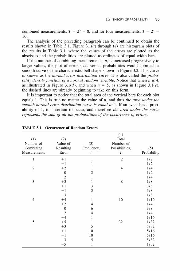
3.2 THEORY OF PROBABILITY 35
TABLE 3.1 Occurrence of Random Errors
(1)Number ofCombining
Measurements
(2)Value ofResulting
Error
(3)Frequency,
t
(4)Total
Number ofPossibilities,
T(5)
Probability
1 �1�1
11
2 1/21/2
2 �20
�2
121
4 1/41/21/4
3 �3�1�1�3
1331
8 1/83/83/81/8
4 �4�2
0�2�4
14641
16 1/161/43/81/41/16
5 �5�3�1�1�3�5
15
1010
51
32 1/325/325/165/165/321/32
combined measurements, T � 23 � 8, and for four measurements, T � 24 �16.
The analysis of the preceding paragraph can be continued to obtain theresults shown in Table 3.1. Figure 3.1(a) through (e) are histogram plots ofthe results in Table 3.1, where the values of the errors are plotted as theabscissas and the probabilities are plotted as ordinates of equal-width bars.
If the number of combining measurements, n, is increased progressively tolarger values, the plot of error sizes versus probabilities would approach asmooth curve of the characteristic bell shape shown in Figure 3.2. This curveis known as the normal error distribution curve. It is also called the proba-bility density function of a normal random variable. Notice that when n is 4,as illustrated in Figure 3.1(d), and when n � 5, as shown in Figure 3.1(e),the dashed lines are already beginning to take on this form.
It is important to notice that the total area of the vertical bars for each plotequals 1. This is true no matter the value of n, and thus the area under thesmooth normal error distribution curve is equal to 1. If an event has a prob-ability of 1, it is certain to occur, and therefore the area under the curverepresents the sum of all the probabilities of the occurrence of errors.
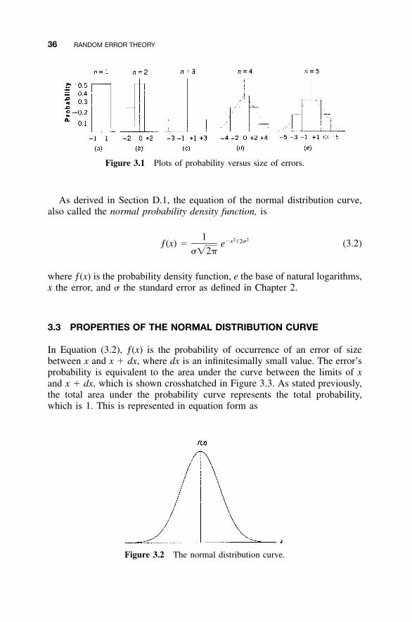
36 RANDOM ERROR THEORY
Figure 3.1 Plots of probability versus size of errors.
Figure 3.2 The normal distribution curve.
As derived in Section D.1, the equation of the normal distribution curve,also called the normal probability density function, is
1 2 2�x / 2�ƒ(x) � e (3.2)��2�
where ƒ(x) is the probability density function, e the base of natural logarithms,x the error, and � the standard error as defined in Chapter 2.
3.3 PROPERTIES OF THE NORMAL DISTRIBUTION CURVE
In Equation (3.2), ƒ(x) is the probability of occurrence of an error of sizebetween x and x � dx, where dx is an infinitesimally small value. The error’sprobability is equivalent to the area under the curve between the limits of xand x � dx, which is shown crosshatched in Figure 3.3. As stated previously,the total area under the probability curve represents the total probability,which is 1. This is represented in equation form as
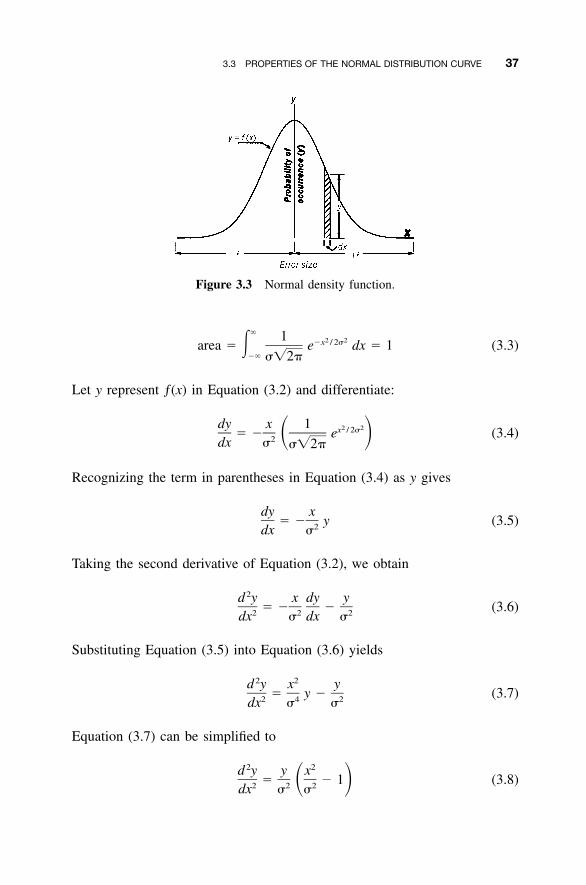
3.3 PROPERTIES OF THE NORMAL DISTRIBUTION CURVE 37
Figure 3.3 Normal density function.
� 1 2 2�x / 2�area � � e dx � 1 (3.3)�� ��2�
Let y represent ƒ(x) in Equation (3.2) and differentiate:
dy x 1 2 2x / 2�� � e (3.4)� �2dx � ��2�
Recognizing the term in parentheses in Equation (3.4) as y gives
dy x� � y (3.5)2dx �
Taking the second derivative of Equation (3.2), we obtain
2d y x dy y� � � (3.6)2 2 2dx � dx �
Substituting Equation (3.5) into Equation (3.6) yields
2 2d y x y� y � (3.7)2 4 2dx � �
Equation (3.7) can be simplified to
2 2d y y x� � 1 (3.8)� �2 2 2dx � �
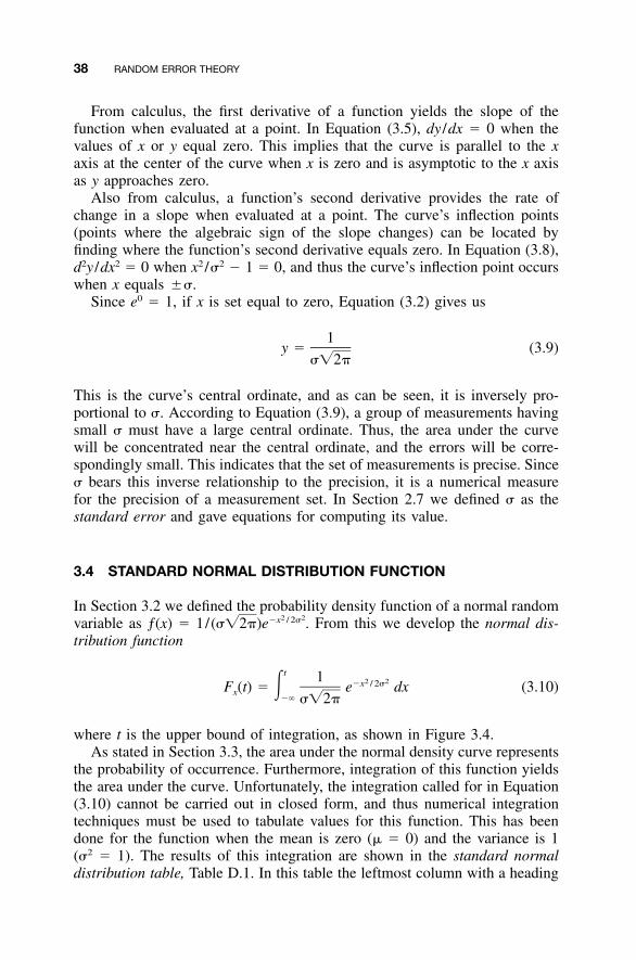
38 RANDOM ERROR THEORY
From calculus, the first derivative of a function yields the slope of thefunction when evaluated at a point. In Equation (3.5), dy /dx � 0 when thevalues of x or y equal zero. This implies that the curve is parallel to the xaxis at the center of the curve when x is zero and is asymptotic to the x axisas y approaches zero.
Also from calculus, a function’s second derivative provides the rate ofchange in a slope when evaluated at a point. The curve’s inflection points(points where the algebraic sign of the slope changes) can be located byfinding where the function’s second derivative equals zero. In Equation (3.8),d2y /dx2 � 0 when x2 /�2 � 1 � 0, and thus the curve’s inflection point occurswhen x equals ��.
Since e0 � 1, if x is set equal to zero, Equation (3.2) gives us
1y � (3.9)
��2�
This is the curve’s central ordinate, and as can be seen, it is inversely pro-portional to �. According to Equation (3.9), a group of measurements havingsmall � must have a large central ordinate. Thus, the area under the curvewill be concentrated near the central ordinate, and the errors will be corre-spondingly small. This indicates that the set of measurements is precise. Since� bears this inverse relationship to the precision, it is a numerical measurefor the precision of a measurement set. In Section 2.7 we defined � as thestandard error and gave equations for computing its value.
3.4 STANDARD NORMAL DISTRIBUTION FUNCTION
In Section 3.2 we defined the probability density function of a normal randomvariable as ƒ(x) � 1/ From this we develop the normal dis-2 2�x / 2�(��2�)e .tribution function
t 1 2 2�x / 2�F (t) � � e dx (3.10)x�� ��2�
where t is the upper bound of integration, as shown in Figure 3.4.As stated in Section 3.3, the area under the normal density curve represents
the probability of occurrence. Furthermore, integration of this function yieldsthe area under the curve. Unfortunately, the integration called for in Equation(3.10) cannot be carried out in closed form, and thus numerical integrationtechniques must be used to tabulate values for this function. This has beendone for the function when the mean is zero (� � 0) and the variance is 1(�2 � 1). The results of this integration are shown in the standard normaldistribution table, Table D.1. In this table the leftmost column with a heading
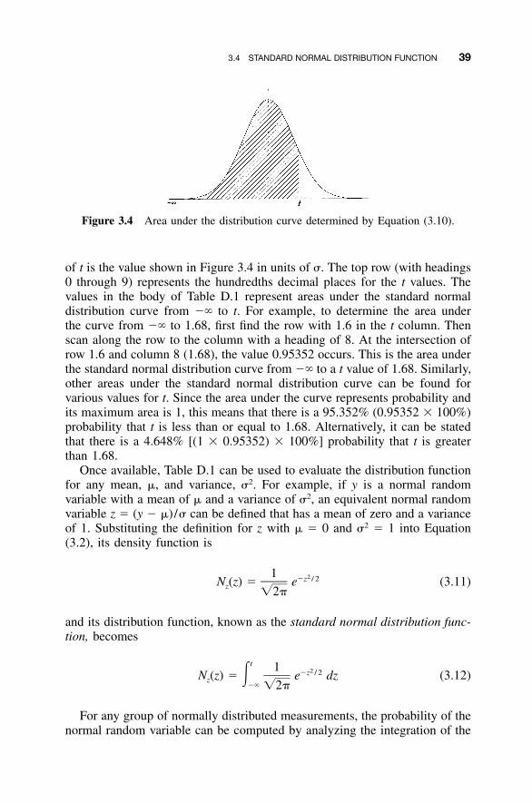
3.4 STANDARD NORMAL DISTRIBUTION FUNCTION 39
Figure 3.4 Area under the distribution curve determined by Equation (3.10).
of t is the value shown in Figure 3.4 in units of �. The top row (with headings0 through 9) represents the hundredths decimal places for the t values. Thevalues in the body of Table D.1 represent areas under the standard normaldistribution curve from �� to t. For example, to determine the area underthe curve from �� to 1.68, first find the row with 1.6 in the t column. Thenscan along the row to the column with a heading of 8. At the intersection ofrow 1.6 and column 8 (1.68), the value 0.95352 occurs. This is the area underthe standard normal distribution curve from �� to a t value of 1.68. Similarly,other areas under the standard normal distribution curve can be found forvarious values for t. Since the area under the curve represents probability andits maximum area is 1, this means that there is a 95.352% (0.95352 � 100%)probability that t is less than or equal to 1.68. Alternatively, it can be statedthat there is a 4.648% [(1 � 0.95352) � 100%] probability that t is greaterthan 1.68.
Once available, Table D.1 can be used to evaluate the distribution functionfor any mean, �, and variance, �2. For example, if y is a normal randomvariable with a mean of � and a variance of �2, an equivalent normal randomvariable z � (y � �) /� can be defined that has a mean of zero and a varianceof 1. Substituting the definition for z with � � 0 and �2 � 1 into Equation(3.2), its density function is
1 2�z / 2N (z) � e (3.11)z �2�
and its distribution function, known as the standard normal distribution func-tion, becomes
t 1 2�z / 2N (z) � � e dz (3.12)z�� �2�
For any group of normally distributed measurements, the probability of thenormal random variable can be computed by analyzing the integration of the
40 RANDOM ERROR THEORY
Figure 3.5 Area representing the probability in Equation (3.14).
distribution function. Again, as stated previously, the area under the curve inFigure 3.4 represents probability. Let z be a normal random variable, then theprobability that z is less than some value of t is given by
P(z � t) � N (t) (3.13)z
To determine the area (probability) between t values of a and b (the cross-hatched area in Figure 3.5), the difference in the areas between a and b,respectively, can be computed. By Equation (3.13), the area from �� to b isP(z � b) � Nz(b). By the same equation, the area from �� to a is P(z � a)� Nz(a). Thus, the area between a and b is the difference in these values andis expressed as
P(a � z � b) � N (b) � N (a) (3.14)z z
If the bounds are equal in magnitude but opposite in sign (i.e., �a � b � t),the probability is
P(�z� � t) � N (t) � N (�t) (3.15)z z
From the symmetry of the normal distribution in Figure 3.6 it is seen that
P(z � t) � P(z � �t) (3.16)
for any t � 0. This symmetry can also be shown with Table D.1. The tabularvalue (area) for a t value of �1.00 is 0.15866. Furthermore, the tabular valuefor a t value of �1.00 is 0.84134. Since the maximum probability (area) is1, the area above �1.00 is 1 � 0.84134, or 0.15866, which is the same asthe area below �1.00. Thus, since the total probability is always 1, we candefine the following relationship:
1 � N (t) � N (�t) (3.17)z z
Now substituting Equation (3.17) into Equation (3.15), we have
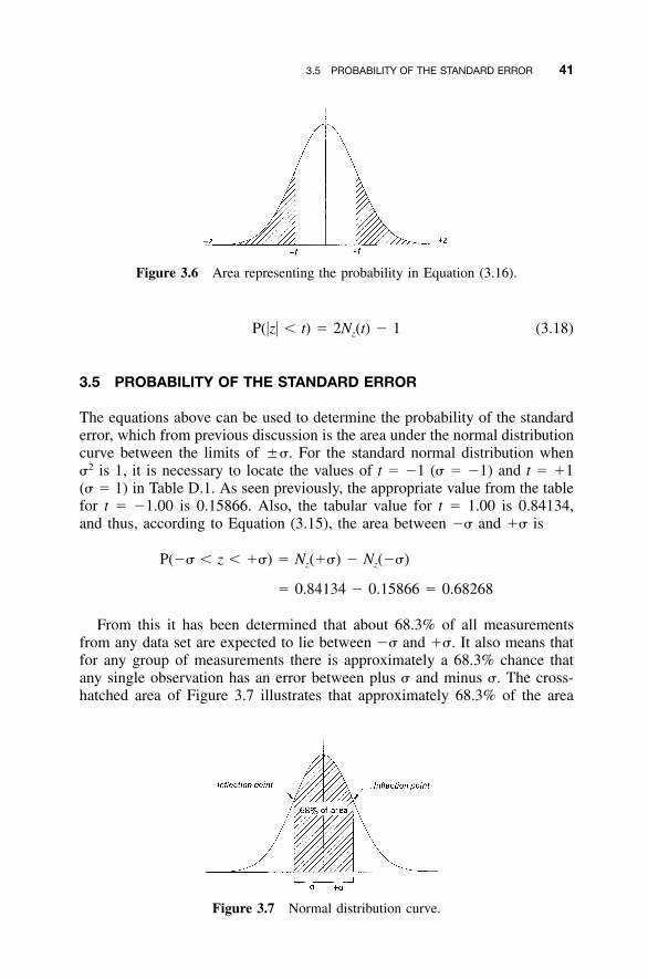
3.5 PROBABILITY OF THE STANDARD ERROR 41
Figure 3.6 Area representing the probability in Equation (3.16).
Figure 3.7 Normal distribution curve.
P(�z� � t) � 2N (t) � 1 (3.18)z
3.5 PROBABILITY OF THE STANDARD ERROR
The equations above can be used to determine the probability of the standarderror, which from previous discussion is the area under the normal distributioncurve between the limits of ��. For the standard normal distribution when�2 is 1, it is necessary to locate the values of t � �1 (� � �1) and t � �1(� � 1) in Table D.1. As seen previously, the appropriate value from the tablefor t � �1.00 is 0.15866. Also, the tabular value for t � 1.00 is 0.84134,and thus, according to Equation (3.15), the area between �� and �� is
P(�� � z � ��) � N (��) � N (��)z z
� 0.84134 � 0.15866 � 0.68268
From this it has been determined that about 68.3% of all measurementsfrom any data set are expected to lie between �� and ��. It also means thatfor any group of measurements there is approximately a 68.3% chance thatany single observation has an error between plus � and minus �. The cross-hatched area of Figure 3.7 illustrates that approximately 68.3% of the area
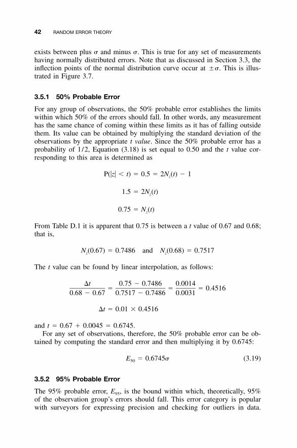
42 RANDOM ERROR THEORY
exists between plus � and minus �. This is true for any set of measurementshaving normally distributed errors. Note that as discussed in Section 3.3, theinflection points of the normal distribution curve occur at ��. This is illus-trated in Figure 3.7.
3.5.1 50% Probable Error
For any group of observations, the 50% probable error establishes the limitswithin which 50% of the errors should fall. In other words, any measurementhas the same chance of coming within these limits as it has of falling outsidethem. Its value can be obtained by multiplying the standard deviation of theobservations by the appropriate t value. Since the 50% probable error has aprobability of 1/2, Equation (3.18) is set equal to 0.50 and the t value cor-responding to this area is determined as
P(�z� � t) � 0.5 � 2N (t) � 1z
1.5 � 2N (t)z
0.75 � N (t)z
From Table D.1 it is apparent that 0.75 is between a t value of 0.67 and 0.68;that is,
N (0.67) � 0.7486 and N (0.68) � 0.7517z z
The t value can be found by linear interpolation, as follows:
�t 0.75 � 0.7486 0.0014� � � 0.4516
0.68 � 0.67 0.7517 � 0.7486 0.0031
�t � 0.01 � 0.4516
and t � 0.67 � 0.0045 � 0.6745.For any set of observations, therefore, the 50% probable error can be ob-
tained by computing the standard error and then multiplying it by 0.6745:
E � 0.6745� (3.19)50
3.5.2 95% Probable Error
The 95% probable error, E95, is the bound within which, theoretically, 95%of the observation group’s errors should fall. This error category is popularwith surveyors for expressing precision and checking for outliers in data.
3.6 USES FOR PERCENT ERRORS 43
TABLE 3.2 Multipliers for Various Percent Probable Errors
Symbol MultiplierPercent Probable
Errors
E50 0.6745� 50E90 1.645� 90E95 1.960� 95E99 2.576� 99E99.7 2.968� 99.7E99.9 3.29� 99.9
Using the same reasoning as in developing the equation for the 50% probableerror, substituting into Equation (3.18) gives
0.95 � P(�z� � t) � 2N (t) � 1z
1.95 � 2N (t)z
0.975 � N (t)z
Again from the Table D.1, it is determined that 0.975 occurs with a t valueof 1.960. Thus, to find the 95% probable error for any group of measurements,the following equation is used:
E � 1.960� (3.20)95
3.5.3 Other Percent Probable Errors
Using the same computational techniques as in Sections 3.5.1 and 3.5.2, otherpercent probable errors can be calculated. One other percent error worthy ofparticular note is E99.7. It is obtained by multiplying the standard error by2.968:
E � 2.968� (3.21)99.7
This value is often used for detecting blunders, as discussed in Section 3.6.A summary of probable errors with varying percentages, together with theirmultipliers, is given in Table 3.2.
3.6 USES FOR PERCENT ERRORS
Standard errors and errors of other percent probabilities are commonly usedto evaluate measurements for acceptance. Project specifications and contracts
44 RANDOM ERROR THEORY
often require that acceptable errors be within specified limits, such as the 90%and 95% errors. The 95% error, sometimes called the two-sigma (2�) errorbecause it is computed as approximately 2�, is most often specified. Standarderror is also frequently used. The probable error, E50, is seldom employed.
Higher percent errors are used to help isolate outliers (very large errors)and blunders in data sets. Since outliers seldom occur in a data set, measure-ments outside a selected high percentage range can be rejected as possibleblunders. Generally, any data that differ from the mean by more than 3� canbe considered as blunders and removed from a data set. As seen in Table 3.2,rejecting observations greater that 3� means that about 99.7% of all mea-surements should be retained. In other words, only about 0.3% of the mea-surements in a set of normally distributed random errors (or 3 observationsin 1000) should lie outside the range �3�.
Note that as explained in Chapter 2, standard error and standard deviationare often used interchangeably, when in practice it is actually the standarddeviation that is computed, not the standard error. Thus, for practical appli-cations, � in the equations of the preceding sections is replaced by S todistinguish between these two related values.
3.7 PRACTICAL EXAMPLES
Example 3.1 Suppose that the following values (in feet) were obtained in15 independent distance observations, Di: 212.22, 212.25, 212.23, 212.15,212.23, 212.11, 212.29, 212.34, 212.22, 212.24, 212.19, 212.25, 212.27,212.20, and 212.25. Calculate the mean, S, E50, E95, and check for any ob-servations outside the 99.7% probability level.
SOLUTION From Equation (2.1), the mean is
� D 3183.34iD � � � 212.22 ftn 15
From Equation (2.10), S is
2675,576.955 � 15(212.223 ) 0.051298S � � � �0.055 ft� �15 � 1 14
where � Di � 675,576.955. By scanning the data, it is seen that 10 obser-vations are between 212.22 � 0.06 ft or within the range (212.16, 212.28).1
1 The expression (x, y) represents a range between x and y. That is, the population mean liesbetween 212.16 and 212.28 in this example.
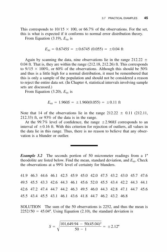
3.7 PRACTICAL EXAMPLES 45
This corresponds to 10/15 � 100, or 66.7% of the observations. For the set,this is what is expected if it conforms to normal error distribution theory.
From Equation (3.19), E50 is
E � 0.6745S � �0.6745 (0.055) � �0.04 ft50
Again by scanning the data, nine observations lie in the range 212.22 �0.04 ft. That is, they are within the range (212.18, 212.26) ft. This correspondsto 9/15 � 100%, or 60% of the observations. Although this should be 50%and thus is a little high for a normal distribution, it must be remembered thatthis is only a sample of the population and should not be considered a reasonto reject the entire data set. (In Chapter 4, statistical intervals involving samplesets are discussed.)
From Equation (3.20), E95 is
E � 1.960S � �1.960(0.055) � �0.11 ft95
Note that 14 of the observations lie in the range 212.22 � 0.11 (212.11,212.33) ft, or 93% of the data is in the range.
At the 99.7% level of confidence, the range �2.968S corresponds to aninterval of �0.16 ft. With this criterion for rejection of outliers, all values inthe data lie in this range. Thus, there is no reason to believe that any obser-vation is a blunder or outlier.
Example 3.2 The seconds portion of 50 micrometer readings from a 1�theodolite are listed below. Find the mean, standard deviation, and E95. Checkthe observations at a 99% level of certainty for blunders.
41.9 46.3 44.6 46.1 42.5 45.9 45.0 42.0 47.5 43.2 43.0 45.7 47.6
49.5 45.5 43.3 42.6 44.3 46.1 45.6 52.0 45.5 43.4 42.2 44.3 44.1
42.6 47.2 47.4 44.7 44.2 46.3 49.5 46.0 44.3 42.8 47.1 44.7 45.6
45.5 43.4 45.5 43.1 46.1 43.6 41.8 44.7 46.2 43.2 46.8
SOLUTION The sum of the 50 observations is 2252, and thus the mean is2252/50 � 45.04�. Using Equation (2.10), the standard deviation is
2101,649.94 � 50(45.04)S � � �2.12�� 50 � 1
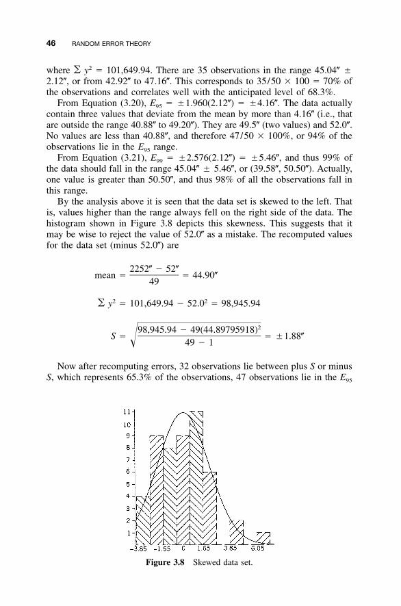
46 RANDOM ERROR THEORY
Figure 3.8 Skewed data set.
where � y2 � 101,649.94. There are 35 observations in the range 45.04� �2.12�, or from 42.92� to 47.16�. This corresponds to 35/50 � 100 � 70% ofthe observations and correlates well with the anticipated level of 68.3%.
From Equation (3.20), E95 � �1.960(2.12�) � �4.16�. The data actuallycontain three values that deviate from the mean by more than 4.16� (i.e., thatare outside the range 40.88� to 49.20�). They are 49.5� (two values) and 52.0�.No values are less than 40.88�, and therefore 47/50 � 100%, or 94% of theobservations lie in the E95 range.
From Equation (3.21), E99 � �2.576(2.12�) � �5.46�, and thus 99% ofthe data should fall in the range 45.04� � 5.46�, or (39.58�, 50.50�). Actually,one value is greater than 50.50�, and thus 98% of all the observations fall inthis range.
By the analysis above it is seen that the data set is skewed to the left. Thatis, values higher than the range always fell on the right side of the data. Thehistogram shown in Figure 3.8 depicts this skewness. This suggests that itmay be wise to reject the value of 52.0� as a mistake. The recomputed valuesfor the data set (minus 52.0�) are
2252� � 52�mean � � 44.90�
49
2 2� y � 101,649.94 � 52.0 � 98,945.94
298,945.94 � 49(44.89795918)S � � �1.88�� 49 � 1
Now after recomputing errors, 32 observations lie between plus S or minusS, which represents 65.3% of the observations, 47 observations lie in the E95
PROBLEMS 47
range, which represents 95.9% of the data, and no values are outside the E99
range. Thus, there is no reason to reject any additional data at a 99% levelof confidence.
PROBLEMS
3.1 Determine the t value for E80.
3.2 Determine the t value for E75.
3.3 Use STATS to determine t for E90.
3.4 Use STATS to determine t for E99.9.
3.5 Assuming a normal distribution, explain the statement: ‘‘As the stan-dard deviation of the group of observations decreases, the precision ofthe group increases.’’
3.6 If the mean of a population is 2.456 and its variance is 2.042, what isthe peak value for the normal distribution curve and the points ofinflection?
3.7 If the mean of a population is 13.4 and its variance is 5.8, what is thepeak value for the normal distribution curve and the points ofinflection?
3.8 Plot the curve in Problem 3.6 using Equation (3.2) to determine ordi-nate and abscissa values.
3.9 Plot the curve in Problem 3.7 using Equation (3.2) to determine ordi-nate and abscissa values.
3.10 The following data represent 60 planimeter observations of the areawithin a plotted traverse.
1.677 1.676 1.657 1.667 1.673 1.671 1.673 1.670 1.675 1.664 1.664 1.668
1.664 1.651 1.663 1.665 1.670 1.671 1.651 1.665 1.667 1.662 1.660 1.667
1.660 1.667 1.667 1.652 1.664 1.690 1.649 1.671 1.675 1.653 1.654 1.665
1.668 1.658 1.657 1.690 1.666 1.671 1.664 1.685 1.667 1.655 1.679 1.682
1.662 1.672 1.667 1.667 1.663 1.670 1.667 1.669 1.671 1.660 1.683 1.663
(a) Calculate the mean and standard deviation.(b) Plot the relative frequency histogram (of residuals) for the data
above using a class interval of one-half of the standard deviation.(c) Calculate the E50 and E90 intervals.
48 RANDOM ERROR THEORY
(d) Can any observations be rejected at a 99% level of certainty?(e) What is the peak value for the normal distribution curve, and where
are the points of inflection on the curve?
3.11 Discuss the normality of each set of data below and whether any ob-servations may be removed at the 99% level of certainty as blundersor outliers. Determine which set is more precise after apparent blundersand outliers are removed. Plot the relative frequency histogram to de-fend your decisions.
Set 1:
468.09 468.13 468.11 468.13 468.10 468.13 468.12 468.09 468.14
468.10 468.10 468.12 468.14 468.16 468.12 468.10 468.10 468.11
468.13 468.12 468.18
Set 2:
750.82 750.86 750.83 750.88 750.88 750.86 750.86 750.85 750.86
750.86 750.88 750.84 750.84 750.88 750.86 750.87 750.86 750.83
750.90 750.84 750.86
3.12 Using the following data set, answer the questions that follow.
17.5 15.0 13.4 23.9 25.2 19.5 25.8 30.0 22.5 35.3
39.5 23.5 26.5 21.3 22.3 21.6 27.2 21.1 24.0 23.5
32.5 32.2 24.2 35.7 28.0 24.0 16.8 21.1 19.0 30.7
30.2 33.7 19.7 19.7 25.1 27.9 28.5 22.7 31.0 28.4
31.2 24.6 30.2 16.8 26.9 23.3 21.5 18.8 21.4 20.7
(a) What are the mean and standard deviation of the data set?(b) Construct a centered relative frequency histogram of the data using
seven intervals and discuss whether it appears to be a normal dataset.
(c) What is the E95 interval for this data set?(d) Would there be any reason to question the validity of any obser-
vation at the 95% level?
PROBLEMS 49
3.13 Repeat Problem 3.12 using the following data:
2.898 2.918 2.907 2.889 2.901 2.901 2.899 2.899 2.911 2.909
2.904 2.905 2.895 2.920 2.899 2.896 2.907 2.897 2.900 2.897
Use STATS to do each problem.
3.14 Problem 3.10
3.15 Problem 3.11
3.16 Problem 3.12
3.17 Problem 3.13
Programming Problems
3.18 Create a computational package that solves Problem 3.11.
3.19 Create a computational package that solves Problem 3.12.
50
CHAPTER 4
CONFIDENCE INTERVALS
4.1 INTRODUCTION
Table 4.1 contains a discrete population of 100 values. The mean (�) andvariance (�2) of that population are 26.1 and 17.5, respectively. By randomlyselecting 10 values from Table 4.1, an estimate of the mean and variance ofthe population can be determined. However, it should not be expected thatthese estimates and S2) will exactly match the mean and variance of the(ypopulation. Sample sets of 10 values each could continue to be selected fromthe population to determine additional estimates for the mean and varianceof the population. However, it is just as unlikely that these additional valueswould match those obtained from either the population or the first sample set.
As the sample size is increased, the mean and variance of the sampleshould approach the values of the population. In fact, as the sample sizebecomes very large, the mean and variance of the samples should be closeto those of the population. This procedure was carried out for various samplesizes starting at 10 values and increasing the sample by 10 values, with theresults shown in Table 4.2. Note that the value computed for the mean of thesample approaches the value of the population as the sample size is increased.Similarly, the value computed for the variance of the sample tends to approachthe value of the population as the sample size is increased.
Since the mean of a sample set and its variance S2 are computed fromyrandom variables, they are also random variables. This means that even if thesize of the sample is kept constant, varying values for the mean and variancecan be expected from the samples, with greater confidence given to largersamples. Also, it can be concluded that the values computed from a samplealso contain errors. To illustrate this, an experiment was run for four randomly
Adjustment Computations: Spatial Data Analysis, Fourth Edition. C. D. Ghilani and P. R. Wolf© 2006 John Wiley & Sons, Inc. ISBN: 978-0-471-69728-2
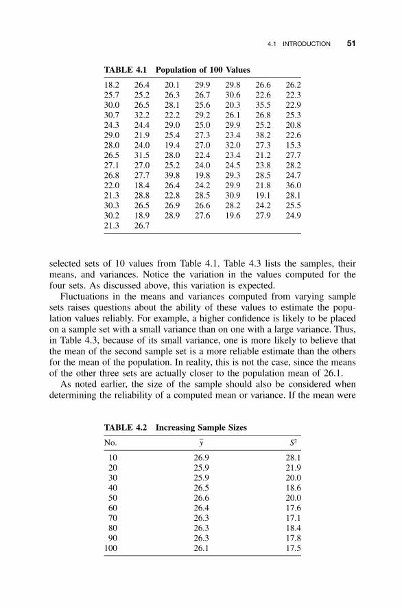
4.1 INTRODUCTION 51
TABLE 4.1 Population of 100 Values
18.2 26.4 20.1 29.9 29.8 26.6 26.225.7 25.2 26.3 26.7 30.6 22.6 22.330.0 26.5 28.1 25.6 20.3 35.5 22.930.7 32.2 22.2 29.2 26.1 26.8 25.324.3 24.4 29.0 25.0 29.9 25.2 20.829.0 21.9 25.4 27.3 23.4 38.2 22.628.0 24.0 19.4 27.0 32.0 27.3 15.326.5 31.5 28.0 22.4 23.4 21.2 27.727.1 27.0 25.2 24.0 24.5 23.8 28.226.8 27.7 39.8 19.8 29.3 28.5 24.722.0 18.4 26.4 24.2 29.9 21.8 36.021.3 28.8 22.8 28.5 30.9 19.1 28.130.3 26.5 26.9 26.6 28.2 24.2 25.530.2 18.9 28.9 27.6 19.6 27.9 24.921.3 26.7
TABLE 4.2 Increasing Sample Sizes
No. y S2
10 26.9 28.120 25.9 21.930 25.9 20.040 26.5 18.650 26.6 20.060 26.4 17.670 26.3 17.180 26.3 18.490 26.3 17.8
100 26.1 17.5
selected sets of 10 values from Table 4.1. Table 4.3 lists the samples, theirmeans, and variances. Notice the variation in the values computed for thefour sets. As discussed above, this variation is expected.
Fluctuations in the means and variances computed from varying samplesets raises questions about the ability of these values to estimate the popu-lation values reliably. For example, a higher confidence is likely to be placedon a sample set with a small variance than on one with a large variance. Thus,in Table 4.3, because of its small variance, one is more likely to believe thatthe mean of the second sample set is a more reliable estimate than the othersfor the mean of the population. In reality, this is not the case, since the meansof the other three sets are actually closer to the population mean of 26.1.
As noted earlier, the size of the sample should also be considered whendetermining the reliability of a computed mean or variance. If the mean were
52 CONFIDENCE INTERVALS
TABLE 4.3 Random Sample Sets from a Population
Set 1: 29.9, 18.2, 30.7, 24.4, 36.0, 25.6, 26.5, 29.9, 19.6, 27.9 � 26.9, S2 � 28.1ySet 2: 26.9, 28.1, 29.2, 26.2, 30.0, 27.1, 26.5, 30.6, 28.5, 25.5 � 27.9, S2 � 2.9ySet 3: 32.2, 22.2, 23.4, 27.9, 27.0, 28.9, 22.6, 27.7, 30.6, 26.9 � 26.9, S2 � 10.9ySet 4: 24.2, 36.0, 18.2, 24.3, 24.0, 28.9, 28.8, 30.2, 28.1, 29.0 � 27.2, S2 � 23.0y
computed from a sample of five values, and another computed from a sampleof 30 values, more confidence is likely to be placed on the values derivedfrom the larger sample set than on those from the smaller one, even if bothsample sets have the same mean and standard deviation.
In statistics, this relationship between the sample sets, the number of sam-ples, and the values computed for the means and variances is part of samplingdistribution theory. This theory recognizes that estimates for the mean andvariance do vary from sample to sample. Estimators are the functions usedto compute these estimates. Examples of estimator functions are Equations(2.1) and (2.5), which are used to compute estimates of the mean and variancefor a population, respectively. As demonstrated and discussed, these estimatesvary from sample to sample and thus have their own population distributions.In Section 4.2, three distributions are defined that are used for describing orquantifying the reliability of mean and variance estimates. By applying thesedistributions, statements can be written for the reliability at any given levelof confidence of the estimates computed. In other words, a range called theconfidence interval can be determined within which the population mean andpopulation variance can be expected to fall for varying levels of probability.
4.2 DISTRIBUTIONS USED IN SAMPLING THEORY
4.2.1 �2 Distribution
The chi-square distribution, symbolized as �2, compares the relationship be-tween the population variance and the variance of a sample set based on thenumber of redundancies, �, in the sample. If a random sample of n obser-vations, y1, y2, . . . , yn, is selected from a population that has a normaldistribution with mean � and variance �2, then, by definition, the �2 samplingdistribution is
2�S2� � (4.1)2�
where � is the number of degrees of freedom in the sample and the otherterms are as defined previously.
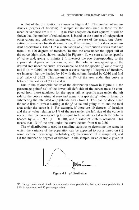
4.2 DISTRIBUTIONS USED IN SAMPLING THEORY 53
Figure 4.1 �2 distribution.
A plot of the distribution is shown in Figure 4.1. The number of redun-dancies (degrees of freedom) in sample set statistics such as those for themean or variance are � � n � 1; in later chapters on least squares it will beshown that the number of redundancies is based on the number of independentobservations and unknown parameters. In the case of the mean, one obser-vation is necessary for its determination, thus leaving n � 1 values as redun-dant observations. Table D.2 is a tabulation of �2 distribution curves that havefrom 1 to 120 degrees of freedom. To find the area under the upper tail ofthe curve (right side, shown hatched in Figure 4.1), we start at some specific�2 value and, going to infinity (�), intersect the row corresponding to theappropriate degrees of freedom, �, with the column corresponding to thedesired area under the curve. For example, to find the specific �2 value relatingto 1% (� � 0.010) of the area under a curve having 10 degrees of freedom,we intersect the row headed by 10 with the column headed by 0.010 and finda �2 value of 23.21. This means that 1% of the area under this curve isbetween the values of 23.21 and �.
Due to the asymmetric nature of the distribution shown in Figure 4.1, thepercentage points1 (�) of the lower tail (left side of the curve) must be com-puted from those tabulated for the upper tail. A specific area under the leftside of the curve starting at zero and going to a specific �2 value is found bysubtracting the tabulated � (right-side area) from 1. This can be done sincethe table lists � (areas) starting at the �2 value and going to �, and the totalarea under the curve is 1. For example, if there are 10 degrees of freedomand the �2 value relating to 1% of the area under the left side of the curve isneeded, the row corresponding to � equal to 10 is intersected with the columnheaded by � � 0.990 (1 � 0.010), and a value of 2.56 is obtained. Thismeans that 1% of the area under the curve occurs from 0 to 2.56.
The �2 distribution is used in sampling statistics to determine the range inwhich the variance of the population can be expected to occur based on (1)some specified percentage probability, (2) the variance of a sample set, and(3) the number of degrees of freedom in the sample. In an example given in
1 Percentage points are decimal equivalents of percent probability; that is, a percent probability of95% is equivalent to 0.95 percentage points.
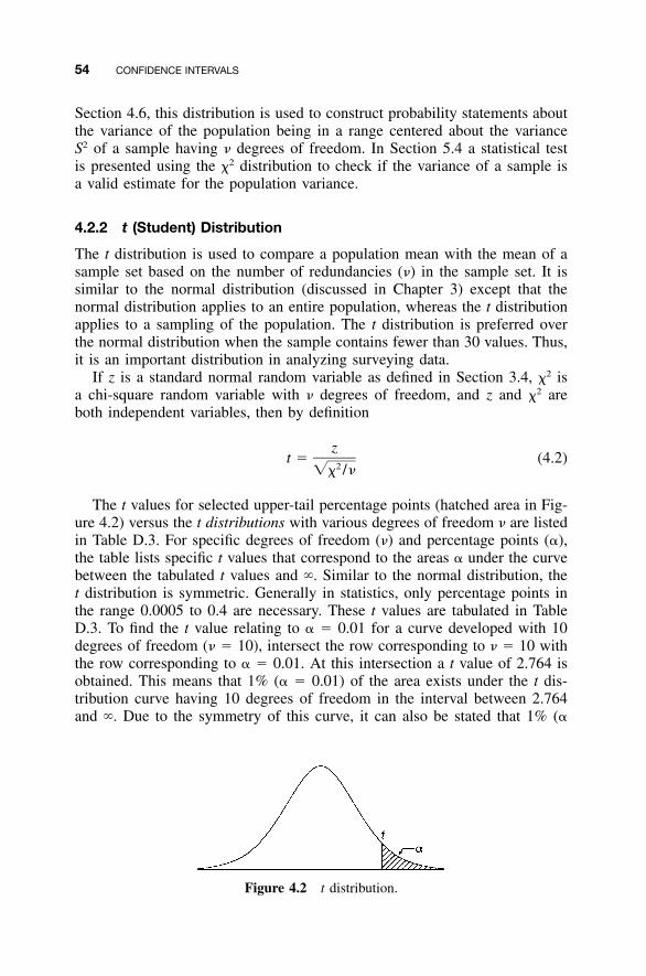
54 CONFIDENCE INTERVALS
Figure 4.2 t distribution.
Section 4.6, this distribution is used to construct probability statements aboutthe variance of the population being in a range centered about the varianceS2 of a sample having � degrees of freedom. In Section 5.4 a statistical testis presented using the �2 distribution to check if the variance of a sample isa valid estimate for the population variance.
4.2.2 t (Student) Distribution
The t distribution is used to compare a population mean with the mean of asample set based on the number of redundancies (�) in the sample set. It issimilar to the normal distribution (discussed in Chapter 3) except that thenormal distribution applies to an entire population, whereas the t distributionapplies to a sampling of the population. The t distribution is preferred overthe normal distribution when the sample contains fewer than 30 values. Thus,it is an important distribution in analyzing surveying data.
If z is a standard normal random variable as defined in Section 3.4, �2 isa chi-square random variable with � degrees of freedom, and z and �2 areboth independent variables, then by definition
zt � (4.2)
2�� /�
The t values for selected upper-tail percentage points (hatched area in Fig-ure 4.2) versus the t distributions with various degrees of freedom � are listedin Table D.3. For specific degrees of freedom (�) and percentage points (�),the table lists specific t values that correspond to the areas � under the curvebetween the tabulated t values and �. Similar to the normal distribution, thet distribution is symmetric. Generally in statistics, only percentage points inthe range 0.0005 to 0.4 are necessary. These t values are tabulated in TableD.3. To find the t value relating to � � 0.01 for a curve developed with 10degrees of freedom (� � 10), intersect the row corresponding to � � 10 withthe row corresponding to � � 0.01. At this intersection a t value of 2.764 isobtained. This means that 1% (� � 0.01) of the area exists under the t dis-tribution curve having 10 degrees of freedom in the interval between 2.764and �. Due to the symmetry of this curve, it can also be stated that 1% (�
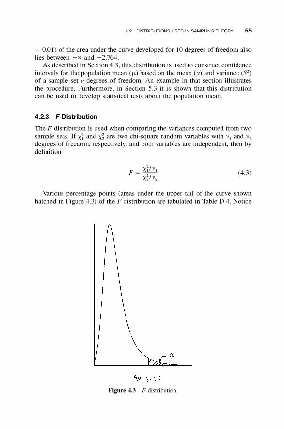
4.2 DISTRIBUTIONS USED IN SAMPLING THEORY 55
Figure 4.3 F distribution.
� 0.01) of the area under the curve developed for 10 degrees of freedom alsolies between �� and �2.764.
As described in Section 4.3, this distribution is used to construct confidenceintervals for the population mean (�) based on the mean and variance (S2)(y)of a sample set � degrees of freedom. An example in that section illustratesthe procedure. Furthermore, in Section 5.3 it is shown that this distributioncan be used to develop statistical tests about the population mean.
4.2.3 F Distribution
The F distribution is used when comparing the variances computed from twosample sets. If and are two chi-square random variables with �1 and �2
2 2� �1 2
degrees of freedom, respectively, and both variables are independent, then bydefinition
2� /�1 1F � (4.3)2� /�2 2
Various percentage points (areas under the upper tail of the curve shownhatched in Figure 4.3) of the F distribution are tabulated in Table D.4. Notice
56 CONFIDENCE INTERVALS
that this distribution has �1 numerator degrees of freedom and �2 denominatordegrees of freedom, which correspond to the two sample sets. Thus, unlikethe �2 and t distributions, each desired � percentage point must be representedin a separate table. In Appendix D, tables for the more commonly used valuesof � (0.20, 0.10, 0.05, 0.025, 0.01, 0.005, and 0.001) are listed.
To illustrate the use of the tables, suppose that the F value for 1% of thearea under the upper tail of the curve is needed. Also assume that 5 is thenumerator degrees of freedom relating to S1 and 10 is the denominator degreesof freedom relating to S2. In this example, � equals 0.01 and thus the F tablein Table D.4 that is written for � � 0.01 must be used. In that table, intersectthe row headed by �2 equal to 10 with the column headed by �1 equal to 5,and find the F value of 5.64. This means that 1% of the area under the curveconstructed using these degrees of freedom lies in the region from 5.64 to �.
To determine the area in the lower tail of this distribution, use the followingfunctional relationship:
1F � (4.4)�,� ,�1 2 F1��,� ,�2 1
The critical F value for the data in the preceding paragraph [�1 equal to 5and �2 equal to 10 with � equal to 0.99 (0.01 in the lower tail)] is determinedby going to the intersection of the row headed by 5 with the column headedby 10 in the section � � 0.01. The intersection is at F equal to 2.19. Ac-cording to Equation (4.4), the critical F0.99,5,10 is 1/F0.01,10,5 � 1/2.19 � 0.457.Thus, 1% of the area is under the F-distribution curve from �� to 0.457.
The F distribution is used to answer the question of whether two samplesets come from the same population. For example, suppose that two sampleshave variances of and If these two sample variances represent the same2 2S S .1 2
population variance, the ratio of their population variances / should2 2(� � )1 2
equal 1 (i.e., � As discussed in Section 4.7, this distribution enables2 2� � ).1 2
confidence intervals to be established for the ratio of the population variances.Also, as discussed in Section 5.5, the distribution can be used to test whetherthe ratio of the two variances is statistically equal to 1.
4.3 CONFIDENCE INTERVAL FOR THE MEAN: t STATISTIC
In Chapter 3 the standard normal distribution was used to predict the rangein which the mean of a population can exist. This was based on the meanand standard deviation for a sample set. However, as noted previously, thenormal distribution is based on an entire population, and as was demonstrated,variations from the normal distribution are expected from sample sets havinga small number of values. From this expectation, the t distribution was de-veloped. As demonstrated later in this section by an example, the t distribution
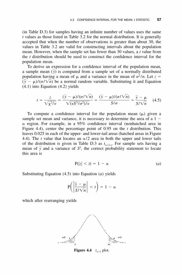
4.3 CONFIDENCE INTERVAL FOR THE MEAN: t STATISTIC 57
Figure 4.4 t� / 2 plot.
(in Table D.3) for samples having an infinite number of values uses the samet values as those listed in Table 3.2 for the normal distribution. It is generallyaccepted that when the number of observations is greater than about 30, thevalues in Table 3.2 are valid for constructing intervals about the populationmean. However, when the sample set has fewer than 30 values, a t value fromthe t distribution should be used to construct the confidence interval for thepopulation mean.
To derive an expression for a confidence interval of the population mean,a sample mean is computed from a sample set of a normally distributed(y)population having a mean of � and a variance in the mean of �2 /n. Let z �
� �) /(� / be a normal random variable. Substituting it and Equation(y �n)(4.1) into Equation (4.2) yields
(y � �) /(� /�n) (y � �) /(� /�n)z y � �t � � � � (4.5)
2 2 2 S /��� /� �(�S /� ) /� S /�n
To compute a confidence interval for the population mean (�) given asample set mean and variance, it is necessary to determine the area of a 1 �� region. For example, in a 95% confidence interval (nonhatched area inFigure 4.4), center the percentage point of 0.95 on the t distribution. Thisleaves 0.025 in each of the upper- and lower-tail areas (hatched areas in Figure4.4). The t value that locates an � /2 area in both the upper and lower tailsof the distribution is given in Table D.3 as t� / 2,�. For sample sets having amean of and a variance of S2, the correct probability statement to locateythis area is
P(�z� � t) � 1 � � (a)
Substituting Equation (4.5) into Equation (a) yields
y � �P � t � 1 � ��� � �
S /�n
which after rearranging yields
58 CONFIDENCE INTERVALS
S SP y � t � � � y � t � 1 � � (4.6)� �� / 2 � / 2�n �n
Thus, given t� / 2,�, n, and S, it is seen from Equation (4.6) that a 1 � �y,probable error interval for the population mean � is computed as
S Sy � t � � � y � t (4.7)� / 2 � / 2�n �n
where t� / 2 is the t value from the t distribution based on � degrees of freedomand � /2 percentage points.
The following example illustrates the use of Equation (4.7) and Table D.3for determining the 95% confidence interval for the population mean basedon a sample set having a small number of values (n) with a mean of and ayvariance of S.
Example 4.1 In carrying out a control survey, 16 directional readings weremeasured for a single line. The mean (seconds’ portion only) of the readingswas 25.4�, with a standard deviation of �1.3�. Determine the 95% confidenceinterval for the population mean. Compare this with the interval determinedby using a t value determined from the standard normal distribution tables(Table 3.2).
SOLUTION In this example the confidence level 1 � � is 0.95, and thus �is 0.05. Since the interval is to be centered about the population mean �, avalue of � /2 in Table D.3 is used. This yields equal areas in both the lowerand upper tails of the distribution, as shown in Figure 4.4. Thus, for thisexample, � /2 is 0.025. The appropriate t value for this percentage point with� equal to 15 (16 � 1) degrees of freedom is found in Table D.3 as follows:
Step 1: In the leftmost column of Table D.3, find the row with the correctnumber of degrees of freedom (�) for the sample. In this case it is 16 �1, or 15.
Step 2: Find the column headed by 0.025 for � /2.Step 3: Locate the value at the intersection of this row and column, which is
2.131.Step 4: Then by Equation (4.7), the appropriate 95% confidence interval is
1.3 S24.7 � 25.4 � 2.131 � y � t� � 0.025�16 �n
S 1.3� � � y � t � 25.4 � 2.131 � 26.1� �0.025 �n �16
4.4 TESTING THE VALIDITY OF THE CONFIDENCE INTERVAL 59
This computation can be written more compactly as
S 1.3y � t or 25.4 � 2.131 � 25.4 � 0.7� �0.025 �n �16
After making the calculation above, it can be stated that for this sample,with 95% confidence, the population mean (�) lies in the range (24.7, 26.1).If this were a large sample, the t value from Table 3.2 could be used for 95%.That t value for 95% is 1.960, and the standard error of the mean then wouldbe �1.3/ � �0.325. Thus, the population’s mean would be in the range�1625.4 � 1.960 � 0.325�, or (24.8, 26.0). Notice that due to the small samplesize, the t distribution gives a larger range for the population mean than doesthe standard normal distribution. Notice also that in the t distribution of TableD.3, for a sample of infinite size (i.e., � � �), the t value tabulated for �equal to 0.025 is 1.960, which matches Table 3.2.
The t distribution is often used to isolate outliers or blunders in observa-tions. To do this, a percent confidence interval is developed about the meanfor a single observation as
y � t S � y � y � t S (4.8)� / 2 i � / 2
Using the data from Example 4.1 and Equation (4.8), the 95% range for the16 directional readings is
25.4� � 2.131(1.3�) � 22.63� � y � 28.17� � 25.4� � 2.131(1.3�)i
Thus, 95% of the data should be in the range (22.6�, 28.2�). Any data valuesoutside this range can be considered as outliers and rejected with a 95% levelof confidence. It is important to note that if the normal distribution value of1.960 was used to compute this interval, the range would be smaller, (22.85�,27.95�). Using the normal distribution could result in discarding more obser-vations than is justified when using sample estimates of the mean and vari-ance. It is important to note that this will become more significant as thenumber of observations in the sample becomes smaller. For example, if onlyfour directional readings are obtained, the t-distribution multiplier would be-come 3.183. The resulting 95% confidence interval for a single observationwould be 1.6 times larger than that derived using a normal distribution t value.
4.4 TESTING THE VALIDITY OF THE CONFIDENCE INTERVAL
A test that demonstrates the validity of the theory of the confidence intervalis illustrated as follows. Using a computer and normal random number gen-
60 CONFIDENCE INTERVALS
erating software, 1000 sample data sets of 16 values each were collectedrandomly from a population with mean � � 25.4 and standard error � ��1.3. Using a 95% confidence interval (� � 0.05) and Equation (4.7), theinterval for the population mean derived for each sample set was computedand compared with the actual population mean. If the theory is valid, theinterval constructed would be expected to contain the population’s mean 95%of the time based on the confidence level of 0.05. Appendix E shows the 95%intervals computed for the 1000 samples. The intervals not containing thepopulation mean of 25.4 are marked with an asterisk. From the data tabulatedit is seen that 50 of 1000 sample sets failed to contain the population mean.This corresponds to exactly 5% of the samples. In other words, the proportionof samples that do enclose the mean is exactly 95%. This demonstrates thatthe bounds calculated by Equation (4.7) do, in fact, enclose the populationmean � at the confidence level selected.
4.5 SELECTING A SAMPLE SIZE
A common problem encountered in surveying practice is to determine thenumber of repeated observations necessary to meet a specific precision. Inpractice, the size of S cannot be controlled absolutely. Rather, as seen inEquation (4.7), the confidence interval can be controlled only by varying thenumber of repeated observations. In general, the larger the sample size, thesmaller the confidence interval. From Equation (4.7), the range in which thepopulation mean (�) resides at a selected level of confidence (�) is
Sy � t (b)� / 2 �n
Now let I represent one-half of the interval in which the population meanlies. Then from Equation (b), I is
SI � t (4.9)� / 2 �n
Rearranging Equation (4.9) yields
2t S� / 2n � (4.10)� �I
In Equation (4.10), n is the number of repeated measurements, I the desiredconfidence interval, t� / 2 the t value based on the number of degrees of freedom(�), and S the sample set standard deviation. In the practical application ofEquation (4.10), t� / 2 and S are unknown since the data set has yet to be
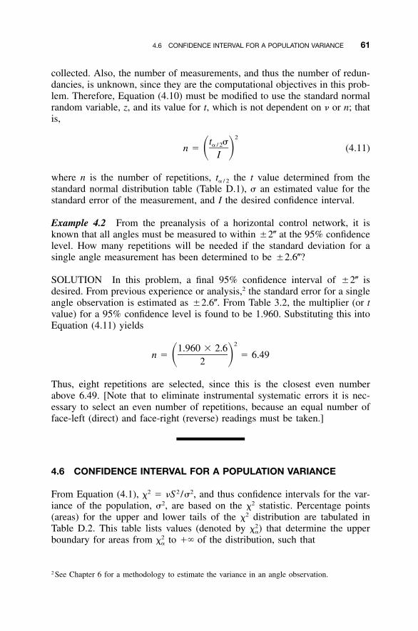
4.6 CONFIDENCE INTERVAL FOR A POPULATION VARIANCE 61
collected. Also, the number of measurements, and thus the number of redun-dancies, is unknown, since they are the computational objectives in this prob-lem. Therefore, Equation (4.10) must be modified to use the standard normalrandom variable, z, and its value for t, which is not dependent on � or n; thatis,
2t �� / 2n � (4.11)� �I
where n is the number of repetitions, t� / 2 the t value determined from thestandard normal distribution table (Table D.1), � an estimated value for thestandard error of the measurement, and I the desired confidence interval.
Example 4.2 From the preanalysis of a horizontal control network, it isknown that all angles must be measured to within �2� at the 95% confidencelevel. How many repetitions will be needed if the standard deviation for asingle angle measurement has been determined to be �2.6�?
SOLUTION In this problem, a final 95% confidence interval of �2� isdesired. From previous experience or analysis,2 the standard error for a singleangle observation is estimated as �2.6�. From Table 3.2, the multiplier (or tvalue) for a 95% confidence level is found to be 1.960. Substituting this intoEquation (4.11) yields
21.960 � 2.6n � � 6.49� �2
Thus, eight repetitions are selected, since this is the closest even numberabove 6.49. [Note that to eliminate instrumental systematic errors it is nec-essary to select an even number of repetitions, because an equal number offace-left (direct) and face-right (reverse) readings must be taken.]
4.6 CONFIDENCE INTERVAL FOR A POPULATION VARIANCE
From Equation (4.1), �2 � �S2 /�2, and thus confidence intervals for the var-iance of the population, �2, are based on the �2 statistic. Percentage points(areas) for the upper and lower tails of the �2 distribution are tabulated inTable D.2. This table lists values (denoted by that determine the upper2� )�
boundary for areas from to �� of the distribution, such that2��
2 See Chapter 6 for a methodology to estimate the variance in an angle observation.
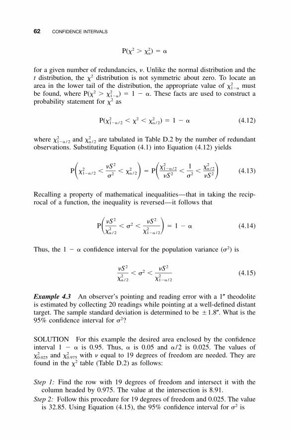
62 CONFIDENCE INTERVALS
2 2P(� � � ) � ��
for a given number of redundancies, �. Unlike the normal distribution and thet distribution, the �2 distribution is not symmetric about zero. To locate anarea in the lower tail of the distribution, the appropriate value of must2�1��
be found, where P(�2 � � 1 � �. These facts are used to construct a2� )1��
probability statement for �2 as
2 2 2P(� � � � � ) � 1 � � (4.12)1�� / 2 � / 2
where and are tabulated in Table D.2 by the number of redundant2 2� �1�� / 2 � / 2
observations. Substituting Equation (4.1) into Equation (4.12) yields
2 2 2�S � 1 �1�� / 2 � / 22 2P � � � � � P � � (4.13)� � � �1�� / 2 � / 22 2 2 2� �S � �S
Recalling a property of mathematical inequalities—that in taking the recip-rocal of a function, the inequality is reversed—it follows that
2 2�S �S2P � � � � 1 � � (4.14)� �2 2� �� / 2 1�� / 2
Thus, the 1 � � confidence interval for the population variance (�2) is
2 2�S �S2� � � (4.15)2 2� �� / 2 1�� / 2
Example 4.3 An observer’s pointing and reading error with a 1� theodoliteis estimated by collecting 20 readings while pointing at a well-defined distanttarget. The sample standard deviation is determined to be �1.8�. What is the95% confidence interval for �2?
SOLUTION For this example the desired area enclosed by the confidenceinterval 1 � � is 0.95. Thus, � is 0.05 and � /2 is 0.025. The values of
and with � equal to 19 degrees of freedom are needed. They are2 2� �0.025 0.975
found in the �2 table (Table D.2) as follows:
Step 1: Find the row with 19 degrees of freedom and intersect it with thecolumn headed by 0.975. The value at the intersection is 8.91.
Step 2: Follow this procedure for 19 degrees of freedom and 0.025. The valueis 32.85. Using Equation (4.15), the 95% confidence interval for �2 is

4.7 CONFIDENCE INTERVAL FOR THE RATIO OF TWO POPULATION VARIANCES 63
2 2(20 � 1)1.8 (20 � 1)1.82� � �32.85 8.91
21.87 � � � 6.91
Thus, 95% of the time, the population’s variance should lie between 1.87and 6.91.
4.7 CONFIDENCE INTERVAL FOR THE RATIO OF TWOPOPULATION VARIANCES
Another common statistical procedure is used to compare the ratio of twopopulation variances. The sampling distribution of the ratio / is well2 2� �1 2
known when samples are collected randomly from a normal population. Theconfidence interval for / is based on the F distribution using Equation2 2� �1 2
(4.3) as
2� /�1 1F � 2� /�2 2
Substituting Equation (4.1) and reducing yields
2 2 2 2 2 2(� S /� ) /� S /� S �1 1 1 1 1 1 1 2F � � � (4.16)2 2 2 2 2 2(� S /� ) /� S /� S �2 2 2 2 2 2 2 1
To establish a confidence interval for the ratio, the lower and upper valuescorresponding to the tails of the distribution must be found. A probabilitystatement to find the confidence interval for the ratio is constructed as follows:
P(F � F � F ) � 1 � �1�� / 2,� ,� � / 2,� ,�1 2 1 2
Substituting in Equation (4.16) and rearranging yields
2 2S �1 2P(F � F � F ) � P F � � � F� �l u l u2 2S �2 1
2 2 2S � S2 2 2� P F � � F� �l u2 2 2S � S1 1 1
2 2 21 S � S 11 1 1� P � � � 1 � � (4.17)� �2 2 2F S � S Fu 2 2 2 l
Substituting Equation (4.4) into (4.17) yields
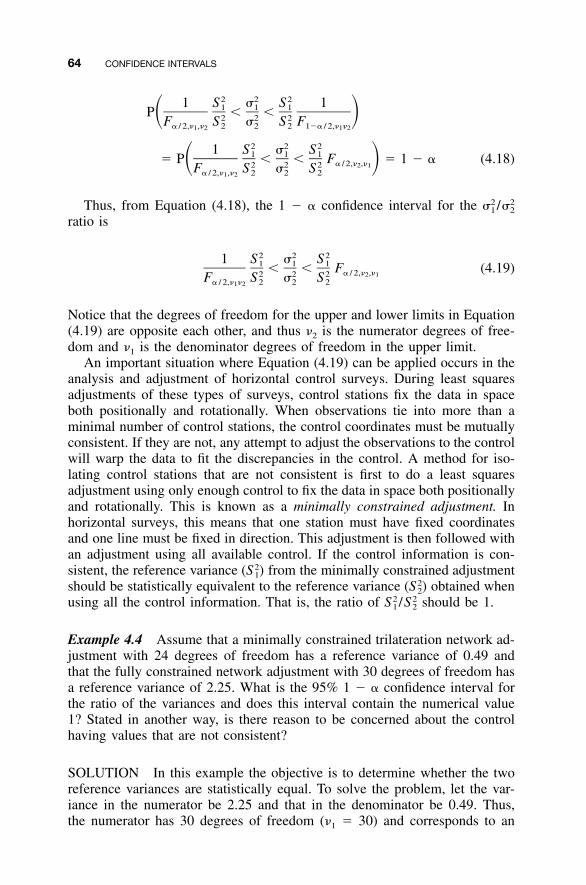
64 CONFIDENCE INTERVALS
2 2 21 S � S 11 1 1P � �� �2 2 2F S � S F� / 2,� ,� 2 2 2 1�� / 2,� �1 2 1 2
2 2 21 S � S1 1 1� P � � F � 1 � � (4.18)� �� / 2,� ,�2 12 2 2F S � S� / 2,� ,� 2 2 21 2
Thus, from Equation (4.18), the 1 � � confidence interval for the /2 2� �1 2
ratio is
2 2 21 S � S1 1 1� � F (4.19)� / 2,� ,�2 12 2 2F S � S� / 2,� � 2 2 21 2
Notice that the degrees of freedom for the upper and lower limits in Equation(4.19) are opposite each other, and thus �2 is the numerator degrees of free-dom and �1 is the denominator degrees of freedom in the upper limit.
An important situation where Equation (4.19) can be applied occurs in theanalysis and adjustment of horizontal control surveys. During least squaresadjustments of these types of surveys, control stations fix the data in spaceboth positionally and rotationally. When observations tie into more than aminimal number of control stations, the control coordinates must be mutuallyconsistent. If they are not, any attempt to adjust the observations to the controlwill warp the data to fit the discrepancies in the control. A method for iso-lating control stations that are not consistent is first to do a least squaresadjustment using only enough control to fix the data in space both positionallyand rotationally. This is known as a minimally constrained adjustment. Inhorizontal surveys, this means that one station must have fixed coordinatesand one line must be fixed in direction. This adjustment is then followed withan adjustment using all available control. If the control information is con-sistent, the reference variance from the minimally constrained adjustment2(S )1
should be statistically equivalent to the reference variance obtained when2(S )2
using all the control information. That is, the ratio of / should be 1.2 2S S1 2
Example 4.4 Assume that a minimally constrained trilateration network ad-justment with 24 degrees of freedom has a reference variance of 0.49 andthat the fully constrained network adjustment with 30 degrees of freedom hasa reference variance of 2.25. What is the 95% 1 � � confidence interval forthe ratio of the variances and does this interval contain the numerical value1? Stated in another way, is there reason to be concerned about the controlhaving values that are not consistent?
SOLUTION In this example the objective is to determine whether the tworeference variances are statistically equal. To solve the problem, let the var-iance in the numerator be 2.25 and that in the denominator be 0.49. Thus,the numerator has 30 degrees of freedom (�1 � 30) and corresponds to an
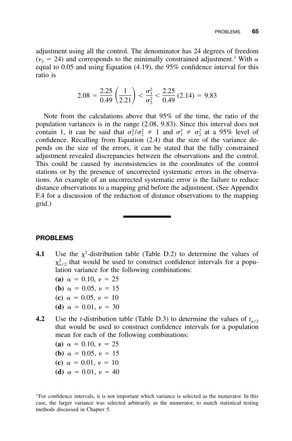
PROBLEMS 65
adjustment using all the control. The denominator has 24 degrees of freedom(�2 � 24) and corresponds to the minimally constrained adjustment.3 With �equal to 0.05 and using Equation (4.19), the 95% confidence interval for thisratio is
22.25 1 � 2.2512.08 � � � (2.14) � 9.83� � 20.49 2.21 � 0.492
Note from the calculations above that 95% of the time, the ratio of thepopulation variances is in the range (2.08, 9.83). Since this interval does notcontain 1, it can be said that / � 1 and � at a 95% level of2 2 2 2� � � �1 2 1 2
confidence. Recalling from Equation (2.4) that the size of the variance de-pends on the size of the errors, it can be stated that the fully constrainedadjustment revealed discrepancies between the observations and the control.This could be caused by inconsistencies in the coordinates of the controlstations or by the presence of uncorrected systematic errors in the observa-tions. An example of an uncorrected systematic error is the failure to reducedistance observations to a mapping grid before the adjustment. (See AppendixF.4 for a discussion of the reduction of distance observations to the mappinggrid.)
PROBLEMS
4.1 Use the �2-distribution table (Table D.2) to determine the values ofthat would be used to construct confidence intervals for a popu-2�� / 2
lation variance for the following combinations:(a) � � 0.10, � � 25(b) � � 0.05, � � 15(c) � � 0.05, � � 10(d) � � 0.01, � � 30
4.2 Use the t-distribution table (Table D.3) to determine the values of t� / 2
that would be used to construct confidence intervals for a populationmean for each of the following combinations:(a) � � 0.10, � � 25(b) � � 0.05, � � 15(c) � � 0.01, � � 10(d) � � 0.01, � � 40
3 For confidence intervals, it is not important which variance is selected as the numerator. In thiscase, the larger variance was selected arbitrarily as the numerator, to match statistical testingmethods discussed in Chapter 5.
66 CONFIDENCE INTERVALS
4.3 Use the F-distribution table (Table D.4) to determine the values ofthat would be used to construct confidence intervals for a pop-F�,� ,�1 2
ulation mean for each of the following combinations:(a) � � 0.20, �1 � 24, �2 � 2(b) � � 0.01, �1 � 15, �2 � 8(c) � � 0.05, �1 � 60, �2 � 20(d) � � 0.80, �1 � 2, �2 � 24
Use STATS to do Problems 4.4 through 4.6.
4.4 Problem 4.1
4.5 Problem 4.2
4.6 Problem 4.3
4.7 A least squares adjustment is computed twice on a data set. When thedata are minimally constrained with 10 degrees of freedom, a varianceof 1.07 is obtained. In the second run, the fully constrained networkhas 12 degrees of freedom with a standard deviation of 1.53. The apriori estimates for the reference variances in both adjustments are 1;that is, � � 1.2 2� �1 2
(a) What is the 95% confidence interval for the ratio of the two vari-ances? Is there reason to be concerned about the consistency ofthe control? Justify your response statistically.
(b) What is the 95% confidence interval for the reference variance inthe minimally constrained adjustment? The population variance is1. Does this interval contain 1?
(c) What is the 95% confidence interval for the reference variance inthe fully constrained adjustment? The population variance is 1.Does this interval contain 1?
4.8 The calibrated length of a baseline is 402.167 m. An average distanceof 402.151 m with a standard deviation of �0.0055 m is computedafter the line is observed five times with an EDM.(a) What is the 95% confidence interval for the measurement?(b) At a 95% level of confidence, can you state that the EDM is work-
ing properly? Justify your response statistically.(c) At a 90% level of confidence can you state that the EDM is work-
ing properly? Justify your response statistically.
4.9 An observer’s pointing and reading standard deviation is determinedto be �1.8� after pointing and reading the circles of a particular in-strument six times (n � 6). What is the 99% confidence interval forthe population variance?
PROBLEMS 67
4.10 Using sample statistics and the data in Example 3.1, construct a 90%confidence interval:(a) for a single observation, and identify any observations that may be
identified as possible outliers.(b) for the population variance.
4.11 Using sample statistics and the data in Example 3.2, construct a 90%confidence interval:(a) for a single observation, and identify any observations that may be
identified as possible outliers.(b) for the population variance.
4.12 Using sample statistics and the data from Problem 3.10 construct a95% confidence interval:(a) for a single observation, and identify any observations that may be
identified as possible outliers.(b) for the population variance.
4.13 For the data in Problem 3.11, construct a 95% confidence interval forthe ratio of the two variances for sets 1 and 2. Are the variances equalstatistically at this level of confidence? Justify your response statis-tically.
4.14 Using sample statistics and the data from Problem 3.12, construct a95% confidence interval:(a) for a single observation, and identify any observations that may be
identified as possible outliers in the data.(b) for the mean.
68
CHAPTER 5
STATISTICAL TESTING
5.1 HYPOTHESIS TESTING
In Example 4.4 we were not concerned about the actual bounds of the intervalconstructed, but rather, whether the interval contained the expected ratio ofthe variances. This is often the case in statistics. That is, the actual values ofthe interval are not as important as is answering the question: Is the samplestatistic consistent with what is expected from the population? The proceduresused to test the validity of a statistic are known as hypothesis testing. Thebasic elements of hypothesis testing are
1. The null hypothesis, H0, is a statement that compares a population sta-tistic with a sample statistic. This implies that the sample statistic iswhat is ‘‘expected’’ from the population. In Example 4.4, this would bethat the ratio of the variances is statistically 1.
2. The alternative hypothesis, Ha, is what is accepted when a decision ismade to reject the null hypothesis, and thus represents an alternativepopulation of data from which the sample statistic was derived. In Ex-ample 4.4 the alternative hypothesis would be that the ratio of the var-iances is not equal to 1 and thus the variance did not come from thesame population of data.
3. The test statistic is computed from the sample data and is the valueused to determine whether the null hypothesis should be rejected. Whenthe null hypothesis is rejected, it can be said that the sample statisticcomputed is not consistent with what is expected from the population.In Example 4.4 a rejection of the null hypothesis would occur when theratio of the variances is not statistically equivalent to 1.
Adjustment Computations: Spatial Data Analysis, Fourth Edition. C. D. Ghilani and P. R. Wolf© 2006 John Wiley & Sons, Inc. ISBN: 978-0-471-69728-2
5.1 HYPOTHESIS TESTING 69
4. The rejection region is the value for the test statistic where the nullhypothesis is rejected. In reference to confidence intervals, this numbertakes the place of the confidence interval bounds. That is, when the teststatistic computed is greater than the value defining the rejection region,it is equivalent to the sample statistic of the null hypothesis being out-side the bounds of the confidence interval. That is, when the rejectioncriterion is true, the null hypothesis is rejected.
Whenever a decision is made concerning the null hypothesis, there is apossibility of making a wrong decision since we can never be 100% certainabout a statistic or a test. Returning to Example 4.4, a confidence interval of95% was constructed. With this interval, there is a 5% chance that the decisionwas wrong. That is, it is possible that the larger-than-expected ratio of thevariances is consistent with the population of observations. This reasoningsuggests that further analysis of statistical testing is needed.
Two basic errors can occur when a decision is made about a statistic. Avalid statistic could be rejected, or an invalid statistic could be accepted. Thesetwo errors can be stated in terms of statistical testing elements as Type I andType II errors. If the null hypothesis is rejected when in fact it is true, a TypeI error is committed. If the null hypothesis is not rejected when in fact it isfalse, a Type II error occurs. Since these errors are not from the same pop-ulation, the probability of committing each error is not directly related. Adecision must be made as to the type of error that is more serious for thesituation, and the decision should be based on the consequences of commit-ting each error. For instance, if a contract calls for positional accuracies on95% of the stations to be within �0.3 ft, the surveyor is more inclined tocommit a Type I error to ensure that the contract specifications are met.However, the same surveyor, needing only 1-ft accuracy on control to supporta small-scale mapping project, may be more inclined to commit a Type IIerror. In either case, it is important to compute the probabilities of committingboth Type I and Type II errors to assess the reliability of the inferences derivedfrom a hypothesis test. For emphasis, the two basic hypothesis-testing errorsare repeated.
• Type I error: rejecting the null hypothesis when it is, in fact, true (sym-bolized by �)
• Type II error: not rejecting the null hypothesis when it is, in fact, false(symbolized by �)
Table 5.1 shows the relationship between the decision, the probabilities of� and �, and the acceptance or rejection of the null hypothesis, H0. In Figure5.1 the left distribution represents the data from which the null hypothesis isderived. That is, this distribution represents a true null hypothesis. Similarly,the distribution on the right represents the distribution of data for the truealternative. These two distributions could be attributed to measurements that
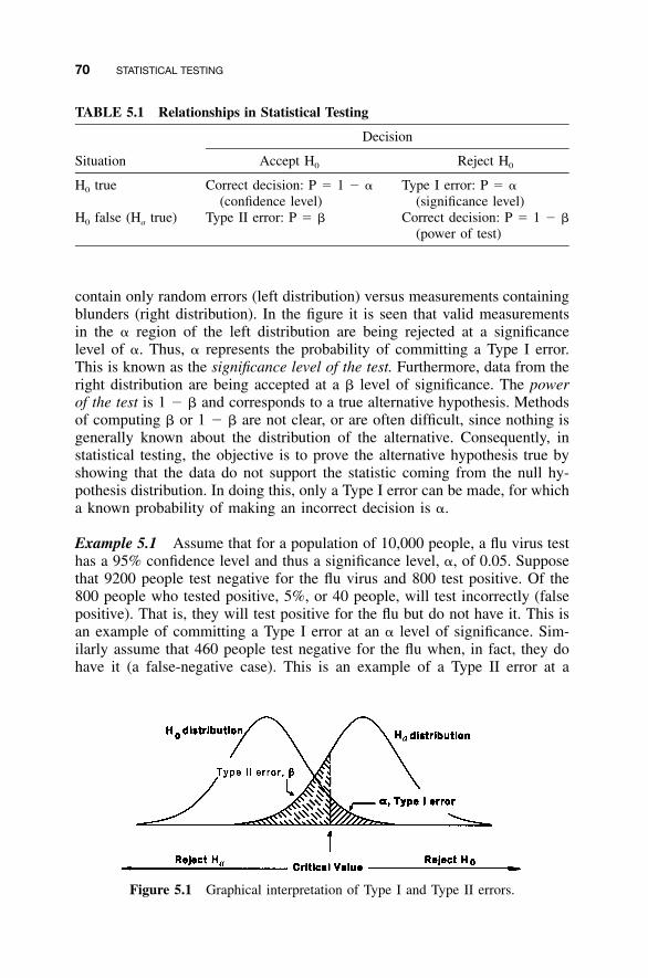
70 STATISTICAL TESTING
TABLE 5.1 Relationships in Statistical Testing
Situation
Decision
Accept H0 Reject H0
H0 true Correct decision: P � 1 � �(confidence level)
Type I error: P � �(significance level)
H0 false (Ha true) Type II error: P � � Correct decision: P � 1 � �(power of test)
Figure 5.1 Graphical interpretation of Type I and Type II errors.
contain only random errors (left distribution) versus measurements containingblunders (right distribution). In the figure it is seen that valid measurementsin the � region of the left distribution are being rejected at a significancelevel of �. Thus, � represents the probability of committing a Type I error.This is known as the significance level of the test. Furthermore, data from theright distribution are being accepted at a � level of significance. The powerof the test is 1 � � and corresponds to a true alternative hypothesis. Methodsof computing � or 1 � � are not clear, or are often difficult, since nothing isgenerally known about the distribution of the alternative. Consequently, instatistical testing, the objective is to prove the alternative hypothesis true byshowing that the data do not support the statistic coming from the null hy-pothesis distribution. In doing this, only a Type I error can be made, for whicha known probability of making an incorrect decision is �.
Example 5.1 Assume that for a population of 10,000 people, a flu virus testhas a 95% confidence level and thus a significance level, �, of 0.05. Supposethat 9200 people test negative for the flu virus and 800 test positive. Of the800 people who tested positive, 5%, or 40 people, will test incorrectly (falsepositive). That is, they will test positive for the flu but do not have it. This isan example of committing a Type I error at an � level of significance. Sim-ilarly assume that 460 people test negative for the flu when, in fact, they dohave it (a false-negative case). This is an example of a Type II error at a
5.2 SYSTEMATIC DEVELOPMENT OF A TEST 71
probability of �, that is equal to 0.046 (460/10,000). The power of the testis 1 � � or 0.954.
From the foregoing it is seen that it is possible to set the probability ofcommitting a Type I error for a given H0. However, for a fixed level of � andsample size n, the probability of a Type II error, �, is generally unknown. Ifthe null hypothesis, H0, and � are fixed, the power of the test can only beincreased by increasing the sample size, n. Since the power of the test maybe low or unknown, statisticians always say that the test failed to reject thenull hypothesis, rather than making any statements about its acceptance. Thisis an important statistical concept. That is, it should never be stated that thenull hypothesis is accepted since the power of the test is unknown. It shouldonly be said that ‘‘there is no statistical evidence to reject the null hypothesis.’’Because of this small but important distinction, it is important to construct atest that rejects the null hypothesis whenever possible.
A similar situation exists with surveying measurements. If a distance mea-surement contains a large systematic error, it is possible to detect this with afully constrained adjustment and thus reject the null hypothesis. However, ifa distance contains a very small systematic error, the ability to detect thesystematic error may be low. Thus, although some confidence can be placedin the rejection of the null hypothesis, it can never be said that the nullhypothesis should be accepted since the probability of undetected small sys-tematic errors or blunders cannot be determined. What we strive to do isminimize the size of these errors so that they have little effect on the computedresults.
5.2 SYSTEMATIC DEVELOPMENT OF A TEST
When developing a statistical test, the statistician must determine the testvariables and the type of test to perform. This book will look at statisticaltests for the mean, variance, and ratio of two sample variances. The t test isused when comparing a sample mean versus a population mean. This testcompares the mean of a set of observations against a known calibrated value.The �2 test is used when comparing a sample variance against a populationvariance. As discussed in Section 16.7, this test is used in a least squaresadjustment when comparing the reference variance from an adjustmentagainst its population value. Finally, when comparing variances from twodifferent sample sets, the F test is used. As discussed in Section 21.6, thistest is used in least squares adjustments when comparing the reference vari-ances from a minimally constrained and fully constrained adjustment. Table5.2 lists the test variables of these three statistical tests.
72 STATISTICAL TESTING
TABLE 5.2 Test Variables and Statistical Tests
Variable 1,Test Statistic
Variable 2,Sample Statistic Null Hypothesis Test Statistic
Population mean, � Sample mean, y H0: � � y tPopulation variance, �2 Sample variance, S2 H0: �2 � S2 �2
Ratio of samplevariances equals 1
/2 2S S1 2 H0: / � 12 2S S1 2 F
A test can take two forms based on the distributions. A one-tailed test usesthe critical value from either the left or right side of a distribution, whereasthe two-tailed test is much like a confidence interval, with the critical valuedivided equally on both sides of the distribution.
In the one-tailed test, the concern is whether the sample statistic is eithergreater or less than the statistic being tested. In the two-tailed test, the concernis whether the sample statistic is different from the statistic being tested. Forexample, when checking the angle-reading capabilities of a total stationagainst the manufacturer’s specifications, a surveyor would not be concernedif the instrument were working at a level better than the manufacturer’s statedaccuracy. However, the surveyor would probably send the instrument in forrepairs if it was performing at a level below the manufacturer’s stated accu-racy. In this case, it would be appropriate to perform a one-tailed test. On theother hand, when checking the mean distance observed using an EDM againsta known calibration baseline length, the surveyor wants to know if the meanlength is statistically different from the calibrated length. In this case it isappropriate to perform a two-tailed test. In the following sections it is im-portant (1) identify the appropriate test statistic and (2) the type of test toperform.
In all forms of statistical testing, a test statistic is developed from the data.The test statistic is then compared against a critical value from the distribu-tion. If the rejection region statement is true, the null hypothesis is rejectedat the level of significance selected. As stated earlier, this is the goal of awell-developed test since only Type I error occurs at the selected level ofsignificance. If the rejection region statement is false, the test fails to rejectnull hypothesis. Because of the possibility of Type II error and due to thelack of knowledge about the alternative distribution, no statement about thevalidity of the null hypothesis can be made; at best it can be stated that thereis no reason to reject the null hypothesis.
5.3 TEST OF HYPOTHESIS FOR THE POPULATION MEAN
At times it may be desirable to test a sample mean against a known value.The t distribution is used to build this test. The null hypothesis for this testcan take two forms: one- or two-tailed tests. In the one-tailed test, the concern
5.3 TEST OF HYPOTHESIS FOR THE POPULATION MEAN 73
is whether the sample mean is either statistically greater or less than thepopulation mean. In the two-tailed test, the concern is whether the samplemean is statistically different from the population mean. These two tests areshown below.
One-Tailed Test Two-Tailed Test
Null hypothesis: Ha: � � y H0: � � y
Alternative hypothesis: Ha: � � (� �y y) Ha: � � y
The test statistic is
y � �t � (5.1)
S /�n
The region where the null hypothesis is rejected is
t � t� (or t � t�) �t� � t� / 2
It should be stated that for large samples (n � 30), the t value can bereplaced by the standard normal variate, z.
Example 5.2 A baseline of calibrated length 400.008 m is observed repeat-edly with an EDM instrument. After 20 observations, the average of the ob-served distances is 400.012 m with a standard deviation of �0.002 m. Is thedistance observed significantly different from the distance calibrated at a 0.05level of significance?
SOLUTION Assuming that proper field and office procedures were fol-lowed, the fundamental question is whether the EDM is working within itsspecifications and thus providing distance observations in a population ofcalibrated values. To answer this question, a two-tailed test is used to deter-mine whether the distance is the same or is different from the distance cali-brated at a 0.05 level of significance. That is, the mean of the distancesobserved will be rejected if it is statistically either too short or too long tobe considered the same as the calibration value. The rationale behind usinga two-tailed test is similar to that used when constructing a confidence inter-val, as in Example 4.1. That is, 2.5% of the area from the lower and uppertails of the t distribution is to be excluded from the interval constructed, orin this case, the test.
The null hypothesis is
H : � � 400.0120
and the alternative hypothesis is

74 STATISTICAL TESTING
H : � � 400.012a
By Equation (5.1), the test statistic is
y � � 400.012 � 400.008t � � � 8.944
S /�n 0.002/�20
and the rejection region is
t � 8.944 � t� / 2
Since a two-tailed test is being done, the � /2 (0.025) column in the t-distribution table is intersected with the � � n � 1, or 19 degrees of freedom,row. From the t distribution (Table D.3), t0.025, 19 is found to be 2.093, andthus the rejection region is satisfied. In other words, the value computed fort is greater than the tabulated value, and thus the null hypothesis can berejected at a 95% level of confidence. That is,
t � 8.944 � t � 2.093� / 2
Based on the foregoing, there is reason to believe that the average lengthobserved is significantly different from its calibrated value at a 5% signifi-cance level. This implies that at least 5% of the time, the decision will bewrong. As stated earlier, a 95% confidence interval for the population meancould also have been constructed to derive the same results. Using Equation(4.7), that interval would yield
0.002400.011 � 400.012 � 2.093� ��20
0.002� � � 400.012 � 2.093 � 400.013� ��20
Note that the 95% confidence interval fails to contain the baseline value of400.008, and similarly, there is reason to be concerned about the calibrationstatus of the instrument. That is, it may not be working properly and shouldbe repaired.
5.4 TEST OF HYPOTHESIS FOR THE POPULATION VARIANCE
In Example 5.2, the procedure for checking whether an observed length com-pares favorably with a calibrated value was discussed. The surveyor may also
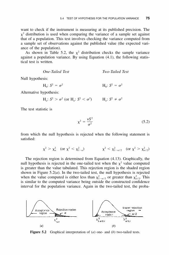
5.4 TEST OF HYPOTHESIS FOR THE POPULATION VARIANCE 75
Figure 5.2 Graphical interpretation of (a) one- and (b) two-tailed tests.
want to check if the instrument is measuring at its published precision. The�2 distribution is used when comparing the variance of a sample set againstthat of a population. This test involves checking the variance computed froma sample set of observations against the published value (the expected vari-ance of the population).
As shown in Table 5.2, the �2 distribution checks the sample varianceagainst a population variance. By using Equation (4.1), the following statis-tical test is written.
One-Tailed Test Two-Tailed Test
Null hypothesis:
H0: S2 � �2 H0: S2 � �2
Alternative hypothesis:
Ha: S2 � �2 (or Ha: S2 � �2) Ha: S2 � �2
The test statistic is
2�S2� � (5.2)2�
from which the null hypothesis is rejected when the following statement issatisfied:
�2 � (or �2 �2 2� � )� 1�� �2 � (or �2 �2 2� � )1�� / 2 � / 2
The rejection region is determined from Equation (4.13). Graphically, thenull hypothesis is rejected in the one-tailed test when the �2 value computedis greater than the value tabulated. This rejection region is the shaded regionshown in Figure 5.2(a). In the two-tailed test, the null hypothesis is rejectedwhen the value computed is either less than or greater than This2 2� � .1�� / 2 � / 2
is similar to the computed variance being outside the constructed confidenceinterval for the population variance. Again in the two-tailed test, the proba-
76 STATISTICAL TESTING
bility selected is evenly divided between the upper and lower tails of thedistribution such that the acceptance region is centered on the distribution.These rejection regions are shown graphically in Figure 5.2(b).
Example 5.3 The owner of a surveying firm wants all surveying techniciansto be able to read a particular instrument to within �1.5�. To test this value,the owner asks the senior field crew chief to perform a reading test with theinstrument. The crew chief reads the circle 30 times and obtains �r � �0.9�.Does this support the 1.5� limit at a 5% level of significance?
SOLUTION In this case the owner wishes to test the hypothesis that thecomputed sample variance is the same as the population variance rather thanbeing greater than the population variance. That is, all standard deviationsthat are equal to or less than 1.5� will be accepted. Thus, a one-tailed test isconstructed as follows (note that � � 30 � 1, or 29): The null hypothesis is
2 2H : S � �0
and the alternative hypothesis is
2 2H : S � �a
The test statistic is
2(30 � 1)0.92� � � 10.4421.5
The null hypothesis is rejected when the computed test statistic exceeds thetabulated value, or when the following statement is true:
2 2 2� � 10.44 � � � � � 42.56�,� 0.05,29
where 42.56 is from Table D.2 for Since the computed �2 value (10.44)2� .0.05,29
is less than the tabulated value (42.56), the null hypothesis cannot be rejected.However, simply failing to reject the null hypothesis does not mean that
the value of �1.5� is valid. This example demonstrates a common problemin statistical testing when results are interpreted incorrectly. A valid sampleset from the population of all surveying employees cannot be obtainedby selecting only one employee. Furthermore, the test is flawed since everyinstrument reads differently and thus new employees may initially haveproblems reading an instrument, due to their lack of experience with theinstrument. To account properly for this lack of experience, the employercould test a random sample of prospective employees during the interviewprocess, and again after several months of employment. The owner could thencheck for a correlation between the company’s satisfaction with the employee,
5.5 TEST OF HYPOTHESIS FOR THE RATIO OF TWO POPULATION VARIANCES 77
and the employee’s initial ability to read the instrument. However, it is un-likely that any correlation would be found. This is an example of misusingstatistics.
Example 5.3 illustrates an important point to be made when using statistics.The interpretation of statistical testing requires judgment by the person per-forming the test. It should always be remembered that with a test, the objec-tive is to reject and not accept the null hypothesis. Furthermore, a statisticaltest should be used only where appropriate.
5.5 TEST OF HYPOTHESIS FOR THE RATIO OF TWOPOPULATION VARIANCES
When adjusting data, surveyors have generally considered control to be ab-solute and without error. However, like any other quantities derived fromobservations, it is a known fact that control may contain error. As discussedin Example 4.4, one method of detecting both errors in control and possiblesystematic errors in horizontal network measurements is to do both a mini-mally constrained and a fully constrained least squares adjustment with thedata. After doing both adjustments, the post-adjustment reference variancescan be compared. If the control is without error and no systematic errors arepresent in the data, the ratio of the two reference variances should be closeto 1. Using Equation (4.18), a hypothesis test can be constructed to comparethe ratio of variances for two sample sets as follows:
One-Tailed Test Two-Tailed Test
Null hypothesis:
H0: � 1 (i.e., �2S1 2 2S S )1 22S2
H0: � 1 (i.e., �2S1 2 2S S )1 22S2
Alternative hypothesis:
Ha: � 1 (i.e., �2S1 2 2S S )1 22S2
Ha: � 1 (i.e., �2S1 2 2S S )1 22S2
or
2S1 2 2H : � 1 (i.e., S � S )a 1 22S2
The test statistic that will be used to determine rejection of the null hypothesisis
78 STATISTICAL TESTING
F � or F �2 2S S1 22 2S S2 1
F �larger sample variance
smaller sample variance
The null hypothesis should be rejected when the following statement issatisfied:
F � F� F � F� / 2
F� and F� / 2 are values that locate the � and � /2 areas, respectively, in theupper tail of the F distribution with �1 numerator degrees of freedom and �2
denominator degrees of freedom. Notice that in the two-tailed test, the degreesof freedom of the numerator are taken from the numerically larger samplevariance, and the degrees of freedom of the denominator are from the smallervariance.
Example 5.4 Using the same data as presented in Example 4.4, would thenull hypothesis be rejected?
SOLUTION In this example, a two-tailed test is appropriate since the onlyconcern is whether the two reference variances are equal statistically. In thisproblem, the interval is centered on the F distribution with an � /2 area in thelower and upper tails. In the analysis, 30 degrees of freedom in the numeratorcorrespond to the larger sample variance, and 24 degrees of freedom in thedenominator to the smaller variance, so that the following test is constructed:The null hypothesis is
2S1H : � 10 2S2
and the alternative hypothesis is
2S1H : � 1a 2S2
The test statistic for checking rejection of the null hypothesis is
2.25F � � 4.59
0.49
Rejection of the null hypothesis occurs when the following statement is true:
F � 4.59 � F � F � 2.21� / 2,�1,�2 0.025,30,24
5.5 TEST OF HYPOTHESIS FOR THE RATIO OF TWO POPULATION VARIANCES 79
Here it is seen that the F value computed (4.59) is greater than its valuefrom Table D.4 (2.21). Thus, the null hypothesis can be rejected. In otherwords, the fully constrained adjustment does not have the same variance asits minimally constrained counterpart at the 0.05 level of significance. Noticethat the same result was obtained here as was obtained in Example 4.4 withthe 95% confidence interval. Again, the network should be inspected for thepresence of systematic errors, followed by an analysis of possible errors inthe control stations. This post-adjustment analysis is revisited in greater detailin Chapter 20.
Example 5.5 Ron and Kathi continually debate who measures angles moreprecisely with a particular total station. After listening to enough of this de-bate, their supervisor describes a test where each is to measure a particulardirection by pointing and reading the instrument 51 times. They must thencompute the variance for their data. At the end of the 51 readings, Kathidetermines her variance to be 0.81 and Ron finds his to be 1.21. Is Kathi abetter instrument operator at a 0.01 level of significance?
SOLUTION In this situation, even though Kathi’s variance implies that herobservations are more precise than Ron’s, a determination must be made tosee if the reference variances are statistically equal versus Kathi’s being betterthan the Ron’s. This test requires a one-tailed F test with a significance levelof � � 0.01. The null hypothesis is
2SR 2 2H : � 1 (S � S )0 R K2SK
and the alternative hypothesis is
2SR 2 2H : � 1 (S � S )a R K2SK
The test statistic is
1.21F � � 1.49
0.81
The null hypothesis is rejected when the computed value for F (1.49) isgreater than the tabulated value for F0.01,50,50 (1.95). Here it is seen that thevalue computed for F is less than its tabulated value, and thus the test statisticdoes not satisfy the rejection region. That is,
80 STATISTICAL TESTING
F � 1.49 � F � 1.95 is false�,50,50
Therefore, there is no statistical reason to believe that Kathi is better thanRon at a 0.01 level of significance.
Example 5.6 A baseline is observed repeatedly over a period of time usingan EDM instrument. Each day, 10 observations are taken and averaged. Thevariances for the observations are listed below. At a significance level of 0.05,are the results of day 2 significantly different from those of day 5?
Day 1 2 3 4 5
Variance, S 2 (mm2) 50.0 61.0 51.0 53.0 54.0
SOLUTION This problem involves checking whether the variances of days2 and 5 are statistically equal or are different. This is the same as constructinga confidence interval involving the ratio of the variances. Because the concernis about equality or inequality, this will require a two-tailed test. Since 10observations were collected each day, both variances are based on 9 degreesof freedom (�1 and �2). Assume that the variance for day 2 is and the2S2
variance for day 5 is The test is constructed as follows: The null hypo-2S .5
thesis is
2S2H : � 10 2S5
and the alternative hypothesis is
2S2H : � 1a 2S5
The test statistic is
61F � � 1.13
54
The null hypothesis is rejected when the computed F value (1.13) is greaterthan the value in Table D.4 (4.03). In this case the rejection region is F �1.13 � F0.025,9,9 � 4.03 and is not satisfied. Consequently, the test fails toreject the null hypothesis, and there is no statistical reason to believe that thedata of day 2 are statistically different from those of day 5.
PROBLEMS 81
PROBLEMS
5.1 In your own words, state why the null hypothesis can never beaccepted.
5.2 Explain why medical tests on patients are performed several times ina laboratory before the results of the test are returned to the doctor.
5.3 In your own words, discuss when it is appropriate to use:(a) a one-tailed test.(b) a two-tailed test.
5.4 Match the following comparison with the appropriate test.(a) A calibration baseline length against a value measured using an
EDM.(b) Two sample variances.(c) The reference variance of a fully constrained adjustment against a
minimally constrained adjustment.(d) The reference variance of a least squares adjustment against its a
priori value of 1.
5.5 Compare the variances of days 2 and 5 in Example 5.6 at a level ofsignificance of 0.20 (� � 0.20). Would testing the variances of days 1and 2 result in a different finding?
5.6 Compare the variances of days 1 and 4 in Example 5.6 at a levelsignificance of 0.05 (� � 0.05). Would testing the variances of days 1and 3 result in a different finding?
5.7 Using the data given in Example 5.5, determine if Kathi is statisticallybetter with the equipment than Ron at a significance level of:(a) 0.05.(b) 0.10.
5.8 The population value for the reference variance from a properlyweighted least squares adjustment is 1. After running a minimally con-strained adjustment having 15 degrees of freedom, the reference vari-ance is computed 1.52. Is this variance statistically equal to 1 at:(a) a 0.01 level of significance?(b) a 0.05 level of significance?(c) a 0.10 level of significance?
5.9 When all the control is added to the adjustment in Problem 5.8, thereference variance for the fully constrained adjustment with 15 degreesof freedom is found to be 1.89. Are the reference variances from theminimally constrained and fully constrained adjustments statisticallyequal at:
82 STATISTICAL TESTING
(a) a 0.01 level of significance?(b) a 0.05 level of significance?(c) a 0.10 level of significance?
5.10 The calibrated length of a baseline is 402.267 m. A mean observationfor the distance is 402.251 m with a standard deviation of �0.0052 mafter six readings with an EDM.(a) Is the distance observed statistically different from the length cal-
ibrated at a 5% level of significance?(b) Is the distance observed statistically different from the length cal-
ibrated at a 10% level of significance?
5.11 A mean length of 1023.573 m with a standard deviation of �0.0056m is obtained for a distance after five observations. Using the technicalspecifications, it is found that the standard deviation for this observa-tion should be �0.0043 m.(a) Perform a statistical test to check the repeatability of the instrument
at a level of significance of 0.05.(b) Perform a statistical test to check the repeatability of the instru-
ment at a level of significance of 0.01.
5.12 A least squares adjustment is computed twice on a data set. When thedata are minimally constrained with 24 degrees of freedom, a referencevariance of 0.89 is obtained. In the second run, the fully constrainednetwork, which also has 24 degrees of freedom, has a reference vari-ance of 1.15. The a priori estimate for the reference variance in bothadjustments is 1; that is, � � 1.2 2� �1 2
(a) Are the two variances statistically equal at a 0.05 level ofsignificance?
(b) Is the minimally constrained adjustment reference variance statis-tically equal to 1 at a 0.05 level of significance?
(c) Is the fully constrained adjustment reference variance statisticallyequal to 1 at a 0.05 level of significance?
(d) Is there a statistical reason to be concerned about the presence oferrors in either the control or the observations?
5.13 A total station with a manufacturer’s specified angular accuracy of �5�was used to collect the data in Problem 5.12. Do the data warrant thisaccuracy at a 0.05 level of significance? Develop a statistical test tovalidate your response.
5.14 A surveying company decides to base a portion of their employees’salary raises on improvement in their use of equipment. To determinethe improvement, the employees measure their ability to point on atarget and read the circles of a theodolite every six months. One em-

PROBLEMS 83
ployee is tested six weeks after starting employment and obtains astandard deviation of �1.5� with 25 measurements. Six months laterthe employee obtains a standard deviation of �1.2� with 30 measure-ments. Did the employee improve statistically over six months at a 5%level of significance? Is this test an acceptable method of determiningimprovements in quality? What suggestion, if any, would you give tomodify the test?
5.15 An EDM is placed on a calibration baseline and the distance betweentwo monuments is determined to be 1200.012 m � 0.047 m after 10observations. The length between the monuments is calibrated as1200.005 m. Is the instrument measuring the length properly at:(a) a 0.01 level of significance?(b) a 0.05 level of significance?(c) a 0.10 level of significance?
84
CHAPTER 6
PROPAGATION OF RANDOMERRORS IN INDIRECTLYMEASURED QUANTITIES
6.1 BASIC ERROR PROPAGATION EQUATION
As discussed in Section 1.2, unknown values are often determined indirectlyby making direct measurements of other quantities which are functionallyrelated to the desired unknowns. Examples in surveying include computingstation coordinates from distance and angle observations, obtaining stationelevations from rod readings in differential leveling, and determining the az-imuth of a line from astronomical observations. As noted in Section 1.2, sinceall quantities that are measured directly contain errors, any values computedfrom them will also contain errors. This intrusion, or propagation, of errorsthat occurs in quantities computed from direct measurements is called errorpropagation. This topic is one of the most important discussed in this book.
In this chapter it is assumed that all systematic errors have been eliminated,so that only random errors remain in the direct observations. To derive thebasic error propagation equation, consider the simple function, z � a1x1 �a2x2, where x1 and x2 are two independently observed quantities with standarderrors �1 and �2, and a1 and a2 are constants. By analyzing how errors prop-agate in this function, a general expression can be developed for the propa-gation of random errors through any function.
Since x1 and x2 are two independently observed quantities, they each havedifferent probability density functions. Let the errors in n determinations ofx1 be . . . , and the errors in n determinations of x2 be . . . ,i ii n i iiε , ε , ε ε , ε ,1 1 1 2 2
then zT , the true value of z for each independent measurement, isnε ;2
Adjustment Computations: Spatial Data Analysis, Fourth Edition. C. D. Ghilani and P. R. Wolf© 2006 John Wiley & Sons, Inc. ISBN: 978-0-471-69728-2
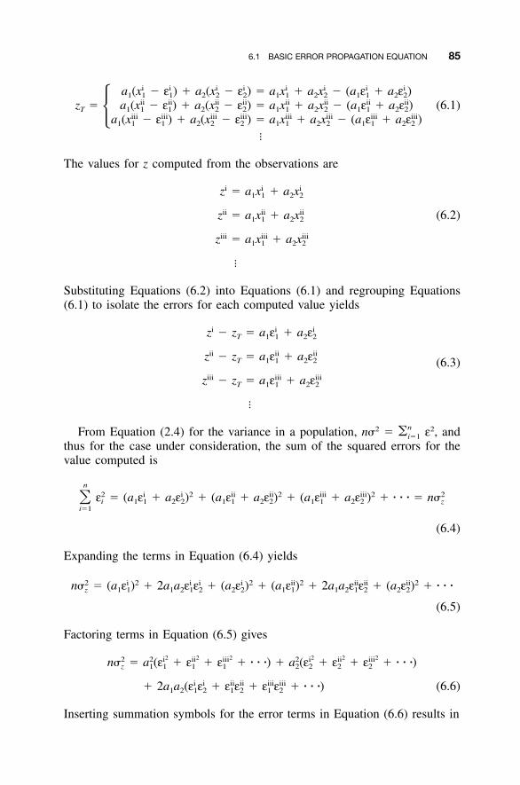
6.1 BASIC ERROR PROPAGATION EQUATION 85
i i i i i i i ia (x � ε ) � a (x � ε ) � a x � a x � (a ε � a ε )1 1 1 2 2 2 1 1 2 2 1 1 2 2ii ii ii ii ii ii ii iiz � a (x � ε ) � a (x � ε ) � a x � a x � (a ε � a ε ) (6.1)T 1 1 1 2 2 2 1 1 2 2 1 1 2 2� iii iii iii iii iii iii iii iiia (x � ε ) � a (x � ε ) � a x � a x � (a ε � a ε )1 1 1 2 2 2 1 1 2 2 1 1 2 2
�
The values for z computed from the observations are
i i iz � a x � a x1 1 2 2
ii ii iiz � a x � a x (6.2)1 1 2 2
iii iii iiiz � a x � a x1 1 2 2
�
Substituting Equations (6.2) into Equations (6.1) and regrouping Equations(6.1) to isolate the errors for each computed value yields
i i iz � z � a ε � a εT 1 1 2 2
ii ii iiz � z � a ε � a εT 1 1 2 2 (6.3)iii iii iiiz � z � a ε � a εT 1 1 2 2
�
From Equation (2.4) for the variance in a population, n�2 � ε2, andn�i�1
thus for the case under consideration, the sum of the squared errors for thevalue computed is
n2 i i 2 ii ii 2 iii iii 2 2ε � (a ε � a ε ) � (a ε � a ε ) � (a ε � a ε ) � � � � � n�� i 1 1 2 2 1 1 2 2 1 1 2 2 z
i�1
(6.4)
Expanding the terms in Equation (6.4) yields
2 i 2 i i i 2 ii 2 ii ii ii 2n� � (a ε ) � 2a a ε ε � (a ε ) � (a ε ) � 2a a ε ε � (a ε ) � � � �z 1 1 1 2 1 2 2 2 1 1 1 2 1 2 2 2
(6.5)
Factoring terms in Equation (6.5) gives
2 2 2 2 2 22 2 i ii iii 2 i ii iiin� � a (ε � ε � ε � � � �) � a (ε � ε � ε � � � �)z 1 1 1 1 2 2 2 2
i i ii ii iii iii� 2a a (ε ε � ε ε � ε ε � � � �) (6.6)1 2 1 2 1 2 1 2
Inserting summation symbols for the error terms in Equation (6.6) results in
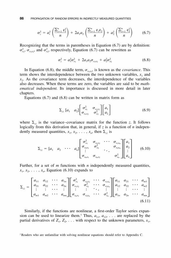
86 PROPAGATION OF RANDOM ERRORS IN INDIRECTLY MEASURED QUANTITIES
n n n2 2� ε � ε ε � ε1 1 2 2i�1 i�1 i�12 2 2� � a � 2a a � a (6.7)� � � � � �z i 1 2 2n n n
Recognizing that the terms in parentheses in Equation (6.7) are by definition:and respectively, Equation (6.7) can be rewritten as2 2� , � , � ,x x x x1 1 2 2
2 2 2 2 2� � a � � 2a a � � a � (6.8)z 1 x 1 2 x x 2 x1 1 2 2
In Equation (6.8), the middle term, is known as the covariance. This� ,x x1 2
term shows the interdependence between the two unknown variables, x1 andx2. As the covariance term decreases, the interdependence of the variablesalso decreases. When these terms are zero, the variables are said to be math-ematical independent. Its importance is discussed in more detail in laterchapters.
Equations (6.7) and (6.8) can be written in matrix form as
2� � ax x x 11 1 2� [a a ] (6.9)� �� �zz 1 2 2� � ax x x 21 2 2
where �zz is the variance–covariance matrix for the function z. It followslogically from this derivation that, in general, if z is a function of n indepen-dently measured quantities, x1, x2, . . . , xn, then �zz is
2� � � � � � ax x x x x 11 1 2 1 n2� � � ax x x x x 22 1 2 2 n� � [a a � � � a ] (6.10)zz 1 2 n �� � ��� � 2� � � ax x x x x nn 1 n 2 n
Further, for a set of m functions with n independently measured quantities,x1, x2, . . . , xn, Equation (6.10) expands to
2a a � � � a � � � � � � a a � � � a11 12 1n x x x x x 11 21 m11 1 2 1 n2a a � � � a � � � � � � a a � � � a21 22 2n x x x x x 12 22 m21 2 2 2 n� �zz �� � � � � � � � � � � � � � � ��� � � 2a a � � � a � � � � � � a a � � � am1 m2 mn x x x x x 1n 2n mnn 1 2 n n
(6.11)
Similarly, if the functions are nonlinear, a first-order Taylor series expan-sion can be used to linearize them.1 Thus, a11, a12, . . . are replaced by thepartial derivatives of Z1, Z2, . . . with respect to the unknown parameters, x1,
1 Readers who are unfamiliar with solving nonlinear equations should refer to Appendix C.
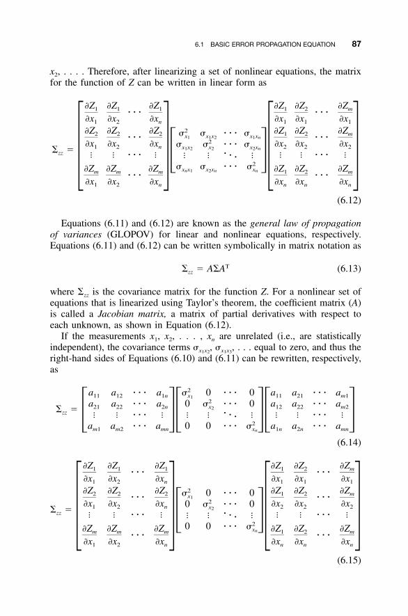
6.1 BASIC ERROR PROPAGATION EQUATION 87
x2, . . . . Therefore, after linearizing a set of nonlinear equations, the matrixfor the function of Z can be written in linear form as
�Z �Z �Z �Z �Z �Z1 1 1 1 2 m� � � � � ��x �x �x �x �x �x1 2 n 1 1 1
2�Z �Z �Z �Z �Z �Z2 2 2 1 2 m� � � � � �x x x x x1 1 2 1 n� � � � � �2�x �x �x �x �x �x� � � � � �1 2 n 2 2 2x x x x x1 2 2 2 n� �zz �� � � � � � � � � � � �� � � ��� 2� � � � � �� � x x x x x�Z �Z �Z �Z �Z �Zn 1 2 n nm m m 1 2 m� � � � � �
�x �x �x �x �x �x1 2 n n n n
(6.12)
Equations (6.11) and (6.12) are known as the general law of propagationof variances (GLOPOV) for linear and nonlinear equations, respectively.Equations (6.11) and (6.12) can be written symbolically in matrix notation as
T� � A�A (6.13)zz
where �zz is the covariance matrix for the function Z. For a nonlinear set ofequations that is linearized using Taylor’s theorem, the coefficient matrix (A)is called a Jacobian matrix, a matrix of partial derivatives with respect toeach unknown, as shown in Equation (6.12).
If the measurements x1, x2, . . . , xn are unrelated (i.e., are statisticallyindependent), the covariance terms . . . equal to zero, and thus the� , � ,x x x x1 2 1 3
right-hand sides of Equations (6.10) and (6.11) can be rewritten, respectively,as
2a a � � � a � 0 � � � 0 a a � � � a11 12 1n x 11 21 m112a a � � � a 0 � � � � 0 a a � � � a21 22 2n x 12 22 m22� �zz �� � � � � � � � � � � � � � � ��� � � 2a a � � � a 0 0 � � � � a a � � � am1 m2 mn x 1n 2n mnn
(6.14)
�Z �Z �Z �Z �Z �Z1 1 1 1 2 m� � � � � ��x �x �x �x �x �x1 2 n 1 1 1
2�Z �Z �Z �Z �Z �Z2 2 2 1 2 m� 0 � � � 0x1� � � � � �2�x �x �x �x �x �x0 � � � � 01 2 n 2 2 2x2� �zz �� � � � � � � � � � � �� � � ��� 20 0 � � � �� � x�Z �Z �Z �Z �Z �Znm m m 1 2 m� � � � � �
�x �x �x �x �x �x1 2 n n n n
(6.15)
88 PROPAGATION OF RANDOM ERRORS IN INDIRECTLY MEASURED QUANTITIES
If there is only one function Z, involving n unrelated quantities, x1, x2,. . . , xn, Equation (6.15) can be rewritten in algebraic form as
2 2 2�Z �Z �Z
� � � � � � � � � � � (6.16)� � � � � �Z x x x1 2 n �x �x �x1 2 n
Equations (6.14), (6.15), and (6.16) express the special law of propagationof variances (SLOPOV). These equations govern the manner in which errorsfrom statistically independent measurements (i.e., � 0) propagate in a�x xi j
function. In these equations, individual terms (�Z /�xi) represent the indi-�xi
vidual contributions to the total error that occur as the result of observationalerrors in each independent variable. When the size of a function’s estimatederror is too large, inspection of these individual terms will indicate the largestcontributors to the error. The most efficient way to reduce the overall errorin the function is to closely examine ways to reduce the largest error termsin Equation (6.16).
6.1.1 Generic Example
Let A � B � C, and assume that B and C are independently observed quan-tities. Note that �A /�B � 1 and �Z /�C � 1. Substituting these into Equation(6.16) yields
2 2� � �(1� ) � (1� ) (6.17)A B C
Using Equation (6.15) yields
2� 0 1B 2 2� � [1 1] � [� � � ]� �� �AA 2 B C0 � 1C
Equation (6.17) yields the same results as Equation (6.16) after the squareroot of the single element is determined. In the equations above, standarderror (�) and standard deviation (S) can be used interchangeably.
6.2 FREQUENTLY ENCOUNTERED SPECIFIC FUNCTIONS
6.2.1 Standard Deviation of a Sum
Let A � B1 � B2 � � � � � Bn, where the B’s are n independently observedquantities having standard deviations of . . . , Then by EquationS , S , S .B B B1 2 n
(6.16),
6.3 NUMERICAL EXAMPLES 89
2 2 2S � �S � S � � � � � S (6.18)A B B B1 2 n
6.2.2 Standard Deviation in a Series
Assume that the error for each observed value in Equation (6.18) is equal;that is, . . . , � SB then Equation (6.18) simplifies toS , S , SB B B1 2 n
S � S �n (6.19)A B
6.2.3 Standard Deviation of the Mean
Let be the mean obtained from n independently observed quantities y1, y2,y. . . , yn, each of which has the same standard deviation S. As given inEquation (2.1), the mean is expressed as
y � y � � � � � y1 2 ny �n
An equation for the standard deviation of is obtained by substitutingS , y,y
the expression above into Equation (6.16). Since the partial derivatives of ywith respect to the observed quantities, y1, y2, . . . , yn, is /�y1 � /�y2 ��y �y� � � � /�yn � 1/n, the resulting error in is�y y
2 2 2 21 1 1 nS SS � S � S � � � � � S � � (6.20)� � � � � �y y y y1 2 n 2 n n n n �n
Note that Equation (6.20) is the same as Equation (2.8).
6.3 NUMERICAL EXAMPLES
Example 6.1 The dimensions of the rectangular tank shown in Figure 6.1are measured as
L � 40.00 ft S � �0.05 ftL
W � 20.00 ft S � �0.03 ftW
H � 15.00 ft S � �0.02 ftH
Find the tank’s volume and the standard deviation in the volume using themeasurements above.
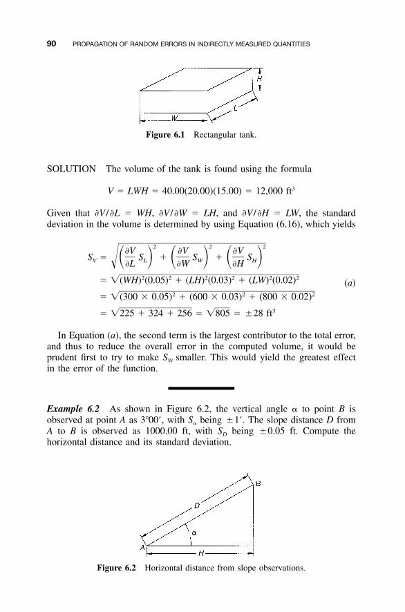
90 PROPAGATION OF RANDOM ERRORS IN INDIRECTLY MEASURED QUANTITIES
Figure 6.1 Rectangular tank.
Figure 6.2 Horizontal distance from slope observations.
SOLUTION The volume of the tank is found using the formula
3V � LWH � 40.00(20.00)(15.00) � 12,000 ft
Given that �V /�L � WH, �V /�W � LH, and �V /�H � LW, the standarddeviation in the volume is determined by using Equation (6.16), which yields
2 2 2�V �V �V
S � S � S � S� � � � � �V L W H �L �W �H2 2 2 2 2 2� �(WH) (0.05) � (LH) (0.03) � (LW) (0.02) (a)
2 2 2� �(300 � 0.05) � (600 � 0.03) � (800 � 0.02)3� �225 � 324 � 256 � �805 � �28 ft
In Equation (a), the second term is the largest contributor to the total error,and thus to reduce the overall error in the computed volume, it would beprudent first to try to make SW smaller. This would yield the greatest effectin the error of the function.
Example 6.2 As shown in Figure 6.2, the vertical angle � to point B isobserved at point A as 3�00�, with S� being �1�. The slope distance D fromA to B is observed as 1000.00 ft, with SD being �0.05 ft. Compute thehorizontal distance and its standard deviation.
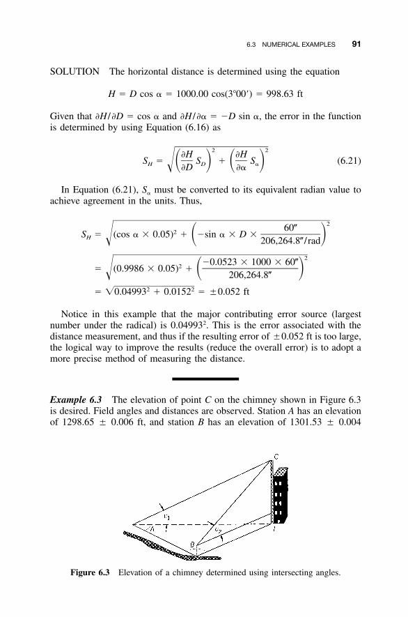
6.3 NUMERICAL EXAMPLES 91
Figure 6.3 Elevation of a chimney determined using intersecting angles.
SOLUTION The horizontal distance is determined using the equation
H � D cos � � 1000.00 cos(3�00�) � 998.63 ft
Given that �H /�D � cos � and �H /�� � �D sin �, the error in the functionis determined by using Equation (6.16) as
2 2�H �H
S � S � S (6.21)� � � �H D � �D ��
In Equation (6.21), S� must be converted to its equivalent radian value toachieve agreement in the units. Thus,
260�2S � (cos � � 0.05) � �sin � � D �� �H 206,264.8� / rad
2�0.0523 � 1000 � 60�2� (0.9986 � 0.05) � � � 206,264.8�
2 2� �0.04993 � 0.0152 � �0.052 ft
Notice in this example that the major contributing error source (largestnumber under the radical) is 0.049932. This is the error associated with thedistance measurement, and thus if the resulting error of �0.052 ft is too large,the logical way to improve the results (reduce the overall error) is to adopt amore precise method of measuring the distance.
Example 6.3 The elevation of point C on the chimney shown in Figure 6.3is desired. Field angles and distances are observed. Station A has an elevationof 1298.65 � 0.006 ft, and station B has an elevation of 1301.53 � 0.004
92 PROPAGATION OF RANDOM ERRORS IN INDIRECTLY MEASURED QUANTITIES
ft. The instrument height, hiA, at station A is 5.25 � 0.005 ft, and the instru-ment height, hiB, at station B is 5.18 � 0.005 ft. The other observations andtheir errors are
AB � 136.45 � 0.018
A � 44�12�34� � 8.6� B � 39�26�56� � 11.3�
v � 8�12�47� � 4.1� v � 5�50�10� � 5.1�1 2
What are the elevation of the chimney and the error in this computed value?
SOLUTION Normally, this problem is worked in several steps. The stepsinclude computing distances AI and BI and then solving for the average el-evation of C using observations obtained from stations A and B. However,caution must be exercised when doing error analysis in a stepwise fashionsince the computed values could be correlated and the stepwise method mightlead to an incorrect analysis of the errors. To avoid this, either GLOPOV canbe used or a single function can be derived that includes all quantities ob-served when the elevation is calculated. The second method is demonstratedas follows.
From the sine law, the solution of AI and BI can be derived as
AB sin B AB sin BAI � � (6.22)
sin[180� � (A � B)] sin(A � B)
AB sin ABI � (6.23)
sin(A � B)
Using Equations (6.22) and (6.23), the elevations for C from stations A andB are
Elev � AI tan v � Elev � hi (6.24)C 1 A AA
Elev � BI tan v � Elev � hi (6.25)C 2 B BB
Thus, the chimney’s elevation is computed as the average of Equations (6.24)and (6.25), or
1–Elev � (Elev � Elev ) (6.26)C 2 C CA B
Substituting Equations (6.22) through (6.25) into (6.26), a single expressionfor the chimney elevation can be written as
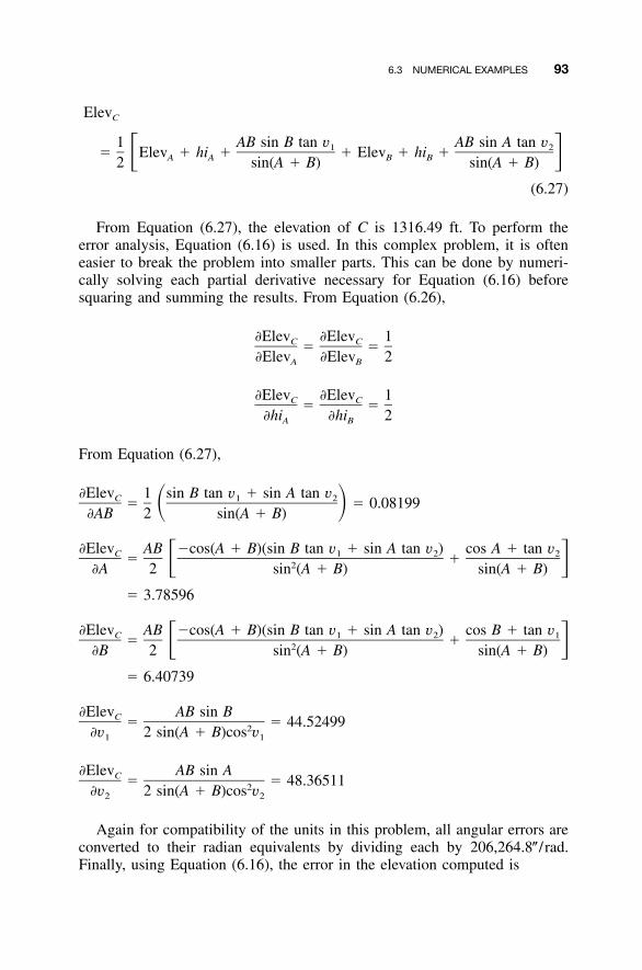
6.3 NUMERICAL EXAMPLES 93
ElevC
1 AB sin B tan v AB sin A tan v1 2� Elev � hi � � Elev � hi �� �A A B B2 sin(A � B) sin(A � B)
(6.27)
From Equation (6.27), the elevation of C is 1316.49 ft. To perform theerror analysis, Equation (6.16) is used. In this complex problem, it is ofteneasier to break the problem into smaller parts. This can be done by numeri-cally solving each partial derivative necessary for Equation (6.16) beforesquaring and summing the results. From Equation (6.26),
�Elev �Elev 1C C� ��Elev �Elev 2A B
�Elev �Elev 1C C� ��hi �hi 2A B
From Equation (6.27),
�Elev 1 sin B tan v � sin A tan vC 1 2� � 0.08199� ��AB 2 sin(A � B)
�Elev AB �cos(A � B)(sin B tan v � sin A tan v ) cos A � tan vC 1 2 2� �� �2�A 2 sin (A � B) sin(A � B)
� 3.78596
�Elev AB �cos(A � B)(sin B tan v � sin A tan v ) cos B � tan vC 1 2 1� �� �2�B 2 sin (A � B) sin(A � B)
� 6.40739
�Elev AB sin BC � � 44.524992�v 2 sin(A � B)cos v1 1
�Elev AB sin AC � � 48.365112�v 2 sin(A � B)cos v2 2
Again for compatibility of the units in this problem, all angular errors areconverted to their radian equivalents by dividing each by 206,264.8� / rad.Finally, using Equation (6.16), the error in the elevation computed is
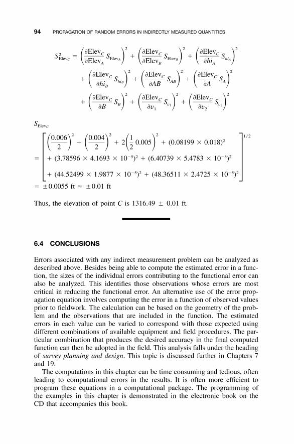
94 PROPAGATION OF RANDOM ERRORS IN INDIRECTLY MEASURED QUANTITIES
2 2 2�Elev �Elev �ElevC C C2S � S � S � S� � � � � �Elev Elev Elev hiC A B A�Elev �Elev �hiA B A
2 2 2�Elev �Elev �ElevC C C� S � S � S� � � � � �hi AB AB�hi �AB �AB
2 2 2�Elev �Elev �ElevC C C� S � S � S� � � � � �B v v1 2�B �v �v1 2
SElevC
2 2 2 1 / 20.006 0.004 1 2� � 2 0.005 � (0.08199 � 0.018)� � � � � �2 2 2�5 2 �5 2� � (3.78596 � 4.1693 � 10 ) � (6.40739 � 5.4783 � 10 )�
�5 2 �5 2� (44.52499 � 1.9877 � 10 ) � (48.36511 � 2.4725 � 10 )
� �0.0055 ft � �0.01 ft
Thus, the elevation of point C is 1316.49 � 0.01 ft.
6.4 CONCLUSIONS
Errors associated with any indirect measurement problem can be analyzed asdescribed above. Besides being able to compute the estimated error in a func-tion, the sizes of the individual errors contributing to the functional error canalso be analyzed. This identifies those observations whose errors are mostcritical in reducing the functional error. An alternative use of the error prop-agation equation involves computing the error in a function of observed valuesprior to fieldwork. The calculation can be based on the geometry of the prob-lem and the observations that are included in the function. The estimatederrors in each value can be varied to correspond with those expected usingdifferent combinations of available equipment and field procedures. The par-ticular combination that produces the desired accuracy in the final computedfunction can then be adopted in the field. This analysis falls under the headingof survey planning and design. This topic is discussed further in Chapters 7and 19.
The computations in this chapter can be time consuming and tedious, oftenleading to computational errors in the results. It is often more efficient toprogram these equations in a computational package. The programming ofthe examples in this chapter is demonstrated in the electronic book on theCD that accompanies this book.
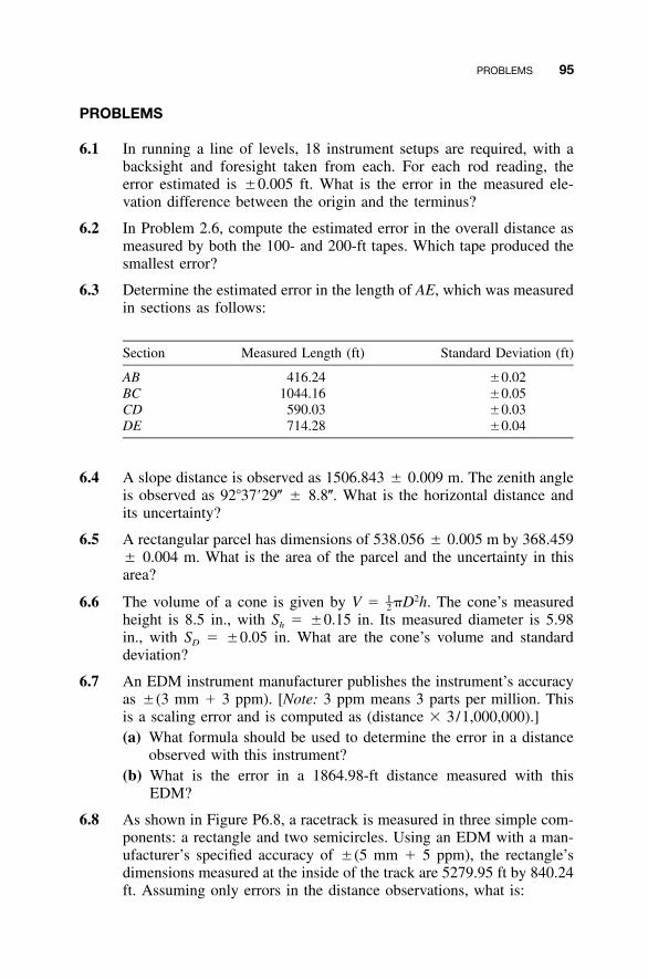
PROBLEMS 95
PROBLEMS
6.1 In running a line of levels, 18 instrument setups are required, with abacksight and foresight taken from each. For each rod reading, theerror estimated is �0.005 ft. What is the error in the measured ele-vation difference between the origin and the terminus?
6.2 In Problem 2.6, compute the estimated error in the overall distance asmeasured by both the 100- and 200-ft tapes. Which tape produced thesmallest error?
6.3 Determine the estimated error in the length of AE, which was measuredin sections as follows:
Section Measured Length (ft) Standard Deviation (ft)
AB 416.24 �0.02BC 1044.16 �0.05CD 590.03 �0.03DE 714.28 �0.04
6.4 A slope distance is observed as 1506.843 � 0.009 m. The zenith angleis observed as 92�37�29� � 8.8�. What is the horizontal distance andits uncertainty?
6.5 A rectangular parcel has dimensions of 538.056 � 0.005 m by 368.459� 0.004 m. What is the area of the parcel and the uncertainty in thisarea?
6.6 The volume of a cone is given by V � �D2h. The cone’s measured1–2height is 8.5 in., with Sh � �0.15 in. Its measured diameter is 5.98in., with SD � �0.05 in. What are the cone’s volume and standarddeviation?
6.7 An EDM instrument manufacturer publishes the instrument’s accuracyas �(3 mm � 3 ppm). [Note: 3 ppm means 3 parts per million. Thisis a scaling error and is computed as (distance � 3/1,000,000).](a) What formula should be used to determine the error in a distance
observed with this instrument?(b) What is the error in a 1864.98-ft distance measured with this
EDM?
6.8 As shown in Figure P6.8, a racetrack is measured in three simple com-ponents: a rectangle and two semicircles. Using an EDM with a man-ufacturer’s specified accuracy of �(5 mm � 5 ppm), the rectangle’sdimensions measured at the inside of the track are 5279.95 ft by 840.24ft. Assuming only errors in the distance observations, what is:
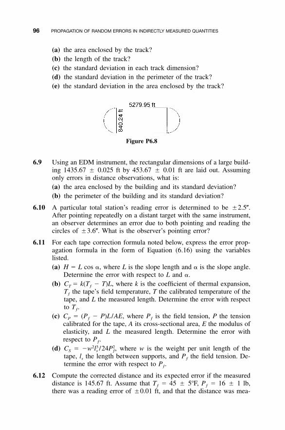
96 PROPAGATION OF RANDOM ERRORS IN INDIRECTLY MEASURED QUANTITIES
(a) the area enclosed by the track?(b) the length of the track?(c) the standard deviation in each track dimension?(d) the standard deviation in the perimeter of the track?(e) the standard deviation in the area enclosed by the track?
Figure P6.8
6.9 Using an EDM instrument, the rectangular dimensions of a large build-ing 1435.67 � 0.025 ft by 453.67 � 0.01 ft are laid out. Assumingonly errors in distance observations, what is:(a) the area enclosed by the building and its standard deviation?(b) the perimeter of the building and its standard deviation?
6.10 A particular total station’s reading error is determined to be �2.5�.After pointing repeatedly on a distant target with the same instrument,an observer determines an error due to both pointing and reading thecircles of �3.6�. What is the observer’s pointing error?
6.11 For each tape correction formula noted below, express the error prop-agation formula in the form of Equation (6.16) using the variableslisted.(a) H � L cos �, where L is the slope length and � is the slope angle.
Determine the error with respect to L and �.(b) CT � k(Tƒ � T)L, where k is the coefficient of thermal expansion,
Tƒ the tape’s field temperature, T the calibrated temperature of thetape, and L the measured length. Determine the error with respectto Tƒ.
(c) CP � (Pƒ � P)L /AE, where Pƒ is the field tension, P the tensioncalibrated for the tape, A its cross-sectional area, E the modulus ofelasticity, and L the measured length. Determine the error withrespect to Pƒ.
(d) CS � / where w is the weight per unit length of the2 3 2�w l 24P ,s ƒ
tape, ls the length between supports, and Pƒ the field tension. De-termine the error with respect to Pƒ.
6.12 Compute the corrected distance and its expected error if the measureddistance is 145.67 ft. Assume that Tƒ � 45 � 5�F, Pƒ � 16 � 1 lb,there was a reading error of �0.01 ft, and that the distance was mea-
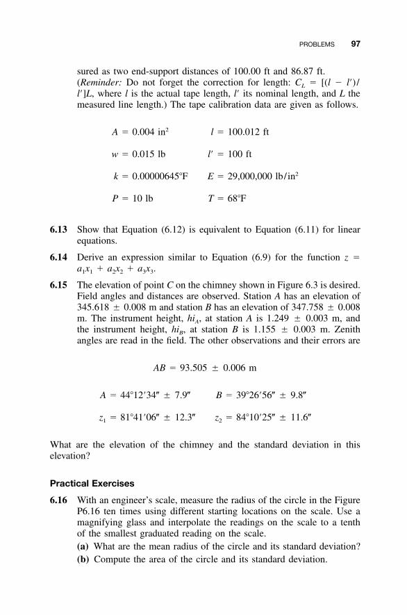
PROBLEMS 97
sured as two end-support distances of 100.00 ft and 86.87 ft.(Reminder: Do not forget the correction for length: CL � [(l � l�) /l�]L, where l is the actual tape length, l� its nominal length, and L themeasured line length.) The tape calibration data are given as follows.
2A � 0.004 in l � 100.012 ft
w � 0.015 lb l� � 100 ft
2k � 0.00000645�F E � 29,000,000 lb/in
P � 10 lb T � 68�F
6.13 Show that Equation (6.12) is equivalent to Equation (6.11) for linearequations.
6.14 Derive an expression similar to Equation (6.9) for the function z �a1x1 � a2x2 � a3x3.
6.15 The elevation of point C on the chimney shown in Figure 6.3 is desired.Field angles and distances are observed. Station A has an elevation of345.618 � 0.008 m and station B has an elevation of 347.758 � 0.008m. The instrument height, hiA, at station A is 1.249 � 0.003 m, andthe instrument height, hiB, at station B is 1.155 � 0.003 m. Zenithangles are read in the field. The other observations and their errors are
AB � 93.505 � 0.006 m
A � 44�12�34� � 7.9� B � 39�26�56� � 9.8�
z � 81�41�06� � 12.3� z � 84�10�25� � 11.6�1 2
What are the elevation of the chimney and the standard deviation in thiselevation?
Practical Exercises
6.16 With an engineer’s scale, measure the radius of the circle in the FigureP6.16 ten times using different starting locations on the scale. Use amagnifying glass and interpolate the readings on the scale to a tenthof the smallest graduated reading on the scale.(a) What are the mean radius of the circle and its standard deviation?(b) Compute the area of the circle and its standard deviation.
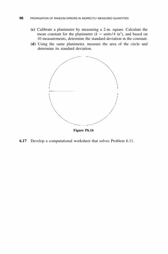
98 PROPAGATION OF RANDOM ERRORS IN INDIRECTLY MEASURED QUANTITIES
(c) Calibrate a planimeter by measuring a 2-in. square. Calculate themean constant for the planimeter (k � units/4 in2), and based on10 measurements, determine the standard deviation in the constant.
(d) Using the same planimeter, measure the area of the circle anddetermine its standard deviation.
Figure P6.16
6.17 Develop a computational worksheet that solves Problem 6.11.
99
CHAPTER 7
ERROR PROPAGATION IN ANGLEAND DISTANCE OBSERVATIONS
7.1 INTRODUCTION
All surveying observations are subject to errors from varying sources. Forexample, when observing an angle, the major error sources include instrumentplacement and leveling, target placement, circle reading, and target pointing.Although great care may be taken in observing the angle, these error sourceswill render inexact results. To appreciate fully the need for adjustments, sur-veyors must be able to identify the major observational error sources, knowtheir effects on the measurements, and understand how they can be modeled.In this chapter, emphasis is placed on analyzing the errors in observed hori-zontal angles and distances. In Chapter 8 the manner in which these errorspropagate to produce traverse misclosures is studied. In Chapter 9 the prop-agation of angular errors in elevation determination is covered.
7.2 ERROR SOURCES IN HORIZONTAL ANGLES
Whether a transit, theodolite, or total station instrument is used, errors arepresent in every horizontal angle observation. Whenever an instrument’s cir-cles are read, a small error is introduced into the final angle. Also, in pointingto a target, a small amount of error always occurs. Other major error sourcesin angle observations include instrument and target setup errors and the in-strument leveling error. Each of these sources produces random errors. Theymay be small or large, depending on the instrument, the operator, and theconditions at the time of the angle observation. The effects of reading, point-
Adjustment Computations: Spatial Data Analysis, Fourth Edition. C. D. Ghilani and P. R. Wolf© 2006 John Wiley & Sons, Inc. ISBN: 978-0-471-69728-2
100 ERROR PROPAGATION IN ANGLE AND DISTANCE OBSERVATIONS
ing, and leveling errors can be reduced by increasing the number of anglerepetitions. However, the effects of instrument and target setup errors can bereduced only by increasing sight distances.
7.3 READING ERRORS
Errors in reading conventional transits and theodolites depend on the qualityof the instrument’s optics, the size of the smallest division of the circle, andthe operator’s abilities: for example, the ability to set and read a transit ver-nier, or to set and read the micrometer of a theodolite. Typical reading errorsfor a 1� micrometer theodolite can range from tenths of a second to severalseconds. Reading errors also occur with digital instruments, their size beingdependent on the sensitivity of the particular electronic angular resolutionsystem. Manufacturers quote the estimated combined pointing and readingprecision for an individual direction measured face I (direct) and face II (re-versed) with their instruments in terms of standard deviations. Typical valuesrange from �1� for the more precise instruments to �10� for the less ex-pensive ones. These errors are random, and their effects on an angle dependon the observation method and the number of repeated observations.
7.3.1 Angles Observed by the Repetition Method
When observing a horizontal angle by repetition using a repeating instrument,the circle is first zeroed so that angles can be accumulated on the horizontalcircle. The angle is turned a number of times, and finally, the cumulativeangle is read and divided by the number of repetitions, to determine theaverage angular value. In this method, a reading error exists in just two po-sitions, regardless of the number of repetitions. The first reading error occurswhen the circle is zeroed and the second when reading the final cumulativeangle. For this procedure, the average angle is computed as
� � � � � � � � �1 2 n� � (a)n
where � is the average angle, and �1, �2, . . . , �n are the n repetitions of theangle. Recognizing that readings occur only when zeroing the plates andreading the final direction �n and applying Equation (6.16) to Equation (a),the standard error in reading the angle using the repetition method is
2 2�� � �0 r� � (7.1)�r n
7.3 READING ERRORS 101
where is the error in the average angle due to reading, �0 the estimated��r
error in setting zero on the circle, �r the estimated error in the final reading,and n the number of repetitions of the angle. Note that the number of repe-titions should always be an even number, with half being turned face I (direct)and half face II (reversed). This procedure compensates for systematic instru-mental errors.
Assuming that the observer’s ability to set zero and to read the circle areequal, Equation (7.1) is simplified to
� �2r� � (7.2)�r n
Example 7.1 Suppose that an angle is turned six times using the repetitionmethod. For an observer having a personal reading error of �1.5�, what isthe error in the final angle due to circle reading?
SOLUTION From Equation (7.2),
1.5��2� � � � �0.4��r 6
7.3.2 Angles Observed by the Directional Method
When a horizontal angle is observed by the directional method, the horizontalcircle is read in both the backsight and foresight directions. The angle is thenthe difference between the two readings. Multiple observations of the angleare made, with the circle being advanced prior to each reading to compensatefor the systematic errors. The final angle is taken as the average of all valuesobserved. Again, an even number of repetitions are made, with half taken inthe face I and half in the face II position. Since each repetition of the anglerequires two readings, the error in the average angle due to the reading erroris computed using Equation (6.16), which yields
2 2 2 2 2 2�(� � � ) � (� � � ) � � � � � (� � � )r r r r r r1b 1ƒ 2b 2ƒ nb nƒ� � (7.3)�r n
where and are the estimated errors in reading the circle for the back-� �r rib iƒ
sight and foresight directions, respectively, and n is the number of repetitions.Assuming that one’s ability to read the circle is independent of the particulardirection, so that � � �r, Equation (7.3) simplifies to� �r rib iƒ
102 ERROR PROPAGATION IN ANGLE AND DISTANCE OBSERVATIONS
� �2r� � (7.4)�r �n
Example 7.2 Using the same parameters of six repetitions and an estimatedobserver reading error of �1.5� as given in Example 7.1, find the error es-timated in the average angle due to reading when the directional method isused.
SOLUTION
1.5��2� � � � �0.9��P �6
Note that the additional readings required in the directional method producea larger error in the angle than that obtained using the repetition method.
7.4 POINTING ERRORS
Accuracy in pointing to a target depends on several factors. These includethe optical qualities of the instrument, target size, the observer’s personalability to place the crosswires on a target, and the weather conditions at thetime of observation. Pointing errors are random, and they will occur in everyangle observation no matter the method used. Since each repetition of anangle consists of two pointings, the pointing error for an angle that is themean of n repetitions can be estimated using Equation (6.16) as
2 2 2�2� � 2� � � � � � 2�p1 p2 pn� � (7.5)�p n
where is the error due to pointing and �p1, �p2, . . . , �pn are the estimated��p
errors in pointings for the first repetition, second repetition, and so on. Againfor a given instrument and observer, the pointing error can be assumed thesame for each repetition (i.e., �p1 � �p2 � � � � � �pn � �p), and Equation(7.5) simplifies to
� �2p� � (7.6)�p �n
Example 7.3 An angle is observed six times by an observer whose abilityto point on a well-defined target is estimated to be �1.8�. What is the esti-mated error in the average angle due to the pointing error?
7.5 ESTIMATED POINTING AND READING ERRORS WITH TOTAL STATIONS 103
SOLUTION From Equation (7.6),
1.8��2� � � � �1.0��p �6
7.5 ESTIMATED POINTING AND READING ERRORS WITHTOTAL STATIONS
With the introduction of electronic theodolites and subsequently, total stationinstruments, new standards were developed for estimating errors in angleobservations. The new standards, called DIN 18723, provide values for esti-mated errors in the mean of two direction observations, one each in the faceI and face II positions. Thus, in terms of a single pointing and reading error,�pr, the DIN value, �DIN, can be expressed as
� �2 �pr pr� � �DIN 2 �2
Using this equation, the expression for the estimated error in the observationof a single direction due to pointing and reading with an electronic theodoliteis
� � � �2 (b)pr DIN
Using a procedure similar to that given in Equation (7.6), the estimated errorin an angle measured n times and averaged due to pointing and reading is
� �2pr� � (c)�pr �n
Substituting Equation (b) into Equation (c) yields
2�DIN� � (7.7)�pr �n
Example 7.4 An angle is observed six times by an operator with a totalstation instrument having a published DIN 18723 value for the pointing andreading error of �5�. What is the estimated error in the angle due to thepointing and reading error?
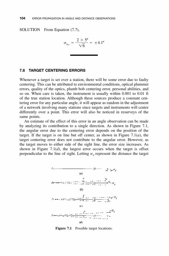
104 ERROR PROPAGATION IN ANGLE AND DISTANCE OBSERVATIONS
Figure 7.1 Possible target locations.
SOLUTION From Equation (7.7),
2 � 5�� � � �4.1��pr �6
7.6 TARGET CENTERING ERRORS
Whenever a target is set over a station, there will be some error due to faultycentering. This can be attributed to environmental conditions, optical plummeterrors, quality of the optics, plumb bob centering error, personal abilities, andso on. When care is taken, the instrument is usually within 0.001 to 0.01 ftof the true station location. Although these sources produce a constant cen-tering error for any particular angle, it will appear as random in the adjustmentof a network involving many stations since targets and instruments will centerdifferently over a point. This error will also be noticed in resurveys of thesame points.
An estimate of the effect of this error in an angle observation can be madeby analyzing its contribution to a single direction. As shown in Figure 7.1,the angular error due to the centering error depends on the position of thetarget. If the target is on line but off center, as shown in Figure 7.1(a), thetarget centering error does not contribute to the angular error. However, asthe target moves to either side of the sight line, the error size increases. Asshown in Figure 7.1(d), the largest error occurs when the target is offsetperpendicular to the line of sight. Letting �d represent the distance the target
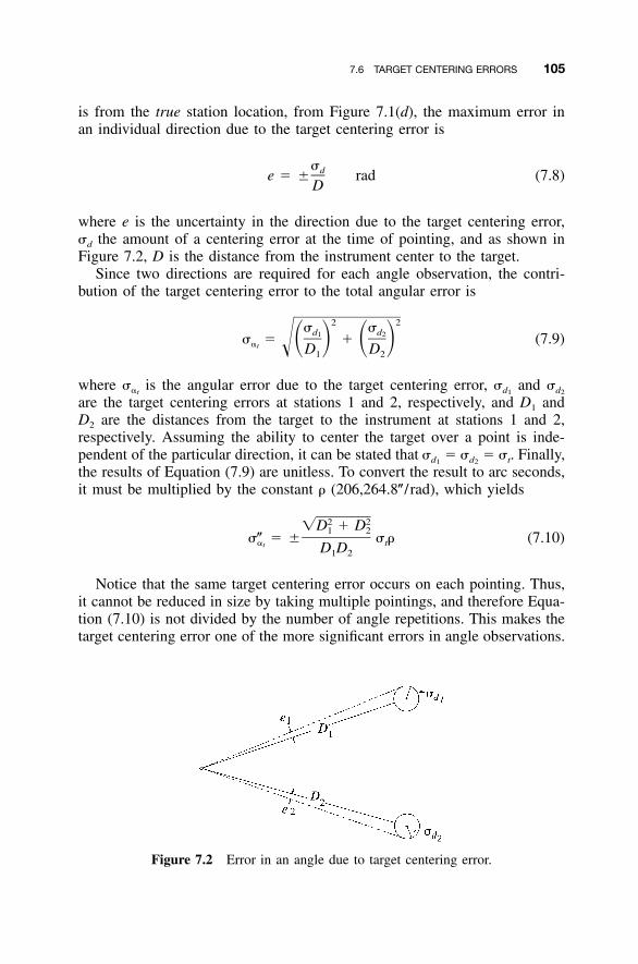
7.6 TARGET CENTERING ERRORS 105
Figure 7.2 Error in an angle due to target centering error.
is from the true station location, from Figure 7.1(d), the maximum error inan individual direction due to the target centering error is
�de � � rad (7.8)D
where e is the uncertainty in the direction due to the target centering error,�d the amount of a centering error at the time of pointing, and as shown inFigure 7.2, D is the distance from the instrument center to the target.
Since two directions are required for each angle observation, the contri-bution of the target centering error to the total angular error is
2 2� �d d1 2� � � (7.9)� � � ��t � D D1 2
where is the angular error due to the target centering error, and� � �� d dt 1 2
are the target centering errors at stations 1 and 2, respectively, and D1 andD2 are the distances from the target to the instrument at stations 1 and 2,respectively. Assuming the ability to center the target over a point is inde-pendent of the particular direction, it can be stated that � � �t. Finally,� �d d1 2
the results of Equation (7.9) are unitless. To convert the result to arc seconds,it must be multiplied by the constant � (206,264.8� / rad), which yields
2 2�D � D1 2�� � � � � (7.10)� tt D D1 2
Notice that the same target centering error occurs on each pointing. Thus,it cannot be reduced in size by taking multiple pointings, and therefore Equa-tion (7.10) is not divided by the number of angle repetitions. This makes thetarget centering error one of the more significant errors in angle observations.
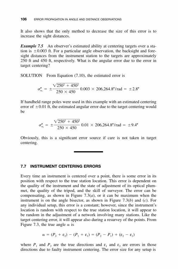
106 ERROR PROPAGATION IN ANGLE AND DISTANCE OBSERVATIONS
It also shows that the only method to decrease the size of this error is toincrease the sight distances.
Example 7.5 An observer’s estimated ability at centering targets over a sta-tion is �0.003 ft. For a particular angle observation, the backsight and fore-sight distances from the instrument station to the targets are approximately250 ft and 450 ft, respectively. What is the angular error due to the error intarget centering?
SOLUTION From Equation (7.10), the estimated error is
2 2�250 � 450�� � � 0.003 � 206,264.8� / rad � �2.8��t 250 � 450
If handheld range poles were used in this example with an estimated centeringerror of �0.01 ft, the estimated angular error due to the target centering wouldbe
2 2�250 � 450�� � � 0.01 � 206,264.8� / rad � �9.4��t 250 � 450
Obviously, this is a significant error source if care is not taken in targetcentering.
7.7 INSTRUMENT CENTERING ERRORS
Every time an instrument is centered over a point, there is some error in itsposition with respect to the true station location. This error is dependent onthe quality of the instrument and the state of adjustment of its optical plum-met, the quality of the tripod, and the skill of surveyor. The error can becompensating, as shown in Figure 7.3(a), or it can be maximum when theinstrument is on the angle bisector, as shown in Figure 7.3(b) and (c). Forany individual setup, this error is a constant; however, since the instrument’slocation is random with respect to the true station location, it will appear tobe random in the adjustment of a network involving many stations. Like thetarget centering error, it will appear also during a resurvey of the points. FromFigure 7.3, the true angle � is
� � (P � ε ) � (P � ε ) � (P � P ) � (ε � ε )2 2 1 1 2 1 2 1
where P1 and P2 are the true directions and ε1 and ε2 are errors in thosedirections due to faulty instrument centering. The error size for any setup is
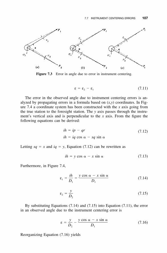
7.7 INSTRUMENT CENTERING ERRORS 107
Figure 7.3 Error in angle due to error in instrument centering.
ε � ε � ε (7.11)2 1
The error in the observed angle due to instrument centering errors is an-alyzed by propagating errors in a formula based on (x,y) coordinates. In Fig-ure 7.4 a coordinate system has been constructed with the x axis going fromthe true station to the foresight station. The y axis passes through the instru-ment’s vertical axis and is perpendicular to the x axis. From the figure thefollowing equations can be derived:
ih � ip � qr (7.12)
ih � iq cos � � sq sin �
Letting sq � x and iq � y, Equation (7.12) can be rewritten as
ih � y cos � � x sin � (7.13)
Furthermore, in Figure 7.4,
ih y cos � � x sin �ε � � (7.14)1 D D1 1
yε � (7.15)2 D2
By substituting Equations (7.14) and (7.15) into Equation (7.11), the errorin an observed angle due to the instrument centering error is
y y cos � � x sin �ε � � (7.16)
D D2 1
Reorganizing Equation (7.16) yields
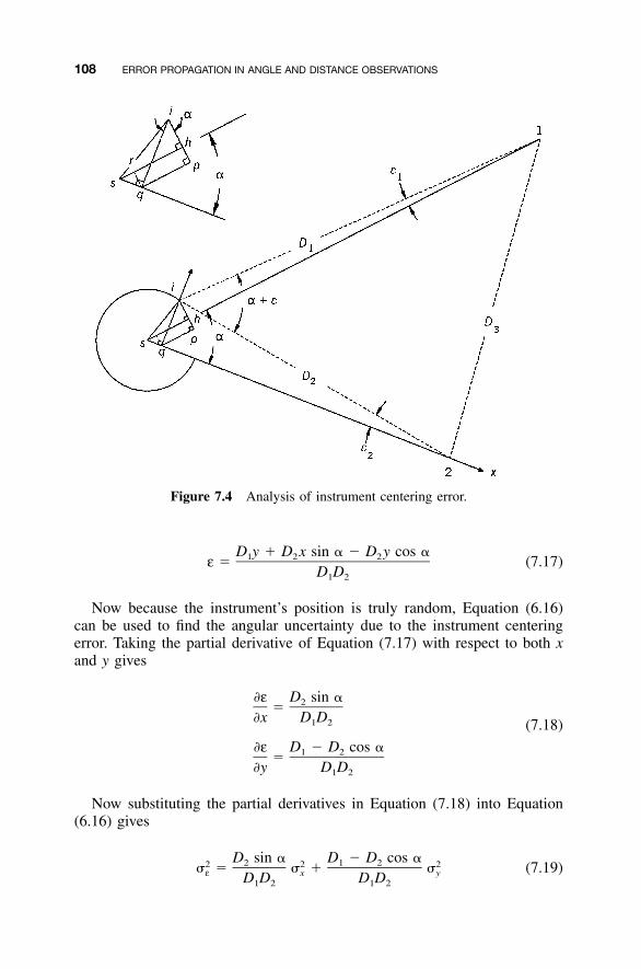
108 ERROR PROPAGATION IN ANGLE AND DISTANCE OBSERVATIONS
Figure 7.4 Analysis of instrument centering error.
D y � D x sin � � D y cos �1 2 2ε � (7.17)D D1 2
Now because the instrument’s position is truly random, Equation (6.16)can be used to find the angular uncertainty due to the instrument centeringerror. Taking the partial derivative of Equation (7.17) with respect to both xand y gives
�ε D sin �2��x D D1 2 (7.18)
�ε D � D cos �1 2��y D D1 2
Now substituting the partial derivatives in Equation (7.18) into Equation(6.16) gives
D sin � D � D cos �2 1 22 2 2� � � � � (7.19)ε x yD D D D1 2 1 2
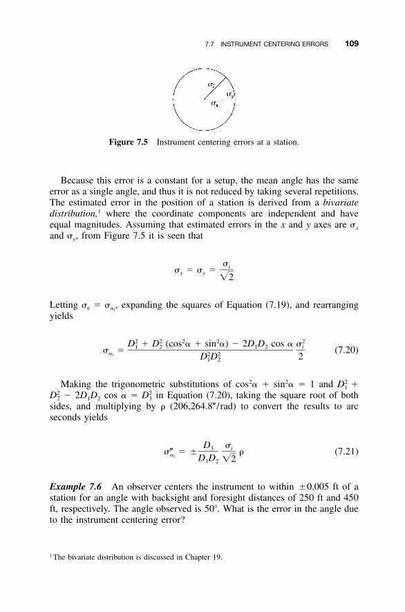
7.7 INSTRUMENT CENTERING ERRORS 109
Figure 7.5 Instrument centering errors at a station.
Because this error is a constant for a setup, the mean angle has the sameerror as a single angle, and thus it is not reduced by taking several repetitions.The estimated error in the position of a station is derived from a bivariatedistribution,1 where the coordinate components are independent and haveequal magnitudes. Assuming that estimated errors in the x and y axes are �x
and �y, from Figure 7.5 it is seen that
�i� � � �x y �2
Letting �ε � expanding the squares of Equation (7.19), and rearranging� ,�i
yields
2 2 2 2 2D � D (cos � � sin �) � 2D D cos � �1 2 1 2 i� � (7.20)�i 2 2D D 21 2
Making the trigonometric substitutions of cos2� � sin2� � 1 and 2D �1
� 2D1D2 cos � � in Equation (7.20), taking the square root of both2 2D D2 3
sides, and multiplying by � (206,264.8� / rad) to convert the results to arcseconds yields
D �3 i�� � � � (7.21)�i D D �21 2
Example 7.6 An observer centers the instrument to within �0.005 ft of astation for an angle with backsight and foresight distances of 250 ft and 450ft, respectively. The angle observed is 50�. What is the error in the angle dueto the instrument centering error?
1 The bivariate distribution is discussed in Chapter 19.
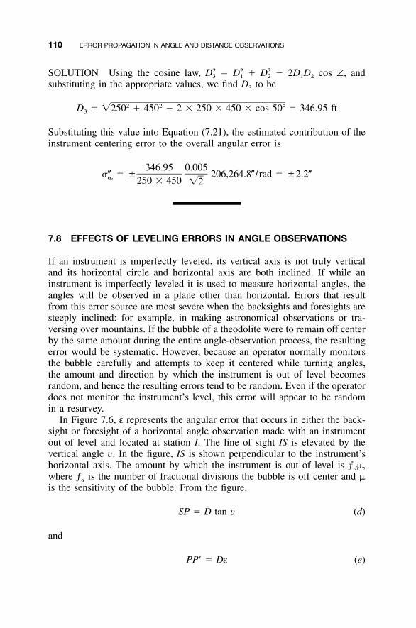
110 ERROR PROPAGATION IN ANGLE AND DISTANCE OBSERVATIONS
SOLUTION Using the cosine law, � � � 2D1D2 cos ∠, and2 2 2D D D3 1 2
substituting in the appropriate values, we find D3 to be
2 2D � �250 � 450 � 2 � 250 � 450 � cos 50� � 346.95 ft3
Substituting this value into Equation (7.21), the estimated contribution of theinstrument centering error to the overall angular error is
346.95 0.005�� � � 206,264.8� / rad � �2.2��i 250 � 450 �2
7.8 EFFECTS OF LEVELING ERRORS IN ANGLE OBSERVATIONS
If an instrument is imperfectly leveled, its vertical axis is not truly verticaland its horizontal circle and horizontal axis are both inclined. If while aninstrument is imperfectly leveled it is used to measure horizontal angles, theangles will be observed in a plane other than horizontal. Errors that resultfrom this error source are most severe when the backsights and foresights aresteeply inclined: for example, in making astronomical observations or tra-versing over mountains. If the bubble of a theodolite were to remain off centerby the same amount during the entire angle-observation process, the resultingerror would be systematic. However, because an operator normally monitorsthe bubble carefully and attempts to keep it centered while turning angles,the amount and direction by which the instrument is out of level becomesrandom, and hence the resulting errors tend to be random. Even if the operatordoes not monitor the instrument’s level, this error will appear to be randomin a resurvey.
In Figure 7.6, ε represents the angular error that occurs in either the back-sight or foresight of a horizontal angle observation made with an instrumentout of level and located at station I. The line of sight IS is elevated by thevertical angle v. In the figure, IS is shown perpendicular to the instrument’shorizontal axis. The amount by which the instrument is out of level is ƒd�,where ƒd is the number of fractional divisions the bubble is off center and �is the sensitivity of the bubble. From the figure,
SP � D tan v (d)
and
PP� � Dε (e)
7.8 EFFECTS OF LEVELING ERRORS IN ANGLE OBSERVATIONS 111
Figure 7.6 Effects of instrument leveling error.
where D is the horizontal component of the sighting distance and the angularerror ε is in radians. Because the amount of leveling error is small, PP� canbe approximated as a circular arc, and thus
PP� � ƒ �(SP) (f)d
Substituting Equation (d) into Equation (f) yields
PP� � ƒ �D tan v (7.22)d
Now substituting Equation (7.22) into Equation (e) and reducing, the error inan individual pointing due to the instrument leveling error is
ε � ƒ � tan v (7.23)d
As noted above, Figure 7.6 shows the line of sight oriented perpendicularto the instrument’s horizontal axis. Also, the direction in which a bubble runsis random. Thus, Equation (6.18) can be used to compute the combined an-gular error that results from n repetitions of an angle made with an imperfectlyleveled instrument (note that each angle measurement involves both backsightand foresight pointings):
2 2�(ƒ � tan v ) � (ƒ � tan v )d b d ƒ� � � (7.24)�l �n
where vb and vƒ are the vertical angles to the backsight and foresight targets,respectively, and n is the number of repetitions of the angle.
112 ERROR PROPAGATION IN ANGLE AND DISTANCE OBSERVATIONS
Example 7.7 A horizontal angle is observed on a mountainside where thebacksight is to the peak and the foresight is in the valley. The average zenithangles to the backsight and foresight are 80� and 95�, respectively. The in-strument has a level bubble with a sensitivity of 30� /div and is leveled towithin 0.3 div. For the average angle obtained from six repetitions, what isthe contribution of the leveling error to the overall angular error?
SOLUTION The zenith angles converted to vertical angles are �10� and�5�, respectively. Substituting the appropriate values into Equation (7.24)yields
2[0.3 div(30� /div) tan 10�]2� � [0.3 div(30� /div) tan(�5�)]
� � ��l �6
� �0.7�
This error is generally small for traditional surveying work when normalcare is taken in leveling the instrument. Thus, it can generally be ignored forall but the most precise work. However, as noted earlier, for astronomicalobservations this error can become quite large, due to the steeply inclinedsights to celestial objects. Thus, for astronomical observations it is extremelyimportant to keep the instrument leveled precisely for each observation.
7.9 NUMERICAL EXAMPLE OF COMBINED ERROR PROPAGATIONIN A SINGLE HORIZONTAL ANGLE
Example 7.8 Assume that an angle is observed four times with a directional-type instrument. The observer has an estimated reading error of �1� and apointing error of �1.5�. The targets are well defined and placed on an opticalplummet tribrach with an estimated centering error of �0.003 ft. The instru-ment is in adjustment and centered over the station to within �0.003 ft. Thehorizontal distances from the instrument to the backsight and foresight targetsare approximately 251 ft and 347 ft, respectively. The average angle is65�37�12�. What is the estimated error in the angle observation?
SOLUTION The best way to solve this type of problem is to computedestimated errors for each item in Sections 7.3 to 7.8 individually, and thenapply Equation (6.18).
Error due to reading: Substituting the appropriate values into Equation(7.4) yields
7.9 NUMERICAL EXAMPLE OF COMBINED ERROR PROPAGATION 113
1��2� � � � �0.71��r �4
Error due to pointing: Substituting the appropriate values into Equation(7.6) yields
1.5��2� � � � �1.06��p �4
Error due to target centering: Substituting the appropriate values intoEquation (7.10) yields
2 2�251 � 347�� � (0.003)206,264.8� / rad � �3.04��t 251 � 347
Error due to instrument centering: From the cosine law we have
2 2 2D � 251 � 347 � 2(251)(347) cos (65�37�12�)3
D � 334 ft3
Substituting the appropriate values into Equation (7.21) yields
334 0.003�� � � 206,264.8� / rad � �1.68��t 251 � 347 �2
Combined error: From Equation (6.18), the estimated angular error is
2 2 2 2� � �0.71 � 1.06 � 3.04 � 1.68 � �3.7��
In Example 7.8, the largest error sources are due to the target and instru-ment centering errors, respectively. This is true even when the estimated errorin centering the target and instrument are only �0.003 ft. Unfortunately,many surveyors place more confidence in their observations than is warranted.Since these two error sources do not decrease with increased repetitions, thereis a limit to what can be expected from any survey. For instance, assume thatthe targets were handheld reflector poles with an estimated centering error of�0.01 ft. Then the error due to the target centering error becomes �10.1�.This results in an estimated angular error of �10.3�. If a 99% probable errorwere computed, a value as large as �60� would be possible!
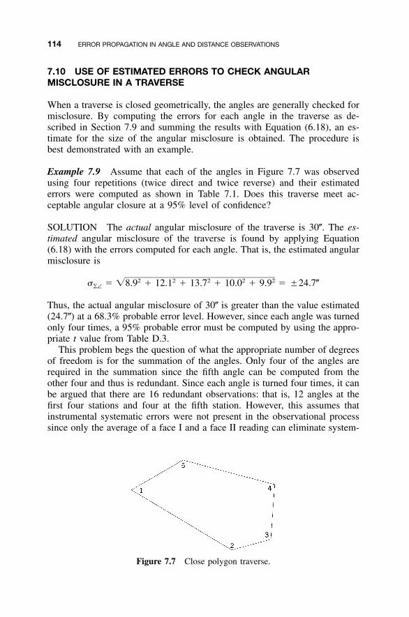
114 ERROR PROPAGATION IN ANGLE AND DISTANCE OBSERVATIONS
Figure 7.7 Close polygon traverse.
7.10 USE OF ESTIMATED ERRORS TO CHECK ANGULARMISCLOSURE IN A TRAVERSE
When a traverse is closed geometrically, the angles are generally checked formisclosure. By computing the errors for each angle in the traverse as de-scribed in Section 7.9 and summing the results with Equation (6.18), an es-timate for the size of the angular misclosure is obtained. The procedure isbest demonstrated with an example.
Example 7.9 Assume that each of the angles in Figure 7.7 was observedusing four repetitions (twice direct and twice reverse) and their estimatederrors were computed as shown in Table 7.1. Does this traverse meet ac-ceptable angular closure at a 95% level of confidence?
SOLUTION The actual angular misclosure of the traverse is 30�. The es-timated angular misclosure of the traverse is found by applying Equation(6.18) with the errors computed for each angle. That is, the estimated angularmisclosure is
2 2 2 2 2� � �8.9 � 12.1 � 13.7 � 10.0 � 9.9 � �24.7��∠
Thus, the actual angular misclosure of 30� is greater than the value estimated(24.7�) at a 68.3% probable error level. However, since each angle was turnedonly four times, a 95% probable error must be computed by using the appro-priate t value from Table D.3.
This problem begs the question of what the appropriate number of degreesof freedom is for the summation of the angles. Only four of the angles arerequired in the summation since the fifth angle can be computed from theother four and thus is redundant. Since each angle is turned four times, it canbe argued that there are 16 redundant observations: that is, 12 angles at thefirst four stations and four at the fifth station. However, this assumes thatinstrumental systematic errors were not present in the observational processsince only the average of a face I and a face II reading can eliminate system-
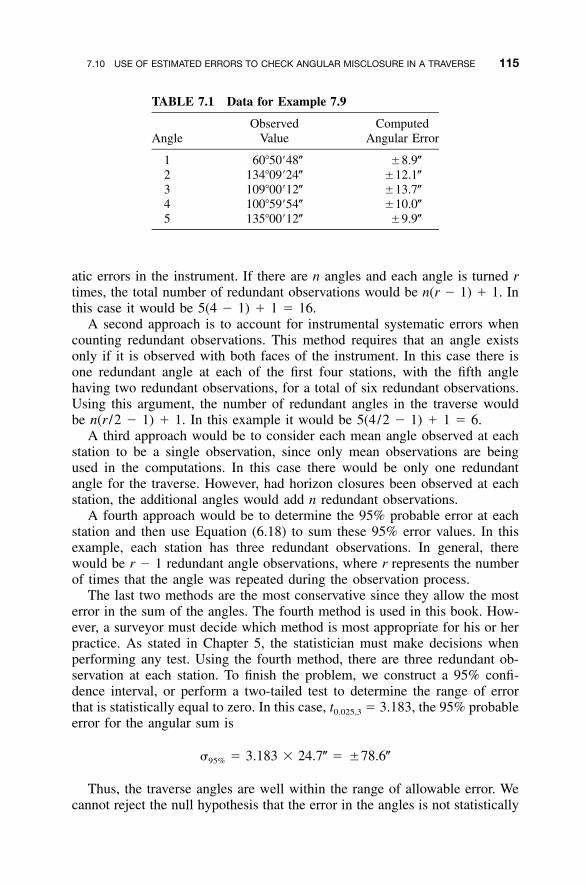
7.10 USE OF ESTIMATED ERRORS TO CHECK ANGULAR MISCLOSURE IN A TRAVERSE 115
TABLE 7.1 Data for Example 7.9
AngleObserved
ValueComputed
Angular Error
1 60�50�48� �8.9�2 134�09�24� �12.1�3 109�00�12� �13.7�4 100�59�54� �10.0�5 135�00�12� �9.9�
atic errors in the instrument. If there are n angles and each angle is turned rtimes, the total number of redundant observations would be n(r � 1) � 1. Inthis case it would be 5(4 � 1) � 1 � 16.
A second approach is to account for instrumental systematic errors whencounting redundant observations. This method requires that an angle existsonly if it is observed with both faces of the instrument. In this case there isone redundant angle at each of the first four stations, with the fifth anglehaving two redundant observations, for a total of six redundant observations.Using this argument, the number of redundant angles in the traverse wouldbe n(r /2 � 1) � 1. In this example it would be 5(4/2 � 1) � 1 � 6.
A third approach would be to consider each mean angle observed at eachstation to be a single observation, since only mean observations are beingused in the computations. In this case there would be only one redundantangle for the traverse. However, had horizon closures been observed at eachstation, the additional angles would add n redundant observations.
A fourth approach would be to determine the 95% probable error at eachstation and then use Equation (6.18) to sum these 95% error values. In thisexample, each station has three redundant observations. In general, therewould be r � 1 redundant angle observations, where r represents the numberof times that the angle was repeated during the observation process.
The last two methods are the most conservative since they allow the mosterror in the sum of the angles. The fourth method is used in this book. How-ever, a surveyor must decide which method is most appropriate for his or herpractice. As stated in Chapter 5, the statistician must make decisions whenperforming any test. Using the fourth method, there are three redundant ob-servation at each station. To finish the problem, we construct a 95% confi-dence interval, or perform a two-tailed test to determine the range of errorthat is statistically equal to zero. In this case, t0.025,3 � 3.183, the 95% probableerror for the angular sum is
� � 3.183 � 24.7� � �78.6�95%
Thus, the traverse angles are well within the range of allowable error. Wecannot reject the null hypothesis that the error in the angles is not statistically
116 ERROR PROPAGATION IN ANGLE AND DISTANCE OBSERVATIONS
equal to zero. Thus, the survey meets the minimum level of angular closureat a 95% probable error. However, it must be remembered that because ofthe possibility of Type II errors, we can only state that there is no statisticalreason to believe that there is a blunder in the angle observations.
Example 7.9 presents another question for the statistician or surveyor. Thatis, should a surveyor allow a field crew to have this large an angular misclo-sure in the traverse? Statistically, the answer would seem to be yes, but itmust remembered that the target and instrument centering errors affect angleobservations only if the instrument and targets are reset after each observation.Since this is never done in practice, these two errors should not be includedin the summation of the angles. Instead, the allowable angular misclosureshould be based solely on pointing and reading errors. For example, if theangles were observed with a total station having a DIN 18723 standard of�1�, by Equation (7.7) the pointing and reading error for each angle wouldbe
2 � 1�� � � � �1.4��pr �2
By Equation (6.19), the error in the summation of the five angles would beUsing the same critical t value of 3.183, the allowable�1.4��5 � �3.2�.
error in the angular misclosure should only be 3.183 � 3.2� � �10�. If thisinstrument had be used in Example 7.9, the field-observed angular closure of30� would be unacceptable and would warrant reobservation of some or allof the angles.
As stated in Sections 7.6 and 7.7, the angular misclosure of 78.6� computedin Example 7.9 will be noticed only when the target and instrument are reseton a survey. This will happen during the resurvey, when the centering errorsof the target and instrument from the original survey will be present in therecord directions. Thus, record azimuths and/or bearings could disagree fromthose determined in the resurvey by this amount, assuming that the equipmentused in the resurvey is comparable or of higher quality than that used in theoriginal survey.
7.11 ERRORS IN ASTRONOMICAL OBSERVATIONS FORAN AZIMUTH
The total error in an azimuth determined from astronomical observations de-pends on errors from several sources, including those in timing, the observer’slatitude and longitude, the celestial object’s position at observation time, tim-ing accuracy, observer response time, instrument optics, atmospheric condi-
7.11 ERRORS IN ASTRONOMICAL OBSERVATIONS FOR AN AZIMUTH 117
tions, and others, as identified in Section 7.2. The error in an astronomicalobservation can be estimated by analyzing the hour–angle formula, which is
sin t�1z � tan (7.25)
cos � tan � sin � cos t
In Equation (7.25), z is the azimuth of the celestial object at the time of theobservation, t the t angle of the PZS triangle at the time of observation, � theobserver’s latitude, and the object’s declination at the time of theobservation.
The t angle is a function of the local hour angle (LHA) of the sun or astar at the time of observation. That is, when the LHA � 180�, t � LHA;otherwise, t � 360� � LHA. Furthermore, LHA is a function of the Greenwichhour angle (GHA) of the celestial body and the observer’s longitude; that is,
LHA � GHA � (7.26)
where is the observer’s longitude, considered positive for eastern longitudeand negative for western longitude. The GHA increases approximately 15�per hour of time, and thus an estimate of the error in the GHA isapproximately
� � 15� � �t T
where �T is the estimated error in time (in hours). Similarly, by using thedeclination at 0h and 24h, the amount of change in declination per second canbe derived and thus the estimated error in declination determined.
Using Equation (6.16), the error in a star’s azimuth is estimated by takingthe partial derivative of Equation (7.25) with respect to t, , �, and . To dothis, simplify Equation (7.25) by letting
F � cos � tan � sin � cos t (7.27a)
and
�1u � sin t � F (7.27b)
Substituting in Equations (7.27), Equation (7.25) is rewritten as
sin t�1 �1z � tan � tan u (7.28)
F
From calculus it is known that
118 ERROR PROPAGATION IN ANGLE AND DISTANCE OBSERVATIONS
�1d tan u 1 du� 2dx 1 � u dx
Applying this fundamental relation to Equation (7.28) and letting G representGHA yields
2�z 1 du F du� � (7.29)2 2 2�G 1 � [sin(G � ) /F] dG F � sin (G � ) dG
Now du /dG is
du cos(G � ) sin(G � )� � sin � sin(G � )2dG F F
2cos(G � ) sin (G � ) sin �� � 2F F
and thus,
2du F cos(G � ) � sin (G � ) sin �� (7.30)2dG F
Substituting Equation (7.30) into Equation (7.29) and substituting in t for G� yields
2�z F cos t � sin t sin �� (7.31)2 2�G F � sin t
In a similar fashion, the following partial derivatives are developed fromEquation (7.25):
dz sin t cos �� � (7.32)2 2 2d cos (F � sin t)
�z sin t cos t cos � � sin t sin � tan � (7.33)2 2�� F � sin t
2�z sin t sin � � F cost t� (7.34)2 2� F � sin t
where t is the t angle of the PZS triangle, z the celestial object’s azimuth, the celestial object’s declination, � the observer’s latitude, the observer’slongitude, and F � cos � tan � sin � cos t.
7.11 ERRORS IN ASTRONOMICAL OBSERVATIONS FOR AN AZIMUTH 119
If the horizontal angle, H, is the angle to the right observed from the lineto the celestial body, the equation for a line’s azimuth is
Az � z � 360� � H
Therefore, the error contributions from the horizontal angle observation mustbe included in computing the overall error in the azimuth. Since the distanceto the star is considered infinite, the estimated contribution to the angularerror due to the instrument centering error can be determined with a formulasimilar to that for the target centering error with one pointing. That is,
�i� � (7.35)�i D
where �i is the centering error in the instrument and D is the length of theazimuth line in the same units. Note that the results of Equation (7.35) arein radian units and must be multiplied by � to yield a value in arc seconds.
Example 7.10 Using Equation (7.25), the azimuth to Polaris was found tobe 0�01�31.9�. The observation time was 1:00:00 UTC with an estimated errorof �T � �0.5s. The Greenwich hour angles to the star at 0h and 24h UTCwere 243�27�05.0� and 244�25�50.0�, respectively. The LHA at the time ofthe observation was 181�27�40.4�. The declinations at 0h and 24h were89�13�38.18� and 89�13�38.16�, respectively. At the time of observation, thedeclination was 89�13�38.18�. The clockwise horizontal angle measured fromthe backsight to a target 450.00 ft was 221�25�55.9�. The observer’s latitudeand longitude were scaled from a map as 40�13�54�N and 77�01�51.5�W,respectively, with estimated errors of �1�. The vertical angle to the star was39�27�33.1�. The observer’s estimated errors in reading and pointing are �1�and �1.5�, respectively, and the instrument was leveled to within 0.3 of adivision with a bubble sensitivity of 25� /div. The estimated error in instrumentand target centering is �0.003 ft. What are the azimuth of the line and itsestimated error? What is the error at the 95% level of confidence?
SOLUTION The azimuth of the line is Az � 0�01�31.9� � 360 �221�25�55.9� � 138�35�36�. Using the Greenwich hour angles at 0h and 24h,an error of 0.5s time will result in an estimated error in the GHA of
360� � (244�25�50.0� � 243�27�05.0�) s� 0.05 � �7.52�h s / h24 � 3600
Since t � 360� � LHA � 178�32�19.6�, F in Equations (7.29) through (7.34)is
120 ERROR PROPAGATION IN ANGLE AND DISTANCE OBSERVATIONS
F � cos(40�13�54�) tan(89�13�38.18�) � sin(40�13�54�) cos(178�32�19.6�)
� 57.249
The error in the observed azimuth can be estimated by computing the indi-vidual error terms as follows:
(a) From Equation (7.31), the error with respect to the GHA, G, is
�z� �G�G
257.249 cos(178�32�19.6�) � sin (178�32�19.6�) sin(40�13�54�)(7.52�)2 257.249 � sin (178�32�19.6�)
� �0.13�
(b) By observing the change in declination, it is obvious that for this ob-servation, the error in a time of 0.5s is insignificant. In fact, for theentire day, the declination changes only 0.02�. This situation is com-mon for stars. However, the sun’s declination may change from onlya few seconds daily to more than 23 minutes per day, and thus forsolar observations, this error term should not be ignored.
(c) From Equation (7.33) the error with respect to latitude, �, is
�z sin t cos t cos � � sin t sin � tan � � � � � �0.0004�� �2 2�� F � sin t
(d) From Equation (7.34) the error with respect to longitude, , is
�z�
�
2sin (178�32�19.6�) sin(40�13�54�) � 57.249 cos(178�32�19.6�)� (1�)2 257.249 � sin (178�32�19.6�)
� �0.02�
(e) The circles are read both when pointing on the star and on the azimuthmark. Thus, from Equation (7.2), the reading contribution to the esti-mated error in the azimuth is
� � �� �2 � �1��2 � �1.41�� rr
(f) Using Equation (7.6), the estimated error in the azimuth due to pointingis
� � �� �2 � �1.5��2 � �2.12�� pp
7.12 ERRORS IN ELECTRONIC DISTANCE OBSERVATIONS 121
(g) From Equation (7.8), the estimated error in the azimuth due to targetcentering is
d 0.003�� � � � � 206,264.8� / rad � �1.37�� ��t D 450
(h) Using Equation (7.35), the estimated error in the azimuth due to in-strument centering is
d 0.003�� � � � � 206,264.8� / rad � �1.37�� ��i D 450
(i) From Equation (7.23), the estimated error in the azimuth due to theleveling error is
� � �ƒ � tan v � �0.3 � 25� tan(39�27�33.1�) � �6.17�� db
Parts (a) through (i) are the errors for each individual error source. UsingEquation (6.18), the estimated error in the azimuth observation is
2 2 2 2(0.13�) � (1.32�) � (0.02�) � (0.0004�)� �AZ 2 2 2� � (2.12�) � 2(1.37�) � (6.17�)
� �7.0�
Using the appropriate t value of t0.025,1 from Table D.3, the 95% error is
� � �12.705 � 7.0� � �88.9�Az
Notice that in this problem, the largest error source in the azimuth error iscaused by the instrument leveling error.
7.12 ERRORS IN ELECTRONIC DISTANCE OBSERVATIONS
All EDM observations are subject to instrumental errors that manufacturerslist as constant, a, and scalar, b, error. A typical specified accuracy is �(a �b ppm). In this expression, a is generally in the range 1 to 10 mm, and b isa scalar error that typically has the range 1 to 10 ppm. Other errors involvedin electronic distance observations stem from the target and instrument cen-tering errors. Since in any survey involving several stations these errors tendto be random, they should be combined using Equation (6.18). Thus, theestimated error in an EDM observed distance is
2 2 2 2� � �� � � � a � (D � b ppm) (7.36)D i t
122 ERROR PROPAGATION IN ANGLE AND DISTANCE OBSERVATIONS
where �D is the error in the observed distance D, �i the instrument centeringerror, �t the reflector centering error, and a and b the instrument’s specifiedaccuracy parameters.
Example 7.11 A distance of 453.87 ft is observed using an EDM with amanufacturer’s specified accuracy of �(5 mm � 10 ppm). The instrument iscentered over the station with an estimated error of �0.003 ft, and the re-flector, which is mounted on a handheld prism pole, is centered with anestimated error of �0.01 ft. What is the error in the distance? What is theE95 value?
SOLUTION Converting millimeters to feet using the survey foot2 definitiongives us
0.005 m � 39.37 in. /12 in. � 0.0164 ft
The scalar portion of the manufacturer’s estimated standard error is computedas
distance � b1,000,000
In this example, the error is 453.87 � 10/1,000,000 � 0.0045 ft. Thus, ac-cording to Equation (7.36), the distance error is
2 2 2 2� � �(0.003) � (0.01) � (0.164) � (0.0045) � �0.02 ft
Using the appropriate t value from Table 3.2, the 95% probable error is
E � 1.6449 � � �0.03 ft95
Notice in this example that the instrument’s constant error is the largestsingle contributor to the overall error in the observed distance, and it is fol-lowed closely by the target centering error. Furthermore, since both errors areconstants, their contribution to the total error is unchanged regardless of thedistance. Thus, for this particular EDM instrument, distances under 200 ftcould probably be observed more accurately with a calibrated steel tape. How-ever, this statement depends on the terrain and the skill of the surveyors inusing a steel tape.
2 The survey foot definition is 1 meter � 39.37 inches, exactly.
PROBLEMS 123
7.13 USE OF COMPUTATIONAL SOFTWARE
The computations demonstrated in this chapter are rather tedious and timeconsuming when done by hand, and this often leads to mistakes. This prob-lem, and many others in surveying that involve repeated computations of afew equations with different values, can be done conveniently with a spread-sheet, worksheet, or program. On the CD that accompanies this book, theelectronic book prepared with Mathcad demonstrates the programming of thecomputational examples in this chapter. When practicing the following prob-lems, the reader should consider writing software to perform the aforemen-tioned computations.
PROBLEMS
7.1 Plot a graph of vertical angles from 0� to 50� versus the error in hor-izontal angle measurement due to an instrument leveling error of 5�.
7.2 For a direction with sight distances to the target of 100, 200, 300, 400,600, 1000, and 1500 ft, construct:(a) a table of estimated standard deviations due to target centering
when �d � �0.005 ft.(b) a plot of distance versus the standard deviations computed in part
(a).
7.3 For an angle of size 125� with equal sight distances to the target of100, 200, 300, 400, 600, 1000, and 1500 ft, construct:(a) a table of standard deviations due to instrument centering when �i
� �0.005 ft.(b) a plot of distance versus the standard deviations computed in part
(a).
7.4 Assuming setup errors of �i � �0.002 m and �t � �0.005 m, whatis the estimated error in a distance of length 684.326 m using an EDMwith stated accuracies of 3 mm � 3 ppm?
7.5 Repeat Problem 7.4 for a distance of length 1304.597 m.
7.6 Assuming setup errors of �i � �0.005 ft and �t � �0.005 ft, what isthe estimated error in a distance of length 1234.08 ft using an EDMwith stated accuracies of 3 mm � 3 ppm?
7.7 Repeat Problem 7.6 for a target centering error of 0.02 ft and a distanceof length 423.15 ft.
7.8 A 67�13�46� angle having a backsight length of 312.654 m and a fore-sight length of 205.061 m is observed, with the total station twice
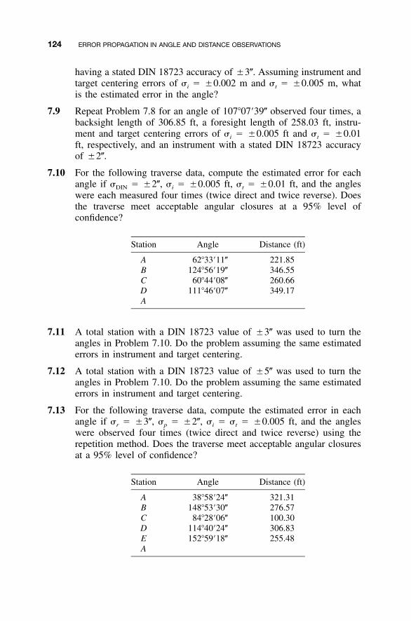
124 ERROR PROPAGATION IN ANGLE AND DISTANCE OBSERVATIONS
having a stated DIN 18723 accuracy of �3�. Assuming instrument andtarget centering errors of �i � �0.002 m and �t � �0.005 m, whatis the estimated error in the angle?
7.9 Repeat Problem 7.8 for an angle of 107�07�39� observed four times, abacksight length of 306.85 ft, a foresight length of 258.03 ft, instru-ment and target centering errors of �i � �0.005 ft and �t � �0.01ft, respectively, and an instrument with a stated DIN 18723 accuracyof �2�.
7.10 For the following traverse data, compute the estimated error for eachangle if �DIN � �2�, �i � �0.005 ft, �t � �0.01 ft, and the angleswere each measured four times (twice direct and twice reverse). Doesthe traverse meet acceptable angular closures at a 95% level ofconfidence?
Station Angle Distance (ft)
A 62�33�11� 221.85B 124�56�19� 346.55C 60�44�08� 260.66D 111�46�07� 349.17A
7.11 A total station with a DIN 18723 value of �3� was used to turn theangles in Problem 7.10. Do the problem assuming the same estimatederrors in instrument and target centering.
7.12 A total station with a DIN 18723 value of �5� was used to turn theangles in Problem 7.10. Do the problem assuming the same estimatederrors in instrument and target centering.
7.13 For the following traverse data, compute the estimated error in eachangle if �r � �3�, �p � �2�, �i � �t � �0.005 ft, and the angleswere observed four times (twice direct and twice reverse) using therepetition method. Does the traverse meet acceptable angular closuresat a 95% level of confidence?
Station Angle Distance (ft)
A 38�58�24� 321.31B 148�53�30� 276.57C 84�28�06� 100.30D 114�40�24� 306.83E 152�59�18� 255.48A
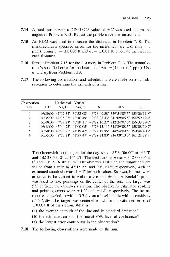
PROBLEMS 125
7.14 A total station with a DIN 18723 value of �2� was used to turn theangles in Problem 7.13. Repeat the problem for this instrument.
7.15 An EDM was used to measure the distances in Problem 7.10. Themanufacturer’s specified errors for the instrument are �(3 mm � 3ppm). Using �i � �0.005 ft and �r � �0.01 ft, calculate the error ineach distance.
7.16 Repeat Problem 7.15 for the distances in Problem 7.13. The manufac-turer’s specified error for the instrument was �(5 mm � 5 ppm). Use�i and �r from Problem 7.13.
7.17 The following observations and calculations were made on a sun ob-servation to determine the azimuth of a line:
ObservationNo. UTC
HorizontalAngle
VerticalAngle LHA z
1 16:30:00 41�02�33� 39�53�08� �3�28�00.58� 339�54�05.5� 153�26�51.8�2 16:35:00 42�35�28� 40�16�49� �3�28�05.43� 341�09�06.5� 154�59�42.4�3 16:40:00 44�09�23� 40�39�11� �3�28�10.27� 342�24�07.5� 156�33�39.0�4 16:45:00 45�44�25� 41�00�05� �3�28�15.11� 343�39�08.5� 158�08�39.2�5 16:50:00 47�20�21� 41�19�42� �3�28�19.96� 344�54�09.5� 159�44�40.2�6 16:55:00 48�57�24� 41�37�47� �3�28�24.80� 346�09�10.5� 161�21�38.9�
The Greenwich hour angles for the day were 182�34�06.00� at 0h UT,and 182�38�53.30� at 24h UT. The declinations were �3�12�00.80� at0h and �3�35�16.30� at 24h. The observer’s latitude and longitude werescaled from a map as 43�15�22� and 90�13�18�, respectively, with anestimated standard error of �1� for both values. Stopwatch times wereassumed to be correct to within a error of �0.5s. A Roelof’s prismwas used to take pointings on the center of the sun. The target was535 ft from the observer’s station. The observer’s estimated readingand pointing errors were �1.2� and �1.8�, respectively. The instru-ment was leveled to within 0.3 div on a level bubble with a sensitivityof 20� /div. The target was centered to within an estimated error of�0.003 ft of the station. What is:(a) the average azimuth of the line and its standard deviation?(b) the estimated error of the line at 95% level of confidence?(c) the largest error contributor in the observation?
7.18 The following observations were made on the sun.
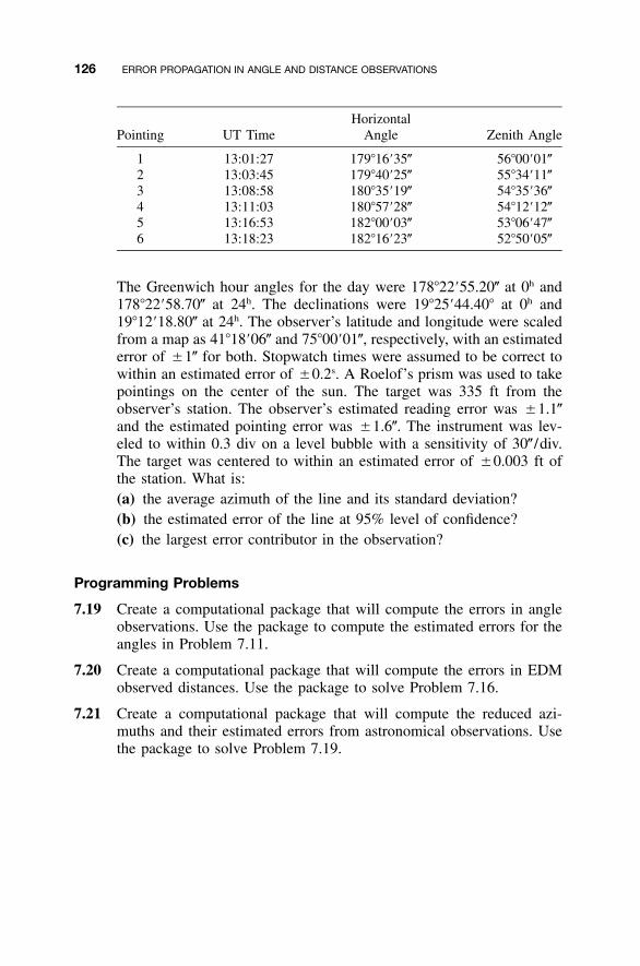
126 ERROR PROPAGATION IN ANGLE AND DISTANCE OBSERVATIONS
Pointing UT TimeHorizontal
Angle Zenith Angle
1 13:01:27 179�16�35� 56�00�01�2 13:03:45 179�40�25� 55�34�11�3 13:08:58 180�35�19� 54�35�36�4 13:11:03 180�57�28� 54�12�12�5 13:16:53 182�00�03� 53�06�47�6 13:18:23 182�16�23� 52�50�05�
The Greenwich hour angles for the day were 178�22�55.20� at 0h and178�22�58.70� at 24h. The declinations were 19�25�44.40� at 0h and19�12�18.80� at 24h. The observer’s latitude and longitude were scaledfrom a map as 41�18�06� and 75�00�01�, respectively, with an estimatederror of �1� for both. Stopwatch times were assumed to be correct towithin an estimated error of �0.2s. A Roelof’s prism was used to takepointings on the center of the sun. The target was 335 ft from theobserver’s station. The observer’s estimated reading error was �1.1�and the estimated pointing error was �1.6�. The instrument was lev-eled to within 0.3 div on a level bubble with a sensitivity of 30� /div.The target was centered to within an estimated error of �0.003 ft ofthe station. What is:(a) the average azimuth of the line and its standard deviation?(b) the estimated error of the line at 95% level of confidence?(c) the largest error contributor in the observation?
Programming Problems
7.19 Create a computational package that will compute the errors in angleobservations. Use the package to compute the estimated errors for theangles in Problem 7.11.
7.20 Create a computational package that will compute the errors in EDMobserved distances. Use the package to solve Problem 7.16.
7.21 Create a computational package that will compute the reduced azi-muths and their estimated errors from astronomical observations. Usethe package to solve Problem 7.19.
127
CHAPTER 8
ERROR PROPAGATION INTRAVERSE SURVEYS
8.1 INTRODUCTION
Even though the specifications for a project may allow lower accuracies, thepresence of blunders in observations is never acceptable. Thus, an importantquestion for every surveyor is: How can I tell when blunders are present inthe data? In this chapter we begin to address that question, and in particular,stress traverse analysis. The topic is discussed further in Chapter 20.
In Chapter 6 it was shown that the estimated error in a function of obser-vations depends on the individual errors in the observations. Generally, ob-servations in horizontal surveys (e.g., traverses) are independent. That is, themeasurement of a distance observation is independent of the azimuth obser-vation. But the latitude and departure of a line, which are computed from thedistance and azimuth observations, are not independent. Figure 8.1 shows theeffects of errors in distance and azimuth observations on the computed latitudeand departure. In the figure it can be seen that there is correlation betweenthe latitude and departure; that is, if either distance or azimuth observationchanges, it causes changes in both latitude and departure.
Because the observations from which latitudes and departures are com-puted are assumed to be independent with no correlation, the SLOPOV ap-proach [Equation (6.16)] can be used to determine the estimated error in thesecomputed values. However, for proper computation of estimated errors infunctions that use these computed values (i.e., latitudes and departures), theeffects of correlation must be considered, and thus the GLOPOV approach[Equation (6.13)] will be used.
Adjustment Computations: Spatial Data Analysis, Fourth Edition. C. D. Ghilani and P. R. Wolf© 2006 John Wiley & Sons, Inc. ISBN: 978-0-471-69728-2
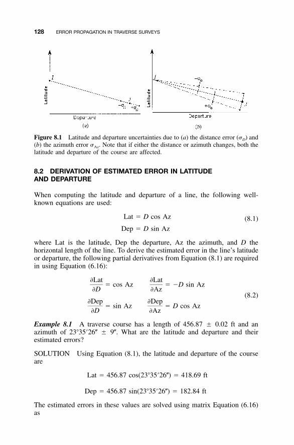
128 ERROR PROPAGATION IN TRAVERSE SURVEYS
Figure 8.1 Latitude and departure uncertainties due to (a) the distance error (�D) and(b) the azimuth error �Az. Note that if either the distance or azimuth changes, both thelatitude and departure of the course are affected.
8.2 DERIVATION OF ESTIMATED ERROR IN LATITUDEAND DEPARTURE
When computing the latitude and departure of a line, the following well-known equations are used:
Lat � D cos Az (8.1)
Dep � D sin Az
where Lat is the latitude, Dep the departure, Az the azimuth, and D thehorizontal length of the line. To derive the estimated error in the line’s latitudeor departure, the following partial derivatives from Equation (8.1) are requiredin using Equation (6.16):
�Lat �Lat� cos Az � �D sin Az
�D �Az(8.2)
�Dep �Dep� sin Az � D cos Az
�D �Az
Example 8.1 A traverse course has a length of 456.87 � 0.02 ft and anazimuth of 23�35�26� � 9�. What are the latitude and departure and theirestimated errors?
SOLUTION Using Equation (8.1), the latitude and departure of the courseare
Lat � 456.87 cos(23�35�26�) � 418.69 ft
Dep � 456.87 sin(23�35�26�) � 182.84 ft
The estimated errors in these values are solved using matrix Equation (6.16)as

8.3 DERIVATION OF ESTIMATED STANDARD ERRORS IN COURSE AZIMUTHS 129
�Lat �Lat �Lat �Dep2 2�D �Az �D �D� 0 � �D Lat Lat,Dep� � �� � � �Lat,Dep 2 20 � � ��Dep �Dep �Lat �DepAz Lat,Dep Dep� � � �
�D �Az �Az �Az
Substituting partial derivatives into the above yields
2cos Az �D sin Az 0.02 0 cos Az sin Az� � � �� �� �Lat,Dep 2sin Az D cos Az 0 (9� /�) �D sin Az D cos Az
(8.3)
Entering in the appropriate numerical values into Equation (8.3), the covari-ance matrix is
0.9167 �456.87(0.4002) 0.0004 0� � � �� �Lat,Dep 20.4002 456.87(0.9164) 0 (9� /�)
0.9167 0.4002� ��456.87(0.4002) 456.87(0.9164)
from which
0.00039958 0.00000096� � (8.4)� �Lat,Dep 0.00000096 0.00039781
In Equation (8.4), is the variance of the latitude, the variance of2 2� �11 22
the departure, and �12 and �21 their covariances. Thus, the standard errors are
2� � �� � �0.00039958 � �0.020 ft andLat 11
2� � �� � �0.00039781 � �0.020 ftDep 22
Note that the off-diagonal of �Lat,Dep is not equal to zero, and thus the com-puted values are correlated as illustrated in Figure 8.1.
8.3 DERIVATION OF ESTIMATED STANDARD ERRORS INCOURSE AZIMUTHS
Equation (8.1) is based on the azimuth of a course. In practice, however,traverse azimuths are normally computed from observed angles rather thanbeing measured directly. Thus, another level of error propagation exists incalculating the azimuths from angular values. In the following analysis, con-
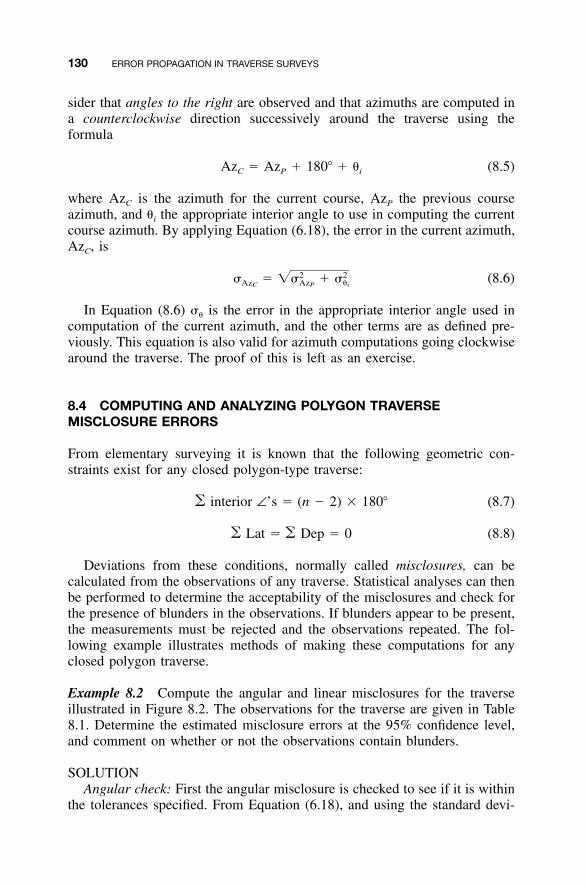
130 ERROR PROPAGATION IN TRAVERSE SURVEYS
sider that angles to the right are observed and that azimuths are computed ina counterclockwise direction successively around the traverse using theformula
Az � Az � 180� � � (8.5)C P i
where AzC is the azimuth for the current course, AzP the previous courseazimuth, and �i the appropriate interior angle to use in computing the currentcourse azimuth. By applying Equation (6.18), the error in the current azimuth,AzC, is
2 2� � �� � � (8.6)Az Az �C P i
In Equation (8.6) �� is the error in the appropriate interior angle used incomputation of the current azimuth, and the other terms are as defined pre-viously. This equation is also valid for azimuth computations going clockwisearound the traverse. The proof of this is left as an exercise.
8.4 COMPUTING AND ANALYZING POLYGON TRAVERSEMISCLOSURE ERRORS
From elementary surveying it is known that the following geometric con-straints exist for any closed polygon-type traverse:
� interior ∠’s � (n � 2) � 180� (8.7)
� Lat � � Dep � 0 (8.8)
Deviations from these conditions, normally called misclosures, can becalculated from the observations of any traverse. Statistical analyses can thenbe performed to determine the acceptability of the misclosures and check forthe presence of blunders in the observations. If blunders appear to be present,the measurements must be rejected and the observations repeated. The fol-lowing example illustrates methods of making these computations for anyclosed polygon traverse.
Example 8.2 Compute the angular and linear misclosures for the traverseillustrated in Figure 8.2. The observations for the traverse are given in Table8.1. Determine the estimated misclosure errors at the 95% confidence level,and comment on whether or not the observations contain blunders.
SOLUTIONAngular check: First the angular misclosure is checked to see if it is within
the tolerances specified. From Equation (6.18), and using the standard devi-
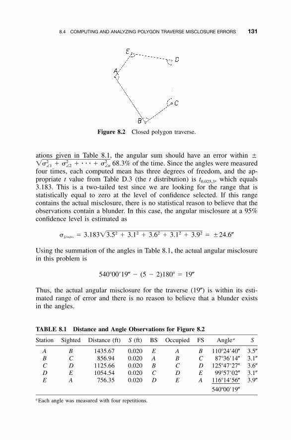
8.4 COMPUTING AND ANALYZING POLYGON TRAVERSE MISCLOSURE ERRORS 131
Figure 8.2 Closed polygon traverse.
TABLE 8.1 Distance and Angle Observations for Figure 8.2
Station Sighted Distance (ft) S (ft) BS Occupied FS Angle a S
A B 1435.67 0.020 E A B 110�24�40� 3.5�B C 856.94 0.020 A B C 87�36�14� 3.1�C D 1125.66 0.020 B C D 125�47�27� 3.6�D E 1054.54 0.020 C D E 99�57�02� 3.1�E A 756.35 0.020 D E A 116�14�56� 3.9�
540�00�19�
a Each angle was measured with four repetitions.
ations given in Table 8.1, the angular sum should have an error within �68.3% of the time. Since the angles were measured2 2 2�� � � � � � � � �∠1 ∠2 ∠n
four times, each computed mean has three degrees of freedom, and the ap-propriate t value from Table D.3 (the t distribution) is t0.025,3, which equals3.183. This is a two-tailed test since we are looking for the range that isstatistically equal to zero at the level of confidence selected. If this rangecontains the actual misclosure, there is no statistical reason to believe that theobservations contain a blunder. In this case, the angular misclosure at a 95%confidence level is estimated as
2 2 2 2 2� � 3.183�3.5 � 3.1 � 3.6 � 3.1 � 3.9 � �24.6�Angles�
Using the summation of the angles in Table 8.1, the actual angular misclosurein this problem is
540�00�19� � (5 � 2)180� � 19�
Thus, the actual angular misclosure for the traverse (19�) is within its esti-mated range of error and there is no reason to believe that a blunder existsin the angles.
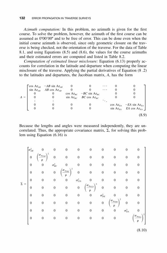
132 ERROR PROPAGATION IN TRAVERSE SURVEYS
Azimuth computation: In this problem, no azimuth is given for the firstcourse. To solve the problem, however, the azimuth of the first course can beassumed as 0�00�00� and to be free of error. This can be done even when theinitial course azimuth is observed, since only geometric closure on the trav-erse is being checked, not the orientation of the traverse. For the data of Table8.1, and using Equations (8.5) and (8.6), the values for the course azimuthsand their estimated errors are computed and listed in Table 8.2.
Computation of estimated linear misclosure: Equation (6.13) properly ac-counts for correlation in the latitude and departure when computing the linearmisclosure of the traverse. Applying the partial derivatives of Equation (8 .2)to the latitudes and departures, the Jacobian matrix, A, has the form
cos Az �AB sin Az 0 0 � � � 0 0AB AB
sin Az AB cos Az 0 0 � � � 0 0AB AB
0 0 cos Az �BC sin Az 0 0BC BC
A � 0 0 sin Az BC cos Az 0 0BC BC�� � � �� �0 0 0 0 cos Az �EA sin AzEA EA
0 0 0 0 sin Az EA cos AzEA EA
(8.9)
Because the lengths and angles were measured independently, they are un-correlated. Thus, the appropriate covariance matrix, �, for solving this prob-lem using Equation (6.16) is
2� 0 0 0 0 0 0 0 0 0AB
2�AzAB0 0 0 0 0 0 0 0 0� ��
20 0 � 0 0 0 0 0 0 0BC
2�AzBC0 0 0 0 0 0 0 0 0� ��
20 0 0 0 � 0 0 0 0 0CD
2� � �AzCD0 0 0 0 0 0 0 0 0� ��
20 0 0 0 0 0 � 0 0 0DE
2�AzDE0 0 0 0 0 0 0 0 0� ��
20 0 0 0 0 0 0 0 � 0EA
2�AzEA0 0 0 0 0 0 0 0 � ��
(8.10)
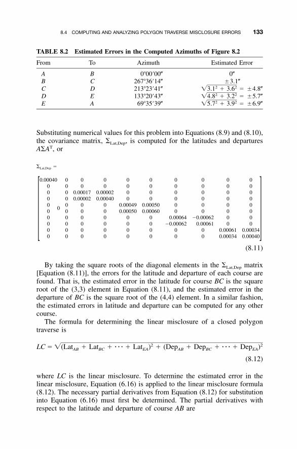
8.4 COMPUTING AND ANALYZING POLYGON TRAVERSE MISCLOSURE ERRORS 133
TABLE 8.2 Estimated Errors in the Computed Azimuths of Figure 8.2
From To Azimuth Estimated Error
A B 0�00�00� 0�B C 267�36�14� �3.1�C D 213�23�41� � �4.8�2 2�3.1 � 3.6D E 133�20�43� � �5.7�2 2�4.8 � 3.2E A 69�35�39� � �6.9�2 2�5.7 � 3.9
Substituting numerical values for this problem into Equations (8.9) and (8.10),the covariance matrix, �Lat,Dep, is computed for the latitudes and departuresA�AT, or
� �Lat,Dep
0.00040 0 0 0 0 0 0 0 0 00 0 0 0 0 0 0 0 0 00 0 0.00017 0.00002 0 0 0 0 0 00 0 0.00002 0.00040 0 0 0 0 0 00 0 0 0 0.00049 0.00050 0 0 0 0
00 0 0 0 0.00050 0.00060 0 0 0 00 0 0 0 0 0 0.00064 �0.00062 0 00 0 0 0 0 0 �0.00062 0.00061 0 00 0 0 0 0 0 0 0 0.00061 0.000340 0 0 0 0 0 0 0 0.00034 0.00040
(8.11)
By taking the square roots of the diagonal elements in the �Lat,Dep matrix[Equation (8.11)], the errors for the latitude and departure of each course arefound. That is, the estimated error in the latitude for course BC is the squareroot of the (3,3) element in Equation (8.11), and the estimated error in thedeparture of BC is the square root of the (4,4) element. In a similar fashion,the estimated errors in latitude and departure can be computed for any othercourse.
The formula for determining the linear misclosure of a closed polygontraverse is
2 2LC � �(Lat � Lat � � � � � Lat ) � (Dep � Dep � � � � � Dep )AB BC EA AB BC EA
(8.12)
where LC is the linear misclosure. To determine the estimated error in thelinear misclosure, Equation (6.16) is applied to the linear misclosure formula(8.12). The necessary partial derivatives from Equation (8.12) for substitutioninto Equation (6.16) must first be determined. The partial derivatives withrespect to the latitude and departure of course AB are
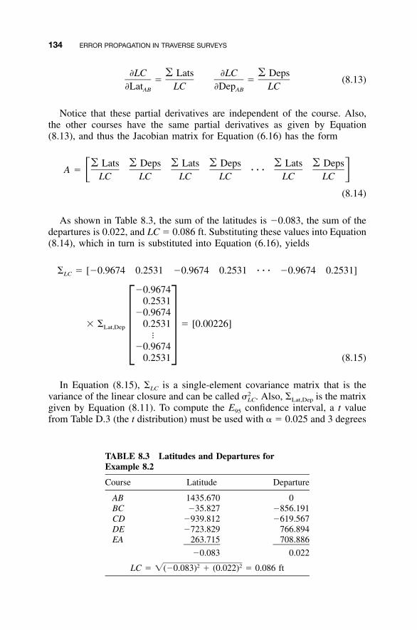
134 ERROR PROPAGATION IN TRAVERSE SURVEYS
TABLE 8.3 Latitudes and Departures forExample 8.2
Course Latitude Departure
AB 1435.670 0BC �35.827 �856.191CD �939.812 �619.567DE �723.829 766.894EA 263.715 708.886
�0.083 0.022
LC � 2 2�(�0.083) � (0.022) � 0.086 ft
�LC � Lats �LC � Deps� � (8.13)
�Lat LC �Dep LCAB AB
Notice that these partial derivatives are independent of the course. Also,the other courses have the same partial derivatives as given by Equation(8.13), and thus the Jacobian matrix for Equation (6.16) has the form
� Lats � Deps � Lats � Deps � Lats � DepsA � � � �� �LC LC LC LC LC LC
(8.14)
As shown in Table 8.3, the sum of the latitudes is �0.083, the sum of thedepartures is 0.022, and LC � 0.086 ft. Substituting these values into Equation(8.14), which in turn is substituted into Equation (6.16), yields
� � [�0.9674 0.2531 �0.9674 0.2531 � � � �0.9674 0.2531]LC
�0.96740.2531
�0.9674� � 0.2531 � [0.00226]Lat,Dep
�� ��0.96740.2531 (8.15)
In Equation (8.15), �LC is a single-element covariance matrix that is thevariance of the linear closure and can be called Also, �Lat,Dep is the matrix2� .LC
given by Equation (8.11). To compute the E95 confidence interval, a t valuefrom Table D.3 (the t distribution) must be used with � � 0.025 and 3 degrees
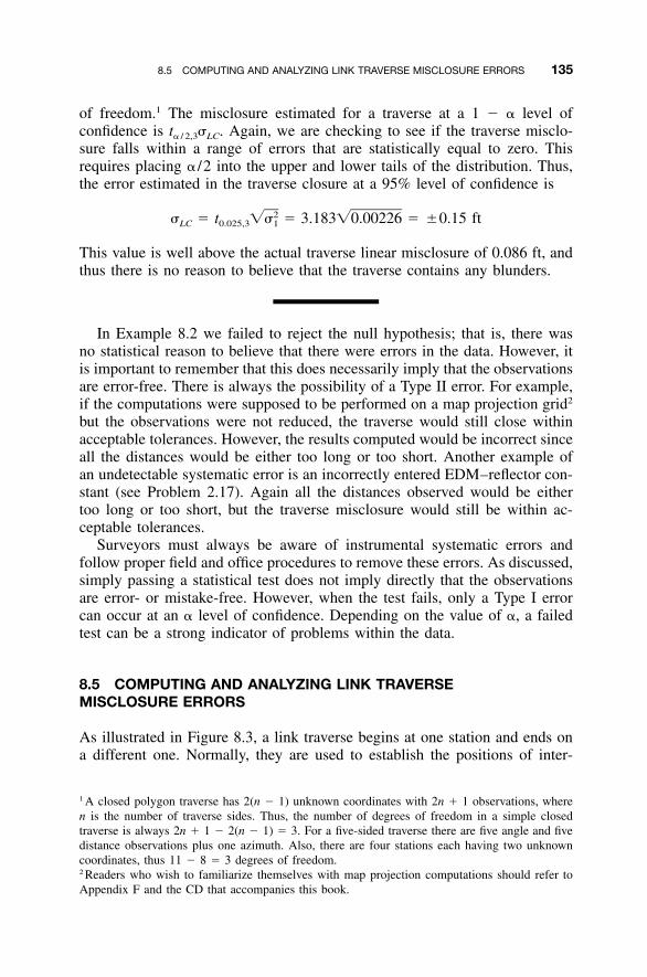
8.5 COMPUTING AND ANALYZING LINK TRAVERSE MISCLOSURE ERRORS 135
of freedom.1 The misclosure estimated for a traverse at a 1 � � level ofconfidence is t� / 2,3�LC. Again, we are checking to see if the traverse misclo-sure falls within a range of errors that are statistically equal to zero. Thisrequires placing � /2 into the upper and lower tails of the distribution. Thus,the error estimated in the traverse closure at a 95% level of confidence is
2� � t �� � 3.183�0.00226 � �0.15 ftLC 0.025,3 1
This value is well above the actual traverse linear misclosure of 0.086 ft, andthus there is no reason to believe that the traverse contains any blunders.
In Example 8.2 we failed to reject the null hypothesis; that is, there wasno statistical reason to believe that there were errors in the data. However, itis important to remember that this does necessarily imply that the observationsare error-free. There is always the possibility of a Type II error. For example,if the computations were supposed to be performed on a map projection grid2
but the observations were not reduced, the traverse would still close withinacceptable tolerances. However, the results computed would be incorrect sinceall the distances would be either too long or too short. Another example ofan undetectable systematic error is an incorrectly entered EDM–reflector con-stant (see Problem 2.17). Again all the distances observed would be eithertoo long or too short, but the traverse misclosure would still be within ac-ceptable tolerances.
Surveyors must always be aware of instrumental systematic errors andfollow proper field and office procedures to remove these errors. As discussed,simply passing a statistical test does not imply directly that the observationsare error- or mistake-free. However, when the test fails, only a Type I errorcan occur at an � level of confidence. Depending on the value of �, a failedtest can be a strong indicator of problems within the data.
8.5 COMPUTING AND ANALYZING LINK TRAVERSEMISCLOSURE ERRORS
As illustrated in Figure 8.3, a link traverse begins at one station and ends ona different one. Normally, they are used to establish the positions of inter-
1 A closed polygon traverse has 2(n � 1) unknown coordinates with 2n � 1 observations, wheren is the number of traverse sides. Thus, the number of degrees of freedom in a simple closedtraverse is always 2n � 1 � 2(n � 1) � 3. For a five-sided traverse there are five angle and fivedistance observations plus one azimuth. Also, there are four stations each having two unknowncoordinates, thus 11 � 8 � 3 degrees of freedom.2 Readers who wish to familiarize themselves with map projection computations should refer toAppendix F and the CD that accompanies this book.
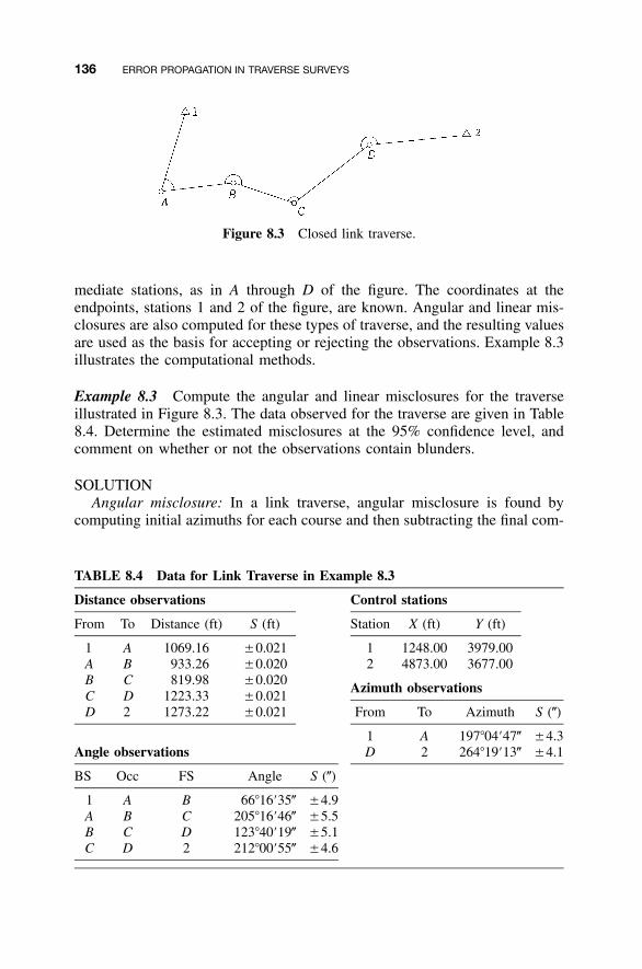
136 ERROR PROPAGATION IN TRAVERSE SURVEYS
Figure 8.3 Closed link traverse.
TABLE 8.4 Data for Link Traverse in Example 8.3
Distance observations Control stations
From To Distance (ft) S (ft) Station X (ft) Y (ft)
1 A 1069.16 �0.021 1 1248.00 3979.00A B 933.26 �0.020 2 4873.00 3677.00BCD
CD2
819.981223.331273.22
�0.020�0.021�0.021
Azimuth observations
From To Azimuth S (�)
1 A 197�04�47� �4.3Angle observations D 2 264�19�13� �4.1
BS Occ FS Angle S (�)
1 A B 66�16�35� �4.9A B C 205�16�46� �5.5B C D 123�40�19� �5.1C D 2 212�00�55� �4.6
mediate stations, as in A through D of the figure. The coordinates at theendpoints, stations 1 and 2 of the figure, are known. Angular and linear mis-closures are also computed for these types of traverse, and the resulting valuesare used as the basis for accepting or rejecting the observations. Example 8.3illustrates the computational methods.
Example 8.3 Compute the angular and linear misclosures for the traverseillustrated in Figure 8.3. The data observed for the traverse are given in Table8.4. Determine the estimated misclosures at the 95% confidence level, andcomment on whether or not the observations contain blunders.
SOLUTIONAngular misclosure: In a link traverse, angular misclosure is found by
computing initial azimuths for each course and then subtracting the final com-
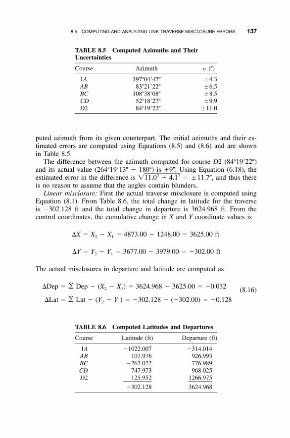
8.5 COMPUTING AND ANALYZING LINK TRAVERSE MISCLOSURE ERRORS 137
TABLE 8.5 Computed Azimuths and TheirUncertainties
Course Azimuth � (�)
1A 197�04�47� �4.3AB 83�21�22� �6.5BC 108�38�08� �8.5CD 52�18�27� �9.9D2 84�19�22� �11.0
TABLE 8.6 Computed Latitudes and Departures
Course Latitude (ft) Departure (ft)
1A �1022.007 �314.014AB 107.976 926.993BC �262.022 776.989CD 747.973 968.025D2 125.952 1266.975
�302.128 3624.968
puted azimuth from its given counterpart. The initial azimuths and their es-timated errors are computed using Equations (8.5) and (8.6) and are shownin Table 8.5.
The difference between the azimuth computed for course D2 (84�19�22�)and its actual value (264�19�13� � 180�) is �9�. Using Equation (6.18), theestimated error in the difference is � �11.7�, and thus there2 2�11.0 � 4.1is no reason to assume that the angles contain blunders.
Linear misclosure: First the actual traverse misclosure is computed usingEquation (8.1). From Table 8.6, the total change in latitude for the traverseis �302.128 ft and the total change in departure is 3624.968 ft. From thecontrol coordinates, the cumulative change in X and Y coordinate values is
X � X � X � 4873.00 � 1248.00 � 3625.00 ft2 1
Y � Y � Y � 3677.00 � 3979.00 � �302.00 ft2 1
The actual misclosures in departure and latitude are computed as
Dep � � Dep � (X � X ) � 3624.968 � 3625.00 � �0.0322 1 (8.16)
Lat � � Lat � (Y � Y ) � �302.128 � (�302.00) � �0.1282 1
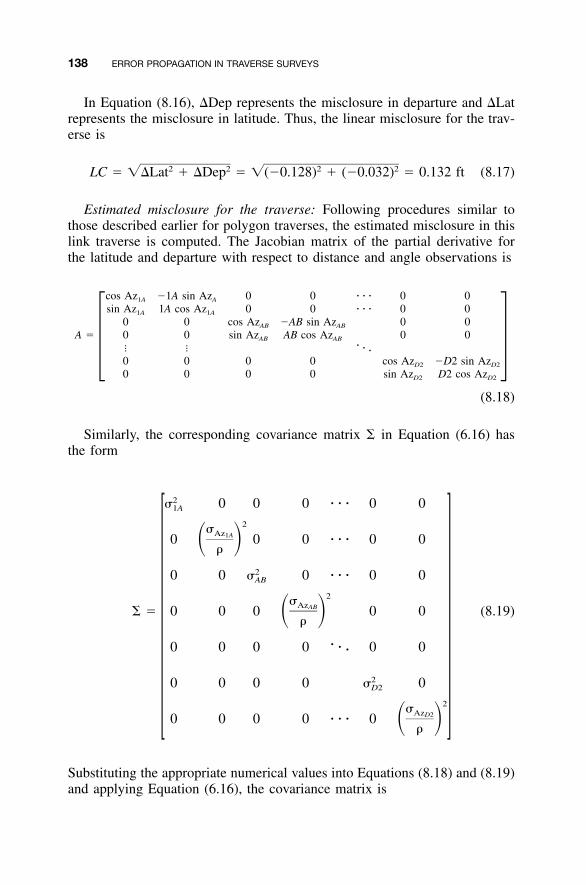
138 ERROR PROPAGATION IN TRAVERSE SURVEYS
In Equation (8.16), Dep represents the misclosure in departure and Latrepresents the misclosure in latitude. Thus, the linear misclosure for the trav-erse is
2 2 2 2LC � �Lat � Dep � �(�0.128) � (�0.032) � 0.132 ft (8.17)
Estimated misclosure for the traverse: Following procedures similar tothose described earlier for polygon traverses, the estimated misclosure in thislink traverse is computed. The Jacobian matrix of the partial derivative forthe latitude and departure with respect to distance and angle observations is
cos Az �1A sin Az 0 0 � � � 0 01A A
sin Az 1A cos Az 0 0 � � � 0 01A 1A
0 0 cos Az �AB sin Az 0 0AB AB
A � 0 0 sin Az AB cos Az 0 0AB AB�� � � �� �0 0 0 0 cos Az �D2 sin AzD2 D2
0 0 0 0 sin Az D2 cos AzD2 D2
(8.18)
Similarly, the corresponding covariance matrix � in Equation (6.16) hasthe form
2� 0 0 0 � � � 0 01A
2�Az1A0 0 0 � � � 0 0� ��
20 0 � 0 � � � 0 0AB
2�AzAB� � 0 0 0 0 0 (8.19)� ��
�0 0 0 0 � 0 0�
20 0 0 0 � 0D2
2�AzD20 0 0 0 � � � 0 � ��
Substituting the appropriate numerical values into Equations (8.18) and (8.19)and applying Equation (6.16), the covariance matrix is
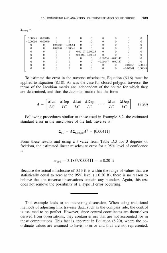
8.5 COMPUTING AND ANALYZING LINK TRAVERSE MISCLOSURE ERRORS 139
� �Lat,Dep
0.00045 �0.00016 0 0 0 0 0 0 0 0�0.00016 0.00049 0 0 0 0 0 0 0 0
0 0 0.00086 �0.00054 0 0 0 0 0 00 0 �0.00054 0.00041 0 0 0 0 0 00 0 0 0 0.00107 0.00023 0 0 0 00 0 0 0 0.00023 0.00048 0 0 0 00 0 0 0 0 0 0.00234 �0.00147 0 00 0 0 0 0 0 �0.00147 0.00157 0 00 0 0 0 0 0 0 0 0.00453 �0.000410 0 0 0 0 0 0 0 �0.00041 0.00048
To estimate the error in the traverse misclosure, Equation (6.16) must beapplied to Equation (8.18). As was the case for closed polygon traverse, theterms of the Jacobian matrix are independent of the course for which theyare determined, and thus the Jacobian matrix has the form
Lat Dep Lat Dep Lat DepA � � � � (8.20)� �LC LC LC LC LC LC
Following procedures similar to those used in Example 8.2, the estimatedstandard error in the misclosure of the link traverse is
T� � A� A � [0.00411]LC Lat,Dep
From these results and using a t value from Table D.3 for 3 degrees offreedom, the estimated linear misclosure error for a 95% level of confidenceis
� � 3.183�0.00411 � �0.20 ft95%
Because the actual misclosure of 0.13 ft is within the range of values that arestatistically equal to zero at the 95% level (�0.20 ft), there is no reason tobelieve that the traverse observations contain any blunders. Again, this testdoes not remove the possibility of a Type II error occurring.
This example leads to an interesting discussion. When using traditionalmethods of adjusting link traverse data, such as the compass rule, the controlis assumed to be perfect. However, since control coordinates are themselvesderived from observations, they contain errors that are not accounted for inthese computations. This fact is apparent in Equation (8.20), where the co-ordinate values are assumed to have no error and thus are not represented.
140 ERROR PROPAGATION IN TRAVERSE SURVEYS
These equations can easily be modified to consider the control errors, but thisis left as an exercise for the student.
One of the principal advantages of the least squares adjustment method isthat it allows application of varying weights to the observations, and controlcan be included in the adjustment with appropriate weights. A full discussionof this subject is presented in Section 21.6.
8.6 CONCLUSIONS
In this chapter, propagation of observational errors through traverse compu-tations has been discussed. Error propagation is a powerful tool for the sur-veyor, enabling an answer to be obtained for the question: What is anacceptable traverse misclosure? This is an example of surveying engineering.Surveyors are constantly designing measurement systems and checking theirresults against personal or legal standards. The subjects of error propagationand detection of measurement blunders are discussed further in later chapters.
PROBLEMS
8.1 Show that Equation (8.6) is valid for clockwise computations about atraverse.
8.2 Explain the significance of the standard error in the azimuth of the firstcourse of a polygon traverse.
8.3 Given a course with an azimuth of 105�27�44� with an estimated errorof �5� and a distance of 638.37 ft with an estimated error of �0.02ft, what are the latitude and departure and their estimated errors?
8.4 Given a course with an azimuth of 272�14�08� with an estimated errorof �9.2� and a distance of 215.69 ft with an estimated error of �0.016ft, what are the latitude and departure and their estimated errors?
8.5 Given a course with an azimuth of 328�49�06� with an estimated errorof �4.4� and a distance of 365.977 m with an estimated error of �6.5mm, what are the latitude and departure and their estimated errors?
8.6 Given a course with an azimuth of 44�56�22� with an estimated errorof �6.7� and a distance of 138.042 m with an estimated error of �5.2mm, what are the latitude and departure and their estimated errors?
8.7 A traverse meets statistical closures at the 95% level of confidence. Inyour own words, explain why this does not necessarily imply that thetraverse is without error.
8.8 A polygon traverse has the following angle measurements and relatedstandard deviations. Each angle was observed twice (one direct and
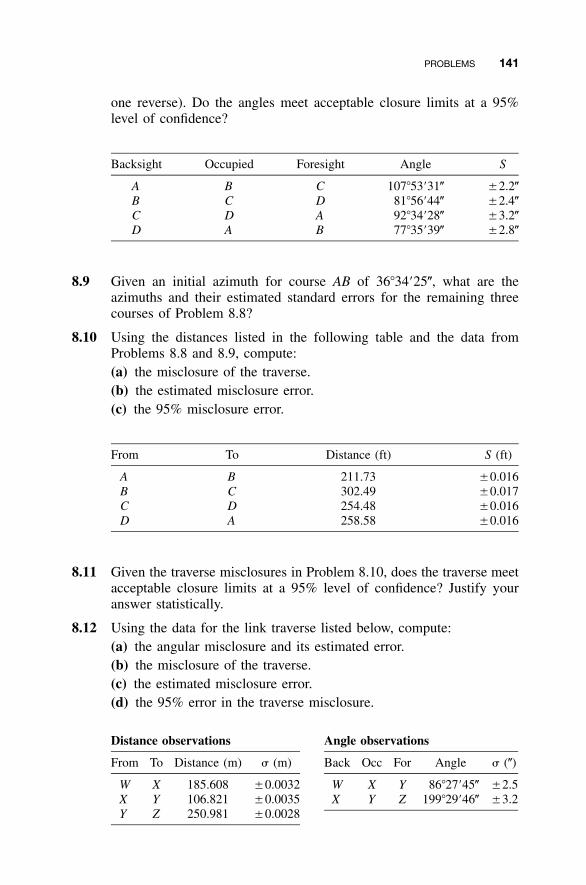
PROBLEMS 141
one reverse). Do the angles meet acceptable closure limits at a 95%level of confidence?
Backsight Occupied Foresight Angle S
A B C 107�53�31� �2.2�B C D 81�56�44� �2.4�C D A 92�34�28� �3.2�D A B 77�35�39� �2.8�
8.9 Given an initial azimuth for course AB of 36�34�25�, what are theazimuths and their estimated standard errors for the remaining threecourses of Problem 8.8?
8.10 Using the distances listed in the following table and the data fromProblems 8.8 and 8.9, compute:(a) the misclosure of the traverse.(b) the estimated misclosure error.(c) the 95% misclosure error.
From To Distance (ft) S (ft)
A B 211.73 �0.016B C 302.49 �0.017C D 254.48 �0.016D A 258.58 �0.016
8.11 Given the traverse misclosures in Problem 8.10, does the traverse meetacceptable closure limits at a 95% level of confidence? Justify youranswer statistically.
8.12 Using the data for the link traverse listed below, compute:(a) the angular misclosure and its estimated error.(b) the misclosure of the traverse.(c) the estimated misclosure error.(d) the 95% error in the traverse misclosure.
Distance observations Angle observations
From To Distance (m) � (m) Back Occ For Angle � (�)
W X 185.608 �0.0032 W X Y 86�27�45� �2.5X Y 106.821 �0.0035 X Y Z 199�29�46� �3.2Y Z 250.981 �0.0028
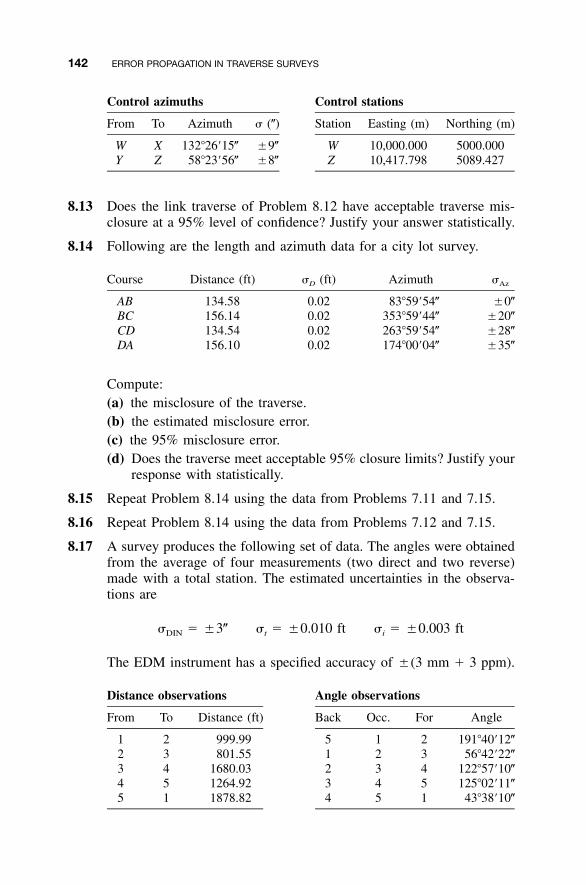
142 ERROR PROPAGATION IN TRAVERSE SURVEYS
Control azimuths Control stations
From To Azimuth � (�) Station Easting (m) Northing (m)
W X 132�26�15� �9� W 10,000.000 5000.000Y Z 58�23�56� �8� Z 10,417.798 5089.427
8.13 Does the link traverse of Problem 8.12 have acceptable traverse mis-closure at a 95% level of confidence? Justify your answer statistically.
8.14 Following are the length and azimuth data for a city lot survey.
Course Distance (ft) �D (ft) Azimuth �Az
AB 134.58 0.02 83�59�54� �0�BC 156.14 0.02 353�59�44� �20�CD 134.54 0.02 263�59�54� �28�DA 156.10 0.02 174�00�04� �35�
Compute:(a) the misclosure of the traverse.(b) the estimated misclosure error.(c) the 95% misclosure error.(d) Does the traverse meet acceptable 95% closure limits? Justify your
response with statistically.
8.15 Repeat Problem 8.14 using the data from Problems 7.11 and 7.15.
8.16 Repeat Problem 8.14 using the data from Problems 7.12 and 7.15.
8.17 A survey produces the following set of data. The angles were obtainedfrom the average of four measurements (two direct and two reverse)made with a total station. The estimated uncertainties in the observa-tions are
� � �3� � � �0.010 ft � � �0.003 ftDIN t i
The EDM instrument has a specified accuracy of �(3 mm � 3 ppm).
Distance observations Angle observations
From To Distance (ft) Back Occ. For Angle
1 2 999.99 5 1 2 191�40�12�2 3 801.55 1 2 3 56�42�22�3 4 1680.03 2 3 4 122�57�10�4 5 1264.92 3 4 5 125�02�11�5 1 1878.82 4 5 1 43�38�10�
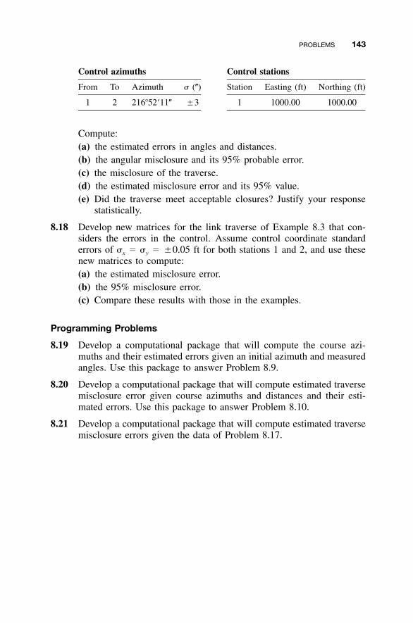
PROBLEMS 143
Control azimuths Control stations
From To Azimuth � (�) Station Easting (ft) Northing (ft)
1 2 216�52�11� �3 1 1000.00 1000.00
Compute:(a) the estimated errors in angles and distances.(b) the angular misclosure and its 95% probable error.(c) the misclosure of the traverse.(d) the estimated misclosure error and its 95% value.(e) Did the traverse meet acceptable closures? Justify your response
statistically.
8.18 Develop new matrices for the link traverse of Example 8.3 that con-siders the errors in the control. Assume control coordinate standarderrors of �x � �y � �0.05 ft for both stations 1 and 2, and use thesenew matrices to compute:(a) the estimated misclosure error.(b) the 95% misclosure error.(c) Compare these results with those in the examples.
Programming Problems
8.19 Develop a computational package that will compute the course azi-muths and their estimated errors given an initial azimuth and measuredangles. Use this package to answer Problem 8.9.
8.20 Develop a computational package that will compute estimated traversemisclosure error given course azimuths and distances and their esti-mated errors. Use this package to answer Problem 8.10.
8.21 Develop a computational package that will compute estimated traversemisclosure errors given the data of Problem 8.17.
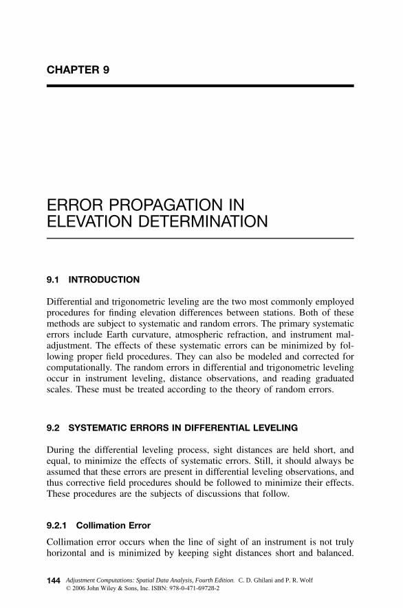
144
CHAPTER 9
ERROR PROPAGATION INELEVATION DETERMINATION
9.1 INTRODUCTION
Differential and trigonometric leveling are the two most commonly employedprocedures for finding elevation differences between stations. Both of thesemethods are subject to systematic and random errors. The primary systematicerrors include Earth curvature, atmospheric refraction, and instrument mal-adjustment. The effects of these systematic errors can be minimized by fol-lowing proper field procedures. They can also be modeled and corrected forcomputationally. The random errors in differential and trigonometric levelingoccur in instrument leveling, distance observations, and reading graduatedscales. These must be treated according to the theory of random errors.
9.2 SYSTEMATIC ERRORS IN DIFFERENTIAL LEVELING
During the differential leveling process, sight distances are held short, andequal, to minimize the effects of systematic errors. Still, it should always beassumed that these errors are present in differential leveling observations, andthus corrective field procedures should be followed to minimize their effects.These procedures are the subjects of discussions that follow.
9.2.1 Collimation Error
Collimation error occurs when the line of sight of an instrument is not trulyhorizontal and is minimized by keeping sight distances short and balanced.
Adjustment Computations: Spatial Data Analysis, Fourth Edition. C. D. Ghilani and P. R. Wolf© 2006 John Wiley & Sons, Inc. ISBN: 978-0-471-69728-2
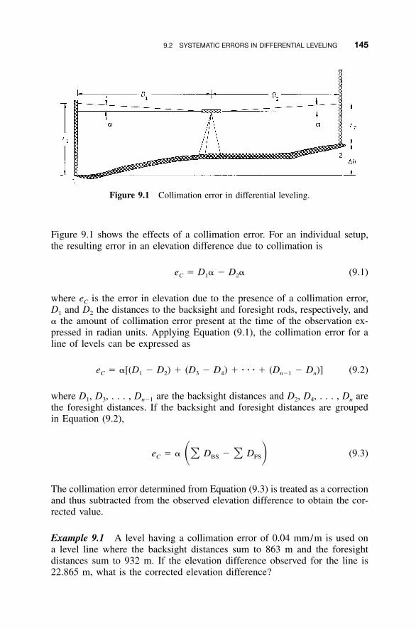
9.2 SYSTEMATIC ERRORS IN DIFFERENTIAL LEVELING 145
Figure 9.1 Collimation error in differential leveling.
Figure 9.1 shows the effects of a collimation error. For an individual setup,the resulting error in an elevation difference due to collimation is
e � D � � D � (9.1)C 1 2
where eC is the error in elevation due to the presence of a collimation error,D1 and D2 the distances to the backsight and foresight rods, respectively, and� the amount of collimation error present at the time of the observation ex-pressed in radian units. Applying Equation (9.1), the collimation error for aline of levels can be expressed as
e � �[(D � D ) � (D � D ) � � � � � (D � D )] (9.2)C 1 2 3 4 n�1 n
where D1, D3, . . . , Dn�1 are the backsight distances and D2, D4, . . . , Dn arethe foresight distances. If the backsight and foresight distances are groupedin Equation (9.2),
e � � D � D (9.3)� �� �C BS FS
The collimation error determined from Equation (9.3) is treated as a correctionand thus subtracted from the observed elevation difference to obtain the cor-rected value.
Example 9.1 A level having a collimation error of 0.04 mm/m is used ona level line where the backsight distances sum to 863 m and the foresightdistances sum to 932 m. If the elevation difference observed for the line is22.865 m, what is the corrected elevation difference?
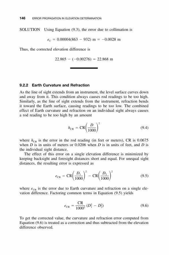
146 ERROR PROPAGATION IN ELEVATION DETERMINATION
SOLUTION Using Equation (9.3), the error due to collimation is
e � 0.00004(863 � 932) m � �0.0028 mC
Thus, the corrected elevation difference is
22.865 � (�0.00276) � 22.868 m
9.2.2 Earth Curvature and Refraction
As the line of sight extends from an instrument, the level surface curves downand away from it. This condition always causes rod readings to be too high.Similarly, as the line of sight extends from the instrument, refraction bendsit toward the Earth surface, causing readings to be too low. The combinedeffect of Earth curvature and refraction on an individual sight always causesa rod reading to be too high by an amount
2Dh � CR (9.4)� �CR 1000
where hCR is the error in the rod reading (in feet or meters), CR is 0.0675when D is in units of meters or 0.0206 when D is in units of feet, and D isthe individual sight distance.
The effect of this error on a single elevation difference is minimized bykeeping backsight and foresight distances short and equal. For unequal sightdistances, the resulting error is expressed as
2 2D D1 2e � CR � CR (9.5)� � � �CR 1000 1000
where eCR is the error due to Earth curvature and refraction on a single ele-vation difference. Factoring common terms in Equation (9.5) yields
CR 2 2e � (D � D ) (9.6)CR 1 221000
To get the corrected value, the curvature and refraction error computed fromEquation (9.6) is treated as a correction and thus subtracted from the elevationdifference observed.
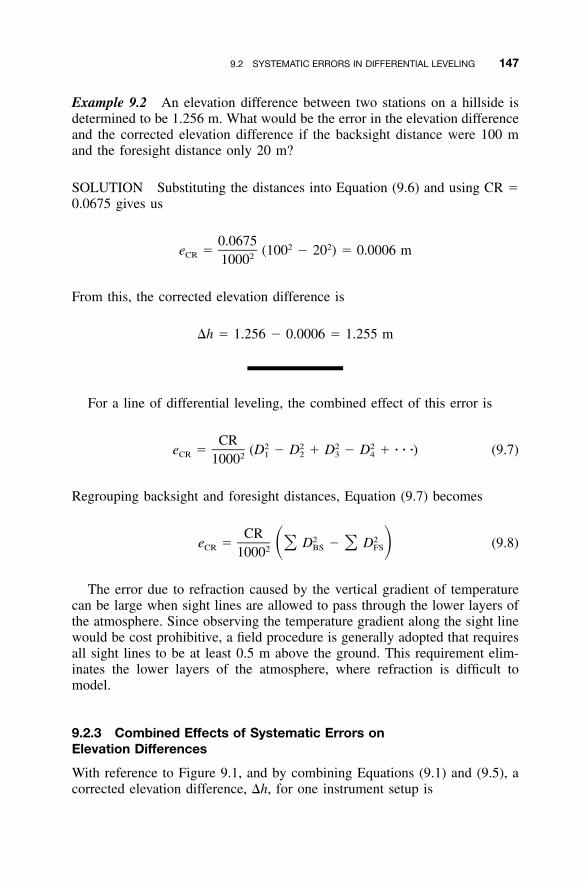
9.2 SYSTEMATIC ERRORS IN DIFFERENTIAL LEVELING 147
Example 9.2 An elevation difference between two stations on a hillside isdetermined to be 1.256 m. What would be the error in the elevation differenceand the corrected elevation difference if the backsight distance were 100 mand the foresight distance only 20 m?
SOLUTION Substituting the distances into Equation (9.6) and using CR �0.0675 gives us
0.0675 2 2e � (100 � 20 ) � 0.0006 mCR 21000
From this, the corrected elevation difference is
�h � 1.256 � 0.0006 � 1.255 m
For a line of differential leveling, the combined effect of this error is
CR 2 2 2 2e � (D � D � D � D � � � �) (9.7)CR 1 2 3 421000
Regrouping backsight and foresight distances, Equation (9.7) becomes
CR 2 2e � D � D (9.8)� �� �CR BS FS21000
The error due to refraction caused by the vertical gradient of temperaturecan be large when sight lines are allowed to pass through the lower layers ofthe atmosphere. Since observing the temperature gradient along the sight linewould be cost prohibitive, a field procedure is generally adopted that requiresall sight lines to be at least 0.5 m above the ground. This requirement elim-inates the lower layers of the atmosphere, where refraction is difficult tomodel.
9.2.3 Combined Effects of Systematic Errors onElevation Differences
With reference to Figure 9.1, and by combining Equations (9.1) and (9.5), acorrected elevation difference, �h, for one instrument setup is
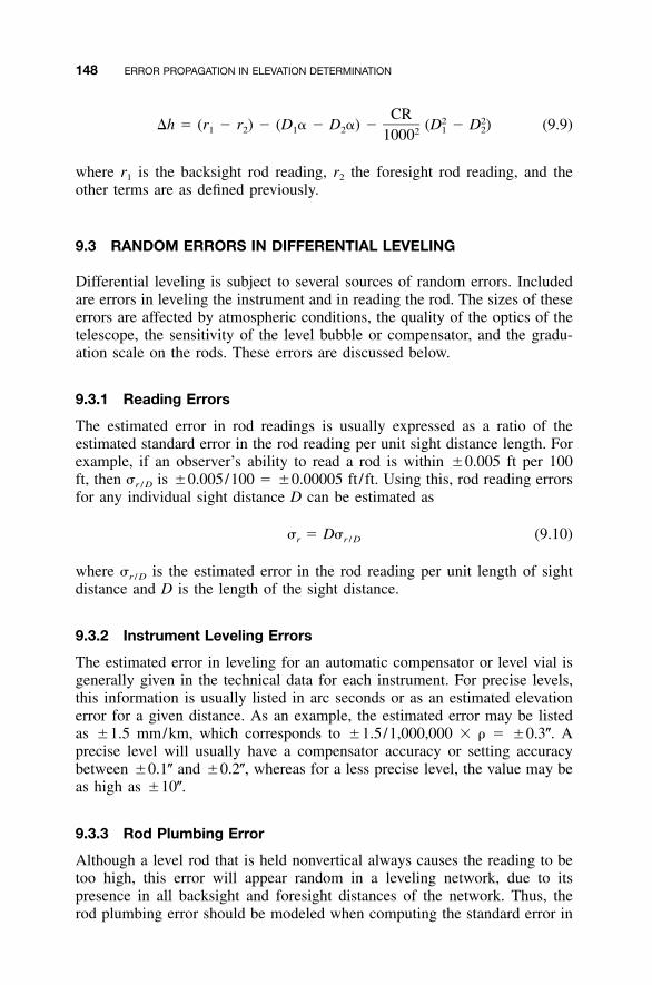
148 ERROR PROPAGATION IN ELEVATION DETERMINATION
CR 2 2�h � (r � r ) � (D � � D �) � (D � D ) (9.9)1 2 1 2 1 221000
where r1 is the backsight rod reading, r2 the foresight rod reading, and theother terms are as defined previously.
9.3 RANDOM ERRORS IN DIFFERENTIAL LEVELING
Differential leveling is subject to several sources of random errors. Includedare errors in leveling the instrument and in reading the rod. The sizes of theseerrors are affected by atmospheric conditions, the quality of the optics of thetelescope, the sensitivity of the level bubble or compensator, and the gradu-ation scale on the rods. These errors are discussed below.
9.3.1 Reading Errors
The estimated error in rod readings is usually expressed as a ratio of theestimated standard error in the rod reading per unit sight distance length. Forexample, if an observer’s ability to read a rod is within �0.005 ft per 100ft, then is �0.005/100 � �0.00005 ft/ft. Using this, rod reading errors�r / D
for any individual sight distance D can be estimated as
� � D� (9.10)r r / D
where is the estimated error in the rod reading per unit length of sight�r / D
distance and D is the length of the sight distance.
9.3.2 Instrument Leveling Errors
The estimated error in leveling for an automatic compensator or level vial isgenerally given in the technical data for each instrument. For precise levels,this information is usually listed in arc seconds or as an estimated elevationerror for a given distance. As an example, the estimated error may be listedas �1.5 mm/km, which corresponds to �1.5/1,000,000 � � � �0.3�. Aprecise level will usually have a compensator accuracy or setting accuracybetween �0.1� and �0.2�, whereas for a less precise level, the value may beas high as �10�.
9.3.3 Rod Plumbing Error
Although a level rod that is held nonvertical always causes the reading to betoo high, this error will appear random in a leveling network, due to itspresence in all backsight and foresight distances of the network. Thus, therod plumbing error should be modeled when computing the standard error in

9.3 RANDOM ERRORS IN DIFFERENTIAL LEVELING 149
Figure 9.2 Novertical level rod.
an elevation difference. With reference to Figure 9.2 for any rod reading, therod plumbing error is approximated as
2de � r � r� � (9.11)LS 2r
where d is the linear amount that the rod is out of plumb at the location ofthe rod reading, r. The size of d is dependent on the rod level bubble centeringerror and the reading location. If the rod bubble is out of level by �, then dis
d � r sin � (9.12)
Substituting Equation (9.12) into (9.11) gives
r 2e � sin � (9.13)LS 2
Example 9.3 Assume that a rod level bubble is within �5� of level and therod reading is at 4 m. What is the estimated error in the rod reading?
SOLUTION
4 2e � sin (5�) � 0.004 mmLS 2
150 ERROR PROPAGATION IN ELEVATION DETERMINATION
Since the rod plumbing error occurs on every sighting, backsight errorswill tend to cancel foresight errors. Thus, with precise leveling techniques,the combined effect of this error can be written as
2 2 2 2r sin � r sin � r sin � r sin �1 2 3 4e � � � � � � � � (9.14)� � � �2 2 2 2
Grouping like terms in Equation (9.14) yields
1 2–e � sin � (r � r � r � r � � � �) (9.15)2 1 2 3 4
Recognizing that the quantity in parentheses in Equation (9.15) is the eleva-tion difference for the leveling line yields
�Elev 2e � sin � (9.16)LS 2
Example 9.4 If a level rod is maintained to within �5� of level and theelevation difference is 22.865 m, the estimated error in the final elevation is
22.865 2e sin (5�) � 0.02 mmLS 2
The rod plumbing error can be practically eliminated by carefully centeringthe bubble of a well-adjusted rod level. It is generally small, as the exampleillustrates, and thus will be ignored in subsequent computations.
9.3.4 Estimated Errors in Differential Leveling
From the preceding discussion, the major random error sources in differentialleveling are caused by random errors in rod readings and instrument leveling.Furthermore, in Equation (9.9), the collimation error is considered to be sys-tematic and is effectively negated by balancing the backsight and foresightdistances. However, no matter what method is used to observe the lengths ofthe sight distances, some random error in these lengths will be present. Thiscauses random errors in the elevation differences, due to the effects of Earthcurvature, refraction, and instrumental collimation errors. Equation (6.16) canbe applied to Equation (9.9) to model the effects of the random errors in rodreadings, leveling, and sighting lengths. The following partial derivatives areneeded:
9.3 RANDOM ERRORS IN DIFFERENTIAL LEVELING 151
��h ��h ��h ��h� � 1 � �D � �D1 2�r �r �� ��1 2 1 2 (9.17)
��h CR(D ) ��h CR(D )1 2� � � � � � � �� � � ��D 500,000 �D 500,0001 2
By substituting Equations (9.17) into (6.16) with their corresponding esti-mated standard errors, the standard error in a single elevation difference canbe estimated as
2 2 2 2(D � ) � (D � ) � (�D � ) � (�D � )1 r / D 2 r / D 1 � 2 �1 2
� � (9.18)�h 2 2CR(D ) CR(D )1 2� � � � � � � � �� � � � � �� � �D D1 2500,000 500,000
where is the estimated error in a rod reading, and the estimated� � �r / D �1 �2
collimation errors in the backsight and foresight, respectively, and and�D1
the errors estimated in the sight lengths D1 and D2, respectively.�D2
In normal differential leveling procedures, D1 � D2 � D. Also, the esti-mated standard errors in the sight distances are equal: � � �D. Fur-� �D D1 2
thermore, the estimated collimation error for the backsight and foresight canbe assumed equal: � � ��. Thus, Equation (9.18) simplifies to� �� �1 2
2CR(D)2 2 2 2� � 2D (� � � ) � 2� � � (9.19)� ��h r / D � D� 500,000
Equation (9.19) is appropriate for a single elevation difference when thesight distances are approximately equal. In general, if sight distances are keptequal for N instrument setups, the total estimated error in an elevation dif-ference is
2CR(D)2 2 2 2� � 2ND (� � � ) � 2N� � � (9.20)� ��h r / D � D� 500,000
Since the error estimated in the elevation difference due to Earth curvatureand refraction, and the actual collimation error, �, are small, the last term isignored. Thus, the final equation for the standard error estimated in differ-ential leveling is
2 2� � D�2N(� � � ) (9.21)�h r / D �
152 ERROR PROPAGATION IN ELEVATION DETERMINATION
Example 9.5 A level line is run from benchmark A to benchmark B. Thestandard error estimated in rod readings is �0.01 mm/m. The instrument ismaintained to within �2.0� of level. A collimation test shows that the instru-ment is within 4 mm per 100 m. Fifty-meter sight distances are maintainedwithin an uncertainty of �2 m. The total line length from A to B is 1000 m.What is the estimated error in the elevation difference between A and B? IfA had an elevation of 212.345 � 0.005 m, what is the estimated error in thecomputed elevation of B?
SOLUTION The total number of setups in this problem is 1000/(2 � 50)� 10 setups. Substituting the appropriate values into Equation (8.20) yields
2 2 20.01 2.0� 0.004 0.0675(50)2 2� � 2(10)50 � � 2(10)2 ��� � � � � � ��h � 1000 � 100 500,0002 2� �0.0031 � 0.0004 � 0.0031 m � �3.1 mm
From an analysis of the individual error components in the equation above,it is seen that the error caused by the errors in the sight distances is negligiblefor all but the most precise leveling. Thus, like the error due to rod bubblecentering, this error can be ignored in all but the most precise work. Thus,the simpler Equation (9.21) can be used to solve the problem:
2 20.01 2.0�� � 50 2 � 10 ��� � � � ��h � 1000 �
2� �0.0031 � �0.0031 m � �3.1 mm
The estimated error in the elevation of B is found by applying Equation (6.18)as
2 2 2 2� � �� � � � �5 � 3.1 � �5.9 mmElev Elev �ElevB A
9.4 ERROR PROPAGATION IN TRIGONOMETRIC LEVELING
With the introduction of total station instruments, it is becoming increasinglyconvenient to observe elevation differences using trigonometric methods.However, in this procedure, because sight distances cannot be balanced, it isimportant that the systematic effects of Earth curvature and refraction, andinclination in the instrument’s line of sight (collimation error), be removed.
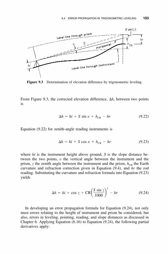
9.4 ERROR PROPAGATION IN TRIGONOMETRIC LEVELING 153
Figure 9.3 Determination of elevation difference by trigonometric leveling.
From Figure 9.3, the corrected elevation difference, �h, between two pointsis
�h � hi � S sin v � h � hr (9.22)CR
Equation (9.22) for zenith-angle reading instruments is
�h � hi � S cos v � h � hr (9.23)CR
where hi is the instrument height above ground, S is the slope distance be-tween the two points, v the vertical angle between the instrument and theprism, z the zenith angle between the instrument and the prism, hCR the Earthcurvature and refraction correction given in Equation (9.4), and hr the rodreading. Substituting the curvature and refraction formula into Equation (9.23)yields
2S sin z�h � hi � cos z � CR � hr (9.24)� �1000
In developing an error propagation formula for Equation (9.24), not onlymust errors relating to the height of instrument and prism be considered, butalso, errors in leveling, pointing, reading, and slope distances as discussed inChapter 6. Applying Equation (6.16) to Equation (9.24), the following partialderivatives apply:
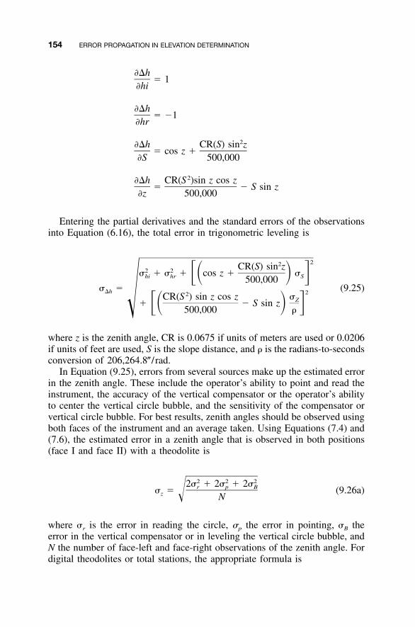
154 ERROR PROPAGATION IN ELEVATION DETERMINATION
��h� 1
�hi
��h� �1
�hr
2��h CR(S) sin z� cos z �
�S 500,000
2��h CR(S )sin z cos z� � S sin z
�z 500,000
Entering the partial derivatives and the standard errors of the observationsinto Equation (6.16), the total error in trigonometric leveling is
22CR(S) sin z2 2� � � � cos z � ��� � �hi hr S500,000� � (9.25)�h 22CR(S ) sin z cos z �Z� � S sin z�� � �� 500,000 �
where z is the zenith angle, CR is 0.0675 if units of meters are used or 0.0206if units of feet are used, S is the slope distance, and � is the radians-to-secondsconversion of 206,264.8� / rad.
In Equation (9.25), errors from several sources make up the estimated errorin the zenith angle. These include the operator’s ability to point and read theinstrument, the accuracy of the vertical compensator or the operator’s abilityto center the vertical circle bubble, and the sensitivity of the compensator orvertical circle bubble. For best results, zenith angles should be observed usingboth faces of the instrument and an average taken. Using Equations (7.4) and(7.6), the estimated error in a zenith angle that is observed in both positions(face I and face II) with a theodolite is
2 2 22� � 2� � 2�r p B� � (9.26a)z � N
where �r is the error in reading the circle, �p the error in pointing, �B theerror in the vertical compensator or in leveling the vertical circle bubble, andN the number of face-left and face-right observations of the zenith angle. Fordigital theodolites or total stations, the appropriate formula is
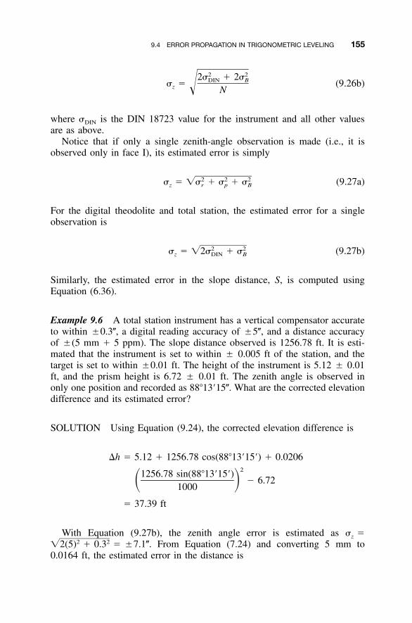
9.4 ERROR PROPAGATION IN TRIGONOMETRIC LEVELING 155
2 22� � 2�DIN B� � (9.26b)z � N
where �DIN is the DIN 18723 value for the instrument and all other valuesare as above.
Notice that if only a single zenith-angle observation is made (i.e., it isobserved only in face I), its estimated error is simply
2 2 2� � �� � � � � (9.27a)z r p B
For the digital theodolite and total station, the estimated error for a singleobservation is
2 2� � �2� � � (9.27b)z DIN B
Similarly, the estimated error in the slope distance, S, is computed usingEquation (6.36).
Example 9.6 A total station instrument has a vertical compensator accurateto within �0.3�, a digital reading accuracy of �5�, and a distance accuracyof �(5 mm � 5 ppm). The slope distance observed is 1256.78 ft. It is esti-mated that the instrument is set to within � 0.005 ft of the station, and thetarget is set to within �0.01 ft. The height of the instrument is 5.12 � 0.01ft, and the prism height is 6.72 � 0.01 ft. The zenith angle is observed inonly one position and recorded as 88�13�15�. What are the corrected elevationdifference and its estimated error?
SOLUTION Using Equation (9.24), the corrected elevation difference is
�h � 5.12 � 1256.78 cos(88�13�15�) � 0.020621256.78 sin(88�13�15�)
� 6.72� �1000
� 37.39 ft
With Equation (9.27b), the zenith angle error is estimated as � �z
From Equation (7.24) and converting 5 mm to2 2�2(5) � 0.3 � �7.1�.0.0164 ft, the estimated error in the distance is
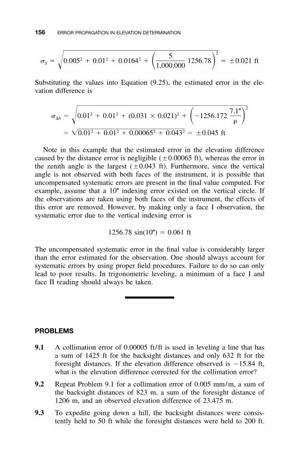
156 ERROR PROPAGATION IN ELEVATION DETERMINATION
252 2 2� � 0.005 � 0.01 � 0.0164 � 1256.78 � �0.021 ft� �S � 1,000,000
Substituting the values into Equation (9.25), the estimated error in the ele-vation difference is
27.1�2 2 2� � 0.01 � 0.01 � (0.031 � 0.021) � �1256.172� ��h � �
2 2 2 2� �0.01 � 0.01 � 0.00065 � 0.043 � �0.045 ft
Note in this example that the estimated error in the elevation differencecaused by the distance error is negligible (�0.00065 ft), whereas the error inthe zenith angle is the largest (�0.043 ft). Furthermore, since the verticalangle is not observed with both faces of the instrument, it is possible thatuncompensated systematic errors are present in the final value computed. Forexample, assume that a 10� indexing error existed on the vertical circle. Ifthe observations are taken using both faces of the instrument, the effects ofthis error are removed. However, by making only a face I observation, thesystematic error due to the vertical indexing error is
1256.78 sin(10�) � 0.061 ft
The uncompensated systematic error in the final value is considerably largerthan the error estimated for the observation. One should always account forsystematic errors by using proper field procedures. Failure to do so can onlylead to poor results. In trigonometric leveling, a minimum of a face I andface II reading should always be taken.
PROBLEMS
9.1 A collimation error of 0.00005 ft/ft is used in leveling a line that hasa sum of 1425 ft for the backsight distances and only 632 ft for theforesight distances. If the elevation difference observed is �15.84 ft,what is the elevation difference corrected for the collimation error?
9.2 Repeat Problem 9.1 for a collimation error of 0.005 mm/m, a sum ofthe backsight distances of 823 m, a sum of the foresight distance of1206 m, and an observed elevation difference of 23.475 m.
9.3 To expedite going down a hill, the backsight distances were consis-tently held to 50 ft while the foresight distances were held to 200 ft.
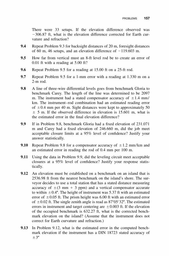
PROBLEMS 157
There were 33 setups. If the elevation difference observed was�306.87 ft, what is the elevation difference corrected for Earth cur-vature and refraction?
9.4 Repeat Problem 9.3 for backsight distances of 20 m, foresight distancesof 60 m, 46 setups, and an elevation difference of �119.603 m.
9.5 How far from vertical must an 8-ft level rod be to create an error of0.01 ft with a reading at 5.00 ft?
9.6 Repeat Problem 9.5 for a reading at 15.00 ft on a 25-ft rod.
9.7 Repeat Problem 9.5 for a 1-mm error with a reading at 1.330 m on a2-m rod.
9.8 A line of three-wire differential levels goes from benchmark Gloria tobenchmark Carey. The length of the line was determined to be 2097m. The instrument had a stated compensator accuracy of �1.4 mm/km. The instrument–rod combination had an estimated reading errorof �0.4 mm per 40 m. Sight distances were kept to approximately 50� 5 m. If the observed difference in elevation is 15.601 m, what isthe estimated error in the final elevation difference?
9.9 If in Problem 9.8, benchmark Gloria had a fixed elevation of 231.071m and Carey had a fixed elevation of 246.660 m, did the job meetacceptable closure limits at a 95% level of confidence? Justify youranswer statistically.
9.10 Repeat Problem 9.8 for a compensator accuracy of �1.2 mm/km andan estimated error in reading the rod of 0.4 mm per 100 m.
9.11 Using the data in Problem 9.9, did the leveling circuit meet acceptableclosures at a 95% level of confidence? Justify your response statis-tically.
9.12 An elevation must be established on a benchmark on an island that is2536.98 ft from the nearest benchmark on the island’s shore. The sur-veyor decides to use a total station that has a stated distance measuringaccuracy of �(3 mm � 3 ppm) and a vertical compensator accurateto within �0.4�. The height of instrument was 5.37 ft with an estimatederror of �0.05 ft. The prism height was 6.00 ft with an estimated errorof �0.02 ft. The single zenith angle is read as 87�05�32�. The estimatederrors in instrument and target centering are �0.003 ft. If the elevationof the occupied benchmark is 632.27 ft, what is the corrected bench-mark elevation on the island? (Assume that the instrument does notcorrect for Earth curvature and refraction.)
9.13 In Problem 9.12, what is the estimated error in the computed bench-mark elevation if the instrument has a DIN 18723 stated accuracy of�3�
158 ERROR PROPAGATION IN ELEVATION DETERMINATION
9.14 After completing the job in Problem 9.12, the surveyor discovered thatthe instrument had a vertical indexing error that caused the sight lineto be inclined by 15�.(a) How much error would be created in the elevation of the island
benchmark if the indexing error were ignored?(b) What is the corrected elevation?
9.15 A tilting level is used to run a set of precise levels to a constructionproject from benchmark DAM, whose elevation is 101.865 m. The lineis run along a road that goes up a steep incline. To expedite the job,backsight distances are kept to 50 � 1 m and foresight distances are20 � 1 m. The total length of differential levels is 4410 m. The ele-vation difference observed is 13.634 m. What is the corrected projectelevation if the instrument has a sight line that declines at the rate of0.3 mm per 50 m?
9.16 In Problem 9.15, the instrument’s level is centered to within �0.4� foreach sight and the rod is read to �1.2 mm per 50 m.(a) What is the estimated error in the elevation difference?(b) What is the 95% error in the final established benchmark?
9.17 Which method of leveling presented in this chapter offers the mostprecision? Defend your answer statistically.
Programming Problems
9.18 Create a computational package that will compute a corrected elevationdifference and its estimated error using the method of differential lev-eling. Use this package to solve Problem 9.15.
9.19 Create a computational package that will compute a corrected elevationdifference and its estimated error using the method of trigonometricleveling. Use this package to solve Problem 9.12.
159
CHAPTER 10
WEIGHTS OF OBSERVATIONS
10.1 INTRODUCTION
When surveying data are collected, they must usually conform to a given setof geometric conditions, and when they do not, the measurements are adjustedto force that geometric closure. For a set of uncorrelated observations, ameasurement with high precision, as indicated by a small variance, implies agood observation, and in the adjustment it should receive a relatively smallportion of the overall correction. Conversely, a measurement with lower pre-cision, as indicated by a larger variance, implies an observation with a largererror, and should receive a larger portion of the correction.
The weight of an observation is a measure of its relative worth comparedto other measurements. Weights are used to control the sizes of correctionsapplied to measurements in an adjustment. The more precise an observation,the higher its weight; in other words, the smaller the variance, the higher theweight. From this analysis it can be stated intuitively that weights are in-versely proportional to variances. Thus, it also follows that correction sizesshould be inversely proportional to weights.
In situations where measurements are correlated, weights are related to theinverse of the covariance matrix, �. As discussed in Chapter 6, the elementsof this matrix are variances and covariances. Since weights are relative, var-iances and covariances are often replaced by cofactors. A cofactor is relatedto its covariance by the equation
�ijq � (10.1)ij 2�0
Adjustment Computations: Spatial Data Analysis, Fourth Edition. C. D. Ghilani and P. R. Wolf© 2006 John Wiley & Sons, Inc. ISBN: 978-0-471-69728-2
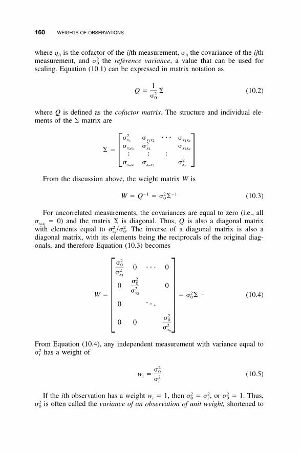
160 WEIGHTS OF OBSERVATIONS
where qij is the cofactor of the ijth measurement, �ij the covariance of the ijthmeasurement, and the reference variance, a value that can be used for2�0
scaling. Equation (10.1) can be expressed in matrix notation as
1Q � � (10.2)2�0
where Q is defined as the cofactor matrix. The structure and individual ele-ments of the � matrix are
2� � � � � �x x x x x1 1 2 1 n2� � �x x x x x2 1 2 2 n� �
� � �� �2� � �x x x x xn 1 n 2 n
From the discussion above, the weight matrix W is
�1 2 �1W � Q � � � (10.3)0
For uncorrelated measurements, the covariances are equal to zero (i.e., all� 0) and the matrix � is diagonal. Thus, Q is also a diagonal matrix�x xi j
with elements equal to The inverse of a diagonal matrix is also a2 2� /� .x 0i
diagonal matrix, with its elements being the reciprocals of the original diag-onals, and therefore Equation (10.3) becomes
2�0 0 � � � 02�x12�00 02�x 2 �12W � � � � (10.4)0
�0 � �� �2�00 0 2�xn
From Equation (10.4), any independent measurement with variance equal tohas a weight of2�i
2�0w � (10.5)i 2�i
If the ith observation has a weight wi � 1, then � or � 1. Thus,2 2 2� � , �0 i 0
is often called the variance of an observation of unit weight, shortened to2�0
10.2 WEIGHTED MEAN 161
variance of unit weight or simply unit variance. Its square root is called thestandard deviation of unit weight. If is set equal to 1 in Equation (10.5),2�0
then
1w � (10.6)i 2�i
Note in Equation (10.6) that as stated earlier, the weight of an observation isinversely proportional to its variance.
With correlated observations, it is possible to have a covariance matrix, �,and a cofactor matrix, Q, but not a weight matrix. This occurs when thecofactor matrix is singular, and thus an inverse for Q does not exist. Mostsituations in surveying involve uncorrelated observations. For the remainderof this chapter, only the uncorrelated case with variance of unit weight isconsidered.
10.2 WEIGHTED MEAN
If two measurements are taken of a quantity and the first is twice as good asthe second, their relative worth can be expressed by giving the first measure-ment a weight of 2 and the second a weight of 1. A simple adjustmentinvolving these two measurements would be to compute the mean value. Inthis calculation, the observation of weight 2 could be added twice, and theobservation of weight 1 added once. As an illustration, suppose that a distanceis measured with a tape to be 151.9 ft, and the same distance is measuredwith an EDM instrument as 152.5 ft. Assume that experience indicates thatthe electronically measured distance is twice as good as the taped distance,and accordingly, the taped distance is given a weight of 1 and the electroni-cally measured distance is given a weight of 2. Then one method of com-puting the mean from these observations is
151.9 � 152.5 � 152.5M � � 152.3
3
As an alternative, the calculation above can be rewritten as
1(151.9) � 2(152.5)M � � 152.3
1 � 2
Note that the weights of 1 and 2 were entered directly into the secondcomputation and that the result of this calculation is the same as the first.Note also that the computed mean tends to be closer to the measured value
162 WEIGHTS OF OBSERVATIONS
having the higher weight (i.e., 152.3 is closer to 152.5 than it is to 151.9). Amean value computed from weighted observations is called the weightedmean.
To develop a general expression for computing the weighted mean, supposethat we have m independent uncorrelated observations (z1, z2, . . . , zm) for aquantity z and that each observation has standard deviation �. Then the meanof the observations is
m� zii�1z � (10.7)m
If these m observations were now separated into two sets, one of size ma andthe other mb such that ma � mb � m, the means for these two sets would be
ma� zii�1z � (10.8)a ma
m� zii�m �1az � (10.9)b mb
The mean is found by combining the means of these two sets asz
m m m ma a� z � � z � z � � zi i i ii�1 i�m �1 i�1 i�m �1a az � � (10.10)m m � ma b
But from Equations (10.8) and (10.9),
m maz m � � z and z m � � z (10.11)a a i b b ii�1 i�m �1a
Thus,
z m � z ma a b bz � (10.12)m � ma b
Note the correspondence between Equation (10.12) and the second equationused to compute the weighted mean in the simple illustration given earlier.By intuitive comparison it should be clear that ma and mb correspond toweights that could be symbolized as wa and wb, respectively. Thus, Equation(10.12) can be written as
w z � w z � wza a b bz � � (10.13)w � w � wa b
Equation (10.13) is used in calculating the weighted mean for a group ofuncorrelated observations having unequal weights. In Chapter 11 it will be
10.3 RELATION BETWEEN WEIGHTS AND STANDARD ERRORS 163
shown that the weighted mean is the most probable value for a set of weightedobservations.
Example 10.1 As a simple example of computing a weighted mean usingEquation (10.13), suppose that a distance d is measured three times, with thefollowing results: 92.61 with weight 3, 92.60 with weight 2, and 92.62 withweight 1. Calculate the weighted mean.
3(92.61) � 2(92.60) � 1(92.62)d � � 92.608
3 � 2 � 1
Note that if weight had been neglected, the simple mean would have been92.61.
10.3 RELATION BETWEEN WEIGHTS AND STANDARD ERRORS
By applying the special law of propagation of variances [Equation (6.16)] toEquation (10.8), the variance in Equation (10.8) isza
2 2 2�z �z �za a a2 2 2 2� � � � � � � � � � � (10.14)� � � � � �za �z �z �z1 2 ma
Substituting partial derivatives with respect to the measurements into Equation(10.14) yields
2 2 21 1 12 2 2 2� � � � � � � � � � �� � � � � �za m m ma a a
Thus,
21 12 2 2� � m � � � (10.15)� �z aa m ma a
Using a similar procedure, the variance of iszb
12 2� � � (10.16)zb mb
In Equations (10.15) and (10.16), � is a constant, and the weights of za
and were established as ma and mb, respectively, from Equation (10.13).zb
Since the weights are relative, from Equations (10.15) and (10.16),
164 WEIGHTS OF OBSERVATIONS
1 1w � and w � (10.17)a b2 2� �z za b
Conclusion: With uncorrelated observations, the weights of the observationsare inversely proportional to their variances.
10.4 STATISTICS OF WEIGHTED OBSERVATIONS
10.4.1 Standard Deviation
By definition, an observation is said to have a weight w when its precision isequal to that of the mean of w observations of unit weight. Let �0 be thestandard error of an observation of weight 1, or unit weight. If y1, y2, . . . ,yn are observations having standard errors �1, �2, . . . , �n and weights w1,w2, . . . , wn, then, by Equation (10.5),
� � �0 0 0� � , � � , . . . , � � (10.18)1 2 n�w �w �w1 2 n
In Section 2.7, the standard error for a group of observations of equalweight was defined as
n 2� εii�1� � � n
Now, in the case where the observations are not equal in weight, the equationabove becomes
n2 2 2 2w ε � w ε � � � � w ε � w ε1 1 2 2 n n i ii�1� � � (10.19)� �n n
When modified for the standard deviation in Equation (2.7), it is
n2 2 2 2w v � w v � � � � � w v � w v1 1 2 2 n n i ii�1S � � (10.20)� �n � 1 n � 1
10.4.2 Standard Error of Weight w and Standard Error of theWeighted Mean
The relationship between standard error and standard error of weight w wasgiven in Equation (10.18). Combining this with Equation (10.19) and drop-
10.5 WEIGHTS IN ANGLE OBSERVATIONS 165
ping the summation limits, equations for standard errors of weight w areobtained in terms of �0 as follows:
2 2� � wε 1 � wε0� � � �1 � �n nw�w �w 11 1
2 2� � wε 1 � wε0� � � � (10.21)2 � �n nw�w �w 22 2
�
2 2� � wε 1 � wε0� � � �n � �n nw�w �w nn n
Similarly, standard deviations of weight w can be expressed as
2 2 2� wv � wv � wvS � , S � , . . . , S � (10.22)1 2 n� � �w (n � 1) w (n � 1) w (n �1)1 2 n
Finally, the reference standard error of the weighted mean is calculated as
2� wε� � (10.23)M �n � w
and the standard deviation of the weighted mean is
2� wv� � (10.24)M �(n �1)� w
10.5 WEIGHTS IN ANGLE OBSERVATIONS
Suppose that the three angles �1, �2, and �3 in a plane triangle are observedn1, n2, and n3 times, respectively, with the same instrument under the sameconditions. What are the relative weights of the angles?
To analyze the relationship between weights and the number of times anangle is turned, let S be the standard deviation of a single angle observation.The means of the three angles are
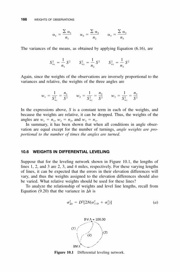
166 WEIGHTS OF OBSERVATIONS
Figure 10.1 Differential leveling network.
� � � � � �1 2 3� � � � � �1 2 3n n n1 2 3
The variances of the means, as obtained by applying Equation (6.16), are
1 1 12 2 2 2 2 2S � S S � S S � S� � �1 2 3n n n1 2 3
Again, since the weights of the observations are inversely proportional to thevariances and relative, the weights of the three angles are
1 n 1 n 1 n1 2 3w � � w � � w � �1 2 32 2 2 2 2 2S S S S S S� � �1 2 3
In the expressions above, S is a constant term in each of the weights, andbecause the weights are relative, it can be dropped. Thus, the weights of theangles are w1 � n1, w2 � n2, and w3 � n3.
In summary, it has been shown that when all conditions in angle obser-vation are equal except for the number of turnings, angle weights are pro-portional to the number of times the angles are turned.
10.6 WEIGHTS IN DIFFERENTIAL LEVELING
Suppose that for the leveling network shown in Figure 10.1, the lengths oflines 1, 2, and 3 are 2, 3, and 4 miles, respectively. For these varying lengthsof lines, it can be expected that the errors in their elevation differences willvary, and thus the weights assigned to the elevation differences should alsobe varied. What relative weights should be used for these lines?
To analyze the relationship of weights and level line lengths, recall fromEquation (9.20) that the variance in �h is
2 2 2 2� � D [2N(� � � )] (a)�h r / D �
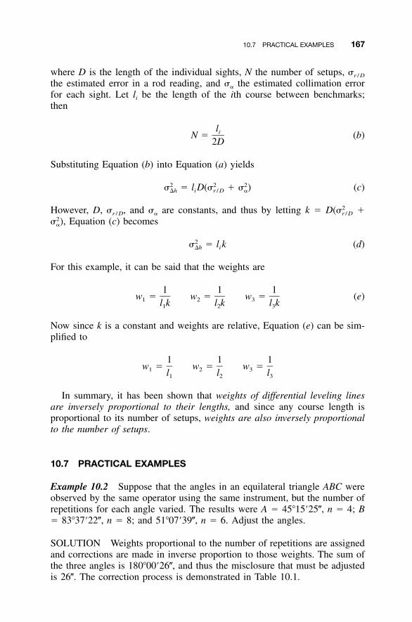
10.7 PRACTICAL EXAMPLES 167
where D is the length of the individual sights, N the number of setups, �r / D
the estimated error in a rod reading, and �� the estimated collimation errorfor each sight. Let li be the length of the ith course between benchmarks;then
liN � (b)2D
Substituting Equation (b) into Equation (a) yields
2 2 2� � l D(� � � ) (c)�h i r / D �
However, D, , and �� are constants, and thus by letting k � D �2� (�r / D r / D
Equation (c) becomes2� ),�
2� � l k (d)�h i
For this example, it can be said that the weights are
1 1 1w � w � w � (e)1 2 3l k l k l k1 2 3
Now since k is a constant and weights are relative, Equation (e) can be sim-plified to
1 1 1w � w � w �1 2 3l l l1 2 3
In summary, it has been shown that weights of differential leveling linesare inversely proportional to their lengths, and since any course length isproportional to its number of setups, weights are also inversely proportionalto the number of setups.
10.7 PRACTICAL EXAMPLES
Example 10.2 Suppose that the angles in an equilateral triangle ABC wereobserved by the same operator using the same instrument, but the number ofrepetitions for each angle varied. The results were A � 45�15�25�, n � 4; B� 83�37�22�, n � 8; and 51�07�39�, n � 6. Adjust the angles.
SOLUTION Weights proportional to the number of repetitions are assignedand corrections are made in inverse proportion to those weights. The sum ofthe three angles is 180�00�26�, and thus the misclosure that must be adjustedis 26�. The correction process is demonstrated in Table 10.1.
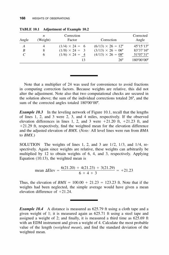
168 WEIGHTS OF OBSERVATIONS
TABLE 10.1 Adjustment of Example 10.2
Anglen
(Weight)Correction
Factor CorrectionCorrected
Angle
ABC
486
(1/4) � 24 � 6(1/8) � 24 � 3(1/6) � 24 � 4
13
(6/13) � 26 � 12�(3 /13) � 26 � 06�(4 /13) � 26 � 08�
26�
45�15�13�83�37�16�51�07�31�
180�00�00�
Note that a multiplier of 24 was used for convenience to avoid fractionsin computing correction factors. Because weights are relative, this did notalter the adjustment. Note also that two computational checks are secured inthe solution above; the sum of the individual corrections totaled 26�, and thesum of the corrected angles totaled 180�00�00�.
Example 10.3 In the leveling network of Figure 10.1, recall that the lengthsof lines 1, 2, and 3 were 2, 3, and 4 miles, respectively. If the observedelevation differences in lines 1, 2, and 3 were �21.20 ft, �21.23 ft, and�21.29 ft, respectively, find the weighted mean for the elevation differenceand the adjusted elevation of BMX. (Note: All level lines were run from BMAto BMX.)
SOLUTION The weights of lines 1, 2, and 3 are 1/2, 1/3, and 1/4, re-spectively. Again since weights are relative, these weights can arbitrarily bemultiplied by 12 to obtain weights of 6, 4, and 3, respectively. ApplyingEquation (10.13), the weighted mean is
6(21.20) � 4(21.23) � 3(21.29)mean �Elev � � �21.23
6 � 4 � 3
Thus, the elevation of BMX � 100.00 � 21.23 � 123.23 ft. Note that if theweights had been neglected, the simple average would have given a meanelevation difference of �21.24.
Example 10.4 A distance is measured as 625.79 ft using a cloth tape and agiven weight of 1; it is measured again as 625.71 ft using a steel tape andassigned a weight of 2; and finally, it is measured a third time as 625.69 ftwith an EDM instrument and given a weight of 4. Calculate the most probablevalue of the length (weighted mean), and find the standard deviation of theweighted mean.
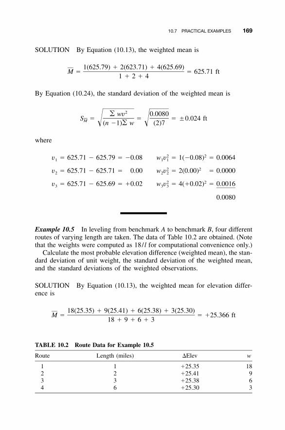
10.7 PRACTICAL EXAMPLES 169
TABLE 10.2 Route Data for Example 10.5
Route Length (miles) �Elev w
1 1 �25.35 182 2 �25.41 93 3 �25.38 64 6 �25.30 3
SOLUTION By Equation (10.13), the weighted mean is
1(625.79) � 2(623.71) � 4(625.69)M � � 625.71 ft
1 � 2 � 4
By Equation (10.24), the standard deviation of the weighted mean is
2� wv 0.0080S � � � �0.024 ftM � �(n �1)� w (2)7
where
2 2v � 625.71 � 625.79 � �0.08 w v � 1(�0.08) � 0.00641 1 1
2 2v � 625.71 � 625.71 � 0.00 w v � 2(0.00) � 0.00002 2 2
2 2v � 625.71 � 625.69 � �0.02 w v � 4(�0.02) � 0.00163 3 3
0.0080
Example 10.5 In leveling from benchmark A to benchmark B, four differentroutes of varying length are taken. The data of Table 10.2 are obtained. (Notethat the weights were computed as 18/ l for computational convenience only.)
Calculate the most probable elevation difference (weighted mean), the stan-dard deviation of unit weight, the standard deviation of the weighted mean,and the standard deviations of the weighted observations.
SOLUTION By Equation (10.13), the weighted mean for elevation differ-ence is
18(25.35) � 9(25.41) � 6(25.38) � 3(25.30)M � � �25.366 ft
18 � 9 � 6 � 3
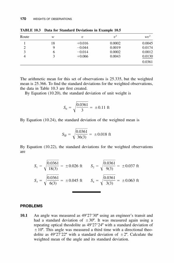
170 WEIGHTS OF OBSERVATIONS
TABLE 10.3 Data for Standard Deviations in Example 10.5
Route w v v2 wv2
1 18 �0.016 0.0002 0.00452 9 �0.044 0.0019 0.01743 6 �0.014 0.0002 0.00124 3 �0.066 0.0043 0.0130
0.0361
The arithmetic mean for this set of observations is 25.335, but the weightedmean is 25.366. To find the standard deviations for the weighted observations,the data in Table 10.3 are first created.
By Equation (10.20), the standard deviation of unit weight is
0.0361S � � �0.11 ft0 � 3
By Equation (10.24), the standard deviation of the weighted mean is
0.0361S � � �0.018 ftM � 36(3)
By Equation (10.22), the standard deviations for the weighted observationsare
0.0361 0.0361S � � �0.026 ft S � � �0.037 ft1 2� �18(3) 9(3)
0.0361 0.0361S � � �0.045 ft S � � �0.063 ft3 4� �6(3) 3(3)
PROBLEMS
10.1 An angle was measured as 49�27�30� using an engineer’s transit andhad a standard deviation of �30�. It was measured again using arepeating optical theodolite as 49�27�24� with a standard deviation of�10�. This angle was measured a third time with a directional theo-dolite as 49�27�22� with a standard deviation of �2�. Calculate theweighted mean of the angle and its standard deviation.
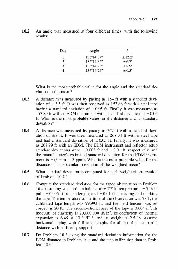
PROBLEMS 171
10.2 An angle was measured at four different times, with the followingresults:
Day Angle S
1 136�14�34� �12.2�2 136�14�36� �6.7�3 136�14�28� �8.9�4 136�14�26� �9.5�
What is the most probable value for the angle and the standard de-viation in the mean?
10.3 A distance was measured by pacing as 154 ft with a standard devi-ation of �2.5 ft. It was then observed as 153.86 ft with a steel tapehaving a standard deviation of �0.05 ft. Finally, it was measured as153.89 ft with an EDM instrument with a standard deviation of �0.02ft. What is the most probable value for the distance and its standarddeviation?
10.4 A distance was measured by pacing as 267 ft with a standard devi-ation of �3 ft. It was then measured as 268.94 ft with a steel tapeand had a standard deviation of �0.05 ft. Finally, it was measuredas 268.99 ft with an EDM. The EDM instrument and reflector setupstandard deviations were �0.005 ft and �0.01 ft, respectively, andthe manufacturer’s estimated standard deviation for the EDM instru-ment is �(3 mm � 3 ppm). What is the most probable value for thedistance and the standard deviation of the weighted mean?
10.5 What standard deviation is computed for each weighted observationof Problem 10.4?
10.6 Compute the standard deviation for the taped observation in Problem10.4 assuming standard deviations of �5�F in temperature, �3 lb inpull, �0.005 ft in tape length, and �0.01 ft in reading and markingthe tape. The temperature at the time of the observation was 78�F, thecalibrated tape length was 99.993 ft, and the field tension was re-corded as 20 lb. The cross-sectional area of the tape is 0.004 in2, itsmodulus of elasticity is 29,000,000 lb/in2, its coefficient of thermalexpansion is 6.45 � 10�5 �F�1, and its weight is 2.5 lb. Assumehorizontal taping with full tape lengths for all but the last partialdistance with ends-only support.
10.7 Do Problem 10.3 using the standard deviation information for theEDM distance in Problem 10.4 and the tape calibration data in Prob-lem 10.6.
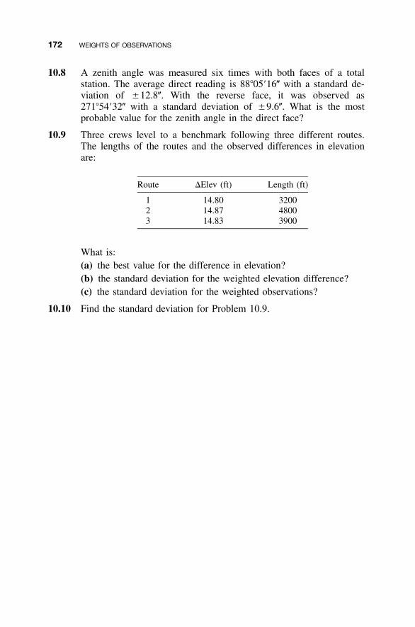
172 WEIGHTS OF OBSERVATIONS
10.8 A zenith angle was measured six times with both faces of a totalstation. The average direct reading is 88�05�16� with a standard de-viation of �12.8�. With the reverse face, it was observed as271�54�32� with a standard deviation of �9.6�. What is the mostprobable value for the zenith angle in the direct face?
10.9 Three crews level to a benchmark following three different routes.The lengths of the routes and the observed differences in elevationare:
Route �Elev (ft) Length (ft)
1 14.80 32002 14.87 48003 14.83 3900
What is:(a) the best value for the difference in elevation?(b) the standard deviation for the weighted elevation difference?(c) the standard deviation for the weighted observations?
10.10 Find the standard deviation for Problem 10.9.
173
CHAPTER 11
PRINCIPLES OF LEAST SQUARES
11.1 INTRODUCTION
In surveying, observations must often satisfy established numerical relation-ships known as geometric constraints. As examples, in a closed polygon trav-erse, horizontal angle and distance measurements should conform to thegeometric constraints given in Section 8.4, and in a differential leveling loop,the elevation differences should sum to a given quantity. However, becausethe geometric constraints meet perfectly rarely, if ever, the data are adjusted.
As discussed in earlier chapters, errors in observations conform to the lawsof probability; that is, they follow normal distribution theory. Thus, theyshould be adjusted in a manner that follows these mathematical laws. Whereasthe mean has been used extensively throughout history, the earliest works onleast squares started in the late eighteenth century. Its earliest application wasprimarily for adjusting celestial observations. Laplace first investigated thesubject and laid its foundation in 1774. The first published article on thesubject, entitled ‘‘Methode des moindres quarres’’ (Method of Least Squares),was written in 1805 by Legendre. However, it is well known that althoughGauss did not publish until 1809, he developed and used the method exten-sively as a student at the University of Gottingen beginning in 1794 and thusis given credit for the development of the subject. In this chapter, equationsfor performing least squares adjustments are developed and their use is illus-trated with several examples.
Adjustment Computations: Spatial Data Analysis, Fourth Edition. C. D. Ghilani and P. R. Wolf© 2006 John Wiley & Sons, Inc. ISBN: 978-0-471-69728-2
174 PRINCIPLES OF LEAST SQUARES
11.2 FUNDAMENTAL PRINCIPLE OF LEAST SQUARES
To develop the principle of least squares, a specific case is considered. Sup-pose that there are n independent equally weighted measurements, z1, z2,. . . , zn, of the same quantity z, which has a most probable value denoted byM. By definition,
M � z � v1 1
M � z � v2 2 (11.1)
�
M � z � vn n
where the v’s are the residual errors. Note that residuals behave in a mannersimilar to errors, and thus they can be used interchangeably in the normaldistribution function given by Equation (3.2). Substituting v for x, there results
1 2 2 2 2�v / 2� �h vƒ (v) � y � e � Ke (11.2)x��2�
where h � 1/ and K � h /��2 ��.As discussed in Chapter 3, probabilities are represented by areas under the
normal distribution curve. Thus, the individual probabilities for the occurrenceof residuals v1, v2, . . . , vn are obtained by multiplying their respectiveordinates y1, y2, . . . , yn by some infinitesimally small increment of v, �v.The following probability statements result:
2 2�h v1P � y �v � Ke �v1 1
2 2�h v2P � y �v � Ke �v2 2 (11.3)
�2 2�h vnP � y �v � Ke �vn n
From Equation (3.1), the probability of the simultaneous occurrence of all theresiduals v1 through vn is the product of the individual probabilities and thus
2 2 2 2 2 2�h v �h v �h v1 2 nP � (Ke �v)(Ke �v) � � � (Ke �v) (11.4)
Simplifying Equation (11.4) yields
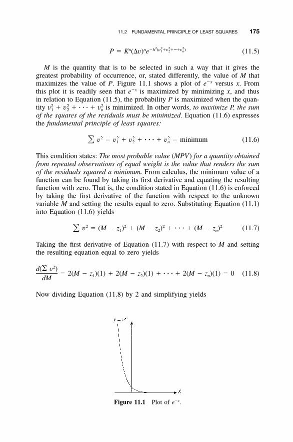
11.2 FUNDAMENTAL PRINCIPLE OF LEAST SQUARES 175
Figure 11.1 Plot of e�x.
2 2 2 2n n �h (v �v �����v )1 2 nP � K (�v) e (11.5)
M is the quantity that is to be selected in such a way that it gives thegreatest probability of occurrence, or, stated differently, the value of M thatmaximizes the value of P. Figure 11.1 shows a plot of e�x versus x. Fromthis plot it is readily seen that e�x is maximized by minimizing x, and thusin relation to Equation (11.5), the probability P is maximized when the quan-tity � � � � � � is minimized. In other words, to maximize P, the sum2 2 2v v v1 2 n
of the squares of the residuals must be minimized. Equation (11.6) expressesthe fundamental principle of least squares:
2 2 2 2v � v � v � � � � � v � minimum (11.6)� 1 2 n
This condition states: The most probable value (MPV) for a quantity obtainedfrom repeated observations of equal weight is the value that renders the sumof the residuals squared a minimum. From calculus, the minimum value of afunction can be found by taking its first derivative and equating the resultingfunction with zero. That is, the condition stated in Equation (11.6) is enforcedby taking the first derivative of the function with respect to the unknownvariable M and setting the results equal to zero. Substituting Equation (11.1)into Equation (11.6) yields
2 2 2 2v � (M � z ) � (M � z ) � � � � � (M � z ) (11.7)� 1 2 n
Taking the first derivative of Equation (11.7) with respect to M and settingthe resulting equation equal to zero yields
2d(� v )� 2(M � z )(1) � 2(M � z )(1) � � � � � 2(M � z )(1) � 01 2 ndM
(11.8)
Now dividing Equation (11.8) by 2 and simplifying yields
176 PRINCIPLES OF LEAST SQUARES
M � z � M � z � � � � � M � z � 01 2 n
nM � z � z � � � � � z1 2 n
z � z � � � � � z1 2 nM � (11.9)n
In Equation (11.9) the quantity (z1 � z2 � � � � � zn) /n is the mean of thevalues observed. This is proof that when a quantity has been observed inde-pendently several times, the MPV is the arithmetic mean.
11.3 FUNDAMENTAL PRINCIPLE OF WEIGHTED LEAST SQUARES
In Section 11.2, the fundamental principle of a least squares adjustment wasdeveloped for observations having equal or unit weights. The more generalcase of least squares adjustment assumes that the observations have varyingdegrees of precision, and thus varying weights.
Consider a set of measurements z1, z2, . . . , zn having relative weights w1,w2, . . . , wn and residuals v1, v2, . . . , vn. Denote the weighted MPV as M.As in Section 11.2, the residuals are related to the observations through Equa-tions (11.1), and the total probability of their simultaneous occurrence is givenby Equation (11.5). However, notice in Equation (11.2) that h2 � 1/2�2, andsince weights are inversely proportional to variances, they are directly pro-portional to h2. Thus, Equation (11.5) can be rewritten as
2 2 2n n �(w v �w v �����w v )1 1 2 2 n nP � K (�v) e (11.10)
To maximize P in Equation (11.10), the negative exponent must be mini-mized. To achieve this, the sum of the products of the weights times theirrespective residuals squared must be minimized. This is the condition imposedin weighted least squares adjustment. The condition of weighted least squaresadjustment in equation form is
2 2 2 2w v � w v � � � � � w v � � wv → minimum (11.11)1 1 2 2 n n
Substituting the values for the residuals given in Equation (11.1) into Equa-tion (11.11) yields
2 2 2w (M � z ) � w (M � z ) � � � � � w (M � z ) → minimum (11.12)1 1 2 2 n n
The condition for a weighted least squares adjustment is: The most prob-able value for a quantity obtained from repeated observations having variousweights is that value which renders the sum of the weights times their re-spective squared residuals a minimum.
11.5 FUNCTIONAL MODEL 177
The minimum condition is imposed by differentiating Equation (11.12)with respect to M and setting the resulting equation equal to zero. This yields
2w (M � z )(1) � 2w (M � z )(1) � � � � � 2w (M � z )(1) � 0 (11.13)1 1 2 2 n n
Dividing Equation (11.13) by 2 and rearranging results in
w (M � z ) � w (M � z ) � � � � � w (M � z ) � 0 (11.14a)1 1 2 2 n n
Rearranging Equation (11.14a) gives
w z � w z � � � � � w z � w M � w M � � � � � w M (11.14b)1 1 2 2 n n 1 2 n
Equation (11.14b) can be written as � wz � � wM. Thus,
� wzM � (11.15)� w
Notice that Equation (11.15) is the same as Equation (10.13), which is theformula for computing the weighted mean.
11.4 STOCHASTIC MODEL
The determination of variances, and subsequently the weights of the obser-vations, is known as the stochastic model in a least squares adjustment. InSection 11.3 the inclusion of weights in the adjustment was discussed. It iscrucial to the adjustment to select a proper stochastic (weighting) model since,as was discussed in Section 10.1, the weight of an observation controls theamount of correction it receives during the adjustment. However, developmentof the stochastic model is important not only to weighted adjustments. Whendoing an unweighted adjustment, all observations are assumed to be of equalweight, and thus the stochastic model is created implicitly. The foundationsfor selecting a proper stochastic model in surveying were established in Chap-ters 7 to 10. It will be shown in Chapter 21 that failure to select the stochasticmodel properly will also affect one’s ability to isolate blunders in observationsets.
11.5 FUNCTIONAL MODEL
A functional model in adjustment computations is an equation or set of equa-tions that represents or defines an adjustment condition. It must be eitherknown or assumed. If the functional model represents the physical situation
178 PRINCIPLES OF LEAST SQUARES
adequately, the observational errors can be expected to conform to the normaldistribution curve. For example, a well-known functional model states thatthe sum of angles in a triangle is 180�. This model is adequate if the surveyis limited to a small region. However, when the survey covers very largeareas, this model does not account for the systematic errors caused by Earth’scurvature. In this case, the functional model is inadequate and needs to bemodified to include corrections for spherical excess. In traversing, the func-tional model of plane computations is suitable for smaller surveys, but if theextent of the survey becomes too large, the model must again be changed toaccount for the systematic errors caused by Earth’s curvature. This can beaccomplished by transforming the observations into a plane mapping systemsuch as the state plane coordinate system or by using geodetic observationequations. Needless to say, if the model does not fit the physical situation, anincorrect adjustment will result. In Chapter 23 we discuss a three-dimensionalgeodetic and the systematic errors that must be taken into account in a three-dimensional geodetic adjustment.
There are two basic forms for functional models: the conditional and par-ametric adjustments. In a conditional adjustment, geometric conditions areenforced on the observations and their residuals. Examples of conditionaladjustment are: (1) the sum of the angles in a closed polygon is (n � 2)180�,where n is the number of sides in the polygon; (2) the latitudes and departuresof a polygon traverse sum to zero; and (3) the sum of the angles in the horizonequal 360�. A least squares adjustment example using condition equations isgiven in Section 11.13.
When performing a parametric adjustment, observations are expressed interms of unknown parameters that were never observed directly. For example,the well-known coordinate equations are used to model the angles, directions,and distances observed in a horizontal plane survey. The adjustment yieldsthe most probable values for the coordinates (parameters), which in turn pro-vide the most probable values for the adjusted observations.
The choice of the functional model will determine which quantities orparameters are adjusted. A primary purpose of an adjustment is to ensure thatall observations are used to find the most probable values for the unknownsin the model. In least squares adjustments, no matter if conditional or para-metric, the geometric checks at the end of the adjustment are satisfied andthe same adjusted observations are obtained. In complicated networks, it isoften difficult and time consuming to write the equations to express all con-ditions that must be met for a conditional adjustment. Thus, this book willfocus on the parametric adjustment, which generally leads to larger systemsof equations but is straightforward in its development and solution and, as aresult, is well suited to computers.
The combination of stochastic and functional models results in a mathe-matical model for the adjustment. The stochastic and functional models mustboth be correct if the adjustment is to yield the most probable values for theunknown parameters. That is, it is just as important to use a correct stochastic
11.6 OBSERVATION EQUATIONS 179
model as it is to use a correct functional model. Improper weighting of ob-servations will result in the unknown parameters being determined incorrectly.
11.6 OBSERVATION EQUATIONS
Equations that relate observed quantities to both observational residuals andindependent unknown parameters are called observation equations. One equa-tion is written for each observation and for a unique set of unknowns. For aunique solution of unknowns, the number of equations must equal the numberof unknowns. Usually, there are more observations (and hence equations) thanunknowns, and this permits determination of the most probable values for theunknowns based on the principle of least squares.
11.6.1 Elementary Example of Observation Equation Adjustment
As an example of a least squares adjustment by the observation equationmethod, consider the following three equations:
(1) x � y � 3.0
(2) 2x � y � 1.5 (11.16)
(3) x � y � 0.2
Equations (11.16) relate the two unknowns, x and y, to the quantities ob-served (the values on the right side of the equations). One equation isredundant since the values for x and y can be obtained from any two of thethree equations. For example, if Equations (1) and (2) are solved, x wouldequal 1.5 and y would equal 1.5, but if Equations (2) and (3) are solved, xwould equal 1.3 and y would equal 1.1, and if Equations (1) and (3) aresolved, x would equal 1.6 and y would equal 1.4. Based on the inconsistencyof these equations, the observations contain errors. Therefore, new expres-sions, called observation equations, can be rewritten that include residuals.The resulting set of equations is
(4) x � y � 3.0 � v1
(5) 2x � y � 1.5 � v (11.17)2
(6) x � y � 0.2 � v3
Equations (11.17) relate the unknown parameters to the observations andtheir errors. Obviously, it is possible to select values of v1, v2, and v3 thatwill yield the same values for x and y no matter which pair of equations areused. For example, to obtain consistencies through all of the equations, ar-
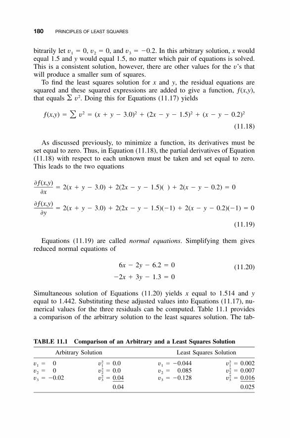
180 PRINCIPLES OF LEAST SQUARES
TABLE 11.1 Comparison of an Arbitrary and a Least Squares Solution
Arbitrary Solution Least Squares Solution
v1 � 0 � 0.02v1 v1 � �0.044 � 0.0022v1
v2 � 0 � 0.02v2 v2 � 0.085 � 0.0072v2
v3 � �0.02 � 0.042v3 v3 � �0.128 � 0.0162v3
0.04 0.025
bitrarily let v1 � 0, v2 � 0, and v3 � �0.2. In this arbitrary solution, x wouldequal 1.5 and y would equal 1.5, no matter which pair of equations is solved.This is a consistent solution, however, there are other values for the v’s thatwill produce a smaller sum of squares.
To find the least squares solution for x and y, the residual equations aresquared and these squared expressions are added to give a function, ƒ(x,y),that equals � v2. Doing this for Equations (11.17) yields
2 2 2 2ƒ(x,y) � v � (x � y � 3.0) � (2x � y � 1.5) � (x � y � 0.2)�(11.18)
As discussed previously, to minimize a function, its derivatives must beset equal to zero. Thus, in Equation (11.18), the partial derivatives of Equation(11.18) with respect to each unknown must be taken and set equal to zero.This leads to the two equations
�ƒ(x,y)� 2(x � y � 3.0) � 2(2x � y � 1.5)( ) � 2(x � y � 0.2) � 0
�x
�ƒ(x,y)� 2(x � y � 3.0) � 2(2x � y � 1.5)(�1) � 2(x � y � 0.2)(�1) � 0
�y
(11.19)
Equations (11.19) are called normal equations. Simplifying them givesreduced normal equations of
6x � 2y � 6.2 � 0 (11.20)
�2x � 3y � 1.3 � 0
Simultaneous solution of Equations (11.20) yields x equal to 1.514 and yequal to 1.442. Substituting these adjusted values into Equations (11.17), nu-merical values for the three residuals can be computed. Table 11.1 providesa comparison of the arbitrary solution to the least squares solution. The tab-
11.7 SYSTEMATIC FORMULATION OF THE NORMAL EQUATIONS 181
ulated summations of residuals squared shows that the least squares solutionyields the smaller total and thus the better solution. In fact, it is the mostprobable solution for the unknowns based on the observations.
11.7 SYSTEMATIC FORMULATION OF THE NORMAL EQUATIONS
11.7.1 Equal-Weight Case
In large systems of observation equations, it is helpful to use systematic pro-cedures to formulate the normal equations. In developing these procedures,consider the following generalized system of linear observation equations hav-ing variables of (A, B, C, . . . , N):
a A � b B � c C � � � � � n N � l � v1 1 1 1 1 1
a A � b B � c C � � � � � n N � l � v2 2 2 2 2 2 (11.21)
�
a A � b B � c C � � � � � n N � l � vm m m m m m
The squares of the residuals for Equations (11.21) are
2 2v � (a A � b B � c C � � � � � n N � l )1 1 1 1 1 1
2 2v � (a A � b B � c C � � � � � n N � l )2 2 2 2 2 2 (11.22)
�
2 2v � (a A � b B � c C � � � � � n N � l )m m m m m m
Summing Equations (11.22), the function ƒ(A,B,C, . . . , N) � � v2 is ob-tained. This expresses the equal-weight least squares condition as
2 2v � (a A � b B � c C � � � � � n N � l )� 1 1 1 1 1
2� (a A � b B � c C � � � � � n N � l )2 2 2 2 2
2� � � � � (a A � b B � c C � � � � � n N � l ) (11.23)m m m m m
According to least squares theory, the minimum for Equation (11.23) isfound by setting the partial derivatives of the function with respect to eachunknown equal to zero. This results in the normal equations
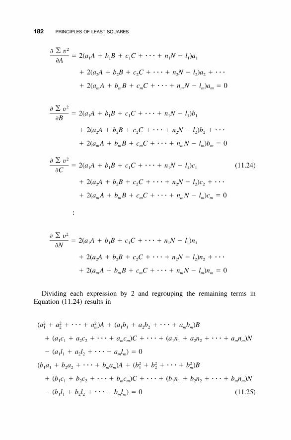
182 PRINCIPLES OF LEAST SQUARES
2� � v� 2(a A � b B � c C � � � � � n N � l )a1 1 1 1 1 1�A
� 2(a A � b B � c C � � � � � n N � l )a � � � �2 2 2 2 2 2
� 2(a A � b B � c C � � � � � n N � l )a � 0m m m m m m
2� � v� 2(a A � b B � c C � � � � � n N � l )b1 1 1 1 1 1�B
� 2(a A � b B � c C � � � � � n N � l )b � � � �2 2 2 2 2 2
� 2(a A � b B � c C � � � � � n N � l )b � 0m m m m m m
2� � v� 2(a A � b B � c C � � � � � n N � l )c (11.24)1 1 1 1 1 1�C
� 2(a A � b B � c C � � � � � n N � l )c � � � �2 2 2 2 2 2
� 2(a A � b B � c C � � � � � n N � l )c � 0m m m m m m
�
2� � v� 2(a A � b B � c C � � � � � n N � l )n1 1 1 1 1 1�N
� 2(a A � b B � c C � � � � � n N � l )n � � � �2 2 2 2 2 2
� 2(a A � b B � c C � � � � � n N � l )n � 0m m m m m m
Dividing each expression by 2 and regrouping the remaining terms inEquation (11.24) results in
2 2 2(a � a � � � � � a )A � (a b � a b � � � � � a b )B1 2 m 1 1 2 2 m m
� (a c � a c � � � � � a c )C � � � � � (a n � a n � � � � � a n )N1 1 2 2 m m 1 1 2 2 m m
� (a l � a l � � � � � a l ) � 01 1 2 2 m m
2 2 2(b a � b a � � � � � b a )A � (b � b � � � � � b )B1 1 2 2 m m 1 2 m
� (b c � b c � � � � � b c )C � � � � � (b n � b n � � � � � b n )N1 1 2 2 m m 1 1 2 2 m m
� (b l � b l � � � � � b l ) � 01 1 2 2 m m (11.25)
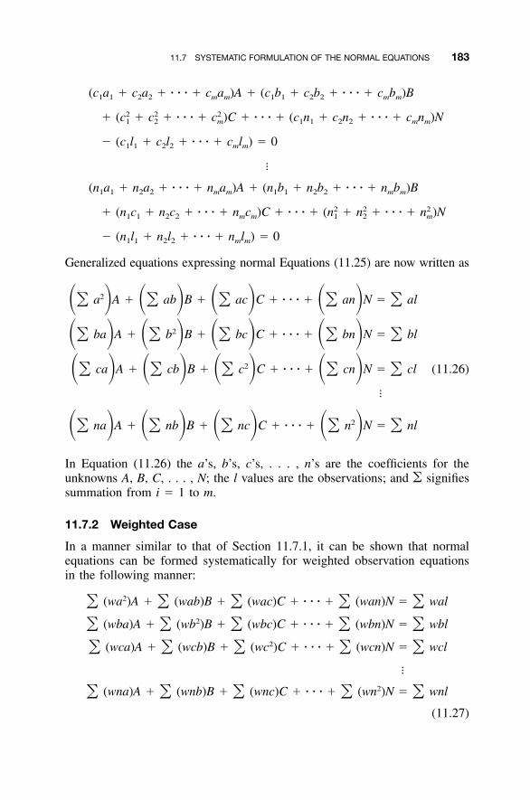
11.7 SYSTEMATIC FORMULATION OF THE NORMAL EQUATIONS 183
(c a � c a � � � � � c a )A � (c b � c b � � � � � c b )B1 1 2 2 m m 1 1 2 2 m m
2 2 2� (c � c � � � � � c )C � � � � � (c n � c n � � � � � c n )N1 2 m 1 1 2 2 m m
� (c l � c l � � � � � c l ) � 01 1 2 2 m m
�
(n a � n a � � � � � n a )A � (n b � n b � � � � � n b )B1 1 2 2 m m 1 1 2 2 m m
2 2 2� (n c � n c � � � � � n c )C � � � � � (n � n � � � � � n )N1 1 2 2 m m 1 2 m
� (n l � n l � � � � � n l ) � 01 1 2 2 m m
Generalized equations expressing normal Equations (11.25) are now written as
2a A � ab B � ac C � � � � � an N � al� � � � �� � � � � � � �2ba A � b B � bc C � � � � � bn N � bl� � � � �� � � � � � � �
2ca A � cb B � c C � � � � � cn N � cl (11.26)� � � � �� � � � � � � ��
2na A � nb B � nc C � � � � � n N � nl� � � � �� � � � � � � �In Equation (11.26) the a’s, b’s, c’s, . . . , n’s are the coefficients for theunknowns A, B, C, . . . , N; the l values are the observations; and � signifiessummation from i � 1 to m.
11.7.2 Weighted Case
In a manner similar to that of Section 11.7.1, it can be shown that normalequations can be formed systematically for weighted observation equationsin the following manner:
2(wa )A � (wab)B � (wac)C � � � � � (wan)N � wal� � � � �2(wba)A � (wb )B � (wbc)C � � � � � (wbn)N � wbl� � � � �
2(wca)A � (wcb)B � (wc )C � � � � � (wcn)N � wcl� � � � ��
2(wna)A � (wnb)B � (wnc)C � � � � � (wn )N � wnl� � � � �(11.27)
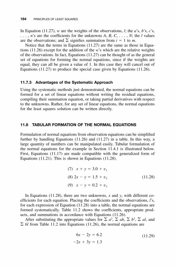
184 PRINCIPLES OF LEAST SQUARES
In Equation (11.27), w are the weights of the observations, l; the a’s, b’s, c’s,. . . , n’s are the coefficients for the unknowns A, B, C, . . . , N; the l valuesare the observations; and � signifies summation from i � 1 to m.
Notice that the terms in Equations (11.27) are the same as those in Equa-tions (11.26) except for the addition of the w’s which are the relative weightsof the observations. In fact, Equations (11.27) can be thought of as the generalset of equations for forming the normal equations, since if the weights areequal, they can all be given a value of 1. In this case they will cancel out ofEquations (11.27) to produce the special case given by Equations (11.26).
11.7.3 Advantages of the Systematic Approach
Using the systematic methods just demonstrated, the normal equations can beformed for a set of linear equations without writing the residual equations,compiling their summation equation, or taking partial derivatives with respectto the unknowns. Rather, for any set of linear equations, the normal equationsfor the least squares solution can be written directly.
11.8 TABULAR FORMATION OF THE NORMAL EQUATIONS
Formulation of normal equations from observation equations can be simplifiedfurther by handling Equations (11.26) and (11.27) in a table. In this way, alarge quantity of numbers can be manipulated easily. Tabular formulation ofthe normal equations for the example in Section 11.4.1 is illustrated below.First, Equations (11.17) are made compatible with the generalized form ofEquations (11.21). This is shown in Equations (11.28).
(7) x � y � 3.0 � v1
(8) 2x � y � 1.5 � v (11.28)2
(9) x � y � 0.2 � v3
In Equations (11.28), there are two unknowns, x and y, with different co-efficients for each equation. Placing the coefficients and the observations, l’s,for each expression of Equation (11.28) into a table, the normal equations areformed systematically. Table 11.2 shows the coefficients, appropriate prod-ucts, and summations in accordance with Equations (11.26).
After substituting the appropriate values for � a2, � ab, � b2, � al, and� bl from Table 11.2 into Equations (11.26), the normal equations are
6x � 2y � 6.2 (11.29)
�2x � 3y � 1.3
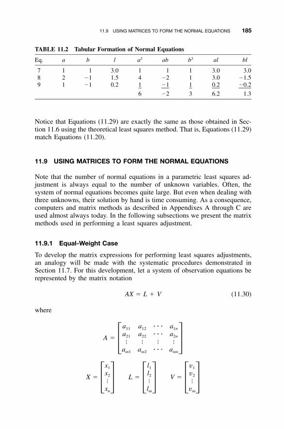
11.9 USING MATRICES TO FORM THE NORMAL EQUATIONS 185
TABLE 11.2 Tabular Formation of Normal Equations
Eq. a b l a2 ab b2 al bl
7 1 1 3.0 1 1 1 3.0 3.08 2 �1 1.5 4 �2 1 3.0 �1.59 1 �1 0.2 1 �1 1 0.2 �0.2
6 �2 3 6.2 1.3
Notice that Equations (11.29) are exactly the same as those obtained in Sec-tion 11.6 using the theoretical least squares method. That is, Equations (11.29)match Equations (11.20).
11.9 USING MATRICES TO FORM THE NORMAL EQUATIONS
Note that the number of normal equations in a parametric least squares ad-justment is always equal to the number of unknown variables. Often, thesystem of normal equations becomes quite large. But even when dealing withthree unknowns, their solution by hand is time consuming. As a consequence,computers and matrix methods as described in Appendixes A through C areused almost always today. In the following subsections we present the matrixmethods used in performing a least squares adjustment.
11.9.1 Equal-Weight Case
To develop the matrix expressions for performing least squares adjustments,an analogy will be made with the systematic procedures demonstrated inSection 11.7. For this development, let a system of observation equations berepresented by the matrix notation
AX � L � V (11.30)
where
a a � � � a11 12 1n
a a � � � a21 22 2nA �� � � �� �
a a � � � am1 m2 mn
x l v1 1 1
x l v2 2 2X � L � V �� � �� � � � � �x l vn m m
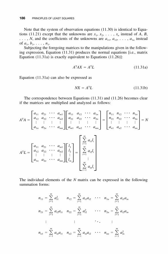
186 PRINCIPLES OF LEAST SQUARES
Note that the system of observation equations (11.30) is identical to Equa-tions (11.21) except that the unknowns are x1, x2, . . . , xn instead of A, B,. . . , N, and the coefficients of the unknowns are a11, a12, . . . , a1n insteadof a1, b1, . . . , n1.
Subjecting the foregoing matrices to the manipulations given in the follow-ing expression, Equation (11.31) produces the normal equations [i.e., matrixEquation (11.31a) is exactly equivalent to Equations (11.26)]:
T TA AX � A L (11.31a)
Equation (11.31a) can also be expressed as
TNX � A L (11.31b)
The correspondence between Equations (11.31) and (11.26) becomes clearif the matrices are multiplied and analyzed as follows:
a a � � � a a a � � � a n n � � � n11 21 m1 11 12 1n 11 12 1n
a a � � � a a a � � � a n n � � � aT 12 22 m2 21 22 2n 21 22 2nA A � � � N� � � � � � � � � � � �� �� � � �
a a � � � a a a � � � a a a � � � a1n 2n mn m1 m2 mn n1 n2 nn
m
a l� i1 ii�1
a a � � � a l m11 21 m1 1
a a � � � a l a l�T 12 22 m2 2 i2 iA L � � i�1� � � � �� �� ��a a � � � a l1n 2n mn m � �m
a l� in ii�1
The individual elements of the N matrix can be expressed in the followingsummation forms:
m m m2n � a n � a a � � � n � a a� � �11 i1 12 i1 i2 1n i1 in
i�1 i�1 i�1
m m m2n � a a n � a � � � n � a a� � �21 i2 i1 22 i2 2n i2 in
i�1 i�1 i�1
�� � � ��
m m m2n � a a n � a a � � � n � a� � �n1 in i1 n2 in i2 nn in
i�1 i�1 i�1
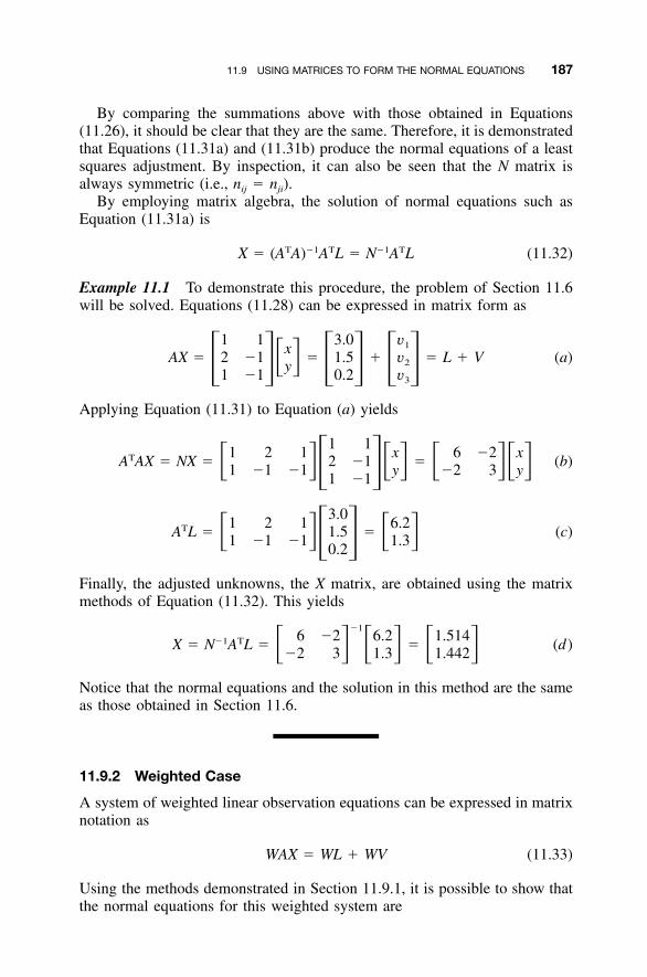
11.9 USING MATRICES TO FORM THE NORMAL EQUATIONS 187
By comparing the summations above with those obtained in Equations(11.26), it should be clear that they are the same. Therefore, it is demonstratedthat Equations (11.31a) and (11.31b) produce the normal equations of a leastsquares adjustment. By inspection, it can also be seen that the N matrix isalways symmetric (i.e., nij � nji).
By employing matrix algebra, the solution of normal equations such asEquation (11.31a) is
T �1 T �1 TX � (A A) A L � N A L (11.32)
Example 11.1 To demonstrate this procedure, the problem of Section 11.6will be solved. Equations (11.28) can be expressed in matrix form as
1 1 3.0 v1xAX � 2 �1 � 1.5 � v � L � V (a)� 2y� � � � � �1 �1 0.2 v3
Applying Equation (11.31) to Equation (a) yields
1 11 2 1 x 6 �2 xTA AX � NX � 2 �1 � (b)� � � � 1 �1 �1 y �2 3 y� �1 �1
3.01 2 1 6.2TA L � 1.5 � (c)� � 1 �1 �1 1.3� �0.2
Finally, the adjusted unknowns, the X matrix, are obtained using the matrixmethods of Equation (11.32). This yields
�16 �2 6.2 1.514�1 TX � N A L � � (d)� � � �2 3 1.3 1.442
Notice that the normal equations and the solution in this method are the sameas those obtained in Section 11.6.
11.9.2 Weighted Case
A system of weighted linear observation equations can be expressed in matrixnotation as
WAX � WL � WV (11.33)
Using the methods demonstrated in Section 11.9.1, it is possible to show thatthe normal equations for this weighted system are
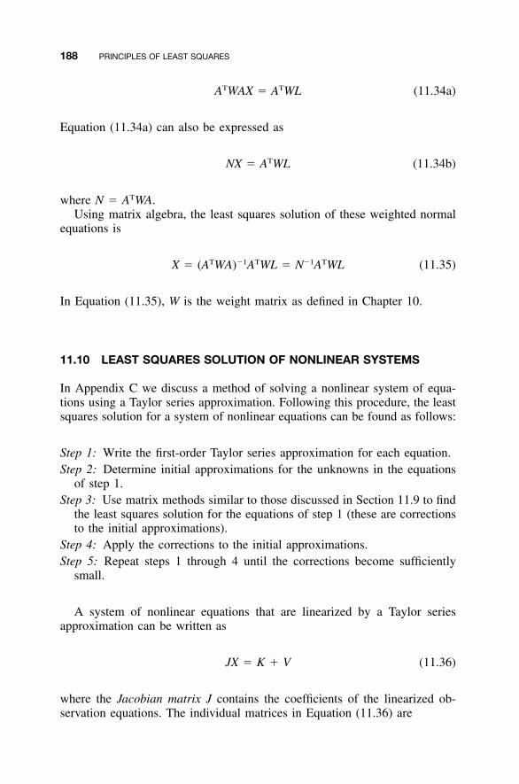
188 PRINCIPLES OF LEAST SQUARES
T TA WAX � A WL (11.34a)
Equation (11.34a) can also be expressed as
TNX � A WL (11.34b)
where N � ATWA.Using matrix algebra, the least squares solution of these weighted normal
equations is
T �1 T �1 TX � (A WA) A WL � N A WL (11.35)
In Equation (11.35), W is the weight matrix as defined in Chapter 10.
11.10 LEAST SQUARES SOLUTION OF NONLINEAR SYSTEMS
In Appendix C we discuss a method of solving a nonlinear system of equa-tions using a Taylor series approximation. Following this procedure, the leastsquares solution for a system of nonlinear equations can be found as follows:
Step 1: Write the first-order Taylor series approximation for each equation.Step 2: Determine initial approximations for the unknowns in the equations
of step 1.Step 3: Use matrix methods similar to those discussed in Section 11.9 to find
the least squares solution for the equations of step 1 (these are correctionsto the initial approximations).
Step 4: Apply the corrections to the initial approximations.Step 5: Repeat steps 1 through 4 until the corrections become sufficiently
small.
A system of nonlinear equations that are linearized by a Taylor seriesapproximation can be written as
JX � K � V (11.36)
where the Jacobian matrix J contains the coefficients of the linearized ob-servation equations. The individual matrices in Equation (11.36) are
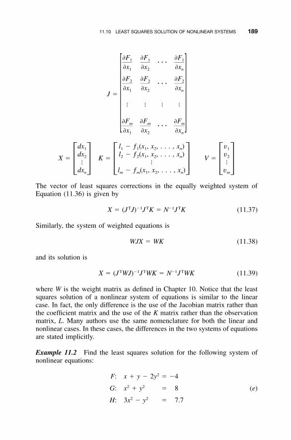
11.10 LEAST SQUARES SOLUTION OF NONLINEAR SYSTEMS 189
�F �F �F1 1 1� � ��x �x �x1 2 n
�F �F �F2 2 2� � ��x �x �x1 2 n
J �
� � � �
�F �F �Fm m m� � ��x �x �x1 2 n
dx l � ƒ (x , x , . . . , x ) v1 1 1 1 2 n 1
dx l � ƒ (x , x , . . . , x ) v2 2 2 1 2 n 2X � K � V �� � �� � � � � �
dx l � ƒ (x , x , . . . , x ) vn m m 1 2 n m
The vector of least squares corrections in the equally weighted system ofEquation (11.36) is given by
T �1 T �1 TX � (J J) J K � N J K (11.37)
Similarly, the system of weighted equations is
WJX � WK (11.38)
and its solution is
T �1 T �1 TX � (J WJ) J WK � N J WK (11.39)
where W is the weight matrix as defined in Chapter 10. Notice that the leastsquares solution of a nonlinear system of equations is similar to the linearcase. In fact, the only difference is the use of the Jacobian matrix rather thanthe coefficient matrix and the use of the K matrix rather than the observationmatrix, L. Many authors use the same nomenclature for both the linear andnonlinear cases. In these cases, the differences in the two systems of equationsare stated implicitly.
Example 11.2 Find the least squares solution for the following system ofnonlinear equations:
2F: x � y � 2y � �42 2G: x � y � 8 (e)
2 2H: 3x � y � 7.7
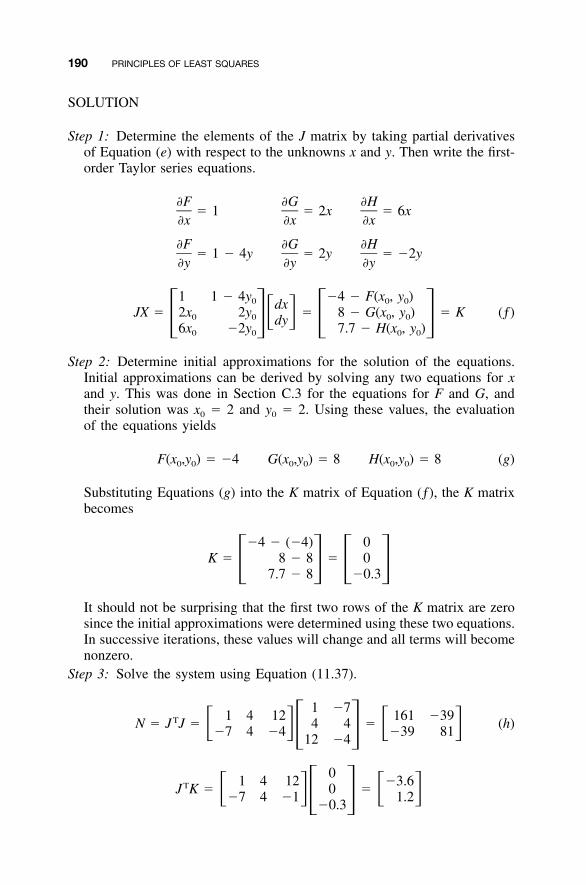
190 PRINCIPLES OF LEAST SQUARES
SOLUTION
Step 1: Determine the elements of the J matrix by taking partial derivativesof Equation (e) with respect to the unknowns x and y. Then write the first-order Taylor series equations.
�F �G �H� 1 � 2x � 6x
�x �x �x
�F �G �H� 1 � 4y � 2y � �2y
�y �y �y
1 1 � 4y �4 � F(x , y )0 0 0dxJX � 2x 2y � 8 � G(x , y ) � K (ƒ)� 0 0 0 0dy� � � �6x �2y 7.7 � H(x , y )0 0 0 0
Step 2: Determine initial approximations for the solution of the equations.Initial approximations can be derived by solving any two equations for xand y. This was done in Section C.3 for the equations for F and G, andtheir solution was x0 � 2 and y0 � 2. Using these values, the evaluationof the equations yields
F(x ,y ) � �4 G(x ,y ) � 8 H(x ,y ) � 8 (g)0 0 0 0 0 0
Substituting Equations (g) into the K matrix of Equation (ƒ), the K matrixbecomes
�4 � (�4) 0K � 8 � 8 � 0� � � �7.7 � 8 �0.3
It should not be surprising that the first two rows of the K matrix are zerosince the initial approximations were determined using these two equations.In successive iterations, these values will change and all terms will becomenonzero.
Step 3: Solve the system using Equation (11.37).
1 �71 4 12 161 �39TN � J J � 4 4 � (h)� � �7 4 �4 �39 81� �12 �4
01 4 12 �3.6TJ K � 0 �� � �7 4 �1 1.2� ��0.3
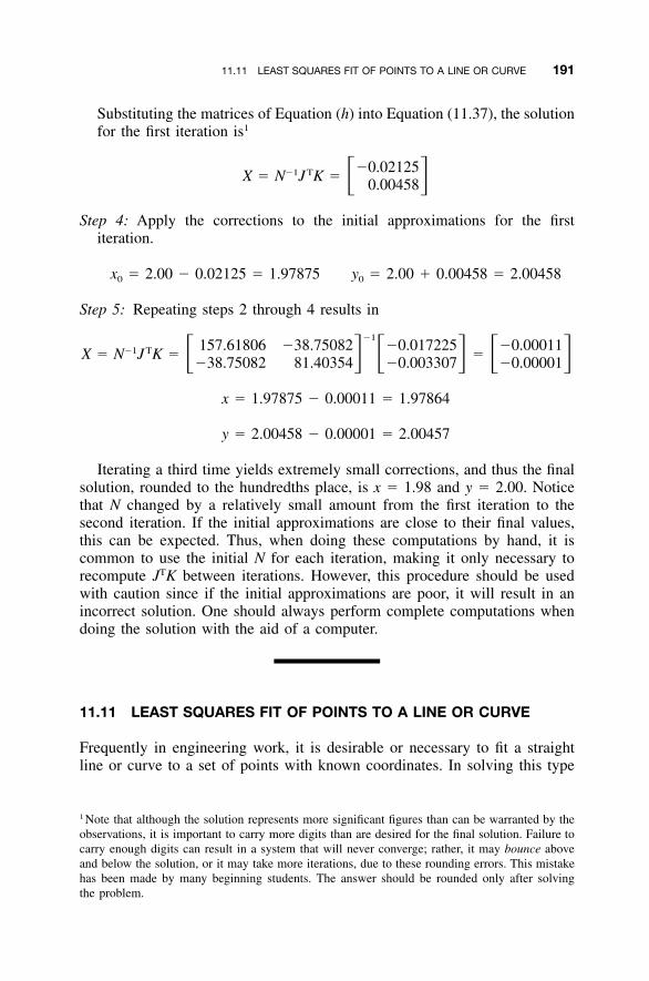
11.11 LEAST SQUARES FIT OF POINTS TO A LINE OR CURVE 191
Substituting the matrices of Equation (h) into Equation (11.37), the solutionfor the first iteration is1
�0.02125�1 TX � N J K � � 0.00458
Step 4: Apply the corrections to the initial approximations for the firstiteration.
x � 2.00 � 0.02125 � 1.97875 y � 2.00 � 0.00458 � 2.004580 0
Step 5: Repeating steps 2 through 4 results in
�1157.61806 �38.75082 �0.017225 �0.00011�1 TX � N J K � �� � � �38.75082 81.40354 �0.003307 �0.00001
x � 1.97875 � 0.00011 � 1.97864
y � 2.00458 � 0.00001 � 2.00457
Iterating a third time yields extremely small corrections, and thus the finalsolution, rounded to the hundredths place, is x � 1.98 and y � 2.00. Noticethat N changed by a relatively small amount from the first iteration to thesecond iteration. If the initial approximations are close to their final values,this can be expected. Thus, when doing these computations by hand, it iscommon to use the initial N for each iteration, making it only necessary torecompute JTK between iterations. However, this procedure should be usedwith caution since if the initial approximations are poor, it will result in anincorrect solution. One should always perform complete computations whendoing the solution with the aid of a computer.
11.11 LEAST SQUARES FIT OF POINTS TO A LINE OR CURVE
Frequently in engineering work, it is desirable or necessary to fit a straightline or curve to a set of points with known coordinates. In solving this type
1 Note that although the solution represents more significant figures than can be warranted by theobservations, it is important to carry more digits than are desired for the final solution. Failure tocarry enough digits can result in a system that will never converge; rather, it may bounce aboveand below the solution, or it may take more iterations, due to these rounding errors. This mistakehas been made by many beginning students. The answer should be rounded only after solvingthe problem.
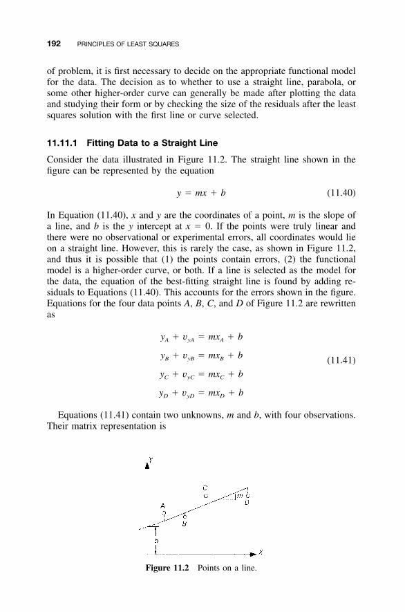
192 PRINCIPLES OF LEAST SQUARES
Figure 11.2 Points on a line.
of problem, it is first necessary to decide on the appropriate functional modelfor the data. The decision as to whether to use a straight line, parabola, orsome other higher-order curve can generally be made after plotting the dataand studying their form or by checking the size of the residuals after the leastsquares solution with the first line or curve selected.
11.11.1 Fitting Data to a Straight Line
Consider the data illustrated in Figure 11.2. The straight line shown in thefigure can be represented by the equation
y � mx � b (11.40)
In Equation (11.40), x and y are the coordinates of a point, m is the slope ofa line, and b is the y intercept at x � 0. If the points were truly linear andthere were no observational or experimental errors, all coordinates would lieon a straight line. However, this is rarely the case, as shown in Figure 11.2,and thus it is possible that (1) the points contain errors, (2) the functionalmodel is a higher-order curve, or both. If a line is selected as the model forthe data, the equation of the best-fitting straight line is found by adding re-siduals to Equations (11.40). This accounts for the errors shown in the figure.Equations for the four data points A, B, C, and D of Figure 11.2 are rewrittenas
y � v � mx � bA yA A
y � v � mx � bB yB B (11.41)
y � v � mx � bC yC C
y � v � mx � bD yD D
Equations (11.41) contain two unknowns, m and b, with four observations.Their matrix representation is
11.11 LEAST SQUARES FIT OF POINTS TO A LINE OR CURVE 193
AX � L � V (11.42)
where
x 1 y va a ya
x 1 m y vb b ybA � X � L � V �� x 1 b y vc c yc� � � � � �x 1 y vd d yd
Equation (11.42) is solved by the least squares method using Equation(11.32). If some data were more reliable than others, relative weights couldbe introduced and a weighted least squares solution could be obtained usingEquation (11.35).
Example 11.3 Find the best-fit straight line for the following points, whosex and y coordinates are given in parentheses.
A: (3.00, 4.50) B: (4.25, 4.25) C: (5.50, 5.50) D: (8.00, 5.50)
SOLUTION Following Equations (11.41), the four observation equationsfor the coordinate pairs are
3.00m � b � 4.50 � va
4.25m � b � 4.25 � vb (i)
5.50m � b � 5.50 � vc
8.00m � b � 5.50 � vd
Rewriting Equations (i) into matrix form yields
3.00 1 4.50 vA
4.25 1 m 4.25 vB� � ( j)� 5.50 1 b 5.50 vC� � � � � �8.00 1 5.50 vD
To form the normal equations, premultiply matrices A and L of Equation ( j)by AT and get
121.3125 20.7500 m 105.8125� (k)� � � 20.7500 4.0000 b 19.7500
The solution of Equation (k) is
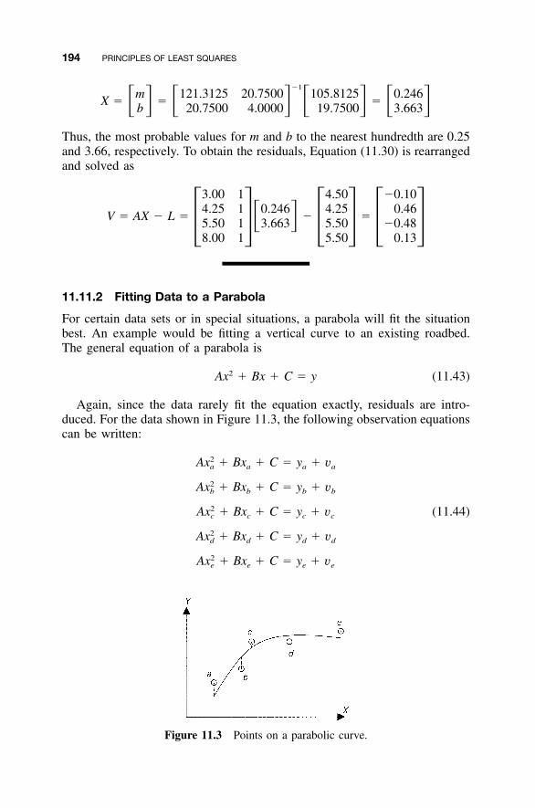
194 PRINCIPLES OF LEAST SQUARES
Figure 11.3 Points on a parabolic curve.
�1m 121.3125 20.7500 105.8125 0.246
X � � �� � � � b 20.7500 4.0000 19.7500 3.663
Thus, the most probable values for m and b to the nearest hundredth are 0.25and 3.66, respectively. To obtain the residuals, Equation (11.30) is rearrangedand solved as
3.00 1 4.50 �0.104.25 1 0.246 4.25 0.46
V � AX � L � � �� 5.50 1 3.663 5.50 �0.48� � � � � �8.00 1 5.50 0.13
11.11.2 Fitting Data to a Parabola
For certain data sets or in special situations, a parabola will fit the situationbest. An example would be fitting a vertical curve to an existing roadbed.The general equation of a parabola is
2Ax � Bx � C � y (11.43)
Again, since the data rarely fit the equation exactly, residuals are intro-duced. For the data shown in Figure 11.3, the following observation equationscan be written:
2Ax � Bx � C � y � va a a a
2Ax � Bx � C � y � vb b b b
2Ax � Bx � C � y � v (11.44)c c c c
2Ax � Bx � C � y � vd d d d
2Ax � Bx � C � y � ve e e e
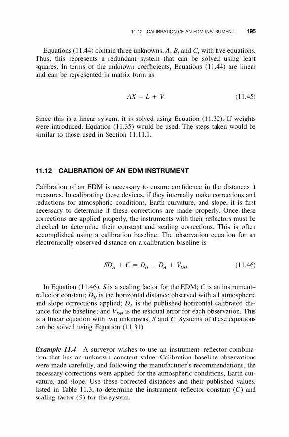
11.12 CALIBRATION OF AN EDM INSTRUMENT 195
Equations (11.44) contain three unknowns, A, B, and C, with five equations.Thus, this represents a redundant system that can be solved using leastsquares. In terms of the unknown coefficients, Equations (11.44) are linearand can be represented in matrix form as
AX � L � V (11.45)
Since this is a linear system, it is solved using Equation (11.32). If weightswere introduced, Equation (11.35) would be used. The steps taken would besimilar to those used in Section 11.11.1.
11.12 CALIBRATION OF AN EDM INSTRUMENT
Calibration of an EDM is necessary to ensure confidence in the distances itmeasures. In calibrating these devices, if they internally make corrections andreductions for atmospheric conditions, Earth curvature, and slope, it is firstnecessary to determine if these corrections are made properly. Once thesecorrections are applied properly, the instruments with their reflectors must bechecked to determine their constant and scaling corrections. This is oftenaccomplished using a calibration baseline. The observation equation for anelectronically observed distance on a calibration baseline is
SD � C � D � D � V (11.46)A H A DH
In Equation (11.46), S is a scaling factor for the EDM; C is an instrument–reflector constant; DH is the horizontal distance observed with all atmosphericand slope corrections applied; DA is the published horizontal calibrated dis-tance for the baseline; and VDH is the residual error for each observation. Thisis a linear equation with two unknowns, S and C. Systems of these equationscan be solved using Equation (11.31).
Example 11.4 A surveyor wishes to use an instrument–reflector combina-tion that has an unknown constant value. Calibration baseline observationswere made carefully, and following the manufacturer’s recommendations, thenecessary corrections were applied for the atmospheric conditions, Earth cur-vature, and slope. Use these corrected distances and their published values,listed in Table 11.3, to determine the instrument–reflector constant (C) andscaling factor (S) for the system.
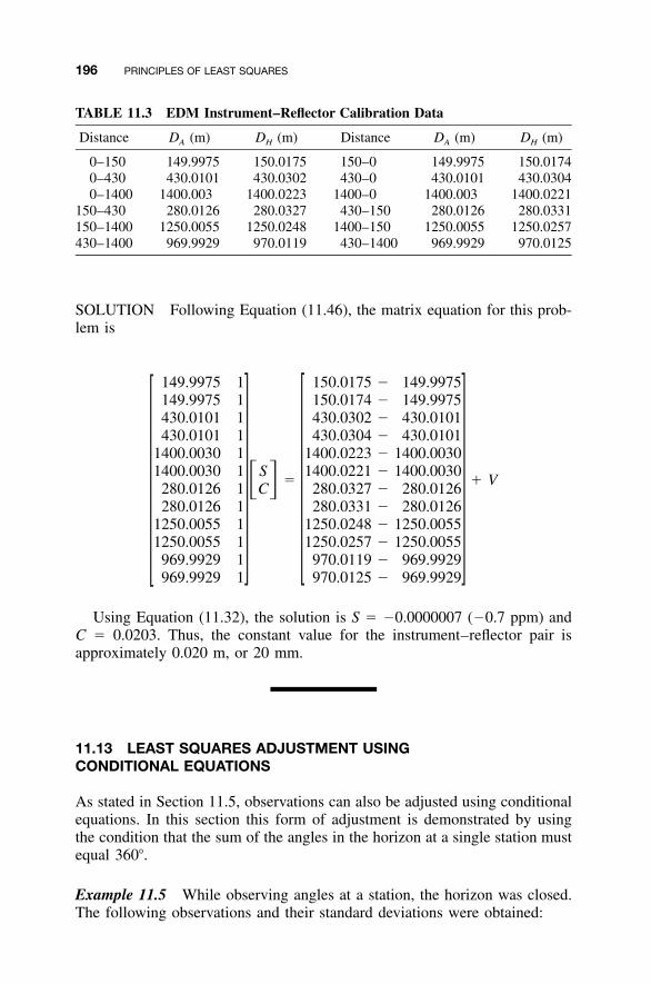
196 PRINCIPLES OF LEAST SQUARES
TABLE 11.3 EDM Instrument–Reflector Calibration Data
Distance DA (m) DH (m) Distance DA (m) DH (m)
0–150 149.9975 150.0175 150–0 149.9975 150.01740–430 430.0101 430.0302 430–0 430.0101 430.03040–1400 1400.003 1400.0223 1400–0 1400.003 1400.0221
150–430 280.0126 280.0327 430–150 280.0126 280.0331150–1400 1250.0055 1250.0248 1400–150 1250.0055 1250.0257430–1400 969.9929 970.0119 430–1400 969.9929 970.0125
SOLUTION Following Equation (11.46), the matrix equation for this prob-lem is
149.9975 1 150.0175 � 149.9975149.9975 1 150.0174 � 149.9975430.0101 1 430.0302 � 430.0101430.0101 1 430.0304 � 430.0101
1400.0030 1 1400.0223 � 1400.00301400.0030 1 S 1400.0221 � 1400.0030
� � V� 280.0126 1 C 280.0327 � 280.0126280.0126 1 280.0331 � 280.0126
1250.0055 1 1250.0248 � 1250.00551250.0055 1 1250.0257 � 1250.0055
969.9929 1 970.0119 � 969.9929969.9929 1 970.0125 � 969.9929
Using Equation (11.32), the solution is S � �0.0000007 (�0.7 ppm) andC � 0.0203. Thus, the constant value for the instrument–reflector pair isapproximately 0.020 m, or 20 mm.
11.13 LEAST SQUARES ADJUSTMENT USINGCONDITIONAL EQUATIONS
As stated in Section 11.5, observations can also be adjusted using conditionalequations. In this section this form of adjustment is demonstrated by usingthe condition that the sum of the angles in the horizon at a single station mustequal 360�.
Example 11.5 While observing angles at a station, the horizon was closed.The following observations and their standard deviations were obtained:
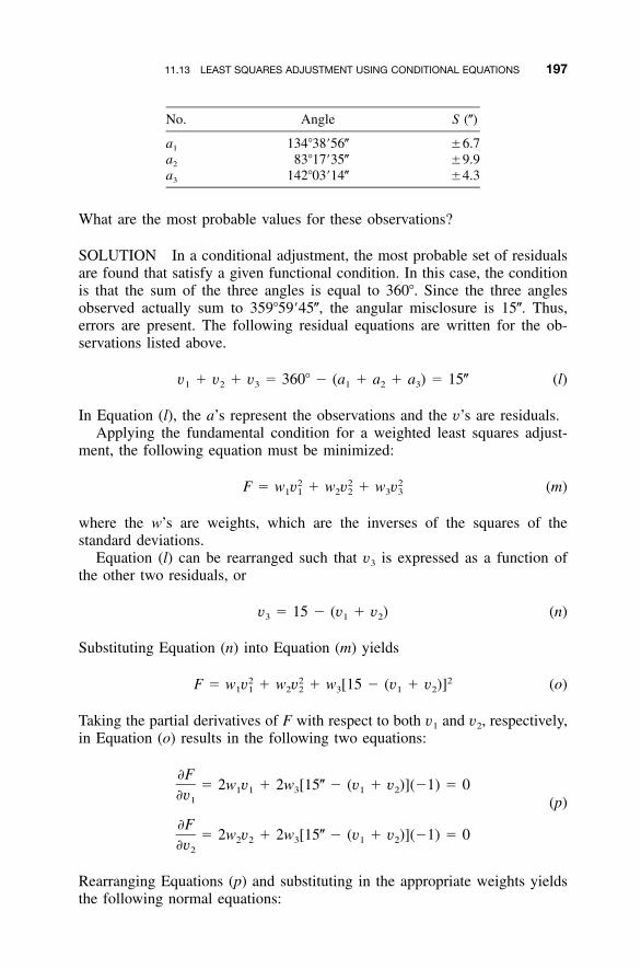
11.13 LEAST SQUARES ADJUSTMENT USING CONDITIONAL EQUATIONS 197
No. Angle S (�)
a1 134�38�56� �6.7a2 83�17�35� �9.9a3 142�03�14� �4.3
What are the most probable values for these observations?
SOLUTION In a conditional adjustment, the most probable set of residualsare found that satisfy a given functional condition. In this case, the conditionis that the sum of the three angles is equal to 360�. Since the three anglesobserved actually sum to 359�59�45�, the angular misclosure is 15�. Thus,errors are present. The following residual equations are written for the ob-servations listed above.
v � v � v � 360� � (a � a � a ) � 15� (l)1 2 3 1 2 3
In Equation (l), the a’s represent the observations and the v’s are residuals.Applying the fundamental condition for a weighted least squares adjust-
ment, the following equation must be minimized:
2 2 2F � w v � w v � w v (m)1 1 2 2 3 3
where the w’s are weights, which are the inverses of the squares of thestandard deviations.
Equation (l) can be rearranged such that v3 is expressed as a function ofthe other two residuals, or
v � 15 � (v � v ) (n)3 1 2
Substituting Equation (n) into Equation (m) yields
2 2 2F � w v � w v � w [15 � (v � v )] (o)1 1 2 2 3 1 2
Taking the partial derivatives of F with respect to both v1 and v2, respectively,in Equation (o) results in the following two equations:
�F� 2w v � 2w [15� � (v � v )](�1) � 01 1 3 1 2�v1 (p)
�F� 2w v � 2w [15� � (v � v )](�1) � 02 2 3 1 2�v2
Rearranging Equations (p) and substituting in the appropriate weights yieldsthe following normal equations:
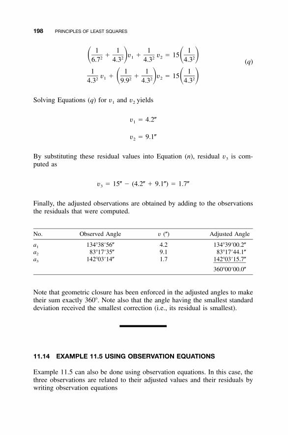
198 PRINCIPLES OF LEAST SQUARES
1 1 1 1� v � v � 15� � � �1 22 2 2 26.7 4.3 4.3 4.3 (q)
1 1 1 1v � � v � 15� � � �1 22 2 2 24.3 9.9 4.3 4.3
Solving Equations (q) for v1 and v2 yields
v � 4.2�1
v � 9.1�2
By substituting these residual values into Equation (n), residual v3 is com-puted as
v � 15� � (4.2� � 9.1�) � 1.7�3
Finally, the adjusted observations are obtained by adding to the observationsthe residuals that were computed.
No. Observed Angle v (�) Adjusted Angle
a1 134�38�56� 4.2 134�39�00.2�a2 83�17�35� 9.1 83�17�44.1�a3 142�03�14� 1.7 142�03�15.7�
360�00�00.0�
Note that geometric closure has been enforced in the adjusted angles to maketheir sum exactly 360�. Note also that the angle having the smallest standarddeviation received the smallest correction (i.e., its residual is smallest).
11.14 EXAMPLE 11.5 USING OBSERVATION EQUATIONS
Example 11.5 can also be done using observation equations. In this case, thethree observations are related to their adjusted values and their residuals bywriting observation equations
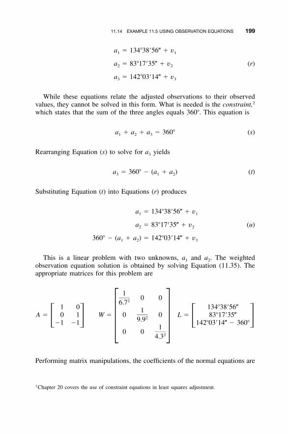
11.14 EXAMPLE 11.5 USING OBSERVATION EQUATIONS 199
a � 134�38�56� � v1 1
a � 83�17�35� � v (r)2 2
a � 142�03�14� � v3 3
While these equations relate the adjusted observations to their observedvalues, they cannot be solved in this form. What is needed is the constraint,2
which states that the sum of the three angles equals 360�. This equation is
a � a � a � 360� (s)1 2 3
Rearranging Equation (s) to solve for a3 yields
a � 360� � (a � a ) (t)3 1 2
Substituting Equation (t) into Equations (r) produces
a � 134�38�56� � v1 1
a � 83�17�35� � v (u)2 2
360� � (a � a ) � 142�03�14� � v1 2 3
This is a linear problem with two unknowns, a1 and a2. The weightedobservation equation solution is obtained by solving Equation (11.35). Theappropriate matrices for this problem are
10 026.7
1 0 134�38�56�1A � 0 1 W � 0 0 L � 83�17�35�29.9� � � ��1 �1 142�03�14� � 360�
1� �0 0 24.3
Performing matrix manipulations, the coefficients of the normal equations are
2 Chapter 20 covers the use of constraint equations in least squares adjustment.
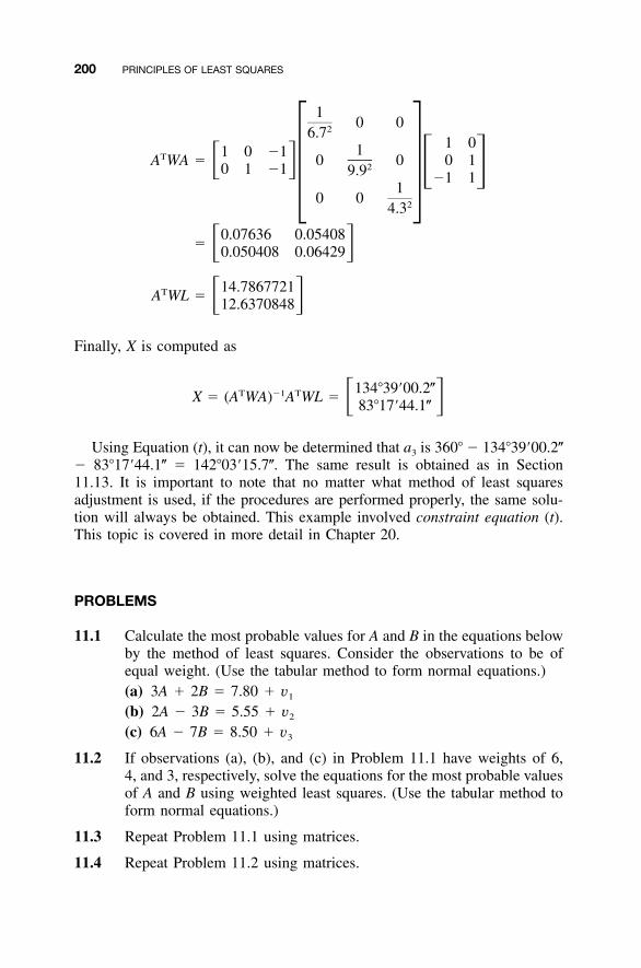
200 PRINCIPLES OF LEAST SQUARES
10 026.7
1 011 0 �1TA WA � 0 0 0 1� 20 1 �1 9.9 � ��1 11� �0 0 24.3
0.07636 0.05408� � 0.050408 0.06429
14.7867721TA WL � � 12.6370848
Finally, X is computed as
134�39�00.2�T �1 TX � (A WA) A WL � � 83�17�44.1�
Using Equation (t), it can now be determined that a3 is 360� � 134�39�00.2�� 83�17�44.1� � 142�03�15.7�. The same result is obtained as in Section11.13. It is important to note that no matter what method of least squaresadjustment is used, if the procedures are performed properly, the same solu-tion will always be obtained. This example involved constraint equation (t).This topic is covered in more detail in Chapter 20.
PROBLEMS
11.1 Calculate the most probable values for A and B in the equations belowby the method of least squares. Consider the observations to be ofequal weight. (Use the tabular method to form normal equations.)(a) 3A � 2B � 7.80 � v1
(b) 2A � 3B � 5.55 � v2
(c) 6A � 7B � 8.50 � v3
11.2 If observations (a), (b), and (c) in Problem 11.1 have weights of 6,4, and 3, respectively, solve the equations for the most probable valuesof A and B using weighted least squares. (Use the tabular method toform normal equations.)
11.3 Repeat Problem 11.1 using matrices.
11.4 Repeat Problem 11.2 using matrices.
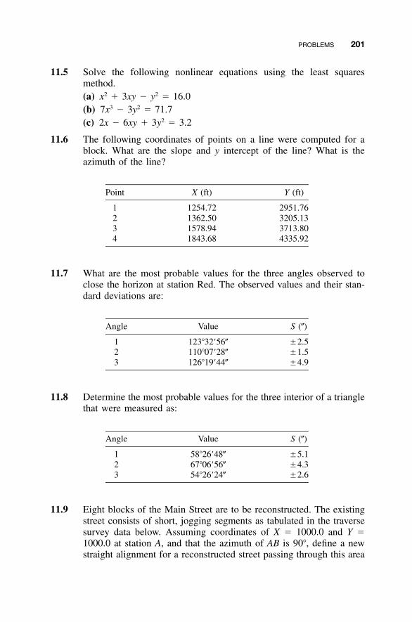
PROBLEMS 201
11.5 Solve the following nonlinear equations using the least squaresmethod.(a) x2 � 3xy � y2 � 16.0(b) 7x3 � 3y2 � 71.7(c) 2x � 6xy � 3y2 � 3.2
11.6 The following coordinates of points on a line were computed for ablock. What are the slope and y intercept of the line? What is theazimuth of the line?
Point X (ft) Y (ft)
1 1254.72 2951.762 1362.50 3205.133 1578.94 3713.804 1843.68 4335.92
11.7 What are the most probable values for the three angles observed toclose the horizon at station Red. The observed values and their stan-dard deviations are:
Angle Value S (�)
1 123�32�56� �2.52 110�07�28� �1.53 126�19�44� �4.9
11.8 Determine the most probable values for the three interior of a trianglethat were measured as:
Angle Value S (�)
1 58�26�48� �5.12 67�06�56� �4.33 54�26�24� �2.6
11.9 Eight blocks of the Main Street are to be reconstructed. The existingstreet consists of short, jogging segments as tabulated in the traversesurvey data below. Assuming coordinates of X � 1000.0 and Y �1000.0 at station A, and that the azimuth of AB is 90�, define a newstraight alignment for a reconstructed street passing through this area
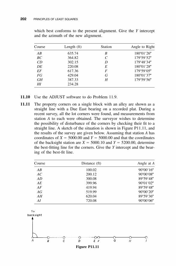
202 PRINCIPLES OF LEAST SQUARES
which best conforms to the present alignment. Give the Y interceptand the azimuth of the new alignment.
Course Length (ft) Station Angle to Right
AB 635.74 B 180�01�26�BC 364.82 C 179�59�52�CD 302.15 D 179�48�34�DE 220.08 E 180�01�28�EF 617.36 F 179�59�05�FG 429.04 G 180�01�37�GH 387.33 H 179�59�56�HI 234.28
11.10 Use the ADJUST software to do Problem 11.9.
11.11 The property corners on a single block with an alley are shown as astraight line with a Due East bearing on a recorded plat. During arecent survey, all the lot corners were found, and measurements fromstation A to each were obtained. The surveyor wishes to determinethe possibility of disturbance of the corners by checking their fit to astraight line. A sketch of the situation is shown in Figure P11.11, andthe results of the survey are given below. Assuming that station A hascoordinates of X � 5000.00 and Y � 5000.00 and that the coordinatesof the backsight station are X � 5000.10 and Y � 5200.00, determinethe best-fitting line for the corners. Give the Y intercept and the bear-ing of the best-fit line.
Course Distance (ft) Angle at A
AB 100.02 90�00�16�AC 200.12 90�00�08�AD 300.08 89�59�48�AE 399.96 90�01�02�AF 419.94 89�59�48�AG 519.99 90�00�20�AH 620.04 89�59�36�AI 720.08 90�00�06�
Figure P11.11
PROBLEMS 203
11.12 Use the ADJUST software to do Problem 11.11.
11.13 Calculate a best-fit parabola for the following data obtained on asurvey of an existing vertical curve, and determine the deviation (re-siduals) of the road from this best-fit curve. The curve starts at station10�00 and ends at station 18�00. List the adjusted station elevationsand their residuals.
Station Elevation Station Elevation
10�00 51.2 15�00 46.911�00 49.5 16�00 47.312�00 48.2 17�00 48.313�00 47.3 18�00 49.614�00 46.8
11.14 Use the ADJUST software to do Problem 11.13.
11.15 Using a procedure similar to that in Section 11.7.1, derive Equations(11.27).
11.16 Using a procedure similar to that used in Section 11.9.1, show thatthe matrix operations in Equation (11.34) result in the normal equa-tions for a linear set of weighted observation equations.
11.17 Discuss the importance of selecting the stochastic model when ad-justing data.
11.18 The values for three angles in a triangle, observed using a total stationand the directional method, are
AngleNumber ofRepetitions Value
A 2 14�25�20�B 3 58�16�00�C 6 107�19�10�
The observed lengths of the course are
AB � 971.25 ft BC � 253.25 ft CA � 865.28 ft
The following estimated errors are assumed for each measurement:
�i � �0.003 ft �t � �0.020 ft �DIN � �2.0�
What are the most probable values for the angles? Use the conditionalequation method.

204 PRINCIPLES OF LEAST SQUARES
11.19 Do Problem 11.18 using observation equations and a constraint aspresented in Section 11.13.
11.20 The following data were collected on a calibration baseline. Atmos-pheric refraction and Earth curvature corrections were made to themeasured distances, which are in units of meters. Determine theinstrument–reflector constant and any scaling factor.
Distance DA DH Distance DA DH
0–150 149.9104 149.9447 150–0 149.9104 149.94350–430 430.001 430.0334 430–0 430.001 430.0340–1400 1399.9313 1399.9777 1400–0 1399.9313 1399.9519
150–430 280.0906 280.1238 430–150 280.0906 280.123150–1400 1250.0209 1250.0795 1400–150 1250.0209 1250.0664430–1400 969.9303 969.9546 1400–430 969.9303 969.9630
11.21 A survey of the centerline of a horizontal metric curve is done todetermine the as-built curve specifications. The coordinates for thepoints along the curve are:
Point X (ft) Y (ft)
1 10,006.82 10,007.312 10,013.12 10,015.073 10,024.01 10,031.834 10,032.44 10,049.955 10,038.26 10,069.046 10,041.39 10,088.83
(a) Using Equation (C.10), compute the most probable values for theradius and center of the circle.
(b) If two points located on the tangents have coordinates of(9987.36, 9987.40) and (10,044.09, 10,119.54), what are the co-ordinates of the PC and PT of the curve?
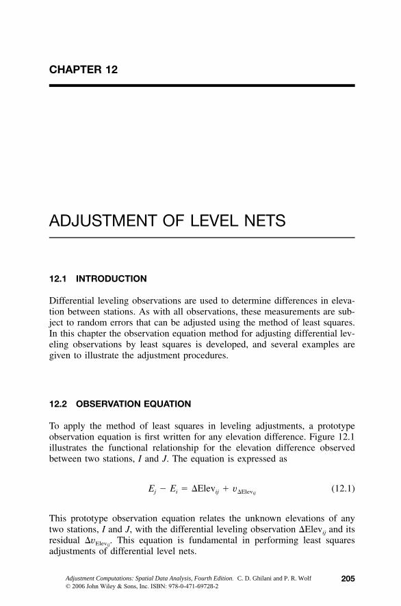
205
CHAPTER 12
ADJUSTMENT OF LEVEL NETS
12.1 INTRODUCTION
Differential leveling observations are used to determine differences in eleva-tion between stations. As with all observations, these measurements are sub-ject to random errors that can be adjusted using the method of least squares.In this chapter the observation equation method for adjusting differential lev-eling observations by least squares is developed, and several examples aregiven to illustrate the adjustment procedures.
12.2 OBSERVATION EQUATION
To apply the method of least squares in leveling adjustments, a prototypeobservation equation is first written for any elevation difference. Figure 12.1illustrates the functional relationship for the elevation difference observedbetween two stations, I and J. The equation is expressed as
E � E � �Elev � v (12.1)j i ij �Elevij
This prototype observation equation relates the unknown elevations of anytwo stations, I and J, with the differential leveling observation �Elevij and itsresidual This equation is fundamental in performing least squares�v .Elevij
adjustments of differential level nets.
Adjustment Computations: Spatial Data Analysis, Fourth Edition. C. D. Ghilani and P. R. Wolf© 2006 John Wiley & Sons, Inc. ISBN: 978-0-471-69728-2
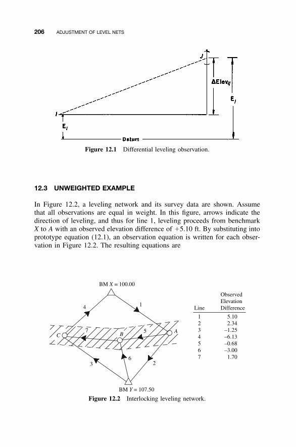
206 ADJUSTMENT OF LEVEL NETS
Figure 12.1 Differential leveling observation.
C
4
7B A5
Line
ObservedElevationDifference
1234567
5.102.34
–1.25–6.13–0.68–3.001.706
3 2
BM X = 100.00
BM Y = 107.50
1
Figure 12.2 Interlocking leveling network.
12.3 UNWEIGHTED EXAMPLE
In Figure 12.2, a leveling network and its survey data are shown. Assumethat all observations are equal in weight. In this figure, arrows indicate thedirection of leveling, and thus for line 1, leveling proceeds from benchmarkX to A with an observed elevation difference of �5.10 ft. By substituting intoprototype equation (12.1), an observation equation is written for each obser-vation in Figure 12.2. The resulting equations are
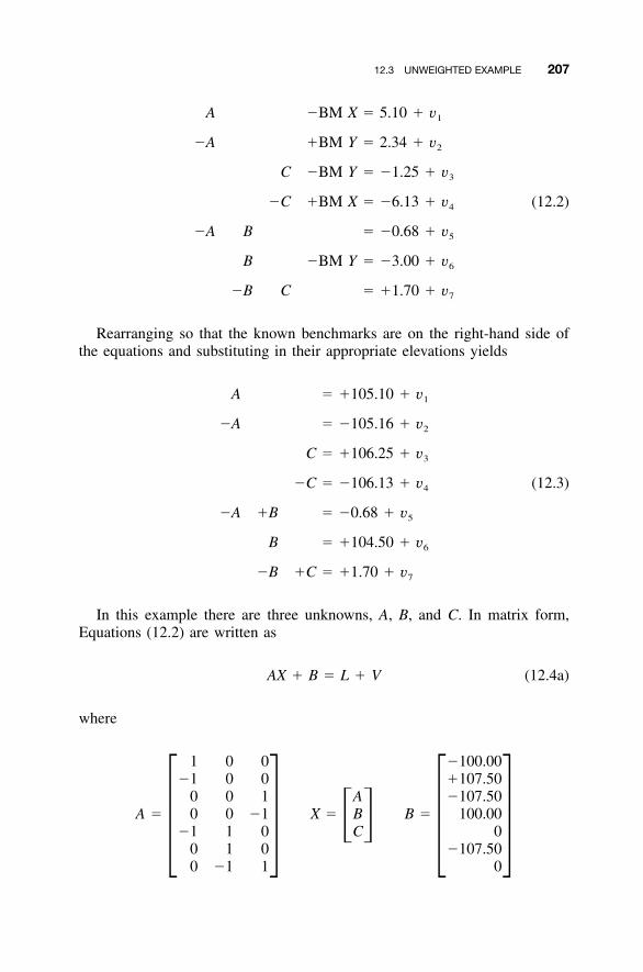
12.3 UNWEIGHTED EXAMPLE 207
A �BM X � 5.10 � v1
�A �BM Y � 2.34 � v2
C �BM Y � �1.25 � v3
�C �BM X � �6.13 � v (12.2)4
�A B � �0.68 � v5
B �BM Y � �3.00 � v6
�B C � �1.70 � v7
Rearranging so that the known benchmarks are on the right-hand side ofthe equations and substituting in their appropriate elevations yields
A � �105.10 � v1
�A � �105.16 � v2
C � �106.25 � v3
�C � �106.13 � v (12.3)4
�A �B � �0.68 � v5
B � �104.50 � v6
�B �C � �1.70 � v7
In this example there are three unknowns, A, B, and C. In matrix form,Equations (12.2) are written as
AX � B � L � V (12.4a)
where
1 0 0 �100.00�1 0 0 �107.50
0 0 1 A �107.50A � 0 0 �1 X � B B � 100.00� ��1 1 0 C 0� � � �0 1 0 �107.50
0 �1 1 0
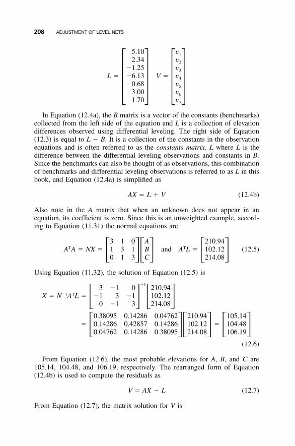
208 ADJUSTMENT OF LEVEL NETS
5.10 v1
2.34 v2
�1.25 v3
L � �6.13 V � v4
�0.68 v5� � � ��3.00 v6
1.70 v7
In Equation (12.4a), the B matrix is a vector of the constants (benchmarks)collected from the left side of the equation and L is a collection of elevationdifferences observed using differential leveling. The right side of Equation(12.3) is equal to L � B. It is a collection of the constants in the observationequations and is often referred to as the constants matrix, L where L is thedifference between the differential leveling observations and constants in B.Since the benchmarks can also be thought of as observations, this combinationof benchmarks and differential leveling observations is referred to as L in thisbook, and Equation (12.4a) is simplified as
AX � L � V (12.4b)
Also note in the A matrix that when an unknown does not appear in anequation, its coefficient is zero. Since this is an unweighted example, accord-ing to Equation (11.31) the normal equations are
3 1 0 A 210.94T TA A � NX � 1 3 1 B and A L � 102.12 (12.5)� �� � � �0 1 3 C 214.08
Using Equation (11.32), the solution of Equation (12.5) is
�13 �1 0 210.94�1 TX � N A L � �1 3 �1 102.12� � � �0 �1 3 214.08
0.38095 0.14286 0.04762 210.94 105.14� 0.14286 0.42857 0.14286 102.12 � 104.48� �� � � �0.04762 0.14286 0.38095 214.08 106.19
(12.6)
From Equation (12.6), the most probable elevations for A, B, and C are105.14, 104.48, and 106.19, respectively. The rearranged form of Equation(12.4b) is used to compute the residuals as
V � AX � L (12.7)
From Equation (12.7), the matrix solution for V is
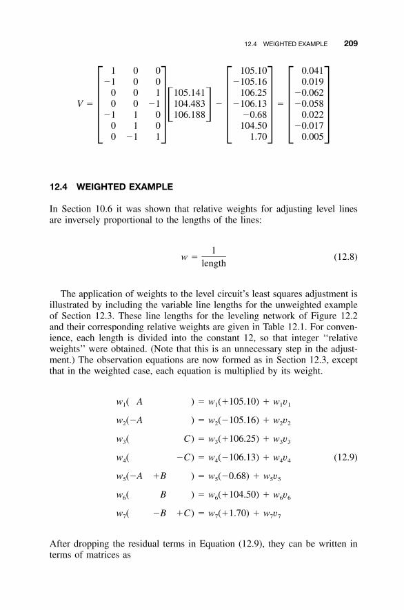
12.4 WEIGHTED EXAMPLE 209
1 0 0 105.10 0.041�1 0 0 �105.16 0.019
0 0 1 105.141 106.25 �0.062V � 0 0 �1 104.483 � �106.13 � �0.058� ��1 1 0 106.188 �0.68 0.022� � � � � �0 1 0 104.50 �0.017
0 �1 1 1.70 0.005
12.4 WEIGHTED EXAMPLE
In Section 10.6 it was shown that relative weights for adjusting level linesare inversely proportional to the lengths of the lines:
1w � (12.8)
length
The application of weights to the level circuit’s least squares adjustment isillustrated by including the variable line lengths for the unweighted exampleof Section 12.3. These line lengths for the leveling network of Figure 12.2and their corresponding relative weights are given in Table 12.1. For conven-ience, each length is divided into the constant 12, so that integer ‘‘relativeweights’’ were obtained. (Note that this is an unnecessary step in the adjust-ment.) The observation equations are now formed as in Section 12.3, exceptthat in the weighted case, each equation is multiplied by its weight.
w ( A ) � w (�105.10) � w v1 1 1 1
w (�A ) � w (�105.16) � w v2 2 2 2
w ( C) � w (�106.25) � w v3 3 3 3
w ( �C) � w (�106.13) � w v (12.9)4 4 4 4
w (�A �B ) � w (�0.68) � w v5 5 5 5
w ( B ) � w (�104.50) � w v6 6 6 6
w ( �B �C) � w (�1.70) � w v7 7 7 7
After dropping the residual terms in Equation (12.9), they can be written interms of matrices as
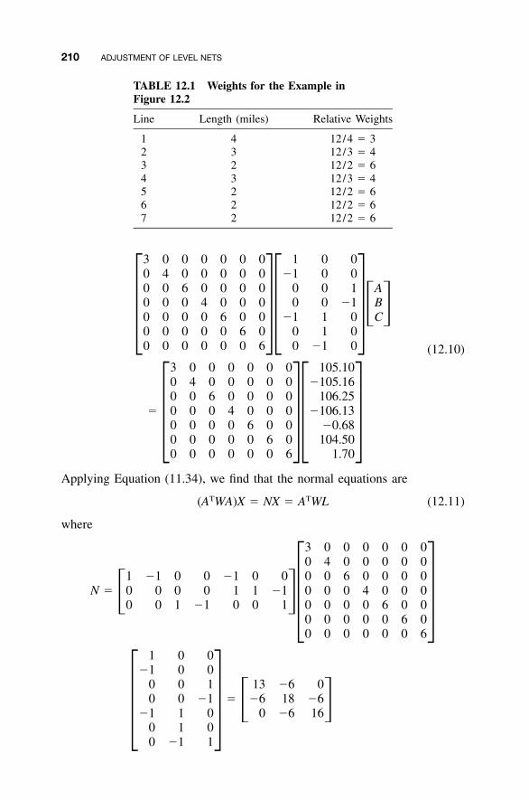
210 ADJUSTMENT OF LEVEL NETS
TABLE 12.1 Weights for the Example inFigure 12.2
Line Length (miles) Relative Weights
1 4 12/4 � 32 3 12/3 � 43 2 12/2 � 64 3 12/3 � 45 2 12/2 � 66 2 12/2 � 67 2 12/2 � 6
3 0 0 0 0 0 0 1 0 00 4 0 0 0 0 0 �1 0 00 0 6 0 0 0 0 0 0 1 A0 0 0 4 0 0 0 0 0 �1 B� �0 0 0 0 6 0 0 �1 1 0 C� �� �0 0 0 0 0 6 0 0 1 00 0 0 0 0 0 6 0 �1 0 (12.10)
3 0 0 0 0 0 0 105.100 4 0 0 0 0 0 �105.160 0 6 0 0 0 0 106.25
� 0 0 0 4 0 0 0 �106.130 0 0 0 6 0 0 �0.68� �� �0 0 0 0 0 6 0 104.500 0 0 0 0 0 6 1.70
Applying Equation (11.34), we find that the normal equations are
T T(A WA)X � NX � A WL (12.11)
where
3 0 0 0 0 0 00 4 0 0 0 0 0
1 �1 0 0 �1 0 0 0 0 6 0 0 0 0N � 0 0 0 0 1 1 �1 0 0 0 4 0 0 0� �0 0 1 �1 0 0 1 0 0 0 0 6 0 0� �0 0 0 0 0 6 0
0 0 0 0 0 0 6
1 0 0�1 0 0
0 0 1 13 �6 00 0 �1 � �6 18 �6� ��1 1 0 0 �6 16� �0 1 00 �1 1
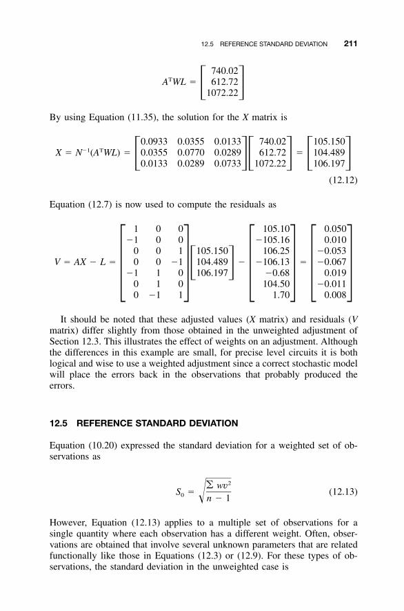
12.5 REFERENCE STANDARD DEVIATION 211
740.02TA WL � 612.72� �1072.22
By using Equation (11.35), the solution for the X matrix is
0.0933 0.0355 0.0133 740.02 105.150�1 TX � N (A WL) � 0.0355 0.0770 0.0289 612.72 � 104.489� �� � � �0.0133 0.0289 0.0733 1072.22 106.197
(12.12)
Equation (12.7) is now used to compute the residuals as
1 0 0 105.10 0.050�1 0 0 �105.16 0.010
0 0 1 105.150 106.25 �0.053V � AX � L � 0 0 �1 104.489 � �106.13 � �0.067� ��1 1 0 106.197 �0.68 0.019� � � � � �0 1 0 104.50 �0.011
0 �1 1 1.70 0.008
It should be noted that these adjusted values (X matrix) and residuals (Vmatrix) differ slightly from those obtained in the unweighted adjustment ofSection 12.3. This illustrates the effect of weights on an adjustment. Althoughthe differences in this example are small, for precise level circuits it is bothlogical and wise to use a weighted adjustment since a correct stochastic modelwill place the errors back in the observations that probably produced theerrors.
12.5 REFERENCE STANDARD DEVIATION
Equation (10.20) expressed the standard deviation for a weighted set of ob-servations as
2� wvS � (12.13)0 �n � 1
However, Equation (12.13) applies to a multiple set of observations for asingle quantity where each observation has a different weight. Often, obser-vations are obtained that involve several unknown parameters that are relatedfunctionally like those in Equations (12.3) or (12.9). For these types of ob-servations, the standard deviation in the unweighted case is
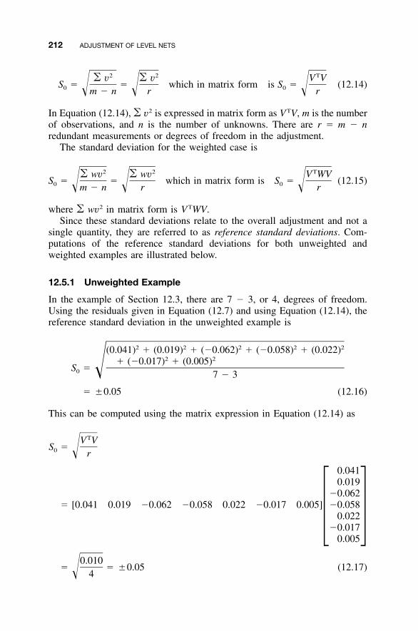
212 ADJUSTMENT OF LEVEL NETS
2 2 T� v � v V VS � � which in matrix form is S � (12.14)0 0� � �m � n r r
In Equation (12.14), � v2 is expressed in matrix form as VTV, m is the numberof observations, and n is the number of unknowns. There are r � m � nredundant measurements or degrees of freedom in the adjustment.
The standard deviation for the weighted case is
2 2 T� wv � wv V WVS � � which in matrix form is S �0 0� � �m � n r r
(12.15)
where � wv2 in matrix form is VTWV.Since these standard deviations relate to the overall adjustment and not a
single quantity, they are referred to as reference standard deviations. Com-putations of the reference standard deviations for both unweighted andweighted examples are illustrated below.
12.5.1 Unweighted Example
In the example of Section 12.3, there are 7 � 3, or 4, degrees of freedom.Using the residuals given in Equation (12.7) and using Equation (12.14), thereference standard deviation in the unweighted example is
2 2 2 2 2(0.041) � (0.019) � (�0.062) � (�0.058) � (0.022)2 2� (�0.017) � (0.005)
S � �0 7 � 3
� �0.05 (12.16)
This can be computed using the matrix expression in Equation (12.14) as
TV VS �0 � r
0.0410.019
�0.062� [0.041 0.019 �0.062 �0.058 0.022 �0.017 0.005] �0.058
0.022� ��0.0170.005
0.010� � �0.05� 4
(12.17)

12.6 ANOTHER WEIGHTED ADJUSTMENT 213
Figure 12.3 Differential leveling network for Example 12.1.
12.5.2 Weighted Example
Notice that the weights are used when computing the reference standard de-viation in Equation (12.15). That is, each residual is squared and multipliedby its weight, and thus the reference standard deviation computed using non-matrix methods is
2 2 2 2 23(0.050) � 4(0.010) � 6(�0.053) � 4(�0.067) � 6(0.019)2 2� 6(�0.011) � 6(0.008)
S � �0 7 � 3
0.04598� � �0.107� 4
(12.18)
It is left as an exercise to verify this result by solving the matrix expressionof Equation (12.15).
12.6 ANOTHER WEIGHTED ADJUSTMENT
Example 12.1 The level net shown in Figure 12.3 is observed with thefollowing results (the elevation differences and standard deviations are givenin meters, and the elevation of A is 437.596 m):
From To �Elev (m) � (m) From To �Elev (m) � (m)
A B 10.509 0.006 D A �7.348 0.003B C 5.360 0.004 B D �3.167 0.004C D �8.523 0.005 A C 15.881 0.012
What are the most probable values for the elevations of B, C, and D?
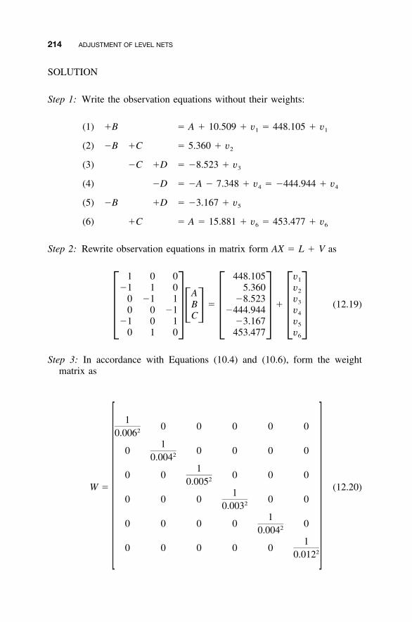
214 ADJUSTMENT OF LEVEL NETS
SOLUTION
Step 1: Write the observation equations without their weights:
(1) �B � A � 10.509 � v � 448.105 � v1 1
(2) �B �C � 5.360 � v2
(3) �C �D � �8.523 � v3
(4) �D � �A � 7.348 � v � �444.944 � v4 4
(5) �B �D � �3.167 � v5
(6) �C � A � 15.881 � v � 453.477 � v6 6
Step 2: Rewrite observation equations in matrix form AX � L � V as
1 0 0 448.105 v1
�1 1 0 5.360 v2A0 �1 1 �8.523 v3B � � (12.19)0 0 �1 �444.944 v� � 4C��1 0 1� � �3.167� �v �50 1 0 453.477 v6
Step 3: In accordance with Equations (10.4) and (10.6), form the weightmatrix as
10 0 0 0 020.0061
0 0 0 0 020.0041
0 0 0 0 020.005W � (12.20)
10 0 0 0 020.003
10 0 0 0 020.004
10 0 0 0 0 20.012
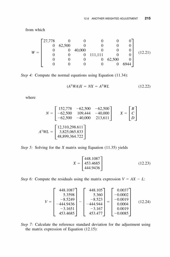
12.6 ANOTHER WEIGHTED ADJUSTMENT 215
from which
27,778 0 0 0 0 00 62,500 0 0 0 00 0 40,000 0 0 0
W � (12.21)0 0 0 111,111 0 0� 0 0 0 0 62,500 0�0 0 0 0 0 6944
Step 4: Compute the normal equations using Equation (11.34):
T T(A WA)X � NX � A WL (12.22)
where
152,778 �62,500 �62,500 BN � �62,500 109,444 �40,000 X � C� � � ��62,500 �40,000 213,611 D
12,310,298.611TA WL � 3,825,065.833� �48,899,364.722
Step 5: Solving for the X matrix using Equation (11.35) yields
448.1087X � 453.4685 (12.23)� �444.9436
Step 6: Compute the residuals using the matrix expression V � AX � L:
448.1087 448.105 0.00375.3598 5.360 �0.0002
�8.5249 �8.523 �0.0019V � � � (12.24)
�444.9436 �444.944 0.0004� �3.1651� � �3.167� � 0.0019�453.4685 453.477 �0.0085
Step 7: Calculate the reference standard deviation for the adjustment usingthe matrix expression of Equation (12.15):
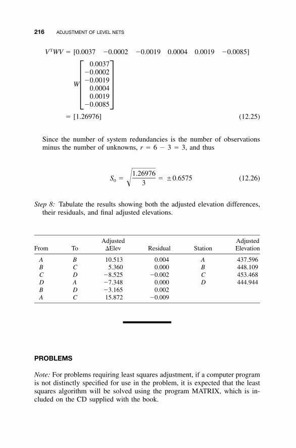
216 ADJUSTMENT OF LEVEL NETS
TV WV � [0.0037 �0.0002 �0.0019 0.0004 0.0019 �0.0085]
0.0037�0.0002�0.0019
W0.0004� 0.0019�
�0.0085
� [1.26976] (12.25)
Since the number of system redundancies is the number of observationsminus the number of unknowns, r � 6 � 3 � 3, and thus
1.26976S � � �0.6575 (12.26)0 � 3
Step 8: Tabulate the results showing both the adjusted elevation differences,their residuals, and final adjusted elevations.
From ToAdjusted
�Elev Residual StationAdjustedElevation
A B 10.513 0.004 A 437.596B C 5.360 0.000 B 448.109C D �8.525 �0.002 C 453.468D A �7.348 0.000 D 444.944B D �3.165 0.002A C 15.872 �0.009
PROBLEMS
Note: For problems requiring least squares adjustment, if a computer programis not distinctly specified for use in the problem, it is expected that the leastsquares algorithm will be solved using the program MATRIX, which is in-cluded on the CD supplied with the book.
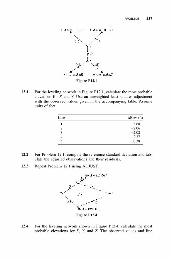
PROBLEMS 217
Figure P12.1
12.1 For the leveling network in Figure P12.1, calculate the most probableelevations for X and Y. Use an unweighted least squares adjustmentwith the observed values given in the accompanying table. Assumeunits of feet.
Line �Elev (ft)
1 �3.682 �2.063 �2.024 �2.375 �0.38
12.2 For Problem 12.1, compute the reference standard deviation and tab-ulate the adjusted observations and their residuals.
12.3 Repeat Problem 12.1 using ADJUST.
Figure P12.4
12.4 For the leveling network shown in Figure P12.4, calculate the mostprobable elevations for X, Y, and Z. The observed values and line
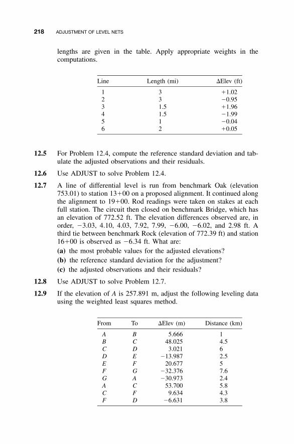
218 ADJUSTMENT OF LEVEL NETS
lengths are given in the table. Apply appropriate weights in thecomputations.
Line Length (mi) �Elev (ft)
1 3 �1.022 3 �0.953 1.5 �1.964 1.5 �1.995 1 �0.046 2 �0.05
12.5 For Problem 12.4, compute the reference standard deviation and tab-ulate the adjusted observations and their residuals.
12.6 Use ADJUST to solve Problem 12.4.
12.7 A line of differential level is run from benchmark Oak (elevation753.01) to station 13�00 on a proposed alignment. It continued alongthe alignment to 19�00. Rod readings were taken on stakes at eachfull station. The circuit then closed on benchmark Bridge, which hasan elevation of 772.52 ft. The elevation differences observed are, inorder, �3.03, 4.10, 4.03, 7.92, 7.99, �6.00, �6.02, and 2.98 ft. Athird tie between benchmark Rock (elevation of 772.39 ft) and station16�00 is observed as �6.34 ft. What are:(a) the most probable values for the adjusted elevations?(b) the reference standard deviation for the adjustment?(c) the adjusted observations and their residuals?
12.8 Use ADJUST to solve Problem 12.7.
12.9 If the elevation of A is 257.891 m, adjust the following leveling datausing the weighted least squares method.
From To �Elev (m) Distance (km)
A B 5.666 1B C 48.025 4.5C D 3.021 6D E �13.987 2.5E F 20.677 5F G �32.376 7.6G A �30.973 2.4A C 53.700 5.8C F 9.634 4.3F D �6.631 3.8
PROBLEMS 219
(a) What are the most probable values for the elevations of thestations?
(b) What is the reference standard deviation?(c) Tabulate the adjusted observations and their residuals.
12.10 Use ADJUST to solve Problem 12.9.
12.11 If the elevation of station 1 is 2395.67 ft, use weighted least squaresto adjust the following leveling.
From To�Elev
(ft)Distance
(mi) From To�Elev
(ft)Distance
(mi)
1 2 37.17 3.00 2 3 �9.20 3.633 4 34.24 1.56 4 5 �10.92 1.985 6 �23.12 0.83 6 1 �28.06 0.931 7 16.99 1.61 7 3 11.21 1.212 7 �19.99 2.91 7 6 10.89 1.416 3 �0.04 3.06 3 8 74.93 1.778 5 �51.96 2.98 6 8 74.89 8.038 4 �41.14 1.08
(a) What are the most probable values for the elevations for thestations?
(b) What is the adjustment’s reference standard deviation?(c) Tabulate the adjusted observations and their residuals.
12.12 Use ADJUST to solve Problem 12.11.
12.13 Precise procedures were applied with a level that can be read to within�0.4 mm/1 m. The line of sight was held to within �3� of horizon-tal, and the sight distances were approximately 50 m in length. Usethese specifications and Equation (9.20) to compute standard devia-tions and hence weights. The elevation of A is 100.000 m. Adjust thenetwork by weighted least squares.
From To�Elev
(m)Number
of Setups From To�Elev(m)
Numberof Setups
A B 12.383 16 M D �38.238 23B C �16.672 25 C M 30.338 16C D �7.903 37 M B �13.676 38D A 12.190 26 A M 26.058 19
(a) What are the most probable values for the elevations of thestations?
220 ADJUSTMENT OF LEVEL NETS
(b) What is the reference standard deviation for the adjustment?(c) Tabulate the adjusted observations and their residuals.
12.14 Repeat Problem 12.13 using the number of setups for weighting fol-lowing the procedures discussed in Section 10.6.
12.15 In Problem 12.13, the estimated error in reading the rod is 1.4 mm/km. The bubble sensitivity of the instrument is 12 mm/km and theaverage sight distances are 50 m. What are:(a) the estimated standard errors for the observations?(b) the most probable values for the elevations of the stations?(c) the reference variance for the adjustment?(d) Tabulate the adjusted observations and their residuals.
12.16 Demonstrate that � v2 � VTV.
12.17 Demonstrate that � wv2 � VTWV.
Programming Problems
12.18 Write a program that reads a file of differential leveling observationsand writes the matrices A, W, and L in a format suitable for theMATRIX program. Using this package, solve Problem 12.11.
12.19 Write a computational package that reads the matrices A, W, and L,computes the least squares solution for the unknown station eleva-tions, and writes a file of adjusted elevation differences and theirresiduals. Using this package, solve Problem 12.11.
12.20 Write a computational package that reads a file of differential levelingobservations, computes the least squares solution for the adjusted sta-tion elevations, and writes a file of adjusted elevation differences andtheir residuals. Using this package, solve Problem 12.11.
221
CHAPTER 13
PRECISION OF INDIRECTLYDETERMINED QUANTITIES
13.1 INTRODUCTION
Following an adjustment, it is important to know the estimated errors in boththe adjusted observations and the derived quantities. For example, after ad-justing a level net as described in Chapter 12, the uncertainties in both ad-justed elevation differences and computed benchmark elevations should bedetermined. In Chapter 5, error propagation formulas were developed forindirectly measured quantities which were functionally related to observedvalues. In this chapter, error propagation formulas are developed for the quan-tities computed in a least squares solution.
13.2 DEVELOPMENT OF THE COVARIANCE MATRIX
Consider an adjustment involving weighted observation equations like thosein the level circuit example of Section 12.4. The matrix form for the systemof weighted observation equation is
WAX � WL � WV (13.1)
and the least squares solution of the weighted observation equations is givenby
T �1 TX � (A WA) A WL (13.2)
Adjustment Computations: Spatial Data Analysis, Fourth Edition. C. D. Ghilani and P. R. Wolf© 2006 John Wiley & Sons, Inc. ISBN: 978-0-471-69728-2
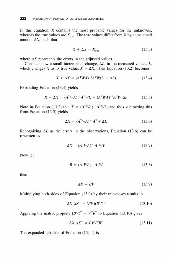
222 PRECISION OF INDIRECTLY DETERMINED QUANTITIES
In this equation, X contains the most probable values for the unknowns,whereas the true values are Xtrue. The true values differ from X by some smallamount �X, such that
X � �X � X (13.3)true
where �X represents the errors in the adjusted values.Consider now a small incremental change, �L, in the measured values, L,
which changes X to its true value, X � �X. Then Equation (13.2) becomes
T �1 TX � �X � (A WA) A W(L � �L) (13.4)
Expanding Equation (13.4) yields
T �1 T T �1 TX � �X � (A WA) A WL � (A WA) A W �L (13.5)
Note in Equation (13.2) that X � (ATWA)�1ATWL, and thus subtracting thisfrom Equation (13.5) yields
T �1 T�X � (A WA) A W �L (13.6)
Recognizing �L as the errors in the observations, Equation (13.6) can berewritten as
T �1 T�X � (A WA) A WV (13.7)
Now let
T �1 TB � (A WA) A W (13.8)
then
�X � BV (13.9)
Multiplying both sides of Equation (13.9) by their transposes results in
T T�X �X � (BV)(BV) (13.10)
Applying the matrix property (BV)T � VTBT to Equation (13.10) gives
T T T�X �X � BVV B (13.11)
The expanded left side of Equation (13.11) is

13.2 DEVELOPMENT OF THE COVARIANCE MATRIX 223
2�x �x �x �x �x � � � �x �x1 1 2 1 3 1 n2�x �x �x �x �x � � � �x �x2 1 2 2 3 2 n
T 2�X �X � �x �x �x �x �x � � � �x �x (13.12)3 1 3 2 3 3 n�� � � � ��� �
2�x �x �x �x �x �x � � � �xn 1 n 2 n 3 n
Also, the expanded right side of Equation (13.11) is
2v v v v v � � � v v1 1 2 1 3 1 m2v v v v v � � � v v2 1 2 2 3 2 m
2 TB v v v v v � � � v v B (13.13)3 1 3 2 3 3 m�� � � � ��� �
2v v v v v v � � � vm 1 m 2 m 3 m
Assume that it is possible to repeat the entire sequence of observationsmany times, say a times, and that each time a slightly different solutionoccurs, yielding a different set of X’s. Averaging these sets, the left side ofEquation (13.11) becomes
2�x �x �x �x �x� � �1 1 2 1 n� � �
a a a2�x �x �x �x �x� � �2 1 2 2 n
� � �a a a1 T(�X)(�X) � (13.14)�
a � �� � ��2�x �x �x �x �x� � �n 1 n 2 n
� � �a a a
If a is large, the terms in Equation (13.14) are the variances and covari-ances as defined in Equation (6.7) and Equation (13.14) can be rewritten as
2S S � � � Sx x x x x1 1 2 1 n2S S � � � Sx x x x x 22 1 2 2 n � S (13.15)x�� � � ��� �2S S � � � Sx x x x xn 1 n 2 n
Also, considering a sets of observations, Equation (13.13) becomes
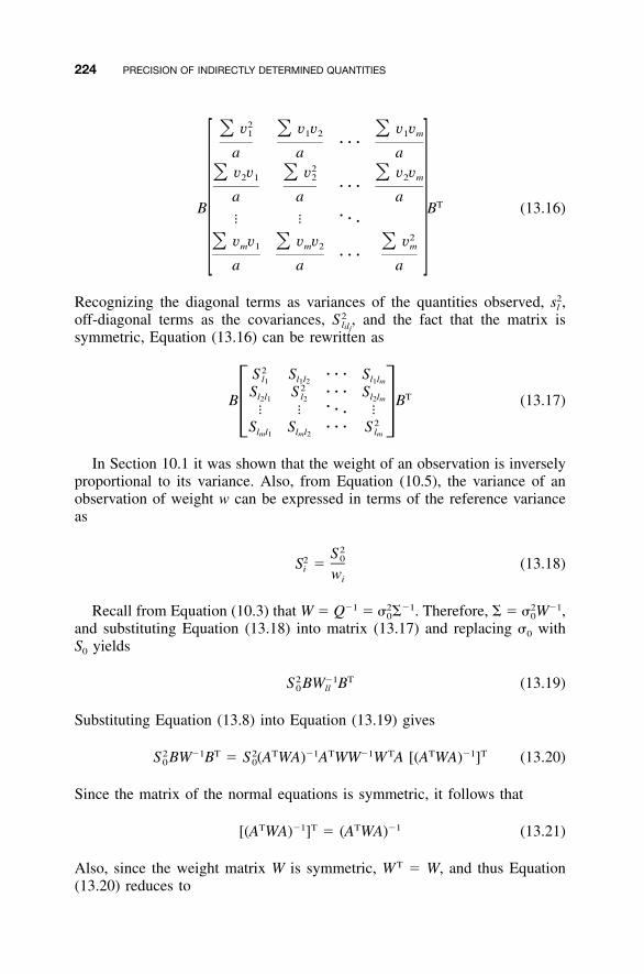
224 PRECISION OF INDIRECTLY DETERMINED QUANTITIES
2v v v v v� � �1 1 2 1 m� � �
a a a2v v v v v� � �2 1 2 2 m
� � �a a a
TB B (13.16)�� � � �
2v v v v v� � �m 1 m 2 m� � �
a a a
Recognizing the diagonal terms as variances of the quantities observed, 2s ,l
off-diagonal terms as the covariances, and the fact that the matrix is2S ,liljsymmetric, Equation (13.16) can be rewritten as
2S S � � � Sl l l l l1 1 2 1 m2S S � � � Sl l l l l T2 1 2 2 mB B (13.17)�� � � ��� �2S S � � � Sl l l l lm 1 m 2 m
In Section 10.1 it was shown that the weight of an observation is inverselyproportional to its variance. Also, from Equation (10.5), the variance of anobservation of weight w can be expressed in terms of the reference varianceas
2S02S � (13.18)i wi
Recall from Equation (10.3) that W � Q�1 � ��1. Therefore, � � W�1,2 2� �0 0
and substituting Equation (13.18) into matrix (13.17) and replacing �0 withS0 yields
2 �1 TS BW B (13.19)0 ll
Substituting Equation (13.8) into Equation (13.19) gives
2 �1 T 2 T �1 T �1 T T �1 TS BW B � S (A WA) A WW W A [(A WA) ] (13.20)0 0
Since the matrix of the normal equations is symmetric, it follows that
T �1 T T �1[(A WA) ] � (A WA) (13.21)
Also, since the weight matrix W is symmetric, WT � W, and thus Equation(13.20) reduces to
13.3 NUMERICAL EXAMPLES 225
2 T �1 T T �1 2 T �1S (A WA) (A WA)(A WA) � S (A WA) (13.22)0 0
Equation (13.15) is the left side of Equation (13.11), for which Equation(13.22) is the right. That is,
2 2 T �1 2 �1 2S � S (A WA) � S N � S Q (13.23)x 0 0 0 xx
In least squares adjustment, the matrix Qxx of Equation (13.23) is knownas the variance–covariance matrix, or simply the covariance matrix. Diagonalelements of the matrix when multiplied by give variances of the adjusted2S0
quantities, and the off-diagonal elements multiplied by yield covariances.2S0
From Equation (13.23), the estimated standard deviation Si for any unknownparameter computed from a system of observation equations is expressed as
S � S �q (13.24)i 0 x xi i
where is the diagonal element (from the ith row and ith column) of theqx xi i
Qxx matrix, which as noted in Equation (13.23), is equal to the inverse of thematrix of normal equations. Since the normal equation matrix is symmetric,its inverse is also symmetric, and thus the covariance matrix is a symmetricmatrix (i.e., element ij � element ji).1
13.3 NUMERICAL EXAMPLES
The results of the level net adjustment in Section 12.3 will be used to illustratethe computation of estimated errors for the adjusted unknowns. From Equa-tion (12.6), the N�1 matrix, which is also the Qxx matrix, is
0.38095 0.14286 0.04762Q � 0.14286 0.42857 0.14286xx � �0.04762 0.14286 0.38095
Also, from Equation (12.17), S0 � �0.05. Now by Equation (13.24), theestimated standard deviations for the unknown benchmark elevations A, B,and C are
1 Note that an estimate of the reference variance, may be computed using either Equation2� ,0
(12.13) or (12.14). However, it should be remembered that this only gives an estimate of the apriori (before the adjustment) value for the reference variance. The validity of this estimate canbe checked using a �2 test as discussed in Chapter 5. If it is a valid estimate for the a priori2� ,0
value for the reference variance should be used in the computations discussed in this and sub-sequent chapters. Thus, if the a priori value for is known, it should be used when computing2�0
the a posteriori (after the adjustment) statistics. When weights are determined as the implicit21 /� ,i
assumption made is that the a priori value for � 1 [see Equations (10.5) and (10.6)].2�0
226 PRECISION OF INDIRECTLY DETERMINED QUANTITIES
S � S �q � �0.05�0.38095 � �0.031 ftA 0 AA
S � S �q � �0.05�0.42857 � �0.033 ftB 0 BB
S � S �q � �0.05�0.38095 � �0.031 ftC 0 CC
In the weighted example of Section 12.4, it should be noted that althoughthis is a weighted adjustment, the a priori value for the reference variance isnot known because weights were determined as 1/distance and not 21/� .i
From Equation (12.12), the Qxx matrix is
0.0933 0.0355 0.0133Q � 0.0355 0.0770 0.0289XX � �0.0133 0.0289 0.0733
Recalling that in Equation (12.18), S0 � �0.107, the estimated errors in thecomputed elevations of benchmarks A, B, and C are
S � S �q � �0.07�0.0933 � �0.033 ftA 0 AA
S � S �q � �0.07�0.0770 � �0.030 ftB 0 BB
S � S �q � �0.07�0.0733 � �0.029 ftC 0 CC
These standard deviations are at the 68% probability level, and if other per-centage errors are desired, these values should be multiplied by their re-spective t values as discussed in Chapter 3.
13.4 STANDARD DEVIATIONS OF COMPUTED QUANTITIES
In Section 6.1 the generalized law of propagation of variances was developed.Recalled here for convenience, Equation (6.13) was written as
T� � A� Aˆˆll xx
where represents the adjusted observations, the covariance matrix of thel �ˆˆll
adjusted observations, �xx the covariance matrix of the unknown parameters[i.e., (ATWA)�1], and A, the coefficient matrix. Rearranging Equation (10.2)and using sample statistics, there results �xx � Also, from Equation2S Q .0 xx
(13.23), � � (ATWA)�1 and thus �xx � Substituting this equal-2 2 2 2S S Q S S .x 0 xx 0 x
ity into Equation (a), the estimated standard deviations of the adjusted ob-servations is
13.4 STANDARD DEVIATIONS OF COMPUTED QUANTITIES 227
2 2 T 2 T �1 T 2 T 2� � S � A� A � AS (A WA) A � S AQ A � S Q (13.25)ˆˆ ˆ ˆˆll l xx 0 0 xx 0 ll
where AQxxAT � , which is known as the covariance matrix of the adjustedQˆˆll
observations.
Example 13.1 Consider the linear example in Section 12.3. By Equation(13.25), the estimated standard deviations in the adjusted elevation differencesare
1 0 0�1 0 0
0 0 1 0.38095 0.14286 0.047622 2S � 0.050 0 0 �1 0.14286 0.42857 0.14286l � ��1 1 0 0.04762 0.14286 0.38095� �0 1 0
0 �1 1
1 �1 0 0 �1 0 0� 0 0 0 0 1 1 �1 (13.26)� �0 0 1 �1 0 0 1
Performing the required matrix multiplications in Equation (13.26) yields
2 2S � 0.050l
0.38095 �0.38095 0.04762 �0.04762 �0.23810 0.14286 �0.09524�0.38095 0.38095 �0.04762 0.04762 0.23810 �0.14286 0.09524
0.04762 �0.04762 0.38095 �0.38095 0.09524 0.14286 0.23810� �0.04762 0.04762 �0.38095 0.38095 �0.09524 �0.14286 �0.23810
�0.23810 0.23810 0.09524 �0.09524 0.52381 0.28571 �0.19048� �0.14286 �0.14286 0.14286 �0.14286 0.28571 0.42857 �0.28571�0.09524 0.09524 0.23810 �0.23810 �0.19048 �0.28571 0.52381
(13.27)
The estimated standard deviation of an observation is found by taking thesquare root of the corresponding diagonal element of the matrix (leveling2S l
from A to B). For instance, for the fifth observation, (5,5) applies and theSl
estimated error in the adjusted elevation difference of that observation is
S � �0.050�0.52381 � �0.036 ft� AB
An interpretation of the meaning of the value just calculated is that thereis a 68% probability that the true value is within the range �0.036 ft of theadjusted elevation difference (l5 � v5 � �0.68 � 0.022 � �0.658). That
228 PRECISION OF INDIRECTLY DETERMINED QUANTITIES
is, the true value lies between �0.694 and �0.622 ft with 68% proba-bility.
Careful examination of the matrix manipulations involved in solving Equa-tion (13.25) for Example 13.1 reveals that the effort can be reduced signifi-cantly. In fact, to obtain the estimated standard deviation in the fifth element,only the fifth row of the coefficient matrix, A, which represents the elevationdifference between A and B, need be used in the calculations. That row is[�1 1 0]. Thus, to compute the standard deviation in this observation, thefollowing computations could be made:
0.38095 0.14286 0.04762 �12 2S � 0.050 [�1 1 0] 0.14286 0.42857 0.14286 1� AB � �� �0.04762 0.14286 0.38095 0
�12� 0.050 [0.2389 �0.28571 �0.09524] 1� �0 (13.28)2� 0.050 [0.52381]
S � �0.050�0.52381 � �0.036 ft� AB
Note that this shortcut method produces the same value. Furthermore, be-cause of the zero in the third position of this row from the coefficient matrix,the matrix operations in Equation (13.28) could be further reduced to
0.38095 0.14286 �12 2 2S � 0.050 [�1 1] � 0.050 [0.52381]� �� �� AB 0.14286 0.42857 1
Another use for Equation (13.25) is in the computation of adjusted uncer-tainties for observations that were never made. For instance, in the exampleof Section 12.3, the elevation difference between benchmarks X and B wasnot observed. But from the results of the adjustment, this elevation differenceis 104.48 � 100.00 � 4.48 ft. The estimated error in this difference can befound by writing an observation equation for it (i.e., B � X � �ElevXB). Thisequation does not involve either A or C, and thus in matrix form this differ-ence would be expressed as
[0 1 0] (13.29)
Using this row matrix in the same procedure as in Equation (13.28) yields
PROBLEMS 229
0.38095 0.14286 0.04762 02 2S � 0.050 [0 1 0] 0.14286 0.42857 0.14286 1� XB � �� �0.04762 0.14286 0.38095 0
2� 0.050 [0.42857]
Hence,
S � �0.050�0.42857 � �0.033 ft� XB
Again, recognizing the presence of the zeros in the row matrix, these com-putations can be simplified to
2 1 2S � 0.050 [1][0.42857][1] � 0.050 [0.42857]� XB
The method illustrated above of eliminating unnecessary matrix computationsis formally known as matrix partitioning.
Computing uncertainties of quantities that were not actually observed hasapplication in many areas. For example, suppose that in a triangulation ad-justment, the x and y coordinates of stations A and B are calculated and thecovariance matrix exists. Equation (13.25) could be applied to determine theestimated error in the length of line AB calculated from the adjusted coordi-nates of A and B. This is accomplished by relating the length AB to theunknown parameters as
2 2AB � �(X � X ) � (Y � Y ) (13.30)b a b a
This subject is discussed further in Chapter 15.An important observation that should be made about the and Qxx ma-Qˆˆll
trices is that only the coefficient matrix, A, is used in their formation. Sincethe A matrix contains coefficients that express the relationships of the un-knowns to each other, it depends only on the geometry of the problem. Theonly other term in Equation (13.25) is the reference variance, and that dependson the quality of the measurements. These are important concepts that willbe revisited in Chapter 21 when simulation of surveying networks is dis-cussed.
PROBLEMS
For each problem, calculate the estimated errors for the adjusted benchmarkelevations.
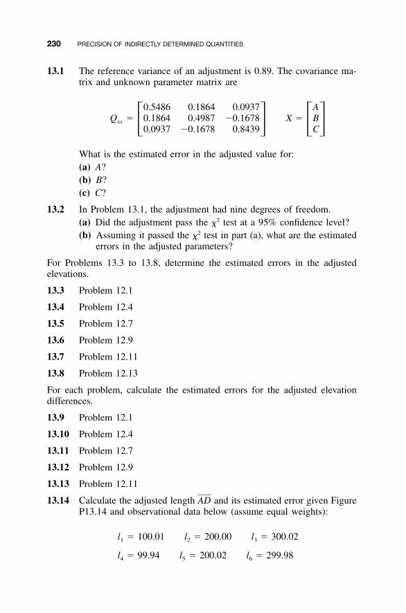
230 PRECISION OF INDIRECTLY DETERMINED QUANTITIES
13.1 The reference variance of an adjustment is 0.89. The covariance ma-trix and unknown parameter matrix are
0.5486 0.1864 0.0937 AQ � 0.1864 0.4987 �0.1678 X � Bxx � � � �0.0937 �0.1678 0.8439 C
What is the estimated error in the adjusted value for:(a) A?(b) B?(c) C?
13.2 In Problem 13.1, the adjustment had nine degrees of freedom.(a) Did the adjustment pass the �2 test at a 95% confidence level?(b) Assuming it passed the �2 test in part (a), what are the estimated
errors in the adjusted parameters?
For Problems 13.3 to 13.8, determine the estimated errors in the adjustedelevations.
13.3 Problem 12.1
13.4 Problem 12.4
13.5 Problem 12.7
13.6 Problem 12.9
13.7 Problem 12.11
13.8 Problem 12.13
For each problem, calculate the estimated errors for the adjusted elevationdifferences.
13.9 Problem 12.1
13.10 Problem 12.4
13.11 Problem 12.7
13.12 Problem 12.9
13.13 Problem 12.11
13.14 Calculate the adjusted length and its estimated error given FigureADP13.14 and observational data below (assume equal weights):
l � 100.01 l � 200.00 l � 300.021 2 3
l � 99.94 l � 200.02 l � 299.984 5 6
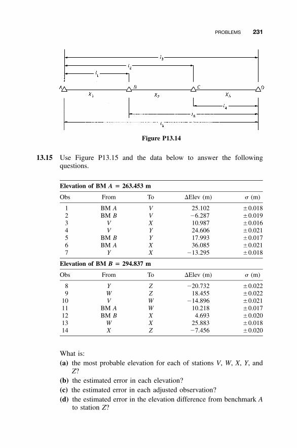
PROBLEMS 231
Figure P13.14
13.15 Use Figure P13.15 and the data below to answer the followingquestions.
Elevation of BM A � 263.453 m
Obs From To �Elev (m) � (m)
1 BM A V 25.102 �0.0182 BM B V �6.287 �0.0193 V X 10.987 �0.0164 V Y 24.606 �0.0215 BM B Y 17.993 �0.0176 BM A X 36.085 �0.0217 Y X �13.295 �0.018
Elevation of BM B � 294.837 m
Obs From To �Elev (m) � (m)
8 Y Z �20.732 �0.0229 W Z 18.455 �0.022
10 V W �14.896 �0.02111 BM A W 10.218 �0.01712 BM B X 4.693 �0.02013 W X 25.883 �0.01814 X Z �7.456 �0.020
What is:(a) the most probable elevation for each of stations V, W, X, Y, and
Z?(b) the estimated error in each elevation?(c) the estimated error in each adjusted observation?(d) the estimated error in the elevation difference from benchmark A
to station Z?
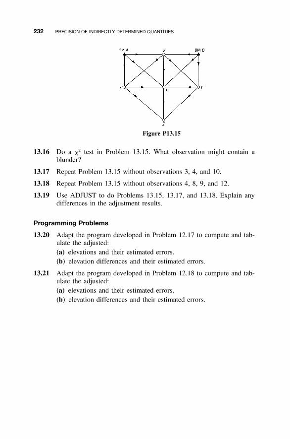
232 PRECISION OF INDIRECTLY DETERMINED QUANTITIES
Figure P13.15
13.16 Do a �2 test in Problem 13.15. What observation might contain ablunder?
13.17 Repeat Problem 13.15 without observations 3, 4, and 10.
13.18 Repeat Problem 13.15 without observations 4, 8, 9, and 12.
13.19 Use ADJUST to do Problems 13.15, 13.17, and 13.18. Explain anydifferences in the adjustment results.
Programming Problems
13.20 Adapt the program developed in Problem 12.17 to compute and tab-ulate the adjusted:(a) elevations and their estimated errors.(b) elevation differences and their estimated errors.
13.21 Adapt the program developed in Problem 12.18 to compute and tab-ulate the adjusted:(a) elevations and their estimated errors.(b) elevation differences and their estimated errors.
233
CHAPTER 14
ADJUSTMENT OF HORIZONTALSURVEYS: TRILATERATION
14.1 INTRODUCTION
Horizontal surveys are performed for the purpose of determining precise rel-ative horizontal positions of points. They have traditionally been accom-plished by trilateration, triangulation, and traverse. These traditional types ofsurveys involve making distance, direction, and angle observations. As withall types of surveys, errors will occur in making these measurements, andthus they must be analyzed and if acceptable, adjusted. In the following threechapters, procedures are described for adjusting trilateration, triangulation,and traverse surveys, in that order.
In recent years, the global positioning system (GPS) has gradually beenreplacing these traditional procedures for conducting precise horizontal con-trol surveys. In fact, GPS not only yields horizontal positions, but it givesellipsoidal heights as well. Thus, GPS provides three-dimensional surveys.Again as with all observations, GPS observations contain errors and must beadjusted. In Chapter 17 we discuss the subject of GPS surveying in moredetail and illustrate methods for adjusting networks surveyed by thisprocedure.
Horizontal surveys, especially those covering a large extent, must accountfor the systematic effects of the Earth’s curvature. One way this can be ac-complished is to do the computations using coordinates from a mathemati-cally rigorous map projection system such as the state plane system or a localplane coordinate system that accounts rigorously for the Earth’s curvature.Map projection coordinate systems are presented in Appendix F. In the fol-lowing chapters, methods are developed for adjusting horizontal surveys usingparametric equations that are based on plane coordinates. In Chapter 23, a
Adjustment Computations: Spatial Data Analysis, Fourth Edition. C. D. Ghilani and P. R. Wolf© 2006 John Wiley & Sons, Inc. ISBN: 978-0-471-69728-2
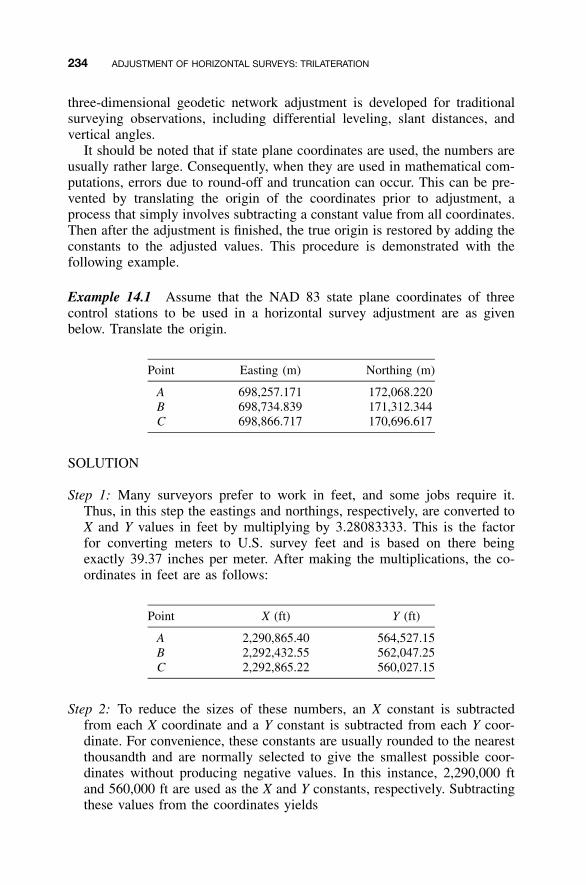
234 ADJUSTMENT OF HORIZONTAL SURVEYS: TRILATERATION
three-dimensional geodetic network adjustment is developed for traditionalsurveying observations, including differential leveling, slant distances, andvertical angles.
It should be noted that if state plane coordinates are used, the numbers areusually rather large. Consequently, when they are used in mathematical com-putations, errors due to round-off and truncation can occur. This can be pre-vented by translating the origin of the coordinates prior to adjustment, aprocess that simply involves subtracting a constant value from all coordinates.Then after the adjustment is finished, the true origin is restored by adding theconstants to the adjusted values. This procedure is demonstrated with thefollowing example.
Example 14.1 Assume that the NAD 83 state plane coordinates of threecontrol stations to be used in a horizontal survey adjustment are as givenbelow. Translate the origin.
Point Easting (m) Northing (m)
A 698,257.171 172,068.220B 698,734.839 171,312.344C 698,866.717 170,696.617
SOLUTION
Step 1: Many surveyors prefer to work in feet, and some jobs require it.Thus, in this step the eastings and northings, respectively, are converted toX and Y values in feet by multiplying by 3.28083333. This is the factorfor converting meters to U.S. survey feet and is based on there beingexactly 39.37 inches per meter. After making the multiplications, the co-ordinates in feet are as follows:
Point X (ft) Y (ft)
A 2,290,865.40 564,527.15B 2,292,432.55 562,047.25C 2,292,865.22 560,027.15
Step 2: To reduce the sizes of these numbers, an X constant is subtractedfrom each X coordinate and a Y constant is subtracted from each Y coor-dinate. For convenience, these constants are usually rounded to the nearestthousandth and are normally selected to give the smallest possible coor-dinates without producing negative values. In this instance, 2,290,000 ftand 560,000 ft are used as the X and Y constants, respectively. Subtractingthese values from the coordinates yields
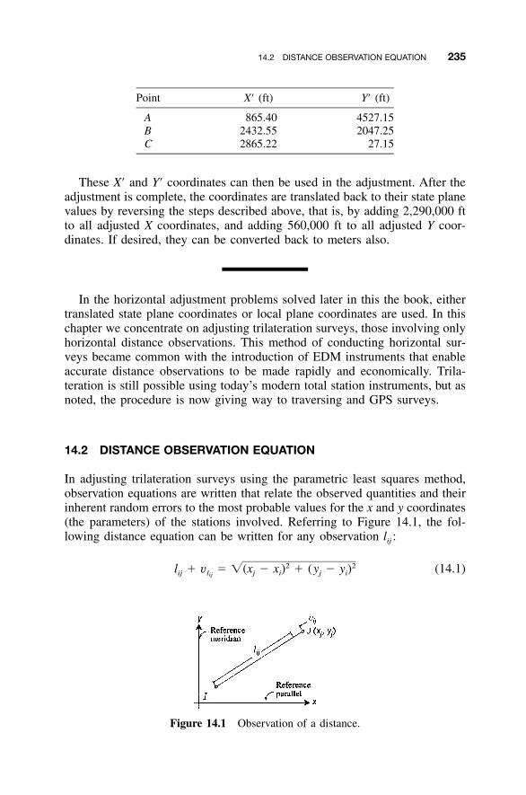
14.2 DISTANCE OBSERVATION EQUATION 235
Figure 14.1 Observation of a distance.
Point X� (ft) Y� (ft)
A 865.40 4527.15B 2432.55 2047.25C 2865.22 27.15
These X� and Y� coordinates can then be used in the adjustment. After theadjustment is complete, the coordinates are translated back to their state planevalues by reversing the steps described above, that is, by adding 2,290,000 ftto all adjusted X coordinates, and adding 560,000 ft to all adjusted Y coor-dinates. If desired, they can be converted back to meters also.
In the horizontal adjustment problems solved later in this the book, eithertranslated state plane coordinates or local plane coordinates are used. In thischapter we concentrate on adjusting trilateration surveys, those involving onlyhorizontal distance observations. This method of conducting horizontal sur-veys became common with the introduction of EDM instruments that enableaccurate distance observations to be made rapidly and economically. Trila-teration is still possible using today’s modern total station instruments, but asnoted, the procedure is now giving way to traversing and GPS surveys.
14.2 DISTANCE OBSERVATION EQUATION
In adjusting trilateration surveys using the parametric least squares method,observation equations are written that relate the observed quantities and theirinherent random errors to the most probable values for the x and y coordinates(the parameters) of the stations involved. Referring to Figure 14.1, the fol-lowing distance equation can be written for any observation lij :
2 2l � v � �(x � x ) � (y � y ) (14.1)ij l j i j iij
236 ADJUSTMENT OF HORIZONTAL SURVEYS: TRILATERATION
In Equation (14.1), lij is the observed distance of a line between stations Iand J, the residual in the observation lij, xi and yi the most probable co-vlij
ordinate values for station I, and xj and yj the most probable coordinate valuesfor station J. Equation (14.1) is a nonlinear function involving the unknownvariables xi, yi, xj, and yj that can be rewritten as
F(x ,y ,x ,y ) � l � v (14.2)i i j j ij lij
where
2 2F(x ,y ,x ,y ) � �(x � x ) � (y � y )i i j j j i j i
As discussed in Section 11.10, a system of nonlinear equations such asEquation (14.2) can be linearized and solved using a first-order Taylor seriesapproximation. The linearized form of Equation (14.2) is
�F �FF(x ,y ,x ,y ) � F(x ,y ,x ,y ) � dx � dy� � � �i i j j i i j j i i0 0 0 0 �x �yi i0 0
�F �F� dx � dy (14.3)� � � �j j�x �yj j0 0
where (�F /�xi)0, (�F /�yi)0, (�F /�xj)0, and (�F /�yj)0 are the partial derivativesof F with respect to xi, yi xj, and yj, respectively, evaluated with the approx-imate coordinate values and xi, yi, xj, and yj are the unknownx , y , x , y ;i i j j0 0 0 0
parameters; and dxi, dyi, dxj, and dyj are the corrections to the approximationcoordinate values such that
x � x � dx y � y � dyi i i i i i0 0 (14.4)
x � x � dx y � y � dyj j j j j j0 0
The evaluation of partial derivatives is straightforward and will be illus-trated with �F /�xi. Equation (14.2) can be rewritten as
2 2 1 / 2F(x ,y ,x ,y ) � [(x � x ) � (y � y ) ] (14.5)i i j j j i j i
Taking the derivative of Equation (14.5) with respect to xi yields
�F 1 2 2 �1 / 2� [(x � x ) � (y � y ) ] [2(x � x )(�1)] (14.6)j i j i j i�x 2i
Simplifying Equation (14.6) yields
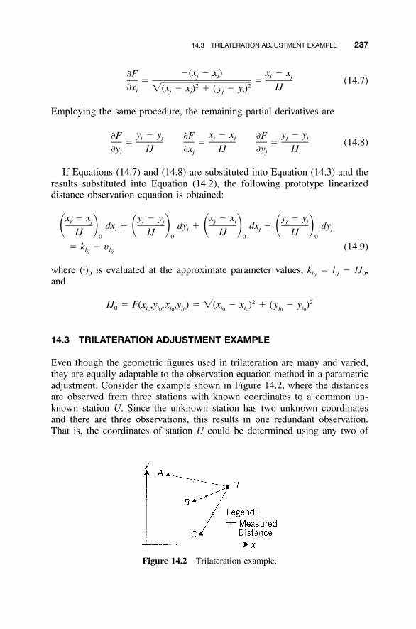
14.3 TRILATERATION ADJUSTMENT EXAMPLE 237
Figure 14.2 Trilateration example.
�(x � x ) x � x�F j i i j� � (14.7)
2 2�x IJ�(x � x ) � (y � y )i j i j i
Employing the same procedure, the remaining partial derivatives are
y � y x � x y � y�F �F �Fi j j i j i� � � (14.8)
�y IJ �x IJ �y IJi j j
If Equations (14.7) and (14.8) are substituted into Equation (14.3) and theresults substituted into Equation (14.2), the following prototype linearizeddistance observation equation is obtained:
x � x y � y x � x y � yi j i j j i j idx � dy � dx � dy� � � � � � � �i i j jIJ IJ IJ IJ0 0 0 0
� k � v (14.9)l lij ij
where (�)0 is evaluated at the approximate parameter values, � lij � IJ0,klij
and
2 2IJ � F(x ,y ,x ,y ) � �(x � x ) � (y � y )0 i i j j j i j i0 0 0 0 0 0 0 0
14.3 TRILATERATION ADJUSTMENT EXAMPLE
Even though the geometric figures used in trilateration are many and varied,they are equally adaptable to the observation equation method in a parametricadjustment. Consider the example shown in Figure 14.2, where the distancesare observed from three stations with known coordinates to a common un-known station U. Since the unknown station has two unknown coordinatesand there are three observations, this results in one redundant observation.That is, the coordinates of station U could be determined using any two of

238 ADJUSTMENT OF HORIZONTAL SURVEYS: TRILATERATION
the three observations. But all three observations can be used simultaneouslyand adjusted by the method of least squares to determine the most probablevalue for the coordinates of the station.
The observation equations are developed by substituting into prototypeequation (14.9). For example, the equation for distance AU is formed byinterchanging subscript I with A and subscript J with U in Equation (14.9).In a similar fashion, an equation can be created for each line observed usingthe following subscript substitutions:
I J
A UB UC U
When one end of the observed line is a control station, its coordinates arefixed, and thus those terms can be dropped in prototype equation (14.9).1 Thiscan be thought of as setting the dx and dy corrections for the control stationequal to zero. In this example, station U always takes the position of J in theprototype equation, and thus only the coefficients corresponding to dxj anddyj are used. Using the appropriate substitutions, the following three linearizedobservation equations result.
x � x y � yu a u a0 0dx � dy � (l � AU ) � vu u AU 0 lAUAU AU0 0
x � x y � yu b u b0 0dx � dy � (l � AU ) � v (14.10)u u BU 0 lBUBU BU0 0
x � x y � yu c u c0 0dx � dy � (l � CU ) � vu u CU 0 lCUCU CU0 0
In Equation (14.10),
2 2 2 2AU � �(x � x ) � (y � y ) BU � �(x � x ) � (y � y )0 u a u a 0 u b u b0 0 0 0
2 2CU � �(x � x ) � (y � y )0 u c u c0 0
lau, lbu, and lcu are the observed distances with residuals v; and and arex yu u0 0
initial coordinate approximations for station U. Equations (14.10) can be ex-pressed in matrix form as
1 The method of dropping control station coordinates from the adjustment, known as eliminationof constraints, is covered in Chapter 20.
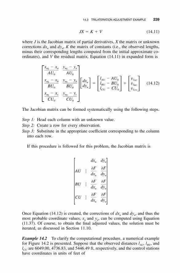
14.3 TRILATERATION ADJUSTMENT EXAMPLE 239
JX � K � V (14.11)
where J is the Jacobian matrix of partial derivatives, X the matrix or unknowncorrections dxu and dyu, K the matrix of constants (i.e., the observed lengths,minus their corresponding lengths computed from the initial approximate co-ordinates), and V the residual matrix. Equation (14.11) in expanded form is
x � x y � yu a u a0 0
AU AU0 0
l � AU vAU 0 lAUx � x y � y dxu b u b0 0 u � l � BU � v (14.12)� � BU 0 lBUdyBU BU � � � �u0 0 l � CU vCU 0 lCU� �x � x y � yu c u c0 0
CU CU0 0
The Jacobian matrix can be formed systematically using the following steps.
Step 1: Head each column with an unknown value.Step 2: Create a row for every observation.Step 3: Substitute in the appropriate coefficient corresponding to the column
into each row.
If this procedure is followed for this problem, the Jacobian matrix is
dx dyu u
�F �FAU �
dx dyu u
�F �FBU �
dx dyu u
�F �FCU �
dx dyu u
Once Equation (14.12) is created, the corrections of dxu and dyu, and thus themost probable coordinate values, xu and yu, can be computed using Equation(11.37). Of course, to obtain the final adjusted values, the solution must beiterated, as discussed in Section 11.10.
Example 14.2 To clarify the computational procedure, a numerical examplefor Figure 14.2 is presented. Suppose that the observed distances lAU, lBU, andlCU are 6049.00, 4736.83, and 5446.49 ft, respectively, and the control stationshave coordinates in units of feet of
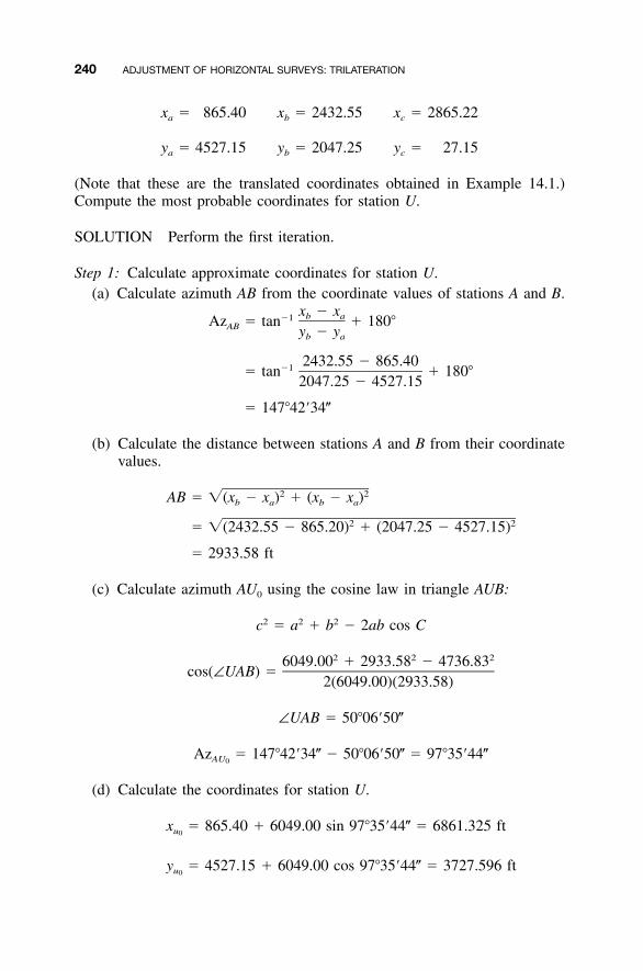
240 ADJUSTMENT OF HORIZONTAL SURVEYS: TRILATERATION
x � 865.40 x � 2432.55 x � 2865.22a b c
y � 4527.15 y � 2047.25 y � 27.15a b c
(Note that these are the translated coordinates obtained in Example 14.1.)Compute the most probable coordinates for station U.
SOLUTION Perform the first iteration.
Step 1: Calculate approximate coordinates for station U.(a) Calculate azimuth AB from the coordinate values of stations A and B.
x � xb a�1Az � tan � 180�AB y � yb a
2432.55 � 865.40�1� tan � 180�
2047.25 � 4527.15
� 147�42�34�
(b) Calculate the distance between stations A and B from their coordinatevalues.
2 2AB � �(x � x ) � (x � x )b a b a
2 2� �(2432.55 � 865.20) � (2047.25 � 4527.15)
� 2933.58 ft
(c) Calculate azimuth AU0 using the cosine law in triangle AUB:
2 2 2c � a � b � 2ab cos C
2 2 26049.00 � 2933.58 � 4736.83cos(∠UAB) �
2(6049.00)(2933.58)
∠UAB � 50�06�50�
Az � 147�42�34� � 50�06�50� � 97�35�44�AU0
(d) Calculate the coordinates for station U.
x � 865.40 � 6049.00 sin 97�35�44� � 6861.325 ftu0
y � 4527.15 � 6049.00 cos 97�35�44� � 3727.596 ftu0
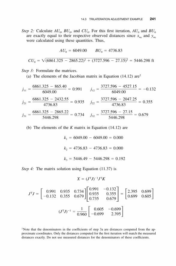
14.3 TRILATERATION ADJUSTMENT EXAMPLE 241
Step 2: Calculate AU0, BU0, and CU0. For this first iteration, AU0 and BU0
are exactly equal to their respective observed distances since andx yu u0 0
were calculated using these quantities. Thus,
AU � 6049.00 BU � 4736.830 0
2 2CU � �(6861.325 � 2865.22) � (3727.596 � 27.15) � 5446.298 ft0
Step 3: Formulate the matrices.(a) The elements of the Jacobian matrix in Equation (14.12) are2
6861.325 � 865.40 3727.596 � 4527.15j � � 0.991 j � � �0.13211 126049.00 6049.00
6861.325 � 2432.55 3727.596 � 2047.25j � � 0.935 j � � 0.35521 224736.83 4736.83
6861.325 � 2865.22 3727.596 � 27.15j � � 0.734 j � � 0.67931 325446.298 5446.298
(b) The elements of the K matrix in Equation (14.12) are
k � 6049.00 � 6049.00 � 0.0001
k � 4736.83 � 4736.83 � 0.0002
k � 5446.49 � 5446.298 � 0.1923
Step 4: The matrix solution using Equation (11.37) is
T �1 TX � (J J) J K
0.991 �0.1320.991 0.935 0.734 2.395 0.699TJ J � 0.935 0.355 �� � � ��0.132 0.355 0.679 0.699 0.605� �0.735 0.679
1 0.605 �0.699T �1(J J) � � ��0.699 2.3950.960
2 Note that the denominators in the coefficients of step 3a are distances computed from the ap-proximate coordinates. Only the distances computed for the first iteration will match the measureddistances exactly. Do not use measured distances for the denominators of these coefficients.
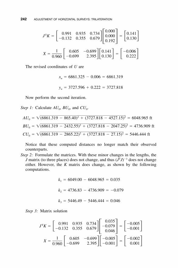
242 ADJUSTMENT OF HORIZONTAL SURVEYS: TRILATERATION
0.0000.991 0.935 0.734 0.141TJ K � 0.000 �� � � ��0.132 0.355 0.679 0.130� �0.192
1 0.605 �0.699 0.141 �0.006X � �� �� � � ��0.699 2.395 0.130 0.2220.960
The revised coordinates of U are
x � 6861.325 � 0.006 � 6861.319u
y � 3727.596 � 0.222 � 3727.818u
Now perform the second iteration.
Step 1: Calculate AU0, BU0, and CU0.
2 2AU � �(6861.319 � 865.40) � (3727.818 � 4527.15) � 6048.965 ft0
2 2BU � �(6861.319 � 2432.55) � (3727.818 � 2047.25) � 4736.909 ft0
2 2CU � �(6861.319 � 2865.22) � (3727.818 � 27.15) � 5446.444 ft0
Notice that these computed distances no longer match their observedcounterparts.
Step 2: Formulate the matrices. With these minor changes in the lengths, theJ matrix (to three places) does not change, and thus (JTJ)�1 does not changeeither. However, the K matrix does change, as shown by the followingcomputations.
k � 6049.00 � 6048.965 � 0.0351
k � 4736.83 � 4736.909 � �0.0792
k � 5446.49 � 5446.444 � 0.0463
Step 3: Matrix solution
0.0350.991 0.935 0.734 �0.005TJ K � �0.079 �� � � ��0.132 0.355 0.679 �0.001� �0.046
1 0.605 �0.699 �0.005 �0.002X � �� �� � � ��0.699 2.395 �0.001 0.0010.960

14.4 FORMULATION OF A GENERALIZED COEFFICIENT MATRIX 243
The revised coordinates of U are
x � 6861.319 � 0.002 � 6861.317u
y � 3727.818 � 0.001 � 3727.819u
Satisfactory convergence is shown by the very small corrections in thesecond iteration. This problem has also been solved using the program AD-JUST. Values computed include the most probable coordinates for station U,their standard deviations, the adjusted lengths of the observed distances, theirresiduals and standard deviations, and the reference variance and referencestandard deviation. These are tabulated as shown below.
*****************Adjusted stations*****************Station X Y Sx Sy========================================================
U 6,861.32 3,727.82 0.078 0.154
*******************************Adjusted Distance Observations*******************************Station StationOccupied Sighted Distance V S========================================================
A U 6,048.96 �0.037 0.090B U 4,736.91 0.077 0.060C U 5,446.44 �0.047 0.085
Adjustment Statistics
� 0.009542S0S0 � �0.10
14.4 FORMULATION OF A GENERALIZED COEFFICIENT MATRIXFOR A MORE COMPLEX NETWORK
In the trilaterated network of Figure 14.3, all lines were observed. Assumethat stations A and C are control stations. For this network, there are 10observations and eight unknowns. Stations A and C can be fixed by givingthe terms dxa, dya, dxc, and dyc zero coefficients, which effectively drops these

244 ADJUSTMENT OF HORIZONTAL SURVEYS: TRILATERATION
Figure 14.3 Trilateration network.
TABLE 14.1 Structure of the Normal Matrix for the Complex Network inFigure 14.3
Distance,IJ
Unknown
dxb dyb dxd dyd dxe dye dxƒ dyƒ
AB dxj dyj 0 0 0 0 0 0AE 0 0 0 0 dxj dyj 0 0BC dxi dyi 0 0 0 0 0 0BF dxi dyi 0 0 0 0 dxj dyj
BE dxi dyi 0 0 dxj dyj 0 0CD 0 0 dxj dyj 0 0 0 0CF 0 0 0 0 0 0 dxj dyj
DF 0 0 dxi dyi 0 0 dxj dyj
DE 0 0 dxi dyi dxj dyj 0 0EF 0 0 0 0 dxi dyi dxj dyj
terms from the solution. The coefficient matrix formulated from prototypeequation (14.9) has nonzero elements, as indicated in Table 14.1. In this tablethe appropriate coefficient from Equation (14.9) is indicated by its corre-sponding unknown terms of dxi, dyi, dxj, or dyj.
14.5 COMPUTER SOLUTION OF A TRILATERATED QUADRILATERAL
The quadrilateral shown in Figure 14.4 was adjusted using the softwareMATRIX. In this problem, points Bucky and Badger are control stationswhose coordinates are held fixed. The five distances observed are:
Line Distance (ft)
Badger–Wisconsin 5870.302Badger–Campus 7297.588Wisconsin–Campus 3616.434Wisconsin–Bucky 5742.878Campus–Bucky 5123.760
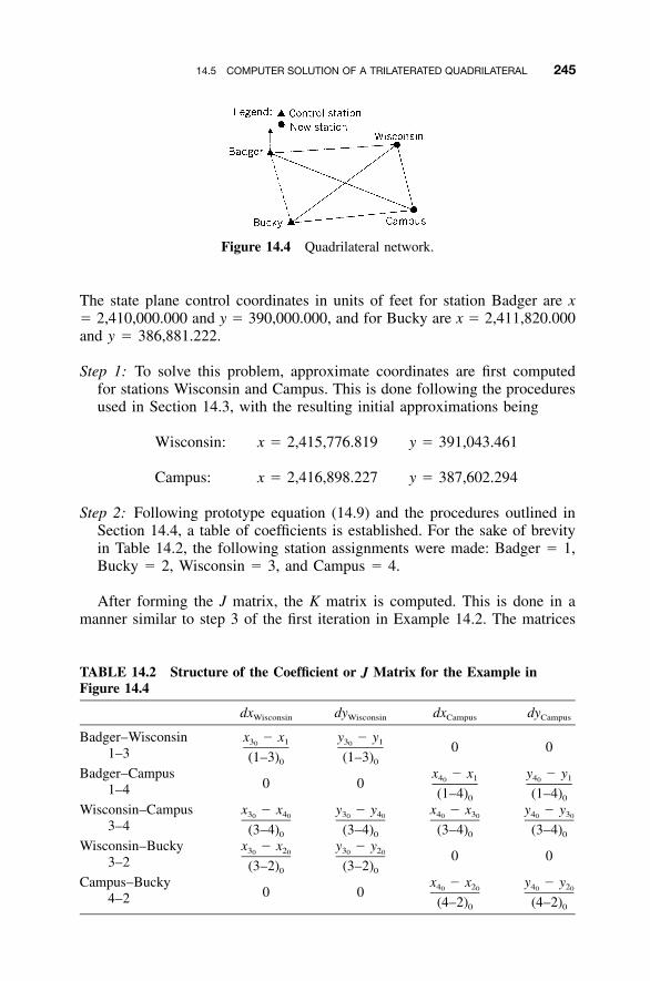
14.5 COMPUTER SOLUTION OF A TRILATERATED QUADRILATERAL 245
Figure 14.4 Quadrilateral network.
TABLE 14.2 Structure of the Coefficient or J Matrix for the Example inFigure 14.4
dxWisconsin dyWisconsin dxCampus dyCampus
Badger–Wisconsin1–3
x � x3 10
(1–3)0
y � y3 10
(1–3)0
0 0
Badger–Campus1–4 0 0
x � x4 10
(1–4)0
y � y4 10
(1–4)0
Wisconsin–Campus3–4
x � x3 40 0
(3–4)0
y � y3 40 0
(3–4)0
x � x4 30 0
(3–4)0
y � y4 30 0
(3–4)0
Wisconsin–Bucky3–2
x � x3 20 0
(3–2)0
y � y3 20 0
(3–2)0
0 0
Campus–Bucky4–2 0 0
x � x4 20 0
(4–2)0
y � y4 20 0
(4–2)0
The state plane control coordinates in units of feet for station Badger are x� 2,410,000.000 and y � 390,000.000, and for Bucky are x � 2,411,820.000and y � 386,881.222.
Step 1: To solve this problem, approximate coordinates are first computedfor stations Wisconsin and Campus. This is done following the proceduresused in Section 14.3, with the resulting initial approximations being
Wisconsin: x � 2,415,776.819 y � 391,043.461
Campus: x � 2,416,898.227 y � 387,602.294
Step 2: Following prototype equation (14.9) and the procedures outlined inSection 14.4, a table of coefficients is established. For the sake of brevityin Table 14.2, the following station assignments were made: Badger � 1,Bucky � 2, Wisconsin � 3, and Campus � 4.
After forming the J matrix, the K matrix is computed. This is done in amanner similar to step 3 of the first iteration in Example 14.2. The matrices
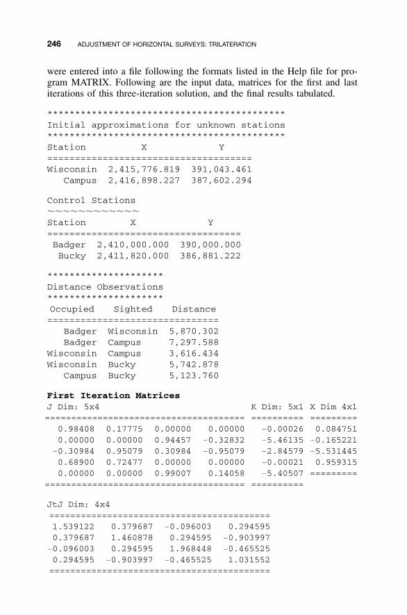
246 ADJUSTMENT OF HORIZONTAL SURVEYS: TRILATERATION
were entered into a file following the formats listed in the Help file for pro-gram MATRIX. Following are the input data, matrices for the first and lastiterations of this three-iteration solution, and the final results tabulated.
*******************************************Initial approximations for unknown stations*******************************************Station X Y=====================================Wisconsin 2,415,776.819 391,043.461
Campus 2,416,898.227 387,602.294
Control StationsStation X Y===================================Badger 2,410,000.000 390,000.000Bucky 2,411,820.000 386,881.222
*********************Distance Observations*********************Occupied Sighted Distance===============================
Badger Wisconsin 5,870.302Badger Campus 7,297.588
Wisconsin Campus 3,616.434Wisconsin Bucky 5,742.878
Campus Bucky 5,123.760
First Iteration MatricesJ Dim: 5x4======================================
K Dim: 5x1==========
X Dim 4x1=========
0.98408 0.17775 0.00000 0.00000 �0.00026 0.0847510.00000 0.00000 0.94457 �0.32832 �5.46135 �0.165221
�0.30984 0.95079 0.30984 �0.95079 �2.84579 �5.5314450.68900 0.72477 0.00000 0.00000 �0.00021 0.9593150.00000 0.00000 0.99007 0.14058 �5.40507 =========
====================================== ==========
JtJ Dim: 4x4==========================================1.539122 0.379687 �0.096003 0.2945950.379687 1.460878 0.294595 �0.903997
�0.096003 0.294595 1.968448 �0.4655250.294595 �0.903997 �0.465525 1.031552==========================================
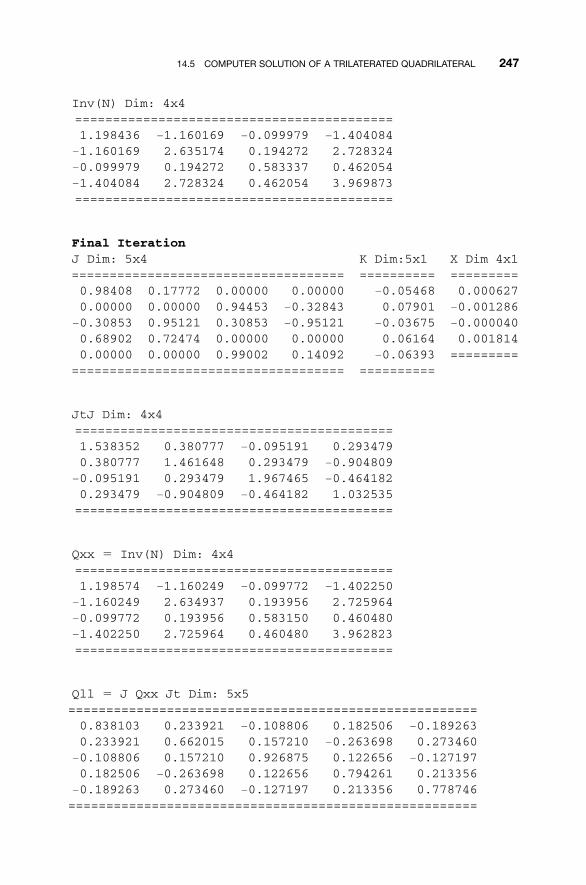
14.5 COMPUTER SOLUTION OF A TRILATERATED QUADRILATERAL 247
Inv(N) Dim: 4x4==========================================1.198436 �1.160169 �0.099979 �1.404084
�1.160169 2.635174 0.194272 2.728324�0.099979 0.194272 0.583337 0.462054�1.404084 2.728324 0.462054 3.969873==========================================
Final IterationJ Dim: 5x4====================================
K Dim:5x1==========
X Dim 4x1=========
0.98408 0.17772 0.00000 0.00000 �0.05468 0.0006270.00000 0.00000 0.94453 �0.32843 0.07901 �0.001286
�0.30853 0.95121 0.30853 �0.95121 �0.03675 �0.0000400.68902 0.72474 0.00000 0.00000 0.06164 0.0018140.00000 0.00000 0.99002 0.14092 �0.06393 =========
==================================== ==========
JtJ Dim: 4x4==========================================1.538352 0.380777 �0.095191 0.2934790.380777 1.461648 0.293479 �0.904809
�0.095191 0.293479 1.967465 �0.4641820.293479 �0.904809 �0.464182 1.032535==========================================
Qxx � Inv(N) Dim: 4x4==========================================1.198574 �1.160249 �0.099772 �1.402250
�1.160249 2.634937 0.193956 2.725964�0.099772 0.193956 0.583150 0.460480�1.402250 2.725964 0.460480 3.962823==========================================
Qll � J Qxx Jt Dim: 5x5======================================================0.838103 0.233921 �0.108806 0.182506 �0.1892630.233921 0.662015 0.157210 �0.263698 0.273460
�0.108806 0.157210 0.926875 0.122656 �0.1271970.182506 �0.263698 0.122656 0.794261 0.213356
�0.189263 0.273460 �0.127197 0.213356 0.778746======================================================

248 ADJUSTMENT OF HORIZONTAL SURVEYS: TRILATERATION
*****************Adjusted stations*****************Station X Y Sx Sy=====================================================Wisconsin 2,415,776.904 391,043.294 0.1488 0.2206
Campus 2,416,892.696 387,603.255 0.1038 0.2705
*******************************Adjusted Distance Observations*******************************Occupied Sighted Distance V S===============================================
Badger Wisconsin 5,870.357 0.055 0.1244Badger Campus 7,297.509 �0.079 0.1106
Wisconsin Campus 3,616.471 0.037 0.1308Wisconsin Bucky 5,742.816 �0.062 0.1211
Campus Bucky 5,123.824 0.064 0.1199
-----Reference Standard Deviation � �0.135905-----Iterations » 3
Notes
1. As noted earlier, it is important that observed distances not be used inthe denominator of the coefficients matrix, J. This is not only theoret-ically incorrect but can cause slight differences in the final solution, oreven worse, it can cause the system to diverge from any solution! Al-ways compute distances based on the current approximate coordinates.
2. The final portion of the output lists the adjusted x and y coordinates ofthe stations, the reference standard deviation, the standard deviations ofthe adjusted coordinates, the adjusted line lengths, and their residuals.
3. The Qxx matrix was listed on the last iteration only. It is needed forcalculating the estimated errors of the adjusted coordinates using Equa-tion (14.24) and is also necessary for calculating error ellipses. Thesubject of error ellipses is discussed in Chapter 19.
14.6 ITERATION TERMINATION
When programming a nonlinear least squares adjustment, some criteria mustbe established to determine the appropriate point at which to stop the iterationprocess. Since it is possible to have a set of data that has no solution, it isalso important to determine when that condition occurs. In this section we
14.6 ITERATION TERMINATION 249
describe three methods commonly used to indicate the appropriate time toend the iteration process.
14.6.1 Method of Maximum Iterations
The simplest procedure of iteration termination involves limiting the numberof iterations to a predetermined maximum. The risk with this method is thatif this maximum is too low, a solution may not be reached at the conclusionof the process, and if it is too high, time is wasted on unnecessary iterations.Although this method does not assure convergence, it can prevent the ad-justment from continuing indefinitely, which could occur if the solution di-verges. When good initial approximations are supplied for the unknownparameters, a limit of 10 iterations should be well beyond what is requiredfor a solution since the least squares method converges quadratically.
14.6.2 Maximum Correction
This method was used in earlier examples. It involves monitoring the absolutesize of the corrections. When all corrections become negligibly small, theiteration process is stopped. The term negligible is relative. For example, ifdistances are observed to the nearest foot, it would be foolish to assume thatthe size of the corrections will become less than some small fraction of afoot. Generally, negligible is interpreted as a correction that is less than one-half the least count of the smallest unit of measure. For instance, if all dis-tances are observed to the nearest 0.01 ft, it would be appropriate to assumeconvergence when the absolute size of all corrections is less than 0.005 ft.Although the solution may continue to converge with continued iterations,the work to get these corrections is not warranted based on the precision ofthe observations.
14.6.3 Monitoring the Adjustment’s Reference Variance
The best method for determining convergence involves monitoring the ref-erence variance and its changes between iterations. Since the least squaresmethod converges quadratically, the iteration process should definitely bestopped if the reference variance increases. An increasing reference variancesuggests a diverging solution, which happens when one of two things hasoccurred: (1) a large blunder exists in the data set and no solution is possible,or (2) the maximum correction size is less than the precision of the obser-vations. In the second case, the best solution for the given data set has alreadybeen reached, and when another iteration is attempted, the solution will con-verge, only to diverge on the next iteration. This apparent bouncing in thesolution is caused by convergence limits being too stringent for the qualityof the data.
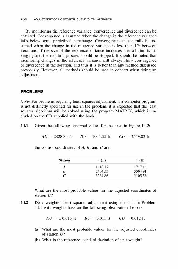
250 ADJUSTMENT OF HORIZONTAL SURVEYS: TRILATERATION
By monitoring the reference variance, convergence and divergence can bedetected. Convergence is assumed when the change in the reference variancefalls below some predefined percentage. Convergence can generally be as-sumed when the change in the reference variance is less than 1% betweeniterations. If the size of the reference variance increases, the solution is di-verging and the iteration process should be stopped. It should be noted thatmonitoring changes in the reference variance will always show convergenceor divergence in the solution, and thus it is better than any method discussedpreviously. However, all methods should be used in concert when doing anadjustment.
PROBLEMS
Note: For problems requiring least squares adjustment, if a computer programis not distinctly specified for use in the problem, it is expected that the leastsquares algorithm will be solved using the program MATRIX, which is in-cluded on the CD supplied with the book.
14.1 Given the following observed values for the lines in Figure 14.2:
AU � 2828.83 ft BU � 2031.55 ft CU � 2549.83 ft
the control coordinates of A, B, and C are:
Station x (ft) y (ft)
A 1418.17 4747.14B 2434.53 3504.91C 3234.86 2105.56
What are the most probable values for the adjusted coordinates ofstation U?
14.2 Do a weighted least squares adjustment using the data in Problem14.1 with weights base on the following observational errors.
AU � �0.015 ft BU � 0.011 ft CU � 0.012 ft
(a) What are the most probable values for the adjusted coordinatesof station U?
(b) What is the reference standard deviation of unit weight?
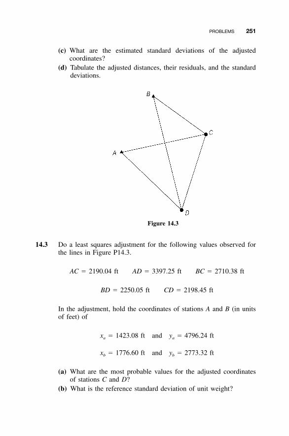
PROBLEMS 251
(c) What are the estimated standard deviations of the adjustedcoordinates?
(d) Tabulate the adjusted distances, their residuals, and the standarddeviations.
Figure 14.3
14.3 Do a least squares adjustment for the following values observed forthe lines in Figure P14.3.
AC � 2190.04 ft AD � 3397.25 ft BC � 2710.38 ft
BD � 2250.05 ft CD � 2198.45 ft
In the adjustment, hold the coordinates of stations A and B (in unitsof feet) of
x � 1423.08 ft and y � 4796.24 fta a
x � 1776.60 ft and y � 2773.32 ftb b
(a) What are the most probable values for the adjusted coordinatesof stations C and D?
(b) What is the reference standard deviation of unit weight?
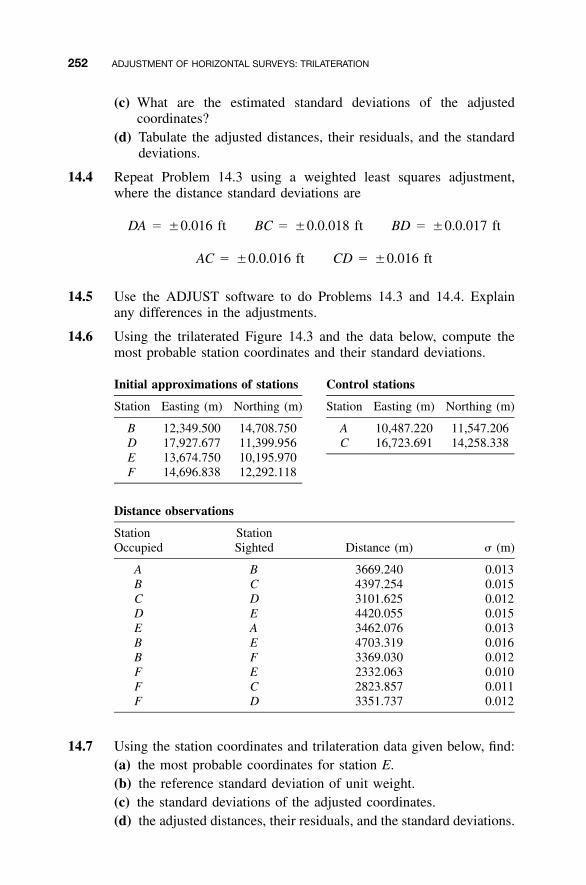
252 ADJUSTMENT OF HORIZONTAL SURVEYS: TRILATERATION
(c) What are the estimated standard deviations of the adjustedcoordinates?
(d) Tabulate the adjusted distances, their residuals, and the standarddeviations.
14.4 Repeat Problem 14.3 using a weighted least squares adjustment,where the distance standard deviations are
DA � �0.016 ft BC � �0.0.018 ft BD � �0.0.017 ft
AC � �0.0.016 ft CD � �0.016 ft
14.5 Use the ADJUST software to do Problems 14.3 and 14.4. Explainany differences in the adjustments.
14.6 Using the trilaterated Figure 14.3 and the data below, compute themost probable station coordinates and their standard deviations.
Initial approximations of stations Control stations
Station Easting (m) Northing (m) Station Easting (m) Northing (m)
B 12,349.500 14,708.750 A 10,487.220 11,547.206DEF
17,927.67713,674.75014,696.838
11,399.95610,195.97012,292.118
C 16,723.691 14,258.338
Distance observations
StationOccupied
StationSighted Distance (m) � (m)
A B 3669.240 0.013B C 4397.254 0.015C D 3101.625 0.012D E 4420.055 0.015E A 3462.076 0.013B E 4703.319 0.016B F 3369.030 0.012F E 2332.063 0.010F C 2823.857 0.011F D 3351.737 0.012
14.7 Using the station coordinates and trilateration data given below, find:(a) the most probable coordinates for station E.(b) the reference standard deviation of unit weight.(c) the standard deviations of the adjusted coordinates.(d) the adjusted distances, their residuals, and the standard deviations.
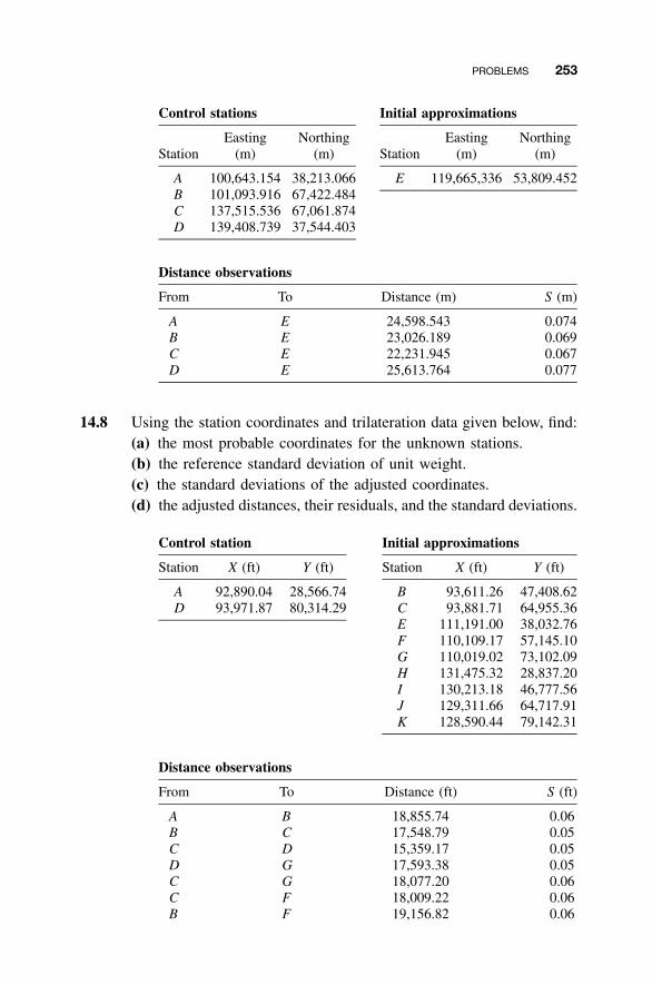
PROBLEMS 253
Control stations Initial approximations
StationEasting
(m)Northing
(m) StationEasting
(m)Northing
(m)
ABCD
100,643.154101,093.916137,515.536139,408.739
38,213.06667,422.48467,061.87437,544.403
E 119,665,336 53,809.452
Distance observations
From To Distance (m) S (m)
A E 24,598.543 0.074B E 23,026.189 0.069C E 22,231.945 0.067D E 25,613.764 0.077
14.8 Using the station coordinates and trilateration data given below, find:(a) the most probable coordinates for the unknown stations.(b) the reference standard deviation of unit weight.(c) the standard deviations of the adjusted coordinates.(d) the adjusted distances, their residuals, and the standard deviations.
Control station Initial approximations
Station X (ft) Y (ft) Station X (ft) Y (ft)
AD
92,890.0493,971.87
28,566.7480,314.29
BCEFGHIJK
93,611.2693,881.71
111,191.00110,109.17110,019.02131,475.32130,213.18129,311.66128,590.44
47,408.6264,955.3638,032.7657,145.1073,102.0928,837.2046,777.5664,717.9179,142.31
Distance observations
From To Distance (ft) S (ft)
A B 18,855.74 0.06B C 17,548.79 0.05C D 15,359.17 0.05D G 17,593.38 0.05C G 18,077.20 0.06C F 18,009.22 0.06B F 19,156.82 0.06
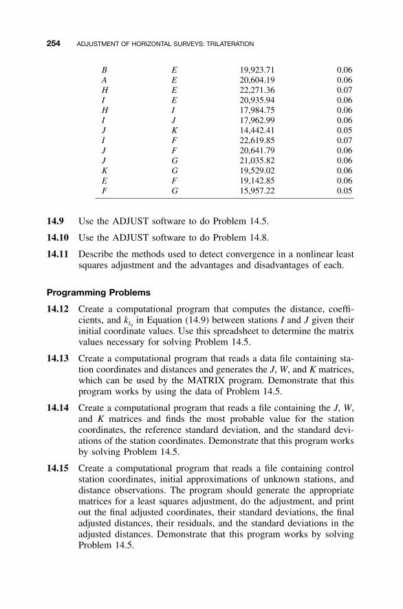
254 ADJUSTMENT OF HORIZONTAL SURVEYS: TRILATERATION
B E 19,923.71 0.06A E 20,604.19 0.06H E 22,271.36 0.07I E 20,935.94 0.06H I 17,984.75 0.06I J 17,962.99 0.06J K 14,442.41 0.05I F 22,619.85 0.07J F 20,641.79 0.06J G 21,035.82 0.06K G 19,529.02 0.06E F 19,142.85 0.06F G 15,957.22 0.05
14.9 Use the ADJUST software to do Problem 14.5.
14.10 Use the ADJUST software to do Problem 14.8.
14.11 Describe the methods used to detect convergence in a nonlinear leastsquares adjustment and the advantages and disadvantages of each.
Programming Problems
14.12 Create a computational program that computes the distance, coeffi-cients, and in Equation (14.9) between stations I and J given theirklij
initial coordinate values. Use this spreadsheet to determine the matrixvalues necessary for solving Problem 14.5.
14.13 Create a computational program that reads a data file containing sta-tion coordinates and distances and generates the J, W, and K matrices,which can be used by the MATRIX program. Demonstrate that thisprogram works by using the data of Problem 14.5.
14.14 Create a computational program that reads a file containing the J, W,and K matrices and finds the most probable value for the stationcoordinates, the reference standard deviation, and the standard devi-ations of the station coordinates. Demonstrate that this program worksby solving Problem 14.5.
14.15 Create a computational program that reads a file containing controlstation coordinates, initial approximations of unknown stations, anddistance observations. The program should generate the appropriatematrices for a least squares adjustment, do the adjustment, and printout the final adjusted coordinates, their standard deviations, the finaladjusted distances, their residuals, and the standard deviations in theadjusted distances. Demonstrate that this program works by solvingProblem 14.5.
255
CHAPTER 15
ADJUSTMENT OF HORIZONTALSURVEYS: TRIANGULATION
15.1 INTRODUCTION
Prior to the development of electronic distance measuring equipment and theglobal positioning system, triangulation was the preferred method for extend-ing horizontal control over long distances. The positions of widely spacedstations were computed from measured angles and a minimal number of mea-sured distances called baselines. This method was used extensively by theNational Geodetic Survey in extending much of the national network. Tri-angulation is still used by many surveyors in establishing horizontal control,although surveys that combine trilateration (distance observations) with tri-angulation (angle observations) are more common. In this chapter, methodsare described for adjusting triangulation networks using least squares.
A least squares triangulation adjustment can use condition equations orobservation equations written in terms of either azimuths or angles. In thischapter the observation equation method is presented. The procedure involvesa parametric adjustment where the parameters are coordinates in a plane rec-tangular system such as state plane coordinates. In the examples, the specifictypes of triangulations known as intersections, resections, and quadrilateralsare adjusted.
15.2 AZIMUTH OBSERVATION EQUATION
The azimuth equation in parametric form is
azimuth � � � C (15.1)
Adjustment Computations: Spatial Data Analysis, Fourth Edition. C. D. Ghilani and P. R. Wolf© 2006 John Wiley & Sons, Inc. ISBN: 978-0-471-69728-2
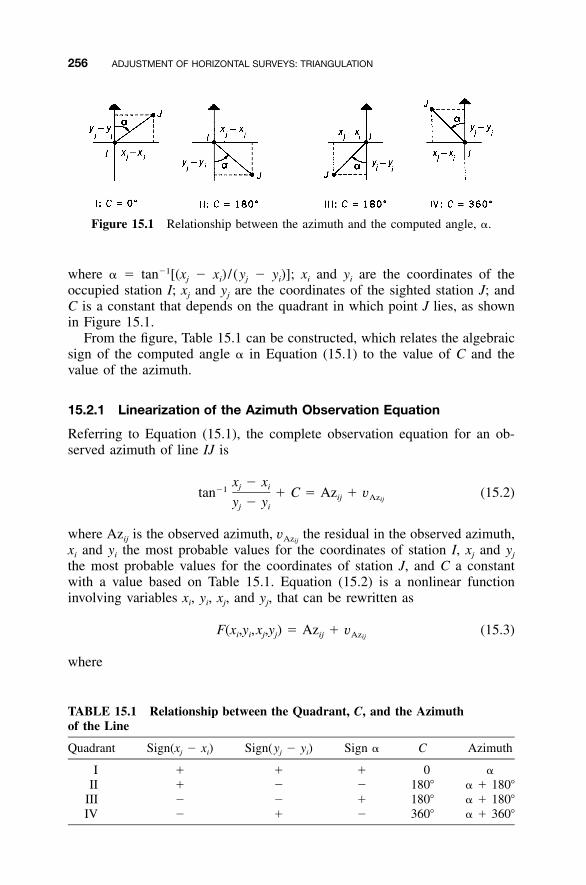
256 ADJUSTMENT OF HORIZONTAL SURVEYS: TRIANGULATION
Figure 15.1 Relationship between the azimuth and the computed angle, �.
TABLE 15.1 Relationship between the Quadrant, C, and the Azimuthof the Line
Quadrant Sign(xj � xi) Sign(yj � yi) Sign � C Azimuth
I � � � 0 �II � � � 180� � � 180�
III � � � 180� � � 180�IV � � � 360� � � 360�
where � � tan�1[(xj � xi) /(yj � yi)]; xi and yi are the coordinates of theoccupied station I; xj and yj are the coordinates of the sighted station J; andC is a constant that depends on the quadrant in which point J lies, as shownin Figure 15.1.
From the figure, Table 15.1 can be constructed, which relates the algebraicsign of the computed angle � in Equation (15.1) to the value of C and thevalue of the azimuth.
15.2.1 Linearization of the Azimuth Observation Equation
Referring to Equation (15.1), the complete observation equation for an ob-served azimuth of line IJ is
x � xj i�1tan � C � Az � v (15.2)ij Azijy � yj i
where Azij is the observed azimuth, the residual in the observed azimuth,vAzij
xi and yi the most probable values for the coordinates of station I, xj and yj
the most probable values for the coordinates of station J, and C a constantwith a value based on Table 15.1. Equation (15.2) is a nonlinear functioninvolving variables xi, yi, xj, and yj, that can be rewritten as
F(x ,y ,x ,y ) � Az � v (15.3)i i j j ij Azij
where
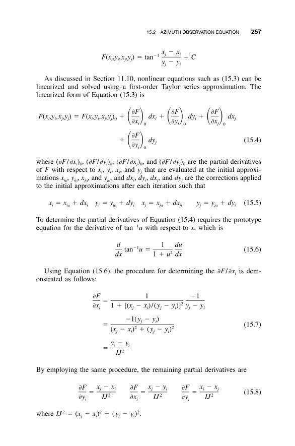
15.2 AZIMUTH OBSERVATION EQUATION 257
x � xj i�1F(x ,y ,x ,y ) � tan � Ci i j j y � yj i
As discussed in Section 11.10, nonlinear equations such as (15.3) can belinearized and solved using a first-order Taylor series approximation. Thelinearized form of Equation (15.3) is
�F �F �FF(x ,y ,x ,y ) � F(x ,y ,x ,y ) � dx � dy � dx� � � � � �i i j j i i j j 0 i i j�x �y �xi i j0 0 0
�F� dy (15.4)� � j�yj 0
where (�F /�xi)0, (�F /�yi)0, (�F /�xj)0, and (�F /�yj)0 are the partial derivativesof F with respect to xi, yi, xj, and yj that are evaluated at the initial approxi-mations and and dxi, dyi, dxj, and dyj are the corrections appliedx , y , x , y ,i i j j0 0 0 0
to the initial approximations after each iteration such that
x � x � dx y � y � dy x � x � dx y � y � dy (15.5)i i i i i i j j ji j j i0 0 0 0
To determine the partial derivatives of Equation (15.4) requires the prototypeequation for the derivative of tan�1u with respect to x, which is
d 1 du�1tan u � (15.6)2dx 1 � u dx
Using Equation (15.6), the procedure for determining the �F /�xi is dem-onstrated as follows:
�F 1 �1� 2�x 1 � [(x � x ) /(y � y )] y � yi j i j i j i
�1(y � y )j i� (15.7)2 2(x � x ) � (y � y )j i j i
y � yi j� 2IJ
By employing the same procedure, the remaining partial derivatives are
x � x x � y x � x�F �F �Fj i j i i j� � � (15.8)2 2 2�y IJ �x IJ �y IJi j j
where IJ2 � (xj � xi)2 � (yj � yi)
2.
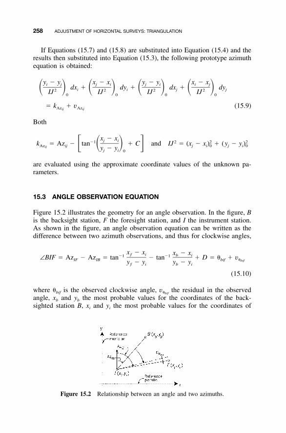
258 ADJUSTMENT OF HORIZONTAL SURVEYS: TRIANGULATION
Figure 15.2 Relationship between an angle and two azimuths.
If Equations (15.7) and (15.8) are substituted into Equation (15.4) and theresults then substituted into Equation (15.3), the following prototype azimuthequation is obtained:
y � y x � x y � y x � xi j j i j i i jdx � dy � dx � dy� � � � � � � �i i j j2 2 2 2IJ IJ IJ IJ0 0 0 0
� k � v (15.9)Az Azij ij
Both
x � xj i�1 2 2 2k � Az � tan � C and IJ � (x � x ) � (y � y )� � � �Az ij j i 0 j i 0ij y � yj i 0
are evaluated using the approximate coordinate values of the unknown pa-rameters.
15.3 ANGLE OBSERVATION EQUATION
Figure 15.2 illustrates the geometry for an angle observation. In the figure, Bis the backsight station, F the foresight station, and I the instrument station.As shown in the figure, an angle observation equation can be written as thedifference between two azimuth observations, and thus for clockwise angles,
x � x x � xƒ i b i�1 �1∠BIF � Az � Az � tan � tan � D � � � vIF IB bif �bify � y y � yƒ i b i
(15.10)
where �bif is the observed clockwise angle, the residual in the observedv�bif
angle, xb and yb the most probable values for the coordinates of the back-sighted station B, xi and yi the most probable values for the coordinates of
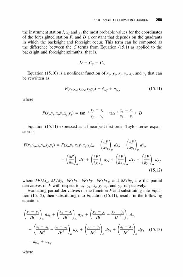
15.3 ANGLE OBSERVATION EQUATION 259
the instrument station I, xƒ and yƒ the most probable values for the coordinatesof the foresighted station F, and D a constant that depends on the quadrantsin which the backsight and foresight occur. This term can be computed asthe difference between the C terms from Equation (15.1) as applied to thebacksight and foresight azimuths; that is,
D � C � Cif ib
Equation (15.10) is a nonlinear function of xb, yb, xi, yi, xƒ, and yƒ that canbe rewritten as
F(x ,y ,x ,y ,x ,y ) � � � v (15.11)b b i i ƒ ƒ bif �bif
where
x � x x � xƒ i b i�1 �1F(x ,y ,x ,y ,x ,y ) � tan � tan � Db b i i ƒ ƒ y � y y � yƒ i b i
Equation (15.11) expressed as a linearized first-order Taylor series expan-sion is
�F �FF(x ,y ,x ,y ,x ,y ) � F(x ,y ,x ,y ,x ,y ) � dx � dy� � � �b b i i ƒ ƒ b b i i ƒ ƒ 0 b b�x �yb b0 0
�F �F �F �F� dx � dy � dx � dy� � � � � � � �i i ƒ ƒ�x �y �x �yi i ƒ ƒ0 0 0 0
(15.12)
where �F /�xb, �F /�yb, �F /�xi, �F /�yi, �F /�xƒ, and �F /�yƒ are the partialderivatives of F with respect to xb, yb, xi, yi, xƒ, and yƒ, respectively.
Evaluating partial derivatives of the function F and substituting into Equa-tion (15.12), then substituting into Equation (15.11), results in the followingequation:
y � yy � y x � x y � y ƒ ii b b i b idx � dy � � dx� � � � � �b b i2 2 2 2IB IB IB IF0 0 0
x � x y � y x � xx � x i ƒ ƒ i i ƒi b� � dy � dx � dy (15.13)� � � � � �i ƒ ƒ2 2 2 2IB IF IF IF0 0 0
� k � v� �bif bif
where
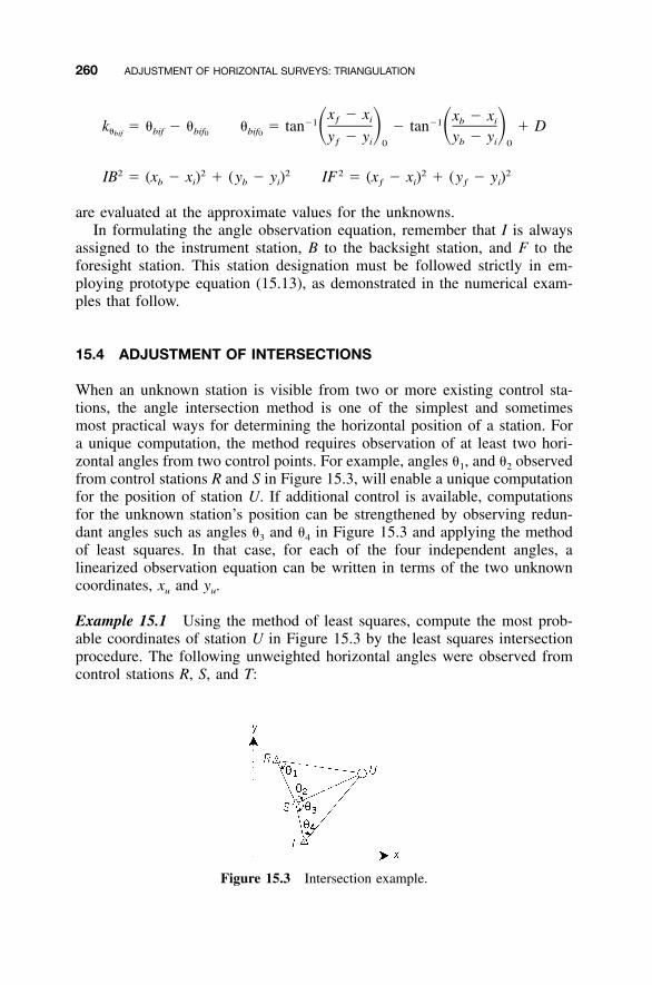
260 ADJUSTMENT OF HORIZONTAL SURVEYS: TRIANGULATION
Figure 15.3 Intersection example.
x � x x � xƒ i b i�1 �1k � � � � � � tan � tan � D� � � �� bif bif bifbif 0 0 y � y y � yƒ i b i0 0
2 2 2 2 2 2IB � (x � x ) � (y � y ) IF � (x � x ) � (y � y )b i b i ƒ i ƒ i
are evaluated at the approximate values for the unknowns.In formulating the angle observation equation, remember that I is always
assigned to the instrument station, B to the backsight station, and F to theforesight station. This station designation must be followed strictly in em-ploying prototype equation (15.13), as demonstrated in the numerical exam-ples that follow.
15.4 ADJUSTMENT OF INTERSECTIONS
When an unknown station is visible from two or more existing control sta-tions, the angle intersection method is one of the simplest and sometimesmost practical ways for determining the horizontal position of a station. Fora unique computation, the method requires observation of at least two hori-zontal angles from two control points. For example, angles �1, and �2 observedfrom control stations R and S in Figure 15.3, will enable a unique computationfor the position of station U. If additional control is available, computationsfor the unknown station’s position can be strengthened by observing redun-dant angles such as angles �3 and �4 in Figure 15.3 and applying the methodof least squares. In that case, for each of the four independent angles, alinearized observation equation can be written in terms of the two unknowncoordinates, xu and yu.
Example 15.1 Using the method of least squares, compute the most prob-able coordinates of station U in Figure 15.3 by the least squares intersectionprocedure. The following unweighted horizontal angles were observed fromcontrol stations R, S, and T:
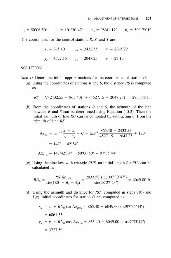
15.4 ADJUSTMENT OF INTERSECTIONS 261
� � 50�06�50� � � 101�30�47� � � 98�41�17� � � 59�17�01�1 2 3 4
The coordinates for the control stations R, S, and T are
x � 865.40 x � 2432.55 x � 2865.22r s t
y � 4527.15 y � 2047.25 y � 27.15r s t
SOLUTION
Step 1: Determine initial approximations for the coordinates of station U.(a) Using the coordinates of stations R and S, the distance RS is computed
as
2 2RS � �(2432.55 � 865.40) � (4527.15 � 2047.25) � 2933.58 ft
(b) From the coordinates of stations R and S, the azimuth of the linebetween R and S can be determined using Equation (15.2). Then theinitial azimuth of line RU can be computed by subtracting �1 from theazimuth of line RS:
x � x 865.40 � 2432.55s r�1 �1Az � tan � C � tan � 180�RS y � y 4527.15 � 2047.25s r
� 147� � 42�34�
Az � 147�42�34� � 50�06�50� � 97�35�44�RU0
(c) Using the sine law with triangle RUS, an initial length for RU0 can becalculated as
RS sin � 2933.58 sin(100�30�47�)2RU � � � 6049.00 ft0 sin(180� � � � � ) sin(28�27�23�)1 2
(d) Using the azimuth and distance for RU0 computed in steps 1(b) and1(c), initial coordinates for station U are computed as
x � x � RU sin Az � 865.40 � 6049.00 sin(97�35�44�)u r 0 RU0 0
� 6861.35
y � y � RU cos Az � 865.40 � 6049.00 cos(97�35�44�)u r 0 RU0 0
� 3727.59
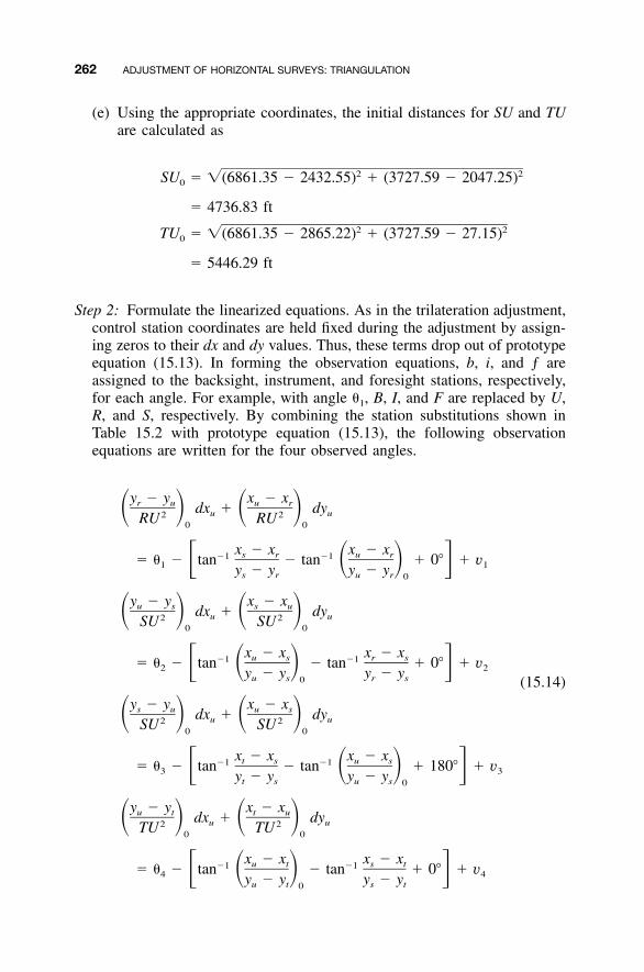
262 ADJUSTMENT OF HORIZONTAL SURVEYS: TRIANGULATION
(e) Using the appropriate coordinates, the initial distances for SU and TUare calculated as
2 2SU � �(6861.35 � 2432.55) � (3727.59 � 2047.25)0
� 4736.83 ft2 2TU � �(6861.35 � 2865.22) � (3727.59 � 27.15)0
� 5446.29 ft
Step 2: Formulate the linearized equations. As in the trilateration adjustment,control station coordinates are held fixed during the adjustment by assign-ing zeros to their dx and dy values. Thus, these terms drop out of prototypeequation (15.13). In forming the observation equations, b, i, and ƒ areassigned to the backsight, instrument, and foresight stations, respectively,for each angle. For example, with angle �1, B, I, and F are replaced by U,R, and S, respectively. By combining the station substitutions shown inTable 15.2 with prototype equation (15.13), the following observationequations are written for the four observed angles.
y � y x � xr u u rdx � dy� � � �u u2 2RU RU0 0
x � x x � xs r u r�1 �1� � � tan � tan � 0� � v� � � �1 1y � y y � ys r u r 0
y � y x � xu s s udx � dy� � � �u u2 2SU SU0 0
x � x x � xu s r s�1 �1� � � tan � tan � 0� � v� � � �2 2y � y y � yu s r s0 (15.14)
y � y x � xs u u sdx � dy� � � �u u2 2SU SU0 0
x � x x � xt s u s�1 �1� � � tan � tan � 180� � v� � � �3 3y � y y � yt s u s 0
y � y x � xu t t udx � dy� � � �u u2 2TU TU0 0
x � x x � xu t s t�1 �1� � � tan � tan � 0� � v� � � �4 4y � y y � yu t s t0
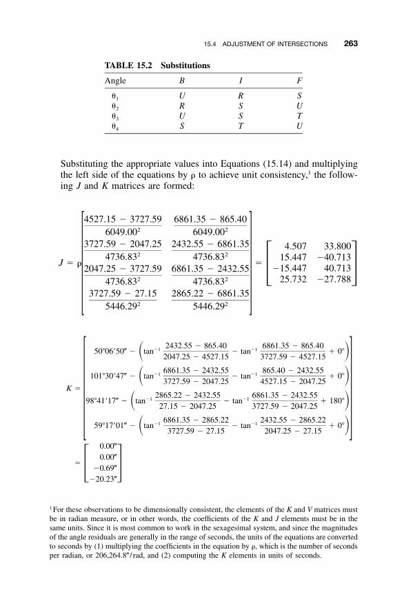
15.4 ADJUSTMENT OF INTERSECTIONS 263
TABLE 15.2 Substitutions
Angle B I F
�1 U R S�2 R S U�3 U S T�4 S T U
Substituting the appropriate values into Equations (15.14) and multiplyingthe left side of the equations by � to achieve unit consistency,1 the follow-ing J and K matrices are formed:
4527.15 � 3727.59 6861.35 � 865.402 26049.00 6049.00
3727.59 � 2047.25 2432.55 � 6861.35 4.507 33.8002 24736.83 4736.83 15.447 �40.713
J � � ��15.447 40.7132047.25 � 3727.59 6861.35 � 2432.55 � �
2 2 25.732 �27.7884736.83 4736.833727.59 � 27.15 2865.22 � 6861.35
2 25446.29 5446.29
2432.55 � 865.40 6861.35 � 865.40�1 �150�06�50� � tan � tan � 0�� �2047.25 � 4527.15 3727.59 � 4527.15
6861.35 � 2432.55 865.40 � 2432.55�1 �1101�30�47� � tan � tan � 0�� �3727.59 � 2047.25 4527.15 � 2047.25
K �2865.22 � 2432.55 6861.35 � 2432.55
�1 �198�41�17� � tan � tan � 180�� �27.15 � 2047.25 3727.59 � 2047.25
6861.35 � 2865.22 2432.55 � 2865.22�1 �159�17�01� � tan � tan � 0�� �3727.59 � 27.15 2047.25 � 27.15
0.00�
0.00��
�0.69�� ��20.23�
1 For these observations to be dimensionally consistent, the elements of the K and V matrices mustbe in radian measure, or in other words, the coefficients of the K and J elements must be in thesame units. Since it is most common to work in the sexagesimal system, and since the magnitudesof the angle residuals are generally in the range of seconds, the units of the equations are convertedto seconds by (1) multiplying the coefficients in the equation by �, which is the number of secondsper radian, or 206,264.8� / rad, and (2) computing the K elements in units of seconds.
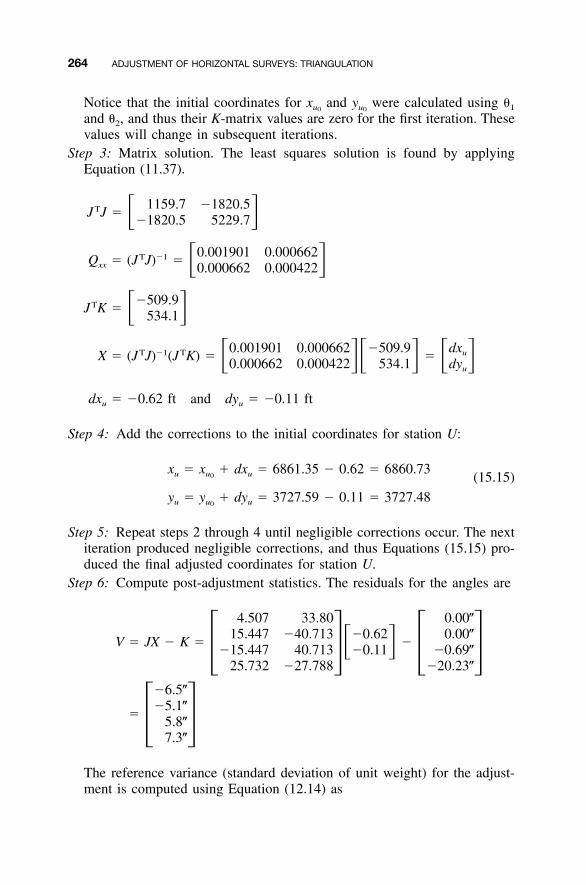
264 ADJUSTMENT OF HORIZONTAL SURVEYS: TRIANGULATION
Notice that the initial coordinates for and were calculated using �1x yu u0 0
and �2, and thus their K-matrix values are zero for the first iteration. Thesevalues will change in subsequent iterations.
Step 3: Matrix solution. The least squares solution is found by applyingEquation (11.37).
1159.7 �1820.5TJ J � � ��1820.5 5229.7
0.001901 0.000662T �1Q � (J J) � � �xx 0.000662 0.000422
�509.9TJ K � � �534.1
0.001901 0.000662 �509.9 dxT �1 T uX � (J J) (J K) � �� �� � � �0.000662 0.000422 534.1 dyu
dx � �0.62 ft and dy � �0.11 ftu u
Step 4: Add the corrections to the initial coordinates for station U:
x � x � dx � 6861.35 � 0.62 � 6860.73u u u0 (15.15)
y � y � dy � 3727.59 � 0.11 � 3727.48u u u0
Step 5: Repeat steps 2 through 4 until negligible corrections occur. The nextiteration produced negligible corrections, and thus Equations (15.15) pro-duced the final adjusted coordinates for station U.
Step 6: Compute post-adjustment statistics. The residuals for the angles are
4.507 33.80 0.00�15.447 �40.713 �0.62 0.00�
V � JX � K � �� ��15.447 40.713 �0.11 �0.69�� � � �25.732 �27.788 �20.23�
�6.5��5.1�
�5.8�� �7.3�
The reference variance (standard deviation of unit weight) for the adjust-ment is computed using Equation (12.14) as
15.5 ADJUSTMENT OF RESECTIONS 265
�6.5�5.1TV V � [�6.5 �5.1 5.8 7.3] � [155.2]
5.8� �7.3
TV V 155.2S � � � �8.8�0 � �m � n 4 � 2
The estimated errors for the adjusted coordinates of station U, given byEquation (13.24), are
S � S �Q � �8.8�0.001901 � �0.38 ftx 0 x xu u u
S � S �Q � �8.8�0.000422 � �0.18 fty 0 y yu u u
The estimated error in the position of station U is given by
2 2 2 2S � �S � S � �0.38 � 0.18 � �0.42 ftu x y
15.5 ADJUSTMENT OF RESECTIONS
Resection is a method used for determining the unknown horizontal positionof an occupied station by observing a minimum of two horizontal angles toa minimum of three stations whose horizontal coordinates are known. If morethan three stations are available, redundant observations are obtained and theposition of the unknown occupied station can be computed using the leastsquares method. Like intersection, resection is suitable for locating an occa-sional station and is especially well adapted over inaccessible terrain. Thismethod is commonly used for orienting total station instruments in locationsfavorable for staking projects by radiation using coordinates.
Consider the resection position computation for the occupied station U ofFigure 15.4 having observed the three horizontal angles shown between sta-tions P, Q, R, and S whose positions are known. To determine the positionof station U, two angles could be observed. The third angle provides a checkand allows a least squares solution for computing the coordinates of sta-tion U.
Using prototype equation (15.13), a linearized observation equation can bewritten for each angle. In this problem, the vertex station is occupied and isthe only unknown station. Thus, all coefficients in the Jacobian matrix followthe form used for the coefficients of dxi and dyi in prototype equation (15.13).
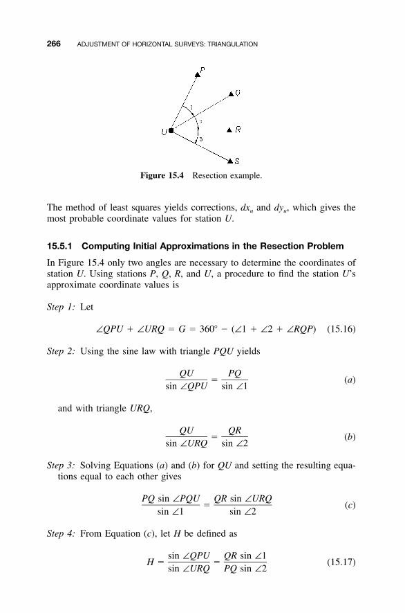
266 ADJUSTMENT OF HORIZONTAL SURVEYS: TRIANGULATION
Figure 15.4 Resection example.
The method of least squares yields corrections, dxu and dyu, which gives themost probable coordinate values for station U.
15.5.1 Computing Initial Approximations in the Resection Problem
In Figure 15.4 only two angles are necessary to determine the coordinates ofstation U. Using stations P, Q, R, and U, a procedure to find the station U’sapproximate coordinate values is
Step 1: Let
∠QPU � ∠URQ � G � 360� � (∠1 � ∠2 � ∠RQP) (15.16)
Step 2: Using the sine law with triangle PQU yields
QU PQ� (a)
sin ∠QPU sin ∠1
and with triangle URQ,
QU QR� (b)
sin ∠URQ sin ∠2
Step 3: Solving Equations (a) and (b) for QU and setting the resulting equa-tions equal to each other gives
PQ sin ∠PQU QR sin ∠URQ� (c)
sin ∠1 sin ∠2
Step 4: From Equation (c), let H be defined as
sin ∠QPU QR sin ∠1H � � (15.17)
sin ∠URQ PQ sin ∠2
15.5 ADJUSTMENT OF RESECTIONS 267
Step 5: From Equation (15.16),
∠QPU � G � ∠URQ (d)
Step 6: Solving Equation (15.17) for the sin∠QPU, and substituting Equation(d) into the result gives
sin(G � ∠URQ) � H sin∠URQ (e)
Step 7: From trigonometry
sin(� � �) � sin � cos � � cos � sin �
Applying this relationship to Equation (e) yields
sin G � ∠URQ � sin G cos∠URQ � cos G sin∠URQ (ƒ)
sin G � ∠URQ � H sin ∠URQ (g)
Step 8: Dividing Equation (g) by cos ∠URQ and rearranging yields
sin G � tan∠URQ[H � cos(G)] (h)
Step 9: Solving Equation (h) for ∠URQ gives
sin G�1∠URQ � tan (15.18)
H � cos G
Step 10: From Figure 15.4,
∠RQU � 180� � (∠2 � ∠URQ) (15.19)
Step 11: Again applying the sine law yields
QR sin ∠RQURU � (15.20)
sin ∠2
Step 12: Finally, the initial coordinates for station U are
x � x � RU sin(Az � ∠URQ)u r RQ (15.21)
y � y � RU cos(Az � ∠URQ)u r RQ
268 ADJUSTMENT OF HORIZONTAL SURVEYS: TRIANGULATION
Example 15.2 The following data are obtained for Figure 15.4. Controlstations P, Q, R, and S have the following (x,y) coordinates: P (1303.599,1458.615), Q (1636.436, 1310.468), R (1503.395, 888.362), and S (1506.262,785.061). The observed values for angles 1, 2, and 3 with standard deviationsare as follows:
Backsight Occupied Foresight Angle S (�)
P U Q 30�29�33� 5Q U R 38�30�31� 6R U S 10�29�57� 6
What are the most probable coordinates of station U?
SOLUTION Using the procedures described in Section 15.5.1, the initialapproximations for the coordinates of station U are:
(a) From Equation (15.10),
∠RQP � Az � Az � 293�59�38.4� � 197�29�38.4�PQ QR
� 96�30�00.0�
(b) Substituting the appropriate angular values into Equation (15.16) gives
G � 360� � (30�29�33� � 38�30�31� � 96�30�00.0�) � 194�29�56�
(c) Substituting the appropriate station coordinates into Equation (14.1)yields
PQ � 364.318 and QR � 442.576
(d) Substituting the appropriate values into Equation (15.17) yields H as
442.576 sin(30�29�33�)H � � 0.990027302
364.318 sin(38�30�31�)
(e) Substituting previously determined G and H into Equation (15.18),∠URQ is computed as
sin(194�29�56�)�1∠URQ � tan � 180�
0.990027302 � cos(194�29�56�)
� �85�00�22� � 180� � 94�59�36.3�
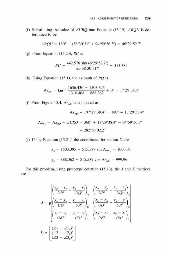
15.5 ADJUSTMENT OF RESECTIONS 269
(f) Substituting the value of ∠URQ into Equation (15.19), ∠RQU is de-termined to be
∠RQU � 180� � (38�30�31� � 94�59�36.3�) � 46�29�52.7�
(g) From Equation (15.20), RU is
442.576 sin(46�29�52.7�)RU � � 515.589
sin(38�30�31�)
(h) Using Equation (15.1), the azimuth of RQ is
1636.436 � 1503.395�1Az � tan � 0� � 17�29�38.4�RQ 1310.468 � 888.362
(i) From Figure 15.4, AzRU is computed as
Az � 197�29�38.4� � 180� � 17�29�38.4�RQ
Az � Az � ∠URQ � 360� � 17�29�38.4� � 94�59�36.3�RU RQ
� 282�30�02.2�
( j) Using Equation (15.21), the coordinates for station U are
x � 1503.395 � 515.589 sin Az � 1000.03u RU
y � 888.362 � 515.589 cos Az � 999.96u RU
For this problem, using prototype equation (15.13), the J and K matricesare
y � y y � y x � x x � xp u q u u p u q� �� � � �2 2 2 2UP UQ UP UQ0 0
y � y x � xy � y x � xq u u qr u u rJ � � � �� � � �2 2 2UQ UR UQ UR0 0
y � y y � y x � x x � xr u s u u r u s� �� � � �2 2 2 2UR US UR US0 0
(∠1 � ∠1 )�0
K � (∠2 � ∠2 )�0� �(∠3 � ∠3 )�0
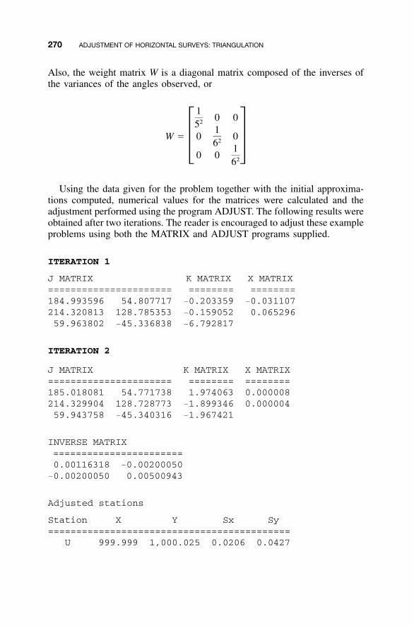
270 ADJUSTMENT OF HORIZONTAL SURVEYS: TRIANGULATION
Also, the weight matrix W is a diagonal matrix composed of the inverses ofthe variances of the angles observed, or
10 0251
W � 0 026� �10 0 26
Using the data given for the problem together with the initial approxima-tions computed, numerical values for the matrices were calculated and theadjustment performed using the program ADJUST. The following results wereobtained after two iterations. The reader is encouraged to adjust these exampleproblems using both the MATRIX and ADJUST programs supplied.
ITERATION 1
J MATRIX K MATRIX X MATRIX====================== ======== ========184.993596 54.807717 �0.203359 �0.031107214.320813 128.785353 �0.159052 0.06529659.963802 �45.336838 �6.792817
ITERATION 2
J MATRIX K MATRIX X MATRIX====================== ======== ========185.018081 54.771738 1.974063 0.000008214.329904 128.728773 �1.899346 0.00000459.943758 �45.340316 �1.967421
INVERSE MATRIX=======================0.00116318 �0.00200050
�0.00200050 0.00500943
Adjusted stations
Station X Y Sx Sy===========================================
U 999.999 1,000.025 0.0206 0.0427
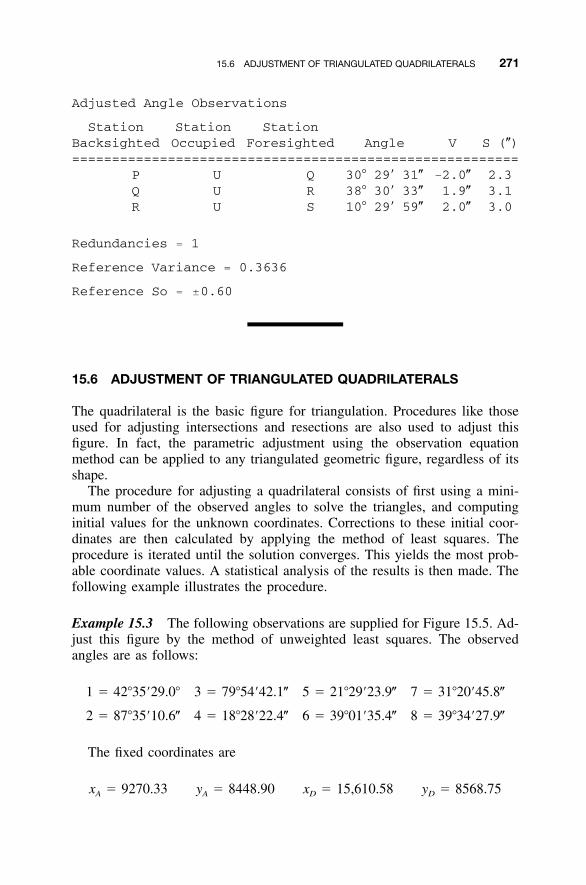
15.6 ADJUSTMENT OF TRIANGULATED QUADRILATERALS 271
Adjusted Angle Observations
Station Station StationBacksighted Occupied Foresighted Angle V S (�)========================================================
P U Q 30� 29� 31� �2.0� 2.3Q U R 38� 30� 33� 1.9� 3.1R U S 10� 29� 59� 2.0� 3.0
Redundancies � 1
Reference Variance � 0.3636
Reference So � �0.60
15.6 ADJUSTMENT OF TRIANGULATED QUADRILATERALS
The quadrilateral is the basic figure for triangulation. Procedures like thoseused for adjusting intersections and resections are also used to adjust thisfigure. In fact, the parametric adjustment using the observation equationmethod can be applied to any triangulated geometric figure, regardless of itsshape.
The procedure for adjusting a quadrilateral consists of first using a mini-mum number of the observed angles to solve the triangles, and computinginitial values for the unknown coordinates. Corrections to these initial coor-dinates are then calculated by applying the method of least squares. Theprocedure is iterated until the solution converges. This yields the most prob-able coordinate values. A statistical analysis of the results is then made. Thefollowing example illustrates the procedure.
Example 15.3 The following observations are supplied for Figure 15.5. Ad-just this figure by the method of unweighted least squares. The observedangles are as follows:
1 � 42�35�29.0� 3 � 79�54�42.1� 5 � 21�29�23.9� 7 � 31�20�45.8�
2 � 87�35�10.6� 4 � 18�28�22.4� 6 � 39�01�35.4� 8 � 39�34�27.9�
The fixed coordinates are
x � 9270.33 y � 8448.90 x � 15,610.58 y � 8568.75A A D D
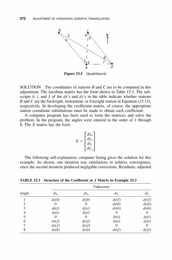
272 ADJUSTMENT OF HORIZONTAL SURVEYS: TRIANGULATION
Figure 15.5 Quadrilateral.
TABLE 15.3 Structure of the Coefficient or J Matrix in Example 15.3
Angle
Unknowns
dxb dyb dxc dyc
1 dx(b) dy(b) dx(ƒ) dy(ƒ)2 0 0 dx(b) dy(b)3 dx(i) dy(i) dx(b) dy(b)4 dx(i) dy(i) 0 05 0 0 dx(i) dy(i)6 dx(ƒ) dy(ƒ) dx(i) dy(i)7 dx(ƒ) dy(ƒ) 0 08 dy(b) dy(b) dx(ƒ) dy(ƒ)
SOLUTION The coordinates of stations B and C are to be computed in thisadjustment. The Jacobian matrix has the form shown in Table 15.3. The sub-scripts b, i, and ƒ of the dx’s and dy’s in the table indicate whether stationsB and C are the backsight, instrument, or foresight station in Equation (15.13),respectively. In developing the coefficient matrix, of course, the appropriatestation coordinate substitutions must be made to obtain each coefficient.
A computer program has been used to form the matrices and solve theproblem. In the program, the angles were entered in the order of 1 through8. The X matrix has the form
dxb
dybX �dxc� �dyc
The following self-explanatory computer listing gives the solution for thisexample. As shown, one iteration was satisfactory to achieve convergence,since the second iteration produced negligible corrections. Residuals, adjusted
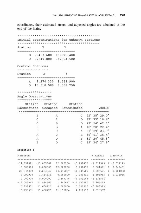
15.6 ADJUSTMENT OF TRIANGULATED QUADRILATERALS 273
coordinates, their estimated errors, and adjusted angles are tabulated at theend of the listing.
*******************************************Initial approximations for unknown stations*******************************************Station X Y==============================
B 2,403.600 16,275.400C 9,649.800 24,803.500
Control StationsStation X Y==============================
A 9,270.330 8,448.900D 15,610.580 8,568.750
******************Angle Observations******************
Station Station StationBacksighted Occupied Foresighted Angle===============================================
B A C 42� 35� 29.0�C A D 87� 35� 10.6�C B D 79� 54� 42.1�D B A 18� 28� 22.4�D C A 21� 29� 23.9�A C B 39� 01� 35.4�A D B 31� 20� 45.8�B D C 39� 34� 27.9�
Iteration 1
J Matrix K MATRIX X MATRIX
---------------------------------------------- --------- -----------
�14.891521 �13.065362 12.605250 �0.292475 �1.811949 1 �0.011149
0.000000 0.000000 �12.605250 0.292475 �5.801621 2 0.049461
20.844399 �0.283839 �14.045867 11.934565 3.508571 3 0.061882
8.092990 1.414636 0.000000 0.000000 1.396963 4 0.036935
0.000000 0.000000 1.409396 �4.403165 �1.833544
�14.045867 11.934565 1.440617 �11.642090 5.806415
6.798531 11.650726 0.000000 0.000000 �5.983393
�6.798531 �11.650726 11.195854 4.110690 1.818557
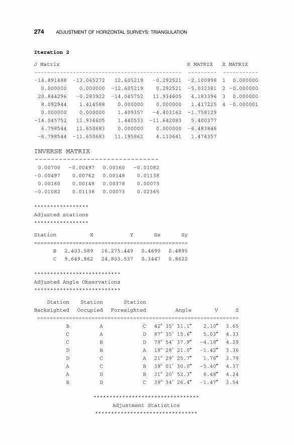
274 ADJUSTMENT OF HORIZONTAL SURVEYS: TRIANGULATION
Iteration 2
J Matrix K MATRIX X MATRIX
---------------------------------------------- --------- -----------
�14.891488 �13.065272 12.605219 �0.292521 �2.100998 1 0.000000
0.000000 0.000000 �12.605219 0.292521 �5.032381 2 �0.000000
20.844296 �0.283922 �14.045752 11.934605 4.183396 3 0.000000
8.092944 1.414588 0.000000 0.000000 1.417225 4 �0.000001
0.000000 0.000000 1.409357 �4.403162 �1.758129
�14.045752 11.934605 1.440533 �11.642083 5.400377
6.798544 11.650683 0.000000 0.000000 �6.483846
�6.798544 �11.650683 11.195862 4.110641 1.474357
INVERSE MATRIX-------------------------------0.00700 �0.00497 0.00160 �0.01082
�0.00497 0.00762 0.00148 0.01138
0.00160 0.00148 0.00378 0.00073
�0.01082 0.01138 0.00073 0.02365
*****************
Adjusted stations
*****************
Station X Y Sx Sy
================================================
B 2,403.589 16,275.449 0.4690 0.4895
C 9,649.862 24,803.537 0.3447 0.8622
***************************
Adjusted Angle Observations
***************************
Station Station Station
Backsighted Occupied Foresighted Angle V S
===============================================================
B A C 42� 35� 31.1� 2.10� 3.65
C A D 87� 35� 15.6� 5.03� 4.33
C B D 79� 54� 37.9� �4.18� 4.29
D B A 18� 28� 21.0� �1.42� 3.36
D C A 21� 29� 25.7� 1.76� 3.79
A C B 39� 01� 30.0� �5.40� 4.37
A D B 31� 20� 52.3� 6.48� 4.24
B D C 39� 34� 26.4� �1.47� 3.54
*********************************
Adjustment Statistics
********************************
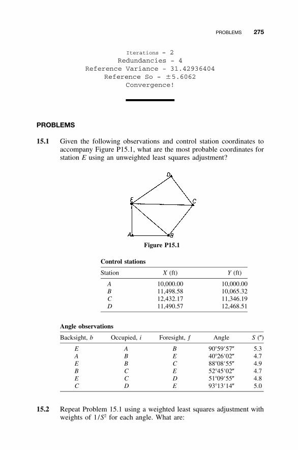
PROBLEMS 275
Iterations � 2Redundancies � 4
Reference Variance � 31.42936404Reference So � �5.6062
Convergence!
PROBLEMS
15.1 Given the following observations and control station coordinates toaccompany Figure P15.1, what are the most probable coordinates forstation E using an unweighted least squares adjustment?
Figure P15.1
Control stations
Station X (ft) Y (ft)
A 10,000.00 10,000.00B 11,498.58 10,065.32C 12,432.17 11,346.19D 11,490.57 12,468.51
Angle observations
Backsight, b Occupied, i Foresight, ƒ Angle S (�)
E A B 90�59�57� 5.3A B E 40�26�02� 4.7E B C 88�08�55� 4.9B C E 52�45�02� 4.7E C D 51�09�55� 4.8C D E 93�13�14� 5.0
15.2 Repeat Problem 15.1 using a weighted least squares adjustment withweights of 1/S2 for each angle. What are:
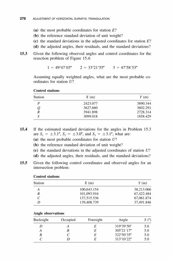
276 ADJUSTMENT OF HORIZONTAL SURVEYS: TRIANGULATION
(a) the most probable coordinates for station E?(b) the reference standard deviation of unit weight?(c) the standard deviations in the adjusted coordinates for station E?(d) the adjusted angles, their residuals, and the standard deviations?
15.3 Given the following observed angles and control coordinates for theresection problem of Figure 15.4:
1 � 49�47�03� 2 � 33�21�55� 3 � 47�58�53�
Assuming equally weighted angles, what are the most probable co-ordinates for station U?
Control stations
Station X (m) Y (m)
P 2423.077 3890.344Q 3627.660 3602.291R 3941.898 2728.314S 3099.018 1858.429
15.4 If the estimated standard deviations for the angles in Problem 15.3are S1 � �3.1�, S2 � �3.0�, and S3 � �3.1�, what are:(a) the most probable coordinates for station U?(b) the reference standard deviation of unit weight?(c) the standard deviations in the adjusted coordinates of station U?(d) the adjusted angles, their residuals, and the standard deviations?
15.5 Given the following control coordinates and observed angles for anintersection problem:
Control stations
Station X (m) Y (m)
A 100,643.154 38,213.066B 101,093.916 67,422.484C 137,515.536 67,061.874D 139,408.739 37,491.846
Angle observations
Backsight Occupied Foresight Angle S (�)
D A E 319�39�50� 5.0A B E 305�21�17� 5.0B C E 322�50�35� 5.0C D E 313�10�22� 5.0
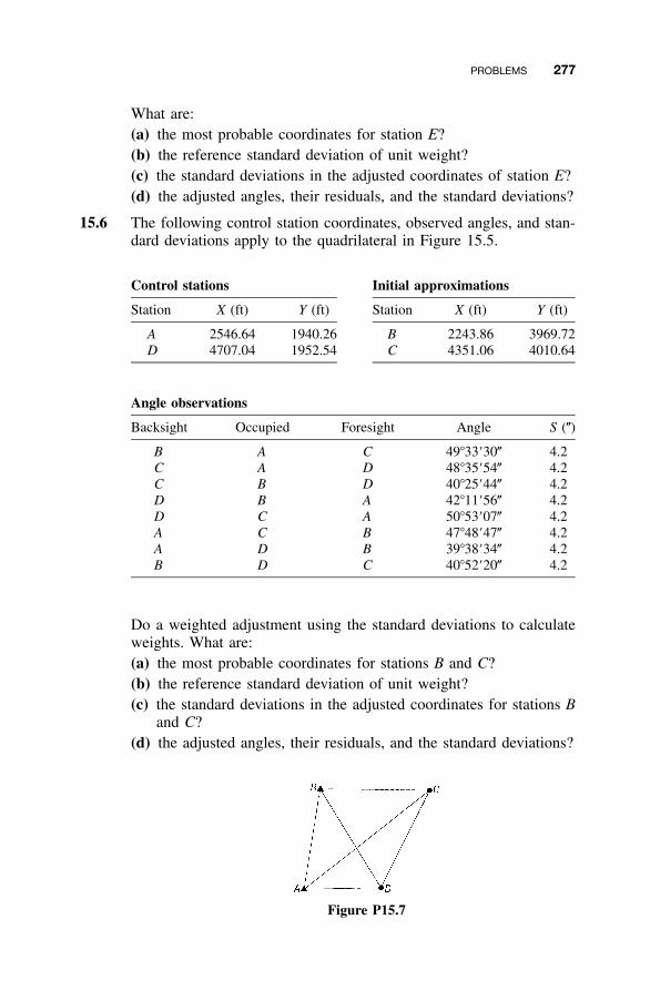
PROBLEMS 277
What are:(a) the most probable coordinates for station E?(b) the reference standard deviation of unit weight?(c) the standard deviations in the adjusted coordinates of station E?(d) the adjusted angles, their residuals, and the standard deviations?
15.6 The following control station coordinates, observed angles, and stan-dard deviations apply to the quadrilateral in Figure 15.5.
Control stations Initial approximations
Station X (ft) Y (ft) Station X (ft) Y (ft)
A 2546.64 1940.26 B 2243.86 3969.72D 4707.04 1952.54 C 4351.06 4010.64
Angle observations
Backsight Occupied Foresight Angle S (�)
B A C 49�33�30� 4.2C A D 48�35�54� 4.2C B D 40�25�44� 4.2D B A 42�11�56� 4.2D C A 50�53�07� 4.2A C B 47�48�47� 4.2A D B 39�38�34� 4.2B D C 40�52�20� 4.2
Do a weighted adjustment using the standard deviations to calculateweights. What are:(a) the most probable coordinates for stations B and C?(b) the reference standard deviation of unit weight?(c) the standard deviations in the adjusted coordinates for stations B
and C?(d) the adjusted angles, their residuals, and the standard deviations?
Figure P15.7
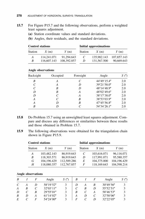
278 ADJUSTMENT OF HORIZONTAL SURVEYS: TRIANGULATION
15.7 For Figure P15.7 and the following observations, perform a weightedleast squares adjustment.(a) Station coordinate values and standard deviations.(b) Angles, their residuals, and the standard deviations.
Control stations Initial approximations
Station X (m) Y (m) Station X (m) Y (m)
A 114,241.071 91,294.643 C 135,982.143 107,857.143B 116,607.143 108,392.857 D 131,567.500 90,669.643
Angle observations
Backsight Occupied Foresight Angle S (�)
B A C 44�49�15.4� 2.0C A D 39�21�58.0� 2.0C B D 48�14�48.9� 2.0D B A 48�02�49.6� 2.0D C A 38�17�38.0� 2.0A C B 38�53�03.9� 2.0A D B 47�45�56.8� 2.0B D C 54�34�26.1� 2.0
15.8 Do Problem 15.7 using an unweighted least squares adjustment. Com-pare and discuss any differences or similarities between these resultsand those obtained in Problem 15.7.
15.9 The following observations were obtained for the triangulation chainshown in Figure P15.9.
Control stations Initial approximations
Station X (m) Y (m) Station X (m) Y (m)
A 103,482.143 86,919.643 C 103,616.071 96,116.071B 118,303.571 86,919.643 D 117,991.071 95,580.357G 104,196.429 112,589.286 E 104,375.000 104,196.429H 118,080.357 112,767.857 F 118,169.643 104,598.214
Angle observations
B I F Angle S (�) B I F Angle S (�)
C A D 58�19�52� 3 D A B 30�49�56� 3A B C 32�03�11� 3 C B D 55�52�51� 3D C B 29�55�01� 3 B C A 58�46�53� 3B D A 61�14�02� 3 A D C 32�58�06� 3E C F 54�24�00� 3 F C D 32�22�05� 3
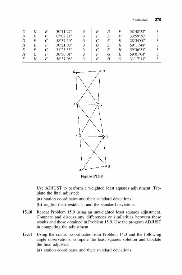
PROBLEMS 279
C D E 30�11�27� 3 E D F 58�48�32� 3D E C 63�02�21� 3 F E D 33�59�36� 3D F C 58�37�50� 3 C F E 28�34�00� 3H E F 30�21�08� 3 G E H 59�11�48� 3E F G 31�25�55� 3 G F H 59�36�31� 3H G F 30�30�01� 3 F G E 59�01�04� 3F H E 58�37�08� 3 E H G 31�17�11� 3
Figure P15.9
Use ADJUST to perform a weighted least squares adjustment. Tab-ulate the final adjusted:(a) station coordinates and their standard deviations.(b) angles, their residuals, and the standard deviations.
15.10 Repeat Problem 15.9 using an unweighted least squares adjustment.Compare and discuss any differences or similarities between theseresults and those obtained in Problem 15.9. Use the program ADJUSTin computing the adjustment.
15.11 Using the control coordinates from Problem 14.3 and the followingangle observations, compute the least squares solution and tabulatethe final adjusted:(a) station coordinates and their standard deviations.
280 ADJUSTMENT OF HORIZONTAL SURVEYS: TRIANGULATION
(b) angles, their residuals, and the standard deviations.
Angle observations
Backsight Occupied Foresight Angle S (�)
B A C 280�41�06� 5.2C A D 39�21�53� 5.1C B D 51�36�16� 5.2D B A 255�50�03� 5.2D C A 101�27�17� 5.2A C B 311�52�38� 5.2A D B 324�07�04� 5.1B D C 75�03�50� 5.2
15.12 The following observations were obtained for a triangulation chain.
Control stations Initial approximations
Station X (ft) Y (ft) Station X (ft) Y (ft)
A 92,890.04 28,566.74 B 93,611.26 47,408.62D 93,971.87 80,314.29 C
E93,881.71
111,191.0064,955.3638,032.76
F 110,109.17 57,145.10G 110,019.02 73,102.09H 131,475.32 28,837.20I 130,213.18 46,777.56J 129,311.66 64,717.91K 128,590.44 79,142.31
Angle observations
B I F Angle S (�) B I F Angle S (�)
B A E 60�27�28� 2.2 E B A 64�07�06� 2.1F B E 58�37�14� 2.1 C B F 58�34�09� 2.1F C B 65�10�51� 2.3 G C F 52�29�14� 2.0D C G 62�52�42� 2.1 G D C 66�08�08� 2.2D G K 137�46�57� 2.4 K G J 41�30�18� 2.7J G F 66�11�15� 2.1 F G C 63�32�13� 2.1C G D 50�59�11� 2.3 B F C 56�14�56� 2.6C F G 63�58�29� 2.1 G F J 68�48�05� 2.1J F I 48�48�05� 2.3 I F E 59�28�49� 2.4E F B 62�41�29� 2.2 A E B 55�25�19� 2.3B E F 58�41�13� 2.5 F E I 68�33�06� 2.0I E H 49�04�27� 2.1 H E A 128�15�52� 2.6E H I 61�35�24� 2.5 H I E 69�20�10� 2.0E I F 51�58�06� 2.1 F I J 59�50�35� 2.2I J F 71�21�12� 2.2 F J G 45�00�39� 2.1G J K 63�38�57� 2.2 J K G 74�50�46� 2.3
PROBLEMS 281
Use ADJUST to perform a weighted least squares adjustment. Tab-ulate the final adjusted:(a) station coordinates and their standard deviations.(b) angles, their residuals, and the standard deviations.
15.13 Do Problem 15.12 using an unweighted least squares adjustment.Compare and discuss any differences or similarities between theseresults and those obtained in Problem 15.12. Use the program AD-JUST in computing the adjustment.
Use the ADJUST software to do the following problems.
15.14 Problem 15.2
15.15 Problem 15.4
15.16 Problem 15.5
15.17 Problem 15.6
15.18 Problem 15.9
Programming Problems
15.19 Write a computational program that computes the coefficients for pro-totype equations (15.9) and (15.13) and their k values given the co-ordinates of the appropriate stations. Use this program to determinethe matrix values necessary to do Problem 15.6.
15.20 Prepare a computational program that reads a file of station coordi-nates, observed angles, and their standard deviations and then:(a) writes the data to a file in a formatted fashion.(b) computes the J, K, and W matrices.(c) writes the matrices to a file that is compatible with the MATRIX
program.(d) test this program with Problem 15.6.
15.21 Write a computational program that reads a file containing the J, K,and W matrices and then:(a) writes these matrices in a formatted fashion.(b) performs one iteration of either a weighted or unweighted least
squares adjustment of Problem 15.6.(c) writes the matrices used to compute the solution and the correc-
tions to the station coordinates in a formatted fashion.
15.22 Write a computational program that reads a file of station coordinates,observed angles, and their standard deviations and then:
282 ADJUSTMENT OF HORIZONTAL SURVEYS: TRIANGULATION
(a) writes the data to a file in a formatted fashion.(b) computes the J, K, and W matrices.(c) performs either a relative or equal weight least squares adjustment
of Problem 15.6.(d) writes the matrices used to compute the solution and tabulates
the final adjusted station coordinates and their estimated errorsand the adjusted angles, together with their residuals and theirestimated errors.
15.23 Prepare a computational program that solves the resection problem.Use this program to compute the initial approximations for Problem15.3.
283
CHAPTER 16
ADJUSTMENT OF HORIZONTALSURVEYS: TRAVERSESAND NETWORKS
16.1 INTRODUCTION TO TRAVERSE ADJUSTMENTS
Of the many methods that exist for traverse adjustment, the characteristic thatdistinguishes the method of least squares from other methods is that distance,angle, and direction observations are adjusted simultaneously. Furthermore,the adjusted observations not only satisfy all geometrical conditions for thetraverse but provide the most probable values for the given data set. Addi-tionally, the observations can be rigorously weighted based on their estimatederrors and adjusted accordingly. Given these facts, together with the compu-tational power now provided by computers, it is hard to justify not using leastsquares for all traverse adjustment work.
In this chapter we describe methods for making traverse adjustments byleast squares. As was the case in triangulation adjustments, traverses can beadjusted by least squares using either observation equations or conditionalequations. Again, because of the relative ease with which the equations canbe written and solved, the parametric observation equation approach is dis-cussed.
16.2 OBSERVATION EQUATIONS
When adjusting a traverse using parametric equations, an observation equationis written for each distance, direction, or angle. The necessary linearizedobservation equations developed previously are recalled in the followingequations.
Adjustment Computations: Spatial Data Analysis, Fourth Edition. C. D. Ghilani and P. R. Wolf© 2006 John Wiley & Sons, Inc. ISBN: 978-0-471-69728-2
284 ADJUSTMENT OF HORIZONTAL SURVEYS: TRAVERSES AND NETWORKS
Distance observation equation:
x � x y � y x � x y � yi j i j j i j idx � dy � dx � dy� � � � � � � �i i j jIJ IJ IJ IJ0 0 0 0
� k � v (16.1)l lij ij
Angle observation equation:
y � yy � y x � x y � y ƒ ii b b i b idx � dy � � dx� � � � � �b b i2 2 2 2IB IB IB IF0 0 0
x � x y � y x � xx � x i ƒ ƒ i i ƒi b� � dy � dx � dy (16.2)� � � � � �i ƒ ƒ2 2 2 2IB IF IF IF0 0 0
� k � v� �bif bif
Azimuth observation equation:
y � y x � x y � y x � xi j j i j i i jdx � dy � dx � dy� � � � � � � �i i j j2 2 2 2IJ IJ IJ IJ0 0 0 0
� k � v (16.3)Az Azij ij
The reader should refer to Chapters 14 and 15 to review the specificnotation for these equations. As demonstrated with the examples that follow,the azimuth equation may or may not be used in traverse adjustments.
16.3 REDUNDANT EQUATIONS
As noted earlier, one observation equation can be written for each angle,distance, or direction observed in a closed traverse. Thus, if there are n sidesin the traverse, there are n distances and n � 1 angles, assuming that oneangle exists for orientation of the traverse. For example, each closed traversein Figure 16.1 has four sides, four distances, and five angles. Each traversealso has three points whose positions are unknown, and each point introducestwo unknown coordinates into the solution. Thus, there is a maximum of2(n � 1) unknowns for any closed traverse. From the foregoing, no matterthe number of sides, there will always be a minimum of r � (n � n � 1) �2(n � 1) � 3 redundant equations for any closed traverse. That is, everyclosed traverse that is fixed in space both positionally and rotationally has aminimum of three redundant equations.
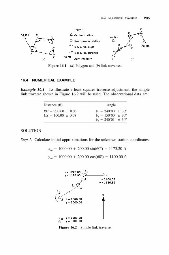
16.4 NUMERICAL EXAMPLE 285
Figure 16.1 (a) Polygon and (b) link traverses.
Figure 16.2 Simple link traverse.
16.4 NUMERICAL EXAMPLE
Example 16.1 To illustrate a least squares traverse adjustment, the simplelink traverse shown in Figure 16.2 will be used. The observational data are:
Distance (ft) Angle
RU � 200.00 � 0.05 �1 � 240�00� � 30�US � 100.00 � 0.08 �2 � 150�00� � 30�
�3 � 240�01� � 30�
SOLUTION
Step 1: Calculate initial approximations for the unknown station coordinates.
x � 1000.00 � 200.00 sin(60�) � 1173.20 ftu0
y � 1000.00 � 200.00 cos(60�) � 1100.00 ftu0
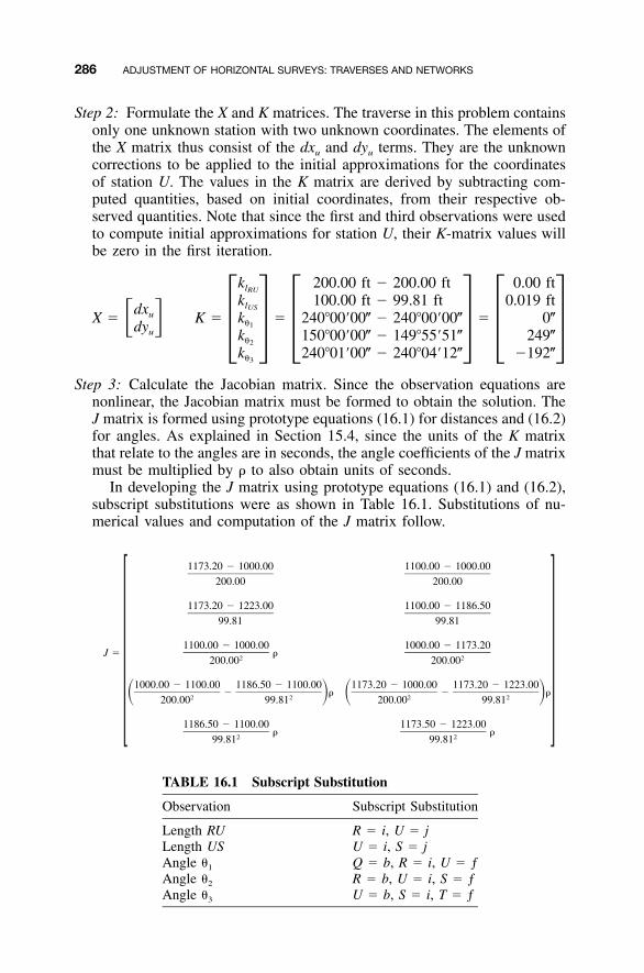
286 ADJUSTMENT OF HORIZONTAL SURVEYS: TRAVERSES AND NETWORKS
TABLE 16.1 Subscript Substitution
Observation Subscript Substitution
Length RU R � i, U � jLength US U � i, S � jAngle �1 Q � b, R � i, U � ƒAngle �2 R � b, U � i, S � ƒAngle �3 U � b, S � i, T � ƒ
Step 2: Formulate the X and K matrices. The traverse in this problem containsonly one unknown station with two unknown coordinates. The elements ofthe X matrix thus consist of the dxu and dyu terms. They are the unknowncorrections to be applied to the initial approximations for the coordinatesof station U. The values in the K matrix are derived by subtracting com-puted quantities, based on initial coordinates, from their respective ob-served quantities. Note that since the first and third observations were usedto compute initial approximations for station U, their K-matrix values willbe zero in the first iteration.
k 200.00 ft � 200.00 ft 0.00 ftlRU
k 100.00 ft � 99.81 ft 0.019 ftlUSdxuX � K � k � 240�00�00� � 240�00�00� � 0�� � �1dyu k 150�00�00� � 149�55�51� 249��� � � � � �2
k 240�01�00� � 240�04�12� �192��3
Step 3: Calculate the Jacobian matrix. Since the observation equations arenonlinear, the Jacobian matrix must be formed to obtain the solution. TheJ matrix is formed using prototype equations (16.1) for distances and (16.2)for angles. As explained in Section 15.4, since the units of the K matrixthat relate to the angles are in seconds, the angle coefficients of the J matrixmust be multiplied by � to also obtain units of seconds.
In developing the J matrix using prototype equations (16.1) and (16.2),subscript substitutions were as shown in Table 16.1. Substitutions of nu-merical values and computation of the J matrix follow.
1173.20 � 1000.00 1100.00 � 1000.00
200.00 200.00
1173.20 � 1223.00 1100.00 � 1186.50
99.81 99.81
1100.00 � 1000.00 1000.00 � 1173.20J � �
2 2200.00 200.00
1000.00 � 1100.00 1186.50 � 1100.00 1173.20 � 1000.00 1173.20 � 1223.00� � � �� � � �2 2 2 2200.00 99.81 200.00 99.81
1186.50 � 1100.00 1173.50 � 1223.00� �
2 299.81 99.81

16.4 NUMERICAL EXAMPLE 287
0.866 0.500�0.499 �0.867
J � 515.7 �893.2�2306.6 1924.2� �
1709.9 �1031.1
Step 4: Formulate the W matrix. The fact that distance and angle observationshave differing observational units and are combined in an adjustment isresolved by using relative weights that are based on observational variancesin accordance with Equation (10.6). This weighting makes the observationequations dimensionally consistent. If weights are not used in traverse ad-justments (i.e., equal weights are assumed), the least squares problem willgenerally either give unreliable results or result in a system of equationsthat has no solution. Since weights influence the correction size that eachobservation will receive, it is extremely important to use variances thatcorrespond closely to the observational errors. The error propagation pro-cedures discussed in Chapter 7 aid in the determination of the estimatederrors. Repeating Equation (10.6), the distance and angle weights for thisproblem are
1 1distances: w � and angles: w � (16.4)l �IJ bif2 2S Sl �IJ bif
Again, the units of the weight matrix must match those of the J and Kmatrices. That is, the angular weights must be in the same units of measure(seconds) as the counterparts in the other two matrices. Based on the es-timated errors in the observations, the W matrix, which is diagonal, is
1(zeros)20.05
120.08
1W � 230
1230
1(zeros) 230
400.00 (zeros)156.2
� 0.00110.0011� �
(zeros) 0.0011
Step 5: Solve the matrix system. This problem is iterative and was solvedaccording to Equation (11.39) using the program MATRIX. (Output from
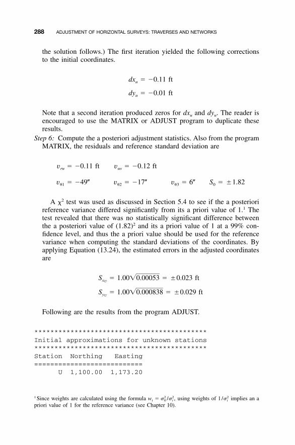
288 ADJUSTMENT OF HORIZONTAL SURVEYS: TRAVERSES AND NETWORKS
the solution follows.) The first iteration yielded the following correctionsto the initial coordinates.
dx � �0.11 ftu
dy � �0.01 ftu
Note that a second iteration produced zeros for dxu and dyu. The reader isencouraged to use the MATRIX or ADJUST program to duplicate theseresults.
Step 6: Compute the a posteriori adjustment statistics. Also from the programMATRIX, the residuals and reference standard deviation are
v � �0.11 ft v � �0.12 ftru us
v � �49� v � �17� v � 6� S � �1.82�1 �2 �3 0
A �2 test was used as discussed in Section 5.4 to see if the a posteriorireference variance differed significantly from its a priori value of 1.1 Thetest revealed that there was no statistically significant difference betweenthe a posteriori value of (1.82)2 and its a priori value of 1 at a 99% con-fidence level, and thus the a priori value should be used for the referencevariance when computing the standard deviations of the coordinates. Byapplying Equation (13.24), the estimated errors in the adjusted coordinatesare
S � 1.00�0.00053 � �0.023 ftxU
S � 1.00�0.000838 � �0.029 ftyU
Following are the results from the program ADJUST.
*******************************************Initial approximations for unknown stations*******************************************Station Northing Easting===========================
U 1,100.00 1,173.20
1 Since weights are calculated using the formula wi � / using weights of 1 / implies an a2 2 2� � , �0 i i
priori value of 1 for the reference variance (see Chapter 10).
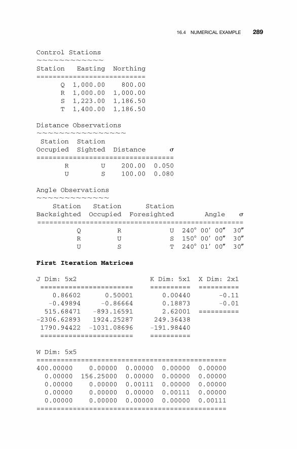
16.4 NUMERICAL EXAMPLE 289
Control Stations������������Station Easting Northing===========================
Q 1,000.00 800.00R 1,000.00 1,000.00S 1,223.00 1,186.50T 1,400.00 1,186.50
Distance Observations����������������Station StationOccupied Sighted Distance �==================================
R U 200.00 0.050U S 100.00 0.080
Angle Observations�������������
Station Station StationBacksighted Occupied Foresighted Angle �===================================================
Q R U 240� 00� 00� 30�R U S 150� 00� 00� 30�U S T 240� 01� 00� 30�
First Iteration Matrices
J Dim: 5x2=======================
K Dim: 5x1==========
X Dim: 2x1==========
0.86602 0.50001 0.00440 �0.11�0.49894 �0.86664 0.18873 �0.01
515.68471 �893.16591 2.62001 ==========�2306.62893 1924.25287 249.364381790.94422 �1031.08696 �191.98440======================= ==========
W Dim: 5x5===============================================400.00000 0.00000 0.00000 0.00000 0.000000.00000 156.25000 0.00000 0.00000 0.000000.00000 0.00000 0.00111 0.00000 0.000000.00000 0.00000 0.00000 0.00111 0.000000.00000 0.00000 0.00000 0.00000 0.00111
===============================================
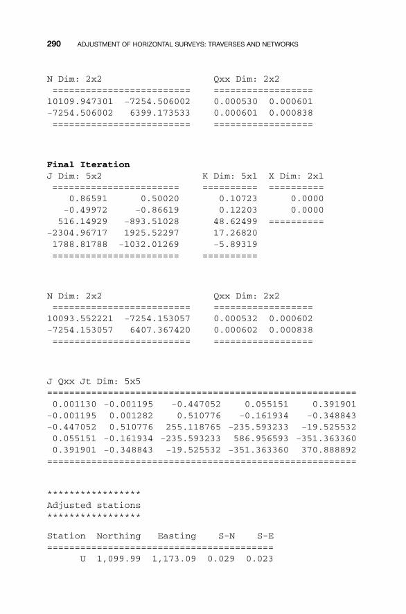
290 ADJUSTMENT OF HORIZONTAL SURVEYS: TRAVERSES AND NETWORKS
N Dim: 2x2=========================
Qxx Dim: 2x2==================
10109.947301 �7254.506002 0.000530 0.000601�7254.506002 6399.173533 0.000601 0.000838========================= ==================
Final IterationJ Dim: 5x2=======================
K Dim: 5x1==========
X Dim: 2x1==========
0.86591 0.50020 0.10723 0.0000�0.49972 �0.86619 0.12203 0.0000
516.14929 �893.51028 48.62499 ==========�2304.96717 1925.52297 17.268201788.81788 �1032.01269 �5.89319======================= ==========
N Dim: 2x2=========================
Qxx Dim: 2x2==================
10093.552221 �7254.153057 0.000532 0.000602�7254.153057 6407.367420 0.000602 0.000838========================= ==================
J Qxx Jt Dim: 5x5========================================================0.001130 �0.001195 �0.447052 0.055151 0.391901
�0.001195 0.001282 0.510776 �0.161934 �0.348843�0.447052 0.510776 255.118765 �235.593233 �19.5255320.055151 �0.161934 �235.593233 586.956593 �351.3633600.391901 �0.348843 �19.525532 �351.363360 370.888892========================================================
*****************Adjusted stations*****************
Station Northing Easting S-N S-E=========================================
U 1,099.99 1,173.09 0.029 0.023
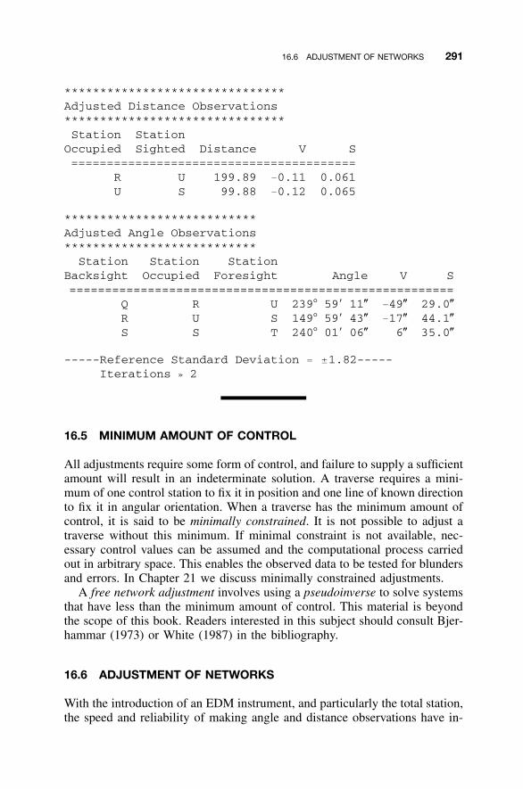
16.6 ADJUSTMENT OF NETWORKS 291
*******************************Adjusted Distance Observations*******************************Station StationOccupied Sighted Distance V S========================================
R U 199.89 �0.11 0.061U S 99.88 �0.12 0.065
***************************Adjusted Angle Observations***************************Station Station Station
Backsight Occupied Foresight Angle V S======================================================
Q R U 239� 59� 11� �49� 29.0�R U S 149� 59� 43� �17� 44.1�S S T 240� 01� 06� 6� 35.0�
-----Reference Standard Deviation � �1.82-----Iterations » 2
16.5 MINIMUM AMOUNT OF CONTROL
All adjustments require some form of control, and failure to supply a sufficientamount will result in an indeterminate solution. A traverse requires a mini-mum of one control station to fix it in position and one line of known directionto fix it in angular orientation. When a traverse has the minimum amount ofcontrol, it is said to be minimally constrained. It is not possible to adjust atraverse without this minimum. If minimal constraint is not available, nec-essary control values can be assumed and the computational process carriedout in arbitrary space. This enables the observed data to be tested for blundersand errors. In Chapter 21 we discuss minimally constrained adjustments.
A free network adjustment involves using a pseudoinverse to solve systemsthat have less than the minimum amount of control. This material is beyondthe scope of this book. Readers interested in this subject should consult Bjer-hammar (1973) or White (1987) in the bibliography.
16.6 ADJUSTMENT OF NETWORKS
With the introduction of an EDM instrument, and particularly the total station,the speed and reliability of making angle and distance observations have in-
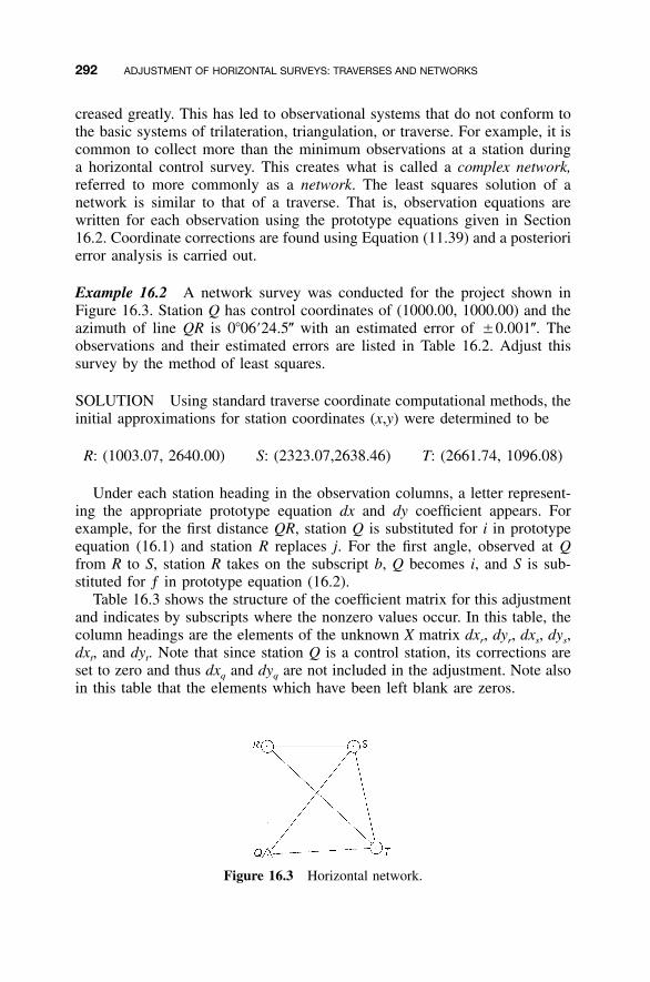
292 ADJUSTMENT OF HORIZONTAL SURVEYS: TRAVERSES AND NETWORKS
Figure 16.3 Horizontal network.
creased greatly. This has led to observational systems that do not conform tothe basic systems of trilateration, triangulation, or traverse. For example, it iscommon to collect more than the minimum observations at a station duringa horizontal control survey. This creates what is called a complex network,referred to more commonly as a network. The least squares solution of anetwork is similar to that of a traverse. That is, observation equations arewritten for each observation using the prototype equations given in Section16.2. Coordinate corrections are found using Equation (11.39) and a posteriorierror analysis is carried out.
Example 16.2 A network survey was conducted for the project shown inFigure 16.3. Station Q has control coordinates of (1000.00, 1000.00) and theazimuth of line QR is 0�06�24.5� with an estimated error of �0.001�. Theobservations and their estimated errors are listed in Table 16.2. Adjust thissurvey by the method of least squares.
SOLUTION Using standard traverse coordinate computational methods, theinitial approximations for station coordinates (x,y) were determined to be
R: (1003.07, 2640.00) S: (2323.07,2638.46) T: (2661.74, 1096.08)
Under each station heading in the observation columns, a letter represent-ing the appropriate prototype equation dx and dy coefficient appears. Forexample, for the first distance QR, station Q is substituted for i in prototypeequation (16.1) and station R replaces j. For the first angle, observed at Qfrom R to S, station R takes on the subscript b, Q becomes i, and S is sub-stituted for ƒ in prototype equation (16.2).
Table 16.3 shows the structure of the coefficient matrix for this adjustmentand indicates by subscripts where the nonzero values occur. In this table, thecolumn headings are the elements of the unknown X matrix dxr, dyr, dxs, dys,dxt, and dyt. Note that since station Q is a control station, its corrections areset to zero and thus dxq and dyq are not included in the adjustment. Note alsoin this table that the elements which have been left blank are zeros.
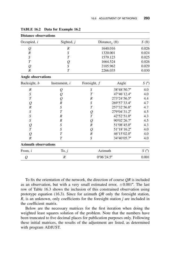
16.6 ADJUSTMENT OF NETWORKS 293
TABLE 16.2 Data for Example 16.2
Distance observations
Occupied, i Sighted, j Distanceij (ft) S (ft)
Q R 1640.016 0.026R S 1320.001 0.024S T 1579.123 0.025T Q 1664.524 0.026Q S 2105.962 0.029R T 2266.035 0.030
Angle observations
Backsight, b Instrument, i Foresight, ƒ Angle S (�)
R Q S 38�48�50.7� 4.0S Q T 47�46�12.4� 4.0T Q R 273�24�56.5� 4.4Q R S 269�57�33.4� 4.7R S T 257�32�56.8� 4.7S T Q 279�04�31.2� 4.5S R T 42�52�51.0� 4.3S R Q 90�02�26.7� 4.5Q S R 51�08�45.0� 4.3T S Q 51�18�16.2� 4.0Q T R 46�15�02.0� 4.0R T S 34�40�05.7� 4.0
Azimuth observations
From, i To, j Azimuth S (�)
Q R 0�06�24.5� 0.001
To fix the orientation of the network, the direction of course QR is includedas an observation, but with a very small estimated error, �0.001�. The lastrow of Table 16.3 shows the inclusion of this constrained observation usingprototype equation (16.3). Since for azimuth QR only the foresight station,R, is an unknown, only coefficients for the foresight station j are included inthe coefficient matrix.
Below are the necessary matrices for the first iteration when doing theweighted least squares solution of the problem. Note that the numbers havebeen truncated to five decimal places for publication purposes only. Followingthese initial matrices, the results of the adjustment are listed, as determinedwith program ADJUST.
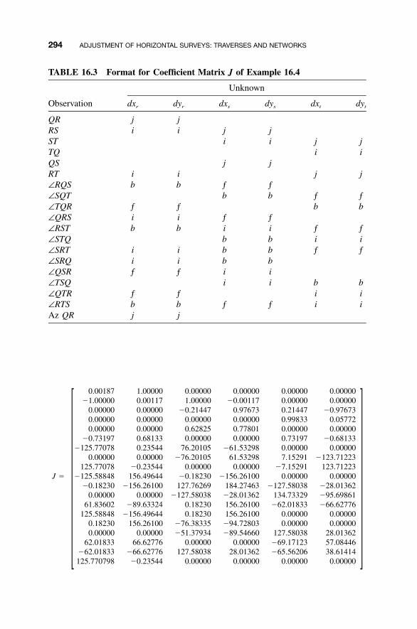
294 ADJUSTMENT OF HORIZONTAL SURVEYS: TRAVERSES AND NETWORKS
TABLE 16.3 Format for Coefficient Matrix J of Example 16.4
Observation
Unknown
dxr dyr dxs dys dxt dyt
QR j jRS i i j jST i i j jTQ i iQS j jRT i i j j∠RQS b b ƒ ƒ∠SQT b b ƒ ƒ∠TQR ƒ ƒ b b∠QRS i i ƒ ƒ∠RST b b i i ƒ ƒ∠STQ b b i i∠SRT i i b b ƒ ƒ∠SRQ i i b b∠QSR ƒ ƒ i i∠TSQ i i b b∠QTR ƒ ƒ i i∠RTS b b ƒ ƒ i iAz QR j j
J �
0.00187�1.00000
0.000000.000000.00000
�0.73197�125.77078
0.00000125.77078
�125.58848�0.18230
0.0000061.83602
125.588480.182300.00000
62.01833�62.01833125.770798
1.000000.001170.000000.000000.000000.681330.235440.00000
�0.23544156.49644
�156.261000.00000
�89.63324�156.49644
156.261000.00000
66.62776�66.62776�0.23544
0.000001.00000
�0.214470.000000.628250.00000
76.20105�76.20105
0.00000�0.18230127.76269
�127.580380.182300.18230
�76.38335�51.37934
0.00000127.58038
0.00000
0.00000�0.00117
0.976730.000000.778010.00000
�61.5329861.532980.00000
�156.26100184.27463
�28.01362156.26100156.26100
�94.72803�89.54660
0.0000028.013620.00000
0.000000.000000.214470.998330.000000.731970.000007.15291
�7.152910.00000
�127.58038134.73329
�62.018330.000000.00000
127.58038�69.17123�65.56206
0.00000
0.000000.00000
�0.976730.057720.00000
�0.681330.00000
�123.71223123.71223
0.00000�28.01362�95.69861�66.62776
0.000000.00000
28.0136257.0844638.614140.00000
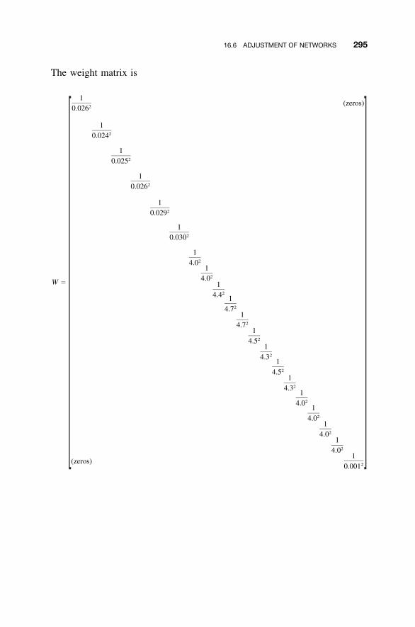
16.6 ADJUSTMENT OF NETWORKS 295
The weight matrix is
1(zeros)
20.026
120.024
120.025
120.026
120.029
120.030
124.0
124.0W � 1
24.4 124.7
124.7
124.5
124.3
124.5
124.3
124.0
124.0
124.0
124.0
1(zeros)
20.001
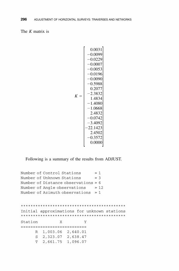
296 ADJUSTMENT OF HORIZONTAL SURVEYS: TRAVERSES AND NETWORKS
The K matrix is
0.0031�0.0099�0.0229�0.0007�0.0053�0.0196�0.0090�0.5988
0.2077�2.3832
K �1.4834
�1.4080�1.0668
2.4832�0.0742�3.4092
�22.14232.4502
�0.35720.0000
Following is a summary of the results from ADJUST.
Number of Control Stations » 1Number of Unknown Stations » 3Number of Distance observations » 6Number of Angle observations » 12Number of Azimuth observations » 1
*******************************************Initial approximations for unknown stations*******************************************
Station X Y===========================
R 1,003.06 2,640.01S 2,323.07 2,638.47T 2,661.75 1,096.07
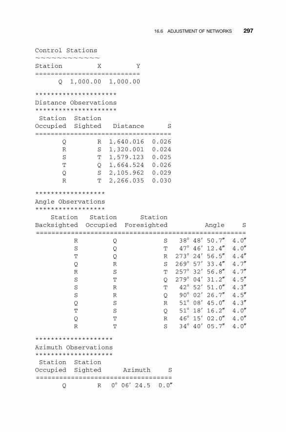
16.6 ADJUSTMENT OF NETWORKS 297
Control Stations������������Station X Y===========================
Q 1,000.00 1,000.00
*********************Distance Observations*********************Station StationOccupied Sighted Distance S===================================
Q R 1,640.016 0.026R S 1,320.001 0.024S T 1,579.123 0.025T Q 1,664.524 0.026Q S 2,105.962 0.029R T 2,266.035 0.030
******************Angle Observations******************
Station Station StationBacksighted Occupied Foresighted Angle S======================================================
R Q S 38� 48� 50.7� 4.0�S Q T 47� 46� 12.4� 4.0�T Q R 273� 24� 56.5� 4.4�Q R S 269� 57� 33.4� 4.7�R S T 257� 32� 56.8� 4.7�S T Q 279� 04� 31.2� 4.5�S R T 42� 52� 51.0� 4.3�S R Q 90� 02� 26.7� 4.5�Q S R 51� 08� 45.0� 4.3�T S Q 51� 18� 16.2� 4.0�Q T R 46� 15� 02.0� 4.0�R T S 34� 40� 05.7� 4.0�
********************Azimuth Observations********************Station StationOccupied Sighted Azimuth S===================================
Q R 0� 06� 24.5 0.0�
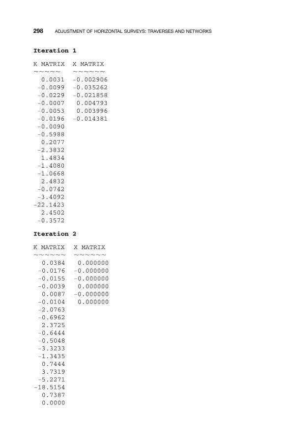
298 ADJUSTMENT OF HORIZONTAL SURVEYS: TRAVERSES AND NETWORKS
Iteration 1
K MATRIX X MATRIX����� ������0.0031 �0.002906
�0.0099 �0.035262�0.0229 �0.021858�0.0007 0.004793�0.0053 0.003996�0.0196 �0.014381�0.0090�0.59880.2077
�2.38321.4834
�1.4080�1.06682.4832
�0.0742�3.4092
�22.14232.4502
�0.3572
Iteration 2
K MATRIX X MATRIX������ ������
0.0384 0.000000�0.0176 �0.000000�0.0155 �0.000000�0.0039 0.0000000.0087 �0.000000
�0.0104 0.000000�2.0763�0.69622.3725
�0.6444�0.5048�3.3233�1.34350.74443.7319
�5.2271�18.51540.73870.0000
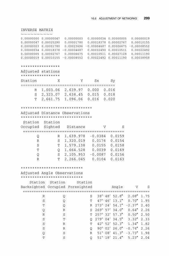
16.6 ADJUSTMENT OF NETWORKS 299
INVERSE MATRIX����������0.00000000 0.00000047 0.00000003 0.00000034 0.00000005 0.000000190.00000047 0.00025290 0.00001780 0.00018378 0.00002767 0.000101550.00000003 0.00001780 0.00023696 �0.00004687 0.00006675 �0.000085520.00000034 0.00018378 �0.00004687 0.00032490 0.00010511 0.000224920.00000005 0.00002767 0.00006675 0.00010511 0.00027128 0.000111900.00000019 0.00010155 �0.00008552 0.00022492 0.00011190 0.00038959
*****************Adjusted stations*****************Station X Y Sx Sy=========================================
R 1,003.06 2,639.97 0.000 0.016S 2,323.07 2,638.45 0.015 0.018T 2,661.75 1,096.06 0.016 0.020
*******************************Adjusted Distance Observations*******************************Station StationOccupied Sighted Distance V S============================================
Q R 1,639.978 �0.0384 0.0159R S 1,320.019 0.0176 0.0154S T 1,579.138 0.0155 0.0158T Q 1,664.528 0.0039 0.0169Q S 2,105.953 �0.0087 0.0156R T 2,266.045 0.0104 0.0163
***************************Adjusted Angle Observations***************************
Station Station StationBacksighted Occupied Foresighted Angle V S==========================================================
R Q S 38� 48� 52.8� 2.08� 1.75S Q T 47� 46� 13.1� 0.70� 1.95T Q R 273� 24� 54.1� �2.37� 2.40Q R S 269� 57� 34.0� 0.64� 2.26R S T 257� 32� 57.3� 0.50� 2.50S T Q 279� 04� 34.5� 3.32� 2.33S R T 42� 52� 52.3� 1.34� 1.82S R Q 90� 02� 26.0� �0.74� 2.26Q S R 51� 08� 41.3� �3.73� 1.98T S Q 51� 18� 21.4� 5.23� 2.04
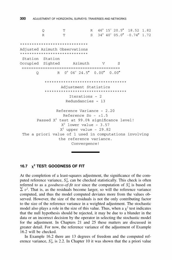
300 ADJUSTMENT OF HORIZONTAL SURVEYS: TRAVERSES AND NETWORKS
Q T R 46� 15� 20.5� 18.52 1.82R T S 34� 40� 05.0� �0.74� 1.72
*****************************Adjusted Azimuth Observations*****************************Station StationOccupied Sighted Azimuth V S==========================================
Q R 0� 06� 24.5� 0.00� 0.00�
***********************************Adjustment Statistics
***********************************Iterations � 2
Redundancies � 13
Reference Variance � 2.20Reference So � �1.5
Passed X2 test at 99.0% significance level!X2 lower value � 3.57X2 upper value � 29.82
The a priori value of 1 used in computations involvingthe reference variance.
Convergence!
16.7 �2 TEST: GOODNESS OF FIT
At the completion of a least-squares adjustment, the significance of the com-puted reference variance, can be checked statistically. This check is often2S ,0
referred to as a goodness-of-fit test since the computation of is based on2S0
v2. That is, as the residuals become larger, so will the reference variancecomputed, and thus the model computed deviates more from the values ob-served. However, the size of the residuals is not the only contributing factorto the size of the reference variance in a weighted adjustment. The stochasticmodel also plays a role in the size of this value. Thus, when a �2 test indicatesthat the null hypothesis should be rejected, it may be due to a blunder in thedata or an incorrect decision by the operator in selecting the stochastic modelfor the adjustment. In Chapters 21 and 25 these matters are discussed ingreater detail. For now, the reference variance of the adjustment of Example16.2 will be checked.
In Example 16.2 there are 13 degrees of freedom and the computed ref-erence variance, is 2.2. In Chapter 10 it was shown that the a priori value2S ,0
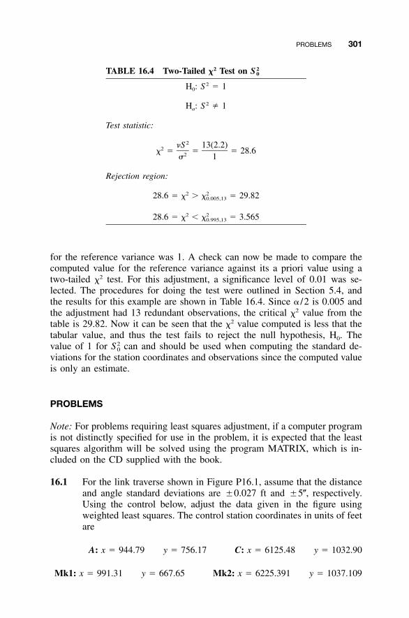
PROBLEMS 301
TABLE 16.4 Two-Tailed �2 Test on 2S 0
H0: S 2 � 1
Ha: S 2 � 1
Test statistic:
2�S 13(2.2)2� � � � 28.62� 1
Rejection region:
2 228.6 � � � � � 29.820.005,13
2 228.6 � � � � � 3.5650.995,13
for the reference variance was 1. A check can now be made to compare thecomputed value for the reference variance against its a priori value using atwo-tailed �2 test. For this adjustment, a significance level of 0.01 was se-lected. The procedures for doing the test were outlined in Section 5.4, andthe results for this example are shown in Table 16.4. Since � /2 is 0.005 andthe adjustment had 13 redundant observations, the critical �2 value from thetable is 29.82. Now it can be seen that the �2 value computed is less that thetabular value, and thus the test fails to reject the null hypothesis, H0. Thevalue of 1 for can and should be used when computing the standard de-2S0
viations for the station coordinates and observations since the computed valueis only an estimate.
PROBLEMS
Note: For problems requiring least squares adjustment, if a computer programis not distinctly specified for use in the problem, it is expected that the leastsquares algorithm will be solved using the program MATRIX, which is in-cluded on the CD supplied with the book.
16.1 For the link traverse shown in Figure P16.1, assume that the distanceand angle standard deviations are �0.027 ft and �5�, respectively.Using the control below, adjust the data given in the figure usingweighted least squares. The control station coordinates in units of feetare
A: x � 944.79 y � 756.17 C: x � 6125.48 y � 1032.90
Mk1: x � 991.31 y � 667.65 Mk2: x � 6225.391 y � 1037.109
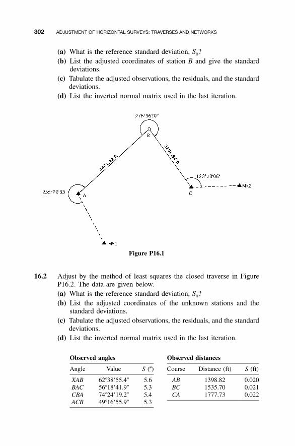
302 ADJUSTMENT OF HORIZONTAL SURVEYS: TRAVERSES AND NETWORKS
(a) What is the reference standard deviation, S0?(b) List the adjusted coordinates of station B and give the standard
deviations.(c) Tabulate the adjusted observations, the residuals, and the standard
deviations.(d) List the inverted normal matrix used in the last iteration.
Figure P16.1
16.2 Adjust by the method of least squares the closed traverse in FigureP16.2. The data are given below.(a) What is the reference standard deviation, S0?(b) List the adjusted coordinates of the unknown stations and the
standard deviations.(c) Tabulate the adjusted observations, the residuals, and the standard
deviations.(d) List the inverted normal matrix used in the last iteration.
Observed angles Observed distances
Angle Value S (�) Course Distance (ft) S (ft)
XAB 62�38�55.4� 5.6 AB 1398.82 0.020BAC 56�18�41.9� 5.3 BC 1535.70 0.021CBAACB
74�24�19.2�49�16�55.9�
5.45.3
CA 1777.73 0.022
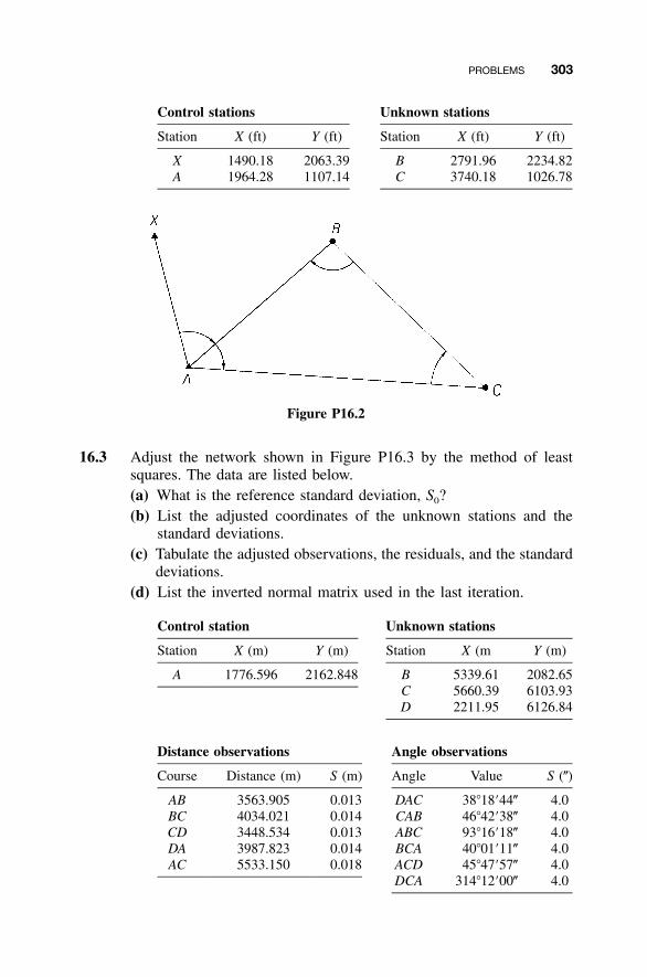
PROBLEMS 303
Control stations Unknown stations
Station X (ft) Y (ft) Station X (ft) Y (ft)
X 1490.18 2063.39 B 2791.96 2234.82A 1964.28 1107.14 C 3740.18 1026.78
Figure P16.2
16.3 Adjust the network shown in Figure P16.3 by the method of leastsquares. The data are listed below.(a) What is the reference standard deviation, S0?(b) List the adjusted coordinates of the unknown stations and the
standard deviations.(c) Tabulate the adjusted observations, the residuals, and the standard
deviations.(d) List the inverted normal matrix used in the last iteration.
Control station Unknown stations
Station X (m) Y (m) Station X (m Y (m)
A 1776.596 2162.848 BC
5339.615660.39
2082.656103.93
D 2211.95 6126.84
Distance observations Angle observations
Course Distance (m) S (m) Angle Value S (�)
AB 3563.905 0.013 DAC 38�18�44� 4.0BC 4034.021 0.014 CAB 46�42�38� 4.0CD 3448.534 0.013 ABC 93�16�18� 4.0DA 3987.823 0.014 BCA 40�01�11� 4.0AC 5533.150 0.018 ACD
DCA45�47�57�
314�12�00�4.04.0
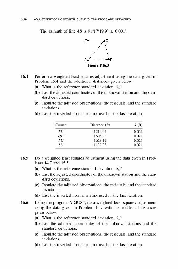
304 ADJUSTMENT OF HORIZONTAL SURVEYS: TRAVERSES AND NETWORKS
The azimuth of line AB is 91�17�19.9� � 0.001�.
Figure P16.3
16.4 Perform a weighted least squares adjustment using the data given inProblem 15.4 and the additional distances given below.(a) What is the reference standard deviation, S0?(b) List the adjusted coordinates of the unknown station and the stan-
dard deviations.(c) Tabulate the adjusted observations, the residuals, and the standard
deviations.(d) List the inverted normal matrix used in the last iteration.
Course Distance (ft) S (ft)
PU 1214.44 0.021QU 1605.03 0.021RU 1629.19 0.021SU 1137.33 0.021
16.5 Do a weighted least squares adjustment using the data given in Prob-lems 14.7 and 15.5.(a) What is the reference standard deviation, S0?(b) List the adjusted coordinates of the unknown station and the stan-
dard deviations.(c) Tabulate the adjusted observations, the residuals, and the standard
deviations.(d) List the inverted normal matrix used in the last iteration.
16.6 Using the program ADJUST, do a weighted least squares adjustmentusing the data given in Problem 15.7 with the additional distancesgiven below.(a) What is the reference standard deviation, S0?(b) List the adjusted coordinates of the unknown stations and the
standard deviations.(c) Tabulate the adjusted observations, the residuals, and the standard
deviations.(d) List the inverted normal matrix used in the last iteration.
PROBLEMS 305
Course Distance (m) S (m)
AD 17,337.708 0.087AC 27,331.345 0.137BD 23,193.186 0.116BC 19,382.380 0.097CD 17,745.364 0.089
16.7 Using the program ADJUST, do a weighted least squares adjustmentusing the data given in Problem 15.9 with the additional distancesgiven below.(a) What is the reference standard deviation, S0?(b) List the adjusted coordinates of the unknown stations and the
standard deviations.(c) Tabulate the adjusted observations, the residuals, and the standard
deviations.(d) List the inverted normal matrix used in the last iteration.
Course Distance (m) S (m)
AC 9197.385 0.028AD 16,897.138 0.051BC 17,329.131 0.052BD 8666.341 0.026CD 14,384.926 0.043CE 8115.898 0.025CF 16,845.056 0.051DE 16,113.175 0.049DF 9019.629 0.027EF 13,800.459 0.042EG 8394.759 0.026EH 16,164.944 0.049FG 16,096.755 0.048FH 8170.129 0.025
16.8 Using the Program ADJUST, do a weighted least squares adjustmentusing the data given in Problems 14.4 and 15.11.(a) What is the reference standard deviation, S0?(b) List the adjusted coordinates of the unknown station and the stan-
dard deviations.(c) Tabulate the adjusted observations, the residuals, and the standard
deviations.(d) List the inverted normal matrix used in the last iteration.
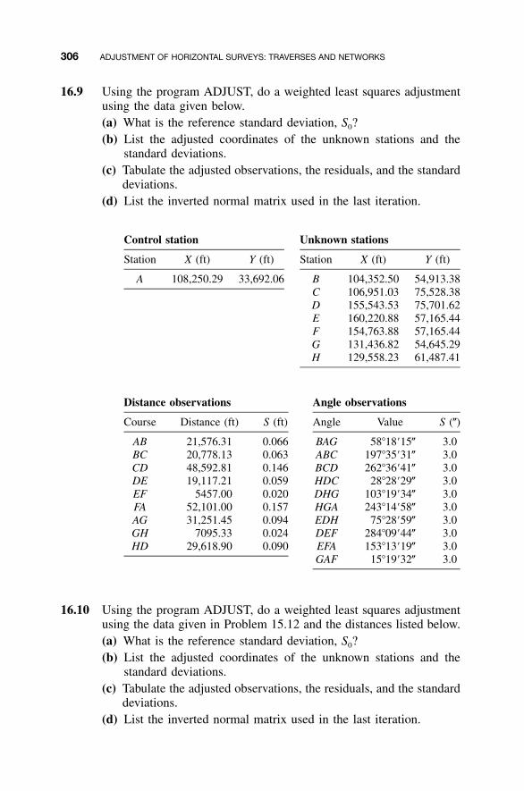
306 ADJUSTMENT OF HORIZONTAL SURVEYS: TRAVERSES AND NETWORKS
16.9 Using the program ADJUST, do a weighted least squares adjustmentusing the data given below.(a) What is the reference standard deviation, S0?(b) List the adjusted coordinates of the unknown stations and the
standard deviations.(c) Tabulate the adjusted observations, the residuals, and the standard
deviations.(d) List the inverted normal matrix used in the last iteration.
Control station Unknown stations
Station X (ft) Y (ft) Station X (ft) Y (ft)
A 108,250.29 33,692.06 BC
104,352.50106,951.03
54,913.3875,528.38
D 155,543.53 75,701.62E 160,220.88 57,165.44F 154,763.88 57,165.44G 131,436.82 54,645.29H 129,558.23 61,487.41
Distance observations Angle observations
Course Distance (ft) S (ft) Angle Value S (�)
AB 21,576.31 0.066 BAG 58�18�15� 3.0BC 20,778.13 0.063 ABC 197�35�31� 3.0CD 48,592.81 0.146 BCD 262�36�41� 3.0DE 19,117.21 0.059 HDC 28�28�29� 3.0EF 5457.00 0.020 DHG 103�19�34� 3.0FA 52,101.00 0.157 HGA 243�14�58� 3.0AG 31,251.45 0.094 EDH 75�28�59� 3.0GH 7095.33 0.024 DEF 284�09�44� 3.0HD 29,618.90 0.090 EFA
GAF153�13�19�
15�19�32�3.03.0
16.10 Using the program ADJUST, do a weighted least squares adjustmentusing the data given in Problem 15.12 and the distances listed below.(a) What is the reference standard deviation, S0?(b) List the adjusted coordinates of the unknown stations and the
standard deviations.(c) Tabulate the adjusted observations, the residuals, and the standard
deviations.(d) List the inverted normal matrix used in the last iteration.
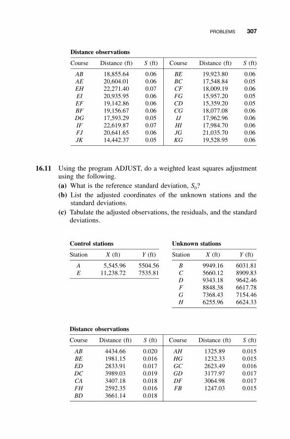
PROBLEMS 307
Distance observations
Course Distance (ft) S (ft) Course Distance (ft) S (ft)
AB 18,855.64 0.06 BE 19,923.80 0.06AE 20,604.01 0.06 BC 17,548.84 0.05EH 22,271.40 0.07 CF 18,009.19 0.06EI 20,935.95 0.06 FG 15,957.20 0.05EF 19,142.86 0.06 CD 15,359.20 0.05BF 19,156.67 0.06 CG 18,077.08 0.06DG 17,593.29 0.05 IJ 17,962.96 0.06IF 22,619.87 0.07 HI 17,984.70 0.06FJ 20,641.65 0.06 JG 21,035.70 0.06JK 14,442.37 0.05 KG 19,528.95 0.06
16.11 Using the program ADJUST, do a weighted least squares adjustmentusing the following.(a) What is the reference standard deviation, S0?(b) List the adjusted coordinates of the unknown stations and the
standard deviations.(c) Tabulate the adjusted observations, the residuals, and the standard
deviations.
Control stations Unknown stations
Station X (ft) Y (ft) Station X (ft) Y (ft)
A 5,545.96 5504.56 B 9949.16 6031.81E 11,238.72 7535.81 C
D5660.129343.18
8909.839642.46
F 8848.38 6617.78G 7368.43 7154.46H 6255.96 6624.33
Distance observations
Course Distance (ft) S (ft) Course Distance (ft) S (ft)
AB 4434.66 0.020 AH 1325.89 0.015BE 1981.15 0.016 HG 1232.33 0.015ED 2833.91 0.017 GC 2623.49 0.016DC 3989.03 0.019 GD 3177.97 0.017CA 3407.18 0.018 DF 3064.98 0.017FH 2592.35 0.016 FB 1247.03 0.015BD 3661.14 0.018
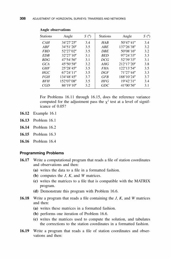
308 ADJUSTMENT OF HORIZONTAL SURVEYS: TRAVERSES AND NETWORKS
Angle observations
Stations Angle S (�) Stations Angle S (�)
CAH 34�27�25� 3.4 HAB 50�47�41� 3.4ABF 34�51�20� 3.5 ABE 137�26�38� 3.2FBD 52�27�02� 3.5 DBE 50�08�16� 3.2EDB 32�27�10� 3.1 BED 97�24�33� 3.3BDG 47�54�56� 3.1 DCG 52�39�33� 3.1GCA 45�50�58� 3.2 AHG 212�17�20� 3.8GHF 25�28�45� 3.5 FHA 122�13�54� 3.5HGC 67�24�11� 3.5 DGF 71�27�44� 3.3FGH 134�48�45� 3.7 GFB 188�10�24� 3.7BFH 152�07�08� 3.5 HFG 19�42�31� 3.4CGD 86�19�10� 3.2 GDC 41�00�56� 3.1
For Problems 16.11 through 16.15, does the reference variancecomputed for the adjustment pass the �2 test at a level of signif-icance of 0.05?
16.12 Example 16.1
16.13 Problem 16.1
16.14 Problem 16.2
16.15 Problem 16.3
16.16 Problem 16.4
Programming Problems
16.17 Write a computational program that reads a file of station coordinatesand observations and then:(a) writes the data to a file in a formatted fashion.(b) computes the J, K, and W matrices.(c) writes the matrices to a file that is compatible with the MATRIX
program.(d) Demonstrate this program with Problem 16.6.
16.18 Write a program that reads a file containing the J, K, and W matricesand then:(a) writes these matrices in a formatted fashion.(b) performs one iteration of Problem 16.6.(c) writes the matrices used to compute the solution, and tabulates
the corrections to the station coordinates in a formatted fashion.
16.19 Write a program that reads a file of station coordinates and obser-vations and then:
PROBLEMS 309
(a) writes the data to a file in a formatted fashion.(b) computes the J, K, and W matrices.(c) performs a weighted least squares adjustment of Problem 16.6.(d) writes the matrices used in computations in a formatted fashion
to a file.(e) computes the final adjusted station coordinates, their estimated
errors, the adjusted observations, their residuals, and their esti-mated errors, and writes them to a file in a formatted fashion.
16.20 Develop a computational program that creates the coefficient, weight,and constant matrices for a network. Write the matrices to a file in aformat usable by the MATRIX program supplied with this book.Demonstrate its use with Problem 16.6.
310
CHAPTER 17
ADJUSTMENT OF GPS NETWORKS
17.1 INTRODUCTION
For the past five decades, NASA and the U.S. military have been engaged ina space research program to develop a precise positioning and navigationsystem. The first-generation system, called TRANSIT, used six satellites andwas based on the Doppler principle. TRANSIT was made available for com-mercial use in 1967, and shortly thereafter its use in surveying began. Theestablishment of a worldwide network of control stations was among its ear-liest and most valuable applications. Point positioning using TRANSIT re-quired very lengthy observing sessions, and its accuracy was at the 1-m level.Thus, in surveying it was suitable only for control work on networks con-sisting of widely spaced points. It was not satisfactory for everyday surveyingapplications such as traversing or engineering layout.
Encouraged by the success of TRANSIT, a new research program wasdeveloped that ultimately led to the creation of the NAVSTAR Global Posi-tioning System (GPS). This second-generation positioning and navigation sys-tem utilizes a constellation of 24 orbiting satellites. The accuracy of GPS wasimproved substantially over that of the TRANSIT system, and the disadvan-tage of lengthy observing sessions was also eliminated. Although developedfor military applications, civilians, including surveyors, also found uses forthe GPS system.
Since its introduction, GPS has been used extensively. It is reliable, effi-cient, and capable of yielding extremely high accuracies. GPS observationscan be taken day or night and in any weather conditions. A significant ad-vantage of GPS is that visibility between surveyed points is not necessary.Thus, the time-consuming process of clearing lines of sight is avoided. Al-
Adjustment Computations: Spatial Data Analysis, Fourth Edition. C. D. Ghilani and P. R. Wolf© 2006 John Wiley & Sons, Inc. ISBN: 978-0-471-69728-2
17.2 GPS OBSERVATIONS 311
though most of the earliest applications of GPS were in control work, im-provements have now made the system convenient and practical for use invirtually every type of survey, including property surveys, topographic map-ping, and construction staking.
In this chapter we provide a brief introduction to GPS surveying. We ex-plain the basic measurements involved in the system, discuss the errors inthose measurements, describe the nature of the adjustments needed to accountfor those errors, and give the procedures for making adjustments of networkssurveyed using GPS. An example problem is given to demonstrate the pro-cedures.
17.2 GPS OBSERVATIONS
Fundamentally, the global positioning system operates by observing distancesfrom receivers located on ground stations of unknown locations to orbitingGPS satellites whose positions are known precisely. Thus, conceptually, GPSsurveying is similar to conventional resection, in which distances are observedwith an EDM instrument from an unknown station to several control points.(The conventional resection procedure was discussed in Chapter 15 and il-lustrated in Example 15.2.) Of course, there are some differences betweenGPS position determination and conventional resection. Among them is theprocess of observing distances and the fact that the control stations used inGPS work are satellites.
All of the 24 satellites in the GPS constellation orbit Earth at nominalaltitudes of 20,200 km. Each satellite continuously broadcasts unique elec-tronic signals on two carrier frequencies. These carriers are modulated withpseudorandom noise (PRN) codes. The PRN codes consist of unique se-quences of binary values (zeros and ones) that are superimposed on the car-riers. These codes appear to be random, but in fact they are generatedaccording to a known mathematical algorithm. The frequencies of the carriersand PRN codes are controlled very precisely at known values.
Distances are determined in GPS surveying by taking observations on thesetransmitted satellite signals. Two different observational procedures are used:positioning by pseudoranging, and positioning by carrier-phase measure-ments. Pseudoranging involves determining distances (ranges) between sat-ellites and receivers by observing precisely the time it takes transmittedsignals to travel from satellites to ground receivers. This is done by deter-mining changes in the PRN codes that occur during the time it takes signalsto travel from the satellite transmitter to the antenna of the receiver. Thenfrom the known frequency of the PRN codes, very precise travel times aredetermined. With the velocity and travel times of the signals known, thepseudoranges can be computed. Finally, based on these ranges, the positionsof the ground stations can be calculated. Because pseudoranging is based on

312 ADJUSTMENT OF GPS NETWORKS
observing PRN codes, this GPS observation technique is also often referredto as the code measurement procedure.
In the carrier-phase procedure, the quantities observed are phase changesthat occur as a result of the carrier wave traveling from the satellites to thereceivers. The principle is similar to the phase-shift method employed byelectronic distance-measuring instruments. However, a major difference is thatthe satellites are moving, so that the signals cannot be returned to the trans-mitters for ‘‘true’’ phase-shift measurements. Instead, the phase shifts mustbe observed at the receivers. But to make true phase-shift observations, theclocks in the satellites and receivers would have to be perfectly synchronized,which of course cannot be achieved. To overcome this timing problem andto eliminate other errors in the system, differencing techniques (taking dif-ferences between phase observations) are used. Various differencing proce-dures can be applied. Single differencing is achieved by simultaneouslyobserving two satellites with one receiver. Single differencing eliminates sat-ellite clock biases. Double differencing (subtracting the results of single dif-ferences from two receivers) eliminates receiver clock biases and othersystematic errors.
Another problem in making carrier-phase measurements is that only thephase shift of the last cycle of the carrier wave is observed, and the numberof full cycles in the travel distance is unknown. (In EDM work this problemis overcome by progressively transmitting longer wavelengths and observingtheir phase shifts.) Again, because the satellites are moving, this cannot bedone in GPS work. However, by extending the differencing technique to whatis called triple differencing, this ambiguity in the number of cycles cancelsout of the solution. Triple differencing consists of differencing the results oftwo double differences and thus involves making observations at two differenttimes to two satellites from two stations.
In practice, when surveys are done by observing carrier phases, four ormore satellites are observed simultaneously using two or more receivers lo-cated on ground stations. Also, the observations are repeated many times.This produces a very large number of redundant observations, from whichmany difference combinations can be computed.
Of the two GPS observing procedures, pseudoranging yields a somewhatlower order of accuracy, but it is preferred for navigation use because it givesinstantaneous point positions of satisfactory accuracy. The carrier-phase tech-nique produces a higher order of accuracy and is therefore the choice forhigh-precision surveying applications. Adjustment of carrier-phase GPS ob-servations is the subject of this chapter.
The differencing techniques used in carrier-phase observations, describedbriefly above, do not yield positions directly for the points occupied by re-ceivers. Rather, baselines (vector distances between stations) are determined.These baselines are actually computed in terms of their coordinate differencecomponents �X, �Y, and �Z. These coordinate differences are reported in the
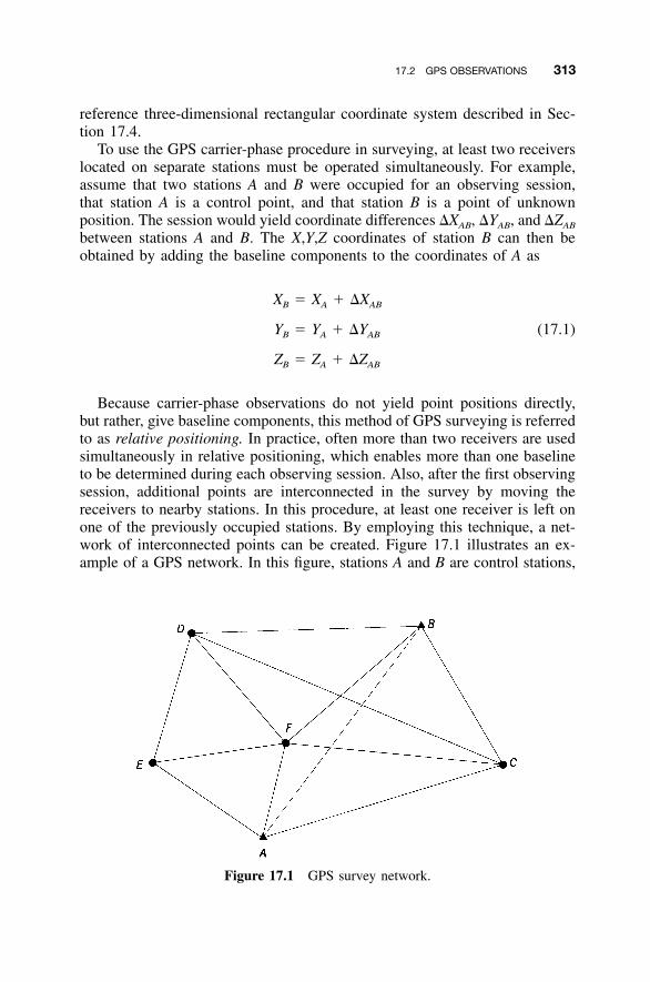
17.2 GPS OBSERVATIONS 313
Figure 17.1 GPS survey network.
reference three-dimensional rectangular coordinate system described in Sec-tion 17.4.
To use the GPS carrier-phase procedure in surveying, at least two receiverslocated on separate stations must be operated simultaneously. For example,assume that two stations A and B were occupied for an observing session,that station A is a control point, and that station B is a point of unknownposition. The session would yield coordinate differences �XAB, �YAB, and �ZAB
between stations A and B. The X,Y,Z coordinates of station B can then beobtained by adding the baseline components to the coordinates of A as
X � X � �XB A AB
Y � Y � �Y (17.1)B A AB
Z � Z � �ZB A AB
Because carrier-phase observations do not yield point positions directly,but rather, give baseline components, this method of GPS surveying is referredto as relative positioning. In practice, often more than two receivers are usedsimultaneously in relative positioning, which enables more than one baselineto be determined during each observing session. Also, after the first observingsession, additional points are interconnected in the survey by moving thereceivers to nearby stations. In this procedure, at least one receiver is left onone of the previously occupied stations. By employing this technique, a net-work of interconnected points can be created. Figure 17.1 illustrates an ex-ample of a GPS network. In this figure, stations A and B are control stations,
314 ADJUSTMENT OF GPS NETWORKS
and stations C, D, E, and F are points of unknown position. Creation of suchnetworks is a common procedure employed in GPS relative positioning work.
17.3 GPS ERRORS AND THE NEED FOR ADJUSTMENT
As in all types of surveying observations, GPS observations contain errors.The principal sources of these errors are (1) orbital errors in the satellite, (2)signal transmission timing errors due to atmospheric conditions, (3) receivererrors, (4) multipath errors (signals being reflected so that they travel indirectroutes from satellite to receiver), and (5) miscentering errors of the receiverantenna over the ground station and receiver height-measuring errors. Toaccount for these and other errors, and to increase the precisions of pointposition, GPS observations are very carefully made according to strictspecifications, and redundant observations are taken. The fact that errors arepresent in the observations makes it necessary to analyze the measurementsfor acceptance or rejection. Also, because redundant observations have beenmade, they must be adjusted so that all observed values are consistent.
In GPS surveying work where the observations are made using carrier-phase observations, there are two stages where least squares adjustment isapplied. The first is in processing the redundant observations to obtain theadjusted baseline components (�X, �Y, �Z), and the second is in adjustingnetworks of stations wherein the baseline components have been observed.The latter adjustment is discussed in more detail later in the chapter.
17.4 REFERENCE COORDINATE SYSTEMS FORGPS OBSERVATIONS
In GPS surveying, three different reference coordinate systems are involved.First, the satellite positions at the instants of their observation are given in aspace-related Xs,Ys,Zs three-dimensional rectangular coordinate system. Thiscoordinate system is illustrated in Figure 17.2. In the figure, the ellipticalorbit of a satellite is shown. It has one of its two foci at G, Earth’s center ofgravity. Two points, perigee (point where the satellite is closest to G) andapogee (point where the satellite is farthest from G), define the line of apsides.This line, which also passes through the two foci, is the Xs axis of the satellitereference coordinate system. The origin of the system is at G, the Ys axis isin the mean orbital plane, and Zs is perpendicular to the Xs–Ys plane. Becausea satellite varies only slightly from its mean orbital plane, values of Zs aresmall. For each specific instant of time that a given satellite is observed, itscoordinates are calculated in its unique Xs,Ys,Zs system.
In processing GPS observations, all Xs, Ys, and Zs coordinates that werecomputed for satellite observations are converted to a common Earth-relatedXe,Ye,Ze three-dimensional geocentric coordinate system. This Earth-centered,Earth-fixed coordinate system, illustrated in Figure 17.3, is also commonly
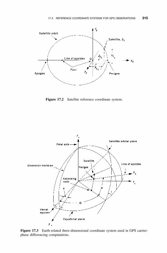
17.4 REFERENCE COORDINATE SYSTEMS FOR GPS OBSERVATIONS 315
Figure 17.2 Satellite reference coordinate system.
Figure 17.3 Earth-related three-dimensional coordinate system used in GPS carrier-phase differencing computations.
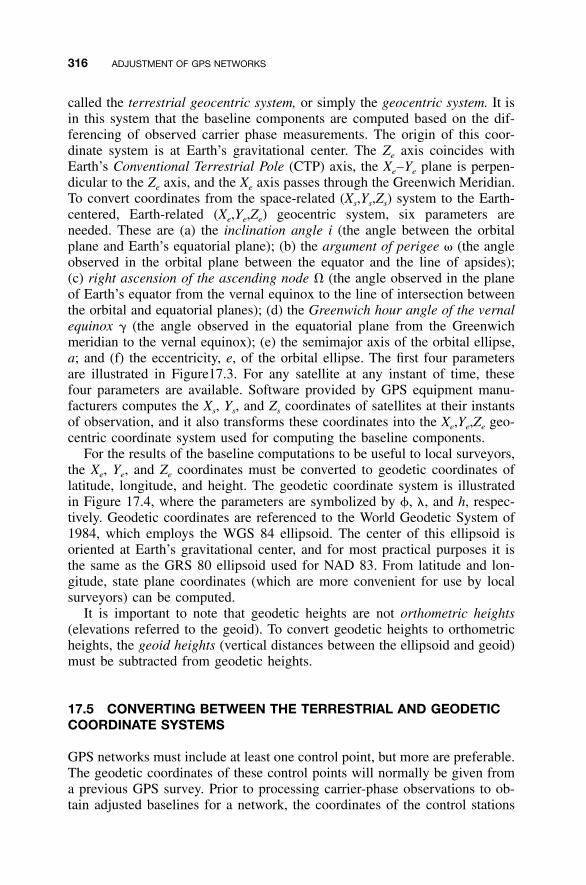
316 ADJUSTMENT OF GPS NETWORKS
called the terrestrial geocentric system, or simply the geocentric system. It isin this system that the baseline components are computed based on the dif-ferencing of observed carrier phase measurements. The origin of this coor-dinate system is at Earth’s gravitational center. The Ze axis coincides withEarth’s Conventional Terrestrial Pole (CTP) axis, the Xe–Ye plane is perpen-dicular to the Ze axis, and the Xe axis passes through the Greenwich Meridian.To convert coordinates from the space-related (Xs,Ys,Zs) system to the Earth-centered, Earth-related (Xe,Ye,Ze) geocentric system, six parameters areneeded. These are (a) the inclination angle i (the angle between the orbitalplane and Earth’s equatorial plane); (b) the argument of perigee � (the angleobserved in the orbital plane between the equator and the line of apsides);(c) right ascension of the ascending node � (the angle observed in the planeof Earth’s equator from the vernal equinox to the line of intersection betweenthe orbital and equatorial planes); (d) the Greenwich hour angle of the vernalequinox � (the angle observed in the equatorial plane from the Greenwichmeridian to the vernal equinox); (e) the semimajor axis of the orbital ellipse,a; and (f) the eccentricity, e, of the orbital ellipse. The first four parametersare illustrated in Figure17.3. For any satellite at any instant of time, thesefour parameters are available. Software provided by GPS equipment manu-facturers computes the Xs, Ys, and Zs coordinates of satellites at their instantsof observation, and it also transforms these coordinates into the Xe,Ye,Ze geo-centric coordinate system used for computing the baseline components.
For the results of the baseline computations to be useful to local surveyors,the Xe, Ye, and Ze coordinates must be converted to geodetic coordinates oflatitude, longitude, and height. The geodetic coordinate system is illustratedin Figure 17.4, where the parameters are symbolized by �, �, and h, respec-tively. Geodetic coordinates are referenced to the World Geodetic System of1984, which employs the WGS 84 ellipsoid. The center of this ellipsoid isoriented at Earth’s gravitational center, and for most practical purposes it isthe same as the GRS 80 ellipsoid used for NAD 83. From latitude and lon-gitude, state plane coordinates (which are more convenient for use by localsurveyors) can be computed.
It is important to note that geodetic heights are not orthometric heights(elevations referred to the geoid). To convert geodetic heights to orthometricheights, the geoid heights (vertical distances between the ellipsoid and geoid)must be subtracted from geodetic heights.
17.5 CONVERTING BETWEEN THE TERRESTRIAL AND GEODETICCOORDINATE SYSTEMS
GPS networks must include at least one control point, but more are preferable.The geodetic coordinates of these control points will normally be given froma previous GPS survey. Prior to processing carrier-phase observations to ob-tain adjusted baselines for a network, the coordinates of the control stations
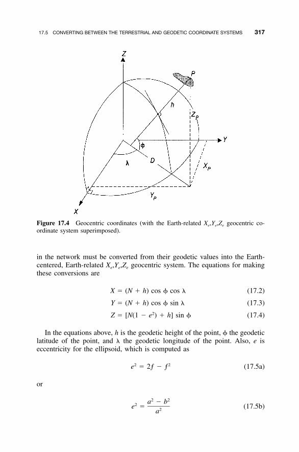
17.5 CONVERTING BETWEEN THE TERRESTRIAL AND GEODETIC COORDINATE SYSTEMS 317
Figure 17.4 Geocentric coordinates (with the Earth-related Xe,Ye,Ze geocentric co-ordinate system superimposed).
in the network must be converted from their geodetic values into the Earth-centered, Earth-related Xe,Ye,Ze geocentric system. The equations for makingthese conversions are
X � (N � h) cos � cos � (17.2)
Y � (N � h) cos � sin � (17.3)2Z � [N(1 � e ) � h] sin � (17.4)
In the equations above, h is the geodetic height of the point, � the geodeticlatitude of the point, and � the geodetic longitude of the point. Also, e iseccentricity for the ellipsoid, which is computed as
2 2e � 2ƒ � ƒ (17.5a)
or
2 2a � b2e � (17.5b)2a
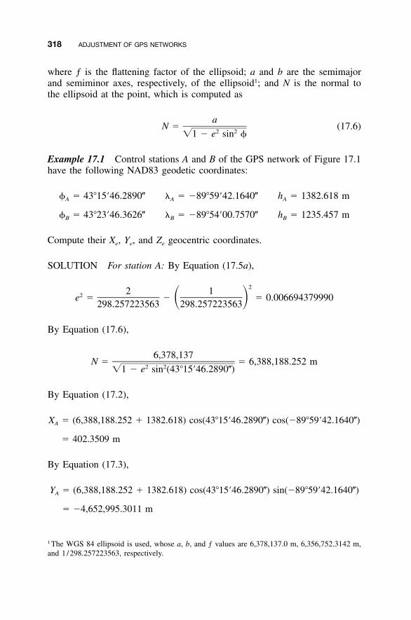
318 ADJUSTMENT OF GPS NETWORKS
where ƒ is the flattening factor of the ellipsoid; a and b are the semimajorand semiminor axes, respectively, of the ellipsoid1; and N is the normal tothe ellipsoid at the point, which is computed as
aN � (17.6)
2 2�1 � e sin �
Example 17.1 Control stations A and B of the GPS network of Figure 17.1have the following NAD83 geodetic coordinates:
� � 43�15�46.2890� � � �89�59�42.1640� h � 1382.618 mA A A
� � 43�23�46.3626� � � �89�54�00.7570� h � 1235.457 mB B B
Compute their Xe, Ye, and Ze geocentric coordinates.
SOLUTION For station A: By Equation (17.5a),
22 12e � � � 0.006694379990� �298.257223563 298.257223563
By Equation (17.6),
6,378,137N � � 6,388,188.252 m
2 2�1 � e sin (43�15�46.2890�)
By Equation (17.2),
X � (6,388,188.252 � 1382.618) cos(43�15�46.2890�) cos(�89�59�42.1640�)A
� 402.3509 m
By Equation (17.3),
Y � (6,388,188.252 � 1382.618) cos(43�15�46.2890�) sin(�89�59�42.1640�)A
� �4,652,995.3011 m
1 The WGS 84 ellipsoid is used, whose a, b, and ƒ values are 6,378,137.0 m, 6,356,752.3142 m,and 1 /298.257223563, respectively.
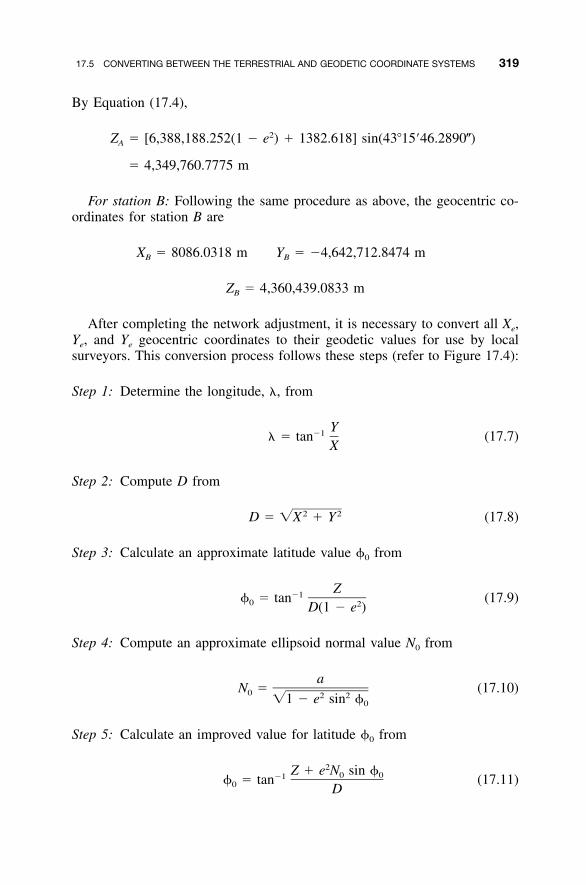
17.5 CONVERTING BETWEEN THE TERRESTRIAL AND GEODETIC COORDINATE SYSTEMS 319
By Equation (17.4),
2Z � [6,388,188.252(1 � e ) � 1382.618] sin(43�15�46.2890�)A
� 4,349,760.7775 m
For station B: Following the same procedure as above, the geocentric co-ordinates for station B are
X � 8086.0318 m Y � �4,642,712.8474 mB B
Z � 4,360,439.0833 mB
After completing the network adjustment, it is necessary to convert all Xe,Ye, and Ye geocentric coordinates to their geodetic values for use by localsurveyors. This conversion process follows these steps (refer to Figure 17.4):
Step 1: Determine the longitude, �, from
Y�1� � tan (17.7)
X
Step 2: Compute D from
2 2D � �X � Y (17.8)
Step 3: Calculate an approximate latitude value �0 from
Z�1� � tan (17.9)0 2D(1 � e )
Step 4: Compute an approximate ellipsoid normal value N0 from
aN � (17.10)0 2 2�1 � e sin �0
Step 5: Calculate an improved value for latitude �0 from
2Z � e N sin �0 0�1� � tan (17.11)0 D
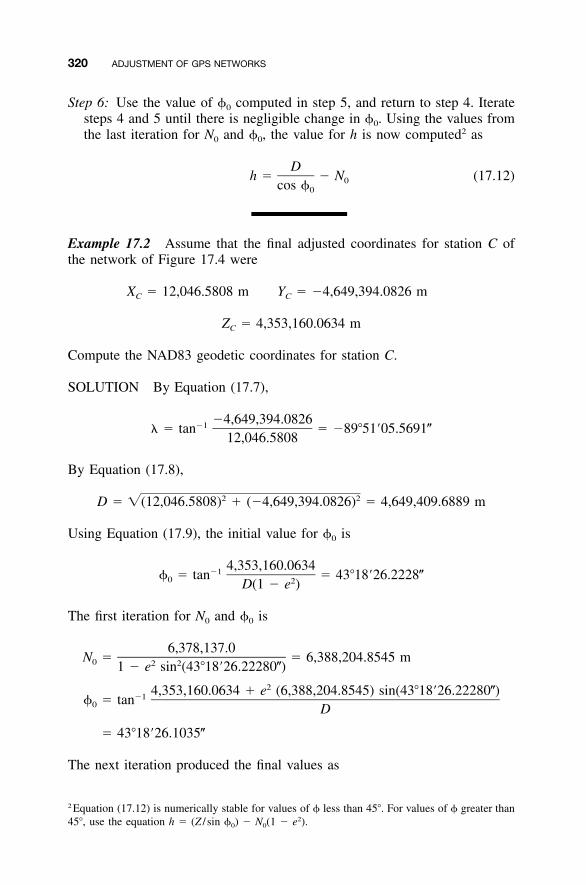
320 ADJUSTMENT OF GPS NETWORKS
Step 6: Use the value of �0 computed in step 5, and return to step 4. Iteratesteps 4 and 5 until there is negligible change in �0. Using the values fromthe last iteration for N0 and �0, the value for h is now computed2 as
Dh � � N (17.12)0cos �0
Example 17.2 Assume that the final adjusted coordinates for station C ofthe network of Figure 17.4 were
X � 12,046.5808 m Y � �4,649,394.0826 mC C
Z � 4,353,160.0634 mC
Compute the NAD83 geodetic coordinates for station C.
SOLUTION By Equation (17.7),
�4,649,394.0826�1� � tan � �89�51�05.5691�
12,046.5808
By Equation (17.8),
2 2D � �(12,046.5808) � (�4,649,394.0826) � 4,649,409.6889 m
Using Equation (17.9), the initial value for �0 is
4,353,160.0634�1� � tan � 43�18�26.2228�0 2D(1 � e )
The first iteration for N0 and �0 is
6,378,137.0N � � 6,388,204.8545 m0 2 21 � e sin (43�18�26.22280�)
24,353,160.0634 � e (6,388,204.8545) sin(43�18�26.22280�)�1� � tan0 D
� 43�18�26.1035�
The next iteration produced the final values as
2 Equation (17.12) is numerically stable for values of � less than 45�. For values of � greater than45�, use the equation h � (Z / sin �0) � N0(1 � e2).

17.6 APPLICATION OF LEAST SQUARES IN PROCESSING GPS DATA 321
N � 6,388,204.8421 � � 43�18�26.1030�0 0
Using Equation (17.12), the elevation of station C is
Dh � �6,388,204.8421 � 1103.101 m
cos(43�18�26.1030�)
A computer program included with the software package ADJUST willmake these coordinate conversions, both from geodetic to geocentric and fromgeocentric to geodetic. These computations are also demonstrated in a Math-cad worksheet on the CD that accompanies this book.
17.6 APPLICATION OF LEAST SQUARES IN PROCESSINGGPS DATA
Least squares adjustment is used at two different stages in processing GPScarrier-phase measurements. First, it is applied in the adjustment that yieldsbaseline components between stations from the redundant carrier-phase ob-servations. Recall that in this procedure, differencing techniques are employedto compensate for errors in the system and to resolve the cycle ambiguities.In the solution, observation equations are written that contain the differencesin coordinates between stations as parameters. The reference coordinate sys-tem for this adjustment is the Xe,Ye,Ze geocentric system. A highly redundantsystem of equations is obtained because, as described earlier, a minimum offour (and often more) satellites are tracked simultaneously using at least two(and often more) receivers. Furthermore, many repeat observations are taken.This system of equations is solved by least squares to obtain the most prob-able �X, �Y, and �Z components of the baseline vectors. The developmentof these observation equations is beyond the scope of this book, and thustheir solution by least squares is also not covered herein.3
Software furnished by manufacturers of GPS receivers will process ob-served phase changes to form the differencing observation equations, performthe least squares adjustment, and output the adjusted baseline vector com-ponents. The software will also output the covariance matrix, which expressesthe correlation between the �X, �Y, and �Z components of each baseline.The software is proprietary and thus cannot be included herein.
The second stage where least squares is employed in processing GPS ob-servations is in adjusting baseline vector components in networks. This ad-justment is made after the least squares adjustment of the carrier-phase
3 Readers interested in studying these observation equations should consult GPS Theory and Prac-tice (Hoffman-Wellenhof et al., 2001) or GPS Satellite Surveying (Leick, 2004) (see thebibliography).
322 ADJUSTMENT OF GPS NETWORKS
observations is completed. It is also done in the Xe,Ye,Ze geocentric coordinatesystem. In network adjustments, the goal is to make all X coordinates (andall X-coordinate differences) consistent throughout the figure. The same ob-jective applies for all Y and Z coordinates. As an example, consider the GPSnetwork shown in Figure 17.1. It consists of two control stations and fourstations whose coordinates are to be determined. A summary of the baselineobservations obtained from the least squares adjustment of carrier-phase mea-surements for this figure is given in Table 17.1. The covariance matrix ele-ments that are listed in the table are used for weighting the observations.These are discussed in Section 17.8 but for the moment can be ignored.
A network adjustment of Figure 17.1 should yield adjusted X coordinatesfor the stations (and adjusted coordinate differences between stations) that areall mutually consistent. Specifically for this network, the adjusted X coordi-nate of station C should be obtained by adding �XAC to the X coordinate ofstation A; and the same value should be obtained by adding �XBC to the Xcoordinate of station B, or by adding �XDC to the X coordinate of station D,and so on. Equivalent conditions should exist for the Y and Z coordinates.Note that these conditions do not exist for the data of Table 17.1, whichcontains the unadjusted baseline measurements. The procedure of adjustingGPS networks is described in detail in Section 17.8 and an example is given.
17.7 NETWORK PREADJUSTMENT DATA ANALYSIS
Prior to adjusting GPS networks, a series of procedures should be followedto analyze the data for internal consistency and to eliminate possible blunders.No control points are needed for these analyses. Depending on the actualobservations taken and the network geometry, these procedures may consistof analyzing (1) differences between fixed and observed baseline components,(2) differences between repeated observations of the same baseline compo-nents, and (3) loop closures. After making these analyses, a minimally con-strained adjustment is usually performed that will help isolate any blundersthat may have escaped the first set of analyses. Procedures for making theseanalyses are described in the following subsections.
17.7.1 Analysis of Fixed Baseline Measurements
GPS job specifications often require that baseline observations be taken be-tween fixed control stations. The benefit of making these observations is toverify the accuracy of both the GPS observational system and the controlbeing held fixed. Obviously, the smaller the discrepancies between observedand known baseline lengths, the better. If the discrepancies are too large tobe tolerated, the conditions causing them must be investigated before pro-ceeding. Note that in the data of Table 17.1, one fixed baseline (betweencontrol points A and B) was observed. Table 17.2 gives the data for comparing

323
TA
BL
E17
.1B
asel
ine
Dat
aO
bser
ved
for
the
Net
wor
kof
Fig
ure
17.1
(1)
(2)
(3)
(4)
(5)
(6)
(7)
(8)
(9)
(10)
(11)
From
To�
X�
Y�
ZC
ovar
ianc
eM
atri
xE
lem
ents
AC
11,6
44.2
232
3,60
1.21
653,
399.
2550
9.88
4E-4
�9.
580E
-69.
520E
-69.
377E
-4�
9.52
0E-6
9.82
7E-4
AE
�5,
321.
7164
3,63
4.07
543,
173.
6652
2.15
8E-4
�2.
100E
-62.
160E
-61.
919E
-4�
2.10
0E-6
2.00
5E-4
BC
3,96
0.54
42�
6,68
1.24
67�
7,27
9.01
482.
305E
-4�
2.23
0E-6
2.07
0E-6
2.54
6E-4
�2.
230E
-62.
252E
-4B
D�
11,1
67.6
076
�39
4.52
04�
907.
9593
2.70
0E-4
�2.
750E
-62.
850E
-62.
721E
-4�
2.72
0E-6
2.67
0E-4
DC
15,1
28.1
647
�6,
286.
7054
�6,
371.
0583
1.46
1E-4
�1.
430E
-61.
340E
-61.
614E
-4�
1.44
0E-6
1.30
8E-4
DE
�1,
837.
7459
�6,
253.
8534
�6,
596.
6697
1.23
1E-4
�1.
190E
-61.
220E
-61.
277E
-4�
1.21
0E-6
1.28
3E-4
FA
�1,
116.
4523
�4,
596.
1610
�43
55.9
062
7.47
5E-5
�7.
900E
-78.
800E
-76.
593E
-5�
8.10
0E-7
7.61
6E-5
FC
10,5
27.7
852
�99
4.93
77�
956.
6246
2.56
7E-4
�2.
250E
-62.
400E
-62.
163E
-4�
2.27
0E-6
2.39
7E-4
FE
�6,
438.
1364
�96
2.06
94�
1,18
2.23
059.
442E
-5�
9.20
0E-7
1.04
0E-6
9.95
9E-5
�8.
900E
-78.
826E
-5F
D�
4,60
0.37
875,
291.
7785
5,41
4.43
119.
330E
-5�
9.90
0E-7
9.00
0E-7
9.87
5E-5
�9.
900E
-71.
204E
-4F
B6,
567.
2311
5,68
6.29
266,
322.
3917
6.64
3E-5
�6.
500E
-76.
900E
-77.
465E
-5�
6.40
0E-7
6.04
8E-5
BF
�6,
567.
2310
�5,
686.
3033
�6,
322.
3807
5.51
2E-5
�6.
300E
-76.
100E
-77.
472E
-5�
6.30
0E-7
6.62
9E-5
AF
1,11
6.45
774,
596.
1553
4,35
5.91
416.
619E
-5�
8.00
0E-7
9.00
0E-7
8.10
8E-5
�8.
200E
-79.
376E
-5A
aB
7,68
3.68
8310
,282
.455
010
,678
.300
87.
2397
E-4
�7.
280E
-67.
520E
-66.
762E
-4�
7.29
0E-6
7.31
0E-4
aFi
xed
base
line
used
only
for
chec
king
,bu
tno
tin
clud
edin
adju
stm
ent.
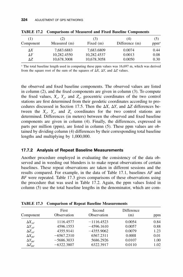
324 ADJUSTMENT OF GPS NETWORKS
TABLE 17.2 Comparisons of Measured and Fixed Baseline Components
(1) (2) (3) (4) (5)Component Measured (m) Fixed (m) Difference (m) ppma
�X 7,683.6883 7,683.6809 0.0074 0.44�Y 10,282.4550 10,282.4537 0.0013 0.08�Z 10,678.3008 10,678.3058 0.0050 0.30
a The total baseline length used in computing these ppm values was 16,697 m, which was derivedfrom the square root of the sum of the squares of �X, �Y, and �Z values.
TABLE 17.3 Comparison of Repeat Baseline Measurements
ComponentFirst
ObservationSecond
ObservationDifference
(m) ppm
�XAF 1116.4577 �1116.4523 0.0054 0.84�YAF 4596.1553 �4596.1610 0.0057 0.88�ZAF 4355.9141 �4355.9062 0.0079 1.23�XBF �6567.2310 6567.2311 0.000l 0.01�YBF �5686.3033 5686.2926 0.0107 1.00�ZBF �6322.3807 6322.3917 0.0110 1.02
the observed and fixed baseline components. The observed values are listedin column (2), and the fixed components are given in column (3). To computethe fixed values, Xe, Ye, and Ze, geocentric coordinates of the two controlstations are first determined from their geodetic coordinates according to pro-cedures discussed in Section 17.5. Then the �X, �Y, and �Z differences be-tween the Xe, Ye, and Ze coordinates for the two control stations aredetermined. Differences (in meters) between the observed and fixed baselinecomponents are given in column (4). Finally, the differences, expressed inparts per million (ppm), are listed in column (5). These ppm values are ob-tained by dividing column (4) differences by their corresponding total baselinelengths and multiplying by 1,000,000.
17.7.2 Analysis of Repeat Baseline Measurements
Another procedure employed in evaluating the consistency of the data ob-served and in weeding out blunders is to make repeat observations of certainbaselines. These repeat observations are taken in different sessions and theresults compared. For example, in the data of Table 17.1, baselines AF andBF were repeated. Table 17.3 gives comparisons of these observations usingthe procedure that was used in Table 17.2. Again, the ppm values listed incolumn (5) use the total baseline lengths in the denominator, which are com-
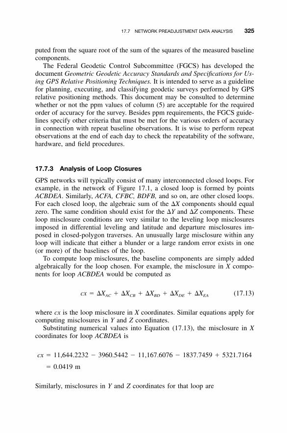
17.7 NETWORK PREADJUSTMENT DATA ANALYSIS 325
puted from the square root of the sum of the squares of the measured baselinecomponents.
The Federal Geodetic Control Subcommittee (FGCS) has developed thedocument Geometric Geodetic Accuracy Standards and Specifications for Us-ing GPS Relative Positioning Techniques. It is intended to serve as a guidelinefor planning, executing, and classifying geodetic surveys performed by GPSrelative positioning methods. This document may be consulted to determinewhether or not the ppm values of column (5) are acceptable for the requiredorder of accuracy for the survey. Besides ppm requirements, the FGCS guide-lines specify other criteria that must be met for the various orders of accuracyin connection with repeat baseline observations. It is wise to perform repeatobservations at the end of each day to check the repeatability of the software,hardware, and field procedures.
17.7.3 Analysis of Loop Closures
GPS networks will typically consist of many interconnected closed loops. Forexample, in the network of Figure 17.1, a closed loop is formed by pointsACBDEA. Similarly, ACFA, CFBC, BDFB, and so on, are other closed loops.For each closed loop, the algebraic sum of the �X components should equalzero. The same condition should exist for the �Y and �Z components. Theseloop misclosure conditions are very similar to the leveling loop misclosuresimposed in differential leveling and latitude and departure misclosures im-posed in closed-polygon traverses. An unusually large misclosure within anyloop will indicate that either a blunder or a large random error exists in one(or more) of the baselines of the loop.
To compute loop misclosures, the baseline components are simply addedalgebraically for the loop chosen. For example, the misclosure in X compo-nents for loop ACBDEA would be computed as
cx � �X � �X � �X � �X � �X (17.13)AC CB BD DE EA
where cx is the loop misclosure in X coordinates. Similar equations apply forcomputing misclosures in Y and Z coordinates.
Substituting numerical values into Equation (17.13), the misclosure in Xcoordinates for loop ACBDEA is
cx � 11,644.2232 � 3960.5442 � 11,167.6076 � 1837.7459 � 5321.7164
� 0.0419 m
Similarly, misclosures in Y and Z coordinates for that loop are
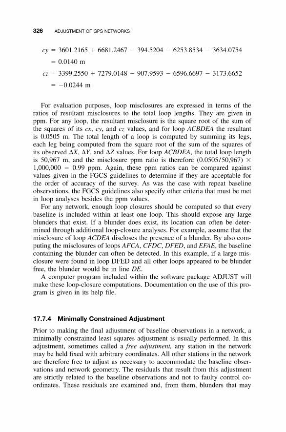
326 ADJUSTMENT OF GPS NETWORKS
cy � 3601.2165 � 6681.2467 � 394.5204 � 6253.8534 � 3634.0754
� 0.0140 m
cz � 3399.2550 � 7279.0148 � 907.9593 � 6596.6697 � 3173.6652
� �0.0244 m
For evaluation purposes, loop misclosures are expressed in terms of theratios of resultant misclosures to the total loop lengths. They are given inppm. For any loop, the resultant misclosure is the square root of the sum ofthe squares of its cx, cy, and cz values, and for loop ACBDEA the resultantis 0.0505 m. The total length of a loop is computed by summing its legs,each leg being computed from the square root of the sum of the squares ofits observed �X, �Y, and �Z values. For loop ACBDEA, the total loop lengthis 50,967 m, and the misclosure ppm ratio is therefore (0.0505/50,967) �1,000,000 � 0.99 ppm. Again, these ppm ratios can be compared againstvalues given in the FGCS guidelines to determine if they are acceptable forthe order of accuracy of the survey. As was the case with repeat baselineobservations, the FGCS guidelines also specify other criteria that must be metin loop analyses besides the ppm values.
For any network, enough loop closures should be computed so that everybaseline is included within at least one loop. This should expose any largeblunders that exist. If a blunder does exist, its location can often be deter-mined through additional loop-closure analyses. For example, assume that themisclosure of loop ACDEA discloses the presence of a blunder. By also com-puting the misclosures of loops AFCA, CFDC, DFED, and EFAE, the baselinecontaining the blunder can often be detected. In this example, if a large mis-closure were found in loop DFED and all other loops appeared to be blunderfree, the blunder would be in line DE.
A computer program included within the software package ADJUST willmake these loop-closure computations. Documentation on the use of this pro-gram is given in its help file.
17.7.4 Minimally Constrained Adjustment
Prior to making the final adjustment of baseline observations in a network, aminimally constrained least squares adjustment is usually performed. In thisadjustment, sometimes called a free adjustment, any station in the networkmay be held fixed with arbitrary coordinates. All other stations in the networkare therefore free to adjust as necessary to accommodate the baseline obser-vations and network geometry. The residuals that result from this adjustmentare strictly related to the baseline observations and not to faulty control co-ordinates. These residuals are examined and, from them, blunders that may
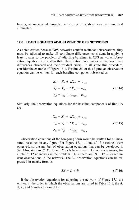
17.8 LEAST SQUARES ADJUSTMENT OF GPS NETWORKS 327
have gone undetected through the first set of analyses can be found andeliminated.
17.8 LEAST SQUARES ADJUSTMENT OF GPS NETWORKS
As noted earlier, because GPS networks contain redundant observations, theymust be adjusted to make all coordinate differences consistent. In applyingleast squares to the problem of adjusting baselines in GPS networks, obser-vation equations are written that relate station coordinates to the coordinatedifferences observed and their residual errors. To illustrate this procedure,consider the example of Figure 16.1. For line AC of this figure, an observationequation can be written for each baseline component observed as
X � X � �X � vC A AC XAC
Y � Y � �Y � v (17.14)C A AC YAC
Z � Z � �Z � vC A AC ZAC
Similarly, the observation equations for the baseline components of line CDare
X � X � �X � vD C CD XCD
Y � Y � �Y � v (17.15)D C CD YCD
Z � Z � �Z � vD C CD ZCD
Observation equations of the foregoing form would be written for all mea-sured baselines in any figure. For Figure 17.1, a total of 13 baselines wereobserved, so the number of observation equations that can be developed is39. Also, stations C, D, E, and F each have three unknown coordinates, fora total of 12 unknowns in the problem. Thus, there are 39 � 12 � 27 redun-dant observations in the network. The 39 observation equations can be ex-pressed in matrix form as
AX � L � V (17.16)
If the observation equations for adjusting the network of Figure 17.1 arewritten in the order in which the observations are listed in Table 17.1, the A,X, L, and V matrices would be
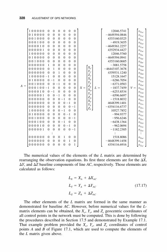
328 ADJUSTMENT OF GPS NETWORKS
A �
1 0 0 0 0 0 0 0 0 0 0 00 1 0 0 0 0 0 0 0 0 0 00 0 1 0 0 0 0 0 0 0 0 00 0 0 1 0 0 0 0 0 0 0 00 0 0 0 1 0 0 0 0 0 0 00 0 0 0 0 1 0 0 0 0 0 01 0 0 0 0 0 0 0 0 0 0 00 1 0 0 0 0 0 0 0 0 0 00 0 1 0 0 0 0 0 0 0 0 00 0 0 0 0 0 1 0 0 0 0 00 0 0 0 0 0 0 1 0 0 0 00 0 0 0 0 0 0 0 1 0 0 01 0 0 0 0 0 �1 0 0 0 0 00 1 0 0 0 0 0 �1 0 0 0 00 0 1 0 0 0 0 0 �1 0 0 00 0 0 1 0 0 �1 0 0 0 0 00 0 0 0 1 0 0 �1 0 0 0 00 0 0 0 0 1 0 0 �1 0 0 00 0 0 0 0 0 0 0 0 �1 0 00 0 0 0 0 0 0 0 0 0 �1 00 0 0 0 0 0 0 0 0 0 0 �11 0 0 0 0 0 0 0 0 �1 0 00 1 0 0 0 0 0 0 0 0 �1 00 0 1 0 0 0 0 0 0 0 0 �10 0 0 1 0 0 0 0 0 �1 0 00 0 0 0 1 0 0 0 0 0 �1 00 0 0 0 0 1 0 0 0 0 0 �1
�
0 0 0 0 0 0 0 0 0 1 0 00 0 0 0 0 0 0 0 0 0 1 00 0 0 0 0 0 0 0 0 0 0 1
X � L �
XC
YC
ZC
XE
YE
ZE
XD
YD
ZD
XF
YF
ZF
12046.5741�4649394.0846
4353160.0325�4919.3655
�4649361.22574352934.4427
12046.5760�4649394.0941
4353160.0685�3081.5758
�46443107.36784359531.1240
15128.1647�6286.7054�6371.0583�1837.7459�6253.8534�6596.6697�1518.8032
4648399.1401�4354116.6737
10527.7852�994.9377�956.6246
�6438.1364�962.0694
�1182.2305�
1518.8086�4648399.1458
4354116.6916
V �
vXAC
vYAC
vZAC
vXAE
vYAE
vZAE
vXBc
vYBC
vZBC
vXBD
vYBD
vZBD
vXDC
vYDC
vZDC
vXDE
vYDE
vZDE
vXFA
vYFA
vZFA
vXFC
vYFC
vZFC
vXFE
vYFE
vZFE
�
vXAF
vYAF
vZAF
The numerical values of the elements of the L matrix are determined byrearranging the observation equations. Its first three elements are for the �X,�Y, and �Z baseline components of line AC, respectively. Those elements arecalculated as follows:
L � X � �XX A AC
L � Y � �Y (17.17)Y A AC
L � Z � �ZZ A AC
The other elements of the L matrix are formed in the same manner asdemonstrated for baseline AC. However, before numerical values for the L-matrix elements can be obtained, the Xe, Ye, and Ze geocentric coordinates ofall control points in the network must be computed. This is done by followingthe procedures described in Section 17.5 and demonstrated by Example 17.1.That example problem provided the Xe, Ye, and Ze coordinates of controlpoints A and B of Figure 17.1, which are used to compute the elements ofthe L matrix given above.

17.8 LEAST SQUARES ADJUSTMENT OF GPS NETWORKS 329
Note that the observation equations for GPS network adjustment are linearand that the only nonzero elements of the A matrix are either 1 and �1. Thisis the same type of matrix that was developed in adjusting level nets by leastsquares. In fact, GPS network adjustments are performed in the very samemanner as level net adjustments, with the exception of the weights. In GPSrelative positioning, the three observed baseline components are correlated.Therefore, a covariance matrix of dimensions 3 � 3 is derived for each base-line as a product of the least squares adjustment of the carrier-phase mea-surements. This covariance matrix is used to weight the observations in thenetwork adjustment in accordance with Equation (10.4). The weight matrixfor any GPS network is therefore a block-diagonal type, with an individual 3� 3 matrix for each baseline observed on the diagonal. When more than tworeceivers are used, additional 3 � 3 matrices are created in the off-diagonalregion of the matrix to provide the correlation that exists between baselinesobserved simultaneously. All other elements of the matrix are zeros.
The covariances for the observations in Table 17.1 are given in columns(6) through (11). Only the six upper-triangular elements of the 3 � 3 covar-iance matrix for each observation are listed. This gives complete weightinginformation, however, because the covariance matrix is symmetrical. Columns6 through 11 list xy, xz, yz, and respectively. Thus, the full 3 �2 2 2 , , ,x y z
3 covariance matrix for baseline AC is
�4 �6 �69.884 � 10 �9.580 � 10 9.520 � 10�4 �6 �6 � �9.580 � 10 9.377 � 10 �9.520 � 10AC � ��4 �6 �69.520 � 10 �9.520 � 10 9.827 � 10
The complete weight matrix for the example network of Figure 17.1 hasdimensions of 39 � 39. After inverting the full matrix and multiplying bythe a priori estimate for the reference variance, in accordance with Equa-2S ,0
tion (10.4), the weight matrix for the network of Figure 17.1 is (note thatis taken as 1.0 for this computation and that no correlation between base-2S0
lines is included):
W �
1011.8 10.2 �9.7 0 0 0 0 0 0 0 0 010.2 1066.6 10.2 0 0 0 0 0 0 0 0 0
�9.7 10.2 1017.7 0 0 0 0 0 0 0 0 00 0 0 4634.5 50.2 �49.4 0 0 0 0 0 00 0 0 50.2 5209.7 54.0 0 0 0 0 0 00 0 0 �49.4 54.0 4988.1 0 0 0 0 0 00 0 0 0 0 0 4339.1 37.7 �39.5 0 0 00 0 0 0 0 0 37.7 3927.8 38.5 0 0 00 0 0 0 0 0 �39.5 38.5 4441.0 0 0 0
� � �0 0 0 0 0 0 0 0 0 1511.8 147.7 �143.80 0 0 0 0 0 0 0 0 147.7 12336.0 106.50 0 0 0 0 0 0 0 0 �143.8 106.5 10667.8
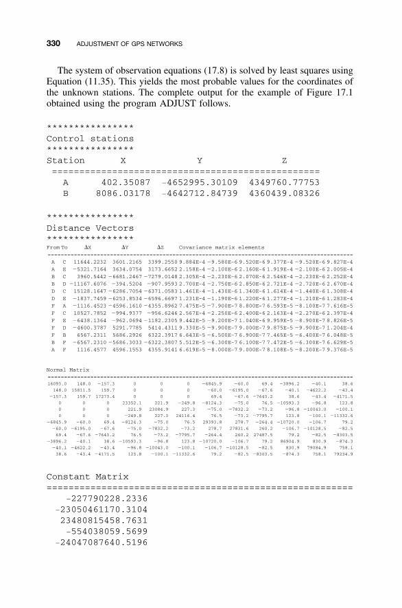
330 ADJUSTMENT OF GPS NETWORKS
The system of observation equations (17.8) is solved by least squares usingEquation (11.35). This yields the most probable values for the coordinates ofthe unknown stations. The complete output for the example of Figure 17.1obtained using the program ADJUST follows.
****************Control stations****************Station X Y Z=================================================
A 402.35087 �4652995.30109 4349760.77753B 8086.03178 �4642712.84739 4360439.08326
****************Distance Vectors****************From To �X �Y �Z Covariance matrix elements
=============================================================================================
A C 11644.2232 3601.2165 3399.2550 9.884E-4 �9.580E-6 9.520E-6 9.377E-4 �9.520E-6 9.827E-4
A E �5321.7164 3634.0754 3173.6652 2.158E-4 �2.100E-6 2.160E-6 1.919E-4 �2.100E-6 2.005E-4
B C 3960.5442 �6681.2467 �7279.0148 2.305E-4 �2.230E-6 2.070E-6 2.546E-4 �2.230E-6 2.252E-4
B D �11167.6076 �394.5204 �907.9593 2.700E-4 �2.750E-6 2.850E-6 2.721E-4 �2.720E-6 2.670E-4
D C 15128.1647 �6286.7054 �6371.0583 1.461E-4 �1.430E-6 1.340E-6 1.614E-4 �1.440E-6 1.308E-4
D E �1837.7459 �6253.8534 �6596.6697 1.231E-4 �1.190E-6 1.220E-6 1.277E-4 �1.210E-6 1.283E-4
F A �1116.4523 �4596.1610 �4355.8962 7.475E-5 �7.900E-7 8.800E-7 6.593E-5 �8.100E-7 7.616E-5
F C 10527.7852 �994.9377 �956.6246 2.567E-4 �2.250E-6 2.400E-6 2.163E-4 �2.270E-6 2.397E-4
F E �6438.1364 �962.0694 �1182.2305 9.442E-5 �9.200E-7 1.040E-6 9.959E-5 �8.900E-7 8.826E-5
F D �4600.3787 5291.7785 5414.4311 9.330E-5 �9.900E-7 9.000E-7 9.875E-5 �9.900E-7 1.204E-4
F B 6567.2311 5686.2926 6322.3917 6.643E-5 �6.500E-7 6.900E-7 7.465E-5 �6.400E-7 6.048E-5
B F �6567.2310 �5686.3033 �6322.3807 5.512E-5 �6.300E-7 6.100E-7 7.472E-5 �6.300E-7 6.629E-5
A F 1116.4577 4596.1553 4355.9141 6.619E-5 �8.000E-7 9.000E-7 8.108E-5 �8.200E-7 9.376E-5
Normal Matrix
=============================================================================================16093.0 148.0 �157.3 0 0 0 �6845.9 �60.0 69.4 �3896.2 �40.1 38.6
148.0 15811.5 159.7 0 0 0 �60.0 �6195.0 �67.6 �40.1 �4622.2 �43.4
�157.3 159.7 17273.4 0 0 0 69.4 �67.6 �7643.2 38.6 �43.4 �4171.5
0 0 0 23352.1 221.9 �249.8 �8124.3 �75.0 76.5 �10593.3 �96.8 123.8
0 0 0 221.9 23084.9 227.3 �75.0 �7832.2 �73.2 �96.8 �10043.0 �100.1
0 0 0 �249.8 227.3 24116.4 76.5 �73.2 �7795.7 123.8 �100.1 �11332.6
�6845.9 �60.0 69.4 �8124.3 �75.0 76.5 29393.8 278.7 �264.4 �10720.0 �106.7 79.2
�60.0 �6195.0 �67.6 �75.0 �7832.2 �73.2 278.7 27831.6 260.2 �106.7 �10128.5 �82.5
69.4 �67.6 �7643.2 76.5 �73.2 �7795.7 �264.4 260.2 27487.5 79.2 �82.5 �8303.5
�3896.2 �40.1 38.6 �10593.3 �96.8 123.8 �10720.0 �106.7 79.2 86904.9 830.9 �874.3
�40.1 �4622.2 �43.4 �96.8 �10043.0 �100.1 �106.7 �10128.5 �82.5 830.9 79084.9 758.1
38.6 �43.4 �4171.5 123.8 �100.1 �11332.6 79.2 �82.5 �8303.5 �874.3 758.1 79234.9
Constant Matrix========================================================
�227790228.2336�23050461170.310423480815458.7631
�554038059.5699�24047087640.5196
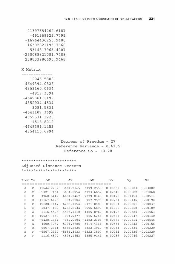
17.8 LEAST SQUARES ADJUSTMENT OF GPS NETWORKS 331
21397654262.6187�491968929.7795
�16764436256.940616302821193.7660�5314817963.4907
�250088821081.7488238833986695.9468
X Matrix=============
12046.5808�4649394.08264353160.0634
�4919.3391�4649361.21994352934.4534
�3081.5831�4643107.36924359531.1220
1518.8012�4648399.14534354116.6894
Degrees of Freedom � 27Reference Variance � 0.6135
Reference So � �0.78
***********************Adjusted Distance Vectors***********************
From To �X �Y �Z Vx Vy Vz����������������������������������A C 11644.2232 3601.2165 3399.2550 0.00669 0.00203 0.03082A E �5321.7164 3634.0754 3173.6652 0.02645 0.00582 0.01068B C 3960.5442 �6681.2467 �7279.0148 0.00478 0.01153 �0.00511B D �11167.6076 �394.5204 �907.9593 �0.00731 �0.00136 �0.00194D C 15128.1647 �6286.7054 �6371.0583 �0.00081 �0.00801 �0.00037D E �1837.7459 �6253.8534 �6596.6697 �0.01005 0.00268 0.00109F A �1116.4523 �4596.1610 �4355.8962 0.00198 0.00524 �0.01563F C 10527.7852 �994.9377 �956.6246 �0.00563 0.00047 �0.00140F E �6438.1364 �962.0694 �1182.2305 �0.00387 �0.00514 �0.00545F D �4600.3787 5291.7785 5414.4311 �0.00561 �0.00232 0.00156F B 6567.2311 5686.2926 6322.3917 �0.00051 0.00534 0.00220B F �6567.2310 �5686.3033 �6322.3807 0.00041 0.00536 �0.01320A F 1116.4577 4596.1553 4355.9141 �0.00738 0.00046 �0.00227
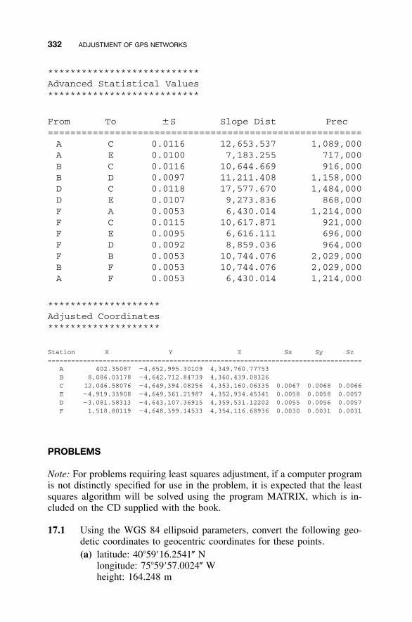
332 ADJUSTMENT OF GPS NETWORKS
***************************Advanced Statistical Values***************************
From To �S Slope Dist Prec========================================================A C 0.0116 12,653.537 1,089,000A E 0.0100 7,183.255 717,000B C 0.0116 10,644.669 916,000B D 0.0097 11,211.408 1,158,000D C 0.0118 17,577.670 1,484,000D E 0.0107 9,273.836 868,000F A 0.0053 6,430.014 1,214,000F C 0.0115 10,617.871 921,000F E 0.0095 6,616.111 696,000F D 0.0092 8,859.036 964,000F B 0.0053 10,744.076 2,029,000B F 0.0053 10,744.076 2,029,000A F 0.0053 6,430.014 1,214,000
********************Adjusted Coordinates********************
Station X Y Z Sx Sy Sz================================================================================
A 402.35087 �4,652,995.30109 4,349,760.77753B 8,086.03178 �4,642,712.84739 4,360,439.08326C 12,046.58076 �4,649,394.08256 4,353,160.06335 0.0067 0.0068 0.0066E �4,919.33908 �4,649,361.21987 4,352,934.45341 0.0058 0.0058 0.0057D �3,081.58313 �4,643,107.36915 4,359,531.12202 0.0055 0.0056 0.0057F 1,518.80119 �4,648,399.14533 4,354,116.68936 0.0030 0.0031 0.0031
PROBLEMS
Note: For problems requiring least squares adjustment, if a computer programis not distinctly specified for use in the problem, it is expected that the leastsquares algorithm will be solved using the program MATRIX, which is in-cluded on the CD supplied with the book.
17.1 Using the WGS 84 ellipsoid parameters, convert the following geo-detic coordinates to geocentric coordinates for these points.(a) latitude: 40�59�16.2541� N
longitude: 75�59�57.0024� Wheight: 164.248 m
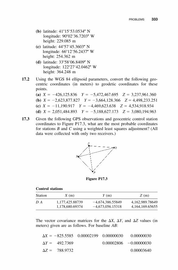
PROBLEMS 333
(b) latitude: 41�15�53.0534� Nlongitude: 90�02�36.7203� Wheight: 229.085 m
(c) latitude: 44�57�45.3603� Nlongitude: 66�12�56.2437� Wheight: 254.362 m
(d) latitude: 33�58�06.8409� Nlongitude: 122�27�42.0462� Wheight: 364.248 m
17.2 Using the WGS 84 ellipsoid parameters, convert the following geo-centric coordinates (in meters) to geodetic coordinates for thesepoints.(a) X � �426,125.836 Y � �5,472,467.695 Z � 3,237,961.360(b) X � �2,623,877.827 Y � �3,664,128.366 Z � 4,498,233.251(c) X � �11,190.917 Y � �4,469,623.638 Z � 4,534,918.934(d) X � 2,051,484.893 Y � �5,188,627.173 Z � 3,080,194.963
17.3 Given the following GPS observations and geocentric control stationcoordinates to Figure P17.3, what are the most probable coordinatesfor stations B and C using a weighted least squares adjustment? (Alldata were collected with only two receivers.)
Figure P17.3
Control stations
Station X (m) Y (m) Z (m)
A 1,177,425.88739 �4,674,386.55849 4,162,989.78649D1,178,680.69374 �4,673,056.15318 4,164,169.65655
The vector covariance matrices for the �X, �Y, and �Z values (inmeters) given are as follows. For baseline AB:
�X � �825.5585 0.00002199 0.00000030 0.00000030
�Y � 492.7369 0.00002806 �0.00000030
�Z � 788.9732 0.00003640
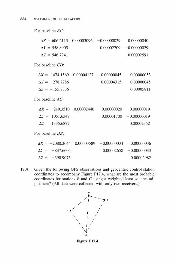
334 ADJUSTMENT OF GPS NETWORKS
For baseline BC:
�X � 606.2113 0.00003096 �0.00000029 0.00000040
�Y � 558.8905 0.00002709 �0.00000029
�Z � 546.7241 0.00002591
For baseline CD:
�X � 1474.1569 0.00004127 �0.00000045 0.00000053
�Y � 278.7786 0.00004315 �0.00000045
�Z � �155.8336 0.00005811
For baseline AC:
�X � �219.3510 0.00002440 �0.00000020 0.00000019
�Y � 1051.6348 0.00001700 �0.00000019
�Z � 1335.6877 0.00002352
For baseline DB:
�X � �2080.3644 0.00003589 �0.00000034 0.00000036
�Y � �837.6605 0.00002658 �0.00000033
�Z � �390.9075 0.00002982
17.4 Given the following GPS observations and geocentric control stationcoordinates to accompany Figure P17.4, what are the most probablecoordinates for stations B and C using a weighted least squares ad-justment? (All data were collected with only two receivers.)
Figure P17.4
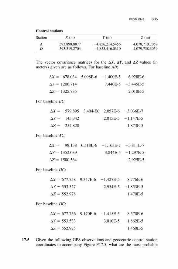
PROBLEMS 335
Control stations
Station X (m) Y (m) Z (m)
A 593,898.8877 �4,856,214.5456 4,078,710.7059D 593,319.2704 �4,855,416.0310 4,079,738.3059
The vector covariance matrices for the �X, �Y, and �Z values (inmeters) given are as follows. For baseline AB:
�X � 678.034 5.098E-6 �1.400E-5 6.928E-6
�Y � 1206.714 7.440E-5 �3.445E-5
�Z � 1325.735 2.018E-5
For baseline BC:
�X � �579.895 3.404-E6 2.057E-6 �3.036E-7
�Y � 145.342 2.015E-5 �1.147E-5
�Z � 254.820 1.873E-5
For baseline AC:
�X � 98.138 6.518E-6 �1.163E-7 �3.811E-7
�Y � 1352.039 3.844E-5 �1.297E-5
�Z � 1580.564 2.925E-5
For baseline DC:
�X � 677.758 9.347E-6 �1.427E-5 8.776E-6
�Y � 553.527 2.954E-5 �1.853E-5
�Z � 552.978 1.470E-5
For baseline DC:
�X � 677.756 9.170E-6 �1.415E-5 8.570E-6
�Y � 553.533 3.010E-5 �1.862E-5
�Z � 552.975 1.460E-5
17.5 Given the following GPS observations and geocentric control stationcoordinates to accompany Figure P17.5, what are the most probable
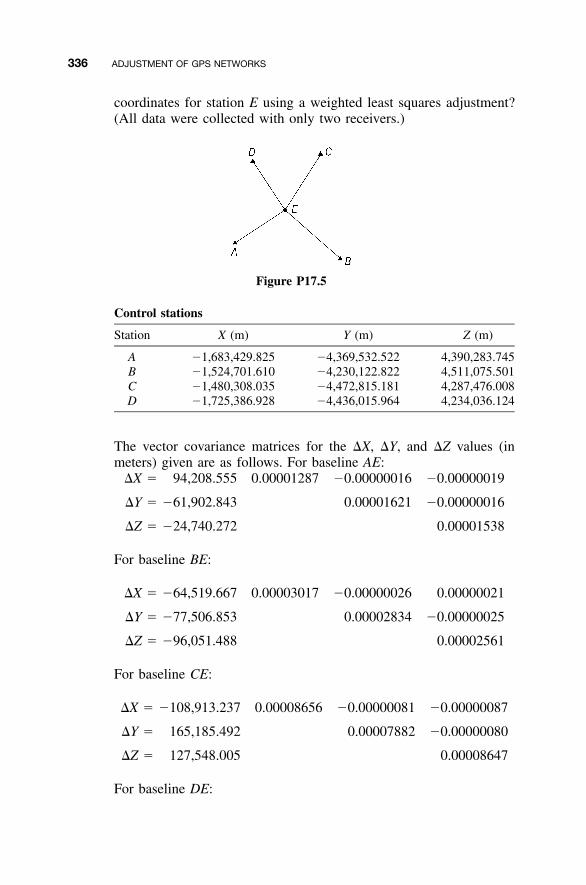
336 ADJUSTMENT OF GPS NETWORKS
coordinates for station E using a weighted least squares adjustment?(All data were collected with only two receivers.)
Figure P17.5
Control stations
Station X (m) Y (m) Z (m)
A �1,683,429.825 �4,369,532.522 4,390,283.745B �1,524,701.610 �4,230,122.822 4,511,075.501C �1,480,308.035 �4,472,815.181 4,287,476.008D �1,725,386.928 �4,436,015.964 4,234,036.124
The vector covariance matrices for the �X, �Y, and �Z values (inmeters) given are as follows. For baseline AE:
�X � 94,208.555 0.00001287 �0.00000016 �0.00000019
�Y � �61,902.843 0.00001621 �0.00000016
�Z � �24,740.272 0.00001538
For baseline BE:
�X � �64,519.667 0.00003017 �0.00000026 0.00000021
�Y � �77,506.853 0.00002834 �0.00000025
�Z � �96,051.488 0.00002561
For baseline CE:
�X � �108,913.237 0.00008656 �0.00000081 �0.00000087
�Y � 165,185.492 0.00007882 �0.00000080
�Z � 127,548.005 0.00008647
For baseline DE:
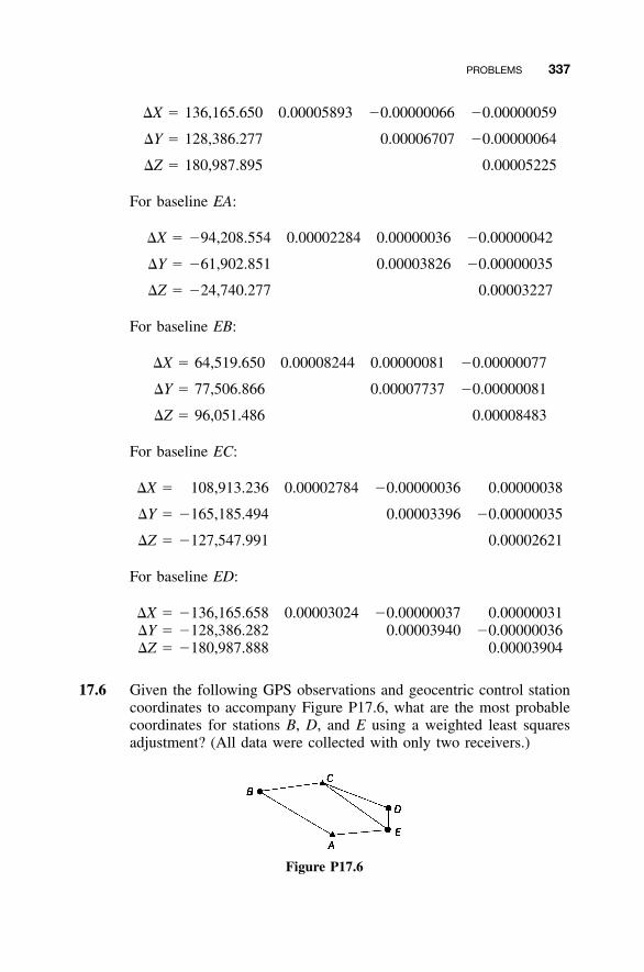
PROBLEMS 337
�X � 136,165.650 0.00005893 �0.00000066 �0.00000059
�Y � 128,386.277 0.00006707 �0.00000064
�Z � 180,987.895 0.00005225
For baseline EA:
�X � �94,208.554 0.00002284 0.00000036 �0.00000042
�Y � �61,902.851 0.00003826 �0.00000035
�Z � �24,740.277 0.00003227
For baseline EB:
�X � 64,519.650 0.00008244 0.00000081 �0.00000077
�Y � 77,506.866 0.00007737 �0.00000081
�Z � 96,051.486 0.00008483
For baseline EC:
�X � 108,913.236 0.00002784 �0.00000036 0.00000038
�Y � �165,185.494 0.00003396 �0.00000035
�Z � �127,547.991 0.00002621
For baseline ED:
�X � �136,165.658 0.00003024 �0.00000037 0.00000031�Y � �128,386.282 0.00003940 �0.00000036�Z � �180,987.888 0.00003904
17.6 Given the following GPS observations and geocentric control stationcoordinates to accompany Figure P17.6, what are the most probablecoordinates for stations B, D, and E using a weighted least squaresadjustment? (All data were collected with only two receivers.)
Figure P17.6
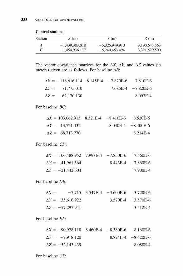
338 ADJUSTMENT OF GPS NETWORKS
Control stations
Station X (m) Y (m) Z (m)
A �1,439,383.018 �5,325,949.910 3,190,645.563C �1,454,936.177 �5,240,453.494 3,321,529.500
The vector covariance matrices for the �X, �Y, and �Z values (inmeters) given are as follows. For baseline AB:
�X � �118,616.114 8.145E-4 �7.870E-6 7.810E-6
�Y � 71,775.010 7.685E-4 �7.820E-6
�Z � 62,170.130 8.093E-4
For baseline BC:
�X � 103,062.915 8.521E-4 �8.410E-6 8.520E-6
�Y � 13,721.432 8.040E-4 �8.400E-6
�Z � 68,713.770 8.214E-4
For baseline CD:
�X � 106,488.952 7.998E-4 �7.850E-6 7.560E-6
�Y � �41,961.364 8.443E-4 �7.860E-6
�Z � �21,442.604 7.900E-4
For baseline DE:
�X � �7.715 3.547E-4 �3.600E-6 3.720E-6
�Y � �35,616.922 3.570E-4 �3.570E-6
�Z � �57,297.941 3.512E-4
For baseline EA:
�X � �90,928.118 8.460E-4 �8.380E-6 8.160E-6
�Y � �7,918.120 8.824E-4 �8.420E-6
�Z � �52,143.439 8.088E-4
For baseline CE:
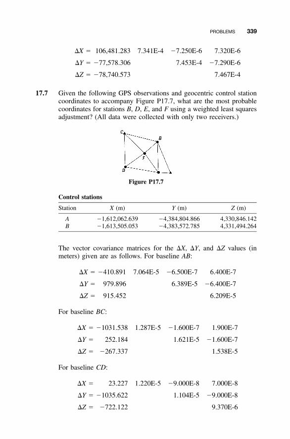
PROBLEMS 339
�X � 106,481.283 7.341E-4 �7.250E-6 7.320E-6
�Y � �77,578.306 7.453E-4 �7.290E-6
�Z � �78,740.573 7.467E-4
17.7 Given the following GPS observations and geocentric control stationcoordinates to accompany Figure P17.7, what are the most probablecoordinates for stations B, D, E, and F using a weighted least squaresadjustment? (All data were collected with only two receivers.)
Figure P17.7
Control stations
Station X (m) Y (m) Z (m)
A �1,612,062.639 �4,384,804.866 4,330,846.142B �1,613,505.053 �4,383,572.785 4,331,494.264
The vector covariance matrices for the �X, �Y, and �Z values (inmeters) given are as follows. For baseline AB:
�X � �410.891 7.064E-5 �6.500E-7 6.400E-7
�Y � 979.896 6.389E-5 �6.400E-7
�Z � 915.452 6.209E-5
For baseline BC:
�X � �1031.538 1.287E-5 �1.600E-7 1.900E-7
�Y � 252.184 1.621E-5 �1.600E-7
�Z � �267.337 1.538E-5
For baseline CD:
�X � 23.227 1.220E-5 �9.000E-8 7.000E-8
�Y � �1035.622 1.104E-5 �9.000E-8
�Z � �722.122 9.370E-6

340 ADJUSTMENT OF GPS NETWORKS
For baseline DE:
�X � 1039.772 5.335E-5 �4.900E-7 5.400E-7
�Y � �178.623 4.731E-5 �4.800E-7
�Z � �3.753 5.328E-5
For baseline EF:
�X � �434.125 7.528E-5 �8.300E-7 7.500E-7
�Y � 603.788 8.445E-5 �8.100E-7
�Z � 566.518 6.771E-5
For baseline EB:
�X � �31.465 3.340E-5 �4.900E-7 5.600E-7
�Y � 962.058 5.163E-5 �4.800E-7
�Z � 993.212 4.463E-5
For baseline FA:
�X � 1845.068 9.490E-6 �9.000E-8 8.000E-8
�Y � �873.794 7.820E-6 �9.000E-8
�Z � �221.422 1.031E-5
For baseline FB:
�X � 402.650 1.073E-5 �1.600E-7 1.800E-7
�Y � 358.278 1.465E-5 �1.600E-7
�Z � 426.706 9.730E-6
For baseline FC:
�X � �628.888 5.624E-5 �6.600E-7 5.700E-7
�Y � 610.467 6.850E-5 �6.300E-7
�Z � 159.360 6.803E-5
For baseline FD:
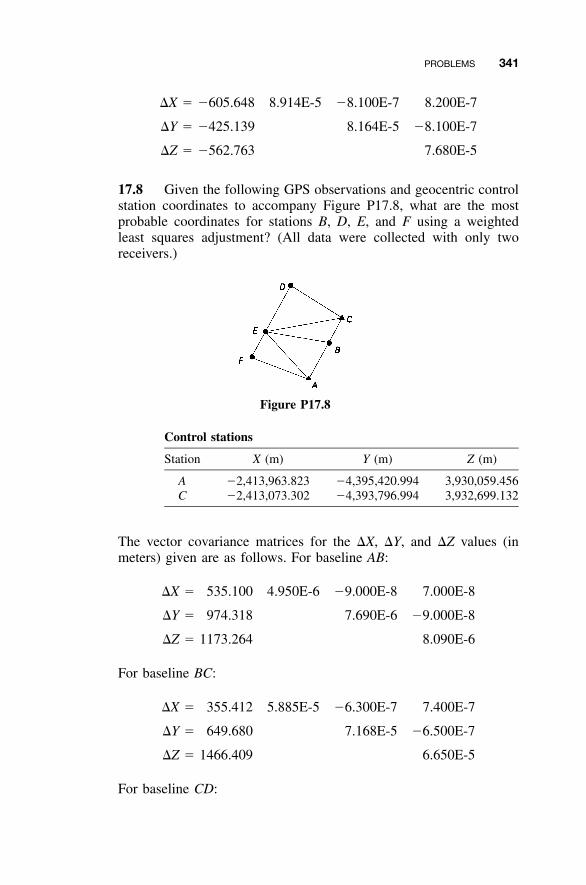
PROBLEMS 341
�X � �605.648 8.914E-5 �8.100E-7 8.200E-7
�Y � �425.139 8.164E-5 �8.100E-7
�Z � �562.763 7.680E-5
17.8 Given the following GPS observations and geocentric controlstation coordinates to accompany Figure P17.8, what are the mostprobable coordinates for stations B, D, E, and F using a weightedleast squares adjustment? (All data were collected with only tworeceivers.)
Figure P17.8
Control stations
Station X (m) Y (m) Z (m)
A �2,413,963.823 �4,395,420.994 3,930,059.456C �2,413,073.302 �4,393,796.994 3,932,699.132
The vector covariance matrices for the �X, �Y, and �Z values (inmeters) given are as follows. For baseline AB:
�X � 535.100 4.950E-6 �9.000E-8 7.000E-8
�Y � 974.318 7.690E-6 �9.000E-8
�Z � 1173.264 8.090E-6
For baseline BC:
�X � 355.412 5.885E-5 �6.300E-7 7.400E-7
�Y � 649.680 7.168E-5 �6.500E-7
�Z � 1466.409 6.650E-5
For baseline CD:
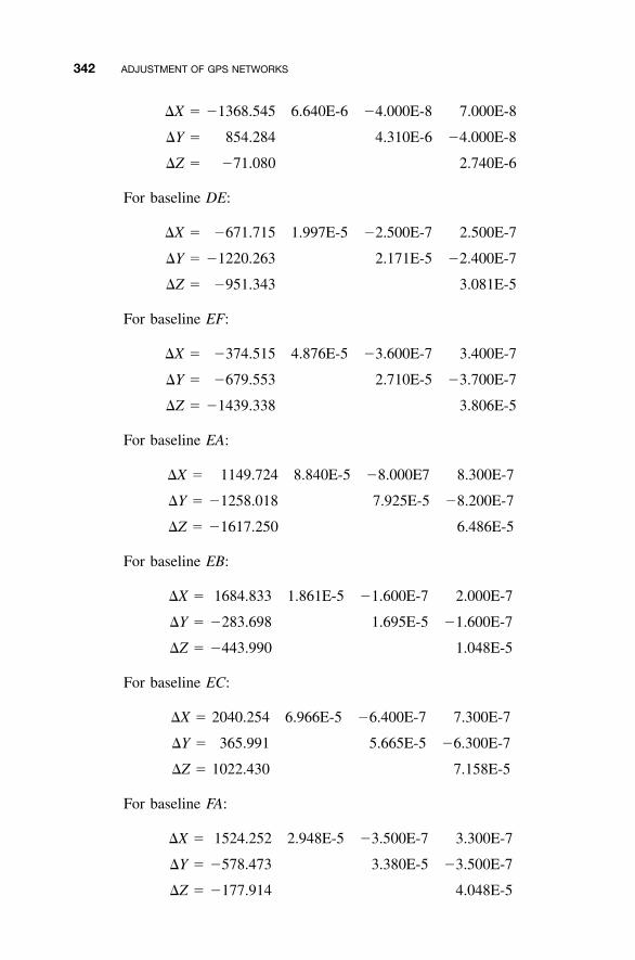
342 ADJUSTMENT OF GPS NETWORKS
�X � �1368.545 6.640E-6 �4.000E-8 7.000E-8
�Y � 854.284 4.310E-6 �4.000E-8
�Z � �71.080 2.740E-6
For baseline DE:
�X � �671.715 1.997E-5 �2.500E-7 2.500E-7
�Y � �1220.263 2.171E-5 �2.400E-7
�Z � �951.343 3.081E-5
For baseline EF:
�X � �374.515 4.876E-5 �3.600E-7 3.400E-7
�Y � �679.553 2.710E-5 �3.700E-7
�Z � �1439.338 3.806E-5
For baseline EA:
�X � 1149.724 8.840E-5 �8.000E7 8.300E-7
�Y � �1258.018 7.925E-5 �8.200E-7
�Z � �1617.250 6.486E-5
For baseline EB:
�X � 1684.833 1.861E-5 �1.600E-7 2.000E-7
�Y � �283.698 1.695E-5 �1.600E-7
�Z � �443.990 1.048E-5
For baseline EC:
�X � 2040.254 6.966E-5 �6.400E-7 7.300E-7
�Y � 365.991 5.665E-5 �6.300E-7
�Z � 1022.430 7.158E-5
For baseline FA:
�X � 1524.252 2.948E-5 �3.500E-7 3.300E-7
�Y � �578.473 3.380E-5 �3.500E-7
�Z � �177.914 4.048E-5
PROBLEMS 343
Given the data in each problem and using the procedure discussedin Section 17.7.2, analyze the repeated baselines.
17.9 Problem 17.4.
17.10 Problem 17.5.
Given the data in each problem and using the procedures discussedin Section 17.7.3, analyze the closures of the loops.
17.11 Problem 17.3, loops ABCDA, ABCA, ACDA, and BCDB
17.12 Problem 17.4, loops ABCDA, ACBA, and ADCA
17.13 Problem 17.6, loops ABCDEA and ABCEA
17.14 Problem 17.7, loops ABEA, DEFD, BFCB, CDFC, and ABCDEA
17.15 Problem 17.8, loops ABFA, BFEB, and BCDEB
Use program ADJUST to do each problem.
17.16 Problem 17.6
17.17 Problem 17.7
17.18 Problem 17.8
17.19 Problem 17.14
17.20 Problem 17.15
Programming Problems
17.21 Write a computational package that reads a file of station coordinatesand GPS baselines and then(a) writes the data to a file in a formatted fashion.(b) computes the A, L, and W matrices.(c) writes the matrices to a file that is compatible with the MATRIX
program.(d) Demonstrate this program with Problem 17.8.
17.22 Write a computational package that reads a file containing the A, L,and W matrices and then:(a) writes these matrices in a formatted fashion.(b) performs a weighted least squares adjustment.(c) writes the matrices used to compute the solution and tabulates the
station coordinates in a formatted fashion.(d) Demonstrate this program with Problem 17.8.
17.23 Write a computational package that reads a file of station coordinatesand GPS baselines and then:

344 ADJUSTMENT OF GPS NETWORKS
(a) writes the data to a file in a formatted fashion.(b) computes the A, L, and W matrices.(c) performs a weighted least squares adjustment.(d) writes the matrices used in computations in a formatted fashion
to a file.(e) computes the final station coordinates, their estimated errors, the
adjusted baseline vectors, their residuals, and their estimated er-rors, and writes them to a file in a formatted fashion.
(f) Demonstrate this program with Problem 17.8.
345
CHAPTER 18
COORDINATE TRANSFORMATIONS
18.1 INTRODUCTION
The transformation of points from one coordinate system to another is acommon problem encountered in surveying and mapping. For instance, asurveyor who works initially in an assumed coordinate system on a projectmay find it necessary to transfer the coordinates to the state plane coordinatesystem. In GPS surveying and in the field of photogrammetry, coordinatetransformations are used extensively. Since the inception of the North Amer-ican Datum of 1983 (NAD 83), many land surveyors, management agencies,state departments of transportation, and others have been struggling with theproblem of converting their multitudes of stations defined in the 1927 datum(NAD 27) to the 1983 datum. Although several mathematical models havebeen developed to make these conversions, all involve some form of coor-dinate transformation. This chapter covers the introductory procedures ofusing least squares to compute several well-known and often used transfor-mations. More rigorous procedures, which employ the general least squaresprocedure, are given in Chapter 22.
18.2 TWO-DIMENSIONAL CONFORMALCOORDINATE TRANSFORMATION
The two-dimensional conformal coordinate transformation, also known as thefour-parameter similarity transformation, has the characteristic that true shapeis retained after transformation. It is typically used in surveying when con-verting separate surveys into a common reference coordinate system. Thistransformation is a three-step process that involves:
Adjustment Computations: Spatial Data Analysis, Fourth Edition. C. D. Ghilani and P. R. Wolf© 2006 John Wiley & Sons, Inc. ISBN: 978-0-471-69728-2

346 COORDINATE TRANSFORMATIONS
Figure 18.1 Two-dimensional coordinate systems.
1. Scaling to create equal dimensions in the two coordinate systems2. Rotation to make the reference axes of the two systems parallel3. Translations to create a common origin for the two coordinate systems
The scaling and rotation are each defined by one parameter. The transla-tions involve two parameters. Thus, there are a total of four parameters inthis transformation. The transformation requires a minimum of two points,called control points, that are common to both systems. With the minimumof two points, the four parameters of the transformation can be determineduniquely. If more than two control points are available, a least squares ad-justment is possible. After determining the values of the transformation pa-rameters, any points in the original system can be transformed.
18.3 EQUATION DEVELOPMENT
Figure 18.1(a) and (b) illustrate two independent coordinate systems. In thesesystems, three common control points, A, B, and C, exist (i.e., their coordi-nates are known in both systems). Points 1 through 4 have their coordinatesknown only in the xy system of Figure 18.1(b). The problem is to determinetheir XY coordinates in the system of Figure 18.1(a). The necessary equationsare developed as follows.
Step 1: Scaling. To make line lengths as defined by the xy coordinate systemequal to their lengths in the XY system, it is necessary to multiply xycoordinates by a scale factor, S. Thus, the scaled coordinates x� and y� are
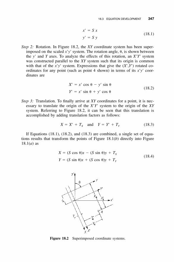
18.3 EQUATION DEVELOPMENT 347
Figure 18.2 Superimposed coordinate systems.
x� � S x(18.1)
y� � S y
Step 2: Rotation. In Figure 18.2, the XY coordinate system has been super-imposed on the scaled x�y� system. The rotation angle, �, is shown betweenthe y� and Y axes. To analyze the effects of this rotation, an X�Y� systemwas constructed parallel to the XY system such that its origin is commonwith that of the x�y� system. Expressions that give the (X�,Y�) rotated co-ordinates for any point (such as point 4 shown) in terms of its x�y� coor-dinates are
X� � x� cos � � y� sin �(18.2)
Y� � x� sin � � y� cos �
Step 3: Translation. To finally arrive at XY coordinates for a point, it is nec-essary to translate the origin of the X�Y� system to the origin of the XYsystem. Referring to Figure 18.2, it can be seen that this translation isaccomplished by adding translation factors as follows:
X � X� � T and Y � Y� � T (18.3)X Y
If Equations (18.1), (18.2), and (18.3) are combined, a single set of equa-tions results that transform the points of Figure 18.1(b) directly into Figure18.1(a) as
X � (S cos �)x � (S sin �)y � TX(18.4)
Y � (S sin �)x � (S cos �)y � TY
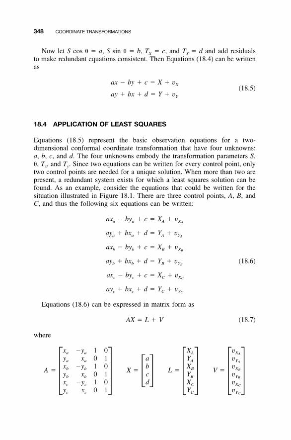
348 COORDINATE TRANSFORMATIONS
Now let S cos � � a, S sin � � b, TX � c, and TY � d and add residualsto make redundant equations consistent. Then Equations (18.4) can be writtenas
ax � by � c � X � vX(18.5)
ay � bx � d � Y � vY
18.4 APPLICATION OF LEAST SQUARES
Equations (18.5) represent the basic observation equations for a two-dimensional conformal coordinate transformation that have four unknowns:a, b, c, and d. The four unknowns embody the transformation parameters S,�, Tx, and Ty. Since two equations can be written for every control point, onlytwo control points are needed for a unique solution. When more than two arepresent, a redundant system exists for which a least squares solution can befound. As an example, consider the equations that could be written for thesituation illustrated in Figure 18.1. There are three control points, A, B, andC, and thus the following six equations can be written:
ax � by � c � X � va a A XA
ay � bx � d � Y � va a A YA
ax � by � c � X � vb b B XB
ay � bx � d � Y � v (18.6)b b B YB
ax � by � c � X � vc c C XC
ay � bx � d � Y � vc c C YC
Equations (18.6) can be expressed in matrix form as
AX � L � V (18.7)
where
x �y 1 0 X va a A XA
y x 0 1 a Y va a A YA
x �y 1 0 b X vb b B XBA � X � L � V �y x 0 1 c Y vb b B YB� ��x �y 1 0� d �X � �v �c c C XC
y x 0 1 Y vc c C YC

18.4 APPLICATION OF LEAST SQUARES 349
TABLE 18.1 Data for Example 18.1
Point E N x y
A 1,049,422.40 51,089.20 121.622 �128.066B 1,049,413.95 49,659.30 141.228 187.718C 1,049,244.95 49,884.95 175.802 135.7281 174.148 �120.2622 513.520 �192.1303 754.444 �67.7064 972.788 120.994
The redundant system is solved using Equation (11.32). Having obtainedthe most probable values for the coefficients from the least squares solution,the XY coordinates of any additional points whose coordinates are known inthe xy system can then be obtained by applying Equations (18.5) (where theresiduals are now considered to be zeros).
After the adjustment, the scale factor S and rotation angle � can be com-puted with the following equations:
b�1� � tan
a(18.8)
aS �
cos �
Example 18.1 A survey conducted in an arbitrary xy coordinate systemproduced station coordinates for A, B, and C as well as for stations 1 through4. Stations A, B, and C also have known state plane coordinates, labeled Eand N. It is required to derive the state plane coordinates of stations 1 through4. Table 18.1 is a tabulation of the arbitrary coordinates and state planecoordinates.
SOLUTION A computer listing from program ADJUST is given below forthe problem. The output includes the input data, the coordinates of trans-formed points, the transformation coefficients, and their estimated errors. Notethat the program formed the A and L matrices in accordance with Equation(18.7). After obtaining the solution using Equation (11.32), the programsolved Equation (18.8) to obtain the rotation angle and scale factor of thetransformation. A complete solution for this example is given in the Mathcadworksheet on the CD that accompanies this book.

350 COORDINATE TRANSFORMATIONS
Two Dimensional Conformal Coordinate Transformation--------------------------------------------------------ax � by � Tx � X � VXbx � ay � Ty � Y � VY
A matrix L matrix~~~~~~~~~~~~~~~~~~~~~~~~~~~~~~~~~~~~~~~~ ~~~~~~~~~~~121.622 128.066 1.000 0.000 1049422.400
�128.066 121.622 0.000 1.000 51089.200141.228 �187.718 1.000 0.000 1049413.950187.718 141.228 0.000 1.000 49659.300175.802 �135.728 1.000 0.000 1049244.950135.728 175.802 0.000 1.000 49884.950
Transformed Control Points
POINT X Y VX VY--------------------------------------------------------A 1,049,422.400 51,089.200 �0.004 0.029B 1,049,413.950 49,659.300 �0.101 0.077C 1,049,244.950 49,884.950 0.105 �0.106
Transformation Parameters:a � �4.51249 � 0.00058b � �0.25371 � 0.00058Tx � 1050003.715 � 0.123Ty � 50542.131 � 0.123
Rotation � 183� 13� 05.0�Scale � 4.51962
Adjustment’s Reference Variance � 0.0195
Transformed Points
POINT X Y ��x ��y--------------------------------------------------------1 1,049,187.361 51,040.629 0.135 0.1352 1,047,637.713 51,278.829 0.271 0.2713 1,046,582.113 50,656.241 0.368 0.3684 1,045,644.713 49,749.336 0.484 0.484
18.5 TWO-DIMENSIONAL AFFINE COORDINATE TRANSFORMATION
The two-dimensional affine coordinate transformation, also known as the six-parameter transformation, is a slight variation from the two-dimensional con-
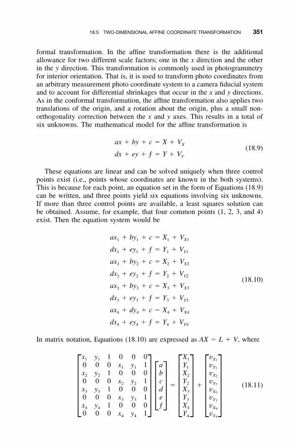
18.5 TWO-DIMENSIONAL AFFINE COORDINATE TRANSFORMATION 351
formal transformation. In the affine transformation there is the additionalallowance for two different scale factors; one in the x direction and the otherin the y direction. This transformation is commonly used in photogrammetryfor interior orientation. That is, it is used to transform photo coordinates froman arbitrary measurement photo coordinate system to a camera fiducial systemand to account for differential shrinkages that occur in the x and y directions.As in the conformal transformation, the affine transformation also applies twotranslations of the origin, and a rotation about the origin, plus a small non-orthogonality correction between the x and y axes. This results in a total ofsix unknowns. The mathematical model for the affine transformation is
ax � by � c � X � VX(18.9)
dx � ey � ƒ � Y � VY
These equations are linear and can be solved uniquely when three controlpoints exist (i.e., points whose coordinates are known in the both systems).This is because for each point, an equation set in the form of Equations (18.9)can be written, and three points yield six equations involving six unknowns.If more than three control points are available, a least squares solution canbe obtained. Assume, for example, that four common points (1, 2, 3, and 4)exist. Then the equation system would be
ax � by � c � X � V1 1 1 X1
dx � ey � ƒ � Y � V1 1 1 Y1
ax � by � c � X � V2 2 2 X2
dx � ey � ƒ � Y � V2 2 2 Y2(18.10)
ax � by � c � X � V3 3 3 X3
dx � ey � ƒ � Y � V3 3 3 Y3
ax � dy � c � X � V4 4 4 X4
dx � ey � ƒ � Y � V4 4 4 Y4
In matrix notation, Equations (18.10) are expressed as AX � L � V, where
x y 1 0 0 0 X v1 1 1 X1
0 0 0 x y 1 a Y v1 1 1 Y1
x y 1 0 0 0 b X v2 2 2 X2
0 0 0 x y 1 c Y v2 2 2 Y2� � (18.11)x y 1 0 0 0 d X v3 3 3 X3
0 0 0 x y 1 �e� Y v3 3 3 Y3� � � � � �x y 1 0 0 0 ƒ X v4 4 4 X4
0 0 0 x y 1 Y v4 4 4 Y4
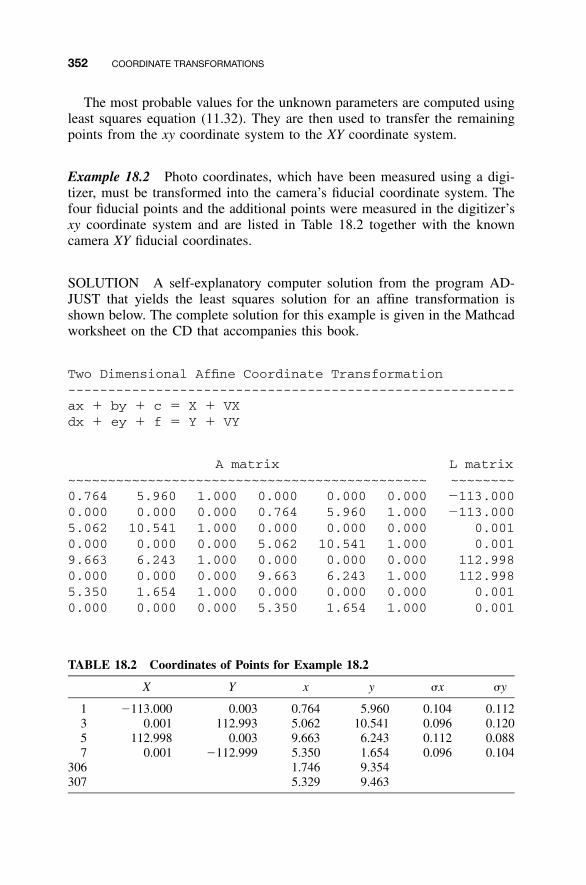
352 COORDINATE TRANSFORMATIONS
TABLE 18.2 Coordinates of Points for Example 18.2
X Y x y �x �y
1 �113.000 0.003 0.764 5.960 0.104 0.1123 0.001 112.993 5.062 10.541 0.096 0.1205 112.998 0.003 9.663 6.243 0.112 0.0887 0.001 �112.999 5.350 1.654 0.096 0.104
306 1.746 9.354307 5.329 9.463
The most probable values for the unknown parameters are computed usingleast squares equation (11.32). They are then used to transfer the remainingpoints from the xy coordinate system to the XY coordinate system.
Example 18.2 Photo coordinates, which have been measured using a digi-tizer, must be transformed into the camera’s fiducial coordinate system. Thefour fiducial points and the additional points were measured in the digitizer’sxy coordinate system and are listed in Table 18.2 together with the knowncamera XY fiducial coordinates.
SOLUTION A self-explanatory computer solution from the program AD-JUST that yields the least squares solution for an affine transformation isshown below. The complete solution for this example is given in the Mathcadworksheet on the CD that accompanies this book.
Two Dimensional Affine Coordinate Transformation--------------------------------------------------------ax � by � c � X � VXdx � ey � f � Y � VY
A matrix L matrix~~~~~~~~~~~~~~~~~~~~~~~~~~~~~~~~~~~~~~~~~~~~~ ~~~~~~~~0.764 5.960 1.000 0.000 0.000 0.000 �113.0000.000 0.000 0.000 0.764 5.960 1.000 �113.0005.062 10.541 1.000 0.000 0.000 0.000 0.0010.000 0.000 0.000 5.062 10.541 1.000 0.0019.663 6.243 1.000 0.000 0.000 0.000 112.9980.000 0.000 0.000 9.663 6.243 1.000 112.9985.350 1.654 1.000 0.000 0.000 0.000 0.0010.000 0.000 0.000 5.350 1.654 1.000 0.001
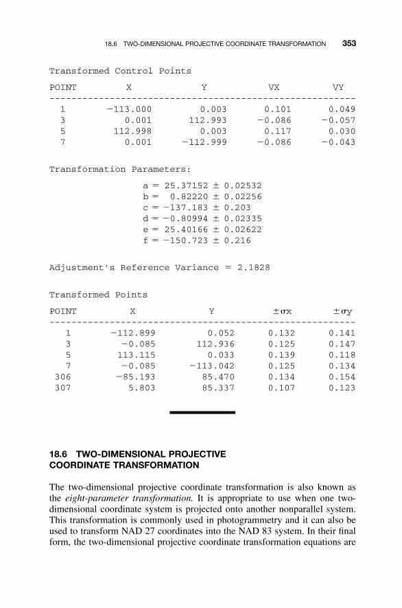
18.6 TWO-DIMENSIONAL PROJECTIVE COORDINATE TRANSFORMATION 353
Transformed Control Points
POINT X Y VX VY--------------------------------------------------------1 �113.000 0.003 0.101 0.0493 0.001 112.993 �0.086 �0.0575 112.998 0.003 0.117 0.0307 0.001 �112.999 �0.086 �0.043
Transformation Parameters:
a � 25.37152 � 0.02532b � 0.82220 � 0.02256c � �137.183 � 0.203d � �0.80994 � 0.02335e � 25.40166 � 0.02622f � �150.723 � 0.216
Adjustment’s Reference Variance � 2.1828
Transformed Points
POINT X Y ��x ��y--------------------------------------------------------
1 �112.899 0.052 0.132 0.1413 �0.085 112.936 0.125 0.1475 113.115 0.033 0.139 0.1187 �0.085 �113.042 0.125 0.134
306 �85.193 85.470 0.134 0.154307 5.803 85.337 0.107 0.123
18.6 TWO-DIMENSIONAL PROJECTIVECOORDINATE TRANSFORMATION
The two-dimensional projective coordinate transformation is also known asthe eight-parameter transformation. It is appropriate to use when one two-dimensional coordinate system is projected onto another nonparallel system.This transformation is commonly used in photogrammetry and it can also beused to transform NAD 27 coordinates into the NAD 83 system. In their finalform, the two-dimensional projective coordinate transformation equations are
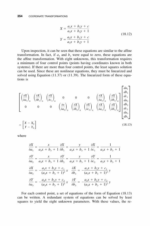
354 COORDINATE TRANSFORMATIONS
a x � b y � c1 1X �a x � b y � 13 3
(18.12)a x � b y � c2 2Y �a x � b y � 13 3
Upon inspection, it can be seen that these equations are similar to the affinetransformation. In fact, if a3 and b3 were equal to zero, these equations arethe affine transformation. With eight unknowns, this transformation requiresa minimum of four control points (points having coordinates known in bothsystems). If there are more than four control points, the least squares solutioncan be used. Since these are nonlinear equations, they must be linearized andsolved using Equation (11.37) or (11.39). The linearized form of these equa-tions is
da1
db1
�X �X �X �X �X dc10 0 0� � � � � � � � � ��a �b �c �a �b da1 1 1 3 30 0 0 0 0 2
db�x �X �X �X �X 2� �0 0 0 � � � � � � � � � � dc�a �b �c �a �b 22 2 2 3 30 0 0 0 0 � �da3
db3
X � X0� � �Y � Y0
(18.13)
where
�X x �X y �X 1� � �
�a a x � b � 1 �b a x � b � 1 �c a x � b � 11 3 3 1 3 3 1 3 3
�Y x �Y y �Y 1� � �
�a a x � b � 1 �b a x � b � 1 �c a x � b � 12 3 3 2 3 3 2 3 3
�X a x � b y � c �X a x � b y � c1 1 1 1 1 1� � x � � y2 2�a (a x � b � 1) �b (a x � b � 1)3 3 3 3 3 3
�Y a x � b y � c �Y a x � b y � c2 2 2 2 2 2� � x � � y2 2�a (a x � b � 1) �b (a x � b � 1)3 3 3 3 3 3
For each control point, a set of equations of the form of Equation (18.13)can be written. A redundant system of equations can be solved by leastsquares to yield the eight unknown parameters. With these values, the re-

18.6 TWO-DIMENSIONAL PROJECTIVE COORDINATE TRANSFORMATION 355
TABLE 18.3 Data for Example 18.3
Point X Y x y �x �y
1 1420.407 895.362 90.0 90.0 0.3 0.32 895.887 351.398 50.0 40.0 0.3 0.33 �944.926 641.434 �30.0 20.0 0.3 0.34 968.084 �1384.138 50.0 �40.0 0.3 0.35 1993.262 �2367.511 110.0 �80.0 0.3 0.36 �3382.284 3487.762 �100.0 80.0 0.3 0.37 �60.0 20.0 0.3 0.38 �100.0 �100.0 0.3 0.3
maining points in the xy coordinate system are transformed into the XYsystem.
Example 18.3 Given the data in Table 18.3, determine the best-fit projectivetransformation parameters and use them to transform the remaining pointsinto the XY coordinate system.
Program ADJUST was used to solve this problem and the results follow.The complete solution for this example is given in the Mathcad worksheet onthe CD that accompanies this book.
Two Dimensional Projective Coordinate Transformation ofFile--------------------------------------------------------a1x � b1y � c1---------------- � X � VXa3x � b3y � 1
a2x � b2y � c2---------------- � Y � VYa3x � b3y � 1
Transformation Parameters:
a1 � 25.00274 � 0.01538b1 � 0.80064 � 0.01896c1 � �134.715 � 0.377a2 � �8.00771 � 0.00954b2 � 24.99811 � 0.01350c2 � �149.815 � 0.398a3 � 0.00400 � 0.00001b3 � 0.00200 � 0.00001
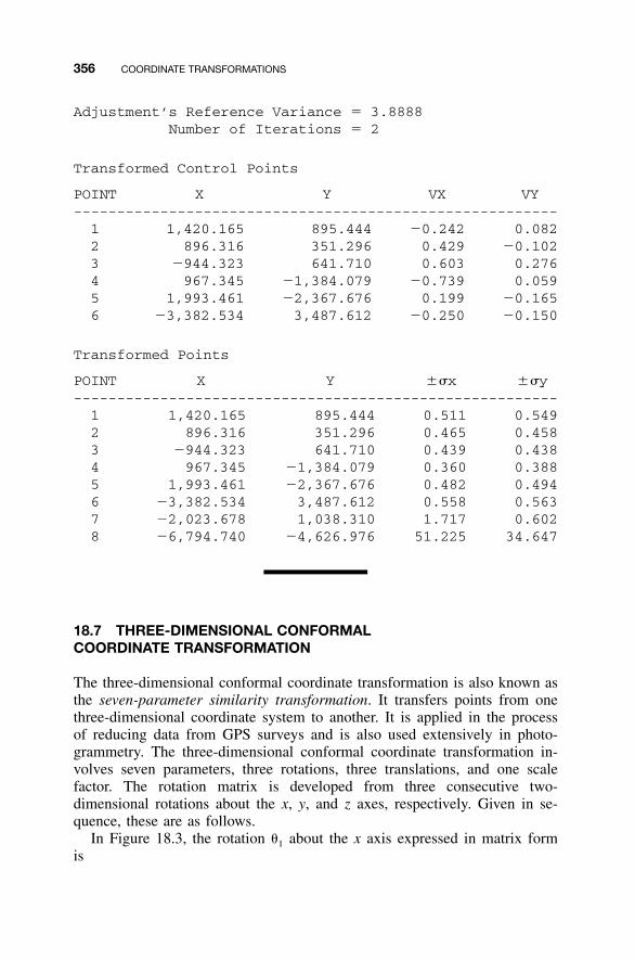
356 COORDINATE TRANSFORMATIONS
Adjustment’s Reference Variance � 3.8888Number of Iterations � 2
Transformed Control Points
POINT X Y VX VY--------------------------------------------------------1 1,420.165 895.444 �0.242 0.0822 896.316 351.296 0.429 �0.1023 �944.323 641.710 0.603 0.2764 967.345 �1,384.079 �0.739 0.0595 1,993.461 �2,367.676 0.199 �0.1656 �3,382.534 3,487.612 �0.250 �0.150
Transformed Points
POINT X Y ��x ��y--------------------------------------------------------1 1,420.165 895.444 0.511 0.5492 896.316 351.296 0.465 0.4583 �944.323 641.710 0.439 0.4384 967.345 �1,384.079 0.360 0.3885 1,993.461 �2,367.676 0.482 0.4946 �3,382.534 3,487.612 0.558 0.5637 �2,023.678 1,038.310 1.717 0.6028 �6,794.740 �4,626.976 51.225 34.647
18.7 THREE-DIMENSIONAL CONFORMALCOORDINATE TRANSFORMATION
The three-dimensional conformal coordinate transformation is also known asthe seven-parameter similarity transformation. It transfers points from onethree-dimensional coordinate system to another. It is applied in the processof reducing data from GPS surveys and is also used extensively in photo-grammetry. The three-dimensional conformal coordinate transformation in-volves seven parameters, three rotations, three translations, and one scalefactor. The rotation matrix is developed from three consecutive two-dimensional rotations about the x, y, and z axes, respectively. Given in se-quence, these are as follows.
In Figure 18.3, the rotation �1 about the x axis expressed in matrix formis
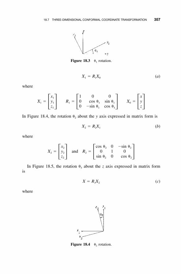
18.7 THREE-DIMENSIONAL CONFORMAL COORDINATE TRANSFORMATION 357
Figure 18.3 �1 rotation.
Figure 18.4 �2 rotation.
X � R X (a)1 1 0
where
x 1 0 0 x1
X � y R � 0 cos � sin � X � y1 1 1 1 1 0� � � � � �z 0 �sin � cos � z1 1 1
In Figure 18.4, the rotation �2 about the y axis expressed in matrix form is
X � R X (b)2 2 1
where
x cos � 0 �sin �2 2 2
X � y and R � 0 1 02 2 2� � � �z sin � 0 cos �2 2 2
In Figure 18.5, the rotation �3 about the z axis expressed in matrix formis
X � R X (c)3 2
where
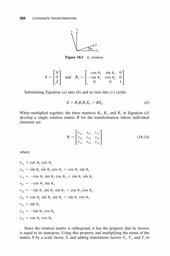
358 COORDINATE TRANSFORMATIONS
Figure 18.5 �3 rotation.
X cos � sin � 03 3
X � Y and R � �sin � cos � 03 3 3� � � �Z 0 0 1
Substituting Equation (a) into (b) and in turn into (c) yields
X � R R R X � RX (d)3 2 1 0 0
When multiplied together, the three matrices R3, R2, and R1 in Equation (d)develop a single rotation matrix R for the transformation whose individualelements are
r r r11 12 13
R � r r r (18.14)21 23 23� �r r r31 32 33
where
r11 � cos �2 cos �3
r12 � sin �1 sin �2 cos �3 � cos �1 sin �3
r13 � �cos �1 sin �2 cos �3 � sin �1 sin �3
r21 � �cos �2 sin �3
r22 � �sin �1 sin �2 sin �3 � cos �1 cos �3
r23 � cos �1 sin �2 sin �3 � sin �1 cos �3
r31 � sin �2
r32 � �sin �1 cos �2
r33 � cos �1 cos �2
Since the rotation matrix is orthogonal, it has the property that its inverseis equal to its transpose. Using this property and multiplying the terms of thematrix X by a scale factor, S, and adding translations factors Tx, Ty, and Tz to
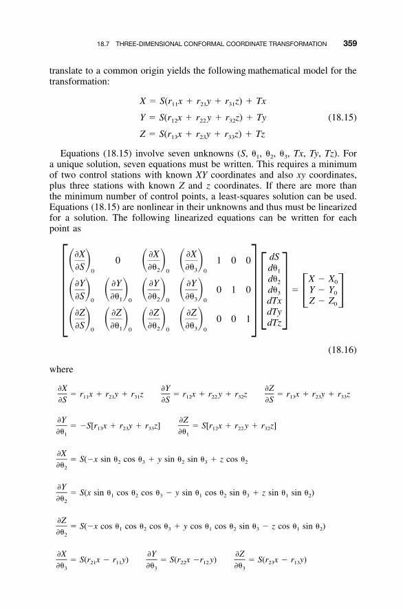
18.7 THREE-DIMENSIONAL CONFORMAL COORDINATE TRANSFORMATION 359
translate to a common origin yields the following mathematical model for thetransformation:
X � S(r x � r y � r z) � Tx11 21 31
Y � S(r x � r y � r z) � Ty (18.15)12 22 32
Z � S(r x � r y � r z) � Tz13 23 33
Equations (18.15) involve seven unknowns (S, �1, �2, �3, Tx, Ty, Tz). Fora unique solution, seven equations must be written. This requires a minimumof two control stations with known XY coordinates and also xy coordinates,plus three stations with known Z and z coordinates. If there are more thanthe minimum number of control points, a least-squares solution can be used.Equations (18.15) are nonlinear in their unknowns and thus must be linearizedfor a solution. The following linearized equations can be written for eachpoint as
�X �X �X dS0 1 0 0� � � � � ��S �� �� d�2 30 0 0 1
d� X � X2 0�Y �Y �Y �Y0 1 0 d� � Y � Y� � � � � � � � 3 0�S �� �� �� � �1 2 30 0 0 0 dTx Z � Z0� �dTy�Z �Z �Z �Z� �0 0 1� � � � � � � � dTz�S �� �� ��1 2 30 0 0 0
(18.16)
where
�X �Y �Z� r x � r y � r z � r x � r y � r z � r x � r y � r z11 21 31 12 22 32 13 23 33�S �S �S
�Y �Z� �S[r x � r y � r z] � S[r x � r y � r z]13 23 33 12 22 32�� ��1 1
�X� S(�x sin � cos � � y sin � sin � � z cos �2 3 2 3 2��2
�Y� S(x sin � cos � cos � � y sin � cos � sin � � z sin � sin � )1 2 3 1 2 3 1 2��2
�Z� S(�x cos � cos � cos � � y cos � cos � sin � � z cos � sin � )1 2 3 1 2 3 1 2��2
�X �Y �Z� S(r x � r y) � S(r x �r y) � S(r x � r y)21 11 22 12 23 13�� �� ��3 3 3
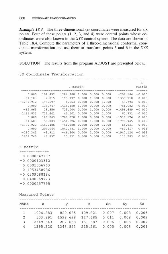
360 COORDINATE TRANSFORMATIONS
Example 18.4 The three-dimensional xyz coordinates were measured for sixpoints. Four of these points (1, 2, 3, and 4) were control points whose co-ordinates were also known in the XYZ control system. The data are shown inTable 18.4. Compute the parameters of a three-dimensional conformal coor-dinate transformation and use them to transform points 5 and 6 in the XYZsystem.
SOLUTION The results from the program ADJUST are presented below.
3D Coordinate Transformation--------------------------------------------------------
J matrixK
matrix~~~~~~~~~~~~~~~~~~~~~~~~~~~~~~~~~~~~~~~~~~~~~~~~~~~~~~~~~~~~~ ~~~~~~
0.000 102.452 1284.788 1.000 0.000 0.000 �206.164 �0.000�51.103 �7.815 �195.197 0.000 1.000 0.000 �1355.718 0.000
�1287.912 195.697 4.553 0.000 0.000 1.000 53.794 0.0000.000 118.747 1418.158 1.000 0.000 0.000 761.082 �0.000
�62.063 28.850 723.004 0.000 1.000 0.000 �1496.689 �0.000�1421.832 �722.441 42.501 0.000 0.000 1.000 65.331 �0.000
0.000 129.863 1706.020 1.000 0.000 0.000 �1530.174 0.060�61.683 �58.003 �1451.826 0.000 1.000 0.000 �1799.945 0.209
�1709.922 1452.485 �41.580 0.000 0.000 1.000 64.931 0.0000.000 204.044 1842.981 1.000 0.000 0.000 �50.417 0.033
�130.341 �1.911 �46.604 0.000 1.000 0.000 �1947.124 �0.053�1849.740 47.857 15.851 0.000 0.000 1.000 137.203 0.043
X matrix~~~~~~~~~~~~~�0.0000347107�0.0000103312�0.00010567630.1953458986
�0.0209088384�0.0400969773�0.0000257795
Measured Points--------------------------------------------------------NAME x y z Sx Sy Sz--------------------------------------------------------1 1094.883 820.085 109.821 0.007 0.008 0.0052 503.891 1598.698 117.685 0.011 0.008 0.0093 2349.343 207.658 151.387 0.006 0.005 0.0074 1395.320 1348.853 215.261 0.005 0.008 0.009
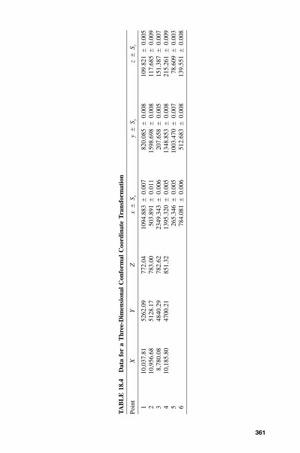
361
TA
BL
E18
.4D
ata
for
aT
hree
-Dim
ensi
onal
Con
form
alC
oord
inat
eT
rans
form
atio
n
Poin
tX
YZ
x�
S xy
�S y
z�
S z
110
,037
.81
5262
.09
772.
0410
94.8
83�
0.00
782
0.08
5�
0.00
810
9.82
1�
0.00
52
10,9
56.6
851
28.1
778
3.00
503.
891
�0.
011
1598
.698
�0.
008
117.
685
�0.
009
38,
780.
0848
40.2
978
2.62
2349
.343
�0.
006
207.
658
�0.
005
151.
387
�0.
007
410
,185
.80
4700
.21
851.
3213
95.3
20�
0.00
513
48.8
53�
0.00
821
5.26
1�
0.00
95
265.
346
�0.
005
1003
.470
�0.
007
78.6
09�
0.00
36
784.
081
�0.
006
512.
683
�0.
008
139.
551
�0.
008
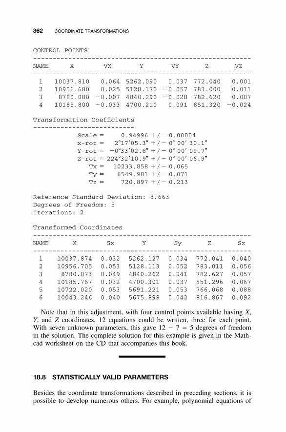
362 COORDINATE TRANSFORMATIONS
CONTROL POINTS--------------------------------------------------------NAME X VX Y VY Z VZ--------------------------------------------------------1 10037.810 0.064 5262.090 0.037 772.040 0.0012 10956.680 0.025 5128.170 �0.057 783.000 0.0113 8780.080 �0.007 4840.290 �0.028 782.620 0.0074 10185.800 �0.033 4700.210 0.091 851.320 �0.024
Transformation Coefficients--------------------------
Scale � 0.94996 �/� 0.00004x-rot � 2�17�05.3� �/� 0� 00� 30.1�Y-rot � �0�33�02.8� �/� 0� 00� 09.7�Z-rot � 224�32�10.9� �/� 0� 00� 06.9�
Tx � 10233.858 �/� 0.065Ty � 6549.981 �/� 0.071Tz � 720.897 �/� 0.213
Reference Standard Deviation: 8.663Degrees of Freedom: 5Iterations: 2
Transformed Coordinates--------------------------------------------------------NAME X Sx Y Sy Z Sz--------------------------------------------------------1 10037.874 0.032 5262.127 0.034 772.041 0.0402 10956.705 0.053 5128.113 0.052 783.011 0.0563 8780.073 0.049 4840.262 0.041 782.627 0.0574 10185.767 0.032 4700.301 0.037 851.296 0.0675 10722.020 0.053 5691.221 0.053 766.068 0.0886 10043.246 0.040 5675.898 0.042 816.867 0.092
Note that in this adjustment, with four control points available having X,Y, and Z coordinates, 12 equations could be written, three for each point.With seven unknown parameters, this gave 12 � 7 � 5 degrees of freedomin the solution. The complete solution for this example is given in the Math-cad worksheet on the CD that accompanies this book.
18.8 STATISTICALLY VALID PARAMETERS
Besides the coordinate transformations described in preceding sections, it ispossible to develop numerous others. For example, polynomial equations of
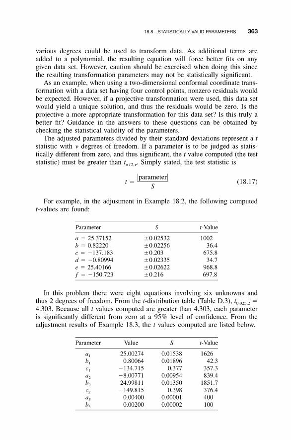
18.8 STATISTICALLY VALID PARAMETERS 363
various degrees could be used to transform data. As additional terms areadded to a polynomial, the resulting equation will force better fits on anygiven data set. However, caution should be exercised when doing this sincethe resulting transformation parameters may not be statistically significant.
As an example, when using a two-dimensional conformal coordinate trans-formation with a data set having four control points, nonzero residuals wouldbe expected. However, if a projective transformation were used, this data setwould yield a unique solution, and thus the residuals would be zero. Is theprojective a more appropriate transformation for this data set? Is this truly abetter fit? Guidance in the answers to these questions can be obtained bychecking the statistical validity of the parameters.
The adjusted parameters divided by their standard deviations represent a tstatistic with � degrees of freedom. If a parameter is to be judged as statis-tically different from zero, and thus significant, the t value computed (the teststatistic) must be greater than t� / 2,�. Simply stated, the test statistic is
�parameter�t � (18.17)
S
For example, in the adjustment in Example 18.2, the following computedt-values are found:
Parameter S t-Value
a � 25.37152 �0.02532 1002b � 0.82220 �0.02256 36.4c � �137.183 �0.203 675.8d � �0.80994 �0.02335 34.7e � 25.40166 �0.02622 968.8ƒ � �150.723 �0.216 697.8
In this problem there were eight equations involving six unknowns andthus 2 degrees of freedom. From the t-distribution table (Table D.3), t0.025,2 �4.303. Because all t values computed are greater than 4.303, each parameteris significantly different from zero at a 95% level of confidence. From theadjustment results of Example 18.3, the t values computed are listed below.
Parameter Value S t-Value
a1 25.00274 0.01538 1626b1 0.80064 0.01896 42.3c1 �134.715 0.377 357.3a2 �8.00771 0.00954 839.4b2 24.99811 0.01350 1851.7c2 �149.815 0.398 376.4a3 0.00400 0.00001 400b3 0.00200 0.00002 100
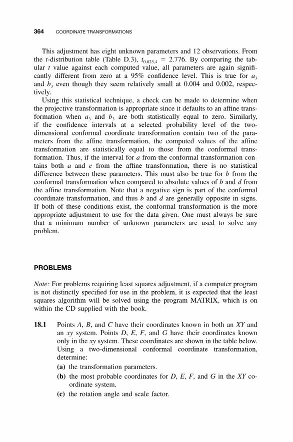
364 COORDINATE TRANSFORMATIONS
This adjustment has eight unknown parameters and 12 observations. Fromthe t-distribution table (Table D.3), t0.025,4 � 2.776. By comparing the tab-ular t value against each computed value, all parameters are again signifi-cantly different from zero at a 95% confidence level. This is true for a3
and b3 even though they seem relatively small at 0.004 and 0.002, respec-tively.
Using this statistical technique, a check can be made to determine whenthe projective transformation is appropriate since it defaults to an affine trans-formation when a3 and b3 are both statistically equal to zero. Similarly,if the confidence intervals at a selected probability level of the two-dimensional conformal coordinate transformation contain two of the para-meters from the affine transformation, the computed values of the affinetransformation are statistically equal to those from the conformal trans-formation. Thus, if the interval for a from the conformal transformation con-tains both a and e from the affine transformation, there is no statisticaldifference between these parameters. This must also be true for b from theconformal transformation when compared to absolute values of b and d fromthe affine transformation. Note that a negative sign is part of the conformalcoordinate transformation, and thus b and d are generally opposite in signs.If both of these conditions exist, the conformal transformation is the moreappropriate adjustment to use for the data given. One must always be surethat a minimum number of unknown parameters are used to solve anyproblem.
PROBLEMS
Note: For problems requiring least squares adjustment, if a computer programis not distinctly specified for use in the problem, it is expected that the leastsquares algorithm will be solved using the program MATRIX, which is onwithin the CD supplied with the book.
18.1 Points A, B, and C have their coordinates known in both an XY andan xy system. Points D, E, F, and G have their coordinates knownonly in the xy system. These coordinates are shown in the table below.Using a two-dimensional conformal coordinate transformation,determine:(a) the transformation parameters.(b) the most probable coordinates for D, E, F, and G in the XY co-
ordinate system.(c) the rotation angle and scale factor.
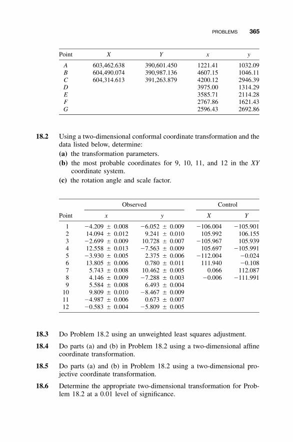
PROBLEMS 365
Point X Y x y
A 603,462.638 390,601.450 1221.41 1032.09B 604,490.074 390,987.136 4607.15 1046.11C 604,314.613 391,263.879 4200.12 2946.39D 3975.00 1314.29E 3585.71 2114.28F 2767.86 1621.43G 2596.43 2692.86
18.2 Using a two-dimensional conformal coordinate transformation and thedata listed below, determine:(a) the transformation parameters.(b) the most probable coordinates for 9, 10, 11, and 12 in the XY
coordinate system.(c) the rotation angle and scale factor.
Point
Observed
x y
Control
X Y
1 �4.209 � 0.008 �6.052 � 0.009 �106.004 �105.9012 14.094 � 0.012 9.241 � 0.010 105.992 106.1553 �2.699 � 0.009 10.728 � 0.007 �105.967 105.9394 12.558 � 0.013 �7.563 � 0.009 105.697 �105.9915 �3.930 � 0.005 2.375 � 0.006 �112.004 �0.0246 13.805 � 0.006 0.780 � 0.011 111.940 �0.1087 5.743 � 0.008 10.462 � 0.005 0.066 112.0878 4.146 � 0.009 �7.288 � 0.003 �0.006 �111.9919 5.584 � 0.008 6.493 � 0.004
10 9.809 � 0.010 �8.467 � 0.00911 �4.987 � 0.006 0.673 � 0.00712 �0.583 � 0.004 �5.809 � 0.005
18.3 Do Problem 18.2 using an unweighted least squares adjustment.
18.4 Do parts (a) and (b) in Problem 18.2 using a two-dimensional affinecoordinate transformation.
18.5 Do parts (a) and (b) in Problem 18.2 using a two-dimensional pro-jective coordinate transformation.
18.6 Determine the appropriate two-dimensional transformation for Prob-lem 18.2 at a 0.01 level of significance.
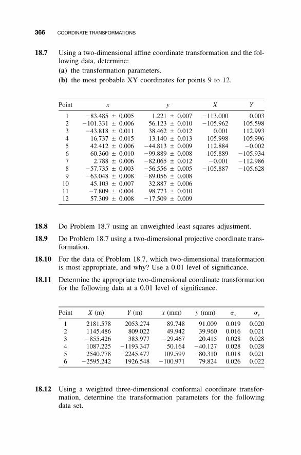
366 COORDINATE TRANSFORMATIONS
18.7 Using a two-dimensional affine coordinate transformation and the fol-lowing data, determine:(a) the transformation parameters.(b) the most probable XY coordinates for points 9 to 12.
Point x y X Y
1 �83.485 � 0.005 1.221 � 0.007 �113.000 0.0032 �101.331 � 0.006 56.123 � 0.010 �105.962 105.5983 �43.818 � 0.011 38.462 � 0.012 0.001 112.9934 16.737 � 0.015 13.140 � 0.013 105.998 105.9965 42.412 � 0.006 �44.813 � 0.009 112.884 �0.0026 60.360 � 0.010 �99.889 � 0.008 105.889 �105.9347 2.788 � 0.006 �82.065 � 0.012 �0.001 �112.9868 �57.735 � 0.003 �56.556 � 0.005 �105.887 �105.6289 �63.048 � 0.008 �89.056 � 0.008
10 45.103 � 0.007 32.887 � 0.00611 �7.809 � 0.004 98.773 � 0.01012 57.309 � 0.008 �17.509 � 0.009
18.8 Do Problem 18.7 using an unweighted least squares adjustment.
18.9 Do Problem 18.7 using a two-dimensional projective coordinate trans-formation.
18.10 For the data of Problem 18.7, which two-dimensional transformationis most appropriate, and why? Use a 0.01 level of significance.
18.11 Determine the appropriate two-dimensional coordinate transformationfor the following data at a 0.01 level of significance.
Point X (m) Y (m) x (mm) y (mm) �x �y
1 2181.578 2053.274 89.748 91.009 0.019 0.0202 1145.486 809.022 49.942 39.960 0.016 0.0213 �855.426 383.977 �29.467 20.415 0.028 0.0284 1087.225 �1193.347 50.164 �40.127 0.028 0.0285 2540.778 �2245.477 109.599 �80.310 0.018 0.0216 �2595.242 1926.548 �100.971 79.824 0.026 0.022
18.12 Using a weighted three-dimensional conformal coordinate transfor-mation, determine the transformation parameters for the followingdata set.
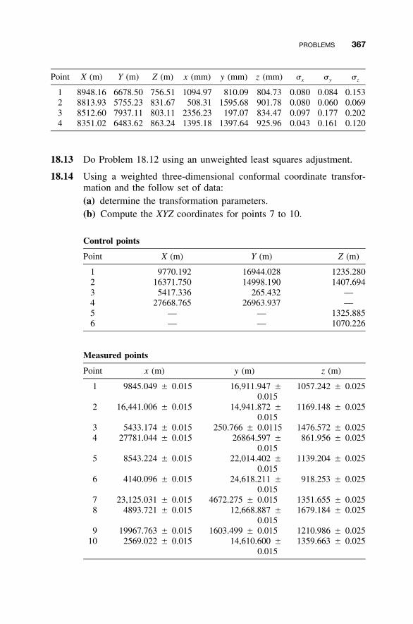
PROBLEMS 367
Point X (m) Y (m) Z (m) x (mm) y (mm) z (mm) �x �y �z
1 8948.16 6678.50 756.51 1094.97 810.09 804.73 0.080 0.084 0.1532 8813.93 5755.23 831.67 508.31 1595.68 901.78 0.080 0.060 0.0693 8512.60 7937.11 803.11 2356.23 197.07 834.47 0.097 0.177 0.2024 8351.02 6483.62 863.24 1395.18 1397.64 925.96 0.043 0.161 0.120
18.13 Do Problem 18.12 using an unweighted least squares adjustment.
18.14 Using a weighted three-dimensional conformal coordinate transfor-mation and the follow set of data:(a) determine the transformation parameters.(b) Compute the XYZ coordinates for points 7 to 10.
Control points
Point X (m) Y (m) Z (m)
1 9770.192 16944.028 1235.2802 16371.750 14998.190 1407.6943 5417.336 265.432 —4 27668.765 26963.937 —5 — — 1325.8856 — — 1070.226
Measured points
Point x (m) y (m) z (m)
1 9845.049 � 0.015 16,911.947 �0.015
1057.242 � 0.025
2 16,441.006 � 0.015 14,941.872 �0.015
1169.148 � 0.025
3 5433.174 � 0.015 250.766 � 0.0115 1476.572 � 0.0254 27781.044 � 0.015 26864.597 �
0.015861.956 � 0.025
5 8543.224 � 0.015 22,014.402 �0.015
1139.204 � 0.025
6 4140.096 � 0.015 24,618.211 �0.015
918.253 � 0.025
7 23,125.031 � 0.015 4672.275 � 0.015 1351.655 � 0.0258 4893.721 � 0.015 12,668.887 �
0.0151679.184 � 0.025
9 19967.763 � 0.015 1603.499 � 0.015 1210.986 � 0.02510 2569.022 � 0.015 14,610.600 �
0.0151359.663 � 0.025
368 COORDINATE TRANSFORMATIONS
18.15 Do Problem 11.19, and determine whether the derived constant andscale factor are statistically significant at a 0.01 level of significance.
Use the program ADJUST to do each problem.
18.16 Problem 18.6
18.17 Problem 18.10
18.18 Problem 18.14
Programming Problems
Develop a computational program that calculates the coefficient and constantsmatrix for each transformation.
18.19 A two-dimensional conformal coordinate transformation
18.20 A two-dimensional affine coordinate transformation
18.21 A two-dimensional projective coordinate transformation
18.22 A three-dimensional conformal coordinate transformation
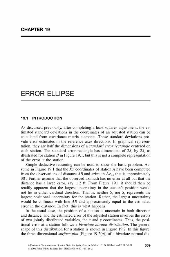
369
CHAPTER 19
ERROR ELLIPSE
19.1 INTRODUCTION
As discussed previously, after completing a least squares adjustment, the es-timated standard deviations in the coordinates of an adjusted station can becalculated from covariance matrix elements. These standard deviations pro-vide error estimates in the reference axes directions. In graphical represen-tation, they are half the dimensions of a standard error rectangle centered oneach station. The standard error rectangle has dimensions of 2Sx by 2Sy asillustrated for station B in Figure 19.1, but this is not a complete representationof the error at the station.
Simple deductive reasoning can be used to show the basic problem. As-sume in Figure 19.1 that the XY coordinates of station A have been computedfrom the observations of distance AB and azimuth AzAB that is approximately30�. Further assume that the observed azimuth has no error at all but that thedistance has a large error, say �2 ft. From Figure 19.1 it should then bereadily apparent that the largest uncertainty in the station’s position wouldnot lie in either cardinal direction. That is, neither Sx nor Sy represents thelargest positional uncertainty for the station. Rather, the largest uncertaintywould be collinear with line AB and approximately equal to the estimatederror in the distance. In fact, this is what happens.
In the usual case, the position of a station is uncertain in both directionand distance, and the estimated error of the adjusted station involves the errorsof two jointly distributed variables, the x and y coordinates. Thus, the posi-tional error at a station follows a bivariate normal distribution. The generalshape of this distribution for a station is shown in Figure 19.2. In this figure,the three-dimensional surface plot [Figure 19.2(a)] of a bivariate normal dis-
Adjustment Computations: Spatial Data Analysis, Fourth Edition. C. D. Ghilani and P. R. Wolf© 2006 John Wiley & Sons, Inc. ISBN: 978-0-471-69728-2
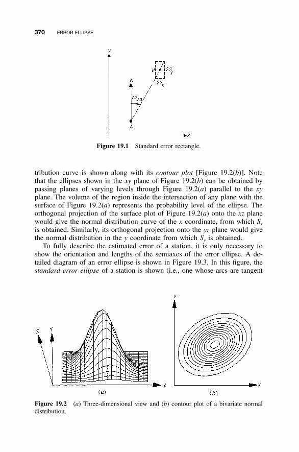
370 ERROR ELLIPSE
Figure 19.1 Standard error rectangle.
Figure 19.2 (a) Three-dimensional view and (b) contour plot of a bivariate normaldistribution.
tribution curve is shown along with its contour plot [Figure 19.2(b)]. Notethat the ellipses shown in the xy plane of Figure 19.2(b) can be obtained bypassing planes of varying levels through Figure 19.2(a) parallel to the xyplane. The volume of the region inside the intersection of any plane with thesurface of Figure 19.2(a) represents the probability level of the ellipse. Theorthogonal projection of the surface plot of Figure 19.2(a) onto the xz planewould give the normal distribution curve of the x coordinate, from which Sx
is obtained. Similarly, its orthogonal projection onto the yz plane would givethe normal distribution in the y coordinate from which Sy is obtained.
To fully describe the estimated error of a station, it is only necessary toshow the orientation and lengths of the semiaxes of the error ellipse. A de-tailed diagram of an error ellipse is shown in Figure 19.3. In this figure, thestandard error ellipse of a station is shown (i.e., one whose arcs are tangent
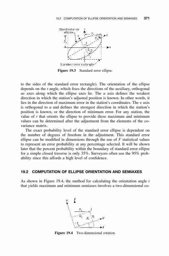
19.2 COMPUTATION OF ELLIPSE ORIENTATION AND SEMIAXES 371
Figure 19.3 Standard error ellipse.
Figure 19.4 Two-dimensional rotation.
to the sides of the standard error rectangle). The orientation of the ellipsedepends on the t angle, which fixes the directions of the auxiliary, orthogonaluv axes along which the ellipse axes lie. The u axis defines the weakestdirection in which the station’s adjusted position is known. In other words, itlies in the direction of maximum error in the station’s coordinates. The v axisis orthogonal to u and defines the strongest direction in which the station’sposition is known, or the direction of minimum error. For any station, thevalue of t that orients the ellipse to provide these maximum and minimumvalues can be determined after the adjustment from the elements of the co-variance matrix.
The exact probability level of the standard error ellipse is dependent onthe number of degrees of freedom in the adjustment. This standard errorellipse can be modified in dimensions through the use of F statistical valuesto represent an error probability at any percentage selected. It will be shownlater that the percent probability within the boundary of standard error ellipsefor a simple closed traverse is only 35%. Surveyors often use the 95% prob-ability since this affords a high level of confidence.
19.2 COMPUTATION OF ELLIPSE ORIENTATION AND SEMIAXES
As shown in Figure 19.4, the method for calculating the orientation angle tthat yields maximum and minimum semiaxes involves a two-dimensional co-
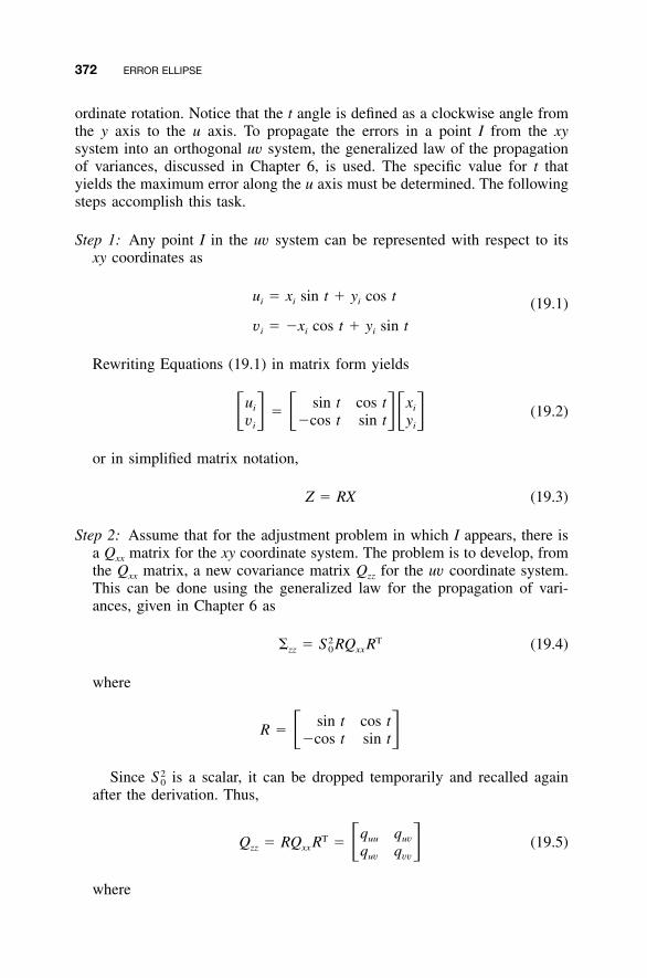
372 ERROR ELLIPSE
ordinate rotation. Notice that the t angle is defined as a clockwise angle fromthe y axis to the u axis. To propagate the errors in a point I from the xysystem into an orthogonal uv system, the generalized law of the propagationof variances, discussed in Chapter 6, is used. The specific value for t thatyields the maximum error along the u axis must be determined. The followingsteps accomplish this task.
Step 1: Any point I in the uv system can be represented with respect to itsxy coordinates as
u � x sin t � y cos ti i i (19.1)
v � �x cos t � y sin ti i i
Rewriting Equations (19.1) in matrix form yields
u sin t cos t xi i� (19.2)� � � �� �v �cos t sin t yi i
or in simplified matrix notation,
Z � RX (19.3)
Step 2: Assume that for the adjustment problem in which I appears, there isa Qxx matrix for the xy coordinate system. The problem is to develop, fromthe Qxx matrix, a new covariance matrix Qzz for the uv coordinate system.This can be done using the generalized law for the propagation of vari-ances, given in Chapter 6 as
2 T� � S RQ R (19.4)zz 0 xx
where
sin t cos tR � � ��cos t sin t
Since is a scalar, it can be dropped temporarily and recalled again2S0
after the derivation. Thus,
q qT uu uvQ � RQ R � (19.5)� �zz xx q quv vv
where
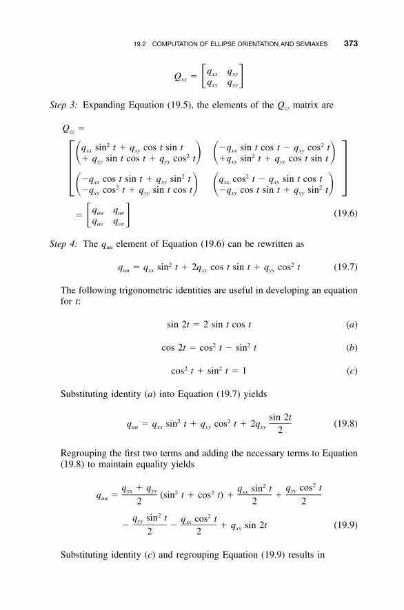
19.2 COMPUTATION OF ELLIPSE ORIENTATION AND SEMIAXES 373
q qxx xyQ � � �xx q qxy yy
Step 3: Expanding Equation (19.5), the elements of the Qzz matrix are
Q �zz
�2q sin t � q cos t sin txx xy� �2� q sin t cos t � q cos txy yy
2�q cos t sin t � q sin txx xy� �2�q cos t � q sin t cos txy yy
2�q sin t cos t � q cos txx xy� �2�q sin t � q cos t sin txy yy
2q cos t � q sin t cos txx xy� �2�q cos t sin t � q sin txy yy
�q quu uv� � �q quv vv
(19.6)
Step 4: The quu element of Equation (19.6) can be rewritten as
2 2q � q sin t � 2q cos t sin t � q cos t (19.7)uu xx xy yy
The following trigonometric identities are useful in developing an equationfor t:
sin 2t � 2 sin t cos t (a)
2 2cos 2t � cos t � sin t (b)
2 2cos t � sin t � 1 (c)
Substituting identity (a) into Equation (19.7) yields
sin 2t2 2q � q sin t � q cos t � 2q (19.8)uu xx yy xy 2
Regrouping the first two terms and adding the necessary terms to Equation(19.8) to maintain equality yields
22q � q q cos tq sin txx yy yyxx2 2q � (sin t � cos t) � �uu 2 2 22 2q sin t q cos tyy xx� � � q sin 2t (19.9)xy2 2
Substituting identity (c) and regrouping Equation (19.9) results in

374 ERROR ELLIPSE
TABLE 19.1 Selection of the Proper Quadrantfor 2t a
Algebraic Sign of
sin 2t cos 2t Quadrant
� � 1� � 2� � 3� � 4
a When calculating for t, always remember to select the properquadrant of 2t before dividing by 2.
q � q qxx yy yy 2 2q � � (cos t � sin t)uu 2 2
qxx 2 2� (cos t � sin t) � q sin 2t (19.10)xy2
Finally, substituting identity (b) into Equation (19.10) yields
q � q q � qxx yy yy xxq � � cos 2t � q sin 2t (19.11)uu xy2 2
To find the value of t that maximizes quu, differentiate quu in Equation(19.8) with respect to t and set the results equal to zero. This results in
q � qdq yy xxuu � � 2 sin 2t � 2q cos 2t � 0 (19.12)xydt 2
Reducing Equation (19.12) yields
(q � q ) sin 2t � 2q cos 2t (19.13)yy xx xy
Finally, dividing Equation (19.13) by cos 2t yields
2qsin 2t xy� tan 2t � (19.14a)
cos 2t q � qyy xx
Equation (19.14a) is used to compute 2t and hence the desired angle tthat yields the maximum value of quu. Note that the correct quadrant of 2tmust be determined by noting the sign of the numerator and denominatorin Equation (19.14a) before dividing by 2 to obtain t. Table 19.1 showsthe proper quadrant for the different possible sign combinations of the
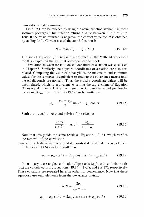
19.2 COMPUTATION OF ELLIPSE ORIENTATION AND SEMIAXES 375
numerator and denominator.Table 19.1 can be avoided by using the atan2 function available in most
software packages. This function returns a value between �180� � 2t �180�. If the value returned is negative, the correct value for 2t is obtainedby adding 360�. Correct use of the atan2 function is
2t � atan 2(q � q , 2q ) (19.14b)yy xx xy
The use of Equation (19.14b) is demonstrated in the Mathcad worksheetfor this chapter on the CD that accompanies this book.
Correlation between the latitude and departure of a station was discussedin Chapter 8. Similarly, the adjusted coordinates of a station are also cor-related. Computing the value of t that yields the maximum and minimumvalues for the semiaxes is equivalent to rotating the covariance matrix untilthe off-diagonals are nonzero. Thus, the u and v coordinate values will beuncorrelated, which is equivalent to setting the quv element of Equation(19.6) equal to zero. Using the trigonometric identities noted previously,the element quv from Equation (19.6) can be written as
q � qxx yyq � sin 2t � q cos 2t (19.15)uv xy2
Setting quv equal to zero and solving for t gives us
2qsin 2t xy� tan 2t � (19.16)
cos 2t q � qyy xx
Note that this yields the same result as Equation (19.14), which verifiesthe removal of the correlation.
Step 5: In a fashion similar to that demonstrated in step 4, the qvv elementof Equation (19.6) can be rewritten as
2 2q � q cos t � 2q cos t sin t � q sin t (19.17)vv xx xy yy
In summary, the t angle, semimajor ellipse axis (quu), and semiminor axis(qvv) are calculated using Equations (19.14), (19.7), and (19.17), respectively.These equations are repeated here, in order, for convenience. Note that theseequations use only elements from the covariance matrix.
2qxytan 2t � (19.18)q � qyy xx
2 2q � q sin t � 2q cos t sin t � q cos t (19.19)uu xx xy yy
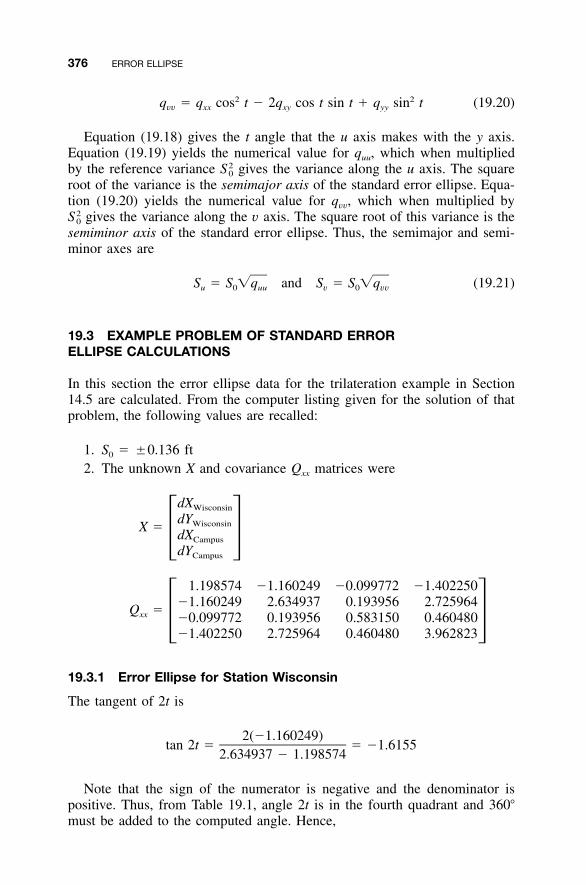
376 ERROR ELLIPSE
2 2q � q cos t � 2q cos t sin t � q sin t (19.20)vv xx xy yy
Equation (19.18) gives the t angle that the u axis makes with the y axis.Equation (19.19) yields the numerical value for quu, which when multipliedby the reference variance gives the variance along the u axis. The square2S0
root of the variance is the semimajor axis of the standard error ellipse. Equa-tion (19.20) yields the numerical value for qvv, which when multiplied by
gives the variance along the v axis. The square root of this variance is the2S0
semiminor axis of the standard error ellipse. Thus, the semimajor and semi-minor axes are
S � S �q and S � S �q (19.21)u 0 uu v 0 vv
19.3 EXAMPLE PROBLEM OF STANDARD ERRORELLIPSE CALCULATIONS
In this section the error ellipse data for the trilateration example in Section14.5 are calculated. From the computer listing given for the solution of thatproblem, the following values are recalled:
1. S0 � �0.136 ft2. The unknown X and covariance Qxx matrices were
dXWisconsin
dYWisconsinX �dXCampus� �dYCampus
1.198574 �1.160249 �0.099772 �1.402250�1.160249 2.634937 0.193956 2.725964
Q �xx �0.099772 0.193956 0.583150 0.460480� ��1.402250 2.725964 0.460480 3.962823
19.3.1 Error Ellipse for Station Wisconsin
The tangent of 2t is
2(�1.160249)tan 2t � � �1.6155
2.634937 � 1.198574
Note that the sign of the numerator is negative and the denominator ispositive. Thus, from Table 19.1, angle 2t is in the fourth quadrant and 360�must be added to the computed angle. Hence,
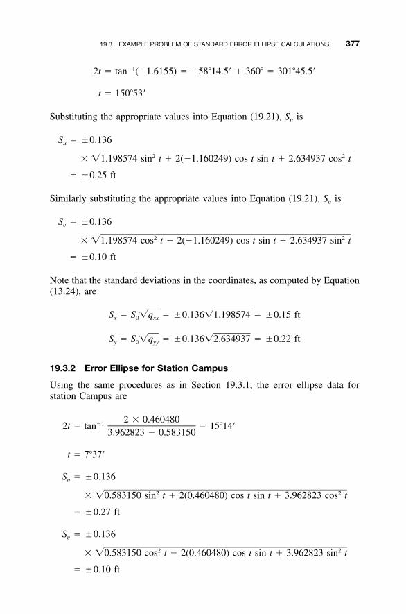
19.3 EXAMPLE PROBLEM OF STANDARD ERROR ELLIPSE CALCULATIONS 377
�12t � tan (�1.6155) � �58�14.5� � 360� � 301�45.5�
t � 150�53�
Substituting the appropriate values into Equation (19.21), Su is
S � �0.136u
2 2� �1.198574 sin t � 2(�1.160249) cos t sin t � 2.634937 cos t
� �0.25 ft
Similarly substituting the appropriate values into Equation (19.21), Sv is
S � �0.136v
2 2� �1.198574 cos t � 2(�1.160249) cos t sin t � 2.634937 sin t
� �0.10 ft
Note that the standard deviations in the coordinates, as computed by Equation(13.24), are
S � S �q � �0.136�1.198574 � �0.15 ftx 0 xx
S � S �q � �0.136�2.634937 � �0.22 fty 0 yy
19.3.2 Error Ellipse for Station Campus
Using the same procedures as in Section 19.3.1, the error ellipse data forstation Campus are
2 � 0.460480�12t � tan � 15�14�
3.962823 � 0.583150
t � 7�37�
S � �0.136u
2 2� �0.583150 sin t � 2(0.460480) cos t sin t � 3.962823 cos t
� �0.27 ft
S � �0.136v
2 2� �0.583150 cos t � 2(0.460480) cos t sin t � 3.962823 sin t
� �0.10 ft
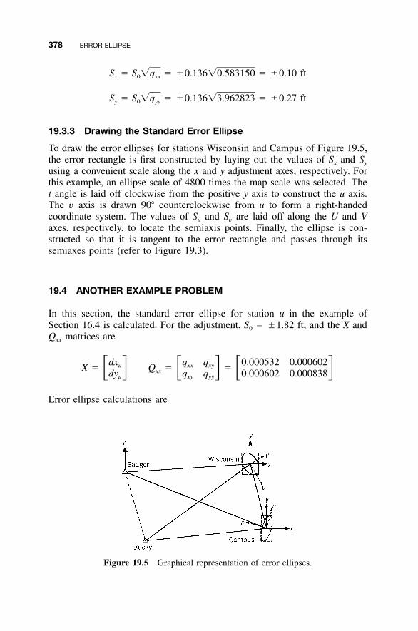
378 ERROR ELLIPSE
Figure 19.5 Graphical representation of error ellipses.
S � S �q � �0.136�0.583150 � �0.10 ftx 0 xx
S � S �q � �0.136�3.962823 � �0.27 fty 0 yy
19.3.3 Drawing the Standard Error Ellipse
To draw the error ellipses for stations Wisconsin and Campus of Figure 19.5,the error rectangle is first constructed by laying out the values of Sx and Sy
using a convenient scale along the x and y adjustment axes, respectively. Forthis example, an ellipse scale of 4800 times the map scale was selected. Thet angle is laid off clockwise from the positive y axis to construct the u axis.The v axis is drawn 90� counterclockwise from u to form a right-handedcoordinate system. The values of Su and Sv are laid off along the U and Vaxes, respectively, to locate the semiaxis points. Finally, the ellipse is con-structed so that it is tangent to the error rectangle and passes through itssemiaxes points (refer to Figure 19.3).
19.4 ANOTHER EXAMPLE PROBLEM
In this section, the standard error ellipse for station u in the example ofSection 16.4 is calculated. For the adjustment, S0 � �1.82 ft, and the X andQxx matrices are
dx q q 0.000532 0.000602u xx xyX � Q � �� � � � � �xxdy q q 0.000602 0.000838u xy yy
Error ellipse calculations are
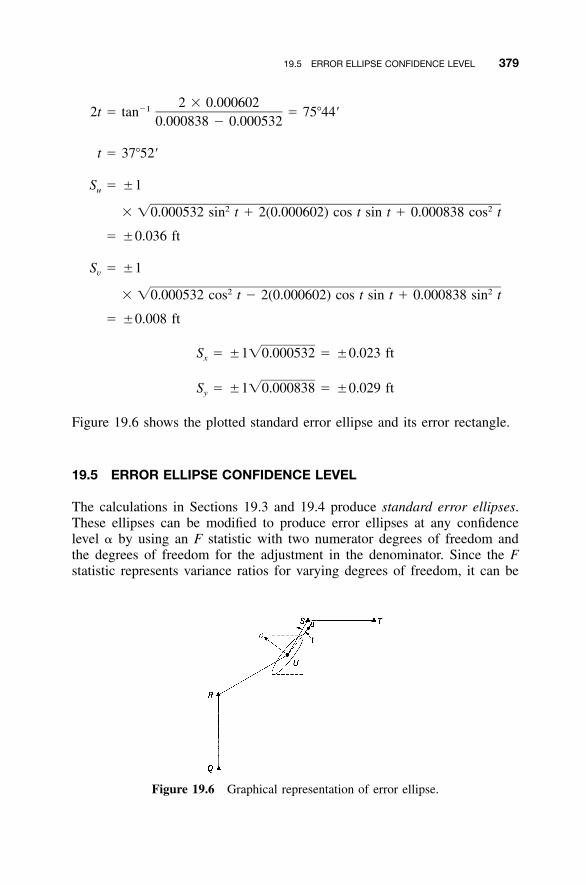
19.5 ERROR ELLIPSE CONFIDENCE LEVEL 379
Figure 19.6 Graphical representation of error ellipse.
2 � 0.000602�12t � tan � 75�44�
0.000838 � 0.000532
t � 37�52�
S � �1u
2 2� �0.000532 sin t � 2(0.000602) cos t sin t � 0.000838 cos t
� �0.036 ft
S � �1v
2 2� �0.000532 cos t � 2(0.000602) cos t sin t � 0.000838 sin t
� �0.008 ft
S � �1�0.000532 � �0.023 ftx
S � �1�0.000838 � �0.029 fty
Figure 19.6 shows the plotted standard error ellipse and its error rectangle.
19.5 ERROR ELLIPSE CONFIDENCE LEVEL
The calculations in Sections 19.3 and 19.4 produce standard error ellipses.These ellipses can be modified to produce error ellipses at any confidencelevel � by using an F statistic with two numerator degrees of freedom andthe degrees of freedom for the adjustment in the denominator. Since the Fstatistic represents variance ratios for varying degrees of freedom, it can be
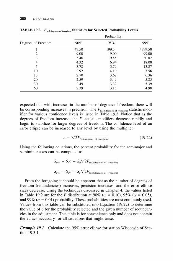
380 ERROR ELLIPSE
TABLE 19.2 F�,2,degrees of freedom Statistics for Selected Probability Levels
Degrees of Freedom
Probability
90% 95% 99%
1 49.50 199.5 4999.502 9.00 19.00 99.003 5.46 9.55 30.824 4.32 6.94 18.005 3.78 5.79 13.27
10 2.92 4.10 7.5615 2.70 3.68 6.3620 2.59 3.49 5.8530 2.49 3.32 5.3960 2.39 3.15 4.98
expected that with increases in the number of degrees of freedom, there willbe corresponding increases in precision. The F(�,2,degrees of freedom) statistic mod-ifier for various confidence levels is listed in Table 19.2. Notice that as thedegrees of freedom increase, the F statistic modifiers decrease rapidly andbegin to stabilize for larger degrees of freedom. The confidence level of anerror ellipse can be increased to any level by using the multiplier
c � �2F (19.22)(�,2,degrees of freedom)
Using the following equations, the percent probability for the semimajor andsemiminor axes can be computed as
S � S c � S �2Fu% u u (�,2,degrees of freedom)
S � S c � S �2Fv% v v (�,2,degrees of freedom)
From the foregoing it should be apparent that as the number of degrees offreedom (redundancies) increases, precision increases, and the error ellipsesizes decrease. Using the techniques discussed in Chapter 4, the values listedin Table 19.2 are for the F distribution at 90% (� � 0.10), 95% (� � 0.05),and 99% (� � 0.01) probability. These probabilities are most commonly used.Values from this table can be substituted into Equation (19.22) to determinethe value of c for the probability selected and the given number of redundan-cies in the adjustment. This table is for convenience only and does not containthe values necessary for all situations that might arise.
Example 19.1 Calculate the 95% error ellipse for station Wisconsin of Sec-tion 19.3.1.
19.6 ERROR ELLIPSE ADVANTAGES 381
SOLUTION Using Equations (19.23) yields
S � �0.25�2(199.50) � �4.99 ftu95%
S � �0.10�2(199.50) � �2.00 ftv95%
S � �2(199.50)S � �(19.97 � 0.15) � 3.00 ftx x95%
S � �2(199.50)S � �(19.97 � 0.22) � 4.39 fty y95%
The probability of the standard error ellipse can be found by setting themultiplier equal to 1 so that � 0.5. For a simple closed traverse2F F�,� ,� �,� ,�1 2 1 2
with three degrees of freedom, this means that F�,2,3 � 0.5. The value of �that satisfies this condition is 0.65 and was found by trial-and-error proceduresusing the program STATS. Thus, the percent probability of the standard errorellipse in a simple closed traverse is (1 � 0.65) � 100%, or 35%. The readeris encouraged to verify this result using program STATS. It is left as anexercise for the reader to show that the percent probability for the standarderror ellipse ranges from 35% to only 39% for horizontal surveys that havefewer than 100 degrees of freedom.
19.6 ERROR ELLIPSE ADVANTAGES
Besides providing critical information regarding the precision of an adjustedstation position, a major advantage of error ellipses is that they offer a methodof making a visual comparison of the relative precisions between any twostations. By viewing the shapes, sizes, and orientations of error ellipses, var-ious surveys can be compared rapidly and meaningfully.
19.6.1 Survey Network Design
The sizes, shapes, and orientations of error ellipses depend on (1) the controlused to constrain the adjustment, (2) the observational precisions, and (3) thegeometry of the survey. The last two of these three elements are variablesthat can be altered in the design of a survey to produce optimal results. Indesigning surveys that involve the traditional observations of distances andangles, estimated precisions can be computed for observations made withdiffering combinations of equipment and field procedures. Also, trial varia-tions in station placement, which creates the network geometry, can be made.Then these varying combinations of observations and geometry can be pro-
382 ERROR ELLIPSE
cessed through least squares adjustments and the resulting station error ellip-ses computed, plotted, and checked against the desired results. Onceacceptable goals are achieved in this process, the observational equipment,field procedures, and network geometry that provide these results can beadopted. This overall process is called network design. It enables surveyorsto select the equipment and field techniques, and to decide on the numberand locations of stations that provide the highest precision at lowest cost. Thiscan be done in the office using simulation software before bidding a contractor entering the field.
In designing networks to be surveyed using the traditional observations ofdistance, angle, and directions, it is important to understand the relationshipsof those observations to the resulting positional uncertainties of the stations.The following relationships apply:
1. Distance observations strengthen the positions of stations in directionscollinear with the lines observed.
2. Angle and direction observations strengthen the positions of stations indirections perpendicular to the lines of sight.
A simple analysis made with reference to Figure 19.1 should clarify thetwo relationships above. Assume first that the length of line AB was measuredprecisely but its direction was not observed. Then the positional uncertaintyof station B should be held within close tolerances by the distance observed,but it would only be held in the direction collinear with AB. The distanceobservation would do nothing to keep line AB from rotating, and in fact theposition of B would be weak perpendicular to AB. On the other hand, if thedirection of AB had been observed precisely but its length had not beenmeasured, the positional strength of station B would be strongest in the di-rection perpendicular to AB. But an angle observation alone does nothing tofix distances between observed stations, and thus the position of station Bwould be weak along line AB. If both the length and direction AB wereobserved with equal precision, a positional uncertainty for station B that ismore uniform in all directions would be expected. In a survey network thatconsists of many interconnected stations, analyzing the effects of observationsis not quite as simple as was just demonstrated for the single line AB. Nev-ertheless, the two basic relationships stated above still apply.
Uniform positional strength in all directions for all stations is the desiredgoal in survey network design. This would be achieved if, following leastsquares adjustment, all error ellipses were circular in shape and of equal size.Although this goal is seldom completely possible, by diligently analyzingvarious combinations of geometric figures together with different combina-tions of observations and precisions, this goal can be approached. Sometimes,however, other overriding factors, such as station accessibility, terrain, andvegetation, preclude actual use of an optimal design.
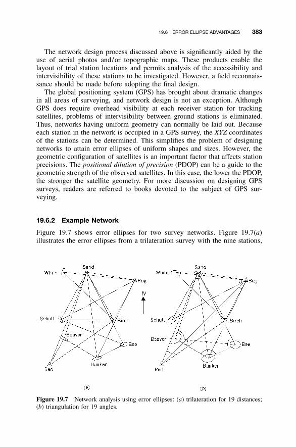
19.6 ERROR ELLIPSE ADVANTAGES 383
Figure 19.7 Network analysis using error ellipses: (a) trilateration for 19 distances;(b) triangulation for 19 angles.
The network design process discussed above is significantly aided by theuse of aerial photos and/or topographic maps. These products enable thelayout of trial station locations and permits analysis of the accessibility andintervisibility of these stations to be investigated. However, a field reconnais-sance should be made before adopting the final design.
The global positioning system (GPS) has brought about dramatic changesin all areas of surveying, and network design is not an exception. AlthoughGPS does require overhead visibility at each receiver station for trackingsatellites, problems of intervisibility between ground stations is eliminated.Thus, networks having uniform geometry can normally be laid out. Becauseeach station in the network is occupied in a GPS survey, the XYZ coordinatesof the stations can be determined. This simplifies the problem of designingnetworks to attain error ellipses of uniform shapes and sizes. However, thegeometric configuration of satellites is an important factor that affects stationprecisions. The positional dilution of precision (PDOP) can be a guide to thegeometric strength of the observed satellites. In this case, the lower the PDOP,the stronger the satellite geometry. For more discussion on designing GPSsurveys, readers are referred to books devoted to the subject of GPS sur-veying.
19.6.2 Example Network
Figure 19.7 shows error ellipses for two survey networks. Figure 19.7(a)illustrates the error ellipses from a trilateration survey with the nine stations,
384 ERROR ELLIPSE
two of which (Red and Bug) were control stations. The survey includes 19distance observations and five degrees of freedom. Figure 19.7(b) shows theerror ellipses of the same network that was observed using triangulation anda baseline from stations Red to Bug. This survey includes 19 observed anglesand thus also has five degrees of freedom.
With respect to these two figures, and keeping in mind that the smaller theellipse, the higher the precision, the following general observations can bemade:
1. In both figures, stations Sand and Birch have the highest precisions.This, of course, is expected due to their proximity to control stationBug and because of the density of observations made to these stations,which included direct measurements from both control stations.
2. The large size of error ellipses at stations Beaver, Schutt, Bunker, andBee of Figure 19.7(b) show that they have lower precision. This, too,is expected because there were fewer observations made to those sta-tions. Also, neither Beaver nor Bee was connected directly by obser-vation to either of the control stations.
3. Stations White and Schutt of Figure 19.7(a) have relatively high east–west precisions and relatively low north–south precisions. Examinationof the network geometry reveals that this could be expected. Distancemeasurements to those two points from station Red, plus an observeddistance between White and Schutt, would have greatly improved thenorth–south precision.
4. Stations Beaver and Bunker of Figure 19.7(a) have relatively low pre-cisions east–west and relatively high precisions north–south. Again, thisis expected when examining the network geometry.
5. The smaller error ellipses of Figure 19.7(a) suggest that the trilaterationsurvey will yield superior precision to the triangulation survey of Figure19.7(b). This is expected since the EDM had a stated uncertainty of�(5 mm � 5 ppm). In a 5000-ft distance this yields an uncertainty of�0.030 ft. To achieve the same precision, the comparable angle uncer-tainty would need to be
S �0.030�� � � � � 206,264.8� / rad � �1.2�
R 5000
The proposed instrument and field procedures for the project thatyielded the error ellipses of Figure 19.7(b) had an expected uncertaintyof only �6�. Very probably, this ultimate design would include bothobserved distances and angles.
These examples serve to illustrate the value of computing station errorellipses in an a priori analysis. The observations were made easily and quickly
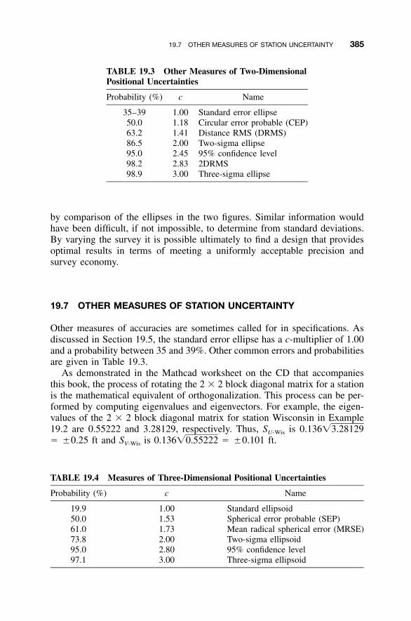
19.7 OTHER MEASURES OF STATION UNCERTAINTY 385
TABLE 19.3 Other Measures of Two-DimensionalPositional Uncertainties
Probability (%) c Name
35–39 1.00 Standard error ellipse50.0 1.18 Circular error probable (CEP)63.2 1.41 Distance RMS (DRMS)86.5 2.00 Two-sigma ellipse95.0 2.45 95% confidence level98.2 2.83 2DRMS98.9 3.00 Three-sigma ellipse
TABLE 19.4 Measures of Three-Dimensional Positional Uncertainties
Probability (%) c Name
19.9 1.00 Standard ellipsoid50.0 1.53 Spherical error probable (SEP)61.0 1.73 Mean radical spherical error (MRSE)73.8 2.00 Two-sigma ellipsoid95.0 2.80 95% confidence level97.1 3.00 Three-sigma ellipsoid
by comparison of the ellipses in the two figures. Similar information wouldhave been difficult, if not impossible, to determine from standard deviations.By varying the survey it is possible ultimately to find a design that providesoptimal results in terms of meeting a uniformly acceptable precision andsurvey economy.
19.7 OTHER MEASURES OF STATION UNCERTAINTY
Other measures of accuracies are sometimes called for in specifications. Asdiscussed in Section 19.5, the standard error ellipse has a c-multiplier of 1.00and a probability between 35 and 39%. Other common errors and probabilitiesare given in Table 19.3.
As demonstrated in the Mathcad worksheet on the CD that accompaniesthis book, the process of rotating the 2 � 2 block diagonal matrix for a stationis the mathematical equivalent of orthogonalization. This process can be per-formed by computing eigenvalues and eigenvectors. For example, the eigen-values of the 2 � 2 block diagonal matrix for station Wisconsin in Example19.2 are 0.55222 and 3.28129, respectively. Thus, SU-Wis is 0.136�3.28129� �0.25 ft and SV-Wis is � �0.101 ft.0.136�0.55222
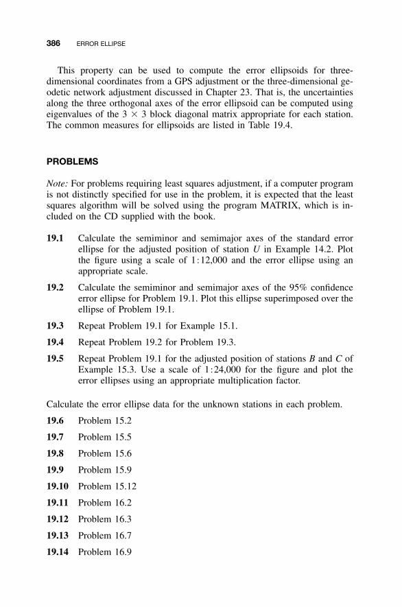
386 ERROR ELLIPSE
This property can be used to compute the error ellipsoids for three-dimensional coordinates from a GPS adjustment or the three-dimensional ge-odetic network adjustment discussed in Chapter 23. That is, the uncertaintiesalong the three orthogonal axes of the error ellipsoid can be computed usingeigenvalues of the 3 � 3 block diagonal matrix appropriate for each station.The common measures for ellipsoids are listed in Table 19.4.
PROBLEMS
Note: For problems requiring least squares adjustment, if a computer programis not distinctly specified for use in the problem, it is expected that the leastsquares algorithm will be solved using the program MATRIX, which is in-cluded on the CD supplied with the book.
19.1 Calculate the semiminor and semimajor axes of the standard errorellipse for the adjusted position of station U in Example 14.2. Plotthe figure using a scale of 1�12,000 and the error ellipse using anappropriate scale.
19.2 Calculate the semiminor and semimajor axes of the 95% confidenceerror ellipse for Problem 19.1. Plot this ellipse superimposed over theellipse of Problem 19.1.
19.3 Repeat Problem 19.1 for Example 15.1.
19.4 Repeat Problem 19.2 for Problem 19.3.
19.5 Repeat Problem 19.1 for the adjusted position of stations B and C ofExample 15.3. Use a scale of 1�24,000 for the figure and plot theerror ellipses using an appropriate multiplication factor.
Calculate the error ellipse data for the unknown stations in each problem.
19.6 Problem 15.2
19.7 Problem 15.5
19.8 Problem 15.6
19.9 Problem 15.9
19.10 Problem 15.12
19.11 Problem 16.2
19.12 Problem 16.3
19.13 Problem 16.7
19.14 Problem 16.9
PROBLEMS 387
Using a level of significance of 0.05, compute the 95% probable error ellipsefor the stations in each problem.
19.15 Problem 15.2
19.16 Problem 16.3
19.17 Using the program STATS, determine the percent probability of thestandard error ellipse for a horizontal survey with:(a) 3 degrees of freedom.(b) 9 degrees of freedom.(c) 20 degrees of freedom.(d) 50 degrees of freedom.(e) 100 degrees of freedom.
Programming Problems
19.18 Develop a computational program that takes the Qxx matrix and 2S0
from a horizontal adjustment and computes error ellipse data for theunknown stations.
19.19 Develop a computational program that does the same as described forProblems 19.15 and 19.16.
388
CHAPTER 20
CONSTRAINT EQUATIONS
20.1 INTRODUCTION
When doing an adjustment, it is sometimes necessary to fix an observationto a specific value. For instance, in Chapter 14 it was shown that the coor-dinates of a control station can be fixed by setting its dx and dy correctionsto zero, and thus the corrections and their corresponding coefficients in the Jmatrix were removed from the solution. This is called a constrained adjust-ment. Another constrained adjustment occurs when the direction or length ofa line is held to a specific value or when an elevation difference between twostations is fixed in differential leveling. In this chapter methods available fordeveloping observational constraints are discussed. However, before discuss-ing constraints, the procedure for including control station coordinates in anadjustment is described.
20.2 ADJUSTMENT OF CONTROL STATION COORDINATES
In examples in preceding chapters, when control station coordinates wereexcluded from the adjustments and hence their values were held fixed, con-strained adjustments were being performed. That is, the observations werebeing forced to fit the control coordinates. However, control is not perfectand not all control is of equal reliability. This is evidenced by the fact thatdifferent orders of accuracy are used to classify control.
When more than minimal control is held fixed in an adjustment, the ob-servations are forced to fit this control. For example, if the coordinates of twocontrol stations are held fixed but their actual positions are not in agreementwith the values given by their held coordinates, the observations will be ad-justed to match the erroneous control. Simply stated, precise observations maybe forced to fit less precise control. This was not a major problem in the days
Adjustment Computations: Spatial Data Analysis, Fourth Edition. C. D. Ghilani and P. R. Wolf© 2006 John Wiley & Sons, Inc. ISBN: 978-0-471-69728-2
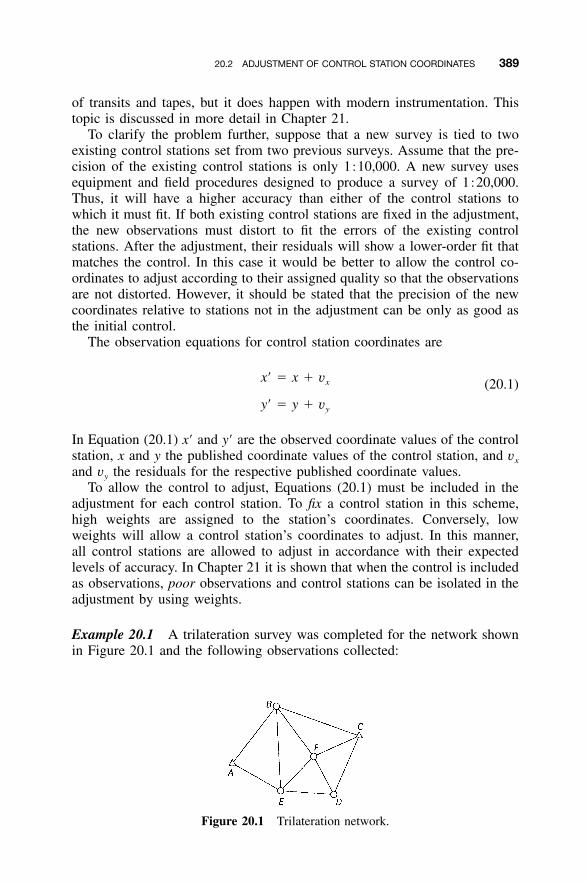
20.2 ADJUSTMENT OF CONTROL STATION COORDINATES 389
Figure 20.1 Trilateration network.
of transits and tapes, but it does happen with modern instrumentation. Thistopic is discussed in more detail in Chapter 21.
To clarify the problem further, suppose that a new survey is tied to twoexisting control stations set from two previous surveys. Assume that the pre-cision of the existing control stations is only 1�10,000. A new survey usesequipment and field procedures designed to produce a survey of 1�20,000.Thus, it will have a higher accuracy than either of the control stations towhich it must fit. If both existing control stations are fixed in the adjustment,the new observations must distort to fit the errors of the existing controlstations. After the adjustment, their residuals will show a lower-order fit thatmatches the control. In this case it would be better to allow the control co-ordinates to adjust according to their assigned quality so that the observationsare not distorted. However, it should be stated that the precision of the newcoordinates relative to stations not in the adjustment can be only as good asthe initial control.
The observation equations for control station coordinates are
x� � x � vx (20.1)
y� � y � vy
In Equation (20.1) x� and y� are the observed coordinate values of the controlstation, x and y the published coordinate values of the control station, and vx
and vy the residuals for the respective published coordinate values.To allow the control to adjust, Equations (20.1) must be included in the
adjustment for each control station. To fix a control station in this scheme,high weights are assigned to the station’s coordinates. Conversely, lowweights will allow a control station’s coordinates to adjust. In this manner,all control stations are allowed to adjust in accordance with their expectedlevels of accuracy. In Chapter 21 it is shown that when the control is includedas observations, poor observations and control stations can be isolated in theadjustment by using weights.
Example 20.1 A trilateration survey was completed for the network shownin Figure 20.1 and the following observations collected:
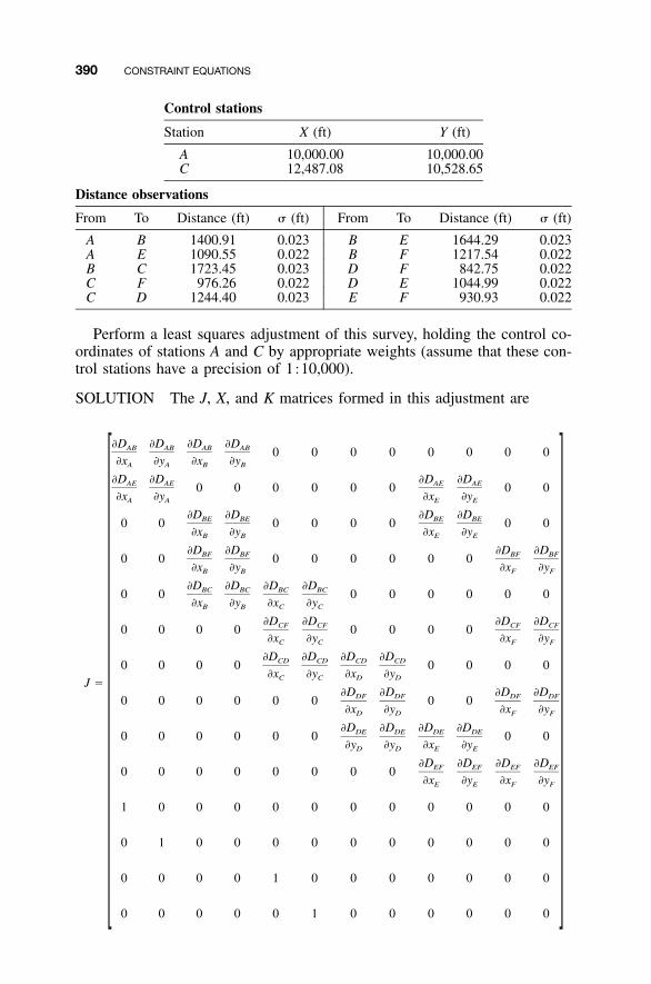
390 CONSTRAINT EQUATIONS
Control stations
Station X (ft) Y (ft)
A 10,000.00 10,000.00C 12,487.08 10,528.65
Distance observations
From To Distance (ft) � (ft) From To Distance (ft) � (ft)
A B 1400.91 0.023 B E 1644.29 0.023A E 1090.55 0.022 B F 1217.54 0.022B C 1723.45 0.023 D F 842.75 0.022C F 976.26 0.022 D E 1044.99 0.022C D 1244.40 0.023 E F 930.93 0.022
Perform a least squares adjustment of this survey, holding the control co-ordinates of stations A and C by appropriate weights (assume that these con-trol stations have a precision of 1�10,000).
SOLUTION The J, X, and K matrices formed in this adjustment are
�D �D �D �DAB AB AB AB 0 0 0 0 0 0 0 0�x �y �x �yA A B B
�D �D �D �DAE AE AE AE0 0 0 0 0 0 0 0�x �y �x �yA A E E
�D �D �D �DBE BE BE BE0 0 0 0 0 0 0 0�x �y �x �yB B E E
�D �D �D �DBF BF BF BF0 0 0 0 0 0 0 0�x �y �x �yB B F F
�D �D �D �DBC BC BC BC0 0 0 0 0 0 0 0�x �y �x �yB B C C
�D �D �D �DCF CF CF CF0 0 0 0 0 0 0 0�x �y �x �yC C F F
�D �D �D �DCD CD CD CD0 0 0 0 0 0 0 0�x �y �x �yC C D DJ �
�D �D �D �DDF DF DF DF0 0 0 0 0 0 0 0�x �y �x �yD D F F
�D �D �D �DDE DE DE DE0 0 0 0 0 0 0 0�y �y �x �yD D E E
�D �D �D �DEF EF EF EF0 0 0 0 0 0 0 0�x �y �x �yE E F F
1 0 0 0 0 0 0 0 0 0 0 0
0 1 0 0 0 0 0 0 0 0 0 0
0 0 0 0 1 0 0 0 0 0 0 0
0 0 0 0 0 1 0 0 0 0 0 0

20.2 ADJUSTMENT OF CONTROL STATION COORDINATES 391
L � ABAB 0
dx L � AEA AE 0
dy L � BEA BE 0
dx L � BFB BF 0
dy L � BCB BC 0
dx L � CFC CF 0
dy L � CDC CD 0X � K �dx L � DFD DF 0
dy L � DED DE 0
dx L � EFE EF 0
dy x � xE A A0
dx y � yF A A0
dy x � xF C C0
y � yC C0
Notice that the last four rows of the J matrix correspond to observationequations (20.1) for the coordinates of control stations A and C. Each coor-dinate has a row with one in the column corresponding to its correction.Obviously, by including the control station coordinates, four unknownshave been added to the adjustment: dxA, dyA, dxC, and dyC. However, fourobservations have also been added. Therefore, the number of redundanciesis unaffected by adding the coordinate observation equations. That is, theadjustment has the same number of redundancies with or without the controlequations.
It is possible to weight a control station according to the precision of itscoordinates. Unfortunately, control stations are published with distance pre-cisions rather than the covariance matrix elements that are required forweighting. However, estimates of the standard deviations of the coordinatescan be computed from the published distance precisions. That is, if the dis-tance precision between stations A and C is 1�10,000 or better, their coor-dinates should have estimated errors that yield a distance precision of1�10,000 between the stations. To find the estimated errors in the coordinatesthat yield the appropriate distance precision between the stations, Equation(6.16) can be applied to the distance formula, resulting in
2 2 2 2�D �D �D �Dij ij ij ij2 2 2 2 2� � � � � � � � � (20.2)� � � � � � � �D x y x yij i i j j�x �y �x �yi i j j
In Equation (20.2), is the variance in distance Dij, and and2 2 2 2� � , � , � ,D x y xij i i j
are the variances in the coordinates of the endpoints of the line. Assuming2�yj
that the estimated errors for the coordinates of Equation (20.2) are equal andsubstituting in the appropriate partial derivatives yields
2 2 2 2�D �D �x �xij ij2 2 2� � 2 � � 2 � � 2 � � 2 � (20.3)� � � � � � � �D x y c cij �x �y IJ IJ
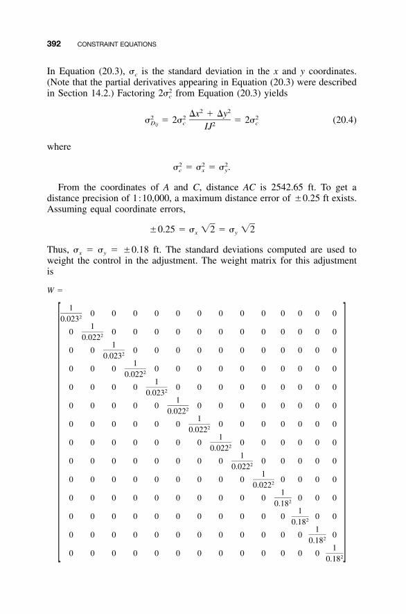
392 CONSTRAINT EQUATIONS
In Equation (20.3), �c is the standard deviation in the x and y coordinates.(Note that the partial derivatives appearing in Equation (20.3) were describedin Section 14.2.) Factoring from Equation (20.3) yields22�c
2 2�x � �y2 2 2� � 2� � 2� (20.4)D c cij 2IJ
where
2 2 2� � � � � .c x y
From the coordinates of A and C, distance AC is 2542.65 ft. To get adistance precision of 1�10,000, a maximum distance error of �0.25 ft exists.Assuming equal coordinate errors,
�0.25 � � �2 � � �2x y
Thus, �x � �y � �0.18 ft. The standard deviations computed are used toweight the control in the adjustment. The weight matrix for this adjustmentis
W �
10 0 0 0 0 0 0 0 0 0 0 0 020.0231
0 0 0 0 0 0 0 0 0 0 0 0 020.0221
0 0 0 0 0 0 0 0 0 0 0 0 020.0231
0 0 0 0 0 0 0 0 0 0 0 0 020.0221
0 0 0 0 0 0 0 0 0 0 0 0 020.0231
0 0 0 0 0 0 0 0 0 0 0 0 020.0221
0 0 0 0 0 0 0 0 0 0 0 0 020.0221
0 0 0 0 0 0 0 0 0 0 0 0 020.0221
0 0 0 0 0 0 0 0 0 0 0 0 020.0221
0 0 0 0 0 0 0 0 0 0 0 0 020.0221
0 0 0 0 0 0 0 0 0 0 0 0 020.181
0 0 0 0 0 0 0 0 0 0 0 0 020.181
0 0 0 0 0 0 0 0 0 0 0 0 020.181
0 0 0 0 0 0 0 0 0 0 0 0 0 20.18
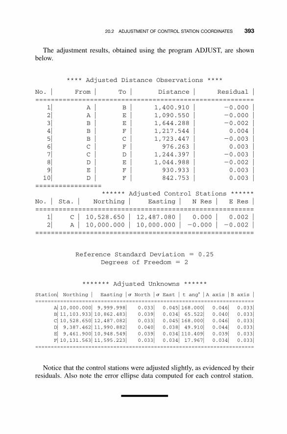
20.2 ADJUSTMENT OF CONTROL STATION COORDINATES 393
The adjustment results, obtained using the program ADJUST, are shownbelow.
**** Adjusted Distance Observations ****
No. � From � To � Distance � Residual �========================================================
1� A � B � 1,400.910 � �0.000 �2� A � E � 1,090.550 � �0.000 �3� B � E � 1,644.288 � �0.002 �4� B � F � 1,217.544 � 0.004 �5� B � C � 1,723.447 � �0.003 �6� C � F � 976.263 � 0.003 �7� C � D � 1,244.397 � �0.003 �8� D � E � 1,044.988 � �0.002 �9� E � F � 930.933 � 0.003 �10� D � F � 842.753 � 0.003 �
=================****** Adjusted Control Stations ******
No. � Sta. � Northing � Easting � N Res � E Res �========================================================
1� C � 10,528.650 � 12,487.080 � 0.000 � 0.002 �2� A � 10,000.000 � 10,000.000 � �0.000 � �0.002 �
========================================================
Reference Standard Deviation � 0.25Degrees of Freedom � 2
******* Adjusted Unknowns ******
Station� Northing � Easting � � North � � East � t ang� � A axis � B axis �======================================================================
A� 10,000.000� 9,999.998� 0.033� 0.045� 168.000� 0.046� 0.033�B� 11,103.933� 10,862.483� 0.039� 0.034� 65.522� 0.040� 0.033�C� 10,528.650� 12,487.082� 0.033� 0.045� 168.000� 0.046� 0.033�D� 9,387.462� 11,990.882� 0.040� 0.038� 49.910� 0.044� 0.033�E� 9,461.900� 10,948.549� 0.039� 0.034� 110.409� 0.039� 0.033�F� 10,131.563� 11,595.223� 0.033� 0.034� 17.967� 0.034� 0.033�
======================================================================
Notice that the control stations were adjusted slightly, as evidenced by theirresiduals. Also note the error ellipse data computed for each control station.
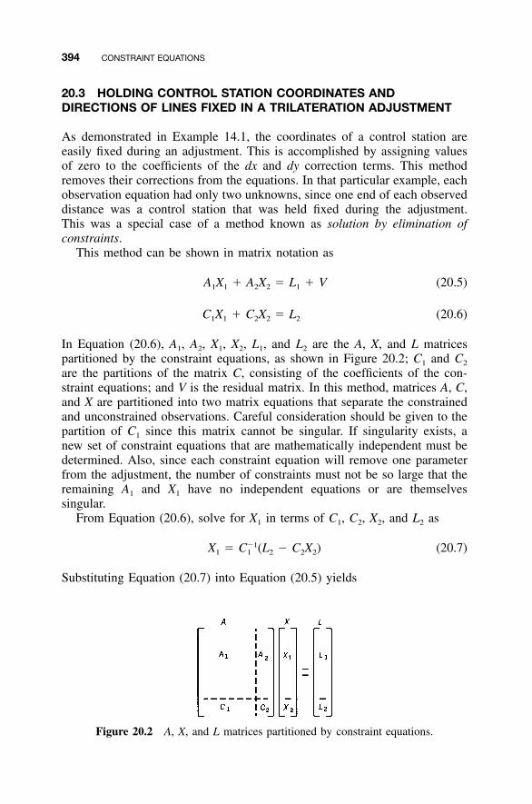
394 CONSTRAINT EQUATIONS
Figure 20.2 A, X, and L matrices partitioned by constraint equations.
20.3 HOLDING CONTROL STATION COORDINATES ANDDIRECTIONS OF LINES FIXED IN A TRILATERATION ADJUSTMENT
As demonstrated in Example 14.1, the coordinates of a control station areeasily fixed during an adjustment. This is accomplished by assigning valuesof zero to the coefficients of the dx and dy correction terms. This methodremoves their corrections from the equations. In that particular example, eachobservation equation had only two unknowns, since one end of each observeddistance was a control station that was held fixed during the adjustment.This was a special case of a method known as solution by elimination ofconstraints.
This method can be shown in matrix notation as
A X � A X � L � V (20.5)1 1 2 2 1
C X � C X � L (20.6)1 1 2 2 2
In Equation (20.6), A1, A2, X1, X2, L1, and L2 are the A, X, and L matricespartitioned by the constraint equations, as shown in Figure 20.2; C1 and C2
are the partitions of the matrix C, consisting of the coefficients of the con-straint equations; and V is the residual matrix. In this method, matrices A, C,and X are partitioned into two matrix equations that separate the constrainedand unconstrained observations. Careful consideration should be given to thepartition of C1 since this matrix cannot be singular. If singularity exists, anew set of constraint equations that are mathematically independent must bedetermined. Also, since each constraint equation will remove one parameterfrom the adjustment, the number of constraints must not be so large that theremaining A1 and X1 have no independent equations or are themselvessingular.
From Equation (20.6), solve for X1 in terms of C1, C2, X2, and L2 as
�1X � C (L � C X ) (20.7)1 1 2 2 2
Substituting Equation (20.7) into Equation (20.5) yields
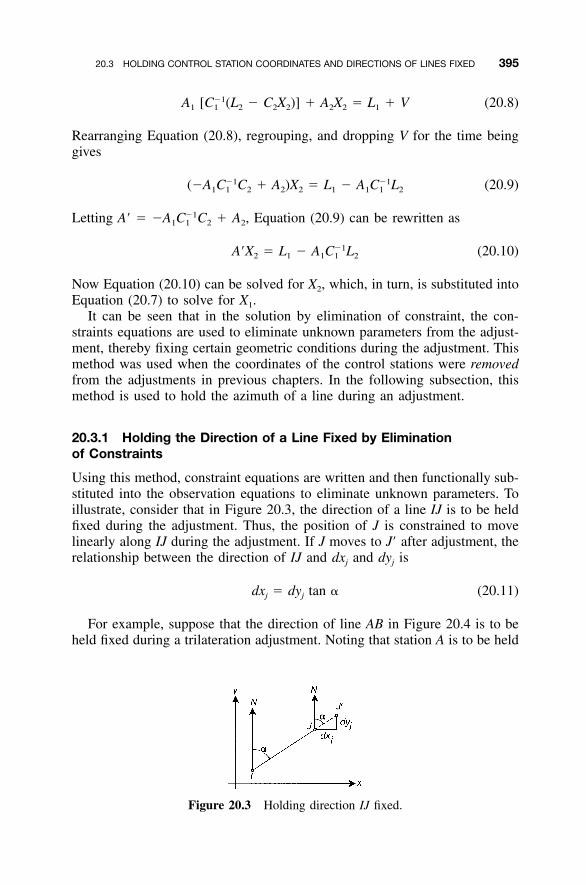
20.3 HOLDING CONTROL STATION COORDINATES AND DIRECTIONS OF LINES FIXED 395
Figure 20.3 Holding direction IJ fixed.
�1A [C (L � C X )] � A X � L � V (20.8)1 1 2 2 2 2 2 1
Rearranging Equation (20.8), regrouping, and dropping V for the time beinggives
�1 �1(�A C C � A )X � L � A C L (20.9)1 1 2 2 2 1 1 1 2
Letting A� � �A1 C2 � A2, Equation (20.9) can be rewritten as�1C1
�1A�X � L � A C L (20.10)2 1 1 1 2
Now Equation (20.10) can be solved for X2, which, in turn, is substituted intoEquation (20.7) to solve for X1.
It can be seen that in the solution by elimination of constraint, the con-straints equations are used to eliminate unknown parameters from the adjust-ment, thereby fixing certain geometric conditions during the adjustment. Thismethod was used when the coordinates of the control stations were removedfrom the adjustments in previous chapters. In the following subsection, thismethod is used to hold the azimuth of a line during an adjustment.
20.3.1 Holding the Direction of a Line Fixed by Eliminationof Constraints
Using this method, constraint equations are written and then functionally sub-stituted into the observation equations to eliminate unknown parameters. Toillustrate, consider that in Figure 20.3, the direction of a line IJ is to be heldfixed during the adjustment. Thus, the position of J is constrained to movelinearly along IJ during the adjustment. If J moves to J� after adjustment, therelationship between the direction of IJ and dxj and dyj is
dx � dy tan � (20.11)j j
For example, suppose that the direction of line AB in Figure 20.4 is to beheld fixed during a trilateration adjustment. Noting that station A is to be held
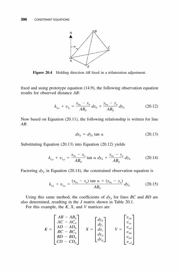
396 CONSTRAINT EQUATIONS
Figure 20.4 Holding direction AB fixed in a trilateration adjustment.
fixed and using prototype equation (14.9), the following observation equationresults for observed distance AB:
x � x y � yb a b a0 0k � v � dx � dy (20.12)l l b bab b AB AB0 0
Now based on Equation (20.11), the following relationship is written for lineAB:
dx � dy tan � (20.13)b b
Substituting Equation (20.13) into Equation (20.12) yields
x � x y � yb a b a0 0k � v � tan � dy � dy (20.14)l l b bab ab AB AB0 0
Factoring dyb in Equation (20.14), the constrained observation equation is
(x � x ) tan � � (y � y )b a b a0 0k � v � dy (20.15)l l bab ab AB0
Using this same method, the coefficients of dyb for lines BC and BD arealso determined, resulting in the J matrix shown in Table 20.1.
For this example, the K, X, and V matrices are
AB � AB v0 abdybAC � AC v0 acdycAD � AD v0 adK � X � dx V �cBC � BC v0 bbdyd� ��BD � BD � �v �0 bddxdCD � CD v0 cd
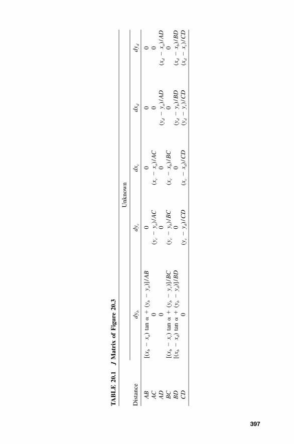
397
TA
BL
E20
.1J
Mat
rix
ofF
igur
e20
.3
Dis
tanc
e
Unk
now
n
dyb
dyc
dxc
dxd
dyd
AB
[(x b
�x a
)ta
n�
�(y
b�
y a)]
/AB
00
00
AC
0(y
c�
y a)/
AC
(xc
�x a
)/A
C0
0A
D0
00
(yd
�y a
)/A
D(x
d�
x a)/
AD
BC
[(x b
�x c
)ta
n�
�(y
b�
y c)]
/BC
(yc
�y b
)/B
C(x
c�
x b)/
BC
00
BD
[(x b
�x d
)ta
n�
�(y
b�
y d)]
/BD
00
(yd
�y b
)/B
D(x
d�
x b)/
BD
CD
0(y
c�
y d)/
CD
(xc
�x d
)/C
D(y
d�
y c)/
CD
(xd
�x c
)/C
D
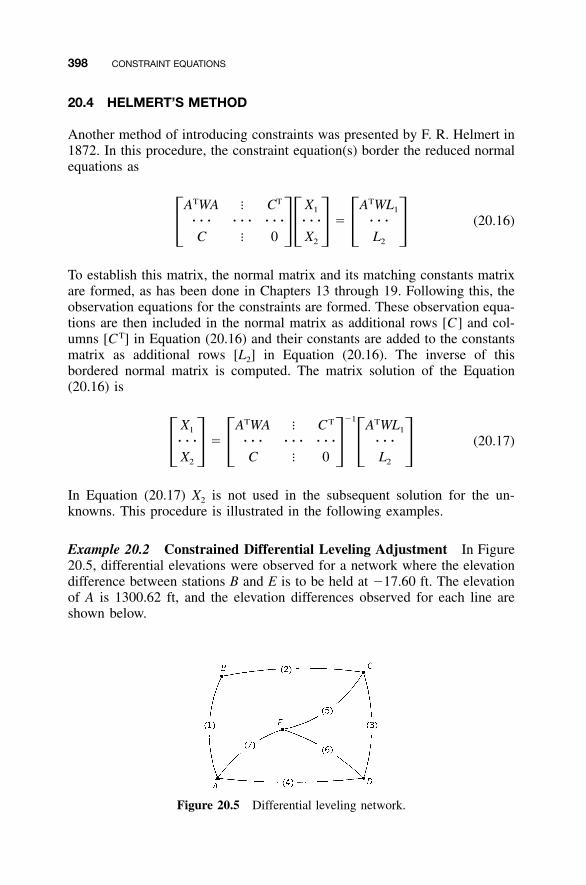
398 CONSTRAINT EQUATIONS
Figure 20.5 Differential leveling network.
20.4 HELMERT’S METHOD
Another method of introducing constraints was presented by F. R. Helmert in1872. In this procedure, the constraint equation(s) border the reduced normalequations as
T T TA WA � C X A WL1 1
� � � � � � � � � � � � � � � � (20.16)� �� � � �C � 0 X L2 2
To establish this matrix, the normal matrix and its matching constants matrixare formed, as has been done in Chapters 13 through 19. Following this, theobservation equations for the constraints are formed. These observation equa-tions are then included in the normal matrix as additional rows [C] and col-umns [CT] in Equation (20.16) and their constants are added to the constantsmatrix as additional rows [L2] in Equation (20.16). The inverse of thisbordered normal matrix is computed. The matrix solution of the Equation(20.16) is
�1T T TX A WA � C A WL1 1
� � � � � � � � � � � � � � � � (20.17)� � � � � �X C � 0 L2 2
In Equation (20.17) X2 is not used in the subsequent solution for the un-knowns. This procedure is illustrated in the following examples.
Example 20.2 Constrained Differential Leveling Adjustment In Figure20.5, differential elevations were observed for a network where the elevationdifference between stations B and E is to be held at �17.60 ft. The elevationof A is 1300.62 ft, and the elevation differences observed for each line areshown below.

20.4 HELMERT’S METHOD 399
Line From To Elevation (ft) S (ft)
1 A B 25.15 0.072 B C �10.57 0.053 C D �1.76 0.034 D A �12.65 0.085 C E �7.06 0.036 E D 5.37 0.057 E A �7.47 0.05
Perform a least squares adjustment of this level net constraining the requiredelevation difference.
SOLUTION The A, X, and L matrices are
1 0 0 0 1325.77�1 1 0 0 �10.55
B0 �1 1 0 �1.76
CA � 0 0 �1 0 X � L � �1313.27
D� �0 �1 0 1 �7.06E� � � �0 0 1 �1 5.37
0 0 0 �1 1308.09
The weight matrix (W) is
204.08 0 0 0 0 0 00 400 0 0 0 0 00 0 1111.11 0 0 0 0
W � 0 0 0 156.25 0 0 00 0 0 0 1111.11 0 0� �0 0 0 0 0 400 00 0 0 0 0 400
The reduced normal equations are
604.08 �400.00 0.00 0.00 B 274,793.30�400.00 2622.22 �1111.11 �1111.11 C 5572.00
� (a)0.00 �1111.11 1667.36 �400.00 D 205,390.90� �� � � �0.00 �1111.11 �400.00 1911.11 E 513,243.60
The reduced normal matrix is now bordered by the constraint equation
E � B � �17.60
which has a matrix form of
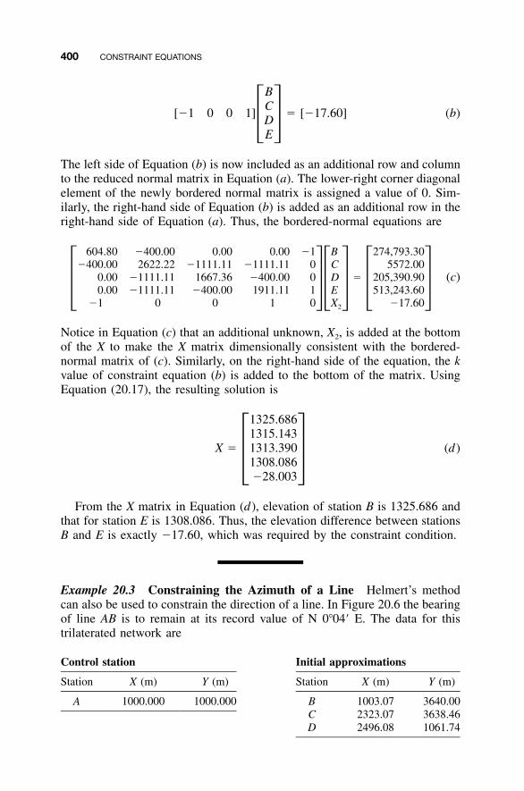
400 CONSTRAINT EQUATIONS
BC
[�1 0 0 1] � [�17.60] (b)D� �E
The left side of Equation (b) is now included as an additional row and columnto the reduced normal matrix in Equation (a). The lower-right corner diagonalelement of the newly bordered normal matrix is assigned a value of 0. Sim-ilarly, the right-hand side of Equation (b) is added as an additional row in theright-hand side of Equation (a). Thus, the bordered-normal equations are
604.80 �400.00 0.00 0.00 �1 B 274,793.30�400.00 2622.22 �1111.11 �1111.11 0 C 5572.00
0.00 �1111.11 1667.36 �400.00 0 D � 205,390.90 (c)0.00 �1111.11 �400.00 1911.11 1 E 513,243.60� �� � � �
�1 0 0 1 0 X �17.602
Notice in Equation (c) that an additional unknown, X2, is added at the bottomof the X to make the X matrix dimensionally consistent with the bordered-normal matrix of (c). Similarly, on the right-hand side of the equation, the kvalue of constraint equation (b) is added to the bottom of the matrix. UsingEquation (20.17), the resulting solution is
1325.6861315.143
X � 1313.390 (d)1308.086� ��28.003
From the X matrix in Equation (d), elevation of station B is 1325.686 andthat for station E is 1308.086. Thus, the elevation difference between stationsB and E is exactly �17.60, which was required by the constraint condition.
Example 20.3 Constraining the Azimuth of a Line Helmert’s methodcan also be used to constrain the direction of a line. In Figure 20.6 the bearingof line AB is to remain at its record value of N 0�04� E. The data for thistrilaterated network are
Control station Initial approximations
Station X (m) Y (m) Station X (m) Y (m)
A 1000.000 1000.000 BCD
1003.072323.072496.08
3640.003638.461061.74
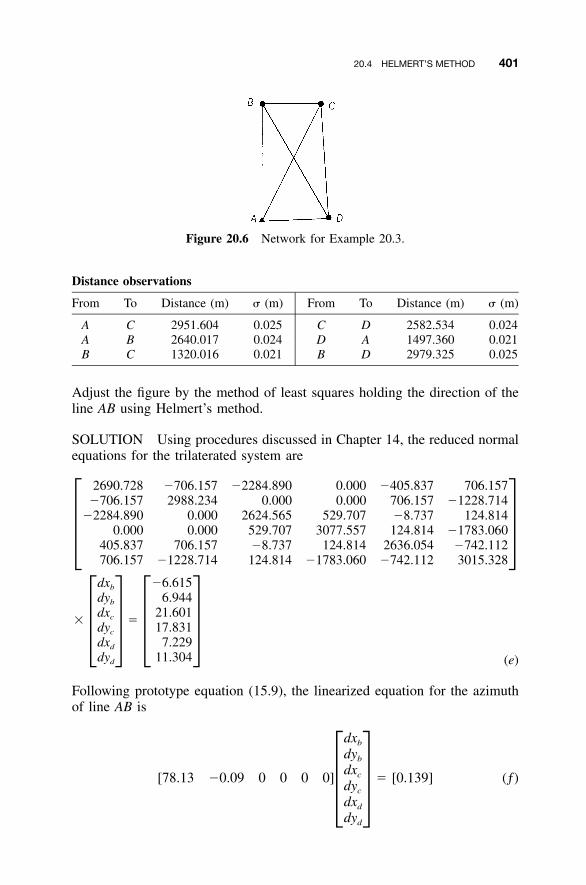
20.4 HELMERT’S METHOD 401
Figure 20.6 Network for Example 20.3.
Distance observations
From To Distance (m) � (m) From To Distance (m) � (m)
A C 2951.604 0.025 C D 2582.534 0.024A B 2640.017 0.024 D A 1497.360 0.021B C 1320.016 0.021 B D 2979.325 0.025
Adjust the figure by the method of least squares holding the direction of theline AB using Helmert’s method.
SOLUTION Using procedures discussed in Chapter 14, the reduced normalequations for the trilaterated system are
2690.728 �706.157 �2284.890 0.000 �405.837 706.157�706.157 2988.234 0.000 0.000 706.157 �1228.714
�2284.890 0.000 2624.565 529.707 �8.737 124.8140.000 0.000 529.707 3077.557 124.814 �1783.060
405.837 706.157 �8.737 124.814 2636.054 �742.112� �706.157 �1228.714 124.814 �1783.060 �742.112 3015.328
dx �6.615b
dy 6.944b
dx 21.601c� �dy 17.831c
dx 7.229� � � �d
dy 11.304d (e)
Following prototype equation (15.9), the linearized equation for the azimuthof line AB is
dxb
dyb
dxc[78.13 �0.09 0 0 0 0] � [0.139] (ƒ)dyc�dx �ddyd
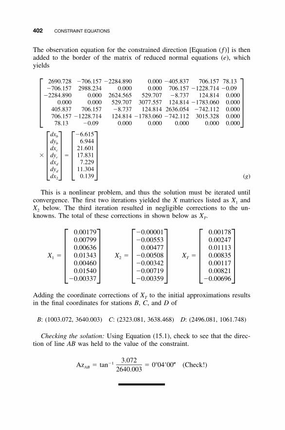
402 CONSTRAINT EQUATIONS
The observation equation for the constrained direction [Equation (ƒ)] is thenadded to the border of the matrix of reduced normal equations (e), whichyields
2690.728 �706.157 �2284.890 0.000 �405.837 706.157 78.13�706.157 2988.234 0.000 0.000 706.157 �1228.714 �0.09
�2284.890 0.000 2624.565 529.707 �8.737 124.814 0.0000.000 0.000 529.707 3077.557 124.814 �1783.060 0.000
405.837 706.157 �8.737 124.814 2636.054 �742.112 0.000� �706.157 �1228.714 124.814 �1783.060 �742.112 3015.328 0.00078.13 �0.09 0.000 0.000 0.000 0.000 0.000
dx �6.615b
dy 6.944b
dx 21.601c
� dy � 17.831c
dx 7.229d� � � �dy 11.304d
dx 0.1392 (g)
This is a nonlinear problem, and thus the solution must be iterated untilconvergence. The first two iterations yielded the X matrices listed as X1 andX2 below. The third iteration resulted in negligible corrections to the un-knowns. The total of these corrections in shown below as XT.
0.00179 �0.00001 0.001780.00799 �0.00553 0.002470.00636 0.00477 0.01113
X � 0.01343 X � �0.00508 X � 0.008351 2 T
0.00460 �0.00342 0.00117� � � � � �0.01540 �0.00719 0.00821�0.00337 �0.00359 �0.00696
Adding the coordinate corrections of XT to the initial approximations resultsin the final coordinates for stations B, C, and D of
B: (1003.072, 3640.003) C: (2323.081, 3638.468) D: (2496.081, 1061.748)
Checking the solution: Using Equation (15.1), check to see that the direc-tion of line AB was held to the value of the constraint.
3.072�1Az � tan � 0�04�00� (Check!)AB 2640.003
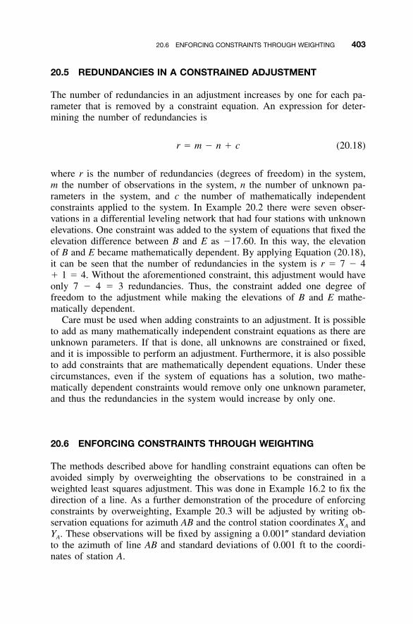
20.6 ENFORCING CONSTRAINTS THROUGH WEIGHTING 403
20.5 REDUNDANCIES IN A CONSTRAINED ADJUSTMENT
The number of redundancies in an adjustment increases by one for each pa-rameter that is removed by a constraint equation. An expression for deter-mining the number of redundancies is
r � m � n � c (20.18)
where r is the number of redundancies (degrees of freedom) in the system,m the number of observations in the system, n the number of unknown pa-rameters in the system, and c the number of mathematically independentconstraints applied to the system. In Example 20.2 there were seven obser-vations in a differential leveling network that had four stations with unknownelevations. One constraint was added to the system of equations that fixed theelevation difference between B and E as �17.60. In this way, the elevationof B and E became mathematically dependent. By applying Equation (20.18),it can be seen that the number of redundancies in the system is r � 7 � 4� 1 � 4. Without the aforementioned constraint, this adjustment would haveonly 7 � 4 � 3 redundancies. Thus, the constraint added one degree offreedom to the adjustment while making the elevations of B and E mathe-matically dependent.
Care must be used when adding constraints to an adjustment. It is possibleto add as many mathematically independent constraint equations as there areunknown parameters. If that is done, all unknowns are constrained or fixed,and it is impossible to perform an adjustment. Furthermore, it is also possibleto add constraints that are mathematically dependent equations. Under thesecircumstances, even if the system of equations has a solution, two mathe-matically dependent constraints would remove only one unknown parameter,and thus the redundancies in the system would increase by only one.
20.6 ENFORCING CONSTRAINTS THROUGH WEIGHTING
The methods described above for handling constraint equations can often beavoided simply by overweighting the observations to be constrained in aweighted least squares adjustment. This was done in Example 16.2 to fix thedirection of a line. As a further demonstration of the procedure of enforcingconstraints by overweighting, Example 20.3 will be adjusted by writing ob-servation equations for azimuth AB and the control station coordinates XA andYA. These observations will be fixed by assigning a 0.001� standard deviationto the azimuth of line AB and standard deviations of 0.001 ft to the coordi-nates of station A.
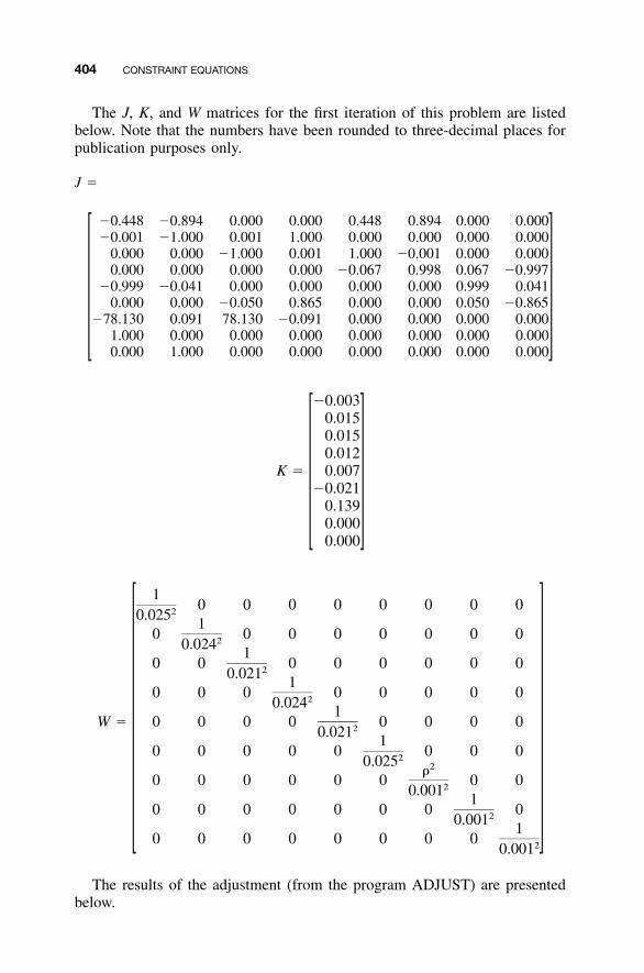
404 CONSTRAINT EQUATIONS
The J, K, and W matrices for the first iteration of this problem are listedbelow. Note that the numbers have been rounded to three-decimal places forpublication purposes only.
J �
�0.448 �0.894 0.000 0.000 0.448 0.894 0.000 0.000�0.001 �1.000 0.001 1.000 0.000 0.000 0.000 0.000
0.000 0.000 �1.000 0.001 1.000 �0.001 0.000 0.0000.000 0.000 0.000 0.000 �0.067 0.998 0.067 �0.997
�0.999 �0.041 0.000 0.000 0.000 0.000 0.999 0.0410.000 0.000 �0.050 0.865 0.000 0.000 0.050 �0.865
�78.130 0.091 78.130 �0.091 0.000 0.000 0.000 0.0001.000 0.000 0.000 0.000 0.000 0.000 0.000 0.0000.000 1.000 0.000 0.000 0.000 0.000 0.000 0.000
�0.0030.0150.0150.012
K � 0.007�0.021
0.1390.0000.000
10 0 0 0 0 0 0 020.0251
0 0 0 0 0 0 0 020.0241
0 0 0 0 0 0 0 020.0211
0 0 0 0 0 0 0 020.0241
W � 0 0 0 0 0 0 0 020.0211
0 0 0 0 0 0 0 020.025 2�0 0 0 0 0 0 0 020.001
10 0 0 0 0 0 0 020.001
10 0 0 0 0 0 0 0 20.001
The results of the adjustment (from the program ADJUST) are presentedbelow.
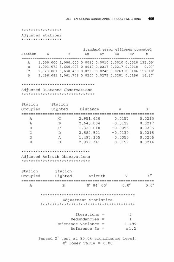
20.6 ENFORCING CONSTRAINTS THROUGH WEIGHTING 405
*****************Adjusted stations*****************
Station X YStandard error ellipses computedSx Sy Su Sv t
==============================================================A 1,000.000 1,000.000 0.0010 0.0010 0.0010 0.0010 135.00�B 1,003.072 3,640.003 0.0010 0.0217 0.0217 0.0010 0.07�C 2,323.081 3,638.468 0.0205 0.0248 0.0263 0.0186 152.10�D 2,496.081 1,061.748 0.0204 0.0275 0.0281 0.0196 16.37�
*******************************Adjusted Distance Observations*******************************
StationOccupied
StationSighted Distance V S
========================================================A C 2,951.620 0.0157 0.0215A B 2,640.004 �0.0127 0.0217B C 1,320.010 �0.0056 0.0205C D 2,582.521 �0.0130 0.0215D A 1,497.355 �0.0050 0.0206B D 2,979.341 0.0159 0.0214
*****************************Adjusted Azimuth Observations*****************************
StationOccupied
StationSighted Azimuth V S�
========================================================A B 0� 04� 00� 0.0� 0.0�
****************************************Adjustment Statistics
****************************************
Iterations � 2Redundancies � 1
Reference Variance � 1.499Reference So � �1.2
Passed X2 test at 95.0% significance level!X2 lower value � 0.00
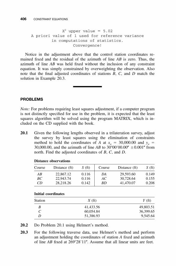
406 CONSTRAINT EQUATIONS
X2 upper value � 5.02A priori value of 1 used for reference variance
in computations of statistics.Convergence!
Notice in the adjustment above that the control station coordinates re-mained fixed and the residual of the azimuth of line AB is zero. Thus, theazimuth of line AB was held fixed without the inclusion of any constraintequation. It was simply constrained by overweighting the observation. Alsonote that the final adjusted coordinates of stations B, C, and D match thesolution in Example 20.3.
PROBLEMS
Note: For problems requiring least squares adjustment, if a computer programis not distinctly specified for use in the problem, it is expected that the leastsquares algorithm will be solved using the program MATRIX, which is in-cluded on the CD supplied with the book.
20.1 Given the following lengths observed in a trilateration survey, adjustthe survey by least squares using the elimination of constraintsmethod to hold the coordinates of A at xa � 30,000.00 and ya �30,000.00, and the azimuth of line AB to 30�00�00.00� �0.001� fromnorth. Find the adjusted coordinates of B, C, and D.
Distance observations
Course Distance (ft) S (ft) Course Distance (ft) S (ft)
AB 22,867.12 0.116 DA 29,593.60 0.149BC 22,943.74 0.116 AC 30,728.64 0.155CD 28,218.26 0.142 BD 41,470.07 0.208
Initial coordinates
Station X (ft) Y (ft)
B 41,433.56 49,803.51C 60,054.84 36,399.65D 51,386.93 9,545.64
20.2 Do Problem 20.1 using Helmert’s method.
20.3 For the following traverse data, use Helmert’s method and performan adjustment holding the coordinates of station A fixed and azimuthof line AB fixed at 269�28�11�. Assume that all linear units are feet.
PROBLEMS 407
Control station Initial coordinates
Station X Y Station X Y
A 15,123.65 9803.10 BC
14,423.2612,620.56
9796.619066.30
Distance observations Angle observations
Course Distance S Stations Angle S (�)
AB 700.42 0.020 ABC 158�28�34� 4.5BC 1945.01 0.022 BCA 5�39�06� 2.9CA 2609.24 0.024 CAB 15�52�22� 4.1
20.4 Given the following differential leveling data, adjust it using Hel-mert’s method. Hold the elevation of A to 100.00 ft and the elevationdifference �ElevAD to �5.00 ft.
From To �Elev (ft) S From To �Elev (ft) S
A B 19.997 0.005 D E 9.990 0.006B C �19.984 0.008 E A �5.000 0.004C D �4.998 0.003
20.5 Using the method of weighting discussed in Section 20.6, adjust thedata in:(a) Problem 20.1.(b) Problem 20.3.(c) Problem 20.4.(d) Compare the results with those of Problem 20.1, 20.3, or 20.4 as
appropriate.
20.6 Do Problem 13.14 holding distance BC to 100.00 ft using:(a) the elimination of constraints method.(b) Helmert’s method.(c) Compare the results of the adjustments from the different
methods.
20.7 Do Problem 14.15 holding the elevation difference between V and Zto 3.600 m using:(a) the elimination of constraints method.(b) Helmert’s method.(c) the method of overweighting technique.(d) Compare the results of the adjustments from the various methods.

408 CONSTRAINT EQUATIONS
20.8 Do Problem 12.11 holding the difference in elevation between stations2 and 8 to 66.00 ft. Use:(a) the elimination of constraints method.(b) Helmert’s method.(c) the method of overweighting technique.
20.9 Assuming that stations A and D are second-order class I horizontalcontrol (1�50,000), do Problem 14.8 by including the control in theadjustment.
20.10 Do Problem 15.7 assuming that station A is first-order horizontal con-trol (1�100,000) and B is second-order class I horizontal control(1�50,000) using the overweighting method.
20.11 Do Problem 15.9 assuming that the control stations are second-orderclass II horizontal control (1�20,000) using the overweightingmethod.
20.12 Do Problem 15.12 assuming that stations A and D are third-orderclass I control (1�10,000) using the overweighting method.
Practical Problems
20.13 Develop a computational program that computes the coefficients forthe J matrix in a trilateration adjustment with a constrained azimuth.Use the program to solve Problem 20.8.
20.14 Develop a computational program that computes a constrained leastsquares adjustment of a trilateration network using Helmert’s method.Use this program to solve Problem 20.11.
409
CHAPTER 21
BLUNDER DETECTION INHORIZONTAL NETWORKS
21.1 INTRODUCTION
Up to this point, data sets are assumed to be free of blunders. However, whenadjusting real observations, the data sets are seldom blunder free. Not allblunders are large, but no matter their sizes, it is desirable to remove themfrom the data set. In this chapter, methods used to detect blunders before andafter an adjustment are discussed.
Many examples can be cited that illustrate mishaps that have resulted fromundetected blunders in survey data. However, few could have been morecostly and embarrassing than a blunder of about 1 mile that occurred in anearly nineteenth-century survey of the border between the United States andCanada near the north end of Lake Champlain. Following the survey, con-struction of a U.S. military fort was begun. The project was abandoned twoyears later when the blunder was detected and a resurvey showed that thefort was actually located on Canadian soil. The abandoned facility was sub-sequently named Fort Blunder!
As discussed in previous chapters, observations are normally distributed.This means that occasionally, large random errors will occur. However, inaccordance with theory, this should seldom happen. Thus, large errors in datasets are more likely to be blunders than random errors. Common blunders indata sets include number transposition, entry and recording errors, stationmisidentifications, and others. When blunders are present in a data set, a leastsquares adjustment may not be possible or will, at a minimum, produce pooror invalid results. To be safe, the results of an adjustment should never beaccepted without an analysis of the post-adjustment statistics.
Adjustment Computations: Spatial Data Analysis, Fourth Edition. C. D. Ghilani and P. R. Wolf© 2006 John Wiley & Sons, Inc. ISBN: 978-0-471-69728-2
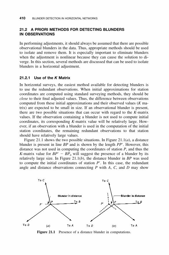
410 BLUNDER DETECTION IN HORIZONTAL NETWORKS
Figure 21.1 Presence of a distance blunder in computations.
21.2 A PRIORI METHODS FOR DETECTING BLUNDERSIN OBSERVATIONS
In performing adjustments, it should always be assumed that there are possibleobservational blunders in the data. Thus, appropriate methods should be usedto isolate and remove them. It is especially important to eliminate blunderswhen the adjustment is nonlinear because they can cause the solution to di-verge. In this section, several methods are discussed that can be used to isolateblunders in a horizontal adjustment.
21.2.1 Use of the K Matrix
In horizontal surveys, the easiest method available for detecting blunders isto use the redundant observations. When initial approximations for stationcoordinates are computed using standard surveying methods, they should beclose to their final adjusted values. Thus, the difference between observationscomputed from these initial approximations and their observed values (K ma-trix) are expected to be small in size. If an observational blunder is present,there are two possible situations that can occur with regard to the K-matrixvalues. If the observation containing a blunder is not used to compute initialcoordinates, its corresponding K-matrix value will be relatively large. How-ever, if an observation with a blunder is used in the computation of the initialstation coordinates, the remaining redundant observations to that stationshould have relatively large values.
Figure 21.1 shows the two possible situations. In Figure 21.1(a), a distanceblunder is present in line BP and is shown by the length PP�. However, thisdistance was not used in computing the coordinates of station P, and thus theK-matrix value for BP� � BP0 will suggest the presence of a blunder by itsrelatively large size. In Figure 21.1(b), the distance blunder in BP was usedto compute the initial coordinates of station P�. In this case, the redundantangle and distance observations connecting P with A, C, and D may show
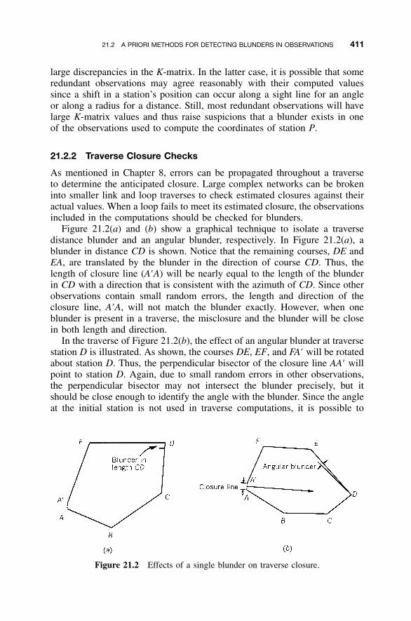
21.2 A PRIORI METHODS FOR DETECTING BLUNDERS IN OBSERVATIONS 411
Figure 21.2 Effects of a single blunder on traverse closure.
large discrepancies in the K-matrix. In the latter case, it is possible that someredundant observations may agree reasonably with their computed valuessince a shift in a station’s position can occur along a sight line for an angleor along a radius for a distance. Still, most redundant observations will havelarge K-matrix values and thus raise suspicions that a blunder exists in oneof the observations used to compute the coordinates of station P.
21.2.2 Traverse Closure Checks
As mentioned in Chapter 8, errors can be propagated throughout a traverseto determine the anticipated closure. Large complex networks can be brokeninto smaller link and loop traverses to check estimated closures against theiractual values. When a loop fails to meet its estimated closure, the observationsincluded in the computations should be checked for blunders.
Figure 21.2(a) and (b) show a graphical technique to isolate a traversedistance blunder and an angular blunder, respectively. In Figure 21.2(a), ablunder in distance CD is shown. Notice that the remaining courses, DE andEA, are translated by the blunder in the direction of course CD. Thus, thelength of closure line (A�A) will be nearly equal to the length of the blunderin CD with a direction that is consistent with the azimuth of CD. Since otherobservations contain small random errors, the length and direction of theclosure line, A�A, will not match the blunder exactly. However, when oneblunder is present in a traverse, the misclosure and the blunder will be closein both length and direction.
In the traverse of Figure 21.2(b), the effect of an angular blunder at traversestation D is illustrated. As shown, the courses DE, EF, and FA� will be rotatedabout station D. Thus, the perpendicular bisector of the closure line AA� willpoint to station D. Again, due to small random errors in other observations,the perpendicular bisector may not intersect the blunder precisely, but itshould be close enough to identify the angle with the blunder. Since the angleat the initial station is not used in traverse computations, it is possible to
412 BLUNDER DETECTION IN HORIZONTAL NETWORKS
isolate a single angular blunder by beginning traverse computations at thestation with the suspected blunder. In this case, when the blunder is not usedin the computations, estimated misclosure errors (see Chapter 8) will be metand the blunder can be isolated to the single unused angle. Thus, in Figure21.2(b), if the traverse computations were started at station D and used anassumed azimuth for the course of CD, the traverse misclosure when returningto D would be within estimated tolerance since the angle at D is not used inthe traverse computations.
21.3 A POSTERIORI BLUNDER DETECTION
When doing a least squares adjustment involving more than the minimumamount of control, both a minimally and fully constrained adjustment shouldbe performed. In a minimally constrained adjustment, the data need to satisfythe appropriate geometric closures and are not influenced by control errors.After the adjustment, a �2 test1 can be used to check the a priori value of thereference variance against its a posteriori estimate. However, this test is nota good indicator of the presence of a blunder since it is sensitive to poorrelative weighting. Thus, the a posteriori residuals should also be checked forthe presence of large discrepancies. If no large discrepancies are present, theobservational weights should be altered and the adjustment rerun. Since thistest is sensitive to weights, the procedures described in Chapters 7 through10 should be used for building the stochastic model of the adjustment.
Besides the sizes of the residuals, the signs of the residuals may alsoindicate a problem in the data. From normal probability theory, residuals areexpected to be small and randomly distributed. A small section of a largernetwork is shown in Figure 21.3. Notice that the distance residuals betweenstations A and B are all positive. This is not expected from normally distrib-uted data. Thus, it is possible that either a blunder or a systematic error ispresent in some or all of the survey. If both A and B are control stations, partof the problem could stem from control coordinate discrepancies. This pos-sibility can be isolated by doing a minimally constrained adjustment.
Although residual sizes can suggest observational errors, they do not nec-essarily identify the observations that contain blunders. This is due to the factthat least squares generally spreads a large observational error or blunder outradially from its source. However, this condition is not unique to least squaresadjustments since any arbitrary adjustment method, including the compassrule for traverse adjustment, will also spread a single observational errorthroughout the entire observational set.
1 Statistical testing was discussed in Chapter 4.
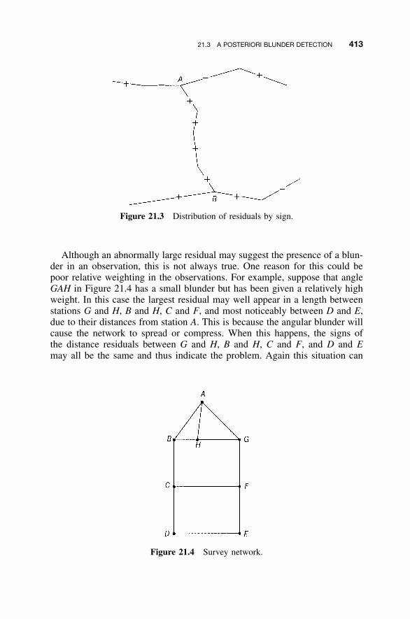
21.3 A POSTERIORI BLUNDER DETECTION 413
Figure 21.3 Distribution of residuals by sign.
Figure 21.4 Survey network.
Although an abnormally large residual may suggest the presence of a blun-der in an observation, this is not always true. One reason for this could bepoor relative weighting in the observations. For example, suppose that angleGAH in Figure 21.4 has a small blunder but has been given a relatively highweight. In this case the largest residual may well appear in a length betweenstations G and H, B and H, C and F, and most noticeably between D and E,due to their distances from station A. This is because the angular blunder willcause the network to spread or compress. When this happens, the signs ofthe distance residuals between G and H, B and H, C and F, and D and Emay all be the same and thus indicate the problem. Again this situation can
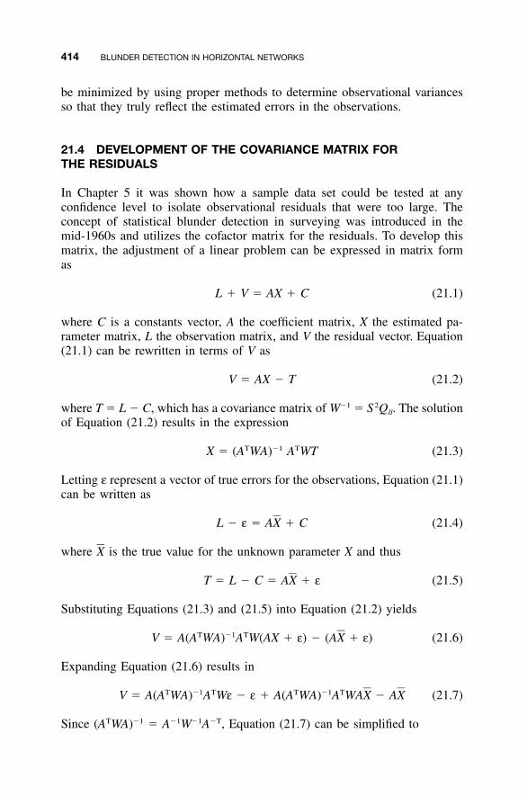
414 BLUNDER DETECTION IN HORIZONTAL NETWORKS
be minimized by using proper methods to determine observational variancesso that they truly reflect the estimated errors in the observations.
21.4 DEVELOPMENT OF THE COVARIANCE MATRIX FORTHE RESIDUALS
In Chapter 5 it was shown how a sample data set could be tested at anyconfidence level to isolate observational residuals that were too large. Theconcept of statistical blunder detection in surveying was introduced in themid-1960s and utilizes the cofactor matrix for the residuals. To develop thismatrix, the adjustment of a linear problem can be expressed in matrix formas
L � V � AX � C (21.1)
where C is a constants vector, A the coefficient matrix, X the estimated pa-rameter matrix, L the observation matrix, and V the residual vector. Equation(21.1) can be rewritten in terms of V as
V � AX � T (21.2)
where T � L � C, which has a covariance matrix of W�1 � S2Qll. The solutionof Equation (21.2) results in the expression
T �1 TX � (A WA) A WT (21.3)
Letting ε represent a vector of true errors for the observations, Equation (21.1)can be written as
L � ε � AX � C (21.4)
where is the true value for the unknown parameter X and thusX
T � L � C � AX � ε (21.5)
Substituting Equations (21.3) and (21.5) into Equation (21.2) yields
T �1 TV � A(A WA) A W(AX � ε) � (AX � ε) (21.6)
Expanding Equation (21.6) results in
T �1 T T �1 TV � A(A WA) A Wε � ε � A(A WA) A WAX � AX (21.7)
Since (ATWA)�1 � A�1W�1A�T, Equation (21.7) can be simplified to
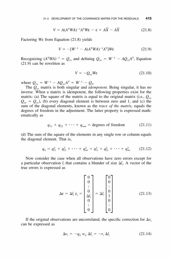
21.4 DEVELOPMENT OF THE COVARIANCE MATRIX FOR THE RESIDUALS 415
T �1 TV � A(A WA) A Wε � ε � AX � AX (21.8)
Factoring Wε from Equation (21.8) yields
�1 T �1 TV � �[W � A(A WA) A ]Wε (21.9)
Recognizing (ATWA)�1 � Qxx and defining Qvv � W�1 � AQxxAT, Equation
(21.9) can be rewritten as
V � �Q Wε (21.10)vv
where Qvv � W�1 � AQxxAT � W�1 � Qll.The Qvv matrix is both singular and idempotent. Being singular, it has no
inverse. When a matrix is idempotent, the following properties exist for thematrix: (a) The square of the matrix is equal to the original matrix (i.e., Qvv
Qvv � Qvv), (b) every diagonal element is between zero and 1, and (c) thesum of the diagonal elements, known as the trace of the matrix, equals thedegrees of freedom in the adjustment. The latter property is expressed math-ematically as
q � q � � � � � q � degrees of freedom (21.11)11 22 mm
(d) The sum of the square of the elements in any single row or column equalsthe diagonal element. That is,
2 2 2 2 2 2q � q � q � � � � � q � q � q � � � � � q (21.12)ii i1 i2 im 1i 2i mi
Now consider the case when all observations have zero errors except fora particular observation li that contains a blunder of size �li. A vector of thetrue errors is expressed as
0 00 0� �
0 0�ε � �l ε � � �l (21.13)i i i�l 1i
0 0� � � �� �
0 0
If the original observations are uncorrelated, the specific correction for �vi
can be expressed as
�v � �q w �l � �r �l (21.14)i ii ii i i i
416 BLUNDER DETECTION IN HORIZONTAL NETWORKS
where qii is the ith diagonal of the Qvv matrix, wii the ith diagonal term ofthe weight matrix, W, and ri � qii wii is the observational redundancy number.
When the system has a unique solution, ri will equal zero, and if theobservation is fully constrained, ri would equal 1. The redundancy numbersprovide insight into the geometric strength of the adjustment. An adjustmentthat in general has low redundancy numbers will have observations that lacksufficient checks to isolate blunders, and thus the chance for undetected blun-ders to exist in the observations is high. Conversely, a high overall redundancynumber enables a high level of internal checking of the observations and thusthere is a lower chance of accepting observations that contain blunders. Thequotient of r /m, where r is the total number of redundant observations in thesystem and m is the number of observations, is called the relative redundancyof the adjustment.
21.5 DETECTION OF OUTLIERS IN OBSERVATIONS
Equation (21.10) defines the covariance matrix for the vector of residuals, vi.From this the standardized residual is computed using the appropriate diag-onal element of the Qvv matrix as
viv � (21.15)i �qii
where is the standardized residual, vi the computed residual, and qii thevi
diagonal element of the Qvv matrix. Using the Qvv matrix, the standard de-viation in the residual is Thus, if the denominator of Equation (21.15)S �q .0 ii
is multiplied by S0, a t statistic is defined. If the residual is significantlydifferent from zero, the observation used to derive the statistic is consideredto be a blunder. The test statistic for this hypothesis test is
v v vi i it � � � (21.16)i S SS �q v 00 ii
Baarda (1968) computed rejection criteria for various significance levels(see Table 21.1) determining the � and � levels for Type I and Type II errors.The interpretation of these criteria is shown in Figure 21.5. When a blunderis present in the data set, the t distribution is shifted, and a statistical test forthis shift may be performed. As with any other statistical test, two types oferrors can occur. A Type I error occurs when data are rejected that do notcontain blunders, and a Type II error occurs when a blunder is not detectedin a data set where one is actually present. The rejection criteria are repre-sented by the vertical line in Figure 21.5 and their corresponding significance
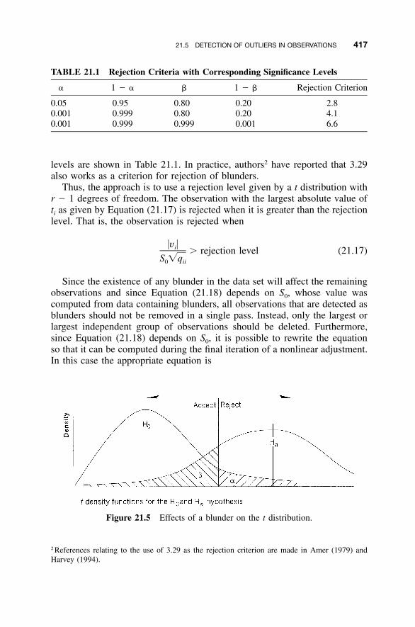
21.5 DETECTION OF OUTLIERS IN OBSERVATIONS 417
TABLE 21.1 Rejection Criteria with Corresponding Significance Levels
� 1 � � � 1 � � Rejection Criterion
0.05 0.95 0.80 0.20 2.80.001 0.999 0.80 0.20 4.10.001 0.999 0.999 0.001 6.6
Figure 21.5 Effects of a blunder on the t distribution.
levels are shown in Table 21.1. In practice, authors2 have reported that 3.29also works as a criterion for rejection of blunders.
Thus, the approach is to use a rejection level given by a t distribution withr � 1 degrees of freedom. The observation with the largest absolute value ofti as given by Equation (21.17) is rejected when it is greater than the rejectionlevel. That is, the observation is rejected when
�v �i � rejection level (21.17)S �q0 ii
Since the existence of any blunder in the data set will affect the remainingobservations and since Equation (21.18) depends on S0, whose value wascomputed from data containing blunders, all observations that are detected asblunders should not be removed in a single pass. Instead, only the largest orlargest independent group of observations should be deleted. Furthermore,since Equation (21.18) depends on S0, it is possible to rewrite the equationso that it can be computed during the final iteration of a nonlinear adjustment.In this case the appropriate equation is
2 References relating to the use of 3.29 as the rejection criterion are made in Amer (1979) andHarvey (1994).
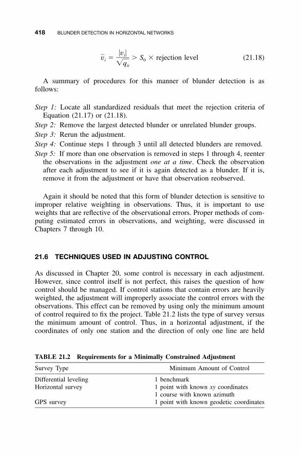
418 BLUNDER DETECTION IN HORIZONTAL NETWORKS
TABLE 21.2 Requirements for a Minimally Constrained Adjustment
Survey Type Minimum Amount of Control
Differential leveling 1 benchmarkHorizontal survey 1 point with known xy coordinates
1 course with known azimuthGPS survey 1 point with known geodetic coordinates
�v �iv � � S � rejection level (21.18)i 0�qii
A summary of procedures for this manner of blunder detection is asfollows:
Step 1: Locate all standardized residuals that meet the rejection criteria ofEquation (21.17) or (21.18).
Step 2: Remove the largest detected blunder or unrelated blunder groups.Step 3: Rerun the adjustment.Step 4: Continue steps 1 through 3 until all detected blunders are removed.Step 5: If more than one observation is removed in steps 1 through 4, reenter
the observations in the adjustment one at a time. Check the observationafter each adjustment to see if it is again detected as a blunder. If it is,remove it from the adjustment or have that observation reobserved.
Again it should be noted that this form of blunder detection is sensitive toimproper relative weighting in observations. Thus, it is important to useweights that are reflective of the observational errors. Proper methods of com-puting estimated errors in observations, and weighting, were discussed inChapters 7 through 10.
21.6 TECHNIQUES USED IN ADJUSTING CONTROL
As discussed in Chapter 20, some control is necessary in each adjustment.However, since control itself is not perfect, this raises the question of howcontrol should be managed. If control stations that contain errors are heavilyweighted, the adjustment will improperly associate the control errors with theobservations. This effect can be removed by using only the minimum amountof control required to fix the project. Table 21.2 lists the type of survey versusthe minimum amount of control. Thus, in a horizontal adjustment, if thecoordinates of only one station and the direction of only one line are held
21.6 TECHNIQUES USED IN ADJUSTING CONTROL 419
fixed, the observations will not be constricted by the control. That is, theobservations will need to satisfy the internal geometric constraints of thenetwork only. If more than minimum control is used, these additional con-straints will be factored into the adjustment.
Statistical blunder detection can help identify weak control or the presenceof systematic errors in observations. Using a minimally constrained adjust-ment, the data set is screened for blunders. After becoming confident that theblunders are removed from the data set, a fully constrained adjustment isperformed. Following the fully constrained adjustment, an F test is used tocompare the ratio of the minimally and fully constrained reference variances.The ratio should be 1.3 If the two reference variances are found to be statis-tically different, two possible causes might exist. The first is that there areerrors in the control that must be isolated and removed. The second is thatthe observations contain systematic error. Since systematic errors are not com-pensating in nature, they will appear as blunders in the fully constrainedadjustment. If systematic errors are suspected, they should be identified andremoved from the original data set and the entire adjustment procedure re-done. If no systematic errors are identified,4 different combinations of controlstations should be used in the constrained adjustments until the problem isisolated. By following this type of systematic approach, a single control sta-tion that has questionable coordinates can be isolated.
With this stated, it should be realized that the ideal amount of control ineach survey type is greater than the minimum. In fact, for all three surveytypes, a minimum of three controls is always preferable. For example, in adifferential leveling survey with only two benchmarks, it would be impossibleto isolate the problem simply by removing one benchmark from the adjust-ment. However, if three benchmarks are used, a separate adjustment contain-ing only two of the benchmarks can be run until the offending benchmark isisolated.
Extreme caution should always be used when dealing with control stations.Although it is possible that a control station was disturbed or that the originalpublished coordinates contained errors, that is seldom the case. A prudentsurveyor should check for physical evidence of disturbance and talk withother surveyors before deciding to discard control. If the station was set bya local, state, or federal agency, the surveyor should contact the proper
3 The ratio of the reference variances from the minimally and fully constrained adjustments shouldbe 1, since both reference variances should be statistically equal. That is, �2�minimally constrained
2� .fully constrained4 When adjusting data that cover a large region (e.g., spherical excess, reduction to the ellipsoid)it is essential that geodetic corrections to the data be considered and applied where necessary.These corrections are systematic in nature and can cause errors when fitting to more than minimalcontrol.
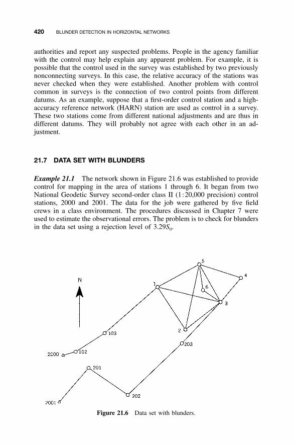
420 BLUNDER DETECTION IN HORIZONTAL NETWORKS
Figure 21.6 Data set with blunders.
authorities and report any suspected problems. People in the agency familiarwith the control may help explain any apparent problem. For example, it ispossible that the control used in the survey was established by two previouslynonconnecting surveys. In this case, the relative accuracy of the stations wasnever checked when they were established. Another problem with controlcommon in surveys is the connection of two control points from differentdatums. As an example, suppose that a first-order control station and a high-accuracy reference network (HARN) station are used as control in a survey.These two stations come from different national adjustments and are thus indifferent datums. They will probably not agree with each other in an ad-justment.
21.7 DATA SET WITH BLUNDERS
Example 21.1 The network shown in Figure 21.6 was established to providecontrol for mapping in the area of stations 1 through 6. It began from twoNational Geodetic Survey second-order class II (1�20,000 precision) controlstations, 2000 and 2001. The data for the job were gathered by five fieldcrews in a class environment. The procedures discussed in Chapter 7 wereused to estimate the observational errors. The problem is to check for blundersin the data set using a rejection level of 3.29S0.
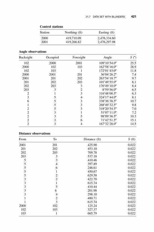
21.7 DATA SET WITH BLUNDERS 421
Control stations
Station Northing (ft) Easting (ft)
2000 419,710.09 2,476,334.602001 419,266.82 2,476,297.98
Angle observations
Backsight Occupied Foresight Angle S (�)
102 2000 2001 109�10�54.0� 25.52000 102 103 162�58�16.0� 28.9
102 103 1 172�01�43.0� 11.82000 2001 201 36�04�26.2� 7.42001 201 202 263�54�18.7� 9.7201 202 203 101�49�55.0� 8.1202 203 3 176�49�10.0� 8.4203 3 2 8�59�56.0� 6.5
2 1 3 316�48�00.5� 6.33 5 4 324�17�44.0� 8.16 5 3 338�36�38.5� 10.71 5 3 268�49�32.5� 9.82 5 3 318�20�54.5� 7.02 3 1 51�07�11.0� 7.22 3 5 98�09�36.5� 10.32 3 6 71�42�51.5� 15.12 3 4 167�32�28.0� 14.5
Distance observations
From To Distance (ft) S (ft)
2001 201 425.90 0.022201 202 453.10 0.022202 203 709.78 0.022203 3 537.18 0.022
5 3 410.46 0.0225 4 397.89 0.0225 6 246.61 0.0225 1 450.67 0.0225 2 629.58 0.0223 2 422.70 0.0223 1 615.74 0.0223 5 410.44 0.0223 6 201.98 0.0223 4 298.10 0.0221 2 480.71 0.0221 3 615.74 0.022
2000 102 125.24 0.022102 103 327.37 0.022103 1 665.79 0.022

422 BLUNDER DETECTION IN HORIZONTAL NETWORKS
Initial approximations were computed for the stations as follows:
Station Northing (ft) Easting (ft)
1 420,353.62 2,477,233.882 419,951.98 2,477,497.993 420,210.17 2,477,832.674 420,438.88 2,478,023.865 420,567.44 2,477,630.646 420,323.31 2,477,665.36
102 419,743.39 2,476,454.17103 419,919.69 2,476,728.88201 419,589.24 2,476,576.25202 419,331.29 2,476,948.76203 419,819.56 2,477,463.90
SOLUTION Do the a priori check of the computed observations versus theirK-matrix values. In this check, only one angle is detected as having a differ-ence great enough to suspect that it contains a blunder. This is angle 3–5–4,which was measured as 324�17�44.0� but was computed as 317�35�31.2�.Since this difference should not create a problem with convergence duringthe adjustment, the angle remained in the data set and the adjustment wasattempted. The results of the first trial adjustment are shown below. The soft-ware used the rejection criteria procedure based on Equation (21.18) for itsblunder detection. A rejection level of 3.29S0 is used for comparison againstthe standardized residuals. The column headed Std. Res. represents the stan-dardized residual of the observation as defined by Equation (21.15) and thecolumn headed Red. Num. represents the redundancy number of the obser-vation as defined by Equation (21.14).
**** Adjusted Distance Observations ****
No. � From � To � Distance � Residual � Std. Res. � Red. Num. �����������������������������������������
1� 1 � 3 � 616.234 � 0.494 � 26.148 � 0.7458 �2� 1 � 2 � 480.943 � 0.233 � 12.926 � 0.6871 �3� 1 � 3 � 616.234 � 0.494 � 26.148 � 0.7458 �4� 3 � 4 � 267.044 � �31.056 � �1821.579 � 0.6169 �5� 3 � 6 � 203.746 � 1.766 � 107.428 � 0.5748 �6� 3 � 5 � 413.726 � 3.286 � 171.934 � 0.7719 �7� 3 � 2 � 422.765 � 0.065 � 3.500 � 0.7312 �8� 5 � 2 � 630.949 � 1.369 � 75.909 � 0.6791 �9� 5 � 1 � 449.398 � �1.272 � �79.651 � 0.5377 �10� 5 � 6 � 247.822 � 1.212 � 75.418 � 0.5488 �11� 5 � 4 � 407.125 � 9.235 � 631.032 � 0.4529 �
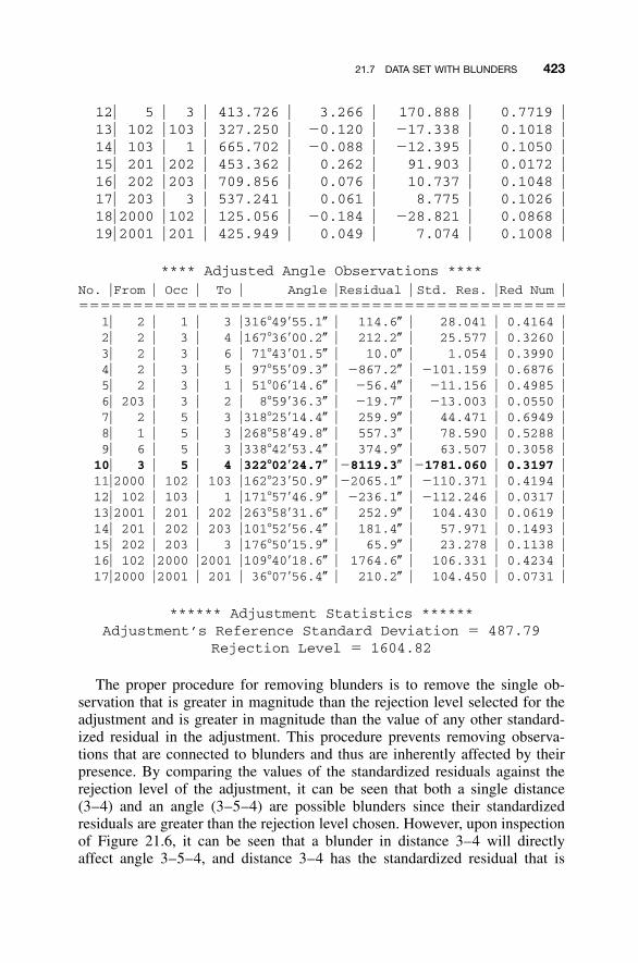
21.7 DATA SET WITH BLUNDERS 423
12� 5 � 3 � 413.726 � 3.266 � 170.888 � 0.7719 �13� 102 � 103 � 327.250 � �0.120 � �17.338 � 0.1018 �14� 103 � 1 � 665.702 � �0.088 � �12.395 � 0.1050 �15� 201 � 202 � 453.362 � 0.262 � 91.903 � 0.0172 �16� 202 � 203 � 709.856 � 0.076 � 10.737 � 0.1048 �17� 203 � 3 � 537.241 � 0.061 � 8.775 � 0.1026 �18� 2000 � 102 � 125.056 � �0.184 � �28.821 � 0.0868 �19� 2001 � 201 � 425.949 � 0.049 � 7.074 � 0.1008 �
**** Adjusted Angle Observations ****No. �From � Occ � To � Angle �Residual � Std. Res. �Red Num ����������������������������������������������
1� 2 � 1 � 3 �316�49�55.1� � 114.6� � 28.041 � 0.4164 �2� 2 � 3 � 4 �167�36�00.2� � 212.2� � 25.577 � 0.3260 �3� 2 � 3 � 6 � 71�43�01.5� � 10.0� � 1.054 � 0.3990 �4� 2 � 3 � 5 � 97�55�09.3� � �867.2� � �101.159 � 0.6876 �5� 2 � 3 � 1 � 51�06�14.6� � �56.4� � �11.156 � 0.4985 �6� 203 � 3 � 2 � 8�59�36.3� � �19.7� � �13.003 � 0.0550 �7� 2 � 5 � 3 �318�25�14.4� � 259.9� � 44.471 � 0.6949 �8� 1 � 5 � 3 �268�58�49.8� � 557.3� � 78.590 � 0.5288 �9� 6 � 5 � 3 �338�42�53.4� � 374.9� � 63.507 � 0.3058 �10� 3 � 5 � 4 �322�02�24.7� � �8119.3� ��1781.060 � 0.3197 �11�2000 � 102 � 103 �162�23�50.9� � �2065.1� � �110.371 � 0.4194 �12� 102 � 103 � 1 �171�57�46.9� � �236.1� � �112.246 � 0.0317 �13�2001 � 201 � 202 �263�58�31.6� � 252.9� � 104.430 � 0.0619 �14� 201 � 202 � 203 �101�52�56.4� � 181.4� � 57.971 � 0.1493 �15� 202 � 203 � 3 �176�50�15.9� � 65.9� � 23.278 � 0.1138 �16� 102 �2000 �2001 �109�40�18.6� � 1764.6� � 106.331 � 0.4234 �17�2000 �2001 � 201 � 36�07�56.4� � 210.2� � 104.450 � 0.0731 �
****** Adjustment Statistics ******Adjustment’s Reference Standard Deviation � 487.79
Rejection Level � 1604.82
The proper procedure for removing blunders is to remove the single ob-servation that is greater in magnitude than the rejection level selected for theadjustment and is greater in magnitude than the value of any other standard-ized residual in the adjustment. This procedure prevents removing observa-tions that are connected to blunders and thus are inherently affected by theirpresence. By comparing the values of the standardized residuals against therejection level of the adjustment, it can be seen that both a single distance(3–4) and an angle (3–5–4) are possible blunders since their standardizedresiduals are greater than the rejection level chosen. However, upon inspectionof Figure 21.6, it can be seen that a blunder in distance 3–4 will directlyaffect angle 3–5–4, and distance 3–4 has the standardized residual that is
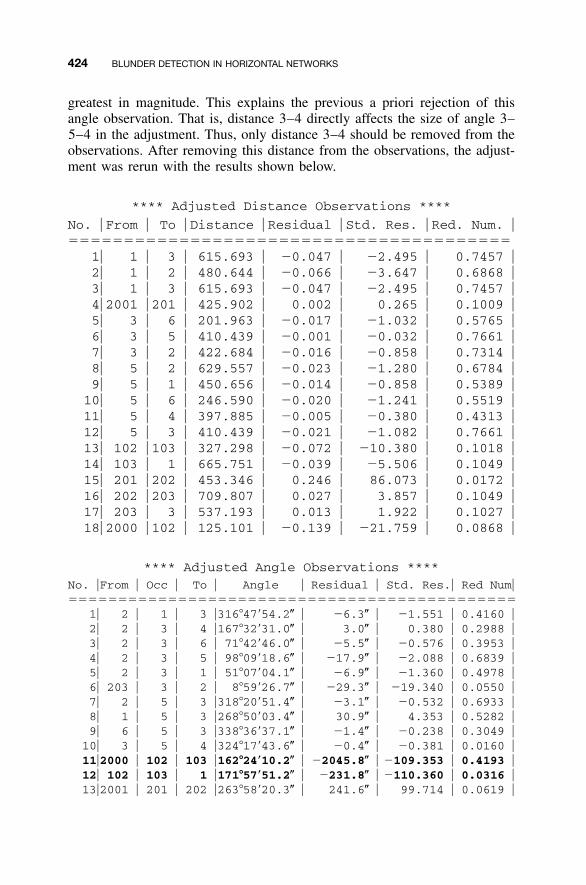
424 BLUNDER DETECTION IN HORIZONTAL NETWORKS
greatest in magnitude. This explains the previous a priori rejection of thisangle observation. That is, distance 3–4 directly affects the size of angle 3–5–4 in the adjustment. Thus, only distance 3–4 should be removed from theobservations. After removing this distance from the observations, the adjust-ment was rerun with the results shown below.
**** Adjusted Distance Observations ****
No. � From � To � Distance � Residual � Std. Res. � Red. Num. �����������������������������������������
1� 1 � 3 � 615.693 � �0.047 � �2.495 � 0.7457 �2� 1 � 2 � 480.644 � �0.066 � �3.647 � 0.6868 �3� 1 � 3 � 615.693 � �0.047 � �2.495 � 0.7457 �4� 2001 � 201 � 425.902 � 0.002 � 0.265 � 0.1009 �5� 3 � 6 � 201.963 � �0.017 � �1.032 � 0.5765 �6� 3 � 5 � 410.439 � �0.001 � �0.032 � 0.7661 �7� 3 � 2 � 422.684 � �0.016 � �0.858 � 0.7314 �8� 5 � 2 � 629.557 � �0.023 � �1.280 � 0.6784 �9� 5 � 1 � 450.656 � �0.014 � �0.858 � 0.5389 �10� 5 � 6 � 246.590 � �0.020 � �1.241 � 0.5519 �11� 5 � 4 � 397.885 � �0.005 � �0.380 � 0.4313 �12� 5 � 3 � 410.439 � �0.021 � �1.082 � 0.7661 �13� 102 � 103 � 327.298 � �0.072 � �10.380 � 0.1018 �14� 103 � 1 � 665.751 � �0.039 � �5.506 � 0.1049 �15� 201 � 202 � 453.346 � 0.246 � 86.073 � 0.0172 �16� 202 � 203 � 709.807 � 0.027 � 3.857 � 0.1049 �17� 203 � 3 � 537.193 � 0.013 � 1.922 � 0.1027 �18� 2000 � 102 � 125.101 � �0.139 � �21.759 � 0.0868 �
**** Adjusted Angle Observations ****No. �From � Occ � To � Angle � Residual � Std. Res.� Red Num����������������������������������������������
1� 2 � 1 � 3 �316�47�54.2� � �6.3� � �1.551 � 0.4160 �2� 2 � 3 � 4 �167�32�31.0� � 3.0� � 0.380 � 0.2988 �3� 2 � 3 � 6 � 71�42�46.0� � �5.5� � �0.576 � 0.3953 �4� 2 � 3 � 5 � 98�09�18.6� � �17.9� � �2.088 � 0.6839 �5� 2 � 3 � 1 � 51�07�04.1� � �6.9� � �1.360 � 0.4978 �6� 203 � 3 � 2 � 8�59�26.7� � �29.3� � �19.340 � 0.0550 �7� 2 � 5 � 3 �318�20�51.4� � �3.1� � �0.532 � 0.6933 �8� 1 � 5 � 3 �268�50�03.4� � 30.9� � 4.353 � 0.5282 �9� 6 � 5 � 3 �338�36�37.1� � �1.4� � �0.238 � 0.3049 �10� 3 � 5 � 4 �324�17�43.6� � �0.4� � �0.381 � 0.0160 �11�2000 � 102 � 103 �162�24�10.2� � �2045.8� � �109.353 � 0.4193 �12� 102 � 103 � 1 �171�57�51.2� � �231.8� � �110.360 � 0.0316 �13�2001 � 201 � 202 �263�58�20.3� � 241.6� � 99.714 � 0.0619 �
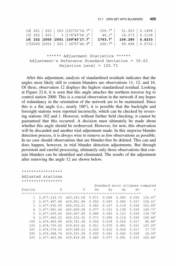
21.7 DATA SET WITH BLUNDERS 425
14� 201 � 202 � 203 �101�52�34.7� � 159.7� � 51.023 � 0.1494 �15� 202 � 203 � 3 �176�49�56.1� � 46.1� � 16.273 � 0.1138 �16� 102 �2000 �2001 �109�40�17.7� � 1763.7� � 106.280 � 0.4233 �17�2000 �2001 � 201 � 36�07�46.9� � 200.7� � 99.688 � 0.0732 �
****** Adjustment Statistics ******Adjustment’s Reference Standard Deviation � 30.62
Rejection Level � 100.73
After this adjustment, analysis of standardized residuals indicates that theangles most likely still to contain blunders are observations 11, 12, and 16.Of these, observation 12 displays the highest standardized residual. Lookingat Figure 21.6, it is seen that this angle attaches the northern traverse leg tocontrol station 2000. This is a crucial observation in the network if any hopesof redundancy in the orientation of the network are to be maintained. Sincethis is a flat angle (i.e., nearly 180�), it is possible that the backsight andforesight stations were reported incorrectly, which can be checked by revers-ing stations 102 and 1. However, without further field checking, it cannot beguaranteed that this occurred. A decision must ultimately be made aboutwhether this angle should be reobserved. However, for now, this observationwill be discarded and another trial adjustment made. In this stepwise blunderdetection process, it is always wise to remove as few observations as possible.In no case should observations that are blunder-free be deleted. This can anddoes happen, however, in trial blunder detection adjustments. But throughpersistent and careful processing, ultimately only those observations that con-tain blunders can be identified and eliminated. The results of the adjustmentafter removing the angle 12 are shown below.
*****************Adjusted stations*****************
Standard error ellipses computedStation X Y Sx Sy Su Sv t���������������������������������������������
1 2,477,233.72 420,353.59 0.071 0.069 0.092 0.036 133.47�
2 2,477,497.89 419,951.98 0.050 0.083 0.090 0.037 156.01�
3 2,477,832.55 420,210.21 0.062 0.107 0.119 0.034 152.80�
4 2,477,991.64 420,400.58 0.077 0.121 0.138 0.039 149.71�
5 2,477,630.43 420,567.45 0.088 0.093 0.123 0.036 136.74�
6 2,477,665.22 420,323.32 0.071 0.096 0.114 0.036 145.44�
102 2,476,455.89 419,741.38 0.024 0.018 0.024 0.017 80.86�
103 2,476,735.05 419,912.42 0.051 0.070 0.081 0.031 147.25�
201 2,476,576.23 419,589.23 0.020 0.022 0.024 0.017 37.73�
202 2,476,948.74 419,331.29 0.029 0.041 0.042 0.029 14.24�
203 2,477,463.84 419,819.58 0.040 0.077 0.081 0.032 160.84�
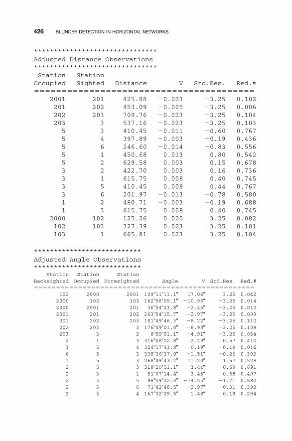
426 BLUNDER DETECTION IN HORIZONTAL NETWORKS
*******************************Adjusted Distance Observations*******************************StationOccupied
StationSighted Distance V Std.Res. Red.#
����������������������������������������2001 201 425.88 �0.023 �3.25 0.102201 202 453.09 �0.005 �3.25 0.006202 203 709.76 �0.023 �3.25 0.104203 3 537.16 �0.023 �3.25 0.1035 3 410.45 �0.011 �0.60 0.7675 4 397.89 �0.003 �0.19 0.4365 6 246.60 �0.014 �0.83 0.5565 1 450.68 0.013 0.80 0.5425 2 629.58 0.003 0.15 0.6783 2 422.70 0.003 0.16 0.7363 1 615.75 0.008 0.40 0.7453 5 410.45 0.009 0.44 0.7673 6 201.97 �0.013 �0.78 0.5801 2 480.71 �0.003 �0.19 0.6881 3 615.75 0.008 0.40 0.745
2000 102 125.26 0.020 3.25 0.082102 103 327.39 0.023 3.25 0.101103 1 665.81 0.023 3.25 0.104
***************************Adjusted Angle Observations***************************
StationBacksighted
StationOccupied
StationForesighted Angle V Std.Res. Red.#
��������������������������������������������������102 2000 2001 109�11�11.1� 17.06� 3.25 0.0422000 102 103 162�58�05.1� �10.95� �3.25 0.0142000 2001 201 36�04�23.8� �2.45� �3.25 0.0102001 201 202 263�54�15.7� �2.97� �3.25 0.009201 202 203 101�49�46.3� �8.72� �3.25 0.110202 203 3 176�49�01.0� �8.98� �3.25 0.109203 3 2 8�59�51.1� �4.91� �3.25 0.054
2 1 3 316�48�02.8� 2.29� 0.57 0.4103 5 4 324�17�43.8� �0.19� �0.19 0.0166 5 3 338�36�37.0� �1.51� �0.26 0.3021 5 3 268�49�43.7� 11.20� 1.57 0.5282 5 3 318�20�51.1� �3.44� �0.59 0.6912 3 1 51�07�14.4� 3.45� 0.68 0.4972 3 5 98�09�22.0� �14.55� �1.71 0.6802 3 6 71�42�48.5� �2.97� �0.31 0.3922 3 4 167�32�29.5� 1.48� 0.19 0.294
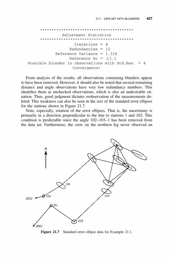
21.7 DATA SET WITH BLUNDERS 427
Figure 21.7 Standard error ellipse data for Example 21.1.
****************************************Adjustment Statistics
****************************************Iterations � 4
Redundancies � 12Reference Variance � 1.316
Reference So � �1.1Possible blunder in observations with Std.Res. � 4
Convergence!
From analysis of the results, all observations containing blunders appearto have been removed. However, it should also be noted that several remainingdistance and angle observations have very low redundancy numbers. Thisidentifies them as unchecked observations, which is also an undesirable sit-uation. Thus, good judgment dictates reobservation of the measurements de-leted. This weakness can also be seen in the size of the standard error ellipsesfor the stations shown in Figure 21.7.
Note, especially, rotation of the error ellipses. That is, the uncertainty isprimarily in a direction perpendicular to the line to stations 1 and 102. Thiscondition is predictable since the angle 102–103–1 has been removed fromthe data set. Furthermore, the crew on the northern leg never observed an
428 BLUNDER DETECTION IN HORIZONTAL NETWORKS
angle at station 1 that would tie into station 103, and thus the position ofstation 103 was found by the intersection of two distances that nearly forma straight line. This results in a larger error in the direction perpendicular tothe lines at this station.
This example demonstrates the process used to statistically detect and re-move observational blunders. Whether the observations should be remeasureddepends on the intended use of the survey. Obviously, additional observationswould strengthen the network and probably reduce the size of the errorellipses.
Observations between stations 102 and 201 also contribute to the overallstrength in the network. However, because a building obstructs that line, theseobservations could not be obtained. This is a common problem in networkdesign. That is, it is sometimes physically impossible to gather observationsthat would contribute to the total network strength. Thus, a compromise mustbe made between the ideal network and what is physically obtainable. Bal-ancing these aspects requires careful planning before the observations arecollected. Of course, line obstructions that occur due to terrain, vegetation,or buildings, can now be overcome by using GPS.
21.8 SOME FURTHER CONSIDERATIONS
Equation (21.14) shows the relationship between blunders and their effectson residuals as �vi � �ri �li. From this relationship note that the effect ofthe blunder, �li, on the residual, �vi, is directly proportional to the redundancynumber, ri. Therefore:
1. If ri is large (� 1), the blunder greatly affects the residual and shouldbe easy to find.
2. If ri is small (� 0), the blunder has little affect on the residual and willbe difficult to find.
3. If ri � 0, the blunder is undetectable and the parameters will be incorrectsince the error has not been detected.
Since redundancy numbers can range from 0 to 1, it is possible to computethe minimum detectable error for a single blunder. For example, suppose thata value of 4.0 is used to isolate observational blunders. Then, if the referencevariance of the adjustment is 6, all observations that have standardized resid-uals greater than 24.0 (4.0 � 6) are possible blunders. However, from Equa-tion (21.14), it can be seen that for an observation with a redundancy numberof 0.2 (ri � 0.2) and a standardized residual of �vi � 24.0, the minimumdetectable error is 24.0/0.2, or 120! Thus, a blunder, �li, in this observationas large as five times the desired level can go undetected due to its low
21.8 SOME FURTHER CONSIDERATIONS 429
redundancy number. This situation can be extended to observations that haveno observational checks; that is, ri is 0. In this case, Equation (21.14) showsthat it is impossible to detect any blunder, �li, in the observation since �vi /�ri is indeterminate.
With this taken into consideration, it has been shown that a marginallydetectable blunder in an individual observation is
�0�l � S (21.19)i 2�q wii ii
where �0 is the mean of the noncentral normal distribution shown in Figure21.5, known as the noncentrality parameter. This parameter is the translationof the normal distribution that leads to rejection of the null hypothesis, whosevalues can be taken from nomograms developed by Baarda (1968). The sizesof the values obtained from Equation (21.19) provide a clear insight into weakareas of the network.
21.8.1 Internal Reliability
Internal reliability is found by examining how well observations check geo-metrically with each other. As mentioned previously, if a station is determineduniquely, qii will be zero in Equation (21.19), and the computed value of �li
is infinity. This indicates the lack of measurement self-checking. Since Equa-tion (21.19) is independent of the actual observations, it provides a methodof detecting weak areas in networks. To minimize the sizes of the undetectedblunders in a network, the redundancy numbers of the individual observationsshould approach their maximum value of 1. Furthermore, for uniform networkstrength, the individual redundancy numbers, ri, should be close to the globalrelative redundancy of r /m, where r is the number of redundant observationsand m is the number of observations in the network. Weak areas in the net-work are located by finding regions where the redundancy numbers becomesmall in comparison to relative redundancy.
21.8.2 External Reliability
An undetected blunder of size �li has a direct effect on the adjusted param-eters. External reliability is the effect of the undetected blunders on theseparameters. As �li (a blunder) increases, so will its effect on �X. The valueof �X is given by
T �1 T�X � (A WA) A W �ε (21.20)
Again, this equation is datum independent. From Equation (21.20) it canbe seen that to minimize the value of �Xi, the size of redundancy numbers
430 BLUNDER DETECTION IN HORIZONTAL NETWORKS
must be increased. Baarda suggested using average coordinate values in de-termining the effect of an undetected blunder with the following equation
T� � �X Q �X (21.21)xx
where � represents the noncentrality parameter.The noncentrality parameter should remain as small as possible to mini-
mize the effects of undetected blunders on the coordinates. Note that as theredundancy numbers on the observations become small, the effects of unde-tected blunders become large. Thus, the effect of the coordinates of a stationfrom a undetected blunder is greater when the redundancy number is low. Infact, an observation with a high redundancy number is likely to be detectedas a blunder.
A traverse sideshot can be used to explain this phenomenon. Since theangle and distance to the station are unchecked in a sideshot, the coordinatesof the station will change according to the size of the observational blunders.The observations creating the sideshot will have redundancy numbers of zerosince they are geometrically unchecked. This situation is neither good noracceptable in a well-designed observational system. In network design, oneshould always check the redundancy numbers of the anticipated observationsand strive to achieve uniformly high values for all observations. Redundancynumbers above 0.5 are generally sufficient to provide well-checked obser-vations.
21.9 SURVEY DESIGN
In Chapters 8 and 19, the topic of observational system design was discussed.Redundancy numbers can now be added to this discussion. A well-designednetwork will provide sufficient geometric checks to allow observational blun-ders to be detected and removed. In Section 21.8.1 it was stated that if blunderremoval is to occur uniformly throughout the system, the redundancy numbersshould be close to the system’s global relative redundancy. Furthermore, inSection 21.8.2 it was noted that redundancy numbers should be greater than0.5. By combining these two additional concepts with the error ellipse sizesand shapes, and stochastic model planning, an overall methodology for de-signing observational systems can be obtained.
To begin the design process, the approximate positions for stations to beincluded in the survey must be determined. These locations can be determinedfrom topographic maps, photo measurements, or previous survey data. Theapproximate locations of the control stations should be dictated by their de-sired locations, the surrounding terrain, vegetation, soils, sight-line obstruc-tions, and so on. Field reconnaissance at this phase of the design process isgenerally worthwhile to verify sight lines and accessibility of stations. Moving
21.9 SURVEY DESIGN 431
a station only a small distance from the original design location may greatlyenhance visibility to and from other stations but not change the geometry ofthe network significantly. By using topographic maps in this process, sight-line ground clearances can be checked by constructing profiles betweenstations.
When approximate station coordinates are determined, a stochastic modelfor the observational system can be designed following the procedures dis-cussed in Chapter 7. In this design process, considerations should be givento the abilities of the field personnel, quality of the equipment, and observa-tional procedures. After the design is completed, specifications for field crewscan be written based on these design parameters. These specifications shouldinclude the type of instrument used, number of turnings for angle observa-tions, accuracy of instrument leveling and centering, misclosure requirements,and many other items.
Once the stochastic model is designed, simulated observations are com-puted from the station coordinates, and a least squares adjustment of theobservations is to be done. Since actual observations have not been made,their values are computed from the station coordinates. The adjustment willconverge in a single iteration, with all residuals equaling zero. Thus, thereference variance must be assigned the a priori value of 1 to compute theerror ellipse axes and coordinate standard deviations. Having completed theadjustment, the network can be checked for geometrically weak areas, un-acceptable error ellipse sizes or shapes, and so on. This inspection may dictatethe need for any or all of the following: (1) more observations, (2) differentobservational procedures, (3) different equipment, (4) more stations, (5) dif-ferent network geometry, and so on. In any event, a clear picture of resultsobtainable from the observational system will be provided by the simulatedadjustment and additional observations, or different network geometry can beused.
It should be noted that what is expected from the design may not actuallyoccur, for numerous and varied reasons. Thus, systems are generally over-designed. However, this tendency to overdesign should be tempered with theknowledge that it will raise the costs of the survey. Thus, a balance shouldbe found between the design and costs. Experienced surveyors know whatlevel of accuracy is necessary for each job and design observational systemsto achieve the accuracy desired. It would be cost prohibitive and foolish al-ways to design an observational system for maximum accuracy regardless ofthe survey’s intended use. As an example, the final adjustment of the surveyin Section 21.7 had sufficient accuracy to be used in a mapping project witha final scale of 1�1200 since the largest error ellipse semimajor axis (0.138ft) would only plot as 0.0014 in. and is thus less than the width of a line onthe final map product.
For convenience, the steps involved in network design are summarizedbelow.
432 BLUNDER DETECTION IN HORIZONTAL NETWORKS
Step 1: Using a topographic map or aerial photos, lay out possible positionsfor stations.
Step 2: Use the topographic map together with air photos to check sight linesfor possible obstructions and ground clearance.
Step 3: Do field reconnaissance, checking sight lines for obstructions notshown on the map or photos, and adjust positions of stations as necessary.
Step 4: Determine approximate coordinates for the stations from the map orphotos.
Step 5: Compute values of observations using the coordinates from step 4.Step 6: Using methods discussed in Chapter 6, compute the standard devia-
tion of each observation based on available equipment and field measuringprocedures.
Step 7: Perform a least squares adjustment, to compute observational redun-dancy numbers, standard deviations of station coordinates, and error ellip-ses at a specified percent probability.
Step 8: Inspect the solution for weak areas based on redundancy numbersand ellipse shapes. Add or remove observations as necessary, or reevaluatemeasurement procedures and equipment.
Step 9: Evaluate the costs of the survey, and determine if some other methodof measurement (e.g., GPS) may be more cost-effective.
Step 10: Write specifications for field crews.
PROBLEMS
Note: For problems requiring least squares adjustment, if a computer programis not distinctly specified for use in the problem, it is expected that the leastsquares algorithm will be solved using the program MATRIX, which is in-cluded on the CD supplied with the book.
21.1 Discuss the effects of a distance blunder on a traverse closure andexplain how it can be identified.
21.2 Discuss the effects of an angle blunder on a traverse closure, andexplain how it can be identified.
21.3 Explain why a well-designed network has observational redundancynumbers above 0.5 and approximately equal.
21.4 Create a list of items that should be included in field specificationsfor a crew in a designed network.
21.5 Summarize the general procedures used in isolating observationalblunders.
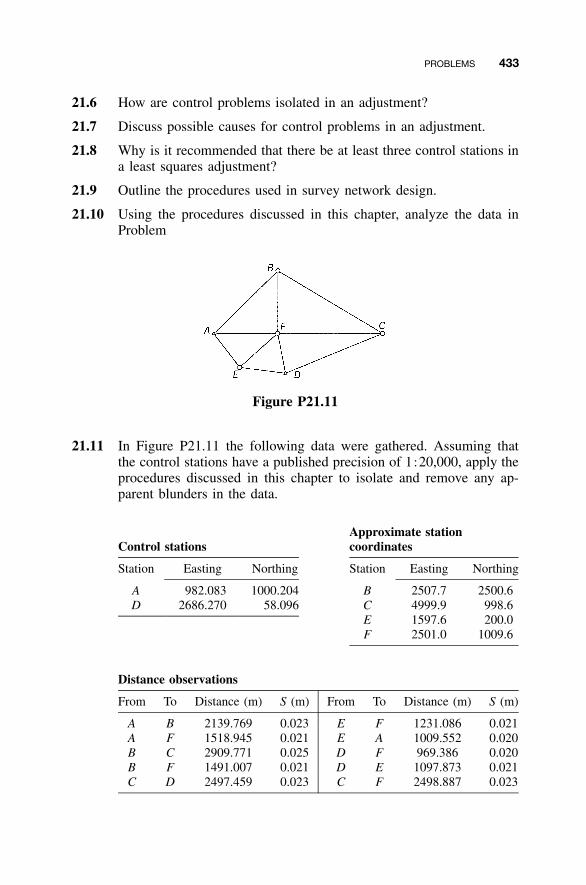
PROBLEMS 433
21.6 How are control problems isolated in an adjustment?
21.7 Discuss possible causes for control problems in an adjustment.
21.8 Why is it recommended that there be at least three control stations ina least squares adjustment?
21.9 Outline the procedures used in survey network design.
21.10 Using the procedures discussed in this chapter, analyze the data inProblem
Figure P21.11
21.11 In Figure P21.11 the following data were gathered. Assuming thatthe control stations have a published precision of 1�20,000, apply theprocedures discussed in this chapter to isolate and remove any ap-parent blunders in the data.
Control stationsApproximate stationcoordinates
Station Easting Northing Station Easting Northing
A 982.083 1000.204 B 2507.7 2500.6D 2686.270 58.096 C
E4999.91597.6
998.6200.0
F 2501.0 1009.6
Distance observations
From To Distance (m) S (m) From To Distance (m) S (m)
A B 2139.769 0.023 E F 1231.086 0.021A F 1518.945 0.021 E A 1009.552 0.020B C 2909.771 0.025 D F 969.386 0.020B F 1491.007 0.021 D E 1097.873 0.021C D 2497.459 0.023 C F 2498.887 0.023
434 BLUNDER DETECTION IN HORIZONTAL NETWORKS
Angle observations
Backsight Occupied Foresight Angle S (�)
F A E 52�47�12.3� 3.4B A F 44�10�04.6� 2.8F B A 45�13�12.5� 2.8C B F 59�10�54.5� 2.7F C B 27�30�00.0� 2.4D C F 22�22�28.2� 2.5F D C 78�53�43.8� 3.3E D F 71�33�18.7� 3.8A E F 85�42�04.9� 3.7F E D 49�17�32.8� 3.4A F B 90�36�40.5� 3.1B F C 89�59�37.6� 2.8C F D 78�43�47.8� 3.3D F E 59�09�10.5� 3.6E F A 41�30�43.3� 3.1
21.12 Apply to procedures discussed in this chapter to isolate any blundersin the following data.
Control stations Approximate coordinates
Station X (ft) Y (ft) Station X (ft) Y (ft)
A 44,680.85 78,314.23 B 21,112.93 151,309.33H 169,721.77 214,157.12 C
D49,263.50
107,855.97213,175.12145,744.68
E 113,747.95 78,968.90F 186,743.04 78,314.24G 206,710.31 138,216.04
Distance observations
Course Distance (ft) S (ft) Course Distance (ft) S (ft)
AB 76,705.18 0.23 BC 67,969.04 0.20CD 89,330.51 0.27 DE 67,035.17 0.20EF 72,998.23 0.22 FG 63,141.95 0.19GH 84,470.07 0.25 CH 120,461.89 0.36AE 69,070.47 0.21 AD 92,401.26 0.28DH 92,236.72 0.28 BD 86,921.33 0.26DG 99,140.58 0.30 DF 103,778.98 0.31
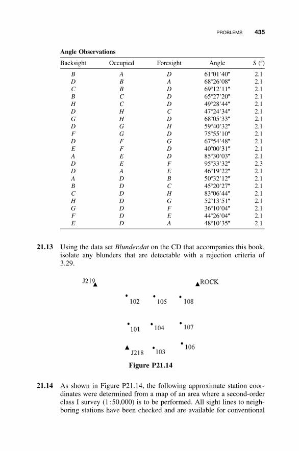
PROBLEMS 435
Angle Observations
Backsight Occupied Foresight Angle S (�)
B A D 61�01�40� 2.1D B A 68�26�08� 2.1C B D 69�12�11� 2.1B C D 65�27�20� 2.1H C D 49�28�44� 2.1D H C 47�24�34� 2.1G H D 68�05�33� 2.1D G H 59�40�32� 2.1F G D 75�55�10� 2.1D F G 67�54�48� 2.1E F D 40�00�31� 2.1A E D 85�30�03� 2.1D E F 95�33�32� 2.3D A E 46�19�22� 2.1A D B 50�32�12� 2.1B D C 45�20�27� 2.1C D H 83�06�44� 2.1H D G 52�13�51� 2.1G D F 36�10�04� 2.1F D E 44�26�04� 2.1E D A 48�10�35� 2.1
21.13 Using the data set Blunder.dat on the CD that accompanies this book,isolate any blunders that are detectable with a rejection criteria of3.29.
Figure P21.14
21.14 As shown in Figure P21.14, the following approximate station coor-dinates were determined from a map of an area where a second-orderclass I survey (1�50,000) is to be performed. All sight lines to neigh-boring stations have been checked and are available for conventional
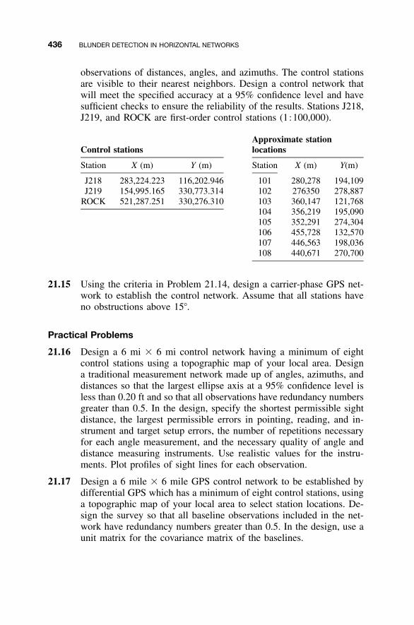
436 BLUNDER DETECTION IN HORIZONTAL NETWORKS
observations of distances, angles, and azimuths. The control stationsare visible to their nearest neighbors. Design a control network thatwill meet the specified accuracy at a 95% confidence level and havesufficient checks to ensure the reliability of the results. Stations J218,J219, and ROCK are first-order control stations (1�100,000).
Control stationsApproximate stationlocations
Station X (m) Y (m) Station X (m) Y(m)
J218 283,224.223 116,202.946 101 280,278 194,109J219 154,995.165 330,773.314 102 276350 278,887
ROCK 521,287.251 330,276.310 103 360,147 121,768104 356,219 195,090105 352,291 274,304106 455,728 132,570107 446,563 198,036108 440,671 270,700
21.15 Using the criteria in Problem 21.14, design a carrier-phase GPS net-work to establish the control network. Assume that all stations haveno obstructions above 15�.
Practical Problems
21.16 Design a 6 mi � 6 mi control network having a minimum of eightcontrol stations using a topographic map of your local area. Designa traditional measurement network made up of angles, azimuths, anddistances so that the largest ellipse axis at a 95% confidence level isless than 0.20 ft and so that all observations have redundancy numbersgreater than 0.5. In the design, specify the shortest permissible sightdistance, the largest permissible errors in pointing, reading, and in-strument and target setup errors, the number of repetitions necessaryfor each angle measurement, and the necessary quality of angle anddistance measuring instruments. Use realistic values for the instru-ments. Plot profiles of sight lines for each observation.
21.17 Design a 6 mile � 6 mile GPS control network to be established bydifferential GPS which has a minimum of eight control stations, usinga topographic map of your local area to select station locations. De-sign the survey so that all baseline observations included in the net-work have redundancy numbers greater than 0.5. In the design, use aunit matrix for the covariance matrix of the baselines.
437
CHAPTER 22
GENERAL LEAST SQUARES METHODAND ITS APPLICATION TO CURVEFITTING AND COORDINATETRANSFORMATIONS
22.1 INTRODUCTION TO GENERAL LEAST SQUARES
When fitting points to a straight line, it must be recognized that both the xand y coordinates contain errors. Yet in the mathematical model presented inSection 11.11.1, illustrated in Figure 11.2, the residuals are applied only tothe y coordinate. Because both coordinates contain errors, this mathematicalmodel fails to account for the x coordinate being a measurement. In thischapter the general least squares method is presented and its use in perform-ing adjustments where the observation equations involve more than a singlemeasurement is demonstrated.
22.2 GENERAL LEAST SQUARES EQUATIONS FOR FITTING ASTRAIGHT LINE
Consider the data illustrated in Figure 11.2. To account properly for both thex and y coordinates being measurements, the observation equation must con-tain residuals for both measurements. That is, Equation (11.40) must be re-written as
F(x,y) � (y � v ) � m(x � v ) � b � 0 (22.1)y x
In Equation (22.1), x and y are a point’s coordinate pair with residuals vx andvy, respectively, m is the slope of the line, and b is the y intercept. Equation(22.1) contains vx, vy, m, and b as unknowns and is nonlinear. Thus, its so-
Adjustment Computations: Spatial Data Analysis, Fourth Edition. C. D. Ghilani and P. R. Wolf© 2006 John Wiley & Sons, Inc. ISBN: 978-0-471-69728-2
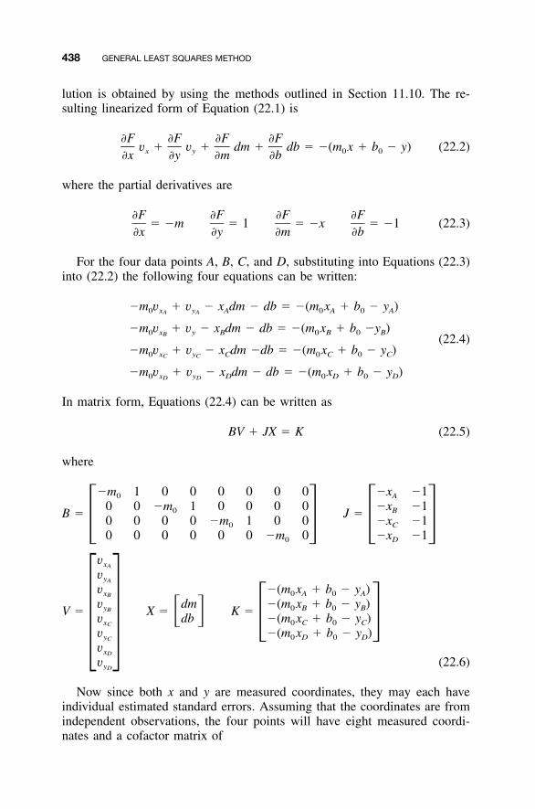
438 GENERAL LEAST SQUARES METHOD
lution is obtained by using the methods outlined in Section 11.10. The re-sulting linearized form of Equation (22.1) is
�F �F �F �Fv � v � dm � db � �(m x � b � y) (22.2)x y 0 0�x �y �m �b
where the partial derivatives are
�F �F �F �F� �m � 1 � �x � �1 (22.3)
�x �y �m �b
For the four data points A, B, C, and D, substituting into Equations (22.3)into (22.2) the following four equations can be written:
�m v � v � x dm � db � �(m x � b � y )0 x y A 0 A 0 AA A
�m v � v � x dm � db � �(m x � b �y )0 x y B 0 B 0 BB (22.4)�m v � v � x dm �db � �(m x � b � y )0 x y C 0 C 0 CC C
�m v � v � x dm � db � �(m x � b � y )0 x y D 0 D 0 DD D
In matrix form, Equations (22.4) can be written as
BV � JX � K (22.5)
where
�m 1 0 0 0 0 0 0 �x �10 A
0 0 �m 1 0 0 0 0 �x �10 BB � J �0 0 0 0 �m 1 0 0 �x �10 C� � � �0 0 0 0 0 0 �m 0 �x �10 D
vxA
vyA
v �(m x � b � y )x 0 A 0 AB
v dm �(m x � b � y )y 0 B 0 BBV � X � K �� �v db �(m x � b � y )x 0 C 0 CC � �v �(m x � b � y )y 0 D 0 DC� �vxD
vyD(22.6)
Now since both x and y are measured coordinates, they may each haveindividual estimated standard errors. Assuming that the coordinates are fromindependent observations, the four points will have eight measured coordi-nates and a cofactor matrix of
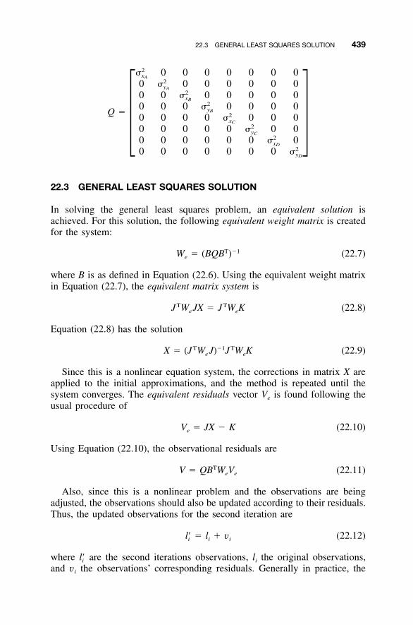
22.3 GENERAL LEAST SQUARES SOLUTION 439
2� 0 0 0 0 0 0 0xA20 � 0 0 0 0 0 0yA
20 0 � 0 0 0 0 0xB20 0 0 � 0 0 0 0yBQ � 20 0 0 0 � 0 0 0xC
20 0 0 0 0 � 0 0yC� �20 0 0 0 0 0 � 0xD20 0 0 0 0 0 0 �yD
22.3 GENERAL LEAST SQUARES SOLUTION
In solving the general least squares problem, an equivalent solution isachieved. For this solution, the following equivalent weight matrix is createdfor the system:
T �1W � (BQB ) (22.7)e
where B is as defined in Equation (22.6). Using the equivalent weight matrixin Equation (22.7), the equivalent matrix system is
T TJ W JX � J W K (22.8)e e
Equation (22.8) has the solution
T �1 TX � (J W J) J W K (22.9)e e
Since this is a nonlinear equation system, the corrections in matrix X areapplied to the initial approximations, and the method is repeated until thesystem converges. The equivalent residuals vector Ve is found following theusual procedure of
V � JX � K (22.10)e
Using Equation (22.10), the observational residuals are
TV � QB W V (22.11)e e
Also, since this is a nonlinear problem and the observations are beingadjusted, the observations should also be updated according to their residuals.Thus, the updated observations for the second iteration are
l� � l � v (22.12)i i i
where are the second iterations observations, li the original observations,l�iand vi the observations’ corresponding residuals. Generally in practice, the
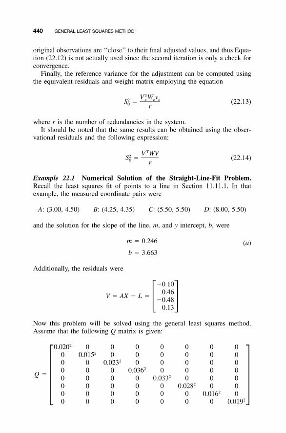
440 GENERAL LEAST SQUARES METHOD
original observations are ‘‘close’’ to their final adjusted values, and thus Equa-tion (22.12) is not actually used since the second iteration is only a check forconvergence.
Finally, the reference variance for the adjustment can be computed usingthe equivalent residuals and weight matrix employing the equation
TV W ve e e2S � (22.13)0 r
where r is the number of redundancies in the system.It should be noted that the same results can be obtained using the obser-
vational residuals and the following expression:
TV WV2S � (22.14)0 r
Example 22.1 Numerical Solution of the Straight-Line-Fit Problem.Recall the least squares fit of points to a line in Section 11.11.1. In thatexample, the measured coordinate pairs were
A: (3.00, 4.50) B: (4.25, 4.35) C: (5.50, 5.50) D: (8.00, 5.50)
and the solution for the slope of the line, m, and y intercept, b, were
m � 0.246 (a)
b � 3.663
Additionally, the residuals were
�0.100.46
V � AX � L ��0.48� �
0.13
Now this problem will be solved using the general least squares method.Assume that the following Q matrix is given:
20.020 0 0 0 0 0 0 020 0.015 0 0 0 0 0 0
20 0 0.023 0 0 0 0 020 0 0 0.036 0 0 0 0
Q � 20 0 0 0 0.033 0 0 020 0 0 0 0 0.028 0 0� �20 0 0 0 0 0 0.016 0
20 0 0 0 0 0 0 0.019
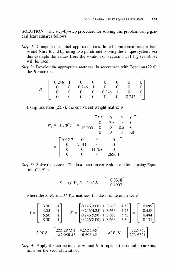
22.3 GENERAL LEAST SQUARES SOLUTION 441
SOLUTION The step-by-step procedure for solving this problem using gen-eral least squares follows.
Step 1: Compute the initial approximations. Initial approximations for bothm and b are found by using two points and solving the unique system. Forthis example the values from the solution of Section 11.11.1 given abovewill be used.
Step 2: Develop the appropriate matrices. In accordance with Equation (22.6),the B matrix is
�0.246 1 0 0 0 0 0 00 0 �0.246 1 0 0 0 0
B �0 0 0 0 �0.246 1 0 0� �0 0 0 0 0 0 �0.246 1
Using Equation (22.7), the equivalent weight matrix is
2.5 0 0 01 0 13.3 0 0T �1W � (BQB ) �e 0 0 8.5 010,000 � �
0 0 0 3.8
4012.7 0 0 00 753.0 0 0
�0 0 1176.6 0� �0 0 0 2656.1
Step 3: Solve the system. The first iteration corrections are found using Equa-tion (22.9) as
�0.0318T �1 TX � (J W J) J W K � � �e e 0.1907
where the J, K, and JTWeJ matrices for the first iteration were
�3.00 �1 0.246(3.00) � 3.663 � 4.50 �0.099�4.25 �1 0.246(4.25) � 3.663 � 4.25 0.458
J � K � ��5.50 �1 0.246(5.50) � 3.663 � 5.50 �0.484� � � � � ��8.00 �1 0.246(8.00) � 3.663 � 5.50 0.131
255,297.91 42,958.45 72.9737T TJ W J � J W K �� � � �e e42,958.45 8,598.40 273.5321
Step 4: Apply the corrections to m0 and b0 to update the initial approxima-tions for the second iteration,
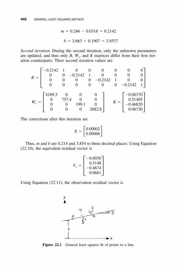
442 GENERAL LEAST SQUARES METHOD
Figure 22.1 General least squares fit of points to a line.
m � 0.246 � 0.0318 � 0.2142
b � 3.663 � 0.1907 � 3.8537
Second iteration. During the second iteration, only the unknown parametersare updated, and thus only B, We, and K matrices differ from their first iter-ation counterparts. Their second iteration values are
�0.2142 1 0 0 0 0 0 00 0 �0.2142 1 0 0 0 0
B �0 0 0 0 �0.2142 1 0 0� �0 0 0 0 0 0 �0.2142 1
4109.3 0 0 0 �0.003700 757.4 0 0 0.51405
W � K �e 0 0 199.1 0 �0.46820� � � �0 0 0 2682.8 0.06730
The corrections after this iteration are
0.00002X � � �0.00068
Thus, m and b are 0.214 and 3.854 to three decimal places. Using Equation(22.10), the equivalent residual vector is
�0.00300.5148
V �e �0.4674� �0.0681
Using Equation (22.11), the observation residual vector is
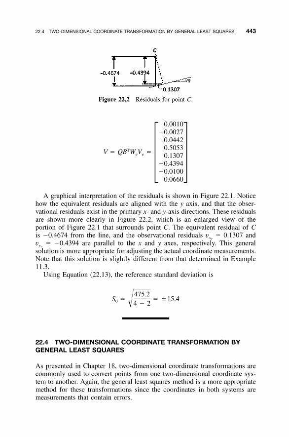
22.4 TWO-DIMENSIONAL COORDINATE TRANSFORMATION BY GENERAL LEAST SQUARES 443
Figure 22.2 Residuals for point C.
0.0010�0.0027�0.0442
0.5053TV � QB W V �e e 0.1307�0.4394� ��0.0100
0.0660
A graphical interpretation of the residuals is shown in Figure 22.1. Noticehow the equivalent residuals are aligned with the y axis, and that the obser-vational residuals exist in the primary x- and y-axis directions. These residualsare shown more clearly in Figure 22.2, which is an enlarged view of theportion of Figure 22.1 that surrounds point C. The equivalent residual of Cis �0.4674 from the line, and the observational residuals � 0.1307 andvxc
� �0.4394 are parallel to the x and y axes, respectively. This generalvyc
solution is more appropriate for adjusting the actual coordinate measurements.Note that this solution is slightly different from that determined in Example11.3.
Using Equation (22.13), the reference standard deviation is
475.2S � � �15.40 �4 � 2
22.4 TWO-DIMENSIONAL COORDINATE TRANSFORMATION BYGENERAL LEAST SQUARES
As presented in Chapter 18, two-dimensional coordinate transformations arecommonly used to convert points from one two-dimensional coordinate sys-tem to another. Again, the general least squares method is a more appropriatemethod for these transformations since the coordinates in both systems aremeasurements that contain errors.
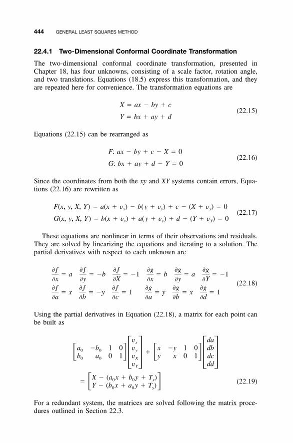
444 GENERAL LEAST SQUARES METHOD
22.4.1 Two-Dimensional Conformal Coordinate Transformation
The two-dimensional conformal coordinate transformation, presented inChapter 18, has four unknowns, consisting of a scale factor, rotation angle,and two translations. Equations (18.5) express this transformation, and theyare repeated here for convenience. The transformation equations are
X � ax � by � c(22.15)
Y � bx � ay � d
Equations (22.15) can be rearranged as
F: ax � by � c � X � 0(22.16)
G: bx � ay � d � Y � 0
Since the coordinates from both the xy and XY systems contain errors, Equa-tions (22.16) are rewritten as
F(x, y, X, Y) � a(x � v ) � b(y � v ) � c � (X � v ) � 0x y x(22.17)
G(x, y, X, Y) � b(x � v ) � a(y � v ) � d � (Y � v ) � 0x y Y
These equations are nonlinear in terms of their observations and residuals.They are solved by linearizing the equations and iterating to a solution. Thepartial derivatives with respect to each unknown are
�ƒ �ƒ �ƒ �g �g �g� a � �b � �1 � b � a � �1
�x �y �X �x �y �Y(22.18)
�ƒ �ƒ �ƒ �g �g �g� x � �y � 1 � y � x � 1
�a �b �c �a �b �d
Using the partial derivatives in Equation (22.18), a matrix for each point canbe built as
v dax
a �b 1 0 v x �y 1 0 db0 0 y �� � � �b a 0 1 v y x 0 1 dc0 0 X� � � �v ddY
X � (a x � b y � T )0 0 x� (22.19)� �Y � (b x � a y � T )0 0 y
For a redundant system, the matrices are solved following the matrix proce-dures outlined in Section 22.3.

22.4 TWO-DIMENSIONAL COORDINATE TRANSFORMATION BY GENERAL LEAST SQUARES 445
TABLE 22.1 Data for a Two-Dimensional Conformal CoordinateTransformation
Point X � SX Y � SY x � sx y � sy
1 �113.000 � 0.002 0.003 � 0.002 0.7637 � 0.026 5.9603 � 0.0283 0.001 � 0.002 112.993 � 0.002 5.0620 � 0.024 10.5407 � 0.0305 112.998 � 0.002 0.003 � 0.002 9.6627 � 0.028 6.2430 � 0.0227 0.001 � 0.002 �112.999 � 0.002 5.3500 � 0.024 1.6540 � 0.026
Example 22.2 Four fiducial points are digitized from an aerial photo, andtheir measured (x,y) and control (X,Y) values are listed in Table 22.1. Thestandard deviations of these measurements are also listed. What are the mostprobable values for the transformation parameters and the resulting residuals?
SOLUTION In this problem, initial approximations for a, b, c, and d mustfirst be computed. These values can be found using a standard least squaresadjustment, or by solving the system with only two points. The former pro-cedure was demonstrated in Example 18.1. Using standard least squares, in-itial approximations for the parameters are determined to be
a � 25.3864580
b � �0.81587080
c � �137.2160
d � �150.6000
Now the B, Q, J, and K matrices described in Section 21.3 can be formed.They are listed below (note that the numbers are rounded to three decimalplaces for publication purposes only):
25.386 0.816 �1 0 0 0 0 0 0 0 0 0 0 0 0 0�0.816 25.386 0 �1 0 0 0 0 0 0 0 0 0 0 0 0
0 0 0 0 25.386 0.816 �1 0 0 0 0 0 0 0 0 00 0 0 0 �0.816 25.386 0 �1 0 0 0 0 0 0 0 0
B �0 0 0 0 0 0 0 0 25.386 0.816 �1 0 0 0 0 00 0 0 0 0 0 0 0 �0.816 25.386 0 �1 0 0 0 0� �0 0 0 0 0 0 0 0 0 0 0 0 25.386 0.816 �1 00 0 0 0 0 0 0 0 0 0 0 0 �0.816 25.386 0 �1
0.764 �5.960 1 0 �0.034472705.960 0.764 0 1 �0.084825095.062 �10.541 1 0 0.11090026
10.541 5.062 0 1 0.13190015J � K �
9.663 �6.243 1 0 �0.181209126.243 9.663 0 1 �0.00114251� � � �5.350 �1.654 1 0 0.049999401.654 5.350 0 1 �0.02329275

446 GENERAL LEAST SQUARES METHOD
Also, the Q matrix is
20.02620.028
20.00220.002
20.02420.030
20.00220.002
Q � 20.02820.022
20.00220.002
20.02420.026
20.00220.002
The solution for the first iteration is
�0.000124503�0.000026212
X ��0.000325016� ��0.000029546
Adding these corrections to the initial approximations, yields
a � 25.38633347
b � �0.815897012
c � �137.2163
d � �150.6000
In the next iteration, only minor corrections occur, and thus the system hasconverged to a solution. The residuals and reference variance are computedas before. Although the solution has changed only slightly from the standardleast squares method, it properly considers the fact that each observationequation contains four measurements. Of course, once the transformation pa-rameters have been determined, any points that exist only in the xy systemcan be transformed into the XY system by substitution into Equations (22.15).This part of the problem is not demonstrated in this example. For the re-mainder of the chapter, only the adjustment model is developed.
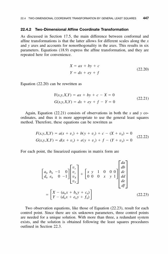
22.4 TWO-DIMENSIONAL COORDINATE TRANSFORMATION BY GENERAL LEAST SQUARES 447
22.4.2 Two-Dimensional Affine Coordinate Transformation
As discussed in Section 17.5, the main difference between conformal andaffine transformations is that the latter allows for different scales along the xand y axes and accounts for nonorthogonality in the axes. This results in sixparameters. Equations (18.9) express the affine transformation, and they arerepeated here for convenience.
X � ax � by � c(22.20)
Y � dx � ey � ƒ
Equation (22.20) can be rewritten as
F(x,y,X,Y) � ax � by � c � X � 0(22.21)
G(x,y,X,Y) � dx � ey � ƒ � Y � 0
Again, Equation (22.21) consists of observations in both the x and y co-ordinates, and thus it is more appropriate to use the general least squaresmethod. Therefore, these equations can be rewritten as
F(x,y,X,Y) � a(x � v ) � b(y � v ) � c � (X � v ) � 0x y X(22.22)
G(x,y,X,Y) � d(x � v ) � e(y � v ) � ƒ � (Y � v ) � 0x y Y
For each point, the linearized equations in matrix form are
dav dbx
a b �1 0 v x y 1 0 0 0 dc0 0 y �� � � �d e 0 �1 v 0 0 0 x y 1 dd0 0 X� �v �de�Y
df
X � (a x � b y � c )0 0 0� (22.23)� �Y � (d x � e y � ƒ )0 0 0
Two observation equations, like those of Equation (22.23), result for eachcontrol point. Since there are six unknown parameters, three control pointsare needed for a unique solution. With more than three, a redundant systemexists, and the solution is obtained following the least squares proceduresoutlined in Section 22.3.
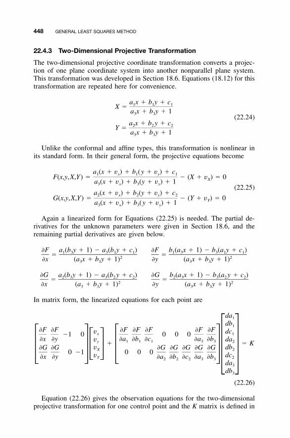
448 GENERAL LEAST SQUARES METHOD
22.4.3 Two-Dimensional Projective Transformation
The two-dimensional projective coordinate transformation converts a projec-tion of one plane coordinate system into another nonparallel plane system.This transformation was developed in Section 18.6. Equations (18.12) for thistransformation are repeated here for convenience.
a x � b y � c1 1 1X �a x � b y � 13 3
(22.24)a x � b y � c2 2 2Y �a x � b y � 13 3
Unlike the conformal and affine types, this transformation is nonlinear inits standard form. In their general form, the projective equations become
a (x � v ) � b (y � v ) � c1 x 1 y 1F(x,y,X,Y) � � (X � v ) � 0Xa (x � v ) � b (y � v ) � 13 x 3 y(22.25)
a (x � v ) � b (y � v ) � c2 x 2 y 2G(x,y,X,Y) � � (Y � v ) � 0Ya (x � v ) � b (y � v ) � 13 x 3 y
Again a linearized form for Equations (22.25) is needed. The partial de-rivatives for the unknown parameters were given in Section 18.6, and theremaining partial derivatives are given below.
�F a (b y � 1) � a (b y � c ) �F b (a x � 1) � b (a y � c )1 3 3 1 1 1 3 3 1 1� �2 2�x (a x � b y � 1) �y (a x � b y � 1)3 3 3 3
�G a (b y � 1) � a (b y � c ) �G b (a x � 1) � b (a y � c )2 3 3 2 2 2 3 3 2 2� �2 2�x (a � b y � 1) �y (a x � b y � 1)3 3 3 3
In matrix form, the linearized equations for each point are
da1
db1�F �F �F �F �F �F �Fv dcx 1�1 0 0 0 0�x �y �a �b �c �a �bv da1 1 1 3 3y 2� � Kv db�G �G �G �G �G �G �GX 2� �0 �1 0 0 0� � � �v dcY 2�x �y �a �b �c �a �b2 2 2 3 3 � �
da3
db3
(22.26)
Equation (22.26) gives the observation equations for the two-dimensionalprojective transformation for one control point and the K matrix is defined in
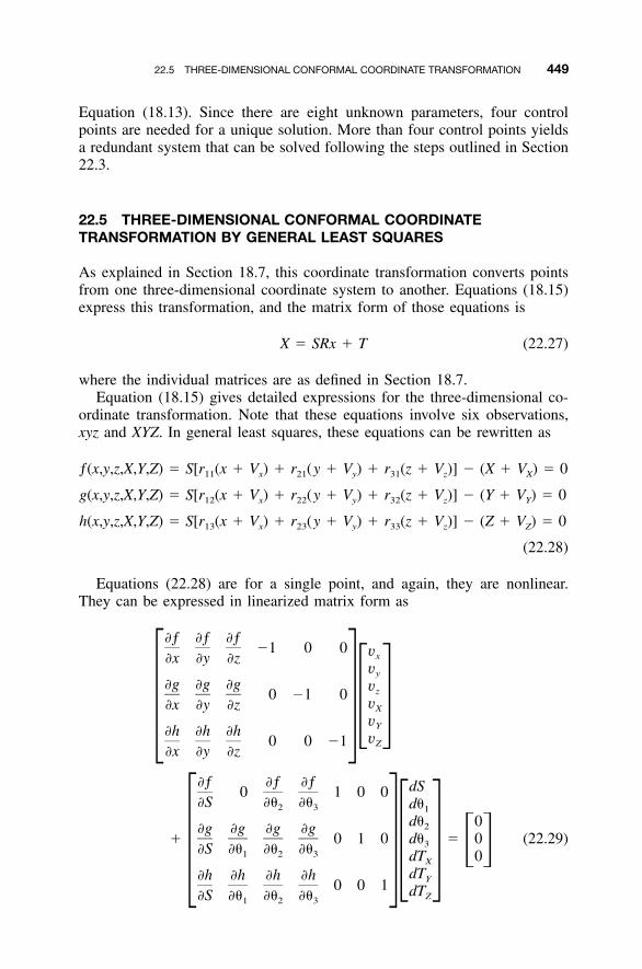
22.5 THREE-DIMENSIONAL CONFORMAL COORDINATE TRANSFORMATION 449
Equation (18.13). Since there are eight unknown parameters, four controlpoints are needed for a unique solution. More than four control points yieldsa redundant system that can be solved following the steps outlined in Section22.3.
22.5 THREE-DIMENSIONAL CONFORMAL COORDINATETRANSFORMATION BY GENERAL LEAST SQUARES
As explained in Section 18.7, this coordinate transformation converts pointsfrom one three-dimensional coordinate system to another. Equations (18.15)express this transformation, and the matrix form of those equations is
X � SRx � T (22.27)
where the individual matrices are as defined in Section 18.7.Equation (18.15) gives detailed expressions for the three-dimensional co-
ordinate transformation. Note that these equations involve six observations,xyz and XYZ. In general least squares, these equations can be rewritten as
ƒ(x,y,z,X,Y,Z) � S[r (x � V ) � r (y � V ) � r (z � V )] � (X � V ) � 011 x 21 y 31 z X
g(x,y,z,X,Y,Z) � S[r (x � V ) � r (y � V ) � r (z � V )] � (Y � V ) � 012 x 22 y 32 z Y
h(x,y,z,X,Y,Z) � S[r (x � V ) � r (y � V ) � r (z � V )] � (Z � V ) � 013 x 23 y 33 z Z
(22.28)
Equations (22.28) are for a single point, and again, they are nonlinear.They can be expressed in linearized matrix form as
�ƒ �ƒ �ƒ�1 0 0 vx�x �y �z
vy
�g �g �g vz0 �1 0 v�x �y �z X�v �Y� ��h �h �h v0 0 �1 Z�x �y �z
�ƒ �ƒ �ƒ dS0 1 0 0�S �� �� d�2 3 1
d� 02�g �g �g �g� 0 1 0 d� � 0 (22.29)3�S �� �� �� � �1 2 3 dT 0X� �� � dT�h �h �h �h Y0 0 1 dTZ�S �� �� ��1 2 3
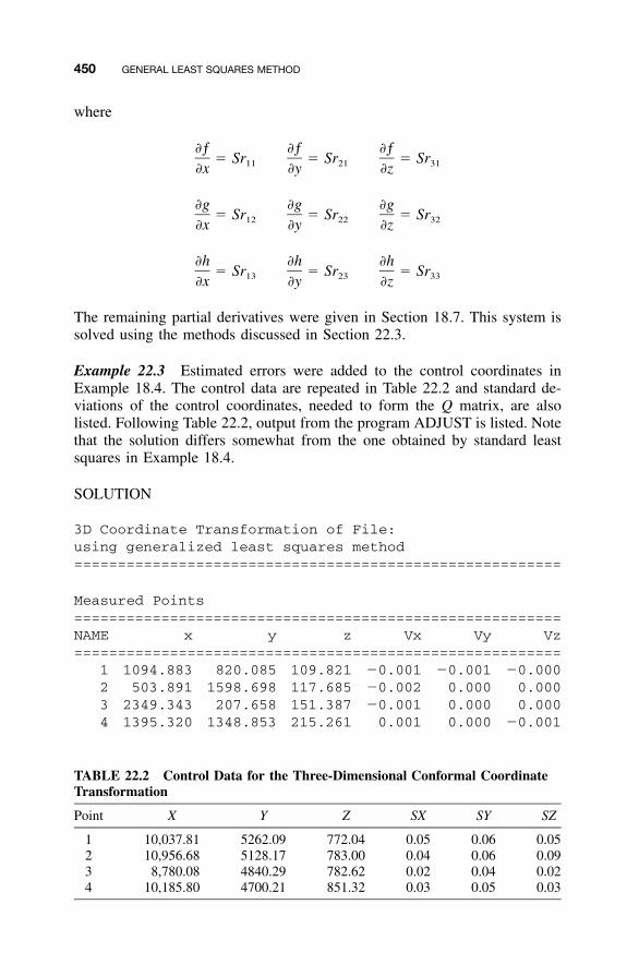
450 GENERAL LEAST SQUARES METHOD
TABLE 22.2 Control Data for the Three-Dimensional Conformal CoordinateTransformation
Point X Y Z SX SY SZ
1 10,037.81 5262.09 772.04 0.05 0.06 0.052 10,956.68 5128.17 783.00 0.04 0.06 0.093 8,780.08 4840.29 782.62 0.02 0.04 0.024 10,185.80 4700.21 851.32 0.03 0.05 0.03
where
�ƒ �ƒ �ƒ� Sr � Sr � Sr11 21 31�x �y �z
�g �g �g� Sr � Sr � Sr12 22 32�x �y �z
�h �h �h� Sr � Sr � Sr13 23 33�x �y �z
The remaining partial derivatives were given in Section 18.7. This system issolved using the methods discussed in Section 22.3.
Example 22.3 Estimated errors were added to the control coordinates inExample 18.4. The control data are repeated in Table 22.2 and standard de-viations of the control coordinates, needed to form the Q matrix, are alsolisted. Following Table 22.2, output from the program ADJUST is listed. Notethat the solution differs somewhat from the one obtained by standard leastsquares in Example 18.4.
SOLUTION
3D Coordinate Transformation of File:using generalized least squares method========================================================
Measured Points========================================================NAME x y z Vx Vy Vz========================================================
1 1094.883 820.085 109.821 �0.001 �0.001 �0.0002 503.891 1598.698 117.685 �0.002 0.000 0.0003 2349.343 207.658 151.387 �0.001 0.000 0.0004 1395.320 1348.853 215.261 0.001 0.000 �0.001
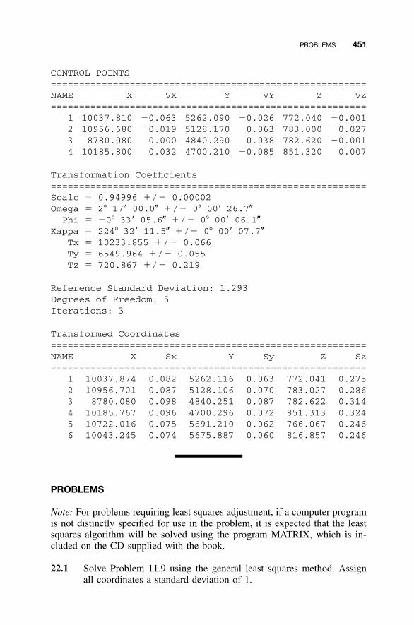
PROBLEMS 451
CONTROL POINTS========================================================NAME X VX Y VY Z VZ========================================================
1 10037.810 �0.063 5262.090 �0.026 772.040 �0.0012 10956.680 �0.019 5128.170 0.063 783.000 �0.0273 8780.080 0.000 4840.290 0.038 782.620 �0.0014 10185.800 0.032 4700.210 �0.085 851.320 0.007
Transformation Coefficients========================================================Scale � 0.94996 �/� 0.00002Omega � 2� 17� 00.0� �/� 0� 00� 26.7�
Phi � �0� 33� 05.6� �/� 0� 00� 06.1�Kappa � 224� 32� 11.5� �/� 0� 00� 07.7�
Tx � 10233.855 �/� 0.066Ty � 6549.964 �/� 0.055Tz � 720.867 �/� 0.219
Reference Standard Deviation: 1.293Degrees of Freedom: 5Iterations: 3
Transformed Coordinates========================================================NAME X Sx Y Sy Z Sz========================================================
1 10037.874 0.082 5262.116 0.063 772.041 0.2752 10956.701 0.087 5128.106 0.070 783.027 0.2863 8780.080 0.098 4840.251 0.087 782.622 0.3144 10185.767 0.096 4700.296 0.072 851.313 0.3245 10722.016 0.075 5691.210 0.062 766.067 0.2466 10043.245 0.074 5675.887 0.060 816.857 0.246
PROBLEMS
Note: For problems requiring least squares adjustment, if a computer programis not distinctly specified for use in the problem, it is expected that the leastsquares algorithm will be solved using the program MATRIX, which is in-cluded on the CD supplied with the book.
22.1 Solve Problem 11.9 using the general least squares method. Assignall coordinates a standard deviation of 1.
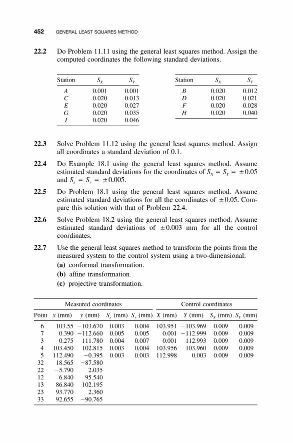
452 GENERAL LEAST SQUARES METHOD
22.2 Do Problem 11.11 using the general least squares method. Assign thecomputed coordinates the following standard deviations.
Station SX SY Station SX SY
A 0.001 0.001 B 0.020 0.012C 0.020 0.013 D 0.020 0.021E 0.020 0.027 F 0.020 0.028GI
0.0200.020
0.0350.046
H 0.020 0.040
22.3 Solve Problem 11.12 using the general least squares method. Assignall coordinates a standard deviation of 0.1.
22.4 Do Example 18.1 using the general least squares method. Assumeestimated standard deviations for the coordinates of SX � SY � �0.05and Sx � Sy � �0.005.
22.5 Do Problem 18.1 using the general least squares method. Assumeestimated standard deviations for all the coordinates of �0.05. Com-pare this solution with that of Problem 22.4.
22.6 Solve Problem 18.2 using the general least squares method. Assumeestimated standard deviations of �0.003 mm for all the controlcoordinates.
22.7 Use the general least squares method to transform the points from themeasured system to the control system using a two-dimensional:(a) conformal transformation.(b) affine transformation.(c) projective transformation.
Measured coordinates Control coordinates
Point x (mm) y (mm) Sx (mm) Sy (mm) X (mm) Y (mm) SX (mm) SY (mm)
6 103.55 �103.670 0.003 0.004 103.951 �103.969 0.009 0.0097 0.390 �112.660 0.005 0.005 0.001 �112.999 0.009 0.0093 0.275 111.780 0.004 0.007 0.001 112.993 0.009 0.0094 103.450 102.815 0.003 0.004 103.956 103.960 0.009 0.0095 112.490 �0.395 0.003 0.003 112.998 0.003 0.009 0.009
32 18.565 �87.58022 �5.790 2.03512 6.840 95.54013 86.840 102.19523 93.770 2.36033 92.655 �90.765
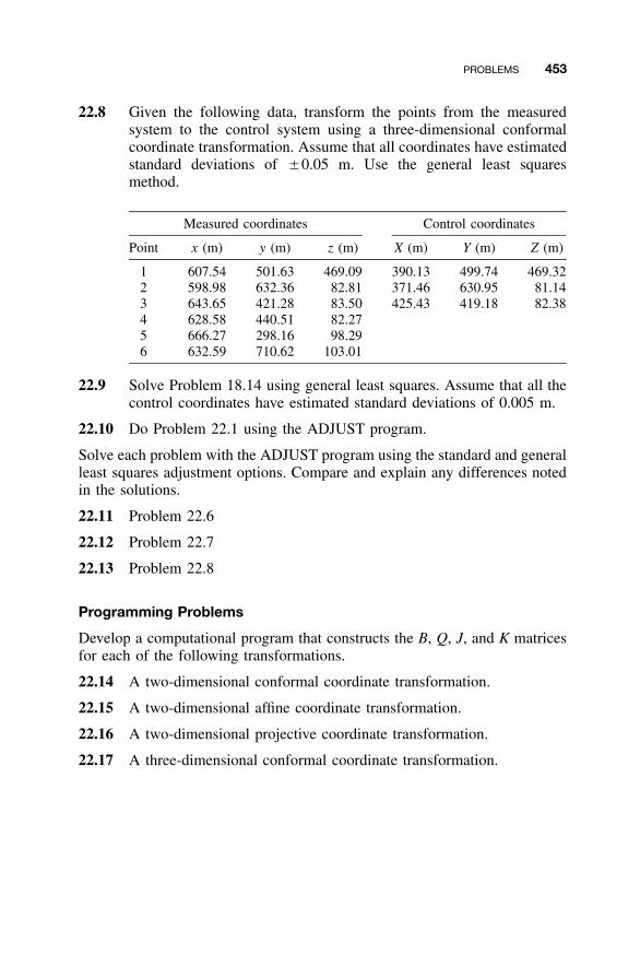
PROBLEMS 453
22.8 Given the following data, transform the points from the measuredsystem to the control system using a three-dimensional conformalcoordinate transformation. Assume that all coordinates have estimatedstandard deviations of �0.05 m. Use the general least squaresmethod.
Measured coordinates Control coordinates
Point x (m) y (m) z (m) X (m) Y (m) Z (m)
1 607.54 501.63 469.09 390.13 499.74 469.322 598.98 632.36 82.81 371.46 630.95 81.143 643.65 421.28 83.50 425.43 419.18 82.384 628.58 440.51 82.275 666.27 298.16 98.296 632.59 710.62 103.01
22.9 Solve Problem 18.14 using general least squares. Assume that all thecontrol coordinates have estimated standard deviations of 0.005 m.
22.10 Do Problem 22.1 using the ADJUST program.
Solve each problem with the ADJUST program using the standard and generalleast squares adjustment options. Compare and explain any differences notedin the solutions.
22.11 Problem 22.6
22.12 Problem 22.7
22.13 Problem 22.8
Programming Problems
Develop a computational program that constructs the B, Q, J, and K matricesfor each of the following transformations.
22.14 A two-dimensional conformal coordinate transformation.
22.15 A two-dimensional affine coordinate transformation.
22.16 A two-dimensional projective coordinate transformation.
22.17 A three-dimensional conformal coordinate transformation.
454
CHAPTER 23
THREE-DIMENSIONAL GEODETICNETWORK ADJUSTMENT
23.1 INTRODUCTION
With the advent of total station instruments, survey data are being collectedin three dimensions. Thus, it is advantageous to develop an adjustment modelthat works in three dimensions. Rigorous triangulation adjustment models dateback to Bruns (1878). The main observational data consist of horizontal an-gles, vertical angles, azimuths, and slant distances. It is also possible to in-clude differential leveling in the model. Since all data are collected on Earth’ssurface, the local geodetic coordinate system provides a natural system inwhich to perform the adjustment.
As shown in Figure 23.1, the local geodetic system is oriented such thatthe n axis points along the meridian of the ellipse (local geodetic north), theu axis is aligned along the normal of the ellipsoid, and the e axis creates aleft-handed coordinate system. The local geodetic coordinate system can berelated to the geocentric coordinate system (see Section 17.5) through a seriesof three-dimensional rotations discussed in Section 18.7. To align the X axiswith the e axis, the Z axis is rotated by an amount of � � 180�. Then the Zaxis is aligned with the u axis by a rotation of � � 90� about the once-rotatedX axis. Changing the sign of e to convert to a right-handed coordinate system,the resulting expression is
�n �X��e � R (� � 90�)R (� � 180�) �Y (23.1)2 3� � � ��u �Z
Adjustment Computations: Spatial Data Analysis, Fourth Edition. C. D. Ghilani and P. R. Wolf© 2006 John Wiley & Sons, Inc. ISBN: 978-0-471-69728-2
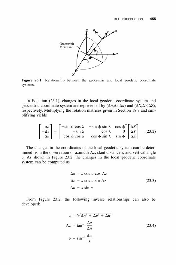
23.1 INTRODUCTION 455
Figure 23.1 Relationship between the geocentric and local geodetic coordinatesystems.
In Equation (23.1), changes in the local geodetic coordinate system andgeocentric coordinate system are represented by (�n,�e,�u) and (�X,�Y,�Z),respectively. Multiplying the rotation matrices given in Section 18.7 and sim-plifying yields
�n �sin � cos � �sin � sin � cos � �X��e � �sin � cos � 0 �Y (23.2)� � � �� ��u cos � cos � cos � sin � sin � �Z
The changes in the coordinates of the local geodetic system can be deter-mined from the observation of azimuth Az, slant distance s, and vertical anglev. As shown in Figure 23.2, the changes in the local geodetic coordinatesystem can be computed as
�n � s cos v cos Az
�e � s cos v sin Az (23.3)
�u � s sin v
From Figure 23.2, the following inverse relationships can also bedeveloped:
2 2 2s � ��n � �e � �u
�e�1Az � tan (23.4)
�n
�u�1v � sin
s
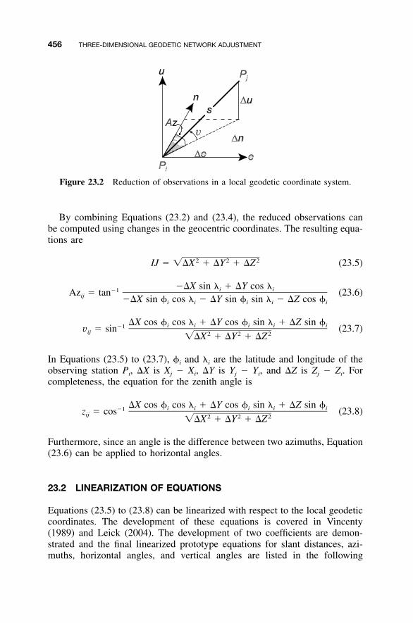
456 THREE-DIMENSIONAL GEODETIC NETWORK ADJUSTMENT
Figure 23.2 Reduction of observations in a local geodetic coordinate system.
By combining Equations (23.2) and (23.4), the reduced observations canbe computed using changes in the geocentric coordinates. The resulting equa-tions are
2 2 2IJ � ��X � �Y � �Z (23.5)
��X sin � � �Y cos �i i�1Az � tan (23.6)ij ��X sin � cos � � �Y sin � sin � � �Z cos �i i i i i
�X cos � cos � � �Y cos � sin � � �Z sin �i i i i i�1v � sin (23.7)ij 2 2 2��X � �Y � �Z
In Equations (23.5) to (23.7), �i and �i are the latitude and longitude of theobserving station Pi, �X is Xj � Xi, �Y is Yj � Yi, and �Z is Zj � Zi. Forcompleteness, the equation for the zenith angle is
�X cos � cos � � �Y cos � sin � � �Z sin �i i i i i�1z � cos (23.8)ij 2 2 2��X � �Y � �Z
Furthermore, since an angle is the difference between two azimuths, Equation(23.6) can be applied to horizontal angles.
23.2 LINEARIZATION OF EQUATIONS
Equations (23.5) to (23.8) can be linearized with respect to the local geodeticcoordinates. The development of these equations is covered in Vincenty(1989) and Leick (2004). The development of two coefficients are demon-strated and the final linearized prototype equations for slant distances, azi-muths, horizontal angles, and vertical angles are listed in the following
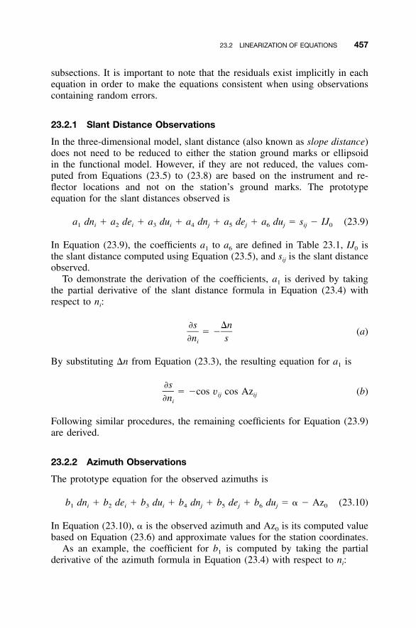
23.2 LINEARIZATION OF EQUATIONS 457
subsections. It is important to note that the residuals exist implicitly in eachequation in order to make the equations consistent when using observationscontaining random errors.
23.2.1 Slant Distance Observations
In the three-dimensional model, slant distance (also known as slope distance)does not need to be reduced to either the station ground marks or ellipsoidin the functional model. However, if they are not reduced, the values com-puted from Equations (23.5) to (23.8) are based on the instrument and re-flector locations and not on the station’s ground marks. The prototypeequation for the slant distances observed is
a dn � a de � a du � a dn � a de � a du � s � IJ (23.9)1 i 2 i 3 i 4 j 5 j 6 j ij 0
In Equation (23.9), the coefficients a1 to a6 are defined in Table 23.1, IJ0 isthe slant distance computed using Equation (23.5), and sij is the slant distanceobserved.
To demonstrate the derivation of the coefficients, a1 is derived by takingthe partial derivative of the slant distance formula in Equation (23.4) withrespect to ni:
�s �n� � (a)
�n si
By substituting �n from Equation (23.3), the resulting equation for a1 is
�s� �cos v cos Az (b)ij ij�ni
Following similar procedures, the remaining coefficients for Equation (23.9)are derived.
23.2.2 Azimuth Observations
The prototype equation for the observed azimuths is
b dn � b de � b du � b dn � b de � b du � � � Az (23.10)1 i 2 i 3 i 4 j 5 j 6 j 0
In Equation (23.10), � is the observed azimuth and Az0 is its computed valuebased on Equation (23.6) and approximate values for the station coordinates.
As an example, the coefficient for b1 is computed by taking the partialderivative of the azimuth formula in Equation (23.4) with respect to ni:
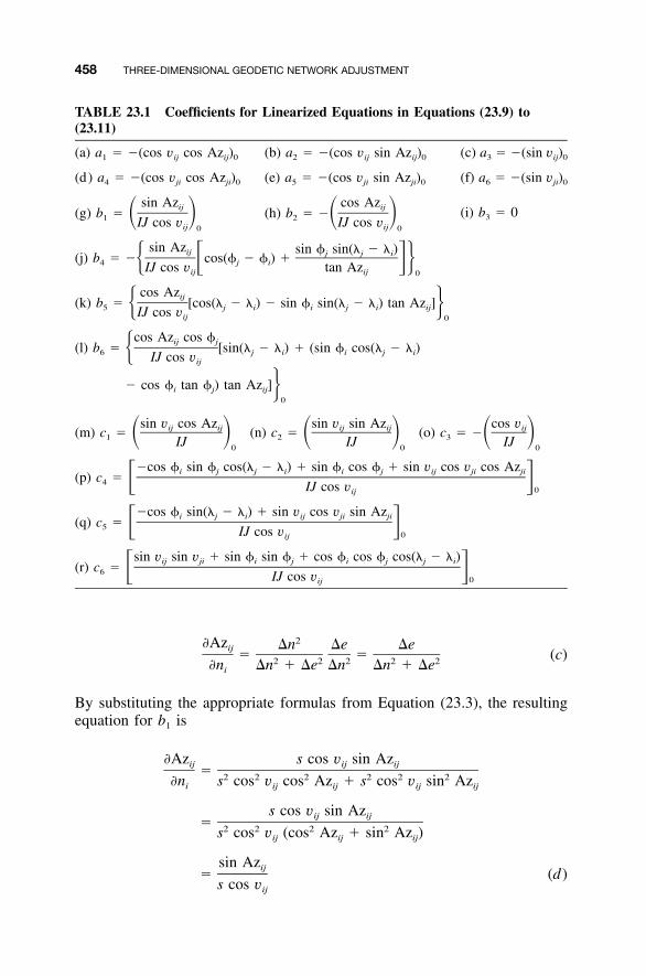
458 THREE-DIMENSIONAL GEODETIC NETWORK ADJUSTMENT
TABLE 23.1 Coefficients for Linearized Equations in Equations (23.9) to(23.11)
(a) a1 � �(cos vij cos Azij)0 (b) a2 � �(cos vij sin Azij)0 (c) a3 � �(sin vij)0
(d) a4 � �(cos vji cos Azji)0 (e) a5 � �(cos vji sin Azji)0 (f) a6 � �(sin vji)0
(g) b1 �sin Azij� �IJ cos vij 0
(h) b2 �cos Azij
�� �IJ cos vij 0
(i) b3 � 0
(j) b4 �sin Az sin � sin(� � � )ij j j i� cos(� � � ) �� � �j iIJ cos v tan Azij ij 0
(k) b5 �cos Azij [cos(� � � ) � sin � sin(� � � ) tan Az ]� j i i j i ijIJ cos vij 0
(l) b6 � [sin(�j � �i) � (sin �i cos(�j � �i)cos Az cos �ij j� IJ cos vij
� cos �i tan �j) tan Az ]ij0
(m) c1 � (n) c2 � (o) c3 �sin v cos Az sin v sin Az cos vij ij ij ij ij�� � � � � �IJ IJ IJ0 0 0
(p) c4 ��cos � sin � cos(� � � ) � sin � cos � � sin v cos v cos Azi j j i i j ij ji ji� �IJ cos v 0ij
(q) c5 ��cos � sin(� � � ) � sin v cos v sin Azi j i ij ji ji� �IJ cos v 0ij
(r) c6 �sin v sin v � sin � sin � � cos � cos � cos(� � � )ij ji i j i j j i� �IJ cos v 0ij
2�Az �n �e �eij� � (c)2 2 2 2 2�n �n � �e �n �n � �ei
By substituting the appropriate formulas from Equation (23.3), the resultingequation for b1 is
�Az s cos v sin Azij ij ij� 2 2 2 2 2 2�n s cos v cos Az � s cos v sin Azi ij ij ij ij
s cos v sin Azij ij� 2 2 2 2s cos v (cos Az � sin Az )ij ij ij
sin Azij� (d)
s cos vij
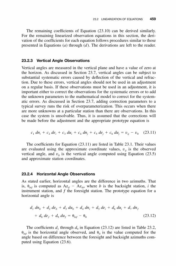
23.2 LINEARIZATION OF EQUATIONS 459
The remaining coefficients of Equation (23.10) can be derived similarly.For the remaining linearized observation equations in this section, the deri-vation of the coefficients for each equation follows procedures similar to thosepresented in Equations (a) through (d). The derivations are left to the reader.
23.2.3 Vertical Angle Observations
Vertical angles are measured in the vertical plane and have a value of zero atthe horizon. As discussed in Section 23.7, vertical angles can be subject tosubstantial systematic errors caused by deflection of the vertical and refrac-tion. Due to these errors, vertical angles should not be used in an adjustmenton a regular basis. If these observations must be used in an adjustment, it isimportant either to correct the observations for the systematic errors or to addthe unknown parameters to the mathematical model to correct for the system-atic errors. As discussed in Section 23.7, adding correction parameters to atypical survey runs the risk of overparameterization. This occurs when thereare more unknowns at a particular station than there are observations. In thiscase the system is unsolvable. Thus, it is assumed that the corrections willbe made before the adjustment and the appropriate prototype equation is
c dn � c de � c du � c dn � c de � c du � v � v (23.11)1 i 2 i 3 i 4 j 5 j 6 j ij 0
The coefficients for Equation (23.11) are listed in Table 23.1. Their valuesare evaluated using the approximate coordinate values, vij is the observedvertical angle, and v0 is the vertical angle computed using Equation (23.5)and approximate station coordinates.
23.2.4 Horizontal Angle Observations
As stated earlier, horizontal angles are the difference in two azimuths. Thatis, �bif is computed as Azif � Azib, where b is the backsight station, i theinstrument station, and ƒ the foresight station. The prototype equation for ahorizontal angle is
d dn � d de � d du � d dn � d de � d du � d dn1 b 2 b 3 b 4 i 5 i 6 i 7 ƒ
� d de � d du � � � � (23.12)8 ƒ 9 ƒ bif 0
The coefficients d1 through d9 in Equation (23.12) are listed in Table 23.2,�bif is the horizontal angle observed, and �0 is the value computed for theangle based on difference between the foresight and backsight azimuths com-puted using Equation (23.6).
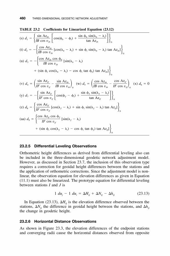
460 THREE-DIMENSIONAL GEODETIC NETWORK ADJUSTMENT
TABLE 23.2 Coefficients for Linearized Equation (23.12)
(s) d1 �sin Az sin � sin(� � � )ib b b icos(� � � ) �� � �b iIB cos v tan Azib ib 0
(t) d2 �cos Azib� [cos(� � � ) � sin � sin(� � � ) tan Az ]� b i i b i ibIB cos vib 0
(u) d3 � [sin(�b � �i)cos Az cos �ib b�� IB cos vib
� (sin �i cos(�b � �i) � cos �i tan �b) tan Az ]ib0
(v) d4 � (w) d5 � (x) d6 � 0sin Az cos Azsin Az cos Azif ifib ib� �� � � �IF cos v IB cos v IB cos v IF cos vif ib ib if0 0
(y) d7 �sin Az sin � sin(� � � )if ƒ ƒ i
� cos(� � � ) �� � �ƒ iIF cos v tan Azif if 0
(z) d8 �cos Azif [cos(� � � ) � sin � sin(� � � ) tan Az ]� ƒ i i ƒ i ifIF cos vif 0
(aa) d9 � [sin(�ƒ � �i)cos Az cos �if ƒ� IF cos vif
� (sin �i � cos �i tancos(� � � ) � ) tan Az ]ƒ i ƒ if0
23.2.5 Differential Leveling Observations
Orthometric height differences as derived from differential leveling also canbe included in the three-dimensional geodetic network adjustment model.However, as discussed in Section 23.7, the inclusion of this observation typerequires a correction for geoidal height differences between the stations andthe application of orthometric corrections. Since the adjustment model is non-linear, the observation equation for elevation differences as given in Equation(11.1) must also be linearized. The prototype equation for differential levelingbetween stations I and J is
1 du � 1 du � �H � �N � �h (23.13)j i ij ij ij
In Equation (23.13), �Hij is the elevation difference observed between thestations, �Nij the difference in geoidal height between the stations, and �hij
the change in geodetic height.
23.2.6 Horizontal Distance Observations
As shown in Figure 23.3, the elevation differences of the endpoint stationsand converging radii cause the horizontal distances observed from opposite
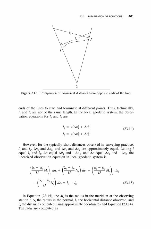
23.2 LINEARIZATION OF EQUATIONS 461
Figure 23.3 Comparison of horizontal distances from opposite ends of the line.
ends of the lines to start and terminate at different points. Thus, technically,l1 and l2 are not of the same length. In the local geodetic system, the obser-vation equations for l1 and l2 are
2 2l � ��n � �e1 1 1 (23.14)2 2l � ��n � �e2 2 2
However, for the typically short distances observed in surveying practice,l1 and l2, �n1 and �n2, and �e1 and �e2 are approximately equal. Letting lequal l1 and l2, �n equal �n1 and ��n2, and �e equal �e1 and ��e2, thelinearized observation equation in local geodetic system is
� � � � � � � � �j i i j j iM dn � N de � M dn� � � � � �i i j i i jIJ IJ IJ0 0
� � �i j� N de � l � l (23.15)� �j j ij 0IJ
In Equation (23.15), the Mi is the radius in the meridian at the observingstation I, Ni the radius in the normal, lij the horizontal distance observed, andl0 the distance computed using approximate coordinates and Equation (23.14).The radii are computed as
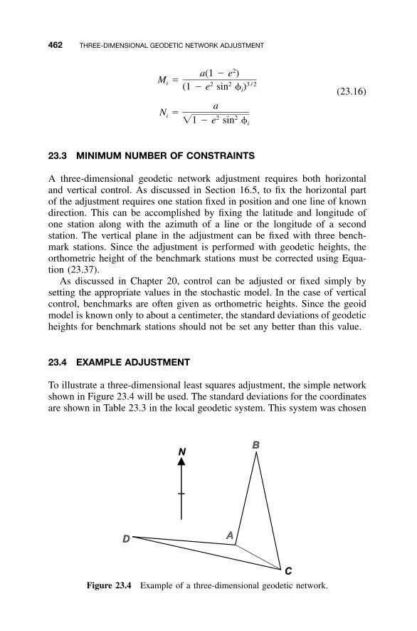
462 THREE-DIMENSIONAL GEODETIC NETWORK ADJUSTMENT
Figure 23.4 Example of a three-dimensional geodetic network.
2a(1 � e )M �i 2 2 3 / 2(1 � e sin � )i (23.16)
aN �i 2 2�1 � e sin �i
23.3 MINIMUM NUMBER OF CONSTRAINTS
A three-dimensional geodetic network adjustment requires both horizontaland vertical control. As discussed in Section 16.5, to fix the horizontal partof the adjustment requires one station fixed in position and one line of knowndirection. This can be accomplished by fixing the latitude and longitude ofone station along with the azimuth of a line or the longitude of a secondstation. The vertical plane in the adjustment can be fixed with three bench-mark stations. Since the adjustment is performed with geodetic heights, theorthometric height of the benchmark stations must be corrected using Equa-tion (23.37).
As discussed in Chapter 20, control can be adjusted or fixed simply bysetting the appropriate values in the stochastic model. In the case of verticalcontrol, benchmarks are often given as orthometric heights. Since the geoidmodel is known only to about a centimeter, the standard deviations of geodeticheights for benchmark stations should not be set any better than this value.
23.4 EXAMPLE ADJUSTMENT
To illustrate a three-dimensional least squares adjustment, the simple networkshown in Figure 23.4 will be used. The standard deviations for the coordinatesare shown in Table 23.3 in the local geodetic system. This system was chosen

463
TABLE 23.3 Data for the Three-Dimensional Geodetic Network
Geodetic positions
Station � � H (m) N (m)
A 41�18�26.04850�N 76�00�10.24860�W 372.221 �31.723B 41�18�40.46660�N 76�00�05.50180�W 351.394 �31.713C 41�18�22.04010�N 76�00�00.94390�W 362.865 �31.726D 41�18�27.65860�N 76�00�31.38550�W 370.874 �31.722
Station Sn (m) Se (m) Sh (m)
A �0.001 �0.001 �0.01B — — �0.01C — — �0.01
Geodetic azimuth
Course Azimuth S (�)
AB 13�56�26.9� �0.001�
Slant distances
Course Distance (m) S (m)
ABACCDDABC
458.796249.462729.122494.214578.393
�0.005�0.005�0.006�0.005�0.005
Horizontal angles
Stations (bif) Angles S (�)
DAB 98�10�25� �2.8BAC 105�47�45� �3.5CAD 156�01�44� �4.1ABC 335�29�37� �2.4CBA 24�30�19� �2.4BCD 294�19�17� �2.3
Zenith angles
Direction Angle S (�)
AC 92�09�01� �2.5CD 89�22�24� �0.8DA 89�50�44� �1.2AB 92�36�12� �1.4BC 88�52�01� �1.1
Elevation differences
Stations �Elev (m) S (m)
AC �9.359 �0.005
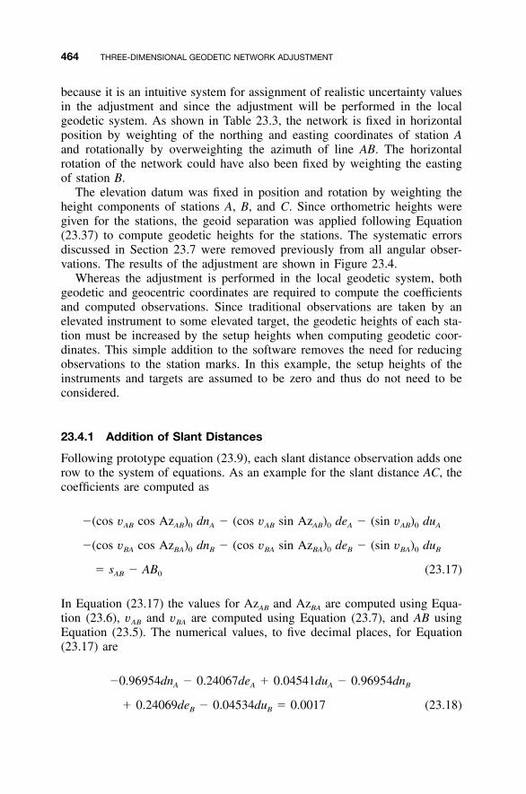
464 THREE-DIMENSIONAL GEODETIC NETWORK ADJUSTMENT
because it is an intuitive system for assignment of realistic uncertainty valuesin the adjustment and since the adjustment will be performed in the localgeodetic system. As shown in Table 23.3, the network is fixed in horizontalposition by weighting of the northing and easting coordinates of station Aand rotationally by overweighting the azimuth of line AB. The horizontalrotation of the network could have also been fixed by weighting the eastingof station B.
The elevation datum was fixed in position and rotation by weighting theheight components of stations A, B, and C. Since orthometric heights weregiven for the stations, the geoid separation was applied following Equation(23.37) to compute geodetic heights for the stations. The systematic errorsdiscussed in Section 23.7 were removed previously from all angular obser-vations. The results of the adjustment are shown in Figure 23.4.
Whereas the adjustment is performed in the local geodetic system, bothgeodetic and geocentric coordinates are required to compute the coefficientsand computed observations. Since traditional observations are taken by anelevated instrument to some elevated target, the geodetic heights of each sta-tion must be increased by the setup heights when computing geodetic coor-dinates. This simple addition to the software removes the need for reducingobservations to the station marks. In this example, the setup heights of theinstruments and targets are assumed to be zero and thus do not need to beconsidered.
23.4.1 Addition of Slant Distances
Following prototype equation (23.9), each slant distance observation adds onerow to the system of equations. As an example for the slant distance AC, thecoefficients are computed as
�(cos v cos Az ) dn � (cos v sin Az ) de � (sin v ) duAB AB 0 A AB AB 0 A AB 0 A
�(cos v cos Az ) dn � (cos v sin Az ) de � (sin v ) duBA BA 0 B BA BA 0 B BA 0 B
� s � ABAB 0 (23.17)
In Equation (23.17) the values for AzAB and AzBA are computed using Equa-tion (23.6), vAB and vBA are computed using Equation (23.7), and AB usingEquation (23.5). The numerical values, to five decimal places, for Equation(23.17) are
�0.96954dn � 0.24067de � 0.04541du � 0.96954dnA A A B
� 0.24069de � 0.04534du � 0.0017 (23.18)B B
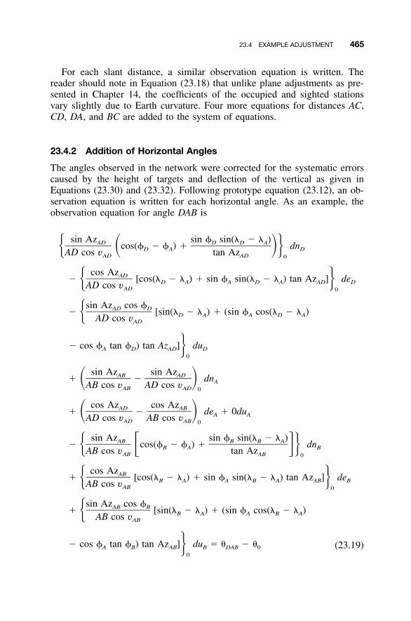
23.4 EXAMPLE ADJUSTMENT 465
For each slant distance, a similar observation equation is written. Thereader should note in Equation (23.18) that unlike plane adjustments as pre-sented in Chapter 14, the coefficients of the occupied and sighted stationsvary slightly due to Earth curvature. Four more equations for distances AC,CD, DA, and BC are added to the system of equations.
23.4.2 Addition of Horizontal Angles
The angles observed in the network were corrected for the systematic errorscaused by the height of targets and deflection of the vertical as given inEquations (23.30) and (23.32). Following prototype equation (23.12), an ob-servation equation is written for each horizontal angle. As an example, theobservation equation for angle DAB is
sin Az sin � sin(� � � )AD D D Acos(� � � ) � dn� � �D A DAD cos v tan AzAD AD 0
cos AzAD� [cos(� � � ) � sin � sin(� � � ) tan Az ] de� D A A D A AD DAD cos vAD 0
sin Az cos �AD D� [sin(� � � ) � (sin � cos(� � � )� D A A D AAD cos vAD
� cos � tan � ) tan Az ] duA D AD D0
sin Az sin AzAB AD� � dn� � AAB cos v AD cos vAB AD 0
cos Az cos AzAD AB� � de � 0du� � A AAD cos v AB cos vAD AB 0
sin Az sin � sin(� � � )AB B B A� cos(� � � ) � dn� � �B A BAB cos v tan AzAB AB 0
cos AzAB� [cos(� � � ) � sin � sin(� � � ) tan Az ] de� B A A B A AB BAB cos vAB 0
sin Az cos �AB B� [sin(� � � ) � (sin � cos(� � � )� B A A B AAB cos vAB
� cos � tan � ) tan Az ] du � � � �A B AB B DAB 00
(23.19)
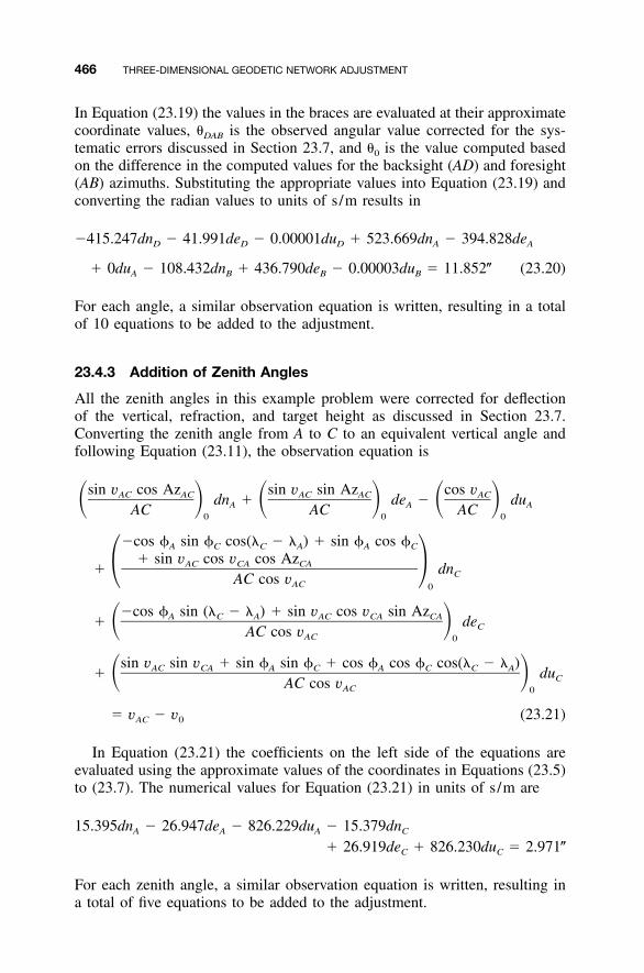
466 THREE-DIMENSIONAL GEODETIC NETWORK ADJUSTMENT
In Equation (23.19) the values in the braces are evaluated at their approximatecoordinate values, �DAB is the observed angular value corrected for the sys-tematic errors discussed in Section 23.7, and �0 is the value computed basedon the difference in the computed values for the backsight (AD) and foresight(AB) azimuths. Substituting the appropriate values into Equation (23.19) andconverting the radian values to units of s/m results in
�415.247dn � 41.991de � 0.00001du � 523.669dn � 394.828deD D D A A
� 0du � 108.432dn � 436.790de � 0.00003du � 11.852�A B B B (23.20)
For each angle, a similar observation equation is written, resulting in a totalof 10 equations to be added to the adjustment.
23.4.3 Addition of Zenith Angles
All the zenith angles in this example problem were corrected for deflectionof the vertical, refraction, and target height as discussed in Section 23.7.Converting the zenith angle from A to C to an equivalent vertical angle andfollowing Equation (23.11), the observation equation is
sin v cos Az sin v sin Az cos vAC AC AC AC ACdn � de � du� � � � � �A A AAC AC AC0 0 0
�cos � sin � cos(� � � ) � sin � cos �A C C A A C
� sin v cos v cos AzAC CA CA� dn � CAC cos vAC 0
�cos � sin (� � � ) � sin v cos v sin AzA C A AC CA CA� de� � CAC cos vAC 0
sin v sin v � sin � sin � � cos � cos � cos(� � � )AC CA A C A C C A� du� � CAC cos vAC 0
� v � vAC 0 (23.21)
In Equation (23.21) the coefficients on the left side of the equations areevaluated using the approximate values of the coordinates in Equations (23.5)to (23.7). The numerical values for Equation (23.21) in units of s/m are
15.395dn � 26.947de � 826.229du � 15.379dnA A A C
� 26.919de � 826.230du � 2.971�C C
For each zenith angle, a similar observation equation is written, resulting ina total of five equations to be added to the adjustment.
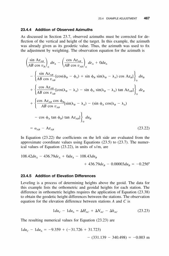
23.4 EXAMPLE ADJUSTMENT 467
23.4.4 Addition of Observed Azimuths
As discussed in Section 23.7, observed azimuths must be corrected for de-flection of the vertical and height of the target. In this example, the azimuthwas already given as its geodetic value. Thus, the azimuth was used to fixthe adjustment by weighting. The observation equation for the azimuth is
sin Az cos AzAB ABdn � de � 0du� � � �A A AAB cos v AB cos vB AB0 0
sin AzAB� [cos(� � � ) � sin � sin(� � � ) cos Az ] dn� B A B B A B BAB cos vAB 0
cos AzAB� [cos(� � � ) � sin � sin(� � � ) tan Az ] de� B A A B A AB BAB cos vAB 0
cos Az cos �AB B� [sin(� � � ) � (sin � cos(� � � )� B A A B AAB cos vAB
� cos � tan � ) tan Az ] duA B AB B0
� � � AzAB AB (23.22)
In Equation (23.22) the coefficients on the left side are evaluated from theapproximate coordinate values using Equations (23.5) to (23.7). The numer-ical values of Equation (23.22), in units of s/m, are
108.42dn � 436.79de � 0du � 108.43dnA A A B
� 436.79de � 0.00003du � �0.256�B B
23.4.5 Addition of Elevation Differences
Leveling is a process of determining heights above the geoid. The data forthis example lists the orthometric and geoidal heights for each station. Thedifference in orthometric heights requires the application of Equation (23.38)to obtain the geodetic height differences between the stations. The observationequation for the elevation difference between stations A and C is
1du � 1du � �H � �N � �h (23.23)C A AC AC AC
The resulting numerical values for Equation (23.23) are
1du � 1du � �9.359 � (�31.726 � 31.723)C A
� (331.139 � 340.498) � �0.003 m
468 THREE-DIMENSIONAL GEODETIC NETWORK ADJUSTMENT
23.4.6 Adjustment of Control Stations
With the addition of the u coordinate, observation equations similar to thosepresented in Section 20.2 can be added for each control coordinate. As statedin Section 23.1, the local geodetic coordinate system has its origin at eachinstrument station. Thus it is not a true coordinate system with a single origin.Because of this, the approximate coordinates for each station must be storedin either the geocentric or geodetic coordinate system. In this discussion, itis assumed that the values are stored in the geodetic coordinate system. Again,nonlinear versions of the equations must be written to match the overall non-linear nature of the adjustment. The observation equations are
1dn � N � n (23.24)
1de � E � e (23.25)
1du � U � u (23.26)
where (N,E,U) are the given control coordinate values and (n,e,u) are theiradjusted values. In the first iteration, the control coordinate values and theiradjusted values will be the same. In subsequent iterations, small variationsbetween the control coordinate values and their adjusted counterparts will beobserved. The observation equations for station A in the first iteration are
1dn � 0
1de � 0
1du � 0
Since the control coordinate values and approximate station coordinatevalues will be expressed in terms of geodetic coordinates, the initial K-matrixvalues given in Equations (23.24) to (23.26) will be expressed as changes ingeodetic coordinates. These values must then be transformed into the localgeodetic coordinate system. The relationships between changes in the twosystems are
dn M � h 0 0 d� d�de � 0 (N � h) cos � 0 d� � R d� (23.27)LG� � � �� � � �du 0 0 1 dh dh
In Equation (23.27), M represents the radius in the meridian and N theradius in the normal at a station with latitude � as given by Equation (23.16),h the geodetic height, and RLG the transformation matrix between changes inthe geodetic and local geodetic coordinate systems. The K-matrix values ex-
23.4 EXAMPLE ADJUSTMENT 469
pressed in terms of geodetic coordinate system can be transformed into K-matrix values of the local geodetic coordinate system using Equation (23.27).
23.4.7 Results of Adjustment
A partial list of the results of the adjustment from the ADJUST softwarepackage is given in Figure 23.5. The solution converged in two iterations.Note that the latitude and longitude of station A were held fixed, as was theazimuth of line AB.
23.4.8 Updating Geodetic Coordinates
At the completion of each iteration, the corrections of dn, de, and du will bedetermined for each station in the adjustment. However, geodetic coordinatesare used to represent station positions. Thus, after each iteration the localgeodetic coordinate system corrections of dn, de, and du must be transformedinto changes in the geodetic system using the inverse relationship of Equation(23.27), or
dn dei id� � d� � dh � de (23.28)i i i iM � h (N � h ) cos �i i i i i
In Equation (23.28), the corrections to the latitude, longitude, and geodeticheight of station I are d�i, d�i, and dhi, respectively. All other terms are asdefined previously. Similarly, the uncertainties for each station will be in thelocal geodetic system. Although these uncertainties can be used to representnorthing, easting, and geodetic height errors at each station, Equation (6.13)must be used to transform these uncertainties into the geodetic system as
�1 �T� � R � R (23.29)�,�,h n,e,u
where
2 M � h 0 0� �,� �,h2� � � R � 0 (N � h) cos � 0�,� � �,h�,�,h � � � �2 0 0 1�,h �,h h
2 n n,e n,u2� � n,e e e,un,e,u � �2 n,u e,u u
Note that each station’s uncertainties can be computed using the 3 � 3 blockdiagonal elements from the Qxx matrix of the adjustment.
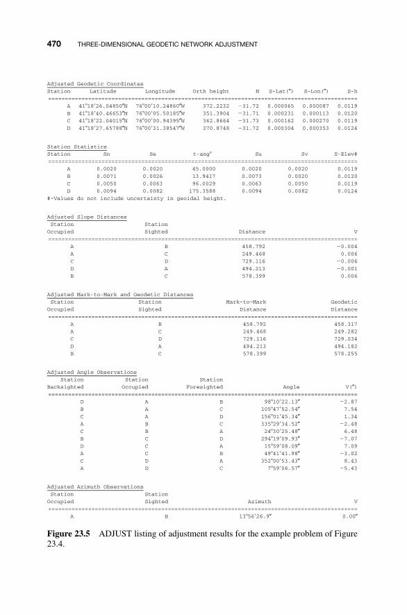
470 THREE-DIMENSIONAL GEODETIC NETWORK ADJUSTMENT
Adjusted Geodetic Coordinates
Station Latitude Longitude Orth height N S-Lat(�) S-Lon(�) S-h
=============================================================================================
A 41�18�26.04850�N 76�00�10.24860�W 372.2232 �31.72 0.000065 0.000087 0.0119
B 41�18�40.46653�N 76�00�05.50185�W 351.3904 �31.71 0.000231 0.000113 0.0120
C 41�18�22.04015�N 76�00�00.94395�W 362.8664 �31.73 0.000162 0.000270 0.0119
D 41�18�27.65788�N 76�00�31.38547�W 370.8748 �31.72 0.000304 0.000353 0.0124
Station Statistics
Station Sn Se t-ang� Su Sv S-Elev#
=============================================================================================
A 0.0020 0.0020 45.0000 0.0020 0.0020 0.0119
B 0.0071 0.0026 13.9417 0.0073 0.0020 0.0120
C 0.0050 0.0063 96.0029 0.0063 0.0050 0.0119
D 0.0094 0.0082 175.3588 0.0094 0.0082 0.0124
#-Values do not include uncertainty in geoidal height.
Adjusted Slope Distances
Station
Occupied
Station
Sighted Distance V
=============================================================================================
A B 458.792 �0.004
A C 249.468 0.006
C D 729.116 �0.006
D A 494.213 �0.001
B C 578.399 0.006
Adjusted Mark-to-Mark and Geodetic Distances
Station
Occupied
Station
Sighted
Mark-to-Mark
Distance
Geodetic
Distance
=============================================================================================
A B 458.792 458.317
A C 249.468 249.282
C D 729.116 729.034
D A 494.213 494.182
B C 578.399 578.255
Adjusted Angle Observations
Station
Backsighted
Station
Occupied
Station
Foresighted Angle V(�)
=============================================================================================
D A B 98�10�22.13� �2.87
B A C 105�47�52.54� 7.54
C A D 156�01�45.34� 1.34
A B C 335�29�34.52� �2.48
C B A 24�30�25.48� 6.48
B C D 294�19�09.93� �7.07
D C A 15�59�08.09� 7.09
A C B 49�41�41.98� �3.02
C D A 352�00�53.43� 8.43
A D C 7�59�06.57� �5.43
Adjusted Azimuth Observations
Station
Occupied
Station
Sighted Azimuth V
=============================================================================================
A B 13�56�26.9� 0.00�
Figure 23.5 ADJUST listing of adjustment results for the example problem of Figure23.4.
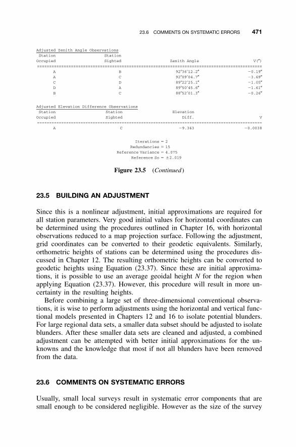
23.6 COMMENTS ON SYSTEMATIC ERRORS 471
Adjusted Zenith Angle Observations
Station
Occupied
Station
Sighted Zenith Angle V(�)
=============================================================================================
A B 92�36�12.2� �0.19�
A C 92�09�04.7� �3.69�
C D 89�22�25.1� �1.05�
D A 89�50�45.6� �1.61�
B C 88�52�01.3� �0.26�
Adjusted Elevation Difference Observations
Station
Occupied
Station
Sighted
Elevation
Diff. V
=============================================================================================
A C �9.363 �0.0038
Iterations � 2
Redundancies � 15
Reference Variance � 4.075
Reference So � �2.019
Figure 23.5 (Continued )
23.5 BUILDING AN ADJUSTMENT
Since this is a nonlinear adjustment, initial approximations are required forall station parameters. Very good initial values for horizontal coordinates canbe determined using the procedures outlined in Chapter 16, with horizontalobservations reduced to a map projection surface. Following the adjustment,grid coordinates can be converted to their geodetic equivalents. Similarly,orthometric heights of stations can be determined using the procedures dis-cussed in Chapter 12. The resulting orthometric heights can be converted togeodetic heights using Equation (23.37). Since these are initial approxima-tions, it is possible to use an average geoidal height N for the region whenapplying Equation (23.37). However, this procedure will result in more un-certainty in the resulting heights.
Before combining a large set of three-dimensional conventional observa-tions, it is wise to perform adjustments using the horizontal and vertical func-tional models presented in Chapters 12 and 16 to isolate potential blunders.For large regional data sets, a smaller data subset should be adjusted to isolateblunders. After these smaller data sets are cleaned and adjusted, a combinedadjustment can be attempted with better initial approximations for the un-knowns and the knowledge that most if not all blunders have been removedfrom the data.
23.6 COMMENTS ON SYSTEMATIC ERRORS
Usually, small local surveys result in systematic error components that aresmall enough to be considered negligible. However as the size of the survey
472 THREE-DIMENSIONAL GEODETIC NETWORK ADJUSTMENT
increases, variations in the direction of plumb lines must be taken into ac-count. This error can be removed from angular observations prior to the ad-justment with a priori knowledge of the deflection components and � ateach station. Modeled values for these components can be obtained usingsoftware such as DEFLEC99,1 which is available from the National GeodeticSurvey. The systematic error corrections to the zenith angles, azimuths, andhorizontal angles are
z � z� � � cos Az � sin Az (23.30)ij ij i ij i ij
Az � Az � tan � � (� sin Az � cos Az ) cot z (23.31)ij obs i i i obs i obs ij
∠BIF � ∠BIF � (� sin Az � cos Az ) cot zobs i if i if if
� (� sin Az � cos Az ) cot z (23.32)i ib i ib ib
where i and �i are the deflection of the vertical components at the observationstation I; zij� is the zenith angle observed from station I to J; zij the correctedzenith angle between the same stations; Azobs the astronomical azimuth ob-served between station I and J; Azij the corrected azimuth; ∠BIFobs the angleobserved where station B is the backsight station, I the instrument station,and F the foresight station; and ∠BIF the corrected horizontal angle.
Additionally, target height differences must also be considered for bothdirections and angles. The azimuth of a line corrected for target height is
20.108� cos � sin 2� hicAz � � � (23.33)1000
In Equation (23.33), Azc is the corrected azimuth, � the observed azimuth,�i the latitude of the observation station, and h the geodetic height of thetarget in meters. Since an angle is simply the difference between the foresightand backsight azimuths, the correction to an angle due to the height of thetargets is
h sin 2� sin 2� hƒ if ib bc 2� � � � 0.108� cos � � (23.34)� �bif i 1000 1000
where �c is the corrected angle, �bif the observed angle, and �if and �ib theazimuths of the foresight and backsight lines, respectively.
Atmospheric refraction must be considered when including vertical or ze-nith angles in an adjustment. Since the correction for atmospheric refraction
1 DEFLEC99 is available at http: / /www.ngs.noaa.gov /PC PROD/pc prod.shtml#DEFLEC99.
23.6 COMMENTS ON SYSTEMATIC ERRORS 473
is so difficult to model, one can only hope to account for a portion of cor-rection in an adjustment. The remainder of the correction must be modeledin the adjustment or be absorbed in the residuals of the observation. Thecorrection of the first-order effect of refraction can be determined by observ-ing simultaneously vertical or zenith angles at each end of the line IJ. Fromthese observations, the first-order correction �Zij for reciprocal zenith anglesis determined as
�Z � �Z � 90� � [0.5(Z � Z ) � �] (23.35)ij ji ij ji
In Equation (23.35), Zij and Zji are the reciprocal zenith angles observed si-multaneously and � is the correction for the deflection of vertical, computedas
� � �(� cos Az � sin Az ) (23.36)i ij i ij
It is possible to create an adjustment model that includes correction termsfor , �, and atmospheric refraction. However, due to the limited number ofobservations in a typical survey network, there is a danger of overparameter-ization (Leick, 2004). Thus, it is recommended that these corrections be ap-plied to the angles before carrying out the adjustment.
Unfortunately, to determine the deflection of the vertical components (and �), the latitude and longitude of the station must be known before com-pletion of the adjustment. Approximate values for latitude and longitude willsuffice in most instances. However, in instances where good approximationsfor the geodetic coordinates are not known, it is possible to correct the originalobservations after an initial adjustment to ensure that the geodetic coordinatesfor each station are close to their final values. In this case, after correctingthe observations, the adjustment could be run a second time.
A similar problem exists with differential leveling observations. Geodeticheight h and orthometric height H differ by the geoidal height N, or
h � H � N (23.37)
Elevation differences as determined by differential leveling must accountfor the differences in geoidal height between the benchmark stations. Thissituation can be described mathematically as
h � h � (H � N ) � (H � N )j i j j i i
�h � �H � �N (23.38)
The correction to leveled height differences should be performed whenthese observations are included in the three-dimensional geodetic network
474 THREE-DIMENSIONAL GEODETIC NETWORK ADJUSTMENT
adjustment. Values for geoidal height can be determined using the GEOID03software available from the National Geodetic Survey.2 Similar to deflectionof the vertical parameters, it is possible to include geoidal height parametersin the mathematical model of the adjustment. Again, this approach runs a riskof overparameterization in the adjustment.
The orthometric correction OC for a leveling line can be approximatedusing a formula derived by Bomford (1980) as
�H(���)(0.0053 sin 2�)O � (23.39)C
where H is the orthometric height at the instrument station in meters, ��� thechange in latitude between the backsight and foresight stations in units ofseconds, � the latitude of the instrument station, and the conversion fromseconds to radians, which is approximately 206,264.8� / rad. Obviously, Equa-tion (23.39) would be tedious to apply for a substantial north–south levelingcircuit. However, for most typical surveys involving small regions, this cor-rection can be very small and easily absorbed in the residuals of the adjust-ment. For instance, a 120-km north–south leveling line at approximately 42�latitude would result in an orthometric correction of about 2 cm.
PROBLEMS
Note: Unless otherwise specified, use the GRS 80 ellipsoidal parameters of a� 6.378.137.0 m and ƒ � 1/298.257222101 for the following problems.
23.1 Using the data supplied in Figure 23.4, what value is computed forthe slant distance AB?
23.2 Repeat Problem 23.1 for slant distance AC.
23.3 Using the data supplied in Figure 23.4, what value is computed forthe azimuth AB?
23.4 Using the data supplied in Figure 23.4, what value is computed forthe horizontal angle DAB?
23.5 Repeat Problem 23.4 for horizontal angle ACB.
23.6 Using the data supplied in Figure 23.4, what value is computed forvAB?
2GEOID03 software is available at http: / /www.ngs.noaa.gov.
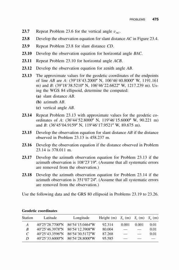
PROBLEMS 475
23.7 Repeat Problem 23.6 for the vertical angle vAC.
23.8 Develop the observation equation for slant distance AC in Figure 23.4.
23.9 Repeat Problem 23.8 for slant distance CD.
23.10 Develop the observation equation for horizontal angle BAC.
23.11 Repeat Problem 23.10 for horizontal angle ACB.
23.12 Develop the observation equation for zenith angle AB.
23.13 The approximate values for the geodetic coordinates of the endpointsof line AB are A: (39�18�43.2000� N, 106�46�40.8000� W, 1191.161m) and B: (39�18�38.5210� N, 106�46�22.6822� W, 1217.239 m). Us-ing the WGS 84 ellipsoid, determine the computed:(a) slant distance AB.(b) azimuth AB.(c) vertical angle AB.
23.14 Repeat Problem 23.13 with approximate values for the geodetic co-ordinates of A: (36�44�52.8000� N, 119�46�15.6000� W, 90.221 m)and B: (36�45�04.9159� N, 119�46�17.9521� W, 89.675 m).
23.15 Develop the observation equation for slant distance AB if the distanceobserved in Problem 23.13 is 458.237 m.
23.16 Develop the observation equation if the distance observed in Problem23.14 is 378.011 m.
23.17 Develop the azimuth observation equation for Problem 23.13 if theazimuth observation is 108�23�19�. (Assume that all systematic errorsare removed from the observation.)
23.18 Develop the azimuth observation equation for Problem 23.14 if theazimuth observation is 351�07�24�. (Assume that all systematic errorsare removed from the observation.)
Use the following data and the GRS 80 ellipsoid in Problems 23.19 to 23.26.
Geodetic coordinates
Station Latitude Longitude Height (m) Sn (m) Se (m) Su (m)
A 40�25�28.7700�N 86�54�15.0464�W 92.314 0.001 0.001 0.01B 40�25�46.3978�N 86�54�12.3908�W 80.004 — — 0.01C 40�25�43.3596�N 86�54�30.5172�W 87.268 — — 0.01D 40�25�33.6000�N 86�54�28.8000�W 95.585 — — —
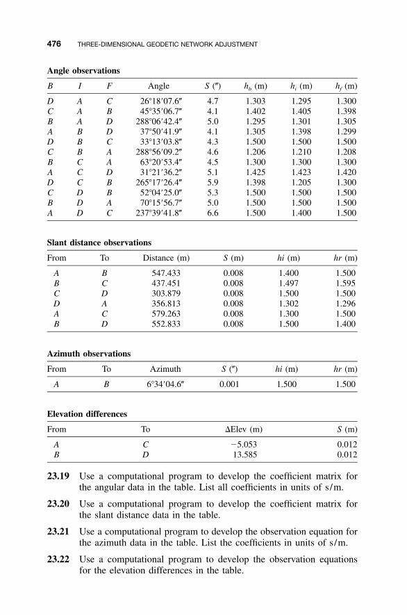
476 THREE-DIMENSIONAL GEODETIC NETWORK ADJUSTMENT
Angle observations
B I F Angle S (�) hb (m) hi (m) hf (m)
D A C 26�18�07.6� 4.7 1.303 1.295 1.300C A B 45�35�06.7� 4.1 1.402 1.405 1.398B A D 288�06�42.4� 5.0 1.295 1.301 1.305A B D 37�50�41.9� 4.1 1.305 1.398 1.299D B C 33�13�03.8� 4.3 1.500 1.500 1.500C B A 288�56�09.2� 4.6 1.206 1.210 1.208B C A 63�20�53.4� 4.5 1.300 1.300 1.300A C D 31�21�36.2� 5.1 1.425 1.423 1.420D C B 265�17�26.4� 5.9 1.398 1.205 1.300C D B 52�04�25.0� 5.3 1.500 1.500 1.500B D A 70�15�56.7� 5.0 1.500 1.500 1.500A D C 237�39�41.8� 6.6 1.500 1.400 1.500
Slant distance observations
From To Distance (m) S (m) hi (m) hr (m)
A B 547.433 0.008 1.400 1.500B C 437.451 0.008 1.497 1.595C D 303.879 0.008 1.500 1.500D A 356.813 0.008 1.302 1.296A C 579.263 0.008 1.300 1.500B D 552.833 0.008 1.500 1.400
Azimuth observations
From To Azimuth S (�) hi (m) hr (m)
A B 6�34�04.6� 0.001 1.500 1.500
Elevation differences
From To �Elev (m) S (m)
A C �5.053 0.012B D 13.585 0.012
23.19 Use a computational program to develop the coefficient matrix forthe angular data in the table. List all coefficients in units of s/m.
23.20 Use a computational program to develop the coefficient matrix forthe slant distance data in the table.
23.21 Use a computational program to develop the observation equation forthe azimuth data in the table. List the coefficients in units of s/m.
23.22 Use a computational program to develop the observation equationsfor the elevation differences in the table.
PROBLEMS 477
23.23 Use ADJUST to determine the most probable values for the geodeticcoordinates in the table using only the angle, azimuth, and slant dis-tance observations.
23.24 Use ADJUST to determine the most probable values for the geodeticcoordinates in the table using all the observations. Remember to ac-count for the geoidal height at each station.
23.25 Repeat Problem 23.24 by removing azimuth AB from the adjustmentand overweighting the easting of station B. The standard deviationsof station B should be Sn � �1000 m, Se � �0.001 m, and Su ��0.01 m.
23.26 What are the adjusted orthometric heights of the stations in the table?
23.27 If � � 4.87� and � 0.01� are the deflection of the vertical compo-nents at station A in Section 23.4, what is the correction to the zenithangle going from station A to B?
23.28 Repeat Problem 23.27 for the zenith angle from station A to C.
23.29 If the zenith angle observed from A to B in Figure 23.6 is 91�04�54�and the deflection of the vertical components are � � 1.28� and �3.58�, what is the corrected zenith angle?
23.30 Using the data given in Problem 23.27, what is the deflection of thevertical correction for the azimuth AB?
23.31 Using the data given in Problem 23.29, what is the deflection of thevertical correction for the azimuth AB?
23.32 Using the data given in Problem 23.27, what is the deflection of thevertical correction for the angle DAB?
23.33 Using the data given in Problem 23.29, what is the deflection of thevertical correction for the angle DAC?
23.34 Do Problem 23.33 using angle CAB.
Programming Problems
23.35 Develop a computational program that corrects vertical angles fordeflection of the vertical components.
23.36 Develop a computational program that computes the coefficients forthe azimuths, angles, slant distances, and elevation differences. Checkyour program using data from Figure 23.6.
23.37 Modify the Mathcad worksheets provided for Chapter 23 on the CDthat accompanies this book to incorporate target and instrumentheights. Solve Problem 23.6.
478
CHAPTER 24
COMBINING GPS ANDTERRESTRIAL OBSERVATIONS
24.1 INTRODUCTION
Ellipsoids define the mathematical shape of Earth or a portion thereof. Ellip-soids are commonly defined by the length of their semimajor axis, a, and theflattening factor, ƒ. Commonly used ellipsoids are the Geodetic ReferenceSystem of 1980 (GRS 80) and the World Geodetic System of 1984 (WGS84). Table 24.1 lists the length of the semimajor axis and flattening factor forthese ellipsoids.
A network of points determined with respect to an ellipsoid is a datum.Datums define the geodetic coordinates of the points and thus the origin andorientation of the datum. Most datums are regional in nature since the networkof points covers only a portion of the Earth. These are known as local datums.For example, the North American Datum of 1983 (NAD 83) is a local datumconsisting of a network of points in Canada, the United States, Mexico, andsome Caribbean islands. However, the International Terrestrial ReferenceFrame (ITRF) is an example of a datum defined by a multitude of pointslocated on all of Earth’s major land masses. This is known as a global datum.Similarly, the coordinates of the GPS satellites are determined by a globalnetwork of tracking stations on a unique datum. Stated incorrectly, GPS issaid to be using the WGS 84 datum. This statement should be interpreted bythe reader as the datum defined by the global network of tracking stationsthat use the WGS 84 ellipsoid.
Besides their reference ellipsoid, datums differ in origin (translation), scale,and rotations about the three cardinal axes. Many modern local datums andglobal datums have nearly aligned coordinate axes and differ by only a fewmeters in their origins. Thus, it is possible to use a three-dimensional coor-
Adjustment Computations: Spatial Data Analysis, Fourth Edition. C. D. Ghilani and P. R. Wolf© 2006 John Wiley & Sons, Inc. ISBN: 978-0-471-69728-2
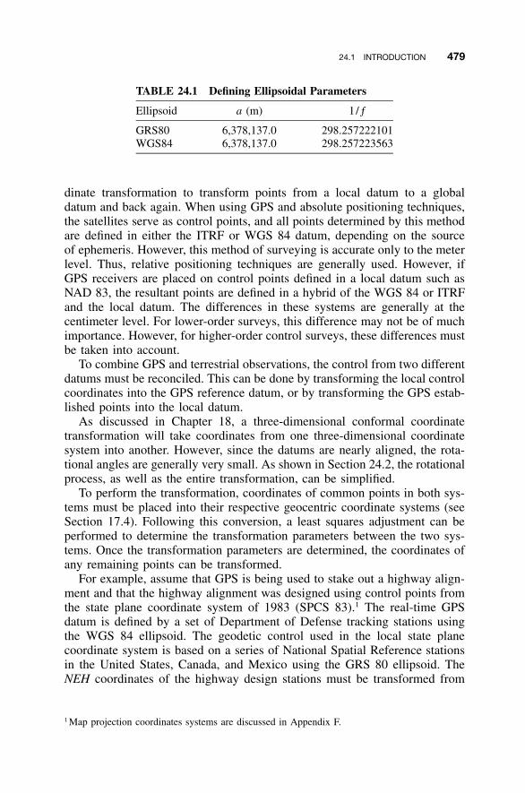
24.1 INTRODUCTION 479
TABLE 24.1 Defining Ellipsoidal Parameters
Ellipsoid a (m) 1/ƒ
GRS80 6,378,137.0 298.257222101WGS84 6,378,137.0 298.257223563
dinate transformation to transform points from a local datum to a globaldatum and back again. When using GPS and absolute positioning techniques,the satellites serve as control points, and all points determined by this methodare defined in either the ITRF or WGS 84 datum, depending on the sourceof ephemeris. However, this method of surveying is accurate only to the meterlevel. Thus, relative positioning techniques are generally used. However, ifGPS receivers are placed on control points defined in a local datum such asNAD 83, the resultant points are defined in a hybrid of the WGS 84 or ITRFand the local datum. The differences in these systems are generally at thecentimeter level. For lower-order surveys, this difference may not be of muchimportance. However, for higher-order control surveys, these differences mustbe taken into account.
To combine GPS and terrestrial observations, the control from two differentdatums must be reconciled. This can be done by transforming the local controlcoordinates into the GPS reference datum, or by transforming the GPS estab-lished points into the local datum.
As discussed in Chapter 18, a three-dimensional conformal coordinatetransformation will take coordinates from one three-dimensional coordinatesystem into another. However, since the datums are nearly aligned, the rota-tional angles are generally very small. As shown in Section 24.2, the rotationalprocess, as well as the entire transformation, can be simplified.
To perform the transformation, coordinates of common points in both sys-tems must be placed into their respective geocentric coordinate systems (seeSection 17.4). Following this conversion, a least squares adjustment can beperformed to determine the transformation parameters between the two sys-tems. Once the transformation parameters are determined, the coordinates ofany remaining points can be transformed.
For example, assume that GPS is being used to stake out a highway align-ment and that the highway alignment was designed using control points fromthe state plane coordinate system of 1983 (SPCS 83).1 The real-time GPSdatum is defined by a set of Department of Defense tracking stations usingthe WGS 84 ellipsoid. The geodetic control used in the local state planecoordinate system is based on a series of National Spatial Reference stationsin the United States, Canada, and Mexico using the GRS 80 ellipsoid. TheNEH coordinates of the highway design stations must be transformed from
1 Map projection coordinates systems are discussed in Appendix F.
480 COMBINING GPS AND TERRESTRIAL OBSERVATIONS
the SPCS 83 coordinate system and orthometric heights to geodetic coordi-nates. The geodetic coordinates are then transformed to geocentric coordi-nates2 of (X,Y,Z)LS. These points must be occupied using a GPS receiver andGPS coordinates (X,Y,Z)GPS derived from satellite observations. Once threecommon points are occupied, the transformation parameters can be deter-mined using a Helmert transformation. However, the prudent surveyor willuse four common points to increase the number of redundant measurements.Following this, all GPS coordinates are transferred into the local coordinatesystem, and stakeout of stations can be performed.
24.2 HELMERT TRANSFORMATION
Local datums such as NAD 83 are known as Earth-centered, Earth-fixed(ECEF) coordinate systems. This means that the Z axis is nearly aligned withthe Conventional Terrestrial Pole, X axis with the Greenwich Meridian, andthe origin is at the mass center of the Earth as derived by the datum pointsused in the definition. International datums such as the International Terres-trial Reference Frame use the same definitions for the axes, origin, and ellip-soid, but differ slightly due to the difference in the datum points used in itsdetermination. Thus, the rotational parameters and translations between twoECEF coordinate systems are usually very small. The scale factor betweentwo datums using the same units of measure should be nearly 1.
Since the sine of a very small angle is equal to the angle in radians, thecosine of a very small angle is nearly 1, and the product of two very smallnumbers is nearly zero, for two nearly aligned coordinate systems Equation(18.14) can be simplified as
1 � �� 0 �� ���3 2 3 2
R� � �� 1 � � I � ��� 0 �� � I � �R3 1 3 1� � � �� �� 1 �� ��� 02 1 2 1
(24.1)
In Equation (24.1) ��1, ��2, and ��3 are in units of radians and have beenseparated from the full matrix by the addition of the unit matrix. The intro-duction of � indicates that these values are differentially small.
The transformation of coordinates from one local datum to another datumis performed as
X � sR�X � T (24.2)LD GD
2 Equations to convert geodetic coordinates to geocentric coordinates are given in Section 17.5.Appendix F has equations to convert geodetic coordinates to state plane coordinates.
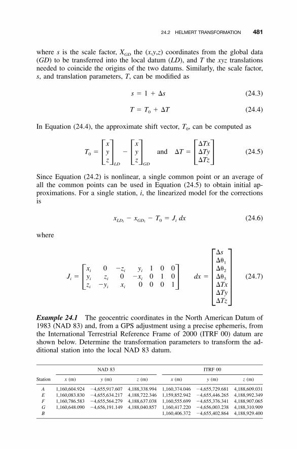
24.2 HELMERT TRANSFORMATION 481
where s is the scale factor, XGD the (x,y,z) coordinates from the global data(GD) to be transferred into the local datum (LD), and T the xyz translationsneeded to coincide the origins of the two datums. Similarly, the scale factor,s, and translation parameters, T, can be modified as
s � 1 � �s (24.3)
T � T � �T (24.4)0
In Equation (24.4), the approximate shift vector, T0, can be computed as
x x �TxT � y � y and �T � �Ty (24.5)0 � � � � � �z z �Tz
LD GD
Since Equation (24.2) is nonlinear, a single common point or an average ofall the common points can be used in Equation (24.5) to obtain initial ap-proximations. For a single station, i, the linearized model for the correctionsis
x � x � T � J dx (24.6)LD GD 0 ii i
where
�s��1
x 0 �z y 1 0 0 ��i i i 2
J � y z 0 �x 0 1 0 dx � �� (24.7)i i i i 3� �z �y x 0 0 0 1 �Txi i i � ��Ty�Tz
Example 24.1 The geocentric coordinates in the North American Datum of1983 (NAD 83) and, from a GPS adjustment using a precise ephemeris, fromthe International Terrestrial Reference Frame of 2000 (ITRF 00) datum areshown below. Determine the transformation parameters to transform the ad-ditional station into the local NAD 83 datum.
NAD 83 ITRF 00
Station x (m) y (m) z (m) x (m) y (m) z (m)
A 1,160,604.924 �4,655,917.607 4,188,338.994 1,160,374.046 �4,655,729.681 4,188,609.031E 1,160,083.830 �4,655,634.217 4,188,722.346 1,159,852.942 �4,655,446.265 4,188,992.349F 1,160,786.583 �4,655,564.279 4,188,637.038 1,160,555.699 �4,655,376.341 4,188,907.065G 1,160,648.090 �4,656,191.149 4,188,040.857 1,160,417.220 �4,656,003.238 4,188,310.909B 1,160,406.372 �4,655,402.864 4,188,929.400

482 COMBINING GPS AND TERRESTRIAL OBSERVATIONS
SOLUTION First iteration: Using station A, T0 is
1,160,604.924 � 1,160,374.046 230.877T � �4,655,917.607 � 4,655,729.681 � �187.9260 � � � �4,188,338.994 � 4,188,609.031 �270.037
The J and K matrices are
1160374.046 0.000 �4188609.031 �4655729.681 1 0 0�4655729.681 4188609.031 0.000 �1160374.046 0 1 0
4188609.031 4655729.681 1160374.0464 0.000 0 0 11159852.942 0.000 �4188992.349 �4655446.265 1 0 0
�4655446.265 4188992.349 0.000 �1159852.942 0 1 04188992.349 4655446.265 1159852.942 0.000 0 0 1
J �1160555.699 0.000 �4188907.065 �4655376.341 1 0 0
�4655376.341 4188907.065 0.000 �1160555.699 0 1 04188907.065 4655376.341 1160555.699 0.000 0 0 11160417.220 0.000 �4188310.909 �4656003.238 1 0 0
�4656003.238 4188310.909 0.000 �1160417.220 0 1 041883120.909 4656003.238 1160417.220 0.000 0 0 1
0.0000.0000.0000.011
�0.0260.034
K �0.006
�0.0120.010
�0.0080.015
�0.015
Solving Equation (11.37) using the matrices above and adding X to the initialvalues results in
0.0000000256 s � 1 � 0.0000000256 � 1.0000000256�0.0000486262 � � �0�00�10.02987�1
�0.0000388234 � � �0�00�08.0079�2
X � �0.0000146664 � � �0�00�03.02517�3
�230.9285 Tx � 230.877 � 230.92 � �0.052� �186.7768 Ty � �187.926 � 186.7768 � �1.149271.3325 Tz � �270.037 � 271.3325 � 1.295
24.2 HELMERT TRANSFORMATION 483
The next iteration resulted in negligible changes in the translations, andthus the transformation parameters are as listed. Using Equation (24.2), trans-formation parameters, and the GPS-derived ITRF 00 coordinates for stationB, the NAD 83 coordinates for station B are
geocentric coordinates � (1,160,637.257 �4,655,590.805, 4,188,659.377)
geodetic coordinates � (41�18�40.46653� N, 76�00�05.50185� W,
319.677 m)
SPCS 83 coordinates � (746,397.796 m, 128,586.853 m)
The reader should note that the NAD 83 coordinates for station B are thesame as those listed in Figure 23.5. However, slight differences in coordinatescan be expected, due to random errors in the transformation.
Example 24.1 demonstrates the mathematical relationship between the twodatums for this small set of points. This process should always be consideredwhen combining traditional observations with GPS coordinates in higher-order surveys. That is, if GPS derived coordinates are to be entered into anadjustment, they should first be transformed into the local datum. In theUnited States, the National Geodetic Survey has developed horizontal time-dependent positioning (HTDP) software3 that allows the users to transformcoordinates between NAD 83, WGS 84, and ITRF 00. This software alsotakes into account plate tectonics by applying velocity vectors to stationswhen they are known.
The process of transforming points from global datums to local datums isimportant when performing RTK-GPS stakeout surveys. A GPS survey im-plicitly uses the points located in a global datum. Since engineering plans aregenerally developed in a local datum such as NAD 83, the GPS-derived co-ordinate values must be transformed into the local coordinate system. Thisprocess is known as localization (sometimes called site calibration) by man-ufacturers. From a design point of view, it is important to recognize that thebest results will be obtained if points common in both datums surround theproject area. After entering in the local datum coordinates, the GPS receivershould occupy each station. The software will then compute the transforma-
3 A description of the HTDP software can be located on the NGS Web site at http: / /www.ngs.noaa.gov /TOOLS/Htdp /Htdp.shtml. A Mathcad worksheet that demonstrates this softwareis available on the CD that accompanies this book.
484 COMBINING GPS AND TERRESTRIAL OBSERVATIONS
tion parameters and use these to determine the coordinate values for the pointsto be surveyed.
24.3 ROTATIONS BETWEEN COORDINATE SYSTEMS
GPS uses the geocentric coordinate system and list its baseline vectors in thissystem. Often, it is preferable to obtain the coordinate changes in terms ofgeodetic coordinates. From geodesy, the relationship between changes in thegeodetic coordinate system and the geocentric coordinate system is
dXdx � dY� �dZ
�(M � h) sin � sin � �(N � h) cos � sin � cos � cos � d�� �(M � h) sin � sin � (N � h) cos � cos � cos � sin � d�� �� �(M � h) cos � 0 sin � dh
d�� R d�XG� �dh
(24.8)
where dx represents the changes in the geocentric coordinates, M is the radiusin the meridian, and N the radius in the normal at latitude � as given byEquation (23.16), h is the geodetic height of the point, and RXG is the trans-formation matrix.
The transformation between changes in the geodetic coordinate system andthe local geodetic coordinate system are given in Equation (23.29), which isrepeated here for convenience:
dn M � h 0 0 d� d�de � 0 (N � h) cos � 0 d� � R d� (24.9)LG� � � �� � � �du 0 0 1 dh dh
where RLG is the rotation matrix between the geodetic and local geodeticcoordinate systems.
24.4 COMBINING GPS BASELINE VECTORS WITHTRADITIONAL OBSERVATIONS
As discussed in Chapter 23, the three-dimensional geodetic adjustment allowsthe adjustment of all traditional surveying observations. If the control isknown in the local coordinate system, Equation (24.2) can be included inadjustment to account for datum differences.
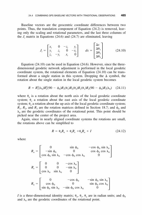
24.4 COMBINING GPS BASELINE VECTORS WITH TRADITIONAL OBSERVATIONS 485
Baseline vectors are the geocentric coordinate differences between twopoints. Thus, the translation component of Equation (24.2) is removed, leav-ing only the scaling and rotational parameters, and the last three columns ofthe Ji matrix in Equations (24.6) and (24.7) are eliminated, leaving
�sx 0 �z yi i i ��1J � y z 0 �x dx � (24.10)i i i i ��� � 2� �z �y x 0i i i ��3
Equation (24.10) can be used in Equation (24.6). However, since the three-dimensional geodetic network adjustment is performed in the local geodeticcoordinate system, the rotational elements of Equation (24.10) can be trans-formed about a single station in this system. Dropping the � symbol, therotation about the single station in the local geodetic system becomes
T TR � R (� )R (90 � � )R (� )R (� )R (� )R (90 � � )R (� ) (24.11)3 0 2 0 3 3 2 2 1 1 2 0 3 0
where �n is a rotation about the north axis of the local geodetic coordinatesystem; �e a rotation about the east axis of the local geodetic coordinatesystem; �u a rotation about the up axis of the local geodetic coordinate system;R1, R2, and R3 are the rotation matrices defined in Section 18.7; and �0 and�0 are the geodetic coordinates of the rotational point. This point should bepicked near the center of the project area.
Again, since in nearly aligned coordinate systems the rotations are small,the rotations above can be simplified to
R � � R � � R �� R � I (24.12)n n e e u u
where
0 sin � �cos � sin �0 0 0
R � �sin � 0 cos � cos �u 0 0 0� �cos � sin � �cos � cos � 00 0 0 0
0 0 �cos �0
R � 0 0 �sin �e 0� �cos � sin � 00 0
0 �cos � �sin � sin �0 0 0
R � cos � 0 sin � cos �n 0 0 0� �sin � sin � �sin � cos � 00 0 0 0
I is a three-dimensional identity matrix; �n, �e, �u are in radian units; and �0
and �0 are the geodetic coordinates of the rotational point.

486 COMBINING GPS AND TERRESTRIAL OBSERVATIONS
Finally, the transformation going from the observed GPS vector to its localgeodetic equivalent between stations I and J is
�X �XIJ IJ
�Y � (1 � s)R �Y (24.13)IJ IJ� � � ��Z �ZIJ IJ2 1
where s represents the differential scale change between systems 1 and 2, Ris defined in Equation (24.12), [�]1 represents the GPS baseline vector com-ponents in the local coordinate system, and [�]2 represents the GPS observedbaseline vector components between stations I and J.
In Chapter 23 the three-dimensional geodetic network adjustment was de-veloped in the local geodetic system. Thus, the addition of the GPS baselinevectors into this adjustment requires that the coefficient matrix be rotated intothe same system. Recall from Chapter 17 that the coefficient matrix (A) foreach GPS baseline vectors consisted of three rows containing �1, 0, and 1.This matrix must be rotated into the local geodetic system. Thus, for thebaseline vector IJ, the new coefficient matrix values are derived as
�1For station I: �(1 � s)R R (� , � ) R (� )XG i i LG i (24.14)�1For station J: (1 � s)R R (� , � ) R (� )XG j j LG j
where s is the change in scale between the two systems, rotation matrix R isdefined in Equation (24.12), rotation matrix RXG is defined in Equation (24.8),rotation matrix RLG is defined in Equation (24.9), and (�i, �i) and (�j, �j) arethe geodetic coordinates from stations I and J, respectively.
When developing the matrices for a least squares adjustment, the unknownparameters for scale and rotation should be set to zero. After the first iterationthese values will be modified and updated. At the end of the adjustment, theseparameters can be checked for statistical significance as described in Section18.8.
The elements of the coefficient matrix for the unknown rotation angles andscale are
X � X r r rJ I n e u1 1 1
J � Y � Y r r r (24.15)J I n e u2 2 2� �Z � Z r r rJ I n e u3 3 3
where XT � [�s ��n ��e ��u],
X � X X � X X � XJ I J I J I
r � R Y � Y , r � R Y � Y , r � R Y � Yn n J I e e J I u u J I� � � � � �Z � Z Z � Z Z � ZJ I J I J I
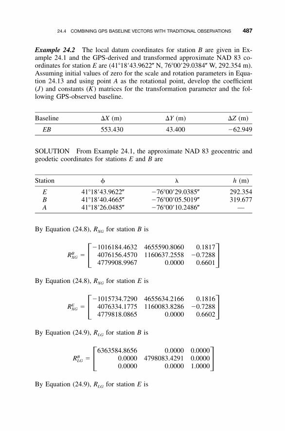
24.4 COMBINING GPS BASELINE VECTORS WITH TRADITIONAL OBSERVATIONS 487
Example 24.2 The local datum coordinates for station B are given in Ex-ample 24.1 and the GPS-derived and transformed approximate NAD 83 co-ordinates for station E are (41�18�43.9622� N, 76�00�29.0384� W, 292.354 m).Assuming initial values of zero for the scale and rotation parameters in Equa-tion 24.13 and using point A as the rotational point, develop the coefficient(J) and constants (K) matrices for the transformation parameter and the fol-lowing GPS-observed baseline.
Baseline �X (m) �Y (m) �Z (m)
EB 553.430 43.400 �62.949
SOLUTION From Example 24.1, the approximate NAD 83 geocentric andgeodetic coordinates for stations E and B are
Station � � h (m)
E 41�18�43.9622� �76�00�29.0385� 292.354B 41�18�40.4665� �76�00�05.5019� 319.677A 41�18�26.0485� �76�00�10.2486� —
By Equation (24.8), RXG for station B is
�1016184.4632 4655590.8060 0.1817BR � 4076156.4570 1160637.2558 �0.7288XG � �4779908.9967 0.0000 0.6601
By Equation (24.8), RXG for station E is
�1015734.7290 4655634.2166 0.1816ER � 4076334.1775 1160083.8286 �0.7288XG � �4779818.0865 0.0000 0.6602
By Equation (24.9), RLG for station B is
6363584.8656 0.0000 0.0000BR � 0.0000 4798083.4291 0.0000LG � �0.0000 0.0000 1.0000
By Equation (24.9), RLG for station E is
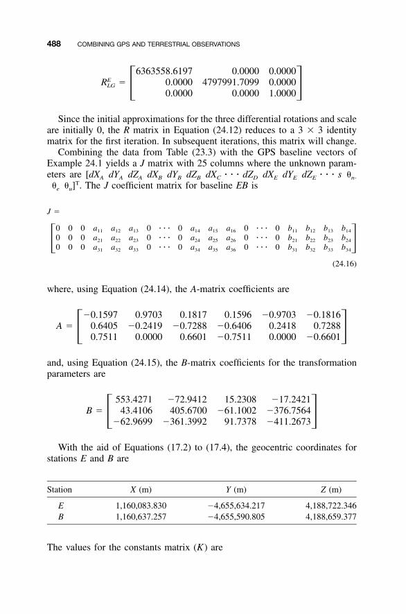
488 COMBINING GPS AND TERRESTRIAL OBSERVATIONS
6363558.6197 0.0000 0.0000ER � 0.0000 4797991.7099 0.0000LG � �0.0000 0.0000 1.0000
Since the initial approximations for the three differential rotations and scaleare initially 0, the R matrix in Equation (24.12) reduces to a 3 � 3 identitymatrix for the first iteration. In subsequent iterations, this matrix will change.
Combining the data from Table (23.3) with the GPS baseline vectors ofExample 24.1 yields a J matrix with 25 columns where the unknown param-eters are [dXA dYA dZA dXB dYB dZB dXC � � � dZD dXE dYE dZE � � � s �n-
�e �u]T. The J coefficient matrix for baseline EB is
J �
0 0 0 a a a 0 � � � 0 a a a 0 � � � 0 b b b b11 12 13 14 15 16 11 12 13 14
0 0 0 a a a 0 � � � 0 a a a 0 � � � 0 b b b b21 22 23 24 25 26 21 22 23 24� �0 0 0 a a a 0 � � � 0 a a a 0 � � � 0 b b b b31 32 33 34 35 36 31 32 33 34
(24.16)
where, using Equation (24.14), the A-matrix coefficients are
�0.1597 0.9703 0.1817 0.1596 �0.9703 �0.1816A � 0.6405 �0.2419 �0.7288 �0.6406 0.2418 0.7288� �0.7511 0.0000 0.6601 �0.7511 0.0000 �0.6601
and, using Equation (24.15), the B-matrix coefficients for the transformationparameters are
553.4271 �72.9412 15.2308 �17.2421B � 43.4106 405.6700 �61.1002 �376.7564� ��62.9699 �361.3992 91.7378 �411.2673
With the aid of Equations (17.2) to (17.4), the geocentric coordinates forstations E and B are
Station X (m) Y (m) Z (m)
E 1,160,083.830 �4,655,634.217 4,188,722.346B 1,160,637.257 �4,655,590.805 4,188,659.377
The values for the constants matrix (K) are
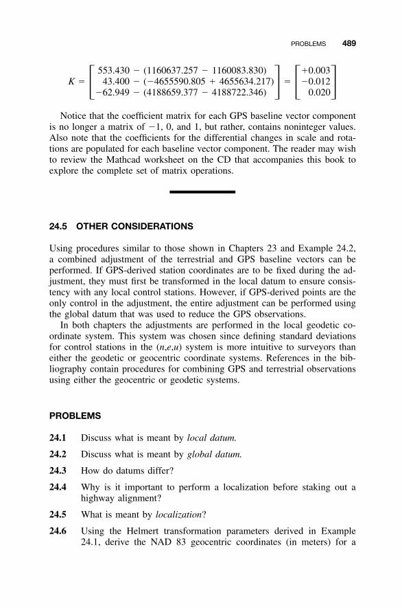
PROBLEMS 489
553.430 � (1160637.257 � 1160083.830) �0.003K � 43.400 � (�4655590.805 � 4655634.217) � �0.012� � � ��62.949 � (4188659.377 � 4188722.346) 0.020
Notice that the coefficient matrix for each GPS baseline vector componentis no longer a matrix of �1, 0, and 1, but rather, contains noninteger values.Also note that the coefficients for the differential changes in scale and rota-tions are populated for each baseline vector component. The reader may wishto review the Mathcad worksheet on the CD that accompanies this book toexplore the complete set of matrix operations.
24.5 OTHER CONSIDERATIONS
Using procedures similar to those shown in Chapters 23 and Example 24.2,a combined adjustment of the terrestrial and GPS baseline vectors can beperformed. If GPS-derived station coordinates are to be fixed during the ad-justment, they must first be transformed in the local datum to ensure consis-tency with any local control stations. However, if GPS-derived points are theonly control in the adjustment, the entire adjustment can be performed usingthe global datum that was used to reduce the GPS observations.
In both chapters the adjustments are performed in the local geodetic co-ordinate system. This system was chosen since defining standard deviationsfor control stations in the (n,e,u) system is more intuitive to surveyors thaneither the geodetic or geocentric coordinate systems. References in the bib-liography contain procedures for combining GPS and terrestrial observationsusing either the geocentric or geodetic systems.
PROBLEMS
24.1 Discuss what is meant by local datum.
24.2 Discuss what is meant by global datum.
24.3 How do datums differ?
24.4 Why is it important to perform a localization before staking out ahighway alignment?
24.5 What is meant by localization?
24.6 Using the Helmert transformation parameters derived in Example24.1, derive the NAD 83 geocentric coordinates (in meters) for a
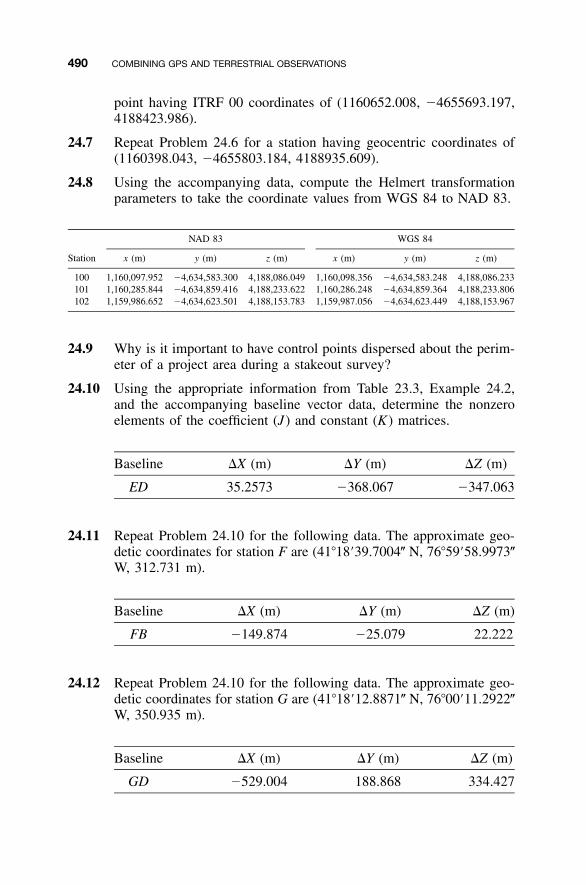
490 COMBINING GPS AND TERRESTRIAL OBSERVATIONS
point having ITRF 00 coordinates of (1160652.008, �4655693.197,4188423.986).
24.7 Repeat Problem 24.6 for a station having geocentric coordinates of(1160398.043, �4655803.184, 4188935.609).
24.8 Using the accompanying data, compute the Helmert transformationparameters to take the coordinate values from WGS 84 to NAD 83.
NAD 83 WGS 84
Station x (m) y (m) z (m) x (m) y (m) z (m)
100 1,160,097.952 �4,634,583.300 4,188,086.049 1,160,098.356 �4,634,583.248 4,188,086.233101 1,160,285.844 �4,634,859.416 4,188,233.622 1,160,286.248 �4,634,859.364 4,188,233.806102 1,159,986.652 �4,634,623.501 4,188,153.783 1,159,987.056 �4,634,623.449 4,188,153.967
24.9 Why is it important to have control points dispersed about the perim-eter of a project area during a stakeout survey?
24.10 Using the appropriate information from Table 23.3, Example 24.2,and the accompanying baseline vector data, determine the nonzeroelements of the coefficient (J) and constant (K) matrices.
Baseline �X (m) �Y (m) �Z (m)
ED 35.2573 �368.067 �347.063
24.11 Repeat Problem 24.10 for the following data. The approximate geo-detic coordinates for station F are (41�18�39.7004� N, 76�59�58.9973�W, 312.731 m).
Baseline �X (m) �Y (m) �Z (m)
FB �149.874 �25.079 22.222
24.12 Repeat Problem 24.10 for the following data. The approximate geo-detic coordinates for station G are (41�18�12.8871� N, 76�00�11.2922�W, 350.935 m).
Baseline �X (m) �Y (m) �Z (m)
GD �529.004 188.868 334.427
PROBLEMS 491
24.13 Using station A as the central point in a project and the baselinevectors given in Problem 24.10, what are the first iteration coefficientsfor the transformation parameters?
24.14 Repeat Problem 24.12 using the baseline from Problem 24.11.
24.15 Repeat Problem 24.12 using the baseline from Problem 24.12.
Programming Problem
24.16 Develop software that solves Problem 24.8.
492
CHAPTER 25
ANALYSIS OF ADJUSTMENTS
25.1 INTRODUCTION
An initial run of a least squares adjustment is not the end of the adjustment.Rather, it is the beginning of the data analysis process. Throughout this book,the mechanics of performing a least squares adjustment properly have beendiscussed. Additionally, statistical methods have been introduced to analyzethe quality of observations. In this chapter we explore the procedures used inanalyzing the results of an adjustment beginning with the analysis of residualsand reviewing data snooping as discussed in Chapter 21.
25.2 BASIC CONCEPTS, RESIDUALS, AND THENORMAL DISTRIBUTION
The normal distribution and statistical testing were introduced in the begin-ning chapters using simple data sets. These basic concepts also apply in theanalysis of data after an adjustment. When viewing Figure 25.1, the guidingprinciples used in analyzing observations from normally distributed data are:
1. Data tend to be clustered around a single value.2. Errors tend to be equally distributed about this value.3. Errors are equally distributed in sign.4. Most errors tend to be small in magnitude and errors large in magnitude
seldom occur.
Adjustment Computations: Spatial Data Analysis, Fourth Edition. C. D. Ghilani and P. R. Wolf© 2006 John Wiley & Sons, Inc. ISBN: 978-0-471-69728-2
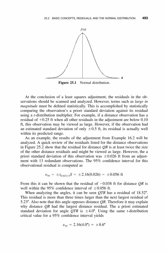
25.2 BASIC CONCEPTS, RESIDUALS, AND THE NORMAL DISTRIBUTION 493
Figure 25.1 Normal distribution.
At the conclusion of a least squares adjustment, the residuals in the ob-servations should be scanned and analyzed. However, terms such as large inmagnitude must be defined statistically. This is accomplished by statisticallycomparing the observation’s a priori standard deviation against its residualusing a t-distribution multiplier. For example, if a distance observation has aresidual of �0.25 ft when all other residuals in the adjustment are below 0.10ft, this observation may be viewed as large. However, if the observation hadan estimated standard deviation of only �0.5 ft, its residual is actually wellwithin its predicted range.
As an example, the results of the adjustment from Example 16.2 will beanalyzed. A quick review of the residuals listed for the distance observationsin Figure 25.2 show that the residual for distance QR is at least twice the sizeof the other distance residuals and might be viewed as large. However, the apriori standard deviation of this observation was �0.026 ft from an adjust-ment with 13 redundant observations. The 95% confidence interval for thisobservational residual is computed as
v � �t S � �2.16(0.026) � �0.056 ft95 0.025,13
From this it can be shown that the residual of �0.038 ft for distance QR iswell within the 95% confidence interval of �0.056 ft.
When analyzing the angles, it can be seen QTR has a residual of 18.52�.This residual is more than three times larger than the next largest residual of5.23�. Also note that this angle opposes distance QR. Therefore it may explainwhy distance QR had the largest distance residual. The a priori estimatedstandard deviation for angle QTR is �4.0�. Using the same t-distributioncritical value for a 95% confidence interval yields
v � 2.16(4.0�) � �8.6�95
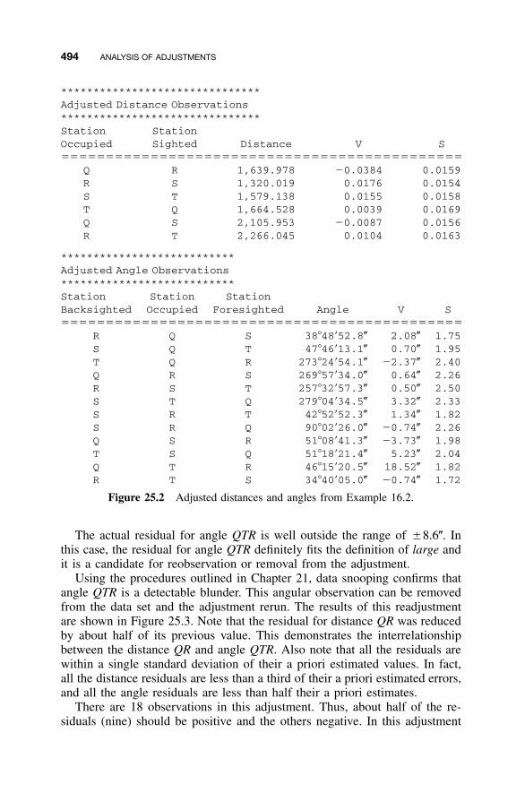
494 ANALYSIS OF ADJUSTMENTS
*******************************Adjusted Distance Observations*******************************StationOccupied
StationSighted Distance V S
���������������������������������������������Q R 1,639.978 �0.0384 0.0159R S 1,320.019 0.0176 0.0154S T 1,579.138 0.0155 0.0158T Q 1,664.528 0.0039 0.0169Q S 2,105.953 �0.0087 0.0156R T 2,266.045 0.0104 0.0163
***************************Adjusted Angle Observations***************************StationBacksighted
StationOccupied
StationForesighted Angle V S
���������������������������������������������R Q S 38�48�52.8� 2.08� 1.75S Q T 47�46�13.1� 0.70� 1.95T Q R 273�24�54.1� �2.37� 2.40Q R S 269�57�34.0� 0.64� 2.26R S T 257�32�57.3� 0.50� 2.50S T Q 279�04�34.5� 3.32� 2.33S R T 42�52�52.3� 1.34� 1.82S R Q 90�02�26.0� �0.74� 2.26Q S R 51�08�41.3� �3.73� 1.98T S Q 51�18�21.4� 5.23� 2.04Q T R 46�15�20.5� 18.52� 1.82R T S 34�40�05.0� �0.74� 1.72
Figure 25.2 Adjusted distances and angles from Example 16.2.
The actual residual for angle QTR is well outside the range of �8.6�. Inthis case, the residual for angle QTR definitely fits the definition of large andit is a candidate for reobservation or removal from the adjustment.
Using the procedures outlined in Chapter 21, data snooping confirms thatangle QTR is a detectable blunder. This angular observation can be removedfrom the data set and the adjustment rerun. The results of this readjustmentare shown in Figure 25.3. Note that the residual for distance QR was reducedby about half of its previous value. This demonstrates the interrelationshipbetween the distance QR and angle QTR. Also note that all the residuals arewithin a single standard deviation of their a priori estimated values. In fact,all the distance residuals are less than a third of their a priori estimated errors,and all the angle residuals are less than half their a priori estimates.
There are 18 observations in this adjustment. Thus, about half of the re-siduals (nine) should be positive and the others negative. In this adjustment
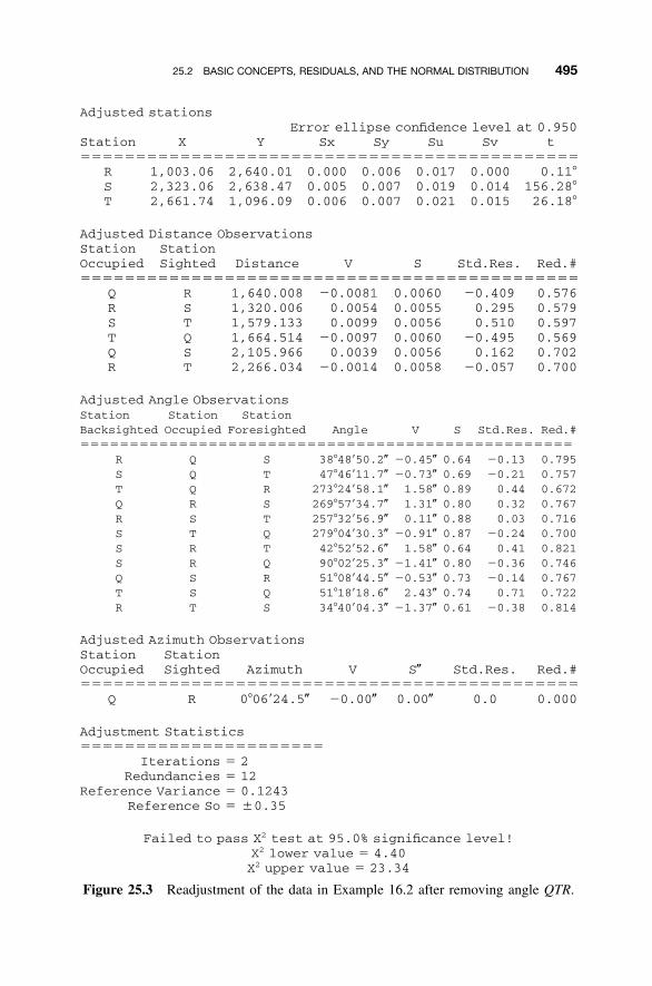
25.2 BASIC CONCEPTS, RESIDUALS, AND THE NORMAL DISTRIBUTION 495
Adjusted stationsError ellipse confidence level at 0.950
Station X Y Sx Sy Su Sv t���������������������������������������������
R 1,003.06 2,640.01 0.000 0.006 0.017 0.000 0.11�S 2,323.06 2,638.47 0.005 0.007 0.019 0.014 156.28�T 2,661.74 1,096.09 0.006 0.007 0.021 0.015 26.18�
Adjusted Distance ObservationsStationOccupied
StationSighted Distance V S Std.Res. Red.#
���������������������������������������������Q R 1,640.008 �0.0081 0.0060 �0.409 0.576R S 1,320.006 0.0054 0.0055 0.295 0.579S T 1,579.133 0.0099 0.0056 0.510 0.597T Q 1,664.514 �0.0097 0.0060 �0.495 0.569Q S 2,105.966 0.0039 0.0056 0.162 0.702R T 2,266.034 �0.0014 0.0058 �0.057 0.700
Adjusted Angle ObservationsStationBacksighted
StationOccupied
StationForesighted Angle V S Std.Res. Red.#
��������������������������������������������������R Q S 38�48�50.2� �0.45� 0.64 �0.13 0.795S Q T 47�46�11.7� �0.73� 0.69 �0.21 0.757T Q R 273�24�58.1� 1.58� 0.89 0.44 0.672Q R S 269�57�34.7� 1.31� 0.80 0.32 0.767R S T 257�32�56.9� 0.11� 0.88 0.03 0.716S T Q 279�04�30.3� �0.91� 0.87 �0.24 0.700S R T 42�52�52.6� 1.58� 0.64 0.41 0.821S R Q 90�02�25.3� �1.41� 0.80 �0.36 0.746Q S R 51�08�44.5� �0.53� 0.73 �0.14 0.767T S Q 51�18�18.6� 2.43� 0.74 0.71 0.722R T S 34�40�04.3� �1.37� 0.61 �0.38 0.814
Adjusted Azimuth ObservationsStationOccupied
StationSighted Azimuth V S� Std.Res. Red.#
���������������������������������������������Q R 0�06�24.5� �0.00� 0.00� 0.0 0.000
Adjustment Statistics����������������������
Iterations � 2Redundancies � 12
Reference Variance � 0.1243Reference So � �0.35
Failed to pass X2 test at 95.0% significance level!X2 lower value � 4.40X2 upper value � 23.34
Figure 25.3 Readjustment of the data in Example 16.2 after removing angle QTR.
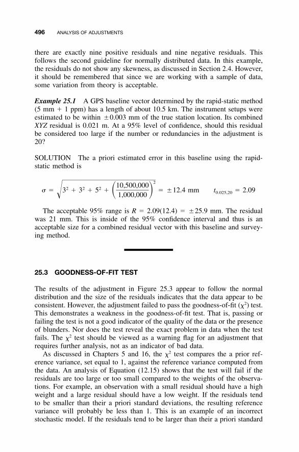
496 ANALYSIS OF ADJUSTMENTS
there are exactly nine positive residuals and nine negative residuals. Thisfollows the second guideline for normally distributed data. In this example,the residuals do not show any skewness, as discussed in Section 2.4. However,it should be remembered that since we are working with a sample of data,some variation from theory is acceptable.
Example 25.1 A GPS baseline vector determined by the rapid-static method(5 mm � 1 ppm) has a length of about 10.5 km. The instrument setups wereestimated to be within �0.003 mm of the true station location. Its combinedXYZ residual is 0.021 m. At a 95% level of confidence, should this residualbe considered too large if the number or redundancies in the adjustment is20?
SOLUTION The a priori estimated error in this baseline using the rapid-static method is
210,500,0002 2 2� � 3 � 3 � 5 � � �12.4 mm t � 2.09� � 0.025,20� 1,000,000
The acceptable 95% range is R � 2.09(12.4) � �25.9 mm. The residualwas 21 mm. This is inside of the 95% confidence interval and thus is anacceptable size for a combined residual vector with this baseline and survey-ing method.
25.3 GOODNESS-OF-FIT TEST
The results of the adjustment in Figure 25.3 appear to follow the normaldistribution and the size of the residuals indicates that the data appear to beconsistent. However, the adjustment failed to pass the goodness-of-fit (�2) test.This demonstrates a weakness in the goodness-of-fit test. That is, passing orfailing the test is not a good indicator of the quality of the data or the presenceof blunders. Nor does the test reveal the exact problem in data when the testfails. The �2 test should be viewed as a warning flag for an adjustment thatrequires further analysis, not as an indicator of bad data.
As discussed in Chapters 5 and 16, the �2 test compares the a prior ref-erence variance, set equal to 1, against the reference variance computed fromthe data. An analysis of Equation (12.15) shows that the test will fail if theresiduals are too large or too small compared to the weights of the observa-tions. For example, an observation with a small residual should have a highweight and a large residual should have a low weight. If the residuals tendto be smaller than their a priori standard deviations, the resulting referencevariance will probably be less than 1. This is an example of an incorrectstochastic model. If the residuals tend to be larger than their a priori standard
25.3 GOODNESS-OF-FIT TEST 497
deviations, the reference variance will be greater than 1 and the �2 test willfail in the upper bounds of the distribution.
The original data set of Example 16.2 failed the goodness-of-fit test. In theoriginal adjustment, it failed because the computed reference variance wasgreater than 1. This was probably caused by the large residual for angle QTR.After angle QTR was removed from the data, the �2 test failed because thereference variance was statistically less than 1. Since the residuals appear tobe much smaller than their a priori standard deviations, an incorrect stochasticmodel is to blame. In this case, the distance residuals were about three timesless than the estimated standard deviations and the angles were one-half oftheir estimated standard deviations. Thus, to pass the �2 test with this adjust-ment, the stochastic model needs to be modified.
In developing the stochastic model for this problem, it was originally be-lieved that the field crew had use a total station with a DIN 18723 accuracyof �4� and an EDM accuracy of 5 mm � 5 ppm. It was later discovered thatthe crew used an instrument having a DIN 18723 accuracy of �2� and anEDM accuracy of 2 mm � 2 ppm. Estimated standard deviations using thisnew information resulted in the adjustment shown in Figure 25.4. This ad-justment passed the goodness-of-fit test. However, this did not change theadjustment results significantly. That is, the adjusted coordinate values andadjusted observations are nearly the same in the adjustments shown in Figures25.3 and 25.4. What did change in Figure 25.4 were the statistical results.Since the statistical results of the adjustment are of little value to the surveyoronce analyzed, the adjustment shown in Figure 25.3 is sufficient for mostapplications.
Practitioners often view the goodness-of-fit test as an indicator of a possibleproblem. If the goodness-of-fit test failed because the computed referencevariance was too small, the test result is often ignored, since correcting itdoes not change the adjusted coordinates significantly. In this case, somepractitioners will say that the adjustment failed the goodness-of-fit test on the‘‘good’’ side. That is, the reference variance was too small because the resid-uals are too small for their given weights. However, if the reference variancecomputed is greater than 1, the results should be analyzed for possible blun-ders in the observations. After the identifiable blunders have been eliminatedfrom the data set, the stochastic model might still exhibit a problem. In thiscase, if the computed reference variance is greater than 1, the estimated stan-dard deviations for the observations should be increased. In the precedingexample the computed reference variance is less than 1. To correct this, theestimated standard deviations for the observations were decreased.
This adjustment brings about another important discussion point. Had allthe a priori standard deviations been reduced by a single scale factor, theresults of the adjustment would be the same.1 That is, if the a priori standard
1 Readers are encouraged to rerun the data in Example 16.2 with the a priori standard deviationsreduced by a factor of to compare the adjustment results.1–2
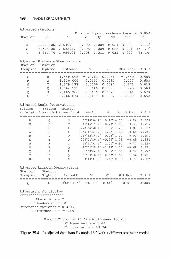
498 ANALYSIS OF ADJUSTMENTS
Adjusted stationsError ellipse confidence level at 0.950
Station X Y Sx Sy Su Sv t���������������������������������������������
R 1,003.06 2,640.00 0.000 0.009 0.024 0.000 0.11�S 2,323.06 2,638.47 0.008 0.009 0.028 0.021 151.27�T 2,661.74 1,096.09 0.008 0.011 0.031 0.022 26.14�
Adjusted Distance ObservationsStationOccupied
StationSighted Distance V S Std.Res. Red.#
��������������������������������������������Q R 1,640.008 �0.0083 0.0086 �0.830 0.580R S 1,320.006 0.0053 0.0081 0.527 0.603S T 1,579.133 0.0100 0.0081 0.971 0.615T Q 1,664.515 �0.0089 0.0087 �0.895 0.568Q S 2,105.966 0.0039 0.0079 0.341 0.673R T 2,266.034 �0.0011 0.0082 �0.097 0.658
Adjusted Angle ObservationsStationBacksighted
StationOccupied
StationForesighted Angle V S Std.Res. Red.#
��������������������������������������������������R Q S 38�48�50.2� �0.46� 0.95 �0.24 0.808S Q T 47�46�11.7� �0.73� 1.02 �0.38 0.776T Q R 273�24�58.1� 1.59� 1.29 0.87 0.667Q R S 269�57�34.7� 1.27� 1.14 0.64 0.751R S T 257�32�56.8� 0.03� 1.27 0.02 0.696S T Q 279�04�30.4� �0.79� 1.25 �0.43 0.684S R T 42�52�52.6� 1.55� 0.94 0.77 0.820S R Q 90�02�25.3� �1.37� 1.14 �0.69 0.751Q S R 51�08�44.4� �0.57� 1.06 �0.29 0.772T S Q 51�18�18.7� 2.53� 1.09 1.34 0.751R T S 34�40�04.3� �1.42� 0.90 �0.72 0.827
Adjusted Azimuth ObservationsStationOccupied
StationSighted Azimuth V S� Std.Res. Red.#
���������������������������������������������Q R 0�06�24.5� �0.00� 0.00� 0.0 0.000
Adjustment Statistics*********************
Iterations � 2Redundancies � 12
Reference Variance � 0.4572Reference So � �0.68
Passed X2 test at 95.0% significance level!X2 lower value � 4.40X2 upper value � 23.34
Figure 25.4 Readjusted data from Example 16.2 with a different stochastic model.
25.4 COMPARISON OF RESIDUAL PLOTS 499
deviations for all the observations had been cut in half, this would have re-sulted in increasing all the weights by a factor of 4. Since weights are relative,performing a scalar reduction in the standard deviations does not change theadjustment.
This example demonstrates the importance of selecting appropriate a prioristandard deviations for the observations. Estimated standard deviations forobservations cannot be selected from the recesses of one’s mind. Doing thisnot only affects how the errors in the observations are distributed but alsohow the results of the adjustment are analyzed. For traditional surveys it isalways best to select a stochastic model that reflects the estimated accuraciesin the observations using procedures discussed in Chapters 7 and 9. Goodestimates of setup errors will typically result in a sound stochastic model.
However, the network adjustment of GPS baseline vectors derives its sto-chastic model from the least squares reduction of each baseline. As discussedin Chapter 17, the stochastic model is part of the printout from the baselinereduction. Assuming proper field procedures, if the GPS network adjustmentfails to pass the �2 test, there is little one can do to modify the model. Infact, if field procedures are consistent, scaling the entire stochastic modelmight be the only option. Although this procedure may result in a ‘‘passed’’�2 test, it will not change the coordinates in the solution since weights arerelative. In fact, it will only change the a posteriori statistics. Thus, scalingthe entire stochastic model by a single factor is important only if the statisticsare important. Since this is seldom true, there is little value in scaling thestochastic model.
Better adjustments could be obtained if the commercial GPS software em-ployed the multipoint solution technique. This solution takes the individualpseudoranges from the satellites and computes baseline vectors and the un-known coordinates of the network stations simultaneously. Current softwareofferings compute the baseline vectors from the pseudoranges and then co-ordinates of the network stations from these computed vectors. This is a two-step process. The multipoint solution is similar to the three-dimensionalgeodetic network and the photogrammetric block-bundle adjustment in thatall unknowns are computed in one adjustment. However, it is important toremove any large blunders before attempting a multipoint solution. Thus, thetwo-step solution process must be maintained to ferret out problems in thedata. Since the main advantage of the multipoint solution lies in the devel-opment of the stochastic model, only a few examples of this solution tech-nique exist.
25.4 COMPARISON OF RESIDUAL PLOTS
Massive quantities of data can be collected and reduced during the reductionof GPS carrier-phase observations. Software manufacturers typically plotpseudorange residuals against a time line. Examples of this are shown in
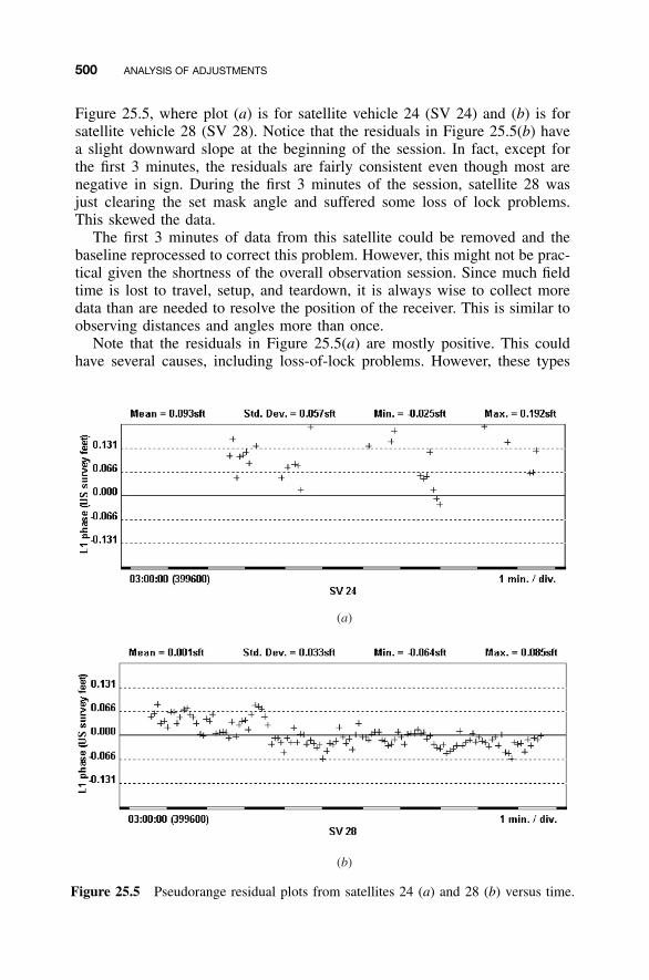
500 ANALYSIS OF ADJUSTMENTS
(a)
(b)
Figure 25.5 Pseudorange residual plots from satellites 24 (a) and 28 (b) versus time.
Figure 25.5, where plot (a) is for satellite vehicle 24 (SV 24) and (b) is forsatellite vehicle 28 (SV 28). Notice that the residuals in Figure 25.5(b) havea slight downward slope at the beginning of the session. In fact, except forthe first 3 minutes, the residuals are fairly consistent even though most arenegative in sign. During the first 3 minutes of the session, satellite 28 wasjust clearing the set mask angle and suffered some loss of lock problems.This skewed the data.
The first 3 minutes of data from this satellite could be removed and thebaseline reprocessed to correct this problem. However, this might not be prac-tical given the shortness of the overall observation session. Since much fieldtime is lost to travel, setup, and teardown, it is always wise to collect moredata than are needed to resolve the position of the receiver. This is similar toobserving distances and angles more than once.
Note that the residuals in Figure 25.5(a) are mostly positive. This couldhave several causes, including loss-of-lock problems. However, these types

25.5 USE OF STATISTICAL BLUNDER DETECTION 501
of plots are typically seen when the broadcast ephemeris is used in the re-duction. The broadcast ephemeris is a near-future prediction of the locationof the satellite. For various reasons, satellites often stray from their predictedpaths. When this happens, the coordinates for the satellite’s position at thetime of broadcast are in error. This problem results in plots like Figure25.5(a), where most of the residuals typically have one sign indicating askewed data set. This problem can be corrected by downloading and pro-cessing with a precise ephemeris. In general, the best solutions can alwaysbe obtained with a precise ephemeris. Since the ultrarapid ephemeris is avail-able within a few hours of data collection, it is wise to wait for this ephemerisbefore processing the data.
Figure 25.5 also depicts a problem with real-time kinematic GPS (RTK-GPS) surveys. That is, by its very nature, the broadcast ephemeris must beused in processing the data. Thus, the option of downloading a precise ephem-eris is not available. RTK-GPS has its place in stakeout and mapping surveys.However, it should never be used to establish anything other than very low-order control. The RTK-GPS survey is the equivalent of a radial total stationsurvey, leaving only minimal checks in the quality of the data. Since all GPSsurveys can be seriously affected by solar activity, the RTK-GPS procedureleaves the surveyor open to poor results without any indication at the receiver.
25.5 USE OF STATISTICAL BLUNDER DETECTION
When more than one blunder exists in a given data set, the statistical blunderdetection methods presented in Chapter 21 help isolate the offending obser-vations. These methods along with graphical techniques, were presented thor-oughly in that chapter.
The problem of having multiple blunders usually exists in large controlsurveys. When adjusting large data sets, it is wise to break the data intosmaller subsets that can be checked for blunders before attempting the largeradjustment. By breaking a larger adjustment into smaller subsets of data, dataproblems can often be isolated, corrected, or removed from the observations.
GPS provides a similar example. When performing a large GPS adjust-ment, it is often wise initially to download and process GPS data by session.Since a GPS campaign typically involves several observational sessions, try-ing to combine all sessions into one large adjustment generally takes moretime than individually processing the data by session. Processing GPS databy session simplifies the process of isolating poor and trivial baselines. Afterprocessing each session in a GPS survey satisfactorily, a combined networkadjustment can be attempted and analyzed for blunders. It may be importantat this point to reanalyze and possibly reprocess baselines to obtain the bestsolution. Again, statistical blunder detection will help analyze possible blun-ders in baselines. If the observation sessions are long enough, it is possibleto eliminate data from the session to remove possible problems caused by
502 ANALYSIS OF ADJUSTMENTS
obstructions and loss-of-lock problems. This again indicates the need to col-lect more data than are minimally required to obtain a solution. A few extraminutes used to observe additional data can often result in improved solutionswithout returning to the field for reobservation.
PROBLEMS
25.1 Following an adjustment, how is the term large defined in relation toresiduals?
25.2 What are the basic concepts of a normal distribution, and how arethese concepts used to analyze the results of a least squares adjust-ment?
25.3 An adjustment has 20 observations. Only nine of these residuals arenegative in sign. Should this cause concern during the analysis?
25.4 Discuss why the goodness-of-fit test is not always a reliable indicatorof a blunder in data.
25.5 What does it mean to ‘‘fail on the good side’’ of the �2 test?
25.6 Discuss the importance of a proper stochastic model.
25.7 Discuss why the scaling of the stochastic model does not affect theadjusted parameters.
25.8 What is the possible reason for the residual plot in Figure 25.5a?
25.9 Discuss the importance of collecting more than the minimum amountof data in a GPS survey.
25.10 Why should the RTK-GPS method not be used to establish high-ordercontrol stations?
25.11 Why should GPS baseline vectors be processed by session rather thanby job?
25.12 A GPS baseline vector determined by the rapid-static method (5 mm� 1 ppm) has a length of about 5.5 km. The instrument setups wereestimated to be within �0.003 m of the true station location. Itscombined XYZ residual is 2.5 cm. At a 95% confidence level, shouldthis residual be considered too large if the number redundancies inthe adjustment is 15?
In Problems 25.13 through 25.20, analyze the results of the least squaresadjustment, indicating if there are any areas of concern in the data or sto-chastic model. When possible, isolate and remove questionable data and sto-chastic models. After the changes, rerun the adjustment and compare theresults. (Note: Not all of the problems have questionable data.)
PROBLEMS 503
25.13 Problem 12.1
25.14 Problem 12.13
25.15 Problem 13.15
25.16 Problem 15.9
25.17 Problem 16.7
25.18 Problem 16.9
25.19 Problem 16.11
25.20 Problem 17.8
504
CHAPTER 26
COMPUTER OPTIMIZATION
26.1 INTRODUCTION
Large amounts of computer time and storage requirements can be used whenperforming least squares adjustments. This is due to the fact that as the prob-lems become more complex, the matrices become larger, and the storagerequirements and time consumed in doing numerical operations both growrapidly. As an example, in analyzing the storage requirements of a 25-stationhorizontal least squares adjustment that has 50 distance and 50 angle obser-vations, the coefficient matrix would have dimensions of 100 rows and 50columns. If this adjustment were done in double precision,1 it would require40,000 bytes of storage for the coefficient matrix alone. The weight matrixwould require an additional 80,000 bytes of storage. Also, at least two ad-ditional intermediate matrices2 must be formed in computing the solution.From this example it is easy to see that large quantities of computer time andcomputer memory can be required in least squares adjustments. Thus, whenwriting least squares software, it is desirable to take advantage of some stor-age and computing optimization techniques. In this chapter some of thesetechniques are described.
26.2 STORAGE OPTIMIZATION
Many matrices used in a surveying adjustment are large but sparse. Using theexample above, a single row of the coefficient matrix for a distance obser-
1 The storage requirements of a double-precision number is 8 bytes.2 The intermediate matrices developed are AT and ATW or J T and J TW, depending on whether theadjustment is linear or nonlinear.
Adjustment Computations: Spatial Data Analysis, Fourth Edition. C. D. Ghilani and P. R. Wolf© 2006 John Wiley & Sons, Inc. ISBN: 978-0-471-69728-2
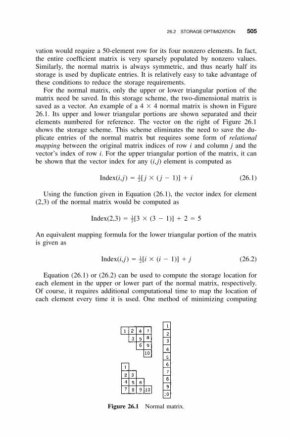
26.2 STORAGE OPTIMIZATION 505
Figure 26.1 Normal matrix.
vation would require a 50-element row for its four nonzero elements. In fact,the entire coefficient matrix is very sparsely populated by nonzero values.Similarly, the normal matrix is always symmetric, and thus nearly half itsstorage is used by duplicate entries. It is relatively easy to take advantage ofthese conditions to reduce the storage requirements.
For the normal matrix, only the upper or lower triangular portion of thematrix need be saved. In this storage scheme, the two-dimensional matrix issaved as a vector. An example of a 4 � 4 normal matrix is shown in Figure26.1. Its upper and lower triangular portions are shown separated and theirelements numbered for reference. The vector on the right of Figure 26.1shows the storage scheme. This scheme eliminates the need to save the du-plicate entries of the normal matrix but requires some form of relationalmapping between the original matrix indices of row i and column j and thevector’s index of row i. For the upper triangular portion of the matrix, it canbe shown that the vector index for any (i, j) element is computed as
1–Index(i, j) � [ j � ( j � 1)] � i (26.1)2
Using the function given in Equation (26.1), the vector index for element(2,3) of the normal matrix would be computed as
1–Index(2,3) � [3 � (3 � 1)] � 2 � 52
An equivalent mapping formula for the lower triangular portion of the matrixis given as
1–Index(i, j) � [i � (i � 1)] � j (26.2)2
Equation (26.1) or (26.2) can be used to compute the storage location foreach element in the upper or lower part of the normal matrix, respectively.Of course, it requires additional computational time to map the location ofeach element every time it is used. One method of minimizing computing
506 COMPUTER OPTIMIZATION
TABLE 26.1 Creation of a Mapping Table
VI(1) � 0
For i going from 2 to the number of unknowns: VI(i) � VI(i � 1) � i � 1
time is to utilize a mapping table. The mapping table is an integer vector thatidentifies the storage location for only the initial element of a row or column.To reduce total computational time, the indices are stored as one number lessthan their actual value. The example matrix stored in Figure 26.1 would havea relational mapping table of
TVI � [0 1 3 6 10]
Although the storage location of the first element is 1, it can be seen abovethat it is identified as 0. Similarly, every other mapping index is one numberless than its actual location in the vector, as shown in Figure 26.1. The map-ping vector is found using the pseudocode shown in Table 26.1.
By using this type of mapping table, the storage location for the first ele-ment of any upper triangular column is computed as
Index(i, j) � VI( j) � i (26.3)
Using the mapping table, the storage location for the (2,3) element is
Index(2,3) � VI(3) � 2 � 3 � 2 � 5
The equivalent formula for the lower triangular portion is
Index(i, j) � VI(i) � j (26.4)
Obviously, this method of indexing an element’s position requires addi-tional storage in a mapping table, but the additional storage is offset by thedecreased computational time that is created by the operations equation (26.1)or (26.2). Since the mapping table replaces the more time-consuming multi-plication and division operations of Equations (26.1) and (26.2), it is prudentto use this indexing method whenever memory is available. Although everycompiler and machine are different, a set of times to compare indexing meth-ods are shown in Table 26.2. The best times were achieved by minimizingboth the number of operations and calls to the mapping function. Thus, inmethod C the mapping table was created to be a global variable in the pro-gram, and the table was accessed directly as needed. For comparison, the timeto access the matrix elements directly using the loop shown in method D was1.204 seconds. Thus, method C uses only slightly more time than method D
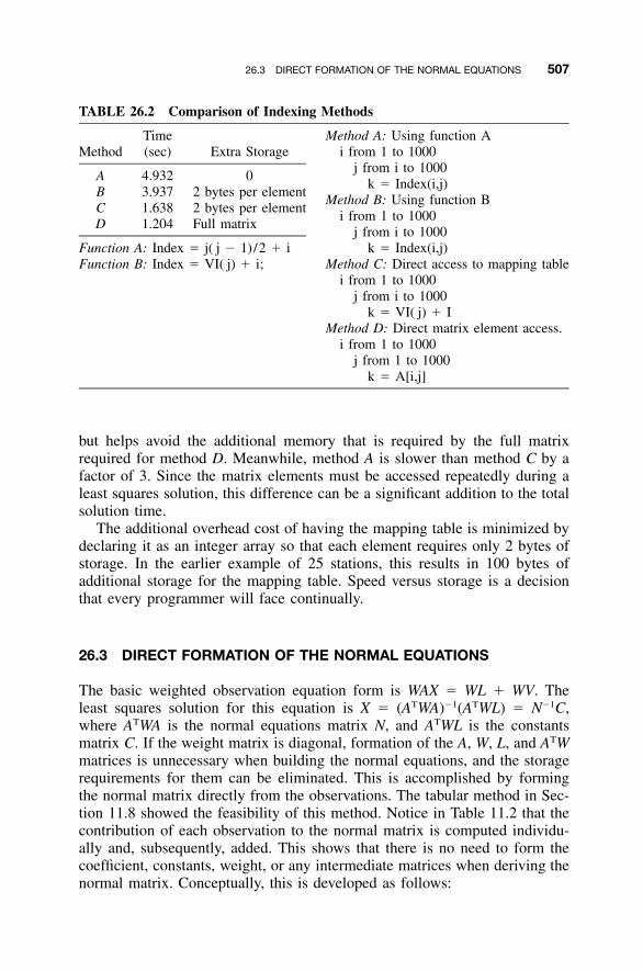
26.3 DIRECT FORMATION OF THE NORMAL EQUATIONS 507
TABLE 26.2 Comparison of Indexing Methods
MethodTime(sec) Extra Storage
A 4.932 0B 3.937 2 bytes per elementC 1.638 2 bytes per elementD 1.204 Full matrix
Function A: Index � j( j � 1) /2 � iFunction B: Index � VI( j) � i;
Method A: Using function Ai from 1 to 1000
j from i to 1000k � Index(i,j)
Method B: Using function Bi from 1 to 1000
j from i to 1000k � Index(i,j)
Method C: Direct access to mapping tablei from 1 to 1000
j from i to 1000k � VI( j) � I
Method D: Direct matrix element access.i from 1 to 1000
j from 1 to 1000k � A[i,j]
but helps avoid the additional memory that is required by the full matrixrequired for method D. Meanwhile, method A is slower than method C by afactor of 3. Since the matrix elements must be accessed repeatedly during aleast squares solution, this difference can be a significant addition to the totalsolution time.
The additional overhead cost of having the mapping table is minimized bydeclaring it as an integer array so that each element requires only 2 bytes ofstorage. In the earlier example of 25 stations, this results in 100 bytes ofadditional storage for the mapping table. Speed versus storage is a decisionthat every programmer will face continually.
26.3 DIRECT FORMATION OF THE NORMAL EQUATIONS
The basic weighted observation equation form is WAX � WL � WV. Theleast squares solution for this equation is X � (ATWA)�1(ATWL) � N�1C,where ATWA is the normal equations matrix N, and ATWL is the constantsmatrix C. If the weight matrix is diagonal, formation of the A, W, L, and ATWmatrices is unnecessary when building the normal equations, and the storagerequirements for them can be eliminated. This is accomplished by formingthe normal matrix directly from the observations. The tabular method in Sec-tion 11.8 showed the feasibility of this method. Notice in Table 11.2 that thecontribution of each observation to the normal matrix is computed individu-ally and, subsequently, added. This shows that there is no need to form thecoefficient, constants, weight, or any intermediate matrices when deriving thenormal matrix. Conceptually, this is developed as follows:
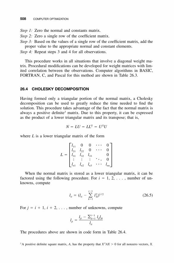
508 COMPUTER OPTIMIZATION
Step 1: Zero the normal and constants matrix.Step 2: Zero a single row of the coefficient matrix.Step 3: Based on the values of a single row of the coefficient matrix, add the
proper value to the appropriate normal and constant elements.Step 4: Repeat steps 3 and 4 for all observations.
This procedure works in all situations that involve a diagonal weight ma-trix. Procedural modifications can be developed for weight matrices with lim-ited correlation between the observations. Computer algorithms in BASIC,FORTRAN, C, and Pascal for this method are shown in Table 26.3.
26.4 CHOLESKY DECOMPOSITION
Having formed only a triangular portion of the normal matrix, a Choleskydecomposition can be used to greatly reduce the time needed to find thesolution. This procedure takes advantage of the fact that the normal matrix isalways a positive definite3 matrix. Due to this property, it can be expressedas the product of a lower triangular matrix and its transpose; that is,
T TN � LU � LL � U U
where L is a lower triangular matrix of the form
l 0 0 � � � 011
l l 0 � � � 021 22
L � l l l 031 32 33�� � � � 0�� �
l l l � � � ln1 n2 n3 nn
When the normal matrix is stored as a lower triangular matrix, it can befactored using the following procedure. For i � 1, 2, . . . , number of un-knowns, compute
i�12 1 / 2l � (l � l ) (26.5)�ii ii ik
k�1
For j � i � 1, i � 2, . . . , number of unknowns, compute
i�1l � � l lji ij jkk�1l �ji lii
The procedures above are shown in code form in Table 26.4.
3 A positive definite square matrix, A, has the property that X TAX � 0 for all nonzero vectors, X.

509
TA
BL
E26
.3A
lgor
ithm
sfo
rB
uild
ing
the
Nor
mal
Equ
atio
nsD
irec
tly
from
The
irO
bser
vati
ons
BA
SIC
Lan
guag
e:F
OR
TR
AN
Lan
guag
e:Fo
ri
�1
toun
know
nix
�V
I(i)
:ix
i�
ix�
iN
(ixi
)�
N(i
xi)
�A
(i)�
2*
W(i
)C
(i)
�C
(i)
�A
(i)*
W(i
)*L
(i)
For
j�
i�1
toun
know
nN
(ix �
j)�
N(i
x�j)
�A
(i)*
W(i
)*A
(j)
Nex
tj
Nex
tI
Do
100
i�
1,un
know
nix
�V
I(i)
ixi
�ix
�i
N(i
xi)
�N
(ixi
)�
A(i
)**2
*W
(i)
C(i
)�
C(i
)�
A(i
)*W
(i)*
L(i
)D
o10
0j
�i�
1,un
know
nN
(ix �
j)�
N(i
x�j)
�A
(i)*
W(i
)*A
(j)
100
Con
tinue
CL
angu
age:
Pas
cal
Lan
guag
e:fo
r(i
�1;
i��
unkn
own;
i��
){
ix�
VI[
i];
ixi
�ix
�i;
n[ix
i]�
n[ix
i]�
a[i]
*a[i
]*
w[i
];c[
i]�
c[i]
�a[
i]*w
[i]*
l[i]
;fo
r(j
�i�
1;j�
�un
know
n;j�
�)
n[ix
�j]
�n[
ix�
j]�
a[i]
*w[i
]*a[
j];
}//
for
i
For
i: �
1to
unkn
own
dobe
gin
ix: �
VI[
i];
ixi
:�ix
�i;
N[i
xi]
: �N
[ixi
]�
Sqr(
A[i
])*
W[i
];C
[i]
: �C
[i]
�A
[i]*
W[i
]*L
[i];
For
j: �
i�1
toun
know
ndo
N[i
x �j]
:�N
[ix�
j]�
A[i
]*W
[i]*
A[j
]E
nd;
{for
i}

510
TA
BL
E26
.4C
ompu
ter
Alg
orit
hms
for
Com
puti
ngC
hole
sky
Fac
tors
ofa
Nor
mal
Mat
rix
BA
SIC
Lan
guag
e:F
OR
TR
AN
Lan
guag
e:FO
Ri
�1
TO
unkn
own
ix�
VI(
i):
ixi
�ix
�i:
s�
0#FO
Rk
�1
TO
i�
1s
�s
�N
(ix
�k)
ˆ2:
NE
XT
kN
(ixi
)�
SQR
(N(i
xi)
�s)
FOR
j�
i�
1T
Oun
know
ns
�0#
:jx
�V
I(j)
FOR
k�
1T
Oi
�1
s�
s�
N(j
x�
k)*
N(i
x�
k):
NE
XT
kN
(jx
�i)
�(N
(jx
�i)
�s)
/N(i
xi)
NE
XT
jN
EX
Ti
Do
30i
�1,
Unk
now
nix
�V
I(i)
i1�
i�
1S
�0.
0D
o10
k �1,
i110
s�
s�
N(i
x�k)
**2
N(i
x �i)
�Sq
rt(N
(ix�
i)�
s)D
o30
j�
i�1,
Unk
now
ns
�0.
0D
o20
k�
1,i1
20s
�s
�N
(VI[
j]�
k)*
N(i
x�k)
N(V
I[j]
�i)
�(N
(VI[
j]�
i)�
s)/N
(ix�
i)30
Con
tinue
CL
angu
age:
Pas
cal
Lan
guag
e:fo
r(i
�1;
i��
unkn
own;
i��
){
ix�
VI[
i];
ixi
�ix
�i;
s�
0.0;
for
(k�
1;k�
i;k�
�)
s�
s�
n[ix
�k]
*n[i
x�k]
;n[
ixi]
�sq
rt(n
[ixi
]�
s);
for
(j�
i�1;
j��
unkn
own;
j��
){
s�
0;jx
�V
I[j]
;fo
r(k
�1;
k�i;
k��
)s
�s
�n[
jx�
k]*
n[ix
�k]
;n[
jx�
i]�
(n[j
x�i]
�s)
/n[
ixi]
;}
//fo
rj
}//
for
I
For
i: �
1to
unkn
own
doB
egin
ix: �
VI[
i];
ixi
:�ix
�i;
S:�
0;Fo
rk
: �1
toPr
ed(i
)do
S: �
S�
Sqr(
N[i
x�k]
);N
[ixi
]: �
Sqrt
(N[i
xi]
�S)
;Fo
rj
: �Su
cc(i
)to
unkn
own
doB
egin
S: �
0;jx
:�V
I[j]
;Fo
rk
: �1
toPr
ed(i
)do
S: �
S�
N[j
x�k]
*N[i
x�k]
;N
[jx �
i]:�
(N[j
x�i]
�S)
/N
[ixi
]E
nd;
{for
j}E
nd;
{for
i}
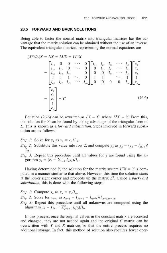
26.5 FORWARD AND BACK SOLUTIONS 511
26.5 FORWARD AND BACK SOLUTIONS
Being able to factor the normal matrix into triangular matrices has the ad-vantage that the matrix solution can be obtained without the use of an inverse.The equivalent triangular matrices representing the normal equations are
T T(A WA)X � NX � LUX � LL X
l 0 0 � � � 0 l l l � � � l x11 11 21 31 n1 1
l l 0 � � � 0 0 l l � � � l x21 22 22 32 n2 2
� l l l 0 0 0 l � � � l x31 32 33 33 n3 3� �� � � � 0 � � � � �� �� �� �� �
l l l � � � l 0 0 0 0 l xn1 n2 n3 nn nn n
c1
c2
� c � C3
�� �cn
(26.6)
Equation (26.6) can be rewritten as LY � C, where LTX � Y. From this,the solution for Y can be found by taking advantage of the triangular form ofL. This is known as a forward substitution. Steps involved in forward substi-tution are as follows:
Step 1: Solve for y1 as y1 � c1 / l11.Step 2: Substitute this value into row 2, and compute y2 as y2 � (c2 � l21y1)/
l22.Step 3: Repeat this procedure until all values for y are found using the al-
gorithm yi � (ci � likyk) / lii.i�1�k�1
Having determined Y, the solution for the matrix system LTX � Y is com-puted in a manner similar to that above. However, this time the solution startsat the lower right corner and proceeds up the matrix LT. Called a backwardsubstitution, this is done with the following steps:
Step 1: Compute xn as xn � yn / lnn.Step 2: Solve for xn�1 as xn�1 � (yn�1 � lmnxn) / l(n�1)(n�1).Step 3: Repeat this procedure until all unknowns are computed using the
algorithm xk � (yk � lkjyj) / lkk.n�j�k�1
In this process, once the original values in the constant matrix are accessedand changed, they are not needed again and the original C matrix can beoverwritten with Y and X matrices so that the entire process requires noadditional storage. In fact, this method of solution also requires fewer oper-
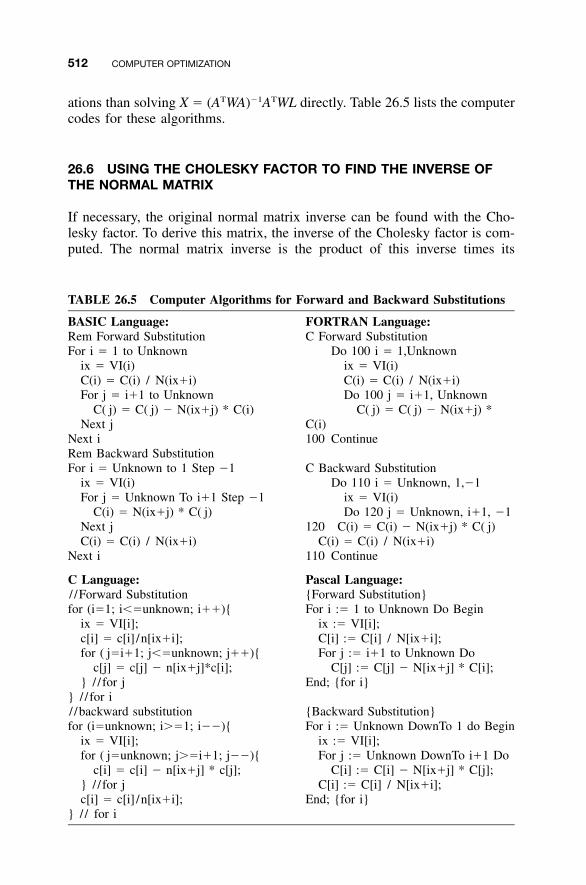
512 COMPUTER OPTIMIZATION
TABLE 26.5 Computer Algorithms for Forward and Backward Substitutions
BASIC Language: FORTRAN Language:Rem Forward SubstitutionFor i � 1 to Unknown
ix � VI(i)C(i) � C(i) / N(ix�i)For j � i�1 to Unknown
C( j) � C( j) � N(ix�j) * C(i)Next j
Next iRem Backward SubstitutionFor i � Unknown to 1 Step �1
ix � VI(i)For j � Unknown To i�1 Step �1
C(i) � N(ix�j) * C( j)Next jC(i) � C(i) / N(ix�i)
Next i
C Forward SubstitutionDo 100 i � 1,Unknown
ix � VI(i)C(i) � C(i) / N(ix�i)Do 100 j � i�1, Unknown
C( j) � C( j) � N(ix�j) *C(i)100 Continue
C Backward SubstitutionDo 110 i � Unknown, 1,�1
ix � VI(i)Do 120 j � Unknown, i�1, �1
120 C(i) � C(i) � N(ix�j) * C( j)C(i) � C(i) / N(ix�i)
110 Continue
C Language: Pascal Language:/ /Forward Substitutionfor (i�1; i��unknown; i��){
ix � VI[i];c[i] � c[i] /n[ix�i];for ( j�i�1; j��unknown; j��){
c[j] � c[j] � n[ix�j]*c[i];} / / for j
} / / for i/ /backward substitutionfor (i�unknown; i��1; i��){
ix � VI[i];for ( j�unknown; j��i�1; j��){
c[i] � c[i] � n[ix�j] * c[j];} / / for jc[i] � c[i] /n[ix�i];
} / / for i
{Forward Substitution}For i :� 1 to Unknown Do Begin
ix :� VI[i];C[i] :� C[i] / N[ix�i];For j :� i�1 to Unknown Do
C[j] :� C[j] � N[ix�j] * C[i];End; {for i}
{Backward Substitution}For i :� Unknown DownTo 1 do Begin
ix :� VI[i];For j :� Unknown DownTo i�1 Do
C[i] :� C[i] � N[ix�j] * C[j];C[i] :� C[i] / N[ix�i];
End; {for i}
ations than solving X � (ATWA)�1ATWL directly. Table 26.5 lists the computercodes for these algorithms.
26.6 USING THE CHOLESKY FACTOR TO FIND THE INVERSE OFTHE NORMAL MATRIX
If necessary, the original normal matrix inverse can be found with the Cho-lesky factor. To derive this matrix, the inverse of the Cholesky factor is com-puted. The normal matrix inverse is the product of this inverse times its
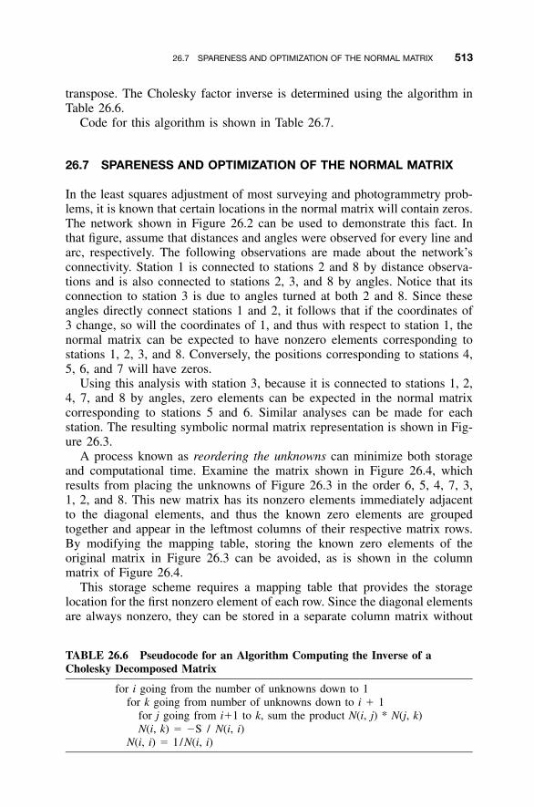
26.7 SPARENESS AND OPTIMIZATION OF THE NORMAL MATRIX 513
TABLE 26.6 Pseudocode for an Algorithm Computing the Inverse of aCholesky Decomposed Matrix
for i going from the number of unknowns down to 1for k going from number of unknowns down to i � 1
for j going from i�1 to k, sum the product N(i, j) * N(j, k)N(i, k) � �S / N(i, i)
N(i, i) � 1/N(i, i)
transpose. The Cholesky factor inverse is determined using the algorithm inTable 26.6.
Code for this algorithm is shown in Table 26.7.
26.7 SPARENESS AND OPTIMIZATION OF THE NORMAL MATRIX
In the least squares adjustment of most surveying and photogrammetry prob-lems, it is known that certain locations in the normal matrix will contain zeros.The network shown in Figure 26.2 can be used to demonstrate this fact. Inthat figure, assume that distances and angles were observed for every line andarc, respectively. The following observations are made about the network’sconnectivity. Station 1 is connected to stations 2 and 8 by distance observa-tions and is also connected to stations 2, 3, and 8 by angles. Notice that itsconnection to station 3 is due to angles turned at both 2 and 8. Since theseangles directly connect stations 1 and 2, it follows that if the coordinates of3 change, so will the coordinates of 1, and thus with respect to station 1, thenormal matrix can be expected to have nonzero elements corresponding tostations 1, 2, 3, and 8. Conversely, the positions corresponding to stations 4,5, 6, and 7 will have zeros.
Using this analysis with station 3, because it is connected to stations 1, 2,4, 7, and 8 by angles, zero elements can be expected in the normal matrixcorresponding to stations 5 and 6. Similar analyses can be made for eachstation. The resulting symbolic normal matrix representation is shown in Fig-ure 26.3.
A process known as reordering the unknowns can minimize both storageand computational time. Examine the matrix shown in Figure 26.4, whichresults from placing the unknowns of Figure 26.3 in the order 6, 5, 4, 7, 3,1, 2, and 8. This new matrix has its nonzero elements immediately adjacentto the diagonal elements, and thus the known zero elements are groupedtogether and appear in the leftmost columns of their respective matrix rows.By modifying the mapping table, storing the known zero elements of theoriginal matrix in Figure 26.3 can be avoided, as is shown in the columnmatrix of Figure 26.4.
This storage scheme requires a mapping table that provides the storagelocation for the first nonzero element of each row. Since the diagonal elementsare always nonzero, they can be stored in a separate column matrix without

514 COMPUTER OPTIMIZATION
TABLE 26.7 Computer Algorithms to Find the Inverse of a Cholesky FactoredMatrix
BASIC Language: Fortran Language:{Inverse}For i � Unknown To 1 Step �1
ix � VI(i): ixi � ix � iFor k � Unknown To i�1 Step �1
S � 0!For j � i�1 To k
S � S � N(ix�j) * N(VI( j)�k)Next jN(ix�k) � �S / N(ixi)
Next kN(ixi) � 1.0 / N(ixi)
Next i
{Inverse * Transpose of Inverse}For j � 1 to Unknown
ixj � VI( j)For k � j to Unknown
S � 0!For i � k to Unknown
S � S � N(VI(k)�i) *N(ixj�i)
Next iN(ixj�k) � S
Next kNext j
C InverseDo 10 i � Unknown, 1,�1
ix � VI(i)ixi � ix � iDo 11 k � Unknown, i�1,�1
S � 0.0Do 12 j � i�1,k
12 S � S � N(ix�j) * N(VI( j)�k)N(ix�k) � �S / N(ixi)
11 ContinueN(ixi) � 1.0 / N(ixi)
10 Continue
C Inverse * Transpose of Inverse}Do 20 j � 1, Unknown
ixj � VI( j)Do 21 k � j, Unknown
S � 0.0Do 22 i � k,Unknown
22 S � S � N(VI(k)�i) * N(ixj�i)N(ixj�k) � S
21 Continue20 Continue
C Language: Pascal Language:{Inverse}for (i�unknown; i��1; i��) {
ix � VI[i]; ixi � ix � i;for(k�unknown; k��i�1; k��) {
s � 0.0;for ( j�i�1; j��k; j��)
s � s � n[ix�j] * n[VI[j]�k];n[ix�k] � �s / n[ixi];
} / / for kn[ixi] � 1.0 / n[ixi];
} / / for i
{inverse * transpose of inverse}for ( j�1; j��unknown; j��) {
ixj � VI[j];for (k�j; k��unknown; k��) {
s � 0.0;For (i�k; i��unknown; i��)
s � s � n[VI[k]�i] * n[ixj�i];n[ixj�k] � s
} / / for k} / / for j
{Inverse}For i :� Unknown DownTo 1 do Begin
ix :� VI[i]; ixi :� ix � i;For k :� Unknown DownTo i�1 Do Begin
S :� 0.0;For j :� i�1 To k Do
S :� S � N[ix�j] * N[VI[j]�k];N[ix�k] :� �S / N[ixi];
End; {For k}N[ixi] :� 1.0 / N[ixi];
End; {For i}
{Inverse * Transpose of Inverse}For j :� 1 to Unknown Do Begin
ixj :� VI[j];For k :� j to Unknown Do Begin
S :� 0.0;For i :� k to Unknown Do
S :� S � N[VI[k]�i] * N[ixj�i];N[ixj�k] :� S
End; {For k}End; {For j}
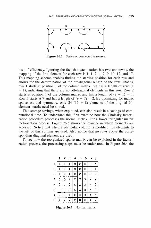
26.7 SPARENESS AND OPTIMIZATION OF THE NORMAL MATRIX 515
Figure 26.2 Series of connected traverses.
Figure 26.3 Normal matrix.
loss of efficiency. Ignoring the fact that each station has two unknowns, themapping of the first element for each row is 1, 1, 2, 4, 7, 9, 10, 12, and 17.This mapping scheme enables finding the starting position for each row andallows for the determination of the off-diagonal length of the row. That is,row 1 starts at position 1 of the column matrix, but has a length of zero (1� 1), indicating that there are no off-diagonal elements in this row. Row 2starts at position 1 of the column matrix and has a length of (2 � 1) � 1.Row 5 starts at 7 and has a length of (9 � 7) � 2. By optimizing for matrixsparseness and symmetry, only 24 (16 � 8) elements of the original 64-element matrix need be stored.
This storage savings, when exploited, can also result in a savings of com-putational time. To understand this, first examine how the Cholesky factori-zation procedure processes the normal matrix. For a lower triangular matrixfactorization process, Figure 26.5 shows the manner in which elements areaccessed. Notice that when a particular column is modified, the elements tothe left of this column are used. Also notice that no rows above the corre-sponding diagonal element are used.
To see how the reorganized sparse matrix can be exploited in the factori-zation process, the processing steps must be understood. In Figure 26.4 the
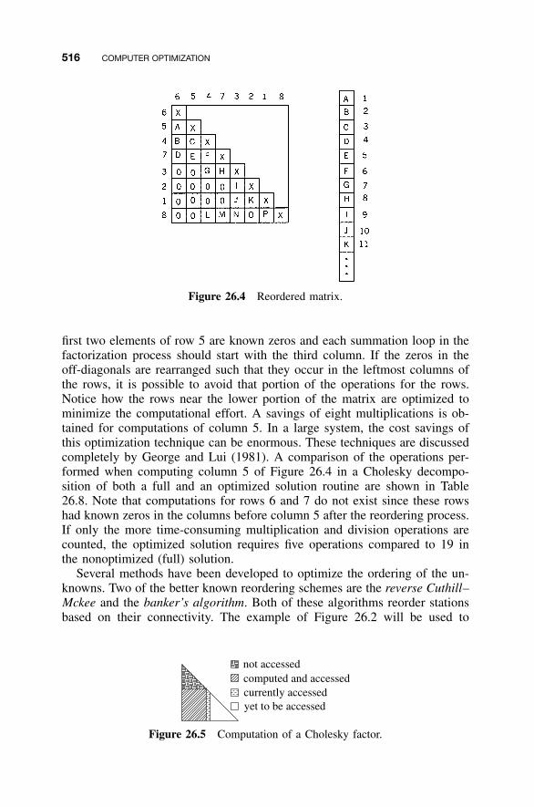
516 COMPUTER OPTIMIZATION
Figure 26.4 Reordered matrix.
not accessedcomputed and accessedcurrently accessedyet to be accessed
Figure 26.5 Computation of a Cholesky factor.
first two elements of row 5 are known zeros and each summation loop in thefactorization process should start with the third column. If the zeros in theoff-diagonals are rearranged such that they occur in the leftmost columns ofthe rows, it is possible to avoid that portion of the operations for the rows.Notice how the rows near the lower portion of the matrix are optimized tominimize the computational effort. A savings of eight multiplications is ob-tained for computations of column 5. In a large system, the cost savings ofthis optimization technique can be enormous. These techniques are discussedcompletely by George and Lui (1981). A comparison of the operations per-formed when computing column 5 of Figure 26.4 in a Cholesky decompo-sition of both a full and an optimized solution routine are shown in Table26.8. Note that computations for rows 6 and 7 do not exist since these rowshad known zeros in the columns before column 5 after the reordering process.If only the more time-consuming multiplication and division operations arecounted, the optimized solution requires five operations compared to 19 inthe nonoptimized (full) solution.
Several methods have been developed to optimize the ordering of the un-knowns. Two of the better known reordering schemes are the reverse Cuthill–Mckee and the banker’s algorithm. Both of these algorithms reorder stationsbased on their connectivity. The example of Figure 26.2 will be used to
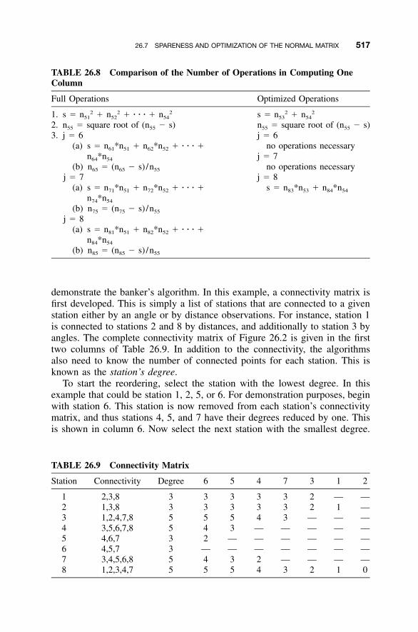
26.7 SPARENESS AND OPTIMIZATION OF THE NORMAL MATRIX 517
TABLE 26.8 Comparison of the Number of Operations in Computing OneColumn
Full Operations Optimized Operations
1. s � n512 � n52
2 � � � � � n542 s � n53
2 � n542
2. n55 � square root of (n55 � s) n55 � square root of (n55 � s)3. j � 6
(a) s � n61*n51 � n62*n52 � � � � �n64*n54
(b) n65 � (n65 � s) /n55
j � 7(a) s � n71*n51 � n72*n52 � � � � �
n74*n54
(b) n75 � (n75 � s) /n55
j � 8(a) s � n81*n51 � n82*n52 � � � � �
n84*n54
(b) n85 � (n85 � s) /n55
j � 6no operations necessary
j � 7no operations necessary
j � 8s � n83*n53 � n84*n54
TABLE 26.9 Connectivity Matrix
Station Connectivity Degree 6 5 4 7 3 1 2
1 2,3,8 3 3 3 3 3 2 — —2 1,3,8 3 3 3 3 3 2 1 —3 1,2,4,7,8 5 5 5 4 3 — — —4 3,5,6,7,8 5 4 3 — — — — —5 4,6,7 3 2 — — — — — —6 4,5,7 3 — — — — — — —7 3,4,5,6,8 5 4 3 2 — — — —8 1,2,3,4,7 5 5 5 4 3 2 1 0
demonstrate the banker’s algorithm. In this example, a connectivity matrix isfirst developed. This is simply a list of stations that are connected to a givenstation either by an angle or by distance observations. For instance, station 1is connected to stations 2 and 8 by distances, and additionally to station 3 byangles. The complete connectivity matrix of Figure 26.2 is given in the firsttwo columns of Table 26.9. In addition to the connectivity, the algorithmsalso need to know the number of connected points for each station. This isknown as the station’s degree.
To start the reordering, select the station with the lowest degree. In thisexample that could be station 1, 2, 5, or 6. For demonstration purposes, beginwith station 6. This station is now removed from each station’s connectivitymatrix, and thus stations 4, 5, and 7 have their degrees reduced by one. Thisis shown in column 6. Now select the next station with the smallest degree.
518 COMPUTER OPTIMIZATION
Since station 5 had its degree reduced to 2 when station 6 was selected, itnow has the smallest degree. This process is continued; that is, the next stationwith the smallest degree is selected and is removed from the connectivity ofthe remaining stations. If two or more stations have the smallest degree, themost recently changed station with the smallest degree is chosen. In thisexample, this happened after choosing station 5. Station 4 was selected overstations 1 and 2 simply because it just had its degree reduced. Althoughstation 7 qualified equally to station 4, station 4 was higher on the list andwas selected for that reason. This happened again after selecting station 7.Station 3 was the next choice since it was the first station reduced to a degreeof 3. Note that the final selection of station 8 was omitted from the list.
A similar optimized reordering can be found by starting with station 1, 2,or 5. This is left as an exercise. For a computer algorithm of this reordering,the reader should refer to the NOAA Technical Memorandum NGS 4 byRichard Snay (1976); the computer algorithm for the reverse Cuthill–McKeeis given by George and Lui (1981).
PROBLEMS
26.1 Explain why computer optimization techniques are necessary for do-ing large least squares adjustments.
26.2 When using double precision, how much computer memory is re-quired in forming the J, W, K, JT, JTW, JTWK, and JTWJ matricesfor a 20-station adjustment having 50 total observations?
26.3 If the normal matrix of Problem 26.2 were stored in lower triangularform and computed directly from the observations, how much storagewould be required?
26.4 Discuss how computational savings are created when solving the nor-mal equations by Cholesky factorization and substitution.
26.5 Write a comparison of an operations table similar to that in Table26.8 for column 3 of the matrix shown in Figure 26.4.
26.6 Repeat Problem 26.5 for column 6.
26.7 Using the station reordering algorithm presented in Section 26.7, de-velop a connectivity matrix and reorder the stations when startingwith station 1. Draw the normal matrix of the newly reordered station,which is similar to the sketch shown in Figure 26.4.
26.8 Repeat Problem 26.7, starting the reordering with station 2.
26.9 Repeat Problem 26.7, starting the reordering with station 5.

PROBLEMS 519
Programming Problems
26.10 Develop a least squares program similar to those developed in Chapter16 that builds the normal equations directly from the observations anduses a Cholesky factorization procedure to find the solution.
26.11 Develop a Mathcad worksheet that will solve Problem 26.10.
520
APPENDIX A
INTRODUCTION TO MATRICES
A.1 INTRODUCTION
Matrix algebra provides at least two important advantages: (1) it enables re-ducing complicated systems of equations to simple expressions that can bevisualized and manipulated more easily, and (2) it provides a systematic,mathematical method for solving problems that is well adapted to computers.Problems are frequently encountered in surveying, geodesy, and photogram-metry that require the solution of large systems of equations. This book dealsspecifically with the analysis and adjustment of redundant measurements thatmust satisfy certain geometric conditions. This frequently results in largeequation systems which, when solved according to the least squares method,yield most probable estimates for adjusted observations and unknown para-meters. As will be demonstrated, matrix methods are particularly well suitedfor least squares computations, and in this book they are used for analyzingand solving these equation systems.
A.2 DEFINITION OF A MATRIX
A matrix is a set of numbers or symbols arranged in a square or rectangulararray of m rows and n columns. The arrangement is such that certain definedmathematical operations can be performed in a systematic and efficient man-ner. As an example of a matrix representation, consider the following systemof three linear equations involving three unknowns:
Adjustment Computations: Spatial Data Analysis, Fourth Edition. C. D. Ghilani and P. R. Wolf© 2006 John Wiley & Sons, Inc. ISBN: 978-0-471-69728-2
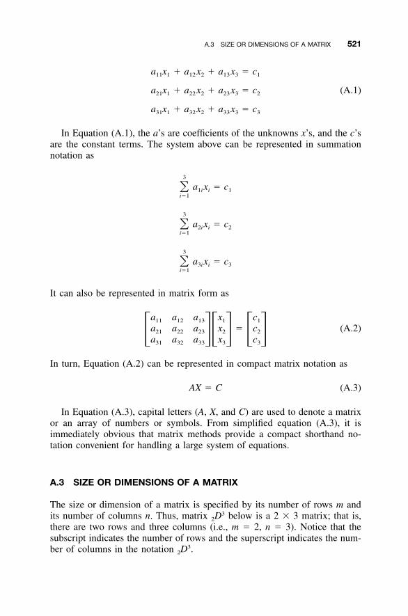
A.3 SIZE OR DIMENSIONS OF A MATRIX 521
a x � a x � a x � c11 1 12 2 13 3 1
a x � a x � a x � c (A.1)21 1 22 2 23 3 2
a x � a x � a x � c31 1 32 2 33 3 3
In Equation (A.1), the a’s are coefficients of the unknowns x’s, and the c’sare the constant terms. The system above can be represented in summationnotation as
3
a x � c� 1i i 1i�1
3
a x � c� 2i i 2i�1
3
a x � c� 3i i 3i�1
It can also be represented in matrix form as
a a a x c11 12 13 1 1
a a a x � c (A.2)21 22 23 2 2� �� � � �a a a x c31 32 33 3 3
In turn, Equation (A.2) can be represented in compact matrix notation as
AX � C (A.3)
In Equation (A.3), capital letters (A, X, and C) are used to denote a matrixor an array of numbers or symbols. From simplified equation (A.3), it isimmediately obvious that matrix methods provide a compact shorthand no-tation convenient for handling a large system of equations.
A.3 SIZE OR DIMENSIONS OF A MATRIX
The size or dimension of a matrix is specified by its number of rows m andits number of columns n. Thus, matrix 2D
3 below is a 2 � 3 matrix; that is,there are two rows and three columns (i.e., m � 2, n � 3). Notice that thesubscript indicates the number of rows and the superscript indicates the num-ber of columns in the notation 2D
3.
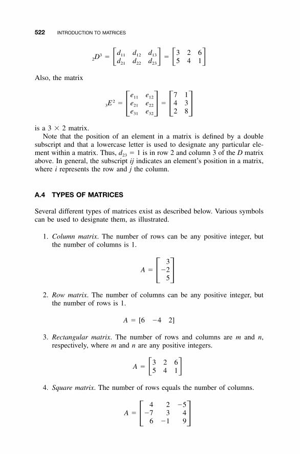
522 INTRODUCTION TO MATRICES
d d d 3 2 63 11 12 13D � �� � � �2 d d d 5 4 121 22 23
Also, the matrix
e e 7 111 122E � e e � 4 33 21 22� � � �e e 2 831 32
is a 3 � 2 matrix.Note that the position of an element in a matrix is defined by a double
subscript and that a lowercase letter is used to designate any particular ele-ment within a matrix. Thus, d23 � 1 is in row 2 and column 3 of the D matrixabove. In general, the subscript ij indicates an element’s position in a matrix,where i represents the row and j the column.
A.4 TYPES OF MATRICES
Several different types of matrices exist as described below. Various symbolscan be used to designate them, as illustrated.
1. Column matrix. The number of rows can be any positive integer, butthe number of columns is 1.
3A � �2� �5
2. Row matrix. The number of columns can be any positive integer, butthe number of rows is 1.
A � [6 �4 2]
3. Rectangular matrix. The number of rows and columns are m and n,respectively, where m and n are any positive integers.
3 2 6A � � �5 4 1
4. Square matrix. The number of rows equals the number of columns.
4 2 �5A � �7 3 4� �6 �1 9
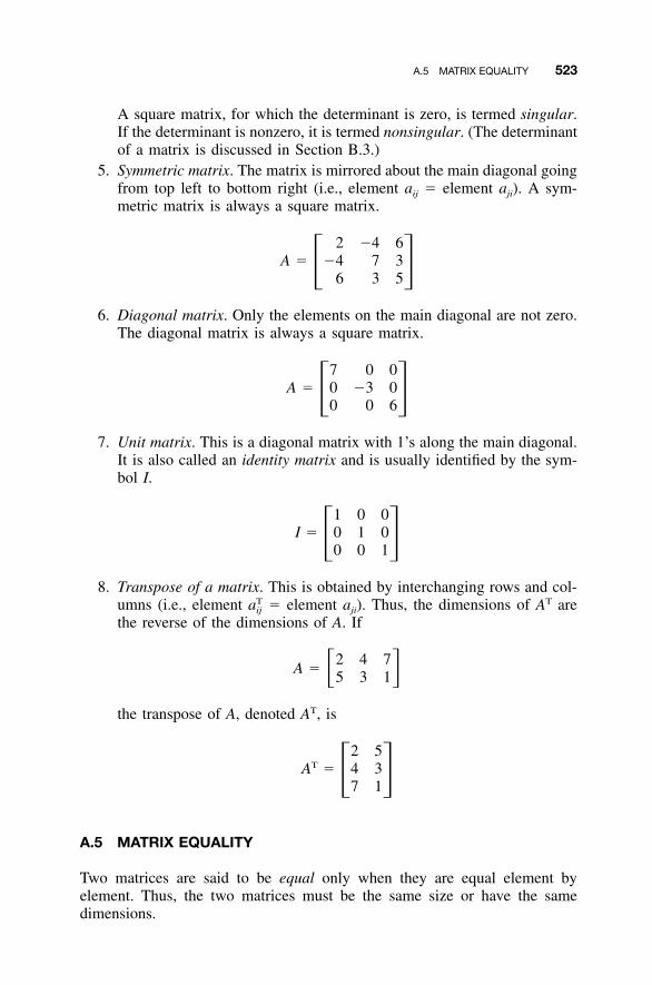
A.5 MATRIX EQUALITY 523
A square matrix, for which the determinant is zero, is termed singular.If the determinant is nonzero, it is termed nonsingular. (The determinantof a matrix is discussed in Section B.3.)
5. Symmetric matrix. The matrix is mirrored about the main diagonal goingfrom top left to bottom right (i.e., element aij � element aji). A sym-metric matrix is always a square matrix.
2 �4 6A � �4 7 3� �6 3 5
6. Diagonal matrix. Only the elements on the main diagonal are not zero.The diagonal matrix is always a square matrix.
7 0 0A � 0 �3 0� �0 0 6
7. Unit matrix. This is a diagonal matrix with 1’s along the main diagonal.It is also called an identity matrix and is usually identified by the sym-bol I.
1 0 0I � 0 1 0� �0 0 1
8. Transpose of a matrix. This is obtained by interchanging rows and col-umns (i.e., element � element aji). Thus, the dimensions of AT areTaij
the reverse of the dimensions of A. If
2 4 7A � � �5 3 1
the transpose of A, denoted AT, is
2 5TA � 4 3� �7 1
A.5 MATRIX EQUALITY
Two matrices are said to be equal only when they are equal element byelement. Thus, the two matrices must be the same size or have the samedimensions.
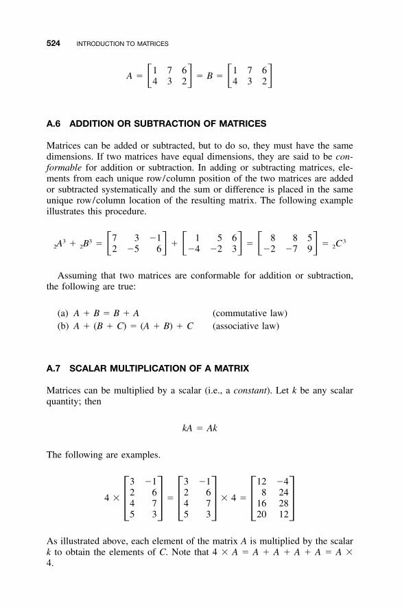
524 INTRODUCTION TO MATRICES
1 7 6 1 7 6A � � B �� � � �4 3 2 4 3 2
A.6 ADDITION OR SUBTRACTION OF MATRICES
Matrices can be added or subtracted, but to do so, they must have the samedimensions. If two matrices have equal dimensions, they are said to be con-formable for addition or subtraction. In adding or subtracting matrices, ele-ments from each unique row/column position of the two matrices are addedor subtracted systematically and the sum or difference is placed in the sameunique row/column location of the resulting matrix. The following exampleillustrates this procedure.
7 3 �1 1 5 6 8 8 53 3 3A � B � � � � C� � � � � �2 2 22 �5 6 �4 �2 3 �2 �7 9
Assuming that two matrices are conformable for addition or subtraction,the following are true:
(a) A � B � B � A (commutative law)(b) A � (B � C) � (A � B) � C (associative law)
A.7 SCALAR MULTIPLICATION OF A MATRIX
Matrices can be multiplied by a scalar (i.e., a constant). Let k be any scalarquantity; then
kA � Ak
The following are examples.
3 �1 3 �1 12 �42 6 2 6 8 24
4 � � � 4 �4 7 4 7 16 28� � � � � �5 3 5 3 20 12
As illustrated above, each element of the matrix A is multiplied by the scalark to obtain the elements of C. Note that 4 � A � A � A � A � A � A �4.
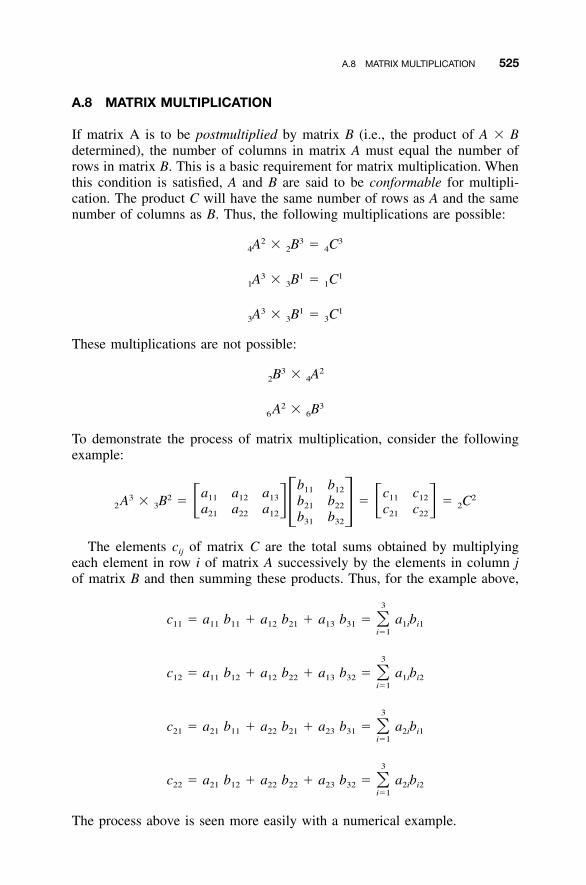
A.8 MATRIX MULTIPLICATION 525
A.8 MATRIX MULTIPLICATION
If matrix A is to be postmultiplied by matrix B (i.e., the product of A � Bdetermined), the number of columns in matrix A must equal the number ofrows in matrix B. This is a basic requirement for matrix multiplication. Whenthis condition is satisfied, A and B are said to be conformable for multipli-cation. The product C will have the same number of rows as A and the samenumber of columns as B. Thus, the following multiplications are possible:
2 3 3A � B � C4 2 4
3 1 1A � B � C1 3 1
3 1 1A � B � C3 3 3
These multiplications are not possible:
3 2B � A2 4
2 3A � B6 6
To demonstrate the process of matrix multiplication, consider the followingexample:
b b11 12a a a c c3 2 11 12 13 11 12 2A � B � b b � � C� � � �2 3 21 22 2a a a c c� �21 22 12 21 22b b31 32
The elements cij of matrix C are the total sums obtained by multiplyingeach element in row i of matrix A successively by the elements in column jof matrix B and then summing these products. Thus, for the example above,
3
c � a b � a b � a b � a b�11 11 11 12 21 13 31 1i i1i�1
3
c � a b � a b � a b � a b�12 11 12 12 22 13 32 1i i2i�1
3
c � a b � a b � a b � a b�21 21 11 22 21 23 31 2i i1i�1
3
c � a b � a b � a b � a b�22 21 12 22 22 23 32 2i i2i�1
The process above is seen more easily with a numerical example.
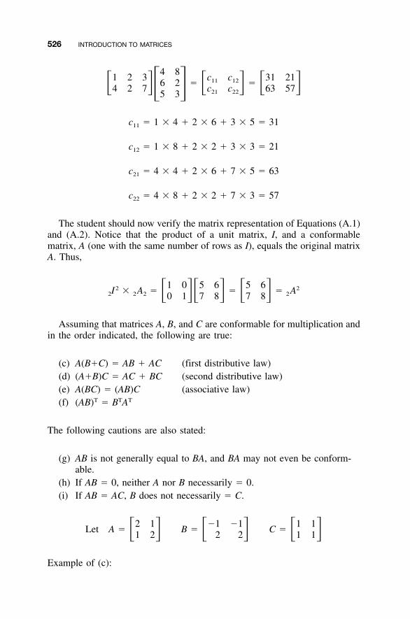
526 INTRODUCTION TO MATRICES
4 81 2 3 c c 31 2111 126 2 � �� � � � � �4 2 7 c c 63 57� � 21 225 3
c � 1 � 4 � 2 � 6 � 3 � 5 � 3111
c � 1 � 8 � 2 � 2 � 3 � 3 � 2112
c � 4 � 4 � 2 � 6 � 7 � 5 � 6321
c � 4 � 8 � 2 � 2 � 7 � 3 � 5722
The student should now verify the matrix representation of Equations (A.1)and (A.2). Notice that the product of a unit matrix, I, and a conformablematrix, A (one with the same number of rows as I), equals the original matrixA. Thus,
1 0 5 6 5 62 2I � A � � � A� �� � � �2 2 2 20 1 7 8 7 8
Assuming that matrices A, B, and C are conformable for multiplication andin the order indicated, the following are true:
(c) A(B�C) � AB � AC (first distributive law)(d) (A�B)C � AC � BC (second distributive law)(e) A(BC) � (AB)C (associative law)
T T T(f) (AB) � B A
The following cautions are also stated:
(g) AB is not generally equal to BA, and BA may not even be conform-able.
(h) If AB � 0, neither A nor B necessarily � 0.(i) If AB � AC, B does not necessarily � C.
2 1 �1 �1 1 1Let A � B � C �� � � � � �1 2 2 2 1 1
Example of (c):
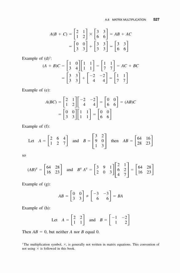
A.8 MATRIX MULTIPLICATION 527
2 1 3 3A(B � C) � � � AB � AC� � � �1 2 6 6
0 0 3 3 3 3� � �� � � � � �3 3 3 3 6 6
Example of (d)1:1 0 1 1 1 1
(A � B)C � � � AC � BC� �� � � �3 4 1 1 7 7
3 3 �2 �2 1 1� � �� � � � � �3 3 4 4 7 7
Example of (e):
2 1 �2 �2 0 0A(BC) � � � (AB)C� �� � � �1 2 4 4 6 6
0 0 1 1 0 0� �� �� � � �3 3 1 1 6 6
Example of (f):
3 22 6 4 64 16
Let A � and B � 9 0 then AB �� � � �1 2 7 28 23� �1 3
so
2 164 28 3 9 1 64 28T T T(AB) � and B A � 6 2 �� � � � � �16 23 2 0 3 16 23� �4 7
Example of (g):
0 0 �3 �3AB � � � BA� � � �3 3 6 6
Example of (h):
2 2 �1 �2Let A � and B �� � � �1 1 1 2
Then AB � 0, but neither A nor B equal 0.
1 The multiplication symbol, �, is generally not written in matrix equations. This convention ofnot using � is followed in this book.
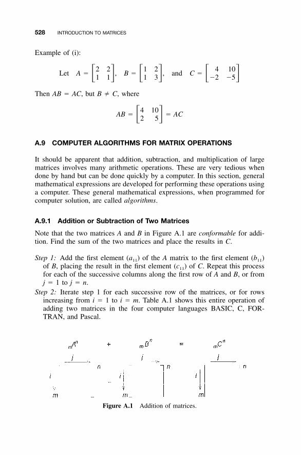
528 INTRODUCTION TO MATRICES
Figure A.1 Addition of matrices.
Example of (i):
2 2 1 2 4 10Let A � , B � , and C �� � � � � �1 1 1 3 �2 �5
Then AB � AC, but B � C, where
4 10AB � � AC� �2 5
A.9 COMPUTER ALGORITHMS FOR MATRIX OPERATIONS
It should be apparent that addition, subtraction, and multiplication of largematrices involves many arithmetic operations. These are very tedious whendone by hand but can be done quickly by a computer. In this section, generalmathematical expressions are developed for performing these operations usinga computer. These general mathematical expressions, when programmed forcomputer solution, are called algorithms.
A.9.1 Addition or Subtraction of Two Matrices
Note that the two matrices A and B in Figure A.1 are conformable for addi-tion. Find the sum of the two matrices and place the results in C.
Step 1: Add the first element (a11) of the A matrix to the first element (b11)of B, placing the result in the first element (c11) of C. Repeat this processfor each of the successive columns along the first row of A and B, or fromj � 1 to j � n.
Step 2: Iterate step 1 for each successive row of the matrices, or for rowsincreasing from i � 1 to i � m. Table A.1 shows this entire operation ofadding two matrices in the four computer languages BASIC, C, FOR-TRAN, and Pascal.
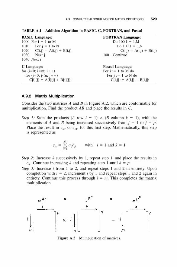
A.9 COMPUTER ALGORITHMS FOR MATRIX OPERATIONS 529
TABLE A.1 Addition Algorithm in BASIC, C, FORTRAN, and Pascal
BASIC Language: FORTRAN Language:1000 For i � 1 to M1010 For j � 1 to N1020 C(i,j) � A(i,j) � B(i,j)1030 Next j1040 Next i
Do 100 I � 1,MDo 100 J � 1,N
C(i,j) � A(i,j) � B(i,j)100 Continue
C Language: Pascal Language:for (i�0; i�m; i��)
for (j�0; j�n; j��)C[i][j] � A[i][j] � B[i][j];
For i :� 1 to M doFor j :� 1 to N do
C[i,j] :� A[i,j] � B[i,j];
Figure A.2 Multiplication of matrices.
A.9.2 Matrix Multiplication
Consider the two matrices A and B in Figure A.2, which are conformable formultiplication. Find the product AB and place the results in C.
Step 1: Sum the products (A row i � 1) � (B column k � 1), with theelements of A and B being increased successively from j � 1 to j � p.Place the result in cik, or c11, for this first step. Mathematically, this stepis represented as
p
c � a b with i � 1 and k � 1�ik ij jkj�1
Step 2: Increase k successively by 1, repeat step 1, and place the results incik. Continue increasing k and repeating step 1 until k � p.
Step 3: Increase i from 1 to 2, and repeat steps 1 and 2 in entirety. Uponcompletion with i � 2, increment i by 1 and repeat steps 1 and 2 again inentirety. Continue this process through i � m. This completes the matrixmultiplication.

530
TA
BL
EA
.2M
ulti
plic
atio
nA
lgor
ithm
inB
ASI
C,
C,
FO
RT
RA
N,
and
Pas
cal
BA
SIC
Lan
guag
e:F
OR
TR
AN
Lan
guag
e:Fo
ri
�1
toM
For
k�
1to
NC
(i,k
)�
0.0
For
j�
1to
PC
(i,k
)�
C(i
,k)
�A
(i,j)
*B(j
,k)
Nex
tj
:N
ext
k:N
ext
I
Do
100
i�
1,M
Do
100
k�
1,N
C(i
,k)
�0.
0D
o10
0j
�1,
PC
(i,k
) �C
(i,k
)�A
(i,j)
*B(j
,k)
100
Con
tinue
CL
angu
age:
Pas
cal
Lan
guag
e:fo
r(i
�0;
i�m
;i�
�)
for
(k�
0;k�
n;k�
�)
{C
[i][
k]�
0;fo
r(j
�0;
j�p;
j��
)C
[i][
k]�
C[i
][k]
�A
[i][
j]*B
[j][
k];
}//
for
k
For
i: �
1to
Mdo
For
k: �
1to
Ndo
Beg
inC
[i,k
]: �
0.0;
For
j: �
1to
Pdo
C[i
,k]
: �C
[i,k
]�
A[i
,j]*B
[j,k
]E
nd;
{for
k}
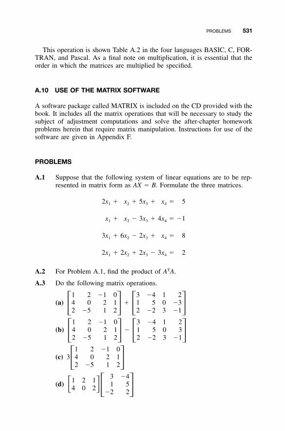
PROBLEMS 531
This operation is shown Table A.2 in the four languages BASIC, C, FOR-TRAN, and Pascal. As a final note on multiplication, it is essential that theorder in which the matrices are multiplied be specified.
A.10 USE OF THE MATRIX SOFTWARE
A software package called MATRIX is included on the CD provided with thebook. It includes all the matrix operations that will be necessary to study thesubject of adjustment computations and solve the after-chapter homeworkproblems herein that require matrix manipulation. Instructions for use of thesoftware are given in Appendix F.
PROBLEMS
A.1 Suppose that the following system of linear equations are to be rep-resented in matrix form as AX � B. Formulate the three matrices.
2x � x � 5x � x � 51 2 3 4
x � x � 3x � 4x � �11 2 3 4
3x � 6x � 2x � x � 81 2 3 4
2x � 2x � 2x � 3x � 21 2 3 4
A.2 For Problem A.1, find the product of ATA.
A.3 Do the following matrix operations.
(a) �1 2 �1 0 3 �4 1 24 0 2 1 1 5 0 �3� � � �2 �5 1 2 2 �2 3 �1
(b) �1 2 �1 0 3 �4 1 24 0 2 1 1 5 0 3� � � �2 �5 1 2 2 �2 3 �1
(c)1 2 �1 0
3 4 0 2 1� �2 �5 1 2
(d)3 �4
1 2 11 5� �4 0 2 � ��2 2
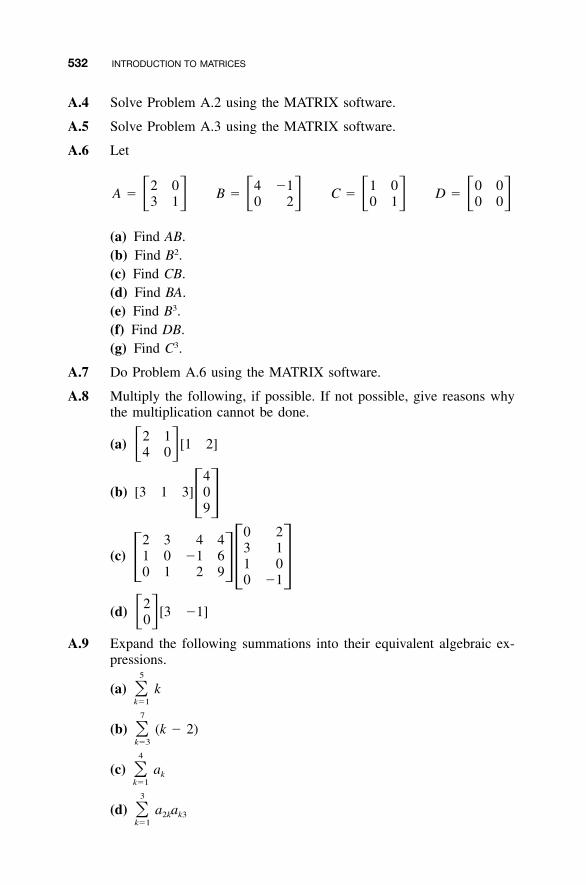
532 INTRODUCTION TO MATRICES
A.4 Solve Problem A.2 using the MATRIX software.
A.5 Solve Problem A.3 using the MATRIX software.
A.6 Let
2 0 4 �1 1 0 0 0A � B � C � D �� � � � � � � �3 1 0 2 0 1 0 0
(a) Find AB.(b) Find B2.(c) Find CB.(d) Find BA.(e) Find B3.(f) Find DB.(g) Find C3.
A.7 Do Problem A.6 using the MATRIX software.
A.8 Multiply the following, if possible. If not possible, give reasons whythe multiplication cannot be done.
(a) 2 1[1 2]� �4 0
(b)4
[3 1 3] 0� �9
(c)
0 22 3 4 4
3 11 0 �1 6
1 0� �� �0 1 2 90 �1
(d) 2[3 �1]� �0
A.9 Expand the following summations into their equivalent algebraic ex-pressions.
(a)5
k�k�1
(b)7
(k � 2)�k�3
(c)4
a� kk�1
(d)3
a a� 2k k3k�1
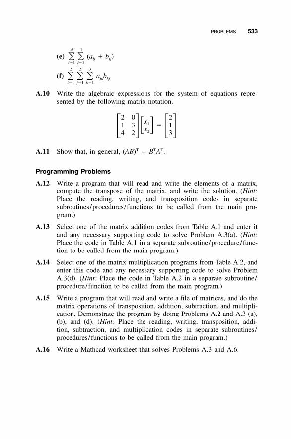
PROBLEMS 533
(e)3 4
(a � b )� � ij iji�1 j�1
(f)2 2 3
a b� � � ik kji�1 j�1 k�1
A.10 Write the algebraic expressions for the system of equations repre-sented by the following matrix notation.
2 0 2x11 3 � 1� �x� � � �24 2 3
A.11 Show that, in general, (AB)T � BTAT.
Programming Problems
A.12 Write a program that will read and write the elements of a matrix,compute the transpose of the matrix, and write the solution. (Hint:Place the reading, writing, and transposition codes in separatesubroutines/procedures/functions to be called from the main pro-gram.)
A.13 Select one of the matrix addition codes from Table A.1 and enter itand any necessary supporting code to solve Problem A.3(a). (Hint:Place the code in Table A.1 in a separate subroutine/procedure/func-tion to be called from the main program.)
A.14 Select one of the matrix multiplication programs from Table A.2, andenter this code and any necessary supporting code to solve ProblemA.3(d). (Hint: Place the code in Table A.2 in a separate subroutine/procedure/function to be called from the main program.)
A.15 Write a program that will read and write a file of matrices, and do thematrix operations of transposition, addition, subtraction, and multipli-cation. Demonstrate the program by doing Problems A.2 and A.3 (a),(b), and (d). (Hint: Place the reading, writing, transposition, addi-tion, subtraction, and multiplication codes in separate subroutines/procedures/functions to be called from the main program.)
A.16 Write a Mathcad worksheet that solves Problems A.3 and A.6.
534
APPENDIX B
SOLUTION OF EQUATIONSBY MATRIX METHODS
B.1 INTRODUCTION
As stated in Appendix A, an advantage offered by matrix algebra is its adapt-ability to computer use. Using matrix algebra, large systems of simultaneouslinear equations can be programmed for general computer solution using onlya few systematic steps. The simplicities of programming matrix additions andmultiplications, for example, were presented in Section A.9. To solve a systemof equations using matrix methods, it is first necessary to define and computethe inverse matrix.
B.2 INVERSE MATRIX
If a square matrix is nonsingular (its determinant is not zero), it possesses aninverse matrix. When a system of simultaneous linear equations consisting ofn equations and involving n unknowns is expressed as AX � B, the coefficientmatrix (A) is a square matrix of dimensions n � n. Consider the system oflinear equations
AX � B (B.1)
The inverse of matrix A, symbolized as A�1, is defined as
�1A A � I (B.2)
where I is the identity matrix. Premultiplying both sides of matrix Equation(B.1) by A�1 gives
Adjustment Computations: Spatial Data Analysis, Fourth Edition. C. D. Ghilani and P. R. Wolf© 2006 John Wiley & Sons, Inc. ISBN: 978-0-471-69728-2
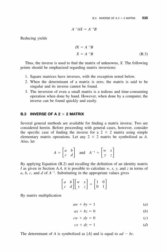
B.3 INVERSE OF A 2 � 2 MATRIX 535
�1 �1A AX � A B
Reducing yields
�1IX � A B�1X � A B (B.3)
Thus, the inverse is used to find the matrix of unknowns, X. The followingpoints should be emphasized regarding matrix inversions:
1. Square matrices have inverses, with the exception noted below.2. When the determinant of a matrix is zero, the matrix is said to be
singular and its inverse cannot be found.3. The inversion of even a small matrix is a tedious and time-consuming
operation when done by hand. However, when done by a computer, theinverse can be found quickly and easily.
B.3 INVERSE OF A 2 � 2 MATRIX
Several general methods are available for finding a matrix inverse. Two areconsidered herein. Before proceeding with general cases, however, considerthe specific case of finding the inverse for a 2 � 2 matrix using simpleelementary matrix operations. Let any 2 � 2 matrix be symbolized as A.Also, let
a b w x�1A � and A �� � � �c d y z
By applying Equation (B.2) and recalling the definition of an identity matrixI as given in Section A.4, it is possible to calculate w, x, y, and z in terms ofa, b, c, and d of A�1. Substituting in the appropriate values gives
a b w x 1 0�� �� � � �c d y z 0 1
By matrix multiplication
aw � by � 1 (a)
ax � bz � 0 (b)
cw � dy � 0 (c)
cx � dz � 1 (d)
The determinant of A is symbolized as �A� and is equal to ad � bc.
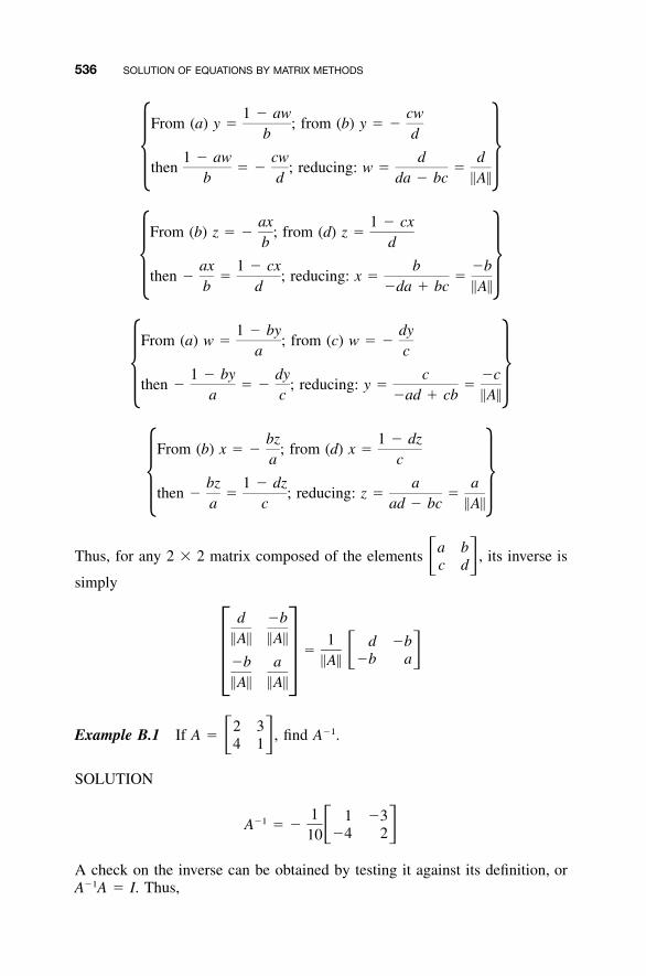
536 SOLUTION OF EQUATIONS BY MATRIX METHODS
1 � aw cwFrom (a) y � ; from (b) y � �
b d
1 � aw cw d d� �then � � ; reducing: w � �b d da � bc �A�
ax 1 � cxFrom (b) z � � ; from (d) z �
b d
ax 1 � cx b �b� �then � � ; reducing: x � �b d �da � bc �A�
1 � by dyFrom (a) w � ; from (c) w � �
a c
1 � by dy c �c� �then � � � ; reducing: y � �a c �ad � cb �A�
bz 1 � dzFrom (b) x � � ; from (d) x �
a c
bz 1 � dz a a� �then � � ; reducing: z � �a c ad � bc �A�
Thus, for any 2 � 2 matrix composed of the elements , its inverse isa b� �c d
simply
d �b�A� �A� 1 d �b
� � ��b a�A��b a� ��A� �A�
Example B.1 If find A�1.2 3
A � ,� �4 1
SOLUTION
1 1 �3�1A � � � ��4 210
A check on the inverse can be obtained by testing it against its definition, orA�1A � I. Thus,

B.4 INVERSES BY ADJOINTS 537
Figure B.1 Cofactor of the a12 element.
1 1 �3 2 3 1 0� � � I� �� � � ��4 2 4 1 0 110
B.4 INVERSES BY ADJOINTS
The inverse of A can be found using the method of adjoints with the followingequation:
adjoint of A adjoint of A�1A � � (B.4)
determinant of A �A�
The adjoint of A is obtained by first replacing each matrix element by itssigned minor or cofactor, and then transposing the resulting matrix. The co-factor of element aij equals (�1)i�j times the numerical value of the deter-minant for the remaining elements after row i and column j have beenremoved from the matrix. This procedure is illustrated in Figure B.1, wherethe cofactor of a12 is
1�2(�1) (a a � a a ) � a a � a a21 33 31 23 31 23 21 33
Using this procedure, the inverse of the following A matrix is found:
a a a 4 3 211 12 13
A � a a a � 3 4 121 22 23� � � �a a a 2 3 431 32 33
For this A matrix, the cofactors are calculated as follows
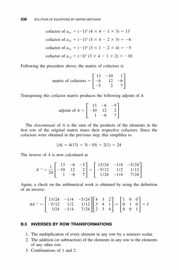
538 SOLUTION OF EQUATIONS BY MATRIX METHODS
2cofactor of a � (�1) (4 � 4 � 1 � 3) � 1311
3cofactor of a � (�1) (3 � 4 � 2 � 3) � �621
4cofactor of a � (�1) (3 � 1 � 2 � 4) � �531
3cofactor of a � (�l) (3 � 4 � 1 � 2) � �1012
Following the procedure above, the matrix of cofactors is
13 �10 1matrix of cofactors � �6 12 �6� ��5 2 7
Transposing this cofactor matrix produces the following adjoint of A:
13 �6 �5adjoint of A � �10 12 2� �1 �6 7
The determinant of A is the sum of the products of the elements in thefirst row of the original matrix times their respective cofactors. Since thecofactors were obtained in the previous step, this simplifies to
�A� � 4(13) � 3(�10) � 2(1) � 24
The inverse of A is now calculated as
13 �6 �5 13/24 �1/4 �5/241�1A � �10 12 2 � �5/12 1/2 1/12
24 � � � �1 �6 7 1/24 �1/4 7/24
Again, a check on the arithmetical work is obtained by using the definitionof an inverse:
13/24 �1/4 �5/24 4 3 2 1 0 0�1AA � �5/12 1/2 1/12 3 4 1 � 0 1 0 � I� �� � � �1/24 �1/4 7/24 2 3 4 0 0 1
B.5 INVERSES BY ROW TRANSFORMATIONS
1. The multiplication of every element in any row by a nonzero scalar.2. The addition (or subtraction) of the elements in any row to the elements
of any other row.3. Combinations of 1 and 2.
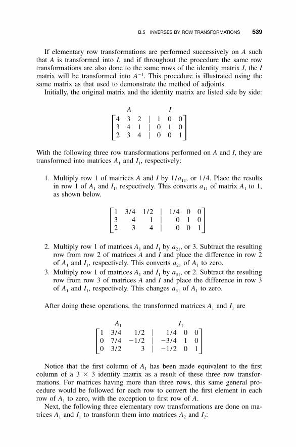
B.5 INVERSES BY ROW TRANSFORMATIONS 539
If elementary row transformations are performed successively on A suchthat A is transformed into I, and if throughout the procedure the same rowtransformations are also done to the same rows of the identity matrix I, the Imatrix will be transformed into A�1. This procedure is illustrated using thesame matrix as that used to demonstrate the method of adjoints.
Initially, the original matrix and the identity matrix are listed side by side:
A I4 3 2 � 1 0 03 4 1 � 0 1 0� �2 3 4 � 0 0 1
With the following three row transformations performed on A and I, they aretransformed into matrices A1 and I1, respectively:
1. Multiply row 1 of matrices A and I by 1/a11, or 1/4. Place the resultsin row 1 of A1 and I1, respectively. This converts a11 of matrix A1 to 1,as shown below.
1 3/4 1/2 � 1/4 0 03 4 1 � 0 1 0� �2 3 4 � 0 0 1
2. Multiply row 1 of matrices A1 and I1 by a21, or 3. Subtract the resultingrow from row 2 of matrices A and I and place the difference in row 2of A1 and I1, respectively. This converts a21 of A1 to zero.
3. Multiply row 1 of matrices A1 and I1 by a31, or 2. Subtract the resultingrow from row 3 of matrices A and I and place the difference in row 3of A1 and I1, respectively. This changes a31 of A1 to zero.
After doing these operations, the transformed matrices A1 and I1 are
A1 I1
1 3/4 1/2 � 1/4 0 00 7/4 �1/2 � �3/4 1 0� �0 3/2 3 � �1/2 0 1
Notice that the first column of A1 has been made equivalent to the firstcolumn of a 3 � 3 identity matrix as a result of these three row transfor-mations. For matrices having more than three rows, this same general pro-cedure would be followed for each row to convert the first element in eachrow of A1 to zero, with the exception to first row of A.
Next, the following three elementary row transformations are done on ma-trices A1 and I1 to transform them into matrices A2 and I2:
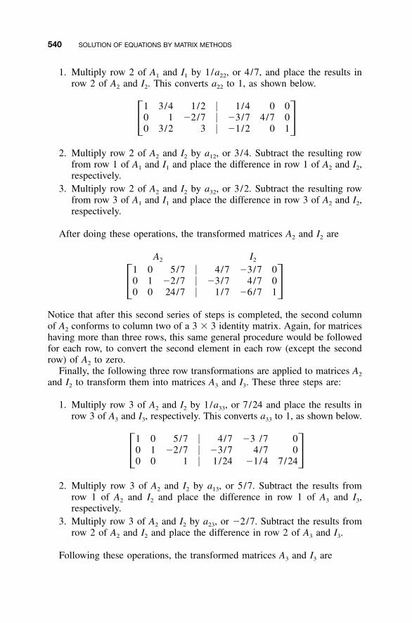
540 SOLUTION OF EQUATIONS BY MATRIX METHODS
1. Multiply row 2 of A1 and I1 by 1/a22, or 4/7, and place the results inrow 2 of A2 and I2. This converts a22 to 1, as shown below.
1 3/4 1/2 � 1/4 0 00 1 �2/7 � �3/7 4/7 0� �0 3/2 3 � �1/2 0 1
2. Multiply row 2 of A2 and I2 by a12, or 3/4. Subtract the resulting rowfrom row 1 of A1 and I1 and place the difference in row 1 of A2 and I2,respectively.
3. Multiply row 2 of A2 and I2 by a32, or 3/2. Subtract the resulting rowfrom row 3 of A1 and I1 and place the difference in row 3 of A2 and I2,respectively.
After doing these operations, the transformed matrices A2 and I2 are
A2 I2
1 0 5/7 � 4/7 �3/7 00 1 �2/7 � �3/7 4/7 0� �0 0 24/7 � 1/7 �6/7 1
Notice that after this second series of steps is completed, the second columnof A2 conforms to column two of a 3 � 3 identity matrix. Again, for matriceshaving more than three rows, this same general procedure would be followedfor each row, to convert the second element in each row (except the secondrow) of A2 to zero.
Finally, the following three row transformations are applied to matrices A2
and I2 to transform them into matrices A3 and I3. These three steps are:
1. Multiply row 3 of A2 and I2 by 1/a33, or 7/24 and place the results inrow 3 of A3 and I3, respectively. This converts a33 to 1, as shown below.
1 0 5/7 � 4/7 �3 /7 00 1 �2/7 � �3/7 4/7 0� �0 0 1 � 1/24 �1/4 7/24
2. Multiply row 3 of A2 and I2 by a13, or 5/7. Subtract the results fromrow 1 of A2 and I2 and place the difference in row 1 of A3 and I3,respectively.
3. Multiply row 3 of A2 and I2 by a23, or �2/7. Subtract the results fromrow 2 of A2 and I2 and place the difference in row 2 of A3 and I3.
Following these operations, the transformed matrices A3 and I3 are

541
TA
BL
EB
.1In
vers
eA
lgor
ithm
inB
ASI
C,
C,
FO
RT
RA
N,
and
PASC
AL
BA
SIC
Lan
guag
e:R
EM
INV
ER
TA
MA
TR
IXFO
Rk
�1
TO
nFO
Rj
�1
TO
nIF
j ��
kT
HE
NA
(k,j)
�A
(k,j)
/A(k
,k)
NE
XT
jA
(k,k
)�
1/A
(k,k
)FO
Ri
�1
TO
nIF
i ��
kT
HE
NFO
Rj �
1T
On
IFj �
�k
TH
EN
A(i
,j)�
A(i
,j)�
A(i
,k)*
A(k
,j)N
EX
Tj
A(i
,k)
��
A(i
,k)*
A(k
,k)
EN
DIF
NE
XT
i:N
EX
Tk
FO
RT
RA
NL
angu
age:
Do
560
k�
1,N
Do
520
j�
1,N
If(j
.NE
.k)
The
nA
(k,j)
�A
(k,j)
/A(k
,k)
520
Con
tinue
A(K
,K)
�1.
0/A
(K,K
)D
o56
0i
�1,
NIf
(i.E
Q.k
)T
hen
GO
TO
560
Do
550
j�
1,N
If(j
.NE
.k)
The
nA
(i,j)
�A
(i,j)
�A
(i,k
)*A
(k,j)
550
Con
tinue
A(i
,k)
��
A(i
,k)
*A
(k,k
)56
0C
ontin
ueC
Lan
guag
e:fo
r(k
�0;
k�n;
k��
){
for
(j�
0;j�
n;j�
�)
if(j
! �k)
A[k
][j]
�A
[k][
j]/A
[k][
k];
A[k
][k]
�1.
0/A
[k][
k];
for
(i�
0;i�
n;i�
�)
if(i
! �k)
{fo
r(j
�0;
j�n;
j��
)if
(j! �
k)A
[i][
j]�
A[i
][j]
�A
[i][
k]*A
[k][
j];
A[i
][k]
��
A[i
][k]
*A[k
][k]
;}
//if
i ��
k}
//fo
rk
Pas
cal
Lan
guag
e:Fo
rk
: �1
toN
doB
egin
For
j: �
1to
Ndo
If(j
��
k)th
enA
[k,j]
:�A
[k,j]
/A[k
,k];
A[k
,k]
: �1.
0/A
[k,k
];Fo
ri
: �1
toN
doIf
(i�
�k)
then
Beg
inFo
rj
: �1
toN
doIf
(j�
�k)
then
A[i
,j]:�
A[i
,j]�
A[i
,k]*
A[k
,j];
A[i
,k]
: ��
A[i
,k]*
A[k
,k];
End
;{I
fi �
�k}
End
;{f
ork}
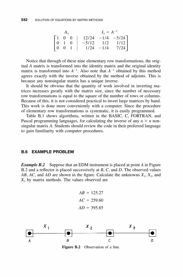
542 SOLUTION OF EQUATIONS BY MATRIX METHODS
Figure B.2 Observation of a line.
A3 I3 � A�1
1 0 0 � 12/24 �1/4 �5/240 1 0 � �5/12 1/2 1/12� �0 0 1 � 1/24 �1/4 7/24
Notice that through of these nine elementary row transformations, the orig-inal A matrix is transformed into the identity matrix and the original identitymatrix is transformed into A�1. Also note that A�1 obtained by this methodagrees exactly with the inverse obtained by the method of adjoints. This isbecause any nonsingular matrix has a unique inverse.
It should be obvious that the quantity of work involved in inverting ma-trices increases greatly with the matrix size, since the number of necessaryrow transformations is equal to the square of the number of rows or columns.Because of this, it is not considered practical to invert large matrices by hand.This work is done more conveniently with a computer. Since the procedureof elementary row transformations is systematic, it is easily programmed.
Table B.1 shows algorithms, written in the BASIC, C, FORTRAN, andPascal programming languages, for calculating the inverse of any n � n non-singular matrix A. Students should review the code in their preferred languageto gain familiarity with computer procedures.
B.6 EXAMPLE PROBLEM
Example B.2 Suppose that an EDM instrument is placed at point A in FigureB.2 and a reflector is placed successively at B, C, and D. The observed valuesAB, AC, and AD are shown in the figure. Calculate the unknowns X1, X2, andX3 by matrix methods. The values observed are
AB � 125.27
AC � 259.60
AD � 395.85
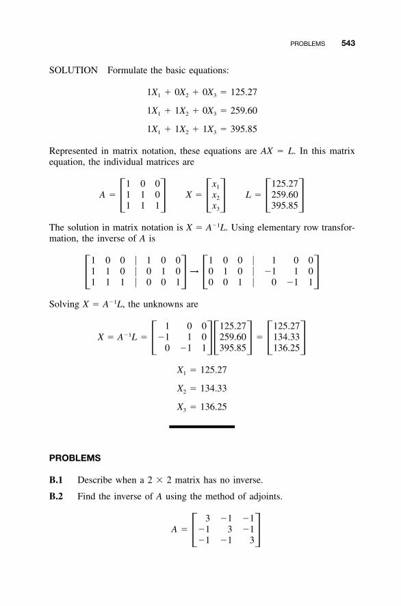
PROBLEMS 543
SOLUTION Formulate the basic equations:
1X � 0X � 0X � 125.271 2 3
1X � 1X � 0X � 259.601 2 3
1X � 1X � 1X � 395.851 2 3
Represented in matrix notation, these equations are AX � L. In this matrixequation, the individual matrices are
1 0 0 x 125.271
A � 1 1 0 X � x L � 259.602� � � � � �1 1 1 x 395.853
The solution in matrix notation is X � A�1L. Using elementary row transfor-mation, the inverse of A is
1 0 0 � 1 0 0 1 0 0 � 1 0 01 1 0 � 0 1 0 → 0 1 0 � �1 1 0� � � �1 1 1 � 0 0 1 0 0 1 � 0 �1 1
Solving X � A�1L, the unknowns are
1 0 0 125.27 125.27�1X � A L � �1 1 0 259.60 � 134.33� �� � � �0 �1 1 395.85 136.25
X � 125.271
X � 134.332
X � 136.253
PROBLEMS
B.1 Describe when a 2 � 2 matrix has no inverse.
B.2 Find the inverse of A using the method of adjoints.
3 �1 �1A � �1 3 �1� ��1 �1 3
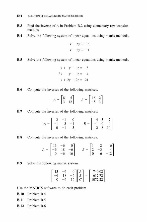
544 SOLUTION OF EQUATIONS BY MATRIX METHODS
B.3 Find the inverse of A in Problem B.2 using elementary row transfor-mations.
B.4 Solve the following system of linear equations using matrix methods.
x � 5y � �8
�x � 2y � �1
B.5 Solve the following system of linear equations using matrix methods.
x � y � z � �8
3x � y � z � �4
�x � 2y � 2z � 21
B.6 Compute the inverses of the following matrices.
8 5 16 2A � B �� � � �3 12 �8 3
B.7 Compute the inverses of the following matrices.
3 �1 0 4 3 7A � �1 3 �1 B � �1 0 4� � � �0 �1 3 2 8 10
B.8 Compute the inverses of the following matrices.
13 �6 0 1 2 6A � �6 18 �6 B � 2 �3 4� � � �0 �6 16 0 6 �12
B.9 Solve the following matrix system.
13 �6 0 A 740.02�6 18 �6 B � 612.72� �� � � �0 �6 16 C 1072.22
Use the MATRIX software to do each problem.
B.10 Problem B.4
B.11 Problem B.5
B.12 Problem B.6
PROBLEMS 545
B.13 Problem B.7
B.14 Problem B.8
B.15 Problem B.9
Programming Problems
B.16 Select one of the coded matrix inverse routines from Table B.1, enterthe code into a computer, and use it to solve Problem B.7. (Hint: Placethe code in Table B.1 in a separate subroutine/function/procedure tobe called from the main program.)
B.17 Add a block of code to the inverse routine in the language of yourchoice that will inform the user when a matrix is singular.
B.18 Write a program that reads and writes a file with a nonsingular matrix;finds its inverse, and write the results. Use this program to solve Prob-lem B.7. (Hint: Place the reading, writing, and inversing code inseparate subroutines/functions/procedures to be called from the mainprogram. Provide a way to identify each matrix in the output file.)
B.19 Write a program that reads and writes a file containing a system ofequations written in matrix form, solves the system using matrix op-erations, and writes the solution. Use this program to solve ProblemB.9. (Hint: Place the reading, writing, and inversing code in separatesubroutines/functions/procedures to be called from the main program.Provide a way to identify each matrix in the output file.)
546
APPENDIX C
NONLINEAR EQUATIONS ANDTAYLOR’S THEOREM
C.1 INTRODUCTION
In adjustment computations it is frequently necessary to deal with nonlinearequations. For example, some observation equations relate observed quantitiesto unknown parameters through the transcendental functions of sine, cosine,or tangent; others relate them through terms raised to second- and higher-order powers. The task of solving a system of nonlinear equations is formi-dable. To facilitate the solution, a first-order Taylor series approximation maybe used to create a set of linear equations. The equations can then be solvedby matrix methods discussed in Appendix B.
C.2 TAYLOR SERIES LINEARIZATION OF NONLINEAR EQUATIONS
Suppose that the following equation relates a observed value L to its unknownparameters x and y through nonlinear coefficients as
L � ƒ(x,y) (C.1)
By Taylor’s theorem, the equation is represented as
L � ƒ(x,y)2 2 n n(�L /�x) (� L /�x ) (� L /�x )0 0 02 n� ƒ(x ,y ) � dx � dx � � � � � dx0 0 1! 2! n!
2 2 n n(�L /�y) (� L /�y ) (� L /�y )0 0 02 n� dy � dy � � � � � dy � R (C.2)1! 2! n!
Adjustment Computations: Spatial Data Analysis, Fourth Edition. C. D. Ghilani and P. R. Wolf© 2006 John Wiley & Sons, Inc. ISBN: 978-0-471-69728-2
C.3 NUMERICAL EXAMPLE 547
In Equation (C.2), x0 and y0 are approximations of x and y; ƒ(x0,y0) is thenonlinear function evaluated at these approximations; R is the remainder, anddx and dy are corrections to the initial approximations, such that
x � x � dx0 (C.3)
y � y � dy0
A more exact Taylor series approximation is obtained by increasing thevalue of n in Equation (C.2). However, as the order of each successive termincreases, its significance in the overall expression decreases. If all termscontaining derivatives higher than the first are dropped, the following linearexpression is obtained:
�L �LL � ƒ(x,y) � ƒ(x ,y ) � dx � dy (C.4)� � � �0 0 �x �y0 0
Once the initial approximations are selected, the only unknowns in Equa-tion (C.4) are the corrections dx and dy. Of course, by dropping thehigher-order terms from the Taylor series, Equation (C.4) becomes only agood approximation of the original equation. However, in the solution, aniterative procedure can be followed that yields accurate answers. This iterativeprocedure uses the following steps:
Step 1: Determine initial approximations for the unknowns. They may beobtained by guessing or from observations. It should be understood thatthe closer the initial approximations are to the final solution, the faster itwill be obtained. For some problems, initial approximations can be ob-tained from graphical solutions or computed from available data or obser-vations. For others, the determination of initial approximations can involveconsiderable computational effort.
Step 2: Substitute the initial approximations into Equation (C.4) and solvefor the corrections dx and dy.
Step 3: Calculate revised values of x and y using Equations (C.3).Step 4: Using these newly revised values for x and y, repeat steps 2 and 3.Step 5: Continue the procedure until the corrections dx and dy are small
enough to bring x and y within tolerable accuracy. When this occurs, thesolution is said to have converged.
C.3 NUMERICAL EXAMPLE
To clarify this procedure further, a numerical example will be solved.
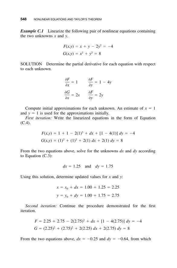
548 NONLINEAR EQUATIONS AND TAYLOR’S THEOREM
Example C.1 Linearize the following pair of nonlinear equations containingthe two unknowns x and y.
2F(x,y) � x � y � 2y � �42 2G(x,y) � x � y � 8
SOLUTION Determine the partial derivative for each equation with respectto each unknown.
�F �F� 1 � 1 � 4y
�x �y
�G �F� 2x � 2y
�x �y
Compute initial approximations for each unknown. An estimate of x � 1and y � 1 is used for the approximations initially.
First iteration: Write the linearized equations in the form of Equation(C.4).
2F(x,y) � 1 � 1 � 2(1) � dx � [1 � 4(1)] dy � �42 2G(x,y) � (1) � (1) � 2(1) dx � 2(1) dy � 8
From the two equations above, solve for the unknowns dx and dy accordingto Equation (C.3):
dx � 1.25 and dy � 1.75
Using this solution, determine updated values for x and y:
x � x � dx � 1.00 � 1.25 � 2.250
y � y � dy � 1.00 � 1.75 � 2.750
Second iteration: Continue the procedure demonstrated for the firstiteration.
2F � 2.25 � 2.75 � 2(2.75) � dx � [1 � 4(2.75)] dy � �42 2G � (2.25) � (2.75) � 2(2.25) dx � 2(2.75) dy � 8
From the two equations above, dx � �0.25 and dy � �0.64, from which
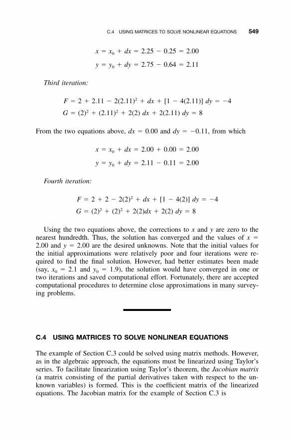
C.4 USING MATRICES TO SOLVE NONLINEAR EQUATIONS 549
x � x � dx � 2.25 � 0.25 � 2.000
y � y � dy � 2.75 � 0.64 � 2.110
Third iteration:
2F � 2 � 2.11 � 2(2.11) � dx � [1 � 4(2.11)] dy � �42 2G � (2) � (2.11) � 2(2) dx � 2(2.11) dy � 8
From the two equations above, dx � 0.00 and dy � �0.11, from which
x � x � dx � 2.00 � 0.00 � 2.000
y � y � dy � 2.11 � 0.11 � 2.000
Fourth iteration:
2F � 2 � 2 � 2(2) � dx � [1 � 4(2)] dy � �42 2G � (2) � (2) � 2(2)dx � 2(2) dy � 8
Using the two equations above, the corrections to x and y are zero to thenearest hundredth. Thus, the solution has converged and the values of x �2.00 and y � 2.00 are the desired unknowns. Note that the initial values forthe initial approximations were relatively poor and four iterations were re-quired to find the final solution. However, had better estimates been made(say, x0 � 2.1 and y0 � 1.9), the solution would have converged in one ortwo iterations and saved computational effort. Fortunately, there are acceptedcomputational procedures to determine close approximations in many survey-ing problems.
C.4 USING MATRICES TO SOLVE NONLINEAR EQUATIONS
The example of Section C.3 could be solved using matrix methods. However,as in the algebraic approach, the equations must be linearized using Taylor’sseries. To facilitate linearization using Taylor’s theorem, the Jacobian matrix(a matrix consisting of the partial derivatives taken with respect to the un-known variables) is formed. This is the coefficient matrix of the linearizedequations. The Jacobian matrix for the example of Section C.3 is
550 NONLINEAR EQUATIONS AND TAYLOR’S THEOREM
�F �F�x �y
J ��G �G� ��x �y
In the Jacobian matrix above, the first column contains the partial derivativefor each equation with respect to x, and the second column contains the partialderivative of each equation with respect to y. The linearized form of theequations may then be expressed in matrix notation as
JX � K (C.5)
In Equation (C.5), J is the Jacobian matrix, X the matrix of unknowncorrections dx and dy, and K the matrix of constants. Specifically, for theexample of Section C.3, these matrices are
1 1 � 4y dx �4 � F(x , y )0 0 0J � X � K �� � � � � �2x 2y dy 8 � G(x , y )0 0 0 0
where F(x0,y0) and G(x0,y0) are the equations F and G solved at the initialapproximations of x0 and y0.
Beginning with a set of initial approximations x0 and y0, the J and Kmatrices of Equation (C.5) are formed. X is computed using the matrix meth-ods presented in Appendix B. Having updated the unknowns according toEquations (C.3), the J and K matrices are formed again and the solution forX is computed. This procedure is iterated until convergence is achieved.
C.5 SIMPLE MATRIX EXAMPLE
Example C.2 Find the solution of the nonlinear system of equations shownbelow using matrix methods.
2 2F(x, y) � x � 3xy � 4y � 62G(x, y) � x � xy � y � 3
SOLUTION The partial derivatives of functions F and G with respect tothe unknowns, x and y, are
�F �F� 2x � 3y � 3x � 8y
�x �y
�G �G� 1 � y � x � 2y
�x �y
Thus, the Jacobian matrix is
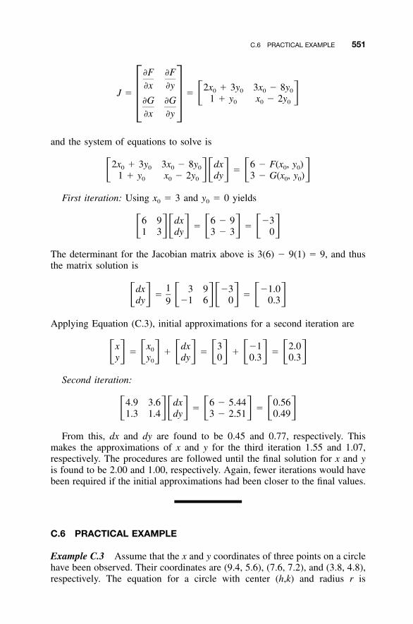
C.6 PRACTICAL EXAMPLE 551
�F �F�x �y 2x � 3y 3x � 8y0 0 0 0J � � � �1 � y x � 2y�G �G 0 0 0� ��x �y
and the system of equations to solve is
2x � 3y 3x � 8y dx 6 � F(x , y )0 0 0 0 0 0�� �� � � �1 � y x � 2y dy 3 � G(x , y )0 0 0 0 0
First iteration: Using x0 � 3 and y0 � 0 yields
6 9 dx 6 � 9 �3� �� �� � � � � �1 3 dy 3 � 3 0
The determinant for the Jacobian matrix above is 3(6) � 9(1) � 9, and thusthe matrix solution is
1dx 3 9 �3 �1.0� �� � � �� � � �dy �1 6 0 0.39
Applying Equation (C.3), initial approximations for a second iteration are
x x dx 3 �1 2.00� � � � �� � � � � � � � � � � �y y dy 0 0.3 0.30
Second iteration:
4.9 3.6 dx 6 � 5.44 0.56� �� �� � � � � �1.3 1.4 dy 3 � 2.51 0.49
From this, dx and dy are found to be 0.45 and 0.77, respectively. Thismakes the approximations of x and y for the third iteration 1.55 and 1.07,respectively. The procedures are followed until the final solution for x and yis found to be 2.00 and 1.00, respectively. Again, fewer iterations would havebeen required if the initial approximations had been closer to the final values.
C.6 PRACTICAL EXAMPLE
Example C.3 Assume that the x and y coordinates of three points on a circlehave been observed. Their coordinates are (9.4, 5.6), (7.6, 7.2), and (3.8, 4.8),respectively. The equation for a circle with center (h,k) and radius r is
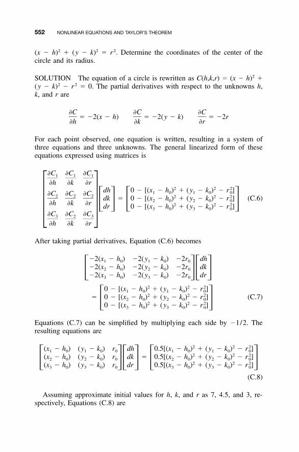
552 NONLINEAR EQUATIONS AND TAYLOR’S THEOREM
(x � h)2 � (y � k)2 � r2. Determine the coordinates of the center of thecircle and its radius.
SOLUTION The equation of a circle is rewritten as C(h,k,r) � (x � h)2 �(y � k)2 � r2 � 0. The partial derivatives with respect to the unknowns h,k, and r are
�C �C �C� �2(x � h) � �2(y � k) � �2r
�h �k �r
For each point observed, one equation is written, resulting in a system ofthree equations and three unknowns. The general linearized form of theseequations expressed using matrices is
�C �C �C1 1 1
�h �k �r2 2 2dh 0 � [(x � h ) � (y � k ) � r ]1 0 1 0 0�C �C �C2 2 2 2 2 2dk � 0 � [(x � h ) � (y � k ) � r ] (C.6)2 0 2 0 0�h �k �r � � � �2 2 2dr 0 � [(x � h ) � (y � k ) � r ]3 0 3 0 0� ��C �C �C3 2 3
�h �k �r
After taking partial derivatives, Equation (C.6) becomes
�2(x � h ) �2(y � k ) �2r dh1 0 1 0 0
�2(x � h ) �2(y � k ) �2r dk2 0 2 0 0� �� ��2(x � h ) �2(y � k ) �2r dr3 0 3 0 0
2 2 20 � [(x � h ) � (y � k ) � r ]1 0 1 0 02 2 2� 0 � [(x � h ) � (y � k ) � r ] (C.7)2 0 2 0 0� �2 2 20 � [(x � h ) � (y � k ) � r ]3 0 3 0 0
Equations (C.7) can be simplified by multiplying each side by �1/2. Theresulting equations are
2 2 2(x � h ) (y � k ) r dh 0.5[(x � h ) � (y � k ) � r ]1 0 1 0 0 1 0 1 0 02 2 2(x � h ) (y � k ) r dk � 0.5[(x � h ) � (y � k ) � r ]2 0 2 0 0 2 0 2 0 0� �� � � �2 2 2(x � h ) (y � k ) r dr 0.5[(x � h ) � (y � k ) � r ]3 0 3 0 0 3 0 3 0 0
(C.8)
Assuming approximate initial values for h, k, and r as 7, 4.5, and 3, re-spectively, Equations (C.8) are
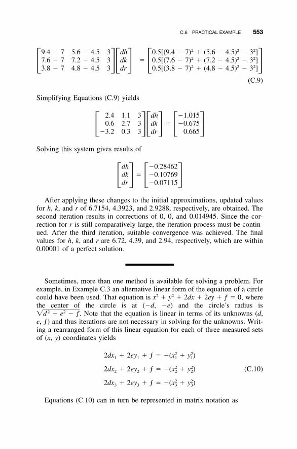
C.6 PRACTICAL EXAMPLE 553
2 2 29.4 � 7 5.6 � 4.5 3 dh 0.5[(9.4 � 7) � (5.6 � 4.5) � 3 ]2 2 27.6 � 7 7.2 � 4.5 3 dk � 0.5[(7.6 � 7) � (7.2 � 4.5) � 3 ]� �� � � �2 2 23.8 � 7 4.8 � 4.5 3 dr 0.5[(3.8 � 7) � (4.8 � 4.5) � 3 ]
(C.9)
Simplifying Equations (C.9) yields
2.4 1.1 3 dh �1.0150.6 2.7 3 dk � �0.675� �� � � ��3.2 0.3 3 dr 0.665
Solving this system gives results of
dh �0.28462dk � �0.10769� � � �dr �0.07115
After applying these changes to the initial approximations, updated valuesfor h, k, and r of 6.7154, 4.3923, and 2.9288, respectively, are obtained. Thesecond iteration results in corrections of 0, 0, and 0.014945. Since the cor-rection for r is still comparatively large, the iteration process must be contin-ued. After the third iteration, suitable convergence was achieved. The finalvalues for h, k, and r are 6.72, 4.39, and 2.94, respectively, which are within0.00001 of a perfect solution.
Sometimes, more than one method is available for solving a problem. Forexample, in Example C.3 an alternative linear form of the equation of a circlecould have been used. That equation is x2 � y2 � 2dx � 2ey � ƒ � 0, wherethe center of the circle is at (�d, �e) and the circle’s radius is
Note that the equation is linear in terms of its unknowns (d,2 2�d � e � ƒ.e, ƒ) and thus iterations are not necessary in solving for the unknowns. Writ-ing a rearranged form of this linear equation for each of three measured setsof (x, y) coordinates yields
2 22dx � 2ey � ƒ � �(x � y )1 1 1 1
2 22dx � 2ey � ƒ � �(x � y ) (C.10)2 2 2 2
2 22dx � 2ey � ƒ � �(x � y )3 3 3 3
Equations (C.10) can in turn be represented in matrix notation as
554 NONLINEAR EQUATIONS AND TAYLOR’S THEOREM
2 22x 2y 1 d �(x � y )1 1 1 12 22x 2y 1 e � �(x � y )2 2 2 2� �� � � �2 22x 2y 1 ƒ �(x � y )3 3 3 3
Solving this matrix system, the center of the circle is again found to be(6.72, 4.39), and its radius is determined to be 2.94.
In this appendix, the Taylor series has been applied to solve for the un-knowns in nonlinear equations. Many equations in surveying, geodesy, andphotogrammetry are nonlinear. In surveying, examples include the distanceand angle formulas, which are nonlinear in terms of station coordinates. TheTaylor series is used to linearize these equations and find least squares solu-tions. Thus, when performing least squares adjustments of plane observations,the techniques presented in this appendix must be used in the solutions.
PROBLEMS
C.1 Solve for the unknowns x and y in the following nonlinear equationsusing Taylor’s theorem. (Use x0 � 5 and y0 � 5 for initial approx-imations.)
2 2x y � 3x � 752x � y � 19
C.2 Solve for the unknown values of x, y, and z in the following threenonlinear equations using the Taylor series. (Use x0 � y0 � z0 � 2 forinitial approximations.)
2 2x � y � 2xy � z � 4
�x � y � z � 42 3�2x � y � z � 23
C.3 Use the MATRIX software to solve Problem C.1.
C.4 Use the MATRIX software to solve Problem C.2.
C.5 Find the center and radius of a circle using the equation (x � h)2 �(y � k)2 � r2 given the coordinates of points A, B, and C on the circle.Follow the procedures discussed in Section C.5. Use initial approxi-mations of h0 � 5, k0 � 4, and r0 � 2 for the first iteration.
A: (7.2,5.2) B: (4.0, 6.4) C: (4.0, 2.4)
C.6 Repeat Problem C.5 using the linear equation: x2 � y2 � 2dx � 2ey� ƒ � 0.
PROBLEMS 555
C.7 Repeat Problem C.5 using the points A: (0.50, �0.70), B: (1.00, 0.00),C: (0.70, 0.70). Use initial approximations of h0 � 0, k0 � 0, and r0
� 1.
C.8 Repeat Problem C.7 using the linear equation x2 � y2 � 2dx � 2ey� ƒ � 0.
C.9 Use the ADJUST software to solve Problem C.5.
C.10 Use the ADJUST software to solve Problem C.7.
C.11 The distance formula between two stations i and j is Dij �Write the linearized form of in terms of the2 2�(x � x ) � (y � y ) .j i j i
variables xi, yi, xj, and yj.
C.12 The azimuth formula between two stations i and j is �ij � tan�1
[(xj � xi) /(yj � yi)]. Write the linearized form of this equation in termsof the variables xi, yi, xj, and yj.
C.13 The formula for an angle ∠jik is �ik � �ij, where � is defined inProblem C.12. Write the linearized form of this equation in terms ofthe variables xi, yi, xj, yj, xk, and yk.
Programming Problems
C.14 Create a programmed package that solves Problem C.6.
C.15 Create a programmed package that solves Problem C.5.
556
APPENDIX D
NORMAL ERROR DISTRIBUTIONCURVE AND OTHERSTATISTICAL TABLES
D.1 DEVELOPMENT OF THE NORMAL DISTRIBUTIONCURVE EQUATION
In Section 2.4 the histogram and frequency polygon were presented as meth-ods for graphical portrayal of random error distributions. If a large numberof these distributions were examined for sets, measurements in surveying,geodesy, and photogrammetry, it would be found that they conform to normal(or Gaussian) distributions. The general laws governing normal distributionsare stated as follows:
1. Positive and negative errors occur with equal probability and equalfrequency.
2. Small errors are more common than large errors.3. Large errors seldom occur, and there is a limit to the size of the greatest
random error that will occur in any set of observations.
A curve that conforms to these laws, plotted with the size of the error onthe abscissa and the probability of occurrence on the ordinate, is shown inFigure 3.3. This curve is repeated in Figure D.1 and is called the normaldistribution curve, the normal curve of error, or simply the probability curve.A smooth curve of this same shape would be obtained if for a very largegroup of measurements, a histogram were plotted with an infinitesimally smallclass interval. In this section, the equation for this curve is developed.
Assume that the normal distribution curve is continuous and that the prob-ability of an error occurring between x and x � dx is given by the function
Adjustment Computations: Spatial Data Analysis, Fourth Edition. C. D. Ghilani and P. R. Wolf© 2006 John Wiley & Sons, Inc. ISBN: 978-0-471-69728-2
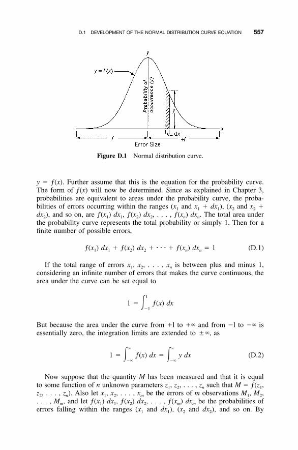
D.1 DEVELOPMENT OF THE NORMAL DISTRIBUTION CURVE EQUATION 557
Figure D.1 Normal distribution curve.
y � ƒ(x). Further assume that this is the equation for the probability curve.The form of ƒ(x) will now be determined. Since as explained in Chapter 3,probabilities are equivalent to areas under the probability curve, the proba-bilities of errors occurring within the ranges (x1 and x1 � dx1), (x2 and x2 �dx2), and so on, are ƒ(x1) dx1, ƒ(x2) dx2, . . . , ƒ(xn) dxn. The total area underthe probability curve represents the total probability or simply 1. Then for afinite number of possible errors,
ƒ(x ) dx � ƒ(x ) dx � � � � � ƒ(x ) dx � 1 (D.1)1 1 2 2 n n
If the total range of errors x1, x2, . . . , xn is between plus and minus 1,considering an infinite number of errors that makes the curve continuous, thearea under the curve can be set equal to
1
1 � � ƒ(x) dx�1
But because the area under the curve from �l to �� and from �l to �� isessentially zero, the integration limits are extended to ��, as
� �
1 � � ƒ(x) dx � � y dx (D.2)�� ��
Now suppose that the quantity M has been measured and that it is equalto some function of n unknown parameters z1, z2, . . . , zn such that M � ƒ(z1,z2, . . . , zn). Also let x1, x2, . . . , xm be the errors of m observations M1, M2,. . . , Mm, and let ƒ(x1) dx1, ƒ(x2) dx2, . . . , ƒ(xm) dxm be the probabilities oferrors falling within the ranges (x1 and dx1), (x2 and dx2), and so on. By
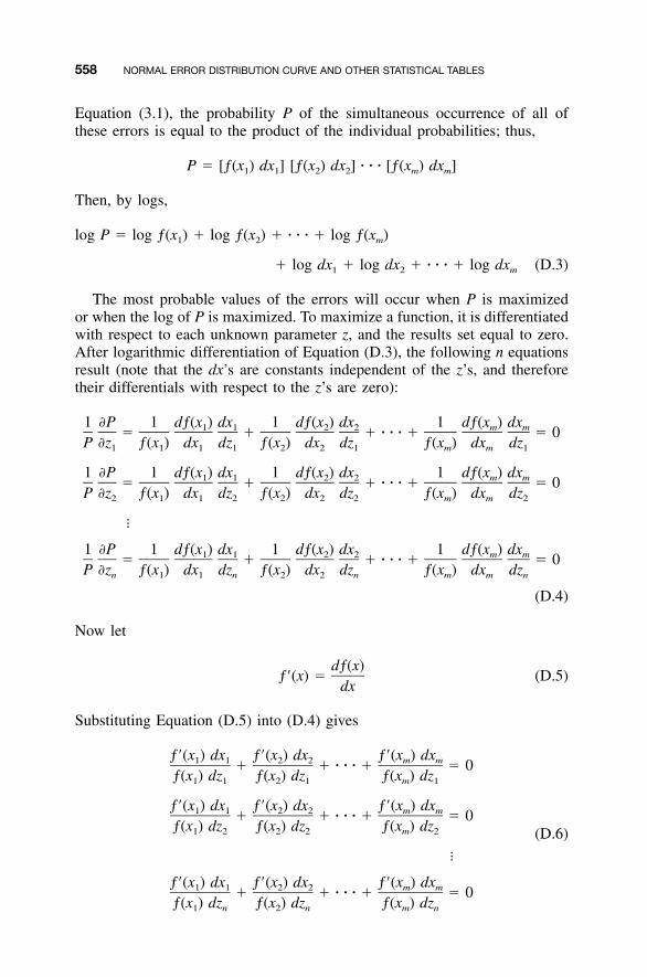
558 NORMAL ERROR DISTRIBUTION CURVE AND OTHER STATISTICAL TABLES
Equation (3.1), the probability P of the simultaneous occurrence of all ofthese errors is equal to the product of the individual probabilities; thus,
P � [ƒ(x ) dx ] [ƒ(x ) dx ] � � � [ƒ(x ) dx ]1 1 2 2 m m
Then, by logs,
log P � log ƒ(x ) � log ƒ(x ) � � � � � log ƒ(x )1 2 m
� log dx � log dx � � � � � log dx (D.3)1 2 m
The most probable values of the errors will occur when P is maximizedor when the log of P is maximized. To maximize a function, it is differentiatedwith respect to each unknown parameter z, and the results set equal to zero.After logarithmic differentiation of Equation (D.3), the following n equationsresult (note that the dx’s are constants independent of the z’s, and thereforetheir differentials with respect to the z’s are zero):
1 �P 1 dƒ(x ) dx 1 dƒ(x ) dx 1 dƒ(x ) dx1 1 2 2 m m� � � � � � � � 0P �z ƒ(x ) dx dz ƒ(x ) dx dz ƒ(x ) dx dz1 1 1 1 2 2 1 m m 1
1 �P 1 dƒ(x ) dx 1 dƒ(x ) dx 1 dƒ(x ) dx1 1 2 2 m m� � � � � � � � 0P �z ƒ(x ) dx dz ƒ(x ) dx dz ƒ(x ) dx dz2 1 1 2 2 2 2 m m 2
�
1 �P 1 dƒ(x ) dx 1 dƒ(x ) dx 1 dƒ(x ) dx1 1 2 2 m m� � � � � � � � 0P �z ƒ(x ) dx dz ƒ(x ) dx dz ƒ(x ) dx dzn 1 1 n 2 2 n m m n
(D.4)
Now let
dƒ(x)ƒ�(x) � (D.5)
dx
Substituting Equation (D.5) into (D.4) gives
ƒ�(x ) dx ƒ�(x ) dx ƒ�(x ) dx1 1 2 2 m m� � � � � � � 0ƒ(x ) dz ƒ(x ) dz ƒ(x ) dz1 1 2 1 m 1
ƒ�(x ) dx ƒ�(x ) dx ƒ�(x ) dx1 1 2 2 m m� � � � � � � 0ƒ(x ) dz ƒ(x ) dz ƒ(x ) dz1 2 2 2 m 2 (D.6)
�
ƒ�(x ) dx ƒ�(x ) dx ƒ�(x ) dx1 1 2 2 m m� � � � � � � 0ƒ(x ) dz ƒ(x ) dz ƒ(x ) dz1 n 2 n m n
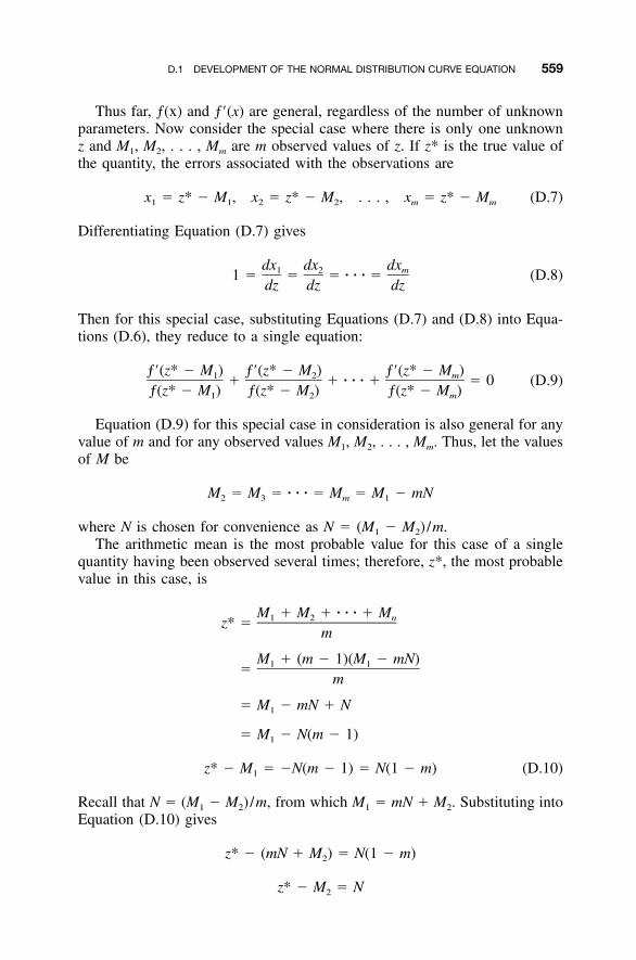
D.1 DEVELOPMENT OF THE NORMAL DISTRIBUTION CURVE EQUATION 559
Thus far, ƒ(x) and ƒ�(x) are general, regardless of the number of unknownparameters. Now consider the special case where there is only one unknownz and M1, M2, . . . , Mm are m observed values of z. If z* is the true value ofthe quantity, the errors associated with the observations are
x � z* � M , x � z* � M , . . . , x � z* � M (D.7)1 1 2 2 m m
Differentiating Equation (D.7) gives
dx dx dx1 2 m1 � � � � � � � (D.8)dz dz dz
Then for this special case, substituting Equations (D.7) and (D.8) into Equa-tions (D.6), they reduce to a single equation:
ƒ�(z* � M ) ƒ�(z* � M ) ƒ�(z* � M )1 2 m� � � � � � � 0 (D.9)ƒ(z* � M ) ƒ(z* � M ) ƒ(z* � M )1 2 m
Equation (D.9) for this special case in consideration is also general for anyvalue of m and for any observed values M1, M2, . . . , Mm. Thus, let the valuesof M be
M � M � � � � � M � M � mN2 3 m 1
where N is chosen for convenience as N � (M1 � M2) /m.The arithmetic mean is the most probable value for this case of a single
quantity having been observed several times; therefore, z*, the most probablevalue in this case, is
M � M � � � � � M1 2 nz* �m
M � (m � 1)(M � mN)1 1�m
� M � mN � N1
� M � N(m � 1)1
z* � M � �N(m � 1) � N(1 � m) (D.10)1
Recall that N � (M1 � M2) /m, from which M1 � mN � M2. Substituting intoEquation (D.10) gives
z* � (mN � M ) � N(1 � m)2
z* � M � N2
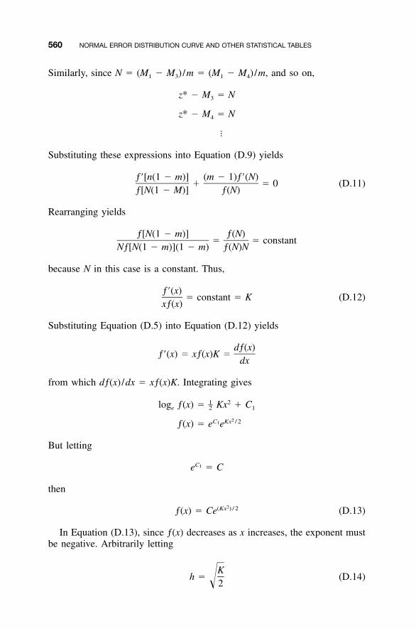
560 NORMAL ERROR DISTRIBUTION CURVE AND OTHER STATISTICAL TABLES
Similarly, since N � (M1 � M3) /m � (M1 � M4) /m, and so on,
z* � M � N3
z* � M � N4
�
Substituting these expressions into Equation (D.9) yields
ƒ�[n(1 � m)] (m � 1)ƒ�(N)� � 0 (D.11)
ƒ[N(1 � M)] ƒ(N)
Rearranging yields
ƒ[N(1 � m)] ƒ(N)� � constant
Nƒ[N(1 � m)](1 � m) ƒ(N)N
because N in this case is a constant. Thus,
ƒ�(x)� constant � K (D.12)
xƒ(x)
Substituting Equation (D.5) into Equation (D.12) yields
dƒ(x)ƒ�(x) � xƒ(x)K �
dx
from which dƒ(x) /dx � xƒ(x)K. Integrating gives
1 2–log ƒ(x) � Kx � Ce 2 1
2C Kx / 21ƒ(x) � e e
But letting
C1e � C
then
2(Kx ) / 2ƒ(x) � Ce (D.13)
In Equation (D.13), since ƒ(x) decreases as x increases, the exponent mustbe negative. Arbitrarily letting
Kh � (D.14)�2
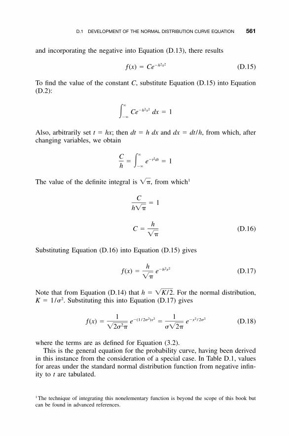
D.1 DEVELOPMENT OF THE NORMAL DISTRIBUTION CURVE EQUATION 561
and incorporating the negative into Equation (D.13), there results
2 2�h xƒ(x) � Ce (D.15)
To find the value of the constant C, substitute Equation (D.15) into Equation(D.2):
�2 2�h x� Ce dx � 1
��
Also, arbitrarily set t � hx; then dt � h dx and dx � dt /h, from which, afterchanging variables, we obtain
�C 2�t dt� � e � 1��h
The value of the definite integral is from which1��,
C� 1
h��
hC � (D.16)
��
Substituting Equation (D.16) into Equation (D.15) gives
h 2 2�h xƒ(x) � e (D.17)��
Note that from Equation (D.14) that h � For the normal distribution,�K /2.K � 1/�2. Substituting this into Equation (D.17) gives
1 12 2 2 2�(1 / 2� )x �x / 2�ƒ(x) � e � e (D.18)2�2� � ��2�
where the terms are as defined for Equation (3.2).This is the general equation for the probability curve, having been derived
in this instance from the consideration of a special case. In Table D.1, valuesfor areas under the standard normal distribution function from negative infin-ity to t are tabulated.
1 The technique of integrating this nonelementary function is beyond the scope of this book butcan be found in advanced references.
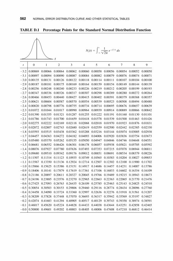
562 NORMAL ERROR DISTRIBUTION CURVE AND OTHER STATISTICAL TABLES
TABLE D.1 Percentage Points for the Standard Normal Distribution Function
t
� 1 2�x / 2N (t) � � e dxz�� �2�
t 0 1 2 3 4 5 6 7 8 9
�3.2 0.00069 0.00066 0.00064 0.00062 0.00060 0.00058 0.00056 0.00054 0.00052 0.00050�3.1 0.00097 0.00094 0.00090 0.00087 0.00084 0.00082 0.00079 0.00076 0.00074 0.00071�3.0 0.00135 0.00131 0.00126 0.00122 0.00118 0.00114 0.00111 0.00107 0.00104 0.00100�2.9 0.00187 0.00181 0.00175 0.00169 0.00164 0.00159 0.00154 0.00149 0.00144 0.00139�2.8 0.00256 0.00248 0.00240 0.00233 0.00226 0.00219 0.00212 0.00205 0.00199 0.00193�2.7 0.00347 0.00336 0.00326 0.00317 0.00307 0.00298 0.00289 0.00280 0.00272 0.00264�2.6 0.00466 0.00453 0.00440 0.00427 0.00415 0.00402 0.00391 0.00379 0.00368 0.00357�2.5 0.00621 0.00604 0.00587 0.00570 0.00554 0.00539 0.00523 0.00508 0.00494 0.00480�2.4 0.00820 0.00798 0.00776 0.00755 0.00734 0.00714 0.00695 0.00676 0.00657 0.00639�2.3 0.01072 0.01044 0.01017 0.00990 0.00964 0.00939 0.00914 0.00889 0.00866 0.00842�2.2 0.01390 0.01355 0.01321 0.01287 0.01255 0.01222 0.01191 0.01160 0.01130 0.01101�2.1 0.01786 0.01743 0.01700 0.01659 0.01618 0.01578 0.01539 0.01500 0.01463 0.01426�2.0 0.02275 0.02222 0.02169 0.02118 0.02068 0.02018 0.01970 0.01923 0.01876 0.01831�1.9 0.02872 0.02807 0.02743 0.02680 0.02619 0.02559 0.02500 0.02442 0.02385 0.02330�1.8 0.03593 0.03515 0.03438 0.03362 0.03288 0.03216 0.03144 0.03074 0.03005 0.02938�1.7 0.04457 0.04363 0.04272 0.04182 0.04093 0.04006 0.03920 0.03836 0.03754 0.03673�1.6 0.05480 0.05370 0.05262 0.05155 0.05050 0.04947 0.04846 0.04746 0.04648 0.04551�1.5 0.06681 0.06552 0.06426 0.06301 0.06178 0.06057 0.05938 0.05821 0.05705 0.05592�1.4 0.08076 0.07927 0.07780 0.07636 0.07493 0.07353 0.07215 0.07078 0.06944 0.06811�1.3 0.09680 0.09510 0.09342 0.09176 0.09012 0.08851 0.08691 0.08534 0.08379 0.08226�1.2 0.11507 0.11314 0.11123 0.10935 0.10749 0.10565 0.10383 0.10204 0.10027 0.09853�1.1 0.13567 0.13350 0.13136 0.12924 0.12714 0.12507 0.12302 0.12100 0.11900 0.11702�1.0 0.15866 0.15625 0.15386 0.15151 0.14917 0.14686 0.14457 0.14231 0.14007 0.13786�0.9 0.18406 0.18141 0.17879 0.17619 0.17361 0.17106 0.16853 0.16602 0.16354 0.16109�0.8 0.21186 0.20897 0.20611 0.20327 0.20045 0.19766 0.19489 0.19215 0.18943 0.18673�0.7 0.24196 0.23885 0.23576 0.23270 0.22965 0.22663 0.22363 0.22065 0.21770 0.21476�0.6 0.27425 0.27093 0.26763 0.26435 0.26109 0.25785 0.25463 0.25143 0.24825 0.24510�0.5 0.30854 0.30503 0.30153 0.29806 0.29460 0.29116 0.28774 0.28434 0.28096 0.27760�0.4 0.34458 0.34090 0.33724 0.33360 0.32997 0.32636 0.32276 0.31918 0.31561 0.31207�0.3 0.38209 0.37828 0.37448 0.37070 0.36693 0.36317 0.35942 0.35569 0.35197 0.34827�0.2 0.42074 0.41683 0.41294 0.40905 0.40517 0.40129 0.39743 0.39358 0.38974 0.38591�0.1 0.46017 0.45620 0.45224 0.44828 0.44433 0.44038 0.43644 0.43251 0.42858 0.42465�0.0 0.50000 0.49601 0.49202 0.48803 0.48405 0.48006 0.47608 0.47210 0.46812 0.46414
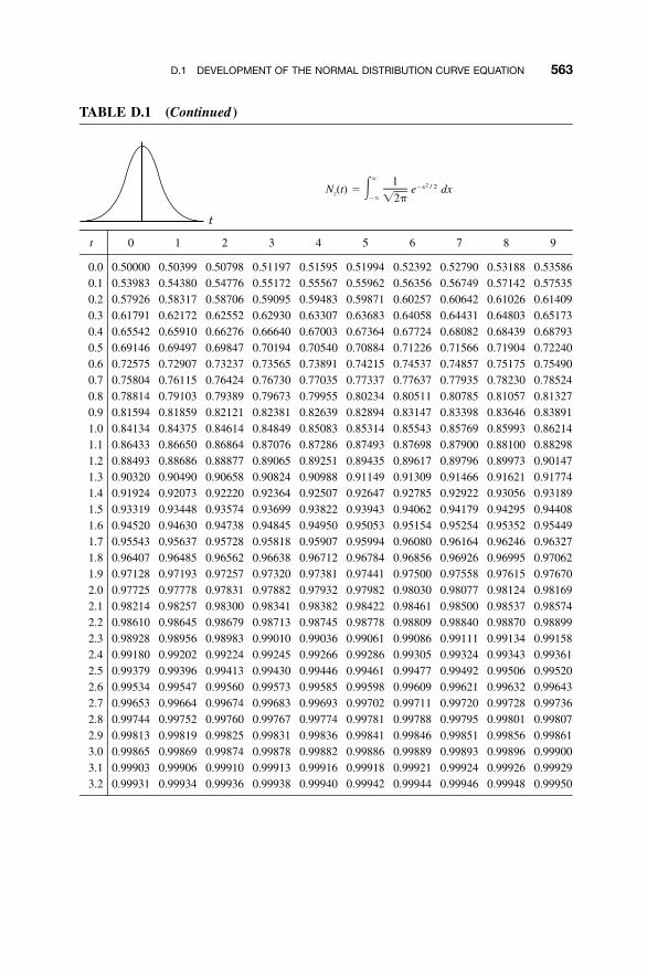
D.1 DEVELOPMENT OF THE NORMAL DISTRIBUTION CURVE EQUATION 563
TABLE D.1 (Continued )
t
� 1 2�x / 2N (t) � � e dxz�� �2�
t 0 1 2 3 4 5 6 7 8 9
0.0 0.50000 0.50399 0.50798 0.51197 0.51595 0.51994 0.52392 0.52790 0.53188 0.535860.1 0.53983 0.54380 0.54776 0.55172 0.55567 0.55962 0.56356 0.56749 0.57142 0.575350.2 0.57926 0.58317 0.58706 0.59095 0.59483 0.59871 0.60257 0.60642 0.61026 0.614090.3 0.61791 0.62172 0.62552 0.62930 0.63307 0.63683 0.64058 0.64431 0.64803 0.651730.4 0.65542 0.65910 0.66276 0.66640 0.67003 0.67364 0.67724 0.68082 0.68439 0.687930.5 0.69146 0.69497 0.69847 0.70194 0.70540 0.70884 0.71226 0.71566 0.71904 0.722400.6 0.72575 0.72907 0.73237 0.73565 0.73891 0.74215 0.74537 0.74857 0.75175 0.754900.7 0.75804 0.76115 0.76424 0.76730 0.77035 0.77337 0.77637 0.77935 0.78230 0.785240.8 0.78814 0.79103 0.79389 0.79673 0.79955 0.80234 0.80511 0.80785 0.81057 0.813270.9 0.81594 0.81859 0.82121 0.82381 0.82639 0.82894 0.83147 0.83398 0.83646 0.838911.0 0.84134 0.84375 0.84614 0.84849 0.85083 0.85314 0.85543 0.85769 0.85993 0.862141.1 0.86433 0.86650 0.86864 0.87076 0.87286 0.87493 0.87698 0.87900 0.88100 0.882981.2 0.88493 0.88686 0.88877 0.89065 0.89251 0.89435 0.89617 0.89796 0.89973 0.901471.3 0.90320 0.90490 0.90658 0.90824 0.90988 0.91149 0.91309 0.91466 0.91621 0.917741.4 0.91924 0.92073 0.92220 0.92364 0.92507 0.92647 0.92785 0.92922 0.93056 0.931891.5 0.93319 0.93448 0.93574 0.93699 0.93822 0.93943 0.94062 0.94179 0.94295 0.944081.6 0.94520 0.94630 0.94738 0.94845 0.94950 0.95053 0.95154 0.95254 0.95352 0.954491.7 0.95543 0.95637 0.95728 0.95818 0.95907 0.95994 0.96080 0.96164 0.96246 0.963271.8 0.96407 0.96485 0.96562 0.96638 0.96712 0.96784 0.96856 0.96926 0.96995 0.970621.9 0.97128 0.97193 0.97257 0.97320 0.97381 0.97441 0.97500 0.97558 0.97615 0.976702.0 0.97725 0.97778 0.97831 0.97882 0.97932 0.97982 0.98030 0.98077 0.98124 0.981692.1 0.98214 0.98257 0.98300 0.98341 0.98382 0.98422 0.98461 0.98500 0.98537 0.985742.2 0.98610 0.98645 0.98679 0.98713 0.98745 0.98778 0.98809 0.98840 0.98870 0.988992.3 0.98928 0.98956 0.98983 0.99010 0.99036 0.99061 0.99086 0.99111 0.99134 0.991582.4 0.99180 0.99202 0.99224 0.99245 0.99266 0.99286 0.99305 0.99324 0.99343 0.993612.5 0.99379 0.99396 0.99413 0.99430 0.99446 0.99461 0.99477 0.99492 0.99506 0.995202.6 0.99534 0.99547 0.99560 0.99573 0.99585 0.99598 0.99609 0.99621 0.99632 0.996432.7 0.99653 0.99664 0.99674 0.99683 0.99693 0.99702 0.99711 0.99720 0.99728 0.997362.8 0.99744 0.99752 0.99760 0.99767 0.99774 0.99781 0.99788 0.99795 0.99801 0.998072.9 0.99813 0.99819 0.99825 0.99831 0.99836 0.99841 0.99846 0.99851 0.99856 0.998613.0 0.99865 0.99869 0.99874 0.99878 0.99882 0.99886 0.99889 0.99893 0.99896 0.999003.1 0.99903 0.99906 0.99910 0.99913 0.99916 0.99918 0.99921 0.99924 0.99926 0.999293.2 0.99931 0.99934 0.99936 0.99938 0.99940 0.99942 0.99944 0.99946 0.99948 0.99950
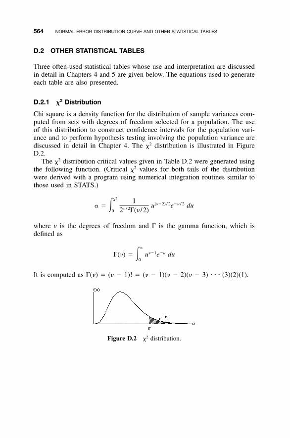
564 NORMAL ERROR DISTRIBUTION CURVE AND OTHER STATISTICAL TABLES
D.2 OTHER STATISTICAL TABLES
Three often-used statistical tables whose use and interpretation are discussedin detail in Chapters 4 and 5 are given below. The equations used to generateeach table are also presented.
D.2.1 �2 Distribution
Chi square is a density function for the distribution of sample variances com-puted from sets with degrees of freedom selected for a population. The useof this distribution to construct confidence intervals for the population vari-ance and to perform hypothesis testing involving the population variance arediscussed in detail in Chapter 4. The �2 distribution is illustrated in FigureD.2.
The �2 distribution critical values given in Table D.2 were generated usingthe following function. (Critical �2 values for both tails of the distributionwere derived with a program using numerical integration routines similar tothose used in STATS.)
2� 1 (��2) / 2 �u / 2� � � u e du� / 2
0 2 �(� /2)
where v is the degrees of freedom and � is the gamma function, which isdefined as
���1 �u�(�) � � u e du
0
It is computed as �(�) � (� � 1)! � (� � 1)(� � 2)(� � 3) � � � (3)(2)(1).
Figure D.2 �2 distribution.
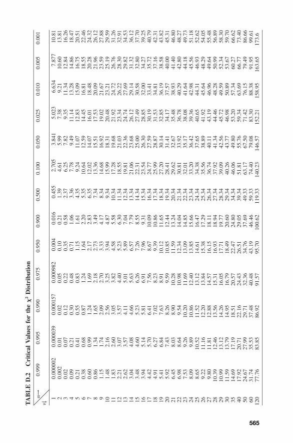
565
TA
BL
ED
.2C
riti
cal
Val
ues
for
the
�2
Dis
trib
utio
n
�→
�↓
0.99
90.
995
0.99
00.
975
0.95
00.
900
0.50
00.
100
0.05
00.
025
0.01
00.
005
0.00
1
10.
0000
020.
0000
390.
0001
570.
0009
820.
004
0.01
60.
455
2.70
53.
841
5.02
36.
634
7.87
710
.81
20.
002
0.01
0.02
0.05
0.10
0.21
1.39
4.61
5.99
7.38
9.21
10.6
013
.81
30.
020.
070.
120.
220.
350.
582.
376.
257.
829.
3511
.34
12.8
416
.26
40.
090.
210.
300.
480.
711.
063.
367.
789.
4911
.14
13.2
814
.86
18.4
75
0.21
0.41
0.55
0.83
1.15
1.61
4.35
9.24
11.0
712
.83
15.0
916
.75
20.5
16
0.38
0.68
0.87
1.24
1.64
2.20
5.35
10.6
412
.59
14.4
516
.81
18.5
522
.46
70.
600.
991.
241.
692.
172.
836.
3512
.02
14.0
716
.01
18.4
820
.28
24.3
28
0.86
1.34
1.65
2.18
2.73
3.49
7.34
13.3
615
.51
17.5
320
.09
21.9
626
.12
91.
151.
742.
092.
703.
334.
178.
3414
.68
16.9
219
.02
21.6
723
.59
27.8
810
1.48
2.16
2.56
3.25
3.94
4.87
9.34
15.9
918
.31
20.4
823
.21
25.1
929
.59
111.
832.
603.
053.
824.
585.
5810
.34
17.2
819
.68
21.9
224
.72
26.7
631
.26
122.
213.
073.
574.
405.
236.
3011
.34
18.5
521
.03
23.3
426
.22
28.3
032
.91
132.
623.
574.
115.
015.
897.
0412
.34
19.8
122
.36
24.7
427
.69
29.8
234
.53
143.
044.
084.
665.
636.
577.
7913
.34
21.0
623
.68
26.1
229
.14
31.3
236
.12
153.
484.
605.
236.
267.
268.
5514
.34
22.3
125
.00
27.4
930
.58
32.8
037
.70
163.
945.
145.
816.
917.
969.
3115
.34
23.5
426
.30
28.8
532
.00
34.2
739
.25
174.
425.
706.
417.
568.
6710
.09
16.3
424
.77
27.5
930
.19
33.4
135
.72
40.7
918
4.91
6.27
7.02
8.23
9.39
10.8
617
.34
25.9
928
.87
31.5
334
.81
37.1
642
.31
195.
416.
847.
638.
9110
.12
11.6
518
.34
27.2
030
.14
32.8
536
.19
38.5
843
.82
205.
927.
438.
269.
5910
.85
12.4
419
.34
28.4
131
.41
34.1
737
.57
40.0
045
.31
216.
458.
038.
9010
.28
11.5
913
.24
20.3
429
.62
32.6
735
.48
38.9
341
.40
46.8
022
6.98
8.64
9.54
10.9
812
.34
14.0
421
.34
30.8
133
.92
36.7
840
.29
42.8
048
.27
237.
539.
2610
.20
11.6
913
.09
14.8
522
.34
32.0
135
.17
38.0
841
.64
44.1
849
.73
248.
099.
8910
.86
12.4
013
.85
15.6
623
.34
33.2
036
.42
39.3
642
.98
45.5
651
.18
258.
6510
.52
11.5
213
.12
14.6
116
.47
24.3
434
.38
37.6
540
.65
44.3
146
.93
52.6
226
9.22
11.1
612
.20
13.8
415
.38
17.2
925
.34
35.5
638
.89
41.9
245
.64
48.2
954
.05
279.
8011
.81
12.8
814
.57
16.1
518
.11
26.3
436
.74
40.1
143
.19
46.9
649
.64
55.4
828
10.3
912
.46
13.5
615
.31
16.9
318
.94
27.3
437
.92
41.3
444
.46
48.2
850
.99
56.8
929
10.9
913
.12
14.2
616
.05
17.7
119
.77
28.3
439
.09
42.5
645
.72
49.5
952
.34
58.3
030
11.5
913
.79
14.9
516
.79
18.4
920
.60
29.3
440
.26
43.7
746
.98
50.8
953
.67
59.7
035
14.6
917
.19
18.5
120
.57
22.4
724
.80
34.3
446
.06
49.8
053
.20
57.3
460
.27
66.6
240
17.9
220
.71
22.1
624
.43
26.5
129
.05
39.3
451
.81
55.7
659
.34
63.6
966
.77
73.4
050
24.6
727
.99
29.7
132
.36
34.7
637
.69
49.3
363
.17
67.5
071
.42
76.1
579
.49
86.6
660
31.7
435
.53
37.4
840
.48
43.1
946
.46
59.3
374
.40
79.0
883
.30
88.3
891
.95
99.6
112
077
.76
83.8
586
.92
91.5
795
.70
100.
6211
9.33
140.
2314
6.57
152.
2115
8.95
163.
6517
3.6
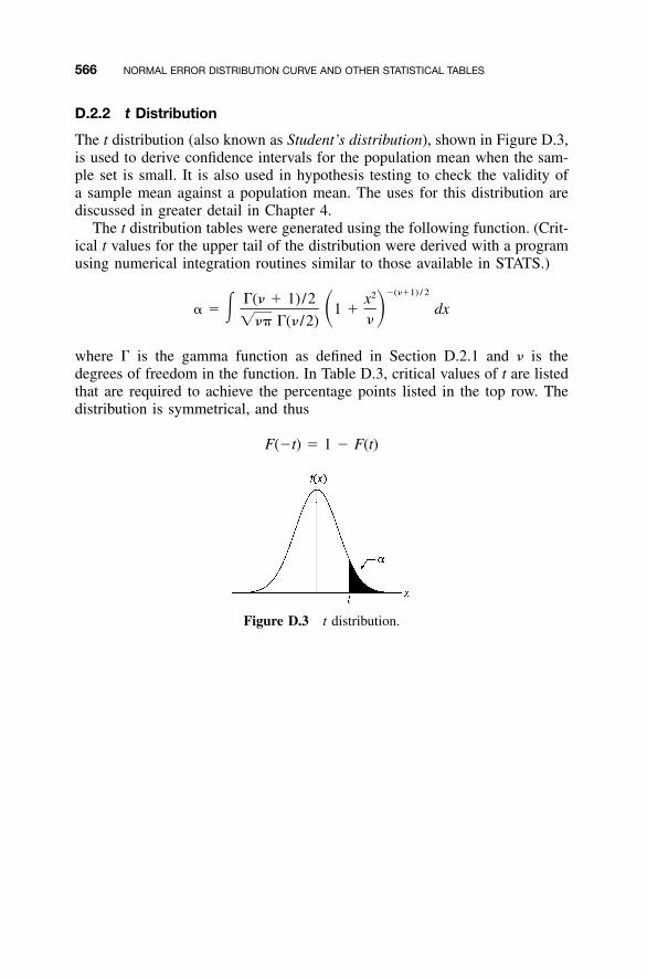
566 NORMAL ERROR DISTRIBUTION CURVE AND OTHER STATISTICAL TABLES
D.2.2 t Distribution
The t distribution (also known as Student’s distribution), shown in Figure D.3,is used to derive confidence intervals for the population mean when the sam-ple set is small. It is also used in hypothesis testing to check the validity ofa sample mean against a population mean. The uses for this distribution arediscussed in greater detail in Chapter 4.
The t distribution tables were generated using the following function. (Crit-ical t values for the upper tail of the distribution were derived with a programusing numerical integration routines similar to those available in STATS.)
�(��1) / 22�(� � 1)/2 x� � � 1 � dx� �
���� �(� /2)
where � is the gamma function as defined in Section D.2.1 and � is thedegrees of freedom in the function. In Table D.3, critical values of t are listedthat are required to achieve the percentage points listed in the top row. Thedistribution is symmetrical, and thus
F(�t) � 1 � F(t)
Figure D.3 t distribution.
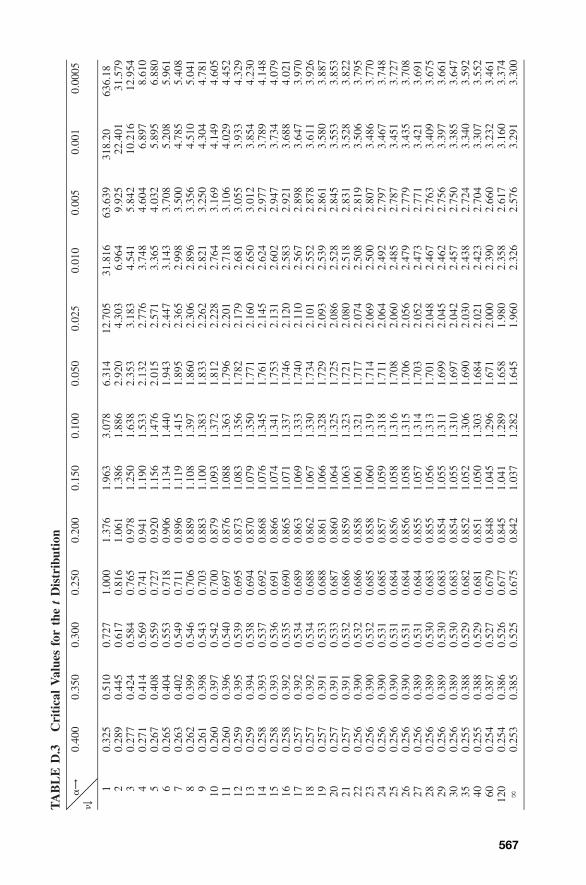
567
TA
BL
ED
.3C
riti
cal
Val
ues
for
the
tD
istr
ibut
ion
�→
�↓
0.40
00.
350
0.30
00.
250
0.20
00.
150
0.10
00.
050
0.02
50.
010
0.00
50.
001
0.00
05
10.
325
0.51
00.
727
1.00
01.
376
1.96
33.
078
6.31
412
.705
31.8
1663
.639
318.
2063
6.18
20.
289
0.44
50.
617
0.81
61.
061
1.38
61.
886
2.92
04.
303
6.96
49.
925
22.4
0131
.579
30.
277
0.42
40.
584
0.76
50.
978
1.25
01.
638
2.35
33.
183
4.54
15.
842
10.2
1612
.954
40.
271
0.41
40.
569
0.74
10.
941
1.19
01.
533
2.13
22.
776
3.74
84.
604
6.89
78.
610
50.
267
0.40
80.
559
0.72
70.
920
1.15
61.
476
2.01
52.
571
3.36
54.
032
5.89
56.
880
60.
265
0.40
40.
553
0.71
80.
906
1.13
41.
440
1.94
32.
447
3.14
33.
708
5.20
85.
961
70.
263
0.40
20.
549
0.71
10.
896
1.11
91.
415
1.89
52.
365
2.99
83.
500
4.78
55.
408
80.
262
0.39
90.
546
0.70
60.
889
1.10
81.
397
1.86
02.
306
2.89
63.
356
4.51
05.
041
90.
261
0.39
80.
543
0.70
30.
883
1.10
01.
383
1.83
32.
262
2.82
13.
250
4.30
44.
781
100.
260
0.39
70.
542
0.70
00.
879
1.09
31.
372
1.81
22.
228
2.76
43.
169
4.14
94.
605
110.
260
0.39
60.
540
0.69
70.
876
1.08
81.
363
1.79
62.
201
2.71
83.
106
4.02
94.
452
120.
259
0.39
50.
539
0.69
50.
873
1.08
31.
356
1.78
22.
179
2.68
13.
055
3.93
34.
329
130.
259
0.39
40.
538
0.69
40.
870
1.07
91.
350
1.77
12.
160
2.65
03.
012
3.85
44.
230
140.
258
0.39
30.
537
0.69
20.
868
1.07
61.
345
1.76
12.
145
2.62
42.
977
3.78
94.
148
150.
258
0.39
30.
536
0.69
10.
866
1.07
41.
341
1.75
32.
131
2.60
22.
947
3.73
44.
079
160.
258
0.39
20.
535
0.69
00.
865
1.07
11.
337
1.74
62.
120
2.58
32.
921
3.68
84.
021
170.
257
0.39
20.
534
0.68
90.
863
1.06
91.
333
1.74
02.
110
2.56
72.
898
3.64
73.
970
180.
257
0.39
20.
534
0.68
80.
862
1.06
71.
330
1.73
42.
101
2.55
22.
878
3.61
13.
926
190.
257
0.39
10.
533
0.68
80.
861
1.06
61.
328
1.72
92.
093
2.53
92.
861
3.58
03.
887
200.
257
0.39
10.
533
0.68
70.
860
1.06
41.
325
1.72
52.
086
2.52
82.
845
3.55
33.
853
210.
257
0.39
10.
532
0.68
60.
859
1.06
31.
323
1.72
12.
080
2.51
82.
831
3.52
83.
822
220.
256
0.39
00.
532
0.68
60.
858
1.06
11.
321
1.71
72.
074
2.50
82.
819
3.50
63.
795
230.
256
0.39
00.
532
0.68
50.
858
1.06
01.
319
1.71
42.
069
2.50
02.
807
3.48
63.
770
240.
256
0.39
00.
531
0.68
50.
857
1.05
91.
318
1.71
12.
064
2.49
22.
797
3.46
73.
748
250.
256
0.39
00.
531
0.68
40.
856
1.05
81.
316
1.70
82.
060
2.48
52.
787
3.45
13.
727
260.
256
0.39
00.
531
0.68
40.
856
1.05
81.
315
1.70
62.
056
2.47
92.
779
3.43
53.
708
270.
256
0.38
90.
531
0.68
40.
855
1.05
71.
314
1.70
32.
052
2.47
32.
771
3.42
13.
691
280.
256
0.38
90.
530
0.68
30.
855
1.05
61.
313
1.70
12.
048
2.46
72.
763
3.40
93.
675
290.
256
0.38
90.
530
0.68
30.
854
1.05
51.
311
1.69
92.
045
2.46
22.
756
3.39
73.
661
300.
256
0.38
90.
530
0.68
30.
854
1.05
51.
310
1.69
72.
042
2.45
72.
750
3.38
53.
647
350.
255
0.38
80.
529
0.68
20.
852
1.05
21.
306
1.69
02.
030
2.43
82.
724
3.34
03.
592
400.
255
0.38
80.
529
0.68
10.
851
1.05
01.
303
1.68
42.
021
2.42
32.
704
3.30
73.
552
600.
254
0.38
70.
527
0.67
90.
848
1.04
51.
296
1.67
12.
000
2.39
02.
660
3.23
23.
461
120
0.25
40.
386
0.52
60.
677
0.84
51.
041
1.28
91.
658
1.98
02.
358
2.61
73.
160
3.37
4�
0.25
30.
385
0.52
50.
675
0.84
21.
037
1.28
21.
645
1.96
02.
326
2.57
63.
291
3.30
0
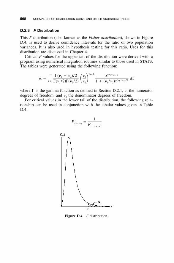
568 NORMAL ERROR DISTRIBUTION CURVE AND OTHER STATISTICAL TABLES
D.2.3 F Distribution
This F distribution (also known as the Fisher distribution), shown in FigureD.4, is used to derive confidence intervals for the ratio of two populationvariances. It is also used in hypothesis testing for this ratio. Uses for thisdistribution are discussed in Chapter 4.
Critical F values for the upper tail of the distribution were derived with aprogram using numerical integration routines similar to those used in STATS.The tables were generated using the following function:
� / 21� (� �2) / 21�(� � � ) /2 � x1 2 1� � � dx� � (� �� ) / 21 2F �(� /2)�(� /2) � 1 � (� /� )x1 2 2 1 2
where � is the gamma function as defined in Section D.2.1, �1 the numeratordegrees of freedom, and �2 the denominator degrees of freedom.
For critical values in the lower tail of the distribution, the following rela-tionship can be used in conjunction with the tabular values given in TableD.4.
1F ��,� ,�1 2 F1��,� ,�2 1
Figure D.4 F distribution.

569
TA
BL
ED
.4C
riti
cal
Val
ues
for
the
FD
istr
ibut
ion
��
0.20
�1→
�2↓
12
34
56
78
910
1215
2024
3040
6012
0
19.
4712
.00
13.0
613
.64
14.0
114
.26
14.4
414
.58
14.6
814
.77
14.9
015
.04
15.1
715
.24
15.3
115
.37
15.4
415
.51
23.
564.
004.
164.
244.
284.
324.
344.
364.
374.
384.
404.
424.
434.
444.
454.
464.
464.
473
2.68
2.89
2.94
2.96
2.97
2.97
2.97
2.98
2.98
2.98
2.98
2.98
2.98
2.98
2.98
2.98
2.98
2.98
42.
352.
472.
482.
482.
482.
472.
472.
472.
462.
462.
462.
452.
442.
442.
442.
442.
432.
435
2.18
2.26
2.25
2.24
2.23
2.22
2.21
2.20
2.20
2.19
2.18
2.18
2.17
2.16
2.16
2.15
2.15
2.14
62.
072.
132.
112.
092.
082.
062.
052.
042.
032.
032.
022.
012.
001.
991.
981.
981.
971.
967
2.00
2.04
2.02
1.99
1.97
1.96
1.94
1.93
1.93
1.92
1.91
1.89
1.88
1.87
1.86
1.86
1.85
1.84
81.
951.
981.
951.
921.
901.
881.
871.
861.
851.
841.
831.
811.
801.
791.
781.
771.
761.
759
1.91
1.93
1.90
1.87
1.85
1.83
1.81
1.80
1.79
1.78
1.76
1.75
1.73
1.72
1.71
1.70
1.69
1.68
101.
881.
901.
861.
831.
801.
781.
771.
751.
741.
731.
721.
701.
681.
671.
661.
651.
641.
6311
1.86
1.87
1.83
1.80
1.77
1.75
1.73
1.72
1.70
1.69
1.68
1.66
1.64
1.63
1.62
1.61
1.60
1.59
121.
841.
851.
801.
771.
741.
721.
701.
691.
671.
661.
651.
631.
611.
601.
591.
581.
561.
5513
1.82
1.83
1.78
1.75
1.72
1.69
1.68
1.66
1.65
1.64
1.62
1.60
1.58
1.57
1.56
1.55
1.53
1.52
141.
811.
811.
761.
731.
701.
671.
651.
641.
631.
621.
601.
581.
561.
551.
531.
521.
511.
4915
1.80
1.80
1.75
1.71
1.68
1.66
1.64
1.62
1.61
1.60
1.58
1.56
1.54
1.53
1.51
1.50
1.49
1.47
161.
791.
781.
741.
701.
671.
641.
621.
611.
591.
581.
561.
541.
521.
511.
491.
481.
471.
4517
1.78
1.77
1.72
1.68
1.65
1.63
1.61
1.59
1.58
1.57
1.55
1.53
1.50
1.49
1.48
1.46
1.45
1.43
181.
771.
761.
711.
671.
641.
621.
601.
581.
561.
551.
531.
511.
491.
481.
461.
451.
431.
4219
1.76
1.75
1.70
1.66
1.63
1.61
1.58
1.57
1.55
1.54
1.52
1.50
1.48
1.46
1.45
1.44
1.42
1.40
201.
761.
751.
701.
651.
621.
601.
581.
561.
541.
531.
511.
491.
471.
451.
441.
421.
411.
3921
1.75
1.74
1.69
1.65
1.61
1.59
1.57
1.55
1.53
1.52
1.50
1.48
1.46
1.44
1.43
1.41
1.40
1.38
221.
751.
731.
681.
641.
611.
581.
561.
541.
531.
511.
491.
471.
451.
431.
421.
401.
391.
3723
1.74
1.73
1.68
1.63
1.60
1.57
1.55
1.53
1.52
1.51
1.49
1.46
1.44
1.42
1.41
1.39
1.38
1.36
241.
741.
721.
671.
631.
591.
571.
551.
531.
511.
501.
481.
461.
431.
421.
401.
391.
371.
3525
1.73
1.72
1.66
1.62
1.59
1.56
1.54
1.52
1.51
1.49
1.47
1.45
1.42
1.41
1.39
1.38
1.36
1.34
261.
731.
711.
661.
621.
581.
561.
531.
521.
501.
491.
471.
441.
421.
401.
391.
371.
351.
3327
1.73
1.71
1.66
1.61
1.58
1.55
1.53
1.51
1.49
1.48
1.46
1.44
1.41
1.40
1.38
1.36
1.35
1.33
281.
721.
711.
651.
611.
571.
551.
521.
511.
491.
481.
461.
431.
411.
391.
371.
361.
341.
3229
1.72
1.70
1.65
1.60
1.57
1.54
1.52
1.50
1.49
1.47
1.45
1.43
1.40
1.39
1.37
1.35
1.33
1.31
301.
721.
701.
641.
601.
571.
541.
521.
501.
481.
471.
451.
421.
391.
381.
361.
351.
331.
3150
1.69
1.66
1.60
1.56
1.52
1.49
1.47
1.45
1.43
1.42
1.39
1.37
1.34
1.32
1.30
1.28
1.26
1.24
601.
681.
651.
591.
551.
511.
481.
461.
441.
421.
411.
381.
351.
321.
311.
291.
271.
241.
2280
1.67
1.64
1.58
1.53
1.50
1.47
1.44
1.42
1.41
1.39
1.37
1.34
1.31
1.29
1.27
1.25
1.22
1.19
120
1.66
1.63
1.57
1.52
1.48
1.45
1.43
1.41
1.39
1.37
1.35
1.32
1.29
1.27
1.25
1.23
1.20
1.17
(con
tinu
es)
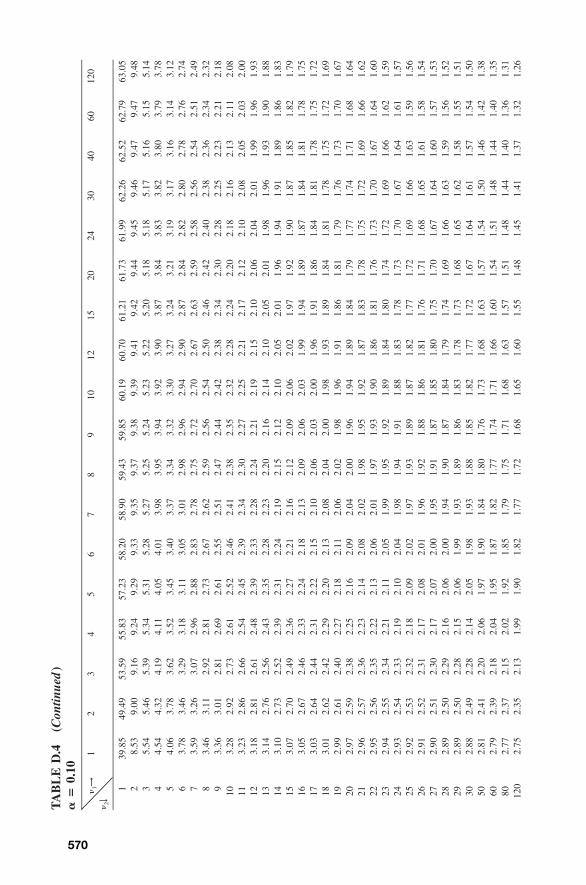
570
TA
BL
ED
.4(C
ontin
ued
)�
�0.
10
�1→
�2↓
12
34
56
78
910
1215
2024
3040
6012
0
139
.85
49.4
953
.59
55.8
357
.23
58.2
058
.90
59.4
359
.85
60.1
960
.70
61.2
161
.73
61.9
962
.26
62.5
262
.79
63.0
52
8.53
9.00
9.16
9.24
9.29
9.33
9.35
9.37
9.38
9.39
9.41
9.42
9.44
9.45
9.46
9.47
9.47
9.48
35.
545.
465.
395.
345.
315.
285.
275.
255.
245.
235.
225.
205.
185.
185.
175.
165.
155.
144
4.54
4.32
4.19
4.11
4.05
4.01
3.98
3.95
3.94
3.92
3.90
3.87
3.84
3.83
3.82
3.80
3.79
3.78
54.
063.
783.
623.
523.
453.
403.
373.
343.
323.
303.
273.
243.
213.
193.
173.
163.
143.
126
3.78
3.46
3.29
3.18
3.11
3.05
3.01
2.98
2.96
2.94
2.90
2.87
2.84
2.82
2.80
2.78
2.76
2.74
73.
593.
263.
072.
962.
882.
832.
782.
752.
722.
702.
672.
632.
592.
582.
562.
542.
512.
498
3.46
3.11
2.92
2.81
2.73
2.67
2.62
2.59
2.56
2.54
2.50
2.46
2.42
2.40
2.38
2.36
2.34
2.32
93.
363.
012.
812.
692.
612.
552.
512.
472.
442.
422.
382.
342.
302.
282.
252.
232.
212.
1810
3.28
2.92
2.73
2.61
2.52
2.46
2.41
2.38
2.35
2.32
2.28
2.24
2.20
2.18
2.16
2.13
2.11
2.08
113.
232.
862.
662.
542.
452.
392.
342.
302.
272.
252.
212.
172.
122.
102.
082.
052.
032.
0012
3.18
2.81
2.61
2.48
2.39
2.33
2.28
2.24
2.21
2.19
2.15
2.10
2.06
2.04
2.01
1.99
1.96
1.93
133.
142.
762.
562.
432.
352.
282.
232.
202.
162.
142.
102.
052.
011.
981.
961.
931.
901.
8814
3.10
2.73
2.52
2.39
2.31
2.24
2.19
2.15
2.12
2.10
2.05
2.01
1.96
1.94
1.91
1.89
1.86
1.83
153.
072.
702.
492.
362.
272.
212.
162.
122.
092.
062.
021.
971.
921.
901.
871.
851.
821.
7916
3.05
2.67
2.46
2.33
2.24
2.18
2.13
2.09
2.06
2.03
1.99
1.94
1.89
1.87
1.84
1.81
1.78
1.75
173.
032.
642.
442.
312.
222.
152.
102.
062.
032.
001.
961.
911.
861.
841.
811.
781.
751.
7218
3.01
2.62
2.42
2.29
2.20
2.13
2.08
2.04
2.00
1.98
1.93
1.89
1.84
1.81
1.78
1.75
1.72
1.69
192.
992.
612.
402.
272.
182.
112.
062.
021.
981.
961.
911.
861.
811.
791.
761.
731.
701.
6720
2.97
2.59
2.38
2.25
2.16
2.09
2.04
2.00
1.96
1.94
1.89
1.84
1.79
1.77
1.74
1.71
1.68
1.64
212.
962.
572.
362.
232.
142.
082.
021.
981.
951.
921.
871.
831.
781.
751.
721.
691.
661.
6222
2.95
2.56
2.35
2.22
2.13
2.06
2.01
1.97
1.93
1.90
1.86
1.81
1.76
1.73
1.70
1.67
1.64
1.60
232.
942.
552.
342.
212.
112.
051.
991.
951.
921.
891.
841.
801.
741.
721.
691.
661.
621.
5924
2.93
2.54
2.33
2.19
2.10
2.04
1.98
1.94
1.91
1.88
1.83
1.78
1.73
1.70
1.67
1.64
1.61
1.57
252.
922.
532.
322.
182.
092.
021.
971.
931.
891.
871.
821.
771.
721.
691.
661.
631.
591.
5626
2.91
2.52
2.31
2.17
2.08
2.01
1.96
1.92
1.88
1.86
1.81
1.76
1.71
1.68
1.65
1.61
1.58
1.54
272.
902.
512.
302.
172.
072.
001.
951.
911.
871.
851.
801.
751.
701.
671.
641.
601.
571.
5328
2.89
2.50
2.29
2.16
2.06
2.00
1.94
1.90
1.87
1.84
1.79
1.74
1.69
1.66
1.63
1.59
1.56
1.52
292.
892.
502.
282.
152.
061.
991.
931.
891.
861.
831.
781.
731.
681.
651.
621.
581.
551.
5130
2.88
2.49
2.28
2.14
2.05
1.98
1.93
1.88
1.85
1.82
1.77
1.72
1.67
1.64
1.61
1.57
1.54
1.50
502.
812.
412.
202.
061.
971.
901.
841.
801.
761.
731.
681.
631.
571.
541.
501.
461.
421.
3860
2.79
2.39
2.18
2.04
1.95
1.87
1.82
1.77
1.74
1.71
1.66
1.60
1.54
1.51
1.48
1.44
1.40
1.35
802.
772.
372.
152.
021.
921.
851.
791.
751.
711.
681.
631.
571.
511.
481.
441.
401.
361.
3112
02.
752.
352.
131.
991.
901.
821.
771.
721.
681.
651.
601.
551.
481.
451.
411.
371.
321.
26
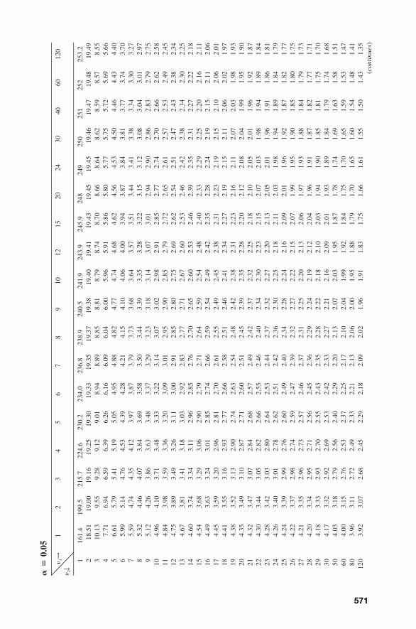
571
��
0.05
�1→
�2↓
12
34
56
78
910
1215
2024
3040
6012
0
116
1.4
199.
521
5.7
224.
623
0.2
234.
023
6.8
238.
924
0.5
241.
924
3.9
245.
924
824
925
025
125
225
3.2
218
.51
19.0
019
.16
19.2
519
.30
19.3
319
.35
19.3
719
.38
19.4
019
.41
19.4
319
.45
19.4
519
.46
19.4
719
.48
19.4
93
10.1
39.
559.
289.
129.
018.
948.
898.
858.
818.
798.
748.
708.
668.
648.
628.
598.
578.
554
7.71
6.94
6.59
6.39
6.26
6.16
6.09
6.04
6.00
5.96
5.91
5.86
5.80
5.77
5.75
5.72
5.69
5.66
56.
615.
795.
415.
195.
054.
954.
884.
824.
774.
744.
684.
624.
564.
534.
504.
464.
434.
406
5.99
5.14
4.76
4.53
4.39
4.28
4.21
4.15
4.10
4.06
4.00
3.94
3.87
3.84
3.81
3.77
3.74
3.70
75.
594.
744.
354.
123.
973.
873.
793.
733.
683.
643.
573.
513.
443.
413.
383.
343.
303.
278
5.32
4.46
4.07
3.84
3.69
3.58
3.50
3.44
3.39
3.35
3.28
3.22
3.15
3.12
3.08
3.04
3.01
2.97
95.
124.
263.
863.
633.
483.
373.
293.
233.
183.
143.
073.
012.
942.
902.
862.
832.
792.
7510
4.96
4.10
3.71
3.48
3.33
3.22
3.14
3.07
3.02
2.98
2.91
2.85
2.77
2.74
2.70
2.66
2.62
2.58
114.
843.
983.
593.
363.
203.
093.
012.
952.
902.
852.
792.
722.
652.
612.
572.
532.
492.
4512
4.75
3.89
3.49
3.26
3.11
3.00
2.91
2.85
2.80
2.75
2.69
2.62
2.54
2.51
2.47
2.43
2.38
2.34
134.
673.
813.
413.
183.
032.
922.
832.
772.
712.
672.
602.
532.
462.
422.
382.
342.
302.
2514
4.60
3.74
3.34
3.11
2.96
2.85
2.76
2.70
2.65
2.60
2.53
2.46
2.39
2.35
2.31
2.27
2.22
2.18
154.
543.
683.
293.
062.
902.
792.
712.
642.
592.
542.
482.
402.
332.
292.
252.
202.
162.
1116
4.49
3.63
3.24
3.01
2.85
2.74
2.66
2.59
2.54
2.49
2.42
2.35
2.28
2.24
2.19
2.15
2.11
2.06
174.
453.
593.
202.
962.
812.
702.
612.
552.
492.
452.
382.
312.
232.
192.
152.
102.
062.
0118
4.41
3.55
3.16
2.93
2.77
2.66
2.58
2.51
2.46
2.41
2.34
2.27
2.19
2.15
2.11
2.06
2.02
1.97
194.
383.
523.
132.
902.
742.
632.
542.
482.
422.
382.
312.
232.
162.
112.
072.
031.
981.
9320
4.35
3.49
3.10
2.87
2.71
2.60
2.51
2.45
2.39
2.35
2.28
2.20
2.12
2.08
2.04
1.99
1.95
1.90
214.
323.
473.
072.
842.
682.
572.
492.
422.
372.
322.
252.
182.
102.
052.
011.
961.
921.
8722
4.30
3.44
3.05
2.82
2.66
2.55
2.46
2.40
2.34
2.30
2.23
2.15
2.07
2.03
1.98
1.94
1.89
1.84
234.
283.
423.
032.
802.
642.
532.
442.
372.
322.
272.
202.
132.
052.
011.
961.
911.
861.
8124
4.26
3.40
3.01
2.78
2.62
2.51
2.42
2.36
2.30
2.25
2.18
2.11
2.03
1.98
1.94
1.89
1.84
1.79
254.
243.
392.
992.
762.
602.
492.
402.
342.
282.
242.
162.
092.
011.
961.
921.
871.
821.
7726
4.22
3.37
2.98
2.74
2.59
2.47
2.39
2.32
2.27
2.22
2.15
2.07
1.99
1.95
1.90
1.85
1.80
1.75
274.
213.
352.
962.
732.
572.
462.
372.
312.
252.
202.
132.
061.
971.
931.
881.
841.
791.
7328
4.20
3.34
2.95
2.71
2.56
2.45
2.36
2.29
2.24
2.19
2.12
2.04
1.96
1.91
1.87
1.82
1.77
1.71
294.
183.
332.
932.
702.
552.
432.
352.
282.
222.
182.
102.
031.
941.
901.
851.
811.
751.
7030
4.17
3.32
2.92
2.69
2.53
2.42
2.33
2.27
2.21
2.16
2.09
2.01
1.93
1.89
1.84
1.79
1.74
1.68
504.
033.
182.
792.
562.
402.
292.
202.
132.
072.
031.
951.
871.
781.
741.
691.
631.
581.
5160
4.00
3.15
2.76
2.53
2.37
2.25
2.17
2.10
2.04
1.99
1.92
1.84
1.75
1.70
1.65
1.59
1.53
1.47
803.
963.
112.
722.
492.
332.
212.
132.
062.
001.
951.
881.
791.
701.
651.
601.
541.
481.
4112
03.
923.
072.
682.
452.
292.
182.
092.
021.
961.
911.
831.
751.
661.
611.
551.
501.
431.
35(c
onti
nues
)
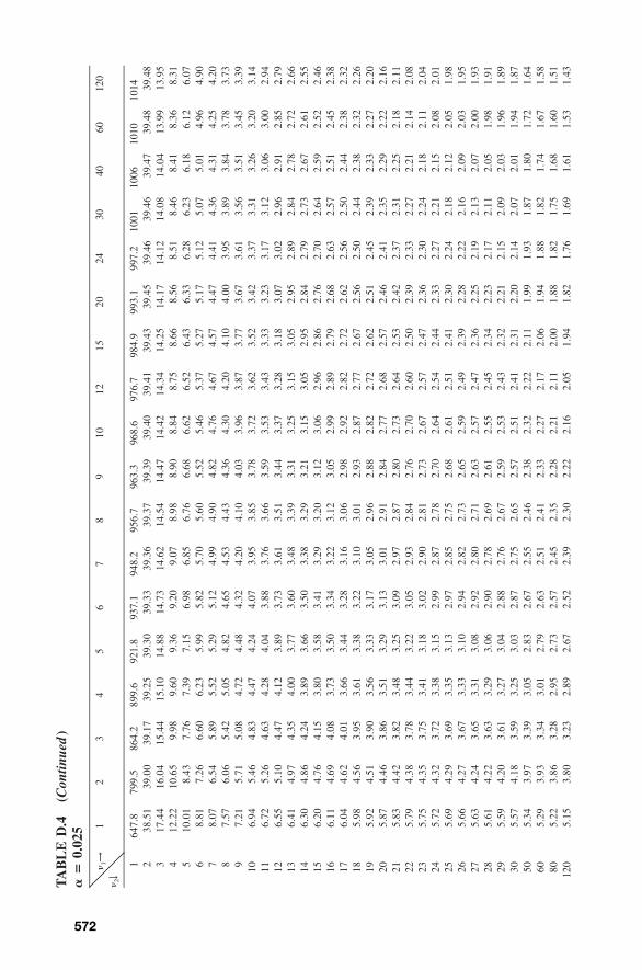
572
TA
BL
ED
.4(C
ontin
ued
)�
�0.
025
�1→
�2↓
12
34
56
78
910
1215
2024
3040
6012
0
164
7.8
799.
586
4.2
899.
692
1.8
937.
194
8.2
956.
796
3.3
968.
697
6.7
984.
999
3.1
997.
210
0110
0610
1010
142
38.5
139
.00
39.1
739
.25
39.3
039
.33
39.3
639
.37
39.3
939
.40
39.4
139
.43
39.4
539
.46
39.4
639
.47
39.4
839
.48
317
.44
16.0
415
.44
15.1
014
.88
14.7
314
.62
14.5
414
.47
14.4
214
.34
14.2
514
.17
14.1
214
.08
14.0
413
.99
13.9
54
12.2
210
.65
9.98
9.60
9.36
9.20
9.07
8.98
8.90
8.84
8.75
8.66
8.56
8.51
8.46
8.41
8.36
8.31
510
.01
8.43
7.76
7.39
7.15
6.98
6.85
6.76
6.68
6.62
6.52
6.43
6.33
6.28
6.23
6.18
6.12
6.07
68.
817.
266.
606.
235.
995.
825.
705.
605.
525.
465.
375.
275.
175.
125.
075.
014.
964.
907
8.07
6.54
5.89
5.52
5.29
5.12
4.99
4.90
4.82
4.76
4.67
4.57
4.47
4.41
4.36
4.31
4.25
4.20
87.
576.
065.
425.
054.
824.
654.
534.
434.
364.
304.
204.
104.
003.
953.
893.
843.
783.
739
7.21
5.71
5.08
4.72
4.48
4.32
4.20
4.10
4.03
3.96
3.87
3.77
3.67
3.61
3.56
3.51
3.45
3.39
106.
945.
464.
834.
474.
244.
073.
953.
853.
783.
723.
623.
523.
423.
373.
313.
263.
203.
1411
6.72
5.26
4.63
4.28
4.04
3.88
3.76
3.66
3.59
3.53
3.43
3.33
3.23
3.17
3.12
3.06
3.00
2.94
126.
555.
104.
474.
123.
893.
733.
613.
513.
443.
373.
283.
183.
073.
022.
962.
912.
852.
7913
6.41
4.97
4.35
4.00
3.77
3.60
3.48
3.39
3.31
3.25
3.15
3.05
2.95
2.89
2.84
2.78
2.72
2.66
146.
304.
864.
243.
893.
663.
503.
383.
293.
213.
153.
052.
952.
842.
792.
732.
672.
612.
5515
6.20
4.76
4.15
3.80
3.58
3.41
3.29
3.20
3.12
3.06
2.96
2.86
2.76
2.70
2.64
2.59
2.52
2.46
166.
114.
694.
083.
733.
503.
343.
223.
123.
052.
992.
892.
792.
682.
632.
572.
512.
452.
3817
6.04
4.62
4.01
3.66
3.44
3.28
3.16
3.06
2.98
2.92
2.82
2.72
2.62
2.56
2.50
2.44
2.38
2.32
185.
984.
563.
953.
613.
383.
223.
103.
012.
932.
872.
772.
672.
562.
502.
442.
382.
322.
2619
5.92
4.51
3.90
3.56
3.33
3.17
3.05
2.96
2.88
2.82
2.72
2.62
2.51
2.45
2.39
2.33
2.27
2.20
205.
874.
463.
863.
513.
293.
133.
012.
912.
842.
772.
682.
572.
462.
412.
352.
292.
222.
1621
5.83
4.42
3.82
3.48
3.25
3.09
2.97
2.87
2.80
2.73
2.64
2.53
2.42
2.37
2.31
2.25
2.18
2.11
225.
794.
383.
783.
443.
223.
052.
932.
842.
762.
702.
602.
502.
392.
332.
272.
212.
142.
0823
5.75
4.35
3.75
3.41
3.18
3.02
2.90
2.81
2.73
2.67
2.57
2.47
2.36
2.30
2.24
2.18
2.11
2.04
245.
724.
323.
723.
383.
152.
992.
872.
782.
702.
642.
542.
442.
332.
272.
212.
152.
082.
0125
5.69
4.29
3.69
3.35
3.13
2.97
2.85
2.75
2.68
2.61
2.51
2.41
2.30
2.24
2.18
2.12
2.05
1.98
265.
664.
273.
673.
333.
102.
942.
822.
732.
652.
592.
492.
392.
282.
222.
162.
092.
031.
9527
5.63
4.24
3.65
3.31
3.08
2.92
2.80
2.71
2.63
2.57
2.47
2.36
2.25
2.19
2.13
2.07
2.00
1.93
285.
614.
223.
633.
293.
062.
902.
782.
692.
612.
552.
452.
342.
232.
172.
112.
051.
981.
9129
5.59
4.20
3.61
3.27
3.04
2.88
2.76
2.67
2.59
2.53
2.43
2.32
2.21
2.15
2.09
2.03
1.96
1.89
305.
574.
183.
593.
253.
032.
872.
752.
652.
572.
512.
412.
312.
202.
142.
072.
011.
941.
8750
5.34
3.97
3.39
3.05
2.83
2.67
2.55
2.46
2.38
2.32
2.22
2.11
1.99
1.93
1.87
1.80
1.72
1.64
605.
293.
933.
343.
012.
792.
632.
512.
412.
332.
272.
172.
061.
941.
881.
821.
741.
671.
5880
5.22
3.86
3.28
2.95
2.73
2.57
2.45
2.35
2.28
2.21
2.11
2.00
1.88
1.82
1.75
1.68
1.60
1.51
120
5.15
3.80
3.23
2.89
2.67
2.52
2.39
2.30
2.22
2.16
2.05
1.94
1.82
1.76
1.69
1.61
1.53
1.43
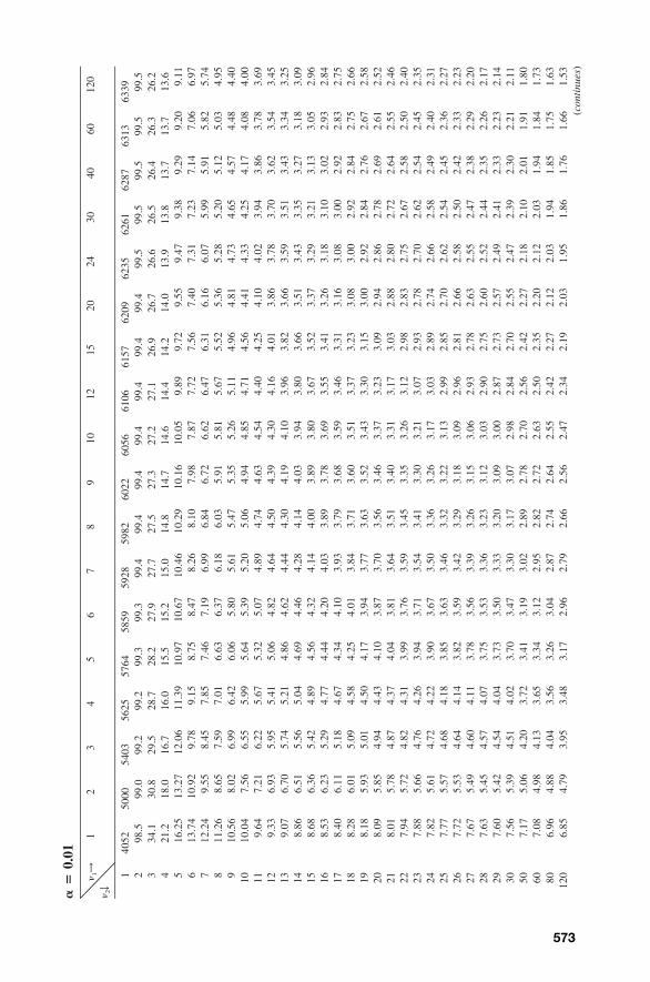
573
��
0.01
�1→
�2↓
12
34
56
78
910
1215
2024
3040
6012
0
140
5250
0054
0356
2557
6458
5959
2859
8260
2260
5661
0661
5762
0962
3562
6162
8763
1363
392
98.5
99.0
99.2
99.2
99.3
99.3
99.4
99.4
99.4
99.4
99.4
99.4
99.4
99.5
99.5
99.5
99.5
99.5
334
.130
.829
.528
.728
.227
.927
.727
.527
.327
.227
.126
.926
.726
.626
.526
.426
.326
.24
21.2
18.0
16.7
16.0
15.5
15.2
15.0
14.8
14.7
14.6
14.4
14.2
14.0
13.9
13.8
13.7
13.7
13.6
516
.25
13.2
712
.06
11.3
910
.97
10.6
710
.46
10.2
910
.16
10.0
59.
899.
729.
559.
479.
389.
299.
209.
116
13.7
410
.92
9.78
9.15
8.75
8.47
8.26
8.10
7.98
7.87
7.72
7.56
7.40
7.31
7.23
7.14
7.06
6.97
712
.24
9.55
8.45
7.85
7.46
7.19
6.99
6.84
6.72
6.62
6.47
6.31
6.16
6.07
5.99
5.91
5.82
5.74
811
.26
8.65
7.59
7.01
6.63
6.37
6.18
6.03
5.91
5.81
5.67
5.52
5.36
5.28
5.20
5.12
5.03
4.95
910
.56
8.02
6.99
6.42
6.06
5.80
5.61
5.47
5.35
5.26
5.11
4.96
4.81
4.73
4.65
4.57
4.48
4.40
1010
.04
7.56
6.55
5.99
5.64
5.39
5.20
5.06
4.94
4.85
4.71
4.56
4.41
4.33
4.25
4.17
4.08
4.00
119.
647.
216.
225.
675.
325.
074.
894.
744.
634.
544.
404.
254.
104.
023.
943.
863.
783.
6912
9.33
6.93
5.95
5.41
5.06
4.82
4.64
4.50
4.39
4.30
4.16
4.01
3.86
3.78
3.70
3.62
3.54
3.45
139.
076.
705.
745.
214.
864.
624.
444.
304.
194.
103.
963.
823.
663.
593.
513.
433.
343.
2514
8.86
6.51
5.56
5.04
4.69
4.46
4.28
4.14
4.03
3.94
3.80
3.66
3.51
3.43
3.35
3.27
3.18
3.09
158.
686.
365.
424.
894.
564.
324.
144.
003.
893.
803.
673.
523.
373.
293.
213.
133.
052.
9616
8.53
6.23
5.29
4.77
4.44
4.20
4.03
3.89
3.78
3.69
3.55
3.41
3.26
3.18
3.10
3.02
2.93
2.84
178.
406.
115.
184.
674.
344.
103.
933.
793.
683.
593.
463.
313.
163.
083.
002.
922.
832.
7518
8.28
6.01
5.09
4.58
4.25
4.01
3.84
3.71
3.60
3.51
3.37
3.23
3.08
3.00
2.92
2.84
2.75
2.66
198.
185.
935.
014.
504.
173.
943.
773.
633.
523.
433.
303.
153.
002.
922.
842.
762.
672.
5820
8.09
5.85
4.94
4.43
4.10
3.87
3.70
3.56
3.46
3.37
3.23
3.09
2.94
2.86
2.78
2.69
2.61
2.52
218.
015.
784.
874.
374.
043.
813.
643.
513.
403.
313.
173.
032.
882.
802.
722.
642.
552.
4622
7.94
5.72
4.82
4.31
3.99
3.76
3.59
3.45
3.35
3.26
3.12
2.98
2.83
2.75
2.67
2.58
2.50
2.40
237.
885.
664.
764.
263.
943.
713.
543.
413.
303.
213.
072.
932.
782.
702.
622.
542.
452.
3524
7.82
5.61
4.72
4.22
3.90
3.67
3.50
3.36
3.26
3.17
3.03
2.89
2.74
2.66
2.58
2.49
2.40
2.31
257.
775.
574.
684.
183.
853.
633.
463.
323.
223.
132.
992.
852.
702.
622.
542.
452.
362.
2726
7.72
5.53
4.64
4.14
3.82
3.59
3.42
3.29
3.18
3.09
2.96
2.81
2.66
2.58
2.50
2.42
2.33
2.23
277.
675.
494.
604.
113.
783.
563.
393.
263.
153.
062.
932.
782.
632.
552.
472.
382.
292.
2028
7.63
5.45
4.57
4.07
3.75
3.53
3.36
3.23
3.12
3.03
2.90
2.75
2.60
2.52
2.44
2.35
2.26
2.17
297.
605.
424.
544.
043.
733.
503.
333.
203.
093.
002.
872.
732.
572.
492.
412.
332.
232.
1430
7.56
5.39
4.51
4.02
3.70
3.47
3.30
3.17
3.07
2.98
2.84
2.70
2.55
2.47
2.39
2.30
2.21
2.11
507.
175.
064.
203.
723.
413.
193.
022.
892.
782.
702.
562.
422.
272.
182.
102.
011.
911.
8060
7.08
4.98
4.13
3.65
3.34
3.12
2.95
2.82
2.72
2.63
2.50
2.35
2.20
2.12
2.03
1.94
1.84
1.73
806.
964.
884.
043.
563.
263.
042.
872.
742.
642.
552.
422.
272.
122.
031.
941.
851.
751.
6312
06.
854.
793.
953.
483.
172.
962.
792.
662.
562.
472.
342.
192.
031.
951.
861.
761.
661.
53(c
onti
nues
)
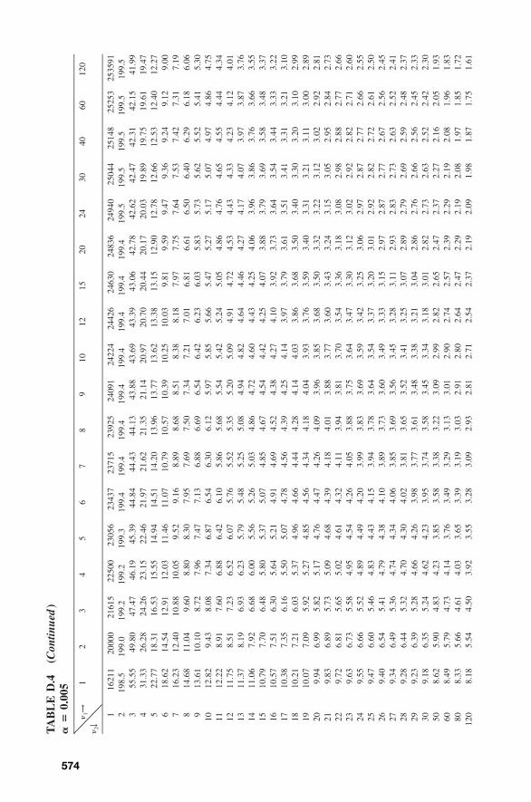
574
TA
BL
ED
.4(C
ontin
ued
)�
�0.
005
�1→
�2↓
12
34
56
78
910
1215
2024
3040
6012
0
116
211
2000
021
615
2250
023
056
2343
723
715
2392
524
091
2422
424
426
2463
024
836
2494
025
044
2514
825
253
2535
912
198.
519
9.0
199.
219
9.2
199.
319
9.4
199.
419
9.4
199.
419
9.4
199.
419
9.4
199.
419
9.5
199.
519
9.5
199.
519
9.5
355
.55
49.8
047
.47
46.1
945
.39
44.8
444
.43
44.1
343
.88
43.6
943
.39
43.0
642
.78
42.6
242
.47
42.3
142
.15
41.9
94
31.3
326
.28
24.2
623
.15
22.4
621
.97
21.6
221
.35
21.1
420
.97
20.7
020
.44
20.1
720
.03
19.8
919
.75
19.6
119
.47
522
.77
18.3
116
.53
15.5
514
.94
14.5
114
.20
13.9
613
.77
13.6
213
.38
13.1
512
.90
12.7
812
.66
12.5
312
.40
12.2
76
18.6
214
.54
12.9
112
.03
11.4
611
.07
10.7
910
.57
10.3
910
.25
10.0
39.
819.
599.
479.
369.
249.
129.
007
16.2
312
.40
10.8
810
.05
9.52
9.16
8.89
8.68
8.51
8.38
8.18
7.97
7.75
7.64
7.53
7.42
7.31
7.19
814
.68
11.0
49.
608.
808.
307.
957.
697.
507.
347.
217.
016.
816.
616.
506.
406.
296.
186.
069
13.6
110
.10
8.72
7.96
7.47
7.13
6.88
6.69
6.54
6.42
6.23
6.03
5.83
5.73
5.62
5.52
5.41
5.30
1012
.82
9.43
8.08
7.34
6.87
6.54
6.30
6.12
5.97
5.85
5.66
5.47
5.27
5.17
5.07
4.97
4.86
4.75
1112
.22
8.91
7.60
6.88
6.42
6.10
5.86
5.68
5.54
5.42
5.24
5.05
4.86
4.76
4.65
4.55
4.44
4.34
1211
.75
8.51
7.23
6.52
6.07
5.76
5.52
5.35
5.20
5.09
4.91
4.72
4.53
4.43
4.33
4.23
4.12
4.01
1311
.37
8.19
6.93
6.23
5.79
5.48
5.25
5.08
4.94
4.82
4.64
4.46
4.27
4.17
4.07
3.97
3.87
3.76
1411
.06
7.92
6.68
6.00
5.56
5.26
5.03
4.86
4.72
4.60
4.43
4.25
4.06
3.96
3.86
3.76
3.66
3.55
1510
.79
7.70
6.48
5.80
5.37
5.07
4.85
4.67
4.54
4.42
4.25
4.07
3.88
3.79
3.69
3.58
3.48
3.37
1610
.57
7.51
6.30
5.64
5.21
4.91
4.69
4.52
4.38
4.27
4.10
3.92
3.73
3.64
3.54
3.44
3.33
3.22
1710
.38
7.35
6.16
5.50
5.07
4.78
4.56
4.39
4.25
4.14
3.97
3.79
3.61
3.51
3.41
3.31
3.21
3.10
1810
.21
7.21
6.03
5.37
4.96
4.66
4.44
4.28
4.14
4.03
3.86
3.68
3.50
3.40
3.30
3.20
3.10
2.99
1910
.07
7.09
5.92
5.27
4.85
4.56
4.34
4.18
4.04
3.93
3.76
3.59
3.40
3.31
3.21
3.11
3.00
2.89
209.
946.
995.
825.
174.
764.
474.
264.
093.
963.
853.
683.
503.
323.
223.
123.
022.
922.
8121
9.83
6.89
5.73
5.09
4.68
4.39
4.18
4.01
3.88
3.77
3.60
3.43
3.24
3.15
3.05
2.95
2.84
2.73
229.
726.
815.
655.
024.
614.
324.
113.
943.
813.
703.
543.
363.
183.
082.
982.
882.
772.
6623
9.63
6.73
5.58
4.95
4.54
4.26
4.05
3.88
3.75
3.64
3.47
3.30
3.12
3.02
2.92
2.82
2.71
2.60
249.
556.
665.
524.
894.
494.
203.
993.
833.
693.
593.
423.
253.
062.
972.
872.
772.
662.
5525
9.47
6.60
5.46
4.83
4.43
4.15
3.94
3.78
3.64
3.54
3.37
3.20
3.01
2.92
2.82
2.72
2.61
2.50
269.
406.
545.
414.
794.
384.
103.
893.
733.
603.
493.
333.
152.
972.
872.
772.
672.
562.
4527
9.34
6.49
5.36
4.74
4.34
4.06
3.85
3.69
3.56
3.45
3.28
3.11
2.93
2.83
2.73
2.63
2.52
2.41
289.
286.
445.
324.
704.
304.
023.
813.
653.
523.
413.
253.
072.
892.
792.
692.
592.
482.
3729
9.23
6.39
5.28
4.66
4.26
3.98
3.77
3.61
3.48
3.38
3.21
3.04
2.86
2.76
2.66
2.56
2.45
2.33
309.
186.
355.
244.
624.
233.
953.
743.
583.
453.
343.
183.
012.
822.
732.
632.
522.
422.
3050
8.62
5.90
4.83
4.23
3.85
3.58
3.38
3.22
3.09
2.99
2.82
2.65
2.47
2.37
2.27
2.16
2.05
1.93
608.
495.
794.
734.
143.
763.
493.
293.
133.
012.
902.
742.
572.
392.
292.
192.
081.
961.
8380
8.33
5.66
4.61
4.03
3.65
3.39
3.19
3.03
2.91
2.80
2.64
2.47
2.29
2.19
2.08
1.97
1.85
1.72
120
8.18
5.54
4.50
3.92
3.55
3.28
3.09
2.93
2.81
2.71
2.54
2.37
2.19
2.09
1.98
1.87
1.75
1.61
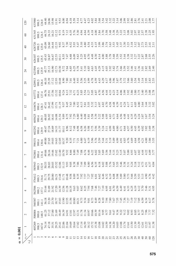
575
��
0.00
1
�1→
�2↓
12
34
56
78
910
1215
2024
3040
6012
0
140
5269
5000
0454
0387
5625
0657
6412
5859
4359
2881
5981
5160
2292
6056
2561
0676
6157
7262
0913
6235
0462
6107
6287
2063
1345
6339
802
998.
599
9.0
999.
199
9.2
999.
399
9.3
999.
499
9.4
999.
499
9.4
999.
499
9.4
999.
599
9.5
999.
599
9.5
999.
599
9.5
316
7.0
148.
514
1.1
137.
113
4.6
132.
913
1.6
130.
612
9.9
129.
312
8.3
127.
412
6.4
125.
912
5.5
125.
012
4.5
124.
04
74.1
461
.25
56.1
853
.44
51.7
150
.53
49.6
649
.00
48.4
748
.05
47.4
146
.76
46.1
045
.77
45.4
345
.09
44.7
544
.40
547
.18
37.1
233
.20
31.0
929
.75
28.8
328
.16
27.6
527
.24
26.9
226
.42
25.9
125
.39
25.1
324
.87
24.6
024
.33
24.0
66
35.5
127
.00
23.7
021
.92
20.8
020
.03
19.4
619
.03
18.6
918
.41
17.9
917
.56
17.1
216
.90
16.6
716
.44
16.2
115
.98
729
.25
21.6
918
.77
17.2
016
.21
15.5
215
.02
14.6
314
.33
14.0
813
.71
13.3
212
.93
12.7
312
.53
12.3
312
.12
11.9
18
25.4
118
.49
15.8
314
.39
13.4
812
.86
12.4
012
.05
11.7
711
.54
11.1
910
.84
10.4
810
.30
10.1
19.
929.
739.
539
22.8
616
.39
13.9
012
.56
11.7
111
.13
10.7
010
.37
10.1
19.
899.
579.
248.
908.
728.
558.
378.
198.
0010
21.0
414
.91
12.5
511
.28
10.4
89.
939.
529.
208.
968.
758.
458.
137.
807.
647.
477.
307.
126.
9411
19.6
913
.81
11.5
610
.35
9.58
9.05
8.66
8.35
8.12
7.92
7.63
7.32
7.01
6.85
6.68
6.52
6.35
6.18
1218
.64
12.9
710
.80
9.63
8.89
8.38
8.00
7.71
7.48
7.29
7.00
6.71
6.40
6.25
6.09
5.93
5.76
5.59
1317
.82
12.3
110
.21
9.07
8.35
7.86
7.49
7.21
6.98
6.80
6.52
6.23
5.93
5.78
5.63
5.47
5.30
5.14
1417
.14
11.7
89.
738.
627.
927.
447.
086.
806.
586.
406.
135.
855.
565.
415.
255.
104.
944.
7715
16.5
911
.34
9.34
8.25
7.57
7.09
6.74
6.47
6.26
6.08
5.81
5.54
5.25
5.10
4.95
4.80
4.64
4.47
1616
.12
10.9
79.
017.
947.
276.
806.
466.
195.
985.
815.
555.
274.
994.
854.
704.
544.
394.
2317
15.7
210
.66
8.73
7.68
7.02
6.56
6.22
5.96
5.75
5.58
5.32
5.05
4.78
4.63
4.48
4.33
4.18
4.02
1815
.38
10.3
98.
497.
466.
816.
356.
025.
765.
565.
395.
134.
874.
594.
454.
304.
154.
003.
8419
15.0
810
.16
8.28
7.27
6.62
6.18
5.85
5.59
5.39
5.22
4.97
4.70
4.43
4.29
4.14
3.99
3.84
3.68
2014
.82
9.95
8.10
7.10
6.46
6.02
5.69
5.44
5.24
5.08
4.82
4.56
4.29
4.15
4.00
3.86
3.70
3.54
2114
.59
9.77
7.94
6.95
6.32
5.88
5.56
5.31
5.11
4.95
4.70
4.44
4.17
4.03
3.88
3.74
3.58
3.42
2214
.38
9.61
7.80
6.81
6.19
5.76
5.44
5.19
4.99
4.83
4.58
4.33
4.06
3.92
3.78
3.63
3.48
3.32
2314
.20
9.47
7.67
6.70
6.08
5.65
5.33
5.09
4.89
4.73
4.48
4.23
3.96
3.82
3.68
3.53
3.38
3.22
2414
.03
9.34
7.55
6.59
5.98
5.55
5.23
4.99
4.80
4.64
4.39
4.14
3.87
3.74
3.59
3.45
3.29
3.14
2513
.88
9.22
7.45
6.49
5.89
5.46
5.15
4.91
4.71
4.56
4.31
4.06
3.79
3.66
3.52
3.37
3.22
3.06
2613
.74
9.12
7.36
6.41
5.80
5.38
5.07
4.83
4.64
4.48
4.24
3.99
3.72
3.59
3.44
3.30
3.15
2.99
2713
.61
9.02
7.27
6.33
5.73
5.31
5.00
4.76
4.57
4.41
4.17
3.92
3.66
3.52
3.38
3.23
3.08
2.92
2813
.50
8.93
7.19
6.25
5.66
5.24
4.93
4.69
4.50
4.35
4.11
3.86
3.60
3.46
3.32
3.18
3.02
2.86
2913
.39
8.85
7.12
6.19
5.59
5.18
4.87
4.64
4.45
4.29
4.05
3.80
3.54
3.41
3.27
3.12
2.97
2.81
3013
.29
8.77
7.05
6.12
5.53
5.12
4.82
4.58
4.39
4.24
4.00
3.75
3.49
3.36
3.22
3.07
2.92
2.76
4012
.61
8.25
6.59
5.70
5.13
4.73
4.44
4.21
4.02
3.87
3.64
3.40
3.14
3.01
2.87
2.73
2.57
2.41
5012
.22
7.96
6.34
5.46
4.90
4.51
4.22
4.00
3.82
3.67
3.44
3.20
2.95
2.82
2.68
2.53
2.38
2.21
6011
.97
7.77
6.17
5.31
4.76
4.37
4.09
3.86
3.69
3.54
3.32
3.08
2.83
2.69
2.55
2.41
2.25
2.08
120
11.3
87.
325.
784.
954.
424.
043.
773.
553.
383.
243.
022.
782.
532.
402.
262.
111.
951.
77
576
APPENDIX E
CONFIDENCE INTERVALSFOR THE MEAN
Table E.1 represents 1000 95% confidence intervals constructed from samplesets selected from a population with a mean (�) of 25.4 and a variance (�2)of 1.69. These data are discussed in Chapter 4. (Note: Intervals with asterisksfail to include �.)
Adjustment Computations: Spatial Data Analysis, Fourth Edition. C. D. Ghilani and P. R. Wolf© 2006 John Wiley & Sons, Inc. ISBN: 978-0-471-69728-2
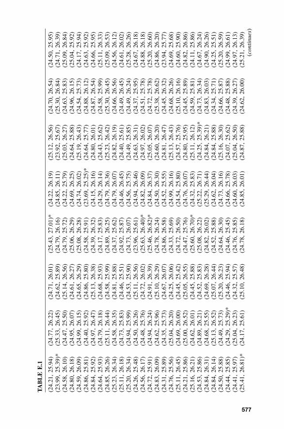
577
TA
BL
EE
.1
(24.
21,
25.9
4)(2
4.77
,26
.22)
(24.
71,
26.0
1)(2
5.43
,27
.01)
*(2
4.22
,26
.19)
(25.
12,
26.5
6)(2
4.70
,26
.54)
(24.
50,
25.9
5)(2
3.99
,25
.39)
*(2
5.33
,26
.45)
(24.
62,
25.8
9)(2
4.79
,26
.16)
(24.
85,
26.1
1)(2
3.92
,25
.67)
(25.
30,
26.8
4)(2
4.71
,26
.39)
(24.
58,
26.1
0)(2
4.47
,25
.50)
(25.
14,
26.5
6)(2
4.79
,25
.72)
(24.
22,
25.7
9)(2
5.03
,26
.27)
(24.
63,
25.8
3)(2
5.09
,26
.84)
(24.
80,
26.1
8)(2
4.95
,26
.07)
(24.
61,
26.2
7)(2
5.06
,26
.29)
(24.
69,
26.2
5)(2
4.64
,25
.88)
(24.
96,
26.1
5)(2
5.04
,25
.92)
(24.
59,
26.0
9)(2
4.99
,26
.15)
(24.
65,
26.2
9)(2
5.08
,26
.28)
(24.
74,
26.0
2)(2
5.19
,26
.43)
(24.
54,
25.7
3)(2
4.17
,25
.94)
(24.
86,
25.8
1)(2
4.40
,25
.92)
(24.
86,
25.8
0)(2
4.58
,25
.91)
(23.
69,
25.2
5)*
(24.
64,
25.7
7)(2
4.88
,26
.12)
(24.
63,
25.9
2)(2
4.84
,25
.92)
(24.
97,
26.4
7)(2
5.13
,26
.38)
(24.
39,
26.3
2)(2
4.15
,26
.16)
(24.
80,
26.0
1)(2
4.87
,26
.54)
(24.
66,
25.9
5)(2
4.64
,25
.93)
(24.
79,
26.1
8)(2
4.68
,25
.93)
(24.
17,
25.8
3)(2
4.29
,26
.14)
(24.
43,
25.6
2)(2
4.58
,25
.99)
(25.
11,
26.3
3)(2
4.85
,26
.26)
(25.
11,
26.4
4)(2
4.58
,25
.99)
(24.
89,
26.2
5)(2
4.79
,26
.36)
(25.
23,
26.4
2)(2
5.30
,26
.45)
(25.
09,
26.5
3)(2
5.23
,26
.34)
(24.
58,
26.3
5)(2
4.81
,25
.88)
(24.
37,
25.6
2)(2
4.79
,26
.07)
(24.
82,
26.1
9)(2
4.66
,26
.56)
(24.
56,
26.1
2)(2
5.11
,26
.18)
(24.
73,
25.8
3)(2
4.46
,25
.51)
(24.
92,
25.8
7)(2
4.46
,26
.45)
(24.
40,
25.6
1)(2
4.49
,26
.45)
(24.
61,
26.0
2)(2
5.20
,26
.34)
(24.
94,
25.9
9)(2
4.53
,25
.90)
(24.
73,
26.0
7)(2
4.56
,25
.75)
(24.
49,
25.8
5)(2
4.49
,26
.24)
(25.
28,
26.2
6)(2
4.26
,25
.48)
(24.
50,
26.2
6)(2
5.11
,26
.56)
(23.
96,
25.6
1)(2
4.94
,26
.46)
(24.
63,
26.3
1)(2
4.37
,25
.95)
(24.
67,
26.1
8)(2
4.56
,26
.17)
(24.
48,
25.7
6)(2
4.72
,26
.02)
(25.
63,
26.4
0)*
(24.
82,
26.0
9)(2
4.97
,26
.02)
(24.
51,
25.7
8)(2
4.88
,26
.18)
(24.
72,
25.9
1)(2
4.94
,26
.24)
(24.
91,
26.3
9)(2
5.46
,26
.82)
*(2
4.84
,26
.37)
(25.
05,
26.0
7)(2
4.72
,25
.78)
(25.
20,
26.6
0)(2
4.83
,26
.09)
(24.
62,
25.9
6)(2
5.10
,26
.29)
(24.
78,
26.2
4)(2
4.50
,26
.30)
(24.
60,
26.2
0)(2
5.38
,26
.62)
(24.
86,
26.2
0)(2
4.31
,25
.89)
(24.
35,
25.7
3)(2
4.67
,26
.07)
(24.
86,
26.5
8)(2
4.52
,25
.55)
(24.
81,
26.4
7)(2
4.45
,26
.32)
(23.
94,
25.7
7)(2
4.76
,25
.56)
(25.
04,
26.2
0)(2
4.25
,26
.06)
(24.
33,
25.6
9)(2
4.99
,26
.16)
(25.
13,
26.4
3)(2
4.68
,26
.26)
(24.
69,
25.6
8)(2
5.11
,26
.45)
(24.
69,
26.0
0)(2
4.45
,25
.42)
(24.
72,
26.5
0)(2
4.54
,25
.80)
(24.
57,
25.7
6)(2
5.10
,26
.16)
(24.
60,
25.9
0)(2
4.21
,25
.86)
(25.
00,
26.5
2)(2
5.05
,26
.55)
(24.
47,
25.7
6)(2
4.76
,26
.07)
(24.
80,
25.9
5)(2
4.45
,25
.89)
(24.
82,
26.8
6)(2
5.16
,26
.21)
(24.
62,
26.0
1)(2
4.45
,25
.88)
(25.
60,
26.7
0)*
(24.
32,
25.8
3)(2
5.11
,26
.12)
(24.
59,
25.8
1)(2
4.11
,25
.86)
(24.
53,
25.8
6)(2
4.89
,26
.21)
(24.
52,
25.8
3)(2
5.08
,26
.22)
(25.
22,
26.7
1)(2
4.25
,25
.39)
*(2
4.73
,26
.34)
(24.
67,
26.2
4)(2
4.84
,26
.31)
(24.
68,
25.5
5)(2
4.69
,26
.28)
(24.
82,
26.0
2)(2
5.29
,26
.44)
(24.
84,
26.2
1)(2
4.83
,26
.03)
(24.
90,
26.2
6)(2
4.84
,26
.14)
(25.
13,
26.5
2)(2
5.07
,26
.44)
(24.
52,
25.8
8)(2
4.62
,26
.04)
(24.
84,
25.8
8)(2
4.34
,25
.71)
(24.
25,
25.5
1)(2
4.50
,25
.88)
(24.
49,
25.7
3)(2
5.20
,26
.23)
(24.
64,
26.3
0)(2
4.73
,26
.16)
(25.
16,
26.3
0)(2
4.66
,25
.87)
(25.
20,
26.5
9)(2
4.44
,25
.85)
(24.
29,
25.2
9)*
(24.
46,
25.9
4)(2
4.46
,25
.45)
(24.
66,
25.7
8)(2
4.07
,25
.62)
(24.
48,
25.8
8)(2
4.99
,26
.61)
(24.
41,
25.9
7)(2
5.04
,26
.23)
(24.
32,
25.5
7)(2
4.76
,25
.85)
(24.
60,
26.0
3)(2
5.04
,26
.50)
(24.
39,
26.2
7)(2
4.97
,26
.13)
(25.
41,
26.8
1)*
(24.
17,
25.6
1)(2
5.10
,26
.48)
(24.
78,
26.1
8)(2
4.85
,26
.01)
(24.
87,
25.8
8)(2
4.62
,26
.00)
(25.
21,
26.3
9)(c
onti
nues
)
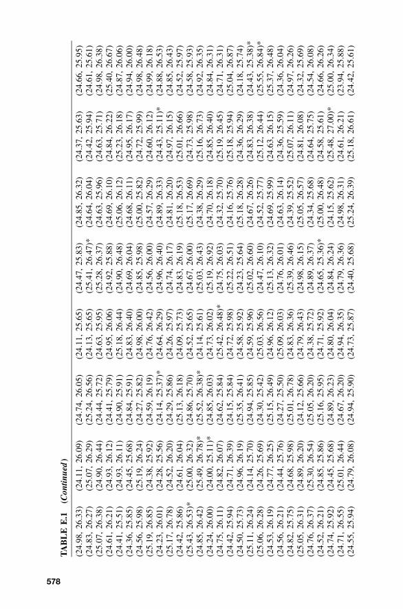
578
TA
BL
EE
.1(C
ontin
ued
)
(24.
98,
26.3
3)(2
4.11
,26
.09)
(24.
74,
26.0
5)(2
4.11
,25
.65)
(24.
47,
25.8
3)(2
4.85
,26
.32)
(24.
37,
25.6
3)(2
4.66
,25
.95)
(24.
83,
26.2
7)(2
5.07
,26
.29)
(25.
24,
26.5
6)(2
4.13
,25
.65)
(25.
41,
26.4
7)*
(24.
64,
26.0
4)(2
4.42
,25
.94)
(24.
61,
25.6
1)(2
5.07
,26
.38)
(24.
90,
26.4
4)(2
4.44
,25
.72)
(24.
63,
25.9
5)(2
5.28
,26
.37)
(24.
63,
25.9
6)(2
4.63
,25
.71)
(24.
98,
26.3
8)(2
4.61
,26
.21)
(24.
93,
26.1
2)(2
4.41
,25
.79)
(24.
95,
26.0
6)(2
4.92
,25
.88)
(24.
69,
26.1
0)(2
4.84
,26
.22)
(25.
40,
26.6
7)(2
4.41
,25
.51)
(24.
93,
26.1
1)(2
4.90
,25
.91)
(25.
18,
26.4
4)(2
4.90
,26
.48)
(25.
06,
26.1
2)(2
5.23
,26
.18)
(24.
87,
26.0
6)(2
4.36
,25
.85)
(24.
45,
25.6
8)(2
4.84
,25
.91)
(24.
83,
26.4
0)(2
4.69
,26
.04)
(24.
68,
26.1
1)(2
4.95
,26
.17)
(24.
94,
26.0
0)(2
4.56
,25
.98)
(25.
19,
26.2
4)(2
4.27
,25
.82)
(24.
98,
26.0
0)(2
4.85
,25
.98)
(25.
00,
25.8
2)(2
4.72
,25
.99)
(24.
98,
26.4
8)(2
5.19
,26
.85)
(24.
38,
25.9
2)(2
4.59
,26
.19)
(24.
76,
26.4
2)(2
4.56
,26
.00)
(24.
57,
26.2
9)(2
4.60
,26
.12)
(24.
99,
26.1
8)(2
4.23
,26
.01)
(24.
28,
25.5
6)(2
4.14
,25
.37)
*(2
4.64
,26
.29)
(24.
96,
26.4
0)(2
4.89
,26
.33)
(24.
43,
25.1
1)*
(24.
88,
26.5
3)(2
5.17
,26
.78)
(24.
52,
26.2
0)(2
4.29
,25
.86)
(24.
26,
25.9
7)(2
4.74
,26
.17)
(24.
81,
26.2
0)(2
4.97
,26
.15)
(24.
85,
26.4
3)(2
4.42
,25
.86)
(24.
61,
26.0
4)(2
5.13
,26
.18)
(24.
09,
25.7
3)(2
4.83
,26
.19)
(25.
18,
26.5
3)(2
5.01
,26
.66)
(24.
52,
25.9
7)(2
5.43
,26
.53)
*(2
5.00
,26
.32)
(24.
86,
25.7
0)(2
4.52
,25
.65)
(24.
67,
26.0
0)(2
5.17
,26
.69)
(24.
73,
25.9
8)(2
4.58
,25
.93)
(24.
85,
26.4
2)(2
5.49
,26
.78)
*(2
5.52
,26
.38)
*(2
4.14
,25
.61)
(25.
03,
26.4
3)(2
4.38
,26
.29)
(25.
16,
26.7
3)(2
4.92
,26
.35)
(24.
24,
26.0
0)(2
4.00
,25
.11)
*(2
4.85
,26
.03)
(24.
73,
26.0
2)(2
5.19
,26
.92)
(24.
70,
26.1
8)(2
4.85
,26
.40)
(24.
84,
26.3
1)(2
4.75
,26
.11)
(24.
82,
26.0
7)(2
4.62
,25
.84)
(25.
42,
26.4
8)*
(24.
75,
26.0
3)(2
4.32
,25
.70)
(25.
19,
26.4
5)(2
4.71
,26
.31)
(24.
42,
25.9
4)(2
4.71
,26
.39)
(24.
15,
25.8
4)(2
4.72
,25
.98)
(25.
22,
26.5
1)(2
4.16
,25
.76)
(25.
18,
25.9
4)(2
5.04
,26
.87)
(24.
50,
25.7
3)(2
4.96
,26
.19)
(25.
35,
26.4
1)(2
4.58
,25
.92)
(24.
23,
25.6
4)(2
5.18
,26
.28)
(24.
36,
26.2
9)(2
4.18
,25
.74)
(25.
11,
26.2
4)(2
4.14
,25
.70)
(24.
94,
25.8
5)(2
4.59
,25
.96)
(25.
02,
26.6
0)(2
4.67
,26
.26)
(24.
83,
26.3
8)(2
4.43
,25
.38)
*(2
5.06
,26
.28)
(24.
26,
25.6
9)(2
4.30
,25
.42)
(25.
03,
26.5
6)(2
4.47
,26
.10)
(24.
52,
25.7
7)(2
5.12
,26
.44)
(25.
55,
26.8
4)*
(24.
53,
26.1
9)(2
4.77
,26
.25)
(25.
15,
26.4
9)(2
4.96
,26
.12)
(25.
13,
26.3
2)(2
4.69
,25
.99)
(24.
63,
26.1
5)(2
5.37
,26
.48)
(24.
56,
26.2
1)(2
4.44
,25
.76)
(24.
27,
25.5
0)(2
5.09
,26
.03)
(24.
76,
26.0
1)(2
4.63
,26
.14)
(24.
36,
25.5
9)(2
4.36
,26
.04)
(24.
82,
25.7
5)(2
4.68
,25
.98)
(25.
01,
26.7
8)(2
4.83
,26
.36)
(25.
39,
26.4
6)(2
4.39
,25
.52)
(25.
07,
26.1
1)(2
4.97
,26
.26)
(25.
05,
26.3
1)(2
4.89
,26
.20)
(24.
12,
25.6
6)(2
4.79
,26
.43)
(24.
98,
26.1
5)(2
5.05
,26
.57)
(24.
81,
26.0
8)(2
4.32
,25
.69)
(24.
76,
26.3
7)(2
5.30
,26
.54)
(25.
05,
26.2
0)(2
4.38
,25
.72)
(24.
89,
26.3
7)(2
4.34
,25
.68)
(24.
64,
25.7
5)(2
4.54
,26
.08)
(24.
52,
26.2
1)(2
4.85
,25
.86)
(25.
16,
25.9
5)(2
4.71
,25
.92)
(24.
65,
25.3
6)*
(25.
00,
26.4
8)(2
4.58
,25
.61)
(24.
66,
26.2
6)(2
4.74
,25
.92)
(24.
45,
25.6
8)(2
4.89
,26
.23)
(24.
80,
26.0
4)(2
4.84
,26
.24)
(24.
15,
25.6
2)(2
5.48
,27
.00)
*(2
5.00
,26
.34)
(24.
71,
26.5
5)(2
5.01
,26
.44)
(24.
67,
26.2
0)(2
4.94
,26
.35)
(24.
79,
26.3
6)(2
4.98
,26
.31)
(24.
61,
26.2
1)(2
3.94
,25
.88)
(24.
55,
25.9
4)(2
4.79
,26
.08)
(24.
94,
25.9
0)(2
4.73
,25
.87)
(24.
40,
25.6
8)(2
5.24
,26
.39)
(25.
18,
26.6
1)(2
4.42
,25
.61)
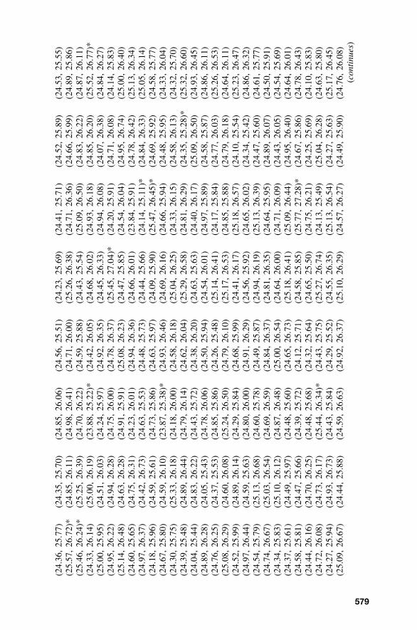
579
(24.
36,
25.7
7)(2
4.35
,25
.70)
(24.
85,
26.0
6)(2
4.56
,25
.51)
(24.
23,
25.6
9)(2
4.41
,25
.71)
(24.
52,
25.8
9)(2
4.53
,25
.55)
(25.
57,
26.7
2)*
(24.
85,
26.1
1)(2
4.98
,26
.41)
(24.
71,
26.0
0)(2
5.26
,26
.38)
(24.
71,
26.3
6)(2
4.66
,25
.99)
(24.
89,
25.8
6)(2
5.46
,26
.24)
*(2
5.25
,26
.39)
(24.
70,
26.2
2)(2
4.59
,25
.88)
(24.
43,
25.5
4)(2
5.09
,26
.50)
(24.
83,
26.2
2)(2
4.87
,26
.11)
(24.
33,
26.1
4)(2
5.00
,26
.19)
(23.
88,
25.2
2)*
(24.
42,
26.0
5)(2
4.68
,26
.02)
(24.
93,
26.1
8)(2
4.85
,26
.20)
(25.
52,
26.7
7)*
(25.
00,
25.9
5)(2
4.51
,26
.03)
(24.
24,
25.9
7)(2
4.92
,26
.35)
(24.
45,
26.3
3)(2
4.94
,26
.08)
(24.
07,
26.3
8)(2
4.84
,26
.27)
(24.
95,
26.2
2)(2
4.94
,26
.28)
(24.
75,
26.0
0)(2
4.78
,26
.37)
(25.
45,
27.0
4)*
(24.
20,
25.9
1)(2
4.71
,26
.08)
(24.
14,
25.8
3)(2
5.14
,26
.48)
(24.
63,
26.2
8)(2
4.91
,25
.91)
(25.
08,
26.2
3)(2
4.47
,25
.85)
(24.
54,
26.0
4)(2
4.95
,26
.74)
(25.
00,
26.4
0)(2
4.60
,25
.65)
(24.
75,
26.3
1)(2
4.23
,26
.01)
(24.
94,
26.3
6)(2
4.66
,26
.01)
(23.
84,
25.9
1)(2
4.78
,26
.42)
(25.
13,
26.3
4)(2
4.97
,26
.37)
(24.
42,
26.7
3)(2
4.63
,25
.53)
(24.
48,
25.7
3)(2
4.44
,25
.66)
(24.
14,
25.1
1)*
(24.
84,
26.3
3)(2
5.05
,26
.14)
(24.
18,
25.9
6)(2
4.59
,25
.61)
(24.
73,
25.8
6)(2
4.63
,25
.97)
(24.
09,
25.9
0)(2
5.47
,26
.45)
*(2
4.69
,25
.92)
(24.
58,
25.7
7)(2
4.67
,25
.80)
(24.
59,
26.1
0)(2
3.87
,25
.38)
*(2
4.93
,26
.46)
(24.
69,
26.1
6)(2
4.66
,25
.94)
(24.
48,
25.9
5)(2
4.33
,26
.04)
(24.
30,
25.7
5)(2
5.33
,26
.18)
(24.
18,
26.0
0)(2
4.58
,26
.18)
(25.
04,
26.2
5)(2
4.33
,26
.15)
(24.
58,
26.1
3)(2
4.32
,25
.70)
(24.
39,
25.4
8)(2
4.89
,26
.44)
(24.
79,
26.1
4)(2
4.62
,26
.04)
(25.
29,
26.5
8)(2
4.81
,26
.29)
(24.
35,
25.2
8)*
(25.
32,
26.6
0)(2
4.04
,25
.44)
(24.
83,
26.2
2)(2
4.43
,25
.72)
(24.
38,
26.2
0)(2
4.63
,25
.63)
(24.
40,
26.1
7)(2
5.09
,26
.50)
(24.
93,
26.4
5)(2
4.89
,26
.28)
(24.
05,
25.4
3)(2
4.78
,26
.06)
(24.
50,
25.9
4)(2
4.54
,26
.01)
(24.
97,
25.8
9)(2
4.58
,25
.87)
(24.
86,
26.1
1)(2
4.76
,26
.25)
(24.
37,
25.5
3)(2
4.85
,25
.86)
(24.
26,
25.4
8)(2
5.14
,26
.41)
(24.
17,
25.8
4)(2
4.77
,26
.03)
(25.
26,
26.5
3)(2
5.08
,26
.29)
(24.
60,
26.0
8)(2
5.24
,26
.50)
(24.
79,
26.1
0)(2
5.17
,26
.53)
(24.
85,
25.8
8)(2
4.79
,26
.18)
(24.
64,
26.1
1)(2
4.52
,25
.99)
(24.
89,
26.1
4)(2
4.29
,25
.84)
(24.
68,
25.9
9)(2
4.41
,26
.17)
(25.
18,
26.5
7)(2
4.10
,25
.54)
(25.
23,
26.4
7)(2
4.97
,26
.44)
(24.
59,
25.6
3)(2
4.80
,26
.00)
(24.
91,
26.2
9)(2
4.56
,25
.92)
(24.
65,
26.0
2)(2
4.34
,25
.42)
(24.
86,
26.3
2)(2
4.54
,25
.79)
(25.
13,
26.6
8)(2
4.60
,25
.78)
(24.
49,
25.8
7)(2
4.94
,26
.19)
(25.
13,
26.3
9)(2
4.47
,25
.60)
(24.
61,
25.7
7)(2
4.74
,26
.67)
(25.
03,
26.5
4)(2
4.69
,26
.59)
(24.
84,
26.3
7)(2
4.81
,26
.35)
(24.
64,
25.9
5)(2
4.89
,26
.07)
(24.
50,
25.9
1)(2
4.34
,25
.83)
(25.
10,
26.1
2)(2
4.87
,26
.48)
(25.
00,
26.5
4)(2
4.64
,26
.00)
(24.
71,
26.0
9)(2
4.43
,26
.05)
(24.
54,
25.6
9)(2
4.37
,25
.61)
(24.
49,
25.9
7)(2
4.48
,25
.60)
(24.
65,
26.7
3)(2
5.18
,26
.41)
(25.
09,
26.4
4)(2
4.95
,26
.40)
(24.
64,
26.0
1)(2
4.58
,25
.81)
(24.
47,
25.6
6)(2
4.39
,25
.72)
(24.
12,
25.7
1)(2
4.58
,25
.85)
(25.
77,
27.2
8)*
(24.
67,
25.8
6)(2
4.78
,26
.43)
(24.
44,
26.1
6)(2
4.70
,26
.25)
(24.
48,
25.6
8)(2
4.32
,25
.64)
(24.
65,
25.5
0)(2
4.75
,26
.21)
(24.
25,
25.6
9)(2
4.10
,25
.83)
(24.
72,
26.0
8)(2
4.73
,26
.17)
(25.
44,
26.3
4)*
(24.
43,
25.7
5)(2
5.27
,26
.74)
(24.
13,
25.4
9)(2
5.04
,26
.28)
(24.
63,
25.8
0)(2
4.27
,25
.94)
(24.
93,
26.7
3)(2
4.43
,25
.84)
(24.
29,
25.5
2)(2
4.55
,26
.35)
(25.
13,
26.5
4)(2
4.27
,25
.63)
(25.
17,
26.4
5)(2
5.09
,26
.67)
(24.
44,
25.8
8)(2
4.59
,26
.63)
(24.
92,
26.3
7)(2
5.10
,26
.29)
(24.
57,
26.2
7)(2
4.49
,25
.90)
(24.
76,
26.0
8)(c
onti
nues
)
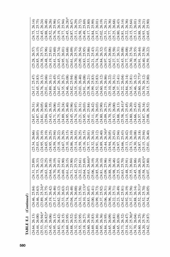
580
TA
BL
EE
.1(C
ontin
ued
)
(24.
64,
26.1
3)(2
4.46
,25
.84)
(24.
31,
25.8
9)(2
5.34
,26
.66)
(24.
87,
26.3
1)(2
4.17
,25
.47)
(25.
28,
26.5
7)(2
4.75
,26
.14)
(24.
44,
26.0
0)(2
4.46
,25
.63)
(24.
75,
26.3
3)(2
5.03
,26
.03)
(24.
87,
26.3
6)(2
4.45
,25
.83)
(24.
85,
26.1
5)(2
4.12
,25
.75)
(25.
53,
26.9
4)*
(23.
89,
25.2
4)*
(24.
78,
26.1
2)(2
4.95
,26
.19)
(24.
81,
26.0
5)(2
4.76
,26
.13)
(24.
38,
25.7
7)(2
4.45
,26
.24)
(25.
72,
26.8
2)*
(24.
36,
25.7
5)(2
4.63
,26
.25)
(24.
65,
26.1
9)(2
5.04
,25
.80)
(25.
01,
26.6
6)(2
4.48
,25
.96)
(24.
88,
26.4
8)(2
4.45
,26
.06)
(25.
19,
26.4
2)(2
4.64
,26
.18)
(24.
95,
26.2
5)(2
4.43
,26
.35)
(24.
89,
26.1
1)(2
4.19
,25
.61)
(24.
52,
26.2
6)(2
4.95
,26
.13)
(25.
17,
26.4
6)(2
4.70
,26
.19)
(24.
59,
25.9
4)(2
4.71
,26
.06)
(24.
84,
26.4
5)(2
4.41
,25
.60)
(24.
76,
25.9
6)(2
4.83
,26
.42)
(24.
62,
26.1
2)(2
4.39
,25
.41)
(25.
18,
26.2
2)(2
4.75
,26
.33)
(24.
47,
26.3
7)(2
4.45
,25
.74)
(25.
19,
26.3
7)(2
4.75
,26
.15)
(25.
33,
26.6
3)(2
4.69
,25
.90)
(24.
67,
26.2
9)(2
4.89
,26
.24)
(24.
35,
26.2
7)(2
4.95
,26
.01)
(24.
77,
25.9
4)(2
4.69
,25
.95)
(24.
74,
26.2
2)(2
4.61
,26
.15)
(25.
10,
26.1
5)(2
4.95
,26
.40)
(24.
46,
26.0
8)(2
5.07
,26
.68)
(25.
45,
26.2
8)*
(24.
88,
26.5
2)(2
5.04
,26
.48)
(24.
71,
25.9
0)(2
4.86
,26
.18)
(24.
45,
25.9
6)(2
4.82
,25
.94)
(24.
61,
26.0
9)(2
4.87
,26
.67)
(24.
32,
25.9
3)(2
4.74
,26
.00)
(24.
42,
25.7
2)(2
5.14
,26
.53)
(24.
74,
25.9
7)(2
4.35
,26
.08)
(24.
70,
25.7
5)(2
5.11
,26
.29)
(24.
55,
25.9
5)(2
4.33
,25
.56)
(24.
22,
25.6
1)(2
4.59
,26
.25)
(25.
21,
26.3
1)(2
5.03
,26
.40)
(25.
09,
26.5
4)(2
4.58
,25
.72)
(25.
18,
26.2
7)(2
4.10
,25
.13)
*(2
4.64
,25
.69)
(25.
16,
26.1
5)(2
4.95
,26
.03)
(24.
91,
26.0
8)(2
4.83
,25
.95)
(24.
49,
25.6
9)(2
4.60
,26
.16)
(24.
83,
26.0
7)(2
5.63
,26
.64)
*(2
4.77
,26
.01)
(24.
41,
25.8
4)(2
5.38
,26
.21)
(24.
53,
25.8
6)(2
4.17
,25
.80)
(24.
69,
25.8
3)(2
5.00
,26
.41)
(25.
06,
26.1
9)(2
4.32
,26
.34)
(25.
11,
26.4
2)(2
3.99
,25
.83)
(24.
21,
25.4
3)(2
4.84
,25
.99)
(24.
89,
26.1
6)(2
4.99
,26
.73)
(24.
85,
26.2
4)(2
4.91
,26
.12)
(24.
79,
26.0
3)(2
4.52
,25
.83)
(24.
74,
26.2
1)(2
4.37
,26
.01)
(24.
95,
26.3
6)(2
4.37
,25
.92)
(24.
81,
26.1
0)(2
4.89
,26
.40)
(24.
80,
25.9
0)(2
4.60
,26
.12)
(24.
84,
26.3
2)(2
5.02
,26
.19)
(24.
84,
25.9
5)(2
5.06
,26
.51)
(25.
09,
25.9
6)(2
5.44
,26
.34)
*(2
5.09
,26
.27)
(25.
19,
26.8
6)(2
4.97
,26
.15)
(25.
31,
26.2
1)(2
4.65
,26
.09)
(24.
96,
26.3
6)(2
4.88
,26
.18)
(24.
94,
26.0
5)(2
4.70
,25
.78)
(25.
10,
26.2
2)(2
4.63
,26
.06)
(24.
77,
26.3
6)(2
4.86
,26
.81)
(24.
22,
25.7
1)(2
4.98
,26
.46)
(24.
29,
25.4
3)(2
4.53
,26
.00)
(24.
58,
26.3
1)(2
4.27
,25
.58)
(25.
25,
26.6
8)(2
4.65
,26
.09)
(25.
23,
26.4
9)(2
5.25
,26
.83)
(24.
97,
25.9
4)(2
4.88
,26
.13)
(24.
37,
25.4
1)(2
5.37
,26
.31)
(24.
80,
26.4
3)(2
4.73
,26
.32)
(24.
42,
25.8
1)(2
4.63
,25
.70)
(24.
66,
25.4
3)(2
5.58
,26
.41)
*(2
4.22
,26
.04)
(24.
43,
26.0
8)(2
4.81
,26
.14)
(25.
14,
26.4
7)(2
4.92
,26
.19)
(24.
48,
25.9
1)(2
5.13
,26
.42)
(24.
15,
25.4
5)(2
4.84
,26
.14)
(24.
77,
26.0
8)(2
5.22
,26
.36)
(24.
27,
25.3
6)*
(24.
37,
25.5
6)(2
5.35
,26
.84)
(24.
73,
26.1
0)(2
4.80
,26
.20)
(24.
35,
25.8
1)(2
4.30
,25
.74)
(24.
15,
25.6
4)(2
4.70
,26
.04)
(24.
88,
26.1
4)(2
4.45
,25
.86)
(24.
30,
26.0
8)(2
4.66
,25
.43)
(24.
46,
26.1
2)(2
4.38
,25
.55)
(25.
13,
26.0
1)(2
4.60
,26
.25)
(25.
52,
26.5
1)*
(24.
68,
26.2
0)(2
4.87
,26
.18)
(24.
57,
25.6
5)(2
5.60
,26
.77)
*(2
4.91
,26
.44)
(24.
88,
26.1
4)(2
4.20
,25
.79)
(24.
52,
25.7
0)(2
5.58
,26
.83)
*(2
5.15
,25
.94)
(24.
87,
26.3
4)(2
4.70
,26
.12)
(24.
40,
25.5
6)(2
4.93
,26
.21)
(24.
62,
25.8
7)(2
4.54
,26
.05)
(24.
07,
25.8
0)(2
5.01
,26
.40)
(25.
08,
26.5
2)(2
4.15
,25
.80)
(24.
59,
26.2
2)(2
4.65
,25
.90)
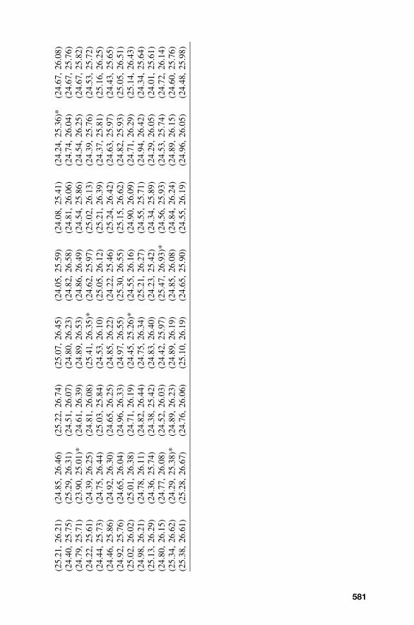
581
(25.
21,
26.2
1)(2
4.85
,26
.46)
(25.
22,
26.7
4)(2
5.07
,26
.45)
(24.
05,
25.5
9)(2
4.08
,25
.41)
(24.
24,
25.3
6)*
(24.
67,
26.0
8)(2
4.40
,25
.75)
(25.
29,
26.3
1)(2
4.51
,26
.07)
(24.
80,
26.2
3)(2
4.82
,26
.58)
(24.
81,
26.0
6)(2
4.74
,26
.04)
(24.
67,
25.7
6)(2
4.79
,25
.71)
(23.
90,
25.0
1)*
(24.
61,
26.3
9)(2
4.89
,26
.53)
(24.
86,
26.4
9)(2
4.54
,25
.86)
(24.
54,
26.2
5)(2
4.67
,25
.82)
(24.
22,
25.6
1)(2
4.39
,26
.25)
(24.
81,
26.0
8)(2
5.41
,26
.35)
*(2
4.62
,25
.97)
(25.
02,
26.1
3)(2
4.39
,25
.76)
(24.
53,
25.7
2)(2
4.44
,25
.73)
(24.
75,
26.4
4)(2
5.03
,25
.84)
(24.
53,
26.1
0)(2
5.05
,26
.12)
(25.
21,
26.3
9)(2
4.37
,25
.81)
(25.
16,
26.2
5)(2
4.46
,25
.86)
(24.
92,
26.3
0)(2
4.65
,26
.25)
(24.
85,
26.2
2)(2
4.22
,25
.46)
(25.
24,
26.4
2)(2
4.63
,25
.97)
(24.
43,
25.6
5)(2
4.92
,25
.76)
(24.
65,
26.0
4)(2
4.96
,26
.33)
(24.
97,
26.5
5)(2
5.30
,26
.55)
(25.
15,
26.6
2)(2
4.82
,25
.93)
(25.
05,
26.5
1)(2
5.02
,26
.02)
(25.
01,
26.3
8)(2
4.71
,26
.19)
(24.
45,
25.2
6)*
(24.
55,
26.1
6)(2
4.90
,26
.09)
(24.
71,
26.2
9)(2
5.14
,26
.43)
(24.
98,
26.2
1)(2
4.78
,26
.11)
(24.
82,
26.4
4)(2
4.75
,26
.34)
(25.
21,
26.2
7)(2
4.55
,25
.71)
(24.
94,
26.4
2)(2
4.34
,25
.64)
(25.
13,
26.2
9)(2
4.36
,25
.74)
(24.
38,
25.4
2)(2
4.83
,26
.40)
(24.
23,
25.4
2)(2
4.34
,25
.89)
(24.
29,
26.0
5)(2
4.01
,25
.61)
(24.
80,
26.1
5)(2
4.77
,26
.08)
(24.
52,
26.0
3)(2
4.42
,25
.97)
(25.
47,
26.9
3)*
(24.
56,
25.9
3)(2
4.53
,25
.74)
(24.
72,
26.1
4)(2
5.34
,26
.62)
(24.
29,
25.3
8)*
(24.
89,
26.2
3)(2
4.89
,26
.19)
(24.
85,
26.0
8)(2
4.84
,26
.24)
(24.
89,
26.1
5)(2
4.60
,25
.76)
(25.
38,
26.6
1)(2
5.28
,26
.67)
(24.
76,
26.0
6)(2
5.10
,26
.19)
(24.
65,
25.9
0)(2
4.55
,26
.19)
(24.
96,
26.0
5)(2
4.48
,25
.98)
582
APPENDIX F
MAP PROJECTIONCOORDINATE SYSTEMS
F.1 INTRODUCTION
Most local surveyors are well served by using map projections such as thestate plane coordinate system. These two-dimensional grid systems allow sur-veyors to perform accurate computations over large regions of land usingplane surveying computations. They are the basis for the adjustments dis-cussed in Chapters 14 through 16.
Map projections provide a one-to-one mathematical relationship withpoints on the ellipsoid and those on the mapping surface. There are an infinitenumber of map projections. Most map projections are defined by a series ofmathematical transformations used to convert a point’s geodetic coordinatesof latitude, �, and longitude, �, to xy grid coordinates. Some map projectionspreserve the shape of objects (conformal); others, areas, directions, or dis-tances of lines. However, since Earth is ellipsoidal in shape and a mappingsurface is a plane, all map projections introduce some form of distortion toobservations. For example, distances and areas are distorted in a conformalmap projection.
To reduce the size of these distortions, the developable surface is oftenmade secant to the ellipsoid and the width of the mapping zone is limited indistance. For instance, when the National Geodetic Survey originally designedthe state plane coordinate system during the 1930s, the zone widths werelimited to 158 miles so that precision between the ellipsoid distance and thegrid distance was no worse than 1�10,000. Since most surveys at that timewere only accurate to a precision of 1�5000, this was an acceptable limit.However, with today’s modern instruments, observations must be reducedproperly if survey accuracy is to be preserved in a map projection system.
Adjustment Computations: Spatial Data Analysis, Fourth Edition. C. D. Ghilani and P. R. Wolf© 2006 John Wiley & Sons, Inc. ISBN: 978-0-471-69728-2
F.2 MATHEMATICS OF THE LAMBERT CONFORMAL CONIC MAP PROJECTION 583
All map projections are based on the ellipsoid selected, such as the Geo-detic Reference System of 1980 (GRS 80), and defining zone parameters.Typically, the zone parameters define the grid origin (�0, �0); the secant linesof the projection, also known as standard parallels, or scale factor, k0, at thecentral meridian, �0; and the offset distances (E0, Nb) from the grid origin.Once defined, each map projection has a series of zone constants that arecomputed using the defining zone parameters. These zone constants are com-puted only once for each projection. Once the zone constants are computed,the direct and inverse problems can be carried out for any point in the system.The direct problem takes the geodetic coordinates of a point and transformsthem into grid coordinates, and the inverse problem takes the grid coordinatesof a point and transforms them into geodetic coordinates.
The two primary map projection systems used in the United States are theLambert Conformal Conic for states that have a long east–west extent andthe Transverse Mercator for states that have a long north–south extent. Bothmap projections are conformal; that is, they preserve angles in infinitesimallysmall regions about a point. This property is advantageous to surveyors sinceangles are minimally distorted when using a conformal projection. On theother hand, as shown in Figure F.1, horizontal distances observed must bereduced to the mapping surface to eliminate the distortions of the projection.However, if these reductions are performed properly, the resulting plane com-putations are as accurate as geodetic computations such as those shown inChapter 23. In this appendix we look at the mathematics of the LambertConformal Conic and Transverse Mercator map projections and demonstrateproper methods in reducing observations before an adjustment.
F.2 MATHEMATICS OF THE LAMBERT CONFORMALCONIC MAP PROJECTION
The Lambert Conformal Conic map projection was introduced by JohannLambert in 1772. As its name implies, this map projection uses a cone as itsdevelopable surface. The projection is conformal, so angles are preserved butdistances are distorted. A Lambert Conformal Conic map projection is definedby two ellipsoidal parameters,1 grid origin (�0, �0); latitude of the north stan-dard parallel, �N, and south standard parallel,2 �S; false easting, E0; and falsenorthing, Nb.
1 Typically, an ellipsoid is defined by the length of its semimajor axis, a, and its flattening factor,ƒ. The first eccentricity is computed as e � The GRS 80 ellipsoid has defining2�2ƒ � ƒ .parameters of a � 6,378,137.0 m and ƒ � 1 /298.2572221008.2 The standard parallels are the latitudes of the north and south secant lines for the cone on theellipsoid.
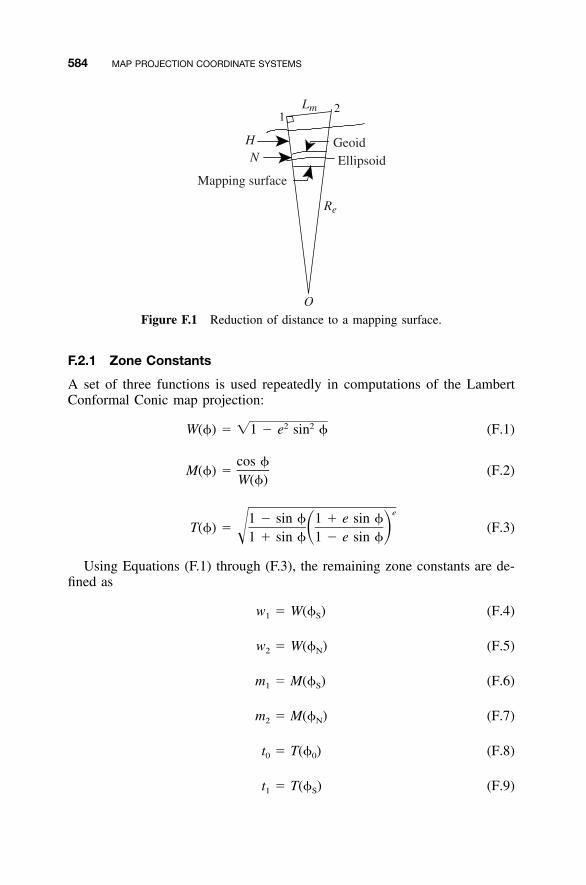
584 MAP PROJECTION COORDINATE SYSTEMS
Mapping surface
GeoidEllipsoid
HN
O
Re
Lm
Figure F.1 Reduction of distance to a mapping surface.
F.2.1 Zone Constants
A set of three functions is used repeatedly in computations of the LambertConformal Conic map projection:
2 2W(�) � �1 � e sin � (F.1)
cos �M(�) � (F.2)
W(�)
e1 � sin � 1 � e sin �T(�) � (F.3)� ��1 � sin � 1 � e sin �
Using Equations (F.1) through (F.3), the remaining zone constants are de-fined as
w � W(� ) (F.4)1 S
w � W(� ) (F.5)2 N
m � M(� ) (F.6)1 S
m � M(� ) (F.7)2 N
t � T(� ) (F.8)0 0
t � T(� ) (F.9)1 S
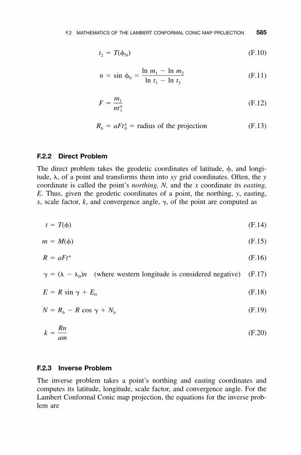
F.2 MATHEMATICS OF THE LAMBERT CONFORMAL CONIC MAP PROJECTION 585
t � T(� ) (F.10)2 N
ln m � ln m1 2n � sin � � (F.11)0 ln t � ln t1 2
m1F � (F.12)nnt1
nR � aFt � radius of the projection (F.13)b 0
F.2.2 Direct Problem
The direct problem takes the geodetic coordinates of latitude, �, and longi-tude, �, of a point and transforms them into xy grid coordinates. Often, the ycoordinate is called the point’s northing, N, and the x coordinate its easting,E. Thus, given the geodetic coordinates of a point, the northing, y, easting,x, scale factor, k, and convergence angle, �, of the point are computed as
t � T(�) (F.14)
m � M(�) (F.15)
nR � aFt (F.16)
� � (� � � )n (where western longitude is considered negative) (F.17)0
E � R sin � � E (F.18)0
N � R � R cos � � N (F.19)b b
Rnk � (F.20)
am
F.2.3 Inverse Problem
The inverse problem takes a point’s northing and easting coordinates andcomputes its latitude, longitude, scale factor, and convergence angle. For theLambert Conformal Conic map projection, the equations for the inverse prob-lem are
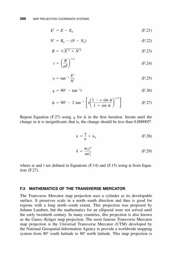
586 MAP PROJECTION COORDINATE SYSTEMS
E� � E � E (F.21)0
N� � R � (N � N ) (F.22)b b
2 2R � �E� � N� (F.23)
1 / nRt � (F.24)� �aF
E��1� � tan (F.25)
N�
�1� � 90� � tan t (F.26)
e / 21 � e sin ��1� � 90� � 2 tan t (F.27)� � � �1 � sin �
Repeat Equation (F.27) using � for � in the first iteration. Iterate until thechange in � is insignificant; that is, the change should be less than 0.000005�.
�� � � � (F.28)0n
nm t1k � (F.29)nmt1
where m and t are defined in Equations (F.14) and (F.15) using � from Equa-tion (F.27).
F.3 MATHEMATICS OF THE TRANSVERSE MERCATOR
The Transverse Mercator map projection uses a cylinder as its developablesurface. It preserves scale in a north–south direction and thus is good forregions with a long north–south extent. This projection was proposed byJohann Lambert, but the mathematics for an ellipsoid were not solved untilthe early twentieth century. In many countries, this projection is also knownas the Gauss–Kruger map projection. The most famous Transverse Mercatormap projection is the Universal Transverse Mercator (UTM) developed bythe National Geospatial-Information Agency to provide a worldwide mappingsystem from 80� south latitude to 80� north latitude. This map projection is
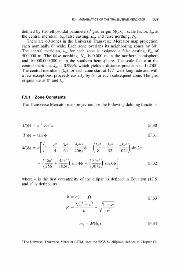
F.3 MATHEMATICS OF THE TRANSVERSE MERCATOR 587
defined by two ellipsoidal parameters,3 grid origin (�0,�0), scale factor, k0, atthe central meridian, �0, false easting, E0, and false northing, Nb.
There are 60 zones in the Universal Transverse Mercator map projection,each nominally 6� wide. Each zone overlaps its neighboring zones by 30�.The central meridian, �0, for each zone is assigned a false easting, E0, of500,000 m. The false northing, Nb, is 0.000 m in the northern hemisphereand 10,000,000.000 m in the southern hemisphere. The scale factor at thecentral meridian, k0, is 0.9996, which yields a distance precision of 1�2500.The central meridians (�0) for each zone start at 177� west longitude and witha few exceptions, proceeds easterly by 6� for each subsequent zone. The gridorigins are at 0� and �0.
F.3.1 Zone Constants
The Transverse Mercator map projection use the following defining functions:
2 2C(�) � e� cos � (F.30)
T(�) � tan � (F.31)
2 4 6 2 4 6e 3e 5e 3e 3e 45eM(�) � a 1 � � � � � � � sin 2��� � � �4 64 256 8 32 1024
4 6 615e 45e 35e� � sin 4� � sin 6� (F.32)� � � � �256 1024 3072
where e is the first eccentricity of the ellipse as defined in Equation (17.5)and e� is defined as
b � a(1 � ƒ) (F.33)2 2 2�a � b 1 � e
e� � � 2�b e
m � M(� ) (F.34)0 0
3 The Universal Transverse Mercator (UTM) uses the WGS 84 ellipsoid, defined in Chapter 17.
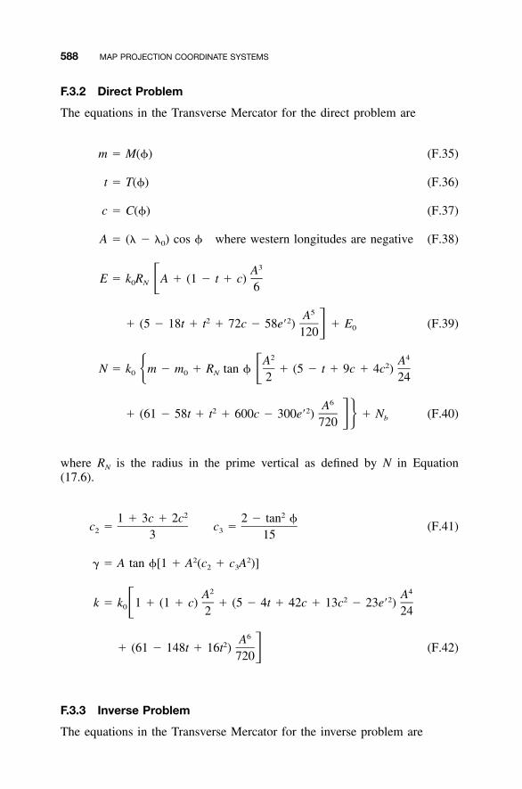
588 MAP PROJECTION COORDINATE SYSTEMS
F.3.2 Direct Problem
The equations in the Transverse Mercator for the direct problem are
m � M(�) (F.35)
t � T(�) (F.36)
c � C(�) (F.37)
A � (� � � ) cos � where western longitudes are negative (F.38)0
3AE � k R A � (1 � t � c)�0 N 6
5A2 2� (5 � 18t � t � 72c � 58e� ) � E (F.39)� 0120
2 4A A2N � k m � m � R tan � � (5 � t � 9c � 4c )� �0 0 N 2 24
6A2 2� (61 � 58t � t � 600c � 300e� ) � N (F.40)�� b720
where RN is the radius in the prime vertical as defined by N in Equation(17.6).
2 21 � 3c � 2c 2 � tan �c � c � (F.41)2 33 15
2 2� � A tan �[1 � A (c � c A )]2 3
2 4A A2 2k � k 1 � (1 � c) � (5 � 4t � 42c � 13c � 23e� )�0 2 24
6A2� (61 � 148t � 16t ) (F.42)�720
F.3.3 Inverse Problem
The equations in the Transverse Mercator for the inverse problem are
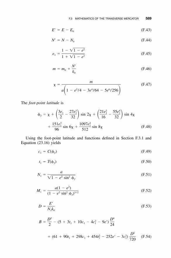
F.3 MATHEMATICS OF THE TRANSVERSE MERCATOR 589
E� � E � E (F.43)0
N� � N � N (F.44)b
21 � �1 � ee � (F.45)1 21 � �1 � e
N�m � m � (F.46)0 k0
m� � (F.47)
2 4 6a 1 � e /4 � 3e /64 � 5e /256� �The foot-point latitude is
3 2 43e 27e 21e 55e1 1 1 1� � � � � sin 2� � � sin 4�� � � �ƒ 2 32 16 323 4151e 1097e1 1� sin 6� � sin 8� (F.48)
96 512
Using the foot-point latitude and functions defined in Section F.3.1 andEquation (23.16) yields
c � C(� ) (F.49)1 ƒ
t � T(� ) (F.50)1 ƒ
aN � (F.51)1 2 2�1 � e sin �ƒ
2a(1 � e )M � (F.52)1 2 2 3 / 2(1 � e sin � )ƒ
E�D � (F.53)
N k1 0
2 4D D2B � � (5 � 3t � 10c � 4c � 9e�)1 1 12 24
6D2 2� (61 � 90t � 298c � 454t � 252e� � 3c ) (F.54)1 1 1 1 720
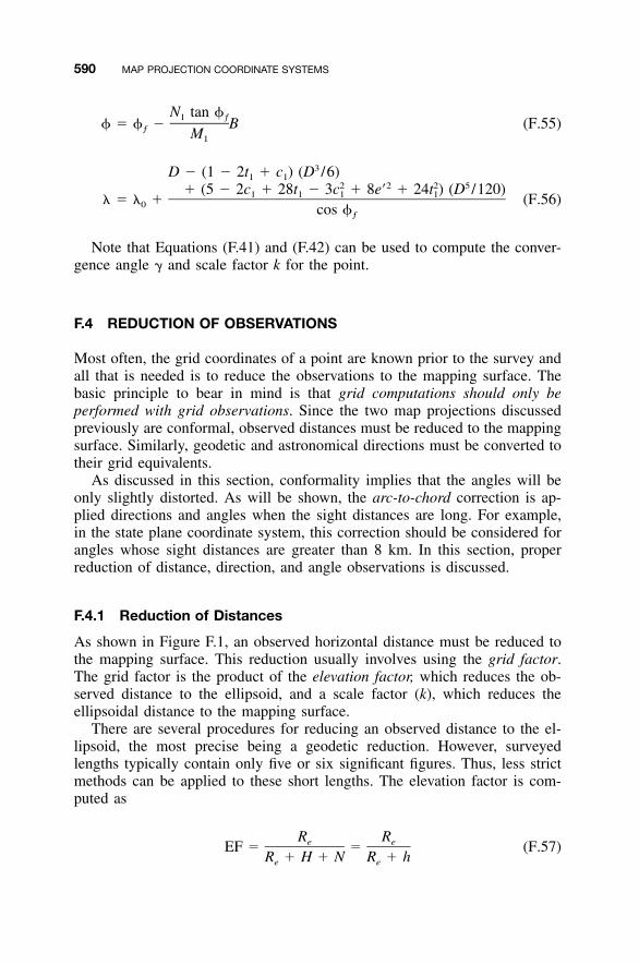
590 MAP PROJECTION COORDINATE SYSTEMS
N tan �1 ƒ� � � � B (F.55)ƒ M1
3D � (1 � 2t � c ) (D /6)1 12 2 2 5� (5 � 2c � 28t � 3c � 8e� � 24t ) (D /120)1 1 1 1� � � � (F.56)0 cos �ƒ
Note that Equations (F.41) and (F.42) can be used to compute the conver-gence angle � and scale factor k for the point.
F.4 REDUCTION OF OBSERVATIONS
Most often, the grid coordinates of a point are known prior to the survey andall that is needed is to reduce the observations to the mapping surface. Thebasic principle to bear in mind is that grid computations should only beperformed with grid observations. Since the two map projections discussedpreviously are conformal, observed distances must be reduced to the mappingsurface. Similarly, geodetic and astronomical directions must be converted totheir grid equivalents.
As discussed in this section, conformality implies that the angles will beonly slightly distorted. As will be shown, the arc-to-chord correction is ap-plied directions and angles when the sight distances are long. For example,in the state plane coordinate system, this correction should be considered forangles whose sight distances are greater than 8 km. In this section, properreduction of distance, direction, and angle observations is discussed.
F.4.1 Reduction of Distances
As shown in Figure F.1, an observed horizontal distance must be reduced tothe mapping surface. This reduction usually involves using the grid factor.The grid factor is the product of the elevation factor, which reduces the ob-served distance to the ellipsoid, and a scale factor (k), which reduces theellipsoidal distance to the mapping surface.
There are several procedures for reducing an observed distance to the el-lipsoid, the most precise being a geodetic reduction. However, surveyedlengths typically contain only five or six significant figures. Thus, less strictmethods can be applied to these short lengths. The elevation factor is com-puted as
R Re eEF � � (F.57)R � H � N R � he e
F.4 REDUCTION OF OBSERVATIONS 591
In Equation (F.57), Re is the radius of the Earth, H the orthometric height,N the geoidal height, and h the geodetic height. All of these parameters aredetermined at the observation station. The relationship between the geodeticheight, h, and orthometric height, H, is
h � H � N (F.58)
In Equation (F.57), the radius in the azimuth of the line should be usedfor Re. Again since surveyors observe short distances typically, an averageradius of the Earth of 6,371,000 m can be used in computing EF. Theseapproximations are demonstrated in Example F.1.
In a map projection system, the scale factor computed using Equation(F.20), (F.29), or (F.42) is for a point. Generally, the scale factor changescontinuously along the length of the line. Thus, a weighted mean using twoendpoints of the line (k1 and k2) and midpoint (km) is a logical choice forcomputing a single scale factor for a line. It can be computed as
k � 4k � k1 m 2k � (F.59)avg 6
However, as with the elevation factor, this type of precision is seldom neededfor the typical survey. Thus, the mean of the two endpoint scale factors isgenerally of sufficient accuracy for most surveys. In fact, it is not uncommonto use a single mean scale factor for an entire project.
The grid factor, GF, for the line is a product of the elevation factor, EF,and a scale factor, kavg, and is computed as
GF � k � EF (F.60)avg
Thus, a reduced grid distance, Lgrid, is the product of the horizontal distance,Lm, and the grid factor, GF, and is computed as
L � L � GF (F.61)grid m
Example F.1 A distance of 536.07 ft is observed from station 1. The scalefactors at observing, midpoint, and sighted stations are 0.9999587785,0.9999587556, and 0.9999587328, respectively. The orthometric height at ob-serving station is 1236.45 ft. Its geoidal height is �30.12 m and the radiusin the azimuth is 6,366,977.077 m. Determine the length of the line on themapping surface.
592 MAP PROJECTION COORDINATE SYSTEMS
SOLUTION This solution will compare the grid factor computed using dif-ferent radii in Equation (F.57) and different scale factors in Equation (F.60).Using the more precise methods, the grid factor is computed as follows. Theorthometric height of the observing station in meters is
12H � 1236.45 ft � � 376.871 m
39.37
Using the radius in the azimuth of the line and Equation (F.57), the elevationfactor, EF, is
6,366,977.077EF � � 0.999945542
6,366,977.077 � 376.871 � 30.12
From Equation (F.59), the scale factor for the lines is
0.9999587785 � 4(0.9999587556) � 0.9999587328k � � 0.999958756avg 6
From Equation (F.60), the grid factor for the line is
GF � 0.999945542 � 0.999958756 � 0.99990430
Finally, the grid distance for this line is
L � 0.99990430 � 536.07 ft � 536.02 ftgrid
Doing the problem again, this time with the mean radius of the Earth and theaverage of the two endpoint scale factors, yields
6,371,000EF � � 0.999945577
6,371,000 � 376.871 � 30.12
0.9999587785 � 0.9999587328k � � 0.999958756avg 2
GF � 0.999945577 � 0.999958756 � 0.99990433
L � 0.99990433 � 536.07 ft � 536.02 ftgrid
Note that using the approximate radius of the Earth and the average scalefactor for the endpoints of the line resulted in the same solution as the moreprecise computations. This is because the length of the distance observed has
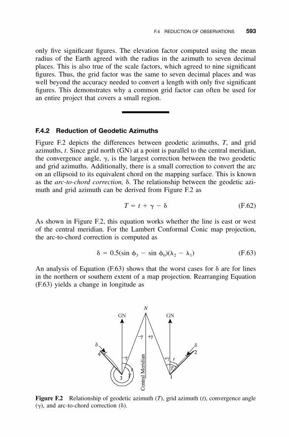
F.4 REDUCTION OF OBSERVATIONS 593
GN GN
Figure F.2 Relationship of geodetic azimuth (T), grid azimuth (t), convergence angle(�), and arc-to-chord correction (�).
only five significant figures. The elevation factor computed using the meanradius of the Earth agreed with the radius in the azimuth to seven decimalplaces. This is also true of the scale factors, which agreed to nine significantfigures. Thus, the grid factor was the same to seven decimal places and waswell beyond the accuracy needed to convert a length with only five significantfigures. This demonstrates why a common grid factor can often be used foran entire project that covers a small region.
F.4.2 Reduction of Geodetic Azimuths
Figure F.2 depicts the differences between geodetic azimuths, T, and gridazimuths, t. Since grid north (GN) at a point is parallel to the central meridian,the convergence angle, �, is the largest correction between the two geodeticand grid azimuths. Additionally, there is a small correction to convert the arcon an ellipsoid to its equivalent chord on the mapping surface. This is knownas the arc-to-chord correction, �. The relationship between the geodetic azi-muth and grid azimuth can be derived from Figure F.2 as
T � t � � � � (F.62)
As shown in Figure F.2, this equation works whether the line is east or westof the central meridian. For the Lambert Conformal Conic map projection,the arc-to-chord correction is computed as
� � 0.5(sin � � sin � )(� � � ) (F.63)3 0 2 1
An analysis of Equation (F.63) shows that the worst cases for � are for linesin the northern or southern extent of a map projection. Rearranging Equation(F.63) yields a change in longitude as
594 MAP PROJECTION COORDINATE SYSTEMS
2�� � � � �� � (F.64)2 1 sin � � sin �3 0
As an example, assume that �3 is 42�30�. Further assume that the project isin the Pennsylvania North Zone, which has a sin �0 of 0.661539733812. If �is to be kept below 0.5�, the maximum line in arc-seconds of longitude canbe
2(0.5�)�� � � 71.2�
sin 42�30� � 0.661539733812
At latitude 42�30�, this corresponds to a line of length of about 5334 ft, or1.6 km. Few surveyors in northeastern Pennsylvania could find a line of thislength to observe. Thus, the arc-to-chord correction is generally ignored inreductions, and Equation (F.62) can be simplified as
T � t � � (F.65)
595
APPENDIX G
COMPANION CD
G.1 INTRODUCTION
The companion CD that accompanies this book has several programs andinstructional worksheets to aid students in the learning process. The CD con-tains the software ADJUST, MATRIX, and STATS that were available withthe preceding edition of the book. Mathcad worksheets have been added tothis edition. For those who do not own Mathcad, html files of these work-sheets have been created. These files can be viewed using your computer’sWeb browser.
All of the software contained on the CD is Windows-based and will runon most Windows-based computers. The CD has an autoinstall program thatwill allow you to select the packages for installation. Before installing thesoftware on the companion CD, it is important to remove any versions of thesoftware already on your computer. This can be done using the Windows‘‘Add/Remove programs’’ feature in your Windows control panel. Refer tothe Windows help system if you are not familiar with this feature in Windows.If the program fails to autoload on your machine, browse the CD and run the‘‘setup.exe’’ file from the root directory of the CD. Each program containedon the CD has different system memory requirements; although all will runin less than 2 megabytes of memory.
This software is ‘‘freeware’’ and as such can be freely distributed with thisbook. However, it is not intended for commercial use, is not guaranteed tobe computationally correct, and is not supported in any manner. It is simplyprovided to aid your understanding of the topics contained in the book. Asthe software is updated, it will be posted at http:/ /surveying.wb.psu.edu underthe FREE GOODIES button. You should visit this site occasionally to down-load newer versions of the software on this CD.
Adjustment Computations: Spatial Data Analysis, Fourth Edition. C. D. Ghilani and P. R. Wolf© 2006 John Wiley & Sons, Inc. ISBN: 978-0-471-69728-2
596 COMPANION CD
G.2 FILE FORMATS AND MEMORY MATTERS
Most options in the software packages ADJUST, MATRIX, and STATS useformatted ASCII text files for data entry. Each package is equipped with aneditor that allows the user to create these files. The help file for each softwareprogram describes the format of the data files. It is also possible to createdata files using other ASCII editors, such as Notepad. The file-reading rou-tines contained in ADJUST, MATRIX, and STATS can use either commas,spaces, or tabs as delimiters between fields. It is therefore important to avoidcommas in large numbers such as coordinates, since the software will readeach part of the number individually. For example, a coordinate of675,301.213 will be read as the numbers 675 and 301.213 since the commais a delimiter. The use of the TAB delimiter is especially useful in Matrixsince this allows you to ‘‘cut and paste’’ values from spreadsheets such asExcel and Quattro Pro.
Starting with Version 4.0, ADJUST has used dynamic memory allocation.That is, data storage structures are not created until their sizes have beendefined at runtime. Therefore, users familiar with earlier versions of ADJUSTshould be aware that some file formats have changed to accommodate thisprogramming change. As a user, this feature means that the size limits of datatypes in various options in the software are now limited only by your com-puter’s memory resources. Thus, much larger problems can be handled withthis software.
G.3 SOFTWARE
G.3.1 ADJUST
ADJUST is the main computational program on the companion CD. It con-tains programs that either support computation of problems in the book orperform the computations. Several least squares programs and several sup-porting options are contained in ADJUST. A list of the least squares optionsand supporting software is provided in Table G.1. For example, the traverseoption in ADJUST can compute initial approximations for unknown stationsin a horizontal plane survey. The ‘‘Horizontal Data’’ under ‘‘Least SquaresAdjustments’’ can perform the least squares adjustment of the data as dis-cussed in Chapters 14 through 16.
File formats required by this software are discussed in the accompanyingHelp file. At installation, sample data files of some of the numerical examplespresented in this book can be loaded onto your computer. By default, thesefiles are loaded in the ‘‘Adjustment Computations’’ subdirectory of the ‘‘MYDOCUMENTS’’ directory. Along with the Help file, these sample data filescan be viewed and compared with the accompanying example problem in thebook to assist you in creating your own files.
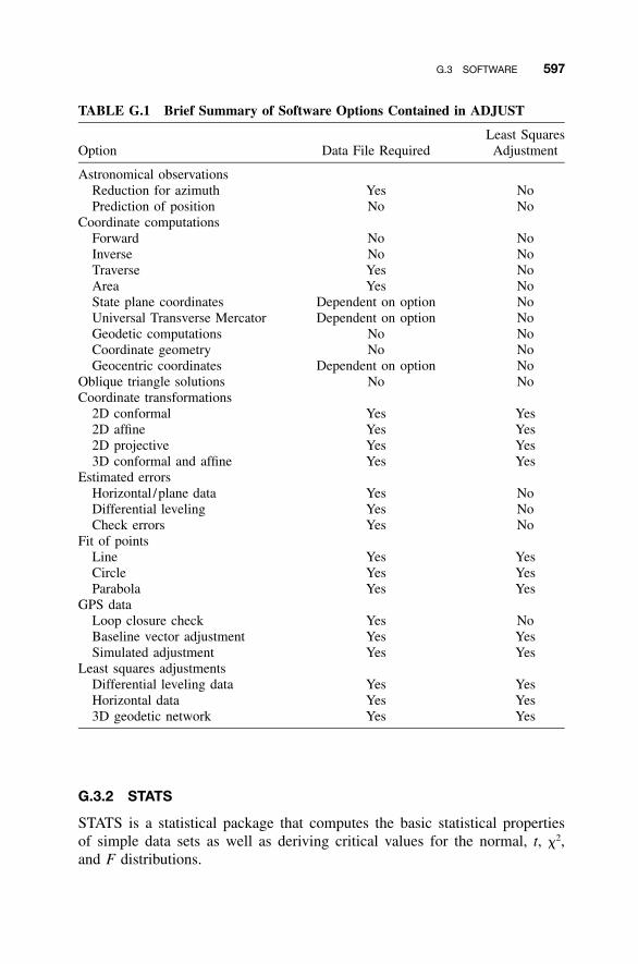
G.3 SOFTWARE 597
TABLE G.1 Brief Summary of Software Options Contained in ADJUST
Option Data File RequiredLeast Squares
Adjustment
Astronomical observationsReduction for azimuthPrediction of position
YesNo
NoNo
Coordinate computationsForwardInverseTraverseAreaState plane coordinatesUniversal Transverse MercatorGeodetic computationsCoordinate geometryGeocentric coordinates
NoNoYesYes
Dependent on optionDependent on option
NoNo
Dependent on option
NoNoNoNoNoNoNoNoNo
Oblique triangle solutions No NoCoordinate transformations
2D conformal2D affine2D projective3D conformal and affine
YesYesYesYes
YesYesYesYes
Estimated errorsHorizontal /plane dataDifferential levelingCheck errors
YesYesYes
NoNoNo
Fit of pointsLineCircleParabola
YesYesYes
YesYesYes
GPS dataLoop closure checkBaseline vector adjustmentSimulated adjustment
YesYesYes
NoYesYes
Least squares adjustmentsDifferential leveling dataHorizontal data3D geodetic network
YesYesYes
YesYesYes
G.3.2 STATS
STATS is a statistical package that computes the basic statistical propertiesof simple data sets as well as deriving critical values for the normal, t, �2,and F distributions.
598 COMPANION CD
G.3.3 MATRIX
MATRIX performs simple matrix operations. This software can be used tosolve many of the least squares problems in this book. It can read and writefiles of matrices, perform the operations of scaling, transposition, addition,subtraction, multiplication, and inversing of matrices, and allow the user toview the results of these operations.
When solving least squares problems with this package, a spreadsheet canbe used to compute the matrices. These matrices can then be ‘‘cut and pasted’’into the Matrix editor. Once saved to disk, the data files can be read by thesoftware and manipulated.
G.3.4 Mathcad Worksheets
The companion CD contains an electronic Mathcad book which will be in-stalled in the HANDBOOK directory under Mathcad. The electronic bookcan be opened from the Mathcad Help menu. For those who do not ownMathcad, html files of the worksheets can be installed on your computer.These files will be located in the ‘‘Mathcad HTML’’ directory in ‘‘MY DOC-UMENTS.’’ The html files can be viewed using your HTML browser. Afterinstallation, a link to these files may be found in the Programs menu.
The worksheets demonstrate most of the numerical examples contained inthis book. Most can be modified to compute other problems in the book.Some of the worksheets read ASCII data files. These files can be created byany ASCII editor, such as those contained in ADJUST, MATRIX, and STATS,or by another package, such as Notepad. With many spreadsheets it is possibleto save a comma-separated values (.csv) text file. These files can also be readby the worksheets. The format of the file is demonstrated by the numericalexample problem being solved in the original worksheet. Thus, when theoriginal worksheet is modified, it should be saved with a different name. Youshould compare the file formats in these worksheets with the example problemin the book to determine the proper format for your data.
These worksheets also provide a guide as to how various problems aresolved using programming. The Mathcad language is very similar to tradi-tional programming languages. However, Mathcad does not provide globalvariables or functions. Thus, all variables, especially those that will be mod-ified, must be passed from function to function in a worksheet and betweenworksheets. Mathcad reads the executable commands and variables from thetop to the bottom of the worksheet and from left to right on a line. This meansthat location of a command or variable on the worksheet can be critical tothe worksheet performing properly. Another difference between a traditionalprogramming language and Mathcad is that Mathcad has both subscriptedvariables and array elements. Unfortunately, although the subscript and arrayelement are entered differently, they look visually the same on the worksheet.
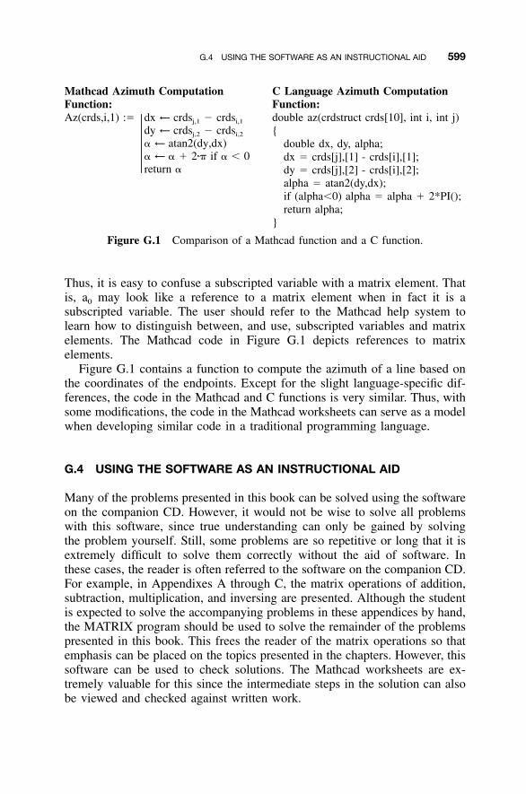
G.4 USING THE SOFTWARE AS AN INSTRUCTIONAL AID 599
Mathcad Azimuth ComputationFunction:
C Language Azimuth ComputationFunction:
Az(crds,i,1) :� dx ← crds � crdsj,1 i,1
dy ← crds � crdsj,2 i,2
� ← atan2(dy,dx)� ← � � 2�� if � � 0�return �
double az(crdstruct crds[10], int i, int j){
double dx, dy, alpha;dx � crds[j],[1] - crds[i],[1];dy � crds[j],[2] - crds[i],[2];alpha � atan2(dy,dx);if (alpha�0) alpha � alpha � 2*PI();return alpha;
}
Figure G.1 Comparison of a Mathcad function and a C function.
Thus, it is easy to confuse a subscripted variable with a matrix element. Thatis, a0 may look like a reference to a matrix element when in fact it is asubscripted variable. The user should refer to the Mathcad help system tolearn how to distinguish between, and use, subscripted variables and matrixelements. The Mathcad code in Figure G.1 depicts references to matrixelements.
Figure G.1 contains a function to compute the azimuth of a line based onthe coordinates of the endpoints. Except for the slight language-specific dif-ferences, the code in the Mathcad and C functions is very similar. Thus, withsome modifications, the code in the Mathcad worksheets can serve as a modelwhen developing similar code in a traditional programming language.
G.4 USING THE SOFTWARE AS AN INSTRUCTIONAL AID
Many of the problems presented in this book can be solved using the softwareon the companion CD. However, it would not be wise to solve all problemswith this software, since true understanding can only be gained by solvingthe problem yourself. Still, some problems are so repetitive or long that it isextremely difficult to solve them correctly without the aid of software. Inthese cases, the reader is often referred to the software on the companion CD.For example, in Appendixes A through C, the matrix operations of addition,subtraction, multiplication, and inversing are presented. Although the studentis expected to solve the accompanying problems in these appendices by hand,the MATRIX program should be used to solve the remainder of the problemspresented in this book. This frees the reader of the matrix operations so thatemphasis can be placed on the topics presented in the chapters. However, thissoftware can be used to check solutions. The Mathcad worksheets are ex-tremely valuable for this since the intermediate steps in the solution can alsobe viewed and checked against written work.
600
BIBLIOGRAPHY
Amer, F. 1979. Theoretical Reliability Studies for Some Elementary PhotogrammetricProcedures, Aerial Triangulation Symposium, Department of Surveying, Universityof Queensland, St. Lucia, Australia.
Baarda, W. 1967. Statistical Concepts in Geodesy, Netherlands Geodetic Commission,Delft.
———. 1968. A Testing Procedure for Use in Geodetic Networks, Netherlands Geo-detic Commission.
Bjerhammar, A. 1973. Theory of Errors and Generalized Matrix Inverses, ElsevierScience, New York.
Box, George E. P., et al. 1978. Statistics for Experimenters, Wiley, New York.Bomford, G. 1980. Geodesy, 4th ed., Claredon Press, Oxford.Bruns, H. 1878. Die Figur der Erde, Preuss. Geod. Inst., Berlin.Buckner, R. B. 1983. Surveying Measurements and Their Analysis, Landmark Enter-
prises, Rancho Cordova, CA.Burse, Michelle L. 1995. Profile of a Least Squares Convert, Point of Beginning, 20(2):
76–82.Conte, S. D., and Carl de Boor. 1980. Elementary Numerical Analysis, 3rd ed.,
McGraw-Hill, New York.Dewitt, Bon A. 1994. An Efficient Memory Paging Scheme for Least Squares Ad-
justment of Horizontal Surveys, Surveying and Land Information Science, 54(3):147–156.
Dracup, Joseph F. 1994. Squares Adjustment by the Method of Observation Equationswith Accuracy Estimates, Surveying and Land Information Science, 55:2.
El-Hakim, S. F. 1981. A Practical Study of Gross-Error Detection in a Bundle Ad-justment, Canadian Surveyor, 35(4):373–386.
———. 1984. On the Detection of Gross and Systematic Errors in Combined Adjust-ment of Terrestrial and Photogrammetric Data, Commission III, International Ar-chives of Photogrammetry and Remote Sensing, pp. 151–163.
———. 1986. The Detection of Gross and Systematic Errors in Combined Adjustmentof Terrestrial and Photogrametric Data, Photogrammetric Engineering and RemoteSensing, 52(1):59–66.
Adjustment Computations: Spatial Data Analysis, Fourth Edition. C. D. Ghilani and P. R. Wolf© 2006 John Wiley & Sons, Inc. ISBN: 978-0-471-69728-2

BIBLIOGRAPHY 601
Fubara, D. M. J. 1972. Three-Dimensional Adjustment of Terrestrial Geodetic Net-works, Canadian Surveyor, 26:4.
George, Alan, and Joseph W.-H. Liu. 1981. Computer Solution of Large Sparse Pos-itive Definite Systems, Prentice-Hall, Englewood Cliffs, NJ.
Ghilani, Charles D. 1990. A Surveyor’s Guide to Practical Least Squares Adjustments,Surveying and Land Information Science, 50(4):287–297.
———. 1994. Some Thoughts on Boundary Survey Measurement Standards, Surveyingand Land Information Science, 54(3):161–167.
———. 2003a. Statistics and Adjustments Explained, Part 1: Basic Concepts, Survey-ing and Land Information Science, 63(2):73.
———. 2003b. Statistics and Adjustments Explained, Part 2: Sample Sets and Relia-bility,’’ Surveying and Land Information Science, 63(3):141.
———. 2004. Statistics and Adjustments Explained, Part 3: Error Propagation, Sur-veying and Land Information Science, 64(1):29–33.
Hartzell, P., L. Strunk, and C. Ghilani. 2002. Pennsylvania State Plane CoordinateSystem: Converting to a Single Zone, Surveying and Land Information Science,62(2):95–103.
Harvey, Bruce R. 1994. Practical Least Squares and Statistics for Surveyors, Schoolof Surveying, University of New South Wales, Australia.
Heiskanen, W. A., and H. Moritz. 1967. Physical Geodesy. W. H. Freeman and Com-pany, San Francisco.
Hirvonen, R. A. 1965. Adjustment by Least Squares in Geodesy and Photogrammetry,Frederick Ungar, New York.
Hoffman-Wellenhof, B., et al. 2001. GPS Theory and Practice, 5th ed., Springer-Verlag, New York.
Hogg, Robert V., and Johannes Ledolter. 1992. Applied Statistics for Engineers andPhysical Scientists, Macmillan, New York.
Hotine, M. 1959. A Primer of Non-classical Geodesy, Presented to the First Symposiumon Three-Dimensional Geodesy, Venice.
Kuang, Shanlong. 1994. A Strategy for GPS Survey Planning: Choice of OptimumBaselines, Surveying and Land Information Science, 54(4):187–201.
Leick, Alfred. 2004. GPS Satellite Surveying, 3rd edition, Wiley-Interscience, NewYork.
McMillan, Kent Neal. 1995a. Least Squares: Older and Better Than Barbed Wire,Point of Beginning, 20(2):82–84.
———. 1995b. Least Squares Under the Hood, Point of Beginning, 20(2):84–88.Mendenhall, William, and Terry Sincich. 1994. Statistics for Engineering and the Sci-
ences, Dellen Publishing, San Francisco.Mikhail, Edward M. 1976. Observations and Least Squares, University Press of Amer-
ica, Washington, DC.Mikhail, Edward M., and Gordon, Gracie. 1981. Analysis and Adjustment of Survey
Measurements, Van Nostrand Reinhold, New York.Millbert, Kathryn O., and Dennis G. Milbert. 1994. State Readjustments at the National
Geodetic Survey, Surveying and Land Information Science, 54(4):219–230.Misra, Pratap, and Per Enge. 2001. Global Positioning System: Signals, Measurements,
and Performance, Ganga-Jamuna Press, MA.
602 BIBLIOGRAPHY
Schwarz, Charles R. 1994. The Trouble with Constrained Adjustments, Surveying andLand Information Science, 54(4):202–209.
Schwarz, K. P., E. H. Knickmeyer, and H. Martell. 1990. Assessment of ObservationsUsing Minimum Norm Quadratic Unbiased Estimation, CISM Journal ACSGC,44(1):29–37.
Seber, G. A. F. 1977. Linear Regression Analysis, Wiley, New York.Sideris, Michael G. 1990. The Role of the Geoid in One, Two-, and Three-Dimensional
Network Adjustments, CISM Journal ACSGC, 44:1:9–18.Snay, Richard A. 1976. Reducing the Profile of Large Sparse Matrices, NOAA Tech-
nical Memorandum NOS-NGS 4, republished in Bulletin Geodesique, 50(4):341.Strang, G., and Kai Borre. 1997. Linear Algebra, Geodesy, and GPS, Wellesley–
Cambridge Press, Wellesley, MA.Vanicek, P., and E. Krakiwsky. 1992. Geodesy: The Concepts,. Elsevier, New York.Veis, G. 1960. Geodetic Use of Artificial Satellites, Smithsonian Contributions to As-
trophysics. 3(9):95–161.Vincenty, T. 1979. The HAVAGO Three-Dimensional Adjustment Program. NOAA
Technical Memorandum NOS NGS 17. National Technical Information Service,NOAA, Silver Spring, MD.
White, L. A. 1987. Calculus of Observations 380/580, Western Australian Institute ofTechnology, Perth, Australia.
Wolf, Paul R., and Charles D. Ghilani. 2006. Elementary Surveying, 11th ed., PrenticeHall, Upper Saddle River, NJ.

603
INDEX
Accuracy, 4, 5example of, 5, 6
Adjoints, 537ADJUST, 596
options, 597Adjustment
analysis of, 492conditional, 178, 196constrained, 64, 78, 388, 395, 398,
400, 412of control stations, 388, 395, 412,
418, 468free, 291, 326fully constrained, 64, 291, 412,
419geodetic network, 454leveling, 205minimally constrained, 64, 291,
326, 412, 418networks, 291–300parametric, 178traverse, 283triangulation, 255trilateration, 233
Alternative hypothesis, 68Analysis of adjustments, 492Arc-to-chord correction, 593Associative law, 526
Astronomical observations forazimuth, 116
Atmospheric refraction, 472Azimuth
astronomical observations for, 116constraint, 295equation for, 255, 603errors in astronomical observations
for, 116
Baarda, 416Back-substitution, 511Blunder detection
a posteriori, 406, 412, 416, 420,492–502
a priori, 322–326, 410–412data snooping, 416, 494example of, 420–428, 493–496graphical methods, 411, 499handling of control, 326, 388, 418,
468network, 291, 327, 409, 492numerical example, 420, 493procedures, 418, 492residuals, 413, 492by residual sign, 413, 492, 494statistical methods, 44, 416, 501
Adjustment Computations: Spatial Data Analysis, Fourth Edition. C. D. Ghilani and P. R. Wolf© 2006 John Wiley & Sons, Inc. ISBN: 978-0-471-69728-2
604 INDEX
Blunder detection (continued )traverse closure checks, 114, 130,
135, 411by traverse closures, 114, 127, 130,
411Bomford, 474Bruns, 454
Calibration, EDM, 32, 73, 195Centering error
instrument, 100, 106, 121target, 100, 104, 121
Central meridian, 583, 587� 2 distribution, 52, 564
goodness of fit test, 300, 412, 496test, 74, 300, 412, 496use of table, 62, 74
Cholesky decomposition, 508Class
example of use, 27frequency, 15interval, 15, 16width, 14
Closure check, angular, 114Cofactor, definition of, 537Companion CD, 595
ADJUST, 596file formats, 596MATRIX, 598STATS, 597
Computer optimization, 504processing, 507, 508, 513storage, 504, 513
Confidence interval, 50interpretation of, 59for mean, 56, 59for population variance, 61ratio of two population variances,
63variance, 61
Confidence interval for mean,computation of, 58
Confidence interval for populationvariance, computation of, 62
Constraint equations, 388azimuth example, 395control coordinates, 388, 395, 468differential leveling example, 398
by elimination, 394geometric, 173Helmert’s method, 398
Control, adjustment of, 139, 326,388, 418, 468
Conventional Terrestrial Pole, 316,480
Coordinate systemsgeocentric, 316, 481geodetic, 316, 478global, 478, 480local, 478, 480local geodetic, 455NAD 83, 316, 478nearly aligned, 479rotations between, 480satellite, 314state plane coordinate system, 233,
582WGS 84, 316, 318, 478, 479
Coordinate transformationsadjustment of, 345datums, 480eight parameter, 353, 448four parameter, 345, 444Helmert, 480rotations, 357scaling, 346, 351, 356seven parameter, 356, 449six parameter, 350, 447statistically valid parameters, 362three-dimensional conformal, 356,
449two-dimensional conformal, 345,
444two-dimensional affine, 350, 447two-dimensional projective, 353,
448Coordinates
geocentric, 316, 481geodetic, 316, 478global, 478, 480local, 478, 480local geodetic, 455state plane, 233, 582
Covariancedefinition of, 86development of matrix, 221matrix, 159
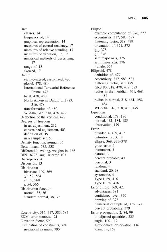
INDEX 605
Dataclasses, 14frequency of, 14graphical representation, 14measures of central tendency, 17measures of relative standing, 17measures of variation, 17, 19numerical methods of describing,
17range of, 13skewed, 17
Datumearth-centered, earth-fixed, 480global, 478, 480International Terrestrial Reference
Frame, 478local, 478, 480North American Datum of 1983,
316, 478transformation of, 480WGS84, 316, 318, 478, 479
Deflection of the vertical, 472Degrees of freedom
in an adjustment, 212constrained adjustment, 403definition of, 19in a sample set, 53
Density function, normal, 36Determinant, 535, 538Differential leveling, weights in, 166DIN 18723, angular error, 103Discrepancy, 4Dispersion, 13Distribution
bivariate, 109, 369� 2, 52, 564F, 55, 568t, 54, 566
Distribution functionnormal, 35, 36standard normal, 38, 39
Eccentricity, 316, 317, 583, 587EDM, error sources, 121Elevation factor, 590Elimination of constraints, 394
numerical example, 395
Ellipseexample computation of, 376, 377eccentricity, 317, 583, 587flattening factor, 318, 479orientation of, 371, 375quu, 375qvv, 376semimajor axis, 376semiminor axis, 376t angle, 374
Ellipsoid, 478definition of, 479eccentricity, 317, 583, 587flattening factor, 318, 479GRS 80, 318, 478, 479, 583radius in the meridian, 461, 468,
484radius in normal, 318, 461, 468,
484WGS 84, 316, 318, 478, 479
Equationsconditional, 178, 196normal, 181, 184, 185observation, 179
Errorblunder, 4, 409, 417definition of, 3, 18ellipse, 369, 375–378gross error, 4instrument, 3natural, 3percent probable, 43personal, 3random, 4standard, 20, 38systematic, 4Type I, 69, 416Type II, 69, 416
Error ellipse, 369, 427advantages, 381confidence level, 379drawing of, 378numerical example of, 376, 377percent probability, 379
Error propagation, 2, 84, 99in adjusted quantities, 225angle, 100–112astronomical observation, 116azimuths, 169
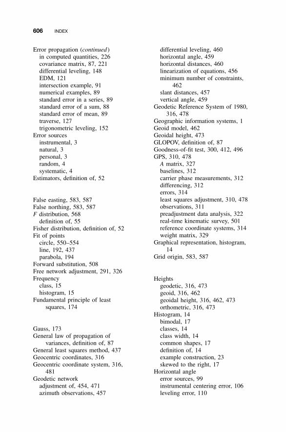
606 INDEX
Error propagation (continued )in computed quantities, 226covariance matrix, 87, 221differential leveling, 148EDM, 121intersection example, 91numerical examples, 89standard error in a series, 89standard error of a sum, 88standard error of mean, 89traverse, 127trigonometric leveling, 152
Error sourcesinstrumental, 3natural, 3personal, 3random, 4systematic, 4
Estimators, definition of, 52
False easting, 583, 587False northing, 583, 587F distribution, 568
definition of, 55Fisher distribution, definition of, 52Fit of points
circle, 550–554line, 192, 437parabola, 194
Forward substitution, 508Free network adjustment, 291, 326Frequency
class, 15histogram, 15
Fundamental principle of leastsquares, 174
Gauss, 173General law of propagation of
variances, definition of, 87General least squares method, 437Geocentric coordinates, 316Geocentric coordinate system, 316,
481Geodetic network
adjustment of, 454, 471azimuth observations, 457
differential leveling, 460horizontal angle, 459horizontal distances, 460linearization of equations, 456minimum number of constraints,
462slant distances, 457vertical angle, 459
Geodetic Reference System of 1980,316, 478
Geographic information systems, 1Geoid model, 462Geoidal height, 473GLOPOV, definition of, 87Goodness-of-fit test, 300, 412, 496GPS, 310, 478
A matrix, 327baselines, 312carrier phase measurements, 312differencing, 312errors, 314least squares adjustment, 310, 478observations, 311preadjustment data analysis, 322real-time kinematic survey, 501reference coordinate systems, 314weight matrix, 329
Graphical representation, histogram,14
Grid origin, 583, 587
Heightsgeodetic, 316, 473geoid, 316, 462geoidal height, 316, 462, 473orthometric, 316, 473
Histogram, 14bimodal, 17classes, 14class width, 14common shapes, 17definition of, 14example construction, 23skewed to the right, 17
Horizontal angleerror sources, 99instrumental centering error, 106leveling error, 110
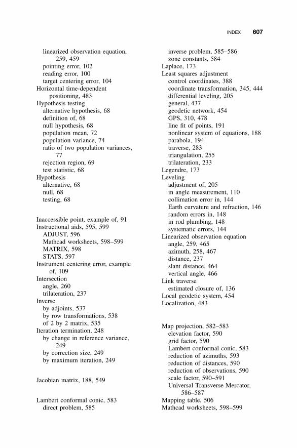
INDEX 607
linearized observation equation,259, 459
pointing error, 102reading error, 100target centering error, 104
Horizontal time-dependentpositioning, 483
Hypothesis testingalternative hypothesis, 68definition of, 68null hypothesis, 68population mean, 72population variance, 74ratio of two population variances,
77rejection region, 69test statistic, 68
Hypothesisalternative, 68null, 68testing, 68
Inaccessible point, example of, 91Instructional aids, 595, 599
ADJUST, 596Mathcad worksheets, 598–599MATRIX, 598STATS, 597
Instrument centering error, exampleof, 109
Intersectionangle, 260trilateration, 237
Inverseby adjoints, 537by row transformations, 538of 2 by 2 matrix, 535
Iteration termination, 248by change in reference variance,
249by correction size, 249by maximum iteration, 249
Jacobian matrix, 188, 549
Lambert conformal conic, 583direct problem, 585
inverse problem, 585–586zone constants, 584
Laplace, 173Least squares adjustment
control coordinates, 388coordinate transformation, 345, 444differential leveling, 205general, 437geodetic network, 454GPS, 310, 478line fit of points, 191nonlinear system of equations, 188parabola, 194traverse, 283triangulation, 255trilateration, 233
Legendre, 173Leveling
adjustment of, 205in angle measurement, 110collimation error in, 144Earth curvature and refraction, 146random errors in, 148in rod plumbing, 148systematic errors, 144
Linearized observation equationangle, 259, 465azimuth, 258, 467distance, 237slant distance, 464vertical angle, 466
Link traverseestimated closure of, 136
Local geodetic system, 454Localization, 483
Map projection, 582–583elevation factor, 590grid factor, 590Lambert conformal conic, 583reduction of azimuths, 593reduction of distances, 590reduction of observations, 590scale factor, 590–591Universal Transverse Mercator,
586–587Mapping table, 506Mathcad worksheets, 598–599
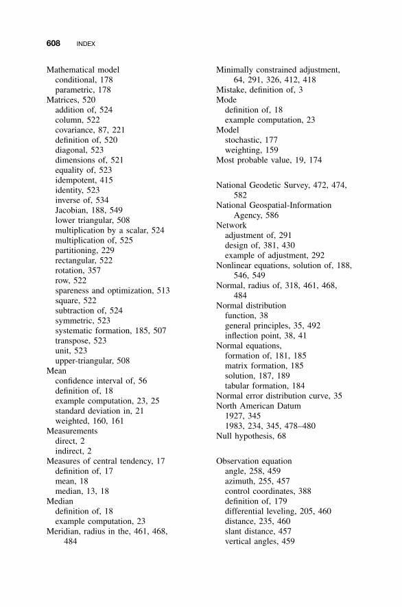
608 INDEX
Mathematical modelconditional, 178parametric, 178
Matrices, 520addition of, 524column, 522covariance, 87, 221definition of, 520diagonal, 523dimensions of, 521equality of, 523idempotent, 415identity, 523inverse of, 534Jacobian, 188, 549lower triangular, 508multiplication by a scalar, 524multiplication of, 525partitioning, 229rectangular, 522rotation, 357row, 522spareness and optimization, 513square, 522subtraction of, 524symmetric, 523systematic formation, 185, 507transpose, 523unit, 523upper-triangular, 508
Meanconfidence interval of, 56definition of, 18example computation, 23, 25standard deviation in, 21weighted, 160, 161
Measurementsdirect, 2indirect, 2
Measures of central tendency, 17definition of, 17mean, 18median, 13, 18
Mediandefinition of, 18example computation, 23
Meridian, radius in the, 461, 468,484
Minimally constrained adjustment,64, 291, 326, 412, 418
Mistake, definition of, 3Mode
definition of, 18example computation, 23
Modelstochastic, 177weighting, 159
Most probable value, 19, 174
National Geodetic Survey, 472, 474,582
National Geospatial-InformationAgency, 586
Networkadjustment of, 291design of, 381, 430example of adjustment, 292
Nonlinear equations, solution of, 188,546, 549
Normal, radius of, 318, 461, 468,484
Normal distributionfunction, 38general principles, 35, 492inflection point, 38, 41
Normal equations,formation of, 181, 185matrix formation, 185solution, 187, 189tabular formation, 184
Normal error distribution curve, 35North American Datum
1927, 3451983, 234, 345, 478–480
Null hypothesis, 68
Observation equationangle, 258, 459azimuth, 255, 457control coordinates, 388definition of, 179differential leveling, 205, 460distance, 235, 460slant distance, 457vertical angles, 459
INDEX 609
Observation weight, 160Optimization
direct formation of normalequations, 507
storage, 513Orthometric height, 316, 473Outliers, detection of, 42, 44, 59, 416
Percent errors, uses of, 43Percentage points, definition of, 53Pointing and reading errors
DIN 18723, 103example of, 101–103, 112
Populationdefinition of, 13sampling, 12standard deviation, 20variance, 19, 74
Precisiondefinition of, 4example of, 5
Probabilitydefinition of, 33in compound event, 33joint, 34
Probable errorexample of, 4450%, 4295%, 42other percent errors, 43standard error, 41table of, 43use of, 45, 46
Propagation, errors, 84, 221Pseudorandom noise, 311Pseudorange, 311, 499
Radius in the meridian, 461, 468,484
Random error, definition of, 4Random samples, 50Range, 13, 16
example of, 23, 25Ratio of variances, confidence
interval of, 63, 74Reading error
horizontal angle, 101–103, 112
leveling, 148Redundancies, see Degrees of
freedomRedundancy number, 416, 428Reference standard deviation
computation of, 212, 213definition of, 211
Reference standard deviation of unitweight, 161
Reference variancedefinition of, 160goodness-of-fit test, 300, 412, 496
Rejection region, 69Reliability
external, 429internal, 429
Resectioninitial approximations, 265least squares adjustment of, 270
Residualanalysis of, 442comparison of, 493, 500definition of, 19plots, 500
RTK-GPS, 501
Sampledefinition of, 12distribution theory, 52mean, 18, 23, 25size, 41, 60variance, 19, 20, 21, 52
Satellite orbitapogee, 314argument of perigee, 316ascending node, 316line of apsides, 314perigee, 314right ascension, 316
Site calibration, 483Slant distance, 455, 457SLOPOV
definition of, 88example of, 88, 127
SoftwareADJUST, 596Mathcad worksheets, 598–599
610 INDEX
Software (continued )MATRIX, 598STATS, 597spreadsheets, 123
Stakeout surveys, RTK-GPS, 501Standard deviation
for computed quantities, 226definition of, 20example computation, 23, 27mean, 21, 89sample, 20series, 89sum, 88
Standard errordefinition of, 20probability of, 41
Standard parallel, 583State plane coordinate system, 233,
582Statistics, 17, 52STATS, 597Stochastic model, 177
importance of, 499Student distribution, definition of, 54,
562Survey design, 381, 430
field specifications, 431procedures, 430use of maps, 430uses of, 94
Systematic errorsin angles, 472collimation, 144definition of, 4in heights, 473in leveling, 144
Tables� 2 distribution, 565F distribution, 569–575standard normal distribution, 562–
563t distribution, 567
Target centering errorexample of, 101, 104, 121
Taylor series approximation, 546t distribution, 54, 566
definition of, 54
use of, 56, 72, 114, 131, 134, 363,416, 493
Terrestrial observationwith GPS baseline vectors, 478
Test� 2, 74, 300, 412, 496F, 55, 419goodness of fit, 300, 412, 496hypothesis, 68population mean, 19, 72population variance, 74ratio of population variances, 77significance of, 70statistic, 68t, 72
Three-dimensional coordinatetransformation
conformal, 356Total station, DIN 18723, 103Transformation
Helmert, 480three-dimensional conformal, 356,
449two-dimensional affine, 350, 447two-dimensional conformal, 345,
444two-dimensional projective, 353,
448TRANSIT, 310Transverse Mercator, 586–587
direct problem, 588inverse problem, 588–589zone constants, 587
Traverseestimated closure, 128, 135minimally constrained, 291minimum control, 291numerical example, 128, 136, 285redundant equations, 135, 284
Traverse adjustmentdegrees of freedom, 284example of, 285observation equations, 284redundancies, 284
Traverse closureanticipated, 128, 136numerical example, 128, 136
Triangular matrices, forward andbackward solution, 511
INDEX 611
Triangulation adjustment, 255Trilateration adjustment, 233True value, 3, 18Two-dimensional coordinate
transformationaffine, 350, 447conformal, 356, 443projective, 353, 448
Type I error, 69, 416Type II error, 69, 416
Universal Transverse Mercator, 586–587
Varianceconfidence interval of, 61
definition of, 19, 22population, 19sample, 19
Vincenty, 456
Weighted mean, 161angles, 165example of, 168leveling, 166
Weight, 159constrained adjustment, 403relationship to corrections, 159relationship to variances, 160uncorrelated observations, 160uses of, 159
World Geodetic System of 1984, 316,318, 478, 479