Adjusting content to individual student needs: Further

evidences from a teacher training program

Adrien Bouguen

To cite this version:

Adrien Bouguen. Adjusting content to individual student needs: Further evidences from ateacher training program. PSE Working Papers n 2015-09. 2015. <halshs-01128184>

HAL Id: halshs-01128184

https://halshs.archives-ouvertes.fr/halshs-01128184

Submitted on 26 Mar 2015

HAL is a multi-disciplinary open accessarchive for the deposit and dissemination of sci-entific research documents, whether they are pub-lished or not. The documents may come fromteaching and research institutions in France orabroad, or from public or private research centers.

L’archive ouverte pluridisciplinaire HAL, estdestinee au depot et a la diffusion de documentsscientifiques de niveau recherche, publies ou non,emanant des etablissements d’enseignement et derecherche francais ou etrangers, des laboratoirespublics ou prives.

WORKING PAPER N° 2015 – 09

Adjusting content to individual student needs: Further evidences from a teacher

training program

Adrien Bouguen

JEL Codes: I21, I24 Keywords: early childcare program, teacher training, teaching practices and content, inequality

PARIS-JOURDAN SCIENCES ECONOMIQUES

48, BD JOURDAN – E.N.S. – 75014 PARIS TÉL. : 33(0) 1 43 13 63 00 – FAX : 33 (0) 1 43 13 63 10

www.pse.ens.fr

CENTRE NATIONAL DE LA RECHERCHE SCIENTIFIQUE – ECOLE DES HAUTES ETUDES EN SCIENCES SOCIALES

ÉCOLE DES PONTS PARISTECH – ECOLE NORMALE SUPÉRIEURE – INSTITUT NATIONAL DE LA RECHERCHE AGRONOMIQUE

Adjusting content to individual studentneeds: Further evidences from a teacher

training program*

Adrien Bouguen �

March 9, 2015

Abstract

Adapting instruction to the specific needs of each student is a promising strategyto improve overall academic achievement. In this article, I study the impact of anintensive teacher training program on reading skills offered to kindergarten teachersin France. The program modifies the lesson content and encourages teachers to adaptinstruction to student needs by dividing the class according to initial achievement.While assessing impact is usually difficult due to the presence of ability bias andteacher selection, I show that in this context, a value-added model that controls forschool and teacher characteristics constitutes a legitimate strategy to estimate at leasta low bound of the true treatment effect. Weaker students progressed faster on less-advanced competences (such as letter recognition), while stronger students improvedtheir reading skills. This suggests that teachers adjusted content to students’ needs.Finally, a cost-effectiveness analysis reveals that the program is approximately threetimes more cost-effective than reducing class size in France.

JEL classification: I21, I24

Keywords: Early childcare program, teacher training, teaching practices and content, in-

equality

*This research was funded by a grant from the “Fond d’Experimentation de la Jeunesse” and by “Agir

pour l’Ecole”. This work has been realized with the support of the Statistical department of the National

Education in France (DEPP) and of NGO “Agir pour l’Ecole” (APE). Special thanks to Laurent Cros

(APE) and Alice Bougnere (APE) for their constant support and to Thierry Rocher, Sandra Andreu and

Marion Le Cam (DEPP) without whom this work would not have been possible. I wish to express my

gratitude to the 118 schools and their teachers who have participated as beneficiary or not to the data

collection. I also thanks Marc Gurgand, Eric Maurin, Camille Terrier, Julien Grenet for their usefull

comments in the seminar in Paris. Likewise, comments from Sandra Mc Nally, Clement Malgouyres,

Maxime To after the Institute of Education (UCL) seminar in London were all very useful.�Paris School of Economics, 48 boulevard Jourdan Paris, adrien.bouguen@ipp.org

1

The existence of large variation in teacher quality is indicative of the central role that

teacher plays in the overall performance of an education system. The most reliable studies

suggest that a one standard deviation increase in teacher quality raises student performance

by at least 9.5% of a standard deviation,1a magnitude that is equivalent to a 5- to 10-

year increase in teaching experience2 or to a class size reduction of 4–5 children.3 Giving

the right incentives, selecting the right teachers, and providing them with the right skills

are all being investigated as potential ways to improve teaching in both developed and

developing settings. The latter solution – pre-service and in-service teacher training –

has been widely studied in developed countries. Teacher-training programs are appealing

because, when effective, they are potentially a cost-efficient and lasting strategy to enhance

student achievement.4 Available empirical results are not always consistent, however, and

the literature is still unable to reach consensus on the effectiveness of teacher training.

Four main challenges plague the literature on teacher training. First, it has proven

difficult to isolate the causal effect of training from the effect of selection into training

(“teacher selection”) and the effect of assignment of trained teachers to students (“student

selection). Second, isolating the effect of training from other policies implemented at the

same time is sometimes challenging. Third, the vast diversity of teacher training programs

– in term of content, nature, level, intensity, or even quality – renders difficult any sort of

general statement on the effectiveness of such policy; a more refined approach is needed to

parse what may be effective from what is not. Fourth, as mentioned, while teacher training

19.5% is the effect found by Rivkin et al. (2005), and 10% by Rockoff (2004), using a different strategy,correcting for overestimation due to measurement error. Using simple teacher fixed effect, the literaturereview provided by Nye et al. (2004) gives effects from .26 to .46. Applying the same naive strategy on mydata, I find consistent effects from .19 to .39, depending on the cognitive measure used.

2Hanushek (1971), Rockoff (2004), or more recently Harris and Sass (2011) all provide estimationsvarying from 1% to 2% of a standard deviation per year of experience. As we will see, I provide aslightly smaller estimation of the teacher experience effect (around 0.9%), maybe because experience isless meaningful in preschool than in primary school. Note that, for comparison matter, I report theexperience effects per year, although this is probably not the most meaningful way. Most authors are ableto identify a nonlinear relationship in which the experience effect is strongest during the first years andreaches a cutoff year above which experience is not predictive anymore. Due to lack of power, I am notable to implement such a model.

3This is based on a class size effect estimated between 2.2% and 3% per additional pupil in class(Bressoux et al., 2009, Bressoux and Lima, 2011, Piketty and Valdenaire, 2006). Note, however, that thisestimate is clearly larger than the one found with STAR data (1.7).

4Training one teacher “treats” many students at once, and if “good” teaching practices are employedthroughout the teacher’s career, these practices may have an effect on several generations of students.

2

programs are cheap when compared to programs that directly target students, they have

only little effect on them (typically around 10% of a standard deviation). Lack of detection

power has affected the quality of some studies.

This article alleviates some of these concerns. It suggests that well-defined and intensive

pedagogical training (based on explicit teaching, phonological awareness,5 and small group

tracking), when applied to one specific subject (reading) during one specific period of teach-

ing time (when pupils start reading lessons, around 5 years old) is instrumental in improving

kindergarten children’s short-term reading achievement. Using a value-added model, I find

an overall treatment effect of 15.3% of a standard deviation with results varying from no

effect on the dimensions not stimulated by the program (vocabulary, comprehension) up

to 44% of a standard deviation in decoding (non-lexical reading). A back-of-the-envelope

cost-benefit calculation gives 12.5 e per percentage point of standard deviation gain: less

cost-effective than a similar experiment run in England (see Section 2), but still much

less expensive than my assessment of a class size reduction policy implemented in France

(between 36–48 e per s.d.).

Equally important are the heterogeneous effects found by initial achievement. Since the

training program was based on an explicit teaching pedagogy implemented on four groups

of initial achievement (tracked group), one of the expectations was that the program would

help teachers instruct at the right level. Heteregeneous effect by initial achievement shows

that initially weaker-performing students progressed faster on less-advanced competences

(letter recognition, phonological awareness), while initially stronger-performing students

progressed faster on more-advanced competences (reading and-non reading skills). These

results suggest that the training programs have indeed helped teachers adjust content to

all students’ needs. Such results echo those found in a very different context by Duflo

et al. (2011), where teaching to the right level was particularly effective in improving all

students’ achievements. The results presented in the following, therefore, provide further

evidence that adjusting content to every student’s needs – whether via tracking, within-class

5To simplify, I will use phonology and phonological awareness interchangeably and define the conceptas the ability to hear, repeat, mix, and decompose sounds, and to link them to graphemes. I will alsoregroup under the the term “phonological awareness” concepts such as phonics (the ability to link soundsto graphems) or phonemic awareness (the ability to mix sounds), which are not necessarily equivalent butclosely related. To match the wording of some other authors, I will sometimes use the term “code-relatedskills,” which regroup both phonological awareness and letter recognition.

3

tracked groups, or via a new pedagogy – is instrumental in improving student achievement.

I believe that this is the first time such results are presented in a developed country and

in an experimental environment that is arguably very close to the existing institutional

context.

The conceptual framework developed in Section 2 suggests that simple regression re-

sults, controlling for baseline test scores, provide low bounds of the true treatment effects.

The empirical part, Section 3, shows that results are robust to inclusion of both school

and teacher characteristics and that attrition seems not to have affected results in any

particular direction. Finally, the program trains teachers to a pedagogy that is sufficiently

standard to be compared to the one used in at least three other contexts (France, the

United States and England). Contrasting the results from these three contexts to the ones

found here allows for more specific conclusions.

In the rest of the article, I will describe and expand upon the available literature. I

will then develop a simple empirical model that clarifies the conditions in which the value-

added models used in this article properly identify the teacher program effect. I will also

present how pre-schooling is organized in the French education system and give details on

the training program. Finally, I will describe the school, teacher, and student-level data

on which my analysis relies, and I will present my results. I conclude by contrasting my

results with three other comparable studies.

1 Literature Review

The literature on teacher training is indirectly related to studies about teacher certification,

as certified teachers are usually trained in preparation centers. Using a rich dataset from

New York City, Kane et al. (2008) argue that certified teachers perform only marginally

better than non-certified ones (around 1.5% of a standard deviation for reading skills), and

such a small difference compares poorly with the large teacher variation within training

centers (as mentioned in the introduction, around 10% of a standard deviation for one

standard deviation improvement in teacher quality).The authors conclude that selecting

the right teachers is a more cost-effective strategy than training the wrong teachers. This

is in line with the positions taken by Rivkin et al. (2005) and, in many instances, by

4

Eric Hanusheck (Hanushek, 1971, Hanushek and Rivkin, 2006). Under different identifica-

tion strategies, similar conclusions are reached by Goldhaber et al. (2013) in Washington,

Koedel et al. (2012) in Missouri, and Harris and Sass (2011) in Florida. Yet these re-

sults imperfectly control for teacher selection into certification centers; differences between

certified and non-certified teachers hence capture both selection into certification and the

effect of the initial training offered to certified teachers The same limitation affects the

impact evaluation of Teach for America (TFA) conducted by Decker et al. (2004). While

randomization at the class level ensures that TFA and non-TFA teachers are assigned to

initially similar students, both experimental groups of teachers did not have the same ini-

tial characteristics. As a result, as acknowledged by the authors, all of these experiments

estimate the overall effect of certification, selection and training.

It is worth noting, as mentioned by Goldhaber et al. (2013), that this literature is

not directly interested in the effect of training as it compares to different sorts of training

programs. In addition, this literature looks at the heterogeneous offer of teacher preparation

central to one region of the US. It does not shed light on the kind of training that a teacher

should receive, or whether investment in teacher training should be preferred to extensive

education policies such as class size reduction. Relating more to my purpose, Boyd et al.

(2009), using the same New York City panel data used by Kane et al. (2008), have described

is more effective in improving teacher quality. They find that teachers who received more

practical preparation – those who are more prepared for the curriculum and have more

classroom experience – are more likely to perform slightly better in their first teaching years.

Although small in magnitude, such effects suggest that teacher training content matters,

and more specific and intensive training might be instrumental in improving teacher quality.

This claim is supported by additional articles on certification and in-service training that

look at the net effect of intensive teacher trainings. In France, for instance, Bressoux et al.

(2009) have compared the student performances of two cohorts of newly recruited primary

school teachers, one which has benefited from two years of primary school preparation, and

the other which has received no training at all. The authors find a strong and significant

impact in mathematics (+.25 standard deviation), but not in reading. Likewise, in Israel,

Angrist and Lavy (2001) investigated the effect of an intensive in-service training (five

hours per week) and showed very strong results (+.3 s.d.). When comparing these with

5

the aforementioned results from the US, it is worth noting that in both cases, the authors

contrast very intensive training programs (a two-year pre-service training in France and a

five-hour-per-week training in Israel) to a counterfactual which receives no training at all.

Yet, as very little is known about the content of each training, these two local examples

are difficult to compare, and results may be context-specific. As mentioned before, the

diversity of contexts (developed and less developed), of training content and intensity, of the

multitude of dimensions that can be stimulated, of the multitude of subjects (mathematics,

literacy, science, and so on) and of grades make any general statement about teacher

training per se not fully meaningful.

To avoid such general statements, this article analyzes the effects of well-defined ped-

agogical training, based on explicit teaching6 and aiming at strengthening code-related

early skills (with a strong emphasis on the recognition of letters and sounds, as well as

phonological awareness), and applied to one specific subject (reading) at one specific pe-

riod of teaching time (when pupils learn how to read between the ages of 5 and 7 years).

The focus on phonological awareness at an early stage (before the official beginning of

reading classes) is justified by a vivid psychological literature that explores the founda-

tion of reading success and links code-related early skills to grade 1/grade 2 reading skills.

Using a longitudinal three-year panel data of children aged 5 to 8, Schatschneider et al.

(2004)confirm the interest of focusing on phonological awareness at early stages by showing

the strong predictive power of code-related skills (letter recognition, sound recognition, and

phonological awareness). While still debated,7 this view is in line with the conclusions of

the National Reading Panel (1999), which canvassed a large body of evidence on literacy

6There is no clear definition of “explicit teaching,” but the general idea is that the method promotesa very structured pedagogy where teaching content is adjusted as much as possible to student progress,clear objectives are set, and specific tasks are completed before accessing new tasks. Such an approach isdefended by Success For All, an influential NGO in the US and UK. It is often opposed to exploratoryteaching such as the inquiry-based learning defended by alternative education models such as Montessori.

7As summarized by NICHD (2005), there is a fierce debate in the psychological research on the respec-tive predictive power of code-related skills versus oral language skills (early vocabulary or comprehension).Earlier work from Storch and Whitehurst (2002) suggests that while code-related skills predict early andmid-early skills (end of grade 1), later reading skills (grade 4) are best predicted by oral language skills.Yet several other articles conclude in radically different ways Schatschneider et al. (2004). To my under-standing of the literature, much of the results hinge on (1) the quality of the data and (2) the test scoresused to assess endline reading skills. A middle-ground position might be to consider code-related skills asnecessary, but not sufficient, steps in the road to reading, justifying the focus on phonological awarenessat early stages.

6

in the 90s in the US.

Yet there is still a dearth of evidence on the impact of a public policy specifically de-

signed to improve phonological awareness in kindergarten. To my knowledge, only two

reports from the Institute of Education Studies, as well as two scientific articles, can be

directly compared with the results of this article. Both IES reports, which rely on random-

ized experiments, find no effect of the teacher training programs (Garet et al. (2008);Garet

et al. (2011)). The older report is particularly meaningful for my purpose, as it evaluates

the effect of a training program aimed at improving first graders’ reading skills. This train-

ing program, as is the case here, is based on the findings of the National Reading Panel

(see Section 4.3 below, where the training program is described). Also similar to the pro-

gram studied here is the one implemented recently in France where researchers analyzed

the impact of a similar teaching pedagogy in first grade, again with no results on student

achievement (Gentaz et al. (2013)). Finally, using a cross section difference-in-differences

strategy on a large dataset, Machin and McNally (2008) were able to convincingly identify

an overall effect of 8.3% of a standard deviation in England from a training program called

the “Literacy Hour,” which resembles those evaluated both in France and in the US. It

could be argued that these three results are not necessarily inconsistent, as both random-

ized experiments could only satisfactory identify effects above .22 s.d. (Garet et al. (2008))

and .25 s.d. (Gentaz et al., 2013),8 far from the 8.3% found in England.9

While small in magnitude, 8.3% of a standard deviation is arguably a very cost-effective

strategy. Since training programs are mainly composed of fixed costs, when scaled up, the

cost per child is dramatically reduced. In England, the cost was as low as 38 e per child, or

5 e per percentage point of a standard deviation gain.10 In comparison, class size reduction

programs have been reported to increase student performance from +2.2% to +3% of a

8I recalculate the Minimum Detectable Effect (MDE) using data provided by the authors (see Gentazet al. (2013)), with an inter-cluster correlation and a baseline-endline correlation assumed respectively at

10% and 30%. This gives MDE = 2.8√( 2148 )∗(

1−2348 )∗48)

∗√0.1+ 0.9

83023

∗√1− 0.3 = .25

9It seems that the researchers in France and in the US were misguided by the very optimistic effectsizes reported in the National Reading Panel. According to the National Reading Panel (1999), a phono-logical awareness pedagogical approach should increase student achievement by at least 60% of a standarddeviation. Such optimistic results were in fact obtained in very controlled environments, on small samplesand with supposedly motivated teachers. When implemented in “real life,” such programs seem to yield amuch more moderate impact.

10In 2011, 25.52 £ corresponded approximately to 38 e.

7

standard deviation per child in French primary schools (Bressoux et al., 2009, Bressoux

and Lima, 2011, Piketty and Valdenaire, 2006), for a cost of about 107 e per child, or

36-48 e per percentage point of standard deviation gain11; all being equal, a “Literacy

Hour” training program implemented in France would then be at least eight times more

cost-effective then a class size reduction. As said, the program evaluated here is more

effective, more costly, but less cost effective than the English experiment, but is at least

three time less expensive than a class-size reduction program.

2 conceptual framework

2.1 Model

Achievement in period 1 (after the training program) can be modeled by four additive

effects:

Ai1 = βTs + µi + ιi1 + εi1 (1)

T is the teacher training provided to all teachers in school s, µi is the fixed capacity of

student i, ιi1 is the non-fixed capacity effect (later called “ability to progress”), and εi1 is

the measurement error, unrelated to any observed and unobserved characteristics. In this

model, β measures the effect of the teacher training on the pupil i.

In a non-randomized setting, a main source of worry is ιi1 (“ability to progress”) that

can be correlated with both T and µ. ιi1 can hence be decomposed as follows:

ιi1 = ρµi + νi1 (2)

where ρ is a measure of the correlation between µ and ι, and ν is the part of the

progression that is unrelated to the initial endowment. To rephrase, ρµi is a part of

11This is an approximate assessment of the overall cost of the reduction of one pupil per class in primaryschool. It is based on an average net monthly teacher salary of 2323 ein France, multiplied by two toaccount for social contributions, and then multiplied by 12 months, to which I add an administrative costof 15%. Since in my data set, class size is in average composed of 25 students, a reduction by 1 student isequal to (2323*2*1.15*12)/24- (2323*2*1.15*12)/25 ≈ 107e.

8

the progression due to the child, and νi is the external shock: typically teacher, school,

or parental involvement effect can be included in νi. Besides, the sign of ρ indicates

the underlying students’ progression model. ρ > 0 indicates a model where students’

achievement tends to diverge naturally over the year: weaker students progress at a slower

pace than advanced ones. Inversely, ρ < 0 indicates that weaker students tend to catch

up with the rest of the class, while ρ = 0 indicates that progress is unrelated to students’

initial level, and hence all children have a common progression trend.

Inserting (2) in (1) gives:

Ai1 = βTi1 + (1+ ρ)µi + νi1 + εi1 (3)

Similarly, achievement at time 0 can be defined as:

Ai0 = µi + εi0 (4)

Note ιi0 is here normalized in µi. It follows that achievement at time 1 can be written:

Ai1 = βTi1 + µi + ιi1 + εi1

= βT + (1+ ρ)µi + νi1 + εi1

= βT + (1+ ρ)Ai0 + νi1 + εi1 − (1+ ρ)εi0 (5)

Estimating 5 is difficult for two main reasons. First, as Ai0 is correlated to εi0, esti-

mating (1+ρ) will suffer from an attenuation bias due to measurement error. This will in

turn bias β. Second, ν1i is uncontrolled for shocks unrelated to achievement (such as being

enrolled in a function schools, benefiting from a good teacher, and so on) that will bias the

estimation if they are related to T.

2.2 Value-Added Models and Lower Bound Estimates

Putting aside the latter concern (teacher and school selection), two strategies are tradi-

tionally used to cope with the first one (estimating 1+ρ). In the first model, later called

9

value added Model 2 (VAM2), ρ is constrained to zero, and then each student progression

is regressed against treatment variable. Hence, from (5), VAM2 strategy gives:

Ai1 = βT +Ai0 + νi1 + εi1 − εi0 (6)

Ai1 −Ai0 = βT + νi1 + εi1 − εi0 (7)

as a result when E(νi1|T) = 0, β is consistently estimated using a simple OLS regression

model. According to 2, ρ = 0 means that the initial endowed capacities will not influence

students’ progression; e.g., weaker students will not spontaneously catch up with the rest

of the class (or inversely). This is another way to express the common trend assumption,

and (6) is commonly called a difference in differences estimation.

Since imposing a constant progression among young children may not be an acceptable

assumption, especially in an education setting,12 one may want to relax this constraint.

Relaxing the constraint on ρ supposes to estimate 1+ ρ in the following model:

Ai1 = βT + γAi0 + νi1 + εi1 − γεi0 (8)

with γ = 1 + ρ. As said, because E(εi0|Ai0) 6= 0, γ will be downward biased. What

consequence would such bias have on β? We know that it is likely to be biased, as T and

Ai0 are likely to be correlated. But can the direction of the bias be derived?

Using a well-known result from the omitted variable biased model, considering ε0 as

the omitted variable, it can be shown (see Appendix) that:

E(βvam1) = β+ γr(A0, T) ∗ Vε01− r(A0, T)2

Sε0ST

(9)

With r(A0, T), the correlation between baseline test score A0 and T, Vε0 the variance of

the baseline measurement error, Sε0 its standard deviation, and ST the standard deviation

12In this context, with the outcomes being early reading skills (decoding, phonology, and so on), onemay expect that initial differences may be reduced when the first classes are given. A convergent modelwhere ρ<0 is hence more likely, although there is no tangible evidence of such a pattern.

10

of the Treatment group. With γ = 1 + ρ > 0, the sign of the bias is fully determined by

r(A0, T). Since, in this study, the treatment group’s students were initially weaker than the

ones enrolled in control group schools, r(A0, T) < 0 and βvam1 is the value added model

1 gives a low bound of the true treatment effect, I will rely on that model, keeping VAM2

only as a benchmark.

2.3 Coping with Teacher and School Selection

This is, of course, leaving the second concern aside, i.e. E(νi1|T) 6= 0. Different νi1

may be due to children themselves (children in the treatment school happened to have a

different ability to progress, even conditional on their endowed capacities), to their parents

(parents may be more involved in one of the two groups or may compensate low school

or teacher performance), to the school (school administration may be different), or to the

teacher (some teachers may simply be better in treatment than in control). Obviously,

one major concern is the selection at the teacher level, as the training program is directed

to them. If only volunteer teachers (or schools) participated in the teacher training, we

may expect νi1>0 and the estimation to be biased upward. Alternatively, if school district

administrators have chosen the schools that were the most in need of training, bias might

be reversed.

As we will see, in that case, the school district managers were asked to select the schools

in which the program was the most needed. Although they were in a position to impose

the training program in any specific school, they have most likely asked the opinion of

the school directors and maybe of teachers. Participation was hence decided between the

teachers, the school director, and the school district manager. In any case, I do not believe

that other sources of bias (either parents or children) have ruled over this decision.

To investigate whether a selection at school or teacher level has occurred, I will rely on

additional data from the school and the teacher, and estimate modified version of value

added model 1 accordingly:

Ai1 = βT + (1+ ρ)Ai0 + κi1 + Pc1α+ Ss0α2 + εi1 − (1+ ρ)εi0 (10)

11

where Pc1 is a matrix of teacher level characteristics collected at follow-up 13 and S0 a

set of school level characteristics collected at baseline.14Both sets of control variables are

supposed to remove any correlation between κi1 and T and make :

E(κi1|T,Pc1,Ss0) = 0 (11)

a valid assumption.

There are at least two reasons we might not be fully satisfied by this strategy. First,

teacher characteristics were collected from teachers themselves after the training programs,

and were thus potentially affected by the intervention. The intervention may have impacted

the way teachers answer, their practices, and also their propensities in responding (attrition

bias). Second, we may be worried that both teacher and school characteristics are imper-

fectly measured (Hanushek (1986), Hanushek et al. (2005)). In the forthcoming empirical

part, however, I will show that among the few variables collected at teacher level, some are

predictive of the teacher value added and are effectively removing teacher selection.

Taken together, the conclusions drawn from this model present rather favorable experi-

mental settings. In the absence of school or teacher selection, and since treatment students

were initially weaker, the treatment effect estimating with VAM1 can serve as a lower

bound of the treatment effect. Using school and teacher data, I will show why selection

at school or teacher level is probably not a major concern. After having quickly described

the data and the context, I will analyze precisely both sources of bias and try to find an

empirical solution for both.

13Although we would ideally want to control for information collected before the inception of the trainingprogram, this was not possible. The teacher characteristics were collected one year after the end of theprogram. Yet I rely essentially on constant information or information that is unlikely linked to theprogram.

14on administrative data

12

3 The Kindergarten Intervention within the French Educa-

tional System

3.1 The French Educational System

In France, the educational system is organized in three tiers that mimic the political or-

ganization. The three tiers are under the central authority of the Ministry of National

Education. The highest tier, the Regional School District (rectorat), is at the regional

level.15 The middle tier, the Departmental School District (Inspection d’Academie), is

at the sub-regional level (departement). The lowest tier, the School District (Inspection

de l’Education Nationale), is the first authority above the school director and the teach-

ers. School district managers have a direct authority over the school directors and the

teachers of his or her ward (circonscription). Importantly, they are responsible for teach-

ers’ assessment (inspection), which partly determines teachers’ wage increases and transfer

possibilities (mutation).

As we will see in the following section, the training program’s evaluation was imple-

mented in three rectorats(Creteil, Versailles, and Lille), two rectorats situated in suburban

Paris (Creteil and Versailles), and one in the region Nord (Lille’s region). The three rec-

torats authorized the experiment in four department school districts: two in Lille (numbers

59 and 62), and two in suburban Paris (numbers 92 and 93). In each department school

district, the program was implemented in two school districts, hence eight in total. The

original sample was composed of 59 beneficiary schools and 59 control schools.

3.2 Kindergarten in France

In France, a three-year-old child (or a child who will turn three before the end of the

calendar year) is allowed to be enrolled in the first year of kindergarten. Kindergarten

is free of charge, and the education provision is organized at the national level by the

Ministry of Education (teachers are paid by the central state, with the curriculum designed

nationally). While enrollment at three is not compulsory, enrollment rate at that age is

15This is subject to some exceptions. Large regions such as Ile de France (suburban Paris) are, forinstance, divided into three regional school district (Creteil, Versailles, and Paris).

13

near 100% (DEPP (2013)). Kindergarten is composed of three school years: Petite Section

(PS), Moyenne Section (MS) and Grande Section (GS). Kindergarten teachers must follow

a national curriculum specific to each year. This curriculum is agreed upon at the national

level and is published in the Bulletin Officiel de l’Education Nationale (official ministry

register) whenever it is modified.16 So far, the kindergarten curriculum has been relatively

nonrestrictive, leaving much freedom to teachers; the curriculum does not impose any

specific teaching methods, nor does it provide guidance on how school days should be

broken up or how progress should be organized over the school year. It only gives general

objectives to be met at the end of kindergarten. In that sense, the last 2008 curriculum

respects the general principle of liberte pedagogique(teaching freedom), a principle that is

recognized by law.17 This principle is probably more manifest in kindergarten than in

primary school, when curricula start to be more precisely specified.

Nonetheless, in the “GS’s national curriculum, teachers are asked to start develop-

ing phonological awareness,18 i.e. (1) connecting sounds and letters (phonemics) and de-

composingwords into syllables (phonological awareness). According to the report of the

National Reading Panel (NRP), both skills are supposed to constitute the first phase of

reading, and failure to master them is strongly predictive of reading difficulties in first

grade (National Reading Panel (1999)).

3.3 Training Intervention: Changing the Teaching Practices

In the wake of the conclusions of the National Reading Panel, an NGO called Agir pour

l’ecole, in collaboration with researchers from Cogniscience at University Pierre Mendes

France, designed a new reading pedagogy composed of teacher training sessions, books,

and specific guidelines that promote an intensification of the amount of phonology in GS

teaching. Although phonological awareness is recognized in the curriculum as one of the

main skills to be developed in GS, there are reasons to believe that the level provided

16The last version of the kindergarten curriculum was published in the Bulletin Officiel in June 2008.See Bulletin Officiel hors-serie n° 3 du 19 juin 2008.

17See, for instance, article 48 from Loi d’orientation et de programme pour l’avenir de l’ecole L. n°2005-380 du 23-4-2005. JO du 24-4-2005.

18distinguer les sons de la parole and aborder le principe alphabetique, BO hors serie n°3 du 19 Juin2008.

14

in French classes is not sufficient to prevent reading difficulties among the weakest pupils

(Bougnere et al. (2014)). The pedagogy defended by the NGO explicitly runs counter to

the principle of pedagogical freedom, which prevails in the French educational system by

giving explicit instructions for teachers to follow every week (“explicit teaching”). Teachers

are asked to give two sessions of 30 minutes of phonological awareness per day, starting in

January until the end of the school year. The trained teachers are expected to provide a

total of 20 hours maximum phonological awareness, which is supposedly much higher than

the amount received by a GS student in a standard school.

In addition, the methodology is designed to be implemented in small groups of 5–6

children with similar achievement levels (“tracked achievement groups”). Again, the idea

is to counteract another potentially detrimental practice that provides the same content

to the whole class, regardless of individual pupil’s development stage. At the beginning

of the year, all GS pupils’ early phonological awareness is assessed, and four achievement

groups are created.19 Each small group has a certain number of exercises that must be

completed before moving to the next stage. The idea is to insure that the teaching content

would stick to the progress of each child. Once again, this is supposedly different from the

general practices in a standard French school.

To insure that the program is properly implemented, the NGO trained one pedagogical

advisor (conseiller pedagogique) to the new methodology in each school district. The

pedagogical advisers were then supposed to train all the teachers in the intervention schools

during three hours. They were also responsible for monitoring the way the methodology was

implemented on the field (through class visits) and were able to offer additional training

hours (up to 18 hours). The NGO also directly monitored the implementation of the

program by visiting numerous schools during the year. Although the original objective was

to create a methodology that could be easily implementable in any context (through precise

learning instructions), it seems relatively clear that the implication of the local education

administration partly determines the effectiveness of the policy. Although I do not have

extensive information on teacher practices, I will show in Table 3 that the program seems

to have significantly modified the teacher practices.

19Teachers were also allowed to modify the groups composition as they wished, but rarely did so inpractice.

15

4 Data and Sample

4.1 Sample Creation

The empirical analysis of the training program essentially relies on a sample created by

the Bureau for Evaluation and Statistics of the Ministry of Education in France (DEPP).

Fifty-nine treated schools were selected in three “rectorats” (Regional School Districts),

four “IAs” (Departmental School Districts) and eight IENs (School Districts).It is not clear

how schools within each treatment school district were recruited in the program; the school

district managers possibly selected some schools eligible to participate (schools with a GS

class and which had no other ongoing program), and these schools were then contacted by

the NGO. As schools are under the direct authority of their managers, they cannot refuse

to participate in a program supported by their manager. However, selection probably

depended on the commitment of the manager into the program. All in all, if selection has

happened at that stage, it would probably come more from the manager than from the

schools themselves.

To create a credible control group, the DEPP selected schools situated in the same

Departmental School District (but not in same School District), from the same priority

education level,20 and from schools composed of the same number of children. Based on

these three criteria, 24 strata were created, and among the 1807 schools included in the

sampling frame, the DEPP randomly selected 59 control schools (one for each treatment

school).

If we believe that the few stratification variables used to select the 59 control schools

are at least partially correlated with the outcome as well as school and teacher quality,

the original sample should somehow be balanced in term of school, teacher, and children

characteristics. Of course, since treatment schools were selected by the School District

manager (or were able to self-select into the treatment), one may worry that schools and

teachers in the treatment and control branches would be initially different. In addition, as

20At the time, schools could benefit from two levels of priority education RRS (“Reseau de ReussiteEducative”) or RAR (“Reseau Ambition Reussite”). RAR schools are composed of the most underprivilegedchildren and are the primary target of the priority education policy. They notably receive additionalfinancial support from the Ministry (teachers and teaching assistants). Children enrolled in RRS schoolsare less deprived and benefit from special policies from their regional school district (“Rectorat”).

16

we will see in the coming subsections, attrition was relatively high.

4.2 School-Level Data

As shown in Table 1, not all schools complied with the initial evaluation design. Twenty-

one control schools did not administer the baseline test score, while only four did so in the

treatment group. As shown in the first row of the table, the attrition rate before baseline is

high and is significantly different between treatment and control schools (-28.8%). It seems

relatively clear that some control schools refused to administer the baseline test because

they were not getting the benefit of the training program.

In Table 1, I also look at the more traditional attrition between baseline and follow-

up. Although some additional schools did drop from the sample (15%) between baseline

and follow-up, this has not aggravated the differential attrition. As shown in row 3, final

attrition is large (32%) and differential (-27%). Also, selection has occurred differently

in the four Departmental School Districts (IAs) in which the program was implemented.

In Lille’s district, for instance (IA 59 and IA 62), the average attrition remains relatively

low (around 20%), and attrition is exactly similar in treatment and control group in IA

59, where the implementation conditions were certainly the most favorable. The situation

looks less favorable in the two IAs in the Parisian regions (IA 92 and IA 93): both display

large average attrition rates, and attrition is significantly different in treatment and control.

The reasons for these differences in compliance and implementation are down to the local

context. While the program was well accepted by the teachers and pedagogical advisers in

Lille, it was less positively received in IA 92 and 93.

17

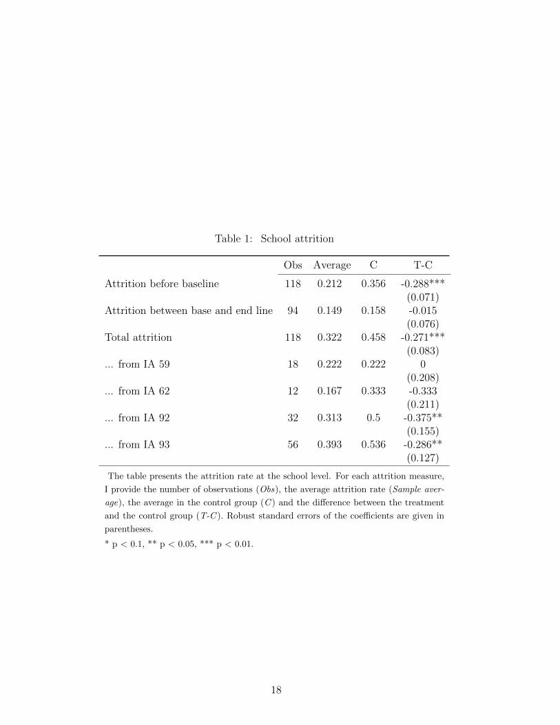
Table 1: School attrition

Obs Average C T-C

Attrition before baseline 118 0.212 0.356 -0.288***(0.071)

Attrition between base and end line 94 0.149 0.158 -0.015(0.076)

Total attrition 118 0.322 0.458 -0.271***(0.083)

... from IA 59 18 0.222 0.222 0(0.208)

... from IA 62 12 0.167 0.333 -0.333(0.211)

... from IA 92 32 0.313 0.5 -0.375**(0.155)

... from IA 93 56 0.393 0.536 -0.286**(0.127)

The table presents the attrition rate at the school level. For each attrition measure,

I provide the number of observations (Obs), the average attrition rate (Sample aver-

age), the average in the control group (C ) and the difference between the treatment

and the control group (T-C ). Robust standard errors of the coefficients are given in

parentheses.

* p < 0.1, ** p < 0.05, *** p < 0.01.

18

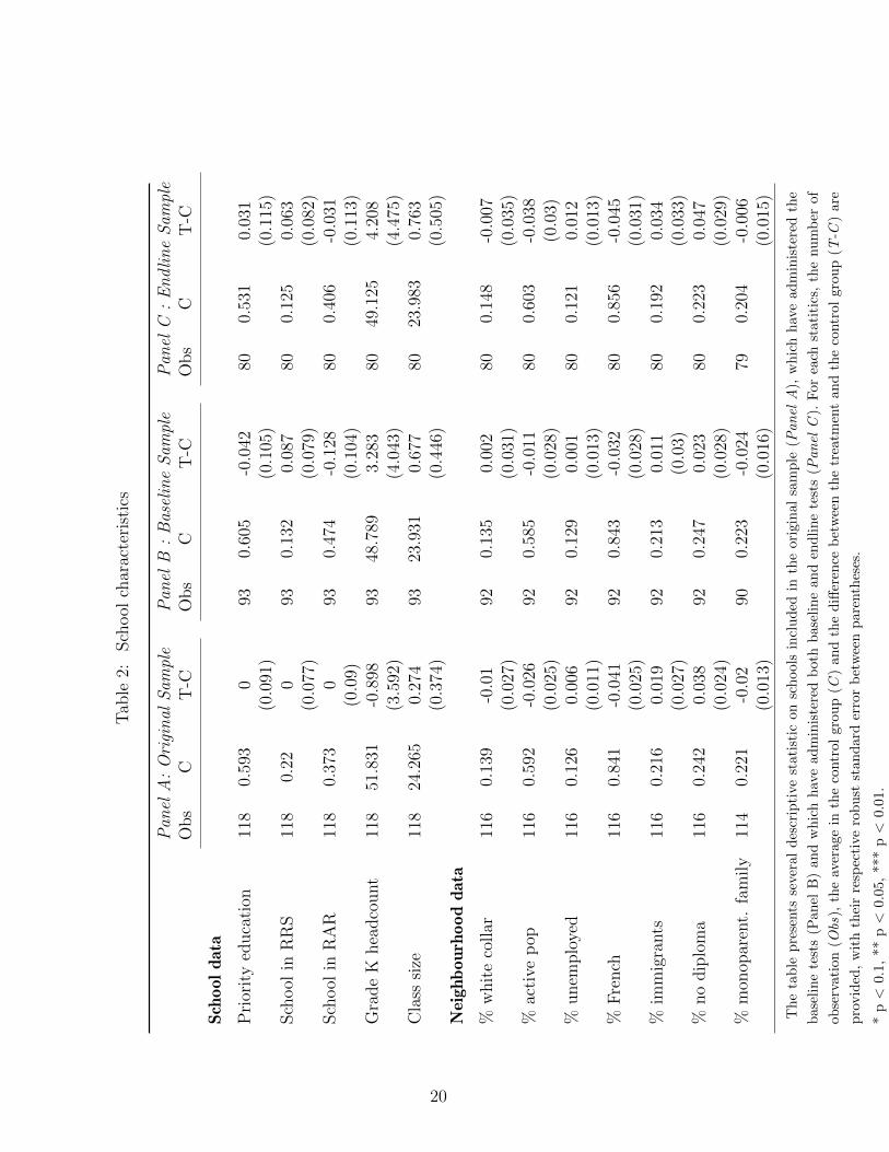
In Table 2, I use the few school-level variables available21 and some socioeconomic data

from neighborhoods to investigate further how attrition may affect the estimation.22 In

Panel A, I describe the schools included in the original 118 schools sample. The schools

selected for this experiment were primarily from poor neighborhoods; the original sample

is composed of a large proportion of schools in priority education, 59% (resp. 37% in

RAR), while the national average is 17.9% (resp. 6.3%) (DEPP (2010)). Schools are also

situated in disadvantaged neighborhoods: unemployment is high at 12.6% (compared to

7.8% in the total population), and the share of immigrants is much higher than the rest

of the population (21.6% versus 6.2% in the total population). This corresponds with

the desired objective to implement the new methodology in the poorest schools. Not

surprisingly at that stage, there are no differences between treatment and control schools,

as size, location, and priority education were used to stratify the sample. Other variables

not used for stratification are also very well balanced.

In Panel B, I look at the same characteristics after the first wave of attrition (before

baseline), allegedly the most worrisome analytically. Average results in the control group

and differences between treatment and control group are not affected significantly by at-

trition before baseline. The same conclusion applies to Panel C where I look at the sample

that have replied to the endline survey.

21Unlike primary schools or secondary schools, data at kindergarten level are scarce in France.22Data from the National Institute of Statistics using IRIS zone.

19

Tab

le2:

Sch

ool

char

acte

rist

ics

Pan

elA

:O

rigi

nal

Sam

ple

Pan

elB

:B

asel

ine

Sam

ple

Pan

elC

:E

nd

lin

eS

ampl

eO

bs

CT

-CO

bs

CT

-CO

bs

CT

-C

Sch

ool

dat

a

Pri

orit

yed

uca

tion

118

0.59

30

930.

605

-0.0

4280

0.53

10.

031

(0.0

91)

(0.1

05)

(0.1

15)

Sch

ool

inR

RS

118

0.22

093

0.13

20.

087

800.

125

0.06

3(0

.077

)(0

.079

)(0

.082

)Sch

ool

inR

AR

118

0.37

30

930.

474

-0.1

2880

0.40

6-0

.031

(0.0

9)(0

.104

)(0

.113

)G

rade

Khea

dco

unt

118

51.8

31-0

.898

9348

.789

3.28

380

49.1

254.

208

(3.5

92)

(4.0

43)

(4.4

75)

Cla

sssi

ze11

824

.265

0.27

493

23.9

310.

677

8023

.983

0.76

3(0

.374

)(0

.446

)(0

.505

)N

eigh

bou

rhood

dat

a

%w

hit

eco

llar

116

0.13

9-0

.01

920.

135

0.00

280

0.14

8-0

.007

(0.0

27)

(0.0

31)

(0.0

35)

%ac

tive

pop

116

0.59

2-0

.026

920.

585

-0.0

1180

0.60

3-0

.038

(0.0

25)

(0.0

28)

(0.0

3)%

unem

plo

yed

116

0.12

60.

006

920.

129

0.00

180

0.12

10.

012

(0.0

11)

(0.0

13)

(0.0

13)

%F

rench

116

0.84

1-0

.041

920.

843

-0.0

3280

0.85

6-0

.045

(0.0

25)

(0.0

28)

(0.0

31)

%im

mig

rants

116

0.21

60.

019

920.

213

0.01

180

0.19

20.

034

(0.0

27)

(0.0

3)(0

.033

)%

no

dip

lom

a11

60.

242

0.03

892

0.24

70.

023

800.

223

0.04

7(0

.024

)(0

.028

)(0

.029

)%

mon

opar

ent.

fam

ily

114

0.22

1-0

.02

900.

223

-0.0

2479

0.20

4-0

.006

(0.0

13)

(0.0

16)

(0.0

15)

The

table

pre

sents

seve

ral

des

crip

tive

stat

isti

con

schools

incl

uded

inth

eori

gin

al

sam

ple

(Pan

elA

),w

hic

hhav

eadm

inis

tere

dth

e

bas

elin

ete

sts

(Pan

elB

)an

dw

hic

hh

ave

adm

inis

tere

db

oth

base

lin

ean

den

dline

test

s(P

an

elC

).F

or

each

stati

tics

,th

enum

ber

of

obse

rvat

ion

(Obs

),th

eav

erag

ein

the

contr

ol

gro

up

(C)

an

dth

ediff

eren

ceb

etw

een

the

trea

tmen

tand

the

contr

ol

gro

up

(T-C

)are

pro

vid

ed,

wit

hth

eir

resp

ecti

vero

bust

stan

dard

erro

rb

etw

een

pare

nth

eses

.

*p<

0.1,

**p<

0.05

,**

*p<

0.01

.

20

4.3 Teacher-Level Data

To obtain additional information besidesschool characteristics, a teacher questionnaire was

sent to all teachers who benefited from the training program. In order to have a point of

comparison, the same questionnaire was also sent to control schools. Unfortunately, lack

of political support rendered surveying control schools in IA 93 and 59 difficult. In both

IAs, therefore, the response rate was significantly lower and highly differential. Generally

speaking, surveying teachers in France is a difficult task.23 Teachers rarely agree to give

their names in surveys and they do not readily answer questionnaires, as they and their

unions often fear that such data would be used for evaluating their individual performances.

Furthermore, school administration is often reluctant to communicate teacher-level infor-

mation. As a result, response rate is not satisfactory: sometimes teachers refused to

communicate the names of their children, sometimes they refused to communicate their

own names, and sometimes they simply neglected to return the questionnaire at all.24

On the full sample, results are undermined by a high and differential attrition level

(a significant -21.6%). Hence, results should be interpreted with care. Yet it seems that

teachers in the treatment group are significantly older and more experienced than those

in the control group. Point estimates suggest that treatment teachers have on average 3.6

years of experience and are 3.6 years older. To a lesser extent, treatment teachers appear

to have more experience in kindergarten. Besides, teachers in the treatment group have

a lower attainment of higher education (-0.6 years). As the minimum requirements to be-

come an elementary teacher have increased during the last 30 years in France, both results

are potentially related. Yet when I condition by birth year, higher education attainment

remains negative and significant (-0.53 years). Treatment teachers are also significantly

more likely to have studied a hard science discipline and less likely to have studied hu-

manities (all subjects). This might be indicative of selection, as scientific studies allegedly

23For instance, France is one of the rare OECD countries that refused to administer the PISA teacherquestionnaire (TALIS) the first year.

24For the cases where I received a questionnaire but either the teacher’s name or the classroom numberwas missing, I simply averaged the results obtained by the teacher(s) and apply the result(s) to all GSchildren enrolled in the school. In subsequent models using teacher characteristics, I will always controlfor a dummy, indicating whether such procedure was implemented. In Table 3, I present the results fromthe teacher survey both on the original sample and on the sample of schools from IA 92 and 62, where thecontrol group was more willing to participate in the survey.

21

attract better students. Finally, in terms of job status, both groups are relatively compa-

rable: teachers are usually full time (permanent), and the vast majority work in only one

school (they are not substitutes). Interestingly, treatment teachers are less likely to work

in mixed-level classes25. As the training program was specifically designed for the last year

of kindergarten, treatment schools may have decided to exclude mixed classes from the

program.

I also present in Table 3 some information on the teacher practices. I first look at the

amount of hours spent on literacy and non-literacy subjects. Although treatment teachers

tend to spend less time on non-literacy subjects, they do not report spending more time on

literacy subjects. More convincing are the variables about the way teaching was structured

in treatment schools: treatment teachers report working more systematically with small

groups of students of the same initial achievement level (tracked small groups) and are

significantly more likely to use only one reading method. Results suggest that the program

has not modified the amount of literacy provided, but has probably more significantly

modified the way literacy classes were given: in small groups, formed by initial achievement

level, and using solely one method (certainly the one provided by the NGO).

Results from the sub-sample composed of schools from IA 92 and IA 62, for which

attrition is lower and not significantly differential26, confirmed and even amplified the

findings. Teachers are on average four years older in the treatment group; they are more

experienced (four additional years), and have more years of experiences in kindergarten.

Similarly to the results obtained on the full sample, treatment teachers have spent fewer

years in higher education and are more likely to be from a hard science background and

less likely from a humanities background.

25Classes were composed of children from different grades. When the preschool is attached to a primaryschool, grade 1 and GS students are usually mixed together, as they belong to the same teaching ”cycle”;otherwise, GS can be mixed with MS, or ”Moyenne Section” (4–5 years old).

26Since detection power is low and differential attrition is not significantly different on the sub-sampleand full sample, absence of significance at this level should be interpreted with caution.

22

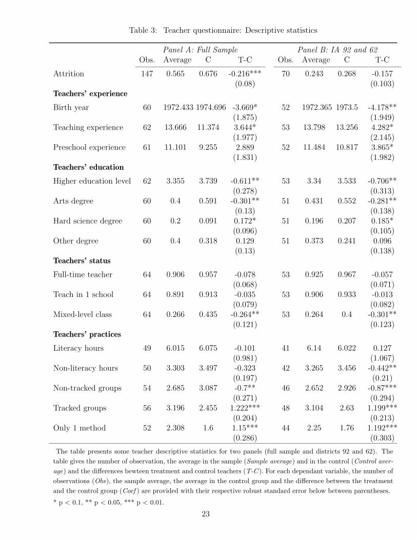
Table 3: Teacher questionnaire: Descriptive statistics

Panel A: Full Sample Panel B: IA 92 and 62Obs. Average C T-C Obs. Average C T-C

Attrition 147 0.565 0.676 -0.216*** 70 0.243 0.268 -0.157(0.08) (0.103)

Teachers’ experience

Birth year 60 1972.433 1974.696 -3.669* 52 1972.365 1973.5 -4.178**(1.875) (1.949)

Teaching experience 62 13.666 11.374 3.644* 53 13.798 13.256 4.282*(1.977) (2.145)

Preschool experience 61 11.101 9.255 2.889 52 11.484 10.817 3.865*(1.831) (1.982)

Teachers’ education

Higher education level 62 3.355 3.739 -0.611** 53 3.34 3.533 -0.706**(0.278) (0.313)

Arts degree 60 0.4 0.591 -0.301** 51 0.431 0.552 -0.281**(0.13) (0.138)

Hard science degree 60 0.2 0.091 0.172* 51 0.196 0.207 0.185*(0.096) (0.105)

Other degree 60 0.4 0.318 0.129 51 0.373 0.241 0.096(0.13) (0.138)

Teachers’ status

Full-time teacher 64 0.906 0.957 -0.078 53 0.925 0.967 -0.057(0.068) (0.071)

Teach in 1 school 64 0.891 0.913 -0.035 53 0.906 0.933 -0.013(0.079) (0.082)

Mixed-level class 64 0.266 0.435 -0.264** 53 0.264 0.4 -0.301**(0.121) (0.123)

Teachers’ practices

Literacy hours 49 6.015 6.075 -0.101 41 6.14 6.022 0.127(0.981) (1.067)

Non-literacy hours 50 3.303 3.497 -0.323 42 3.265 3.456 -0.442**(0.197) (0.21)

Non-tracked groups 54 2.685 3.087 -0.7** 46 2.652 2.926 -0.87***(0.271) (0.294)

Tracked groups 56 3.196 2.455 1.222*** 48 3.104 2.63 1.199***(0.204) (0.213)

Only 1 method 52 2.308 1.6 1.15*** 44 2.25 1.76 1.192***(0.286) (0.303)

The table presents some teacher descriptive statistics for two panels (full sample and districts 92 and 62). The

table gives the number of observation, the average in the sample (Sample average) and in the control (Control aver-

age) and the differences bewteen treatment and control teachers (T-C ). For each dependant variable, the number of

observations (Obs), the sample average, the average in the control group and the difference between the treatment

and the control group (Coef ) are provided with their respective robust standard error below between parentheses.

* p < 0.1, ** p < 0.05, *** p < 0.01.

23

The literature usually suggests that observable characteristics are not very predictive

of teacher effect. Yet, among the various studies about teacher effect, years of experience

were reported to be the most predictive. In the most recent work on this topic, Harris

and Sass (2011) find for instance that, in elementary school, each year of experience is

associated with approximately 0.65% of a standard deviation increase in reading skills.

To verify whether such a relationship is present here, I look at the correlation between

teachers’ characteristics and follow-up test scores, controlling for baseline test scores and

some individual characteristics. Results are presented in Table 4.

Given the small sample size and the classroom-level clustering, I lack statistical power

to precisely identify the effect.27 Some suggestive correlations, however, can be significantly

identified. Teaching experience is, for instance, estimated to have a positive effect of 0.6%

to 1% per year. This is very close to the estimation found by Harris and Sass (2011)(0.65%

per year of experience).28 Taken linearly at face value, this rough estimate would translate

into a .20 to .33 s.d. difference between the youngest teacher (0 years of experience)

and the oldest teacher in my sample (33 years of experience). I then look at the effect

previous education track on pupil progression. I divide degrees into three groups: arts,

hard science, and others.29 I find that art and hard science degrees outperform other

degrees by a significant 15% s.d., with art and hard science effect being similar most of

the time. The coefficient for higher education level (attainment) is also significant. Since

teachers in the treatment group are both more experienced but less educated and less likely

to have specialized in arts, it is uncertain in which direction a teacher selection bias would

go. Further investigations on the impact of teacher effect will be undertaken in Section 7.

27Note that Harris and Sass (2011) do not cluster at the teacher level, but use the panel structure oftheir dataset by adding a teacher fixed effect.

28In fact, Harris and Sass estimate a more flexible model allowing for a nonlinear impact of experience.They find, for instance, that after 15–24 years of experience, teachers have a value-added effect of .13standard deviation above teachers with no experience, which translates to a rough linear effect of .13/20 =6.5% per year of experience. Due to the small sample size, my dataset does not allow a similar non-linearestimation.

29Others are grouped into all field not included in art and hard science: political science, law, vocationaltraining, computer science, and so forth.

24

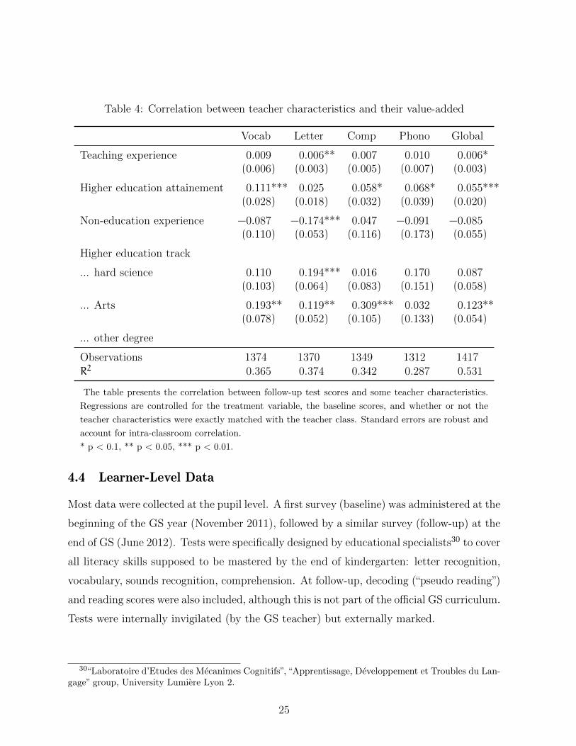
Table 4: Correlation between teacher characteristics and their value-added

Vocab Letter Comp Phono Global

Teaching experience 0.009 0.006** 0.007 0.010 0.006*(0.006) (0.003) (0.005) (0.007) (0.003)

Higher education attainement 0.111*** 0.025 0.058* 0.068* 0.055***(0.028) (0.018) (0.032) (0.039) (0.020)

Non-education experience −0.087 −0.174*** 0.047 −0.091 −0.085(0.110) (0.053) (0.116) (0.173) (0.055)

Higher education track

... hard science 0.110 0.194*** 0.016 0.170 0.087(0.103) (0.064) (0.083) (0.151) (0.058)

... Arts 0.193** 0.119** 0.309*** 0.032 0.123**(0.078) (0.052) (0.105) (0.133) (0.054)

... other degree

Observations 1374 1370 1349 1312 1417R2 0.365 0.374 0.342 0.287 0.531

The table presents the correlation between follow-up test scores and some teacher characteristics.

Regressions are controlled for the treatment variable, the baseline scores, and whether or not the

teacher characteristics were exactly matched with the teacher class. Standard errors are robust and

account for intra-classroom correlation.

* p < 0.1, ** p < 0.05, *** p < 0.01.

4.4 Learner-Level Data

Most data were collected at the pupil level. A first survey (baseline) was administered at the

beginning of the GS year (November 2011), followed by a similar survey (follow-up) at the

end of GS (June 2012). Tests were specifically designed by educational specialists30 to cover

all literacy skills supposed to be mastered by the end of kindergarten: letter recognition,

vocabulary, sounds recognition, comprehension. At follow-up, decoding (“pseudo reading”)

and reading scores were also included, although this is not part of the official GS curriculum.

Tests were internally invigilated (by the GS teacher) but externally marked.

30“Laboratoire d’Etudes des Mecanimes Cognitifs”, “Apprentissage, Developpement et Troubles du Lan-gage” group, University Lumiere Lyon 2.

25

Tab

le5:

Att

riti

onra

tes:

pupil

asse

ssm

ents

Pan

elA

:F

ull

Sam

ple

Pan

elB

:N

on-m

issi

ng

stra

taO

bs.

Clu

st.

aver

age

CT

-CO

bs.

Clu

st.

aver

age

CT

-C

Ove

rall

Tot

alat

trit

ion

6222

118

0.37

90.

531

−0.

322*

**20

0042

0.19

50.

217

−0.

047

(0.0

79)

(0.1

18)

Sch

ool

leve

lat

trit

ion

6222

118

0.30

50.

484

−0.

38**

*20

0042

0.13

70.

132

0.01

(0.0

82)

(0.1

24)

Pupil

leve

lat

trit

ion

6222

118

0.07

50.

047

0.05

8*20

0042

0.05

80.

085

−0.

056*

*(0

.034)

(0.0

24)

Bet

wee

nba

seli

ne

and

end

lin

e

Tot

alat

trit

ion

4429

930.

214

0.21

20.

004

1885

420.

205

0.22

3−

0.03

8(0

.073)

(0.1

23)

Sch

ool

leve

lat

trit

ion

4429

930.

120.

131

−0.

019

1885

420.

144

0.13

60.

017

(0.0

71)

(0.1

3)P

upil

leve

lat

trit

ion

4429

930.

094

0.08

10.

023

1885

420.

060.

086

−0.

055*

*(0

.04)

(0.0

25)

Bef

ore

Bas

elin

e

Tot

alat

trit

ion

6222

118

0.28

80.

426

−0.

293*

**20

0042

0.05

80.

037

0.04

3(0

.077)

(0.0

3)Sch

ool

leve

lat

trit

ion

6222

118

0.22

40.

407

−0.

387*

**20

0042

0.00

00.

000

0.00

0(0

.071)

(.)

Pupil

leve

lat

trit

ion

6222

118

0.06

40.

019

0.09

5***

2000

420.

058

0.03

70.

043

(0.0

35)

(0.0

3)

The

table

pre

sents

the

pupil

asse

ssm

ent

attr

itio

nra

teat

diff

eren

tti

me

per

iod

and

for

diff

eren

tatt

riti

on

leve

l:to

tal

att

riti

on

isth

esu

mof

sch

ool

-lev

elat

trit

ion

(the

all

sch

ool

did

not

resp

ond)

and

pupil-l

evel

att

riti

on

(som

ech

ild

ren

or

teach

ers

ina

resp

on

din

gsc

hool

did

not

re-

spon

ded

).O

bs.

isth

eto

tal

num

ber

ofpup

ils,

Clu

st.

the

tota

lnum

ber

of

schools

,A

vera

geth

eav

erage

att

riti

on

inb

oth

gro

up

s,C

the

att

riti

on

inth

eco

ntr

olan

dT

-Cth

ediff

eren

tial

attr

itio

nw

ith

the

robu

stan

dcl

ust

ered

standard

erro

rb

elow

bet

wee

npare

nth

eses

.A

ttri

tion

rate

sare

give

nfo

rth

efu

llsa

mple

(Pan

elA

)an

dfo

rth

est

rata

wher

eall

the

schools

resp

ond

ed(P

an

elB

).

*p<

0.1,

**p<

0.05

,**

*p<

0.01

.

26

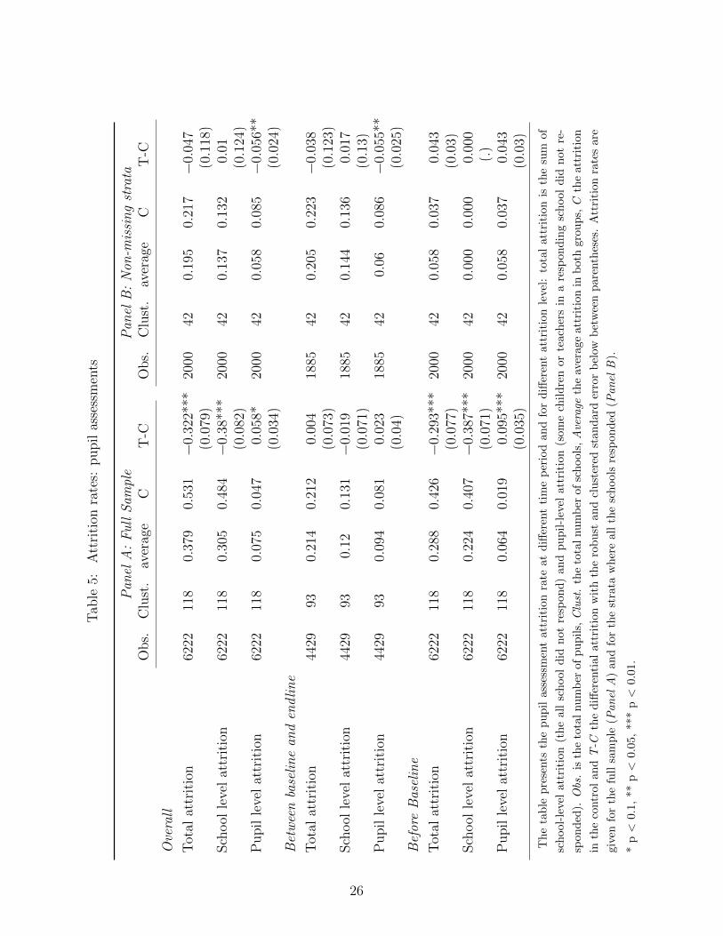
Panel A of Table 5 describes the rate of response obtained from the pupil survey.

Taken together and on the full sample (first 3 rows), overall attrition (the child has not

responded to either baseline or follow-up) is high (38% from the original sample of 6222

students and 118 schools) and significantly different in control and treatment (-32%). As

mentioned before, school-level attrition (the whole school refused to respond) fully drives

down the response rates. This illustrates the fact that in many instances, schools – more

systematically, control schools – refused to administer the tests. More surprising is the

+5.8% significant effect for pupil’s attrition (the school responded but not the pupil).

Although one could imagine that the teachers in the treatment schools might have been

more motivated to have every child present for the test, this is probably not the most

probable explanation.31 Rather, in control schools that accepted to participate in the

evaluation, it is probable that some teachers refused to administer the tests.

Then, I decompose “overall attrition” into attrition before baseline and between base-

line and follow-up. Although attrition remains important between baseline and follow-up,

at that stage, attrition is not differential, suggesting that when schools accepted the pro-

tocol, the intervention did not change their response behavior. Hence, attrition between

baseline and follow-up is less likely to pose an analytic threat. More worrisome is attrition

before baseline (between the sample formation and the baseline assessment), which is high

(28.8%), still driven by attrition at school level (22.4%), and strongly differential (-29% in

total, -38.7% from schools). On the full sample, attrition poses a real threat to analysis.

32

One way to circumvent the attrition issue is to compare similar respondent schools

(composed of supposedly more similar teachers), using the way the sample was formed be-

fore baseline. As said, to select the control schools, 24 strata were formed based on district

location, school size, and priority education level. For each treatment school included in a

strata, one control school was randomly selected. Treatment and control schools included

in the same strata are allegedly more comparable, especially if the variables used for strat-

ification are predictive of the school/teacher effect. As a result, it is interesting to look at

31I doubt teachers would have sufficient leverage to convince parents to send their children to school onthat day.

32Note that while downward bias is more credible as complier schools and teachers are more likely tobe better performing, an upward bias cannot be ruled out.

27

the results obtained on the strata in which no schools have dropped before baseline (10

strata out of 24). Results for this sub-sample are presented in Panel B.

By definition in Panel B, attrition rate at school level “before baseline” is 0, and total

attrition remains small and not significantly different in the treatment and control group.

Although some pupil level attrition has occurred between baseline and follow-up, the overall

differential attrition is reduced to a nonsignificant -4.7%. Panel B sample is hence a credible

sample to estimate the treatment effect purified from most teacher/school selection due to

attrition.

Interesting as well are the results obtained in both experimental groups at baseline and

follow-up as displayed in Table 6. In Panel A, I look at the results obtained at baseline

and follow-up on test scores on the full sample. At baseline, the treatment group under-

performed significantly compared to the control group (around a quarter of a standard

deviation below). Since both groups were not formed randomly, initial disequilibrium may

be contingent, and should not pose an analytical problem as long as the VAM’s assumptions

mentioned in Section 2 are met. Yet it may also be indicative of selection at the teacher or

the school level. For instance, if the district managers have chosen the traditionally poorer

performing schools (composed of the least performing teachers) to implement the program

in their district (and if stratification did not control for this selection), estimation results

should be biased. If selection has occurred, treatment effect should be a priori biased

toward zero. Overestimation of the treatment effect would only be possible if district

managers have chosen the schools composed of both low performing students but good

performing teachers. This would be at odds with some previous results regarding the way

teachers are allocated in France.33 Attrition before baseline, as documented previously,

may also account for the differences in initial performance. For instance, if the least

performing control schools dropped out from the sample before baseline, the population

of respondent control schools would obtain better results. Again, downward bias is more

credible here. If one assumes no teacher or school selection, the study is, in fact, in a

relatively favorable situation. As mentioned in Section 2, when no selection occurs at the

teacher or school level, the sign of the VAM1 bias is fully determined by r(A0, T), the initial

33See Bressoux et al. (2009), where they suggest that more experienced teachers are assigned to betterperforming schools in France.

28

group’s equilibrium. Since the treatment group’s students initially under-perform versus

the controls, the VAM1 should give a downward biased estimate of the true treatment

effect.

More interesting at that point are the results obtained on the students in schools not

affected by baseline attrition (non-missing strata). This subsample, which is allegedly less

affected by attrition bias, is highly comparable to the full sample. Column C of Panel B

shows that results of the control group are almost similar in both panels.34

At endline, the treatment group seems to have caught up with the control group in

the full sample and in the sample composed of strata without missing schools in a similar

fashion: naive difference-in-differences estimates (“T-C” columns) give comparable effect

sizes in both samples. To give statistical weight to this assertion, I compare in column

“A-B Panel” the naive difference-in-differences estimate. They are all near zero and never

significant.

34Results are standardized using the standard deviation of the control group; hence, the control groupestimates on the non missing strata sub-sample indicates the difference between the full sample and thissub-sample. For instance, on the sub-sample, control children in panel B outperform the full sample by anonsignificant 1.8% of a standard deviation.

29

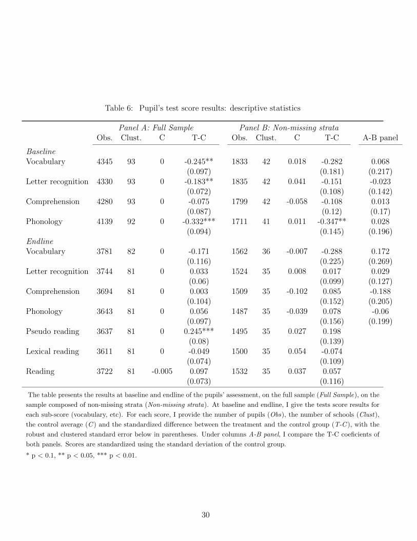
Table 6: Pupil’s test score results: descriptive statistics

Panel A: Full Sample Panel B: Non-missing strataObs. Clust. C T-C Obs. Clust. C T-C A-B panel

BaselineVocabulary 4345 93 0 -0.245** 1833 42 0.018 -0.282 0.068

(0.097) (0.181) (0.217)Letter recognition 4330 93 0 -0.183** 1835 42 0.041 -0.151 -0.023

(0.072) (0.108) (0.142)Comprehension 4280 93 0 -0.075 1799 42 -0.058 -0.108 0.013

(0.087) (0.12) (0.17)Phonology 4139 92 0 -0.332*** 1711 41 0.011 -0.347** 0.028

(0.094) (0.145) (0.196)EndlineVocabulary 3781 82 0 -0.171 1562 36 -0.007 -0.288 0.172

(0.116) (0.225) (0.269)Letter recognition 3744 81 0 0.033 1524 35 0.008 0.017 0.029

(0.06) (0.099) (0.127)Comprehension 3694 81 0 0.003 1509 35 -0.102 0.085 -0.188

(0.104) (0.152) (0.205)Phonology 3643 81 0 0.056 1487 35 -0.039 0.078 -0.06

(0.097) (0.156) (0.199)Pseudo reading 3637 81 0 0.245*** 1495 35 0.027 0.198

(0.08) (0.139)Lexical reading 3611 81 0 -0.049 1500 35 0.054 -0.074

(0.074) (0.109)Reading 3722 81 -0.005 0.097 1532 35 0.037 0.057

(0.073) (0.116)

The table presents the results at baseline and endline of the pupils’ assessment, on the full sample (Full Sample), on the

sample composed of non-missing strata (Non-missing strata). At baseline and endline, I give the tests score results for

each sub-score (vocabulary, etc). For each score, I provide the number of pupils (Obs), the number of schools (Clust),

the control average (C ) and the standardized difference between the treatment and the control group (T-C ), with the

robust and clustered standard error below in parentheses. Under columns A-B panel, I compare the T-C coeficients of

both panels. Scores are standardized using the standard deviation of the control group.

* p < 0.1, ** p < 0.05, *** p < 0.01.

30

In all, I have no reason to believe that the non-missing strata sample is significantly

different from the full sample. It presents no different baseline test scores and is comparable

in terms of school level characteristics (results not displayed here). Unfortunately, I am

able to provide a similar argument for teacher-level characteristics, as the schools that

did not drop out are not necessarily composed of teachers who responded to the teacher

questionnaire. I am here facing one limitation of my data: I can either deal with attrition

or teacher-level selection, but not both at the same time. Fortunately, results are quite

consistent whatever strategy is used.

5 Results

5.1 Comparing Value-Added Models

I first present in Table 8 the results from both value added models presented in Section 2,

using the competences that were tested at both baseline and follow-up. Results from VAM1

are generally positive and significant for competences that were primarily stimulated by

the new pedagogy (i.e., phonology and letter recognition). Results are closer to zero for

competences not directly related to the treatment (vocabulary and comprehension). These

results have both a positive and negative side. On one hand, it means that the training

program was able, in the short run, to enhance the desired competences (phonology). On

the other, the training program did not improve other competences that are relevant for

literacy (vocabulary comprehension). Note, however, that the children are 5.5 years old

on average, and so the majority are not readers. One may think that comprehension and

vocabulary are competences that will be improved when decoding is secured. Besides, the

fact that not all competences were improved suggests that results are not fully driven by

selection at the teacher or school level, as such selection would have affected positively all

competences indistinctly.

31

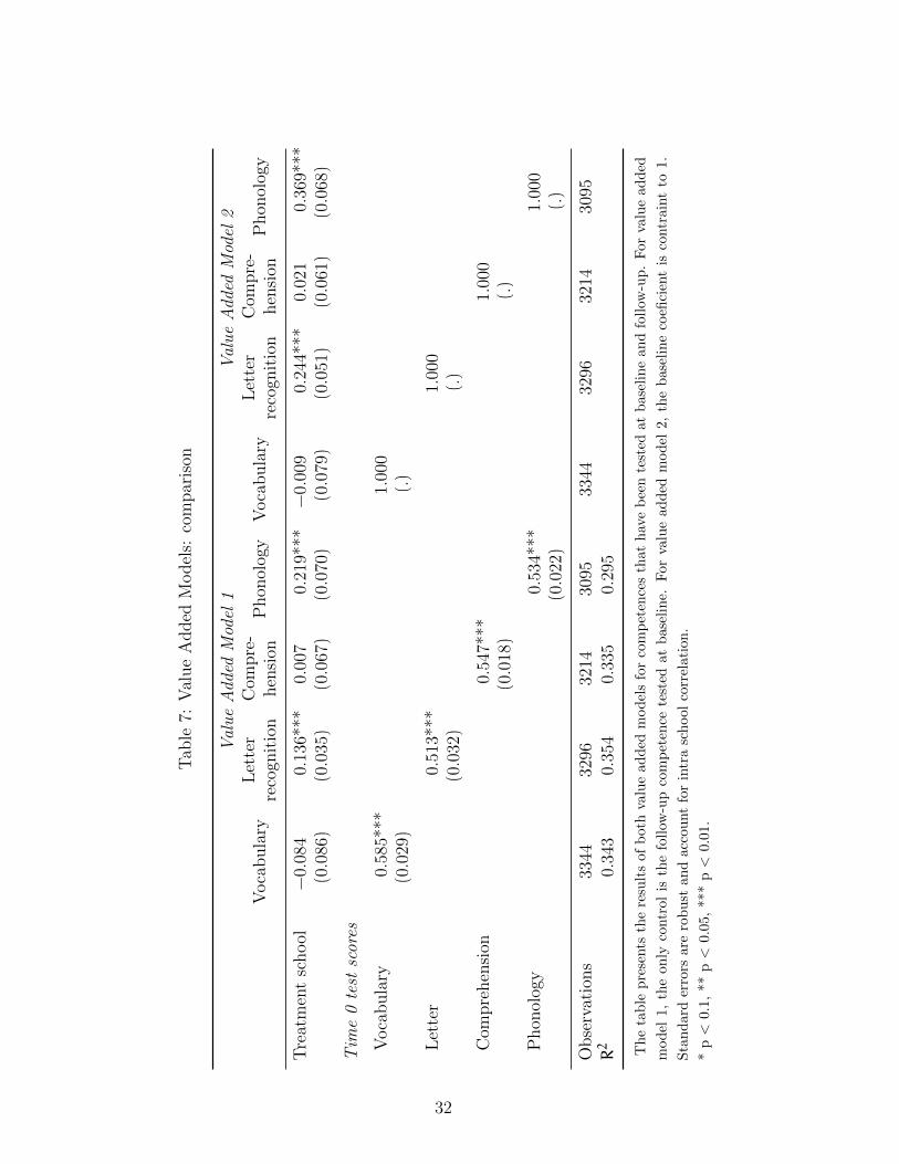
Tab

le7:

Val

ue

Added

Model

s:co

mpar

ison

Val

ue

Add

edM

odel

1V

alu

eA

dded

Mod

el2

Voca

bula

ryL

ette

rre

cogn

itio

nC

ompre

-hen

sion

Phon

olog

yV

oca

bula

ryL

ette

rre

cogn

itio

nC

ompre

-hen

sion

Phon

olog

y

Tre

atm

ent

school

−0.

084

0.13

6***

0.00

70.

219*

**−

0.00

90.

244*

**0.

021

0.36

9***

(0.0

86)

(0.0

35)

(0.0

67)

(0.0

70)

(0.0

79)

(0.0

51)

(0.0

61)

(0.0

68)

Tim

e0

test

scor

es

Voca

bula

ry0.

585*

**1.

000

(0.0

29)

(.)

Let

ter

0.51

3***

1.00

0(0

.032)

(.)

Com

pre

hen

sion

0.54

7***

1.00

0(0

.018)

(.)

Phon

olog

y0.

534*

**1.

000

(0.0

22)

(.)

Obse

rvat

ions

3344

3296

3214

3095

3344

3296

3214

3095

R2

0.34

30.

354

0.33

50.

295

The

table

pre

sents

the

resu

lts

ofb

oth

valu

ead

ded

model

sfo

rco

mp

eten

ces

that

hav

eb

een

test

edat

base

line

and

follow

-up

.F

or

valu

ead

ded

model

1,th

eon

lyco

ntr

olis

the

follow

-up

com

pet

ence

test

edat

base

lin

e.F

or

valu

ead

ded

model

2,

the

base

lin

eco

efici

ent

isco

ntr

ain

tto

1.

Sta

ndar

der

rors

are

rob

ust

and

acco

unt

for

intr

asc

hool

corr

elati

on

.

*p<

0.1,

**p<

0.05

,**

*p<

0.01

.

32

As expected from the model, since VAM1’s γs are below 1 and hence below VAM2’s,

VAM2’s (constrained to 1), results are larger than those of VAM1’s. Besides, γs are

far below from 1 (around .5), suggesting that ρs are likely to be below 0, and hence, the

underlying progression model is convergent.35 This is in line with what one may intuitively

think about child development: the initial gap in early reading skills is expected to be filled

(at least partly) when reading lessons start. In what follows, I will exclusively rely on VAM1

’s results, which are a low bound of the true treatment effect.

5.2 Pupil-Level Characteristics Estimates

To improve my estimation, I add in Table 8 several additional baseline characteristics to

the value added model 1 (quarter of birth, gender, and whether or not the child has a

foreign-sounding first name), and I control for a full set of baseline test scores. I also add

as co-variate the average within classroom of the baseline global test score (“peer effect”):

I intend to capture the effect of being enrolled in a classroom with higher-performing

peers.36 I finally estimate the effect on dimensions that were not evaluated at baseline:

pseudo reading (decoding, reading of nonlexical words) and lexical reading (ability to read

actual words, a skill that is not supposed to be mastered at that age).

Results are consistently positive and significant for the dimensions most directly stim-

ulated by the training program: segmentation and sounds recognition (later regrouped

into a phonology index) are, for instance, positive and significant (.18 s.d. and .24 s.d.),

while comprehension and vocabulary are unaffected. The strongest effect is found on the

“Pseudo-reading” competence, whose effect is particularly large (.45 s.d.). Point estimate

for the lexical reading score is smaller but remains significant. Note, however, that at

that the ages of 5 to 6, pupils are not supposed to be readers, and baseline test scores

are not good predictors of this competence (lower R2, smaller baseline follow-up corre-

lation). Besides, I can relatively precisely detect a significant effect of 13.5% standard

deviation on letter recognition skills, a competence only indirectly covered by the training

35As said, γ is biased downward. As a result, the convergence of the model can only be suggested, notproven. The fact that γs are far from 1 indicates, however, that only a large measurement error wouldmake a divergent model credible.

36Following Manski (1993), I here estimate the combined endogenous and exogenous peer effect.

33

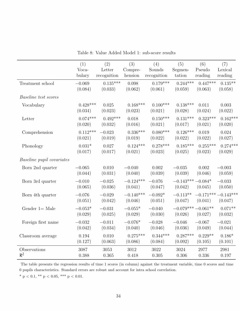
Table 8: Value Added Model 1: sub-score results

(1) (2) (3) (4) (5) (6) (7)Voca-bulary

Letterrecognition

Compre-hension

Soundsrecognition

Segmen-tation

Pseudoreading

Lexicalreading

Treatment school −0.069 0.135*** 0.098 0.179*** 0.244*** 0.447*** 0.135**(0.084) (0.033) (0.062) (0.061) (0.059) (0.063) (0.058)

Baseline test scores

Vocabulary 0.428*** 0.025 0.168*** 0.100*** 0.138*** 0.011 0.003(0.034) (0.023) (0.023) (0.021) (0.028) (0.024) (0.022)

Letter 0.074*** 0.492*** 0.018 0.150*** 0.131*** 0.323*** 0.162***(0.020) (0.032) (0.016) (0.021) (0.017) (0.021) (0.020)

Comprehension 0.112*** −0.023 0.336*** 0.080*** 0.126*** 0.019 0.024(0.021) (0.019) (0.019) (0.022) (0.022) (0.022) (0.027)

Phonology 0.031* 0.027 0.124*** 0.278*** 0.185*** 0.255*** 0.274***(0.017) (0.017) (0.021) (0.023) (0.025) (0.023) (0.029)

Baseline pupil covariates

Born 2nd quarter −0.065 0.010 −0.040 0.002 −0.035 0.002 −0.003(0.044) (0.031) (0.040) (0.039) (0.039) (0.046) (0.059)

Born 3rd quarter −0.010 −0.025 −0.124*** −0.076 −0.143*** −0.084* −0.033(0.065) (0.036) (0.041) (0.047) (0.042) (0.045) (0.050)

Born 4th quarter −0.076 −0.029 −0.140*** −0.092* −0.113** −0.171*** −0.143***(0.051) (0.042) (0.046) (0.051) (0.047) (0.041) (0.047)

Gender 1= Male −0.053* −0.031 −0.055* −0.040 −0.079*** −0.061** 0.071**(0.029) (0.025) (0.029) (0.030) (0.026) (0.027) (0.032)

Foreign first name −0.032 −0.011 −0.076* −0.028 −0.046 −0.067 −0.021(0.042) (0.034) (0.040) (0.046) (0.036) (0.049) (0.044)

Classroom average 0.194 0.010 0.275*** 0.344*** 0.287*** 0.229** 0.186*(0.127) (0.063) (0.086) (0.084) (0.092) (0.105) (0.101)

Observations 3087 3053 3012 3022 3024 2977 2981R2 0.388 0.365 0.418 0.305 0.306 0.336 0.197

The table presents the regression results of time 1 scores (in column) against the treatment variable, time 0 scores and time

0 pupils characteristics. Standard errors are robust and account for intra school correlation.

* p < 0.1, ** p < 0.05, *** p < 0.01.

34

program.37 Finally, correlation between baseline variables and follow-up test score suggests

that letter recognition and phonology competences (segmentation and sounds recognition)

are the most predictive competences for reading, while comprehension and vocabulary are

barely positively correlated with reading competences. These correlations legitimate the

focus given by the training program to phonology, and also suggest that such short-term

phonological stimulation will translate into better reading skills at a later stage.38

Incidentally, Table 8 allows to infer a few other interesting relationships. Not surpris-

ingly, maturity matters for cognition, as at the end of the year, students achieve on average

around 12% standard deviation lower than children born at the beginning of the year. Also

not surprisingly, boys underperform girls on most competences (at timesby around 6 %for

reading (but reading estimates are more noisy). Having a foreign first name is negative, but

rarely significant effect, and close to zero. In fact, having a foreign first name is associated

with a 15% s.d. lower performance at baseline, but ability to progress is not significantly

affected. Finally, I find strong and significant peer effects: having better-performing peers

does influence positively on a student’s results. Whether such positive results are due to di-

rect interactions in the classroom (endogenous effect) or to the socioeconomic composition

of the classroom (exogenous effect) is outside the scope of this paper.

5.3 Results by Initial Achievement Level

One of the expected outcomes of the program is to reinforce the reading skills of the weakest

students and prevent their reading difficulty in grade 1. Since pupils were assigned to four

tracked groups depending on their initial achievement level, it is natural to split the sample

into four groups based on baseline results within schools. Using the VAM1 and keeping

the same control variable used in Table 8, I estimate the effect by initial achievement and

present the result in Table 9. Results of the control in each group show that the weakest,

group 1, is quite significantly delayed (between .4 and .7 standard deviation below the

control average), with a large chunk of the distribution (around 15%) falling even below

37The letter recognition test consists of identifying the “name” of the letter, not its sound. While themethodology focuses mostly on sounds recognition, it is likely that it indirectly made the pupils familiarwith the letters.

38Hence confirming some of the findings in the psychological literature.

35

one standard deviation from the average achievement in the control.39

As expected, the program is particularly effective on the weakest pupils. Impacts on

group 1 are strongest on dimensions directly stimulated by the program (letter recognition,

segmentation), and the magnitude of the effects tend toward zero as initial achievement

improved. The progressive nature of the treatment effect for both dimensions is confirmed

when the treatment variable interacts with the group variable40 (“TxGroup”column). Like-

wise, absence of positive treatment effect on comprehension found in Table 8 is nuanced,

as the program is quite significantly helpful for the weakest children (+.22 s.d.), a possible

consequence of the letter and segmentation’s positive effects. Finally, no such heteroge-

neous effect can be found on reading scores and on sounds recognition, while vocabulary,

a dimension not directly stimulated by the program, is never positively affected. These

effects are consistent with one of the desired effects of the program, adjusting content to

everyone’s initial achievement. The weakest children progress faster in skills that arguably

constitute the first reading steps (letter recognition and segmentation), while the impact is

more “flat” on skills that may benefit more advanced students (nonlexical reading sounds

recognition).

39Such results are consistent with international comparisons where France is often characterized bylarge achievement inequalities (see the PISA report 2014 for France).

40The group variable takes value 1 for the weakest, and 4 for the strongest group.

36

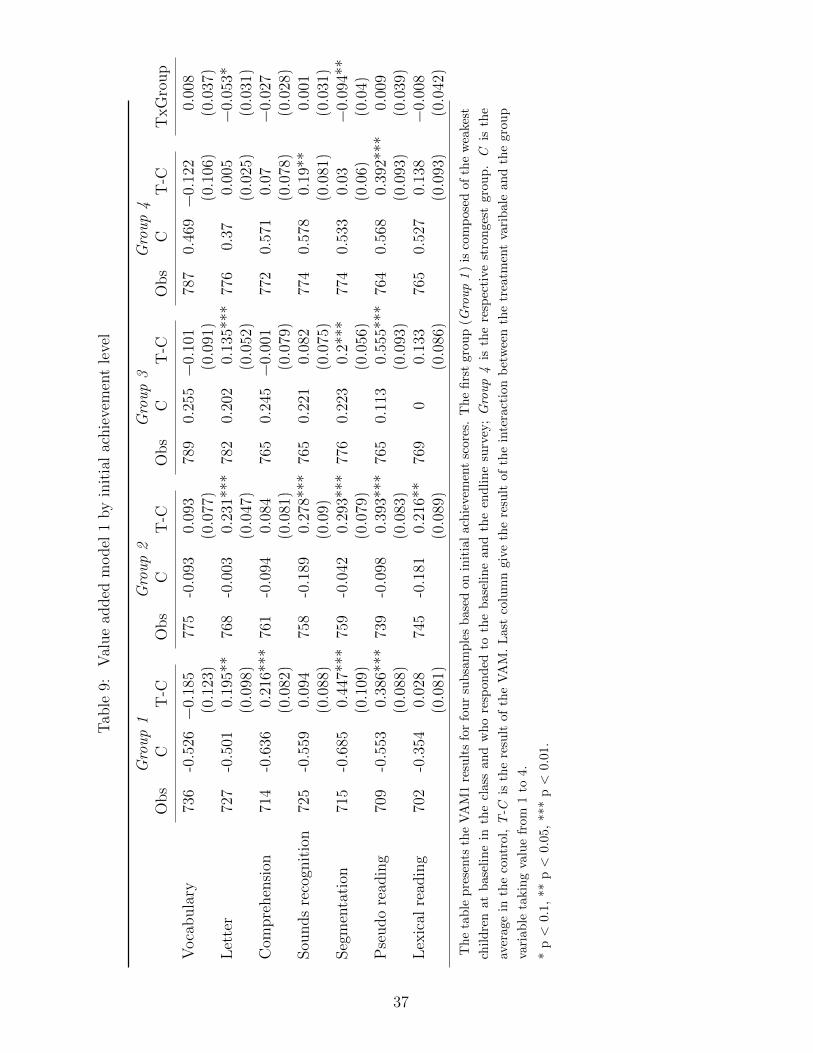
Tab

le9:

Val

ue

added

model

1by

init

ial

achie

vem

ent

leve

l

Gro

up

1G

rou

p2

Gro

up

3G

rou

p4

Obs

CT

-CO

bs

CT

-CO

bs

CT

-CO

bs

CT

-CT

xG

roup

Voca

bula

ry73

6-0

.526

−0.

185

775

-0.0

930.

093

789

0.25

5−

0.10

178

70.

469

−0.

122

0.00

8(0

.123)

(0.0

77)

(0.0

91)

(0.1

06)

(0.0

37)

Let

ter

727

-0.5

010.

195*

*76

8-0

.003

0.23

1***

782

0.20

20.

135*

**77

60.

370.

005

−0.

053*

(0.0

98)

(0.0

47)

(0.0

52)

(0.0

25)

(0.0

31)

Com

pre

hen

sion

714

-0.6

360.

216*

**76

1-0

.094

0.08

476

50.

245

−0.

001

772

0.57

10.

07−

0.02

7(0

.082)

(0.0

81)

(0.0

79)

(0.0

78)

(0.0

28)

Sou

nds

reco

gnit

ion

725

-0.5

590.

094

758

-0.1

890.

278*

**76

50.

221

0.08

277

40.

578

0.19

**0.

001

(0.0

88)

(0.0

9)(0

.075)

(0.0

81)

(0.0

31)

Seg

men

tati

on71

5-0

.685

0.44

7***

759

-0.0

420.

293*

**77

60.

223

0.2*

**77

40.

533

0.03

−0.

094*

*(0

.109)

(0.0

79)

(0.0

56)

(0.0

6)(0

.04)

Pse

udo

read

ing

709

-0.5

530.

386*

**73

9-0

.098

0.39

3***

765

0.11

30.

555*

**76

40.

568

0.39

2***

0.00

9(0

.088)

(0.0

83)

(0.0

93)

(0.0

93)

(0.0

39)

Lex

ical

read

ing

702

-0.3

540.

028

745

-0.1

810.

216*

*76

90

0.13

376

50.

527

0.13

8−

0.00

8(0

.081)

(0.0

89)

(0.0

86)

(0.0

93)

(0.0

42)

The

table

pre

sents

the

VA

M1

resu

lts

for

fou

rsu

bsa

mple

sbase

don

init

ial

ach

ieve

men

tsc

ore

s.T

he

firs

tgro

up

(Gro

up

1)

isco

mp

ose

dof

the

wea

kest

child

ren

atbas

elin

ein

the

clas

san

dw

ho

resp

onded

toth

ebase

line

and

the

endline

surv

ey;

Gro

up

4is

the

resp

ecti

vest

ron

ges

tgro

up

.C

isth

e

aver

age

inth

eco

ntr

ol,

T-C

isth

ere

sult

ofth

eV

AM

.L

ast

colu

mn

giv

eth

ere

sult

of

the

inte

ract

ion

bet

wee

nth

etr

eatm

ent

vari

bale

and

the

gro

up

vari

able

takin

gva

lue

from

1to

4.

*p<

0.1,

**p<

0.05

,**

*p<

0.01

.

37

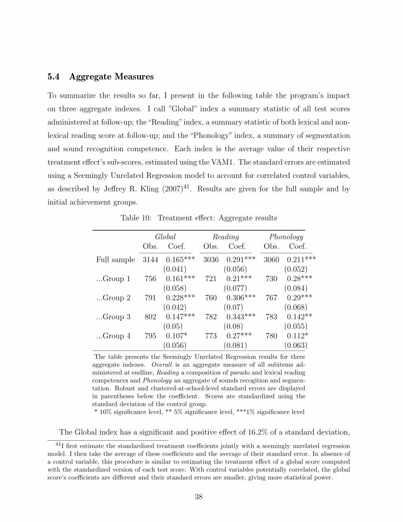
5.4 Aggregate Measures

To summarize the results so far, I present in the following table the program’s impact

on three aggregate indexes. I call ”Global” index a summary statistic of all test scores

administered at follow-up; the“Reading”index, a summary statistic of both lexical and non-

lexical reading score at follow-up; and the “Phonology” index, a summary of segmentation

and sound recognition competence. Each index is the average value of their respective

treatment effect’s sub-scores, estimated using the VAM1. The standard errors are estimated

using a Seemingly Unrelated Regression model to account for correlated control variables,

as described by Jeffrey R. Kling (2007)41. Results are given for the full sample and by

initial achievement groups.

Table 10: Treatment effect: Aggregate results

Global Reading PhonologyObs. Coef. Obs. Coef. Obs. Coef.

Full sample 3144 0.165*** 3036 0.291*** 3060 0.211***(0.041) (0.056) (0.052)

...Group 1 756 0.161*** 721 0.21*** 730 0.28***(0.058) (0.077) (0.084)

...Group 2 791 0.228*** 760 0.306*** 767 0.29***(0.042) (0.07) (0.068)

...Group 3 802 0.147*** 782 0.343*** 783 0.142**(0.05) (0.08) (0.055)

...Group 4 795 0.107* 773 0.27*** 780 0.112*(0.056) (0.081) (0.063)

The table presents the Seemingly Unrelated Regression results for threeaggregate indexes. Overall is an aggregate measure of all subitems ad-ministered at endline, Reading a composition of pseudo and lexical readingcompetences and Phonology an aggregate of sounds recogition and segmen-tation. Robust and clustered-at-school-level standard errors are displayedin parentheses below the coefficient. Scores are standardized using thestandard deviation of the control group.* 10% significance level, ** 5% significance level, ***1% significance level

The Global index has a significant and positive effect of 16.2% of a standard deviation,

41I first estimate the standardized treatment coefficients jointly with a seemingly unrelated regressionmodel. I then take the average of these coefficients and the average of their standard error. In absence ofa control variable, this procedure is similar to estimating the treatment effect of a global score computedwith the standardized version of each test score. With control variables potentially correlated, the globalscore’s coefficients are different and their standard errors are smaller, giving more statistical power.

38

while effect sizes are stronger for the reading and phonological summary statistics, respec-

tively 29% and 21%. As students’ initial achievement increase, the impact on the global

index decreases slightly. Yet estimates from the different groups are never significantly

different. The pattern is sharper for the Phonology index, where effect size is 27% for the

lowest achievement group and only 11% for the top group, the difference between both

estimates being significant at 10%. On Reading, a competence which is arguably more

advanced, such pattern cannot be identified; top groups seem to progress as fast, and even

faster, than the low-achieving groups.

Taken together, results from Table 9 and 10 seem to validate a“tracked group” interpre-

tation a la Duflo et al. (2011), where teaching is adjusted more to every student’s needs:

the training program is here suggested to have homogenized teaching in such a manner

that progress was faster on dimensions that were more within the reach of each student.

Ultimately in that study as in this one, everyone, weak and strong students alike, benefit

from the program.

6 Dealing with Selection at School or Teacher Level

As mentioned in Section 2, if E(ν|T) 6= 0, all results presented so far are potentially

biased. This assumption is violated if teachers or schools are systematically different in

both experimental groups, either because they were originally different, or because they

responded to the survey in a non-random fashion. In the first scenario, the original 118

schools were initially similar (the stratification worked), but schools self-selected out by

refusing to participate in the baseline or follow-up survey: a classical case of differential

attrition bias. In the second scenario, treatment and control schools, together with their

teachers, were initially different. This would occur if, for instance, school district managers

have selected treatment schools on unobserved criteria, or schools have volunteered to the

program in a non-random fashion. Of course, the most adverse case would be if the best

schools were assigned or self-selected into the program, as that would bias upward the

estimation.42 In that case, selection may be controlled by appropriate teacher/school level

42School district managers usually have strong leverage on schools; school directors do not usually decidewhether or not to implement a policy. A selection from the school district manager is certainly more likely.

39

information.

Note that Table 8 provides a first way to look at these threats. Given that the largest

effect sizes are found on dimensions directly stimulated by the teacher training program

(reading and phonology) and not on others (vocabulary and comprehension), it is unlikely

that school or teacher selection have strongly biased the results. If selection has occurred

at the school or teacher level, it should indeed have positively affected the vocabulary and

comprehension skills of the same magnitude than the other test scores. Besides, since

treatment schools were initially weaker than control ones, an upward bias selection would

only occur if treatment schools were composed of both weak students and efficient teachers

and schools. This is not what one would expect, especially in the French context, where

good students tend to be enrolled in schools composed of more experienced teachers.43

Keeping both arguments in mind, I offer the following two additional robustness tests.

6.1 Dealing with Attrition at the School Level

As documented in Table 1, control and treatment schools have not responded in a similar

fashion to the surveys, a phenomenon which is fully due to differential attrition before base-

line.44 Yet, since strata were formed before attrition, on those where no schools dropped

out from the sample (“strata without missing schools”), I may be able, under certain con-

ditions analyzed hereafter, to identify the training’s impact, cleansed from attrition bias.

VAM1 results on the “strata without missing schools” are presented in Table 11.

Results are still positive and significant, notably on competences that matter for lit-

eracy. More importantly, they are not systematically different from those found in Table

8: results are smaller for vocabulary, lexical reading, and letter recognition, but higher for

comprehension and sounds recognition. Statistically speaking, results are not significantly

different in this sub-sample and in the rest of the school, suggesting that attrition has not

affected the estimation in a systematic manner. The second “selection” scenario, where

“efficient” control schools would have dropped out from the sample before baseline, may

43In their articles on initial teacher training, Bressoux et al. (2009) suggest that more experiencedteachers are assigned to initial better students.

44Note that participating in the program implied only “cost” for control schools as they were notpromised any compensatory program, even after the first year of implementation.

40

not be the most likely one.

Yet there are at least two reasons one may not be fully convinced by this test of

robustness. First, one may argue that the results obtained on the “strata without missing

schools” concerns peculiar schools (the ones that always respond to surveys) and are hence

not externally valid. Baseline results found in 6 tend to suggest otherwise: the schools that

belong to these strata have similar characteristics than do the rest of the sample. There

exists a second, more worrisome issue when estimating effect on strata without missing

values. As mentioned by Gerber and Green (2012) and Glennerster and Takavarasha

(2013), dropping strata with missing values yields an unbiased treatment effect only when

the potential treatment effect45 of nonrespondent schools is similar to the rest of the sample

(i.e., the potential outcomes are not a function of attrition).46 Yet this problem is arguably

less likely to occur than “traditional” attrition bias.47 Besides, the fact that treatment

effects are very similar in both sub-samples should convince that such selection on potential

treatment effect should not be a major problem in my case. In all, although this is not

a definitive proof, the fact that results are not significantly different on this sub-sample

constitute an extra argument in favor of an absence of attrition bias.

45I here call “potential treatment effect” the difference between the potential effect when treated andwhen not treated, potential because only one of the two statuses is observed, and thus treatment effectcan’t be assessed for each individual.

46Imagine that the sample is composed of specific schools that refuse to respond when they are control,yet would respond if assigned to treatment. Let’s imagine these schools have a high return from thetraining program (the teachers or district managers were more convinced by this new approach, studentsmore receptive to it, or similar) and thus have a larger treatment effect size than the other schools. If stratawith missing schools are dropped from the sample, the “high return” schools will be dropped, together withtheir whole strata, only when they are in control. As a result, the remaining strata are likely to have ahigher share of high-return schools and hence estimation to be biased upward.

47It would occur only when (1) the non respondent schools have different returns from the programthan other schools, and (2) high-return schools in the treatment group (in the example given in footnote48), and which responded to the survey, belong to strata without missing schools.

41

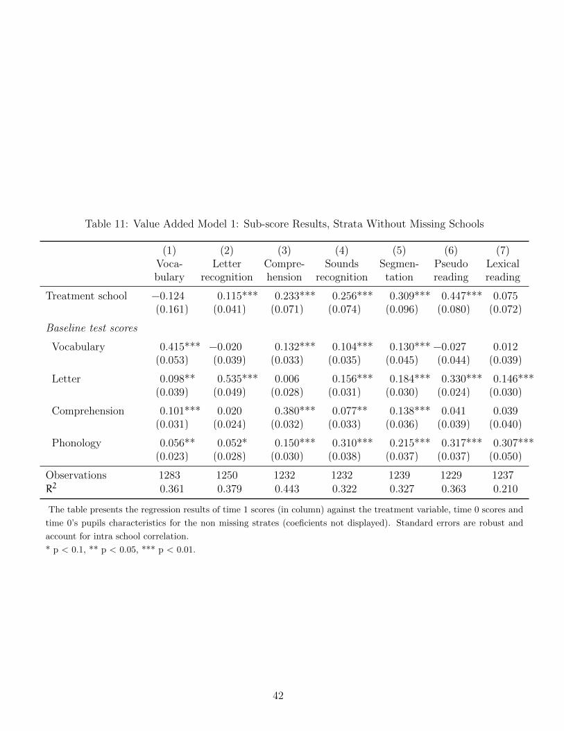
Table 11: Value Added Model 1: Sub-score Results, Strata Without Missing Schools

(1) (2) (3) (4) (5) (6) (7)Voca-bulary

Letterrecognition

Compre-hension

Soundsrecognition

Segmen-tation

Pseudoreading

Lexicalreading

Treatment school −0.124 0.115*** 0.233*** 0.256*** 0.309*** 0.447*** 0.075(0.161) (0.041) (0.071) (0.074) (0.096) (0.080) (0.072)

Baseline test scores

Vocabulary 0.415*** −0.020 0.132*** 0.104*** 0.130*** −0.027 0.012(0.053) (0.039) (0.033) (0.035) (0.045) (0.044) (0.039)

Letter 0.098** 0.535*** 0.006 0.156*** 0.184*** 0.330*** 0.146***(0.039) (0.049) (0.028) (0.031) (0.030) (0.024) (0.030)

Comprehension 0.101*** 0.020 0.380*** 0.077** 0.138*** 0.041 0.039(0.031) (0.024) (0.032) (0.033) (0.036) (0.039) (0.040)

Phonology 0.056** 0.052* 0.150*** 0.310*** 0.215*** 0.317*** 0.307***(0.023) (0.028) (0.030) (0.038) (0.037) (0.037) (0.050)

Observations 1283 1250 1232 1232 1239 1229 1237R2 0.361 0.379 0.443 0.322 0.327 0.363 0.210

The table presents the regression results of time 1 scores (in column) against the treatment variable, time 0 scores and

time 0’s pupils characteristics for the non missing strates (coeficients not displayed). Standard errors are robust and

account for intra school correlation.

* p < 0.1, ** p < 0.05, *** p < 0.01.

42

6.2 Controlling for School and Teacher Characteristics

As mentioned earlier, another potential source of bias may come from the fact that treat-

ment and control schools were initially not comparable. This would occur if, for instance,

school district managers had selected better performing schools (and teachers) into the

treatment. As seen in Table 2, schools in the treatment and control groups do not seem to

present very different characteristics. In the following table, I use the school level charac-

teristics presented in Table 2 to re-estimate the VAM1.

Controlling for school-level characteristics do not modify results systematically from

Table 8; they are similar and positive in reading skills, similar and close to zero in com-

prehension and vocabulary, and may be slightly smaller in phonological skills and letter

recognition. They are never different to the extent that this new specification would change

the global interpretation: results are still very much positive and significant. Since con-

trolling for school characteristics is certainly the more comprehensive model, I consider the

estimates found here as the final results of this study.

43

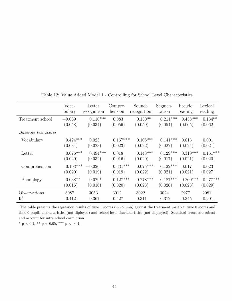
Table 12: Value Added Model 1 - Controlling for School Level Characteristics

Voca-bulary

Letterrecognition

Compre-hension

Soundsrecognition

Segmen-tation

Pseudoreading

Lexicalreading

Treatment school −0.069 0.110*** 0.083 0.150** 0.211*** 0.438*** 0.134**(0.058) (0.034) (0.056) (0.059) (0.054) (0.065) (0.062)

Baseline test scores

Vocabulary 0.424*** 0.023 0.167*** 0.105*** 0.141*** 0.013 0.001(0.034) (0.023) (0.023) (0.022) (0.027) (0.024) (0.021)

Letter 0.076*** 0.494*** 0.018 0.148*** 0.129*** 0.319*** 0.161***(0.020) (0.032) (0.016) (0.020) (0.017) (0.021) (0.020)

Comprehension 0.103*** −0.026 0.331*** 0.075*** 0.122*** 0.017 0.023(0.020) (0.019) (0.019) (0.022) (0.021) (0.021) (0.027)

Phonology 0.038** 0.029* 0.127*** 0.278*** 0.187*** 0.260*** 0.277***(0.016) (0.016) (0.020) (0.023) (0.026) (0.023) (0.029)

Observations 3087 3053 3012 3022 3024 2977 2981R2 0.412 0.367 0.427 0.311 0.312 0.345 0.201

The table presents the regression results of time 1 scores (in column) against the treatment variable, time 0 scores and

time 0 pupils characteristics (not diplayed) and school level characteristics (not displayed). Standard errors are robust

and account for intra school correlation.

* p < 0.1, ** p < 0.05, *** p < 0.01.

44

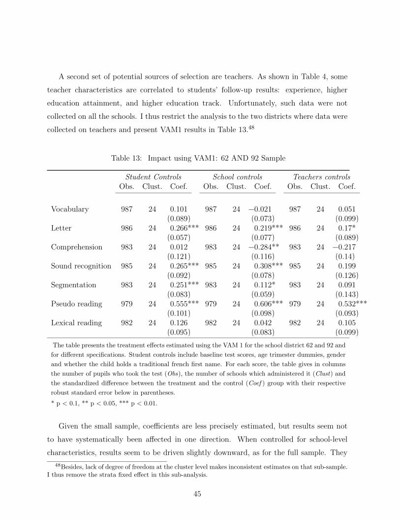
A second set of potential sources of selection are teachers. As shown in Table 4, some

teacher characteristics are correlated to students’ follow-up results: experience, higher

education attainment, and higher education track. Unfortunately, such data were not

collected on all the schools. I thus restrict the analysis to the two districts where data were

collected on teachers and present VAM1 results in Table 13.48

Table 13: Impact using VAM1: 62 AND 92 Sample

Student Controls School controls Teachers controlsObs. Clust. Coef. Obs. Clust. Coef. Obs. Clust. Coef.

Vocabulary 987 24 0.101 987 24 −0.021 987 24 0.051(0.089) (0.073) (0.099)

Letter 986 24 0.266*** 986 24 0.219*** 986 24 0.17*(0.057) (0.077) (0.089)

Comprehension 983 24 0.012 983 24 −0.284** 983 24 −0.217(0.121) (0.116) (0.14)

Sound recognition 985 24 0.265*** 985 24 0.308*** 985 24 0.199(0.092) (0.078) (0.126)

Segmentation 983 24 0.251*** 983 24 0.112* 983 24 0.091(0.083) (0.059) (0.143)

Pseudo reading 979 24 0.555*** 979 24 0.606*** 979 24 0.532***(0.101) (0.098) (0.093)

Lexical reading 982 24 0.126 982 24 0.042 982 24 0.105(0.095) (0.083) (0.099)

The table presents the treatment effects estimated using the VAM 1 for the school district 62 and 92 and

for different specifications. Student controls include baseline test scores, age trimester dummies, gender

and whether the child holds a traditional french first name. For each score, the table gives in columns

the number of pupils who took the test (Obs), the number of schools which administered it (Clust) and

the standardized difference between the treatment and the control (Coef ) group with their respective

robust standard error below in parentheses.

* p < 0.1, ** p < 0.05, *** p < 0.01.

Given the small sample, coefficients are less precisely estimated, but results seem not

to have systematically been affected in one direction. When controlled for school-level

characteristics, results seem to be driven slightly downward, as for the full sample. They

48Besides, lack of degree of freedom at the cluster level makes inconsistent estimates on that sub-sample.I thus remove the strata fixed effect in this sub-analysis.

45

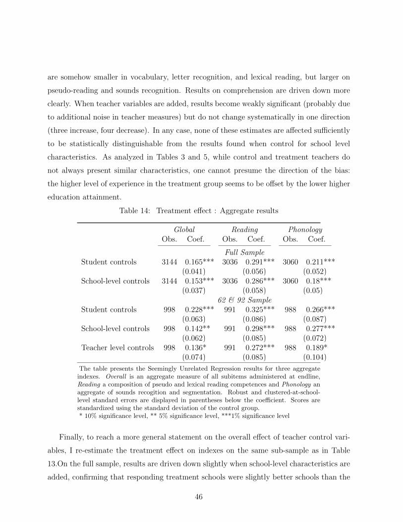
are somehow smaller in vocabulary, letter recognition, and lexical reading, but larger on

pseudo-reading and sounds recognition. Results on comprehension are driven down more

clearly. When teacher variables are added, results become weakly significant (probably due

to additional noise in teacher measures) but do not change systematically in one direction

(three increase, four decrease). In any case, none of these estimates are affected sufficiently

to be statistically distinguishable from the results found when control for school level

characteristics. As analyzed in Tables 3 and 5, while control and treatment teachers do

not always present similar characteristics, one cannot presume the direction of the bias:

the higher level of experience in the treatment group seems to be offset by the lower higher

education attainment.

Table 14: Treatment effect : Aggregate results

Global Reading PhonologyObs. Coef. Obs. Coef. Obs. Coef.

Full SampleStudent controls 3144 0.165*** 3036 0.291*** 3060 0.211***

(0.041) (0.056) (0.052)School-level controls 3144 0.153*** 3036 0.286*** 3060 0.18***

(0.037) (0.058) (0.05)62 & 92 Sample

Student controls 998 0.228*** 991 0.325*** 988 0.266***(0.063) (0.086) (0.087)

School-level controls 998 0.142** 991 0.298*** 988 0.277***(0.062) (0.085) (0.072)

Teacher level controls 998 0.136* 991 0.272*** 988 0.189*(0.074) (0.085) (0.104)

The table presents the Seemingly Unrelated Regression results for three aggregateindexes. Overall is an aggregate measure of all subitems administered at endline,Reading a composition of pseudo and lexical reading competences and Phonology anaggregate of sounds recogition and segmentation. Robust and clustered-at-school-level standard errors are displayed in parentheses below the coefficient. Scores arestandardized using the standard deviation of the control group.* 10% significance level, ** 5% significance level, ***1% significance level

Finally, to reach a more general statement on the overall effect of teacher control vari-

ables, I re-estimate the treatment effect on indexes on the same sub-sample as in Table

13.On the full sample, results are driven down slightly when school-level characteristics are

added, confirming that responding treatment schools were slightly better schools than the

46

respective controls. Yet results on the global aggregate measure remain positive and signif-

icant at 15.3% of a standard deviation. All indexes are only slightly affected by additional

control, the direction of the bias being uncertain.

7 Conclusion

Several important findings can be drawn from this analysis. First, as shown in Table

3, teachers’ practices can be affected by an intensive training program; treatment group

teachers report working in small groups more often, are less likely to work in non-tracked

small groups, and seem to devote less time to non-reading activity. Second, I show that

the new teaching practices introduced in class seem to have a positive and strong effect

on early reading skills: depending on the competence considered, when positive, impacts

range from 11% to 44% of a standard deviation. Effects are particularly strong in compe-

tences that were directly stimulated by the program (pseudo-reading), while competences

only indirectly stimulated were impacted either weakly (letter recognition) or not at all

(vocabulary comprehension). Although it cannot be given a direct interpretation, the final

effect on the global index (+15.3%) is useful for purposes of comparison. Overall results are

thus smaller than the those found in Israel (Angrist and Lavy (2001)) or France (Bressoux

et al. (2009)), but the intensity, length, take-up, and context render a direct comparison

irrelevant. My results are more comparable to the ones found in UK (Machin and McNally

(2008)) on an overall reading index (+8.3%). The program studied here is, however, sig-

nificantly more effective on competences that were specifically stimulated (decoding and

phonology). The intensity of results seen in the UK was apparently lighter and, as it was

scaled up to a large number of schools, was probably less closely monitored. However, the

English program cost approximately 5 e per percentage point gain, while the one studied

here is evaluated to have cost around 13 e.

Thirdly,the analysis stresses the fact that the program had a differential impact on

children depending on their initial level. Progress was stronger for weak children on less-

advanced domains (phonology letter recognition), while everyone seems to have benefited

from the program on more advanced ones (reading). These differential impacts are probably

47

a consequence of the four achievement groups formed at the beginning of the year and of

the explicit teaching approach undertaken. In the French education system, known to

be particularly ill adept at reducing the initial social and cognitive gap, such results are

particularly meaningful. Besides, they echo other results found in developing countries,

such as Duflo et al. (2011), and reinforce the idea that teaching at the right level is a

very powerful approach to improve the education supply. An audacious observer might

even suggest that many of the classical supply-side education policies’ impact (class-size

reduction, computer-assisted teaching, remedial education, boarding school, charter school,

and so on) could be analyzed in light of these findings. Some policies may help in teaching to

the right level (new pedagogy, computer-assisted teaching, class-size reduction), while some

others may help in reducing initial achievement variance (tracking, class-size reduction).

Finally, this article contributes to a more general debate on the way teachers should be

managed and trained. While it seems clear that monitoring, selecting, and incentivizing

teachers is a way to improve education supply, this and other recent studies stress the

fact that, as with any job, teaching, especially teaching how to read, requires concrete

skills and practices that can be transmitted. To move forward, we need further evidence,

possibly using exogeneous program assignment. How do such programs affect children and

teachers in the long run? Are there negative spillovers on other competences (non-cognitive

competences or mathematics, for instance)? Is the end of kindergarten the right time for

such programs? These are all legitimate questions that remain to be investigated further.

48

References

Angrist, J. D. and Lavy, V. (2001). Does teacher training affect pupil learning? evidencefrom matched comparisons in jerusalem public schools. Journal of Labor Economics,19(2):343–69.

Bougnere, A., Suchaut, B., and Bouguen, A. (2014). Sept minutes pour apprendre a lire.Working paper.

Boyd, D., Grossman, P., Lankford, H., Loeb, S., and Wyckoff, J. (2009). Teacher Prepara-tion and Student Achievement. Educational Evaluation and Policy Analysis, 31(4):416–440.

Bressoux, P., Kramarz, F., and Prost, C. (2009). Teachers’ training, class size and stu-dents’ outcomes: Learning from administrative forecasting mistakes. Economic Journal,119(536):540–561.

Bressoux, P. and Lima, L. (2011). La place de l’evaluation dans les politiques educatives:le cas de la taille des classes a l’ ecole primaire en france. Raisons Educatives, 15:99–123.

Decker, P., Mayer, D., and Glazerman, S. (2004). The Effects of Teach For America onStudents: Findings from a National Evaluation . Technical report, Mathematica PolicyResearch.

DEPP (2010). Etat de l’ecole, 30 indicateurs sur le systeme educatif francais. Technicalreport, Departement de l’Evaluation, de la Prospective et de la Performance, Ministerede l’Education Nationale.

DEPP (2013). Etat de l’ecole, 30 indicateurs sur le systeme educatif francais. Technicalreport, Departement de l’Evaluation, de la Prospective et de la Performance, Ministerede l’Education Nationale.

Duflo, E., Dupas, P., and Kremer, M. (2011). Peer effects, teacher incentives, and the im-pact of tracking: Evidence from a randomized evaluation in kenya. American EconomicReview, 101(5):1739–74.

Garet, M., Cronen, S., Eaton, M., Kurki, A., Meredith, L., Wehmah, J., Kazuaki, U.,Falk, A., Bloom, H., Doolitlle, F., Zhu, P., Sztejnberg, L., and Silverberg, M. (2008).The impact of two professional development interventions on early reading instructionand achievement. Technical report, Institute of Education Sciences.

Garet, M. S., Wayne, A. J., Stancavage, F., , Taylor, J., Eaton, M., Walters, K., Song, M.,Brown, S., and Hurlburt, S. (2011). Middle school mathematics professional developmentimpact study. Technical report, Institute of Education Sciences.

49

Gentaz, E., Sprenger-Charolles, L., Cole, P., Theurel, A., Gurgand, M., Huron, C., Rocher,T., and Le Cam, M. (2013). Evaluation quantitative dun entrainement a la lecturea grande echelle pour des enfants de cp scolarises en reseaux d’education prioritaire:Apports et limites. Approche Neuropsychologique des Apprentissages chez l’Enfant, 123.

Gerber, A. and Green, D. (2012). Field Experiments: Design, Analysis and Interpretation.W.W.Norton Company.

Glennerster, R. and Takavarasha, K. (2013). Running randomized evaluation, A practicalguide. Princeton University Press.

Goldhaber, D., Liddle, S., and Theobald, R. (2013). The gateway to the profession: Assess-ing teacher preparation programs based on student achievement. Economics of EducationReview, 34(C):29–44.

Greene, W. (2003). Econometric Analysis. Prentice Hall.

Hanushek, Jackson, and Rossi (1977). Statistical Method for Social Scientist. New York:Academic Press.

Hanushek, E. (1971). Teacher Characteristics and Gains in Student Achievement: Estima-tion Using Micro Data. American Economic Review, 61(2):280–88.

Hanushek, E. A. (1986). The economics of schooling: Production and efficiency in publicschools. Journal of Economic Literature, 24(3):1141–77.

Hanushek, E. A., Kain, J. F., O’Brien, D. M., and Rivkin, S. G. (2005). The Market forTeacher Quality. NBER Working Papers 11154, National Bureau of Economic Research,Inc.

Hanushek, E. A. and Rivkin, S. G. (2006). Teacher Quality, volume 2 of Handbook of theEconomics of Education, chapter 18, pages 1051–1078. Elsevier.

Harris, D. N. and Sass, T. R. (2011). Teacher training, teacher quality and student achieve-ment. Journal of Public Economics, 95(7-8):798–812.

Jeffrey R. Kling, Jeffrey B. Liebman, L. F. K. (2007). Experimental analysis of neighbor-hood effects. Econometrica, 75(1):83–119.

Kane, T. J., Rockoff, J. E., and Staiger, D. O. (2008). What does certification tell us aboutteacher effectiveness? Evidence from New York City. Economics of Education Review,27(6):615–631.

Koedel, C., Ehlert, M., Podgursky, M., and Parsons, E. (2012). Teacher PreparationPrograms and Teacher Quality: Are There Real Differences Across Programs? WorkingPapers 1204, Department of Economics, University of Missouri.

50

Machin, S. and McNally, S. (2008). The literacy hour. Journal of Public Economics,92(5-6):1441–1462.

Manski, C. F. (1993). Identification of endogenous social effects: The reflection problem.Review of Economic Studies, 60(3):531–42.

National Reading Panel (1999). Teaching children to read. Technical report, NationalReading Panel.

NICHD (2005). Pathway to reading: The role of oral language in the transition to reading.Development Psychology, 41(2):428–442.

Nye, B., Konstantopoulous, S., and V.Hedges, L. (2004). How large are teacher effects?Educational Evaluation and Policy Analysis, 26(3):237–257.

Piketty, T. and Valdenaire, M. (2006). L’impact de la taille des classes sur la reussite sco-laire dans les ecoles, colleges et lyces francais. Technical report, Ministere de l’educationNationale.

Rivkin, S. G., Hanushek, E. A., and Kain, J. F. (2005). Teachers, schools, and academicachievement. Econometrica, 73(2):417–458.

Rockoff, J. E. (2004). The Impact of Individual Teachers on Student Achievement: Evi-dence from Panel Data. American Economic Review, paper and proceedings, 94(2):247–252.

Schatschneider, C., J.Francis, D., Carlson, C., Fletcher, J., and B.Foorman (2004). Kinder-garten prediction of reading skills: A longitudinal comparative analysis. Journal ofEducational Psychology, 96(2):265–282.

Storch, S. and Whitehurst, G. (2002). Oral language and coded-related precursors to read-ing: evidences from a longitudinal structural model. Development Psychology, 38(6):265–282.

8 Appendix

In section 3, we use a well-known result from Greene (2003) to the expression of the omittedbias created in that case. Greene (2003) [p.148] states that :

E(α) = α+ (X ′1X1)

−1(X ′1X2)α2

where X1 are explanatory variables included in the model and X2 are the ones omitted.According to (8), the omitted variable is the error term ε0,and the explained part includestwo vectors T and A0 and is hence a nx2 matrix. α is a column vector 2x1 composed of

51

two parameters β and γ and α2 is scalar γ. Note that according to (8), γ comes in themodel with a negative sign. The bias of the VAM 1 estimator :

E(α) = α− (X ′X)−1(X ′εi0)γ

with X =

1 A01 T1...

...

1 A0n Tn

, ε0 =

ε1,0...εn,0

, α =

β0γβ1

.

with,

X ′X =

N∑Ai0

∑Ti∑

Ai0∑A2i0

∑Ai0Ti∑

Ti∑Ai0Ti

∑T2i

= (X ′X) ′

Determinant of XX

det(X ′X) =∑

A2T2 − (∑

A0T)2

− A0∑

A0∑

T2 + A0∑

T∑

A0T

+ T∑

A0∑

TA0 − T∑

A20

∑T

with T = 1/N∑T and A = 1/N

∑A.

Adding and subtracting n2T2A02, and regrouping the terms, we get:

det(X ′X) =∑

A2T2 − A0∑

A0∑

T2 − T∑

A20

∑T + n2T2A0

2

−[(∑

A0T)2 − 2nA0T

∑TA0 + n

2T2A20]

det(X ′X) =(∑

A20 − nA20)(

∑T2 − nT2)

− (∑

A0T − nTA0)2

=V(A0)V(T) − C(A0, T)

with :

V(A0) =∑

A20 − nA20)

V(T) =∑

T2 − nT2

C(A0, T) =∑

A0T − nTA0

Inverting the matrix (XX−1)

52

(X ′X)−1 =1

V(A0)V(T) − C(A0, T)

|M1,1| −|M1,2| |M1,3|

−|M2,1| |M2,2| −|M2,3|

|M3,1 −|M3,2| |M3,3|

where the Mi,js form the matrix of minor of (X’X)’.Matrix product

X ′ε0 =

∑εi0∑A0iεi0∑Tiεi0

and finally

E(α) =

β0γβ1

−1

V(A0)V(T) − C(A0, T)2

∑εi0∑A0iεi0∑Tiεi0

|M1,1| −|M1,2| |M1,3|

−|M2,1| |M2,2| −|M2,3|

|M3,1| −|M3,2| |M3,3|

γwhere each row gives the bias generated by the measurement error on the three param-

eters of the model (β0, β1 and γ). It can easily be shown that the bias generated by thesecond row is downward (classical attenuation bias). We are primarily interested by thedirection of the bias on β1.

E(β1) = β− γ1

V(A0)V(T) − C(A0, T)2∗[

A0∑

A0T − T∑

A20)∑

εi0 −∑

A0iεi0(∑

A0T − A0T) +∑

Tiεi0(∑

A20 − A20

]Adding and subtracting n2A20ε0T , and rearranging terms, I get:

E(β1) = β− γV(A0)C(T, ε0) − C(A0, T)C(A0, ε0)

V(A0)V(T) − C(A0, T)2(12)

with V the variance and C the covariance. Multiplying the denominator and numeratorby 1

V(A0)V(T)S(ε0)(with S(ε0) =

√Vε), we get:

E(βvam1) = β− γr(T,ε0) − r(A0, T)r(A0, ε)

1− r2(A0,T)

Sε0ST

(13)

with r the respective correlations. This scalar result can also be found in Hanushek et al.(1977). Besides, since in a classical measurement error model rε0,T = 0 and rε0,A0

=r(ε0, µ+ ε0) = r(ε0, ε0) = Vε, then :

53

E(β) = β+ γr(A0, T) ∗ Vε01− r(A0, T)2

Sε0ST

(14)

The sign of the bias is determined by r(A0, T) if 0<γ<1. It will be the case if theprocess is stationary.

To look at the direction of the bias more intuitively, I present in Figure 1 a visualrepresentation of the treatment effect under different values of ρ. As said, when ρ equalszero, we are in the classical difference-in-differences model, where the treatment group’strend is equal to the one of the control group (first panel). Alternatively, when ρ isnegative, we are in a convergent model, where weaker students (here the treatment group)catch up with more advanced students. The more negative ρ is, the smaller is the treatmenteffect. Inversely, when ρ is positive, we are in a divergent model, where the gap betweenunder-achievers (treatment group) and the others increases. As ρ increases, the estimatedtreatment effect β increases. As a result, a downward bias on ρ will automatically producea downward bias on β.

54

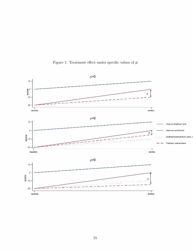
Figure 1: Treatment effect under specific values of ρ

55