Document1 - 1 -

ADHESIVE CONTACT OF VISCOELASTIC SPHERES:

A HAND-WAVING INTRODUCTION

E. Barthe1l and G. Haiat

2,

1) Surface du Verre et Interfaces, CNRS/Saint-Gobain, Aubervilliers, France,

2) CEA, Laboratoire de Simulation Ultrasonore et de Traitement, Gif-sur-Yvette,

France.

etienne.barthel@saint-gobain.com

Abstract :

We give an overview of the general features of the linear viscoelastic adhesive contact model.

The two main features are 1) a delay between the contraction of the contact radius and the

onset of the indenter retraction; 2) the enhancement of the adherence force. We emphasize the

role played by stress relaxation within the contact zone in these phenomena and give simple

forms of the viscoelastic adhesive contact equations to account for it. Two characteristic

timescales are identified, respectively associated with the crack tip and the contact zone. Their

asymmetric roles in the growing and receding contact phases is evidenced. Energy release

rates for both phases are calculated together with their irreversible components.

Keywords: adhesion, adherence, contact mechanics, linear viscoelasticity, viscoelastic crack

propagation.

1 Introduction

Probing the adherence of soft viscoelastic solids, as in the JKR test [1,2], assessing the

mechanical properties of polymers in small scale contact experiments like nanoindentation [3]

Document1 - 2 -

or AFM [4-6], where surface forces interfere, or understanding the adhesion of molten glass

to hot molds all require a model for the adhesive contact of viscoelastic bodies.

Sometime ago, in this same journal, we had shown that the Sneddon method, based on the

systematic application of Hankel transforms, provides wide reaching insight into the elastic

contact problems of axisymmetric bodies [7]. Relying on the same method, we have recently

proposed a theory of the adhesive contact within the linear viscoelastic regime [8,9]. The aim

of the present contribution is to parallel our previous paper on the elastic case [7] with an

exposition of the main ideas behind the adhesive contact of viscoelastic bodies.

Let us recall the main steps in the development of the viscoelastic adhesive contact theory; a

more comprehensive bibliographical list may be found in [8,9].

In the 60s', the viscoelastic adhesionless contact problem has spurred a number of efforts,

finally yielding Ting’s completely satisfactory theory in 1966 [10]. The next step, in the 70s’,

was taken by Schapery, who described crack propagation in a viscoelastic medium by

embedding a process zone into a linear elastic solid [11-14]. Coupling a viscoelastic crack

behavior with an elastic contact has provided a first category of viscoelastic adhesive contact

models [15]. One further step was taken when Hui et al. coupled a viscoelastic contact model

to a viscoelastic crack model [16], as initially suggested by Schapery [14]. Their theory,

however, is valid for an increasing contact radius only. Their attempt for a decreasing contact

radius proved less successful [17,18].

The model for the viscoelastic adhesive contact we have recently proposed [8] is based on the

Sneddon method of Hankel transform [7]. In a suitable limit [9], it turns out to simply couple

Ting’s model for the adhesionless viscoelastic contact and Schapery’s viscoelastic crack

approach. Under this form, it takes a particularly simple structure, in close connection with

the JKR model [19] for elastic adhesive contacts. The aim of the present paper is to highlight

Document1 - 3 -

this connection and to present the main concepts underlying the adhesive linear viscoelastic

contact model.

2 Description of the adhesive contact

The physics of the contact between two bodies is subtle and has to be simplified to be

efficiently accounted for in a mechanical model. Several paths [20] may be followed for that

purpose: one of them is to assume infinite repulsion at contact; and before contact, attractive

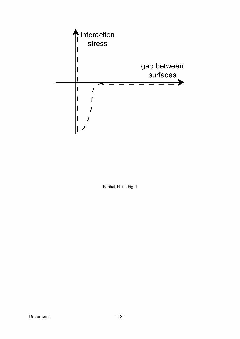
interaction between surfaces over some finite range (Fig. 1). Then, in the adhesive contact, we

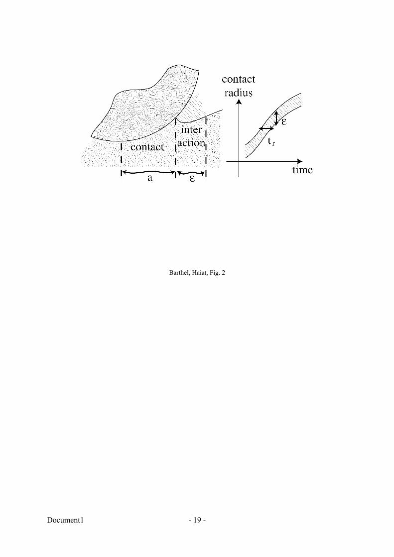
can identify two zones: in the contact zone, the surfaces touch each other; outside this zone, in

the interaction zone, tensile stresses are present without contact (Fig. 2).

We now examine the consequence of these assumptions on the mechanics of the contact.

2.1 Boundary conditions

2.1.1 The inner problem: contact variables

Inside the contact zone, the fact that the surfaces come to contact is specified by the following

boundary conditions:

)(for )()(),( tarrftrtu <−= δ (1)

where ),( rtu is the normal surface displacement, )(tδ the penetration, )(rf the shape of the

indenter and )(ta the contact radius. The main variables for the contact problem itself are thus

the penetration and the contact radius. The third contact variable, the force, although often

directly measured in practice, plays a less direct role in the theory, because it is the integral of

the surface stress distribution and therefore specifies the boundary conditions less directly.

2.1.2 The outer problem: the interaction zone variables

Adhesion is expressed by the following boundary conditions:

<+=+<<−=

rr

ararpr

)(afor 0)(

)(for )()(

εσεσ

(2)

Document1 - 4 -

where )(rp is a stress distribution relevant to the physics of the adhesive process, )(rσ is the

normal surface stress, and ε the size of the interaction zone (Fig. 2).

2.2 Self-consistent description of the interaction zone

In the interaction zone, normal surface stress, deformation and interactions are intimately

coupled: the normal surface stress is a function of the of the gap between surfaces (Fig. 1),

which itself depends upon the surface deformation, which is controlled by the normal surface

stresses. As a result, a self consistent treatment is required [7,11]. The final useful equation is

typically of the form

∫∞

=a

dr

rdhrdrw

)()(σ (3)

where w is the adhesion energy and )(rh the gap between surfaces. Although we more or

less implicitly assume an interaction potential here, there is a priori no limitation to

generalizing this method to more complex adhesive phenomena.

The difficult issue here is that the mechanical relation between stress and surface

displacement (and therefore the gap )(rh ) is non local, so that explicit expressions for (5) are

often intricate. This treatment is simplified if we assume that the contribution of the

interaction zone surface stresses to the interaction zone surface deformation dominates the

contribution of contact zone stresses. An equivalent assumption is that the interaction zone

size ε is much smaller than the contact radius a . This is the essence of the JKR limit [19].

Then, the gap shape is dominated by the adhesive stress induced deformations [7], and

equation (3) reduces to

∗∝E

wεσ 2

(4)

in which *E is the reduced modulus defined by (A4) in the appendix and the proportionality

coefficient depends upon the details of the interaction. Under this form, the form of an elastic

Document1 - 5 -

energy release rate, the self-consistency equation (4) lends itself to a linear elastic fracture

mechanics interpretation. For that purpose, in our formalism, we introduce a new quantity,

)(ag , which, as will be shown below, naturally couples the contact and the interaction zones.

On the interaction zone side, )(ag , which is defined in the appendix by (A1), is a function of

the interaction stress distribution )(rp (as defined in (2)) only. We have also shown

previously [7] that in the elastic case, (4) can be written

aE

agw ∗=

π

2)(2 (5)

Therefore, )(ag assumes the status of a stress intensity factor. Indeed, denoting K the

interaction zone stress intensity factor at a , we have shown [9] that

a

agK

π)(2−= (6)

Thus, the self consistent treatment of the interaction zone essentially specifies the stress

intensity factor, K or )(ag , characteristic of the adhesive interaction stress distribution. We

now discuss how )(ag determines the contact variables.

2.3 Coupling the interaction zone to the contact zone

If the adhesive interaction is zero, then the solution to the contact problem is the Hertz theory

[21] for a spherical indenter (and its extensions for other geometries), which specifies the

penetration δ as a function of the contact radius a . This function )(0 aδ depends upon the

shape of the indenter )(rf only. A general approach to the adhesive contact problem is then

to specify the adhesive process and solve the interaction zone problem. The actual attractive

stress distribution is thus determined. However, this attractive stress distribution pulls on the

surfaces and, for a given penetration, increases the contact radius. The penetration is then

Document1 - 6 -

)(2

)()( 0 agE

at ∗+= δδ (7)

This equation shows that for a given contact radius, the additional term for the penetration is

proportional to the adhesive interaction stress intensity factor, or more directly to )(ag . Note

that )(ag is negative, so that, for a given contact radius, a reduction of the penetration with

adhesion is predicted by (7).

Another interpretation of (7) stems from the observation that the quantity )(4

0δδπ −∗Ea

is

the stress intensity factor generated by the additional stress distribution due to the additional

flat punch displacement )( 0δδ − . Then, (7) states that this stress singularity is cancelled by

the stress singularity due to the outer attractive stress distribution [22-23].

The penetration equation (7) and the force equation [7], which can be derived from (A9) in

the appendix, form the contact equations which, together with the self consistency equation

(5), provide the solution to the linear elastic adhesive contact problem.

3 Viscoelastic Contact: main results

We are now in a position to extend the previous model to viscoelastic behaviour by assuming

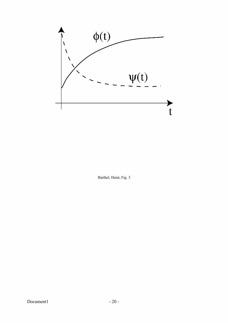
a delayed elastic behaviour. We introduce the usual viscoelastic creep ϕ and relaxation ψ

functions (Fig. 3). Stress σ and deformation ε now obey

∫ −=t

d

dtdt

0

)()(τεττψσ

and

∫ −=t

d

dtdt

0

)()(τσττϕε .

Under suitable conditions [8], this results in the description of the mechanics in terms of

reduced creep ∗ϕ and relaxation ∗ψ functions.

Document1 - 7 -

As mentioned previously, in section 2.2, it is usually reasonable to assume that the interaction

zone problem is local to the crack tip ( a<ε ). Then contact zone and interaction zone are

coupled only through the variable )(ag . Under this assumption, we first consider the

viscoelastic crack propagation.

3.1 Self consistent crack problem

The adhesive viscoelastic problem also requires some details of the physical process giving

rise to adhesion. In the present approach, we suppose a “double-Hertz” interaction zone with

characteristic stress 0σ and adhesion energy w [24]. This model is similar to a Dugdale

model [22].

We have shown [9] that

εσπaag 2

4)( 0−= (8)

In the viscoelastic case, time now plays a role so that a local timescale appears: rt , the time

required by the crack to move a distance equal to the interaction zone size ε (Fig. 2). As a

result, we have a relation between the crack velocity (or contact radius velocity) dtda / , ε

and rt :

rtdt

da ε= (9)

Then, we obtain [9] that the viscoelastic crack behavior is given by:

=w )()(2

1

2

rta

ag ∗ϕπ

(10)

where

ττϕτϕ dttt

t

t

)()(2

)(0

121 −−= ∫∗∗

> (11)

when the contact radius increases and

Document1 - 8 -

τττϕϕ dtt

t

t

)(2

)(0

121 −= ∫∗∗

< (12)

when the contact radius decreases.

We note that the form of (10) is identical to the form of (5), but the stress intensity factor is

calculated from an effective compliance )(1 rt∗ϕ , which depends upon the crack tip velocity.

This effective compliance amounts to the instantaneous compliance when rt is zero, is the

long time compliance when rt is infinite, and lies in between for intermediate rt .

These results, which are arrived at through the treatment of the full contact problem [9], are

comparable to Schapery’s viscoelastic crack propagation models.

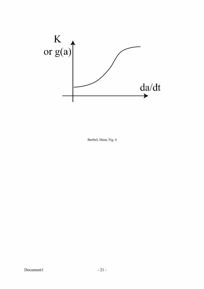
From (10-12), the stress intensity factor of the attractive interaction stress distribution can be

calculated as a function of crack tip velocity. The typical behavior is exemplified in Fig. 4.

This stress intensity factor has been identified above as the key parameter in the determination

of the penetration, as we now discuss in more details.

3.2 Penetration

We now couple the viscoelastic crack problem to the viscoelastic contact problem.

3.2.1 Inward (closing crack)

We obtain [9] for increasing contact radius

)())((2))(()( 00 rttagtat ∗+= ϕδδ (13)

where

∫ −= ∗∗t

dtt

t0

0 )(1

)( ττϕϕ (14)

This penetration equation is equivalent to the elastic case (Eq. (7)) provided the effective

compliance )(0 rt∗ϕ is substituted to the elastic compliance ∗E/1 . Setting 0=g , we recover

the adhesionless viscoelastic case

Document1 - 9 -

))(()( 0 tat δδ = (15)

Note that )(0 t∗ϕ is larger than )0(∗ϕ : due to creep, the penetration correction is larger than in

the elastic case.

3.2.2 Outward (opening crack)

For decreasing contact radius, the main term is [9]

))(()(2

1tagd

t

d

dt

t

=−∫−

∗ ττδτψ (16)

A corrective term which is not essential to understand the physics of the adhesive contact has

not been included here. The time −t is the time at which the present contact radius )(ta was

met during the increasing contact radius phase. Once again, setting 0=g , we recover the

adhesionless solution by Ting [10]

ττδτψ d

t

d

dt

t

∫−

−= ∗ )(0 (17)

Equation (16) is central to the viscoelastic contact rupture. Comparing with (13), we observe

that its structure is exactly inverse. The right-hand side is proportional to the attractive

interaction stress intensity factor. But the viscoelastic effect, instead of scaling the stress

intensity factor with the creep function and the local timescale rt , now appears under the form

of a convolution of the penetration with the relaxation function over the full history of the

system – that is to say between −t and t .

This form of the penetration equation is best explained if the cancellation of inner and outer

stress intensity factors formulation (§ 2.3) is retained. This formulation gives to the left hand

side in (16) the meaning of an inner stress intensity factor at t and )(ta , which results from

the flat punch displacement )(tδ convoluted by the stress relaxation function .ψ

Document1 - 10 -

3.3 Force

Although the force is a less direct expression of the contact boundary conditions, it is useful in

practice because it is most readily obtained experimentally.

Introducing ∫−=a

rdraaf0

0 )(),( δδδ , where the second term depends only upon the shape of

the indenting body, from (A9) in the appendix, we have:

a) for adhesionless elastic contact: )),((2)(2)( 000 aafEafEaF δ∗∗ ≡= ; (18)

b) for an adhesive elastic contact: )(4)()( 0 aagaFaF += . (19)

3.3.1 Inward

In the viscoelastic case, in the increasing contact radius case, the force is

( ) ττ

ττδτψ dd

adfttF

t

∫ −= ∗

0

)(),()(2)( (20)

from which the stress intensity factor may be extracted as

)(4

)()0()(

)(

)(0

00

r

t

ta

aFdF

t

ag ∗

∗∗∫ −

∂∂−

=ϕ

ϕττττϕ

(21)

From this equation and the self-consistency equation (10), dtda / can be extracted, so that by

integration )(ta , and ultimately )(tδ are known.

For instance, penetration under vanishing external force entails ( ) 0)(),( =tatf δ . Therefore,

Rat 3/)( 2=δ . (22)

3.3.2 Outward

The force is

( ))(4

)(),()(2

0aagd

d

adftF

t

+−= ∫− ∗ τ

τττδτψ . (23)

from which )(ag is directly extracted. Here again, the adhesionless case is readily obtained.

Document1 - 11 -

3.4 The adhesive viscoelastic contact: main phenomena

The two main phenomena which signal viscoelastic behaviour in the adhesive contact will

now be explained briefly.

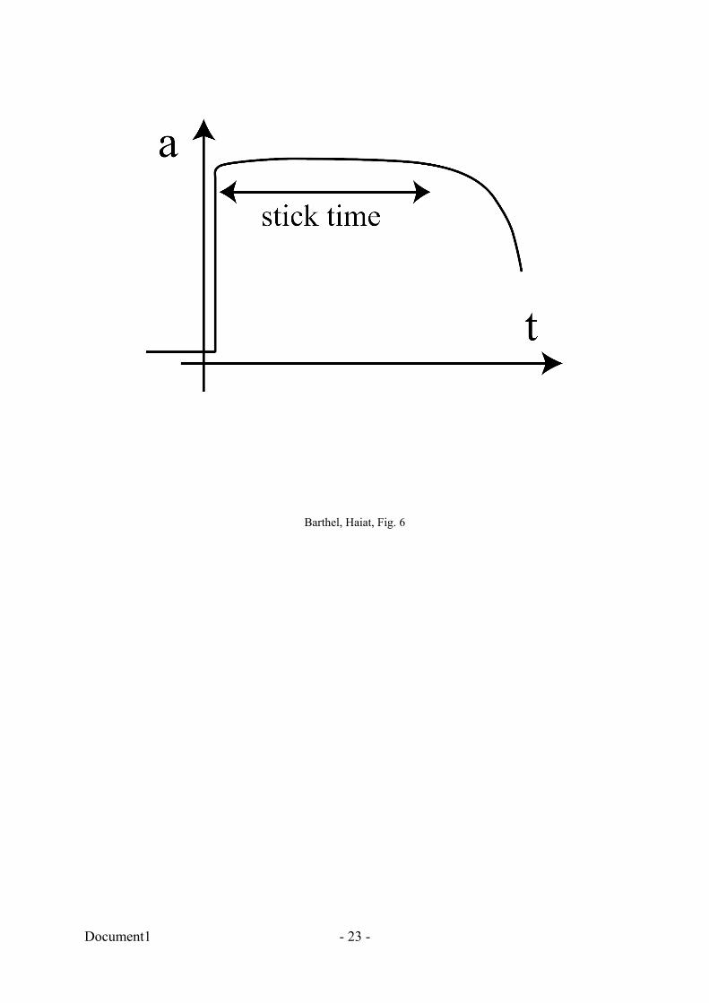
3.4.1 The stick zone

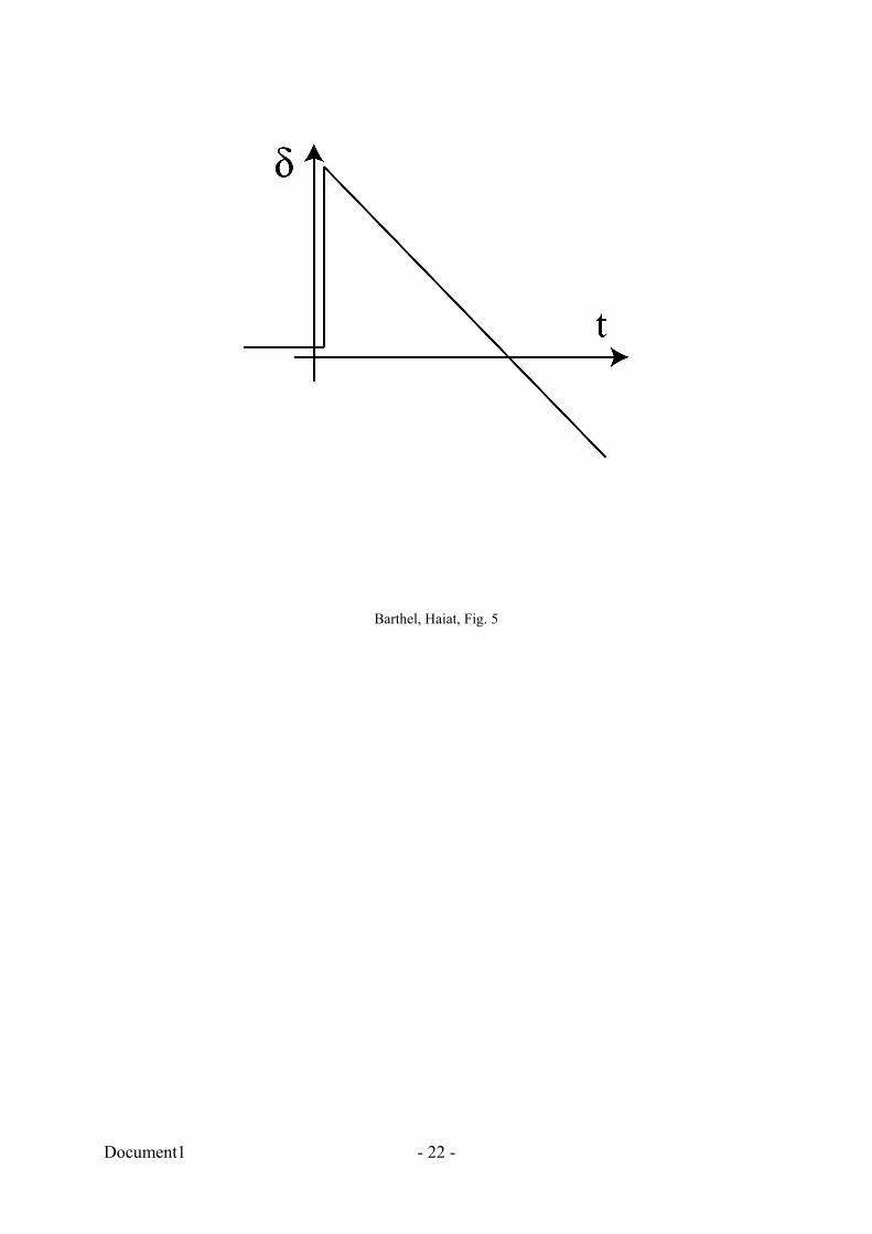
The first characteristics of the viscoelastic adhesive contact is the delay between the time

when the indenter starts moving backwards (Fig. 5) and the time when the contact radius

starts to recede markedly. This delay we called the stick time [9] (Fig. 6). It is due to the fact

that, in the region where the contact radius is maximum, the contact radius velocity is close to

zero. Then, the interaction stress intensity factor, and )(ag , are small (Fig. 4). To get

significant propagation, we must restore a higher )(ag . This is obtained by the backward

motion of the indenter, but the effect is qualified by the stress relaxation (16). The condition

for propagation is achieved only when the right hand side member in (16) is large enough, i.e.

when the backward motion of the indenter overcomes the stress relaxation. This is the origin

of the stick time.

3.4.2 Adherence force enhancement

The pull-out force in the elastic adhesive contact, in the small interaction zone size (or JKR)

limit is Rwπ2/3 . Its independence from the actual elastic modulus of the contacting bodies is

most noteworthy. It is due to the fact that compressive and tensile stresses within the contact

zone balance each other at pull-out.

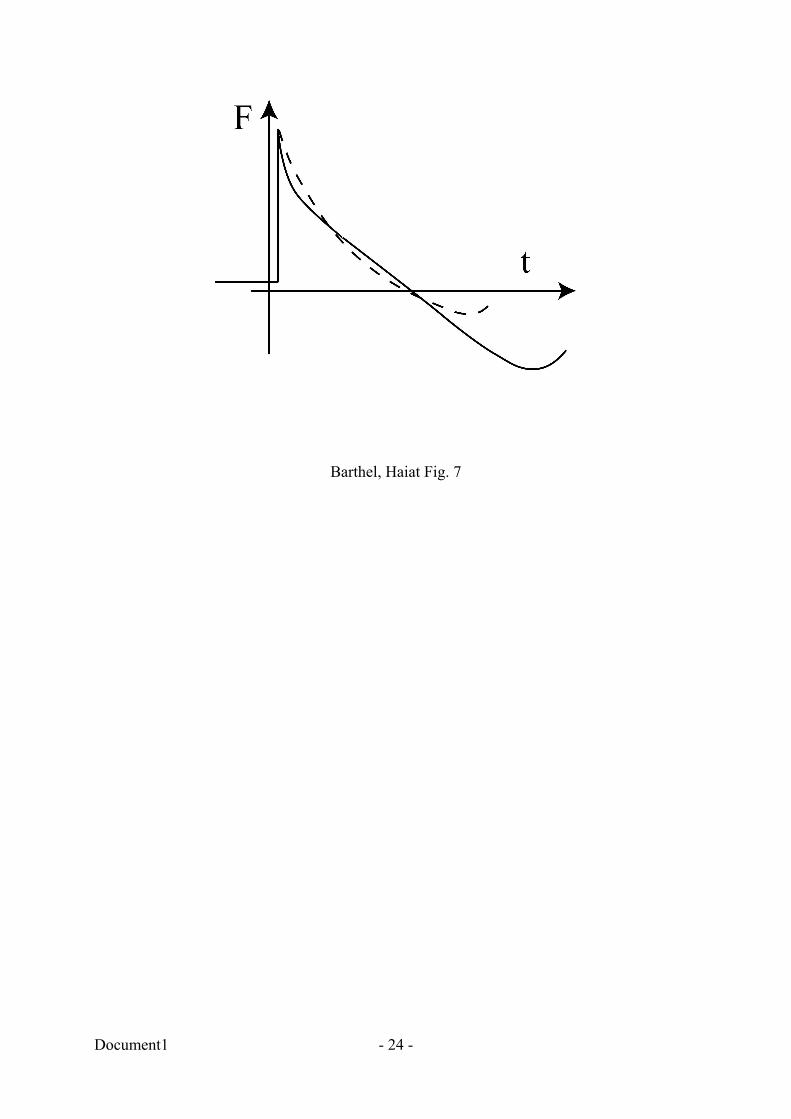
For viscoelastic bodies, however, the picture is quite different (Fig. 7). Restoring a large stress

intensity factor by the motion of the indenter )(tδ brings back a sizeable tensile flat punch

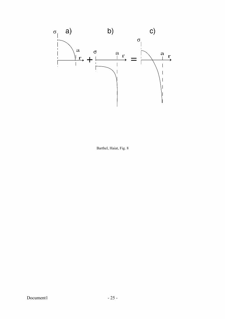
stress distribution within the contact zone (Fig. 8). At the same time, the compressive stresses

within the contact zone have also decayed but are not restored by the present motion. This is

apparent for instance in (23) where the first (compressive) term decays as )(t∗ψ while the

Document1 - 12 -

second (tensile), originating from the flat punch tensile stress distribution, is identical in the

elastic case.

Once again neglecting corrective terms in the increasing contact radius part of the contact,

(23) may be written simply

( ) ( ))(4)()( 0 taagtaftF += ∗ψ (24)

We conclude that the decay of the compressive stress distribution within the contact zone, and

therefore of its contribution to the total force, leads to the enhancement of the overall adhesive

force (Fig. 8).

3.5 Energy

3.5.1 Energy release rate

The energy release rate, which is the mechanical energy expended in propagating the contact

per unit area, is expressed from (A10) in the appendix, as

)),(()),((1

ttattagadA

dG θ

π=Ω= (25)

where the quantity )()(),( 0 atta δδθ −= is closely connected with the penetration equations

(7), (13) and (16). G is zero in the absence of adhesion. If the contact is elastic, (5), (7) and

(25) show that wG = . Since w is the adhesion energy, gained from the crack propagation,

this equality means reversible propagation.

In the viscoelastic case, let us denote >G the energy release rate for increasing contact radius.

Equation (13) results in

a

ttagG r

πϕ )())((2 0

2 ∗

> = (26)

Comparison with (10) shows that for increasing contact radius (closing crack),

1)(

)(

1

0 ≤= ∗>

∗>

r

r

t

t

w

G

ϕϕ

(27)

Document1 - 13 -

Mathematically, the wG /> ratio is smaller than one because ∗ϕ is a monotonic increasing

function. Physically, it means that the propagation of the crack is dissipative. However, we

note that equality holds when the crack is very fast and also when it is very slow: the system

is then effectively elastic. Reversibility of the crack propagation at high velocity is at variance

with results by Schapery [11,12] and subsequently Greenwood and Johnson [13]. The reason

is that Schapery assumes the relaxed state as the reference state. With fast cracks, however,

this relaxed reference state is reached nowhere near the crack tip. Our present estimate of the

dissipation is purely local, at the crack tip; dissipation due to stress relaxation inside the

contact itself, which is also present in the adhesionless contact, is not included in the present

expression for >G .

A similar discussion for the receding contact radius phase is less straightforward because (16),

however approximate, takes into account the full history of the system. We will therefore

provide an approximate discussion, restricted to a special case. We assume that (Fig. 5)

1) loading to the maximum penetration mδ is fast;

2) unloading takes place immediately after loading;

3) the unloading rate dtd /δ is constant.

Then, (16) becomes:

( ) ( )mm tt

tat

tag δδψδδψ −+−=∗

)(2

)())((

2

)())(( 0

0 (28)

where

∫ −= ∗∗t

dtt

t0

0 )(1

)( ττψψ (29)

Now )()(0 0 tt ∗∗ << ψψ , so that, since )),(( ttag is negative, we have

0)),(()(/))((2)(/))((2 0 <<< ∗∗ ttattagttag θψψ

and )),(( ttaθ is also negative

Document1 - 14 -

)(

))((2 2

ta

tagG ∗< >

ψπ (30)

As a result, in the decreasing contact radius phase (growing crack)

)()(

1

1 rttw

G∗<

∗< ≥

ϕψ (31)

Typically, we may expect the experimental time t to be large and rt to be small, at least

when the contact recedes markedly. Then )(0 t∗ψ is of the order of the relaxed modulus

)(+∞∗ψ : Schapery's relaxed reference state is recovered. Simultaneously, )(1 rt∗<ϕ is of the

order of the instantaneous compliance )0(/1 ∗ψ , and [15]

)(

)0(

)()(

1

1 +∞∝ ∗

∗

∗<

∗ ψψ

ϕψ rtt (32)

which is much larger than 1 for a significantly viscoelastic material: a large dissipation

appears in the outward phase.

Then wG ≥< , but equality is restored at slow velocities (for a finite long time compliance) or

for a loading cycle faster than any typical relaxation time.

This dissipation can be rationalized in the following manner: the crack tip, which moves fast,

with characteristic time rt , feels an effectively harder material (10). The flat punch

displacement, however, applies to an effectively softer material, because of the viscoelastic

stress relaxation (28) applies to the characteristic time t . As a result, for the same stress

intensity factor, the flat punch energy release rate is much larger than the crack energy release

rate. The energy difference is dissipated.

4 Discussion

Within the contact zone, we find both compressive (at the center) and tensile stresses (at the

periphery). The normalized 1.5 adherence force for an elastic adhesive (JKR [19]) contact

Document1 - 15 -

results from a balance between these two stress contribution. For viscoelastic bodies,

however, the stress distribution inside the contact zone relaxes. As a result, the contact zone

does not recede as soon as the indenter is pulled back, because the stress intensity factor is

low, which leads to low contact radius velocities (Fig. 4). One requires sufficient (and

sufficiently fast) backward motion of the indenter to restore a stress intensity factor large

enough for the contact radius to actually decrease (Eq. 16).

However, this additional tensile stress distribution (a flat-punch like stress distribution) does

not contribute compressive stresses. Consequently, the balance between compressive and

tensile stresses one finds in the elastic case is now offset, resulting in an enhanced adherence

force.

5 Conclusion

Two phenomena must be included in a complete model for the adhesive contact of

viscoelastic spheres. Creep in the interaction zone reduces the stress intensity factor though a

larger effective compliance. At the same time, stress relaxation inside the contact zone

induces both a time lag between indenter retraction and contact radius decrease (“stick”

effect) and an enhancement of the adherence force through unbalance between compressive

and tensile stresses. Our models [8,9] provides a complete description of this combination of

phenomena.

References

[1] Falsafi A., Tirrell M. and Pocius A., Langmuir 16, 1816 - 24 (2000).

[2] Crosby A. J., Shull K. R., Lin Y. Y. and Hui C.-Y., J. Rheol. 46, 273 - 94 (2002).

[3] Giri M., Bousfield D. B. and Unertl W. N., Langmuir 17, 2973 - 81 (2001).

[4] Basire C. and Frétigny C., Tribology Letters 10, 189 - 93 (2001).

Document1 - 16 -

[5] Portigliatti M., Koutsos V., Hervet H. and Leger L., Langmuir 16, 6374 - 76 (2000).

[6] Pickering J. P. and Vancso G. J., J. Macromol. Symp., 166, 189 - 99 (2001).

[7] Huguet A.-S. and Barthel E., J. Adhesion 74, 143 - 75 (2000).

[8] Haiat G., Phan Huy M.-C. and Barthel E., J. Mech. Phys. Solids 51, 69 - 99 (2003).

[9] Barthel E. and Haiat G., Langmuir 18, 9362 - 70 (2002).

[10] Ting T. C. T., J. Appl. Mech. 33, 845 - 54 (1966).

[11] Schapery R. A., Int. J. Fract. 11, 141 - 59 (1975).

[12] Schapery R. A, Int. J. Fract. 11, 369 – 88 (1975).

[13] Greenwood J. A. and Johnson K. L., Philos. Mag. A 43, 697 – 711 (1981).

[14] Schapery R. A., Int. J. Fract. 39, 163 – 189 (1989).

[15] Johnson K. L. in Tsukruk, V. V., Wahl, K. J. (Eds.), Microstructure and Microtribology

of Polymer Surfaces, ACS, Washington, D.C., (1999).

[16] Hui C. H., Baney J. M. and Kramer E. J., Langmuir 14, 6570 - 78 (1998).

[17] Lin Y. Y., Hui C. Y., and Baney J. M., Journal of physics D, Applied physics 32, 2250 -

60 (1999).

[18] Lin Y. Y. and Hui C. Y., J. Polymer Sci. B, 40, 772 - 93 (2002).

[19] Johnson K. L., Kendall K. and Roberts A. D., Proc. Roy. Soc. London A 324, 301 – 13

(1971).

[20] Barthel, E., J. Colloid Inter. Sci. 200, 7 – 18 (1998).

[21] Hertz H., J. Reine Angew. Math. 92, 156 -171 (1882).

[22] Maugis D., J. Colloid Inter. Sci. 150, 243 - 69 (1992).

[23] Maugis D. and Barquins M., J. Phys. D:Appl. Phys., 11, 1989 - 2023 (1978).

[24] Greenwood J. A. and Johnson K. L., J. Phys. D: Appl. Phys. 31, 3279 (1998).

[25] Sneddon I. N., Fourier Transforms, McGraw Hill: New York (1951).

Document1 - 17 -

Captions:

Fig. 1: Typical dependence of the interaction stresses with the gap (or distance) between

surfaces, as assumed in the present contact model.

Fig. 2: Left: contact zone (radius a ) and interaction zone (size ε ) in a typical adhesive

contact. Right: definition of the dwell time rt .

Fig. 3: Typical time dependence of the viscoelastic stress relaxation ψ and creep ϕ

functions.

Fig. 4: Typical stress intensity factor K or )(ag dependence upon contact radius velocity. K

decreases with velocity because the materials is effectively softer at lower velocity.

Fig. 5: Typical penetration history for an adhesive contact experiment.

Fig. 6: Typical contact radius history for a penetration history as in Fig. 5: most prominent is

the so-called stick phase, where the contact radius stays close to constant while the

penetration decreases.

Fig. 7: Typical behavior of force as function of time: elastic (dashed) and viscoelastic (full)

for the penetration history in Fig. 5. The prominent feature is the enhancement of the

adherence force mainly due to stress relaxation within the contact zone.

Fig. 8: Typical stress distribution in an adhesive contact (c): it is the linear superposition of

the compressive adhesionless contact stress distribution for a penetration )(0 aδ (shown here

for a sphere) (a) and the tensile flat punch distribution (b). The stress singularity in (b) is

proportional to the displacement correction )(0 aδδ − . In the viscoelastic contact, the contact

time t controls the amplitude of the compressive stress distribution through the stress

relaxation function. A reduced compressive stress distribution leads to an enhanced adherence

force.

Document1 - 18 -

Barthel, Haiat, Fig. 1

Document1 - 19 -

Barthel, Haiat, Fig. 2

Document1 - 20 -

Barthel, Haiat, Fig. 3

Document1 - 21 -

Barthel, Haiat, Fig. 4

Document1 - 22 -

Barthel, Haiat, Fig. 5

Document1 - 23 -

Barthel, Haiat, Fig. 6

Document1 - 24 -

Barthel, Haiat Fig. 7

Document1 - 25 -

Barthel, Haiat, Fig. 8

Document1 - 26 -

6 Appendix: Surface Elasticity: linear viscoelastic case

6.1 Equilibrium

Our usual method is to resort to specific transforms of the surface normal stress ( )rσ and

surface normal displacement ( )ru distributions, as suggested by Sneddon [25]. These

transforms are:

( ) ∫+∞

−−=

r

dsrs

ssrg

22

)(σ (A1)

( ) ∫ −=

r

dssr

ssu

dr

dr

022

)(θ (A2)

They are easily expressed in terms of the boundary conditions and simultaneously result in a

local equilibrium equation:

)(2

)( rE

rg θ∗

= (A3)

where the elastic surface compliance

21 ν−=∗ E

E (A4)

(Young’s modulusE and Poisson ratio ν )1.

This approach contrasts with the direct method in the sense that the relation between surface

stress and surface penetration

1 Note that in contrast to our previous papers, we will here use the contact mechanics standard definition ∗E for

the reduced modulus instead of 2/∗= EK . Similarly, we will use the notation ψψ 2=∗ and ϕϕ 2=∗

,

where ψ and ϕ were the reduced stress and relaxation functions in our previous papers. The ∗ notation is used

throughout the paper to denote such reduced quantities, not dynamic material properties.

Document1 - 27 -

sr

rp

Esu

−= ∗

)(1)(

π (A5)

has now been diagonalized.

Boundary conditions determine

)(for )()(),( 0 tarrtrt <−= δδθ (A6)

In addition, it is easily generalized to the linear viscoelastic case. Following the standard

treatment of linear viscoelasticity as delayed elasticity, we introduce the reduced creep

function )(t∗ϕ and relaxation function )(t∗ψ . Then, the equilibrium equation for a

viscoelastic contact becomes

∫ −= ∗t

dd

rdttrg

0

),()(),( τ

ττθτψ (A7)

or inversely

∫ −= ∗t

dd

rdgttr

0

),()(),( τ

τττϕθ (A8)

6.2 Force and Energy Stored

With these notations, we obtain simple expressions for the total force

∫+∞

=0

)(4 drrgF (A9)

and total elastic energy stored

∫+∞

=Ω0

)()(2 drrrg θ (A10)