Embed Size (px)
Citation preview

Addressing the Challenges of Crude Oil
Processing Utilising Chemometric
Approaches
By
Frederick J. Stubbins
A thesis submitted for the degree of
Doctor of Engineering at Newcastle University
Biopharmaceutical Bioprocessing Technology Centre
School of Chemical Engineering and Advanced Materials
November, 2017

i
Abstract
Throughout the hydrocarbon supply chain, process optimisation is driven by the desire to
maximise profit margins. In the global refining marketplace, the biggest cost is crude oil and to
improve margins increasing use of non-conventional crude oils (also called opportunity crudes)
lowers the cost of the crude blend. Opportunity crudes are selected based on market forces, for
example in North America, the production booms in shale oil and tar sands have provided ample
amounts of new low-cost oils which refineries are buying and processing.
However, as these oils are new to the marketplace many refineries have never processed them
before which brings about challenges. These are mainly a lack of understanding of the quality
of the crude oil being processed (shale oils for example can come from many thousands of
wells) and how these oils interact with the more conventional refinery feedstocks (such as Brent
or West Texas Intermediate).
The Eng.D project was carried out in collaboration with Intertek Group plc, a multinational
corporate organisation consisting of more than 42,000 employees in over 1,000 locations in
over 100 countries across the globe, and was aimed at developing solutions to address crude oil
processing problems. The issues covered over the course of the project fall into the areas of:
enhancing understanding of crude oil quality, addressing issues of hydrocarbon blend stability
because of blending and better utilisation of process data to promote efficiency and facilitate
process troubleshooting.
As such, the Eng.D project was firstly concerned with developing a robust chemometric model,
based on Near Infrared spectra, for use in a major Asian refinery. Once built and tuned this
model was ultimately used to predict physical properties (such as density, sulphur content and
distillation properties) of every crude oil delivery and also online in the refinery for frequent
prediction of crude oil blend properties.
The second project was then aimed at solving refinery issues of the deposition of undesirable
material (such as wax and asphaltenes) in pipes and process units. The research carried out
during the course of the Eng.D project resulted in a patented approach to characterise these
issues and provide refineries strategies to mitigate the problems. This approach is not just
limited to crude oils but can be applied to any blended hydrocarbon streams and detects the
precipitation of undesirable material using Near Infrared spectroscopy and microscopy. This

ii
approach has now been applied to solving problems of blending crude oils in refineries and
offshore, heavy fuel oils, shale oils and marine fuels.
Finally, the application of smart data analytics in an upstream installation was investigated. The
objective of this application was to provide a customer with process troubleshooting for a
historical recurring pump failure issue. To achieve this, the root cause of the issue first needed
to be identified and then a solution developed.

iii
Publications
Patents
I. Frederick Stubbins, John Wade, Paul Winstone
Method and System for Analysing a Blend of Two or More
Hydrocarbon Feed Streams
GB Patent 2931790
WO2015087049 A1
Conference Papers
I. Frederick Stubbins, Colin Stewart
Optimising Refinery Crude Blends to Minimise Organic Deposition
Presented at the Haverly MUGI Conference, Edinburgh, April
2014
II. Frederick Stubbins, Colin Stewart
Quality Tracking, Property Predictions and the Intertek Organic
Deposition Programme
Presented at the 4th Opportunity Crudes Conference, Houston,
September 2014
III. Frederick Stubbins
Toolbox to Deal with Changing Crudes
Presented at the 5th Opportunity Crudes Conference, Houston,
October 2016
IV. Frederick Stubbins
The Hydrocarbon Supply Chain – Assuring Quality
Presented at the Crude Oil Quality Association, Houston, October
2016

iv
Article
I. Frederick Stubbins
Optimising the Value of Big Data
Oil Review Middle East, Volume 19, Issue 5, 2016
II. Frederick Stubbins
Near Infrared Spectra Prediction of Hydrocarbon Streams to
Benefit Refiners
Oil Review Middle East, Volume 19, Issue 7, 2016

v
Acknowledgements
I would like to express my sincerest gratitude to the following people all of which have
contributed to my thesis and engaged with me during my Eng.D programme.
I would like to say a very large thank you to my academic supervisor’s Dr Chris J. O’Malley
and Prof. Elaine B. Martin for supporting throughout the course of the programme.
My heartfelt gratitude also goes out to my industrial supervisors John Wade and Paul
Winstone. John passed away before the thesis was completed but his lessons in life and
business will never leave me.
I would also like to thank my current manager at Intertek Colin Stewart who challenges me on
a daily basis and I trust will continue to do so for the foreseeable future!
I would like to express my gratitude to the team at Intertek who I work closely with on a daily
basis, Harvey Henderson, Daniel Thom, Iain Fairclough and Megan Finlay.
Financial support from both the EPSRC (Grant Number EP/GO 37620/1) and Intertek Group
plc. is sincerely appreciated.
To my friends and family, my parents John and Christine thank you for all your support
throughout my 28 years on this planet. To my mates Matthew and Andy, thanks for all your
help and advice – whether it was wanted or not!
Finally, to my partner Laurie, you have always stood by me when I needed you (which is
always) and I look forward to many more happy years together.

vi
Contents
Chapter 1. Introduction ............................................................................................................... 2
Intertek ................................................................................................................................. 2
PT5Technology ................................................................................................................... 3
Objectives ............................................................................................................................ 4
Contributions ....................................................................................................................... 4
Thesis Overview .................................................................................................................. 4
Chapter 2. Literature Review...................................................................................................... 7
Formation ............................................................................................................................ 7
Composition ........................................................................................................................ 8
Exploration and Production ............................................................................................... 10
Enhanced Oil Recovery (EOR) ...................................................................................... 12
Refining ............................................................................................................................. 13
Primary Reference Data..................................................................................................... 16
ASTM D2892/D5236 – Distillation Curve .................................................................... 16
ASTM D5002 - Density ................................................................................................. 17
ASTM D4294 - Sulphur ................................................................................................. 18
Spectroscopy ...................................................................................................................... 19
Near Infrared ..................................................................................................................... 20
Applications of Infrared Spectroscopy in the Hydrocarbon Processing Industry ............. 21
Gas Chromatography ......................................................................................................... 25
Nuclear Magnetic Resonance ......................................................................................... 27
Organic Deposition .......................................................................................................... 28
Background to the problem ............................................................................................. 28
Refining Economics ........................................................................................................ 29
Net Cash Margin ........................................................................................................... 29
Margin Improvement Strategy? .................................................................................... 31
Asphaltenes ...................................................................................................................... 31
Oil compatibility model and SARA relationship ............................................................ 33
Investigating asphaltene precipitation and behaviour ..................................................... 34
Techniques for Dealing with Aggregation ...................................................................... 41
Oil in Water Emulsions ................................................................................................... 42
Modelling ........................................................................................................................ 43
Pre-processing .............................................................................................................. 43
vii
Principal Component Analysis ..................................................................................... 44
Partial Least Squares .................................................................................................... 50
Nearest Neighbour ........................................................................................................ 51
Chapter 3. Refinery Crude Oil Quality Monitoring ................................................................. 54
Introduction ....................................................................................................................... 55
Methodology ...................................................................................................................... 55
NIR Spectra in PT5 ........................................................................................................ 57
PT5Technology - Chemometric Modelling Process ...................................................... 58
PT5Technology Aggregate Plots ....................................................................................... 60
Finding properties for spectra ......................................................................................... 63
Sparse Data ..................................................................................................................... 68
Treatment of outliers ......................................................................................................... 69
Case Study 1 – PT5Technology in an Asian Refinery ...................................................... 71
Utilising the Aggregate Plot ........................................................................................... 72
Crude Type XX Analysis .................................................................................................. 75
Net Back Calculations ....................................................................................................... 83
Conclusion ......................................................................................................................... 84
Chapter 4. Blended Hydrocarbon Stability............................................................................... 86
Introduction ....................................................................................................................... 88
Methodology ...................................................................................................................... 88
Observing Organic Deposition by Spectral Inflection ................................................... 93
Neat Crude Tracking ...................................................................................................... 94
Neat Crude Stability and Instability Assessments .......................................................... 96
Generating Blend Stability / Instability Coefficients by Experimentation ..................... 98
Blending and regression fitting.......................................................................................... 99
N-1 Factor Blend ............................................................................................................ 99
Comparison of Methodologies ..................................................................................... 101
Condensate Testing of Crude Blends .............................................................................. 102
Blend Feasibility Report ............................................................................................... 103
Experimental Results from Blend Titration.................................................................. 105
Blend Evaluation Report .............................................................................................. 106
Case Study 2: Assessment of Heavy Fuel Oil Blending in a Refinery............................ 108
Methodology ................................................................................................................. 109
NIR Spectroscopy ......................................................................................................... 110
Microscopy ................................................................................................................... 110
viii
Physical Property Testing ............................................................................................. 111
Microscopy ................................................................................................................... 112
Neat HFO Blend Tests .................................................................................................. 116
HVN Titrations (Instantaneous) - Observations ........................................................... 119
HVN Titrations (Time Dependent) - Observations ...................................................... 119
Reference Crude Titrations ........................................................................................... 119
Conclusions ................................................................................................................ 119
Recommended action: ................................................................................................ 121
Part 1 – Characterisation and Feasibility Phase.......................................................... 122
Methodology ............................................................................................................... 123
Results ........................................................................................................................ 125
Microscopy ................................................................................................................. 127
Part 2 – Additive Efficacy Assessments ..................................................................... 129
Physical Properties ..................................................................................................... 130
Results ........................................................................................................................ 130
Blend 1 (DL242838/DL243169) ................................................................................ 132
Blend 2 (DL242840/DL243094) ................................................................................ 133
Additive ...................................................................................................................... 134
Conclusions ................................................................................................................ 135
Chapter 5. Troubleshooting Upstream Process Issues with Data Analytics........................... 137
Case Study 4: Offshore Data Analysis ............................................................................ 138
Data Pre-Processing ...................................................................................................... 140
Univariate Analysis – Pump A ..................................................................................... 140
Univariate Analysis – Pump B ..................................................................................... 151
General Observations and Future analysis ...................................................................... 156
Axial Displacement ...................................................................................................... 156
Lean fluid periods ......................................................................................................... 157
Density .......................................................................................................................... 157
Torque and pump power ............................................................................................... 157
Multivariate Data Analysis .............................................................................................. 158
Data Cleansing .............................................................................................................. 158
Investigation of Variables ............................................................................................. 158
Interpolation during Data Export .................................................................................. 158
Variable Statistics ......................................................................................................... 160
Variable Histograms ..................................................................................................... 161
ix
Variable Autocorrelation .............................................................................................. 162
Comparison of Variables .............................................................................................. 165
Partial least squares regression ..................................................................................... 167
Part 3 – Dimensionality Reduction by Principal Component Analysis .......................... 168
Pump A PCA ................................................................................................................ 169
Pump B PCA ................................................................................................................ 174
Linking Univariate with Multivariate ........................................................................... 177
Conclusions ..................................................................................................................... 178
Future directions ........................................................................................................... 179
Chapter 6. Conclusion ............................................................................................................ 181
Chapter 7. Future Work .......................................................................................................... 185
References .............................................................................................................................. 189
Appendix A - Additional Heavy Fuel Oil Assessment Results .............................................. 195
1% Sulphur HFO ............................................................................................................. 195
1.8% Sulphur HFO .......................................................................................................... 196
1.8% Used Sulphur HFO ................................................................................................. 197
3% Sulphur HFO ............................................................................................................. 198
Appendix B – Additional Marine Fuel Blending Results ...................................................... 200
Blend 3 (DL242837/DL243017) ..................................................................................... 200
Appendix C - Algorithms ....................................................................................................... 202
Principal Components Analysis ...................................................................................... 202
Principal Components Analysis ...................................................................................... 203
x
Index of Figures
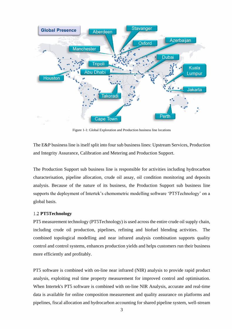
Figure 1-1: Global Exploration and Production business line locations .................................... 3
Figure 2-1: Showing an anticline trap (a) and a fault trap (b) taken from Burg et al. (1997) .... 8
Figure 2-2: A representation of the chemical forms of Paraffin’s, Naphthenes and Aromatics
taken from Naskar (2015) ........................................................................................................... 9
Figure 2-3: SARA separation taken from Lundanes and Greibrokk (1994) ............................ 10
Figure 2-4: A seismic survey taken from Grace (2007) ........................................................... 11
Figure 2-5: Showing an oil drilling rig (a) and a schematic of drilling (b) taken from Grace
(2007) ....................................................................................................................................... 12
Figure 2-6: Refinery flowsheet taken from Kraus (1996) ........................................................ 14
Figure 2-7: showing the fraction temperatures and chain lengths taken from Energia (2010) 15
Figure 2-8: The spectrum of light taken from NG (2012) ........................................................ 19
Figure 2-9: Different Crude Oil Spectra Baselines .................................................................. 21
Figure 2-10: Showing the comparison of errors for several models used to predict the
composition of gasoline taken from Balabin et al. (2007) ....................................................... 25
Figure 2-11: A representation of the GC equipment taken from Sheffield Hallam (2010) ...... 26
Figure 2-12: A plot comparing margins of refineries in Europe, FSU and Africa taken from
Wood-Mackenzie (2012a) ........................................................................................................ 30
Figure 2-13: Showing NCM in $/bbl. for a selection of major European refineries taken from
Wood-Mackenzie (2012a) ........................................................................................................ 31
Figure 2-14: Showing NCM in $/bbl. of major European Refiners taken from Wood-Mackenzie
(2012a) ...................................................................................................................................... 31
Figure 2-15: Solvents and precipitants for asphaltenes taken from Wiehe and Kennedy (2000b)
.................................................................................................................................................. 32
Figure 2-16: A hypothetical asphaltene molecule taken from Aurdal et al., (1998) ................ 32
Figure 2-17: Physical model of a petroleum system, showing the SARA balance taken from
Wiehe and Kennedy (2000b) .................................................................................................... 34
Figure 2-18: Showing a typical Vapour Pressure Osmometer setup taken from UCI (2016) .. 35
Figure 2-19: VPO determined molar masses in Athabasca bitumen taken from Gawrys and
Kilpatrick (2004) ...................................................................................................................... 36
Figure 2-20: SARA Fractions Methodology taken from Lundanes and Greibrokk (1994) ..... 38
Figure 2-21: A Plot Showing the Shift in Principal Component Scores of a Crude Oil Sample
during Depressurisation taken from Aske (2002b) .................................................................. 40
Figure 2-22: PCA Example 1 ................................................................................................... 45
xi
Figure 2-23: First Principal Component ................................................................................... 45
Figure 2-24: Second Principal Component .............................................................................. 46
Figure 2-25: Projection to Principal Component 1 taken from Richardson (2009) ................. 47
Figure 2-26: Bivariate Scores plot (PC1 v PC2) taken from Richardson (2009) ..................... 48
Figure 2-27: Bivariate loadings plot (PC1 v PC2) taken from Richardson (2009) .................. 48
Figure 2-28: Bivariate Scores Applied to a Refinery Dataset .................................................. 49
Figure 2-29: Showing modelling errors for different methods used to build a gasoline model
taken from Balabin et al. (2012) ............................................................................................... 52
Figure 3-1 - Typical Spectrometers (courtesy of ABB 2017) .................................................. 56
Figure 3-2 - Laboratory Crude Oil Sample Handling and Spectrometer ................................. 57
Figure 3-3 - Hydrocarbon absorption in Near Infra-Red radiation .......................................... 58
Figure 3-4 - Link Spectrum to Properties ................................................................................. 58
Figure 3-5 - NIR as Information Vector ................................................................................... 59
Figure 3-6 - Same Sample have Same Spectrum ..................................................................... 59
Figure 3-7 - Same Spectra Same Properties ............................................................................. 60
Figure 3-8: Simple sample spectra ........................................................................................... 61
Figure 3-9: Simple Aggregate .................................................................................................. 62
Figure 3-10 – Spectral Plane with Boxes of sample families ................................................... 63
Figure 3-11 - PT5Technology Prediction - Database Search ................................................... 64
Figure 3-12 - Topological Modelling Using Nearest Neighbours ............................................ 65
Figure 3-13 - Topological Modelling Using Artificial Nearest Neighbours ............................ 66
Figure 3-14 - Effect of R-Sphere .............................................................................................. 67
Figure 3-15 - Change of property with distance ....................................................................... 68
Figure 3-16 - Prediction and Model Update ............................................................................. 70
Figure 3-17: Case Study Crude Spectra ................................................................................... 73
Figure 3-18: PT5 Aggregate Plots of all Example Crudes showing API gravity aggregate (a)
and 565°C+ aggregate (b) ......................................................................................................... 74
Figure 3-19: Showing PT5 Aggregate plot (a) and a physical properties correlation (b) ........ 75
Figure 3-20: PT5Crude Aggregate Plot of Crude Type XX showing cluster and difference .. 76
Figure 3-21: TBP Curves for all four crude samples ............................................................... 77
Figure 3-22: Showing Average TBP v Sample_03 .................................................................. 78
Figure 3-23: the difference between the average and Sample_03 ............................................ 78
Figure 3-24: TBP curves from PT5 prediction ......................................................................... 79
Figure 4-1: Binary Crude Blend Exhibiting linear behaviour .................................................. 90
Figure 4-2: Linear Blend Aggregate ......................................................................................... 90
xii
Figure 4-3: Transmitted Light Microscopy 100% Crude A (a), 50% Crude A (b), 0% Crude A
(c) .............................................................................................................................................. 91
Figure 4-4: Binary Crude Blend Exhibiting Non-Linear Behaviour ........................................ 91
Figure 4-5: 8,000 Region of NIR Spectra Showing Non-Linearity ......................................... 92
Figure 4-6: Linear Blend Aggregate ......................................................................................... 92
Figure 4-7: Transmitted Light Microscopy 100% Crude A (a), 50% Crude A (b), 0% Crude A
(c) .............................................................................................................................................. 93
Figure 4-8: Showing inflection point........................................................................................ 94
Figure 4-9 - Crude Tracking on PT5 Aggregate....................................................................... 94
Figure 4-10 - Aggregate plot of instability observed from blend titrations .............................. 96
Figure 4-11: Determination of Insolubility Number and Solubility Blending Number for Forties
and Souedie Crude Oils taken from Wiehe, Kennedy and Dickakian (2001) .......................... 97
Figure 4-12 - Example Blend Recipe Feasibility Report ....................................................... 104
Figure 4-13 - Example Experimental Results from Matrix Blend Algorithm ........................ 105
Figure 4-14 - Example Blend Evaluation Report ................................................................... 106
Figure 4-15: HFO Laser Microscopy 1% Sulphur HFO (a), 1.8% Sulphur HFO (b), 1.8%
Sulphur Used HFO (c) and 3% Sulphur HFO (d) .................................................................. 112
Figure 4-16: HFO Microscopy with Transmitted Light on 1% Sulphur HFO (a), 1.8% Sulphur
HFO (b), 1.8% Sulphur Used HFO (c) and 3% Sulphur HFO (d) ......................................... 113
Figure 4-17: 1.8% Used Sulphur HFO with 50% HVN at time 0 hrs (a) and time 72 hours (b)
................................................................................................................................................ 114
Figure 4-18: Cross Polar Microscopy 1% Sulphur HFO (a), 1.8% Sulphur HFO (b), 1.8%
Sulphur Used HFO (c) and 3% Sulphur HFO (d) .................................................................. 115
Figure 4-19: Showing full spectra for 1.8% Sulphur Blend (a) and 9000 wavenumber region (b)
................................................................................................................................................ 117
Figure 4-20: Showing full spectra for 20% HVN titration (a) and 9000 wavenumber region (b)
................................................................................................................................................ 118
Figure 4-21: Comparison of physical properties to average .................................................. 120
Figure 4-22: Showing the an inflection point ......................................................................... 124
Figure 4-23: Linear Spectral Blending ................................................................................... 125
Figure 4-24: Blend 1 (a) and Blend 2 (b) aggregate plots ...................................................... 126
Figure 4-25: Blend 1- MDO in HFO at 0% (a), 30% (b), 60% (c) and 90% (d) .................... 127
Figure 4-26: Blend 2 - MDO in HFO ..................................................................................... 128
Figure 4-27: Showing blends with additive (a) and (c) and without additive (b) and (d) ..... 132
Figure 4-28: Showing blends with additive (a) and (c) and without additive (b) and (d) ..... 133
xiii
Figure 4-29: Neat Additive ..................................................................................................... 134
Figure 5-1: Process Flow Diagram ......................................................................................... 138
Figure 5-2: Pump Schematic .................................................................................................. 139
Figure 5-3: Pump A throughout time period 1 ....................................................................... 142
Figure 5-4: Pump A throughout period 4 ............................................................................... 143
Figure 5-5: Pump A throughout Period 5 ............................................................................... 145
Figure 5-6: Axial Displacement ............................................................................................. 146
Figure 5-7: Buffer Tank Level................................................................................................ 146
Figure 5-8 Flow Rate and Torque .......................................................................................... 147
Figure 5-9: Inlet Temperature vs DP ...................................................................................... 149
Figure 5-10: Axial Displacement of MPP B through time period 1 ....................................... 152
Figure 5-11: Axial displacement of MPPB throughout time period 4 ................................... 153
Figure 5-12: Pump B event 1 period 4 ................................................................................... 154
Figure 5-13: Buffer tank level through event 1 ...................................................................... 154
Figure 5-14: Flow and Torque through event 1 ...................................................................... 155
Figure 5-15: Pump B event 2 period 4 Torque and DP over the venturi ................................ 155
Figure 5-16: Venturi DP vs Torque ........................................................................................ 156
Figure 5-17: Example of Interpolation histogram .................................................................. 159
Figure 5-18: Close examination of interpolation .................................................................... 160
Figure 5-19: Example frequency histogram ........................................................................... 162
Figure 5-20: Example Autocorrelation plot............................................................................ 163
Figure 5-21: Autocorrelation plot for buffer tank percentage in pump A .............................. 164
Figure 5-22: Inlet Temperature (left) and axial vibration (right) ........................................... 165
Figure 5-23: heatmap of mean Pearson’s correlation coefficient across the longer time periods
(1, 4, 5) ................................................................................................................................... 166
Figure 5-24: PLS Loadings for each pump’s non-temperature sensors against the pump’s Z-axis
displacement as an objective function. ................................................................................... 168
Figure 5-25: Variance explained by the Principal Components fitted to the dataset. ............ 169
Figure 5-26: Plotting the individual time points by their position each principle component,
coloured by the period of origin. ............................................................................................ 170
Figure 5-27: Bar plots of how each sensor value contributes to the first 3 principal components
in the PCAs with (above) and without (below) temperature sensors. .................................... 171
Figure 5-28: Operating Regions PCA .................................................................................... 173
Figure 5-29: Variance explained by the Principal Components fitted to the dataset with
temperature sensors (a) and without temperature sensors and period 5 (b) ........................... 174
xiv
Figure 5-30: Plotting the individual time points by their position each principle component,
coloured by the period of origin. ............................................................................................ 175
Figure 5-31: Bar plots of how each sensor value contributes to the first 3 principal components
in the PCAs where period 5 is included and excluded. .......................................................... 176
Figure 5-32: Projecting the data values of an event noticed in the technical analysis event 2 in
period 5 for Pump A ............................................................................................................... 177
Figure 5-33: Projecting the data values of an event noticed in the technical analysis (event 1 in
period 5 for Pump A ............................................................................................................... 178
Figure 7-1: Forties Pipeline System (FPS) North Sea taken from Subsea (2017) ................. 185
Figure 7-2: North Sea Fields Aggregate Plot ......................................................................... 187
Figure A-1: 1% Sulphur HFO - 5% HVN .............................................................................. 195
Figure A-2: 1% Sulphur HFO - 10% HVN ............................................................................ 195
Figure A-3: 1% Sulphur HFO - 50% HVN ............................................................................ 195
Figure A-4: 1.8% Sulphur HFO - 5% HVN ........................................................................... 196
Figure A-5: 1.8% Sulphur HFO - 10% HVN ......................................................................... 196
Figure A-6: 1.8% Sulphur HFO - 50% HVN ......................................................................... 196
Figure A-7: 1.8% Used Sulphur HFO - 5% HVN .................................................................. 197
Figure A-8: 1.8% Used Sulphur HFO - 10% HVN (left) and (right) ..................................... 197
Figure A-9: 3% Sulphur HFO - 5% HVN .............................................................................. 198
Figure A-10: 3% Sulphur HFO - 10% HVN .......................................................................... 198
Figure A-11: 3% Sulphur HFO - 50% HVN .......................................................................... 198
Figure B-1: Marine Fuel Blends ............................................................................................. 200
xv
Index of Tables
Table 1: Food Consumpton in the UK (g/person/week) taken from Richardson (2009) ......... 47
Table 3-1: Database Structure .................................................................................................. 64
Table 3-2: Database Management ............................................................................................ 69
Table 3-3: Four samples of type XX with their API, Sulphur and the cut 565°C+ from TBP 72
Table 3-4: Property Prediction Statistics .................................................................................. 79
Table 3-5: Aggregate Distance Matrix ..................................................................................... 80
Table 3-6: Difference between prediction and laboratory analysis expressed as a percentage of
method reproducibility R .......................................................................................................... 82
Table 3-7: Simple Refinery Netbacks ...................................................................................... 83
Table 3-8: Complex Refinery Netbacks ................................................................................... 83
Table 4-1: Example Blend Experiment .................................................................................... 98
Table 4-2: Stability testing for variation in crude ratios ......................................................... 101
Table 4-3: Laboratory Results, condensate Matrix ................................................................ 103
Table 4-4: Showing the Full set of blend tested ..................................................................... 109
Table 4-5: HFO Physical Properties ....................................................................................... 111
Table 4-6: Percentages of Reference Crude (RC) around the point of instability .................. 119
Table 4-7: Physical Properties for Samples ............................................................................ 123
Table 4-8: Physical Properties for Samples ............................................................................ 130
Table 4-9: Summary table ...................................................................................................... 131
Table 5-1: Summary of histogram observations .................................................................... 162
Table 7-1: Showing properties measured for the FPS Application on Whole crude (Left) and
Light Ends (Right) .................................................................................................................. 186

xvi
Index of Definitions
American Petroleum Institute API
American Petroleum Institute Gravity °API
American Society for Testing and Materials ASTM
Artificial Neural Network ANN
Artificial Neural Network Multilayer Perceptron ANN - MLP
Assurance, Testing, Inspection and Certification ATIC
Atmospheric Pressure Photoionisation APPI
Barrel (Typically used for crude oil, Volume = 42 US Gallons) BBL
Binding Resins BR
Carbon Dioxide CO2
Crude Distillation Unit CDU
Enhanced Oil Recovery EOR
Equations of State EOS
Exploration and Production E&P
Final Boiling Point FBP
Former Soviet Union FSU
Forties Pipeline System FPS
Fourier Transform Infrared (spectroscopy) FTIR
Fourier Transform Ion Cyclotron Resonance Mass Spectrometry FT-ICR MS
Freeze Fracture and Transmission Electron Microscopy FF-TEM
Gas Chromatography GC
Hierarchical Partial Least Squares (regression) H - PLS
High Performance Liquid Chromatography HPLC
High Sulphur Fuel Oil HSFO
Infrared IR
Instability Coefficient IC
Initial Boiling Point IBP
Intertek Proprietary Chemometric Modelling Technology PT5
K Nearest Neighbours KNN
Knock Index KI
Latent Variable LV
Light Virgin Naphtha LVN
Linear Discriminant Analysis LDA
Linear Predictive Coding LPC
Linear Solvation Energy Relation LSER
Low Sulphur Fuel Oil LSFO
Mid InfraRed MIR
Motor Octane Number MON
Multi-Block Partial Least Squares (regression) MB-PLS
MultiLayer Perceptron MLP
Multiple Linear Regression MLR
Multiplicative Scatter Correction MSC
Near InfraRed NIR
Net Cash Margin NCM
Neural Network NN
xvii
Nuclear Magnetic Resonance NMR
Octane Number ON
Open Column Chromatography OPC
Order Derivative OrD
Organic Deposition OD
Oxides of Carbon COx
Oxides of Nitrogen NOx
Oxides of Sulphur SOx
Partial Least Squares (regression) PLS
Polynomial Partial Least Squares (regression) Poly - PLS
Partial Least Squares Discriminant Analysis PLS - DA
Pour Point PP
Principal Component PC
Principal Component Analysis PCA
Process Assurance Group PAG
Pulse-Field Gradient Spin Echo Nuclear Magnetic Resonance PFG-SE NMR
Principal Component Regression PCR
Probabilistic Neural Network PNN
Quadratic Discriminant Analysis QDA
Regularised Discriminant Analysis RDA
Refinery Gross Margin RGM
Refractive Index RI
Research Octane Number RON
Residual Asphaltenes RA
Root Mean Squared Error of Cross Validation RMSECV
Root Mean Squared Error of Prediction RMSEP
Saturates Aromatics, Resins and Asphaltenes SARA
Serial PLS S-PLS
Simulated Distillation SimDis
Small Angle Neutron Scattering SANS
Soft Independent Modelling of Class Analogy SIMCA
Spline Partial Least Squares (regression) Spline - PLS
Stability Coefficient SC
Standard Error of Prediction SEP
Standard Normal Variance SNV
Statistical Association Fluid Theory for Potentials of Variable Range SAFT - VR
Support Vector Machines SVM
TetraHydroFuran THF
Total Acid Number TAN
Transmission Electron Microscope TEM
TriChloroEthylene TCE
True Boiling Point TBP
Vapour Pressure Osmometry VPO
Wavelet Neural Network WNN

1
Chapter 1:
Introduction
2
Chapter 1. Introduction
Throughout the hydrocarbon supply chain, process optimisation is driven by the desire to
maximise profit margins. In the global refining marketplace, the biggest cost is crude oil and to
improve margins increasing use of non-conventional crude oils such as shale oils or tar sands
high (also called opportunity crudes) lowers the cost of the crude blend. Opportunity crudes are
selected based on market forces, for example in North America, the production booms in shale
oil and tar sands have provided ample amounts of new low-cost oils which refineries are buying
and processing.
However, as these oils are new to the marketplace and many refineries have never processed
them before it brings about challenges including: lack of understanding of the quality of the
crude oil being processed (shale oils for example can come from many thousands of wells) and
how these oils interact with the more conventional refinery feedstocks (such as Brent or West
Texas Intermediate).
Intertek
Intertek Group plc are a multinational corporate organisation consisting of more than 42,000
employees in over 1,000 locations in over 100 countries across the globe.
Through their global network of state-of-the-art facilities and industry-leading technical
expertise Intertek provides innovative and bespoke Assurance, Testing, Inspection and
Certification (ATIC) services to customers in a variety of sectors including food,
pharmaceuticals, electrical, automotive and oil and gas. (Intertek, 2016).
The Exploration and Production (E&P) division is one of Intertek’s oil and gas focussed
business lines and primarily deals with upstream operations, the locations of the E&P division
globally are shown in Figure 1-1.
3
Figure 1-1: Global Exploration and Production business line locations
The E&P business line is itself split into four sub business lines: Upstream Services, Production
and Integrity Assurance, Calibration and Metering and Production Support.
The Production Support sub business line is responsible for activities including hydrocarbon
characterisation, pipeline allocation, crude oil assay, oil condition monitoring and deposits
analysis. Because of the nature of its business, the Production Support sub business line
supports the deployment of Intertek’s chemometric modelling software ‘PT5Technology’ on a
global basis.
PT5Technology
PT5 measurement technology (PT5Technology) is used across the entire crude oil supply chain,
including crude oil production, pipelines, refining and biofuel blending activities. The
combined topological modelling and near infrared analysis combination supports quality
control and control systems, enhances production yields and helps customers run their business
more efficiently and profitably.
PT5 software is combined with on-line near infrared (NIR) analysis to provide rapid product
analysis, exploiting real time property measurement for improved control and optimisation.
When Intertek's PT5 software is combined with on-line NIR Analysis, accurate and real-time
data is available for online composition measurement and quality assurance on platforms and
pipelines, fiscal allocation and hydrocarbon accounting for shared pipeline system, well-stream

4
allocations, multiphase meter validation and distillation column reconciliation. The technology
can be used across the whole spectrum, including MIR (Mid Infra-Red), NIR (Near Infra-Red),
Nuclear Magnetic Resonance (NMR) and Gas Chromatography (GC).
Objectives
This Eng.D project has been focused on working in collaboration with the industrial partner
Intertek to develop commercially viable solutions to provide customers in the hydrocarbon-
processing sector with the following:
1. Develop a methodology for rapid identification of crude oil composition both online
and offline.
2. Implement a tool to facilitate optimisation of crude blending performance utilising
the information from objective 1.
3. Develop an approach to characterise the stability and compatibility of blended
hydrocarbon streams
4. Apply data analytics approaches to solve historical hydrocarbon processing issues
Contributions
My contribution has been to firstly critique and improve existing chemometric approaches for
helping refineries understand and predict the quality of crude oils from Near Infrared (NIR)
spectra. Using this information has helped refineries to inform crude processing and process
control decisions.
Secondly, as a consequence of the research, a process was developed to assess the compatibility
of blended crude oils. This is of critical importance to the industry because blending
incompatible crude oils can elicit precipitation of problematic material such as wax and
asphaltene. These can contribute to heat exchanger and distillation column fouling, block pipes
and storage tank offtakes to name a few of the multitude of undesirable effects.
Finally, further development of the data analytics approach of the industrial partner to solving
client specific issues has shown exciting outcomes including maximisation of refinery fractions
and improving process stability.
Thesis Overview
This thesis is designed to build up the story of the work, to take the reader on the research
journey and ultimately present the achievements of the project in a series of case studies.

5
As such an initial literature review draws attention to literature relevant to the research and
covers the oil & gas industry in general as well as the principles of oil refining. It then drills
down to the chemistry of crude oil stability and the economic drivers to develop a solution.
Finally, it looks at spectroscopic techniques for hydrocarbon characterisation and modelling
techniques for both chemometric and process data analysis
The first case study then explores the contributions of the thesis to the field of chemometrics.
It describes the refinement of the modelling tool and then demonstrates its application within
an Asian refinery.
The thesis then goes on to describe the development and application of an innovative
methodology, patented during the course of the Eng.D project, for describing and predicting
the stability of blended crude oils. The benefits of the research and development are then
contextualised in two case studies, one that looks at the blending of heavy fuel oil in refineries
and another which looks at challenges of fuel blending in the maritime sector.
Finally, the thesis presents a study of the application of multivariate statistics to an offshore
facility and talks through an example of the application of data analytics to resolve a historical
pump failure problem.

6
Chapter 2:
Literature Review
7
Chapter 2. Literature Review
In this section different themes from the literature, relevant to the industry and the research will
be explored. Examples of the application of various techniques to the characterisation of
hydrocarbon process streams, as well as non oil and gas applications will be explored with the
intention of drawing out the strengths and weaknesses of the methodologies used in the rearach.
As this project is predominantly focussed in the oil and gas industry, an overview of crude oil
formation, exploration, production and refining will be examined. Crude oil is the key resource
in the world today, almost everyone comes into contact with a crude oil derivative product on
a daily basis, whether it is in the form of plastics, fuels or paints and as such the price of oil is
an important factor, which affects daily lives.
A voracious appetite for crude oil from rapidly growing economies such as China and India
was driving the price up. However, due to the shale oil boom, weaker than anticipated global
demand, and the refusal of OPEC countries (particularly Saudi Arabia) to cut production means
that the price of oil has fallen dramatically since the start of the project in 2011.
This literature review draws attention to key areas relevant to the research and covers the oil &
gas industry in general as well as the principles of oil refining. It then drills down to the
chemistry of crude oil stability and the economic drivers to develop a solution. Finally, it looks
at spectroscopic techniques for hydrocarbon characterisation and modelling techniques for both
chemometric and process data analysis
Formation
Crude oil is formed from prehistoric flora and fauna falling to the beds of lakes and warm
shallow seas. This was mixed with the mud and sediments forming anaerobic conditions. As a
consequence of the conditions, the organic material did not decompose in the normal manner
by aerobic bacteria.
Over a period of many years, more layers of mud and sediment build up burying the material
deeper. As more weight pressed down the heat and pressure increased, this caused a
transformation of the material into Kerogen (a collection of organic compounds found in
8
sedimentary rock). with the addition of more heat and pressure the Kerogen was then altered
into liquid and gaseous hydrocarbons by a process called catagenesis (Braun and Burnham,
1993).
To trap oil after it has formed it is necessary for three conditions to exist. First of all a rock rich
in organic matter has to have been buried deep enough to have experienced the intense heat and
pressure required for the formation of oil. Secondly, a porous rock must be in place, which can
act as a reservoir for the oil to accumulate. Finally, a non-porous rock must sit over the porous
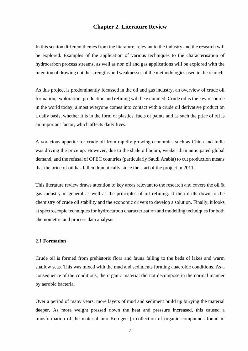
and act as a cap to stop the oil seeping out of the reservoir. Shown in Figure 2-1 are two types
of traps that occur to create oil reservoirs. The first (Figure 2-1a) is an anticline trap; this is
caused by ripples in the earth’s plate due to tectonic movement. The ripples are called anticlines
at the crest and synclines at the trough (Grace, 2007). Figure 2-1b is a fault trap, this is caused
by tectonic plate shearing (Burg, Selves and Colin, 1997).
a.
b.
Figure 2-1: Showing an anticline trap (a) and a fault trap (b) taken from Burg et al. (1997)
Composition
The precise chemical composition of petroleum can vary with location and the age of the field
in additions to any variations that occur with the depth of the individual well (Speight, 2001).
It is also possible that two wells that are adjacent to each other may produce oil that is of varying
composition. However all crude oils contain at least some of the following components:
Hydrocarbons, nitrogen compounds, oxygen compounds, sulphur compounds and metallic
constituents (Speight, 2001).
Speight (2001) also states that the consideration of the atomic hydrogen-carbon ratio, sulphur
content, and API gravity are no longer adequate to the task of determining refining behaviour.
This is in strong agreement with the research work carried out in this project, a large constituent
of which is aimed at providing refiners with more information in a shorter time space to allow
9
for improved process optimisation. As will be seen in a case study later on, the measurement
of API gravity and Sulphur measurements of both neat crudes and blends are the predominant
metrics used by refineries for quality monitoring and economic optimisation, as they are quick,
simple and cheap tests.
Although crude oil is composed of a plethora of components including inorganic components
such as salts and metals (such as vanadium, nickel and iron), by far the most abundant and
useful constituent of crude oils are the hydrocarbons, for convenience these can be divided into
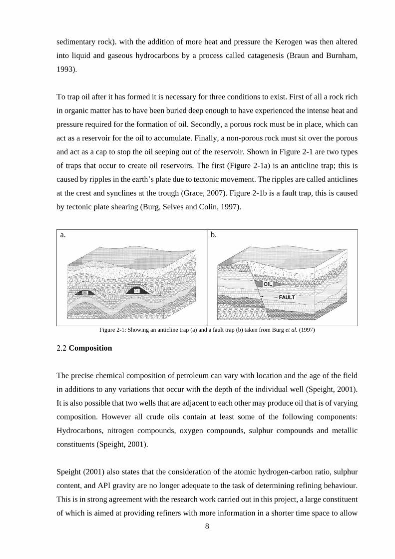
three groups (paraffin’s, napthenes and aromatics) (Speight, 2001) and are shown in Figure 2-2:
Figure 2-2: A representation of the chemical forms of Paraffin’s, Naphthenes and Aromatics taken from Naskar (2015)
1. Paraffin’s - Saturated hydrocarbons with straight or branched chains, but without any ring
structure.
2. Naphthenes - Saturated hydrocarbons containing one or more rings, each of which may have
one or more paraffinic side chains (more correctly known as alicyclic hydrocarbons).
3. Aromatics Hydrocarbons containing one or more aromatic nuclei, such as benzene,
naphthalene, and phenanthrene ring systems, which may be linked up with (substituted)
naphthene rings and/or paraffinic side chains.
A variant of this classifies crude oils depending on the characteristics of the distillation residues
and whether it is asphalt-base, paraffin base or mixed base. (Guthrie, 1960).
However the above classifications do not work well for heavy oils (Speight, 2016) and does not
describe all the constituents which must be considered when describing crude oil blending
10
behaviour (particularly with respect to crude oil stability) and as a consequence a four group
classification of crude oils is more widely used.
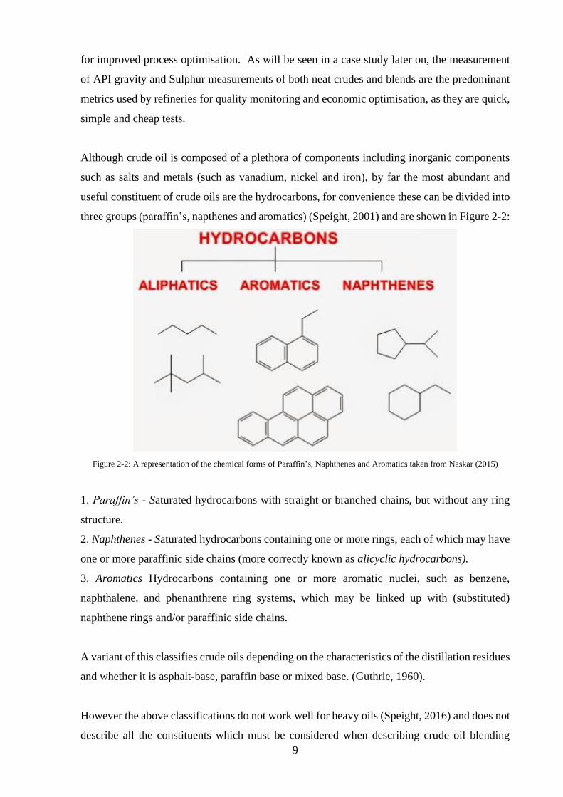
This model, named SARA, is discussed in more detail in section 2.14 and includes Saturates
(S) as an umbrella term covering paraffin’s and naphthenes. Aromatics (A), Resins (R) which
are a solubility group of molecules with both polar and non-polar constituent, miscible with
heptane and Asphaltenes (A) which are the most polar fraction of crude oil, soluble in toluene
and insoluble in heptane. In this process, the oil is first deasphalted to obtain asphaltenes + SAR
fraction. This is then separated by HPLC using either bonded phase columns or a combination
of silica and bonded phase columns (Lundanes and Greibrokk, 1994).
Figure 2-3: SARA separation taken from Lundanes and Greibrokk (1994)
Exploration and Production
Petroleum exploration is the domain of geologists and geophysicists. It is not economically
viable to drill holes in the ground and hope to strike lucky, although this has been historically
undertaken by both large and small energy companies, a practice known as ‘wildcatting’. The
normal practice before drilling, however, is to carry out full and proper geographical surveys.
It is a well understood fact that there are locations in the world where oil is more prevalent.
Indeed, there are parts of the world (such as Casper, Wyoming) where oil seeps to the surface,
drilling in that area found a vast oil field, which is still producing to this day. In other places
visible mounds where the earth has been pushed up by the pressure of subterranean oil (such as
tea pot dome, Wyoming) has also yielded oil strikes (Grace, 2007).
Crude Oil
Asphaltenes Resins Aromatics Saturates
Maltenes
n-Hexane
Solution
N-Hexane
Silica
N-HexaneTrichloromethane
Precipitate
11
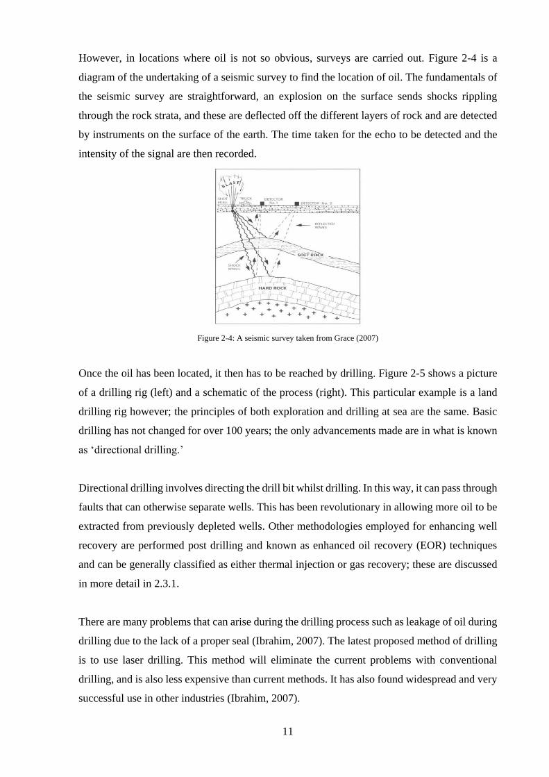
However, in locations where oil is not so obvious, surveys are carried out. Figure 2-4 is a
diagram of the undertaking of a seismic survey to find the location of oil. The fundamentals of
the seismic survey are straightforward, an explosion on the surface sends shocks rippling
through the rock strata, and these are deflected off the different layers of rock and are detected
by instruments on the surface of the earth. The time taken for the echo to be detected and the
intensity of the signal are then recorded.
Figure 2-4: A seismic survey taken from Grace (2007)
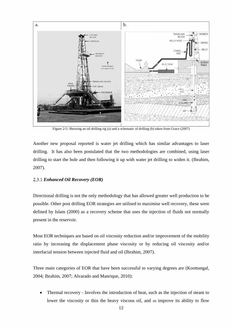
Once the oil has been located, it then has to be reached by drilling. Figure 2-5 shows a picture
of a drilling rig (left) and a schematic of the process (right). This particular example is a land
drilling rig however; the principles of both exploration and drilling at sea are the same. Basic
drilling has not changed for over 100 years; the only advancements made are in what is known
as ‘directional drilling.’
Directional drilling involves directing the drill bit whilst drilling. In this way, it can pass through
faults that can otherwise separate wells. This has been revolutionary in allowing more oil to be
extracted from previously depleted wells. Other methodologies employed for enhancing well
recovery are performed post drilling and known as enhanced oil recovery (EOR) techniques
and can be generally classified as either thermal injection or gas recovery; these are discussed
in more detail in 2.3.1.
There are many problems that can arise during the drilling process such as leakage of oil during
drilling due to the lack of a proper seal (Ibrahim, 2007). The latest proposed method of drilling
is to use laser drilling. This method will eliminate the current problems with conventional
drilling, and is also less expensive than current methods. It has also found widespread and very
successful use in other industries (Ibrahim, 2007).
12
a.
b.
Figure 2-5: Showing an oil drilling rig (a) and a schematic of drilling (b) taken from Grace (2007)
Another new proposal reported is water jet drilling which has similar advantages to laser
drilling. It has also been postulated that the two methodologies are combined, using laser
drilling to start the hole and then following it up with water jet drilling to widen it. (Ibrahim,
2007).
Enhanced Oil Recovery (EOR)
Directional drilling is not the only methodology that has allowed greater well production to be
possible. Other post drilling EOR strategies are utilised to maximise well recovery, these were
defined by Islam (2000) as a recovery scheme that uses the injection of fluids not normally
present in the reservoir.
Most EOR techniques are based on oil viscosity reduction and/or improvement of the mobility
ratio by increasing the displacement phase viscosity or by reducing oil viscosity and/or
interfacial tension between injected fluid and oil (Ibrahim, 2007).
Three main categories of EOR that have been successful to varying degrees are (Koottungal,
2004; Ibrahim, 2007; Alvarado and Manrique, 2010):
• Thermal recovery - Involves the introduction of heat, such as the injection of steam to
lower the viscosity or thin the heavy viscous oil, and so improve its ability to flow
13
through the reservoir. Thermal techniques account for over 50% of US EOR production
and enjoy extensive popularity throughout the Canadian tar sands fields.
• Gas injection - Uses gases such as natural gas, nitrogen, or carbon dioxide that expand
in a reservoir to push additional oil to a production wellbore, or other gases that dissolve
in the oil to lower its viscosity and improve its flow rate.
• Chemical Injection – Widely used in the 1980’s but has been in decline ever since.
Chemical injection strategies involve flooding wells with manufactured compounds,
usually polymeric in nature, to increase well production. This is achieved by adding the
polymer to waterflood (a technique for maintaining well pressure by injecting water into
the well to displace the oil) fluids alter viscosity and thus increase pore mobility and
waterflood characteristics.
Refining
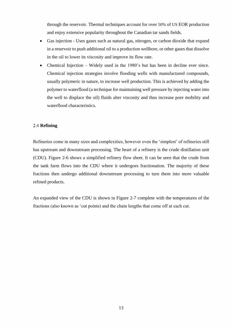
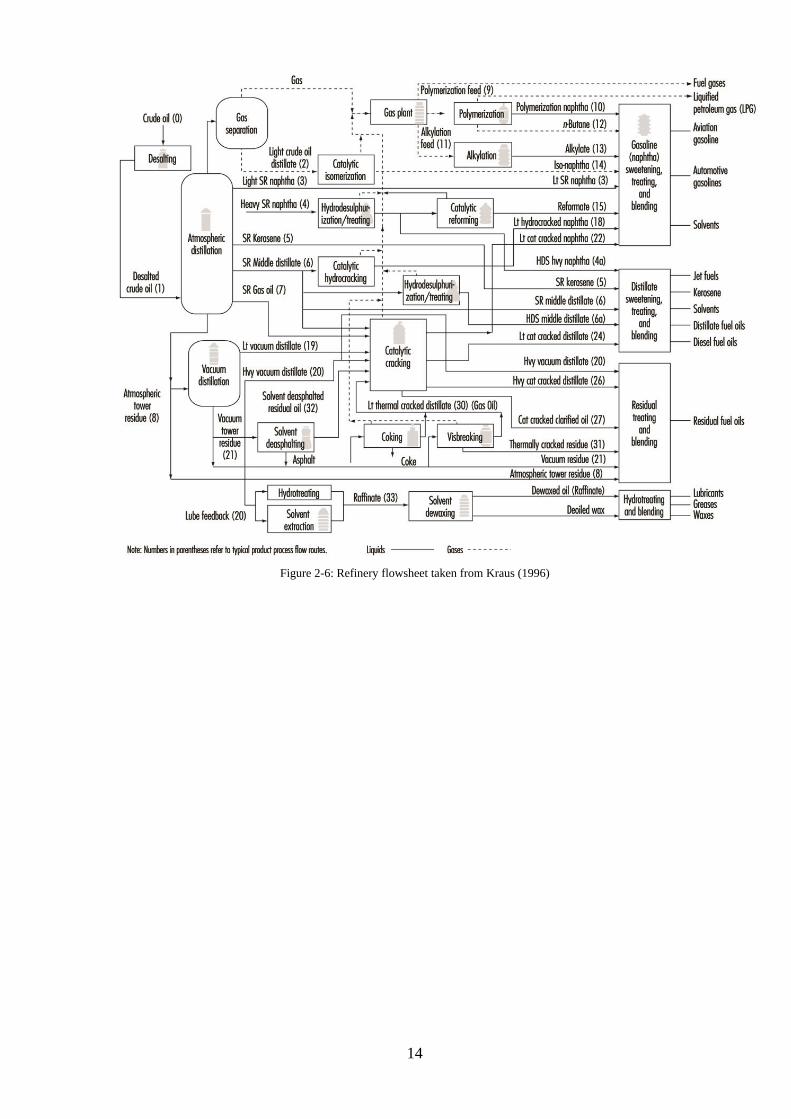
Refineries come in many sizes and complexities, however even the ‘simplest’ of refineries still
has upstream and downstream processing. The heart of a refinery is the crude distillation unit
(CDU). Figure 2-6 shows a simplified refinery flow sheet. It can be seen that the crude from
the tank farm flows into the CDU where it undergoes fractionation. The majority of these
fractions then undergo additional downstream processing to turn them into more valuable
refined products.
An expanded view of the CDU is shown in Figure 2-7 complete with the temperatures of the
fractions (also known as ‘cut points) and the chain lengths that come off at each cut.
14
Figure 2-6: Refinery flowsheet taken from Kraus (1996)
15
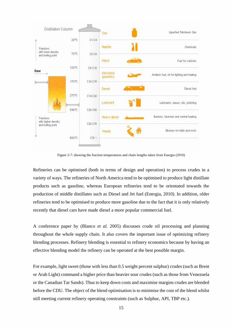
Figure 2-7: showing the fraction temperatures and chain lengths taken from Energia (2010)
Refineries can be optimised (both in terms of design and operation) to process crudes in a
variety of ways. The refineries of North America tend to be optimised to produce light distillate
products such as gasoline, whereas European refineries tend to be orientated towards the
production of middle distillates such as Diesel and Jet fuel (Energia, 2010). In addition, older
refineries tend to be optimised to produce more gasoline due to the fact that it is only relatively
recently that diesel cars have made diesel a more popular commercial fuel.
A conference paper by (Blanco et al. 2005) discusses crude oil processing and planning
throughout the whole supply chain. It also covers the important issue of optimizing refinery
blending processes. Refinery blending is essential to refinery economics because by having an
effective blending model the refinery can be operated at the best possible margin.
For example, light sweet (those with less than 0.5 weight percent sulphur) crudes (such as Brent
or Arab Light) command a higher price than heavier sour crudes (such as those from Venezuela
or the Canadian Tar Sands). Thus to keep down costs and maximise margins crudes are blended
before the CDU. The object of the blend optimisation is to minimise the cost of the blend whilst
still meeting current refinery operating constraints (such as Sulphur, API, TBP etc.).
16
Extensive work has been carried out on the subject of scheduling refinery crude oil operations
and processing. Mouret (2010) produced an extensive Ph.D. dissertation on the subject of
scheduling refinery operations, in the thesis the problem of scheduling refinery processes is
approached by using both linear and non-linear mixed integer procedures.
Blending of crude oils to maximise refinery economics is a key theme for the Eng.D project.
The organic deposition work was sparked by the identified need to develop a methodology to
assess stability of blended crude oils. This is becoming more important with the increased
amount of low cost (but also not well understood) opportunity oils in the marketplace such as
U.S. shale oils and Canadian tar sands.
Primary Reference Data
No two crude oils are the same, each has unique molecular and chemical characteristics
resulting in crucial differences in crude oil quality. These in turn have an effect on the valuation
of each individual crude.
The physical testing results of the individual fractions contained within each crude provide
extensive detailed analysis data for refiners, oil traders and producers. The data also helps
producers design new refineries to maximise product output and or type according to the
feedstock provided.
Existing refineries can determine if a new crude feedstock is compatible, or if the crude could
cause yield, quality, production, environmental and other problems. Feedstock assay data is
used for detailed refinery engineering, client marketing purposes and an important tool in the
refining process.
To generate the data used within the chemometric models, ASTM methodologies for crude oil
analysis are applied to generate the primary reference data. The case studies presented later
focus primarily on distillation data, density and sulphur content so those will now be described.
ASTM D2892/D5236 – Distillation Curve
Used to produce True Boiling Point (TBP) curve for the determination of the %wt or %vol
against temperature curve and also to produce fractions for further analysis. This distillation
corresponds very closely to the type of fractionation obtained in a refinery.
17
The method is split over two stages, firstly the atmospheric (D2892) still is charged
with crude oil and then distilled up to 350°C. The residue from this distillation is then
taken and charged to the high vacuum (D5236) still where it is then taken to 565°C.
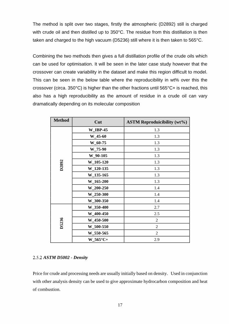
Combining the two methods then gives a full distillation profile of the crude oils which
can be used for optimisation. It will be seen in the later case study however that the
crossover can create variability in the dataset and make this region difficult to model.
This can be seen in the below table where the reproducibility in wt% over this the
crossover (circa. 350°C) is higher than the other fractions until 565°C+ is reached, this
also has a high reproducibility as the amount of residue in a crude oil can vary
dramatically depending on its molecular composition
Method Cut ASTM Reproduicibility (wt%)
D28
92
W_IBP-45 1.3
W_45-60 1.3
W_60-75 1.3
W_75-90 1.3
W_90-105 1.3
W_105-120 1.3
W_120-135 1.3
W_135-165 1.3
W_165-200 1.3
W_200-250 1.4
W_250-300 1.4
W_300-350 1.4
D5
236
W_350-400 2.7
W_400-450 2.5
W_450-500 2
W_500-550 2
W_550-565 2
W_565°C+ 2.9
ASTM D5002 - Density
Price for crude and processing needs are usually initially based on density. Used in conjunction
with other analysis density can be used to give approximate hydrocarbon composition and heat
of combustion.
18
The ASTM method uses a digital densitometer and stipulates the results must be reported in
grams per centimetre cubed (g/cm3) to 4 decimal place accuracy. Density is a quick and simple
test for crude oil quality and is subject to the following reproducibility:
0.00412*X (2-1)
Where X is the average of two results. To critique modelling data this is taken as the average
of the laboratory data and the prediction generate by the chemometric model for the same
sample.
ASTM D4294 - Sulphur
High sulphur content in petroleum products may be undesirable as it can be corrosive and create
an environmental hazard when burned. For these reasons, sulphur limitations are specified in
the quality control of fuels, solvents etc. Hydrogen sulphide deactivates catalysts; feed
pretreating can be used to remove these materials.
A hydrotreater is used to convert organic sulphur and nitrogen compounds to hydrogen sulphide
and ammonia, which are then removed from the system with the unreacted hydrogen. The
hydrogen required is obtained from the catalytic reformer. Sulphur is removed to reduce or
eliminate corrosion during refining, handling or in the use of various products. To produce
products with an acceptable odour and specification and to improve burning characteristics of
fuel oils.
In the laboratory Sulphur is measured using X-Ray Diffraction (XRD) and is subject to the
following reproducibility
1.9182*((X*10,000) ^ 0.6446))/10000 (2-2)
Where X is once again the average of two results. To critique modelling data this is taken as
the average of the laboratory data and the prediction generate by the chemometric model for
the same sample.
19
Spectroscopy
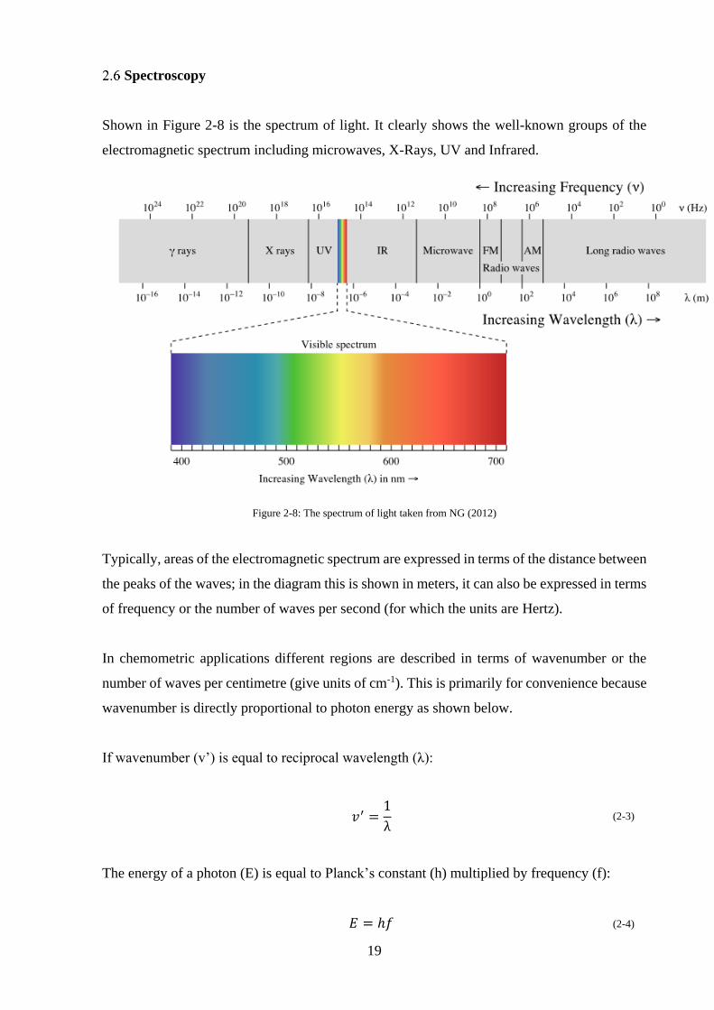
Shown in Figure 2-8 is the spectrum of light. It clearly shows the well-known groups of the
electromagnetic spectrum including microwaves, X-Rays, UV and Infrared.
Figure 2-8: The spectrum of light taken from NG (2012)
Typically, areas of the electromagnetic spectrum are expressed in terms of the distance between
the peaks of the waves; in the diagram this is shown in meters, it can also be expressed in terms
of frequency or the number of waves per second (for which the units are Hertz).
In chemometric applications different regions are described in terms of wavenumber or the
number of waves per centimetre (give units of cm-1). This is primarily for convenience because
wavenumber is directly proportional to photon energy as shown below.
If wavenumber (v’) is equal to reciprocal wavelength (λ):
𝑣′ =1
λ (2-3)
The energy of a photon (E) is equal to Planck’s constant (h) multiplied by frequency (f):
𝐸 = ℎ𝑓 (2-4)
20
And the relationship between velocity (v), frequency and wavelength is:
𝑣 = 𝑓λ (2-5)
By substituting the velocity of a photon as the speed of light (c) the equation becomes:
𝑐 = 𝑓λ (2-6)
Rearranging:
𝑓 =𝑐
λ (2-7)
And substituting back into Equation (2-4):
𝐸 = ℎ𝑐×1
λ (2-8)
𝐸 = ℎ𝑐𝑣′ (2-9)
Near Infrared
The Near Infrared Region covers the 4000cm-1 to 12,820cm-1 region (780nm to 2500nm) and
contains regions known as the combination region and overtone regions. NIR has been used in
the hydrocarbon processing industry for decades, primarily for fuels blending (Rohrback,
1991). The attraction of NIR is due to its strong response to functional groups such as
methylinic, olefinic or aromatic C-H stretching vibrations that are independent of the molecule
(Kelly and Callis, 1990; Aske et al., 2001).
Near Infrared is a particular focus of this thesis because it has the ability to describe changes in
both the chemical composition of a hydrocarbon stream (Blanco et al., 2000; Chung and Ku,
2000) and the physical composition of a hydrocarbon stream (Gossen, MacGregor and Pelton,
1993; Pasikatan et al., 2003). This has a twofold implication for the analysis of crude oils, that
the chemical changes in blended oils change and therefore so do the spectra, and also that if any
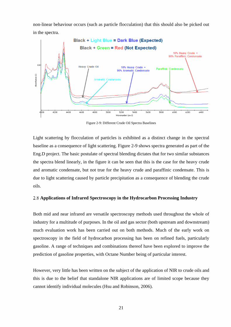
21
non-linear behaviour occurs (such as particle flocculation) that this should also be picked out
in the spectra.
Figure 2-9: Different Crude Oil Spectra Baselines
Light scattering by flocculation of particles is exhibited as a distinct change in the spectral
baseline as a consequence of light scattering. Figure 2-9 shows spectra generated as part of the
Eng.D project. The basic postulate of spectral blending dictates that for two similar substances
the spectra blend linearly, in the figure it can be seen that this is the case for the heavy crude
and aromatic condensate, but not true for the heavy crude and paraffinic condensate. This is
due to light scattering caused by particle precipitation as a consequence of blending the crude
oils.
Applications of Infrared Spectroscopy in the Hydrocarbon Processing Industry
Both mid and near infrared are versatile spectroscopy methods used throughout the whole of
industry for a multitude of purposes. In the oil and gas sector (both upstream and downstream)
much evaluation work has been carried out on both methods. Much of the early work on
spectroscopy in the field of hydrocarbon processing has been on refined fuels, particularly
gasoline. A range of techniques and combinations thereof have been explored to improve the
prediction of gasoline properties, with Octane Number being of particular interest.
However, very little has been written on the subject of the application of NIR to crude oils and
this is due to the belief that standalone NIR applications are of limited scope because they
cannot identify individual molecules (Hsu and Robinson, 2006).
22
Other work demonstrates that this is not strictly true and the Eng.D project has proven that with
the application of good chemometrics, extensive crude oil data can be predicted from NIR
spectra. For example Hidajat & Chong (2000) built PLS models to predict distillation data and
density of 110 crude oil samples. In their work, they report that the correlations were very good
and the predictions had reproducibility limits equivalent to those stated by American Society
for Testing and Materials, a benchmark for global laboratories and the standard against which
the models in the Eng.D project were compared.
An evaluation by (Chung et al. 1999) on kerosene found that in a comparative study of MIR
and NIR modelling with PLS that although both techniques showed good correlation with the
reference method, NIR provided better calibration performance over MIR. NIR was also found
to have a greater signal to noise ratio than MIR. This meant that although more qualitative
information could be gained from the MIR spectra (due to the specific, sharp and highly
absorbing peaks); the NIR gave more spectral variation and quantitative information necessary
for PLS modelling.
NIR and MIR was compared by (Felicio et al. 2005) for the prediction of Research Octane
Number (RON) for gasoline and flash point for gas oil. Models of NIR and MIR spectra were
built individually and a combined model was also created using single PLS, multiblock PLS
(MB-PLS) and Serial PLS (S-PLS). The single PLS models were found to be the preferable
method as they achieved accurate results and in a reasonable time. The overall best predictive
results however were achieved using S-PLS which consistently achieved better results than both
single PLS and MB-PLS on both MIR and NIR and proved to be a robust model. MB-PLS was
found to give results that were an average between the single PLS and S-PLS. This was offset
however by the fact that S-PLS is a time consuming and computationally expensive algorithm
for which only marginal predictive gains were achieved.
When comparing the three PLS methods, MIR gave a smaller Root Mean Squared Error of
Prediction (RMSEP) for benzene (6.41 for MIR versus 12.80 for NIR) when predicting gasoline
properties, however, NIR was much better when predicting flash point for gas oil (2.98 for NIR
versus 3.38 for MIR). NIR was also superior when predicting RON number in gasoline (0.52
for NIR versus 1.83 for MIR).
A comparison of three techniques (NIR, MIR and Raman spectroscopy) was carried out by
Qiao & Kempen (2004) for characterising amino acids in animal feeds. This investigation found
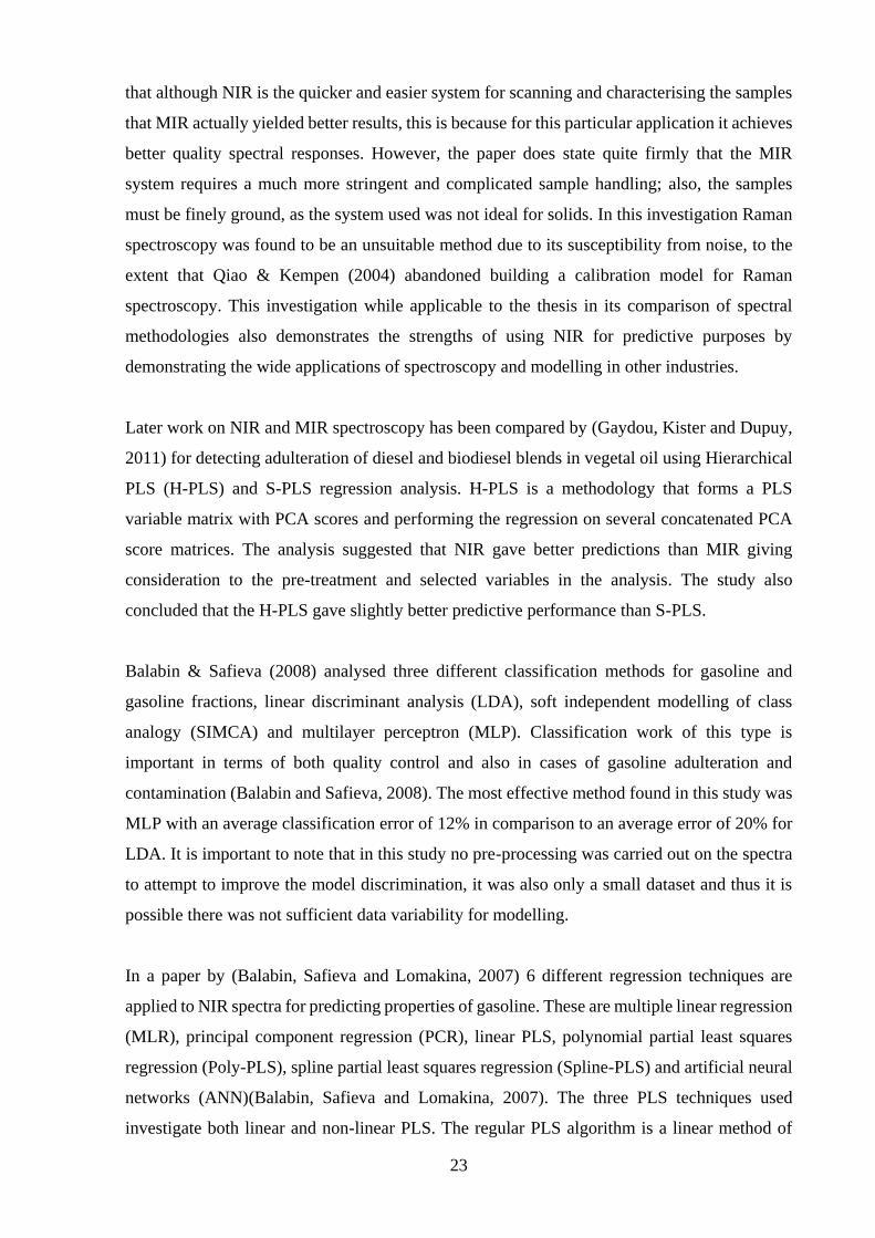
23
that although NIR is the quicker and easier system for scanning and characterising the samples
that MIR actually yielded better results, this is because for this particular application it achieves
better quality spectral responses. However, the paper does state quite firmly that the MIR
system requires a much more stringent and complicated sample handling; also, the samples
must be finely ground, as the system used was not ideal for solids. In this investigation Raman
spectroscopy was found to be an unsuitable method due to its susceptibility from noise, to the
extent that Qiao & Kempen (2004) abandoned building a calibration model for Raman
spectroscopy. This investigation while applicable to the thesis in its comparison of spectral
methodologies also demonstrates the strengths of using NIR for predictive purposes by
demonstrating the wide applications of spectroscopy and modelling in other industries.
Later work on NIR and MIR spectroscopy has been compared by (Gaydou, Kister and Dupuy,
2011) for detecting adulteration of diesel and biodiesel blends in vegetal oil using Hierarchical
PLS (H-PLS) and S-PLS regression analysis. H-PLS is a methodology that forms a PLS
variable matrix with PCA scores and performing the regression on several concatenated PCA
score matrices. The analysis suggested that NIR gave better predictions than MIR giving
consideration to the pre-treatment and selected variables in the analysis. The study also
concluded that the H-PLS gave slightly better predictive performance than S-PLS.
Balabin & Safieva (2008) analysed three different classification methods for gasoline and
gasoline fractions, linear discriminant analysis (LDA), soft independent modelling of class
analogy (SIMCA) and multilayer perceptron (MLP). Classification work of this type is
important in terms of both quality control and also in cases of gasoline adulteration and
contamination (Balabin and Safieva, 2008). The most effective method found in this study was
MLP with an average classification error of 12% in comparison to an average error of 20% for
LDA. It is important to note that in this study no pre-processing was carried out on the spectra
to attempt to improve the model discrimination, it was also only a small dataset and thus it is
possible there was not sufficient data variability for modelling.
In a paper by (Balabin, Safieva and Lomakina, 2007) 6 different regression techniques are
applied to NIR spectra for predicting properties of gasoline. These are multiple linear regression
(MLR), principal component regression (PCR), linear PLS, polynomial partial least squares
regression (Poly-PLS), spline partial least squares regression (Spline-PLS) and artificial neural
networks (ANN)(Balabin, Safieva and Lomakina, 2007). The three PLS techniques used
investigate both linear and non-linear PLS. The regular PLS algorithm is a linear method of
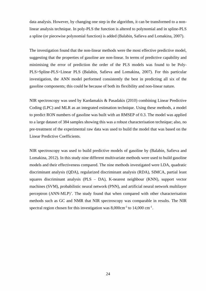
24
data analysis. However, by changing one step in the algorithm, it can be transformed to a non-
linear analysis technique. In poly-PLS the function is altered to polynomial and in spline-PLS
a spline (or piecewise polynomial function) is added (Balabin, Safieva and Lomakina, 2007).
The investigation found that the non-linear methods were the most effective predictive model,
suggesting that the properties of gasoline are non-linear. In terms of predictive capability and
minimising the error of prediction the order of the PLS models was found to be Poly-
PLS>Spline-PLS>Linear PLS (Balabin, Safieva and Lomakina, 2007). For this particular
investigation, the ANN model performed consistently the best in predicting all six of the
gasoline components; this could be because of both its flexibility and non-linear nature.
NIR spectroscopy was used by Kardamakis & Pasadakis (2010) combining Linear Predictive
Coding (LPC) and MLR as an integrated estimation technique. Using these methods, a model
to predict RON numbers of gasoline was built with an RMSEP of 0.3. The model was applied
to a large dataset of 384 samples showing this was a robust characterisation technique; also, no
pre-treatment of the experimental raw data was used to build the model that was based on the
Linear Predictive Coefficients.
NIR spectroscopy was used to build predictive models of gasoline by (Balabin, Safieva and
Lomakina, 2012). In this study nine different multivariate methods were used to build gasoline
models and their effectiveness compared. The nine methods investigated were LDA, quadratic
discriminant analysis (QDA), regularized discriminant analysis (RDA), SIMCA, partial least
squares discriminant analysis (PLS – DA), K-nearest neighbour (KNN), support vector
machines (SVM), probabilistic neural network (PNN), and artificial neural network multilayer
perceptron (ANN-MLP)’. The study found that when compared with other characterisation
methods such as GC and NMR that NIR spectroscopy was comparable in results. The NIR
spectral region chosen for this investigation was 8,000cm-1 to 14,000 cm-1.
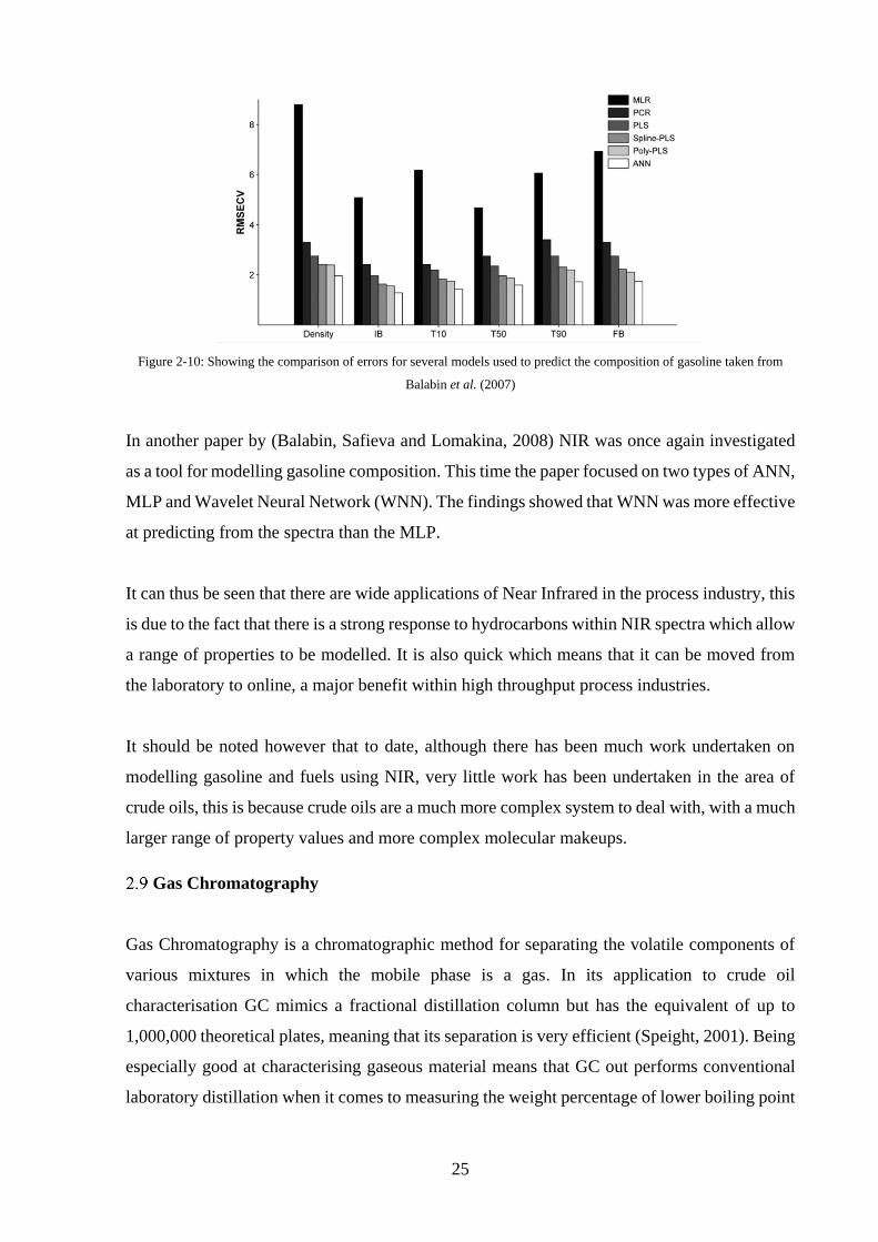
25
Figure 2-10: Showing the comparison of errors for several models used to predict the composition of gasoline taken from
Balabin et al. (2007)
In another paper by (Balabin, Safieva and Lomakina, 2008) NIR was once again investigated
as a tool for modelling gasoline composition. This time the paper focused on two types of ANN,
MLP and Wavelet Neural Network (WNN). The findings showed that WNN was more effective
at predicting from the spectra than the MLP.
It can thus be seen that there are wide applications of Near Infrared in the process industry, this
is due to the fact that there is a strong response to hydrocarbons within NIR spectra which allow
a range of properties to be modelled. It is also quick which means that it can be moved from
the laboratory to online, a major benefit within high throughput process industries.
It should be noted however that to date, although there has been much work undertaken on
modelling gasoline and fuels using NIR, very little work has been undertaken in the area of
crude oils, this is because crude oils are a much more complex system to deal with, with a much
larger range of property values and more complex molecular makeups.
Gas Chromatography
Gas Chromatography is a chromatographic method for separating the volatile components of
various mixtures in which the mobile phase is a gas. In its application to crude oil
characterisation GC mimics a fractional distillation column but has the equivalent of up to
1,000,000 theoretical plates, meaning that its separation is very efficient (Speight, 2001). Being
especially good at characterising gaseous material means that GC out performs conventional
laboratory distillation when it comes to measuring the weight percentage of lower boiling point
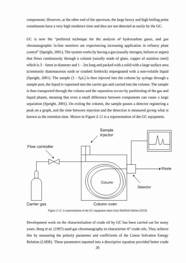
26
components. However, at the other end of the spectrum, the large heavy and high boiling point
constituents have a very high residence time and thus are not detected as easily by the GC.
GC is now the “preferred technique for the analysis of hydrocarbon gases, and gas
chromatographic in-line monitors are experiencing increasing application in refinery plant
control” (Speight, 2001). The system works by having a gas (usually nitrogen, helium or argon)
that flows continuously through a column (usually made of glass, copper of stainless steel)
which is 3 – 6mm in diameter and 1 – 2m long and packed with a solid with a large surface area
(commonly diatomaceous earth or crushed firebrick) impregnated with a non-volatile liquid
(Speight, 2001). The sample (1 - 5μL) is then injected into the column by syringe through a
sample port, the liquid is vaporised into the carrier gas and carried into the column. The sample
is then transported through the column and the separation occurs by partitioning of the gas and
liquid phases, meaning that even a small difference between components can cause a large
separation (Speight, 2001). On exiting the column, the sample passes a detector registering a
peak on a graph, and the time between injection and the detection is measured giving what is
known as the retention time. Shown in Figure 2-11 is a representation of the GC equipment.
Figure 2-11: A representation of the GC equipment taken from Sheffield Hallam (2010)
Development work on the characterisation of crude oil by GC has been carried out for many
years. Burg et al. (1997) used gas chromatography to characterise 47 crude oils. They achieve
this by measuring the polarity parameter and coefficients of the Linear Solvation Energy
Relation (LSER). These parameters inputted into a descriptive equation provided better crude
27
oil characterisation than by just using standard chromatographic polarity (Burg, Selves and
Colin, 1997). The study found that characterisation of 47 crude oils using this method gave
good agreement with the chemical composition measured by other methods.
However, the main drawback of the GC method versus NIR is the time taken to undertake the
analysis. A typical GC run can take 30 minutes and with data interpretation, to generate a
boiling point distillation for a crude oil takes in the region of 1 hour, whereas an NIR spectrum
takes 30 seconds and linked to a chemometric model, property generation takes only a few
minutes.
Nuclear Magnetic Resonance
Nuclear Magnetic Resonance (NMR) spectroscopy is a relative new technique under
investigation for the characterisation of crude oils. NMR directly measures aromatic and
aliphatic carbon as well as hydrogen distributions. The most common types of NMR
spectroscopy in use utilise the Proton (1H) and carbon-13 (13C) nuclei, however, for specialist
petroleum analyses, nitrogen (15N and 14N) and sulphur (33S) have also been used (Speight,
2001). To perform an NMR analysis only a small amount of sample (<10mg) is needed,
dissolved in a solvent such as deuteron-chloroform. It is placed in a glass tube approximately
5mm in diameter, which is then placed in a homogenous magnetic field surrounded by one (or
more) coils. If the hydrogen nuclei are imagined to be small magnets these interact with a weak
radio frequency emitted by the coils, at the correct frequency the nuclei resonate and the spin
resonance is detected by a receiver coil (Speight, 2001). The sample position relative to the
standard of tetramethylsilane (TMS) is then reported as a chemical shift (δ) which can then be
characterised using reference tables.
Work on the characterisation of crude by Flumignan et al. (2012) looked at the use of 1H NMR
profiles in predicting a whole manner of physiochemical properties of crudes, such as density,
distillation curve, octane numbers etc. To model the spectra standard PLS modelling was used.
The investigation found that NMR-PLS modelling gave good results when compared to ASTM
standard reproducibility’s. Excellent accuracy and precision were also reported. Also the 13C
NMR spectra was used in conjunction with Principal Components Analysis (PCA), PLS and
PCR to discriminate olive oils and attempt to detect any adulteration in a study by Shaw et al.,
(1997). The study found that of 66 samples predicted, 65 predicted correctly and the models
achieved consistent predictions of over 90% of the samples.
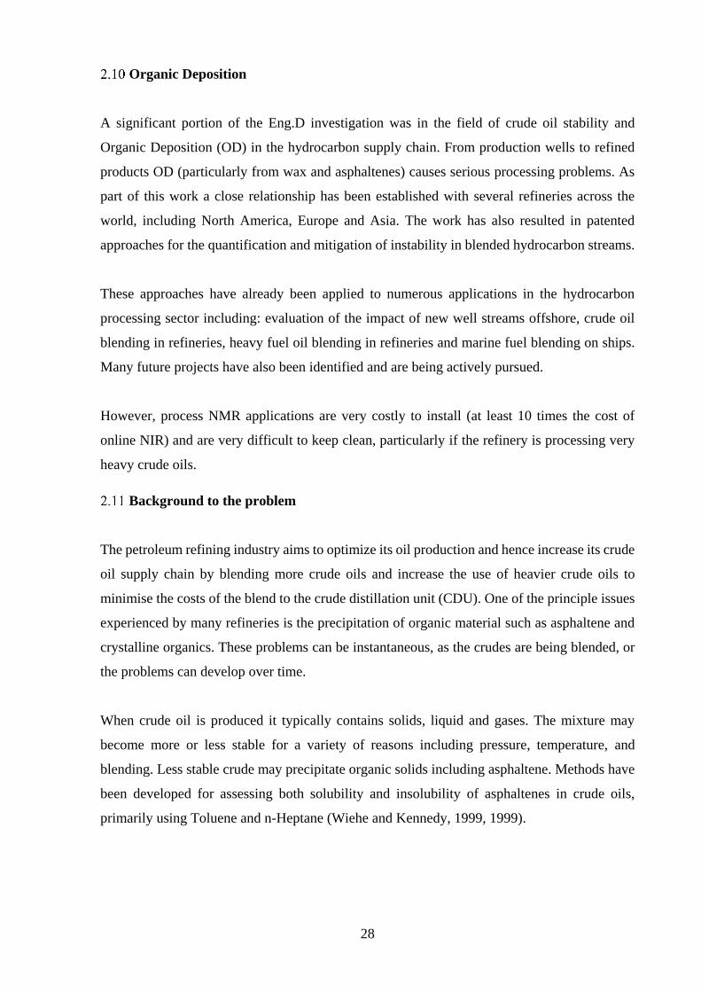
28
Organic Deposition
A significant portion of the Eng.D investigation was in the field of crude oil stability and
Organic Deposition (OD) in the hydrocarbon supply chain. From production wells to refined
products OD (particularly from wax and asphaltenes) causes serious processing problems. As
part of this work a close relationship has been established with several refineries across the
world, including North America, Europe and Asia. The work has also resulted in patented
approaches for the quantification and mitigation of instability in blended hydrocarbon streams.
These approaches have already been applied to numerous applications in the hydrocarbon
processing sector including: evaluation of the impact of new well streams offshore, crude oil
blending in refineries, heavy fuel oil blending in refineries and marine fuel blending on ships.
Many future projects have also been identified and are being actively pursued.
However, process NMR applications are very costly to install (at least 10 times the cost of
online NIR) and are very difficult to keep clean, particularly if the refinery is processing very
heavy crude oils.
Background to the problem
The petroleum refining industry aims to optimize its oil production and hence increase its crude
oil supply chain by blending more crude oils and increase the use of heavier crude oils to
minimise the costs of the blend to the crude distillation unit (CDU). One of the principle issues
experienced by many refineries is the precipitation of organic material such as asphaltene and
crystalline organics. These problems can be instantaneous, as the crudes are being blended, or
the problems can develop over time.
When crude oil is produced it typically contains solids, liquid and gases. The mixture may
become more or less stable for a variety of reasons including pressure, temperature, and
blending. Less stable crude may precipitate organic solids including asphaltene. Methods have
been developed for assessing both solubility and insolubility of asphaltenes in crude oils,
primarily using Toluene and n-Heptane (Wiehe and Kennedy, 1999, 1999).

29
Refining Economics
The biggest cost to a refinery on a global basis is the cost of crude, and although this has recently
fallen refineries continue to source lower cost oils for blending to maximise margins. These
opportunity oils have affected market and refinery economics globally; this problem
particularly affects European refineries (Figure 2-12, Figure 2-13 and Figure 2-14) due to their
aging designs and stringent EU environmental legislation.
Figure 2-12 also shows that the majority of European refineries are in the first quartile when
compared to Former Soviet Union (FSU) and African refineries. However, when other factors
such as domestic tariffs or crude oil availability are taken into account this is not necessarily a
true benchmark of a refineries ability to be profitable. This reinforces the need for refiners to
have a thorough understanding of neat crude composition as well as the interactions between
crudes during crude blending as it is only through a full understanding of this can process be
optimised and margins maximised, thus maintaining a competitive edge. Recognition of this
need is a driver for improvement of existing technology and innovation of new technology.
Figure 2-13 shows European refineries identified as most at risk, many have already have
already been forced to close with many smaller refineries making less than $1.00 per barrel net
cash margin (NCM), indeed Coryton refinery identified as being at risk in this graph has since
closed.
Net Cash Margin
NCM is a method of expressing a refineries economics and is defined as:
NCM = Refinery Gross Margin (RGM) – Operating Costs
Where:
Refinery gross margin = the sum of barrels of each product multiplied by the price of each
product (PetroleumOnline, 2012)
Operating Costs = Costs to operate refinery, excluding income taxes, depreciation and
financial charges (PetroleumOnline, 2012)
According to Wood-Mackenzie (2012) the benchmark figure for refinery performance is an
NCM of $1 per barrel. Figure 2-14 shows European refiners and their respective NCM. It can
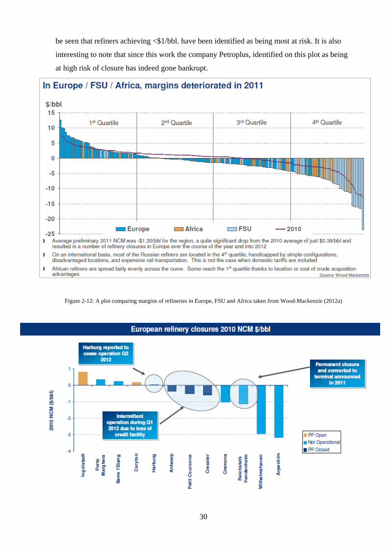
30
be seen that refiners achieving <$1/bbl. have been identified as being most at risk. It is also
interesting to note that since this work the company Petroplus, identified on this plot as being
at high risk of closure has indeed gone bankrupt.
Figure 2-12: A plot comparing margins of refineries in Europe, FSU and Africa taken from Wood-Mackenzie (2012a)
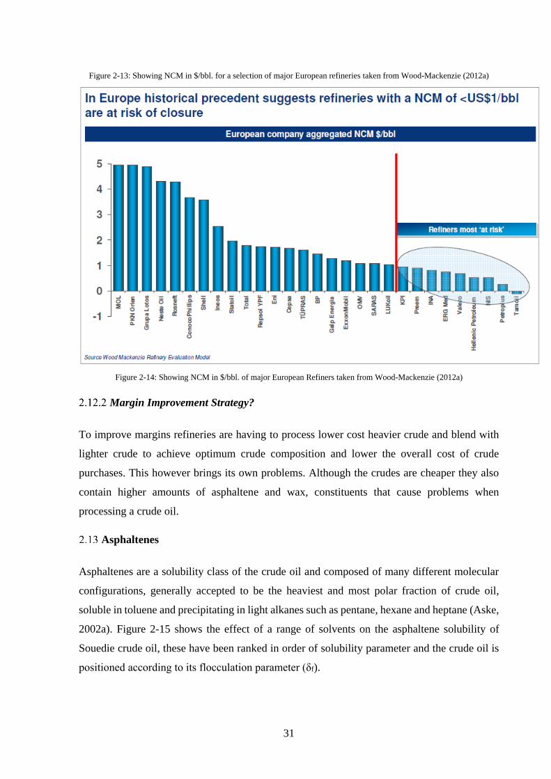
31
Figure 2-13: Showing NCM in $/bbl. for a selection of major European refineries taken from Wood-Mackenzie (2012a)
Figure 2-14: Showing NCM in $/bbl. of major European Refiners taken from Wood-Mackenzie (2012a)
Margin Improvement Strategy?
To improve margins refineries are having to process lower cost heavier crude and blend with
lighter crude to achieve optimum crude composition and lower the overall cost of crude
purchases. This however brings its own problems. Although the crudes are cheaper they also
contain higher amounts of asphaltene and wax, constituents that cause problems when
processing a crude oil.
Asphaltenes
Asphaltenes are a solubility class of the crude oil and composed of many different molecular
configurations, generally accepted to be the heaviest and most polar fraction of crude oil,
soluble in toluene and precipitating in light alkanes such as pentane, hexane and heptane (Aske,
2002a). Figure 2-15 shows the effect of a range of solvents on the asphaltene solubility of
Souedie crude oil, these have been ranked in order of solubility parameter and the crude oil is
positioned according to its flocculation parameter (δf).
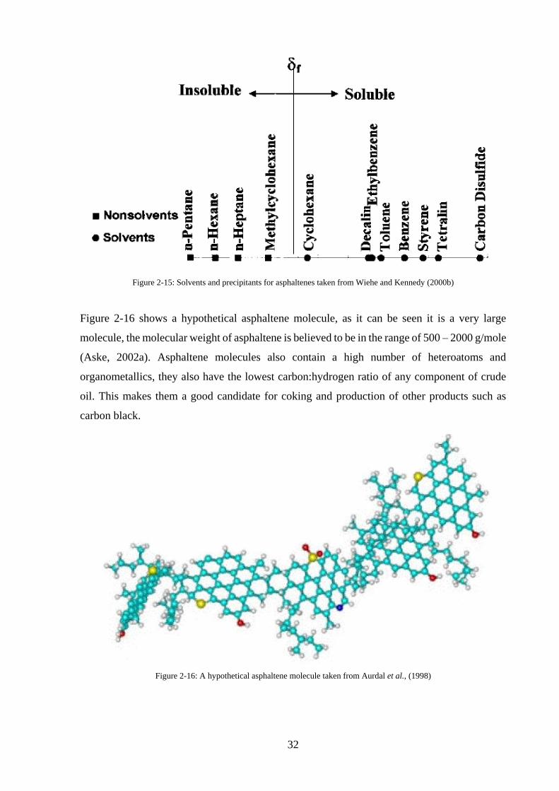
32
Figure 2-15: Solvents and precipitants for asphaltenes taken from Wiehe and Kennedy (2000b)
Figure 2-16 shows a hypothetical asphaltene molecule, as it can be seen it is a very large
molecule, the molecular weight of asphaltene is believed to be in the range of 500 – 2000 g/mole
(Aske, 2002a). Asphaltene molecules also contain a high number of heteroatoms and
organometallics, they also have the lowest carbon:hydrogen ratio of any component of crude
oil. This makes them a good candidate for coking and production of other products such as
carbon black.
Figure 2-16: A hypothetical asphaltene molecule taken from Aurdal et al., (1998)
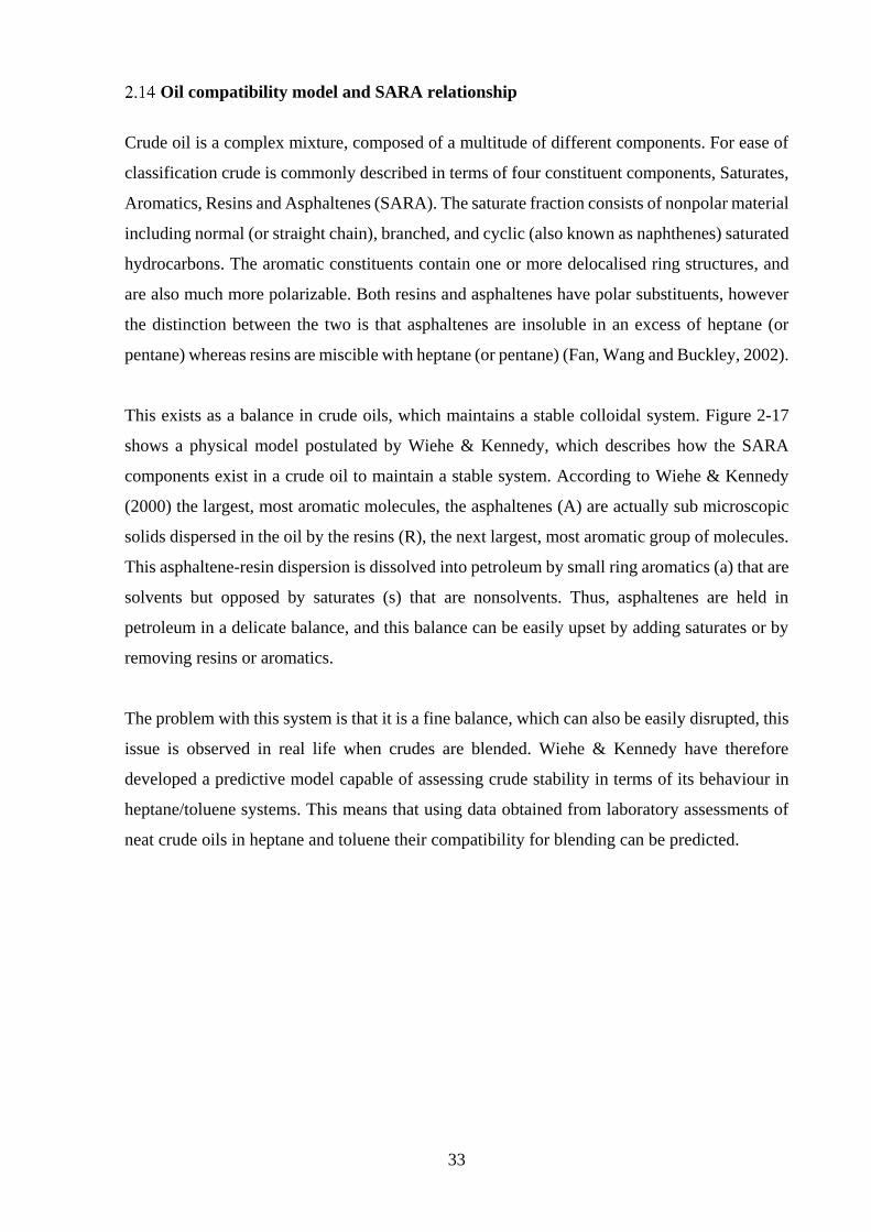
33
Oil compatibility model and SARA relationship
Crude oil is a complex mixture, composed of a multitude of different components. For ease of
classification crude is commonly described in terms of four constituent components, Saturates,
Aromatics, Resins and Asphaltenes (SARA). The saturate fraction consists of nonpolar material
including normal (or straight chain), branched, and cyclic (also known as naphthenes) saturated
hydrocarbons. The aromatic constituents contain one or more delocalised ring structures, and
are also much more polarizable. Both resins and asphaltenes have polar substituents, however
the distinction between the two is that asphaltenes are insoluble in an excess of heptane (or
pentane) whereas resins are miscible with heptane (or pentane) (Fan, Wang and Buckley, 2002).
This exists as a balance in crude oils, which maintains a stable colloidal system. Figure 2-17
shows a physical model postulated by Wiehe & Kennedy, which describes how the SARA
components exist in a crude oil to maintain a stable system. According to Wiehe & Kennedy
(2000) the largest, most aromatic molecules, the asphaltenes (A) are actually sub microscopic
solids dispersed in the oil by the resins (R), the next largest, most aromatic group of molecules.
This asphaltene-resin dispersion is dissolved into petroleum by small ring aromatics (a) that are
solvents but opposed by saturates (s) that are nonsolvents. Thus, asphaltenes are held in
petroleum in a delicate balance, and this balance can be easily upset by adding saturates or by
removing resins or aromatics.
The problem with this system is that it is a fine balance, which can also be easily disrupted, this
issue is observed in real life when crudes are blended. Wiehe & Kennedy have therefore
developed a predictive model capable of assessing crude stability in terms of its behaviour in
heptane/toluene systems. This means that using data obtained from laboratory assessments of
neat crude oils in heptane and toluene their compatibility for blending can be predicted.
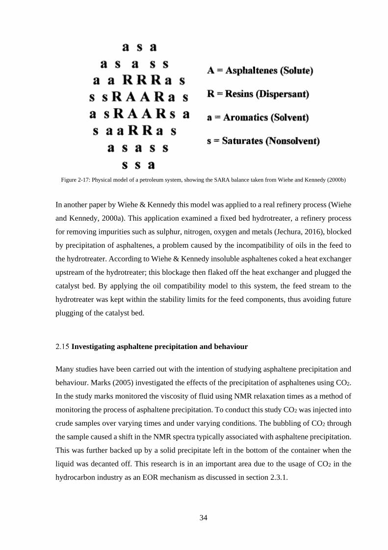
34
Figure 2-17: Physical model of a petroleum system, showing the SARA balance taken from Wiehe and Kennedy (2000b)
In another paper by Wiehe & Kennedy this model was applied to a real refinery process (Wiehe
and Kennedy, 2000a). This application examined a fixed bed hydrotreater, a refinery process
for removing impurities such as sulphur, nitrogen, oxygen and metals (Jechura, 2016), blocked
by precipitation of asphaltenes, a problem caused by the incompatibility of oils in the feed to
the hydrotreater. According to Wiehe & Kennedy insoluble asphaltenes coked a heat exchanger
upstream of the hydrotreater; this blockage then flaked off the heat exchanger and plugged the
catalyst bed. By applying the oil compatibility model to this system, the feed stream to the
hydrotreater was kept within the stability limits for the feed components, thus avoiding future
plugging of the catalyst bed.
Investigating asphaltene precipitation and behaviour
Many studies have been carried out with the intention of studying asphaltene precipitation and
behaviour. Marks (2005) investigated the effects of the precipitation of asphaltenes using CO2.
In the study marks monitored the viscosity of fluid using NMR relaxation times as a method of
monitoring the process of asphaltene precipitation. To conduct this study CO2 was injected into
crude samples over varying times and under varying conditions. The bubbling of CO2 through
the sample caused a shift in the NMR spectra typically associated with asphaltene precipitation.
This was further backed up by a solid precipitate left in the bottom of the container when the
liquid was decanted off. This research is in an important area due to the usage of CO2 in the
hydrocarbon industry as an EOR mechanism as discussed in section 2.3.1.

35
Gawrys & Kilpatrick (2004) made a study of techniques for observing aggregation of
asphaltene particles, primarily Pulse-Field Gradient Spin Echo Nuclear Magnetic Resonance
(PFG-SE NMR), Small Angle Neutron Scattering (SANS), NIR and Vapour Pressure
Osmometry (VPO). In the analysis they observed that NIR is a quick, simple and non-invasive
method of studying flocculation and can be used to observe aggregation with changes in
temperature, pressure, solvents and additives. However, they note that NIR is not a particle
sizing method and although it can see the onset of aggregation it cannot be used to quantify
particle size. This is in stark contrast to work by Gossen et al. (1993) and Pasikatan et al. (2003)
where NIR was used for such a purpose, albeit not for determination of asphaltene aggregate
size.
Morphology work was carried out using PFG-SE NMR is a “non-invasive, relatively fast
instrumental technique to probe molecular self-diffusion coefficients using magnetic field
gradients of varying strength to effect large signal attenuation” (Gawrys and Kilpatrick, 2004).
Using this technique, it was determined that asphaltene aggregates are not spherical in shape
but rather disc like.
The technique also proved that the addition of n-alkane to a model asphaltene solution induces
asphaltene flocculation. VPO is a method that monitors change in vapour pressure when a small
amount of solute is added to a pure solvent.
Figure 2-18: Showing a typical Vapour Pressure Osmometer setup taken from UCI (2016)
Figure 2-18 shows the typical apparatus setup which consists of a solvent reservoir with two
wicks providing a saturated solvent atmosphere around two thermistors. Within this apparatus
a solvent is condensed from the atmosphere into a solution containing the asphaltene placed at
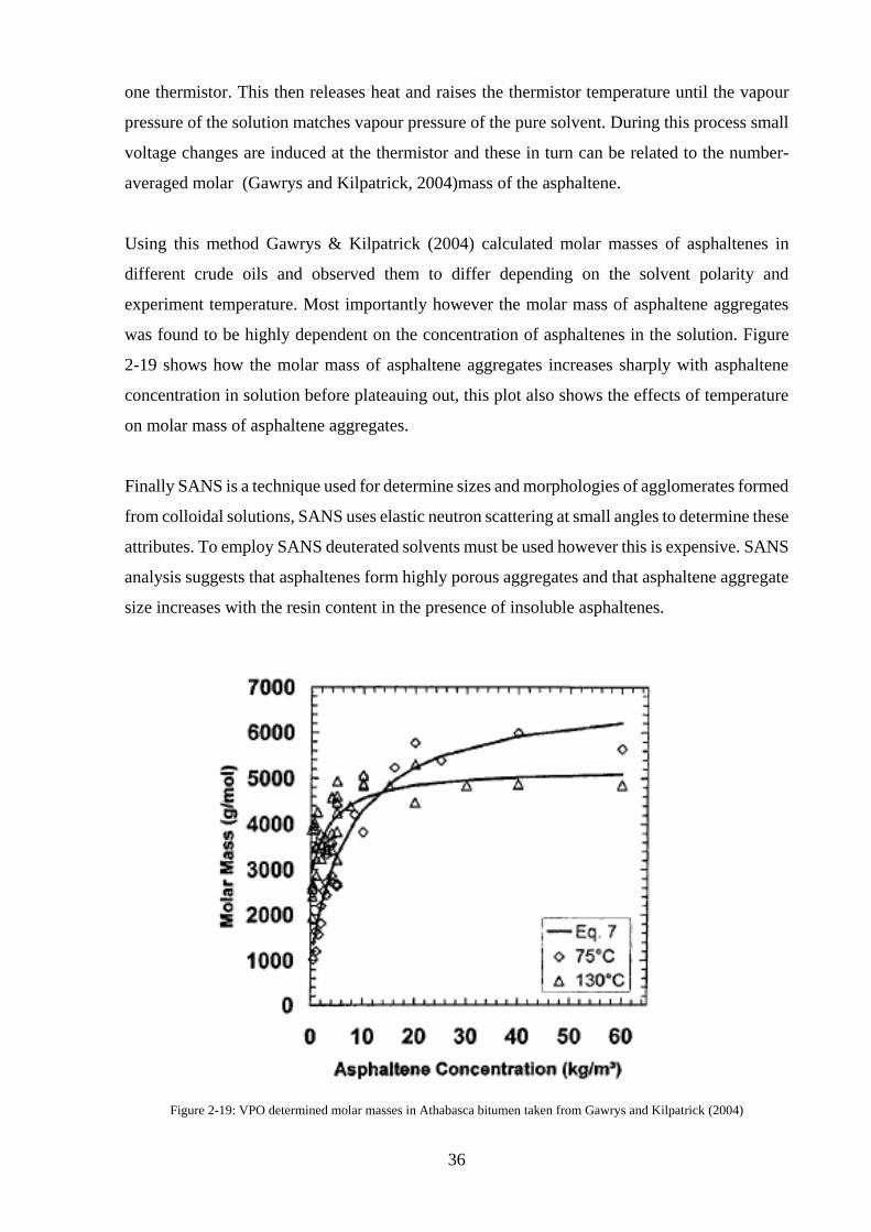
36
one thermistor. This then releases heat and raises the thermistor temperature until the vapour
pressure of the solution matches vapour pressure of the pure solvent. During this process small
voltage changes are induced at the thermistor and these in turn can be related to the number-
averaged molar (Gawrys and Kilpatrick, 2004)mass of the asphaltene.
Using this method Gawrys & Kilpatrick (2004) calculated molar masses of asphaltenes in
different crude oils and observed them to differ depending on the solvent polarity and
experiment temperature. Most importantly however the molar mass of asphaltene aggregates
was found to be highly dependent on the concentration of asphaltenes in the solution. Figure
2-19 shows how the molar mass of asphaltene aggregates increases sharply with asphaltene
concentration in solution before plateauing out, this plot also shows the effects of temperature
on molar mass of asphaltene aggregates.
Finally SANS is a technique used for determine sizes and morphologies of agglomerates formed
from colloidal solutions, SANS uses elastic neutron scattering at small angles to determine these
attributes. To employ SANS deuterated solvents must be used however this is expensive. SANS
analysis suggests that asphaltenes form highly porous aggregates and that asphaltene aggregate
size increases with the resin content in the presence of insoluble asphaltenes.
Figure 2-19: VPO determined molar masses in Athabasca bitumen taken from Gawrys and Kilpatrick (2004)
37
VPO and SANS was also used by Spiecker, Gawrys & Kilpatrick (2003). In this work
asphaltenes were fractionated from four different crude oils using heptane and toluene, the
fractions were then analysed using VPO and SANS. Studies conducted using these techniques
indicated that the fractions generated from the crude oils that were less soluble formed
asphaltene aggregates much larger than those sub-fractions which were more soluble. This
described a general trend, which saw aggregate size increasing as a function of decreasing
aromaticity of the solvent. It was also observed that the individual aggregate sizes increased to
a maximum at the solubility limit and after that began to decrease. This was due to flocculation
of individual asphaltene aggregates.
In another paper Spiecker et al. (2003) also employed SARA fractionation of crude oils
combined with SANS analysis to analyse the effect of petroleum resins on asphaltene stability
in crudes. It was found that addition of resins to the crude oil reduced the aggregate size of
asphaltenes by interrupting the chemical bonding of asphaltene molecules. Increasing
concentration of resins also reduced the interfacial tension of the asphaltenes, reducing the
ability of asphaltenes to stabilise water in oil emulsions. It was also observed that reducing the
amount of resin in crude rendered the higher molecular weight asphaltenes insoluble in
solutions of heptane/toluene. Thus proving the importance, asserted by Wiehe & Kennedy
(2000b) of resins for stabilising asphaltenes in crude oils.
Work by Tharnivasan (2012) centred around the whole area of asphaltene precipitation from
crude oil blends and emulsions. The thesis main focus was to develop a model to describe the
phase behaviour of these systems and to be able to predict the onset and amount of precipitation
from oils and oil blends being subjected to depressurisation. The research and development
work drew conclusions for three main areas: blends, live oils and the effects of water on
asphaltene precipitation.
For blends, Tharnivasan (2012) developed a model which would predict unstable blends;
however, the model did not work as well with high concentrations of diluents such as toluene.
This is to be expected due to the definition of asphaltenes as the most polar toluene soluble
fraction of crude oil, asphaltene precipitation becomes more difficult to force even with large
amounts of saturates in the presence of large amounts of toluene.
In live oils, a methodology was developed which characterised live crude oils for solubility
parameters of asphaltenes. Ultimately, a model was configured to predict precipitation onset
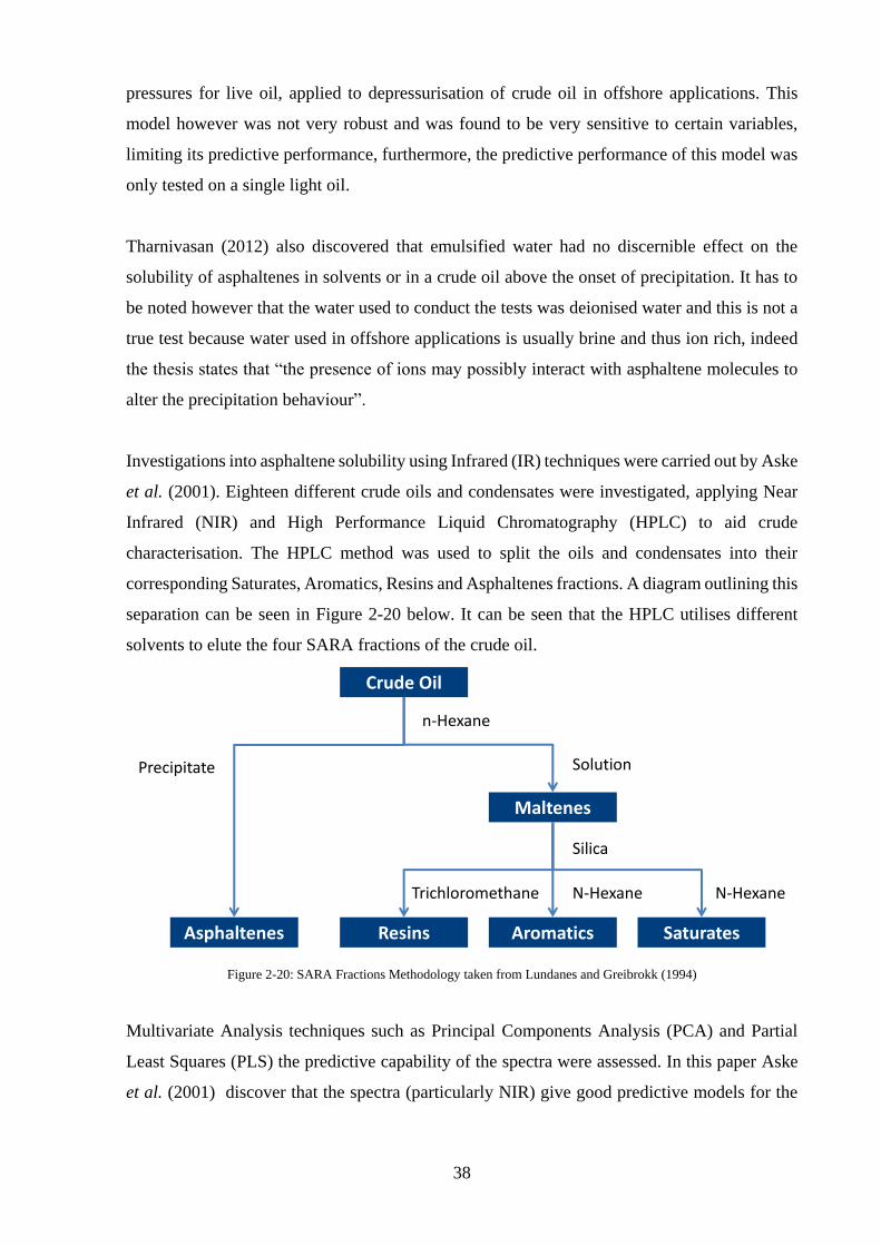
38
pressures for live oil, applied to depressurisation of crude oil in offshore applications. This
model however was not very robust and was found to be very sensitive to certain variables,
limiting its predictive performance, furthermore, the predictive performance of this model was
only tested on a single light oil.
Tharnivasan (2012) also discovered that emulsified water had no discernible effect on the
solubility of asphaltenes in solvents or in a crude oil above the onset of precipitation. It has to
be noted however that the water used to conduct the tests was deionised water and this is not a
true test because water used in offshore applications is usually brine and thus ion rich, indeed
the thesis states that “the presence of ions may possibly interact with asphaltene molecules to
alter the precipitation behaviour”.
Investigations into asphaltene solubility using Infrared (IR) techniques were carried out by Aske
et al. (2001). Eighteen different crude oils and condensates were investigated, applying Near
Infrared (NIR) and High Performance Liquid Chromatography (HPLC) to aid crude
characterisation. The HPLC method was used to split the oils and condensates into their
corresponding Saturates, Aromatics, Resins and Asphaltenes fractions. A diagram outlining this
separation can be seen in Figure 2-20 below. It can be seen that the HPLC utilises different
solvents to elute the four SARA fractions of the crude oil.
Figure 2-20: SARA Fractions Methodology taken from Lundanes and Greibrokk (1994)
Multivariate Analysis techniques such as Principal Components Analysis (PCA) and Partial
Least Squares (PLS) the predictive capability of the spectra were assessed. In this paper Aske
et al. (2001) discover that the spectra (particularly NIR) give good predictive models for the
Crude Oil
Asphaltenes Resins Aromatics Saturates
Maltenes
n-Hexane
Solution
N-Hexane
Silica
N-HexaneTrichloromethane
Precipitate
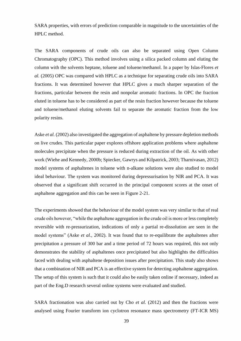
39
SARA properties, with errors of prediction comparable in magnitude to the uncertainties of the
HPLC method.
The SARA components of crude oils can also be separated using Open Column
Chromatography (OPC). This method involves using a silica packed column and eluting the
column with the solvents heptane, toluene and toluene/methanol. In a paper by Islas-Flores et
al. (2005) OPC was compared with HPLC as a technique for separating crude oils into SARA
fractions. It was determined however that HPLC gives a much sharper separation of the
fractions, particular between the resin and nonpolar aromatic fractions. In OPC the fraction
eluted in toluene has to be considered as part of the resin fraction however because the toluene
and toluene/methanol eluting solvents fail to separate the aromatic fraction from the low
polarity resins.
Aske et al. (2002) also investigated the aggregation of asphaltene by pressure depletion methods
on live crudes. This particular paper explores offshore application problems where asphaltene
molecules precipitate when the pressure is reduced during extraction of the oil. As with other
work (Wiehe and Kennedy, 2000b; Spiecker, Gawrys and Kilpatrick, 2003; Tharnivasan, 2012)
model systems of asphaltenes in toluene with n-alkane solutions were also studied to model
ideal behaviour. The system was monitored during depressurisation by NIR and PCA. It was
observed that a significant shift occurred in the principal component scores at the onset of
asphaltene aggregation and this can be seen in Figure 2-21.
The experiments showed that the behaviour of the model system was very similar to that of real
crude oils however, “while the asphaltene aggregation in the crude oil is more or less completely
reversible with re-pressurization, indications of only a partial re-dissolution are seen in the
model systems” (Aske et al., 2002). It was found that to re-equilibrate the asphaltenes after
precipitation a pressure of 300 bar and a time period of 72 hours was required, this not only
demonstrates the stability of asphaltenes once precipitated but also highlights the difficulties
faced with dealing with asphaltene deposition issues after precipitation. This study also shows
that a combination of NIR and PCA is an effective system for detecting asphaltene aggregation.
The setup of this system is such that it could also be easily taken online if necessary, indeed as
part of the Eng.D research several online systems were evaluated and studied.
SARA fractionation was also carried out by Cho et al. (2012) and then the fractions were
analysed using Fourier transform ion cyclotron resonance mass spectrometry (FT-ICR MS)
40
equipped with atmospheric pressure photoionisation (APPI). The analysis performed produced
expected results, with each fraction containing compounds with expected behaviour and
appearance, i.e. “the saturates fraction was composed of less aromatic molecules with long or
multiple alkyl chains”(Cho et al., 2012).
Figure 2-21: A Plot Showing the Shift in Principal Component Scores of a Crude Oil Sample during Depressurisation taken
from Aske (2002b)
Oh et al. (2004) investigated asphaltene precipitation using n-heptane from four different
solvents; tetrahydrofuran (THF), toluene, trichloroethylene (TCE) and pyridine. The onset of
asphaltene aggregation was monitored using NIR and observing the optical density at 1600nm
every thirty seconds. The onset of aggregation was determined as the point at which the optical
density was at its minimum, i.e. when asphaltene aggregation occurs an increase in optical
density is observed despite diluting with heptane. It was also observed that the solubility
parameters of the asphaltenes increased linearly with increasing solvent solubility parameter. It
was also found that the best asphaltene solvent of these four was pyridine.
Buckley et al. (1998) conducted a study to try and predict the onset of asphaltene precipitation
by using refractive index (RI) to characterise neat oils and mixtures of crude oils with
precipitants and solvents. It was found that the onset of asphaltene precipitation occurs at a
characteristic RI for each oil/precipitant combination.
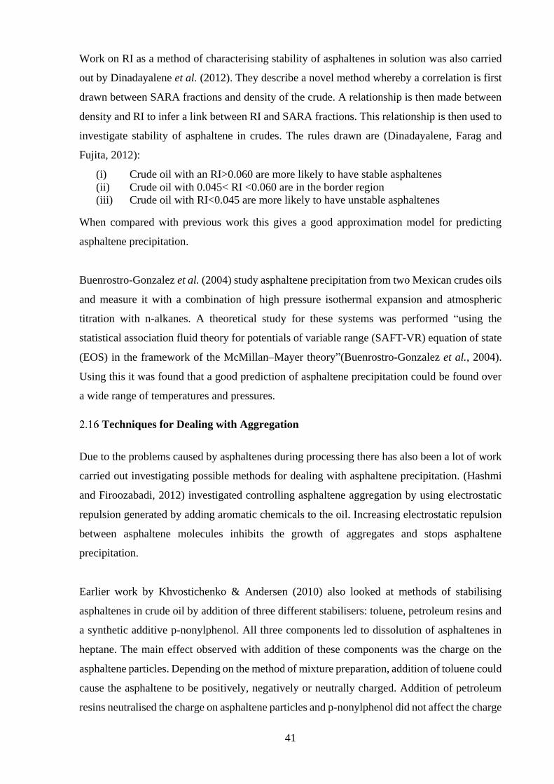
41
Work on RI as a method of characterising stability of asphaltenes in solution was also carried
out by Dinadayalene et al. (2012). They describe a novel method whereby a correlation is first
drawn between SARA fractions and density of the crude. A relationship is then made between
density and RI to infer a link between RI and SARA fractions. This relationship is then used to
investigate stability of asphaltene in crudes. The rules drawn are (Dinadayalene, Farag and
Fujita, 2012):
(i) Crude oil with an RI>0.060 are more likely to have stable asphaltenes
(ii) Crude oil with 0.045< RI <0.060 are in the border region
(iii) Crude oil with RI<0.045 are more likely to have unstable asphaltenes
When compared with previous work this gives a good approximation model for predicting
asphaltene precipitation.
Buenrostro-Gonzalez et al. (2004) study asphaltene precipitation from two Mexican crudes oils
and measure it with a combination of high pressure isothermal expansion and atmospheric
titration with n-alkanes. A theoretical study for these systems was performed “using the
statistical association fluid theory for potentials of variable range (SAFT-VR) equation of state
(EOS) in the framework of the McMillan–Mayer theory”(Buenrostro-Gonzalez et al., 2004).
Using this it was found that a good prediction of asphaltene precipitation could be found over
a wide range of temperatures and pressures.
Techniques for Dealing with Aggregation
Due to the problems caused by asphaltenes during processing there has also been a lot of work
carried out investigating possible methods for dealing with asphaltene precipitation. (Hashmi
and Firoozabadi, 2012) investigated controlling asphaltene aggregation by using electrostatic
repulsion generated by adding aromatic chemicals to the oil. Increasing electrostatic repulsion
between asphaltene molecules inhibits the growth of aggregates and stops asphaltene
precipitation.
Earlier work by Khvostichenko & Andersen (2010) also looked at methods of stabilising
asphaltenes in crude oil by addition of three different stabilisers: toluene, petroleum resins and
a synthetic additive p-nonylphenol. All three components led to dissolution of asphaltenes in
heptane. The main effect observed with addition of these components was the charge on the
asphaltene particles. Depending on the method of mixture preparation, addition of toluene could
cause the asphaltene to be positively, negatively or neutrally charged. Addition of petroleum
resins neutralised the charge on asphaltene particles and p-nonylphenol did not affect the charge
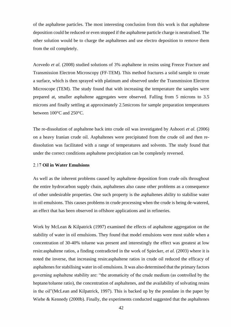
42
of the asphaltene particles. The most interesting conclusion from this work is that asphaltene
deposition could be reduced or even stopped if the asphaltene particle charge is neutralised. The
other solution would be to charge the asphaltenes and use electro deposition to remove them
from the oil completely.
Acevedo et al. (2008) studied solutions of 3% asphaltene in resins using Freeze Fracture and
Transmission Electron Microscopy (FF-TEM). This method fractures a solid sample to create
a surface, which is then sprayed with platinum and observed under the Transmission Electron
Microscope (TEM). The study found that with increasing the temperature the samples were
prepared at, smaller asphaltene aggregates were observed. Falling from 5 microns to 3.5
microns and finally settling at approximately 2.5microns for sample preparation temperatures
between 100°C and 250°C.
The re-dissolution of asphaltene back into crude oil was investigated by Ashoori et al. (2006)
on a heavy Iranian crude oil. Asphaltenes were precipitated from the crude oil and then re-
dissolution was facilitated with a range of temperatures and solvents. The study found that
under the correct conditions asphaltene precipitation can be completely reversed.
Oil in Water Emulsions
As well as the inherent problems caused by asphaltene deposition from crude oils throughout
the entire hydrocarbon supply chain, asphaltenes also cause other problems as a consequence
of other undesirable properties. One such property is the asphaltenes ability to stabilise water
in oil emulsions. This causes problems in crude processing when the crude is being de-watered,
an effect that has been observed in offshore applications and in refineries.
Work by McLean & Kilpatrick (1997) examined the effects of asphaltene aggregation on the
stability of water in oil emulsions. They found that model emulsions were most stable when a
concentration of 30-40% toluene was present and interestingly the effect was greatest at low
resin:asphaltene ratios, a finding contradicted in the work of Spiecker, et al. (2003) where it is
noted the inverse, that increasing resin:asphaltene ratios in crude oil reduced the efficacy of
asphaltenes for stabilising water in oil emulsions. It was also determined that the primary factors
governing asphaltene stability are: “the aromaticity of the crude medium (as controlled by the
heptane/toluene ratio), the concentration of asphaltenes, and the availability of solvating resins
in the oil”(McLean and Kilpatrick, 1997). This is backed up by the postulate in the paper by
Wiehe & Kennedy (2000b). Finally, the experiments conducted suggested that the asphaltenes
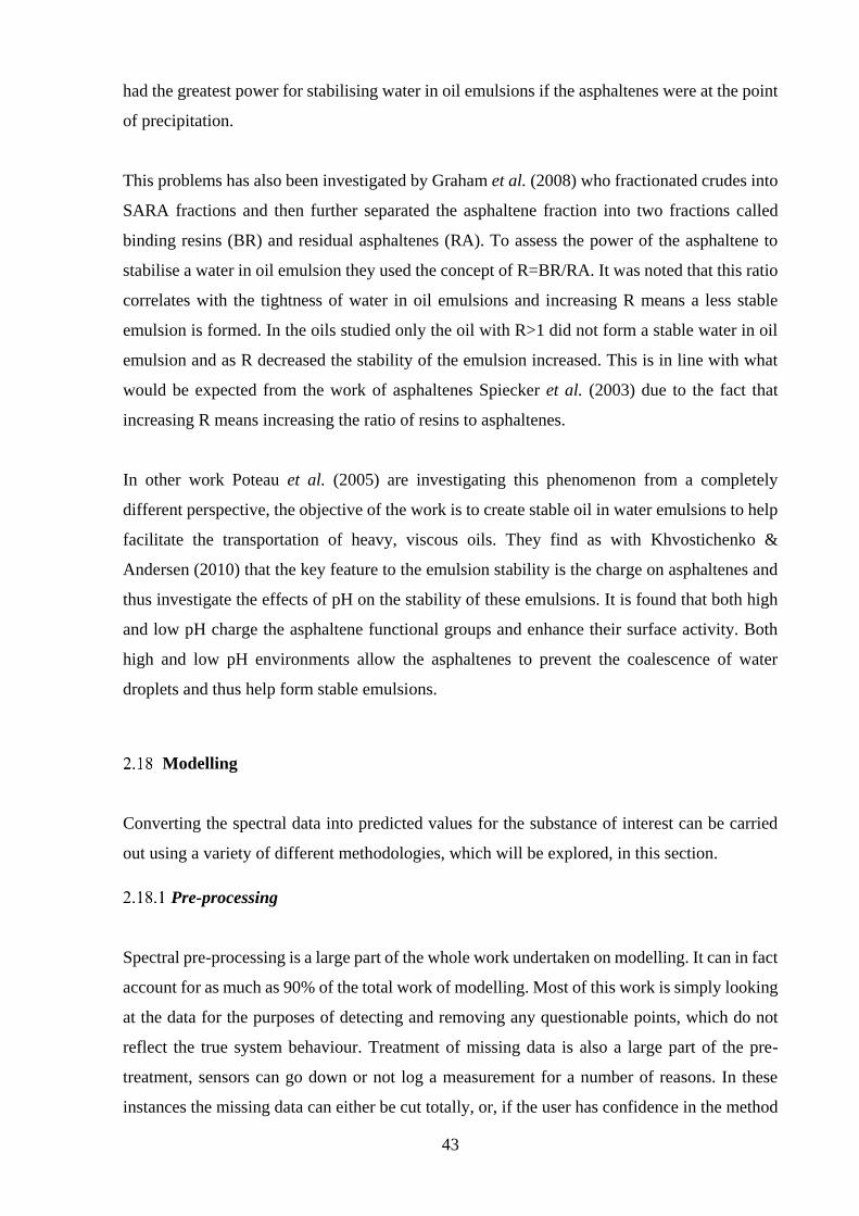
43
had the greatest power for stabilising water in oil emulsions if the asphaltenes were at the point
of precipitation.
This problems has also been investigated by Graham et al. (2008) who fractionated crudes into
SARA fractions and then further separated the asphaltene fraction into two fractions called
binding resins (BR) and residual asphaltenes (RA). To assess the power of the asphaltene to
stabilise a water in oil emulsion they used the concept of R=BR/RA. It was noted that this ratio
correlates with the tightness of water in oil emulsions and increasing R means a less stable
emulsion is formed. In the oils studied only the oil with R>1 did not form a stable water in oil
emulsion and as R decreased the stability of the emulsion increased. This is in line with what
would be expected from the work of asphaltenes Spiecker et al. (2003) due to the fact that
increasing R means increasing the ratio of resins to asphaltenes.
In other work Poteau et al. (2005) are investigating this phenomenon from a completely
different perspective, the objective of the work is to create stable oil in water emulsions to help
facilitate the transportation of heavy, viscous oils. They find as with Khvostichenko &
Andersen (2010) that the key feature to the emulsion stability is the charge on asphaltenes and
thus investigate the effects of pH on the stability of these emulsions. It is found that both high
and low pH charge the asphaltene functional groups and enhance their surface activity. Both
high and low pH environments allow the asphaltenes to prevent the coalescence of water
droplets and thus help form stable emulsions.
Modelling
Converting the spectral data into predicted values for the substance of interest can be carried
out using a variety of different methodologies, which will be explored, in this section.
Pre-processing
Spectral pre-processing is a large part of the whole work undertaken on modelling. It can in fact
account for as much as 90% of the total work of modelling. Most of this work is simply looking
at the data for the purposes of detecting and removing any questionable points, which do not
reflect the true system behaviour. Treatment of missing data is also a large part of the pre-
treatment, sensors can go down or not log a measurement for a number of reasons. In these
instances the missing data can either be cut totally, or, if the user has confidence in the method
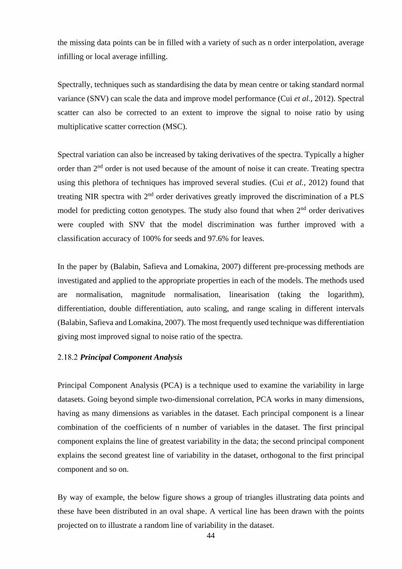
44
the missing data points can be in filled with a variety of such as n order interpolation, average
infilling or local average infilling.
Spectrally, techniques such as standardising the data by mean centre or taking standard normal
variance (SNV) can scale the data and improve model performance (Cui et al., 2012). Spectral
scatter can also be corrected to an extent to improve the signal to noise ratio by using
multiplicative scatter correction (MSC).
Spectral variation can also be increased by taking derivatives of the spectra. Typically a higher
order than 2nd order is not used because of the amount of noise it can create. Treating spectra
using this plethora of techniques has improved several studies. (Cui et al., 2012) found that
treating NIR spectra with 2nd order derivatives greatly improved the discrimination of a PLS
model for predicting cotton genotypes. The study also found that when 2nd order derivatives
were coupled with SNV that the model discrimination was further improved with a
classification accuracy of 100% for seeds and 97.6% for leaves.
In the paper by (Balabin, Safieva and Lomakina, 2007) different pre-processing methods are
investigated and applied to the appropriate properties in each of the models. The methods used
are normalisation, magnitude normalisation, linearisation (taking the logarithm),
differentiation, double differentiation, auto scaling, and range scaling in different intervals
(Balabin, Safieva and Lomakina, 2007). The most frequently used technique was differentiation
giving most improved signal to noise ratio of the spectra.
Principal Component Analysis
Principal Component Analysis (PCA) is a technique used to examine the variability in large
datasets. Going beyond simple two-dimensional correlation, PCA works in many dimensions,
having as many dimensions as variables in the dataset. Each principal component is a linear
combination of the coefficients of n number of variables in the dataset. The first principal
component explains the line of greatest variability in the data; the second principal component
explains the second greatest line of variability in the dataset, orthogonal to the first principal
component and so on.
By way of example, the below figure shows a group of triangles illustrating data points and
these have been distributed in an oval shape. A vertical line has been drawn with the points
projected on to illustrate a random line of variability in the dataset.
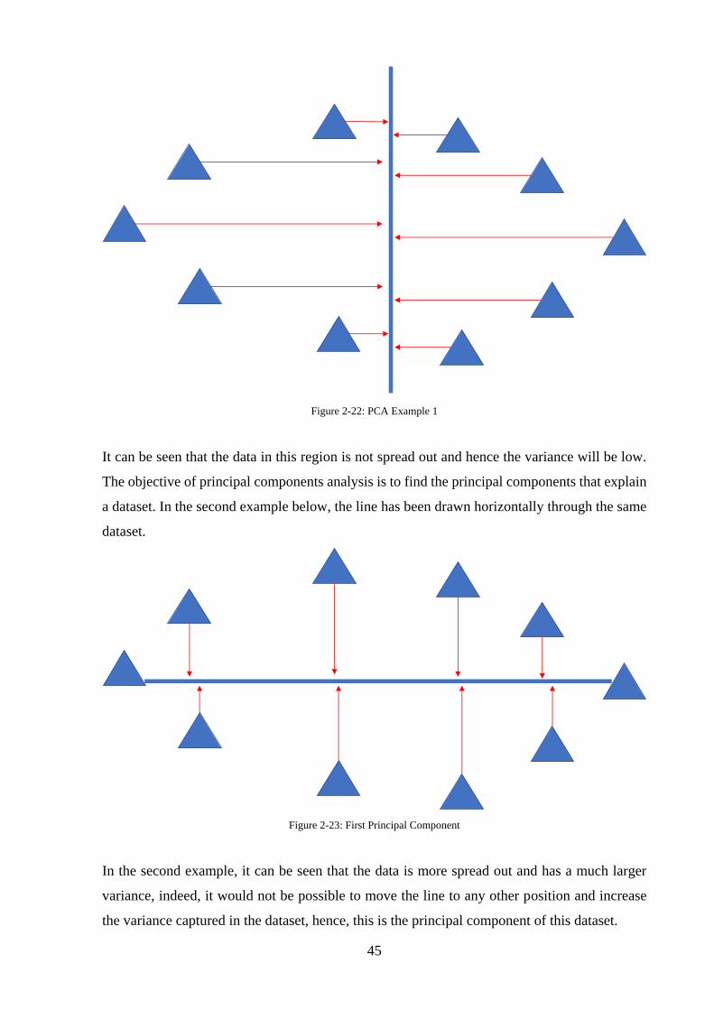
45
Figure 2-22: PCA Example 1
It can be seen that the data in this region is not spread out and hence the variance will be low.
The objective of principal components analysis is to find the principal components that explain
a dataset. In the second example below, the line has been drawn horizontally through the same
dataset.
Figure 2-23: First Principal Component
In the second example, it can be seen that the data is more spread out and has a much larger
variance, indeed, it would not be possible to move the line to any other position and increase
the variance captured in the dataset, hence, this is the principal component of this dataset.
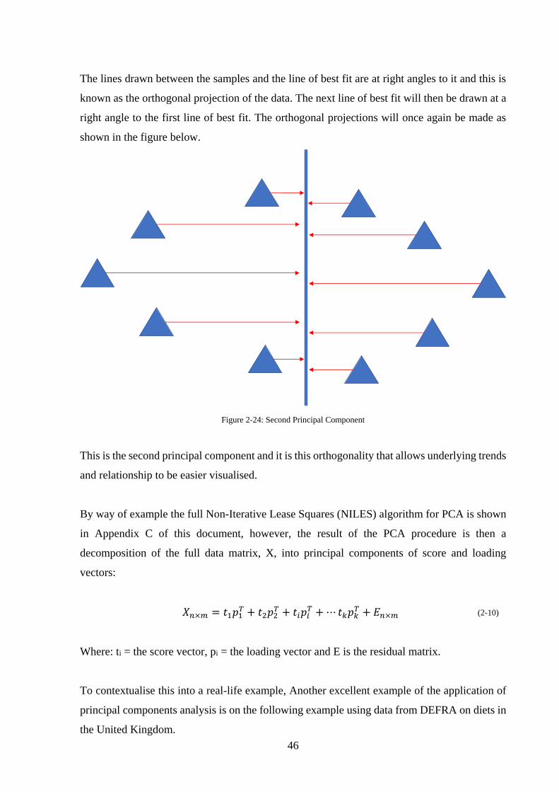
46
The lines drawn between the samples and the line of best fit are at right angles to it and this is
known as the orthogonal projection of the data. The next line of best fit will then be drawn at a
right angle to the first line of best fit. The orthogonal projections will once again be made as
shown in the figure below.
Figure 2-24: Second Principal Component
This is the second principal component and it is this orthogonality that allows underlying trends
and relationship to be easier visualised.
By way of example the full Non-Iterative Lease Squares (NILES) algorithm for PCA is shown
in Appendix C of this document, however, the result of the PCA procedure is then a
decomposition of the full data matrix, X, into principal components of score and loading
vectors:
𝑋𝑛×𝑚 = 𝑡1𝑝1𝑇 + 𝑡2𝑝2
𝑇 + 𝑡𝑖𝑝𝑖𝑇 + ⋯ 𝑡𝑘𝑝𝑘
𝑇 + 𝐸𝑛×𝑚 (2-10)
Where: ti = the score vector, pi = the loading vector and E is the residual matrix.
To contextualise this into a real-life example, Another excellent example of the application of
principal components analysis is on the following example using data from DEFRA on diets in
the United Kingdom.
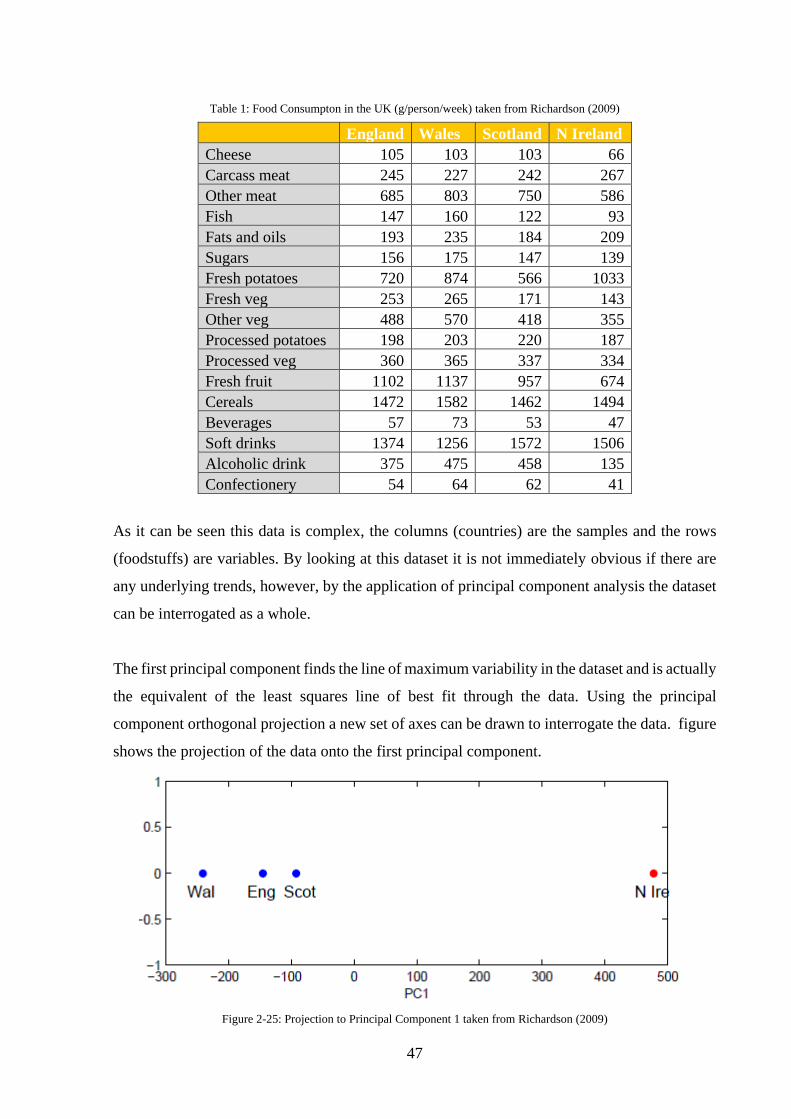
47
Table 1: Food Consumpton in the UK (g/person/week) taken from Richardson (2009)
England Wales Scotland N Ireland
Cheese 105 103 103 66
Carcass meat 245 227 242 267
Other meat 685 803 750 586
Fish 147 160 122 93
Fats and oils 193 235 184 209
Sugars 156 175 147 139
Fresh potatoes 720 874 566 1033
Fresh veg 253 265 171 143
Other veg 488 570 418 355
Processed potatoes 198 203 220 187
Processed veg 360 365 337 334
Fresh fruit 1102 1137 957 674
Cereals 1472 1582 1462 1494
Beverages 57 73 53 47
Soft drinks 1374 1256 1572 1506
Alcoholic drink 375 475 458 135
Confectionery 54 64 62 41
As it can be seen this data is complex, the columns (countries) are the samples and the rows
(foodstuffs) are variables. By looking at this dataset it is not immediately obvious if there are
any underlying trends, however, by the application of principal component analysis the dataset
can be interrogated as a whole.
The first principal component finds the line of maximum variability in the dataset and is actually
the equivalent of the least squares line of best fit through the data. Using the principal
component orthogonal projection a new set of axes can be drawn to interrogate the data. figure
shows the projection of the data onto the first principal component.
Figure 2-25: Projection to Principal Component 1 taken from Richardson (2009)
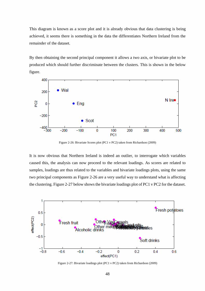
48
This diagram is known as a score plot and it is already obvious that data clustering is being
achieved, it seems there is something in the data the differentiates Northern Ireland from the
remainder of the dataset.
By then obtaining the second principal component it allows a two axis, or bivariate plot to be
produced which should further discriminate between the clusters. This is shown in the below
figure.
Figure 2-26: Bivariate Scores plot (PC1 v PC2) taken from Richardson (2009)
It is now obvious that Northern Ireland is indeed an outlier, to interrogate which variables
caused this, the analysis can now proceed to the relevant loadings. As scores are related to
samples, loadings are thus related to the variables and bivariate loadings plots, using the same
two principal components as Figure 2-26 are a very useful way to understand what is affecting
the clustering. Figure 2-27 below shows the bivariate loadings plot of PC1 v PC2 for the dataset.
Figure 2-27: Bivariate loadings plot (PC1 v PC2) taken from Richardson (2009)
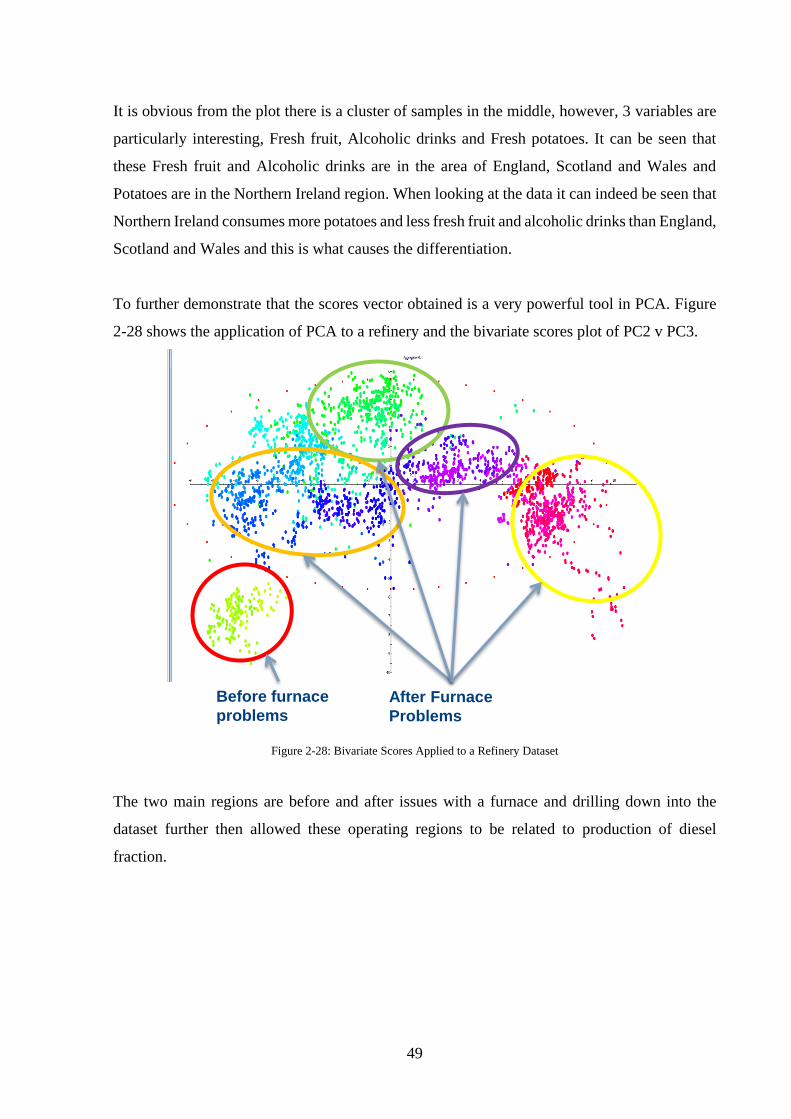
49
It is obvious from the plot there is a cluster of samples in the middle, however, 3 variables are
particularly interesting, Fresh fruit, Alcoholic drinks and Fresh potatoes. It can be seen that
these Fresh fruit and Alcoholic drinks are in the area of England, Scotland and Wales and
Potatoes are in the Northern Ireland region. When looking at the data it can indeed be seen that
Northern Ireland consumes more potatoes and less fresh fruit and alcoholic drinks than England,
Scotland and Wales and this is what causes the differentiation.
To further demonstrate that the scores vector obtained is a very powerful tool in PCA. Figure
2-28 shows the application of PCA to a refinery and the bivariate scores plot of PC2 v PC3.
Figure 2-28: Bivariate Scores Applied to a Refinery Dataset
The two main regions are before and after issues with a furnace and drilling down into the
dataset further then allowed these operating regions to be related to production of diesel
fraction.
Before furnace
problemsAfter Furnace
Problems
50
Partial Least Squares
Partial least squares (Projection to Latent Structures or PLS) is a powerful regression tool and
is in essence an extension of PCA. However, whereas in PCA decomposition the scores and
loadings are the vectors that best describe the variance of the X matrix, in PLS decomposition
the scores and loadings are the vectors that have the highest covariance with the response vector
Y. After decomposition a regression between score vectors and the response is then
performed”(Aske, 2002a).
In practice, this means that a regression can be formed on a full block of X values rather than
just one as with ordinary least squares. If once again the UK diet example is taken this means
that by taking the diet of an unknown individual, a PLS model could be built on the dataset
which would allow the user to predict the country of origin of te individual.
The full algorithm for the Non-Iterative Partial Least Squares Approach used later in the thesis
is shown in Appendix C of the document.
Many examples of the industrial applications of PLS are documented in the literature. In a study
on detecting vegetal oil adulteration in diesel and biodiesel by Gaydou, Kister and Dupuy
(2011) using PLS predictive models found that NIR gave better results than MIR. (Gaydou,
Kister and Dupuy, 2011) also discusses the use of multiblock PLS to combine the two methods
to form a predictive model based on a combination of analyses. Three methods of multiblock
PLS are investigated in the paper.
The first method is called the concatenated method and works by combining the matrices of
both NIR and MIR data into a signal matrix, the PLS method is then applied to this matrix, it is
important to ensure that if this method is applied both matrices of data are correctly scaled to
achieve sensible results.
The second method discussed considers each data matrix independently, by application of PCA
to the data scores are obtained for each block of data. The scores are then collected and
combined to form a super matrix (Gaydou, Kister and Dupuy, 2011). This method is called
Hierarchical-PLS (H-PLS) and is also described by Bastien, Vinzi and Tenehaus (2005).
51
The third method used by Gaydou, Kister and Dupuy (2011) is known as Serial Partial least
squares (S-PLS) and was proposed by (Berglund and Wold, 1999). This method uses PLS on
each data matrix to obtain scores. As with H-PLS the scores are then combined into a single
super matrix upon which PLS is once again applied. Out of the three methods the one that
yielded the best results was H-PLS with a prediction error of 2.03%. These findings raise the
intriguing possibility of improving model discrimination by using combined analytical
methods.
In a study by (Balabin, Safieva and Lomakina, 2012) PLS was used as to predict gasoline data
using NIR spectra. The method was found to be only moderately effective for predicting
gasoline composition. K nearest neighbour modelling was found to be the simplest of the
algorithm assessed and also more effective. This is a well-known phenomenon and is due to the
simplicity and lack of variability in gasoline datasets.
Nearest Neighbour
Nearest neighbour (or K Nearest Neighbours or KNN) is a non-parametric classification method
whereby a distance (Euclidean distance) is assigned between all points in a dataset. The distance
between each point is expressed as the root of square differences between the coordinates of
the objects being examined and is described by the following formula:
𝑑 = √∑(𝑥𝑖 − 𝑦𝑖)2
𝑛
𝑖=1
(2-11)
The neighbours of the sample under scrutiny are then ordered by distance and a parameter (K)
is then given to optimise the numbers of neighbours selected to describe the sample. Variations
on this method have been also been applied, for example a weighted KNN is a similar algorithm
which tries to introduce bias to the model by assigning weights to the samples nearest
neighbours to alter the effects that nearest neighbour samples have on the final predicted result.
(Balabin, Safieva and Lomakina, 2012) investigated the use of (amongst other algorithms)
KNN modelling for predicting gasoline composition. The study showed that it was actually one
of the most effective methods for classification all three of the datasets investigated. This is
shown by the model errors shown in Figure 2-29. It can be seen that in all three models the
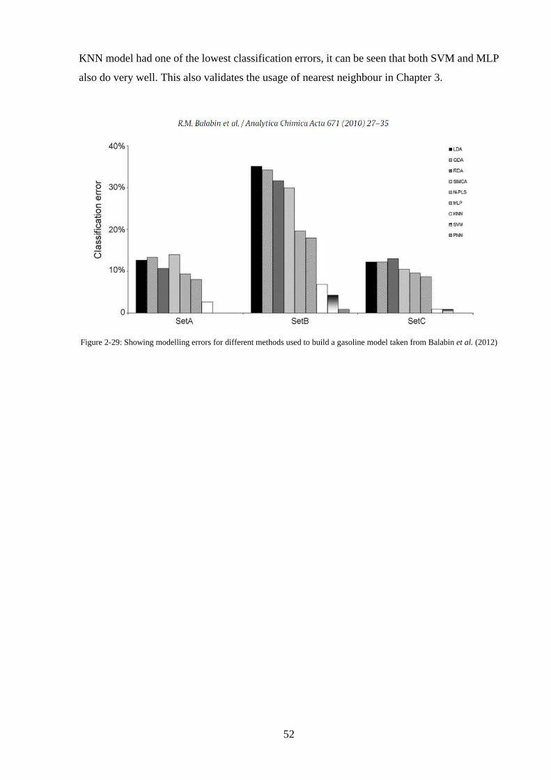
52
KNN model had one of the lowest classification errors, it can be seen that both SVM and MLP
also do very well. This also validates the usage of nearest neighbour in Chapter 3.
Figure 2-29: Showing modelling errors for different methods used to build a gasoline model taken from Balabin et al. (2012)

53
Chapter 3:
Refinery Crude Oil Quality
Monitoring
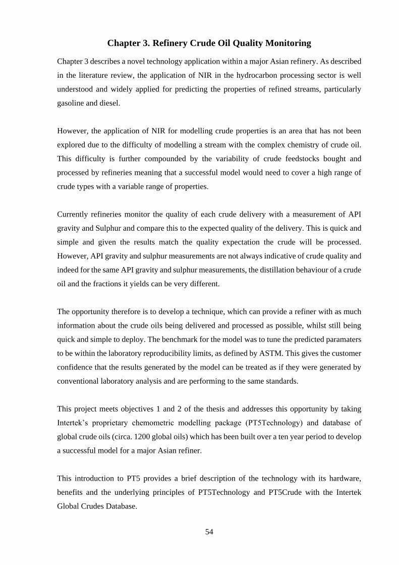
54
Chapter 3. Refinery Crude Oil Quality Monitoring
Chapter 3 describes a novel technology application within a major Asian refinery. As described
in the literature review, the application of NIR in the hydrocarbon processing sector is well
understood and widely applied for predicting the properties of refined streams, particularly
gasoline and diesel.
However, the application of NIR for modelling crude properties is an area that has not been
explored due to the difficulty of modelling a stream with the complex chemistry of crude oil.
This difficulty is further compounded by the variability of crude feedstocks bought and
processed by refineries meaning that a successful model would need to cover a high range of
crude types with a variable range of properties.
Currently refineries monitor the quality of each crude delivery with a measurement of API
gravity and Sulphur and compare this to the expected quality of the delivery. This is quick and
simple and given the results match the quality expectation the crude will be processed.
However, API gravity and sulphur measurements are not always indicative of crude quality and
indeed for the same API gravity and sulphur measurements, the distillation behaviour of a crude
oil and the fractions it yields can be very different.
The opportunity therefore is to develop a technique, which can provide a refiner with as much
information about the crude oils being delivered and processed as possible, whilst still being
quick and simple to deploy. The benchmark for the model was to tune the predicted paramaters
to be within the laboratory reproducibility limits, as defined by ASTM. This gives the customer
confidence that the results generated by the model can be treated as if they were generated by
conventional laboratory analysis and are performing to the same standards.
This project meets objectives 1 and 2 of the thesis and addresses this opportunity by taking
Intertek’s proprietary chemometric modelling package (PT5Technology) and database of
global crude oils (circa. 1200 global oils) which has been built over a ten year period to develop
a successful model for a major Asian refiner.
This introduction to PT5 provides a brief description of the technology with its hardware,
benefits and the underlying principles of PT5Technology and PT5Crude with the Intertek
Global Crudes Database.
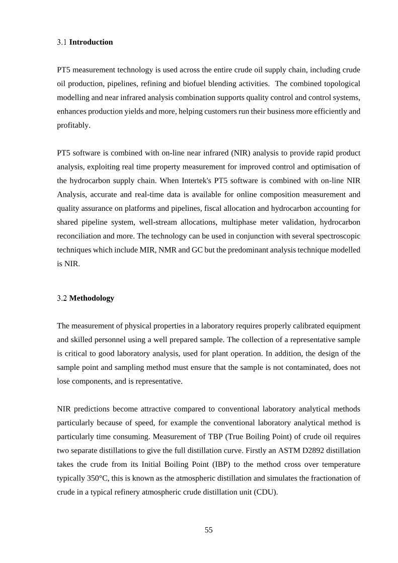
55
Introduction
PT5 measurement technology is used across the entire crude oil supply chain, including crude
oil production, pipelines, refining and biofuel blending activities. The combined topological
modelling and near infrared analysis combination supports quality control and control systems,
enhances production yields and more, helping customers run their business more efficiently and
profitably.
PT5 software is combined with on-line near infrared (NIR) analysis to provide rapid product
analysis, exploiting real time property measurement for improved control and optimisation of
the hydrocarbon supply chain. When Intertek's PT5 software is combined with on-line NIR
Analysis, accurate and real-time data is available for online composition measurement and
quality assurance on platforms and pipelines, fiscal allocation and hydrocarbon accounting for
shared pipeline system, well-stream allocations, multiphase meter validation, hydrocarbon
reconciliation and more. The technology can be used in conjunction with several spectroscopic
techniques which include MIR, NMR and GC but the predominant analysis technique modelled
is NIR.
Methodology
The measurement of physical properties in a laboratory requires properly calibrated equipment
and skilled personnel using a well prepared sample. The collection of a representative sample
is critical to good laboratory analysis, used for plant operation. In addition, the design of the
sample point and sampling method must ensure that the sample is not contaminated, does not
lose components, and is representative.
NIR predictions become attractive compared to conventional laboratory analytical methods
particularly because of speed, for example the conventional laboratory analytical method is
particularly time consuming. Measurement of TBP (True Boiling Point) of crude oil requires
two separate distillations to give the full distillation curve. Firstly an ASTM D2892 distillation
takes the crude from its Initial Boiling Point (IBP) to the method cross over temperature
typically 350°C, this is known as the atmospheric distillation and simulates the fractionation of
crude in a typical refinery atmospheric crude distillation unit (CDU).
56
The second method, ASTM D5236, is charged with the 350°C+ atmospheric residue from the
first method and the distilled under vacuum to approximately 550°C equivalent. This is known
as a vacuum distillation and the remaining crude portion of 550°C+ is the vacuum residue, this
simulates a typical refinery vacuum distillation unit.
The measurement can form part of an on-line or at-line measurement which is updated every
few minutes. These measurements can be used as the input to a control loop and / or input to a
process optimiser. Typical spectrometers are shown in Figure 1.
Figure 3-1 - Typical Spectrometers (courtesy of ABB 2017)
To take measurements a transmission cell is used. This enables the NIR beam to be used to
check for deposits on cell windows and to measure path length to ensure that the instrument is
working as designed. The technology is used within Intertek to deliver a valued service to many
key customers. A picture of the laboratory in Aberdeen is shown in Figure 3-2.
Laboratory NIR spectrometer
On-line NIR spectrometer
57
Figure 3-2 - Laboratory Crude Oil Sample Handling and Spectrometer
In the case of crude oil analysis, live crude oil and on-line systems can operate at pressures of
up to 100 Bar. For refinery blending operations the sample can be handled at atmospheric
pressure.
NIR Spectra in PT5
Typical industrial application using NIR utilises spectra with wavenumbers between 4000 and
4800 cm-1 which is the combination band between MIR and the first overtone (as described in
section 2.7). In MIR each chemical compound has a specific finger print and in mixtures the
individual amounts of the compounds can be deduced.
In the NIR spectra there are no peaks for individual compounds and the absorption spectra
overlap for different compounds (Figure 3-3). When measuring refinery streams or crude oil
the problem is further complicated by the very large number of chemical compounds present in
the analyte.
When combined with the inherent signal to noise ratio of the instrument there is no practical
way of reading the spectra. The shape of the spectra does however give a qualitative view of
the composition as shown in Figure 3-3.
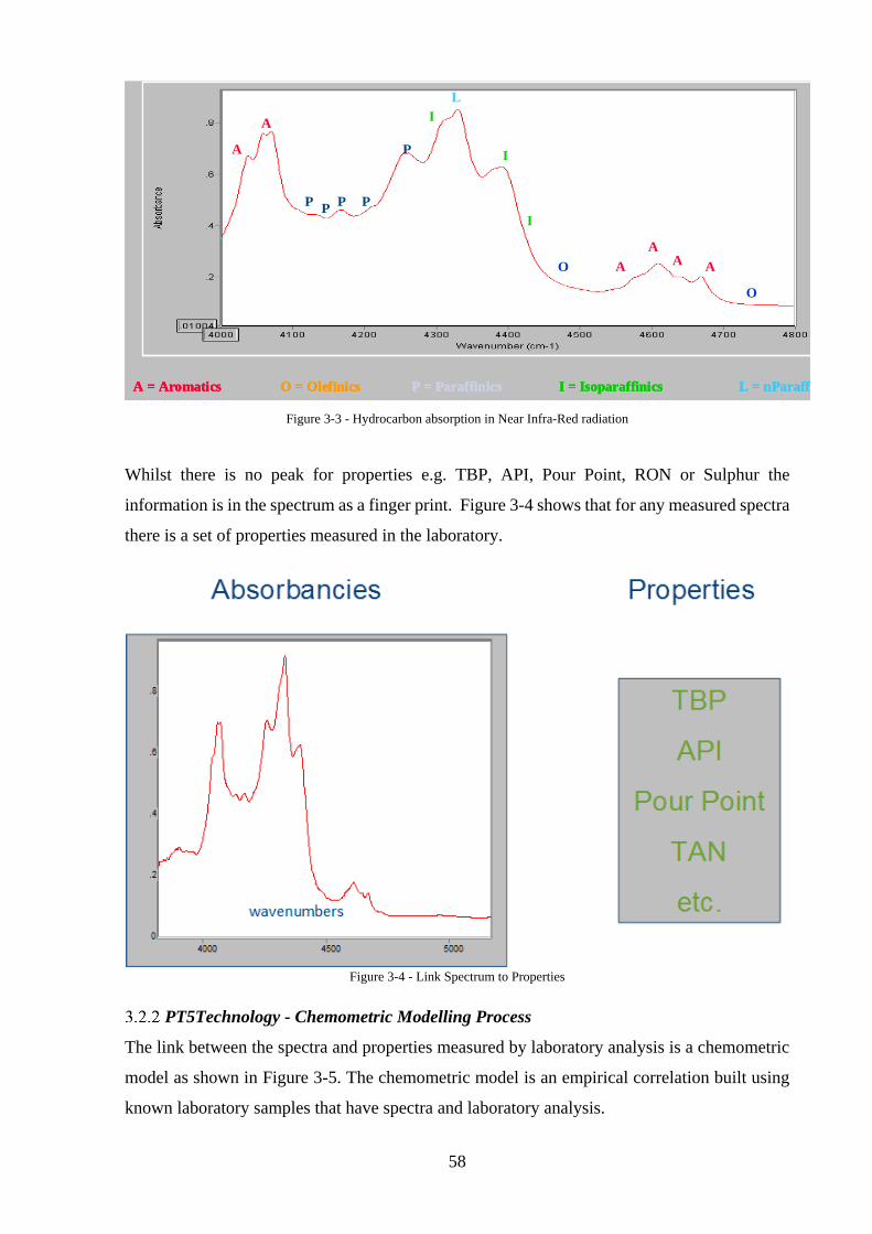
58
Figure 3-3 - Hydrocarbon absorption in Near Infra-Red radiation
Whilst there is no peak for properties e.g. TBP, API, Pour Point, RON or Sulphur the
information is in the spectrum as a finger print. Figure 3-4 shows that for any measured spectra
there is a set of properties measured in the laboratory.
Figure 3-4 - Link Spectrum to Properties
PT5Technology - Chemometric Modelling Process
The link between the spectra and properties measured by laboratory analysis is a chemometric
model as shown in Figure 3-5. The chemometric model is an empirical correlation built using
known laboratory samples that have spectra and laboratory analysis.
KARO KISO KENE NARO KAROL KOX PAROX
A
A
PP
P P
P
I
L
I
I
O A
AA
A
O
A = Aromatics O = Olefinics P = Paraffinics I = Isoparaffinics L = nParaffinics
KARO KISO KENE NARO KAROL KOX PAROX
A
A
PP
P P
P
I
L
I
I
O A
AA
A
O
KARO KISO KENE NAROKARO KISO KENE NARO KAROL KOX PAROX
A
A
PP
P P
P
I
L
I
I
O A
AA
A
O
A = Aromatics O = Olefinics P = Paraffinics I = Isoparaffinics L = nParaffinicsA = Aromatics O = Olefinics P = Paraffinics I = Isoparaffinics L = nParaffinics
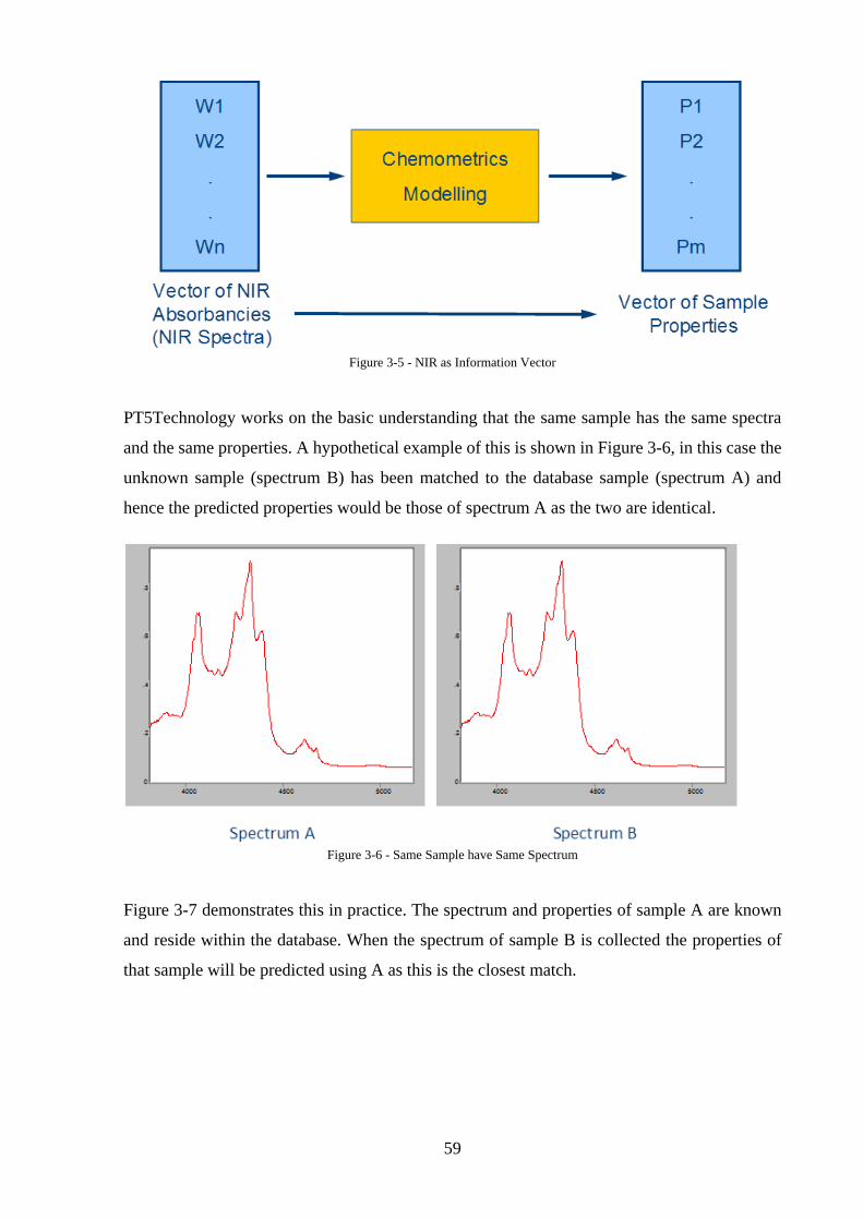
59
Figure 3-5 - NIR as Information Vector
PT5Technology works on the basic understanding that the same sample has the same spectra
and the same properties. A hypothetical example of this is shown in Figure 3-6, in this case the
unknown sample (spectrum B) has been matched to the database sample (spectrum A) and
hence the predicted properties would be those of spectrum A as the two are identical.
Figure 3-6 - Same Sample have Same Spectrum
Figure 3-7 demonstrates this in practice. The spectrum and properties of sample A are known
and reside within the database. When the spectrum of sample B is collected the properties of
that sample will be predicted using A as this is the closest match.
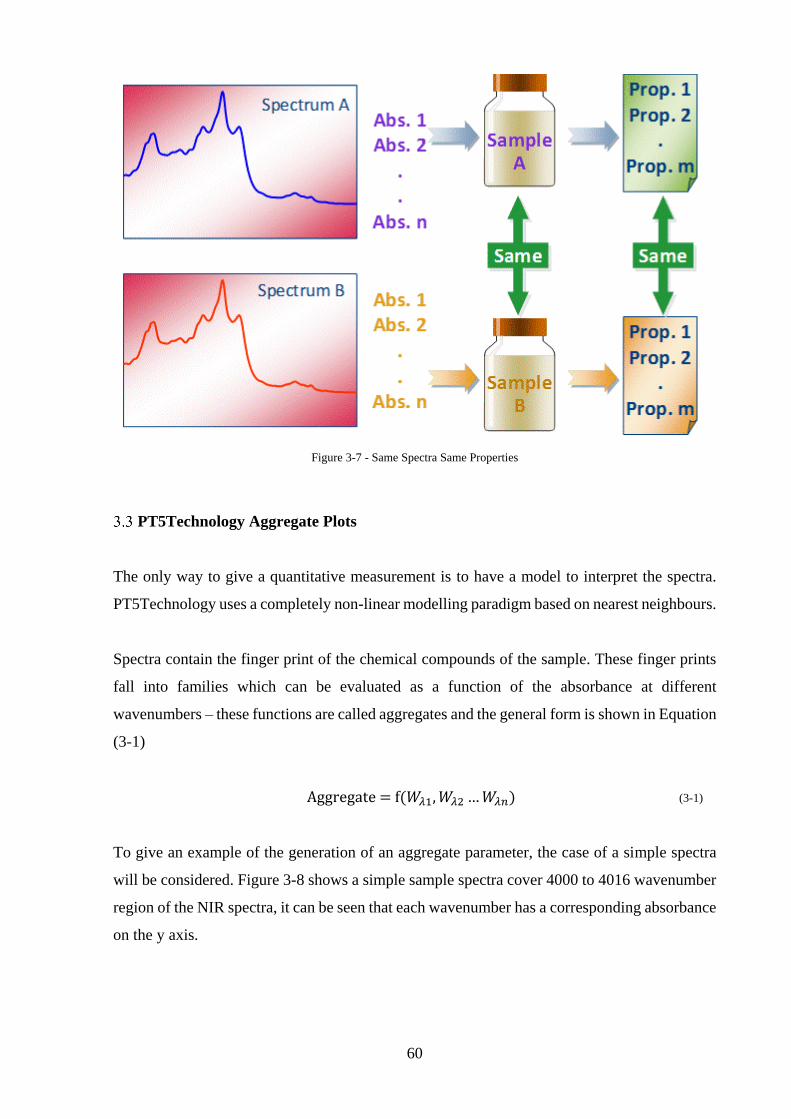
60
Figure 3-7 - Same Spectra Same Properties
PT5Technology Aggregate Plots
The only way to give a quantitative measurement is to have a model to interpret the spectra.
PT5Technology uses a completely non-linear modelling paradigm based on nearest neighbours.
Spectra contain the finger print of the chemical compounds of the sample. These finger prints
fall into families which can be evaluated as a function of the absorbance at different
wavenumbers – these functions are called aggregates and the general form is shown in Equation
(3-1)
Aggregate = f(𝑊𝜆1, 𝑊𝜆2 … 𝑊𝜆𝑛) (3-1)
To give an example of the generation of an aggregate parameter, the case of a simple spectra
will be considered. Figure 3-8 shows a simple sample spectra cover 4000 to 4016 wavenumber
region of the NIR spectra, it can be seen that each wavenumber has a corresponding absorbance
on the y axis.
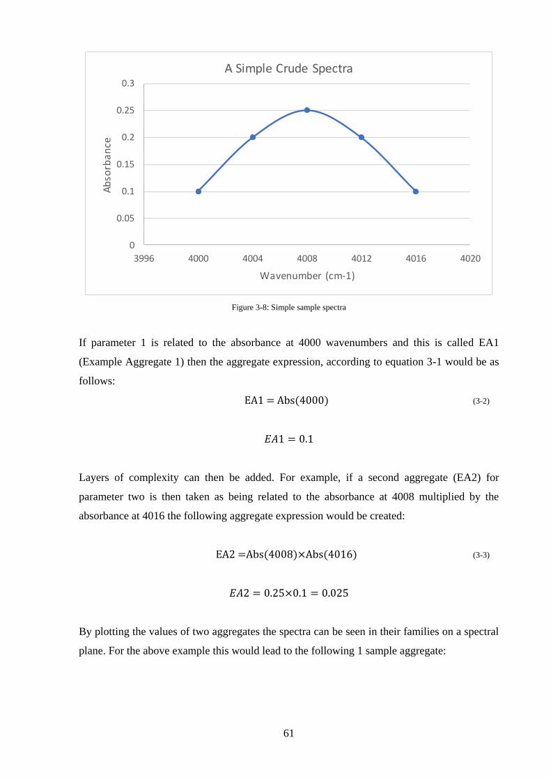
61
Figure 3-8: Simple sample spectra
If parameter 1 is related to the absorbance at 4000 wavenumbers and this is called EA1
(Example Aggregate 1) then the aggregate expression, according to equation 3-1 would be as
follows:
EA1 = Abs(4000) (3-2)
𝐸𝐴1 = 0.1
Layers of complexity can then be added. For example, if a second aggregate (EA2) for
parameter two is then taken as being related to the absorbance at 4008 multiplied by the
absorbance at 4016 the following aggregate expression would be created:
EA2 =Abs(4008)×Abs(4016) (3-3)
𝐸𝐴2 = 0.25×0.1 = 0.025
By plotting the values of two aggregates the spectra can be seen in their families on a spectral
plane. For the above example this would lead to the following 1 sample aggregate:
0
0.05
0.1
0.15
0.2
0.25
0.3
3996 4000 4004 4008 4012 4016 4020
Ab
sorb
an
ce
Wavenumber (cm-1)
A Simple Crude Spectra
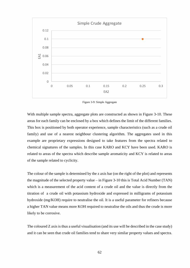
62
Figure 3-9: Simple Aggregate
With multiple sample spectra, aggregate plots are constructed as shown in Figure 3-10. These
areas for each family can be enclosed by a box which defines the limit of the different families.
This box is positioned by both operator experience, sample characteristics (such as a crude oil
family) and use of a nearest neighbour clustering algorithm. The aggregates used in this
example are proprietary expressions designed to take features from the spectra related to
chemical signatures of the samples. In this case KARO and KCY have been used. KARO is
related to areas of the spectra which describe sample aromaticity and KCY is related to areas
of the sample related to cyclicity.
The colour of the sample is determined by the z axis bar (on the right of the plot) and represents
the magnitude of the selected property value – in Figure 3-10 this is Total Acid Number (TAN)
which is a measurement of the acid content of a crude oil and the value is directly from the
titration of a crude oil with potassium hydroxide and expressed in milligrams of potassium
hydroxide (mg/KOH) require to neutralise the oil. It is a useful parameter for refiners because
a higher TAN value means more KOH required to neutralise the oils and thus the crude is more
likely to be corrosive.
The coloured Z axis is thus a useful visualisation (and its use will be described in the case study)
and it can be seen that crude oil families tend to share very similar property values and spectra.
0
0.02
0.04
0.06
0.08
0.1
0.12
0 0.05 0.1 0.15 0.2 0.25 0.3
EA1
EA2
Simple Crude Aggregate
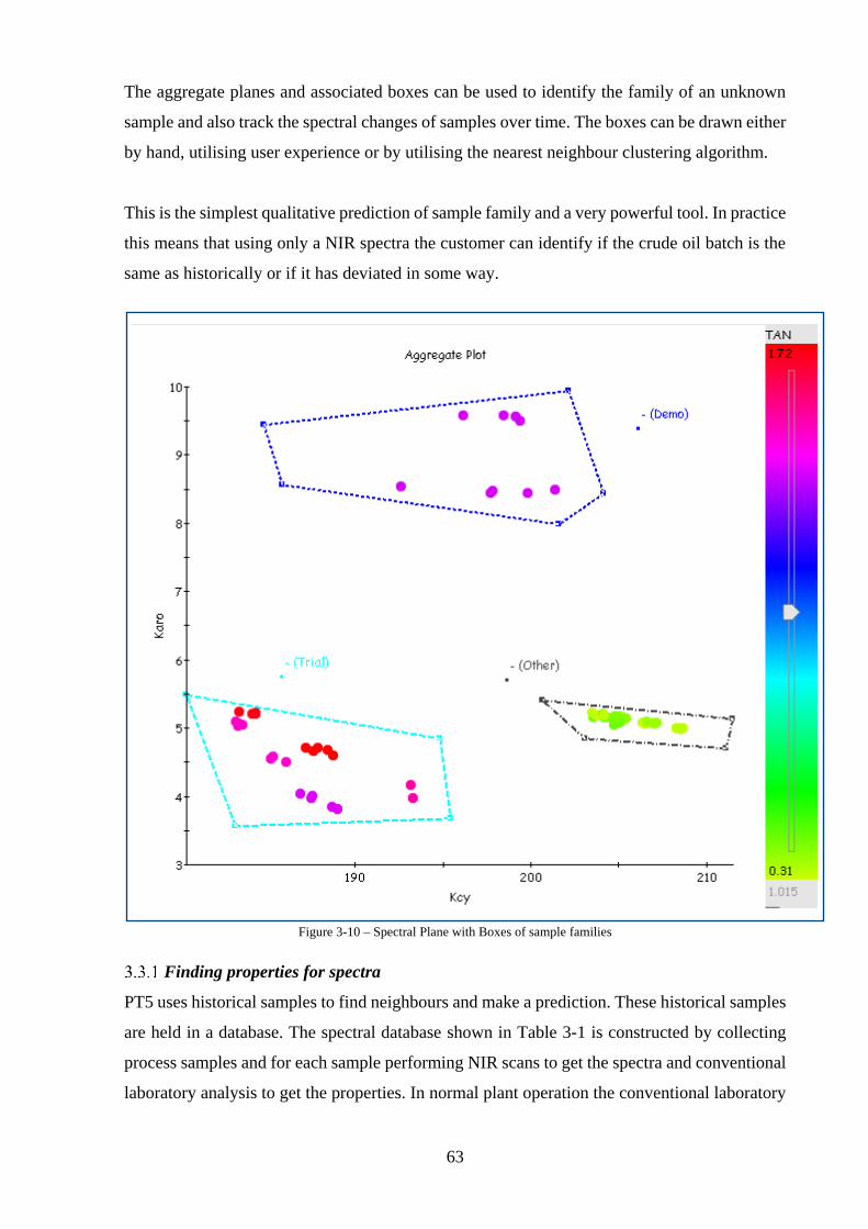
63
The aggregate planes and associated boxes can be used to identify the family of an unknown
sample and also track the spectral changes of samples over time. The boxes can be drawn either
by hand, utilising user experience or by utilising the nearest neighbour clustering algorithm.
This is the simplest qualitative prediction of sample family and a very powerful tool. In practice
this means that using only a NIR spectra the customer can identify if the crude oil batch is the
same as historically or if it has deviated in some way.
Figure 3-10 – Spectral Plane with Boxes of sample families
Finding properties for spectra
PT5 uses historical samples to find neighbours and make a prediction. These historical samples
are held in a database. The spectral database shown in Table 3-1 is constructed by collecting
process samples and for each sample performing NIR scans to get the spectra and conventional
laboratory analysis to get the properties. In normal plant operation the conventional laboratory
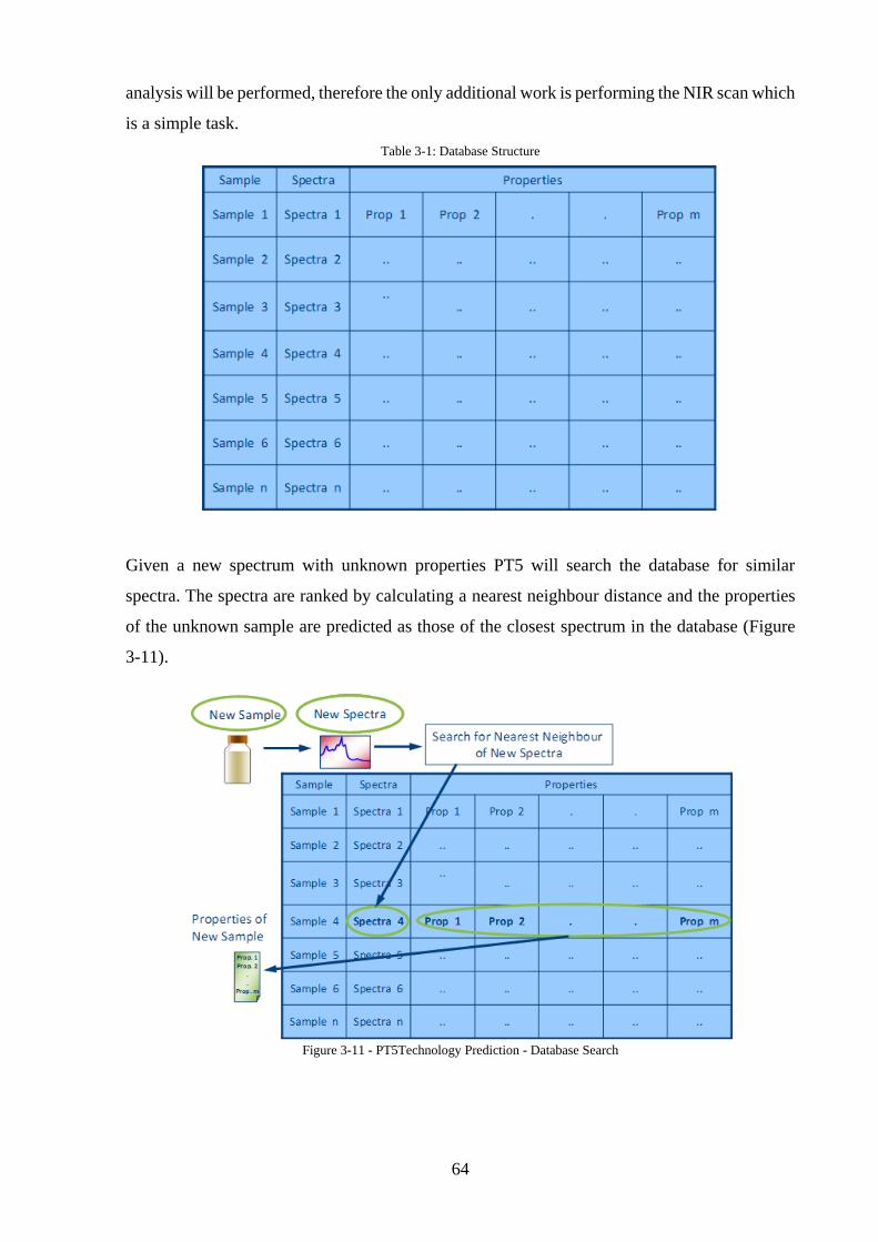
64
analysis will be performed, therefore the only additional work is performing the NIR scan which
is a simple task.
Table 3-1: Database Structure
Given a new spectrum with unknown properties PT5 will search the database for similar
spectra. The spectra are ranked by calculating a nearest neighbour distance and the properties
of the unknown sample are predicted as those of the closest spectrum in the database (Figure
3-11).
Figure 3-11 - PT5Technology Prediction - Database Search
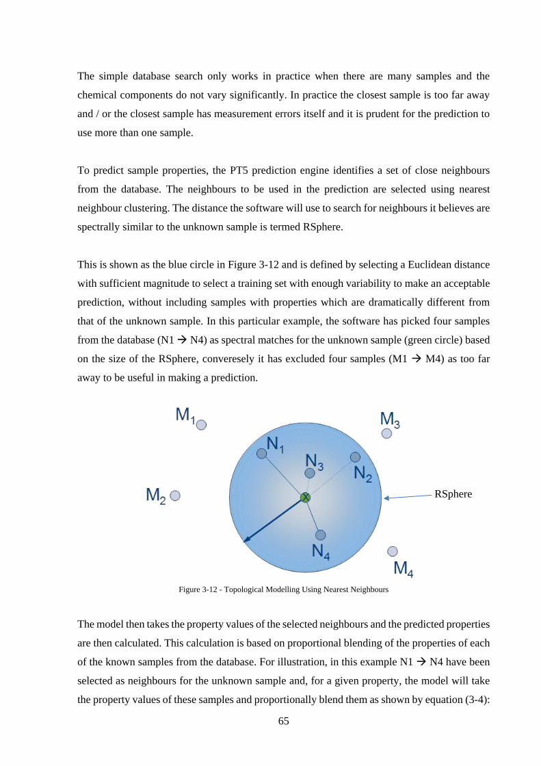
65
The simple database search only works in practice when there are many samples and the
chemical components do not vary significantly. In practice the closest sample is too far away
and / or the closest sample has measurement errors itself and it is prudent for the prediction to
use more than one sample.
To predict sample properties, the PT5 prediction engine identifies a set of close neighbours
from the database. The neighbours to be used in the prediction are selected using nearest
neighbour clustering. The distance the software will use to search for neighbours it believes are
spectrally similar to the unknown sample is termed RSphere.
This is shown as the blue circle in Figure 3-12 and is defined by selecting a Euclidean distance
with sufficient magnitude to select a training set with enough variability to make an acceptable
prediction, without including samples with properties which are dramatically different from
that of the unknown sample. In this particular example, the software has picked four samples
from the database (N1 N4) as spectral matches for the unknown sample (green circle) based
on the size of the RSphere, converesely it has excluded four samples (M1 M4) as too far
away to be useful in making a prediction.
Figure 3-12 - Topological Modelling Using Nearest Neighbours
The model then takes the property values of the selected neighbours and the predicted properties
are then calculated. This calculation is based on proportional blending of the properties of each
of the known samples from the database. For illustration, in this example N1 N4 have been
selected as neighbours for the unknown sample and, for a given property, the model will take
the property values of these samples and proportionally blend them as shown by equation (3-4):
RSphere
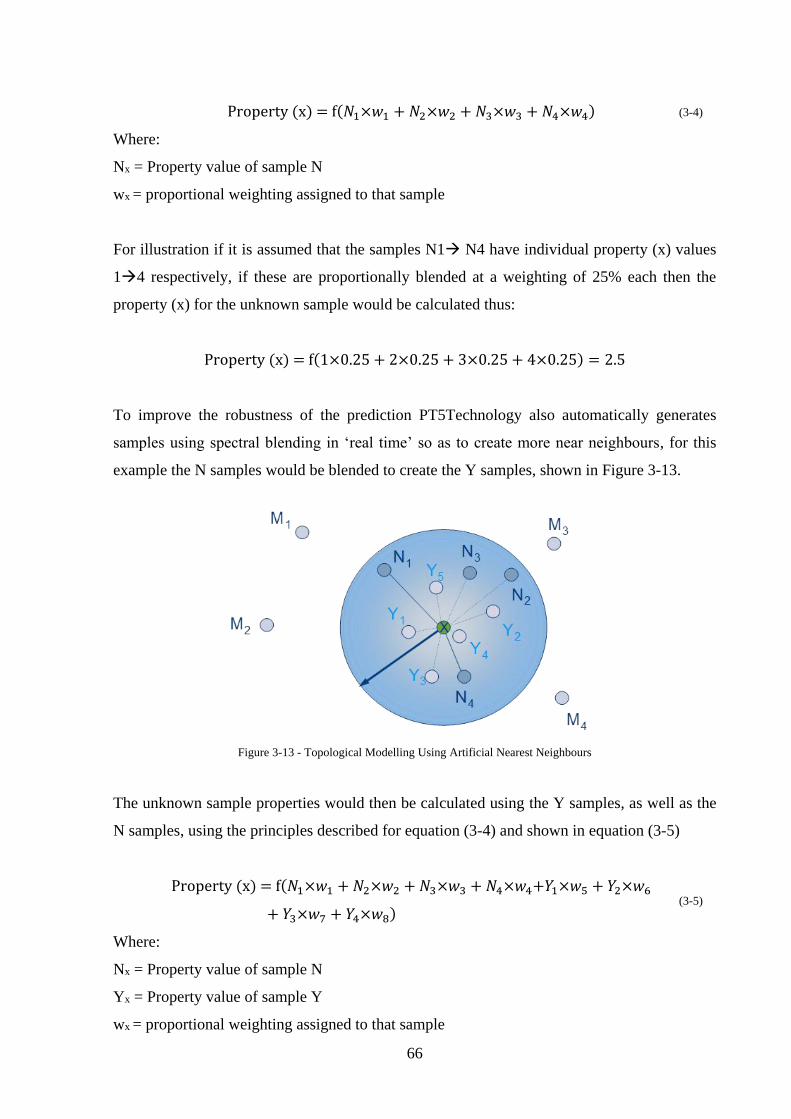
66
Property (x) = f(𝑁1×𝑤1 + 𝑁2×𝑤2 + 𝑁3×𝑤3 + 𝑁4×𝑤4) (3-4)
Where:
Nx = Property value of sample N
wx = proportional weighting assigned to that sample
For illustration if it is assumed that the samples N1 N4 have individual property (x) values
14 respectively, if these are proportionally blended at a weighting of 25% each then the
property (x) for the unknown sample would be calculated thus:
Property (x) = f(1×0.25 + 2×0.25 + 3×0.25 + 4×0.25) = 2.5
To improve the robustness of the prediction PT5Technology also automatically generates
samples using spectral blending in ‘real time’ so as to create more near neighbours, for this
example the N samples would be blended to create the Y samples, shown in Figure 3-13.
Figure 3-13 - Topological Modelling Using Artificial Nearest Neighbours
The unknown sample properties would then be calculated using the Y samples, as well as the
N samples, using the principles described for equation (3-4) and shown in equation (3-5)
Property (x) = f(𝑁1×𝑤1 + 𝑁2×𝑤2 + 𝑁3×𝑤3 + 𝑁4×𝑤4+𝑌1×𝑤5 + 𝑌2×𝑤6
+ 𝑌3×𝑤7 + 𝑌4×𝑤8) (3-5)
Where:
Nx = Property value of sample N
Yx = Property value of sample Y
wx = proportional weighting assigned to that sample
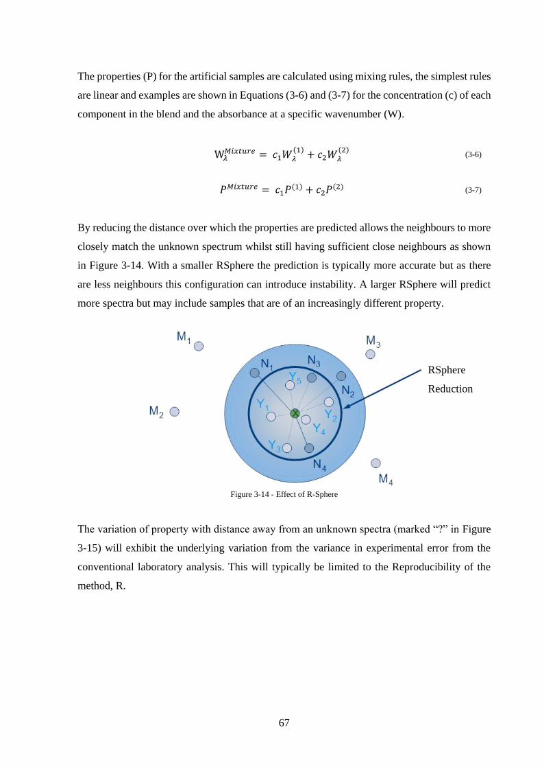
67
The properties (P) for the artificial samples are calculated using mixing rules, the simplest rules
are linear and examples are shown in Equations (3-6) and (3-7) for the concentration (c) of each
component in the blend and the absorbance at a specific wavenumber (W).
W𝜆𝑀𝑖𝑥𝑡𝑢𝑟𝑒 = 𝑐1𝑊 𝜆
(1)+ 𝑐2𝑊 𝜆
(2) (3-6)
𝑃𝑀𝑖𝑥𝑡𝑢𝑟𝑒 = 𝑐1𝑃(1) + 𝑐2𝑃(2) (3-7)
By reducing the distance over which the properties are predicted allows the neighbours to more
closely match the unknown spectrum whilst still having sufficient close neighbours as shown
in Figure 3-14. With a smaller RSphere the prediction is typically more accurate but as there
are less neighbours this configuration can introduce instability. A larger RSphere will predict
more spectra but may include samples that are of an increasingly different property.
Figure 3-14 - Effect of R-Sphere
The variation of property with distance away from an unknown spectra (marked “?” in Figure
3-15) will exhibit the underlying variation from the variance in experimental error from the
conventional laboratory analysis. This will typically be limited to the Reproducibility of the
method, R.
RSphere
Reduction
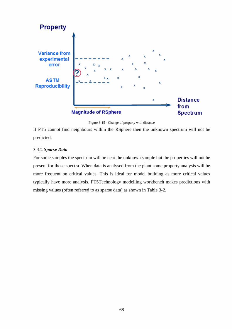
68
Figure 3-15 - Change of property with distance
If PT5 cannot find neighbours within the RSphere then the unknown spectrum will not be
predicted.
Sparse Data
For some samples the spectrum will be near the unknown sample but the properties will not be
present for those spectra. When data is analysed from the plant some property analysis will be
more frequent on critical values. This is ideal for model building as more critical values
typically have more analysis. PT5Technology modelling workbench makes predictions with
missing values (often referred to as sparse data) as shown in Table 3-2.
Magnitude of RSphere
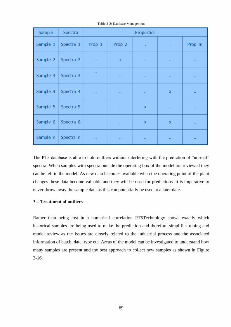
69
Table 3-2: Database Management
The PT5 database is able to hold outliers without interfering with the prediction of “normal”
spectra. When samples with spectra outside the operating box of the model are reviewed they
can be left in the model. As new data becomes available when the operating point of the plant
changes these data become valuable and they will be used for predictions. It is imperative to
never throw away the sample data as this can potentially be used at a later date.
Treatment of outliers
Rather than being lost in a numerical correlation PT5Technology shows exactly which
historical samples are being used to make the prediction and therefore simplifies tuning and
model review as the issues are closely related to the industrial process and the associated
information of batch, date, type etc. Areas of the model can be investigated to understand how
many samples are present and the best approach to collect new samples as shown in Figure
3-16.
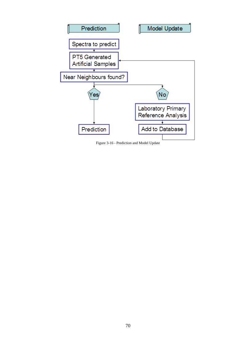
70
Figure 3-16 - Prediction and Model Update
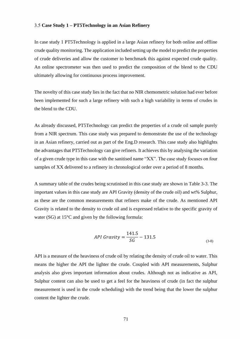
71
Case Study 1 – PT5Technology in an Asian Refinery
In case study 1 PT5Technology is applied in a large Asian refinery for both online and offline
crude quality monitoring. The application included setting up the model to predict the properties
of crude deliveries and allow the customer to benchmark this against expected crude quality.
An online spectrometer was then used to predict the composition of the blend to the CDU
ultimately allowing for continuous process improvement.
The novelty of this case study lies in the fact that no NIR chemometric solution had ever before
been implemented for such a large refinery with such a high variability in terms of crudes in
the blend to the CDU.
As already discussed, PT5Technology can predict the properties of a crude oil sample purely
from a NIR spectrum. This case study was prepared to demonstrate the use of the technology
in an Asian refinery, carried out as part of the Eng.D research. This case study also highlights
the advantages that PT5Technology can give refiners. It achieves this by analysing the variation
of a given crude type in this case with the sanitised name “XX”. The case study focuses on four
samples of XX delivered to a refinery in chronological order over a period of 8 months.
A summary table of the crudes being scrutinised in this case study are shown in Table 3-3. The
important values in this case study are API Gravity (density of the crude oil) and wt% Sulphur,
as these are the common measurements that refiners make of the crude. As mentioned API
Gravity is related to the density to crude oil and is expressed relative to the specific gravity of
water (SG) at 15°C and given by the following formula:
𝐴𝑃𝐼 𝐺𝑟𝑎𝑣𝑖𝑡𝑦 =
141.5
𝑆𝐺− 131.5
(3-8)
API is a measure of the heaviness of crude oil by relating the density of crude oil to water. This
means the higher the API the lighter the crude. Coupled with API measurements, Sulphur
analysis also gives important information about crudes. Although not as indicative as API,
Sulphur content can also be used to get a feel for the heaviness of crude (in fact the sulphur
measurement is used in the crude scheduling) with the trend being that the lower the sulphur
content the lighter the crude.
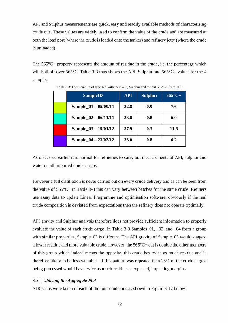
72
API and Sulphur measurements are quick, easy and readily available methods of characterising
crude oils. These values are widely used to confirm the value of the crude and are measured at
both the load port (where the crude is loaded onto the tanker) and refinery jetty (where the crude
is unloaded).
The 565°C+ property represents the amount of residue in the crude, i.e. the percentage which
will boil off over 565°C. Table 3-3 thus shows the API, Sulphur and 565°C+ values for the 4
samples.
Table 3-3: Four samples of type XX with their API, Sulphur and the cut 565°C+ from TBP
SampleID API Sulphur 565°C+
Sample_01 – 05/09/11 32.8 0.9 7.6
Sample_02 – 06/11/11 33.8 0.8 6.0
Sample_03 – 19/01/12 37.9 0.3 11.6
Sample_04 – 23/02/12 33.0 0.8 6.2
As discussed earlier it is normal for refineries to carry out measurements of API, sulphur and
water on all imported crude cargos.
However a full distillation is never carried out on every crude delivery and as can be seen from
the value of 565°C+ in Table 3-3 this can vary between batches for the same crude. Refiners
use assay data to update Linear Programme and optimisation software, obviously if the real
crude composition is deviated from expectations then the refinery does not operate optimally.
API gravity and Sulphur analysis therefore does not provide sufficient information to properly
evaluate the value of each crude cargo. In Table 3-3 Samples_01, _02, and _04 form a group
with similar properties, Sample_03 is different. The API gravity of Sample_03 would suggest
a lower residue and more valuable crude, however, the 565°C+ cut is double the other members
of this group which indeed means the opposite, this crude has twice as much residue and is
therefore likely to be less valuable. If this pattern was repeated then 25% of the crude cargos
being processed would have twice as much residue as expected, impacting margins.
Utilising the Aggregate Plot
NIR scans were taken of each of the four crude oils as shown in Figure 3-17 below.
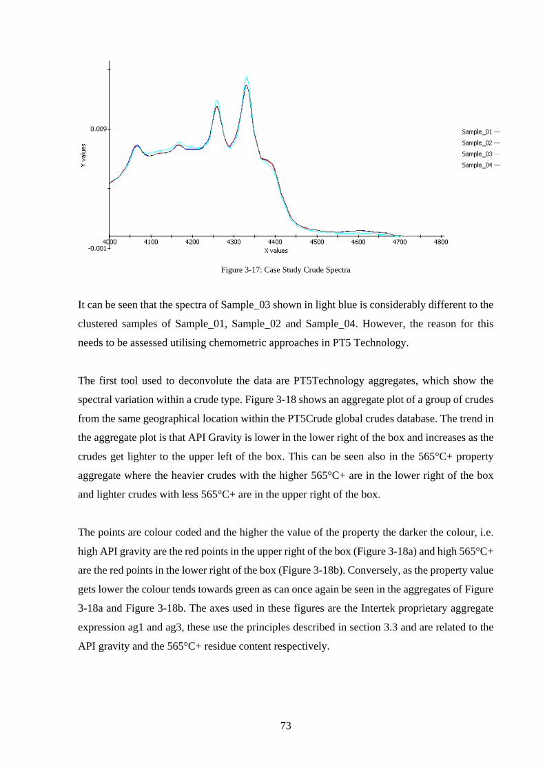
73
Figure 3-17: Case Study Crude Spectra
It can be seen that the spectra of Sample_03 shown in light blue is considerably different to the
clustered samples of Sample_01, Sample_02 and Sample_04. However, the reason for this
needs to be assessed utilising chemometric approaches in PT5 Technology.
The first tool used to deconvolute the data are PT5Technology aggregates, which show the
spectral variation within a crude type. Figure 3-18 shows an aggregate plot of a group of crudes
from the same geographical location within the PT5Crude global crudes database. The trend in
the aggregate plot is that API Gravity is lower in the lower right of the box and increases as the
crudes get lighter to the upper left of the box. This can be seen also in the 565°C+ property
aggregate where the heavier crudes with the higher 565°C+ are in the lower right of the box
and lighter crudes with less 565°C+ are in the upper right of the box.
The points are colour coded and the higher the value of the property the darker the colour, i.e.
high API gravity are the red points in the upper right of the box (Figure 3-18a) and high 565°C+
are the red points in the lower right of the box (Figure 3-18b). Conversely, as the property value
gets lower the colour tends towards green as can once again be seen in the aggregates of Figure
3-18a and Figure 3-18b. The axes used in these figures are the Intertek proprietary aggregate
expression ag1 and ag3, these use the principles described in section 3.3 and are related to the
API gravity and the 565°C+ residue content respectively.
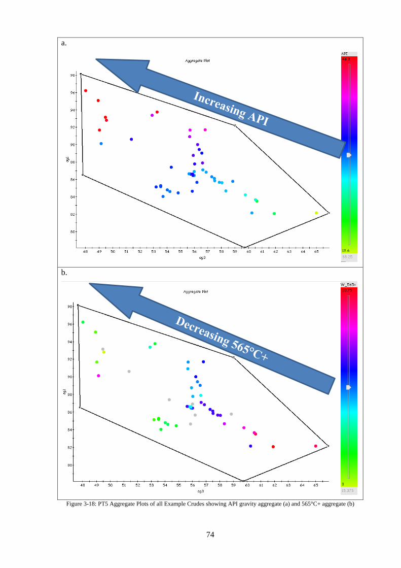
74
a.
b.
Figure 3-18: PT5 Aggregate Plots of all Example Crudes showing API gravity aggregate (a) and 565°C+ aggregate (b)
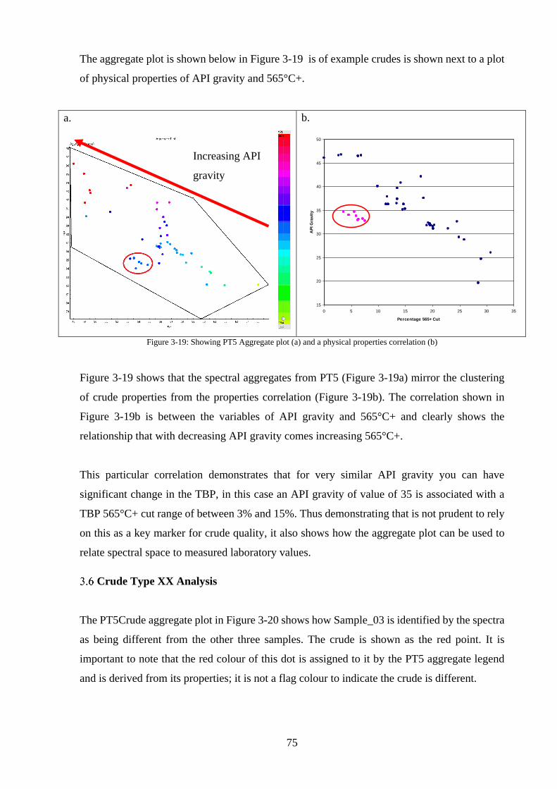
75
The aggregate plot is shown below in Figure 3-19 is of example crudes is shown next to a plot
of physical properties of API gravity and 565°C+.
a.
b.
Figure 3-19: Showing PT5 Aggregate plot (a) and a physical properties correlation (b)
Figure 3-19 shows that the spectral aggregates from PT5 (Figure 3-19a) mirror the clustering
of crude properties from the properties correlation (Figure 3-19b). The correlation shown in
Figure 3-19b is between the variables of API gravity and 565°C+ and clearly shows the
relationship that with decreasing API gravity comes increasing 565°C+.
This particular correlation demonstrates that for very similar API gravity you can have
significant change in the TBP, in this case an API gravity of value of 35 is associated with a
TBP 565°C+ cut range of between 3% and 15%. Thus demonstrating that is not prudent to rely
on this as a key marker for crude quality, it also shows how the aggregate plot can be used to
relate spectral space to measured laboratory values.
Crude Type XX Analysis
The PT5Crude aggregate plot in Figure 3-20 shows how Sample_03 is identified by the spectra
as being different from the other three samples. The crude is shown as the red point. It is
important to note that the red colour of this dot is assigned to it by the PT5 aggregate legend
and is derived from its properties; it is not a flag colour to indicate the crude is different.
15
20
25
30
35
40
45
50
0 5 10 15 20 25 30 35
Percentage 565+ Cut
AP
I G
ravit
y
Increasing API
gravity
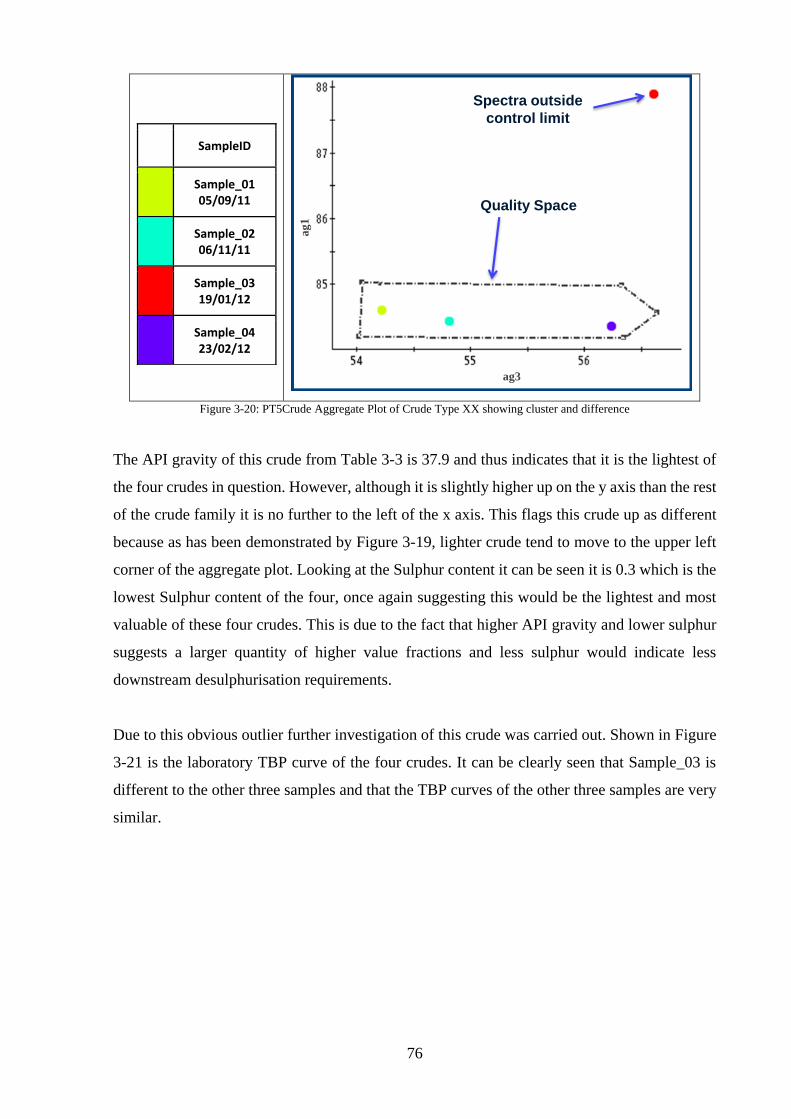
76
SampleID
Sample_01 05/09/11
Sample_02 06/11/11
Sample_03 19/01/12
Sample_04 23/02/12
Figure 3-20: PT5Crude Aggregate Plot of Crude Type XX showing cluster and difference
The API gravity of this crude from Table 3-3 is 37.9 and thus indicates that it is the lightest of
the four crudes in question. However, although it is slightly higher up on the y axis than the rest
of the crude family it is no further to the left of the x axis. This flags this crude up as different
because as has been demonstrated by Figure 3-19, lighter crude tend to move to the upper left
corner of the aggregate plot. Looking at the Sulphur content it can be seen it is 0.3 which is the
lowest Sulphur content of the four, once again suggesting this would be the lightest and most
valuable of these four crudes. This is due to the fact that higher API gravity and lower sulphur
suggests a larger quantity of higher value fractions and less sulphur would indicate less
downstream desulphurisation requirements.
Due to this obvious outlier further investigation of this crude was carried out. Shown in Figure
3-21 is the laboratory TBP curve of the four crudes. It can be clearly seen that Sample_03 is
different to the other three samples and that the TBP curves of the other three samples are very
similar.
Spectra outside
control limit
Quality Space
Quality Aggregate 2
Qu
ality
Ag
gre
gate
1
ag3
ag1
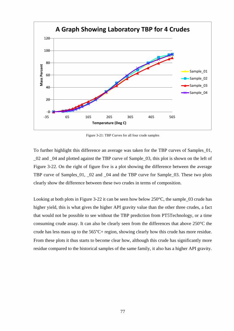
77
Figure 3-21: TBP Curves for all four crude samples
To further highlight this difference an average was taken for the TBP curves of Samples_01,
_02 and _04 and plotted against the TBP curve of Sample_03, this plot is shown on the left of
Figure 3-22. On the right of figure five is a plot showing the difference between the average
TBP curve of Samples_01, _02 and _04 and the TBP curve for Sample_03. These two plots
clearly show the difference between these two crudes in terms of composition.
Looking at both plots in Figure 3-22 it can be seen how below 250°C, the sample_03 crude has
higher yield, this is what gives the higher API gravity value than the other three crudes, a fact
that would not be possible to see without the TBP prediction from PT5Technology, or a time
consuming crude assay. It can also be clearly seen from the differences that above 250°C the
crude has less mass up to the 565°C+ region, showing clearly how this crude has more residue.
From these plots it thus starts to become clear how, although this crude has significantly more
residue compared to the historical samples of the same family, it also has a higher API gravity.
0
20
40
60
80
100
120
-35 65 165 265 365 465 565
Mas
s P
erc
en
t
Temperature (Deg C)
A Graph Showing Laboratory TBP for 4 Crudes
Sample_01
Sample_02
Sample_03
Sample_04
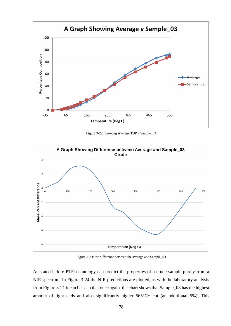
78
Figure 3-22: Showing Average TBP v Sample_03
Figure 3-23: the difference between the average and Sample_03
As stated before PT5Technology can predict the properties of a crude sample purely from a
NIR spectrum. In Figure 3-24 the NIR predictions are plotted, as with the laboratory analysis
from Figure 3-21 it can be seen that once again the chart shows that Sample_03 has the highest
amount of light ends and also significantly higher 565°C+ cut (an additional 5%). This
0
20
40
60
80
100
120
-35 65 165 265 365 465 565
Pe
rce
nta
ge C
om
po
siti
on
Temperature (Deg C)
A Graph Showing Average v Sample_03
Average
Sample_03
-8
-6
-4
-2
0
2
4
0 100 200 300 400 500 600 700
Ma
ss
Pe
rce
nt
Dif
fere
nc
e
Temperature (Deg C)
A Graph Showing Difference between Average and Sample_03 Crude

79
demonstrates that both methodologies are picking up the compositional difference in this
sample from the rest of its family, however, it should be noted that the laboratory analysis takes
a number of days to produce whereas the prediction can be generated within a few minutes.
Figure 3-24: TBP curves from PT5 prediction
The distillation curves show clearly that Sample_03 is heavier than the other 3 samples, having
more 565°C+ residues. Looking at the predicted values it can be seen they follow the same
trend as the actual values. It is also important to note that the outlying crude has been predicted
to be different to the other crudes in the same family, this is important because it shows the
capability of PT5Technology.
Table 3-4 below shows the Standard error of prediction (SEP) for each of the properties
modelled for a database of 60 samples from the same geographical area as the case study crudes.
The SEP value is calculated by adding the absolute of the average to two times the standard
deviation of the differences between the predicted and laboratory methods. An SEP <100%
indicates the model performance is good enough to be released for use.
Table 3-4: Property Prediction Statistics
Property SEP
API 74%
Sulphur 29%
565C+ 91%
0
20
40
60
80
100
120
-35 65 165 265 365 465 565
Pe
rce
nta
ge C
om
po
siti
on
Temperature (Deg C)
A Graph Showing NIR TBP Predictions for 4 Crudes
Sample_01PredictionSample_02PredictionSample_03PredictionSample_04Prediction
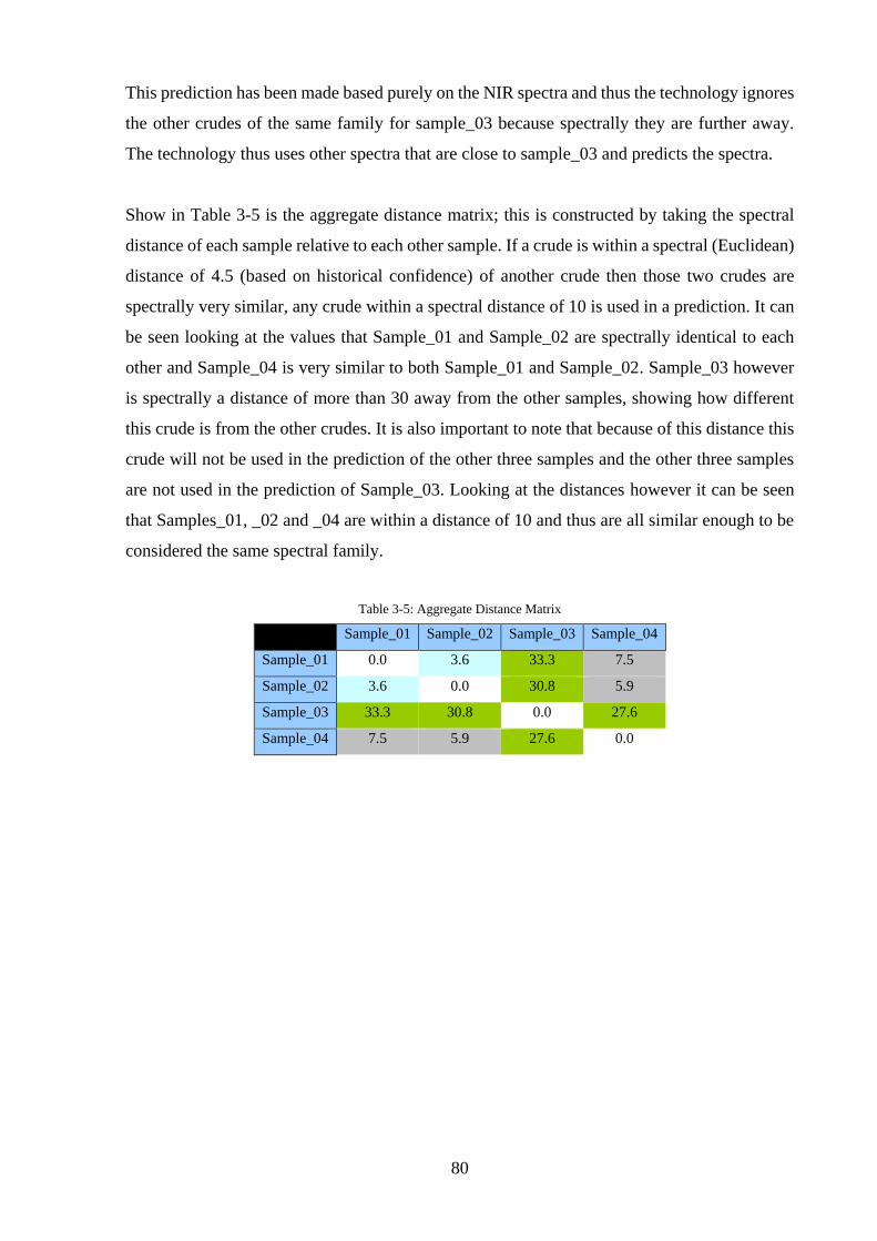
80
This prediction has been made based purely on the NIR spectra and thus the technology ignores
the other crudes of the same family for sample_03 because spectrally they are further away.
The technology thus uses other spectra that are close to sample_03 and predicts the spectra.
Show in Table 3-5 is the aggregate distance matrix; this is constructed by taking the spectral
distance of each sample relative to each other sample. If a crude is within a spectral (Euclidean)
distance of 4.5 (based on historical confidence) of another crude then those two crudes are
spectrally very similar, any crude within a spectral distance of 10 is used in a prediction. It can
be seen looking at the values that Sample_01 and Sample_02 are spectrally identical to each
other and Sample_04 is very similar to both Sample_01 and Sample_02. Sample_03 however
is spectrally a distance of more than 30 away from the other samples, showing how different
this crude is from the other crudes. It is also important to note that because of this distance this
crude will not be used in the prediction of the other three samples and the other three samples
are not used in the prediction of Sample_03. Looking at the distances however it can be seen
that Samples_01, _02 and _04 are within a distance of 10 and thus are all similar enough to be
considered the same spectral family.
Table 3-5: Aggregate Distance Matrix
Sample 10 Sample_01 Sample_02 Sample_03 Sample_04
Sample_01 0.0 3.6 33.3 7.5
Sample_02 3.6 0.0 30.8 5.9
Sample_03 33.3 30.8 0.0 27.6
Sample_04 7.5 5.9 27.6 0.0
81
Table 3-6 shows the difference between the laboratory analysis and the prediction by PT5Crude
Technology. The values were achieved by taking the difference between the laboratory value
and predicted value. If the difference between the values lies within the ASTM reproducibility
for a particular cut then there is a high confidence in the prediction and laboratory method.
In the table (overleaf) the differences are normalised against the ASTM reproducibility for the
laboratory method and expressed as a percentage of the method reproducibility (R). Thus,
≤100% is within R and >100% is outside R. Method reproducibility is an important metric to
understand the applicability of the prediction. This is because the model results are treated in
industry as if they were laboratory generated values and, the reproducibility is the maximum
limit, as stipulated by ASTM that any two laboratories are allowed to differ by.
It is generated by conducting round robin testing between laboratories all over the globe with
the same capability and in this case, is expressed in mass percent.
It can be seen that not all fractions predict within ASTM reproducibility, and two example
values have been highlighted. These values are in the region of the distillation curve known as
the ‘crossover region’ and this is where the residue from the atmospheric ASTM D2892
distillation is taken and moved over to the high vacuum ASTM D5236 distillation. As a
consequence, modelling in this region can be difficult as the laboratory primary reference data
can have a high inherent reproducibility.
However, despite some deviations, utilising the predictions instead of historical assay data to
update the LP results in a much closer match to the measured crude oil composition and thus
more optimal refinery operation.
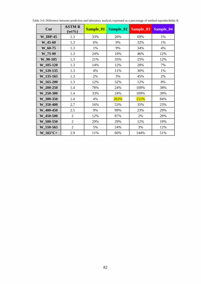
82
Table 3-6: Difference between prediction and laboratory analysis expressed as a percentage of method reproducibility R
Cut ASTM R
(wt%) Sample_01 Sample_02 Sample_03 Sample_04
W_IBP-45 1.3 33% 26% 69% 1%
W_45-60 1.3 6% 9% 32% 1%
W_60-75 1.3 1% 9% 34% 4%
W_75-90 1.3 24% 10% 46% 12%
W_90-105 1.3 21% 35% 25% 12%
W_105-120 1.3 14% 12% 28% 7%
W_120-135 1.3 4% 11% 30% 1%
W_135-165 1.3 2% 3% 45% 2%
W_165-200 1.3 12% 32% 12% 8%
W_200-250 1.4 78% 24% 100% 38%
W_250-300 1.4 33% 24% 109% 39%
W_300-350 1.4 4% 263% 151% 84%
W_350-400 2.7 16% 53% 35% 23%
W_400-450 2.5 9% 99% 23% 29%
W_450-500 2 12% 87% 2% 29%
W_500-550 2 29% 29% 12% 19%
W_550-565 2 5% 24% 3% 12%
W_565°C+ 2.9 11% 60% 144% 51%
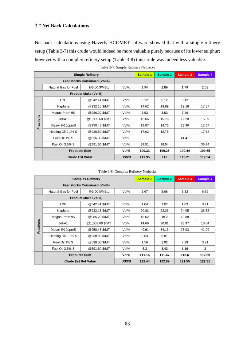
83
Net Back Calculations
Net back calculations using Haverly HCOMET software showed that with a simple refinery
setup (Table 3-7) this crude would indeed be more valuable purely because of its lower sulphur;
however with a complex refinery setup (Table 3-8) this crude was indeed less valuable.
Table 3-7: Simple Refinery Netbacks
Simple Refinery Sample 1 Sample 2 Sample 3 Sample 4
Feedstocks Consumed (Vol%)
Natural Gas for Fuel @3.00 $/MBtu Vol% 1.94 1.89 1.79 2.03
Product Make (Vol%)
Fra
cti
on
s
LPG @542.41 $/MT Vol% 0.12 0.12 0.12
Naphtha @932.15 $/MT Vol% 14.62 14.89 19.18 17.87
Mogas Prem 95 @986.20 $/MT Vol% 3.53 3.53 3.46
Jet-A1 @1,009.60 $/MT Vol% 13.66 15.76 12.28 15.59
Diesel @10ppmS @958.45 $/MT Vol% 12.87 14.75 23.99 12.67
Heating Oil 0.1% S @930.80 $/MT Vol% 17.02 12.76 17.68
Fuel Oil 1% S @636.08 $/MT Vol% 41.41
Fuel Oil 3.5% S @591.60 $/MT Vol% 38.51 38.54 36.84
Products Sum Vol% 100.33 100.35 100.44 100.65
Crude Est Value US$/B 111.95 112 112.21 112.94
Table 3-8: Complex Refinery Netbacks
Complex Refinery Sample 1 Sample 2 Sample 3 Sample 4
Feedstocks Consumed (Vol%)
Natural Gas for Fuel @3.00 $/MBtu Vol% 5.67 5.66 5.33 6.69
Product Make (Vol%)
Fra
cti
on
s
LPG @542.41 $/MT Vol% 1.04 1.07 1.03 3.21
Naphtha @932.15 $/MT Vol% 20.82 22.26 24.05 36.88
Mogas Prem 95 @986.20 $/MT Vol% 18.62 18.2 18.88
Jet-A1 @1,009.60 $/MT Vol% 14.69 20.81 23.97 16.64
Diesel @10ppmS @958.45 $/MT Vol% 40.61 34.13 27.03 41.99
Heating Oil 0.1% S @930.80 $/MT Vol% 0.63 0.81
Fuel Oil 1% S @636.08 $/MT Vol% 1.56 2.92 7.29 3.21
Fuel Oil 3.5% S @591.60 $/MT Vol% 5.3 3.43 1.16 3
Products Sum Vol% 111.16 111.47 110.6 112.69
Crude Est Ref Value US$/B 122.44 122.89 121.55 122.31
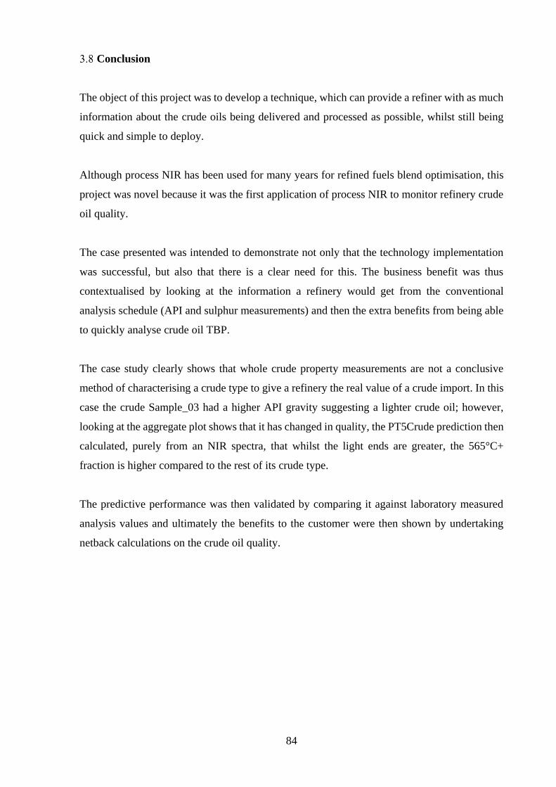
84
Conclusion
The object of this project was to develop a technique, which can provide a refiner with as much
information about the crude oils being delivered and processed as possible, whilst still being
quick and simple to deploy.
Although process NIR has been used for many years for refined fuels blend optimisation, this
project was novel because it was the first application of process NIR to monitor refinery crude
oil quality.
The case presented was intended to demonstrate not only that the technology implementation
was successful, but also that there is a clear need for this. The business benefit was thus
contextualised by looking at the information a refinery would get from the conventional
analysis schedule (API and sulphur measurements) and then the extra benefits from being able
to quickly analyse crude oil TBP.
The case study clearly shows that whole crude property measurements are not a conclusive
method of characterising a crude type to give a refinery the real value of a crude import. In this
case the crude Sample_03 had a higher API gravity suggesting a lighter crude oil; however,
looking at the aggregate plot shows that it has changed in quality, the PT5Crude prediction then
calculated, purely from an NIR spectra, that whilst the light ends are greater, the 565°C+
fraction is higher compared to the rest of its crude type.
The predictive performance was then validated by comparing it against laboratory measured
analysis values and ultimately the benefits to the customer were then shown by undertaking
netback calculations on the crude oil quality.

85
Chapter 4:
Blended Hydrocarbon
Stability
86
Chapter 4. Blended Hydrocarbon Stability
Crude oil blending to maximise margins is carried out by the majority of refineries across the
globe (single source crude oil refineries are very rare) and has been for many years. The
increasing numbers of different crude oils available in today’s marketplace gives refineries
more chances to source low cost, unconventional crude oils to blend and process, thus giving
the opportunity to maximise margins hence the terminology ‘opportunity crudes.’
Unconventional crude oils can fall into many categories such as highly paraffinic (waxy), highly
acidic (giving rise to corrosion issues) and highly asphaltenic (causing instability issues). As
such the chemistry and composition of some of these oils can be very different to those
processed historically and as a consequence unexpected issues can arise from blending these
opportunity oils.
One issue is the deposition of wax and asphaltene. This can cause problems as serious as
causing refinery shutdowns from blocked pipes and process units. The science of asphaltene
deposition in isolation is reasonably well understood and can be explained using models such
as SARA (discussed in section 2.14), however, how this relates to blending multiple crude oils
is not as well understood and much research is being carried out around the world to try and
address this issue.
As part of the Eng.D research an innovative approach has been developed to address the issue
of deposition of undesirable material that can arise from blending crude oils such as wax and
asphaltene. This was undertaken as a consequence of identified weaknesses in existing test
methodologies (such as ASTM D7060, ASTM D7112 and ASTM D7157). These weaknesses
are significant in that although refineries are blending multiple crude oils, these methodologies
assess the crude oils in isolation and instead use pure solvents such as heptane and toluene to
assess stability.
Furthermore, the stability is assessed as the titrants are added and does not give consideration
to the effects of time on blend stability. As crude is a colloidal system and asphaltene deposition
is as a consequence of the colloidal balance being disturbed, time is a major factor when
considering crude blend stability. In addition, due to the nature of the assessments they are only
considering asphaltenic deposition and not other components such as wax.

87
Finally the assessment is only on the crude oil sampled at that time and gives no consideration
to the quality deviations that can happen in the same crude oil family.
The methodology developed and patented as part of the Eng.D project addresses all the above
issues, it assesses stability of the oils being blended in the refinery without addition of
components not in the blend (i.e. heptane and toluene). Because of the way the assessments are
carried out any time period of interest to the customer can be assessed, indeed in Case Study 2:
Assessment of Heavy Fuel Oil Blending in a Refinery the customer was very interested in the
effects of time as once the blend was made up it was then stored.
The analysis is carried out using a combination of near infrared (NIR) spectra, microscopy
chemometric models and mathematical modelling algorithms meaning it is not specific to the
deposition of asphaltene but also wax precipitation, making the methodology very flexible.
Using NIR also means that the crude quality monitoring approach can be applied to monitor
deviations in quality of crude oil, as significant quality changes can mean the interactions in the
blend, and therefore the stability behaviour, can change.
Finally, the methodology can be applied to any hydrocarbon stream as demonstrated in the two
applications discussed below where one focuses on a heavy fuel oil blending project and the
other one on blends of marine fuels.
88
Introduction
To address challenges of instability of crude oil blends in a refinery, the Eng.D project carried
out innovative research in this area, resulting in a patented approach which has been used in
many different applications and continues to be rolled out across the globe.
The assessment of wax and asphaltene precipitation, known as Organic Deposition (OD), is
based on blending hydrocarbon streams from the process. Therefore, the assessment is
representative of actual operating parameters and the experimental measurements reveal the
interaction between crudes during and after blending.
To allow refiners flexibility in the application of this technique, and also to ensure a robust and
representative model, a variety of different ratios in the crude blend are assessed to generate
instability and stability limits, this is called a blend recipe evaluation report. The blend recipe
evaluation report is kept up to date using NIR spectra from neat crude quality tracking (using
PT5Technology).
The samples are assessed for organic deposition by a both NIR spectroscopy and microscopy
to ensure that stability is both observed and validated. To assess the response over time multiple
samples are stored, NIR scanned and validated by microscopy and mathematical calculations.
The output from the Intertek OD Programme is a series of reports which are described in detail
later, however, the main purpose is to provide assessment of combinations of stable and
unstable crude oils which can allow the refinery to optimise the process with respect to stability
as well as normal operating constraints.
Methodology
To develop the methodology it was first decided that the spectral behaviour of crude oils when
blended should be assessed, particularly how linear blending can be expressed, what happens
to the spectra at the point of deposition and after, and also, if this is quantifiable, repeatable and
can be validated.
This is why microscopy was undertaken on all blends made up as it is a very visual
representation of asphaltene deposition. The drawback of microscopy is that it is a more

89
laborious process than Near Infrared and also, crucially cannot be take online in a process
environment.
The analytical technique selected as the primary reference method was NIR spectroscopy. This
was for several reasons. Firstly, the equipment was readily available and widely used within
Intertek already, and as the business groups core business is supporting online and offline
laboratory NIR solutions to the refining marketplace, additional benefits that could be derived
from existing hardware was a very lucrative business proposition, especially given that crude
oil stability services is a rapidly growing marketplace.
To visualise deposition, the principals of light scattering by small particles was anticipated to
be an observable phenomenon within the NIR spectra. TO be effective this effect has to be
greater than the effect on the spectra as a consequence of the dilution of crude oil A in crude oil
B.
As discussed previously a spectrometer measures the difference between detected light, with
and without the sample. This difference is caused by the following three phenomena (ASTM,
2013):
• Obstacles – When radiation strikes a bluff body, it is scattered back to the source and
within solid bodies without retransmission. This baseline shift is not a function of
wavenumber. The amount of baseline shift is proportional to the area of the sample
obscured by opaque particles.
• Reflection and Refraction - Some radiation is scattered due to the particle size where
the light fails to reach the detector as its direction has been changed. The amount of light
refracted is a function of wavenumber, particle size, and particle density.
• Absorption – Accelerated electric charges may transform some of the energy into
another type of energy, i.e. radiation is absorbed and retransmitted where the
retransmitted energy spectrum does not contain energy where the chemical bonds have
absorbed the energy.
By monitoring absorption, the chemical composition of the neat crudes and blends can be
characterised using PT5Technology, thus giving OD constraints.
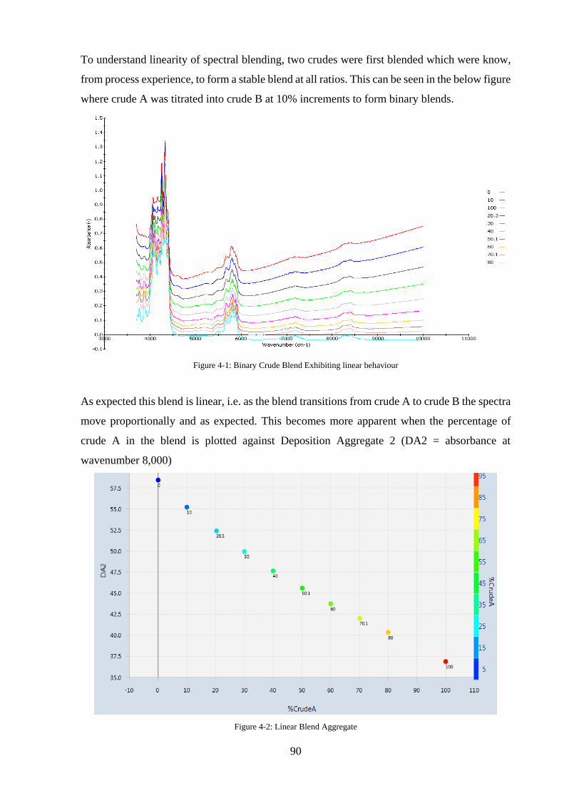
90
To understand linearity of spectral blending, two crudes were first blended which were know,
from process experience, to form a stable blend at all ratios. This can be seen in the below figure
where crude A was titrated into crude B at 10% increments to form binary blends.
Figure 4-1: Binary Crude Blend Exhibiting linear behaviour
As expected this blend is linear, i.e. as the blend transitions from crude A to crude B the spectra
move proportionally and as expected. This becomes more apparent when the percentage of
crude A in the blend is plotted against Deposition Aggregate 2 (DA2 = absorbance at
wavenumber 8,000)
Figure 4-2: Linear Blend Aggregate
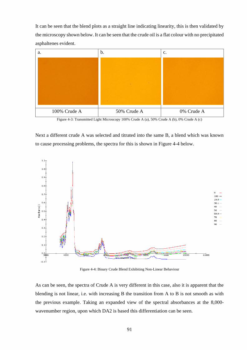
91
It can be seen that the blend plots as a straight line indicating linearity, this is then validated by
the microscopy shown below. It can be seen that the crude oil is a flat colour with no precipitated
asphaltenes evident.
a.
b.
c.
100% Crude A 50% Crude A 0% Crude A
Figure 4-3: Transmitted Light Microscopy 100% Crude A (a), 50% Crude A (b), 0% Crude A (c)
Next a different crude A was selected and titrated into the same B, a blend which was known
to cause processing problems, the spectra for this is shown in Figure 4-4 below.
Figure 4-4: Binary Crude Blend Exhibiting Non-Linear Behaviour
As can be seen, the spectra of Crude A is very different in this case, also it is apparent that the
blending is not linear, i.e. with increasing B the transition from A to B is not smooth as with
the previous example. Taking an expanded view of the spectral absorbances at the 8,000-
wavenumber region, upon which DA2 is based this differentiation can be seen.
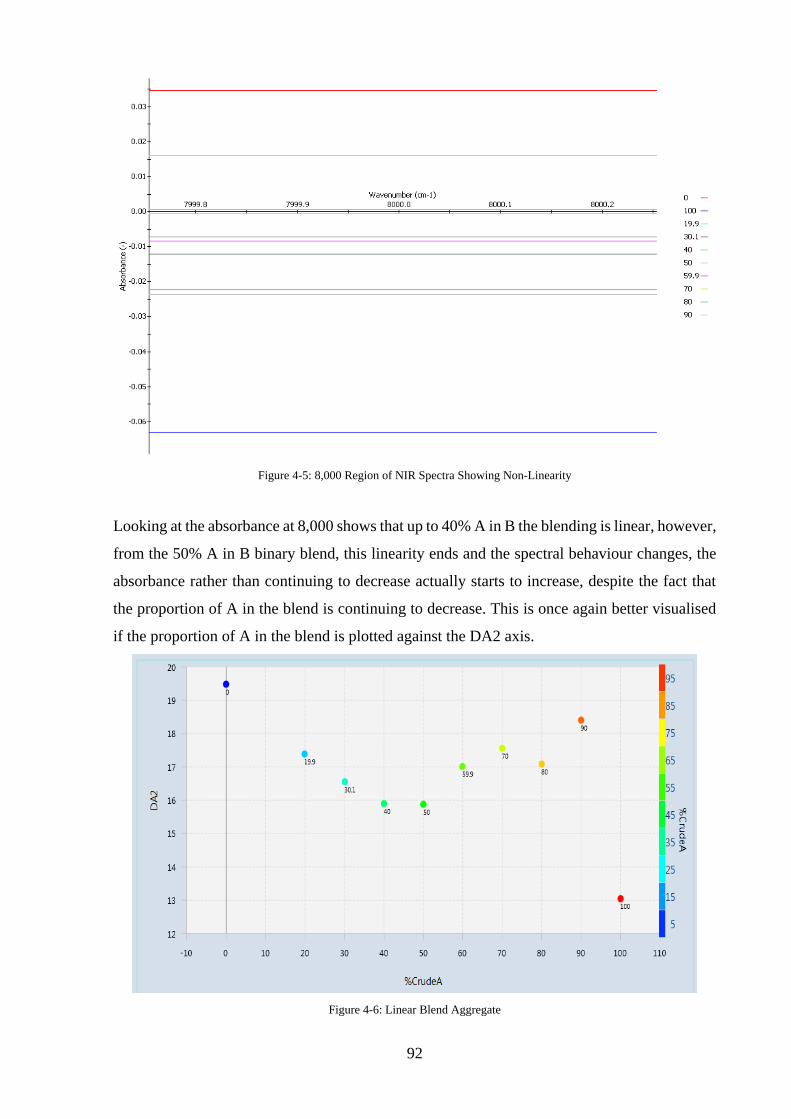
92
Figure 4-5: 8,000 Region of NIR Spectra Showing Non-Linearity
Looking at the absorbance at 8,000 shows that up to 40% A in B the blending is linear, however,
from the 50% A in B binary blend, this linearity ends and the spectral behaviour changes, the
absorbance rather than continuing to decrease actually starts to increase, despite the fact that
the proportion of A in the blend is continuing to decrease. This is once again better visualised
if the proportion of A in the blend is plotted against the DA2 axis.
Figure 4-6: Linear Blend Aggregate
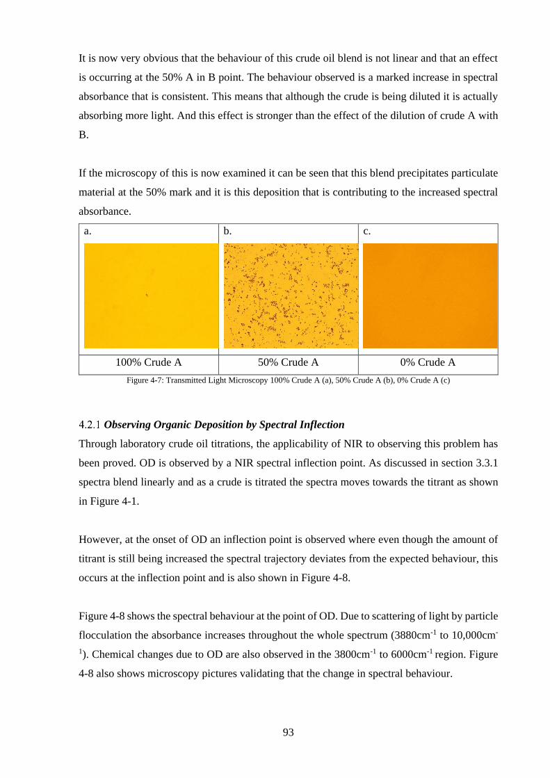
93
It is now very obvious that the behaviour of this crude oil blend is not linear and that an effect
is occurring at the 50% A in B point. The behaviour observed is a marked increase in spectral
absorbance that is consistent. This means that although the crude is being diluted it is actually
absorbing more light. And this effect is stronger than the effect of the dilution of crude A with
B.
If the microscopy of this is now examined it can be seen that this blend precipitates particulate
material at the 50% mark and it is this deposition that is contributing to the increased spectral
absorbance.
a.
b.
c.
100% Crude A 50% Crude A 0% Crude A
Figure 4-7: Transmitted Light Microscopy 100% Crude A (a), 50% Crude A (b), 0% Crude A (c)
Observing Organic Deposition by Spectral Inflection
Through laboratory crude oil titrations, the applicability of NIR to observing this problem has
been proved. OD is observed by a NIR spectral inflection point. As discussed in section 3.3.1
spectra blend linearly and as a crude is titrated the spectra moves towards the titrant as shown
in Figure 4-1.
However, at the onset of OD an inflection point is observed where even though the amount of
titrant is still being increased the spectral trajectory deviates from the expected behaviour, this
occurs at the inflection point and is also shown in Figure 4-8.
Figure 4-8 shows the spectral behaviour at the point of OD. Due to scattering of light by particle
flocculation the absorbance increases throughout the whole spectrum (3880cm-1 to 10,000cm-
1). Chemical changes due to OD are also observed in the 3800cm-1 to 6000cm-1 region. Figure
4-8 also shows microscopy pictures validating that the change in spectral behaviour.
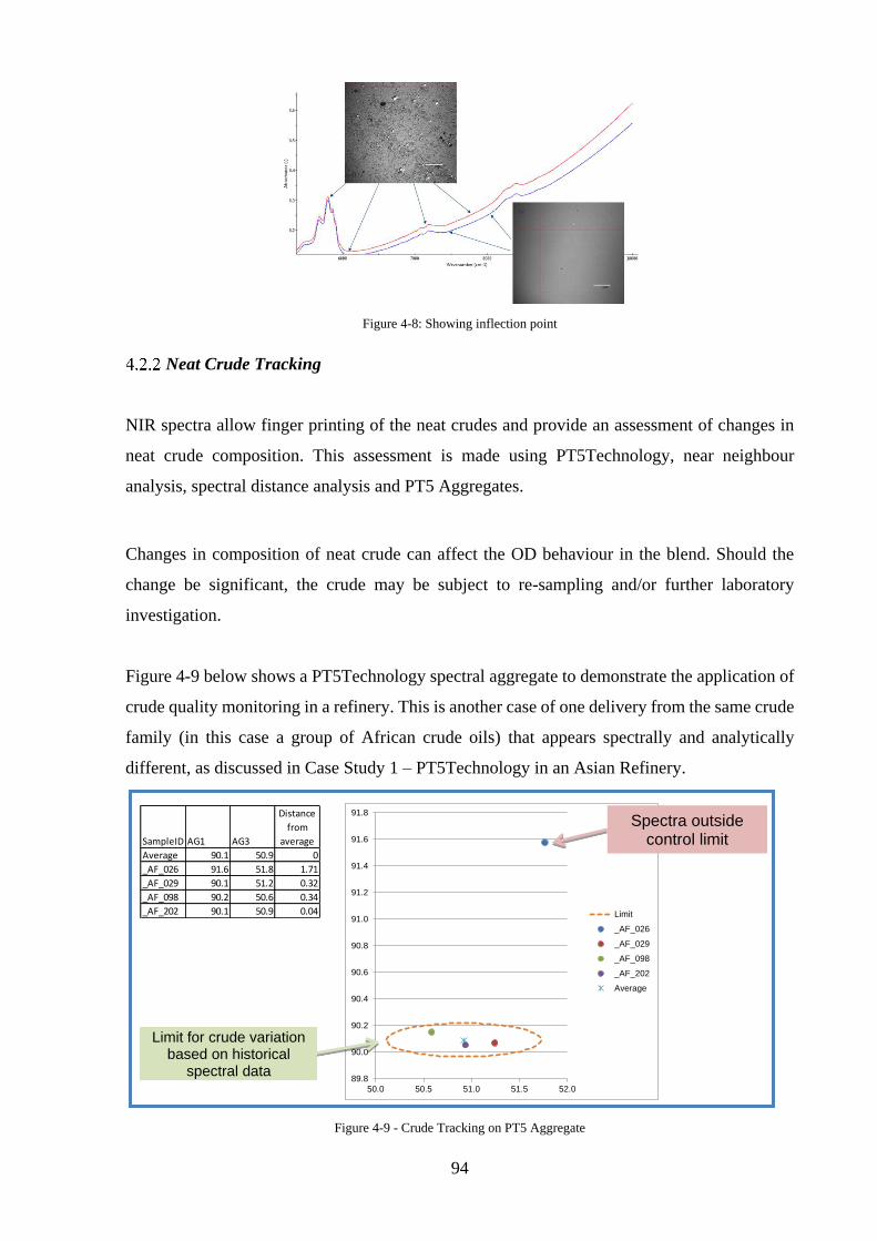
94
Figure 4-8: Showing inflection point
Neat Crude Tracking
NIR spectra allow finger printing of the neat crudes and provide an assessment of changes in
neat crude composition. This assessment is made using PT5Technology, near neighbour
analysis, spectral distance analysis and PT5 Aggregates.
Changes in composition of neat crude can affect the OD behaviour in the blend. Should the
change be significant, the crude may be subject to re-sampling and/or further laboratory
investigation.
Figure 4-9 below shows a PT5Technology spectral aggregate to demonstrate the application of
crude quality monitoring in a refinery. This is another case of one delivery from the same crude
family (in this case a group of African crude oils) that appears spectrally and analytically
different, as discussed in Case Study 1 – PT5Technology in an Asian Refinery.
Figure 4-9 - Crude Tracking on PT5 Aggregate
89.8
90.0
90.2
90.4
90.6
90.8
91.0
91.2
91.4
91.6
91.8
50.0 50.5 51.0 51.5 52.0
Limit
_AF_026
_AF_029
_AF_098
_AF_202
Average
Spectra outside control limit
Limit for crude variation based on historical
spectral data
SampleID AG1 AG3
Distance
from
average
Average 90.1 50.9 0
_AF_026 91.6 51.8 1.71
_AF_029 90.1 51.2 0.32
_AF_098 90.2 50.6 0.34
_AF_202 90.1 50.9 0.04
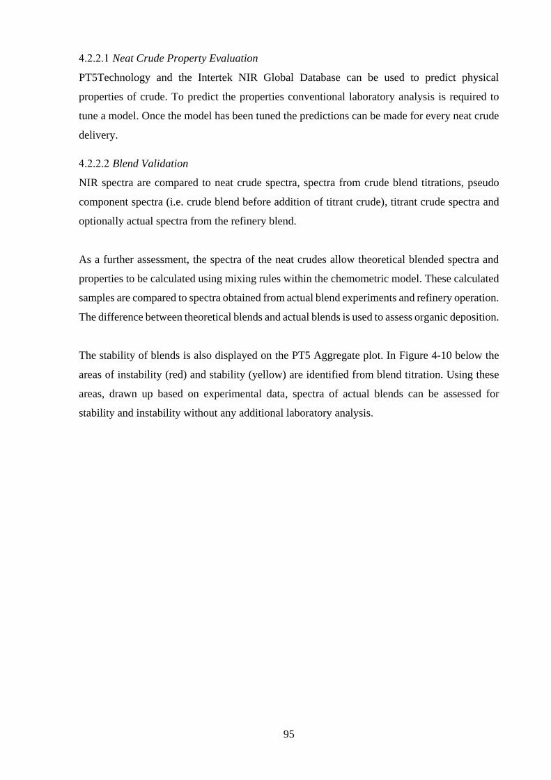
95
Neat Crude Property Evaluation
PT5Technology and the Intertek NIR Global Database can be used to predict physical
properties of crude. To predict the properties conventional laboratory analysis is required to
tune a model. Once the model has been tuned the predictions can be made for every neat crude
delivery.
Blend Validation
NIR spectra are compared to neat crude spectra, spectra from crude blend titrations, pseudo
component spectra (i.e. crude blend before addition of titrant crude), titrant crude spectra and
optionally actual spectra from the refinery blend.
As a further assessment, the spectra of the neat crudes allow theoretical blended spectra and
properties to be calculated using mixing rules within the chemometric model. These calculated
samples are compared to spectra obtained from actual blend experiments and refinery operation.
The difference between theoretical blends and actual blends is used to assess organic deposition.
The stability of blends is also displayed on the PT5 Aggregate plot. In Figure 4-10 below the
areas of instability (red) and stability (yellow) are identified from blend titration. Using these
areas, drawn up based on experimental data, spectra of actual blends can be assessed for
stability and instability without any additional laboratory analysis.
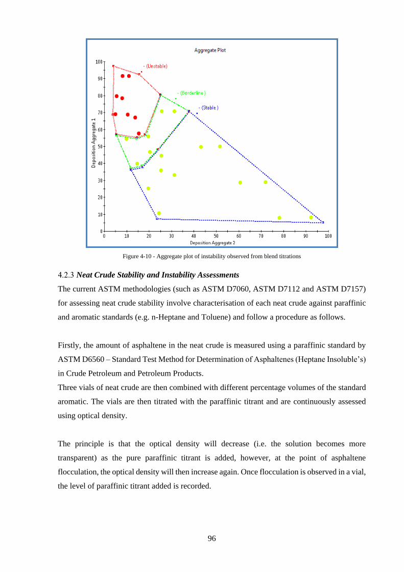
96
Figure 4-10 - Aggregate plot of instability observed from blend titrations
Neat Crude Stability and Instability Assessments
The current ASTM methodologies (such as ASTM D7060, ASTM D7112 and ASTM D7157)
for assessing neat crude stability involve characterisation of each neat crude against paraffinic
and aromatic standards (e.g. n-Heptane and Toluene) and follow a procedure as follows.
Firstly, the amount of asphaltene in the neat crude is measured using a paraffinic standard by
ASTM D6560 – Standard Test Method for Determination of Asphaltenes (Heptane Insoluble’s)
in Crude Petroleum and Petroleum Products.
Three vials of neat crude are then combined with different percentage volumes of the standard
aromatic. The vials are then titrated with the paraffinic titrant and are continuously assessed
using optical density.
The principle is that the optical density will decrease (i.e. the solution becomes more
transparent) as the pure paraffinic titrant is added, however, at the point of asphaltene
flocculation, the optical density will then increase again. Once flocculation is observed in a vial,
the level of paraffinic titrant added is recorded.
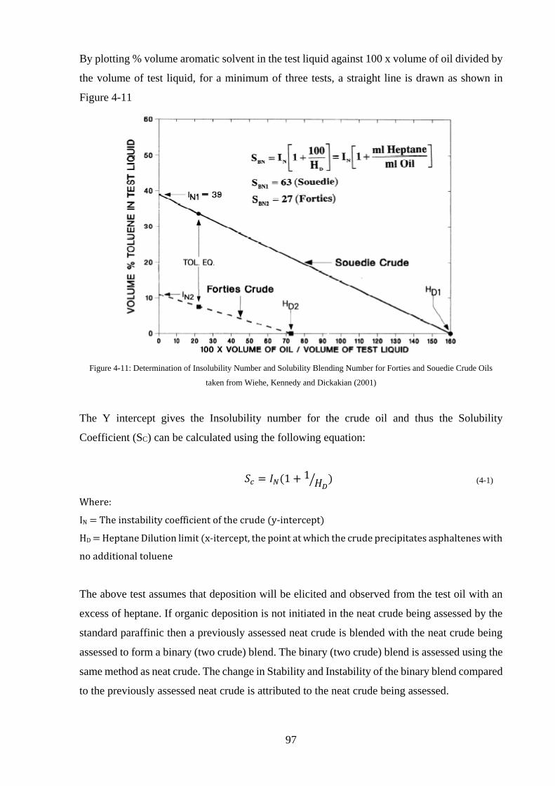
97
By plotting % volume aromatic solvent in the test liquid against 100 x volume of oil divided by
the volume of test liquid, for a minimum of three tests, a straight line is drawn as shown in
Figure 4-11
Figure 4-11: Determination of Insolubility Number and Solubility Blending Number for Forties and Souedie Crude Oils
taken from Wiehe, Kennedy and Dickakian (2001)
The Y intercept gives the Insolubility number for the crude oil and thus the Solubility
Coefficient (SC) can be calculated using the following equation:
𝑆𝑐 = 𝐼𝑁(1 + 1𝐻𝐷
⁄ ) (4-1)
Where:
IN = The instability coefficient of the crude (y-intercept)
HD = Heptane Dilution limit (x-itercept, the point at which the crude precipitates asphaltenes with
no additional toluene
The above test assumes that deposition will be elicited and observed from the test oil with an
excess of heptane. If organic deposition is not initiated in the neat crude being assessed by the
standard paraffinic then a previously assessed neat crude is blended with the neat crude being
assessed to form a binary (two crude) blend. The binary (two crude) blend is assessed using the
same method as neat crude. The change in Stability and Instability of the binary blend compared
to the previously assessed neat crude is attributed to the neat crude being assessed.

98
The SC and IN are produced for each crude in the blend and then proportionally blending
(according to the percentage of each crude in the blend) to determine the overall blend SC. Blend
stability is assessed by ensuring that the blend SC is no less than 1.4 times the IN of any neat
crude in the blend.
However, this methodology does not account for the interactions between crudes when blended,
the batch to batch variations in crude quality as well as any time dependent stability effects,
Generating Blend Stability / Instability Coefficients by Experimentation
To address the weaknesses of the neat crude assessment methodologies, the Eng.D project
focussed on developing a new methodology which could provide a true to life assessment of
the stability of crude oil blends in a refinery.
This first starts by assessing all the neat crudes in a recipe cluster (see section 4.4.1) and
establishing the practical minimum and maximum percentage volume (based on refinery design
constraints) These percentage volume ranges are used to design a series of blend experiments
which cover the range of refinery blending.
For each blend experiment a titrant is chosen, from the blend (usually the most paraffinic) that
will make the blend go from stable to unstable. The remaining neat crudes are then blended into
a pseudo component to be used with the titrant crude. In the example below (Table 4-1) a set
of five refinery crude oil have been blended in various ratios to form a designed experiment.
Table 4-1: Example Blend Experiment
The experimental methodology is then as follows. The pseudo component is blended for the
experiment (i.e. blend 110). Vials of the pseudo component are combined with different
percentage volumes of the titrant crude (in this case Crude_05). The vials are scanned and an
algorithm in the chemometric model monitors the NIR-spectra and identifies when flocculation
has occurred by looking for an inflection point (section 4.2.1) and validating whenever possible
using microscopy.
Blend Crude_01 Crude_02 Crude_03 Crude_04 Crude_05110 74.4% 4.7% 4.7% 16.3% 0.0%
111 52.1% 3.3% 3.3% 11.4% 30.0%
112 44.7% 2.8% 2.8% 9.8% 40.0%
113 37.2% 2.3% 2.3% 8.1% 50.0%
114 29.8% 1.9% 1.9% 6.5% 60.0%
115 22.3% 1.4% 1.4% 4.9% 70.0%
99
The initial screening series of vials uses large increments of titrant (e.g. 10%). To fine tune the
assessment of the point of instability, after screening with large increments, smaller increments
are used (e.g. 1%). The vials are scanned following mixing and after one or more retention
times (e.g. 0 hrs. +24 hrs). As time increases, the crude blends can become more instable
resulting in increased precipitation. Duplicate vials are available for microscopy and laboratory
analysis which can be selectively triggered based on the information obtained from the
assessment from the NIR spectra.
The onset of OD for each blend is then input into the Matrix Blending Algorithm to calculate
the coefficients for each crude in the blend.
Blending and regression fitting
Having obtained the experimental data from the blend titration it is useful to fit a regression to
enable stability of any crude ratio in a blend recipe to be calculated. The confidence in the
regression can also be calculated to ensure that sufficient, repeatable measurements have been
made in the blend titrations.
N-1 Factor Blend
Using N-1 factors gives one more set of results to estimate the error purely from
experimentation and also eliminates the collinearity within the equation, as the proportions of
each crude in the blend will add to 1 (Deming and Morgan, 1993).
When all the experimental blends have been completed the relative stability of the neat crudes
in the blend can be calculated. Over the range of the experimental blends a linear approximation
is practical.
At the point of flocculation, the coefficient of instability for the blend is equal to the coefficient
of stability for each component in the blend, multiplied by its percentage volume. Thus the
following assertion can be made:
𝐼𝐶 = 𝑆𝐶0𝑉0 + 𝑆𝐶1𝑉1 + 𝑆𝐶2𝑉2 + ⋯ + 𝑆𝐶𝑛𝑉𝑛 (4-2)
Where
𝐼𝐶 - Instability Coefficient
𝑆𝐶𝑛 - Stability Coefficient for component n
𝑉𝑛 - Percentage Volume of Component n

100
In addition, the sum of the volumes of the components must equal to 1:
1 = 𝑉0 + 𝑉1 + 𝑉2 + ⋯ + 𝑉𝑛 (4-3)
Therefore
𝑉𝑛 = 1 − 𝑉0 − 𝑉1 − ⋯ − 𝑉𝑛−1 (4-4)
Substituting into (4-2) gives:
𝑉0 =𝐼𝐶 − 𝑆𝐶𝑛
(𝑆𝐶0 − 𝑆𝐶𝑛)+
(𝑆𝐶𝑛 − 𝑆𝐶1)
(𝑆𝐶0 − 𝑆𝐶𝑛)𝑉1 + ⋯ +
(𝑆𝐶𝑛 − 𝑆𝐶𝑛−1)
(𝑆𝐶0 − 𝑆𝐶𝑛)𝑉𝑛−1 (4-5)
Which is also of the multiple linear regression form:
𝑌 = 𝛽0 + 𝛽1𝑋1 + 𝛽2𝑋2 + ⋯ + 𝛽𝑛−1𝑋𝑛−1
Where:
𝛽0 =𝐼𝐶 − 𝑆𝐶𝑛
(𝑆𝐶0 − 𝑆𝐶𝑛)
𝛽𝑛−1 =𝑆𝐶𝑛 − 𝑆𝐶𝑛−1
(𝑆𝐶0 − 𝑆𝐶𝑛)
Thus solving for the stability coefficient of the nth component (𝑆𝐶𝑛):
𝑆𝐶𝑛 =𝐼𝐶 − 𝛽0𝑆𝐶0
(1 − 𝛽0) (4-6)
And solving for the n-1 component (𝑆𝐶n−1):
𝑆𝐶𝑛−1 = 𝑆𝐶𝑛 − 𝛽𝑛−1(𝑆𝐶0 − 𝑆𝐶𝑛) (4-7)
As this type of assessment is a designed experiment conducted on a relatively small number of
samples covering a narrow operating region, a matrix solution to the least squares fit is
appropriate. This generates the coefficients for this range of neat crude blends for refinery
organic deposition.
𝑩^ = (𝑿′𝑿)−𝟏𝑿′𝒀 (4-8)
Where

101
𝑩^ - Regression coefficients 𝛽0 … 𝛽𝑛
𝒀 - Vector of percentage of Titrant Crude in each blend
𝑿 - Matrix of percentages of each crude in the pseudo component
blends
Once the coefficients have been calculated for each crude oil equation (4-2) instructs us that at
the point of instability the volumetrically blended coefficients of each crude in the blend will
give a number equal to the instability coefficient. If this overall SC is higher than IC it means
that the blend is stable and vice versa.
Comparison of Methodologies
The SC and IC from the developed methodology were then compared to the IN and SN from the
established ASTM methodology on the same crude blends. It was envisaged that two scenarios
are possible.
1. All of the SC and SN are similar and within experimental repeatability. This means there
is little interaction between the crudes when blended and the coefficients can be used
for any of the crudes in the recipe. In this case the ASTM methodology would be quicker
and simpler to implement as it requires less crude blending and analysis.
2. Some of the SC and SN are not similar and different by more than experimental
repeatability. This means that interactions between crudes are observed when blending
and the ASTM methodology would not work in this case.
In Table 4-2 below two different blends are shown (where L denotes a low percentage of a
crude in the blend and M a medium percentage of the crude in the blend) and were tested using
both methodologies. It was established that Crude001 had a destabilising effect on Crude003
and thus Blend A was more stable than Blend B. In this case more testing would be involved
to provide stability coefficients for specific combinations and ratios of crude.
Table 4-2: Stability testing for variation in crude ratios
Blends Cru
de0
01
Cru
de0
02
Cru
de0
03
Cru
de0
04
Cru
de0
05
Cru
de0
06
Cru
de0
07
Cru
de0
08
A L M M M M L L L
B M L M M M L L L
102
Assessing the blended crudes thus allows SC to more accurately match the refinery operating
conditions. Providing more accurate constraints will improve the optimisation of the financial
and operating outcomes of the blend under specific conditions.
Condensate Testing of Crude Blends
The recipes processed by refineries are planned to stay away from instability. In practice, the
plan will use previously generated coefficients to assess blend stability. However, when the
crude qualities change and / or a new crude is introduced then the stability of the new blend
needs to be assessed in the laboratory.
Ideally a titration is required for each crude in the blend, so the number of titrations equals the
number of crudes. However, this is a significant amount of testing and a simpler way is
desirable.
Thus, a single titration with a reference crude determines if the new recipe with the new crude
is more or less stable than expected. The single test provides enough information to inform
processing decisions. The reference crude is a yard stick to measure the relative stability of
recipes.
Whilst the reference crude is not in the refinery recipe, the crude recipe tested exactly matches
the chemistry of the refinery. Close to instability the amount of reference crude added is small
and therefore the assessment of instability is close to refinery conditions.
Table 4-3 shows an example titration dataset for a blend of 4 crudes which have been titrated
with reference crude to determine the point of instability. Each row shows the percentages of
each crude in the blend, plus the reference crude.
It can be seen that depending on the ratio of the four crudes in the blend, differing amounts of
reference crude are required to force the precipitation of asphaltenes from the blend. TO
understand the impact of crude 4 on the blend stability it can be seen that blends 06 – 09 do not
contain any crude 04.
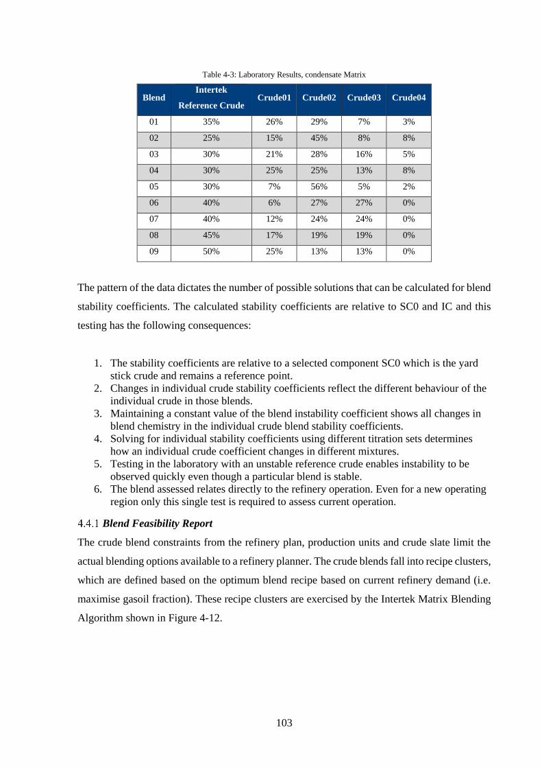
103
Table 4-3: Laboratory Results, condensate Matrix
Blend Intertek
Reference Crude Crude01 Crude02 Crude03 Crude04
01 35% 26% 29% 7% 3%
02 25% 15% 45% 8% 8%
03 30% 21% 28% 16% 5%
04 30% 25% 25% 13% 8%
05 30% 7% 56% 5% 2%
06 40% 6% 27% 27% 0%
07 40% 12% 24% 24% 0%
08 45% 17% 19% 19% 0%
09 50% 25% 13% 13% 0%
The pattern of the data dictates the number of possible solutions that can be calculated for blend
stability coefficients. The calculated stability coefficients are relative to SC0 and IC and this
testing has the following consequences:
1. The stability coefficients are relative to a selected component SC0 which is the yard
stick crude and remains a reference point.
2. Changes in individual crude stability coefficients reflect the different behaviour of the
individual crude in those blends.
3. Maintaining a constant value of the blend instability coefficient shows all changes in
blend chemistry in the individual crude blend stability coefficients.
4. Solving for individual stability coefficients using different titration sets determines
how an individual crude coefficient changes in different mixtures.
5. Testing in the laboratory with an unstable reference crude enables instability to be
observed quickly even though a particular blend is stable.
6. The blend assessed relates directly to the refinery operation. Even for a new operating
region only this single test is required to assess current operation.
Blend Feasibility Report
The crude blend constraints from the refinery plan, production units and crude slate limit the
actual blending options available to a refinery planner. The crude blends fall into recipe clusters,
which are defined based on the optimum blend recipe based on current refinery demand (i.e.
maximise gasoil fraction). These recipe clusters are exercised by the Intertek Matrix Blending
Algorithm shown in Figure 4-12.
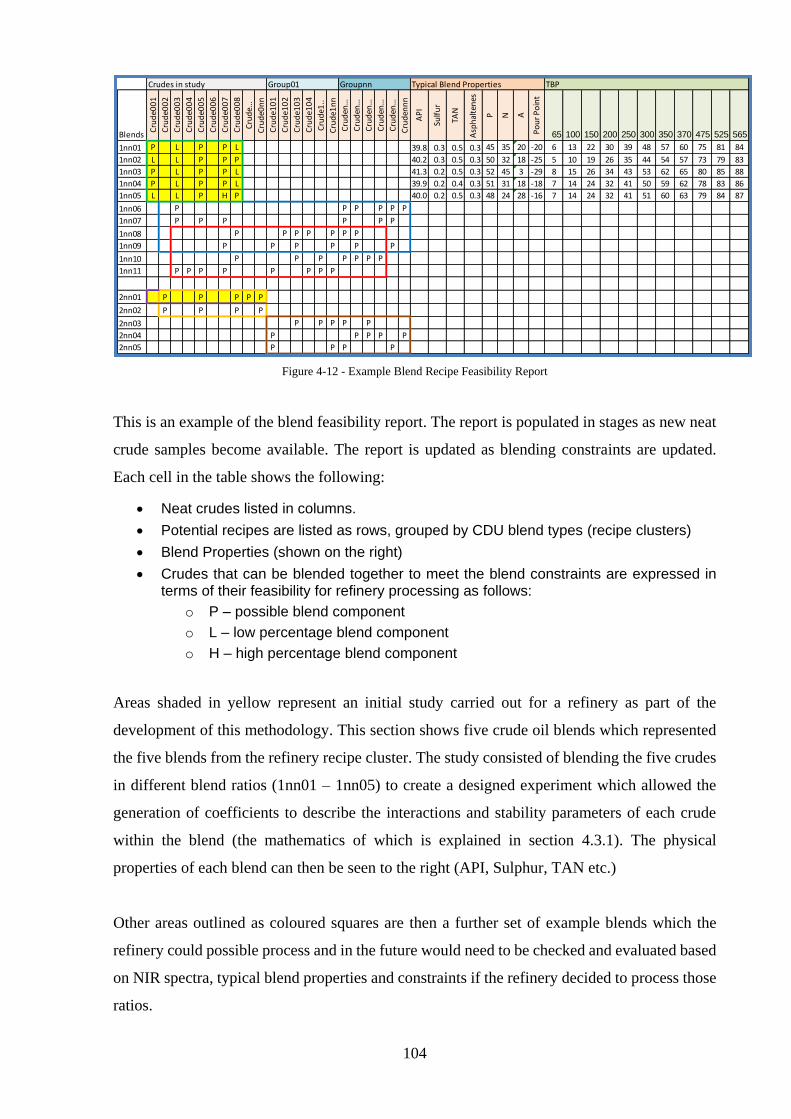
104
Figure 4-12 - Example Blend Recipe Feasibility Report
This is an example of the blend feasibility report. The report is populated in stages as new neat
crude samples become available. The report is updated as blending constraints are updated.
Each cell in the table shows the following:
• Neat crudes listed in columns.
• Potential recipes are listed as rows, grouped by CDU blend types (recipe clusters)
• Blend Properties (shown on the right)
• Crudes that can be blended together to meet the blend constraints are expressed in terms of their feasibility for refinery processing as follows:
o P – possible blend component
o L – low percentage blend component
o H – high percentage blend component
Areas shaded in yellow represent an initial study carried out for a refinery as part of the
development of this methodology. This section shows five crude oil blends which represented
the five blends from the refinery recipe cluster. The study consisted of blending the five crudes
in different blend ratios (1nn01 – 1nn05) to create a designed experiment which allowed the
generation of coefficients to describe the interactions and stability parameters of each crude
within the blend (the mathematics of which is explained in section 4.3.1). The physical
properties of each blend can then be seen to the right (API, Sulphur, TAN etc.)
Other areas outlined as coloured squares are then a further set of example blends which the
refinery could possible process and in the future would need to be checked and evaluated based
on NIR spectra, typical blend properties and constraints if the refinery decided to process those
ratios.
Crudes in study Group01 Groupnn Typical Blend Properties TBP
Blends
Cru
de0
01
Cru
de0
02
Cru
de0
03
Cru
de0
04
Cru
de0
05
Cru
de0
06
Cru
de0
07
Cru
de0
08
Crude…
Cru
de0
nn
Cru
de1
01
Cru
de1
02
Cru
de1
03
Cru
de1
04
Cru
de1
..
Cru
de1
nn
Cruden
…
Cruden
…
Cruden
…
Cruden
…
Cruden
…
Cru
den
nn
AP
I
Sulf
ur
TAN
Asp
hal
ten
es
P N A
Po
ur
Po
int
65 100 150 200 250 300 350 370 475 525 565
1nn01 P L P P L 39.8 0.3 0.5 0.3 45 35 20 -20 6 13 22 30 39 48 57 60 75 81 84
1nn02 L L P P P 40.2 0.3 0.5 0.3 50 32 18 -25 5 10 19 26 35 44 54 57 73 79 83
1nn03 P L P P L 41.3 0.2 0.5 0.3 52 45 3 -29 8 15 26 34 43 53 62 65 80 85 88
1nn04 P L P P L 39.9 0.2 0.4 0.3 51 31 18 -18 7 14 24 32 41 50 59 62 78 83 86
1nn05 L L P H P 40.0 0.2 0.5 0.3 48 24 28 -16 7 14 24 32 41 51 60 63 79 84 87
1nn06 P P P P P P
1nn07 P P P P P P
1nn08 P P P P P P P
1nn09 P P P P P P
1nn10 P P P P P P P
1nn11 P P P P P P P P
2nn01 P P P P P
2nn02 P P P P
2nn03 P P P P P
2nn04 P P P P P
2nn05 P P P P
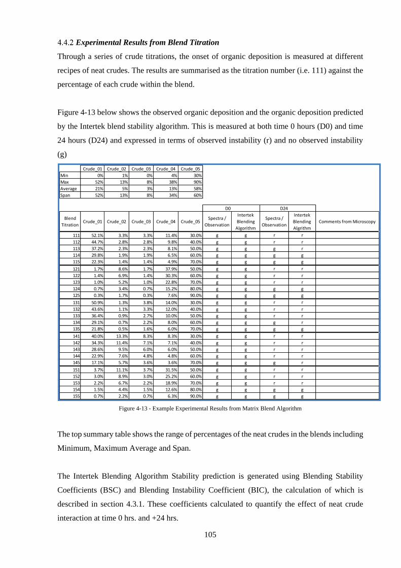
105
Experimental Results from Blend Titration
Through a series of crude titrations, the onset of organic deposition is measured at different
recipes of neat crudes. The results are summarised as the titration number (i.e. 111) against the
percentage of each crude within the blend.
Figure 4-13 below shows the observed organic deposition and the organic deposition predicted
by the Intertek blend stability algorithm. This is measured at both time 0 hours (D0) and time
24 hours (D24) and expressed in terms of observed instability (r) and no observed instability
(g)
Figure 4-13 - Example Experimental Results from Matrix Blend Algorithm
The top summary table shows the range of percentages of the neat crudes in the blends including
Minimum, Maximum Average and Span.
The Intertek Blending Algorithm Stability prediction is generated using Blending Stability
Coefficients (BSC) and Blending Instability Coefficient (BIC), the calculation of which is
described in section 4.3.1. These coefficients calculated to quantify the effect of neat crude
interaction at time 0 hrs. and +24 hrs.
Crude_01 Crude_02 Crude_03 Crude_04 Crude_05
Min 0% 1% 0% 4% 30%
Max 52% 13% 8% 38% 90%
Average 21% 5% 3% 13% 58%
Span 52% 13% 8% 34% 60%
D0 D24
Blend
TitrationCrude_01 Crude_02 Crude_03 Crude_04 Crude_05
Spectra /
Observation
Intertek
Blending
Algorithm
Spectra /
Observation
Intertek
Blending
Algrithm
Comments from Microscopy
111 52.1% 3.3% 3.3% 11.4% 30.0% g g r r
112 44.7% 2.8% 2.8% 9.8% 40.0% g g r r
113 37.2% 2.3% 2.3% 8.1% 50.0% g g g r
114 29.8% 1.9% 1.9% 6.5% 60.0% g g g g
115 22.3% 1.4% 1.4% 4.9% 70.0% g g g g
121 1.7% 8.6% 1.7% 37.9% 50.0% g g r r
122 1.4% 6.9% 1.4% 30.3% 60.0% g g r r
123 1.0% 5.2% 1.0% 22.8% 70.0% g g r r
124 0.7% 3.4% 0.7% 15.2% 80.0% g g g g
125 0.3% 1.7% 0.3% 7.6% 90.0% g g g g
131 50.9% 1.3% 3.8% 14.0% 30.0% g g r r
132 43.6% 1.1% 3.3% 12.0% 40.0% g g r r
133 36.4% 0.9% 2.7% 10.0% 50.0% g g r r
134 29.1% 0.7% 2.2% 8.0% 60.0% g g g r
135 21.8% 0.5% 1.6% 6.0% 70.0% g g g g
141 40.0% 13.3% 8.3% 8.3% 30.0% g g r r
142 34.3% 11.4% 7.1% 7.1% 40.0% g g r r
143 28.6% 9.5% 6.0% 6.0% 50.0% g g r r
144 22.9% 7.6% 4.8% 4.8% 60.0% g g r r
145 17.1% 5.7% 3.6% 3.6% 70.0% g g g r
151 3.7% 11.1% 3.7% 31.5% 50.0% g g r r
152 3.0% 8.9% 3.0% 25.2% 60.0% g g r r
153 2.2% 6.7% 2.2% 18.9% 70.0% g g r r
154 1.5% 4.4% 1.5% 12.6% 80.0% g g g g
155 0.7% 2.2% 0.7% 6.3% 90.0% g g g g
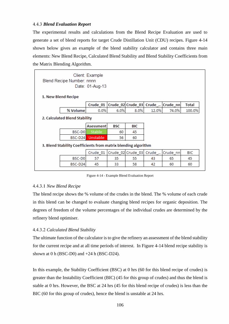
106
Blend Evaluation Report
The experimental results and calculations from the Blend Recipe Evaluation are used to
generate a set of blend reports for target Crude Distillation Unit (CDU) recipes. Figure 4-14
shown below gives an example of the blend stability calculator and contains three main
elements: New Blend Recipe, Calculated Blend Stability and Blend Stability Coefficients from
the Matrix Blending Algorithm.
Figure 4-14 - Example Blend Evaluation Report
New Blend Recipe
The blend recipe shows the % volume of the crudes in the blend. The % volume of each crude
in this blend can be changed to evaluate changing blend recipes for organic deposition. The
degrees of freedom of the volume percentages of the individual crudes are determined by the
refinery blend optimiser.
Calculated Blend Stability
The ultimate function of the calculator is to give the refinery an assessment of the blend stability
for the current recipe and at all time periods of interest. In Figure 4-14 blend recipe stability is
shown at 0 h (BSC-D0) and +24 h (BSC-D24).
In this example, the Stability Coefficient (BSC) at 0 hrs (60 for this blend recipe of crudes) is
greater than the Instability Coefficient (BIC) (45 for this group of crudes) and thus the blend is
stable at 0 hrs. However, the BSC at 24 hrs (45 for this blend recipe of crudes) is less than the
BIC (60 for this group of crudes), hence the blend is unstable at 24 hrs.

107
Calculated Blend Stability Coefficients from the matrix blending algorithm
This section details the calculated coefficients at time 0 and 24 hours for each of the crudes
assessed.
108
Case Study 2: Assessment of Heavy Fuel Oil Blending in a Refinery
This work forms the final deliverable to a refinery customer for the characterisation of the
stability of heavy fuel oil blends. The customer was an early adopter of the patented
methodology and as such this was the first application of the patented approach to a heavy fuel
blending process.
The client had experienced significant organic deposition with 1.8% sulphur blended Heavy
Fuel Oil. This initial study was aimed at assessing the stability of 1.8% sulphur Heavy Fuel
(HFO) when it is produced by blending 3.0% sulphur HFO from the refinery CDU with 1%
sulphur HFO bought in from an external supplier. It is also noted that an additional blend
component of Heavy Virgin Naphtha (HVN) also from the CDU is sometimes used to control
viscosity of the blend.
The assessment used an Intertek proprietary methodology under patent GB2516126 /
P130065WO “Method and System for Analysing a Blend of two or more Hydrocarbon Feed
Streams”. By blending the actual hydrocarbon streams the interactions that affect stability are
observed. The samples received from the client were as follows:
August 2014:
• 1% Sulphur Heavy Fuel Oil (HFO)
• 1.8% Sulphur HFO (Blended at the refinery but not sold to a customer)
• 1.8% Sulphur Used HFO (Sent back by the refinery’s customer due to observed stability
issues)
• 3% Sulphur HFO
December 2014:
• 3% Sulphur HFO (not used in study)
• Heavy Virgin Naphtha (HVN)
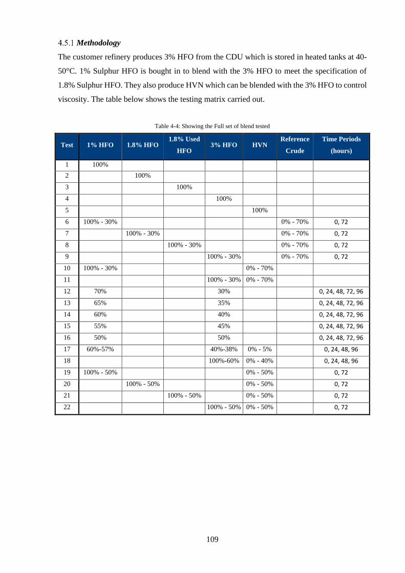
109
Methodology
The customer refinery produces 3% HFO from the CDU which is stored in heated tanks at 40-
50°C. 1% Sulphur HFO is bought in to blend with the 3% HFO to meet the specification of
1.8% Sulphur HFO. They also produce HVN which can be blended with the 3% HFO to control
viscosity. The table below shows the testing matrix carried out.
Table 4-4: Showing the Full set of blend tested
Test 1% HFO 1.8% HFO 1.8% Used
HFO 3% HFO HVN
Reference
Crude
Time Periods
(hours)
1 100%
2 100%
3 100%
4 100%
5 100%
6 100% - 30% 0% - 70% 0, 72
7 100% - 30% 0% - 70% 0, 72
8 100% - 30% 0% - 70% 0, 72
9 100% - 30% 0% - 70% 0, 72
10 100% - 30% 0% - 70%
11 100% - 30% 0% - 70%
12 70% 30% 0, 24, 48, 72, 96
13 65% 35% 0, 24, 48, 72, 96
14 60% 40% 0, 24, 48, 72, 96
15 55% 45% 0, 24, 48, 72, 96
16 50% 50% 0, 24, 48, 72, 96
17 60%-57% 40%-38% 0% - 5% 0, 24, 48, 96
18 100%-60% 0% - 40% 0, 24, 48, 96
19 100% - 50% 0% - 50% 0, 72
20 100% - 50% 0% - 50% 0, 72
21 100% - 50% 0% - 50% 0, 72
22 100% - 50% 0% - 50% 0, 72

110
NIR Spectroscopy
The stability of the sample was assessed using an ABB MB3600 NIR spectrometer and high-
pressure cell. All scanning was carried out at 60°C. Samples were assessed for both
instantaneous stability (i.e. as materials are added) and time dependent (over a period of five
days) stability.
Microscopy
Microscopy was performed on the samples to validate spectral observations; this was
undertaken on both a Nikon 90i laser microscope and a Nikon Eclipse LV100ND.
Microscopy was carried out in the following forms:
• Transmitted light: Shows sample magnified under normal light, asphaltenes show as
black particles, wax appears as light coloured, translucent aggregates.
• Cross Polar: Subjects the samples to polarised light, wax crystals appear as bright star
like objects on a black background.
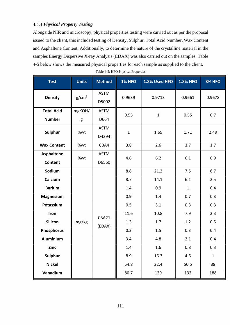
111
Physical Property Testing
Alongside NIR and microscopy, physical properties testing were carried out as per the proposal
issued to the client, this included testing of Density, Sulphur, Total Acid Number, Wax Content
and Asphaltene Content. Additionally, to determine the nature of the crystalline material in the
samples Energy Dispersive X-ray Analysis (EDAX) was also carried out on the samples. Table
4-5 below shows the measured physical properties for each sample as supplied to the client.
Table 4-5: HFO Physical Properties
Test Units Method 1% HFO 1.8% Used HFO 1.8% HFO 3% HFO
Density g/cm3 ASTM
D5002 0.9639 0.9713 0.9661 0.9678
Total Acid
Number
mgKOH/
g
ASTM
D664 0.55 1 0.55 0.7
Sulphur %wt ASTM
D4294 1 1.69 1.71 2.49
Wax Content %wt CBA4 3.8 2.6 3.7 1.7
Asphaltene
Content %wt
ASTM
D6560 4.6 6.2 6.1 6.9
Sodium
mg/kg CBA21
(EDAX)
8.8 21.2 7.5 6.7
Calcium 8.7 14.1 6.1 2.5
Barium 1.4 0.9 1 0.4
Magnesium 0.9 1.4 0.7 0.3
Potassium 0.5 3.1 0.3 0.3
Iron 11.6 10.8 7.9 2.3
Silicon 1.3 1.7 1.2 0.5
Phosphorus 0.3 1.5 0.3 0.4
Aluminium 3.4 4.8 2.1 0.4
Zinc 1.4 1.6 0.8 0.3
Sulphur 8.9 16.3 4.6 1
Nickel 54.8 32.4 50.5 38
Vanadium 80.7 129 132 188
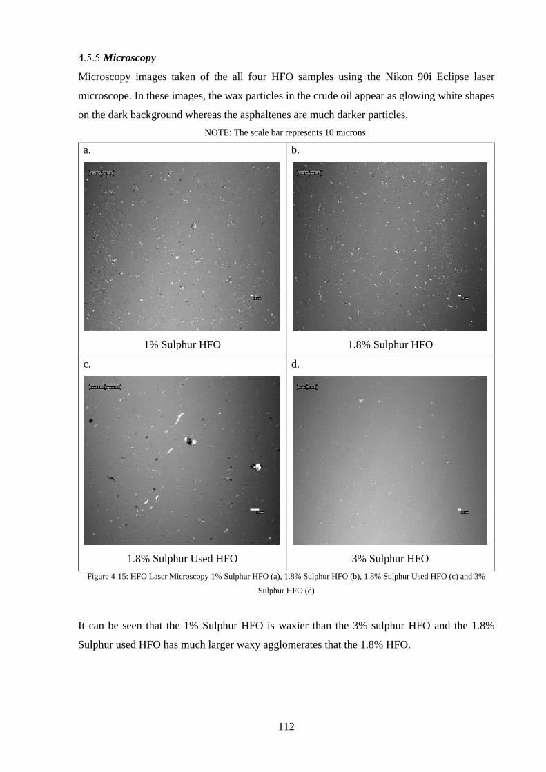
112
Microscopy
Microscopy images taken of the all four HFO samples using the Nikon 90i Eclipse laser
microscope. In these images, the wax particles in the crude oil appear as glowing white shapes
on the dark background whereas the asphaltenes are much darker particles.
NOTE: The scale bar represents 10 microns.
a.
1% Sulphur HFO
b.
1.8% Sulphur HFO
c.
1.8% Sulphur Used HFO
d.
3% Sulphur HFO
Figure 4-15: HFO Laser Microscopy 1% Sulphur HFO (a), 1.8% Sulphur HFO (b), 1.8% Sulphur Used HFO (c) and 3%
Sulphur HFO (d)
It can be seen that the 1% Sulphur HFO is waxier than the 3% sulphur HFO and the 1.8%
Sulphur used HFO has much larger waxy agglomerates that the 1.8% HFO.
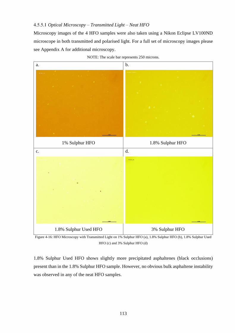
113
Optical Microscopy – Transmitted Light – Neat HFO
Microscopy images of the 4 HFO samples were also taken using a Nikon Eclipse LV100ND
microscope in both transmitted and polarised light. For a full set of microscopy images please
see Appendix A for additional microscopy.
NOTE: The scale bar represents 250 microns.
a.
1% Sulphur HFO
b.
1.8% Sulphur HFO
c.
1.8% Sulphur Used HFO
d.
3% Sulphur HFO
Figure 4-16: HFO Microscopy with Transmitted Light on 1% Sulphur HFO (a), 1.8% Sulphur HFO (b), 1.8% Sulphur Used
HFO (c) and 3% Sulphur HFO (d)
1.8% Sulphur Used HFO shows slightly more precipitated asphaltenes (black occlusions)
present than in the 1.8% Sulphur HFO sample. However, no obvious bulk asphaltene instability
was observed in any of the neat HFO samples.
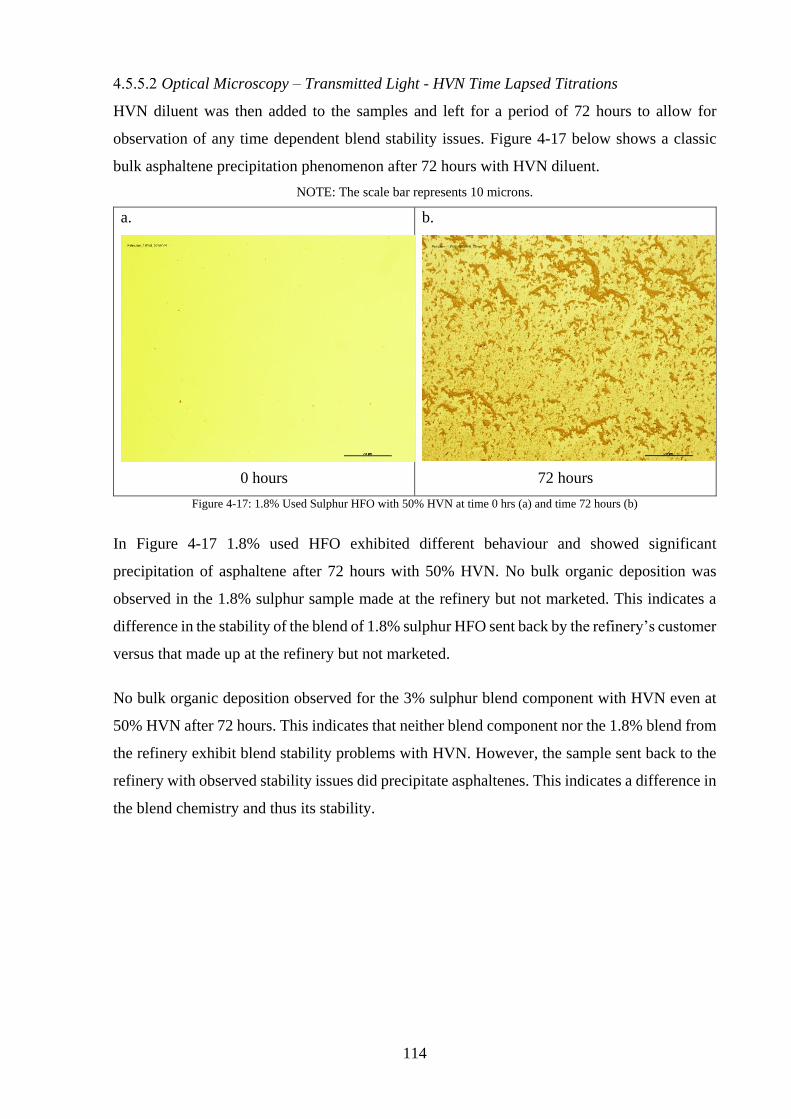
114
Optical Microscopy – Transmitted Light - HVN Time Lapsed Titrations
HVN diluent was then added to the samples and left for a period of 72 hours to allow for
observation of any time dependent blend stability issues. Figure 4-17 below shows a classic
bulk asphaltene precipitation phenomenon after 72 hours with HVN diluent.
NOTE: The scale bar represents 10 microns.
a.
0 hours
b.
72 hours
Figure 4-17: 1.8% Used Sulphur HFO with 50% HVN at time 0 hrs (a) and time 72 hours (b)
In Figure 4-17 1.8% used HFO exhibited different behaviour and showed significant
precipitation of asphaltene after 72 hours with 50% HVN. No bulk organic deposition was
observed in the 1.8% sulphur sample made at the refinery but not marketed. This indicates a
difference in the stability of the blend of 1.8% sulphur HFO sent back by the refinery’s customer
versus that made up at the refinery but not marketed.
No bulk organic deposition observed for the 3% sulphur blend component with HVN even at
50% HVN after 72 hours. This indicates that neither blend component nor the 1.8% blend from
the refinery exhibit blend stability problems with HVN. However, the sample sent back to the
refinery with observed stability issues did precipitate asphaltenes. This indicates a difference in
the blend chemistry and thus its stability.
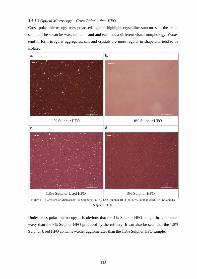
115
Optical Microscopy – Cross Polar – Neat HFO
Cross polar microscopy uses polarised light to highlight crystalline structures in the crude
sample. These can be wax, salt and sand and each has a different visual morphology. Waxes
tend to form irregular aggregates, salt and crystals are more regular in shape and tend to be
isolated.
a.
1% Sulphur HFO
b.
1.8% Sulphur HFO
c.
1.8% Sulphur Used HFO
d.
3% Sulphur HFO
Figure 4-18: Cross Polar Microscopy 1% Sulphur HFO (a), 1.8% Sulphur HFO (b), 1.8% Sulphur Used HFO (c) and 3%
Sulphur HFO (d)
Under cross polar microscopy it is obvious that the 1% Sulphur HFO bought in is far more
waxy than the 3% Sulphur HFO produced by the refinery. It can also be seen that the 1.8%
Sulphur Used HFO contains waxier agglomerates than the 1.8% Sulphur HFO sample.

116
Neat HFO Blend Tests
1% Sulphur HFO and 3% Sulphur HFO were blended to make 1.6%, 1.7%, 1.8%, 1.9% and
2% Sulphur HFO to test the effects of varying the blend ratios without addition of HVN. These
blends were scanned at time 0, +24, +48 and +96 hours to check time dependent sample
stability.
All the spectra show change in stability with time, Figure 4-19 and Figure 4-20 shows the time
dependent stability test for a blended 1.8% Sulphur HFO with no HVN and a 3% Sulphur HFO
with 20% HVN diluent respectively. It can be seen that although there is some spectral
movement (circa 0.04AU) at the 5000cm-1 region for the 1.8% Sulphur HFO this less is than
half the movement from the HFO with diluent (circa 0.1AU).
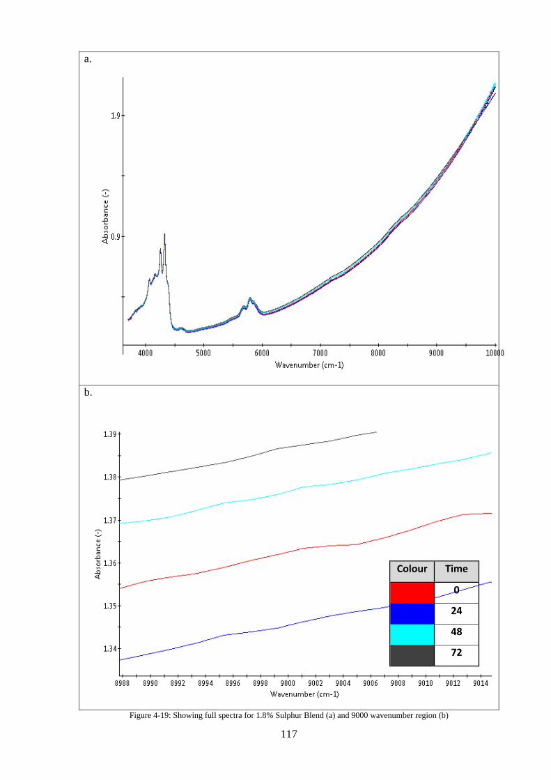
117
a.
b.
Figure 4-19: Showing full spectra for 1.8% Sulphur Blend (a) and 9000 wavenumber region (b)
Colour Time
0
24
48
72
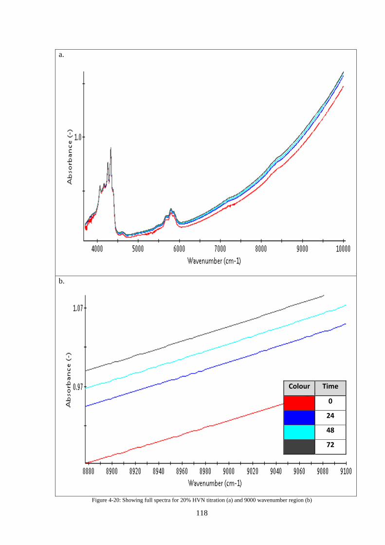
118
a.
b.
Figure 4-20: Showing full spectra for 20% HVN titration (a) and 9000 wavenumber region (b)
Colour Time
0
24
48
72
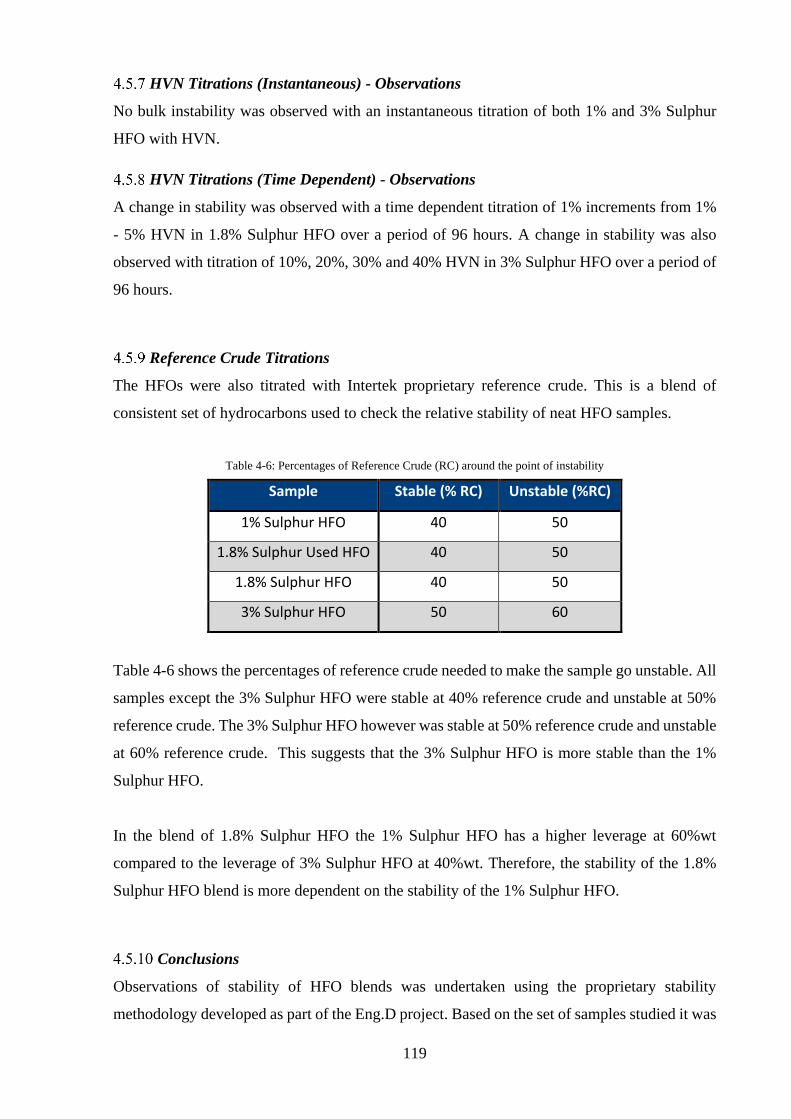
119
HVN Titrations (Instantaneous) - Observations
No bulk instability was observed with an instantaneous titration of both 1% and 3% Sulphur
HFO with HVN.
HVN Titrations (Time Dependent) - Observations
A change in stability was observed with a time dependent titration of 1% increments from 1%
- 5% HVN in 1.8% Sulphur HFO over a period of 96 hours. A change in stability was also
observed with titration of 10%, 20%, 30% and 40% HVN in 3% Sulphur HFO over a period of
96 hours.
Reference Crude Titrations
The HFOs were also titrated with Intertek proprietary reference crude. This is a blend of
consistent set of hydrocarbons used to check the relative stability of neat HFO samples.
Table 4-6: Percentages of Reference Crude (RC) around the point of instability
Sample Stable (% RC) Unstable (%RC)
1% Sulphur HFO 40 50
1.8% Sulphur Used HFO 40 50
1.8% Sulphur HFO 40 50
3% Sulphur HFO 50 60
Table 4-6 shows the percentages of reference crude needed to make the sample go unstable. All
samples except the 3% Sulphur HFO were stable at 40% reference crude and unstable at 50%
reference crude. The 3% Sulphur HFO however was stable at 50% reference crude and unstable
at 60% reference crude. This suggests that the 3% Sulphur HFO is more stable than the 1%
Sulphur HFO.
In the blend of 1.8% Sulphur HFO the 1% Sulphur HFO has a higher leverage at 60%wt
compared to the leverage of 3% Sulphur HFO at 40%wt. Therefore, the stability of the 1.8%
Sulphur HFO blend is more dependent on the stability of the 1% Sulphur HFO.
Conclusions
Observations of stability of HFO blends was undertaken using the proprietary stability
methodology developed as part of the Eng.D project. Based on the set of samples studied it was
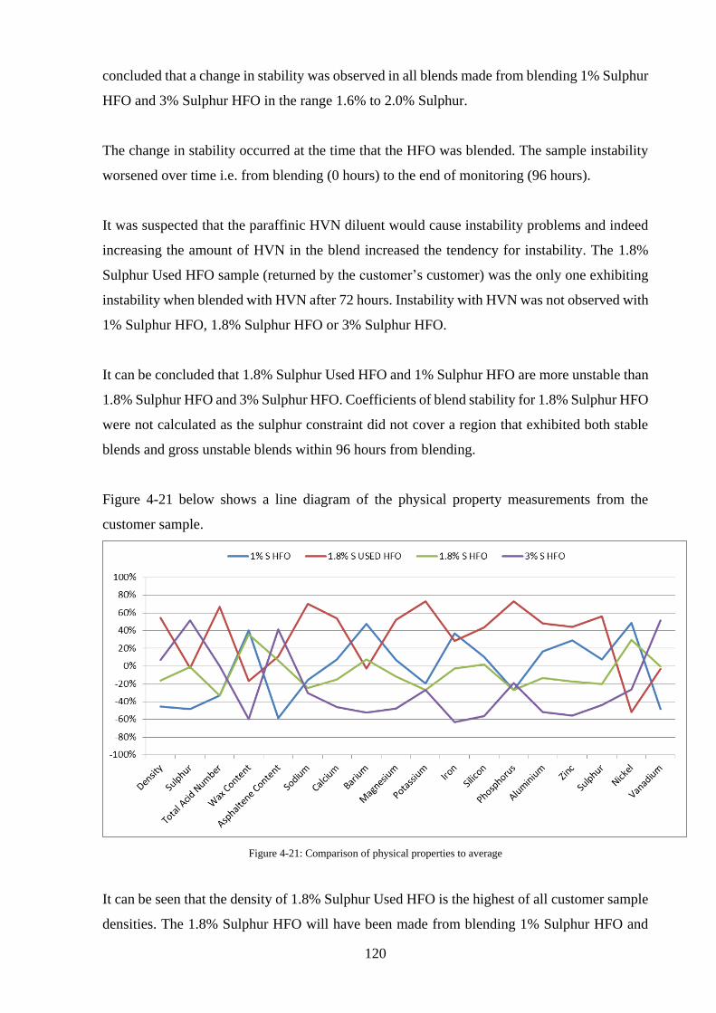
120
concluded that a change in stability was observed in all blends made from blending 1% Sulphur
HFO and 3% Sulphur HFO in the range 1.6% to 2.0% Sulphur.
The change in stability occurred at the time that the HFO was blended. The sample instability
worsened over time i.e. from blending (0 hours) to the end of monitoring (96 hours).
It was suspected that the paraffinic HVN diluent would cause instability problems and indeed
increasing the amount of HVN in the blend increased the tendency for instability. The 1.8%
Sulphur Used HFO sample (returned by the customer’s customer) was the only one exhibiting
instability when blended with HVN after 72 hours. Instability with HVN was not observed with
1% Sulphur HFO, 1.8% Sulphur HFO or 3% Sulphur HFO.
It can be concluded that 1.8% Sulphur Used HFO and 1% Sulphur HFO are more unstable than
1.8% Sulphur HFO and 3% Sulphur HFO. Coefficients of blend stability for 1.8% Sulphur HFO
were not calculated as the sulphur constraint did not cover a region that exhibited both stable
blends and gross unstable blends within 96 hours from blending.
Figure 4-21 below shows a line diagram of the physical property measurements from the
customer sample.
Figure 4-21: Comparison of physical properties to average
It can be seen that the density of 1.8% Sulphur Used HFO is the highest of all customer sample
densities. The 1.8% Sulphur HFO will have been made from blending 1% Sulphur HFO and
121
3% Sulphur HFO in the ratio 60:40 and therefore the density must be between the density of
the two blend components. As the density is higher than 3% Sulphur HFO the blend components
of the 1.8% Sulphur Used HFO must be different from the samples tested.
After further discussion of the results with the customer it was determined that the 1% sulphur
HFO blend component was sourced from different suppliers. The two 1.8% Sulphur HFO
samples were made with different 1% Sulphur blend components and it was thus determined
that 1% Sulphur blend component from a particular supplier was not compatible with the
customer 3% Sulphur HFO.
1% Sulphur HFO is waxier than 3% Sulphur HFO and the EDAX results in conjunction with
the physical properties analysis and cross polar microscopy suggest the crystalline material to
be predominantly organic in nature.
From the microscopy observations, it was determined that the 1% Sulphur HFO is less stable
than 3% Sulphur HFO when blended with reference crude and bulk organic deposition was only
observed with 1.8% Sulphur Used HFO with 50% HVN after 72 hours but not with 1% Sulphur
HFO, 1.8% Sulphur HFO or 3% Sulphur HFO.
1% Sulphur HFO is less stable than 3% Sulphur HFO when blended with reference crude and
blends of 1.6% to 2% Sulphur HFO without HVN exhibit a change in stability with time.
However, 3% Sulphur HFO with HVN does exhibit change in stability with time. Blends of
1.8% Sulphur HFO made from 3% and 1% Sulphur HFO and HVN from 0% to 5% do exhibit
a change in stability with time.
Recommended action:
• Blend order and mixing is critical to prevent bulk instability when blending with HVN. At
the point of mixing there is the potential for a local high concentration of HVN.
• Establish the level and quality of HVN, 1% Sulphur HFO, and 3% Sulphur HFO, storage
times and the blend order that have been associated with customer issues.
• Monitor quality of blend components and evaluate blend stability before making up
batches of 1.8% Sulphur HFO
• Monitoring the quality of 1.8% Sulphur HFO is critical based on the significant difference
between 1.8% Sulphur HFO and 1.8% Sulphur Used HFO.
• Establish the critical processing parameters for the customer i.e. the level of organic
deposition that can occur whilst the HFO remains usable.
122
Case Study 3 – Assessment of Blends of Marine Fuels
This application of the organic deposition programme was directed at solving issues
experienced with deposition in the marine fuels industry. This can cause major issues because
if asphaltene precipitates whilst fuels are blended on board they can block fuel filters and
potentially shut down the engines.
This issue arises because ships have two tanks of fuel on board. One containing a high sulphur
(residual) fuel oil and one containing a low sulphur (distillate) marine diesel. It is necessary for
ships to transition between fuels when passing through Emission Control Areas (ECAs).
Currently the global Sulphur cap is 3.5% however in European waters (Baltic, North Sea and
English Channel) this drops to 0.1% (Commission, 2016). This blending within the fuel line
can cause stability problems when the paraffinic diesel is mixed with the highly asphaltenic
duel oil.
This study saw intensive collaboration with both marine operatives and refineries producing
the fuel. Furthermore, studies have been undertaken with additive manufacturers to assess the
levels and efficacy of additives used to help prevent these problems occurring.
Part 1 – Characterisation and Feasibility Phase
This details the results of blending marine fuel oils. The assessments focused particularly on
the linearity of spectral blending of fuel oils and the stability of blended fuel oils
The work was initiated following a discussion between Intertek and a spectrometer
manufacturer regarding the possibility of installing a spectrometer in a ships fuel line to monitor
the progression from Heavy Fuel Oil (HFO) to Marine Diesel Oil (MDO). This monitoring is a
value-added service to shippers in ECAs.
A selection of samples of HFO and MDO were selected for testing in the Intertek laboratory.
Testing work was carried out in April - June 2015 with various blend recipes assessed using
Near Infrared (NIR) spectroscopy and microscopy.
Blends were made up at 10% increments of the following pairs of samples:
• Blend 1: DL231202 – HFO (3.43% Sulphur) / DL231229 – MDO (0.03% Sulphur)
• Blend 2: DL231193 – HFO (3.30% Sulphur) / DL231311 – MDO (0.04% Sulphur)
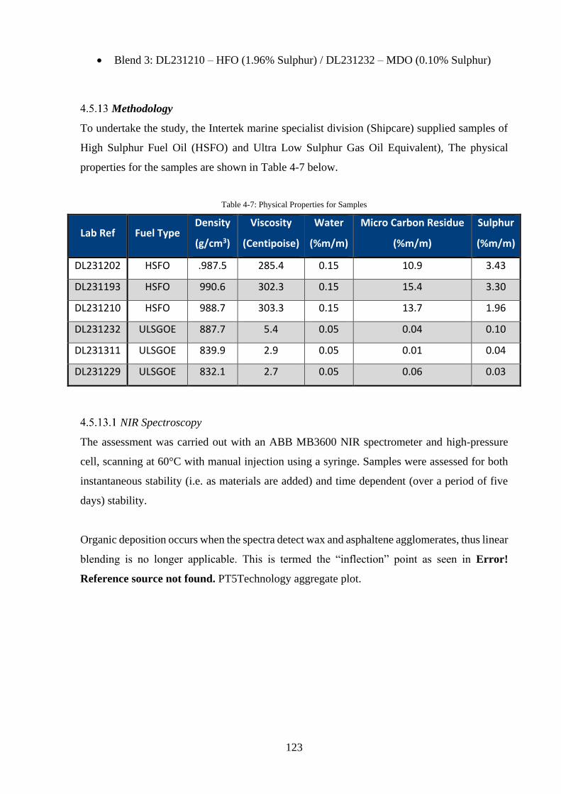
123
• Blend 3: DL231210 – HFO (1.96% Sulphur) / DL231232 – MDO (0.10% Sulphur)
Methodology
To undertake the study, the Intertek marine specialist division (Shipcare) supplied samples of
High Sulphur Fuel Oil (HSFO) and Ultra Low Sulphur Gas Oil Equivalent), The physical
properties for the samples are shown in Table 4-7 below.
Table 4-7: Physical Properties for Samples
Lab Ref Fuel Type Density
(g/cm3)
Viscosity
(Centipoise)
Water
(%m/m)
Micro Carbon Residue
(%m/m)
Sulphur
(%m/m)
DL231202 HSFO .987.5 285.4 0.15 10.9 3.43
DL231193 HSFO 990.6 302.3 0.15 15.4 3.30
DL231210 HSFO 988.7 303.3 0.15 13.7 1.96
DL231232 ULSGOE 887.7 5.4 0.05 0.04 0.10
DL231311 ULSGOE 839.9 2.9 0.05 0.01 0.04
DL231229 ULSGOE 832.1 2.7 0.05 0.06 0.03
NIR Spectroscopy
The assessment was carried out with an ABB MB3600 NIR spectrometer and high-pressure
cell, scanning at 60°C with manual injection using a syringe. Samples were assessed for both
instantaneous stability (i.e. as materials are added) and time dependent (over a period of five
days) stability.
Organic deposition occurs when the spectra detect wax and asphaltene agglomerates, thus linear
blending is no longer applicable. This is termed the “inflection” point as seen in Error!
Reference source not found. PT5Technology aggregate plot.
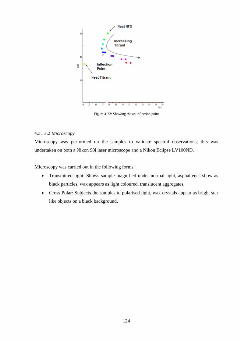
124
Figure 4-22: Showing the an inflection point
Microscopy
Microscopy was performed on the samples to validate spectral observations; this was
undertaken on both a Nikon 90i laser microscope and a Nikon Eclipse LV100ND.
Microscopy was carried out in the following forms:
• Transmitted light: Shows sample magnified under normal light, asphaltenes show as
black particles, wax appears as light coloured, translucent aggregates.
• Cross Polar: Subjects the samples to polarised light, wax crystals appear as bright star
like objects on a black background.
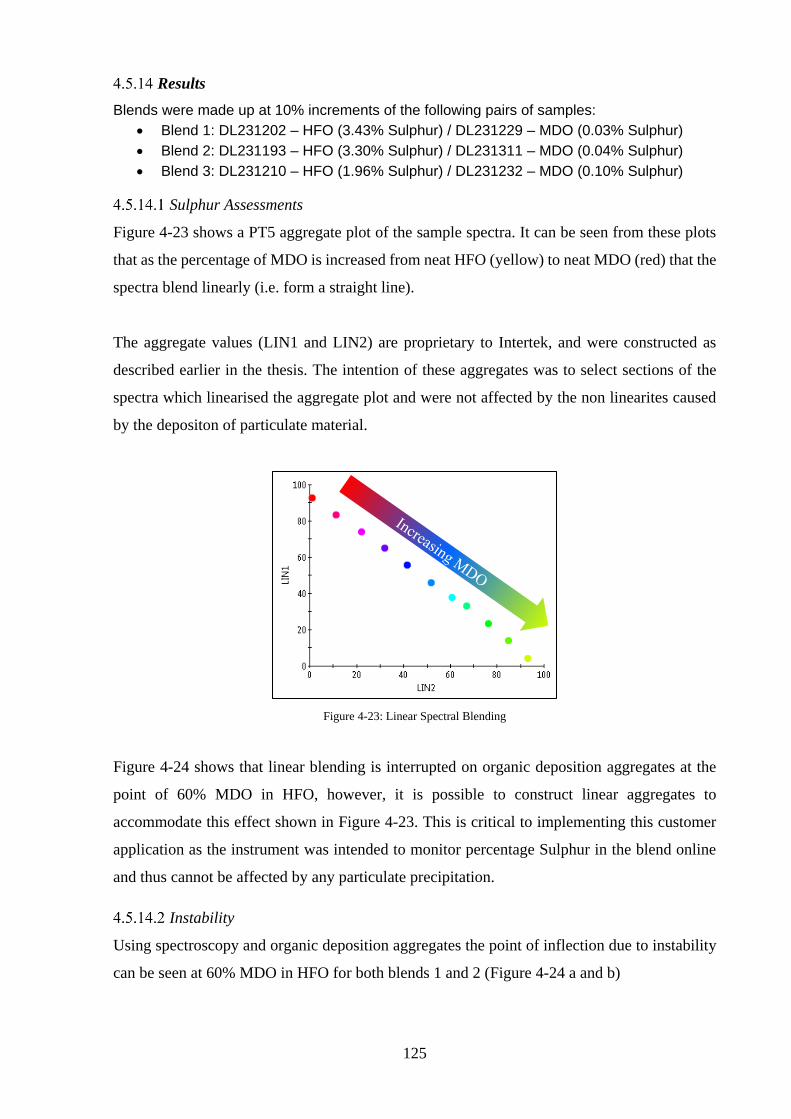
125
Results
Blends were made up at 10% increments of the following pairs of samples:
• Blend 1: DL231202 – HFO (3.43% Sulphur) / DL231229 – MDO (0.03% Sulphur)
• Blend 2: DL231193 – HFO (3.30% Sulphur) / DL231311 – MDO (0.04% Sulphur)
• Blend 3: DL231210 – HFO (1.96% Sulphur) / DL231232 – MDO (0.10% Sulphur)
Sulphur Assessments
Figure 4-23 shows a PT5 aggregate plot of the sample spectra. It can be seen from these plots
that as the percentage of MDO is increased from neat HFO (yellow) to neat MDO (red) that the
spectra blend linearly (i.e. form a straight line).
The aggregate values (LIN1 and LIN2) are proprietary to Intertek, and were constructed as
described earlier in the thesis. The intention of these aggregates was to select sections of the
spectra which linearised the aggregate plot and were not affected by the non linearites caused
by the depositon of particulate material.
Figure 4-23: Linear Spectral Blending
Figure 4-24 shows that linear blending is interrupted on organic deposition aggregates at the
point of 60% MDO in HFO, however, it is possible to construct linear aggregates to
accommodate this effect shown in Figure 4-23. This is critical to implementing this customer
application as the instrument was intended to monitor percentage Sulphur in the blend online
and thus cannot be affected by any particulate precipitation.
Instability
Using spectroscopy and organic deposition aggregates the point of inflection due to instability
can be seen at 60% MDO in HFO for both blends 1 and 2 (Figure 4-24 a and b)
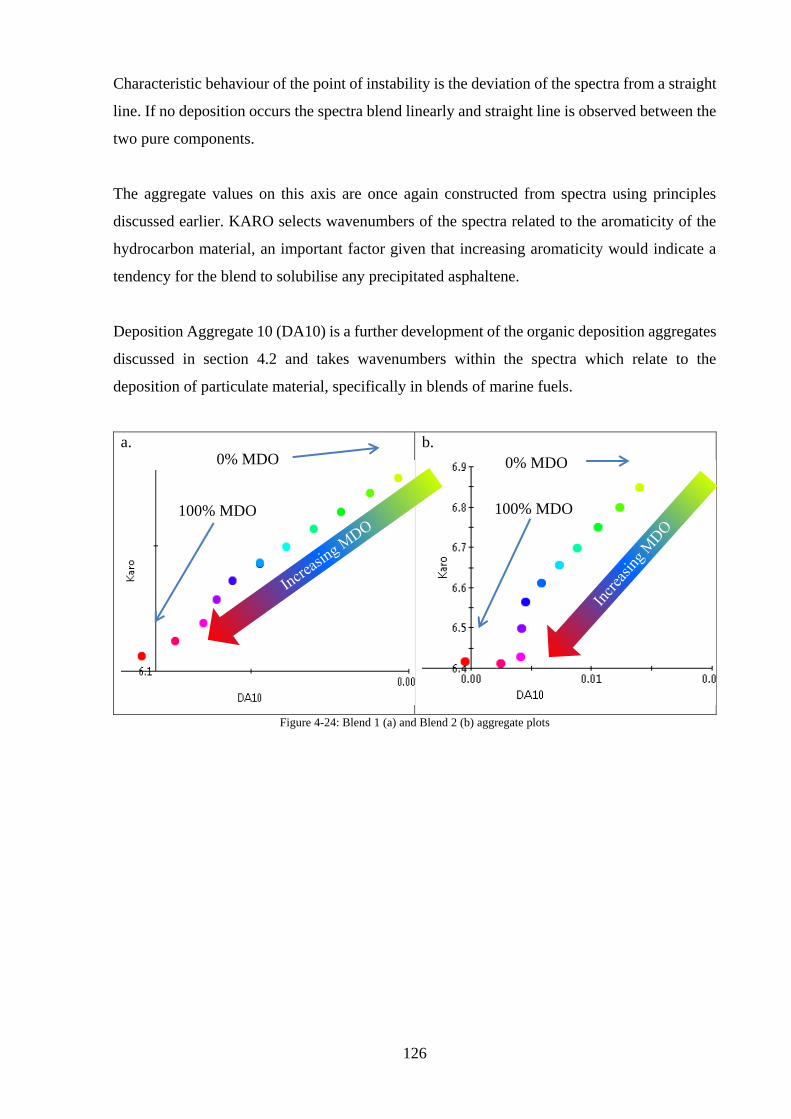
126
Characteristic behaviour of the point of instability is the deviation of the spectra from a straight
line. If no deposition occurs the spectra blend linearly and straight line is observed between the
two pure components.
The aggregate values on this axis are once again constructed from spectra using principles
discussed earlier. KARO selects wavenumbers of the spectra related to the aromaticity of the
hydrocarbon material, an important factor given that increasing aromaticity would indicate a
tendency for the blend to solubilise any precipitated asphaltene.
Deposition Aggregate 10 (DA10) is a further development of the organic deposition aggregates
discussed in section 4.2 and takes wavenumbers within the spectra which relate to the
deposition of particulate material, specifically in blends of marine fuels.
a.
b.
Figure 4-24: Blend 1 (a) and Blend 2 (b) aggregate plots
0% MDO
100% MDO
0% MDO
100% MDO
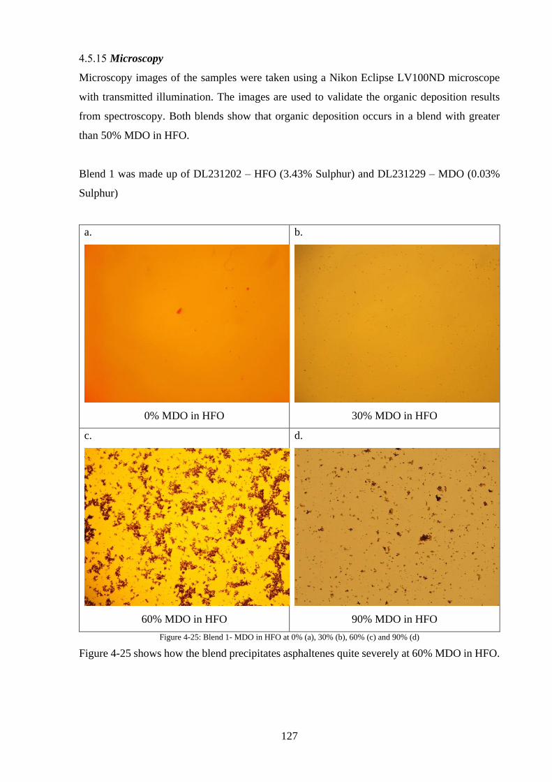
127
Microscopy
Microscopy images of the samples were taken using a Nikon Eclipse LV100ND microscope
with transmitted illumination. The images are used to validate the organic deposition results
from spectroscopy. Both blends show that organic deposition occurs in a blend with greater
than 50% MDO in HFO.
Blend 1 was made up of DL231202 – HFO (3.43% Sulphur) and DL231229 – MDO (0.03%
Sulphur)
a.
0% MDO in HFO
b.
30% MDO in HFO
c.
60% MDO in HFO
d.
90% MDO in HFO
Figure 4-25: Blend 1- MDO in HFO at 0% (a), 30% (b), 60% (c) and 90% (d)
Figure 4-25 shows how the blend precipitates asphaltenes quite severely at 60% MDO in HFO.
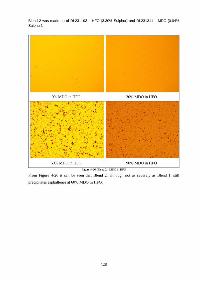
128
Blend 2 was made up of DL231193 – HFO (3.30% Sulphur) and DL231311 – MDO (0.04%
Sulphur).
0% MDO in HFO
30% MDO in HFO
60% MDO in HFO
90% MDO in HFO
Figure 4-26: Blend 2 - MDO in HFO
From Figure 4-26 it can be seen that Blend 2, although not as severely as Blend 1, still
precipitates asphaltenes at 60% MDO in HFO.
129
Part 2 – Additive Efficacy Assessments
Part 2 goes on to show the results of blending marine fuel oils and additives. The assessments
focused particularly on the stability of blends of fuel oils containing Marine Diesel Oil (MDO)
and Heavy Fuel Oil (HFO) with and without an additive.
The project work was initiated following discussions between Intertek Process Assurance
Group and Intertek Shipcare. Part 1 of the study demonstrated that blends of HFO and MDO
precipitate asphaltenes both instantaneously and over time.
Following on from further discussions there was significant interest in assessing the effects of
investigating a solution to the problem in the form of asphaltene stabilising additives. The
ability to quantify the effects of additives on fuel oil blend stability will allow Intertek to offer
solutions to customers experiencing these issues.
A selection of samples including HFO and MDO were selected for testing in the laboratory.
Testing work was carried out in September - November 2015 with various blend recipes
assessed using Near Infrared (NIR) spectroscopy and microscopy. The oils were blended at
predetermined ratios (shown below) and tested with and without additive.
Blends were made up at 20% ratios of the following pairs of samples:
• Blend 1 DL242838 – HFO (2.57% Sulphur) / DL243169 – MDO (0.076% Sulphur)
• Blend 2 DL242840 – HFO (2.49% Sulphur) / DL243094 – MDO (0.083% Sulphur)
• Blend 3 DL242837 – HFO (2.41% Sulphur) / DL243017 – MDO (0.083% Sulphur)
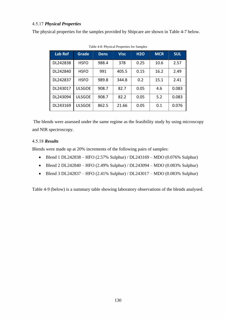
130
Physical Properties
The physical properties for the samples provided by Shipcare are shown in Table 4-7 below.
Table 4-8: Physical Properties for Samples
Lab Ref Grade Dens Visc H2O MCR SUL
DL242838 HSFO 988.4 378 0.25 10.6 2.57
DL242840 HSFO 991 405.5 0.15 16.2 2.49
DL242837 HSFO 989.8 344.8 0.2 15.1 2.41
DL243017 ULSGOE 908.7 82.7 0.05 4.6 0.083
DL243094 ULSGOE 908.7 82.2 0.05 5.2 0.083
DL243169 ULSGOE 862.5 21.66 0.05 0.1 0.076
The blends were assessed under the same regime as the feasibility study by using microscopy
and NIR spectroscopy.
Results
Blends were made up at 20% increments of the following pairs of samples:
• Blend 1 DL242838 – HFO (2.57% Sulphur) / DL243169 – MDO (0.076% Sulphur)
• Blend 2 DL242840 – HFO (2.49% Sulphur) / DL243094 – MDO (0.083% Sulphur)
• Blend 3 DL242837 – HFO (2.41% Sulphur) / DL243017 – MDO (0.083% Sulphur)
Table 4-9 (below) is a summary table showing laboratory observations of the blends analysed.
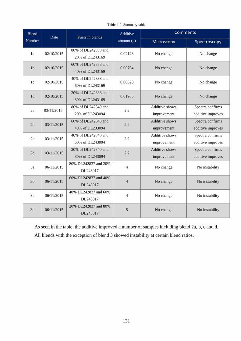
131
Table 4-9: Summary table
Blend
Number Date Fuels in blends
Additive
amount (g)
Comments
Microscopy Spectroscopy
1a 02/10/2015 80% of DL242838 and
20% of DL243169 0.02123 No change No change
1b 02/10/2015 60% of DL242838 and
40% of DL243169 0.00764 No change No change
1c 02/10/2015 40% of DL242838 and
60% of DL243169 0.00828 No change No change
1d 02/10/2015 20% of DL242838 and
80% of DL243169 0.01965 No change No change
2a 03/11/2015 80% of DL242840 and
20% of DL243094 2.2
Additive shows
improvement
Spectra confirms
additive improves
2b 03/11/2015 60% of DL242840 and
40% of DL233094 2.2
Additive shows
improvement
Spectra confirms
additive improves
2c 03/11/2015 40% of DL242840 and
60% of DL243094 2.2
Additive shows
improvement
Spectra confirms
additive improves
2d 03/11/2015 20% of DL242840 and
80% of DL243094 2.2
Additive shows
improvement
Spectra confirms
additive improves
3a 06/11/2015 80% DL242837 and 20%
DL243017 4 No change No instability
3b 06/11/2015 60% DL242837 and 40%
DL243017 4 No change No instability
3c 06/11/2015 40% DL242837 and 60%
DL243017 4 No change No instability
3d 06/11/2015 20% DL242837 and 80%
DL243017 5 No change No instability
As seen in the table, the additive improved a number of samples including blend 2a, b, c and d.
All blends with the exception of blend 3 showed instability at certain blend ratios.

132
Blend 1 (DL242838/DL243169)
a.
Blend 1b (80% HFO/ 20% MDO)
With additive
b.
Blend 1b (80% HFO/20% MDO)
Without additive
c.
Blend 1c (60% HFO/40% MDO)
With additive
d.
Blend 1c (60% HFO/40% MDO)
Without additive
Figure 4-27: Showing blends with additive (a) and (c) and without additive (b) and (d)
In blend 1 the additive did not improve the stability of the blend, the blend was equally as
unstable without the additive as it was with the additive.
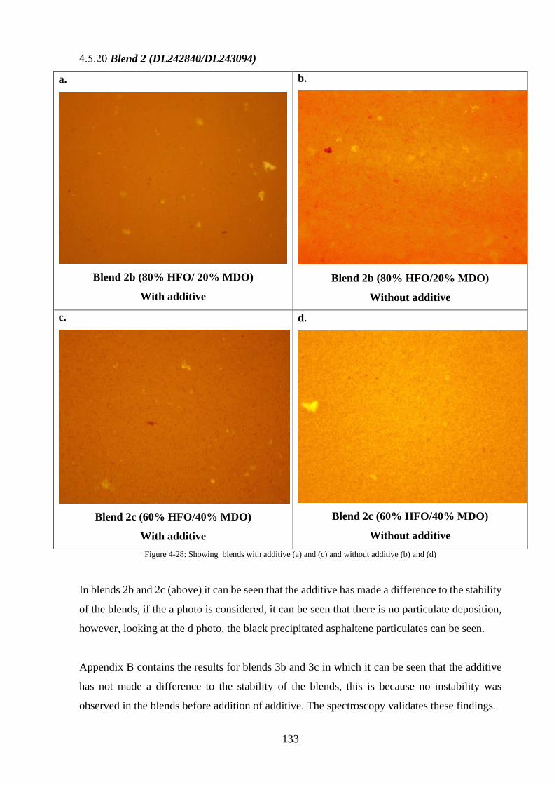
133
Blend 2 (DL242840/DL243094)
a.
Blend 2b (80% HFO/ 20% MDO)
With additive
b.
Blend 2b (80% HFO/20% MDO)
Without additive
c.
Blend 2c (60% HFO/40% MDO)
With additive
d.
Blend 2c (60% HFO/40% MDO)
Without additive
Figure 4-28: Showing blends with additive (a) and (c) and without additive (b) and (d)
In blends 2b and 2c (above) it can be seen that the additive has made a difference to the stability
of the blends, if the a photo is considered, it can be seen that there is no particulate deposition,
however, looking at the d photo, the black precipitated asphaltene particulates can be seen.
Appendix B contains the results for blends 3b and 3c in which it can be seen that the additive
has not made a difference to the stability of the blends, this is because no instability was
observed in the blends before addition of additive. The spectroscopy validates these findings.

134
Additive
Additive
Figure 4-29: Neat Additive
By scanning and taking microscope pictures of the additive, validation of the physical effects
of the additive on the crude blend is possible i.e. the additive does not contain (in itself)
particulate asphaltene or waxy agglomerates which would affect spectra.

135
Conclusions
From the assessment of marine fuels it is clear that the methodology developed can also deal
with instability problems in the marine industry. This has the potential to be developed into a
ship fuel monitoring service to profile sulphur levels as the transition occurs from HFO to MDO
when passing through SECA’s.
It was also proved that the chemometric modelling technique discussed in 0 can be applied to
monitor sulphur transition during marine fuels blending. This has the potential to be rolled into
an online service which can be placed on board a ship to monitor both Sulphur transition and
blend stability.
Furthermore the case study demonstrated the applicability for the technique to assess the
efficacy of additives on blends of marine fuels. A capability that can be applied in other areas
of the hydrocarbon processing sector.
Intertek can offer this as a service to additive manufacturers to assess efficacy of additives and
provide them value added information to take to the marketplace.
136
Chapter 5:
Troubleshooting Upstream
Process Issues with Data
Analytics
137
Chapter 5. Troubleshooting Upstream Process Issues with Data Analytics
As part of the provision of chemometric modelling services to clients of Intertek, it was a logical
next step to widen the modelling capability of the PT5 toolbox and provide troubleshooting for
client issues based on data other than NIR spectra.
The process industry in general has a multitude of online instrumentation, interfaced to process
data historians (such as PI). Contained within these datasets is valuable information and
knowledge that, when coupled with domain expertise, can be used to achieve a variety of
benefits including: more efficient maintenance scheduling, improved performance, reduced
downtime and maximised margins.
However, this valuable information is hidden in the quantity of data and further compounded
by dataset issues such as the noise from unrepresentative operation such as process upsets and
malfunctioning instrumentation. Hence, to simplify analytics, operators usually focus on time
series trending and first order effects.
Much work has been undertaken on the application of multivariate data analytics to process
data, particularly for its applications in Process Analytical Technology (PAT) and Quality by
Design (QbD). A review of these approaches to bioprocess datasets was undertaken by (Mercier
et al., 2014) with the conclusion that data analytics in this industry, although implemented, is
still in its infancy and much more development work is required to achieve wider marketplace
penetration
Furthermore, applications are also implemented in the pharmaceutical industry, (Rioloa et al.,
2017) undertook a review of the applications of data analytics for PAT within the
pharmaceutical industry, with a specific focus on Raman spectroscopy.
However, the drivers for development of this technology in food and pharmaceuticals is clear,
these are tightly regulated industries producing goods generally for human consumption and
thus the margin for error is very slim. Very little has been written on the implementation within
the oil and gas industry however, this is due to a traditional mindset and an attitude that the
status quo works and thus the balance should not be upset.
During the course of the Eng.D project, an opportunity was identified with an upstream client
experiencing problems with two pumps on an offshore installation. Pump failure not only
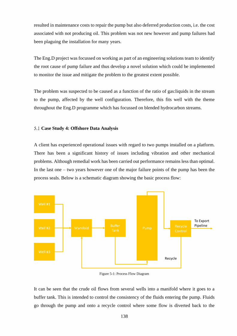
138
resulted in maintenance costs to repair the pump but also deferred production costs, i.e. the cost
associated with not producing oil. This problem was not new however and pump failures had
been plaguing the installation for many years.
The Eng.D project was focussed on working as part of an engineering solutions team to identify
the root cause of pump failure and thus develop a novel solution which could be implemented
to monitor the issue and mitigate the problem to the greatest extent possible.
The problem was suspected to be caused as a function of the ratio of gas:liquids in the stream
to the pump, affected by the well configuration. Therefore, this fits well with the theme
throughout the Eng.D programme which has focussed on blended hydrocarbon streams.
Case Study 4: Offshore Data Analysis
A client has experienced operational issues with regard to two pumps installed on a platform.
There has been a significant history of issues including vibration and other mechanical
problems. Although remedial work has been carried out performance remains less than optimal.
In the last one – two years however one of the major failure points of the pump has been the
process seals. Below is a schematic diagram showing the basic process flow:
Figure 5-1: Process Flow Diagram
It can be seen that the crude oil flows from several wells into a manifold where it goes to a
buffer tank. This is intended to control the consistency of the fluids entering the pump. Fluids
go through the pump and onto a recycle control where some flow is diverted back to the
Well #1
Well #2
Well #3
ManifoldBuffer Tank
Pump Recycle Control
Recycle
To Export Pipeline
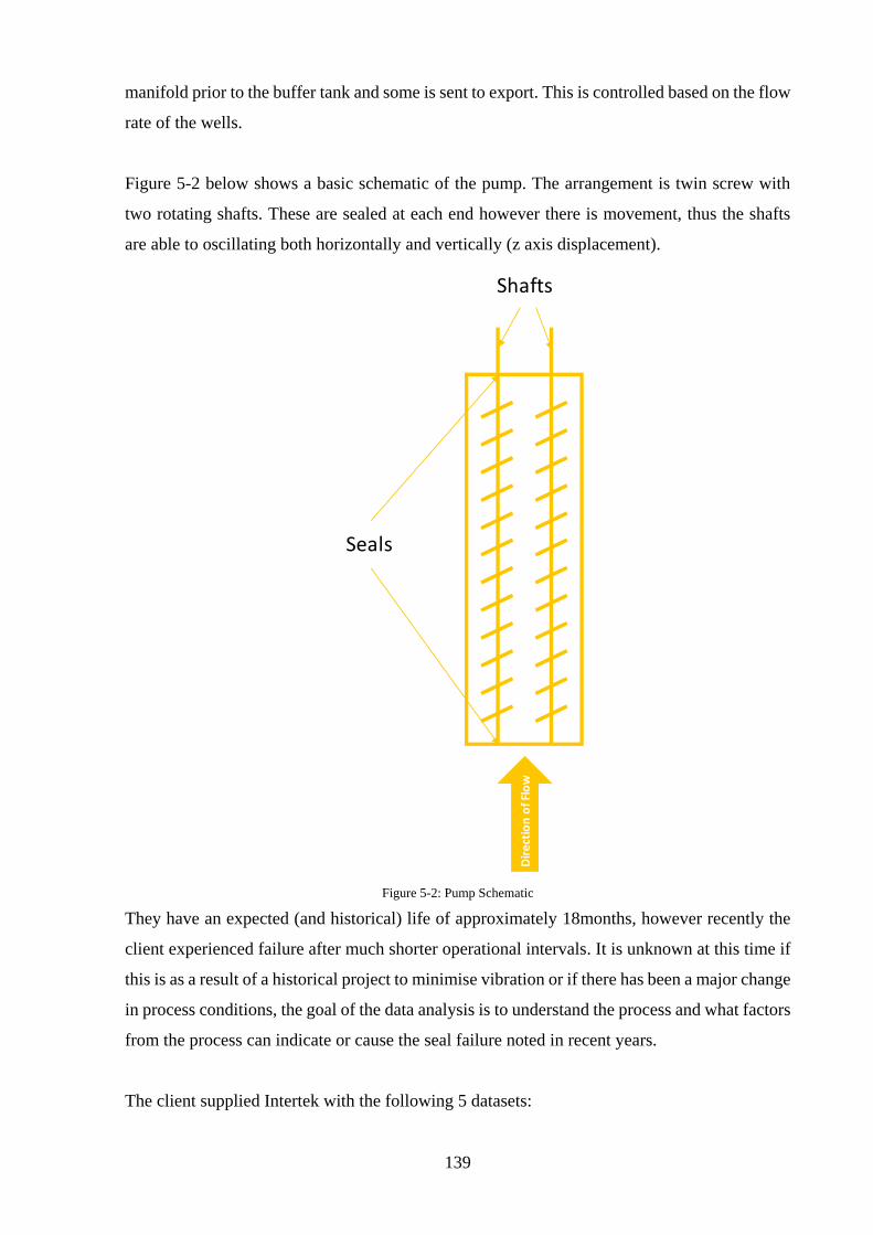
139
manifold prior to the buffer tank and some is sent to export. This is controlled based on the flow
rate of the wells.
Figure 5-2 below shows a basic schematic of the pump. The arrangement is twin screw with
two rotating shafts. These are sealed at each end however there is movement, thus the shafts
are able to oscillating both horizontally and vertically (z axis displacement).
Figure 5-2: Pump Schematic
They have an expected (and historical) life of approximately 18months, however recently the
client experienced failure after much shorter operational intervals. It is unknown at this time if
this is as a result of a historical project to minimise vibration or if there has been a major change
in process conditions, the goal of the data analysis is to understand the process and what factors
from the process can indicate or cause the seal failure noted in recent years.
The client supplied Intertek with the following 5 datasets:
PumpSeals
Shafts
Dir
ect
ion
of
Flo
w
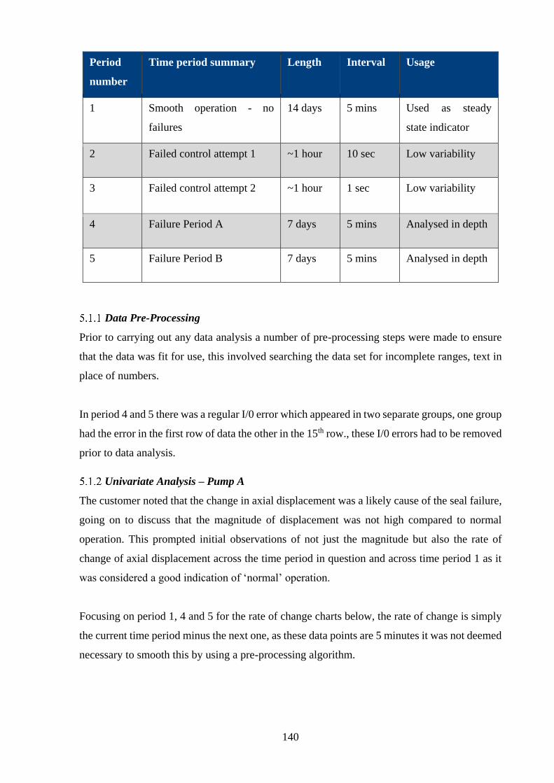
140
Period
number
Time period summary Length Interval Usage
1 Smooth operation - no
failures
14 days 5 mins Used as steady
state indicator
2 Failed control attempt 1 ~1 hour 10 sec Low variability
3 Failed control attempt 2 ~1 hour 1 sec Low variability
4 Failure Period A 7 days 5 mins Analysed in depth
5 Failure Period B 7 days 5 mins Analysed in depth
Data Pre-Processing
Prior to carrying out any data analysis a number of pre-processing steps were made to ensure
that the data was fit for use, this involved searching the data set for incomplete ranges, text in
place of numbers.
In period 4 and 5 there was a regular I/0 error which appeared in two separate groups, one group
had the error in the first row of data the other in the 15th row., these I/0 errors had to be removed
prior to data analysis.
Univariate Analysis – Pump A
The customer noted that the change in axial displacement was a likely cause of the seal failure,
going on to discuss that the magnitude of displacement was not high compared to normal
operation. This prompted initial observations of not just the magnitude but also the rate of
change of axial displacement across the time period in question and across time period 1 as it
was considered a good indication of ‘normal’ operation.
Focusing on period 1, 4 and 5 for the rate of change charts below, the rate of change is simply
the current time period minus the next one, as these data points are 5 minutes it was not deemed
necessary to smooth this by using a pre-processing algorithm.

141
As can be seen below, when looking at ZI-37261A (z axis displacement sensor), throughout
period 1 (Figure 5-3) and period 4 (Figure 5-4) pump A has a very small rate of change of axial
displacement, the blue line is the rate of change and the red is the actual value of the sensor.
The only exception to this small rate of change is noted at the end of period 4 when there is a
sudden change in axial displacement caused by pump B shutting down due to seal failure. This
change is so large that the shaft actually moves past its calibrated 0 and hence shows as a
negative displacement.
This also demonstrates that the two pumps interact with one another to a certain extent and this
could be due to a number of factors including the physical proximity of the two units or (more
likely) the common discharge.
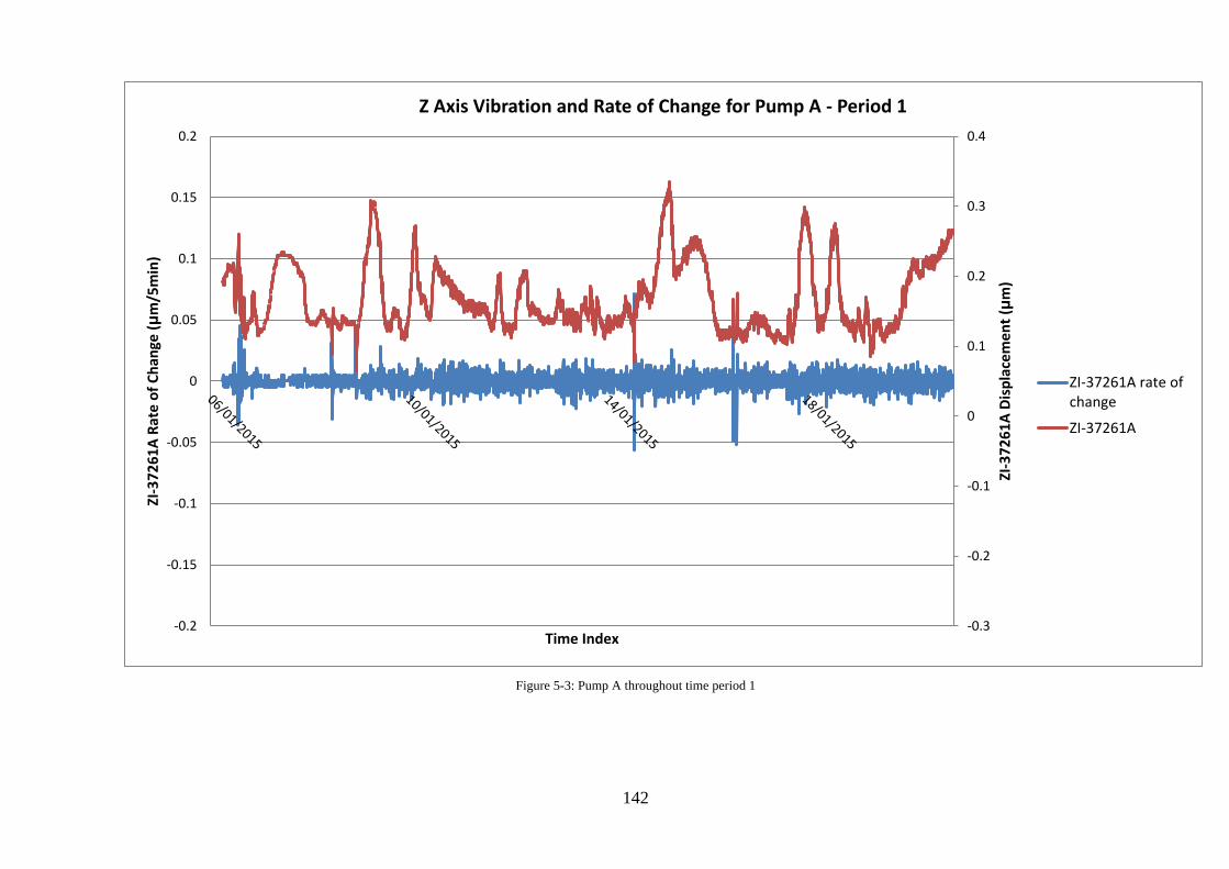
142
Figure 5-3: Pump A throughout time period 1
-0.3
-0.2
-0.1
0
0.1
0.2
0.3
0.4
-0.2
-0.15
-0.1
-0.05
0
0.05
0.1
0.15
0.2
ZI-3
72
61
A D
isp
lace
me
nt
(μm
)
ZI-3
72
61
A R
ate
of
Ch
ange
(μ
m/5
min
)
Time Index
Z Axis Vibration and Rate of Change for Pump A - Period 1
ZI-37261A rate ofchange
ZI-37261A
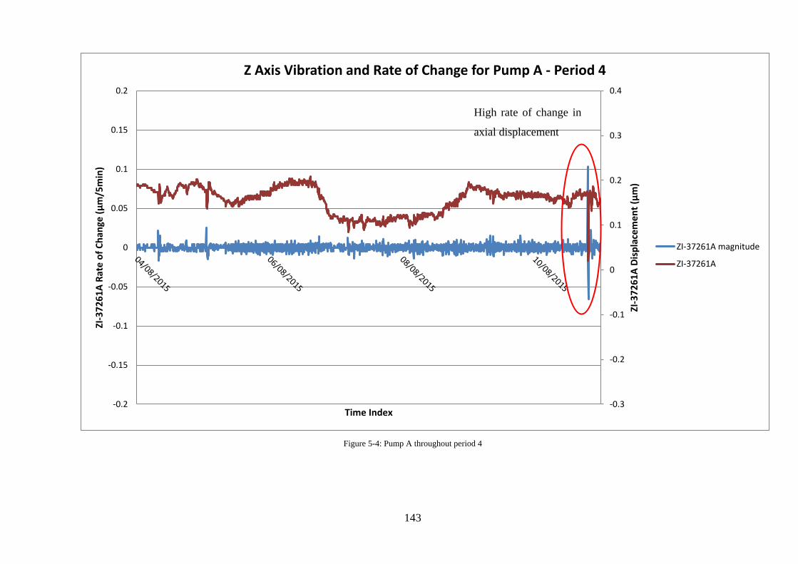
143
Figure 5-4: Pump A throughout period 4
-0.3
-0.2
-0.1
0
0.1
0.2
0.3
0.4
-0.2
-0.15
-0.1
-0.05
0
0.05
0.1
0.15
0.2
ZI-3
72
61
A D
isp
lace
me
nt
(μm
)
ZI-3
72
61
A R
ate
of
Ch
ange
(μ
m/5
min
)
Time Index
Z Axis Vibration and Rate of Change for Pump A - Period 4
ZI-37261A magnitude
ZI-37261A
High rate of change in
axial displacement

144
In Figure 5-5 which examines ZI-37261A (z axis displacement sensor) for pump A in period 5
there only one pump in operation (pump A), however, towards the end of the period pump A is
initially shut down and attempts are made to restart B which ultimately are unsuccessful. After
this A is brought back online again but subsequently suffers a seal failure and has to be shut
down. As only one pump is online throughout time period 5 it may have slightly different
characteristics to a time when both pumps are running.
In Figure 5-5 there are three clear periods where there is a sudden change in the axial
displacement as shown by high values on the rate of change plot (blue). Event 3 is the point
where the pump shuts down due to the failure of the seal.
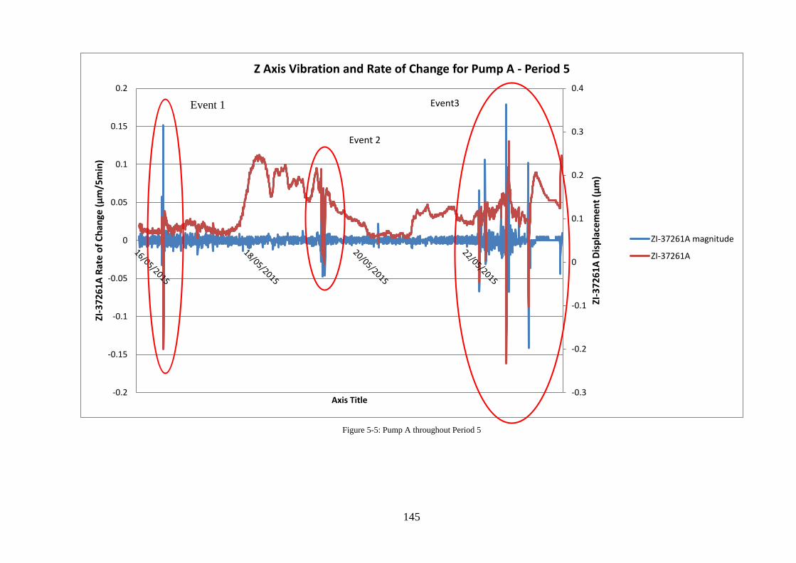
145
Figure 5-5: Pump A throughout Period 5
-0.3
-0.2
-0.1
0
0.1
0.2
0.3
0.4
-0.2
-0.15
-0.1
-0.05
0
0.05
0.1
0.15
0.2
ZI-3
72
61
A D
isp
lace
me
nt
(μm
)
ZI-3
72
61
A R
ate
of
Ch
ange
(μ
m/5
min
)
Axis Title
Z Axis Vibration and Rate of Change for Pump A - Period 5
ZI-37261A magnitude
ZI-37261A
Event 2
Event3Event 1
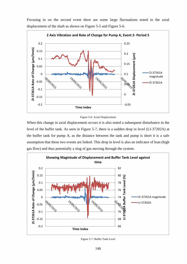
146
Focusing in on the second event there are some large fluctuations noted in the axial
displacement of the shaft as shown on Figure 5-5 and Figure 5-6.
Figure 5-6: Axial Displacement
When this change in axial displacement occurs it is also noted a subsequent disturbance in the
level of the buffer tank. As seen in Figure 5-7, there is a sudden drop in level (LI-37202A) at
the buffer tank for pump A, as the distance between the tank and pump is short it is a safe
assumption that these two events are linked. This drop in level is also an indicator of lean (high
gas flow) and thus potentially a slug of gas moving through the system.
Figure 5-7: Buffer Tank Level
-0.05
0
0.05
0.1
0.15
0.2
0.25
-0.2
-0.15
-0.1
-0.05
0
0.05
0.1
0.15
0.2
ZI-3
72
61
A D
isp
lace
me
nt
(μm
)
ZI-3
72
61
A R
ate
of
Ch
ange
(μ
m/5
min
)
Time Index
Z Axis Vibration and Rate of Change for Pump A, Event 2- Period 5
ZI-37261Amagnitude
ZI-37261A
66
68
70
72
74
76
78
80
82
-0.2
-0.15
-0.1
-0.05
0
0.05
0.1
0.15
0.2
LI-3
72
02
A B
uff
er
Tan
k Le
vel (
%)
ZI-3
72
61
A R
ate
of
Ch
ange
(μ
m/5
min
)
Time Index
Showing Magintude of Displacement and Buffer Tank Level against time
ZI-37261A magnitude
LI-37202A
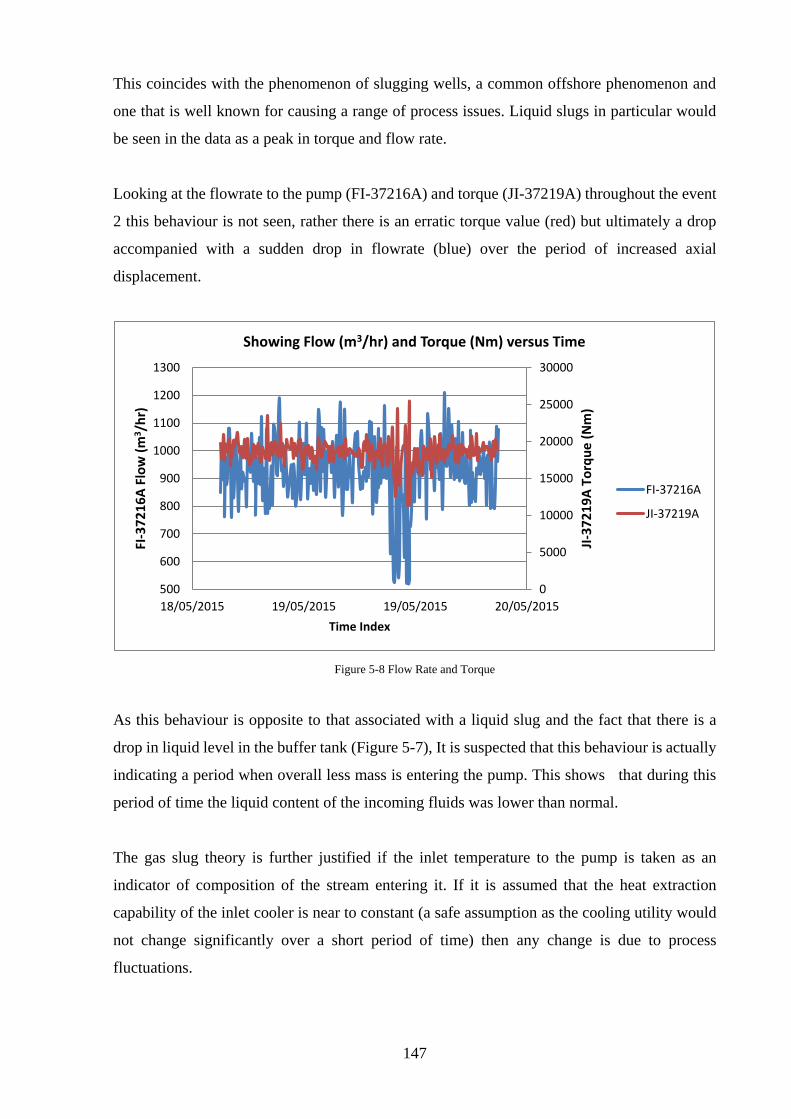
147
This coincides with the phenomenon of slugging wells, a common offshore phenomenon and
one that is well known for causing a range of process issues. Liquid slugs in particular would
be seen in the data as a peak in torque and flow rate.
Looking at the flowrate to the pump (FI-37216A) and torque (JI-37219A) throughout the event
2 this behaviour is not seen, rather there is an erratic torque value (red) but ultimately a drop
accompanied with a sudden drop in flowrate (blue) over the period of increased axial
displacement.
Figure 5-8 Flow Rate and Torque
As this behaviour is opposite to that associated with a liquid slug and the fact that there is a
drop in liquid level in the buffer tank (Figure 5-7), It is suspected that this behaviour is actually
indicating a period when overall less mass is entering the pump. This shows that during this
period of time the liquid content of the incoming fluids was lower than normal.
The gas slug theory is further justified if the inlet temperature to the pump is taken as an
indicator of composition of the stream entering it. If it is assumed that the heat extraction
capability of the inlet cooler is near to constant (a safe assumption as the cooling utility would
not change significantly over a short period of time) then any change is due to process
fluctuations.
0
5000
10000
15000
20000
25000
30000
500
600
700
800
900
1000
1100
1200
1300
18/05/2015 19/05/2015 19/05/2015 20/05/2015
JI-3
72
19
A T
orq
ue
(N
m)
FI-3
72
16
A F
low
(m
3/h
r)
Time Index
Showing Flow (m3/hr) and Torque (Nm) versus Time
FI-37216A
JI-37219A
148
Therefore, an increase in temperature would show that the incoming energy from the system ad
also increased and this could be caused by one or a combination of the following: a general
temperature increase of the fluids, an increase in total flowrate or an increase in the liquid
fraction. Conversely if a temperature drop was noted it would indicate a combination of a
reduction in specific heat capacity of the fluid (i.e. more gaseous), a drop in temperature for the
system or an overall reduction in flowrate.
Figure 5-9 shows the DP vs inlet temperature for pump A in period 5, coloured by events. Event
1 is the large axial displacement change noted at the beginning of the period, event 2 is the
event discussed in detail earlier.
As can be seen event 2 begins in the main cluster, then moves to an area of lower temperature
and DP, indicating a reduction in flowrate or a reduction in specific heat capacity, showing
either a disruption in flow or a change in density and then returning to the cluster which
indicates normal operation. Event 1 goes through a very similar process but with much lower
temperatures. Event 3 is the actual failure event, again is very similar to the two others, but
most closely resembles event 1.
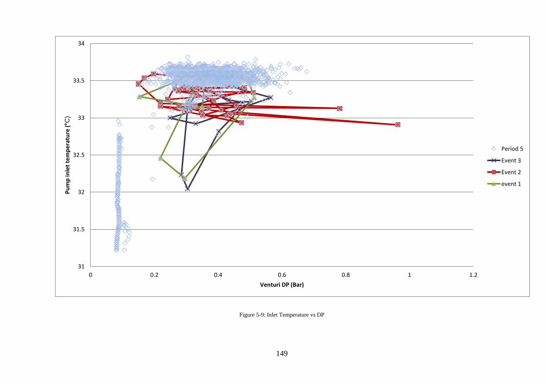
149
Figure 5-9: Inlet Temperature vs DP
31
31.5
32
32.5
33
33.5
34
0 0.2 0.4 0.6 0.8 1 1.2
Pu
mp
inle
t te
mp
era
ture
(°C
)
Venturi DP (Bar)
Period 5
Event 3
Event 2
event 1

150
All three of these events were similar as they all had a high rate of change in axial displacement
of the pump. In conclusion, the failure event can be categorised by a large change in axial
displacement in the pump, the cause of this will require further investigation using multivariate
analysis.
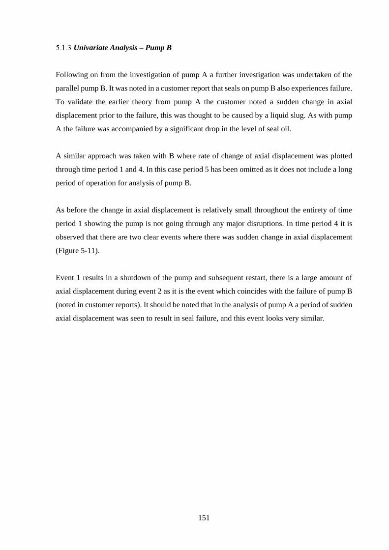
151
Univariate Analysis – Pump B
Following on from the investigation of pump A a further investigation was undertaken of the
parallel pump B. It was noted in a customer report that seals on pump B also experiences failure.
To validate the earlier theory from pump A the customer noted a sudden change in axial
displacement prior to the failure, this was thought to be caused by a liquid slug. As with pump
A the failure was accompanied by a significant drop in the level of seal oil.
A similar approach was taken with B where rate of change of axial displacement was plotted
through time period 1 and 4. In this case period 5 has been omitted as it does not include a long
period of operation for analysis of pump B.
As before the change in axial displacement is relatively small throughout the entirety of time
period 1 showing the pump is not going through any major disruptions. In time period 4 it is
observed that there are two clear events where there was sudden change in axial displacement
(Figure 5-11).
Event 1 results in a shutdown of the pump and subsequent restart, there is a large amount of
axial displacement during event 2 as it is the event which coincides with the failure of pump B
(noted in customer reports). It should be noted that in the analysis of pump A a period of sudden
axial displacement was seen to result in seal failure, and this event looks very similar.
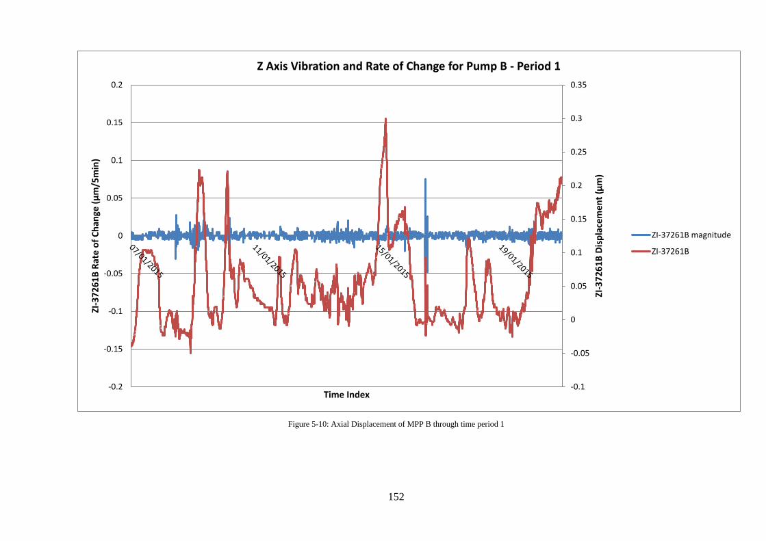
152
Figure 5-10: Axial Displacement of MPP B through time period 1
-0.1
-0.05
0
0.05
0.1
0.15
0.2
0.25
0.3
0.35
-0.2
-0.15
-0.1
-0.05
0
0.05
0.1
0.15
0.2
ZI-3
72
61
B D
isp
lace
me
nt
(μm
)
ZI-3
72
61
B R
ate
of
Ch
ange
(μ
m/5
min
)
Time Index
Z Axis Vibration and Rate of Change for Pump B - Period 1
ZI-37261B magnitude
ZI-37261B
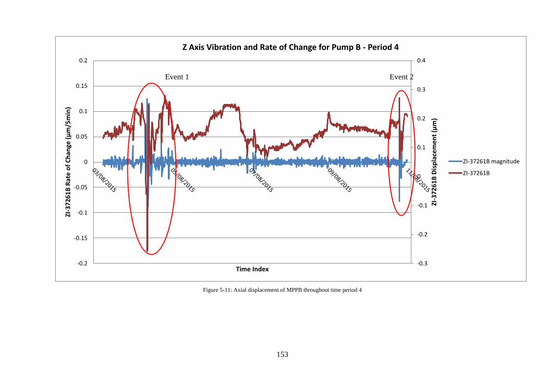
153
Figure 5-11: Axial displacement of MPPB throughout time period 4
-0.3
-0.2
-0.1
0
0.1
0.2
0.3
0.4
-0.2
-0.15
-0.1
-0.05
0
0.05
0.1
0.15
0.2
ZI-3
72
61
B D
isp
lace
me
nt
(μm
)
ZI-3
72
61
B R
ate
of
Ch
ange
(μ
m/5
min
)
Time Index
Z Axis Vibration and Rate of Change for Pump B - Period 4
ZI-37261B magnitude
ZI-37261B
Event 1 Event 2
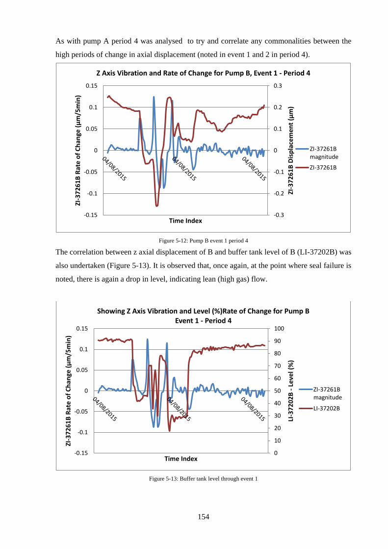
154
As with pump A period 4 was analysed to try and correlate any commonalities between the
high periods of change in axial displacement (noted in event 1 and 2 in period 4).
Figure 5-12: Pump B event 1 period 4
The correlation between z axial displacement of B and buffer tank level of B (LI-37202B) was
also undertaken (Figure 5-13). It is observed that, once again, at the point where seal failure is
noted, there is again a drop in level, indicating lean (high gas) flow.
Figure 5-13: Buffer tank level through event 1
-0.3
-0.2
-0.1
0
0.1
0.2
0.3
-0.15
-0.1
-0.05
0
0.05
0.1
0.15
ZI-3
72
61
B D
isp
lace
me
nt
(μm
)
ZI-3
72
61
B R
ate
of
Ch
ange
(μ
m/5
min
)
Time Index
Z Axis Vibration and Rate of Change for Pump B, Event 1 - Period 4
ZI-37261Bmagnitude
ZI-37261B
0
10
20
30
40
50
60
70
80
90
100
-0.15
-0.1
-0.05
0
0.05
0.1
0.15
LI-3
72
02
B -
Leve
l (%
)
ZI-3
72
61
B R
ate
of
Ch
ange
(μ
m/5
min
)
Time Index
Showing Z Axis Vibration and Level (%)Rate of Change for Pump B Event 1 - Period 4
ZI-37261Bmagnitude
LI-37202B
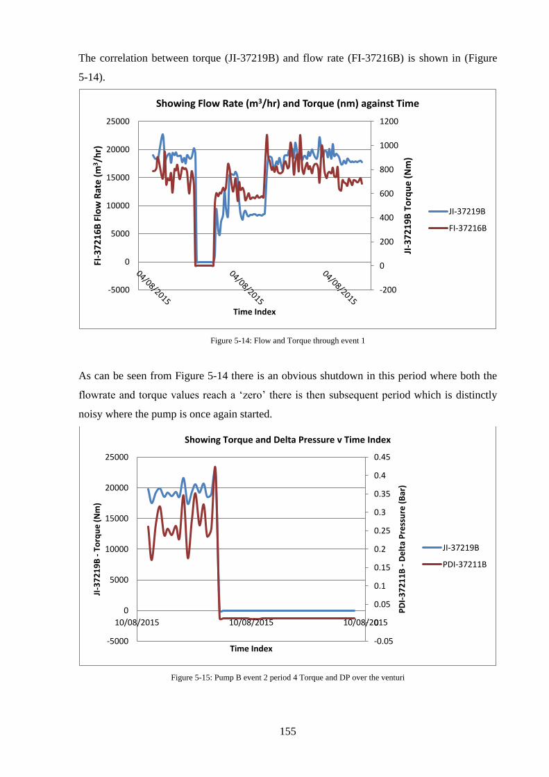
155
The correlation between torque (JI-37219B) and flow rate (FI-37216B) is shown in (Figure
5-14).
Figure 5-14: Flow and Torque through event 1
As can be seen from Figure 5-14 there is an obvious shutdown in this period where both the
flowrate and torque values reach a ‘zero’ there is then subsequent period which is distinctly
noisy where the pump is once again started.
Figure 5-15: Pump B event 2 period 4 Torque and DP over the venturi
-200
0
200
400
600
800
1000
1200
-5000
0
5000
10000
15000
20000
25000
JI-3
72
19
B T
orq
ue
(N
m)
FI-3
72
16
B F
low
Rat
e (
m3/h
r)
Time Index
Showing Flow Rate (m3/hr) and Torque (nm) against Time
JI-37219B
FI-37216B
-0.05
0
0.05
0.1
0.15
0.2
0.25
0.3
0.35
0.4
0.45
-5000
0
5000
10000
15000
20000
25000
10/08/2015 10/08/2015 10/08/2015
PD
I-3
72
11
B -
De
lta
Pre
ssu
re (
Bar
)
JI-3
72
19
B -
Torq
ue
(N
m)
Time Index
Showing Torque and Delta Pressure v Time Index
JI-37219B
PDI-37211B
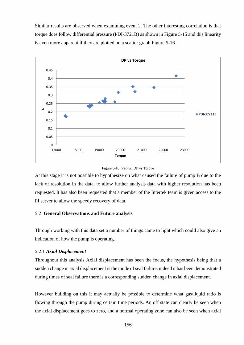
156
Similar results are observed when examining event 2. The other interesting correlation is that
torque does follow differential pressure (PDI-3721B) as shown in Figure 5-15 and this linearity
is even more apparent if they are plotted on a scatter graph Figure 5-16.
Figure 5-16: Venturi DP vs Torque
At this stage it is not possible to hypothesize on what caused the failure of pump B due to the
lack of resolution in the data, to allow further analysis data with higher resolution has been
requested. It has also been requested that a member of the Intertek team is given access to the
PI server to allow the speedy recovery of data.
General Observations and Future analysis
Through working with this data set a number of things came to light which could also give an
indication of how the pump is operating.
Axial Displacement
Throughout this analysis Axial displacement has been the focus, the hypothesis being that a
sudden change in axial displacement is the mode of seal failure, indeed it has been demonstrated
during times of seal failure there is a corresponding sudden change in axial displacement.
However building on this it may actually be possible to determine what gas/liquid ratio is
flowing through the pump during certain time periods. An off state can clearly be seen when
the axial displacement goes to zero, and a normal operating zone can also be seen when axial
0
0.05
0.1
0.15
0.2
0.25
0.3
0.35
0.4
0.45
17000 18000 19000 20000 21000 22000 23000
DP
Torque
DP vs Torque
PDI-37211B
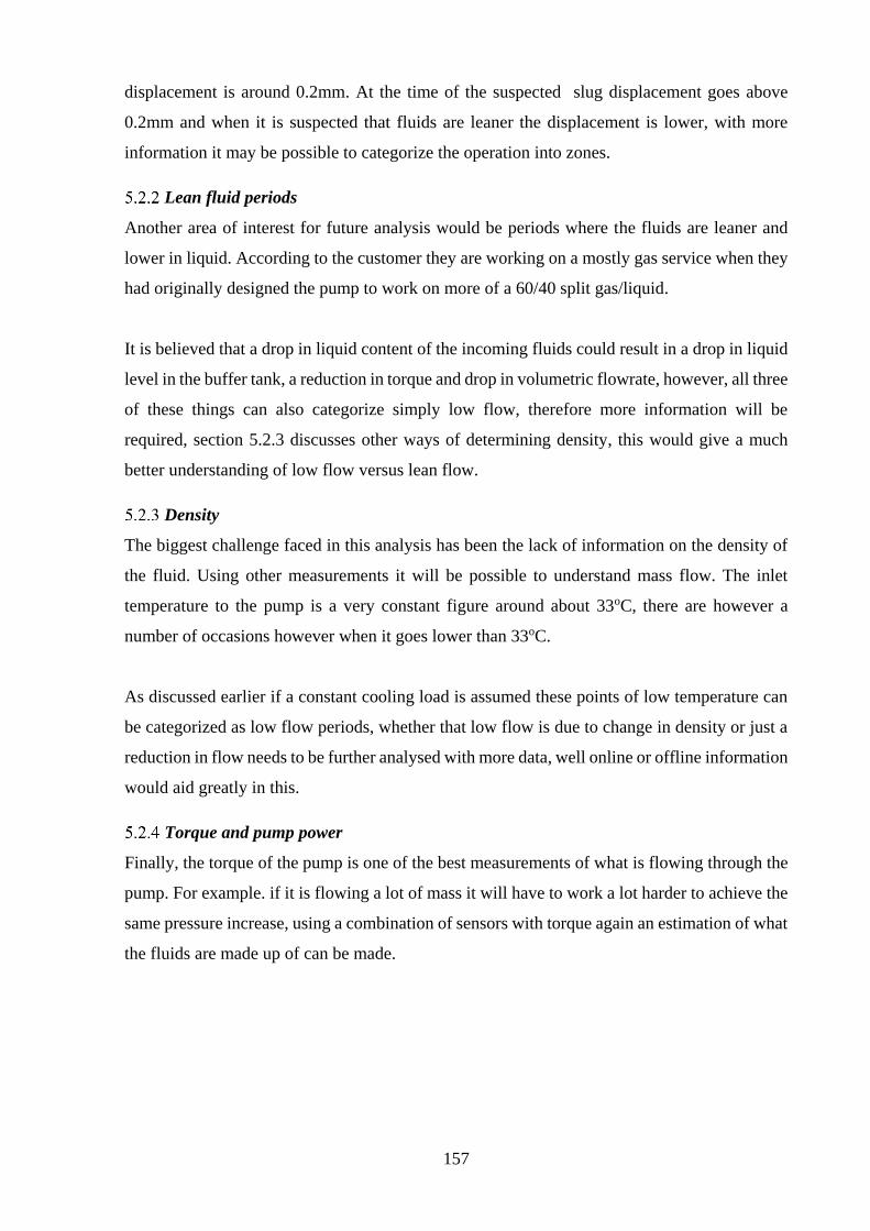
157
displacement is around 0.2mm. At the time of the suspected slug displacement goes above
0.2mm and when it is suspected that fluids are leaner the displacement is lower, with more
information it may be possible to categorize the operation into zones.
Lean fluid periods
Another area of interest for future analysis would be periods where the fluids are leaner and
lower in liquid. According to the customer they are working on a mostly gas service when they
had originally designed the pump to work on more of a 60/40 split gas/liquid.
It is believed that a drop in liquid content of the incoming fluids could result in a drop in liquid
level in the buffer tank, a reduction in torque and drop in volumetric flowrate, however, all three
of these things can also categorize simply low flow, therefore more information will be
required, section 5.2.3 discusses other ways of determining density, this would give a much
better understanding of low flow versus lean flow.
Density
The biggest challenge faced in this analysis has been the lack of information on the density of
the fluid. Using other measurements it will be possible to understand mass flow. The inlet
temperature to the pump is a very constant figure around about 33oC, there are however a
number of occasions however when it goes lower than 33oC.
As discussed earlier if a constant cooling load is assumed these points of low temperature can
be categorized as low flow periods, whether that low flow is due to change in density or just a
reduction in flow needs to be further analysed with more data, well online or offline information
would aid greatly in this.
Torque and pump power
Finally, the torque of the pump is one of the best measurements of what is flowing through the
pump. For example. if it is flowing a lot of mass it will have to work a lot harder to achieve the
same pressure increase, using a combination of sensors with torque again an estimation of what
the fluids are made up of can be made.
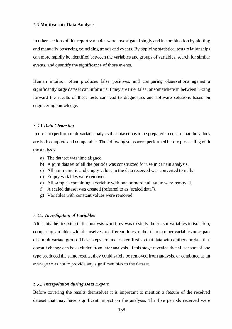
158
Multivariate Data Analysis
In other sections of this report variables were investigated singly and in combination by plotting
and manually observing coinciding trends and events. By applying statistical tests relationships
can more rapidly be identified between the variables and groups of variables, search for similar
events, and quantify the significance of those events.
Human intuition often produces false positives, and comparing observations against a
significantly large dataset can inform us if they are true, false, or somewhere in between. Going
forward the results of these tests can lead to diagnostics and software solutions based on
engineering knowledge.
Data Cleansing
In order to perform multivariate analysis the dataset has to be prepared to ensure that the values
are both complete and comparable. The following steps were performed before proceeding with
the analysis.
a) The dataset was time aligned.
b) A joint dataset of all the periods was constructed for use in certain analysis.
c) All non-numeric and empty values in the data received was converted to nulls
d) Empty variables were removed
e) All samples containing a variable with one or more null value were removed.
f) A scaled dataset was created (referred to as ‘scaled data’).
g) Variables with constant values were removed.
Investigation of Variables
After this the first step in the analysis workflow was to study the sensor variables in isolation,
comparing variables with themselves at different times, rather than to other variables or as part
of a multivariate group. These steps are undertaken first so that data with outliers or data that
doesn’t change can be excluded from later analysis. If this stage revealed that all sensors of one
type produced the same results, they could safely be removed from analysis, or combined as an
average so as not to provide any significant bias to the dataset.
Interpolation during Data Export
Before covering the results themselves it is important to mention a feature of the received
dataset that may have significant impact on the analysis. The five periods received were
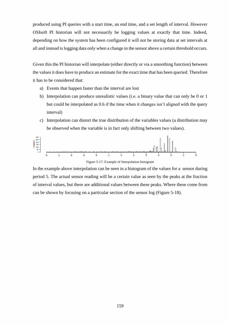
159
produced using PI queries with a start time, an end time, and a set length of interval. However
OSIsoft PI historian will not necessarily be logging values at exactly that time. Indeed,
depending on how the system has been configured it will not be storing data at set intervals at
all and instead is logging data only when a change in the sensor above a certain threshold occurs.
Given this the PI historian will interpolate (either directly or via a smoothing function) between
the values it does have to produce an estimate for the exact time that has been queried. Therefore
it has to be considered that:
a) Events that happen faster than the interval are lost
b) Interpolation can produce unrealistic values (i.e. a binary value that can only be 0 or 1
but could be interpolated as 0.6 if the time when it changes isn’t aligned with the query
interval)
c) Interpolation can distort the true distribution of the variables values (a distribution may
be observed when the variable is in fact only shifting between two values).
Figure 5-17: Example of Interpolation histogram
In the example above interpolation can be seen in a histogram of the values for a sensor during
period 5. The actual sensor reading will be a certain value as seen by the peaks at the fraction
of interval values, but there are additional values between these peaks. Where these come from
can be shown by focusing on a particular section of the sensor log (Figure 5-18).
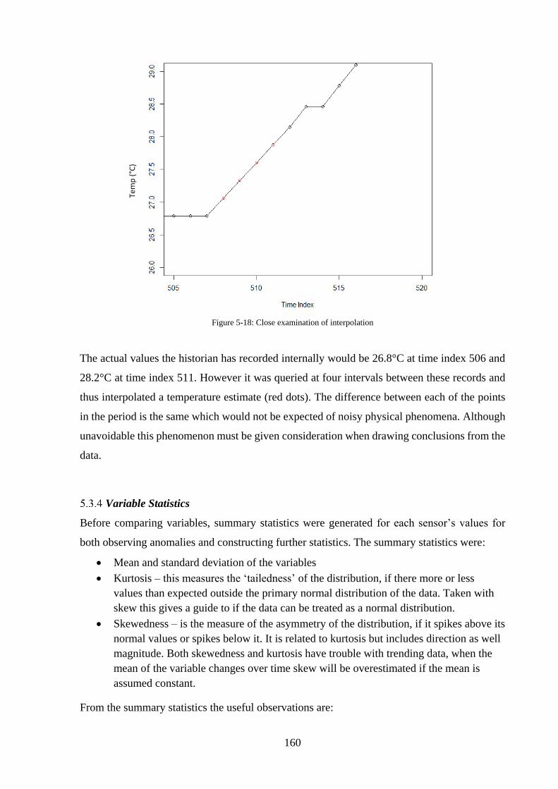
160
Figure 5-18: Close examination of interpolation
The actual values the historian has recorded internally would be 26.8°C at time index 506 and
28.2°C at time index 511. However it was queried at four intervals between these records and
thus interpolated a temperature estimate (red dots). The difference between each of the points
in the period is the same which would not be expected of noisy physical phenomena. Although
unavoidable this phenomenon must be given consideration when drawing conclusions from the
data.
Variable Statistics
Before comparing variables, summary statistics were generated for each sensor’s values for
both observing anomalies and constructing further statistics. The summary statistics were:
• Mean and standard deviation of the variables
• Kurtosis – this measures the ‘tailedness’ of the distribution, if there more or less
values than expected outside the primary normal distribution of the data. Taken with
skew this gives a guide to if the data can be treated as a normal distribution.
• Skewedness – is the measure of the asymmetry of the distribution, if it spikes above its
normal values or spikes below it. It is related to kurtosis but includes direction as well
magnitude. Both skewedness and kurtosis have trouble with trending data, when the
mean of the variable changes over time skew will be overestimated if the mean is
assumed constant.
From the summary statistics the useful observations are:
Tem
p (
°C)

161
a) The values for sensors of motor RPM and torque on both pumps have zero standard
deviation and do not change within the dataset. They are therefore not useful for
statistical analysis and have been discarded
b) Period 3 is only for 1 hour and as a consequence many variables do not change over
its time. This suggests period 3 is less useful for statistical analysis.
c) Periods 1 and 5 had the most skewedness results for pump A, this implies either that in
these periods the pump was more unstable or saw a significant shift in operation.
Period 4 is similar for pump B. Although the events causing these are known (A shuts
down in period 5, B in period 4, and A is turned down in period 1) it is useful to see
how high level summary statistics can quickly categorise and compare the data.
d) Period 4 has the lowest kurtosis, suggesting the values for the sensors are the closest to
a normal distribution during this period, with fewer large outliers or data trending.
Variable Histograms
Following from summary statistics, particularly after observing the high skew value of some
variables, distributions can then be directly visualised. Producing histograms of the frequency
of the values for the variables in each period will provide a way to spot interpolation, outlier
events, and the overall differences between the periods.
For example in the histogram of a temperature sensor from pump B (Figure 5-19) it can be
seen that periods 1 and 4 are broadly comparable with one or more outliers of lower temperature
in period 4. It can also be seen that period 5 is substantially different, and periods 2 and 3 are
both small samples of the larger distribution seen in period 1 & 4.
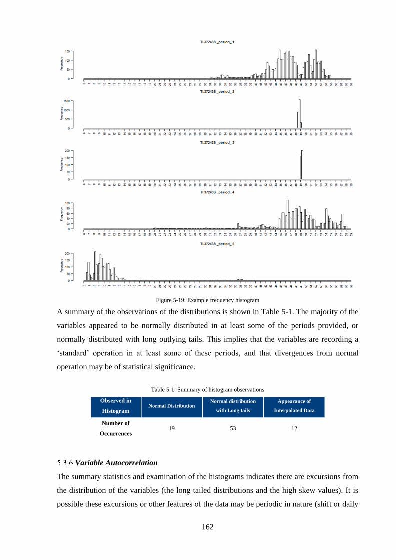
162
Figure 5-19: Example frequency histogram
A summary of the observations of the distributions is shown in Table 5-1. The majority of the
variables appeared to be normally distributed in at least some of the periods provided, or
normally distributed with long outlying tails. This implies that the variables are recording a
‘standard’ operation in at least some of these periods, and that divergences from normal
operation may be of statistical significance.
Table 5-1: Summary of histogram observations
Observed in
Histogram Normal Distribution
Normal distribution
with Long tails
Appearance of
Interpolated Data
Number of
Occurrences 19 53 12
Variable Autocorrelation
The summary statistics and examination of the histograms indicates there are excursions from
the distribution of the variables (the long tailed distributions and the high skew values). It is
possible these excursions or other features of the data may be periodic in nature (shift or daily
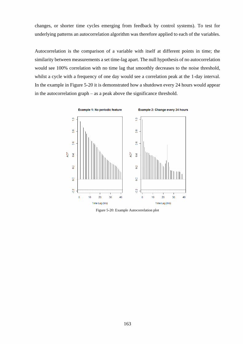
163
changes, or shorter time cycles emerging from feedback by control systems). To test for
underlying patterns an autocorrelation algorithm was therefore applied to each of the variables.
Autocorrelation is the comparison of a variable with itself at different points in time; the
similarity between measurements a set time-lag apart. The null hypothesis of no autocorrelation
would see 100% correlation with no time lag that smoothly decreases to the noise threshold,
whilst a cycle with a frequency of one day would see a correlation peak at the 1-day interval.
In the example in Figure 5-20 it is demonstrated how a shutdown every 24 hours would appear
in the autocorrelation graph – as a peak above the significance threshold.
Figure 5-20: Example Autocorrelation plot
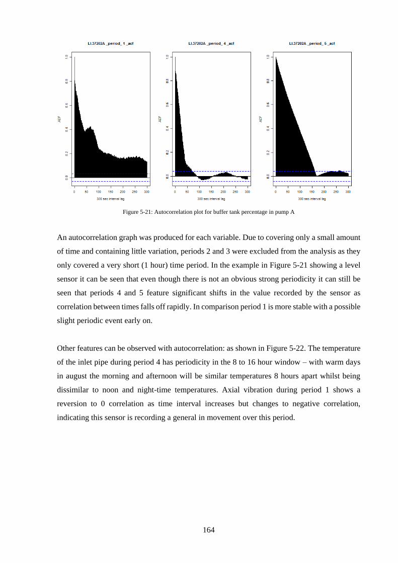
164
Figure 5-21: Autocorrelation plot for buffer tank percentage in pump A
An autocorrelation graph was produced for each variable. Due to covering only a small amount
of time and containing little variation, periods 2 and 3 were excluded from the analysis as they
only covered a very short (1 hour) time period. In the example in Figure 5-21 showing a level
sensor it can be seen that even though there is not an obvious strong periodicity it can still be
seen that periods 4 and 5 feature significant shifts in the value recorded by the sensor as
correlation between times falls off rapidly. In comparison period 1 is more stable with a possible
slight periodic event early on.
Other features can be observed with autocorrelation: as shown in Figure 5-22. The temperature
of the inlet pipe during period 4 has periodicity in the 8 to 16 hour window – with warm days
in august the morning and afternoon will be similar temperatures 8 hours apart whilst being
dissimilar to noon and night-time temperatures. Axial vibration during period 1 shows a
reversion to 0 correlation as time interval increases but changes to negative correlation,
indicating this sensor is recording a general in movement over this period.

165
Figure 5-22: Inlet Temperature (left) and axial vibration (right)
It was noted that other sensors also demonstrated some periodic correlation including additional
temperature sensors showing periodic variation in line with ambient temperature flow sensors
of a pump exhibiting autocorrelation with its partner suggesting interaction when the two pumps
are flowing.
Comparison of Variables
The second step in the analysis workflow was to compare the sensor variables with each other
(a ‘pairwise’ comparison). With the less statistically interesting variables excluded by the first
stage and a greater understanding of the ranges and periods, pairwise comparison bridges the
gap between univariate and multivariate analysis. Sets of variables with high correlation and
even collinearity will be examined and combined or removed as appropriate prior to the
multivariate analysis, it is also of note that the pairwise comparisons can yield important
discoveries on their own.
Correlation is variables co-varying and indicates some kind of dependent relationship between
the variables. Correlations are useful for grouping variables and developing predictive
relationships to work out the unknown values from known.
Since the previous statistical tests revealed each period is substantially different rather than
forming a continuum of values, it was therefore decided that correlation tests should be
performed on the periods separately and then the results aggregated.
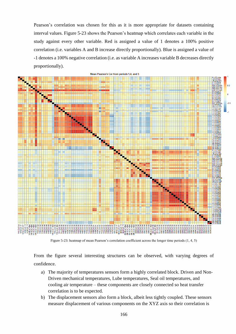
166
Pearson’s correlation was chosen for this as it is more appropriate for datasets containing
interval values. Figure 5-23 shows the Pearson’s heatmap which correlates each variable in the
study against every other variable. Red is assigned a value of 1 denotes a 100% positive
correlation (i.e. variables A and B increase directly proportionally). Blue is assigned a value of
-1 denotes a 100% negative correlation (i.e. as variable A increases variable B decreases directly
proportionally).
Figure 5-23: heatmap of mean Pearson’s correlation coefficient across the longer time periods (1, 4, 5)
From the figure several interesting structures can be observed, with varying degrees of
confidence.
a) The majority of temperatures sensors form a highly correlated block. Driven and Non-
Driven mechanical temperatures, Lube temperatures, Seal oil temperatures, and
cooling air temperature – these components are closely connected so heat transfer
correlation is to be expected.
b) The displacement sensors also form a block, albeit less tightly coupled. These sensors
measure displacement of various components on the XYZ axis so their correlation is
167
understandable. Also, linking this displacement to heat is a sensible assumption as
more energy will drive vibration and cause components to expand.
c) Flow and Torque are correlated with each other and broadly with the temperature
sensors.
d) Several of the pressure sensors are strongly correlated with other pressure sensors in
both pumps, for example lube oil pressure with the pressure of the lube oil pump and
lube oil seal are all correlated.
e) The Seal Oil pressure appears to have negative correlation with nearly all the other
variables within the same pump. This is an interesting relationship as it seems unclear
why the seal oil pressure should vary against all the other values.
f) The controller for Seal Oil Pressure appears to have strong positive correlation with
nearly all the other variables within the same pump, but only in pump A. This
behaviour not being as noticeable in both pumps is interesting and indicates the
correlation is due to outliers.
g) When comparing between pumps, the sensors for non driven end have positive
correlation. This may be due to vibration within the structure of the platform affecting
both pumps at the same time.
h) When comparing between pumps there is a general negative correlation between the
pressures and flows of one pump and the other. This is likely due to two of the periods
provided having one pump shut down whilst the other is turned on.
Correlations within the pump and between the pumps were investigated even though they are
operated independently there may still be feedback or other interaction between the pumps via
the surrounding infrastructure or human operators.
Partial least squares regression
The crucial choice in a PLS investigation is what to use as the objective measurement; in other
invesitgations measures such as production volumes, profit, or composition have been used.
In this study the client emphasised stability as one measure (without an overt quantification)
and seal wearing on the Non-Driven End of the shaft. If stability was to be measured by
frequency of failure events, there aren’t a sufficient number of samples to attempt to fit a PLS
model. One possible proxy for wear on the seals is when the shaft is closer to the end of the
pump – the Z-axis displacement, so a PLS analysis was performed on how the value of Z-axis
displacement varied against all the other non-temperature sensors, with results shown in Figure
5-24.
For pump A in the Z-axis displacement the first two components explain 24% of the variance
in the axial displacement; this is a weak relationship and suggests high variability in the dataset.
The second component features the on/off state of the data, whilst the first component is
composed of the other displacement measures, the pump speed (and pump speed controller),
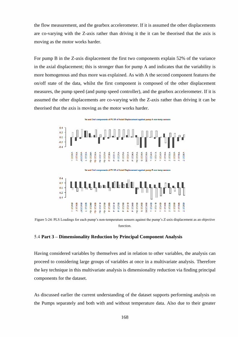
168
the flow measurement, and the gearbox accelerometer. If it is assumed the other displacements
are co-varying with the Z-axis rather than driving it the it can be theorised that the axis is
moving as the motor works harder.
For pump B in the Z-axis displacement the first two components explain 52% of the variance
in the axial displacement; this is stronger than for pump A and indicates that the variability is
more homogenous and thus more was explained. As with A the second component features the
on/off state of the data, whilst the first component is composed of the other displacement
measures, the pump speed (and pump speed controller), and the gearbox accelerometer. If it is
assumed the other displacements are co-varying with the Z-axis rather than driving it can be
theorised that the axis is moving as the motor works harder.
Figure 5-24: PLS Loadings for each pump’s non-temperature sensors against the pump’s Z-axis displacement as an objective
function.
Part 3 – Dimensionality Reduction by Principal Component Analysis
Having considered variables by themselves and in relation to other variables, the analysis can
proceed to considering large groups of variables at once in a multivariate analysis. Therefore
the key technique in this multivariate analysis is dimensionality reduction via finding principal
components for the dataset.
As discussed earlier the current understanding of the dataset supports performing analysis on
the Pumps separately and both with and without temperature data. Also due to their greater
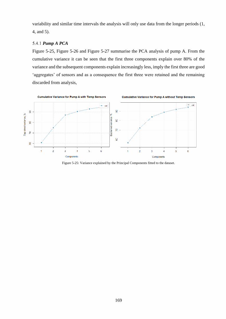
169
variability and similar time intervals the analysis will only use data from the longer periods (1,
4, and 5).
Pump A PCA
Figure 5-25, Figure 5-26 and Figure 5-27 summarise the PCA analysis of pump A. From the
cumulative variance it can be seen that the first three components explain over 80% of the
variance and the subsequent components explain increasingly less, imply the first three are good
‘aggregates’ of sensors and as a consequence the first three were retained and the remaining
discarded from analysis,
Figure 5-25: Variance explained by the Principal Components fitted to the dataset.

170
.
Figure 5-26: Plotting the individual time points by their position each principle component, coloured by the period of origin.
.
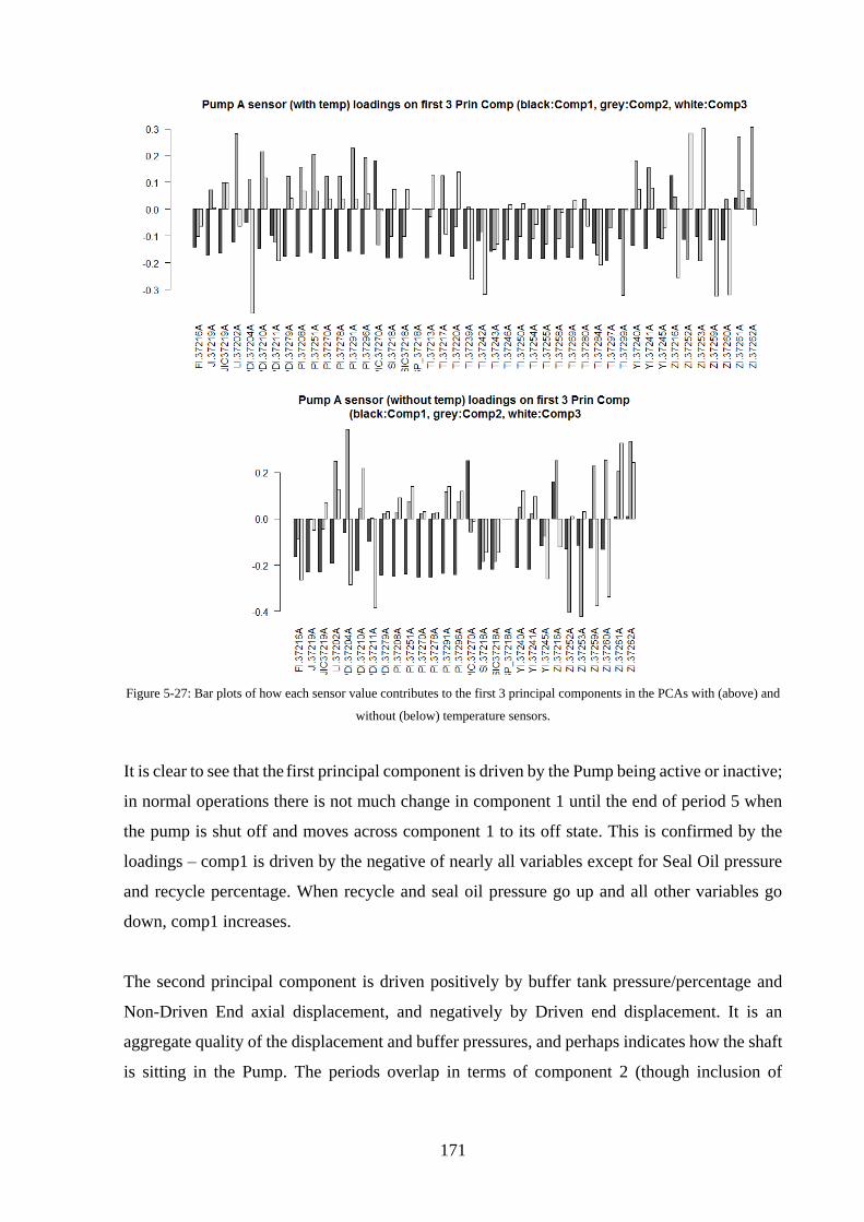
171
Figure 5-27: Bar plots of how each sensor value contributes to the first 3 principal components in the PCAs with (above) and
without (below) temperature sensors.
It is clear to see that the first principal component is driven by the Pump being active or inactive;
in normal operations there is not much change in component 1 until the end of period 5 when
the pump is shut off and moves across component 1 to its off state. This is confirmed by the
loadings – comp1 is driven by the negative of nearly all variables except for Seal Oil pressure
and recycle percentage. When recycle and seal oil pressure go up and all other variables go
down, comp1 increases.
The second principal component is driven positively by buffer tank pressure/percentage and
Non-Driven End axial displacement, and negatively by Driven end displacement. It is an
aggregate quality of the displacement and buffer pressures, and perhaps indicates how the shaft
is sitting in the Pump. The periods overlap in terms of component 2 (though inclusion of
172
temperature separates the generally warmer period 4 out), though it is interesting that period 5
is nearest the off state.
The third principal component also emerges from Non-Driven End displacement, but in
combination with Venturi Pressure differential and discharge flow rather than the buffer tanks.
Although the other components explain more variance, it is possibly component 3 that is most
interesting in terms of best operation during normal circumstances. Again the periods overlap
in terms of component 3, suggesting a ‘normal’ operational envelope.
In the aggregate plot of component 2 against component 3 it can be seen that the various
structures of the periods operation – period 1 begins at higher flow (similar to period 5) before
being moved to a lower flow rate making its values move positive in terms of component 3.
The period 4 cloud has a clear separation between most of the period and the end (when pump
B turns off and more stress is put on pump A), and that ending sees a decrease in component 3.
It is possible that component 3 can be taken as a measure of the ‘stress’ the pump is undergoing.
Taking these components, the path of the pumps variables through the component space over
the course of the periods was investigated. Period 5 data points projected against components
1 and 3 are shown in Figure 5-28, coloured by time. It can be clearly seen that the Pumps state
moves through the ‘normal’ region over time, with numerous excursions at different points over
the seven days, before eventually moving away from the normal region of components 1 and 3
when it reaches the shutdown period in the last half a day. This may provide useful diagnostic
tools if the excursions from the normal can be tied to particular events, and if further data reveals
whether or not that their frequency and structure precedes other shutdowns.
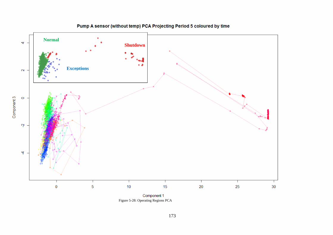
173
Exceptions
Shutdown
Normal
Figure 5-28: Operating Regions PCA
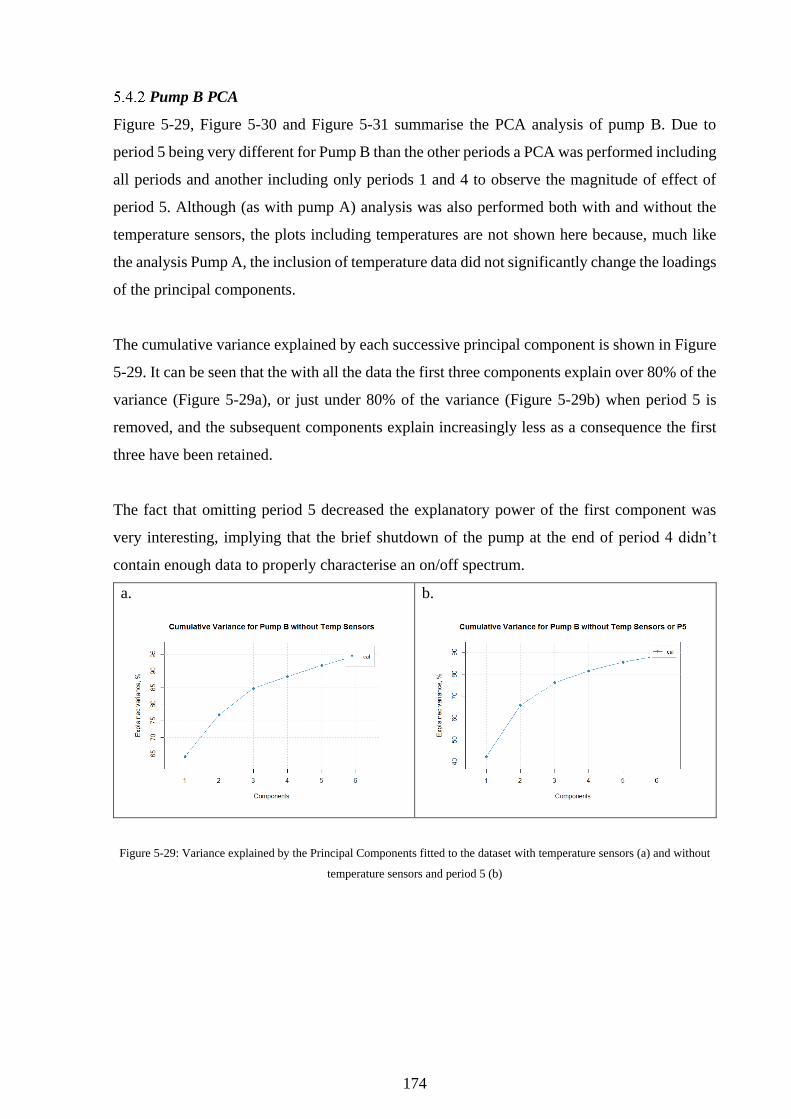
174
Pump B PCA
Figure 5-29, Figure 5-30 and Figure 5-31 summarise the PCA analysis of pump B. Due to
period 5 being very different for Pump B than the other periods a PCA was performed including
all periods and another including only periods 1 and 4 to observe the magnitude of effect of
period 5. Although (as with pump A) analysis was also performed both with and without the
temperature sensors, the plots including temperatures are not shown here because, much like
the analysis Pump A, the inclusion of temperature data did not significantly change the loadings
of the principal components.
The cumulative variance explained by each successive principal component is shown in Figure
5-29. It can be seen that the with all the data the first three components explain over 80% of the
variance (Figure 5-29a), or just under 80% of the variance (Figure 5-29b) when period 5 is
removed, and the subsequent components explain increasingly less as a consequence the first
three have been retained.
The fact that omitting period 5 decreased the explanatory power of the first component was
very interesting, implying that the brief shutdown of the pump at the end of period 4 didn’t
contain enough data to properly characterise an on/off spectrum.
a.
b.
Figure 5-29: Variance explained by the Principal Components fitted to the dataset with temperature sensors (a) and without
temperature sensors and period 5 (b)
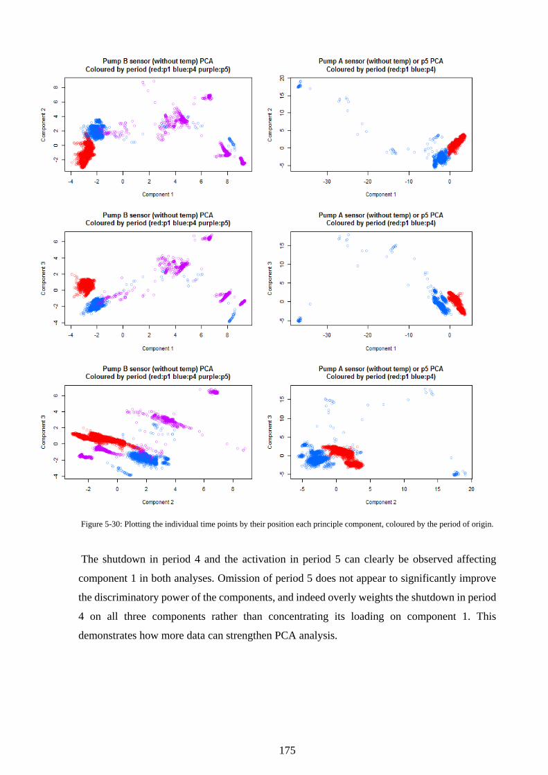
175
Figure 5-30: Plotting the individual time points by their position each principle component, coloured by the period of origin.
The shutdown in period 4 and the activation in period 5 can clearly be observed affecting
component 1 in both analyses. Omission of period 5 does not appear to significantly improve
the discriminatory power of the components, and indeed overly weights the shutdown in period
4 on all three components rather than concentrating its loading on component 1. This
demonstrates how more data can strengthen PCA analysis.
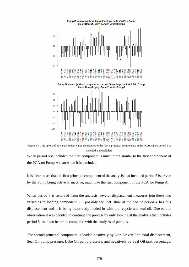
176
Figure 5-31: Bar plots of how each sensor value contributes to the first 3 principal components in the PCAs where period 5 is
included and excluded.
When period 5 is included the first component is much more similar to the first component of
the PCA on Pump A than when it is excluded.
It is clear to see that the first principal component of the analysis that included period 5 is driven
by the Pump being active or inactive, much like the first component of the PCA for Pump A.
When period 5 is removed from the analysis, several displacement measures join these two
variables in loading component 1 – possibly the ‘off’ time at the end of period 4 has this
displacement and it is being incorrectly loaded in with the recycle and seal oil. Due to this
observation it was decided to continue the process by only looking at the analysis that includes
period 5, as it can better be compared with the analysis of pump A.
The second principal component is loaded positively by Non-Driven End axial displacement,
Seal Oil pump pressure, Lube Oil pump pressure, and negatively by Seal Oil tank percentage.
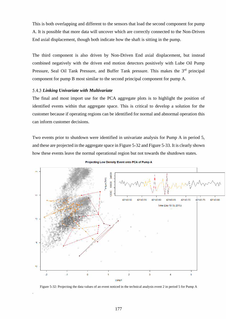
177
This is both overlapping and different to the sensors that load the second component for pump
A. It is possible that more data will uncover which are correctly connected to the Non-Driven
End axial displacement, though both indicate how the shaft is sitting in the pump.
The third component is also driven by Non-Driven End axial displacement, but instead
combined negatively with the driven end motion detectors positively with Lube Oil Pump
Pressure, Seal Oil Tank Pressure, and Buffer Tank pressure. This makes the 3rd principal
component for pump B most similar to the second principal component for pump A.
Linking Univariate with Multivariate
The final and most import use for the PCA aggregate plots is to highlight the position of
identified events within that aggregate space. This is critical to develop a solution for the
customer because if operating regions can be identified for normal and abnormal operation this
can inform customer decisions.
Two events prior to shutdown were identified in univariate analysis for Pump A in period 5,
and these are projected in the aggregate space in Figure 5-32 and Figure 5-33. It is clearly shown
how these events leave the normal operational region but not towards the shutdown states.
Figure 5-32: Projecting the data values of an event noticed in the technical analysis event 2 in period 5 for Pump A
.
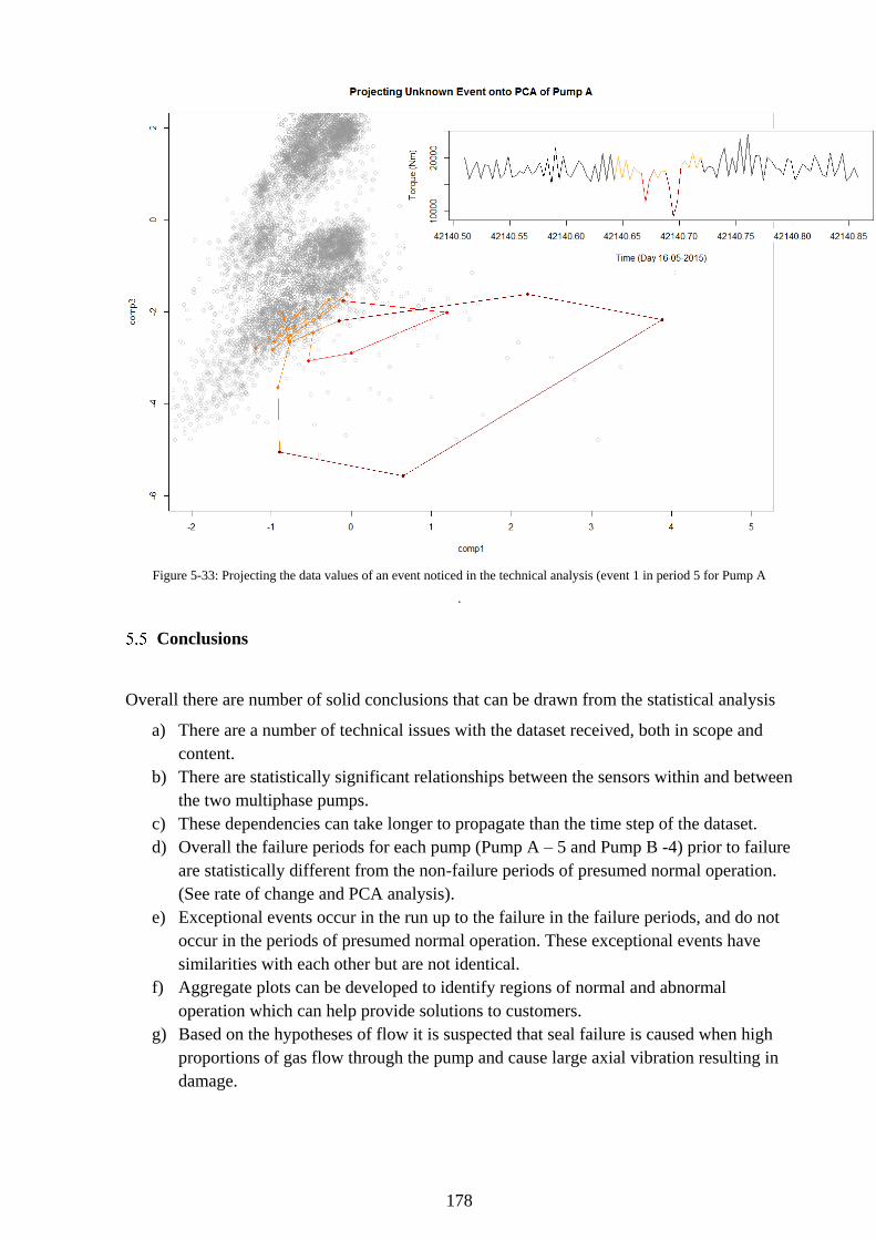
178
Figure 5-33: Projecting the data values of an event noticed in the technical analysis (event 1 in period 5 for Pump A
.
Conclusions
Overall there are number of solid conclusions that can be drawn from the statistical analysis
a) There are a number of technical issues with the dataset received, both in scope and
content.
b) There are statistically significant relationships between the sensors within and between
the two multiphase pumps.
c) These dependencies can take longer to propagate than the time step of the dataset.
d) Overall the failure periods for each pump (Pump A – 5 and Pump B -4) prior to failure
are statistically different from the non-failure periods of presumed normal operation.
(See rate of change and PCA analysis).
e) Exceptional events occur in the run up to the failure in the failure periods, and do not
occur in the periods of presumed normal operation. These exceptional events have
similarities with each other but are not identical.
f) Aggregate plots can be developed to identify regions of normal and abnormal
operation which can help provide solutions to customers.
g) Based on the hypotheses of flow it is suspected that seal failure is caused when high
proportions of gas flow through the pump and cause large axial vibration resulting in
damage.

179
Future directions
Further work will be dependent on data with both greater scope and types beyond the small
number of time periods and sensors provided.
If additional data and resources were available, there are a number of immediate steps to be
taken with the aim of producing additional diagnostic tools and operational insight:
a) With access to the PI historians direct values the analysis can be repeated with greater
certainty in the outcome.
b) Hypotheses can be strengthened or rejected for the operating regions in aggregate
space, and better define their borders if they are confirmed.
c) Furthermore, measures of composition and/or well status would be ideal to align and
characterise the sensor data. Compositional data may help to explain the differences
over time, and diagnostics may need to vary based on which wells are feeding the
pumps.
d) Additional data could help to test if excursions from presumed normal region do occur
prior to failures in a statistically significant manner or not.
e) Further to (a) and (b) software tools could be developed using existing technology to
integrate with the data historian that would identify when excursions are occurring and
offer predictive insights into pump failure probability.

180
Chapter 6:
Conclusions
181
Chapter 6. Conclusion
The Eng.D project was directed at addressing problems in the hydrocarbon-processing sector,
this was undertaken through both the development and implementation of tools to address
identified needs. At the start of the thesis a set of objectives for the research were established
and now the approaches and solutions developed to address each of these objectives will be
examined.
The first two objectives were to develop a methodology for rapid identification of crude oil
composition both online and offline and then implement a tool to facilitate optimisation of crude
blending performance utilising the information from the first objective.
These objectives 1 were met in case study 1 where the application of chemometric modelling
software based on NIR spectra was applied to a major Asian refinery. This was an innovative
approach as successful implementation of NIR in a refinery for gasoline blending was well
understood (Balabin and Safieva, 2008; Balabin, Safieva and Lomakina, 2010) however crude
compositional analysis is not covered in literature sources. This is because of the highly variable
nature of crude oil and the difficulty this brings in developing an appropriate chemometric
model.
The case study demonstrated that whole crude property measurements (i.e. API gravity and
Sulphur) are not a conclusive method of characterising a crude type to give a refinery the real
value of each crude delivery, they are also not sufficient to inform blend optimisation decisions.
A crude oil family was examined and whole crude property measurements suggested one
sample to be of higher value than the rest of the family.
However, implementation of PT5Technology and the chemometric modelling approach
allowed the refiner to quickly and easily assess not only API gravity and Sulphur but also the
distillation properties for this oil. Application of netback calculations to value this crude oil
demonstrated that the refiner was losing >$1/bbl. on each barrel refined given the deviation in
quality.
Using the updated quality information the refinery was able to use the predicted TBP, API
gravity, Sulphur, Pour Point and TAN to update the crude blend properties and perform more
effective economic optimisation.

182
The next objective was to develop an approach to characterise the stability and compatibility of
blended hydrocarbon streams
To meet this objective a new approach was developed to characterise the stability of blended
hydrocarbon streams. Firstly previous work was critiqued, particularly the current ASTM
methodologies (D7060, D7112 and D7157) and the work of Wiehe & Kennedy 1999a and
Wiehe & Kennedy 1999b. This was deemed to be not fully appropriate to addressing the
compatibility issues experienced in blended hydrocarbon streams.
The methodologies use pure materials (such as heptane and toluene) to assess blend stability
and do not blend the oils, hence no account is taken for unexpected interactions between crude
oils when blended. Another major drawback is there is no provision for time dependent blend
stability, which is a well-known phenomenon when dealing with colloidal systems.
The methodology developed was patented and has been granted by the UKIPO. The novel
methodology utilises crude oils in the blend to undertake stability assessments and is able to
assess any time periods of interest.
The method was applied in two case studies. Firstly for blended Heavy Fuel Oil in a Refinery
where observations of stability of HFO blends was undertaken using the proprietary stability
methodology developed as part of the Eng.D project. Based on the set of samples studied it was
concluded that a change in stability was observed in all blends made from blending 1% Sulphur
HFO and 3% Sulphur HFO in the range 1.6% to 2.0% Sulphur.
The change in stability occurred after the time that the HFO was blended and it was shown that
although the sample appeared stable initially, the instability worsened over time. This ability to
characterise time dependent stability is a key feature of the innovative approach.
It was also suspected that a paraffinic HVN diluent would cause instability problems and indeed
increasing the amount of HVN in the blend increased the tendency for instability. The 1.8%
Sulphur Used HFO sample (returned by the customer’s customer) was the only one exhibiting
instability when blended with HVN after 72 hours. Instability with HVN was not observed with
1% Sulphur HFO, 1.8% Sulphur HFO or 3% Sulphur HFO.

183
Secondly blended marine fuels were assessed for stability which was detected using NIR and
microscopy. Once characterised the sample was then additised to assess the effects of additive
on sample stability. It was shown that at certain blend ratios the additive was effective and at
others it was not. This was the first test of the methodology in blends containing additives.
The final objective was to implement a novel application of data analytics approaches to solve
historical hydrocarbon processing issues
This objective was addressed by applying the PT5Technology big data analytics tool to an
upstream client experiencing problems with two pumps on an offshore installation. This
problem was historic and pump failures had been plaguing the installation for many years.
The Eng.D project was focussed on working as part of an engineering solutions team to identify
the root cause of pump failure and thus develop a novel solution which could be implemented
to monitor the issue and mitigate the problem to the greatest extent possible.
Through application of data analytics the problem was found to be caused by the ratio of
gas:liquids in the stream to the pump, specifically gas slugs hitting the pump caused large axial
vibration effects, which would cause cumulative damage to the pumps.
Thus through application of four case studies each of the objectives set out at the start of the
thesis were addressed.

184
Chapter 7:
Future Work
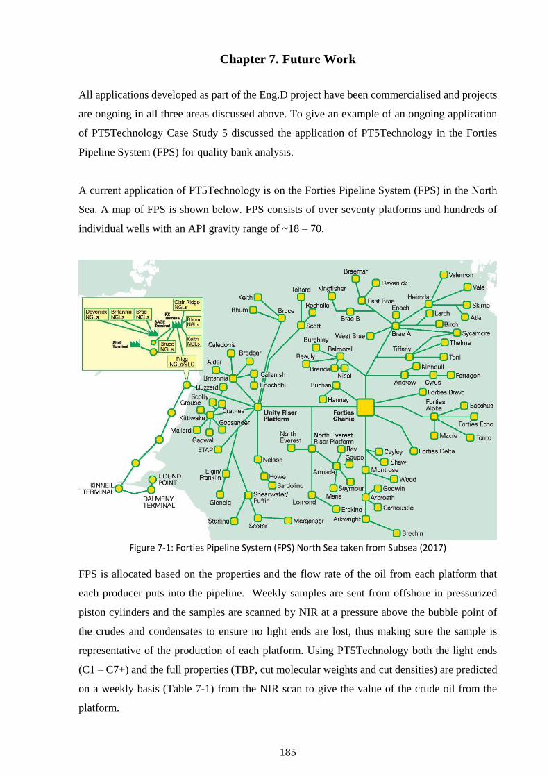
185
Chapter 7. Future Work
All applications developed as part of the Eng.D project have been commercialised and projects
are ongoing in all three areas discussed above. To give an example of an ongoing application
of PT5Technology Case Study 5 discussed the application of PT5Technology in the Forties
Pipeline System (FPS) for quality bank analysis.
A current application of PT5Technology is on the Forties Pipeline System (FPS) in the North
Sea. A map of FPS is shown below. FPS consists of over seventy platforms and hundreds of
individual wells with an API gravity range of ~18 – 70.
Figure 7-1: Forties Pipeline System (FPS) North Sea taken from Subsea (2017)
FPS is allocated based on the properties and the flow rate of the oil from each platform that
each producer puts into the pipeline. Weekly samples are sent from offshore in pressurized
piston cylinders and the samples are scanned by NIR at a pressure above the bubble point of
the crudes and condensates to ensure no light ends are lost, thus making sure the sample is
representative of the production of each platform. Using PT5Technology both the light ends
(C1 – C7+) and the full properties (TBP, cut molecular weights and cut densities) are predicted
on a weekly basis (Table 7-1) from the NIR scan to give the value of the crude oil from the
platform.
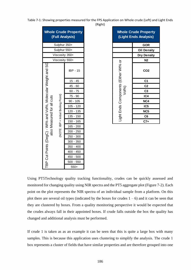
186
Table 7-1: Showing properties measured for the FPS Application on Whole crude (Left) and Light Ends (Right)
Using PT5Technology quality tracking functionality, crudes can be quickly assessed and
monitored for changing quality using NIR spectra and the PT5 aggregate plot (Figure 7-2). Each
point on the plot represents the NIR spectra of an individual sample from a platform. On this
plot there are several oil types (indicated by the boxes for crudes 1 – 6) and it can be seen that
they are clustered by boxes. From a quality monitoring perspective it would be expected that
the crudes always fall in their appointed boxes. If crude falls outside the box the quality has
changed and additional analysis must be performed.
If crude 1 is taken as as an example it can be seen that this is quite a large box with many
samples. This is because this application uses clustering to simplify the analysis. The crude 1
box represents a cluster of fields that have similar properties and are therefore grouped into one
IBP - 15
15 - 45
45 - 60
60 - 75
75 - 90
90 - 105
105 - 120
120 - 135
135 - 150
150 - 165
165 - 200
200 - 250
250 - 300
300 - 350
350 - 400
400 - 450
450 - 500
500 - 550
550+
Whole Crude Property
(Full Analysis)
Sulphur 350+
Sulphur 550+
Viscosity 350+
Viscosity 550+
TB
P C
ut P
oin
ts (
DegC
) -
Wt%
and V
ol%
, M
ole
cula
r W
eig
ht and S
G
als
o M
easure
d for
all
cuts
(NO
TE
: IB
P =
In
itia
l B
oilin
g P
oin
t)
GOR
Oil Density
Dry Density
N2
CO2
C1
C2
C3
IC4
NC4
IC5
NC5
C6
C7+
Whole Crude Property
(Light Ends Analysis)
Lig
ht E
nds C
om
ponents
(E
ither
Wt%
or
Vol%
)
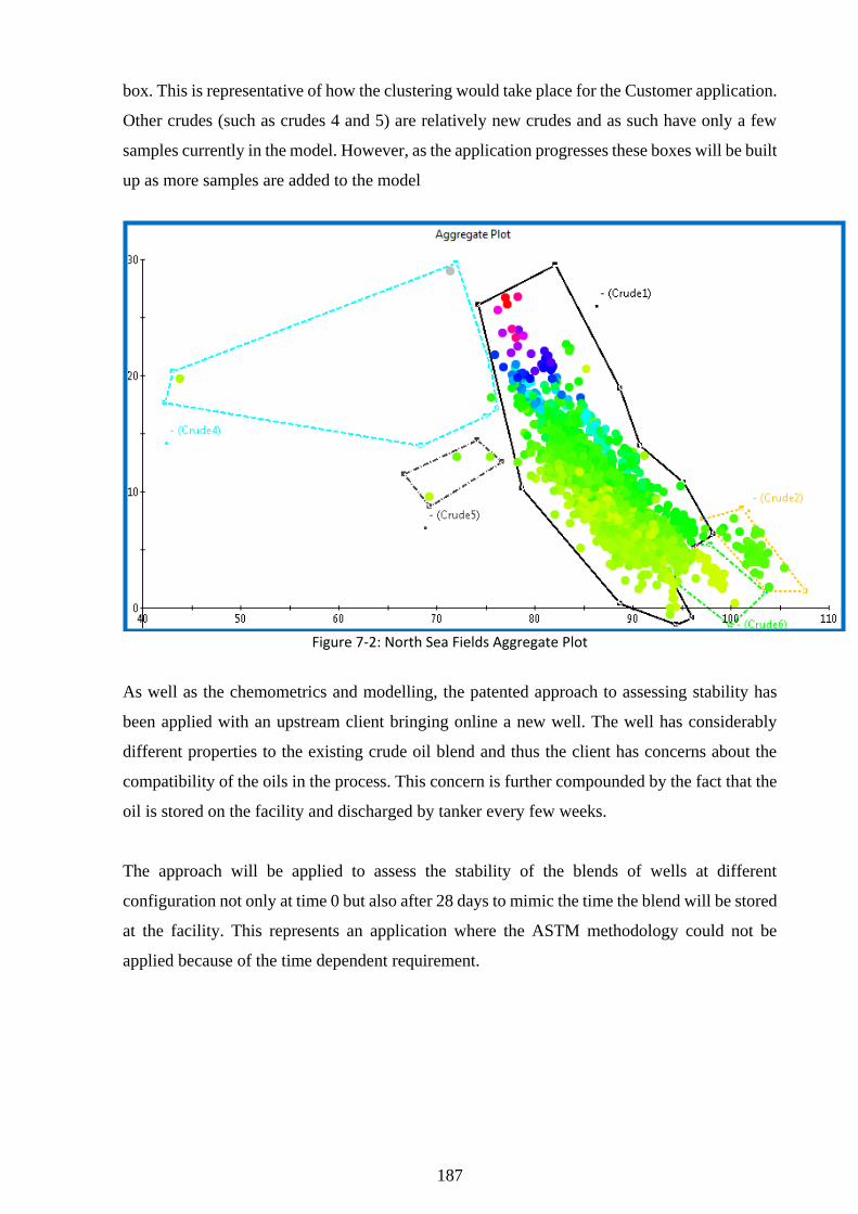
187
box. This is representative of how the clustering would take place for the Customer application.
Other crudes (such as crudes 4 and 5) are relatively new crudes and as such have only a few
samples currently in the model. However, as the application progresses these boxes will be built
up as more samples are added to the model
Figure 7-2: North Sea Fields Aggregate Plot
As well as the chemometrics and modelling, the patented approach to assessing stability has
been applied with an upstream client bringing online a new well. The well has considerably
different properties to the existing crude oil blend and thus the client has concerns about the
compatibility of the oils in the process. This concern is further compounded by the fact that the
oil is stored on the facility and discharged by tanker every few weeks.
The approach will be applied to assess the stability of the blends of wells at different
configuration not only at time 0 but also after 28 days to mimic the time the blend will be stored
at the facility. This represents an application where the ASTM methodology could not be
applied because of the time dependent requirement.

188
References
189
References
Acevedo, S., Zuloaga, C. and Rodrı, P. (2008) ‘Aggregation-Dissociation Studies of Asphaltene
Solutions in Resins Performed Using the Combined Freeze Fracture-Transmission Electron
Microscopy Technique’, Energy & Fuels, 22(5), pp. 2332–2340.
Alvarado, V. and Manrique, E. (2010) ‘Enhanced oil recovery: An update review’, Energies,
3(9), pp. 1529–1575. doi: 10.3390/en3091529.
Ashoori, S. et al. (2006) ‘Investigation of reversibility of asphaltene precipitation and
deposition for an Iranian crude oil’, Iranian Journal of Chemical Engineering, 25(3), pp. 41–
47. Available at: http://www.sid.ir/en/VEWSSID/J_pdf/84320060307.pdf.
Aske, N. et al. (2001) ‘Determination of Saturate, Aromatic, Resin, and Asphaltenic (SARA)
Components in Crude Oils by Means of Infrared and Near-Infrared Spectroscopy’, Energy &
Fuels, 15(5), pp. 1304–1312. doi: 10.1021/ef010088h.
Aske, N. et al. (2002) ‘Asphaltene Aggregation from Crude Oils and Model Systems Studied
by High-Pressure NIR Spectroscopy’, Energy & Fuels, 16(7), pp. 1287–1295.
Aske, N. (2002a) Characterisation of crude oil components, asphaltene aggregation and
emulsion stability by means of near infrared spectroscopy and multivariate analysis, Chemical
Engineering. Thesis. Norwegian University of Science and Technology.
Aske, N. (2002b) ‘Characterisation of Crude Oil Components , Asphaltene Aggregation and
Emulsion Stability by means of Near Infrared Spectroscopy and Multivariate Analysis by Narve
Aske Department of Chemical Engineering’, Advances in Colloid and Interface Science, (June),
p. 3.
ASTM (2013) ‘D7060 - Standard Test Method for Determination of the Maximum Flocculation
Ratio and Peptizing Power in Residual and Heavy Fuel Oils (Optical Detection Method)’, pp.
1–12. doi: 10.1520/D7060-12.2.
Aurdal, T. et al. (1998) ‘Annual Report Saga Petroleum’, Statoil Research Cooperation on
Asphaltenes, p. 100.
Balabin, R. M. and Safieva, R. Z. (2008) ‘Gasoline Classification by Source and Type based
on Near Infrared (NIR) Spectroscopy Data’, Fuel, 87(7), pp. 1096–1101. doi:
10.1016/j.fuel.2007.07.018.
Balabin, R. M., Safieva, R. Z. and Lomakina, E. I. (2007) ‘Comparison of Linear and Nonlinear
Calibration Models Based on Near Infrared (NIR) Spectroscopy Data for Gasoline Properties
Prediction’, Chemometrics and Intelligent Laboratory Systems, 88(2), pp. 183–188. doi:
10.1016/j.chemolab.2007.04.006.
Balabin, R. M., Safieva, R. Z. and Lomakina, E. I. (2008) ‘Wavelet Neural Network (WNN)
Approach for Calibration Model Building Based on Gasoline Near Infrared (NIR) Spectra’,
Chemometrics and Intelligent Laboratory Systems, 93(1), pp. 58–62. doi:
10.1016/j.chemolab.2008.04.003.
Balabin, R. M., Safieva, R. Z. and Lomakina, E. I. (2010) ‘Gasoline classification using near
infrared (NIR) spectroscopy data: Comparison of multivariate techniques’, Analytica Chimica
Acta. Elsevier B.V., 671(1–2), pp. 27–35. doi: 10.1016/j.aca.2010.05.013.
Balabin, R. M., Safieva, R. Z. and Lomakina, E. I. (2012) ‘Gasoline classification using near
infrared (NIR) spectroscopic data: Comparison of multivariate techniques’, Analytica Chimica
Acta, 671, pp. 27–35.
Bastien, P., Vinzi, V. E. and Tenehaus, M. (2005) ‘PLS Generalised Linear Regression’,
Computational Statsitics and Data Analysis, 48, pp. 17–46.
Berglund, A. and Wold, S. (1999) ‘A Serial Extension of Multiblock PLS’, Chemometrics, 13,
190
pp. 461–471.
Blanco, A. M. et al. (2005) ‘Operational Planing of Crude Oil Processing Terminals’, European
Symposium on Computer Aided Process Engineering, 15(1).
Blanco, M. et al. (2000) ‘Determination of the Penetration Value of Bitumens by Near Infrared
Spectroscopy’, The Analyst, 125(10), pp. 1823–1828. doi: 10.1039/b004121l.
Braun, R. L. and Burnham, I. K. (1993) Chemical Model for Oil and Gas Generation from Type
I and II Kerogen. Report. Lawrence Livermore National Laboratory.
Buckley, J. S. et al. (1998) ‘Asphaltene Precipitation and Solvent Properties of Crude Oils’,
Petroleum Science and Technology, 16(3–4), pp. 251–285. doi: 10.1080/10916469808949783.
Buenrostro-Gonzalez, E. et al. (2004) ‘Asphaltene Precipitation in Crude Oils: Theory and
Experiments’, AIChE Journal, 50(10), pp. 2552–2570. doi: 10.1002/aic.10243.
Burg, P., Selves, J. L. and Colin, J. P. (1997) ‘Crude Oils : Modelling from Chromatographic
Data- A New Tool for Classification’, Fuel, 76(1), pp. 85–91.
Cho, Y. et al. (2012) ‘Application of Saturates, Aromatics, Resins, and Asphaltenes Crude Oil
Fractionation for Detailed Chemical Characterization of Heavy Crude Oils by Fourier
Transform Ion Cyclotron Resonance Mass Spectrometry Equipped with Atmospheric Pressure
Photoionizati’, Energy & Fuels, 26(5), pp. 2558–2565. doi: 10.1021/ef201312m.
Chung, H. and Ku, M.-S. (2000) ‘Comparison of Near-Infrared, Infrared, and Raman
Spectroscopy for the Analysis of Heavy Petroleum Products’, Applied Spectroscopy, 54(2), pp.
239–245.
Chung, H., Ku, M.-S. and Lee, J.-S. (1999) ‘Comparison of Near-Infrared and Mid-Infrared
Spectroscopy for the Determination of Distillation Property of Kerosene’, Vibrational
Spectroscopy, 20(2), pp. 155–163.
Cui, H.-F. et al. (2012) ‘Automatic and Rapid Discrimination of Cotton Genotypes by Near
Infrared Spectroscopy and Chemometrics’, Journal of Analytical Methods in Chemistry, p. 7.
doi: 10.1155/2012/793468.
Deming, S. M. and Morgan, S. L. (1993) Experimental Design: A Chemometric Approach. 2nd
edn. Elsevier.
Dinadayalene, T. C., Farag, A. M. and Fujita, N. (2012) ‘Correlation between SARA Fractions,
Density and RI to Investigate the Stability of Asphaltene’, Analytical Chemistry.
Energia, G. (2010) Refining Fundamentals.
Fan, T., Wang, J. and Buckley, J. S. (2002) ‘Evaluating Crude Oils by SARA Analysis’,
Improved Oil Recovery Symposium. Tulsa, Oklahoma: Society of Petroleum Engineers.
Felicio, C. C. et al. (2005) ‘Comparison of PLS algorithms in gasoline and gas oil parameter
monitoring with MIR and NIR’, Chemometrics and Intelligent Laboratory Systems, 78(1), pp.
74–80. doi: 10.1016/j.chemolab.2004.12.009.
Flumignan, D. L. et al. (2012) ‘Multivariate Calibrations on 1H NMR Profiles for Prediction
of Physicochemical Parameters of Brazilian Commercial Gasoline’, Fuel. Elsevier Ltd, 99, pp.
180–187. doi: 10.1016/j.fuel.2012.04.037.
Gawrys, K. L. and Kilpatrick, P. K. (2004) ‘Asphaltene Aggregation: Techniques for Analysis’,
Instrumentation Science & Technology, 32(3), pp. 247–253. doi: 10.1081/CI-120030536.
Gaydou, V., Kister, J. and Dupuy, N. (2011) ‘Evaluation of Multiblock NIR/MIR PLS
Predictive Models to Detect Adulteration of Diesel/Biodiesel Blends by Vegetal Oil’,
Chemometrics and Intelligent Laboratory Systems. Elsevier B.V., 106(2), pp. 190–197. doi:
10.1016/j.chemolab.2010.05.002.
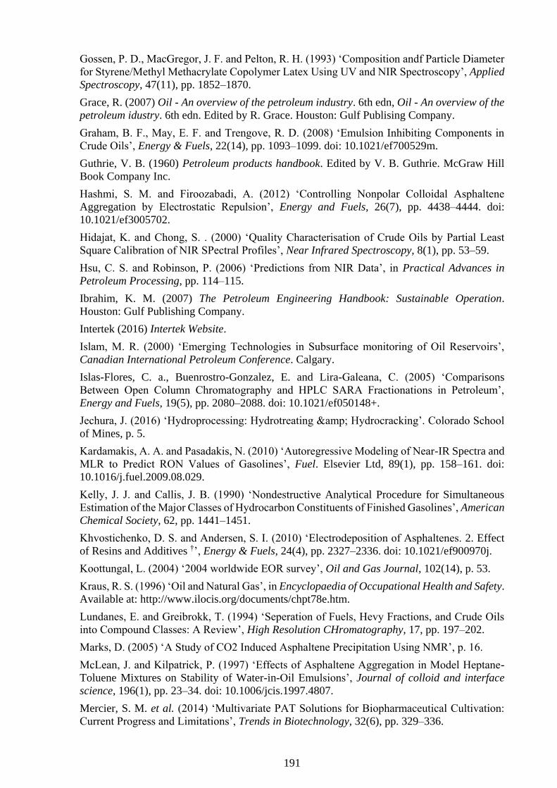
191
Gossen, P. D., MacGregor, J. F. and Pelton, R. H. (1993) ‘Composition andf Particle Diameter
for Styrene/Methyl Methacrylate Copolymer Latex Using UV and NIR Spectroscopy’, Applied
Spectroscopy, 47(11), pp. 1852–1870.
Grace, R. (2007) Oil - An overview of the petroleum industry. 6th edn, Oil - An overview of the
petroleum idustry. 6th edn. Edited by R. Grace. Houston: Gulf Publising Company.
Graham, B. F., May, E. F. and Trengove, R. D. (2008) ‘Emulsion Inhibiting Components in
Crude Oils’, Energy & Fuels, 22(14), pp. 1093–1099. doi: 10.1021/ef700529m.
Guthrie, V. B. (1960) Petroleum products handbook. Edited by V. B. Guthrie. McGraw Hill
Book Company Inc.
Hashmi, S. M. and Firoozabadi, A. (2012) ‘Controlling Nonpolar Colloidal Asphaltene
Aggregation by Electrostatic Repulsion’, Energy and Fuels, 26(7), pp. 4438–4444. doi:
10.1021/ef3005702.
Hidajat, K. and Chong, S. . (2000) ‘Quality Characterisation of Crude Oils by Partial Least
Square Calibration of NIR SPectral Profiles’, Near Infrared Spectroscopy, 8(1), pp. 53–59.
Hsu, C. S. and Robinson, P. (2006) ‘Predictions from NIR Data’, in Practical Advances in
Petroleum Processing, pp. 114–115.
Ibrahim, K. M. (2007) The Petroleum Engineering Handbook: Sustainable Operation.
Houston: Gulf Publishing Company.
Intertek (2016) Intertek Website.
Islam, M. R. (2000) ‘Emerging Technologies in Subsurface monitoring of Oil Reservoirs’,
Canadian International Petroleum Conference. Calgary.
Islas-Flores, C. a., Buenrostro-Gonzalez, E. and Lira-Galeana, C. (2005) ‘Comparisons
Between Open Column Chromatography and HPLC SARA Fractionations in Petroleum’,
Energy and Fuels, 19(5), pp. 2080–2088. doi: 10.1021/ef050148+.
Jechura, J. (2016) ‘Hydroprocessing: Hydrotreating & Hydrocracking’. Colorado School
of Mines, p. 5.
Kardamakis, A. A. and Pasadakis, N. (2010) ‘Autoregressive Modeling of Near-IR Spectra and
MLR to Predict RON Values of Gasolines’, Fuel. Elsevier Ltd, 89(1), pp. 158–161. doi:
10.1016/j.fuel.2009.08.029.
Kelly, J. J. and Callis, J. B. (1990) ‘Nondestructive Analytical Procedure for Simultaneous
Estimation of the Major Classes of Hydrocarbon Constituents of Finished Gasolines’, American
Chemical Society, 62, pp. 1441–1451.
Khvostichenko, D. S. and Andersen, S. I. (2010) ‘Electrodeposition of Asphaltenes. 2. Effect
of Resins and Additives †’, Energy & Fuels, 24(4), pp. 2327–2336. doi: 10.1021/ef900970j.
Koottungal, L. (2004) ‘2004 worldwide EOR survey’, Oil and Gas Journal, 102(14), p. 53.
Kraus, R. S. (1996) ‘Oil and Natural Gas’, in Encyclopaedia of Occupational Health and Safety.
Available at: http://www.ilocis.org/documents/chpt78e.htm.
Lundanes, E. and Greibrokk, T. (1994) ‘Seperation of Fuels, Hevy Fractions, and Crude Oils
into Compound Classes: A Review’, High Resolution CHromatography, 17, pp. 197–202.
Marks, D. (2005) ‘A Study of CO2 Induced Asphaltene Precipitation Using NMR’, p. 16.
McLean, J. and Kilpatrick, P. (1997) ‘Effects of Asphaltene Aggregation in Model Heptane-
Toluene Mixtures on Stability of Water-in-Oil Emulsions’, Journal of colloid and interface
science, 196(1), pp. 23–34. doi: 10.1006/jcis.1997.4807.
Mercier, S. M. et al. (2014) ‘Multivariate PAT Solutions for Biopharmaceutical Cultivation:
Current Progress and Limitations’, Trends in Biotechnology, 32(6), pp. 329–336.
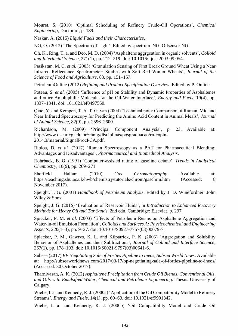
192
Mouret, S. (2010) ‘Optimal Scheduling of Refinery Crude-Oil Operations’, Chemical
Engineering, Doctor of, p. 189.
Naskar, A. (2015) Liquid Fuels and their Characteristics.
NG, O. (2012) ‘The Spectrum of Light’. Edited by spectrum_NG. Oilsensor NG.
Oh, K., Ring, T. a. and Deo, M. D. (2004) ‘Asphaltene aggrgeation in organic solvents’, Colloid
and Interfacial Science, 271(1), pp. 212–219. doi: 10.1016/j.jcis.2003.09.054.
Pasikatan, M. C. et al. (2003) ‘Granulation Sensing of First Break Ground Wheat Using a Near
Infrared Reflectance Spectrometer: Studies with Soft Red Winter Wheats’, Journal of the
Science of Food and Agriculture, 83, pp. 151–157.
PetroleumOnline (2012) Refining and Product Specification Overview. Edited by P. Online.
Poteau, S. et al. (2005) ‘Influence of pH on Stability and Dynamic Properties of Asphaltenes
and other Amphiphilic Molecules at the Oil-Water Interface’, Energy and Fuels, 19(4), pp.
1337–1341. doi: 10.1021/ef0497560.
Qiao, Y. and Kempen, T. A. T. G. van (2004) ‘Technical note: Comparison of Raman, Mid and
Near Infrared Spectroscopy for Predicting the Amino Acid Content in Animal Meals’, Journal
of Animal Science, 82(9), pp. 2596–2600.
Richardson, M. (2009) ‘Principal Component Analysis’, p. 23. Available at:
http://www.dsc.ufcg.edu.br/~hmg/disciplinas/posgraduacao/rn-copin-
2014.3/material/SignalProcPCA.pdf.
Rioloa, D. et al. (2017) ‘Raman Spectroscopy as a PAT for Pharmaceutical Blending:
Advantages and Disadvantages’, Pharmaceutical and Biomedical Analysis.
Rohrback, B. G. (1991) ‘Computer-assisted rating of gasoline octane’, Trends in Analytical
Chemiostry, 10(9), pp. 269–271.
Sheffield Hallam (2010) Gas Chromatography. Available at:
https://teaching.shu.ac.uk/hwb/chemistry/tutorials/chrom/gaschrm.htm (Accessed: 8
November 2017).
Speight, J. G. (2001) Handbook of Petroleum Analysis. Edited by J. D. Winefordner. John
Wiley & Sons.
Speight, J. G. (2016) ‘Evaluation of Reservoir Fluids’, in Introduction to Enhanced Recovery
Methods for Heavy Oil and Tar Sands. 2nd edn. Cambridge: Elsevier, p. 237.
Spiecker, P. M. et al. (2003) ‘Effects of Petroleum Resins on Asphaltene Aggregation and
Water-in-oil Emulsion Formation’, Colloids and Surfaces A: Physicochemical and Engineering
Aspects, 220(1–3), pp. 9–27. doi: 10.1016/S0927-7757(03)00079-7.
Spiecker, P. M., Gawrys, K. L. and Kilpatrick, P. K. (2003) ‘Aggregation and Solubility
Behavior of Asphaltenes and their Subfractions’, Journal of Colloid and Interface Science,
267(1), pp. 178–193. doi: 10.1016/S0021-9797(03)00641-6.
Subsea (2017) BP Negotiating Sale of Forties Pipeline to Ineos, Subsea World News. Available
at: http://subseaworldnews.com/2017/03/17/bp-negotiating-sale-of-forties-pipeline-to-ineos/
(Accessed: 30 October 2017).
Tharnivasan, A. K. (2012) Asphaltene Precipitation from Crude Oil Blends, Conventional Oils,
and Oils with Emulsified Water, Chemical and Petroleum Engineering. Thesis. Univeristy of
Calgary.
Wiehe, I. a. and Kennedy, R. J. (2000a) ‘Application of the Oil Compatibility Model to Refinery
Streams’, Energy and Fuels, 14(1), pp. 60–63. doi: 10.1021/ef9901342.
Wiehe, I. a. and Kennedy, R. J. (2000b) ‘Oil Compatibility Model and Crude Oil

193
Incompatibility’, Energy and Fuels, 14(1), pp. 56–59. doi: 10.1021/ef990133+.
Wiehe, I. A. and Kennedy, R. J. (1999) ‘Process for Blending Petroleum Oils to Avoid Being
Nearly Incompatible’, US Patent 5,997,723. Available at:
http://www.google.com/patents/US5997723.
Wiehe, I. A. and Kennedy, R. J. (1999) ‘Process for Blending Potentially Incompatible
Petroleum Oils’, US Patent 5,871,634. Available at:
http://www.google.com/patents/US5871634.
Wiehe, I. A., Kennedy, R. J. and Dickakian, G. (2001) ‘Fouling of Nearly Incompatible Oils’,
Energy & Fuels, 15(5), pp. 1057–1058. doi: 10.1021/ef010063i.
Wood-Mackenzie (2012a) Refinery Evaluation Model.
Wood-Mackenzie (2012b) ‘The Outlook for Europe’s Refinining Industry - a changing
landscape’, (April).

194
Appendix A
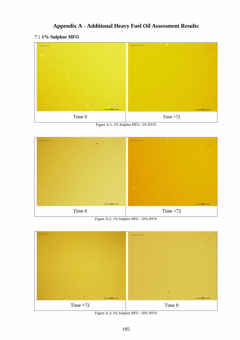
195
Appendix A - Additional Heavy Fuel Oil Assessment Results
1% Sulphur HFO
Time 0 Time +72
Figure A-1: 1% Sulphur HFO - 5% HVN
Time 0
Time +72
Figure A-2: 1% Sulphur HFO - 10% HVN
Time +72
Time 0
Figure A-3: 1% Sulphur HFO - 50% HVN

196
It can be seen that no bulk organic deposition observed with HVN even at 50% HVN after 72 hours.
1.8% Sulphur HFO
Time 0
Time +72
Figure A-4: 1.8% Sulphur HFO - 5% HVN
Time 0
Time +72
Figure A-5: 1.8% Sulphur HFO - 10% HVN
Time 0
Time +72
Figure A-6: 1.8% Sulphur HFO - 50% HVN
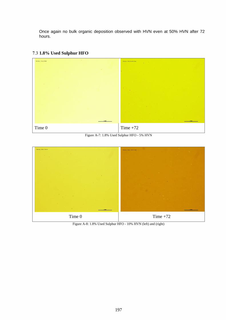
197
Once again no bulk organic deposition observed with HVN even at 50% HVN after 72 hours.
1.8% Used Sulphur HFO
Time 0
Time +72
Figure A-7: 1.8% Used Sulphur HFO - 5% HVN
Time 0
Time +72
Figure A-8: 1.8% Used Sulphur HFO - 10% HVN (left) and (right)
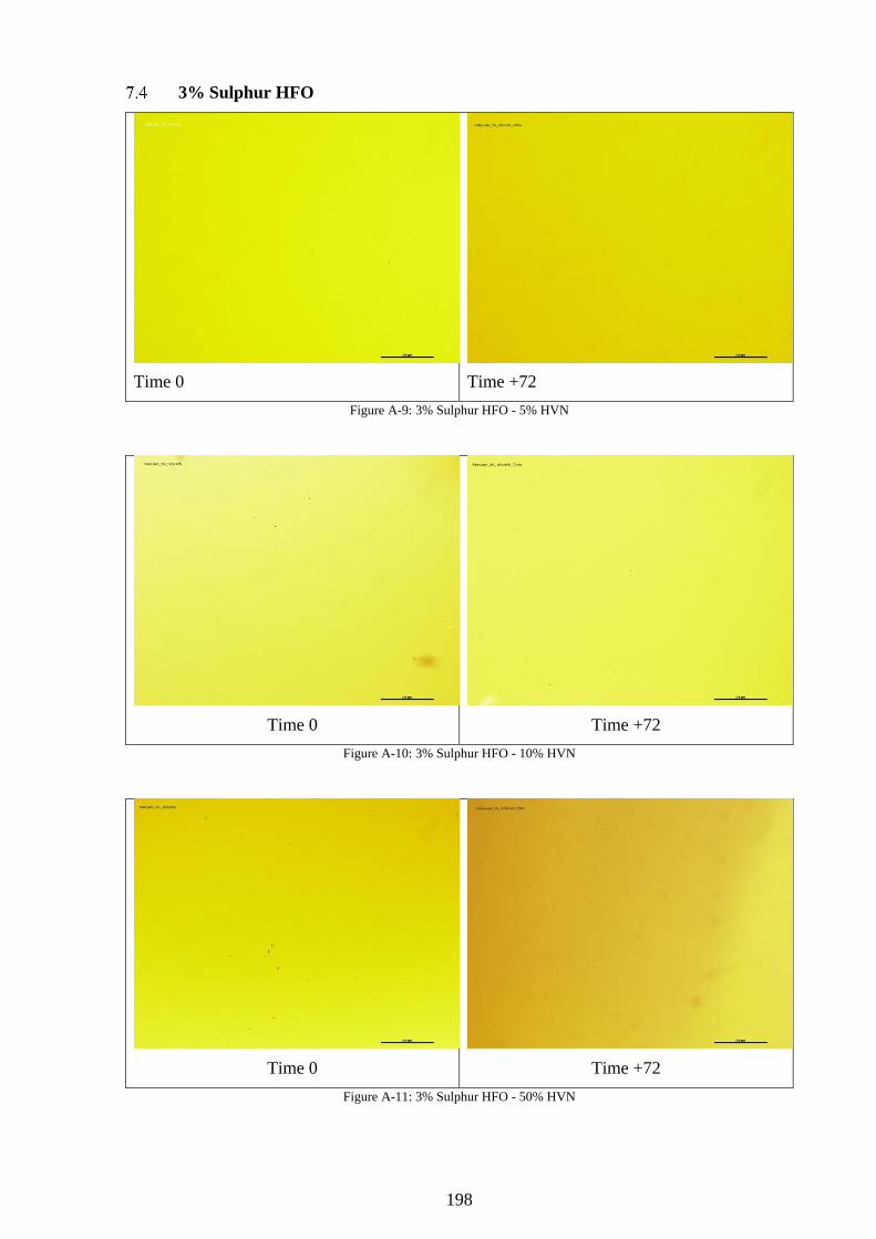
198
3% Sulphur HFO
Time 0
Time +72
Figure A-9: 3% Sulphur HFO - 5% HVN
Time 0
Time +72
Figure A-10: 3% Sulphur HFO - 10% HVN
Time 0
Time +72
Figure A-11: 3% Sulphur HFO - 50% HVN

199
Appendix B
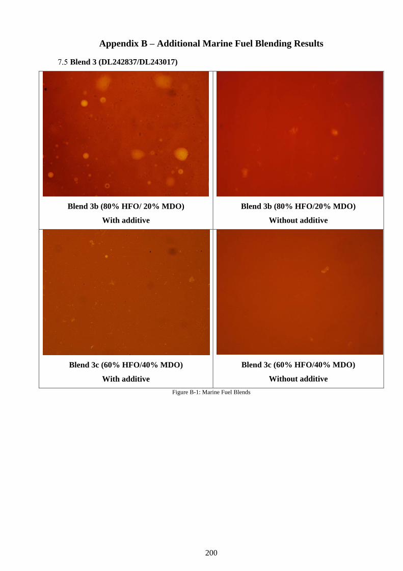
200
Appendix B – Additional Marine Fuel Blending Results
Blend 3 (DL242837/DL243017)
Blend 3b (80% HFO/ 20% MDO)
With additive
Blend 3b (80% HFO/20% MDO)
Without additive
Blend 3c (60% HFO/40% MDO)
With additive
Blend 3c (60% HFO/40% MDO)
Without additive
Figure B-1: Marine Fuel Blends

201
Appendix C
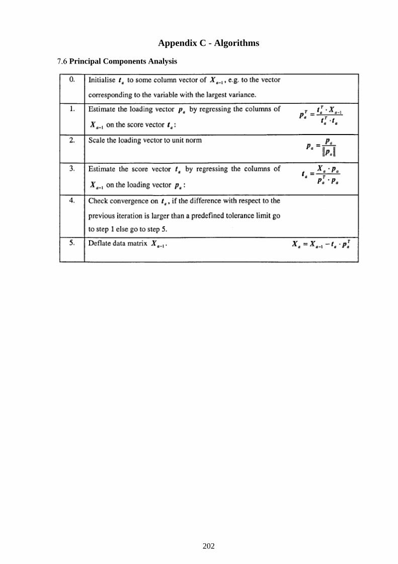
202
Appendix C - Algorithms
Principal Components Analysis

203
Principal Components Analysis