Embed Size (px)
Citation preview

Adaptive Management to Improve De-Icing Operations
Larry Baker, Principal InvestigatorDepartment of Bioproducts and Biosystems EngineeringUniversity of Minnesota
MARCH 2021
Research ProjectFinal Report 2021-07
Office of Research & Innovation • mndot.gov/research

To request this document in an alternative format, such as braille or large print, call 651-366-4718 or 1-800-657-3774 (Greater Minnesota) or email your request to [email protected]. Pleaserequest at least one week in advance.

Technical Report Documentation Page 1. Report No.
MN 2021-07 2. 3. Recipients Accession No.
4. Title and Subtitle
Adaptive Management to Improve De-Icing Operations 5. Report Date
March 2021 6.
7. Author(s)
Lawrence A. Baker, Brue Wilson, Doug Klimbal, Dan Furuta, Melissa Friese, Jacob Bierman
8. Performing Organization Report No.
9. Performing Organization Name and Address
Department of Bioproducts and Biosystems Engineering University of Minnesota St. Paul, MN 55108
10. Project/Task/Work Unit No.
CTS #2018002 11. Contract (C) or Grant (G) No.
(c) 1003325 (wo) 35
12. Sponsoring Organization Name and Address
Minnesota Department of Transportation Office of Research & Innovation 395 John Ireland Boulevard, MS 330, St. Paul, Minnesota 55155-1899
13. Type of Report and Period Covered
Final Report
14. Sponsoring Agency Code
15. Supplementary Notes
Final Report: https://www.mndot.gov/research/reports/2021/202107.pdf Educational Videos: https://www.youtube.com/watch?v=D4qtXc-BuFQ and https://youtu.be/kTKtOw4fFy4 Training Manual: https://www.mndot.gov/research/reports/2021/202107TM.pdf Urban Planning Tool For CI Balance: https://www.mndot.gov/research/reports/2021/202107S1.xlsx Groundwater Steady-State Chloride Estimator: https://www.mndot.gov/research/reports/2021/202107S1.xlsx 16. Abstract (Limit: 250 words)
Road de-icing is a major cause of chloride impairment in Minnesota’s urban waters. The goal of our study was to develop an adaptive management (AM) strategy to reduce chloride impacts caused by de-icing operations. The AM process was informed by our analysis of chloride movement in a residential watershed, providing feedback to the street department of our collaborator, the City of Edina. A key finding was that most the chloride movement occurred during a small number of events, with half of annual chloride movement occurring in less than 50 hours during each of the two years of study. This observation means that targeting these events might be a more effective way to reduce chloride impacts than more generalized approaches. We also found that a significant amount of chloride added to streets during de-icing accumulated in roadside snow piles, likely contributing to groundwater contamination. To address this concern, we developed a spreadsheet tool to estimate steady-state (long-term) chloride concentrations in groundwater. Scenario analyses indicated that groundwater chloride levels in highly urbanized watersheds would eventually exceed water quality standards. We developed a second model, intended for use by urban planners, to estimate the impact of changing the percentage of salted impervious surface on chloride movement in re-developed watersheds. Researchers also developed an Active Management Toolkit with a deicing spreadsheet calculator and educational videos.
17. Document Analysis/Descriptors
Deicing, chlorides, runoff, winter maintenance, snowplows
18. Availability StatementNo restrictions. Document available from: National Technical Information Services, Alexandria,Virginia 22312
19. Security Class (this report) 20. Security Class (this page) 21. No. of Pages
63 22. Price
ADAPTIVE MANAGEMENT TO IMPROVE DE-ICING OPERATIONS
FINAL REPORT
Prepared by:
Lawrence A. Baker and Bruce Wilson (co-PIs), Doug Klimbal, and Daniel Furuta (graduate students) Melissa Friese, and Jacob Bierman (undergraduate technicians)
Department of Bioproducts and Biosystems Engineering University of Minnesota
March 2021
Published by:
Minnesota Department of Transportation
Office of Research & Innovation
395 John Ireland Boulevard, MS 330
St. Paul, Minnesota 55155-1899
This report represents the results of research conducted by the authors and does not necessarily represent the views or policies
of the Minnesota Department of Transportation or the University of Minnesota. This report does not contain a standard or
specified technique.
The authors, the Minnesota Department of Transportation, and the University of Minnesota do not endorse products or
manufacturers. Trade or manufacturers’ names appear herein solely because they are considered essential to this report.

ACKNOWLEDGMENTS
We thank our departmental technicians, Derrick Ferguson and Brian Hetchler, for ably designing, constructing, and installing sampling equipment.
We also thank members of Edina’s Street Department for their participation in lively discussions at the adaptive management workshops; Jessica Vanderwerf Wilson, Edina’s water resources coordinator for coordinating workshops and leading the effort to purchase new Joma blades; and street supervisors Shawn Anderson and John Sheerer for supporting the project in many ways. Finally, we would like to thank members of our Technical Advisory Panel: Ross Bintner (technical liaison), Dwayne Stenlund (MnDOT), Clark Moe (MnDOT), Ryan Peterson (Burnsville), Bob Fossum (Capital Region Watershed District), Brooke Asleson (MPCA), Brian Wagstrom (Minnetonka), and D. Ellinsgon (Minnetonka) for reviewing task reports and providing feedback on research findings

TABLE OF CONTENTS
CHAPTER 1: Introduction ........................................................................................................................ 1
1.1 The Chloride Problem in Minnesota ......................................................................................... 1
1.1.1 Current conditions .................................................................................................................. 1
1.1.2 Progress in reducing chloride contamination .......................................................................... 2
1.1.3 Previous Research ............................................................................................................ 3
1.1.4 Project Goal ...................................................................................................................... 5
CHAPTER 2: Methods .............................................................................................................................. 6
2.1 Overall Case study design .............................................................................................................. 6
2.2 Design of catch basin sampler........................................................................................................ 6
2.2.1 Initial (year 1, winter of 2017-2018) design process ................................................................ 6
2.2.2 Case study site and installation of sampler. ............................................................................ 7
2.2.3 De-icing operations ................................................................................................................ 8
2.2.4 Modifications to improve operations in year 2 (winter of 2018-2019) ..................................... 9
2.2.5 Meltwater metrics ................................................................................................................ 11
2.2.6 Snow core sampling ............................................................................................................. 11
2.3 Event interpretation .................................................................................................................... 13
2.4 DevelopMent of Adaptive management framework .................................................................... 14
2.4.1 Design of AM workshops ...................................................................................................... 15
CHAPTER 3: Results ............................................................................................................................... 17
3.1 Weather during the two winter seasons ...................................................................................... 17
3.2 Temporal pattern of meltwater flows, cl concentrations, and cl loads.......................................... 18
3.3 Event-by-event analysis ............................................................................................................... 21
3.4 Predicting Cl loads and event mean concentrations. .................................................................... 23
3.4.1 Approach for event interpretation ........................................................................................ 23

3.4.2 Predictive relationships. ....................................................................................................... 25
3.4.2.1 Relationships with temperature. .................................................................................... 25
3.4.2.2 Relationships with precipitation and snow...................................................................... 26
3.4.2.3 Relationships with road salt input. .................................................................................. 27
3.5 Analysis of snow pile Cl ................................................................................................................ 27
3.6 Take-aways.................................................................................................................................. 30
CHAPTER 4: Scenario modeling ............................................................................................................. 32
4.1 Baseflow chloride model ............................................................................................................. 32
4.1.1 Modeling approach .............................................................................................................. 32
4.1.2 Scenario modeling of steady-state groundwater Cl concentrations ....................................... 34
4.1.2.1 25% plow-off scenarios................................................................................................... 34
4.1.2.2 50% plow-off scenarios................................................................................................... 34
4.2 Regression-based scenario modeling for large watersheds. ......................................................... 37
4.2.1 Data mining .......................................................................................................................... 37
4.2.2 Regression equations ........................................................................................................... 37
4.2.3 Utilization of regression equations for predictions ................................................................ 40
4.3 conclusions .................................................................................................................................. 41
CHAPTER 5: Moving toward implementation ....................................................................................... 42
5.1 Adaptive Management (AM) Workshops ..................................................................................... 42
5.1.1 Rationale .............................................................................................................................. 42
5.1.2 Workshop Summaries .......................................................................................................... 42
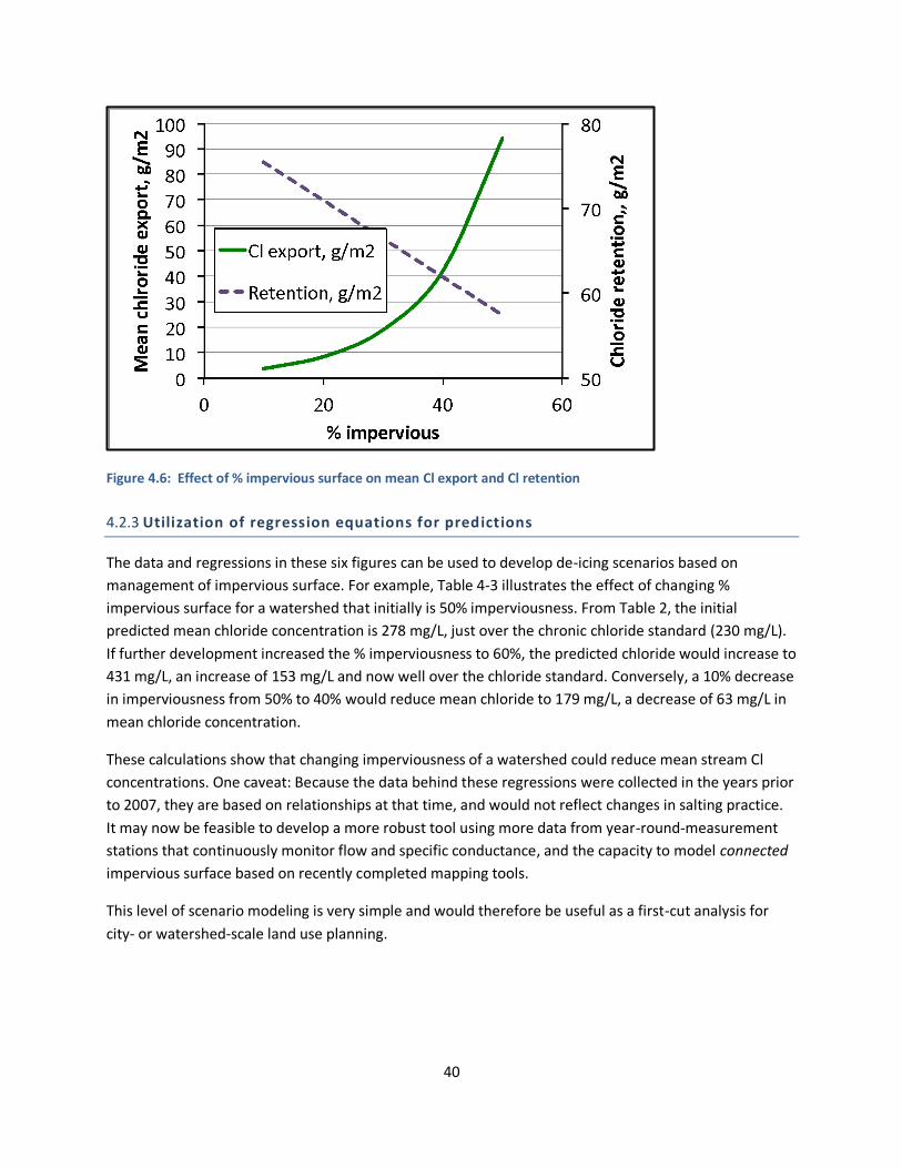
5.1.2.1 Workshop #1 (May 18, 2018). ......................................................................................... 42
5.1.2.2 Workshop #2 (May 29, 2019).......................................................................................... 43
5.2 Outcome from workshop #1: Purchase of Joma blades ................................................................ 43
5.3 Recommendations....................................................................................................................... 44
CHAPTER 6: CONCLUSIONS AND Recommendations ............................................................................ 46

6.1 De-icing practice .......................................................................................................................... 46
6.2 Future research ........................................................................................................................... 46
REFERENCES .......................................................................................................................................... 48

LIST OF FIGURES
Figure 1.1: Cl impairments in Minnesota (MPCA 2010). ........................................................................... 1
Figure 1.2: Importance of Cl as a water pollutant in Minnesota, as perceived by urban watershed
managers (Baker et al., 2018). ................................................................................................................. 2
Figure 1.3: Cl decay as a function of distance from the curb of residential streets (Stoner et al. 2006). .... 4
Figure 2.1: Meltwater sampler being calibrated in the lab flume in our department. ............................... 7
Figure 2.2: Location of case study basin in relation to the larger Nine-Mile Creek watershed. .................. 8
Figure 2.3: Top left: metal support frame for sampler. Bottom left sampler being lowered onto frame.
Bottom right: sampler in place, with “Dandy” bag to filter runoff. ........................................................... 9
Figure 2.4: Modified meltwater sampler used in. winter #2 (2018-2019) ............................................... 11
Figure 2.5: Snow coring device used in year 2. ....................................................................................... 13
Figure 2.6: Using the snow coring device in the field. ............................................................................. 13
Figure 2.7: Schematic of adaptive management framework. .................................................................. 15
Figure 2.8: First year AM workshop. ...................................................................................................... 16
Figure 3.1: Temporal pattern of flow (top), Cl concentrations (middle) and flow (bottom) for the second
winter. .................................................................................................................................................. 19
Figure 3.2: Cumulative hours to reach specified levels of annual Cl loading............................................ 20
Figure 3.3: Characteristics of a melt event from January 2018. Top: hourly temperatures and cumulative
DH>32. Middle: Hourly inflow (flue) and hourly Cl. Bottom: salt mass (lb/hour). .................................... 22
Figure 3.4: Relationship between cumulative DH>32 and total flow (volume) for an event. ................... 25
Figure 3.5: Relationship between degree hours > 32 during event and Cl loading. ................................. 26
Figure 3.6: Relationship between snow depth at beginning of a melt event and event volume. ............. 27
Figure 3.7: Distribution of Cl concentrations across all snow core samples. ............................................ 28
Figure 3.8: Cl concentrations and snow water content (inches) observed in roadside snow piles. .......... 29
Figure 3.9: Distribution of Cl mass from 2/9/19 to 3/21/19. ................................................................... 30
Figure 4.1: Percent impervious surface vs. Cl added as road salt. The blue axis and plot is in English units;
the red in metric. ................................................................................................................................... 33

Figure 4.2: Percent impervious surface vs. mean Cl concentration for 11 Metro region streams. ........... 38
Figure 4.3: Percent impervious surface vs. Cl export for 11 Metro region streams. ................................ 38
Figure 4.4: Percent connected impervious surface vs. Cl retention for 11 Metro region drains............... 39
Figure 4.5: Effect of % impervious surface on Cl input and mean Cl concentration. ................................ 39
Figure 4.6: Effect of % impervious surface on mean Cl export and Cl retention ..................................... 40
Figure 5.1: Slide used to show peak Cl loading event during winter #1. .................................................. 42
Figure 5.2: Top: traditional plow blade. Bottom right: Newly installed Joma blade. Bottom right: Road
clearing with the traditional plow blade (bottom) and the Joma blade (top). ......................................... 44
LIST OF TABLES
Table 3.1: Weather during the two study winters. Data from the NOAA MSP weather station. .............. 17
Table 3.2: Comparison of the two study winters with previous winters. For consistency, all winters
started Oct. 1 and end on May 30. ......................................................................................................... 18
Table 3.3: Time to reach various percentages of annual Cl load and percent of cumulative flow at that
time. ..................................................................................................................................................... 21
Table 3.4: Measured parameters for major melt events. Events are ranked by Cl loading. ..................... 24
Table 4.1: Modeled steady-state Cl concentrations in groundwater. Assumed plow-off rates: 25% (top)
and 50% (bottom). ................................................................................................................................ 36
Table 4.2: Summary data from Novotny et al. 2008. .............................................................................. 37
Table 4.3: Effect of reducing % impervious surface on mean annual Cl concentration in drainage from
large watersheds. .................................................................................................................................. 41
LIST OF ABBREVIATIONS AM – adaptive management BMP- best management practice Cl – chloride DH- degree-hours EMC- Event mean concentration LLRB – Local Roads Research Board TMDL- Total daily maximum load MCL- maximum contaminant limit (for drinking water) MNDOT – Minnesota Department of Transportation MPCA- Minnesota Pollution Control Agency

EXECUTIVE SUMMARY
Background and goals
Chloride (Cl) from road de-icing has become a critical urban environmental problem in Minnesota,
mainly in cities. Nearly 80 Minnesota waters are Cl-impaired or at high risk of impairment for aquatic
life. Moreover, more than half of waters with long-term trend data exhibit upward Cl trends, and only
one water body (a non-urban lake) showed a downward trend. Cl concentrations are also increasing in
shallow groundwater in the Metro region, with more than a quarter having Cl concentrations of about
250 mg/L (the Maximum Contaminant Level for municipal drinking water). Finally, Cl causes widespread
damage to roads, bridges and other infrastructure, costing hundreds of millions of dollars.
Unfortunately, the Cl added by road salt cannot be removed from meltwater economically using
structural best management practices (BMPs). The only way to reduce Cl contamination is to apply less
salt – which causes undesirable reductions in traffic mobility – or use more expensive compounds that
do not include Cl.
The goal of this project was to develop an adaptive management (AM) process to inform de-icing
practice. The general idea was to measure Cl in meltwater coming from snow and ice during melt events
and to provide feedback to city de-icing crews to enable them to devise ways to reduce the amount of
salt they would use, with a focus on the melts with the largest Cl loads (mass).
The Edina de-icing study
Approach. When we started this project, there were no published studies to relate the amounts of road
salt used to Cl concentrations or loadings in meltwater. To do this, we first had to develop a “meltwater”
sampler that could be mounted in a stormwater catch basin, below the grate. The sampler had to
withstand temperatures as low as -20o F, resist corrosion, and have no moving parts that could freeze
up. After much design and experimentation, we developed a meltwater sampler that met these
requirements.
We deployed the sampler across two winters, 2017-18 and 2018-19, measuring specific conductance (a
surrogate for Cl), flow, and temperature continuously through most of the two winters.
We also developed a technique for collecting cores of snow and ice from roadside snow piles caused by
plow-off. Briefly, we collected cores from six locations across a snow pile (sometimes at several depths),
melted the water, measured specific conductance in the lab, and then analyzed Cl directly at the
University of Minnesota’s Research Analytical Lab.
Findings
Cumulative Cl loading. As one might expect, both flow rate and Cl concentrations varied enormously
throughout the winter. To make sense of the data, we analyzed data on an event-by-event basis. For
each winter, most of the Cl loading occurred during short periods of time. During winters 1 and 2, 50%
of Cl loading occurred in just 41 hours and 31 hours, respectively. At the time 50% Cl loading occurred,

cumulative flow was only 15% of total winter flow in year 1 and 31% of seasonal flow in year 2. Nearly all
(90%) of the Cl load occurred in just 181 hours (7.5 days) in winter 1 and 190 days (7.0 days) in winter 2.
Regression analysis of main melt events. To understand the dynamics of meltwater events, we focused
on eight major melt events, which contributed 54% of the cumulative Cl loading over the two years of
study. We then used regression analysis to relate independent variables that might influence dependent
variables (characteristics of meltwater). Independent variables included variables such as event volume
(total flow throughout the event), event mean concentration (EMC), and Cl load (flow x concentration,
expressed in pounds/event).
Results of this analysis revealed several statistically significant (0.05 level) equations:
1) Event flow vs. CDH > 32 (where CDH > 32 is cumulative degree days > 32o F:
Flow = 41 x CDH>32 + 1238 R2 = 0.84
2) Cl load vs. CDH>32:
Cl load = 0.48 x CDH>32+35 R2 = 0.45
3) Snow depth (in snow water equivalents) at start of event (t=0) vs. event flow:
Flow = 924 x d +=146 R2 = 0.62
Both Cl EMC and Cl load were weakly correlated with snow depth (SWE) at t=0, but these relationships
were not a statistically significant event at the 0.20 level.
Interestingly, the amount of salt added during the event (lb) or during the event and the preceding week
was not significantly related to event flow, Cl loading, or Cl EMC. This suggests that much of the Cl
entering meltwater may have been temporarily stored within the watershed prior to the start of a melt
event, then released during an event. Cl storage may have occurred on the road surface itself, in
roadside snow piles, or on pervious surfaces.
Snow pile Cl accumulation. We also measured Cl along plow-off snow piles during the second winter.
Snow pile cores were collected along a transect running perpendicular to the road, extending about 20
feet into the adjacent yard on Cl on six occasions. The total mass of Cl increased through early March,
then declined rapidly. The total mass of Cl (160 lbs at peak) was about 40% of Cl added in road salt. We
could not quantify how much of the snow pile Cl re-entered the street, but the lack of relationship
between Cl load and salt application in key events suggests that snow piles may be an indirect source of
Cl.
Scenario modeling
Scenario modeling for larger watersheds was conducted using data from the study of Novotny et al.
(2008), which analyzed Cl balances for 11 large watersheds in the Twin Cities region.

Groundwater Cl model. One major concern regarding continued inputs of road salt to watersheds is
accumulation of Cl in watersheds. In particular, Cl that moves to pervious (usually vegetated) surfaces
will likely pass downward, eventually reaching and potentially contaminating groundwater that is used
for drinking water. As a first step, we conducted scenario analysis to estimate the potential for
groundwater Cl contamination. We estimated the input of Cl to pervious surfaces based on the
relationship between road salt inputs to each watershed and two assumptions of Cl movement from
roads to pervious surfaces: 25% and 50% of added road salt. We then used reasonable estimates of
baseflow from Metro watersheds to develop an equation to estimate steady-state Cl concentration from
the equation: [Cl]ss = MCl/QB , where [Cl]ss = steady-state, baseflow Cl concentration, mg/L, MCl = mass of
Cl input to pervious surface, g/m2-yr., and QB = baseflow, cm/yr.
Scenario modeling revealed that steady-state Cl concentrations increased directly with mass of Cl input
(which was directly proportional to the percent impervious surface in the watershed) and the plow-off
percent and inversely in relation to baseflows. Many modeled scenarios with watershed percent
impervious surface > 40% had steady-state Cl concentrations well above the drinking water Maximum
Contaminant Level of 250 mg/L.
Regression models for watershed Cl dynamics. Again, using data from Novotny et al. (2008), we used a
series of regression equations to relate road salt inputs to mean stream Cl concentrations, Cl mass
export, and percent Cl retention. This level of analysis would be best used by urban planners, to develop
estimates of how future urban designs might meet the challenge of reducing Cl contamination.
Adaptive management approach
We developed an adaptive management (AM) approach to develop the connection between road salt
application and Cl export in meltwater. To do this, we developed end-of-season workshops with Edina’s
Streets Department, and in particular, the snowplow operators. Briefly, the AM workshops were about
1.5 hours long. The first half hour was a presentation of our findings throughout the winter, and the
second hour was dedicated to open discussion.
One outcome of these workshops was the suggestion by the road crews to purchase snowplow blades
that could improve the removal of hard ice and thereby reduce the amount of salt needed to soften the
ice before plowing. This would reduce the extremely high Cl concentrations and loadings associated with
“winter mix” situations that often create icy conditions. This led to the purchase of several Joma blades
in 2018, which were mounted and used in the winter of 2018-19. Observations included improved snow
removal and less noise compared with conventional blades.
Several other ideas from these workshops that were being planned or implemented by the end of the
study were: measurement of the water content of purchased salt; making better use of the Precise
database for daily salt management; and acquiring sensors to measure road temperature directly.

1
CHAPTER 1: INTRODUCTION
1.1 THE CHLORIDE PROBLEM IN MINNESOTA
1.1.1 Current conditions
Chloride (Cl) is now a major water quality problem in cities throughout Minnesota, with 123 surface
waters Cl- impaired or high-risk waters throughout the state (Figure 1-1).
Figure 1.1: Cl impairments in Minnesota (MPCA 2010).
2
Salt causes hundreds of millions of dollars in corrosion damage to roads and bridges. Infiltration of Cl has
also led to increases of Cl in shallow, porous aquifers in the Metro region, which now have a median Cl
concentration of 86 mg/L (Kroening, 2012). Twenty-seven percent of sampled wells, mostly shallow (<
10 m), had concentrations of Cl > 250 mg/L (the drinking water Maximum Contaminant level). Some of
these wells may be used for domestic water supply (MGWA, 2020).
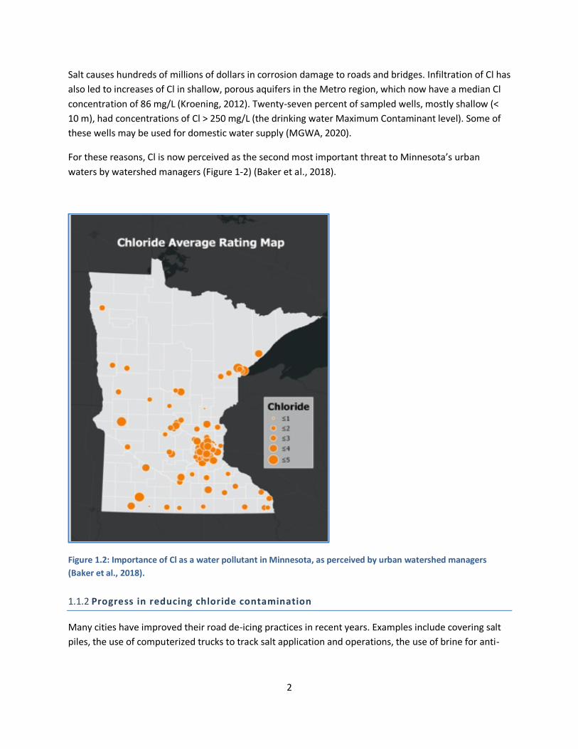
For these reasons, Cl is now perceived as the second most important threat to Minnesota’s urban
waters by watershed managers (Figure 1-2) (Baker et al., 2018).
Figure 1.2: Importance of Cl as a water pollutant in Minnesota, as perceived by urban watershed managers
(Baker et al., 2018).
1.1.2 Progress in reducing chloride contamination
Many cities have improved their road de-icing practices in recent years. Examples include covering salt
piles, the use of computerized trucks to track salt application and operations, the use of brine for anti-

3
icing (to prevent attachment of ice during an early freeze), pre-wetting to improve salt spreading, the
use of non-Cl de-icers, and improved operator training.
Despite these efforts, Cl contamination does not appear to be improving and may be getting worse. A
statistical analysis of Cl concentration trends in 114 lakes and streams with more than 10 years of data
showed the following with significant trends (MPCA, 2019):
⮚ 60 waters with increasing trends (46 in the Metro region)
⮚ 50 waters with no significant trend
⮚ One with a downward trend (none in the Metro region)
The few shallow wells that have been sampled for a decade or more also show mostly upward trends
(Kroening & Ferry, 2013). Several heavily urbanized Cl impaired streams have also exhibited upward
trends (MPCA, 2019).
1.1.3 Previous Research
Research on the movement of chloride originating from road salt through watersheds is sparse. Oberts
(1987) developed a conceptual sequence of water and salt movement in urban watersheds that
included snowfall, roadway melt, melting from roadsides, and melting through pervious surfaces near
roads. Obert’s focus was on how the snowmelt process affected the movement of pollutants other than
chloride, especially during spring melts.
A major advance toward understanding chloride pollution in Minnesota was a chloride balance study for
11 watersheds conducted at the St. Anthony Falls (Sander et al., 2008; Novotny et al., 2008, 2009). Some
key findings were: (1) chloride applications rates (lb/acre of watershed) were directly related to the
percentage of impervious surface in the watershed; (2) more than half of applied chloride (55% to 83%)
were retained within the watershed; (3) chloride retention decreased as the percent impervious surface
increased; and (4) chloride concentration in watershed outflow increased with increasing percent
impervious area. Their work suggests that the chronic chloride concentration for protection of aquatic
life was reached at about 40% imperviousness.
More recently, Herb et al. (2017) studied the transport of Cl in surface waters of a metro-area
watershed (Lake McCarrons) to characterize Cl transport by surface runoff, residence time in surface
water, and the influence of weather on Cl transport and accumulation processes. Monitoring over three
winters showed that the residence time of Cl in small, sewered watersheds varied from 14 to 26 days,
with 37% to 63% of Cl applied as de-icers exported in snowmelt and rainfall runoff. A monitored
highway ditch exported less than 5% of Cl applied to the adjacent road. Stormwater ponds were found
to act as temporary storage for Cl, with persistent layers of high Cl at the bottom.
Several studies have examined movement of chloride from de-icing operations on roadways to pervious
surfaces. Blomquist and Gustafsson (2004) reported that chloride from road salt was dispersed by wind,

4
with concentrations from highways decreasing exponentially over several hundred meters. For city
streets, Stone et al. (2010) reported mid-winter chloride accumulation rates in roadside snow piles of
(medians) 0.79 kg/m2 (0.16 lb/ft2) for an arterial road and 0.41 kg/m2 (0.08 lb/ft2) for a residential street.
Stone et al. (2010) data showed that chloride accumulation decreased exponentially within 10 m of the
curb (Figure 1-3).
Figure 1.3: Cl decay as a function of distance from the curb of residential streets (Stoner et al. 2006).
Despite these studies, we have low capacity to quantify the movement of Cl from roadways to pervious
surfaces. This is important because much of the downward movement of Cl occurs through pervious
surfaces. Some mechanisms of this movement include direct “plow-off” followed by snow pile melt,
wind dispersal, and deliberate design to divert meltwater from streets to green stormwater
infrastructure. The latter is important, because infiltration-based green stormwater infrastructure
provides a pathway for Cl transport to groundwater (Taguchi et al., 2020).
Once Cl enters watersheds, much of it infiltrates downward to groundwater. In Minnesota, median
groundwater Cl concentrations across four studies (MGA, 2020) were > 40 mg/L in residential sewered
areas and less than 5 mg/L in forested areas, strongly implicating urban development as an important
source of Cl contamination. In this context, “sewered” was contrasted with residential land served by
septic systems (which are a potential source of Cl) and was therefore a metric of urban development,
not the impact of sewers per se. In several of the major storm drains in the Capital Region Watershed
District, groundwater contamination was indicated by summer baseflow Cl concentrations exceeding

5
Minnesota’s Cl standard for protection of aquatic life (230 mg/L) (Janke et al., 2013). Most wells in
Minnesota that exceeded the drinking water standard (Secondary Maximum Contaminant Limit) were
located in the Twin Cities Metro Area ( TCMA). The highest groundwater concentrations in the TCMA
have been found in shallow aquifers with sandy soils (Kroening & Ferry, 2013). Most groundwater
samples with > 250 mg/L were from wells < 10 m deep.
Let’s consider the likely consequences of decreasing salt applications. (There are no good case studies of
this.) Concentrations of Cl in groundwater and baseflow would not respond immediately due to a “lag
effect” (also called “legacy effect”). A pollutant’s lag time is determined by the pathway in the
watershed, retarded movement of the pollutant, and the relative size of the soil and groundwater pools
compared to annual export. Bester et al. (2006), using a 3-D groundwater model of Waterloo, concluded
that recovery from groundwater Cl contamination would take several decades. Conversely, the rate of
increase of Cl in streams in rural New York lagged inputs of road salt input, not reaching a new steady-
state Cl concentration over a period of 20 years (Kelly et al., 2008).
A statewide salt balance developed by Overrbo et al. (2019) showed that road salting accounted for 42%
of total chloride input to surface waters, followed by fertilizer inputs (23% of total) and wastewater
(22%). Seventy-six percent of road salt used within Minnesota was used by MDOT, counties, cities and
other de-icing agencies and the rest was used by private applicators; 37% was used within the TCMA.
There is little doubt that road salt is the dominant source of Cl to urbanized watersheds.
1.1.4 Project Goal
The goal of this project was to develop an adaptive management (AM) framework for de-icing
operations to enable de-icing entities (cities, counties, state) to observe the impact of individual de-icing
operations on the movement and concentrations of Cl within a watershed. Road de-icing is ideally suited
for AM for five reasons: (1) road salt crews are a small, captive audience, enabling communication; (2)
road salt is overused, so there is potential for reduction; (3) there are many ways to reduce salt inputs
(4) rapid feedback (road condition, salt use, etc.) can be provided; and (5) there are many learning
events (each de-icing event) in every winter season.
We used the link between actions taken (road de-icing) and environmental response (Cl concentrations
and loading) to develop an AM process to guide de-icing operations. The relatively recent adoption of
highly instrumented de-icing trucks over the past decade makes quantification of salt additions to
specific streets feasible. Building on this capability on the “upstream” side, we designed a sampling
device that can be installed into catch basins to measure flow and specific conductance (a surrogate for
Cl concentration) on the “downstream” side of small catchments, and then use this device to measure
meltwater throughout two winters. These data were used to inform adaptive management workshops
held at the end of each winter, leading to discussion of how Cl in meltwater could be reduced by altering
operations for specific types of snow and plow events.
6
CHAPTER 2: METHODS
2.1 OVERALL CASE STUDY D ESIGN
Very few studies have been conducted to measure runoff from streets during the harsh conditions of
Minnesota in the winter and early spring. The goal of the field case study was to learn how to measure
flow, Cl concentrations, and Cl loadings in meltwater as it moves from the road to catch basins, and to
process that information in such a way that these data could be used to inform de-icing management.
2.2 DESIGN OF CATCH BASIN SAMPLER
Prior to this study, no studies have been completed that measured directly Cl loadings or Cl event mean
concentrations (Cl EMC) from the application of de-icing salt. To be useful for the development of an
adaptive management strategy, we designed and installed a unique meltwater sampler. Key features are
1. Capacity to continuously measure the flow of meltwater entering a catch basin, from the onset of
melting (very low flows but high Cl concentrations) to large melt events (often lower Cl EMCs but high
loads).
2. Durability to withstand temperatures down to -20 oF and other potential sampling disruptions (like
filling with debris).
3. Ability to operate under the catch basin grate, with no above-grate protrusions to interfere with
plowing or car traffic.
2.2.1 Initial (year 1, winter of 2017-2018) design process
We needed to be able to measure a very large range of flows with alternating periods of melting and
freezing. We evaluated several potential alternatives for flow measurement, including a tipping bucket,
a weighing trough, and a weir, but found none of these options met the needs of the project, especially
with respect icing problems. In the end, we built a flow-control box with holes drilled on one side (flow
panel), with diameters graduated with depth from ¼” diameter near the bottom to 1 -inch diameter
near the top. We configured the pattern of holes in the flow panel to enable us to measure a range of
flows from less than 1 gallon per minute, as might be expected early during a melt period, to flows
greater than 100 gallons per minute, large enough to capture a rain-on-snow melt event. The flow-
control box was built using 1/2-inch thick sheet sheets of polyethylene (PE), a material selected to retain
structural integrity in low temperatures (PE has a glass-phase transition temperature of -78 oF). The PE
sheets were welded together by a professional fabrication company.
A liquid Level “eTape” (Milone Technologies used to measure water level was placed inside a stilling well
in the middle of the samplers, which also included a lab-constructed conductivity probe and a digital
thermistor, which was calibrated against solutions with known chloride concentrations. A depth-flow
calibration curve was determined using a laboratory flume (Figure 2.1). Details regarding the assembly

7
of the instrumentation pod and calibration of both the flume and the conductivity probe are presented
in the Task 2. Modifications developed for the second winter (2018-19) are summarized in Appendix A of
Task 3.
Figure 2.1: Meltwater sampler being calibrated in the lab flume in our department.
2.2.2 Case study site and installation of sampler.
Our case study catchment was in a residential neighborhood in Edina, located at 44°52'0.18"N, 93°20'38.20"W. We selected a catch basin ~ 6’ in depth in order to have sufficient depth to hold the meltwater sampler and a supporting frame. The catchment area was approximately 2-acre (designated “LE-8” in Edina’s GIS). The catchment comprises single-family homes along 0.124 miles of roadway, which is roughly 30 feet wide on an East-West orientation. The case study catchment (outline in white in Figure 2.2) drains to Lake Edina, which in turn drains to Nine Mile Creek (flow routing in yellow).

8
Figure 2.2: Location of case study basin in relation to the larger Nine-Mile Creek watershed.
The meltwater sampler was installed on a steel rack mounted to the catch basin’s concrete interior
(Figure 2-3). Water was diverted into the sampler with aluminum sheeting. Finally, a Dandy Curb bag
sediment trap device was installed below the catch basin grate to trap solid particles.
2.2.3 De-icing operations
Edina “manages every storm as an individual animal” (per. Comm., John Sheerer, Streets Department).
They practice anti-icing with brine before snow. For ice and light snow, they plow and salt together,
with liquid to activate and reduce salt bounce, going up one side and down the other, using about 150
lb/mile. For a solid ice storm, the use whatever it takes to “chase the salt”, usually during warmer days.
They do not plow over ice. For very cold temperatures, salt isn’t used because it doesn’t work and
migrates to the gutter. Under these conditions, coarse sand is applied, especially at intersections. Edina
has a brine mixing tank in the Public Works garage and has a liquid-only truck for brine applications.

9
2.2.4
Figure 2.3: Top left: metal support frame for sampler. Bottom left sampler being lowered onto frame. Bottom
right: sampler in place, with “Dandy” bag to filter runoff.
4/13/2018 IMG_20180304_143843010.j g
h ://d i e.g g e.c /d i e/f de /1 RC 7 h PdPXGfLU_I Jc0 2T SBI 1/1
Modifications to improve operations in year 2 (winter of 2018 -2019)
During the first winter of operation, the meltwater sampler performed reasonably well, but we
experienced several problems. First, water sometimes froze on the bottom of the sampler. When this

10
happened, we added warm water to melt the ice and restore normal flow. On one occasion, a large
amount of snow was packed on the top of the grate, which was removed by shoveling. Finally, sediment
and solid debris entered the sampler (despite the Dandy bag), resulting in minor clogging of the smaller
drainage holes near the bottom. When this occurred, sediment was manually removed.
To resolve these problems, we modified the meltwater sampler during the warm season of 2018. To
prevent ice formation on the bottom, we enlarged the small holes near the bottom of the flume plate
(from ¼” to ½”) and recalibrated to determine a new flow-elevation curve using our hydraulic flume. We
had quicker drainage and less ice formation during the winter of 2018/2019. We also installed two
screens at the top of the box toireduce entry of solids into the meltwater sampler, seen in Figure 2-4.
Finally, we -designed the conductivity probe for the second season to be smaller to better fit into the
confined space of the collection box and to be more robust. As a result of a design error, we had to
develop a more complex algorithm to calculate specific conductance from measured voltage changes;
rather than based on the height of voltage peaks, it relied on area under the peaks. The modified
algorithm resulted in successful calibration of probe response vs. known chloride values in both
synthetic lab standards of NaCl and with meltwater samples of known (measured) chloride
concentrations.

11
Figure 2.4: Modified meltwater sampler used in. winter #2 (2018-2019)
2.2.5 Meltwater metrics
Specific conductance and flow were measured nearly continuously at 15-minute intervals throughout
the two winters. Cl concentrations were calculated from specific conductance using a calibration curve.
For a given melt event, the following meltwater metrics were calculated:
⮚ Total flow volume = sum of hourly flows throughout the event, gallons.
⮚ Average hourly flow, gallons/hour.
⮚ Total Cl loading = sum of hourly Cl loadings (lb/hour) throughout the event.
⮚ Event mean concentration (EMC) = total Cl loading/total flow volume for the event, in mg/L.
2.2.6 Snow core sampling
Snowplowing and wind move Cl from impervious surfaces to pervious surfaces (Oberts, 2003;
Lysbakken, 2011). Although it is well known that roadside snow piles can have greatly elevated Cl

12
concentrations (reviewed by Novotny 2009), there has been no quantification of Cl fluxes to snow piles
from residential streets (Cl accumulation) nor losses from snow piles during melt periods, transporting Cl
either downward (ultimately to groundwater) or laterally, back to the street).
During the winter of 2018/19 we developed a transect approach that involved digging a trench through
a snow pile parallel to the street, then digging vertical “steps” into the side wall, collecting samples from
each step. Though this worked, it was too time-consuming to be used as a routine sampling method for
cities and other entities that might want to measure Cl in snow piles. For the second winter, we
developed a coring sampler that included a coring end (a hardware store door saw) mounted into a
stainless steel rod with a top coupling that could be attached to a commercial drill (Figure 2-5). A plastic
sleeve was inserted into the coring tube. With this device, it took a few minutes to drill a 3-foot core,
measure the depth of the snow, remove the core, label it, and store it for transport (Figure 2-6). Coring
an entire transect (typically six cores) took about a half hour.
In the lab, snow and ice from each core was ejected into a large beaker and the volume recorded.
Specific conductance was measured using a YSI conductance meter and then samples were stored
(frozen) for analysis.
Chloride was measured for all snow core samples and about 20 meltwater samples using ion
chromatography at the University of Minnesota’s Research Analytical Lab. For meltwater, we had an
overlapping set of field specific conductivity, lab conductivity, and chloride measurement to use for
quality assurance evaluation.
Total mass of water and Cl was determining mass for each core, across each transect, and then along the
length of road (lb/mile).

13
2.3 EVENT INTERPRETATION
Because most Cl loading occurred during specific melt events, we focused on the interpretation of these
events. In addition to the response meltwater metrics described, we also develop interpretive causal
metrics associated with each melt event.
First, we used data on salt applications rates downloaded from the plow truck Precise database system
to calculate salt application mas for each melt event:
⮚ De-icing salt applied during the event, lb
⮚ De-icing salt applied during the event and during the prior week, lb
We then used weather data from the Minneapolis-St. Paul (MSP) NOAA weather station, located about 6 miles from the study site to calculate weather metrics:
Figure 2.5: Snow coring device used in year 2. Figure 2.6: Using the snow coring device in the field.

14
⮚ Average temperature during the event, oF
⮚ Cumulative degree-hours > 32oF during the event.
⮚ Cumulative degree-hours > 32oF during the event and during the prior week
⮚ Snow depth at the start of the melt event, inches
⮚ Duration of event, hours
⮚ Total precipitation during the event, including snow and rain.
Using these data, a “melt event” for the purpose of interpretation was defined based on flow (> 10
gallons/minute) and Cl loading > lb. We then used regression analysis to examine relationships between
the independent variables (salting rates, weather) and independent variables (flow, Cl concentration, Cl
load).
2.4 DEVELOPMENT OF ADAPTIVE MANAGEMENT FRAMEWORK
The basic premise of this project is that road salting could be managed through adaptive management
(AM). The AM approach for de-icing is illustrated in Figure 2-7. Early in the project we met with Edina’s
de-icing staff to introduce ourselves and discuss our research plan. De-icing was started (Box 1) and
throughout the first winter, our research team measured meltwater metrics continuously, and also
sampled snow piles (Box 2). We synthesized our data, reducing it to simple metrics, like “pounds of Cl”,
“event flow”, etc. (Box 3) and then held a second workshop to provide feedback (synthesized data) and
initiate a discussion (Box 4), resulting in adapted plans for the next year (Box 5).

15
.
2.4.1 Design of AM workshops
Time and place. We held two end-of-season AM workshops were held at the Edina Public Works
Department. Each was 1.5 hours long. These conditions meant that it was convenient for staff to attend.
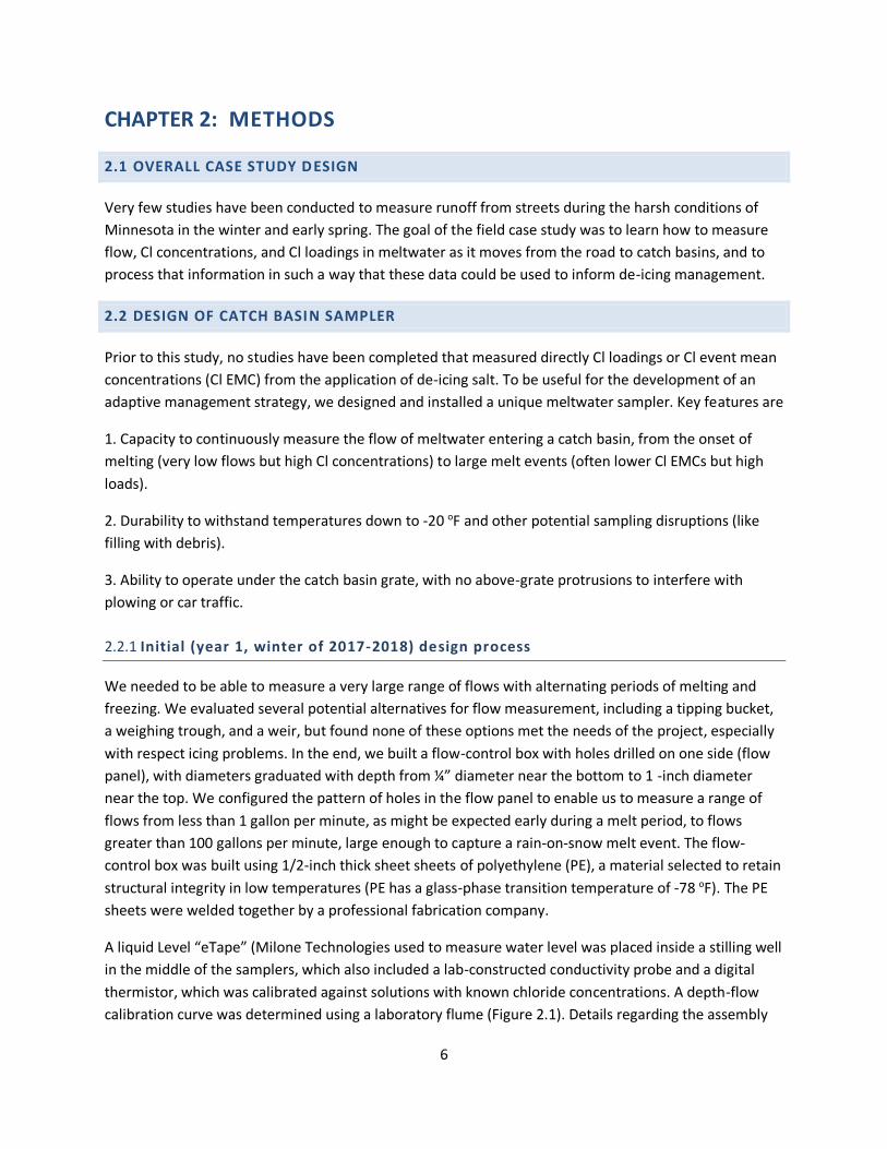
Audience. Both workshops included 15-20 Edina staff members, including (in one or both years) most of
the plow operators (wearing the yellow vests in Figure 2-8) and their supervisors, the Water Resources
Coordinator, the Engineering Services Manager, and the Public Works Director. We believe that
attendance by supervisors improved the chance of moving adaptive management ideas to fruition.
Figure 2.7: Schematic of adaptive management framework.
16
Figure 2.8: First year AM workshop.
Format. We kept research presentations short – 30 minutes total, divided among 3-4 short talks. To
develop context, this included descriptions of what we did, accompanied by site photos and a few
diagrams. Graphics were designed to be easily understood. The second part of each AM workshop was
an informal discussion of ideas to improve de-icing practice, with a focus on reducing Cl contamination.
Outcomes of these discussions are presented in chapter 5 (Moving Toward Implementation).

17
CHAPTER 3: RESULTS
3.1 WEATHER DURING THE TWO WINTER SEASONS
Weather for both winters of the study is shown below (Table 3-1). Because sampling in year 1 started
late (there was very little snow prior to January), we adjusted year 2 for the Jan. 25-May 3 time frame of
year 1 for comparison (see row 3). Winter 1 was a bit warmer on average, with more days having a
maximum temperature > 32 oF (days vs. 58 days). Winter 1 had less overall precipitation than year 2 (5.3
vs. 9.1 inches), with most precipitation occurring as “winter mix”, whereas most precipitation in year 2
occurred as mainly as rain and winter mix. In contrast winter #1 had more days of winter mix (20 vs. 13).
Table 3.1: Weather during the two study winters. Data from the NOAA MSP weather station.
Total days
Total precip, "
Rain, "
Snow (SWE), "
Winter mix, "
Days with winter
mix
Ave temp,
oF
Days with
Tmax > 32 oF
Year 1, Jan 25 -May 3, 2018 98 5.34 0.58 0.36 4.4 20 29.5 63
Year 2, Nov. 1, 2018-June 6, 2019 248 21.93 15.33 2.36 4.24 28 33.2 158
*Year 2, Jan 25 2019-May 3 2019 98 9.13 3.94 2.18 3.01 13 27.6 58
*Year 2, with comparable dates to winter #1.
The two study winters were not unusual compared with other winters (2010-2018) with respect to these
weather variables (Table 3.2).

18
Start of winter
Snow days Average
temperature
Plowable days
(Snow>2" & min>15)
Melt days ( max > 32, snow deph on
prior day >0.1)
Winter mix days
(Precip> 0, max >32 & min >28)
2010 51 34 5 27 21
2011 29 42 3 1 27
2012 46 31 9 37 18
2013 49 30 3 27 22
2014 42 31 2 7 14
2015 31 37 5 12 28
2016 21 36 2 6 45
2017 42 30 7 27 19
2018 46 29 5 17 35
Average 39.7 33.2 4.6 17.9 25.4
Min 21.0 29.1 2.0 1.0 14.0
Max 51.0 42.0 9.0 37.0 45.0
3.2 TEMPORAL PATTERN OF MELTWATER FLOWS, CL CONCENTRATIONS, AND CL LOADS.
The temporal pattern of meltwater was very irregular, as illustrated by the continuous record for the
2018-2019 winter (Figure 3.1) (the winter of 2017-2018 also had irregular flows and loadings). For most
of the 2018-2018 winter there was no flow into the catch basin, with most flow occurring in March. High
chloride concentrations of Cl often occurred with very low flows, especially early during a melt period,
representing a “first flush” of salt to the catch basin. For the 2018-2019 winter, high flows and elevated
Cl concentrations led to high Cl loads throughout March (Figure 3.1.)
Table 3.2: Comparison of the two study winters with previous winters. For consistency, all winters
started Oct. 1 and end on May 30.

19
Figure 3.1: Temporal pattern of flow (top), Cl concentrations (middle) and flow (bottom) for the second winter.

20
The disproportionality of Cl loadings is illustrated by plots of cumulative Cl loadings over time for the
two winters (Figure 3.2). Note that 50% of annual Cl load in meltwater occurred in only 41 hours (1.7
days) in year 1 and 31 hours (1.3 days) in year 2 (Table 3.3). Nearly all (90%) of the annual Cl loading
occurred within 181 hours (7.5 days) in year 1 and 190 hours (7.9 days) in year 2. At the 90% Cl loading
mark, cumulative flow was only 44% of total winter flow in year 1 and 71% of total winter flow in year 2.
Figure 3.2: Cumulative hours to reach specified levels of annual Cl loading.

21
% of annual salt load Year 1 Year 2
25 12 10
50 41 31
75 99 88
90 181 190
3.3 EVENT-BY-EVENT ANALYSIS
When we started this study, there were no completed studies to relate road salting practice directly to
the characteristics of meltwater1 Our intent was to find fairly direct relationships between road salting
(lb added) and meltwater Cl loading (lb Cl), with predictable variations among events based on weather.
Finding simple relationships between salt application and Cl loading across events was challenging
because of the complexity of meltwater runoff and corresponding Cl concentrations. Consider the
temporal pattern of monitoring data for a January 2018 melt event (Figure 3.3). During this event,
temperatures rose, as illustrated the metric “degree hours > 32 oF (which we will abbreviate as DH>32).
For a given hour, a DH>32 is the product of time (one hour here) and the temperature relative to 32 oF.
For example, one hour at 40 oF is (1 h) x = (40-32) F = 8 DH>32. These accumulate over time, so if the
temperature is 45 oF in a second hour (DH>32) = (1 hr) x (45-32) F = 13 DH>32. For the two hours, the
cumulative DH > 32 is 8 + 13 = 21. This metric is useful for thinking about road salt management,
because the accumulation of DH> 32 represents melting potential without road salt.
An example of a major melt event is depicted in Figure 3-3. During this January melt, temperatures
increased from 28 oF at the beginning of the melt (time = 0 hours), then increased over the next 10
hours to 46 oF. The cumulative DH>32 increased to 167. As one might expect, this heating caused a melt
event, with peak flow occurring at hour 13. As we have often seen, peak Cl concentrations occur prior to
the peak flow, in this case, about 2 hours after the melt started.
1 Since then, a complementary MNDOT project was completed Herb et al. 2017 (see references),
Table 3.3: Time to reach various percentages of annual Cl load and percent of cumulative flow at that time.

22
Figure 3.3: Characteristics of a melt event from January 2018. Top: hourly temperatures and cumulative DH>32.
Middle: Hourly inflow (flue) and hourly Cl. Bottom: salt mass (lb/hour).
23
3.4 PREDICTING CL LOADS AND EVENT MEAN CONCENTRATIONS.
We then sought to develop statistical models to relate independent develop metrics for both the
meltwater and independent variables that might predict meltwater metrics.
3.4.1 Approach for event interpretation
Independent variables included the following:
⮚ De-icing salt applied during the event, lb
⮚ De-icing salt applied during the event and during the prior week, lb
⮚ Average temperature during the event, oF
⮚ Cumulative degree-hours > 32oF during the event.
⮚ Cumulative degree-hours > 32o during the event and during the prior week
⮚ Snow depth at the start of the melt event, inches
⮚ Duration of event, hours
⮚ Total precipitation during the event, including snow and rain.
Dependent (response) variables included the following:
⮚ Total flow volume = sum of hourly flows throughout the event, gallons.
⮚ Average hourly flow, gallons/hour.
⮚ Total Cl loading = sum of hourly Cl loadings (lb/hour) throughout the event.
⮚ Event mean concentration (EMC) = total Cl loading/total flow volume for the event, in mg/L.
⮚ First hour Cl concentration = the average Cl concentration during the first hour of flow
Table 3-4 summarizes measured parameters for eight major events monitored during the winters of
2017/18 and 2018/19, sorted by Cl loading. “Major” events were selected on the basis of Cl load
(generally > 10 lb), event volume (> 800 gallons) and Cl EMC (> 230 mg/L). We then analyzed these data
using regression analysis. Of the several dozen relationships we tested, only four were both statistically
significant and useful (a close fit, indicated by the r2 values).

24
Event name and duration Road salt parameters Temperature parameters
Precipitaiton parameters
Flow parameters Chloride parameters
Event n
ame
Start and en
d date
for event
Du
ration
, ho
urs
Ro
ad salt add
ed
du
ring event, lb
Ro
ad salt add
ed
du
ring and 1 w
eek p
rior
Melt-w
ater salt, lb
Event C
l load
, lb
DH
>32 d
urin
g event
DH
> 32 o
F 1 wee
k p
rior to
event
DH
> 32 du
ring event
and
1 week befo
re
Average tem
p du
ring
event
Preicip as sn
ow
+mix,
inch
es
Sno
w dep
th at t=0,
inch
es
SWE o
f sno
w at t0
*
Event vo
lum
e, gallon
s
average flow
pe
r h
ou
r du
ring event
First ho
ur chlo
ride, m
g/L
lb C
l in
meltw
ater/gallons
flow
Ch
lorid
e EMC, m
g/L
Event 1
Jan 26-27, 2018 43 0 288 220 117 168 282 450 37.7 0.00 8.0
0.800 9,875 230 2234 44.9 3,128
Event 2A
Feb. 13, 2018 36 201 301 201 106 118 0 118 23.1 0.00 5.0
0.500 4,907 136 103 24.5 2,604
Event 3A
April 2, 82018 14 0 0 168 89 3 501 504 30.3 0.32 0.0
0.321 1421 101 7358 8.4 7,552
3B April 3, 2018 10 238 238 129 69 0 450 450 31.1 0.46 4.0
0.862 2,292 229 1791 17.7 3,600
Event 2B
February 16, 2018
110 129 129 128 68 99 114 213 15.9 0.43 3.0
0.734 3,812 35 1721 29.8 2,139
3C April 4, 2018 8 0 0 24 13 0 314 314 28.4 0.00 6.0
0.600 2,248 281 2374 92.1 692
Event 2C
February 21, 2018 38 0 375 18 9 0 124 124 27 0.88 2.0
1.080 874 23 1,039 5.0 1,302
Event 4
Dec. 22, 2018 78 63 63 4 2 20 67 87 27.8 0.00 2.0
0.200 1,126 15 526 272.6 234
Table 3.4: Measured parameters for major melt events. Events are ranked by Cl loading.

25
3.4.2 Predictive relationships.
3.4.2.1 Relationships with temperature.
As one might expect, total flow during an event correlated well with CDHs during the event. The
high r2 for the regression shows that flow is largely controlled by warmth (Figure 3-4).
Figure 3.4: Relationship between cumulative DH>32 and total flow (volume) for an event.
Cumulative degree hours > 32 was also a fair predictor (r2 = 0.50) of Cl loading (Figure 3-5):

26
Figure 3.5: Relationship between degree hours > 32 during event and Cl loading.
3.4.2.2 Relationships with precipitation and snow.
There were no statistically significant relationships between precipitation amount within an event and
the event volume, Cl load, or Cl EMC. There was, however, a significant and close relationship between
snow depth at the beginning of the event and event volume (Figure 5)
27
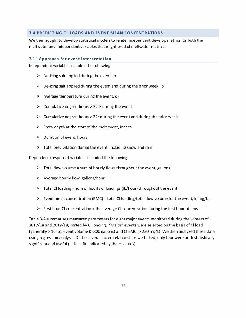
Figure 3.6: Relationship between snow depth at beginning of a melt event and event volume.
Although not statistically significant, both Cl EMC and Cl load appear to be a function of snow depth at
t=0 (graphs not shown).
3.4.2.3 Relationships with road salt input.
Interestingly, the amount of salt added during the event (lb) or during the event and the preceding week
was not significantly related to event flow, Cl loading, or Cl EMC. This suggests that much of the Cl
entering meltwater may have been temporarily stored within the watershed prior to the start of a melt
event, then released during an event. Cl storage may have occurred on the road surface itself, in
roadside snow piles, or on other pervious surfaces.
3.5 ANALYSIS OF SNOW PILE CL
During the winter of 2018-2018 we collected snow cores along a transect (seven per transect to a
distance of six feet from the curb) on nine occasions throughout the winter. Across 42 cores, about 40%
had chloride concentrations < 250 mg/L and about 60% had concentrations > 230 mg/L (the water
quality standard for protection of aquatic life in Minnesota) (Figure 3-7). The average Cl concentration of
all cores was 425 mg/L and the highest value was 1,863 mg/L.

28
Figure 3.7: Distribution of Cl concentrations across all snow core samples.
Because most of the snow pile was within 6 feet of the curb, the snow piles were very likely “plow off”
from the street, not “blow off” or salt “bounce” observed in several studies of longer snow pile transects
(some up to 100 m) (Blomqvist and Gustofsson 2004, MichDOT 2012). Because of this, we did not
observe a systematic decay of snow pile Cl concentrations across the transects (Figure 3-8). The overall
average Cl concentration for cores nearest the curb was 531 mg/L. For comparison, a snow pile analysis
of six residential streets in Waterloo, Canada was 865 mg/L (Stoner et al. 2010). We did not observe the
extremely high values (>5000 mg/L) reported for larger streets summarized by Novotny et al. (1999).

29
Figure 3.8: Cl concentrations and snow water content (inches) observed in roadside snow piles.
The pattern of Cl and SWE shows the effect of preferential elution, with Cl decreasing early, from 500
mg/L in February to near 0 by 3/15.
Total Cl mass (Cl concentration x water mass) increases from 2/11 to 3/7, peaking at 75 kg (160 lb)
(Figure 3-9). This mass was almost entirely lost, down to 7 kg (15 lb) by 3/15. Some of the snow pile Cl
moves into the underlying soil, and presumably migrates to groundwater and some re-enters the street
as snowmelt, contributing to the Cl flux in meltwater. We cannot calculate the percentage of meltwater
Cl mass comes from melting snow piles because we experienced an instrument failure in the meltwater
sampler during part of March.

30
Figure 3.9: Distribution of Cl mass from 2/9/19 to 3/21/19.
3.6 TAKE-AWAYS
For both winters of analysis, meltwater flows, Cl concentrations, and Cl loadings were highly variable
across time, from hour-to-hour, day-to-day, and month-to-month.
1. A substantial fraction of the measured Cl loading occurred during very short periods of time. For
both winters, 90% of measured meltwater Cl loadings occurred within 8 hours.
2. Analysis of key events to relate independent variables (weather variables and salt input) and
depending variables (flow, Cl concentrations, and Cl loading) showed the following:
● Warmth (as measured by CDH>32 during the event and CDH>32 during the event + prior
week) is a good predictor of event volume and event Cl loading.
● Road salt input during an event, or during an event and the prior week, is not a good
predictor of event volume, Cl loading, or Cl EMC. This suggests that much of the Cl in a given
melt event entered the watershed well before the event and was stored in the roadway,
snow piles, and pervious landscapes.
● Snow depth at the beginning of an event is a good predictor of event volume.

31
3. Substantial Cl accumulated in roadside snow piles, with a maximum Cl storage of about 150 lb
(71 kg). Much of this plow-off Cl probably moves through soil and into groundwater and some
re-enters the street, contributing to meltwater Cl loading.

32
CHAPTER 4: SCENARIO MODELING The Edina case study was done in a small catchment (2 acres) with the purpose of understanding the
patterns of road salt movement. Because the area was small and entirely residential, we used other
types of data to develop scenario models to evaluate Cl movement throughout larger watersheds. We
focused on two types of responses:
1. Steady-state Cl in groundwater
2. Annual Cl concentration and loads from larger watersheds
4.1 BASEFLOW CHLORIDE MODEL
Road de-icing operation has increased Cl concentrations in shallow aquifers in the Metro region and
probably in other cities throughout the state (MPCA, 2019). This is important for two reasons. First,
wells that withdraw water from salt-contaminated aquifers will also have high sodium, which
contributes to high blood pressure in humans. The maximum recommended consumption of sodium is
500 mg/day, an amount that would be almost entirely supplied by consuming three liters of water
containing 250 mg chloride/L (Figure 4-1). Some domestic wells in the Metro region already exceed this
level (MPCA, 2019). Second, groundwater provides the baseflow to streams and groundwater seeps add
Cl to lakes and ponds, to the point that baseflow Cl can exceed MPCA’s aquatic life standard during the
summertime (Janke et al. 2013).
4.1.1 Modeling approach
Because baseflow in streams and storm drains is often primarily groundwater, we can estimate the
steady-state concentration of chloride in groundwater as follows:
[Cl]ss = MCl/QB ( 4-1)
where [Cl]ss = steady-state, baseflow Cl concentration, mg/L
MCl = mass of Cl input to pervious surface, g/m2-yr.
and QB = baseflow, cm/yr.
Chloride input (MCl) was estimated as a function or impervious surface for 11 major watersheds in the
TCMA studied by Novotny et al. 2008 (Figure 4-1).

33
Figure 4.1: Percent impervious surface vs. Cl added as road salt. The blue axis and plot is in English units; the red
in metric.
The regression equation can be used to estimate chloride loading from road salt:
LCl = 2.045x – 2.25 (4-2)
where x = % impervious surface and Lcl is chloride load in g/(m2-yr).
The downward flux of Cl to groundwater (LCl,GW) was estimated as follows:
LCl,GW = F*LCl (4-3)
where F = fraction of LCl transported to pervious surfaces.
Transport of salt to pervious surfaces may occur by several mechanisms: salt “bounce”, wind drift, plow-
off, and meltwater entering pervious surfaces (e.g. rain gardens, infiltration basins. Salt bounce is greatly
reduced by pre-wetting and is probably much lower for residential streets than highways. Plow-off is
probably a significant mechanism.
Because there are virtually no estimates of salt loading to pervious surfaces in relation to road salt
added, we used F values of 0.25 and 0.50 in scenario modeling.

34
We then bracketed baseflow based on an analysis of flow data from the Capital Region Watershed
District (CRWD, Janke et al. 2013) to yield a range of 10 to 20 cm/yr.
4.1.2 Scenario modeling of steady-state groundwater Cl concentrations
Using equations 4-1 to 4-3 and the assumptions stated above, we modeled steady-state Cl
concentrations in groundwater (Table 4-1). For both 25% and 50% plow-off rates, Cl loading to pervious
surfaces increased, in response to the increased Cl loading to watersheds that occurs with increasing %
impervious surfaces.
4.1.2.1 25% plow-off scenarios.
For the 25% plow-off scenarios), baseflow [Cl]ss did not exceed 230 mg/ under any modeled scenarios of
the scenarios with <40% impervious surface and exceeded 230 mg/L but did exceed 230 mg/L when the
% impervious surface was > 50% and baseflow = 10 cm/yr and when % impervious surface was >80%
and baseflow was 15 cm/yr.
4.1.2.2 50% plow-off scenarios.
When we increased the plow-off to 50%, [Cl]ss often exceeded 230 mg/L, specifically:
● Always when watershed % imperviousness exceeded 30% and baseflow was set to 10 cm/yr;
● Always when % imperviousness was >40% and baseflow was 15 cm/yr.
● Always when % imperviousness was >50% and baseflow was set to 20 cm/yr. Scenario
modeling calculations reveal that baseflow chloride concentrations could readily exceed the
chloride standard, especially for watersheds with >50% impervious surface.
The highest modeled [Cl]ss was 748 mg/L, in the scenario with 80% impervious surface, 50% plow-off,
and 10 cm/yr baseflow (Table 4-1). In summary, our baseflow scenario modeling indicates that Cl values
well above water quality standards could occur in watersheds with high levels of impervious surface,
suggesting that additional modeling research on baseflow chloride might be useful in managing road
salt.
We believe that the range of modeled scenarios is credible. Although we did not measure plow-off
directly there is good reason to believe that substantial amounts of Cl in de-icing salt moves from streets
to pervious surfaces.
● Novotny et al. (2008) reported a range of Cl retention of 61% to 80% in 11 Metro region
watersheds.
● Herb and Janke (2017) reported Cl retention rates of 37% to 63% in small sewered watersheds in
the Roseville area.
● Chloride concentrations in shallow groundwater in the Metro region are increasing, mostly likely
the result of de-icing salts.

35
● Our study and the study of Stone et al. (2010) show substantial net accumulation of Cl in
roadside snow piles, although these measurements alone cannot be used to quantify annual
retention.
In the User’s Manual, we expanded this approach to include Cl from household septic leachate
(Appendix A). This version may be useful for modeling in peri-urban areas with low %
imperviousness but large numbers of septic systems.

36
% chloride to pervious landscapes 0.25 watershed % impervious 10 20 30 40 50 60 70 80
Cl loading to whole watershed, g/m2 18.15 37.4 56.1 74.8 93.5 112.2 130.9 149.6
Direct Cl loading to impervious surface, g/m2 (100% of watershed input) 18.15 37.4 56.1 74.8 93.5 112.2 130.9 149.6
Cl loading to pervious surface, g/m2 4.5 9.4 14.0 18.7 23.4 28.1 32.7 37.4
% impervious 10 20 30 40 50 60 70 80
10 cm/yr 45 94 140 187 234 281 327 374
15 cm/yr 30 62 94 125 156 187 218 249
20 cm/yr 23 47 70 94 117 140 164 187 % chloride to pervious landscapes 0.5 linked to equations in matrix watershed % impervious 10 20 30 40 50 60 70 80
Cl loading to whole watershed, g/m2 18.15 37.4 56.1 74.8 93.5 112.2 130.9 149.6
Direct Cl loading to impervious surface, g/m2 (100% of watershed input) 18.15 37.4 56.1 74.8 93.5 112.2 130.9 149.6
Cl loading to pervious surface, g/m2 9.1 18.7 28.1 37.4 46.8 56.1 65.5 74.8
% impervious 10 20 30 40 50 60 70 80
10 cm/yr 91 187 281 374 468 561 655 748
15 cm/yr 61 125 187 249 312 374 436 499
20 cm/yr 45 94 140 187 234 281 327 374
Table 4.1: Modeled steady-state Cl concentrations in groundwater. Assumed plow-off rates: 25% (top) and 50% (bottom).

37
4.2 REGRESSION-BASED SCENARIO MODELING FOR LARGE WATERSHEDS.
4.2.1 Data mining
We used data from the road salt study report by Novotny et al. 2008 (Table 4-2) to develop several
regression models that could be used for scenario modeling at the scale of large urban watersheds
(3,000 to 114,000 acres).
Table 4.2: Summary data from Novotny et al. 2008.
Area, ha Total Cl added,tonnes/yr
Imperivous %
Mean Cl in outflow, mg/L
% retained
Cl export, tonnes/yr
Ave. flow, m3/sec
Bassett 11,100 8,100 34 138 55 3648 0.966
Battle 3,000 2400 32 147 63 896 0.221
Bluff 2,300 600 11 65 71 153 0.105
Carver 21,600 1,800 4 37 68 563 0.983
Credit R. 13,300 1,800 9 44 75 395 0.498
Fish 1,300 600 27 100 64 240 0.093
Minnehaha 46,100 17,700 15 68 85 2617 1.685
Nine mile 9,900 4,700 29 74 76 1234 0.709
Riley 3,400 600 18 53 83 120 0.113
Shingle 10,800 7,000 35 185 63 2584 0.493
4.2.2 Regression equations
Figure 4-1 (above) shows the relationship between % impervious surface and Cl loading from road salt.
Figure 4-2 can be used to estimate mean annual Cl concentration as a function of % impervious surface;
Figure 4-3 can be used to estimate Cl export; and Figure 4-4 can be used to estimate Cl retention in
relation to % impervious surface. The relationship between % impervious surface and Cl retention is
somewhat weaker than the relationships shown in figures 4-1 to 4-3. The only equations shown are
those that are statistically significant at the 0.05 level and have r2 high enough to have predictive value.

38
Figure 4.2: Percent impervious surface vs. mean Cl concentration for 11 Metro region streams.
Figure 4.3: Percent impervious surface vs. Cl export for 11 Metro region streams.

39
Figure 4.4: Percent connected impervious surface vs. Cl retention for 11 Metro region drains.
Combining these relationships into nomographs can be used to visualize scenarios of watershed
imperviousness on the environmental behavior of chloride (Figures 4-5 and 4-6).
Figure 4.5: Effect of % impervious surface on Cl input and mean Cl concentration.
40
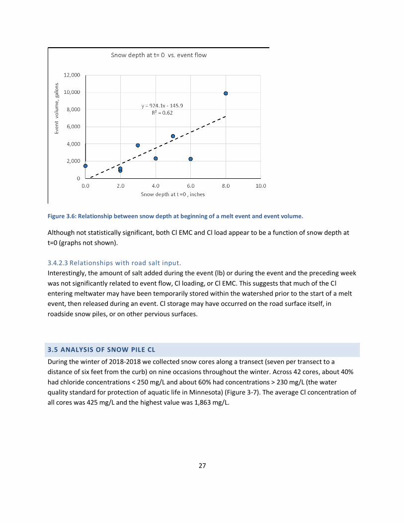
Figure 4.6: Effect of % impervious surface on mean Cl export and Cl retention
4.2.3 Utilization of regression equations for predictions
The data and regressions in these six figures can be used to develop de-icing scenarios based on
management of impervious surface. For example, Table 4-3 illustrates the effect of changing %
impervious surface for a watershed that initially is 50% imperviousness. From Table 2, the initial
predicted mean chloride concentration is 278 mg/L, just over the chronic chloride standard (230 mg/L).
If further development increased the % imperviousness to 60%, the predicted chloride would increase to
431 mg/L, an increase of 153 mg/L and now well over the chloride standard. Conversely, a 10% decrease
in imperviousness from 50% to 40% would reduce mean chloride to 179 mg/L, a decrease of 63 mg/L in
mean chloride concentration.
These calculations show that changing imperviousness of a watershed could reduce mean stream Cl
concentrations. One caveat: Because the data behind these regressions were collected in the years prior
to 2007, they are based on relationships at that time, and would not reflect changes in salting practice.
It may now be feasible to develop a more robust tool using more data from year-round-measurement
stations that continuously monitor flow and specific conductance, and the capacity to model connected
impervious surface based on recently completed mapping tools.
This level of scenario modeling is very simple and would therefore be useful as a first-cut analysis for
city- or watershed-scale land use planning.

41
Table 4.3: Effect of reducing % impervious surface on mean annual Cl concentration in drainage from large
watersheds.
% impervious
surface
Initial modeled Cl
concentration, mg/L
Reduction in mean Cl, mg/L,
with 10% change in
imperviousness
60% 431 153
50% 278 99
40% 179 63
30% 116 -
4.3 CONCLUSIONS
1. Scenario analysis to forecast steady-state Cl concentrations in groundwater indicate that very
high levels of Cl will occur in many Metro region watersheds, particularly highly urbanized
watersheds with >40% impervious surfaces. This analysis is limited by the quality of input data –
especially the Cl flux from streets to pervious surfaces. Further studies of fluxes to and from
roadside snow piles may elucidate management activities to reduce these fluxes.
2. For large watersheds, the data from the Novotny et al. (2008) study was used to model annual
Cl inputs from road salt, mean Cl in drainage, and Cl export. This level of modeling may be useful
to urban planners who design future urban landscapes, and hence % impervious cover.
42
CHAPTER 5: MOVING TOWARD IMPLEMENTATION
The broad goal of this study was to learn how to reduce the use of de-icing salts through adaptive
management (AM), by linking meltwater Cl data to salt truck application data to measured Cl output to
storm drains.
5.1 ADAPTIVE MANAGEMENT (AM) WORKSHOPS
5.1.1 Rationale
The key idea of this study was to measure Cl loading in meltwater directly while also tracking the
amount of road salt added and to share this information with plow truck operators. Originally, the idea
was to share information soon after each salt application, but this proved to be unworkable. Instead, we
convened adaptive management workshops, one at the end of each winter, to share our findings and to
start a discussion on how de-icing practice could be improved. The format of these workshops was
described in Chapter 2 (Methods).
5.1.2 Workshop Summaries
5.1.2.1 Workshop #1 (May 18, 2018).
A key focus was on high-Cl meltwater “events” – periods of snowmelt with high Cl mass loadings
(lb/day) to the catch basin. We focused particularly on the event with the highest Cl loading (Figure 5.1)
Staff recalled this being a winter mix event, and as one staff member noted,
“Management of the plows themselves is more important than the application of salt. Different types of
blades, angles of the blade, and possibly using graders could substantially change the needs for salt”
Figure 5.1: Slide used to show peak Cl loading event during winter #1.

43
5.1.2.2 Workshop #2 (May 29, 2019)
The format for the year 2 workshop was similar. One main point of discussion was the problem of
“chunky” salt, which was perceived to be poor quality of purchased salt. Operators noted that their
salting augers were getting clogged using this salt, forcing them to hit the “blast” button… This has led
the Street Department to develop a way to quickly measure water content of salt that can be done
quickly – while the delivery truck is still parked at the Public Works building. Briefly, the methodology is
to weigh a small amount of delivered salt, microwave it to remove water, and weight the salt again.
Water percentage is calculated from these measurements and loads with excess water are rejected. This
is expected to reduce the clumping problem in future years.
A second topic that came up was the possibility of downloading the truck monitoring data from all of the
trucks immediately after each de-icing event, to enable the plow crew to evaluate how each truck
performed, and to discuss these data within their group, to develop ways to reduce salt use. This rapid
downloading of data is now possible due to improvements in the Precis database tools.
Note that the action items coming out of the Year 2 workshop, unlike those in year 1, were not directly
based on the U of M monitoring data. This points to the idea that when an adaptive management
process is started, it takes a life of its own, stimulating creative thinking among participants.
5.2 OUTCOME FROM WORKSHOP #1: PURCHASE OF JOMA BLADES
The discussion in workshop #1 regarding better plow blades that could cut through ice better, so that
less (or no) salt would be needed to soften the ice prior to scraping. Ultimately the city decided to
purchase five “Joma “blades, equipped with carbide blades that promised to clear ice better. The City of
Edina, with a grant from the Nine Mile Creek Watershed District purchased five of these blades and
installed them on their trucks during the fall of 2018, prior to the 2018-2019 winter.
Some observations from operators who used the new blades:
⮚ Increase in the quantity of snow that the blades were able to pick up and the service they were
able to provide on road surfaces when compared to the traditional blades on the same route
⮚ Easier to operate and noticeably quieter ride.
⮚ Less salt needed. Visual improvement in the mechanical removal with the new blades (See
Figure 5-2).

44
Figure 5.2: Top: traditional plow blade. Bottom right: Newly installed Joma blade. Bottom right: Road clearing
with the traditional plow blade (bottom) and the Joma blade (top).
5.3 RECOMMENDATIONS
⮚ Adaptive management is well-suited for de-icing operations because (1) road salt crews are
a small, captive audience, enabling communication; (2) road salt is overused, so there is
potential for reduction; (3) there are many ways to reduce salt inputs (4) rapid feedback
(road condition, salt use, etc.) can be provided; and (5) there are many learning events (each
de-icing event) in every winter season.
⮚ Inclusion of supervisors is valuable because supervisors can provide support for creative
ideas emanating from plow truck operators.

45
⮚ We used a 2:1 time ratio of discussion (~ 1 hour) to formal data presentation (~ 30 minutes).
This resulted in creative ideas, many of which were implemented. An ongoing process (many
years) would probably enable continuous improvement.
⮚ Providing some form of environmental feedback was very important, giving the operators
“eyes to the environment” for the first time.

46
CHAPTER 6: CONCLUSIONS AND RECOMMENDATIONS
Reflecting on this research, we make the following recommendations on de-icing practice and on future
research to reach the goal of reducing the Cl impact of road de-icing.
6.1 DE-ICING PRACTICE
1. Target “winter mix” conditions, with large swings in temperature and often significant mixed
precipitation. These seem to be the events that result in largest spikes in Cl mass in the
meltwater.
2. Monitor the quality of salt as it is received to avoid high-moisture contents that lead to
clumping, which in turn makes it difficult to apply salt evenly.
3. Add infrared road temperature sensors to trucks to guide salting. Road temperatures can be
much different (by as much as 20o F) from air temperatures, so air temperatures are not a
reliable guide to melt predictions.
4. Use reliable salt application sensors and recording systems to quantify the application rates
directly with road location.
5. Develop post-event operator workshops to share data, experiences and ideas among operators.
6. Consider expanded use of Joma blades, while continuing to compare maintenance costs
(compared to conventional blades).
6.2 FUTURE RESEARCH
1. Conduct a study to analyze meltwater Cl patterns in large stormwater drains in relation to
weather conditions and de-icing practice. Several watershed districts now monitor flow and
specific conductance continuously and are generally willing to share data after they are quality
assured.
2. Investigate effectiveness of pre-wetting and anti-icing practices for a wide range of Minnesota
conditions and application rates.
3. Develop a user-friendly tool to predict pavement melting over the period of 4-8 hours to help
street departments plan de-icing application rates during a shift.
4. Install low-cost pavement temperature sensors and runoff samplers to better understand the
dynamics of melting processes, including the fraction of salt application that is plowed or
removed from streets.

47
5. Develop GIS software to integrate records of application rates and effectiveness of melting
based on operator input and field data.
6. Take advantage of the re-building of the MnROAD research facility to include de-icing studies
under controlled conditions, such as the use of snow-making equipment to provide specific
volumes of snow, perhaps heated road sections, and automated measurement stations to allow
continuous measurements of temperature, runoff, conductivity and other parameters. A few
examples of the types of studies that might be conducted include:
⮚ Further experiments on de-icing melt efficiency conducted under various
experimental treatments
⮚ Development of a tool to predict roadway melting with varying levels of active de-
icing
⮚ Evaluation of the efficiency of plow designs for removing ice and/or snow on roads
built with various designs and materials
⮚ Evaluation of the durability of plow designs for specific types of road surfaces
⮚ Impact of salt on road corrosion

48
REFERENCES
Baker, L. (2007, November). Urban stormwater: Getting at the Source (Feature article). Stormwater
Magazine 8(8).
Baker, L.A., D. Klimbal, & B. Wilson. 2018. Adaptive Management to Improve De‐Icing Operations. Paper presented at the Minnesota Water Resources Conference, Oct. 16, St. Paul.
Baker, L.A., J. Chapman, J. Bilotta, & S. Missaghi. 2019. Minnesota’s Stormwater Research Roadmap.
Prepared for the Minnesota Pollution Control Agency and the Clean Water Legacy Program. Retrieved
from https://www.wrc.umn.edu/sites/wrc.umn.edu/files/stormwater_research_roadmap_-_11-26-
18_submitted.pdf
Bester, M.L., E.O. Frind, J.W. Molson, & D.L. Rudolph 2006. Numerical Investigation of Road Salt Impact
on an Urban Wellfield. Ground Water, 44(2), 165–175.
Blomqvist, G. & M. Gustafsson. 2004. Patterns of Residual Salt on Road Surface: Case Study (Paper 04-
017). In Transportation Research E-Circular Number E-C063, June 2004 ISSN 0097-8515, Proc. of the
Sixth International Symposium on Snow Removal and Ice Control Technology, June 7–9, Spokane, WA.
Friese, M., L. Baker, B. Wilson, & D. Kimbal. 2020. Analyzing Watershed Cl Loading Patterns to Inform
Adaptive Management for Road De-Icing. Research Project of the Undergraduate Research
Opportunities Program, University of Minnesota, Minneapolis.
Friese, M., L. Baker, B. Wilson, & D. Klimbal. 2020. Analyzing Watershed Chloride Loading Patterns to
Inform Adaptive Management for Road De-Icing. Paper presented at the Minnesota Water Resources
Conference, October 2019, St. Paul, MN.
Herb, W., B. Janke, & H. Stefan 2017. Study of De-icing Salt Accumulation and Transport Through a
Watershed (Research Project Final Report 2017-50). St. Anthony Falls Laboratory, University of
Minnesota, Minneapolis.
Janke, B., J. Finlay, S. Hobbie, L. Baker, R. Sterner, D. Nidgorski, & B. Wilson. 2013. Contrasting Influences
of Stormflow and Baseflow Pathways on Nitrogen and Phosphorus Export from an Urban Watershed.
Biogeochemistry. http://doi.10.1007/s10533-013-9926-1
Kelley, V.R., G.M. Lovett, K.C. Weathers, S.E.G. Findlay, D. Strayer, D. J. Burns, & G. E. Likens. 2008. Long-
Term Sodium Chloride Retention in a Rural Watershed: Legacy Effects of Road Salt on Streamwater
Concentration. ES&T, 42, 410-415.
Kroening, S., & M. Ferrey. 2013. The Condition of Minnesota’s Groundwater, 2007 – 2011 (Document
wq-am1-06). Minnesota Pollution Control Agency, Saint Paul, MN.

49
Lysbakken, K.R., & H. Norem. 2011. Processes That Control Development of Quantity of Salt on Road
Surfaces After Salt Application. Transportation Research Record: Journal of the Transportation Research
Board, 2258, 139–146. http://doi.10.3141/2258-17
MGA (Minnesota Groundwater Association). 2020. Impacts of stormwater infiltration on chloride in Minnesota groundwater. Retrieved from https://www.mgwa.org/documents/whitepapers/impacts_of_tormwater_infiltration_on_chloride_in_minnesota_groundwater.pdf
Novotny, V., D.W. Smith, D.A. Kuemmel, J. Mastriano, & A. Bartosvova. 1999. Urban and Highway
Snowmelt: Minimizing the Impact on Receiving Waters (Project 94-IRM-2). Water Environmental
Research Foundation, Alexandria, VA.
Novotny, E., A. Sander, O. Mohseni, & H. Stefan 2008. A Salt (Chloride) Balance for the Minneapolis/St.
Paul Metropolitan Area Environment (Report 513). St. Anthony Falls Hydraulics Lab (SAHFL),
Minneapolis, MN.
MGWA. 2020. Impacts of stormwater infiltration on Cl in Minnesota groundwater (White Paper 04).
Minnesota Ground Water Association, White Bear Lake, MN.
MPCA. 2019. Statewide Cl Management Plan (Draft wwq-s1-94). Minnesota Pollution Control Agency, St.
Paul, MN.
MichDOT. 2012. Salt Bounce and Scatter Study. Michigan Dept. of Transportation, Operations Field
Services Division, Lansing, MI.
Novotny, V., D. W. Smith, D. A. Duemmel, J. Mastriano, & A. Bartosova. 1999. Urban and Highway
Snowmelt: Minimizing the Impact on Receiving Water. Water Environment Research Foundation,
Alexandria, VA.
Oberts, G. 2003. Influence of Snowmelt Dynamics on Stormwater Runoff Quality. Watershed Protection
Techniques, 1(2), 55-61.
Overbo, A., S. Heger, S. Kyser, B. Asleson, & J. Gulliver. 2019. Chloride Contributions from Water
Softeners and Other Domestic, Commercial, Industrial, and Agricultural Sources to Minnesota Waters.
Legislative-Citizens Commission on Minnesota Resources, XXXX, MN.
Sander, A. R., E. V. Novotny, O. Mohseni, & H. G. Stefan. 2007. Inventory of road salt use in the
Minneapolis/St. Paul metropolitan area. St. Anthony Falls Lab., Univ. of Minn., Minneapolis.
Stone, M., M. Emelko, J. Marsalak, J. Price, D. Rudolph, H. Saini, & S. Tighe. 2010. Assessing the Efficiency
of Current Road Salt Management Programs. University of Waterloo and the National Water Research
Institute, Waterloo, Ontario.
Wilson, J., & M. Allen. 2018. Final Report: Plow Blade Grant City of Edina 2018-20. CIty of Edina Publish
Works Department, Edina, MN.