Embed Size (px)
Citation preview

ADAPTIVE GRIDS IN WEATHER
AND CLIMATE MODELING
by
Christiane Jablonowski
A dissertation submitted in partial fulfillmentof the requirements for the degree of
Doctor of Philosophy(Atmospheric and Space Sciences and Scientific Computing)
in The University of Michigan2004
Doctoral Committee:
Professor Joyce E. Penner, ChairpersonProfessor John P. BoydProfessor Quentin F. StoutProfessor Bram van Leer


c© Christiane Jablonowski 2004All Rights Reserved


ACKNOWLEDGEMENTS
This dissertation is the result of a joint interdisciplinary effort and would not have
been possible without the support of many people. First of all, I would like to say
thank you to my committee, my advisor Joyce E. Penner, Quentin F. Stout, Bram
van Leer and John P. Boyd. I very much appreciated the support and advice you
provided. In addition, many thanks to Michael Herzog for our project discussions
and often spontaneous brain-storming sessions.
Many thanks go to Quentin Stout who always had time for discussions about
all the numerical and computational difficulties I encountered during this endeavor.
This often led to very long lunch meetings or coffee breaks. Special thanks also
go to Bram van Leer who gave me very good advice with respect to the numerical
interpolation methods. Furthermore, I wish to thank Ken Powell for his insights. And
of course, this work would have never been possible without Robert Oehmke. He is
the developer of the spherical adaptive grid library that he wrote for his Ph.D. thesis
in the Electrical Engineering and Computer Science Department at the University of
Michigan. The library is a major building block of the project. A thousand thanks,
Bob. I very much appreciated your friendship, work, our meetings and e-mails that
answered all upcoming questions.
Many more people were involved who made this interdisciplinary collaboration
work. I owe a great deal of thanks to the NASA/GSFC team S.-J. Lin, Kevin Yeh
and Ricky Rood who provided me with the atmospheric model and their expertise.
iii

Furthermore, special thanks to the NCAR team, especially to David Williamson, for
the collaboration, invaluable advice and generous computing resources. I thank Steve
Thomas, Rich Loft and Aime Fournier (NCAR) and Frank Giraldo (NRL, Monterey)
for testing the newly developed test case with their models. I am now very much
looking forward to joining NCAR as a postdoctoral researcher. In addition, thanks
to Detlev Majewski from the German Weather Service DWD for providing me with
the weather code GME.
In addition, thank you, Margaret Reid, Jan Beltran, Sandy Pytlinski, Kathy
Norris and Sue Griffin for the excellent administrative support in the department.
You made things a lot easier.
Last but not least I wish to say thank you to my family and friends who accompa-
nied me during this long journey. In particular, thanks to my Mom, Jabi and Tanja
who I at least saw twice a year. In addition, thank you, Anne and Michael, for your
friendship, feisty squash and ‘Doppelkopf’ matches and countless dinner meetings.
Thank you, Dave, Laurie, A.J. and Heather for your friendship, companionship and
fun evenings. Dave, I hope I was a good housemate. And of course special thanks
to you, Rainer, for our long-lasting relationship that kept me grounded during all
those years. You kept up with our friend ‘Mr. Pole’ and all his neighbors. I deeply
appreciate your patience and support.
This work was supported by NASA Headquarters under the Earth System Science
Fellowship Grant NGT5-30359. In addition, partial funding was provided by the
Department of Energy under the SciDAC grant DE-FG02-01ER63248. I am grateful
for the support.
iv

TABLE OF CONTENTS
ACKNOWLEDGEMENTS . . . . . . . . . . . . . . . . . . . . . . . . . . iii
LIST OF FIGURES . . . . . . . . . . . . . . . . . . . . . . . . . . . . . . . ix
LIST OF TABLES . . . . . . . . . . . . . . . . . . . . . . . . . . . . . . . . xv
LIST OF APPENDICES . . . . . . . . . . . . . . . . . . . . . . . . . . . . xvii
CHAPTER
I. Introduction: Adaptive grids in weather and climate modeling 1
1.1 Motivation and research questions . . . . . . . . . . . . . . . 11.2 Adaptive and nonuniform grids . . . . . . . . . . . . . . . . . 7
1.2.1 Nested grids . . . . . . . . . . . . . . . . . . . . . . 71.2.2 Stretched grids . . . . . . . . . . . . . . . . . . . . . 91.2.3 Dynamically adaptive mesh refinements . . . . . . . 111.2.4 Summary: Dynamic grid adaptation . . . . . . . . . 14
1.3 Adaptive grid libraries . . . . . . . . . . . . . . . . . . . . . . 151.4 Overview of the thesis . . . . . . . . . . . . . . . . . . . . . . 20
II. The hydrostatic finite-volume dynamical core . . . . . . . . . 23
2.1 Model design and numerics . . . . . . . . . . . . . . . . . . . 242.1.1 Governing equations . . . . . . . . . . . . . . . . . . 242.1.2 Horizontal discretization . . . . . . . . . . . . . . . 282.1.3 Vertical representation . . . . . . . . . . . . . . . . 372.1.4 Summary . . . . . . . . . . . . . . . . . . . . . . . . 39
2.2 Pole problem in latitude-longitude grids . . . . . . . . . . . . 402.2.1 Polar cap . . . . . . . . . . . . . . . . . . . . . . . . 412.2.2 Polar filters . . . . . . . . . . . . . . . . . . . . . . 46
2.3 Divergence damping . . . . . . . . . . . . . . . . . . . . . . . 60
III. Adaptive mesh refinements in spherical geometry . . . . . . . 67
3.1 The adaptive finite-volume dynamical core . . . . . . . . . . . 68
v

3.1.1 Block data structure . . . . . . . . . . . . . . . . . 683.1.2 Model resolution . . . . . . . . . . . . . . . . . . . . 723.1.3 Grid point positions . . . . . . . . . . . . . . . . . . 76
3.2 Software engineering aspects . . . . . . . . . . . . . . . . . . 793.2.1 Adaptive spherical grid library . . . . . . . . . . . . 793.2.2 Program flow . . . . . . . . . . . . . . . . . . . . . 863.2.3 Performance . . . . . . . . . . . . . . . . . . . . . . 87
3.3 Fine-coarse grid interfaces . . . . . . . . . . . . . . . . . . . . 913.3.1 Interpolation and averaging techniques . . . . . . . 913.3.2 Model interfaces . . . . . . . . . . . . . . . . . . . . 1083.3.3 Flux corrections . . . . . . . . . . . . . . . . . . . . 110
IV. Reduced grid and static adaptations . . . . . . . . . . . . . . . 113
4.1 Error measures and global diagnostics . . . . . . . . . . . . . 1144.1.1 Normalized error norms . . . . . . . . . . . . . . . . 1144.1.2 Global invariants . . . . . . . . . . . . . . . . . . . 1174.1.3 Reference solutions . . . . . . . . . . . . . . . . . . 117
4.2 Reduced grid . . . . . . . . . . . . . . . . . . . . . . . . . . . 1194.2.1 Design of the reduced grid . . . . . . . . . . . . . . 1204.2.2 Advection tests . . . . . . . . . . . . . . . . . . . . 1224.2.3 Non-linear shallow water tests . . . . . . . . . . . . 125
4.3 Static adaptations . . . . . . . . . . . . . . . . . . . . . . . . 136
V. Adaptation criteria and 2D dynamic adaptations . . . . . . . 147
5.1 Adaptation criteria . . . . . . . . . . . . . . . . . . . . . . . . 1485.1.1 Flow-based criteria . . . . . . . . . . . . . . . . . . 1505.1.2 Adaptation criteria for the finite-volume dynamical
core . . . . . . . . . . . . . . . . . . . . . . . . . . . 1525.2 Dynamic adaptations: Shallow water tests . . . . . . . . . . . 157
5.2.1 Advection tests with the full grid . . . . . . . . . . 1575.2.2 Advection tests with the reduced grid . . . . . . . . 1705.2.3 Flow over a mountain . . . . . . . . . . . . . . . . . 173
VI. Test of the adaptive 3D dynamical core . . . . . . . . . . . . . 189
6.1 New idealized test cases for dynamical cores:The Jablonowski-Williamson test . . . . . . . . . . . . . . . . 190
6.1.1 Design of the test case . . . . . . . . . . . . . . . . 1926.1.2 Formal test definition and test strategy . . . . . . . 196
6.2 Static adaptations . . . . . . . . . . . . . . . . . . . . . . . . 2016.3 Dynamic adaptations . . . . . . . . . . . . . . . . . . . . . . 208
vi

VII. Summary and future research directions . . . . . . . . . . . . . 213
APPENDICES . . . . . . . . . . . . . . . . . . . . . . . . . . . . . . . . . . 221
BIBLIOGRAPHY . . . . . . . . . . . . . . . . . . . . . . . . . . . . . . . . 257
vii


LIST OF FIGURES
1.1 Components of a General Circulation Model. . . . . . . . . . . . . . 6
1.2 Stretched grid. . . . . . . . . . . . . . . . . . . . . . . . . . . . . . . 10
2.1 Grid staggering techniques after Arakawa. . . . . . . . . . . . . . . 34
2.2 Latitude-longitude regular grid. . . . . . . . . . . . . . . . . . . . . 34
2.3 Terrain-following Lagrangian control-volume coordinate system ofthe Lin-Rood dynamical core. . . . . . . . . . . . . . . . . . . . . . 38
2.4 Orientation of the local unit vectors in spherical coordinates nearthe North Pole. . . . . . . . . . . . . . . . . . . . . . . . . . . . . . 42
2.5 Relationship between the multi-valued wind components in spheri-cal coordinates and the unique wind vector in a North Polar stereo-graphic projection. . . . . . . . . . . . . . . . . . . . . . . . . . . . 44
2.6 Response function of different Shapiro filters. . . . . . . . . . . . . . 53
2.7 Meridional velocity at day 4 (McDonalds and Bates [1989] test case)with and without additional Shapiro filtering in meridional directionat the poles. . . . . . . . . . . . . . . . . . . . . . . . . . . . . . . . 55
2.8 Geopotential height (test case 6) with Shapiro filtering. . . . . . . . 57
2.9 Differences of the Shapiro-filtered run (test case 6). . . . . . . . . . 58
2.10 Geopotential height (test case 3) with and without Shapiro filtering. 59
2.11 Coefficients for the divergence damping mechanism. . . . . . . . . . 63
2.12 Differences of the zonal wind with the analytic solution at day 10with and without divergence damping (test case 2, α = 90). . . . . . 65
3.1 Distribution of grid points over the sphere with and without blockstructure. . . . . . . . . . . . . . . . . . . . . . . . . . . . . . . . . 68
3.2 Refinement and coarsening principles with 2 refinement levels. . . . 69
3.3 Adapted blocks. . . . . . . . . . . . . . . . . . . . . . . . . . . . . . 70
3.4 Ghost cell updates for blocks at the same refinement level. . . . . . 70
3.5 Ghost cell updates for blocks at different refinement levels. . . . . . 71
3.6 Splitting of one coarse cell into 4 fine-grid cells. . . . . . . . . . . . 76
3.7 Flux calculations at a fine-coarse grid interface . . . . . . . . . . . . 77
3.8 Cascading refinements. . . . . . . . . . . . . . . . . . . . . . . . . . 83
ix
3.9 Information exchange among nearest neighbors. . . . . . . . . . . . 83
3.10 Load-balancing strategy. . . . . . . . . . . . . . . . . . . . . . . . . 85
3.11 High level view of the program flow with adaptive mesh functionality. 87
3.12 CPU timing data for different block sizes. . . . . . . . . . . . . . . . 88
3.13 Differences of the geopotential height with the analytic solution afterrefining the whole domain with refinement level 1. Comparison oftwo normalized coordinates. . . . . . . . . . . . . . . . . . . . . . . 100
3.14 Cascade interpolations of the wind components. . . . . . . . . . . . 102
3.15 Differences of the zonal wind with the analytic solution. Comparisonof different interpolation techniques. . . . . . . . . . . . . . . . . . . 104
3.16 Differences of the geopotential height with the analytic solution (testcase 6). . . . . . . . . . . . . . . . . . . . . . . . . . . . . . . . . . . 105
3.17 Fine-coarse grid interface. . . . . . . . . . . . . . . . . . . . . . . . 108
3.18 Reduced grid interface without adaptations. . . . . . . . . . . . . . 109
3.19 Reduced grid interface with adaptations. . . . . . . . . . . . . . . . 109
3.20 Flux and kinetic energy updates at fine-coarse grid interfaces. . . . 110
4.1 Distribution of blocks and grid points over the sphere with a reducedgrid. . . . . . . . . . . . . . . . . . . . . . . . . . . . . . . . . . . . 121
4.2 Physical grid distance (km) in longitudinal direction for the full gridand reduced grid setups. . . . . . . . . . . . . . . . . . . . . . . . . 121
4.3 Reduced grid: Polar stereographic projections of the cosine belltransported over the North Pole. . . . . . . . . . . . . . . . . . . . . 124
4.4 Reduced grid: North polar stereographic projections of the geopo-tential height, the zonal and meridional wind (McDonald test case). 126
4.5 Zonal wind at day 14 (test case 2, α = 45) with different reducedgrid setups. . . . . . . . . . . . . . . . . . . . . . . . . . . . . . . . 127
4.6 Zonal wind differences with reference solution at day 14 (test case 2,α = 45). . . . . . . . . . . . . . . . . . . . . . . . . . . . . . . . . . 128
4.7 Normalized l2 height and wind error norms for reduced grid runs(test case 2, α = 45). . . . . . . . . . . . . . . . . . . . . . . . . . . 129
4.8 Reduced grid simulations with 1 reduction (test case 6). Comparisonof interpolation techniques. . . . . . . . . . . . . . . . . . . . . . . . 131
4.9 Normalized l2 and l∞ height errors for the full and different reducedgrid. . . . . . . . . . . . . . . . . . . . . . . . . . . . . . . . . . . . 132
4.10 Normalized global integrals of total energy and potential enstrophyfor the full grid and reduced grids (test case 6). . . . . . . . . . . . 133
4.11 Normalized global integrals of the mass for reduced grid simulationswith 1 reduction (test case 6). . . . . . . . . . . . . . . . . . . . . . 134
4.12 Geopotential height at day 14 (test case 2, α = 45) with staticrefinements. . . . . . . . . . . . . . . . . . . . . . . . . . . . . . . . 136
x

4.13 Zonal and meridional wind at day 14 (test case 2, α = 45) withstatic refinements. . . . . . . . . . . . . . . . . . . . . . . . . . . . . 137
4.14 Normalized l2 height errors (test case 2, α = 45) for staticallyadapted runs. . . . . . . . . . . . . . . . . . . . . . . . . . . . . . . 138
4.15 Geopotential height fields at day 7 with statically refined blocks (testcase 6). . . . . . . . . . . . . . . . . . . . . . . . . . . . . . . . . . . 140
4.16 Normalized l2 height errors for statically adapted runs (test case 6). 141
4.17 Initial geopotential height and static adaptations (test case 4). . . . 142
4.18 Geopotential height and height errors at day 5 (test case 4). . . . . 145
4.19 Normalized l2 and l∞ height error norms for adapted and non-adaptedmodel runs (test case 4). . . . . . . . . . . . . . . . . . . . . . . . . 146
5.1 Choices for refinement criteria illustrated with the initial state oftest case 4. . . . . . . . . . . . . . . . . . . . . . . . . . . . . . . . . 154
5.2 Snapshots of the cosine bell with adapted grid at different time steps(test case 1, α = 90). . . . . . . . . . . . . . . . . . . . . . . . . . . 159
5.3 Cosine bell after one revolution with refinement and different rota-tion angles. . . . . . . . . . . . . . . . . . . . . . . . . . . . . . . . 161
5.4 Cosine bell after one revolution with different refinement levels (α =45). . . . . . . . . . . . . . . . . . . . . . . . . . . . . . . . . . . . 162
5.5 North polar stereographic projections of the cosine bell with differentrefinement levels. . . . . . . . . . . . . . . . . . . . . . . . . . . . . 163
5.6 Normalized l2 and l∞ height errors (test case 1). . . . . . . . . . . . 169
5.7 North polar stereographic projections of the cosine bell (test case 1,α = 90) with reduced grid and refinements. . . . . . . . . . . . . . 171
5.8 Normalized l2 and l∞ height errors for the full grid and differentreduced grids (test case 1, α = 90). . . . . . . . . . . . . . . . . . . 173
5.9 Initial geopotential height and orography with statically adaptedgrid (test case 5). . . . . . . . . . . . . . . . . . . . . . . . . . . . . 174
5.10 Initial absolute values of the relative vorticity and the geopotentialgradient (test case 5). . . . . . . . . . . . . . . . . . . . . . . . . . . 175
5.11 Relative vorticity and the geopotential height field & orography(statically adapted) with relative vorticity-based refinement (testcase 5). . . . . . . . . . . . . . . . . . . . . . . . . . . . . . . . . . . 179
5.12 Geopotential gradient and the geopotential height field & orographywith gradient-based refinement criterion (test case 5). . . . . . . . . 180
5.13 Meridional wind at day 15 with two adaptation criteria (test case 5). 182
5.14 Normalized l2 and l∞ height errors for adapted and non-adaptedruns (test case 5). . . . . . . . . . . . . . . . . . . . . . . . . . . . . 183
5.15 Normalized global total energy and potential enstrophy for adaptedand non-adapted runs (test case 5). . . . . . . . . . . . . . . . . . . 185
xi

5.16 Relative vorticity and the geopotential height field & orographywith relative vorticity refinement criterion and dynamically adaptedmountain (test case 5). . . . . . . . . . . . . . . . . . . . . . . . . . 187
6.1 Jablonowski-Williamson test: Initial zonal wind and temperature. . 193
6.2 Jablonowski-Williamson test: Surface geopotential and initial tem-perature profiles. . . . . . . . . . . . . . . . . . . . . . . . . . . . . 194
6.3 Jablonowski-Williamson test: Absolute and potential vorticity of theinitial state. . . . . . . . . . . . . . . . . . . . . . . . . . . . . . . . 194
6.4 Jablonowski-Williamson test: Potential temperature and Brunt-Vaisalafrequency. . . . . . . . . . . . . . . . . . . . . . . . . . . . . . . . . 195
6.5 Zonal wind perturbation. . . . . . . . . . . . . . . . . . . . . . . . . 196
6.6 Jablonowski-Williamson test: Surface pressure at day 8 for dynam-ical core runs with static adaptations. . . . . . . . . . . . . . . . . . 203
6.7 Jablonowski-Williamson test: Surface pressure at day 10 for dynam-ical core runs with static adaptations. . . . . . . . . . . . . . . . . . 204
6.8 Global minimum and maximum surface pressure. . . . . . . . . . . 206
6.9 Refinement of one block versus a latitudinal band: Surface pressureafter eight hours. . . . . . . . . . . . . . . . . . . . . . . . . . . . . 207
6.10 Polvani test: Surface pressure in the Northern Hemisphere at day 3,4, 8 and 10 with dynamic refinements. . . . . . . . . . . . . . . . . . 210
A.1 Test case 1: Initial geopotential height of the cosine bell. . . . . . . 224
A.2 Test case 1 & 2: Zonal wind for α = 0. . . . . . . . . . . . . . . . . 225
A.3 Test case 1 & 2: Zonal and meridional wind for the rotation anglesα = 45 and α = 90. . . . . . . . . . . . . . . . . . . . . . . . . . . 226
A.4 Test case 2: Initial geopotential height for α = 45. . . . . . . . . . 227
A.5 Test case 2: Initial geopotential height for α = 90. . . . . . . . . . 227
A.6 Test case 3: Initial latitude-height profiles of the geopotential heightand zonal wind. . . . . . . . . . . . . . . . . . . . . . . . . . . . . . 228
A.7 Test case 4: Initial geopotential height and analytic solution at day 5.229
A.8 Test case 5: Initial latitude-height profile of the zonal wind. . . . . . 230
A.9 Test case 5: NCAR reference solution of h = h∗+hs at day 10 and 15.231
A.10 Test case 5: NCAR reference solution of the zonal wind at day 15. . 232
A.11 Test case 5: NCAR reference solution of the meridional wind at day15. . . . . . . . . . . . . . . . . . . . . . . . . . . . . . . . . . . . . 232
A.12 Test case 6: Initial geopotential height, zonal and meridional wind. . 234
A.13 Test case 6: NCAR reference solution of the geopotential height atday 7 & 14, the zonal wind and meridional wind at day 14. . . . . . 235
A.14 McDonald shallow water test: Initial geopotential height. . . . . . . 236
xii

A.15 McDonald shallow water test: Initial zonal and meridional wind. . . 237
A.16 Jablonowski-Williamson test: Surface pressure at day 8. . . . . . . . 243
A.17 Jablonowski-Williamson test: Surface pressure and surface temper-ature in the Northern Hemisphere at day 10 for the horizontal reso-lutions 1.25 × 1 and 0.625 × 0.5. . . . . . . . . . . . . . . . . . . 244
A.18 Polvani test: Initial zonal wind, temperature, potential temperatureand temperature perturbation. . . . . . . . . . . . . . . . . . . . . . 246
A.19 Polvani test: Surface pressure fields in the Northern Hemisphere atday 8 and 10, resolutions are 2.5 × 2 and 1.25 × 1. . . . . . . . . 247
xiii


LIST OF TABLES
3.1 Refinement levels and corresponding global grid resolutions on thesphere. . . . . . . . . . . . . . . . . . . . . . . . . . . . . . . . . . . 74
3.2 Characteristics of the reduced grid configurations in comparison tothe regular longitude-latitude grid (full grid). . . . . . . . . . . . . . 76
3.3 Impact of the equidistant and non-equidistant y-coordinate on theaccuracy of the PPM interpolation scheme . . . . . . . . . . . . . . 101
3.4 Height and wind error norms for different interpolation schemes. . . 106
4.1 Error statistics for the cosine bell advection test over the poles (testcase 1, α = 90) with two reduced grid configurations. . . . . . . . . 122
4.2 Error statistics for the Rossby Haurwitz test (test case 6). . . . . . 132
4.3 Error measures and statistics for test case 4 after five model days. . 146
5.1 Dynamic adaptation strategies. . . . . . . . . . . . . . . . . . . . . 153
5.2 Minimum amplitude of the cosine bell after one revolution for adaptedand non-adapted runs (test case 1). . . . . . . . . . . . . . . . . . . 164
5.3 Error measures and statistics for the solid body rotation of the cosinebell for different refinement levels and rotation angles. . . . . . . . . 166
5.4 Error measures and statistics for the solid body rotation of the cosinebell at day 12 with different CLF numbers (test case 1, α = 0). . . 168
5.5 Error measures and statistics for the solid body rotation of the cosinebell with reduced grids and one refinement level (test case 1, α = 90).172
5.6 Characteristics of the dynamically adapted runs with vorticity andgeopotential gradient criteria (test case 5). . . . . . . . . . . . . . . 176
5.7 Maximum refinement levels in different geographical regions (testcase 5). . . . . . . . . . . . . . . . . . . . . . . . . . . . . . . . . . . 177
B.1 Vertical coefficients for the 26 model levels. . . . . . . . . . . . . . . 251
xv


LIST OF APPENDICES
A. Overview of the 2D shallow water and 3D dynamical core test set . . . 223
A.1 The standard test suite for the 2D shallow water equations . 223A.1.1 Test case 1: Advection of a cosine bell . . . . . . . . 223A.1.2 Test case 2: Steady state geostrophic flow . . . . . . 225A.1.3 Test case 3: Steady state geostrophic flow with com-
pact support . . . . . . . . . . . . . . . . . . . . . . 228A.1.4 Test case 4: Forced nonlinear system with a trans-
lating low . . . . . . . . . . . . . . . . . . . . . . . 228A.1.5 Test case 5: Flow over a mountain . . . . . . . . . . 229A.1.6 Test case 6: Rossby-Haurwitz wave . . . . . . . . . 233
A.2 McDonald-Bates shallow water test . . . . . . . . . . . . . . . 236A.3 Idealized tests for 3D dynamical cores . . . . . . . . . . . . . 238
A.3.1 Jablonowski-Williamson baroclinic wave test . . . . 238A.3.2 Polvani baroclinic wave test . . . . . . . . . . . . . 245
B. Vertical coordinate . . . . . . . . . . . . . . . . . . . . . . . . . . . . . 249
C. Symbols and Acronyms . . . . . . . . . . . . . . . . . . . . . . . . . . 253
xvii


CHAPTER I
Introduction: Adaptive grids in weather and
climate modeling
1.1 Motivation and research questions
Adaptive Mesh Refinement (AMR) techniques provide an attractive framework
for atmospheric flows since they allow an improved resolution in limited regions with-
out requiring a fine grid resolution throughout the entire model domain. The model
regions at high resolution are kept at a minimum and can be individually tailored
towards the research problem associated with atmospheric model simulations.
A solution-adaptive grid is a virtual necessity for resolving a problem with dif-
ferent length scales. In order to avoid under-resolving high-gradient regions in the
problem, or conversely, over-resolving low-gradient regions at the expense of more
critical regions, solution adaptation is a powerful tool saving several orders of mag-
nitude in computing resources for many problems. Climate and weather models, or
generally speaking computational fluid dynamics (CFD) codes, are among the many
applications that are characterized by multiscale phenomena and their resulting in-
teractions. For instance, large-scale weather systems such as midlatitude cyclones
drive small-scale frontal zones, thunderstorms or rain events. These small-scale fea-
tures may then influence the larger scale if, as an example, evaporation processes
1

2
and turbulence at the surface trigger sensible and latent heat fluxes. But although
today’s atmospheric general circulation models (GCMs), and in particular weather
prediction codes, are already capable of uniformly resolving horizontal scales of or-
der 20km (e.g. the model IFS of the European Centre for Medium-Range Weather
Forecasts), the atmospheric motions of interest span many more scales than those
captured in a fixed resolution model run. The widely varying spatial and temporal
scales, in addition to the nonlinearity of the dynamical system, raise an interest-
ing and challenging modeling problem. Solving such a problem more efficiently and
accurately requires variable resolution.
Grid refinement techniques in atmospheric modeling are a relatively new and
powerful tool, which will enable the atmospheric science community to address fu-
ture scientific questions. For example, one of today’s most important atmospheric
research problems deals with the role of clouds within the climate system. Cloud
convective processes change the vertical distribution of heat and water substances.
Although small in scale on a cloud-by-cloud basis, the cumulative effect alters the
large-scale flow in general circulation models and is considered one of the key feed-
back mechanisms in climate change scenarios. Today’s climate models with typical
horizontal resolutions of order 200− 300km, and even smaller scale weather predic-
tions codes, do not capture the cloud activities on their computational grids. They
rather treat these processes as sub-grid scale phenomena. Cloud processes, as well
as many other small-scale components like radiation or friction, become part of the
so-called physics parameterization package of a GCM. The parameterizations approx-
imate the cumulative effect of small-scale transactions in order to take their average
effect on the climate system into consideration. It is this, often empirically tuned
but state-of-the-art, forcing mechanism that drives the resolved dynamics scale.

3
In the future AMR climate and weather codes might offer an interesting alter-
native to today’s standard uniform grid approaches. If adaptive grids are capable
of actually resolving selected features of interest as they appear, such as convection
in tropical regions, then the corresponding parameterizations can locally be dropped
and replaced by the underlying physics principles. This poses new and interesting
questions concerning the small-scale large-scale flow interactions as well as possible
hydrostatic and non-hydrostatic model interplays. The goal of the adaptive mesh
model run is not only to capture the onset and evolution of small-scale phenomena
but also to simulate their consequent interaction with the surrounding large-scale
flow pattern. Every scale of atmospheric motion affects every other scale due to
the nonlinearity in the equations. Thus the trend of increased spatial resolution
for short-term weather predictions and even long-term climate predictions (Duffy
et al. [2003]) is on-going and today mostly determined by the availability of suffi-
cient computing resources. As a result, resolving the so-called mesoscale phenomena
with typical length scales of tens or hundreds of kilometers has been one of the key
aspects to improving forecasts in past decades. As pointed out by Boville [1991],
improvements can be found in nearly all aspects of the climatic state at finer resolu-
tions. However, Boyle [1993] and Williamson et al. [1995] also noted that improving
the horizontal resolution alone does not necessarily lead to a more accurate climate
prediction. The nonlinear dynamics-physics interactions demand a careful tuning of
the physics parameterizations with respect to the underlying computational mesh.
The discussion about suitable horizontal resolutions raises an important research
problem for atmospheric AMR applications. What are the features of interest for an
adaptive weather or climate simulation and will the adaptive model be capable of
detecting them early on the coarse initial grid? In contrast to today’s typical AMR

4
implementations, such as shock-tracking codes in CFD, the features of interest are
less well-defined for atmospheric flows. Shocks or discontinuities that are common
in aerodynamic or astrophysical applications are rarely found in meteorological flows
that are, from a global climate or weather perspective, dominated by large-scale
wave perturbations. In such a rather smoothly varying flow field, detectable features
of interest on a coarse grid may therefore be characterized by the atmospheric wave
activity with corresponding vorticity patterns, pressure gradients, temperature fronts
or tracer distributions.
Adaptive models, even if statically adaptive with only few refinement levels, can
play another key role with respect to today’s orography treatment in GCMs, espe-
cially for climate studies. Static adaptations in mountainous terrain with reinitialized
orography profile can improve the rather crude representation of topographic features
on the computational grid. This will lead to a more realistic topographic forcing of
waves on all atmospheric scales. As an alternative, static refinement options for cli-
mate studies could also include broad bands in the midlatitudes in order to capture
the baroclinic wave activities at higher resolutions (see also the statically adaptive
approach by Prusa and Smolarkiewicz [2003]). The waves are a key mechanism for
the energy transfer from tropical to polar regions and therefore determine the result-
ing energy budgets. Today, it is an open question whether AMR techniques will be
an efficient alternative to the classical nested grid or even stretched-grid approaches
that are currently used to improve local weather or regional climate predictions.
To summarize, dynamically adaptive grids offer an attractive framework for future
high resolution climate and weather studies that can focus on certain geographical
regions or atmospheric events. So far, dynamically adaptive general circulation mod-
els on the sphere are not standard in the atmospheric science community. They are a

5
current research trend that is pursued by research groups at the National Center for
Atmospheric Research (NCAR, Boulder, Colorado, USA), the University of Cam-
bridge (Great Britain), the Center for Atmospheric Science (Science Applications
International Corporation, Virginia, USA) and the University of Michigan (Ann Ar-
bor, MI, USA). This thesis is a step towards developing adaptive grid techniques for
future weather and climate predictions.
Whether adaptive atmospheric models for climate and weather predictions will
prevail in the future crucially depends on two major aspects. First, it must be shown
that adaptive atmospheric modeling is not just feasible, but also accurate with re-
spect to the resulting flow patterns and furthermore, capable of detecting the features
of interest reliably. Second, adaptive model simulations must also be computation-
ally less expensive than comparable uniform high resolution runs. As a consequence
(and with respect to the fact that climate modeling is a grand-challenge application)
any adaptive climate model and its numerics need to perform and scale well on to-
day’s distributed-memory parallel computer architectures. Adaptive modeling is a
truly interdisciplinary scientific computing effort. Not only does it raise atmospheric
science questions, but also computer science and applied mathematics aspects.
This thesis will address many of these research questions. It is concentrated on
the design, implementation and analysis of one component of an adaptive climate or
weather model, the so-called dynamical core. Besides the physics parameterization
package, the dynamical core is the second building block of a GCM and describes the
adiabatic equations of motion. The two components dynamics and physics, together
with their processes and closely interconnected nonlinear interactions, are illustrated
in figure 1.1. The encircled areas differentiate the two building blocks. Despite the
large number of interconnections, a dynamical core can quickly be isolated from the

6
Wind
Diffusion
Pressure
Temperature CloudsHumidity
Radiation
Friction Sensible heat
Ground Groundtemperature
Melting
Snowhumidityroughness
Evaporation
Cumulusconvection
Precipitation
flux
Ground
Adiabaticprocesses
Process Variable Interaction
Dynamics Physics
Figure 1.1: Processes and interactions modeled in a typical General CirculationModel. The model components dynamics and physics are indicated bythe encircled areas.

7
physics package and is considered an independent program unit in modern software
engineering designs. In particular, this is true for the NASA/NCAR finite-volume
dynamical core used in this thesis which is the foundation for the adaptive grid design.
This hydrostatic dynamical core, based on the so-called 3D primitive equations (PE),
can furthermore easily be transformed into a 2D shallow water system. Therefore,
the adaptive approach can not only be assessed with newly developed 3D idealized
test cases for dynamical cores, but also with the well-established standard test suite
for the shallow water equations on the sphere. This is a distinct advantage of the
model formulation.
1.2 Overview of adaptive and nonuniform grids in climate,weather and ocean modeling
The advantages of using nonuniform grids with increased resolution over areas
of interest have been discussed in the context of atmospheric regional modeling for
decades (see also Fox-Rabinovitz et al. [1997] for an overview). In particular, nested
grids, stretched grids and dynamically adaptive mesh refinement methods have been
discussed in the literature. The following section gives an overview of past and
current research trends with respect to non-uniform and adaptive grid modeling
ideas. Special attention is paid to atmospheric science applications.
1.2.1 Nested grids
Nested-grid approaches are widely used at National Weather Centers for detailed
local forecasts. Here, a finer grid is permanently embedded in a coarse resolution
model, which periodically updates the initial and lateral boundary conditions of the
refined region. Even multiple nested models are feasible as demonstrated by Ginis
et al. [1998] with a primitive-equation ocean model. This nested-grid configuration
8
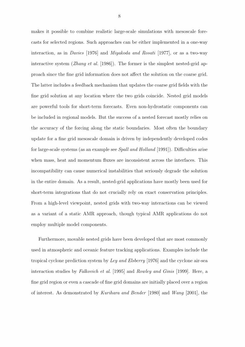
makes it possible to combine realistic large-scale simulations with mesoscale fore-
casts for selected regions. Such approaches can be either implemented in a one-way
interaction, as in Davies [1976] and Miyakoda and Rosati [1977], or as a two-way
interactive system (Zhang et al. [1986]). The former is the simplest nested-grid ap-
proach since the fine grid information does not affect the solution on the coarse grid.
The latter includes a feedback mechanism that updates the coarse grid fields with the
fine grid solution at any location where the two grids coincide. Nested grid models
are powerful tools for short-term forecasts. Even non-hydrostatic components can
be included in regional models. But the success of a nested forecast mostly relies on
the accuracy of the forcing along the static boundaries. Most often the boundary
update for a fine grid mesoscale domain is driven by independently developed codes
for large-scale systems (as an example see Spall and Holland [1991]). Difficulties arise
when mass, heat and momentum fluxes are inconsistent across the interfaces. This
incompatibility can cause numerical instabilities that seriously degrade the solution
in the entire domain. As a result, nested-grid applications have mostly been used for
short-term integrations that do not crucially rely on exact conservation principles.
From a high-level viewpoint, nested grids with two-way interactions can be viewed
as a variant of a static AMR approach, though typical AMR applications do not
employ multiple model components.
Furthermore, movable nested grids have been developed that are most commonly
used in atmospheric and oceanic feature tracking applications. Examples include the
tropical cyclone prediction system by Ley and Elsberry [1976] and the cyclone air-sea
interaction studies by Falkovich et al. [1995] and Rowley and Ginis [1999]. Here, a
fine grid region or even a cascade of fine grid domains are initially placed over a region
of interest. As demonstrated by Kurihara and Bender [1980] and Wang [2001], the

9
grids are then shifted during the model run according to appropriate criteria like the
location of the minimum surface pressure or the gravitational center of the cyclone
(see also Kurihara et al. [1979]). In some cases, nested-grid models require prior
knowledge about future refinement regions, e.g. the main trajectory path (Jones
[1977]). Consequently, they can not be considered truly adaptive since the nesting
remains subjective and inflexible. Despite those different aspects, nested grids and
movable nested grids have one important principle in common. The total number
of grid points stays constant during a model simulation and is determined by the
subjective choice of the initial setup.
1.2.2 Stretched grids
Another kind of variable-resolution model is based on the static, stretched grid ap-
proach. With such an approach, grid intervals outside a uniform fine-resolution area
of interest are stretched uniformly over the rest of the globe (e.g. Staniforth and
Mitchell [1978]). As a result, a single global variable-resolution grid is obtained that
is held fixed during the model integrations. In a later study, Gravel and Staniforth
[1992] concluded that the forecast accuracy and reliability on such a smoothly vary-
ing grid is superior in comparison to abruptly varying meshes. This conclusion was
formulated although, in contrast to the earlier paper, no noise or grid shocks were
found in the abruptly varying systems.
Figure 1.21 shows a stretched grid that is characterized by two high-resolution bands
surrounding the globe (see also the stretched grids by Fox-Rabinovitz et al. [1997],
Fox-Rabinovitz et al. [2001]). Here, the two intersections indicate the regions of
1The figure shows the stretched grid of the model GEM developed by the Canadian Meteoro-logical Centre, courtesy of Jean Cote.

10
interest which can be shifted according to user-defined criteria. For example, the
Canadian Meteorological Center focuses its operational weather forecast model with
stretched grid bands over portions of North America in order to gain resolution and
forecast accuracy for this region (Cote et al. [1998]). Other stretched grids, like the
variable-resolution conformal-cubic grid developed by McGregor [1996] and McGre-
gor and Katzfey [1998], are focused only on a single region of interest. They therefore
avoid the computational overhead invoked by the global band structure. As an al-
ternative, non-uniform resolutions can also be achieved when applying a stretching
coordinate transformation with relocated pole points. This approach has been inves-
tigated by Hardiker [1997] with respect to hurricane forecast studies. Additionally,
the technique proposed by Courtier and Geleyn [1988] with conformal grid trans-
formations has been applied to the operational French numerical weather prediction
system ARPEGE.
In contrast to statically stretched grids, dynamically
Figure 1.2: Stretched grid.
stretched grids offer additional flexibility concerning the
feature of interest during a model simulation. They do
not require prior knowledge about refinement regions
and can therefore be viewed as a globally adaptive vari-
ant of the adaptive mesh approach. Dynamic grid defor-
mations are based on time-dependent global coordinate
transformations. As in the statically stretched case, the total number of grid points
stays constant during the model run, but grid points can now be dynamically focused
according to user criteria. In atmospheric modeling, this continuous dynamic grid
adaptation technique was first applied by Dietachmayer and Droegemeier [1992a]
and Dietachmayer and Droegemeier [1992b]. They used the adaptive zoning method

11
by Brackbill and Saltzmann [1982] with weighting functions for idealized studies of
Burger’s equation and frontogenesis experiments. More recent examples include the
adaptive advection tests by Iselin et al. [2002] and the 3D anelastic, non-hydrostatic
dynamics package with grid deformations by Prusa and Smolarkiewicz [2003].
1.2.3 Dynamically adaptive mesh refinements
The goal of dynamic grid adaptations pursued in this thesis is not to move the
grid, but rather to refine the grid in advance of any important physical process that
needs additional grid resolution, and to coarsen the grid behind the region. Dynam-
ically adaptive grid approaches have long been used in astrophysical, aeronautical
and other computational fluid dynamics problems (Berger and Oliger [1984], Berger
and Colella [1989]). However, in atmospheric science they were first applied approx-
imately a decade ago when Skamarock et al. [1989] and Skamarock and Klemp [1993]
published their adaptive grid techniques for limited-area models in Cartesian coor-
dinates. For example, Skamarock et al. [1989] described the model problem of a 2D
barotropic cyclone that is embedded in a rectangular refinement block. This block
tracked the cyclone controlled by a local truncation error estimate. The refinements
were limited to one block and the applied nesting of the refinement block within
the coarse model domain developed some discontinuities at the interface boundaries.
These oscillations were then avoided with an extended overlap region at fine-coarse
grid interfaces as also discussed by Skamarock [1988] with a multi-level primitive-
equation model. Both Skamarock and Klemp’s research efforts were based on an
adaptive grid library developed by Berger and Oliger [1984].
Recently, Bacon et al. [2000] and Boybeyi et al. [2001] introduced an adaptive
non-hydrostatic regional weather and dispersion model OMEGA which addresses

12
atmospheric transport and diffusion questions. This operational multiscale envi-
ronment model is based on unstructured, triangulated grids with rotated Cartesian
coordinates that can dynamically and statically be adapted to features of interest.
The sophisticated modeling system has mainly been designed to assess real-time, re-
gional hazards as well as plume-modeling scenarios, but it also has adaptive weather
forecasting capabilities. Meanwhile, OMEGA has been used as a hurricane fore-
casting system in limited-area regions on the sphere (Gopalakrishnan et al. [2002],
Bacon et al. [2002]). The hurricanes were well-tracked with triangulated adaptation
regions. Current research activities by the OMEGA team also include the adaptive
simulation of the atmospheric general circulation with physics modules.
Dynamically adaptive advection codes
Atmospheric dynamics on all scales is dominated by the advection process. The
numerical solution of the advection problem is therefore fundamentally important
for the overall accuracy of the flow solvers and tracer transport mechanisms. Various
dynamically adaptive advection codes have been designed so far. Most recently,
Hubbard and Nikiforakis [2003] described the development of an adaptive 3D passive
advection code for tracer transport problems on the sphere (see also brief discussion
in section 1.3). Other dynamically adaptive transport approaches for atmospheric
science applications include the passive 2D advection algorithms by Behrens [1996]
and Behrens et al. [2000] who formulated an adaptive grid triangulation method
in the x-y plane. Kessler [1999] implemented a finite element advection technique
and evaluated different refinement criteria for the adaptive transport process. Other
studies by Stevens and Bretherton [1996] and Stevens et al. [1999] concentrate on
numerical aspects of adaptive multi-level solvers and Tomlin et al. [1997] investigated

13
adaptive gridding options for modeling chemical transports with multiscale sources.
In particular, Tomlin et al. [1997] focused on interactions among emission plumes
and the ambient air. This is also discussed by Odman et al. [1997], Sarma et al.
[1999] and Srivastava et al. [2000] in their adaptive air quality studies.
Adaptive and non-uniform shallow water models
The shallow water equations describe the 2D non-linear flow of an incompressible
fluid. They represent the 2D atmospheric flow conditions in a shallow, hydrostatic
atmospheric layer and are therefore considered an idealized testbed for 3D model
developments. Most often, the horizontal discretization for primitive-equation based
dynamics packages is designed and tested within this 2D shallow water framework.
Due to their close resemblance to the full 3D dynamical core equations, adaptive
shallow water models are of particular interest for future adaptive 3D dynamics
packages. Several statically and dynamically adaptive shallow water models have
been proposed in the literature. So far, all dynamically adaptive approaches deal
with the shallow water equations in the x-y Cartesian plane, whereas the statically
adaptive models are predominantly in spherical coordinates. Statically adaptive
models on the sphere have been developed by Ruge et al. [1995], Fournier et al.
[2000], Fournier et al. [2004] and Barros and Garcia [2004]. The first two studies
discuss a refined representation of the orography data, whereas Fournier et al. [2004]
resolved a pre-determined cyclone track in midlatitudes at higher resolutions. Barros
and Garcia [2004], on the other hand, nested a fine-resolution region of interest within
the coarse global mesh and provided intermediate refinement levels in order to ensure
a smooth transition zone. Here the resolution between neighboring grid points can
only differ by a factor of 2. Alternatively, Cote et al. [1993] designed a shallow water
14
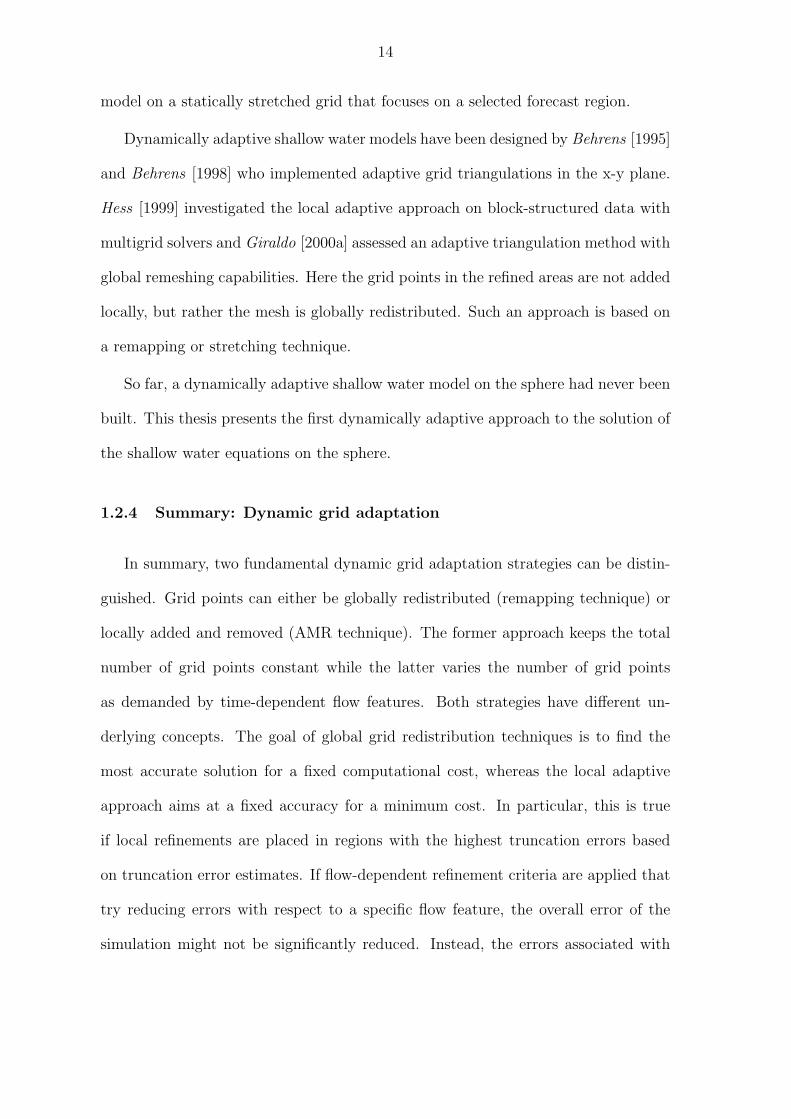
model on a statically stretched grid that focuses on a selected forecast region.
Dynamically adaptive shallow water models have been designed by Behrens [1995]
and Behrens [1998] who implemented adaptive grid triangulations in the x-y plane.
Hess [1999] investigated the local adaptive approach on block-structured data with
multigrid solvers and Giraldo [2000a] assessed an adaptive triangulation method with
global remeshing capabilities. Here the grid points in the refined areas are not added
locally, but rather the mesh is globally redistributed. Such an approach is based on
a remapping or stretching technique.
So far, a dynamically adaptive shallow water model on the sphere had never been
built. This thesis presents the first dynamically adaptive approach to the solution of
the shallow water equations on the sphere.
1.2.4 Summary: Dynamic grid adaptation
In summary, two fundamental dynamic grid adaptation strategies can be distin-
guished. Grid points can either be globally redistributed (remapping technique) or
locally added and removed (AMR technique). The former approach keeps the total
number of grid points constant while the latter varies the number of grid points
as demanded by time-dependent flow features. Both strategies have different un-
derlying concepts. The goal of global grid redistribution techniques is to find the
most accurate solution for a fixed computational cost, whereas the local adaptive
approach aims at a fixed accuracy for a minimum cost. In particular, this is true
if local refinements are placed in regions with the highest truncation errors based
on truncation error estimates. If flow-dependent refinement criteria are applied that
try reducing errors with respect to a specific flow feature, the overall error of the
simulation might not be significantly reduced. Instead, the errors associated with

15
the feature of interest are diminished.
Although all approaches to refining the grid domain are different in nature, they
all have one aspect in common. The varying resolution may cause artificial reflections
and refractions of waves due to compatibility problems at the interface between two
resolutions. For instance, a disturbance that propagates from the fine to a coarser
mesh may undergo false reflection back to the fine grid or aliasing when entering the
coarser domain. These interface-generated problem may further lead to numerical
oscillations that can seriously affect the results over the entire computational domain.
In addition, local interactions in non-uniform grids are no longer isotropic since the
derivatives in horizontal directions might not involve the same scales (Courtier and
Geleyn [1988]). Therefore, an optimal interface should not only allow all resolvable
waves to propagate smoothly with minimal changes in amplitude and phase, but
also needs to conserve the exchanged energy, mass and momentum between the grid
systems (Zhang et al. [1986]). This poses additional questions concerning the optimal
interpolation schemes between refinement levels (Alapaty et al. [1998]).
1.3 Adaptive grid libraries
Public-domain adaptive-mesh libraries have increasingly become available over
the last two decades. The rapid development in recent years shows the importance
of current AMR research activities which are greatly facilitated by enhanced com-
puting resources. This section provides a brief, concise overview of possible starting
points for AMR model developments. From a historic viewpoint, an important mile-
stone was the adaptive mesh package pioneered by Berger and Oliger [1984] which
successfully showed the feasibility and efficiency of adaptive methods for hyperbolic
equations. It can be considered the first viable approach to adaptive modeling for

16
CFD applications.
A collection of today’s publicly available adaptive mesh refinement libraries is
listed below. The majority of these software packages support dynamic grid adap-
tations in Cartesian coordinates on structured grids. The range of applications that
utilize the libraries covers a broad field of disciplines. Among them are the classi-
cal CFD areas like models for hydrodynamic and magnetohydrodynamic simulations
with shocks. In addition, particle problems, laser-plasma interactions and electro-
magnetic wave distributions have been successfully tracked with AMR approaches.
Overview of adaptive grid libraries
AMR library by Berger-Oliger The Berger-Oliger AMR library is a collection
of FORTRAN routines for the numerical solution of hyperbolic conservation
laws in 2 and 3 space dimensions. The underlying data structure is based on
rectangular boxes in Cartesian coordinates. The library has been developed
by Berger and Oliger [1984] and Berger and Colella [1989] for serial computer
architectures (see also Berger [2003]).
AMRCLAW AMRCLAW is a joint project between Randall LeVeque (University
of Washington, Seattle) and Marsha Berger (Courant Institute, New York Uni-
versity). The package contains the Berger AMR library (see above, also Berger
and LeVeque [1998]) and LeVeque’s numerics toolbox CLAWPACK, the Con-
servation LAW PACKage (LeVeque and Berger [2003]).
AMR library in BATS-R-US BATS-R-US is a parallel AMR space-weather first-
principles magnetohydrodynamic (MHD) model developed at the University of
Michigan (Ann Arbor, Michigan, see also Hansen et al. [2002]). The data struc-
ture is based on Cartesian self-similar blocks which can be adaptively refined

17
in 3 dimensions. The AMR package in BATS-R-US has been the predecessor
of the newly developed spherical adaptive grid library with block data used in
this thesis. The BATS-R-US software has been successful developed and used
in space weather modeling for over 10 years. It is most commonly run to model
the solar-wind interaction with solar-system bodies.
CHOMBO The CHOMBO infrastructure provides a set of tools for implementing
finite difference methods for the solution of partial differential equations on
Cartesian, block-structured adaptively refined rectangular grids. Chombo has
been designed at the Lawrence Berkeley National Laboratory (LBNL, Berkeley,
California). Both elliptic and time-dependent modules are included, as well
as support for parallel platforms and standardized self-describing file formats
(HDF5). In addition, a visualization package ChomboVis is publicly available.
DAGH The Distributed Adaptive Grid Hierarchy (DAGH) is a software framework
that supports adaptive finite difference techniques for the solution of partial
differential equations in Cartesian coordinates. It has been designed for sequen-
tial or parallel computing environments and provides a programming interface
for traditional Fortran 77/90, C or C++ kernels (see also Parashar and Browne
[1999]). The DAGH library is no longer under further development.
AMR++ library in Overture AMR++ is an adaptive mesh refinement class li-
brary that is a part of the Overture framework developed at the Lawrence
Livermore National Laboratory (LLNL, Livermore, California). Overture (see
also Brown et al. [2003]) is an object-oriented library which manages over-
lapping grids for partial differential equations in serial or parallel computing
environments. The AMR toolkit provides additional adaptive mesh refine-
18
ment capabilities on these structured, even curvilinear, overlapping grids. The
framework is designed for finite difference or finite-volume methods.
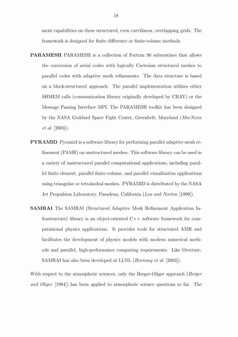
PARAMESH PARAMESH is a collection of Fortran 90 subroutines that allows
the conversion of serial codes with logically Cartesian structured meshes to
parallel codes with adaptive mesh refinements. The data structure is based
on a block-structured approach. The parallel implementation utilizes either
SHMEM calls (communication library originally developed by CRAY) or the
Message Passing Interface MPI. The PARAMESH toolkit has been designed
by the NASA Goddard Space Fight Center, Greenbelt, Maryland (MacNeice
et al. [2003]).
PYRAMID Pyramid is a software library for performing parallel adaptive mesh re-
finement (PAMR) on unstructured meshes. This software library can be used in
a variety of unstructured parallel computational applications, including paral-
lel finite element, parallel finite-volume, and parallel visualization applications
using triangular or tetrahedral meshes. PYRAMID is distributed by the NASA
Jet Propulsion Laboratory, Pasadena, California (Lou and Norton [1999]).
SAMRAI The SAMRAI (Structured Adaptive Mesh Refinement Application In-
frastructure) library is an object-oriented C++ software framework for com-
putational physics applications. It provides tools for structured AMR and
facilitates the development of physics models with modern numerical meth-
ods and parallel, high-performance computing requirements. Like Overture,
SAMRAI has also been developed at LLNL (Hornung et al. [2003]).
With respect to the atmospheric sciences, only the Berger-Oliger approach (Berger
and Oliger [1984]) has been applied to atmospheric science questions so far. The

19
underlying concept of this software package supports a Cartesian grid hierarchy of
fine grids that overlay the coarse grid domain. All grids at all refinement levels are
not only maintained, but are actively used for boundary data updates during the
course of the integration. Grid boxes are dynamically created and removed based on
a Richardson-type estimate of the local truncation error. Here, the overall goal is to
maintain a fixed accuracy of the simulation at minimum cost.
The Berger-Oliger library has been applied multiple times in the context of lim-
ited area or regional atmospheric modeling. Examples include Skamarock et al.
[1989] and Skamarock and Klemp [1993] (see also section 1.2.3 on page 11) who
investigated adaptive meshes for regional weather prediction applications in Carte-
sian coordinates. They implemented an adaptive 3D hydrostatic (Skamarock et al.
[1989]) as well as an adaptive non-hydrostatic (Skamarock and Klemp [1993]) model
and simulated flow fields in limited-area regions. Fulton [1997] focused on movable
nested meshes for hurricane track predictions and later used the truncation error esti-
mates for an adaptive multigrid cyclone track application (Fulton [2001]). Blayo and
Debreu [1999] applied the Berger-Oliger approach to an adaptive ocean model and
most recently, Hubbard and Nikiforakis [2003] developed a fully 3D adaptive, passive
advection code on the sphere. This model in spherical coordinates transports a tracer
component with prescribed wind speeds. The grid resolution adapts in 3 dimensions
according to a local gradient indicator of the tracer compound. This model is the
first dynamically adaptive 3D advection code on the sphere. Its numerics is based
on a monotonic, conservative finite-volume approach.

20
1.4 Overview of the thesis
The goal of this thesis is to design, build and test a block-structured hydrostatic
dynamical core for GCMs that can adapt its horizontal resolution statically and
dynamically based on user-defined adaptation criteria.
In this thesis, adaptive grid techniques are applied to a revised version of NASA/
NCAR’s next-generation dynamical core for climate and weather research. This
hydrostatic so-called Lin-Rood dynamics package (Lin and Rood [1997]) is based
on a conservative 2D finite-volume discretization in flux form and utilizes a floating
Lagrangian coordinate in the vertical direction. The algorithmic design and the
numerics are reviewed in chapter II. Furthermore, questions concerning the so-
called pole problem, the convergence of the meridians in spherical coordinates, are
addressed. This includes a discussion about the polar cap treatment and various
polar filters that help stabilize the gravity waves in high latitudes. In addition, the
divergence damping mechanism is explained.
Chapter III introduces the fundamental ideas behind the adaptive mesh refine-
ment strategy used in this thesis. One of the main building blocks of the adaptive
model is an AMR grid library that manages a block-structured data layout in spher-
ical coordinates. This communication library for parallel processors has been newly
developed by Oehmke and Stout [2001] and Oehmke [2004] in the Computer Science
Department at the University of Michigan, Ann Arbor. The block-wise data struc-
ture allows cache-efficient high-performance computations with minimal changes to
the existing finite-volume flow solvers. Besides discussing these computing and per-
formance aspects, chapter III also gives an overview of interpolation techniques for
ghost cell updates and split-join operations in case of adaptations. Additionally, flux

21
updates across interfaces are addressed which ensure global mass conservation.
The adaptive dynamical core is run in two model configurations: the full 3D
hydrostatic dynamical core on the sphere and the corresponding 2D shallow water
configuration that has been extracted out of the 3D version. This shallow water setup
serves as an ideal testbed for the horizontal discretization and the 2D adaptive mesh
strategy. 2D test cases are chosen from the standard test suite for the shallow water
equations (Williamson et al. [1992]). An idealized 3D test case is newly derived as
part of this research effort.
Chapter IV concentrates on the assessment of solely static adaptations in the
2D shallow water framework. The shallow water tests evaluate the design and ac-
curacy of a so-called reduced grid setup that can be viewed as a static coarsening
in longitudinal direction at the poles. Furthermore, static refinements in pre-defined
regions of interest are assessed which reveal the stability of the scheme in presence of
the varying resolution at grid interfaces. Appropriate error measures are introduced
which are also used in the following chapters.
Chapter V is focused on dynamic adaptations in the 2D shallow water setup.
Dynamic adaptations are based on flow characteristics and guided by refinement
criteria that detect user-defined features of interest at run time. Possible choices for
refinement criteria are reviewed with emphasis on flow-based refinement indicators,
like vorticity or gradient assessments. The shallow water tests reveal the feasibility
of the dynamically adaptive approach and furthermore are used to compare different
choices for the adaptation criterion.
In chapter VI, 3D idealized dynamical core tests of the static and dynamic
adaptations are presented. This chapter includes the derivation of the newly devel-
oped Jablonowski-Williamson baroclinic wave test case (Jablonowski and Williamson

22
[2004]). This test case, together with the new Polvani et al. [2004] test case, shows
that adaptive mesh refinements are a viable choice for future adaptive weather and
climate models. Furthermore, new questions concerning the orography representa-
tion in adaptive model runs are revealed.
Chapter VII provides a summary of the scientific merit and major accomplish-
ments of this thesis. It opens the discussion about future research directions and
points out the challenging steps towards an adaptive, complete General Circulation
Model with physics modules.

CHAPTER II
The hydrostatic finite-volume dynamical core
In this thesis the development of the adaptive dynamical core for weather and
climate research is based on the so-called Lin-Rood finite-volume dynamical core that
has been designed at the NASA Goddard Space Flight Center (NASA/GSFC) in the
late 1990’s. This hydrostatic global dynamics package in flux form is built upon the
Lin and Rood [1996] advection algorithm, which utilizes advanced oscillation-free
numerical approaches to solving the transport equation. In particular, Lin and Rood
[1996] extended a Godunov-type methodology to multiple dimensions and made use
of 2nd order van Leer-type (van Leer [1974], van Leer [1977]) and 3rd order piecewise
parabolic (PPM) methods (Colella and Woodward [1984], Carpenter et al. [1990]).
In 1997, the advection scheme became the fundamental building block of a shallow
water code (Lin and Rood [1997], Lin [1998a]) which then led to the development of
the current 3D, primitive-equation (PE) based, finite-volume dynamics package (Lin
et al. [2001]).
Today, the 3D dynamical core is used operationally for data assimilation appli-
cations at NASA/GSFC and, in 2001, it was included in NCAR’s climate-prediction
system CCSM, the Community Climate System Model. This climate prediction
system contains the Community Atmosphere Model, CAM, with physics and dy-
23

24
namics components. In particular, the finite-volume dynamical core is now one of
the three standard dynamics modules in CAM and can be chosen at compile time
for the individual model setup. The Lin-Rood finite-volume core performs well in
NCAR/NASA’s internal comparative studies (S.-J. Lin, personal communication). It
has the potential to become NCAR’s dynamics package of choice for future long-term
climate change scenario calculations (CCSM [2003]).
Chapter II is organized in three sections. The overall model design and its un-
derlying numerical scheme are reviewed in Section 2.1. This includes a discussion
about the governing equations in 2 and 3 dimensions and addresses horizontal as
well as vertical discretization issues. Section 2.2 examines the special treatment of
the polar regions in the regular latitude-longitude spherical grid. Besides the polar
cap concept, filtering techniques are introduced that help stabilize high-frequency
gravity waves in polar regions. Gravity waves are also the main focus of Section 2.3.
Here the divergence damping mechanism and its impact on the resulting flow field
are explained.
2.1 Model design and numerics
2.1.1 Governing equations
The dynamical core is built upon a 2D shallow water approach in the horizontal
plane with floating Lagrangian coordinates in the vertical direction (see also Section
2.1.3). The underlying hyperbolic shallow water system is comprised of the mass
continuity equation and momentum equation as shown in equations 2.1 and 2.2.
Here the flux-form of the mass conservation law and the vector-invariant form of the

25
momentum equation are selected (see also Lin and Rood [1997])
∂
∂th +∇ · (h~v) = 0 (2.1)
∂
∂t~v + Ωa
~k × ~v +∇(Φ +K)
= 0 (2.2)
where ~v = u~i+v~j is the horizontal velocity vector and Ωa = ζ+f denotes the absolute
vorticity. The absolute vorticity is composed of the relative vorticity ζ = ~k · (∇× ~v)
and the Coriolis force f = 2Ω sin ϕ with the latitude ϕ and the physical constant
Ω = angular velocity of the earth (see also Appendix C for an overview of physical
constants). Furthermore, ~k is the unit vector in the vertical direction, ∇ represents
the horizontal gradient operator, Φ = Φs+gh symbolizes the free surface geopotential
with Φs = surface geopotential, h = depth or mass of the fluid and g = gravitational
acceleration. In addition, K = ~v·~v2
stands for the kinetic energy. A distinct advantage
of this vector-invariant formulation is that the metric terms, which are singular at
the poles in the curvilinear spherical coordinate system, are hidden by the definition
of the relative vorticity.
In three dimensions, the set of equations is very closely related to the shallow
water system when replacing the height of the shallow water system with the pressure
thickness δp of a Lagrangian layer. Furthermore, the thermodynamic equation 2.4
in conservation form is added to the set
∂
∂tδp +∇ · (δp~v) = 0 (2.3)
∂
∂t(Θ δp) +∇ · (Θ δp~v) = 0 (2.4)
∂
∂t~v + Ωa
~k × ~v +∇pΦ +∇K = 0 (2.5)
where δp = −ρgδz is the pressure thickness of a layer bounded by two Lagrangian
surfaces in the hydrostatic system with density ρ and height z. The thermodynamic

26
variable Θ is the potential temperature and ∇p symbolizes a newly derived pressure
gradient operator for the finite-volume representation of the pressure gradient force.
This operator constitutes the main difference between the shallow water system and
the 3D model setup. The underlying method has been developed by Lin [1997]
and was furthermore discussed by Janjic [1998] and Lin [1998b]. In this primitive-
equation formulation, the prognostic variables of the dynamical core are the wind
components u and v, the potential temperature Θ and the pressure thickness δp.
The geopotential Φ, on the other hand, is computed diagnostically via the vertical
integration of the hydrostatic relation in pressure coordinates
∂Φ
∂p=−1
ρ(2.6)
with cell-averaged density ρ. In the presence of orography as a lower boundary
condition this integration then starts at the geopotential level Φs of the surface field.
It is important to note that the hydrostatic relationship is the vertical coupling
mechanism for the dynamical system. In addition, the pressure level pn of each
Lagrangian surface can be directly derived when adding the pressure thicknesses
within the vertical column
pn = ptop +n∑
k=1
δpk for n = 1,2,3, · · · , Nlev (2.7)
Here n denotes the vertical index starting from 1 at the lower bounding surface of the
uppermost Lagrangian layer. The pressure at the model top ptop is prescribed and
set to 2.19hPa in the current formulation. There are a total of Nlev + 1 Lagrangian
surfaces that enclose Nlev Lagrangian layers. The lowermost Lagrangian surface
coincides with the Earth’s surface field and, as a consequence, the surface pressure
is then automatically determined by the pressure pNlevat the lowest level. In all 3D
simulations presented in chapter VI, Nlev = 26 vertical levels have been selected (see

27
also Appendix B for more detailed information on the vertical coordinate system).
They are identical to the vertical levels operationally used for climate studies with
NCAR’s modeling system CCSM.
The rather unusual form of the primitive equations and in particular the mass
continuity equation 2.3 can be derived when integrating the standard form of the
3D continuity equation (see Durran [1999]) in the vertical direction. This is demon-
strated starting from the continuity equation with a generalized vertical coordinate
ξ. Starting from the mass conservation law
∂
∂t
(∂p
∂ξ
)+∇ξ ·
(~v
∂p
∂ξ
)+
∂
∂ξ
(ξ
∂p
∂ξ
)= 0 (2.8)
with pressure p and ∇ξ as the horizontal gradient operator on constant ξ-surfaces,
the continuity equation for the pressure thickness δp of a Lagrangian layer with
bounding upper and lower surfaces at ξu and ξl can be determined via the vertical
integration∫ ξu
ξl
[∂
∂t
(∂p
∂ξ
)+∇ξ ·
(~v
∂p
∂ξ
)+
∂
∂ξ
(ξ
∂p
∂ξ
)]dξ = 0. (2.9)
In practice, ξ is often replaced by an orography following coordinate system like the
hybrid η coordinate used in the finite-volume dynamical core (see also description in
Appendix B). After rearranging terms, expression 2.9 becomes
∂
∂t
∫ ξu
ξl
∂p
∂ξdξ +∇ξ ·
(~v
∫ ξu
ξl
∂p
∂ξdξ
)+
∂
∂ξ
∫ ξu
ξl
(ξ
∂p
∂ξ
)dξ = 0. (2.10)
The integrated form is then given by
∂
∂t
[p(ξu)− p(ξl)
]+∇ξ ·
(~v[p(ξu)− p(ξl)
])+
∂[ξup(ξu)− ξlp(ξl)
]
∂ξ= 0 (2.11)
where the overbar denotes the volume-mean wind speeds. Since there are no vertical
transport processes across the bounding surfaces of a Lagrangian layer, the last term

28
on the left hand side vanishes and the general form of the continuity equation for δp
follows
∂
∂tδp +∇ξ ·
(~v δp
)= 0 . (2.12)
The integrated form of the momentum equation and thermodynamic equation can
be derived accordingly.
Because of their equivalent designs, the 2D shallow water version can be easily
extracted out of the full 3D dynamical core. The main idea is to eliminate the
influence of the thermodynamic equation in the momentum equation for the shallow
water setup. The thermodynamic equation is linked to the momentum equation only
via the computation of the geopotential gradient. Overall, three steps need to be
performed. First, the number of vertical layers needs to be set to 1. Second, the
potential temperature field Θ must be initialized with the constant 1 K and must
not change during the shallow water run (e.g. the transport and updates of δp Θ
can be omitted). Furthermore, the δp field now stands for the geopotential height
h instead of a pressure thickness. Third, the physical constants cp, Rd and κ need
to be overwritten and set to unity. This guarantees that the operator ∇p in the 3D
momentum equations (explained in Lin [1997]) becomes equivalent to the operator
∇ in the 2D momentum equation (eqn. 2.2).
2.1.2 Horizontal discretization
The finite-volume dynamical core utilizes a flux form algorithm for the horizontal
discretization, which, from the physical point of view, can be considered a discrete
representation of the basic physical laws in the finite-volume space. However, from
the mathematical standpoint, it can be viewed as a numerical method for solving
the governing equations in integral form. This leads to a more natural and often

29
more precise representation of the advection processes, especially in comparison to
finite difference techniques. The transport processes are modeled by two-dimensional
fluxes into and out of the finite control-volume where volume-mean quantities are
predicted. This underlying finite-volume principle of the Lin-Rood advection algo-
rithm is reviewed below using the mass continuity equation of the shallow water
equations as an example.
Finite-volume discretization
Finite-volume methods are closely related to finite difference schemes. They are
often viewed as a finite flux-differencing approximation to the differential equation
and derived on the basis of the integral form of the conservation law (see discussion
in LeVeque [2002]). The mass conservation law (equation 2.1) in integral form is
given by ∫ tn+1
tn
∫
Ω
( ∂
∂th)
dΩ dt +
∫
Ω
∫ tn+1
tn
∇ · (h~v) dt dΩ = 0 (2.13)
where Ω represents a control volume. In the following derivation only two-dimensional
control volumes with surface areas AΩ are considered. Using the relationships
∫
Ω
h dΩ = h
∫
Ω
dΩ = h AΩ (2.14)
∫ tn+1
tn
(h~v) dt = < h~v >
∫ tn+1
tn
dt = < h~v > ∆t = ~F ∆t (2.15)
where ∆t = tn+1 − tn is the duration of a time step, the overbar denotes a spatially-
averaged quantity, the angled brackets indicate the averaging over a time step ( ~F is
defined as the time-averaged flux vector), equation 2.13 can be rewritten as
∫ tn+1
tn
( ∂
∂th)
dt +∆t
AΩ
∫
Ω
∇ · ~F dΩ = 0 . (2.16)
Applying the Gauss divergence theorem yields
∫ tn+1
tn
( ∂
∂th)
dt +∆t
AΩ
∮
∂Ω
~F · d~n = 0 (2.17)
30
in which ~n is an outward-pointing normal to the boundary ∂Ω of the control volume.
With ∫ tn+1
tn
( ∂
∂th)
dt = h∣∣tn+1
tn= hn+1 − hn (2.18)
the discrete representation of the conservation law becomes
hn+1 = hn − ∆t
AΩ
4∑i=1
li ~Fi · ~ni (2.19)
where the sum comprises the 4 line segments with lengths li that surround a rectan-
gular 2D control volume. Fi symbolizes the time-averaged fluxes at the cell interfaces
and ni indicates the normal surface vectors to the ith line segment. Assuming an
orthogonal x-y control volume with surface area AΩ = ∆x ∆y and corresponding
fluxes F and G in x and y direction, equation 2.19 is equivalent to
hn+1i,j = hn
i,j −∆t
∆xi ∆yj
[(∆yj (Fi+ 1
2,j − Fi− 1
2,j)
)+
(∆xi (Gi,j+ 1
2−Gi,j− 1
2))]
(2.20)
= hni,j −
∆t
∆xi
(Fi+ 1
2,j − Fi− 1
2,j
)− ∆t
∆yj
(Gi,j+ 1
2−Gi,j− 1
2
)(2.21)
in which the indices i, j define the grid point position of the cell center and the half
index represents the boundaries of the grid box.
For a spherical grid, the lengths of the line segments ∆x, ∆y and the surface
area AΩ = ∆xi ∆yj in equation 2.20 need to be substituted with the corresponding
representation in spherical space
∆xi = a cos ϕ ∆λi (2.22)
∆yj = a ∆ϕj (2.23)
AΩ = a2(sin ϕj+ 1
2− sin ϕj− 1
2
)∆λi (2.24)
with a = Earth’s radius, ∆λi = (λi+ 12− λi− 1
2) and ∆ϕi = (ϕj+ 1
2− ϕj− 1
2) measured
in radians.

31
In the NASA/NCAR Lin-Rood finite-volume dynamical core though, a slightly
different flux-differencing approach has been implemented (see Lin and Rood [1997])
that corresponds to equation 2.20 when replacing AΩ with the approximation AΩ =
a2 cos ϕ ∆λ ∆ϕ. As a result, the discrete finite-volume conservation law for the cell-
averaged height field in spherical coordinates becomes
hn+1i,j = hn
i,j −∆t
a cos ϕj ∆λi
(Fi+ 1
2,j − Fi− 1
2,j
)
− ∆t
a cos ϕj ∆ϕj
(cos ϕj+ 1
2Gi,j+ 1
2− cos ϕj− 1
2Gi,j− 1
2
). (2.25)
Here F and G denote the time-averaged 1D numerical fluxes in longitudinal and
meridional direction. In a more compact notation, equation 2.25 can also be written
as
hn+1i,j = hn
i,j + Fnet + Gnet (2.26)
where the net fluxes for the grid box i, j are defined as
Fnet = − ∆t
a cos ϕj ∆λi
(Fi+ 1
2,j − Fi− 1
2,j
)
= − ∆t
a cos ϕj ∆λi
δλ F (2.27)
Gnet = − ∆t
a cos ϕj ∆ϕj
(cos ϕj+ 1
2Gi,j+ 1
2− cos ϕj− 1
2Gi,j− 1
2
)
= − ∆t
a cos ϕj ∆ϕj
δϕ
(cos ϕG
)(2.28)
with the standard discrete difference operator δ. This notation closely resembles the
form of the equations in Lin and Rood [1997] and Lin [1998a] when defining the
time-averaged fluxes as X and Y and omitting the subscript ’net’ in equations 2.27
and 2.28.
Equation 2.26 states that the rate of change of the scalar field h is only due to
the net fluxes, which are solely determined by the fluxes through the interfaces of the

32
control volume. Such an approach automatically leads to a conservative discretiza-
tion. There are many ways of computing the numerical fluxes F and G which so far
have not been discussed. Here the choices are focused on higher-order Godunov-type
schemes. In particular, the second-order van Leer algorithm (van Leer [1977]) and
the third-order piecewise parabolic method (PPM, Colella and Woodward [1984])
have been selected. These methods are outlined later in this chapter.
The Lin-Rood advection algorithm
The advection algorithm developed by Lin and Rood [1996] is based on the finite-
volume representation shown in equation 2.26. The following section briefly describes
the transport process and flux computations as applied in the NASA/NCAR finite-
volume dynamical core. In order to match the Lin and Rood [1996] notation the
shallow water height h is replaced by a density-like field Q
∂
∂tQ +∇ · (Q~v) = 0 . (2.29)
When advancing the Q field for one time step from Qn to Qn+1, a sequential operator-
splitting approach
Qx = Qn + Fnet(Qn) (2.30)
Qyx = Qx + Gnet(Qx) (2.31)
⇒ Qyx = Qn + Fnet(Qn) + Gnet(Q
x) + GnetFnet(Qn) (2.32)
is applied which introduces a directionally anti-symmetric splitting error. A directional-
bias free algorithm can then be obtained when averaging two asymmetric operations
12(Qyx + Qxy) to arrive at
Qn+1 = Qn + Fnet
[Qn +
1
2Gnet(Q
n)]+ Gnet
[Qn +
1
2Fnet(Q
n)]. (2.33)

33
Equation 2.33 still suffers from a so-called deformational error (Smolarkiewicz [1982])
which is removed by replacing the inner flux form operators with their advective
counterparts f and g. The resulting symmetric scheme, which is implemented in the
finite-volume dynamical core, is given by
Qn+1 = Qn + Fnet
[Qn +
1
2gnet(Q
n)]+ Gnet
[Qn +
1
2fnet(Q
n)]. (2.34)
For the inner, advective 1D operators f and g, a first-order upwind method is
employed. The outer 1D fluxes are either modeled by the van Leer [1977] algo-
rithm (scheme I with or without monotonicity constraints) or by the monotonicity-
preserving PPM method (piecewise parabolic method, see Colella and Woodward
[1984] and Carpenter et al. [1990]). The choice of the flux scheme is guided by Lin-
Rood’s two-step algorithmic approach to advancing the prognostic variables from tn
to tn+1 on a so-called D-grid (see also figure 2.1). During the first step, time-centered
velocity components at tn+ 12 are calculated on a C-grid with the unconstrained 2nd
order van Leer algorithm. In step 2, these auxiliary time-centered winds are then
used in order to approximate the time-averaged fluxes for the update of the prognos-
tic variables on the D-grid. This is done with the more accurate 3rd order monotonic
PPM method. The use of the time-centered wind speeds at the staggered C-grid po-
sitions avoids tackling a so-called Riemann-problem for the approximation of the
time-averaged fluxes at cell interfaces.
The grid staggering techniques are illustrated in figure 2.1. In the dynamical
core, all staggering options displayed in figure 2.1 are employed at different stages
of the algorithm (see details in Lin and Rood [1997]). Wind data other than the
prognostic wind fields on the D-grid are interpolated via linear interpolations.
In practice, it has been observed (Lin and Rood [1997]) that the PPM method

34
u v
v u
u, vu, v
u, v u, v
D grid C grid B grid A grid
u, vΦ,ΦΦ Φ
Figure 2.1: Grid staggering techniques (named after Arakawa, see Arakawa and Lamb[1977]). u and v indicate the positions of the zonal and meridional wind,Φ symbolizes a scalar quantity, e.g. the geopotential, which is defined atthe cell center.
does not lead to superior results in polar regions in comparison to the more economi-
cal 2nd order van Leer approach. Since the chosen computational latitude-longitude
grid converges at the pole points (figure 2.2) an increased resolution in longitudinal
direction is provided in physical space. With respect to accuracy, this allows switch-
ing from the PPM method to the van Leer scheme poleward of 75 N/S. On the other
hand, the flux calculations in the meridional direction remain unchanged (PPM).
Test results with and without the switch of the al-
Figure 2.2: Regular grid.
gorithm are almost indistinguishable from each other
while the former reduces the computational costs on
the order of 10-15%. Furthermore, the switch to the
van Leer approach in polar regions is beneficial as it
adds slightly more implicit diffusion. This helps stabi-
lize high-speed gravity waves in high latitudes as dis-
cussed in Section 2.2.2.

35
Numerical schemes: van Leer and PPM method
The advection method implemented in the Lin-Rood dynamical core can be
viewed as a multi-dimensional extension of higher-order Godunov-type schemes like
the van Leer or PPM method. These are based on the reconstruct-evolve-average
approach (REA as explained by LeVeque [2002]) and use piecewise linear (van Leer)
or piecewise parabolic (PPM) subgrid distributions for the piecewise continuous re-
construction of the flow field. The transport problem is then solved exactly and new
initial data at time tn+1 are obtained by averaging the transported quantity over
each control volume.
The advection step is upstream-biased and monotonic if limiters are applied to the
subgrid distributions. These are used in case of PPM (see details in Lin and Rood
[1996]) which leads to a total variation diminishing (TVD) method. The selected
slope limiter is the monotonized central-difference limiter (MC limiter) proposed by
van Leer [1977] which is applied as a pure 1D operator during the reconstruction
step. Limiting can enforce a strictly monotonic advection algorithm in the 1D case.
However, very minor violations of the monotonicity constraint in the two-dimensional
flow are possible and have indeed been observed by Lin and Rood [1996] and in the
adaptive grid runs in Chapter V.
In general, the selected order of the subgrid distribution determines the overall
accuracy of the transport scheme. In the van Leer case with piecewise linear re-
constructions, the resulting fluxes (for example the fluxes F at an interface in the
longitudinal direction) are first-order accurate. On an equidistant 1D grid this leads
to a locally second-order advection algorithm since the leading error term cancels
when calculating the flux difference. The numerical fluxes are given by (see also

36
Allen et al. [1991] or Lin et al. [1994])
Fi+ 12
=
ui+ 12
[Qi + ∆Qi
2
(1− u
i+12∆t
∆xi
)]for ui+ 1
2≥ 0
ui+ 12
[Qi+1 − ∆Qi+1
2
(1 +
ui+1
2∆t
∆xi+1
)]for ui+ 1
2< 0
(2.35)
where Q stands for the transported quantity and ∆Q symbolizes the slope of the
linear subgrid distribution in the longitudinal direction. Here the slope is evaluated
with a central differencing approximation ∆Qi = 12(Qi+1 − Qi−1) and can further
be limited as indicated above (see also Lin et al. [1994] for a comparison of suitable
slope limiters or alternative positive definite constraints). The same basic algorithm
applies to the fluxes G in meridional direction.
In order to gain accuracy in the PPM case, the piecewise polynomials in a con-
trol volume are approximated by parabolic functions with two degrees of freedom,
denoted with δax and bx (Nair and Machenhauer [2002], compare also to notation
δa, a6 in Carpenter et al. [1990]). They represent the slope and the curvature of the
parabola
h(x) = h + δax x + bx( 1
12− x2
)(2.36)
with h = cell average (see also van Leer [1977]). This quadratic subgrid distribution
is further analyzed in Section 3.3.1 on page 91 with respect to the interpolation
mechanisms in an adaptive grid run. The resulting fluxes of the PPM algorithm are
derived in Colella and Woodward [1984]. The PPM advection scheme is 3rd order
accurate for linear advection problems on uniform 1D grids.
The advection algorithm is the fundamental building block of the horizontal dis-
cretization. It is not only used to predict the time evolution of the mass (eqn. 2.3)
and potential temperature field (eqn. 2.4), but also determines the absolute vorticity

37
fluxes and kinetic energy in the momentum equation (eqn. 2.5). Further details are
presented in Lin and Rood [1997].
If the PPM scheme is selected as the primary transport algorithm for an adaptive
mesh refinement (AMR) design, Berger and Colella [1989] ask
Why is an adaptive grid needed provided that the solution technique, a
third-order Godunov scheme, has quite high resolution? Provided AMR
is used is it still necessary to use a high order scheme or could we reduce
the order of the accuracy and therefore the computational cost ?
As shown in Woodward and Colella [1984] a higher order method still gives more
resolution per computational cost than a simpler, lower order scheme on a finer
grid. Therefore it is not recommended to decrease the order of accuracy even in the
AMR application. Lin and Rood [1997] also confirmed that the PPM simulations
are far more accurate and less diffusive, especially in a long-term 60-day shallow
water test run with uniform resolution. Minor deviations after day 14 grew into
clearly visible differences of the height field by day 30 when comparing the van Leer
scheme to the PPM advection algorithm. This is an important observation for long-
term climate studies. Consequently, since the PPM method is more expensive than
simple schemes the computational savings of an AMR run versus a uniform grid run
can be substantial as demonstrated later in Chapter V.
2.1.3 Vertical representation
The vertical discretization utilizes a “Lagrangian control-volume” approach, which
is based on a terrain-following “floating” Lagrangian coordinate system and a fixed
“Eulerian” reference frame. The underlying idea is to start the time integration from
the terrain-following Eulerian reference system. The finite-volumes are then allowed

38
to float vertically as dictated by the hydrostatic flow and, as a consequence, the
two Lagrangian surfaces bounding the finite-volumes will deform as illustrated in
figure 2.3. This deformation can be strong, especially in the presence of persistent
x-z cross section of the atmosphere
Lagrangian surfaces
Earth’s surface
model top
T = t
flux flux
orography
δp
T = t + dt
Figure 2.3: Terrain-following Lagrangian control-volume coordinate system of theLin-Rood dynamical core. The pressure thickness δp of a cell is propor-tional to the total mass. The cell boundaries deform during the forecast(right) and after specific time intervals they are mapped back onto afixed Eulerian reference system (not shown).
diabatic heating and cooling which ultimately will degrade the accuracy of the 2D
flow simulation within a Lagrangian layer. Therefore, the surfaces are mapped back
monotonically and conservatively to the fixed Eulerian reference system. Here, a
hybrid σ − p coordinate system has been chosen for the reference framework, which
is most commonly called an η system (see also Simmons and Burridge [1981]). The
η coordinate is a combination of the orography-following σ coordinate and fixed
pressure levels. Further explanations are given in Appendix B on page 249.
It is essential to note that Lagrangian surfaces are non-penetrable material sur-
faces that do not allow transport processes across the boundaries. This approach
effectively reduces the dimensionality of the transport problem from 3 to 2. The 3D
model can therefore also be viewed as a vertically staggered shallow water system
with 2D transport algorithms within each layer. The periodic vertical remapping
step essentially performs the function of a conservative vertical advection process as

39
viewed from the fixed Eulerian reference frame (van Leer [1979],?]). It vertically re-
distributes mass, momentum and total energy from the floating Lagrangian volumes
back to the fixed coordinate system. In the adaptive dynamical core formulation, a
one-hour remapping interval has been chosen.
The conservative and monotonic mapping is described in detail in the theoretical
basis document by Lin et al. [2001]. Here a brief overview of the fundamental 3-step
principle is given. In general, the one-dimensional mapping is based on a vertical
reconstruction of the pressure thickness (mass) δp, the wind components u, v and
the volume mean total energy Γ which is composed of the mean internal, potential
and kinetic energy. In step 1 of the algorithm, monotonic piecewise parabolic sub-
grid distributions of the aforementioned quantities are computed (compare also to
PPM algorithm by Colella and Woodward [1984]). These are then used to calculate
the redistributed δp, u, v and Γ values in the Eulerian reference frame (step 2). In
order to ensure conservation, the hydrostatic pressure is selected as the mapping
coordinate. Finally the layer-mean internal energy, and consequently the tempera-
ture, are recovered using the redistributed total, kinetic and potential energy. This
step guarantees the conservation of the total energy. Any dissipated kinetic energy
that is lost during the remapping process gets automatically transformed into local
frictional heating.
2.1.4 Summary
In summary, the novel attributes of the Lin-Rood finite-volume dynamical core
are:
• its built-in physical conservation laws.
• the terrain-following, “floating” Lagrangian vertical coordinate which elimi-

40
nates vertical advection and therefore reduces the dimension of the problem
from 3 to 2.
• a monotonicity-preserving and mass-, momentum- and total energy-conserving
algorithm that maps the vertical coordinate back to a “fixed” Eulerian reference
coordinate.
• the two-dimensional conservative transport between two bounding “horizontal”
Lagrangian surfaces that define the control volume (Lin and Rood [1996]). The
transport algorithm is free of Gibb’s oscillations.
• the precise representation of the terrain. An accurate and physically consis-
tent finite-volume integration of the pressure gradient force for the Lagrangian
control-volume is used (Lin [1997], Lin [1998b]).
• the highly efficient computational design of the algorithm which has been de-
veloped for vector- or RISC based parallel computers. The algorithm is highly
local in nature, which not only has an advantage for modeling flows with sharp
gradients, but also makes the code more suitable for domain decomposition
techniques in distributed computing environments (resulting in low communi-
cation overhead on parallel processors).
2.2 Pole problem in latitude-longitude grids
NASA/NCAR’s finite-volume dynamical core is implemented in spherical coordi-
nates on a regular latitude-longitude grid. As a result, the meridians converge at the
pole points as illustrated in figure 2.2 on page 34. Most commonly, this is called the
pole problem on the spherical grid. It leads to extremely small grid boxes or, more

41
appropriately finite-volumes, in the immediate vicinity of the poles. This is further
quantified in table 3.1 in Chapter III.
Although the longitudinal resolution in radians stays nominally constant, the
physical distance between neighboring nodes in the longitudinal direction contracts.
As a consequence, the Courant-Friedrichs-Lewy (CFL) stability condition near the
pole is rather restrictive in comparison to the midlatitudes or the tropical region.
In order to maintain numerical stability in the explicit finite-volume scheme, the
CFL < 1 condition poses a severe time step limitation. In an explicit method, the
time step is then determined by the CFL condition for the fastest traveling wave in
the system. In a hydrostatic fluid, these are the gravity waves at speeds of order
200− 300m/s.
In addition, pole points in the spherical grid raise a different problem. They are
singularities in the curvilinear coordinate system that do not allow the evaluation
of metric terms directly at the poles. Therefore, special polar treatment is needed
with respect to wind speed and vorticity considerations. These aspects are covered
in Section 2.2.1. In Section 2.2.2, filtering strategies are presented that help relax
the severe polar time step restriction.
2.2.1 Polar cap
Polar stereographic projections
The wind speeds at the poles in the spherical coordinate system are multi-valued
vector components, although in physical (e.g. Cartesian) space the vector is uniquely
defined. This is a consequence of the rapidly varying spherical unit vectors at high
latitudes as illustrated by the orientation of the coordinate directions for u and v in
figure 2.4. In particular, the spherical wind components undergo a complete reversal

42
NPv
u
v
u
v
u
v
windvector
NPuStereographicprojection atthe North Pole
270o
0o
v
u180o
90o
Figure 2.4: Orientation of the local unit vectors in spherical coordinates near theNorth Pole. The wind vector at the pole is indicated by the thick arrow,the wind components u and v in a stereographic projection are labeledwith ’NP’.
of sign when viewed from the local coordinate system of a cross polar position.
Therefore, even a very smoothly varying wind field in polar regions, as observed
from space, appears to change quickly in the spherical representation.
Due to the singularities of the pole points in the spherical grid, the wind speeds
at the poles can not be directly computed. A standard solution to this problem
has long been proposed in the literature (e.g. see Williamson and Browning [1973]
or Phillips [1959]). The basic idea is to apply a coordinate transformation or map
projection to the polar region in order to compute a unique solution to the transport
problem in the transformed system. The solution can then be mapped back onto the
spherical mesh.
Alternatively, this idea can also be used to approximate the wind components
at the pole points. Instead of solving the transport problem in the map-projected
43
system, the wind vector is then estimated based on the averaged wind information
at the adjacent neighbors in the closest latitudinal ring around the pole. This is the
so-called polar cap. Typically, a polar stereographic projection is used for the trans-
formation. The wind vector in the polar tangent plane is then uniquely defined and
can be projected back in order to recover the multi-valued spherical representation.
The corresponding formalism for the North Polar stereographic projection is given
by (see also Phillips [1959])
uNP =1
N
N∑i=1
[− ui sin λi − vi cos λi
](2.37)
vNP =1
N
N∑i=1
[ui cos λi − vi sin λi
](2.38)
where N stands for the number of grid points along the subpolar latitude circle
and (ui, vi) symbolize the wind components in spherical coordinates. This averag-
ing procedure incorporates all subpolar neighbors and, as an aside, requires extra
communication on parallel computer architectures. The resulting unique wind rep-
resentations uNP and vNP in the north polar tangent plane are then used for the
consequent remapping step
ui = −uNP sin λi + vNP cos λi (2.39)
vi = −uNP cos λi − vNP sin λi (2.40)
that retrieves the multi-valued components. This relationship is illustrated in figure
2.5 where the North Pole is symbolically stretched out in the longitudinal direction.
The equivalent expressions for the Southern Hemisphere are specified below (eqn.
2.41-2.44). Here it needs to be taken into account that the sense of the meridional

44
0 90 180 270
NP NP
NP
NP
o o ooLongitudes
North
Pole
u = v
v = −u NP
NP u = −v
v = u NPNP
u = u
v = v
u = −u
v = −v
Figure 2.5: Relationship between the multivalued wind components in spherical co-ordinates and the unique wind vector in a North Polar stereographicprojection labeled with ’NP’ (see also figure 2.4).
wind at the South Pole (SP) is reversed in comparison to the North Polar represen-
tation
uSP =1
N
N∑i=1
[− ui sin λi + vi cos λi
](2.41)
vSP =1
N
N∑i=1
[ui cos λi + vi sin λi
]. (2.42)
As before, the remapping step
ui = −uSP sin λi + vSP cos λi (2.43)
vi = uSP cos λi + vSP sin λi (2.44)
recovers the spherical wind components at the South Pole.
Vorticity calculation
In the chosen set of equations (see Section 2.1.1), the absolute vorticity Ωa = ζ+f
is treated as a transported variable. As a consequence, the relative vorticity ζ as well
as the Coriolis term f need to be computed in the whole model domain including
both pole points. This can easily be done for the Coriolis parameter, but poses a
problem for the standard relative vorticity formulation in spherical coordinates.
In spherical coordinates, the relative vorticity is defined by
ζ = ~k · (∇× ~v) =1
a cos ϕ
[∂v
∂λ− ∂u cos ϕ
∂ϕ
](2.45)
45
which requires the evaluation of the metric term 1cos ϕ
at any given location. Such a
term is undefined at both poles, although from a physical standpoint the vorticity is
well-defined throughout the model domain. Therefore, a different approach has been
applied at the pole points. The underlying idea is based on an alternative circulation
measure and the Stokes’ theorem which allow the non-singular computation of the
vorticity at arbitrary points in the mesh.
Besides the definition shown in equation 2.45, the vertical component of the
relative vorticity ζ is also defined as the circulation C about a closed contour in the
horizontal plane divided by the area A of the enclosed region.
ζ =C
A= lim
A→0
( ∮~v · d~l
)A−1 (2.46)
This relationship is exact in the limit where the area A approaches 0 (see also Holton
[1992] for further details). In a discrete spherical system, the circulation about a
closed latitude ring, in particular near the poles, can be approximated by
∮~v · d~l =
∮|~v| cos ϕ dl
=
∫ 2π
0
u cos ϕ a dλ
≈N∑
i=1
ui cos ϕa ∆λi (2.47)
=2 π
Na cos ϕ
N∑i=1
ui for constant ∆λ only. (2.48)
where dl represents a line element of the contour, u stands for the locally tangential
(here longitudinal) component of the velocity vector ~v, N symbolizes the number of
grid points along the latitude circle, ∆λ stands for the longitudinal grid resolution
in radians, a is the Earth’s radius and ϕ is the chosen latitute for the line integral.
Typically, this latitude is determined by the position of the closest neighbors sur-
rounding the poles (polar cap). The vorticity is then given by ζ = C/A where the

46
area of the (north) polar cap A is equal to
A =
∫ 2π
0
∫ π2
π2−∆ϕ
2
a2 cos ϕdϕ dλ
= 2 π a2
(sin
(π
2
)− sin
(π
2− ∆ϕ
2
))
= 2 π a2
(1− sin
(π
2− ∆ϕ
2
)). (2.49)
Here the area of the north polar cap is computed at the latitude ϕ = (π2− ∆ϕ
2) where
∆ϕ represents the constant latitudinal grid spacing at the pole in the adaptive model.
The south polar cap calculation can be derived accordingly. Based on equations 2.48
and 2.49 it follows that the resulting relative vorticity value at the North Pole is
equal to
ζ =C
A=
cos ϕ∑N
i=1 ui
N a(1− sin (π
2− ∆ϕ
2))
which substitutes for the standard relative vorticity calculation (eqn. 2.45). The for-
mulation derived above requires an identical grid resolution along the chosen subpolar
latitude circle. As a consequence, the adaptive grid strategy discussed in Chapter
III must take this requirement into account.
2.2.2 Polar filters
As discussed earlier in this chapter, the maximum stable time step in an explicit
time stepping scheme is constrained by the CFL condition for the fastest propagating
modes, which are the gravity modes in a hydrostatically approximated atmosphere or
ocean model. A non-hydrostatic model contains additional sound waves that travel
at comparable speeds of order 300ms−1. These high-frequency but low-energy waves
are often of minor geophysical importance for accurate climate or weather forecasts.
They are most commonly considered noise for the large scale slow-moving waves
of interest, the Rossby-wave modes, with typical wind speeds that are an order of

47
magnitude slower than gravity wave motions. The accuracy of the forecast solely
depends on the ability of the model to capture these relevant atmospheric processes.
Gravity waves, if incorrectly treated in the explicit forecasting system, can sig-
nificantly add noise to the solution or may even cause numerical instabilities. Other
sources for numerically unstable integrations include nonlinear instabilities, e.g. the
aliasing effect (see also Haltiner and Williams [1980] or Durran [1999]), that can
lead to a spurious growth of short unresolvable waves, which if left unchecked create
unstable simulations.
The following example illustrates the severity of the time step problem on a
spherical grid. In a shallow water model, the gravity wave speed is given by c =√
gh
with the gravitational constant g and the height h of the shallow water system.
A representative height of h = 10km leads to a gravity wave speed of 313m/s.
Considering that typical horizontal resolutions for climate studies are of order 2.5×
2.5 with 144x72 grid points, the shortest grid distance closest to the poles (here e.g.
at ϕ = 88.75) is determined by the circumference of this latitude ring divided by
the number of longitudinal grid points. Here the shortest physical spacing between
neighbors is given by ∆x = 2π a cos(88.75)/144 = 6064.48m. As a consequence,
the CFL = u ∆t∆x
< 1 condition requires a time step of about 19.37s for stable
calculations. This small time step at such a coarse resolution is very impractical,
especially with respect to future adaptive mesh refinements in polar regions. In
particular, the time step needs to be divided by a factor of 4 at the next refinement
level 1.25 in order to obey the CFL < 1 condition. Here a factor of 2 comes from
the doubling of the number of grid points that reduces the grid distance by a factor
of 2. The second factor of 2 emerges due to the metric term cos ϕ in the distance
calculation. The refined grid points lie even closer to the poles which effectively

48
halves the circumference of the shortest polar latitude ring (see also table 3.1 on
page 74).
In order to obtain a reasonably efficient numerical scheme, several strategies can
be pursued that circumvent the rather severe time step limitations imposed by high-
speed but physically insignificant waves. As pointed out above, these techniques
are especially important for models with regular latitude-longitude grids, since the
convergence of the meridians provide an unnecessarily high longitudinal resolution for
gravity waves in polar regions. Gravity waves contain comparatively small amounts
of energy which justifies a slightly inaccurate treatment of these wave motions1. In
particular, gravity waves are not important for short-term synoptic or planetary-
scale circulations. For long-term climate studies though, the zonal drag force owing
to gravity waves must be included in the momentum balance, most commonly in
form of a parameterization.
The standard numerical approaches to stable simulations with increased global
time steps are listed below.
1. Use of massive dissipation (e.g. explicit diffusion), which acts mainly on the
shortest waves.
2. Implicit or semi-implicit numerical scheme for gravity waves.
3. Filtering of the high frequency modes in the longitudinal direction without
changing the well-resolved low frequency waves. Examples include Fourier or
digital filtering techniques.
1This conclusion does not apply to atmospheric science questions that are particularly targetedat gravity-wave induced mesoscale phenomena.

49
4. Fractional step methods: Time-splitting approach in polar regions with itera-
tive sub-cycling of terms in the equation that are responsible for gravity waves.
5. Use of a reduced grid which effectively increases the grid spacing in polar
regions.
6. Use of alternative computational meshes (icosahedral grid or a cubed sphere)
that avoid converging grid lines at the poles.
Other techniques include the use of a modified set of equations, so-called filtered
equations, that do not contain the high-speed modes. It is important to note that
the CFL condition can be violated in options 1-3, whereas it needs to be fulfilled in
options 4-6, provided no additional filtering is applied. Options 1-3 are most com-
monly used in today’s GCMs, but an increasing trend towards alternative gridding
schemes has been observed in recent years (Majewski et al. [2002], Giraldo and Ros-
mond [2004], Fournier et al. [2004]). Using an alternative grid with appropriate time
step might not entirely prevent a model from becoming unstable. Aliasing errors, or
the misrepresentation of unresolved waves at longer wavelengths, tend to accumu-
late energy at the finest grid point scales in a nonlinear model. This effect is due
to nonlinear wave interactions and also called nonlinear computational instability
(Haltiner and Williams [1980]). The energy may need to be removed by a filter on a
periodic basis depending on the particular numerical method. Alternatively, a strong
diffusion mechanism, whether explicit or implicit as part of the numerical scheme,
could provide the necessary dissipation.

50
Polar filtering strategy in the finite-volume dynamical core
In the adaptive finite-volume dynamical core, the polar filtering technique (option
3) has been selected that slightly deviates from the polar filtering mechanism used in
NASA/NCAR’s finite-volume model (Lin et al. [2001]). The filtering is exclusively
applied at latitudes poleward of 60 N/S and selectively dampens the fast-traveling
modes in the longitudinal direction. A combination of a Fast-Fourier-Transformation
(FFT) filter developed at ECMWF and a digital 2nd order Shapiro filter is used. This
is a similar approach as applied by Kalnay-Rivas et al. [1977]. The FFT algorithm
is confined to few latitude circles closest to the poles whereas the more economical
digital filter covers the remaining model domains down to 60 N/S. As a result, the
maximum stable time step is now mostly determined by the CFL condition for gravity
waves at 60 N/S which is far less restrictive than the previous example. In particular,
when assuming the same 2.5 resolution with a grid spacing of 134.678km at 60
N/S, this leads to a maximum stable time step of ∆t = 134678m/313ms−1 = 430s.
Though, in the presence of high advective wind speeds in polar regions this time
step might need to be reduced. The gravity wave time step limitation at 60 N/S
is then overwritten by the now even more restrictive advective flow speed. Further
more aggressive filtering at lower latitudes could allow an even longer maximum
time step with respect to gravity wave motions but possibly with some adverse side
effects on the flow fields. This can be observed if filter effects are cumulative in time.
This is true for the digital Shapiro filters (Shapiro [1970]) especially when selecting
a low-order filtering mechanism.
Filtering techniques have long been used for global atmospheric modeling. Ex-
amples include Williamson and Browning [1973], Williamson [1976], Takacs and
Balgovind [1983] and Purser [1988a] who examined different FFT filtering strategies

51
and their advantageous or detrimental effects. For instance, Takacs and Balgovind
[1983] compared the filtering of tendencies versus the filtering of the prognostic vari-
ables which led to a discussion of conservation properties. In general, filtering pre-
vents nonlinear instabilities, but conservation properties are lost unless a-posteriori
restoration mechanisms are applied (Takacs [1988]). For example the conservation
of mass principle is violated if the mass variable needs to be filtered for numerical
stability reasons. Similar difficulties emerge with respect to the conservation of total
energy. In the adaptive finite-volume dynamical core, filtering of the prognostic mass
variable h or δp is not applied, whereas the filtering of the horizontal wind speed
components u and v has been found to be imperative for stable calculations. Other-
wise, a false energy cascade to small scales develops in polar regions with significant
energy build-ups and instabilities after short time intervals (see discussion below).
Digital filter
The digital filtering technique selected for the adaptive dynamical core simula-
tions is a one-dimensional 2nd order Shapiro filter (Shapiro [1975]). It replaces the
original 3-point digital filter with variable coefficients developed by S.-J. Lin (un-
published) that is applied in the subtropics and midlatitude regions up to 66 N/S
(NASA/NCAR version). Its filter coefficients depend not only on the given latitude
ϕ but also on the underlying grid resolutions ∆λ, ∆ϕ so that the filter is strongest at
66 N/S and becomes weaker towards the equator. Although this strategy works well
for uniform grids, it poses a problem for an adaptive grid simulation with varying
resolutions along latitude circles. In order to provide a consistent, quasi-resolution-
independent filtering technique, the digital filters proposed by Shapiro [1970], Ray-

52
mond and Garder [1988], Raymond [1988] and Purser [1987] have therefore been
assessed. These filters are based on constant coefficient, one-dimensional grid point
operators where the order n of the filtering technique depends on the width of the
numerical stencil. In general, the wider the stencil (= 2n+1), the more scale-selective
the filter which leads to less dampening of the flow-relevant longer waves.
The smoothing operation of the so-called optimal 2nd order Shapiro filter (Shapiro
[1975]) is defined by
fi =1
16
(− fi−2 + 4fi−1 + 10fi + 4fi+1 − fi+2
)(2.50)
where the overbar denotes the smoothed variable f at grid point index i. This
filter completely eliminates the unwanted 2∆x waves and significantly reduces the
amplitudes of other poorly-resolved short waves, especially the 4∆x wave that also
tends to accumulate energy during the model integration. Its response or damping
function ρn(k) is given by (Shapiro [1971])
ρn(k) = 1− sin2n(k∆x
2
)
= 1− sin2n(π
∆x
L
)(2.51)
where k, the wavenumber, is 2π/L and L is the wavelength of the components in
terms of the grid resolution ∆x. n stands for the order of the filter. The response
of different Shapiro filters with respect to the wave spectrum is illustrated in fig-
ure 2.6 on the next page. The figure shows the filter responses after 1 and 1000
applications and clearly depicts the cumulative character of the smoothing opera-
tion, especially for low order filters. This is not a concern for waves close to the pole
points (compare also figure 2.8 on page 57), but must be taken into consideration in
case filtering techniques are to be applied at lower latitudes. For example, if filtering
in midlatitudes or even in the tropics becomes necessary due to stability reasons, a

53
(a) 1 application
0.0
0.2
0.4
0.6
0.8
1.0
Res
pons
e fu
nctio
n
4 8 12 16 20 24 28
Wavelength L/∆x
n = 2n = 3n = 4n = 8n = 16
(b) 1000 applications
0.0
0.2
0.4
0.6
0.8
1.0
Res
pons
e fu
nctio
n
4 8 12 16 20 24 28
Wavelength L/∆x
n = 2n = 3n = 4n = 8n = 16
Figure 2.6: Response function of different Shapiro filters after (a) 1 application and(b) 1000 applications. n indicates the order of the Shapiro filter.
low order filter like the 2nd order Shapiro filter must be avoided and replaced by
either a highly scale-selective FFT or higher order digital filters like the commonly
used 8th or 16th order Shapiro filter. An 8th order Shapiro operator effectively elim-
inates all components with wavelengths less than four grid intervals but does not
damp the waves with wavelengths greater than six grid intervals (Shapiro [1975]).
This filter has been successfully applied by Ruge et al. [1995].
In practice, a high order digital filter is desirable but can not be easily imple-
mented in the block-structured adaptive grid model discussed in this thesis (the block
structure is explained in Chapter III). The wide numerical stencils of the higher or-
der methods pose a problem for the data structure that is based on independent,
comparatively small, block units with e.g. 9x6 cells plus surrounding ghost regions
with 3 cells in each direction. In particular, the 2nd order Shapiro filter applied
here has a 5-point stencil which already requires the use of 2 ghost cells at a block
boundary. A 3rd order Shapiro filter is still feasible in the 3-ghost-cell setup without
sacrificing the order of the filtering mechanism close to the block boundaries. Any

54
higher order filter would suffer from this boundary effect or would require a wider
ghost cell region.
Applications of the Shapiro filter
The following section provides a brief overview of the advantages and disadvan-
tages of the Shapiro filtering approach. In general, filtering is solely applied in the
longitudinal direction poleward of 60
N/S, whereas filtering in the meridional di-
rection does not need to be considered with one exception. Despite the longitudinal
filtering, shallow water test runs with uniform grids have shown that numerical noise
can still develop in close proximity to both pole points. This effect is displayed in
figure 2.7 using the McDonalds and Bates [1989] test case. Here the meridional
wind v at day 4 is presented with and without one additional smoothing operation
in meridional direction across the pole points. The effect can clearly be observed
in subfigure (b). The noisy but stable perturbations (subfigure a), which originate
solely at the poles, are successfully dampened by this strategy. The same conclusion
can be drawn for similar perturbations in shallow water test case 5 (not shown, see
also Appendix A for explanations of the test cases).
Filtering techniques must be carefully handled. As discussed earlier, strong low
order filters, like the 2nd, 3rd or 4th order Shapiro filters, applied at low- or midlat-
itudes can significantly diffuse and degenerate the flow pattern and should therefore
only be rarely used, if not completely avoided. An example that illustrates the detri-
mental effects of rather aggressive and unnecessary filtering is presented in figure
2.8. The example depicts test case 6 of the standard shallow water test suite. This
flow field comprises a wave number 4 pattern that should move to the east without

55
00
0
0
0
0
0
7.5
7.5
7.5
7.5
15
15
-15
-15
-15
-7.5
-7.5
(a) No Shapiro filtering in meridional direction
-90
-45
0
45
90L
atitu
de
0 90 180 270 360Longitude
00
0
0
0
0
0
7.5
7.5
15
-15
-7.5
-7.5
(b) Shapiro filtering in meridional direction
-90
-45
0
45
90
Lat
itude
0 90 180 270 360Longitude
Figure 2.7: Meridional velocity v at day 4 (McDonalds and Bates [1989] test case).(a) No additional Shapiro filtering of v in meridional direction at thepoles, (b) additional Shapiro filtering of v (confined to the circle closestto the poles). Contour interval is 2.5 m/s. Resolution is 2.5× 2.5 with∆t = 240s.

56
changing its shape (compare also to figure A.13 on page 235 for the high resolution
reference field). In both model runs, an identical FFT filter is applied to the hor-
izontal wind components poleward of 75 N/S. Additionally, the strong 2nd order
Shapiro filter is used at every time step in (a) the regular model domain 60 − 75
N/S and (b) the whole remaining 75 S - 75 N model area. Figure 2.8 shows the
geopotential height field at model day 14. It can clearly be seen that the additional
digital filtering in midlatitudes and the tropics leads to a very diffusive and inac-
curate solution in comparison to the reference run. The filter effects significantly
accumulate during the course of the 3360 time step simulation (see also cumulative
effect in figure 2.6 on page 53).
The difference of the strongly filtered flow pattern with the NCAR reference
solution (A.13d) is further quantified in figure 2.9 on page 58. Here, the difference
field of the meridional velocity v at day 14 is displayed which shows a ±21 m/s or
almost 25% decrease in the top wind speeds. The errors are pure amplitude errors
without changes in the phase speed of the wave.
As an alternative to 2nd order filtering, a 3rd order or 7-point stencil Shapiro filter
can also be applied poleward of 60 N/S. This leads to almost indistinguishable flow
patterns in most cases. Though one difficulty has been encountered when applying
the 3rd order Shapiro filter to shallow water test 3 which consists of a steady state flow
with compact support (see Appendix A). The slightly more lenient filter response
function of the 3rd order filter (compare figure 2.6) allowed the growth of a 4∆x
numerical instability (not shown) when long time steps were used (∆t = 600s, 2.5
grid). These waves, as well as the even shorter 3∆x or 2∆x waves, are only marginally
resolved on the computational grid. In practice, the slightly stronger 2nd order
Shapiro filter is therefore recommended. It is the default option for all following

57
85008500
85008500
9000
9000
9000
9000
9500
9500
9500
9500
(a) Filtering polewards of 60o N/S
-90
-45
0
45
90L
atitu
de
0 90 180 270 360Longitude
100001000010000
100001000010000
10500 10500 10500 10500
(a) Filtering polewards of 60o N/S
-90
-45
0
45
90L
atitu
de
0 90 180 270 360Longitude
85008500
85008500
90009000
9000
90009000
9000
9500
9500
9500
9500
10000
10000
10000
10000
(b) Filtering of the whole domain
-90
-45
0
45
90
Lat
itude
0 90 180 270 360Longitude
Figure 2.8: Geopotential height at day 14 (test case 6). (a) 2nd order Shapiro filteris applied to the wind fields u and v poleward of 60oN/S. (b) Same filteris applied in the whole 75 S - 75 N domain. Contour interval is 100 m.Resolution is 2.5 × 2.5 with ∆t = 360s.

58
0 0 0 0
0
000
9 9 9
9 9 9 9
-9 -9 -9 -9
-9 -9 -9
-90
-45
0
45
90
Lat
itude
0 90 180 270 360Longitude
Figure 2.9: Differences of the Shapiro-filtered run (filtered in the whole domain) withthe analytic solution. Here, the meridional wind v at day 14 (test case6) is shown. Contour interval is 3 m/s.
model runs.
The crucial need for a filtering mechanism in the polar 60−75 N/S range is fur-
ther depicted in figure 2.10 which displays the flow field of test case 3 in the Northern
Hemisphere. Test results for the geopotential height field after a 23-hour simulation
are shown with and without the digital 2nd order Shapiro filtering technique. An
FFT filter is applied poleward of 75 N/S. Here, the chosen time step ∆t = 600s
purposely violates the CFL condition for gravity waves in the polar region and as a
consequence, a numerical instability at 75 N develops in subfigure (a). This position
clearly marks the edge of the FFT filtering mechanism.
Besides filtering, two alternative approaches to stable solutions have also been
examined for this scenario. First, the time step has been reduced in order to resolve
the gravity wave activity in polar regions south and north of 75 N/S. Second, a so-
called reduced grid setup with 2 reductions has been tested that effectively increases
the longitudinal grid spacing poleward of 60 N/S. This concept is explained in detail
in Chapter IV. As before, the FFT filter is still applied in regions poleward of 75
N/S. All alternative strategies suppressed the unstable waves successfully and led to

59
2100
2400
2400
2700 2700
2700
(a) without Shapiro filtering
0˚
90˚
180˚
270˚
2100
2400
2400
2700 2700
2700
(b) with Shapiro filtering
0˚
90˚
180˚270˚
Figure 2.10: Geopotential height field after 23 model hours (test case 3) plotted ona North polar stereographic projection (outer circle is the equator).(a) No Shapiro filtering poleward of 60o, (b) 2nd order Shapiro filteris applied poleward of 60o. Contour interval is 100 m. Resolution is2.5 × 2.5 with ∆t = 600s.

60
almost indistinguishable test simulations.
In conclusion, digital filtering promotes computational stability by eliminating
or severely dampening the highly noisy short waves at high latitudes. The filtering
must be selectively applied in order to avoid a detrimental damping effect in the
midlatitudes or tropical regions. In the finite-volume dynamical core, digital filter-
ing techniques complement, but do not substitute for the even more effective FFT
filtering technique used near the pole points. Attempts to replace the FFT filter with
a digital Shapiro [1975] or Purser [1987] algorithm did not prevent the numerical
instabilities at the latitude circle closest to the poles. Therefore, all adaptive model
runs presented in this thesis employ the FFT filtering technique in blocks adjacent
to the pole points (see also Chapter III concerning the block data structure). As an
important consequence, all blocks at the poles are kept at the same refinement level
in order to fulfill the global longitudinal data dependencies of the FFT algorithm.
This constraint has also been formulated for the vorticity calculation at the poles in
Section 2.2.1.
2.3 Divergence damping
In a model simulation, gravitational noise can severely contaminate the atmo-
spheric flow patterns and needs to be removed during the calculation (as discussed
in the preceding section 2.2.2). One alternative approach to reducing gravitational
noise is the use of a divergence damping mechanism that selectively dampens the
amplitude of the velocity divergence fluctuations. This effectively reduces the grav-
ity wave activity since gravity waves are associated with high-frequency variations
of the divergence field. Here, a weak divergence damping mechanism is applied in
the whole model domain which is based on S.-J. Lin’s divergence damping imple-

61
mentation (unpublished). Such a damping mechanism is typically included in the
horizontal momentum equation as shown in equation 2.52 (for an explanation of the
symbols see also equation 2.2 in section 2.1.1).
∂~v
∂t= −Ωa
~k × ~v −∇(Φ +K − cD
)(2.52)
Here c is the coefficient of the divergence damping and D denotes the divergence. In
spherical coordinates D is given by
D =1
a cos ϕ
[∂u
∂λ+
∂
∂ϕ(v cos ϕ)
](2.53)
≈ 1
a cos ϕ
[∆u
∆λ+
∆(v cos ϕ)
∆ϕ
](2.54)
where a is the radius of the Earth (see also appendix C) and (λ, ϕ) denote the lon-
gitude and latitude. The second expression 2.54 shows the discretized form with the
finite-difference operator ∆ that involves the two surrounding neighbors at staggered
grid locations. ∆λ and ∆ϕ are the longitudinal and latitudinal grid distances in ra-
dians, respectively. It must be noted that the inclusion of the divergence damping
does not modify the character of the hyperbolic equation. It can be considered an
additional right hand side term that adds some diffusion to the momentum equation.
In the current shallow water formulation, the empirical divergence damping co-
efficient c is computed as a time step, resolution and latitude dependent parameter.
It is defined by
c =
a2 cos ϕ ∆ϕ ∆λ32 ∆t
for cos ϕ ≤ 0.5
a2 ∆ϕ ∆λ64∆t
for cos ϕ > 0.5
. (2.55)
with the units areaAtime
= m2
s. ∆t denotes the time step. In polar regions (poleward
of 60N/S) the corresponding area A is chosen to be the approximated area of the

62
actual grid cell at the latitude ϕ
A =
∫ λ+∆λ
λ
∫ ϕ+∆ϕ
ϕ
a2 cos ϕ dϕ dλ (2.56)
≈ a2 cos ϕ ∆ϕ ∆λ . (2.57)
In the midlatitudes and the tropics though, the area is set to the approximated area
of a grid cell at the equator (with cos ϕ = 1). After inserting equations 2.55 and 2.54
into equation 2.52 it follows
∂~v
∂t= −Ωa
~k × ~v −∇(Φ +K − [
cu ∆u + cv ∆(v cos ϕ)])
(2.58)
where cu and cv symbolize the damping coefficients that are already divided by the
metric terms of the discretized divergence operator (eqn. 2.54). In the tropics and
midlatitudes with cos ϕ > 0.5, cu and cv are given by
cu =a ∆ϕ
64 ∆t cos ϕ(2.59)
cv =a ∆λ
64 ∆t cos ϕ. (2.60)
In the polar regions with cos ϕ ≤ 0.5 the coefficients are
cu =a ∆ϕ
32 ∆t(2.61)
cv =a ∆λ
32 ∆t(2.62)
accordingly. Here the cu and cv coefficients no longer depend on the given latitude.
In contrast to S.-J. Lin’s derivation of the divergence damping mechanism (unpub-
lished), the coefficients cu and cv have been multiplied by an empirical factor of
2 in order to moderately increase the damping effect. This eliminates very mild
oscillations at lower and mid-latitudes which have been observed with the original
coefficients (in the absence of S.-J. Lin’s digital filtering technique in midlatitudes,
unpublished).

63
In case of an identical grid resolution ∆λ = ∆ϕ in both dimensions this formula-
tion leads to the profiles illustrated in figure 2.11. The figure shows the coefficients
10
20
30
40
50
60
coef
fici
ent (
m/s
)
-90 -60 -30 0 30 60 90
Latitude
dt = 150s, ∆λ=2.5o
dt = 150s, ∆λ=1.25o
dt = 360s, ∆λ=2.5o
Figure 2.11: Coefficients cu = cv for the divergence damping mechanism at differentresolutions ∆λ with varying time steps.
cu = cv for selected grid resolutions ∆λ and some corresponding time steps.
It is important to note that the divergence damping coefficient c in equation 2.55
is rather small in comparison to typical values suggested in the literature. Depending
on the grid resolution, the latitude and the time step the coefficient is most often
close to 106m2s−1. This is the lower limit for divergence damping coefficients pub-
lished in the literature. For example, McDonalds and Bates [1989] and Bates et al.
[1990] used constant coefficients of order 106 − 107m2s−1. In addition, Haltiner and
Williams [1980] reported on typical coefficients of order 107 − 108m2s−1. In their
model simulations the gravitational noise was greatly reduced. But it was also con-
cluded that negative side effects can be observed as coefficients exceed 107m2s−1. In
a full GCM, it led to abnormal high pressure buildups in the vicinity of orography
and eliminated precipitation in an 8-layer primitive-equation model.
In the 2D finite-volume dynamical core the damping is rather mild and does
not degrade the overall solution. In the 3D version, the coefficients additionally
64
depend on the vertical level (S.-J. Lin, unpublished). The effective diffusion of the
velocity divergence helps stabilize the flow patterns and complements the Shapiro
and Fourier filtering techniques, already applied in polar regions. In order to assess
the damping effect more closely, non-adapted shallow water experiments with and
without divergence damping have been performed. The tests are based on the steady-
state shallow water test 2 with an α = 90 rotation angle at a uniform 2.5 × 2.5
resolution (see also appendix A). The time step is ∆t = 360s. Figure 2.12 on
the next page illustrates the difference of the zonal velocity field with the analytic
solution at day 10 for both model runs. It can clearly be seen that the divergence
damping smoothes the spurious oscillations in the error field. The abrupt decrease
in noise poleward of 60 N/S is a consequence of the additional digital Shapiro and
FFT filtering at those latitudes. In order to assess the effect of the time step on the
smoothness of the flow pattern, test case 2 has been repeated using a reduced time
step (∆t = 150s) and no damping mechanism. The tests showed that the spurious
oscillations were not prevented and resulted in an even noisier field (not shown).
In all test cases shown in the thesis, divergence damping has always been applied
although most of these idealized tests do not need the damping mechanism with
respect to computational stability. In general, the divergence damping effect will
become more important in full GCM model simulations with real orography.

65
0
0
0
0
00
0
0
0
0
0
0
0
0
0
00
0
0
00
0 0
0.15
-0.15
-0.15
(a) without divergence damping
-90
-45
0
45
90L
atitu
de
0 90 180 270 360Longitude
0 0
00
0
0
0
0
0
0
0
0.15
-0.15
(b) with divergence damping
-90
-45
0
45
90
Lat
itude
0 90 180 270 360Longitude
Figure 2.12: Differences of the zonal wind u with the analytic solution at day 10 (testcase 2, α = 90), (a) without divergence damping, (b) with divergencedamping. Contour interval is 0.05 m/s.


CHAPTER III
Adaptive mesh refinements in spherical geometry
In the past, dynamically adaptive mesh refinements for atmospheric science ap-
plications have been mostly concerned with refinement regions in limited-area models
on a Cartesian grid. Cartesian grids are well-suited for AMR techniques due to their
regular structure and clear relationships among neighboring grid points. For exam-
ple, the location of a neighbor in the Cartesian system is unambiguously defined by
its coordinate position.
In a spherical coordinate system this is not necessarily true. The main differences
occur due to the singular nature of the spherical grid at the pole points. The iden-
tification of neighbors across the poles, together with their special treatments, adds
extra complexity to the AMR problem in spherical geometry. As a consequence, an
adaptive grid library for AMR applications on the sphere must be able to address
these additional pole point issues.
This chapter gives an overview of an adaptive mesh refinement strategy in spher-
ical geometry that has been applied to the NASA/NCAR finite-volume dynamical
core. The two main building blocks of the adaptations are the underlying block data
structure and a newly-developed spherical adaptive grid library for parallel computer
architectures (Oehmke and Stout [2001]). This data structure, the refinement princi-
67

68
ples, a reduced grid setup and the corresponding model resolutions are introduced in
Section 3.1. Section 3.2 is primarily focused on the software engineering aspects of
the adaptive mesh approach. First, the design of the spherical adaptive mesh library
is reviewed which leads to a brief discussion about the AMR software concept of
the dynamical core. In addition, performance issues are addressed. In Section 3.3
the fine-coarse grid interfaces in an adaptive grid simulation are closely examined.
This includes an assessment of suitable interpolation strategies and surveys the grid
arrangements and flux interactions at the grid interfaces.
3.1 The adaptive finite-volume dynamical core
3.1.1 Block data structure
The foundation of the AMR design is based on a block-structured data layout
that allows cache-efficient, high performance computations with minimal changes to
the transport algorithms of the finite-volume dynamical core. The concept of the
block data structure is displayed in figure 3.1 that shows an orthographic projection
of the Earth with a regular and block-structured grid point distribution. Each self-
Figure 3.1: Distribution of grid points over the sphere (orthographic projection cen-tered at 0E,45N), without a block-structure (left) and with the block-structure (right). The resolution is 5 in both figures.
similar block comprises a constant number of Nx × Ny grid cells in longitudinal

69
and latitudinal direction. The computational grid covering the Earth can then be
viewed as a collection of individual blocks that are independent data units. Here the
block data principle is solely applied to the horizontal directions so that the whole
vertical column is contained in a block in case of 3D model setups. Other block data
approaches, as described in Stout et al. [1997] or MacNeice et al. [2003], employ a
3D strategy that includes a block distribution in the third dimension.
The block data structure is well-suited for adaptive mesh applications. The basic
AMR principle is explained in figure 3.2. Starting from an initial mesh at constant
resolution with for example 3 × 3 cells per block, a ‘parent’ block is divided into 4
‘children’ in the event of refinement requests. Each child becomes an independent
new block with the same number of grid cells in each dimension, thereby doubling
the resolution in the region of interest. Coarsening, on the other hand, reverses the
Coarsen
Refine
Figure 3.2: Refinement and coarsening principles with 2 refinement levels. Eachblock contains 3x3 cells.
refinement principle. Then 4 children are coalesced into a single self-similar parent
block which reduces the grid resolution in each direction by a factor of 2. In the
present AMR design, neighboring blocks can only differ by one refinement level.
This guarantees accurate inflow and outflow conditions at the interface boundaries
and leads to continuously cascading refinement regions.

70
An example of such a cascading grid projected onto the sphere is given in figure 3.3.
Here a single region of interest, an idealized mountain as indicated by the contour
lines, is refined at a maximum refinement level of 3. The figure clearly depicts the
consequent refinement requests in order to ensure the adaptation constraint. In
addition, the blocks adjacent to the pole are held at a constant refinement level.
This fulfills the requirements of the polar cap and gravity wave treatment in the
polar region as discussed in Section 2.2.
Each block is a logically rectangular unit with ad-
1000
Figure 3.3: Adapted blocks.
ditional ghost cell regions around its boundaries. As a
result, the information along adjacent block interfaces
is shared which allows the use of an iterative solution
procedure. The flow solver is then individually applied
to all blocks within the grid before ghost cell updates
along the boundaries become necessary. Here, 3 ghost
cells in each direction are added in order to satisfy the requirements of the solution
technique.
There are two types of interfaces in the adaptive grid setup as illustrated in fig-
ures 3.4 and 3.5. If the adjacent blocks are at the same refinement level (figure
3.4) the neighboring information can easily be exchanged since the data locations
Ghost cells Computational cells
Figure 3.4: Ghost cell updates for blocks at the same refinement level.

71
overlap. The ghost cell data are then assigned the appropriate solution values of the
neighboring block which is indicated by the gray-shaded areas. If on the other hand
the resolution changes between adjacent blocks (figure 3.5), interpolation and aver-
Computational cells
Ghost cells
Figure 3.5: Ghost cell updates for blocks at different refinement levels.
aging routines become necessary in order to fill in the missing ghost cell information
at different grid point positions. These techniques are further explained in Section
3.3.1. Special attention is paid to ensure conservation principles along the varying
grid interfaces.
It is important to note that blocks do not overlay each other in the current setup.
Instead, each block is assigned a unique surface patch on the sphere. This is in
contrast to alternative approaches presented in the literature (Berger and Colella
[1989], Brown et al. [2003]). For example, Berger and Colella [1989] reported on a
block data AMR principle with variable block sizes that maintains all the blocks at all
refinement levels during the course of an integration. The flow is solved concurrently
on the coarse and overlaying fine meshes. The fine resolution regions then overwrite
the coarse resolution data wherever the properly nested grids overlap.
Adaptive blocks are also well-suited for parallel computing concepts with a dis-
tributed memory architecture. Since blocks are treated as independent units they
can easily be distributed among many processors. During the simulation each pro-

72
cessor loops over its assigned blocks in order to solve the PDEs on a block-by-block
basis. At the end of the time step procedure the processors are synchronized which
allows the update of the ghost cell regions across the communication network.
Self-similar blocks are flexible and from a computational viewpoint efficient units
that can be used for static and dynamic adaptations. Static refinements are placed
in user-determined regions of interest, like mountain ranges or coastlines, at the
beginning of a forecast. This approach even allows an accurate reinitialization of the
initial data after refinements occurred, for example with an improved representation
of the orography profile. Another static adaptation option is the reduced grid that
statically coarsens the longitudinal resolution in polar regions (see also Chapter IV).
Dynamic adaptations, on the other hand, are a powerful method when features of
interest are to be tracked according to user-defined refinement criteria. These can
include flow-dependent indicators or measures of the numerical error (discussed in
Chapter V).
3.1.2 Model resolution
The horizontal resolutions as well as the total number of blocks in an adaptive
grid run can vary considerably during the course of an integration. Although there
are from a computational standpoint no limits other than memory size and processor
speed, the physical problem to be solved might well pose restrictions on the adaptive
grid simulation. This is in particular true for hydrostatic dynamical cores in atmo-
spheric science. The range of sensible resolutions varies from hundreds of kilometers
to tens of kilometers which sets an upper limit on the number of suitable refinement
levels. This limit is on the order of 3-5 depending on the initial coarse resolution.
In contrast, other adaptive mesh applications like BATS-R-US, the interplanetary

73
magnetohydrodynamics model at the University of Michigan (Hansen et al. [2002]),
typically work with 10-15 refinement levels (Stout et al. [1998]).
The initial uniform grid setup not only determines the coarsest horizontal resolu-
tion for the adaptive model run, but also the geometrical flexibility of the adaptations.
Here a trade-off must be considered since an increased number of cells per block leads
to more efficient but less flexible adaptive model simulations. From a computational
viewpoint, these larger blocks are more efficient since, as an example, the ghost-cell
to computational-cell ratio is improved. But on the other hand, large block sizes
can not be optimally adapted and are therefore less flexible with respect to refining
local atmospheric phenomena. These aspects are further discussed in Section 3.2.3.
The initial resolution solely depends on user-defined input parameters. These are
the number of blocks in longitudinal and meridional direction (Bx × By) as well as
the number of cells per block (Nx × Ny) in each dimension. The only constraints
are Bx, By ≥ 2 (with Bx = even) and Nx, Ny ≥ 6. The latter guarantees that the
3-ghost-cell region of a neighboring coarse block is completely contained in the fine
block. The former is necessary in order to find unique neighboring blocks across the
pole points.
Typical resolutions considered here are mainly driven by the flexibility argument.
Therefore, the number of cells per block is rather marginal with respect to computa-
tional efficiency. Unless noted otherwise, most model runs presented in the following
chapters start with the initial parameter set [Bx = 8, By = 6, Nx = 9, Ny = 6] which
describes a global 5×5 resolution. The maximum refinement level is set to 4. Table
3.1 gives an overview of the corresponding resolutions in spherical coordinates and
physical space. The effect of the converging meridians in polar regions can clearly
be seen which significantly reduces the physical grid spacing. This has far-reaching

74
Refin. Resolution Max. # grid points Resolution ∆x (km) at different ϕ
level ∆λ, ∆ϕ lon x lat (full grid) equator 60 N/S 75 N/S near pole
0 5 72 x 36 556.0 278.0 143.9 24.26
1 2.5 144 x 72 278.0 139.0 72.0 6.06
2 1.25 288 x 144 139.0 69.5 36.0 1.52
3 0.625 576 x 288 69.5 34.8 18.0 0.38
4 0.3125 1152 x 576 34.8 17.4 9.0 0.09
Table 3.1: Refinement levels and corresponding global grid resolutions on the sphere.
consequences with respect to numerical stability and time stepping issues as already
discussed in Section 2.2.2. Furthermore, it can be observed that the grid spacing
at refinement level 4 approaches the limits of the hydrostatic approximation. The
hydrostatic approximation, or the neglect of the vertical acceleration in the verti-
cal momentum equation, is well-represented in the atmosphere down to horizontal
scales around 10 km. At smaller scales, additional dynamical effects, like internal
wave breaking events, start to become important. Therefore, the adaptive model is
restricted to 4 refinement levels when starting with a coarse initial 5 × 5 setup.
In case of a more typical 2.5 × 2.5 climate resolution, which corresponds to the
spectral T42 setup, 3 refinement levels are feasible before non-hydrostatic motions
should be taken into consideration. In addition, questions arise whether an even
higher horizontal resolution would be still consistent with the fixed non-adapted
vertical resolution (Lindzen and Fox-Rabinovitz [1989], Fox-Rabinovitz and Lindzen
[1993]).
In a realistic model setup, for example for weather prediction applications, an even
finer initial grid must be considered. Otherwise the calculation might suffer from a
severe underrepresentation of the initial field at the 5 × 5 resolution (Simmons

75
and Hollingsworth [2002]) and no significant improvements of the simulation can be
expected by an adapted model run. This is due to the fact that the initial data on
adapted blocks are interpolated from the coarse parent grid. However, in idealized
test cases an initial resolution of 5 × 5 is often sufficient since the initial data are
considerably smooth. This is particularly true for the shallow water test cases 2,3,5
in Chapters IV-V and the 3D baroclinic wave simulations in Chapter VI.
Reduced grid resolution
Adaptive blocks can also be used to define a static coarsening step in longitudinal
direction at the beginning of the forecast. These coarsenings are confined to the
polar regions and are most commonly called a reduced grid arrangement (see also
figure 4.1 on page 121). Numerous reduced grid setups have been proposed in the
literature and a detailed overview is given in Chapter IV. The reduced grid proposed
here is a new variant since it is based on the self-similar adaptive block design which
offers less flexibility with respect to the positions of the reduction levels. Therefore,
a finer initial grid based on the parameter set [Bx = 16, By = 12, Nx = 9, Ny = 6] has
been chosen. This 2.5× 2.5 grid resolution allows two reduction levels poleward of
60 N/S which marks the southern/northernmost limit for the selected design. The
corresponding grid resolutions for a uniform grid with 1 and 2 reduction levels at
75 N/S and 60 N/S, respectively, are listed in table 3.2. The table clearly depicts
the increase in the grid spacing in polar latitudes. As a consequence, the time step
is less restricted by the CFL numbers near the poles (see also discussion in Section
2.2.2).

76
Reduced Resolution ∆λ x ∆ϕ at different ϕ Resolution ∆x (km) at different ϕ
grid equator 60 N/S 75 N/S equator 60 N/S 75 N/S near pole
0 (fg) 2.5 x 2.5 278.0 139.0 72.0 6.06
1 (rg1) 2.5 x 2.5 5 x 2.5 278.0 139.0 143.9 12.13
2 (rg2) 2.5 x 2.5 5 x 2.5 10 x 2.5 278.0 278.0 287.8 24.26
Table 3.2: Characteristics of the reduced grid configurations in comparison to theregular longitude-latitude grid (full grid).
3.1.3 Grid point positions
As pointed out in Section 2.1.2 the prognostic data in the finite-volume dynamical
core are arranged on an Arakawa D-grid (figure 2.1 on page 34). In case of adapta-
tions this leads to a slightly more complicated grid staggering pattern in comparison
to the most commonly used Arakawa A-grids in adaptive CFD applications. The
assignment of the variables u, v and Φ to their grid locations is shown in figure 3.6.
Here the coarse cell, as indicated by the blue color, is split into 4 children whose
positions are marked in black.
Φ
Φ Φ
Φ
u
v
u
Φvv
u
vv
u u
Figure 3.6: Splitting of one coarse cell into 4 fine-grid cells. The location of thecoarse data is indicated in blue, the fine grid data are in black.
This grid has a built-in asymmetric property. Since the velocity components are
defined at staggered positions, the scalar quantities Φ in a block with Nx ×Ny grid
cells are not completely surrounded by the velocity field. The northernmost and

77
easternmost boundaries of the block do not contain prognostic wind data and the
missing information is provided by the ghost regions. This is not a problem in a
uniform grid simulations since neighboring blocks are at the same resolution and
replace the missing ghost cell information with accurate data. But it has important
implications with respect to transport processes at the interfaces of an adapted grid
where ghost cell information needs to be interpolated. When examining the flux
calculations at a fine-coarse grid boundary, it can be observed that the precision of
the flux computation relies on the direction of the wind speed. This is illustrated
in figure 3.7 which depicts a simple monotone approximation to the advective flux,
the upstream or donor cell method. Here the meridional flux G at the cell edge is
Φ
v
v
Φ
Φ
v
v
v
Ghost cell data
Flux calculation at
North
South
the cell interfaces v
Figure 3.7: Flux calculations at a fine-coarse grid interface with asymmetric coordi-nate positions.
calculated by G = vΦ with respect to the upstream direction. The figure shows two
fine-coarse grid interfaces with opposite v wind directions. The goal is to compute G
at the northernmost interface of the refined block. The available information for the
flux computation is either given as a true model variable (black) or as a ghost-cell
value (red). In the left part of the figure with a northerly wind component a flux
calculation at the cell interface involves the 2 ghost-cell data indicated in red. Both

78
values enclosed in the gray-shaded box are interpolated from the neighboring coarse
cell. This might be slightly less accurate than the comparable flux computation
shown on the right hand side. With the southerly wind direction, the flux can now
be computed with the true variable Φ and 1 interpolated wind component (ghost cell
in red in the gray-shaded box).
The differences in the precision of the fluxes at the boundaries are marginal but
certainly have an impact over time, especially if low order interpolation schemes
are used for the ghost cell updates at the boundaries. For example, it has been
observed in shallow water test case 6 with first-order interpolations that a reduced
grid simulation developed an asymmetric solution in the two Hemispheres over time.
This effect was then diminished when applying a second-order interpolation scheme at
the interfaces which enhanced the accuracy of the ghost cell information (figure 4.8 on
page 131).
If asymmetric solutions are to be reduced further, true overlap regions can be
introduced (e.g. with the width of 1 for the velocity field at the northernmost or
easternmost boundary). Then the wind components can be computed concurrently
at the interface on the two meshes, though at staggered locations (see figure 3.6).
Special care must be taken to avoid spurious noise. This can include a synchroniza-
tion step that assigns the averaged fine-grid wind data to the coarse neighboring
cell. Whether the asymmetric property can be completely avoided by this procedure
remains open. As indicated on the left hand side in figure 3.7, even the simple flux
calculation still involves a second ghost value Φ. Furthermore, many more ghost cell
data are involved in higher order flux calculations like the van Leer or PPM method
outlined in Chapter II. The same ideas apply to the zonal fluxes in the W-E direction
at the easternmost boundary.

79
3.2 Software engineering aspects
3.2.1 Adaptive spherical grid library
Besides the block-structured data layout, the second building block of the adap-
tive finite-volume dynamical core is a newly-developed spherical adaptive grid li-
brary for parallel computer architectures. This library has been designed by Oehmke
[2004] and Oehmke and Stout [2001] who give detailed information on the underlying
principles and software engineering aspects. The following section presents a brief
overview.
The AMR library manages the block data structure on the sphere and adds the
adaptive grid functionality. All details of the AMR technique are hidden inside the
library. The user then utilizes the library functions by subroutine calls and provides
additional user-specific routines that, for example, compute the interpolations within
ghost cell regions. The characteristics and functions of the library are:
Sphere The library provides functions for the creation of a sphere or a reduced
sphere with a block-structured data layout. It maintains the geometric in-
formation for the initialization of the spherical coordinates and later allows
the reinitialization of the blocks after adaptations occur. Each block covers a
unique surface patch on the sphere.
Book-keeping The library maintains the adjacency information for all blocks at
arbitrary refinement levels including the blocks at the pole points.
Iterators Iterators allow users to loop over all the blocks on a processor. They
can be viewed as pointers that pick out the next independent block index for
user-specific computations. Consecutive blocks may lie at arbitrary positions
on the sphere.

80
Communication The library provides transfer functions that enable the ghost cell
updates especially on distributed memory machines. The communication is
based on the message passing interface MPI (for distributed neighboring blocks)
or on memory copies for adjacent blocks on the same processor. The transfer
module maintains send and receive buffers and utilizes the adjacency informa-
tion during the user-initiated ghost cell exchange.
Load-balancing The load-balancing module is responsible for distributing the blocks
among the processors during the adaptive run. Blocks are transfered among
processors in order to assign an equal amount of work to the each processor.
Adaptations The library manages the coarsenings and refinements of the blocks
based on adaptation flags. These flags are set by the user via library functions.
The adaptation module redefines the block connections after adaptations oc-
curred and enforces the adaptation constraint that adjacent blocks can differ
by no more than one refinement level.
User interface The user can easily access the library functions by Fortran90 sub-
routine calls. In addition, user-defined subroutines need to be provided that
specify the algorithms for the split & join operations as well as the ghost cell up-
dates. These routines then include the interpolation and averaging procedures
for the initialization of new blocks and the data exchange among neighboring
blocks at different resolution. The interface routines need to cover three cat-
egories: (1) the exchange of data among blocks at the same refinement level,
(2) the fine-to-coarse and the (3) coarse-to-fine interfaces.
In order to utilize the adaptive grid library in the finite-volume dynamical core the
basic data structure of the former 3D arrays like Φ(Nlon, Nlat, Nlev) has been changed

81
to accommodate the block design. Here Nlon, Nlat and Nlev stand for the total number
of longitudes, latitudes (in a latitude stripe due to a 1D data decomposition) and
vertical levels on the sphere. The new data structure Φ(Nx, Ny, Nlev, NBlock) then
contains the block index as a fourth dimension where Nx, Ny indicate the number of
cells per block and NBlock is the total number of blocks on a processor. This input
parameter stays constant and needs to provide enough buffer space for newly created
blocks during the adaptive model run. The vertical dimension remains unchanged.
Typical values for Nx and Ny are reported in Section 3.1.2.
There is one more imperative revision to be noted. The original Lin-Rood design
contained a grid point distribution that placed cell centers with scalar variables
directly at the poles. Such a fixed position of variables at the poles contradicts
the flexible AMR paradigm and would prevent adaptations near the pole points.
Therefore, the grid point distribution has been shifted by half a grid length in the
meridional direction in order to avoid this difficulty.
Adaptations
During the course of a model run adaptations are triggered according to adapta-
tion flags. In the current implementation, the refinement or coarsening flag is set if
one or more grid points within a block fulfill the user-defined adaptation criterion.
Then the whole block is flagged so that, in case of refinements, the block is split into
four children during the next adaptation cycle. Coarsenings are slightly harder to
trigger than refinements. They require that all four children set the coarsening flag
simultaneously. Additionally, coarsenings are only allowed if they do not violate the
constraint that neighboring blocks can only differ by one refinement level. This is
checked by the AMR library functions. Typically, a time interval of n time steps is

82
required before new adaptations are allowed. This is called an adaptation cycle that
needs to be determined by the user. For pure advection tests an adaptation interval
of n = 1 time step has been successfully selected (Chapter V) but such a short cycle
is not recommended for non-linear flow simulations. This is due not only to compu-
tational overhead considerations (e.g. calling the AMR library functions produces
overhead) but also to the observation that refinements and coarsenings might toggle
if the refinement criterion is only marginally met. A longer time interval allows the
flow to evolve smoothly before new adaptations are triggered. Here, a time interval
of 2 hours has been selected for the adaptive runs in Chapters V and VI. This time
interval ensured that the selected features of interest did not leave the regions of
interest during the adaptation cycle. Otherwise a shorter time interval needs to be
selected.
As a first glimpse, it is interesting to see how the adaptations are able to track
a selected feature. This is qualitatively displayed in figure 3.8 on the next page
where 3 refinement levels are used to follow a Gaussian hill around the globe. In this
passive advection test the Gaussian hill is transported by prescribed wind speeds.
No coarsenings have been applied in order to illustrate the trace of the feature with
its cascading refinement regions. The figure shows the adapted blocks during this
12-day simulation and clearly depicts the neighboring constraint that also applies to
adjacent blocks in the diagonal direction.
Neighbors
These neighboring relationships are more closely examined in figure 3.9, which
shows a schematic view of the block setup in the spherical system. In general, all
blocks in a non-adapted grid have eight neighbors as denoted by the North/South

83
-90
-60
-30
0
30
60
90
Lat
itude
0 90 180 270 360Longitude
Figure 3.8: Cascading refinements: Advection of a tracer (Gaussian hill, colored con-tours) around the globe tracked with 3 refinement levels (in the figurewithout coarsening). The adapted blocks are shown. Base resolution is2.5 × 2.5, each block contains 9x6 cells.
Lat
itu
de
0 180 360
Equator
South Pole
North PoleLongitude
S
EW
SW
−90
90
NW NE
SE
N
Figure 3.9: Information exchange among nearest neighbors. Neighbors at the polesare located across the poles.

84
and East/West direction. These neighbors can easily be determined by their λ, ϕ
coordinate position. At the poles though, 3 of the 8 neighbors lie at cross-pole
positions as indicated schematically by the long arrows. The spherical adaptive grid
library takes this requirement into account and correctly locates the neighbors of the
pole blocks. Therefore, an even number of blocks in longitudinal direction must be
selected. If all neighbors of the coarse block in the gray-shaded box (figure 3.9) were
refined once then the total number of neighbors would increase to 12.
Load-balancing
The load-balancing strategy currently implemented in the spherical adaptive grid
library strives to maintain an approximately equal number of blocks on all processors.
Assuming that the workload per block is equal, this ensures a well-balanced work
load per processor. No attention is paid to the actual location of the blocks which
consequently leads to a scattered 2D domain decomposition on the parallel machine.
This is displayed in figure 3.10 on the facing page which shows two snapshots of an
adapted passive advection test with 4 processors. Here, a cosine bell (contours not
shown) is transported around the globe and crosses the pole at day 3 in subfigure
(a). Subfigure (b) depicts the final stage after 12 days. The adapted blocks are
colored according to the assigned processors. It can clearly be seen that the domains
of the processors are discontinuous which increases the amount of data that needs to
be communicated across the network. In continuous regions, such a communication
is replaced by memory copies. The slightly enhanced overhead of the scattered
approach might still have negligible effects as far as the overall parallel performance is
concerned. For example, such a load-balancing strategy has not been found to present
a problem in the magnetohydrodynamics code BATS-R-US. In this code the blocks

85
(a) 72 hours
-90
-45
0
45
90L
atitu
de
0 90 180 270 360Longitude
(b) 288 hours
-90
-45
0
45
90
Lat
itude
0 90 180 270 360Longitude
Figure 3.10: Load-balancing strategy illustrated with the cosine bell advection test(test case 1, α = 90) after (a) 72 hours and (b) 288 hours (1 evolution).The contours of the cosine bells are omitted (see figure 5.2). Each colorrepresents a processor, the blocks are colored accordingly.

86
have a high ratio of calculation to communication so that the actual mapping of the
blocks to processors does not play a key role with respect to the parallel performance
(Stout et al. [1998]). As indicated by Dennis [2003], this conclusion might not apply
to an atmospheric dynamical core and needs to be evaluated further in the future.
As an alternative, a load-balancing strategy could be employed that is based on the
space-filling curve approach. Such an approach has already been successfully applied
to parallel oceanic and atmospheric science applications as documented by Blayo
et al. [1999], Behrens and Zimmermann [2000] and Dennis [2003] (see also Griebel
and Zumbusch [1999]). The space-filling curve principle ensures that blocks from the
same geometric regions are mapped onto the same processors which minimizes the
communication across the network. This offers an interesting perspective for future
high-performance computing assessments.
3.2.2 Program flow
The adaptive finite-volume dynamical core is built upon the spherical adaptive
grid library whose function calls are predominantly visible in the main driver rou-
tines for the dynamics calculations. From a high level viewpoint, the program flow
can be described as in figure 3.11. Besides initial initialization procedures, the pro-
gram mainly consists of an outermost time loop in which the adaptive dynamics are
embedded. Here, the pure dynamics calculation can be viewed as a black-box solver
that iteratively computes the transport processes on a block-by-block basis until all
blocks are updated. Such a loop over the blocks is hidden in the “Calculate the
Dynamics” box that is succeeded by a ghost cell exchange. If an adaptation cycle
is reached after n time steps, the adaptation criterion is evaluated which determines
the resulting program flow. In case of adaptation requests the corresponding AMR

87
Adaptation flag set ?no yes
Adapt the mesh and initialize
new blocks and ghost cells
Load−balance
Check adaptation criterion
Exchange ghost cells
Calculate the dynamics
every n time steps
Time loop
Figure 3.11: High level view of the program flow with adaptive mesh functionality.
library functions are called that create or destroy the flagged blocks. This is followed
by a load-balancing step before returning to the main time loop. On the other hand,
if no adaptation flags are set the program continues directly with the next time step.
3.2.3 Performance
The computational performance of the adaptive blocks strongly relies on the
number of cells per block. In general, it can be observed that bigger block sizes lead
to a sharp increase in efficiency until a saturation level is reached (Stout et al. [1997]).
This saturation level is associated with the cache size of the individual computer
architecture and no improvements could be measured with further increases in block
sizes. On the contrary, Stout et al. [1997] reported a slight decrease in efficiency after
exceeding the optimal block size. The same characteristic has also been found in the
adaptive Lin-Rood simulations. Here, the 2D shallow water version at a constant

88
2.5 × 2.5 resolution has been used in order to assess the performance with respect
to varying block sizes. For these runs, shallow water test case 2 (α = 0) has been
chosen. All runs employ the same ∆t = 400s time step and are integrated over a
14-day period or 3024 time steps.
Various combinations of the input parameters Bx, By, Nx, Ny (see Section 3.1.2 for
an explanation of the symbols) have been selected that arrive at the identical initial
2.5 × 2.5 setup. The smallest block size considered in this study is the standard
block size for the adaptive model runs. Here the 16x12 blocks are comprised of only
9x6=54 cells per block which offers maximum flexibility with respect to adaptation
regions. On the other hand, the biggest block size with 72x36=2592 cells per block
and 2x2 blocks in each direction does not allow finely tuned adaptive feature tracking
simulations. These are the trade-offs that need to be considered. The comparison
is displayed in figure 3.12. The figure shows the total CPU time, as measured on a
SUN Ultrix workstation, for the 14-day integration with different block sizes. It is
600
900
1200
1500
Tim
e (s
)
0 500 1000 1500 2000 2500
# Grid points per block
Figure 3.12: CPU timing data for different block sizes (test case 2, α = 90).
apparent that the ideal block size lies between 1500-2000 cells per block. Here, the
saturation point is reached with a 72x24=1728 cell setup that leads to an increase
in speed by a factor of approximately 2.5 in comparison to the standard 54 cells per
block. However, in case of adaptive grid refinements the larger block size will lessen

89
the speed advantage since many more blocks need to be refined in order to resolve a
feature of interest at a fine resolution. In addition, the speed advantage of the large
blocks is diminished when switching from the 2D regime to the full 3D simulation.
Then a block contains the whole vertical column with e.g. 26 layers which increases
the new standard block size with 9x6x26=1404 cells considerably. This block size
is very close to the optimal block size found in Stout et al. [1997]. In practice, the
ideal block size for the finite-volume dynamical core is a compromise between speed,
memory requirements and flexibility. It needs to be determined empirically and
probably is close to 10x10 cells per block.
The memory requirement is another aspect that is closely related to the initial
block setup. Each block is surrounded by an additional 3-ghost-cell zone in the
horizontal directions. This noticeably increases the memory requirements in case
small blocks are used. For example, the ghost cell to computational cell ratio for
the 9x6 grid setup is 2.33 whereas the ratio is 1.56 if 10x10 cells are chosen. Other
applications, like BATS-R-US, typically work with ratios between 1.37 and 7 (Hansen
et al. [2002]). In practice, the enhanced memory requirements are less of a concern
in comparison to the speed of the computations.
Overhead
Adding the adaptive grid functionality to the finite-volume dynamical core signif-
icantly enhances the flexibility of the model simulations but also adds computational
overhead. A thorough assessment of the overhead can be found in Oehmke [2004].
Here, a rough estimate is given that is based on a comparison of an adaptive ad-
vection test and a constant resolution model run. The tests have been performed
with shallow water test case 1 (α = 0) which describes the transport of a cosine bell

90
along the equator. An adapted run with a 5 × 5 base resolution and 2 refinement
levels is compared to a uniform run on a 1.25 × 1.25 grid. Identical time steps
with |CFL| = 0.95 are used and both runs resolve the feature of interest at the
same 1.25 resolution. The overhead is assessed by measuring the total CPU time
of the 12-day model simulation and counting the number of blocks (with 9x6 cells)
involved in the computation. Then the CPU time per block can be estimated for
both model runs which gives an indication of the additional workload in the adapted
case. In the concrete example, the uniform grid run with 32x24=768 blocks finished
the transport of the cosine bell after 13800 CPU seconds. On the other hand, the
number of blocks in the adapted run varied between 72-84 during the simulation and
needed 1920 CPU seconds. These two run times differ by a factor of ≈ 7.2. As a
result, the CPU time spent per block is 13800768
= 17.97 CPU s/block in the uniform
case and approximately 19200.5(72+84)
= 24.61 CPUs / block in the adapted run.
Based on this preliminary assessment, the overhead in the adapted run is on
the order of 27% which compares well to the 20% overhead reported by Berger and
Colella [1989]. Other hints in the literature are given by Skamarock and Klemp
[1993]. They discussed that the break-even point where the cost of an adaptive
run will be approximately equivalent to a fixed-grid simulation occurs when nearly
50-60% of the coarse domain needs refinement at the finest refinement level.
In order to gain more insight into the performance of the adaptive run two aspects
need to be considered. First, it must be kept in mind that the pure advection test
does not represent the full complexity of the nonlinear equations. The workload
per block is low so that the communication and interpolation routines represent a
higher percentage of the total workload. When switching to the nonlinear set the
workload per block is increased by approximately a factor of 3 in the 2D shallow

91
water setup. Furthermore in a full 3D simulation, this workload then gets multiplied
by the number of vertical levels. This could lead to a relative decrease in overhead
although additional communication steps need to be introduced in the two latter
cases as well.
Second, the advection test used here depicts an idealized scenario where one
adapted region tracks the cosine bell in a narrow ring around the equator. In a more
realistic simulation, the blocks at different refinement levels are distributed among
the model domain and many more refinement regions are present. Consequently, such
a flow field requires more communication and interpolations at the mesh interfaces
which increases the overhead.
Therefore the overhead assessment performed here should be considered a rough
estimate to which future studies can be compared.
3.3 Fine-coarse grid interfaces
3.3.1 Interpolation and averaging techniques
In an adaptive model run grids at different resolutions require the use of inter-
polation and averaging routines in order to fill the ghost cell regions. In addition,
interpolation and averaging procedures become necessary for split-join operations if
block adaptations are requested. These routines are user-defined modules for the
AMR library. They need to be carefully designed in order to guarantee not only the
accuracy of the algorithm but also its conservative nature.
Numerous interpolation techniques can be found in the literature. For example,
Williamson and Rasch [1989] (also Rasch and Williamson [1990]) investigated shape-
preserving interpolation techniques and Alapaty et al. [1998] assessed various spatial
interpolation schemes for nested grid models. In general, interpolation schemes are

92
widely used in atmospheric semi-Lagrangian (SL) models that need to map the trans-
ported data onto a fixed spherical reference mesh. But a general difficulty needs to
be considered. Most of the interpolation techniques and especially the high-order
conservative interpolation techniques are well-designed and efficient for 1D problems
on the Cartesian plane. But in the multi-dimensional case in curvilinear coordinates
the multi-dimensional extensions of the 1D algorithms may not be straightforward or
they may be computationally very expensive. The former is also due to the polar sin-
gularities in the global domain. The latter was shown by Rancic [1992] who extended
the conservative PPM advection and remapping algorithm to 2 dimensions in Carte-
sian coordinates. The resulting mass-conserving semi-Lagrangian scheme performed
well but increased the compute time by a factor of 2.5. Therefore, more efficient
solutions to the multi-dimensional interpolation problem were proposed by Purser
and Leslie [1991], Leslie and Purser [1995] and Sun and Yeh [1997] who introduced
the new concept of “cascade interpolations” or “split interpolations” for SL models.
Then the true multi-dimensional interpolation problem is broken up into a series of
consecutive 1D interpolations that approximate the solution with high accuracy. For
instance, Rancic [1995] showed the viable combination of the cascade interpolation
principle with 1D PPM-like interpolations and Nair et al. [1999] applied the cascade
interpolations to SL transport problems in spherical coordinates. Furthermore, Nair
and Machenhauer [2002] presented a mass-conserving advection scheme on the basis
of the PPM approach. This publication serves as one of the key references in the
following section.
There are two design principles concerning the interpolation scheme for the adap-
tive finite-volume dynamical core. First, the interpolation method must conserve
mass, but is allowed to be non-conservative for the wind components (no conserva-

93
tion of the momentum). Second, the order of the scheme to be selected should be a
method that is consistent with the design of the transport algorithm as also postu-
lated by Clark and Farley [1984]. These two principles lead to a natural 2D extension
of the underlying 1D finite-volume approaches, the van Leer principle with linear sub-
grid distribution and a PPM-like interpolation scheme with quasi-biparabolic subgrid
distribution. The latter PPM-type remapping algorithm is second-order accurate.
2D extensions of the van Leer approach
The first-order van Leer interpolation mechanism (van Leer [1977]) is based on the
construction of linear subgrid distributions in each cell. In the 1D case in x-direction
this requires the specification of a slope ∆ax in order to arrive at the polynomial
h(x)
h(x) = h + ∆ax x (3.1)
where h =∫ 1/2
−1/2h(x) dx is the cell-averaged (finite-volume) value and x ∈ [−1
2, 1
2]
a normalized local coordinate defined in equation 3.6. For the straightforward 2D
extension, a second slope ∆ay in y-direction is added to equation 3.1 which yields
h(x, y) = h + ∆ax x + ∆ay y (3.2)
with y ∈ [−12
, 12] and h =
∫ 1/2
−1/2
∫ 1/2
−1/2h(x, y) dx dy. The slopes at a point (i, j) are
then defined as in van Leer’s scheme I using centered finite differences
∆ax =1
2
(hi+1,j − hi−1,j
)(3.3)
∆ay =1
2
(hi,j+1 − hi,j−1
). (3.4)
The (i, j) indices for ∆ax and ∆ay are dropped for convenience. These slopes can be
further manipulated if monotonicity constraints are required. Then the monotonized

94
central-difference (MC) slope limiter (van Leer [1977])
∆ax = min(|∆ax|, 2|hi+1,j − hi,j|, 2|hi,j − hi−1,j|
)sgn(∆ax) (3.5)
if (hi+1,j − hi,j)(hi,j − hi−1,j) > 0
= 0 otherwise
picks out the smallest magnitude of three slopes: the centered difference and the two
one-sided differences. However, if the value of hi,j represents an extreme value, the
slope is set to zero. The same principle applies to the MC slope limiter in y direction
(not shown).
When transforming the Cartesian coordinates to the spherical coordinate system
(λ, ϕ) the local normalized (x,y) coordinates for each cell are defined by (see also
Nair and Machenhauer [2002])
x =λ− λi
∆λi
− 1
2(3.6)
y =µ− µj
∆µj
− 1
2(3.7)
with ∆λi = λi+1 − λi, ∆µj = µj+1 − µj and µj = sin ϕj. For each left and right
position λ = λi and λ = λi+1 follows x = −12
and x = 12, respectively. The same idea
applies to µ.
It is important to note that the slope ∆ay in the meridional direction is calculated
with h values that are equidistant in the spherical ϕ coordinate. On the other hand,
the local normalized y coordinate is computed in the non-equidistant µ system. In
particular, the µ- coordinate lines become increasingly compressed toward the poles.
This causes a slight inconsistency, namely the polynomial h(x, y) ∼= h(λ, µ) does
not fully represent the subgrid distribution in the transformed (λ, µ) system. It
can be considered a mix of the (λ, µ) and (λ, ϕ) coordinates due to the equidistant

95
slope ∆ay. There are three options that have been evaluated. First, the equidistant
slope calculation (eqn. 3.4) could be replaced by a consistent non-equidistant slope
calculation based on the µ-coordinate (as shown in Colella and Woodward [1984]).
Second, the inconsistency can be ignored when assuming that the equidistant slope is
still a good approximation even in polar latitudes when µ-values become compressed.
This option is motivated by the findings in Veldman and Verstappen [1998] who
argued in case of a convection-diffusion problem that the derivatives should still
be estimated in an equidistant fashion on a nonuniform grid. Third, the equidistant
slope calculation can be kept throughout the model domain but the local variable y is
switched from the µ-system to the ϕ-system in polar regions. Then the y calculation
poleward of 60 N/S is replaced by the equidistant expression
y =ϕ− ϕj
∆ϕj
− 1
2(3.8)
with ∆ϕj = ϕi+1 − ϕj. In practice, options (2) and (3) have been assessed and the
results are presented in figure 3.13 on page 100.
In order to use the van Leer approach for the interpolation of a conservative
scalar (for example during a split operation for Φ as indicated in blue and black
in figure 3.6 on page 76), two steps become necessary. First, a monotonic subgrid
distribution h(x, y) is computed that is based on the coarse grid data. Then the
subgrid distribution needs to be integrated over the fine grid regions which guarantees
the conservative mapping of the coarse cell. If assuming that the fine grid region of
interest lies within the boundaries x ∈ [xl, xu], y ∈ [yl, yu] inside a coarse grid cell,
the new hr value for the refined grid cell is determined by
hr =1
∆x∆y
∫ yu
yl
∫ xu
xl
(h + ∆ax x + ∆ay y
)dx dy (3.9)
= h +∆ax
2 ∆x
(x2
u − x2l
)+
∆ay
2 ∆y
(y2
u − y2l
)

96
with ∆x = (xu − xl) and ∆y = (yu − yl).
In case of a non-monotonic non-conservative interpolation request, the uncon-
strained subgrid distribution does not need to be integrated. Instead, h(x, y) can be
immediately evaluated at the new refined grid position (xr, yr).
Both approaches, the monotonic-conservative and the non-monotonic non-conser-
vative interpolations, have been tested in the finite-volume dynamical core and the
results are documented in table 3.4 on page 106. In general, the van Leer interpola-
tion approach is first-order accurate.
2D extensions of the PPM approach
The extension of the Colella and Woodward [1984] PPM interpolation scheme to
two dimensions is closely related to the van Leer principles outlined above. Therefore,
most of the symbols are reused. The starting point is the underlying quadratic sub-
grid distribution in x direction (see also Nair and Machenhauer [2002] and Carpenter
et al. [1990])
h(x) = h + δax x + bx( 1
12− x2
)(3.10)
where δax denotes the slope and bx symbolizes the curvature of the parabola. These
are defined by
δax = hR − hL (3.11)
bx = 6 h − 3 (hL + hR) . (3.12)
Here the subscripts L and R indicate the left and right cell edge value of h. For
example, the left cell edge value in the ith cell is approximated by
hL,i =1
2
(hi−1 + hi
) − 1
6
(∆ax
i −∆axi−1
)(3.13)

97
where ∆ax stands for the van Leer slope (eqn. 3.3) with or without monotonicity
constraint 3.5. The right edge value is given by hR,i = hL,i+1. The coefficients of the
parabola δax and bx can then be further modified in order to enforce monotonicity.
The details are given in Colella and Woodward [1984] and Lin and Rood [1996].
For the 2D extension of the algorithm, a biparabolic function needs to be found.
As shown by Rancic [1992], a true 2D extension of the PPM scheme requires the
calculation of nine coefficients which leads to a rather expensive method. Therefore,
a quasi-biquadratic approach with six coefficients is derived that closely resembles
the scheme proposed by Nair and Machenhauer [2002] with four coefficients (exclud-
ing the readily available cell average). Here, a directionally bias-free cross-term is
added to the Nair and Machenhauer [2002] algorithm that helps smooth the subgrid
distribution near sharp edges. A similar mixed derivative term was also introduced
by van Leer [1985] in an alternative definition of a biparabolic subgrid distribution
function. Here the 2D subgrid distribution is given by
h(x, y) = h + δax x + bx( 1
12− x2
)+ δay y + by
( 1
12− y2
)+
1
2
(cxy + cyx
)x y (3.14)
where δay and by are defined as in equations 3.11-3.12 with respect to the meridional
direction. The cross term consists of the two components cxy and cyx that are aver-
aged in order to avoid a directional bias. In particular, cxy and cyx at a point (i, j)
are determined by
cxy =1
2(∆ax
i,j+1 −∆axi,j−1) (3.15)
cyx =1
2(∆ay
i+1,j −∆ayi−1,j) (3.16)
where ∆ax and ∆ay are the slope limited centered difference slopes (eqns. 3.3,
3.4 and 3.5 as in the van Leer case). In addition, it is imperative that the cross

98
terms be further limited via a second application of the MC slope limiter before the
interpolation step is applied.
As mentioned in the linear case, such a subgrid distribution can either be used
for conservative or non-conservative interpolation strategies. Here the same princi-
ples apply. In case of a conservative variable, h(x, y) needs to be integrated in the
fine grid domain as principally shown in equation 3.9. In case of non-conservative
interpolations the biparabolic subgrid distribution can be evaluated immediately at
any position within the x ∈ [−12
, 12], y ∈ [−1
2, 1
2] cell boundaries. The PPM algorithm
can be used with or without the monotonicity constraints for the slopes ∆ax and
∆ay whereas the limiting of the bx, by and cross parameters is essential with respect
to accuracy. Otherwise, severe under- or overshoots at the cell corners might be
generated. The PPM interpolation algorithm is a second-order interpolation scheme
in each direction, although the order of accuracy is formally slightly reduced in the
2D quasi-biparabolic approach. Nevertheless, the PPM method is referred to as
a second-order scheme in the following chapters in order to clearly distinguish the
different methods in subsequent comparisons.
Averaging
Besides interpolations, data also need to be averaged for fine to coarse grid trans-
fers and during join-operations in case of coarsenings. In particular, this is true
for scalar components that are defined at cell centers. The staggered wind data on
the other hand need 1D interpolations in order to update the coarse grid ghost re-
gions with fine grid information. For scalar variables, the averaging step involves the
four fine grid cells that are completely contained in the corresponding coarse grid
box (compare figure 3.6 on page 76). Then a coarse grid value hc can be directly

99
determined by the weighted average
hc =1
Ac
4∑i=1
hri Ar
i (3.17)
where Ac, Ar stand for the area of the coarse and refined surface patches and hri
symbolizes the fine grid value in the ith grid box. This averaging strategy is mass-
conservative. In case of a reduced grid setup, averaging processes at the reduced
interfaces only involve two neighboring grid boxes (see also figure 3.18 on page 109).
Normalized local y coordinate
Both the van Leer and PPM interpolation algorithms are based on coordinate
positions in a normalized local (x,y)-coordinate system. As discussed in Section 3.3.1
for the van Leer approach such a coordinate system might lead to slight inconsisten-
cies in polar regions if spherical geometry is used. This has been assessed in figure
3.13 which shows a comparison of two spherical domains after refinements occurred.
Both domains are completely refined and reinitialized via monotonic conservative
PPM interpolations. In subfigure (a) the non-equidistant µ-coordinate is used for
the computation of the local y position (eqn. 3.7) whereas this calculation is replaced
by the equidistant y position poleward of 60 N/S (eqn. 3.8) in subfigure (b). The
plots depict the difference of the geopotential height field with the analytic refer-
ence solution for shallow water test case 2 with the rotation angle α = 45 (see also
Appendix A.1 for the description of the test case). It can clearly be seen that the non-
equidistant approach leads to large errors near the poles which are eliminated when
switching to the equidistant y-coordinate. This indicates that the non-equidistant
µ-system, together with an equidistant slope assessment, no longer represents a good
approximation in polar latitudes. Similar conclusions have also been drawn by Nair
and Machenhauer [2002] who consequently applied special algorithms in the polar

100
00
0
0
0
0
0
00
3
-3
(a) Non-equidistant µ-coordinate polewards of 60o N/S
-90
-45
0
45
90
Lat
itude
0 90 180 270 360Longitude
0
0
0
0
0
0
0
0
(b) Equidistant y-coordinate polewards of 60o N/S
-90
-45
0
45
90
Lat
itude
0 90 180 270 360Longitude
Figure 3.13: Differences of the geopotential height with the analytic solution afterrefining the whole domain with refinement level 1 (from a 2.5× 2.5 toa 1.25 × 1.25 resolution). The data are initialized with second-orderconservative interpolations (PPM method). (a) Interpolations with thenon-equidistant µ-coordinate, (b) interpolations with the equidistant y-coordinate poleward of 60N/S (test case 2, α = 45). Contour intervalis 1 m.

101
Latitudinal domain of the interpolation coordinate y Height error norms
non-equidistant µ equidistant ϕ l1 l2 l∞
whole globe 6.988E-5 8.616E-5 5.703E-4
60S - 60N poleward of 60 N/S 7.344E-5 9.027E-5 5.704E-4
75S - 75N poleward of 75 N/S 7.618E-5 9.330E-5 5.704E-4
whole globe 8.958E-5 1.546E-4 3.463E-3
Table 3.3: Impact of the equidistant and non-equidistant y-coordinate on the accu-racy of the monotonic, conservative PPM-type interpolation scheme. Thewhole domain is refined and reinitialized (test case 2, α = 45).
regions.
The errors are further quantified in table 3.3 which lists the normalized height
error norms (see also Chapter IV for the definitions) for four refinement scenarios.
In each scenario, the y-coordinate is based on a different combination of the equidis-
tant and non-equidistant approaches and the errors assess the overall, horizontally
integrated, error of the interpolation procedure. The table shows that the smallest
errors are measured when the equidistant y coordinate occupies large portions of the
domain. In practice, the second option has been selected for all adaptive runs pre-
sented in the following chapters. Then the µ-based y-coordinate is used in the region
60S - 60N, which is replaced by the equidistant ϕ-based y coordinate poleward of
60 N/S.
Interpolation strategies
In the adaptive Lin-Rood dynamical core a variety of interpolation strategies
needs to be distinguished. This is due to the staggered positions of the prognostic
variables (see figure 3.6 on page 76 and further details in Section 3.3.2) which do not
allow a unified approach to the interpolation problem. In general, all scalar variables

102
that are defined at the cell centers are interpolated with a monotonic conservative in-
terpolation scheme. The scheme of choice is the 2D PPM method with monotonicity
constraints as outlined in the previous section.
For the wind components though, the 2D PPM approach can not be applied
because of the relative positions of coarse and fine grid wind data. This is documented
in figure 3.14 that illustrates the interpolation problem for the zonal wind u (left
figure) and the meridional wind v (right figure). Here, the coarse data are indicated
in blue, the fine grid data are marked in black. The key interpolation strategy for this
u u
uu
uu
u u
uu
First interpolation Second interpolationv v
v v
vv
v v
v
v
First interpolation
Second interpolation
Figure 3.14: Cascade interpolations of the wind components u (left) and v (right).The zonal wind u is first interpolated in longitudinal direction (W-E) and then in meridional direction (N-S). The meridional wind v isinterpolated in reverse order. The blue color indicates the coarse grid,the fine grid is in black.
setup is based on the cascade-interpolation principle which makes use of consecutive
one-dimensional operations. For example the fine grid u data are first interpolated
in the zonal direction before the sweep in the meridional direction completes the
interpolation cycle. This interpolation order is reversed for v. As in the scalar

103
case, the second-order PPM interpolation approach is chosen, but now as a 1D
unconstrained non-conservative method. This approach has been observed to be
more accurate than the monotonicity-constrained variant (see next paragraph).
In order to justify the selection of the more expensive PPM-type interpolation
method as the default scheme, a comparison of three different interpolation tech-
niques has been performed. This includes not only the van Leer and PPM-type
methods but also takes a simple bilinear interpolation scheme into account. Bilinear
interpolations are purely based on an assessment of the four nearest neighbors of a
particular grid point. Then area weights are used to find a weighted average of the
four neighbors at the new location. As in the van Leer case, such an approach is a
first-order method.
The three interpolation schemes are compared in figure 3.15 using the initial
zonal wind field of the shallow water test case 6 (see also Appendix A.1). Here the
whole model domain at base resolution 2.5×2.5 is refined once and new blocks are
initialized via the three, non-conservative interpolation approaches (in (c) and (d)
with and without monotonicity constraint). The figure depicts the difference of the
interpolated wind field with the analytic reference solution on the refined grid. As
expected, it can be seen that the interpolation error clearly diminishes when applying
the finite-volume-type methods (b-d), especially in case of the second-order PPM-
type interpolation scheme. In addition, it is apparent that the error significantly
increases in the PPM case when monotonicity constraints are applied (d). Then the
extrema in the wind field (compare also to the initial wind data in figure A.12 on
page 234) are clipped which is a characteristic feature of both the van Leer and PPM
monotonic algorithm. This leads to the typical error streaks displayed in subfigure
(d).

104
00
00
00
0
00
00
0.05
0.05
0.05
0.05
0.05
0.05
0.05
0.05
0.05
0.05
0.05
0.1
0.1
0.1
-0.1
-0.1
-0.1
-0.1
(a)
Firs
t-or
der
(bili
near
)
-90
-4504590
Latitude
090
180
270
360
Lon
gitu
de
00
00
00
00
0
0
0
0
0
0
00
00
00
00
0.05
0.05
0.05
0.05
-0.0
5-0
.05
-0.0
5
(b)
Firs
t-or
der
(van
Lee
r ap
proa
ch),
unc
onst
rain
ed
-90
-4504590
Latitude
090
180
270
360
Lon
gitu
de
0
00
0
0
0
00
0
0
00
00
(c)
Seco
nd-o
rder
(PP
M a
ppro
ach)
, unc
onst
rain
ed
-90
-4504590
Latitude
090
180
270
360
Lon
gitu
de
0
0
0
0
0
00
0
0
0
0
0
0
00
0
0
0
0
0
0
0
0
0
00
00
00
0
(d)
Seco
nd-o
rder
(PP
M a
ppro
ach)
, con
stra
ined
-90
-4504590
Latitude
090
180
270
360
Lon
gitu
de
Fig
ure
3.15
:D
iffer
ence
sof
the
zonal
win
du
wit
hth
ean
alyti
cso
luti
onaf
ter
refinin
gth
ew
hol
edom
ain
from
a2.
5×
2.5
toa
1.25×
1.25
reso
luti
on.
The
dat
aar
ein
itia
lize
dw
ith
(a)
1st
order
bilin
ear
inte
rpol
atio
ns,
(b)
1st
order
unco
nst
rain
edva
nLee
r-ty
pe
schem
e,(c
)2n
dor
der
unco
nst
rain
edP
PM
inte
rpol
atio
nap
pro
ach
and
(d)
sam
eas
(c)
but
wit
hm
onot
onic
ity
const
rain
t.C
onto
ur
inte
rval
sar
e0.
025
ms−
1(t
est
case
6).

105
Error streaks are also present in the conservative monotonic PPM interpolations
shown in figure 3.16. The plot shows the differences of the interpolated geopotential
00
00
000
0
0
00
00
00
000
0
0
0000
00
0 0 00
-90
-45
0
45
90
Lat
itude
0 90 180 270 360Longitude
Figure 3.16: Differences of the geopotential height with the analytic solution af-ter refining the whole domain as in figure 3.15. The data are initial-ized with second-order conservative interpolations (PPM method withmonotonicity constraint). Contour interval is 1 m (test case 6).
height field with its analytic solution after refinements occurred. Despite the distinct
error bands, the use of the monotonicity constraint is imperative for the mass vari-
able and other conserved scalars. It prevents the model from developing over- and
undershoots and therefore suppresses the introduction of spurious noise.
The overall performance of the three interpolation mechanisms is summarized in
table 3.4. Here, the normalized height and wind error norms (see also Section 4.1 on
page 114) are used as quantitative measures of the interpolation error. The table
lists the errors for unconstrained and constrained non-conservative wind interpola-
tions (middle column) as well as for the conservative monotonicity-preserving inter-
polations of the scalar height field (right column). As above, the error norms are
reported for shallow water test case 6. The table confirms the significant decrease in
the interpolation error in case of unconstrained interpolations. This decrease in error

106
Wind error norms Height error normsInterpolation order
l1 l2 l∞ l1 l2 l∞
Monotonicity: constrained constrained
1 van Leer approach 1.160E-3 1.281E-3 2.791E-3 7.794E-5 1.123E-4 6.043E-4
2 PPM approach 6.655E-4 8.633E-4 2.249E-3 6.758E-5 1.063E-4 6.043E-4
Monotonicity: unconstrained
1 bilinear 2.997E-3 3.003E-3 2.802E-3
1 van Leer approach 1.011E-3 1.015E-3 9.683E-4
2 PPM approach 4.178E-4 4.135E-4 5.080E-4
Table 3.4: Height and wind error norms for different interpolation schemes after re-fining the whole domain from a 2.5 × 2.5 to a 1.25 × 1.25 resolution.Results are for test case 6 (see also figures 3.15 and 3.16).
is less obvious but still present in the case of monotonicity-preserving conservative or
non-conservative interpolations. The error is then mostly dominated by the clipping
of the extreme values in both monotonic van Leer and PPM approaches. Further as-
sessments of the interpolation error and its interaction with the overall solution error
in a shallow water run are presented in figure 4.8 on page 131 in Chapter IV. This fig-
ure illustrates the time evolution of the error measures in statically adapted (reduced
grid) and non-adapted model simulations with different interpolation schemes.
In practice, third-order interpolation techniques are sometimes used in adaptive
grid simulations (e.g. Almgren et al. [1998]) although lower order methods are also of-
ten discussed in the AMR literature (Berger and Colella [1989]). Low-order methods
are attractive due their simplicity and reduced computational overhead. Though the
choice of the ideal interpolation scheme also depends on the flow characteristics. For
example, the reduced grid shallow water tests in Section 4.3 (figure 4.7 on page 129)
show that a first-order bilinear method can be sufficient in case of a very smooth flow
pattern. But a higher order method is preferable in the presence of strong gradients

107
in high wind speed regimes (figure 4.9 on page 132). This aspect is discussed later.
In the finite-volume dynamical core, the default quasi-biparabolic PPM interpolation
method almost matches the underlying numerical PPM transport scheme which is
also second-order accurate in two dimensions. This has been one of the design as-
pects and furthermore was recommended by Clark and Farley [1984] and Chesshire
and Henshaw [1990]. In addition, Chesshire and Henshaw [1990] pointed out that
the boundary value interpolations for elliptic equations on overlapping grids should
be at least as accurate as the model’s numerical scheme. This principle also applies
to hyperbolic systems. Ideally, an even higher order interpolation method should be
applied in the finite-volume model which, on the other hand, is impracticle due to
the computational costs.
High-order interpolations were also suggested by Skamarock [1988] who initialized
the new blocks with a third-order scheme. In this study it was found that bilinear
initializations excited spurious gravity waves which took several hours to decay. The
higher order interpolations significantly reduced the noise on the fine mesh. For
interfaces though, Skamarock [1988] used bilinear interpolations for the inflow and
outflow boundary conditions which worked satisfactorily in a short 3-day barotropic
cyclone simulation. Later, when switching to a non-hydrostatic regime, Skamarock
and Klemp [1993] proposed quadratic interpolations for interface updates.
In the adaptive Lin-Rood model, the aforementioned quasi-biparabolic interpo-
lation techniques are applied to the prognostic variable u,v,δp and to the conserved
scalar δp Θ. Θ is then retrieved by dividing the interpolated value by δp on the
new mesh. As Skamarock [1988] indicated, care must be taken not to violate the
hydrostatic approximation when interpolating variables independently. This is not
a concern here since the geopotential is not a prognostic variable. Instead, it is di-
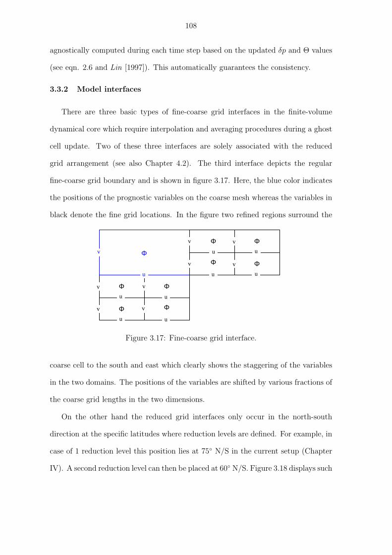
108
agnostically computed during each time step based on the updated δp and Θ values
(see eqn. 2.6 and Lin [1997]). This automatically guarantees the consistency.
3.3.2 Model interfaces
There are three basic types of fine-coarse grid interfaces in the finite-volume
dynamical core which require interpolation and averaging procedures during a ghost
cell update. Two of these three interfaces are solely associated with the reduced
grid arrangement (see also Chapter 4.2). The third interface depicts the regular
fine-coarse grid boundary and is shown in figure 3.17. Here, the blue color indicates
the positions of the prognostic variables on the coarse mesh whereas the variables in
black denote the fine grid locations. In the figure two refined regions surround the
Φ
Φ
Φ
ΦΦ
Φ
ΦΦ
Φ
u
uu
u
u
u u
u
u
vv
vv
v
v
v
v
v
Figure 3.17: Fine-coarse grid interface.
coarse cell to the south and east which clearly shows the staggering of the variables
in the two domains. The positions of the variables are shifted by various fractions of
the coarse grid lengths in the two dimensions.
On the other hand the reduced grid interfaces only occur in the north-south
direction at the specific latitudes where reduction levels are defined. For example, in
case of 1 reduction level this position lies at 75 N/S in the current setup (Chapter
IV). A second reduction level can then be placed at 60 N/S. Figure 3.18 displays such

109
an interface in the Northern Hemisphere which can be viewed as a static coarsening
step in the longitudinal direction. The variables in blue denote the reduced grid
u u
ΦΦ vv
Φ ΦΦ Φ
uuuu
v v v v
Figure 3.18: Reduced grid interface without adaptations.
arrangement, while the variables in black indicate the regular grid positions. The
u and Φ positions are shifted by a quarter of the coarse grid length in the zonal
direction. In contrast, the v positions coincide so that the the ghost cell data can be
directly injected during the ghost cell update.
In case refinements are applied in the reduced grid domain this interface changes
as illustrated in figure 3.19 As before, the blue color denotes the variables in the
Φ ΦΦ Φ
uuuu
v v v v
Φ
Φ Φ
Φ Φ
Φ
Φ
Φu
u
u u u
uuuv
v
v
v
v
v
v
v
Figure 3.19: Reduced grid interface with adaptations.
now refined reduced grid domain. The regular grid to the south (in black) remains
unchanged. Here all variable locations are only shifted in meridional direction. In-
terpolation and averaging routines need to be fully applied to v and Φ whereas u can
be partly copied (also called injection) during the ghost cell exchange.
The API interface of the spherical adaptive grid library requires that the user
provides the interpolation and averaging routines for all possible scenarios. These

110
program modules have been implemented in this research project which, in addition,
allow the choice of the three different interpolation schemes via an input parameter
(as discussed in Section 3.3.1).
3.3.3 Flux corrections
In an adaptive grid setup flux corrections at fine-coarse grid interfaces are imper-
ative in order to ensure mass conservation properties. Several flux correction strate-
gies have been discussed in the literature. For example, Berger and Colella [1989]
and Almgren et al. [1998] present flux correction mechanisms at the fine-coarse grid
boundary when different time steps are used in the two domains. Then fluxes need
to be accumulated until a synchronization point is reached. In contrast, the in-situ
fluxes can be directly assessed in case of a constant time step in both regions. This
simplifies the interface condition as shown in figure 3.20. In general, it is assumed
fyfy
fx
fx
fx
fy
KE KE
KEKE KE
KE KE
Coarse cell
Refined neighboringcells
Figure 3.20: Flux and kinetic energy (KE) updates at fine-coarse grid interfaces, fxand fy symbolize the fluxes in longitudinal and meridional direction.Fine grid fluxes are averaged and override the coarse grid flux at theinterface.
that the fluxes in the fine grid domain are more accurate than the corresponding flux
on the coarse grid. Therefore, the goal is to average the fine grid fluxes appropriately

111
in order to override the coarse grid information.
In the finite-volume dynamical core, three types of interface corrections are con-
sidered. These are the updates of the mass and heat fluxes across boundaries as
well as the synchronization of kinetic energy (KE) values at cell corner positions.
The mass and heat fluxes are defined at identical locations and are denoted by their
generic names fx and fy in figure 3.20. Here fx represents the flux in the zonal
direction whereas fy stands for the flux in the meridional direction.
The correct average of the fine grid fluxes in the spherical coordinate system must
take weighting functions into account that correspond to the areas of the surface
patches. In particular, each position of a flux needs to be considered a cell center of
a representative grid box around it. Then the boundary condition becomes
f c Ac =n∑
i=1
f ri Ar
i
⇔ f c =1
Ac
[f r
1 Ar1 + f r
2 Ar2
](3.18)
where the superscripts c and r stand for the coarse and refined grid, A represents
the surface area and the sum adds all fluxes f along the interface. Here n = 2
fluxes need to be considered in the 2D setup. This flux update algorithm ensures
mass conservation up to the last digit which is further documented in figure 4.11 on
page 134 (Section 4.2). On the other hand, such an averaging procedure is not
necessary for the scalar KE component. The coarse grid KE values can simply be
replaced with the matching KE components on the fine grid.


CHAPTER IV
Reduced grid and static adaptations
Adaptive blocks are flexible tools that can be used for static and dynamic grid
adaptations. Static adaptations are placed in user-defined regions of interest at the
beginning of a forecast and are held fixed during the model run. Typical applications
include static refinements in mountainous terrain or static refinements over selected
geographical areas e.g. for weather prediction applications. Such an approach could
replace today’s nested grid configurations that employ regional high-resolution mod-
els with coarse grid forcing along the boundaries. Adaptive blocks can also be used
to define a special type of grid, the so-called reduced grid. In a reduced grid, grid
points are coarsened in longitudinal direction as the poles are approached. This ef-
fectively relaxes the strict time step restrictions in a regular latitude-longitude grid
with |CFL| < 1 and, in addition, reduces the overall workload of the model by up to
20%. From a high level viewpoint, such a grid can be considered a statically adapted
grid with 1D coarsenings.
In this chapter, the adaptive finite-volume shallow water model is used in two
basic configurations, the reduced grid setup and the statically adapted setup with
an underlying full grid. The discussion of the results starts with an introduction
of suitable error measures and global invariants in Section 4.1. These measures are
113

114
used throughout Chapter IV-V and provide important information on the accuracy
and performance of the adaptive simulations. Section 4.2 is concentrated on the
reduced grid design. In particular, two reduced grid configurations with one and two
reduction levels are compared. Furthermore, Section 4.3 surveys more general static
adaptation setups and raises new questions concerning adapted model simulations
with external forcing functions.
4.1 Error measures and global diagnostics
Global error norms and global invariants, like the mass, energy or enstrophy, pro-
vide quantitative and objective measures for the performance of a model run. They
are used extensively in the following chapters that describe the adaptive simulations
with the finite-volume dynamical core. Here, an overview of the global measures is
given, together with their continuous and discrete definitions (see also Williamson
et al. [1992]).
4.1.1 Normalized error norms
The normalized l1, l2 and l∞ error norms assess the horizontally integrated relative
error of the model results. The error assessment requires the computation of the 2D
global integral I of a variable h(λ, ϕ) in spherical space
I(h) =1
4 π
∫ 2π
0
∫ π/2
−π/2
h(λ, ϕ) cos ϕdϕ dλ . (4.1)
The discrete approximation to this integral in an adaptive model setup is then given
by
I(h) =1
Asphere
#all cells∑
k=1
hk Ak (4.2)
where the sum adds up the weighted h values at all grid points covering the sphere.
The weights, or more precisely the spherical surface patches, Ak of a rectangular cell
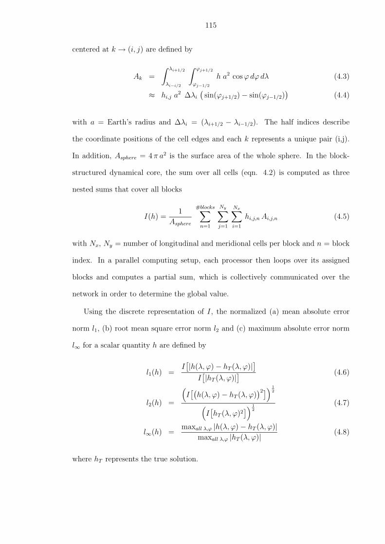
115
centered at k → (i, j) are defined by
Ak =
∫ λi+1/2
λi−i/2
∫ ϕj+1/2
ϕj−1/2
h a2 cos ϕdϕ dλ (4.3)
≈ hi,j a2 ∆λi
(sin(ϕj+1/2)− sin(ϕj−1/2)
)(4.4)
with a = Earth’s radius and ∆λi = (λi+1/2 − λi−1/2). The half indices describe
the coordinate positions of the cell edges and each k represents a unique pair (i,j).
In addition, Asphere = 4 π a2 is the surface area of the whole sphere. In the block-
structured dynamical core, the sum over all cells (eqn. 4.2) is computed as three
nested sums that cover all blocks
I(h) =1
Asphere
#blocks∑n=1
Ny∑j=1
Nx∑i=1
hi,j,n Ai,j,n (4.5)
with Nx, Ny = number of longitudinal and meridional cells per block and n = block
index. In a parallel computing setup, each processor then loops over its assigned
blocks and computes a partial sum, which is collectively communicated over the
network in order to determine the global value.
Using the discrete representation of I, the normalized (a) mean absolute error
norm l1, (b) root mean square error norm l2 and (c) maximum absolute error norm
l∞ for a scalar quantity h are defined by
l1(h) =I[|h(λ, ϕ)− hT (λ, ϕ)|]
I[|hT (λ, ϕ)|] (4.6)
l2(h) =
(I[(
h(λ, ϕ)− hT (λ, ϕ))2]) 1
2
(I[hT (λ, ϕ)2
]) 12
(4.7)
l∞(h) =maxall λ,ϕ |h(λ, ϕ)− hT (λ, ϕ)|
maxall λ,ϕ |hT (λ, ϕ)| (4.8)
where hT represents the true solution.

116
The corresponding error norms for a vector quantity ~v = (u, v) are given by
l1(~v) =I[(
(u(λ, ϕ)− uT (λ, ϕ))2 + (v(λ, ϕ)− vT (λ, ϕ))2) 1
2
]
I[(
uT (λ, ϕ)2 + vT (λ, ϕ)2) 1
2
] (4.9)
l2(~v) =
(I[(u(λ, ϕ)− uT (λ, ϕ))2 + (v(λ, ϕ)− vT (λ, ϕ))2
]) 12
(I[uT (λ, ϕ)2 + vT (λ, ϕ)2
]) 12
(4.10)
l∞(~v) =maxall λ,ϕ
[((u(λ, ϕ)− uT (λ, ϕ))2 + (v(λ, ϕ)− vT (λ, ϕ))2
) 12
]
maxall λ,ϕ
[(uT (λ, ϕ)2 + vT (λ, ϕ)2
) 12
] (4.11)
with the true wind speeds uT and vT . Here, a difficulty arises due to the grid stag-
gering of the wind components in the finite-volume dynamical core. The error norms
require that the u and v data are defined at the same grid point position. Therefore,
the D-grid wind is linearly interpolated to the A-grid (cell center) position before
the error norms are computed. This introduces an interpolation error, but tests with
shallow water test 2 showed that this error is at least one order of magnitude smaller
than the model errors.
In addition, the definitions of the normalized maximum and minimum of a scalar h
are
hmax =maxall λ,ϕ h(λ, ϕ)−maxall λ,ϕ hT (λ, ϕ)
∆h(4.12)
hmin =minall λ,ϕ h(λ, ϕ)−minall λ,ϕ hT (λ, ϕ)
∆h(4.13)
where ∆h is the difference between the maximum and minimum values of the true
solution at the beginning of the forecast. These error measures are used for 2D
advection experiments in the shallow water setup. For example hmax assesses the
decrease in the peak amplitude of the transported feature.

117
4.1.2 Global invariants
Additional model assessments are based on normalized global invariants. The
normalized integral Ii(ξ(t)) (notation as in Williamson et al. [1992]) is defined by
Ii(ξ(t)) =I[ξ(λ, ϕ, t)]− I[ξ(λ, ϕ, 0)]
I[ξ(λ, ϕ, 0)](4.14)
where the discrete integral is given as in equation 4.2. Here, the time-dependent
variable ξ stands for e.g. the mass (i = 1) which is defined by the geopotential
height ξ = h in the shallow water system or the surface pressure ξ = ps in the 3D
case. Alternatively, the total energy (i = 2) in the shallow water system can be
assessed via
ξ =1
2h~v · ~v +
1
2g
((h + hs)
2 − h2s
)(4.15)
and the potential enstrophy (i = 3) is given by
ξ =1
2
(ζ + f
)2/ h (4.16)
where g is the gravitational acceleration, hs denotes the height of the surface orogra-
phy, ζ represents for the relative vorticity and f symbolizes the Coriolis parameter.
These global invariants are normalized with the integral at time step t = 0. As
in Section 4.1.1 the wind data need to be interpolated to the cell center before the
total energy can be evaluated. This interpolation error will be visible as an initial
error in figure 4.10 on page 133.
4.1.3 Reference solutions
For the error measures, the model results need to be compared to a reference or
“true” solution hT , uT and vT . In case of the shallow water runs this solution is either
an analytic solution (shallow water tests 1-4) or a high-resolution reference solution
(test 5 and 6) computed with an NCAR spectral model at resolution T213. This

118
resolution corresponds to approximately 50km in grid point space near the equator.
The NCAR reference solution (see details in Jakob et al. [1993] and Jakob-Chien et al.
[1995]) is provided in the form of spectral expansion coefficients using the portable
NetCDF data format. The solution can then be evaluated in grid point space at
arbitrary locations.
The analytic solutions for the test cases 1-4 can be directly calculated in any grid
configuration, although test case 3 and 4 require the computation of integrals. These
are approximated with a numerical method, in particular the trapezoidal rule. In
addition, the reference solution for test case 1, the advection of a cosine bell, relies
on an accurate estimate of the location of the cosine bell at any time. Since the
advection can be specified with a rotation angle α this position (λ, ϕ) of the center
is not obvious. It can either be assessed via coordinate transformations or with an
iterative trajectory calculation. Here, the second option is chosen. The trajectory or
path s of a parcel in the Cartesian system (see also Holton [1992])
D s
D t= V (x, y, t) (4.17)
is then replaced with
D ϕ
D t=
v
a(4.18)
D λ
D t=
u
a cos ϕ(4.19)
in the spherical representation. This system is solved iteratively
ϕn+1 = ϕn +v(λn, ϕn)
a∆t (4.20)
λn+1 = λn +u(λn, ϕn)
a cos ϕn∆t (4.21)
with small time steps ∆t starting at the initial location (λ0, ϕ0) = (λc, ϕc). The
velocities u and v are specified analytically (see Williamson et al. [1992])..

119
4.2 Reduced grid
“Reduced” or “skipped” grid setups have long been used in atmospheric general
circulation modeling. The first reduced grid configurations for finite difference mod-
els were proposed by Gates and Riegel [1962], Kurihara [1965] and Kurihara and
Holloway [1967]. The latter designed the so-called Kurihara grid with only four grid
points next to the poles which offered a more homogeneous grid distribution from a
physical standpoint. But when serious deficiencies of the Kurihara grid were discov-
ered, which e.g. included an excessive pressure build-up in polar regions, more grid
points in longitudinal direction needed to be added again to significantly improve
the accuracy (see Rao and Umscheid [1969] and Dey [1969]). It was soon realized by
Shuman [1970] and Williamson and Browning [1973] that reduced grid setups need to
be carefully constructed for grid point models with finite difference approximations.
The difficulties arise due to the polar singularities in curvilinear coordinates that
result in an extreme curvature of the inner circle of data. As a consequence, large
truncation errors are present when longitudinal differences are taken over large longi-
tudinal grid intervals. As shown in Williamson and Browning [1973] this is in partic-
ular true for terms containing the spherical vector components u and v whereas the
approximation of terms with only scalar quantities, like the pressure or geopotential
gradient, are not necessarily affected. It was concluded that very coarse longitudinal
resolutions near the poles are not able to properly handle even the large-scale, small
wavenumber features. Shuman [1970] in fact recommended that grid points should
be added in high latitudes rather than dropped. As an alternative, derivatives could
be calculated in Cartesian coordinates on cones locally tangent to each grid point.
Similar findings were also reported by Lanser et al. [2000] and Layton [2002] for

120
finite-volume approaches and cubic spline collocation methods, respectively.
In order to improve the accuracy of the zonal gradients in the immediate vicinity
of the poles special treatments can be introduced as suggested by Purser [1988b].
Purser [1988b] pointed out that zonal derivatives can still be calculated with suffi-
cient precision when high frequency information is interpolated through an assump-
tion of smoothness from nearest neighbors in the polar region. The difficulties of the
reduced grid setup can further be avoided when switching to a spectral model that
does not need to calculate difference operators in grid point space. Instead, deriva-
tives are evaluated in a spherical representation after applying Fourier and Legen-
dre transforms. These so-called reduced Gaussian grids have been successfully used
in spectral models for many years. Examples include Hortal and Simmons [1991],
Courtier and Naughton [1994] and Williamson and Rosinski [2000] who developed
reduced grids for weather and climate applications that are partly in operational use
today. No significant loss of accuracy has been observed in comparison to full grid
simulations.
4.2.1 Design of the reduced grid in the finite-volume dynamical core
Decreasing the number of grid points near the poles is attractive due to compu-
tational performance considerations. This is in particular true if the CFL condition
in the polar regions limits the time step for the global domain.
In the finite-volume dynamical core, two new reduced grid designs have been
tested that are based on the block-structured data layout. They are shown in fig-
ure 4.1 on the facing page which illustrates the reduced grid setups with one and
two reduction levels projected onto the sphere. Here, the initial grid parameter set
with 16x12 blocks and 9x6 cells per block is chosen as in table 3.2 on page 76 which

121
Figure 4.1: Distribution of blocks and grid points over the sphere (orthographic pro-jection centered at 0E,45N). Reduced grid with 1 reduction (left) and 2reductions (right) in the polar regions. Base resolution is 2.5 × 2.5.
consequently places the reduction levels at 75 N/S and 60 N/S, respectively. At
each transition point, the physical grid spacing in longitudinal direction then changes
abruptly by a factor of 2 as depicted in figure 4.2. The figure also displays the under-
0
30
60
90
Lat
itude
0 50 100 150 200 250 300
∆x (km)
full grid (fg)
1 reduction (rg1)
2 reductions (rg2)
Figure 4.2: Physical grid distance (km) in longitudinal direction for the full grid andreduced grid setups.
lying design principle that the physical distances at any latitude should not greatly
exceed the maximum grid spacing at the equator. This condition is well-met by both
designs, although a small overshoot at 75 N/S is present in case of 2 reductions.
The reduced grid setups can be convieniently chosen via input parameters at run
time. The resulting number of blocks for the two designs is documented in table 4.1.

122
4.2.2 Advection tests
The reduced grid designs are tested with shallow water test case 1 (see also
Appendix A.1) that describes the passive advection of a cosine bell once around the
sphere. This test does not deal with the complete nonlinear shallow water equations
but evaluates the advection algorithm in isolation. Here, the rotation angle α = 90
is chosen so that the feature is transported over the poles.
Three model runs with the base resolution 2.5×2.5 have been performed. These
include the full grid (fg) control run as well as the reduced grid (rg) simulations with
1 and 2 reduction levels. The numerical transport scheme used in the whole domain
is the monotonicity-preserving PPM method. No filtering techniques need to be
applied due to the absence of gravity wave motions in the advection experiment.
The error measures for the geopotential height field after one revolution of the
cosine bell (day 12) are shown in table 4.1. In addition, the table contains informa-
Base Refin. Reduced Height error norms Final # Time CPUresol. level grid l1 l2 l∞ h (m)
# Blockssteps time (s)
α = 90
2.5 0 0 0.0965 0.0952 0.1285 853.5 192 7200 1202
2.5 0 1 0.0927 0.0911 0.1264 855.5 176 3744 415
2.5 0 2 0.0881 0.0889 0.1333 848.8 152 2016 205
Table 4.1: Error statistics for the cosine bell advection test over the poles (test case1, α = 90) with two reduced grid configurations.
tion on timing data and the total number of time steps that are necessary for the
completion of one revolution. The timing results represent the total CPU time for
the simulations on a SUN Ultrix workstation. The time steps are severely limited
by the CFL condition in the longitudinal direction at the circle next to the poles.
123
Here, CFL=0.95 is chosen for all model runs which results in time steps ∆t ≈ 149 s
(fg), ∆ ≈ 297.5 s (rg1) and ∆ ≈ 597 s (rg2), respectively. Due to the increase in the
length of the time step, a sharp decrease in the total number of integration steps is
observed for the two reduced grid simulations. It is interesting to note that the re-
duction in integration steps leads to improved l1 and l2 error measures despite the use
of the reduced grid. Though, this is not true for the l∞ norm and the final amplitude
that slightly degrades in case of 2 reduction levels. Here, the initial peak amplitude
is 979.0 m. The error measures in table 4.1 compare favorably to similar advection
experiments documented in the literature. In particular, Rasch [1994] performed the
cosine bell advection test with a reduced grid design and comparable base resolu-
tion (2.8). The error measures for Rasch’s RG2.8 configuration with a monotonic
upstream-biased transport scheme exceed the errors in table 4.1 by a factor of 1.5-2.
In comparison to the control run, both reduced grid simulations perform well
which is further depicted in figure 4.3 on the next page. The figure shows 5 snap-
shots of the solution at day 1 through 5 mapped onto a North polar stereographic
projection. Here, the cosine bell is transported over the North Pole (from the bot-
tom to the top) in the reduced grid setups with one and two reduction levels. It
can clearly be seen that the cosine bell crosses the pole without spatial distortions
in both cases, although a very minor loss in peak amplitude is visible in the rg2 run.
The full grid control run is almost indistinguishable from the rg1 case (not shown).
This confirms the conclusion by Williamson and Browning [1973] that the reduced
grid can be successfully employed for the transport of scalar quantities.

124
300
600
300
300
300
600
(a) 2.5o grid, 1 reduction
0˚
90˚
180˚
270˚
300
600
300
300
300
600
(b) 2.5o grid, 2 reductions
0˚
90˚
180˚
270˚
Figure 4.3: Polar stereographic projection of the cosine bell (test case 1, α = 90)transported over the North Pole (from the bottom to the top of thefigure, the outer cricle is located at 15N). Snapshots are taken after 1,2, 3, 4 and 5 days, respectively. Base resolution is 2.5 × 2.5. Reducedgrid runs with (a) 1 reduction, (b) 2 reductions. The block distributionis indicated by dotted lines. Contour intervals of the geopotential heightfield are 100 m.

125
4.2.3 Non-linear shallow water tests
In order to assess the performance of the reduced grid setups in the nonlinear
shallow water system, three test scenarios are examined. These include the McDon-
alds and Bates [1989] test case as well as shallow water test 2 and 6 (see Appendix
A).
First, the results of the control run and reduced grid simulations are evaluated
qualitatively using the McDonalds and Bates [1989] test. This sometimes called
dancing high-low wave test case comprises a flow straight over the poles, which is a
particularly suitable test for the reduced grid assessments. The wind speeds at the
poles are on the order of 10-15 m/s.
The results of the simulations in the Northern Hemisphere at day 10 are illus-
trated in figure 4.4 which displays the flow pattern of the fg control run (upper
row), the rg1 simulation (middle row) and the rg2 setup (bottom row). Here, the
geopotential height field and the wind components u and v (from left to right) are
shown. The reduced grid simulations in this moderate wind speed regime are almost
indistinguishable from the control run. There are no distortions in any of the large-
scale flow patterns which are still well-resolved even in the rg2 case with only 36 grid
points next to the poles.
Such a conclusion can only partly be drawn in the subsequent examples. The
second test scenario is based on shallow water test 2 with chosen rotation angle
α = 45. This steady state flow field (see also initial data in figures A.3 and A.4) is
expected to remain unchanged during the course of the integration. It describes a
strong flow over the poles with wind speeds on the order of 28 m/s that accentuate
possible errors in polar regions resulting from the reduced grid coarsenings. Both
reduced grid setups have been tested in a 14-day simulation as documented by the

126
5600
5800
5800
6000
6000
6200
0˚
180˚
0
0
0
0
0
9
9
9
9
18
18
-18-9
-9-9
-9
0˚
180˚
0
0
0
0
0
6
6-6
-6
0˚
180˚
5600
5800
5800
6000
6000
6200
0˚
180˚
0
0
0
0
0
9
9
9
9
18
18
-18-9
-9-9
-9
0˚
180˚
0
0
0
0
0
6
6-6
-6
0˚
180˚
5600
5800
5800
6000
6000
6200
0˚
180˚
0
0
0
0
0
9
9
9
9
18
18
-18-9
-9-9
-9
0˚
180˚
0
0
0
0
0
6
6-6
-6
0˚
180˚
Figure 4.4: North polar stereographic projections of the geopotential height h, thezonal wind u and meridional wind v (from left to right) at day 10 (Mc-Donalds and Bates [1989] test case). Contour intervals are 50 m, 3 ms−1
and 1.5 ms−1, respectively. The base resolution is 2.5. Top row: simu-lation with the full grid. Middle row: grid with 1 reduction at the poles.Bottom row: grid with 2 reductions in the polar regions.

127
zonal wind field at day 14 in figure 4.5. Although the flow patterns are very similar, a
0
7.5 7.5
7.5
7.5
15 15
1515
22.5 22.5
22.522.5
22.5
30
30
30
30
30
37.5
-15
-7.5
(a) Reduced grid with 1 reduction (rg1)
-90
-45
0
45
90
Lat
itude
0 90 180 270 360Longitude
0
7.5 7.5
7.5
7.5
15 15
15
15
22.5 22.5
22.522.5
22.5
30
30
30
30
30
37.5
-15
-7.5
(b) Reduced grid with 2 reductions (rg2)
-90
-45
0
45
90
Lat
itude
0 90 180 270 360Longitude
Figure 4.5: Zonal wind u at day 14 (test case 2, α = 45), (a) reduced grid simulationwith 1 reduction, (b) with 2 reductions. Contour interval is 2.5 ms−1.
close examination of the rg2 case reveals a slightly slanted distortion of the zonal wind
field. This is confirmed in figure 4.6 which displays the differences of the zonal wind
fields with the reference solution for both reduced grid setups. In case of 1 reduction
level, a moderate error pattern in the zonal wind field can be observed, but errors
increase considerably when adding a second reduction level. Here it is interesting to
see that the errors of the reduced grid are concentrated but not confined to the polar

128
00
00
0
0
00
00
0
-0.3
-0.3
a) Reduced grid with 1 reduction (rg1)
-90
-60
-30
0
30
60
90
Lat
itude
0 90 180 270 360Longitude
0
0
0
0
00
0
0
0
0.6
0.6
0.6
0.60.6
-1.2
-1.2-0.6 -0.6
-0.6
-0.6-0.6
-0.6
-0.6
-0.6-0.6
-0.6
b) Reduced grid with 2 reductions (rg2)
-90
-60
-30
0
30
60
90
Lat
itude
0 90 180 270 360Longitude
Figure 4.6: Zonal wind differences with reference solution at day 14 (test case 2, α =45), (a) reduced grid simulation with 1 reduction, (b) with 2 reductions.Contour intervals are (a) 0.1 ms−1 and (b) 0.2 ms−1.

129
regions. Instead, the errors propagate and interact with other model errors over time
so that the whole domain is affected.
This qualitative assessment is further quantified in figure 4.7 which illustrates
the corresponding l2 height and wind error norms of the fg, rg1 and rg2 model runs.
In addition, the plots assess the impact of the first- and second-order interpolation
methods on the overall accuracy of the rg1 simulation. The temporal evolution
0.0000
0.0005
0.0010
0.0015
0.0020
0.0025
0.0030
0.0035
Nor
mal
ized
l 2(h
)
0 48 96 144 192 240 288 336
Hours
full grid (fg)1 reduction (rg1), 1st order1 reduction (rg1), 2nd order2 reductions (rg2), 2nd order
0.000
0.005
0.010
0.015
0.020
Nor
mal
ized
l 2(v
)
0 48 96 144 192 240 288 336
Hours
full grid (fg)1 reduction (rg1), 1st order1 reduction (rg1), 2nd order2 reductions (rg2), 2nd order
Figure 4.7: Normalized l2 height errors (left) and l2 wind errors (right) for the fullgrid (fg) and the reduced grids with 1 reduction (rg1) and 2 reductions(rg2). The order indicates the interpolation order at the reduced gridinterfaces (test case 2, α = 45).
of the normalized l2 error norms confirms the significant increase in the solution
error in case of the rg2 setup, whereas error levels remain low for one reduction
step. For comparison, Tolstykh [2002] also reports comparable error measures with
l2(h) = 4.3×10⁻⁴ after 120 hours. In general, the error curves depict a linear increase
in the solution error which is overlaid by inertio-gravity wave oscillations. The latter
are damped out over time. In practice, the sharp rise in the error level for rg2 is no
longer considered acceptable and therefore, the rg2 design can not be recommended
for future nonlinear adaptive grid applications. As an aside, it is interesting to note
that the order of the interpolation scheme at the reduced grid boundaries hardly

130
affects the error norms in the rg1 case. This is true for the idealized very smooth
flow field selected here. But as shown in the next paragraph, such a conclusion
does not generally hold when more complex flow patterns with strong gradients are
simulated.
The third assessment of the reduced grid design is based on shallow water test 6
which comprises a Rossby-Haurwitz wave with wavenumber 4. The test translates
the symmetric wave pattern without change of shape from west to east. Here, special
attention is paid to the order of the interpolation scheme in a reduced grid setup that
needs to be applied at the polar interfaces. This aspect is assessed in figure 4.8 on
the next page that presents the geopotential height field at day 14 on a reduced
grid with 1 reduction level. Two interpolation strategies are employed. In subfigure
(a), the wind data are interpolated via bilinear interpolations whereas the first-order
conservative van Leer approach is applied to the geopotential height field h. In
subfigure (b), the second-order PPM interpolation method is used for all variables.
The impact of the interpolation error in this high-wind speed regime is clearly visible.
The low-order methods (subfigure (a)) introduce a slightly asymmetric flow pattern
over time (see also discussion in Section 3.1.3 on page 76) whereas the more accurate
second-order method can maintain the symmetry.
This effect is quantified in figure 4.9 on page 132 that reviews the performance
of the reduced grid setups in comparison to the NCAR reference solution. Here it is
interesting to see that the l2 and l∞ height errors in the rg1 design almost overlay the
full grid control run until the errors split after day 11. The overall solution error is
therefore hardly affected by one reduction step which is a considered a viable option
for nonlinear runs. In contrast, the rg2 model simulation again shows unacceptable
large errors and can not be recommended for future use. The superior performance

131
850085008500
85008500
9000
90009000
9000
90009000
9500
9500
9500
9500
100001000010000
100001000010000
(a) rg1 with 1st order wind (bilinear) and height (van Leer) interpolation
-90
-45
0
45
90L
atitu
de
0 90 180 270 360Longitude
85008500
8500
8500
9000
9000
9000
9000
9500
9500
9500
9500
100001000010000
100001000010000
10500 10500 10500 10500
(b) rg1 with 2nd order wind and height (PPM) interpolation
-90
-45
0
45
90
Lat
itude
0 90 180 270 360Longitude
Figure 4.8: Geopotential height at day 14 (test case 6), reduced grid simulationswith 1 reduction. (a) 1st order wind interpolation (bilinear) and 1storder height interpolation (conservative van Leer scheme), (b) 2nd orderwind and conservative height interpolations (PPM method). Contourintervals are 100 m.

132
0.000
0.002
0.004
0.006
0.008
0.010
0.012N
orm
aliz
ed l 2
(h)
0 48 96 144 192 240 288 336
Hours
full grid (fg)1 reduction (rg1), 1st order1 reduction (rg1), 2nd order2 reductions (rg2), 2nd order
0.000
0.005
0.010
0.015
0.020
0.025
0.030
Nor
mal
ized
l inf
(h)
0 48 96 144 192 240 288 336
Hours
full grid (fg)
1 reduction (rg1), 1st order
1 reduction (rg1), 2nd order
2 reductions (rg2), 2nd order
Figure 4.9: Normalized l2 (left) and l∞ (right) height errors for the full grid (fg)and the reduced grids with 1 reduction (rg1) and 2 reductions (rg2).The order indicates the interpolation order at the reduced grid interfaces(test case 6).
of the second-order interpolation scheme is clearly demonstrated at the end of the
14-day forecast when the l2 and l∞ norm still closely resemble the full grid control
run. The l2 height error in both the fg model run with l2(h) = 0.0033 and the rg1
simulation with l2(h) = 0.0036 at day 14 compare favorably to values published in
the literature. These are listed for comparable resolutions in table 4.2. All model
Author Model Resolution l2(h) at day 14
Jakob-Chien et al. [1995] spectral T42 0.0054
Taylor et al. [1997] spectral elements ≈ 2.5 0.0079
Spotz et al. [1998] spectral T42 0.0044
Spotz et al. [1998] double Fourier method T42 0.011
Cheong [2000] double Fourier method T42 0.0042
Tolstykh [2002] finite differences 2.5 0.0052
Layton and Spotz [2003] double Fourier method T42 ≈ 0.02
Table 4.2: Error statistics for the Rossby Haurwitz test (test case 6) based on liter-ature search.
runs are compared to the NCAR high-resolution reference solution. Here, it must
be kept in mind that this reference solution is also not free of numerical errors as

133
assessed in Taylor et al. [1997] and Jakob-Chien et al. [1995]. The uncertainty of the
normalized l2 norm is estimated to be 0.0008.
Besides error norms, it is also interesting to examine the impact of the grid
reductions on global invariants. This is depicted in figure 4.10 which shows the time
evolution of the normalized total energy and potential enstrophy for the fg, rg1 and
rg2 model runs. Both quantities are not formally conserved in the finite-volume
-0.0012
-0.0009
-0.0006
-0.0003
0.0000
Nor
mal
ized
tota
l ene
rgy
0 48 96 144 192 240 288 336
Hours
full grid1 reduction2 reductions
-0.012
-0.009
-0.006
-0.003
0.000
Nor
mal
ized
pot
entia
l ens
trop
hy
0 48 96 144 192 240 288 336
Hours
full grid1 reduction2 reductions
Figure 4.10: Normalized global integrals of total energy (left) and potential enstro-phy (right) for the full grid and the reduced grids with 1 reduction and 2reductions using second-order interpolations at the interfaces (test case6).
model. But the decrease in total energy (TE) and potential enstrophy in the fg and
rg1 case is moderate in comparison to the rg2 simulation. The initial decrease in the
normalized total energy at t=0 is an artifact of the staggered D-grid arrangement.
It requires the interpolation of the wind data for the kinetic energy (KE) calculation
which decreases the KE value on the order of 10−4. This is the starting point of the
TE curves.
In addition, tests have been performed that assess the conservation of mass in the
reduced grid setup with 1 reduction level. This comparison is shown in figure 4.11 on
the next page which compares the impact of the flux corrections at the reduced grid

134
boundaries (see Section 3.3.3 on page 110) as well as filtering effects. As discussed
in Section 2.2.2, filtering leads to a violation of conservation laws if no a-posterioi
restoration mechanisms are applied. For example the filtering of the mass variable Φ
violates the conservation of mass principle. It is important to observe that only the
-2e-07
0
2e-07
4e-07
6e-07
8e-07
Nor
mal
ized
mas
s
0 48 96 144 192 240 288 336
Hours
flux correction, no Φ filterflux correction, Φ filterno flux correction, no Φ filterno flux correction, Φ filter
Figure 4.11: Normalized global integrals of the mass for reduced grid simulationswith 1 reduction (test case 6). The different model setups include sim-ulations with or without a flux corrected transport at the reduced gridinterfaces and polar filtering of the geopotential polewards of 60 N/S,see figure for combinations.
flux-corrected, unfiltered1 simulation conserves the mass up to machine precision.
The filter effect on the other hand leads to an increase in mass, whereas the omission
of the flux correction at the interfaces tends to decrease the mass. Both effects
overlay each other.
Another aspect must be noted concerning the reduced grid setup in the finite-
volume shallow water model. In test case 6 presented above, the time step ∆t = 360s
can not be reduced in the two reduced grid simulations as seen before in the advection
experiment. This is due to the fact that the time step in case 6 is not restricted by the
1Unfiltered with respect to the geopotential Φ, the wind components need to be filtered tomaintain stability.

135
advection speed in polar regions, but by the gravity wave activity in midlatitudes.
Coarsening the polar regions has therefore no impact on the stability criterion and
identical time step must be used for all three simulations. This has far-reaching
implications with respect to the performance of the model runs. The clear speedup
of a reduced grid run in the advection experiment can no longer be achieved. On
the contrary, choosing the rg1 reduced grid setup adds extra work at the reduced
grid interfaces despite the 9% reduction in the number of blocks. When using 16x12
blocks with 9x6 cells per block, the full grid control run needs 1522 CPU seconds
on a SUN Ultrix workstation for the 14-day simulation, whereas the rg1 run finishes
after 1915 CPU seconds. As a result, the overhead estimate again yields (compare
Section 3.2.3) 1522 s192 blocks
/1915 s
176 blocks≈ 27%, which clearly outweighs the advantages of
the reduced number of blocks in the rg1 case. Therefore, it is not recommended to use
a reduced grid if the global time step is not limited by the CFL restrictions in polar
regions. However, it may be possible that future optimizations of the AMR library
and the user-provided interpolation routines will reduce the overhead significantly.
In the present example, where no dynamic or static adaptations are requested, the
most efficient simulation is indeed a uniform model run with big block sizes (see also
performance discussion in Section 3.2.3). E.g. the setup with 2x2 blocks and 72x36
cells per block requires only 568 CPU seconds for the 14-day model run. As observed
earlier, the large block sizes in the 2D framework lead to a speedup by a factor of
approximately 2.5.

136
4.3 Static adaptations
Adaptive blocks can not only be used for reduced grid configurations but also
for user-defined, pre-determined regions of interest that need to be resolved at fine
resolutions. Typical examples include high resolution regions in mountainous terrain
or grid adaptations for locally refined weather forecasts.
Static adaptations are chosen at the beginning of a model run and remain fixed
during the simulation. They can be viewed as a two-way interactive nesting approach
that provides consistent inflow and outflow conditions along the interfaces. The
following section examines the impact of these high-resolution regions on the global
domain. Three test scenarios are assessed in the shallow water framework.
First, steady state shallow water test case 2 with α = 45 is selected. Here, a high
resolution refinement area at refinement level 2 is placed in the Northern Hemisphere
as illustrated in figure 4.12. The figure shows the geopotential height field with
1200
1600
2000
2000
2000
2000
2400
24002400
2400
2800
2800
2800
2800
-90
-60
-30
0
30
60
90
Lat
itude
0 90 180 270 360Longitude
Figure 4.12: Geopotential height at day 14 (test case 2, α = 45) with static refine-ments (refinement level 2) centered at 135E,30N. The distribution ofthe blocks is drawn in red. Base resolution is 2.5, contour interval is100 m.
overlaid blocks (in red) at model day 14. The base resolution in this example is
a 2.5 × 2.5 grid so that the finest resolution represents a 0.625 grid spacing. It

137
can be seen that the flow passes through the refined area without noise and almost
no distortions, despite the fact that the refinements are purposely placed in a region
with strong geopotential gradients. As discussed later this has measurable impact on
the simulation results in comparison to low gradient regimes. A closer examination
of the wind components u and v at day 14 in figure 4.13 reveals that only very minor
errors are induced at the coarse-fine grid interfaces. The errors are mostly visible in
7.5
15
22.5
-15
-7.5
(a) Zonal wind u (m/s)
-30
0
30
60
90
Lat
itude
45 90 135 180 225Longitude
7.5 15-22.5 -22.5 -15 -7.5
(b) Meridional wind v (m/s)
-30
0
30
60
90
Lat
itude
45 90 135 180 225Longitude
Figure 4.13: (a) Zonal and (b) meridional wind at day 14 (test case 2, α = 45) withstatic refinements (refinement level 2). The distribution of the blocks isdrawn in red. Base resolution is 2.5, contour intervals are 2.5 ms−1.
the v field at the outflow boundary east of the refined area.
In order to quantify the performance of such a refined model run, the corre-
sponding height error norms are displayed in figure 4.14 on the next page. The plot
shows the time evolution of the normalized l2 norm in three model runs, the full
grid control run at the base resolution and two statically adapted runs, where the
center of the refined patch is placed at two different locations. The first location
135E, 30N coincides with the previous example, whereas the second position at
180E, 45N symmetrically refines the low pressure center in the Northern Hemi-
sphere (not shown). This region is characterized by lower geopotential gradients
which lead to improved l2 error norm statistics. The error in the first anti-symmetric

138
0.0000
0.0002
0.0004
0.0006
0.0008
0.0010
norm
aliz
ed l 2
(h)
0 48 96 144 192 240 288 336
Hours
non-adapted grid (2.5deg)static, placed at (135E,30N) as shown earlierstatic, placed at (180E,45N)Tolstykh (2.5deg), MWR 2002
Figure 4.14: Normalized l2 height errors (test case 2, α = 45) for a non-adapted run(2.5 resolution) and 2 statically adapted runs with 2 refinement levels.
case is slightly enhanced but still well within the expected error margins for this test
case. This is shown by a comparison with Tolstykh’s results.
There are two possible sources for the increased errors in the statically adapted
runs. First, it must be noted that the initial data in the adapted patches are interpo-
lated via quadratic interpolations at the beginning of the forecast. This introduces
an interpolation error in comparison to an analytically reinitialized field that obeys
the underlying geostrophic balance more accurately. Especially at refinement level 2,
the initial conditions are then interpolated based on the already interpolated data at
refinement level 1. Second, the interpolations of the ghost cells at fine-coarse grid in-
terfaces take place multiple times per time step during the course of the integration.
Since the accuracy of the fluxes across interfaces relies on ghost cell information, an
interpolation error in the ghost cell update becomes transparent in the flux calcula-
tion.
In order to asses the relative importance of the two error sources, tests with
analytically reinitialized initial conditions have been performed. The results of this
run (not shown) are almost indistinguishable from the run with interpolated initial

139
data. For this idealized smooth scenario, it can therefore be concluded that the
errors in the initial data are not responsible for the resulting higher error norms.
The error is clearly dominated by the inaccuracies of the ghost cells and fluxes at the
interfaces. In general, these errors do not accumulate along the edges of the blocks
but rather interact with the truncation error of the numerical scheme. It has also
been observed that errors are higher in regions where the monotonicity constraint is
applied, especially in the neighborhood of maxima and minima of the geopotential.
Furthermore, it is also interesting to note that the l2 error trends are again overlaid
by typical inertio-gravity wave oscillations (compare also to figure 4.7). These are
due to the geostrophic adjustment process that describes the mutual adaptation of
mass and momentum toward a steady geostrophic state. Here the period is on the
order of 16 hours which is very close to the period of pure inertial oscillations in
midlatitudes. For example, at 45 N/S inertial oscillation are characterized by a
period of 2π|f | = 12h
| sin 45| = 16.97h (Holton [1992]). Inertio-gravity waves are generated
by small deviations from the geostrophic balance in the discrete system. The final
state is achieved by the decaying inertial oscillations that dissipate the energy. The
wave motion is clearly emphasized in this idealized test setup. In the real atmosphere
though, the motions are predominantly generated and maintained by the pressure
gradient force. Therefore the conditions for purely inertial oscillations only rarely
exist.
High wind speed regimes
The second assessment of the static adaptations is based on shallow water test 6,
the Rossby-Haurwitz wave with extremely strong gradients in both the geopotential
and wind fields. This test is very hard for adaptive grid simulations due not only to
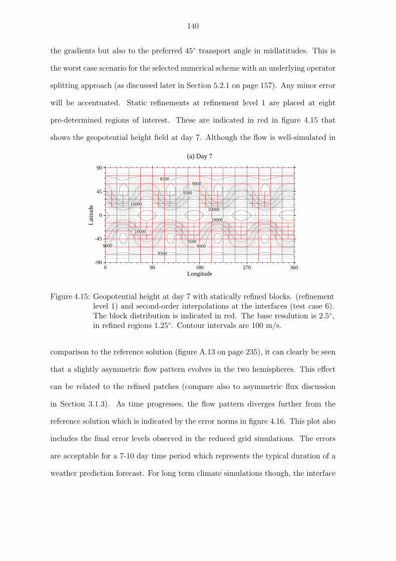
140
the gradients but also to the preferred 45 transport angle in midlatitudes. This is
the worst case scenario for the selected numerical scheme with an underlying operator
splitting approach (as discussed later in Section 5.2.1 on page 157). Any minor error
will be accentuated. Static refinements at refinement level 1 are placed at eight
pre-determined regions of interest. These are indicated in red in figure 4.15 that
shows the geopotential height field at day 7. Although the flow is well-simulated in
8500
8500
90009000
9000
9500
9500
10000
10000
1000010000
(a) Day 7
-90
-45
0
45
90
Lat
itude
0 90 180 270 360Longitude
Figure 4.15: Geopotential height at day 7 with statically refined blocks. (refinementlevel 1) and second-order interpolations at the interfaces (test case 6).The block distribution is indicated in red. The base resolution is 2.5,in refined regions 1.25. Contour intervals are 100 m/s.
comparison to the reference solution (figure A.13 on page 235), it can clearly be seen
that a slightly asymmetric flow pattern evolves in the two hemispheres. This effect
can be related to the refined patches (compare also to asymmetric flux discussion
in Section 3.1.3). As time progresses, the flow pattern diverges further from the
reference solution which is indicated by the error norms in figure 4.16. This plot also
includes the final error levels observed in the reduced grid simulations. The errors
are acceptable for a 7-10 day time period which represents the typical duration of a
weather prediction forecast. For long term climate simulations though, the interface

141
0.000
0.002
0.004
0.006
0.008
0.010
0.012
Nor
mal
ized
l 2(h
)0 48 96 144 192 240 288 336
Hours
uniform grid, 2.5o resolutionreduced grid with 1 reduction, 1st orderreduced grid with 1 reduction, 2nd orderreduced grid with 2 reductions, 2nd orderstatic refinements, 2nd order
Figure 4.16: Normalized l2 height errors for the non-adapted run (2.5 resolution)and statically adapted run with 1 refinement level (test case 6). Theadditional data points show the error norms of reduced grid simulationsand are taken from figure 4.9.
treatment must be very carefully examined. True overlap regions as in Brown et al.
[2003] can possibly be introduced to enhance the accuracy.
Forced nonlinear system with translating low
The third assessment of the statically adapted shallow water model increases the
complexity of the test scenario even further. It is based on shallow water test 4
that describes a forced nonlinear system with an embedded translating low pressure
center. For this test the shallow water equations need to be modified. In particular,
time and grid resolution dependent forcing functions are added to the right hand side
of the equations (details in Williamson et al. [1992]). This forcing then leads to a
translation of the system from west to east without change of shape. From a higher
level viewpoint, such a forcing can also be considered a forcing mechanism provided
by physics routines in a complete GCM. The test therefore assesses an important
aspect concerning future adaptive climate or weather prediction models.
Static adaptations are used to refine the pre-determined cyclone path. A similar

142
approach has also been used by Fournier et al. [2004] who used the a-priori knowl-
edge for a statically adapted spectral element model with rather smoothly varying
resolution changes. The initial setup in the finite-volume model is displayed in fig-
ure 4.17 which shows the geopotential height field with overlaid adapted blocks (in
red) at refinement level 1. In contrast to the other simulations discussed so far, a
10200
10200
10400
10400
10400
10600
10600
10200
10200
10400
10400
10400
10600
10600
Figure 4.17: Initial geopotential height and static adaptations with 1 refinement level(test case 4) plotted on an orthographic projection centered at (0E,45N).The blocks are drawn in red. Base resolution is 2, in refined areas 1.Contour interval is 50 m.
different initial block parameter set is chosen. Here, 10x5 blocks with 18x18 cells per
block are selected that define a 2× 2 base resolution. In addition, a coarser 4× 4
base resolution with 9x9 cells per block has also been assessed. All resolutions are
listed in table 4.3 on page 146.
It is important to note that the addition of the grid size dependent forcing func-
tions can cause numerical instabilities in an adapted run, especially at the interface
boundaries. This has been discussed by Berger and LeVeque [1998] who observed
that source terms can generate excessive noise at the interfaces which ultimately
contaminate the whole solution. Therefore, the source terms need to be handled
with care. For example, Berger and LeVeque [1998] applied a fractional step method

143
or the so-called splitting approach. In this approach, the solution is first computed
without source terms which are then reintroduced during a second sweep. Such an
approach has also been applied here.
Nevertheless, some noise still develops at the interfaces. This poses new research
questions for future adaptive GCMs that also need to compute local forcings with grid
size dependent data. The difficulties can primarily be detected at grid boundaries as
shown later. Here, the following strategy is employed. In order to minimize the noise
at the interfaces and in the refined regions the data are reinitialized analytically. In
particular, this smoothes the initial height field, whereas the wind data can also be
determined via interpolations without detrimental effects.
During each time step, the forcing then needs to be calculated twice. First, the
forcing is evaluated for half a time step in order to compute the time-centered wind
speeds at the staggered C-grid positions. Second, the forcing is recalculated for the
full time step to represent the time-averaged cell-averaged data for the prognostic
D-grid variables. This 2-step algorithmic Lin-Rood approach causes slight inconsis-
tencies with respect to the latter forcing functions. The analytically and numerically
evaluated forcing expressions are based on grid point data at discrete time steps
that only approximate the true volume-mean time-mean representation. Here the
best estimate of the time-mean forcing on the D-grid involves calculating the spatial
derivatives of the forcing functions at the time-centered step tn+ 12 . On the other hand
the forcing of the C grid winds uses spatial derivatives at tn. This mixed technique
has led to the most accurate and stable simulations. However, the still existing in-
consistencies of the forcing in the finite-volume sense clearly lead to increased error
measures in comparison to literature values (e.g. Taylor et al. [1997]). Alternatively,
the forcing could also be computed in a purely analytic way, e.g. with the help of

144
Mathematica as suggested by Heikes and Randall [1995]. This approach enhances
the accuracy of the spatial representation but does not offer a better time-averaged
estimate. Therefore, this option is not considered here. The present formulation
already gives sufficient insight into the performance of the adaptive simulation with
forcing constraints.
The comparison of a fine grid 1 control run with a statically adapted 2 run
at refinement level 1 is shown in figure 4.18 on the next page. The subfigures (a,c)
depict the geopotential height field at day 5 in an orthographic projection centered at
the position of the low. Additionally, subfigures (b,d) display the differences with the
analytic solution. Both runs develop model errors that are partly attributable to the
phase error between the numerical and analytical solutions. In particular, the low
pressure system is not moved fast enough in the control run as also seen by Heikes
and Randall [1995]. In addition, the introduction of the static adaptation leads to a
different error pattern that is spread out over a large domain. A closer examination
reveals that most of the errors are generated at the static grid boundaries. These
interface errors then interact with the solution error of the transported feature.
The model errors are quantified in figure 4.19 on page 146 which compares a
collection of adapted and non-adapted model runs (see also summary in table 4.3).
Here, the time evolution of the l2 and l∞ height errors for the 5-day simulations
are displayed. As suggested by Williamson et al. [1992], the mean zonal background
flow is subtracted from the fields which emphasizes the errors associated with the low
pressure system. It is interesting to observe that the l∞ errors decrease continuously
with increasing resolution. The adapted runs closely resemble the uniform runs with
respect to this error measure. Here, the l∞ norm represents the maximum error of
the transported feature which can be found close to the center of the low pressure

145
(a) 1o uniform resolution
10200
10200
10400
1040010400
10600
10600
0
0
0
0
0
0
0
(b) Difference with analytic solution
10200
10200
10400
1040010400
10600
10600
(c) 2o resolution with static refinements (1o)
10200
10200
10400
1040010400
10600
10600
0
0
0
0
0
(d) Difference with analytic solution
3
3
3
6
-3
Figure 4.18: Geopotential height (a,c) and height errors (b,d) at day 5 (test case 4)plotted on an orthographic projection centered at 45N and the longitudeof the trough 77.7E. The top row (a,b) shows the non-adapted run witha uniform 1 resolution, the bottom row (c,d) shows a statically adaptedrun (base resolution 2) with 1 refinement level. The block distributionis indicated by the dotted lines. Contour intervals are 50 m (a,c) and 1m (b,d).
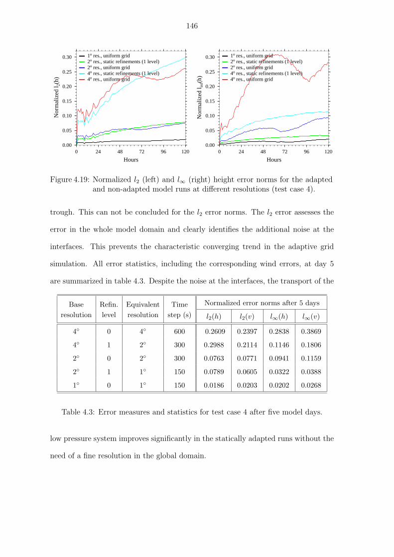
146
0.00
0.05
0.10
0.15
0.20
0.25
0.30 N
orm
aliz
ed l 2
(h)
0 24 48 72 96 120
Hours
1o res., uniform grid2o res., static refinements (1 level)2o res., uniform grid4o res., static refinements (1 level)4o res., uniform grid
0.00
0.05
0.10
0.15
0.20
0.25
0.30
Nor
mal
ized
l inf
(h)
0 24 48 72 96 120
Hours
1o res., uniform grid2o res., static refinements (1 level)2o res., uniform grid4o res., static refinements (1 level)4o res., uniform grid
Figure 4.19: Normalized l2 (left) and l∞ (right) height error norms for the adaptedand non-adapted model runs at different resolutions (test case 4).
trough. This can not be concluded for the l2 error norms. The l2 error assesses the
error in the whole model domain and clearly identifies the additional noise at the
interfaces. This prevents the characteristic converging trend in the adaptive grid
simulation. All error statistics, including the corresponding wind errors, at day 5
are summarized in table 4.3. Despite the noise at the interfaces, the transport of the
Base Refin. Equivalent Time Normalized error norms after 5 days
resolution level resolution step (s) l2(h) l2(v) l∞(h) l∞(v)
4 0 4 600 0.2609 0.2397 0.2838 0.3869
4 1 2 300 0.2988 0.2114 0.1146 0.1806
2 0 2 300 0.0763 0.0771 0.0941 0.1159
2 1 1 150 0.0789 0.0605 0.0322 0.0388
1 0 1 150 0.0186 0.0203 0.0202 0.0268
Table 4.3: Error measures and statistics for test case 4 after five model days.
low pressure system improves significantly in the statically adapted runs without the
need of a fine resolution in the global domain.

CHAPTER V
Adaptation criteria and 2D dynamic adaptations
Adaptive blocks have long been used for dynamic grid adaptations that can track
features of interest during a model run. Examples include the pioneering work of
Berger and Oliger [1984] which was applied to atmospheric science questions by
Skamarock et al. [1989] and other investigators (see Section 1.3). Adaptive blocks
offer the advantages of regular data structures that allow the use of a single solution
technique in all adapted patches. Then the flow can be independently solved on a
block-by-block basis, which is in particular true for the self-similar block approach
used here.
In this chapter, the dynamically adaptive finite-volume model is assessed in the
2D shallow water framework. The discussion starts with an introduction to suitable
adaptation criteria which are reviewed in Section 5.1. Here a variety of adaptation
indicators are suggested that are based on flow characteristics. The results of the
dynamically adapted shallow water runs are then examined in Section 5.2. These
simulations are presented in an increasing order of complexity. First, the adaptive
passive advection test is shown with and without an additional reduced grid setup
(Sections 5.2.1 and 5.2.2). Second, the adaptive nonlinear shallow water system
is assessed using an idealized flow over a single mountain (Section 5.2.3). This test
147

148
combines statically and dynamically adaptive grid approaches and serves as a testbed
for different refinement criteria.
5.1 Adaptation criteria
Setting the right criteria for grid refinements and coarsenings is very important
due to the significant cost associated with adaptations. The ideal criteria are those
that require minimum computational efforts to evaluate and still indicate the refine-
ment and coarsening regions reliably. Two basic adaptation principles need to be
distinguished, namely, the “physical” flow based adaptation indicators and the local
truncation error estimators. The latter are built upon a purely numerical idea since
they limit the global solution or local discretization error of the numerical scheme.
This technique was for example used by Berger and Oliger [1984] and further assessed
by Skamarock [1989] and Skamarock and Klemp [1993]. Here Richardson-type trun-
cation error estimators were applied that are based on the difference of the numerical
solution on fine and coarse overlapping meshes. Regions with high truncation errors
get then refined by comparison to user-defined tolerances. In general, numerical
error estimation techniques can be further classified as “a-priori” or “a-posteriori”
methods. The a-priori schemes predict the numerical errors prior to the actual time
step, whereas the a-posteriori estimates are based on results obtained during the
prior run. Such an a-posteriori approach is most commonly selected if adaptations
are to be guided by the numerical errors (see also Verfurt [1993] for an overview of
error estimators).
In practice though, flow-based adaptation criteria are predominantly used in
adaptive CFD applications. They typically rely on measures of a solution gradient
or curvature that are compared to user-defined and problem-dependent thresholds.

149
In addition, assessments of the vorticity, potential vorticity, divergence or instability
indicators like the Richardson number are feasible options for atmospheric AMR ap-
plications. Today, gradient-based adaptation criteria are most commonly applied to
atmospheric transport problems, e.g. by Behrens [1996] who developed an adaptive
passive semi-Lagrangian advection algorithm. Here the adaptations are based on a
simple two-dimensional assessment of the local gradient of a tracer component. Such
an indicator works well for pure passive advection scenarios as also shown by Hub-
bard and Nikiforakis [2003]. The grid is refined in regions with sharp gradients and
coarsenings are applied in areas where the gradient lies under a specified threshold.
In general, a gradient-based indicator is scale-dependent.
Similar gradient-based criteria are also popular in CFD applications where shock
waves and discontinuities dominate the flow (Hansen et al. [2002]). But atmospheric
flows, and here in particular hydrostatically approximated climate and weather pre-
diction models, are mainly characterized by smoothly varying large-scale motions.
In the absence of real discontinuities, the features of interest are less well-defined.
This is especially true for long-term climate studies that typically assess time-mean
spatially averaged climatic states. Nevertheless, scale contradictions with sharp gra-
dients do frequently occur in geophysical flows as the result of stretching and shear-
ing deformation by the velocity field. Therefore, the features of interest could be
associated with the atmospheric wave patterns and their resulting vorticity distri-
butions and temperature fronts. Such flow-based adaptation criteria are in partic-
ular suitable for short-term weather predictions runs. In general, adaptations are
problem-dependent and specifically tailored indicators need to be examined for dif-
ferent flow scenarios. An ’optimal’ criterion then captures the evolving features early
in the developing stages and tracks their evolution and decay reliably. Such an ideal

150
adaptation indicator might possibly combine numerical truncation error information
and the physical flow characteristics. Both refinement strategies were compared by
Kessler [1999] when developing a two-dimensional, adaptive finite element advection
scheme for tracer transports. It was found that the gradient indicator tended to
track sharp, single concentration peaks more closely, whereas the numerical residual
estimator recognized multiple smooth concentration peaks and their transition re-
gions effectively. Overall, both error indicators captured the emergence of a plume
in an idealized test problem satisfactorily, but the gradient indicator maintained a
more accurate tracer mass distribution.
5.1.1 Flow-based criteria
What are the flow features of interest in a weather prediction or climate run?
This is the basic question that determines the subsequent adaptive refinement and
coarsening strategy based on purely flow-based characteristics. In general, the cri-
terion must be well-suited to the research problem and numerous decisions need
to be made. For example, the aspects to be considered include the choice of the
vertical level at which a refinement criterion is evaluated as well as the selection
of one or more primary model variables. Alternatively, post-processing quantities,
like the mean sea level pressure or potential vorticity gradients on isentropes (as in
Hubbard and Nikiforakis [2003]), could be assessed that then require extra compu-
tations during the adaptation cycle. As indicated in Section 3.2.1 the length of an
ideal adaptation cycle is also problem-dependent. It relies on the time scales of the
observed phenomenon, e.g. a quickly changing phenomenon, like ’the emergence of
cumulus clouds’, requires very short assessment periods on the order of minutes. On
the other hand, the evolution of a low pressure center can be sufficiently captured

151
on a time scale of hours. In any case, it must be guaranteed that the tracked feature
can not be transported out of the refined area during the selected time interval. This
creates a fine balance between accuracy and computational overhead.
There are many answers to the above-mentioned research question that have been
proposed in the literature. Here a snapshot of the discussion is presented that is
primarily focused on feature tracking approaches. These are mainly developed in the
context of uniform resolution model runs and serve as a guideline for adaptive grid
applications. For example, a variety of feature tracking techniques were reviewed
for long-term AMIP-II assessments (Atmospheric Model Intercomparison Project,
see Boyle et al. [1998]). The study included the tracking of the 850hPa relative
vorticity pattern as well as the tracing of potential vorticity features on upper level
Θ-surfaces. Here the tracking algorithms by Murray and Simmonds [1991], Jones and
Simmonds [1993], Hodges [1994] and Hodges [1995] were used. They were also applied
to alternative levels and variables, such as the 250hPa and 500hPa geopotential and
the 850hPa temperature. It was concluded that the tracking of the relative vorticity
field allows a precise diagnosis of the initial stages of cyclogenesis in the extratropics.
Furthermore, the vorticity assessment also enables studies in tropical regions that
are not characterized by low and high pressure regimes with closed contours.
In an alternative study by Sinclair [1994] the geostrophic relative vorticity at
1000hPa was used as an objective measure of cyclonic disturbances. It was found
that the relative vorticity criterion detected the cyclone centers more reliably than the
more traditional use of local pressure minima. As also pointed out by Sinclair [1997]
the use of pressure minima favors the detection of more intense slow-moving systems
and misses many mobile centers where a local minimum can not instantly be found.
Most often the local pressure minimum does not appear until after considerable

152
cyclogenesis has already occurred. Therefore, the pressure-based criterion might not
capture the very early stages of a developing system.
These pressure-based criteria for cyclone tracking applications were further eval-
uated by Jones and Simmonds [1993] who suggested a combined assessment of the
mean sea level pressure value, its gradient and curvature. Additionally, Konig et al.
[1993] identified cyclones via a combination of three synoptic criteria: the local geopo-
tential height minimum at 1000hPa, a pronounced intensity of the system and a
lifetime longer than one day. A comparison of this scheme to the Murray and Sim-
monds [1991] approach (also Jones and Simmonds [1993]) is provided in Leonard
et al. [1999]. A simpler algorithm was used by Lambert [1988] who just focused on
local minima of the geopotential height at 1000hPa that were surrounded by four
grid points at higher height levels. Such an approach is clearly grid size dependent.
In general, it must be kept in mind that all evaluated quantities, like the mean
sea level pressure or variables on pressure or potential temperature surfaces, are
not readily available in a model with orography following model levels. Rather
they are diagnostically derived quantities that require additional calculations and
vertical interpolations. The overhead and trade-off also need to be considered if
more elaborate vortex tracking algorithms are to be used as suggested by Jeong and
Hussain [1995].
5.1.2 Adaptation criteria for the finite-volume dynamical core
How can the life cycles of the “features of interest” reliably be captured with an
adapted grid? This is the key question for the adaptive finite-volume simulations
presented in the subsequent sections. The adaptations are assessed not only in the
2D shallow water system but also in the 3D hydrostatic framework. The selected test

153
cases cover a variety of flow scenarios that require individual adaptation strategies.
Among them are assessments of the vorticity, the geopotential gradient or simple
threshold values in mountainous areas or for advection tests. Here the shallow water
equations serve as an idealized test bed for the 3D adaptive design.
Table 5.1 lists the adaptation strategies applied to the different test cases. The
Dim. Test scenario AMR setup Adaptation criteria
Advection (test 1) dynamic Φ threshold
Advection using a reduced grid dynamic + static Φ threshold
2D dynamic + static vorticity threshold + mountain
Flow over a mountain (test 5) dynamic + static Φ gradient threshold + mount.
dynamic vorticity threshold
Baroclinic wave with orography static adapted storm track3D
Baroclinic wave without orography dynamic vorticity threshold (surface)
Table 5.1: Strategies for dynamically and statically adapted model runs.
tests are represented in an increasing order of complexity. The dynamically adaptive
approach for the pure advection tests is based on a simple assessment of the geopoten-
tial. Such a concept works well for the passive transport problem in a nondivergent
flow field. Alternatively, a gradient-based indicator can also be recommended (not
shown). As pointed out earlier, the gradient of a tracer field was successfully used
by e.g. Hubbard and Nikiforakis [2003] and other investigators for passive advection
tests.
Solution gradients are also the refinement criterion of choice for many nonlin-
ear CFD applications. In this study, the performance of the geopotential gradient
indicator is tested using an idealized flow over a single mountain (test case 5). Alter-
natively, a vorticity-based criterion is tested that allows the direct comparison of the
two approaches. Both simulations combine the dynamic adaptations with static re-

154
finements of the mountain. In addition, tests are also performed without the adapted
orography.
In three dimensions two adaptation strategies are examined for the hydrostatic
dynamical core. First, the storm track of a developing idealized baroclinic wave
(Jablonowski and Williamson [2004]) is statically adapted. Second, the baroclinic
wave test without orography (Polvani et al. [2004]) is evaluated with purely dynamic
adaptations based on vorticity thresholds. Here the model level closest to the surface
is selected for the assessment. Tests with combined criteria, like the combination of
surface pressure extrema and vorticity thresholds, have also been performed and led
to similar results (not shown). As discussed earlier, vorticity-based refinements are
appealing since they detect the developing wave trains early. In addition they have
been successfully used in idealized adaptive hurricane track predictions as shown by
Fulton [1997].
As a first glimpse, three choices of possible adaptation criteria are presented in
figure 5.1. The figure displays an analysis of the initial state of shallow water test
(a) Relative vorticity (10-5 s-1)
2
2
2
2
2
2
2
2
(b) Gradient of Φ (10-3ms-2), abs. value (c) Laplacian of Φ (10-9s-2)
Figure 5.1: Possible choices for refinement criteria illustrated with the initial stateof test case 4 (orthographic projections centered at 0E,45N). (a) Rela-tive vorticity, (b) absolute value of the gepotential gradient and (c) theLaplacian of the geopotential. Contour intervals are 10−5s−1, 10−3ms−2
and 10−9s−2, respectively.
155
case 4. This test is comprised of a forced nonlinear system with translating low
(see also figure A.7). Here the relative vorticity as well as the gradient and the
curvature (Laplace) of the geopotential height field are illustrated. It can clearly be
seen that all three indicators pick out the center of the low pressure system that
is surrounded by a rotating wind field. In practice though, tests have suggested
that the Laplacian of the geopotential height field is not a suitable indicator for
curvature-based refinement regions. Instead, the vorticity pattern is recommended
as a measure of the curvilinearity of the geopotential or pressure field. This is due to
the observation that the second-order derivative of the geopotential height field tends
to develop small scale noise over time that misleads the refinement strategy. On the
other hand, the vorticity and the gradient indicator performed reliably in all studies.
Overall, the main difficulty arises when setting the user-defined threshold values.
These are highly problem-dependent, but crucially important when considering that
features of interest need to be detected early on the coarse mesh. The sensitivity
of the empirical threshold values again determines a fine balance between accuracy
and efficiency. The threshold values for the adaptive finite-volume dynamical core
are documented in the corresponding sections.
There are lots of choices for possible adaptation criteria. For example, single
indicators can be combined to form a more elaborate system. Additionally, weighted
refinement criteria are feasible that are based on varying threshold values at different
refinement levels. In practice though, the latter strategy will be impossible to meet
exactly in the adaptive block setup. This is due to the requirement that neighboring
blocks can only differ by one refinement level, which triggers cascading refinement
requests. Therefore, such an option has not been implemented in the dynamical
core. If the adaptation criterion is fulfilled, the blocks are flagged by the user and

156
adapted by calling the AMR library functions. Currently, refinements are triggered
consecutively up to the highest user-defined refinement level as soon as at least one
grid point within a block exceeds the threshold value. Coarsenings occur if all grid
points of four neighboring blocks (children) no longer meet the refinement criterion.
Furthermore, the neighboring block constraint needs to allow a coarsening step.
Here it is important to keep in mind that there are two factors that limit the
refinement levels. Besides the user-defined thresholds and maximum number of re-
finement levels, the hydrostatic approximation also restricts the adaptations from a
physical viewpoint to horizontal scales larger than 10km (see Section 3.1.2).
Refinement indicators are implemented as plug-and-play components. Therefore,
they can be easily exchanged and adjusted for future assessments.

157
5.2 Dynamic adaptations: Shallow water tests
The dynamically adaptive finite-volume model is tested in the 2D shallow water
configuration. Two basic test scenarios are assessed using the standard test suite
for the shallow water equations. First, the tests are concentrated on the assessment
of the adaptive advection algorithm. Second, the full nonlinear system is examined
with a flow field over a single mountain.
5.2.1 Advection tests with the full grid
The advection algorithm is one of the fundamental building blocks of atmospheric
flow simulations. It is therefore imperative to evaluate its performance not only in
the adaptive shallow water setup but also in a non-adapted case. Therefore, the
adapted model results are both compared with the analytical reference solution and
the solution from uniform-grid model runs.
There are a variety of standard test cases for advection schemes. For example
Zalesak [1979] introduced the two dimensional solid body rotation problem with a
slotted cylinder. Furthermore, Doswell [1984] developed an idealized cyclogenesis
test that defines a strong deformational flow field. This test was later reformulated
for spherical coordinates by Nair et al. [1999] and Nair and Machenhauer [2002] and
consequently tested with an adaptive advection model by Hubbard and Nikiforakis
[2003].
Here the adaptive finite-volume advection scheme is tested with an alternative
standard approach that has been most commonly used in the atmospheric science
literature. It is the cosine bell advection test (shallow water test case 1, see Appendix
A) that was already applied to the reduced grid in Section 4.2.2. The advection of
the cosine bell is tested with different rotation angles α. In particular, α = 0,

158
α = 45 and α = 90 are selected that describe the transport of the cosine bell along
the equator, at a 45 angle in the tropics and midlatitudes as well as the transport
straight over the poles.
The refinement criterion for the adaptive transport of the cosine bell is a simple
threshold criterion that assesses the value of the geopotential at each grid point. In
case the geopotential exceeds the empirical limit Φ ≥ 520m2s−2 the block is flagged
for refinement. This value corresponds to h ≈ 53m, which is approximately 5% of
the initial peak with h ≈ 1000m. If on the other hand the grid points no longer meet
the adaptation criterion the coarsening flag in the corresponding block is set. The
refinement criterion is examined during each time step that is held variable in order
to match the |CFL| = 0.95 limit. All adaptations occur consecutively until either
the maximum refinement level or the coarse 5×5 initial resolution is reached. This
resolution is the base resolution for all adaptive shallow water runs. The grid can
not be coarsened further than the initial setup. The passive advection is driven by
pre-determined analytical wind speeds. These are reinitialized analytically whenever
adaptations occur. This applies also to the initial state of the geopotential at the
various refinement levels. During the model run though, the geopotential in newly
adapted blocks is initialized via second-order conservative PPM-like interpolations.
The chosen advection algorithm is also based on the PPM scheme and no filtering of
any variable is applied. For the adaptive model simulations the maximum refinement
level is user-defined and varies between 0 and 4. These model setups correspond to
the grid spacings 5, 2.5, 1.25, 0.625 and 0.3125 at the finest level, respectively.
The resolutions and initial block parameter sets are further explained in table 3.1 on
page 74.
The basic adaptation principle is illustrated in figure 5.2 with α = 90 that shows

159
(a)
Initi
al s
tate
-90
-4504590
Latitude
090
180
270
360
Lon
gitu
de
(b)
24 h
ours
-90
-4504590
Latitude
090
180
270
360
Lon
gitu
de
300
600
900
(c)
72 h
ours
-90
-4504590
Latitude
090
180
270
360
Lon
gitu
de
300
(d)
96 h
ours
-90
-4504590
Latitude
090
180
270
360
Lon
gitu
de
Fig
ure
5.2:
Geo
pot
enti
alhei
ght
ofth
eco
sine
bel
l(t
est
case
1,α
=90 )
wit
h3
refinem
ent
leve
ls(0
.625 )
atdiff
eren
tpoi
nts
inti
me.
(a)
Init
ialst
ate,
(b)
afte
r24
hou
rs,(c
)72
hou
rsan
d(d
)96
hou
rs.
The
adap
ted
blo
cks
are
indic
ated
inre
d.
Con
tour
inte
rval
sar
e10
0m
,th
eze
roco
nto
ur
isom
itte
d.

160
four snapshots of the adaptive simulation at refinement level 3. The figure depicts the
cosine bell at day 0, 1, 3 and 4 with overlaid adapted blocks (in red) that track the
“feature of interest”. As it can clearly be seen, the cosine bell passes over the North
Pole without distortions or noise. The pole point itself with its converging grid lines is
spread out in the chosen equidistant cylindrical map projection. This emphasizes the
numerous grid boxes in polar regions that need to be refined for transport processes
at high latitudes. They severely restrict the maximum allowable time step that obeys
the |CFL| = 0.95 condition in polar regions. For example, in this simulation with
three refinement levels and a maximum zonal wind speed of u ≈ 38.6ms−1 at the
poles the adaptive time step varies between ∆t ≈ 597.3 s in equatorial regions and
∆t ≈ 9.3 s at very high latitudes. In this passive advection test, the grid boxes
adjacent to the poles do not need to be kept at the same refinement level since there
is neither a need to filter gravity wave motions nor to calculate vorticity and wind
data at the pole points (see also Section 2.2.1 and 2.2.2).
The cosine bell is advected once around the sphere and reaches its initial position
after 12 days. Then the solution can be compared to the initial conditions that serve
as the true reference field. A closer examination of the final states at refinement level
1 and different rotation angles α is illustrated in figure 5.3 on the next page that also
presents the overlaid true solution with dotted lines. The figure shows that the co-
sine bell undergoes a stretching in the flow direction which is a typically observed for
monotonicity-constrained finite-volume advection algorithms (see also Lin and Rood
[1996], Nair and Machenhauer [2002] and Hubbard and Nikiforakis [2003]). The ef-
fect is clearly visible at this relatively coarse resolution and diminishes significantly
with decreasing grid sizes (figure 5.4). As pointed out by Nair and Machenhauer
[2002] the degradation of the shape caused by the monotonocity constraint trans-

161
300
300
600
(a) α = 0o
-20
-10
0
10
20
Lat
itude
250 260 270 280 290Longitude
300
300
600
(b) α = 45o
-20
-10
0
10
20
Lat
itude
250 260 270 280 290Longitude
300
300
600
(c) α = 90o
-20
-10
0
10
20
Lat
itude
250 260 270 280 290Longitude
Figure 5.3: Geopotential height of the cosine bell (test case 1) after 1 revolution (12days) with one refinement level (2.5) and different rotation angles α.(a) α = 0: advection along the equator, (b) α = 45: advection at a45 degree angle, (c) α = 90: advection over the poles. The analyticsolution is overlaid (indicated by the dotted lines). Contour intervals are100 m, the zero contour is omitted.
lates into slightly less accurate error norms in comparison to e.g. positive definite
methods. A similar result was also found in Section 3.3.1 with respect to constrained
and unconstrained interpolation strategies (table 3.4). Nevertheless, the advantages
of the monotonicity preserving advection algorithm outweigh the slight decrease in
accuracy (see also comparisons in van Leer [1977]).
Figure 5.4 confirms that the shape of the cosine bell after one rotation is well-
preserved at high resolutions. The figure depicts a sequence of model runs with
increasing number of refinement levels at rotation angle 45. This transport direction
represents the “worst case” scenario for the advection algorithm with underlying
operator splitting approach. The results at the highest refinement levels 3 and 4
are almost indistinguishable from each other. It is also interesting to note that the
cosine bell in (c)-(e) no longer shows the small phase error, which is visible in the
subfigures (a) and (b). The solutions then resemble the true solution very closely
which is demonstrated in subfigure (f). This subfigure displays the difference of the

162
300300
(a) Refinement level 0 (5ox5o)
-20
-10
0
10
20
Lat
itude
250 260 270 280 290Longitude
300
300
600
(b) Refinement level 1
-20
-10
0
10
20
Lat
itude
250 260 270 280 290Longitude
300
300
600
(c) Refinement level 2
-20
-10
0
10
20
Lat
itude
250 260 270 280 290Longitude
300
300
600
(d) Refinement level 3
-20
-10
0
10
20
Lat
itude
250 260 270 280 290Longitude
300
300
600
(e) Refinement level 4
-20
-10
0
10
20
Lat
itude
250 260 270 280 290Longitude
0 0
0
0
3
(f) (e) - analytic solution
-20
-10
0
10
20
Lat
itude
250 260 270 280 290Longitude
-3
Figure 5.4: (a-e) Geopotential height of the cosine bell (test case 1) and (f) heighterrors after 1 revolution (day 12) with rotation angle α = 45. (a) Norefinements (5 resolution), (b) 1 refinement level (2.5), (c) 2 refinementlevels (1.25), (d) 3 refinement levels (0.625), (e) 4 refinement levels(0.3125) and (f) difference of the solution on the finest mesh (case (e))with the analytic solution. Contour intervals are 100 m (a-e) and 1 m(f). The zero contour is omitted (a-e).

163
cosine bell at refinement level 4 with the reference state. The differences mainly
develop along the edges in the 45 flow direction. In particular, the leading edge
shows slightly enhanced geopotential height values, whereas the tail drops below
the reference state. These errors are small in comparison to the peak amplitude of
the cosine bell. In general, the same type of error patterns can also be found in
non-adapted model runs.
Further, it is interesting to assess the adaptive model performance with a cross
polar flow field at α = 90. Dynamic adaptations in polar regions are demanding
since they involve many more adapted blocks close to the poles (see also figure 5.2).
Nevertheless, the adapted advection scheme performs very well at all refinement
levels as displayed in figure 5.5. Each subfigure shows three snapshots of the cosine
300
300
(a) 1 refinement level (2.5o)0˚
90˚
180˚
270˚
300
300
(b) 2 refinement levels (1.25o)
0˚
90˚
180˚
270˚
300
300
(c) 3 refinement levels (0.625o)
0˚
90˚
180˚
270˚
Figure 5.5: Polar stereographic projections of the cosine bell (test case 1, α = 90)transported over the North Pole (from the bottom to the top of thefigure, the outer circle is located at 45N). Snapshots are taken after 48,72 and 96 hours, respectively, with refinement levels (a) 1, (b) 2 and (c)3. Contour intervals of the geopotential height fields are 100 m, zerocontour is omitted.
bell at day 2, 3 and 4 in a north polar stereographic projection. There are no visible
distortions of the height field at any resolution as the cosine bell approaches, passes
over and leaves the North Pole. The increased resolution clearly helps preserve the

164
shape and peak amplitude.
Here it is important to point out that the multidimensional transport of the
cosine bell is not strictly monotonic. Tiny under- and overshoots are possible in
the current formulation that have been especially observed at a 45 transport angle.
This is documented in table 5.2 that lists the minimum geopotential height values
after one rotation for uniform and adapted runs at refinement level 2. The latter
are tested with and without flux corrections at the interface boundaries (see also
Section 3.3.3). Even in the non-adapted runs (second column), vanishingly small
Test case 1 Non-adapted runs with Adapted 5 × 5 runs and 2 refinementswith angle α uniform 1.25 resolution flux corrections no flux corrections
α = 0 0. 0. 0.
α = 45 −0.5605 ∗ 10−44 −0.1761 −0.6557 ∗ 10−3
α = 90 −0.8178 ∗ 10−54 −0.5999 ∗ 10−5 −0.1383 ∗ 10−10
Table 5.2: Minimum amplitude of the cosine bell in m (test case 1) after one rev-olution for adapted and non-adapted runs at the equivalent resolution1.25 × 1.25. Adapted runs are tested with and without flux correctionsat coarse-fine grid interfaces.
negative height values develop in case of non-zero rotation angles. Then the cosine
bell is truly transported in both dimensions. Such an effect has also been observed by
Lin and Rood [1996] for the equivalent 2D advection tests in Cartesian coordinates.
The violation of the monotonicity constraint in two dimensions is a consequence of
applying a sequence of solely 1D limiters during the transport calculations. Such an
approach does not guarantee that the resulting multidimensional advection scheme
keeps the monotonic attribute. In practice, the negative values are small, but may
be significant when transporting positive definite quantities, like atmospheric tracer
components or water vapor. Then these undershoots may cause difficulties in other

165
code modules. If negative values need to be avoided, three strategies can be employed.
First, the subgrid distributions could be further manipulated in order to guarantee a
positive definite constraint. Second, an a-posteriori filling algorithm can be applied
that borrows the missing tracer mass from neighboring grid cells. Such an algorithm
is in fact implemented in today’s NASA/NCAR dynamical core. Third, a strictly
monotonic Zalesak-type multidimensional transport algorithm could be used (Zalesak
[1979]).
Here these three options are not considered in the adaptive finite-volume model.
Instead, special attention needs to be paid to an even more dominant effect in the
adaptive simulations. This is indicated in column 3 of table 5.2 which shows the min-
imum height values in the adapted runs with flux corrections at interface boundaries.
These flux corrections are necessary to ensure the mass conservation principle in the
adapted model. It can clearly be seen that the flux corrections lead to an additional
violation of the monotonicity principle. The undershoots, although still small, are
orders of magnitude bigger then the negative values in the non-flux corrected runs.
The latter also show enhanced undershoots in comparison to the uniform grid simu-
lations. They are caused by the conservative PPM-type interpolations that are used
for the adaptive split-join operations as well as for the ghost cell updates at inter-
faces. When looking at the spatial pattern, the undershoots can be pre-dominantly
found around the feature’s non-smooth circular base, which has a discontinuous first
derivative. This minor undershoot effect of the interpolation scheme can be avoided
when applying additional monotonicity constraints to the 2D PPM-type subgrid dis-
tribution. Especially corner values of the subgrid distribution need to be checked.
However, it is an open question whether a truly monotonic multi-dimensional con-
servative transport scheme with flux corrections can be developed for adaptive grid

166
simulations.
The overall performance of the adapted advection tests with different rotation
angles and increasing refinement levels is summarized in table 5.3. The table shows
not only the l1, l2, l∞ and hmax errors after one revolution (see also Section 4.1)
but also contains information on the final peak amplitude, the number of blocks and
Base Refin. Height error norms Final # Blocks # Time CPUresol. level l1 l2 l∞
hmax h (m) min max steps time (s)
α = 0
1.25 0 0.0073 0.0078 0.0107 -0.0106 984.2 768 312 230
5 0 0.1157 0.1001 0.0949 -0.0869 838.0 48 84 4
5 1 0.0341 0.0301 0.0317 -0.0305 949.1 54 60 156 12
5 2 0.0097 0.0103 0.0150 -0.0106 984.2 72 84 312 32
5 3 0.0016 0.0021 0.0044 -0.0036 995.0 174 204 612 159
5 4 0.0003 0.0005 0.0014 -0.0012 998.4 348 384 1224 642
α = 45
1.25 0 0.0264 0.0259 0.0557 -0.0555 939.5 768 19872 13873
5 0 0.5077 0.4194 0.4835 -0.4762 480.8 48 1440 64
5 1 0.0927 0.0911 0.1525 -0.1514 830.7 54 60 1440 97
5 2 0.0278 0.0251 0.0507 -0.0505 944.4 72 106 3333 418
5 3 0.0088 0.0080 0.0159 -0.0159 982.8 171 210 3871 994
5 4 0.0031 0.0030 0.0053 -0.0039 995.8 348 462 4120 2407
α = 90
1.25 0 0.0250 0.0256 0.0421 -0.0420 953.0 768 27936 19551
5 0 0.4683 0.3860 0.3923 -0.3902 559.7 48 2016 97
5 1 0.0924 0.0898 0.1253 -0.1250 856.6 60 72 4085 305
5 2 0.0244 0.0240 0.0405 -0.0405 954.5 72 200 11152 1885
5 3 0.0048 0.0052 0.0125 -0.0125 986.2 192 480 33288 15465
5 4 0.0010 0.0011 0.0038 -0.0038 995.9 348 1440 107199 159708
Table 5.3: Error measures and statistics for the solid body rotation of the cosine bell(test case 1) after one revolution (12 model days) for different refinementlevels and rotation angles α. The CFL number is 0.95. The CPU time isthe user time on a single processor of a SUN workstation.

167
time steps as well as the total CPU time measured on a SUN Ultrix workstation. In
addition, the error statistics of selected uniform model runs are listed for comparison.
It can clearly be observed that the cosine bell is successfully tracked in the adapted
model simulations. This is not only true for the l1 and l2 error norms that assess
the overall shape, but also for the peak amplitudes evaluated by the l∞ errors. The
peak amplitudes improve considerably with increasing refinement levels. In addition,
the table shows that the CPU time in the adapted runs is significantly reduced
in comparison to the uniform resolution runs. For example, when comparing the
uniform 1.25 runs with the corresponding adapted runs at refinement level 2 the
speed-up factors are approximately 7, 33 and 10 for the rotation angle α = 0,
α = 45 and α = 90, respectively. The speed-up is determined by two main factors.
First, the number of blocks and therefore the overall work load is decreased in the
adapted simulations. Second, the total number of time steps necessary for the 12-
day integration is drastically reduced. The latter is due to the fact that the adaptive
time step can be greatly increased if the fine grid does not cover the polar regions.
In particular, this effect can be seen in the α = 45 case where the time step in the
uniform run solely depends on the CFL restriction at the poles. This consequently
leads to a rather short time step and large number of iterations. In the corresponding
adapted run, the grid around the poles is mostly kept at the coarse resolution so
that the time step is mainly determined by the traveling cosine bell. The latter is
especially true for the α = 0 test case, where the time step exclusively relies on the
true advective wind speeds and grid distances at the equator. Therefore, an identical
number of time steps is required for both the uniform and adapted runs at the 1.25
resolution and the computational savings are only due to the reduced work load.
The error norms for the adapted simulations in table 5.3 compare well to values
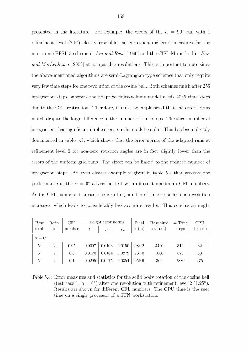
168
presented in the literature. For example, the errors of the α = 90 run with 1
refinement level (2.5) closely resemble the corresponding error measures for the
monotonic FFSL-3 scheme in Lin and Rood [1996] and the CISL-M method in Nair
and Machenhauer [2002] at comparable resolutions. This is important to note since
the above-mentioned algorithms are semi-Lagrangian type schemes that only require
very few time steps for one revolution of the cosine bell. Both schemes finish after 256
integration steps, whereas the adaptive finite-volume model needs 4085 time steps
due to the CFL restriction. Therefore, it must be emphasized that the error norms
match despite the large difference in the number of time steps. The sheer number of
integrations has significant implications on the model results. This has been already
documented in table 5.3, which shows that the error norms of the adapted runs at
refinement level 2 for non-zero rotation angles are in fact slightly lower than the
errors of the uniform grid runs. The effect can be linked to the reduced number of
integration steps. An even clearer example is given in table 5.4 that assesses the
performance of the α = 0 advection test with different maximum CFL numbers.
As the CFL numbers decrease, the resulting number of time steps for one revolution
increases, which leads to considerably less accurate results. This conclusion might
Base Refin. CFL Height error norms Final Base time # Time CPUresol. level number l1 l2 l∞ h (m) step (s) steps time (s)
α = 0
5 2 0.95 0.0097 0.0103 0.0150 984.2 3420 312 32
5 2 0.5 0.0170 0.0184 0.0279 967.0 1800 576 58
5 2 0.1 0.0295 0.0275 0.0354 959.6 360 2880 275
Table 5.4: Error measures and statistics for the solid body rotation of the cosine bell(test case 1, α = 0) after one revolution with refinement level 2 (1.25).Results are shown for different CFL numbers. The CPU time is the usertime on a single processor of a SUN workstation.
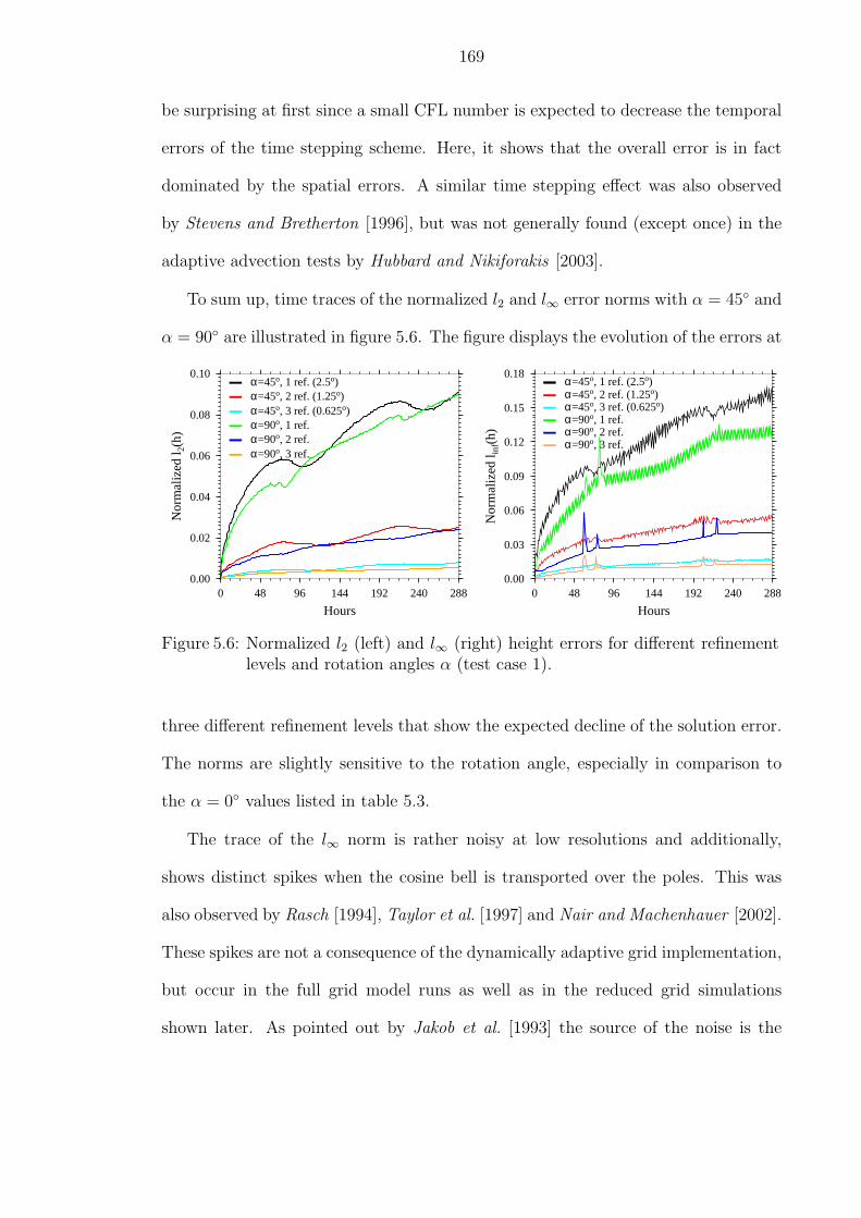
169
be surprising at first since a small CFL number is expected to decrease the temporal
errors of the time stepping scheme. Here, it shows that the overall error is in fact
dominated by the spatial errors. A similar time stepping effect was also observed
by Stevens and Bretherton [1996], but was not generally found (except once) in the
adaptive advection tests by Hubbard and Nikiforakis [2003].
To sum up, time traces of the normalized l2 and l∞ error norms with α = 45 and
α = 90 are illustrated in figure 5.6. The figure displays the evolution of the errors at
0.00
0.02
0.04
0.06
0.08
0.10
Nor
mal
ized
l 2(h
)
0 48 96 144 192 240 288
Hours
α=45o, 1 ref. (2.5o)α=45o, 2 ref. (1.25o)α=45o, 3 ref. (0.625o)α=90o, 1 ref.α=90o, 2 ref.α=90o, 3 ref.
0.00
0.03
0.06
0.09
0.12
0.15
0.18
Nor
mal
ized
l inf
(h)
0 48 96 144 192 240 288
Hours
α=45o, 1 ref. (2.5o)α=45o, 2 ref. (1.25o)α=45o, 3 ref. (0.625o)α=90o, 1 ref.α=90o, 2 ref.α=90o, 3 ref.
Figure 5.6: Normalized l2 (left) and l∞ (right) height errors for different refinementlevels and rotation angles α (test case 1).
three different refinement levels that show the expected decline of the solution error.
The norms are slightly sensitive to the rotation angle, especially in comparison to
the α = 0 values listed in table 5.3.
The trace of the l∞ norm is rather noisy at low resolutions and additionally,
shows distinct spikes when the cosine bell is transported over the poles. This was
also observed by Rasch [1994], Taylor et al. [1997] and Nair and Machenhauer [2002].
These spikes are not a consequence of the dynamically adaptive grid implementation,
but occur in the full grid model runs as well as in the reduced grid simulations
shown later. As pointed out by Jakob et al. [1993] the source of the noise is the

170
discrete sampling of the numerical and reference solution. Here the reference solution
is computed analytically during the course of the integration using the trajectory
approach as outlined in Section 4.1.3. This leads to an occasional small increase in
the peak amplitude of the reference field depending on the distance of the center to
the closest grid point. This effect diminishes with increasing resolution.
5.2.2 Advection tests with the reduced grid
The cross polar advection test with α = 90 is also applied to the reduced grid
setups discussed in Section 4.2.1. This approach combines the statically coarsened re-
duced grids with the additional flexibility of dynamic grid adaptations. The interface
treatment of the adaptive reduced grids is quite elaborate since all three fine-coarse
grid interfaces (discussed in Section 3.3.2) play a crucial role at different stages dur-
ing the integration. This requires a variety of different interpolation modules for the
ghost cell exchange.
As argued in Section 4.2.1, the base resolution for the reduced grid simulations
needs to be finer than the typical 5 grid. This allows the introduction of up to
two reduction levels north or south of 60 N/S. Therefore, the following examples
are computed on a 2.5 × 2.5 base grid with one or two reduction levels. A single
refinement level is then used to track the path of the cosine bell. All other initial
parameter settings are identical to the advection tests presented in Section 5.2.1. In
particular, the maximum CFL number is also set to |CFL| = 0.95 and the refinement
criterion assesses the geopotential threshold value Φ ≥ 520m2s−2.
Figure 5.7 on the facing page shows snapshots of the adapted reduced grid sim-
ulations with one and two reduction levels. The cosine bell is displayed at day 1
through 5 as it passes over the North Pole. Here the layout of the reduced blocks

171
300
300
300
300
600
(a) 2.5o grid, 1 reduction, 1 refinement (1.25o)
0˚
90˚
180˚
270˚
300
300
300
300
600
(b) 2.5o grid, 2 reductions, 1 refinement (1.25o)
0˚
90˚
180˚
270˚
Figure 5.7: Polar stereographic projections of the cosine bell (test case 1, α = 90)transported over the North Pole (from the bottom to the top of thefigure, the outer circle is located at 15N). Snapshots are taken after 24,48, 72, 96 and 120 hours, respectively. Base resolution is 2.5 with 1refinement level. (a) Reduced grid with 1 reduction, (b) reduced gridwith 2 reductions. Contour intervals of the geopotential height fields are100 m, zero contour is omitted.

172
is indicated by the dotted grid lines. For clarity, no attempt is made to overlay
the adaptations. Both model runs are almost indistinguishable from each other and
furthermore, compare very well to the full grid adaptive advection tests depicted
in figure 5.5 on page 163. As seen before, the cosine bell crosses the pole point
without visible distortions or noise. In addition, a comparison with figure 4.3 on
page 124 reveals that the refinement area not only improves the shape but also the
peak amplitude of the advected feature.
This is quantified in table 5.5 which lists the error norms for the adapted reduced
grid runs and the full grid 1.25 control simulation after one revolution. All error
norms are very similar in the adapted model setups. Here it is interesting to note,
that the adapted reduced grid simulations show slightly improved l1 and l2 error
measures despite the coarser longitudinal resolution at high latitudes. This effect is
Base Refin. Reduced Height error norms Final # Blocks # Time CPUresol. level grid l1 l2 l∞ h (m) min max steps time (s)
α = 90
1.25 0 0 0.0250 0.0256 0.0421 953.0 768 27936 19551
2.5 1 0 0.0269 0.0262 0.0419 953.1 204 276 13218 3529
2.5 1 1 0.0254 0.0249 0.0409 954.1 188 236 8696 2175
2.5 1 2 0.0239 0.0237 0.0427 952.3 164 194 5484 1228
Table 5.5: Error measures and statistics for the solid body rotation of the cosine bell(test case 1, α = 90) after one revolution for different reduced grids andrefinement levels. Base resolution is 2.5. The CPU time is the user timeon a single processor of a SUN workstation.
mainly attributable to the decrease in the total number of integration steps. The
enhanced zonal grid spacing now allows a longer time step, which helps preserve the
peak amplitude in case of one reduction level. In case of two reduction levels this
time stepping effect is overshadowed by the slight smoothing effect of the second
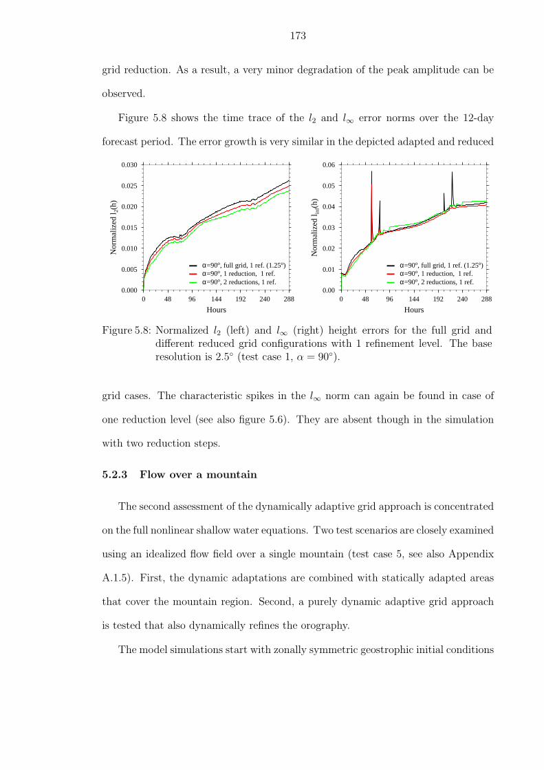
173
grid reduction. As a result, a very minor degradation of the peak amplitude can be
observed.
Figure 5.8 shows the time trace of the l2 and l∞ error norms over the 12-day
forecast period. The error growth is very similar in the depicted adapted and reduced
0.000
0.005
0.010
0.015
0.020
0.025
0.030
Nor
mal
ized
l 2(h
)
0 48 96 144 192 240 288
Hours
α=90o, full grid, 1 ref. (1.25o)α=90o, 1 reduction, 1 ref.α=90o, 2 reductions, 1 ref.
0.00
0.01
0.02
0.03
0.04
0.05
0.06
Nor
mal
ized
l inf
(h)
0 48 96 144 192 240 288
Hours
α=90o, full grid, 1 ref. (1.25o)α=90o, 1 reduction, 1 ref.α=90o, 2 reductions, 1 ref.
Figure 5.8: Normalized l2 (left) and l∞ (right) height errors for the full grid anddifferent reduced grid configurations with 1 refinement level. The baseresolution is 2.5 (test case 1, α = 90).
grid cases. The characteristic spikes in the l∞ norm can again be found in case of
one reduction level (see also figure 5.6). They are absent though in the simulation
with two reduction steps.
5.2.3 Flow over a mountain
The second assessment of the dynamically adaptive grid approach is concentrated
on the full nonlinear shallow water equations. Two test scenarios are closely examined
using an idealized flow field over a single mountain (test case 5, see also Appendix
A.1.5). First, the dynamic adaptations are combined with statically adapted areas
that cover the mountain region. Second, a purely dynamic adaptive grid approach
is tested that also dynamically refines the orography.
The model simulations start with zonally symmetric geostrophic initial conditions

174
that do not balance the orography field. As a result, a complex flow pattern evolves
over time that is characterized by a lee-side wave train. Due to the complexity of
the flow, this test case represents an idealized test bed for 3D hydrostatic regimes.
Here, the test is primarily used to assess different refinement criteria and strategies.
Statically adapted orography
A combination of static and dynamic refinement strategies is evaluated over a
15-day forecast period. The initial setup of the grid is displayed in figure 5.9 which
shows the initial geopotential height field with overlaid orography contours and cor-
responding statically adapted blocks. Here the static adaptations refine the single
5100 5400 5700 6000Geopotential height [m]
-90
-60
-30
0
30
60
90
Lat
itude
-180 -90 0 90 180Longitude
Figure 5.9: Initial geopotential height (m) and orography with the overlaid staticallyrefined blocks at refinement level 3. The mountain is 2000 m high.
mountain in the Northern Hemisphere. This grid arrangement has also been shown
earlier in an orthographic map projection in figure 3.3 on page 70. The underlying
base resolution is the standard 5 × 5 grid that is comprised of 8x6 initial blocks
with 9x6 cells per block.
After the initial adaptations are applied, the geopotential height and orogra-

175
phy fields are reinitialized analytically, whereas the wind components in the newly
adapted blocks are computed via second-order non-conservative interpolations. This
provides a slightly more consistent flow representation at the block interfaces and
suppresses spurious noise at the beginning of the forecast. However, since the ini-
tial wind field is very smooth such an approach is almost indistinguishable from
analytically reinitialized wind patterns in this scenario.
The test is concentrated on the assessment of two dynamic adaptation criteria.
First, a vorticity-based criterion is selected that is based on the evaluation of the
relative vorticity ζ at each grid point. Grid points are then flagged for refinement
if the absolute value of the relative vorticity exceeds the empirical threshold |ζ| ≥
2× 10⁻⁵s−1. Alternatively, a threshold value of |ζ| ≥ 2.5× 10⁻⁵s−1 is also reviewed.
Second, a gradient-based refinement criterion is examined that assesses the absolute
value of the geopotential gradient. Here, a threshold value of |∇Φ| ≥ 2× 10⁻³ms−2
is chosen. Both thresholds lie above the relative vorticity and Φ gradient values of
the initial setup which are illustrated in figure 5.10. These profiles clearly depict
0.0
0.3
0.6
0.9
1.2
1.5
Rel
ativ
e vo
rtic
ity |ζ
| (10
-5s-1
)
-90 -60 -30 0 30 60 90
Latitude
0.0
0.3
0.6
0.9
1.2
1.5
Abs
. gra
dien
t of
Φ (
10-3
ms-2
)
-90 -60 -30 0 30 60 90
Latitude
Figure 5.10: Initial absolute values of the relative vorticity (left) and the geopotentialgradient (right) at the model level closest to the surface (test case 5).
the idealized nature of the test since its initial vorticity and gradient values are very
small and furthermore zonally symmetric. The test therefore provides an excellent

176
example of a smoothly developing system based on a homogeneous basic state.
The test scenarios are listed in more detail in table 5.6. The table gives not
only information on the selected constant time steps and corresponding integration
steps for the 15-day forecast, but also shows some block statistics. In particular, the
Refinement Number of blocks at day Time # Modelcriterion
Threshold0 5 10 15 step (s) steps
|ζ| ≥ 2.5 ∗ 10−5s−1 228 312 444 582 120 10800
|ζ| ≥ 2.0 ∗ 10−5s−1 228 366 573 831 13313 9720
|∇Φ| ≥ 2.0 ∗ 10−3ms−2 228 291 513 816 150 8640
Table 5.6: Characteristics of the dynamically adapted runs with vorticity and geopo-tential gradient criteria (test case 5).
number of blocks at different stages of the simulation is presented. As expected the
user-defined threshold values play an important role with respect to the sensitivity
of the block adaptations. This can be seen in the direct comparison of the two runs
with vorticity thresholds. A minor increase in the vorticity limit from 2.0 ∗ 10−5s−1
to 2.5∗10−5s−1 leads to a 30% reduction in the number of total blocks after 15 days.
For a thorough comparison of the adapted model runs, the vorticity and gradient-
based refinement criteria with threshold values 2.0 ∗ 10−5s−1 and 2.0 ∗ 10−3ms−2 are
selected. These generate a comparable number of adapted blocks so that the dif-
ferences in the positions of the adaptations can clearly be assessed. The following
adaptation strategy is employed. Both grids are statically adapted at the beginning
of the model runs. Here the maximum refinement level is set to 3, which corresponds
to a 0.625 resolution on the finest grid. The static adaptations (with criterion
Φs > 0m2s−2) are confined to the mountainous area and stay fixed during the model
simulations. The dynamic adaptations are assessed every two hours, which is a suit-

177
able adaptation cycle for the selected slowly evolving features of interest. In principal,
an even longer time interval can also be used, for example a nine hour adaptation
cycle as in Skamarock [1988]. These intervals allow the flow to evolve smoothly be-
fore new adaptations are applied (see also discussion in Section 3.2.1). Furthermore,
two additional adaptation constraints are selected that restrict the number of the
refinement levels at high latitudes. In particular, the blocks adjacent to the poles
are only allowed to refine once and the subsequent neighboring blocks are limited to
two refinement levels. The latter is necessary in order to prevent a passive second
refinement request for the pole blocks due to cascading refinements at the lower lati-
tudes. In practice when starting with a 5 initial grid, these constraints result in the
setup shown in table 5.7. The restriction on the total number of refinement levels in
Maximum refinement level Geographical region
1 75 − 90 N/S
2 67.5 − 75 N/S
3 67.5 S - 67.5 N
Table 5.7: Maximum refinement levels in different geographical regions for the dy-namically adapted runs with vorticity and geopotential gradient criteria.
polar regions is recommended for efficiency reasons since the global time step should
not be further limited by extremely small longitudinal grid distances at the poles.
In the current setup the global time steps are already short since the |CFL| < 1
condition for gravity waves in midlatitudes needs to be obeyed for grid distances at
the finest refinement level. In addition, the restriction limits computational noise at
high latitudes.
First, the performance of the adapted simulation with the vorticity refinement
criterion is evaluated. Figure 5.11 on page 179 shows two snapshots of the geopoten-

178
tial height field (including orography) at day 10 and day 15 with overlaid adapted
blocks (subfigures c,d). Additionally, subfigures (a,b) depict the relative vorticity
field that guides the refinement and coarsening requests. It can clearly be seen that
the vorticity criterion picks out the lee-side wave train effectively and refines the
regions with strong curvature in the geopotential height field. These regions are as-
sociated with high vorticity values. The criterion detects both troughs and ridges in
the flow field since its absolute value is used for the assessments. The overall num-
ber of adapted blocks increases steadily during the course of the simulation despite
the coarsenings in some regions. This is due to the selection of the rather sensitive
threshold value that favors early refinements in the developing system. It can also
be observed that there is some minor noise in the vorticity field at 60 N (day 10)
and 75 N/S (day 15). These latitudes mark the positions of the digital Shapiro
and FFT filtering mechanisms that are applied poleward of 60 N/S and 75 N/S,
respectively (see also Section 2.2.2). Such small scale noise can possibly mislead the
adaptation requests, which is suggested by the adapted patch in the smooth region at
170E, 60N . This effect must therefore closely be observed in the AMR simulations.
For example, the noise pattern could be reduced by additional or alternative filtering
strategies at high latitudes.
For comparison, the same simulation with the gradient-based refinement indicator
is presented in figure 5.12 on page 180. Here subfigures (a,b) show the absolute value
of the geopotential gradient, which determines the refined regions in the geopotential
height field with incorporated orography (subfigures c,d). The resulting flow fields
closely resemble the vorticity-guided solutions although minor differences can be
detected at day 15. In general though, both simulations match the NCAR high
resolution reference solution (figure A.9) very well. The gradient indicator clearly

179
2
0
00
0
0
0
0
0
0
0-2
-2
a) D
ay 1
0, r
elat
ive
vort
icity
(to
p) a
nd h
eigh
t (bo
ttom
)
-90
-60
-300306090
Latitude
-180
-90
090
180
2
0
0
0
00
0
0
0
0
0
0
0
-2
-2
b) D
ay 1
5, r
elat
ive
vort
icity
(to
p) a
nd h
eigh
t (bo
ttom
)
-90
-60
-300306090
Latitude
-180
-90
090
180
5100
5400
5700
6000
Geo
pote
ntia
l hei
ght [
m]
-90
-60
-300306090
Latitude
-180
-90
090
180
Lon
gitu
de
5100
5400
5700
6000
Geo
pote
ntia
l hei
ght [
m]
-90
-60
-300306090
Latitude
-180
-90
090
180
Lon
gitu
de
Fig
ure
5.11
:R
elat
ive
vort
icity
(top
row
)an
dth
ege
opot
enti
alhei
ght
fiel
d&
stat
ical
lyad
apte
dor
ogra
phy
(bot
tom
row
)at
(a)
day
10an
d(b
)day
15w
ith
refinem
ent
crit
erio
n|ζ|≥
2∗1
0−5s−
1.
The
adap
ted
blo
cks
wit
hre
finem
ent
leve
l3
over
lay
the
hei
ght
fiel
d.

180
11
1
1
11
11
11
1
11
11
a) D
ay 1
0, a
bs. g
radi
ent (
top)
and
hei
ght (
botto
m)
-90
-60
-300306090
Latitude
-180
-90
090
180
-90
-60
-300306090
Latitude
-180
-90
090
180
22
22
11
1
1
11
11
1
11
1
11
1 1
11
1
1
2
2
2
22
2
b) D
ay 1
5, a
bs. g
radi
ent (
top)
and
hei
ght (
botto
m)
-90
-60
-300306090
Latitude
-180
-90
090
180
5100
5400
5700
6000
Geo
pote
ntia
l hei
ght [
m]
-90
-60
-300306090
Latitude
-180
-90
090
180
Lon
gitu
de
5100
5400
5700
6000
Geo
pote
ntia
l hei
ght [
m]
-90
-60
-300306090
Latitude
-180
-90
090
180
Lon
gitu
de
Fig
ure
5.12
:A
bso
lute
valu
eof
the
geop
oten
tial
grad
ient(t
opro
w)an
dth
ege
opot
enti
alhei
ghtfiel
d&
orog
raphy
(bot
tom
row
)at
(a)
day
10an
d(b
)day
15w
ith
refinem
ent
crit
erio
n|∇
Φ|≥
2e−3
ms−
2.
The
adap
ted
blo
cks
wit
hre
finem
ent
leve
l3
over
lay
the
hei
ght
fiel
d.

181
marks the frontal zones that particularly develop in the Southern Hemisphere. It
reliably detects the strong gradient regimes that are again associated with the lee-
side wave train in the evolving flow field. The gradient criterion consequently tends
to select confined geographical areas that are clearly aligned. In comparison, the
refinements based on the vorticity criterion seem to cover slightly broader areas. The
number of refined blocks in the gradient-guided adaptive simulation also increases
continuously due to the choice of the sensitive threshold value. In addition, there is
some minor evidence of noise at high latitudes.
A second comparison of the vorticity- and gradient-based adapted simulations is
provided in figure 5.13. Here the meridional velocity fields of the two adapted runs at
day 15 are shown. Both fields closely resemble the NCAR reference solution, which
is depicted in figure A.11 on page 232. Though this qualitative comparison suggests
that the gradient-based adaptive simulation shows slightly more deviations from the
reference field than the vorticity-based run. Here it must be kept in mind that
the adapted runs are not expected to completely match the uniform high resolution
reference state. Instead, they resolve only selected features or regions of interest at
comparable high resolutions. The adaptive simulations therefore represent a true mix
of the four resolutions that vary by a total factor of 8. Nevertheless, the adapted runs
should be a good representation of the solution since the evolving flow field is still
characterized by rather large-scale wave patterns that can be adequately captured
at resolutions around 1.25 − 2.
In addition to the qualitative assessments, a quantitative comparison of the
vorticity-guided simulation with a variety of uniform grid control runs is presented
in figure 5.14. The figure illustrates the evolution of the l2 and l∞ height errors
over the 15-day forecast period. Here the uniform resolution runs serve as an indi-

182
15
0
0
0
0
0
0
00
0
0
0
a) with relative vorticity criterion
-90
-60
-30
0
30
60
90
Lat
itude
-180 -90 0 90 180Longitude
15
0
0
0
0
0
0
0
0
00
0
b) with geopotential gradient criterion
-90
-60
-30
0
30
60
90
Lat
itude
-180 -90 0 90 180Longitude
Figure 5.13: Meridional wind v at day 15. (a) Adapted run with vorticity crite-rion, (b) adapted run with the geopotential gradient criterion. Contourintervals are 5 ms−1.

183
cator for the expected error margins in the adapted case. They cover the horizontal
mesh resolution 5 - 0.625 that also occur in the adapted run. All model runs are
0.000
0.002
0.004
0.006
Nor
mal
ized
l 2(h
)
0 72 144 216 288 360
Hours
5o, uniform resolution2.5o, uniform0.625o, uniformadapted, rel. vorticity
0.000
0.005
0.010
0.015
0.020
0.025
Nor
mal
ized
l inf
(h)
0 72 144 216 288 360
Hours
5o, uniform resolution2.5o, uniform0.625o, uniformadapted, rel. vorticity
Figure 5.14: Normalized l2 (left) and l∞ (right) height errors for different uniformgrids (at varying resolutions) and the adapted run with vorticity crite-rion (test case 5).
compared to the NCAR high resolution reference state. This solution has an un-
certainty of 0.00072 as estimated by Taylor et al. [1997]. As an aside, the l2 errors
for the finite-volume model compare well to values presented in the literature e.g.
by Jakob-Chien et al. [1995], Taylor et al. [1997]) and Spotz et al. [1998]. In figure
5.14 the errors for the uniform grid simulations show the expected convergence with
increasing resolution and can be considered the upper and lower error margin for
the adapted simulation. It can clearly be seen that the adapted run falls within
this range. Both l2 and l∞ errors closely resemble the 2.5 uniform model run with
respect to these global solution errors.
In practice though, this conclusion is slightly misleading since the primary goal
of the adapted run presented here is not to improve the global solution error, but the
local representation of features of interest. The global solution error might then de-
crease as a consequence of the improved local representation of the selected features,

184
but it can not be guaranteed in a strict sense. This must clearly be distinguished.
More precisely, if the global solution error is the target of an adaptive grid simulation
as e.g. in Berger and Colella [1989] then the adaptation criterion needs to be modi-
fied. It requires the replacement of the current flow-based indicator with a numerical
criterion like the truncation error estimator as in Skamarock and Klemp [1993]. Then
the refinements can be placed in regions with the highest truncation errors that are
often associated with second and third-order derivatives of the horizontal velocities.
Skamarock and Klemp [1993] pointed out that
Truncation errors can only be associated with flow physics in so far as
interesting flow phenomena are likely to contain regions in which there
are large higher order derivatives; thus, interesting flow phenomena may
possibly, but not necessarily, indicate locations of large truncation er-
ror. Large truncation errors are not necessarily linked to regions of large
gradients.
If a flow-based refinement criterion is selected, then the questions to be asked are
• whether the AMR results closely resemble the full grid high-resolution simula-
tion with respect to the features of interest.
• whether the overall errors, including the newly introduced interpolation errors,
are acceptable.
In addition to the error norms, global invariants also provide more general infor-
mation on the model runs (see Section 4.1.2). Figure 5.15 depicts a comparison of
the total energy and potential enstrophy. Here, the uniform resolution simulations
are compared to the two adapted approaches with the vorticity and gradient-based

185
-2e-05
0
2e-05
4e-05
6e-05
8e-05
0.0001
Nor
mal
ized
tota
l ene
rgy
0 72 144 216 288 360
Hours
5o, uniform resolution2.5o, uniform0.625o, uniformadapted, rel. vorticityadapted, abs. gradient
-0.0020
-0.0015
-0.0010
-0.0005
0.0000
Nor
mal
ized
pot
entia
l ens
trop
hy
0 72 144 216 288 360
Hours
5o, uniform resolution2.5o, uniform0.625o, uniformadapted, rel. vorticityadapted, abs. gradient
Figure 5.15: Normalized global total energy (left) and potential enstrophy (right) fordifferent uniform grids (at varying resolutions) and the adapted runswith vorticity and geopotential gradient criteria (test case 5).
adaptation indicators. In general, it can be observed that the total energy tends to
increase over time, whereas the potential enstrophy decreases moderately. As seen
before, the uniform resolution simulations span a range in which the adapted runs
are likely to fall. This is true in the potential enstrophy case where both adapted
runs lie almost entirely in the given envelope. Further, it is approximately true for
the adapted total energy curves that closely follow the trend of the high resolution
uniform runs. In both cases though the adapted simulations are rather noisy.
In conclusion, both adaptation indicators perform well with respect to detecting
the features of interest. They both reliably refine flow patterns that are associated
with the lee-side wave train. In general, the relative vorticity criterion is recom-
mended as the criterion of choice. It has the potential to detect the vortices in the
flow early and tracks them reliably during their life time.
Dynamically adapted orography
In the preceding discussion all model runs started with a statically adapted moun-
tain region with analytically reinitialized orography and geopotential data. This en-
sured that the representation of the topographic forcing was optimal with respect to

186
the finest resolution in the adapted simulation.
In order to assess whether an adapted run can also be successfully integrated
with a dynamically adapted orography field, tests are performed that only take the
aforementioned vorticity adaptation criterion with threshold |ζ| ≥ 2 × 10⁻⁵s−1 into
account. The initial data are then entirely represented at the coarse 5×5 resolution.
As a consequence, the initial height of the mountain peak is reduced by approximately
19% on the coarse resolution mesh as the mountain top is not well-captured by the
sparse grid (1955.81 m versus 1646.45 m).
In the event of dynamic adaptations in mountainous terrain, the mountain height
is analytically reinitialized in order to match the refined grid. As a result, the moun-
tain height increases if adaptations near the peak are requested by the refinement
criterion. Figure 5.16 shows the resulting fully adaptive flow patterns. Here, snap-
shots of the geopotential height field (including orography) at day 1, 5, 10 and 15
with overlaid orography contours and block adaptations are presented. The flow
field is successfully refined and undisturbed despite the adaptively varying mountain
top and refined shape. It is interesting to observe, that the resulting flow patterns
closely resemble the model simulations with the statically adapted mountain region
(figure 5.11 on page 179). Since major parts of the mountainous terrain are refined
early during the course of the integration (after 13 hours), the initial coarse repre-
sentation does not strongly influence the final flow fields. In addition, no evidence
of noise near the adapted mountainous terrain is noticeable.

187
(a)
Day
1
-90
-60
-300306090
Latitude
-180
-90
090
180
(b)
Day
5
-90
-60
-300306090
Latitude
-180
-90
090
180
5100
5400
5700
6000
Geo
pote
ntia
l hei
ght [
m]
(c)
Day
10
-90
-60
-300306090
Latitude
-180
-90
090
180
Lon
gitu
de
5100
5400
5700
6000
Geo
pote
ntia
l hei
ght [
m]
(d)
Day
15
-90
-60
-300306090
Latitude
-180
-90
090
180
Lon
gitu
de
Fig
ure
5.16
:G
eopot
enti
alhei
ght
fiel
d&
orog
raphy
(dynam
ical
lyad
apte
d)
at(a
)day
1,(b
)day
5,(c
)day
10an
d(d
)day
15w
ith
refinem
ent
crit
erio
n|ζ|≥
2∗1
0−5s−
1.
The
adap
ted
blo
cks
wit
hre
finem
ent
leve
l3
over
lay
the
hei
ght
fiel
d.

CHAPTER VI
Test of the adaptive 3D dynamical core
Dynamically adaptive general circulation models on the sphere are not standard
in the atmospheric science community. So far, an adaptive dynamical core for global
atmospheric general circulation models with regular data-structures has never been
built before. This chapter provides insight into the newly developed adaptive finite-
volume model in the 3D configuration. As in the 2D shallow water framework, the
adaptations are based on the block structured data layout. They are confined to the
horizontal directions so that the whole vertical column is always contained in a block.
From a higher level viewpoint, the 3D model can be considered a staggered shallow
water system with a floating Lagrangian vertical coordinate. All 2D adaptation
principles apply.
This chapter discusses the first experiences with the adaptive 3D dynamical core.
It is divided into three sections. First, a new deterministic test case for 3D dynamical
cores is introduced in Section 6.1. This Jablonowski-Williamson test case describes
the evolution of an idealized baroclinic wave that develops from a perturbed balanced
initial state over a short 10-day forecast period. It is an ideal test example for the
3D adaptive grid simulations since the evolving wave train is confined to a small
geographical area. The adaptive dynamical core is tested both in a statically and
189

190
dynamically adaptive setup. In Section 6.2 statically adapted model simulations with
up to three refinement levels along the storm track are assessed using the baroclinic
wave test. Here new questions arise with respect to adapted orography fields in
the 3D framework. In Section 6.3 the dynamically adapted simulations with one
refinement level are presented. These results are based on an alternative idealized
baroclinic wave test case without orography (Polvani et al. [2004]).
6.1 New idealized test cases for dynamical cores:The Jablonowski-Williamson test
Tests of general circulation models and, in particular, dynamical core tests are
an important step towards future model improvements. They reveal the influence of
an individual model design on climate and weather simulations and indicate whether
the circulation is described representatively by the numerical approach.
Testing a 3D dynamical core is not straightforward even in a non-adapted case.
This research topic has received increased attention in recent years. In the absence of
non-trivial analytical solutions the model assessments most commonly rely on intu-
ition, experience or model intercomparisons. Furthermore, full GCMs with physics
modules are typically compared to observations. These are not available for pure
dynamical core assessments that isolate the dynamics package from the physical
parameterizations.
Very few standard test cases for 3D dynamical cores have been developed so far.
Among them are the long-term assessments of idealized climatic states suggested by
Held and Suarez [1994] and Boer and Denis [1997]. They require a 1000-day model
integration with analytically specified forcing functions that replace the physics com-
ponents. Typically time-mean zonal-mean flow fields are evaluated for both test

191
scenarios that assess the model’s climate and its variability. But as a consequence,
the averaging of the flow patterns essentially eliminates all small-scale flow features
in the analysis although they are the main contributors to the mean state. Im-
provements in the statistical mean state are therefore directly related to improved
local representations of the flow pattern. Nevertheless, such a long-term simulation
is rather impractical for the adaptive grid simulations considered here. The real
strengths of the adaptive grid approach would then be masked by the averaging pro-
cedure. Therefore, short-term tests are recommended for the AMR simulations that
are mainly targeted at resolving and tracking features of interest at high resolutions.
Standard techniques for short-term dynamical core assessments can only rarely be
found in the literature. This is in contrast to the long history of test cases available
for shallow water models. Only recently, Polvani and Saravanan [2000] suggested a
short-term assessment technique that simulates the breakdown of the polar vortex
in a 3D dynamical core. The definition of this test case was inspired by earlier 1D
and 2D studies of the vortex erosion problem. These were conducted by Juckes and
McIntyre [1987] and Bates and Li [1997], respectively, who applied the 1D principles
to the 2D shallow water framework. In addition, Giraldo and Rosmond [2004] used a
3D version of the classical Rossby-Haurwitz test (Phillips [1959]) for dynamical core
assessments. This 3D extension of the 2D shallow water Rossby-Haurwitz test was
derived by Monaco and Williams [1975].
The lack of standard short-term dynamical core tests was one of the main mo-
tivations for the development of a new test technique that is in particular suitable
for the assessment of an adaptive grid simulation. The test assesses the evolution of
an idealized baroclinic wave in the Northern Hemisphere over a short 10-day period.
The design principles as well as the derivation and discussion of the initial data set

192
are presented in the following sections 6.1.1 and 6.1.2 as well as in Appendix A.3.1. A
more detailed description of suitable diagnostics and a comparison of high resolution
reference states are given in Jablonowski and Williamson [2004]. This is joint work
with David L. Williamson (NCAR) who helped decide on the optimal test strategy
and developed diagnostics tools. At the same time, a similar baroclinic wave test was
independently developed by Polvani et al. [2004] (later also referenced as the Polvani
test). The two tests complement each other and have created renewed interest in
building a standard test suite for 3D dynamical cores in the future. Both tests, the
Jablonowski-Williamson test and the Polvani test have the potential to become part
of such a test suite. The Jablonowski-Williamson test has already been used for
dynamical core assessment by Giraldo and Rosmond [2004].
6.1.1 Design of the test case
The new baroclinic wave test case has been developed for dynamical cores with
pressure-based vertical coordinates. The underlying concept of this initial value test
was inspired by ideas in Hoskins and Simmons [1975] and Simmons and Hoskins
[1975]. In contrast to these authors though, the new idealized test is entirely de-
scribed by analytic initial conditions. These allow an easy use regardless of the grid
point arrangement of the selected computational grid.
The deterministic test is comprised of two parts. First, the dynamical core is
initialized with steady state, balanced initial conditions that are an analytic solution
to the hydrostatic primitive equations. Second, this flow is perturbed which triggers
the development of a baroclinic wave train after several days. The initial flow con-
sists of a zonally symmetric basic state with two jets in midlatitudes and a realistic
temperature distribution, which are displayed in figure 6.1. Here, the atmospheric

193
0
9
9
9
9
9
9
18
18
18
18
27
27
27
27
Zonal wind (m/s)
0.0
0.2
0.4
0.6
0.8
1.0
Eta
-90 -60 -30 0 30 60 90Latitude
240240 240240
240240
240
240255
255
255
270
270 285
300
Temperature (K)
0.0
0.2
0.4
0.6
0.8
1.0
Eta
-90 -60 -30 0 30 60 90Latitude
225225
225
195210
210
Figure 6.1: Initial zonal wind (left) and temperature field (right). Contour intervalsare 3 ms−1 and 3 K, respectively.
conditions closely resemble the climatic state of a winter hemisphere. The centers
of the midlatitudinal jets at 45 N/S are placed at the pressure level p = 252 hPa,
which purposely lies just below the tropopause level at p = 200 hPa. Furthermore,
the globally averaged temperature of this distribution is approximately 255 K, which
matches that of the observed value in the atmosphere. The horizontally averaged
temperature at the surface is selected to be < T > = 288 K which corresponds ex-
actly to the temperature in the so-called U.S. standard atmosphere. The vertical
temperature profiles are shown in more detail in figure 6.2. The figure also illus-
trates the geopotential of the surface orography field that is necessary to balance the
initial state with non-zero wind speeds at the surface. As an aside, this is one of
the differences to the Polvani et al. [2004] test case. It can clearly be seen that the
initial temperature profiles at the equator, in midlatitudes and at the poles show the
characteristic behaviors found in the atmosphere with e.g. a low level inversion at
high latitudes. In addition, the stratospheric and mesospheric temperature profiles
are approximated at upper levels.
The careful test design guarantees static, inertial and symmetric stability proper-

194
Surface geopotential (m2/s2)
-3000
-2000
-1000
0
1000
Geo
pote
ntia
l
-90 -60 -30 0 30 60 90Latitude
Temperature profiles (K)
1e-6
1e-51e-5
1e-4
0.001
0.01
0.1
1.0
Eta
200 220 240 260 280 300Temperature
Equator
Midlatitudes (45o)Pole
Figure 6.2: Surface geopotential (left) and temperature profiles at 0N, 45N and 90N(right).
ties, but is unstable with respect to baroclinic or barotropic instability mechanisms.
These two forms of instabilities result from the vertical and horizontal wind shear
characteristics. The inertial and symmetric stability criteria are analyzed in figure
6.3. The figure shows the absolute and potential vorticity fields. The flow is stable
0 0.5 1 1.5
1.5
-1.5
-1.5
-1 -0.5 0
Absolute vorticity (10-4 s-1)
0.0
0.2
0.4
0.6
0.8
1.0
Eta
-90 -60 -30 0 30 60 90Latitude
0
0
0.5
0.5
1
1
1
1
2
2
520100
-1
-1
-0.5
-0.5
0
0
Potential vorticity (PV units)
0.0
0.2
0.4
0.6
0.8
1.0
Eta
-90 -60 -30 0 30 60 90Latitude
-2
-2
-1
-1
-5-20
-100
Figure 6.3: Absolute vorticity (left) and potential vorticity (right) of the initializedfields. Contour intervals are 2.5∗10−5s−1 and 0.25 PV units (1 PV unit =10−6 K kg−1 m2 s−1).
with respect to inertial motions since the absolute vorticity field of the basic flow is
positive in the Northern Hemisphere and negative in the Southern Hemisphere (see
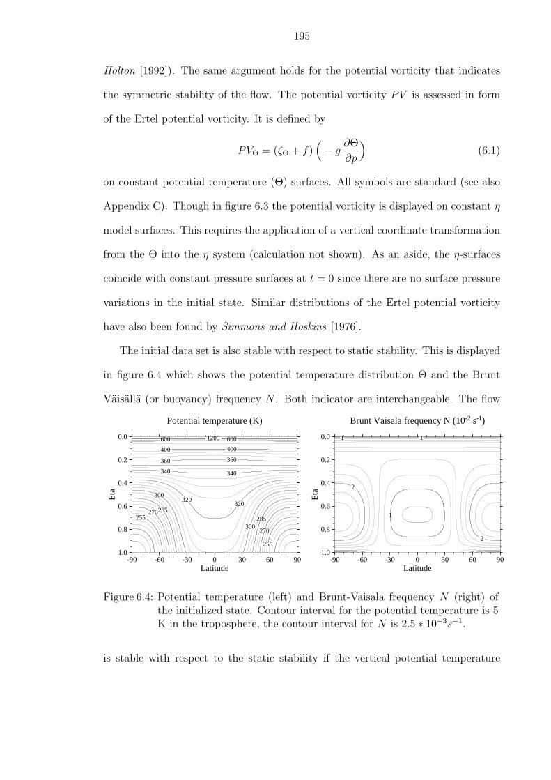
195
Holton [1992]). The same argument holds for the potential vorticity that indicates
the symmetric stability of the flow. The potential vorticity PV is assessed in form
of the Ertel potential vorticity. It is defined by
PVΘ = (ζΘ + f)(− g
∂Θ
∂p
)(6.1)
on constant potential temperature (Θ) surfaces. All symbols are standard (see also
Appendix C). Though in figure 6.3 the potential vorticity is displayed on constant η
model surfaces. This requires the application of a vertical coordinate transformation
from the Θ into the η system (calculation not shown). As an aside, the η-surfaces
coincide with constant pressure surfaces at t = 0 since there are no surface pressure
variations in the initial state. Similar distributions of the Ertel potential vorticity
have also been found by Simmons and Hoskins [1976].
The initial data set is also stable with respect to static stability. This is displayed
in figure 6.4 which shows the potential temperature distribution Θ and the Brunt
Vaisalla (or buoyancy) frequency N . Both indicator are interchangeable. The flow
255
255
270
270285
285
300
300320
320
340340
360360
400400
600600 1200
Potential temperature (K)
0.0
0.2
0.4
0.6
0.8
1.0
Eta
-90 -60 -30 0 30 60 90Latitude
11
1
1
2
2
Brunt Vaisala frequency N (10-2 s-1)
0.0
0.2
0.4
0.6
0.8
1.0
Eta
-90 -60 -30 0 30 60 90Latitude
Figure 6.4: Potential temperature (left) and Brunt-Vaisala frequency N (right) ofthe initialized state. Contour interval for the potential temperature is 5K in the troposphere, the contour interval for N is 2.5 ∗ 10−3s−1.
is stable with respect to the static stability if the vertical potential temperature

196
gradient dΘ/dz is positive or equivalently, if the frequency N is positive everywhere
(as shown).
The initial conditions can be used for two model setups. First, the model can be
initialized with the steady-state conditions and run without an overlaid perturbation.
Then model integrations over e.g. thirty days reveal how well a dynamical core can
keep its initial state (which is the analytical solution
0.3
30
40
50
Lat
itude
0 20 40Longitude
Figure 6.5: u perturbation(m/s).
for this scenario). This is a stringent test of the stabil-
ity of the numerical scheme. Second, a well-resolved
small amplitude Gaussian hill perturbation can be su-
perimposed on the initial state. This triggers baro-
clinic wave activities after several days which are char-
acterized by explosive cyclogenesis at model day 8. In the current setup, the Gaussian
perturbation as shown in figure 6.5 with a maximum amplitude of 1m/s is superim-
posed on the zonal wind field in midlatitudes at (20E,40N).
6.1.2 Formal test definition and test strategy
The initial state is defined via analytic expressions. All parameters and physical
constants are also listed in Appendix C and are not necessarily repeated in the
following description. For a hydrostatic dynamical core with a pressure based vertical
coordinate η the auxiliary variable ηv is defined by
ηv = (η − η0)π
2(6.2)
with η0 = 0.252. In case of a vertical σ coordinate the η level in equation 6.2 can
be simply replaced with the σ value. This is true for all following equations. Both
representations are equivalent since there are no initial pressure variations at the
surface. Expression 6.2 can also easily be modified for models with a pure pressure
197
coordinate p. The surface pressure ps is constant and given by
ps(λ, ϕ) = 100000 Pa (6.3)
The flow field is comprised of two symmetric zonal jets in midlatitudes. The zonal
wind u and meridional wind v in m/s are defined as
u(λ, ϕ, η) = u0 cos32 ηv sin2 (2 ϕ) (6.4)
v(λ, ϕ, η) = 0 . (6.5)
Here the maximum amplitude u0 is set to 35 m/s which is close to the wind speed
of the zonal-mean time-mean jet stream in the atmosphere. Furthermore, the hori-
zontally averaged temperature 〈T (η)〉 in degree K is split into two representations
for the lower (eqn. 6.6) and upper (eqn. 6.7) atmosphere. This introduces the
characteristic stratospheric and mesospheric temperature profiles. Both background
profiles are given by
〈T (η)〉 = T0 ηRdΓ
g (for ηs ≥ η ≥ ηt) (6.6)
〈T (η)〉 = T0 ηRdΓ
g + ∆T (ηt − η)5 (for ηt > η) (6.7)
with the tropopause level ηt = 0.2 and the horizontal-mean temperature at the
surface T0 = 288K. The temperature lapse rate Γ is set to 0.005 K/m which is
similar to the observed diabatic lapse rate. Additionally, the empirical temperature
difference ∆T = 48 ∗ 104K is chosen. The resulting temperature distribution is
comprised of the horizontal-mean temperature and a horizontal variation at each
level. It is given by
T (λ, ϕ, η) = 〈T (η)〉+3
4
η π u0
Rd
sin ηv cos12 ηv ∗
[(− 2 sin6 ϕ (cos2 ϕ +
1
3) +
10
63
)2 u0 cos
32 ηv +
( 8
5cos3 ϕ (sin2 ϕ +
2
3)− π
4
)a Ω
]. (6.8)

198
The surface geopotential Φs in m2/s2 completes the description of the steady state
initial conditions. The orography field balances the zonal wind field at the surface
and is determined by
Φs(λ, ϕ) = u0 cos32
((ηs − η0)
π
2
)∗
[(− 2 sin6 ϕ (cos2 ϕ +
1
3) +
10
63
)u0 cos
32
((ηs − η0)
π
2
)+
( 8
5cos3 ϕ (sin2 ϕ +
2
3)− π
4
)a Ω
]. (6.9)
When initializing the finite-volume dynamical core with this data set the simula-
tions have been observed to stay stable for typical time periods on the order of
weeks. During this time period the basic flow remains almost unchanged despite the
initial generation of gravity wave motions. They adjust the geostrophic balance in
the discrete system since the analytic balanced state is not entirely balanced in a
discrete representation. This is the typical geostrophic adjustment process that is
characterized by decaying gravity waves.
For an irregular computational grid such as an icosahedral grid, simulations with
the German weather model GME have shown that the truncation error of the nu-
merical scheme has a wave number 5 structure. This is due to the built-in wave
number 5 of the grid. It introduces small-scale wave number 5 perturbations dur-
ing the steady state integration that are unstable and considerably grow over time.
Such a model maintains the initial state for shorter time periods on the order of only
days. The balance improves with increasing resolution. This is an artifact of the
computational grid and not necessarily a model problem for a real atmospheric flow
that represents the whole wave number spectrum. The effect is clearly enhanced
by the idealized zonally symmetric setup. The same conclusion applies to models
that utilize a cubed sphere computational grid with a built-in wave number 4, es-

199
pecially when using low-order numerical schemes. High-order methods postpone the
breakdown of the steady-state pattern.
If possible, the unperturbed model simulations should be run without horizontal
diffusion or Rayleigh friction near the model top (if implemented). Otherwise, the
diffusion mechanism damps the initial data over time.
Besides the assessment of the steady state solution, the test is primarily designed
to simulate a baroclinic wave. It can be triggered if the initial conditions are overlaid
with an unbalanced perturbation. Here a perturbation with a Gaussian profile is
selected and centered at
(λc, ϕc) =(π
9,2 π
9
)(6.10)
which points to the location (20E,40N). The perturbation u′
u′(λ, ϕ) = exp(−
( r
R
)2 )(6.11)
with R = a10
is superimposed on the zonal wind field at each vertical level by adding
u′ to u at each grid point. The great circle distance r is defined by
r = a arccos(
sin ϕc sin ϕ + cos ϕc cos ϕ cos(λ− λc))
(6.12)
where a is the Earth’s radius. Typically the simulation should cover a 10-12 day
time period, but simulations over longer time intervals (e.g. 30 days) have also been
successfully performed. The baroclinic wave in the Northern Hemisphere starts grow-
ing noticeably around day 4 and evolves rapidly thereafter. The wave train breaks
around day 9 and generates a full circulation in both hemispheres around day 20.
Until day 20 the Southern Hemisphere does not show baroclinic wave activities. This
makes the test ideal for adaptive grid simulations since the features of interest are
well-defined and confined to the Northern Hemisphere. The adaptive grid is capable
200
of tracking the localized wave train at high horizontal resolutions. The baroclinic
wave, although idealized, represents very realistic flow features. For example, strong
temperature fronts develop that are associated with the low and high pressure sys-
tems. In addition, the wave number of maximum growth rate lies between 5-9 which
agrees well with observations and assessments in the literature (e.g. Simmons and
Hoskins [1977]).
The baroclinic wave test sequence with unperturbed and perturbed initial condi-
tions has been applied to NCAR’s dynamical cores that are part of the CAM2 climate
model framework. In particular, these are the NASA/NCAR finite-volume dynam-
ical core and NCAR’s semi-Lagrangian and Eulerian spectral dynamics packages.
In addition, model results based on cubed meshes (Aime Fournier, Steve Thomas,
NCAR, personal communication) and icosahedral grids are available. The icosahe-
dral dynamical core is part of the operational German weather forecast model GME.
The code was kindly provided for the baroclinic wave studies by Detlev Majew-
ski (German Weather Service, DWD). This model intercomparison and convergence
studies reveal interesting flow characteristics that have already led to model improve-
ments with respect to NCAR’s semi-Lagrangian dynamical core. Typical diagnostics
applied to the test results include error norm statistics, grid point data compar-
isons, phase shift assessments and wave number analyses that has been done in close
collaboration with David L. Williamson (NCAR). Furthermore, potential vorticity
analyses have been performed.
The baroclinic wave test case does not have an analytic solution, but high reso-
lution reference solutions can be derived. This has been done during the baroclinic
wave studies with NCAR’s dynamical cores and GME. The comparison of all high
resolution reference fields reveals that the dynamical cores converge despite their

201
individual design and that a reference state can be recommended with a specific
uncertainty estimate (see details in Jablonowski and Williamson [2004]). With re-
spect to the adaptive grid simulations, the results can therefore be compared not
only to the equivalent uniform resolution runs, but also to a high resolution refer-
ence simulation. Plots of uniform resolution runs generated with the NCAR/NASA
finite-volume dynamical core are shown in the Appendix A.3.1.
6.2 Dynamical core tests with static adaptations
In this section, the 3D adaptive finite-volume dynamical core is assessed with a
statically adaptive setup that utilizes prior knowledge of the developing flow field.
The model is evaluated with the Jablonowski-Williamson baroclinic wave test case.
The flow field is characterized by a baroclinic wave train in the Northern Hemisphere
that is triggered by a small perturbation superimposed upon the smooth initial zonal
wind field.
The adapted blocks are used to refine the pre-determined storm track in the
midlatitudes (Northern Hemisphere) with increasing horizontal resolutions. The re-
finements are confined to the horizontal directions so that the whole vertical column
is refined in the event of refinement requests. Refinements are selected at the be-
ginning of the forecast, which is followed by an analytical reinitialization step. The
convergence tests with uniform resolutions have shown that the representation of the
baroclinic wave improves considerably with increasing horizontal resolution until the
pattern converges at resolutions around 0.5 − 1 (see figures A.16 and A.17). It
has also been observed that the flow is rather insensitive to the number of vertical
levels which justifies a purely horizontal refinement strategy. The same convergence
behavior is expected for the locally adapted finite-volume dynamical core.
202
Four scenarios are assessed that all start with the basic 8x6 block setup and 9x6
cells per block. This parameter set represents an initial 5 × 5 grid. In addition,
26 vertical levels are selected (see Appendix B). The four simulations comprise a
coarse uniform 5 run as well as adapted grid simulations with 1, 2 and 3 refinement
levels. The refinements at each level then cover the whole latitudinal band structure.
Snapshots of the simulations at day 8 and day 10 are shown in figures 6.6 and 6.7
Here the analysis of the baroclinic wave train is concentrated on the surface
pressure field. The figures show the surface pressure patterns for all four grid setups
(a-d) at day 8 and 10. In addition, the adapted blocks are overlaid that clearly
illustrate the band structure of the refinement approach. The Southern Hemisphere
is passive in all simulations and therefore kept at the coarsest resolution at any time.
The corresponding time steps for the four model runs are determined by the gravity
wave activity at the finest refinement level in the midlatitudes. In particular the
chosen global time steps are 720 s, 360 s, 180 s and 90 s, respectively. In addition,
a mild filtering mechanism is applied to the wind components in tropical regions
in case of subfigures (d), which show the model simulation at the highest adapted
resolution. The filtering suppresses small-scale noise in the tropics and has negligible
effects on the evolution of the baroclinic wave in midlatitudes. Filtering other than
the regular FFT filtering in blocks adjacent to the poles and the digital Shapiro
filtering poleward of 60 N/S is not applied in the coarser model runs (a) through
(c). The latter two filtering strategies are identical to the mechanisms in the 2D
shallow water framework.
It can clearly be seen at both model day 8 and 10 that the representation of
the baroclinic wave improves significantly with an increasing number of refinement
levels. The baroclinic wave intensifies as expected in the fine grid adaptive runs and

203
(a)
no
stat
ic r
efin
emen
ts, f
ines
t res
olut
ion
5o x5o
-300306090
Latitude
090
180
270
360
Lon
gitu
de
972
984
996
1008
Surf
ace
pres
sure
[hP
a]
(b)
1 s
tatic
ref
inem
ent,
fine
st r
esol
utio
n 2.
5o x2.5
o
-300306090
Latitude
090
180
270
360
Lon
gitu
de
972
984
996
1008
Surf
ace
pres
sure
[hP
a]
(c)
2 s
tatic
ref
inem
ents
, fin
est r
esol
utio
n 1.
25o x1
.25o
-300306090
Latitude
090
180
270
360
Lon
gitu
de
972
984
996
1008
Surf
ace
pres
sure
[hP
a]
(d)
3 s
tatic
ref
inem
ents
, fin
est r
esol
utio
n 0.
625o x0
.625
o
-300306090
Latitude
090
180
270
360
Lon
gitu
de
972
984
996
1008
Surf
ace
pres
sure
[hP
a]
Fig
ure
6.6:
Surf
ace
pre
ssure
atday
8fo
rdynam
ical
core
runs
wit
h(a
)no,
(b)
1,(c
)2
and
(d)
3st
atic
refinem
ents
.T
he
adap
ted
blo
cks
are
over
laid
,th
efines
tre
solu
tion
isin
dic
ated
inth
eti
tles
.C
onto
ur
inte
rval
sar
e6h
Pa.

204
(a)
no
stat
ic r
efin
emen
ts, f
ines
t res
olut
ion
5o x5o
-300306090
Latitude
090
180
270
360
Lon
gitu
de
940
960
980
1000
1020
Surf
ace
pres
sure
[hP
a]
(b)
1 s
tatic
ref
inem
ent,
fine
st r
esol
utio
n 2.
5o x2.5
o
-300306090
Latitude
090
180
270
360
Lon
gitu
de
940
960
980
1000
1020
Surf
ace
pres
sure
[hP
a]
(c)
2 s
tatic
ref
inem
ents
, fin
est r
esol
utio
n 1.
25o x1
.25o
-300306090
Latitude
090
180
270
360
Lon
gitu
de
940
960
980
1000
1020
Surf
ace
pres
sure
[hP
a]
(d)
3 s
tatic
ref
inem
ents
, fin
est r
esol
utio
n 0.
625o x0
.625
o
-300306090
Latitude
090
180
270
360
Lon
gitu
de
940
960
980
1000
1020
Surf
ace
pres
sure
[hP
a]
Fig
ure
6.7:
Surf
ace
pre
ssure
atday
10fo
rdynam
ical
core
runs
wit
h(a
)no,
(b)
1,(c
)2
and
(d)
3st
atic
refinem
ents
.T
he
adap
ted
blo
cks
are
over
laid
,th
efines
tre
solu
tion
isin
dic
ated
inth
eti
tles
.C
onto
ur
inte
rval
sar
e10
hPa.

205
is rather damped on the coarse uniform 5 grid. Here the two model days represent
different growth stages of the system. Model day 8 in figure 6.6 shows the wave in
an explosive cyclogenesis state, whereas model day 10 in figure 6.7 depicts the wave
after wave breaking events set in. After day 10 all forecasts, even on non-adapted
grids, slowly start diverging from each other when predictability issues come into
play.
The model results at all refinement levels compare very well to the corresponding
uniform grid reference solutions. Especially the reference surface pressure fields at
day 8 (figure A.16 on page 243) are almost indistinguishable from the adapted sim-
ulations (figure 6.6). Minor differences can be seen in the maximum amplitudes of
the low and high pressure systems. But it must be kept in mind that the reference
solutions are computed with a slightly finer grid in meridional direction that could
also cause minor deviations. The same conclusions apply to the surface pressure
fields at model day 10. The two highest resolutions in figure 6.7 closely resemble the
reference fields in figure A.17 on page 244. Slight deviations are again detectable in
the maximum amplitudes of the baroclinic wave train, especially around the position
(210E,45N). No noise or distortions of the flow fields are visible in the adapted runs.
The flow varies smoothly at fine-coarse grid interfaces.
An additional comparison of the surface pressure fields for both the adapted and
uniform model runs is displayed in figure 6.8. The figure illustrates the time evolu-
tion of the minimum and maximum surface pressure in the global domain. Such an
analysis clearly shows the convergence with increasing resolutions, but on the other
hand does not indicate the spatial positions of the global extrema. Consequently,
phase shifts of the baroclinic wave are possible which can be assessed in grid point
space (see also Jablonowski and Williamson [2004]). For brevity, they are not dis-

206
930
940
950
960
970
980
990
1000M
inim
um s
urfa
ce p
ress
ure
(hPa
)
0 48 96 144 192 240
Hours
uniform 5o x 4o griduniform 2.5o x 2o griduniform 1.25o x 1o griduniform 0.625o x 0.5o grid1 static refinement (2.5o)2 static refinements (1.25o)3 static refinements (0.625o)
1000
1005
1010
1015
1020
1025
Max
imum
sur
face
pre
ssur
e (h
Pa)
0 48 96 144 192 240
Hours
uniform 5o x 4o griduniform 2.5o x 2o griduniform 1.25o x 1o griduniform 0.625o x 0.5o grid1 static refinement (2.5o)2 static refinements (1.25o)3 static refinements (0.625o)
Figure 6.8: Global minimum and maximum surface pressure evolution (hPa) for runswith uniform grids and static adaptations with three different refinementlevels.
cussed here. The time evolution of the extreme surface pressure values confirms
that the adapted runs closely match the uniform grid reference solutions. This is
in particular true for all simulations until day 8. After day 8, the minimum surface
pressure in the adapted run at the highest resolution slightly diverges which could be
related to the wave breaking processes in both simulations. It must be kept in mind
that an exact match can not necessarily be expected since the truncation errors in
the remaining coarse grid domain and the interpolation errors at the interfaces will
ultimately interact with the flow field.
The static adaptation are successfully used for the 3D adaptive model assess-
ment with band-structured refinement regions. However, attempts to relax the band
structure in order to avoid the overhead in regions without significant baroclinic
wave activity raised new questions concerning the underlying topography field. This
problem is depicted in figure 6.9. Two refinement strategies are employed. The
figures show a very early stage of the surface pressure field after eight model hours
with one refinement level. In the left figure one adapted block (in red) only refines
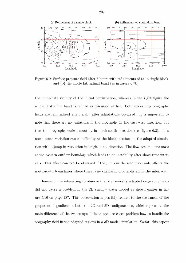
207
1000
1000.2
1000.2
1000.2
1000.4
1000.4
(a) Refinement of a single block
20
40
60
80
Lat
itude
0.0 22.5 45.0 67.5 90.0Longitude
1000
1000.2
1000.2
(b) Refinement of a latitudinal band
20
40
60
80
Lat
itude
0.0 22.5 45.0 67.5 90.0Longitude
Figure 6.9: Surface pressure field after 8 hours with refinements of (a) a single blockand (b) the whole latitudinal band (as in figure 6.7b).
the immediate vicinity of the initial perturbation, whereas in the right figure the
whole latitudinal band is refined as discussed earlier. Both underlying orography
fields are reinitialized analytically after adaptations occurred. It is important to
note that there are no variations in the orography in the east-west direction, but
that the orography varies smoothly in north-south direction (see figure 6.2). This
north-south variation causes difficulty at the block interface in the adapted simula-
tion with a jump in resolution in longitudinal direction. The flow accumulates mass
at the eastern outflow boundary which leads to an instability after short time inter-
vals. This effect can not be observed if the jump in the resolution only affects the
north-south boundaries where there is no change in orography along the interface.
However, it is interesting to observe that dynamically adapted orography fields
did not cause a problem in the 2D shallow water model as shown earlier in fig-
ure 5.16 on page 187. This observation is possibly related to the treatment of the
geopotential gradient in both the 2D and 3D configurations, which represents the
main difference of the two setups. It is an open research problem how to handle the
orography field in the adapted regions in a 3D model simulation. So far, this aspect

208
has not been well-documented in the literature. Only Bacon et al. [2000] reported
on adaptive orography data and lower boundary conditions for adaptive limited-area
simulations. Future research activities will address this topic further.
6.3 Dynamical core tests with dynamic adaptations
In addition to static adaptations in the 3D framework, it is of particular interest
to assess the dynamically adaptive approach without prior knowledge of the flow
field. This is the classical application of adaptive mesh refinements. The dynam-
ically adapted model is tested using an alternative idealized baroclinic wave test.
This test was developed by Polvani et al. [2004]. The underlying test strategy of
the Polvani test is very similar to the Jablonowski-Williamson test case. The sim-
ulation starts with smooth balanced initial conditions that are perturbed to trigger
a baroclinic wave over a 10-day forecast period. The initial data are displayed in
Appendix A.3.2 on page 245. One of the main differences is that the wind speed
at the surface is identically zero in the Polvani test case. Therefore the orography
field is zero since there is no active flow field to be balanced. In addition, all initial
data only show patterns in the Northern Hemisphere where the baroclinic wave is ob-
served. This leads to a less realistic global initial data set, which on the other hand is
irrelevant with respect to the developing wave train. Furthermore, the specification
of the initial data is only partly analytic and partly based on numerical integrals.
As argued before, the evolution of a baroclinic wave train with strong gradients
is an ideal test example for adaptive grid simulations. Here the baroclinic wave is
triggered by perturbing the initial temperature field at each level. It must be noted
that the base resolution for this test is increased in order to allow a more accurate
representation of the initial data at the coarsest level. It is recommended for this test

209
case since the initial conditions contain rather strong gradients. As a consequence,
the adaptive grid simulation does not suffer from a severe underrepresentation of the
initial data. The base resolution is 2.5 × 2.5 with 16x12 blocks and 9x6 cells per
block.
The adaptations are guided by a user-defined refinement criterion. Based on
the experiences in Chapter V a vorticity-based refinement indicator at the model
level closest to the surface (at approximately 992hPa) is selected. In particular,
the refinement criterion for the runs depicted in figure 6.10 is set to |ζ| ≥ 0.75 ∗
10−5s−1 As an aside, the initial relative vorticity at the surface is zero. The rather
sensitive threshold for the absolute value of the relative vorticity is chosen in order
to capture the evolution of the wave early in its developing stages. Here the first
adaptations occur at day 3. An alternative increased threshold such as |ζ| ≥ 2 ∗
10−5s−1 triggers the first refinements at model day 4. Day 4 is the point in time when
the baroclinic wave enters its rapid development phase. Therefore, the increased
refinement threshold does not capture the initial organization of the wave disturbance
by a refined area. In practice though, a compromise must be found in order to balance
the accuracy and efficiency of an adapted run.
For the dynamically adaptive 3D tests, the maximum number of refinement levels
is set to 1. The integrations cover a 10-day time period and snapshots of the adaptive
simulation at day 3, 4, 8 and 10 are shown in figure 6.10. The refinement region
clearly captures and tracks the developing wave. As in the statically adapted case the
additional resolution leads to a more accurate representation of the wave train. This
can be seen in comparison to figure A.19 on page 247 that displays the comparable
uniform grid solutions at day 8 and 10. The surface pressure distributions are very
similar at the refined resolution 1.25. The adapted run successfully predicts the

210
994
996
998
1000
1002
Surf
ace
pres
sure
[hP
a]
(a)
Day
3
0306090 Latitude
090
180
270
360
Lon
gitu
de
994
996
998
1000
1002
Surf
ace
pres
sure
[hP
a]
(b)
Day
4
0306090 Latitude
090
180
270
360
Lon
gitu
de
920
940
960
980
1000
1020
1040
Surf
ace
pres
sure
[hP
a]
(c)
Day
8
0306090 Latitude
090
180
270
360
Lon
gitu
de
920
940
960
980
1000
1020
1040
Surf
ace
pres
sure
[hP
a]
(d)
Day
10
0306090 Latitude
090
180
270
360
Lon
gitu
de
Fig
ure
6.10
:Surf
ace
pre
ssure
inth
eN
orth
ern
Hem
ispher
eat
(a)
day
3,(b
)day
4,(c
)day
8an
d(d
)day
10fo
ra
dynam
ical
lyad
apte
d3d
model
run
wit
h1
refinem
ent
leve
l.R
efinem
ent
crit
erio
nis|ζ s
fc|≥
0.75∗1
0−5s−
1.
Con
tour
inte
rval
sar
e(a
,b)
1hPa
and
(c,d
)10
hPa.

211
intensification of the wave train with increased resolution. Minor differences can
again be found with respect the amplitudes of the extreme values. In this test case
the wave breaking event sets in after day 8 which can contribute to slowly diverging
flow patterns thereafter.
Here no static pre-determined refinement regions are defined. In the event that
the developing wave needs to be detected even earlier than day 3, a combination
of several refinement criteria is feasible. For example, a combination of a surface
pressure indicator and a vorticity-based assessment could replace the pure vorticity
criterion. Initial tests with a surface pressure indicator that locates the positions of
the maximum and minimum pressure centers have been successfully performed.

CHAPTER VII
Summary and future research directions
Climate and weather systems are true multi-scale phenomena that are charac-
terized by widely varying spatial and temporal scales. Solving such a problem more
efficiently and accurately requires variable resolution that tracks small-scale features
embedded in a large-scale flow. This approach provides new insight into small-scale
large-scale flow interactions that are unresolved by uniform grid applications. A
dynamically adaptive model for global climate and weather research with regular
data-structures has never been built before. So far, only irregular triangulated data
have been discussed for adaptive atmospheric modeling systems (Bacon et al. [2002],
Gopalakrishnan et al. [2002]) on the sphere. This dissertation is a step towards de-
veloping new adaptive methods for future weather and climate studies. It documents
the design principles and successful implementation of a statically and dynamically
adaptive dynamical core for general circulation models on the sphere.
The adaptive grid techniques have been applied to a revised version of NCAR/
NASA’s next generation dynamical core for climate and weather research. The adap-
tive model design is based on two fundamental building blocks, a block structured
data layout and a spherical adaptive grid library. This AMR communication library
for parallel processors has been newly developed at the Computer Science Depart-
213

214
ment at the University of Michigan.
The adaptive dynamical core has been run in two model configurations: the
full 3D hydrostatic dynamical core on the sphere and the corresponding 2D shallow
water configuration that is extracted out of the 3D version. This shallow water setup
serves as an ideal testbed for the horizontal discretizations and the 2D adaptive mesh
strategies.
The static and dynamic adaptations have been tested using the standard shal-
low water suite and a newly-developed idealized 3d baroclinic wave test case. Static
adaptations are used to vary the resolution in pre-defined regions of interest. This
includes static refinements near mountain ranges or static coarsenings in longitudinal
direction for the implementation of a so-called reduced grid in polar regions. Dy-
namic adaptations are based on flow characteristics and guided by refinement criteria
that detect user-defined features of interest during a simulation. In particular, flow-
based refinement criteria, like vorticity or gradient indicators, have been suggested.
Refinements and coarsenings occur according to pre-defined threshold values.
Summary
Static and dynamic adaptations have been assessed both in the 2D and 3D model
framework. The statically adaptive runs in the 2D shallow water setup show that the
reduced grid with two reduction levels can be successfully used for passive advection
problems. The model results are almost indistinguishable from the full grid control
run. In case of nonlinear model simulations, the reduced grid performs well in case of
one reduction level close to the poles, whereas the addition of the second reduction
can not be recommended. The second reduction level increases the solution error in
the spherical grid system to unacceptable levels. Overall, the reduced grid with one
reduction is in particular a viable choice if the global time step is constrained by the

215
advective wind speeds in polar regions. Then it allows an increase in the time step
which saves computational costs despite the overhead associated with adaptations.
In addition, 2D shallow water tests with static refinements in user-determined
regions of interest have revealed that refinement regions can be successfully placed
at arbitrary positions within the model domain. The flow passes through the inter-
face boundaries without noise or significant distortions for at least a 7-14 day time
period. Such a time period represents the typical duration of a weather prediction
forecast. After this time span grid interface effects might play a role in flow fields
with strong gradients and high wind speeds. Statically adapted runs with external
forcing though, present a challenge for the adaptive grid approach. Although the
transport of a low pressure system has been well-simulated in the adapted runs, the
noise along the boundaries prevents the overall solution error from decreasing ac-
cordingly. In future studies, the interface treatment in a forced system needs to be
revisited.
Static adaptations have also been tested in the 3D dynamical core setup. For
these studies, a new idealized baroclinic wave test case for short-term dynamical
core assessments has been developed. The design principles and test strategies are
documented in the dissertation. The test has the potential to become part of a future
standard test suite for dynamical cores. The 3D evaluations of the static adaptations
along the storm track have shown that the evolution of the baroclinic wave can be
successfully predicted without noise or distortions at fine-coarse grid boundaries.
The refinements capture the correct intensification of the wave train with increased
resolution without the need of a fine resolution in the global domain.
Besides static adaptations, dynamically adaptive simulations have been success-
fully performed in both the 2D and 3D framework with up to four refinement levels.

216
The dynamically adaptive grid is able to track selected features of interest according
to user-defined adaptation criteria. A variety of flow based adaptation indicators has
been investigated that reliably detect features such as a lee-side wave train behind a
mountain or a cosine bell in a pure advection experiment. Special attention has been
paid to a relative vorticity based refinement criterion that is compared to a gradient
based indicator. Both perform well in the 2D shallow water setup. For future stud-
ies, a vorticity criterion is recommended that captures the waves in an evolving flow
field early. The vorticity criterion at the lowermost model level has also been used
for 3D assessments of the dynamically adaptive approach. Tests with an alternative
baroclinic wave test case show that the flow is well-captured with increased accuracy
in the refined region. Overall, the selection of the optimal adaptation criterion and
threshold is highly problem dependent and balances the efficiency and accuracy of
the run. In general, significant computational savings can be made in comparison
to fine-grid fixed resolution runs as shown by the timing results for the dynamically
adapted advection tests.
The development of the dynamically adaptive dynamical core also raised ques-
tions concerning numerical and computational stability issues. Among them has
been the so-called pole problem in a regular latitude-longitude grid that leads to
the convergence of the grid lines in polar regions. The resulting extremely small
grid boxes then require efficient filtering strategies. Several filtering and divergence
damping techniques for the adaptive grid framework have been assessed that success-
fully smooth the gravity wave motions without distorting the relevant atmospheric
wave patterns. Filtering has been found to be imperative for stable simulations.
Furthermore, numerical questions have been addressed with respect to suitable in-
terpolation techniques for adaptive simulations. Interpolations are necessary for split

217
and join operations as well as for ghost cells updates along the interfaces. A variety
of conservative and non-conservative techniques with increased accuracy have been
investigated. A second-order scheme based on a quasi-biparabolic PPM approach
is recommended for accuracy reasons. The applied interpolation scheme has been
slightly modified in comparison to published techniques.
Accomplishments and highlights of the research project
Significance: Adaptive methods offer an attractive framework for future climate
and weather models. For the first time, it has been shown that the adaptive
grid approach can be successfully applied to a dynamical core of a GCM with
regular data structures in spherical geometry. In the future, AMR has the po-
tential to become a key technique for improved atmospheric flow simulations
that resolve features of interest, like regions with strong gradients or curvature,
more adequately. The keys to the success of adaptive grid methods in the atmo-
spheric sciences lie in their parallel performance on high- speed supercomputers
and high accuracy with respect to the underlying numerical scheme.
Relevance and future potential: NCAR’s future climate model is likely to be
based on the NASA finite-volume dynamical core and NCAR’s physics package.
This finite-volume dynamical core has been one of the building blocks of the
adaptive grid research project. It therefore represents an essential step towards
an adaptive full GCM with dynamics and physics package. Future research will
address the incorporation of physics components into the model. Furthermore,
a new idealized test case for dynamical cores has been developed that is targeted
at short-term deterministic 3D model assessments. This test case might become
a standard tool for model developers.
218
Collaboration: The research project has established a collaboration between the
University of Michigan, the NASA Goddard Space Flight Center (GSFC) and
the National Center for Atmospheric Research. In particular, the science team
supporting the research consisted of Joyce E. Penner and Michael Herzog1,
Robert Oehmke and Quentin F. Stout2, Bram van Leer and Ken Powell3, Shian-
Jiann Lin and Kevin Yeh4, and David L. Williamson5.
Interdisciplinary research: This project involves interdisciplinary ideas and re-
quires knowledge of atmospheric science, computer science and numerical tech-
niques. It ideally combines global climate modeling aspects, the newest parallel
and high performance computing techniques and advanced numerical methods
pioneered for CFD applications in other disciplines. The adaptive model is
based on the physical-motivated finite-volume approach and is designed for
distributed-memory parallel computer architectures.
Future research direction
Dynamic grid adaptations for climate and weather applications are a current re-
search topic for the atmospheric science community. New studies are under way at
NCAR, the University of Cambridge, UK and the Center for Atmospheric Physics
(Science Applications International Corporation, Virginia, USA). The promising re-
sults of this dissertation and the efforts of the community will help answer the open
1Atmospheric Science, University of Michigan, Ann Arbor
2Computer Science, University of Michigan, Ann Arbor
3Aerospace Engineering, University of Michigan, Ann Arbor
4NASA/GSFC, Data Assimilation Office, Greenbelt, Maryland
5NCAR, Climate and Global Dynamics Division, Boulder, Colorado

219
question whether AMR can be successfully used in full GCMs with dynamics and
physics components. Incorporating physics into an adaptive model represents a chal-
lenging research problem. So far, only Bacon et al. [2000] and Gopalakrishnan et al.
[2002] have included a complete physics package in their adaptive modeling system
OMEGA. As observed by Skamarock and Klemp [1993], the truncation error esti-
mates in adaptive grid simulations with parameterized mixing do not exhibit the
expected rate of decrease when refining the mesh. Even error increases were ap-
parent that can not be found in dynamical core simulations without parameterized
physics. As a consequence. a fundamental concern in adaptive mesh applications is
the validity and consistency of grid-scale dependent physical parameterizations that
are used over a wide range of refinement levels. Two aspects need to be considered.
On the one hand, grid-dependent model parameters like the horizontal diffusion co-
efficient are no longer optimal or even valid when changing the mesh resolution. On
the other hand, it is unclear at what grid scale the parameterizations like convection
or turbulence packages become unnecessary or even detrimental.
In addition, the influence of the lower boundary conditions in adaptive mesh
applications is of equal importance. Atmospheric models rely on worldwide data
sets for the surface elevation, land/water coverage, soil types, land use, deep soil
temperatures, deep soil moisture and sea surface temperatures at varying grid reso-
lutions. These are used to derive important secondary parameters such as the surface
roughness and albedo. Therefore, in adaptive mesh applications the treatment of the
refined lower boundary conditions needs to be carefully addressed in order to improve
the overall accuracy. A starting point for future research efforts could be the assess-
ment of adaptive orography based on experiences with nested grid models (Zhang
et al. [1986] and Fox and Maskell [1995]) and the adaptive modeling system OMEGA

220
(Bacon et al. [2000]). The latter provides routines and data bases for dynamically
adaptive lower boundary conditions.
From a computational standpoint, future developments could include a new load-
balancing strategy for the AMR communication library that is based on the space-
filling curve approach. Furthermore, library support for adaptive time steps is de-
sirable that allows different time steps for each refinement level. This reduces the
overhead of the adaptive simulation. In addition, refinements in the vertical direc-
tion might become imperative for very high horizontal resolutions, especially if the
underlying equations are switched from a hydrostatic to a non-hydrostatic regime.
In conclusion, in the future dynamically and statically adaptive mesh refinements
are feasible for short-term weather predictions. A statically refined model could
possibly replace today’s nested grid approaches for improved local weather forecasts.
It furthermore guarantees consistent boundary conditions that do not violate the
conservation principles across interfaces. Dynamically adaptive techniques could
add extra flexibility to a weather prediction system that allows, for example, the
tracking of low pressure centers in the global domain. Static adaptations in pre-
determined regions of interest, especially near mountain ranges, are also a viable
option for long-term climate predictions with a regional focus.
On the other hand whether dynamic adaptations can be successfully applied to
climate simulations remains an open research question that needs to identify the
features of interest for long-term climate assessments.

APPENDICES
221


223
APPENDIX A
Overview of the 2D shallow water and 3D
dynamical core test set
A.1 The standard test suite for the 2D shallow water equa-tions
The standard test suite for the shallow water equations in spherical coordinates
has been proposed by Williamson et al. [1992]. It comprises a collection of 7 test
cases with increasing complexity which have been designed by various authors. Here,
six of the seven test scenarios have been used in order to assess the performance of
the adaptive finite-volume dynamical core. In addition, a shallow water test case
suggested by McDonalds and Bates [1989] has been applied. All test cases start with
analytic initial data sets that are briefly described in the following section. A general
overview of the shallow water test results is provided by Jakob et al. [1993].
A.1.1 Test case 1: Advection of a cosine bell
Test case 1 assesses the advection scheme in isolation and does not deal with
the complete nonlinear shallow water equations. In this two-dimensional solid body
rotation test case a cosine bell is passively advected around the sphere at various

224
rotation angles α to the equator. The nondivergent velocity is defined by
u = u0 (cos α cos ϕ + sin α cos λ sin ϕ) (A.1)
v = −u0 sin α sin λ (A.2)
where u0 ≈ 38.61ms−1 (details in Williamson et al. [1992]). The initial distribution
of the geopotential height field h is given by
h(λ, ϕ) =
(h0
2
)(1 + cos(πr/R)
)if r < R
0 if r ≥ R
(A.3)
with the peak amplitude h0 = 1000m. r is the great circle distance between a position
(λ, ϕ) and the center of the cosine bell, initially set to (λc, ϕc) = (3π/2, 0). The
orography hs is set to zero. The numerical scheme is expected to translate the cosine
bell without any change in shape. The true solution can be analytically computed
when updating the position of the cell center (see also the trajectory calculation in
Section 4.1.3).
The initial cosine bell and the zonal wind field for α = 0 are displayed in figures
A.1 and A.2. The meridional wind v is zero for α = 0 .
-90
-60
-30
0
30
60
90
Lat
itude
0 90 180 270 360Longitude
Figure A.1: Initial geopotential height (and reference solution after 12 days) of thecosine bell. Contour interval is 100 m, the zero contour is omitted.

225
7.57.5
7.57.5
1515
1515
22.522.5
22.522.5
3030
3030
37.537.5
37.537.5
Zonal wind u (m/s) for α=0o
-90
-60
-30
0
30
60
90
Lat
itude
0 90 180 270 360Longitude
Figure A.2: Zonal wind u for α = 0. Contour interval is 2.5 ms−1.
Figure A.3 on the next page displays the advective wind components for the
rotation angles α = 45 and α = 90. Then the wind field advects the feature
slantwise (α = 45) or across the poles (α = 90) around the sphere.
A.1.2 Test case 2: Steady state geostrophic flow
Test case 2 is a steady state solution to the nonlinear shallow water equations. It
is comprised of a solid body rotation with a balanced geostrophic height field. As in
test 1, several rotation angles α can be specified which then require the recalculation
of the Coriolis parameter f . The wind field is identical to the wind definitions in
test case 1 (eqn. A.1 and A.2). The analytic geopotential Φ = g h is defined by
gh = g h0 −(a Ω u0 +
u20
2
)∗ (− cos λ cos ϕ sin α + sin ϕ cos α)2 (A.4)
with g h0 = 2.94 × 10⁴m2/s2 and u0 as in test case 1. The reference solution or
true solution at any time is the initial data set. The initial geopotential height fields
for the rotation angles α = 45 and α = 90 are shown in figures A.4 and A.5 on
page 227. The corresponding initial wind fields are displayed in figure A.3 (test cases
1 & 2).

226
0
7.5
1515
15
15
22.5
22.5
22.5
22.5
30
30
30
30
37.5
-7.5
(a)
Zon
al w
ind
u (m
/s)
for
α=45
o
-90
-60
-300306090
Latitude
090
180
270
360
Lon
gitu
de
07.
57.
515
1522
.522
.5-2
2.5
-22.
5-1
5-1
5-7
.5-7
.5
(b)
Mer
idio
nal w
ind
v (m
/s)
for
α=45
o
-90
-60
-300306090
Latitude
090
180
270
360
Lon
gitu
de
00
0
0
7.5
7.5
7.5
7.5
15
22.5
-22.
5
-15
-7.5
-7.5
-7.5
-7.5(c)
Zon
al w
ind
u (m
/s)
for
α=90
o
-90
-60
-300306090
Latitude
090
180
270
360
Lon
gitu
de
015
1530
30-3
0-3
0-1
5-1
5
(d)
Mer
idio
nal w
ind
v (m
/s)
for
α=90
o
-90
-60
-300306090
Latitude
090
180
270
360
Lon
gitu
de
Fig
ure
A.3
:(a
,c)
Zon
alw
ind
uan
d(b
,d)
mer
idio
nal
win
dv
for
diff
eren
tro
tati
onan
gles
α.
Top
row
(a,b
):α
=45 ,
bot
tom
row
(c,d
):α
=90 .
Con
tour
inte
rval
sar
e2.
5m
s−1
(tes
tca
ses
1&
2).

227
1200
1600
1600
1600
1600
2000
2000
2000
2000
2000
2400
2400
2400
2400
2400
2400
2800
2800
2800
2800
2800
2800
-90
-60
-30
0
30
60
90
Lat
itude
0 90 180 270 360Longitude
Figure A.4: Initial geopotential height and reference solution of test case 2 withα = 45. Contour interval is 100 m.
1600
2000
2000
2400
2400
2400
2400
2800
2800
2800
2800
2800
-90
-60
-30
0
30
60
90
Lat
itude
0 90 180 270 360Longitude
Figure A.5: Initial geopotential height and reference solution of test case 2 withα = 90. Contour interval is 100 m.

228
A.1.3 Test case 3: Steady state geostrophic flow with compact support
Test case 3 is similar to test case 2 as it defines a steady state flow field that
should remain constant during the course of the integration. Here, the wind field is
nonzero only in a limited region. The rotation angle has been set to α = 0. Then
the initial conditions describe a zonal flow whose u and h profiles are illustrated in
figure A.6. The meridional wind is zero. In this test case, the geopotential height can
2000
2200
2400
2600
2800
3000
Geo
pote
ntia
l hei
ght h
(m
)
-90 -60 -30 0 30 60 90
Latitude
0
10
20
30
40
Zon
al w
ind
u (m
/s)
-90 -60 -30 0 30 60 90
Latitude
Figure A.6: Initial latitudinal profiles and reference solutions of the geopotentialheight (left) and the zonal wind u (right).
no longer be evaluated analytically but with a numerical integration method (e.g.
trapezoidal rule). The initial conditions are also the reference solution (see details
in Williamson et al. [1992]. The height of the mountain hs is zero.
A.1.4 Test case 4: Forced nonlinear system with a translating low
The flow field of test case 4 is the solution to a forced shallow water system
where the right hand sides of the equations 2.1 and 2.2 are replaced with the time-
dependent forcing functions Fh, Fu and Fv (see Williamson et al. [1992]). The flow is
a translating low pressure center in the Northern Hemisphere which is superimposed
on a symmetric jet stream about the equator. The maximum translating wind speed
is u0 = 20m/s. The initial and analytic solution at day 5 of the geopotential height

229
field are displayed in figure A.7. The reference position (λ, ϕ) of the low pressure
center at day 5 is 77.7 E, 45 N . The orography field is set to zero.
1020010200
10400
10400
10400
10600
10600
10600
10600
(a) Initial height field (m)
1020010200
10400
10400
10400
10600
10600
10600
10600
10200
10200
10400
10400
10400
10600
10600
10600
10600
(b) Day 5
10200
10200
10400
10400
10400
10600
10600
10600
10600
Figure A.7: (a) Initial geopotential height and (b) analytic reference solution after5 days plotted on an orthographic projection centered at 45N and thelongitude of the through ((a) 0E and (b) 77.7E). The contour intervalsare 100 m.
A.1.5 Test case 5: Flow over a mountain
Test case 5 consists of a zonal flow over an isolated mountain on the Northern
Hemisphere. The wind components and geostrophic initial height field are defined
as in test case 2 with α = 0, but h0 = 5960m and u0 = 20m/s. The height of the
mountain is given by
hs = hs0 (1− r/R) (A.5)
where hs0 = 2000m, R = π/9 and r2 = min[R2, (λ − λc)2 + (ϕ − ϕc)
2]. The center
of the mountain is placed at (λc, ϕc) = (3π/2, π/6). The initial geopotential height
and orography fields are depicted in Chapter V in figure 5.9 on page 174. The initial
meridional wind v is zero and the initial zonal wind profile u is shown in figure A.8.

230
0
5
10
15
20
Zon
al w
ind
u (m
/s)
-90 -60 -30 0 30 60 90
Latitude
Figure A.8: Initial latitude-height profile of the zonal wind u.
The initial flow is not in geostrophic equilibrium with the topography, resulting
in gravity waves of significant amplitude. Over time a complex flow pattern develops
that illustrates the evolution of a lee-side trough with subsequent wave trains. This
flow field does not have an analytic solution. Therefore, a high resolution reference
solution in form of spectral expansion coefficients has been provided by NCAR (see
also explanations in Section 4.1.3 on page 117 and Jakob et al. [1993]). The NCAR
reference solutions for the geopotential height plus orography field at day 10 and 15
are presented in figure A.9 on the next page. The mountain is overlaid for illustration
purposes. In addition, figures A.10 and A.11 on page 232 show the NCAR reference
solution for the wind components u and v at day 15.
These reference flow fields are used for the computation of the normalized error norms
in Chapter V.

231
5100 5400 5700 6000Geopotential height [m]
a) Day 10
-90
-60
-30
0
30
60
90L
atitu
de
-180 -90 0 90 180Longitude
52005200
52005200
54005400
54005400
56005600
56005600
58005800
58005800
5100 5400 5700 6000Geopotential height [m]
b) Day 15
-90
-60
-30
0
30
60
90
Lat
itude
-180 -90 0 90 180Longitude
5200
5200
5200
54005400
54005400
56005600
56005600
58005800
58005800
Figure A.9: NCAR reference solution of h = h∗ + hs (geopotential height plus orog-raphy) at (a) day 10 and (b) day 15. The mountain is overlaid forillustration purposes.

232
15
15
15
151515
1515
15
15
15
1515
15
15
15
15
15
0
0
-90
-60
-30
0
30
60
90L
atitu
de
-180 -90 0 90 180Longitude
Figure A.10: NCAR reference solution of the zonal wind u at day 15. Contour in-terval is 5 ms−1.
15
0
0
0 0
0
0
0
0
0
0 0
-90
-60
-30
0
30
60
90
Lat
itude
-180 -90 0 90 180Longitude
Figure A.11: NCAR reference solution of the meridional wind v at day 15. Contourinterval is 5 ms−1.

233
A.1.6 Test case 6: Rossby-Haurwitz wave
Shallow water test case 6 comprises a Rossby-Haurwitz wave with wavenumber
4 which is an analytic solution to the nonlinear barotropic vorticity equation on
the sphere. However, the flow field is not an analytic solution of the shallow water
equations but has been used many times for shallow water model assessments.
The initial h and nondivergent u and v fields are defined by analytic expressions
(see Phillips [1959] or Williamson et al. [1992]) which describe a global wavenumber
4 pattern. This flow field is depicted in figure A.12 on the next page. During the
course of the integration the pattern moves from west to east without change of
shape. The orography field is set to zero.
As in test case 5, the reference solutions to test case 6 are provided by high
resolution spectral model integrations (NCAR). The corresponding flow fields of the
geopotential height h at day 7 and 14 as well as the wind components u and v at
day 14 are shown in figure A.13 on page 235.

234
8000
8000
8500
8500
8500
8500
9000
9000
9000
9000
9500
9500
9500
9500
1000
010
000
1000
0
1000
010
000
1000
0 1050
010
500
1050
0
(a)
Initi
al h
eigh
t fie
ld (
m)
-90
-4504590
Latitude
090
180
270
360
Lon
gitu
de
15
15
15
15
30
30
30
30 3030
30
4545
45
4545
4545
4545
45
6060
6060
7575
7575
(b)
Initi
al z
onal
win
d u
(m/s
)
-90
-60
-300306090
Latitude
090
180
270
360
Lon
gitu
de
0
0
0
00
0
015
1515
15
1515
1515
3030
3030
3030
3030
-30
-30
-30
-30
-30
-30
-30
-30
-15
-15
-15
-15
-15
-15
-15
-15
(c)
Initi
al m
erid
iona
l win
d v
(m/s
)
-90
-60
-300306090
Latitude
090
180
270
360
Lon
gitu
de
Fig
ure
A.1
2:In
itia
l(a
)ge
opot
enti
alhei
ght,
(b)
zonal
win
du
and
(c)
mer
idio
nal
win
dv
for
test
case
6.C
onto
ur
inte
rval
sar
e(a
)10
0m
and
(b,c
)5
ms−
1.

235
8500
8500
8500
8500
9000
9000
9000
9000
9500
9500
9500
9500
1000
010
000
1000
0
1000
010
000
1000
010
500
1050
010
500
(a)
Day
7, g
eopo
tent
ial h
eigh
t (m
)
-90
-4504590
Latitude
090
180
270
360
Lon
gitu
de
8500
8500
8500
8500
8500
8500
9000
9000
9000
9000
9000
9000
9500
9500
9500
9500
1000
010
000
1000
0
1000
010
000
1000
0
1050
010
500
1050
010
500
(b)
Day
14,
geo
pote
ntia
l hei
ght (
m)
-90
-60
-300306090
Latitude
090
180
270
360
Lon
gitu
de
1515
15
1515
15
30
30
30
30
30
30
3030
3030
45
4545
45
4545
4545
4545
6060
6060
7575
7575
(c)
Day
14,
zon
al w
ind
u (m
/s)
-90
-60
-300306090
Latitude
090
180
270
360
Lon
gitu
de
0
0
0
0
0
0
0
0
0
0
0
015
1515
15
1515
15
3030
3030
3030
30
-30
-30
-30
-30
-30
-30
-30
-15
-15
-15
-15
-15
-15
-15
(d)
Day
14,
mer
idio
nal w
ind
v (m
/s)
-90
-60
-300306090
Latitude
090
180
270
360
Lon
gitu
de
Fig
ure
A.1
3:N
CA
Rre
fere
nce
solu
tion
of(a
,b)
the
geop
oten
tial
hei
ght
at(a
)day
7an
d(b
)day
14,(c
)th
ezo
nal
win
dan
d(d
)m
erid
ional
win
dat
day
14.
Con
tour
inte
rval
sar
e(a
,b)
100
man
d(c
,d)
5m
s−1.

236
A.2 McDonald-Bates shallow water test
The McDonalds and Bates [1989] shallow water test case is not part of the stan-
dard shallow test suite but could be considered an extension of the standard testing
framework. The test has been e.g. used by Bates et al. [1990], Giraldo [2000b]
and Giraldo et al. [2002] who also coined the name “Dancing High-Low Waves”.
The initial condition consists of a geostrophically balanced flow pattern where the
geopotential is given by
Φ(λ, ϕ) = Φ + 2 Ω a v0 sin3 ϕ cos ϕ sin λ (A.6)
with Φ = 5.768 × 10⁴ m2s−2 and v0 = 20ms−1. The corresponding geopotential
height field is displayed in figure A.14. The wind components u and v can then be
5400
5400
5700
5700
5700
5700
6000
6000
6000
6000
6300
6300
Initial geopotential height (m)
-90
-60
-30
0
30
60
90
Lat
itude
0 90 180 270 360Longitude
Figure A.14: Initial geopotential height for the McDonald test. Contour interval is100 m.
derived from expression A.6 using the geostrophic relationship. The resulting wind
field is shown in figure A.15 on the facing page.
This test does not have an analytic solution. It consists of two large waves with
the high wave in the west and the low wave in the east (in the Northern Hemisphere).
The positions in the Southern Hemisphere are reversed. The wave rotates clockwise

237
0 0
0 0
0 0
7.5
7.5
7.5
7.5
7.5
7.5
15
15
-15
-15
-7.5
-7.5
-7.5
-7.5
-7.5
-7.5
(a) Initial zonal wind u (m/s)
-90
-60
-30
0
30
60
90
Lat
itude
0 90 180 270 360Longitude
0
0
0
0
7.5 7.5
7.5
7.5
-15
-15
-7.5
-7.5
(b) Initial meridional wind v (m/s)
-90
-60
-30
0
30
60
90
Lat
itude
0 90 180 270 360Longitude
Figure A.15: Initial (a) zonal wind and (b) meridional wind for the McDonald test.Contour intervals are 2.5 m−1.
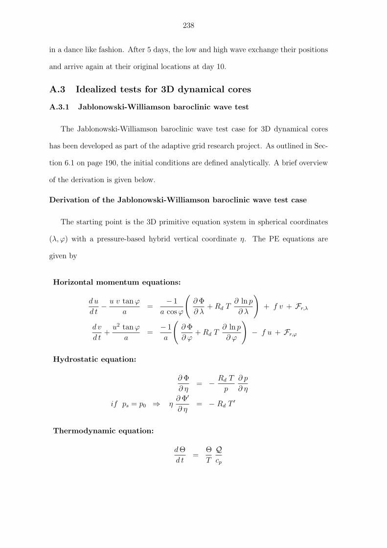
238
in a dance like fashion. After 5 days, the low and high wave exchange their positions
and arrive again at their original locations at day 10.
A.3 Idealized tests for 3D dynamical cores
A.3.1 Jablonowski-Williamson baroclinic wave test
The Jablonowski-Williamson baroclinic wave test case for 3D dynamical cores
has been developed as part of the adaptive grid research project. As outlined in Sec-
tion 6.1 on page 190, the initial conditions are defined analytically. A brief overview
of the derivation is given below.
Derivation of the Jablonowski-Williamson baroclinic wave test case
The starting point is the 3D primitive equation system in spherical coordinates
(λ, ϕ) with a pressure-based hybrid vertical coordinate η. The PE equations are
given by
Horizontal momentum equations:
d u
d t− u v tan ϕ
a=
− 1
a cos ϕ
(∂ Φ
∂ λ+ Rd T
∂ ln p
∂ λ
)+ f v + Fr,λ
d v
d t+
u2 tan ϕ
a=
− 1
a
(∂ Φ
∂ ϕ+ Rd T
∂ ln p
∂ ϕ
)− f u + Fr,ϕ
Hydrostatic equation:
∂ Φ
∂ η= − Rd T
p
∂ p
∂ η
if ps = p0 ⇒ η∂ Φ′
∂ η= − Rd T ′
Thermodynamic equation:
d Θ
d t=
Θ
T
Qcp

239
Continuity equation:
∂
∂ t
(∂ p
∂ η
)+
1
a cos ϕ
∂
∂ λ
(∂ p
∂ ηu)+
1
a cos ϕ
∂
∂ ϕ
(∂ p
∂ η(v cos ϕ)
)+
∂
∂ η
(∂ p
∂ ηη)
= 0
Equation of state for dry air:
p = ρRd T
with:
η =d η
d td
d t() =
∂
∂ t() + (~v∇)()
=∂
∂ t() +
u
a cos ϕ
∂
∂ λ() +
v
a
∂
∂ ϕ() + η
∂
∂ η()
Based on this formulation the goal is to derive a steady state, balanced initial data
set for the model variables u, v, ps, T, Φs where u and v stand for the horizontal wind
components, ps symbolizes the surface pressure, T denotes the temperature field and
Φs is the geopotential of the surface orography. The derivation of such an initial data
set contains several degrees of freedom, e.g. the chosen wind profiles and constant
parameters. Here, the selected profiles and parameters guarantee that the resulting
initial data closely resemble a realistic climatic state and fulfill the symmetric and
static stability criterion. On the other hand, the flow is designed to be baroclinically
and barotropically unstable. The design principles and derivation steps are
1. Assume adiabatic and frictionless atmosphere, set Q and ~F to zero.
2. Choose nondivergent wind field u and v (e.g. as in Section 6.1).
3. Choose constant surface pressure ps, e.g. ps = p0 = 1000 hPa.

240
4. Choose the horizontally averaged temperature profile 〈T (η) 〉. This can easily
be done in z coordinates, e.g. 〈T 〉 = T0 − Γ z where Γ is the vertical tem-
perature gradient. This equation can then be transformed into the p system
(or equivalently into the η− or σ-systems) via integration of the hydrostatic
relationship ∂ pp
= − gRd 〈T 〉 ∂z. It follows z = T0
Γ
(1− (
pp0
)Rd Γ
g
).
5. Derive the geopotential Φ and compute the surface geopotential Φs:
• start with v momentum equation
• assume steady state solution: set d vd t
to zero
• take chosen equation for u, plug it into the momentum equation for v and
integrate (note that ∂ ln ps
∂ ϕ= 0 on η-surfaces)
1
a
∂Φ′
∂ϕ= − u (2 Ω sin ϕ +
u
atan ϕ)
Φ′ is the deviation of the geopotential from a horizontal mean value 〈Φ 〉
• integrate analytically in order to arrive at the expression Φ′ = (. . .) + Φ0
• find integration constant Φ0 using the condition that the deviations vanish
when averaged horizontally
1
4π
∫ 2π
0
∫ π2
−π2
Φ′ cos ϕ dϕ dλ = 0
• calculate: Φ(ϕ, λ, η) = 〈Φ(η) 〉 + Φ′(ϕ, λ, η) where 〈Φ(η) 〉 is the hori-
zontally averaged geopotential. In hydrostatic GCMs, it is only neces-
sary to calculate the surface geopotential Φs which represents the orog-
raphy. Therefore, the horizontally averaged geopotential at the surface
〈Φ(η) 〉 = 〈Φ(ηs) 〉 is set to zero. In general, 〈Φ 〉 can be computed via
〈Φ 〉 = gz(p).

241
6. Derive the temperature T :
• Determine the horizntal temperature deviation T ′ using the hydrostatic
equation (differentiate Φ′)
T ′(λ, ϕ, η) =−η
Rd
∂Φ′(λ, ϕ, η)
∂η
• calculate: T (ϕ, λ, η) = 〈T (η) 〉 + T ′(ϕ, λ, η) where 〈T (η) 〉 is the hori-
zontally averaged temperature discussed in step 4.
In this setup, the initial vertical velocity is zero and the thermodynamic equation
is automatically fulfilled. A baroclinic wave can then be triggered when disturbing
the steady state initial conditions as explained in Section 6.1. All constants are listed
in Appendix C.
High resolution reference solution
The baroclinic wave test case can be used in two configurations. First, model runs
without a perturbation can be performed. They assess how well the model keeps its
initial state which ultimately could break down over time due to the possible accumu-
lation of truncation errors. In this configuration, error norms can be computed using
the initial state as the true solution. Second, when adding the perturbation to the
zonal wind field a complex flow field evolves over time that no longer has an analytic
solution. Therefore, high-resolution runs can serve as the best estimate of the true
reference field. High resolution simulations with the baroclinic wave test case have
been performed with 4 different dynamical cores, namely with the dynamics package
of the weather prediction code GME (German Weather Service DWD) and the three
dynamical cores in the NCAR CCSM/CAM2.0 model framework. Among theses
three NCAR dynamics modules is the NASA/NCAR finite-volume dynamical core.

242
The results of this comparison are presented in Jablonowski and Williamson [2004].
In summary, the high resolution reference simulations converge (see also figure A.16)
and produce very similar 10-day forecasts.
As an example of the reference flow pattern, the results of the NASA/NCAR
finite-volume dynamical core (CAM2 model framework) at the resolution 0.625×0.5
are selected. It is important to note, that this dynamical core is very similar to the
adaptive finite-volume dynamical core. The numerical concepts are identical but
the computational grid in the CAM2 framework is shifted by half a grid length
in longitudinal and meridional direction. This adds one more grid point in the
meridional direction that now includes the two grid boxes centered at the pole points.
The selected horizontal resolutions, e.g. the 0.625 × 0.5 grid, represent a standard
NCAR setting with a slightly finer resolution in the meridional direction. Though,
this resolution is comparable to the finest adapted grid run with a 0.625 × 0.625
grid (Section 6.2 on page 201). 26 vertical levels are chosen (see also Appendix B).
In figure A.16 on the next page snapshots of the surface pressure field in the
Northern Hemisphere at day 8 are presented that have been computed with the
CAM2.0 finite-volume dynamical core at three different horizontal resolutions. This
plot provides a reference for the statically adapted 3D runs in Section 6.2. The
flow has evolved rapidly up to this point and wave breaking processes set in shortly
thereafter.
In addition, figure A.17 on page 244 shows the surface pressure and surface1
temperature field at day 10 for two different horizontal resolutions. The flow fields
have almost converged at these resolutions and only a minor intensification of the low
1Temperature at the lowermost η model level.

243
(a) Resolution 2.5ox2o
0
30
60
90
Lat
itude
0 90 180 270 360
(b) Resolution 1.25ox1o
0
30
60
90
Lat
itude
0 90 180 270 360
(c) Resolution 0.625ox0.5o
0
30
60
90
Lat
itude
0 90 180 270 360Longitude
972 984 996 1008Surface pressure [hPa]
Figure A.16: Surface pressure in the Northern Hemisphere at day 8 for the horizontalresolutions (lon x lat) (a) 2.5×2, (b) 1.25×1 and (c) 0.625×0.5.The contour intervals are 6 hPa.

244
(a)
Surf
ace
pres
sure
, res
olut
ion
1.25
o x1o
-90
-60
-300306090
Latitude
090
180
270
360
Lon
gitu
de
940
960
980
1000
1020
Surf
ace
pres
sure
[hP
a]
(b)
Surf
ace
pres
sure
, res
olut
ion
0.62
5o x0.5
o
-90
-60
-300306090
Latitude
090
180
270
360
Lon
gitu
de
940
960
980
1000
1020
Surf
ace
pres
sure
[hP
a]
240 27
0
270
300
(c)
Surf
ace
tem
pera
ture
(K
), r
esol
utio
n 1.
25o x1
o
0306090 Latitude
090
180
270
360
Lon
gitu
de
240 27
0
270
300
(d)
Surf
ace
tem
pera
ture
(K
), r
esol
utio
n 0.
625o x1
o
0306090 Latitude
090
180
270
360
Lon
gitu
de
Fig
ure
A.1
7:(a
,b)
Surf
ace
pre
ssure
and
(c,d
)su
rfac
ete
mper
ature
inth
eN
orth
ern
Hem
ispher
eat
day
10fo
rth
ehor
izon
tal
reso
luti
ons
(a,c
)1.
25×
1an
d(b
,d)
0.62
5×
0.5
.T
he
conto
ur
inte
rval
sar
e10
hPa
and
10K
,re
spec
tive
ly.

245
pressure system is apparent in the 0.625 × 0.5 plot. In the Southern Hemisphere,
no wave activities develop during the first 10 days, which makes the test ideal for
adaptive mesh simulations.
A.3.2 Polvani baroclinic wave test
An alternative test case for idealized baroclinic wave assessments in 3D dynamical
cores has recently been suggested by Polvani et al. [2004]. The test strategy is similar
to the aforementioned Jablonowski-Williamson test. The Polvani test case also starts
with a steady state initial data set. Baroclinic waves are then triggered by an unbal-
anced temperature perturbation that overlays the temperature field. The forecast
period also covers 10-12 model days. In the Polvani test, the initial conditions are
not entirely based on analytic expressions. Here, numerically approximated integrals
need to be computed for the initial temperature field. The resulting flow pattern
resembles the realistic climatic state only in the Northern Hemisphere whereas the
Southern Hemisphere is held passive.
Figure A.18 on the next page shows the initial conditions for the zonal wind u
and temperature T (see details in Polvani et al. [2004]). In addition, the potential
temperature field and initial temperature perturbation are presented. It must be
noted that the temperature perturbation is placed at (λc, ϕc) = (67.5E, 45N) which
is different from the position mentioned in the publication. Furthermore, the initial
meridional wind v as well as the surface geopotential Φs are zero and the surface
pressure field is set to ps = 1000 hPa.
As before, reference solutions have been computed with the NASA/NCAR CAM2.0
finite-volume dynamical core with 26 vertical levels. Examples of the surface pressure
field in the Northern Hemisphere at day 8 and day 10 are shown in figure A.19. These

246
15
15
30
(a) Zonal wind (m/s)
0.0
0.2
0.4
0.6
0.8
1.0
Eta
-90 -60 -30 0 30 60 90Latitude
225
225
240
240
255
270
285
(b) Temperature (K)
0.0
0.2
0.4
0.6
0.8
1.0
Eta
-90 -60 -30 0 30 60 90Latitude
270
285
300
320
340
360400
600 1200
(c) Potential temperature (K)
0.0
0.2
0.4
0.6
0.8
1.0
Eta
-90 -60 -30 0 30 60 90Latitude
0.30.3 0.6
(d) Temperature perturbation (K)
15
30
45
60
75
Lat
itude
20 40 60 80 100Longitude
Figure A.18: Initial (a) zonal wind, (b) temperature, (c) potential temperature and(d) temperature perturbation that is added to the temperature field ateach level. Contour intervals are (a) 5 ms−1, (b) 5 K, (c) 5 K (exceptat upper levels) and (d) 0.1 K. The zero contour is omitted.

247
(a)
Day
8, u
nifo
rm r
esol
utio
n 2.
5o x2o
0306090 Latitude
090
180
270
360
Lon
gitu
de
920
940
960
980
1000
1020
1040
Surf
ace
pres
sure
[hP
a]
(b)
Day
10,
uni
form
res
olut
ion
2.5o x2
o
0306090 Latitude
090
180
270
360
Lon
gitu
de
920
940
960
980
1000
1020
1040
Surf
ace
pres
sure
[hP
a]
(c)
Day
8, u
nifo
rm r
esol
utio
n 1.
25o x1
o
0306090 Latitude
090
180
270
360
Lon
gitu
de
920
940
960
980
1000
1020
1040
Surf
ace
pres
sure
[hP
a]
(d)
Day
10,
uni
form
res
olut
ion
1.25
o x1o
0306090 Latitude
090
180
270
360
Lon
gitu
de
920
940
960
980
1000
1020
1040
Surf
ace
pres
sure
[hP
a]
Fig
ure
A.1
9:Surf
ace
pre
ssure
fiel
ds
inth
eN
orth
ern
Hem
ispher
efo
rtw
odiff
eren
tm
odel
day
sat
the
reso
luti
ons
2.5×
2(t
opro
w,a
&b)
and
1.25×
1(b
otto
mro
w,c
&d).
(a,c
)sh
owm
odel
day
8,(b
,d)
day
10.
Con
tour
inte
rval
sar
e10
hPa.

248
two days illustrate the baroclinic wave shortly before and after the wave breaking
event. Subfigures A.19 (c,d) represent an almost converged solution (see also conver-
gence discussion for this test case in Polvani et al. [2004]. Here they are considered
the reference solution for the adaptive run in Section 6.3. Higher resolution runs
with a uniform 0.625× 0.5 grid have also been performed with the CAM2.0 finite-
volume dynamical core (not shown). The figures are almost indistinguishable from
subfigures (c,d) although a slight intensification of the main low pressure system can
be observed.

249
APPENDIX B
Vertical coordinate
The Eulerian reference frame of the NASA/NCAR dynamical core is based on the
hybrid, orography following η-coordinate in the vertical direction (see also Simmons
and Burridge [1981]. It is comprised of a pure pressure and the so-called σ-component
with σ = pps
. Here, p and ps symbolize the pressure and surface pressure, respectively.
The pressure at any model level η is given by
p(λ, ϕ, η, t) = a(η) + b(η) ps(λ, ϕ, t)
where the coefficients a(η) and b(η) are solely height-dependent and provided in
tabular form (see table B.1).
In the discrete system, the vertical direction is subdivided into Nlev model levels
which are bounded by Nlev + 1 interfaces, here also viewed as Lagrangian surfaces.
This leads to the following discrete representation
pk+ 12
= ak+ 12
+ bk+ 12ps ,
with k = 0, 1, 2, · · ·Nlev. The index 12
denotes the positions of the level interfaces,
the index Nlev +1 symbolizes the model level at the ground. In order to ensure, that
this lowermost Lagrangian surface follows the actual topography in the system the

250
following boundary conditions are imposed
aNlev+ 12
= 0 and bNlev+ 12
= 1 .
This guarantees that the pressure at the lowermost interface is the actual surface
pressure at any given location.
If the pressure needs to be evaluated at the center of a model layer, then the
pressure values can be linearly interpolated based on the surrounding surfaces
pk =1
2(pk+ 1
2+ pk− 1
2) .
Furthermore, the pressure thickness ∆pk in the Eulerian reference frame is defined
by
∆pk = pk+ 12− pk− 1
2.
and the thickness in terms of the time-invariant η levels is given by
ηk+ 12
=ak+ 1
2
p0
+ bk+ 12
where the parameter p0 symbolizes a constant reference surface pressure, usually set
to 1000hPa or 1013.25hPa. Here the lower boundary condition is ηNlev+ 12
= 1.
If η values are required that lie in between two model interfaces, then they can
be computed via linear interpolations
η = ηk+ 12
+(p− pk+ 1
2)(ηk+ 1
2− ηk− 1
2)
(pk+ 12− pk− 1
2)
for pk− 12≤ p ≤ pk+ 1
2.
Table B.1 on the facing page shows the vertical coefficients ak+ 12
and bk+ 12
that
have been used for the 3D dynamical core model runs. The table contains the
Nlev+1 = 27 coefficients for the Lagrangian model surfaces that enclose the Nlev = 26
model layers. These model levels have been derived for NCAR’s atmosphere model
CAM and represent the current 26 standard layers for climate simulations with CAM.

251
26 model layersLevel k
ak+ 12
(Pa) bk+ 12
0 219.4067 0.00000000
1 489.5209 0.00000000
2 988.2418 0.00000000
3 1805.201 0.00000000
4 2983.724 0.00000000
5 4462.334 0.00000000
6 6160.587 0.00000000
7 7851.243 0.00000000
8 7731.271 0.01505309
9 7590.131 0.03276228
10 7424.086 0.05359622
11 7228.744 0.07810627
12 6998.933 0.10694110
13 6728.574 0.14086370
14 6410.509 0.18077200
15 6036.322 0.22772200
16 5596.111 0.28295620
17 5078.225 0.34793640
18 4468.96 0.42438220
19 3752.191 0.51431680
20 2908.949 0.62012020
21 2084.739 0.72353550
22 1334.443 0.81767680
23 708.499 0.89621530
24 252.136 0.95347610
25 0. 0.98511220
26 0. 1.00000000
Table B.1: Vertical coefficients for the 26 model levels. The parameter ak+ 12
denotes
the pure pressure component (in Pa), bk+ 12
defines the σ part of the hybridη-system.


253
APPENDIX C
Symbols and Acronyms
Model variables
σ vertical coordinate (σ = pps
)
η vertical coordinate (hybrid σ-p system)
ϕ geographical latitude in spherical coordinates (−π2≤ ϕ ≤ π
2)
λ geographical longitude in spherical coordinates (0 ≤ λ ≤ 2π)
u zonal wind (m/s)
v meridional wind (m/s)
h geopotential height in m (shallow water system)
hs height of the orography in m (shallow water system)
T temperature (K)
Θ potential temperature (K), Θ = T(
p0
p
)κ
ps surface pressure (Pa)
p pressure (Pa)
δp pressure thickness of a Lagrangian layer (Pa)
ρ density (kgm−3), ρ = pRd T
Φ geopotential (m2/s2)
Φs surface geopotential (m2/s2)

254
ζ relative vorticity (s−1), ζ = ~k · (∇× ~v)
D divergence (s−1), D = ∇ · ~v
〈 〉 horizontal average
( )′ deviation from the horizontal average
Model parameters for the idealized test case
u0 maximum wind speed of the zonal jet u0 = 35 m/s
η0 center of the jet stream η0 = 0.252
ηt tropopause level ηt = 0.2
ηs surface level ηs = 1.0
Γ lapse rate of the horizontally averaged temperature Γ = 0.005 K/m
p0 reference pressure at the ground p0 = 100000 Pa
T0 reference temperature T0 = 288 K
∆T parameter to adjust the temperature at upper levels ∆T = 480000 K
(λc, ϕc) center of the Gaussian perturbation (λc, ϕc) = (π9, 2 π
9)
R radius of the Gaussian perturbation R = a10
Physical constants and parameters
a radius of the earth a = 6371229 m
Ω angular velocity Ω = 7.29211 ∗ 10−5 s−1
f Coriolis parameter f = 2Ω sin ϕ
Rd gas constant for dry air Rd = 287.0 J/kgK
cp specific heat at constant pressure cp = 1004 J/kgK
κ κ = Rd
cp= 2
7

255
g gravitational acceleration g = 9.80616 m/s2
Acronyms
AMIP Atmospheric Model Intercomparison Project conducted by LLNL
AMR Adaptive Mesh Refinement
AMR++ AMR class library in the software package Overture
AMRCLAW Software package: Berger-Oliger AMR library and CLAWPACK
API Application Programmable Interface
ARPEGE Numerical Weather Prediction model at Meteo France
BATS-R-US Block Adaptive Tree Solar-wind Roe Upwind Scheme, UM
C, C++ Programming languages
CAM Community Atmosphere Model, dynamics package for CCSM
CCSM Community Climate System Model, developed at NCAR
CFD Computational Fluid Dynamics
CFL Courant-Friedrichs-Lewy condition for numerical stability
CHOMBO AMR software infrastructure
CLAWPACK Numerical toolbox ’Conservation LAW PACKage’
DAGH AMR software library (Distributed Adaptive Grid Hierarchy)
DWD German Weather Service, Offenbach, Germany
ECMWF European Centre for Medium-Range Weather Forecasts, England
FFT Fast Fourier Transformation
Fortran Programming language, Fortran77 or Fortran90
GCM General Circulation Model
GME Global weather prediction model at DWD

256
GSFC Goddard Space Flight Center, Greenbelt, Maryland, USA
HDF5 Hierachical Data Format: self-describing data convention
IFS Integrated Forecasting System: ECMWF weather prediction code
KE Kinetic Energy
LBNL Lawrence Berkeley National Laboratory, Berkeley, CA, USA
LLNL Lawrence Livermore National Laboratory, Livermore, CA, USA
MC Monotonized central-difference limiter for finite-volume methods
MHD Magnetohydrodynamics
MPI Message Passing Interface, parallel communication library
NASA National Aeronautics and Space Administration, USA
NCAR National Center for Atmospheric Research, Boulder, CO, USA
NetCDF Portable data format, developed by NCAR
OpenMP Communication constructs for shared memory architectures
Overture Object-oriented library for overlapping grids for PDEs
PE Primitive Equations
PDE Partial Differential Equation
PARAMESH AMR software library for block-structured data
PPM Piecewise Parabolic Method
PV Potential vorticity
PYRAMID AMR software library for unstructured data
SAMRAI Structured AMR Application Infrastructure
SHMEM Parallel communication library (designed by CRAY)
SL semi-Lagrangian approach
T42 spectral resolution of a GCM, ≈ 2.8 × 2.8 grid
TE Total Energy

BIBLIOGRAPHY
257

258
BIBLIOGRAPHY
Alapaty, K., R. Mathur, and T. Odman, Intercomparison of spatial interpo-lation schemes for use in nested grid models, Monthly Weather Review , 126 ,243–249, 1998.
Allen, D. J., A. R. Douglass, R. B. Rood, and P. D. Guthrie, Application of amonotonic upstream-biased transport scheme to three-dimensional constituenttransport calculations, Monthly Weather Review , 119 , 2456–2464, 1991.
Almgren, A. S., J. B. Bell, P. Colella, L. H. Howell, and M. L. Welcome, Aconservative adaptive projection method for the variable density incompressibleNavier-Stokes equations, Journal of Computational Physics , 142 , 1–46, 1998.
Arakawa, A., and V. R. Lamb, Computational design of the basic dynamicalprocess of the UCLA general circulation model, in Methods in ComputationalPhysics , edited by J. Chang, pp. 173–265, Academic Press, 1977.
Bacon, D. P., et al., A dynamically adapting weather and dispersionmodel: The Operational Multiscale Environment Model with Grid Adaptivity(OMEGA), Monthly Weather Review , 128 , 2044–2076, 2000.
Bacon, D. P., et al., Dynamically adapting unstructured triangular grids: Anew paradigm for geophysical fluid dynamics modeling, Proceedings of the In-dian Academy of Science, 2002, Accepted for publication. Pre-print availableat URL: http://vortex.atgteam.com/papers/.
Barros, S. R. M., and C. I. Garcia, A global semi-implicit semi-Lagrangianshallow-water model on locally refined grids, Monthly Weather Review , 132 ,53–65, 2004.
Bates, J., and Y. Li, Simulation of stratospheric vortex erosion using threeglobal shallow water numerical models, in Numerical Methods in Atmosphericand Oceanic Modelling: The Andre J. Robert Memorial Volume of Atmos.-Ocean, edited by J. Cote, pp. 55–73, 1997.
Bates, J. R., F. H. M. Semazzi, and R. W. Higgins, Integration of the shallowwater equations on the sphere using a vector semi-Lagrangian scheme with amultigrid solver, Monthly Weather Review , 118 , 1615–1627, 1990.

259
Behrens, J., Adaptive Semi-Lagrange-Finite-Elemente-Methode zur Losung derFlachwassergleichungen. Implementierung und Parallelisierung, Ph.D. thesis,Universitat Bremen, Germany, 1995, Fachbereich Mathematik und Informatik.
Behrens, J., An adaptive semi-Lagrangian advection scheme and its paralleliza-tion, Monthly Weather Review , 124 , 2386–2395, 1996.
Behrens, J., Atmospheric and ocean modelling with an adaptive finite elementsolver for the shallow-water equations, Applied Numerical Mathematics , 26 ,217–226, 1998.
Behrens, J., and J. Zimmermann, Parallelizing an unstructured grid genera-tor with a space-filling curce approach, in Euro-Par 2000, Lecture Notes inComputer Science, edited by A. Bode, vol. 1900, pp. 815–823, Springer-VerlagBerlin Heidelberg, 2000.
Behrens, J., K. Dethloff, W. Hiller, and A. Rinke, Evolution of small-scalefilaments in an adaptive advection model for idealized tracer transport, MonthlyWeather Review , 128 , 2976–2982, 2000.
Berger, M., Adaptive mesh refinement software for hyperbolic con-servation laws, 2003, Courant Institute, New York, N.Y. URL:http://cs.nyu.edu/cs/faculty/berger/amrsoftware.html.
Berger, M., and R. J. LeVeque, Adaptive mesh refinement using wave-propagation algorithms for hyperbolic systems, Siam J. Num. Anal., 35 (6),2298–2316, 1998.
Berger, M., and J. Oliger, Adaptive mesh refinement for hyperbolic partialdifferential equations, Journal of Computational Physics , 53 , 484–512, 1984.
Berger, M. J., and P. Colella, Local adaptive mesh refinement for shock hydro-dynamics, Journal of Computational Physics , 82 (1), 64–84, 1989.
Blayo, E., and L. Debreu, Adaptive mesh refinement for finite-difference oceanmodels: First experiments, Journal of Physical Oceanography , 29 , 1239–1250,1999.
Blayo, E., L. Debreu, G. Mounie, and D. Trystram, Dynamic load balancingfor ocean circulation model with adaptive meshing, in Euro-Par 1999, LectureNotes in Computer Science, edited by P. Amestoy, vol. 1685, pp. 303–312,Springer-Verlag Berlin Heidelberg, 1999.
Boer, G. J., and B. Denis, Numerical covergence of the dynamics of a GCM,Climate Dynamics , 13 , 359–374, 1997.
Boville, B. A., Sensitivity of simulated climate to model resolution, Journal ofClimate, 4 , 469–485, 1991.

260
Boybeyi, Z., N. N. Ahmad, D. P. Bacon, T. J. Dunn, M. S. Hall, P. C. S.Lee, and R. A. Sarma, Evaluation of the Operational Multiscale EnvironmentModel with Grid Adaptivity against the European tracer experiment, Journalof Applied Meteorology , 40 , 1541–1558, 2001.
Boyle, J., K. Hodges, I. Simmonds, and D. Jones, AMIP II Diagnostic Subpro-ject No. 3: Statistics of transient circulation systems, 1998, URL http://www-pcmdi.llnl.gov/amip/DIAGSUBS/sp3.html.
Boyle, J. S., Sensitivity of dynamical quantities to horizontal resolution for aclimate simulation using the ECMWF (Cycle 33) model, Journal of Climate,6 , 796–815, 1993.
Brackbill, J. U., and J. S. Saltzmann, Adaptive zoning and singular problemsin two dimensions, Journal of Computational Physics , 46 , 342–368, 1982.
Brown, D., W. Henshaw, and D. Quinlan, Overview of Overture,2003, Lawrence Livermore National Laboratory, Livermore, CA. URL:http://www.llnl.gov/CASC/Overture.
Carpenter, R. L., K. K. Droegemeier, P. R. Woodward, and C. E. Hane, Appli-cation of the Piecewise Parabolic Method (PPM) to meteorological modeling,Monthly Weather Review , 118 , 586–612, 1990.
CCSM, Eighth annual CCSM workshop: Atmosphere Model WorkingGroup Report, 2003, 25 June 2003, Breckenridge, CO. Available atURL: http://www.ccsm.ucar.edu/working groups/Atmosphere/reports/
062503.html.
Cheong, H.-B., Application of double Fourier series to the shallow-water equa-tions on the sphere, Journal of Computational Physics , 155 , 1–27, 2000.
Chesshire, G., and W. D. Henshaw, Composite overlapping meshes for thesolution of partial differential equations, Journal of Computational Physics ,90 , 1–64, 1990.
Clark, T. L., and R. D. Farley, Severe downslope windstorm calculations in twoand three spatial dimensions using anelastic interactive grid nesting: A possiblemeachanism for gustiness, Journal of the Atmospheric Sciences , 41 (3), 329–350, 1984.
Colella, P., and P. R. Woodward, The Piecewise Parabolic Method (PPM) forgas-dynamical simulations, Journal of Computational Physics , 54 , 174–201,1984.
Cote, J., M. Roch, A. Stanisforth, and L. Fillion, A variable-resolution semi-Lagrangian finite-element global model of the shallow water equations, MonthlyWeather Review , 121 , 231–243, 1993.

261
Cote, J., S. Gravel, A. Methot, A. Patoine, M. Roch, and A. Stanisforth,The operational CMC-MRB Global Environmental Multiscale (GEM) model.Part I: Design considerations and formulation, Monthly Weather Review , 126 ,1373–1395, 1998.
Courtier, P., and J. F. Geleyn, A global numerical weather prediction modelwith variable resolution: Application to the shallow water equations, Quart.J. Royal Meteor. Soc., 114 , 1321–1346, 1988.
Courtier, P., and M. Naughton, A pole problem in the reduced Gaussian grid,Quart. J. Royal Meteor. Soc., 120 , 1389–1407, 1994.
Davies, H. C., A lateral boundary formulation for multi-level prediction models,Quart. J. Royal Meteor. Soc., 102 , 405–418, 1976.
Dennis, J. M., Partitioning with space-filling curces on the cubed sphere, inProceedings of the International Parallel and Distributed Processing Symposium(IPDPS), Nice, France, 2003, Workshop on Massively Parallel Processing atIPDPS.
Dey, C. H., A note on global forecasting with the Kurihara grid, MonthlyWeather Review , 97 , 597–601, 1969.
Dietachmayer, G. S., and K. K. Droegemeier, Applications of continuous dy-namic grid adaptation techniques to meteorological modeling. Part I: Basicformulation and accuracy, Monthly Weather Review , 120 , 1675–1706, 1992a.
Dietachmayer, G. S., and K. K. Droegemeier, Applications of continuous dy-namic grid adaptation techniques to meteorological modeling. Part II: Effi-ciency, Monthly Weather Review , 120 , 1707–1722, 1992b.
Doswell, C. A., A kinematic analysis associated with a nondivergent flow, Jour-nal of the Atmospheric Sciences , 41 , 1242–1248, 1984.
Duffy, P. B., B. Govindasamy, J. Milovich, K. Taylor, M. Wehner, A. Lam-ont, and S. Thompson, High resolution simulations of global climate, Part 1:Present climate, Climate Dynamics , 21 (5-6), 2003.
Durran, D. R., Numerical Methods for Wave Equations in Geophysical FluidDynamics , Springer, 1999, ISBN 0-387-98376-7.
Falkovich, A. I., A. P. Khain, and I. Ginis, The influence of air-sea interactionon the development and motion of a tropical cyclone: Numerical experimentswith a triply nested model, Meteorol. Atmos. Phys., 55 , 167–184, 1995.
Fournier, A., M. A. Taylor, and J. J. Tribbia, Spectral ele-ment method part I: Numerical algorithms, in Proc. 8th AnnualConf. CFD Soc. Canada, pp. 173–180, 2000, Available on-line atftp://ftp.cgd.ucar.edu/pub/fournier/publications/AlNu.ps.gz.

262
Fournier, A., M. A. Taylor, and J. J. Tribbia, The spectral element atmosphericmodel: High-resolution parallel computation and response to regional forcing,Monthly Weather Review , 132 , 726–748, 2004.
Fox, A. D., and S. J. Maskell, Two-way interactive nesting of primitive equationocean models with topography, Journal of Physical Oceanography , 25 , 2977–2996, 1995.
Fox-Rabinovitz, M., and R. S. Lindzen, Numerical experiments on consistenthorizontal and vertical resolution for atmospheric models and observing sys-tems, Monthly Weather Review , 121 , 264–271, 1993.
Fox-Rabinovitz, M. S., G. L. Stenchikov, M. J. Suarez, and L. L. Takacs, Afinite-difference GCM dynamical core with a variable-resolution stretched grid,Monthly Weather Review , 125 , 2943–2968, 1997.
Fox-Rabinovitz, M. S., L. L. Takacs, R. C. Govindaraju, and M. J. Suarez, Avariable-resolution stretched grid general circulation model: Regional climatesimulation, Monthly Weather Review , 129 , 453–469, 2001.
Fulton, S. R., A comparison of multilevel adaptive methods for hurricane trackprediction, Electronic Transactions on Numerical Analysis , 6 , 120–132, 1997.
Fulton, S. R., An adaptive multigrid barotropic tropical cyclone track model,Monthly Weather Review , 129 , 138–151, 2001.
Gates, W. L., and C. A. Riegel, A study of numerical errors in the integrationof barotropic flow on a spherical grid, Journal of Geophysical Research, 67 (2),773–784, 1962.
Ginis, I., R. A. Richardson, and L. M. Rothstein, Design of a multiply nestedprimitive equation ocean model, Monthly Weather Review , 126 , 1054–1079,1998.
Giraldo, F., The Lagrange-Galerkin method for the two-dimensional shallowwater equations on adaptive grids, International Journal for Numerical Meth-ods in Fluids , 33 , 789–832, 2000a.
Giraldo, F., Lagrange-Galerkin methods on spherical geodesic grids: the shal-low water equations, Journal of Computational Physics , 160 , 336–368, 2000b.
Giraldo, F., and T. E. Rosmond, A scalable spectral element eulerian atmo-spheric model (SEE-AM) for NWP: Dynamical core tests, Monthly WeatherReview , 132 , 133–153, 2004.
Giraldo, F., J. S. Hesthaven, and T. Wartburton, Nodal high-order discontinousgalerkin methods for the shallow water equations, Journal of ComputationalPhysics , 181 , 499–525, 2002.

263
Gopalakrishnan, S. G., et al., An operational multiscale hurricane forecastingsystem, Monthly Weather Review , 130 , 1830–1847, 2002.
Gravel, S., and A. N. Staniforth, Variable resolution and robustness, MonthlyWeather Review , 120 , 2633–2639, 1992.
Griebel, M., and G. Zumbusch, Parallel multigrid in an adaptive PDE solverbased on hashing and space-filling curves, Parallel Computing , 25 , 827–843,1999.
Haltiner, G. J., and R. T. Williams, Numerical Prediction and Dynamic Me-teorology , John Wiley & Sons, 1980, ISBN 0-471-05971-4.
Hansen, K. C., G. Toth, A. Ridley, and D. DeZeeuw, BATS-R-US Design,Code Version 7.5.0 , 2002, University of Michigan, Ann Arbor, Departmentof Atmospheric, Oceanic and Space Sciences, Center for Space EnvironmentModeling. URL: http://csem.engin.umich.edu/docs/DESIGN.pdf.
Hardiker, V., A global numerical weather prediction model with variable reso-lution, Monthly Weather Review , 125 , 59–73, 1997.
Heikes, R., and D. A. Randall, Numerical integration of the shallow waterequations on a twisted icosahedral grid. Part I: Basic design and results oftests, Monthly Weather Review , 123 , 1862–1880, 1995.
Held, I. M., and M. J. Suarez, A proposal for the intercomparison of the dynam-ical cores of atmospheric general circulation models, Bulletin of the AmericanMeteorological Society , 75 (10), 1825–1830, 1994.
Hess, R., Dynamically adaptive multigrid on parallel computers for a semi-implicit discretization of the shallow-water equations, Tech. Rep. No. 9, GMD– German National Research Center for Information Technology, St. Augustin,Germany, 1999.
Hodges, K. I., A general method for tracking analysis and its application tometeorological data, Monthly Weather Review , 122 , 2573–2586, 1994.
Hodges, K. I., Feature tracking on the unit sphere, Monthly Weather Review ,123 , 3458–3465, 1995.
Holton, J. R., An Introduction to Dynamic Meteorology , Academic Press, Inc.,1992, ISBN 0-12-354355-X.
Hornung, R., A. Wissink, S. Smith, and N. Elliott, SAMRAI -structured adaptive mesh refinement application infrastructure, 2003,Lawrence Livermore National Laboratory, Livermore, CA. URL:http://www.llnl.gov/CASC/SAMRAI/.

264
Hortal, M., and A. J. Simmons, Use of reduced grids in spectral models,Monthly Weather Review , 119 , 1057–1074, 1991.
Hoskins, B. J., and A. J. Simmons, A multi-layer spectral model and the semi-implicit method, Quart. J. R. Met. Soc., 101 , 637–655, 1975.
Hubbard, M. E., and N. Nikiforakis, A three-dimensional, adaptive, Godunov-type model for global atmospheric flows, Monthly Weather Review , 131 , 1848–1864, 2003.
Iselin, J. P., J. M. Prusa, and W. J. Gutowski, Dynamic grid adaptation usingthe MPDATA scheme, Monthly Weather Review , 130 , 1026–1039, 2002.
Jablonowski, C., and D. L. Williamson, A baroclinic instabilitiy test case foratmospheric model dynamical cores, 2004, In preparation.
Jakob, R., J. J. Hack, and D. L. Williamson, Solutions to the shallow-watertest set using the spectral transform method, Tech. Rep. NCAR/TN-388+STR,National Center for Atmospheric Research, Boulder, Colorado, 1993.
Jakob-Chien, R., J. J. Hack, and D. L. Williamson, Spectral transform solu-tions to the shallow water test set, Journal of Computational Physics , 119 ,164–187, 1995.
Janjic, T., Comments on ’A finite volume integration method for computingpressure gradient forces in general vertical coordinates’ by Shian-Jiann Lin(July B, 1997, 123, 1749–1762), Quart. J. Royal Meteor. Soc., 124 , 2527–2529,1998.
Jeong, J., and F. Hussain, On the identification of a vortex, J. Fluid Mech.,285 , 69–94, 1995.
Jones, D. A., and I. Simmonds, A climatology of southern hemisphere extrat-ropical cyclones, Climate Dynamics , 9 , 131–145, 1993.
Jones, R. W., A nested grid for a three-dimensional model of a tropical cyclone,Journal of the Atmospheric Sciences , 34 , 1528–1553, 1977.
Juckes, M. N., and M. E. McIntyre, A high-resolution one-layer model of break-ing planetary waves in the stratosphere, Nature, 328 , 590–596, 1987.
Kalnay-Rivas, E., A. Bayliss, and J. Storch, The 4th GISS model of the globalatmosphere, Beitrage zur Physik der Atmosphare, 50 , 299–311, 1977.
Kessler, M., Development and analysis of an adaptive transport scheme, At-mospheric Environment , 33 (15), 2347–2360, 1999.
Konig, W., R. Sausen, and F. Sielmann, Objective identification of cyclones inGCM simulations, Journal of Climate, 6 , 2217–2231, 1993.

265
Kurihara, Y., Numerical integration of the primitive equations on a sphericalgrid, Monthly Weather Review , 93 , 399–415, 1965.
Kurihara, Y., and M. A. Bender, Use of a movable nested-mesh model fortracking a small vortex, Monthly Weather Review , 108 , 1792–1809, 1980.
Kurihara, Y., and L. Holloway, Numerical integration of a nine-level globalprimitive equations model formulated by the box method, Monthly WeatherReview , 95 , 509–530, 1967.
Kurihara, Y., G. J. Tripoli, and M. A. Bender, Design of a movable nested-meshprimitive equation model, Monthly Weather Review , 107 , 239–249, 1979.
Lambert, S. J., A cyclone climatology of the Canadian Centre General Circu-lation Model, Journal of Climate, 1 , 109–115, 1988.
Lanser, D., J. G. Blom, and J. G. Verwer, Spatial discretization of the shal-low water equations in spherical geometry using Osher’s scheme, Journal ofComputational Physics , 165 , 542–564, 2000.
Layton, A. T., Cubic spline collocation method for the shallow water equationson the sphere, Journal of Computational Physics , 179 , 578–592, 2002.
Layton, A. T., and W. F. Spotz, A semi-Lagrangian double Fourier method forthe shallow water equations on the sphere, Journal of Computational Physics ,189 , 180–196, 2003.
Leonard, S. R., J. Turner, and A. V. D. Wal, An assessment of three automaticdepression tracking systems, Meteorol. Appl., 6 , 173–183, 1999.
Leslie, L. M., and R. J. Purser, Three dimensional mass-conserving semi-Lagrangian schemes employing forward trajectories, Monthly Weather Review ,123 , 2551–2566, 1995.
LeVeque, R., and M. Berger, AMRCLAW: A synthesis ofCLAWPACK with marsha berger’s adaptive mesh refinementcodes, 2003, University of Washington, Seattle, WA. URL:http://www.amath.washington.edu/˜rjl/amrclaw/.
LeVeque, R. J., Finite Volume Methods for Hyperbolic Problems , CambridgeUniversity Press, 2002, ISBN 0-521-00924-3.
Ley, G. W., and R. L. Elsberry, Forecasts of typhoon Irma using a nested-gridmodel, Monthly Weather Review , 104 , 1154–1161, 1976.
Lin, S.-J., A finite volume integration method for computing pressure gradientforces in general vertical coordinates, Quart. J. Royal Meteor. Soc., 123 , 1749–1762, 1997.

266
Lin, S.-J., The flux-form semi-Lagrangian transport scheme and its applicationsin atmospheric models, in MPI Workshop on Conservative Transport Schemes,Report No. 265 , edited by B. Machenhauer, pp. 54–64, Max-Planck-Institutfur Meteorologie, 1998a.
Lin, S.-J., Reply to comments by T. Janjic on ‘A finite volume integrationmethod for computing pressure gradient forces in general vertical coordinates’(July B, 1997, 123, 1749–1762), Quart. J. Royal Meteor. Soc., 124 , 2531–2533,1998b.
Lin, S.-J., and R. B. Rood, Multidimensional flux-form semi-Lagrangian trans-port scheme, Monthly Weather Review , 124 , 2046–2070, 1996.
Lin, S.-J., and R. B. Rood, An explicit flux-form semi-Lagrangian shallowwater model on the sphere, Quart. J. Royal Meteor. Soc., 123 , 2477–2498,1997.
Lin, S.-J., W. C. Chao, Y. C. Sud, and G. K. Walker, A class of the vanLeer-type transport schemes and its application to the moisture transport in ageneral circulation model, Monthly Weather Review , 122 , 1575–1593, 1994.
Lin, S.-J., R. B. Rood, and K.-S. Yeh, Development of the NASA finite-volumedynamical core for global models, 2001, Internal report, NASA Goddard SpaceFlight Center, Greenbelt, Maryland.
Lindzen, R. S., and M. Fox-Rabinovitz, Consistent vertical and horizontal res-olution, Monthly Weather Review , 117 , 2575–2583, 1989.
Lou, J. Z., and C. D. Norton, PYRAMID – unstructured adaptive meshrefinement, 1999, NASA Jet Propulsion Laboratory, Pasadena, CA. URL:http://www-hpc.jpl.nasa.gov/APPS/AMR/.
MacNeice, P., K. Olson, C. Mobarry, R. de Fainchtein, andC. Packer, PARAMESH 3.0 – structured adaptive mesh refinement,2003, NASA Goddard Space Flight Center, Greenbelt, MD. URL:http://ct.gsfc.nasa.gov/paramesh/Users manual/amr.html.
Majewski, D., D. Liermann, P. Prohl, B. Ritter, M. Buchhold, T. Hanisch,G. Paul, W. Wergen, and J. Baumgardner, The operational global icosahedral-hexagonal gridpoint model GME: Description and high-resolution tests,Monthly Weather Review , 130 , 319–338, 2002.
McDonalds, A., and J. R. Bates, Semi-Lagrangian integration of a gridpointshallow-water model on the sphere, Monthly Weather Review , 117 , 130–137,1989.
McGregor, J. L., Semi-Lagrangian advection on conformal-cubic grids, MonthlyWeather Review , 124 , 1311–1322, 1996.

267
McGregor, J. L., and J. J. Katzfey, NWP experiments with a variable-resolution conformal-cubic primitive equations model, in Research Activitiesin Atmospheric and Oceanic Modelling , edited by A. Staniforth, pp. 3.20–3.21,CAS/JSC Working Group on Numerical Experimentation, WMO/TD–No. 865,1998, Report No. 27.
Miyakoda, K., and A. Rosati, One-way nested grid models: The interfaceconditions and the numerical accuracy, Monthly Weather Review , 105 , 1092–1107, 1977.
Monaco, A. V., and R. T. Williams, An atmospheric global prediction modelusing a modified Arakawa differencing scheme, Tech. rep., Naval PostgraduateSchool, Monterey, CA, 1975, NPS-51WU75041.
Murray, R. J., and I. Simmonds, A numerical scheme for tracking cyclonecenters from digital data. Part I: Dvelopment and operation of the scheme,Aust. Meteorol. Mag., 39 , 155–166, 1991.
Nair, R., J. Cote, and A. Stanisforth, Cascade interpolation for semi-Lagrangian advection over the sphere, Quart. J. Royal Meteor. Soc., 125 ,1445–1468, 1999.
Nair, R. D., and B. Machenhauer, The mass-conservative cell-integrated semi-Lagrangian advection scheme on the sphere, Monthly Weather Review , 130 ,649–667, 2002.
Odman, M. T., R. Mathur, K. Alapaty, R. K. Srivastava, D. S. McRae, andR. J. Yamartino, Nested and adaptive grids for multiscale air quality modeling,in Next generation environmental models and computational methods , editedby G. Delic, and M. F. Wheeler, pp. 59–68, Society for Industrial and AppliedMathematics (SIAM), 1997.
Oehmke, R., High performance dynamic array structures, Ph.D. thesis, Univer-sity of Michigan, Ann Arbor, USA, 2004, Department of Electrical Engineeringand Computer Science.
Oehmke, R., and Q. F. Stout, Parallel adaptive blocks on a sphere, in Proc.11th SIAM Conference on Parallel Processing for Scientific Computing , 2001,URL: http://www.eecs.umich.edu/˜qstout/pap/SIAMPP01.ps.
Parashar, M., and J. C. Browne, System engineering for high per-formance computing software: The HDDA/DAGH infrastructurefor implementation of parallel structured adaptive mesh refine-ments, in Structured Adaptive Mesh Grid Methods: IMA Volumesin Mathematics and its Applications , Springer-Verlag, 1999, URL:http://www.caip.rutgers.edu/˜parashar/Personal/pubs.html.

268
Phillips, N. A., Numerical integration of the primitive equations on the hemi-sphere, Monthly Weather Review , pp. 333–345, 1959.
Polvani, L. M., and R. Saravanan, The three-dimensional structure of breakingrossby waves in the polar wintertime stratosphere, Journal of the AtmosphericSciences , 57 , 3663–3685, 2000.
Polvani, L. M., R. K. Scott, and S. J. Thomas, Numerically converged solutionsof the global primitive equations for testing the dynamical core of atmosphericGCMs, Monthy Weather Review , 2004, Accepted for publication.
Prusa, J. M., and P. K. Smolarkiewicz, An all-scale anelastic model for geo-physical flows: Dynamic grid deformation, Journal of Computational Physics ,190 (2), 601–622, 2003.
Purser, R. J., The filtering of meteorological fields, Journal of Climate andApplied Meteorology , 26 , 1764–1769, 1987.
Purser, R. J., Degradation of numerical differencing caused by Fourier filteringat high latitudes, Monthly Weather Review , 116 , 1057–1066, 1988a.
Purser, R. J., Accurate numerical differencing near a polar singularity skippedgrid, Monthly Weather Review , 116 , 1067–1076, 1988b.
Purser, R. J., and L. M. Leslie, An efficient interpolation procedure for high-order three-dimensional semi-Lagrangian models, Monthly Weather Review ,119 , 2492–2498, 1991.
Rancic, M., Semi-Lagrangian piecewise biparabolic scheme for two-dimensionalhorizontal advection of a passive scalar, Monthly Weather Review , 120 , 1394–1406, 1992.
Rancic, M., An efficient, conservative, monotonic remapping for semi-Lagrangian transport algorithms, Monthly Weather Review , 123 , 1213–1217,1995.
Rao, M. S., and L. Umscheid, Tests of the effect of grid resolution in a globalprediction model, Monthly Weather Review , 97 , 659–664, 1969.
Rasch, P., Conservative shape-preserving two-dimensional transport on aspherical reduced grid, Monthly Weather Review , 122 , 1337–1350, 1994.
Rasch, P. J., and D. L. Williamson, On shape-preserving interpolation andsemi-Lagrangian transport, SIAM J. Sci. Stat. Comput., 11 (4), 656–687, 1990.
Raymond, W. H., High-order low-pass implicit tangent filters for use in finitearea calculations, Monthly Weather Review , 116 , 2132–2141, 1988.
Raymond, W. H., and A. Garder, A spatial filter for use in finite area calcula-tions, Monthly Weather Review , 116 , 209–222, 1988.

269
Rowley, C., and I. Ginis, Implementation of a mesh movement scheme in amultiply nested ocean model and its application to air-sea interaction studies,Monthly Weather Review , 127 , 1879–1896, 1999.
Ruge, J. W., S. F. McCormick, and S. Y. K. Yee, Multilevel adaptive methodsfor semi-implicit solution of shallow-water equations on the sphere, MonthlyWeather Review , 123 , 2197–2205, 1995.
Sarma, A., N. Ahmad, D. P. Bacon, Z. Boybeyi, T. J. Dunn, M. S. Hall, andP. C. S. Lee, Application of adaptive grid refinement to plume modeling, in Airpollution VII, Computational Mechanics Publications , edited by C. A. Brebbia,M. Jacobson, and H. Powell, pp. 59–68, 1999, Also available from WIT Press,Southampton, UK, Advances in Air Pollution, Volume 7 (2000).
Shapiro, R., Smoothing, filtering, and boundary effects, Reviews of Geophysicsand Space Physics , 8 (2), 359–387, 1970.
Shapiro, R., The use of linear filtering as a parameterization of atmosphericdiffusion, Journal of the Atmospheric Sciences , 28 , 523–531, 1971.
Shapiro, R., Linear filtering, Mathmatics of Computation, 29 (132), 1094–1097,1975.
Shuman, F. G., On certain truncation errors associated with spherical coordi-nates, Journal of Applied Meteorology , 9 , 564–570, 1970.
Simmons, A. J., and D. M. Burridge, An energy and angular-momentumconserving vertical finite-difference scheme and hybrid vertical coordinates,Monthly Weather Review , 109 , 758–766, 1981.
Simmons, A. J., and A. Hollingsworth, Some aspects of the improvement inskill of numerical weather prediction, Quart. J. Royal Meteor. Soc., 128 (580),647–677, 2002.
Simmons, A. J., and B. J. Hoskins, A comparison of spectral and finite-difference simulations of a growing baroclinic wave, Quart. J. R. Met. Soc.,101 , 551–565, 1975.
Simmons, A. J., and B. J. Hoskins, Baroclinic instability on the sphere: Nor-mal modes of the primitive and quasi-geostrophic equations, Journal of theAtmospheric Sciences , 33 , 1454–1477, 1976.
Simmons, A. J., and B. J. Hoskins, Baroclinic instability on the sphere: Solu-tions with a more realistic tropopause, Journal of the Atmospheric Sciences ,34 , 581–588, 1977.
Sinclair, M. R., An objective cyclone climatology for the southern hemisphere,Monthly Weather Review , 122 , 2239–2256, 1994.
270
Sinclair, M. R., Objective identification of cyclones and their circulation inten-sity, and climatology, Weather and Forecasting , 12 , 595–612, 1997.
Skamarock, W. C., Adaptive grid refinements for numerical weather prediction,Ph.D. thesis, Stanford University, California, 1988.
Skamarock, W. C., Truncation error estimates for refinement criteria in nestedand adaptive models, Monthly Weather Review , 117 , 872–886, 1989.
Skamarock, W. C., and J. B. Klemp, Adaptive grid refinements for two-dimensional and three-dimensional nonhydrostatic atmospheric flow, MonthlyWeather Review , 121 , 788–804, 1993.
Skamarock, W. C., J. Oliger, and R. L. Street, Adaptive grid refinements fornumerical weather prediction, Journal of Computational Physics , 80 , 27–60,1989.
Smolarkiewicz, P. K., The multi-dimensional Crowley advection scheme,Monthly Weather Review , 110 , 1968–1983, 1982.
Spall, M. A., and W. R. Holland, A nested primitive equation model for oceanicapplications, Journal of Physical Oceanography , 21 , 205–220, 1991.
Spotz, W. F., M. A. Taylor, and P. N. Swarztrauber, Fast shallow-waterequation solvers in latitude-longitude coordinates, Journal of ComputationalPhysics , 145 , 432–444, 1998.
Srivastava, R. K., D. S. McRae, and M. T. Odman, An adaptive grid algo-rithm for air-quality modeling, Journal of Computational Physics , 165 , 437–472, 2000.
Staniforth, A. N., and H. L. Mitchell, A variable-resolution finite-element tech-nique for regional forecasting with the primitive equations, Monthly WeatherReview , 106 , 439–447, 1978.
Stevens, D. E., and S. Bretherton, A forward-in-time advection scheme andadaptive multilevel flow solver for nearly incompressible atmospheric flows,Journal of Computational Physics , 129 , 284–295, 1996.
Stevens, D. E., A. S. Almgren, and J. B. Bell, Adaptive simulations of trade cu-mulus convection, Tech. rep., Lawrence Livermore National Laboratory, 1999,UCRL-JC-133201.
Stout, Q. F., D. L. DeZeeuw, T. I. Gombosi, C. P. T. Groth,H. G. Marshall, and K. G. Powell, Adaptive blocks: A high-performance data structure, in Proceedings SC’97 , 1997, URL:http://www.eecs.umich.edu/˜qstout/pap/SC97.ps.
271
Stout, Q. F., D. L. DeZeeuw, T. I. Gombosi, C. P. T. Groth, H. G. Marshall,and K. G. Powell, Adaptive parallel computation of a grand-challenge problem:Prediction of the path of a solar-coronal mass ejection, in Proceedings SC’98 ,1998, URL: http://www.eecs.umich.edu/˜qstout/pap/SC98.ps.
Sun, W.-Y., and K.-S. Yeh, A general semi-Lagrangian advection scheme em-ploying forward trajectories, Quart. J. Royal Meteor. Soc., 123 , 2463–2476,1997.
Takacs, L. L., Effect of using a posteriori methods for the conservation ofintegral invariants, Monthly Weather Review , 116 , 525–545, 1988.
Takacs, L. L., and R. C. Balgovind, High-latitude filtering in global grid-pointmodels, Monthly Weather Review , 111 , 2005–2015, 1983.
Taylor, M., J. Tribbia, and M. Iskandarani, The spectral element method forthe shallow water equations on the sphere, Journal of Computational Physics ,130 , 92–108, 1997.
Tolstykh, M. A., Vorticity-divergence semi-Lagrangian shallow-water modelof the sphere based on compacy finite differences, Journal of ComputationalPhysics , 179 , 180–200, 2002.
Tomlin, A., M. Berzins, J. Ware, J. Smith, and M. J. Pilling, On the use ofadaptive gridding methods for modelling chemical transport from multi-scalesources, Atmospheric Environment , 31 (18), 2945–2959, 1997.
van Leer, B., Towards the ultimate conservative difference scheme. II. Mono-tonicity and conservation combined in a second-order scheme, Journal of Com-putational Physics , 14 , 361–370, 1974.
van Leer, B., Towards the ultimate conservative difference scheme. IV. A newapproach to numerical convection, Journal of Computational Physics , 23 , 276–299, 1977.
van Leer, B., Towards the ultimate conservative difference scheme. V. A second-order sequel to Godunov’s method, Journal of Computational Physics , 32 ,101–136, 1979.
van Leer, B., Upwind-difference methods for aerodynamic problems governedby the Euler equations, in Lectures in Applied Mathematics , vol. 22, pp. 327–336, American Mathematical Society, 1985.
Veldman, A. E. P., and R. W. C. P. Verstappen, Symmetry-conserving dis-cretization with application to the simulation of turbulent flow, in NumericalMethods for Fluid Dynamics VI , edited by M. J. Baines, pp. 539–545, WillPrint, Oxford, England, 1998.

272
Verfurt, R., A posteriori error estimators and adaptive mesh refinement tech-niques for the Navier-Stokes equations, in Incompressible Computational FluidDynamics Trends and Advances , edited by M. D. Gunzenburger, and R. A.Nicolaides, pp. 447–475, Cambridge University Press, 1993.
Wang, Y., An explicit simulation of tropical cyclones with a triply nestedmovable mesh primitive equation model: TCM3. Part I: Model desciption andcontrol experiment, Monthly Weather Review , 129 , 1370–1394, 2001.
Williamson, D. L., Linear stability of finite-difference approximations on a uni-form latitude-longitude grid with Fourier filtering, Monthly Weather Review ,104 , 31–41, 1976.
Williamson, D. L., and G. L. Browning, Comparison of grids and differenceapproximations for numerical weather prediction over the sphere, Journal ofApplied Meteorology , 12 , 264–274, 1973.
Williamson, D. L., and P. J. Rasch, Two-dimensional semi-Lagrangian trans-port with shape-preserving interpolation, Monthly Weather Review , 117 , 102–129, 1989.
Williamson, D. L., and J. M. Rosinski, Accuracy of reduced grid calculations,Quart. J. Royal Meteor. Soc., 126 , 1619–1640, 2000.
Williamson, D. L., J. B. Drake, J. J. Hack, R. Jakob, and P. N. Swarztrauber, Astandard test set for numerical approximations to the shallow water equationsin spherical geometry, Journal of Computational Physics , 102 , 211–224, 1992.
Williamson, D. L., J. T. Kiehl, and J. J. Hack, Climate sensitivity of theNCAR community climate model (CCM2) to horizontal resolution, ClimateDynamics , 11 , 377–397, 1995.
Woodward, P. R., and P. Colella, The numerical simulation of two-dimensionalfluid flow with strong shocks, Journal of Computational Physics , 54 , 115–173,1984.
Zalesak, S. T., Fully multidimensional flux-corrected transport algorithms forfluids, Journal of Computational Physics , 31 , 335–362, 1979.
Zhang, D.-L., H.-R. Chang, N. L. Seaman, T. T. Warner, and J. M. Fritsch, Atwo-way interactive nesting procedure with variable terrain resolution, MonthlyWeather Review , 114 , 1330–1339, 1986.


![Adaptive Grids for Weather and Climate Models · grids are feasible as demonstrated byWang [2001] with a primitive-equation model. This nested-grid configura-tion makes it possible](https://img.pdfslide.us/doc/110x75/5f95dd9b3802611651508fc2/adaptive-grids-for-weather-and-climate-models-grids-are-feasible-as-demonstrated.jpg)