Block-Structured Adaptive Grids On The Sphere:

Advection Experiments

Christiane Jablonowski∗, Michael Herzog†, Joyce E. Penner

Department of Atmospheric, Oceanic and Space Sciences,

University of Michigan, Ann Arbor, Michigan

Robert C. Oehmke, Quentin F. Stout

Department of Electrical Engineering and Computer Science,

University of Michigan, Ann Arbor, Michigan

Bram van Leer, Kenneth G. Powell

Department of Aerospace Engineering,

University of Michigan, Ann Arbor, Michigan

Submitted on 1 June 2005

Accepted on 23 Jan 2006

to appear in Mon. Wea. Rev., December 2006

∗Corresponding author address: Dr. Christiane Jablonowski, University of Michigan, Department of Atmospheric,Oceanic and Space Sciences, 2455 Hayward St., Ann Arbor, MI 48109, USA, E-mail: cjablono@umich.edu

†Current affiliation: Geophysical Fluid Dynamics Laboratory, Princeton, NJ, USA

Abstract

A spherical 2D Adaptive Mesh Refinement (AMR) technique is applied to the so-called Lin-

Rood advection algorithm which is built upon a conservative and oscillation-free finite-volume

discretization in flux form. The AMR design is based on two modules, a block-structured data

layout and a spherical AMR grid library for parallel computer architectures. The latter defines

and manages the adaptive blocks in spherical geometry, provides user interfaces for interpolation

routines and supports the communication and load-balancing aspects for parallel applications.

The adaptive grid simulations are guided by user-defined adaptation criteria. Both statically

and dynamically adaptive setups are supported that start from a regular block-structured latitude-

longitude grid. All blocks are logically rectangular, self-similar and independent data units that are

split into four in the event of refinement requests, thereby doubling the horizontal resolution. Grid

coarsenings reverse this refinement principle. Refinement and coarsening levels are constrained so

that there is a uniform 2:1 mesh ratio at all fine-coarse grid interfaces.

The adaptive advection model is tested using three standard advection tests with increasing

complexity. These include the transport of a cosine bell around the sphere, the advection of a

slotted cylinder and a smooth deformational flow that describes the roll-up of two vortices. The

latter two examples exhibit very sharp edges and gradients that challenge not only the numerical

scheme but also the AMR approach. The adaptive simulations show that all features of interest are

reliably detected and tracked with high-resolution grids. These are steered by either a threshold- or

gradient-based adaptation criterion that depends on the characteristics of the advected tracer field.

The additional resolution clearly helps preserve the shape and amplitude of the transported tracer

while saving computing resources in comparison to uniform-grid model runs.

1

1. Introduction

Adaptive Mesh Refinement (AMR) techniques provide an attractive framework for atmospheric

flows since they allow improved spatial resolutions in limited regions without requiring a fine

grid resolution throughout the entire model domain. The model regions at high resolution are

kept at a minimum and can be individually tailored towards the atmospheric flow conditions. A

solution-adaptive grid is a virtual necessity for resolving a problem with different length scales. In

order to avoid, for example, under-resolving high-gradient regions in the problem, or conversely,

over-resolving low-gradient regions at the expense of more critical regions, solution adaptation

is a powerful tool saving several orders of magnitude in computing resources for many problems

(Gombosi et al. 2004).

Climate and weather models, or generally speaking computational fluid dynamics codes, are

among the many applications that are characterized by multiscale phenomena and their resulting

interactions. But although today’s atmospheric General Circulation Models (GCMs), and in par-

ticular weather prediction codes, are already capable of uniformly resolving horizontal scales of

order 25 km (Temperton 2004), the atmospheric motions of interest span many more scales than

those captured in a fixed resolution model run. As an example, the resolution of convective mo-

tions and cloud dynamics may require resolutions of order 1 km or even finer mesh sizes (Bryan

et al. 2003). The widely varying spatial and temporal scales, in addition to the nonlinearity of the

dynamical system, raise an interesting and challenging modeling problem. Solving such a problem

more efficiently and accurately requires variable resolution.

Today, AMR techniques are rarely applied to atmospheric flow simulations. More commonly,

two alternative non-uniform grid approaches are utilized. These are the widely used nested and

stretched grid techniques both of which can be implemented in a statically or dynamically adaptive

way (see also Fox-Rabinovitz et al. (1997) for an overview). The fundamental differences between

AMR and the nested or stretched grid strategies lie in their flexibilities to adapt readily to arbitrary

flow situations. While AMR varies the number of grid points as demanded by the adaptation crite-

2

rion and evolving flow features, the total number of grid points in nested or stretched meshes stays

constant during the simulation. They may therefore be considered global remapping approaches

that, in case of dynamic remappings, move the fine resolution regions at the expense of other coars-

ened model areas. Recent examples of dynamic grid deformations include Iselin et al. (2002) and

Prusa and Smolarkiewicz (2003). Iselin et al. (2002) applied flow-dependent weighting functions

to steer the varying grid resolution whereas Prusa and Smolarkiewicz (2003) used a priori informa-

tion about the evolving flow field for their remapping strategy. AMR, on the other hand, adds and

removes grid points locally without affecting the resolution in distant model domains and, most

importantly, does not require a priori knowledge of future refinement regions. Both aspects are

a strength of the AMR design. However, despite the differences between the three non-uniform

grid paradigms they all have one aspect in common. The varying resolution can cause artificial

reflections and refractions of waves due to incompatible mechanisms at fine-coarse grid interfaces.

As an example, a traveling wave may undergo false reflections or aliasing when propagating from

the fine grid to the coarse domain. Therefore, special attention needs to be paid to the fine-coarse

grid interface conditions. Here, mass-conserving interpolation and flux-matching mechanisms are

employed that foster the smooth transport of the advected feature across varying grid resolutions.

In this paper, a 2D adaptive grid technique on the sphere is introduced which is built upon a

block-structured data layout and an AMR grid library for parallel computer architectures (Oehmke

and Stout 2001; Oehmke 2004). For conciseness, the discussion is focused on an adaptive advec-

tion problem although the underlying principles are readily applicable to nonlinear model setups

(Jablonowski 2004; Jablonowski et al. 2004). These will be are further addressed in an accompa-

nying paper that illustrates the AMR technique for 2D shallow water and 3D primitive equation

models. In general, atmospheric dynamics on all scales is dominated by the advection process. A

precise numerical solution of the advection problem is therefore fundamentally important to the

overall accuracy of atmospheric flow solvers and tracer transport schemes. To date, various dynam-

ically adaptive advection codes have been presented in the atmospheric science literature. These

include the 2D passive advection algorithms by Behrens (1996) and Behrens et al. (2000) who

3

formulated an adaptive grid triangulation method in the x-y plane. Kessler (1999) implemented

a finite element advection technique and evaluated different refinement criteria for the adaptive

transport process. Another AMR advection study by Stevens and Bretherton (1996) concentrated

on numerical aspects of adaptive multi-level solvers, and Tomlin et al. (1997) investigated adaptive

gridding options for modeling chemical transports with multiscale sources. In particular, the analy-

sis of Tomlin et al. (1997) was focused on the interactions among emission plumes and the ambient

air. Similar emission scenarios were also discussed by Odman et al. (1997), Sarma et al. (1999)

and Srivastava et al. (2000) in their adaptive air quality studies. In addition, Bacon et al. (2000) and

Boybeyi et al. (2001) introduced the adaptive regional weather and tracer transport model OMEGA

which is based on unstructured, triangulated meshes with rotated Cartesian coordinates. The tri-

angulations can statically or dynamically be adapted to user-defined regions or features of interest.

This operational modeling system has mainly been designed for real-time aerosol and gas hazard

predictions.

Most recently and most relevant to the study presented here, Hubbard and Nikiforakis (2003)

described the design of an adaptive 3D passive advection code for tracer transport problems on

the sphere. They utilized an extended version of the publicly available Berger-Oliger AMR grid

library (Berger and Oliger 1984) which was originally designed for logically-rectangular block-

data approaches in Cartesian coordinates. To date the Berger-Oliger AMR approach has also been

used multiple times in the context of limited area or regional atmospheric modeling in Cartesian

geometry. Examples include Skamarock et al. (1989) and Skamarock and Klemp (1993) who

investigated adaptive meshes for regional weather prediction applications. Furthermore, the mov-

able nested grids for cyclone track predictions by Fulton (1997, 2001) as well as the adaptive ocean

model by Blayo and Debreu (1999) are based on the Berger-Oliger AMR design. The main differ-

ences between Berger and Oliger (1984), Hubbard and Nikiforakis (2003) and the AMR approach

discussed here are the underlying space-time refinement paradigms, the native coordinate systems

and grid hierarchies, the AMR user interfaces and most importantly, the software engineering as-

pects like the parallel computing support for modern distributed-memory hardware architectures.

4

This parallel computing support is not provided by the Berger-Oliger AMR library but will be-

come fundamentally important for more complex fully nonlinear AMR applications, especially in

3D. Therefore, the AMR library proposed here has built-in parallel communication and dynamic

load-balancing mechanisms.

The paper is organized as follows. In Section 2 the basic AMR design principles are explained.

This section includes a discussion of the block-data grid configuration in spherical geometry, the

refinement and coarsening strategies as well as the interpolation, averaging and numerical flux

matching mechanisms at fine-coarse grid interfaces. In addition, the functionality of the AMR grid

library is described. Section 3 reviews the so-called Lin-Rood finite-volume advection algorithm

(Lin and Rood (1996), referred to as LR96 hereafter) which serves as an example application for

the adaptive mesh approach. The adaptive transport code is tested using three standard advection

examples that increase in complexity. In particular, these are the transport of a cosine bell around

the sphere at various rotation angles, the advection of a slotted cylinder and a smooth deformational

flow (cyclogenesis) problem. The model setups, error measures, test definitions and the results of

the adaptive advection simulations are presented in Section 4. Section 5 summarizes the findings

and outlines the future potential of AMR for nonlinear atmospheric flow problems.

2. AMR design on the sphere

To date, dynamically adaptive meshes in atmospheric modeling have mostly been applied to limited-

area models in Cartesian geometry. Cartesian grids are well-suited for AMR techniques since the

physical locations of neighboring grid points are uniquely defined by their coordinate positions.

This is in contrast to global grids in spherical geometry, especially if regular latitude-longitude

grids with converging meridians are selected as discussed here. The main differences occur at

the pole points due to the singularity of the grid and its coordinate system. The identification of

neighbors across the poles, together with the cross-polar sign reversal of the velocity components

in spherical coordinates (see also Hubbard and Nikiforakis (2003)), adds extra complexity to the

5

AMR approach on the sphere. As a consequence, the AMR design in spherical coordinates needs

special provisions for polar regions that take a 180 shift in longitudinal direction for cross-polar

neighbors into account. This is further discussed in Section 2b. In addition, the periodicity of the

spherical grid in longitudinal direction needs to be supported by the AMR library.

a. Block-structured adaptive grids

The AMR approach is based on a 2D block-structured data configuration in spherical coordinates

that only requires minimal changes to the pre-existing Lin-Rood transport algorithm (LR96). The

concept of the block data structure is displayed in Fig. 1 that shows an orthographic projection of

the Earth with a blocked latitude-longitude grid. Each self-similar block is logically rectangular

and comprises a constant number of Nx × Ny grid cells in longitudinal and latitudinal direction.

Here, 9 × 6 grid points per block are selected with Bx × By = 8 × 6 blocks on the entire sphere.

These parameters corresponds to a 5 × 5 uniform mesh resolution. The computational grid

can then be viewed as a collection of individual blocks that are independent data units. Here

the block-data principle is solely applied to the horizontal directions so that the whole vertical

column is contained in a block in case of 3D model configurations. Other block-data approaches,

as described in Stout et al. (1997), MacNeice et al. (2000) and Hubbard and Nikiforakis (2003),

employ a 3D strategy that includes a block distribution in the vertical direction as well.

The block data structure is well-suited for adaptive mesh applications. The basic AMR princi-

ple is illustrated in Fig. 2. Starting from an initial mesh at constant resolution with, for example,

3× 3 cells per block, a parent block is divided into 4 children in the event of refinement requests.

Each child becomes an independent new block with the same number of grid cells in each dimen-

sion, thereby doubling the horizontal resolution in the region of interest. Coarsening, on the other

hand, reverses the refinement principle. Then 4 children are coalesced into a single self-similar

parent block which reduces the grid resolution in each direction by a factor of 2. Both the refine-

ment and coarsening steps are mass-conservative. In the present AMR setup, neighboring blocks

can only differ by one refinement level, guaranteeing a uniform 2:1 mesh resolution at fine-coarse

6

grid interfaces. As a result, continuously cascading refinement regions are created that provide a

desired buffer zone around the blocks at the finest nesting level (see also Section 4b).

Each block is surrounded by ghost cell regions that share the information along adjacent block

interfaces. This makes each block independent of its neighbors since the solution technique can

now be individually applied to each block. The ghost cell information ensures that the require-

ments for the numerical stencils are satisfied. The advection algorithm then loops over all available

blocks on the sphere before a communication step with ghost cell exchanges becomes necessary.

The number of required ghost cells highly depends on the numerical scheme. In the LR96 advec-

tion scheme a Piecewise Parabolic Method (PPM) (Colella and Woodward 1984) is chosen. As a

consequence, three ghost cells in each horizontal direction are needed. Note that all ghost regions

are at the same resolution as the inner domain of the block. There are two types of interfaces in

the adaptive grid configuration as illustrated in Fig. 3. If the adjacent blocks are at the same refine-

ment level (Fig. 3a) the neighboring information can easily be exchanged since the data locations

overlap. The ghost cell data are then assigned the appropriate solution values of the neighboring

block which is indicated by the gray-shaded areas. If, on the other hand, the resolution changes

between adjacent blocks (Fig. 3b), averaging and interpolation routines are invoked at fine-coarse

mesh boundaries. Here, an interpolation method is chosen that is based on the PPM approach. This

conservative and monotonic remapping technique matches the order of accuracy of the underlying

LR96 advection algorithm.

It is important to note that the adapted blocks do not overlay each other in the AMR approach

presented here. Instead, each block is assigned a unique surface patch on the sphere and, as a

consequence, any coarse grid information is no longer accessible in refined regions. This is in con-

trast to the AMR block-data design by Berger and Oliger (1984). In particular, the Berger-Oliger

AMR method is built upon a hierarchy of nested grids that are individually sized and furthermore,

all actively used during the simulation. The solution is then concurrently computed on all blocks

at all refinement levels and in a second step, the coarse resolution data are overwritten wherever

the fine resolution nests overlap. This approach adds overhead to the AMR simulation but, on the

7

other hand, allows a Richardson-type estimation of the local truncation error. Such an adaptation

criterion was for example used by Skamarock (1989). In the study presented here, a flow-based

refinement criterion is examined instead. Also note that the Berger-Oliger library allows the re-

finement factor between neighboring blocks to be any positive integer number whereas a constant

2:1 ratio is chosen for the AMR approach here. This guarantees rather accurate inflow and out-

flow conditions at the fine-coarse grid interfaces but on the other hand, limits the flexibility of

the adapted grid. For 3D applications, the Berger-Oliger library also supports refinements in the

vertical direction. Another difference between the AMR approaches lies in their time stepping

procedures. The Berger-Oliger AMR design provides smaller time steps at fine resolutions and as

a result, the solvers are subcycled in the nested domains. This requires temporal interpolations of

the coarse boundary data during the subcycling steps which are not applied in the AMR approach

here. Instead, the time step is held constant at all refinement levels which provides instantaneous

updates of the boundary information. Only spatial interpolations are invoked in the ghost regions

at fine-coarse grid interfaces. However, there are also limitations to such an approach. The cho-

sen time step must be numerically stable on the finest grid in an adapted model run. Therefore,

overhead is added to the coarse resolution regions that do not require a short time step for stability

reasons. These pros and cons of the two time stepping techniques need to be further examined for

future AMR applications.

In general, the Berger-Oliger AMR design is based on Cartesian meshes. Thus, special exten-

sions for polar regions were introduced by Hubbard and Nikiforakis (2003) when customizing the

approach for global grids on the sphere. By contrast, the AMR grid library applied here is specif-

ically designed for spherical coordinate systems. Therefore, it has built-in pole point provisions,

provides user interfaces for application-specific interpolation and averaging routines and, most im-

portantly, supports the AMR approach on today’s parallel computing architectures. An overview

of the AMR library is given in the following section.

8

b. Overview of the AMR grid library

The adaptive blocks are managed by a spherical adaptive grid library for distributed memory ar-

chitectures (Oehmke and Stout 2001; Oehmke 2004). The library functions can be accessed via

Fortran90 subroutine calls. In brief, the characteristics and functions of the library are listed as

follows:

Sphere The library provides functions for the creation of a sphere that is built upon a block-

structured latitude-longitude grid configuration. In addition, reduced spherical grids are

supported that widen the zonal grid intervals in polar regions. In both cases, the size of

the blocks as well as the number of blocks on the sphere are user-defined and determine the

initial, and thereby coarsest, resolution of the adaptive simulation. Overall, the library main-

tains and initializes the geometric information and allows the reinitialization of the geometry

data after adaptations have occurred. Here, each block covers a unique surface patch on the

sphere.

Book-keeping The library maintains the adjacency information for all blocks at arbitrary refine-

ment levels. These comprise the cross-polar neighbors for blocks at the pole points which

are shifted by 180 in longitudinal direction. A schematic view of the neighboring blocks

is shown in Fig. 4. In this constant resolution example, each block has 8 neighbors which

includes the neighboring blocks in the cross directions. The communication in the cross

direction is provided to allow for a wide range of user-selected algorithms. In the transport

example discussed in this paper, the cross directions are needed for the cross derivatives of

the interpolation algorithm (see below) as well as the advective-form inner operators of the

Lin-Rood advection scheme (Lin and Rood 1996). In a more general setting with varying

neighboring resolutions, the number of neighbors lies between 6 and 12.

Iterators Iterators enable the user to loop over all assigned blocks on a given processor. They can

be viewed as pointers that pick out the next independent block index for application-specific

calculations. Note that consecutive blocks in the data structure may lie at arbitrary positions

9

on the sphere.

Communication The library provides transfer functions that manage the ghost cell updates on

parallel computer architectures. The communication is either based on the MPI (the Mes-

sage Passing Interface library) or memory copies. The former is invoked for neighboring

blocks on different processors whereas memory copies speed up the ghost cell exchange

for neighbors on the same processor. The transfer module utilizes send-and-receive buffers

and accesses the block-adjacency information during the ghost cell exchange. The details of

the parallel communication are hidden from the user. Instead, user-friendly communication

functions are provided.

Load-balancing The load-balancing module redistributes the blocks among the processors during

the adaptive model run. Currently, the dynamic load-balancing strategy is guided by the total

number of blocks. Here, the goal is to assign an approximately equal number of blocks to

each processor. For the future, a space-filling-curve load-balancing approach is planned that

takes data locality aspects into account (Dennis 2003; Behrens and Zimmermann 2000).Note

that the parallel performance, especially of complex adaptive 3D GCM applications, strongly

depends on an efficient domain decomposition and load-balancing strategy.

Adaptation module The library manages the coarsenings and refinements of the blocks based on

adaptation flags. These flags are set via library functions during a model run and guided

by user-defined adaptation criteria. The adaptation module redefines the block connectivity

after adaptations occurred and enforces the constraint that adjacent blocks can differ by no

more than one refinement level.

User interface User-defined subroutines need to be provided that specify the algorithms for split-

and-join and ghost cell operations. These routines include the interpolation and averaging

procedures for the initialization of new blocks and the data exchange algorithms for neigh-

boring blocks at both identical and varying resolutions.

10

Adaptive blocks are well-suited for distributed memory computing concepts. Since ghosted

blocks are self-sufficient they can be readily distributed among many processors. During the sim-

ulation each processor then iterates over its assigned blocks to solve the model equations on a

block-by-block basis. When ghost cell exchanges are required all processors reach a synchroniza-

tion point and execute a parallel exchange of ghost cell information. A schematic view of the

program flow is presented in Fig. 5 which shows the time loop of the adaptive grid application

discussed in this paper. In particular, an adaptation cycle of n = 1 is chosen which checks the

adaptation criterion at every time step. Refinements are triggered if the refinement flag for one or

more grid points in a block is set. Coarsenings, on the other hand, are slightly harder to activate.

They not only require all four children to set the coarsening flag but also must ensure a uniform 2:1

mesh ratio at all fine-coarse grid boundaries after an adaptation step. This is checked by the adapta-

tion module of the AMR library. Note that the gray-shaded areas in Fig. 5 indicate the AMR library

calls which are added to the advection model. In general, such an AMR principle is universally

applicable to any flow solver that can utilize block-structured data setups on the sphere.

c. Fine-coarse grid interfaces

In an adaptive model run, neighboring blocks at different resolutions require the use of interpola-

tion and averaging routines to update the ghost cell regions at every time step. In addition, blocks

need to be reinitialized after adaptation requests. An overview of these AMR user-routines for the

ghost cell exchange is presented below. In addition, a flux matching strategy at fine-coarse grid

interfaces is discussed that ensures mass conservation in an adapted application.

1. INTERPOLATION METHOD

A suitable interpolation technique for the ghost cell update in an AMR application is required to

be (a) monotonic, (b) conservative and (c) consistent with the selected transport algorithm. These

three design principles lead to a natural 2D extension of the underlying 1D finite-volume Piece-

wise Parabolic Method (PPM) algorithm as applied in LR96. Details of PPM’s 1D reconstruct-

11

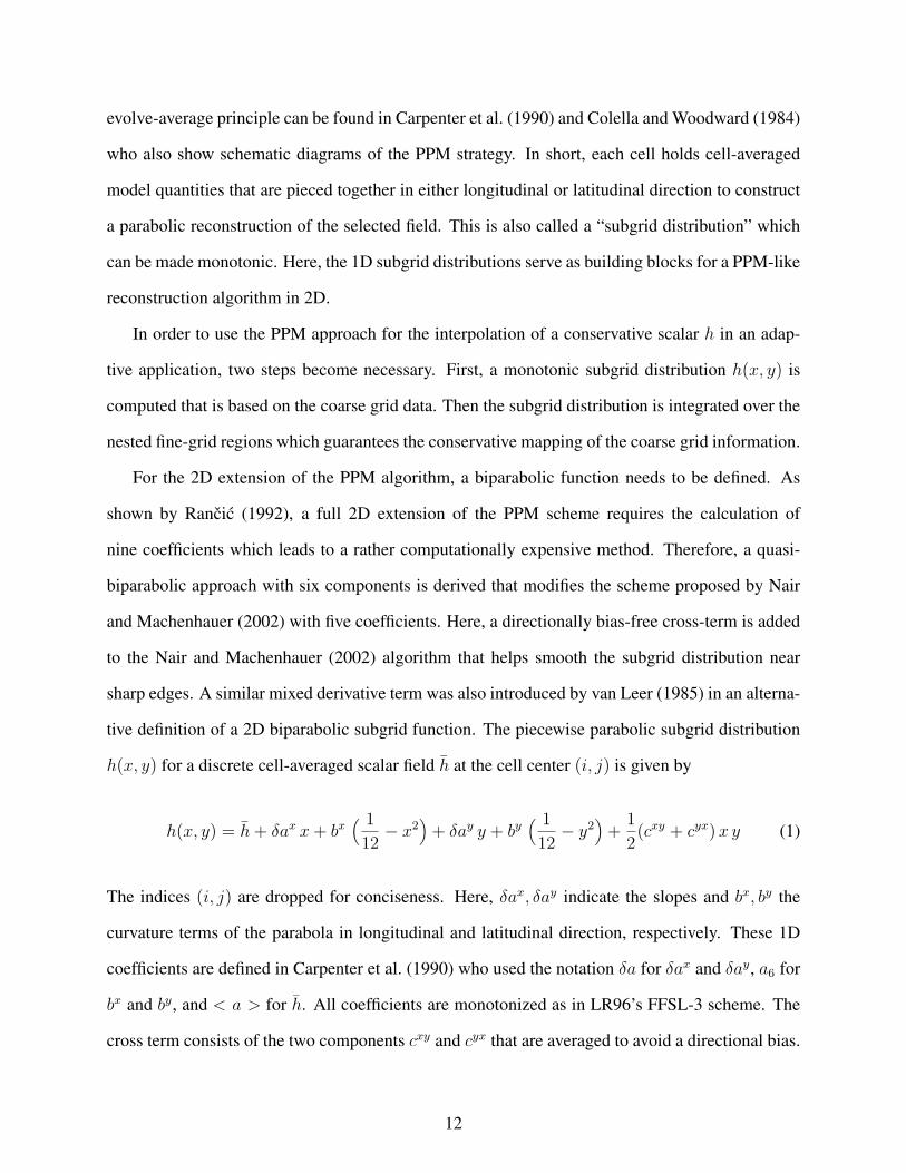
evolve-average principle can be found in Carpenter et al. (1990) and Colella and Woodward (1984)

who also show schematic diagrams of the PPM strategy. In short, each cell holds cell-averaged

model quantities that are pieced together in either longitudinal or latitudinal direction to construct

a parabolic reconstruction of the selected field. This is also called a “subgrid distribution” which

can be made monotonic. Here, the 1D subgrid distributions serve as building blocks for a PPM-like

reconstruction algorithm in 2D.

In order to use the PPM approach for the interpolation of a conservative scalar h in an adap-

tive application, two steps become necessary. First, a monotonic subgrid distribution h(x, y) is

computed that is based on the coarse grid data. Then the subgrid distribution is integrated over the

nested fine-grid regions which guarantees the conservative mapping of the coarse grid information.

For the 2D extension of the PPM algorithm, a biparabolic function needs to be defined. As

shown by Rancic (1992), a full 2D extension of the PPM scheme requires the calculation of

nine coefficients which leads to a rather computationally expensive method. Therefore, a quasi-

biparabolic approach with six components is derived that modifies the scheme proposed by Nair

and Machenhauer (2002) with five coefficients. Here, a directionally bias-free cross-term is added

to the Nair and Machenhauer (2002) algorithm that helps smooth the subgrid distribution near

sharp edges. A similar mixed derivative term was also introduced by van Leer (1985) in an alterna-

tive definition of a 2D biparabolic subgrid function. The piecewise parabolic subgrid distribution

h(x, y) for a discrete cell-averaged scalar field h at the cell center (i, j) is given by

h(x, y) = h + δax x + bx( 1

12− x2

)+ δay y + by

( 1

12− y2

)+

1

2(cxy + cyx) x y (1)

The indices (i, j) are dropped for conciseness. Here, δax, δay indicate the slopes and bx, by the

curvature terms of the parabola in longitudinal and latitudinal direction, respectively. These 1D

coefficients are defined in Carpenter et al. (1990) who used the notation δa for δax and δay, a6 for

bx and by, and < a > for h. All coefficients are monotonized as in LR96’s FFSL-3 scheme. The

cross term consists of the two components cxy and cyx that are averaged to avoid a directional bias.

12

In particular, cxy and cyx at a cell center (i, j) are determined by

cxy =1

2(∆ax

i,j+1 −∆axi,j−1) (2)

cyx =1

2(∆ay

i+1,j −∆ayi−1,j) (3)

where ∆ax and ∆ay are the centered-difference slopes

∆axi,j =

1

2(hi+1,j − hi−1,j) (4)

∆ayi,j =

1

2(hi,j+1 − hi,j−1) (5)

that are further monotonized via the van Leer (1977) monotonized-central (MC) slope limiter. This

limiter is given by

∆axi,j = min (|∆ax

i,j|, 2|hi+1,j − hi,j|, 2|hi,j − hi−1,j|) sgn(∆axi,j) (6)

if (hi+1,j − hi,j)(hi,j − hi−1,j) > 0

= 0 otherwise.

The MC slope limiter is also applied to ∆ay with respect to the y-direction and both cross compo-

nents cxy and cyx. Furthermore, the cell-averaged value h is defined as

h =∫ 1/2

−1/2

∫ 1/2

−1/2h(x, y) dx dy (7)

where x, y are the local normalized coordinates in each grid cell with x, y ∈ [−1/2, 1/2]. For the

spherical coordinate system (λ, ϕ) they are given as in Nair and Machenhauer (2002)

x =λ− λi

∆λi

− 1

2(8)

y =µ− µj

∆µj

− 1

2(9)

13

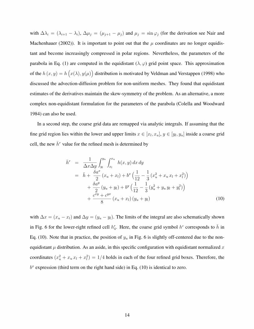
with ∆λi = (λi+1 − λi), ∆µj = (µj+1 − µj) and µj = sin ϕj (for the derivation see Nair and

Machenhauer (2002)). It is important to point out that the µ coordinates are no longer equidis-

tant and become increasingly compressed in polar regions. Nevertheless, the parameters of the

parabola in Eq. (1) are computed in the equidistant (λ, ϕ) grid point space. This approximation

of the h (x, y) = h(x(λ), y(µ)

)distribution is motivated by Veldman and Verstappen (1998) who

discussed the advection-diffusion problem for non-uniform meshes. They found that equidistant

estimates of the derivatives maintain the skew-symmetry of the problem. As an alternative, a more

complex non-equidistant formulation for the parameters of the parabola (Colella and Woodward

1984) can also be used.

In a second step, the coarse grid data are remapped via analytic integrals. If assuming that the

fine grid region lies within the lower and upper limits x ∈ [xl, xu], y ∈ [yl, yu] inside a coarse grid

cell, the new hr value for the refined mesh is determined by

hr =1

∆x∆y

∫ yu

yl

∫ xu

xl

h(x, y) dx dy

= h +δax

2(xu + xl) + bx

( 1

12− 1

3(x2

u + xu xl + x2l )

)

+δay

2(yu + yl) + by

( 1

12− 1

3(y2

u + yu yl + y2l )

)

+cxy + cyx

8(xu + xl) (yu + yl) (10)

with ∆x = (xu − xl) and ∆y = (yu − yl). The limits of the integral are also schematically shown

in Fig. 6 for the lower-right refined cell hr4. Here, the coarse grid symbol hc corresponds to h in

Eq. (10). Note that in practice, the position of yu in Fig. 6 is slightly off-centered due to the non-

equidistant µ distribution. As an aside, in this specific configuration with equidistant normalized x

coordinates (x2u + xu xl + x2

l ) = 1/4 holds in each of the four refined grid boxes. Therefore, the

bx expression (third term on the right hand side) in Eq. (10) is identical to zero.

14

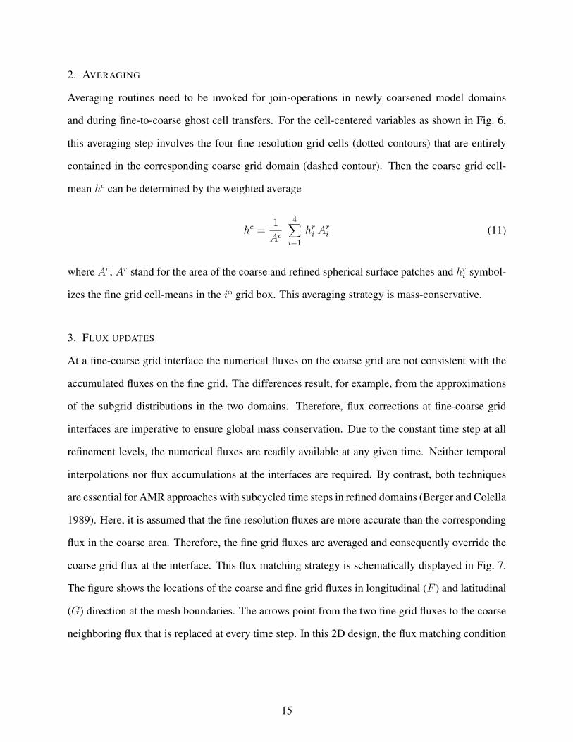
2. AVERAGING

Averaging routines need to be invoked for join-operations in newly coarsened model domains

and during fine-to-coarse ghost cell transfers. For the cell-centered variables as shown in Fig. 6,

this averaging step involves the four fine-resolution grid cells (dotted contours) that are entirely

contained in the corresponding coarse grid domain (dashed contour). Then the coarse grid cell-

mean hc can be determined by the weighted average

hc =1

Ac

4∑

i=1

hri Ar

i (11)

where Ac, Ar stand for the area of the coarse and refined spherical surface patches and hri symbol-

izes the fine grid cell-means in the ith grid box. This averaging strategy is mass-conservative.

3. FLUX UPDATES

At a fine-coarse grid interface the numerical fluxes on the coarse grid are not consistent with the

accumulated fluxes on the fine grid. The differences result, for example, from the approximations

of the subgrid distributions in the two domains. Therefore, flux corrections at fine-coarse grid

interfaces are imperative to ensure global mass conservation. Due to the constant time step at all

refinement levels, the numerical fluxes are readily available at any given time. Neither temporal

interpolations nor flux accumulations at the interfaces are required. By contrast, both techniques

are essential for AMR approaches with subcycled time steps in refined domains (Berger and Colella

1989). Here, it is assumed that the fine resolution fluxes are more accurate than the corresponding

flux in the coarse area. Therefore, the fine grid fluxes are averaged and consequently override the

coarse grid flux at the interface. This flux matching strategy is schematically displayed in Fig. 7.

The figure shows the locations of the coarse and fine grid fluxes in longitudinal (F ) and latitudinal

(G) direction at the mesh boundaries. The arrows point from the two fine grid fluxes to the coarse

neighboring flux that is replaced at every time step. In this 2D design, the flux matching condition

15

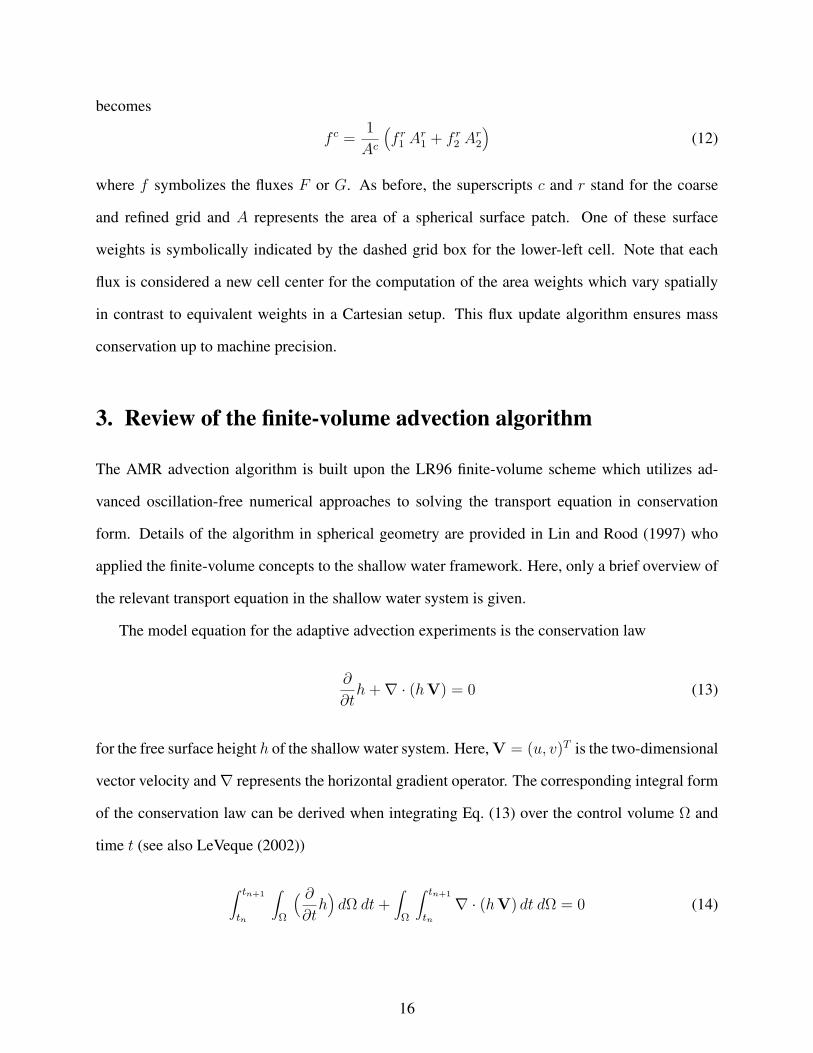
becomes

f c =1

Ac

(f r

1 Ar1 + f r

2 Ar2

)(12)

where f symbolizes the fluxes F or G. As before, the superscripts c and r stand for the coarse

and refined grid and A represents the area of a spherical surface patch. One of these surface

weights is symbolically indicated by the dashed grid box for the lower-left cell. Note that each

flux is considered a new cell center for the computation of the area weights which vary spatially

in contrast to equivalent weights in a Cartesian setup. This flux update algorithm ensures mass

conservation up to machine precision.

3. Review of the finite-volume advection algorithm

The AMR advection algorithm is built upon the LR96 finite-volume scheme which utilizes ad-

vanced oscillation-free numerical approaches to solving the transport equation in conservation

form. Details of the algorithm in spherical geometry are provided in Lin and Rood (1997) who

applied the finite-volume concepts to the shallow water framework. Here, only a brief overview of

the relevant transport equation in the shallow water system is given.

The model equation for the adaptive advection experiments is the conservation law

∂

∂th +∇ · (hV) = 0 (13)

for the free surface height h of the shallow water system. Here, V = (u, v)T is the two-dimensional

vector velocity and∇ represents the horizontal gradient operator. The corresponding integral form

of the conservation law can be derived when integrating Eq. (13) over the control volume Ω and

time t (see also LeVeque (2002))

∫ tn+1

tn

∫

Ω

( ∂

∂th

)dΩ dt +

∫

Ω

∫ tn+1

tn∇ · (hV) dt dΩ = 0 (14)

16

where n denotes the discrete time level and ∆t = tn+1 − tn stands for the duration of a time

step. In the following derivation, only two-dimensional control volumes with surface areas AΩ are

considered. Equation (14) can be rewritten as

∫ tn+1

tn

( d

dth

)dt +

∆t

AΩ

∫

Ω∇ · F dΩ = 0 (15)

where the overbar ( ) symbolizes the spatial average over the area AΩ and F = 1∆t

∫ tn+1tn hV dt

indicates the temporal average of the flux vector. Applying the Gauss divergence theorem yields

∫ tn+1

tn

( d

dth

)dt +

∆t

AΩ

∮

∂ΩF · n dl = 0 (16)

in which n is an outward-pointing unit normal vector to the boundary ∂Ω of the control volume

and dl is an infinitesimal line segment along the contour. Thus, the discrete representation of the

conservation law becomes

hn+1 = hn − ∆t

AΩ

4∑

i=1

Fi · ni li (17)

where the sum comprises the 4 line segments with lengths li that surround a rectangular 2D region.

Fi symbolizes the time-averaged flux vectors at the cell interfaces and ni indicates the unit normal

vectors to the ith contour line. Assuming an orthogonal x-y control volume with surface area

Ai,j = ∆xi,j ∆yi,j and corresponding 1D numerical fluxes F and G in x- and y-direction, Eq. (17)

is equivalent to

hn+1i,j = hn

i,j −∆t

Ai,j

(∆yi+ 1

2,j Fi+ 1

2,j −∆yi− 1

2,j Fi− 1

2,j + ∆xi,j+ 1

2Gi,j+ 1

2−∆xi,j− 1

2Gi,j− 1

2

)(18)

in which the indices i, j define the grid point position of the cell center and the half index repre-

sents the boundaries of the grid box. In such a Cartesian setup, the lengths of the line segments

∆xi,j = (xi+ 12,j − xi− 1

2,j) and ∆yi,j = (yi,j+ 1

2− yi,j− 1

2) are independent of the y- and x-direction,

respectively. This is in contrast to grids in spherical geometry where ∆xi,j, ∆yi,j and the surface

17

area Ai,j in Eq. (18) are substituted with the corresponding representation in spherical space

∆xi,j = a cos ϕj ∆λi (19)

∆yi,j = a ∆ϕj (20)

Ai,j = a2∫ λ

i+12

λi− 1

2

∫ ϕj+1

2

ϕj− 1

2

cos ϕ dϕ dλ

= a2 ( sin ϕj+ 12− sin ϕj− 1

2) ∆λi. (21)

Here, a = 6.371229 × 106 m represents the Earth’s radius and ∆λi = (λi+ 12− λi− 1

2) and

∆ϕj = (ϕj+ 12− ϕj− 1

2) denote the longitudinal (λ) and latitudinal (ϕ) grid spacings measured

in radians. In the Lin-Rood advection algorithm though (Lin and Rood 1997), a slightly different

flux-differencing approach has been chosen that corresponds to Eq. (18) if Ai,j is replaced with

the approximation Ai,j = a2 cos ϕj ∆λi ∆ϕj . As a result, the discrete conservation law for the

cell-averaged free surface height in spherical coordinates becomes

hn+1i,j = hn

i,j + Fnet + Gnet (22)

with

Fnet = − ∆t

a cos ϕj ∆λi

(Fi+ 12,j − Fi− 1

2,j) (23)

Gnet = − ∆t

a cos ϕj ∆ϕj

( cos ϕj+ 12Gi,j+ 1

2− cos ϕj− 1

2Gi,j− 1

2). (24)

Here, Fnet and Gnet denote the net fluxes through the interfaces in longitudinal and latitudinal

direction that solely determine the rate of change of the spatially averaged scalar field h. This

notation corresponds exactly to the Eqs. (4)-(5) in Lin and Rood (1997) when defining the time-

averaged fluxes as X and Y and omitting the subscript “net” in the preceding equations. Note that

Eq. (22) still contains a directional bias when operating splitting methods are applied. Therefore,

18

the following directional-bias free 2D scheme is employed

hn+1i,j = hn

i,j + Fnet

[hn

i,j +1

2g(hn

i,j)]+ Gnet

[hn

i,j +1

2f(hn

i,j)]

(25)

where f and g symbolize advection operators in longitudinal and latitudinal direction, respec-

tively. These advective operators avoid a deformational error (details in LR96). In particular,

LR96 combined a first-order Euler upwind scheme in advective form (inner operator) with higher-

order finite-volume methods in flux form (outer operator). Both a second-order van Leer-type flux

algorithm (van Leer 1974, 1977) and the third-order PPM scheme were implemented for the flux

calculations which are both monotonic, upstream-biased and fully conservative. For the adaptive

advection experiments discussed here, the PPM approach has been chosen for the fluxes F and

G. Details of the flux computations and monotonicity constraints are provided in Carpenter et al.

(1990), Colella and Woodward (1984) and LR96 (with monotonicity constraint FFSL-3). Note that

the scheme is in fact not strictly monotonic in two dimensions. As explained in LR96, very minor

violations of the monotonicity constraint can be observed near sharp edges due to the application

of purely 1D monotonicity operators. The time-stepping scheme is explicit and stable for zonal

and meridional Courant numbers |CFL| < 1. This restriction arises since the semi-Lagrangian

extension of the LR96 algorithm is not utilized in the AMR model experiments to keep the width

of the ghost cell regions small. Note that the variables u, v and h for the advection experiment are

staggered as in the Arakawa C-grid with originally (prior to the AMR extension) two cell centers

at the poles. For the adaptive mesh implementations though, this base C-grid configuration needed

to be shifted by half a grid length in latitudinal direction. Such a shift places velocity points at the

poles and avoids fixed polar mass centers which would inhibit the flexible AMR principle.

19

4. Results

The advection algorithm is one of the fundamental building blocks of atmospheric flow simula-

tions. It is therefore imperative to evaluate its performance not only in the adaptive model runs

but also in the non-adapted model setups. This allows comparisons of the AMR approach to both

analytic reference solutions and uniform-grid model experiments. This section discusses results

from three standard advection tests with increasing complexity. These are the transport of a cosine

bell, the advection of a slotted cylinder and a smooth deformational flow that describes the roll-up

of two vortices.

Different adaptation criteria are assessed. In general, each criterion is compared to a problem-

dependent threshold value. If one or more grid points within a block exceed this user-determined

limit the block is flagged for refinement. If, on the other hand, the grid points in an adapted block

no longer meet the adaptation criterion the coarsening flag in the corresponding block is set. The

refinement criterion is examined at each time step which is determined dynamically during the

simulation to match a chosen |CFL| = 0.95 limit. All adaptations occur consecutively until either

the user-defined maximum refinement level or the initial resolution is reached. The mesh can not

be coarsened further than the initial layout. Here, the block configuration Bx = 8, By = 6, Nx =

9, Ny = 6 (as introduced in Fig. 1) is chosen for all test cases with a maximum refinement level

between 0 and 4. Such a setup corresponds to the uniform ∆λ, ∆ϕ grid spacings 5, 2.5, 1.25,

0.625 and 0.3125 at the individual nesting levels. They are further explained in Table 1 that

gives an overview of the corresponding resolutions in spherical coordinates and physical space.

The effect of the converging meridians in the latitude-longitude grid can clearly be seen at all

refinement levels. This significantly reduces the physical grid spacings in polar regions and, as a

consequence, the maximum allowable time step for stable computations.

All three passive advection tests are driven by prescribed wind speeds. These are reinitialized

analytically whenever adaptations occur during the course of the simulation. In addition, the initial

geopotential height field is reinitialized analytically if initial adaptations are requested. This is

20

the case for the cosine bell and slotted cylinder test scenarios. During the model runs though,

the geopotential height field in newly adapted blocks is initialized via the conservative averaging

algorithm and the PPM-based interpolation method as discussed earlier.

a. Error statistics

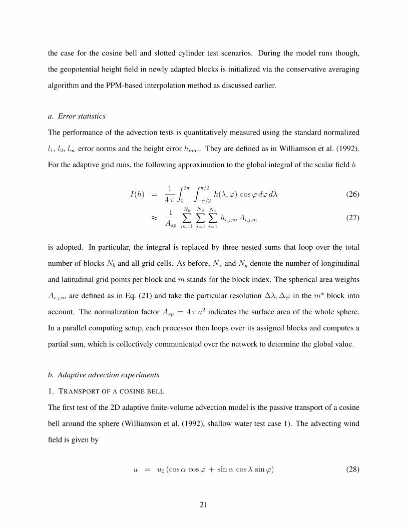
The performance of the advection tests is quantitatively measured using the standard normalized

l1, l2, l∞ error norms and the height error hmax. They are defined as in Williamson et al. (1992).

For the adaptive grid runs, the following approximation to the global integral of the scalar field h

I(h) =1

4 π

∫ 2π

0

∫ π/2

−π/2h(λ, ϕ) cos ϕdϕ dλ (26)

≈ 1

Asp

Nb∑

m=1

Ny∑

j=1

Nx∑

i=1

hi,j,m Ai,j,m (27)

is adopted. In particular, the integral is replaced by three nested sums that loop over the total

number of blocks Nb and all grid cells. As before, Nx and Ny denote the number of longitudinal

and latitudinal grid points per block and m stands for the block index. The spherical area weights

Ai,j,m are defined as in Eq. (21) and take the particular resolution ∆λ, ∆ϕ in the mth block into

account. The normalization factor Asp = 4 π a2 indicates the surface area of the whole sphere.

In a parallel computing setup, each processor then loops over its assigned blocks and computes a

partial sum, which is collectively communicated over the network to determine the global value.

b. Adaptive advection experiments

1. TRANSPORT OF A COSINE BELL

The first test of the 2D adaptive finite-volume advection model is the passive transport of a cosine

bell around the sphere (Williamson et al. (1992), shallow water test case 1). The advecting wind

field is given by

u = u0 (cos α cos ϕ + sin α cos λ sin ϕ) (28)

21

v = −u0 sin α sin λ (29)

where u and v stand for the nondivergent zonal and meridional velocities with maximum wind

speed u0 = 2πa/(12 days) ≈ 38.61 m s−1. Various flow orientation angles α to the equator can

be chosen. Here, α = 0, α = 45 and α = 90 are tested that define the advection of the cosine

bell along the equator, at a 45 angle through the tropics and midlatitudes as well as the transport

across the poles.

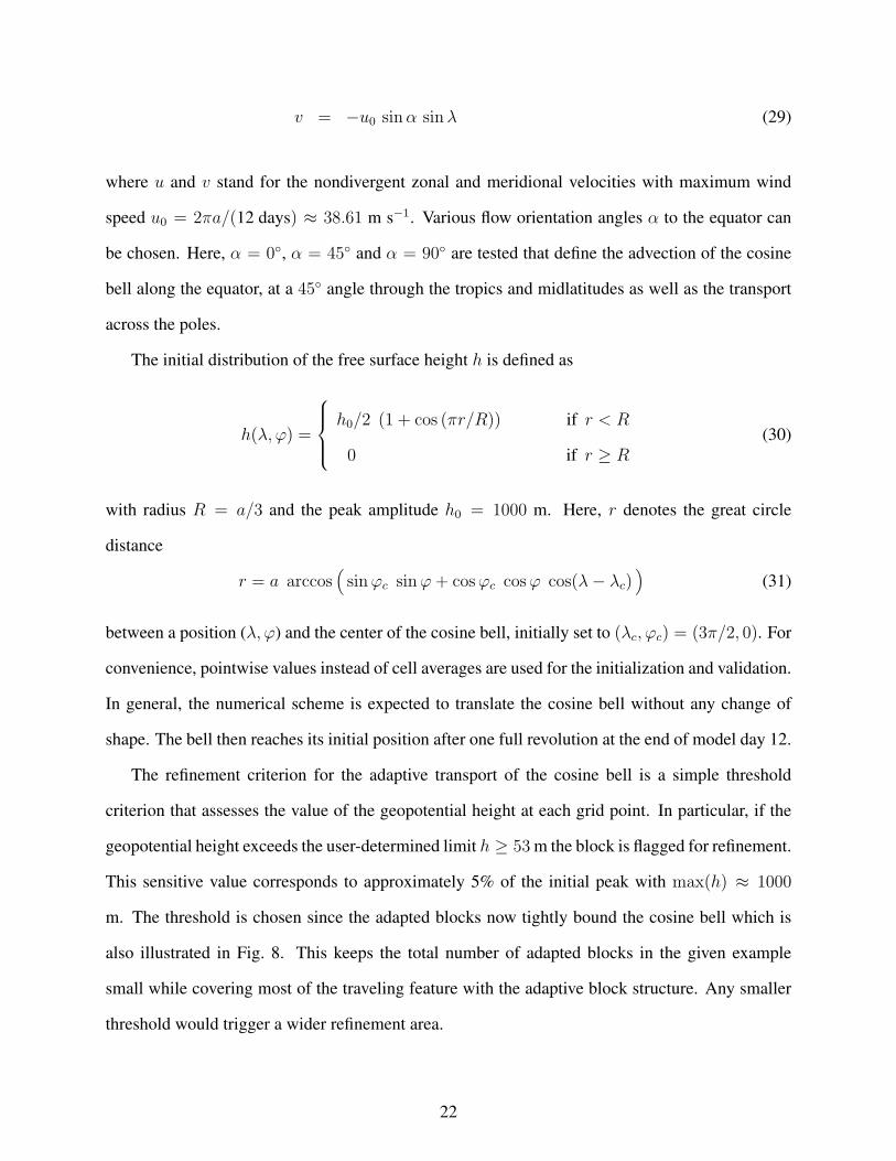
The initial distribution of the free surface height h is defined as

h(λ, ϕ) =

h0/2 (1 + cos (πr/R)) if r < R

0 if r ≥ R(30)

with radius R = a/3 and the peak amplitude h0 = 1000 m. Here, r denotes the great circle

distance

r = a arccos(

sin ϕc sin ϕ + cos ϕc cos ϕ cos(λ− λc))

(31)

between a position (λ, ϕ) and the center of the cosine bell, initially set to (λc, ϕc) = (3π/2, 0). For

convenience, pointwise values instead of cell averages are used for the initialization and validation.

In general, the numerical scheme is expected to translate the cosine bell without any change of

shape. The bell then reaches its initial position after one full revolution at the end of model day 12.

The refinement criterion for the adaptive transport of the cosine bell is a simple threshold

criterion that assesses the value of the geopotential height at each grid point. In particular, if the

geopotential height exceeds the user-determined limit h ≥ 53 m the block is flagged for refinement.

This sensitive value corresponds to approximately 5% of the initial peak with max(h) ≈ 1000

m. The threshold is chosen since the adapted blocks now tightly bound the cosine bell which is

also illustrated in Fig. 8. This keeps the total number of adapted blocks in the given example

small while covering most of the traveling feature with the adaptive block structure. Any smaller

threshold would trigger a wider refinement area.

22

Figure 8 explains the basic adaptation principle and gives insight into the load-balancing strat-

egy on parallel computing platforms. The left column shows four snapshots of the adaptive

α = 90 simulation at day 0, 1, 3 and 4 with three refinement levels. The adapted blocks reliably

track the geopotential height field of the cosine bell as indicated by the overlaid block distribu-

tion. It can clearly be seen that the cosine bell passes over the North Pole without distortions or

noise. The pole point itself with its converging grid lines is spread out in the chosen equidistant

cylindrical map projection. This emphasizes the numerous grid boxes in polar regions that need to

be refined for transport processes at high latitudes. They severely restrict the maximum allowable

time step that obeys the |CFL| = 0.95 condition in polar regions. For example, in this simulation

with three refinement levels and a maximum zonal wind speed of u ≈ 38.61 m s−1 at the poles, the

adaptive time step depends greatly on the position of the cosine bell. It varies between ∆t ≈ 597.3

s in equatorial regions and ∆t ≈ 9.3 s at very high latitudes. The right column in Fig. 8 displays

the corresponding distribution of the adaptive blocks in a parallel execution mode. Here four pro-

cessors are used which are indicated by the gray shadings. The current load-balancing strategy

assumes an equal work load per block and therefore, assigns an approximately equal number of

blocks to each processor. If needed, new blocks are readily redistributed after adaptations occurred.

Here, the redistribution of the blocks does not take data locality issues into account. For the future,

a space-filling-curve load-balancing approach (Dennis 2003; Behrens and Zimmermann 2000) is

planned which improves the data locality and thereby is expected to reduce the communication

across the parallel network. Note that the parallel speed-ups which can be achieved with the AMR

library highly depend on several factors. Among them are the size of the blocks, the ratio between

compute cells and ghost cells, the work load per block and the frequency of the ghost cell updates

due to the algorithmic design, the data locality of the blocks and the performance of the network.

These issues will be thoroughly discussed in a different publication.

The cosine bell is advected once around the sphere and reaches its initial position after 12 days.

Then the solution can be compared to the initial conditions that serve as the true reference field.

A closer examination of the final states at refinement level 1 (2.5) and different rotation param-

23

eters α is illustrated in Fig. 9 that also presents the overlaid true solution with dotted contours.

Here it is shown that the cosine bell undergoes a stretching in the flow direction which is a typ-

ically observed for monotonic finite-volume advection algorithms (Lin and Rood 1996; Nair and

Machenhauer 2002; Hubbard and Nikiforakis 2003). The effect is clearly visible at this relatively

coarse resolution and diminishes significantly with decreasing grid sizes (Fig. 10). As pointed

out by Nair and Machenhauer (2002) the degradation of the shape is caused by the monotonic-

ity constraint that translates into slightly less accurate error norms in comparison to, for example,

positive definite methods. Nevertheless, in practice the advantages of the monotonicity preserving

advection algorithm outweigh the slight decrease in accuracy (see also comparisons in van Leer

(1977)).

Figure 10 confirms that the shape of the cosine bell after one revolution is well-preserved at

high resolutions. The figure depicts a sequence of model runs with increasing number of refinement

levels at rotation angle α = 45. This transport direction represents the “worst case” scenario for

the advection algorithm with underlying operator splitting approach. The results at the highest

refinement levels 3 and 4 are almost indistinguishable from each other. It is also interesting to note

that the cosine bells at the higher resolutions (Figs. 10c-e) no longer show the small phase error,

which is visible in the coarser runs (Figs. 10a-b). The solutions then resemble the true solution

very closely which is demonstrated in Fig. 10f. Figure 10f displays the difference of the cosine

bell at refinement level 4 with the analytic reference state. The differences mainly develop along

the edges in the 45 flow direction. In particular, the leading edge in the upper right corner shows

slightly enhanced geopotential height values, whereas the tail in the lower left corner drops below

the reference state. These errors are small in comparison to the peak amplitude of the cosine bell.

In general, the same type of error patterns can also be found in non-adapted model runs.

In addition, it is interesting to assess the adaptive model performance with a cross polar flow

field at α = 90. Dynamic adaptations in polar regions are demanding since they involve many

more adapted blocks close to the poles as discussed before. Nevertheless, the adapted advection

scheme performs satisfactorily at all three refinement levels displayed in Fig. 11. Here, three snap-

24

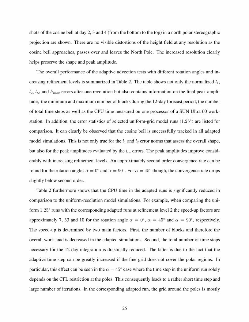
shots of the cosine bell at day 2, 3 and 4 (from the bottom to the top) in a north polar stereographic

projection are shown. There are no visible distortions of the height field at any resolution as the

cosine bell approaches, passes over and leaves the North Pole. The increased resolution clearly

helps preserve the shape and peak amplitude.

The overall performance of the adaptive advection tests with different rotation angles and in-

creasing refinement levels is summarized in Table 2. The table shows not only the normalized l1,

l2, l∞ and hmax errors after one revolution but also contains information on the final peak ampli-

tude, the minimum and maximum number of blocks during the 12-day forecast period, the number

of total time steps as well as the CPU time measured on one processor of a SUN Ultra 60 work-

station. In addition, the error statistics of selected uniform-grid model runs (1.25) are listed for

comparison. It can clearly be observed that the cosine bell is successfully tracked in all adapted

model simulations. This is not only true for the l1 and l2 error norms that assess the overall shape,

but also for the peak amplitudes evaluated by the l∞ errors. The peak amplitudes improve consid-

erably with increasing refinement levels. An approximately second order convergence rate can be

found for the rotation angles α = 0 and α = 90. For α = 45 though, the convergence rate drops

slightly below second order.

Table 2 furthermore shows that the CPU time in the adapted runs is significantly reduced in

comparison to the uniform-resolution model simulations. For example, when comparing the uni-

form 1.25 runs with the corresponding adapted runs at refinement level 2 the speed-up factors are

approximately 7, 33 and 10 for the rotation angle α = 0, α = 45 and α = 90, respectively.

The speed-up is determined by two main factors. First, the number of blocks and therefore the

overall work load is decreased in the adapted simulations. Second, the total number of time steps

necessary for the 12-day integration is drastically reduced. The latter is due to the fact that the

adaptive time step can be greatly increased if the fine grid does not cover the polar regions. In

particular, this effect can be seen in the α = 45 case where the time step in the uniform run solely

depends on the CFL restriction at the poles. This consequently leads to a rather short time step and

large number of iterations. In the corresponding adapted run, the grid around the poles is mostly

25

kept at the coarse resolution so that the time step is mainly determined by the traveling cosine bell.

The latter is also true for the α = 0 test case, where the time step exclusively relies on the true ad-

vective wind speeds and grid distances at the equator. Therefore, an identical number of time steps

is required for both the uniform and adapted runs at the 1.25 resolution and the computational

savings are exclusively due to the reduced work load.

The error norms for the adaptive simulations in Table 2 compare well to similar monotonic and

conservative advection schemes presented in the literature. For example, the errors of the α = 90

run with 1 refinement level (2.5) closely resemble the corresponding error measures for the WAF

scheme in Hubbard and Nikiforakis (2003), the FFSL-3 algorithm in Lin and Rood (1996) and

the CISL-M method in Nair and Machenhauer (2002) at comparable resolutions (and a slightly

wider bell radius R = a 7π/64). This is important to note since the latter two algorithms are semi-

Lagrangian type schemes that only require very few time steps for one revolution of the cosine

bell. Both schemes finish after 256 integration steps, whereas the adaptive finite-volume model

needs 4085 time steps due to the CFL restriction. Therefore, it is emphasized that the error norms

match despite the large difference in the number of time steps. The sheer number of integration

steps has significant implications on the model results. This has already been documented in Table

2, which shows that the error norms of the adapted runs at refinement level 2 for non-zero rotation

angles are in fact slightly lower than the errors of the uniform-grid runs. The effect can be linked to

the reduced number of integration steps. An even clearer example is given in Table 3 that assesses

the performance of the α = 0 advection test with different maximum CFL numbers. As the CFL

numbers decrease, the resulting number of time steps for one revolution increases, which leads

to considerably less accurate results in this constant-flow test case. Here, an increased number of

time steps adds numerical diffusion to the transport problem which flattens the peak of the cosine

bell. A similar time stepping effect was also observed by Stevens and Bretherton (1996).

The time traces of the normalized l2 and l∞ error norms with α = 45 and α = 90 are

illustrated in Fig. 12. The figure displays the evolution of the errors at three different refinement

levels that show the expected decline of the solution error at finer resolutions. The norms are

26

slightly sensitive to the rotation angle, especially in comparison to the α = 0 values listed in

Table 2. This is in contrast to findings by Taylor et al. (1997) who utilized a high-order spectral

element method on a cubed-sphere computational grid. The trace of the l∞ norm is rather noisy

at low resolutions and additionally, shows distinct spikes when the cosine bell is transported over

the poles. This was also observed by Rasch (1994) and Nair and Machenhauer (2002). These

spikes are not a consequence of the dynamically adaptive grid implementation, but also occur in

uniform-grid model runs. As pointed out by Jakob-Chien et al. (1995) the source of the noise is the

discrete sampling of the numerical and reference solution. Here the reference solution is computed

analytically during the course of the integration. This leads to an occasional small increase in the

peak amplitude of the reference field depending on the distance of the center to the closest grid

point. This effect diminishes with increasing resolution.

2. TRANSPORT OF A SLOTTED CYLINDER

In the second example the cosine bell is replaced with a slotted cylinder. All other parameters

and flow fields stay the same as discussed above. Such an advection test was originally proposed

by Zalesak (1979) and has recently been applied in spherical geometry by Nair et al. (2003) and

Lipscomb and Ringler (2005). The slotted cylinder exhibits very sharp non-smooth edges in com-

parison to the rather smoothly varying cosine bell. Therefore, it challenges not only the numerical

scheme but also the interpolation algorithm in an adaptive model simulation. The radius of the

cylinder is set to R = a× π/4 with a slot of width a× π/8 and length a× 3π/8. This rather wide

slotted cylinder is chosen to allow grid coarsenings within the slot. As in Lipscomb and Ringler

(2005), the initial height of the cylinder is set to h = 1000 m, whereas h is set to zero for all

r > R and inside the slot. The long axis of the slot is perpendicular to the equator and the cylinder

is initially centered at (λc, ϕc) = (3π/2, 0). The flow orientation angle α = 30 is selected that

avoids any grid symmetries along the trajectory path.

The model is run for 12 days which completes a full revolution of the advected cylinder. As

before, the initial conditions then serve as the true reference solution. Four refinement levels are

27

used that start from a coarse 5 × 5 base grid. Here, a grid-scale dependent gradient criterion is

applied that flags a block for refinement if one or more grid points with grid indices (i, j) exceed

the user-defined threshold

ξi,j = max(|hi+1,j − hi,j|, |hi,j+1 − hi,j|) ≥ 10 m (32)

for 0 ≤ i ≤ Nx and 0 ≤ j ≤ Ny. This criterion evaluates the local height difference between

neighboring cells which incorporates some ghost cell information along a block boundary. A

similar criterion was also formulated by Hubbard and Nikiforakis (2003) who evaluated ξ with

centered differences.

Figures 13a-e show snapshots of the adaptive simulation at model day 0, 3, 6, 9 and 12. The

positive height field is shaded in gray with overlaid adapted blocks. It can clearly be seen that the

grid is refined along the sharp edges of the advected cylinder and kept coarse elsewhere. At this

high resolution within the refined area (0.3125) there is some minor numerical diffusion along

the sharp edges. This leads to a slight broadening of the cylinder and its refined area during the

course of the simulation. The broadening can also be seen in Fig. 13f that shows a cross section

of the slotted cylinder along the equator for 4 different refinement levels at day 12. Here, the

slotted cylinder can be compared to its reference shape. The adapted grids clearly help preserve

the sharpness of the edges with increased resolution. This trend seems to level off at refinement

level 3 and 4 which visually overlay each other.

The performance of the refined and corresponding uniform-resolution model runs after one

revolution (day 12) is quantitatively measured in Table 4. The table lists not only the normalized l2

and l∞ geopotential height error norms but also gives information on the minimum and maximum

number of blocks during the 12-day simulation, the total number of time steps and the CPU time

on a single AMD Opteron processor. The model runs are grouped according to their finest grid

resolution. It can be seen that the l2 errors of the adaptive and corresponding uniform-resolution

runs closely match and slowly decrease with increasing resolution. This error reduction cannot be

28

observed for the l∞ norms that measure the maximum deviations from the reference solution. In

particular, the l∞ norms stay almost constant. Here, the reduced convergence rate of both error

norms is most likely due to the highly non-smooth characteristics of the initial data set. Overall,

the AMR simulations show considerable speed-up factors of about 17 and 120 at the two highest

resolutions.

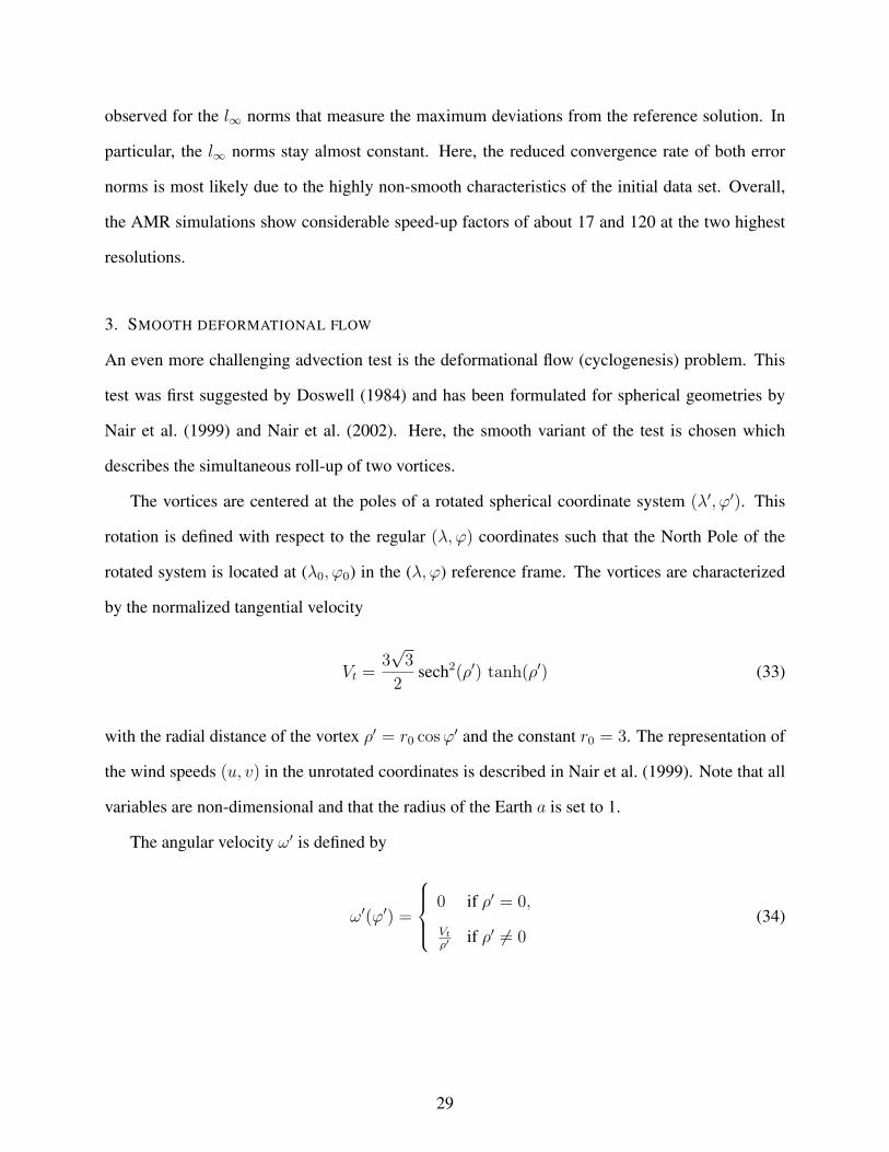
3. SMOOTH DEFORMATIONAL FLOW

An even more challenging advection test is the deformational flow (cyclogenesis) problem. This

test was first suggested by Doswell (1984) and has been formulated for spherical geometries by

Nair et al. (1999) and Nair et al. (2002). Here, the smooth variant of the test is chosen which

describes the simultaneous roll-up of two vortices.

The vortices are centered at the poles of a rotated spherical coordinate system (λ′, ϕ′). This

rotation is defined with respect to the regular (λ, ϕ) coordinates such that the North Pole of the

rotated system is located at (λ0, ϕ0) in the (λ, ϕ) reference frame. The vortices are characterized

by the normalized tangential velocity

Vt =3√

3

2sech2(ρ′) tanh(ρ′) (33)

with the radial distance of the vortex ρ′ = r0 cos ϕ′ and the constant r0 = 3. The representation of

the wind speeds (u, v) in the unrotated coordinates is described in Nair et al. (1999). Note that all

variables are non-dimensional and that the radius of the Earth a is set to 1.

The angular velocity ω′ is defined by

ω′(ϕ′) =

0 if ρ′ = 0,

Vt

ρ′ if ρ′ 6= 0(34)

29

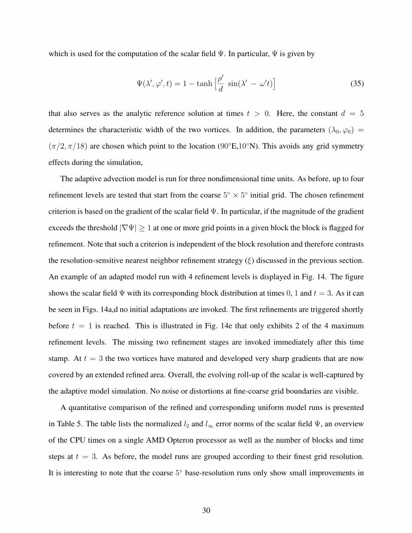
which is used for the computation of the scalar field Ψ. In particular, Ψ is given by

Ψ(λ′, ϕ′, t) = 1− tanh[ρ′

dsin(λ′ − ω′t)

](35)

that also serves as the analytic reference solution at times t > 0. Here, the constant d = 5

determines the characteristic width of the two vortices. In addition, the parameters (λ0, ϕ0) =

(π/2, π/18) are chosen which point to the location (90E,10N). This avoids any grid symmetry

effects during the simulation,

The adaptive advection model is run for three nondimensional time units. As before, up to four

refinement levels are tested that start from the coarse 5 × 5 initial grid. The chosen refinement

criterion is based on the gradient of the scalar field Ψ. In particular, if the magnitude of the gradient

exceeds the threshold |∇Ψ| ≥ 1 at one or more grid points in a given block the block is flagged for

refinement. Note that such a criterion is independent of the block resolution and therefore contrasts

the resolution-sensitive nearest neighbor refinement strategy (ξ) discussed in the previous section.

An example of an adapted model run with 4 refinement levels is displayed in Fig. 14. The figure

shows the scalar field Ψ with its corresponding block distribution at times 0, 1 and t = 3. As it can

be seen in Figs. 14a,d no initial adaptations are invoked. The first refinements are triggered shortly

before t = 1 is reached. This is illustrated in Fig. 14e that only exhibits 2 of the 4 maximum

refinement levels. The missing two refinement stages are invoked immediately after this time

stamp. At t = 3 the two vortices have matured and developed very sharp gradients that are now

covered by an extended refined area. Overall, the evolving roll-up of the scalar is well-captured by

the adaptive model simulation. No noise or distortions at fine-coarse grid boundaries are visible.

A quantitative comparison of the refined and corresponding uniform model runs is presented

in Table 5. The table lists the normalized l2 and l∞ error norms of the scalar field Ψ, an overview

of the CPU times on a single AMD Opteron processor as well as the number of blocks and time

steps at t = 3. As before, the model runs are grouped according to their finest grid resolution.

It is interesting to note that the coarse 5 base-resolution runs only show small improvements in

30

the error statistics when refined up to a refinement level of 4. On the contrary, the errors slightly

increase at refinement level 4. It suggests that the initial errors on the coarse mesh (until t = 1)

can not be successfully recovered by later refinement regions that are initialized via interpolations

from the coarser mesh. Therefore, even an AMR run must reasonably represent the solution on

the coarsest mesh if accuracy is expected to be gained in the refined areas. A good compromise

between accuracy and computational costs are the 1.25 model simulations with 1 or 2 refinement

levels. They show the smallest error measures even in comparison to the uniform high-resolution

model runs 0.625 and 0.3125. This is mainly attributable to the reduced number of integration

steps that also lead to the considerable speed-up factors of ≈ 8.6 and ≈ 108, respectively.

5. Conclusions

A spherical 2D Adaptive Mesh Refinement (AMR) technique has been applied to a revised version

of the conservative and monotonic Lin and Rood (1996) advection algorithm. The adaptive grid

design is based on two building blocks, a block-structured data layout and a spherical AMR grid

library for parallel computer architectures. The library contains special provisions for ghost cell

exchanges in polar regions and supports both static and dynamic grid adaptations. Furthermore,

it has built-in parallel communication and load-balancing support which reduces the development

time for parallel AMR applications. The latter is especially important for more complex, nonlinear

AMR models in 3D.

Three advection examples with increasing complexity have been tested. These include the ad-

vection of a cosine bell around the sphere at different rotation angles, the transport of a slotted

cylinder with sharp edges and a smooth deformational cyclogenesis test case which describes the

roll-up of two vortices. Up to four refinement levels have been tested with a minimal mesh spacing

of 0.3125. The adaptations were guided by user-defined adaptation criteria. In particular, sim-

ple height-based and gradient-based refinement strategies were chosen that triggered refinements

whenever the problem-specific threshold values were reached. All three test examples showed that

31

the chosen features of interest were reliably detected and tracked by the refinement regions. The

additional resolution clearly helped preserve the shape and amplitude of the transported field while

saving computing resources in comparison to uniform-grid model runs. Overall, the adaptive sim-

ulations demonstrate that AMR might be a viable option for atmospheric transport schemes. For

practical applications, the adaptation criterion can then be tailored towards the specific advected

quantities and flow conditions.

The AMR block design is readily applicable to non-linear model configurations that can utilize

a block-data structure on the sphere. This research effort is therefore a step towards a statically and

dynamically adaptive GCM that can focus its resolution on user-determined regions or features of

interest. The refined domains could, for example, include static adaptations in mountainous terrain

or dynamic adaptations for cyclones or convective regions. Tests with an adaptive nonlinear 2D

and 3D version of the finite-volume dynamical core have already been successfully performed

which we will discuss in a follow-up paper.

Whether adaptive mesh approaches for climate and weather research will prevail in the future

will crucially depend on two major aspects. First, it must be shown that adaptive atmospheric mod-

eling is not just feasible, but also accurate with respect to the resulting flow patterns and further-

more, capable of detecting the features of interest reliably in 3D setups. Second, adaptive model

simulations must also be computationally less expensive than comparable uniform high resolution

runs. We argue that both goals are within reach for future atmospheric model generations.

Acknowledgments. We would like to thank S.-J. Lin (Geophysical Fluid Dynamics Laboratory,

Princeton, NJ) and K. Yeh (NASA Goddard Space Flight Center, Greenbelt, MD) for their sup-

port and discussions about the Lin-Rood advection algorithm. We also wish to thank the two

anonymous reviewers for their suggestions and helpful comments. This work was supported by

NASA Headquarters under the Earth System Science Fellowship Grant NGT5-30359. In addition,

partial funding was provided by the Department of Energy under the SciDAC grant DE-FG02-

01ER63248.

32

References

Bacon, D. P., N. N. Ahmad, Z. Boybeyi, T. J. Dunn, M. S. Hall, P. C. S. Lee, R. A. Sarma, M. D.

Turner, K. T. Waight III, S. H. Young, and J. W. Zack, 2000: A dynamically adapting weather

and dispersion model: The Operational Multiscale Environment Model with Grid Adaptivity

(OMEGA). Mon. Wea. Rev., 128, 2044–2076.

Behrens, J., 1996: An adaptive semi-Lagrangian advection scheme and its parallelization. Mon.

Wea. Rev., 124, 2386–2395.

Behrens, J., K. Dethloff, W. Hiller, and A. Rinke, 2000: Evolution of small-scale filaments in an

adaptive advection model for idealized tracer transport. Mon. Wea. Rev., 128, 2976–2982.

Behrens, J. and J. Zimmermann, 2000: Parallelizing an unstructured grid generator with a space-

filling curve approach. Euro-Par 2000, Lecture Notes in Computer Science, A. Bode, ed.,

Springer-Verlag Berlin Heidelberg, volume 1900, 815–823.

Berger, M. and P. Colella, 1989: Local adaptive mesh refinement for shock hydrodynamics. J.

Comput. Phys., 82, 64–84.

Berger, M. and J. Oliger, 1984: Adaptive mesh refinement for hyperbolic partial differential equa-

tions. J. Comput. Phys., 53, 484–512.

Blayo, E. and L. Debreu, 1999: Adaptive mesh refinement for finite-difference ocean models: First

experiments. J. Phys. Oceanography, 29, 1239–1250.

Boybeyi, Z., N. N. Ahmad, D. P. Bacon, T. J. Dunn, M. S. Hall, P. C. S. Lee, and R. A. Sarma, 2001:

Evaluation of the Operational Multiscale Environment Model with Grid Adaptivity against the

European tracer experiment. J. Appl. Meteor., 40, 1541–1558.

Bryan, G. H., J. C. Wyngaard, and J. M. Fritsch, 2003: Resolution requirements for the simulation

of deep moist convection. Mon. Wea. Rev., 131, 2394–2416.

33

Carpenter, R. L., K. K. Droegemeier, P. R. Woodward, and C. E. Hane, 1990: Application of the

Piecewise Parabolic Method (PPM) to meteorological modeling. Mon. Wea. Rev., 118, 586–612.

Colella, P. and P. R. Woodward, 1984: The Piecewise Parabolic Method (PPM) for gas-dynamical

simulations. J. Comput. Phys., 54, 174–201.

Dennis, J. M., 2003: Partitioning with space-filling curves on the cubed sphere. Proc. International

Parallel and Distributed Processing Symposium (IPDPS), IEEE/ACM, Nice, France, CD-ROM.

No. 269a.

Doswell, C. A., 1984: A kinematic analysis associated with a nondivergent flow. J. Atmos. Sci.,

41, 1242–1248.

Fox-Rabinovitz, M. S., G. L. Stenchikov, M. J. Suarez, and L. L. Takacs, 1997: A finite-difference

GCM dynamical core with a variable-resolution stretched grid. Mon. Wea. Rev., 125, 2943–2968.

Fulton, S. R., 1997: A comparison of multilevel adaptive methods for hurricane track prediction.

Electronic Transactions on Numerical Analysis, 6, 120–132.

— 2001: An adaptive multigrid barotropic tropical cyclone track model. Mon. Wea. Rev., 129,

138–151.

Gombosi, T. I., K. G. Powell, D. I. D. Zeeuw, C. R. Clauer, K. C. Hansen, W. Manchester, A. J.

Ridley, I. I. Roussev, I. V. Sokolov, Q. F. Stout, and G. Toth, 2004: Solution adaptive MHD for

space plasmas: Sun-to-Earth simulations. Comp. Sci. Engin., 6, 14–35.

Hubbard, M. E. and N. Nikiforakis, 2003: A three-dimensional, adaptive, Godunov-type model

for global atmospheric flows. Mon. Wea. Rev., 131, 1848–1864.

Iselin, J. P., J. M. Prusa, and W. J. Gutowski, 2002: Dynamic grid adaptation using the MPDATA

scheme. Mon. Wea. Rev., 130, 1026–1039.

34

Jablonowski, C., 2004: Adaptive Grids in Weather and Climate Modeling. Ph.D. dissertation, Uni-

versity of Michigan, Ann Arbor, MI, Department of Atmospheric, Oceanic and Space Sciences,

292 pp.

Jablonowski, C., M. Herzog, J. E. Penner, R. C. Oehmke, Q. F. Stout, and B. van Leer, 2004:

Adaptive grids for weather and climate models. ECMWF Seminar Proceedings on Recent De-

velopments in Numerical Methods for Atmosphere and Ocean Modeling, ECMWF, Reading,

United Kingdom, 233–250.

Jakob-Chien, R., J. J. Hack, and D. L. Williamson, 1995: Spectral transform solutions to the

shallow water test set. J. Comput. Phys., 119, 164–187.

Kessler, M., 1999: Development and analysis of an adaptive transport scheme. Atmospheric Envi-

ronment, 33, 2347–2360.

LeVeque, R. J., 2002: Finite Volume Methods for Hyperbolic Problems. Cambridge University

Press, ISBN 0-521-00924-3, 558 pp.

Lin, S.-J. and R. B. Rood, 1996: Multidimensional flux-form semi-Lagrangian transport scheme.

Mon. Wea. Rev., 124, 2046–2070.

— 1997: An explicit flux-form semi-Lagrangian shallow water model on the sphere. Quart. J. Roy.

Meteor. Soc., 123, 2477–2498.

Lipscomb, W. H. and T. D. Ringler, 2005: An incremental remapping transport scheme on a spher-

ical geodesic grid. Mon. Wea. Rev., 133, 2335–2350.

MacNeice, P., K. M. Olson, C. Mobarry, R. deFainchtein, and C. Packer, 2000: PARAMESH: A

parallel adaptive mesh refinement community toolkit. Comput. Phys. Comm., 126, 330–354.

Nair, R. D., J. Cote, and A. Stanisforth, 1999: Cascade interpolation for semi-Lagrangian advection

over the sphere. Quart. J. Roy. Meteor. Soc., 125, 1445–1468.

35

Nair, R. D. and B. Machenhauer, 2002: The mass-conservative cell-integrated semi-Lagrangian

advection scheme on the sphere. Mon. Wea. Rev., 130, 649–667.

Nair, R. D., J. S. Scroggs, and F. H. M. Semazzi, 2002: Efficient conservative global transport

schemes for climate and atmospheric chemistry models. Mon. Wea. Rev., 130, 2059–2073.

— 2003: A forward-trajectory global semi-Lagrangian transport scheme. J. Comput. Phys., 190,

275–294.

Odman, M. T., R. Mathur, K. Alapaty, R. K. Srivastava, D. S. McRae, and R. J. Yamartino, 1997:

Nested and adaptive grids for multiscale air quality modeling. Next generation environmental

models and computational methods, G. Delic and M. F. Wheeler, eds., SIAM, 59–68.

Oehmke, R. C., 2004: High Performance Dynamic Array Structures. Ph.D. dissertation, University

of Michigan, Ann Arbor, MI, Department of Electrical Engineering and Computer Science, 93

pp.

Oehmke, R. C. and Q. F. Stout, 2001: Parallel adaptive blocks on a sphere. Proc. 10th SIAM

Conference on Parallel Processing for Scientific Computing, SIAM, Portsmouth, Virginia, USA,

CD-ROM.

Prusa, J. M. and P. K. Smolarkiewicz, 2003: An all-scale anelastic model for geophysical flows:

Dynamic grid deformation. J. Comput. Phys., 190, 601–622.

Rancic, M., 1992: Semi-Lagrangian piecewise biparabolic scheme for two-dimensional horizontal

advection of a passive scalar. Mon. Wea. Rev., 120, 1394–1406.

Rasch, P., 1994: Conservative shape-preserving two-dimensional transport on a spherical reduced

grid. Mon. Wea. Rev., 122, 1337–1350.

Sarma, A., N. Ahmad, D. P. Bacon, Z. Boybeyi, T. J. Dunn, M. S. Hall, and P. C. S. Lee, 1999:

Application of adaptive grid refinement to plume modeling. Air pollution VII, C. A. Brebbia,

M. Jacobson, and H. Power, eds., WIT Press, Southampton, United Kingdom, 59–68.

36

Skamarock, W. C., 1989: Truncation error estimates for refinement criteria in nested and adaptive

models. Mon. Wea. Rev., 117, 872–886.

Skamarock, W. C. and J. B. Klemp, 1993: Adaptive grid refinements for two-dimensional and

three-dimensional nonhydrostatic atmospheric flow. Mon. Wea. Rev., 121, 788–804.

Skamarock, W. C., J. Oliger, and R. L. Street, 1989: Adaptive grid refinements for numerical

weather prediction. J. Comput. Phys., 80, 27–60.

Srivastava, R. K., D. S. McRae, and M. T. Odman, 2000: An adaptive grid algorithm for air-quality

modeling. J. Comput. Phys., 165, 437–472.

Stevens, D. E. and S. Bretherton, 1996: A forward-in-time advection scheme and adaptive multi-

level flow solver for nearly incompressible atmospheric flows. J. Comput. Phys., 129, 284–295.

Stout, Q. F., D. L. DeZeeuw, T. I. Gombosi, C. P. T. Groth, H. G. Marshall, and K. G. Powell,

1997: Adaptive blocks: A high-performance data structure. Proceedings SC1997, IEEE/ACM,

San Jose, California, USA, CD-ROM.

Taylor, M., J. Tribbia, and M. Iskandarani, 1997: The spectral element method for the shallow

water equations on the sphere. J. Comput. Phys., 130, 92–108.

Temperton, C., 2004: Horizontal representation by double Fourier series on the sphere. ECMWF

Seminar Proceedings on Recent Developments in Numerical Methods for Atmosphere and

Ocean Modeling, ECMWF, Reading, United Kingdom, 135–137.

Tomlin, A., M. Berzins, J. Ware, J. Smith, and M. J. Pilling, 1997: On the use of adaptive gridding

methods for modelling chemical transport from multi-scale sources. Atmospheric Environment,

31, 2945–2959.

van Leer, B., 1974: Towards the ultimate conservative difference scheme. II. Monotonicity and

conservation combined in a second-order scheme. J. Comput. Phys., 14, 361–370.

37

— 1977: Towards the ultimate conservative difference scheme. IV. A new approach to numerical

convection. J. Comput. Phys., 23, 276–299.

— 1985: Upwind-difference methods for aerodynamic problems governed by the Euler equations.

Lectures in Applied Mathematics, American Mathematical Society, volume 22, 327–336.

Veldman, A. E. P. and R. W. C. P. Verstappen, 1998: Symmetry-conserving discretization with

application to the simulation of turbulent flow. Numerical Methods for Fluid Dynamics VI, M. J.

Baines, ed., Will Print, Oxford, England, 539–545.

Williamson, D. L., J. B. Drake, J. J. Hack, R. Jakob, and P. N. Swarztrauber, 1992: A standard

test set for numerical approximations to the shallow water equations in spherical geometry. J.

Comput. Phys., 102, 211–224.

Zalesak, S. T., 1979: Fully multidimensional flux-corrected transport algorithms for fluids. J. Com-

put. Phys., 31, 335–362.

38

List of Figures

1 Distribution of grid points and blocks over the sphere in an orthographic projection

centered at (45N,0). The resolution is 5 × 5 (non-adapted case). . . . . . . . . 42

2 Refinement and coarsening principles with 2 refinement levels. . . . . . . . . . . . 43

3 Ghost cell updates for blocks at the (a) same and (b) different refinement levels.

The shading indicates the overlap regions of the ghost cells. In this example 6× 6

grid points per block with 3 ghost cells are chosen. . . . . . . . . . . . . . . . . . 44

4 Information exchange amongst nearest neighbors. Blocks at the poles (NP or SP)

have neighbors across the poles that are 180 shifted in longitudinal direction. The

letters N, E, S and W symbolize the orientation of neighboring blocks. . . . . . . . 45

5 Program flow with adaptive mesh functionality. AMR library calls are shaded in

gray. The user-defined parameter n denotes the number of time steps before the

adaptation criterion is checked. . . . . . . . . . . . . . . . . . . . . . . . . . . . . 46

6 Location of the scalar cell-mean variable h on the coarse and refined grid (the

overbar is omitted). The coarse cell is dashed with gray shaded symbol hc. The

four refined cells are denoted with hr (dotted contours). For cell hr4, the upper

(u) and lower (l) limits of the integral are shown which span the longitudinal and

latitudinal distances ∆x and ∆y in the normalized coordinate system. . . . . . . . 47

7 Flux updates at fine-coarse model interfaces, F and G symbolize the numerical

fluxes in longitudinal and latitudinal direction. Fine grid fluxes are averaged and

override the coarse grid flux at the interface. The dashed box indicates the area

weight of G in box 1. . . . . . . . . . . . . . . . . . . . . . . . . . . . . . . . . . 48

39

8 Snapshots of the adaptive cosine bell advection test (α = 90) with 3 refinement

levels (0.625) at day 0, 1, 3 and 4 (from top to bottom). The left column shows

the geopotential height field of the cosine bell with overlaid adapted blocks. The

contour intervals are 100 m, the zero contour line is omitted. The right column

shows the distribution of the adapted blocks among four parallel processors as

indicated by the gray shadings. . . . . . . . . . . . . . . . . . . . . . . . . . . . . 49

9 Geopotential height of the cosine bell after 1 revolution (12 days) with one refine-

ment level (2.5) and different rotation angles α. (a) α = 0: advection along the

equator, (b) α = 45: advection at a 45 degree angle, (c) α = 90: advection over

the poles. The analytic solution is overlaid (dotted contours). Contour intervals are

100 m, the zero contour is omitted. . . . . . . . . . . . . . . . . . . . . . . . . . . 50

10 (a-e) Geopotential height of the cosine bell and (f) height errors after one revolution

(12 days) with rotation angle α = 45. (a) No refinements (5 resolution), (b)

1 refinement level (2.5), (c) 2 refinement levels (1.25), (d) 3 refinement levels

(0.625), (e) 4 refinement levels (0.3125) and (f) difference of the solution on the

finest mesh (case (e)) with the analytic solution. Contour intervals are 100 m (a-e)

and 1 m (f). The zero contour is omitted (a-e). . . . . . . . . . . . . . . . . . . . . 51

11 Polar stereographic projections of the cosine bell transported over the North Pole

(from the bottom to the top of the figure, the outer circle is located at 45N). Snap-

shots are taken after 2, 3 and 4 days, respectively, with refinement levels (a) 1, (b)

2 and (c) 3. Contour intervals of the geopotential height fields are 100 m, zero

contour is omitted. . . . . . . . . . . . . . . . . . . . . . . . . . . . . . . . . . . 52

12 Normalized (a) l2 and (b) l∞ height errors of the cosine bell for different refinement

levels and rotation angles α = 45 and α = 90. . . . . . . . . . . . . . . . . . . . 53

40

13 Advection of a slotted cylinder with rotation angle α = 30 and 4 refinement

levels (0.3125). The positive height field is shaded in gray. (a) Initial height field

(h = 1000 m), (b) height field at day 3, (c) day 6 (half a revolution), (d) day 9 and

(e) day 12 (full revolution). Figure (f) shows a cross section of h along the equator

at day 12 for different refinement levels. The curves for the refinement levels 3 and

4 overlay each other. The adapted blocks are guided by the resolution-dependent

criterion ξ ≥ 10 m (see text). . . . . . . . . . . . . . . . . . . . . . . . . . . . . . 54

14 Smooth deformational vortex test case with 4 refinement levels (0.3125). The left

column shows the scalar field Ψ at the nondimensional times (a) t = 0, (b) t = 1

and (c) t = 3. The right column (d-f) depicts the corresponding adapted blocks

which are steered by the nondimensional gradient criterion |∇Ψ| ≥ 1. . . . . . . . 55

41

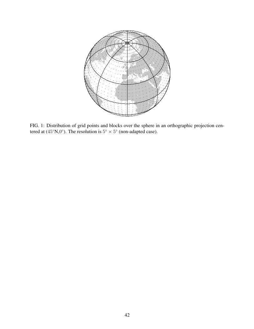
FIG. 1: Distribution of grid points and blocks over the sphere in an orthographic projection cen-tered at (45N,0). The resolution is 5 × 5 (non-adapted case).

42

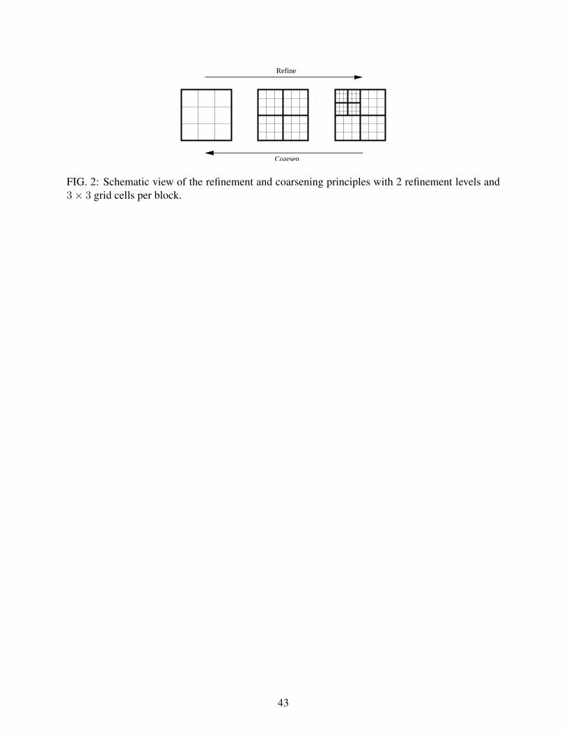
Refine

Coarsen

FIG. 2: Schematic view of the refinement and coarsening principles with 2 refinement levels and3× 3 grid cells per block.

43

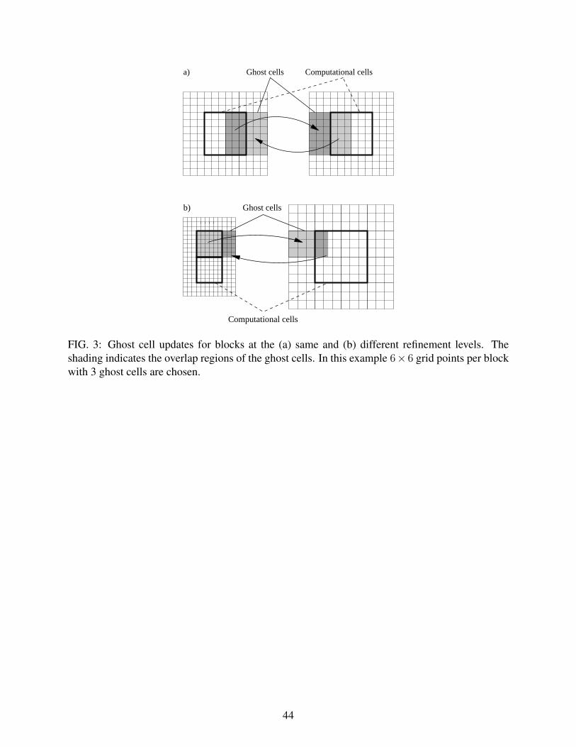
Ghost cells Computational cellsa)

Ghost cells

Computational cells

b)

FIG. 3: Ghost cell updates for blocks at the (a) same and (b) different refinement levels. Theshading indicates the overlap regions of the ghost cells. In this example 6× 6 grid points per blockwith 3 ghost cells are chosen.

44

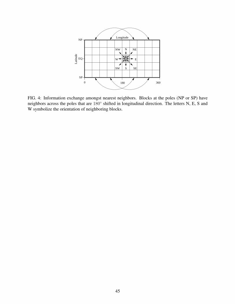
0 180

Longitude

S

EW

SW

NW NE

SE

N

EQ

360

NP

SPL

atitu

de

FIG. 4: Information exchange amongst nearest neighbors. Blocks at the poles (NP or SP) haveneighbors across the poles that are 180 shifted in longitudinal direction. The letters N, E, S andW symbolize the orientation of neighboring blocks.

45

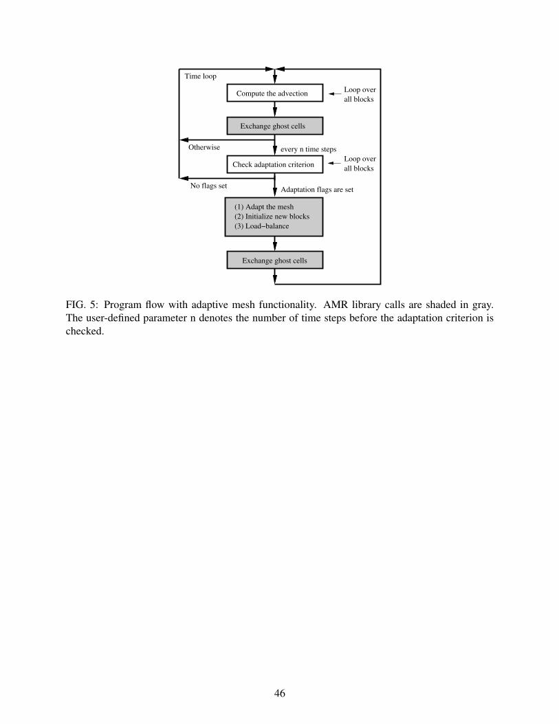
every n time steps

Exchange ghost cells

Compute the advection

Check adaptation criterion

(1) Adapt the mesh

(2) Initialize new blocks

(3) Load−balance

Time loop

Loop over

all blocks

Loop over

all blocks

Adaptation flags are set

Otherwise

No flags set

Exchange ghost cells

FIG. 5: Program flow with adaptive mesh functionality. AMR library calls are shaded in gray.The user-defined parameter n denotes the number of time steps before the adaptation criterion ischecked.

46

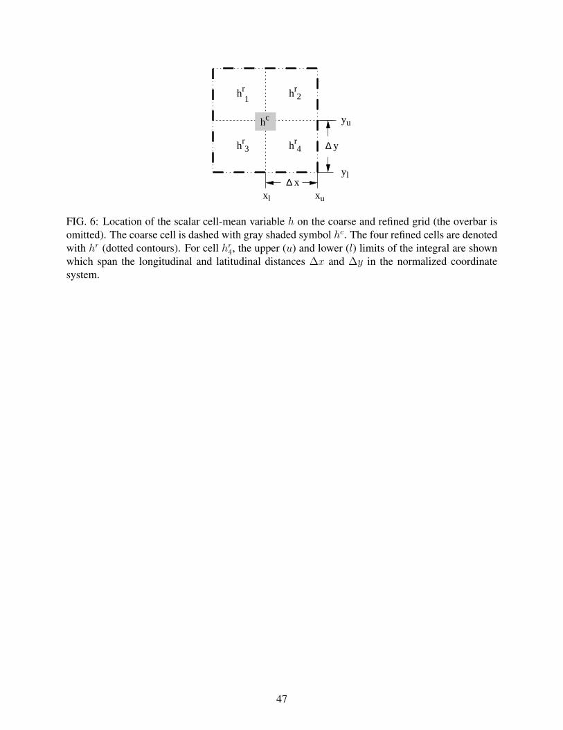
hc

h

h

h

hr r

rr

3

1 2

4 y∆

x x

y

y

u

l

u

l

x∆

FIG. 6: Location of the scalar cell-mean variable h on the coarse and refined grid (the overbar isomitted). The coarse cell is dashed with gray shaded symbol hc. The four refined cells are denotedwith hr (dotted contours). For cell hr

4, the upper (u) and lower (l) limits of the integral are shownwhich span the longitudinal and latitudinal distances ∆x and ∆y in the normalized coordinatesystem.

47

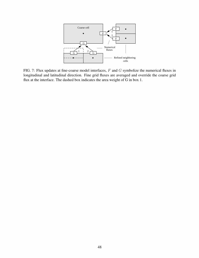
G

Refined neighboringcells

Coarse cell

Numericalfluxes21

1

2

G

G

F

F

F

FIG. 7: Flux updates at fine-coarse model interfaces, F and G symbolize the numerical fluxes inlongitudinal and latitudinal direction. Fine grid fluxes are averaged and override the coarse gridflux at the interface. The dashed box indicates the area weight of G in box 1.

48

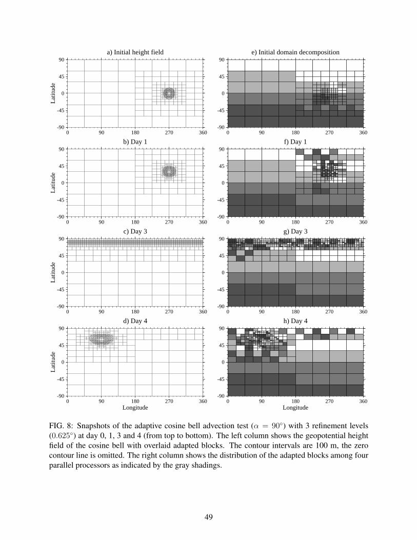
a) Initial height field

-90

-45

0

45

90L

atitu

de

0 90 180 270 360

e) Initial domain decomposition

-90

-45

0

45

90

0 90 180 270 360

b) Day 1

-90

-45

0

45

90

Lat

itude

0 90 180 270 360

f) Day 1

-90

-45

0

45

90

0 90 180 270 360

c) Day 3

-90

-45

0

45

90

Lat

itude

0 90 180 270 360

g) Day 3

-90

-45

0

45

90

0 90 180 270 360

d) Day 4

-90

-45

0

45

90

Lat

itude

0 90 180 270 360Longitude

h) Day 4

-90

-45

0

45

90

0 90 180 270 360Longitude

FIG. 8: Snapshots of the adaptive cosine bell advection test (α = 90) with 3 refinement levels(0.625) at day 0, 1, 3 and 4 (from top to bottom). The left column shows the geopotential heightfield of the cosine bell with overlaid adapted blocks. The contour intervals are 100 m, the zerocontour line is omitted. The right column shows the distribution of the adapted blocks among fourparallel processors as indicated by the gray shadings.

49

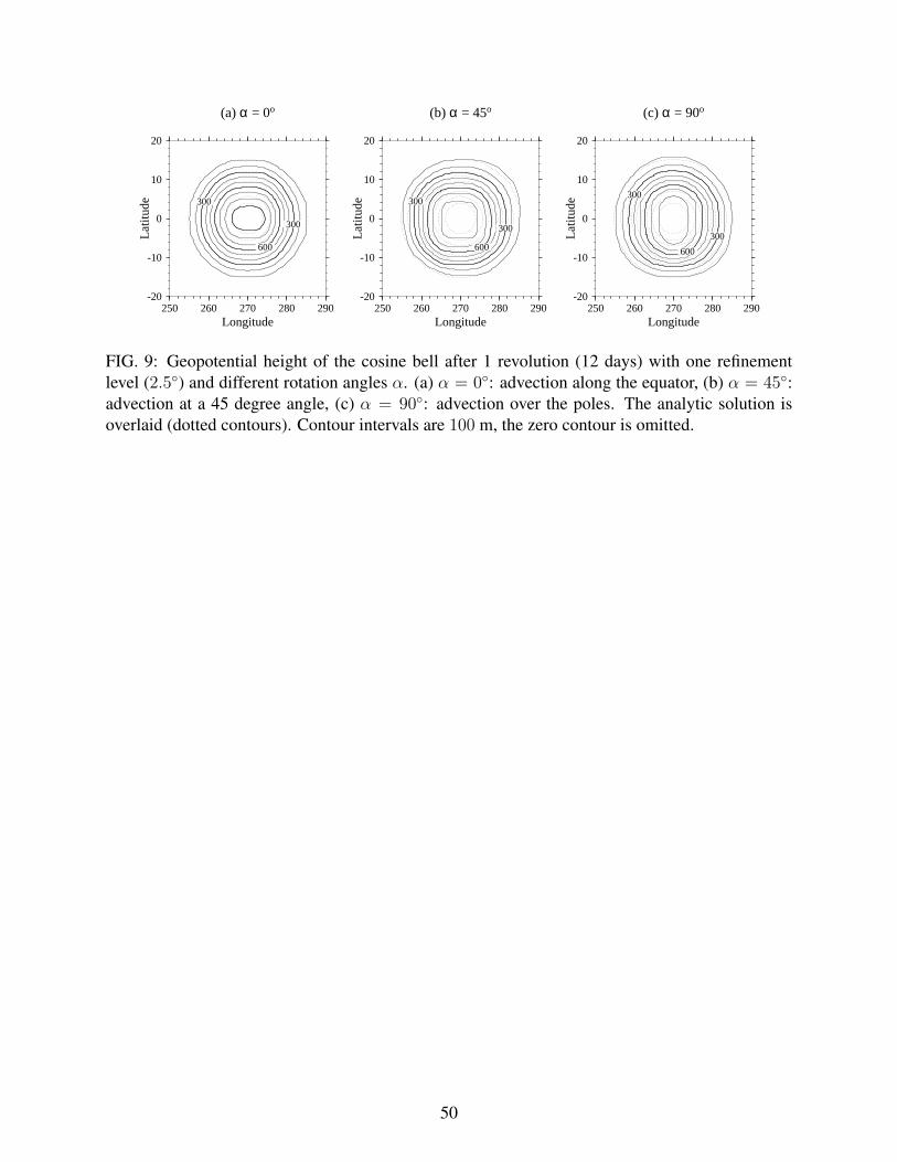
300

300

600

(a) α = 0o

-20

-10

0

10

20L

atitu

de

250 260 270 280 290Longitude

300

300

600

(b) α = 45o

-20

-10

0

10

20

Lat

itude

250 260 270 280 290Longitude

300

300

600

(c) α = 90o

-20

-10

0

10

20

Lat

itude

250 260 270 280 290Longitude

FIG. 9: Geopotential height of the cosine bell after 1 revolution (12 days) with one refinementlevel (2.5) and different rotation angles α. (a) α = 0: advection along the equator, (b) α = 45:advection at a 45 degree angle, (c) α = 90: advection over the poles. The analytic solution isoverlaid (dotted contours). Contour intervals are 100 m, the zero contour is omitted.

50

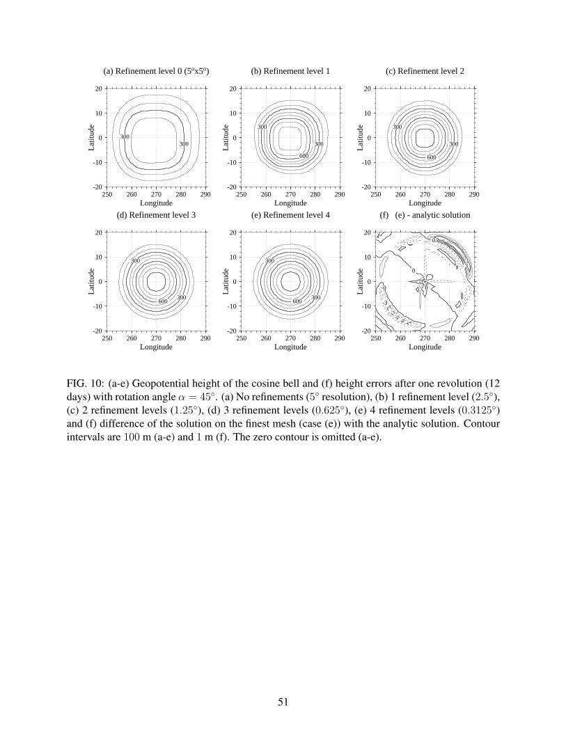
300300

(a) Refinement level 0 (5ox5o)

-20

-10

0

10

20L

atitu

de

250 260 270 280 290Longitude

300

300

600

(b) Refinement level 1

-20

-10

0

10

20

Lat

itude

250 260 270 280 290Longitude

300

300

600

(c) Refinement level 2

-20

-10

0

10

20

Lat

itude

250 260 270 280 290Longitude

300

300

600

(d) Refinement level 3

-20

-10

0

10

20

Lat

itude

250 260 270 280 290Longitude

300

300

600

(e) Refinement level 4

-20

-10

0

10

20L

atitu

de

250 260 270 280 290Longitude

0 0

0

0

3

(f) (e) - analytic solution

-20

-10

0

10

20

Lat

itude

250 260 270 280 290Longitude

-3

FIG. 10: (a-e) Geopotential height of the cosine bell and (f) height errors after one revolution (12days) with rotation angle α = 45. (a) No refinements (5 resolution), (b) 1 refinement level (2.5),(c) 2 refinement levels (1.25), (d) 3 refinement levels (0.625), (e) 4 refinement levels (0.3125)and (f) difference of the solution on the finest mesh (case (e)) with the analytic solution. Contourintervals are 100 m (a-e) and 1 m (f). The zero contour is omitted (a-e).

51

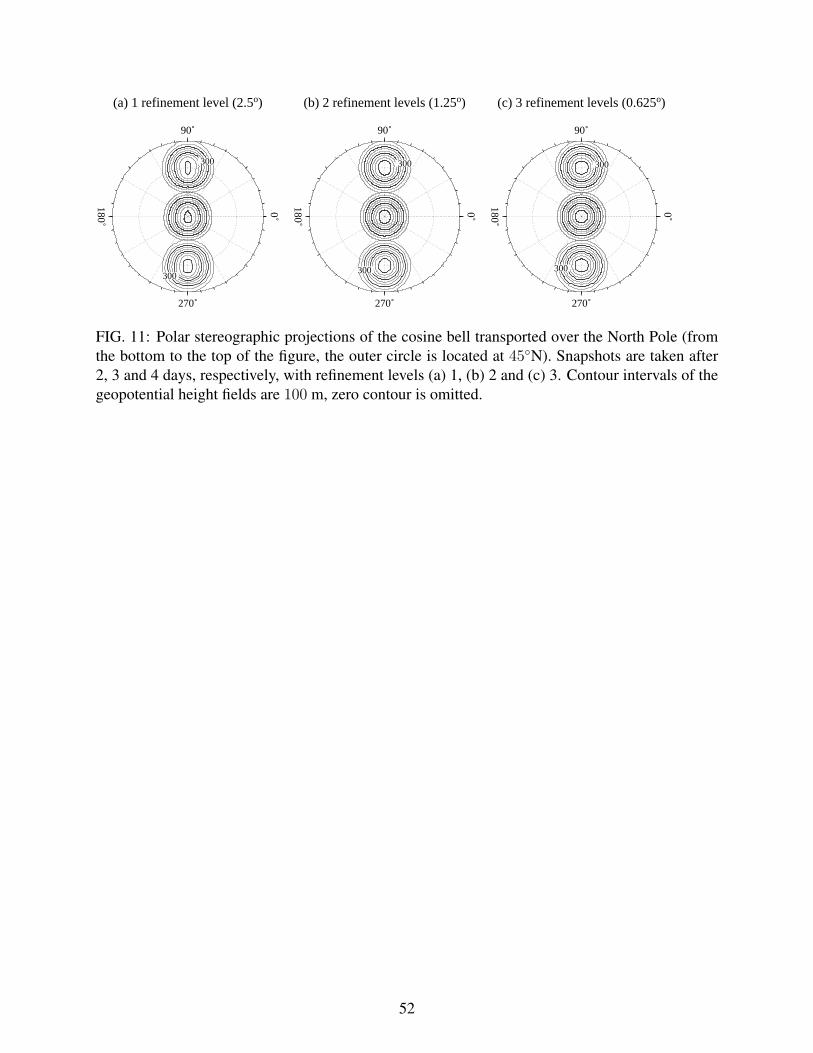
300

300

(a) 1 refinement level (2.5o)

0˚

90˚

180˚

270˚

300

300

(b) 2 refinement levels (1.25o)

0˚

90˚

180˚

270˚

300

300

(c) 3 refinement levels (0.625o)

0˚

90˚

180˚

270˚

FIG. 11: Polar stereographic projections of the cosine bell transported over the North Pole (fromthe bottom to the top of the figure, the outer circle is located at 45N). Snapshots are taken after2, 3 and 4 days, respectively, with refinement levels (a) 1, (b) 2 and (c) 3. Contour intervals of thegeopotential height fields are 100 m, zero contour is omitted.

52

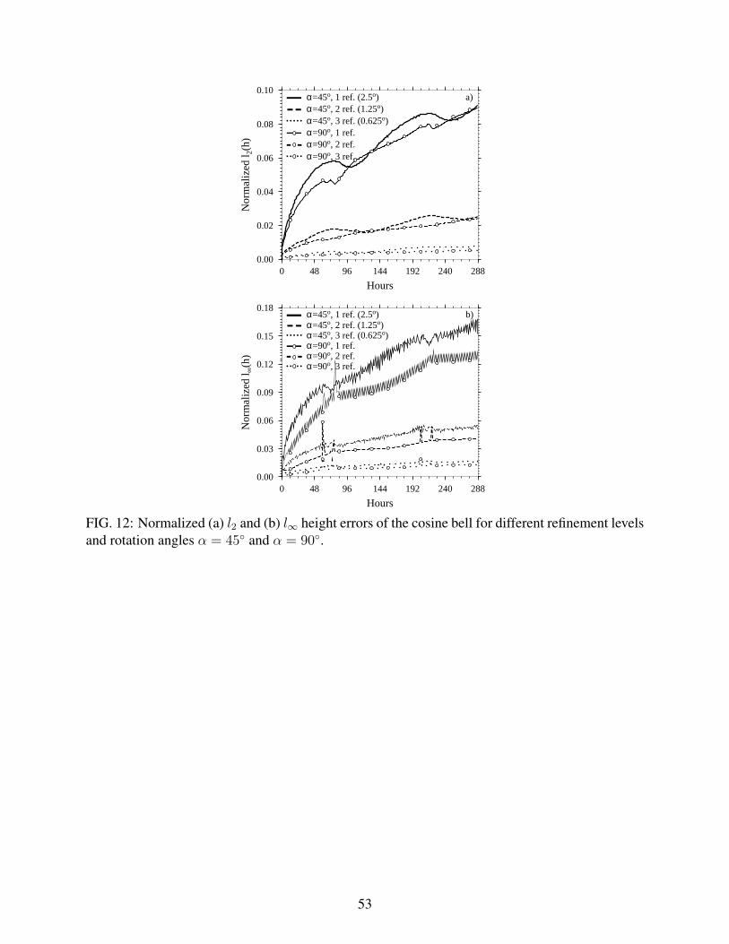
0.00

0.02

0.04

0.06

0.08

0.10

Nor

mal

ized

l 2(h

)

0 48 96 144 192 240 288

Hours

a)α=45o, 1 ref. (2.5o)α=45o, 2 ref. (1.25o)α=45o, 3 ref. (0.625o)α=90o, 1 ref.α=90o, 2 ref.α=90o, 3 ref.

0.00

0.03

0.06

0.09

0.12

0.15

0.18

Nor

mal

ized

l ∞(h

)

0 48 96 144 192 240 288

Hours

b)α=45o, 1 ref. (2.5o)α=45o, 2 ref. (1.25o)α=45o, 3 ref. (0.625o)α=90o, 1 ref.α=90o, 2 ref.α=90o, 3 ref.

FIG. 12: Normalized (a) l2 and (b) l∞ height errors of the cosine bell for different refinement levelsand rotation angles α = 45 and α = 90.

53

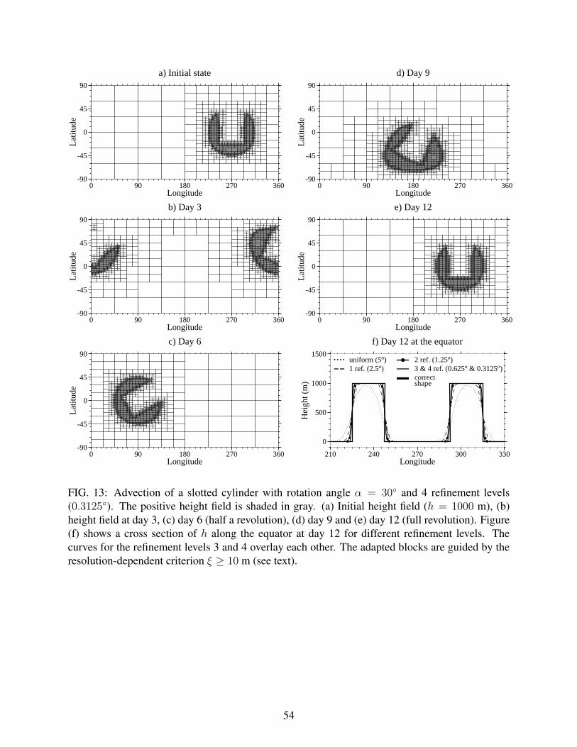
a) Initial state

-90

-45

0

45

90

Lat

itude

0 90 180 270 360Longitude

d) Day 9

-90

-45

0

45

90

Lat

itude

0 90 180 270 360Longitude

b) Day 3

-90

-45

0

45

90

Lat

itude

0 90 180 270 360Longitude

e) Day 12

-90

-45

0

45

90

Lat

itude

0 90 180 270 360Longitude

c) Day 6

-90

-45

0

45

90

Lat

itude

0 90 180 270 360Longitude

f) Day 12 at the equator

0

500

1000

1500

Hei

ght (

m)

210 240 270 300 330Longitude

uniform (5o)1 ref. (2.5o)

2 ref. (1.25o)3 & 4 ref. (0.625o & 0.3125o)correctshape

FIG. 13: Advection of a slotted cylinder with rotation angle α = 30 and 4 refinement levels(0.3125). The positive height field is shaded in gray. (a) Initial height field (h = 1000 m), (b)height field at day 3, (c) day 6 (half a revolution), (d) day 9 and (e) day 12 (full revolution). Figure(f) shows a cross section of h along the equator at day 12 for different refinement levels. Thecurves for the refinement levels 3 and 4 overlay each other. The adapted blocks are guided by theresolution-dependent criterion ξ ≥ 10 m (see text).

54

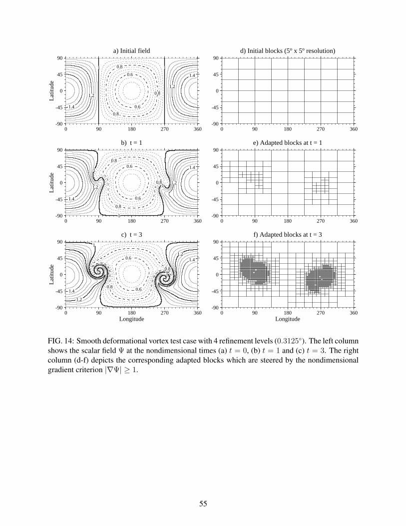
1 1

1.2

1.2

1.4

1.4 0.6

0.6

0.8

0.8

0.8

a) Initial field

-90

-45

0

45

90L

atitu

de

0 90 180 270 360

d) Initial blocks (5o x 5o resolution)

-90

-45

0

45

90

0 90 180 270 360

1

1

1

1.21.2

1.4

1.4 0.6

0.6

0.8

0.8

0.8

b) t = 1

-90

-45

0

45

90

Lat

itude

0 90 180 270 360

e) Adapted blocks at t = 1

-90

-45

0

45

90

0 90 180 270 360

1.2

1.2

1

1

1

1.4

1.4 0.6

0.6

0.8

0.8

c) t = 3

-90

-45

0

45

90

Lat

itude

0 90 180 270 360Longitude

f) Adapted blocks at t = 3

-90

-45

0

45

90

0 90 180 270 360Longitude

FIG. 14: Smooth deformational vortex test case with 4 refinement levels (0.3125). The left columnshows the scalar field Ψ at the nondimensional times (a) t = 0, (b) t = 1 and (c) t = 3. The rightcolumn (d-f) depicts the corresponding adapted blocks which are steered by the nondimensionalgradient criterion |∇Ψ| ≥ 1.

55

TABLE 1: Refinement levels and corresponding global grid resolutions on the sphere for a 5× 5

base grid.

Refin. Resolution Max. # grid points Resolution ∆x (km) at different positions ϕ

level ∆λ, ∆ϕ lon x lat (full grid) Equator 60 N/S 75 N/S Near pole

0 5 72 x 36 556.0 278.0 143.9 24.26

1 2.5 144 x 72 278.0 139.0 72.0 6.06

2 1.25 288 x 144 139.0 69.5 36.0 1.52

3 0.625 576 x 288 69.5 34.8 18.0 0.38

4 0.3125 1152 x 576 34.8 17.4 9.0 0.09

56

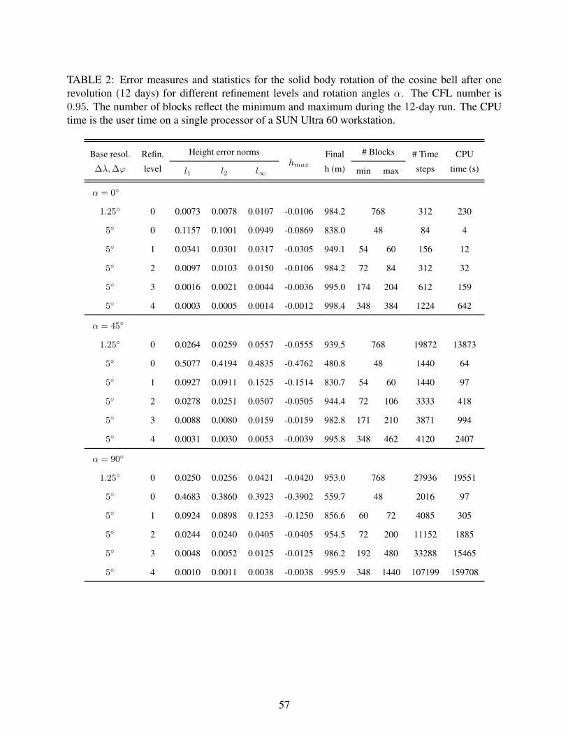
TABLE 2: Error measures and statistics for the solid body rotation of the cosine bell after onerevolution (12 days) for different refinement levels and rotation angles α. The CFL number is0.95. The number of blocks reflect the minimum and maximum during the 12-day run. The CPUtime is the user time on a single processor of a SUN Ultra 60 workstation.

Base resol. Refin. Height error norms Final # Blocks # Time CPU

∆λ, ∆ϕ level l1 l2 l∞hmax h (m) min max steps time (s)

α = 0

1.25 0 0.0073 0.0078 0.0107 -0.0106 984.2 768 312 230

5 0 0.1157 0.1001 0.0949 -0.0869 838.0 48 84 4

5 1 0.0341 0.0301 0.0317 -0.0305 949.1 54 60 156 12

5 2 0.0097 0.0103 0.0150 -0.0106 984.2 72 84 312 32

5 3 0.0016 0.0021 0.0044 -0.0036 995.0 174 204 612 159

5 4 0.0003 0.0005 0.0014 -0.0012 998.4 348 384 1224 642

α = 45

1.25 0 0.0264 0.0259 0.0557 -0.0555 939.5 768 19872 13873

5 0 0.5077 0.4194 0.4835 -0.4762 480.8 48 1440 64

5 1 0.0927 0.0911 0.1525 -0.1514 830.7 54 60 1440 97

5 2 0.0278 0.0251 0.0507 -0.0505 944.4 72 106 3333 418

5 3 0.0088 0.0080 0.0159 -0.0159 982.8 171 210 3871 994

5 4 0.0031 0.0030 0.0053 -0.0039 995.8 348 462 4120 2407

α = 90

1.25 0 0.0250 0.0256 0.0421 -0.0420 953.0 768 27936 19551

5 0 0.4683 0.3860 0.3923 -0.3902 559.7 48 2016 97

5 1 0.0924 0.0898 0.1253 -0.1250 856.6 60 72 4085 305

5 2 0.0244 0.0240 0.0405 -0.0405 954.5 72 200 11152 1885

5 3 0.0048 0.0052 0.0125 -0.0125 986.2 192 480 33288 15465

5 4 0.0010 0.0011 0.0038 -0.0038 995.9 348 1440 107199 159708

57

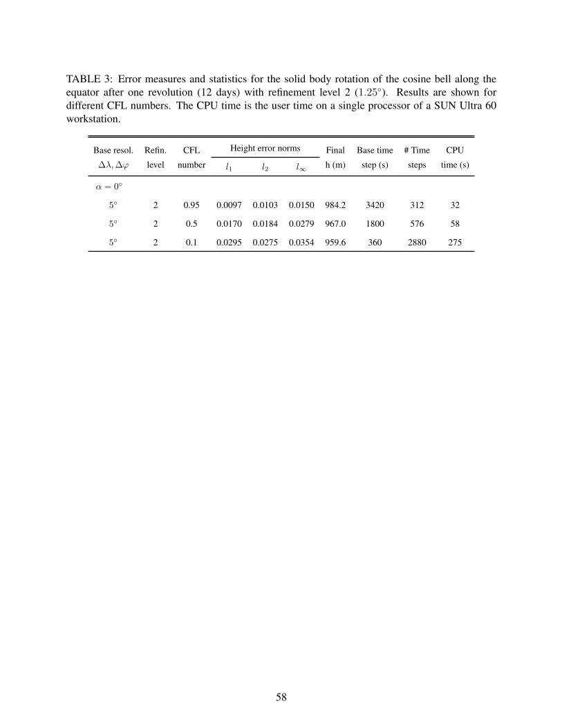
TABLE 3: Error measures and statistics for the solid body rotation of the cosine bell along theequator after one revolution (12 days) with refinement level 2 (1.25). Results are shown fordifferent CFL numbers. The CPU time is the user time on a single processor of a SUN Ultra 60workstation.

Base resol. Refin. CFL Height error norms Final Base time # Time CPU

∆λ, ∆ϕ level number l1 l2 l∞ h (m) step (s) steps time (s)

α = 0

5 2 0.95 0.0097 0.0103 0.0150 984.2 3420 312 32

5 2 0.5 0.0170 0.0184 0.0279 967.0 1800 576 58

5 2 0.1 0.0295 0.0275 0.0354 959.6 360 2880 275

58

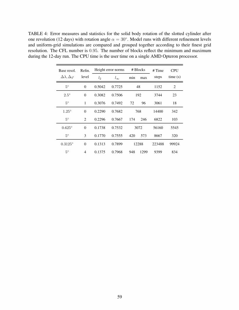
TABLE 4: Error measures and statistics for the solid body rotation of the slotted cylinder afterone revolution (12 days) with rotation angle α = 30. Model runs with different refinement levelsand uniform-grid simulations are compared and grouped together according to their finest gridresolution. The CFL number is 0.95. The number of blocks reflect the minimum and maximumduring the 12-day run. The CPU time is the user time on a single AMD Opteron processor.

Base resol. Refin. Height error norms # Blocks # Time CPU

∆λ,∆ϕ level l2 l∞ min max steps time (s)

5 0 0.5042 0.7725 48 1152 2

2.5 0 0.3082 0.7506 192 3744 23

5 1 0.3076 0.7492 72 96 3061 18

1.25 0 0.2290 0.7682 768 14400 342

5 2 0.2296 0.7667 174 246 6822 103

0.625 0 0.1738 0.7532 3072 56160 5545

5 3 0.1770 0.7555 420 573 8667 320

0.3125 0 0.1313 0.7899 12288 223488 99924

5 4 0.1375 0.7968 948 1299 9399 834

59

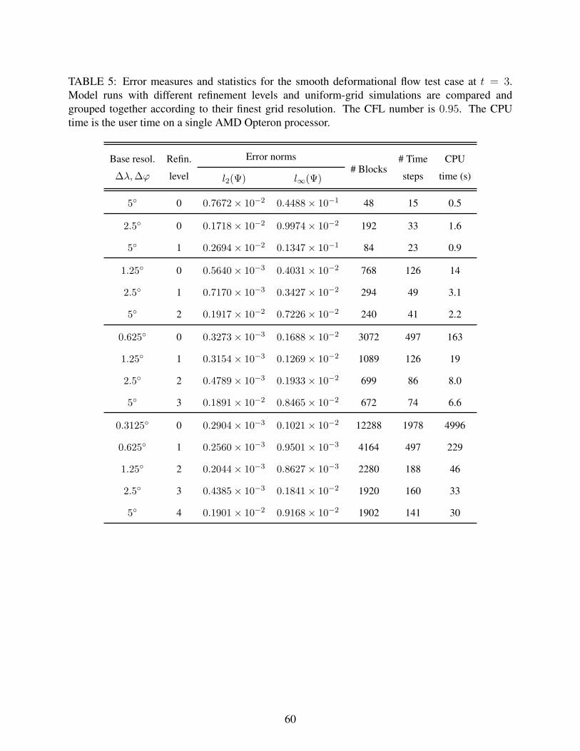
TABLE 5: Error measures and statistics for the smooth deformational flow test case at t = 3.Model runs with different refinement levels and uniform-grid simulations are compared andgrouped together according to their finest grid resolution. The CFL number is 0.95. The CPUtime is the user time on a single AMD Opteron processor.

Base resol. Refin. Error norms # Time CPU

∆λ,∆ϕ level l2(Ψ) l∞(Ψ)# Blocks

steps time (s)

5 0 0.7672× 10−2 0.4488× 10−1 48 15 0.5

2.5 0 0.1718× 10−2 0.9974× 10−2 192 33 1.6

5 1 0.2694× 10−2 0.1347× 10−1 84 23 0.9

1.25 0 0.5640× 10−3 0.4031× 10−2 768 126 14

2.5 1 0.7170× 10−3 0.3427× 10−2 294 49 3.1

5 2 0.1917× 10−2 0.7226× 10−2 240 41 2.2

0.625 0 0.3273× 10−3 0.1688× 10−2 3072 497 163

1.25 1 0.3154× 10−3 0.1269× 10−2 1089 126 19

2.5 2 0.4789× 10−3 0.1933× 10−2 699 86 8.0

5 3 0.1891× 10−2 0.8465× 10−2 672 74 6.6

0.3125 0 0.2904× 10−3 0.1021× 10−2 12288 1978 4996

0.625 1 0.2560× 10−3 0.9501× 10−3 4164 497 229

1.25 2 0.2044× 10−3 0.8627× 10−3 2280 188 46

2.5 3 0.4385× 10−3 0.1841× 10−2 1920 160 33

5 4 0.1901× 10−2 0.9168× 10−2 1902 141 30

60