Embed Size (px)
Citation preview
ADAPTIVE DEPLOYMENT OF MOBILE SENSOR NODES
by
Steven J Erdmanczyk Jr.
A thesis submitted to the faculty ofThe University of North Carolina at Charlotte
in partial fulfillment of the requirementsfor the degree of Master of Science in
Electrical Engineering
Charlotte
2013
Approved by:
Dr. James Conrad
Dr. Asis Nasipuri
Dr. Thomas Weldon

ii
c©2013Steven J Erdmanczyk Jr.
ALL RIGHTS RESERVED
iii
ABSTRACT
STEVEN J ERDMANCZYK JR.. Adaptive deployment of mobile sensor nodes.(Under the direction of DR. JAMES CONRAD)
There are many desirable applications that involve the deployment of mobile nodes
into environments that may not be favorable to humans in order to gather data or
perform manipulative tasks. In some of these environments, direct wireless commu-
nication may not be possible from the point of deployment to the desired endpoint.
This can be due to radio interference from the environment such as fading effects
from obstacles and walls or signal attenuation due to distance. One solution to this
scenario is to deploy a chain of mobile bread-crumb nodes between the base station
and end node. For this thesis, an algorithm was researched and implemented to intel-
ligently deploy mobile nodes to create such a tether, as well as maintain an optimal
distance between the nodes.
iv
ACKNOWLEDGMENTS
Thanks goes first and foremost to my advisor Dr. Conrad for his guidance through
my graduate career. Dr. Conrad is tireless and consistent in managing his students,
without his help none of the work in thesis would have been possible. I sincerely
thank Dr. Conrad for believing in me and guiding me through the work performed
in this document. Thanks also goes to Dr. Asis Nasipuri and Dr. Thomas Weldon
for providing support and accepting their positions as my committee members.
Thanks also goes to all of my colleagues and classmates in the masters program
who, through their presence, have helped lighten the load of many long hours. I
would like to thank Malcolm Zapata, Thomas Meiswinkel, Richard McKinney, Onkar
Raut, Suraj Swami, and Aswin Ramakrishnan for being there for help, advice, and
moral support throughout my graduate career.
Lastly I would like to give thanks to my family for all of their love and support.
I would like to thank my mother and father for always proudly encouraging and
congratulating me in my academic accomplishments. I would especially like to thank
my wife Kelly for being kind, patient, understanding, and always there for support
throughout the time I was performing the research in this thesis.
v
TABLE OF CONTENTS
LIST OF FIGURES vii
LIST OF TABLES ix
LIST OF ABBREVIATIONS x
CHAPTER 1: INTRODUCTION 1
1.1. Motivation 1
1.2. Organization of Thesis 3
CHAPTER 2: BACKGROUND 4
2.1. Received Signal Strength 4
2.2. IEEE 802.15.4 6
2.3. Previous Work 9
CHAPTER 3: HARDWARE AND SOFTWARE SETUP 14
3.1. Hardware Setup 14
3.2. Interfacing with XBee 802.15.4 Radios 16
3.3. Multi-Hop Message Delivery 20
3.4. Syncing RSS Between Neighboring Nodes 21
3.5. Verifying Node Network Quality 24
CHAPTER 4: ALGORITHMS 26
4.1. Intelligent Node Deployment 26
4.2. Maintaining Effective Distance for Communications 29
4.3. Recovering from a Lost-Node Scenario 31

vi
CHAPTER 5: SYSTEM OVERVIEW 34
5.1. Mobile Node 35
5.2. Base Station 38
CHAPTER 6: TESTS AND OBSERVATIONS 42
6.1. Measuring RSS vs. Distance with One Node 42
6.2. Measuring RSS vs. Distance with Two Nodes 44
6.3. Nine Node System Test 46
CHAPTER 7: CONCLUSIONS 51
7.1. Conclusions 51
7.2. Future Work 51
REFERENCES 52
vii
LIST OF FIGURES
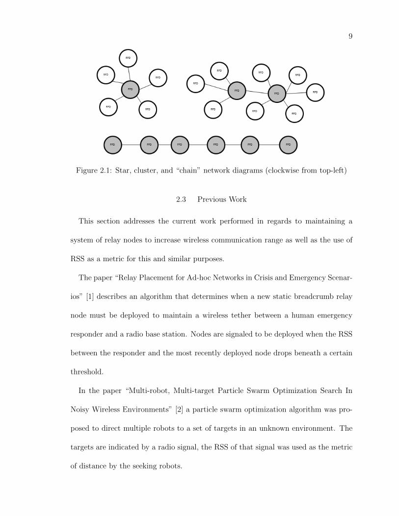
FIGURE 2.1: Star, cluster, and “chain” network diagrams 9
FIGURE 3.1: Renesas Sakura board with XBee and power module 15
FIGURE 3.2: Full system setup: base station with eight nodes 16
FIGURE 3.3: XBee internal buffers diagram [3] 17
FIGURE 3.4: XBee api frames used for this thesis 19
FIGURE 3.5: Rss sync frames 22
FIGURE 3.6: Syncing node rss 23
FIGURE 3.7: Reporting node rss 24
FIGURE 3.8: Ping messages 24
FIGURE 4.1: Deployment and address assignment frames 26
FIGURE 4.2: Process for deploying first node 27
FIGURE 4.3: Process for deploying subsequent nodes 28
FIGURE 4.4: Lost node recovery 31
FIGURE 4.5: Lost node messages 32
FIGURE 5.1: Software layer frames summary 34
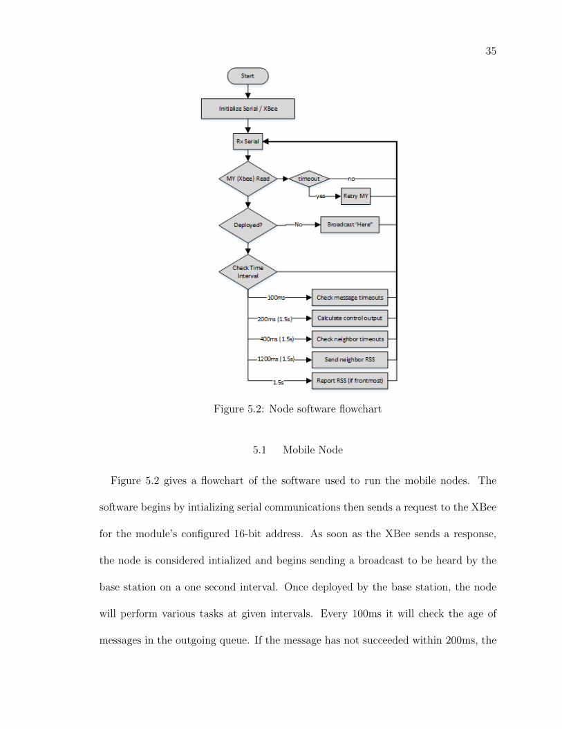
FIGURE 5.2: Node software flowchart 35
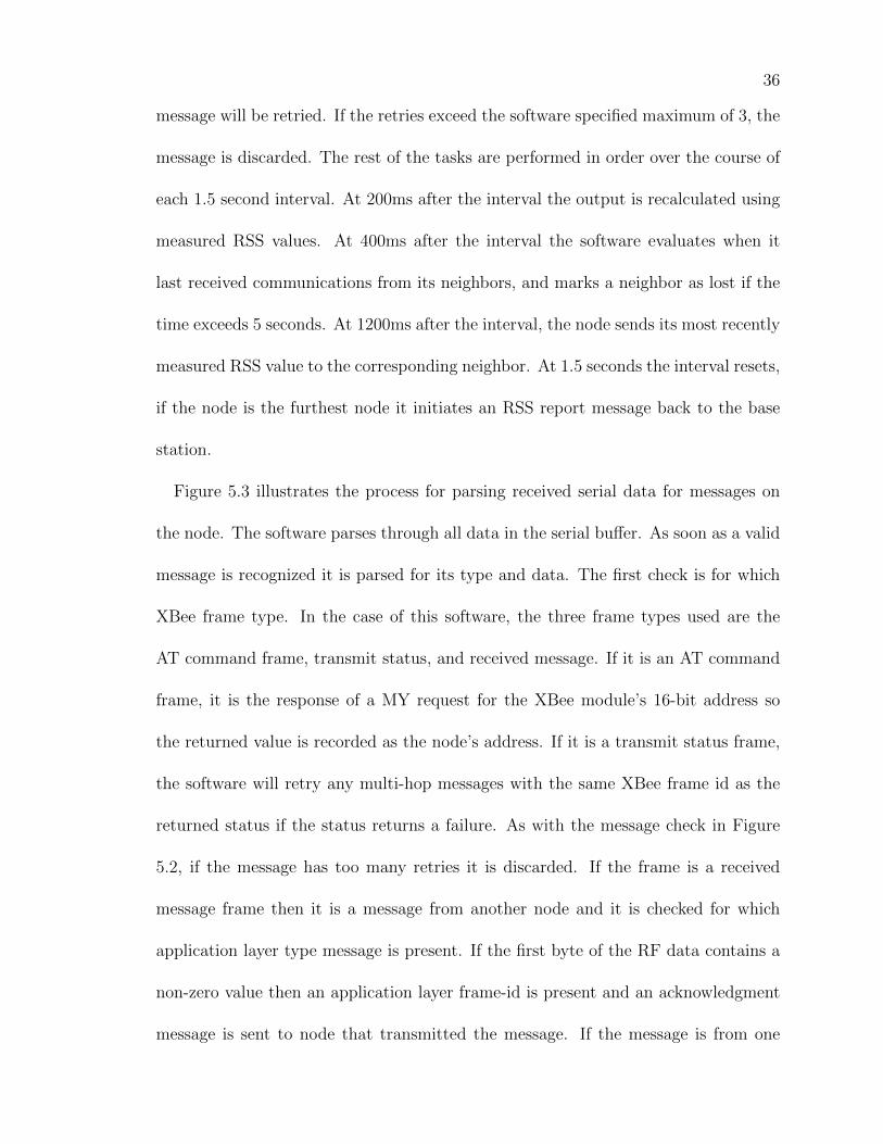
FIGURE 5.3: Node message reception 37
FIGURE 5.4: Base station program flow 39
FIGURE 5.5: Base station message reception 40
FIGURE 6.1: Test one: measured rss and success rate between one nodeand base station vs. time
42
viii
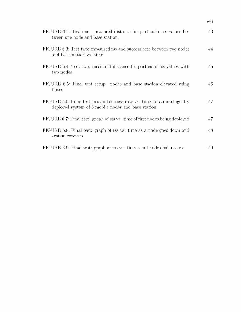
FIGURE 6.2: Test one: measured distance for particular rss values be-tween one node and base station
43
FIGURE 6.3: Test two: measured rss and success rate between two nodesand base station vs. time
44
FIGURE 6.4: Test two: measured distance for particular rss values withtwo nodes
45
FIGURE 6.5: Final test setup: nodes and base station elevated usingboxes
46
FIGURE 6.6: Final test: rss and success rate vs. time for an intelligentlydeployed system of 8 mobile nodes and base station
47
FIGURE 6.7: Final test: graph of rss vs. time of first nodes being deployed 47
FIGURE 6.8: Final test: graph of rss vs. time as a node goes down andsystem recovers
48
FIGURE 6.9: Final test: graph of rss vs. time as all nodes balance rss 49
ix
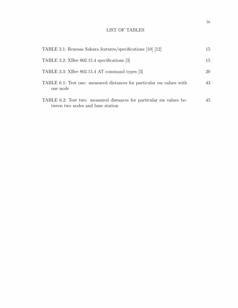
LIST OF TABLES
TABLE 3.1: Renesas Sakura features/specifications [10] [12] 15
TABLE 3.2: XBee 802.15.4 specifications [3] 15
TABLE 3.3: XBee 802.15.4 AT command types [3] 20
TABLE 6.1: Test one: measured distances for particular rss values withone node
43
TABLE 6.2: Test two: measured distances for particular rss values be-tween two nodes and base station
45
x
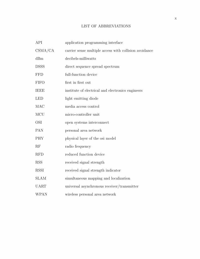
LIST OF ABBREVIATIONS
API application programming interface
CSMA/CA carrier sense multiple access with collision avoidance
dBm decibels-milliwatts
DSSS direct sequence spread spectrum
FFD full-function device
FIFO first in first out
IEEE institute of electrical and electronics engineers
LED light emitting diode
MAC media access control
MCU micro-controller unit
OSI open systems interconnect
PAN personal area network
PHY physical layer of the osi model
RF radio frequency
RFD reduced function device
RSS received signal strength
RSSI received signal strength indicator
SLAM simultaneous mapping and localization
UART universal asynchronous receiver/transmitter
WPAN wireless personal area network
CHAPTER 1: INTRODUCTION
1.1 Motivation
Research in the area of remote controlled or autonomous mobile robot applications
has been popular for many decades now. Common applications for such technologies
include automating industrial maintenance in areas that are either tedious, hazardous,
or impossible for humans to reach. Other applications include sending robots into dis-
aster areas to locate or rescue survivors without risking the lives of rescue personnel.
As technologies become cheaper, more available, and easier to implement, researchers
continue to look into applications where robots can assist where they were unable to
before.
For these kinds of applications, even in the case of autonomous robots, it’s common
to establish and maintain a communications link with the robot to either control
its movement or observe sensor readings. Advancements in wireless communication
technologies have allowed manipulators to maintain this link without the need for
cables that would otherwise be too costly or prohibit the needed degree of movement.
Despite the freedoms wireless technologies enable, all forms of radio communications
still pose the same drawbacks. One drawback is that there will always be a maximum
distance a radio signal of any strength can travel before it has attenuated to greatly
to be received. Another drawback is that obstacles in the environment will cause
2
interference with the radio signal. These effects are briefly covered in Chapter 2.
These drawbacks pose problems in indoor or sub-terranean applications where di-
rect line-of-sight communication is almost always impossible. In these situations the
robot will be unable to go far from the deployment point without exceeding the ca-
pable communication range. One solution to mitigate this problem is to implement
multi-hop radio relays that propagate the radio signal for longer distances or around
interfering obstacles.
There are many methods for implementing these types of radio relays, one of which
is to statically place radio relay nodes prior to robot deployment. This is a viable
solution in industrial maintenance scenarios where prior knowledge of deployment
routes can be known. However, this solution would not be helpful in many disaster
scenarios as needed deployment routes would be difficult or impossible to predict.
Furthermore, in disaster scenarios the environment may change due to collapsing
structures. Another solution is for the robot to dynamically place static wireless relay
nodes as needed whenever signal strength to the deployment point or previous relay
node has dropped beneath a sufficient threshold. This method allows deployment
into new areas, but is still limited by the inability, once deployed, of the relay nodes
to adjust distance to each other should changes in the environment cause a decrease
in signal. Another problem that affects this scenario is the inability to react when
one of the relay nodes turns out to be defective or is destroyed.
The motivation of this thesis is to extend on these solutions by creating an algo-
rithm that intelligently deploys a trail of mobile wireless relay nodes or “breadcrumbs”
capable of dynamically adjusting distance between each other in a way that maxi-
3
mizes distance between the relays without moving beyond the capable range of radio
communications. This allows deployment in dynamic scenarios, as well as the ability
to cope with changing environments. This also allows the system to handle situations
where one of the nodes is defective or destroyed.
This algorithm was designed with the intention to be used in a future project
that will implement a system of small, low powered quad-rotor robots that will be
deployed through a tunnel system to gather data and perform maintenance. Future
work will be to implement this algorithm alongside other algorithms that handle
obstacle avoidance, path-planning, mapping, and localization in order to create a
complete deployment system.
1.2 Organization of Thesis
This thesis is organized into 6 chapters. Chapter 2 covers background information
concerning Received Signal Strength (RSS) metrics, the Institute of Electrical and
Electronic Engineers (IEEE) 802.15.4 specification, and existing research in the usage
of signal strength in the deployment of mobile robots and radio relays. Chapter 3
covers the initial hardware and software setup. Chapter 4 covers the algorithms
designed and implemented to handle the deployment of nodes, the maintenance of
distance between nodes, and handling of scenarios where nodes are lost. Chapter 5
gives an overview of the resulting software architecture. Chapter 6 covers tests and
observations. Chapter 7 presents the conclusions of this research and future work.
CHAPTER 2: BACKGROUND
2.1 Received Signal Strength
Received signal strength is a metric calculated during message reception on the
media access control (MAC) layer. RSS in low powered systems is often measured in
units of decibel-milliwatt or dBm, which is a ratio of the power of the electric field
carrying the signal received at the antenna compared to 1 milliwatt. Given the power
of the signal in milliwatts, signal strength can be computed in dBm by the equation
PdBm = 10 · log10(PmW/1mW ). A change in 10 dBm represents a change of power
in milliwatts by a factor of ten. For the 802.15.4 protocol there is no standard for
the how the MAC layer should provide the RSS, so determining RSS and the number
format used to provide it will vary by device. The specific term for the number
provided by the MAC layer is Received Signal Strength Indicator (RSSI). In the case
of XBee 802.15.4 radios, the RSSI is the absolute value of the measured RSS, so an
RSSI byte of 0x45 (90) would indicate an RSS of -90dBm, 0x2d (45) would indicate
-45dBm, 0x48 (72) would indicate -72dBm, etc.
The RSS of a radio signal is subject to a number of factors including the power
of the transmitting radio, distance between transmitters, orientation of the transmit-
ting and receiving antennas, type of antenna used, backround radio noise, and any
interference from fading effects due to obstacles in the environment. Fading effects
5
include shadowing and multi-path propagation. Shadowing is an effect where an ob-
stacle positioned directly between the communicating radios is casting a “shadow”
in the wave of the transmitted signal similar to how objects cast shadows in light.
Multi-path propagation, is an effect where the signal is partially deflected off of an
object and the deflected signal arrives at the destination alongside the original signal.
The deflected signal will often have shifted phase and amplitude, causing it to interact
destructively with the original signal.
There are various methods for modeling the expected RSS within an application.
The most simplistic model is to assume all other effects ideal and only calculate for
distance. Calculating distance in three dimensional space can become costly because
the robot’s position must first be known. Bayesian modeling techniques such as
Kalman Filters or Monte Carlo particle filters are example methods for generating an
estimate of a mobile robots position. In order to compute an estimate of a robot’s
position, a map of the environment must also be previously known or generated on the
fly. Simultaneous location and mapping (SLAM) algorithms specifies one category of
techniques for generating a map of an environment on the fly. The localization portion
of SLAM algorithms typically employs one of the previously mentioned localization
techniques. If a map is known and a robot is localized, it is also possible to estimate
the effect of antenna position and orientation on RSS. To create a as comprehensive
an estimate of the expected RSS as possible, an application will also need to estimate
the effects of multi-path propagation and shadowing. Attempting to model these
effects deterministically is very difficultand would be prohibitively computationally
expensive, so these effects are often modeled stochastically as random processes.
6
Sensors needed to provide measurements for localization techniques are often costly,
require additional power, and may be too large or heavy for feasibility in smaller
systems. Additionally, the computational requirements of localization, mapping, and
modeling fading effects will often surpass the specifications of the micro-controller
units (MCU) used to perform computations in low-powered systems.
One of the goals in this thesis was to provide an algorithm that maximizes distance
between a series of mobile node without exceeding the range needed for radio commu-
nications. This algorithm was intended to be implemented in low-powered systems so
computational and sensor requirements needed to be minimized. Previous research
such as that in [11] demonstrates that as RSS in a system decreases, the number of
messages lost stays consistently low until the RSS dropped below the devices thresh-
old for sensitivity. Research in [4] also demonstrates how signal strength metrics are
superior to relying on distance for predicting communications effectiveness because
it allows the application to avoid locations that are subject to fading effects without
the requirement for extra computations. Thus for this algorithm it was chosen to
negate calculations for distance and modeling fading effects, and simply use the RSS
provided by the MAC layer as the estimate of communications effectiveness. This
proved to be an effective method of determining wireless link quality in a low-cost
system.
2.2 IEEE 802.15.4
The IEEE 802.15 group is a set of standards for wireless personal area network
(WPAN) communications. A WPAN is a network of wireless devices that are only
7
intended to communicate locally without a link to the outside world. WPANs typ-
ically consist of groups of devices that share data between one other or transmit
data back to an internet enabled base station such as in wireless sensor networks.
802.15.4 is a sub-standard specifically intended for low cost, low powered devices that
don’t require high speed communication rates. Many devices that use 802.15.4 are
intended to run for extended periods of time, such as months or years, without the
need of maintenance or battery replacement. 802.15.4 specifies the mechanisms on
the physical (PHY) and media access control (MAC) layers of the OSI networking
model.
802.15.4 controls access to the physical communications medium using carrier sense
multiple access with collision avoidance (CSMA/CA). Before sending a message,
CSMA/CA will sense for energy on the transmitting frequency. If energy is detected
above the configured threshold, the algorithm will delay based on a randomized back-
off algorithm. The back-off algorithm chooses the back-off delay by randomly selecting
from a sequence of pseudo-random values based on a configurable exponent. As the
retries increase the values, as well as number of possible values, generated by the
back-off algorithm increase. CSMA/CA will retry up to three times before discarding
the message. 802.15.4 also avoids communication interference by using the direct
sequence spread spectrum (DSSS) technique. DSSS effectively “spreads” the signal
across multiple frequencies by injecting a pseudo-random string of “chips” into the
signal that are at a higher frequency . The receiver is made aware of the pseudo-
random sequence so it can decode the signal at reception. Through this process,
DSSS decreases the chances of interference by spreading the signal across multiple
8
frequencies, effectively increasing the signal-to-noise ratio.
802.15.4 enables nodes to communicate to each other using either peer-to-peer,
point-to-point, or point-to-multipoint communications such as in star network topol-
ogy. A star network topology is enabled by specifying two types of nodes: full-function
devices (FFD) and reduced-function devices (RFD). An FFD is capable of coordi-
nating communications between other RFD’s assigned to it by forwarding packets
between them and specifying when they are allowed to communicate. When perform-
ing this role it is referred to as the personal area network (PAN) coordinator. An
RFD is only capable of sending and receiving to an FFD and cannot coordinate other
nodes. FFD’s cannot enter sleep mode, whilst an RFD can in order to save power.
In a star network topology, a PAN coordinator acts as the central point relaying all
communications between multiple RFD end-points. A PAN coordinator can connect
to other coordinators to mimick a cluster topology. However, because 802.15.4 it
is only specified on the PHY and MAC layers, 802.15.4 does not support routing
or functionality to ensure multi-hop message delivery. By default, XBee devices are
configured as FFD’s using peer-to-peer communications.
In the application for this thesis, the resulting topology when many nodes are
deployed would resemble a “chain” where each node only speaks to the nodes in front
of or behind it. Star or cluster topologies would not prove useful in this scenario so
this research did not make use of the 802.15.4 PAN coordinator functionality. All
radios were used as FFD’s communicating with a peer-to-peer topology. Routing and
multi-hop message delivery was handled using software.
9
Figure 2.1: Star, cluster, and “chain” network diagrams (clockwise from top-left)
2.3 Previous Work
This section addresses the current work performed in regards to maintaining a
system of relay nodes to increase wireless communication range as well as the use of
RSS as a metric for this and similar purposes.
The paper “Relay Placement for Ad-hoc Networks in Crisis and Emergency Scenar-
ios” [1] describes an algorithm that determines when a new static breadcrumb relay
node must be deployed to maintain a wireless tether between a human emergency
responder and a radio base station. Nodes are signaled to be deployed when the RSS
between the responder and the most recently deployed node drops beneath a certain
threshold.
In the paper “Multi-robot, Multi-target Particle Swarm Optimization Search In
Noisy Wireless Environments” [2] a particle swarm optimization algorithm was pro-
posed to direct multiple robots to a set of targets in an unknown environment. The
targets are indicated by a radio signal, the RSS of that signal was used as the metric
of distance by the seeking robots.
10
The paper “Electronic Leashing of an Unmanned Aircraft to a Radio Source” [4]
defines an algorithm that allows an unmanned aerial vehicle to seek and maintain an
orbit around a sensor node based on the RSS and signal-to-noise ratio between the
aircraft and the targeted node. The algorithm was naive to distance measurements
and has an advantage over distance based orbiting because the signal-to-noise ratio
method better helps it avoid taking paths that make the craft susceptible to signal
fading from interference.
The paper “Online Methods For Radio Signal Mapping With Mobile Robots” [5]
implements a path planning method for a single mobile robot to create a Gaussian
map of RSS to a base station at an unknown location. The map was used to deter-
mine a maximum likelihood estimate of the station’s location as well as estimates for
RSS with the base station in unexplored locations. The paper explores methods for
stochastically modeling the effects of fading from shadowing that can develop a prior
to use during on-line execution.
The paper “Constructing Radio Signal Strength Maps with Multiple Robots” [6]
presented an algorithm for navigating robots to create a map of locations with good
RSS between them. The geography of the map was known a priori and was drawn into
sectors between which the RSS was desired to be known. The algorithm determines
the most efficient paths and positions for the robots to take while measuring the
desired RSS values.
The paper “A Methodology for Autonomous Radio Repeating Based on the A *
Algorithm” [7] determines a path planning algorithm for a deployed unmanned aerial
vehicle (UAV) and unmanned ground vehicle (UGV). The UGV in the algorithm
11
was to move to a goal location while the UAV flies at an appropriate distance so it
can provide a communications tether between the UGV and the base station. The
purpose of the algorithm proposed in the paper was to determine the best paths for
the UAV and UGV so that an optimal communications path was maintained between
the two and the base station.
The paper “Experiments With Autonomous Mobile Radios For Wireless Tethering
In Tunnels” [8] maintains a wireless tether between a leader robot, a follower robot,
and a base station while navigating through underground tunnels. The algorithm was
implemented on vehicles modified for autonomous operation such as an Ez-Go and
mini-baja buggies. The follower robot maintains a distance behind the leader robot
in order to provide a wireless tether to the base station. Based on the RSS values
between the follower, its lead robot, and base station the follower vehicle was sped
up or slowed down.
The paper “Autonomous Communication Relays for Tactical Robots” [9] like [8]
discusses maintaining distance between a follower and a leader robot so that the
follower may act as a communication relay between the leader and the base station.
Distance between nodes was determined using LADAR and reflective bar codes on
the rear of the robots instead of RSS. The algorithm used was a hybrid between two
methods. In the first method the lead robot navigates until it can go no further
without losing signal, then a relay node was deployed to its position and afterwards
a new node was deployed every time RSS was lost between a leader and the previous
node. In the second method the follower robots maintain a constant distance from
the leading robot and a new follower was deployed each time signal to the base station
12
was about to break.
The paper “Real-time Deployment Of Multi-hop Relays For Range Extension” [11]
like [1] was concerned with the deployment of relay nodes for maintaining a wireless
tether between an explorer robot and a base station. This paper discusses methods
for avoiding deep fades due to shadowing and multi-path propagation. Some methods
discussed are direct spectrum sequence spreading, frequency hopping, and orthogonal
frequency division multiplexing. Another method was to set a threshold RSS a fair
margin lower than the threshold for transfer success. The paper also implements
power control varying signal strength so as to decrease when a strong signal was
not needed as to reduce fading from propagation, and to increase strength when
transmitting to weaker links. The paper also reduces communications traffic and
interference by reducing polling between nodes for RSS when nodes are stationary.
Like in [1] the algorithm isn’t implemented with mobile nodes but with statically
deployed nodes.
The paper “Advanced Communication Protocols For Swarm Robotics” [13] pro-
vides a survey of communications protocols viable for use in swarm robots appli-
cations. It discusses the pros and cons of protocols such as Zigbee, mobile ad-hoc
networks, Bluetooth and wireless sensor networks. It points out the strengths of
Zigbee and an advantage for combining aspects of it with those of wireless sensor
networks.
Research in [1] and [11] show similar scenarios to this thesis, where an algorithm
was used to deploy nodes when RSS is too weak along the chain between a mobile
robot and its base station. Research in these papers doesn’t include considerations
13
for mobile nodes maintaining their own distance, autonomously adapting when signal
strength changes, or contending with disaster scenarios such as a lost node. [9] is
similar to [1] and [11] except RSS was not used as an input. [8] demonstrates an
algorithm for using RSS to maintain a good distance between nodes for sufficient
data transmission. The work in [5] effectively demonstrates that radio signal metrics
can be used as a singular input metric to an algorithm that will output control
commands that will maintain a path that yields effective data transmission. [2], [5],
[6] and [7] implement path planning and mapping algorithms based on the measured
RSS between nodes.
CHAPTER 3: HARDWARE AND SOFTWARE SETUP
This chapter covers the hardware and software setup used to test and verify the
research performed for this thesis. It starts by giving an overview of the hardware used
and how it was interfaced. It then goes into initial software functions implemented
to provide functionality needed by the algorithms to be covered in Chapter 4.
3.1 Hardware Setup
For this thesis, Renesas Sakura boards provided by Renesas Electronics Corpora-
tion were used to simulate mobile nodes. The Sakura is a development board built
on the Renesas RX63N processor, some specs and features of the board are listed in
Table 3.1. The boards were programmed using C++. Electronic motors were not
available to test with during the research for this thesis, so control outputs were sim-
ulated by illuminating light emitting diodes (LEDs) on the Sakura board and moving
the units by hand. The front-most LED was illuminated if the node was desired to
move forwards and the rear-most LED was illuminated if the node was desired to
move backwards.
The base station for this thesis was implemented with the python programming
language on both an Apple 15” Macbook and Acer Aspire M laptop computer. Using
python it was possible to implement and test modifications on the fly without the
need to recompile, which sped up debugging significantly. Python also enabled the
15
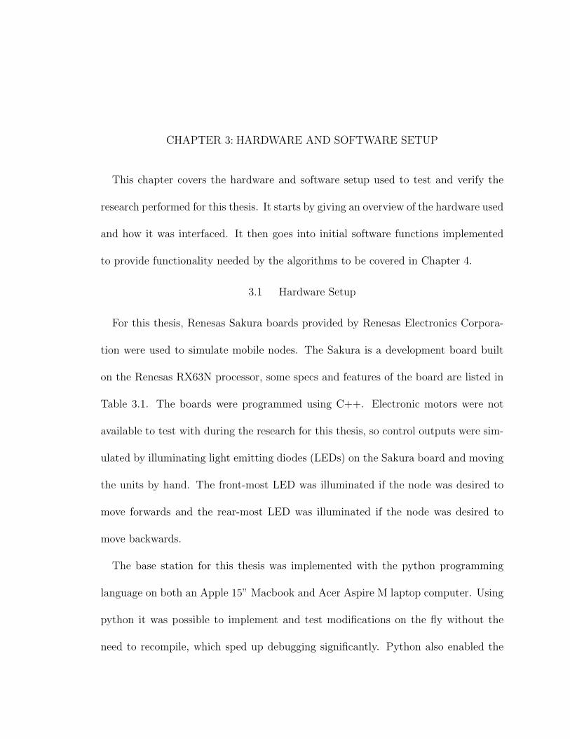
Table 3.1: Renesas Sakura features/specifications [10] [12]
CPU96 MHzsingle precision 32-bit floating point unit32-bit multiplier / divider
MemoryFlash ROM: 1MBRAM 128KBData flash 32KB
Timers
4-channels 16-bit comparator timers6-channel 16-bit MTU with PWM, input capture, output compare, phase counting mode12-channels 16-bit TPU with input capture, output compare, phase-counting mode4-channels 8-bit TMRindependent watchdog timer
CommunicationsUSB (host/function), Ether-MAC, I2C, SPI, CAN, IEBusdata transfer (DMAC, DTC)
Figure 3.1: Renesas Sakura board with XBee and power module
ability to easily switch between computers or operating systems when needed.
XBee 802.15.4 radio modules by Digi International were used to handle all radio
communications between mobile nodes and the base station. The radios provide the
802.15.4 protocol on a simple to implement and low-powered device. Table 3.2 shows
a few of the data-sheet specifications.
Table 3.2: A brief summary of specifications for XBee 802.15.4 modules [3]
Spec ValesTx Current (typical) 45mARx Current (typical) 50mAIndoor Range 30mOutdoor Range 90mRF Data Rate 250kbpsTransmit Power Output 1mWReceiver Sensitivity -92 dBmRadio Frequency 2.4 GHz
16
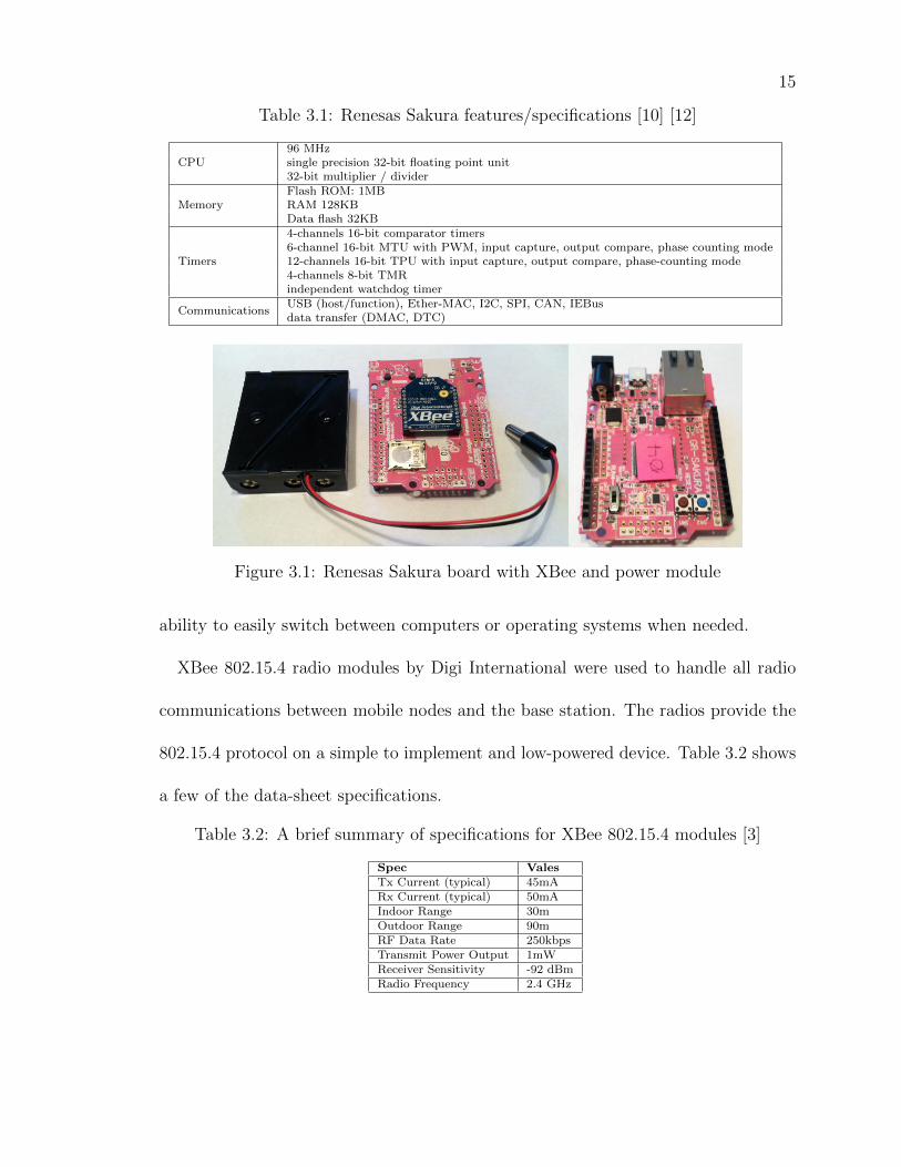
Figure 3.2: Full system setup: base station with eight nodes
3.2 Interfacing with XBee 802.15.4 Radios
All data to be sent using the XBee modules is sent to the module via a Universal
Asynchronous Receiver/Transmitter (UART) interface. Interfacing with the UART
on the Sakura boards was made simple by a set of pin holes that match the XBee
footprint allowing the module itself or a set of connecting headers to be soldered onto
the board. Software interfacing with the Sakura board was made simple by Rxduino
libraries made available by Renesas’ code compilation software. The Rxduino libraries
provide several common functionalities including a serial communication library that
17
wraps UART setup, transmission, and reception into simple function calls. Software
interfacing on the base station was handled by a similar serial communications library
add-on for python.
To request data be sent by the XBee module, it first needs to be transferred to the
XBee module over serial via UART. Once received by the XBee, the data is queued in
the module’s Data-In (DI) buffer. The buffer acts as a first in, first out (FIFO) queue,
delivering data as the CSMA/CA algorithm deems it capable of being delivered. The
device will also keep data queued as it’s receiving transmissions. If the DI buffer is
full, all new data is discarded. Similarly, all radio frequency (RF) data received is
placed into the module’s Data-Out buffer until the device receives it over UART. Any
new transmissions received when the DO buffer is full are discarded. Both the DI and
DO buffer’s are 100 bytes in size. The baud rate chosen for UART communications
in this theis was 57600 baud. 115200 baud was available as a faster option, but was
not chosen because it proved to be buggy during experimentation.
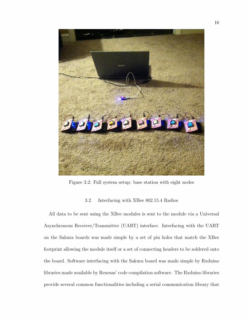
Figure 3.3: XBee internal buffers diagram [3]
The serial library of the Sakura handled clearing the DO buffer in sufficient time it
did not overflow, but the software needed to ensure that the serial library’s internal
18
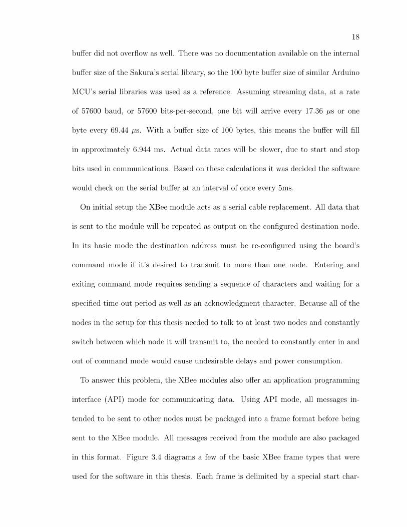
buffer did not overflow as well. There was no documentation available on the internal
buffer size of the Sakura’s serial library, so the 100 byte buffer size of similar Arduino
MCU’s serial libraries was used as a reference. Assuming streaming data, at a rate
of 57600 baud, or 57600 bits-per-second, one bit will arrive every 17.36 µs or one
byte every 69.44 µs. With a buffer size of 100 bytes, this means the buffer will fill
in approximately 6.944 ms. Actual data rates will be slower, due to start and stop
bits used in communications. Based on these calculations it was decided the software
would check on the serial buffer at an interval of once every 5ms.
On initial setup the XBee module acts as a serial cable replacement. All data that
is sent to the module will be repeated as output on the configured destination node.
In its basic mode the destination address must be re-configured using the board’s
command mode if it’s desired to transmit to more than one node. Entering and
exiting command mode requires sending a sequence of characters and waiting for a
specified time-out period as well as an acknowledgment character. Because all of the
nodes in the setup for this thesis needed to talk to at least two nodes and constantly
switch between which node it will transmit to, the needed to constantly enter in and
out of command mode would cause undesirable delays and power consumption.
To answer this problem, the XBee modules also offer an application programming
interface (API) mode for communicating data. Using API mode, all messages in-
tended to be sent to other nodes must be packaged into a frame format before being
sent to the XBee module. All messages received from the module are also packaged
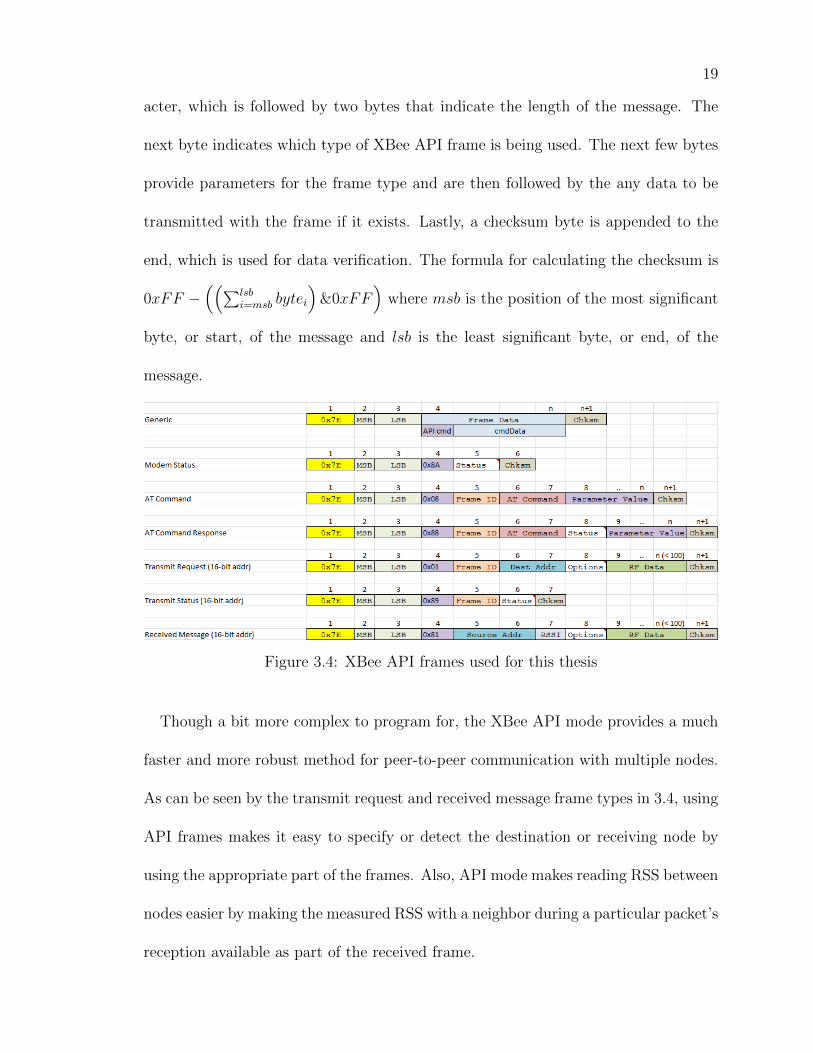
in this format. Figure 3.4 diagrams a few of the basic XBee frame types that were
used for the software in this thesis. Each frame is delimited by a special start char-
19
acter, which is followed by two bytes that indicate the length of the message. The
next byte indicates which type of XBee API frame is being used. The next few bytes
provide parameters for the frame type and are then followed by the any data to be
transmitted with the frame if it exists. Lastly, a checksum byte is appended to the
end, which is used for data verification. The formula for calculating the checksum is
0xFF −((∑lsb
i=msb bytei
)&0xFF
)where msb is the position of the most significant
byte, or start, of the message and lsb is the least significant byte, or end, of the
message.
Figure 3.4: XBee API frames used for this thesis
Though a bit more complex to program for, the XBee API mode provides a much
faster and more robust method for peer-to-peer communication with multiple nodes.
As can be seen by the transmit request and received message frame types in 3.4, using
API frames makes it easy to specify or detect the destination or receiving node by
using the appropriate part of the frames. Also, API mode makes reading RSS between
nodes easier by making the measured RSS with a neighbor during a particular packet’s
reception available as part of the received frame.
20
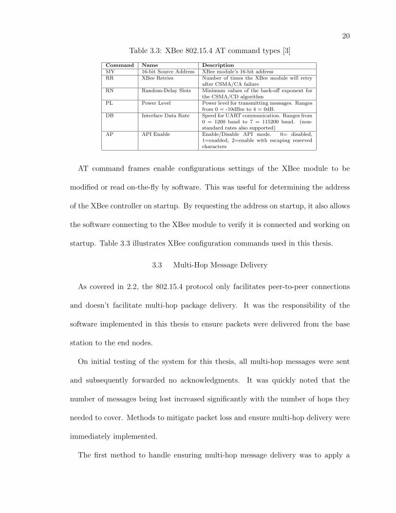
Table 3.3: XBee 802.15.4 AT command types [3]
Command Name DescriptionMY 16-bit Source Address XBee module’s 16-bit addressRR XBee Retries Number of times the XBee module will retry
after CSMA/CA failureRN Random-Delay Slots Minimum values of the back-off exponent for
the CSMA/CD algorithmPL Power Level Power level for transmitting messages. Ranges
from 0 = -10dBm to 4 = 0dB.DB Interface Data Rate Speed for UART communication. Ranges from
0 = 1200 baud to 7 = 115200 baud. (non-standard rates also supported)
AP API Enable Enable/Disable API mode. 0= disabled,1=enabled, 2=enable with escaping reservedcharacters
AT command frames enable configurations settings of the XBee module to be
modified or read on-the-fly by software. This was useful for determining the address
of the XBee controller on startup. By requesting the address on startup, it also allows
the software connecting to the XBee module to verify it is connected and working on
startup. Table 3.3 illustrates XBee configuration commands used in this thesis.
3.3 Multi-Hop Message Delivery
As covered in 2.2, the 802.15.4 protocol only facilitates peer-to-peer connections
and doesn’t facilitate multi-hop package delivery. It was the responsibility of the
software implemented in this thesis to ensure packets were delivered from the base
station to the end nodes.
On initial testing of the system for this thesis, all multi-hop messages were sent
and subsequently forwarded no acknowledgments. It was quickly noted that the
number of messages being lost increased significantly with the number of hops they
needed to cover. Methods to mitigate packet loss and ensure multi-hop delivery were
immediately implemented.
The first method to handle ensuring multi-hop message delivery was to apply a
21
frame-id to the frame of any message that need to cover more than one hop. When
the XBee module is passed a transmit request with a frame-id, it will return a modem
status frame indicating if the message was successfully acknowledged by the receiving
node. The message would be retried if no status message was received within an
alloted time frame. If the modem status message returned with an error, the message
was retried immediately after a random back-off delay. In this case, the random back-
off delay isn’t to ensure an open slot for the message, which is handled by the MAC
layer CSMA/CA protocol, but rather attempts to offset the timing of the node’s
software to avert multiple nodes continuously attempting to send messages at the
exact same time interval. If retried too many times, the message was abandoned.
This functionality was implemented and successfully reduced the factor by which
messages were being lost, but still left room for improvement.
On top of retrying messages based on MAC layer feedback, an acknowledgment
message was implemented on the software level. For all communication frames the
first byte of the RF data portion was allotted for the message’s application layer frame-
id, which is separate from the MAC frame-id. Now if a non-zero byte was present in a
received frame, a receiving node’s software would transmit back an acknowledgment
frame indicating the message was received by the software. With this implemented,
multi-hop message loss was reduced significantly.
3.4 Syncing RSS Between Neighboring Nodes
With the XBee nodes interfaced to the Sakura boards and base station as well as
multi-hop message delivery success facilitated for, the next step was to add function-
22
ality to the software for syncing RSS between nodes. It was important that a node
have an up-to-date record of the RSS to each neighboring node, as well as a record
of the measured signal strength from the neighboring nodes to itself as one may be
weaker. Another objective of this functionality was communicating back the received
signal strength between each node to the base station so an operator can be aware of
the overall strength of the chain.
It was observed early in testing that the RSS to a node will inevitably contain
a small degree of noise due to non-linear effects on RSS from obstacles and walls
as well as signals from other nodes. This matches expectations due to behavior
described in section 2.1. Directly relying on these noisy measurements for control
outputs would lead to jittery movements that would consequentially result in excessive
power consumption by motors. To smooth the measurements, the RSS to a node was
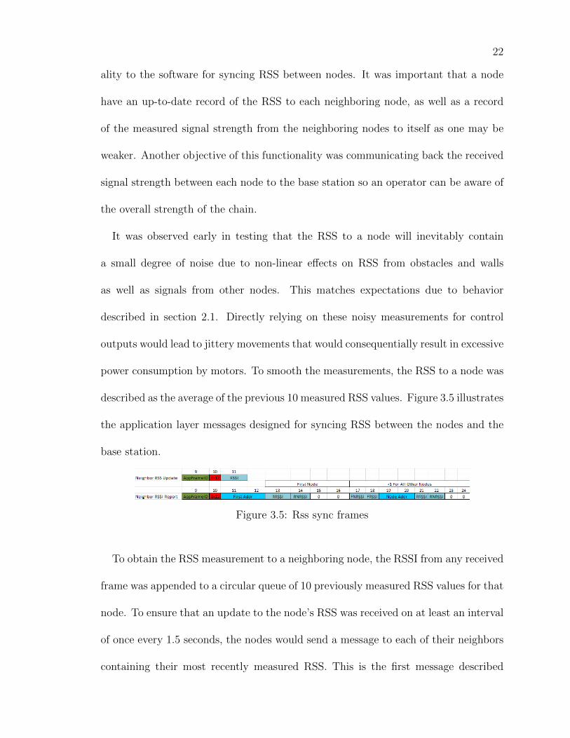
described as the average of the previous 10 measured RSS values. Figure 3.5 illustrates
the application layer messages designed for syncing RSS between the nodes and the
base station.
Figure 3.5: Rss sync frames
To obtain the RSS measurement to a neighboring node, the RSSI from any received
frame was appended to a circular queue of 10 previously measured RSS values for that
node. To ensure that an update to the node’s RSS was received on at least an interval
of once every 1.5 seconds, the nodes would send a message to each of their neighbors
containing their most recently measured RSS. This is the first message described
23
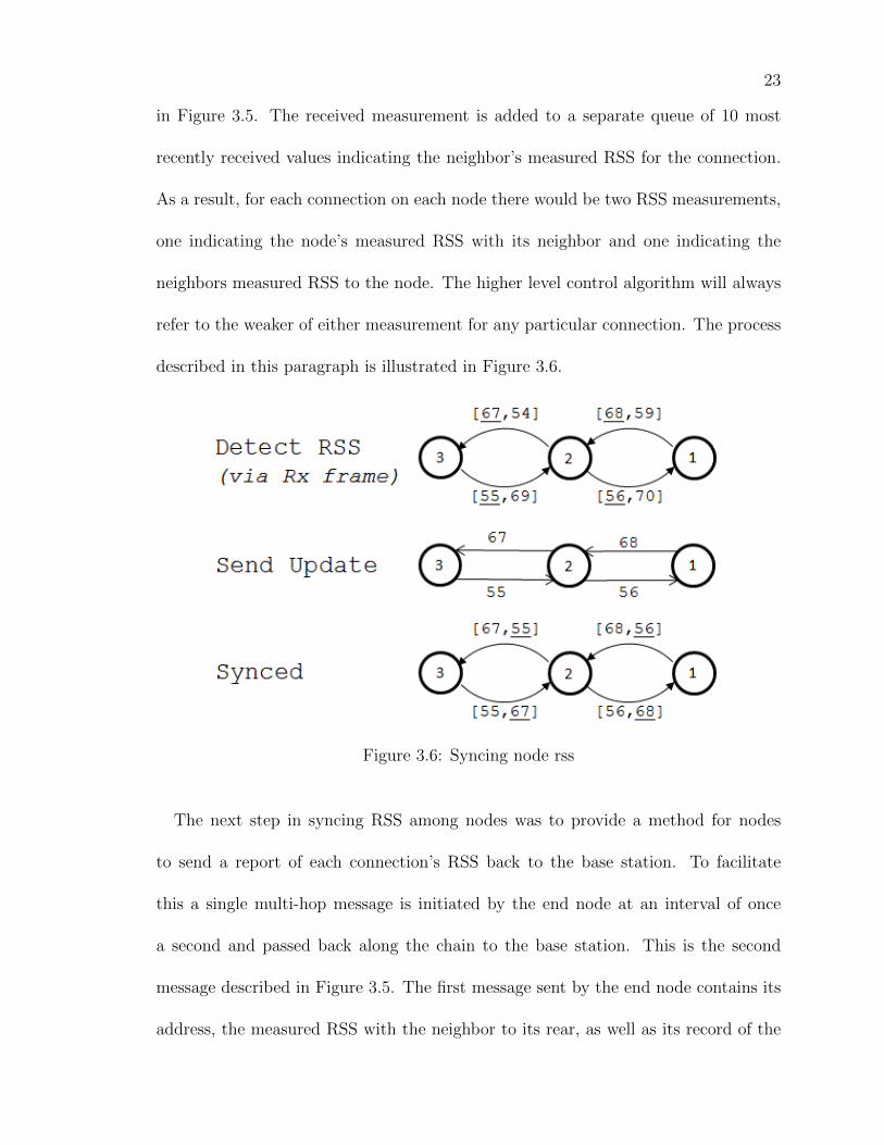
in Figure 3.5. The received measurement is added to a separate queue of 10 most
recently received values indicating the neighbor’s measured RSS for the connection.
As a result, for each connection on each node there would be two RSS measurements,
one indicating the node’s measured RSS with its neighbor and one indicating the
neighbors measured RSS to the node. The higher level control algorithm will always
refer to the weaker of either measurement for any particular connection. The process
described in this paragraph is illustrated in Figure 3.6.
Figure 3.6: Syncing node rss
The next step in syncing RSS among nodes was to provide a method for nodes
to send a report of each connection’s RSS back to the base station. To facilitate
this a single multi-hop message is initiated by the end node at an interval of once
a second and passed back along the chain to the base station. This is the second
message described in Figure 3.5. The first message sent by the end node contains its
address, the measured RSS with the neighbor to its rear, as well as its record of the

24
neighbor’s measured RSS to itself. As each node in the chain receives the message
they append their address as well as the same measurements between itself and the
neighbors to its front and rear. Once the message has arrive at the base station the
message presents a snapshot of the RSS for each connection in the chain for that
point in time. This message also becomes useful later when the base station needs to
be made aware when a node in the chain has stopped communicating. The process
for generating this message is illustrated in Figure 3.7.
Figure 3.7: Reporting node rss
3.5 Verifying Node Network Quality
The final consideration to be made in the software setup before applying the al-
gorithms was to provide a mechanism within the software to measure how well the
nodes are communicating. This mechanism was implemented in the form of a “ping”
message. These messages are illustrated in Figure 3.8.
Figure 3.8: Ping messages
At an interval of once every .5s the base station generates a “ping” with a specified
25
ping-id. This message contains 100 bytes of data, and is passed forwards along the
chain until it reaches the front-most deployed node. Once it successfully reaches
the front-most node, the node sends back a ping acknowledgment message with the
corresponding ping-id. The acknowledgment message is passed backwards along the
chain of deployed nodes to the base station. Once the acknowledgment message is
received by the base station, the base station marks the ping with that id as successful.
If an acknowledgment for a ping is not received within a time frame of 2 seconds the
ping is marked as failed. The base station keeps a record of successes (0’s) and failures
(1’s) for the last 25 pings. The success rate is then presented as a percentage by the
formula 100 ·(
1−∑n
i=0 Recordin
)where n is the number of recorded pings. The success
rate was used as the metric to verify how well all of the nodes in the chain were
communicating at a given time.
CHAPTER 4: ALGORITHMS
The algorithm implemented for this thesis was divided into three parts. The first
part facilitated for the intelligent deployment of new mobile nodes in the event RSS to
the most recently deployed node dropped below a specified threshold. The second part
was concerned with generating a control output that would move the “breadcrumb”
nodes so that they maximize distance with each other without moving so far that
communication quality degrades. The third part handles when a node is lost either
due to consistent communication failure or destruction.
4.1 Intelligent Node Deployment
The first algorithm was tasked with the intelligent deployment of nodes as needed.
The first step in the algorithm is to build a list of nodes that are available to deploy.
On startup, the software in each node will request its address using an AT command
frame specified in Figure 3.4. After it has become aware of its own address, it begins
to send a broadcast on a 1s interval announcing its presence to the base station.
When it hears this broadcast, the base station adds the node to its internal list. The
node will continue to send this broadcast until deployed.
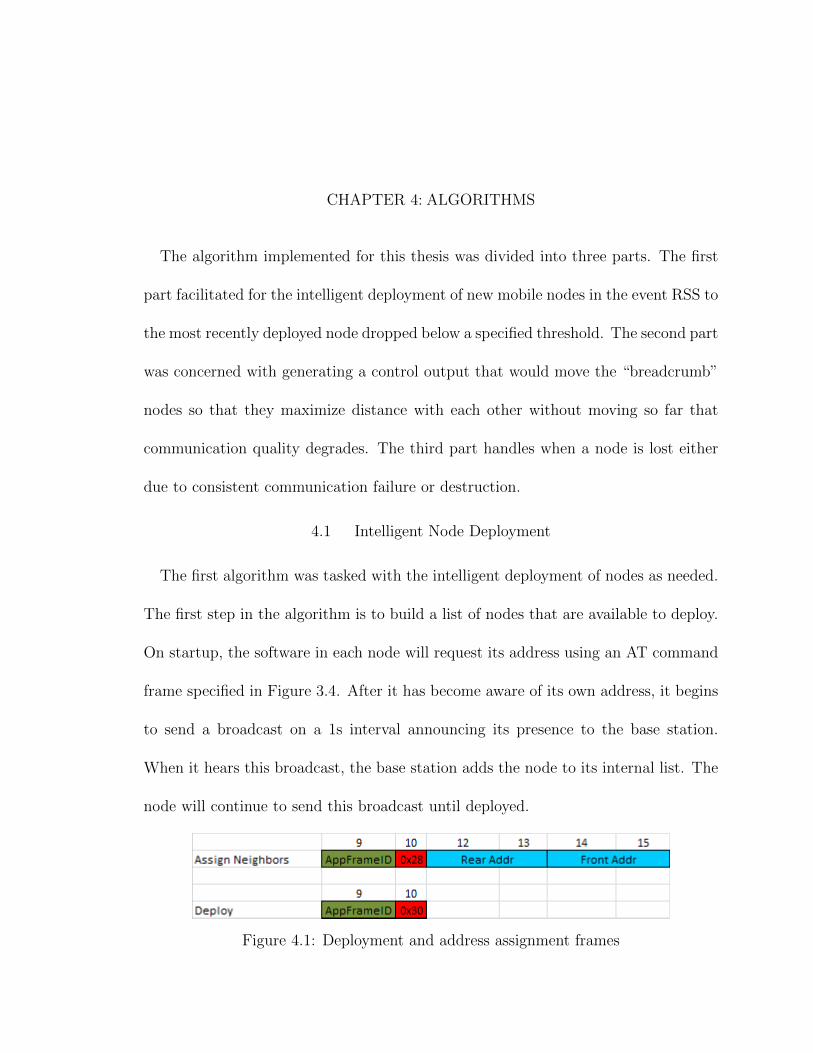
Figure 4.1: Deployment and address assignment frames
27
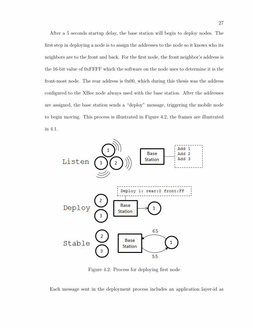
After a 5 seconds startup delay, the base station will begin to deploy nodes. The
first step in deploying a node is to assign the addresses to the node so it knows who its
neighbors are to the front and back. For the first node, the front neighbor’s address is
the 16-bit value of 0xFFFF which the software on the node uses to determine it is the
front-most node. The rear address is 0x00, which during this thesis was the address
configured to the XBee node always used with the base station. After the addresses
are assigned, the base station sends a “deploy” message, triggering the mobile node
to begin moving. This process is illustrated in Figure 4.2, the frames are illustrated
in 4.1.
Figure 4.2: Process for deploying first node
Each message sent in the deployment process includes an application layer-id as
28
described in section 3.3 to monitor that each message is properly received. If an
acknowledgment for any message is not received during the deployment process, the
message will be retried. If a time interval of 5 seconds from the beginning of a
deployment elapses before a deployment succeeds, the current deployment process
will be abandoned and then retried on the next evaluation interval.
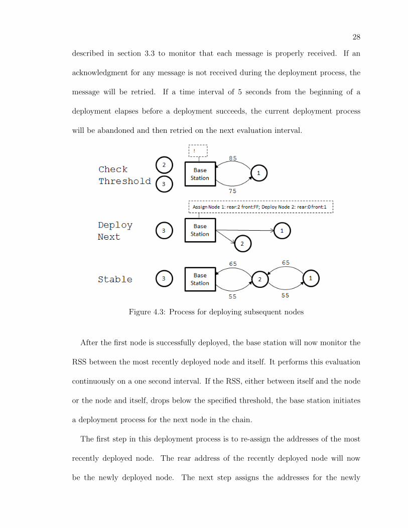
Figure 4.3: Process for deploying subsequent nodes
After the first node is successfully deployed, the base station will now monitor the
RSS between the most recently deployed node and itself. It performs this evaluation
continuously on a one second interval. If the RSS, either between itself and the node
or the node and itself, drops below the specified threshold, the base station initiates
a deployment process for the next node in the chain.
The first step in this deployment process is to re-assign the addresses of the most
recently deployed node. The rear address of the recently deployed node will now
be the newly deployed node. The next step assigns the addresses for the newly
29
deployed node. Its rear address will be the base station and front address will be the
recently deployed noden. The final step sends a deployment message to the node.
As with deploying the first node, if any message in this process fails to return an
acknowledgment the deployment process is abandoned and a retry will be attempted
on the next evaluation interval. This process is illustrated in Figure 4.3.
4.2 Maintaining Effective Distance for Communications
The next piece for this algorithm was to determine a control output that will keep
an effective distance between the nodes without allowing the signal strength to drop
beneath the needed threshold needed to maintain communications.
This algorithm is implemented as a metaphorical “spring” between the mobile
nodes. If a neighbor is too close to the node to its rear, its algorithm will “push” it
forwards until its RSS drops below a sufficient threshold. If it goes too far from the
node to its rear, the “spring” will pull it backwards. As nodes move forwards and
backwards, the corresponding algorithm on its neighbors “pushes” and “pulls” them
until they reach a balance where each of their measured RSS values between each
other is within the allowed threshold. As a sanity check, if the moving node is trying
to move away from the node to its rear but becomes very close to the node in front if
it, the algorithm will tell the node to stand still, expecting the node in front to move
forward. This algorithm is illustrated in the “Distance Management” pseudo-code.
The output was modeled for a continuous servo motor, where a value of 0 indicates
full speed backwards, a value of 180 is full speed forwards and all other inputs are
invalid. The control output begins as the current control output commanded by
30
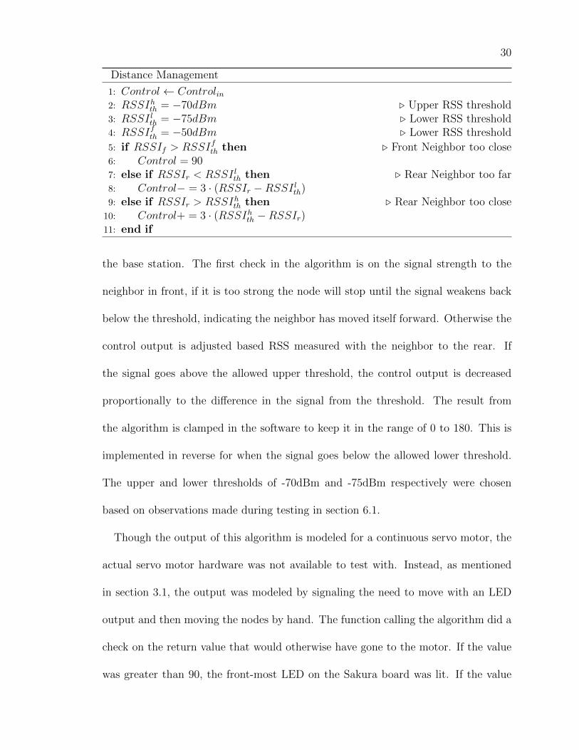
Distance Management
1: Control← Controlin2: RSSIhth = −70dBm . Upper RSS threshold3: RSSI lth = −75dBm . Lower RSS threshold4: RSSIfth = −50dBm . Lower RSS threshold
5: if RSSIf > RSSIfth then . Front Neighbor too close6: Control = 907: else if RSSIr < RSSI lth then . Rear Neighbor too far8: Control− = 3 · (RSSIr −RSSI lth)9: else if RSSIr > RSSIhth then . Rear Neighbor too close10: Control+ = 3 · (RSSIhth −RSSIr)11: end if
the base station. The first check in the algorithm is on the signal strength to the
neighbor in front, if it is too strong the node will stop until the signal weakens back
below the threshold, indicating the neighbor has moved itself forward. Otherwise the
control output is adjusted based RSS measured with the neighbor to the rear. If
the signal goes above the allowed upper threshold, the control output is decreased
proportionally to the difference in the signal from the threshold. The result from
the algorithm is clamped in the software to keep it in the range of 0 to 180. This is
implemented in reverse for when the signal goes below the allowed lower threshold.
The upper and lower thresholds of -70dBm and -75dBm respectively were chosen
based on observations made during testing in section 6.1.
Though the output of this algorithm is modeled for a continuous servo motor, the
actual servo motor hardware was not available to test with. Instead, as mentioned
in section 3.1, the output was modeled by signaling the need to move with an LED
output and then moving the nodes by hand. The function calling the algorithm did a
check on the return value that would otherwise have gone to the motor. If the value
was greater than 90, the front-most LED on the Sakura board was lit. If the value
31
was less than 90, the rear-most LED on the Sakura board was lit. If the value is equal
to 90, no LED is lit, indicating the node no longer needs to be moved.
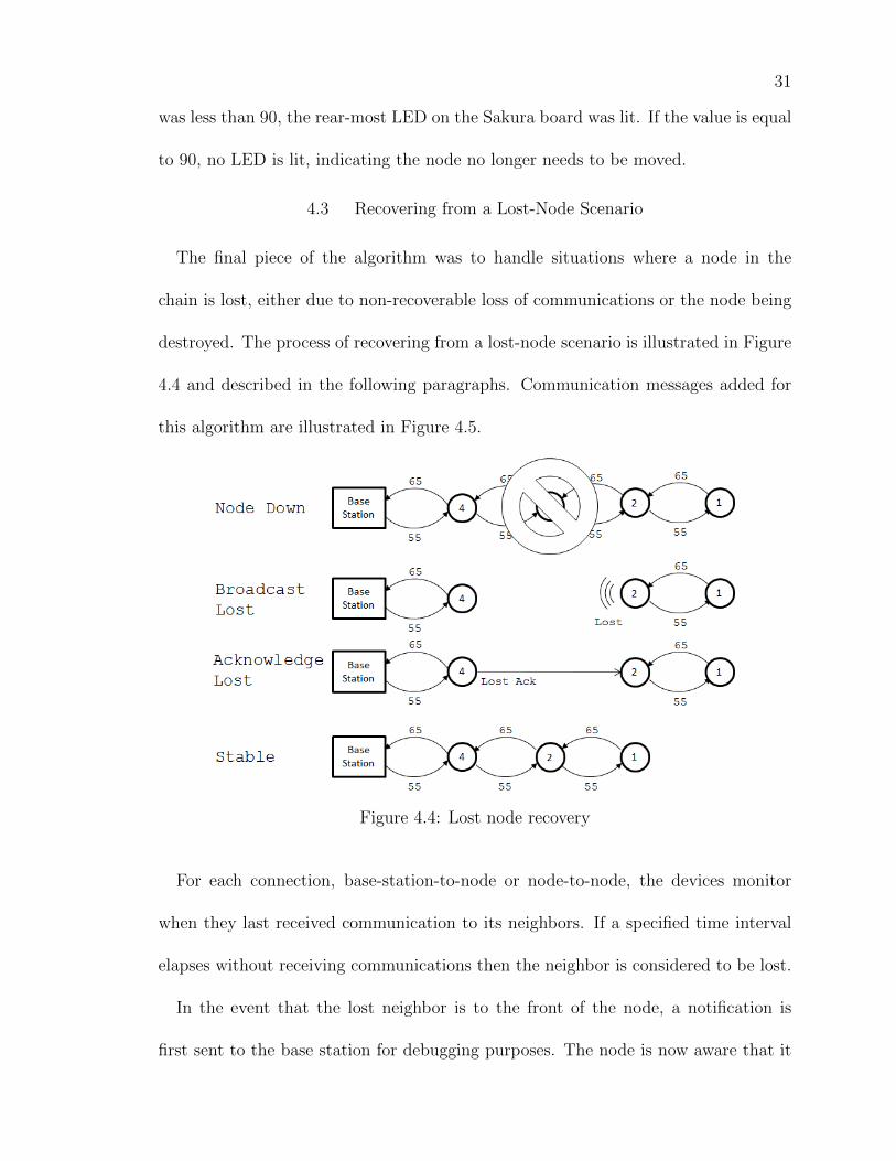
4.3 Recovering from a Lost-Node Scenario
The final piece of the algorithm was to handle situations where a node in the
chain is lost, either due to non-recoverable loss of communications or the node being
destroyed. The process of recovering from a lost-node scenario is illustrated in Figure
4.4 and described in the following paragraphs. Communication messages added for
this algorithm are illustrated in Figure 4.5.
Figure 4.4: Lost node recovery
For each connection, base-station-to-node or node-to-node, the devices monitor
when they last received communication to its neighbors. If a specified time interval
elapses without receiving communications then the neighbor is considered to be lost.
In the event that the lost neighbor is to the front of the node, a notification is
first sent to the base station for debugging purposes. The node is now aware that it
32
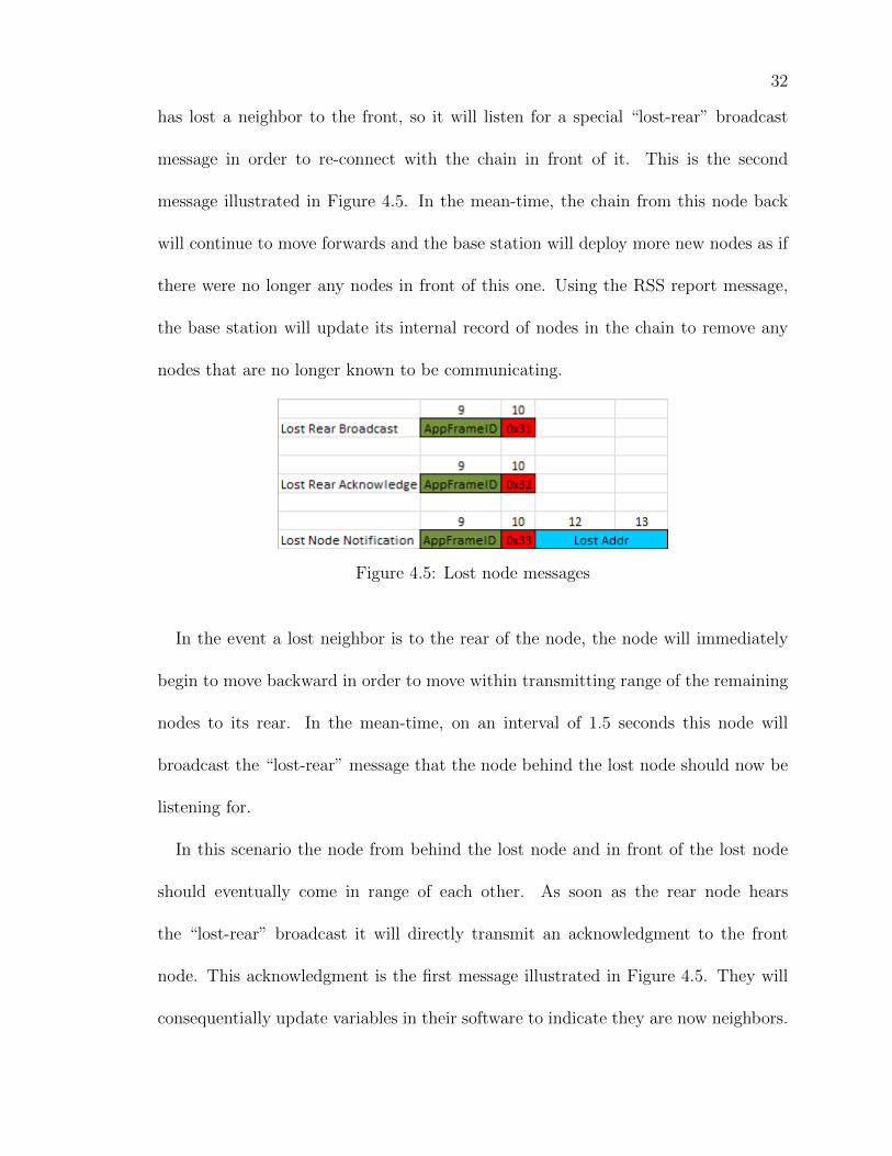
has lost a neighbor to the front, so it will listen for a special “lost-rear” broadcast
message in order to re-connect with the chain in front of it. This is the second
message illustrated in Figure 4.5. In the mean-time, the chain from this node back
will continue to move forwards and the base station will deploy more new nodes as if
there were no longer any nodes in front of this one. Using the RSS report message,
the base station will update its internal record of nodes in the chain to remove any
nodes that are no longer known to be communicating.
Figure 4.5: Lost node messages
In the event a lost neighbor is to the rear of the node, the node will immediately
begin to move backward in order to move within transmitting range of the remaining
nodes to its rear. In the mean-time, on an interval of 1.5 seconds this node will
broadcast the “lost-rear” message that the node behind the lost node should now be
listening for.
In this scenario the node from behind the lost node and in front of the lost node
should eventually come in range of each other. As soon as the rear node hears
the “lost-rear” broadcast it will directly transmit an acknowledgment to the front
node. This acknowledgment is the first message illustrated in Figure 4.5. They will
consequentially update variables in their software to indicate they are now neighbors.
33
Using the RSS report message, the base station will now re-add nodes known to still
be part of the chain in the order which they have been re-connected.
If the lost front node happened to be the most recently deployed node, the base
station will consider the entire chain lost after a time interval of 10 seconds. If it
hears a “rear-lost” broadcast before timing out, it will immediately update its internal
record of the chain, removing the lost node without needing to hear the updated RSS
report message.
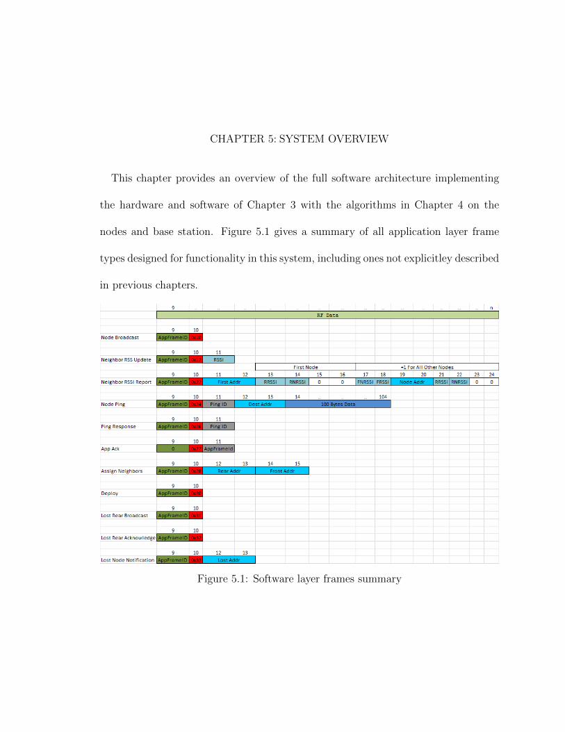
CHAPTER 5: SYSTEM OVERVIEW
This chapter provides an overview of the full software architecture implementing
the hardware and software of Chapter 3 with the algorithms in Chapter 4 on the
nodes and base station. Figure 5.1 gives a summary of all application layer frame
types designed for functionality in this system, including ones not explicitley described
in previous chapters.
Figure 5.1: Software layer frames summary
35
Figure 5.2: Node software flowchart
5.1 Mobile Node
Figure 5.2 gives a flowchart of the software used to run the mobile nodes. The
software begins by intializing serial communications then sends a request to the XBee
for the module’s configured 16-bit address. As soon as the XBee sends a response,
the node is considered intialized and begins sending a broadcast to be heard by the
base station on a one second interval. Once deployed by the base station, the node
will perform various tasks at given intervals. Every 100ms it will check the age of
messages in the outgoing queue. If the message has not succeeded within 200ms, the
36
message will be retried. If the retries exceed the software specified maximum of 3, the
message is discarded. The rest of the tasks are performed in order over the course of
each 1.5 second interval. At 200ms after the interval the output is recalculated using
measured RSS values. At 400ms after the interval the software evaluates when it
last received communications from its neighbors, and marks a neighbor as lost if the
time exceeds 5 seconds. At 1200ms after the interval, the node sends its most recently
measured RSS value to the corresponding neighbor. At 1.5 seconds the interval resets,
if the node is the furthest node it initiates an RSS report message back to the base
station.
Figure 5.3 illustrates the process for parsing received serial data for messages on
the node. The software parses through all data in the serial buffer. As soon as a valid
message is recognized it is parsed for its type and data. The first check is for which
XBee frame type. In the case of this software, the three frame types used are the
AT command frame, transmit status, and received message. If it is an AT command
frame, it is the response of a MY request for the XBee module’s 16-bit address so
the returned value is recorded as the node’s address. If it is a transmit status frame,
the software will retry any multi-hop messages with the same XBee frame id as the
returned status if the status returns a failure. As with the message check in Figure
5.2, if the message has too many retries it is discarded. If the frame is a received
message frame then it is a message from another node and it is checked for which
application layer type message is present. If the first byte of the RF data contains a
non-zero value then an application layer frame-id is present and an acknowledgment
message is sent to node that transmitted the message. If the message is from one
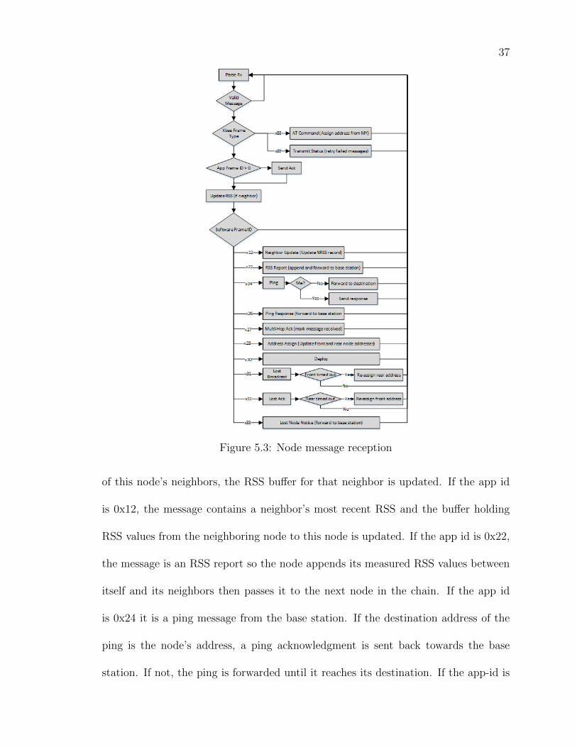
37
Figure 5.3: Node message reception
of this node’s neighbors, the RSS buffer for that neighbor is updated. If the app id
is 0x12, the message contains a neighbor’s most recent RSS and the buffer holding
RSS values from the neighboring node to this node is updated. If the app id is 0x22,
the message is an RSS report so the node appends its measured RSS values between
itself and its neighbors then passes it to the next node in the chain. If the app id
is 0x24 it is a ping message from the base station. If the destination address of the
ping is the node’s address, a ping acknowledgment is sent back towards the base
station. If not, the ping is forwarded until it reaches its destination. If the app-id is
38
0x27 then it is an acknowledgment of one of this node’s multi-hop messages sent to
another node, the corresponding message in the multi-hop outgoing queue is marked
as sent and cleared from the queue. If the app id is 0x26 then the message is a ping
acknowledgment, so it is forwarded towards the base station. An app id value of
0x28 indicates an address assignment from the base station so the node will update
its addresses for its neighbors to the front and back. An app id of 0x31 indicates
a lost broadcast message, after a sanity check that this node has actually lost its
front neighbor a lost acknowledgment is sent, otherwise it is ignored. If the message
is from the node’s current front neighbor and we haven’t lost communications, an
acknowledgment message is still sent. An app id of 0x33 indicates a lost broadcast
acknowledgment record, after a sanity check that we’ve this node has lost its rear
neighbor the rear neighbor address for this node is reset, otherwise the message is
ignored.
5.2 Base Station
This section gives an overview of the software implemented on the base station,
Figure 5.4 shows a flowchart diagram of the architecture. Many functions are similar
to the node software. On startup the base station initializes serial communications
and requests the 16-bit address of the XBee module. If the addres request is successful,
the base station is considered initialized. The station will now delay for an interval
of 5 seconds while listening on the XBee for any broadcasts from new mobile nodes,
adding nodes to the list as they are heard. After the startup delay the software begins
deploying nodes. Message, ping, and neighboring node timeouts are evaluated every
39
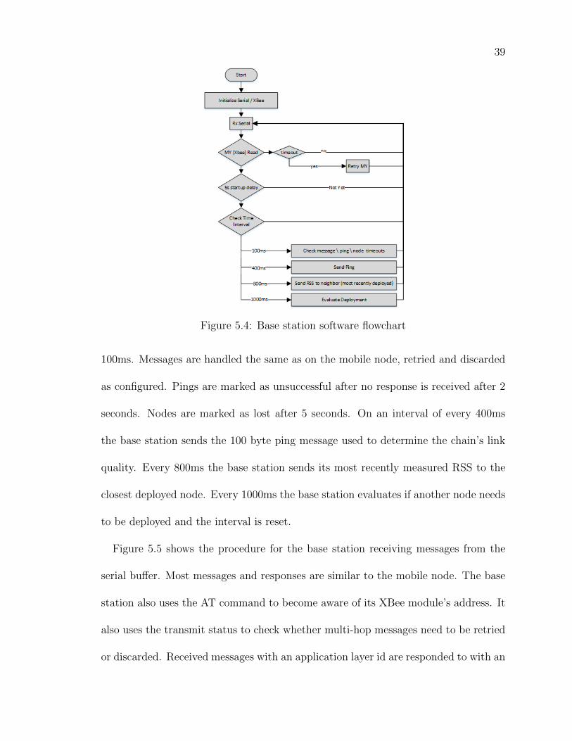
Figure 5.4: Base station software flowchart
100ms. Messages are handled the same as on the mobile node, retried and discarded
as configured. Pings are marked as unsuccessful after no response is received after 2
seconds. Nodes are marked as lost after 5 seconds. On an interval of every 400ms
the base station sends the 100 byte ping message used to determine the chain’s link
quality. Every 800ms the base station sends its most recently measured RSS to the
closest deployed node. Every 1000ms the base station evaluates if another node needs
to be deployed and the interval is reset.
Figure 5.5 shows the procedure for the base station receiving messages from the
serial buffer. Most messages and responses are similar to the mobile node. The base
station also uses the AT command to become aware of its XBee module’s address. It
also uses the transmit status to check whether multi-hop messages need to be retried
or discarded. Received messages with an application layer id are responded to with an
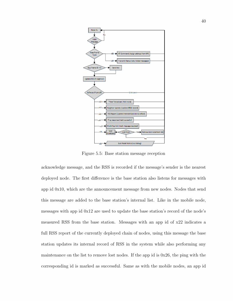
40
Figure 5.5: Base station message reception
acknowledge message, and the RSS is recorded if the message’s sender is the nearest
deployed node. The first difference is the base station also listens for messages with
app id 0x10, which are the announcement message from new nodes. Nodes that send
this message are added to the base station’s internal list. Like in the mobile node,
messages with app id 0x12 are used to update the base station’s record of the node’s
measured RSS from the base station. Messages with an app id of x22 indicates a
full RSS report of the currently deployed chain of nodes, using this message the base
station updates its internal record of RSS in the system while also performing any
maintenance on the list to remove lost nodes. If the app id is 0x26, the ping with the
corresponding id is marked as successful. Same as with the mobile nodes, an app id
41
of 0x27 indicates a multi-hop message acknowledgment. The base station marks the
corresponding message in the multi-hop outgoing queue as successful and removes
it from the queue. If the message has an app id of 0x31, this is a lost broadcast
message. If the address of the message matches the message of the most recently
deployed node, an acknowledgment is sent. If it is another node, an acknowledgment
is sent and the node formerly in front of the base station is removed from the list.
CHAPTER 6: TESTS AND OBSERVATIONS
For the purpose of testing, all XBee nodes were configured for their lowest output
power setting of -10dBm. in order to allow for testing in smaller spaces. Tests were
performed in a vacant hallway of the EPIC building of UNC Charlotte in an attempt
to simulate a tunnel-like environment. The nodes and the base station were elevated
from the floor using cardboard boxes as to reduce multi-path propagation interference
from the floor.
6.1 Measuring RSS vs. Distance with One Node
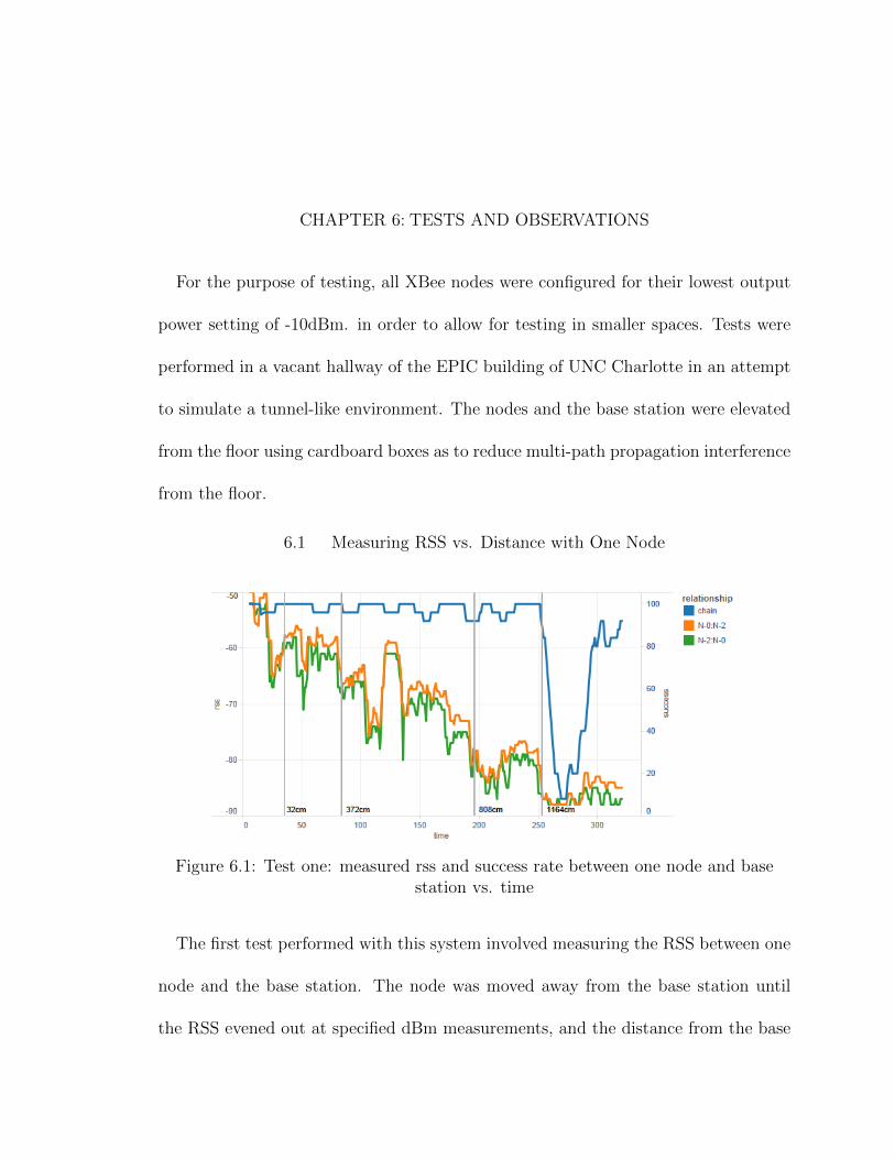
Figure 6.1: Test one: measured rss and success rate between one node and basestation vs. time
The first test performed with this system involved measuring the RSS between one
node and the base station. The node was moved away from the base station until
the RSS evened out at specified dBm measurements, and the distance from the base
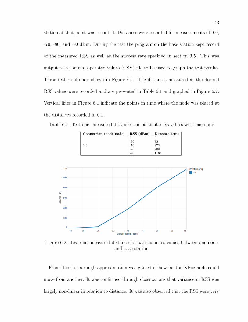
43
station at that point was recorded. Distances were recorded for measurements of -60,
-70, -80, and -90 dBm. During the test the program on the base station kept record
of the measured RSS as well as the success rate specified in section 3.5. This was
output to a comma-separated-values (CSV) file to be used to graph the test results.
These test results are shown in Figure 6.1. The distances measured at the desired
RSS values were recorded and are presented in Table 6.1 and graphed in Figure 6.2.
Vertical lines in Figure 6.1 indicate the points in time where the node was placed at
the distances recorded in 6.1.
Table 6.1: Test one: measured distances for particular rss values with one node
Connection (node-node) RSS (dBm) Distance (cm)
2-0
0 0-60 32-70 372-80 808-90 1164
Figure 6.2: Test one: measured distance for particular rss values between one nodeand base station
From this test a rough approximation was gained of how far the XBee node could
move from another. It was confirmed through observations that variance in RSS was
largely non-linear in relation to distance. It was also observed that the RSS were very
44
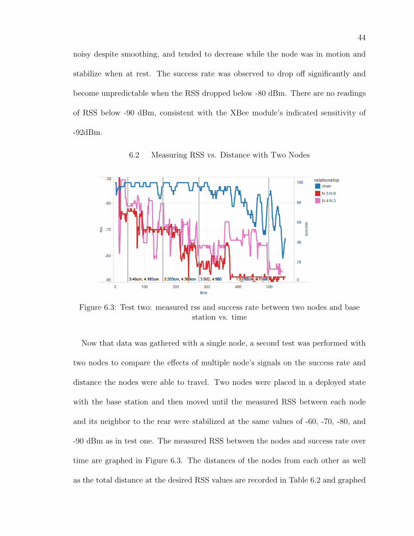
noisy despite smoothing, and tended to decrease while the node was in motion and
stabilize when at rest. The success rate was observed to drop off significantly and
become unpredictable when the RSS dropped below -80 dBm. There are no readings
of RSS below -90 dBm, consistent with the XBee module’s indicated sensitivity of
-92dBm.
6.2 Measuring RSS vs. Distance with Two Nodes
Figure 6.3: Test two: measured rss and success rate between two nodes and basestation vs. time
Now that data was gathered with a single node, a second test was performed with
two nodes to compare the effects of multiple node’s signals on the success rate and
distance the nodes were able to travel. Two nodes were placed in a deployed state
with the base station and then moved until the measured RSS between each node
and its neighbor to the rear were stabilized at the same values of -60, -70, -80, and
-90 dBm as in test one. The measured RSS between the nodes and success rate over
time are graphed in Figure 6.3. The distances of the nodes from each other as well
as the total distance at the desired RSS values are recorded in Table 6.2 and graphed
45
in Figure 6.4. Vertical lines in Figure 6.3 indicate the points in time the nodes were
positioned at the distances measured in Table 6.2.
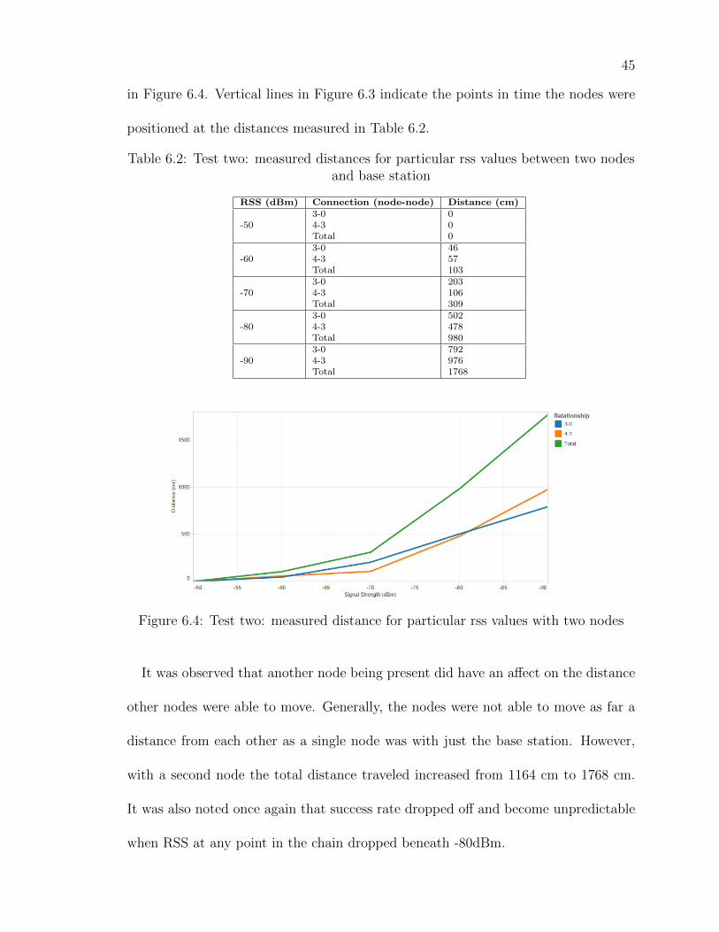
Table 6.2: Test two: measured distances for particular rss values between two nodesand base station
RSS (dBm) Connection (node-node) Distance (cm)
-503-0 04-3 0Total 0
-603-0 464-3 57Total 103
-703-0 2034-3 106Total 309
-803-0 5024-3 478Total 980
-903-0 7924-3 976Total 1768
Figure 6.4: Test two: measured distance for particular rss values with two nodes
It was observed that another node being present did have an affect on the distance
other nodes were able to move. Generally, the nodes were not able to move as far a
distance from each other as a single node was with just the base station. However,
with a second node the total distance traveled increased from 1164 cm to 1768 cm.
It was also noted once again that success rate dropped off and become unpredictable
when RSS at any point in the chain dropped beneath -80dBm.
46
Based on these tests the thresholds for the distance maintenance algorithm in
section 4.2 was set at an upper threshold of -70 dBm and a lower threshold of -
75 dBm. This allowed for some leeway between the threshold and the limit of -80
dBm before success rate drops off. The span of 5 dB between the threshold values
gave some space for noise in the measurements. The threshold for the deployment
algorithm described in 4.1 was set to -75dBm.
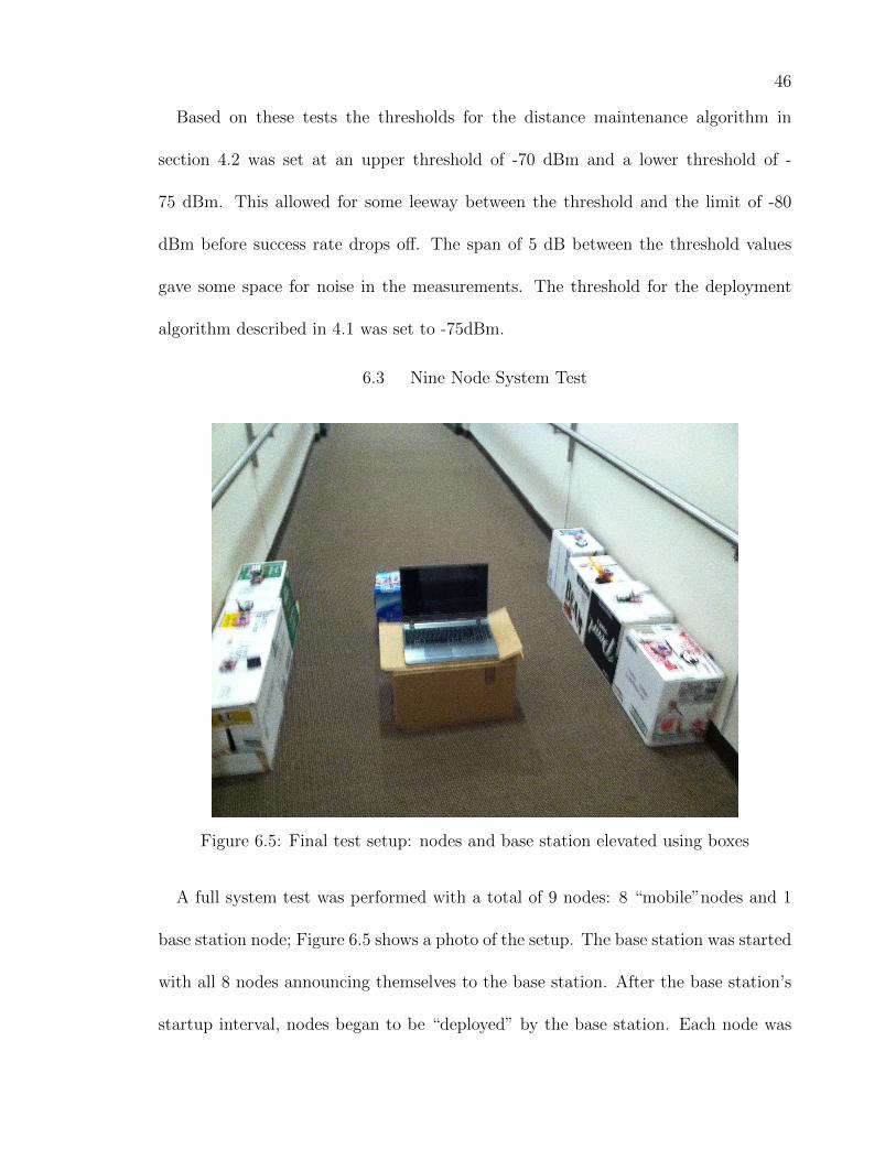
6.3 Nine Node System Test
Figure 6.5: Final test setup: nodes and base station elevated using boxes
A full system test was performed with a total of 9 nodes: 8 “mobile”nodes and 1
base station node; Figure 6.5 shows a photo of the setup. The base station was started
with all 8 nodes announcing themselves to the base station. After the base station’s
startup interval, nodes began to be “deployed” by the base station. Each node was
47
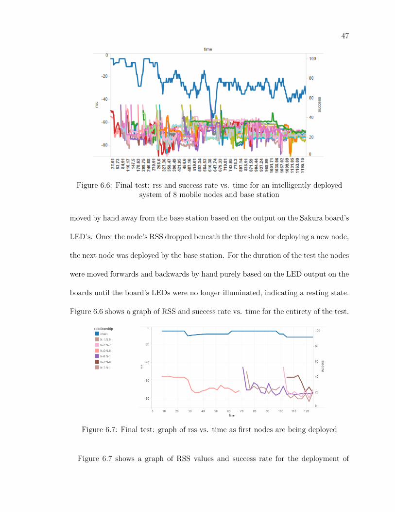
Figure 6.6: Final test: rss and success rate vs. time for an intelligently deployedsystem of 8 mobile nodes and base station
moved by hand away from the base station based on the output on the Sakura board’s
LED’s. Once the node’s RSS dropped beneath the threshold for deploying a new node,
the next node was deployed by the base station. For the duration of the test the nodes
were moved forwards and backwards by hand purely based on the LED output on the
boards until the board’s LEDs were no longer illuminated, indicating a resting state.
Figure 6.6 shows a graph of RSS and success rate vs. time for the entirety of the test.
Figure 6.7: Final test: graph of rss vs. time as first nodes are being deployed
Figure 6.7 shows a graph of RSS values and success rate for the deployment of
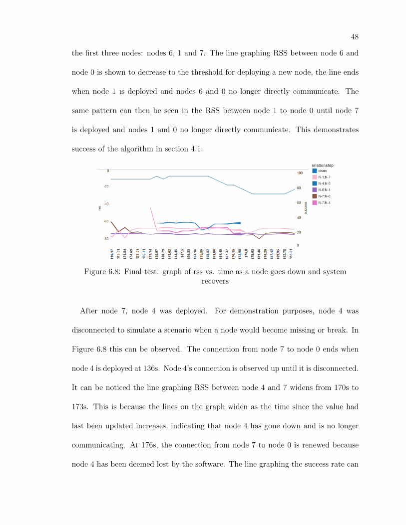
48
the first three nodes: nodes 6, 1 and 7. The line graphing RSS between node 6 and
node 0 is shown to decrease to the threshold for deploying a new node, the line ends
when node 1 is deployed and nodes 6 and 0 no longer directly communicate. The
same pattern can then be seen in the RSS between node 1 to node 0 until node 7
is deployed and nodes 1 and 0 no longer directly communicate. This demonstrates
success of the algorithm in section 4.1.
Figure 6.8: Final test: graph of rss vs. time as a node goes down and systemrecovers
After node 7, node 4 was deployed. For demonstration purposes, node 4 was
disconnected to simulate a scenario when a node would become missing or break. In
Figure 6.8 this can be observed. The connection from node 7 to node 0 ends when
node 4 is deployed at 136s. Node 4’s connection is observed up until it is disconnected.
It can be noticed the line graphing RSS between node 4 and 7 widens from 170s to
173s. This is because the lines on the graph widen as the time since the value had
last been updated increases, indicating that node 4 has gone down and is no longer
communicating. At 176s, the connection from node 7 to node 0 is renewed because
node 4 has been deemed lost by the software. The line graphing the success rate can
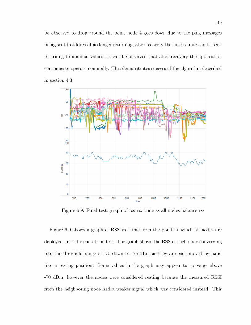
49
be observed to drop around the point node 4 goes down due to the ping messages
being sent to address 4 no longer returning, after recovery the success rate can be seen
returning to nominal values. It can be observed that after recovery the application
continues to operate nominally. This demonstrates success of the algorithm described
in section 4.3.
Figure 6.9: Final test: graph of rss vs. time as all nodes balance rss
Figure 6.9 shows a graph of RSS vs. time from the point at which all nodes are
deployed until the end of the test. The graph shows the RSS of each node converging
into the threshold range of -70 down to -75 dBm as they are each moved by hand
into a resting position. Some values in the graph may appear to converge above
-70 dBm, however the nodes were considered resting because the measured RSSI
from the neighboring node had a weaker signal which was considered instead. This
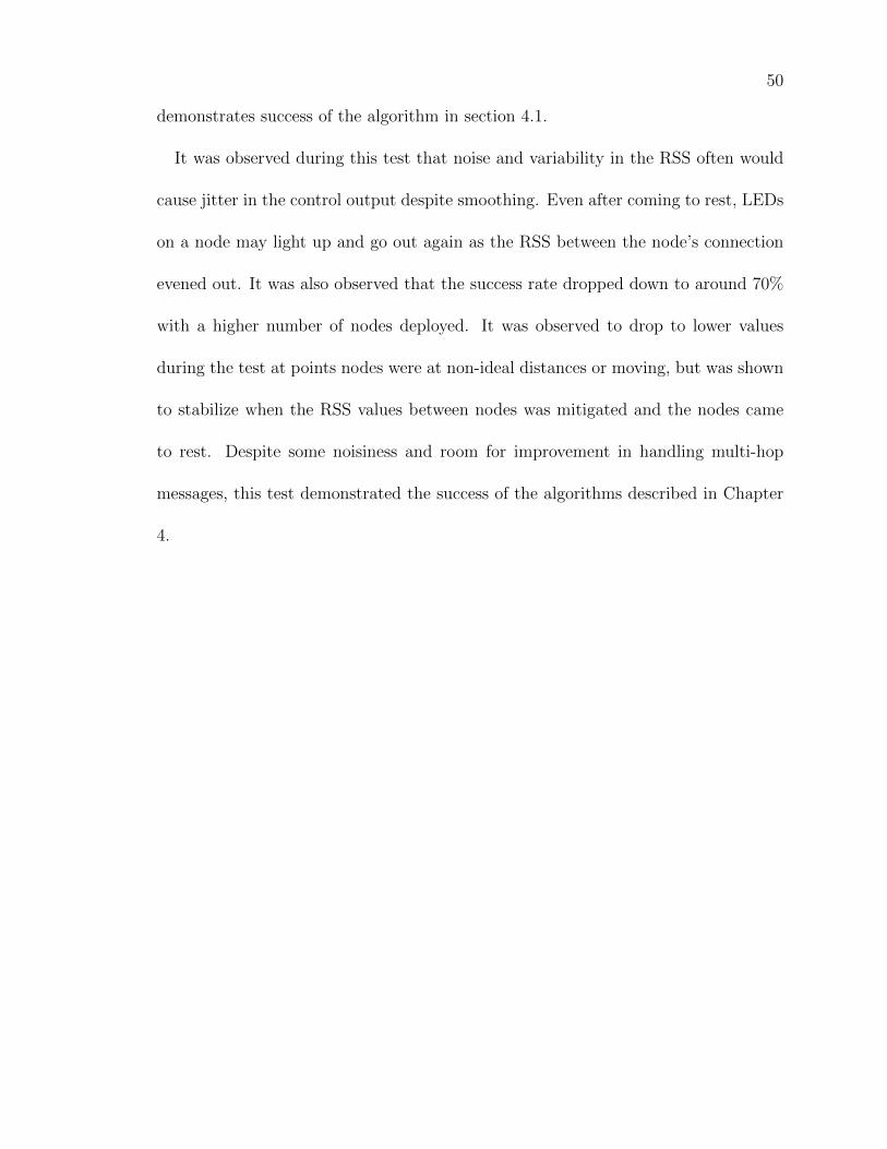
50
demonstrates success of the algorithm in section 4.1.
It was observed during this test that noise and variability in the RSS often would
cause jitter in the control output despite smoothing. Even after coming to rest, LEDs
on a node may light up and go out again as the RSS between the node’s connection
evened out. It was also observed that the success rate dropped down to around 70%
with a higher number of nodes deployed. It was observed to drop to lower values
during the test at points nodes were at non-ideal distances or moving, but was shown
to stabilize when the RSS values between nodes was mitigated and the nodes came
to rest. Despite some noisiness and room for improvement in handling multi-hop
messages, this test demonstrated the success of the algorithms described in Chapter
4.
CHAPTER 7: CONCLUSIONS
7.1 Conclusions
Based on the tests in Chapter 5, it was concluded that a system of “breadcrumb”
nodes that intelligently deploy, maintain distance, and recover from lost-node sce-
narios is possible to implement using RSS between the nodes as the primary metric.
Some things noted to be improved upon include smoothing of measured RSS mea-
surements between nodes, as well as handling of multi-hop communications. Despite
some work to be done in these areas, the algorithm was shown to be successful at
handling a basic system without failure.
7.2 Future Work
Future work for research done in this thesis includes implementing this algorithm
into a system with fully-autonomous mobile nodes. A more sophisticated protocol for
handling multi-hop messages should also be implemented, which can improve upon
the 70% success rates observed with a full chain of nodes in this thesis’ tests. Testing
with higher radio output strengths will allow observations of how the algorithm and
RSS values vary when nodes become further from non-neighboring nodes and their
RF transmissions, reducing interference but also increasing the chance of collisions
due to the hidden node problem.
52
REFERENCES
[1] T. Aurisch and J. Tolle. Relay Placement for Ad-hoc Networks in Crisis andEmergency Scenarios. In Proc. of the Information Systems and Technology Panel(IST) Symposium. Bucharest, Romania: NATO Science and Technology Orga-nization, 2009.
[2] K. Derr and M. Manic. Multi-Robot, Multi-Target Particle Swarm OptimizationSearch in Noisy Wireless Environments. In Human System Interactions, pages81–86. IEEE, 2009.
[3] Digi International Inc. XBee / XBee-PRO RF Modules Product Manual, 2013.
[4] C. Dixon and E. Frew. Electronic Leashing of an Unmanned Aircraft to a RadioSource. In IEEE Conference on Decision and Control, pages 3560–3565. IEEE,2005.
[5] J. Fink and V. Kumar. Online Methods for Radio Signal Mapping with MobileRobots. In International Conference on Robotics and Automation, pages 1940–1945. IEEE, 2010.
[6] M.-Y. Hsieh, V. Kumar, and C. J. Taylor. Constructing Radio Signal StrengthMaps with Multiple Robots. In International Conference on Robotics and Au-tomation, volume 4, pages 4184–4189. IEEE, 2004.
[7] B. Krawiec, K. Kochersberger, and D. C. Conner. A Methodology for Au-tonomous Radio Repeating Based on the A* Algorithm. American Instituteof Aeronautics and Astronautics, 2012.
[8] K. L. Moore, M. D. Weiss, J. P. Steele, C. Meehan, J. Hulbert, E. Larson, andA. Weinstein. Experiments with Autonomous Mobile Radios for Wireless Tether-ing in Tunnels. The Journal of Defense Modeling and Simulation: Applications,Methodology, Technology, 9(1):45–58, 2012.
[9] H. G. Nguyen, N. Pezeshkian, A. Gupta, and N. Farrington. Maintaining Com-munications Link for a Robot Operating in a Hazardous Environment. Technicalreport, Space and Naval Warfare Systems Command, 2004.
[10] Renesas Electronics Corporation. RX63N Group, RX631 Group Renesas MCUs,2013.
[11] M. R. Souryal, J. Geissbuehler, L. E. Miller, and N. Moayeri. Real-time De-ployment of Multi-hop Relays for Range Extension. In Proceedings of the 5thInternational Conference On Mobile Systems, Applications and Services, pages85–98. ACM, 2007.
[12] l. Wakamatsu Tsusho Co. Sakura Board for Gadget Renesas Project. http:
//sakuraboard.net/gr-sakura_en.html, 2013.
53
[13] E. M. H. Zahugi, S. Prasad, and T. Prasad. Advanced Communication Protocolsfor Swarm Robotics: A Survey. International Journal of Engineering Researchand Applications (IJERA), 2:119–123, 2012.


![[WSO2] Deployment Synchronizer for Deployment Artifact Synchronization Between the WSO2 Cluster Nodes](https://img.pdfslide.us/doc/110x75/54582648af7959755d8b5139/wso2-deployment-synchronizer-for-deployment-artifact-synchronization-between-the-wso2-cluster-nodes.jpg)

![Nodes Deployment Strategies for Sensor Networks: An … · 2016-06-05 · deployment strategies [10-11]. In this work, we have analyzed the effect of existing node deployment strategies](https://img.pdfslide.us/doc/110x75/5f19ca41a319cb24081c883c/nodes-deployment-strategies-for-sensor-networks-an-2016-06-05-deployment-strategies.jpg)


![Adaptive Deployment for UAV-Aided Communication Networks · arXiv:1812.03267v1 [cs.IT] 8 Dec 2018 Adaptive Deployment for UAV-Aided Communication Networks Zhe Wang, Member, IEEE,](https://img.pdfslide.us/doc/110x75/5f2cbbd98f78d66232514643/adaptive-deployment-for-uav-aided-communication-networks-arxiv181203267v1-csit.jpg)

![Adaptive Computing Through Strategic Service Deployment › ~christoph › seschool › Adaptive Computi… · Data Distribution Service (DDS) An Object Management Group (OMG)[7]](https://img.pdfslide.us/doc/110x75/5ed726cdc30795314c174a69/adaptive-computing-through-strategic-service-deployment-a-christoph-a-seschool.jpg)