Embed Size (px)
Citation preview
ADAPTIVE CONTROL OF VARIABLE DISPLACEMENT PUMPS
A Thesis
Presented to
The Academic Faculty
by
Longke Wang
In Partial Fulfillment
Of the Requirements for the Degree
Doctor of Philosophy in the
School of Mechanical Engineering
Georgia Institute of Technology
May 2011
Copyright© 2011 by Longke Wang

ADAPTIVE CONTROL OF VARIABLE DISPLACEMENT PUMPS
Approved by: Dr. Wayne J. Book, Advisor George W. Woodruff School of Mechanical Engineering Georgia Institute of Technology
Dr. Kok-Meng Lee George W. Woodruff School of Mechanical Engineering Georgia Institute of Technology
Dr. Nader Sadegh George W. Woodruff School of Mechanical Engineering Georgia Institute of Technology
Dr. David G. Taylor School of Electrical and Computer Engineering Georgia Institute of Technology
Dr. Perry Y. Li Department of Mechanical Engineering University of Minnesota
Date Approved: March 16, 2011

iii
To Xiaohong
and Shuwen.

iv
ACKNOWLEGMENTS
I wish to express sincere appreciation and thanks to Dr. Wayne J. Book for his
support, guidance and encouragement throughout the process of obtaining a Ph.D., for
giving me the opportunity to be part of his research group and for help that extends far
beyond the contents of the dissertation.
I am grateful for the guidance, insights, and feedback provided by my thesis
committee, Dr Kok-Meng Lee, Dr. David G. Taylor, Dr. Nader Sadegh, and Dr. Perry Y.
Li.
This thesis would not have been possible if not for the generous financial support
of Mr. Agustin Ramirez, Chairman of HUSCO, Int’l, and Mr. Dwight Stephenson, Vice
President of Engineering at HUSCO, Int’l. Grateful acknowledgement of additional
funding is given to National Science Foundation Center for Compact and Efficient Fluid
Power for funding this research.
Special thanks are due to Mr. Dwight Stephenson for his encouragements,
valuable suggestions and insights. I especially thank Sun Hydraulics Corporation. They
gave valuable suggestions and denoted equipment for whatever I needed.
A special word of thanks is owed to Mr. James Huggins, not only for his
contributions in the research, but also for his kind help to my personal life.
It is impossible for me to arrive this point without helps from my friends and
colleagues in Georgia Institute of Technology. Particularly, I would like to thank: Dr.
Amir Shenouda, Dr. Matthew Kontz, Dr. Patrick Opdenbosch, Dr. Aaron Enes, Mark
Elton, Ryder Winck, Brian Post, Heather Humphreys and Hannes Daepp. I also
acknowledge the rewarding discussions with Dr. Adam Cardi, Dr. Farhod Farbod, and
Joshua Schultz.

v
I would like to express my deepest gratitude to my parents and parents-in-law.
They raised me, supported me, and are devoting to endless love.
Finally, and most importantly, I owe my loving thanks to my wife Xiaohong Jia,
and my daughter Shuwen Wang. They have sacrificed a lot and experienced a lot of
difficulties, but they have provided an unwavering emotional foundation, an enumerable
quantity of joy, a limitless supply of love. Without their encouragement, understanding,
and support, it would have been impossible for me to complete this work. To them I
dedicate this thesis.

vi
TABLE OF CONTENTS
DEDICATION................................................................................................................... iii
ACKNOWLEDGEMENTS............................................................................................... iv
LIST OF TABLES............................................................................................................. ix
LIST OF FIGURES .............................................................................................................x
SUMMARY..................................................................................................................... xiv
1 INTRODUCTION ............................................................................................................1
1.1 Valve Controlled System and Valve-less Controlled Systems ..........................1
1.2 Research Motivations and Challenges ...............................................................5
1.3 Research Objectives...........................................................................................6
1.4 Thesis Outline ....................................................................................................7
2 BACKGROUND ..............................................................................................................8
2.1 Fluid Power........................................................................................................8
2.2 Hydraulic Circuits for Single-rod Cylinders....................................................14
2.3 Model Reduction..............................................................................................19
2.4 Parameter Estimation .......................................................................................23
2.5 Hydraulic Control ............................................................................................29
2.6 Summary ..........................................................................................................31
3 APPLICATION SINGULAR PERTURBATION TO FLUID POWER........................33
3.1 Variable Displacement Controlled Cylinders ..................................................33
3.2 Singular Perturbation Model............................................................................37
3.3 Control Law Design.........................................................................................40
3.4 Simulation ........................................................................................................44
3.5 Experimental Results .......................................................................................51
3.6 Conclusion .......................................................................................................55

vii
3.7 Further Discussions of Applying Singular Perturbations ................................55
3.8 Summary ..........................................................................................................59
4 A HYDRAULIC CIRCUIT FOR SINGLE ROD CYLINDERS ...................................60
4.1 The Flow Control Circuit with Dynamical Compensations ............................61
4.2 Stationary Stability Analysis............................................................................65
4.3 Dynamic Stability Analysis .............................................................................72
4.4 Compensation Algorithms for the Flow Control Valves .................................81
4.5 Discussions of the Proposed Circuit ................................................................85
4.6 Summary ..........................................................................................................88
5 SIMULATION AND EXPERIMENTAL RESULTS OF THE PROPOSED
HYDRAULIC CIRCUIT.................................................................................................90
5.1 The Flow Control Circuit Test-bed..................................................................90
5.2 Numerical Simulations.....................................................................................95
5.3 Experimental Results without Compensations ................................................99
5.4 Experimental Results with Compensations ...................................................102
5.5 Conclusion .....................................................................................................105
6 ADAPTIVE ROBUST CONTROL OF VARIABLE DISPLACEMENT PUMPS.....107
6.1 Adaptive Tracking Control ............................................................................107
6.2 Parameter Adaptation Algorithm...................................................................112
6.3 Adaptive Control with Recursive Least Squares ...........................................115
6.4 Improved Algorithm I ....................................................................................118
6.5 Improved Algorithm II...................................................................................121
6.6 Controller Design...........................................................................................126
6.7 Summary ........................................................................................................126
7 APPLICATION ADAPTIVE CONTROL TO VARIABLE DISPLACEMENT
PUMPS..........................................................................................................................128
7.1 Experiment Setting.........................................................................................128

viii
7.2 Desired Tracking Using Discrete Time Control ............................................132
7.3 Comparison with PID Control .......................................................................146
7.4 Desired Tracking Using Hybrid Control........................................................147
7.5 Summary ........................................................................................................162
8 SUMMARY, CONTRIBUTIONS, AND FUTURE DIRECTIONS............................164
8.1 Summary and concluding remarks.................................................................164
8.2 Contributions..................................................................................................165
8.3 Future Directions ...........................................................................................166
REFERENCES ................................................................................................................168

ix
LIST OF TABLES
Table 3.1 Parameters used in the simulation .....................................................................45
Table 5.1 Main components used in the test-bed...............................................................93
Table 5.2 Experimental results without compensations ..................................................101
Table 5.3 Experimental results with compensations........................................................105

x
LIST OF FIGURES
Figure 1.1 Constant pressure circuits...................................................................................2
Figure 1.2 Energy losses in a conventional valve controlled system ..................................3
Figure 1.3 Valve-less controlled system..............................................................................4
Figure 1.4 Energy usages for a valve-less system ...............................................................5
Figure 2.1 Axial piston pumps...........................................................................................11
Figure 2.2 A servo-valve controlled axial piston pump.....................................................13
Figure 2.3 A displacement controlled single rod cylinder with flow compensation .........16
Figure 2.4 A typical hydraulic transformer consisting of two hydraulic units ..................16
Figure 2.5 A closed loop circuit for single rod cylinders using 3-way shuttle valves.......18
Figure 2.6 A closed loop circuit for single rod cylinders using pilot check valves...........18
Figure 2.7 Open loop circuits for single rod cylinders ......................................................19
Figure 2.8 Basic concepts of singular perturbations and time scales ................................23
Figure 2.9 Typical system identification structures...........................................................25
Figure 2.10 Close loop of HARF algorithm ......................................................................29
Figure 3.1 Variable displacement controlled actuators......................................................34
Figure 3.2 Pressure responses for the step input................................................................36
Figure 3.3 Step response ....................................................................................................45
Figure 3.4 Control efforts for the step response ................................................................46
Figure 3.5 Bandwidth test ..................................................................................................47
Figure 3.6 Bandwidth test (10 Hz).....................................................................................47
Figure 3.7 Step response ....................................................................................................48
Figure 3.8 Control efforts for the step response ................................................................49
Figure 3.9 Bandwidth Test.................................................................................................49

xi
Figure 3.10 Bandwidth test without heavily compressing fast mode ................................50
Figure 3.11 Step response with the bulk modulus reduced 50% .......................................50
Figure 3.12 Displacement controlled circuit......................................................................52
Figure 3.13 Step input response.........................................................................................53
Figure 3.14 Corresponding pressure response with Fig. 3.13............................................53
Figure 3.15 Tracking test ...................................................................................................54
Figure 3.16 Corresponding pressure response with Fig. 3.15............................................54
Figure 3.17 Approximated response and real response .....................................................59
Figure 4.1 Hydraulic Circuit for a single rod cylinder.......................................................61
Figure 4.2 Pump work plane..............................................................................................62
Figure 4.3 Extending under pumping mode ......................................................................63
Figure 4.4 Extending under motoring mode ......................................................................64
Figure 4.5 Retracting under pumping mode ......................................................................64
Figure 4.6 Retracting under motoring mode......................................................................65
Figure 4.7 Single rod cylinder models...............................................................................65
Figure 4.8 Desired working regions in the pressure plane.................................................67
Figure 4.9 A circuit using pilot operated check valves......................................................68
Figure 4.10 Working regions of ideal P.O. Valves............................................................69
Figure 4.11 Working regions of common P.O. valves ......................................................70
Figure 4.12 Working regions of the shuttle valve..............................................................72
Figure 4.13 Block diagram around the equilibrium point..................................................74
Figure 4.14 Response with varying leakage coefficient ....................................................80
Figure 4.15 pu control signal.............................................................................................84
Figure 4.16 Boom function parameters in a industrial backhoe ........................................86
Figure 4.17 Simulations data of a boom function..............................................................87
Figure 5.1 Hydraulic Circuit for a single rod cylinder.......................................................92
Figure 5.2 Hydraulic lifter test-bed (Cylinder side)...........................................................92

xii
Figure 5.3 Hydraulic lifter test-bed (Driver side) ..............................................................93
Figure 5.4 Measurement noise without applying filters ....................................................94
Figure 5.5 A dynamic pressure measurement....................................................................95
Figure 5.6 (a) Pressures on the cylinder, (b) the cylinder’s displacement and velocity ....96
Figure 5.7 (a) Pressures on the cylinder, (b) the cylinder’s displacement and velocity ....97
Figure 5.8 Pressure limit cycles .........................................................................................98
Figure 5.9 Oscillations is inhibited by increasing leakage ................................................99
Figure 5.10 Experiment responses (M = 0 Kg) ...............................................................100
Figure 5.11 Experiment responses (M = 61.2 Kg) ..........................................................100
Figure 5.12 Experiment responses (M = 142.8 Kg) ........................................................101
Figure 5.13 Simulation result with M= 61.2Kg...............................................................102
Figure 5.14 Experimental response with compensations (M = 0 Kg) .............................103
Figure 5.15 Experimental response with compensations (M = 61.2 Kg) ........................103
Figure 5.16 Experimental response with compensations (M = 142.8 Kg) ......................104
Figure 5.17 Experimental response with compensations (M = 68.2 Kg) ........................105
Figure 6.1 Parameter path ................................................................................................114
Figure 6.2 Ensemble-average leaning curves for LMS and RLS ....................................115
Figure 6.3 Indirect adaptive control.................................................................................115
Figure 7.1 Structure of the test-bed..................................................................................129
Figure 7.2 Input dead-zone of the pump..........................................................................130
Figure 7.3 Diagram of the bandwidth test .......................................................................131
Figure 7.4 Bandwidth test of the variable displacement pump........................................131
Figure 7.5 Parameter identification..................................................................................138
Figure 7.6 Identification error..........................................................................................138
Figure 7.7 Discrete time control structure .......................................................................139
Figure 7.8 Step responses ( 142.8M kg= ).......................................................................142
Figure 7.9 Tracking responses ( 142.8M kg= ) ...............................................................142

xiii
Figure 7.10 Tracking responses ( 81.6M kg= ) ...............................................................143
Figure 7.11 Tracking responses ( 20.4M kg= ) ...............................................................143
Figure 7.12 Tracking responses with varying electrical motor speed .............................145
Figure 7.13 Control Efforts with varying electrical motor speed ....................................145
Figure 7.14 Step responses ( 142.8M kg= ).....................................................................146
Figure 7.15 Tracking performances ( 142.8M kg= ) .......................................................147
Figure 7.16 Hybrid adaptive control................................................................................148
Figure 7.17 Four times sampling rate ..............................................................................152
Figure 7.18 Step responses ( 142.8M kg= ).....................................................................156
Figure 7.19 Tracking performances ( 142.8M kg= ) .......................................................156
Figure 7.20 Tracking performances with variations of motor speeds .............................157
Figure 7.21 Control efforts with variations of motor speeds ...........................................158
Figure 7.22 Identified parameters with the second order model .....................................159
Figure 7.23 Identification errors with the second order model........................................160
Figure 7.24 The tilting cart ..............................................................................................161
Figure 7.25 Identified parameters with the third order model .........................................161
Figure 7.26 Identification errors with the third order model ...........................................162

xiv
SUMMARY
Fluid power technology has been widely used in industrial practice; however, its
energy efficiency became a big concern in the recent years. Much progress has been
made to improve fluid power energy efficiency from many aspects. Among these
approaches, using a valve-less system to replace a traditional valve-controlled system
showed eminent energy reduction. This thesis studies the valve-less solution–pump
displacement controlled actuators– from the view of controls background.
Singular perturbations have been applied to the fluid power to account for fluid
stiffness; and a novel hydraulic circuit for single rod cylinder has been presented to
increase the hydraulic circuit stabilities. Recursive Least Squares has been applied to
account for measurement noise thus the parameters have fast convergence rate, square
root algorithm has further applied to increase the controller’s numerical stability and
efficiency. It was showed that this technique is consistent with other techniques to
increase controller’s robustness. The developed algorithm is further extended to a hybrid
adaptive control scheme to achieve desired trajectory tracking for general cases.
A hardware test-bed using the invented hydraulic circuit was built up. The
experimental results are presents and validated the proposed algorithms and the circuit
itself. The end goal of this project is to develop control algorithms and hydraulic circuit
suitable for industrial practice.

1
CHAPTER I
INTRODUCTION
Fluid power technology has been widely used in many areas of industrial and
mobile applications, for example in construction, forestry, mining and agriculture
machines. Common to these applications is that high power density, the ability to exert
large forces or torques using actuators of relatively small mass, is often required to
perform desired work, for example, digging mud and lifting heavy loads. However, the
energy efficiency of fluid power systems is relatively low when compared with methods
of transmitting power mechanically or electrically. The energy efficiency was not a big
concern in past, but becomes increasingly important with increased fuel costs and stricter
emission regulations in last decades. To increase energy efficiency is one of the
challenges for the next generation of fluid power systems.
Much progress has been made in making individual hydraulic components, such
as valves, motors and pumps, more energy efficient. The problem is that it is rarely
possible to have all components operating in optimized conditions over a wide operating
region when combining these components into a hydraulic system. This leads to poor
overall system energy efficiency. New ways of combining components constantly arise
from academia and industry. Terms used to classify such combining ways are diverse, but
there are two fundamental categories: Valve Controlled Systems and Valve-less
Controlled Systems.
1.1 Valve Controlled System and Valve-less Controlled Systems

2
Figure 1.1 Constant pressure circuits
Figure (1.1) shows a typical hydraulic circuit using valve control [1]. The circuit
consists of a reservoir (1), a motor (2), a pressure compensated variable displacement
pump (3), controlled valves (4) and double rod cylinders (5). The hydraulic circuit
powers the actuator at the constant pressure and variable flow volume. Variable flow
demand is accomplished by the variable displacement capability of the pump reacting to
changes in pressure. When the control valve is centered, the cylinder actuator is locked in
position and resists overrunning loads. When the control valve is actuated manually or
electrically, the pressurized flow, through the valve, drives the actuator cylinder. Similar
hydraulic circuits using valve control includes constant flow circuits, constant
horsepower circuits, Load-Sensing circuits and other customized structures.
In most valve controlled systems used in mobile machinery, one pump, as a
power source, is shared among several actuators which are controlled through valves. The
problem of the system’s energy efficient arises for two main factors: (1) There is a
minimum pressure drop across a control valve for the sake of controllability issues [2],

3
and (2) the desired pressures to drive individual actuators may differ too much. Even in
the load-sensing case–the system highest pressure is minimized to satisfy the current
highest pressure requirement for actuators–any simultaneous motion of actuators with
unequal pressure level results in undesired pressure drops through control valves. The
pressure drop multiplied by the required flow is referred to as metering loss.
Figure 1.2 Energy losses in a conventional valve controlled system
Figure (1.2) shows energy losses in a two-actuator system, e.g. system as
illustrated by Figure (1.1). Where 1PΔ is the minimum pressure in order to properly
control a valve, 2PΔ is the pressure difference between corresponding pressures acted on
the two actuators. The energy losses are drawn in the hatched area as shown in Figure
(1.2). To increase energy efficiency, one solution is to implement a separate pump for
each actuator. Thus the energy loss due to 2PΔ is eliminated. However, control valves
always dissipate some energy because of pressure drops through valves.
One topic of research that has attracted increasing interest is the development of
alternative hydraulic systems where control valves are eliminated along with the
throttling losses.

4
M
1 2 3 4 5 6
7
Figure 1.3 Valve-less controlled system
Figure (1.3) shows a valve-less controlled system. A motor (1), which can be an
electrical motor or an internal combustion engine, drives variable displacement pumps (3)
through a gear-box (2). The fluids powered by a variable displacement pump power an
actuator (6) through a hydraulic circuit consisting of check valves (4), relief valves (5)
and charge pump (7). Compared with the energy losses shown in Figure (1.2), the
throttling losses are eliminated as shown in Figure (1.4).

5
Figure 1.4 Energy usages for a valve-less system
In addition to eliminating throttling losses, another benefit of pump displacement
controlled systems is energy regeneration. Some pumps, for example, piston pumps
designed with some considerations, can interchange working modes between a pumping
mode and a motoring mode. It is possible that one actuator can be (partially) powered by
the energy regenerated from another actuator. For example, in an excavator, the boom
cylinder is pulled down with heavy loads, and the regenerated potential energy and brake
energy can be used to power the steering cylinder through the shared input shaft of the
gear box.
1.2 Research Motivations and Challenges
This research is motivated by the need to improve the performance and reliability
with implementing the valve-less control concept. Currently, displacement controlled
drives with a rotary motor or a double rod cylinder are often used in industrial uses.
However, due to costs and space limits, single rod cylinders are most commonly used
actuators in industry. However, using a single rod cylinder with displacement controlled

6
concepts leads to a differential flow compensation issue, and even more, an instability
problem under some working conditions.
Some hydraulic control questions are still open: in the engineering applications,
there are many time varying parameters such as varying loads, which hamper a
controllers’ performance and measurement noise commonly exits in applications. How to
model a system with balance of model complexity and real time control requirements?
The system layout presented in this thesis is based on displacement controlled
pumps. Whether an excavator or a backhoe, a tip movement can always been
decomposed to corresponding cylinder movements which are separately controlled by
varying pump displacement. Thus, the tip position/velocity control problem is same as a
single cylinder position/velocity control problem. However, the desired tracking becomes
difficult if a system is a non-minimum phase system.
1.3 Research Objectives
The purpose of this research is to explore how the pump displacement control
concept can be applied to a single rod cylinder with considerations of good engineering
practice in order to achieve a better energy efficiency compared with a valve controlled
system.
The system layout presented in this thesis is based on displacement controlled
pumps. The following assumptions are made through the thesis.
(1) Each single rod cylinder is controlled by a variable displacement pump.
(2) The displacement controlled actuator has higher energy efficiency than valve
control systems.
The assumption (1) is predetermined by the displacement controlled actuator
structure in order to eliminate throttling losses and recover potential/braking energy. The
assumption (2) is treated as an axiom in the thesis. That is, the thesis would not prove or
disprove this assumption; using displacement control is the rule of the thesis.

7
Specific aims of the research include:
(1) Develop a stable hydraulic circuit used for a single rod cylinder
(2) Develop control algorithm(s) dealing with measurement noise, real time
control and varying system parameters.
(3) Experimentally validate the proposed circuit and algorithm.
1.4 Thesis Outline
The rest of the thesis is organized as follows. Relevant background information
and literature reviews are presented in Chapter 2. This chapter includes literature reviews
on related control technology. A review on the state-of-the-art hydraulic circuits of single
rod cylinders is presented.
Chapter 3 presents application of singular perturbation theories to hydraulic
applications. Examples of applications are presented and parts of the conclusions will be
used in following chapters.
Theoretical analysis and experimental results of the proposed novel hydraulic
circuit for single rod cylinders are presented in Chapter 4 and Chapter 5 respectively.
This is considered to be one of the main backbones of the research in this thesis. Also,
this is the hardware test-bed for proposed control algorithms.
Chapter 6 introduces the adaptive robust control of variable displacement pumps
with recursive least squares. The motivation and analysis are presented.
In Chapter 7, experimental results of applying the proposed algorithms on the
proposed circuit are presented. The analysis of control techniques to implement desired
trajectory tracking is included in this chapter.
The final remarks and conclusion are included in Chapter 8. In addition, the
research contributions are described in this chapter. The chapter ends with a brief list of
possible extensions of this research and future work.

8
CHAPTER II
BACKGROUND
This chapter presents a discussion on methods employed by industrial and
academic researchers for increasing the performance of hydraulic control. A primary
focus is on applications to hydraulic control originating from literature within the
domains of system dynamics and controls.
Researchers from a broad range of engineering disciplines have been involved in
projects to improve overall hydraulic performance. Not only did they focus on individual
components such as pumps [3–6], valves [7, 8], but also investigate ways to combine
components to new hydraulic circuit topologies, for example, independent metering
control [9, 10], open loop hydraulic circuit [11] etc. In addition to control methods, which
are discussed in more detail in the next sections, other research has been carried out to
increase the overall hydraulic performance, for example, haptic feedback control [12–15],
shared control [16].
The major advantage of pump displacement controlled actuators is higher energy
efficiency. Unfortunately, the dynamic characteristics of these systems are nonlinear,
high order and relatively difficult to control. The difficulties arise from the
compressibility of the hydraulic fluid and from the variable displacement pump itself. In
applications, measurement noise can not be ignored. Some of system parameters are time
varying, for example, work loads. The controller, usually consisting of digital signal
processors and input-output units, has limited data bandwidth. Much research has been
carried out when dealing with this complex and uncertain system. A literature review of
these related topics is given next.
2.1 Fluid Power

9
The basic principle of hydrostatic machines and systems is based on Pascal’s law
formulated in the 17th century. It states: “…Any change of pressure at any point on an
incompressible fluid at rest, which does not disturb the equilibrium of the fluid, is
transmitted to all other points of the fluid without any change. When forces of pressure
balance the gravitational forces, then the pressure at every point of the fluid is the
same…” It took almost 150 years till Pascal’s ideal found practical application during the
industrial revolution, for example, Hydraulic Press by Joseph Bramah [17]. Over the
years, the integration of electronics into hydraulics has lead to further modernization of
hydrostatic systems. A hydrostatic system includes several components including pumps,
valves, pipelines etc. For the perspective of controls, the following literature review
focuses on bulk modulus, which is related to system stiffness, and piston pumps, which is
the input stage of the control efforts.
2.1.1 Bulk modulus
In the field of controls, the term “hydraulic” is used to designate a system using a
liquid as the work media. Density, viscosity, thermal properties and some chemical
related properties are often used to decide which kind of fluid will be used in the
hydraulic system. For control designs, effective bulk modulus is one of the most
important factors.
Spring effects of a liquid and the mass of mechanical parts lead to resonance in
nearly all hydraulic components. In most cases, this resonance is a fundamental limitation
to dynamic performance [1, 2]. Most petroleum fluids have a bulk modulus value more
than 220,000 lb/in2 [2, 18]. In fact, values this large are rarely achieved in practice
because the bulk modulus of fluids decreases sharply with small amounts of entrained air
in the liquid. Cylinder deformations also affect the effective bulk modulus. In many
practical cases, it is difficult to determine the effective bulk modulus because the
estimation error of entrapped air runs as high as 20%. It has been shown that satisfactory

10
simulation results are difficult to be obtained if a constant bulk modulus has been used
[19, 20].
Many studies have been made on bulk modulus dependency on pressure, air, and
temperature [21, 22]. As shown by Magorien [23], if there is some air in a hydraulic
system, the value of bulk modulus will be reduced substantially. According to Merritt [2],
when the air content is one percent by volume in hydraulic oil MIL-H-5606, the bulk
modulus decreases to 25% of the one that is air free. In [18], the air free bulk modulus of
the test system was found to be 1701 MPa, and bulk modulus in a pump-pipe-valve
system was determined to be 1132MPa when the load pressure was approximately at
atmosphere, 1631MPa at 5MPa, 1686MPa at 10MPa.
As pressure is increased, much of this air dissolves into the liquid and does not
affect bulk modulus. Oil temperature also has an influence on bulk modulus because it
affects the density of the air content. However, these effects can be ignored when the oil
temperature is approximately constant. The effect of pipe rigidity on bulk modulus can
also be ignored if rigid pipes are assumed in hydraulic system [19]. In experience, an
effective bulk modulus of 100,000 PSI (686 MPa) has yielded reliable results [2].
2.1.2 Variable displacement pumps
Hydraulic pumps are important parts of a hydraulic system. A hydraulic pump,
also termed as a displacement pump or sometimes as a hydrostatic pump, transforms
mechanical energy into hydraulic energy. A hydraulic motor transforms hydraulic energy
into mechanical energy. Most displacement machines can be used as pumps as well as
motors [24]. This characteristic leads to the possibility of energy regeneration, which is a
way to increase system energy efficiency.

11
Figure 2.1 Axial piston pumps
Pumps commonly used in industry include piston pumps, gear pumps, screw
pump, vane pumps and some special purpose pumps. This research focuses on piston
pumps since they are the most commonly used displacement machines in hydraulic
industry. They possess many advantages especially in the region of higher operating
pressure (above 15MPa) and low cost. Due to friction, leakage, material deformation
and many factors, there are always losses as compared to the ideal machine. The overall
energy efficiency tη is defined as:
t v hmη η η= (2.1)
Where vη is volumetric efficiency which is defined as the ratio of effective output flow to
the derived output flow, hmη is hydraulic-mechanical efficiency which is defined as the
ratio of derived torque to effective torque at a pump input shaft. More precise models
about Equation (2.1) have been researched in [25–29].
Because the dynamic behavior of a variable displacement pump influences the
overall dynamic behavior of the hydraulic system, these machines have been the objects
of considerable research within the past years [3–5, 30–37]. The work of Zeiger and Aker
[3] has been the most influential in this area [38]. In their work, the control torque exerted
on swash plate by the pumping mechanism was derived and numerically simulated.

12
Based on this work, Kim, et al. [4] conducted sensitivity analyses that was aimed at
identifying the most influential system parameters within a hydraulic system. Manring
and Johnson [5] furthered this work. They put forward a closed-form approximation for
the numerical analysis presented by Zeiger and Akers. Piston pump kinematics analysis,
which used six coordinate transformation matrices to calculate piston displacement,
forces, and moments, has been discussed in [39–41].
In variable displacement machines, the geometrical displacement volume of the
units is continuously adjustable. The continuous adjustment of the displacement volume
in piston machines is realized by variation of the piston of the piston stroke. The variable
piston stroke can be achieved due the adjustment of the control element, which is the
swash plate in swash plate machines, the cylinder block in bent axial machines and the
eccentricity of the stroke ring in radial piston units. Different actuating systems are used
for adjustments of displacement machines. They are differentiated as mechanical, electro-
mechanical, hydraulic and electro-hydraulic adjusting devices.
Electro-hydraulic adjusting devices are used increasingly for the control of the
displacement volume of pumps and motors, also called as servo controls of pumps and
motors. The control cylinder is operated through a servo-valve. The servo-valve serves as
an electro-hydraulic converter which converts input electrical signals into valve core
movements. With the application of electrical signal, the armature begins to move due to
interaction with the permanent magnetic field. The armature deflection is transmitted to a
nozzle flapper system through which the movement of the flapper produces a pressure
difference between both the control pressures in the displacement chambers. The
resulting force acts on the valve spool which is the hydraulic power stage to drive swash
plate rotation actuators. The spool position is fed back to the armature through a feedback
wire to control the spool position. An outer loop feedback through a swash plate
feedback spring is used to balance the torque on the armature to control the swash plate
angle.

13
Figure 2.2 A servo-valve controlled axial piston pump (courtesy Moog Inc.)
The majority of variable displacement pumps currently available on the market
are unacceptable slow compared with control valves used in hydraulic systems. However,
the inertial of moving parts of a variable pump is significantly lower than the inertia of a
fixed displacement pump. It is expected that pump control is likely to offer a much faster
system. Hahmann [42] and Berbuer [43] investigated the dynamics of servo pump control
systems considering self adjusting forces based on use of nonlinear models. Their
approach was validated experimentally by pressure measurements in both chambers of
the pump control cylinder. By developing a secondary controlled motor concept, Berg
and Ivantysynova [44] proposed a swash plate controller of higher order for the inner

14
control loop. They achieved a bandwidth of 80Hz of the pump control system for
measured frequency response for 10% amplitude of commanded swash plate angle. Bahr
Khalil et al. [45] improved response dynamics of servo pump swash plate actuation using
a PD design for the wash plate controller. Grabbel et al. showed that electro-hydraulic
pump control allows sufficiently high dynamics for heavy duty actuators which can
compete with conventional valve controlled systems [46].
2.1.3 On/Off Valve
In addition to pump controlled system, there is another parallel approach to
increase system energy efficiency by implementing on/off valves. Li et al. proposed
software enabled variable displacement pumps [47, 48]. This approach combines a fixed
displacement pump with a pulse-width-modulated (PWM) on/off valve, a check valve,
and an accumulator. The effective pump displacement can be varied by adjusting the
PWM duty ratio. Since on/off valves exhibit low loss when fully open or fully closed,
the system is potentially more energy efficient than the one with metering valve control.
Proposals to use on/off valves to control fluid power systems have been around
for a while. Gu et al. [49] uses the switch-mode converter concept to develop hydraulic
transformers; and Barth et al. [50] substituted a PWM valve in place of a proportional
valve to control a pneumatic load. A high speed PWM on/off valve has been designed
and validated in [51], and a model of the system is derived and simulated, with results
indicating that the soft switching approach can reduce transition and compressibility
losses by 79%, and total system losses by 66% [52].
Since systems structure using on/off valve concept is too different from our
research’s, further reviews will not be provided.
2.2 Hydraulic Circuits for Single-rod Cylinders

15
Replacing of valve-controlled systems with displacement control was the subject
of diverse research works at universities in the last decades [53–60] and of the
development industry projects [61–63]. These projects sought to transfer the previously
technology used in hydraulic transmissions into hydraulic actuators. The achievable
dynamic performance and development of control concepts were primary interests [64,
65]. With new circuit solutions, design and control methods, it has been demonstrated
that displacement controlled actuators are able to achieve a dynamic behavior comparable
to valve controlled hydraulic systems [65, 66, 67].
Single rod cylinders are used exclusively as linear actuators in industry. Since
there is a differential area between the cap side and the rod side of a cylinder, a hydraulic
circuit is a necessary part to balance the differential flow when a single rod cylinder is
extending or retracting. Several concepts can be found in the literature that was
developed mainly for stationary applications [57, 58, 66, 69]. These structures usually
require a relatively high number of components and require multi-variable control
techniques. Berbuer [65] complemented a conventional hydrostatic circuit with two
additional hydraulic machines with displacements adapted for the cylinder area ratio. In
1994, work based on the same principle solution was continued by Lodewykes [57,58]. In
his circuit as shown in Figure (2.3), a summing pressure control valve was used to
increase the pressure on the low resonance frequency of a displacement controlled
system. The hydraulic transformer ratio has to be designed as the same as the single rod
cylinder area ratio. Lodewykes also researched the use of two servo pumps for the single
rod cylinder in a multi variable control concept and in a single variable control concept.
The single variable control concept was realized with a sum pressure control valve and an
additional pressure source. Next to the development of suitable control concepts,
Loadewyks proved some of his results on stationary test-beds.

16
Figure 2.3 A displacement controlled single rod cylinder with flow compensation
The use of two servo pumps in a multi-variable control concept was also
introduced by Feuser et al [69, 70]. However, a four-quadrant operation, defined by
pressure directions and flow directions on a pump, of multiple actuators according to this
concept leads to a high installation cost for the pressure controlled units to realize parallel
actuator movements.
Similar to the function of an electrical transformer, a hydraulic transformer is
capable converting an input flow at a certain pressure level to a different output flow at
the expense of a change in pressure level. One common way to build the transformer has
been to combine two hydraulic units, where at least one has a variable displacement as
shown in Figure (2.4).
Figure 2.4 A typical hydraulic transformer consisting of two hydraulic units

17
There are two kinds of typical implementations of hydraulic transformers. One is
similar to the case as shown in Figure (2.4). The common hydraulic pressure is
transformed to individual cylinders through a hydraulic transformer which is connected
to the common driver line connecting with an accumulator and driver pumps. The energy
efficiency is hoped to be higher than valve controlled systems because, ideally, there is
no energy dissipated during pressure conversion. Another application of hydraulic
transformers is similar to the case as illustrated in Figure (2.3). The main purpose of
implementations is to balance differential flows for a single rod cylinder.
However, the energy efficiency of a conventional transformer is limited as it
includes two piston units, of which, in most operating points, at least one of the machines
operates under a partial loading condition resulting in a decrease in overall efficiency
[72]. In order to increase energy efficiency, another hydraulic transformer concept was
developed by the Dutch Company Innas BV [73, 74]. It contains three ports, where the
control of the volume flow to the individual ports is achieved by controlling the valve
plate. This transformer can only be used for a single rod cylinder in four quadrant
operation together with an additional high pressure source. However, this additional high
pressure source has to be sufficient in size for all single rod cylinders; and for each
actuator one bent axis transformer needs to be implemented in the overall machine
system. A lifting machine with a two-quadrant cylinder was equipped with this hydraulic
drive technology as a prototype [74].
In 1994, a displacement controlled closed circuit system consisting of fewer
components, capable of single rod cylinder actuation in four quadrants was patented by
Hewett [75]. The invention was based on a variable displacement pump, a low pressure
charge line for compensating differential flows though the cylinder, a 2-position-3-way
valve and a single rod cylinder. The valve is controlled to connect a charge line to the low
pressure side of the cylinder there by compensating for the differential flows as shown in

18
Figure (2.5). This circuit was successfully implemented on a mobile forestry machine
[57].
Figure 2.5 A closed loop circuit for single rod cylinders using 3-way shuttle valves (courtesy of [75])
A similar concept was developed by Ivantysynova and Rahmfeld [6, 76–80]. The
circuit uses a variable displacement pump with differential flow compensation via a low
pressure charge line and two pilot operated check valves as shown in Figure (2.6).
Figure 2.6 A closed loop circuit for single rod cylinders using pilot check valves (Courtesy of [6])
CE
Controllerxcom
Adjustment
19
Experimental results of this circuit showed that a fuel saving of 15% over a load-
sensing system was demonstrated using prototype wheel loaders [81]. Using the same
circuit, a prototype of the excavator has been built [82, 83]. The prototype of the
excavator showed a reduction in total energy of 50% compared to similar measurements
for the load sense version of the excavator during a typical digging cycle [84].
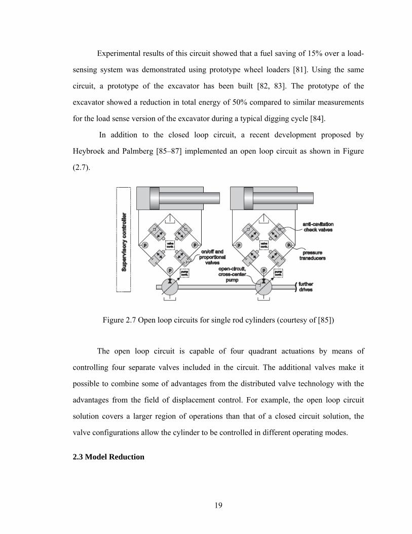
In addition to the closed loop circuit, a recent development proposed by
Heybroek and Palmberg [85–87] implemented an open loop circuit as shown in Figure
(2.7).
Figure 2.7 Open loop circuits for single rod cylinders (courtesy of [85])
The open loop circuit is capable of four quadrant actuations by means of
controlling four separate valves included in the circuit. The additional valves make it
possible to combine some of advantages from the distributed valve technology with the
advantages from the field of displacement control. For example, the open loop circuit
solution covers a larger region of operations than that of a closed circuit solution, the
valve configurations allow the cylinder to be controlled in different operating modes.
2.3 Model Reduction

20
The approximation of high-order plant and controller models by models of lower
order is an integral part of control system design. Until relatively recently model
reduction was often based on physical intuition [88]. For example, mechanical engineers
remove high-frequency vibration modes from models of turbine shafts and flexible
structure. The key idea is that it may be possible to replace high-order controllers by low-
order approximations with little sacrifice in performance [88].
Truncation methods of model reduction seek to remove, or truncate, unimportant
states from state-space models. If a state-space model has its A -matrix in Jordan
canonical form, state-space truncation will amount to classical model truncation. For
example, one way is to remove all those states that correspond to fast eigen-values which
have a large negative real part. The intuition of “fast” depends on the application and
experience. This generally means these modes outside of the control system bandwidth.
The prototype L∞ model reduction problem is to find a low-order approximation G of
G such that 1 2ˆ( )w G G w
∞− is small where 1 2,w w are frequency weighting matrices which
usually depend on control design and applications themselves.
Since any transfer function can be realized in terms of an infinite number of state-
space models, there are also an infinite number of candidate truncation schemes. Further
considerations with model truncations are controllability, observability and truncation
errors. These motivate a solution called balanced realization. The balanced realization has
the properties that mode i is equally controllable and observable and absolute-error is
small. Balanced realization first appeared with work of Mullis and Roberts [79] who were
interested in realization of digital filters that are optimal with respect to round-off errors
in the state update calculation. These issues are developed extensively in the book by
Williamson [90]. Moore applied this idea into control literature [91] and he also proved a
weak version of the stability result.

21
Balanced realization is achieved by simultaneously diagonalizing the
controllability and the observability gramians, which are solutions to the controllability
and the observability Lyapunov equations. When applied to stable systems, balanced
reduction preserves stability [92] and provides a bound on the approximation error [93].
Numerical algorithms for computing balanced realizations need to compute the
controllability and observability gramians which is a serious problem. For small-to-
medium-scale problems, balancing reduction might be implemented efficiently.
However, for large scale settings, exact balancing is expensive to implement because it
requires dense matrix factorizations and results in a computational complexity of 3( )O n
and a storage requirement of 2( )O n . In this case, approximate balanced reduction is an
active research area which aims to obtain an approximately balanced system in a
numerically efficient way [94–97].
Another well know model order reduction method is the singular perturbation
approximation which is usually associated with a fast-slow decomposition of the state-
space. Although the error bounds for balanced truncation and balanced singular
perturbation approximation are identical, the resulting models have different high- and
low-frequency characteristics. Direction truncation gives a good model match at high
frequency, while singular perturbation method has superior low-frequency properties.
Singular perturbation theory has its birth in the boundary layer theory in fluid
dynamics due to Prandtl [98]. Since then, singular perturbation techniques have been a
traditional tool of fluid dynamics. Their uses spread to other areas of mathematical
physics and engineering. In Russia, research activity on singular perturbations for
ordinary differential equations, originated and developed by Tikhononv and his students
[99, 100], continues to be vigorously pursued even today [101].
The methodology of singular perturbations and time scales are considered as a
boon to systems and control engineers. The technique has now attained a high level of

22
maturity in the theory of continuous-time and discrete-time control systems described by
differential and difference equations respectively. From the perspective of systems and
control, Kokotovic and Sannuti [102] were the first to explore the application of the
theory of singular perturbations for ordinary differential equations to optimal control.
Applications to broader classes of control problems followed at an increasing rate, as
shown by more than 500 references by Kotovoic [103, 104], Saksena [105] and
Subbararn Naidu [106]. For control engineer, singular perturbations are a means of taking
into account neglected high-frequency phenomena and considering them in a separate
fast time-scale. This is achieved by treating a change in the dynamic order of a system of
differential equations as a parameter perturbation, which, being more abrupt than a
regular perturbation is called a singular perturbation [107]. The practical advantages of
such a parameterization of changes in model order are significant because the order of
every real dynamic system is higher than that of the model used to represent the system.
Singular perturbations cause a multi-time-scale behavior of dynamic systems
characterized by the presence of both slow and fast transients in the system response to
external stimuli. The slow response or the “quasi-steady-state” is approximated by the
reduced system model while the discrepancy between the response of the reduced model
and that of full order model is the fast transient.
Example:
( , ) ( , )( , ) ( , ) ( , )
x t z tz t x t z t
ε εε ε ε ε
== − −
(2.2)
For this example, with specific values of 0.1ε = , (0) 2x = , (0) 3z = , Figure 2.8 shows
various solutions.

23
Figure 2.8 Basic concepts of singular perturbations and time scales (courtesy of [106])
Although singular perturbation technique is one of main tools used in fluid
dynamics research, its application in fluid power systems is very limited. Kim [108] uses
singular perturbation techniques to improve spool positioning of a servo-valve in an
active car suspension application. The resulting feedback system, based on a first-order
approximation of the servo-valve dynamics, is equivalent to a high gain control system.
Eryilmaz et al [109] considered hydraulic stiffness and applied singular perturbations to
ignore the hydraulic stiffness. Thus the control design is robust to variation of fluid bulk
modulus.
2.4 Parameter Estimation
A linear system can be described by its transfer function or by the corresponding
impulse response. With a confined set of possible models, those functions are determined
by directly evaluating input and output data. The methods of determination include

24
techniques in both the time-domain and the frequency domain. In the time domain, using
plots of the step response or impulse response, some characteristic numbers can be
graphically constructed which in turn can be used to determine parameters in a model of
given order [110]. For example, the Ziegler-Nichols rule is used in the step response.
Sine-wave testing is a kind of direct frequency response application. But if a noise
component is present in the measurement, it may be cumbersome to determine the
transfer function. By assuming some knowledge of noise, the correlation method is
applied in the system identification [110]. More disciplined proofs can be found in
Kailath [111].
These methods can be directly applied to time-invariant systems. To track the
time varying dynamics of a system, the identification algorithm needs to be adaptive so
that it can appropriately track the system dynamics [112, 113]. In control and signal
processing a model of a dynamic system is a mathematical description of the relationship
between inputs and outputs of the system. For the purpose of identification a convenient
way to obtain a parameterized description of the system is to let the model be a predictor
of future outputs of the system [114]
ˆ( | )y t θ (2.3)
Where θ is a parameter vector. For the linear system, the prediction is a linear regression
ˆ( | ) ( )Ty t tθ θ ϕ= (2.4)
Where, ( )tϕ is a vector of input and output data. System identification deals with the
problem of finding the parameter vector that gives the best estimation of the dynamic
system under consideration. For example, to find the parameter vector that minimized the
criteria:
2
1
ˆ( ) ( ( ) ( ))N
kV y k y kθ
=
= −∑ (2.5)

25
If ( )tϕ contains only measurements of outputs, it is called a Finite Impulse
Response (FIR) filter problem. Self-adjusting or adaptive FIR filters have been
successfully applied to antenna, noise canceling etc. due to their inherent stability.
However, system dynamics used in the control domain often have a pole-zero structure,
which is an Infinite Impulse Response (IIR) problem. When studying a time invariant
system, the typical procedure is to first collect a set of data from the system and then to
compute parameter estimates (off-line identification). For a time varying system, the
typical procedure is to compute a new estimate each time whenever a new measurement
becomes available, and this leads to recursive identification illustrated in Figure (2.9).
Figure 2.9 Typical system identification structures
There have been two kinds of approaches to adaptive IIR filtering corresponding
to different formulations of the prediction error. These are known as the equation error
method and the output error method. In the equation error formulation [115],
1 1
ˆ ˆ( ) ( ) ( ) ( ) ( )N M
m mm m
y n a n y n m b n x n m= =
= − + −∑ ∑ (2.6)
output feedback significantly influences the form of the adaptive algorithm, adding
greater complexity due to its nonlinearity. The regression term is:

26
ˆ ˆ( ) [ ( 1),...... ( 1), ( ),... ( 1)]Tt y n y n N x n x n Mϕ = − − + − + (2.7)
The benefit of the output equation error approach is that it does not lead to a
biased solution; however, it may converge to a local minimum of the mean-square-output
error. It can be shown that the solution may be suboptimal unless the transfer function is
Strictly Positive Real (SPR) [113]. To overcome SPR condition, additional processing of
the regression vectors or of the output errors is generally necessary [116, 117].
The equation error methods can be expressed as:
1
1 0
ˆ( ) ( ) ( ) ( ) ( )N M
m mm m
y n a n y n m b n x n m−
= =
= − + −∑ ∑ (2.8)
Different from Equation (2.7), the estimations of the previous outputs are replaced by the
true outputs. Thus the algorithm works like a FIR structure; and it is inherently stable
with adequate update gains and has a global minimum. However, it can lead to biased
estimates when noise exists in the measurement. The convergence rate and stability are
usually determined by the eigen-values of Hessian matrix.
The optimized parameters can be obtained by solving Wiener-Hopf equations if
statistics of the underlying signals are available [111]. In the control domain, a searching
method is often used as described in the following.
1 Steepest descent method:
To minimize 2( ( ) )TE y nξ θ ϕ= − , the cost gradient can yield: 2 2dx xxr rξ θθ
∂= − +
∂,
thus the identification law is given as:
1n n utξθ θ+
∂= −
∂ (2.9)

27
Where, ,dx xxr r are the cross correlation and auto correlation of ( ), ( )y n nϕ , and u is a
sufficiently small update gain. In an application, if there is no previous knowledge of
plant input signal and its output response, this method will not work in most cases.
2 Least Mean Squares (LMS) method
To minimize 2
0( ( ) ( ))
NT
ny n nξ θ ϕ
=
= −∑ , the gradient can be calculated as
1
02 ( ( ) ( )) ( )
NT T
ny n n nξ θ ϕ ϕ
θ
−
=
∂= − −
∂ ∑ , thus the identification law is given as:
1n n utξθ θ+
∂= −
∂ (2.10)
Comparing Equation (2.9) with (2.10), the difference between the two methods is
that the estimated gradient is used to replace the true gradient, making it suitable for
online estimation. Specifically, if one sample is used, the gradient will be
2( ( ) ( )) ( ) 2 ( ) ( )T Ty n n n e n nξ θ ϕ ϕ ϕθ
∂= − − = −
∂ (2.11)
It can be shown that LMS algorithm converges in the mean if
max
20( )Tu
λ φφ< < (2.12)
LMS is suitable for non-stationary signals. To optimize performance in specific
aspects ( e.g., convergence, noise rejection), there are some developed LMS algorithms,
such as normalized LMS, sign algorithms, Leaky LMS, variable step size LMS, block
LMS and gradient smoothing [118].
3 Recursive Least square
The least squares criterion is 2
0( ) ( )
nn i
in e iξ λ −
=
= ∑ .

28
Where 0 1λ< ≤ is called forgetting factor, ( )e i is the estimation error for every output.
RLS algorithm is given as follows (Goodwin, [112]) with an initialized estimation (0)P :
( ) ( 1) ( )z n P n nϕ= −
1( ) ( )( ) ( )Tg n z nn z nλ ϕ
=+
( ) ( 1) ( )[ ( ) ( 1) ( )]Tn n g n y n n nθ θ θ ϕ= − + − −
1( ) [ ( 1) ( ) ( )]TP n P n g n z nλ
= − −
The Kalman filtering algorithm can also be derived from RLS by setting the
forgetting factor to one, taking ( )P n as the post error covariance matrix and setting the
system transmission matrix to identity.
Generally, the RLS algorithm has a faster rate of convergence than LMS
algorithm and is not sensitive to variations in the eigenvalue spread of the correlation
matrix of the input data [118]. This improvement in performance is obtained at the
expense of a large increase in computational complexity. Much has been reported in
literature on a comparative evaluation of the tracking behavior of the LMS and RLS
algorithms [119–122]. A common conclusion is that the LMS algorithm shows a better
tracking behavior than the RLS algorithm. RLS exhibits numerical instability due to
round-off errors arising from the fact that ( )P n , being covariance matrices, have to be
nonnegative definite. During recursive operations, this property can not hold because of
round-off errors. Several variants of the RLS algorithms have been proposed to improve
the performance and robustness of RLS using QR decomposition, U-D factorization and
Singular Value Decomposition [118, 119, 123, 124].
The output error method has an inherent stability issue and local minimum
problem although theoretically it leads to an unbiased estimation. Similar searching

29
algorithms can be applied using the same as the output error approach. But, it does not
necessarily mean that the result is the best estimation. The only exception for the output
error equation method is HARF (Hyper-stable Adaptive Recursive Filter) which
originally came from Landau [117]. Based on his work, the algorithm was further
modified as HARF [125]. The principle of stability can be illustrated in Figure (2.10).
)(1zA
Figure 2.10 Close loop of HARF algorithm
The Figure (2.10) shows the feedback of the algorithm, from the hyper-stability
theory or SPR(Strictly Positive Real) theory, it can be shown that the closed loop system
will be stable if ( )A z is Hurwitz, and a ( )C z such that ( )( )
C zA z
is SPR. Therefore
( )C z needs to be designed and some prior information about the system is required. For a
time varying system, this is not always available.
Other than the above methods, there are still some global searching approaches
reported recently, for example, Genetic Algorithm [126] and Particle Swarm methods
[127]. However, these do not satisfy on-line identification requirement for time varying
system and neither do Neural Network nor Volterra filters [128, 129].
2.5 Hydraulic Control
Hydraulic systems are used extensively in many industrial applications mainly
due to its power density as discussed in previous chapter. However, the presence of
nonlinearities is one reason that limits its applications. These nonlinearities originate

30
from two main groups: the actuation subsystem and the loading subsystem. The actuation
subsystems’ nonlinearities include asymmetric actuation, transmission nonlinearities,
variations in the trapped fluid volume, nonlinearities of hydraulic components themselves
and so on. Nonlinearities of loading subsystems vary with applications: for example,
Coulomb friction in a actuator. In addition to this, hydraulic systems also have a large
extent of model uncertainties which include load changes, parameters drifting, leakages
and disturbances.
Linear control theory is a fundamental approach. Root locus and PID control
techniques still are popularly practiced techniques [130–134]. Robust control [136],
composite control law [137] have also been introduced to hydraulic controls to further
increase some aspects of “performance”. The traditional and widely practiced approach is
based on local linearization of the nonlinear dynamics about a nominal operation point,
with linearization errors usually treated as disturbances to the system. With feedback
linearization, the flow dynamics and fluid compressibility are taken into account with a
nominal nonlinear model, and this model is inverted to produce the appropriate control to
the remaining linear system [138–141]. The concept of passivity has been applied to
hydraulic valves by Li [142]. Li showed that it is possible to have a hydraulic valve
behave passively by either modifying the spool or by using passivity theory and an active
control law that passifies the system using an energy storage function. This work has
been extended and applied to an excavator like manipulator with guaranteed passive
behavior [143].
The two most common approaches developed to compensate for the nonlinear
behavior of hydraulic systems are variable structure control and adaptive control. Several
versions of sliding mode controllers have been developed [142–146]. In addition to the
sliding mode controller, Wang et al [148] also applied a sliding mode observer to get
system states for the controller.

31
In [149], Alleyne et al applied nonlinear adaptive control toward the force control
of an active suspension driven by a double-rod cylinder. Their work demonstrated that
nonlinear control schemes can achieve a much better performance than a conventional
linear controller. Adaptive Robust Control law has been proposed by Yao et al [150–152]
to get a guaranteed response under some assumptions. Bobrow et al [153] has used on-
line identification to get system state space equations by measuring system states. They
showed full state feedback, in conjunction with an LQR compensator, exhibited good
robustness but the system exhibited oscillatory behavior if the forgetting factor was too
low for adaptation process. Yun and Cho [154] neglected the fluid compressibility and
developed an adaptive controller based on a Lyapunov function. They showed the
controller is fairly insensitive to various external load disturbances, yielding good
performance characteristics in comparison to the conventional constant PI controller.
Plummer et al [155] used recursive least squares method to apply indirect adaptive
control. In their work, a constrained model and a Diophantine equation solver were
implemented. They also showed off-line system identification is extremely useful as a
basis for adaptive controller design. Similar to the Plummer’s work, Sun and Tsao [156]
also applied recursive least squares to hydraulic controls. They used an eighth-order
model and higher sampling frequency to demonstrate the adaptive system’s ability in
high bandwidth tracking performance. Furthermore, the controller applies an approximate
stable inverse of the plant using zero-phase-error compensation [157] to render stable
closed loop system without solving a Diophantine equation. In another of Tsao’s work
[158], a square root algorithm has been applied to increase the numerical stability of
recursive least squares adaptation algorithm.
2.6 Summary
The hydraulic industry has a long, storied past. The cost and law regulations are
major driving factors to improve hydraulic energy efficiency. From the literature review

32
presented herein, it can be said that much research efforts are being directed to
developing better control methodologies and efficient hydraulic structures.
It is seen that a valve-less system has higher energy efficiency than valve
controlled systems. However, innovations–especially to systems as fundamental as
system structure–are adopted only after being thoroughly scrutinized. Does the valve-less
circuit function well for industry? The novel circuit developed in this research uses
minimum components to achieve a cost effective, valve-less circuit. Furthermore, the
circuit can be further simplified if a moderate speed variable displacement pump is
applied in practice.
Most methodologies do not consider measurement noise and the calculation loads
of a real time controller. The application of singular perturbation theory to fluid power
would make its design simpler and decrease controller working loads in some working
situations. Furthermore, it gives a good intuition when the design is first considered. The
developed control algorithms fully consider measurement noise, stability of the controller
itself, and abilities to achieve desired trajectory tracking. It is well suited for industry
adoption and practice.

33
CHAPTER III
APPLICATION SINGULAR PERTURBATION TO FLUID POWER
This chapter is dedicated to apply singular perturbation theory to hydraulic
controls. The purposes of this chapter include: (1) providing theoretical conclusions
which will be used in later chapters; (2) applying singular perturbation theory to pump
controlled systems; (3) providing extra application examples illustrating that hydraulic
design can be simplified under some conditions. The goal is to provide evidence that
singular perturbation theory has broad applicability in the hydraulic control domain.
The singular perturbation approach can be intuitively understood as that the
hydraulic stiffness can be neglected under some circumstances. Thus the orders of the
investigated system can be decreased. The direct benefit is that the control design
becomes simple and the fluid bulk modulus, which is a time varying parameter, does not
explicitly affect the controller. Such benefits come from sacrificing control performance,
especially at high frequencies. However, for practical issues, the steady states response
and the low frequency responses are the primary concerns in hydraulic systems. Thus it
makes this approach valuable.
This chapter begins with the motivations to apply singular perturbations followed
by a discussion of the pump displacement controlled system. Then, two cases of control
design are presented for different input stage models followed by the numerical
simulation and experimental results. Finally, other examples are presented which further
illustrate this powerful tool.
3.1 Variable Displacement Controlled Cylinders
Figure (3.1) presents a simplified overview of the variable displacement
controlled cylinder system considered in this chapter.

34
x
Figure 3.1 Variable displacement controlled actuators
The position of the piston of the cylinder is obtained by the oil pumped into/out of
the cylinder. The motor is rotating at a fixed speed; the control input is the voltage to the
variable displacement pump. Limiting the bandwidth of a desired tracking trajectory to
values lower than 10Hz, if the dynamics of pump displacement can be neglected, the
pump displacement will be proportional to the input voltage.
p pD k u= (3.1)
Otherwise, the dynamics of the displacement can be modeled as a first order system by
the transfer function:
p pD k us
αα
=+
(3.2)
Where pD is the displacement of the pump, u is the input control voltage signal
and pk is the proportional gain. Since the circuit is symmetry, the system dynamics can
be described as:
( )Mx PA bx F t= − − (3.3a)
p lV P D Ax c Pωβ
= − − (3.3b)

35
where A is the annulus area of the cylinder, b is the coefficient of friction and ( )F t is the
sum of the Coulomb friction part and other external forces which are assumed to have
been identified.ω is the principle axis rotating speed of the pump, lc is the linear fluid
leakage coefficient, including the cylinder leakage and the internal leakage of the pump,
and accounts for the volumetric losses of the pump. P is the differential pressure between
both sides of the cylinder chambers. β is the bulk modulus of the fluid being used and V
is the effective volume of the cylinder:
0V V Ax= + (3.4)
where 0V is the volume which includes pipe line, internal pump volume etc.
1P is the pressure on one side of the cylinder and 2P is the pressure on the other
side. Thus
1 2P P P= − (3.5)
Some specific hardware mechanisms ensure that, at any time, one of these two pressures
is always equal to the return pressure. For example, the hardware, in this case, includes
the check valves and the shuttle valve implemented in the proposed novel circuit which
will be focused on in the next chapter. The cylinder returning pressure rP is regulated by
the relief valve (usually this is same as the charge pressure for the pump, for example,
150 PSI ). So rP can be deemed as a constant. The delivery pressure and return pressure
alternately changes depending on the working conditions.

36
The static leakage part l rc P , which is very small, is ignored, the Equation (3.3) is
rewritten as:
A b Fx P xM M M
= − − (3.6a)
p lP D Ax c Pε ω= − − (3.6b)
In Equation (3.6b), ε is defined as /Vε β= . For most applications, the maximum volume
V is physically limited, and it is very small in most cases; meanwhile, the bulk modulus
is very large. It is reported that the effective bulk modulus of an average working fluid is
more than 200,000 PSI and the dependence of bulk modulus on pressure will be reduced
as pressure increases [19]. Merritt [2] has pointed out that 100,000 PSI gives a good
estimation for most applications. Thus ε is a very small number. The critical thing is that
Equation (3.6b) will be stiff for control applications. Figure (3.2) illustrates the pressure
response of the system defined by Equation (3.6) for a step input from pD .
0 0.5 1 1.5 2-1
-0.5
0
0.5
1
1.5x 10⁹
Time ( seconds)
Pre
ssur
e( p
ar)
Figure 3.2 Pressure responses for the step input

37
Two adverse factors exist for control applications. First, the oscillation frequency,
which is on the order of 30~40 Hz, is relatively high. This rate is close to the sampling
frequency and data transfer rate. Second, if a state feedback control algorithm is designed
for the system, the control efforts should maintain a high bandwidth. But such high
bandwidth pumps are not practical at the present time. A control algorithm may consume
significant computation time and will accumulate large numerical errors. The
approximation of a high-order plant and controller models by models of lower order is an
integral part of control system design. It is possible to replace high order controllers by
low order approximations with little sacrifice in performance. The dynamics of hydraulic
systems involve slow and fast modes. Because of this, singular perturbation theory can be
applied, significantly simplifying the control design and reducing control efforts.
3.2 Singular Perturbation Model
From the above discussion, a fast mode exists in the system (3.6). It is natural to
use singular perturbation theories to solve these two-time-scale problems.
For a singular system with states[ , ]Ts sx z :
0( , , , ), ( ) ( )s s s sx f t x z x tε ζ ε= = (3.7a)
0( , , , ), z ( ) ( )s s s sz g t x z tε ε η ε= = (3.7b)
The corresponding quasi-steady-state model of the system (3.7) is defined as:
0 0( , , ( , ), ), ( )s s s sx f t x h t x x tε ζ= = (3.8a)
( ) ( , )s sz t h t x= (3.8b)
where Equation (3.8b) is the distinct solution of Equation (3.7b) with 0ε = ,
and ,n ms sx R z R∈ ∈ .

38
Following the singular perturbation theory (Tikhonov’s Theorem), we conclude
that if functions , f g , their first partial derivatives with respect to ( , , )x z ε , and the first
partial derivative of g with respect to t are continuous; the function h and gz
∂∂
have first
partial derivatives with respect to their arguments; the initial data ( )ζ ε and ( )η ε are
smooth function of ε ; Equation (3.8a) has unique solutions on a convex set, the
boundary-layer model is exponentially stable, further if the reduced order system (3.8a) is
also exponentially stable, then: there exists a positive constant *ε such that for *0 ε ε< < ,
the system (3.7) has a unique solution on 0[ , )t ∞ , and ( , ) ( ) ( )s sx t x t Oε ε− = . Moreover,
given any 0bt t> , there exists *0 ε ε< < such that ( , ) ( , ) ( )s sz t h t x Oε ε− = holds
uniformly for [ , )bt t∈ ∞ [107], [159].
The key idea of singular perturbation theory is that the system trajectory is in the
m nR + manifold and there exists a fast manifold in mR . It turns out that under some
assumptions, the manifold will remain within an ( )O ε neighborhood of the slow
manifold.
ε , defined in Equation (3.6b), is mainly determined by the effective bulk
modulus, which is substantially lowered by entrained air. This is often observed when a
hydraulic system, first turned on after a period of shutdown, has allowed air to be
collected in the system. However, we can assume that effective bulk modulus is constant
or that it changes slowly under normal working conditions since entrained air in the
system has a relatively stable level. Even with some changes in the effective bulk
modulus, a conservative bt can be easily identified because the system described by
Equation (3.6) is a SISO system.
Theorem 3.1 The origin of the boundary-layer model in the system defined by (3.6) is an
exponentially stable equilibrium point, uniformly in ( , )t x .

39
Proof:
( , , )
( ) /p
p l
P h t D x
D Ax cω
=
= −
Let ( , , )py P h t D x= −
Hence: y P hε ε ε= −
Define:
dy dydt d
ετ
=
Then:
( , , ,0)
= D ( ( ) / )
=p l p l
l
dy g t x y hd
Ax c y D Ax c
c y
τω ω
= +
− − + −
−
(3.9)
lc is the fluid leakage coefficient of the high pressure side so it is positive. Thus it is
proven that the boundary-layer model is exponentially stable. Furthermore, the region of
attraction of the fast manifold covers the whole domain.
(Q.E.D)
Remark 3.1: As 0ε → , the eigenvalue of the fast mode will approach:
2[ ( )] /lc Oλ ε ε= − + (3.10)
For a practical consideration, one hopes the fast mode plays a small role in system
transient response. Thus, a bigger leakage coefficient lc or a much smaller ε is expected.
This limits the use of this theorem to solve some hydraulic applications.
Remark 3.2:

40
Although there are limits mentioned above, the benefits are obvious: (1) One does
not need to consider the uncertainty of the bulk modulus, which is an often used
complaint for the design of hydraulic system controls; (2) The fast mode will not affect
the steady state, so it is possible to use a secondary design to increase lc for transient
performance, and then to change back to the original value in order to keep energy
efficiency.
Thus the reduced order system can be described as Equation (3.11, 3.12):
Mx PA bx F= − − (3.11)
If the input state is a proportional,
p pD k u= (3.12a)
Or the input stage is modeled as a first order system,
p pD k us
αα
=+
(3.12b)
where P satisfies 0p lD Ax c Pω − − = .
By applying singular perturbation theory with a suitable control law, a closed loop
controller can track the desired trajectory such that the tracking error exponentially
decays.
3.3 Control Law Design
To begin the controller design, practical and reasonable assumptions about the
system have to be made. In general, the system is subjected to parametric uncertainties
due to variations of mass, friction coefficients etc. The main purpose of this chapter is to
introduce singular perturbation theory to simplify control design; thus such uncertainties
have not been considered in this paper (real time parameter identification techniques will

41
be discussed in latter chapters). Also, it is assumed that system states of the slow time
scale are available.
A desired trajectory generation block is necessary. The purpose of the block is to
achieve smooth acceleration to prevent pressure jerks in the cylinder and to get the
desired trajectory signals. Since a reduced order model design is used, the limited
bandwidth of the desired trajectory will ensure that the transient response is within the
neighborhood of the quasi-state and will ensure that the control input will not saturate.
The desired trajectory includes[ , , ]d d dx x x . In this chapter, the desired trajectory is
produced by the transfer function:
3
2 2( ) ( )( )( 2 )
nd d
n n n
x s x ss s s
ωω ξω ω
=+ + +
(3.13)
where dx is the original trajectory, e.g. a step input signal, which may not be smooth.
Define tracking error:
de x x= − (3.14)
and auxiliary symbols ,ls v with some positive scale 1λ
1ls e eλ= + (3.15)
1( )d dv x x xλ= − − (3.16)
Then, we have
ls x v= − (3.17)
System (3.11) combined with (3.17) can be expressed as (3.18) with some
positive constant k .
( )l l lM s ks PA bx F Mv Mks+ = − − − + (3.18)

42
Let:
d lP A bx F Mv Mks= + + − (3.19)
then Equation (3.18) becomes:
( )l l dM s ks PA P A+ = − (3.20)
with (3.20), the system (3.11), (3.12) can be obtained as:
1( )( ) dd dM k e PA P Adt dt
λ+ + = − (3.21)
p pD k u= (3.22a)
or for the first order system
p pD k us
αα
=+
(3.22b)
where P satisfies
0p lD Ax c Pω − − = (3.23)
Case 1:
Suppose the trajectory is very low bandwidth or the pump displacement response
is fast. In such case, the input voltage | pu D→ can be described as in Equation (3.22a).
Select a control law:
( ) / ( )l d pu c P Ax k ω= + (3.24)
Lemma: For the singularly perturbed system (7), if , f g and their partial derivatives
are sufficiently smooth functions, ( , , ,0) 0s sg t x z = has an isolated root ( , )s sz h t x= such
that 0h = at the equilibrium point. Both the reduced order system and the boundary-

43
layer system are exponentially stable on a compact set, then there exists *ε such that for
all *ε ε< , the system (3.7) is exponentially stable at the equilibrium point. (Proof can be
found in [159])
Theorem 3.2: With control law (3.24), the original system is exponentially stable, and the
tracking error decays exponentially.
Proof: Replace (3.21) with (3.24),
1( )( ) 0d dM k edt dt
λ+ + =
Thus the reduced order system is exponentially stable, since the boundary-layer model is
also exponentially stable from Theorem 3.1. By the Lemma above, the original system is
proven to be exponentially stable, and the tracking error is shown to exponentially decay.
(Q.E.D)
Case 2:
Suppose the trajectory is low bandwidth; the input voltage | pu D→ can be
modeled as a first order system as (3.22b).
Let: ( ) /pd l dD c P Ax ω= +
The system (3.21) – (3.23) can be written as:
1( )( ) ( ) /p pd ld dM k e D D A cdt dt
λ ω+ + = − (3.25)
p p pD D k uα α= − +
Select a control law with some positive constant 2λ
21 ( ( ) )p pd pd p
p
u D D D Dk
λ αα
= − − + + (3.26)

44
Theorem 3.3: With control law (3.26), the original system is exponentially stable and the
tracking error decays exponentially.
Proof:
Select Lyapunov function 2( ) / 2p pdV D D= −
( )( )
=( )( )p pd p pd
p pd p p pd
V D D D D
D D D k u Dα α
= − −
− − + −
With the control law (3.26), we have
22 ( )
0p pdV D Dλ= − −
≤
The 2( ) / 2p pdV D D= − is not a true Lyapunov function for the reduced order system.
However, using the Barbalat Lemma, we can see p pdD D→ exponentially. Note that in
(3.25), the mapping ( ) |p pdD D e− → is exponentially stable. Thus it is proven that the
reduced order system is exponentially stable. By using the Lemma and Theorem 3.1
again, the proof is completed.
(Q.E.D)
3.4 Simulation
To illustrate the above design, programs have been developed to simulate the
performance of the proposed singular perturbation approach control algorithms. The
parameters used in the simulation are shown in Table 3.1.
The simulation program includes three parts. First, the desired trajectory is
calculated using (3.13). Then, the control law is implemented following (3.24) and (3.26)
for different cases. Last, the control effort is fed into the original system described as
(3.4a, 3.4b).

45
Table 3.1 Parameters used in the simulation Symbol Physical Meaning Value
β Bulk modulus 86.89 10× Pa M Mass 100 Kg
1D Diameter of the cylinder 23.81 10−× m 1L Length of the cylinder 1.14 m 2D Diameter of pipelines 22.54 10−× m 2L Length of the pipeline 2.03 m
b Friction coefficient 200 N/(m/s) lc Leakage coefficient 12 39.5 10 m / Pa s−× ⋅
Simulation of Case 1:
Step response tests identify several important characteristics of a controller,
including response, overshoot, settling time and steady state error. Figure (3.3) and (3.4)
show the step response and the corresponding control effort of the controller proposed in
(3.24). It can be seen that the cylinder position strictly follows the desired trajectory, and
the control effort signal has very low frequency. This is very useful in practical
engineering.
0 0.5 1 1.5 2 2.5 3-0.2
0
0.2
0.4
0.6
0.8
1
1.2
Time(seconds)
Posi
tion(
m)
Desired trajectory
Real trajectory
Figure 3.3 Step response

46
0 0.5 1 1.5 2 2.5 3-0.5
0
0.5
1
1.5
2
2.5
3x 10⁻³
Time(seconds)
D
pω
Figure 3.4 Control efforts for the step response
Bandwidth tests were performed in order to determine the maximum frequency at
which the controller could accurately track given trajectories. Figure (3.5) shows the
system tracking a 1Hz and 2Hz desired trajectory. There are some obvious tracking errors
for the 2Hz signal. However, this is not a cause for concern. One decides how fast the
controller should correct the error and how the fast mode exists in the response, which
corresponds to the positive number 1λ in (3.15). Generally, the theoretical converging
value *ε is conservative [107, 159]. So the system can achieve a much higher bandwidth
if practical issues such as saturation or pressure jerk are not considered.
An interesting result is shown in Figure (3.6). By increasing the effective leakage
coefficients, for example with a bypass control as mentioned above, the controller can
easily track a 10Hz signal even when the other parameters are not optimized (as in the
above tests). This result shows it is possible to use a dynamic bypass control to increase
performance.

47
0 1 2 3 4 5 6-0.8
-0.6
-0.4
-0.2
0
0.2
0.4
0.6
Time(seconds)
Pos
ition
(m)
Desired trajectoryReal trajectory
Figure 3.5 Bandwidth test
0 0.1 0.2 0.3 0.4 0.5 0.6 0.7 0.8-0.2
-0.15
-0.1
-0.05
0
0.05
0.1
0.15
Time(seconds)
Pos
ition
(m)
Desired trajectoryReal trajectory
Figure 3.6 Bandwidth test (10 Hz) Simulation of Case 2:
Figure (3.7) and (3.8) show the tracking performance for the step input signals
and the corresponding control effort. Note that at the beginning of the simulation, the
cylinder rod is not at the zero position, such that the figure shows a control effort to
retract the cylinder rod. From the response, it is clear that the tracking error exponentially
decays and the bandwidth for the control effort is low.
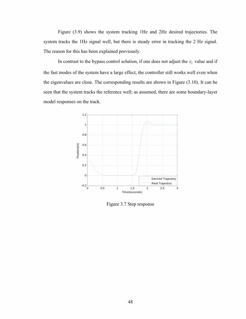
48
Figure (3.9) shows the system tracking 1Hz and 2Hz desired trajectories. The
system tracks the 1Hz signal well, but there is steady error in tracking the 2 Hz signal.
The reason for this has been explained previously.
In contrast to the bypass control solution, if one does not adjust the lc value and if
the fast modes of the system have a large effect, the controller still works well even when
the eigenvalues are close. The corresponding results are shown in Figure (3.10). It can be
seen that the system tracks the reference well; as assumed, there are some boundary-layer
model responses on the track.
0 0.5 1 1.5 2 2.5 3-0.2
0
0.2
0.4
0.6
0.8
1
1.2
Time(seconds)
Pos
ition
(m)
Desired TrajectoryReal Trajectory
Figure 3.7 Step response

49
0 0.5 1 1.5 2 2.5 3-2
-1
0
1
2
3
4
5
6
7
8x 10⁻³
D
pω
Figure 3.8 Control efforts for the step response
0 0.5 1 1.5 2 2.5 3 3.5 4-0.5
0
0.5
Time(seconds)
Posi
tion(
m)
Desired TrajectoryReal Trajectory
Figure 3.9 Bandwidth Test

50
0 0.5 1 1.5 2 2.5 3 3.5 4-0.5
0
0.5
Time(seconds)
Posi
tion(
m)
Desired TrajectoryReal Trajectory
Figure 3.10 Bandwidth test without heavily compressing fast mode
0 0.5 1 1.5 2-0.2
0
0.2
0.4
0.6
0.8
1
1.2
Time(seconds)
Posi
tion
Desired trajectoryReal trajectory
Figure 3.11 Step response with the bulk modulus reduced 50%
A series of simulations with varying bulk modulus have been conducted. Figure
(3.11) shows one of the simulation results using the same parameters as Case 1 except the
bulk modulus has been reduced 50%. It can be seen that the fast mode does change but
the system stability and steady state tracking still hold.

51
3.5 Experimental Results
Experiments were conducted to validate the proposed control approach. A testbed
is illustrated schematically in Figure (3.12). The single rod cylinder has a stroke length
of 20 inches. The diameter of the rod and the piston are 1 inch and 1.5 inch, respectively.
The channel iron platform mounted on the cylinder weighs around 15 kg. Each of the
weights is 20.4 kg. Up to 7 of these weights can be mounted on the platform. All of the
valves used in the circuit are chosen from Sun Hydraulics Corporation’s standard
products. The variable displacement pump is a Sauer Danfoss H1 axial piston pump.
Only one channel of this tandem pump is used. The pump is driven by a Siemens electric
motor running at 1000 rpm. The electric motor also drives a small charging pump to
provide the charging pressure, which is regulated by a relief valve at 150 PSI . The relief
valves are adjusted to 1500 PSI for safety protection. Two pressure sensors, made by
Hydac Technology Corporation, rated at 3000 PSI , are mounted as shown in Figure
(3.12). The control algorithms run on a Matlab xPC Target real time operating system.
The commands for pump displacements and the electric motor controls use a CANBUS
network to connect the target computer, the variable displacement pump, and the motor
driving units together. A National Instruments PCI-6052 A/D & D/A card is used to
collect pressure signals and drive the flow direction control valves. A set of low pass
filters is also used to filter the interference noise from the electrical motor and act as an
anti-aliasing filter. The displacement sensor, made by MTS Systems Corporation, is used
to measure the cylinder’s position.
The hydraulic circuit as shown in Figure (3.12) has an internal instability issue
when the load is close to critical load (More details will be discussed in the following
chapters). The DSP and flow control valves, shown in Figure (3.12), form an inner loop
to stabilize the hydraulic circuit, while the displacement control feedback presented in
this paper is outer loop. The experiments presented in this paper use much larger weight
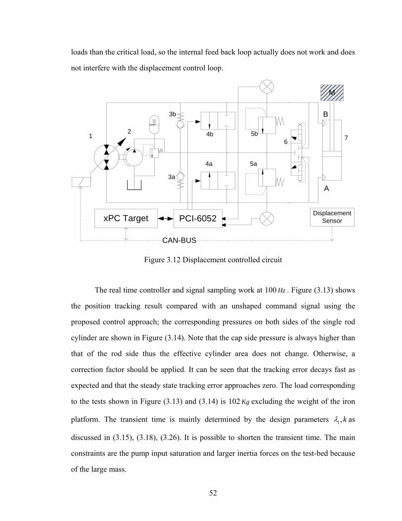
52
loads than the critical load, so the internal feed back loop actually does not work and does
not interfere with the displacement control loop.
A
B
12
3b
3a
4b
4a
5b
5a
6 7
M
xPC Target PCI-6052Displacement
Sensor
CAN-BUS
Figure 3.12 Displacement controlled circuit
The real time controller and signal sampling work at 100 Hz . Figure (3.13) shows
the position tracking result compared with an unshaped command signal using the
proposed control approach; the corresponding pressures on both sides of the single rod
cylinder are shown in Figure (3.14). Note that the cap side pressure is always higher than
that of the rod side thus the effective cylinder area does not change. Otherwise, a
correction factor should be applied. It can be seen that the tracking error decays fast as
expected and that the steady state tracking error approaches zero. The load corresponding
to the tests shown in Figure (3.13) and (3.14) is 102 Kg excluding the weight of the iron
platform. The transient time is mainly determined by the design parameters 1,kλ as
discussed in (3.15), (3.18), (3.26). It is possible to shorten the transient time. The main
constraints are the pump input saturation and larger inertia forces on the test-bed because
of the large mass.
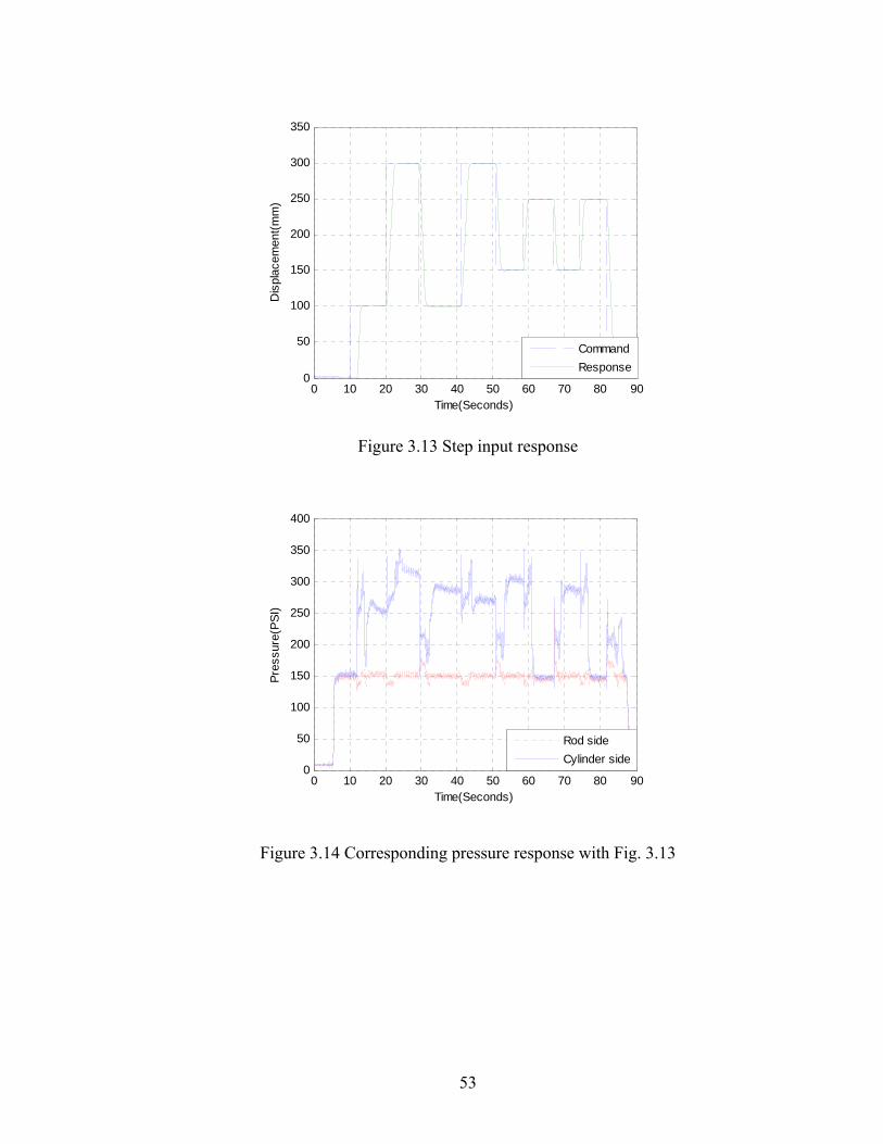
53
0 10 20 30 40 50 60 70 80 900
50
100
150
200
250
300
350
Time(Seconds)
Dis
plac
emen
t(mm
)
CommandResponse
Figure 3.13 Step input response
0 10 20 30 40 50 60 70 80 900
50
100
150
200
250
300
350
400
Time(Seconds)
Pres
sure
(PSI
)
Rod sideCylinder side
Figure 3.14 Corresponding pressure response with Fig. 3.13

54
0 10 20 30 40 50 60 700
50
100
150
200
250
300
350
Time(Seconds)
Dis
plac
emen
t(mm
)
CommandResponse
Figure 3.15 Tracking test
0 10 20 30 40 50 60 700
50
100
150
200
250
300
350
400
Time(Seconds)
Pres
sure
(PSI
)
Rod sideCylinder side
Figure 3.16 Corresponding pressure response with Fig. 3.15
Using the same design parameters as in the previous tests, sinusoid signal tracking
results are shown in Figure (3.15) and (3.16). As shown in Figure (3.15), the tracking
command was issued when the system was starting; the controller was enabled at 13
seconds. After a transient period, the cylinder tracks the desired trajectory well. Finally

55
the control was turned off at 65 seconds. Figure (3.16) shows the corresponding pressure
response on both sides of the cylinder.
A common hydraulic oil (CITGO-A/W-ISO46) found in the market was used in
this series of experiments, and the bulk modulus of the oil has not been explicitly
identified. All algorithms, including proposed controller, inner loop hydraulic circuit
stabilizing controller, data sampling and communication units, consume
65.49 10−× seconds for each loop on a Intel Pentium4 PC with Matlab xPcTarget operation
system.
3.6 Conclusion
In the previous sections, the conditions for applying singular perturbation theories
in hydraulic design have been discussed. The design procedures have been developed
using these theories. The benefits of using this approach are:
(1) It simplifies the controller design.
(2) The control efforts are dominated by low frequency signals.
Since a conservative bulk modulus value is used and the rate of the fast mode is
much faster than the rate of the quasi-state mode, the system is robust to variations in
hydraulic fluid bulk modulus.
In addition to singular perturbation theories, the control algorithm is based on
Lyapunov and other similar backstepping techniques. The results show that the system is
exponentially stable and that tracking errors exponentially decay.
To have good transient response, the suggestion is that the tracking reference
should be kept below the half speed of the fast mode manifolds. For cases of extremely
large duty cylinders, a secondary bypass control can be implemented. However, even
without secondary control, the system still shows high robustness.
3.7 Further Discussions of Applying Singular Perturbations
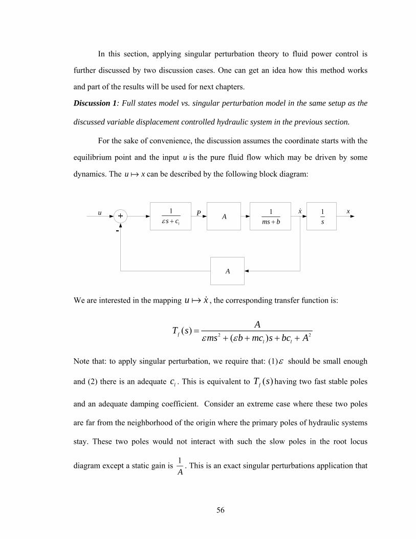
56
In this section, applying singular perturbation theory to fluid power control is
further discussed by two discussion cases. One can get an idea how this method works
and part of the results will be used for next chapters.
Discussion 1: Full states model vs. singular perturbation model in the same setup as the
discussed variable displacement controlled hydraulic system in the previous section.
For the sake of convenience, the discussion assumes the coordinate starts with the
equilibrium point and the input u is the pure fluid flow which may be driven by some
dynamics. The u x can be described by the following block diagram:
1
ls cε + A1
ms b+1s
A
u P x x
We are interested in the mapping u x , the corresponding transfer function is:
2 2( )( )f
l l
AT sms b mc s bc Aε ε
=+ + + +
Note that: to apply singular perturbation, we require that: (1)ε should be small enough
and (2) there is an adequate lc . This is equivalent to ( )fT s having two fast stable poles
and an adequate damping coefficient. Consider an extreme case where these two poles
are far from the neighborhood of the origin where the primary poles of hydraulic systems
stay. These two poles would not interact with such the slow poles in the root locus
diagram except a static gain is 1A
. This is an exact singular perturbations application that

57
the fluid stiffness can be neglected under some circumstances. Now consider another
common cases that there is a slow dynamics for the input stage, 'ku us k
=+
. In industrial
practice, a PD controller is often implemented to stabilized 'u x . If the fluid
compressibility is not considered, the root locus design is shown in the following figure:
-3 -2.5 -2 -1.5 -1 -0.5 0-1
-0.5
0
0.5
1Root Locus
Real Axis
Imag
inar
y Ax
is
Considering the fluid compressibility (under conditions that these two poles are relatively
fast than slow manifold), the full order system’s root locus looks like:
-30 -20 -10 0 10-30
-20
-10
0
10
20
30Root Locus
Real Axis
Imag
inar
y Ax
is
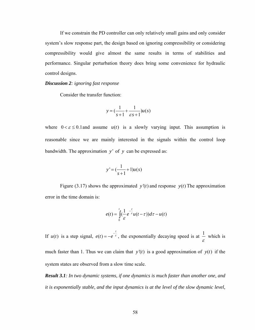
58
If we constrain the PD controller can only relatively small gains and only consider
system’s slow response part, the design based on ignoring compressibility or considering
compressibility would give almost the same results in terms of stabilities and
performance. Singular perturbation theory does bring some convenience for hydraulic
control designs.
Discussion 2: ignoring fast response
Consider the transfer function:
1 1( ) ( )1 1
y u ss sε
= ++ +
where 0 0.1ε< ≤ and assume ( )u t is a slowly varying input. This assumption is
reasonable since we are mainly interested in the signals within the control loop
bandwidth. The approximation 'y of y can be expressed as:
1' ( 1) ( )1
y u ss
= ++
Figure (3.17) shows the approximated '( )y t and response ( )y t The approximation
error in the time domain is:
0
1( ) ( ( )) ( )t
e t e u t d u tτε τ τ
ε−
= − −∫
If ( )u t is a step signal, ( )t
e t e ε−
= − , the exponentially decaying speed is at 1ε
which is
much faster than 1. Thus we can claim that '( )y t is a good approximation of ( )y t if the
system states are observed from a slow time scale.
Result 3.1: In two dynamic systems, if one dynamics is much faster than another one, and
it is exponentially stable, and the input dynamics is at the level of the slow dynamic level,

59
then the fast dynamics’ steady states can be used as the approximated response at the
slow dynamic time scale.
0 1 2 3 4 5 60
0.5
1
1.5
2Step Response
Time (sec)
Ampl
itude
RealApproximation
Figure 3.17 Approximated response and real response
This result will be used in next chapters to analyze the stability of the system.
3.8 Summary
This chapter illustrates how to apply singular perturbation theory to fluid power
systems. Designs for two kinds of input dynamics are presented, the comparison with the
full order system and simplified model are illustrated by root locus techniques. Further
discussions are made in order to show singular perturbations application from other
aspects and parts of these results and the conclusions drawn in this chapter will be used in
the following chapters.

60
CHAPTER IV
A HYDRAULIC CIRCUIT FOR SINGLE ROD CYLINDERS
The major advantage of a pump displacement controlled actuator is that it
provides higher energy efficiency because there are no throttling losses within the main
power lines of the actuators and because the pump is able to regenerate energy using
potential and braking energy from other function units by mechanically sharing the
pumps’ shafts. One immediate problem for pump displacement controlled systems is that
the most common actuators used by the industry are single rod cylinders. An example is
the boom structure used in excavators. When using a single rod cylinder in a pump
displacement controlled circuit, an appropriate circuit arrangement is necessary in order
to balance unequal flow rates entering and leaving the cylinder volumes because of the
differential areas of the cylinder.
Several approaches can be found in literature to solve the differential area
problem as we have reviewed in the literature review chapter. In order to recover energy
from other function units, the hydraulic circuit needs the ability to be operated in four
quadrant modes. A reported problem for kinds of circuits is pump oscillations under some
circumstances. More explicitly, the pressures on the cap side and rod side sometimes
uncontrollably oscillate; correspondingly, the cylinder velocity oscillates and changes
rapidly even though it is continuous because of mass inertia; the system has fast
oscillations between pumping mode and motoring mode. At this stage, the system loses
controllability or is under weak controllability.
In this chapter, a novel flow control circuit for differential flow rates is presented.
The concept is developed from Hewett’s structure [75]. New components and control
algorithms have been added. The circuit inherits advantages of Hewett’s design, but the
principle, the working point analyses, and technical focus are totally different from

61
Hewett’s. The circuit not only preserves energy efficiency, but also eliminates pressure
oscillations. Even more, tracking performance can be adjusted as demanded.
4.1 The Flow Control Circuit with Dynamical Compensations
The proposed closed loop hydraulic circuit is shown in Figure (4.1). The circuit
consists of a pair of check valves, a pair of flow control valves, a pair of relief valves, a
3-position 3-way shuttle valve, two pressure sensors and a controller. Besides the
proposed circuit, the whole system includes a displacement controlled pump, a charge
pump and a single rod cylinder. The differential volume and volumetric losses are
balanced through one of the check valves or the shuttle valve to the low pressure power
line whose pressure is close to the charge pressure depending on the characteristics of the
accumulator and the regulating valve. The controller dynamically adjusts the flow control
valves to allow the circuit to be compensated. Stability compensation is accomplished by
using a small, controlled leakage such that the pressure oscillations are inhibited.
Additional compensation can be issued by the controller to improve the cylinder tracking
performance. The relief valves, which do not operate in normal working situations,
provide a pressure safety protection.
A
B
DSP
2
3b
3a
4b
4a
5b
5a
6 7
M
Figure 4.1 Hydraulic Circuit for a single rod cylinder

62
The circuit works in all four quadrant operations as shown in Figure (4.2). The
positive direction is defined as the direction which makes the cylinder extend under
pumping mode as shown in Figure (4.2(a)). That is: the differential pressure on the pump
is defined as: a bP P P= − , pump flow, Q , is downwards on the pump, the cylinder
displacement, x , is upwards in Figure (4.1). Whenever ,P Q have same sign, the pump
is in pumping mode which means the pump is transferring energy to the cylinder;
otherwise, the pump is in the motoring mode which means the cylinder feeds energy back
to the pump. When 0, 0Q P= ≠ , the pump neither gives energy nor absorbs energy and
the movement of the cylinder is mainly decided by circuit leakage. In another case, when
0, 0P Q≈ ≠ , there is no large energy exchange between the pump and the cylinder;
notice that the cylinder is moving in this case, for example, when it is extending, most of
energy exchange is between the cylinder and the charge pump.
I. Pumping
III. Pumping
II. Motoring
IV. Motoring
P
Q
PQ
Pa
Pb
(a) Positive direction definition (b) four quadrant working domain
Figure 4.2 Pump work plane
When the cylinder is extending, the main flow in the circuit in Figure (4.1) is
counter clockwise (port B → pump → port A). In this circumstance, there are two cases.
In case (1) 0, 0, 0P Q x> > > , the cylinder is providing an up-direction net force as

63
shown in Figure (4.3). The energy is transferred from the pump to the cylinder and the
load. The system is under pumping mode. Notice that the extra flow (usually referred to
as cool oil) is coming through the check valve (3 )b which is connected to the charge
pump where the pressure is lowest in the system. In case (2) 0, 0, 0P Q x< > > ; the rod is
being pulled up by some external force and the system is under motoring mode as shown
in Figure (4.4). In this case, the high pressure flow passes through the variable
displacement pump. Thus the pump could recover this energy. Notice that the cool oil is
entering the system through check valve (3 )a . The arrangement of check valves in the
system has two functions. The first is to ensure the cool oil always enters from the low
pressure side for energy recovering abilities. The second is to replenish the oil lost due to
leakages and to regulate the minimum pressure to prevent cavitations.
PQ x
Figure 4.3 Extending under pumping mode
When the cylinder is retracting, the main flow in the circuit is clockwise in Figure
(4.1) (port A → pump → port B). There are two cases. In case (1): 0; 0, 0P Q x< < < ,
the pump pushes the cylinder rod down as shown in Figure (4.5). Since the pressure at
port B is higher than the pressure at port A, the 3-way shuttle valve connects the power
line at port B to the charge pump such that the extra flow (usually referred to as hot oil)
can be released to the tank/accumulator. Since ,P Q have the same sign, the system is

64
under pumping mode. In case (2) 0, 0, 0P Q x> < < . There is an external force pushing
the cylinder down; thus, the pressure at port A is higher than the pressure at port B. Then
the 3-way shuttle valve switches so that the hot oil is released through the 3-way valve as
shown in Figure (4.6). In this case, the pump is working under motoring mode. The
arrangement of the shuttle valve in the system is to ensure that the hot oil is always
released from the low pressure side to ensure the circuit’s energy recovering abilities.
PQ x
Figure 4.4 Extending under motoring mode
PQ x
Figure 4.5 Retracting under pumping mode

65
P
xQ
Figure 4.6 Retracting under motoring mode
4.2 Stationary Stability Analysis
Figure (4.7) shows a single rod linear actuator model. The dynamics can be
described as:
1 2a bmx bx A P A P mg F= − + − − − (4.1)
Pa
Pb
Figure 4.7 Single rod cylinder models
Where m is the mass consisting of the loads and the rod of the cylinder, b is the linear
friction coefficient, 1A is the area of the piston side, 2A is the annulus area of the rod side,

66
g is the gravitational acceleration. F includes all forces that have not been included in
the equation, e.g. external load force, coulomb friction, nonlinear friction etc.
For convenience, new variables are defined as:
2
1
0
0
1 0(1 )
a a
b b
c
AA
P P P
P P Pm g APF mx F mg bx
α
α
=
= −
= −
= −
= + + +
(4.2)
Where α is the piston area ratio, 0P is the charge pressure (which usually is low, for
example, 150 PSI ), cm g is the critical mass force ( cm is referred to as the critical mass in
the following and g is gravitational acceleration), which is equal to the net force provided
by the cylinder when both sides of the cylinder’s pressure equal 0P . Thus, Equation (4.1)
can be written as:
1( )c a bF m g A P Pα− = − (4.3)
The hydraulic circuit shown in Figure (4.1) works in all four quadrant operations
and can regenerate energy from potential energy and from braking energy applied by
other function units, these observations lead to following results:
(1) Ideally, ,a bP P are nonnegative.
(2) At least one of aP , bP is close to zero under normal working conditions.
(3) The system is under pumping mode if cF m g− and x have the same sign;
otherwise, it is in motoring mode.
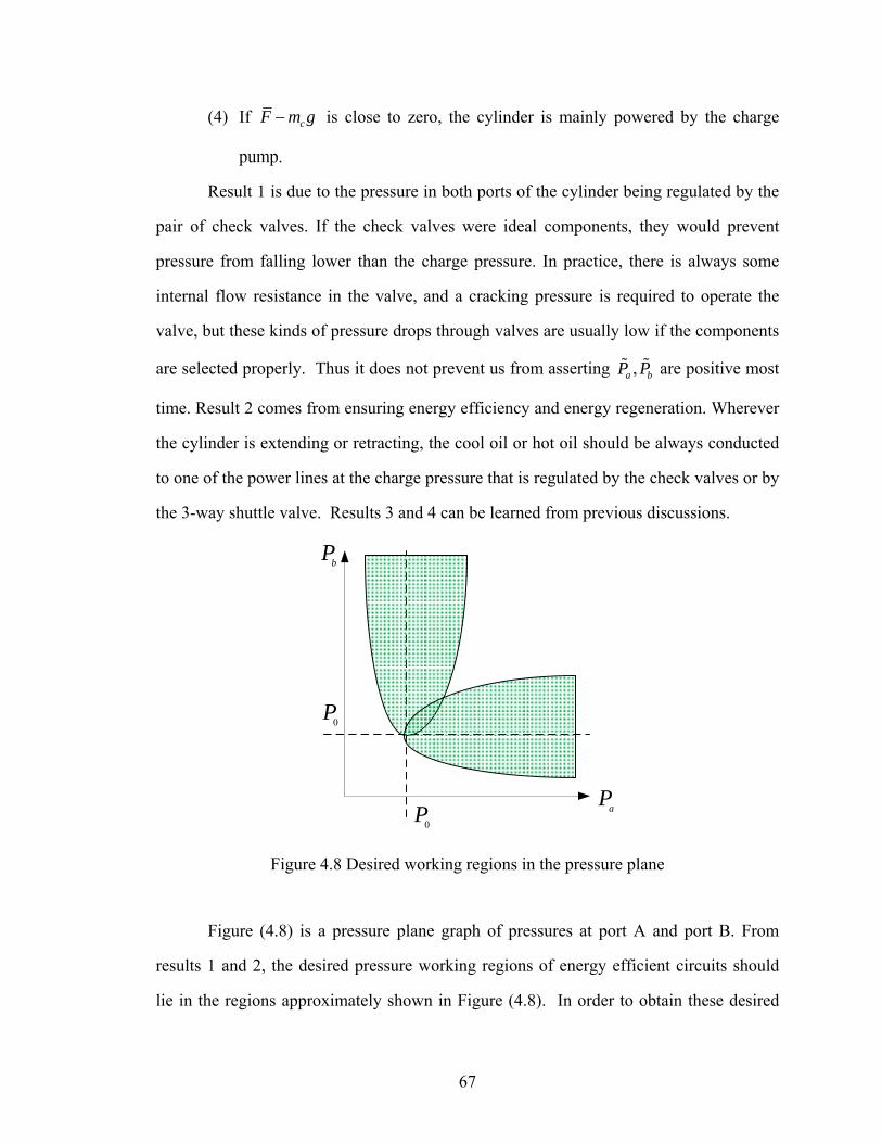
67
(4) If cF m g− is close to zero, the cylinder is mainly powered by the charge
pump.
Result 1 is due to the pressure in both ports of the cylinder being regulated by the
pair of check valves. If the check valves were ideal components, they would prevent
pressure from falling lower than the charge pressure. In practice, there is always some
internal flow resistance in the valve, and a cracking pressure is required to operate the
valve, but these kinds of pressure drops through valves are usually low if the components
are selected properly. Thus it does not prevent us from asserting ,a bP P are positive most
time. Result 2 comes from ensuring energy efficiency and energy regeneration. Wherever
the cylinder is extending or retracting, the cool oil or hot oil should be always conducted
to one of the power lines at the charge pressure that is regulated by the check valves or by
the 3-way shuttle valve. Results 3 and 4 can be learned from previous discussions.
0P
0P aP
bP
Figure 4.8 Desired working regions in the pressure plane
Figure (4.8) is a pressure plane graph of pressures at port A and port B. From
results 1 and 2, the desired pressure working regions of energy efficient circuits should
lie in the regions approximately shown in Figure (4.8). In order to obtain these desired

68
working regions, three kinds of circuit arrangements will be compared, consisting of: (a)
ideal pilot operated check valves; (b) common pilot operated check valves; and (c) the
proposed hydraulic circuit in this paper. Since the main focus of this section is to
compare stationary stability regions and cost, without loss of generality, the cracking
pressure of valves, which is usually determined by static valve springs, is assumed to be
zero; the valve dynamics are neglected.
Pressure plane discussion:
Figure (4.9) shows a circuit used for variable displacement controlled actuators
proposed by Rahmfeld, Ivantysynova [6, 76–80]. A pair of pilot operated check valves
has been implemented to balance differential flows. Pilot operated check valves (also
referred to as P.O. check valves), are check valves which can be opened by an external
pilot pressure. Thus, the P.O. check valves block flows in one direction, like standard
check valves, but can be released once an adequate pilot pressure is applied. Free flow is
allowed in the reverse direction.
A
BPb
Figure 4.9 A circuit using pilot operated check valves
There are two main types of P. O. check valves in popular use in industry. The
first such valve’s operation is triggered when 1 referenceP P> where referenceP usually is a

69
constant pressure independent of the valve itself. An example of this type is valve model
CKCV made by Sun Hydraulics Company. In another kind of P. O. check valve
operation is triggered when 1 3 2( / )P P Pα− > , where α is an area ratio of the valve core
and 3α = for most of these kinds of valves. An example is model CPH124P made by
the Parker Hannifin Corporation. The latter kind of valve has a larger market because it
has no external leakage. For convenience, the former kind is referred to as an ideal P.O.
valve and the latter kind is referred to as a common P. O. valve in this chapter.
The working regions for ideal P. O. valves are shown in Figure (4.10). Valve (A)
shown in Figure (4.9) operates in the cross hatched area 01{ | }a aI P P P= > , Valve (B)
shown in Figure (4.9) takes effect in cross hatched area 01{ | }b bII P P P= > . Both check
valves are closed in the area III I II= ∩ with constraints 0, 0a bP P≥ ≥ . As shown in
Figure (4.10), I II∩ is nonempty.
0P
0P 01P
01P
bP
aP
Figure 4.10 Working regions of ideal P.O. Valves

70
We claim: it is impossible for 01P to collapse to 0P where 0P is the charge
pressure of the circuit. Assume 01 0P P= (or 01 0P P≈ ), I II∩ then will cover most
working regions; this means that both ports of the cylinder are always connected to the
charge pump. Obviously, the circuit loses control or has extremely ineffective control.
This is a contradiction. Thus 01 0P P− should be greater than a specific bound. This also
leads to some problems. (1) Besides the charge pressure, the system needs another
reference pressure, thus the whole cost of the circuit will increase. (2) A high bound of
01 0P P− will decrease the circuit’s energy efficiency, but a low bound can not ensure the
system is controllable. (3) Region III is an internally unstable point because both ports of
the cylinder are blocked. The equilibrium point in this area dooms the system to be
unstable. From the above discussion, we conclude that using ideal P. O. valves is not a
good solution for single rod cylinder control circuits.
bP
aP0P
0P
Figure 4.11 Working regions of common P.O. valves
Figure (4.11) shows the working regions for common P. O. valves. Valve (A)
shown in Figure (4.9) operates in the cross hatched area 0{( , ) | / 3 }a b a bI P P P P P= − > ,
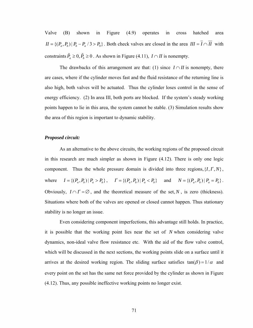
71
Valve (B) shown in Figure (4.9) operates in cross hatched area
0{( , ) | / 3 }a b b aII P P P P P= − > . Both check valves are closed in the area III I II= ∩ with
constraints 0, 0a bP P≥ ≥ . As shown in Figure (4.11), I II∩ is nonempty.
The drawbacks of this arrangement are that: (1) since I II∩ is nonempty, there
are cases, where if the cylinder moves fast and the fluid resistance of the returning line is
also high, both valves will be actuated. Thus the cylinder loses control in the sense of
energy efficiency. (2) In area III, both ports are blocked. If the system’s steady working
points happen to lie in this area, the system cannot be stable. (3) Simulation results show
the area of this region is important to dynamic stability.
Proposed circuit:
As an alternative to the above circuits, the working regions of the proposed circuit
in this research are much simpler as shown in Figure (4.12). There is only one logic
component. Thus the whole pressure domain is divided into three regions,{ , , }I I N′ ,
where {( , ) | }a b a bI P P P P= > , {( , ) | }a b a bI P P P P′ = < and {( , ) | }a b a bN P P P P= = .
Obviously, I I ′∩ = ∅ , and the theoretical measure of the set, N , is zero (thickness).
Situations where both of the valves are opened or closed cannot happen. Thus stationary
stability is no longer an issue.
Even considering component imperfections, this advantage still holds. In practice,
it is possible that the working point lies near the set of N when considering valve
dynamics, non-ideal valve flow resistance etc. With the aid of the flow valve control,
which will be discussed in the next sections, the working points slide on a surface until it
arrives at the desired working region. The sliding surface satisfies tan( ) 1/β α= and
every point on the set has the same net force provided by the cylinder as shown in Figure
(4.12). Thus, any possible ineffective working points no longer exist.

72
bP
aP0P
β
0P
Figure 4.12 Working regions of the shuttle valve
4.3 Dynamic Stability Analysis
The system as shown in Figure (4.1) involves load dynamics, valve dynamics,
variable displacement pump dynamics and fluid dynamics. The main purposes of this
section are to analyze when and how pressure oscillations are triggered by the circuit
itself and how to stabilize the circuit when oscillations occur. Thus the valve dynamics
are neglected, and the input to the circuit is assumed to be the pure flow rate supplied by
the pump. This approximation leads to a conservative conclusion, but the numerical
simulations are simplified because error accumulations are minimized in the
discontinuous system dynamics.
Experiments show that these pressure oscillations seldom occur while the cylinder
is extending. This will become clear at the end of this section, so the following analysis
focuses on the case in which the cylinder is retracting. For convenience, the state
variables are defined as 1 2 3( , , ) ( , , )T Ta bx x x x x P P= = . The positive directions are defined
that they make the cylinder retract. The simplified dynamics are described in Equation
(4.5) using definition Equation (4.4):

73
Vε β= (4.4)
1 3 2 1
22 1 2 3 2
33 1 3 2 3
[ ]
[ ]
on
on
mx Ax Ax bx mg Fxx Flow Ax Cx x xRxx Flow Ax Cx x xR
α
ε
ε α
= − − + +
= − + − − >
= − − − >
(4.5)
Where Flow is the fluid rate supplied by the variable displacement pump, m is the mass
consisting of the load and the rod of the cylinder, A is the area of cylinder defined
previously, α is the area ratio of the rod side to the cap side, b is the linear friction
coefficient, F is the total force excluding those explicitly expressed in the equations, C
is the fluid leakage coefficient and onR is the fluid resistance when the shuttle valve is
operated. Note that, theoretically, onR should be a nonlinear mapping relating the valve
core’s position and the differential pressure through the valve. In Equation (4.5), a first
order model is used to approximate the shuttle valve’s characteristics (to make this
approximation better, we have selected a large capacity rated valve). [cond] is a
conditional operator. The operator output is 1 when cond is true, otherwise, it is zero. β
is the bulk modulus of the fluid used, V is the volume of the fluid chamber which
includes two parts:
( )line cV V V t= + (4.6)
Where lineV refers to the volume of the fluid pipe line, ( )cV t refers to the volume
of the cylinder chamber, which is time varying (i.e. it depends on the position of the rod).
The rod side volume is different from the cap side volume because the cylinder is a single
rod type. Even though the cylinder volume is limited; the bulk modulus is very large. It
is reported that the effective bulk modulus of an average working fluid is at the level of
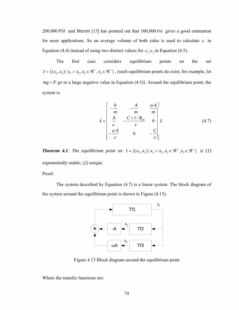
74
200,000 PSI and Merritt [13] has pointed out that 100,000 PSI gives a good estimation
for most applications. So an average volume of both sides is used to calculate ε in
Equation (4.4) instead of using two distinct values for 1 2,ε ε in Equation (4.5).
The first case considers equilibrium points on the set
2 3 3 2 2 3{( , ) | , , }I x x x x x x+ += > ∈ℜ ∈ℜ , (such equilibrium points do exist; for example, let
mg F+ go to a large negative value in Equation (4.5)). Around the equilibrium point, the
system is:
1/ 0
0
on
b A Am m m
C RAx x
A C
α
ε εαε ε
⎡ ⎤− −⎢ ⎥⎢ ⎥
+⎢ ⎥= −⎢ ⎥⎢ ⎥⎢ ⎥− −⎢ ⎥⎣ ⎦
(4.7)
Theorem 4.1: The equilibrium point on 2 3 3 2 2 3{( , ) | , , }I x x x x x x+ += > ∈ℜ ∈ℜ is (1)
exponentially stable; (2) unique.
Proof:
The system described by Equation (4.7) is a linear system. The block diagram of
the system around the equilibrium point is shown in Figure (4.13).
Tf1
Tf2
Tf3
-A
-αA
1x
2x
3x
Figure 4.13 Block diagram around the equilibrium point
Where the transfer functions are:
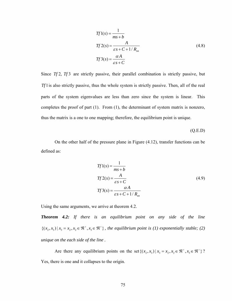
75
11( )
2( )1/
3( )
on
Tf sms b
ATf ss C R
ATf ss C
εα
ε
=+
=+ +
=+
(4.8)
Since 2, 3Tf Tf are strictly passive, their parallel combination is strictly passive, but
1Tf is also strictly passive, thus the whole system is strictly passive. Then, all of the real
parts of the system eigenvalues are less than zero since the system is linear. This
completes the proof of part (1). From (1), the determinant of system matrix is nonzero,
thus the matrix is a one to one mapping; therefore, the equilibrium point is unique.
(Q.E.D)
On the other half of the pressure plane in Figure (4.12), transfer functions can be
defined as:
11( )
2( )
3( )1/ on
Tf sms b
ATf ss C
ATf ss C R
εα
ε
=+
=+
=+ +
(4.9)
Using the same arguments, we arrive at theorem 4.2. Theorem 4.2: If there is an equilibrium point on any side of the line
2 3 3 2 2 3{( , ) | , , }x x x x x x+ += ∈ℜ ∈ℜ , the equilibrium point is (1) exponentially stable; (2)
unique on the each side of the line .
Are there any equilibrium points on the set 2 3 3 2 2 3{( , ) | , , }x x x x x x+ += ∈ℜ ∈ℜ ?
Yes, there is one and it collapses to the origin.

76
Theorem 4.3: there is only one equilibrium point if 2 3x x= and the equilibrium point is
stable.
Proof:
When pressures on the cylinder ports are equal, the shuttle valve lies in the center
position, onR → ∞ , the leakage of cylinder C is very small; thus from Eq. (5),
1 1
1
3 2
2 3
and 0
and 0
Ax Flow Flow Axx
Cx Flow Flow Cxx x
α≈ ≈⇒ ≈− = − − =⇒ = =
The stability can be proven using the previous passivity method.
(Q.E.D)
So far, we have examined the possible equilibrium points in the pressure plane.
The system described by Equation (4.5) is driven by the Flow and mg F+ terms. The
output is ( , , )Ta bvelocity P P . However, this does not necessarily mean that the mapping
from input to output is one to one. Actually, when at steady state and when 2 3x x− is
very small, it is possible that there are two equilibrium points corresponding to the same
input sets. One occurs under the pumping mode. Another occurs under the motoring
mode. The main reason for this comes from friction, which is proportional to the velocity.
Roughly speaking, the ratio of steady velocities at these two modes is α . The difference
of net forces caused by friction happens to move the equilibrium point from one side to
the other side. Notice this only happens when equilibrium points are near the origin of
the pressure plane. The energy dissipated or regenerated is very small compared with the
energy dissipated by the charge pump, so that any equilibrium point in which the system
will stay is acceptable.

77
These equilibrium points, which are near the origin, are trivial from an energy
viewpoint. Thus, we will focus on the stability of the equilibrium points lying farther
from the 2 3x x= line. Note that the exponential stability of the equilibrium points on
each side of the line does not necessarily leads to the stability of the system. The
discontinuity of the operator operation defined in Equation (4.5) can trigger the system’s
limit cycle even when the system has exponentially stable equilibrium points. One
observation is that, if 2 3,x x do not touch in the pressure working plane, then the three-
way-valve does not switch states. Thus there is no switching in Equation (4.5), and
because of the stability proven in Theorem 4.2, the pressures will go to a steady state.
This is the motivation of the stability strategy.
Theorem 4.4: if the control efforts ensure 2 3x x≠ after system enters the region where the
equilibrium point exists, the system in Equation (4.5) is stable.
Proof:
For any input set ( Flow , mg F+ ), the system has the properties:
1
2
3
FlowxAFlowx
CFlowx
C
α
μ
μ
≤
≤
≤
where μ is a positive constant. Thus the state space, x , for a bounded input is a compact
set. There are two cases to consider. The first is when the system does not enter a limit
cycle. The second is when the system enters a limit cycle.
If the system does not enter a limit cycle, then the system must go to some cluster
points. However, by Theorem 4.2, the equilibrium point is stable and unique; therefore,

78
the system will stay at the equilibrium point. Thus, the proof is done for the case of no
limit cycle.
Now suppose the system has limit cycle, we can find the upper bounds of
1 2 3, ,x x x because the limit cycle is an invariant set. We also know 2 3x x= at some time,
(otherwise, the system is stable). Without loss of generality, assume 2 1 3 1( ) ( )x t x t= ,
2 1 3 1( ) ( )x t x t+ > + at some time 1t , and there is an equilibrium point satisfying * *2 3x x> .
Because the control efforts ensure 2 3x x≠ using the assumption, the system will go to the
equilibrium point because of the stability of the equilibrium point by Theorem 4.2.
(Q.E.D)
From another viewpoint, the stability problem works like a zero input response
problem if a limit cycle occurs and we take the equilibrium point as the origin of the state
space. We know the worst initial states are bounded because the limit cycle is bounded.
To ensure 2 3x x≠ when 1t t> , 2 3x x− should decay fast enough to its steady state.
The system, described by Equation (4.5), is a linear time invariant system during
the time interval of consecutive time events when the system passes through the pressure
line 2 3x x= . Without loss of generality, the system can be described in Equation (4.10) in
the 2 3 3 2 2 3{( , ) | , , }x x x x x x+ +< ∈ℜ ∈ℜ
1 3 2 1
2 1 2
33 1 3
on
mx Ax Ax bxx Ax Cx
xx Ax CxR
αε
ε α
= − −= −
= − − −
(4.10)
Where 1 2 3( , , )Tx x x x= is defined with reference to the equilibrium point. Since ε is very
small, as discussed in previous sections, singular perturbation theory is applied. C , the
leakage coefficient, is very small, but onR is the flow resistance of the shuttle valve,

79
which is designed to be very small when the valve is operated (A large rated valve can be
chosen if necessary); thus the third equation of (4.10) achieves steady state in the two
time scales system by Result (3.1). Since 2 3,x x are bounded, the slow manifold satisfies:
3 1onx AR xα= − (4.11)
The reduced order system can be simplified to:
2 2
1 1 2
2 1 2
( )onmx A R b x Axx Ax Cx
αε
= − + −= −
(4.12)
The simplified system can be viewed as a feedback connection of two subsystems
described by the following transfer functions:
2 2( )on
As C
Ams b A R
ε
α
+
+ +
(4.13)
Thus, the characteristic equation of the simplified system can be derived as:
2 2 22 2 2 ( )( ) 0on
onC b A R AmCms b A R s αα
ε ε+ +
+ + + + = (4.14)
Since , C ε are very small, the second term is dominated by mCε in Equation (4.14),
and the third term is dominated by 2Aε . Thus the damping coefficient for the above the
second order system can be derived as:
2C mA
ξε
= (4.15)
As mentioned above, we are investigating the zero input response of the system;
thus the system zeros do not take effect. Equation (4.15) shows that the damping

80
coefficient will increase with the leakage coefficient C . This means the pressure will
decay faster by introducing a virtual leakage. This concept led to addition of the flow
control valves to the system as shown in Figure (4.1) to stabilize pressure oscillations.
The envelope of the pressure response will decay at the speed
2 2( )on
n
mCb A R tte eαξω ε
− + +− = (4.16)
Figure (4.14) is a simulation of the system described by Equation (4.15) by
varying leakage coefficients with the [cond] operator disabled in order to see when the
switching behavior occurs. The figure shows that when leakage increases to 3 times
larger than the original leakage, the system pressures are bounded in one side of the
pressure plane and go to steady state.
0 0.1 0.2 0.3 0.4 0.5-20
0
20
40
60
80
100
Seconds
Pres
sure
(PSI
)
1x2x3x
Figure 4.14 Response with varying leakage coefficient
The above analysis focuses on the case when the cylinder is retracting, but it is
also valid for the case when the cylinder is extending. In the extending case, the system
has a larger safety margin for pressure oscillation problems. This is reasonable because
one port’s pressure is lower than the charge pump pressure due to the internal flow

81
resistance of the check valve and the shuttle valve, while the other port’s pressure is
higher than the charge pump pressure. Therefore, the two pressures are not equal so there
is no switching in the system’s dynamics. The system goes to steady state because of the
stability of the equilibrium points.
Is the circuit still energy efficient? Two flow controlled valves, shown as (4a)
and (4b) in Figure (4.1), normally have no effect. They begin to work only when
pressure oscillations could possibly occur. From the discussion above, one can see that
the pressure oscillations occur when at a steady state * *2 3x x η− ≤ where η is some upper
bound which can be determined by experiments or through experience, for example,
20 PSI .
When the equivalent leakage has been increased; the system’s overall energetic
efficiency will be lowered at first glance. However, the change in overall efficiency is
unnoticeable. Firstly, * *2 3x x η− ≤ occurs only when the force exerted by the cylinder is
close to the critical mass force as defined in Equation (4.2). In practice, the force on the
cylinder from structural weight, such as boom structures of an excavator, is already much
greater than the critical mass. Even more, in normal working situations, the cylinder is
used to lift heavy loads or to pull some object requiring large forces. Thus, the
compensation algorithm is triggered only for a short interval of time compared to the
whole working period. Secondly, when the compensation is triggered, the dissipated
energy is bounded by lQη where lQ is the leakage flow. During this time, the energy
dissipated by the charge pump, which is constantly working, is 0 0P Q where 0Q is the
charge pump flow. But 0 0, lP Q Qη>> >> , thus the energy dissipated by the leakage
compensation can be neglected.
4.4 Compensation Algorithms for the Flow Control Valves

82
The compensation algorithms are implemented using the flow control valves
shown in Figure (4.1). There are at least two kinds of compensations in the circuit:
pressure oscillations, quotient group sliding; and an optional compensation for tracking
performance. Since the circuit has symmetry, the control efforts for the valve (4a) shown
in Figure (4.1) are the example for the following discussions; the control of valve (4b) is
just a mirrored algorithm, so it is omitted in this chapter.
The control signal for the flow control valve is defined as:
p s tu u u u= + + (4.17)
where pu refers to control efforts of compensation for pressure oscillations, su is the part
for forming quotient group sliding, tu is the part to improve the transient response of
trajectory tracking problems.
pu is the necessary part because the pressure oscillations inherently exist in the
circuit due to the circuit’s discontinuous switching. tu is an optional part. A large part of
tu ensures good tracking performance, but it also sacrifices part of the whole system’s
energy efficiency. If the application’s transient response is not critical or if the natural
transient response has already been satisfied, the tracking compensation can be set to
zero. Since there are always some imperfections on the valve’s dynamics and its flow
resistance, the system will, at times, be out of the desired working regions. su ensures
that the working point slides to the desired working region. Since this part never
sacrifices system energy efficiency, it is recommended to keep this compensation.
The inputs to the algorithm are pressures on the cylinder ports. Pressures are
detected by the pressure sensors whose bandwidth is required to be greater than the
pump’s bandwidth. Most commercial sensors in the market satisfy this requirement. In
the following, aP refers to the pressure detected on the power line which connects to the

83
cylinder port of the single rod cylinder, bP is the power line connected to the rod side of
the cylinder.
A low pass filter fτ with time constant τ is defined in transfer function form:
1( )1
f ssτ τ
=+
(4.18)
Let the operator ( ) :fτ ⋅ ℜ → ℜ mean a signal passing through the system fτ . The
mean values of two pressures are evaluated as:
1
1
( )( )
a a
b b
P f PP f P
τ
τ
=
= (4.19)
with a time constant 1τ , for example, 11 20τ π= second. The amplitude of the pressure
oscillations during a period of transient response is evaluated as:
2 ( )a a aP f P PτΔ = − (4.20)
where 2τ is a time constant.
The pressure oscillations occur when a bP P− is close to zero. We will turn on this
type of compensation when a bP P− falls below some bound, osP , then gradually turn it off
in order to maintain a safety margin. The pseudo code for the pressure oscillation
compensation is as follows:
If ( 2 )b a osP P P− >
0pu =
Elseif ( )b a osP P P− >
(2 )b ap
os
P Pu gain
P−
= × −

84
Else
pu gain=
Endif
where gain is a constant value corresponding to the flow valve’s percentage opening.
The pseudo code can be illustrated by Figure (4.15)
pu
gain
a bP P−2 osPosP
Figure 4.15 pu control signal
At least one of either aP or bP should be close to the charge pressure when the
circuit is in the desirable working condition. Abnormal situations occur when the shuttle
valve is not fully opened or the valve core has high frequency oscillations. The flow
control valve, in this case, will be fully opened to let the system find the desired
equivalent equilibrium point. Thus the compensation is described by:
If ( ( )b errorP P>
_su Full Open=
Else
0su =
Endif

85
where errorP is a bound of maximal pressure drop on the shuttle valve when the valve is
operated. _Full Open is a control voltage to fully open the flow control valve.
Pressure surges during tracking periods indicate that the acceleration of the
cylinder is not smooth (Notice that the pressure on other side of the cylinder is almost a
constant value). The compensation is proportional to the pressure oscillation’s envelope.
Thus the compensation is described as:
t au Pκ= Δ
where κ is a constant.
The main computation load for the entire algorithm is decided by four first-order
equations (these can be merged into 3 equations). Since the filter bandwidth is very low,
say, less than 5 Hz , most commercial DSPs or MCUs can complete this algorithm.
4.5 Discussions of the Proposed Circuit
In the proposed circuit, stabilization is implemented through hardware
components, a pair of flow controlled valves. As we will show in next chapter, one of
motivations for this solution is due to high frequency limit cycles such that the feedback
must be a hardware feedback path. However, this concept can be further applied to
software “virtual” feedback provided (1) the frequency of limit cycles is relative low, (2)
the bandwidth of the control efforts can be higher than the frequency of the limit cycle.
Figure (4.16) shows a boom function of an industrial backhoe, related parameters
are measured by Husco Intl and are depicted in the figure. In the following results, the
angle refers to the angle between the Tie Point and positive direction of x-axis, the
positive direction of the angle is defined to be counter clockwise. The charge pressure in
the simulation is 200 PSI.

86
Figure 4.16 Boom function parameters in a industrial backhoe (Courtesy of Husco)
It can be verified that limit cycle frequency is very low at the level of 0.5~ 1 Hz.
The bandwidth of the applied variable displacement pump is at the level of 10 Hz . In this
case, the physical feedback is not necessary because (1) the static pressure would
consume lots of energy; (2) the control can be implemented by pump control efforts.
The control law is:
( ' )virtualP Flow C P Ax CPε = − − − (4.21)
Here the control input is ' virtualFlow C P−
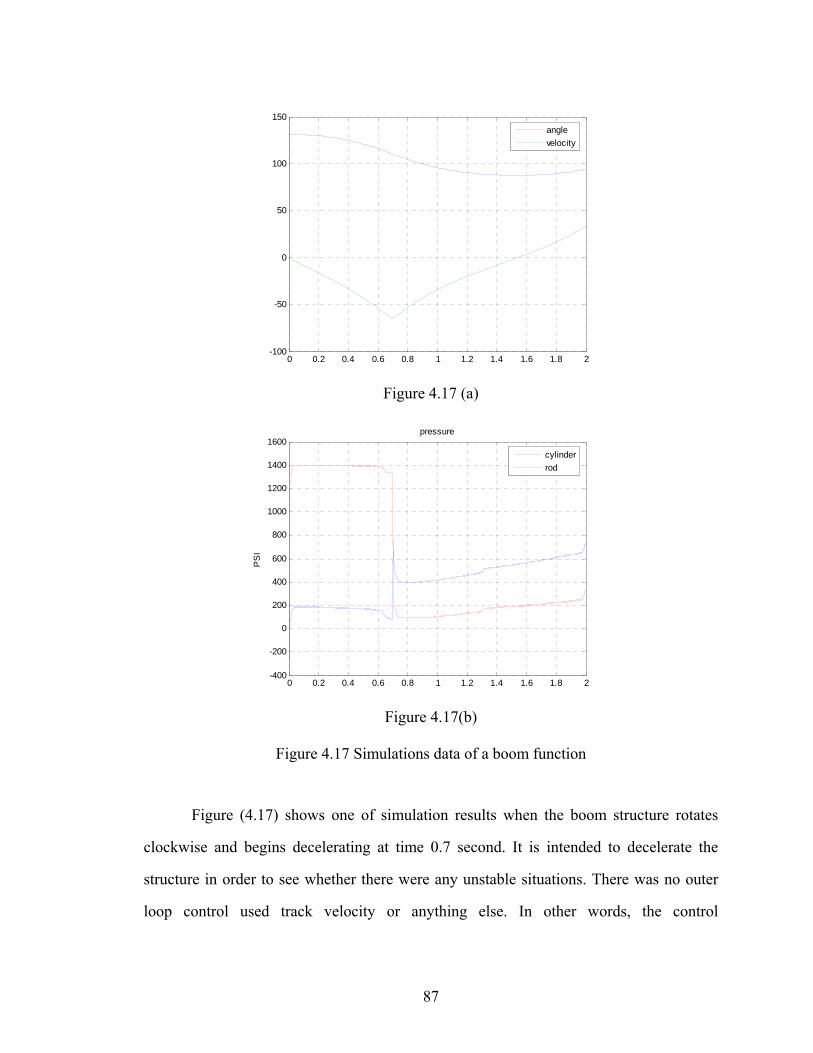
87
0 0.2 0.4 0.6 0.8 1 1.2 1.4 1.6 1.8 2-100
-50
0
50
100
150anglevelocity
Figure 4.17 (a)
0 0.2 0.4 0.6 0.8 1 1.2 1.4 1.6 1.8 2-400
-200
0
200
400
600
800
1000
1200
1400
1600
PS
I
pressure
cylinderrod
Figure 4.17(b)
Figure 4.17 Simulations data of a boom function
Figure (4.17) shows one of simulation results when the boom structure rotates
clockwise and begins decelerating at time 0.7 second. It is intended to decelerate the
structure in order to see whether there were any unstable situations. There was no outer
loop control used track velocity or anything else. In other words, the control

88
implementation is only some controlled virtual flow driven into the system. The results
show that the system/circuit remains stable.
Generally, the best control implementation method depends on pump response
time, load mass, hydraulic volumes, cost and reliabilities. A rough relationship is shown
in Figure (4.18). The curve used in the Figure (4.18) satisfies M constε = , where const is
a measure of the system’s natural frequency. In Figure (4.18) the term “Pump” stands for
the control effort can be implemented by the pump displacement, the term “valves”
stands for an implementation using some kinds of valves to give the system physical
leakages. If the system is very slow, the pump implementation is enough. This is shown
by the area above the curves. There is a region where it is only possible to control by
using valves control because the natural frequency is so much higher that the pump
control is not possible. (This is the case in the hardware testbed which will be discussed
in the next chapter). This situation is shown the area below the curves. The area between
two curves stands for situations where both kinds of controls are needed, i.e. the natural
frequency covers a large range, parts of which are out of pump response time.
Pump
Pump+Valves
Valves
M
ε
Figure 4.18 Feedback application regions
4.6 Summary

89
This chapter proposes a novel hydraulic circuit for a single rod cylinder controlled
by a variable displacement pump. The circuit arrangement not only gives the system high
energy efficiency, but also improves upon the internal instability of traditional circuits.
Stationary stability is illustrated by comparing traditional circuits with the proposed
circuit. The motivations, derivations and proofs of the system dynamical stabilities are
presented. Control algorithms including stability control and sliding to the desired
working region are presented. The concept is further extended to general cases.
Experimental and simulation results will be provided in the next chapter, and
results show that the circuit has good performance.

90
CHAPTER V
SIMULATION AND EXPERIMENTAL RESULTS OF THE
PROPOSED HYDRAULIC CIRCUIT
In the last chapter, a hydraulic circuit for single rod cylinders was presented. This
chapter documents a series of experiments undertaken to show the motivations and the
performance of the proposed circuit. The result consists of three main sections: (1) the
computer simulation results; (2) the experimental results without implementing the
proposed compensations; (3) the experimental results with the compensations
implemented.
The test-bed, based on the proposed hydraulic circuit, was built in the Intelligent
Machine Dynamics Lab at the Georgia Institute of Technology. The test-bed serves as a
hardware platform to verify the hydraulic circuit itself, and to verify the advanced
variable displacement pump control algorithm which will be discussed in detail in the
following chapters.
Energy efficiency improvement usually is evaluated by comparing with fuel
consumption when the same working routines are conducted, for example, a 3-minute
digging cycle is repeated 10 times by the same machine equipped with different circuits.
The focus of the research is to address some critical issues using displacement control
concept, and there are lots of experimental data and demonstrations using this
concept[81–84], thus the used metric for the energy improvement is: (1) whether the
hydraulic circuit can regenerate the energy and (2) whether the circuit is working
smoothly.
5.1 The Flow Control Circuit Test-bed
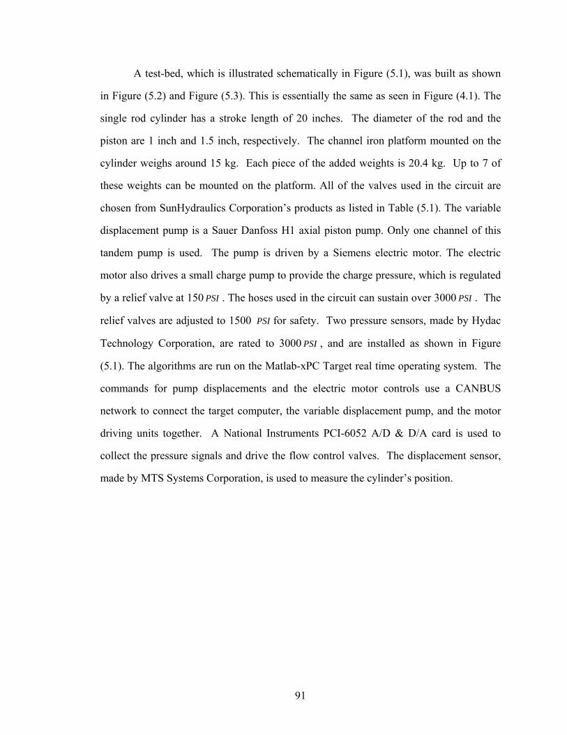
91
A test-bed, which is illustrated schematically in Figure (5.1), was built as shown
in Figure (5.2) and Figure (5.3). This is essentially the same as seen in Figure (4.1). The
single rod cylinder has a stroke length of 20 inches. The diameter of the rod and the
piston are 1 inch and 1.5 inch, respectively. The channel iron platform mounted on the
cylinder weighs around 15 kg. Each piece of the added weights is 20.4 kg. Up to 7 of
these weights can be mounted on the platform. All of the valves used in the circuit are
chosen from SunHydraulics Corporation’s products as listed in Table (5.1). The variable
displacement pump is a Sauer Danfoss H1 axial piston pump. Only one channel of this
tandem pump is used. The pump is driven by a Siemens electric motor. The electric
motor also drives a small charge pump to provide the charge pressure, which is regulated
by a relief valve at 150 PSI . The hoses used in the circuit can sustain over 3000 PSI . The
relief valves are adjusted to 1500 PSI for safety. Two pressure sensors, made by Hydac
Technology Corporation, are rated to 3000 PSI , and are installed as shown in Figure
(5.1). The algorithms are run on the Matlab-xPC Target real time operating system. The
commands for pump displacements and the electric motor controls use a CANBUS
network to connect the target computer, the variable displacement pump, and the motor
driving units together. A National Instruments PCI-6052 A/D & D/A card is used to
collect the pressure signals and drive the flow control valves. The displacement sensor,
made by MTS Systems Corporation, is used to measure the cylinder’s position.

92
Figure 5.1 Hydraulic Circuit for a single rod cylinder
Figure 5.2 Hydraulic lifter test-bed (Cylinder side)

93
Electrical MotorVariable Displacement PumpCharge Pump
Figure 5.3 Hydraulic lifter test-bed (Driver side)
Table 5.1 Main components used in the test-bed Component Manufacturer Model
Check Valve SunHydraulics CXFA Relief Valve SunHydraulics RDDA-LAN Shuttle Valve SunHydraulics DSGH
Flow Control Valve SunHydraulics RDDA Electric Motor Siemens 1PH7167
Variable Displacement Pump Sauer Danfoss H1-045 Tandem Displacement Sensor MTS RPRH
Pressure Sensor Hydac EDS-3478
The electrical motor is controlled by a Siemens Motor Controller consisting of a
rectifier, an inverter and an autotransformer, which is used to feedback regenerated
energy to power grids. All of these equipment produce a wideband, strong
electromagnetic interference on the measurement board. Figure (5.4) shows a
measurement result of a pressure sensor without applying a noise filter when the motor
was turned on at the 2 second mark and was turned off at 21 seconds (the pressure being
measured is constant), the unit of measurement is voltage.

94
0 5 10 15 20 25 30-10
-5
0
5
10Noisy Pressure
second
Inch
/Vol
t
Figure 5.4 Measurement noise without applying filters
It turns out that the interference enters the system not only through radiations but
also through the power grids. The following methods are applied to improve signal
quality.
(1) Shielding
(2) π -type filter with corner frequency set to 200 Hz
(3) Common mode filter at power supply line of instruments
(4) Common mode filter applied before π -type filter
The signal quality has been greatly improved as shown in Figure (5.5) which
illustrates the dynamic pressures on the rod side and the cylinder side of the single rod
cylinder.

95
0 5 10 15 20 25 30 35 40 450
50
100
150
200
250
300
350Pressure
Second
PSI
Figure 5.5 A dynamic pressure measurement
The algorithms presented in the previous chapter are implemented as an inner
control loop of the test-bed. A simple proportional control is designed to be the outer
control loop to track trajectories. The two loop design structure is due to the cylinder
length limitations and nonlinear friction characteristics during cylinder retraction and
extension; however, the inner loop and outer loop are independent of each other.
5.2 Numerical Simulations
To illustrate and solve pressure oscillation problems, a set of simulations were
developed. The parameters used by the code best approximated those used in the
hardware test-bed. Figure (5.6) shows a set of simulation results when the oscillations
have not occurred.

96
0 0.1 0.2 0.3 0.4 0.5 0.6 0.7 0.8 0.9 1100
200
300
400
500
600
700
Time(seconds)
Pre
ssur
e(P
SI)
Pressure
Cylinder sideRod side
(a)
0 0.1 0.2 0.3 0.4 0.5 0.6 0.7 0.8 0.9 1-0.5
-0.4
-0.3
-0.2
-0.1
0
0.1
0.2
Time(seconds)
Position/Velocity
PositionVelocity
(b)
Figure 5.6 (a) Pressures on the cylinder (b) the cylinder’s displacement and velocity
In Figure (5.6), during time interval,0 0.5t< < , the pump has a positive
displacement. That is the cylinder is extending. After that, the pump changes the sign of
the displacement so that the cylinder is retracting. Figure (5.6.a) shows pressures
changes with respect to time. The corresponding position and velocity information are
shown in Figure (5.6.b).

97
0 0.1 0.2 0.3 0.4 0.5 0.6 0.7 0.8 0.9 1100
200
300
400
500
600
700
Time(seconds)
Pre
ssur
e(P
SI)
Pressure
Cylinder sideRod side
(a)
0 0.1 0.2 0.3 0.4 0.5 0.6 0.7 0.8 0.9 1-0.4
-0.3
-0.2
-0.1
0
0.1
0.2
0.3
Time(seconds)
Position/Velocity
PositionVelocity
(b)
Figure 5.7 (a) Pressures on the cylinder (b) the cylinder’s displacement and velocity
Figure (5.7) shows a case when pressure oscillations occur. The same set of
parameters have been used as in the simulation as Figure (5.7) except the mass is changed
to be close to the critical mass as defined in the previous sections (Equation 4.2). Almost
no oscillation occurs during extending, but oscillations do occur while the cylinder is
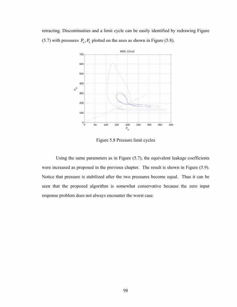
98
retracting. Discontinuities and a limit cycle can be easily identified by redrawing Figure
(5.7) with pressures ,a bP P plotted on the axes as shown in Figure (5.8).
0 50 100 150 200 250 300 350 4000
100
200
300
400
500
600
700
Pa
Pb
IMDL Circuit
Figure 5.8 Pressure limit cycles
Using the same parameters as in Figure (5.7), the equivalent leakage coefficients
were increased as proposed in the previous chapter. The result is shown in Figure (5.9).
Notice that pressure is stabilized after the two pressures become equal. Thus it can be
seen that the proposed algorithm is somewhat conservative because the zero input
response problem does not always encounter the worst case.
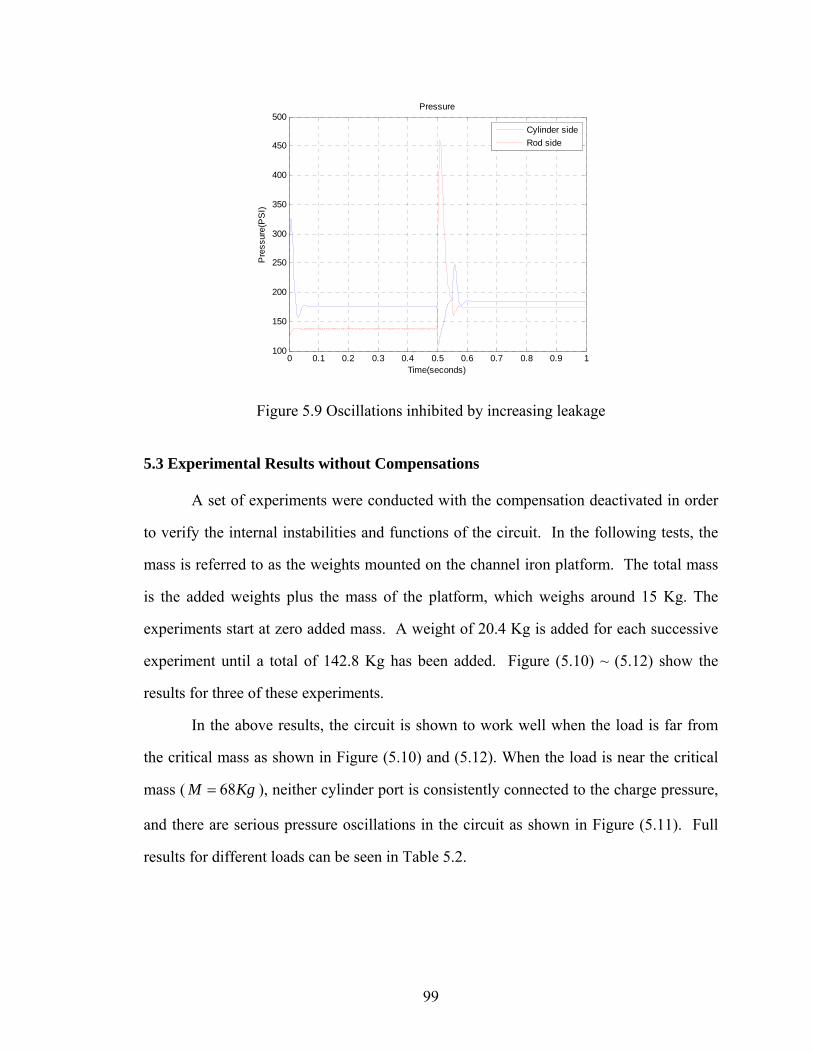
99
0 0.1 0.2 0.3 0.4 0.5 0.6 0.7 0.8 0.9 1100
150
200
250
300
350
400
450
500
Time(seconds)
Pre
ssur
e(P
SI)
Pressure
Cylinder sideRod side
Figure 5.9 Oscillations inhibited by increasing leakage
5.3 Experimental Results without Compensations
A set of experiments were conducted with the compensation deactivated in order
to verify the internal instabilities and functions of the circuit. In the following tests, the
mass is referred to as the weights mounted on the channel iron platform. The total mass
is the added weights plus the mass of the platform, which weighs around 15 Kg. The
experiments start at zero added mass. A weight of 20.4 Kg is added for each successive
experiment until a total of 142.8 Kg has been added. Figure (5.10) ~ (5.12) show the
results for three of these experiments.
In the above results, the circuit is shown to work well when the load is far from
the critical mass as shown in Figure (5.10) and (5.12). When the load is near the critical
mass ( 68M Kg= ), neither cylinder port is consistently connected to the charge pressure,
and there are serious pressure oscillations in the circuit as shown in Figure (5.11). Full
results for different loads can be seen in Table 5.2.

100
0 10 20 30 40 500
80
160
240
320
400
Time (seconds)
Pres
sure
(PSI
)
M=0 Kg
0 10 20 30 40 500
40
80
120
160
200
Posi
tion(
mm
)
Cylinder PressureRod PressurePosition
Figure 5.10 Experiment responses (M = 0 Kg)
0 10 20 30 40 50 600
80
160
240
320
400
Time (seconds)
Pres
sure
(PSI
)
M=61.2 Kg
0 10 20 30 40 50 600
40
80
120
160
200
Posi
tion(
mm
)
Cylinder PressureRod PressurePosition
Figure 5.11 Experiment responses (M = 61.2 Kg)

101
0 10 20 30 40 50 600
100
200
300
400
500
Time (seconds)
Pres
sure
(PSI
)
M=142.8 Kg
0 10 20 30 40 50 600
40
80
120
160
200
Posi
tion(
mm
)
Cylinder PressureRod PressurePosition
Figure 5.12 Experiment responses (M = 142.8 Kg)
Table 5.2 Experimental results without compensations
Mass( Kg) Pressure Oscillation Energetically efficient 0 No Yes
20.4 No Yes 40.8 Yes No 61.2 Yes No 81.6 Yes No 102 Yes No
122.4 No Yes 142.8 No Yes
The results show that the circuit is stable when the active force on the cylinder is
far from the critical mass. The circuit functions well if there are no pressure oscillations.
Otherwise, the performance is not acceptable either from an energy efficiency view or
system safety view because the test-bed makes noise and vibrations when this occurs.
A series of simulations at different loads also has been conducted to compare the
simulation results with experimental results. A simulation example is shown in Figure
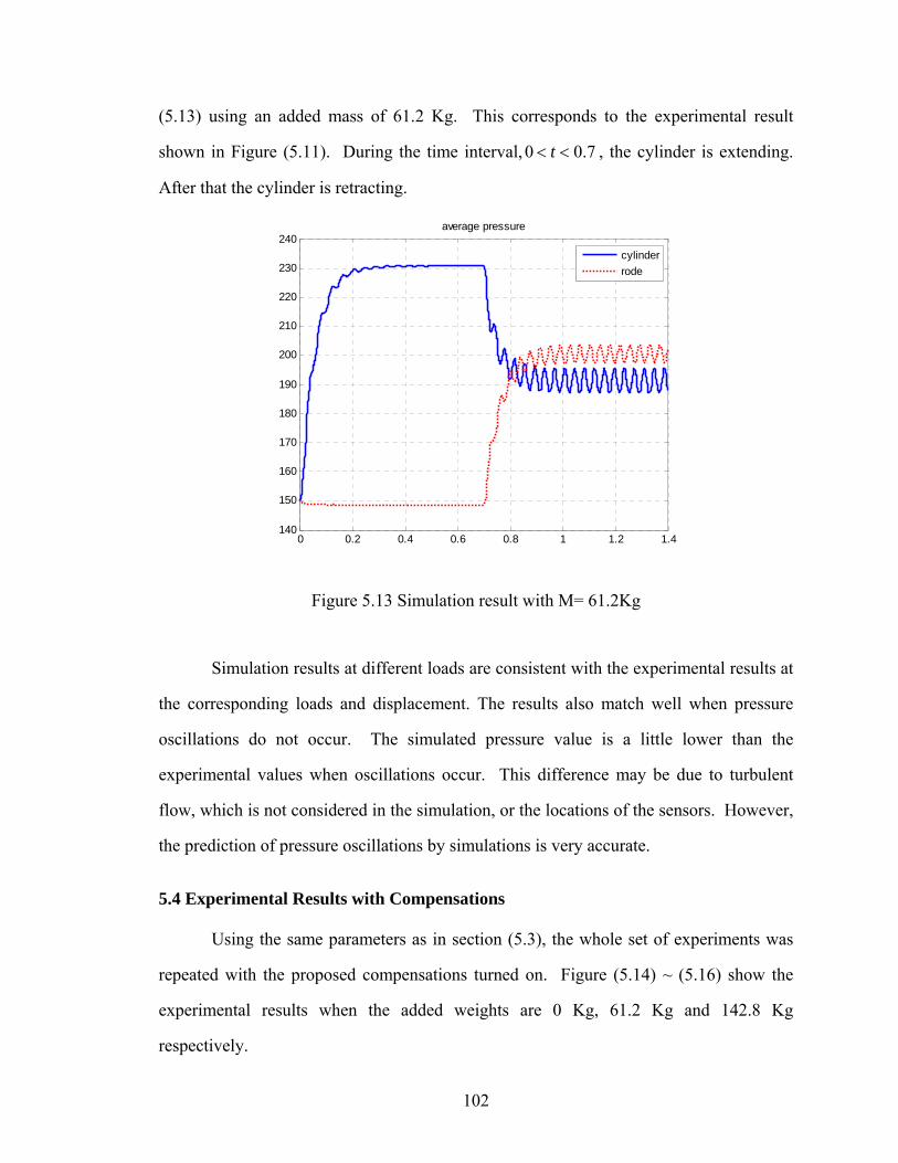
102
(5.13) using an added mass of 61.2 Kg. This corresponds to the experimental result
shown in Figure (5.11). During the time interval, 0 0.7t< < , the cylinder is extending.
After that the cylinder is retracting.
0 0.2 0.4 0.6 0.8 1 1.2 1.4140
150
160
170
180
190
200
210
220
230
240average pressure
cylinderrode
Figure 5.13 Simulation result with M= 61.2Kg
Simulation results at different loads are consistent with the experimental results at
the corresponding loads and displacement. The results also match well when pressure
oscillations do not occur. The simulated pressure value is a little lower than the
experimental values when oscillations occur. This difference may be due to turbulent
flow, which is not considered in the simulation, or the locations of the sensors. However,
the prediction of pressure oscillations by simulations is very accurate.
5.4 Experimental Results with Compensations
Using the same parameters as in section (5.3), the whole set of experiments was
repeated with the proposed compensations turned on. Figure (5.14) ~ (5.16) show the
experimental results when the added weights are 0 Kg, 61.2 Kg and 142.8 Kg
respectively.

103
0 20 40 60 80 1000
80
160
240
320
400
Time (sec)
Pres
sure
(PSI
)
M=0 Kg
0 20 40 60 80 1000
80
160
240
320
400
Posi
tion(
mm
, mm
/s)
Cylinder PressureRod PressurePositionVelocity
Figure 5.14 Experimental response with compensations (M = 0 Kg)
0 20 40 60 80 1000
80
160
240
320
400
Time (sec)
Pres
sure
(PSI
)
M=61.2 Kg
0 20 40 60 80 1000
80
160
240
320
400
Posi
tion(
mm
, mm
/s)
Cylinder Pressure
Rod PressurePosition
Velocity
Figure 5.15 Experimental response with compensations (M = 61.2 Kg)
Figure (5.14) shows the cylinder is working in pumping mode when it is
extending or retracting. This is normal because the load is so small that the pump only

104
needs to overcome some friction to move. It can be seen that one of ports is consistently
connected to the charge pressure. In Figure (5.16), a large load is added to the cylinder,
so the pump is under pumping mode when the load is lifted up, and is under motoring
mode when the cylinder is retracting because of the weight of the load. The cylinder port
on the rod side is always connected to the charge pressure.
0 10 20 30 40 50 60 70 80 900
100
200
300
400
500
Time (sec)
Pres
sure
(PSI
)
M=142.8 Kg
0 10 20 30 40 50 60 70 80 900
100
200
300
400
500
Posi
tion(
mm
, mm
/s)
Cylinder PressureRod PressurePositionVelocity
Figure 5.16 Experimental response with compensations (M = 142.8 Kg)
Things become critical when the load is close to the critical mass; the pump works
in pumping mode in both directions as shown in Figure (5.15). The pressure difference
when the cylinder is retracting is small (around 10 PSI ). Notice that the pressure
oscillation does not occur as seen in the simulations and the experiments with the
compensation turned off. A worse situation will occur if we add a small amount of
weight on the cylinder to more closely the critical mass. This is shown in Figure (5.17).
When the cylinder is retracting, pressures on both cylinder ports are exactly identical;
however, no oscillations were observed. The full set of results is listed in Table 2.

105
0 20 40 60 80 100 1200
80
160
240
320
400
Time (sec)
Pres
sure
(PSI
)
M=68.2 Kg
0 20 40 60 80 100 1200
80
160
240
320
400
Posi
tion(
mm
, mm
/s)
Cylinder PressureRod PressurePositionVelocity
Figure 5.17 Experimental response with compensations (M = 68.2 Kg)
Table 5.3 Experimental results with compensations
Mass( Kg) Pressure Oscillation Energetically efficient 0 No Yes
20.4 No Yes 40.8 No Yes 61.2 No Yes 68.2 No Yes 81.6 No Yes 102 No Yes
122.4 No Yes 142.8 No Yes
The results also show there are no “undesirable working region” phenomena.
One of the ports is always reliably connected to the charge pressure. The robustness of
the circuit also has been tested by varying trajectory profiles, force impulse on the
cylinder and by varying the charge pressure etc. In all cases, the circuit works well.
5.5 Conclusion

106
A hydraulic circuit needs to be operated in four quadrant modes in order to
recover energy from other function units. A reported problem for this kind of circuit is
pump oscillation under some circumstances. More explicitly, the pressures on the cap
side and rod side sometimes uncontrollably oscillate. Correspondingly, the cylinder
velocity oscillates and changes rapidly even though it is continuous because of mass
inertia of the load. The system has fast oscillations between pumping mode and motoring
mode. At this stage, the system loses controllability or is under weak controllability in the
sense of energy efficiency. Clearly, large oscillations of actuator pressure and velocity are
undesirable and may be dangerous. The loss of controllability or weak controllability is
unacceptable for industry applications.
This chapter presents simulation and experimental results of a proposed novel
flow control circuit which is suitable for single rod cylinders in variable controlled
displacement pump applications. The results show that (1) the circuit is energetically
efficient and works in all four quadrants; (2) Pressure oscillations have been effectively
eliminated.
The test-bed based on the proposed hydraulic circuit also serves as a hardware
platform to validate variable displacement control algorithms which will be discussed in
next chapters.

107
CHAPTER VI
ADAPTIVE ROBUST CONTROL OF VARIABLE DISPLACEMENT
PUMPS
Adaptive control is one of the main methods applied in hydraulic control to cope
with system uncertainties and time-varying parameters. Several approaches have been
used as discussed in the review section. These applied Lyapunov functions to prove the
stability of the system and to improve the parameters’ convergence. Most of the applied
parameter identification processes are driven by some kind of error signal. However, the
system stability and parameter convergence have not fully considered measurements that
suffer from noise. Many proposed algorithms are still under theoretical research, so they
are not easily applied to engineering practice. This chapter focuses a control approach
with consideration of measurement noise and parameter convergence rates.
In section 1, we investigate fundamental issues of an adaptive robot control
algorithm with unmatched disturbance. A method to design static gain is also presented.
Several concepts of parameter adaptation will be illustrated and compared in section 2.
The first version of the adaptive robust control algorithm is presented in section 3.
Improved algorithms are presented in sections 4 and 5. Section 6 describes the control
structure. The stabilities and performance for different control schemes will be shown in
the next chapter.
6.1 Adaptive Tracking Control
Consider first the dynamics of a rigid manipulator in the absence of friction and
other disturbances.
( ) ( , ) ( )M q q C q q q G q τ+ + = (6.1)

108
Where q is the 1nR × vector of joint displacements, τ is the 1nR × vector of applied virtual
torques. ( ) n nM q R ×∈ is the inertia matrix, ( , )C q q q and ( )G q are all 1nR × vectors
corresponding to Coriolis, centripetal torques and gravitational torques.
Several properties about Equation (6.1) are given as follows [160, 161].
Property:
P1: The inertial matrix ( )M q is symmetric and there exist positive scalars
1 2,α α such that 1 2( )n n n nI M q Iα α× ×≤ ≤ .
P2: ( ) ( , ) ( , )TM q C q q C q q− − is a skew matrix such that ( ) 0T Ts M C C s− − =
for all 1ns R ×∈ .
P3: the dynamics illustrated by Equation (6.1) is linear in terms of a suitably
selected set of robot and load parameters. That means
( ) ( , ) ( ) ( , , )M q q C q q q G q Y q q q θ+ + =
Where ( , , ) n pY q q q R ×∈ , 1pRθ ×∈ which is a parameter vector.
Let ndq R∈ be a smooth enough desired tracking trajectory. Define tracking
error de q q= − .
Define ancillary symbols s and v by a positive diagonal matrixλ :
( ( ))
( )d d
d d
s e e q q q qv q q q
λ λλ
= + = − − −= − −
(6.2)
ˆ ˆˆ , ,M C G are estimations of parameters in Equation (6.1). By property P3, we have an
estimated parameter vector θ which satisfies:
ˆˆ ˆˆ ( ) ( , ) ( ) ( , , , )M q v C q q v G q Y q q v v θ+ + = (6.3)
For convenience, we denote the true parameter vector as *θ :
109
*( ) ( , ) ( ) ( , , , )M q v C q q v G q Y q q v v θ+ + =
Define the control law and the adaptation law with positive diagonal matrices k and Γ :
ˆ( , , , )Y q q v v ksτ θ= − (6.4)
ˆ ( , , , )TY q q v v sθ = −Γ (6.5)
Then, the following conclusion can be drawn [160]. ( The proofs can be found therein)
CONCLUSION 6.1 The system described by Equation (6.1) has global tracking
convergence with the control laws described by Equation (6.4) and (6.5).
The control law (6.4), (6.5) is a classical in the control domain. Many versions of
its proof also can be found in related literatures. The algorithm can ensure that the
estimated parameters converge to the true ones if the system is persistently excited. Using
the same idea, the algorithm can also be extended to other versions, which deal with
matched disturbance.
It is clear that both the tracking error and the estimation process are driven by the
filtered parameter estimation error. However, the measurement noise and unmatched
disturbance are unavoidable and present studies do not fully investigate these issues.
Reconsider system dynamics Equation (6.1) with control law equations (6.4) and (6.5)
while including noise measurements and mismatched disturbance. Then the system
tracking dynamics can be derived as:
( , , , ) ( ) ( )Ms Cs ks Y q q v v n t f tθ+ + = + + (6.6)
Where ( )n t is measurement noise, ( )f t is unmatched disturbance and θ is
parameter estimation error. We denote a new variable, nw R∈ , for convenience and
without losing generality:
( , , , ) ( ) ( )w Y q q v v n t f tθ= + + (6.7)

110
From (6.6), (6.7), the tracking dynamics is described as,
Ms Cs ks w+ + = (6.8)
THEOREM 6.1: The system described in Equation (6.8) is output strictly passive with
input as w and output as s .
Proof:
Let 12
TV s Ms= , with property P1, 0V > .
By properties P2 and P3, T TV s ks s w= − + .
Thus:
( )
T T T T
T
s w s w s ks s ksV s ks
≥ − +
= +
That completes the proof.
(Q.E.D)
COROLLARY 6.1: The system described in Equation (6.8) is finite-gain 2L stable.
Proof: continuing with the proof of Theorem 6.1, one has:
1 1
1 1/2 1/2 1/2 1/2
1
1 12 21 1 1 = ( ) ( )2 2 21 1 2 2
T T T T
T T T
T T
V w k w w k w s w s ks
w k w k w k s k w k s s ks
w k w s ks
− −
− − −
−
≤ − + −
− − − −
≤ −
Integrating both sides over [0, ]τ and using ( ) 0V s > , one has:
2 22 (0)
L Ls w Vτ τδ δ≤ +
Where 1kδ −= .
(Q.E.D)

111
Theorem (6.1) and Corollary (6.1) show that, whether there is measurement noise
entering the system, or the parameter estimation is biased, the tracking error has
properties such that a bounded disturbance has a bounded tracking error. In other words,
system stability is maintained.
Intuitively, feedback control systems always show some robustness when
suffering from some disturbances. We will prove that a system can have guaranteed
transient response by designing a parameter, k , for the above adaptive control approach.
THEOREM 6.2: With some * 0k > such that * 14
k k= + , if the dynamics in Equation
(6.8) has bounded disturbance such that 2w h≤ , the tracking process has a
guaranteed error response.
Proof:
Let 12
TV s Ms= , with property P1, 0V > .
By properties P2 and P3,
*
*
1 1 ( ) ( )2 2
T T
T T T
T T
T
V s ks s w
s k s s w s w w w
s k s w wV w wβ
= − +
= − − − − +
≤ − +
≤ − +
Where*
min
max
( )( )kM
λβλ
= , β exists because of property 1 and the existence of *k , which is a
design variable. Therefore, it has:
2
0
( ) (0) ( )
(0) (1 )
tt
t t
V t e V e w t d
he V e
β βτ
β β
τ τ
β
− −
− −
≤ + −
≤ + −
∫

112
Since 2
2min ( )
VsMλ
≤ by property P1, and the dynamic tracking error is bounded by
se
λ≤ from Equation (6.2), we have
22
min
1( ) ( (0) (1 ))( )
t the t e V eM
β β
βλ λ− −≤ + − (6.7)
Therefore, the proof is completed.
(Q.E.D)
Remark: The dominant part of the system response is bounded by the hβ
term since other
terms exponentially decay. Thus, the tracking performance can be predetermined by
some prior knowledge of the disturbance level. By designing k as proposed above, the
system response is guaranteed.
6.2 Parameter Adaptation Algorithm
In control and signal processing, a model of a dynamic system is a mathematical
description of the relationship between inputs and outputs of the system. For the purpose
of identification, a convenient way to obtain a parameterized description of the system is
to let the model be a predictor of future outputs of the system [9].
ˆ( | )y t θ (6.8)
Where θ is a parameter vector. For the linear system, the prediction is a linear
regression,
ˆ( | ) ( )Ty t tθ θ ϕ= (6.9)

113
Where, ( )tϕ is a vector of input and output data. System identification deals with the
problem of finding the parameter vector that gives the best estimation of the dynamic
system under consideration. For example, we may wish to find the parameter vector that
minimized the criteria:
2ˆ( ) ( ( ) ( ))V E y t y tθ = − (6.10)
Under such criteria, one way to obtain the optimized parameters is to solve
Wiener-Hopf equations if the statistics of the underlying signals are available. The
solution satisfies
*( ) ( )T TE E yϕϕ θ ϕ= (6.11)
The most common way to find the solution is by using a searching method. The
Steepest Descent Method is one of these; it uses statistical information among inputs and
outputs. This method will not work if prior statistical information is unavailable. This
problem is commonly seen in control literature. To overcome this barrier, the Least Mean
Square (LMS) emerges as a simple and yet effective algorithm. The main difference
between the steepest Descent Method and LMS is that LMS uses an instantaneous
measurement to approximate the current stochastic gradient. Besides the issue of the
search step size, the algorithm suffers from noisy measurements. Figure (6.1) shows a
two-parameter adaptation path by using the LMS algorithm; as shown in the figure, the
adaptive parameters do not converge to the true ones due to measurement noise.
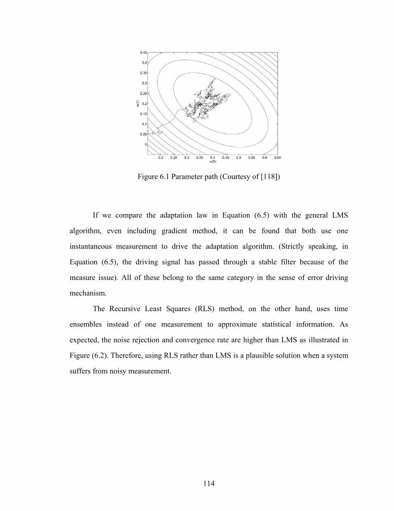
114
Figure 6.1 Parameter path (Courtesy of [118])
If we compare the adaptation law in Equation (6.5) with the general LMS
algorithm, even including gradient method, it can be found that both use one
instantaneous measurement to drive the adaptation algorithm. (Strictly speaking, in
Equation (6.5), the driving signal has passed through a stable filter because of the
measure issue). All of these belong to the same category in the sense of error driving
mechanism.
The Recursive Least Squares (RLS) method, on the other hand, uses time
ensembles instead of one measurement to approximate statistical information. As
expected, the noise rejection and convergence rate are higher than LMS as illustrated in
Figure (6.2). Therefore, using RLS rather than LMS is a plausible solution when a system
suffers from noisy measurement.

115
Figure 6.2 Ensemble-average leaning curves for LMS and RLS (Courtesy of [118])
6.3 Adaptive Control with Recursive Least Squares
As discussed in the previous section, poor convergence rate and noise rejection
motivated the use of Recursive Least Squares in order to improve tracking performance.
The first step in developing parameter estimation algorithms is to find the form of the
predicted output. For the sake of discussions, we are temporally assuming that all
derivative signals of inputs and outputs are available.
Figure 6.3 Indirect adaptive control
We prefer the indirect adaptive control approach as illustrated in Figure (6.3)
because it brings extra benefits that will be explored in the next sections. Given a plant,
the measured torques, displacements, velocities and accelerations satisfy:

116
( ) ( , ) ( )M q q C q q q G q τ+ + = (6.12)
Replacing the parameters in Equation (6.12) with estimated ones, there will be an error
( )tε .
ˆ ˆˆ ( ) ( , ) ( ) ( )M q q C q q q G q tτ ε+ + − = (6.13)
Therefore, the “desired” torques and real torques applied to the robot have a differenceε .
The recursive algorithm will minimize the cost function as follows.
0
( ) min ( ) ( )t
TJ dθ ε τ ε τ τ= ∫ (6.14)
Where ( )tθ includes all undetermined parameters describing Equation (6.13). By
property P3, a linear regression can be expressed as,
ˆ( , , ) ( ) ( )Tq q q t tϕ θ τ ε− = (6.15)
The first version of the proposed algorithm is as follows: define a control law with
a positive diagonal matrix k , which can be designed as shown in Theorem (6.2), to ensure
a guaranteed response under some disturbances:
ˆ ˆˆ ( ) ( , ) ( )M q v C q q v G q ksτ = + + − (6.16)
And define the parameter adaptation law:
ˆ
T
PP P Pθ ϕε
ϕϕ
=
= − (6.17)
The first three terms in Equation (6.16) correspond to computed torque
compensations of inertial, Coriolis, centripetal and gravitational torques by using
estimated parameters. The fourth term actually is a PD controller,

117
( )
: d
ks k e ee x x
λ− = − += −
Where , dx x correspondingly are plant’s trajectory and desired trajectory. The robot
dynamics is a second order system; therefore, with big enough proportional part k and a
zero at λ− , the closed loop plant will be stable, i.e., the states of the system are bounded.
THEOREM 6.3: If the closed loop system states with control laws described by Equation
(6.12), (6.13), (6.16), (6.17) is bounded, then ε converges to zero. Furthermore, if ϕ is
persistently exciting, the parameter error converges to zero.
Proof:
1 ( )T TV P tr PPθ θ−= +
It can be derived:
TV ε ε≤ −
By definition, 0V > therefore, 0ε → by Barbalat’s lemma. If the signal rich enough, the
covariance matrix will be excited in every eigenvector direction, so that θ converges to
the true one.
Then, the closed loop dynamics will be:
0Ms Cs ks+ + =
By Theorem 6.1 with 0w = , the tracking error converges to zero.
(Q.E.D)
The algorithm shows some good properties:
(1) It has a guaranteed response for unmatched uncertainty by theorem 2.
(2) It has a good convergence rate and noise rejection as discussed in section 3.
(3) The algorithm is highly efficient for real time control. This will be shown in
the next section.

118
6.4 Improved Algorithm I
In section 6.3, the proposed algorithm includes a continuous RLS as an adaptation
process, which has been exploited in some control literature, for example [160]. The
following will increase the computational efficiency and algorithm stability. Consider a
special RLS algorithm,
0
( ) min ( ) ( )t
TJ W dθ ε τ ε τ τ= ∫
With adequately selected sampling time T , the weighting matrix W is defined as:
[..., ( ), (( 1) ), (( 2) ),...]W diag nT n T n Tδ δ δ= + +
Where the Dirac delta function ( )tδ is a sampling signal. Now, the cost function actually
is:
0
( ) ( )N
T
nJ nT nTε ε
=
= ∑ (6.18)
This changes a continuous RLS algorithm to a discrete RLS algorithm,
correspondingly, the forgetting factor can be also added. The benefit is that the discrete
RLS is much more efficient than the one described in Equation (6.17) considering
continuous integral needs a smaller step size; thus, it is more suitable for engineering
practice.
The discrete RLS algorithm is as follows:
Initialize the algorithm with a small positiveδ by setting
1(0)P Iδ −=
*ˆ ˆ(0)θ θ=
Loop ( 1..n N= )

119
1
1
1 1
( 1) ( )( )1 ( ) ( 1) ( )
ˆ( ) ( ) ( 1) ( )ˆ ˆ( ) ( 1) ( ) ( )( ) ( 1) ( ) ( ) ( 1)
T
T
T
P n nk nn P n n
n n n n
n n k n nP n P n k n n P n
λ ϕλ ϕ ϕ
ξ τ θ ϕ
θ θ ξ
λ λ ϕ
−
−
− −
−=
+ −
= − −
= − +
= − − −
Loop ends
However, this algorithm still has some critical issues for engineering practice.
During computation, round-off errors arise such that ( )P n , the error covariance matrix, is
not positive definite and symmetrical. A better solution for this issue is to propagate only
half the elements in ( )P n . The algorithm is commonly recognized as QR-RLS or square-
root algorithm [124]. The square-root factor of a positive definite matrix is defined by a
matrix n nA R ×∈ such that,
TP AA= (6.19)
Fact 1. For 0P > , if matrix A is triangular with positive diagonal entries satisfying
Equation (6.19), then that matrix is unique.
Fact 2. n mA R ×∈ , n mB R ×∈ , n m< . T TAA BB= , if and only if there exists a unitary
matrix Θ such that B A= Θ . (Proofs can be found in [124])
Using the square-root algorithm, the nonnegative definite character of the
covariance matrix is preserved by virtue of the fact that the product of any square matrix
and its transpose is always a nonnegative definite matrix.
More details about square root theory can be found in signal processing literature.
For our purposes, we would like to choose the Extended QR-RLS algorithm for its high
efficiency. The key idea is to find a unitary transformation matrix Θ to make the matrix
lower triangular, which consists of all information needed to form the next prediction.
120
12
1 1 12 2 2
1 1 12 2 2
1 ( ) ( 1) ( ) 0( )
0 ( 1) ( ) ( ) ( )
n P n nn
P n g n i P n
λ ϕ γ
λ γ
− −
− −
⎡ ⎤ ⎡ ⎤−⎢ ⎥ ⎢ ⎥Θ =⎢ ⎥ ⎢ ⎥
⎢ ⎥ ⎢ ⎥−⎣ ⎦ ⎣ ⎦
Then, the updated estimation is:
11/2 12ˆ ˆ ˆ( ) ( 1) [ ( ) ( )][ ( )] ( ( ) ( 1) ( ))Tn n g n r n n n n nθ θ γ τ θ ϕ
−− −= − + − − (6.20)
One way to achieve this transformation is to employ a so-called Householder
reflection. The n-th transformation matrix can be written as:
( ) 2T
T
g gn Igg
Θ = − (6.21)
Where g is a vector in the form of [1,0,0,...0] . Every iteration of n , the ( )nΘ will
transform an entry row of the sub-matrix to zeros. The processes are repeated until the
whole matrix is low triangular. The benefit of the transformation is its efficiency; the
explicit form of the transformation matrix is not needed. Instead, all of the calculations
are vector multiplications. Each time, the calculation only includes a smaller sub-matrix.
How to sample the measurement is another issue for controller implementations.
There are two ways to approach this problem: (1) In the continuous domain,
measurements or estimations of acceleration ,q q can be obtained by filtering both sides
of Equation (6.12) through a strictly stable and proper linear filter whose bandwidth is
higher than those of the signals. (2) We are taking advantage of the discrete model of the
system because the RLS algorithm is based on the discrete model such that ,q q
measurements can be avoided.
Both approaches have further problems. In method (1), the controller, actually,
consists of discrete time variables and continuous time variables, thus there is problem
with how to mix discrete time and continuous time control together. In method (2), there

121
is an unstable zeros problem if the controller is requested to track some trajectories.
These problems will be further explained in the next chapter.
6.5 Improved Algorithm II
In addition to numerical stability and efficiency, how well the adaptive scheme
performs in the presence of plant model uncertainties and bounded disturbances are
serious concerns. It was shown that an adaptive scheme designed for a disturbance free
plant model may go unstable in the presence of small disturbances. The instability
phenomena in adaptive systems includes parameter drift, high gain instability, instability
resulting from fast adaptation and so on.
Since the Recursive Least Squares method is used, it is more convenient to use
the Z-transform to describe a plant. Consider a plant with input ( )u t and output ( )y t :
1
11
0 1
( ) 1
( ) (1 )
nn
d mn
A z a z a z
B z b z a z a z
− −
− − −
= + +
= + +
The modeled error ( )tη and bounded dynamics ( )tδ can be expressed as:
1 1( ) ( ) ( ) ( ) ( ) ( )A z y k B z u k k kη δ− −= + + (6.22)
It is reported that[162, 163]: there exist (0,1),u Rσ +∈ ∈ such that:
( ) ( 1) ( 1) ( 1)( ) ( )
m k m k u k y kk um k
ση
= − + − + −
≤ (6.23)
A relatively bounded modeling error is not guaranteed to be bounded unless the plant
input and output sequences are bounded. However, the modeling error should be very
small, e.g. u is less than a small value, otherwise, the modeling 1 1( ), ( )A z B z− − in
Equation (6.22) is not a good model.
122
Dead Zone for bounded disturbance
In some cases, system inputs and outputs are bounded because of the physical
limitations of a plant, system outputs and control efforts. Thus it is a reasonable
assumption that modeling errors are bounded, therefore:
( ) ( )k k Rη δ ++ ≤ Δ ∈ (6.24)
In the following, the Dead Zone method will be applied for improving robustness
of Recursive Least Squares.
ˆ( 1) ( 1) ( 1)( ( ) ( 1) ( 1))ˆ ˆ( ) ( 1)1 ( 1) ( 1) ( 1)
T
T
a n P n n y n n nn nn P n nϕ ϕ θθ θ
ϕ ϕ− − − − − −
= − ++ − − −
( 1) ( 1) ( 1) ( 1) ( 1)( ) ( 1)1 ( 1) ( 1) ( 1)
T
T
a n P n n n P nP n P nn P n n
ϕ ϕϕ ϕ
− − − − −= − −
+ − − − (6.25)
With ˆ(0)θ given and 0(0) (0)TP P P= =
2
2ˆ( ) ( 1) ( 1)
1 if ( 1) 1 ( 1) ( 1) ( 1)0 otherwise
T
T
y n n na n n P n n
ϕ θ
ϕ ϕ
⎧ − − −⎪⎪ > Δ− = ⎨ + − − −⎪⎪⎩
(6.26)
Lemma 6.1 The Recursive Least Square with Dead Zone as in (6.25) and (6.26) has the
property: 2
2( )lim sup1 ( 1) ( 1) ( 1)Tn
e nn P n nϕ ϕ→∞
≤ Δ+ − − −
.
The proof of Lemma 6.1 can be found in [112]. In the proof, it is not necessary
that { ( )}nϕ is bounded because inputs and outputs are automatically normalized;
however, if sequence { ( )}nϕ is bounded, then the limit of ( )e t is bounded.
Lemma 6.2 The Recursive Least Square with Dead Zone can be combined with the
proposed Square Root algorithm.

123
Lemma 6.2 is an obvious result from the Equations (6.25) and (6.26). Note that
( 1)a n − is just a switch signal to decide whether ( ), ( )P n nθ need to be updated, there is
nothing that affects the square root algorithm itself at all.
Relative Dead Zone for Varying Disturbance
Not all plants can assume that the disturbance is bounded. Un-modeled dynamics
usually are related with the system states, system inputs and other factors. The following
assumption is made on the un-modeled dynamics of a plant: the un-modeled error ( )kη is
the sum of a bounded term, plus a term related to the input by a strictly proper
exponentially stable transfer function [162]. With this assumption, it was showed that
[162] :
There exist constants 0 (0,1)σ ∈ , 0 0ε > , 0ε > and a constant vector v such that:
0( ) ( )k kη ερ ε≤ + (6.27)
Where 0( ) sup{ },0T k ik v x i kρ σ −= < ≤ , x is a vector containing past inputs and outputs.
Define relative dead zone and its function:
0( ) ( ( ) )m k kβ ερ ε= + (6.28)
; if e>g
( , ) 0; if ; if e<-g
e gf g e e g
e g
−⎧⎪= <⎨⎪ +⎩
(6.29)
Where 1β ≥ . The relative dead zone RLS is as following:
ˆ( ) ( ) ( ) ( 1)Te n y n n nϕ θ= − −
( ) ( 1) ( ) ( )ˆ ˆ( ) ( 1)1 ( ) ( ) ( 1) ( )T
n P n n e nn nn n P n n
λ ϕθ θλ ϕ ϕ
−= − +
+ −

124
( ) ( 1) ( ) ( ) ( 1)( ) ( 1)1 ( ) ( ) ( 1) ( )
T
T
n P n n n P nP n P nn n P n n
λ ϕ ϕλ ϕ ϕ
− −= − −
+ − (6.30)
( 1 ( ), ( ))( )1 ( ) ( 1) ( ) ( )T
f m n e nnn P n n e n
α αλϕ ϕ
+=
+ − (if ( ) 0e n ≠ )
( ) 0nλ = ; (if ( ) 0e n = )
Where (0,1)α ∈ .
Lemma 6.3 The Recursive Least Square with Relative Dead Zone as in (6.29) and (6.30)
has following properties:
(1) ( )kθ is bounded;
(2) 2 ( 1 ( ), ( )) 0
1 ( ) ( 1) ( )T
f m k e kk P k k
αϕ ϕ
+→
+ − as k → ∞ ;
(3) ( ) ( 1) 0k kθ θ− − → as k → ∞
Proofs of Lemma 6.3 can be found in [163, 164].
Lemma 6.4 The Recursive Least Square with Relative Dead Zone can be combined with
the proposed Square Root algorithm.
The lemma 6.4 is proven and shown as follows:
If ( 1) 0nλ − = , ( ), ( )n P nθ are not updated, otherwise,
Let ( ) ( ) ( )n n nϕ λ ϕ′ =
( ) ( 1) ( )y n n y nλ′ = −
Form the pre-array and post-array matrix and unitary matrix
1/21
1/21
010
Ti i
ii
xPy ZP
ϕ −
−
′⎡ ⎤ ⎡ ⎤Θ =⎢ ⎥ ⎢ ⎥
⎣ ⎦⎣ ⎦ (6.31)

125
Thus, the following hold:
211 T
i ix Pϕ ϕ−′ ′= +
1T
i iyx P ϕ− ′= (6.32)
1T T
iyy ZZ P−+ =
Then, from Equation (6.32), the P is updated by:
12
1
1 11
1
1 11
1
( )( ) /
1
1
T Ti
Ti
Ti i i i
i Ti
Ti i i i i
i Ti i
i
ZZ P yy
P yx yx x
P PPP
P PPP
P
ϕ ϕϕ ϕ
λ ϕ ϕλϕ ϕ
−
−
− −−
−
− −−
−
= −
= −
′ ′= −
′ ′+
= −+
=
The parameter vector:
11 1
21 1
11 1
1
11 1
1
( )
( )
( )1
( )1
i i i
Ti i i i
i ii i iT
i
i i ii i iT
i i
i
yx y
yx x yP y
PP y
P
θ φ θ
θ ϕ θϕθ ϕ θ
ϕ ϕλ ϕθ ϕθλϕ ϕ
θ
−− −
−− −
−− −
−
−− −
−
′ ′+ −
′ ′= + −
′′ ′= + −
′ ′+
= + −+
=
(Q.E.D)
The calculation of the Dead Zone method is simpler than that of the Relative
Dead Zone method. Even more, the Dead Zone method can be approximated by an un-
normalized dead zone switch under some conditions. It brings higher calculation
efficiency. However, the Dead Zone method theoretically can not ensure that parameters

126
converge to a fixed point. By Lemma 6.2 and Lemma 6.4, both algorithms are compatible
with the square-root algorithm.
With some priori knowledge about a plant, parameter distribution boundaries can
be defined. Thus, further parameter projections can be applied to enhance the system
robustness.
6.6 Controller Design
We intend to use Recursive Least Squares to increase controller performance with
noisy measurements. The design procedure is: (1) After trading off sampling time and
performance, the sample time sT is determined; (2) A discrete model or a continuous
model is selected based on prior knowledge of the system and the system uncertainties;
(3) The controller is synthesized.
The proposed control law is as described in (6.16), whose parameter design is
based on Theorem 6.2 and its proof. Parameter adaptation implements square-root and
discrete RLS algorithms as designated in (6.20) and (6.21). Either the Dead Zone method
or the Relative Dead Zone method will be incorporated in the RLS algorithm. If a
continuous controller is adopted, the parameter identified in the discrete domain will
update the continuous domain parameters in real-time in order to implement established
control law. Otherwise, the parameters directly update a discrete controller. The stability
proofs and related conclusions for continuous- and discrete- time control will be provided
in the next chapter.
6.7 Summary
In this chapter, we have discussed a control approach using the recursive least
squares method. The benefits of using this approach include: the system is robust to
disturbance and has a guaranteed response. Parameters convergence rate is good and the
system shows high noise rejection. Numerical stability is solved by implementing the

127
square root algorithm. Rejection for un-modeled system dynamics is improved by
applying (Relative) Dead Zone methods. Furthermore, the scheme is practical for
industrial practice because of its efficiency, stability and noise rejection.
In the next chapter, the control methods will be further discussed and
implemented on the test-bed as discussed in chapter 5.

128
CHAPTER VII
APPLICATION ADAPTIVE CONTROL TO VARIABLE
DISPLACEMENT PUMPS
This chapter documents designs and experiments undertaken to show the
efficiency of the proposed control paradigm. It begins with the description of the
experimental setup. This is followed by two design approaches, in the continuous time
domain and in the discrete time domain. The validation is performed by tracking desired
trajectories.
7.1 Experiment Setting
The test-bed used for the experimental validation is the flow control circuit test-
bed which was discussed in chapter 5. The single rod cylinder has a stroke length of 20
inches. The diameter of the rod and the piston are 1 inch and 1.5 inch, respectively. The
channel iron platform mounted on the cylinder weighs around 15 kg. Each piece of the
added weights is 20.4 kg. Up to 7 of these weights can be mounted on the platform. The
variable displacement pump is a Sauer Danfoss H1 axial piston pump. Only one channel
of this tandem pump is used. The pump is driven by a Siemens electric motor. The
electric motor also drives a small charge pump to provide the charge pressure, which is
regulated by a relief valve at 150 PSI . The relief valves are adjusted to 1500 PSI for
safety. The algorithms are run on a Matlab xPC Target real time operating system. The
commands for pump displacements and the electric motor controls use a CANBUS
network to connect the target computer, the variable displacement pump, and the motor
driving units together. A National Instruments PCI-6052 A/D & D/A card is used to
collect pressure signals and drive the flow control valves. The displacement sensor,
made by MTS Systems Corporation, is used to measure the cylinder’s position.

129
Figure 7.1 Structure of the test-bed
There are two control loops as shown in Figure (7.1): the inner loop, consisting of
pressure sensing signal and control efforts on the flow valves, is used to stabilize the
hydraulic circuit itself as discussed in the chapter 4 and chapter 5. The outer loop detects
the cylinder position information to control the displacement of the pump. If the working
region of the circuit is far from the unstable region, the inner loop does not work. If the
working region of the circuit gets near the unstable region, the control system commands
a leakage flow through the flow valves. However, the leakage is very small and, as we
can see later, such dynamics almost does not affect the whole system dynamics, thus we
assume two loops are decoupled.
The electrical motor, which used to emulate an internal combustion engine, runs
at a constant speed. The system dynamics as we defined in Equation (4.4) is a third order

130
system and assumes the control effort is a pure flow pumped by the variable displacement
pump.
The variable displacement pump being used is a 40 gpm Sauer Danfoss H1 axial
piston pump. The electrical displacement control consists of a pair of proportional
solenoids on each side of a three-position-four-way porting spool. The proportional
solenoid applies a force input to the spool, which ports hydraulic pressure to either side of
a double acting servo piston. Differential pressure across the servo piston rotates the
swash-plate, changing the pump’s displacement from one direction to another direction.
The input characteristic is shown as Figure (7.2).
Figure 7.2 Input dead-zone of the pump
Where 630a mA= , 1650b mA= . Husco HVC-E3 is used as the current driver which
receives current commands from CAN-Bus. Its current updating rate is at most 100 Hz .
A series of experiments were conducted to investigate the pump bandwidth. The
input to the pump is a constant magnitude swept frequency signal which has been
compensated the input dead-zone. A pair of constant value flow resistances was taken as
workloads of the pump as shown in Figure (7.3).

131
CAN-BUS
A
B
a bP P−
Current
Figure 7.3 Diagram of the bandwidth test
0 1 2 3 4 5 6-400
-300
-200
-100
0
100
200
300
Current Frequency (Hz)
Pres
sure
Diff
eren
ce (P
SI)
Figure 7.4 Bandwidth test of the variable displacement pump
The differential pressure across the flow resistances is measured and shown in
Figure (7.4). It can be seen that the pump response is very slow and the bandwidth is less

132
than 1 Hz . By redrawing data in the Bode diagram and analyzing the phase delay, the
model of the pump can be approximated as a first order system. Considering system
dynamics in Equation (4.4), the fast mode in the system, the pressure response, is at the
level of 40 Hz . Thus, we can neglect the dynamics due to the fluid compressibility since
the fast mode is exponentially stable. Finally, the whole system, the mapping from the
input current to the cylinder displacement, is modeled as a second order system with
some un-modeled dynamics.
This approximation has a benefit for desired tracking problems when the control
designs uses discrete time control approaches.
7.2 Desired Tracking Using Discrete Time Control
The dichotomy between the continuous and discrete time control is highlighted
for continuous time systems whose relative degree is greater than two. A key conclusion
is that all continuous time systems having relative degree greater than two give rise to a
discrete model having zeros outside or on the unit circle [165]. This observation leads to
the conclusion that non-minimum phase characteristics are much more prevalent for
sampled data systems than for continuous time systems. A consequence of this is that it is
not sensible in general to use any control law for discrete time systems which implicitly
or explicitly involves cancellation of the discrete zeros. This gives rise to a problem when
a design goal is to track a desired reference trajectory, even if the plant itself is a
minimum phase system (in the continuous time domain).
However, our experiments show that the test-bed can be approximated as to a
second order system. This gives an opportunity to implement desired tracking using
discrete time control.

133
Lemma 7.1 Let ( )G s be a strictly proper, rational transfer function with: (i) Re( ) 0iP < ;
(ii) (0) 0G ≠ ; (iii) arg( ( )) 0, (0, )G iw wπ− < < ∈ ∞ ; then all of zeros of the corresponding
pulse transfer function ( )H z are stable. [165]
Assumption 7.1 The pump dynamics is a minimum phase system.
The swash-plate of the pump is driven by hydraulic pressure on the pistons. The
pressure is controlled by a valve spool whose position is controlled by a force
implemented by current passing though a solenoid. Since the valve dynamics and current
dynamics can be negligible, then the pump can be modeled as a minimum phase system.
In Lemma 7.1, the conditions (i) and (ii) are satisfied because the used pump used is a
stable and the static gain is not zero. Since the pump is approximated by a proper second
order system, condition (iii) is true. Therefore, we conclude the following assumption.
Assumption 7.2 The discrete model of the pump has stable zero dynamics.
The control goal is to track a desired reference trajectory. The control law is
inspired by the one-step-ahead control method which requires the plant have stable zero
dynamics. This is ensured by the Assumption 7.2.
At the sampling time t , the desired trajectory is denoted as ( )dy t , ( )y t is the plant
output and ( )u t is the input to the plant. The plant is described as:
1 1( ) ( ) ( ) ( )dA z y t z B z u t− − −′= (7.1)
Where: 1 11( ) n
nA z I A z A z− − −= + + ; 1 10 1( ) l
lB z B B z B z− − −′ = + + + .
Define tracking error:
( ) ( ) ( )de t y t y t= − (7.2)
Tracking error dynamics is:
1( ) ( ) 0z e t−Λ = (7.3)

134
Where 1( )z−Λ is Hurwitz. Chapter 6 discussed tracking performance when a system
suffers from some disturbance. One conclusion is that the response and robustness finally
are decided by the closed loop eigenvalue assignment. The analysis is carried out in the
continuous domain. Obviously, this conclusion can be further applied in discrete time
control. Here, we assume that a set of eigenvalue assignments has been decided based on
some performance and disturbance knowledge.
The control law is defined as:
1 1 1( ) ( ) ( ( ) ( )) ( ) ( ) ( )dz u t I z e t d y t d z y tβ α− − −= − − Λ + + + − (7.4)
Where:
1 1
1 1 1
1 1 1
( ) ( )( ) ( ) ( )
( ) ( ) ( )d
z G zz F z B z
I F z A z z G z
α
β
− −
− − −
− − − −
=
′=
= +
(7.5)
Lemma 7.2 The control law described by (7.4) sets: (1) the close loop characteristic
equation to 1 1( ) ( ) 0z B z− −′Λ = ,(2) the error dynamics to 1( ) ( ) 0z e t d−Λ + = .
Proof:
Since the plant is controllable and observable (by assumptions, otherwise, we can not use
adaptive control with recursive least squares), 1( )A z− and 1( )B z−′ are relative prime.
Therefore, there is a unique 1( )F z− and 1( )G z− which satisfy Equation (7.5), and the
following expression is unique:
1 1( ) ( ) ( ) ( ) ( )y t d z y t z u tα β− −+ = + (7.6)
Replace Equation (7.4) with Equation (7.6), we get 1( ) ( ) 0z e t d−Λ + = . This proves (2).

135
For the closed loop system, we set ( ) 0dy t ≡ for any t, the control law (7.4)
satisfies:
1 1 1( ) ( ) ( ( ) ) ( ) ( ( )) ( )dz B z u t A z I y t I z y t− − − −′ = − + − Λ
Thus, the closed loop characteristic equation is
1 1( ) ( ) 0B z z− −Λ =
This completes the proof of (1).
(Q.E.D)
Actuarially, the final result with control law (7.4) is the same as the pole
placement algorithm which sets the poles to zeros and some specific locations. There is a
cancellation problem about zeros and poles. However, this is ensured by Assumption
(7.2). Lemma 7.2 ensures the tracking error exponentially decays.
There are some benefits from implementing control law (7.4): (1) the control law
places the poles at desired locations without solving the Diophantine equation, which is
not easy for real time control and has singular issues for adaptive controls. (2) The poles
are set to desired positions instead of at the origin as done by one-step-ahead control.
This avoids control effort saturations. (3) The state vector is sub-optimized that is
explained as follows.
Implementation of the control law (7.4) requires estimations
about ˆ ˆ( 1), ( 2),y t d y t d+ − + − , however, the parameter estimation about 1 1ˆ ˆ( ), ( )A z B z− −′
come from recursive least squares. This automatically means all of the predictions have
been optimized from all of the obtained data (although these are not best optimized
because of the measured ( )y t replaces the optimized estimation ˆ( )y t ). Therefore, there is
no need for optimized observers because ˆ ˆ( 1), ( 2),y t d y t d+ − + − can be learned from
history. Saying this another way, the sub-optimized state vector is available if the control

136
law (7.4) is implemented in state space form. We demonstrate this by the following
example.
Since the zero dynamics is stable, we let ( ) ( )u t B u t′ ′= . For the sake of simplicity,
the dz− is set to the maximum delay (otherwise, the ,B C matrices have corresponding
adjustments). Then the example plant similar to Equation (7.1) is described as:
1 1
1
( 1) 0 1 0 ( ) 00 1 0
( 1) ( ) 1n n n
x k x ku
x k a a x k
+⎡ ⎤ ⎡ ⎤ ⎡ ⎤ ⎡ ⎤⎢ ⎥ ⎢ ⎥ ⎢ ⎥ ⎢ ⎥ ′= +⎢ ⎥ ⎢ ⎥ ⎢ ⎥ ⎢ ⎥⎢ ⎥ ⎢ ⎥ ⎢ ⎥ ⎢ ⎥+ − −⎣ ⎦ ⎣ ⎦ ⎣ ⎦ ⎣ ⎦
(7.7)
[ ][ ]1( ) 1 0 ( ) ( ) Tny k x k x k=
The control law corresponding to Equation (7.4) is:
[ ] [ ]1 1 1
1 1
( ) ( ) ( )( )
( ) ( ) ( )
d
n n
n n n
x k x k x ku a a
x k xd k x kλ λ
⎡ ⎤ ⎡ ⎤ ⎡ ⎤⎢ ⎥ ⎢ ⎥ ⎢ ⎥′ = + −⎢ ⎥ ⎢ ⎥ ⎢ ⎥⎢ ⎥ ⎢ ⎥ ⎢ ⎥⎣ ⎦ ⎣ ⎦ ⎣ ⎦
Where [ ]11, , nλ λ is Hurwitz. There is no problem getting feasible control effort, u ,
because B is stable. The state vector can be learned as:
1
2 1
3 1
( ) ( )ˆ( ) ( 1) ( ) ( ) ( 1)
ˆ ˆ( ) ( 2) ( 1) ( 2)n
x k y kx k u k n a y k a k n y kx k u k n a y k y k
== − + − − − − = += − + − + = +
…
(7.8)
Equation (7.8) gives a recursive algorithm to update an optimized state vector with finite
histories of ( ), ( )u t y t . Then the control law can be implemented.
A general second order model has the form:
1 2
1 0 11 2
1 2
( )1
b z b zH za z a z
− −−
− −
+=
+ + (7.9)
137
The experiments do not give good results if model (7.9) is used. The results show
that the zero is very close to the unit circle, and sometime cancels one of poles;
furthermore, the identification error is large and the zero does not keep constant
(correspondingly, the poles keep drifting). As discussed in previous sections, the fluid
compressibility has minor effects on the system transfer function. The system should
have a pure integral part from the velocity to the displacement, but we know that:
1
1 1
(1 )( )( ) (1 )(1 )
aT
aT
a e zZs s a z e z
− −
− − −
−=
+ − −
1
1 1
( )( )( )( ) (1 )(1 )
aT bT
aT bT
b a e e zZs a s b e z e z
− − −
− − − −
− −=
+ + − − (7.10)
This means some constraints should be applied to the model (7.9). Therefore, the
following model is used:
1
11 2
1 2
( )1
bzH za z a z
−−
− −=+ +
(7.11)
Figure (7.5) shows identified parameters in an off-line experiment and Figure
(7.6) shows the corresponding identification error. In the experiment, the forgetting factor
is set to 0.98 and a swept signal is used varying from 0.1 Hz to 2.5 Hz in 250 seconds.
The result shows that the parameter convergence is very fast and stable, and identification
error is acceptable.

138
0 2000 4000 6000 8000 10000-30
-25
-20
-15
-10
-5
0
5
b
a2
a1
Figure 7.5 Parameter identification
0 2000 4000 6000 8000 10000-0.8
-0.6
-0.4
-0.2
0
0.2
0.4
0.6
0.8Identif ication error
mm
Figure 7.6 Identification error

139
1
1
( )( )
B zA z
−
−
Figure 7.7 Discrete time control structure
The implemented control structure is that: (1) the sampling rate is decided ( the
upper bound of sf is limited by the current driver updating rate); (2) on-line parameters
are identified by a recursive least squares method combined with a square-root algorithm
and (relative) dead-zone algorithm, and the parameter projection is also applied; (3)
identified parameters update the control law as in Equation (7.4) to render desired error
dynamics.
Theorem 7.1 For the indirect adaptive control algorithm proposed as (7.4), if the desired
trajectory dy is uniformly bounded and un-modeled dynamics is small enough, then
( ), ( )y t u t is bounded.
Proof:
If un-modeled dynamics is zero, the stability proof of indirect adaptive control can be
found in many books. Otherwise,
Define:
ˆˆ ˆ ˆ ( ) ( ) i ji j
i jAB a t b t z− −= ∑∑
ˆˆ ˆ ˆ ( ) ( ) i ji j
i j
A B a t b t i z− −• = −∑∑
140
1ˆ ˆ( 1, )B B t z−= −
For a general pole placement, we have
( ) ( )Ay t Bu t=
*ˆ ˆ ˆ ˆAL BP A+ =
Identification error: ˆ ˆ( ) ( ) ( )e t Ay t Bu t= −
Then the following equation holds [Goodwin, 112]:
*
*
ˆˆˆ ˆ ˆ ˆ ˆˆ ˆ ˆ ˆ ˆ ˆ ˆ ˆ ˆ( ) ( ) ( ) ( ) ( )ˆˆ ( )ˆˆ ˆ ˆ ˆ ˆ ˆ ˆ ˆ ˆ ˆ ˆ ˆ ˆ( ) ( ) ( ) ( )
ˆ( ) ( )ˆ( ) ( )
A A L AL P B PB A P AP P A PA u ty tB L BL L B LB A B P BP L A PA
w t Pe t
z t Pe t
⎡ ⎤+ − + − − + − ⎡ ⎤⎢ ⎥ ⎢ ⎥⎢ ⎥ ⎣ ⎦− + − + − + −⎣ ⎦⎡ ⎤−
= ⎢ ⎥+⎢ ⎥⎣ ⎦
i i i i
i i i i (7.12)
Where *ˆ ˆ( ) ( )dw t A PA y t= i , *ˆ ˆ( ) ( )dz t B PA y t= i
In the following, we will use relative dead zone as the identification example (the same
procedure can be applied to the dead zone method).
The recursive least square does not require bounds on ( ), ( )y t u t , thus at a finite
time, parameter ( )tθ is bounded, and ( ), ( )y t u t are also bounded because the plant is a
linear system. Therefore ˆ ˆ ˆ ˆ, , ,A B L P are bounded and the system (7.12) is arbitrarily close
to an asymptotically exponentially stable system having characteristic polynomial
* 1 2( )A z− and its parameters change very slowly. We take this time as 0. Let
[ ( ) ( )]Tx y t u t= , from then on, since dy is bounded (by assumption) and (7.12) is a BIBO
system,
0 1( ) max( ( ) )x t m k e t< +

141
Define ( ) ( 1 ( ), ( ))D t f m t e tα= + where ( ), ()m t f are defined as (6.28),(6.29)
( ) ( ) ( ) ( )e t e t D t D t≤ − +
Thus we have:
0 1
0 1 0 2 1
0 1 0 2 1 3
2 1 2 3
( ) max( ( ) ( ) ( ) )
( max( ( ) )) max( ( ) )
( max( ( ) )) (1 ( ) )
( ) max( ( ) )
x t m k e t D t D t
m k k x t k D t
m k k x t k k x t
m k k k x t
βε βε
βε βε ε
βε ε
< + − +
≤ + + +
′≤ + + + +
′= + +
ε ′ can be arbitrarily small, thus if the un-modeled dynamics has small enough ε such
that 1 2 3( ) 1k k kβε ε ′+ < then [ ( ) ( )]Tx y t u t= is bounded.
(Q.E.D)
Intuitively, the parameters θ will not converge to true parameters *θ because of
un-modeled dynamics and disturbances. Thus the control effort has a extra part which is
proportional to *θ θ− . If this extra part can be dominated by the ks part as we discussed
in previous chapter, then the system will be bounded.
A series of experiments have been conducted to validate the proposed control
design. As discussed above, the sample frequency is set to 50Hz , which is the maximum
reliable update rate of the current driver for the pump coils. The algorithms are run on the
Matlab xPC Target real time operating system. The commands for pump displacements
and the electric motor controls use a CANBUS network to connect the target computer,
the variable displacement pump, and the motor driving units together. The displacement
sensor, made by MTS Systems Corporation, is used to measure the cylinder’s position.
The algorithms presented in the previous section are implemented as an outer control
loop of the test-bed. Different mass loads and electrical motor speeds have been varied
during testing. It turns out that the varying loads have little effects on the controls

142
because the pump bandwidth dominates the system performance and the loads have little
effect on the whole system dynamics of the test-bed.
0 5 10 15 20 25 30 35 40 45
0
50
100
150
200
250
300Tracking
Time(sec)
Dis
plac
emen
t(mm
)
PositionReference
Figure 7.8 Step responses ( 142.8M kg= )
0 20 40 60 80 1000
50
100
150
200
250
300Tracking
Time(sec)
Dis
plac
emen
t(mm
)
PositionReference
Figure 7.9 Tracking responses ( 142.8M kg= )

143
0 20 40 60 80 1000
50
100
150
200
250
300Tracking
Time(sec)
Dis
plac
emen
t(mm
)
Position
Reference
Figure 7.10 Tracking responses ( 81.6M kg= )
0 20 40 60 80 1000
50
100
150
200
250
300Tracking
Time(sec)
Dis
plac
emen
t(mm
)
Position
Reference
Figure 7.11 Tracking responses ( 20.4M kg= )
Figure (7.8) shows a step response when the load is 142.8 Kg. The characteristic
equation is set to 2( 0.9)z − . The system’s control is initiated at 11 seconds and is turned

144
off at around 40 seconds. Figures (7.9)–(7.11) shows tracking performance with varying
loads corresponding to 142.8Kg, 81.6kg and 20.4kg. The desired trajectory consists of
two sinusoid signal with frequency at 11
4f Hz
π= and 2
34
f Hzπ
= . The changes from
one frequency to another are not continuous. The selection of the desired trajectory
mainly relates to two factors: (1) due to some machining errors, the mass center of the
loads is not aligned with the cylinder axis. There are some safety concerns if a large
inertial force is applied to the test-bed. (2) The pump bandwidth is extremely low. There
will be saturation if a fast trajectory is to be tracked, however, the control design does not
consider the saturation problem at the current stage. The error dynamics is set to
2( 0.9) ( ) 0z e t− = .
The figures show good tracking. Note that at the peak points, it seems there are
some mismatches, however, this is not a big concern, the mass cart tilts a little whenever
the cylinder changes direction due to the cart center not being perfectly aligned at the
cylinder pivot point. The displacement sensor, located on one of the support bars of the
test-bed, amplifies the tilting errors in the outputs. From Figure (7.9)–(7.11) and their
corresponding control current figures which were not shown here, the varying mass has
little effect on the system dynamics.
The speed of rotation of the pump can be used to demonstrate the adaptive
control. Intuitively, a fixed displacement at a different rotating rate has a different
pumped flow, so it at least changes the static gain of the pump.

145
0 10 20 30 40 50 60 70 80 900
50
100
150
200
250
300Tracking
Time(sec)
Dis
plac
emen
t(mm
)
PositionReference
Figure 7.12 Tracking responses with varying electrical motor speed
0 10 20 30 40 50 60 70 80 90-800
-600
-400
-200
0
200
400
600
800Control effort
PositionCurrent
Figure 7.13 Control efforts with varying electrical motor speed
Figures (7.12), (7.13) show a tracking performance and its control efforts when
the electrical motor changes speed from 800RPM to 1200RPM at time around 40
seconds. From Figure (7.13), it can be seen that the controller was adjusting control
efforts at 40 seconds and then stabilized after that. After that time, the pump only needs a
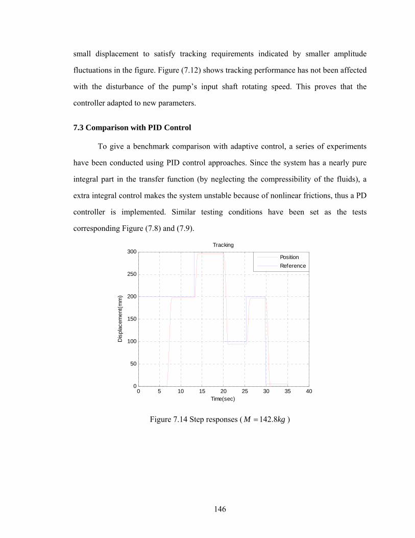
146
small displacement to satisfy tracking requirements indicated by smaller amplitude
fluctuations in the figure. Figure (7.12) shows tracking performance has not been affected
with the disturbance of the pump’s input shaft rotating speed. This proves that the
controller adapted to new parameters.
7.3 Comparison with PID Control
To give a benchmark comparison with adaptive control, a series of experiments
have been conducted using PID control approaches. Since the system has a nearly pure
integral part in the transfer function (by neglecting the compressibility of the fluids), a
extra integral control makes the system unstable because of nonlinear frictions, thus a PD
controller is implemented. Similar testing conditions have been set as the tests
corresponding Figure (7.8) and (7.9).
0 5 10 15 20 25 30 35 400
50
100
150
200
250
300Tracking
Time(sec)
Dis
plac
emen
t(mm
)
PositionReference
Figure 7.14 Step responses ( 142.8M kg= )
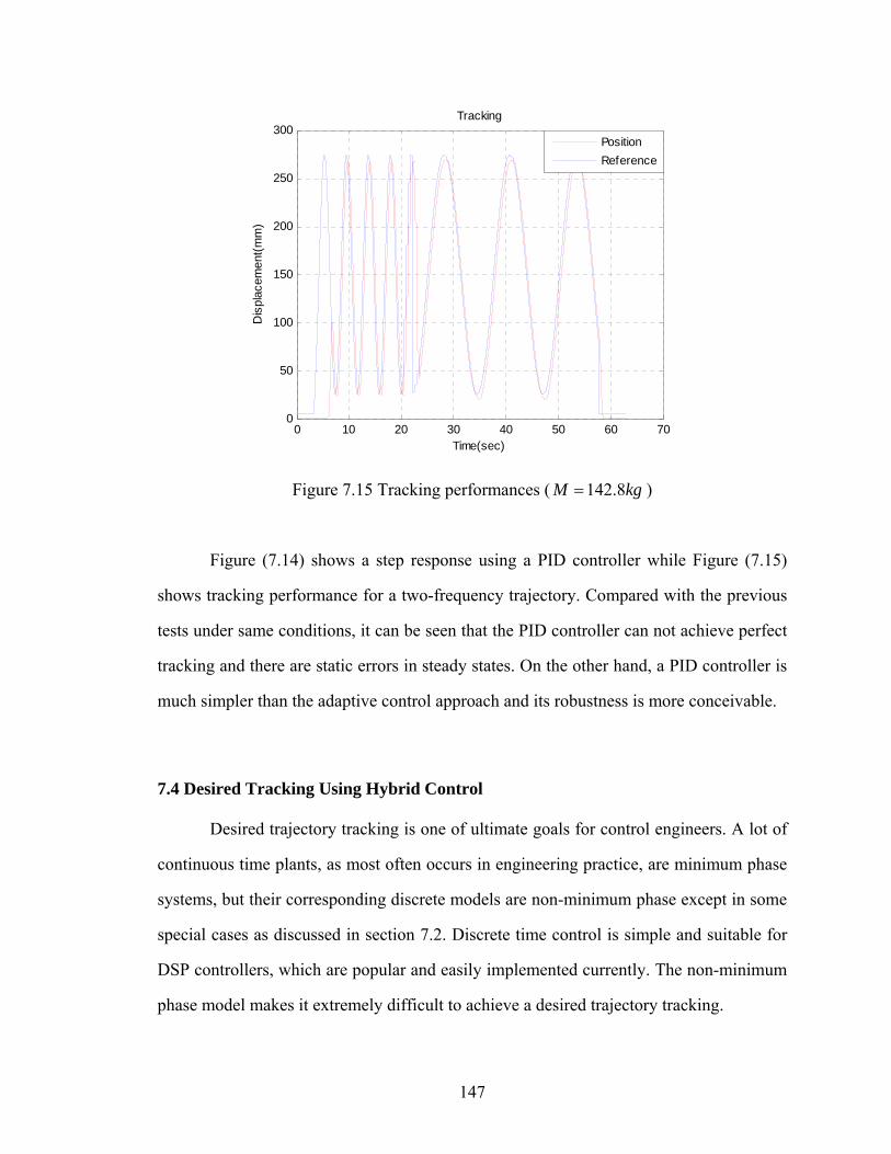
147
0 10 20 30 40 50 60 700
50
100
150
200
250
300Tracking
Time(sec)
Dis
plac
emen
t(mm
)
PositionReference
Figure 7.15 Tracking performances ( 142.8M kg= )
Figure (7.14) shows a step response using a PID controller while Figure (7.15)
shows tracking performance for a two-frequency trajectory. Compared with the previous
tests under same conditions, it can be seen that the PID controller can not achieve perfect
tracking and there are static errors in steady states. On the other hand, a PID controller is
much simpler than the adaptive control approach and its robustness is more conceivable.
7.4 Desired Tracking Using Hybrid Control
Desired trajectory tracking is one of ultimate goals for control engineers. A lot of
continuous time plants, as most often occurs in engineering practice, are minimum phase
systems, but their corresponding discrete models are non-minimum phase except in some
special cases as discussed in section 7.2. Discrete time control is simple and suitable for
DSP controllers, which are popular and easily implemented currently. The non-minimum
phase model makes it extremely difficult to achieve a desired trajectory tracking.

148
As shown above, the proposed Recursive Least Squares (RLS) method has many
benefits such on noise rejection, computation efficiency, numerical stability and so on.
But this method can only works with discrete sequence where unstable zeros prevent us
from achieving desired tracking. This inspire us to propose a hybrid control approach to a
general continuous time plant which is minimum phase, without considering whether
their corresponding discrete model is minimum phase or not.
Figure (7.16) shows the hybrid adaptive control structure. There are two types of
systems: the identification using RLS works in discrete time with sampling period sT , and
the controller and plant works in the continuous time domain. The identified parameters
update the controller to achieve desired tracking.
( )skTθ
Figure 7.16 Hybrid adaptive control
The plant can be described by:
( ) ( 1) ( ) ( 1)1 0 1 0( ) ( ) ( ) ( ) ( ) ( )n n m m
n m my t a y t a y t b u t b u t b u t− −− −+ + + = + + + (7.13)
The system is assumed to be strictly proper and minimum phase system, thus it must be
true that: n m> and zero dynamics of (7.13) is stable. Then it is advisable to let:
( ) ( 1)1 0( ) ( ) ( ) ( )m m
m mu t b u t b u t b u t−−′ = + + + (7.14)

149
The Equation (7.13) then can be rewritten as:
( ) ( 1)1 0( ) ( ) ( ) ( )n n
ny t a y t a y t u t−− ′+ + + = (7.15)
If ( ) ( 1)( ), ( ), , ( ), ( )n ny t y t y t u t− ′ are measurable, the identification error is defined
as:
( ) ( 1)
1 0( )
( ) ( ) ( ) ( ) ( )
( ) ( ) ( )
n nn
n T
t y t a y t a y t u t
y t t t
ε
ϕ θ
−− ′= + + + −
= − (7.16)
( 1) ( )
1 0 0
( ) [ ( ), , ( ), ( ), , ( )]( ) [ , , , , , ]
T n m
n m
t y t y t u t u tt a a b b
ϕθ
−
−
== − −
(7.17)
Most often, it is usually desirable, because of noise considerations, to filter the signals
before parameter identification. The filter 1( )sΛ
is defined:
11 0( ) n n
ns s sλ λ−−Λ = + + + (7.18)
( )sΛ is Hurwitz. Filtering both sides of Equation (7.13), the new linear regression can be
expressed as:
( ) ( ) ( )( ) ( )
s A s B sy y us s
⎡ ⎤ ⎡ ⎤Λ −= +⎢ ⎥ ⎢ ⎥Λ Λ⎣ ⎦ ⎣ ⎦
(7.19)
Where ( ), ( )A s B s are the corresponding transfer function polynomials for (7.13) written
in ( )( )
B sA s
form.
Similar to the definitions of (7.16), (7.17), define:
( ) ( ) ( )( )
( ) ( )
( ) ( )T
s A s B st y y us s
y t t
ε
ϕ θ
⎡ ⎤ ⎡ ⎤Λ −′ = − +⎢ ⎥ ⎢ ⎥Λ Λ⎣ ⎦ ⎣ ⎦= −
(7.20)

150
1
1 1 0 0 0
( ) [ , , , , , ]( ) ( ) ( ) ( )
( ) [ , , , , , ]
n mT
n n m
s y s ut y us s s s
t a a b b
ϕ
θ λ λ
−
− −
=Λ Λ Λ Λ
= − − (7.21)
Where ( )tε defined in (7.16) and ( )tε ′ defined in (7.20) are corresponding to
different measurement scenarios. We will denote these identification errors as ( )tε in the
following discussions.
The Least Squares problem in the continuous time domain is to find the *θ to
minimize:
0
1( ) ( ) ( )T TJ t t dt
Tθ ε ε= ∫ (7.22)
Now, define a new cost function,
0
ˆ( ) ( ) ( )T TsTJ W d
Tθ ε τ ε τ τ= ∫ (7.23)
With adequately selected sampling time sT , the weighting matrix W is defined as:
[..., ( ), (( 1) ), (( 2) ),...]s s sW diag nT n T n Tδ δ δ= + +
Now, the cost function (7.23) actually is:
1
0
1ˆ( ) ( ) ( )N
Ts s
nJ nT nT
Nθ ε ε
−
=
= ∑ (7.24)
Where sT NT= .
Equation (7.24) indeed is a discrete least squares formulation using only discrete
samples of ( )tε , thus it can be implemented in the proposed RLS algorithm. If the
minimized ˆ( )J θ and the minimized ( )J θ converge to the same set *θ , then the proposed
hybrid adaptive control is done since the indirect adaptive control with least square
identification is well known in the control literature. Intuitively, if sampling is very dense

151
such that 0sT → , (7.24) will converge to (7.22) in the sense of the Riemann Integral
provided that ( )tε is well behaved.
Theorem 7.2 If the bandwidths of the plant’s input and output are bounded by 0f , and
sampling frequency 04sf f> , then the continuous least squares defined as (7.22) is
equivalent to discrete least squares defined as (7.24) as time goes to infinity.
Proof:
The bandwidth of ( )tε is bounded by 0f because of the assumption and the
system is linear. Therefore, the bandwidth of ( ) ( )T t tε ε is bounded by 02 f . Note that
( )tε , [0, ]t T∈ is calculated on the latest ( )Tθ , which is a constant vector; the ( )Tθ does
not affect spectrum of ( )tε , [0, ]t T∈ . For the sake of simplicity, we consider ( )tε as a
scalar.
As T → ∞ ,
2
2
2
1( ) ( )2
sin( ( ) / 2)1 ( )2 ( ) / 2
sin( ( ) / 2)1 ( )2 ( ) / 2
T
T
T s ssT
k s s
T s ss T
k s s
J t dtT
t kTkT dtT t kT
t kTkT dtT t kT
θ ε
ωεω
ωεω
−
∞
−=−∞
∞
−=−∞
=
⎡ ⎤−= ⎢ ⎥−⎣ ⎦
−=
−
∫
∑∫
∑ ∫
(7.25)
In the second step, we have applied Shannon’s sampling theorem. Note that the
function sin xx
converge to zero very quickly and sin( ) (0) 1x dx rectxπ
π∞
−∞= =∫ . Then the
right hand side of (7.25) is:
2
2
1 ( )21 ( )
ˆ ( )
s sk
sk
RHS kT TT
kTN
J
ε
ε
θ
∞
=−∞
∞
=−∞
=
=
=
∑
∑

152
That completes the proof.
(Q.E.D)
By Theorem 7.2, minimizing ˆ( )J θ is the equivalent of minimizing ( )J θ and vice
versa and the parameters converge to the same set. Thus, the proposed hybrid adaptive
control is effective if the signal bandwidth is bounded (In practice, all of measured
signals have to pass a low pass filter before processing). In the proof, we have used two
side integrals and sums, that is a little uncomfortable. However, this does not create a
problem in practice. In the application, we can deem that there is a data window applied
to the sampled data such that ( ) 0, ( ,0)t tε = ∈ −∞ . The same idea can be applied to a
forgetting factor < 1 case, that there is an exponential data window applied to the data.
Theoretically, to assume a signal’s spectrum is bounded is not realistic and is hard to
satisfy. However, Theorem 7.2 provides a guidance to select the minimum sampling
frequency for the control design.
It is astonishing at the first glimpse that the sampling frequency should be four
times faster than the bandwidth of the system dynamics. (The general thought is
02sf f> ). This can be demonstrated by the following example.
t2π
1
-1
Figure 7.17 Four times sampling rate

153
Suppose ( ) sin( )t tε = , and the sampling frequency is 42sf Hzπ
= and the two
signals are synchronized at 0t = as shown in Figure (7.17). Then it can be verified:
2 2
0
1 1sin ( )2 2
t dtπ
π=∫
2 2 2 21 2 3 1(sin (0) sin ( ) sin ( ) sin ( ))4 2 2 2 2
π π π+ + + =
Varying the sampling rate, say, 52sf Hzπ
= and it is not necessary the phase
difference is equal to zero, would give the same answer 1/ 2 .
Theorem 7.3 If Sampling frequency 04sf f> ,where 0f is the bandwidth of the plant
dynamics, then the proposed hybrid control algorithm has following properties: all the
signals in the closed-loop are uniformly bounded and the tracking error converges to
zero asymptotically with time.
Proof:
Parameter convergence is ensured by the recursive least squares algorithm. Thus at finite
time, *θ θ ε− < , then we can use the established theorem about indirect adaptive control
[166, Theorem 7.4.1] to show such properties. From the Theorem 7.2, the system
performance will be identical to the continuous lease square case as time goes to infinity.
(Q.E.D)
If the control law were really continuous, then we are done. However, in some
cases, for example, the test-bed we are currently using, control effort is buffered by a
zero-order-hold which works at some sampling frequency. This is a minor concern
provided that the sampling frequency can be high enough. For the sake of the

154
completeness, we provide the following theorem to show the existence of such “high”
sampling frequency.
Theorem 7.4 If a linear system can be exponentially stable by implementing a states
feedback control law, then there exists a sampling rate sf , such that for all sampling rate
sf f> , the same control law, buffered by a zero-order-hold (ZOH), can make the system
exponentially stable.
Proof:
Let the system be x Ax Bu= + with control law u kx= − , then for the nominal
system ˆˆ ˆ ˆ( )x A Bk x Ax= − = , there exists a Lyapunov function ( )V x such that: ( By the
converse Lyapunov Theorem [160])
2 21 2
23
4
( )
( )
c x V x c xdV A Bk x c xdxdV c xdx
≤ ≤
− ≤ −
≤
(7.26)
Let 0t be the start of one of ZOH updating times, and sT is the sampling period,
0 0( )x x t= , then, during 0 0[ , ]st t t T∈ + , the control effort is:
0u kx=
The system dynamics are:
0
0
0
=ˆ = ( )
x Ax BkxAx Bkx Bkx Bkx
Ax Bk x x
= −− + −
+ −
(7.27)
The system states are:

155
00 0( ) ( )
0 0 0
t tA t t A t tx e x Bkx e dτ τ−− − −= + ∫ (7.28)
Since A is finite, then we have:
0 5 sx x c T x− ≤ (7.29)
Then:
0
0
2 23 4 5
2 23 6
ˆ( ( ))
ˆ ( )
s
s
dVV Ax Bk x xdx
dV dVAx Bk x xdx dx
c x c c T x Bk
c x c T x
= + −
≤ + −
≤ − +
≤ − +
Thus: the buffered system is exponentially stable if 3
6s
cTc
<
(Q.E.D)
Theorem 7.4 says if there is a very high sampling frequency, the buffered system
is still exponentially stable although the eigenvalue assignments are possibly different
from the nominal ones. Theorem 7.3 proves the stability of the proposed hybrid adaptive
control. Thus we conclude that the proposed control algorithm can be used to achieve
desired tracking.

156
0 10 20 30 40 50 600
50
100
150
200
250
300
350
400Tracking
Time(sec)
Dis
plac
emen
t(mm
)
Position
Reference
Figure 7.18 Step responses ( 142.8M kg= )
0 10 20 30 40 50 60 70 800
50
100
150
200
250Tracking
Time(sec)
Dis
plac
emen
t(mm
)
PositionReference
Figure 7.19 Tracking performances ( 142.8M kg= )
Experiments were conducted to validate the proposed hybrid control approach.
The experimental setups are similar to the discrete time control ones as discussed in

157
section 2. The tracking error dynamics is set to 2
1 ( ) 0( 3)
e ts
=+
. Figure (7.18) shows the
system’s step response and Figure (7.19) shows the tracking performance to a desired
trajectory consisting of 0.52
Hzπ
and 1.52
Hzπ
sinusoid signals. Note that the change
between two frequency signals is not continuous. Figures show that the system achieved
essentially trajectory tracking.
As discussed and shown by experimental results in the section 2, the system
bandwidth is not sensitive to the load changes. We omit here the experimental results
found using varying loads. The adaptive control is more clearly seen by showing the
speed changes of the pump input shaft, which corresponds to the system forward gain
variations and emulates the speed variations of internal combustion engine in industry
practice.
0 10 20 30 40 50 60 70 800
50
100
150
200
250Tracking
Time(sec)
Dis
plac
emen
t(mm
)
PositionReference
Figure 7.20 Tracking performances with variations of motor speeds

158
0 10 20 30 40 50 60 70 80-800
-600
-400
-200
0
200
400
600
800Control effort
Time(sec)
Dis
plac
emen
t/Cur
rent
PositionCurrent
Figure 7.21 Control efforts with variations of motor speeds
Figure (7.20) shows the tracking performance while the motor speed changes
from 800 RPM to 1200 RPM at approximately 32 seconds. Figure (7.21) shows the
corresponding control current to the pump, it can be seen that the control effort decreased
when the motor speed goes up. This is to be expected since higher motor speed means the
system has a higher forward gain such that the controller should compensate for gain
variations. The system achieves desired tracking with speed increases up to 50%.
At the beginning of this section, for a ( )n th order system, the linear regression
Equation (7.17) requires all measurements up to the ( )n th order. Equation (7.21) utilizes
a low pass filter to implement derivative operation in order to get high order
measurements. Inspired by Equation (7.21), for a ( )n th order system, measurements up to
( 1)n th− order measurement is enough. In our test-bed, there is no velocity sensor; the
velocity information is achieved by differentiating the filtered displacement signal.
The experimental results shown above are based on a second order model.
Compared with the discrete time approach which only requires position information, the
hybrid control approach has some benefits, at the same time, it has some serious

159
problems because high-order information is needed, especially some measurements are
not directly available and the system has discontinuities in the internal stages.
The second order model can be expressed as:
( ) ( ) ( )s s a y s bu s f+ = + (7.30)
Where u is control effort and y is the system output (cylinder position). f includes the
system disturbance. Here we are more interested in gravity and Coulomb friction. Figure
(7.22) shows the identified parameters and Figure (7.23) shows the corresponding errors
compared with acceleration and velocity (obtained by differentiating filtered positions).
As we have explained before, there is tilting problem whenever the cart reverses motion
directions, thus there are lots of spikes in the velocity and acceleration signals. The
identified parameters still converge.
0 1000 2000 3000 4000 5000 6000-30
-25
-20
-15
-10
-5
0
5
10
k
Identif ication (2nd order)
ab
Figure 7.22 Identified parameters with the second order model

160
0 1000 2000 3000 4000 5000 6000-20
-15
-10
-5
0
5
10
15
20Error
error
d1x
d2x
Figure 7.23 Identification errors with the second order model
If we would like to model the pump’s dynamics as a second order system, then
the system transfer function can be expressed as:
21 0( ) ( ) ( )s s a s a y s bu s f+ + = + (7.31)
However, the place where disturbance force enters the system is different from that of the
control efforts. Therefore, f should be expressed in the following form
1( ) ( )f k s b f t′= + (7.32)
Where ( )f t′ stands for disturbance forces. Things become serious if ( )f t′ is not a
continuous function because the differentiated disturbance goes into the identification
regression equation. This case happens in the testbed: there are Coulomb frictions and
such friction behaves too differently when the cylinder reverses the motion directions
because the cart is tilted as shown in Figure (7.24).

161
Figure 7.24 The tilting cart
Figure (7.25) shows the identified parameters using the third order model while
Figure (7.26) shows the corresponding identification errors. It can be seen that the
parameters do not converge and the identification error is much larger than the data itself.
It is hard to say such an identification result is acceptable.
0 1000 2000 3000 4000 5000 6000-60
-50
-40
-30
-20
-10
0
10
20
30
a0a1b
Figure 7.25 Identified parameters with the third order model

162
0 1000 2000 3000 4000 5000 6000-800
-600
-400
-200
0
200
400
600
800Error
errord1x
d2x
Figure 7.26 Identification errors with the third order model
The failure of the third order model identification comes from a lack of reliable
measurements and a regression equation that does not have terms accounting for the
disturbance. If such factors can be avoided in general application, a more reliable result
can be expected.
A general approach to achieve desired trajectory tracking has been proposed and
validated in this section. The algorithm requires the ( 1)n th− order measurement which is
exactly same as the traditional approach such as indirect adaptive control and direct
control. However, our approach provides better numerical stability, efficiency and
convergence rate than these traditional approaches. Compared with discrete time control,
this approach solves tracking issues instead of just stabilizing a system.
7.5 Summary
In this chapter, the proposed adaptive control concept has been implemented in a
discrete time approach and a continuous time approach. The related proofs and
experimental results are provided and the results implementing PID control have been

163
presented as a benchmark. The results validated the proposed algorithms and show their
advantages in applying adaptive control to pump control applications.
One of main focuses is to achieve desired trajectory tracking with using adaptive
control. It turns out that the discrete time control rarely has the ability. Thus a general
approach, not only for the test-bed, has been proposed with using a hybrid control
approach. It not only ensures tracking performance, but also has advantages which exist
in discrete time control.

164
CHAPTER VIII
SUMMARY, CONTRIBUTIONS, AND FUTURE DIRECTIONS
This chapter presents concluding remarks. First, a summary of the contributions
and accomplishments is given. Finally, suggestions and recommendations for further
research are stated.
8.1 Summary and concluding remarks
Fluid power technology has been widely used in industrial practice; however, its
energy efficiency has become a big concern in the recent years. Much progress has been
made to improve fluid power energy efficiency from many aspects. Among these
approaches, using a valve-less system to replace a traditional valve-controlled system
showed eminent energy reduction. This thesis studies the valve-less solution–pump
displacement controlled actuators– from the view of a controls background. The thesis
aims to develop an algorithm suitable for industrial practice. At the same time, parts of
these ideas, techniques and conclusions presented in the thesis not only can be applied to
fluid power applications, but also can benefit general control applications.
To account for the stiffness of the system dynamics and provide a theoretical
basis for the later studies, singular perturbation theory applied to fluid power has been
presented in Chapter 3. Hydraulic control design can be simplified under certain
conditions. This technique makes the control design suitable for real time control.
Although, in general, this technique can not be directly applied in the system level
design, it can be applied for sub-system simplifications.
Higher energy efficiency using a valve-less system mainly benefits from its
hydraulic circuit structure. The traditional and present hydraulic circuits have an internal
instability issue, so a novel hydraulic circuit has been developed in the thesis. Chapter 4

165
focuses on theoretical analysis while experimental validation is presented in Chapter 5.
The novel circuit ensures the circuit stability and keeps a hydraulic system operating
under high energy efficiency.
Measurement noise is inevitable in engineering practice. Chapter 6 discussed a
parameter estimation using least squares that has a faster parameter convergence rate and
lower residual errors than other instantaneous measurement identification schemes. To
enhance the numerical stability and computing efficiency, the square-root technique has
been applied in the proposed algorithm. Chapter 6 also presented that the tracking error
is bounded by tracking dynamics eigen-value assignments if the disturbance is bounded.
In Chapter 7, the proposed algorithm has first been applied in the discrete time
control domain. It has been shown that the algorithm is compatible with developed
techniques to enhance the system robustness and is validated by the experimental results.
Results based on PID control also have been presented as a benchmark. Most often, the
discrete time control can not achieve the desired trajectory tracking. A more general
approach to achieve desired tracking by implementing hybrid adaptive control is
presented in the last section of Chapter 7. The scheme has benefits of high stability,
calculating efficiency, and it can be combined naturally with the existing real time
controller.
8.2 Contributions
This thesis contributed control techniques for fluid power control, and parts of the
contributions are not limited to the fluid power control. The specific contributions can be
outlined as follows:
(1) Singular perturbation theory was applied to fluid power control. The control
design can be simplified making it suitable for real time control. The
conclusions also can be applied to sub-level hydraulic system analysis and
model reduction.

166
(2) A novel hydraulic circuit for single rod cylinders has been developed. The
invention addressed the causes of the system’s instability and developed a
control algorithm to stabilize the system while the system’s energy efficiency
still holds.
(3) An indirect least squares method is applied to account for measurement noise
such that the parameters have fast convergence rate and low residue errors.
The square-root algorithm has been employed in the control techniques to
enhance the controller’s numerical stability and calculating efficiency. The
algorithm is shown compatible with the latest techniques to enhance the
system’s robustness.
(4) A hybrid adaptive control scheme has been developed to deal with the
general non-minimum phase systems using discrete time control in order to
achieve desired trajectory tracking. The scheme is shown to be globally
stable, efficient, and suitable for commonly used real time controls.
8.3 Future Directions
The thesis involves areas of hydraulic control, hydraulic circuit design and
adaptive controls. All of these areas are open to questions and are ongoing. Here are
some possible directions for future work.
(1) Although we oriented the thesis results toward practical industrial practices
and have built a hardware test-bed to emulate industrial scenarios, these have
not been really implemented on a real excavator or backhoe. An immediate
step is to apply the thesis results to real applications to verify the results and
meet possible challenges.
(2) The invented hydraulic circuit utilized a hardware component to stabilize the
system, but a virtual leakage control should be implemented if a fast pump is
commercially available. However, how to decouple of the inner loop control

167
and outer loop control is questionable at this point and this question should be
addressed in the future.
(3) The estimated parameters are continuously updated when the control is
running. In real applications, for example, when an excavator contacts stiff
obstacles, the parameter updating should be stopped because the system
model has an abrupt change and it soon will recover. This kind of parameter
projection should be implemented in practice.
(4) We have implemented hybrid adaptive control; can we step a little further to
include artificial intelligence? During the experiments, a human can “guess”
the true parameters even though parameters do not converge. However,
current adaptive controller does not have this ability. The parameter project
always depends on prior knowledge, which is formed by human. If we can let
the controller learn how to update the parameter by itself, this would be a
good contribution to adaptive control.
(5) The disturbance, causing instability of an adaptive controller, usually comes
from un-modeled dynamics. Currently, un-modeled dynamics are usually
connected with input, output amplitude, but experience shows it is more
related with the frequency. More research about robustness in the frequency
domain is needed.
168
REFERENCES
[1] Sullivan, James A., Fluid Power: Theory and Applications, 4th ed, Prentice Hall, New Jersey, 1998.
[2] H. E. Merritt, Hydraulic Control Systems, New York: Wiley, 1967
[3] Zeiger, G. and Akers, A., “Torque on the Swashplate of an Axial Piston Pump,” ASME Journal of Dynamics Systems, Measurement and Control, 1985. Vol 107, pp.220-26
[4] Kim, S.D., Cho, H.S. and Lee, C.O., “A Parameter Sensitivity Analysis for the Dynamic Model of a Variable Displacement Axial Piston Pump,” Proceedings of Institution of Mechanical Engenderers, 1987,Vol 201
[5] Manring, N. D. and Johnson, R., “Modeling and Designing a Variable Displacement Open-Loop Pump,” ASME Journal of Dynamics Systems, Measurement and Control, 1996. Vol 118, pp.267-271
[6] R. Rahmfeld and M. Ivantysynova, “Displacement controlled linear actuator with differential cylinder-a way to save primary energy in mobile machines,” in Proc. Of 5th International Conference on Fluid Power Transmission and Control (ICFP'2001), Hangzhou, China, 2001, pp. 316-322
[7] P. Opdenbosch, “Auto calibration and control applied to electro hydraulic valves,” Doctoral Thesis, Georgia Instutute of Technology, 2007.
[8] X. Yang, D. B. Stephenson, and M. J. Paik, “Bidirectional pilot operated control valve,” U.S. Patent 6 328 275, 2001
[9] S. Liu and Y. Bin, “Energy-saving control of single-rod hydraulic cylinders with programmable valves and improved working mode selection,” SAE Transactions, Journal of Commercial Vehicle, vol. 2002-01-1343, pp. 51–61, 2002.
[10] A. Shenouda, “Quasi-static hydraulic control systems and energy savings potential using independent metering four-valve assembly configuration,” Doctoral Thesis, Georgia Instutute of Technology, 2006

169
[11] Heybroek, K.; Larsson, J. and Palmberg, J.O., “Open Circuit Solution for Pump Controlled Actuators,” Proceedings of 4th FPNI PhD Symposium, pp. 27-40. Sarasota, Florida, USA, 2006
[12] Anon, “A remotely operated excavator,” Nuclear Engineering International, vol. 37, pp. 41–43, Jan 1992.
[13] Burks, B., Killough, S., and Thompson, D., “Remote excavation using the telerobotic small emplacement excavator,” in Proc. Conf. Robotics and Remote Systems Technolgy, (Chicago,IL), pp. 170–174, Nov 1992.
[14] Sepehri, N., Lawrence, P. D., Sassani, F., and Frenette, R.,“Resolved-mode teleoperation control of heavy-duty hydraulic machines,” ASME J. Dyn. Syst. Meas. and Control, vol. 116, pp. 232–240, Jun 1994.
[15] Kontz, M. E., M. C. Herrera, et al., “Impedance shaping for improved feel in hydraulic systems,” 2007 ASME International Mechanical Engineering Congress and Exposition, November 11-15, 2007, Seattle, Washington, USA
[16] A. Ennes, “Shared control of hydraulic manipulators to decrease cycle time,” Doctoral Thesis, Georgia Institute of Technology, 2007.
[17] Carlisle, Rodney. Scientific American Inventions and Discoveries, p. 266. John Wiley & Sons, Inc., New Jersey, 2004
[18] Stern, H., “On the bulk modulus of hydraulic fluids in the presence of dissolved gas,” American Society of Mechanical Engineers, The Fluid Power and Systems Technology Division (Publication) FPST 4: 113-123. 1997
[19] Yu, J., Z. Chen, et al. "The variation of oil effective bulk modulus with pressure in hydraulic systems." Journal of Dynamic Systems, Measurement and Control, Transactions of the ASME 116: 146-150, 1994
[20] Edge, K. A., Darling J., “Cylinder pressure transients in oil hydraulic pumps with sliding plate valves,” Proceedings of the Institute of Mechanical Engineers, Vol. 12, No. 4, 1986
[21] Blackburn, J. E., Reethof, G. Shearer, J. L., Fluid Power Control, The MIT Press, New York, 1960

170
[22] Peeler, R. L., Green, J., “Measurement of bulk modulus of hydraulic fluids,” ASTM Bulletin, pp. 51-57, 1959
[23] Magorien, V. G. “Effects of air on hydraulic systems,” Hydraulic and Pnematics, June, pp. 104-108, 1967
[24] Ivantysyn, J. and Ivantysynova, M., Hydrostatic Pumps and Motors, Principles, Designs, Performance, Modelling, Analysis, Control and Testing. New Delhi. Academia Books International, 2001
[25] Zarotti G. L., Nervegna N., “Pump efficiency approximation and modeling,” 6th Int. Fluid Power Symposium, Cambridge, Uk. 1981
[26] Dorey R., “Modeling of losses in pumps and motors,” 1st Bath International Fluid Power Workshop, University of Bath, UK 1988
[27] Conrad F., Sorensen P. H., Torstmann E., “On the modeling of flow and torque loss in hydrostatic machines,” 9th International Symposium on Fluid Power, Cambridge, UK, 1990
[28] Huhtala K., Vilenium M., “Comparison of steady-state models of hydraulic pumps,” 5th Scandinavian International Conference on Fluid Power, Linkoping, Sweden, 1997
[29] Ivantysynova M., “Ways for efficiency improvements of modern displacement machines,” 6th Scandinavian International Conference on Fluid Power, Tampere, Finland, 1999
[30] Kaliafetis, P., and Costopoulos, Th., 1995, ‘‘Modeling and simulation of an axial piston variable displacement pump with pressure control’’. Mech. Mach. Theory, 30(4), pp. 599–612.
[31] Inoue, K., and Nakazato, M., 1993, ‘‘A new prediction method of operating moment and cylinder pressure of a swash plate type axial piston pump’’. Fluid Power, ISBN 0419191003. 361–366
[32] Schoenau, G., Burton, R., and Kavanagh, G., 1990, ‘‘Dynamic analysis of a variable displacement pump’’. ASME J. Dyn. Syst., Meas., Control, 112, pp. 122–132.

171
[33] Yamaguchi, A., 1966, ‘‘Studies on the characteristics of axial plunger pumps and motors’’. Bull. JSME, 9~34, pp. 305–313
[34] Manring, N. D., 1999, ‘‘The control and containment forces on the swash plate of an axial-piston pump’’. ASME J. Dyn. Syst., Meas., Control, 121, pp. 599–605
[35] Manring, N. D., 2001, ‘‘Designing a control and containment device for cradle-mounted, transverse-actuated swash plates’’. ASME J. Mech. Des., 123, pp. 447–455
[36] Manring, N. D., 2002, ‘‘Designing a control and containment device forcradle-mounted, axial-actuated swash plates’’. ASME J. Mech. Des., 124, pp. 456–464
[37] Manring, N. D., 1998, ‘‘The torque on the input shaft of an axial-piston swashplate type hydrostatic pump’’. ASME J. Dyn. Syst., Meas., Control, 120, pp. 57–62.
[38] Manring, N. D., 2004, ‘‘The impact of using a secondary swash-plate angle within an axial piston pump’’. ASME J. Dyn. Syst., Meas., Control, 126, pp. 65–74.
[39 Bahr Khalil, M.K., Svoboda, J., Bhat, R.B., 2004, “Modeling of swash plate axial piston pumps with conical cylinder blocks,” ASME J. Mech. Des., 126, pp. 196–200
[40] Kassem S. A., Bahr M. K., 2000, “ On the dynamics of swash plate axial piston pumps with conical cylinder blocks,” 6th Triennial International Symposium on Fluid Control Measurement and Visualization, Sherbrooke University, Sherbrooke, Canada
[41] Shi, Z., G. Parker, et al. (2010). "Kinematic analysis of a swash-plate controlled variable displacement axial-piston pump with a conical barrel assembly." Journal of Dynamic Systems, Measurement and Control, Transactions of the ASME 132, 1-8.
[42] Hahmann W., “Das dynamische Verhaltn hydrostatischer antriebe mit servopumpe und ihr Einstatz in Regelkreisen,” Dissertation, RWTH Aachen, Germany 1973
[43] Berbuer, J., “ Neuartige servoantriebe mit primarer verdrangersteuerung,” Dissertation RWTH Aachen, Germany, 1988

172
[44] Berg, H. and M. Ivantysynova, “Design and testing of a robust linear controller for secondary controlled hydraulic drive” Proc Instn Mech Engrs, 1999
[45] Bahr Khalil, M.K., Yurkevich, V., Svoboda, J., Bhat, R.B., “Implementation of single feedback control loop for constant power regulated swash plate axial piston pumps,” International Journal of Fluid Power, Vol.3, No. 3, 2002
[46] Grabbel, J. and M. Ivantysynova (2005). "An investigation of swash plate control concepts for displacement controlled actuators." International Journal of Fluid Power 6(2): 19-36
[47] Li, P. Y., C. Y. Li, et al. (2005). “Software enabled variable displacement pumps.” 2005 ASME International Mechanical Engineering Congress and Exposition, IMECE 2005, November 5, 2005 - November 11, 2005, Orlando, FL, United states, American Society of Mechanical Engineers.
[48] Rannow, M. B., H. C. Tu, et al. (2006). “Software enabled variable displacement pumps - Experimental studies.” 2006 ASME International Mechanical Engineering Congress and Exposition, IMECE2006, November 5, 2006 - November 10, 2006, Chicago, IL, United states, American Society of Mechanical Engineers.
[49] L. Gu,M. Qiu,W. Feng, and J. Cao, “Switchmode Hydraulic Power Supply Theory,” Proceedings of the 2005 ASMEIMECE, No. IMECE2005-79019, 2005
[50] E. J. Barth, J. Zhang, and M. Goldfarb, “Control Design for Relative Stability in a PWM-Controlled Pneumatic System,” Journal of Dynamic Systems Measurement and Control-Transactions of the ASME, vol. 125, no. 3 pp. 504–508, 2003
[51] Tu, H. C., M. B. Rannow, et al. (2010). “Modeling and validation of a high speed rotary PWM on/off valve.” 2009 ASME Dynamic Systems and Control Conference, DSCC2009, October 12, 2009 - October 14, 2009, Hollywood, CA, United states, American Society of Mechanical Engineers.
[52] Rannow, M. B. and P. Y. Li (2010). “Soft switching approach to reducing transition losses in an on/off hydraulic valve.” 2009 ASME Dynamic Systems and Control Conference, DSCC2009, October 12, 2009 - October 14, 2009, Hollywood, CA, United states, American Society of Mechanical Engineers.
[53] Backé, W. 1994. Verlustarme hydrostatische Antriebe – Grundlagen und Anwendungen. VDI Berichte No. 1132. Dusseldorf: VDI.
173
[54] Backé, W. 1995. “Trends in Mobile Hydraulics.” 4th International Conference on Fluid Power. Tampere, Finland.
[55] Berbuer, J. 1988. Neuartige Servoantriebe mit primärer Verdrängersteuerung. Dissertation, RWTH Aachen, Germany.
[56] Lawrence, P.D. ; Salcudean, S.E. ; Sepehri, N. ; Chan, D. ; Bachmann, S. ; Parker, N ; Zhu, M. and Frenette, R. 1995. “Coordinated and Force-Feedback Control of Hydraulic Excavators.” 4th International Symposium on Experimental Robotics, ISER’95. Stanford, California.
[57] Lodewyks, J. 1993. Differentialzylinder im geschlossenen hydrostatischen Getriebe. Olhydraulik und Pneumatik 37 (1993) No. 5., pp. 394-401.
[58] Lodewyks, J. 1994. Der Differentialzylinder im geschlossenen hydrostatischen Kreislauf. Dissertation, RWTH Aachen, Germany.
[59] Ziegler, R. 1990. Auslegung und Optimierung schneller Servopumpen. Dissertation, Universitat Karlsruhe, Germany.
[60] Ziegler, R. and Wilke, O. 1991. Pumpenregelung: ein energiesparendes Antriebskonzept mit hoher Regelgute. Olhydraulik und Pneumatik 35 (1991) No. 7.
[61] Achten, P.A.J. 1997. “Transforming Future Hydraulics – A new design of a hydraulic transfer.” 8th Scandinavian International Conference on Fluid Power. Linkoping, Sweden.
[62] Achten, P.A.J. 1999. Trennen statt stapeln – Die Nutzung des Centaur Freikolbenmotors bei einem Gabelstapler. (Separation instead of stacking – the application of the Centaur free piston engine in a fork-lift truck. VDI-MEG Tagung Landtechnik, pp. 353-358, Braunschweig, Germany.
[63] Achten, P. A. J. and Palmberg, J.-O. 1999. “What a Difference a Hole Makes – the Commercial Value of the INNAS Hydraulic Transformer.” 6th Scandinavian International Conference on Fluid Power.
[64] Berbuer, J. 1985. Parallelschaltung von Servopumpe und Servoventil – ein Weg zu energiesparenden hochdynamischen Antrieben. Olhydraulik und Pneumatik 29 (1985) No. 10, pp. 742-751.

174
[65] Berbuer, J. 1988. Neuartige Servoantriebe mit primärer Verdrängersteuerung. Dissertation, RWTH Aachen, Germany.
[66] Berg, H. 1999. Robuste Regelung verstellbarer Hydromotoren am Konstantdrucknetz. PhD dissertation. VDI Fortschritt-Berichte. Reihe 8 Nr. 764. Düsseldorf: VDI. ISBN: 3-18-376408-3.
[67] Bindel, R. et al. 2000. Flachheitsbasierte Regelung eines hydraulischen Antriebs mit zwei Ventilen fur einen Grossmanipulator. at Automatisierungstechnik, No. 3/2000, pp. 124-131.
[68] Roosen, K. 1997. Energieeinsparung durch ein neues Schaltungskonzept fur ventilgesteuerte hydraulische Linearantriebe. Olhydraulik und Pneumatik 41 (1997) No. 4, pp. 262-274.
[69] Roosen, K. 2000. Hydraulische Stellantriebe mit Nebenstromregelung. Dissertation, RWTH Aachen, Germany.
[70] Feuser, A.; Dantlgraber, J.; Spath, D. and Wilke, O. 1995. Servopumpenantriebe für Differentialzylinder. Ölhydraulik und Pneumatik 39 (1995) No. 7, pp. 540-544.
[71] Feuser, A.; Liebler, G. and Köckemann, A. 1998. Elektrohydraulische Achsen mit Verstellpumpen zur Verbesserung des Wirkungsgrades. Ölhydraulik und Pneumatik (1998) 42 No. 6, pp. 378-383.
[72] Werndin R. and Palmberg J.O. “Hydraulic transformers - comparison of different designs.” Proceedings of The Eighth Scandinavian International Conference on Fluid Power, SICFP’03, 2003. Tampere, Finland.
[73] Achten, P.A.J. 1997. “Transforming Future Hydraulics – A new design of a hydraulic transfer.” 8th Scandinavian International Conference on Fluid Power. Linkoping, Sweden.
[74] Achten, P.A.J. 1999. Trennen statt stapeln – Die Nutzung des Centaur Freikolbenmotors bei einem Gabelstapler. (Separation instead of stacking – the application of the Centaur free piston engine in a fork-lift truck) VDI-MEG Tagung Landtechnik, pp. 353-358, Braunschweig, Germany.

175
[75] Hewett, Allan J. 1994. Hydraulic Circuit Flow Control. US Patent No. 5,329,767. July 19, 1994.
[76] Ivantysynova, M. 2000. “Displacement Controlled Linear and Rotary Drives for Mobile Machines with Automatic Motion Control.” SAE Int. OFF-Highway & Powerplant Congress, Milwaukee, Wisconsin, USA.
[77] Ivantysynova, M. 2002. “Displacement Controlled Actuator Technology - Future for Fluid Power in Aircraft and other Applications.” Proc. of the 3rd International Fluid Power Conference (3. IFK), Vol. 2, S. 425-440, Aachen.
[78] Rahmfeld, R. 2002. Development and Control of Energy Saving Hydraulic Servo Drives for Mobile Systems. PhD Thesis, VDI Fortschritt-Berichte. Reihe 12 Nr. 527. Düsseldorf: VDI.
[89] Rahmfeld, R. and Ivantysynova, M. 2003. “Energy Saving Hydraulic Displacement Controlled Linear Actuators in Industry Applications and Mobile Machine Systems.” The Fourth International Symposium on Linear Drives for Industry Applications (LDIA03), Birmingham, UK.
[80] Rahmfeld, R.; Ivantysynova, M. and Weber, J. 2003. IBIS – “Advanced Multi-functional Machinery for Outdoor Applications.” The 18th International Conference on Hydraulics and Pneumatics, ICHP 2003, pp. 137-149, Prague, Republic.
[81] Rahmfeld, R. 2002. Development and Control of Energy Saving Hydraulic Servo Drives for Mobile Systems. PhD Thesis, VDI Fortschritt-Berichte. Reihe 12 Nr. 527. Düsseldorf: VDI.
[82] Zimmerman, J. and Ivantysynova, M. 2008. “The effect of System Pressure Level on the Energy Consumption of Displacement Controlled Actuator Systems,” Proc. Of the 5th FPNI PhD symposium, Cracow, Poland, pp77-92
[83] Zimmerman, J. and Ivantysynova, M. 2009. “The effect of Installed Hydraulic Corner Power on the Energy Consumption and Performance of Multi-actuator Displacement Controlled Mobile Machines.” Bath/ASME Symposium on Fluid Power and Motion Control, Hollywood, California
[84] Zimmerman, J. and Ivantysynova, M. 2010. “Reduction of Engine and Cooling Power by Displacement Control,” Proc. Of the 6th FPNI PhD symposium, West Lafayette, IN, USA

176
[85] Heybroek K., Palmberg J.-O. and Larsson J., “Mode Switching and Energy Recuperation in Open-Circuit Pump Control,” in The 10th Scandinavian International Conference of Fluid Power, SICFP´07, (Eds. J. Vilenius and K.T. Koskinen), pp. 197–209, Tampere, Finland, 21st–23rd May, 2007.
[86] Heybroek K. and Palmberg J.-O., “Applied Control Strategies for a Pump Controlled Open Circuit Solution,” in The International Fluid Power Conference, IFK’08, (Eds. S. Helduser), pp. 39–52, Dresden, Germany, 31st March 2nd April, 2008.
[87] Heybroek K. and Palmberg J.-O., “Evaluating a Pump Controlled Open Circuit Solution,” in The International Exposition for Power Transmission, IFPE’08, pp. 681–694, Nevada, USA, 12th–14th March, 2008.
[88] Michael Green, David J. N. Limebeer. Linear Robust Control. Prentice Hall, New Jersey, 1995
[89] C.T. Mullis and R.A. Roberts. “Synthesis of minimum round off noise fixed point digital filters.” IEEE Transactions of Circuits and Systems, 23:551-562, 1976
[90] D. Williamson. Digital Control and Implementation: Finite Word-length Considerations. Prentice-Hall, Englewood Cliffs, N.J., 1990
[91] Moore, B. C., 1981, “Principal component analysis in linear system: controllability, observability and model reduction.” IEEE Transactions on Automatic Control, AC-26
[92] Pernebo, L., and Silverman, L. M., 1982, “Model reduction via balanced state space representation.” IEEE Transactions on Automatic Control, AC-27, 382–382
[93] Enns, D., 1984, “Model reduction with balanced realizations: An error bound and a frequency weighted generalization.” In Proceedings of the 23rd IEEE Conference on Decision and Control, Las Vegas, Nevada, USA
[94] Penzl, T., 2000, “A cyclic low-rank Smith method for large sparse Lyapunov equations.” SIAM Journal of Science and Computing, 21, 1401–1418.
[95] Antoulas, A. C., and Sorensen, D. C., 2002, “The Sylvester equation and approximate balanced reduction,” Fourth Special Issue on Linear Systems and
177
Control (Edited by V. Blondel, D. Hinrichsen, J. Rosenthal and P. M. van Dooren), Linear Algebra and Its Applications, 351–352, 671–700.
[96] Antoulas, A. C., Sorensen, D. C., and Gugercin, S., 2001, “A survey of model reduction methods for large scale systems.” Contemporary Mathematics, AMS Publications, 280, 193–219.
[97] Gugercin, S., Sorensen, D. C., and Antoulas, A. C., 2003, “A modified low-rank Smith method for large-scale Lyapunov equations.” Numerical Algorithms, 32, 27–55.
[98] Prandtl, L., “Uber ussigkeits-bewegung bei kleiner reibung,” Verhandlungen, III International Mathmatical Kongresses, Tuebner, Leipzig, 1905, pp. 484–491
[99] Tikhonov,A. N., “Systems of Differential EquationsContaining Small Parameters Multiplying Some of the Derivatives,” Mathematic Sbovenic, Vol. 31, No. 73, 1952, pp. 575–586.
[100] Vasil’eva, A. B., “Asymptotic Behavior of Solutions to Certain Problems Involving Nonlinear Ordinary Differential Equations Containing a Small Parameter Multiplying the Highest Derivatives,” Russian Mathematical Surveys, Vol. 18, 1963, pp. 13–84.
[101] Vasil’eva, A. B., Butuzov, V. F., and Kalachev, L. V., “The Boundary Function Method for Singular Perturbation Problems,” SIAM Studies in Applied Mathematics, Society for Industrial and Applied Mathematics, Philadelphia, 1995.
[102] Sannuti, P., “Singular Perturbation Method in the Theory of Optimal Control,” Ph.D. Dissertation, Univ. of Illinois, Urbana, IL, 1968
[103] Kokotovi´ c, P. V., “Recent Trends in Feedback Design: An Overview,” Automatica, Vol. 21, 1985, pp. 225–236.
[104] Kokotovi´ c, P. V., and Chow, J. H., “Composite Feedback Control of NonlinearSingularlyPerturbed Systems,” SingularPerturbationsin Systems and Control, edited byM. D. Ardema, Springer-Verlag,Wien, Austria, 1983,pp. 162–167
[105] Saksena, V. R., J. O'Reilly, et al. (1984). "Singular perturbations and time-scale methods in control theory: Survey 1976-1983." Automatica 20(3): 273-293.

178
[106] Subbararn Naidu, D. and A. J. Calise (2001). "Singular perturbations and time scales in guidance and control of aerospace systems: a survey." Journal of Guidance, Control, and Dynamics 24(Copyright 2002, IEEE): 1057-1078.
[107] Kokotovic, V, Khalil H, Reilly J. O., Singular Perturbation Methods in Control: Analysis and Design, Academic Press, New York, NY. 1986.
[108] Eung-Seok, K., “Nonlinear indirect adaptive control of a quarter car active suspension,” Proceedings of the 1996 IEEE International Conference on Control Applications, 1996
[109] Eryilmaz, B. and B.H. Wilson, “Improved Tracking Control of Hydraulic Systems,” Journal of Dynamic Systems, Measurement, and Control, 2001. 123(3): p. 457-462.
[110] Rake, H., “Step Response and Frquency methods.” Automatica, 16, pp519-526, 1980
[111] Kailath T. Lectures on Winner and Kalman Filtering, Spring-Verlag, New York, 1981
[112] Goodwin, G. C. and K. S. Sin, Adaptive Filtering Prediction and Control, Prentice-Hall, New Jersey, 1984
[113] Ljung, L. and T. Soderstrom, Theory and Practice of Recursive Identification, MIT Press, Cambridge, Massachusetts, 1983
[114] Ljung, L. System Idenfication – Theory for the User, Prentice-Hall, New Jersey, 1999
[115] Landau, I.D., R.Lozano and M.M’Sadd, Adaptive Control, Springer, 1997.
[116] Tommizuka, M., “Parallel MRAS without Compensation Block,” IEEE Trans. On Aut. Contr, AC-27(2), 1982
[117] Landau, I.D., “Unbiased Recursive Identification Using Model Reference Adaptive Techniques,” IEEE Trans. Automat. Contro., Vol AC-21, pp.194-202, 1976

179
[118] Simon Haykin, Adaptive Filter Theory, Third edition, Prentice-Hall, 1996
[119] E. Eleftheriou and D. D. Falconer, “Tracking properties and steady-state performance of RLS adaptive filter algorithms,” IEEE Trans. Acoust., Speech, Signal Processing, vol. ASSP-34, pp. 1097–1110, 1986.
[120] A. Benveniste, “Design of adaptive algorithms for the tracking of timevarying systems,” Int. J. Adaptive Contr. Signal Processing, vol. 1, pp. 3–29, 1987.
[121] E. Eweda, “Comparison of RLS, LMS, and sign algorithms for tracking randomly time-varying channels,” IEEE Trans. Signal Processing, vol. 42, pp. 2937–2944, 1994.
[122] Haykin, S., A. H. Sayed, et al. (1997). "Adaptive tracking of linear time-variant systems by extended RLS algorithms." Signal Processing, IEEE Transactions on 45(5): 1118-1128.
[123] A. H. Sayed, Fundamentals of Adaptive Filtering, Wiley, NY, 2003.
[124] T. Kailath, A. H. Sayed, B. Hassibi, Linear Estimation, Prentice-Hall, 2000
[125] Johnson, C. R., Jr., “A Convergence Proof for a Hyper-stable Adaptive Recursive Filter, “IEEE Trans. Inform. Theory, Vol. IT-25, pp 745-749, 1979
[126] R. Nambiar, C.K.K. Tang, and P. Mars, “Genetic and Leaming Automata Algorithms for Adaptive Digital Filters,” Proc. IEEE Int. Conj: on ASSP, 1992, vol. IV, pp. 41-44.
[127] D. J. Krusienski and W. K. Jenkins, “Particle Swarm Optimization for Adaptive IIR Filter Structures,” IEEE, 2004
[128] Mulgerew B., “Applrling Radial Basis Functions,” IEEE SIGNAL PROCESSING MAGAZINE, Mar 1996
[129] Matheews, V. J., “Adaptive Polynimial Filters,” IEEE SP Magazine, July 1991

180
[130] Akers. A. and Lin, S. J.. 1988. “Optimal control Theory Applied to a Pump with single-Stage Electrohydraulic servovalve,” ASME Journal of Dynamic System, Measurement, and Control, Vol. 110, No. 2, pp. 120-125.
[131] Lmtto, B., Jansson, A. and Palmberg, J-O., 1989, “A New Concept of Computer Controlled Electro-Hydraulic System: The PQ Pump. Combined Pump and Valve Control,” Second Bath International Fluid Power Workshop - fluid Power Components and Systems.
[132] Lin, S. J. and Akers, A., 1990, “Optimal control Theory Applied to Pressure-Controlled Axial Piston Pump Design,” ASME Journal of Dynamic
[133] T. J. Lim, "Pole placement control of an electro-hydraulic servo motor," presented at Proceedings of the 1997 2nd International Conference on Power Electronics and Drive Systems, PEDS. Part 1 (of 2), May 26-29 1997, Singapore, Singapore, 1997.
[134] Kim, C.-S. and C.-O. Lee (1996). "SPEED CONTROL OF AN OVERCENTERED VARIABLE-DISPLACEMENT HYDRAULIC MOTOR WITH A LOAD-TORQUE OBSERVER." Control Eng. Practice, Vol. 4, No. 11, pp. 1563-1570, 1996
[135] Haikuo, S. (2006). "RESEARCH ON VARIABLE SPEED ELECTRO-HYDAULIC CONTROL SYSTEM BASED ON ENERGY REGULATING STRATEGY " ASME International Mechanical Engineering Congress.
[136] Hung-Ching, L. and L. Wen-Chen (1993). "Robust controller with disturbance rejection for hydraulic servo systems." Industrial Electronics, IEEE Transactions on 40(1): 157-162.
[137] Guoyang, C. and P. Kemao (2007). "Robust Composite Nonlinear Feedback Control With Application to a Servo Positioning System." Industrial Electronics, IEEE Transactions on 54(2): 1132-1140.
[138] Vossoughi, G. and M. Donath (1995). "Dynamic Feedback Linearization for Electrohydraulically Actuated Control Systems." Journal of Dynamic Systems, Measurement, and Control.
[139] Plummer, A. (1997). "Feedback linearization for acceleration control of electrohydraulic actuators." Proceedings of the Institution of Mechanical Engineers, Part I: Journal of Systems and Control Engineering 211(6): 395-406.

181
[140] L. Del Re and A. Isidori, “Performance enhancement of drives by feedback linearization of linear-bilinear cascade models,”IEEE Trans. Contr. Syst. Technol., vol. 3, pp. 299–308, 1995
[141] H. Hahn, A. Piepenbrink, and K. D. Leimbach, “Input/output linearization control of an electro servo-hydraulic actuator,” in Proc. 3rd IEEE Conf. Contr. Applicat., Glasgow, U.K., Aug. 1994, pp. 995–1000, IEEE.
[142] Li, P. Y., “Toward safe and human friendly hydraulics: The passive valve,” ASME J. Dyn. Syst. Meas. and Control, vol. 122, pp. 402–409, Sep 2000
[143] Krishnaswamy, K. and Li, P. Y., “Bond graph based approach to passive teleoperation of a hydraulic backhoe,” ASME J. Dyn. Syst. Meas. and Control, vol. 128, pp. 176–185, Mar 2006
[144] T. L. Chern and Y. C. Wu, “Design of integral variable structure controller and application to electrohydraulic velocity servosystems,” Proc. Inst. Electr. Eng., pt. D (Control Theory and Applications), vol.138, no. 5, pp. 439–444, Sept. 1991
[145] K.-I. Lee and D.-K. Lee, “Tracking control of a single-rod hydraulic cylinder using sliding mode,” in Proc. 29th SICE Annu. Conf., Tokyo, Japan, July 1990, pp. 865–868.
[146] C. L. Hwang and C. H. Lan, “The position control of electrohydraulic servomechanism via a novel variable structure control,” Mechatronics, vol. 4, no. 4, pp. 369–391, June 1994
[147] Wang, S., S. Habibi, et al. (2008). "Sliding mode control for an electrohydraulic actuator system with discontinuous non-linear friction." Proceedings of the Institution of Mechanical Engineers, Part I (Journal of Systems and Control Engineering) 222(18): 799-815.
[148] WANG, S., R. BURTON, et al. (2005). "SLIDING MODE CONTROLLER AND FILTER APPLIED TO A MODEL OF AN ELECTROHYDRAULIC ACTUATOR SYSTEM." ASME International Mechanical Engineering Congress.
[149] Alleyne, A. and J. K. Hedrick (1995). "Nonlinear adaptive control of active suspensions." Control Systems Technology, IEEE Transactions on 3(1): 94-101.

182
[150] Bin, Y., M. Al-Majed, et al. (1997). "High-performance robust motion control of machine tools: an adaptive robust control approach and comparative experiments." Mechatronics, IEEE/ASME Transactions on 2(2): 63-76.
[151] Bin, Y., B. Fanping, et al. (2000). "Adaptive robust motion control of single-rod hydraulic actuators: theory and experiments." Mechatronics, IEEE/ASME Transactions on 5(1): 79-91.
[152] Li, X. and Y. Bin (2001). "Adaptive robust precision motion control of linear motors with negligible electrical dynamics: theory and experiments." Mechatronics, IEEE/ASME Transactions on 6(4): 444-452.
[153] Bobrow, J. E. and K. Lum (1996). "Adaptive, High Bandwidth Control of a Hydraulic Actuator." Journal of Dynamic Systems, Measurement, and Control 118(4): 714-720.
[154] Yun, J. S. and Cho, H.S., “Application of an Adaptive Model Following Control Technique to a Hydraulic Servo System Subjected to Unknown Disturbances,” ASME Journal of Dynamic Systems, Measurement and Control, Vol. 113, pp479-86, 1991
[155] Plummer, A. R. and N. D. Vaughan (1996). "Robust Adaptive Control for Hydraulic Servosystems." Journal of Dynamic Systems, Measurement, and Control 118(2): 237-244.
[156] Sun, Z. and T.-C. Tsao (2000). "Adaptive Control with Asymptotic Tracking Performance and Its Application to an Electro-Hydraulic Servo System." Journal of Dynamic Systems, Measurement, and Control 122(1): 188-195.
[157] T-C Tsao, M. Tomizuka, “Adaptive zero phase error tracking algorithm for digital control,” Journal of Dynamic Systems, Measurement, and Control 109: 349-454.
[158] Kalyanam, K. and T.-C. Tsao (2010). "Experimental study of adaptive-Q control for disk drive track-following servo problem." IEEE/ASME Transactions on Mechatronics 15(Compendex): 480-491.
[159] Khalil H, Nonlinear Systems, Prentice-Hall, NJ, 1996.

183
[160] Jean-Jacques E. Slotine and Weiping Li, 1987. “Adaptive robot control: A new perspective”. Proceedings of the 26th IEEE Conference on Decision and Control (Cat. No.87CH2505-6).
[161] Sadegh, N., Horowitz, R., 1987. “Stability analysis of an adaptive controller for robotic manipulators”, IEEE Int. Conf. Robotics and Automation, Raleigh, NC.
[162] Middleton, R. H., G. C. Goodwin, et al. (1988). "Design issues in adaptive control." Automatic Control, IEEE Transactions on 33(1): 50-58.
[163] Kreisselmeier, G. and B. Anderson (1986). "Robust model reference adaptive control." Automatic Control, IEEE Transactions on 31(2): 127-133.
[164]Lozano-Leal, R. and R. Ortega (1987). "Reformulation of the parameter identification problem for systems with bounded disturbances." Automatica 23(2): 247-251.
[165] Astrom, K. J., P. Hagander, et al. (1984). "Zeros of sampled systems." Automatica 20(1): 31-38.
[166] Ioannou P. and J. Sun, Robust Adaptive Control, Prentice Hall, 1996