University of Kentucky University of Kentucky

UKnowledge UKnowledge

Theses and Dissertations--Civil Engineering Civil Engineering

2019

Adapting Crash Modification Factors for the Connected and Adapting Crash Modification Factors for the Connected and

Autonomous Vehicle Environment Autonomous Vehicle Environment

Federico Valentin Lause III University of Kentucky, lause0106@gmail.com Author ORCID Identifier:

https://orcid.org/0000-0001-6203-4431 Digital Object Identifier: https://doi.org/10.13023/etd.2019.356

Right click to open a feedback form in a new tab to let us know how this document benefits you. Right click to open a feedback form in a new tab to let us know how this document benefits you.

Recommended Citation Recommended Citation Lause, Federico Valentin III, "Adapting Crash Modification Factors for the Connected and Autonomous Vehicle Environment" (2019). Theses and Dissertations--Civil Engineering. 90. https://uknowledge.uky.edu/ce_etds/90

This Master's Thesis is brought to you for free and open access by the Civil Engineering at UKnowledge. It has been accepted for inclusion in Theses and Dissertations--Civil Engineering by an authorized administrator of UKnowledge. For more information, please contact UKnowledge@lsv.uky.edu.

STUDENT AGREEMENT: STUDENT AGREEMENT:

I represent that my thesis or dissertation and abstract are my original work. Proper attribution

has been given to all outside sources. I understand that I am solely responsible for obtaining

any needed copyright permissions. I have obtained needed written permission statement(s)

from the owner(s) of each third-party copyrighted matter to be included in my work, allowing

electronic distribution (if such use is not permitted by the fair use doctrine) which will be

submitted to UKnowledge as Additional File.

I hereby grant to The University of Kentucky and its agents the irrevocable, non-exclusive, and

royalty-free license to archive and make accessible my work in whole or in part in all forms of

media, now or hereafter known. I agree that the document mentioned above may be made

available immediately for worldwide access unless an embargo applies.

I retain all other ownership rights to the copyright of my work. I also retain the right to use in

future works (such as articles or books) all or part of my work. I understand that I am free to

register the copyright to my work.

REVIEW, APPROVAL AND ACCEPTANCE REVIEW, APPROVAL AND ACCEPTANCE

The document mentioned above has been reviewed and accepted by the student’s advisor, on

behalf of the advisory committee, and by the Director of Graduate Studies (DGS), on behalf of

the program; we verify that this is the final, approved version of the student’s thesis including all

changes required by the advisory committee. The undersigned agree to abide by the statements

above.

Federico Valentin Lause III, Student

Dr. Reginald R. Souleyrette, Major Professor

Dr. Timothy Taylor, Director of Graduate Studies

ADAPTING CRASH MODIFICATION FACTORS FOR THE CONNECTED AND AUTONOMOUS VEHICLE ENVIRONMENT

________________________________________

THESIS ________________________________________

A thesis submitted in partial fulfillment of the requirements for the degree of Master of Science

in Civil Engineering in the College of Engineering at the University of Kentucky

By

Federico Valentin Lause, iii

Lexington, Kentucky

Director: Dr. Reginald R. Souleyrette, Professor of Civil Engineering

Lexington, Kentucky

2019

Copyright © Federico Valentin Lause 2019

ABSTRACT OF THESIS

ADAPTING CRASH MODIFICATION FACTORS FOR THE CONNECTED AND

AUTONOMOUS VEHICLE ENVIRONMENT

The Crash Modification Factor (CMF) clearinghouse can be used to estimate benefits for specific highway safety countermeasures. It assists safety professionals in the allocation of investments. The clearinghouse contains over 7000 entries of which only 446 are categorized as intelligent transportation systems or advanced technology, but none directly address connected or autonomous vehicles (CAVs). Further, the effectiveness of highway safety countermeasures is assumed to remain constant over time, an assumption that is particularly problematic as new technologies are introduced. For example, for the existing fleet of human driven vehicles, installation of rumble strip can potentially reduce “run off road” crashes by 40%. If specific CAV technologies, e.g., lane-tracking, can work without rumble strips, and say, half of all cars are so equipped, only half of the fleet will benefit, reducing the benefits of rumble strips by a commensurate amount. Benefits of the two improvements, e.g., rumble strips and automated vehicles, should not be double-counted. As there will still be human driven and/or non-connected vehicles in the fleet, conventional countermeasures are still necessary, although returns on conventional safety investments may be significantly overestimated. This is important as safety investments should be optimized and geared to future, not past fleets. Moreover, as CMFs are based on historical events, the types of crashes experienced by human-driven, un-connected cars are likely to be much different in the future. This research presents methods to estimate the safety benefits that autonomous vehicles have to offer and the changes needed in CMFs as a result of their adoption. This will primarily be achieved by modifying and enhancing a tool co-developed by the Fellow that estimates safety benefits of different levels of autonomy. This tool, ddSAFCAT, estimates CAV safety benefits using real-world data for crashes, market penetration, and effectiveness.

KEYWORDS: Connected Vehicles, Autonomous Vehicles, Crash Modification Factors,

Highway Safety Analysis.

Federico Valentin Lause iii (Name of Student)

07/18/2019

Date

ADAPTING CRASH MODIFICATION FACTORS FOR THE CONNECTED AND AUTONOMOUS VEHICLE ENVIRONMENT

By

Federico Valentin Lause

Dr. Reginald Souleyrette Director of Thesis

Dr. Timothy Taylor

Director of Graduate Studies

07/18/2019 Date

iii

ACKNOWLEDGMENTS

There are a number of individuals that deserve acknowledgement for creation in

the following thesis. First and foremost, I would like to thank my academic advisor, Dr.

Souleyrette. His assistance and guidance has been extremely valuable to me throughout

my academic career. He is always willing to answer any questions I have and work with

me on any subjects I struggle to understand. I have never met anyone with a true passion

for highway safety like him and I hope to work with him again sometime soon.

Next, I would like to thank my thesis committee including Dr. Reginald

Souleyrette, Dr. Mei Chen, and Dr. Gregory Erhardt. Dr. Chen in particular has taught me

more technical skills and information than likely any other professor in the department,

and I am truly fortunate to have her as a professor. Dr. Erhardt is always available when I

need his assistance and guidance right next door wields the respect of every graduate

student, including myself. These individuals inspire me to work harder in the

transportation field and their input is valuable to this thesis.

I would like to thank all of my friends and family for supporting me throughout

my college career. The hardworking lifestyle of my parents and sister has motivated me

to make the best of what is available. I hope to make them proud with everything I do in

my professional career.

The staff and faculty of the University of Kentucky and the Kentucky

Transportation Center deserve special recognition. Administrators from both

organizations provided wonderful support throughout my academic life. Chris VanDyke

of KTC who provided incredibly valuable questions and insight that went into formatting

and writing this thesis.

iv

A special thank you goes to Austin Obenauf for the completion of this project.

Working alongside him has been a worthwhile experience and I look forward to where he

might go in his professional life. He is a true friend and I am proud to be his colleague.

And finally, I would like to thank Alysia Kohlbrand. She has been my biggest

supporter in graduate school through both the good times and bad. I can’t wait to see what

she accomplishes at the University of California San Diego in her graduate studies. I hope

the support I give to her will be half as valuable as what she has given me.

This research is sponsored by the University of Kentucky Department of Civil

Engineering, the Kentucky Transportation Center, the Kentucky Transportation Cabinet,

and the Dwight D. Eisenhower Transportation Fellowship Program. A special thanks to

all of the faculty and staff of all of these parties.

v

TABLE OF CONTENTS

ACKNOWLEDGMENTS ........................................................................................................................... iii

LIST OF TABLES ..................................................................................................................................... vi

LIST OF FIGURES .................................................................................................................................. vii

CHAPTER 1. Introduction ............................................................................................................... 1 1.1 Background and Motivation ......................................................................................................... 1 1.2 Problem Statement and Objectives .............................................................................................. 2 1.3 Outline .......................................................................................................................................... 3

CHAPTER 2. Current Practice ......................................................................................................... 5 2.1 Introduction .................................................................................................................................. 5 2.2 The Crash Modification Factor ..................................................................................................... 5 2.3 Calculating CMFs .......................................................................................................................... 7 2.4 CMF Selection Processes ............................................................................................................... 8

CHAPTER 3. Methodology ............................................................................................................ 12 3.1 CAV Measures of Effectiveness................................................................................................... 12 3.2 CAV Market penetration ............................................................................................................ 16 3.3 A Tool for Estimating Safety in a CAV Mixed Fleet ..................................................................... 20 3.4 The Dynamics of Countermeasure Effectiveness ........................................................................ 27

CHAPTER 4. Case Studies .............................................................................................................. 35 4.1 Introduction: Using ddSAFCAT to Adapt Countermeasure CMFs ............................................... 35 4.2 Case 1: Reduced Benefit Countermeasures ................................................................................ 36 4.3 Case 2: Increased Benefit Countermeasures .............................................................................. 39 4.4 Case 3: Countermeasures and Capacity ..................................................................................... 41

CHAPTER 5. Conclusions ............................................................................................................... 46 5.1 Summary .................................................................................................................................... 46 5.2 Limitations .................................................................................................................................. 47 5.3 Future Work and Next Steps ....................................................................................................... 48

REFERENCES ........................................................................................................................................ 51

VITA .................................................................................................................................................... 55

vi

LIST OF TABLES

Table 3-1 Kockelmen Surveyed Technology by Crash Type Effectiveness .................... 19 Table 3-2 Sample CMFs for striping ................................................................................ 32 Table 4-1 HCM Exhibit 12-20 .......................................................................................... 44

vii

LIST OF FIGURES

Figure 2-1 Potential for Safety Improvement Graphical Definition ................................... 6 Figure 3-1 CAV Taxonomy .............................................................................................. 14 Figure 3-2 Rand MAVS .................................................................................................... 17 Figure 3-3 Bass Diffusion Market Penetration of CAVs .................................................. 18 Figure 3-4 SAE Levels of Automation ............................................................................. 21 Figure 3-5 Snapshot of crash data used as input for ddSAFCAT ..................................... 24 Figure 3-6 ddSAFCAT user interface ............................................................................... 26 Figure 3-7 Scenario 1: Countermeasure reduces overall Crash rates ............................... 28 Figure 3-8 Scenario 2: Countermeasure reduces overall crash rates, but increasing trends

persist ................................................................................................................................ 29 Figure 3-9 Increasing crash trends are fixed after countermeasure is taken ..................... 30 Figure 3-10 Countermeasure with reduced benefits ......................................................... 31 Figure 3-11 CMF Decline by level of autonomy and Striping quality. ............................ 32 Figure 3-12 ddSAFCAT market penetration .................................................................... 33 Figure 3-13 Sample net effectiveness of striping ............................................................. 34 Figure 4-1 Flow of infrastructure decisions based on CAV evaluation tools ................... 35 Figure 4-2 Change in rumble strip CMF by level of autonomy ....................................... 38 Figure 4-3 Weighted change in rumble strip CMF ........................................................... 39 Figure 4-4 Change in striping CMF by level of autonomy ............................................... 40 Figure 4-5 Weighted change in striping CMF .................................................................. 41 Figure 4-6 Safety-capacity tradeoff of CV technology .................................................... 42 Figure 4-7 Safety-capacity tradeoff for change in lane width for CAVs .......................... 44

1

CHAPTER 1. INTRODUCTION

1.1 Background and Motivation

Although highway crashes and their attendant human and economic losses remain

problematic in the United States (US) and around the world, there has been a downward

trend in the number of crashes and fatalities over the past 30 years — especially in

developed countries. However, after a sustained period of decline, vehicle fatalities have

remained steady over the past 10 years (NHTSA 2019). Officials at transportation agencies

are engaged in a concerted effort to improve safety further, chiefly by adopting substantive

safety practices by using tools such as the Highway Safety Manual (HSM) and Interactive

Highway Safety Design Model (IHSDM). These tools allow for greater flexibility in

highway design and account for many factors that affect highway safety (FHWA 2009).

Stakeholders throughout the transportation industry believe that connected and

automated vehicles (CAVs) hold the greatest promise to significantly reduce highway

crashes. CAVs is a broad term that encompasses both connected vehicles and automated

vehicles. Connected vehicles (CVs) have onboard equipment allowing them to

communicate with other vehicles (vehicle-to-vehicle [V2V]); infrastructure (vehicle-to-

infrastructure [V2I]); or other vehicles, infrastructure, pedestrians, data centers, and the

cloud (vehicle-to-everything [V2X]). Depending on the level of automation, an automated

vehicle (AV) performs some or all driving functions with limited input or entirely without

input from human drivers (vehicles that do not require inputs from humans to execute

driving maneuvers are classified as self-driving or autonomous) (Kalra and Paddock

2016). Vehicles can have connected and automated functions, so the classifications should

not be viewed as mutually exclusive. Despite the promise of CAVs, these new substantive

2

safety approaches do not account for evolutions in vehicle technology. New analytical

procedures are needed.

Given the potential for CAVs to significantly improve highway safety, some

researchers have suggested that funding must be adequately allocated to the geographic

locations that are most likely to experience an increase in market penetration of CAVs

(Zhao and Kockelman 2017). Investment decisions must be guided by reliable estimates

of costs and benefits. While current safety analytics can effectively estimate the benefits

of various safety countermeasures, if they are insensitive to technological changes, they

cannot be used to estimate future benefits.

1.2 Problem Statement and Objectives

The proliferation of CAVs will require changes in many aspects of highway

infrastructure management, from policy to planning, design, operations, maintenance, and

renewal. Major changes are likewise needed in highway safety analytics, particularly given

that countermeasures DOTs currently deploy to mitigate crashes are designed with non-

automated vehicles in mind. Safety countermeasures that are effective in the current

transportation environment may require dramatic transformations as CAV technologies

are adopted more widely. CAVs are likely to have safety benefits similar to conventional

countermeasures. Benefits of the two improvements, e.g., rumble strips and automated

vehicles, should not be double-counted. As there will still be human driven and/or non-

connected vehicles in the fleet, conventional countermeasures are still necessary, although

returns on conventional safety investments may be significantly overestimated. This is

important as safety investments should be optimized and geared to future, not past fleets.

3

Several scenarios can be envisioned that could make these countermeasures more effective

or less effective when taking CAVs into account.

This thesis develops a framework to analyze safety countermeasures in the context

of vehicle fleets with varying levels of automation. A spreadsheet-based tool —

ddSAFCAT — is introduced to demonstrate the utility and application of the framework.

The tool’s main function is to estimate safety gains (i.e., reductions in fatalities) but it can

also be used to estimate changes in countermeasure effectiveness. State departments of

transportation (DOTs) can use ddSAFCAT to make more informed investment decisions

when selecting countermeasures use for projects or include in lists.

1.3 Outline

Extensive literature reviews in Chapters 2 and 3 focus on two areas: 1) current

safety practices and how countermeasures are managed, and 2) CAV capabilities and their

relationship to overall safety. Assumptions are made of how these countermeasures and

their parts might evolve with these technologies.

Chapter 2 discusses the literature on safety practices, focusing in particular on

material the Highway Safety Manual. Countermeasures are defined and a method for

quantifying their effectiveness is outlined. Because a large number of countermeasures

may be considered, and the effectiveness of each countermeasure can be calculated

differently, state DOTs often collect the most appropriate or frequently used

countermeasures into a short list to examine in lieu of larger database.

Chapter 3 provides background on CAV technologies and methodologies for

evaluating them over time. The potential benefits of these technologies must be quantified

in some way. Previous studies have tended to categorize benefits according to the type of

4

technology available. After establishing the potential benefits of CAVs, many studies

indicate they are closely linked to market penetration, and attempt to forecast it. The

influence of CAVs on countermeasures is explored before presenting a unique forecasting

tool.

Chapter 4 demonstrates the use of ddSAFCAT to assess the effectiveness of

countermeasure for mixed vehicles fleets — those with both automated and non-automated

vehicles. While the effectiveness of some countermeasures may increase over time, others

may lose effectiveness; both possibilities must be considered when evaluating

countermeasures for a project or short list. Chapter 5 summarizes techniques for assessing

the effectiveness of countermeasures, presents future research topics, and offers

concluding remarks.

5

CHAPTER 2. CURRENT PRACTICE

2.1 Introduction

Methods for evaluating countermeasures may require adjustment to properly

account for the expanded presence of CAVs on highway networks. Short-term changes are

often accounted for since these countermeasures can yield different results based on

variability in environmental conditions (e.g. day/night, seasonality, weather conditions).

Although DOT officials frequently discuss the lifespan of a countermeasure When it is

considered for a project, long-term changes of its effectiveness are not. While a number of

studies have examined the positive safety impacts of CAVs, these improvements will only

materialize if the physical infrastructure is sufficient enough to support them. As such, a

change in the current safety practices should be made to reflect the increase of CAVs and

changes in infrastructure.

2.2 The Crash Modification Factor

Before identifying potential modifications to how countermeasures are currently

approached, it is important understand what countermeasures are and the tools used to

gauge their effectiveness. A safety countermeasure is treatment designed to influence the

crash characteristics of a site. Examples of countermeasures include road diets, the

installation of median barriers, and the construction of roundabouts, among others (the

Federal Highway Administration [FHWA] has identified 20 proven countermeasures.

Typically, a transportation agency adopts a countermeasure to reduce the number and/or

severity of crashes (HSM 2010). The effectiveness of a countermeasure is quantified using

a crash modification factor (CMF). According to the FHWA, a “CMF estimates a safety

6

countermeasure’s ability to reduce crashes and crash severity” (FHWA 2017). A CMF is

a multiplicative factor applied to either historical crash data or the forecasted output of a

safety performance function (SPF) to estimate a countermeasure’s potential safety benefit.

Many portions of the HSM invoke the term accident modification factors (AMF), which

are essentially the same as CMFs. SPFs are equations used to predict crash frequency. Part

C of the HSM explains how SPFs are developed; generally, their development requires

more data than can be supplied by historical crash data (AASHTO 2010). An SPF is

typically some function of exposure (e.g., AADT, segment length, time) and crash

characteristics. Using forecasted changes in AADT, an SPF can be used to predict crash

frequency at a given point in the future. An example of an SPF curve can be seen below

(FHWA 2009):

Figure 2-1 Potential for Safety Improvement Graphical Definition

SPFs are developed through statistical regression modeling of crash data. SPFs can be

corrected using the Empirical Bayes (EB) method to account for regression to the mean

bias as well as any random fluctuations in the data.

7

2.3 Calculating CMFs

CMFs are frequently used by transportation officials when conducting cost-benefit

analysis to identify countermeasures with the greatest safety benefits (Gan et al. 2005).

HSM Equation 3-5 is typically used to calculate a CMF. It is used to determine the ratio

between the expected average crash frequencies of a site under two conditions (HSM

2010):

𝐶𝐶𝐶𝐶𝐶𝐶 =𝐸𝐸𝐸𝐸𝐸𝐸𝐸𝐸𝐸𝐸𝐸𝐸𝐸𝐸𝐸𝐸 𝐴𝐴𝐴𝐴𝐸𝐸𝐴𝐴𝐴𝐴𝐴𝐴𝐸𝐸 𝐶𝐶𝐴𝐴𝐴𝐴𝐶𝐶ℎ 𝐶𝐶𝐴𝐴𝐸𝐸𝐹𝐹𝐹𝐹𝐸𝐸𝐹𝐹𝐸𝐸𝐹𝐹 𝑤𝑤𝑤𝑤𝐸𝐸ℎ 𝑆𝑆𝑤𝑤𝐸𝐸𝐸𝐸 𝐶𝐶𝐶𝐶𝐹𝐹𝐸𝐸𝑤𝑤𝐸𝐸𝑤𝑤𝐶𝐶𝐹𝐹 𝐵𝐵𝐸𝐸𝐸𝐸𝐸𝐸𝐸𝐸𝐸𝐸𝐸𝐸𝐸𝐸 𝐴𝐴𝐴𝐴𝐸𝐸𝐴𝐴𝐴𝐴𝐴𝐴𝐸𝐸 𝐶𝐶𝐴𝐴𝐴𝐴𝐶𝐶ℎ 𝐶𝐶𝐴𝐴𝐸𝐸𝐹𝐹𝐹𝐹𝐸𝐸𝐹𝐹𝐸𝐸𝐹𝐹 𝑤𝑤𝑤𝑤𝐸𝐸ℎ 𝑆𝑆𝑤𝑤𝐸𝐸𝐸𝐸 𝐶𝐶𝐶𝐶𝐹𝐹𝐸𝐸𝑤𝑤𝐸𝐸𝑤𝑤𝐶𝐶𝐹𝐹 𝐴𝐴

Often, a countermeasure has more than one CMF associated with it because its

effectiveness of varies based on contextual factors. For this reason, some state DOTs create

lists of CMF values to use on their projects. CMFs are often confused with crash reduction

factors (CRFs). The two terms are very similar and mathematically related to one another,

as captured in the following equation:

𝐶𝐶𝐶𝐶𝐶𝐶 = (1 − 𝐶𝐶𝐶𝐶𝐶𝐶) ∗ 100

In many cases, the safety benefit of a countermeasure is quantified using a crash

modification function (CMFunction), which is an equation that calculates a CMF based on

the characteristics of the site to which it will be applied (CMF Clearinghouse). These are

often used to determine the effects of countermeasures which subtly or incrementally alter

site characteristics (e.g., increasing retroreflectivity of striping by a certain amount,

increasing lane width by a specified distance).

Countermeasure benefits vary according to weather type, day/night cycle, crash

type, or other factors; the influence of these variables — specifically, the likelihood they

will affect site conditions — should be examined when choosing countermeasures for a

project (Harkey et al.). The number of potential CMFs is overwhelming, numbering into

8

the thousands. Fortunately, resources are available that compile and categorize CMFs. For

example, the HSM contains numerous CMFs and describes processes on for their

application. However, the most abundant source is the CMF Clearinghouse, an online tool

which contains over 7,000 entries.

2.4 CMF Selection Processes

While the CMF Clearinghouse has excellent tools to search for CMFs, selecting

one from the over 7,000 entries can be a daunting challenge. Because multiple CMFs are

often associated with a given countermeasure, some DOTs develop lists of suggested

CMFs to use on agency projects. The structure of these lists vary by state. CMFs can be

organized by crash type, benefit-cost ratio, jurisdiction, functional class, design type,

quality rating, appropriateness for project funding source, or another factor. To prepare a

short list of CMFs for Kentucky, this research looked at practices in seven states. Practices

were not studied in a particular order, and the examination of these practices relied mainly

on documentation that is available publicly online (with some exceptions).

Readers should be note that some previous work has been done in Kentucky to

develop a list of CMFs. In 2018, the VHB company produced a list of 94 CMFs to use in

the state for planning purposes (Read 2015). The methodology used to develop this list is

unknown. The Kentucky Transportation Center (KTC) also developed a list 1996,

however, the purpose of this list was only to associate CRFs with types of highway

improvement (Agent et al.1996).

The Oregon DOT categorizes CMFs according to countermeasures in its CRF

appendix. Countermeasures are grouped into two categories: 1) those eligible for hotspot

funding, and 2) those eligible for systemic or hotspot funding. The systemic category can

9

be subdivided even further, but for informational purposes only. The appendix contains

relevant information on each countermeasure, and it references the CMF Clearinghouse,

HSM, and the older FHWA’s Desktop Reference for CRFs (McDaniel-Wilson).

The Washington State DOT has adopted a more traditional breakdown for

its CMF Short List. Countermeasures are grouped in a manner similar to the CMF

Clearinghouse, which is the only reference used. Multiple CMFs are presented for each

countermeasure, and entries contain all relevant information that would be found in the

CMF Clearinghouse. Before a countermeasure is added to the list, a CMF Review Form

must be filled out by an engineer and reviewed by a committee. The CMF short list is not

exhaustive and users have the option to explore CMFs from external sources, such as the

FHWA’s Desktop Reference for CRFs or HSM (WSDOT Crash Modification Factor

(CMF) “Short List”).

The North Carolina DOT established a Crash Reduction Factor Committee (CRFC)

to oversee the development and maintenance of the agency’s CMF short list. If multiple

CMFs are associated with a countermeasure, the committee generally selects the CMF

with the highest star rating and lowest standard error. Particular CMFs are put to a vote as

needed. The CRFC is also responsible for deciding when to use values not found in the

CMF clearinghouse. When this occurs, a CMF is calculated in-house using the state’s crash

data and project history until additional research is conducted. Countermeasures are

evaluated by performing a before/after Empirical Bayes analysis on similar projects in the

state; this is done in conjunction with a typical cost-benefit analysis. Specific examples

can be found in short list (Smith and Scopatz 2016).

10

The Wisconsin DOT maintains a table of CMFs organized by countermeasure in

an Excel-based tool. With the tool, users can filter countermeasure categories to identify a

CMF best suited to their project. It contains notes on when and how to properly consider

a CMF. The agency’s tool only includes CMFs for countermeasures frequently used in the

state. If more than one CMF can be used to quantify the effect of a particular treatment,

the agency selects one by matching the CMF characteristics to the roadway features and

crash profiles of the most common sites under evaluation (Traffic Engineering, Operations

& Safety Manual 2005).

The Florida DOT has developed a method to update the agency’s existing list of

CRFs as well as to automate updates to the short list when new improvement projects

become available. The agency has also built a web-based application called the Crash

Reduction Analysis System Hub (CRASH). The system catalogues safety improvement

projects throughout the state and updates CRFs using a before/after analysis of Florida-

specific crash data. CRASH is also equipped to undertake cost-benefit analysis for project

evaluations. When developing its short list and building CRASH, agency personnel

gathered information on best practices used by other state DOTs to manage CRFs (Gan et

al. 2005).

Prepared by the Larson Transportation Institute, the Pennsylvania DOT’s guidance

on the proper application of CMFs outlines methods for transportation officials to integrate

CMFs into their safety plans. Development of this guidance motivated the preparation of

a list of CMFs relevant to the state of Pennsylvania. Along with the CMF list, the guidance

outlines a training protocol for the proper utilization of CMFs. Only high quality CMFs

were considered; criteria such as star rating and standard error were used to determine

11

which CMFs are high quality (Donnell and Gayah 2014). After the initial development of

guidance, the agency narrowed its search criteria for CMFs. It first developed state-specific

SPFs for rural two-lane roads, and then adjusted its CMF list accordingly. The

Pennsylvania DOT privileged CMFs in the CMF Clearinghouse which rely on data unique

to the state or other states with similar characteristics. If CMFs meeting these criteria were

not available, the agency selected CMFs with star ratings of 5. If more than one CMF had

high ratings, stakeholders reviewed each in the Clearinghouse (Scopatz and Smith 2016).

No state DOT reviewed as part of this research has established protocols to

understand the influence of proliferating CAV technologies on how countermeasures —

as well as CMFs and CRFs — are selected. As vehicles equipped with CAV technologies

become more numerous and exert significant influence on both traffic dynamics and

infrastructure management, it is probable that agency officials will need to rethink their

approach to countermeasure selection. New methodologies are therefore needed to analyze

the implications of CAVs for the efficacy of various countermeasures and their associated

CMFs and CRFs.

12

CHAPTER 3. METHODOLOGY

3.1 CAV Measures of Effectiveness

Before exploring how countermeasures might change in response to CAVs,

it is important to grasp the capabilities of CAV technologies. A common assumption is

that CAV technologies will enable vehicles to operate more safely than those helmed by

human drivers alone (Kalra and Groves 2017). While this is likely the case, this argument

is often supported by misleading evidence about the influence of human error on crashes.

One persistent misconception is that 94% of all crashes are due to human error, which is

true to some degree (NHTSA 2017). In reality, the 94% encompasses all people involved

in a crash, not necessarily the driver (Koopman 2018). Another enduring myth is that most

fatal crashes are the product of cell phone distraction — but impairment, not wearing

seatbelts, and speeding are also common contributing factors. National crash statistics

from 2016 indicate that distraction-affected fatalities decreased by 2.2%, while alcohol

impairment and speeding related fatalities increased by 1.7% and 4% respectively

(NHTSA 2017). Potential improvements in vehicle operations from CAV technologies can

help reduce human error; it is possible their use will reduce fatal crashes by half over the

long-term (Koopman 2018).

To gauge the potential benefits of CAVs, researchers have employed a measures of

effectiveness (MOE) framework. An MOE framework includes up to five dimensions:

safety, efficiency, environmental impacts, land use, and user experience (Tian et al. n.d.).

The first three elements are performance-oriented facets of the taxonomy. Bolstering

highway safety is a primary goal of most CAV technologies. Examples of available CAV

technologies intended to enhance safety are numerous — collision warning systems, lane

13

assist, emergency breaking, and adaptive headlights, among others. Mobility applications

of CAV technologies seek improvements in operational efficiency (e.g., increasing

roadway capacity, decreasing travel time). Examples of emerging mobility applications are

truck platooning and advanced traffic signal coordination facilitated by CVs (Tian et al.).

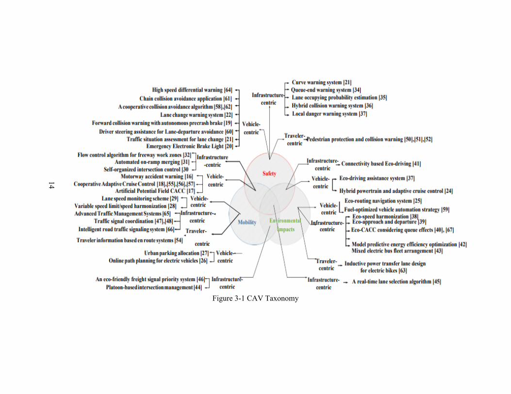
Interactions between the three performance-oriented MOEs can be represented

with a Venn diagram (Figure 1) that classifies CAV applications into infrastructure-

centric, traveler-centric, and vehicle-centric applications (Tian et al.). Environmental

impacts are not generally a priority when assessing the benefits of a countermeasure. A

good portion of Tian et al.’s study merely groups CAV applications into the categories

shown in the diagram.

14

Figure 3-1 CAV Taxonomy

15

With respect to Focusing on the infrastructure-centric CAV applications focused

on safety and mobility, it is probable urban locations will experience the greatest benefits.

Dedicated short range communications (DSRC) and similar CV technologies will play a

critical role by facilitating better intersection coordination. In decentralized locations,

sophisticated ramp-merging systems hold great promise for improving safety and mobility

by leveraging a distance decision algorithm and a fuzzy controller which use information

acquired from V2I technology. Similarly, a lane merging system derived from a flow

control algorithm lets CAVs better navigate work zones.

The MOE framework presented by Koopman and Fratrik (2019) contains four

dimensions: operational design domain (ODD), object and event detection and response

(OEDR), maneuvers, and fault management. ODD limits the operational needs of an

automated system by constraining the operational environment to a subset of all possible

situations. Examples include geometric road designs, environmental/weather conditions,

and infrastructure characteristics (e.g., traffic lights, signage). OEDR describes an

operation within a defined ODD — it generally refers to the proper handling of external

situations. Two subcategories fall under OEDR: object factors and event factors. Object

factors include static or dynamic obstacles (e.g., pedestrians, guardrail, trees) and the

system’s ability to detect them. Event factors account for the behaviors of object factors

as well as the system/operator’s interactions with them (i.e., the Haddon matrix described

in the HSM). Maneuvers are the actions taken to move from one point in space to another

while avoiding obstacles; they are typically guided by some form of navigation. Lastly,

fault management is a multilayered dimension of validation that includes system

limitations, which specify what the system is capable of; system faults, which detail system

16

errors; and fault responses, which is how the system manages and corrects errors

(Koopman and Fratrik 2019).

3.2 CAV Market penetration

The consensus among transportation researchers is that the magnitude of safety,

mobility, and environmental benefits realized through the adoption of CAV technologies

will be contingent upon how rapid and widespread their proliferation is (Bansal and

Kockelman 2017, Lavasani et al. 2016, Kalra and Groves 2017). But market penetration

is likely to be uneven in the US due to demographic variability. Purchasing vehicles

equipped with CAV technologies is a function of age, sex, income, population density,

health, and many other factors. While these technologies are gradually filtering into less

expensive vehicles, the most sophisticated CAV systems tend to be found on vehicles in

the high-end market segment. Additionally, the use of AVs — once they become available

— will probably vary by trip types and travel purposes (Bansal and Kockelman 2017).

Researchers have been turning more and more of their attention to the safety

implications of AVs. Because AVs are not currently available to consumers and are only

present in small numbers on roadways, models for estimating the safety benefits of these

vehicles are generally constructed using historical data on vehicle safety. For example, the

Rand Model of Autonomous Vehicle Safety (MAVS) estimates the safety benefits of AVs

by comparing the rate of market penetration to the time at which penetration begins. Market

penetration is thus a primary model input and is treated an assumed value that the user

inputs. The model suggests that introducing AVs to market sooner and more gradually will

yield greater safety benefits than delaying their introduction and ramping up production

and sales at a much faster pace (Kalra and Groves 2017).

17

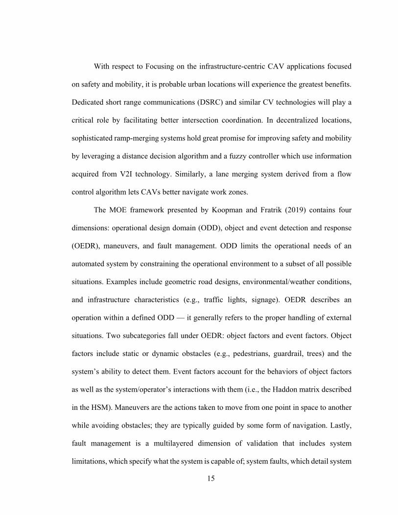
Figure 3-2 Rand MAVS

Estimating market penetration is difficult; the rate of adoption will ultimately be

influenced by the affordability and public acceptance of AV technologies. Statistically

analyzing population demographics is critical, as the likelihood of AV adoption varies by

age, income (and average vehicle cost/maintenance), and vehicle performance (Bansal and

Kockelman 2018). Although forecasting the rate at which fully autonomous vehicles will

penetrate the market is difficult, researchers are attempting to generate predications based

on the current availability of advanced driver assistance systems (ADAS) (Koopman

2017). Lavasani et al. (2016) developed a Bass diffusion model to analyze national market

trends in hybrid-electric vehicles and cell phones to derive parameters for an S-curve

model. (Lavasani et al. 2016).

18

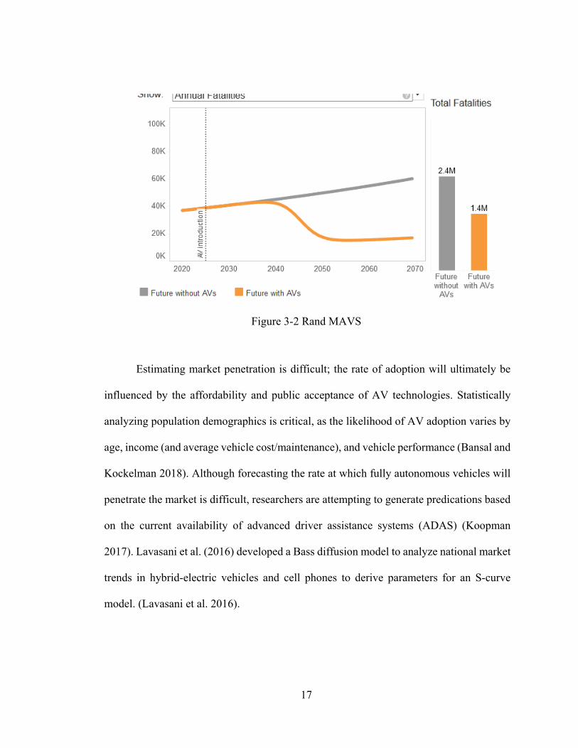
Figure 3-3 Bass Diffusion Market Penetration of CAVs

Figure 3-3 illustrates trends in the cumulative number of adopters predicted by Lavasani et

al.’s (2016) Bass diffusion model. Sales are expected to increase rapidly beginning in the

mid-2030s. The MAVS developed by Kalra and Groves (2017) used an interval regression

model to forecast market penetration several assumptions fill the gaps between an

estimated maximum and minimum adoption, one being that AVs are safer than humans

and that. Bansal and Kockelman (2018) adopted a similar approach but narrowed this

technique down to specific pieces of CAV technology to fill the gaps. This was done by

taking descriptive survey data from the state of Texas to develop various forecast scenarios.

Because CAV technologies are geared toward improving highway safety (NHTSA

2010), it is possible to infer engineering countermeasures will undergo transformations

based on the degree to which the public accepts individual components of technology.

Kockelman’s (2017) paper on long-term adoption of CAVs outlines many scenarios in

which the public will gradually accept the suite of technologies. Although broken down

19

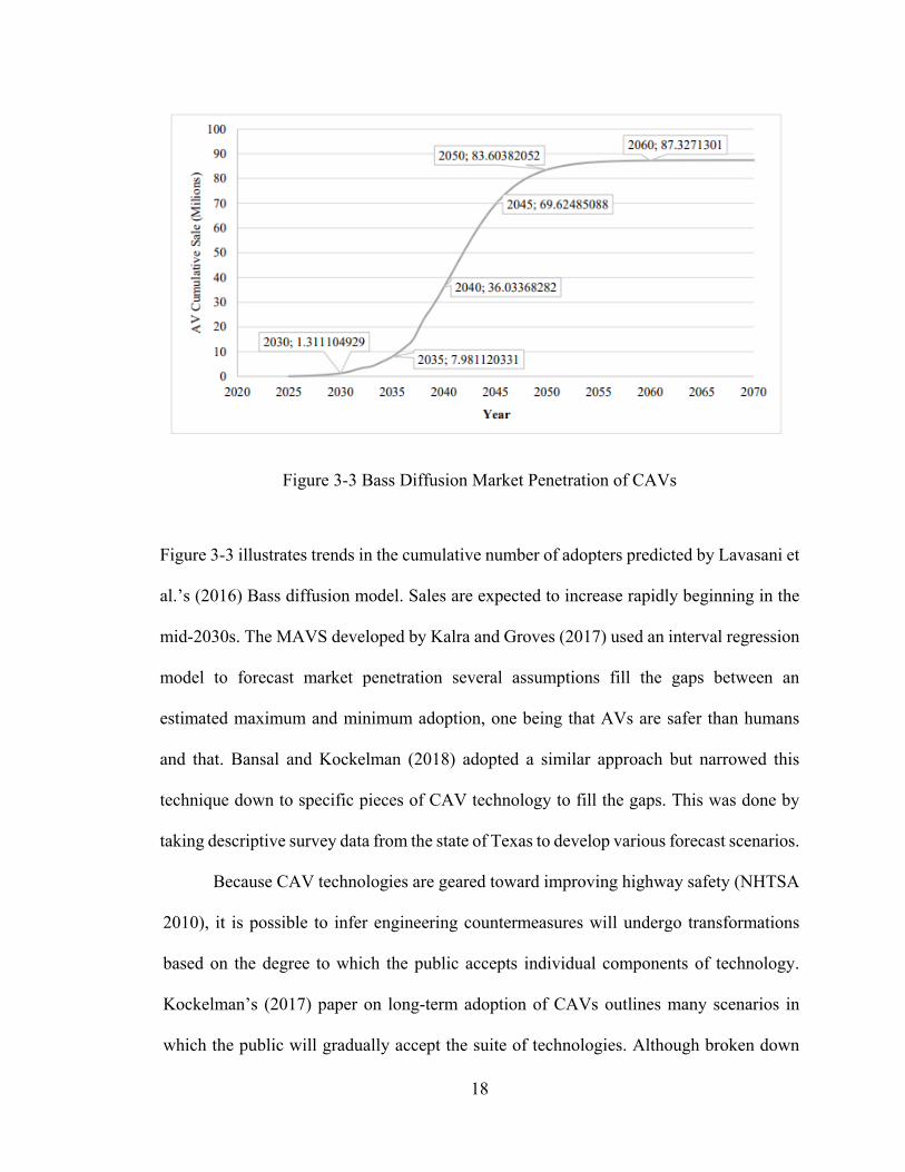
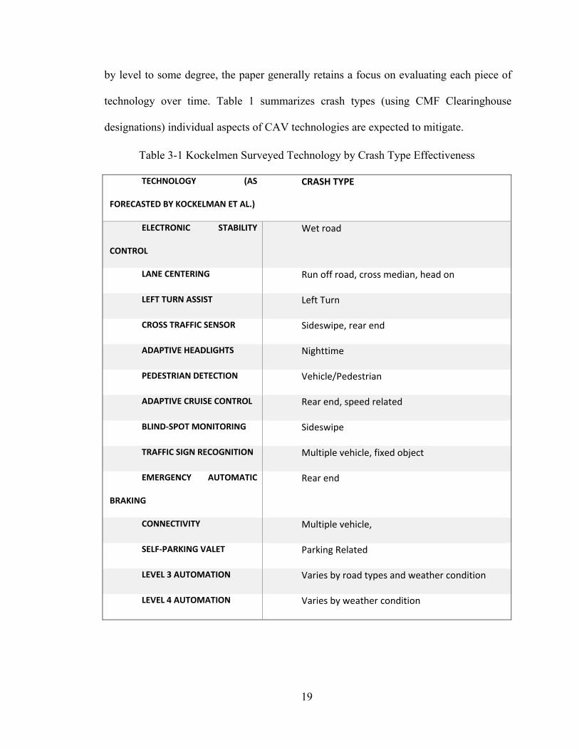
by level to some degree, the paper generally retains a focus on evaluating each piece of

technology over time. Table 1 summarizes crash types (using CMF Clearinghouse

designations) individual aspects of CAV technologies are expected to mitigate.

Table 3-1 Kockelmen Surveyed Technology by Crash Type Effectiveness

TECHNOLOGY (AS

FORECASTED BY KOCKELMAN ET AL.)

CRASH TYPE

ELECTRONIC STABILITY

CONTROL

Wet road

LANE CENTERING Run off road, cross median, head on

LEFT TURN ASSIST Left Turn

CROSS TRAFFIC SENSOR Sideswipe, rear end

ADAPTIVE HEADLIGHTS Nighttime

PEDESTRIAN DETECTION Vehicle/Pedestrian

ADAPTIVE CRUISE CONTROL Rear end, speed related

BLIND-SPOT MONITORING Sideswipe

TRAFFIC SIGN RECOGNITION Multiple vehicle, fixed object

EMERGENCY AUTOMATIC

BRAKING

Rear end

CONNECTIVITY Multiple vehicle,

SELF-PARKING VALET Parking Related

LEVEL 3 AUTOMATION Varies by road types and weather condition

LEVEL 4 AUTOMATION Varies by weather condition

20

Kockelman forecasted market penetration by projecting the public’s willingness to

pay (WTP) for each type of technology over time. Baseline WTP data were collected using

a national survey. A multinomial logit model was developed to project future WTP for

multiple scenarios. Bansal and Kockelman (2018) later developed another model for the

state of Texas, utilizing data collected from a large-scale survey.

3.3 A Tool for Estimating Safety in a CAV Mixed Fleet

Knowing that the effects of countermeasures will change over time as CAVs

become more numerous, it is important to have a reliable forecasting tool to evaluate the

benefits of countermeasures under as CAVs proliferate. This section describes the data-

driven. UK’s data driven Safety Assessment for Connected Autonomous Transportation

(ddSAFCAT) breaks down the safety benefit by specific levels of autonomy and facility

type in which each level is effective. The Society of Automotive Engineers (SAE) has

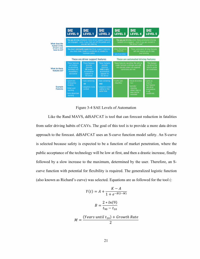
developed a system to classify different levels of automation. Figure 3-4 SAE Levels of

Automation summarizes the main features of vehicles in each category. Level 2

technologies (e.g., lane assist, self-parking) are currently available — although they are

most often seen on pricier vehicles. While vehicles with more advanced automation are in

testing, it is unclear when consumers will be able to purchase them. Upon their initial

release, it is probable that vehicles with Levels 3–5 automations will add $10,000 to the

price of a vehicle, narrowing the window of consumers able to afford them. As prices fall,

it is reasonable to presume AVs will become more ubiquitous, but it remains unclear when

vehicles with high levels of automation will make up a significant proportion of vehicles

on US roadways.

21

Figure 3-4 SAE Levels of Automation

Like the Rand MAVS, ddSAFCAT is tool that can forecast reduction in fatalities

from safer driving habits of CAVs. The goal of this tool is to provide a more data driven

approach to the forecast. ddSAFCAT uses an S-curve function model safety. An S-curve

is selected because safety is expected to be a function of market penetration, where the

public acceptance of the technology will be low at first, and then a drastic increase, finally

followed by a slow increase to the maximum, determined by the user. Therefore, an S-

curve function with potential for flexibility is required. The generalized logistic function

(also known as Richard’s curve) was selected. Equations are as followed for the tool (:

𝑌𝑌(𝐸𝐸) = 𝐴𝐴 +𝐾𝐾 − 𝐴𝐴

1 + 𝐸𝐸−𝐵𝐵(𝑡𝑡−𝑀𝑀)

𝐵𝐵 =2 ∗ 𝑙𝑙𝐹𝐹(9)𝐸𝐸90 − 𝐸𝐸10

𝐶𝐶 =(𝑌𝑌𝐸𝐸𝐴𝐴𝐴𝐴𝐶𝐶 𝐹𝐹𝐹𝐹𝐸𝐸𝑤𝑤𝑙𝑙 𝐸𝐸10) + 𝐺𝐺𝐴𝐴𝐶𝐶𝑤𝑤𝐸𝐸ℎ 𝐶𝐶𝐴𝐴𝐸𝐸𝐸𝐸

2

22

Where Y(t), is the market penetration, A is the lower limit (user input), K is the upper

limit (user input), B is the growth rate, t represents the current year, M represents

the year of 50% market penetration, t90 is the time until market penetration reaches

90%, and t10 is the time until market penetration reaches 10%.

These equations are applied to each level of autonomy. There are 6 levels of

autonomy defined by the Society of Automotive Engineers (SAE) ranging from 0 to 5.

The values for Levels 5 and 0 control the market penetration for the rest of the tool

because level 5 vehicles are likely not to be replaced once deployed, and level 0s are

already on the roadway (there likely always be some number of non-automated

vehicles). The value in the second equation t90 - t10 represents the turnover rate of the

fleet which is about 15 years for the average automobile (though this is could change

from new technologies). In ddSAFCAT, these equations are used to calculate market

penetration of each level, then a series of if statements are in place such that

whenever a new level has sufficiently penetrated the market, the previous level will

decline.

The next step after establishing market penetration is to determine how effective

the vehicles will be at reducing crashes. The tool makes the assumption that automated

vehicles will be safer on the roadway than human drivers. Each level of autonomy will

have varying degrees of effectiveness. Level 5 vehicles are considered to be the most

effective at reducing crashes, and the effectiveness of a level 5 vehicle is determined by

how reliable its software is. Each other level is considered to be as effective as a level 5

vehicle when under the right conditions, and for eliminating certain crash types. Level 4

vehicles are considered to be as effective as level 5 vehicles when the weather conditions

23

are clear. A new level introduced into the tool, level 3.5, is considered to be effective for

all weather conditions, but only on certain roads. Levels 2 and 3 are only effective in clear

weather conditions on arterial roadways. And finally, level 1 vehicles are only as effective

as level 5 vehicles on arterial roadways, and when the human driver is not distracted and

using the vehicle’s features properly.

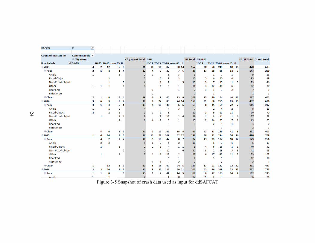
Crash data unique to Kentucky was then analyzed to account for the number of

crashes that happened in these conditions, the data was provided by the Kentucky

Transportation Center.

24

Figure 3-5 Snapshot of crash data used as input for ddSAFCAT

25

The above figure actually displays an excel pivot table to summarize the isolated

crash data. This was done for simplicity in creating the tool, as there are over 785,000

crash entries. Only fatal crashes were observed in the data. The table can be used to filter

out any crashes that occurred on major roads (US or interstate), as well as any crashes that

occurred in poor weather. Poor weather conditions are considered to be anything that is

not “clear.” Driver age may also be filtered out, though this has no input into the tool yet.

The data only contains of crashes from 2013 to 2017.

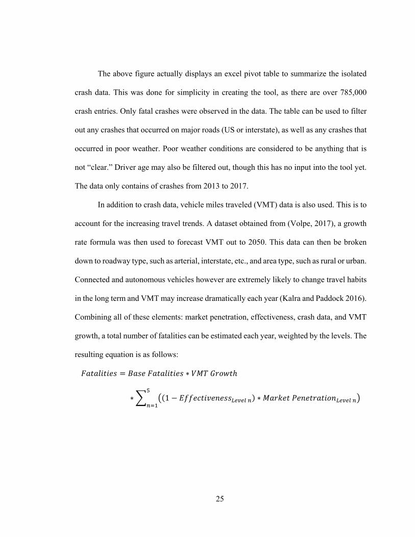
In addition to crash data, vehicle miles traveled (VMT) data is also used. This is to

account for the increasing travel trends. A dataset obtained from (Volpe, 2017), a growth

rate formula was then used to forecast VMT out to 2050. This data can then be broken

down to roadway type, such as arterial, interstate, etc., and area type, such as rural or urban.

Connected and autonomous vehicles however are extremely likely to change travel habits

in the long term and VMT may increase dramatically each year (Kalra and Paddock 2016).

Combining all of these elements: market penetration, effectiveness, crash data, and VMT

growth, a total number of fatalities can be estimated each year, weighted by the levels. The

resulting equation is as follows:

𝐶𝐶𝐴𝐴𝐸𝐸𝐴𝐴𝑙𝑙𝑤𝑤𝐸𝐸𝑤𝑤𝐸𝐸𝐶𝐶 = 𝐵𝐵𝐴𝐴𝐶𝐶𝐸𝐸 𝐶𝐶𝐴𝐴𝐸𝐸𝐴𝐴𝑙𝑙𝑤𝑤𝐸𝐸𝑤𝑤𝐸𝐸𝐶𝐶 ∗ 𝑉𝑉𝐶𝐶𝑉𝑉 𝐺𝐺𝐴𝐴𝐶𝐶𝑤𝑤𝐸𝐸ℎ

∗� �(1 − 𝐸𝐸𝐸𝐸𝐸𝐸𝐸𝐸𝐸𝐸𝐸𝐸𝑤𝑤𝐴𝐴𝐸𝐸𝐹𝐹𝐸𝐸𝐶𝐶𝐶𝐶𝐿𝐿𝐿𝐿𝐿𝐿𝐿𝐿𝐿𝐿 𝑛𝑛) ∗ 𝐶𝐶𝐴𝐴𝐴𝐴𝑀𝑀𝐸𝐸𝐸𝐸 𝑃𝑃𝐸𝐸𝐹𝐹𝐸𝐸𝐸𝐸𝐴𝐴𝐴𝐴𝐸𝐸𝑤𝑤𝐶𝐶𝐹𝐹𝐿𝐿𝐿𝐿𝐿𝐿𝐿𝐿𝐿𝐿 𝑛𝑛�5

𝑛𝑛=1

26

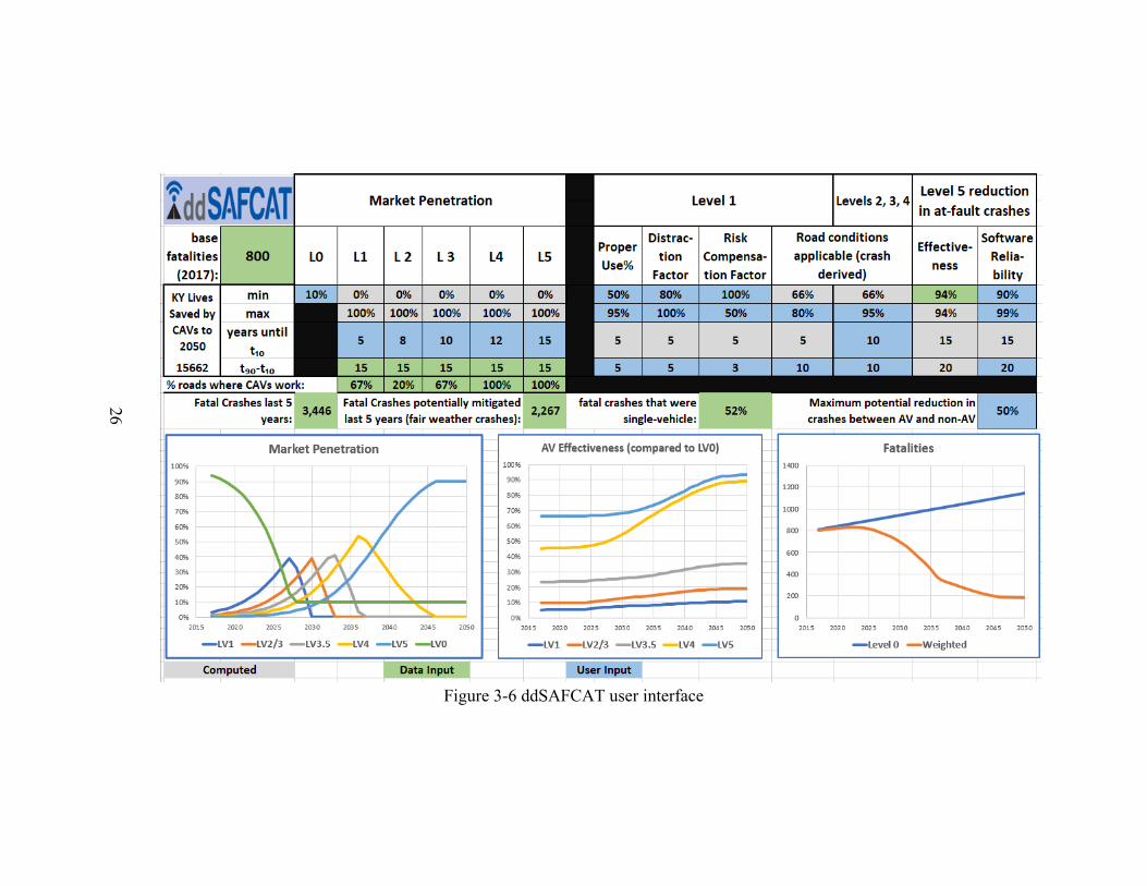
Figure 3-6 ddSAFCAT user interface

27

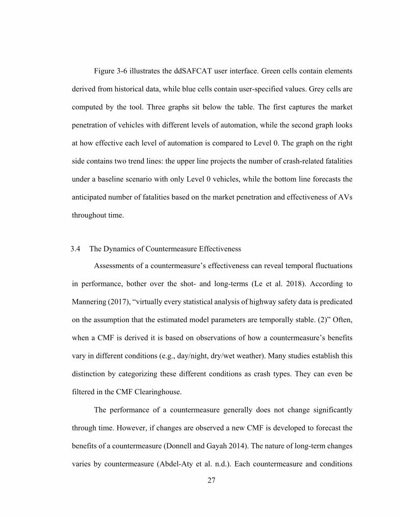
Figure 3-6 illustrates the ddSAFCAT user interface. Green cells contain elements

derived from historical data, while blue cells contain user-specified values. Grey cells are

computed by the tool. Three graphs sit below the table. The first captures the market

penetration of vehicles with different levels of automation, while the second graph looks

at how effective each level of automation is compared to Level 0. The graph on the right

side contains two trend lines: the upper line projects the number of crash-related fatalities

under a baseline scenario with only Level 0 vehicles, while the bottom line forecasts the

anticipated number of fatalities based on the market penetration and effectiveness of AVs

throughout time.

3.4 The Dynamics of Countermeasure Effectiveness

Assessments of a countermeasure’s effectiveness can reveal temporal fluctuations

in performance, bother over the shot- and long-terms (Le et al. 2018). According to

Mannering (2017), “virtually every statistical analysis of highway safety data is predicated

on the assumption that the estimated model parameters are temporally stable. (2)” Often,

when a CMF is derived it is based on observations of how a countermeasure’s benefits

vary in different conditions (e.g., day/night, dry/wet weather). Many studies establish this

distinction by categorizing these different conditions as crash types. They can even be

filtered in the CMF Clearinghouse.

The performance of a countermeasure generally does not change significantly

through time. However, if changes are observed a new CMF is developed to forecast the

benefits of a countermeasure (Donnell and Gayah 2014). The nature of long-term changes

varies by countermeasure (Abdel-Aty et al. n.d.). Each countermeasure and conditions

28

where they may change provides keen insight into how their respective CMFs can be

calculated. It is typical to examine the compound effect of all of these conditions where

countermeasures might be used and look these changes as a whole to simply examine an

overall forecast. Since many of these factors change over time, the many scenarios should

be observed separately and then compounded.

The charts presented in this section demonstrate possible trends in crash rates

following the introduction of a countermeasure. Each chart indicates crash rates before

installing a countermeasure (BCR) and crash rates following implantation (PCCR).

Vertical green lines delineate the point at which a countermeasure is adopted. Crash rates

are represented as wavy lines to indicate their stochastic nature. Over short periods of time

crash rates can fluctuate unpredictably. The charts are for illustrative purposes only, but

they do capture long-term trends in crash frequencies before and after the introduction of

a countermeasure.

Figure 3-7 Scenario 1: Countermeasure reduces overall Crash rates

29

Scenario 1 (Figure 3-7) depicts trends along a problematic roadway segment that

initially suffers from high crash rates. These frequencies oscillate over time, but on average

remain high. Introducing a countermeasure significantly lowers crash rates. Again, there

is natural variability in the rates, but on average they are much lower than prior to adoption

of the countermeasure.

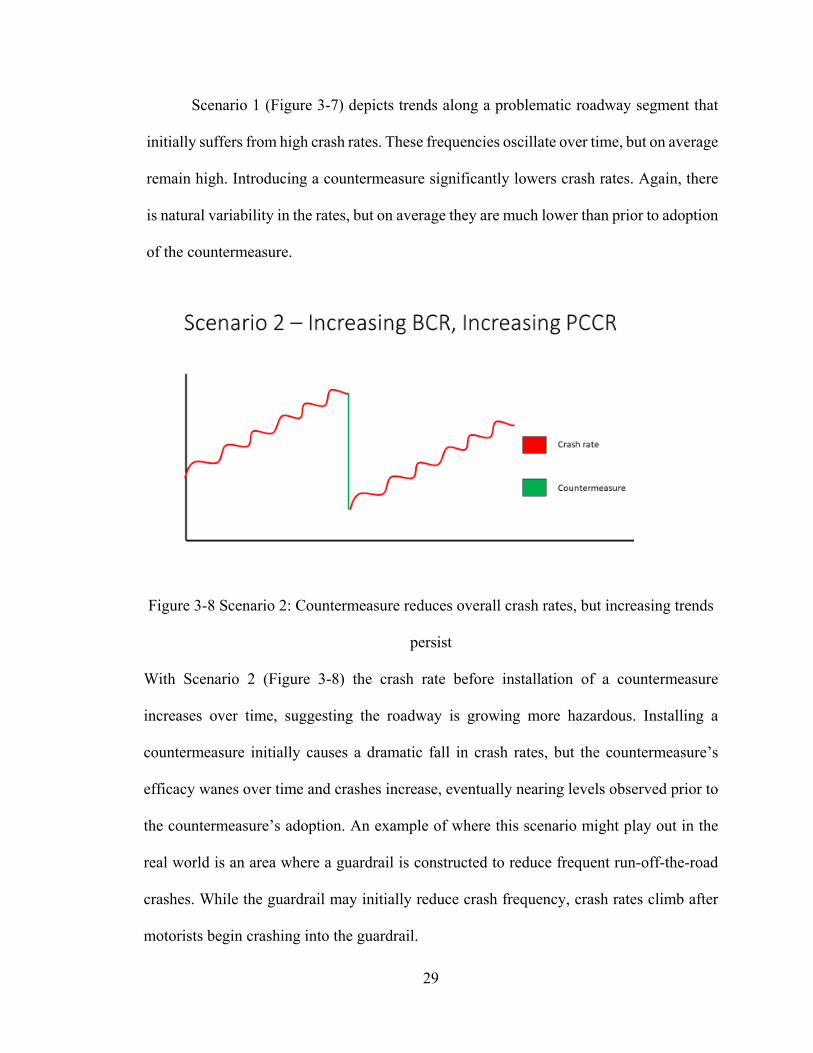
Figure 3-8 Scenario 2: Countermeasure reduces overall crash rates, but increasing trends

persist

With Scenario 2 (Figure 3-8) the crash rate before installation of a countermeasure

increases over time, suggesting the roadway is growing more hazardous. Installing a

countermeasure initially causes a dramatic fall in crash rates, but the countermeasure’s

efficacy wanes over time and crashes increase, eventually nearing levels observed prior to

the countermeasure’s adoption. An example of where this scenario might play out in the

real world is an area where a guardrail is constructed to reduce frequent run-off-the-road

crashes. While the guardrail may initially reduce crash frequency, crash rates climb after

motorists begin crashing into the guardrail.

30

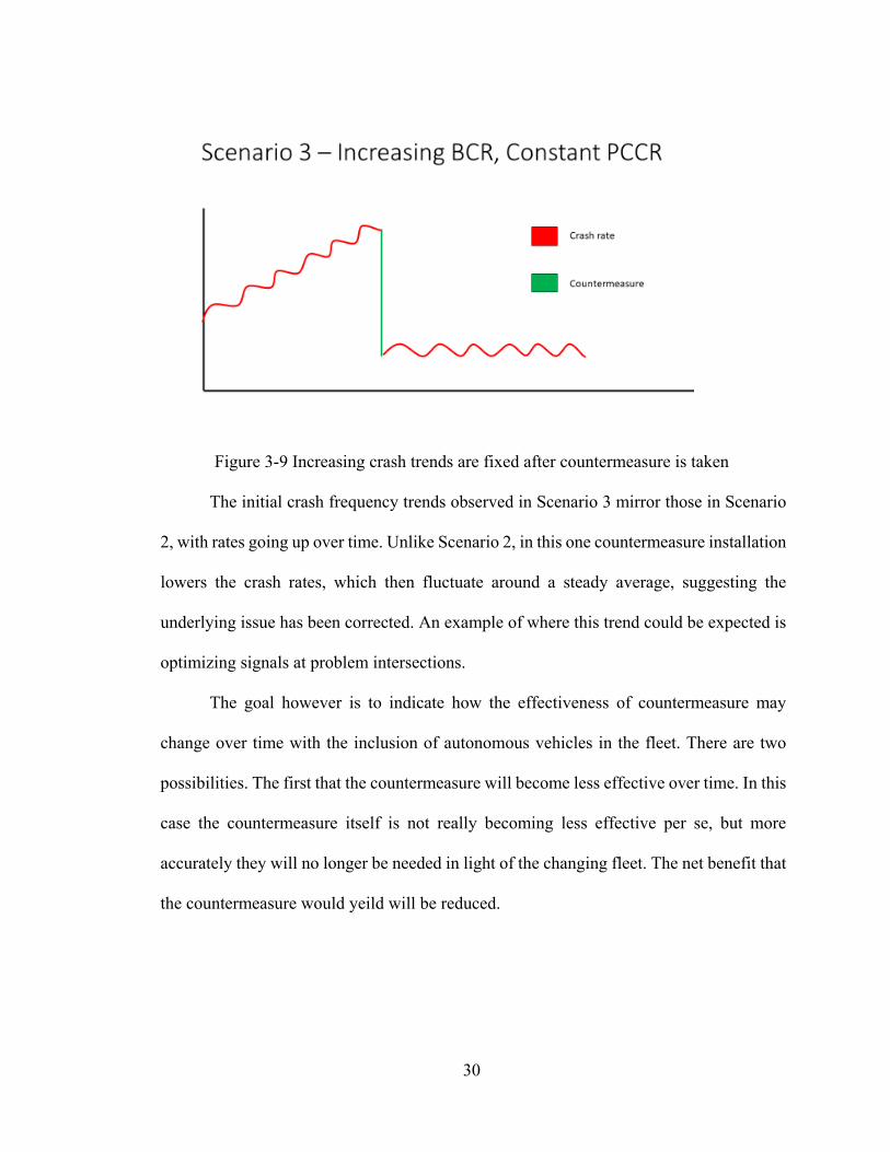
Figure 3-9 Increasing crash trends are fixed after countermeasure is taken

The initial crash frequency trends observed in Scenario 3 mirror those in Scenario

2, with rates going up over time. Unlike Scenario 2, in this one countermeasure installation

lowers the crash rates, which then fluctuate around a steady average, suggesting the

underlying issue has been corrected. An example of where this trend could be expected is

optimizing signals at problem intersections.

The goal however is to indicate how the effectiveness of countermeasure may

change over time with the inclusion of autonomous vehicles in the fleet. There are two

possibilities. The first that the countermeasure will become less effective over time. In this

case the countermeasure itself is not really becoming less effective per se, but more

accurately they will no longer be needed in light of the changing fleet. The net benefit that

the countermeasure would yeild will be reduced.

31

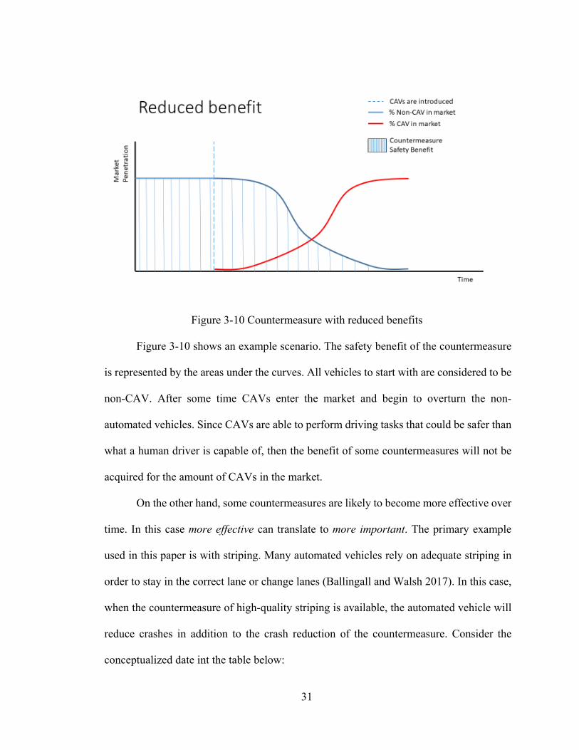
Figure 3-10 Countermeasure with reduced benefits

Figure 3-10 shows an example scenario. The safety benefit of the countermeasure

is represented by the areas under the curves. All vehicles to start with are considered to be

non-CAV. After some time CAVs enter the market and begin to overturn the non-

automated vehicles. Since CAVs are able to perform driving tasks that could be safer than

what a human driver is capable of, then the benefit of some countermeasures will not be

acquired for the amount of CAVs in the market.

On the other hand, some countermeasures are likely to become more effective over

time. In this case more effective can translate to more important. The primary example

used in this paper is with striping. Many automated vehicles rely on adequate striping in

order to stay in the correct lane or change lanes (Ballingall and Walsh 2017). In this case,

when the countermeasure of high-quality striping is available, the automated vehicle will

reduce crashes in addition to the crash reduction of the countermeasure. Consider the

conceptualized date int the table below:

32

Table 3-2 Sample CMFs for striping

POOR MEDIUM GOOD

LEVEL 0 100 90 80

LEVEL 1&2 94 84 74

LEVEL 3 88 78 68

LEVEL 3.5 82 72 62

LEVEL 4 76 66 56

LEVEL 5 70 60 50

The table chows several CMFs expressed as a percentage. Three scenarios are

considered for the case of striping. There is poor, medium, and good quality of striping.

Each level of autonomy is reducing the CMF of the striping quality by some amount. As

the quality of striping improves, the CMF is reduced even further. The values from the

table can be expressed in the form of a chart:

Figure 3-11 CMF Decline by level of autonomy and Striping quality.

10090

80

9484

74

8878

68

8272

62

7666

56

7060

50

0

20

40

60

80

100

120

Poor Medium Good

CMF

Countermeasure Effectiveness

Level 0 Level 1&2 Level 3 Level 3.5 Level 4 Level 5

33

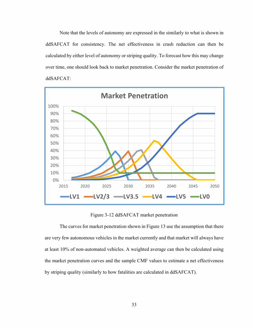
Note that the levels of autonomy are expressed in the similarly to what is shown in

ddSAFCAT for consistency. The net effectiveness in crash reduction can then be

calculated by either level of autonomy or striping quality. To forecast how this may change

over time, one should look back to market penetration. Consider the market penetration of

ddSAFCAT:

Figure 3-12 ddSAFCAT market penetration

The curves for market penetration shown in Figure 13 use the assumption that there

are very few autonomous vehicles in the market currently and that market will always have

at least 10% of non-automated vehicles. A weighted average can then be calculated using

the market penetration curves and the sample CMF values to estimate a net effectiveness

by striping quality (similarly to how fatalities are calculated in ddSAFCAT).

0%10%20%30%40%50%60%70%80%90%

100%

2015 2020 2025 2030 2035 2040 2045 2050

Market Penetration

LV1 LV2/3 LV3.5 LV4 LV5 LV0

34

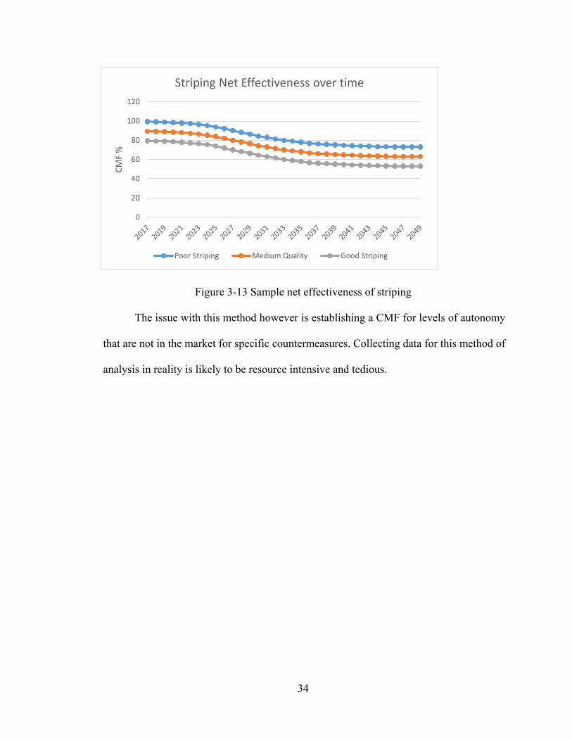
Figure 3-13 Sample net effectiveness of striping

The issue with this method however is establishing a CMF for levels of autonomy

that are not in the market for specific countermeasures. Collecting data for this method of

analysis in reality is likely to be resource intensive and tedious.

0

20

40

60

80

100

120

CMF

%

Striping Net Effectiveness over time

Poor Striping Medium Quality Good Striping

35

CHAPTER 4. CASE STUDIES

4.1 Introduction: Using ddSAFCAT to Adapt Countermeasure CMFs

Determining how CMFs should be adjusted to account for the influence of CAVs

is challenging. Most of the promised safety benefits of CAVs will fail to materialize unless

the infrastructure is there to support their presence on roadways (e.g., adequate striping

and lighting). Tools like ddSAFCAT can be used to guide decisions in infrastructure

investments.

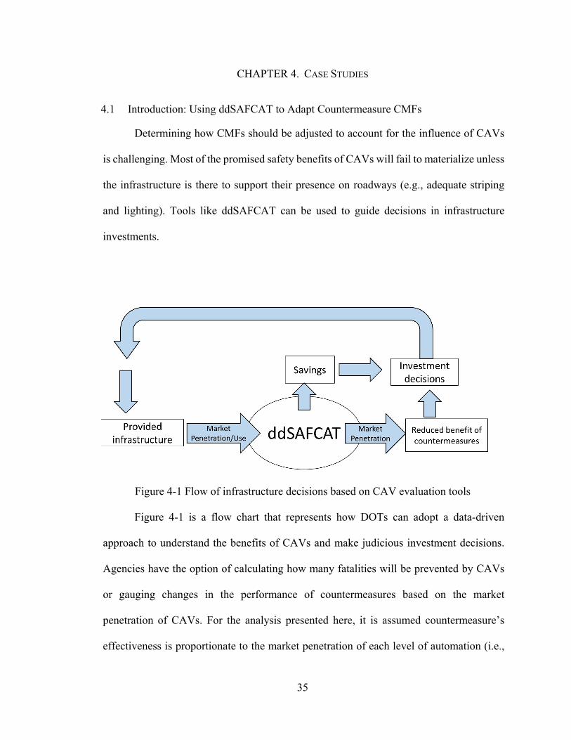
Figure 4-1 Flow of infrastructure decisions based on CAV evaluation tools

Figure 4-1 is a flow chart that represents how DOTs can adopt a data-driven

approach to understand the benefits of CAVs and make judicious investment decisions.

Agencies have the option of calculating how many fatalities will be prevented by CAVs

or gauging changes in the performance of countermeasures based on the market

penetration of CAVs. For the analysis presented here, it is assumed countermeasure’s

effectiveness is proportionate to the market penetration of each level of automation (i.e.,

36

SAE Levels 0–5), similar to how other researchers have tied future safety benefits to

market penetration.

4.2 Case 1: Reduced Benefit Countermeasures

For most countermeasures that have a single CMF, adjustments to the CMF depend

on the proliferation of CAVs. Given the familiarity with the ddSAFCAT model, a

countermeasure that is expected to be to become less effective over time will follow the

same trends as the tool’s market penetration equations. The model multiplies the

percentage of automated vehicles in the market by the CMF (i.e., the number of crashes

reduced). A search of the CMF Clearinghouse returns 700 results for rumble strips. Most

of these exclusively address mitigation of run-off-road crashes. It is likely that fewer

vehicles will run off the road as more vehicles with higher levels of automation are

incorporated into existing fleets, because human reactions and decision making, which

may result in a vehicle being steered off a road, will be progressively eliminated from

driving. As such, rumble strips are likely to become less critical for maintaining highway

safety, and their effectiveness — as measured using a CMF — will decline.

As more AVs increasingly populate the roads, CMFs for rumble strip treatments

will also increase. This is not to suggest the installation of rumble strips will increase

crashes — a CMF for rumble strips will never exceed 1.0. A basic example will clarify

this dynamic. Suppose the CMF for a particular rumble strip treatment is currently 0.85.

This indicates that installing a rumble strip will lower crash rates by 15 percent. With a

different vehicle fleet composition, one that includes more vehicles with varying levels of

automation, that CMF is recalculated for the rumble strip and it increases to 0.95,

suggesting that rumble strip installation will reduce crash rates by 5 percent. What this

37

information tells a practitioner is that the expected benefits of rumble strip installation are

lower under when a greater share of the vehicle fleet is automated, potentially leading

agency personnel to conclude investments should be directed toward safety treatments that

will yield greater benefits. The problem is not that the rumble strips no longer performs its

intended function. What is at issue is that fewer vehicles will benefit from the rumble

strip’s function because they have automated systems designed to prevent them from

departing the roadway. And the successful operation of those systems does not hinge on

whether a rumble strip is present.

The bounds for these changes are kept in check through a short series of if-

statements. When plotting the CMF over time, it will likely assume the shape of an S-

curve, mirroring market penetration. The basic equation for each level and each year is:

𝐶𝐶𝐶𝐶𝐶𝐶𝑁𝑁𝐿𝐿𝑁𝑁 = �1 + 𝐶𝐶𝑃𝑃𝐵𝐵𝐵𝐵 𝐿𝐿𝐿𝐿𝐿𝐿𝐿𝐿𝐿𝐿� ∗ 𝐶𝐶𝐶𝐶𝐶𝐶𝑜𝑜𝐿𝐿𝑜𝑜

This equation will only be applied to the levels where the countermeasure will lose

effect over time (levels 3, 4 and 5).

38

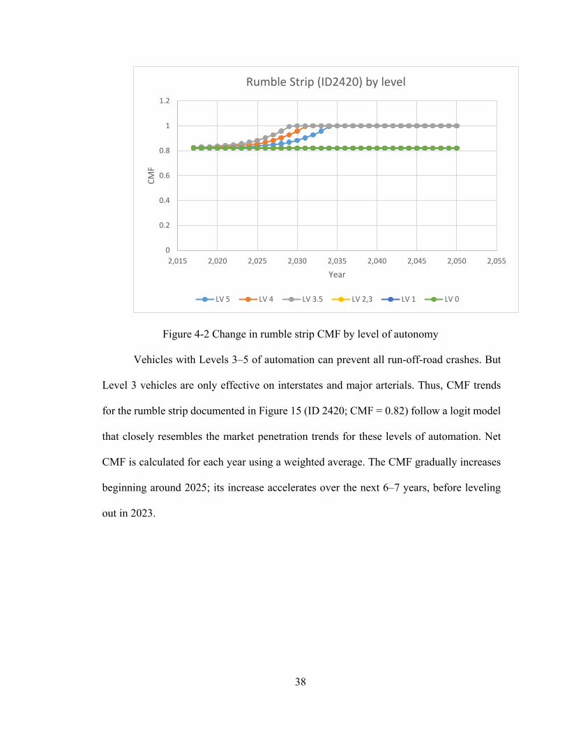
Figure 4-2 Change in rumble strip CMF by level of autonomy

Vehicles with Levels 3–5 of automation can prevent all run-off-road crashes. But

Level 3 vehicles are only effective on interstates and major arterials. Thus, CMF trends

for the rumble strip documented in Figure 15 (ID 2420; CMF = 0.82) follow a logit model

that closely resembles the market penetration trends for these levels of automation. Net

CMF is calculated for each year using a weighted average. The CMF gradually increases

beginning around 2025; its increase accelerates over the next 6–7 years, before leveling

out in 2023.

0

0.2

0.4

0.6

0.8

1

1.2

2,015 2,020 2,025 2,030 2,035 2,040 2,045 2,050 2,055

CMF

Year

Rumble Strip (ID2420) by level

LV 5 LV 4 LV 3.5 LV 2,3 LV 1 LV 0

39

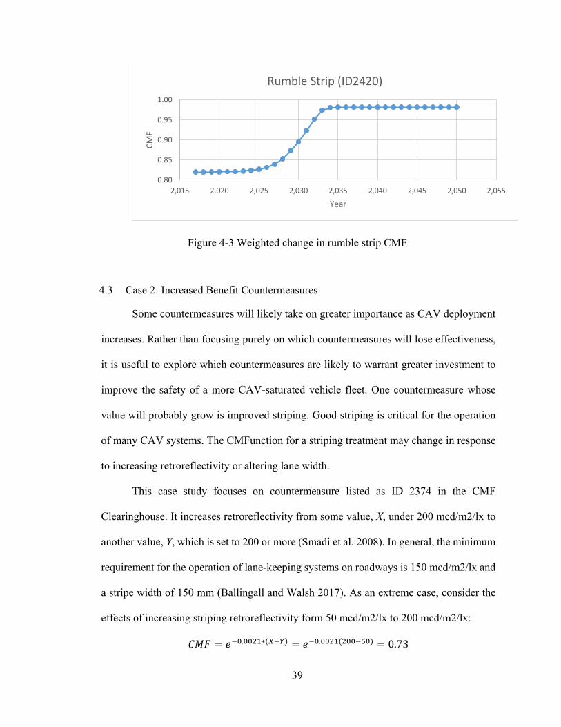
Figure 4-3 Weighted change in rumble strip CMF

4.3 Case 2: Increased Benefit Countermeasures

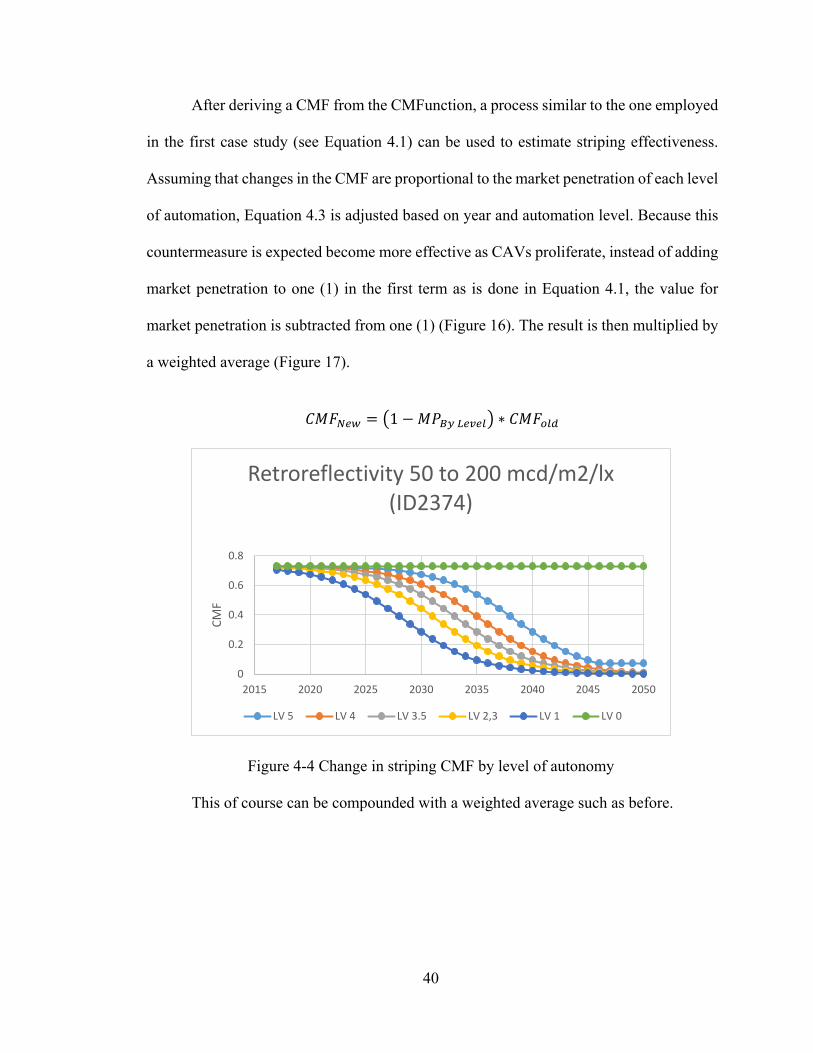
Some countermeasures will likely take on greater importance as CAV deployment

increases. Rather than focusing purely on which countermeasures will lose effectiveness,

it is useful to explore which countermeasures are likely to warrant greater investment to

improve the safety of a more CAV-saturated vehicle fleet. One countermeasure whose

value will probably grow is improved striping. Good striping is critical for the operation

of many CAV systems. The CMFunction for a striping treatment may change in response

to increasing retroreflectivity or altering lane width.

This case study focuses on countermeasure listed as ID 2374 in the CMF

Clearinghouse. It increases retroreflectivity from some value, X, under 200 mcd/m2/lx to

another value, Y, which is set to 200 or more (Smadi et al. 2008). In general, the minimum

requirement for the operation of lane-keeping systems on roadways is 150 mcd/m2/lx and

a stripe width of 150 mm (Ballingall and Walsh 2017). As an extreme case, consider the

effects of increasing striping retroreflectivity form 50 mcd/m2/lx to 200 mcd/m2/lx:

𝐶𝐶𝐶𝐶𝐶𝐶 = 𝐸𝐸−0.0021∗(𝑋𝑋−𝑌𝑌) = 𝐸𝐸−0.0021(200−50) = 0.73

0.80

0.85

0.90

0.95

1.00

2,015 2,020 2,025 2,030 2,035 2,040 2,045 2,050 2,055

CMF

Year

Rumble Strip (ID2420)

40

After deriving a CMF from the CMFunction, a process similar to the one employed

in the first case study (see Equation 4.1) can be used to estimate striping effectiveness.

Assuming that changes in the CMF are proportional to the market penetration of each level

of automation, Equation 4.3 is adjusted based on year and automation level. Because this

countermeasure is expected become more effective as CAVs proliferate, instead of adding

market penetration to one (1) in the first term as is done in Equation 4.1, the value for

market penetration is subtracted from one (1) (Figure 16). The result is then multiplied by

a weighted average (Figure 17).

𝐶𝐶𝐶𝐶𝐶𝐶𝑁𝑁𝐿𝐿𝑁𝑁 = �1 −𝐶𝐶𝑃𝑃𝐵𝐵𝐵𝐵 𝐿𝐿𝐿𝐿𝐿𝐿𝐿𝐿𝐿𝐿� ∗ 𝐶𝐶𝐶𝐶𝐶𝐶𝑜𝑜𝐿𝐿𝑜𝑜

Figure 4-4 Change in striping CMF by level of autonomy

This of course can be compounded with a weighted average such as before.

0

0.2

0.4

0.6

0.8

2015 2020 2025 2030 2035 2040 2045 2050

CMF

Retroreflectivity 50 to 200 mcd/m2/lx (ID2374)

LV 5 LV 4 LV 3.5 LV 2,3 LV 1 LV 0

41

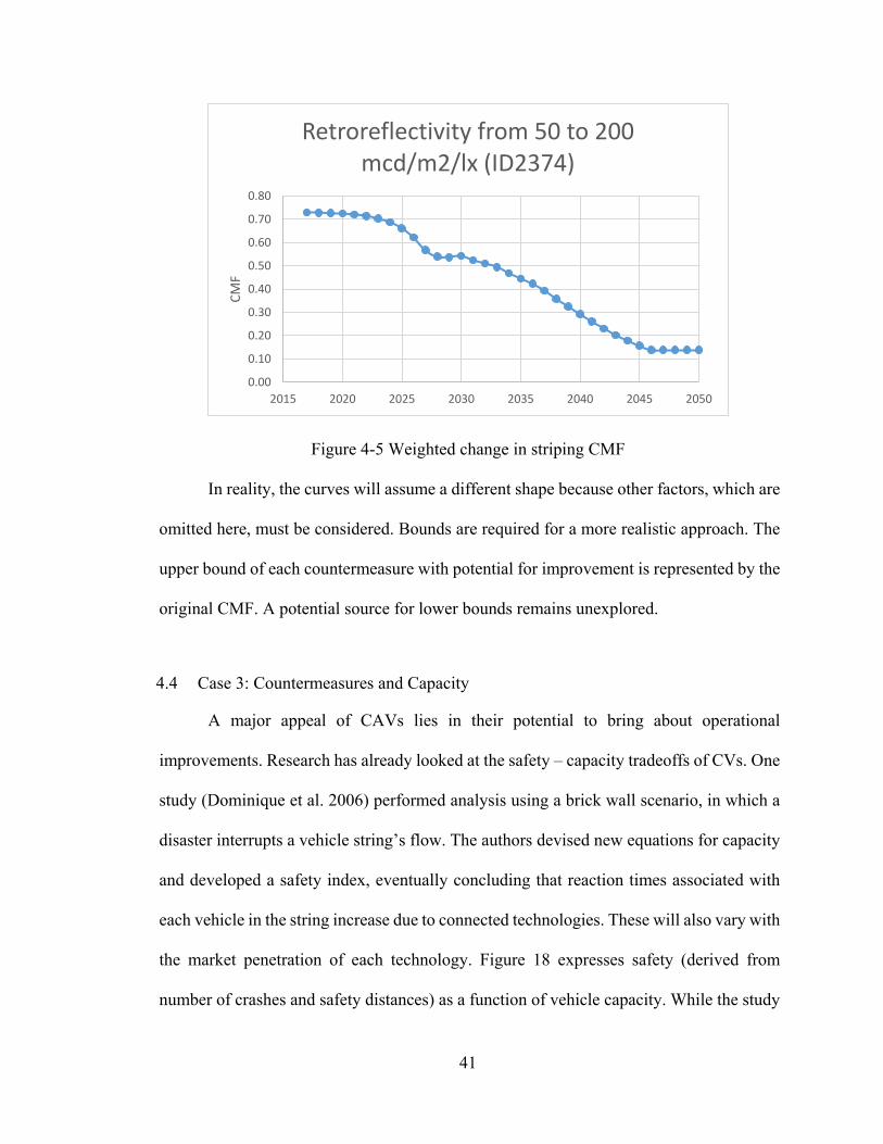
Figure 4-5 Weighted change in striping CMF

In reality, the curves will assume a different shape because other factors, which are

omitted here, must be considered. Bounds are required for a more realistic approach. The

upper bound of each countermeasure with potential for improvement is represented by the

original CMF. A potential source for lower bounds remains unexplored.

4.4 Case 3: Countermeasures and Capacity

A major appeal of CAVs lies in their potential to bring about operational

improvements. Research has already looked at the safety – capacity tradeoffs of CVs. One

study (Dominique et al. 2006) performed analysis using a brick wall scenario, in which a

disaster interrupts a vehicle string’s flow. The authors devised new equations for capacity

and developed a safety index, eventually concluding that reaction times associated with

each vehicle in the string increase due to connected technologies. These will also vary with

the market penetration of each technology. Figure 18 expresses safety (derived from

number of crashes and safety distances) as a function of vehicle capacity. While the study

0.00

0.10

0.20

0.30

0.40

0.50

0.60

0.70

0.80

2015 2020 2025 2030 2035 2040 2045 2050

CMF

Retroreflectivity from 50 to 200 mcd/m2/lx (ID2374)

42

considered equations of both the Highway Capacity Manual (HCM) and the HSM, it does

not discuss specific countermeasures or infrastructure.

Figure 4-6 Safety-capacity tradeoff of CV technology

In the first two case studies, the countermeasures (rumble strips, striping) will not

directly affect highway capacity. Some countermeasures, such as modifying lane width or

sped limits, can influence highway capacity. Examples of countermeasures that could

affect highway capacity can be deduced by examining a standard capacity equation from

the HCM:

Basic freeway Segment (HCM Equation 12-6)

𝐸𝐸 = 2200 + 10 ∗ (𝐶𝐶𝐶𝐶𝑆𝑆𝑎𝑎𝑜𝑜𝑎𝑎 − 50)

Multilane Highway Segment (HCM Equation 12-7)

43

𝐸𝐸 = 1900 + 20 ∗ (𝐶𝐶𝐶𝐶𝑆𝑆𝑎𝑎𝑜𝑜𝑎𝑎 − 45)

Where, (Equations 12-3 and 12-5 in HCM)

𝐶𝐶𝐶𝐶𝑆𝑆𝑎𝑎𝑜𝑜𝑎𝑎 = 𝐶𝐶𝐶𝐶𝑆𝑆 ∗ 𝑆𝑆𝐴𝐴𝐶𝐶 = (𝐵𝐵𝐶𝐶𝐶𝐶𝑆𝑆 − 𝐸𝐸𝐿𝐿𝑁𝑁 − 𝐸𝐸𝑇𝑇𝐿𝐿𝑇𝑇 − 𝐸𝐸𝑀𝑀 − 𝐸𝐸𝐴𝐴) ∗ 𝑆𝑆𝐴𝐴𝐶𝐶

and where: c = capacity and is a function of an adjusted free flow speed. FFS = free flow speed FFSadj = adjusted free flow speed BFFS = base free flow speed SAF = speed adjustment factor fLW = lane width adjustment factor fTLC = lateral clearance adjustment factor fM = median type adjustment factor fA = access point density adjustment factor

The SAF is usually selected from a list of default values in HCM Exhibit 11-21.

The CMF Clearinghouse includes countermeasures with each variable of these capacity

equations. While these countermeasures may not significantly impact safety in the context

of CAV proliferation, when a greater share of vehicles on roadways are CAVs they may

influence capacity. Consider the countermeasures for decreasing lane width, for which

many CMFs have been developed. Most are expressed as a CMFunction. Reducing lane

width tends to increase the frequency of run-off-road crashes (Gross et al. 2009). However,

crashes overall may decrease by encouraging more careful driving habits (Abdel-Aty et al.

n.d.). With respect to capacity, free flow speeds will decline as lane width shrinks. This is

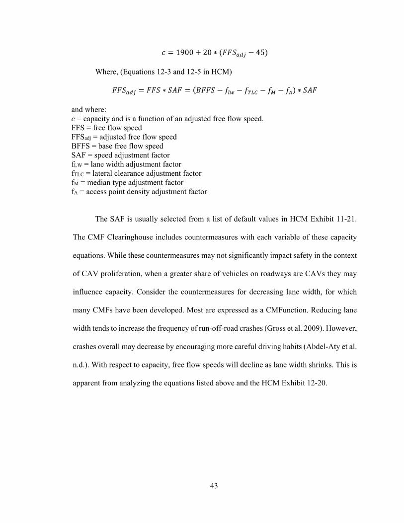
apparent from analyzing the equations listed above and the HCM Exhibit 12-20.

44

Table 4-1 HCM Exhibit 12-20

AVERAGE LANE WIDTH (FT) REDUCTION IN FFS, 𝒇𝒇𝒍𝒍𝒍𝒍 (mi/hr)

≥ 𝟏𝟏𝟏𝟏 0.0

≥ 𝟏𝟏𝟏𝟏 − 𝟏𝟏𝟏𝟏 1.9

≥ 𝟏𝟏𝟏𝟏 − 𝟏𝟏𝟏𝟏 6.6

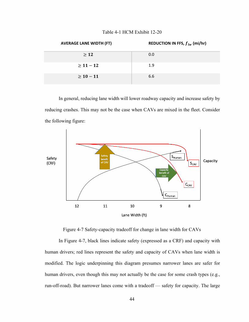
In general, reducing lane width will lower roadway capacity and increase safety by

reducing crashes. This may not be the case when CAVs are mixed in the fleet. Consider

the following figure:

Figure 4-7 Safety-capacity tradeoff for change in lane width for CAVs

In Figure 4-7, black lines indicate safety (expressed as a CRF) and capacity with

human drivers; red lines represent the safety and capacity of CAVs when lane width is

modified. The logic underpinning this diagram presumes narrower lanes are safer for

human drivers, even though this may not actually be the case for some crash types (e.g.,

run-off-road). But narrower lanes come with a tradeoff — safety for capacity. The large

45

arrows indicate the potential benefits (safety and capacity) of CAVs. The CRF for reducing

lane width likely will not change (see Section 4.2). Instead it will be flat, until some width

is reached at which a CAV cannot function properly. Thus, narrower lanes reduce the

safety benefit of CAVs. Capacity benefits trend in the opposite directions, with narrower

lanes yielding a greater benefit.

46

CHAPTER 5. CONCLUSIONS

5.1 Summary

This document opened with a review of SPFs, which are equations used to predict

the average number of crashes each year at a given location. To account for the effects of

installing a countermeasure, SPFs are multiplied by a CMF. Agencies can select from

many countermeasures, and often a single treatment will have several associated CMFs

because the context into which a countermeasure is introduced influences its performance.

Many DOTs compile countermeasures or CMFs into short lists that contain those they use

most frequently. While abundant evidence attests to the benefits of countermeasures and

the utility of CMFs for measuring their impacts on safety, with CAVs likely to proliferate

in the next 20 to 30 years, agencies will need to rethink their approaches to

countermeasures and identify those which are most likely to bring about the greatest safety

benefits as CAVs are gradually integrated into vehicle fleets. Because CMFs are not

tailored to estimate the implications of CAVs for the efficacy of various countermeasures,

they will require modifications as well.

Researchers have catalogued many safety and operational benefits of CAVs.

Typically, these benefits are analyzed using an MOE framework. Studies using MOE

frameworks have routinely cited improved highway safety as a key virtue of CAVs.

However, the magnitude of CAV safety benefits will be proportional to their market

penetration. Most researchers have conceptualized market penetration as following an S-

shaped curve. Building from previous work, a safety forecasting tool — ddSAFCAT —

was presented. It was used to evaluate the future benefits of AVs according to level

47

automation by leveraging Kentucky crash data, VMT data, and CAV crash statistics.

Currently, the tool expresses benefits as a total reduction in fatalities.

ddSAFCAT was then used to investigate how the effectiveness of countermeasures

(rumble strips, striping, adjustments to lane widths) will change as more CAVs get added

into the vehicle fleet. The underlying assumption of ddSAFCAT is that increases or

decreases in safety benefits are proportional CAV market penetration. For example, while

rumble strips might grow less effective over time, because automation systems do not rely

on them to keep a vehicle on the road, the importance and effectiveness of striping will

increase because those same systems require highly visible pavement markings to navigate

roadways. Other countermeasures, such as adjustments to lane width, have the potential to

affect capacity. Evaluating these countermeasures requires an approach rooted in the

HCM’s capacity equations, which can be used to estimate the safety-capacity tradeoff.

5.2 Limitations

ddSAFCAT has several limitations, most of which pertain to its assumed inputs.

Although a model for market penetration was developed, current market data for CAVs

are difficult to obtain and therefore incomplete or potentially unreliable. However, because

the aim of this research was to establish a framework for analyzing CMFs in light of CAV

proliferation, making assumptions was inevitable. As more empirical data on CAVs and

the effectiveness of countermeasures in mixed vehicle fleets become available, the tool

can be refined. Given the myriad countermeasures DOTs can select from, in examining

just three this research only scratched the surface, and many more unique scenarios and

idiosyncrasies remain to explore.

48

5.3 Future Work and Next Steps

The main deliverable of this thesis is to provide a framework of analysis for

countermeasures in the presence of CAVs. This framework needs to be developed further

to proper analysis and evaluation of countermeasures with more data. Work should

continue on ddSAFCAT. Developing and then implementing a method to incorporate more

data into the model will improve its forecasts. One strategy is to rework the equations and

inputs for market penetration by following approaches similar to Zhao and Kockelman

(2017) or Lavasani et al. (2016) — one requires data collection through extensive

surveying, the other mines purchasing data on CAV-related technologies. Surveys are

time-consuming and resource-intensive endeavors, while data mining is more feasible and

economical. Accordingly, the next recommended step is to forecast CAV market

penetration with the Bass diffusion model, rather than the S-curve ddSAFCAT currently

uses, to eliminate assumed values for market penetration. Some historical precedent could

be examined to better inform these forecasts, or perhaps the forecasts of specific

countermeasure. Historically, manufacturers have also made substantial changes to safety

(e.g. seatbelts, antilock brakes, airbags, etc.). Using the experience from these past

innovations, a better forecast could be obtained.

ddSAFCAT should also be equipped with a full list of countermeasures to

facilitate their direct evaluation. Lists of countermeasures are available for download in

the CMF Clearinghouse, however, some are likely to require different treatment from

those evaluated as part of this research. Also, CMFunctions are not included in this

download and cannot be filtered out in the Clearinghouse; each CMFunction is unique as

well. Therefore, CMFunctions must be handled differently when used as an input into

analytical tools. A potentially useful course of action is to create a separate database

49

dedicated to CMFunctions, which can be used in analysis. Once a full list is developed

and implemented into the tool, a fatality analysis could be performed with the

intervention of countermeasure rather than the actual change in the CMF.

It is likely necessary to develop new CMFs for each technology type to allow for

an improved analysis of Countermeasures with increased benefit as seen in section 3.4.

While an assumption was made that vehicles of higher levels of autonomy will still

reduce crashes in the presence of lower quality countermeasure conditions, actual data is

required to confirm this assumption. These lower quality countermeasures could in fact

cause more crashes since the infrastructure may not be capable of supporting the

necessary technology. This could potentially be challenging as it requires collecting

safety performance data of vehicles that are not in the market. This could be remedied by

a more frequent exchange of information between original equipment manufacturers and

local DOTs. However, these types of information exchange are few and infrequent since

these manufacturers tend to withhold information for fear of their competitors acquiring

it (Gibson 2017). Therefore, some policy change could be put into place to facilitate

information exchange and improve the forecast of countermeasure change.

The effect of countermeasures on capacity demand more analytically intensive

evaluations. Their analysis lies beyond the scope of ddSAFCAT and other safety analysis

tools. If these tools are to be used, they will require dramatic adjustments. More likely, a

new tool should be developed to consider the safety-capacity tradeoff of specific

countermeasures, or tools currently available should be enhanced for this. In the example

described for capacity analysis in chapter 4, a mixed fleet is not accounted for, only

vehicles of full autonomy and vehicles with no autonomy. Mixed fleets should be

50

accounted for in this type of analysis. Furthermore, once the fleet is fully autonomous,

allowing for narrower lanes as per the example, the non-CAV vehicles that still operate

(for emergency and construction projects) will require some additional infrastructure to

operate properly such as including shoulders, HOV lanes, or concrete aprons.

Finally, the discussion of discount rates should be included in future works. The

purpose of this thesis is to evaluate the future safety benefit of countermeasures to inform

investment decisions of agencies in a benefit-cost analysis. The purpose of discount rates

is to put all present and future costs and benefits within the common metric of their present

value. These discounts are applied to countermeasures to inform investment decisions.

Performing a benefit-cost analysis using the techniques outlined would demonstrate a use

of this framework. Evaluating costs by this framework and comparing to the base costs

with the discount rates will show one of two outcomes. High discount rates advertise

countermeasure investments over shorter periods of time. It is possible for a

countermeasure may serve its useful life before the introduction of CAVs into the market.

51

REFERENCES

AASHTO. (2010). Highway Safety Manual. American Association of State Highway Transportation Professionals, Washington, DC. Abdel-Aty, M. A., Lee, C., Park, J., Wang, J.-H., Abuzwidah, M., and Al-Arifi, S. (n.d.). “VALIDATION AND APPLICATION OF HIGHWAY SAFETY MANUAL (PART D) IN FLORIDA.” 199.

Agent, K., Jones, S., and Stamatiadis, N. (1996). Development of Accident Reduction Factors. Research Report, Kentucky Transportation Center.

“Average Lifespan for U.S. Vehicles – Berla.co.” (n.d.).

Avery, P. (n.d.). “Implications of Connected and Automated Vehicles on the Safety and Operations of Roadway Networks: A Final Report.” 249.

Bahar, G., Masliah, M., Wolff, R., and Park, P. (2008). Desktop Reference for Crash Reduction Factors. Technical Report, iTRANS Consulting Ltd, Vanasse Hangen Brustlin, Inc.

Bansal, P., and Kockelman, K. M. (2017). “Forecasting Americans’ long-term adoption of connected and autonomous vehicle technologies.” Transportation Research Part A: Policy and Practice, 95, 49–63.

Bansal, P., and Kockelman, K. M. (2018). “Are we ready to embrace connected and self-driving vehicles? A case study of Texans.” Transportation, 45(2), 641–675.

Bruce Simons-Morton, Feng Guo, Shelia Klauer, Johnathon Ehsani, and Anuj Pradhan. (2014). “Keep Your Eyes on the Road: Young Driver Crash Risk Increases According to Duration of Distraction.”

Bryan Gibson. (2017). Analysis of Autonomous Vehicle Policies. Research Report, Kentucky Transportation Center, 95.

CMF Clearinghouse. (n.d.). Using CMFs to Quantify Safety Performance of Design Decisions. Crash Modification Factors in Practice, US Federal Highway Administration, 32.

Donnell, E. T., and Gayah, V. V. (2014). Establishing Crash Modification Factors and Their Use. Technical Report, The Pennsylvania State University Larson Transportation Institute.

Fagnant, D. J., and Kockelman, K. (2015). “Preparing a nation for autonomous vehicles: opportunities, barriers and policy recommendations.” Transportation Research Part A: Policy and Practice, 77, 167–181.

52

Fast Facts for Connected and Automated Technology. (n.d.). Maryland Department of Transportation, 2.

Gan, A., Shen, J., and Rodriguez, A. (2005). Update of Florida Crash Reduction Factors and Countermeasures to Improve the Development of District Safety Improvement Projects. Technical Report, Lehman Center for Transportation Research Florida International University.

Gross, F., Jovanis, P. P., Eccles, K., and Chen, K.-Y. (2009). Safety Evaluation of Lane and Shoulder Width Combinations on Rural, Two-Lane, Undivided Roads. Technical Document, 58.

Harkey, D.L., R. Srinivasan, J. Baek, F. Council, K. Eccles, N. Lefler, F. Gross, B. Persaud, C. Lyon, E. Hauer, and J. Bonneson. National Cooperative Highway Research Report 617: Accident Modification Factors for Traffic Engineering and ITS Improvements, NCHRP, Transportation Research Board, Washington, DC, 2008.

Kalra, N., and Groves, D. G. (2017). “RAND Model of Automated Vehicle Safety (MAVS): Model Documentation.” 56.

Kalra, N., and Paddock, S. M. (2016). “Driving to Safety: How Many Miles of Driving Would It Take to Demonstrate Autonomous Vehicle Reliability?” 15.

Koopman, P. (2018). “Autonomous Vehicle Safety Improvement: Less Hype, More Data.” Koopman, P., and Fratrik, F. (2019). “How Many Operational Design Domains, Objects, and Events?” 4.

Lavasani, M., Jin, X., and Du, Y. (2016). “Market Penetration Model for Autonomous Vehicles on the Basis of Earlier Technology Adoption Experience.” Transportation Research Record: Journal of the Transportation Research Board, 2597(1), 67–74.

Le, T. Q., Gross, F., Harmon, T, & Eccles, K. "Safety Evaluation of Corner Clearance at Signalized Intersections." Report No. 18-03676, Federal Highway Administration, Washington, D.C. (February 2018).

Litman, T. (n.d.). “Implications for Transport Planning.” 39.

Lyons, S., and Babbar, S. (2017). “MARKET FORECAST FOR CONNECTED AND AUTONOMOUS VEHICLES.” Transport Systems Catapult, 45.

Mannering, F. (2018). “Temporal instability and the analysis of highway accident data.” Analytic Methods in Accident Research, 17, 1–13. matthew.lynberg.ctr@dot.gov. (2017). “Automated Vehicles for Safety.” NHTSA, Text, <https://www.nhtsa.gov/technology-innovation/automated-vehicles-safety> (Jul. 8, 2019).

McDaniel-Wilson, C. (2018). ODOT’s HSIP Countermeasures and Crash Reduction Factors (CRF Appendix). Oregon Department of Transportation.

53

“Mitigation Strategies For Design Exceptions - Safety | Federal Highway Administration.” (n.d.). <https://safety.fhwa.dot.gov/geometric/pubs/mitigationstrategies/chapter1/1_resources.cfm> (Jul. 8, 2019).

Mourllion, B., Gruyer, D., and Lambert, A. (2006). “A study on the safety-capacity tradeoff improvement by warning communications.” 2006 IEEE Intelligent Transportation Systems Conference, IEEE, Toronto, ON, Canada, 993–999.

“North Carolina Project Development Crash Reduction Factor Information.” (2018).

Obenauf, A. W. (n.d.). “CONNECTED AND AUTONOMOUS VEHICLES EFFECTS ON EMERGENCY RESPONSE TIMES.” 112.

Read, S. (2015). “VHB KY CMF Table Revised.” VHB.

“Release_Final_VDOT_CAV_Program_Plan_Fall_2017.pdf.” (n.d.). .

Schriber, T., and Chowdhury, S. (n.d.). “Crash Reduction Factor (CRF) Update.” 18.

Scopatz, R. A., and Smith, S. (2016). Pennsylvania’s State-Specific SPFs and CMFs: Roadway Safety Data and Analysis Case Study. Technical Report, VHB, 14.

Smadi, O., R.R. Souleyrette, D.J. Ormand, and N. Hawkins (2008). An Analysis of the Safety Effectiveness of Pavement Marking Retroreflectivity. 87th Annual Meeting of the Transportation Research Board, Paper No. 08-2471, TRB 2008 Annual Meeting CD-ROM.

Smith, S., and Scopatz, R. A. (2016). Roadway Safety Data and Analysis Case Study: North Carolina’s State-Specific CMFs. Technical Report, Vanasse Hangen Brustlin, Inc (VHB), 15.

Sokele, M., and Moutinho, L. (2018). “Bass Model with Explanatory Parameters.” Innovative Research Methodologies in Management, L. Moutinho and M. Sokele, eds., Springer International Publishing, Cham, 145–164.

Stuart Ballingall, and Dennis Walsh. (2017). “AASHTO/Austroads Peer Exchange.” Webinar. Tian, D., Wu, G., Boriboonsomsin, K., and Barth, M. J. (n.d.). “Performance Measurement Evaluation Framework and Co-Benefit / Tradeoff Analysis for Connected and Automated Vehicles (CAV) Applications: A Survey.” 15.

“Traffic Engineering, Operations & Safety Manual.” (2005). Wisconsin Department of Transportation.

Traffic Safety Facts 2017 Data. (2019). NHTSA’s National Center for Statistics and Analysis.

TRB. (2016). Highway Capacity Manual. Transportation Research Board, Washington DC.

54

Veneziano, D. A. (n.d.). “Assessing tradeoffs between safety and operations: an analytical framework.” 294.

“WisDOT CMF Table.” (2017). WisDOT.

“WSDOT Crash Modification Factor (CMF) ‘Short List.’” (2015). WSDOT.

Zhao, Y., and Kockelman, K. M. (2017). “ANTICIPATING THE REGIONAL IMPACTS OF CONNECTED AND AUTOMATED 2 VEHICLE TRAVEL IN AUSTIN, TEXAS.” Under Review for Publication in the International Journal of Sustainable Transportation.

55

VITA

Educational institutions attended and degrees already awarded:

Bachelor’s Degree – University of Kentucky 2018

Professional positions held

• Graduate Research Assistant (2018-Present) • KYTC Engineering Intern (2014-Present)

Scholastic and professional honors

• Dwight D Eisenhower Transportation Fellow (2018) • UK Civil Engineering’s Most Outstanding Senior (2018) • Chi Epsilon Civil Engineering Honor Fraternity (2018) • UK Civil Engineering’s Most Outstanding Junior (2017) • ASCE Outstanding Student Chapter (2017) • Kentucky Transportation Scholar (2014)

Professional publications

• TRB Annual Meeting Presentation o Title: ddSAFCAT: Quantifying Safety of CAVs for CMF Adjustment o Date: 1/15/2019 o Authors: Freddy Lause, Reginald Souleyrette, Austin Obenauf

• Automated Vehicles Symposium Poster o Title: A Data Driven Tool for Estimating Safety Benefits of CAV

Deployment o Date: 7/9/2018 o Authors: Reginald Souleyrette, Austin Obenauf, Freddy Lause