Embed Size (px)
Citation preview
Adaptation or Social Comparison? The e¤ects of
income on happiness.
Luis Angeles�
January 21, 2010
Abstract
Two mechanisms have attracted considerable attention from re-
searchers studying the e¤ects of income on happiness: adaptation and
social comparison. In this paper we study both mechanisms using a
panel of British households. Besides dealing with the UK case in detail,
the paper contributes to the literature by considering the two mecha-
nisms together and testing for them both separately and jointly. Our
results strongly support the existence of adaptation e¤ects but �nd
only weak evidence in favour of social comparison.
Keywords: Income and happiness, adaptation, social comparison,BHPS.
1 Introduction
The e¤ects of income on happiness has been one of the main areas of research
of the rapidly expanding economics of happiness1. In contrast to the un-
ambiguous e¤ects that factors such as health, marital status or employment�Department of Economics, University of Glasgow. Adam Smith Building, Glasgow
G12 8RT, UK. Email: [email protected] Phone: +44 141 330 8517. I thank An-drew Oswald, Claudia Senik, Nattavudh Powdthavee and seminar participants at theconference "Relativity, Inequality and Public Policy" (Edinburgh, June 2009) for veryvaluable comments and suggestions. All remaining errors are of course mine. Please notethat the current version of this paper replaces all previous ones.
1Useful reviews of the literature are Argyle (1999), Di Tella and MacCulloch (2006)and Clark et al. (2008). Clark et al. (2008) discuss the relationship between income andhappiness in greater detail.
1
status have on happiness, the e¤ects of income appear to be more di¢ cult
to discern.
Two well-documented empirical results guide our understanding in this
area. First, income has repeatedly been found to have a positive e¤ect on
happiness in cross-sections of individuals (see Argyle 1999 for a review of this
literature). Rich people tend to be happier than poor people at any given
moment of time, even after controlling for many other variables in�uencing
happiness.
Second, average levels of happiness in a country do not increase over
time despite very large increases in average levels of income. This is the
so-called Easterlin Paradox (Easterlin 1974, 1995) and has been document
for the United States, Japan, the United Kingdom and several other rich
nations.
There is considerable agreement among researchers in the area regarding
the explanation for these two related phenomena: by and large, it is relative
rather than absolute levels of income that make people happy. Relative
incomes are calculated with respect to a certain norm; if that norm has
been growing roughly at the same rate as absolute income over the last few
decades then happiness would have remained approximately constant over
time, explaining the Easterlin Paradox. Moreover, at any given moment
in time absolute income would be highly correlated with relative income,
explaining the cross-sectional results.
If we accept that relative income is the key variable in this context, we
still have to determine what do people compare themselves with. Income
is to be considered in relative terms, but relative to what? The literature
has not yet reached a consensus on this question, but the two main answers
that researchers in the area have been studying over the last few years are
2
linked to the mechanisms of adaptation and social comparison23.
Under the social comparison mechanism the norm that individuals use to
evaluate their income in relative terms is the income of a comparison group.
There are many possible de�nitions of this comparison group: the average
of the society, people of similar socioeconomic characteristics, neighbours,
family, etc. The logic of the mechanism, however, is always the same: we
are happy if we have more than the others and unhappy otherwise. If this
mechanism is present a proportional increase of all incomes in an economy
would leave average happiness una¤ected, in line with the Easterlin Paradox.
The adaptation mechanism posits that relative incomes are calculated
with respect to the individual�s own income in the recent past. In other
words, a one-o¤ increase in our income would produce only a temporary
e¤ect in happiness; lasting only the time needed for individuals to get used
to their new level of comfort4. If incomes are growing at a constant rate,
as they have done to a �rst approximation in countries such as the US, we
would �nd that our current income is always higher than our income of the
last few years, but the relative distance between the two would be constant.
Happiness levels would also be constant, providing another reasonable ex-
planation for the Easterlin Paradox5.
2 In this paper we will study adaptation and social comparison with respect to income.Both phenomena, but most particularly adaptation, can be studied with relation to otherareas such as marital status, employment status or health. Good examples of papersstudying adaptation in these contexts are Lucas et al. (2003, 2004), Lucas (2005), Wu(2001) and Oswald and Powdthavee (2008). Easterlin (2003) discusses the literature onadaptation to several life events other than a changing income.
3This paper will be concerned with the empirical literature on adaptation and socialcomparison e¤ects. For some recent theoretical contributions to this literature the inter-ested reader may consult Clark et al. (2008), Rayo and Becker (forthcoming) and Rablen(2008).
4Alternatively, people may be characterized by partial adaptation, which would implythat a one-o¤ increase in income would produce a long-run e¤ect on happiness which,although smaller than the initial e¤ect, is still positive.
5The adaptation mechanism is related to the concept of growing aspirations, which hasalso �gured in the literature. In both cases a one-o¤ increase in income has temporarye¤ects: either because we adapt to the new level or because we revise the amount ofincome that we aspire to.
3
The empirical literature has found considerable evidence in favour of
these two mechanisms. Recent papers providing support for the adaptation
mechanism are Clark (1999), Di Tella et al. (2003), Burchardt (2005), Grund
and Sliwka (2007) and Di Tella et al. (2007). Clark (1999) and Grund and
Sliwka (2007) study the e¤ects of wage increases on employees and �nd
adaptation e¤ects. Di Tella et al. (2003) show that the happiness e¤ects of
a rise in GDP per capita tends to disappear after two years. Di Tella et al.
(2007), using the German Socio-Economic Panel (GSOEP), estimate that
two thirds of the initial e¤ect of income on happiness is lost after four years,
giving us an order of magnitude with which to compare our �ndings.
The evidence of these recent studies on adaptation is consistent with
an earlier literature using individuals� assessments of what constitutes a
"su¢ cient" level of income. The amount of money that people regard as
"su¢ cient" or "required" turns out to grow in proportion with the respon-
dents�own income (Layard 2005). This is exactly what would be expected
under the adaptation hypothesis: more and more consumption items are
regarded as "required" as our income grows and we take them for granted.
Similarly, an important number of recent papers provide support for so-
cial comparison: Clark and Oswald (1996), Ferrer-i-Carbonel (2005), McBride
(2001), Luttmer (2005), Blanch�ower and Oswald (2004), Senik (2004),
Knight et al. (2007), Graham and Felton (2006) and Vendrik and Woltjer
(2007). In these studies the comparison group used to construct individu-
als�relative incomes has been very diverse: people living in the same coun-
try, region or village (Graham and Felton 2006, Blanch�ower and Oswald
2004, Knight et al. 2007), people of similar age (McBride 2001), neighbours
(Luttmer 2005) and people with similar socioeconomic characteristics such
as age, education and place of residence (Clark and Oswald 1996, Ferrer-i-
Carbonel 2005, Vendrik and Woltjer 2007).
This paper analyzes the existence of adaptation and social comparison
e¤ects in the United Kingdom using the British Household Panel Survey
4
(BHPS). In so doing, it contributes to the ongoing literature in two impor-
tant ways:
(i) It adds to our knowledge of adaptation and social comparison e¤ects
by studying the case of the United Kingdom in detail. Social comparison
e¤ects have been studied with UK data by Clark and Oswald (1996), but
considering only the e¤ects of wages on job satisfaction in a cross section of
workers. The adaptation mechanism has been studied for the UK by Clark
(1999) and Burchardt (2005). Clark (1999) focuses again on the labour
market only whereas Burchardt (2005) looks at overall income and life sat-
isfaction but with a di¤erent approach from the one followed here.
(ii) We test for both adaptation and social comparison with a single
dataset. In particular, we carry out joint tests for the adaptation and social
comparison mechanisms in addition to the separate tests that are common
in the literature. This departs from the rest of the literature, where only
one of the two e¤ects is considered in turn.
Considering the two e¤ects together is only natural since they are al-
ternative explanations for the same empirical observations: the Easterlin
Paradox and the cross-sectional results of absolute income on happiness.
Moreover, joint tests of adaptation and social comparison may be of impor-
tance since the observational consequences of these two mechanisms can be
quite similar. A person whose income is high in relation to his own past
income will tend to be also a person whose income is high in relation to
his comparison group. In other words, we may mistakenly conclude that
social comparison is in place in a world where only adaptation exists and
vice versa.
Identifying whether adaptation, social comparison or both are respon-
sible for the complex relationship between income and happiness is of im-
portance because the two mechanisms have markedly di¤erent consequences
for public policy. Social comparison implies that income distribution should
be a major consideration of public policy. The adaptation mechanism, on
5
the other hand, suggests that income distribution is of no consequence to
individual happiness.
As pointed out by Fayard (2005), social comparison implies that there
exists a negative externality to income-generating activities. The gain in
happiness that we experience when we earn more is accompanied by a loss in
happiness of those in our comparison group. Standard economic arguments
would then imply that income-generating activities ought to be taxed to
internalize such externalities. The adaptation mechanism does not have
such straightforward consequences, though one may argue that people could
tend to work too much if they base their time allocation decisions on short-
term happiness gains. Another area of public policy where this distinction
may matter is the proper measurement of poverty (absolute vs. relative
measures).
Overall, we �nd strong support for the adaptation mechanism but only
weak support for social comparison. When tested separately, adaptation
e¤ects are always strong and statistically signi�cant while social comparison
e¤ects tend to disappear when we control for absolute income. When tested
jointly, the data clearly favours adaptation e¤ects over social comparison
ones.
The rest of the paper is organized as follows. The next section describes
the data and the empirical methodology to be used. Section 3 presents
and discusses our empirical results. The last section o¤ers some concluding
remarks.
2 Data and methodology
Our data source is the British Household Panel Survey (BHPS), waves 1
to 15. The BHPS follows a representative group of British households over
time and collects a wealth of socioeconomic information on a yearly basis.
The �rst year of the survey was 1991 (referred to as wave 1) and covered
6
about 5,000 households and 10,000 individuals. The sample has been sub-
sequently expanded to include more people from Scotland and Wales (in
1999) and from Northern Ireland (in 2001); for a current total of about
9,000 households and 15,000 individuals. The last year of data we had avail-
able corresponds to 2005 (wave 15).
The richness of the BHPS has been exploited in the literature to study
the e¤ects on happiness of factors such as obesity (Oswald and Powdthavee
2007), age (Clark 2006), intra-family e¤ects (Powdthavee 2004) and to
"price" several major life events according to their e¤ects on happiness
(Clark and Oswald 2002). The BHPS provides us with a measure of hap-
piness, a measure of income and a rich set of control variables which the
literature has identi�ed as the main determinants of happiness.
In accordance with the literature, we use as measure of happiness the
answers to a question on life satisfaction. In the BHPS, this question is
stated as follows: "Using the same scale, how dissatis�ed or satis�ed are you
with your life overall?". The scale, which was previously introduced in the
questionnaire, ranges from 1 to 7 with 1 being "Not satis�ed at all" and 7
being "Completely satis�ed".
This type of variable has been used repeatedly in the literature on the de-
terminants of happiness by economists and social scientists alike and can be
found in slightly di¤erent forms in surveys around the world6. The question
induces an overall assessment of one�s life, presumably taking all relevant
social and economic aspects into consideration7.
Our measure of income, the total annual household income, needs to be
adjusted on two accounts to allow for proper comparisons across individuals6For example, the United States� General Social Survey (GSS) asks the question:
"Taken all together, how would you say things are these days, would you say that youare (3) very happy, (2) pretty happy or (1) not too happy?" while the German Socio-economic Panel (GSOEP) asks the question: "Please answer according to the followingscale: 0 means completely dissatis�ed and 10 means completely satis�ed: How satis�ed areyou with your life, all things considered?"
7See Kahneman and Krueger (2006) for an insightful discussion of the strenghts andweaknesses of this type of measures.
7
and over time. First, we use an equivalence scale to allow for the di¤erences
in household size and composition. The equivalence scale is provided by
the BHPS and takes a two-adult household as its base (see Taylor 2007).
Second, we adjust for in�ation using CPI data from the O¢ ce of National
Statistics (UK). The variable thus obtained, and which will be referred to
as "income" throughout the paper, could be described more precisely as
"annual household income, in equivalent terms, in constant 2005 British
pounds". This variable, as all relative income variables to be introduced
later, will be used in logarithmic form in the empirical applications.
Besides income, the other determinants of happiness that will be included
as control variables in our regressions are listed below:
� Health (self-assessment of health status). Individuals have �ve possibleanswers - "Excellent", "Good", "Fair", "Poor" and "Very Poor" -
to the question "Please think back over the last 12 months about
how your health has been. Compared to people of your own age,
would you say that your health has on the whole been...". We create
four dummy variables identifying the four top answers, the excluded
category corresponds to the answer "Very Poor".
� Marital status. We create dummy variables for people describing
themselves as being "married", "living as couple", "widowed", "di-
vorced" and "separated". The excluded category consists of people
who "never married".
� Education (highest academic quali�cation achieved). We construct
dummy variables for each of the academic quali�cations of the British
system. These are, in decreasing order, postgraduate degree, �rst
university degree, HND or HNC, A Level, O Level and CSE. The
excluded category is "None of these".
� Dummy for unemployed persons (created from a question on current
labour force status).
8
� Number of children living in the household.
� Religiosity (attendance at religious services). We create a dummy forpeople who are highly religious (attendance at religious services once
a week or more) and another one for people who are mildly religious
(attendance at least once per month or at least once per year). The
excluded category corresponds to people who attend religious services
"practically never" or "only for weddings/funerals".
� Age
� Sex
� Region within the UK. We create dummy variables for people living inLondon, Scotland, Wales and Northern Ireland. The excluded category
is England outside London.
Following the literature, the baseline empirical speci�cation that we use
for studying the determinants of happiness will be as follows:
hi;t = �+ � log(yi;t) +BXi;t + "i;t (1)
In equation (1), hi;t is a measure of happiness, yi;t a measure of income
and Xi;t a vector of control variables. The equation may be estimated by
di¤erent procedures (OLS, Logit, Tobit) and can include individual-speci�c
�xed e¤ects and time dummies.
Equation (1) can be thought of as the empirical counterpart of a happi-
ness function of the form h(y;X), with y and X de�ned as above. Income
is used in log form since happiness is usually assumed to be concave in
this variable. If we assume that it is not absolute but relative levels of in-
come that matter we would consider a happiness function of the general
form h(yey ; X) ; where ey would be the income of a comparison group underthe social comparison hypothesis or the individual�s own past income under
the adaptation hypothesis. We will test such happiness function with the
following empirical speci�cation:
9
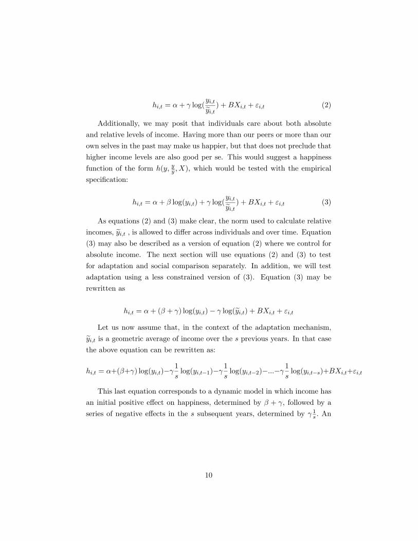
hi;t = �+ log(yi;teyi;t ) +BXi;t + "i;t (2)
Additionally, we may posit that individuals care about both absolute
and relative levels of income. Having more than our peers or more than our
own selves in the past may make us happier, but that does not preclude that
higher income levels are also good per se. This would suggest a happiness
function of the form h(y; yey ; X), which would be tested with the empiricalspeci�cation:
hi;t = �+ � log(yi;t) + log(yi;teyi;t ) +BXi;t + "i;t (3)
As equations (2) and (3) make clear, the norm used to calculate relative
incomes, eyi;t , is allowed to di¤er across individuals and over time. Equation(3) may also be described as a version of equation (2) where we control for
absolute income. The next section will use equations (2) and (3) to test
for adaptation and social comparison separately. In addition, we will test
adaptation using a less constrained version of (3). Equation (3) may be
rewritten as
hi;t = �+ (� + ) log(yi;t)� log(eyi;t) +BXi;t + "i;tLet us now assume that, in the context of the adaptation mechanism,eyi;t is a geometric average of income over the s previous years. In that case
the above equation can be rewritten as:
hi;t = �+(�+ ) log(yi;t)� 1
slog(yi;t�1)�
1
slog(yi;t�2)�:::�
1
slog(yi;t�s)+BXi;t+"i;t
This last equation corresponds to a dynamic model in which income has
an initial positive e¤ect on happiness, determined by � + , followed by a
series of negative e¤ects in the s subsequent years, determined by 1s : An
10
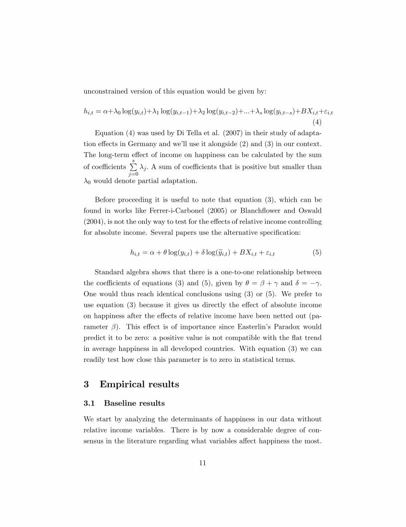
unconstrained version of this equation would be given by:
hi;t = �+�0 log(yi;t)+�1 log(yi;t�1)+�2 log(yi;t�2)+:::+�s log(yi;t�s)+BXi;t+"i;t
(4)
Equation (4) was used by Di Tella et al. (2007) in their study of adapta-
tion e¤ects in Germany and we�ll use it alongside (2) and (3) in our context.
The long-term e¤ect of income on happiness can be calculated by the sum
of coe¢ cientssPj=0
�j : A sum of coe¢ cients that is positive but smaller than
�0 would denote partial adaptation.
Before proceeding it is useful to note that equation (3), which can be
found in works like Ferrer-i-Carbonel (2005) or Blanch�ower and Oswald
(2004), is not the only way to test for the e¤ects of relative income controlling
for absolute income. Several papers use the alternative speci�cation:
hi;t = �+ � log(yi;t) + � log(eyi;t) +BXi;t + "i;t (5)
Standard algebra shows that there is a one-to-one relationship between
the coe¢ cients of equations (3) and (5), given by � = � + and � = � :One would thus reach identical conclusions using (3) or (5). We prefer to
use equation (3) because it gives us directly the e¤ect of absolute income
on happiness after the e¤ects of relative income have been netted out (pa-
rameter �). This e¤ect is of importance since Easterlin�s Paradox would
predict it to be zero: a positive value is not compatible with the �at trend
in average happiness in all developed countries. With equation (3) we can
readily test how close this parameter is to zero in statistical terms.
3 Empirical results
3.1 Baseline results
We start by analyzing the determinants of happiness in our data without
relative income variables. There is by now a considerable degree of con-
sensus in the literature regarding what variables a¤ect happiness the most.
11
Health, marital status and employment status are usually found to have the
largest e¤ect on individuals�answer to life satisfaction questions while age,
education, religious attitudes and income also play sizeable roles.
Table 1 presents the results from estimating equation (1) under four
alternative econometric methodologies: pooled OLS, �xed e¤ects estimation,
ordered probit and ordered logit; all regressions include time dummies.
Most results are similar across the four methodologies. Health has al-
ways a large and positive e¤ect on happiness; although at a decreasing rate.
Married people and those living in couples are happier than people who
have never married, while those divorced or - worse still - separated score
markedly lower. Unemployed persons are universally found to be less happy.
We also �nd, in accordance with the literature, that highly religious
people are happier than non-religious ones and that the partial relationship
between age and happiness is U-shaped. In this baseline regressions income
is included only in absolute terms. As expected, income exerts a positive
e¤ect on happiness in all regressions. Since income is measured in log terms
the associated coe¢ cients can be interpreted as the semi-elasticities of hap-
piness with respect to income. The e¤ects of income are smaller than those
of health or marital status. A 10% increase in income would rise happiness
by just 0:015 points according to the pooled OLS estimates and by 0:005
according to the �xed e¤ects estimate.
Our preferred methodology is the �xed e¤ects estimation of column 2.
The main reason for this is that unobservable person-speci�c factors such as
genetics or early childhood experiences are likely to be major explanatory
factors of happiness. Columns 1, 3 and 4, which do not include �xed e¤ects,
manage to explain at most 17% of the variation in the data whereas the
�xed e¤ects regression in column 2 explains 65% of it. Moreover, these
person-speci�c factors are likely to be correlated with several explanatory
variables such as health, income or marital status. Indeed, think of some
genetic feature that makes us more optimist when facing problems. It is to
12
be expected that such a convenient trait would make us happier but also
more likely to be healthy, rich and married.
Under these circumstances, failure to include �xed e¤ects is likely to
lead to an upward bias in most coe¢ cients. Indeed, when we compare the
size of the coe¢ cients in columns 1 and 2 we �nd that most of them are
considerable smaller once �xed e¤ects are included in column 28. To put it
in other words, we should not deduce the e¤ect of an event like marriage
on happiness by comparing married persons with unmarried ones because
people who are happy to begin with tend to marry more often. Instead, we
should use the within-person variation in the data to deduce the e¤ect that
getting married has on the happiness of a given individual. The rest of this
paper will use �xed e¤ects estimation to analyze the adaptation and social
comparison mechanisms.
3.2 Adaptation and social comparison: separate tests
Before estimating equations (2) and (3) to test for adaptation and social
comparison e¤ects we need to de�ne eyi;t, the norm with respect to which
individuals compare their income to.
In the case of adaptation, eyi;t will be an average of the individual�s ownincome over the last few years. We�ll use a simple average over the previous
3 years, i.e. eyi;t = 13
P3s=1 yi;t�s: The ratio y=ey will be referred to as "income
relative to past income". We have also used the average over the previous 5
years and have obtained almost identical results.
As discussed above, when using equation (5) to test for adaptation we
are implicitly assuming a geometric average of past incomes as the norm.
8An interesting case is that of our education variables, which have a negative e¤ectin the abscence of �xed e¤ects but a positive one when these are included. This impliesthat more educated people tend to be less satis�ed with their life than less educatedones; but that increasing your education level (obtaining a university degree, for instance)does rise your life satisfaction. The result is intuitive: it is probably the sense of notbeing satis�ed that pushes people to follow longer educational paths. In other words,intrinsically unsatis�ed people self-select themselves into higher education.
13

We estimate equation (5) with four lags of income in order to have results
that are directly comparable with Di Tella et al. (2007).
In the case of social comparison we use two alternative de�nitions of eyi;t:First, and in line with Blanch�ower and Oswald 2004, Graham and Felton
2006 or Knight et al. 2007, we use the average income of the individuals�s
region of residence. We call the resulting ratio "income relative to regional
income". The regions we consider for the UK are London, Scotland, Wales,
Northern Ireland and England outside London.
Second, we use a methodology closer in spirit to Ferrer-i-Carbonel (2005)
or Vendrik and Woltjer (2007) to account not just for the individual�s region
of residence but for the diverse socioeconomic characteristics that may de-
termine his comparison group. We calculate for each person a "predicted"
level of income using the �tted values of a regression of income on age and its
square, education, marital status, real GDP per capita, number of children
and a dummy for London. The variable re�ects well the idea that people of
a certain education or age will compare themselves with other individuals
of similar characteristics. The ratio of income to this variable will be called
"income relative to predicted income" in what follows.
Table 2 presents the results of using equation (2) to test separately for
adaptation and social comparison e¤ects, while table 3 presents the corre-
sponding results using equations (3) and (5).
In table 2 we �nd evidence favouring both adaptation and social compar-
ison when each of them is tested separately. Column 1 tests for adaptation
and �nds a clearly signi�cant e¤ect of income relative to past income on
happiness. In columns 2 and 3 we run similar tests using income relative to
regional income (column 2) and income relative to predicted income (column
3). In both cases we obtain a positive e¤ect that is statistically signi�cant.
The size of the coe¢ cient is very similar for the two alternative de�nitions
of comparison group that we use.
14
Table 3 presents a di¤erent picture. Once we control for absolute income
using equation (3), we �nd that only the adaptation mechanism is supported
by the data. In column 1 we see that the coe¢ cient on income relative to
past income is somewhat smaller than previously (0:027 instead of 0:035 in
table 2) and statistically signi�cant at the 10% level. The changes in the
coe¢ cients capturing social comparison e¤ects are more radical. They are
both very di¤erent from the values taken in table 2 and none of them is
statistically signi�cant.
The failure of social comparison e¤ects to survive this test is somewhat
surprising. Equation (3), or a very similar version of it, has been estimated
using German data by Ferrer-i-Carbonel (2005) and using American data
by Blanch�ower and Oswald (2004). Ferrer-i-Carbonel (2005) �nds that the
e¤ect of relative income remains positive and statistically signi�cant whereas
absolute income becomes statistically not signi�cant and its coe¢ cient falls
by more than half. Blanch�ower and Oswald (2004) �nd that both relative
and absolute income have a positive and statistically signi�cant e¤ect when
included simultaneously9. Our estimates imply that these earlier results
cannot be con�rmed for the United Kingdom.
It is also interesting to note that absolute income has a very small and
not signi�cant coe¢ cient when included alongside income relative to past
income, in the �rst column of table 3. As we discussed previously, this is
precisely what would be expected given Easterlin�s Paradox. This result
strengthens the case in favour of adaptation e¤ects in our data.
The last column of table 3 tests for adaptation e¤ects once again by
using equation (5). Once again the results are favorable to this hypothesis,
since the dynamic pattern revealed shows a large positive e¤ect of absolute
income on impact followed by several years where the e¤ects are negative. In
other words, the initial increase in happiness "wears down" over time as we
get used to our new income. Notice, however, that the sum of coe¢ cients on
9We are referring to table 3 in Ferrer-i-Carbonel (2005) and table 8 in Blanch�owerand Oswald (2004).
15
all income variables is still positive (although not statistically signi�cant). A
sum of coe¢ cients of 0:021 suggest that adaptation is only partial, and that
about half of the initial e¤ect of 0:044 is lost after four years. We cannot,
however, rule out the possibility of total adaptation on statistical grounds:
an F-test for the sum of coe¢ cients on current income and all its lags being
equal to zero does not reject the null hypothesis. This, incidentally, is very
similar to the �ndings of Di Tella et al. (2007) for Germany. These authors
�nd that slightly more than two-thirds of the initial e¤ect of income is lost
after four years and that the possibility of total adaptation cannot be ruled
out since the sum of coe¢ cients is not statistically signi�cant.
3.3 Adaptation and social comparison: joint tests
The �nal empirical exercises that we carry out are joint test for the adap-
tation and social comparison mechanisms. Let us note eyAi;t the norm with
respect to which incomes are compared under the adaptation hypothesis andeySCi;t the corresponding norm under social comparison. Then, the empirical
speci�cation that we will use for our joint tests is as follows:
hi;t = �+ �A log(yi;teyAi;t ) + �SC log( yi;teySCi;t ) +BXi;t + "i;t (6)
where all other variables have been previously de�ned.
We estimate equation (6) twice: with eySCi;t de�ned as income relative
to regional income and with eySCi;t as income relative to predicted income.
Results are reported in table 4. The two alternative de�nitions of eySCi;t givevery similar results: in both cases we �nd that it is income relative to past
income that exerts an e¤ect on happiness, with income relative to regional
income (column 1) or income relative to predicted income (column 2) having
an e¤ect close to zero and statistically not signi�cant. The coe¢ cient on
income relative to past income is not only statistically signi�cant but of
similar size to the corresponding estimates from tables 2 and 3.
Overall, the results of these joint tests are consistent with those obtained
16
previously and clearly argue in favour of adaptation, and against social com-
parison, as the main mechanism explaining Easterlin�s Paradox and relating
income to happiness. Income relative to past income appears to be a robust
predictor of happiness; its e¤ects are clearly present when we control for the
e¤ects of absolute income and for income relative to a comparison group.
This is not the case for income relative to regional income or income relative
to predicted income, the two measures of social comparison we have used
here, and the relevance of this latter mechanism is therefore in doubt, at
least within our data.
4 Concluding Remarks
This paper adds the United Kingdom to the set of countries on which the
e¤ects of income on happiness have been studied in the search for adaptation
and social comparison e¤ects. It has the particularity that adaptation and
social comparison are investigated with the same set of data and subjected
to both separate and joint tests.
The paper o¤ers the possibility of interesting comparisons with the rest
of the literature. We �nd, for instance, a very similar pattern of adaptation
e¤ects as the one estimated by Di Tella et al. (2007) using a panel of German
households. Like them, we �nd that the e¤ect of income on happiness losses
about two thirds of its initial e¤ect after four years. While this indicates
an adaptation e¤ect that is still not complete, the null hypothesis of full
adaptation cannot be rejected at conventional con�dence levels.
A di¤erent outcome is obtained in the case of social comparison. Here
our results di¤er from the literature since we �nd that income relative to
a comparison group does not appear to have an e¤ect on happiness once
we control for absolute income or for adaptation e¤ects. While this result
does not overcome the comparatively larger evidence in favour of social
comparison it does ask for further test; particularly tests which, as here,
consider both mechanisms together.
17
A �nal note of caution is in order. We have wished to test and compare
the two main mechanism explaining how income and happiness relate to each
other: adaptation and social comparison. Social comparison, however, is a
very �exible concept given the many possible de�nitions of the comparison
group. The evidence in this paper favours adaptation over social compar-
ison using two particular de�nitions of the comparison group, although it
must be noted that these two de�nitions have been used repeatedly in the
literature. It is still the case, however, that a di¤erent de�nition of the
comparison group may give di¤erent results. Not only that, but social com-
parison and adaptation can be observationally equivalent if the comparison
group is de�ned as "people with similar income as me". In this case, the
income of the comparison group would grow as the individual�s own income
grows, just as in the case of adaptation. Moreover, such a comparison group
may not be all too unlikely: it would be not very di¤erent from the income of
our neighbours if people move to wealthier neighbourhoods as they become
richer. It is apparent, then, that research in this area is far from being over.
18
References
Argyle, M. 1999, Causes and Correlates of Happiness, in: Kahneman, D.,
Diener, E. and Schwarz, N. (eds.), Well-Being: The Foundations of Hedonic
Psychology, New York: Russell Sage Foundation, 353-373.
Blanch�ower, D. G. and Oswald, A. J. 2004, Well-being over time in
Britain and the USA, Journal of Public Economics 88, 1359-1386.
Burchardt, T. 2005, Are one man�s rags another man�s riches? Identi-
fying adaptive preferences using panel data, Social Indicators Research 74,
57-102.
Clark, A. E. 1999, Are wages habit-forming? Evidence from micro data,
Journal of Economic Behavior and Organization 39, 179-200.
Clark, A. E. 2006, Born to be mild? Cohort e¤ects don�t explain why
well-being is U-shaped in age, Working Paper 2006-35, Paris-Jourdan Sci-
ences Economiques
Clark, A. E. and Oswald, A. J. 1996, Satisfaction and comparison in-
come, Journal of Public Economics 61, 359-381.
Clark, A. E. and Oswald, A. J. 2002, A simple statistical method for
measuring how life events a¤ect happiness, International Journal of Epi-
demiology 31, 1139-1144.
Clark, A. E., Frijters, P. and Schields, M. A. 2008, Relative Income,
Happiness and Utility: An Explanation for the Easterlin Paradox and other
Puzzles, Journal of Economic Literature 46 (1), 95-144.
Di Tella, R., MacCulloch, R. and Oswald, A. J. 2003, The macroeco-
nomics of happiness, Review of Economics and Statistics 85(4), 809-827.
Di Tella, R., Haisken-De New, J. and MacCulloch, R. 2007, Happiness
adaptation to income and to status in an individual panel, NBER working
paper 13159.
Easterlin, R. A. 1974, Does Economic Growth Improve the Human Lot?
Some Empirical Evidence, in: Nations and Households in Economic Growth:
Essays in Honor of Moses Abramovitz, R. Davis and M. Reder (eds.), New
York: Academic Press, 89-125.
19
Easterlin, R. A. 1995, Will Raising the Incomes of all increase the Hap-
piness of all?, Journal of Economic Behavior and Organization, 27(1), 35-47.
Easterlin, R. A. 2003, Building a Better Theory of Well-Being, IZA Dis-
cussion Paper 742.
Ferrer-i-Carbonel, A 2005, Income and well-being: an empirical analysis
of the comparison income e¤ect, Journal of Public Economics 89, 997-1019.
Ferrer-i-Carbonel, A. and Frijters, P. 2004, How important is method-
ology for the estimates of the determinants of happiness?, The Economic
Journal 114 (July), 641-659.
Frey, B. and Stutzer, A. 2002, Happiness and Economics: How the Econ-
omy and Institutions A¤ect Human Well-Being, Princeton: Princeton Uni-
versity Press.
Graham, C. and Felton, A. 2006, Inequality and happiness: insights from
Latin America, Journal of Economic Inequality 4, 107-122.
Grund, C. and Sliwka, D. 2007, Reference-dependent preferences and the
impact of wage increases on job satisfaction: Theory and Evidence, Journal
of Institutional and Theoretical Economics 163(2), 313-335.
Knight, J., Song, L. and Gunatilaka, R. 2007, Subjective well-being and
its determinants in rural China, Working Paper 334, Department of Eco-
nomics, University of Oxford.
Layard, R. 2005, Happiness: lessons from a new science, New York: The
Penguin Press.
Lucas, R. 2005, Time does not heal all wounds- A longitudinal study or
reaction and adaptation to divorce, Psychological Science 16, 945-950.
Lucas, R. Clark, A. E., Georgellis, Y. and Diener, E. 2003, Re-examining
adaptation and the setpoint model of happiness: reaction to changes in mar-
ital status, Journal of Personality and Social Psychology 84, 527-539.
Lucas, R. Clark, A. E., Georgellis, Y. and Diener, E. 2004, Unemploy-
ment alters the set-point for life satisfaction, Psychological Science 15, 8-13.
Luttmer, E. 2005, Neighbours as negatives: Relative earnings and well-
being, Quarterly Journal of Economics 120, 963-1002.
McBride, M. 2001, Relative income e¤ects on subjective well-being in the
cross-section, Journal of Economic Behavior and Organization 45, 251-278.
20
Oswald, A. J. 1997, Happiness and Economics Performance, The Eco-
nomic Journal, 107 (November), 1815-1831.
Oswald, A. J. and Powdthavee, N. 2008, Does happiness adapt? A
longitudinal study of disability with implications for Economists and Judges,
Journal of Public Economics 92 (5-6), 1061-1077.
Oswald, A. J. and Powdthavee, N. 2007, Obesity, unhappiness and the
challenge of a�uence: theory and evidence, Research paper 793, Department
of Economics, University of Warwick.
Powdthavee, N. 2004, Testing for utility interdependence in marriage:
evidence from panel data, Research paper 705, Department of Economics,
University of Warwick.
Rablen, M. D. 2008, Relativity, Rank and the Utility of Income, The
Economic Journal 118 (April), 801-821.
Rayo, L. and Becker, G. S. forthcoming, Evolutionary E¢ ciency and
Happiness, Journal of Political Economy.
Senik, C. 2004, When information dominates comparison: learning from
Russian subjective panel data, Journal of Public Economics 88, 2099-2123.
Taylor, M. F. (ed.) 2007, British Household Panel Survey. Users Man-
ual Volume A: Introduction, Technical Report and Appendices, Colchester:
University of Essex.
Vendrik, M. C. M. and Woltjer, G. B. 2007, Happiness and loss aversion:
Is utility concave or convex in relative income?, Journal of Public Economics
91, 1423-1448.
Wu, S. 2001, Adapting to heart conditions: A test of the hedonic tread-
mill, Journal of Health Economics 20, 495-507.
21
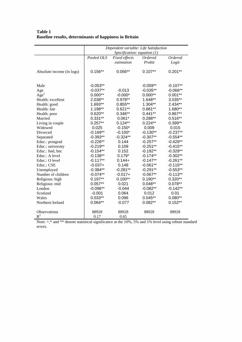
Table 1 Baseline results, determinants of happiness in Britain
Dependent variable: Life Satisfaction Specification: equation (1)
Pooled OLS Fixed effects estimation
Ordered Probit
Ordered Logit
Absolute income (in logs) 0.156** 0.056** 0.107** 0.201** Male -0.053** -0.059** -0.107** Age -0.037** -0.013 -0.035** -0.066** Age2 0.000** -0.000* 0.000** 0.001** Health: excellent 2.038** 0.978** 1.648** 3.035** Health: good 1.693** 0.855** 1.304** 2.434** Health: fair 1.198** 0.621** 0.881** 1.680** Health: poor 0.620** 0.346** 0.441** 0.867** Married 0.331** 0.061* 0.288** 0.516** Living in couple 0.257** 0.124** 0.224** 0.399** Widowed 0.025 -0.150* 0.009 0.015 Divorced -0.169** -0.100* -0.130** -0.237** Separated -0.393** -0.324** -0.307** -0.554** Educ.: postgrad -0.226** 0.144 -0.257** -0.429** Educ.: university -0.219** 0.109 -0.251** -0.415** Educ.: hnd, hnc -0.154** 0.152 -0.192** -0.329** Educ.: A level -0.138** 0.179* -0.174** -0.302** Educ.: O level -0.117** 0.144+ -0.147** -0.261** Educ.: CSE -0.037+ 0.148 -0.061** -0.115** Unemployed -0.384** -0.281** -0.291** -0.553** Number of children -0.074** -0.017+ -0.067** -0.113** Religious: high 0.197** 0.100** 0.190** 0.320** Religious: mid 0.057** 0.021 0.048** 0.078** London -0.096** -0.044 -0.082** -0.142** Scotland -0.001 0.064 0.012 0.01 Wales 0.033** 0.096 0.045** 0.080** Northern Ireland 0.064** -0.077 0.082** 0.152** Observations 88928 88928 88928 88928 R2 0.17 0.65 Note: +,* and ** denote statistical significance at the 10%, 5% and 1% level using robust standard errors.
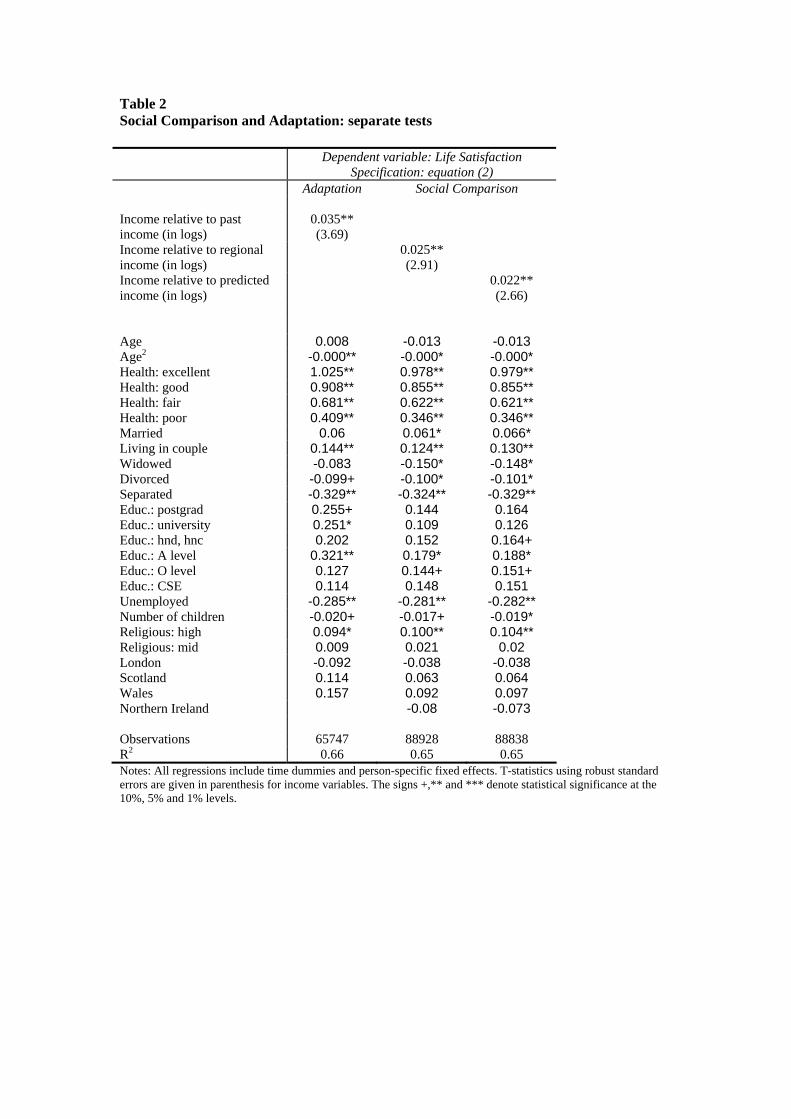
Table 2 Social Comparison and Adaptation: separate tests Dependent variable: Life Satisfaction
Specification: equation (2) Adaptation Social Comparison Income relative to past income (in logs)
0.035** (3.69)
Income relative to regional income (in logs)
0.025** (2.91)
Income relative to predicted income (in logs)
0.022** (2.66)
Age 0.008 -0.013 -0.013 Age2 -0.000** -0.000* -0.000* Health: excellent 1.025** 0.978** 0.979** Health: good 0.908** 0.855** 0.855** Health: fair 0.681** 0.622** 0.621** Health: poor 0.409** 0.346** 0.346** Married 0.06 0.061* 0.066* Living in couple 0.144** 0.124** 0.130** Widowed -0.083 -0.150* -0.148* Divorced -0.099+ -0.100* -0.101* Separated -0.329** -0.324** -0.329** Educ.: postgrad 0.255+ 0.144 0.164 Educ.: university 0.251* 0.109 0.126 Educ.: hnd, hnc 0.202 0.152 0.164+ Educ.: A level 0.321** 0.179* 0.188* Educ.: O level 0.127 0.144+ 0.151+ Educ.: CSE 0.114 0.148 0.151 Unemployed -0.285** -0.281** -0.282** Number of children -0.020+ -0.017+ -0.019* Religious: high 0.094* 0.100** 0.104** Religious: mid 0.009 0.021 0.02 London -0.092 -0.038 -0.038 Scotland 0.114 0.063 0.064 Wales 0.157 0.092 0.097 Northern Ireland -0.08 -0.073 Observations 65747 88928 88838 R2 0.66 0.65 0.65 Notes: All regressions include time dummies and person-specific fixed effects. T-statistics using robust standard errors are given in parenthesis for income variables. The signs +,** and *** denote statistical significance at the 10%, 5% and 1% levels.
Table 3 Social Comparison and Adaptation: separate tests, controlling for absolute income. Dependent variable: Life Satisfaction
Specification: equation (3) Specification: equation (4)
Adaptation Social Comparison Adaptation Income relative to past income (in logs)
0.027+ (1.74)
Income relative to regional income (in logs)
0.090 (0.54)
Income relative to predicted income (in logs)
-0.088 (0.090)
Absolute income (in logs) 0.011 (0.062)
-0.065 (0.39)
0.113+ (1.74)
Absolute income (in logs) at time: t 0.044**
(3.53) t-1 -0.013
(1.12) t-2 -0.003
(0.27) t-3 -0.010
(0.93) t-4 0.003
(0.32) Sum of coefficients on absolute income (in logs)
0.021 (0.30)#
Age 0.008 -0.014 -0.016 -0.002 Age2 -0.000** -0.000* 0 -0.000** Health: excellent 1.025** 0.979** 0.979** 1.075** Health: good 0.908** 0.855** 0.855** 0.959** Health: fair 0.681** 0.622** 0.621** 0.727** Health: poor 0.409** 0.346** 0.346** 0.442** Married 0.058 0.061* 0.036 0.045 Living in couple 0.142** 0.124** 0.097** 0.148** Widowed -0.085 -0.150* -0.171** -0.112 Divorced -0.099+ -0.100* -0.095* -0.110* Separated -0.330** -0.324** -0.322** -0.376** Educ.: postgraduate 0.252+ 0.144 0.079 0.259 Educ.: university 0.249* 0.109 0.053 0.314* Educ.: hnd, hnc 0.201 0.152 0.11 0.257+ Educ.: A level 0.321** 0.179* 0.147+ 0.367** Educ.: O level 0.127 0.144+ 0.118 0.162 Educ.: CSE 0.112 0.147 0.132 0.139 Unemployed -0.284** -0.281** -0.282** -0.300** Number of children -0.019+ -0.017+ 0.003 -0.018 Religious: high 0.095* 0.100** 0.104** 0.099* Religious: mid 0.01 0.021 0.02 0.015 London -0.093 -0.024 -0.059 -0.069 Scotland 0.115 0.059 0.064 0.167 Wales 0.158 0.081 0.096 0.18 Northern Ireland -0.087 -0.077 -- Observations 65747 88928 88838 56595 R2 0.66 0.65 0.65 0.65 Notes: All regressions include time dummies and person-specific fixed effects. Robust standard errors are given in parenthesis for income variables. The signs *,** and *** denote statistical significance at the 10%, 5% and 1% levels. #: p-value of an F-test on the sum of coefficients on current and lagged income being equal to 0.
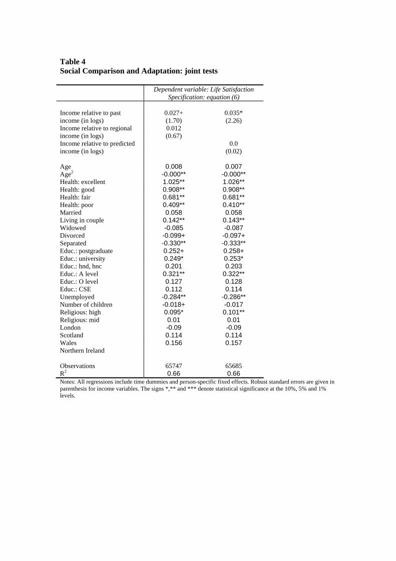
Table 4 Social Comparison and Adaptation: joint tests
Dependent variable: Life Satisfaction Specification: equation (6)
Income relative to past income (in logs)
0.027+ (1.70)
0.035* (2.26)
Income relative to regional income (in logs)
0.012 (0.67)
Income relative to predicted income (in logs)
0.0 (0.02)
Age 0.008 0.007 Age2 -0.000** -0.000** Health: excellent 1.025** 1.026** Health: good 0.908** 0.908** Health: fair 0.681** 0.681** Health: poor 0.409** 0.410** Married 0.058 0.058 Living in couple 0.142** 0.143** Widowed -0.085 -0.087 Divorced -0.099+ -0.097+ Separated -0.330** -0.333** Educ.: postgraduate 0.252+ 0.258+ Educ.: university 0.249* 0.253* Educ.: hnd, hnc 0.201 0.203 Educ.: A level 0.321** 0.322** Educ.: O level 0.127 0.128 Educ.: CSE 0.112 0.114 Unemployed -0.284** -0.286** Number of children -0.018+ -0.017 Religious: high 0.095* 0.101** Religious: mid 0.01 0.01 London -0.09 -0.09 Scotland 0.114 0.114 Wales 0.156 0.157 Northern Ireland Observations 65747 65685 R2 0.66 0.66 Notes: All regressions include time dummies and person-specific fixed effects. Robust standard errors are given in parenthesis for income variables. The signs *,** and *** denote statistical significance at the 10%, 5% and 1% levels.