Embed Size (px)
Citation preview

I| AD-A282 342 1(j)illlnlllllI DTIC
ELECTESJUL2 71994
S vF
ANALYSIS OF A THREE-BEAM RADARAS AN INSTRUMENT FOR DETERMINING
OCEAN WAVE HEIGHTS AN) VECTOR SLOPES
I
Christopher T. EvansS•doc~uient' has b •,lQpra~
!r public. :eleo.se and sale; its e
=Uatio is uAlimite.4
Radar Systems and Remote Sensing LaboratoryI Deprtment of Electrical Engineering and Computer Science, University of Kansas2291 Irving Hill Road, Lawrence, Kansas 66045-2969
TEL: 913/864-4835 * FAX: 913/864-7789 * OMNET: KANSAS.U.RSL
•I
RSL Technical Report 8621-5
June 1994
94-22739 RI i ii lilgL? Sponsored by:
I Office of Naval ResearchArlington VA 22217-5000
SGrant N00014-89-J-3221
1 94 7 19 217

3 Abstract
The Vector Slope Gauge (VSG) is a 35-GHz FM-CW scatterometer that has the
3 unique capability of simultaneously (nearly) measuring the range and backscattered
power to three points on the ocean surface. With three ranges and knowledge of the
experimental geometry, the wave height at each footprint can be obtained. The three
3 ifootprints form a plane surface which enable two orthogonal slope components to be
obtained. Obtaining the slope of ocean waves is important because it is correlated
with the backscattered power. By obtaining the vector slope, one does not have to
make any assumptions about the linearity or long-crestedness of the ocean waves.
With a time series record of ocean wave heights and slopes, one can learn a great
5 Ideal about the ocean surface. Spectral analysis of the recorded time series yields
information about the wave height power spectral density, the mean wave direction
5 Ivs. frequency, and the directional width spectrum. T-,- results from the VSG are
similar to those obtained from a pitch-and-roll buoy. In addition, since the slope
distribution of ocean waves is nearly normal, the moments of a bivariate normal
3• distribution can be used to fit an ellipse to the wave slopes. The orientation of the
major axis of the ellipse indicates the direction of dominant wave travel, with 1800
3 !ambiguity. The ellipse also yields information about the statistics of the slope
distribution. Due to the asymmetry of the waves, the center of the ellipse is shifted
from the origin in the direction from which the dominant waves are traveling. Thus,
3 Ithe wave direction ambiguity can resolved by fitting an ellipse to the directional
histogram of the slope distribution using the least square method.
3 IAs with any instrument, the VSG has some inherent errors due to the method of
measuremenL These errors include phase shifts in the recorded time series due to
measuring along a slant range, phase shifts due to non-simultaneous measurements,
I3'

I
3 and errors due to approximating the slope at a point with a plane. Slant-range
measurements cause the measured time series of slopes to be greater than or equal to
Sthe actual slope at all times in any direction. The overestimate varies from 0* at the
mean sea level to 20 at the crest and trough. The derivative approximation has little
I effect on either the wave height time series or the slope time series. Non-
g simultaneous measurements cause the magnitude of the slope to be overestimated in
both directions at all times. The amount of overestimate is generally around 20. This,
although small, causes an error in the determination of the mean wave direction.
II
Accesion For
S~NTIS CRA&M| ~DOC: T•B [
U;ý:iilO,•.iced •
D ti.'tinAvailabifity Codes
Avail atid/IorSDist Special
I
I

1!
3 Table of Contents
Abstract ii
3 Table of Contents iii
Acknowledgments v
1. Introduction 1
3 1.1 Background of Saxon experiment 1
1.2 Importance of studying ocean waves 2
1 1.3 Outline of thesis and summary of results 3
2. Theoretical Analysis of Errors 4
2.1 The Vector Slope Gauge 4
3 2.2 Coordinate Transformations 6
2.3 Measurement of Wave Height and Slope 9
3 2.4 Inherent errors in VSG measurements 10
2.5 Error in wave height time series due to slant-range measurement 13
1 2.6 Error in wave height time series due to non-simultaneous measurement 21
5 2.7 Error in slope time series due to slant range measurement 22
2.8 Error in slope time series due to first derivative approximation 26
3 2.9 Error in slope time series due to non-simultaneous measurement 32
3. Determination of Mean Wave Direction and the Effect of Errors 36
3 3.1 Two-Dimensional Slope Distribution and Best Fit Ellipse 36
S3.2 Mean Wave Direction and Statistics of Slope Distribution 38
3.3 Resolving the directional ambiguity using a histogram of slopes 40
3.4 Effect of Inherent Measurement Errors on Determination of Direction 46
4. Determination of Ocean Spectra and Comparison with Pitch-and-Roll Buoy 53
5 4.1 Description of Pitch-and-Roll Buoy 53
I'I liio

3 4.2 Directional Distribution of Ocean Waves and Longuet-Higgins Approach 54
4.3 Comparison of VSG and Pitch-and-Roll Buoy in Determining Ocean Spectra 56
1 4.4 Effect of Inherent Errors on VSG's Determination of Ocean Spectra 59
5. Conclusion 67
5.1 Recommendations for Further Study 70
SReferences 72
Appendix A: MATLAB Programs 74
SAppidix B: Ellipses Fit to SAXON Data 96
Appendix C: Wave Spectra of SAXON Data from VSG Measurements 130
I3
II
i1
i i

U
3- 1. Introduction
1.1 Background of Saxon experiment
5- The Synthetic Aperture radar and X-band Ocean Nonlinearities (SAXON)
experiment took place in November of 1990 on the Nordsee research platform. The
3 tower was situated in about 30 meters of water just off the coast of Germany in the
£• North Sea. The University of Kansas was one of several institutions involved in the
experiment. The purpose of the experiment was to study microwave backscatter and
I. SAR images of the ocean surface for high sea states [Plant & Alpers, 1991]. To that
endeavor, The University of Kansas operated a 35-GHz scatterometer, as well as C-
and X-band radars.
I The 35-GHz scatterometer that KU operated is more commonly called the
Vector Slope Gauge (VSG) in light of its unique capabilities (see section 2.1). The
z
U
II
3 Figure 1.1. Diagram of Nordsee platform and location of VSG and 10-i anemometer.
1

VSG was located on the Northwest comer of the platform about 20 meters above the
mean sea level (see Figure 1.1). The VSG was pointed in the general direction of
oncoming waves at moderate angles of incidence. To avoid corruption of the data
due to the location of the tower, we analyzed data collected only when waves were
coming between 225° and 450 (00 is North), and when the wind was within the same
region. The wind speed was obtained, when available, from a sonic anemometer 5
meters above the mean sea surface off the Northeast comer of the tower. When these
data were unavailable the wind speed was obtained from a cup anemometer 47 meters
above the mean sea level at the southwest comer of the platform. An algorithm was
then used to estimate the wind speed at 5 meters.
Ocean measurements were also made with a Wavec pitch-and-roll buoy operated
by the Federal Maritime and Hydrographic Agency of Hamburg, Germany. The
i buoy, located near the tower, recorded time series of heave and pitch and roll angles.
5_ 1.2 Importance of studying ocean waves
In recent years, concern over the environment has increased dramatically with the
revelation of the ozone "hole" and talk of the greenhouse effect. Since 70% of the
I earth's surface is covered by water, understanding the air-sea interface plays a major
role in developing global climate models. To understand how wind affects ocean
I waves, it is important to understand how the energy in ocean waves is distributed with
regard to fiequency and direction (the directional spectrum). Knowledge of the
directional spectrum of ocean waves is also important for determining the effect on
5 shipping [Neumann & Pierson, 1963], on off-shore structures [Kuik et. al., 1988],
coastal sediment trausporti and wave diffraction and refraction from the shore
[Trageser & Elwany, 19901.
2 2

The advantage of using satellite microwave remote-sensing instruments to
measure ocean parameters is that they can be used in any type of weather. The
backscattered power from the radar signal is affected by tilt and hydrodynamic
modulation. Thus, to better understand how the radar signal is modulated by ocean
S waves, The University of Kansas operated several radars as part of the SAXON-FPN
3 experiment.
3 1.3 Outline of thesis and summary of results
The objective of my thesis is to analyze the inherent errors involved with the
£I VSG, and to show that they do not seriously detract from the VSG's capability of
3I determining ocean wave heights and vector slopes. Errors occur with the VSG due to
the radar's distance measurement along a slant range, approximation of the derivative
3 at a point on the ocean surface by the slope of a plane, and nonsimultaneity of the
three range measurements. These errors induce phase shifts in the measured time
series of wave heights and slope. The effect on the slope time series is more
3 significant due to the fact that individual range errors cannot be averaged.
The two-dimensional distribution of wave slopes measured by the VSG is nearly
bivariate Gaussian. The moments of the slope distribution can be used to fit an
ellipse to the wave slopes. The mean direction of wave travel is given by the
orientation of the major axis of the ellipse, with 1800 ambiguity. Due to the
g asymmetry of ocean waves, however, the center of the ellipse is shifted from the
origin in the direction from which the waves are coming. Thus, by fitting an ellipse
5to a histogram of the wave slopes the directional ambiguity can be resolved.
Records of the wave-height time series and slope time series allow calculation of
ithe directional spectrum of ocean waves. From the directional spectrum, the wave
1 3

3 height power spectral density, the mean wave direction spectrum, and the directional
width spectrum can all be calculated. These same spectral properties are routinely
3 calculated from pitch-and-roll buoy data. A WAVEC pitch-and-roll buoy was
operated by the Federal Maritime and Hydrographic Agency of Hamburg, Germany
[I during the SAXON-FPN experiment. The data from this buoy were analyzed by F.
3 Ziemer of GKSS, Geesthacht, Germany, and the results were made available to us for
comparison. The spectral parameters determined from the VSG data compare
5 favorably with those from the pitch-and-roll buoy.
n2. Theoretical Analysis of Errors
2.1 The Vector Slope Gauge
i The VSG is a 35-GHz FM-CW scatterometer that uses a single parabolic
reflector with three switchable feeds to measure simultaneously the range to and the
Ih
I
I~I
ROy
Figure 2.1.1. Area illuminated by a single radar beam.
43i

backscattered power from three closely spaced points on the ocean surface. The three
feeds are situated such that the radar footprints form a right angle on a surface
perpendicular to the center beam. The 3-dB beamwidth of each beam is
approximately 20, and 2.30 separates the center of each beam from the vertex of the
right triangle. The VSG was mounted roughly 20 meters above the mean sea level.
Thus, at 47* the area of each footprint is approximately 1.3 m2, and the center-to-
center distance between footprints in each leg of the right triangle is roughly 1.8 m.
The beams of the VSG were switched at 30 Hz, and a measurement of the
intermediate frequency (IF) and backscattered power was made at each sampling
interval. Thus, data were recorded for each beam at 10 Hz. For an FM-CW radar, the
difference between transmitted frequency and received frequency, fb, is proportional
to the range to the target, and is given by
S=4Brf .A fm Eq. 2. 1. 1
where B is the bandwidth of the sweep signal, r is the range to the target, fm is the
modulation rate, and c is the speed of propagation. The VSG was swept over a 500
M&z bandwidth centered at 6 GHz. The modulation rate was chosen so that the mean
IF frequency was 455 kHz.
3 With the range to three points on the ocean surface, and knowledge of the
orientation of the radar, the height of the ocean surface within each footprint can be
calculated. Since the three points define a plane, the slope of the plane can be
determined with regard to any direction.
35I

I
2.2 Coordinate Transformations
When working with data from the VSG, one needs frequently to transform
between different coordinate systems. Figure 2.2.1 depicts the situation when the
VSG is rotated from the earth coordinate system (non-primed axes) to the antenna
coordinate system (double-primed axes). The VSG is first rotated an angle of 0 about
Z z
z
I Y"y
IIx x .
P~23 y
PIEr3
I F2z "
I ,
Z ,. Z "
Y
I x,x'
I Figure 2.2.1 Transformation of radar coordinate system to earth coordinate system.
16i

IS3 the x axis, and then an angle of 8 about the z! axis. To determine the coordinate
transformation matrix that results from the rotation of 0, see Figure 2.2.2. The
I 3 PP
-0 /
g Figure 2.2.2 Rotation of 0 about the X axis.
coordinates of point P in the XYZ coordinate system are:IS/=- 0 Py = r cos(ct) Pz= r sin(az) Eq 2.2.1
3 In the X'Y'Z' coordinate system, the coordinates of point P are:
x'=Px )Py'=rcos(a-0) Pz'= rsin(a-0)Py'= r(cosa) cos() + sin(a) sin(O)) Pz' r(sin(a)cos(O) - sin(O)cog(a))Py= Pyco8s()+ Pz sin(e) Pz'= Pzco(e)- ysin(e)
Eq. 2.2.2
3 Thus,
A 1 0 0 o ['
- 0 cos(0) sin(0) x Eq. 2.2.33 0-sin(0) cos(O)J
IU 7
3

3 To determine the coordinate transformation matrix that results from the rotation of 8,
see Figure 2.2.3. The coordinates of point P in the X'YZ' coordinate system are:IPx'= r cos(a) Py'= r sin(a) Pz'= 0 Eq. 2.2.4
3YP
r r/
3I Figure 2.2.3 Rotation of 8 about the Z' axis.
3 In the X"Y"Z" coordinate system, the coordinates of point P are:
3 = rcos(a-6) Py"= rsin(a-6)Px'= r(cos(a) cos(8) + sin(a) sin(5)) Py' r(sin(a)cos(8) - sin(5) cos(a))
1 Px' Pxcos(6) + Pysin(8) Py:= Pycos(8) - Psin(8)
Eq. 2.2.5
3 T7hus,
£ [P] cos(8) sin(S) 01 [e'], [ sin(S) cos(6) 0 x [Pyt J Eq. 2.2.6
I Now, to transform from the earth coordinate system to the radar coordinate system,
multiply the coordinate transformation matrix in Eq. 2.2.6 by the coordinate
tramnformation matrix in Eq. 2.2.3.
8

1
I" [ [cos(8) sin(S) 0- [1 0 0 1 Px]
L"J0 0 0 -sin(O) cos(e) PZ
IY" cos(8) sin(8)cos(O) sin(8)sin(O)' [JPx
1•" = -sin(8) cos(8)cos(0) cos(8)sin(O)] x i Eq. 2.2.7UI L 0 -sin(e) cos(0) - Pz
I Conversely, if the coordinates are known with respect to the radar, then the matrix to
3 transform them to the earth coordinate system is:
3 I cos(8) -sin(8) 0 ] X [ Ie[ = sin(8)cos(O) cos(8)cos(O) -sin(O) x P,, Eq. 2.2.8PZ- -sin(8)sin(o) cos(8)sin(O) cos(O) L•"j
I2.3 Measurement of Wave Height and Slope
The vector slope gauge (VSG) measures the range to three separate points on the
3 ocean surface through the use of its switched-beam antenna. Given the ranges, the
location of each point in the antenna coordinate system is given by (see Figure 2.2.1):IA = (r1 sin(1 12 )cos(90- y), rl sin(1312 )sin(90-y), -rl cos(P1 2 ) )
SB=( 0, 0,-r2) Eq. 2.3.1
C =( 0, r3 sin(23, -3 cOs( 23 )
I| 9

5 To determine the wave heights with respect to the mean sea level, the coordinates
in Eq. 2.3.1 are first transformed to the earth coordinate system using Eq. 2.2.8.
3 Then, since the radar is located approximately 20 meters above the mean sea level, 20
meters is added to the z (earth) coordinate of each point.
Since the locations of three points on the ocean surface are known, two
g orthogonal slope components can be obtained. The normal to the plane containing
the three points is given by (see Figure 2.2. 1)IN = BA x BC Eq. 2.3.2
The slope of the plane in the y-direction is tan- Y) and the slope of the plane inI @Nthe x-direction is tan-i (
NzIThe Matlab program slopeab.m was writen by Sam Haimov and Vahid Hesay
3 to determine orthogonal components of the slope, given the range measurements. In
m slopeab.m, the coordinate transformation used is different than the one given in Eq.
2.2.7 or 2.2.8. The two coordinate transformation matrices give the same results,
3 however, because the angles 0 and p in slopeab.m (corresponding to 0 and 8 in the
derivation above) are positive when measured clockwise in program slopeab.m as
I opposed to counter-clockwise in the above derivation.
I3t 2.4 Inherent errors in VSG measurements
In every instrument there are measurement errors due to noise, and potential
I' errors due to calibration problems. With the VSG, there are also errors that occur
3 10

3
3 completely independent of noise and calibration problems. These errors are due
simply to the way the measurements are made and some of them cannot, in general,
5I be reduced purely by system design. (It may be possible, however, to reduce them by
changing the experimental geometry.) The inherent errors are due to measuring along
a slant range, approximating the slope at a point with a plane, and non-simultaneous
3I measurements.
In the ideal situation and neglecting noise, the measured time series of a pure
3 sinusoidal wave of one frequency, direction, and amplitude incident upon the radar
measurement site would be an exact replica of the actual wave. Due to the inherent
SI errors, however, phase shifts occur in the measured time series of wave heights (see
3 Figure 2.4.1). The measured wave height time series depicted in Fig. 2.4.1 was
calculated from the MATLAB program range.m and can be found in Appendix A. ItINbasured vs. Aesml Wave HeigitTirs Sedes
3 .... Wave Ltaswnsnwt
1.50 " -
0.00-------------- 1-
OM
-II
~~~~~- 1.50L-------7 35 64 92 120148 176 205233 261 289 318 346
Phase Waeg)
Figure 2.4.1. Example of phase error in 3-beam average wave height time series for asteep wave due to slant-range, non-simultaneous measurement. Incidence angle, 470;Antenna height, 20 m; Wave frequency, 0.2 Hz, 8 00, Upwave look direction.
"1

i
Measured vs. Actkmi Slope Time Sedes
........ Actual slope Measured Slope
I ~ ~20.00,'
15.001 .~
10.00 1 .- •' "" i
I -10.00 ., ,
7 35 64 92 12D 148 176 205 233 261 288 318 346
Phase (dog)
Measured vs. Actual Slope Time SeriesiIS...Aclual slope M ~easured Slope
a 3.00 - -III
2.O.5. - - -00I1.0 0 . 0 e!
00 - '0-- - - -- -: : ---1-o -2.00,
7 35 64 92 12D148 176 205233 281 289 318 346Phase (deg)
Figure 2.4.2. Example of total error in slope time series due to slant-range, non-I simultaneous measurement, and the derivative approximation. Incidence angle, 47°;
Antenna height, 20 m; Wave frequency, 0.2 Hz; Wave height, 3 m; 8 : 0; Upwave3I look direction.
12

3 takes into account measurement along the slant range as well as non-simultaneous
measurements The maximum phase shift occurs at the crest and the trough because
3at these points the measurement site is a maximum horizontal distance from the true
* location.
In the slope time series, the individual errors in each range measurement have a
I greater effect because they are not averaged. Measuring along the slant range induces
a phase shift in the recorded time series; approximating the derivative causes the
3 recorded time series to be modulated by a sinc function, and non-simultaneous
Smeasurements cause the estimated wave direction to be in error. The total effect of
these errors is depicted in Figure 2.4.2. Since the oncoming wave is headed directly
3 toward the radar, there is no slope in the cross (x) direction. Note that for this
particular example, however, the measured slope in the x direction can be as much as
3 ±*30. As a result, the mean wave direction would be recorded as coming from
I0-it 110
3 an error of 110. Now that the total error can be seen, it is worth looking at each
source of error.
2.5 Error in wave height time series due to slant-range measurement
3l A radar measures the distance to a particular point along the radar beam. Thus,
the VSG measures the distance to the points of intersection between each of the radar
I beams and the ocean surface. Since the ocean surface moves due to the waves, the
-I points of measurement move along the radar beam rather than vertically. This causes
a phase shift in the time series of ranges which affects the determination of ocean
31

(Ii|
5 !wave heights and slope. To estimate the amount of error in the wave height time
series and slope time series induced by the non-vertical displacement for waves of3 various frequencies and directions, it is necessary to simulate the ocean surface.
Simplifying a great deal, the surface of the ocean can be described by:
3 z = Acos(2xft + k(sin+)x + k(cos+)y) Eq. 2.5.1
5 where z is the wave height, A is the wave amplitude, f is the wave frequency, k is the
wave number. and # is the angle (measured clockwise) between the +y-axis (RLD)I and the direction from which the waves are coming. If we assume that the origin of5 the earth coordinate system is located where the radar signal originates with +z
indicating an up direction, then the z coordinate of any point on the ocean surface isIz = A cos(2xft + k(sinm)x + k(cos+)y) - h Eq. 2.5.2
3I where h is the height of the antenna above the mean ocean surface. Now, from Eq.
2.2.8 and Eq. 2.3.1, the locations of the points of mesurement in the earth coordinate
3I system are given by Eq. 2.5.3. The appropriate x, y, and z values from Eq. 2.5.3 can
i -•qI[COS(S)Sin(0 12 )cos(Y - 90) + sin()Sin(P 12 )sin(y - 90)]3 i == rl [co(e) sin(O)sin( 12 )COS(y -90)- cOS(8)coS(O)Sil(P 12 )Sin(y -90) + Sin(O)COS(P 12 )]S=,q [sin(e))sin(8)sin(h 2)coSy - 90) - cos(8)sin() sin(012 ) sin(y - 90) - cos(O)cos(p13 2)]-IX = 0
Y2 = r sin(O)Z2 = r2 coK()X3 = r3 [si(6) si(A23)AY3= r3 [cos(6) cos(e) sin(23) + sin(O) cos(23 )5Z3 -• [1cos() sin(e) sin(23) - Cos(O)COs(23 )] Eq. 2.5.3
14

3lI be substituted into Eq. 2.5.2, resulting in three equations and three unknowns.
Newton's method is then used to solve for the three unknown ranges. Thus,
r,+i =rn - f (rn) Eq. 2.5.4rn~ = n f(rn)
5where rn is the nth value of the range.
In the simple case of waves of one frequency at moderate angles of incidence,
one does not have to worry about local minima vs. global minima because each radar
3 beam intercepts the ocean surface at only one point. However, if waves of multiple
frequencies are added together, or if the angle of incidence is close to grazing angles,
one needs to check to make sure that the range given as the solution to the problem is
the actual range from which the radar signal came. The correct range should be the
I shortest range which is a solution to the nonlinear equation given above.
3I The program slange.m was written in MATLAB 3.5 to determine the x, y, and z
earth coordinates of the points of intersection and also the ranges to the points of
3 intersection. It assumes that each set of three measurements is made simultaneously.
To determine the phase error in wave height - - ts associated with the non-
3 vertical displacement of the point of m one needs to determine the wave
3.• height, assuming that the point of measurement is moving vertically. The MATLAB
3.5 program vrange.m was written to determine the x, y, and z earth coordinates of
3 Ithe points of intersection and also the ranges to the points of intersection given the x
and y coordinates obtained from slrange.m and several other variables. The x and y
I coordinates are required so that the data from the two programs can be properly phase
3i matched (see Figure 2.5.1). That is, the range time series and the wave height time
series of the three points will be in phase exactly at the mean sea level.
3 15

3Ian Wave Hetg[tTins Seod.
--- Verical Slant-Range
1.50
AX1.00-- o, o i
I U5o /t k-1.00-
-1.50 T0 28 56 85 113 141 1W 198 226 254 282 311 339
Phase (dg)
Figure 2.5.1 Mean time series of simulated wave height meaureent illustratingthe phase error due only to a non-vertically moving point of measurement The solidline represents the average of each measurement made along the radar beam. Thedashed line represents the average of three vertical beam msurements. Incidenceangle, 47*; Antenna height, 20 m; Wave frequency, 0.1953125 Hz, 8 - 00, Upwavelook direction.
As .?r-viously noted, phase shifts in the time domain result in harmonics
3 appearing in the frequency domain (see Figure 2.5.2). The particular example shown
in Fig. 2.5.2 is for the same wave height time series depicted in Fig. 2.5.1. It is for a
3 particularly steep wave; the wave height to wave length ratio in this case is near the
theoretical limit of 1/7. As can be seen, even for such an extreme case the second
harmonic is small, and higher order harmonics are even smaller.
3
•!:..16

5 Wave Height Spectrum
-1 . I 1 -.30 . I i i
* -70o
-90. -
.10O0 -
0.M 0.39 0.78 1.17 1.56 19
Frequency (Hz)
Wave Height Phase Spectrum
9- - ------ -I I-I-
a 45 --- -- ..----
45. Slant-Range
-go. IT 11
* ~~~~~-135--------------------180- t -IT .......------ 1
0.x0 0.39 0.78 1.17 1.66 1.95
I
Frequency (Hz)
Figure 2.5.2. Harmonics occurring as a result of slant-range measurement incidenceangle, 47*; Antenna height, 20 m; Wave frequency, 0. 1953125 Hz, Wave height, 3 m;8 00, Upwave look direction.
17
. .JX .... ... . 7 ------ 6 .9

S!
The maximum phase error for a single beam which occurs at the crest and trough
can be determined from the amount of horizontal shift which occurs in the radar look
direction as a result of slant-range measurement. According to Figure 2.5.3, the
horizontal phase shift along the direction of wave propagation is A tan(0). The
. tano KLV"�3 Wave Amplitude
"0 AtanO)"%IMean Sea Level /,af
3-Beam Direction of
3 .Wave Propagation
Side View Top View
Figure 2.5.3. Geometry used to calculate maximum amount of phase error in a singlebeam ocmuring at the crest and trough due to slant-range measurement.
component of that phase shift lying in the radar look direction is simply
.3 Atan(0)cos(,). Thus, the maximum amount of phase error for a single beam, in
degrees, is
.•.A Atan() o)s(+)3W0 Eq. 2.5.5
S. When the wave heights from the three beams are averaged together to form the
5 mean wave height time series, the maximum phase error for the mean wave height
• -- 18

3 time series will be slightly different than this. It will generally be less than the error
in a single beam unless the wave direction is perpendicular to the radar look direction.
3 The examples shown in Figures 2.5.1 and 2.5.2 are worst case scenarios for
several reasons. The radar is looking directly at the oncoming waves so that the
U cos( + Q) term is 1. Both figures are also for steep waves; for the given X, A is near
3 its maximun theoretical limit. From Eq. 2.2.5, one can see that for a wave of a given
length and amplitude and for a given incidence angle, the phase error will be greater
for a wave in the upwave or downwave look direction than for any other direction.
For waves coming from other directions, the component of horizontal shift in the
I radar look direction is less than the horizontal shift in the direction of wave
3 propagation. For a wave of a given frequency, amplitude, and direction, the phase
error will be worse for a larger angle of incidence. As the incidence angle increases,
3m there is more horizontal shift in the radar look direction.
3 Mnlmium Phase Error fpd 'rr(
307 _ w 0.5
25 1__ __ .- __ __
S20---X , 1.5
j10. 2.5
30--- 3.5I 0.08 0.12 0.16 0.20 0.24 0.28 0.32 0.36 0.40
Frequency(Hr) -
Figure 2.5.4. Maximum phase error in wave height time series due to slant-range'1 measurement. Incidence angle, 470; Antenna height, 20 m; 8 - 00; Upwave lookdirection.
19

Table 2.5.1 lists the maximum phase error for waves of various amplitudes and
frequencies given that the angle of incidence is 470 and the direction of wave
propagation is from 00. The values are also plotted in Figure 2.5.4.
Table 2.5.1. Maximum phase error (deg) due to slant-range measurements for wavesof various frequencies and amplitudes. Incidence angle, 470; Antenna height, 20 m;
6 = 0°; Up•wave look direction.
S0; U lokdiecio. Amplitude of Ocean Waves (meters)X (m) f (Hz) 0.25 0.5 0.75 1 1.25243.7 0.08 0.4 0.8 1.2 1.6 2.0156.0 0.10 0.6 1.2 1.9 2.5 3.1108.3 0.12 0.9 1.8 2.7 3.6 4.579.6 0.14 1.2 2.4 3.6 4.9 6.160.9 0.16 1.6 3.2 4.8 6.3 7.948.1 0.18 2.0 4.0 6.0 8.0 10.039.0 0.20 2.5 5.0 7.4 9.9 12.432.2 0.22 3.0 6.0 9.0 12.0 15.027.1 0.24 3.6 7.1 10.7 14.3 17.823.1 0.26 4.2 8.4 12.5 16.7 20.919.9 0.28 4.9 9.7 14.6 19.4 24.317.3 0.30 5.6 11.1 16.7 22.315.2 0.32 6.3 12.7 19.0 25.313.5 0.34 7.2 14.3 21.512.0 0.36 8.0 16.0 24.110.8 0.38 8.9 17.9 26.89.7 0.40 9.9 19.8
_ Amplitude of Ocean Waves (meters)X (m) f(Hz) 1.75 2 2.25 2.5 2.75243.7 0.08 2.8 3.2 3.6 4.0 4.4156.0 0.10 4.3 5.0 5.6 6.2 6.8108.3 0.12 6.2 7.1 8.0 8.9 9.879.6 0.14 8.5 9.7 10.9 12.1 13.3
60.9 0.16 11.1 12.7 14.3 15.8 17.448.1 0.18 14.0 16.0 18.0 20.0 22.1
39.0 0.20 17.3 19.8 22.3 24.832.2 0.22 21.0 24.0 27.0
20

- 2.6 Error in wave height time series due to non-simultaneous measurement
The VSG records the range and backscattered power from the ocean surface
3 every 33 ms. Thus, during the time between measurements the surface moves
slightly. This movement shows up as an additional phase shift in the measurements
I from beams 2 and 3. For example, if the waves are coming directly at the radar,
height measurements from beam 1 and 2 should be identical. Due to the finite
switching time between feeds, however, the wave height measured by beam 2 will be
greater than the wave height measured by beam 1 along the front face of the wave,
while along the back face of the wave, the wave height measured by beam 2 will be
I less than that measured by beam 1.
3 By comparing Fig. 2.5.1 with Fig. 2.4.1, one can see that most of the error in the
wave height time series is a result of measuring along a slant range. The error in theIDifference in Mean Wave Height
I 6 _ ,.,
* -8.0 _\_4_
-10.0 74 -00 36.0 72.0 108.0 144.0 180.0 218.0 252.0 288.0 324.0
Phase (deg)
- I Figure 2.6.1. Difference between mean wave height time series measuredsimultaneously along a slant range and measured non-simultaneously along a slant
S* range. The sampling interval of the non-simultaneous measurements is 33 ms.* Incidence angle, 470; Antenna height, 20 m; Wave frequency, 0.2 Hz, Wave height -
3 m; 8 - 0; Upwave look direction.
21

3• mean wave height time series resulting from non-simultaneous measurement is not
very significant because individual beam errors are averaged out. Figure 2.6.1 shows
3, the difference in the mean wave height time series between measurements made
simultaneously along a slant range and measurements made non-simultaneously along
a slant range. Once again, this is for a steep wave. For a wave having less curvature,
3 the difference will be even less. Since the errors in the mean wave height time series
due to non-simultaneous measurements are so small, there is no point in investigating
i it any further.
U3 2.7 Error in Slope Time Series due to Slant Range Measurement
Measuring along a slant range causes errors in the slope time series similar to those
3i that occurred in the wave-height time series. Once again, there is a phase shift in the
recorded time series (see Figure 2.7.1). In the slope time series, however, the
I maximum phase shift occurs when the measured slope is 00. The slope is 0 when the
3 measuring site is at the crest or trough of the wave; the point where maximum phase
error occurred in the wave height time series. When the measuring site is at the meanIsea levelth phase error inteslope tiesre s0 just as it is in tewave height
time series.
IAnother important observation from Fig. 2.7.1 is that the measured slope is
3 always greater than or equal to the actual slope. The amount of difference can be seen
in Fig. 2.7.2. During the time when the wave is above the mean sea level, the actualIn site is closer to he radar than it would be if oewr esrn
vertically. The slope of the positive portion of a sinusoidal wave is a continuously
I decreasing function. Thus, since the actual measurement site is closer to the radar,
22

I Slope Time Series in y Direction
3 Slan-range ------- Verical
15.
I o __ _ _
""-5 -x> ' - "
-10. _ _ _ _ _-15.•
O 2.0 108.0 144.0 18D.0 216.0 252.0 2880 324.0I Phase (deg)
Figure 2.7.1. Error in slope time series due only to slant-range measurement. Bothtime series were obtained from simultaneous measurements, and slopes werecalculated from the plane formed by the footprints. Incidence angle for slant rangemeasurement, 47*; Antenna height, 20 m; Wave frequency, 0.2 Hz; Wave height = 3m; 8 = 0°; Upwave look direction.
3 the measured slope is greater than it should be. When the wave is below the mean sea
level, the measurement site is farther from the radar than it would be if one were
Smeasuring vertically. The slope of the negative portion of a sinusoidal wave is a
continuously increasing function. Thus, since the actual measurement site is farther
from the radar, the measured slope is once again greater than it should be. It is also
3interesting to note from Fig. 2.7.2 that the difference in slope between slant range
measurements and vertical measurements occurs at the 2nd harmonic of the frequency
I of the wave.
1 Equation 2.5.5 gives the amount of phase error in one height measurement for a
sinusoidal wave of any length, amplitude, and direction. Obtaining a similar
1 expression for the mean wave height time series or slope time series is not practical
U 23I,

I
i Difference in Slope Time Series
I 4.0
3.0 o--_/2.5o
IM2.0
* ~0.54
0.0._ __ _ _ _ _ _
0.0 36.0 72.0 108.0 144.0 180.0 216.0 252.0 288.0 324.0
Phase (dog)
i Figure 2.7.2. Difference in slope between slant range measurement and verticalmeasurement for the time series depicted in Fig. 2.7.1.
I because of the interaction of the three beams with the ocean surface. However, Eq.
32.5.5 can be used qualitatively to estimate how much phase error will occur in the
slope time series. One can see from the equation that larger incidence angles and
3 iI"steeper waves (higher A to X. ratios) will result in more phase error.
Both slope time series shown in Fig. 2.7.1 were calculated from the plane formed
by the three radar footprints. The MATLAB 3.5 program, slopeab.m, detennines the
3 slope time series given the three time series of ranges, the incidence angle, and the
angle of rotation about the z' axis. However, when all three beams are assumed to
£ measure vertically, as in Fig. 2.7.1 and Fig. 2.7.2, the x and y coordinates of each
point of measurement are fixed. (By setting the incidence angle to 0°, only beam 2 is
U' truly vertical. The x and y coordinates of beams 1 and 3 will change, albeit very
3 slightly.) Thus, the incidence angle would have to continuously change in order for
the geometry to be correct. To avoid this problem, the program slopeab2.m was
1 24Kui

I
I Slope in Y Direction
5 slantrange - verical
15.0. _ _ _ _ _ __ _15D
I5.0.__ "
3 i -15.00. 36.0 72.0 108.0 144.0 180.0 216.0 252.0 288.0 324.0
Phase
3 Slope in X Direction
slantrange ------ verical
380.0 . 180 . 1
S~-4.0 Z•/
Phase
IFigure 2.7.3. Error in slope time series due only to slant-range mm Both"time series were obtained from simultaneous measurements. Incidence angle for slantrange measurement, 47°; Antenna height, 20 m; Wave frequency, 0.2 Hz, Waveheight - 3 m, 8 = 0% Wave direction, 300, RLD, 00.
3 25

Il
written and is given in Appendix A. Slopeab2.m calculates the slope time series
given the x, y and z coordinates of the points of intersection.
In Fig. 2.7.1, only the slope in the y direction is shown. In that example, the
waves were coming directly at the radar so there was no slope in the cross direction.
U 1In Fig. 2.7.3, the waves are coming from 300, and all other characteristics of the
3waves are the same as in Fig. 2.7.1. As a result, there is slope in the x direction. As
can be seen in the figure, the phase error in the x direction is similar to the error in the
Ui y direction. Thus, although the VSG accurately measures the slope (neglecting errors
due to the derivative approximation and non-simultaneous measurements), the phase
I shift due to slant range measurements causes the measured slope to be greater than the
3 actual slope at every point except at the mean sea level.
t2.8 Error in Slope Time Series due to First Derivative Approxinmation
I Error occurs in the slope time series whenever the plane used to calculate the
S* slope is tangent to a point other than the one for which the slope is being estimated.
B The estimate of the slope in any given direction is [Hesany, 1994]
( Ar + t)-(r- -,t)"2 (,.,t) 2 2 Eq. 2.8.1
Iassuming the plane is tangent to the midpoint of the radar footprints. The true wave
3 height is given by
j z(r,t) = Acos(0t + k) Eq. 2.8.2
26
e .

from which the slope is obtained as:
3 s(r,t) -kA sin((o t + r) Eq. 2.8.3
I Substituting Eq. 2.8.2 into Eq. 2.8.1 results in:
S(r,t)=s(r,t) Eq. 2.8.4
5
I L 2, Jl'
AR7:
2: E:
,0 215 :.50 :1.00
II
Figure 2.8.1. Location of point P which gives the minimum error in the derivative
27

3 Equation 2.8.1 assumes that we are estimating the slope at the midpoint of the
three radar footprints. Actually, the point within the three radar footprints tangent to
3 the plane is not stationary with respect to the three footprints. Of course, if it were
stationary, there would be no error in the first order approximation of the derivative.
The location of the point where the slope is being estimated that gives the
3 minimum amount of error in the first order approximation of the derivative depends
upon the direction of oncoming waves with respect to the radar look direction. The
3 approximation will have a minimum amount of error for slopes with respect to the
RLD if the point lies along a line perpendicular to the wave direction and passingIthrough point D (see Figure 2.8.1). Conversely, the approximation will have a
SI minimum amount of error for slopes with respect to the cross direction if the point
lies along a line perpendicular to the wave direction and passing through point E. The
3 point of minimal error for both time series, then, lies along a line midway between
and parallel to the lines passing through D and E. All such lines will pass through
point P. Howev, if the radar is looking directly at the oncoming waves then, for the
3 unidirectional waves being considered thus far, there is no slope in the cross direction.
For such a cue, point D will give the minimum error in the first order approxi on.
If me ents are made with all three beams vertical, Ar in Eq. 2.8.4 is a
constant. In such a case the error in the first order apprximation depends only on the
frequency of the waves and Ar. During the SAXON-FPN experiment, a common
3 Idistance between the radar footprints at the mean sea level was 1.8 m. Figure 2.8.2
shows the relative error ( A(r,t) -s(r,t)]/ s(r,t) ) in the first order approximation
3 of the derivative for waves of various frequencies.
28

i
3 Derivative Error for Vertical Measurements
I ILo - -"-- -I-- 1 -'-- - T"-
" 1jm -L L1--1-- -1-r- I-• -I- --1- -
OmDa ~ ~ ~ T T- 1---1-17- 1- 1 -- I-7- ---
010 0.14 0.18 0.22 0.26 0.30 0.34 0.38
Frequency (Hz)
I Figu 2.8.2. Relative er in the first order approximation of the derivativeassuming all three beams ae vertical. Ar - 1.8 meters.
Although Fig 2.8.2 shows the error assuming all three beams are vertical, actual
5 measurements were made along a slat range. Thus, & continuously changes and is a
"fincion of the phase of the ocean wave.
Figure 2.8.3 shows the derivative eror for waves of various f•equencies and
I heights assuming the measurements were made along a slant range. The higher
frequency waves ae steep-their correspoding heights ar large relative to their
Slength. The lower frequency waves, while not steep, are near the maximum height
expected of waves near the Nordsee research platform.
3"S As previously stated, &r varies and is a function of the phase of the ocean wave.
3 Figures 2.8.4a, b, and c illustrate the location and the amount of the error relative to
the position along the wave. Figure 2.8.4a is the wave height time series for a steep
3. 0.4 Hz wave when the radar is looking in the upwave direction. The time series from
I 29
S, ¢

Derivative Error Wave Freq. (Hz),Wave Height(m)
O1IO
om i I 1
0,04 W-Me W4 0 .. 25,13'8
0.0 OR . " "-.. .. 0.3D,122
0.0 -- , -" '- . .. .. -- .-. 0.35,0.90
0 36 72 108 144 180 216 252 288 324 -
Pha(e deqg)
Figure 2.8.3. Error in the first of order approximation of the derivative.Measurements were made along a slant range. Incidence angle, 470; Antenna height,20 m; 8 - 0, Wave direction, 00, RLD, 0°.
beam 2 is not shown because it is identical to the time series from beam 1. Figure
2.8.4b shows the corresponding slope time series from the plane and from the point D
in Fig. 2.8.1.
From Fig. 2.8.4, one can see that the largest error in the derivadive approximation
occurs near the trough of the wave. At this location Ar is the greatest because the
footprints are a maximum distance from the radar. The smallest error occurs near the
crest of the wave because at this location the footprints are a minimum distance from
the radar.
From these results, one can see that the error due to the first order approximation
is not very significanL Even for the steepest wave, the maximum error of 9% is less
than 2*. Furthermore, the majority of energy-bearing waves during the SAXON-FPN
30

Wave Height
0.2 Beam 1
°'W/ . 4/- G.... Beam 3
*~ ~ Q 7i- PzL - i
S0 36 72 108 144 180 216 252 288 324
Phase (dog)
Figure 2.S.4. Wave height time series (a), corresponding slope time series (b), andrelative error due to derivative approximation (c). Measurements were made along aslant range. Incidence angle, 47*; Antenna height, 20 m; 8= 0, Wave frequency, 0.4
I Hz, Wave direction, V, RLD, 00.
3 Slope Time Series
£ 15.0.
10,,.0 .0,--!s I4- -, 400- -
9 5.0------------------U C - - Plane
3.---- Point
0 38 72 1083144 180216252288 324
Phase (dog)
Figure 2.8.4b. Slope time series corresponding to the wave height time series in (a).IThis illustaes where along the wave the eror is located.
Cl~ff31

Relative Error due to Derivative Approximation
3 . I 0 1 I
w0.•O6
* _ _ .... _"_
10.03 7 __ _
0.02 4
0.01 . _ _----_ __
0.00
0 36 72 108 144 180 216 252 288 324
Phase (dog)
Figure 2.8.4c. Relative error in derivative approximation corresponding to the waveheight time series in (a). This illustrates where along the wave the error is located.
3experiment were between 0.1 Hz and 0.2 Hz. For waves in this frequency band, the
derivative error is less than 1%.
IS
2.9 Error in Slope Time Series due to Non-Simultaneous Measurements
3J Errors also occur in the slope measurements due to the fact that the range
easurements are not simultaneous but instead are sampled 33 ms apart. Although
3I 33 ms is a small amount of time compared to the period of waves which are measured
(2.5 sec - 10 sec), enough movement in the ocean surface occurs during this time so
that this problem cannot be neglected. The finite switching time between feeds
3 €causes a phase shift in the recorded time series of beams 2 and 3 (recall section 2.6).
32
:3

Since the delay between the measurement at beam 3 and the measurement at beam I
is 66 ms, the phase error of beam 3 will be twice as great as the error in beam 1 (see
5Figure 2.9.1).
ImPhase Difference due to Finite Sampling Time
t t-33ms ------ t=6m
&80 I-_-b
4.0--2.0.
0.0 .1 _ __ _ ___ _ _ _
0.08 0.12 0.16 0.2 0.24 0.28 0.32 0.36 0.4Frequency (Hz)
Figure 2.9.1. Phase difference in ocean wave due to a finite sampling time. This dataassumes that the footprints are fixed with respect to one another.
3 The error due to non-simultaneous measurements depends upon the wave
steepness. For long, low frequency waves, the height does not change as rapidly as it
does for short, high frequency waves. However, the real importance here isn't the5I relative error but the absolute error. In section 2.6, it was noted that the finite
sampling time did not have much of an effect on the mean wave height time series.
3• From Figure 2.9.2, one can see that for these steep waves the error due to a finite
sampling time is on the order of several centimeters. (Note that the errors shown are
only for a sampling interval of 33 ms. Beam 3 will have twice as much error shown
33
L L]...

a
because it is sampled 66 ms after beam 1.) This is not very significant for the
calculation of the mean wave height time series, but it is significant for the calculation
of the slope time series. The absolute error is greater for the low frequency waves
because they have higher wave heights.
Wave Height Error due to Finite Sampling Time
Wave Freq. (Hz),38. Wave Height(m)
6.0 /00-* FtL;-33ms
460 a-154.80
U iii0 020, 2.80LUOD320 k 0.25,1.38
-4- - 030,122
-8D0"0 45 90 135 180 225 270 315
Phase (dog)
Figure 2.9.2. Absolute error in measured wave heights for waves of variousfrequencies and heights. The error is due to a finite sampling interval. Beams I and 2are assumed to measure vertically.
SIfthefootprintsofbeamsand 2 are assumedtobe 1.8 m apart, then an over-
estimate of the wave height by beam 2 of 7 cm will result in a measured slope in the x
I direction of
1(07
I
I 34

SlopeTim. Series
Slope in y directon Slope in xdireclon20.0
15.0 _ 410.0 ' -
'u -5.0 . •
-10.0
-15.0.0.0 57.0 114.0 171.1 228.1 285.1 342.1
Samnplirng Ilrval -t =33ms Phase Ideg)--- t Ores
Figure 2.9.3. Slope time series calculated with a finite sampling interval betweenbeam measurements vs. no sampling interval between beam measurements. All timeseries were calculated from the plane formed by the footprints along the slant range.Incidence angle, 470; Antenna height, 20 m; 8 = 00, Wave frequency, 0.2 Hz, Wave3 direction, 00, RLD, 0°.
An over-estimate of the height by beam 3 will cause the plane to have an even greater
slope in the x direction and also cause the plane to have a positive y slope. On the
3i back face of the wave the opposite happens. The result of this is that the slope is
over-estimated in both the y and x directions at all times. Evidence of this can be
_3 seen in Figure 2.9.3.
In Chapters 3 and 4, the effects of these errors on the VSG's capability to
determine ocean parameters such as wave height PSD, the mean wave directional
3i spectrum, and the directional width spectrum will be analyzed.
LI1 35

5 !3. Determination of Mean Wave Direction and the Effect of Errors
3.1 Two-Dimensional Slope Distribution and Best Fit Ellipse
3 The distribution of wave slopes measured during the SAXON experiment is
nearly normal in both the radar look direction and the cross direction (see Figure
13.1.1). Thus, the distribution of slopes is approximately bivariate Gaussian.
40 oaRM of Slope in Radar Look Direction
300-
200
* 100
0-30 -20 -10 0 10 20 30
Sy (Deg)
400 -s otium of S1o2e in Cross Dire~cton
1 300-
1 20D0
100-
-3.20 -10 0 10 20 30
U Fig. 3. 1.1 Histogram of x and y slope components for data run 1749 on 11/19/90.
3 The pdf of a bivariate normal distribution is well known and is given by
[Shanmugan and Breipohi]:
1 1"
f(xy) I -0 Eq. 3.1.1
27r Sy 7(DP (
I 0where
36
I

2 2I 2- 2p(x - px)(y - gy) €-r
g(xy) x - 2 Eq. 3.1.2
and a, g, and p represent the standard deviation, mean, and correlation coefficient
3respectively. Since ax, cy, and p are known, Eq. 3.1.1 can be set to a constant and
with some simple algebra gives the equation for the isoprobability lines as:IS¢(l-p2 x--x 2p(x-px)(Y-gY) -- Eq. 3.1.3
I cFl-p
Comparing this with a standard equation for an ellipse,IA(x-jtx)2 + 2B(x- "-tx)(Y-'y)+C(y-_-y) 2 = D Eq. 3.1.4
we see that the isoprobability contours form a family of ellipses. The coefficients in
Eq. 3.1.4 are:
A1a2 B = -pAxa
I~=0 D=c(I-p2 ) 2a 2 CF3..
The desired parameters of the ellipse-the length of the major axis (2a), the length of
3 the minor axis (2b), and the ellipse orientation (0)--can be determined from the
knowledge of these four coefficients [Batschelet, 1981]. The parameters of the
I ellipse are:
S1 37a

1
a= 2 _D b 2DSA+C-R A+C+R
'i0 = tan-'( 2B Eq.3.1.6
A-C-R
where Ris given by V(A -C) 2 + 4B2 .
3 Since the moments of the slope distribution are readily obtainable, it is a simple
procedure to fit an ellipse to the slope distribution. The MATLAB 3.5 program
ellipsef.m in Appendix A was written to determine the parameters given in Eq. 3.1.6,
3 and also calculates the parametric equations that are used to draw the ellipse.
I3.2 Mean Wave Direction and Statistics of Slope Distribution
The geometry of the Gaussian-fit ellipse yields infonnation about the ocean
I waves including their primary direction of travel and their degree of long-crestedness.
Figure 3.2.1 is a two-dimensional slope distribution and its corresponding Gaussian-
3 fit ellipse calculated from data recorded during the SAXON-FPN experiment. The
variable y in Eq. 3.1.1 represents the radar look direction, while x represents the cross
direction. When the constant c in Eq. 3.1.3 is set equal to one, approximately 40% of
3 tthe volume under the bivariate normal distribution will lie above the ellipse. The
particular distribution shown in Fig. 3.2.1 is from data taken between 1649-1739 UTC
3 on Nov. 19,1990.
The orientation of the major axis indicates the mean direction of wave travel
during the time data were recorded. In the direction of mean wave travel, the variance
3 of the wave slopes is greater than in the direction along the crest of the waves. Thus,
38

the data tends to spread farther from the origin in the direction of wave travel than in
the cross direction.
11/19 1749 Slope Dist. an Gausian Fit Ellipse30"
North
* 20.
10-.
0 .............
..... ': . . . ' - i . . : .. .. " " "-10 : .. •• / • .... ........
-20 Dir.2deg.or32deg. .... . .5 Majo Axis 1 41) digMinor Axis=20.0Odeg
-30,"-30 -20 -10 0 10 20 30
Sx (D"g)
B Fig. 3.2.1. Slope Distribution and Best Fit Ellipse for data run 1749 on 11/19/90.Wave direction = 122* or 3020, Major Axis =24.00, Minor Axis =20.0*. The top ofthe diagram is North.
I ~If the ocean waves are long-crested, then the variance of wave slopes will be
3 much greater in the direction of wave travel than along the crest of the waves. How
long crested the waves actually are can be determined by the ratio of the major axis
3 length to the minor axis length. The larger the ratio, the more long-crested the waves
are. From Fig. 3.2. 1, we see that the length of the major axis is 24.00 and the length
I 39
I,•.••."! ......

3 of the minor axis is 20.00. Clearly, the waves within the radar footprint during run
1749 were not long-crested.
3 In addition to giving the mean direction of wave travel, the Gaussian-fit ellipse
enables statistics of the slope distribution to be easily obtained. When c in Eq. 3.1.3
I is equal to one, the variance of the slope in the x-direction (East) is equal to the
3 horizontal distance from the center of the ellipse to the farthest point in the x-direction
on the ellipse. In a similar manner, the vertical component from the center of the
3ellipse to the frthest point in the y-direction on the ellipse is equal to the variance of
the slope in the y-direction (North).
I Although the orientation of the major axis gives the mean direction of wave
3 travel, note that there is a 180* ambiguity in that direction. For example, in Fig. 3.2.1
we do not know if the waves are traveling toward 1220 or if they are traveling toward
3 3020.
3 3.3 Resolving the Directional Ambiguity using a Histogram of Slopes
The 1800 directional ambiguity in Fig. 3.2.1 can be resolved by taking advantage
3 of the asymmetry of ocean waves. Since the VSG recorded data at a constant rate of
time, the VSG recorded more data from the back side of the waves than the front. By
I calculating the directional histogram of the two-dimensional slope time series, this
asymmetry will show up as a shift in the centroid of the histogram. If an ellipse is fit
to the histogram of the slope data, the origin of the ellipse will be shifted in the mean
3 direction from which waves are traveling.
This procedure is illustrated with the data from Figure 3.2.1 and is shown in
I Figure 3.3.1. Due to the asymmetry of ocean waves, the center of the histogram has
40
I:

..........
Sshifted from the center. One can see from Fig. 3.3.1 that the mean direction from
which the waves were traveling was 3010.
11/19 1749 Dir. HisUga fit with LSQ MethodNdfth
0.6-
M 4 ..... .
SI 0.8 ~~ ... . ....... ....... ....... .... ... .. . ...
0 . .. ....... ........... ........ I.. ............ 9. ... ..... ... ......... . . .. .. . . .. . .. .
* 0.... ... ...
1 4.. ..... . ...................
-O A .4 ..... ............ .... ... . .... . . ... ....... ....... I ..... ..... ........... .. . .
U -a6
.0 . ............................ .. ............................. ....................... ........ •.................... ......
-14500.51
Relaive Units
Fig. 3.3.1. Directional Histogram and Ellipse fit with Least Square Method for run1749 on 11/19/90. The deviation of the ellipse center from the origin resolves thedirectional ambiguity.
-! The ellipse in Fig. 3.3.1 indicates that the mean direction of wave travel during
the time data were recorded was 301 0. This differs from the 3020 suggested from Fig.
3 3.2.1 because the ellipse was fit with a different method. In Fig. 3.2.1, the data are
nearly bivariate Gaussian. The moments of the two-dimensional slope distribution
I are used to fit an ellipse to the data. Clearly, the data in Fig. 3.3.1 are not bivariate
"U1 41231

5 Gaussian. For this reason the method of least squares was used to fit an ellipse to the
data in Fig. 3.3.1.
3 Given values of x and y, we want to minimize
F= (Ax? + Bxyg+ + Dxg+Ey,-1) Eq. 3.3.1I i-I
Taking the derivative of F with respect to each of the five constants, k., and setting
them equal to zero results in
aF
2y (Ax?+k xjy,+ Cy?+Dx 1 _y1 -XXi) =O
2T i'-+!,y,+Cy?+Dxi+Eyt-1)(X,)=0
IM2 3(A,•+•Bxjy,,, cy, + y, + Ey, -1)(y,)-0 Eq. 3.3.2
i-!
In matrix form this can be rewritten as
2 2
x,2xiyg Xgy iYj2xjy yjXy xxjyj Yjxjyg B =xjyj q ..S2•y2 xy Y•2 yi xy Y22 iY2 2 C Yy3
x2xg xjy)xj y32xi x;xt yjxI D xix2y, xiYiY, 2yi xiy, yiy, E j yi
"*1 42

I 2 2i2 2 i221 X XYX 1 yX 5 1 1 1X23 B x? iXji Xy x iy Xj xi yXXy2
--- . xiy, yy, y 2 y, x y 2 Eq. 3.3.5X2 Xi YX, Y 2 Xi XiXi )' X i
X2 jiy iYj XjjYj yg XV YjY, YiJ
The MATLAB 3.5 program isqfitm was written to calculate the constants A, B, C, D,
and E given a set of x and y values.
IAfter determining the values of A, B, C, D, and E, the parameters of the ellipse
3I had to be derived as a function of the constants. Since F was assigned to be -1, the
equation of the ellipse is
Ax 2 +&ry +Cy2 + Dx+ Ey- 1 0= Eq. 3.3.6
I| y
I
Figure 3.3.2. Geometry used to obtain ellipse parameters.
The first step is to write the equation of the ellipse in the x'-y' coordinate system.
I From Figure 3.3.2, we see that the x'-y' coordinate system is translated and rotated.
433

5 ~r Th rasomation from the x-y coordinate system to the primed coordinate system is
given by
Ux = I cos(p) +x'cos(a) -y'sin(a) Eq. 3.3.73 y - Ilsin(p) + x'sin(a) + y'cos(a)
5 Substituting the values of x and y into Eq. 3.3.6 gives:
3.4(12 cos2 (p) + 2xlxcos(ax)cos(p) - 2/y'sin(a)cos(I3) + x,2 CO2 (a)
I+B(12 in~pcos(p, +I - 2x'y'sin(a) cos(a) +y2 sin (W))lxsin(a) cos(p) + ly'cos(a) cos(p) + Wxcosca) sin(p)
+ x,2 sin(a) coe(a) + xy'cos2 (a) - ly'sin(a) sin(p) - x'y'sin2 (a)
I - 2 sin(a) cos(a))+.C(12 sin2 (p) + 21x'sin(az) sin(p) + 21y' sin(p) cos(a) + x.2 sin2 (aL)
+ 2x'y'sin(a) cos(a) +y'2C3 (a)) Eq. 3.3.8+ D(l cos(p) + x'cos(a) - y'sin(a))I ~+E(lsin(p) +x'sin(a) +y'cos(a)) -1 = 0
Now, to get the true ellipse equation we need to eliminate the x'y terms. Doing
* so gives:
-2 Ax'y'sin(a) cos(a) + B'y'cos2 (a) - Bxyosin2(a) E 3-+ +2Cx'y'sin(a) cos(a) = 0
Simplifying, '.m get
1X =!a -' Eq. 3.3. 102 lA-C)
I 44

for the angle between the x-axis and the x'-axis. Now the equation of the ellipse in
the primed coordinate system is
(A cos2 (a) + Bsin(a)cos(a) + csin2 (a))X'2
+(Asin2 (a) - Bsin(a)cos(t) + Cos2 (a))y 2
+(2 Al cos(a) cos(P3) + BI sin(a) cos([3) + BI cos(a) sin(3)+ 2Cl sin(a) sin(P) + Dcos(a) + E sin(a))x'
+(-2 Al sin(a) cos(P) + BI cos(a) cos(P) - BI sin(a) sin(p)
+ 2Clsin([P)cos(a) - Dsin(a) + E cos(a))y' Eq. 3.3.11
+A, 2 cos2 (P) + BE2 sin((3)cos(J3) + Cl2 sin 2 (p3)
+Dlcos(p3)+E/sin((3) -1 =0
Since a, P,1,, A, B, C, D, and E are known, Eq. 3.3.11 can be written as
Gx'2 +Hy 2 +x'+Jy'+K=0 Eq. 3.3.12
Dividing through by GH and rearranging
x'2 /x' IY,2 jy, -K- + + +m = -+ Eq. 3.3.13
H GH G GH GH
Now, if we complete the square and do some more rearranging we get
1t )2 (y 2
-4KGH+H12 +GJ2 .4KGH+H12 +GJ 2 Eq.3.3.144G2 H 4GH2
145

I
3 Thus, we see that the parameters of interest are:
Center of Ellipse Eq. 3.3.15
Length of Major Axis 2 j 4G 2H Eq. 3 .16
ILength of Minor Axis H2 Eq. 3.3.17
The MATLAB 3.5 program diist2m ini Appendix A uses thes values to plot
the least-square-fit ellipse to the histogram of slope data. If G2H is larger than GH2 ,
then the length of the major axis will be given by Eq. 3.3.17 and the length of the! minor axis will be given by Eq. 3.3.16.
3.4 Effect of Inherent Memurement Erros on Determination of Direction
In Chapter 2 the inherent errors involved with measurements made by the VSG
5 iwere analyzed. Now, we would like to know what affect those errors have on
determining the mean wave direction using the procedure described in sections 3.1 -
* 3.3.
Figure 3.4.1 shows a two-dimensional slope distribution for a simulated ocean
surface. In this case and in the following examples the waves are coming from 300,
* I and have a frequency and amplitude of 0.2 Hz and 1.5 m respectively. This is an
1 46U.

I
ideal case in which the slope is measured at a single point. Ideally, we would like the
VSG to give the same results, but due to the inherent errors there will be some
differences. The histogram is not shown because with the simulated ocean surfacea_ there is no asymmetry to take advantage of.
Slope Distribution and Gaussian Fit Ellipse*30
North
S20"
10
0 ............. ... ............... ..
- I 0 .... .... ..... ....... ............ . . .__ /
•" ~ ~~-20 ..Dir.O e. r O dg21 20............... .30.........* Major Ai A
-30 -20 -10 0 1 0 3
1 MiSx (Deg)
Figure 3.4.1. Slope distribution of simulated ocean surface. Slope was calculatedanalytically from a single point. Wave fr-equency, 0.2 Hz, Wave height =3 m, 8=0,0True wave direction, 30; RLD, 00.
Figure 3.4.2 shows the slope distribution for the same ocean surfaS ce as in Fig.
S3.4. 1. The difference is that in this case the slope was calculated with the vertical
3I beams making simultaneous measurements. Thus, it illustrates the error due to the
first derivative approximation. We see from Fig. 3.4.2 that the derivative
1 47

approximation has the effect of widening ellipse (the ratio of the major axis length to
minor axis length is reduced), albeit slightly. This occurs because the slope time
5 series evaluated from the plane formed by the radar footprints is no longer a true
sinusoid. Recall from section 2.8 that the derivative approximation has the effect of
modulating the sinusoidal function by a sinc function.
I
3 Slope Distribution and Gaussian Fit Ellipse
-- North
I 20.
3 10 ....
io - ... .. . . . . . . .
-10 . ...... ....
-2-20 Dir 30deg-or216deg . ........... ......Major Axis = 27.7 degMinor Axis a 0.9 deg
3%1-I -30 -20 -10 0 10 20 30
Sx MW
Figure 3.4.2. Slope distribution of simulated ocean surface. Slope was calculatedfrom 3 vertical beams with simultaneous measurements. Wave frequency, 0.2 Hz,Wave height = 3 m, 8 = 0°, True wave direction, 300; RLD, 0°.
j~i Figure 3.4.3 shows what happens when measurements are made simultaneously
along a slant range. Notice that the ratio of the major axis length to the minor axis
1 -48

3 length is slightly less than in Fig. 3.4.2. This occurs because of the increased error in
the derivative approximation when measuring along a slant range (recall section 2.8).
SIn Fig. 3.4.3, the orientation of the major axis indicates that the waves are coming
from 30°-the correct determination. Thus, the error due to slant-range measurement
- and the derivative approximation has no appreciable affect on the determination of the
mean direction of wave travel.
i Slope Distribution and Gaussian Fit Ellipse303 North20-
I10
0-1 ... . . . . . . . . . ... .... . . ... ...
-10 ... 0 ....... 0. ... ......... ..
1-20 - Dir .30 dgor 210deg- ..............Major Axis = 273 deg3 - MinorAxis a 1.0des
"30 -20 -10 0 1 20 30
3 Sx (Deg)
Figure 3.4.3. Slope distribution of simulated ocean surface. Slope was calculatedalong a slant range with simultaneous measurements. Incidence angle, 470; Antenna
- Height, 20 m; Wave frequency, 0.2 Hz; Wave height, 3 m; 8 = 0°; RLD, 00; True* wave direction, 300.
Even though slant-range measurement causes the VSG to over-estimate the slope
-. m in both directions at every point in time (see section 2.7), it has no noticeable effectIg
I4

a
on the determination of the mean wave direction. The reason for this is that the ratioSY remains approximately the same at all times. Thus, the mean direction of wave
SX
travel, which is determined by tan-l(Syl, is not affected by slant range
B measurements
ISlope Distribution and Gaussian Fit Ellipse30
North
3 20-
310--...Q
0i .... .. .. ......
5 -10
..20 ... Dir ..l6 -deg mrl96 -deg , .... ..I Major Axis = 28.7 degMinor Axis = 1.0Odeg
-30 -20 -10 0 10 20 30
Sx (Deg)IFigure 3.4.4. Slope distribution of simulated ocean surface. Slope was calculatedalong a slant range with non-simultaneous measurements. Incidence angle, 47°;Antenna Height, 20 m; Wave frequency, 0.2 Hz; Wave height, 3 m; 8 = 00; RLD, 00;True wave direction, 30°.
The most serious error, as far as determining mean wave direction is concerned,
I is due to a finite switching time between feeds. Figure 3.4.4 shows the results when
all sources of error are taken into account. The slope is calculated from the plane
50
Il

formed by the footprints whose locations are measured along a slant range, non-
simultaneously. From Fig. 3.4.4 we see that the VSG would measure a linear, long-
crested, sinusoidal wave train that is coming from 300 as coming from 160. In this
case, then, the finite time between measurements causes the VSG to estimate the
mean wave direction 140 to the left of where the waves are actually coming from.
Figure 3.4.5 shows the results when the VSG measures the same ocean surface
with 33 Hz switching. This shows that increasing the switching rate by a factor of 3.3
3! significantly improves the determination of the mean wave direction. If greater
accuracy is required, Figure 3.4.6 shows the results if the feeds are switched every 3
ims. We see that at this rate the error is virtually nil.
In conclusion, then, the mean wave direction of ocean waves can be estimated,
with 1800 ambiguity, by the orientation of the major axis of an ellipse that is fit to the
3 ltwo-dimensional slope distribution. The directional ambiguity can be resolved by
taking advantage of the asymmetry of ocean waves. When an ellipse is fit to the
histogram of the slope distribution, the center of the ellipse is shifted in the direction
3i from which waves are coming.
The derivative approximation causes the width of the ellipse to increase, and
3 measuring along a slant range causes the ellipse to widen even further. Non-
simultaneous measurement, however, has the most significant effect on the
determination of the mean wave direction. It causes the VSG to miscalculate the
mean wave direction by a significant amount-140 when 150 separates the RLD and
the wave direction.
51

I
Stops Dimabunti and Gaustan Fit Elipse30
North
S1o0-
-10
S-20 Dir 26 dvSor 206 degMajor Axis - 27.3 deg
Minor Axis = 1.0 dfg330 -20 -1o 0 10 20 30
Sx (1eg)5 Figure 3.4.5. Slope distribution of simulated ocean surface. Slope was calculatedalong a slant range with 10 ms between each measurement. Incidence angle, 470;Antenna Height, 20 m; Wave frequency, 0.2 Hz; Wave height, 3 m; 8 0°; RLD, 0°;I True wave direction, 30°. Sl Dumbd,, ad Gmm Fit Elpse
30
520 North
a20
MinrAxs lOdr 1.0_q
"-30 - to - 0O 0 20 30
Sx (DOe)Figure 3.4.6. Slope distribution of simulated ocean surface. Slope was calculatedalong a slant range with 3 ms between each measurement. Incidence angle, 47*;Anftena Height, 20 m; Wave fr-equency, 0.2 Hz; Wave height, 3 m; 8=00; RLD, 00;True wave direction, 30*.
U 52

4. Determination of Ocean Spectra and Comparison with Pitch-and-
Roll Buoy
4.1 Description of Pitch-and-Roll Buoy
During the SAXON-FPN experiment a WAVEC pitch-and-roll buoy was
operated by the Federal Maritime and Hydrographic Agency of Hamburg, Germany
(Plant and Alpers, 1991] (see Figure 4.1.1). Like the VSG, buoys have their own
sources of error. The horizontal motion of the buoy must be accounted for [Kuik et
al., 1988]. The diameter of the buoy limits the length of ocean waves that can be
accurately measured. In addition, mooring beneath the buoy may affect its capability
to follow the water surface. In order to better understand the capability of directional
wave measurement systems to accurately determine principal wave parameters,
Allender and others [1989] studied the performance of a variety of such systems as
part of the WADIC project.
Figure 4.1.1. WAVEC buoy used during the SAXON-FPN experiment.
53

One such system studied during the WADIC project was the WAVEC buoy. The
WAVEC buoy simultaneously determines three quantities-heave, pitch angle, and
roll angle. Records of these time series are used to determine spectral parameters
such as wave height spectrum, mean direction spectrum, and directional spread
spectrum (see section 4.2). According to results from the WADIC project, the
WAVEC buoy underestimates the wave height spectrum by 10% - 20%/ for high sea
states and by 20% - 50% for low sea states for waves between 0.10 Hz and 0.25 Hz.
These numbers are comparable with other buoy systems, and may be due to the buoy
going through the wave when the wavelength approaches the diameter of the buoy.
The mean wave direction at the spectral peak was generally within a few degrees of
the best estimate data set (BEDS), and the wave spread estimate was not much
different the BEDS either. However, there were a few problems with the WAVEC
buoy capsizing in steep waves, and on one occasion it actually left its mooring. Thus,
the length of the data record used to evaluate the accuracy of the buoy was not very
long, and the results should be used accordingly.
3 4.2 Directional Distribution of Ocean Waves and Logiet-Higgins Approach
The pitch-and-roll buoy operated by the Federal Maritime and Hydrographic
Agency recorded the vertical acceleration, the pitch-angle, and the roll-angle time
series. With this information, the wave height spectrum, the mean-wave-direction
spectrum, and the directional width spectrum can be calculated using the method
developed by Longuet-Higgins et al., [1963]. The directional distribution of energy
can be expanded in a Fourier series representation as:
54

D(Oo)= 1+2 + 2Xan (o)cos(nO) +2b()sin(nO) Eq. 4.2.1
U Where
271
a,(o) -= JD(e,D))cos(nO)dg0
"2xI" bn()) fD'O'' snnOVdg Eq. 4.2.2
3 The first four Fourier coefficients are related to the co- and cross-spectra of the
time series of wave heights and slopes by [Kuik et al., 1988]:
al() C(C) +CQ ,) Eq. 4.2.3
QIb Eq. 4.2.4,JCZZ(CxJ+ +CYfY)
c)- -c7a,2 (W,)- c= c Eq. 41.5
=c +2Cx Eq. 4.2.6
c'M + c,7
where C represents co-spectra, Q represents quad-spectra, z represents the wave
£ height, and x and y represent orthogonal slope components. It is also assumed that k,
Smthe wave number, is given by
55

k_ X X Eq. 4.2.7
iUC
With this information, the spectra of interest are:£wave height spectrum C, (f) Eq. 4.2.8
I mean wave direction spectrum tan-' (Lb tan-'(.-) Eq. 4.2.9
5 directional width spectrum ý/2 -2C 1 (f) Eq. 4.2.10
where C 1(f)-•a +V .
5"1• 4.3 Comparison of VSG and Pitch-and-Rol Buoy in Determining Ocean Spectra
Since the VSG has the capability to record time series of wave heights and
orthogonal slope component, the Longuet-Higgins procedure can also be used with
the data from the VSG. The MATLAB 3.5 program whspec.m was written to
determine the wave spectrum, the mean wave direction spectrum, and the directional
Swidth (about the mean) spectum using the results from section 4.2.
The co- and co spectra from the VSG data were analyzed using 128 data£ points padded with zeros so that a 256 point FFT was used. The data were filtered
3 using 5 point decimation, and each window of data overlapped the previous window
by 32 points.
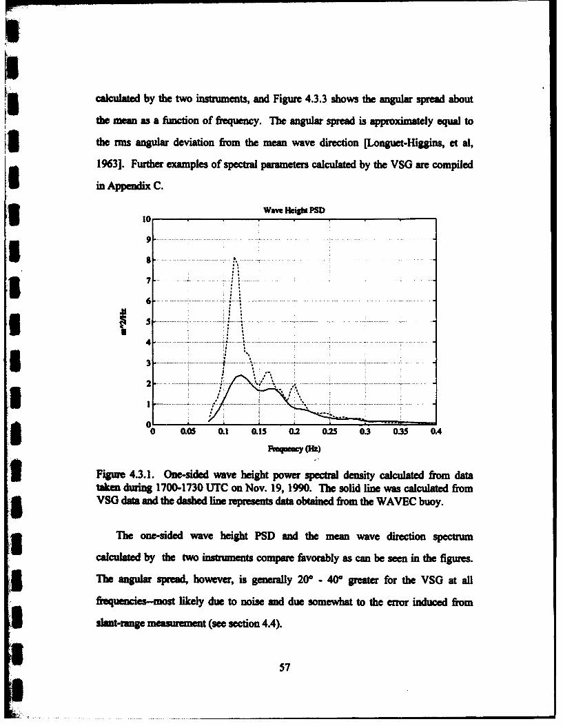
3 Figure 4.3.1 shows the wave height spectrum calculated by the VSG and that
calculated by the pitch-and-roll buoy. The data were taken between 1700 - 1730 UTC
fon November 19, 1990. Figure 4.3.2 shows the mean wave direction spectrum
56
calculated by the two instruments, and Figure 4.3.3 shows the angular spread about
the mean as a function of frequency. The angular spread is approximately equal to
Sthe rms angular deviation from the mean wave direction [Longuet-Higgns, et al,
1963]. Further examples of spectral parameters calculated by the VSG are compiled
in Appendix C.
Wave HeigiE PSD10,
9 ...................... ... ....... . .. ...... . .. .... .. .. .... ... .. . ... .... . . .. . . . ... . ... .... .... .. . . .
3 IC
75:9
6 °
.3 .... ...... I42 ......... ............ .. .... . . ...- .... ....
................................................. . ...... ..... . ..... .. ............. .................
0 US 0.1 01 0.2 0M 03 035 O.
Fiepeuc (Hb)
3 Figure 4.3.1. One-sided wave height power spectral density calculated from datataken during 1700-1730 UTC on Nov. 19, 1990. T7he solid line was calculated fromI ~VSG data and the dashe line represents data obtained from the WAVEC buoy.
3 The one-sided wave height PSD and the mean wave direction spectrum
calculated by the two inistruments compare favorably as can be seen in the figures.
3 The angular spread, however, is generally 200 - 400 greater for the VSG at all
frequencies-most likely due to noise and due somewhat to the error induced from
3 ~ ~slant-range mauent(see section 4.4).
57

i5 Mldm Were Dm•a
ui 300.
200
10 0O05 0. 0.15 0.2 0.25 0.3 0.35 0.4R-gmmIy Oh)
Figure 4.3.2. Mean wave direction spectrum calculated from data taken during 1700-1730 UTC on Nov. 19, 1990. The solid line was calculated from VSG data and the5 dashed line represents data obtained from the WAVEC buoy.
AapI SWWm do habwm
I U ....................
:1 t -~~~~~~~~~~~~~~~7 ... ......................... •........ ..;',,,",s o 4 0 ... ....... .... ... . ..... . . .. ..... . . : ' ..
3 70-
20-I
2 O . ", * ... .
a'0 0. 01 &.15 0.2 0.25 0. 0.35 OA
Figure 43.3. Directional width qptrum calculated from data taken during 1700-1730 UTC on Nov. 19,1990. The solid line was calculated from VSG data and thedashed line repesents data obtained from the WAVEC buoy.
58

4.4 Effect of Inherent Errors on VSG's Determination of Ocean Spectra
The wave height PSD, the mean wave direction spectnrm, and the directional
width spectrum for an ideal measurement system are shown in Figures 4.4.1-3
respectively. The time series of wave heights and slopes were determined
analytically at a single point. The waves have an amplitude of 1.5 m, a frequency of
.1953125 Hz, (the frequency was chosen so that 10 periods is exactly 512 points with
10 Hz sampling) and are coming from 300. The MATLAB program whspec2.m uses
the Longuet-Higgins method given the time series of wave heights and slopes to
calculate the spectra of interest. A 512 point FFT was used with no padding, no
ovpping of data, no decimation, and no windowing.
The cross-spectral components, q12 and q23 (equivalent to Qzy and Qz,
respectively, in Eq. 4.2.9) were set to 1 and 0, respectively whenever either
4• componentfs magnitude was less than 10-8. This has the effect of setting the mean
wave direction to 00 and the angular spread to 00 when data are not present or exists
I in small quantities. Figures 4.4.1-3 show the results for an ideal deterministic noise-
:5 free ocean surface when measured from a single point.
In Figures 4.4.4-6, the wave spectra are shown for the same simulated ocean
surface. In these figures, however, the measurements were made with three beams-
each one measuring vertically. Thus, these figures illustrate the effect of the
derivative approximation on the determination of such spectra. The only noticeable
3 effect is that the angular spread is now 20 at the fundamental frequency.
In Figures 4.4.7-9, the spectra are calculated for the same ocean surface. In these
figures, though, thmeasurements are made along a slant range. The radar in this
simulation is mounted at 20 m and the angle of incidence is 47°. These figures, then,
illustrate the error due to slant-range measurements. Notice the harmonic that appears
59

I Wwahmi PSD
40
• i . . ...... ... ....
11
_. io~~~~~~~~~~3 . ... .... . .... .......... : ..... . .......... ..... ...
L of1 0 .05 0.1 0.15 0.2 0.5 0.3 0.35 OA
Figure 4.4.1. One-sided wave height PSD calculated from simulated ocean surfacedata. Wave Amplitude, 1.5 m; Wave Frequency, 0.1953125 Hz; Wave direction, 30 .
Wane Direciom3 30
205Il U
30 0.05 0.1 0.15 0.2 0.25 0.3 0.35 0.4
Figure 4.4.2. Mean wave direction spectrum calculated from simulated ocean surfacedata. Wave Amplitude, 1.5 m; Wave Frequency, 0.1953125 Hz; Wave direction, 30°.
3 60I1

S
Asaglw Spred
S ~0.240.11.
0.1 6 -
0 . ..... . .- | o ~ ~~ ~~~~~. , ...... ..... ... .... ..... '. ......... . .. . ... ... ......... .. .. ..........
I4 ....... .. 1 ... ...... ........ ... .. .. ....0 .0 . .... . ..... .. ... . ........ .
I0 0.05 0.1 0.15 0.2 0.25 03 0.35 0.4
IFk -w
Figure 4.4.3. Directional width spectrum calculated from simulated ocean surfacedata. Wave Amplitude, 1.5 m; Wave Frequency, .1953125 Hz; Wave direction, 30°.
WS"Awb~b PSD
.. .... .. . .. . . ° ..... ....... .. ... . .
3igre 4.4..Oesdlwv egtPI acltdfo iua~ ca ufc............. ..v ....tde ..5 .. ..v Fre ue.y . .1953125 .. ... W av ...... on ......
2 ~0 ...... .......-... ........
.. .. .... . .. ........
0 0.0 0.1 MI15 &r2 0.25 0.3 0.35 0.
Figure 4.4.4. One-sided wave height PSD calculated from simulated ocean surfacedata. Wave Amplitude, 1.5 m; Wave Frequency, .1953125 Hz-, Wave direction, 300.
Measurements were taken simultaneously along three vertical beams.
3 61

IIjWave Direction
25
II, to
I S -I ~..... .......
30. 0.05 01 0is 0.2 0.25 03 035 0.4
Frequency
I Figure 4.4.5. Mean wave direction spectrum calculated from simulated ocean surfacedata. Wave Amplitude, 1.5 m; Wave Frequency, .1953125 Hz; Wave direction, 300.Measurements were taken simultaneously along three vertical beams.
IJ . ~ ~... ...... ... .... ........ ...... .r
IA
1.23A 1 ......... ...IA - . ...... . . .. .. .... ..... *. . .... .. ...... ...... . ....... . ...... ...... ... ..) .... .. ...... ....... . ...... ...
U ....................... ............. ........... ................... ....... .! ...........
0.43.... ... . ... . ..... .... . ..... - .... ...
0 .2 . .. .. . . . .. . . .... ... ... .. ... ....... ... . . . .. .. . .. ...... .. . . ..... .............. ..... .: .. .. ...... . .
3. .0o.2• o3 o, .0 0.0 U. 0.15 012 0.25 03 0.35 0.4
Figure 4.4.6. Directional width spectrum calculated from simulated ocean surfacedata. Wave Amplitude, 1.5 m; Wave Frequency, .1953125 Hz; Wave direction, 30 .
Measurements were taken simultaneously along three vertical beams.
62
Fi.

Wwetemighl PSD
3 50
* 20-
20 . ....... ... ..
1 0 - . .. .•- ....... . . . :. . . . . . .. . .
S010
0 0.05 0.1 0.15 0.2 0.25 0.3 035 0.4
Figure 4.4.7. One-sided PSD calculated from simulated ocean surface data. WaveAmplitude, 1.5 m; Wave Frequency, .1953125 Hz, Wave direction, 30°, Incidenceangle, 470; Antenna height, 20 m. Measurements were made simultaneously along aslant range. 33WaveWftdwmuo
3 30
25.
I 20-
I10- ... . ........
iU 0-0 0.05 0.1 0.15 0.2 0.25 0.3 0.35 0.4
FnwUency
Figure 4.4.8. Mean wave direction spectrum calculated from simulated ocean surfacedata. Wave Amplitude, 1.5 m; Wave Frequency, .1953125 Hz, Wave direction, 300,Incidence angle, 470; Antenna height, 20 m. Measurements were madesimultaneously along a slant range.
63t

i6 AnuIar Spread
4
2 . ..... .. ..
S0O 0.05 0.1 0.15 0.2 0.25 0.3 0.35 0.4
FrequencyI Figure 4.4.9. Directional width spectrum calculated from simulated ocean surfacedata. Wave Amplitude, 1.5 m; Wave Frequency, .1953125 Hz; Wave direction, 300,Incidence angle, 470; Antenna height, 20 m. Measurements were madesimultaneously along a slant range.
Wavdwtilw PSD
so ........
*40. . ....................
1 30............... . ...............
1o .3 ...... ...... ..... .- ..... -. ..-.
0 m 0.1 L 0.15 0U 0M2 0.3 0.35 OA
Frequenc3: Figure 4.4.10. One-sided PSD calculated from simulated ocean surface data. WaveAmplitude, 1.5 m; Wave Frequency, .1953125 Hz; Wave direction, 300 Incidenceangle, 470; Antenna height, 20 m. Measurements were made non-simultaneouslyalong a slant range.
64
ia

Woe Dim.ia.
14-
13S12-
0do0. 0.15 0.2 M3 0. 03 0.4
I0
Figure 4.4.11. Mean wave direction spectrum calculated from simulated ocean
5 surface data. Wave Amplitude, 1.5 m; Wave Frequency, .1953125 Hz; Wave
direction, 30°, Incidence angle, 470; Antenna height, 20 m. Measurements were made
non-simultaneously along a slant range.
... ... . .... .... ........
I .2U .... ............ . ...20 - . ...... . . ... ..... . . . .... .....
5..-
o0 W . .5 02 02 . 3 .
i Figure 4.4.12. Directional width spectrum calculated from simulated ocean surface
data. Wave Amplitude, 1.5 m; Wave Frequency, .1953 125 Hz; Wave direction, 300,
Incidence angle, 47°; Antenna height, 20 m. Measurements were made non-5 simultaneously along a slant range.
U 65
I

3 in the wave height PSD. Just as slant-range measurement had no appreciable effect
on the determination of mean wave direction with the ellipse fit, it also has no effect
3 using the Longuet-Higgins approach. The angular spread, however, is affected by
slant range measurements. Figure 4.4.9 shows that the angular spread at the second
harmonic is m5.5°. This suggests that in a continuous spectrum, there could be a
I significant increase in the angular spread due to harmonics.
Figures 4.4.10-12 show the ocean spectra taking into account all inherent errors.
3 Measurements were made non-simultaneously along a slant range. The wave height
PSD is still determined accurately, but the mean wave direction spectrum has
dramatically changed. Similar to the ellipse fit, the mean wave direction is now
approximately 160 for most frequencies. Thus, we have further evidence of the
detrimental effects due to non-simultaneous measurements.
3 It is not clearly understood why spectral components appear at all frequencies in
the mean wave direction spectrum and the angular width spectrum. Although 512
data points are used in the FFT, this does not constitute a full 10 periods of data.
3 Since there are 99 ms between samples at the same point, 512 samples takes 50.688
sec. However, 10 periods of data at .1953125 Hz takes 51.2 sec. However, the fact
3 that we do not have a full 10 periods of data does not completely account for the
additional spectral components.
IIII
66
I

5 5. Conclusion
We have seen that, like any system, the VSG has inherent errors associated with
its method of measurement. The errors inherent to the VSG include phase shifts in
time series of wave heights and slopes due to measuring along a slant range,
modulation of the slope time series due to the first order approximation of the
derivative, and miscalculation of the mean direction of wave travel due to finite
switching time between the feeds.
Measuring along a slant range induces phase shifts because the measurement site
has some horizontal motion. The maximum amount of phase error in the wave height
I• and slope time series occurs at the crest and trough of the wave while. The maximum
3m amount of error depends upon the wave steepness, the angle of incidence, and the
wave direction. It is worse for steep waves, large angles of incidence, and for upwave
3I or downwave look direction. Slant-range measurements cause the slope time series to
be overestimated at every point in time in both directions.
I The slant-range measurements cause harmonics to appear in the frequency
3n domain. Even for relatively steep waves the second harmonic is small (w-20 dB), and
higher harmonics are even smaller.
Approximating the slope at point by a plane causes the slope time series to be
modulated by a sinc function. The relative error depends upon the wave number, k,
[I and the distance between the radar footprints. Slant-range measurements cause the
distance between the footprints to be modulated. The error is a maximum near the
trough of a wave when the distance between the footprints is a maximum. For the
3 steepest waves the error is about 9%, but for most of the energy-laden waves the error
is less than 2%. The derivative approximation causes the VSG to underestimate the
iI magnitude of the slope time series at every point.
67

The finite time between beam measurements seems to have the most serious
effect on the slope time series. Due to the finite time between measurements, there is
3 phase error in the second and third measurements. In the wave height time series this
does not have much effect because the three measurements are averaged. However,
the slope time series depends on an accurate measurement of each position.
3 Therefore, any error in single measurement has serious effects.
The distribution of ocean waves measured during the SAXON experiment is
3 nearly bivariate Gaussian. This enabled us to fit an ellipse to the two-dimensional
slope distribution. The orientation of the major axis indicates the mean direction of
wave travel with 1800 ambiguity. In addition, statistics of the slope distribution are
31 easily obtained from the ellipse fit to the distribution.
Slant-range measurements cause the ellipse width to increase slightly, but have
31 no effect on the determination of the mean wave direction. The derivative
approximation also causes the width of the ellipse to increase slightly. This source of
I error also has no affect on the determination of the mean wave direction. Non-
simultaneous measurements, however, cause the mean wave direction to be
miscalculated. For the particular example in section 3.4, the VSG would have
3 measured the waves as coming from 160 when then they were actually coming from
300.
II The directional ambiguity can be resolved by taking advantage of the asymmetry
of ocean waves. Since the back side of ocean waves is longer than the front, and
since the VSG records data at a constant rate of time, more data is recorded along the
3 back side of the waves. Therefore, a histogram of the slope distribution will aid in
resolving the directional ambiguity. By fitting an ellipse to the histogram of slopes
a 68,I

Ii I
5I using the method of least squares, the center of the ellipse will indicate the mean
direction from which waves were traveling.
5 The Longuet-Higgins method for determining ocean spectra has been used for a
number of years with pitch-and-roll buoy data. Since the same parameters are
available from the VSG, the Longuet-Higgins approach can be used with the VSG
3 data. This enabled a comparison to be made between the VSG and a pitch-and-roll
buoy.
5 The wave height spectrum and the mean wave direction spectrum compare
favorably between the two instruments. However, the angular spread about the mean
I is generally 200 - 40° greater at all frequencies for the VSG than for the pitch-and-roll
buoy. There may be several explanations for this. Higher frequency waves have a
shorter wavelength, and thus are more susceptible to changes in the wind direction.
In addition, since the waves are shorter fewer measurements are along each wave
which results in more noise. As the wavelength approaches the size of the buoy, the
I buoy may no longer follow the surface very closely.
5 The derivative approximation causes the angular spread to increase slightly-from
roughly 0* to 2*. Measuring along a slant range causes a harmonic to appear in the
3 spectral parameters. The angular spread at the first harmonic is approximately 5.5°.
Due to non-simultaneous measurements, the mean wave direction was roughly 160
instead of the correct direction of 300. The angular spread at the fundamental
frequency remained about 20.
II3 69
I

MI Recommendations for Further Study
It would seem that the most important item that could be done to improve the
VSG's performance would be to decrease the time between measurements from each
feed. This should improve the accuracy of the determination of the mean wave
direction.
3 Although slant-range measurements do not seem to affect the calculation of the
mean wave direction, they do cause the slope time series to be overestimated at every
3 point in both directions. This may be important when analyzing the modulation of
the radar signal due to tilt modulation. The only solution (and its only partial) is to
i operate the radar at small angles of incidence.
3 It seems that the first order approximation of the derivative does a good job at
estimating the slope at a point within the plane formed by the radar footprints. It has
3 little effect on the wave height time series or the slope time series.
All the analysis in this paper has been done with a deterministic ocean surface.
The next step would be to do the same analysis with a random ocean surface and
i noise added to the system. This would give more realistic examples of the inherent
errors involved with measuring wav- -,-Its and vector slopes with the VSG.
3 iIt would be nice to have an analytical description of the error in the slope time
series due to non-simultaneous measurements. However, it is an extremely
complicated process. A finite time between switching causes the measurements of
3 from beam 1 and beam 2 to have some phase error. The amount of phase error
depends only on the frequency of the wave and the time between sampling (see Fig.
3 2.9.1). Once the phase error has been determined, the error in the height
measurement (which will be a function of time) can be determined. This requires that
mI the height at each footprint be known assuming that the heights were measured
I 70'iU

5 simultmously. The difference in height at each point can be used to determine the
equation of the plane (which will be a function of time), and hence the error in the
slope time series in any direction. Since all three points are required to determine the
slope time series, it is not enough to determine the error in the wave number at each
U point. At this point only empirical evidence is available to illustrate the error due to
non-simultaneous measurements.
IUI
IIIIIIII
r . 7 1
U

Uo
REFERENCES
Allender, J., T. Audunson, S. F. Barstow, S. Bjerken, H. E. Krogstad, P. Steinbakke,L. Vartdal, L. E. Borgman, and C. Graham, "The WADIC Project: A Comprehensivefield evaluation of directional wave instrumentation," Ocean Engng., vol. 16, no 5/6,1989, pp. 505-536.
Batschelet, E., Circular Statistics in Biology, London: Academic Press, 1981, pp 246-274.
Evans, C., S. Haimov, and R. K. Moore, "Calculation of Ocean EnvironmentalParameters from a Ka-Band Scatterometer using the Longuet-Higgins Approach," tobe presented at IGARSS '94, 8-12 Aug., 1994, Pasadena, CA.
Evans, C., S. Haimov, R. K. Moore, and V. Hesany, "Determination of OceanEnvironmental Parameters from a Ka-Band Scatterometer," Proc. of Oceans '93, vol.2, 18-21 October 1993, Victoria, Canada, pp. 1-4.
Gross, M. G., Oceanography: A View of the Earth, Englewood Cliffs, NJ: PrenticeHall, 1982, pp. 211-235.
Hesany, V., R. K. Moore, and S. P. Gogineni, "A Vector Slope Gauge andSctterometer for Ocean Measurements," Proceedings of URSI Microwave Signatures'92 Conference, July 1-3, 1992, IgIs, Austria 1D/25-1D/30.
Hesany, V., A radar vector slope gauge for ocean measurements, Ph.D. Thesis in
Department of Electrical Engineering and Computer Science, The University ofKansas, May 1994, pp 70-73.
Kuik, A. J., G. PH. Van Vledder, and L. H. Holthuijsen, "A Method for the RoutineAnalysis of Pitch-and-Roll Buoy Wave Data," I of Physical Oceanography, vol. 18,July, 1988, pp. 1020-1034.
Longuet-Higgins, M.S., D. E. Cartwright, and N. D. Smith, "Observations of theDirectional Spectrum of Sea Waves Using the Motions of a Floating Buoy,"Proceedings of Ocean Wave Spectra Conference, Easton, Maryland, 1-4 May 1961,3 Ipp. 111-136, Englewood Cliffs, NJ: Prentice Hall, 1963.
I|7

I
Neumann, G., and W. J. Peirson, Jr., "Known and Unknown Properties of theFrequency Spectrum of a Wind-Generated Sea," Proceedings of Ocean Wave SpectraConference, Easton, Maryland, 1-4 May 1961, pp. 9-25, Englewood Cliffs, NJ:Prentice Hall, 1963.
Plant, W. J., and W. Alpers, "The SAXON-FPN Experiment," IGARSS '91 Digest,IEEE 91CH2971-0, Espoo, Finland, 3-6 June, 1991, pp. 1983-1986.
Shanmugan, K. S., and A. M. Breipohl, "Random Signals: Detection, Estimation, and3 Data Analysis," John Wiley & Sons, Inc., New York, 1988, p. 46.
Steele, K. E., C. Teng, and D. W. C. Wang, "Wave Direction Measurements usingPitch-Roll Buoys," Ocean Engng. ,vol. 19, no. 4, 1992, pp. 349-375.
IIIIUUI
II 7
I

Appmedix A
function [ran, x, y, z] = range(thetadeltabetal2,beta23,gammarphi,fA)% [ran, x, y, z] = range(thetadeltabetal2,beta23,gamma,r,phi,fA)% determines the range to the ocean surface along the three beams taking% into account all possible angles. This program solves the nonlinear% equation that arrises from finding the point of intersection of the% radar beam with the ocean surface.
% thet - the angle the radar was rotated about the x-axis (angle of inc.)% delta - the angle the radar was rotated about the z! axis
% betam2 - the angle between beams I and 2iI % beta23 - the angle between beams 2 and 3% gamma - the angle between beams I and 3
% r - initial guess of length of beam 1, 2, and 3 in metersI% [1,2,31% phi - the angle between the RDL and the direction from which the waves% are coming%% Since there may be multiple solutions to the nonlinear equation, it is best% to guess the most accurate length of r, while making sure that the guess is% shorter than the resulting solution.
% Chris Evans, RSL, The University of Kansas, May 26,1994%
theta = theta*pi/I 80; % theta and delta are measured positive from CCWdelta = delta*pi/180;betal2 = betal2*pi/180;beta23 = beta23*pi/180;gamma = gamma*pi/180;phi = phi*pi/I 80;
h = 20; % height of radar (meters) above mean sea surface*/*A = 5.0; % amplitude of ocean wave in meters
RI 1 = cos(delta)*sin(betal2)*cos(gammalpi/2) + sin(delta)-sin(betal2)sin(gamma-p*-2);
I R21 = sin(delta)*cos(theta)*sin(betal2)*cos(gamma-pi/2) -cos(delta)*cos(theta)*sin(betal2)*sin(gamma-pi/2) + sin(theta)*cos(betal2);R31 = sin(delta)*sin(theta)*sin(betal2)*cos(gamma-piI2) -
cos(delta)*sin(&tet)*sin(betal2)*sin(gammaý-piI2) - cos(theta)*cos(betal2);
74

R12 -0;3 R22 -sin(theta);R32 - -cos(theta);R13 - -sin(delta)*sin(beta23);R23 = cos(delta)*cos(theta)*sin(beta23) + sin(theta)*cos(beta23);R33 = cos(delta)*sin(theta)*sin(beta23) - cos(theta)*cos(beta3);
Sk = ((2*pi*f0A2)/9.8; O/ospatial. frequency of waves (2*pi/lambda)
rl(l) =0; rl(2) =r(l);r()-0r()r2(1) = 0; r2(2) = r(2);
I ~fort- 1:10/f+1I, %t isin tenths of seconds; 10/f gives 1 periodi - 2;while (abs(rl(i)-rl(i-1)) > le-13) I (abs(r3(i)-r3(i-l)) > le-13), % error must be less
x l(i) =rl(i)*R31; z2(i) =; r2i) 3(; =z3(i) R 3;zctl(i) = 2pi)*f*33*3i=r(i*R/100 + ki (pi)xl3(i)*+kcs2 h)*l;)I ~ ~~~zet(i) =2l~pi)*f31;z*)r(3)*R+1/10 kzsi(pi)=x2(i)+k*coRpi)y2i)Zeta3(i) =2*pi*f*33(3*t2/1000 + k*sin(pbi)*x3(i) + k~cos(pbi)*y3(i);seal(i) = A~*3*co (3*tal~ ) 100 - ~ i~hi*2i h;~ospi*y(I eta2(i) = A~*3*co (zeta2(i))O - ~ i~h)x()+ ~o~h)y(seal(i) =A*cos(zetal(i)) -h
FI(i) = zl(i) - seal(i); F2(i) = z2(i) - sea2(i); F3(i) = z3(i) - sea3(i);Fderl(i) =R31 + A~sin(zetal(i))*(k*sin(pbi)*R1 1 + k~cos(phi)*R21);Fder2(i) -R32 + A*sin(zeta2(i))*(k~sin(phi)*R12 + k*cos(phi)*R22);Fder3(i) = R33 + AMsin(zeta3(i))*(k~sin(phi)*R13 + k~cos(pbi)*R23);rl(i+l) = rl(i) - F1(i)/Fderl(i);r2(i+l) = r2(i) - F2(i)IFder2(i);'U r3(i+1) = r3(i) - F3(i)/Fder3(i);i =i+1;
end
ran(t,:) = [rl(i), r2(i), r3(i)J;
end
1 75

function [ran, x, y, z] = slrange(theta,deltabetaI2,beta23,gammaphi,fA)% [ran, x, y, z] = slrange(theta,deltabetal2,beta23,gamma,r,phi,fA) determines the% range to the ocean surface along the three beams taking into account all% possible angles. This program solves the nonlinear equation that arrises% from finding the point of intersection of the radar beam with the ocean% surface.%% theta - the angle the radar was rotated about the x-axis (angle of inc.)% delta - the angle the radar was rotated about the z! axis
% betal2 - the angle between beams 1 and2% beta23 - the angle between beams 2 and 3% gamma - the angle between beams I and 3%r -initial guess of length of beam 1, 2, and 3 in metersS% [1,2,3]% phi - the angle between the RDL and the direction from which the waves% are coming
% Since there may be multiple solutions to the nonlinear equation, it is bestI% to guess the most accurate length of r, while making sure that the guess is% shorter than the resulting solution.
_ % Chris Evans, RSL, The University of Kansas, March 1, 1994
S theta = theta*pi/180; % theta and delta are measured positive from CCWdelta = delta*pi/1 80;betal2 = betal2*pi/180;beta23 = beta23*pi/180;gamma = gamma*pi/l 80;phi = phi*pi/180;
h = 20; % height of radar (meters) above mean sea surface
**A = 5.0; % amplitude of ocean wave in meters
RI 1 = cos(delta)*sin(betal2)*cos(gamma-pi/2) + sin(delta)*sin(betal2)*sin(gamma-pi/2);R21 = sin(delta)*cos(theta)*sin(betal2)*cos(gamma-pi/2) -
cos(delta)*cos(theta)*sin(betal2)*sin(gamra-pi/2) + sin(theta)*cos(betal2);R31 = sin(delta)*sin(theta)*sin(betal2)*cos(gamma-pi/2) -cos(delta)*sin(theta)*sin(betal2)*sin(gamma-pi/2) - cos(theta)*cos(betal2);
SR12 = 0;R22 = sin(theta);
3 76
I;

R32 - -cos(theta);R13 - -sin(delta)*sin(beta23);
R2 coscdlta):cos~theta)*:in(ibeta23) + si(theta)*cos(beta23);
k -((2*pi*f)A2)/9.8; %/spatial frequency of waves (2*pi/lamnbda)
rl(l) = 0; rl(2) = l)r2(1) =0; r2(2) =r(2);r3(1) = 0; r3(2) = r(3);
for t = 1: 10/f, % t is in tenths of seconds; 40/f gives 4 periodsi =2;while (Abs(rl(i)-rl(i-1)) > le-13) I (abs(r3(i)-r3(i-1)) > le-13), % error must be less
than this #xl(i) =rI(i)*R1 1; x2(i)= 0; x3(i) = r3(i)*R13;yl(i) =rI(i)*R21; y2(i) =r2(i)*R22; y3(i)=r3(i)*R23;zl(i) =rl(i)*R31; z2(i) =r2(i)*R32; z3(i) =r3(i)*R33;I zetal(i) = 2*pi*fPt/10+ k*sim(phi)*xl(i) + k*cos(phi)*yl(i);zeta2(i) = 2*pi~ft/10+ k*sin(phi)*x2(i) + k*cos(phi)*y2(i);zeta3(i) = 2*pi*fN/10+ k*smn(phi)*x3(i) + k*cos(phi)*y3(i);Iseal(i) -A*cos(zetal(i)) - hsea2(i) = A*cos(zeta2(i)) - hsea3(i) = AMcos(zeta3(i)) - h;S P1(i) = zl(i) - seal(i); P2(i) = z2(i) - sea2(i); F3(i) = z3(i) - sea3(i);Fderl(i) = R31 + A*sin(zetal(i))*(k*sin(phi)*RI I + k*cos(phi)41R21);3 Fder2(i) = R32 + AMsin(zeta2(i))*(k*sin(phi)*R12 + k~cos(phi)*R22);Fder3(i) = R33 + A*sin(zeta3(i))*(k*sin(phi)*R13 + k*cos(phi)OR23);rl(i+1) = rl(i) - F1(i)/Fderl(i);3 r2(i+l) = r2(i) - F2(i)/Fder2(i);r3(i+l) = r3(i) - F3(i)IFder3(i);
endran(t,:) = [rl(i), r2(i), r3(i)];
5 end
k77

I
function [ran, x, y, z] = vrange(x, y, f, A, phi)[ran, x, y, z] = vrange(x, y, f, A, phi) determines the
% range to the ocean surface assuming the three points of intersection are% moving vertically and assuming the measurements are made simultaneously.%% x : time series of x coordinates from range.m [xl, x2, x3]% y : time series of y coordinates from range.m [yl, y2, y3]% f : frequency of ocean waves used in range.m% A amplitude of ocean wave in meters used in range.m% phi direction from which ocean waves are coming in deg. (from range.m)%% ran: time series of ranges [rl, r2, r3]% x time series of x coordinates in earth system [xl, x2, x3]% y time series of y coordinates in earth system [yI, y2, y3]% z time series of z coordinates in earth system [zl, z2, z3]
%% Chris Evans, RSL, The University of Kansas, March 28,1994
I%phi = phi*pi/180;
5 h = 20; % height of radar (meters) above mean sea surfacek = ((2*pi*f)^2)/9.8; %spatial frequency of waves (2*pi/lambda)[r,c] = size(x);xl = mean(x(:,l)); x2 = mean(x(:,2)); x3 = mean(x(:,3));yl f= mean(y(:,1)); y2 = mean(y(',2)); y3 = mean(y(:,3));
I t = 1:r;t=f;
zli = A*cos(2*pi*f*t/10 + k*sin(phi)*xl + k*cos(phi)*yl) - h;z2 = A*cos(2*pi*f*t/10 + k*sin(phi)*x2 + k*cos(phi)*y2) - h;z3 = A*cos(2*pi*f*t/10 + k*sin(phi)*x3 + k*cos(p' ')*y3) - h;
ranI = sqrt(xlA2 + ylA2 + zl .A2);ran2 = sqrt(x2A2 + y2^2 + z2 A2);ran3 = sqrt(x3A2 + y3A2 +z3 .A2);
I x = [xl *ones(r,1), x2*ones(r, 1), x3*ones(r, 1)];y = [y I *ones(r, 1), y2*ones(r, 1), y3*ones(r, 1)];3 z = [zl, z2, z3];ran = [rani, ran2, ran3];
1 78I I"

function [Sy,Sx] = slopeab2(x,y,z)% [Sy,Sx] = slopeab2(x,yz)
% Slopeab2 determines the slope time series from the plane given the x, y,% and z, coordinates of the points of intersection of the radar beamsS~% with the ocean surface.
% x - x coordinate of the point of intersection. (n x 3)% y - y coordinate of the point of intersection. (n x 3)I % z - z coordinate of the point of intersection. (n x 3)%% Sy - time series of slope in y (RLD) direction (degrees)% Sx - time series of slope in x (cross) direction (degrees)%
% Chris Evans, RSL, The University of Kansas, March 28, 1994%
t % B & C are vectors in the plane, and N is the normal to the plane
B = [(x(:,l) - x(:,2)), (y(:,l) - y(:,2)), (z(:,l) - z(:,2))];C = [(x(:,3) - x(:,2)), (y(:,3) - y(:,2 )), (z(:,3) - z(:,2))];
% Normal components are found from the cross product of B and C.
I Nx = B(:,2).*C(:,3) - C(:,2).*B(:,3);Ny = B(:,3).*C(:,I) - C(:,3).*B(:,I);3 Nz = B(:,I).*C(:,2) - C(:,I).*B(:,2);
% The slope of the plane is the negative inverse of the slope of the line.
Sy = 180/pi*atan(-Ny./Nz);Sx = 180/pi*atan(-Nx./Nz);
7£IU!,
3 7

II
function [Sy,Sx] = slopepoi(ranthetadeltabeta 2,beta 23,gam maAphi,f)%% [Sy,Sx] = slopepoi(ran~theta~delta~beta12,beta23,gamnaA~phi,f)
% calculates the slope at the point for which the slope is being% approximated with slopeab.m.
% ran : n x 3 time series of ranges% theta : radar angle of incidence in degrees% delta : angle of CCW rotation about the z' axis% betal2: angle between beamns 1 and 2
I % beta23 "angle between beams 2 and 3% gamma: angle between the planes formed by beams I & 2 and 2 & 3 in degrees% A : amplitude of ocean waves in meters (1/2 waveheight)% phi : direction from which the waves are traveling% f : f-requency of ocean wave in Hz%% Sy : Slope in y direction in degrees% Sx : Slope in x direction in degrees%% Chris Evans, RSL, The University of Kansas, March 10, 1994
I%theta = theta*pi/I 80;delta = delta*pi/1 80;gamma = gamma*pi/l 80;betal2 = betal2*pi/180;3 beta23 = beta23*pi/180;
[r,c] - size(ran);
I % coordinates in the antenna systemxla = ran(:,l)*sin(betal2)*cos(pi/2-gamma);yla = ran(:,l)*sin(betal2)*sin(pi/2-gamma);zla = -ran(:,l)*cos(betal2);x2a = zeros(r,1);y2a = zeros(r, 1);z2a = -ran(:,2);x3a = zeros(r,l);y3a = ran(:,3)*sin(beta23);z3a = -ran(:,3)*cos(beta23);
-% rot transforms from the antenna to the earth coordinate system
3 80

rot - [cos(delta), -sin(delta), 0;Uo~ht)sndlacsdlt)cstea,-i~ht)osi(theta)*sin(delta), cos(delta)*csi(theta), -osn(theta)];
fort= l:r,Ant = [xlIa(t), x2a(t), x3a(t);B y Ila(t), y2a(t), y3a(t);
zla(t), z2a(t), z3a(t)J;
IE = o*Atxle(t) = E(l,l); x2e(t) = E(1,2); x3e(t) = E(1,3);yle(t) = E(2lI); y2e(t) = E(2,2); y3e(t) = E(2,3);
zle(t) = E(3,l); z2e(t) = E(3,2); z3e(t) = E(3,3);
% coordinates are now in the earth system
Al = (y Ie(t)-y2e(t))*(z3e(t)-z2e(t)) - (y3e(t)-y2e(t))*(zl e(t)-z2e(t));I~BI1 = (x3e(t)-x2e(t))*(zl e(t)-z2e(t)) - (xle(t)-x2e(t))*(z3e(t)-z2e(t));Cl = (xle(t)-x2e(t))*(y3e(t)-y2e(t)) - (x3e(t)-x2c(t))*(yl e(t)-y2e(t));A2 = x3e(t)-x2e(t);I B2 = y3e(t)-y2e(t);C2 = z3e(t)-z2e(t);A3 = xle(t)-x2c(t);B3 = ylIe(t)-y2eft);C3 = zle(t)-z2e(t);
I R = [Al, Bi1, Cl1; A2, B2, C2; A3, B3, C3];
3I D l xet)+Byet)+Czet;D2 = 0.5*(x3e(ty^2 + y3e(t)I2 + z3e(t)A2 - x2e(t)A2 - y2e(t)'2 - z2e(t 2);D3 = 0.5*(xle(t)A2 + yle(tr2 + zle(t)A2 - x2e(t)A2 - y2e(t)'2 - z2e(t)A2);
S=[DI; D2; D3];
Q Q imv(R)*S;Px =QMl;3Py =Q2)
k = (2*pi*f)A2/9.8;Sy(t) =
atan(A*k*cos(phi)*cos(2*pi*f~t/l 0+k*sin(pbi)*Px+k*cos(pbi)*Py))* 1 8O/pi;
3 81

Sx(t)
enatan(A*k*sin(phi)*cos(2*pi*femt/1 O+k~sin(phi)*Px+k*cos(phi)*Py))* I 8O/pi;Sy Sy'; Sx =Sx!;
I8

function [a,b,thetaRo,betafreq,ang,X,Y,xr,yr] = elipsef(x,y,dirbinwidth)% ELLIPSEF. Ellipse fit.% [a,b,thetaRo,betafreq,ang,X,Y,xr,yr] = ellipsef(x,y,dir,binwidth)
% x - x-data vector% y - y-data vector% dir - y axis orientation with respect to North in degree (East is 90)% binwidth - bin width for x-y phase histogram (in degree)
% a - length of major axis% b - length of minor axis% theta - major axis orientation in radians:S% theta(l) - standard trig. presentation (with respect to x axis)% theta(2) - with respect to North% Ro - distance from ellipse center to the origin% beta - location angle of ellipse center% freq - frequency counts of the phase histogram
% ang - bin angles of the phase histogram% X x-coordinates of the ellipse for Earth map orientation% Y y-coordinates of the ellipse for Earth map orientationSxr - rotated x-data vector% yr rotated y-data vector (yr axis points North)
£ % Samuel Haimov, 3/23/93, RSL, The University of Kansas
if nargin < 4 binwidth = 18; endifnargin < 3 dir = 0; end
% Rotate the coordinates relative to the RLD and Northr = (360-dir)*pi/I 80;xr = x'cos(r) - y'sin(r);yr = x'sin(r) + y'cos(r);
% Find directional histogram5 binnum = fix(360/binwidth);angp - angleour+j*yr);[freq,ang1 - hist(angpbinnum);
% Ellipse fit (Bivar. Normal Distrb.); A(xr-mx)i2+2B(xr-mx)(yr-my)+C(yr-my)2-D
cv-cov([xr(:) yr(:)J);mx nxr); my-mean(yr); % center of the ellipse
83

beta -0; Ro =0;£ if abs(mx)> Ie"6 absmy)>lIe-6beta-afta2(my,max); % ellipse center in polar
gRo-sqrt(mxA2+myA2); % coordinates
vx-cv(l,l); vy-cv(2,2);A-vy; B-cv(2,l); C=vx; % ellipse eq. polmnomial coeffs.ID=2(VX*VyBA2); % free coeff. in the ellipse polinom.R-sqrt((A-C)A2+4*BA2);a-sqrt(2*D/(A+C-R)); % major axisbmsqrt(2*D/(A+C+R)); % minor axistheta(l)=atan(2*B/(A-C-R)); % ellipse orientation
% also theta=0.5*atan(2*B/(A-C));
% Calculate ellipse parametric equationsphi=O:pi/l 28:2*pi;
%Modify theta with respect to North
I if theta(l) >= -pi & theta(l) < pi/2 theta(2) --theta(l) + pi/2; endif theta(l) >-- pi/2 & theta(l) <= pi theta(2) =-theta(l) + 2.5*pi; end
£8

finction [ab,thetaRbet•freq,angX,Yxryr] = elHpseh(xy,dirbinwidth)% ELLIPSEH. Ellipse fit of the x-y data histogram.% [a,b,thetaRo,beta,freqang,X,Y,xr,yr] = ellipseh(xy,dir,binwidth)
% x - x-data vector (e.g., slope in x-direction)% y - y-data vector (e.g., slope in y-direction)% dir - y axis orientation with respect to North in degree (e.g., RLD)% binwidth - bin width for x-y phase histogram (in degree)
% a - lengthofmajoraxis% b - length of minor axis% theta - major axis orientation with respect to North (radians)% theta(l) - standard trig. presentation (with respect to x axis)% theta(2) - with respect to North% Ro - distance from ellipse center to the origin% beta location angle of ellipse center% freq frequency counts of the phase histogram% ang - bin angles of the phase histogram% X x-coordinates of the ellipse for Earth map orientation% Y - y-coordinates of the ellipse for Earth map orientation% xr rotated x-component of the histogram% yr - rotated y-component of the histogram (yr axis points North)
% Samuel Haimov, 3/23/93, RSL, The University of Kansas
% Rotate the coordinates relative to the RLD and Northr = (360-dir)*pi/1 80;xr = x*cos(r) - y*sin(r);yr = x'sin(r) + y*cos(r);
% Find directional histogrambinnum = fix(360/binwidth);angp = ang(6xr+jhyr);[freqang] = hist(angpbinnum);xr = freq.*cos(ang);yr = freq.*sin(ang);
% Ellipse fit (Bivar. Normal Distrb.); A(xr-mx)A2+2B(xr-mx)(yr-my)+C(yr-my)A2-D
cv=cov([xr(:) yr(:)1);mx-nxr); my=mean(yr); % center of the ellipsebeta = O; Ro = O;
85

if absmx)>le- I absmy)>le-6S beta-atan2(myjnx); % ellipse center in polarR-qrgXA 2+my A2); % coordinates
end£ vx--cv(l,l); vycev(2,2);A~vy; B=-.cv(2,l); C--vx; % ellipse eq. polinomial coeffs.
Dih2*(vx~vy-BA2); % free coeff. in the ellipse polinom.IRm,~t(A-CYA2+4*BA2);a=sqrt(2?D/(A+C-R)); % major axisb-sq4crt(2*D/(A+C+R)); % minor axistheta(1)atan*B/(A-C-R)); % ellipse orientation
% also theta=O.5*atan(2*B/(A-C));
£ % Calculate ellipse parametric equationsphi=O:pi/128:2*pi;X--mx+a*cos(thetal )).*cos(jphi)-b~sin(thetal )).*sin(phi);
Y~mmy+a*sin(ft1)).*Wosphi)+b~cos(thý(1 )).*sin(phi);
if theta(l) >= -pi & theta(l) < pi/2 theta2) -thetl) +pitZ; end3 if theta(l) >= pi/2 & theta(l) <= pi theta(2) =-theta(l) + 2*pi+pi/2; end
I8

function [a,b,thetaRo,betaX,Y]=slopdist(date,fnamendec,incrldbwidthpogo)% SLOPDIST: Plots the data points and the best fit ellipse for the slope dist.
% [ab,thetaRo,beta,X,Y] = slopdist(date,fname,ndec,incrldbwidthpo,go)%% date - day of the month for a particular run i.e. 19% fname - file name of a particular run i.e. 1047% ndec - number of points of decimation. Default is no decimation.% inc - radar incidence angle% rid - radar look direction% bwidth - bin width of phase histogram in degrees (9 is default)% po - print option: 'n' - nothing (default) 'm'-create meta file% V's'create ps file V' create meta & ps files q'- create ps & print% 'p' create meta & ps files & print 'd' dump ps file to network printer% go - graphics option: 'op' - portrait, half page (default)% 'ol' - landscape, 'ot' - portrait, full page% 2a - length of major axis in degrees
% 2b - length of minor axis in degrees% theta - most likely direction of wave propagaton in degrees% Ro - distance from origin to center of ellipse% beta - location angle of ellipse center£ % X -x coordinates of best fit ellipse% Y - y coordinates of best fit ellipse
I% Chris Evans, 4/13/93, RSL, The University of Kansas
if nargin = 5 bwidth = 9; po ='n'; endif nargin = 6 po ='n'; endif nargin -7 go = 'op'; end
Smg = loadsax(fYam c,'r',ndc); % loads the range datas = slopeab(rng,inc); % calculates the x and y slope componentsI s = s - ones(length(s),l)*mean(s);s -s; % positive slope is back face of the wave
£ % Ellipse fit for the slope distribution
[a,b,theta,RobetafreqangX,Y,xr,yr] = ellipsef(s(:, 1),s(:,2),rldbwidth);
% Graphics
xr xr SOpi; yr- yr" ISO/pi; %Convert to degrees
1 87Sl ,

X -X*1I80/pi; Y =Y18I0/pi;a a=a*1I80/pi; b =b*1ISO/pi;
r = min(X):max(X); % x-coordinates = tan(theta(l))*r+Ro; % eqn of line for major axis
u = min(Y):max(Y); % y-coordinate
t = (u-Ro)/tan(pi/2+theta(l)); % eqn of line for minor axis
axisenonnal');I ~axis('square'), axis([-30 30 -30 30]);plot(XY,xr,yr,'.',r,s,'-',t~u,'-'); grid;5 %titleff I I P num2str(date)"' num2str(fname) ' Slope Dist. and Best Fit Ellipse']);%/ylabel('Sy (Deg)');%xldabel('Sx (Deg)');
text(.25,.25,'Dir' sprintf('%/3.0f,l80/Pi*theta(2))' deg'],'sc');text(.25,.20,IIMajor Axis' sprintf/%2.lIf ,2*a)' deg'J,'sc');Itext(.25,.15,['Minor Axis ='sprintf('0/2.lIf ,2*b) 'deg'J,'sc');text(.50,.85,'North','ISO
5if po ==pause
else3 ~printps([num2str(finae) 'dir'],,gopo);end
I8

function [AB,C,D,E,F] = lsqfit(x,y)% LSQFIT: finds the least square fit for a 2nd order, 2-D polynomial.% i.e. AxA2 + Bxy + CyA2 + Dx + Ey + F = 0
% function [AB,C,D,E,F] = lsqfit2(xy)%
% x - x vector of real data values
% y - cor of r ta best
%% A,B,CD,E,F - coefficients of the best-fit polynomialU%
% Written 5/12/93 by Chris Evans, RSL, University of Kansas
x =x(:); y = y(:);
Sv [x.A2 x.*y y.A2 x y];V =v'*v;
3] a = inv(V);b = sum(v)';c = a'b;
A = c(l,1); B = c(2,l); C = c(3,1); D = c(4,1); E = c(5,1); F = -1;
9
I
I
I|9I• : , i I I9

Sfunction [maj,minalpha] = dirdist2(finme,date,incrldndec,bwidth)% DIRDIST2: plots the least square fit for the dir. hist. of the slope data
% fimction [major,minor,alpha] = dirdist2(fname,date,incrldndec,bwidth)%% funame - filename of particular run i.e. 1047%date -dateofrun i.e. 19% inc - radar angle of incidence% rld - radar look direction% ndec - number of decimation points (default is 10)% bwidth - width of bin in deg for phase histogram (9 is default)
% maj - length of major axis% min - length of minor axis% alpha - most likely direction of wave prop. in deg (rel. to North)%% Written 4/20/93 by Chris Evans, RSL, University of Kansas
I%
Mg = sx erndec);s = slopeab(mg,inc);s = s-ones(length(s),1)*mean(s);s = -s; % positive slope is back face of wave
U % Rotate the coordinates relative to the RLD and Northr = (360-rld)*pi/1 80;xr = s(:,l)*cos(r)-s(:,2)*sin(r);yr = s(:,l)*sin(r)+s(:,2)*cos(r);
I % Find the directional histogrambinnum = fix(360/bwidth);angp = angle(xr+j*yr);[freq,ang] = hist(angp,binnum);xr = freq.*cos(ang);
£ yr = freq.*sin(ang);
mx = mean(xr);my = mean(yr);I = sqrt(mx^'2 + myA2); % Distance from origin to center of ellipsebeta = atan2(mymx); % Angle between x-axis and ray to center of ellipse
[AB,C,D,E,F] = lsqfit(xryr);
90Il

j alpha =0.5*atan(BI(A-C)); % angle between major axis and pos. x axis
ca = cos(alpha); sa = sin(alpha); cb = cos(beta); sb = sin(beta);
% Constants needed to calculate ellipse parameters
3~ 0= AMca2 + B~sa*ca + C*saA2;H = A*saA2 - B*sa~ca + C~caA2;I = 2*A*l*ca*cb+B*l*sin(alpha+beta)+2*C*l*sa*sb+D~ca+E~sa;J3= -2*A*1*sa*cb+B*l*osalpha+beta)-*2C*l*sa*ca-D~sa-4E*ca;
KA*1A2*(ca2)+B*1A2*sb*cb+C*1A2*(sbA2)+D*l~cb+E*I*sb+F;
Ih =- I/(2*G); k = -J/(2*H); % center coord. of ellipsenumer =4*K*G*H + H*IA2 + G*JA2;a = sqrt(numer/(4*(GW2)*H)); % 1/2 of major axisb = sqrt(numer/(4*G*HA2)); % 1/2 of minor axis
3 theta - 0:pi/180:2*pi;
3 % Ellipse parametric equations
x = l*cb+(h+a~cos(theta))*ca-(k+b*sin(theta))*sa;3 y = l*sb+(h+a*cos(theta))*sa+(k+b*sin(thfeta))*ca;
% Determine the "true" major axis
I if a>b maia = 2*a; min = 2*b; alpha = (piI2-alpha)* 180/pi;elseif alpha>O alpha = (pi-alpha)* I 80/pi; maj = 2*b; min= 2*a;3 else alpha = -alpha* 1 80/pi; maj = 2*b; min = 2*a;end
5 % Normalize area to 1
norm = sqrt(pi*maj~min);U x = x/norm; y = y/norm; maj = maj/norm; min = min/norm;xr = xr/norm; yr = yr/norm; h = h/norm; k =k/norm;
Iifh < 0alpha alpha + 10n
3 % Graphics
3 91

axis('square), ax*s[-1 1 -If]);plot(xr,yr,'*',hrk,'o',x,y);grid;%/titleff 1 I/f num2str(date)"num2str(fina e) 'Dir. Histogram fit with LSQMethod!]);%/ylabel('Relative Units');
%xlabel('Relative Units');
I text(.25,.25,[Dir' sprintf(VOo3.Of,alpha)' deg'],'sc');text(.25,.20,['Major axis = ' sprintf('%3.2f~maj)],'se);3 ~text(.25,.15,r~fiior axis =' sprintfC%3.2f'min)],'sc');
I9

function whspec(nameinc,rldndecmnoverlap)% WHSPEC(name,incndecrldmnoverlap) calculates the waveheight spectrum% the directional spectrum, and the angular spread about the mean% direction using the Longuet-Higgins approach. It plots the results% along with the results from F. Ziemer of Geekstacht, Germany who% used a pitch-and-roll buoy.U%% name 4 digit name of file run. i.e. for 19111047 enter 1047% inc radar incidence angle% rld radar look direction in deg (North is 0, East is 90, etc.)% ndec number of decimation points% m 3-valued row vector where% m(1) is the length of the Kth segment of data% m(2) is the number of FFT points used (use a power of 2)[ % m(3) is the sampling interval in sec (0.1 *ndec)% noverlap : m(1 - point sections should overlap noverlap points
% For more information about periodogram analysis, see 'hscrete-Time% Signal Processing by Oppenheim and Schafer, pgs 730-742.
% Chris Evans, RSL, The University of Kansas, June 16,1994%clg; hold off;
I rid = rld*pi/180;[wh, mg] = loadsax(name,W'ndec);wh = (wh(:,1) + wh(:,2) + Wh(:,3))J3;[s] = slopeab(mg,inc);s = s - ones(length(s),l)*mean(s);Sx = s(:,l); Sy =s(:,2);
sx = Sy*sin(rid)+Sx*cos(rld); % transforms slopes to North and Eastsy = Sy*cos(rld)-Sx*sin(rld);
[P] = spec(whsxmnoverlap);3 a = P(:,l); b = P(:,2); q13 = P(:,3);
[Q] = spec(wh,sy,m,noverlap);Scl I = Q(:,1); c = Q(:,2); q12 = Q(:,3);
[R] - spec(sxsy,m,noverlap);c33 = R(:,I); c22 = R(:,2); c23 = R(:,3);clear a; clear b; clear c;
3 I93!I

A = q12 Jsqrtgcl 1 .*(c22 + c33)); % Equations are from ZiemerI B =q13 J/sqrt(cl 1 .*(c22 + c33));
3mwd -(180/pi)*atan2(ql2,ql3); % Mean wave directionangsp = (l80/pi)*sqrt(2-2*sqrt(A.A2 + B.A2)); % Angular Spread
mwd - mwd + 90; % Coordinate Transformationa = find(mwd<0);3 mwd(a) - mwd(a) + 360;
% This loop keeps adjacent points near% each other. i.e. 350 deg, 10 deg.
%/for i -2:m(l) + 1; % would be plotted as 350, 370.% if (mwd(i) - mwd(i-1)) > 235, inwd(i) = mwd(i) - 360; end3% if (mwd(i) - mwd(i-1)) < -235, mwd(i) =mwd(i) + 360; end"0/aend
3 ~[n~m] = size(cl 1);if rem(n,2)=-0
f = (I 0/ndec)*(-n:2:n.2)/(2*n);I ~select - [2:n/2 n/2+2:n];else
f = (10/ndec)*(0:n-1)/(2*(n-1));U select- i2-n-1;end
Udf -05asf=)fl)zoom(l) = Wf n~> 0-df & f < 0+df);3zoom(2) = find(f > 0.4-df & f < 04dselect = zoom(1):zoom(2);
IplotQf~select),c Ils1 ct)gifitle([nurn2str(name)'I Waveheight PSD']);xlabelCfrequency');U ~ylabelC([mA2/Hz);%/printps([num2str(name) 'a'J,'op','b);pauseI ~plot(f(select),mwd(select)),gridtitle([num~srname)' Wave Direction¶J);U xlabelCfrequency);ylabelCDegree');

%prinps[nuni2str(nam~e) 'a]'op','b');I pauseplot(f~elect),angsp(seccmt)),gridtitle([num2str(nazne)' Angular Spread]);xlabcleFrequency');ylabcl('Degree);%printps(nwn2str(name) 'b],'op','b');
I9

ILAppendix B
11/19 1047 Slope Dist. and Gaussian Fit Ellipse
3C North
20 .
10-
£ 10-
I-20- Dir.1.1dcg-or208deS ......Major Axis a23.5deg3Minor Auis= 19.0 des
.30 -20 -10 0 10 20 303 Sx (Deg)
3 1 11/19 1047 Dir. Histogram fit with LSQ Method
a ~ 0.2 ...... .
..... .. .
.13-1 -0.5 00.5
Relaive Units
I 96

11/19 1205 Slope Dist. and Gaussian Fit Ellipse
Nonh
* 20-
0 . ........I1 .....
-20. Dir 130 dogor 3I1deg . .....
Major Axis a 23.1 deg-0 Minor Axis= 19.1 des1-30 -20 -10 0 10 20 30
Sx (Deg)
11/19 1205 Dir. Histoptarn fit with LSQ Method
S 0 .2 ...... ... ... ......... ..............
0 - ...... ......
. . . 9... ..... ......... ...
... ........ .....0.
-0 .6-4 -s b94. .. .....
-1 -0.5 0 0.51
Relative Units
97

11/19 1308 Slope Dist. andl Gaussian Fit Ellipse3 30
* 20-
10 .
-20. Dir127.dvgor3O7.deg'Major Axis = 24.0 degMinor Axis - 18.3 degI 30 -20 -10 0 10 20 30
11/19 1308 Dir. Histogram fit with LSQ Method1 Ndrth
* .........
-0.20 ....~.... ......
U- -.2 0 0.P
98

11/19 1406 Slope Dist. and Gaussian Fit Ellipse
North
* 20-
10
.20. ir 15-de-6 - ,.ig
-30
-30 -20 -10 0 10 20 30
Sx (Deg)
3 11/19 1406 Dir. Hfistogram fit with LSQ MethodNdrth
*0 .8 . ........ -. ..I..... ... ..........
0.6 - ..... .....
50.4 ......... ............. ...... ....
.. ..... .... .. .. ... ..
-. 2 - .. .. ..S . .. ... ... .
3-0.6 - . .... .. ..d.....
-0.8-
I-1 -0.5 0 0.51Relative Units
1 99

11/19 1336 Slope Dist. and Gaussian Fit Ellipse
North
* 20-
-10 - .. .....
-2.Dir 1374deg or 317 degMa*rAxis a27.6 (eg.Mfinor Axis = 19.1 dog
.30 -20 -10 0 10 20 30
x SDeg
1 ~11/19 1536 Dir. Histkrm fit with LSQ Method
*0.8 ..... ..............
0.6-
0.4 .... .
-0.8
1 1 -0.5 0 0.51Relatve Units
LI 100

11/19 1749 Slope Dist. and Gaussian Fit Ellipse
North
j 20-
10ý
0A .. .3' ......
-2.Dir 122dv.gor3O2 deg
MnrAxis =20.0 deg
I Sx (Deg) 1 0 3
1 ~11/19 1749 Dir. Histogrmn fit with LSQ Method
*0.4 ..... ...
0. - ....
-02 ................*6 .0.4 ........3 06 Dir 301 deg...............
-0.8 - ......
I 1. 0 0.5
Relative Units
101

11/19 1846 Slope Dist. and Gaussian Fit EllipseI ~30 ..
No hrth
120 -...10-
0 v
10
-20- Dir 142 degor322 degMajor Axis-35.'1. dcg:
Minor Axis = 26.9 deg.301
-30 -20 -10 0 10 20 305 Sx (Deg)
11/19 1846 Dir. Histogram fit with LSQ MethodNdftb
*0 .8 .......... .. . ........... .
0 .6 -. .. .. .... ... .. ...
0 ..... . .. .. ..
-0.2 -.. ........ ... ..
-0 4 ...... 0... '..............
5 -0.6 Dir 312deg
-0.8 ------
-1I.1 -0.5 0 0.51Relative Units
1 102

11/19 2246 Slope Dist. and Gaussian Fit Ellipse30
North
* 20-
10-
-0 Dir 127.deg or 307 decgMajor Axis =29.t1dfg
Mior'Axis = 23.6 dig-30
-30 -20 -10 0 10 20 30I Sx (Deg)
1 11/19 2246 Dir. Histogram fit with LSQ Method
I 0.8t
0.6-
30.4 ...... ....
-~0.2
- 0.6 - .... O........ ... ......
31 --0.2.50 .'
Relative Units
103

11/20 916 Slope DiSt. and Gaussian Fit Ellipse
North
* 20-
* 10-
0-
~-10 ......KY.. ....-20- Dirl39.dcgor3l9-deg.
MajorAxis = 19.1 degMinor Axis = 16.9 deg
-303 30 -20 -10 0 10 20 30
Sx (Deg)
U 11/20 916 Dir. Histogram fit with LSQ MethodNdflh
0 .6 --........... ....
0 .4 . ... ..... ............... ..
.~ 0.2 .. ...........
-1 0.2 .. ~*:~ .: ... ...
1. .0. ......
3 .0.6 Dir 328 deg
-0.8 - .. .
I 1 0.5 0.'0.5
Relative Units
104

I1M20 952 Slope Dist. and Gaussian Fit Ellipse
North.
* 20-
I . -.....
..10 .....
.20 Dir 133 degr. 3 deg...- .... ~
I ~MimorAxis = 29.7 deg. 1 0
I Sx (Dog)
3 ~1 1/20 952 Dir. Histogara fit with LSQ MetOd
Ndrth
*0 .8 ........... ......... .. .... ..I....... .
30.4 ............ ........
S ...... 0.......
-0-6 0
.1.
I-1 -0.5 0 0.51
Relative Units
105

11/20 1705 Slope Dist. and Gaussian Fit Ellipse30I North20-
10-
I10 ' : ..........
B.20..Dr3dgo~~e ... .......Major Axis - 17.6 deg
M anor x s. S d g-20 .10 Sx0 10 20 3
11/20 1705 Dir. MiaOW=a fit with LSQ MethodI Ndnhi10 .8 .............. ....... 1 ......... ...
-0.4 - -7 ...........
3 -0.6
I-0.8 - ..... . .. ............
3 1-0.5 0 0.5
Relative Units
1 106

3 11/20 1733 Slope Dist. and Gaussian Fit Ellipse
Northl3 20-
10-.
0~ ..... .....a ca-10**-
-20- Dirll5.&g-or295.&g.........IMajorAxis = 19.7 fegMinor Axis - 17:3deg3 3 .2,0 -10 0 10O 20 30
Sx (Deg)
1 ~11/20 1733 Dir. Hiatograin fit with LSQ Method
01 0 .2.... ..... . ......... .. .. ........ .. ....
.. ... . .. . . . .. .. .. . .....
-1-0.5 0 0.51 Relative Units
107

U
11/20 1839 Slope Dist. and Gaussian Fit Ellipse33 North
1 20-
10 -
.10
• • . ".,• :- . :
-20. Dir" 32deg or. 3.2d.g
Major Axis - 21.4 deg
301Minor Axis = 18.2 deg
-30 -20 -10 0 10 20 305 Sx (Deg)
I1Ir01839 Dir. Hiuopm fit with LSQ MethodI Ndflh10.8 .. .... .............
0.6 ....
0. .-5 . .. . . . -... . . ..0 ... .. ...
0 .2 -- -- ....... . '. , .. .. ... ... .. ... .. . ... .. . ......... ... .... ..
0 ................... . ,....... ...... W ... .. .. .. ". ..... ..
." . .- 0........2 . .... .... - ..
1-0.4 - ..... ..... ... .. .
.0 6.• ................. .e. o 3. e ... ..... ..... . ..... .• . ...... . ........ ...... ..Disjr 307 2. deg •
M in or -i ..... ... .... ".." ................... . ...... ..
0.8
- 0 0.5 1
Relative Units
1108
~L ....

1 1/20 2018 Slope Dist. and Gausian Fit Ellipse30 . North
20O
10"
-10 .........-..
I :.
.20- .Dir"l6d •g.or296deg: .......
MajorAxis -20-5degMimo Axis = 18.7 des
-301-30 -20 -10 0 10 20 303 Sx (Deg)
1 11/20 2018S Dir. Histogram fit widi LSQ MethodU ~Ndrth: ~ ~~0.8 ........................ . .. . .................... i .... .. ... ...... ..... ................. .... ......
0.6 8 .
I o ~~ ~ ~~~~.4 . ....................... ....... ....................... .. . . .. ...... .......................... ....
"04 .. . . . . . . . ......... • .. ... ................. . . .. . .... .. . .. .. . .. . .
-0.6 .. .. ..
3-0.4 .... ... - ....
S .0 .2 . . ... ..... ..................................... ............ .... ......... ........ ......
"-1 -0.5 0D0..5L"1Relative Units
1 109

11/20 2123 Slope Dist. and Gaussian Fit Ellipse* 30
North3 20-
10-
0in
.0 Dir 121-deg or 301 diMajor Axis a 19.8 degMinorAxis = 17.0deg
-301-30 -20 -10 0 10 20 30I Sx (Deg)
11/20 2123 Dir. Histiram fit with LSQ Method
50 .64 ...... ............-..... ........
D 0 .2 . ............. .... ..... .. .......
3-0.4 - .... . .. . ........... . ..........
I-1 .1 0.5 05 0.
Relative Units
110

11/20 2155 Slope Dixst. and Gaussian Fit Ellipse330 North
3 20-
10.-
0,
-10 -.....
-20. Dir ll6degor296-dcgMajor Axis - 20.0 dog
30 Minor.Axis - 17.7deg
-30 -20 -10 0 10 20 303 Sx (Deg)
111I0 2155 Dir. Histogram fit with LSQ Method
30.8 ... ....... .....................
229 0.2 . ..... ............
I Z 0 .2 .. ........ ...... .........
-0.6 M27
I1 .0.5 0 0.51Relative Units

11/20 2305 Slope Dist. and Gaussian Fit Ellipse
U North3 20-
10-
ILK-10
-20 Dir 123 degor303 deg3Major Axis =21.6degMinor Axis - 18.1 deg
-30-30 *:i5 -10 0 10 20 303 Sx (Deg)
3 1 ~11/20 2305 Du-. Histpai fit with LSQ Metho
0 .6 .. ...... .. ... ..30.4 .... .. .. -............. ..... .....1 0.2
.. ..... .O
3 -0.6 Dir 303d
-1 0.5 0 0.5
Reative units
112

11/21 813 Slope Dist. and Gaussian Fit Ellipse33
10 A
0-w
-20- Dirl32degor.312deS3 ~Major Axis - 231 eMio Ai 20.1I deg
3& .!- -10 0 10 20 3
Sx (Deg)
31 11/21813 Dir. Histgra fit with L Method
0 .6 -... ..........
30.4 .-........ ... .......... .. .....
-1 0.2 - . .. ...
3 ~ ir~ldeg
.- 1 -0.5 0: .Rlative Units
3 113

11/21 1025 Slope Dist. and Gaussian Fit Ellipse
3 20-
.30 - 20i -10 0 10 20 305
5 Sx (Deg)
I1/21 1025 Dir. Histogam fit with LSQ Method
30.4 ........... .... .... ........
-~0.2-
-1 -0.5 0 0.51Reloatve Units
114

11/21 1114 Slope Dist. and Gaussian Fit Ellipse
* 20-
10
3MjrAxis r 24.!. dog'Minor Axis*-' 183 deg.
-30.30 -20 -10 0 10 20 303 Sx (Deg)
3 11/21 11 14 Dir. Hiszogrm fit with LSQ Method
0.6-...
B 0.2 ............
a -0.6 .... .... .... ... .....
-1.3 1 -0.5 0 0.5Relative Units
3 115

11/21 1213 Slope Dist. and Gaussian Fit Ellipse
North
* 20-
10
0 ......
-10 ..... .
-20 Dir.32dcgorww212g3 Major Axis 233 dMfinoir Axis =18.9 dog
-30 -20 -10 0 10 20 30
Sx (Deg)
£ ~11/21 1213 Dir. Hismogrun fit with LSQ Method
*0 .8 ......... ....... ........ 1 ....
*. 0 .2 ....... ........... .... ..............
~000
-0.8 - .-........ .
I 1 0.5 0 0.51
Relatve Units
116

11/21 1648 Slope Dist. and Gaussian Fit Ellipse
North
* 20-
-20. Dir 14 dogorl194 de3 Major Axis =27.4
Minor Aais 21.4 g-301
-30 -20 -10 0 10 20 30
Sx (Deg)
3 11/21 1648 Dir. Histogram fit with LSQ Method
*0 .8 ...... ............. .. .... .. .
0 .6 -........ ....... .
3. ... ... .. ...... . .... ... .
-. 4 ..... ......
5L 0.65 0i 0.5 1
Relative Units
~1 117

11/21 1739 Slope Dist. and Gaussian Fit Ellipse3 30N3 20-
.20) -Dir S-degor l8SdigMajor Axis n.68 degMinor Axis =45dog'
-30 -20 -10 0 10 20 30
Sx %Meg)
I1M21 1739 Dir. Histogram fit with LSQ Mediod
30 .8 .... ... ... .. ....................... .
30 .4 ......... . .. .. ......................
~ 000
-0.6 - i f 6 ': . .... ...
-0.8
-1 0.5 00.5
Relative Units

11/21 1829 Slope Dist. and Gaussian Fit Ellipse
North3 20-
10.
3 -10
-20 - Di .. ....3Major Aiis =31. 404.Miiw Axis=-2504~eg
-303 30 -20 -10 0 10 20 30
Sx (Deg)
U ~11/21 1829 Dir. Histogrm fit with LSQ Method
-~0.2 - ..... ..... ......... . . . ..............
30.: .. ..... ....
I-1 -0.5 0 0.5
Relative Units
119

11/29 913 Slope Dist. and Gaussian Fit Ellipse
North1 20-
-10-
..20 Dirl12Sdegor3O8.deg'3 Major Axis = 45.9 desMinor Axis= 17.7 deg
.30.30 -20 -10 0 10 20 30
Sx (Deg)
1~1 11/29 913 Dir. Histogram fit with LSQ MethodNdrth
*0 .8 ............... ................................ .
0 .6 ......... ..... .. .......... .............
*0 .4 ........... ....... ...... .................. .
-06- d . ..*.*.. ....
I -~1 -0.5 0 0.51
Relative Units
120

11/29 940 Slope Dist. and Gaussian Fit Ellipse30
North
20-
10-
-10......
-20- Dirl127.deg or 307 d4.-... ...Major Axis - 39.9 degMinor Axis =15.9 deS
-30'-30 -20 -10 0 10 20 30
Si (Deg)
11/29 940 Dir. Histogram fit with LSQ MethodL Ndrth
0 ... ..... .. .......0. ........
-0.6
.. ..-. .........0. .8 ....... ... . .....
-1A-1-0.5 0 0.51
Relative Units
121

11/29 1042 Slope Dist. and Gaussian Fit Eflipse
North
20-
-10
-20 -D..M 27deg~or307 dog3 Major Axis = 37A degMinor Axis= 15.7deg
-30 -20 -10 0 10 20 30
Sx (Deg)
11/29 1042 Dir. Histogam fit with LSQ Method
0.4 ............. .
.1 0 .2 .. .... .. .. ... ..... ....... ..... ....... ....0U................... . ......-.... ......
- 0. .. .... .. .... .. .. .. .....1 ...
-1-0.5 0 0.51Reltve Urnis
122

I lMl9 1153 Slope Dist. and Gaussian Fit Ellipse
North
* 20-
0 .... .~
U .~~10 :' A .
-2.Dirl25degmo3o5.deg.....**..L....
Major Axis a 32A deg
MinarAxis - 16il deg
-30 20 -0 0 10 20 3
Sx(Deg)
11/9 153 ir Waogrrnfit with LSQ MethodIlt
NA.
0 .8 . .... ... ... ... ..- . . . ... . . .. ........ .... ... . . ... . . .. . .. .
0 .-.......... .. ......... 9... ......... ... .........I4 ............ ........ .. ..... ........... ....3 0.6 . D i. .... ... .. ........... . ....... ......
I 1 -0.5 00.
Relative Units
123

3 ~11/29 1301 Slope Dist. and Gausian Fit Ellipse
30
North
* 20-
10--
-20. Dirl2gdqgor3D~dsgNIS*Axisaa29A dot
-3 .20~s l610e 0 10 20 30
II
~02 -............ ....... .-. .. ......... ....
-0.6. t5~lde
124

I11/29 1425 Slope Dist. anW GaUSSian Fit ElliPSe
.North
10 -
10-
-20) Dir.132dqgor3l2ds .. t3is MaAxis -31.2dogMinor Axis - 18.0Odeg3-30% 2 -10 0 10 20 3
Sx (Deg)
3~~ 1129 1425 Dir. Histogram fit widi LSQ MehdW
30.4 .-... ...........
1 0.2. ........... .........
0 . .. ...... .. . .... ........
0.1
.1 -0.5 0 0.55 ~Relative Units
125

30 I 1V29 145 Slope DistL an Gausian Fit Ellipse
North
* 20-
10-
-20 Dir.l29degoar3O9fteg .......
Major Axis =31.2desMmorwAxis - 17:5 des
-3S-30 -ý20 -10 0 10 20 3Sx (Deg)
1 1 11/29 1545 Dir. Hissogram fit with LSQ Method
*0 .8 -- ...... . .. .. ...... .... .............. ..
0 .6 -. ..... ............. ............ ........
4 2 - ....... .. ....
Iik -1e ....5 .0..0.5
Relaive Units
126

I1M29 1910 Slope Dist. and Gassian Fit Ellipse
* ~30 -Nonh
* 20-
10.V
U0
-20.Dr17gr3dYMa*o Axbs- 40.2 dog
-30 -20 -10 0 10 20 30
Sx (Deg)
1 11/29 19 10 Dir. Hisugtm fit with LSQ Mediod
* 0.3h
0 .6 .. ... ... . ... ... ........ . ..... . ..... .. ....
0 .6 -- ........... ... .. .....
.10.2aO A . .......... .. . ... ..... ... . ....:. .............
Y 02 ... .. ..... .. ... .. ....... ......... ..............1 142 -aIa
U.1 -0.5 0 0.51
Relaave Units
1 127

11/29 2023 Slope Dist. and Gaussian Fit Ellipse3 30 North
20-
I10* . .....
U ~Major Axis 445 deg.1 0 3
1 ~11/29 2023 Dir. Histogram fit with LSQ Meihod
* 0.8h
0 .6 ......... ....... ... ... ..... .......... ..
~~.0........0. L ..............2 ... ........;. .. ....... ...............
-0.68 -j i i . . ...........*- ... - ...... .. ....
I 1-0.5 0 0.5Reltive Units
128

11/29 2236 Slope Dist. and Gaussian Fit Ellipse
30 North20-
U - 0-
.20- Dirl59re.Ijdq-*
Minor Axis a 16.2 doeg-30 -20 -10 0 10 20 303 ~Sx m"e)
11/29 2236 Dir. Hisogrm fit with LSQ Method
0 .8 .. ........ .... ... .. .. . . . .... ..........
10.6 --..........................
£0.4 .......... , . .. ............ ..... ~ 0 .2 .. . .. ....... .......... ................. ......
.1 000.
Relative Units
1 129

Appmdhx C
1047 Waveheight PSD
3 7-
* 6-
U5
00 0.05 0.1 0.15 0.2 0.25 0.3 0.35 0.4
3 ~1047 Wave Diectiou
400
2 3 0 - - ........ -.. .A...... ...... .. ... .... .
*3k 0 0 - .. ................ ....... .. ... ...... ...
2 5 0 --. ..... .... ... .... ......... ........... ....1...W... .... ..... ..
I0 0.5 0.1 0.'15 0.2 0.25 0.3 0.35 0.4
.3 130

1047 Angular Spfe*A
60-
70-
40-
30....
320....310 .. ........
010 0.05 0.1 0.15 0.2 0.25 0.3 0.35 0.43 Frequency
131

II
1 [ 1205 Waveheight PSD
5
I4-
3 3-2-
00 0.05 0.1 0.15 0.2 0.25 0.3 0.35 0.4U Frequency
1 401205 Wave Direction
* 350 ...........
£ 300-
250-
I 200-...
*15 0 .... ....... ,......... ........
I0o 0.05s 0.1 0.15 0.'2 0.2,5 0.3 0.35 0.4
132

SU
1205 Angulr Spread
80
go-60-
50-
3 1000 0.05 0.1 0.15 0.2 0.25 0.3 0.35 0.4
Frequency
1I
II
1• 133

1308 Waveheight PSD
5-
4-
2-..3...
0
1 0 0.05 0.1 0.15 0.2 0.25 0.3 0.35 0.4
Frqec1 ~1308 Wave Direction
U 4003 0 - ...... .. .. .............
300- 0 .. ....0 0.1. 0.1 0 .2 0 ...2 0.......3 0......... 5 0.... ..
250 134 ...... ... . .....
30 -. .... ............ ....... ........

i
1308 Angular Spread
70O
60-
• 50
30-
* 20-
£0 ................. . ... .... .............0
0 0.05 0.1 0.15 0.2 0.2,5 0.3 0.35 0.4
3 Frequency
£
I3I
In 135

I
3 ~1406 Wavebeght PSD
4-
* 3.5-
.3-2.5-1.5-
| ~ ~~~........... . .. ............. . .. . .............. . . . .
0.5
_ 0 0.05 o.1 0.15 0.2 0.25 0.3 0.35 0.4
3 1406 Wave Dicmon
I o ... ......I. .. ... .! .. ....S.. .... .....i. ... ......O. ...... ....!. ........ . ..... ....400
2 0 0 ... ... ......... . .... ...... ... ........ .. ...... ......... ..... .... .... ... ............ ........ -. .......... ......... .......
!50I S ........... . . .. ... ,... ... ..... ... .. ........ :.... ............... .. ... ..... ........ .... .... ............ ... . . .
,w.. ..... ...... .. .. ..... .. .. .. ... .. ..
I 0 0.05 0. 0.15 0.2 .25 0.3 0.5 0.4
1363

1406 Angular Spread90
1 .....
3 0 . .. .. . . .-r.. . . . . . . . . . . . . . . . . . ..... .. . .. . . .... . ..... . . . . . . . . .
1 0 ........ . .. .. .. .. . . .... .. ... ...... .. .............. . .. . . . .. . ........ . .. .. . . .. .
010 0.05 0.1 0.15 02 0.25 0.3 0.35 0.4
137

3 1536 Wavelitight PSD
3.5-
3 33
2.5-
A2
0 0.05 0.1 0.15 0.2 0.25 0.3 0.35 0.4
5 ~1536 Wave Dbwtchio
100
*3 5 0 -. ... ... .. ........................ .....
3 0 - ..... ............ .. 4
25 0 0 . 0.1. 0 ......1 0 .......2 0 ....2 0. 3 0.................3 0..4..
2 W - ...... ............. ..... ..... ..3...8

1536 Angular Spmad
80
70-
60-
40-
301
10-1 0 .... ... ................. . .....
0 0.05 0.1 0.15 0.2 05 0.3 0.35 0.4
139

1749 Waveheight PSD
3-
2.5-
2-
... ... .
o 0.05 0.1 0.15 0.2 0.25 0.3 0.35 0.4
3 ~1749 Wave Direchon
250-
0 0.05 0.1 0.15 0.2 0.2 0.3 0.35 0.4
140

1749 AnUlar SpreAd90
70--
3 60-80 ....
* ~40-
*3 0 ........
20-
1 0 .......... ... ................ .. .......... . .. ....... .. . .3 10
1 0 0.05 0.1 0.15 0.2 0.25 03 035 0.4
I
1 141
£

1846 Waveheiht PSD
1 2.5-
2-
0.5
0 0.05 0.1 0.15 0.2 0.25 0.3 0.35 0.4
3 ~1846 Wave Direcion
2500
* a0
30 0.05 0.1 0.15 0.2 0.2 0.3 0.35 0.4
142

1846 Angular Spyead90
70 .
600
* 30
20-
1 0 .. .... .. .. . ... .... . .. . .. .. .. .. . .... .. .. ...
o 0.05 0.1 0.15 5.2 0.2,5 0.3 0.35 0.4
143

2246 Waveheight PSD4.5-
* 4-
* 3.5-
3-
* 2.5-
1.5-
0.
0 0.05 0.1 0.15 0.2 0.25 0.3 0.35 0.4
Freqenc3 ~2246 Wave Direcdoa
400
3 5 0 -.... .-. ........ .... ...... .. ...
3 k 0 0 - ............ ..... ..............
5 0 0..... . 0 0.1 0........1 0.. 2- 0....... .2 0.3 . 35...0.4..
3 144

U
l 2246 Angular Spread90
* 70-
* 60-
1 50-
40O
l 30.
20-lo-10.
0 0.05 0.1 0.15 0.2 0.25 0.3 0.35 0.4
Frequency
1
I
1 145
B:

U 1 2305 Waveheight PSD
* 1.6-
1.4-
* 0.6-
0.4 -
1 0.2-
0 0.05 0.1 0.15 0.2 0.25 0.3 0.35 0.4I Frequency
5 2305 Wave Direction
* 300
250-
* 20D ......
1 5 0 .. ... .. -- ... .. .... ...... ... ......
I50 -... ... ........ .........010 0.05 0.1 0.15 0.2 0.25 0.3 0.35 0.4
Frequency
146

I'3 ~2305 Anguilar Spread
80
70-
* 60-
S50-
40
*30 ...... .......
20
t o . .. . ... ......... . ................ ...S0100 0.05 0.1 0.15 02 0.25 0.3 0.35 0.4
Frequency
'14

5~ 813 Waveheight PSD
* 1.6
* 1.2-
II~0.8-
*0.6 ..........
* 0.2-
00 0.05 0.1 0.15 0,2 0.2 0.3 0.35 0.4I Fmquency
3 ~813 Wave Diretwon
*350 - ....................
*o " .........0..
2 5 0 ..... .......... . ...... .. .... . .... .......... ........... ....
I..... .... ..... ....
I50 ............
I 0 -005 0.1 0.15 0.2 0.25 0.3 0.35 0.4*iuec148

8 13 Angular Spread
80-
70-
*960
S50-
I ~40-
*3 0 ........... .. . .
20-
0 .. .... . . . ... ....1
o0 0.05 0.1 0.15 0.2 0.25 0.3 0.35 0.4
IIIiI
I1
149

1.8 1025 Waveheight PSD
'1 1.6-1.4
3 - 1.2-
* 0.6-
* 0.2-
0 0.05 0.1 0.15 0.2 0.25 0.3 0.35 0.4
1025 Wave Direction
*3 5 0 -. .. ..... ... ....... .. ... ..I... ..... .
2 5 0 -..... ......... ...... ..
I j200-
010 0.05 0.1 0.15 0.2 0.25 0.3 0.35 0.4
1 150

1 t1025 Angular Spread
90
I70* 60-
50-.
* 40-
3 0 .......... .- . ...........
20-
* 10
0 0.05 0.1 0.15 0.2 0.25 0.3 0.35 0.4
I Frequency
UIII
II
I 151

I|
1114 Waveheight PSD
* 1.2-
IA
1.8.
* 0.6.
0.4 ..
* 0.2.
0 0.05 0.1 0.15 0.2 0.25 0.3 0.35 0.4
1114 Wave Diecdion
*3 5 0. .... ......... ..... ...... .
I 3~~~~2 0 - .... ..... . . . . .i ... ........... ..... ....... .... ... ........ ....... ...... ... . . . . . .. . . .
* 0
0 0.05 0.1 0.15 0.2 0.25 0.3 0.35 0.4
152
S. .. .-- -aIm= ae m I II l

1114 Ang~ul Spread
i1 70
3 60-s o -...... ..
* adO
40-
* 20-
1 10
S0 . . ...... .. . .
0 0.05 0.1 0.15 o0 0.25 0.3 0.35 0.4
I
UI!I
I153
iI

I,2023 Waveheght PSD
* 2.5-
* 2-
I - 1.5-
0.5-
0 0.05 0.1 0.15 0.2 0.25 0.3 0.35 0.4
5 2023 Wave Dimcon
350 . .. .......
13005.... .. .. ...I1 150'
... ... .. ....- ..........
I0 0.05 0.1 0.15 0.2 0.25 0.3 0.35 0.4
154
-I•.;•. .

2023 Angular Spread
90
3 70-* 60
* 40-
30--
20-
*10 ..... .. . . .. .... ..
00 0o.05 51 0.15 0. 0.25 0.3 0.35 0.4
Ftequewy
IIIIUI

£ 2236 Waveheighi PSD
2
3 1.5
* A
0 .5 . ..........
110 0.05 0.1 0.15 0.2 0.25 0.3 0.35 0.4
2236 Wave Dumecoi
250 .
I 1400
150 ........... .
100..1 5 0 ....... i ...... ......... .... .... .... . ... ........... .. i.... ... .. . .............. . .... .. .....
35 0 -...................
S0 0.0's5 0.15 0.2 .5 0.3 0.35 0.,
I15[:I 156

2236 Angular Spread
80
3 70-
60-
40-
20 ... .....
3 1010 -........ ........".00 0.05 0.1 0.15 0.2 0.2,5 0.3 0.35 0.43 -'Iecy
I15I,
I
1l 157
i, __ _ _ _ _ _ _ _ _

1301 Waveheight PSD
6
3 -4.
S3-
0 0.05 0.1 0.15 0.2 0.25 0.3 0.35 0.4
Freqenc5 1301 Wave Direction
2400
2 50 ... .. ... .......... ..
010 0.05 0.1 0.15 0.2 0.25 0.3 0.35 0.4
Freqen8
1S

90 1301 Angular Spread
70O
3 60
* I30
20-
00 0.05 0.1 0.15 0.2 0.25 0.3 035 0.4U Frequency
15

1425 Waveheight PSD
4.5
3 4-3.5-
3 32.5-
I~2 2
* 1.5
I . ........ . .
0 .5 ............ .. .... .............. ... ........ ...3 ~0.
S0 0.05 0.1 o.15 0.2 0.25 0.3 0.35 0.4
Frequency
3 1425 Wave Direction400
3 0 0 .. .. . .. .. . . . ...... . ................. ................. ................. . ............ .
250-
* 2 0 0 - .. .. ..... . ......... .
3 50 - ........ .......
50
o0 0.05 0.1 0.15 o.l 0.25 0.3 0.35 0.4
* ~Frquency
160I

1425 Angular Spread
80| go-3 70-
I30-
* 20
I 10....... ... ..... .. .......... . . . . . • ... .. .....£ 10
010 0.05 0.1 0.15 0.2 0.25 0.3 0.35 0.4I Frequency
IUII
II3 161
II

1545 Waveheight PSD
3-
2.5-
* 2-
00 o.os 0.1 0.15 0.2 0.25 0.3 0.35 0.4
* ~Frmquecy
5 ~1545 Wave Directon
40D
350- ...
1W -...........*W -150... .... .... ........
5 0 0. ... ....0 0 .1 0. . 1 0...2 0... . 2 0..3 . 35.0.4
Frequecy
5 162

3 0 -. . ... ....
I
1 0 .......... .. . . ............. .. . .. ............... ... . . .
80
0 o.3 0.1 0.15 0. 2 0.2 0. 3 0.35 0.4I I Frequency
I 40
I
tI16
Ia

1910 Waveheight PSD
* 3
2.5
3 2-
0.5
00 0.05 0.1 0.15 0.2 0.25 0.3 0.35 0.4
Frequency
1910 Wave Direction400
3 500 . . . ... ...... . . . . .. .. ..... ........ .• . ... ..... ...... ... .............
150 -100 .... ...
5 0 -l-•. ... . . .. . . .. . . ............ . . . ". .. .... .. ........ ...
50
0 0.05 0.1 0.15 0.2 0.25 0.3 0.35 0.4
3 Frequency
164

I1910 Angular Spread
90
* 70
.601
SSo-
30-
1 20-
*. . . ................
0 0.05 0.1 0.15 0.2 0.25 0.3 0.35 0.4
! Frequency
IIIII
1 165
I

913 Waveheight PSD
4-
1 3.5
3
S2.5..
2-1.5-
*0.5... .. .
00 0.05 0.1 0.15 0.2 0.25 0.3 0.35 0.4I Frequency
3 913 Wave Direction
I ~ ~35 0 -. . .. ... ....... .. .... . .. .. . .. .. .. ...... . ........ .. - .......... - .................£~ 35
I~~~ .5 .......... . . ................... .. .... ............
10"
166
I

II
913 Angular Spread
80
* 70.
60-
30-
* 20-
a 10 - .... .. ..* 10
0 0.05 0.1 0.15 0.2 0.25 0.3 0.35 0.4
*Freuncy
1
IUI
I
U 167
I

940 Waveheight PSD
4
3.5
3
2.5
1.5-
* 0.5-
00 0.05 0.1 0.15 0.2 0.25 0.3 0.35 0.4
Frequen
0 940 Wave Direction
350
I S O ... . ... ................. . . . . . .............. . ...... . . .. ............. . .-. . . . . .
1 0 0 .. . . . . . . . . . ............. ... . ... ......... ........... . . . . .............. . . . . . . . . . . . . . .
s o ... ..... ..................... . . ................ . . . . . . . . . . . . .
0 0.0 0. o1 0.15 o 02 5 0. o3 0.35 0.4
F-requenc
"I ~168
U*

I
940 Angula Spread
90
S70-
*60 - ......
I 50-~40
20
.. ..... .......... ....
00 0.05 0.1 0.15 0. 0.25 0.3 0.35 0.4
IU
I
I1 169
t

1042 Waveheight PSD
4-
* 3.5
3-
2.5
1.5-
* 0.5
0 0.05 0.1 0.15 0.2 0.25 0.3 0.35 0.4
Frequency
1 1042 Wav Direction
1 300-
100
3 10 0 ... . ......... .. . .. . .. ... .. . ...... .. ................ .. . . . .. . . .
I ~ ~~~~~5 0 ........ •.... ..... ....... .... ................ .... . . ................. ....... .... .
* 50
0 0.05 0.1 0.15 0.2 0.25 0.3 0.35 0.4Frequency
1 170I!,,

II
3 1042 Angular Spread
i90801
* 70
* 60-
"50
* 40
* .30
20
010 0.05 0.1 0.15 0.2 0.25 0.3 0.35 0.4
i I
IJ
IIIiI l
i17

1153 Waveheight PSD
* 5-
* 4-
3 3E 2
-
I|C
I .. ....... ......
0 0.05 0.1 0.15 0.2 0.25 0.3 0.35 0.4
1153 Wave DirecdonS~400 •
350 - .............. . .. ............. ............ ... ...
* 35
I 200- . ....* 150
100
0 0.05 0.1 0.15 0.2 0.25 0.3 0.35 0.4
Frequency
I 172U!

3 o1153 Angular Spread
* 90
70-I ~o
S50-
I 40
23 0 .. .. . . .. . .
20-
t o .... .. . . . . .. . . . . .. .. . .. . .. .. . . .. .. ... ... ...... ......* 0
0 0.05 0.1 0.15 o. 0.25 0.3 0.35 OA
Frequency
IIIIII
I 173
I

UI
1213 Waveheight PSD
1.2
* �1N
0.8
* &
II _____________________________
0 0.05 0.1 0.15 0.2 0.25 0.3 0.35 0.4I Frequency
3 1213 WaveDirection
* 350
1 300
250
I3 150
100
I 50
0I 0 3.0, 0.1 0.15 0.2 0.25 0.3 0.35 0.4Frequency
1 174
a

1213 Angular Spread
90
* 70-
* 60-
U g 40-30 - -... ....
20-
* 10
0 0.05 0.1 0.15 0.2 0.25 0.3 0.35 0.4I Frequency
17

1648 Waveheight PSD
1A4
1.2-
I
0o.8-
0.6-
0.2-
0.
0 0.05 0.1 0.15 0.2 0.25 0.3 0.35 0.4
Frequency
1648 Wave Direction400
350-
300 - ... 1 ...
250-
~200
IS1 5 .................0.......
10 0 .. ..... .. .. ....
50
0 0.05 0.1 0.15 0.2 0.25 0.3 0.35 0.4
Frequency
176

I1648 Angular SpreadI ~90.
* 70
60-
~50-
30-
* 20-
I 0 ...........
01 0
0 0.05 0.1 0.15 0.2 0.25 0.3 0.35 0.4
I Frequency
IIIIII
I 177
I,

1739 Waveheight PSD-
1.2-
I 0.8-
~0.6-
0 0.05 0.1 0.15 0.2 0.25 0.3 0.35 0.43 Frequency
3 1739 Wave Durecdon
3350 - .. .....
300-
1250 --..........* 200 ....
*150 --.. .. . ......
U50 ........ .. .......
I0 0.05 0.1 0.15 0.2 0.25 0.3 0.35 0.4
I 178

9. 1739 Angular Spread
90go-70 .
* 60-
I a40-
30-
20-
*10 ......... . ........
0 0.05 0.1 0.15 o0 0.25 0.3 0.35 0.4
Frequency
1IIiII
1l 179

1 829 Waveheight PSD
I 1.2.
I I
3 0.8-
U 0.6-
* 0.4-
0 0.05 0.1 0.15 0.2 0.25 0.3 0.35 0.4I Frequency
3 ~1829 Wave Direction
*350 - ........
250 - .. ..
*150 ....... ...... . ........ ...
10 0 .... ..............
* 50
I0 0.05 0.1 0.15 0.2 0.25 0.3 0.35 0.4
Frequency
180

[III
1829 Angular Spread
80...
* 70.
* 60-
iI V 0 ....~40-
I ~ ~~30.....
20
1 0 .... .... ... ...... .. .. . .. ......
0 100 0.05 0.1 0.15 0.2 0.25 0.3 0.35 0.4
Frequency
IIIIIII
SI 181
U,

916 Waveheight PSD
1.8 ...
I !1.6-
1.4
* 1.2
2 0.8-
* 0.6
S0.2O0
L 0.05 0.1 0.15 0.2 0.25 0.3 0.35 0.4
Frequency
U 916 Wave Direction4G00
3 350[3 05 0 - . . . . . . . . . . . . ...... .. .. . ... . ..... -... . ... .. .. . . . . ....... .... .. .... .. .
250-
* 1 5 0 ........... .. ....... .........................
5 0 . ... .... .- .. . . . .• . . .. ... .. . . .: ... . .. .. .......... .... . .... . . . . . . . . . . . . . .
182I,

916 AnSula Spread
90
3 70-
60-
50-
30-
5 20-
* 10
00 0.05 0.1 0.15 0.2 0.25 0.3 0.35 0.4
I -enc
18

952 Waveheight PSD* 1.6-
1.4-
1 1.2-
0.8-
0.6-
3 0.2
00 0.05 0.1 0.15 0.2 0.25 0.3 0.35 0.45 Frequency
5 *952 Wave Direction
*350 - . .......
300-
*250- ...
100-
O0 0.05 0.1 0.15 0.2 0.25 0.3 0.35 0.4
U 184

952 Angular Spread
90
3 70-
60-
3 ~40-
* 20-
*010
0 0.05 0.1 0.15 0'.2 0.2,5 0'.3 0.3,5 0.4
Freuecy
1I

I
II
1705 Waveheight PSD
1.4
£ 1.2
I IoIC
0.6-I 0.6
* 0.2
0.
0 0.05 0.1 0.15 0.2 0.25 0.3 0.35 0.4
Frequency
5 1705 Wave Direction
400,
I 2
3 50- ...
300 .. . ...
1 5 0 ... ........ .. ... ....... .. .. .. ... . ............ •. .. . . .
1w . ..... ........ ......... ...
s o ..... . . . . . . . . . . .. ........................ . .... . . . .. .. ............ . . . . . . . .
0 0.05 0.1 0.15 0.2 0.25 0.3 0.35 0.4
Frequency
186

IU
1705 Angular Spread
80
* 70-
3 60-
50.
~40-
30-
20-|10 -.........
*010
0 0.05 0.1 0.15 0.2 0.25 0.3 0.35 0.4
Frequency
III
I.3
18
I

U 1.41733 Waveheight PSD
* 1.2-
~0.8-
* 0.4-
0 0.05 0.1 0.15 0.2 0.25 0.3 0.35 0.4I Frequency
1733 Wave Direction
1350 --. ... ...... ....... ..
2 5 0 -.. ... ... -... ....... ... .
20I........ .....
I0 0.05 0.1 0.15 0.2 0.2'5 0.3 0.35 0.4
188

1733 Angular Spread
90
70
3 60-
I 0-~40-
20-I- .... ....
01-0 0.05 0.1 0.15 0.2 0.25 0.3 0.35 0.4
'-y
189

1839 Wavehcight PSD
3 1.4-
* 1.2-
0.4
0.2-
0 0.05 0.1 0.15 0.2 0.25 0.3 0.35 0.4
1839 Wave DirectionU 400
*350 - ... ...
3 0 0 -. . .. .. ... .. ..... ..... .. ... .
*250 -.......
20* .. .12 W...... ... ....
aa15 0 ...... .......... .......... .
:30 0.05 0.1 0.15 0.2 0.25 0.'3 0.35 0.4
190

!I
1839 Angular Spva
90
* 70-
1 60-s o - .0... ....
30-S30--- .-....... ....... ........ .. ...
20 .
!0 ................. •. ...... ....... .... ....
00 0.05 0.1 0.15 0.2 0.3 053 0.
IIII
. 191

2018 Waveheight PSD3 1.6-
1.4-
1 1.2-
10.8-
0.6-
* 0.2-
010 0.05 0.1 0.15 0.2 0.25 0.3 0.35 0.4
I ___ 2018 Wave Dbwedon
*3 5 0 -.... -....s ................ .. ..
300-
12 50 - .... ....... .... ....... ..
* 200- .....
*150 ... ..... .................... .
00
0 0.05 0.1 0.15- 0.,2 0.25 0.3 0.35 0.4
192

20 18 Angular Spread* ~90.
* 70-
60-
30-
1 20-
00 0.05 0.1 0.15 0.2 0.25 0.3 0.35 0.4*fmc
19

2123 Waveheight PSD
1.4-
I 1.2-
1 0.8 -.....
0.6-
*0.2 - ... ..
0 0.05 0 .1 0.15 0.2 0.25 0.3 0-35 0.4
U A2123 Wave Dhredoo
*350- ...
3 0 0 -- ..... .. ... .. ... . .... .. ...
250 -......
I 2 0 0 - ...... ...... . ...........3 150
0 0.05 0.1 0.15 0.2 0.2 0.3 0.35 0.4
194nc

I
90 2123 Angular Spread
80
* 70-
* 60-
30-
20-
00 0.05 0.1 0.15 02 0.25 0.3 0.35 0.4
iI
1II
II
S~195

2155 Waveheight PSD
1.4
* 1.2
* '1
30.8-
0.4-
0 .2 - ..... .. ... ... .- ... .
0
0 0.05 0.1 0.15 0.2 0.25 0.3 0.35 0.4
equency
2155 Wave Direction
*350 - ...... .
3 0 0 .............. ............ .......
I250--.... ...1 0 0 . .. ... ... .. . .. .... .. .... ......... . . . .. ... - .. ... .. ..... . . ..... . . . . . . . . . . . . . . . . . .
* 150 ....
10*50•
S0 0.05 0.1 0.15 0.2 0.25 0.3 035 0.4
196unc

I2'55 Angular Spread
* 7 .......90
* 70-
60-
30-
30-
* 20-
10 ......................................
o0 0.05 0.1 0.15 0.2 0.2 03 0.3 0.4
Freucy
I1-III
•, 197