Embed Size (px)
Citation preview
DREDGING RESEARCH PROGRAM
TECHNICAL REPORT DRP-95-2
TECHNOLOGIES FOR HOPPER DREDGE PRODUCTION AND PROCESS MONITORING
LABORATORY AND FIELD INVESTIGATIONS
by
Stephen H. Scott, Jeffrey D. Jorgeson, Monroe B. Savage, Cary B. Cox
DEPARTMENT OF THE ARMY Waterways Experiment Station, Corps of Engineers
3909 Halls Ferry Road, Vicksburg, Mississippi 39180-6199
mm 063
DTIC ELECTE MAY1 01995
C
February 1995
Final Report
Approved For Public Release; Distribution Is Unlimited
Prepared for DEPARTMENT OF THE ARMY U.S. Army Corps of Engineers Washington, DC 20314-1000
Under Work Unit No. 32475
The Dredging Research Program (DRP) is a seven-year program of the US Army Corps of Engineers. DRP research is managed in these five technical areas:
Area 1 - Analysis of Dredged Material Placed in Open Water
Area 2 - Material Properties Related to Navigation and Dredging
Area 3 - Dredge Plant Equipment and Systems Processes
Area 4 - Vessel Positioning, Survey Controls, and Dredge Monitoring Systems
Area 5 - Management of Dredging Projects
Destroy this report when no longer needed. Do not return it to the originator.
The contents of this report are not to be used for advertising, publication, or promotional purposes. Citation of trade names does not constitute an official endorsement or approval of the use of such
commercial products.
US Army Corps of Engineers Waterways Experiment Station
Dredging Research Program Report Summary
Technologies for Hopper Dredge Production and Process Monitoring; Laboratory and Field Investigations (TR DRP-95-2)
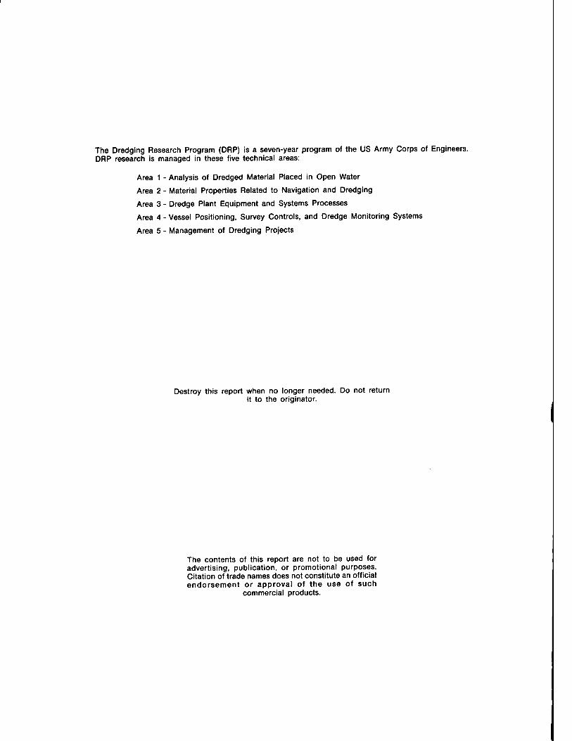
ISSU E: The cost efficiency of a hopper dredge is typically judged by its ability to move dredged sediment from the project area to the disposal area with a minimum of pump- ing and traveling time. The ideal hopper load for accomplishing this is referred to as the eco- nomic load.
An accurate method of monitoring densities within hopper dredge-collected sediment is need to calculate the volume of material dredged and to monitor results of attempts to increase hopper loads.
RESEARCH: Two methods were de- signed, fabricated, tested, and evaluated for effectiveness in providing data to dredge per- sonnel for the purpose of increasing dredge ef- ficiency:
• A resistivity probe for direct measure- ment of the vertical density profile of dredged material in the hopper.
• An instrumentation package of acoustic and pressure sensors to monitor real- time dredge displacement and hopper volume and to measure (indirectly) den- sity of the dredged material in the hopper.
The concept of uncertainty analysis for deter- mining the error potential in the calculation of hopper-dredge production was applied in an example calculation.
SUMMARY: The data resulting from the testing and evaluation of both systems demon- strated that either system can be used for cal- culating dredge production on a load-by-load basis. The results indicate that sufficient knowledge and technology exist for develop- ing a comprehensive hopper dredge monitor- ing system.
These capabilities will allow more efficient contract monitoring and administration, as well as more efficient dredge operation. They will provide the Corps and the dredging indus- try with a tool for making the dredging indus- try more cost efficient.
AVAILABILITY OF REPORT: The report is available through the Interlibrary Loan Ser- vice from the U.S. Army Engineer Waterways Experiment Station (WES) Library, telephone number (601) 634-2355. National Technical Information Service (NTIS) report numbers may be requested from WES Librarians.
About the Authors: Stephen H. Scott and Jeffrey D. Jorgeson are members of the Estuaries Division of the WES Hydraulics Laboratory; Monroe B. Savage and Cary B. Cox are assigned to the Instrumentation Services Division, WES.
Point Of Contact: Stephen H. Scoti. Hydraulics Laboratory, WES. is, Principal Investigator for this work unit. For further information about the DRP, contact Mr. E. Clark McNair, Jr., Manager, DRP, at (601) 634-2070.
February 1995 Please reproduce this page locally, as needed.
Dredging Research Program Technical Report DRP-95-2 February 1995
Technologies for Hopper Dredge Production and Process Monitoring
Laboratory and Field Investigations by Stephen H. Scott, Jeffrey D. Jorgeson,
Monroe B. Savage, Cary B. Cox
U.S. Army Corps of Engineers Waterways Experiment Station 3909 Halls Ferry Road Vicksburg, MS 39180-6199
Final report Approved for public release; distribution is unlimited
Prepared for U.S. Army Corps of Engineers Washington, DC 20314-1000
Under Work Unit No. 32475
Accesion For
NTIS CRA&I DTIC TAB Unannounced Justification
? 0
ey Distribution/
Availability Codes
Dist
PvA
Avail and/or Special
US Army Corps of Engineers Waterways Experiment Station
HEADQUARTERS BUILDING
FOR INFORMATION CONTACT:
PUBLIC AFFAIRS OFFICE
U. 5. ARMY ENGINEER
WATERWAYS EXPERIMENT STATION
3909 HALLS FERRY ROAD
VICKSBURG, MISSISSIPPI 391S0-S199
PHONE: (601)634-2502
AREA OF RESERVATION - 2.7 sq km
Waterways Experiment Station Cataloging-in-Pubiication Data
Technologies for hopper dredge production and process monitoring : laboratory and field investigations / by Stephen H. Scott... [et al.]; prepared for U.S. Army Corps of Engineers.
95 p.: ill.; 28 cm. — (Technical report; DRP-95-2) Includes bibliographical references. 1. Dredges — Equipment and supplies — Testing. 2. Dredges — Investigation.
3. Excavating machinery — Equipment and supplies — Testing. I. Scott, Stephen H. II. United States. Army. Corps of Engineers. III. U.S. Army Engineer Waterways Experiment Station. IV. Dredging Research Program. V. Series: Technical report (U.S. Army Engineer Waterways Experiment Station); DRP-95-2. TA7 W34 no.DRP-95-2
Contents
Preface V11
Conversion Factors, Non-SI to SI Units of Measurement ix
Summary x
1—Introduction 1
Background 1 Objective 2 Approach 2
2—Hopper Monitoring Concepts 4
Indirect Hopper Load Measurement, Bin Measurement Method 4 System Component Design and Application 4
Hopper level/volume measurement 4 Dredge draft/displacement measurement 5
Concept and Theory 5
Automated Load Monitoring System (ALMS) Design 8 Indirect Hopper Monitoring System Tests and Results 8
Laboratory scale test 8 Initial prototype acoustic sensor test 14
Norfolk Contractor Dredge Monitoring 22 Level of material in the hopper 22 Draft of vessel 22 Production meters 23 Ship's position 23 Draghead depth 23
Data Acquisition 23 Data Reduction 24
Volume of material in hopper 24 Vessel displacement 25 Cumulative weight of solids 25
Dredging Project Monitoring 25 Chincoteague Inlet 26
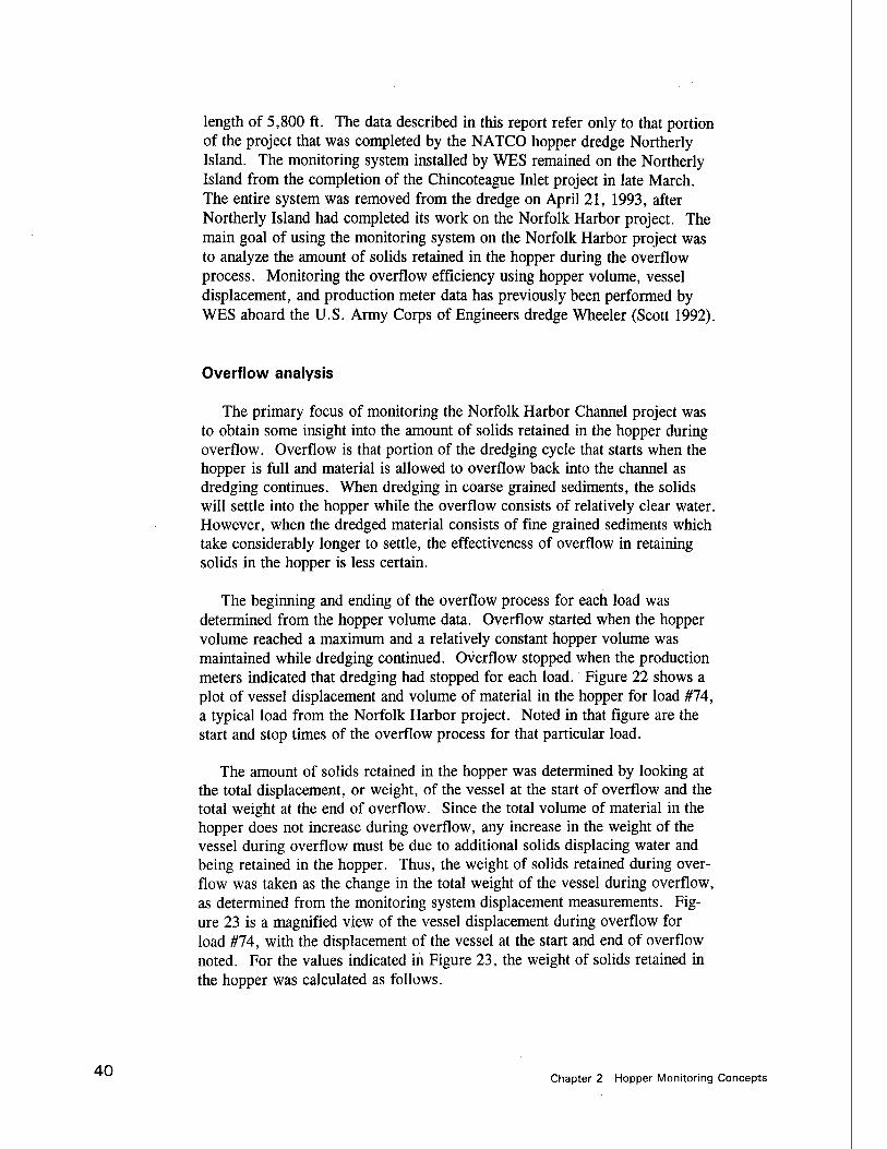
HI
Bin measure load calculations 26 System verification, water tests 34 Norfolk Harbor Channel 38 Overflow analysis 40 ALMS prototype test 45
Direct Hopper Load Monitoring, Resistivity Method 48 Objective 48 Concept and theory 49 Laboratory resistivity probe development and testing 50 Prototype resistivity probe development and testing 52 Automation of the resistivity probe operation 57 Automated system test 58
3—Uncertainty in Hopper Load Calculation 61
4—Monitoring System Applications and Benefits 65
System Applications 65 System Benefits 65
5—Conclusions 67
6—Recommendations 69
7—References 70
Appendix A: Instrumentation Schematic for ALMS Al
Appendix B: Instrumentation Schematic for Resistivity Probe Bl
SF298
List of Figures
Figure 1. Schematic of acoustic and pressure sensor locations on a hopper -dredge 6
Figure 2. Flow chart of ALMS operation 9
Figure 3. Acoustic sensor and attachment bracket and model dump scow 10
Figure 4. Model scow draft/displacement curve and ullage table curve . 12
Figure 5. Model scow draft recorded during filling test 13
IV
Figure 6. Model scow hopper depth recorded during filling test 14
Figure 7. Real-time water density calculation during filling test 15
Figure 8. Acoustic sensor used in prototype test 16
Figure 9. Draft and hopper acoustic sensor mounting locations for the prototype tests 17
Figure 10. Dredge WHEELER draft/displacement curve 18
Figure 11. Dredge WHEELER ullage table curve 19
Figure 12. Acoustic sensor draft data for the prototype test 20
Figure 13. Acoustic sensor hopper depth data for the prototype test .... 21
Figure 14. Vicinity map for Chincoteague Inlet, Virginia 27
Figure 15. Location map for Chincoteague Inlet, Virginia 28
Figure 16. Volume of material in hopper and vessel displacement versus time over a 24 hr period 30
Figure 17. Volume of material in hopper versus time for load #120, Chincoteague inlet project 31
Figure 18. Vessel displacement versus time for load #120, Chincoteague inlet project 32
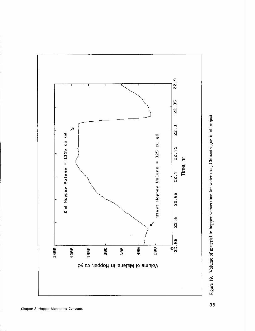
Figure 19. Volume of material in hopper versus time for water test, Chincoteague inlet project 35
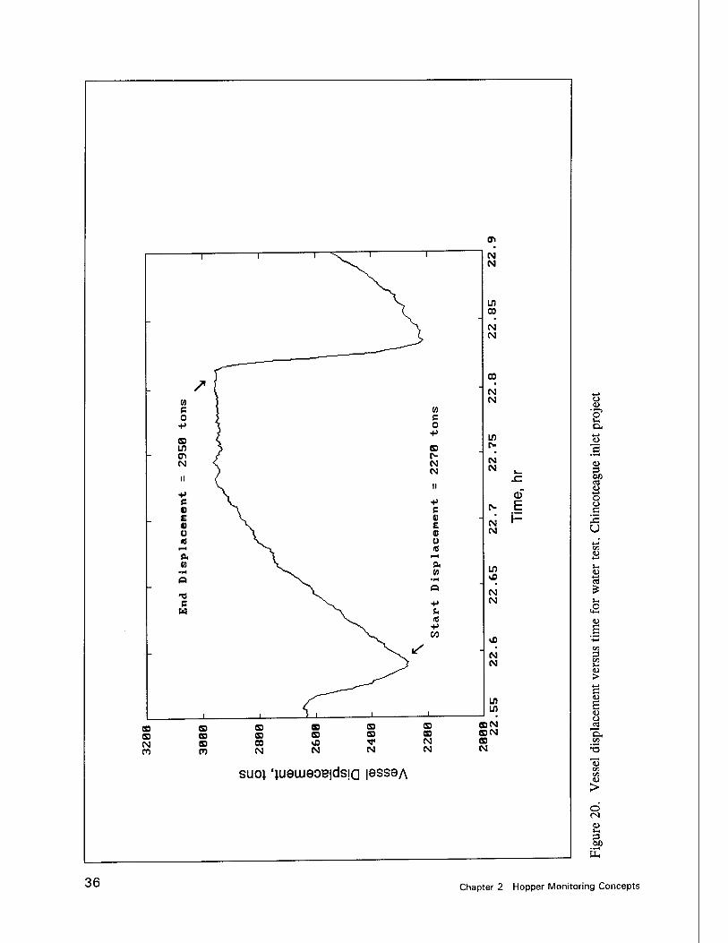
Figure 20. Vessel displacement versus time for water test, Chincoteague inlet project 36
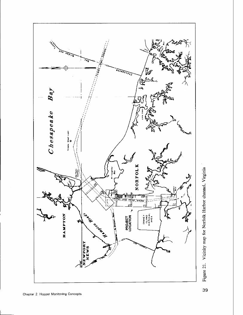
Figure 21. Vicinity map for Norfolk Harbor channel, Virginia 39
Figure 22. Volume of material in hopper and vessel displacement versus time for overflow analysis on load #74, Norfolk Harbor Project . . 41
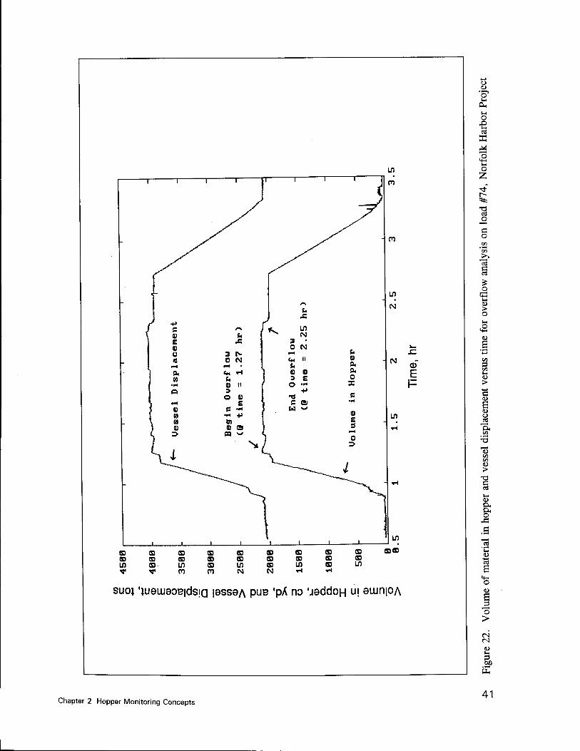
Figure 23. Vessel displacement versus time during overflow on load #74, Norfolk Harbor Project 42
Figure 24. Cumulative weight of solids pumped versus time during overflow on load #74, Norfolk Harbor Project 44
Figure 25. Signal sequencing for seven hopper loads during the ALMS test 46
Figure 26. Initial and final hopper volume and dredge displacement for load LI during the ALMS test 47
Figure 27. Hard copy production report generated from the ALMS test . 48
Figure 28. Initial and final volume and dredge displacement for a water test during the ALMS test 49
Figure 29. Schematic of Wenner Array for making resistivity measurements 50
Figure 30. Laboratory scale resistivity probe 51
Figure 31. Resistivity calibration curve for sand and silt mixture 52
Figure 32. Resistivity calibration curve for a sand, silt, and clay mixture 53
Figure 33. Measured density profiles from the laboratory tests 54
Figure 34. Prototype resistivity probe fabrication 54
Figure 35. Prototype resistivity probe installed in the hopper of the dredge WHEELER 55
Figure 36. Measured density profiles from the dredge WHEELER test . 56
Figure 37. Schematic of the automated resistivity probe system 57
Figure 38. Plot of the settled silt interface as a function of time 59
Figure 39. Automated test density profiles with settled silt interface ... 60
VI
Preface
This study was conducted by the Hydraulics Laboratory (HL) of the U.S. Army Engineer Waterways Experiment Station (WES) during the period April 1989 to October 1993. The study was sponsored by the Headquarters, U.S. Army Corps of Engineers (HQUSACE), as a part of the Dredging Research Program (DRP), Work unit 32475, "Technology for Monitoring and Increas- ing Dredge Payload for Fine-Grained Sediments," managed by the WES Coastal Engineering Research Center (CERC). HQUSACE Technical Monitor for DRP Technical Area 3, Dredge Plant Equipment and Systems Processes, was Mr. Gerald Greener. Mr. Robert H. Campbell was Chief Technical Monitor.
This report was prepared by Messrs. Stephen H. Scott and Jeffrey D. Jorgeson of the Estuaries Division (ED), HL, and Monroe B. Savage and Cary B. Cox of the Instrumentation Services Division (ISD), WES. Mr. Leo Keostler, Instrumentation Services Division assisted with the instrumentation design and testing. Testing of the prototype bin measure design was per- formed on the USACE dredge WHEELER, which operates under the adminis- tration of the Dredge Management Section of the New Orleans District, USACE. Mr. James D. Corville was chief of the Dredge Management Sec- tion. Dr. Robert F. Corwin of SP SURVEYS INC. designed and fabricated the resistivity probes used in this study.
The study was conducted under the general supervision of Mr. Frank A. Herrmann, Jr., Director, HL; Mr. Richard A. Sager, Assistant Director, HL; and Mr. William H. McAnally, Jr., Chief, ED. Mr. William H. Martin, ED, was the Manager of DRP technical area 3. Principle Investigator was Mr. Stephen H. Scott. Program Manager of the DRP was Mr. E. Clark McNair, Jr., CERC. Dr. Lyndell Hales, CERC, was assistant Program Manager.
At the time of publication of this report, Director of WES was Dr. Robert W. Whalin. Commander was COL Bruce K. Howard, EN.
VII
For further information on this report or on the Dredging Research Program, please contact Mr. E. Clark McNair, Jr., Program Manager, at (601) 634-2070.
The contents of this report are not to be used for advertising, publication, or promotional purposes. Citation cf trade names does not constitute an official endorsement or approval of the use of such commercial products.
VIII
Conversion Factors, Non-SI to SI Units of Measurement
Non-SI units of measurement used in this report can be converted to SI units as follows:
Multiply By To Obtain
cubic feet 0.02831685 cubic meters
cubic yards 0.7645549 cubic meters
feet 0.3048 meters
inches 2.54 centimeters
miles (U.S. statute) 1.609347 kilometers
pounds (mass) 0.4535924 kilograms
pounds (mass) per cubic foot 16.01846 kilograms per cubic meter
IX
Summary
Under the Dredging Research Program (DRP) Work Unit, "Technology for Monitoring and Increasing Dredge Payload for Fine-Grained Sediments," two different technical approaches were taken for developing hopper production monitoring technology. The key to determining the production of a hopper dredge is to either directly or indirectly determine the average density of the dredged slurry in the hopper.
Indirect measurement of density entails measuring both the volume of material in the hopper and the mass of the hopper load and then calculating the slurry density. This is typically done with two different instrumentation systems. The depth or volume of the load in the hopper at any given time must be measured, along with the change in dredge displacement due to the load. Hardware and software were developed under this work unit to acquire the necessary data to calculate the average density and subsequent dredge production. Individual components of the system were tested in the laboratory and in the field during the testing phase. The work unit followed an iterative development strategy, testing and evaluating each software and hardware design.
Directly measuring the slurry density in the dredge hopper with nuclear devices as a standard procedure is not an acceptable practice. Regulatory and safety concerns rule out the use of nuclear probes installed inside the hopper. Under this work unit, an innovative non-nuclear technology based on electrical resistivity principles was developed, tested, and evaluated. The work was performed under contract with Dr. Robert Corwin of SP Surveys. A laboratory scale probe was constructed and tested. Based on the laboratory results, a full-scale prototype probe was fabricated, installed, and successfully tested on the Corps dredge WHEELER. The results of the field tests were favorable, therefore the probe was redesigned and automated for computer data acquisition.
Both the direct and indirect methods developed under this work unit were successful in calculating dredge production. The indirect method demonstrated the most potential for not only accurately calculating the dredge production for each load, but also providing valuable needed data on the day- to-day operation of the dredge. The electrical resistivity method, although fully operational, is somewhat limited because of the abrasive and turbulent

environment of a hopper dredge, and the dependence of the method on knowing the exact conductivity of the environmental water.
The indirect method has been successfully tested on the Corps dredge WHEELER, and on a North American Trailing Company (NATCO) contrac- tor dredge working under contract to the US ACE Norfolk District.
XI
1 Introduction
Background
Various methods exist for estimating hopper payloads. The load in the hopper can be estimated by measuring the depth of settled solids in the hopper, and then manually sampling the solids to determine the load density. Since the hopper volume as a function of depth was known, the hopper load could be estimated by multiplying the measured density by the volume of material in the hopper. Not only was this method time consuming and labor intensive, but the accuracy was questionable because of the uncertainty of the sampling locations and procedures, and the difficulty of determining the level of settled fine sediments in the hopper. This method was acceptable because payment to the dredging contractor was not based on solids production, but on an after-dredging survey of the project area performed by a surveying vessel.
Recently, innovations in hopper load monitoring have shown promise for accurately determining dredge hopper load in in situ cubic yards or tons of dry solids. The Dutch dredging community utilizes this advanced technology in the harbor of Rotterdam, Europort. This technology is based on sensors which measure the depth of material in the hopper and the draft of the dredge (Rokosch 1989). Sensor output is then used to calculate the average slurry density in the hopper. This method indirectly measures dredged slurry density because no sensors are positioned in the hopper. Very little has been published concerning the hardware and software used in these monitoring systems. A variety of sensors exist that can be used for making the required measurements, but they may have problems with accuracy, dependability, and durability. Because the majority of the publications concerning these systems are from the.private sector, technical descriptions describing tests of these operating systems are not available to the public.
Direct measurement of dredged slurry density in dredge hoppers has numerous advantages. A direct measurement system would eliminate the need for multiple sensors including the necessary hardware and software. Each additional sensor employed contributes some measurement error which ulti- mately contributes to the total load measurement uncertainty. Direct mea- surement of density in the hopper could result in reliable production data as well as a basis to describe how various types of dredged material will
Chapter 1 Introduction
consolidate in the hopper. The only currently available technology capable of directly monitoring density profiles in dredge hoppers uses nuclear measure- ment principles. The major obstacles to using these devices in or around the dredge hopper are regulatory and safety concerns. The harsh hopper environ- ment prohibits the use of automated mechanical profiling devices for obtaining vertical density profiles in hoppers.
This paper describes the research and development of technologies for both indirectly and directly measuring hopper load densities and monitoring hopper dredge processes.
Objective
The objectives of this research were to design, test, and implement hopper dredge monitoring systems for accomplishing the following goals: (a) reliably calculate hopper dredge production based on the indirect and direct method of hopper density measurement, (b) acquire hopper dredge process data for real time dredge monitoring capability, (c) provide an automated system that produces production reports and graphical output with a minimum of user input and (d) develop a method for determining the uncertainty of production calculations resulting from data from the monitoring system.
Approach
To meet these objectives, two monitoring systems were developed. The monitoring system based on the indirect measurement of hopper density was based on the bin measure approach for determining hopper load. The average hopper density is determined from data from two separate sensors. Acoustic sensors mounted above the hopper bins record the depth of slurry in the hopper at any time. The depth measurements are then converted to volume through the use of the dredge ullage tables which relate hopper depth to volume. Pressure sensors in the dredge bubbler air lines measure the change in hydrostatic pressure as the vessel drafts under load. This change in draft can be converted into displacement using the dredge draft/displacement tables that relate the draft of the dredge to the weight or displacement of the dredge. The total change in displacement of the vessel due to the slurry load along with the bin water load residing in the hopper before loading represents the total hopper load. The total volume that the slurry occupies in the hopper represents the full hopper volume. The total hopper load divided by the full hopper volume is the average hopper density. This calculated density, along with the geophysical and water properties of the dredging environment, is used to calculate dredge production. Laboratory tests of system components were conducted, along with prototype testing on the Corps dredge WHEELER. The system was fully automated by incorporating other dredge processes into the data acquisition loop.
Chapter 1 Introduction
The approach taken for directly measuring slurry density in dredge hoppers was based on the concept of electrical resistivity of sediment slurries. Electri- cal resistivity methods are commonly used in geophysical studies. The feasi- bility of using resistivity methods for measuring sediment densities has been proved under previous studies. The concept involves using a four electrode array for measuring the resistivity of the sediment slurry. Current is injected into the slurry through the outer electrodes, with voltage drop measured between the inner two electrodes. The slurry resistivity is then calculated based on the current input and voltage output, and the spacing of the electrodes. A laboratory scale multi-electrode array was developed and tested at WES. Based on the results of these tests, a prototype probe was built and installed on the dredge WHEELER, tested and evaluated, and finally totally automated.
Chapter 1 Introduction
2 Hopper Monitoring Concepts
Indirect Hopper Load Monitoring, Bin Measure Method
The objectives of the indirect hopper load monitoring method were to (a) evaluate the instrumentation necessary for providing data on hopper volume (acoustic sensors) and dredge displacement (pressure sensors), (b) perform laboratory tests with the instrumentation to determine accuracies, limitations, and application requirements, (c) develop associated hardware and software for data acquisition, manipulation, and display, (d) develop a prototype system for testing and evaluation on a working dredge, and (e) automate the system to produce dredge production reports and load summaries.
System Component Design and Application
Hopper level/volume measurement
The instruments used for monitoring the slurry level and subsequent hopper volume were programmable ultrasonic transducers installed above the dredge hopper. These sensors measure the distance between the slurry level in the hopper and the sensor. These instruments measure distance by sending out acoustic waves in a series of pulses which are reflected by the target. The reflected acoustic energy is then received by the sensor. The distance between the sensor and the target is calculated from the time interval between the transmission of the acoustic pulse and the return of the reflected acoustic energy back to the sensor. The sensors used in the final monitoring system design were accurate to within approximately ±0.2 percent of the measuring range with temperature compensation. Additional information about the acoustic sensors used in this study can be found in Appendix A.
Chapter 2 Hopper Monitoring Concepts
Dredge draft/displacement measurement
The instruments used for monitoring the dredge draft and subsequent dis- placement in the final monitoring system design were strain gage-type pres- sure transducers installed in the bubbler air lines of the dredge. These air lines provide the pressure for the operation of the dredge chart recorder. Typically, two bubbler air lines, fore and aft, run from the pilot house to the keel. A constant flow of air is maintained in the air lines, bubbling out the keel. As the dredge drafts under load, the hydrostatic pressure change in the line is proportional to the pressure required to force air out of the bubbler lines. The sensing element in the transducer consists of a strain gage bridge. When subjected to pressure, the bridge is displaced, and an electrical output proportional to the applied pressure is produced. The pressure reading is converted to feet of water by the following equation:
H = L (1)
where H = feet of water, ft P = hydrostatic pressure measurement, lb/ft2
pw = water density, lb/ft3
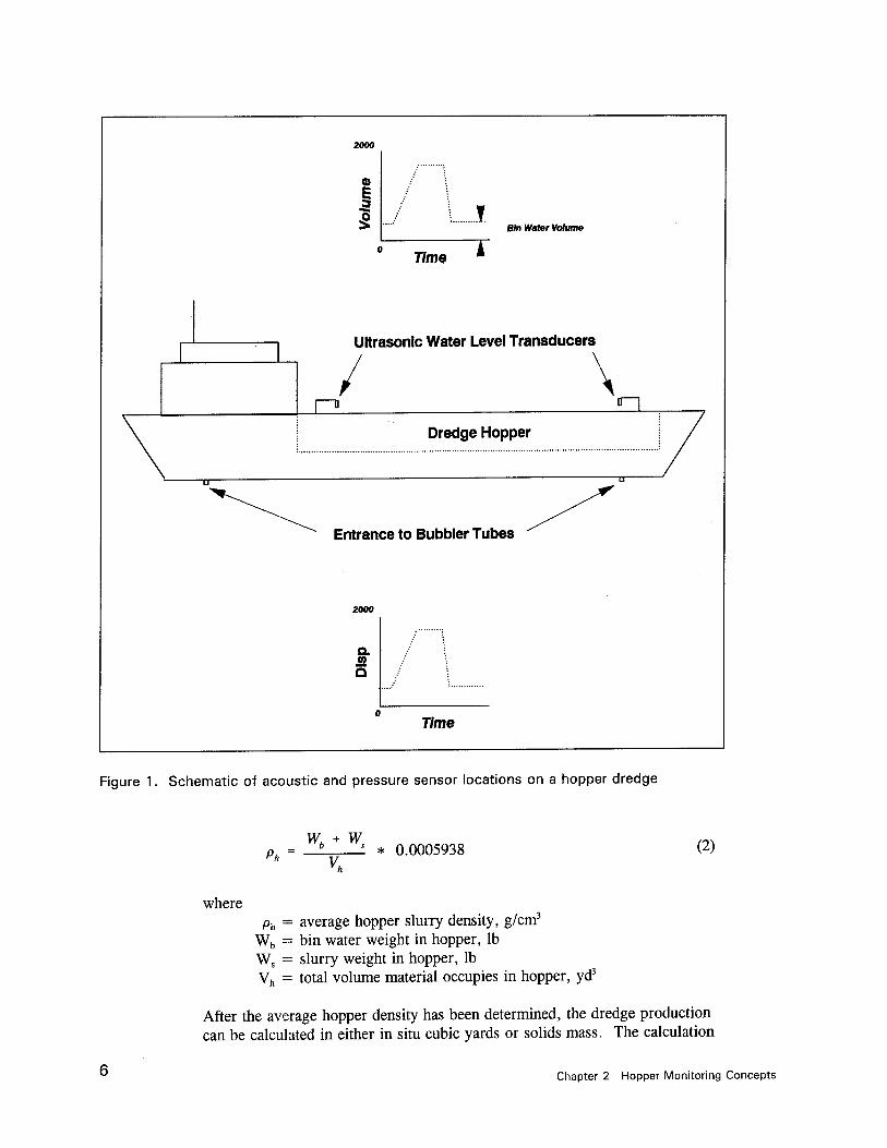
Concept and Theory
The indirect hopper load monitoring concept involves indirectly measuring the average density in the hopper. This is accomplished by measuring two dredge parameters-the level of dredged material in the hopper and the draft of the dredge. Figure 1 is a schematic of a dredge with two instrumentation systems for measuring real time hopper volume with acoustic sensors and dredge displacement with pressure transducers in the air bubbler lines. The hopper volume is determined by measuring the depth of the slurry in the hopper. With the dredge ullage table, which relates hopper depth to hopper volume, the depth of material in the hopper can be converted to volume. The draft of the hopper dredge is directly related to the weight of the dredge, plus loaded water and sediment. The draft can be related to vessel displacement with a draft/displacement table typically available from the shipyard. The total weight of material in the hopper is equal to the weight of bin water in the hopper before the load is taken plus the slurry load added. This total weight divided by the volume that the material occupies in the hopper is the average density of the material in the hopper. The average slurry density in the hopper is calculated by the following expression:
Chapter 2 Hopper Monitoring Concepts
2000
0
1/ \ ■ Bin Water Volume
Time
Ultrasonic Water Level Transducers
Entrance to Bubbler Tubes
2000
a. (0
Time
Figure 1. Schematic of acoustic and pressure sensor locations on a hopper dredge
Wh + W -J. I * 0.0005938 (2)
where ph = average hopper slurry density, g/cm3
Wb = bin water weight in hopper, lb Ws = slurry weight in hopper, lb Vh = total volume material occupies in hopper, yd3
After the average hopper density has been determined, the dredge production can be calculated in either in situ cubic yards or solids mass. The calculation
Chapter 2 Hopper Monitoring Concepts
of production is dependent on the geotechnical and water properties of the dredging site. The first step in calculating the in situ production is to calcu- late the percent of in situ material by volume in the hopper. This is given by the following expression:
Ph - P. (3)
Pi ~ Pw
where Q = percent in situ materials by volume in the hopper ph = average slurry density in the hopper, g/cm3
Pi = in situ density of the sediments in the project area, g/cm3
pw = density of the water at the project area, g/cm3
The in situ production is then given by the following expression
PROt = Ci * Vh W
where PROj = production in cubic yards of in situ material. To calculate the dredge production in solids mass the percent solids in the hopper must be calculated. This is given in the following expression:
r = Ph - Pw (5)
where Csol = percent solids by volume in the hopper pm = solids particle density, g/cm3
The solids mass production is then given by the following expression:
PRO = C * n * V (6)
where PROso, = production in solids mass, lb
pm = solids particle density, lb/yd3
These are the fundamental equations for calculating dredge production in either cubic yards of in situ material or in solids mass. The acoustic sensor output provides data on the bin water volume and total hopper volume, while
Chapter 2 Hopper Monitoring Concepts
the pressure sensors measure the change in vessel displacement due to the slurry load.
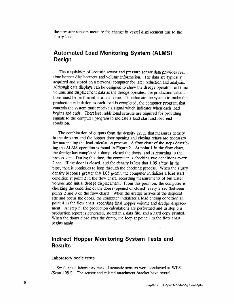
Automated Load Monitoring System (ALMS) Design
The acquisition of acoustic sensor and pressure sensor data provides real time hopper displacement and volume information. The data are typically acquired and stored on a personal computer for later reduction and analysis. Although data displays can be designed to show the dredge operator real time volume and displacement data as the dredge operates, the production calcula- tions must be performed at a later time. To automate the system to make the production calculation as each load is completed, the computer program that controls the system must receive a signal which indicates when each load begins and ends. Therefore, additional sensors are required for providing signals to the computer program to indicate a load start and load end condition.
The combination of outputs from the density gauge that measures density in the dragarm and the hopper door opening and closing relays are necessary for automating the load calculation process. A flow chart of the steps describ- ing the ALMS operation is found in Figure 2. At point 1 in the flow chart, the dredge has completed a dump, closed the doors, and is returning to the project site. During this time, the computer is checking two conditions every 2 sec. If the door is closed, and the density is less that 1.05 g/cm3 in the pipe, then it continues to loop through the checking process. When the slurry density becomes greater that 1.05 g/cm3, the computer initializes a load start condition at point 2 in the flow chart, recording measurements of bin water volume and initial dredge displacement. From this point on, the computer is checking the condition of the doors (opened or closed) every 2 sec (between points 2 and 3 on the flow chart). When the dredge arrives at the disposal site and opens the doors, the computer initializes a load ending condition at point 4 in the flow chart, recording final hopper volume and dredge displace- ment. At step 5, the production calculations are performed and in step 6 a production report is generated, stored in a data file, and a hard copy printed. When the doors close after the dump, the loop at point 1 in the flow chart begins again.
Indirect Hopper Monitoring System Tests and Results
Laboratory scale tests
Small scale laboratory tests of acoustic sensors were conducted at WES (Scott 1991). The sensor and related attachment bracket have overall
Chapter 2 Hopper Monitoring Concepts
©
Record Initial Conditions T YES
Density > 1.05? - ©
-»►LOAD START
NO
NO - ® ' DOOR OPEN
YES
<r ® LOAD END Record Final Conditions
v ® CALCULATIONS Calculate Dredge Production
" ® Print Production Report
Figure 2. Flow chart of ALMS operation
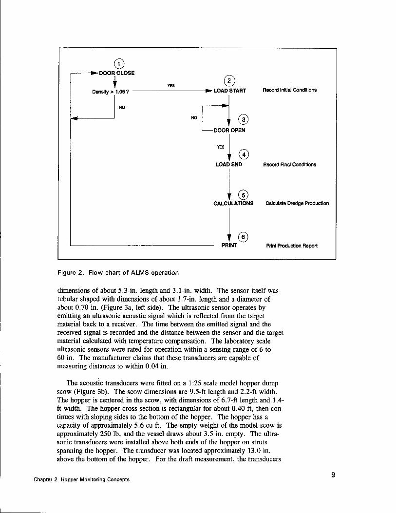
dimensions of about 5.3-in. length and 3.1-in. width. The sensor itself was tubular shaped with dimensions of about 1.7-in. length and a diameter of about 0.70 in. (Figure 3a, left side). The ultrasonic sensor operates by emitting an ultrasonic acoustic signal which is reflected from the target material back to a receiver. The time between the emitted signal and the received signal is recorded and the distance between the sensor and the target material calculated with temperature compensation. The laboratory scale ultrasonic sensors were rated for operation within a sensing range of 6 to 60 in. The manufacturer claims that these transducers are capable of measuring distances to within 0.04 in.
The acoustic transducers were fitted on a 1:25 scale model hopper dump scow (Figure 3b). The scow dimensions are 9.5-ft length and 2.2-ft width. The hopper is centered in the scow, with dimensions of 6.7-ft length and 1.4- ft width. The hopper cross-section is rectangular for about 0.40 ft, then con- tinues with sloping sides to the bottom of the hopper. The hopper has a capacity of approximately 5.6 cu ft. The empty weight of the model scow is approximately 250 lb, and the vessel draws about 3.5 in. empty. The ultra- sonic transducers were installed above both ends of the hopper on struts spanning the hopper. The transducer was located approximately 13.0 in. above the bottom of the hopper. For the draft measurement, the transducers
Chapter 2 Hopper Monitoring Concepts
-%-r' —■«*■"
^^
a. Acoustic sensor and attachment bracket
gj^^ff^^ll
b. Model dump scow
Figure 3. Acoustic sensor and attachment bracket and model dump scow
10 Chapter 2 Hopper Monitoring Concepts
were installed with a metal bracket off the bow and the stern of the model dump scow. They were positioned about 6.0 in. from the water surface.
The signals produced by the above-described transducers were processed using a personal computer. The computer had a 100 MB hard disk with a 1.4 MB flexible disk drive. Lightweight and portable, with a collapsible viewing screen, the entire unit occupied minimal desk space. Calibration tests were performed to obtain data on the draft of the model as a function of scow weight (draft/displacement relationship). The scow ullage table (hopper depth/volume relationship) was determined from the scow hopper cross sec- tion geometry. Figure 4 shows the draft/displacement and ullage table curves for the model scow. The data from these curves were stored in the computer program in the form of calibration tables. The laboratory tests consisted of filling the hopper of the model scow with fresh water and recording the draft and hopper depth acoustic sensor output. The data acquisition software was designed to perform the following calculations:
a. As the model hopper is filled, the sensors detect a change in vessel draft and hopper depth.
b. The sensors send a signal proportional to this change to the computer.
c. The computer takes multiple readings of the sensor output and averages them.
d. The averaged readings of draft and hopper depth are compared with the calibration tables and the appropriate values for the vessel weight and hopper volume are selected for the measured draft and hopper depth.
e. The initial conditions of scow displacement and hopper volume are sub- tracted from each displacement and volume measurement.
/. The density of the water in the hopper was then calculated by the following equation:
Wf~W, (7)
where pw = water density in the hopper, lb/ft3
Wf = measured scow weight, lb Wi = initial scow weight, lb Vf = measured scow hopper volume, ft3
V( = initial scow hopper volume, ft3
The model dump scow was placed in a test sump. Water was fed into the scow hopper with a water hose at an average flow rate of about 10.0 in.3/sec,
Chapter 2 Hopper Monitoring Concepts 11
ouu.uu —
700.00 -
c 0)
E O a Q. 0) Q
$ o o
CO
600.00 -
500.00 -
400.00 —
300.00 -
/
200.00 -
"a o 2
100.00 -
0.00 — I 1 I I 1 1 1 1 1 1 1 1 1 1 1 1 1 1 1 1 1 1 1 i 1 i i i i 2.00 3.00 4.00 5.00 6.00 7.00 8.00
Draft, Inches
a. Draft displacement curve
o CD
-t-t ID eU
U_ O
o o — A
•*- 3 o - V _ E 3 ~ O o > o —
i_ — <u Q. O. O I
o d 1 1 1 1 | 1 1 l l | 1 1 l I | l l I l | l l l
0.0 0 2.50 5.00 7.50 10.00
Depth in . Hopper, Inches
b. Ullage table curve
Figure 4. Model scow draft/displacement curve and ullage table curve
12 Chapter 2 Hopper Monitoring Concepts
for a hopper fill time of about 20 min. Because water was used as the test material for filling the hopper, the average density measured in the hopper was that of water at the testing temperature of 65°F. Four tests were conducted.
The computer program was designed to plot the average density of material in the hopper as it is filling. Figures 5 and 6 show the model scow draft and hopper depth as a function of time recorded during a filling test. Figure 7 is a plot of the computer generated output of water density as a function of time. For the data taken during the undisturbed portion of the filling cycle, the average density in the hopper calculated by the computer program proved to be within 1 percent of the actual water density in the model hopper (62.33 lb/ft3). Note that at the beginning of the filling cycle, the data are noisy due to the motion of the empty scow. As the hopper load increases, the motion is damped, resulting in a more consistent data record. In a prototype application, with sediments in the hopper, the computed average density would be inserted into Equations 2 through 6 for calculating the percent solids and total solids weight or in situ volume load. For the laboratory tests it was only necessary to verify the accuracy of the transducer output and the average density calculation, therefore only water was used to fill the scow hopper.
Time - min
Figure 5. Model scow draft recorded dunng filling test
13 Chapter 2 Hopper Monitoring Concepts
9 1 ■
8
7
| 6
0 z e
5
4
0 a
3
2
1
j/
0 5 IB
Time - win
15 28
Figure 6. Model scow hopper depth recorded during filling test
These laboratory tests of the acoustic sensors and data acquisition hardware and software provided WES engineers with essential information for scaling the concept to prototype. The tests verified the accuracy and reliability of the acoustic transducers, provided an initial hardware and software design for acquiring and processing the data, and revealed potential problems with prototype application.
Initial prototype acoustic sensor test
The initial prototype acoustic sensor tests were conducted on the Corps of Engineers hopper dredge WHEELER during July 1991, by personnel from the U.S. Army Corps of Engineers Waterways Experiment Station (WES), Hydraulics Laboratory (Scott 1992). The WHEELER was dredging in the Mississippi River and off the coast of Galveston, Texas, during the test period.
The WHEELER primarily operates in the Gulf of Mexico, ranging from the mouth of the Mississippi River to the Texas Gulf Coast. The WHEELER
14 Chapter 2 Hopper Monitoring Concepts
ia
65
i i i i i i i
CM .,A UM J, , kij , h/lJlu .1 . . h 3 Ü
\ 60 mfiN*ty ̂w *WH^ ijWfi 0*f$\ ̂ 4
ja 1 "J c I
55 _
0
3
50
45
40 2
-
4 6 8 10 12 14 16 18 20
Tine - - nin
Figure 7. Real-time water density calculation during filling test
hopper has a volume of approximately 8,000 cu yd. Three dragarms are available for dredging, two 28.0 in. diam side dragarms, and a 42.0 in. diam center dragarm.
The acoustic sensors used in the tests were rated for measuring distances up to 70.0 ft. The transducers were about 1.5 ft in length, and approximately 2.0 in. in diameter (Figure 8). The operating frequency of the transducer is high enough so that environmental noise around the hopper area generally does not interfere with the signal, but it is low enough that temperature and density changes in the air can affect the data. The unit has 29 programmable modes available to the user for determining the proper transducer settings for any given application. These functions are used to set the range of measure- ment (minimum and maximum distances), the calibration of the sensor, and the input and output parameters. Additionally, the units can be used to control other remote functions based on the sensor output. For example, when the unit senses a full hopper, a pump might be activated. A temperature sensor is incorporated into the unit to compensate for temperature changes. The dredging environment, especially in the hopper, frequently experiences high humidity as well as temperature fluxuation. One very useful function on the unit is the amplifier gain control. This can be utilized to amplify the
Chapter 2 Hopper Monitoring Concepts 15
liliiiilllllilga immSlimlmmmm
Figure 8. Acoustic sensor used in prototype test
16
desired acoustic signals and eliminate the undesirable signals from environmental effects such as water vapor or signal reflections from objects in the path of the acoustic signal such as structural members in the hopper. The accuracy of the sensor is reported to be 0.2 percent of the maximum range of operation. For our application, the maximum range was approximately 40 ft, with an accuracy of + 0.08 ft.
The draft acoustic sensors were mounted off the bow and stern of the WHEELER for determining the draft as a function of vessel weight (Fig- ure 9a). Sensors were mounted both port and starboard off the bow and stern to account for vessel motion. The data for the four draft sensors were aver- aged for the final draft calculation.
The hopper acoustic sensors were mounted forward and aft, as well as port and starboard in the hopper for determining the depth of bin water in the hopper before dredging (Figure 9b). The WHEELER hopper contained many obstructions such as structural members and pipe runs which could potentially interfere with the acoustic signal transmission and reception. Locations were found that offered the most clearance for proper sensor operation. The data for the four hopper sensors were averaged for the final hopper depth calculation.
Before installation, the sensors were field calibrated. They were positioned normal to a flat, smooth surface at a measured distance. The sensor output was observed and compared with the measured distance. If the sensor dis- tance output was different from the measured distance, it was corrected by
Chapter 2 Hopper Monitoring Concepts
EÜÜ »si
i
A
a. Draft sensor location
dlli
.,"-*
i*i
i;^ÄÄ: All " W
Kw
li-^CT 1
b. Hopper sensor location
Figure 9. Draft and hopper acoustic sensor mounting locations for the prototype tests
Chapter 2 Hopper Monitoring Concepts 17
changing the calibration parameters with the programmable modes of the sensor. This procedure was followed before the installation of both the hop- per and draft sensors. After installation, the calibrations were checked by comparing the sensor output with soundings made with a tape measure.
The acoustic sensors were programmed to continuously average the data over a 10-sec interval. Every 10-sec, the averaged draft and hopper depth data for each transducer were recorded on a 386 personal computer through an RS-232 data interface. Software converted the draft measurement to hop- per load using the draft/displacement table for the WHEELER (Figure 10), and converted the hopper depth measurement to hopper volume using the ullage table for the WHEELER (Figure 11). The software then calculated the average density in the hopper for the load (Equation 2) based on a full hopper volume of approximately 8,000 cu yd. This average density was then used to calculate the in situ cubic yards removed from the navigation channel (Equa- tions 3 and 4). The acoustic transducer data were stored on the computer hard disk in binary format to optimize the storage capacity. The acoustics data were taken for approximately 2 months of dredging in the Mississippi River just below Baton Rouge, Louisiana, and at Sabine Pass off the coast of Galveston Texas.
c o
en c o
c CD
CD o
Q_ (/) Q
CD Q>
CD
o
10.00 15.00 i—i—i—| i i i i | r
20.00 25.00
Dredge Draft, ft
35.00
Figure 10. Dredge WHEELER draft/displacement curve
18 Chapter 2 Hopper Monitoring Concepts
o d o o
X>
ö >-
o d o m r* _
o
ZS
O
>, 'o o CL O Ü
o d o o m _
(D Q_ Q_ O X
o d o to (VI
O i i i i I i i i i 1 i i i i 1 i i i i 1 i i i i 0.00 10.00 20.00 30.00 40.00 50.00
Hopper Depth, ft (From Hopper Bottom to Top)
Figure 11. Dredge WHEELER ullage table curve
Figures 12 and 13 describe acoustic draft and hopper depth data for one of the hopper loads taken from the Mississippi River at Baton Rouge. Figure 12 describes the change in draft as a function of time. Each data point represents 10 sec of averaged data. Four distinct phases of the load are labeled in Fig- ure 12. At the beginning of the load, the WHEELER drafts about 19.0 ft of water. The pumping/filling phase of the load begins and continues until a draft of about 27.5 ft. At this point, the hopper is overflowed to a draft of about 29.0 ft. This 1.5-ft increase in draft reflects an increase in dredge displacement due to solids retention during overflow. The dredge then travels to the dump site. This is reflected on the plot as a slight increase in draft due to vessel squat. The load is then dumped, and the hopper pumped out for the next load.
Figure 13 describes the change in hopper depth as a function of time dur- ing the load. At the beginning of the load, the data indicate about 5.0 ft of bin water in the hopper. As pumping begins, a data spike and resulting noise are shown on the plot. When the WHEELER pumps with all three dragarms at once, the flow rate of slurry into the hopper can approach 30,000 to 40,000 cu yd/hr. The slurry is introduced into the hopper at the top, and falls about 40.0 ft to the bottom of the hopper bins. This creates a heavy mist at the beginning of the filling cycle. The acoustic signals emitted from the
Chapter 2 Hopper Monitoring Concepts 19
CM
Q
es w ►J
w H z
30
28
26
24
22
28
18
_
■' 1 i i i i i
-
-
\
Overtlou
Dumping
-
/ N
- / Pumping
\
-
Punpout
i
v^
2.2 2.4 2.6 2.8 3 3.2
Tine - hrs
3.4 3.6
Figure 12. Acoustic sensor draft data for the prototype test
sensor reflect off of the mist, thus introducing noise into the data. As the hopper fills, the mist subsides and the acoustic sensors resume proper opera- tion. During the overflow cycle, the sensors record a constant hopper level. As the dredge travels to the dump site, the hopper level drops somewhat due to material loss through the overflow weirs.
The hopper acoustic sensors proved to be dependable over the test duration. As the hopper was filled, clouds of mist resulting from the high rate of slurry discharge into the hopper surrounded the adjacent area. Fre- quently, in fine sediments this mist contains clay which coats everything adja- cent to the hopper. The hopper acoustic sensors were subjected to these conditions and maintained their calibration throughout the two months of testing. The data from the hopper sensors had good resolution, with minimal signal noise, with the exception of the initial filling of the hopper. The use of these sensors for determining bin water load represents a significant increase in the efficiency of hopper dredge operations.
The draft acoustic transducers also maintained calibration over the test period. They provided good resolution of the dredging cycle, particularly the overflow sequence. The major problem with using acoustic sensors for draft
20 Chapter 2 Hopper Monitoring Concepts
rrn
45
1 1 1 1 1 "I T"
CH
1
b 0 ft! 9i
48
35
"
/ Ovepflou 0 X ft
■•H b 0 +>
38
25
28
- / \ - / Pumping Dumping ^
CM 0 15 -
ft. 0 a
18 -
/» ^ 5 Pumpout ^
0 i i i i i i i
2.2 2.4 2.6 2.8 3 3.2 3.4
Time - hrs
Figure 13. Acoustic sensor hopper depth data for the prototype test
measurement is the detection of vessel motion at the beginning and ending of the filling cycle. Accurate measurement of starting and ending draft are essential to measurement of load. Wave action as well as vessel motion at these points resulted in data scatter of up to ± 1.0 ft. These tests revealed a need for a more reliable system for providing the dredge draft. Most hopper dredges have a bubbler air system installed on the dredge to drive a chart recorder for recording dredge displacement. To obtain a record of dredge draft independent of the chart recorder, it is necessary to install pressure transducers into the bubbler air lines for recording hydrostatic pressure change due to dredge draft.
The full-scale prototype acoustic sensors installed over the hopper provided accurate and reliable data considering the harsh conditions of the WHEELER hopper. The only problems encountered with data resolution during the tests were during the initial filling of the hopper, when a heavy mist pervaded the hopper. This disruption of the data record as the hopper initially fills is inconsequential because the only two points of the filling cycle that are critical to the calculation of production are at the start of the filling cycle and just before the load is dumped. The data acquisition design proved adequate, with only minor adjustments in the program required.
Chapter 2 Hopper Monitoring Concepts 21
22
Norfolk Contractor Dredge Monitoring
Reimbursable work was initiated with the Norfolk District, USACE, to investigate an alternative method for measuring dredge draft through the bub- bler air system. WES engineers installed pressure transducers in the bubbler air lines of a dredge working under contract to the Norfolk District. This study was performed during the spring of 1992. The study demonstrated that pressure transducers could reliably measure dredge draft/displacement when installed in the bubbler lines. During the spring of 1993, both the acoustic sensors and the pressure sensors were installed on a contractor's dredge for another reimbursable study for the Norfolk District (Jorgeson and Scott 1994).
The monitoring system designed for this study included several instrument systems, each of which monitored a different function of the dredge. Those dredge functions included level of material in the hopper, draft of the vessel, density and velocity of material passing through the production meters, ship's position, and depth of the port and starboard dragheads.
Two separate dredging projects were monitored for this study. The first of those was at Chincoteague Inlet, Virginia, where hopper volume and dredge displacement were used to determine the bin measure production for each load. The second project was in the Norfolk Harbor Channel where hopper volume, dredge displacement, and production meter data were incorporated into an analysis of the amount of solids retained in the hopper during the overflow process. Each of these projects, the data collected, and the results obtained are discussed in the following sections of this report.
Level of material in the hopper
To monitor the level of material in the hopper, the programmable ultra- sonic sensors, which were discussed previously in this report, were installed over each end of the hopper along the longitudinal center line of the hopper. The sensors were installed on specially designed brackets extending out over each end of the hopper and were installed high enough over the maximum water level in the hopper such that direct contact with splashing or spraying slurry or water was minimized. The sensor at the aft end of the hopper was mounted on a catwalk approximately 10 feet above the top of the hopper. The sensor at the forward end of the hopper was mounted on a valve housing approximately 3 feet above the top of the hopper.
Draft of vessel
The draft of the vessel was monitored by inserting pressure sensors into the existing bubbler line system which measures the draft at two bubbling points located in the keel of the ship, one near the dredge's forward perpendicular and one near the dredge's aft perpendicular. In each air line, the pressure was
Chapter 2 Hopper Monitoring Concepts
converted to draft by the process outlined earlier in this report. The pressure transducers installed had a pressure range of 0-25 pounds per square inch (lb/in2).
Production meters
The dredge was equipped with density and velocity meters on both the port and starboard dragarms to measure the density and velocity of the slurry mixture being pumped. The density of the slurry was measured with nuclear density gauges and the velocity was measured with magnetic flowmeters. Signals from those existing gauges and meters were obtained, and the density and velocity of the slurry being pumped through each dragarm were monitored and recorded.
Ship's position
The position of the dredge was provided by a Del Norte positioning system. Output from this system provided Northing and Easting coordinates for the position of the vessel which were recorded by the monitoring system.
Draghead depth
The dredge was equipped with depth indicators for the port and starboard dragheads. The depth indicators for the dragheads consisted of a bubbler system like the system used to measure the draft of the vessel, but with the bubbling points located on each draghead. As with the draft measurement system, pressure taps were placed in the air lines for the port and starboard dragheads. The depth of the dragheads was calculated by converting the air pressure in the bubbler lines into feet of water.
Data Acquisition
The output from all sensors was recorded continuously every 5 sec using a laptop computer installed on the dredge specifically for this project. The data acquisition software was configured such that a binary data file was created at midnight each day which contained the data for the previous 24-hr period. Ten channels of data were recorded, in addition to the time and the location coordinates. Table 1 provides a list of the ten data channels. The computer was capable of continuously recording data for approximately 63 days before the storage capacity on the disk was full.
A program was written to convert each binary data file into two ASCII output files, one containing the location coordinates and another containing the ten channels of data listed in Table 1. The program converted the raw data, which was typically recorded as a voltage or a 4-20 mA signal from the
Chapter 2 Hopper Monitoring Concepts 23
various sensors in the monitoring system, into the appropriate engineering units which are shown in Table 1.
Table 1 Data Acquisition Channels
Data Acquisition Channel
Data Acquired
Engineering Units
1 Aft draft ft
2 Forward draft ft
3 Aft level in hopper ft
4 Forward level in hopper ft
5 Starboard draghead depth ft
6 Port draghead depth ft
7 Density in starboard dragarm g/cm3
8 Velocity in starboard dragarm ft/sec
9 Density in port dragarm g/cm3
10 Velocity in port dragarm ft/sec
Data Reduction
Calculating the bin measure load and analyzing the amount of solids retained in the hopper during the overflow process requires knowledge of the volume of material in the hopper, the total displacement of the vessel, and the cumulative weight of solids as indicated by the production meters. As seen in Table 1, none of the data acquired by the monitoring system provides that information directly. Therefore, the information on the level in the hopper, draft, and density and velocity in the dragarms must be converted from the initial data into volume of material in the hopper, total displacement of the vessel, and cumulative weight of solids pumped.
Volume of material in hopper
As previously discussed, the acoustic sensors over the hopper measured the distance from the sensor to the water or slurry surface in the hopper, and that distance was converted into an average depth of material in the hopper and then into volume of material in the hopper via the dredge's ullage table.
24 Chapter 2 Hopper Monitoring Concepts
Vessel displacement
The draft of the ship was converted into displacement through the use of the hydrostatic curves of form for the vessel. The hydrostatic curves of form include many curves which describe the characteristics of the vessel, among which is a data curve which relates draft and displacement. A curve fit equa- tion was determined for that draft versus displacement curve, and the resulting equation provided displacement, in tons, for any given values of fore and aft draft.
Cumulative weight of solids
To analyze the amount of solids retained in the hopper during the overflow process, the weight of solids pumped during overflow was compared with the weight of solids retained during overflow. The density meter provides the density of material in the dragarm, and the flow meter provides the velocity of the material in feet per second. That data was recorded every 5 sec. The cumulative weight of solids was calculated by the following equation:
Ms = fl Hü. *p*V*A*T (8)
where Ms = solids mass production, lb ps = slurry density in dragarm, lb/ft3
pw = density of interstitial water, lb/ft3
pm = density of solids, lb/ft3
Vm = velocity of mixture in dragarm, ft/sec A = cross-sectional area of dragarm suction pipe, ft2
T = time interval between measurements, sec
For example, if the density of the interstitial water was measured as 62.84 lb/ft3, the density of the solids was 165.36 lb/ft3, the cross-sectional area of the suction pipe was 1.767 ft2, the time interval between measurements was 5 sec, the density of material in the dragarm measured by the density meter was 81.12 lb/ft3, and the velocity of material in the dragarm measured by the flow meter was 15.0 ft/sec, then the weight of solids over that 5-sec interval would be calculated from Equation 8 to be 3908.0 lb.
Dredging Project Monitoring
Two dredging projects were monitored for this study, maintenance dredg- ing at Chincoteague Inlet, Virginia, and maintenance dredging in the Norfolk Harbor Channel, Virginia. The contracts for those projects were awarded to the North American Trailing Company (NATCO). The monitoring system
Chapter 2 Hopper Monitoring Concepts 25
26
was installed aboard the NATCO dredge Northerly Island which performed the dredging work. The Northerly Island, a split hull dredge, has an overall length of 205 ft with an overall beam of 48 feet and two 18-in. dragarms. The dredge generally drafts from 5 to 15 ft. The pumping system consists of two 625-hp pumps, and the dredge has a hopper capacity of 2,178 cu yd.
The Chincoteague Inlet and Norfolk Harbor projects were two separate and unique dredging projects, and each project presented very different conditions under which to evaluate the usefulness and effectiveness of the monitoring system. Although the monitoring system acquired the same type of informa- tion during each project, the primary focus of the monitoring system on the Chincoteague Inlet project was to calculate the bin measure production for each load, while the retention of solids during the overflow process was of primary interest for the Norfolk Harbor project.
Chincoteague Inlet
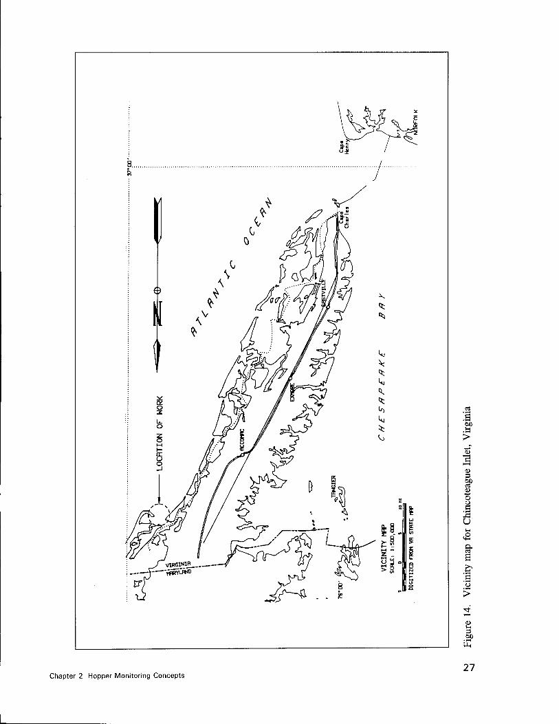
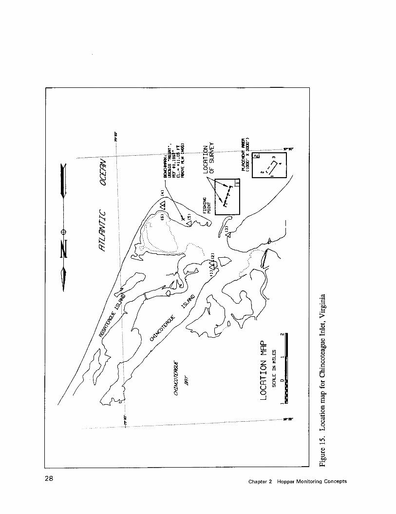
Chincoteague Inlet is located at the entrance to Chincoteague Bay between Assateague Island and Chincoteague Island along the northern coast of Virginia. Figure 14 is a vicinity map for Chincoteague Inlet showing its location with respect to Norfolk, Virginia, and Chesapeake Bay, and Fig- ure 15 is a location map which indicates the dredging area (shown as "Loca- tion of Survey" on the map) and the disposal site (shown as "Placement Area" on the map) near Chincoteague Inlet.
Chincoteague Inlet is subject to fairly rapid and unpredictable shoaling conditions that make bathymetric surveys unreliable. Because of these condi- tions, the maintenance dredging at Chincoteague is paid by bin measure. A predredging survey is performed to provide an estimate of the extent of shoal- ing, and a postdredging survey is performed to verify that the channel is navigable, but payment to the contractor is not based upon those surveys. The material in the inlet is primarily fine sand with less than 5 percent fines and has an average in-place density of 121.9 lb/ft3, as determined by a series of nuclear density measurements taken in the channel.
The monitoring system was installed aboard the dredge Northerly Island during a 3 day period from March 2 through March 4, 1993. Dredging at Chincoteague Inlet began on March 6, 1993 and was completed on March 18, 1993. The estimated volume of material removed from the channel was approximately 112,000 yd3 as reported by the contractor.
Bin measure load calculations
As discussed previously, the process of calculating the bin measure load requires the determination of several variables: the volume of material in the hopper and the vessel displacement at the start of the load cycle, the volume
Chapter 2 Hopper Monitoring Concepts
2 'S •T-H
00
•a I—I
00
4-* O
e U
s
>
3
Chapter 2 Hopper Monitoring Concepts 27
I &
jr so-
rt a
(L>
•a
o Ü c
u
&
c o
• i-H
'S Ü o
3 00
28 Chapter 2 Hopper Monitoring Concepts
of material in the hopper and the vessel displacement at the end of the load cycle, the density of the interstitial water, and the estimated in-place density of the material being dredged. Once those values are determined, then the bin measure load can be calculated using the procedures previously set forth.
For the Chincoteague Inlet project, the density of the interstitial water was determined by measuring the density of five water samples that were randomly taken through the duration of the project. The density of those samples ranged from 1.019 g/cm3 to 1.021 g/cm3, with the average being 1.020 g/cm3. A series of six nuclear density probe measurements were taken in the channel. The in-place sediment density measured by the probe ranged from 1.939 g/cm3 to 1.964 g/cm3, with the average being 1.953 g/cm3.
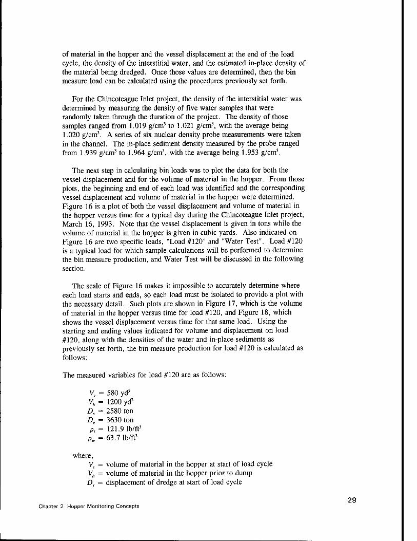
The next step in calculating bin loads was to plot the data for both the vessel displacement and for the volume of material in the hopper. From those plots, the beginning and end of each load was identified and the corresponding vessel displacement and volume of material in the hopper were determined. Figure 16 is a plot of both the vessel displacement and volume of material in the hopper versus time for a typical day during the Chincoteague Inlet project, March 16, 1993. Note that the vessel displacement is given in tons while the volume of material in the hopper is given in cubic yards. Also indicated on Figure 16 are two specific loads, "Load #120" and "Water Test". Load #120 is a typical load for which sample calculations will be performed to determine the bin measure production, and Water Test will be discussed in the following section.
The scale of Figure 16 makes it impossible to accurately determine where each load starts and ends, so each load must be isolated to provide a plot with the necessary detail. Such plots are shown in Figure 17, which is the volume of material in the hopper versus time for load #120, and Figure 18, which shows the vessel displacement versus time for that same load. Using the starting and ending values indicated for volume and displacement on load #120, along with the densities of the water and in-place sediments as previously set forth, the bin measure production for load #120 is calculated as follows:
The measured variables for load #120 are as follows:
Vs = 580 yd3
Vh = 1200 yd3
Ds = 2580 ton De = 3630 ton p, = 121.9 lb/ft3
Pw = 63.7 lb/ft3
where, Vs = volume of material in the hopper at start of load cycle Vh = volume of material in the hopper prior to dump Ds = displacement of dredge at start of load cycle
Chapter 2 Hopper Monitoring Concepts 29
pX no 'jsddoH u\ psueiBW JO own|OA s CD S
89 89 L/1 en
s S3 S3 m
89 89 LD CM
81 8) 89 CM
89 89 LA
89 89 89
89 89 in
89
89 89 89
U)
89
E i-
w
89 85 89 S3 83 83 83 U3 S3 L/) m C3 N
SUOl 'lUOLUOOBldSjQ |9SS9A
T3 O l-H u a.
> o
>
s
CO
•3
CO
>
1 1-1 <D D. CL, O
X!
1 C4-I o
I > ^6
Pi
30 Chapter 2 Hopper Monitoring Concepts
m
CD
E
CM
m
is N
pX no 'J9ddoH u\ |BueiE|/\j J° 9wri|0A
o
l-l ex
13 i>
ä ccj
O o C
U o" <N t—i
T3 a o
a
> l-i
a, o
J3
■*-» CO
s O
I O >
3 «30
•!-H
p-.
Chapter 2 Hopper Monitoring Concepts 31
o <o 'o1
&
-a
u o ä u o" 1—<
=tfc
a) O l-H ,o
CO 0 CO 1-1
>
CO
CO CO 4)
00
u
• IH
32 Chapter 2 Hopper Monitoring Concepts
De = displacement of dredge prior to dump Pi = in-place density of dredged material pw = density of water in dredging area
The bin water weight is calculated by the following equation:
Wb = V, * pH
(9)
Wb = 580 yd3 * 27 ft3/yd3 * 63.7 lb/ft3 = 997542 lb
The total weight in the hopper is calculated by the following equation:
(10)
TW = (De- D) + Wb
TW = ((3630-2580) ton * 2000 lb/ton) + 997542 lb TW = (1050 ton * 2000 lb/ton) + 997542 lb TW = 2100000 lb + 997542 lb TW = 3097542 lb
The average slurry density in the hopper is calculated by:
_ TW (ID Yh
Ps = 3097542 lb / (1200 yd3 * 27 ft3/yd3) p, = 3097542 lb / 32400 ft3
p, = 95.6 lb/ft3
The in-place production is calculated by:
PRO = PJL PJL * Vh
Pi ~ Pw
(12)
PROt = ((95.6 lb/ft3 - 63.7 lb/ft3)/(121 lb/ft3 - 63.7 lb/ft3)) * 1200 yd3
PRO, = 0.55 * 1200 yd3
PRO, = 660 yd3
A total of 147 loads were dredged during the Chincoteague Inlet project. The procedure followed in the preceding example was used to calculate the
33 Chapter 2 Hopper Monitoring Concepts
34
bin measure production for each of those loads. The cumulative in-place bin measure production calculated was 84,110 cu yd, for an average load of 572.2 cu yd over the 147 loads.
System verification, water tests
A potential weakness in this method of calculating production is the dif- ficulty in verifying the accuracy of the data being measured. The total dis- placement of the vessel is not easily verified, and the volume of material in the hopper at any given time is also difficult to verify. Thus, some method was needed to verify that the production calculations based upon the data collected by the monitoring system were accurate. No reasonable method of verifying each measurement could be determined, so a method of verifying the end result of the average hopper density calculation was chosen. The water test method, adopted in this case, consisted of filling the hopper with a material of known density, and then calculating the average density of the material added to the hopper based upon the change in vessel displacement and volume of material added to the hopper as measured by the monitoring system. The hopper was filled with seawater, the density of which was deter- mined from samples taken during the water tests. The vessel displacement and volume of material in the hopper were determined for the beginning and end of each water test. Figures 19 and 20 show the volume of material in the hopper and vessel displacement respectively for a water test. The values indicated in those figures for volume of material in the hopper and vessel displacement at the start and end of the test are used in the following calcula- tions. Note that the same measured variables are used here as were used in the production calculation previously presented.
The total weight of water added to the hopper is defined as:
(13)
W=D- D.
Wa = (2950 ton - 2270 ton) * 2000 lb/ton Wa = 1360000 lb
The volume of water added to the hopper is:
V = V - V (14> ya yh Ys
Va = (1115 yd3 - 325 yd3) * 27 ft3/yd3
V, = 21330 ft3
Chapter 2 Hopper Monitoring Concepts
en
CM 1 i i H. i I
\. CM
^s Lfi
V. CO
J CM CM
r ~~" CO S .
CM
Jl si CM
3 0 3
Ü Ul
m
= 325
N »_
ii \ M
CD u CJ
E E E 3 3 ^ F
I-H 0 CM
0 ^ CM
CJ 0,
Hop
per
m 0 X CM
c w
\ *«
X^ CO
CM
\./ CM CM
Ln
Q
1 i i i i 1 i Lfl
DCM a s cs cs o as cs a Q D cs cs cs cs o cs CM T r CM CS CO ^0 ^ CM T H iH
pX no 'jsddoH m |BU8;B|/\J JO 9iun|0A
o a> 'S1
I-H cu
■«->
.-a
öß
o Ü a
u
I
> l-l
& O
<L>
a o I) a ja "o >
3
Chapter 2 Hopper Monitoring Concepts 35
en
CM i 1 1 -v 1 1 N
if) CO
CM CM
CO
* i - CM ifl CM ? « 0 > c -p X o
CD > CD
in
en . * r*- " CM < i N
CM
) N N >_ ii ( sz
S " +> CD N E
E 0) \ e N H Ü \ » CM 16 V o
l-H \ 16 & I ^H CO IT o ^V "H vfl
CM CM
w V 16
V^ CO ■£>
Q
1 1 1 1 '
CM CM
m LD
a CM 3 CD S3 CD CD CD C c 9 CD Cg CD CD CD C a CM p 4 CD m vD 'tf CM 0 a r ii m CM CM CM N t
suoi 'iuaiii90B|ds!a |9SseA
o
o 0)
'o*
Ig <U
ÖO PS u o a u
I CO
3 CD >
a <D O
"a, CO
>
o
3 00
• i-H
36 Chapter 2 Hopper Monitoring Concepts
The average water density in the hopper is:
W a
T" (15)
pw = 1360000 lb / 21330 ft3
pw = 63.8 lb/ft3
The measured density of the water in the hopper was 63.7 lb/ft3. The percent difference between the calculated and measured density values was 0.16 percent.
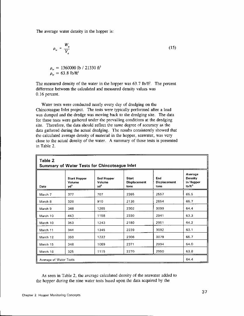
Water tests were conducted nearly every day of dredging on the Chincoteague Inlet project. The tests were typically performed after a load was dumped and the dredge was moving back to the dredging site. The data for these tests were gathered under the prevailing conditions at the dredging site. Therefore, the data should reflect the same degree of accuracy as the data gathered during the actual dredging. The results consistently showed that the calculated average density of material in the hopper, seawater, was very close to the actual density of the water. A summary of those tests is presented in Table 2.
Table 2 Summary of Water Tests for Chincoteague Inlet
Date
Start Hopper Volume yd3
End Hopper Volume yd3
Start Displacement tons
End Displacement tons
Average Density in Hopper lb/ft3
March 7 377 707 2265 2557 65.5
March 8 326 910 2136 2654 65.7
March 9 348 1265 2302 3099 64.4
March 10 443 1158 2330 2941 63.3
March 10 353 1243 2180 2951 64.2
March 11 344 1345 2239 3092 63.1
March 12 350 1222 2306 3079 65.7
March 15 348 1069 2371 2994 64.0
March 16 325 1115 2270 2950 63.8
Average of Water Tests 64.4
As seen in Table 2, the average calculated density of the seawater added to the hopper during the nine water tests based upon the data acquired by the
Chapter 2 Hopper Monitoring Concepts 37
38
monitoring system was 64.4 lb/ft3. The actual density of that water, as deter- mined by analyzing water samples taken during five of the water tests, was 63.7 lb/ft3. The percent difference between the density as determined by the monitoring system and the density as determined from the water samples is as follows.
Average density (Monitoring system) = 64.4 lb/ft3
Average density (Water samples) = 63.7 lb/ft3
Percent difference = ((64.4 - 63.7) / 63.7) * 100 = +1.1%
Norfolk Harbor Channel
The second dredging project monitored during this study was performed in the Norfolk Harbor Channel, which extends from deep water in Hampton Roads into the Elizabeth River. The outbound channel to the coal piers at Lambert Point is maintained to a depth of 50 ft, while other portions of the channel are maintained to depths of 40 and 45 ft. Figure 21 provides a vicinity map of the Norfolk Harbor area, with the general area of this mainte- nance dredging project noted near the Craney Island Disposal Area. The Norfolk Harbor maintenance dredging is typically performed by a cutterhead dredge, but the low bidder chose to perform a portion of the project with a hopper dredge. The channel had not been dredged by a hopper dredge since 1986, when a Government dredge was used. A contract hopper dredge had never been used to perform the maintenance dredging in this portion of the channel.
Monitoring the maintenance dredging in Norfolk Harbor presented an opportunity to analyze the data acquired by the monitoring system in a dredg- ing environment much different than that found in the Chincoteague Inlet project. The sediment in Norfolk Harbor is primarily a fine grained sediment, as opposed to the sandy sediment in Chincoteague Inlet. The dredging depth in Norfolk Harbor was approximately 52 ft while that in Chincoteague Inlet was approximately 15 ft, and the discharge of dredged material from the hopper was done by pumping into a confined disposal area at Craney Island whereas the Chincoteague Inlet project used an unconfmed ocean site for dumping. Additionally, no restrictions exist on overflow of sediment from the hopper in Norfolk Harbor. For the Norfolk Harbor project, the data from the monitoring system was used to analyze the retention rate of solids in the hopper during the overflow period for each load.
The Norfolk Harbor dredging project commenced on April 10, 1993, and the project was performed in two phases. One acceptance section was completed by the NATCO dredge Northerly Island on April 20, 1993, while the remainder of the project was subcontracted and completed by cutterhead dredge. The section completed by the Northerly Island was on the East toe of the outbound channel, between center line sta 138+00 and 196+00 for a
Chapter 2 Hopper Monitoring Concepts
'S '5b i-i
>
si o I-I o
X> t-l
B
& o Z,
&
e
>
Chapter 2 Hopper Monitoring Concepts 39
length of 5,800 ft. The data described in this report refer only to that portion of the project that was completed by the NATCO hopper dredge Northerly Island. The monitoring system installed by WES remained on the Northerly Island from the completion of the Chincoteague Inlet project in late March. The entire system was removed from the dredge on April 21, 1993, after Northerly Island had completed its work on the Norfolk Harbor project. The main goal of using the monitoring system on the Norfolk Harbor project was to analyze the amount of solids retained in the hopper during the overflow process. Monitoring the overflow efficiency using hopper volume, vessel displacement, and production meter data has previously been performed by WES aboard the U.S. Army Corps of Engineers dredge Wheeler (Scott 1992).
Overflow analysis
The primary focus of monitoring the Norfolk Harbor Channel project was to obtain some insight into the amount of solids retained in the hopper during overflow. Overflow is that portion of the dredging cycle that starts when the hopper is full and material is allowed to overflow back into the channel as dredging continues. When dredging in coarse grained sediments, the solids will settle into the hopper while the overflow consists of relatively clear water. However, when the dredged material consists of fine grained sediments which take considerably longer to settle, the effectiveness of overflow in retaining solids in the hopper is less certain.
The beginning and ending of the overflow process for each load was determined from the hopper volume data. Overflow started when the hopper volume reached a maximum and a relatively constant hopper volume was maintained while dredging continued. Overflow stopped when the production meters indicated that dredging had stopped for each load. Figure 22 shows a plot of vessel displacement and volume of material in the hopper for load #74, a typical load from the Norfolk Harbor project. Noted in that figure are the start and stop times of the overflow process for that particular load.
The amount of solids retained in the hopper was determined by looking at the total displacement, or weight, of the vessel at the start of overflow and the total weight at the end of overflow. Since the total volume of material in the hopper does not increase during overflow, any increase in the weight of the vessel during overflow must be due to additional solids displacing water and being retained in the hopper. Thus, the weight of solids retained during over- flow was taken as the change in the total weight of the vessel during overflow, as determined from the monitoring system displacement measurements. Fig- ure 23 is a magnified view of the vessel displacement during overflow for load #74, with the displacement of the vessel at the start and end of overflow noted. For the values indicated in Figure 23, the weight of solids retained in the hopper was calculated as follows.
40 Chapter 2 Hopper Monitoring Concepts
ü a> 'o1 u.
OH
l-i O
■e X M
s o
'S _o c o
cd C
O
> o
<s
1/1
1/3 1-
> G
s <D o cd
>
1 o, OH O
a o
g >
CM
3 SP
Chapter 2 Hopper Monitoring Concepts 41
1— i i i i i 1
-flow
= 2.25 hr)
Lacement
Ü0 tons
- m
\S)
CO 03 ÄG3 =»c :> £ W TT i- o ••* "H -^E^
- C C5J A # W~ II "%.
>* ^^J^' 4_
i- N CD
E 1-
1
p£ lou
1.27 hr)
cement
tons
i
Start Ow
ei
(B tine =
= >
Displa«
= 3972
"^v
G a c
i ■ i i i i 1 m
D CD 3 0
4150
4100
4050
4000
3950
3900
CD C Ul G CO c
SUO; 'lU9LU90B|dS!a I9SS9A
o <D
t-l Pu, l-H o
■s is!
is ll O
r-- =tfc
'S c o
o 1-4 1) > o a
■ l-H H
•§
1
>
o
"E,
en
4)
CO C4
3 00
42 Chapter 2 Hopper Monitoring Concepts
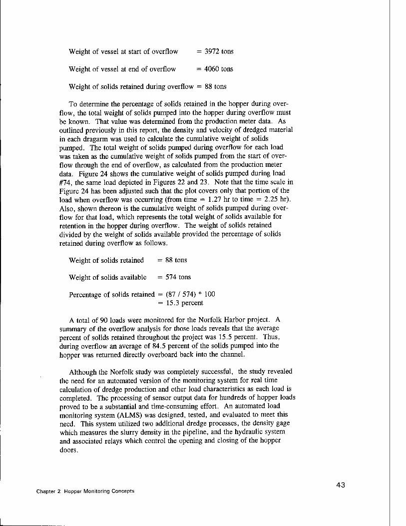
Weight of vessel at start of overflow = 3972 tons
Weight of vessel at end of overflow = 4060 tons
Weight of solids retained during overflow = 88 tons
To determine the percentage of solids retained in the hopper during over- flow, the total weight of solids pumped into the hopper during overflow must be known. That value was determined from the production meter data. As outlined previously in this report, the density and velocity of dredged material in each dragarm was used to calculate the cumulative weight of solids pumped. The total weight of solids pumped during overflow for each load was taken as the cumulative weight of solids pumped from the start of over- flow through the end of overflow, as calculated from the production meter data. Figure 24 shows the cumulative weight of solids pumped during load #74, the same load depicted in Figures 22 and 23. Note that the time scale in Figure 24 has been adjusted such that the plot covers only that portion of the load when overflow was occurring (from time = 1.27 hr to time = 2.25 hr). Also, shown thereon is the cumulative weight of solids pumped during over- flow for that load, which represents the total weight of solids available for retention in the hopper during overflow. The weight of solids retained divided by the weight of solids available provided the percentage of solids retained during overflow as follows.
Weight of solids retained =88 tons
Weight of solids available = 574 tons
Percentage of solids retained = (87 / 574) * 100 = 15.3 percent
A total of 90 loads were monitored for the Norfolk Harbor project. A summary of the overflow analysis for those loads reveals that the average percent of solids retained throughout the project was 15.5 percent. Thus, during overflow an average of 84.5 percent of the solids pumped into the hopper was returned directly overboard back into the channel.
Although the Norfolk study was completely successful, the study revealed the need for an automated version of the monitoring system for real time calculation of dredge production and other load characteristics as each load is completed. The processing of sensor output data for hundreds of hopper loads proved to be a substantial and time-consuming effort. An automated load monitoring system (ALMS) was designed, tested, and evaluated to meet this need. This system utilized two additional dredge processes, the density gage which measures the slurry density in the pipeline, and the hydraulic system and associated relays which control the opening and closing of the hopper doors.
Chapter 2 Hopper Monitoring Concepts 43
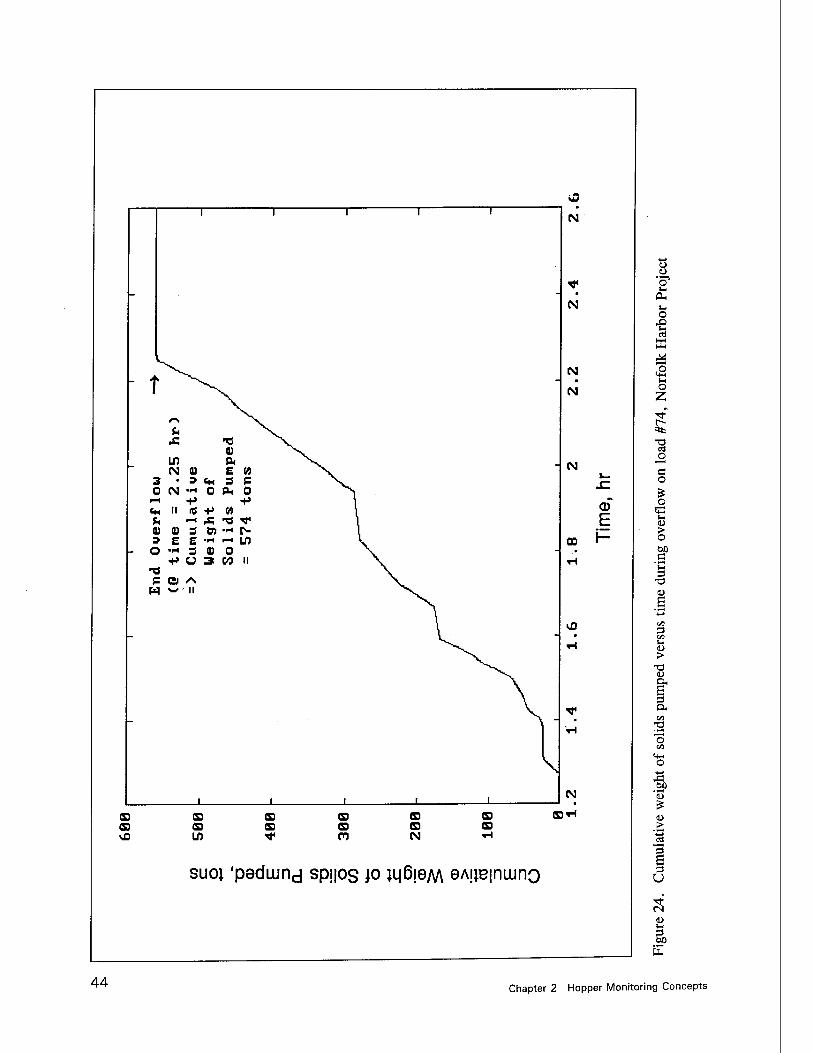
- T
b Ä
0} w cu N 01 £ U
3 • 3 «H s e 0 CM •IH 0 PL, 0
PH +> +» «M II « -p «
SH 1—1 Ä "0 ^ 0) 0) 3 tn "* r*- S E E ■F* -i U5
O ■Ft 3 U 0 "P U 3 CO II
■« P a /S W w II
\
N
N
N
GO
CD
E I-
<&
N
CD CS CD CD CD 63 CD CD CD CD vJ3 LD ^ CO N
CD CO
CDi
suo} 'pediund spnos jo UjßlQM SAiieinwno
o
o •s
a o
=tte
T3 n)
_o c o
o m
> o
c t-l
■§
>
I On
O
>
1 u
3 00
44 Chapter 2 Hopper Monitoring Concepts
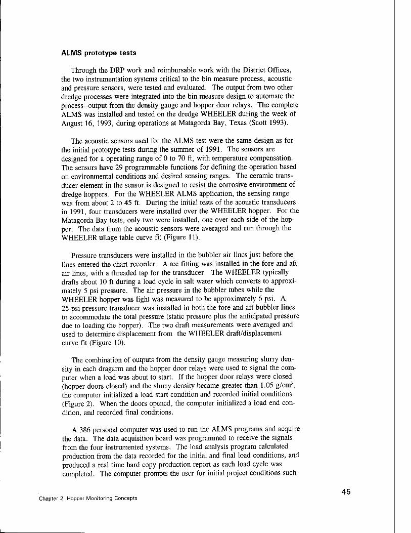
ALMS prototype tests
Through the DRP work and reimbursable work with the District Offices, the two instrumentation systems critical to the bin measure process, acoustic and pressure sensors, were tested and evaluated. The output from two other dredge processes were integrated into the bin measure design to automate the process-output from the density gauge and hopper door relays. The complete ALMS was installed and tested on the dredge WHEELER during the week of August 16, 1993, during operations at Matagorda Bay, Texas (Scott 1993).
The acoustic sensors used for the ALMS test were the same design as for the initial prototype tests during the summer of 1991. The sensors are designed for a operating range of 0 to 70 ft, with temperature compensation. The sensors have 29 programmable functions for defining the operation based on environmental conditions and desired sensing ranges. The ceramic trans- ducer element in the sensor is designed to resist the corrosive environment of dredge hoppers. For the WHEELER ALMS application, the sensing range was from about 2 to 45 ft. During the initial tests of the acoustic transducers in 1991, four transducers were installed over the WHEELER hopper. For the Matagorda Bay tests, only two were installed, one over each side of the hop- per. The data from the acoustic sensors were averaged and run through the WHEELER ullage table curve fit (Figure 11).
Pressure transducers were installed in the bubbler air lines just before the lines entered the chart recorder. A tee fitting was installed in the fore and aft air lines, with a threaded tap for the transducer. The WHEELER typically drafts about 10 ft during a load cycle in salt water which converts to approxi- mately 5 psi pressure. The air pressure in the bubbler tubes while the WHEELER hopper was light was measured to be approximately 6 psi. A 25-psi pressure transducer was installed in both the fore and aft bubbler lines to accommodate the total pressure (static pressure plus the anticipated pressure due to loading the hopper). The two draft measurements were averaged and used to determine displacement from the WIIEELER draft/displacement curve fit (Figure 10).
The combination of outputs from the density gauge measuring slurry den- sity in each dragarm and the hopper door relays were used to signal the com- puter when a load was about to start. If the hopper door relays were closed (hopper doors closed) and the slurry density became greater than 1.05 g/cm3, the computer initialized a load start condition and recorded initial conditions (Figure 2). When the doors opened, the computer initialized a load end con- dition, and recorded final conditions.
A 386 personal computer was used to run the ALMS programs and acquire the data. The data acquisition board was programmed to receive the signals from the four instrumented systems. The load analysis program calculated production from the data recorded for the initial and final load conditions, and produced a real time hard copy production report as each load cycle was completed. The computer prompts the user for initial project conditions such
Chapter 2 Hopper Monitoring Concepts 45
as water density and in situ sediment density. An uninterruptable power sup- ply provided power to the ALMS.
The ALMS was tested during the week of August 16, 1993, on the Corps dredge WHEELER at Matagorda Bay, Texas, east of Corpus Christi, Texas. The dredged sediments were composed mainly of fine sands with some silt. The in situ density of the sediments was approximately 1.80 g/cm3.
Seven hopper loads were recorded during the testing and evaluation period. Figure 25 shows the sequencing of the signals from the acoustic sensor (top curve), the slurry density (middle curve), and the hopper doors (bottom curve) for all seven loads. Note that the load starts when the density in the pipe be- gins to increase, and ends when the hopper door relay is tripped. Figure 26 shows the initial and final hopper volume and dredge displacement for load LI shown in Figure 25. A sample of a hard copy production report is shown as Figure 27.
8000
3 u
0) E 3
I
E o 3 Ü
M C 0) Q
*
500
1.3
10
Hopper Volume
Slurry Density
Start Load
End Load<7 Hopper Door Signal
16 17 18 19 28 21 22 23
line - hrs
24
Figure 25. Signal sequencing for seven hopper loads during the ALMS test
To test the accuracy of the system, two water tests were performed, desig- nated as L2 and L3 in Figure 25. The hopper was filled with seawater and emptied. Because the ALMS is designed to operate automatically only when
46 Chapter 2 Hopper Monitoring Concepts
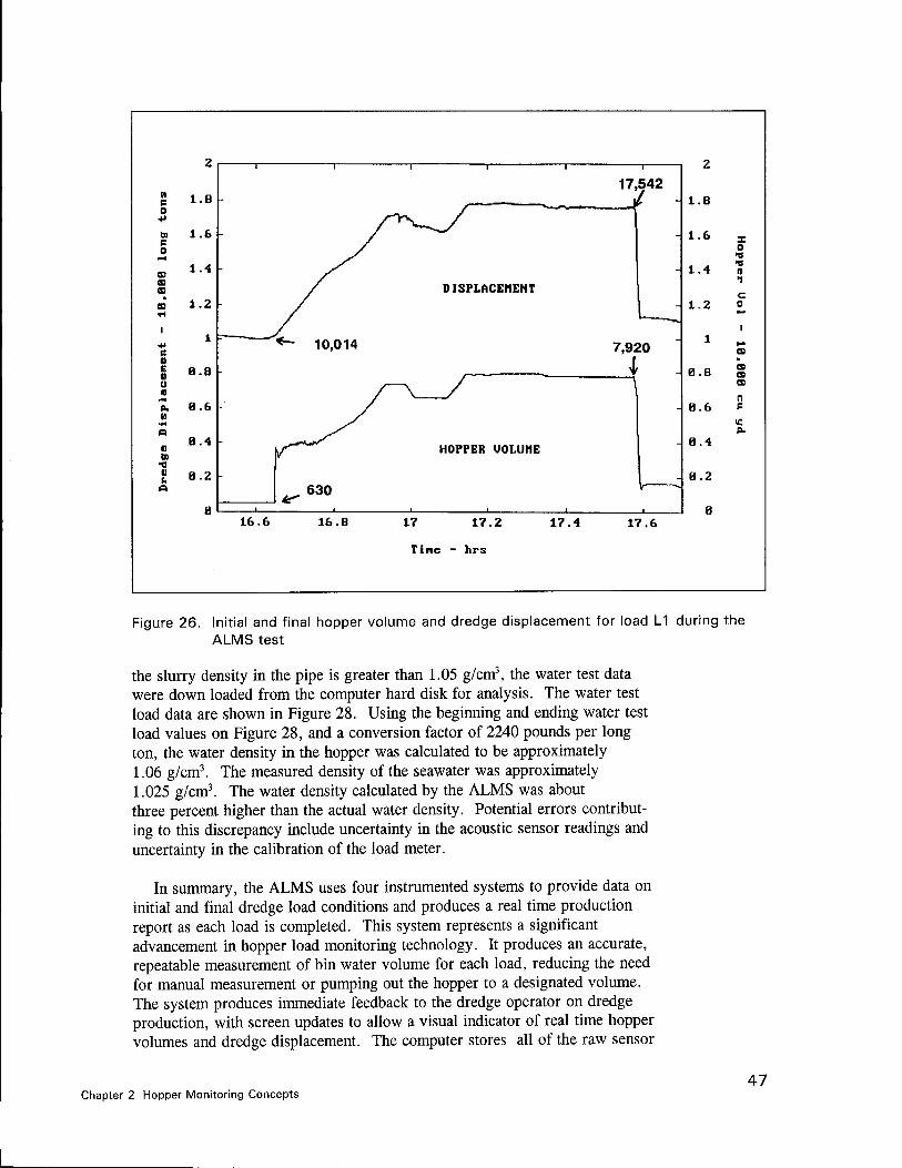
c 1 .8 0
+• tn 1 .6 r 0
I-*
1 4 s s s CD 1 2
1 1
■f c n E 0 a 8 u « »1 a b M
>M
o H 4
0 B) "« II B 2 A
a
17,542
i DISPLACEMENT
10,014 7,920 I
HOPPER UOLUHE
630
2
1.8
1.6
1.4
1.2
1
8.8
8.6
8.4
8.2
8
o
•B (I •J
C 0
CD a a
o B
16.6 16.8 17 17.2 17.4
line - hrs
17.6
Figure 26. Initial and final hopper volume and dredge displacement for load L1 during the ALMS test
the slurry density in the pipe is greater than 1.05 g/cm3, the water test data were down loaded from the computer hard disk for analysis. The water test load data are shown in Figure 28. Using the beginning and ending water test load values on Figure 28, and a conversion factor of 2240 pounds per long ton, the water density in the hopper was calculated to be approximately 1.06 g/cm3. The measured density of the seawater was approximately 1.025 g/cm3. The water density calculated by the ALMS was about three percent higher than the actual water density. Potential errors contribut- ing to this discrepancy include uncertainty in the acoustic sensor readings and uncertainty in the calibration of the load meter.
In summary, the ALMS uses four instrumented systems to provide data on initial and final dredge load conditions and produces a real time production report as each load is completed. This system represents a significant advancement in hopper load monitoring technology. It produces an accurate, repeatable measurement of bin water volume for each load, reducing the need for manual measurement or pumping out the hopper to a designated volume. The system produces immediate feedback to the dredge operator on dredge production, with screen updates to allow a visual indicator of real time hopper volumes and dredge displacement. The computer stores all of the raw sensor
47 Chapter 2 Hopper Monitoring Concepts
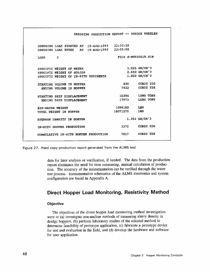
DREDGING PRODUCTION REPORT — DREDGE WHEELER
DREDGING LOAD STARTED AT 19-AUG-1993 22:20:18 DREDGING LOAD ENDED AT 19-AUG-1993 23:03:58
LOAD 2 FILE d:WH930819.BIN
SPECIFIC WEIGHT OF WATER 1.025 GM/CM"3
SPECIFIC WEIGHT OF SOLIDS 2.650 GM/CM*3
SPECIFIC WEIGHT OF IN-SITU SEDIMENTS 1.800 GM/CM"3
STARTING VOLUME IN HOPPER 636 CUBIC YDS
ENDING VOLUME IN HOPPER 7932 CUBIC YDS
STARTING SHIP DISPLACEMENT 10394 LONG TONS
ENDING SHIP DISPLACEMENT 17973 LONG TONS
BIN-WATER WEIGHT 1096180 LBS TOTAL WEIGHT IN HOPPER 18071270 LBS
AVERAGE DENSITY IN HOPPER 1.353 GM/CM~3
IN-SITU HOPPER PRODUCTION 3372 CUBIC YDS
COMMULATIVE IN-SITU HOPPER PRODUCTION 7017 CUBIC YDS
Figure 27. Hard copy production report generated from the ALMS test
data for later analysis or verification, if needed. The data from the production report eliminates the need for time consuming, manual calculation of produc- tion. The accuracy of the instrumentation can be verified through the water test process. Instrumentation schematics of the ALMS electronics and system configuration are found in Appendix A.
Direct Hopper Load Monitoring, Resistivity Method
Objective
The objectives of the direct hopper load monitoring method investigation were to (a) investigate non-nuclear methods of measuring slurry density in dredge hoppers, (b) perform laboratory studies of the selected method to determine feasibility of prototype application, (c) fabricate a prototype device for test and evaluation in the field, and (d) develop the hardware and software for user application.
48 Chapter 2 Hopper Monitoring Concepts
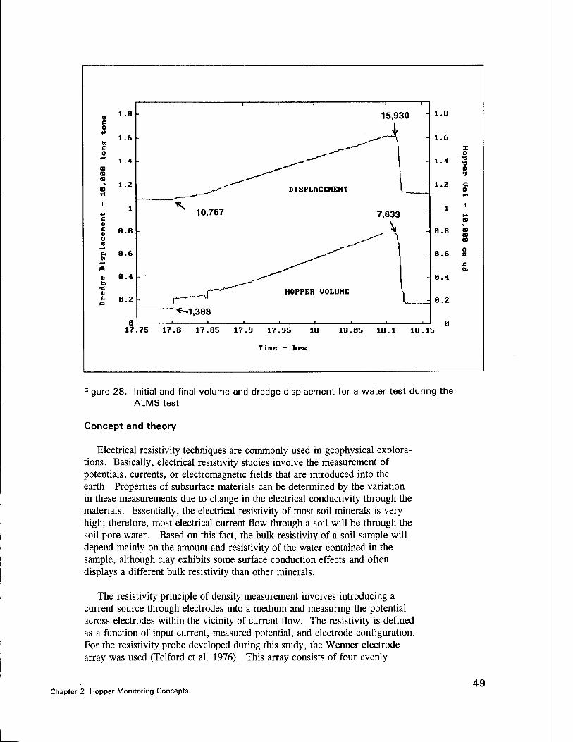
6) C 0
B S s
c D E I) u K
ft:
I) Bl •« D
a
1.8
1.6
1.4
1.2
1
0.8
8.6
8.4
8.2
8 <-1,388
17.75 17.8 17.85 17.9 17.95 18 18.85 18.1 18.15
Tine - hrs
z 0 •H V a i c 0
CD CD CD
O P
l£ ft.
Figure 28. Initial and final volume and dredge displacment for a water test during the ALMS test
Concept and theory
Electrical resistivity techniques are commonly used in geophysical explora- tions. Basically, electrical resistivity studies involve the measurement of potentials, currents, or electromagnetic fields that are introduced into the earth. Properties of subsurface materials can be determined by the variation in these measurements due to change in the electrical conductivity through the materials. Essentially, the electrical resistivity of most soil minerals is very high; therefore, most electrical current flow through a soil will be through the soil pore water. Based on this fact, the bulk resistivity of a soil sample will depend mainly on the amount and resistivity of the water contained in the sample, although clay exhibits some surface conduction effects and often displays a different bulk resistivity than other minerals.
The resistivity principle of density measurement involves introducing a current source through electrodes into a medium and measuring the potential across electrodes within the vicinity of current flow. The resistivity is defined as a function of input current, measured potential, and electrode configuration. For the resistivity probe developed during this study, the Wenner electrode array was used (Telford et al. 1976). This array consists of four evenly
Chapter 2 Hopper Monitoring Concepts 49
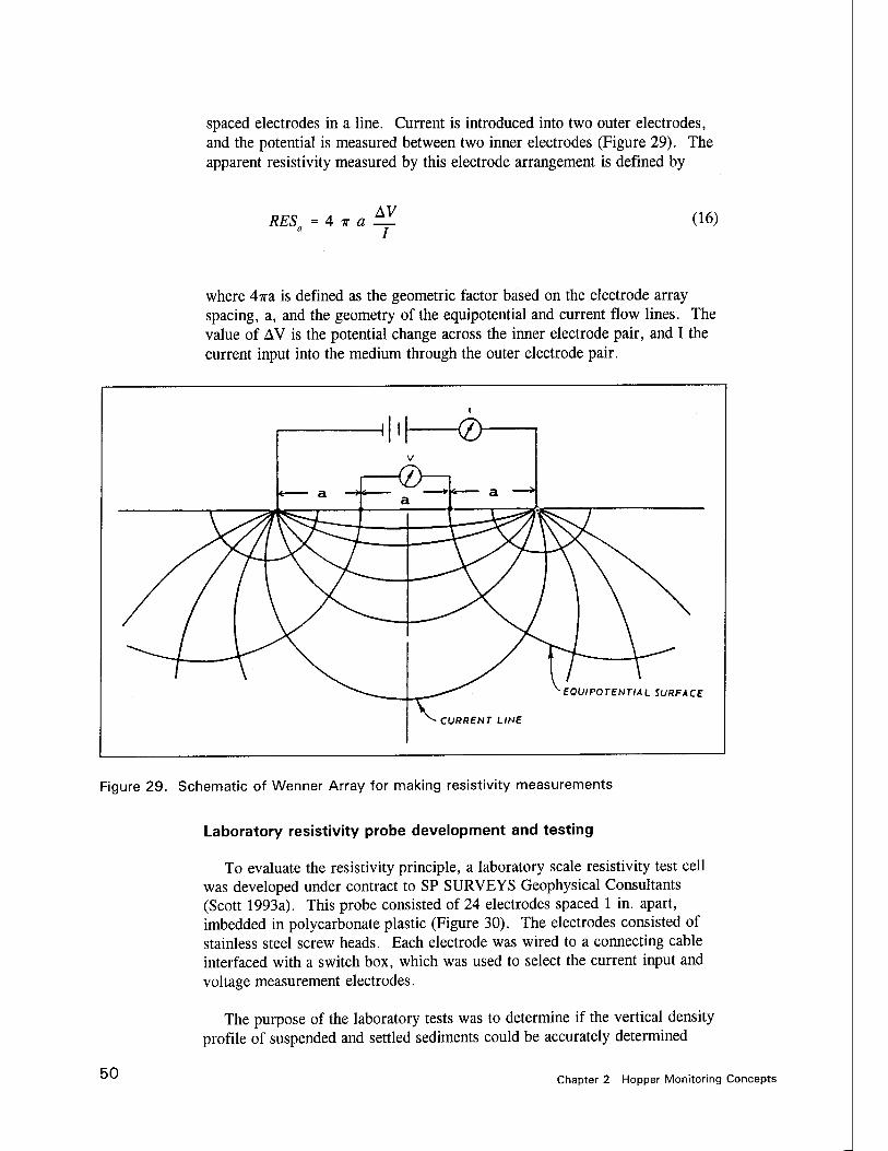
spaced electrodes in a line. Current is introduced into two outer electrodes, and the potential is measured between two inner electrodes (Figure 29). The apparent resistivity measured by this electrode arrangement is defined by
RES_ = 4 7T a AV (16)
where 4-7ra is defined as the geometric factor based on the electrode array spacing, a, and the geometry of the equipotential and current flow lines. The value of AV is the potential change across the inner electrode pair, and I the current input into the medium through the outer electrode pair.
EQUIPOTENTIAL SURFACE
CURRENT LINE
Figure 29. Schematic of Wenner Array for making resistivity measurements
Laboratory resistivity probe development and testing
To evaluate the resistivity principle, a laboratory scale resistivity test cell was developed under contract to SP SURVEYS Geophysical Consultants (Scott 1993a). This probe consisted of 24 electrodes spaced 1 in. apart, imbedded in polycarbonate plastic (Figure 30). The electrodes consisted of stainless steel screw heads. Each electrode was wired to a connecting cable interfaced with a switch box, which was used to select the current input and voltage measurement electrodes.
The purpose of the laboratory tests was to determine if the vertical density profile of suspended and settled sediments could be accurately determined
50 Chapter 2 Hopper Monitoring Concepts
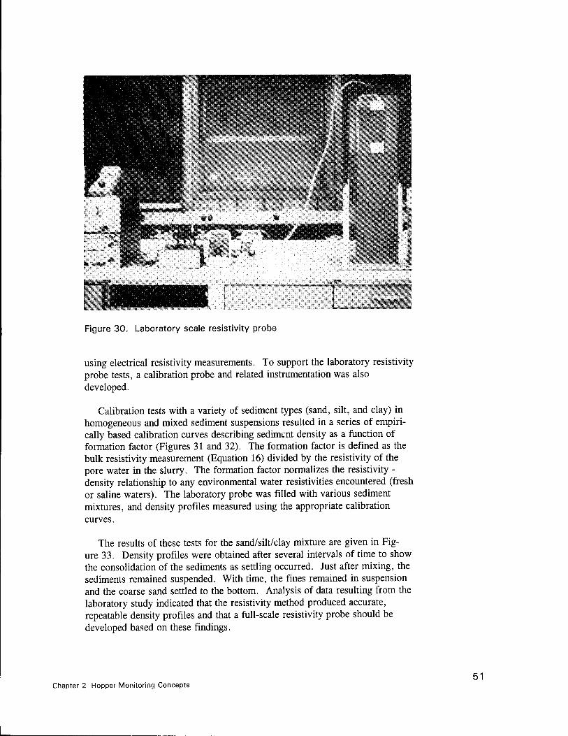
■ag)^mm'§ijp»)!^my^jpiM
- ■: ^itH ya>i»
m\
Figure 30. Laboratory scale resistivity probe
using electrical resistivity measurements. To support the laboratory resistivity probe tests, a calibration probe and related instrumentation was also developed.
Calibration tests with a variety of sediment types (sand, silt, and clay) in homogeneous and mixed sediment suspensions resulted in a series of empiri- cally based calibration curves describing sediment density as a function of formation factor (Figures 31 and 32). The formation factor is defined as the bulk resistivity measurement (Equation 16) divided by the resistivity of the pore water in the slurry. The formation factor normalizes the resistivity - density relationship to any environmental water resistivities encountered (fresh or saline waters). The laboratory probe was filled with various sediment mixtures, and density profiles measured using the appropriate calibration curves.
The results of these tests for the sand/silt/clay mixture are given in Fig- ure 33. Density profiles were obtained after several intervals of time to show the consolidation of the sediments as settling occurred. Just after mixing, the sediments remained suspended. With time, the fines remained in suspension and the coarse sand settled to the bottom. Analysis of data resulting from the laboratory study indicated that the resistivity method produced accurate, repeatable density profiles and that a full-scale resistivity probe should be developed based on these findings.
Chapter 2 Hopper Monitoring Concepts 51
o
o _
O o o
ü_
c o
o E o
q
o
D
D
D A
□ □
A
A|A A i i | i i i i | i i i i | i r 1.00 1.25 1.50 1.75
i—|—1—i—r 2.00
Density, g/cu cm
Figure 31. Resistivity calibration curve for sand and silt mixture
Prototype resistivity probe development and testing
Based on design parameters determined from the laboratory studies, a prototype resistivity probe was designed and constructed under a continuation of the laboratory study contract with SP SURVEYS. The probe was designed for installation in the hopper of the dredge WHEELER operated by the U.S. Army Corps of Engineers New Orleans District. The probe was designed to profile the entire depth of the hopper, requiring a 40-ft probe length. Forty electrodes were required, spaced at 1-ft intervals. The electrodes consisted of stainless steel hose clamps. The probe body was constructed of ten individual 4-ft segments of 0.75-in.- diam plastic pipe. All of the electrodes were hard wired, with the wire bundle sealed inside the pipe segments. The individual electrode connections were connected to a switch box for manual profiling of the probe. The probe was mounted on one side of a 42-ft-long, epoxy-filled fiberglass mounting beam (Figure 34). The noncorrosive structural beam has strength properties of steel, with less than half the weight of steel.
The resistivity probe was installed in the hopper of the dredge WHEELER during shipyard maintenance. Mounting locations in the hopper were
52 Chapter 2 Hopper Monitoring Concepts
o ro
□ = Sand A = Silt
* m _ CM
O -t-> o o
Lt_ O _
*
c o
CM
o E o
in _
o
*
* *
*
.- * T i i i 1 i i i i | i i i i 1 i i i i i i i i 1 -00 1.25 1.50 1.75
Density, g/cu cm
2.00
Figure 32. Resistivity calibration curve for a sand, silt, and clay mixture
determined from previous visits to the dredge while in operation, so the mount could be located in a location with minimal turbulence, thus offering more protection for the probe. The probe was mounted on steel mounting brackets attached to structural members in the hopper (Figure 35). The cable was run to accompanying instrumentation located in a remote area away from the hopper.
Field tests of the prototype probe were conducted when the dredge was operating at the mouth of the Mississippi River in the Head of Passes area. Analysis of sediment samples taken at this location indicate a composition of approximately 59 percent coarse materials by weight (> 63 microns) and 41 percent of fine materials by weight (< 63 microns). The laboratory cali- bration curve generated for a sand/silt/clay mixture (Figure 32) was chosen for this particular sediment.
Initially, the water resistivity was measured for calculation of the formation factor. Then resistivity data were collected on successive dredged material loads in the hopper. Production meter densities also were recorded during the
Chapter 2 Hopper Monitoring Concepts 53
JZ C7>
"<u X
<L>
O
o d CM
o iri
o d
o iri
ooooo 0 hrs DDDDD 19 hrs AAAAA 68 hrs G-W-W 121 hrs ***** 259 hrs
0 l l l l | l l l l | l l l l | l l l l | l l I I | I l I I | l l l I | I l l l 1.00 1.10 1.20 1.30 1.40 1.50 1.60 1.70 1.80
Calculated Density, g/cu cm
Figure 33. Measured density profiles from the laboratory tests
Figure 34. Prototype resistivity probe fabrication
54 Chapter 2 Hopper Monitoring Concepts
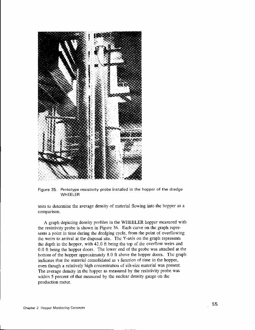
« - ->-lB
Figure 35. Prototype resistivity probe installed in the hopper of the dredge WHEELER
tests to determine the average density of material flowing into the hopper as a comparison.
A graph depicting density profiles in the WHEELER hopper measured with the resistivity probe is shown in Figure 36. Each curve on the graph repre- sents a point in time during the dredging cycle, from the point of overflowing the weirs to arrival at the disposal site. The Y-axis on the graph represents the depth in the hopper, with 42.0 ft being the top of the overflow weirs and 0.0 ft being the hopper doors. The lower end of the probe was attached at the bottom of the hopper approximately 8.0 ft above the hopper doors. The graph indicates that the material consolidated as i function of time in the hopper, even though a relatively high concentration of silt-size material was present. The average density in the hopper as measured by the resistivity probe was within 5 percent of that measured by the nuclear density gauge on the production meter.
Chapter 2 Hopper Monitoring Concepts 55
45
40 — Top cf Weirs
35
O
30
25
< 20 Ld
LÜ 15
10-
0-©^- 1
2f 0 Overt I >wing Under »ay Underlay — asproachinc disposal site
:-si
1.00 1.05 1.10 1.15 1.20 1.25 1.30 1.35 1.40 1.45 1.50 BULK DENSITY (g/cc)
Figure 36. Measured density profiles from the dredge WHEELER test
This study demonstrated that the resistivity method has high potential for measuring the density of dredged material in hopper bins. Sediment density as a function of formation factor (sediment bulk resistivity divided by the water resistivity) was empirically derived in comprehensive laboratory tests. Subsequent prototype development and testing in actual hopper bins demon- strated the applicability of using the laboratory- generated data for calculating dredged material densities.
The development of this technology represents a significant improvement in several areas. The method is nonnuclear and thus presents no safety hazards. The prototype probe has proved its durability in an 8000 cu-yd hopper. Because of the basic design and operation of the resistivity probe, it is a low maintenance and economical method for monitoring dredged material charac- teristics in the hopper. The use of the probe for monitoring the density pro- file in the hopper provides the dredge operator with a graphical record of dredged material density characteristics in the hopper during all phases of the dredging cycle. During overflow operations, the density profile can be monitored in the hopper at any time with the system. This would inform the operator of the level the settled material is in the hopper, the density of the overflow, and the rate of consolidation of solids in the hopper during
56 Chapter 2 Hopper Monitoring Concepts
overflow. For hopper dredges with adjustable weirs, the system could inform the operator of the depth to which the weirs could be lowered, based on the stratification of density in the hopper, for increasing the solids load in the hopper.
Automation of the resistivity probe operation
The final objective in investigating the resistivity method of directly mea- suring dredged slurry density in the hopper was to develop electronic instru- mentation and a pore water resistivity measurement cell to perform automated measurements of density profiles and pore water resistivity. The automated system was originally meant to be designed for the prototype probe installed on the dredge WHEELER, but the WHEELER probe was damaged in the hopper during the summer of 1993.
Figure 37 shows a diagram of the automated density probe system. The instrumentation package includes a transmitter that provides the 100 Hz AC input power to the probe electronics, a rotary switch and associated power supply and control relays that select the current and voltage electrodes in the desired sequence, and meters that measure the probe electrode current and voltage and transmit these values to the computer. Cable B connects the instrumentation package to the resistivity probe in the laboratory cell, and cable A connects the package to the pore water cell. The pore water cell is designed to filter the sediment from the dredged material and measure the
cable A cable B
pore—► water=
f . cell optional 250 ml calibration cell cable D
cable instrumentation 4— C2 package
1 2 COMM ports
N.I. DAQ board computer
Figure 37. Schematic of the automated resistivity probe system
Chapter 2 Hopper Monitoring Concepts 57
resistivity of the filtered pore water for calculation of the formation factor needed to obtain sediment density from the resistivity data.
The measurement process operates under the control of a data acquisition program written in QuickBasic 4.5. The voltage and current meters measure the 100 Hz AC probe electrode output voltage and input current and digitize these values for transmission to the computer. Cables Cl and C2 connect the voltage and current meters to the COMM1 and COMM2 RS-232 serial com- munications ports of the computer. A data acquisition board installed in the computer is used to control the sequencing of the pore water measurement and the scanning of the probe electrodes. Cable D connects the data acquisition board to the instrumentation package. Appendix B contains the instrumenta- tion package design, the wiring of the rotary switch, the rotary solenoid wir- ing, the transmitter and pore water relay wiring, the transmitter schematic, and the pore water cell design.
Automated system tests
The automated resistivity probe was tested by recording the settlement characteristics of silt suspended in salt water. The silt was a loess silt from the Vicksburg, Mississippi, area. The salt water concentration was approxi- mately 27.9 parts per thousand of sodium chloride dissolved in distilled water.
The salt water solution was mixed with the WES silt to obtain a mixture of average density of about 1.20 g/cm3. Before stirring the mixture, the resistiv- ity of the water overlying the settled silt was measured. The resistivity of the water was 23 ohm-cm at a temperature of 22°C. The silt-water mixture was stirred thoroughly in the mixing vessel and poured into the laboratory resistiv- ity test cell. The automated resistivity measurement system was then activated. The system automatically samples the pore water probe to deter- mine the pore water conductivity. The software allows the user to select the sampling time interval desired. As the density profile is automatically mea- sured, a graph appears on the screen showing the density as a function of formation factor. Each point is plotted as the measurement is made and saved to a file previously set up by the user.
The settlement monitoring tests consisted of four sets of measurements. The upper few inches of mixture in the test cell began to clarify within a few seconds after stirring ended, and a well defined settled surface became visible about 10 minutes after the stirring ended. The height of this surface above the bottom of the cell was measured and recorded during the test. This height is plotted as a function of time in Figure 38. The 6.3-in. height observed after a time of the final scan did not change after an additional 3-hr period, indicating that the 6.3-in. value was close to the final settled height.
Figure 39 shows plots of six density profiles selected from the entire test period, including the first scan at 0855 and the final scan at 1143. The visible silt surface heights, taken from Figure 38, correlate well with the "breaks" in
58 Chapter 2 Hopper Monitoring Concepts
o o IN -
V) <ü
-C in -
o K Q c
1 o
i
\ \
■+-> 10 \ C7> ^
'(U X \ (D
in q
(J ,— —
tu O \
vt- \ Z3 tu
CO
-M
o d
. X
CO
(D
>
m _
o
o o Eti o - -Ld--£]
I I I I
--Q. --□
in I I I I | I I I I | I I I I | I I I I | I I I I | I I I | I I I I 0.00 25.00 50.00 75.00 100.00 125.00 150.00 175.00
Elapsed Time — minutes
Figure 38. Plot of the settled silt interface as a function of time
the density profiles in Figure 39, indicating that the resistivity data are providing reasonable density information.
The automated resistivity probe operated as designed. The laboratory probe and associated hardware can readily be scaled to prototype application. This system potentially offers an economical alternative to nuclear density technology for directly measuring the density of slurries in dredge hoppers.
Chapter 2 Hopper Monitoring Concepts 59
Density - g/cu cm
Figure 39. Automated test density profiles with settled silt interface
60 Chapter 2 Hopper Monitoring Concepts
3 Uncertainty in Hopper Load Production Calculations
The data reduction equations used to calculate the production quantities associated with hopper dredges contain variables that introduce error into the final production calculation (Scott 1993b). These variables include not only the measurements made by the instrumentation, but also those associated with the dredging environment such as the density of the water and dredged sedi- ments. The error due to one variable may be insignificant, but the propa- gation of the error through a data reduction equation with multiple variables may result in excessive uncertainty or error in the final result.
The data reduction equations for the hopper production monitoring system contain the following variables: pw, pm, p„ Vh and the average density of the material in the hopper ph. As mentioned before, this average density measurement is calculated by dividing the total weight of the material in the hopper (bin water and slurry load) by the volume of the material in the hopper vh.
Some error is associated with each of these variables. This error may be associated with changing physical conditions in the dredging environment such as water temperature and salinity levels and variations in the mineral and organic content of the sediments, or measurement error inherent in the instru- mentation. The error contributed by each variable will propagate through the production equations into the final production calculation.
The water found within the dredging environment can vary in density due to dissolved and suspended solids content and temperature changes. The density of the water can generally vary within the range of 0.98 to 1.030 g/cm3 due to these conditions. The maximum error introduced into the production calculations due to changes in water density, without compensa- tion, is about 3 percent (Rokosch 1989).
The types of sediment minerals found at dredging sites will vary according to the physical environment. Generally, coarse-grained sediments such as sands and gravel will exist in riverine or coastal environments, while the finer grained materials such as silts and clays will be found in areas such as ports and bays, which have a more suitable environment for the settling of finer
Chapter 3 Uncertainty in Hopper Load Production Calculations 61
62
grained sediments. The density values for sand and minerals will generally vary within 2.60 to 2.70 g/cm3. Cohesive soils such as silts and clays can vary in particle density between 2.68 to about 2.75 g/cm3.
Accurate measurement of the in situ sediment density is essential for the accurate calculation of volumetric production. The density of saturated sedi- ments is dependent on the particle density and the pore volume that the water occupies. A wide variety of in situ conditions exist that can have a significant influence on the density of the sediments.
Uniform sands existing in a loose or dense state can have densities within the range of 1.89 to 2.09 g/cm3 (Peck and Hanson 1967). Mixed sands (fine, medium, and coarse) in a loose or dense state can have densities within the range of 1.99 to 2.16 g/cm3. For finer sediments such as soft silts and clays with organic content, the density can range from 1.4 to 1.58 g/cm3. Fluid mud layers can be found at densities as low as 1.1 g/cm3 or less, while fine, consolidated sediments such as stiff clays can have a density as high as 2.07 g/cm3. Dredging in mixed sediments with layers of fine-grained sedi- ments and coarse sediments can produce significant error if in situ density measurements are not taken and incorporated into the production calculations.
The pressure transducers located in the bubbler air lines of the vessel used to measure the draft of the vessel due to the load in the hopper have approxi- mate accuracies of about ±1.0 percent of the range of measurement when used during field applications. The actual calibrated accuracy of these trans- ducers may be better than 1.0 percent, but additional error is introduced because of the motion of the vessel due to wave action, and variation in density of the surrounding waters due to salinity and temperature changes.
The transducers designed to measure the surface of the material in large dredge hoppers operate on acoustic signal transmission and reception princi- ples. The accuracy of these transducers is estimated to be about 1.0 percent of the range of measurement for field applications. The actual calibrated accuracy of these transducers may be better than 1.0 percent, but disturbance of the surface of the material in the hopper due to motion of the dredge com- bined with environmental effects such as temperature extremes and moisture may result in reduced measurement accuracy.
A general uncertainty analysis is a mathematical method of determining how the error associated with each variable in a data reduction equation (such as a production equation) propagates through the equation to the final calculated result. A detailed description of the principles and theory of the general uncertainty analysis technique is given by Coleman and Steele (1989).
Applying the uncertainty analysis method to the in situ production (Equa- tion 4) and solids mass production (Equation 6) results in the following equa- tions. The final uncertainty analysis expression for the in situ volume content in the hopper is:
Chapter 3 Uncertainty in Hopper Load Production Calculations
u, PRO,
PRO, Ph * .
2
+
Ph - Pw
-u Pi
2
+
Pi - Pw
u u
Ph - Pw
Pi - Pw Ph - Pw
1/2 i 1 2
~p» * "v>
(17)
where Uw = uncertainty in the hopper load calculation, lb Up = uncertainty in the water density, g/cm3
lfp. = uncertainty in the in situ density, g/cm3
Uv' = uncertainty in the hopper volume, yd3
and the final uncertainty analysis expression for the solids mass in the hopper is:
U, PRO,,,,
PMsol
-Ph
WK
2
+
Ph - Pw
P u W Pm
Pm (Pm " Pw)
U
~P» * ^K
V,
u Pw Ph - P*
1/2
-v 1 2
(18)
where Um = the uncertainty in the particle density - g/cm3.
The equations are now in the form to insert the variable values and their associated uncertainties for calculating the percent uncertainty in hopper bin production. In practice, to obtain a reliable estimate of production uncer- tainty, comprehensive data on the project area sediment and water properties should be collected. If sediment and water samples are taken over the project area, a statistical analysis can be performed to determine the uncertainty in the mean value of the variables used in the uncertainty calculation. Assuming that the variation of the sample values follows a normal (gaussian) distribution, confidence intervals can be defined for the sample population. Based on a 95 percent confidence interval, the precision limit can be calculated for the sample population. The precision limit is defined as:
Chapter 3 Uncertainty in Hopper Load Production Calculations 63
PL = t * JN-\
JN (19)
where t = t distribution value
aN_, = standard deviation N = number of samples
For example, 10 in situ density measurements are made (N = 10). The mean value was 1.913 g/cm3, and the standard deviation (aN_,) was calculated to be 0.068312 g/cm3. For N-l degrees of freedom, and a 95 percent confidence level, the t distribution value is 2.262 (Appendix A, Coleman and Steel 1989). Therefore the precision limit value is calculated to be 0.04887 g/cm3, and the uncertainty for the mean value of the in situ density measurements is 1.913 ± 0.04887 g/cm3.
An example of the uncertainty analysis technique can be shown using the load data for load 1 from the ALMS test found in Figure 27. For the example analysis, the dredging variables and their assumed uncertainties are as follows: sediment in situ density = 1.80 g/cm3 + 0.09g/cm3, sediment particle density = 2.70 g/cm3 + 0.054 g/cm3, water density = 1.025 g/cm3
+ 0.01 g/cm3, full hopper volume = 7932 yd3 ± 18 yd3, total hopper load = 8067 long tons + 40 long tons. The slurry density for the load was 1.35 g/cm3. Table 3 lists the variables and their uncertainties. Inserting the variables and their uncertainties into Equation 9 results in an in situ produc- tion uncertainty of 12 percent, or 3372 yd3 + 404 yd3. Inserting the variables and their uncertainties into Equation 10 results in a solids mass production uncertainty of 4 percent, or 3251 long tons ± 130 long tons (solids mass not shown in Table 3). The utility of the uncertainty analysis application is that it can bracket the uncertainty for each hopper load. If a manual method of monitoring the load is performed, and is to be used as justification for con- tract payment, the production data resulting from the manual method should fall within the uncertainty limits assigned through the uncertainty analysis.
Table 3 Example Uncertainty Variables and Uncertainty Values
Variable Name Variable Symbol Nominal Value Uncertainty
In situ density Pi 1.80 g/cm3 0.09 g/cm3
Particle density Pm 2.70 g/cm3 0.54 g/cm3
Water density Pw 1.025 g/cm3 0.01 g/cm3
Hopper volume vh 7932 yd3 18.0 yd3
Hopper load wh 8067 long tons 40.0 long tons
64 Chapter 3 Uncertainty in Hopper Load Production Calculations

4 Monitoring System Applica- tions and Benefits
System Applications
Producing data for bin measure production calculations and overflow analysis are two potential uses for the monitoring system. For bin measure calculations, the volume of in-place sediment in the hopper can be determined for each load, assuming that an accurate measurement of the in-place sediment density is available. For overflow operations, the exact point in time when overflow starts and stops can easily be determined, and if production meter data are being recorded then the amount of material that is overflowed can be calculated. Thus, if overflow is not allowed on a project, or if overflow is allowed only for a specified time, compliance with those overflow parameters can be monitored and verified 24 hours per day.
Another potential use is for monitoring disposal operations. If dumping in a specific location is critical, then the exact location where each dump occurs can be determined if the ship's position is recorded. Therefore, dumping short of the dump site or dumping out of the authorized dump area can be monitored, which may be particularly critical if contaminated sediments are involved.
System Benefits
The benefits of installing an automated load monitoring system during a dredging project are many. The ease, accuracy and reliability with which bin measure production, overflow, dredge location and other dredge processes can be monitored is a vast improvement over the methods typically used. The ability to store data electronically for future use is also extremely helpful, particularly if that information is needed in planning future projects or in dealing with litigation which may arise from a dredging contract.
The focus to this point has been primarily on benefits to the government. There are, however, benefits to the contractor. The data gathered by this system could be used by the contractor to analyze the performance of the
Chapter 4 Monitoring System Applications and Benefits 65
dredge and the crew during a project. Changes in operating procedures aboard the dredge to improve efficiency could result. This load monitoring system also eliminates the need for the contractor to perform a daily "light ship" test with the hopper dredge. Currently, a contractor often performs light ship tests during which the hopper is filled with water to determine the total displacement of the ship with only water in the hopper. When dredging resumes, the weight of dredged material in the hopper is determined by com- paring the total displacement of the ship when the hopper is full of dredged material with the total displacement of the ship from the light ship test. These tests are often performed daily so that variations due to changes in the weight of fuel, water, and other consumables aboard the ship can be accounted for. With the implementation of an automated system, the need for the light ship test will be eliminated because the change in the weight of fuel, water and other consumables aboard the ship is almost always negligible during the time required for one load cycle. Thus, the time and fuel previously required for the light ship tests could then be used by the contractor for productive dredging.
"° Chapter 4 Monitoring System Applications and Benefits
5 Conclusions
The results of the investigations presented in this report indicate that suffi- cient knowledge and technology exist for developing a comprehensive hopper dredge monitoring system. The indirect method of measuring hopper slurry density holds significant promise for not only producing real time hopper dredge production reports, but also providing comprehensive monitoring capability of additional dredge processes. These capabilities will allow more efficient contract monitoring and administration, more efficient dredge opera- tion, and provide the USACE and the dredging industry with a tool for mak- ing the dredging process more cost efficient.
The monitoring technology has been demonstrated under the Dredging Research Program and through reimbursable work with the Norfolk District, USACE. The San Francisco District, USACE, is concurrently pursuing a similar approach to acquiring dredge process data through the Dredge Data Logging System (DDLS), developed under contract to the district. The Dutch dredging community uses similar technology to monitor dredge productivity. The data obtained from the acoustic sensors (hopper volume measurement) and the pressure sensors (dredge displacement measurement) have proved to be accurate and dependable. The versatility of the system allows for the addition of sensors for monitoring other aspects of dredge operations such as dredge position and heading. Modification of the monitoring system hardware and software can be performed by personnel knowledgeable in dredging engineering and computer programming.
The application of electrical resistivity technology to directly measure hopper slurry density is an innovative, non-nuclear approach for measurement of slurry properties inside the dredge hopper. The advantages of this system are significant. This system is non-nuclear and therefore presents no regulatory problems. The electrical resistivity probes developed under this study use low level electrical current, therefore there is no safety hazard asso- ciated with them. The probes are relatively easy to fabricate at low cost, and can be designed for any application. Because of the total automation of the probe and associated data acquisition hardware and software, the system can be set up to run with minimal user input.
There are several drawbacks and limitations to the probe, however. The operating principal depends on an empirically derived relationship between the
67 Chapter 5 Conclusions
resistivity or formation factor and the sediment density. Before the system can be used to obtain accurate data, sediments from the project area must be taken to the laboratory and characterized. This can be time consuming and will require the use of a soils laboratory. The output of the probe is highly dependent on the resistivity of the pore water in the sediment slurry. The pore water resistivity must be measured for each hopper load to ensure accurate data. The pore water cell developed under this study performed well unless it was fully covered with settled sediment. This condition caused clogging of the cell, therefore no pore water was filtered out of the sediment and contacted the cell electrodes. A full-scale prototype pore water cell was not constructed under this study. Such a cell is an essential part of the resistivity probe and must be employed to ensure accurate data.
00 Chapter 5 Conclusions
6 Recommendations
The indirect method of measuring slurry density in dredge hoppers utiliz- ing acoustic and pressure sensor data has been proved accurate and depend- able. More field installations of this method are needed to explore other potential applications. Important parameters that need to be added to the monitoring system are positioning and heading. This will provide valuable XY position data to correlate with dredge process data. Continued develop- ment of software for analyzing and displaying data is needed to make the system more useful to the user and provide real time dredge process data to the dredge operator.
More basic research needs to be performed in the area of measuring slurry density in dredge hoppers using electrical resistivity methods. Further study of the relationship between resistivity and settled and suspended sediments is needed for different types of sediments or sediment slurries. With approximate pore water conductivity readings, this method is adequate for measuring the relative change in density for applications that do not require absolute accuracy. For accurate, dependable density measurement, the resis- tivity probe must be continually updated for slurry pore water conductivity.
Chapter 6 Recommendations 69
7 References
Coleman, H. W., and Steele, W. G. (1989). Experimentation and uncertainty analysis for engineers. John Wiley and Sons, New York, N.Y.
Jorgeson, J. D, and Scott, S. H. (1994). "An automated system for hopper dredge monitoring," WES Technical Report (in preparation), U.S. Army Engineer Waterways Experiment Station, Vicksburg, Ms.
Peck, R. B., and Hanson, W. E. (1967). Foundation engineering. John Wiley and Sons, New York, N.Y.
Rokosch, W. D. 1989 (Dec.) "Measuring dry matter in trailing hopper dredges," Terra et Aqua, No. 41, pp 13-20.
Scott, S. H. (1991). "Laboratory tests of an automated method for monitoring hopper dredge payload, DRP Information Exchange Bulletin DRP-91-3, September.
. (1992a). "Applying ultrasonic surface detectors to hopper dredge production monitoring," DRP Technical Note DRP-3-6, U.S. Army Engineer Waterways Experiment Station, Vicksburg, Ms.
. (1992b). "The application of electrical resistivity for measure- ment of dredged material density in hopper bins,", DRP Technical Note DRP-3-07, U.S. Army Engineer Waterways Experiment Station, Vicksburg, Ms.
. (1993a). "Testing and evaluation of the DRP automated load monitoring system (ALMS)," (in preparation), U.S. Army Engineer Waterways Experiment Station, Vicksburg, Ms.
. (1993b). "An uncertainty analysis of dredge production measurements and calculations," ASCE Journal of Waterway, Port, Coastal, and Ocean Engineering, Vol. 119 No. 2, March/April.
Telford, W. M., and others. 1976. Applied geophysics, Cambridge University Press, New York, p 655.
70 Chapter 7 References
Appendix A Instrumentation Schematic for ALMS
A1 Appendix A Instrumentation Schematic for ALMS
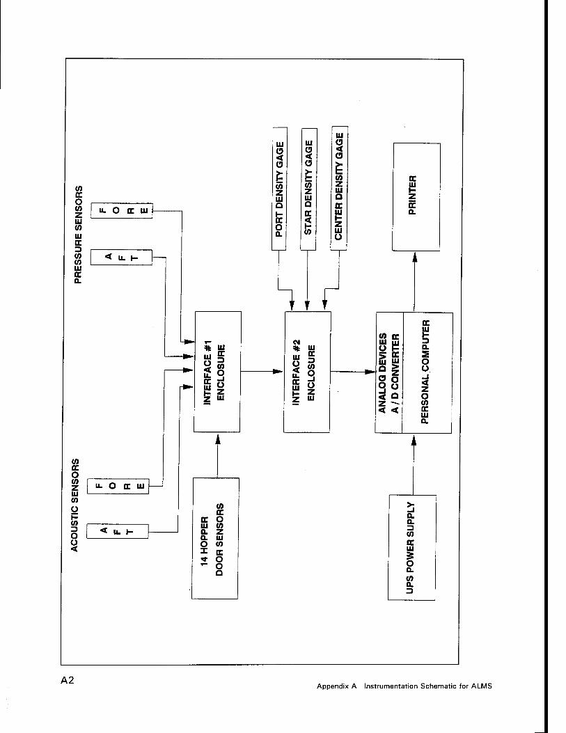
w oc o z UJ W UJ DC 3 (/} (0 UJ oc a.
u. o oc UJ
< u. H
UJ O < a
w z UJ Q
tE O a.
ui o <
0) z UI Q OC
0)
UJ a < a
(0 z UI a oc UJ H Z UJ O
INTE
RFA
CE #
1 E
NC
LOS
UR
E
i r IN
TER
FAC
E #
2
EN
CLO
SU
RE
oc UI H z oc a.
ii
AN
ALO
G D
EV
ICE
S
A / D
CO
NV
ER
TER
PE
RS
ON
AL
CO
MP
UTE
R
</> oc o (0 z UJ CO u b 3 o o <
il
u. O OC UI
< U. H
(0 OC
OC o ui tn a. a O X
z UI tn oc o O a
a. a W OC UJ
o Q. to a. 3
A2 Appendix A Instrumentation Schematic for ALMS
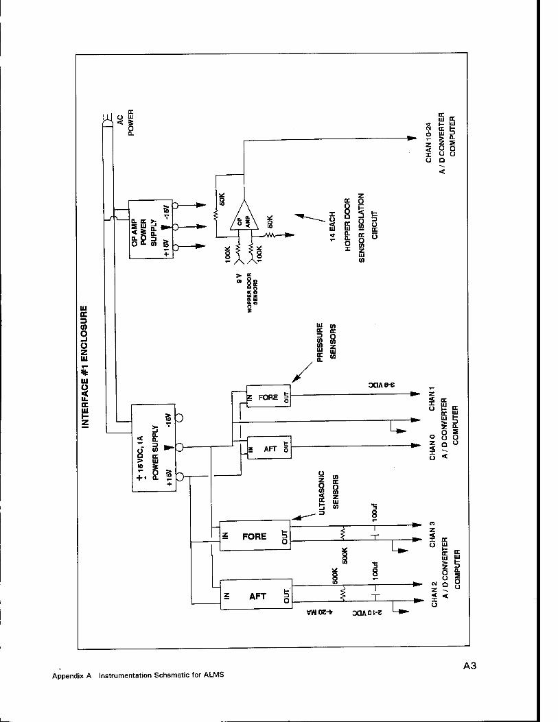
A
m
CO
2 o z Ul
Ul
I oc Ul H Z
DC U UJ
*8
> a
a. w
UJ VI
OL (0
so
> 10
D-
D-
r 5 FORE I
3QA8-e
u: 5 AFT o
Ü to "5 8
5 FORE §
"5 8
(M 6 z < i u
DC UJ H a: ui > z O
oc UJ
CL
Q
Z
u oc
E UJ
z £ o u a
u
z -i ■*• X DC
UJ
EC "C UJ UJ
AFT § z
o u
VWOZ-* MACU-Z u: x< u
Appendix A Instrumentation Schematic for ALMS A3
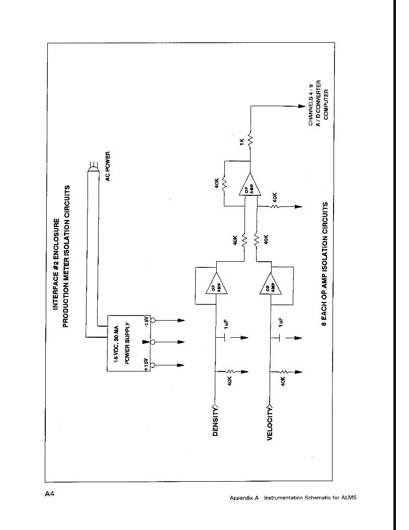
A4 Appendix A Instrumentation Schematic for ALMS
Appendix B Instrumentation Schematic for Resistivity Probe
B1 Appendix B Instrumentation Schematic for Resistivity Probe
2 O 0
a
□ •rl o c ID rH o
>
P o
o a)
o p (0 .0 Ü O
•H C T3 .* C
•H
u P •H X (/)
>
(0 p o 1_
o
i. 0) p
Z rH a)
a) u
&
i 1 c w 1_ a) z tu S3 o u <r
z 1. O 0)
p p •H E in c (0 1_ p
i- <r a) z &
P P o r
«H en •H -rl an
CO
0) rH U (0 c c >
E (0
(0 B z o 1- L.
a) o z
CM z ÜJ a:
E a E D o o
CM
E E o o
E o Ü
CO a E <E
O
+ UJ ^H
i—]
E
DM
M 1
(VO
LT
f
E O O
o L—J
i_ (Ü P TJ 3 i- Q. (0
§5 Ü
B2 Appendix B Instrumentation Schematic for Resistivity Probe
CO
ü Ul Q
I- 3 a Z3 o x ü
to
>- cr <
o cr
o z »-• cr
CM
Ü a o
CM >
CO
u a» a
CVJ
o 0) o
U
a 4 I CM
O
in
to
c x»
Ü r- «_ +J +J -H •i- -r- Ü
100r- o. a
0) .a o L. a
c
o L. o u c c o o
O r- CO ■M a) cr
Appendix B Instrumentation Schematic for Resistivity Probe B3
ROTARY SOLENOID AND HOME DECK WIRING
(not to scale)
R2 (advance)
120 4 VAC
ü n-c'[f]
ä n.o. [-4
2.0 mfd
r-5-| COIIl [-6 r
-0-coil-O-
120 M RR1 VAC
27
-t- DIO — I — 53
B4
1.0 mfd
control (home) deck
a interrupter —D points
rotary solenoid +
1N4004 diode
R1 (home)
fuse!
S1 (manual advance)
"1 120 4- VAC
120 VAC
ü n-c-ü-
-] 3-| n.o. |-4-| -
■ i-5-i com r6 r-
-0-coi 1-0-
RR2
25
DIO
It 12 VDC power
supply -0- +0—
Appendix B Instrumentation Schematic for Resistivity Probe
TRANSMITTER AND PORE WATER RELAY R3 WIRING
(not to scale)
11
11
LTJ
9
11
12 VDC
100 Hz trans- mitter -0 D-
to rotary switch V1 V2 12
2, & & to pore water cell
V1 V2
m 12
fl
COMM 1
r— t— DMM 1 (V)
fol i_
V1 l_
V2 i? 12
13 —relay coil—14 ► 120 VAC
29 —► 120
RR3 DtO I VAC
t COMM 2
DMM 2 (I)
-□ □-
-D switch S2 (normally □ 1 open)
31
RR4 DIO
ii"
Appendix B Instrumentation Schematic for Resistivity Probe B5
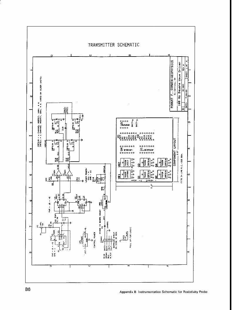
TRANSMITTER SCHEMATIC
<n o L «i a <n .>
•H 3 I 1. 0. U o UJ « o .> « zu 3
•=1 S • m 0i - L o t 0 u •
17 a: . _ ») u. "
N 1- X a: UJ a> CO o *-■ IK a
o o o o ^ m t XXOIflU) J oooo
oooooooo ooooooo ^r) « -4 • — ?J »M«ifl XN -<N^?-NW Xn V « — ;
ooooooo ooooooo
3 tSI»- ooooooo
z>_ix:m<\j*- ooooooo
in o 0
N o si; OO o 8 id nO 0 IS
N Ifl
Of X>
»- _i So CO o t~ »0
xr a
• O
o in uO o « if
° o 0 R ft
io o
B6 Appendix B Instrumentation Schematic for Resistivity Probe
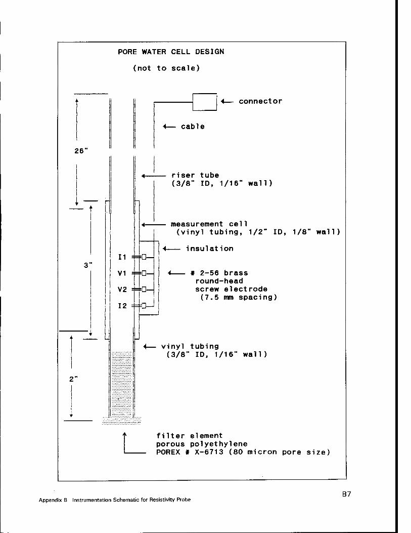
PORE WATER CELL DESIGN
(not to scale)
26"
11
V1
V2
12
connector
cable
=D—j
£3
0—
riser tube (3/8" ID, 1/16" wall)
measurement cell (vinyl tubing, 1/2" ID, 1/8" wall)
— insulation
# 2-56 brass round-head screw electrode (7.5 mm spacing)
vinyl tubing (3/8" ID, 1/16" wall)
filter element porous polyethylene POREX # X-6713 (80 micron pore size)
Appendix B Instrumentation Schematic for Resistivity Probe B7
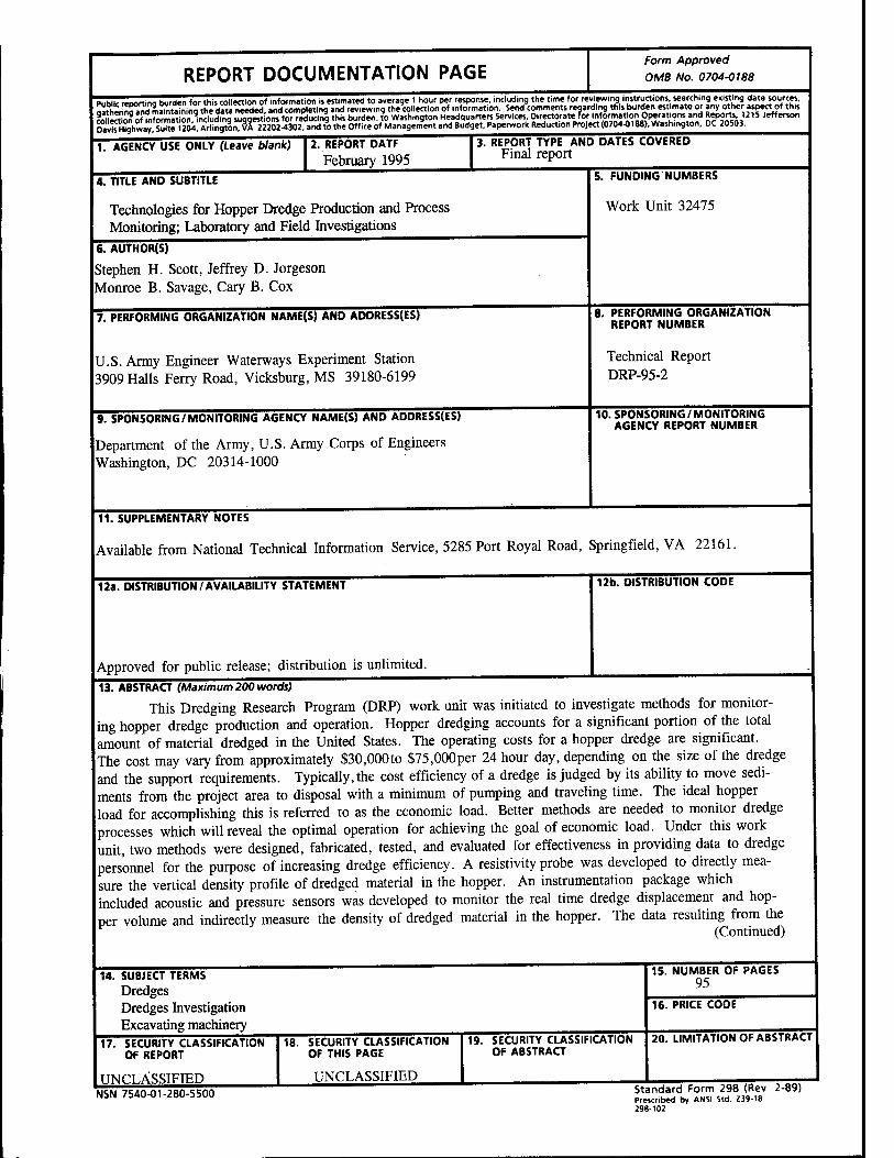
REPORT DOCUMENTATION PAGE Form Approved
OMB No. 0704-0188
Public renortino burden for this collection of information is estimated to average 1 hour per response, including the time for reviewing instructions searching existing datasources. Ml^SSmS^i^^Sameö^. and completing and reviewing the collection of information. Send comments regarding this burden es .mate or any other aspect of this ttä^lfa™m5^™i^™^om for reducing this burden, to Washington Headquarters Services. Directorate forinformation Operations and Reports 1215 Jefferson DivtelSghway Su™204 "Kngton. VA 22202-4302, and to the Office of Management and Budget, Paperwork Reduction Project (0704-0188). Washington, DC 20503.
1. AGENCY USE ONLY (Leave blank) 2. REPORT DATF
February 1995 3. REPORT TYPE AND DATES COVERED
Final report
4. TITLE AND SUBTITLE
Technologies for Hopper Dredge Production and Process Monitoring; Laboratory and Field Investigations
6. AUTHOR(S)
Stephen H. Scott, Jeffrey D. Jorgeson Monroe B. Savage, Cary B. Cox
7. PERFORMING ORGANIZATION NAME(S) AND ADDRESS(ES)
U.S. Army Engineer Waterways Experiment Station 3909 Halls Ferry Road, Vicksburg, MS 39180-6199
9. SPONSORING/MONITORING AGENCY NAME(S) AND ADDRESS(ES)
Department of the Army, U.S. Army Corps of Engineers Washington, DC 20314-1000
5. FUNDING NUMBERS
Work Unit 32475
8. PERFORMING ORGANIZATION REPORT NUMBER
Technical Report DRP-95-2
10. SPONSORING /MONITORING AGENCY REPORT NUMBER
11. SUPPLEMENTARY NOTES
Available from National Technical Information Service, 5285 Port Royal Road, Springfield, VA 22161.
12a. DISTRIBUTION/AVAILABILITY STATEMENT
Approved for public release; distribution is unlimited.
12b. DISTRIBUTION CODE
13. ABSTRACT (Maximum 200 words)
This Dredging Research Program (DRP) work unit was initiated to investigate methods for monitor- ing hopper dredge production and operation. Hopper dredging accounts for a significant portion of the total amount of material dredged in the United States. The operating costs for a hopper dredge are significant. The cost may vary from approximately $30,000to $75,000per 24 hour day, depending on the size of the dredge and the support requirements. Typically, the cost efficiency of a dredge is judged by its ability to move sedi- ments from the project area to disposal with a minimum of pumping and traveling time. The ideal hopper load for accomplishing this is referred to as the economic load. Better methods are needed to monitor dredge processes which will reveal the optimal operation for achieving the goal of economic load. Under this work unit, two methods were designed, fabricated, tested, and evaluated for effectiveness in providing data to dredge personnel for the purpose of increasing dredge efficiency. A resistivity probe was developed to directly mea- sure the vertical density profile of dredged material in the hopper. An instrumentation package which included acoustic and pressure sensors was developed to monitor the real time dredge displacement and hop- per volume and indirectly measure the density of dredged material in the hopper. The data resulting from the * (Continued)
14. SUBJECT TERMS
Dredges Dredges Investigation Excavating machinery
17. SECURITY CLASSIFICATION OF REPORT
UNCLASSIFIED
18. SECURITY CLASSIFICATION OF THIS PAGE
UNCLASSIFIED
19. SECURITY CLASSIFICATION OF ABSTRACT
15. NUMBER OF PAGES 95
16. PRICE CODE
20. LIMITATION OF ABSTRACT
NSN 7540-01-280-5500 Standard Form 298 (Rev 2-89) Prescribed by ANSI Std Z39-18 298-102
13. (Concluded).
application of both systems can be used for calculating dredge production on a load by load basis. This report presents the description and method of the testing programs and the study findings. The concept of uncertainty analysis for determining the error potential in hopper dredge production calculations' is presented and discussed with an example calculation.


![Contents€¦ · .063 Inch [1.59mm] O.D. VINL-063 CLMP-063 TFLN-063 or NYLN-063 NYCLMP-063.125 Inch [3.18mm] O.D. VINL-125 CLMP-125 TFLN-125 NYLN-125HW NYCLMP-125 NYCLMP-125HW Pipe](https://img.pdfslide.us/doc/110x75/6008af2d53ec7b6e9042b7c5/contents-063-inch-159mm-od-vinl-063-clmp-063-tfln-063-or-nyln-063-nyclmp-063125.jpg)