AD-754 949

ON THE DESIGN OF A TOWED ELF 1-f-FIELDANTENNA

Michael L. Burrows

Massachusetts Institute of Technology

Prepared for:

Electronic Systems Division

28 December 1972

DISTRIBUTED BY:

[lational Technical Information ServiceU. S. DEPARTMEIJT OF COMM1ERCE5285 Port Royal Roa, Sringfield Va. 22151

UNCLASSIFIED

Security Classification

DOCUMENT CONTROL DATA - R&D(Securlrv clausiflcatin of title, body of abstract ad Indexing annotation must b entaed when the overall report I# Claeifled)

I. ORIOINATIF e ACTIVITY (Corporate author) 2.. REPORT SECURITY CLASSIFICATIONUnclassified

Lincoln Laboratory, M.I,T. as. GROUP

None3. REPORT TITLE

.On the De-ign of a Towed ELF H-Field Antenna

4. DES(.RIPTIVE NOTES (7 pv oft eport and lncueluve datee)

Technicul Note4.S. AUTHORIS) (Lost now, first name, Initial)

V- Burrows, Michael L.

0. REPORT OATE 7*. ,OTAL . OPm PAOES lb. NO. Of R',S

28 December 1972 19

9a. OIGINATOR'S REPORT NUMERMIS), CONTRACT OR GRANT No, F19628-73-C-002l

C. . ESD-TR-72-355_ d.

- SO1. AVAILABILITY/LIMITATION NOTICE$

.14 Approved for public release; distribution unlimited.

IS. SUPPLEMENTARY NOTES .4 It. SPONSORING MILITARY ACTIVITY

Non., OeVat. a ot the Navy

13. ABSTRACT

The various noise sources known to be troublesome in a towed ELFH-field antenna are examined theoretically and formulas are presentedenabling noise voltages to be predicted from other measurable quantities.The treatment identifies the role played by the various contributing factorssuch as cable vibration, cable properties, core permeability, geomagneticfield, etc., and so indicates the way in which the noises can be reduced.Comparisons with ,xperlmentally measured noise voltages support thetheory.

14. KEY WOROS

Navv comlunication- ELF noise voltagesnoise ,sourcos I I-field antenna

'NCLASSII:Il:[)

Fw'ec,srnt Cla,,Sificaltion

II('~~II I, M N LA N IIAr )t

ON TIE DESIGN OF A TOWED ELF H-FIELD ANTENNA

3l. 1., BURROWS

Grotip 61

TICIINICAI, NOTR 1972-34

28 P)ICEIMBER 1972

ipfo(ved for public tolenme; dItribution unlimited.

I N ii %I A SS A C" It USE T TS.;1'

4f

The work reported in this Jocument was performed at Lincoln Laboratory,

a center for research operted by Massachusetts Institute of TechnoloA'.The work was sponsored by the Department of the Navy under Air ForceCon*.ract F19628-73.C-0002.

This report may be reproduced to satisfy needs oi U.S. Government agencies.

1i

CONTENTS

I. Introduction

II. Measure of Performan.-e ann Effective Length

III. Thermal Noise 11

IV. Motion-Induced Noise 19

V. Magnetostrictive Noise 35

VI. Barkhausen Noise 44

VII. Some Experimental Re s 45

VIII. Conclusion 57

IX. Acknowledgements 58

Appendices

A. Immersion Effect on Antenna Impedance 59

B. Optimum Air-Core Antenna 62

C. Sensitivity Distribution for Antenna with Ferrous Core 64

D. Cable MotioiA lue to Turbk.ent Boundary Layer Stresses 67

E. Cable Dynamics 74

F. Effective Vibrating Mass per Unit Length 80

G. Motion-Induced ENF in the E-Field Antenna 83

H. Effect of Non-Uniform Cable Tension 85

I. Mechanical Properties of 0.65 Inch 0. D. Buoyant Cable 87

Iv

On the Design of a Towed ELF H-Field Antenna

I. Introduction

Oier -the last feW- jears, the possibility of building an ELF loop

antenna (H-field antenna) for towing behind a submarine has been receiving

close attention. The principal result of this work is the conclusion that the

task can be accomplished ohWIhen the many problems are thoroughly

urderstood and then accounted for in the antenna design. Although at pre-

_0sent no design of sufficiently good performance exists, much of the basic

understanding has been nbtained. Thus the work from now on should con -

sist largely of using the understanding as a basis for testing and evaluating

candidate construction materials and fabrication methodb. To facilitate

the work, this report documents that understanding. It does not, however.

j :,ropose a specific antenna design or predict eventual performance. This

cannot be done until a*ter the testing and evaluating stage.

Interest cenhe vs on the frequency range of about .0 to 200 Hz in the

2, LF band beca~isj, in that range the attenuation in the water and in the earth-

."osphere waveg'aide is low enough for long., range broadcasting to sub-

i ,,'ged submarinc-s to be leasible 6]. The problem of radiating enough

energy from an anienna of practical size is a difficult one, but it appears to

'e so vable by v ing a horizontal electric dipole. This kind of antenna can

also 1,' u: 'e' as the receiving antenna on the submarine. Physically it con-

I

sists of two small electrodes built into a cable and separated by some 200

to 300 m and towed well aft away from the Interfering electromagnetic noise

fl d -generated by the boat (FiT. 1). It confers on the boat an ability to

communicate over a very useful range of depths and speeds. Unfortunately,I it is linearly polarized and the downward propagating transmitted signal in

the ocean is also mainly or whoiiy'linarly polarized. It suffers, therefore,

from the disadvantage that it becomes jearly or wholly blind if the submar-

- ine headin; is perpendicular -to the direction vector of the transmitted

electric field. In The far-zone field of the transmitting antenna this occurs - Vwhen the submarine heading is perpendicular to the great-circle path linking

the trr-sunittcr and receiver.

The successful development of an H.-field antenna built into the j1 same cable would provide a receiving polarization perpendicular to that of

the E-field (eteCtrode-pair) antenna. Since the transmitted electric and

magnetic fieldt are mutually perpendicular and essentially horizontal, theIf-field antenna, in the form of a long slender solenoidal vtnding, would be

maxinally sensitive when the E-field antenna is blUnd. Communicatior can

therefore o..' maintained independently of heading (Fig. 2).

The fut-Aamental limitation on ELF communication at the sur'face is

atmospheric noise. Compared with it, the noise generated by the E-field

antenna and the interference generated by the boat are both negligibly small.

- ~~M T Ts-~- - -7

- F T ..

Fig. 1. Electvode-pair E-field antenna towed from the submarine.

ESE

ELECTRODE V, a C, l

Fig. 2. Combined E- and H-field antennas for polarization diversity.(Ce and Ch are factors dependent upon the geometrical details of thetwo antennas.)

3

As the antenna submerge , both signal and atmospheric noise are attenuated-

by the same amount and so the signal to noise ratio is initially not affected.

The communication rate is therefore unimpaired. However, the local

noises--from the antenna and the boat--are essentially unaltered by sub-

merging. If the antenna depth continues to increase, eventually the atmos -

pheric noise level will be equal to that of the local noises, and communica-

tion begins to be degraded. Thus the depth of operation is determined by

the antcnna noise. The design problem, therefore, for te H-field antenna

is to reduce the level of the noise it generates to be no greater"than that of

the E-field antenna.

HfedIt. is shown in Section III that the thermal noise generated by an

H-field antenna without a ferromagnetic core, given the limitations of

available conducting materials and the constraint that the antenna cable be

positively buoyant, is too high unless the antenna is allowed to become in-

conveniently large. One is forced, therefore, to consider using a ferro-

=, magnetic core. Unfortunately, iis gives rise to "magnetostrictive"l

(stress-induced) noise and Barkhausen noise. The former arises because

the geomagnetic bias flux density in the core changes its magnitude when

the core is stressed by mechanical vibration, thereb) inducing a change in

voltage in the antenna winding. The latter occurs because the geomagnetic

bias flux density in the core does not follow smoothly the changing axial

4

component of the geomagnetic field strength as the boat turns. Rather, it

proceeds by a successioifof small jumps, which induce voltage transients

in the antenna winding. [1, pp. 613 and 524].

Magnetostrictive noise can be rcd'.ced by choosing the right core

material, by keeping the net bias flux density close to zero-by means of an

adjustable direct current in the antenna winding (4], by making the antenna

iong and less sensitive towards the two ends than it is in the middle of its 'A

length, by minimizing t'&,e stress transmitted to the core and by reducing the

level of the c'.-e vIbration.

Barkhausen noise can be reduced by choosing the right core mat-

erial, by keeping the net bias flux density as constant as possible [41 and17

by increasing the length of the antenna.

Noise is also generated when the geomagnetic flux linking the turns

of the antenna winding is~odulated by their angular vibration. This is .V t

called motion-induced noise and is present whether or not a ferromagnetic

core is used. Reducing tme cable vibration, making the antenna long,

making it less sensitive towards the two ends that it is in the middle of its

length and making its variation of sensitivity along its length very smooth

are techniques for reducing this noise. A comparison of the motion-induced

noise of an H-field antenna, when this is due to ideal cable flexing, with

that of an E-,,eld antenna shows that in principle a long H-field antenna need

be no more susceptible to motion-induced noise than the E-field antenna [7].

Recently, however, it has befn pointed out that more complicated cable

motion is possible than that due to ideal flexing, but no quantitative esti-

mate is made of te relative magnitude of the resulting noise [19). Th.

there is as yet no evidence that such motion is an important noise source.

On the other hand, the point is valid in principle and deserves closer

attention. OT

T. date, two lbng H-field antennas have been made and tested.

Neither is quiet enough to be useful, but their periormance taken together

with the improvements likely to be realized by applying the additional tech-

niques covered in this report, suggest that a usefully quiet anterna con be

built. One antenna showed that a low enough thermal noise can be

attained, althbigh it suffered from uncontrolled motiln-induced noise due

' ' to independent vibrations of its core elements, while the other antenna

showed that a core construction exists--the helically wound tape core--

which eliminates the offending type of core vi'ration, although it suffered

from a high thermal noise and a vib-' tion induced noise that appears to be

ascribable to its uniform sensitivity di, tribution (see Section VII).

The following Sections treat in d3tail the points mentioned in this

brief summary, except for the newly piuposed motion-induced noise mechan-

ism mentioned above which has yet to be fully explored. A brief survey of

the experimental evidence is also included. It gives strong support to those

asper theorj ", touches.

6

II. Measure of Performance and Effective Length

A convenient measure of antenna quality is one that allows

antennas of different configurations and types to be compared and which,

at the same time, uses the minimum number of additional assumptions. It

should also be some physically identifiable quantity, if possible, to aid in

its application.

A measure that fits this prescription well is the ratio of the

r. m. s. open-circuit noise voltage to the effective length of the antenna,

where the effective. lerigth is the length by which an incident electric field

must be multiplied to give the corresponding open-circuit antenna voltage.

The measure has the dixi-ensions of volts per meter and is physically the

horizontal electric field, evaluated at the depth of the antenna, which pro-

duces an antenna voltage equal to the noise. In general, the ocean conduc-

tivity and, for antennas with an appreciable vertical dimension, a depth

reference point on the antenna must be specified. No assumptions about

the strength of the transmitted field or of the atmospheric noise field are

required. Neither is it necessary to specify any particular depth of

ope ration.

The term "equivalent noise field" or ENF will be used to denote

this measure of performance.

For the trailing E-field (electrode-pair) antenna, the effective

7

length is simply the distance between the electrodes. Thus the total ENF

for this antenna is its measured noise voltage, \vided by the electrode

separation. Typical ENF spectra at 8 a-a 14 knots are shown in Fig. 3

for a 300-meter electrode-pair antenna r3]. For this length of antenna,

the noise is now believed to be dominated by motion-induced noise.

Under the conditions 14 knots and 45 Hz (tobe. adopted here as the

standard), Fig. 3 shows the ENF of the 300 meter E-fleld antenna to be

-205 dBE.

For a horizontal H-field antenna immersed in the ocean, the

effective length can be calculated using Faraday's law. If H is the axial

component of the incident magnetic field, then the induced voltage per

meter length of antenna is given by wtpc HAN, where w is the radian fre-

quency, [1c the reversible permeability of thl4n!enna core, A the cross-

sectional area of the core and N the turns density (turns per meter) in the

antenna winding. The total antenna voltage V is given therefore by

V = wHfVcANdz = eE ()

where the integral is carried out over the complete antenna length, and E

is the incident electric field associated with the magnetic field.

Both signal and atmospheric noise propagate down into the ocean

from the surface. At ELF, the field components E and H are essentially

horizontal and mutually orthogonal. They are related by the wave imped-

ance of the ocean, V -iwi /a , o being the conductivity of the water and

p 0 the permeability of free space. Using this relation in (1), one obtains,

8

-175-

-200- 14-KNOT ANTENNA NOISE

z-2501

0 20 4c 60G 80 100 120 140 160 I80

FREQUENCY (H2)

F ig. 3. Typical. equivalent noise field spectra for a 300-meter trailedE-fielcl antenna at two towing speeds. (From Griffiths [3].

in magnitude

'e f aANdz(2

where ja = 1c/jo is the relative small-signal permeability of the core and

6, defined as V 2/(Wao) , is the i.kin depth for electromagnetic propagation

into the ocean.

This formula has been obtained by neglecting the magnetic flux

in the area occupied by the antenna winding. This flux density links the

outer layers of the antenna winding. T1,e permeability of this part of the

cross section 6 that of free space, however. Thus (2) is valid provided the

addition of the core increases the antenna inductance by a large factor.

The effective length of an H-field antenna can be accurately

estimated by measuring its impedance inair-or in the ocean. Appendix A

shows that its impedance in the ocean is negligibly different from its ir-

pedance in air, and the inductance L in air is given simply by

A 2Lo = J A dz (3)

Thus, if the turns density is uniform, (2) and (3) can be combined to give

= "Lo (4)e 6 11 N

0

If the turns density is not uniform, but the p'ftduct i cA is, then (2) and (3)

yield

I fN dz (5)e 61 0l N 2 dz

in which the ratio of integrals can be evaluated from the winding specifica-

tion of the antenna.

10

III. Thermal Noise

The thermal noise of the antenna is the noise generated by the

resistance of the antenna measured at the antenna terminals. This resist-

ance is the sum of the resistance of the connecting wires, the resistance

of the antenna winding and the "radiation" resistance of the winding, which

represents the losses in the antenna core and in the surrounding ocean.

The core losses can be calculated using standard methods [2, p. 78 ff. J

and can, in any case, be avoided by subdividing the core to interrupt the

-* induced circulating currents. The losses in the water are difficult to cal-

culate in general but Appendix A shows that their contribution to the ENF

is very small. The resistance of the connecting wires can be made small

Srompared with that of the winding by using a large enough number of turns

on the antenna winding. Thus the critical component of the thermal noise

is that contributed by the antenna winding.

It is instructive to examine what can be achieved without

a ferromagnetic core in the antenna. In Appendix B, it is shown that. even

if all the weight of the cable were devoted to the winding and if insulation,

where necessary, could be infinitesimally thin, then the minimum thermal

ENF attainable in a 300 m length of the current 0.65 in. 0. D. buoyant

antenna cable at 45 Hz is about -180 dBE. This could be reduced to the

required -205 dBE by increasing the diameter by a factor of about 4 or

increasing the length by a factor of about 300. The latter is certainly im-

practicable, the former, since it implies an increase of volume by a fac-

tor of sixteen, is still excessive. A ferromagnetic core, th reforewould

seem to be essential.

ii

I- w

Since the reversible permeabiY.ies attained by currently

available ferromagnetic materials can be several tens of thousands times

larger than that of free space, the effective length of the antenna can be

increased enormously, without any increase in the thermal noise. Thus

the thermal ENF can be reduced substantially. The difficulties are that

i) a long, slender, high permeability core may be magnetically saturated

by the geomagnetic field and thereby lose, temporarily, its high reversible

* permeability, ii) the stretching and flexing of the cable may plastically

strain the core materiAl, causing a pernanent loss-of its high reversible

permeability, iii) the longitudinal cable vibrations, transmitted to the core,

generate magnetostrictive (i. e., strain-induced) noise, and iv) the varia-

tions of the axial geomagnetic field component due to heading changs can

generate Barkhausen noise.

Geomagnetic core saturation can be prevented by using a core

material of relatively low permeability or by driving a direct current of the

appropriate magnitude and sense through the antenna winding to bring the

net flux density in the core closc to zero. This latter technique can be

made automatic by using an out-of-band sensing signal to monitor continu-

ously the inductance of the antenna and make appropriate changes in the

bias current [4].

The plastic strain problem must be dealt with by careful

mechanical design, and techniques for reducing magnetostrictive nose

and Barkhausen noise are discussed in later sections.

The addition of a ferromagnetic core raises the question of

12

2;..

determining the optimum proportions of winding and core. The buoyancy

restriction places a limit on the total (reduced) weight per unit length of

the core plus winding. Thus the minimum thermal ENF is achieved at a

proportion somewhere between the all-conductor one. with its low effective

length and the all-core one, with its ver y high resistance.

If a is the core radius, b the outer winding radius, 21the antenna

length and a the wire conductivitythen assuming that t a, the average rela-

tive permeability of the core, is large compared with unity, the effective

length of the antenna is2

- 2r a JL ,/NA/6 (6)e awhile the total winding resistance is

2 I2irN 2 t a (7)aW b - a

assuming in each case :1'-t the turns density N, the permeability, Ila , and the

geometry are independent of length. Thus, from (6) and (7), the power

spectral density S (6) of the thermal ENF is given by~e- kb Tk b

S (W) -- ------- b+a (8)e Z a4b- rq p V 11a -a).

where kb is Boltzmann's constant and Tk the absolute temperature (OK).tI

On the other hand, the reduced mass per unit length wi of the

antenna is given by

w1 = ira 2 0P + r - 2 )O, (9)c

where ' is P -C), and P , is Pw - 0 rhe densities P, and b arew (* w w

those of the tore, the winding and the buoyant flotation material (foamed

13

4- - . 7 .. - -

polyethylene in the current buoyant antenna cable). The reduced densities

P ' and P' appear in (9) because the antenna core and winding displace not

free space or air but the buoyant flotation material.

The problem, then, is to minimize (8) while keeping (9) fixed

at the maximum allowed by the buoyancy restriction. This is easily done,

or at this optimum state, t&he total differential of (8) and of (9) must both

be zero. That is- 2 kb T k ' 162

dSe(0)) 0 =ka C(2a2 +ab._2b 2 )da a2 db]e_ v, awa z 2 a 5 (b - a) 2

w a

dw'- 0 21 ( '-Q 'ada +p 'bdb].c w

For these equations to have a aolution, the determinant of theij coefficient

rntrix must he zero. That is

(2a 2 +ab- ab 2) 'b;a 3 (P 'p ') = 0w w

or, with 0 P c '/ p w = (Pc b)/0w" Pb ) and , b/a,32

2a -3 -2_ a- 0 + = 0. (10)

The functional relationship between a and 0 is presented graphically in

Fig. 4.

Thus, given the densities c , Pw and 0b , one calculates 0 and

then solves (10) (or uses Fig. 4) to evaluafe the optimum radius ratio b/a.

From this, the individual radii a and b can be found by using (9) and

these then substituted in (8) to give the minimum value of the thermal ENF

power spectrum.

14

31. .....

b /a 1.4

1.0

0 1 2 3 4

Fig. 4. Optimum ratio a of outer to inner winding radiias afunction ofP( Pc P )(,vPb

15

AMR-_

It is not necessary in practice to achieve precisely the optimum

proportions, because large deviations from the optimum cause relatively

minor degradation in the thermal ENF. To demonstrate this, one notes

that if w' and 0 Iare given, then (9) shows that /a 2 is proportional tow

8 ' 2 - 1, which means, from (8), that the mean square thermal ENF is

propor~ional to (0 1o 2- 1)2 (0t + l)/(ct- 1). This function is plotted, with v'

(equal to b/a) as the abscissa, for various values of B in Fig. 5. The

cvurves show that the relative winding thickness ot- 1 pan vary over a range

of at least three to one without increasing the minimum thermal ENF by

more than I dB.

The total reduced mass per unit length that the cable can sup-

2port is given simply by it c (0 - ) where c is the outside cable r'tcadits and

0 is the average density required for the complete cable. However, some

of this (say. Wa') may have to be allocated to strength members or some

Ptber essential piece of the structure. Thus the avai-.'ove reduced mass

per Icngth w' to be allocated to the antenna is rr c2 (0-P ) -Wa'.

In the current buoyant antenna cable, for example, c is 0. 325

- , inches, Pb is 0. 63 P° and the 18 fiberglass strength members are each

0. 038 inches in diameter and have a density of about 1. 67 0 . (Here 0

is 103 kg/m 3 , the mass density of water). Thus w a' is 18 x (0. 019x 0. 0254)2

x iT x (1.67- 0,63) and so, Ift is to be 0. 85Pothenw = 0.0334 kg/in.

B"-,', if the core density 0 is 8. 5 po and the winding density Pc 0 w

is 2.7, then 0 = 3. 802 and, from (10), b/a = 1.636. Using (9), one then

finds that a 0. 968 × 10 Vm. .- ,, taking 6 to be 37. 5m, k to beb

16

25-

.4.4

150

+0.

5-

01 1 1

1,0 1.2 1.4 1.6 1.6 2.0

Fig. 5. Relative thermal ENF as a function of the "proportion parameter" a~,the net cable buoyancy being held constant.

17

1. 38 10 - 2 3 J/°K, T to be 300 0 K, w to be 3. 57 x 107 mho/rmand 21 to be

300 m, one finds that On~b'der for the therimal ENt' to be -205 dBE, the

relative core permeability must be 746,

In practice, the cross-soctiolial %4'.a of the ferromagnetic part

of the core will be some fraction y of the total. core cross section, If the

remaining space is filled with a material having the density pn then the

average density of this composite core is given by PC Y + ( - Y)P andC

its average relative permeability is given by lia = YI1 r whem ' and Pc r are

the density and relative P"drineablty of the ferromagnetic component of the

composite core. Table I shows the result of calculatng the relative perme-

ability required for the thermal ENF to be -205 dBE for a range of values

2 of the core utilization factor Y - The assumptions are that ' 8. 5P andC a01S

n = 00. The core diameter is a function of Y because Pc depends on Y and

hence the optimum proportions vary with Y.

Required 'r foc klie Thermal ENF to be -205 dBE

Core 0. D.

Y (inch) b/a

.005 0.291 1.0814 24794

.01 0.280 1.0877 13000

.02 0.260 1.0998 707305 0.220 1.1333 3450.1 O.192 1.1820 2174.2 0.144 1.2622 1471.5 0.101 1.4364 966

1. 0 0.076 1.6355 746

Table I

18

I W-F

The relative permeabilities specified in Table I apply to an

antenna having a uniform sensitivity profile. A more likely profile is one

that is parabolic, because it discriminates better against vibration noise p(both magnetostrictive and motion-induced). In this case, the permeability

would have to be raised by the factor 3/2 to maintain the same antenna ef-

fective length. And, if the ferromagnetic material is applied in Lhe form

of a helix of helix angle 0, then the permeability must be increased by the

further factor l/cos2 e.

It should be noted that the numbers appearing in Table I are the

result of a particular set of assumptions. Changing-the assumptions can

cause a large change in the required permeability. For example, if p (theaverage mass density of the,.complete antenna cable) is taken to be po instead

of 0. 85 po , then w' is nearly twice as large, which means that the required

permeabilities are only one quarter of the values shown.

The permeabilities shown in Table I are mostly small compared

with the high permeabilities attained by modern ferromagnetic alloys. The

mechanical constraints imposed by this application are severe, however.

They make it impossible to realize even a small fraction of this potential.

As a last resort', the cable diameter could be increased, for, as (8) shows,

if all transverse dimens-ons are doubled, the required permeability is re-

duced by a factor of fou:.

IV. Motion - Induced Noise

If v (z, t) is the transverse displacement of the antenna center

)!no, as a function of time and of position along the antenna, from its

41

nominally straight condition, then by/' z is the tangent of the angle it makes

with the z axis. Provided jby/ zI<< 1, therefore, the geomagnetic flux

linkage per unit length is given by A(z)N(z)(B + B by/?z), where A(z)' is thez y

area of the antenna winding, assumed for the moment to have an air core,

and N(z) is its turns density (turns per meter). The geomagnetic field is

assumed to lie in the yz plane, so only its two components B and B appear.y z

The total moticn -induced voltage v(t) I's given by the integral I.

over the length of the antenna of the time rate of.change of the flux linkage

per unit length. Thus, sijice bBz/bt = By/at = 0,y

v(t) = ByA(z)N(z) -- y(z-t) dz.By bz at

In Appendix C it is shown that the same equation applies if the

antenna has a ferromagnetic core, except that A(z)N(z) must include the

additional factor ia' the relative incremental permeability'averaged over t

the core area.

This expression can be simplified in the case of the uniform

solenoidal winding, for then A(zlN(z) is a constant, say A N , over the

length of the antenna, a.V, ks zero elsewhere. The expression then reduces

to

v(t) = B A N 0 (y(1,t) -y (4,t)], (12)

assuming that the antenna extends from -2 to +2 along the z axis. Thus only

the vibration of the two end-points generates the noise voltage, no matter

how long the antenna is. By simply preventing the ends from vibrating,

one can reduce the noise voltage to zero even though the rest of the antenna

20

vibrates in a completely arbitrary way.

It is impractical to prevent a particulra~ppoint on the towed cable

from vibrating, but this uniform-winding example immediately suggests

anobher way of reducing the motion-induced noise voltage. For the noise

voltage is clearly associated wit.. e discontinuities at +I of the "sensitivity

-profile" A(z)N(z). Where the profile is uniform, no noise is generated.

Thus a profile which is as uniform as possible (within the constraint that it

must be zero for I z j>) should generate the least noise.

One cannot simply rembve the disconti UtZes at the ends of a

uniform profile. For then, being zero at :- , the profile must be zero

everywhere and the antenna no longer exists. One seeks therefore a non-

uniform profile which goes to zero at A.1. For this class of function, an

integration by parts converts (11) to the form

v(t) = -B u'(z) 'y(z,t) dz (13)

where the more compact notation u(z) has been used for the sensitivity

profile A(z)N(z) and u'(z) stands for du(z)/dz.

It appears that in the frequency band of interest here, the sources

of the transverse cable vibrations are the stress fluctuations at the cable

surface due to the turbulent fluid flow past the obstacle presented by the cable

itself (see Appendix D), and the large attenuation for transverse mechanical

waves along the -.able (see Appendi, I) isolates the antenna from disturb-

arces generated b, the ship. Th'.s the motion-induced noise arises from a

,tatistically uniform distribution of trar'.verse forces which are essentially

Ada7

uncorrelated from point to point along the calqe. And since they are uncor-

related, the total voltage is equal to the square root of the sum of the

squares of the voltages generated by each elemental force separately.

To calculate the separate voltages it is more convenient to work

in the frequency domain, in which (13) can be ,_, essed as

V(w) = iwByJ'u'( )Y(z, w)dz (14)

where V and Y are the Fourier transforms of v and y. But in this notation,

the displacement Y (z,W) caused by a single tran#.erse force F(w) applied

at the point zo is given by G(z, zo , w) F(w), where G(z, zo , W) is the Green's

function, and is the displacement at z due to a unit force of radian frequency

w applied at z0 . Hence the voltage induced by this force is, from (14),

V(w) = U By fu (z)G(z, 0, w)dz F(w) (15)

AThe power spectral density Sv (W) of the antenna voltage induced by this

single force is, therefore, from (15), given by

9v (w) = 2 By f () G( zoui)dz (16)

Awhere Sf(w) is the power spectral density of the force. Thus, if there is

a uniform distribution of M of these forces per unit length, each one s'atis-

tically independent of the others, then the total power spectral density

S v,) of the antenna voltage is

S (w) = 2B 2 MSf(w) if u'(z) G(z, zo, w)dz I dz 0 (17)v By oz (7A

Now MSf((w) is related to Sf(k, w), the two-dimensional power

spectral density of the transverse force distribution on the cable, defined as

22

<2

s,(k, w) ff(C, T) eik+xw r d d" (18)

where Cf(C, )'), the two-dimensional correlation function, is the expected

value of f(z,t) fz +C, t+1r) and f(z, t) is the transverse force per unit length.

Since the mean square total force on a piece of cable which is long corn-

pared with the correlation length of the force distribution is Sf(OW) times

Athe length, on the onebahid, and MSf(w) tirnes the length, on the other, then,---

': Athe relationship is simply MSf(W) = Sf(O, w).

Te antenna voltage power spectrum can therefore be rewritten

as 2Sv(w) = w? B S (0 f) u'(z)G(z, z ,w )dzI dz (19)

v W~yfUl)J fd0

Further analysis is complicated by the fact that the tension in-,

a towed cable increases linearly from the free end towards the tow point.

This, in turn, means that the mechanical dynamics of the cable are non-

uniform, and so, in particular, that G(z, z 0 W) depends upon the sum of

the pair z, z in addition to their difference. One fundamental result can

be obtained fairly simply, however, on the assumption that the sensitivity

profile u(z) is both perfectly parabolic and aLso very long compared

to tne linear extent of the region of influence of a force applied at a point

i. e. , long compared with the ''width'" of G(z, z 0 1 W). If these conditions

are met, the u'(z) is essentially a constant over the "width' of G (z, Zoo W)

and so can be taken outside the inner integral and assigned the value u'(z ).

But thenfG(z, zo, w)dz, assuming that the tension is essentially invariant

over the ''width'' of G(z, z , w), can be calculated by assuming the tension

23

is constant at the value it takes at zo . Appendix E shows thait the integral

2is then given by -1/(w Mt), where mt is the effective trans-erse vibrtj.ng

-. ,

mass per unit length of cable. Thus, for u(z) sufficiently long aLhd sulffic-

iently smooth, (19) car. be rewritten as.

B 2S (CD) = X -Sf(0, uI(Zo) Id (20v -W2 imti 2 'f .u o (20)

The motion-induced ENF power sectrui,S e% (w) is given, therefore, bye

dividing (20) by the effective length squared. Therefore, from (2). and (20),

and using the relation u(z) = a(z)A(z)N(z), one finds~a

2_2 2 Ou'(z) dz

w e 2 0 )-2W u(z)dz

[fu~z'

For a given cable size, cable buoyancy, measuring frequency

and towing speed, all quantities in the right member of (21) are predeter-

mined except for u(z). Thus the problem is to choose u(z) to minimize the

auotient of integrals appearing in (21) with the constraint that u(z) is con-

tinuous for all z and zero for I zi 1. By app)yng the calculus of variations

one finds the solution to be

S) 1 0 (0)[ l - (z/I)2 ( 22u, 0o(Z) =4 (22)

and this will be referred to as the "parabolic sensitivity profile" on account

of its shape, shown in Fig. 6. For this optimum profile, the quotient of

24

i0

,, - -I

"q!-"Fig. 6. Optimum sensitivity profile (parabolic profile) for minimizing

= the motion-induced ENF.

-1-

w25

I1--487

"-.-

3integrals reduces to the expression 3/(21 ), and- so

2/ 6B

S 3 () Sf (0, w). (23)

Significant features of this formula are, first, that the tension,

bending stiffness and energy absorption of the cable do not appear in Ti, only

the transverse force spectrum and the effective mass. Thus since the buoy-

ancy is essentially predetermined, the motion-induced ENF at a particular

speed and freauency depends only upon cable diameter and antenna Aength

(provided the "long, smooth profile" assumption is not violated).

Also of interest is the fact that the absolute antenna sensitivity

does not appear in the formula. This means that the motion-induced ENF

depends only upon the shape of the sensitivity profile and not upon whedher

or not a ferromagnetic core is used, for e-cample.

in Appendix G, it is shown thatlt 2Don-induced ENF of an

E-field antenna (the electrode-pair antenna) is given by By 2 Sf(0, w )/(2& 2 Imt12).

Comparing this expression with (23), one sees that if the two antennas are of

equal length, then they generate the same motion- induced ENF when they

are \F6 long. When they are shorter than this, the H-field antenna is

noisier than the "-field antenna, and when they are longer than this, _Qe

reverse is true. In a 4 mho/m ocean at 45 Hz, 6 is 37. 5 m. Thus .6 8

is 91. 8 m or about 300 feet. (This comparis6fi-depends upon the additiorai

reasonable assumption that Sf(0, w) is the same for both the x-,and the y-

directed transverse force distribution. That is, that the transverse

26

K

buffeting forces are st atistically azimuthally uniform).

A more difficult question to treat is the modification of (23)

required to take into account the effect of a short, rough sensitiv-

ity profile, This will be carried out under the assumption that the tension

is constant over the whole length of the antenna. The further slight rodi-

fication required to account for varyin. on is examined in A ppendix H.

The basic motion-induced noise equation is (19) in which, since

now the tension is being assumed constant, G(z, zo o w) can be writterrlgs

G o(Z-Z o w). Then, with the definitions-('u( - ikzU(k) z) e dz

u(z) = -- U(k) eikz dkTr f (24)

H (kw) = G(Z w) eikz

G(z, W) fH(kw) eikz dk

the integral u'(Z) Go(z - zO, W) dz ca.n be rewritten as i(21r)1 fkU(k)Ht(k , w)

exp (ikz dk and so (19) reduces to0

S(W) = 13 Sf(0, W) -.- /k2I U(k)l Ht(k, w)2 dk . (25)

If tke assumption that the transverse buffeting forces are essentially un-

correlated from point-to-point along the cable is not valid, then it

follows that Sf(O, w) in (,:) must be included under *Lxe integral sign as

Sf(k, ). Thus the "uncorrelated forces" assumption is equivalent to making

the assumption that the spatial spectrum of the force distribution is white

27

,777

(uniforii) over the range of k for which the product IkU(k)H (k, w) I? has non-

negligible magnitude. In Appendix D, this assunption is shown to be

satisfied in practice.

The functions U(k) and JHt(k,w) 2 appearing in th- integrandin (25) are sketched in Fig. 7. The peak in I U(k) reflects the fact that to

receive the signal, the winding must be unidirectional, so that u(z) has a2

large "d.c. " component at k=0. The peaks of IH (k,w)I occur at k kt

where-kt is the real part of the ordinary characteristic wave number for

transverse wave propagation at radian frequency w along the cable. (Since

the cable is not perfectly flexible, there also exists an "extrao.rdinary"

characteristic wave number. It has a large imaginary part, however, and

so does not have a readily visible effect on the shape of IHt(k,2w) along

the real k axis.)

If the sensitivity profile ui(z) is very long and very smooth, then

its Fourier transform U(k) will be very peaked at the origin and be very

small elsewhere. Then the integrand in (25) (the product with k of the

two functions sketched in Fig. 7), will be of negligible magnitude for all k

except for two narrow regions symmetrically placed either side of-rand close2to the point k=0. But over these regions, I-lt(k,w)I is essentially equal to

IH (0,wl and so the integral in !25) can be rewritten as

IHt(0,w)lf IkU(k)1 2dk , which, by virtue of Parseval's theorem, can be re-

exp&-essed as 27rjHt(0,w)l 2 u'(z)1 dz . Substituting this back in (251, and

noting, from Appendix E, that Ht(0,W) -1/(,t) mr, one finds that (25) re-2duces to (20). Thus the contribution of the peak in I U(k) ! at the origin to

- ~ ~ ~ ~ ~ 1 - ,-'148981----,a-~

IU(k)12

IHt( k, ) 12

-kt 0 ktk -

Fig. 7. Sketch of iU(k) I and IHt(k, w) I

29

/I

the integral in (25) is simply the fundamental long, smooth profile contribu-

tion discussed earlier.

There are two other peaks in the integrand in (25), %owever,

wbose contribution must also be includedi - 'If the pr6fit ewez) is short

enough, but still smooth, then the mrinor peaks of U(k) will make the

contribution of the integrand arising fr6m the peaks of H (k,

tt~~at k = -kt larger than that ar4.8ing from the peak in U(k) at k=O. Since the

peaks of Ht(k,w) are in practice very high aad sharp, their contribution to2 2 2

the integral in (25) can be written kt 2Av (IU(kt)1 flHt(kw)I dk, where2 2

Av( I U(k) t is a local average of I U(k) I centered on the points E kt. But,

fr om Appendix Ef IHt(k,w) 12dk is the same as 2-r SylW )!OW), where

S y (w) is the spectral density at frequency w of the transverse displacerhient

of the antenna at a point.

Thus (25) can be expressed in the approximate foim

Sww 2 B 2 ~ [Ju.(z) 3dz t2 vIS (WJv y f 4 2 tt S (0, W)3

(26)

The magnitude of Avt i U(kt depends upon two things. On thet

one hand, if the profile is very smooth, then U(k) is given asymptotically

for large k by (Lighthill, [5)

U (k) --- X huI(z n e-ikzn ,(27)

k2 n

where Au'(z n ) is the jump in u'(z n ) at the point of discontinuity zn and the

summation includes all points of discontinuity. Thus Av( I U(k) 12) is

30

approxihnately22

Av(I(k)l2 Au(z. (28)n

On the other hand, if the profile is-t4roagh" fue, for example, to variations

in the turns density or in the cc -rmeability, then IU(k) 1, for k not close

to zero, can be much bigger than (27) predicts. For, expressing the actual

rough profile u r(z) as

ur(Z) = u(z) 1 + C (z)], (Z.9)

where e(z) is the "fractional perturbation of the nominally smooth profile

2u(z), then one can show that the expected value of JU(k) I is augmented

by the term SC (kfu 2 (z)dz. Here S,(k) is the spectral density of e(z) and is

defined as the Fourier transforx:%9 the correlation function of e(z), which

in turn is the expected value of e(z)e(z+ ) It is assumed that e(z) has

zero mean and is statistically uniform and stationary in z.

The final general expression, therefore, for the motion-induced

ENF of an antenna for which u(z) is continuous but u'(z) has discontinuities?2

at z (n=l,2,...) is S (W)/ 2 orn v e

2 2 B2 rfU() 2 12W)62B Sf(0,W ) jJ u,(z)__ ___ S (W)

Se(W) 41 Z + 2fJu(z)dzi - . W 4mtI kt Sf(0,W)

kt ( r S(0,wv)

S kt) u2 (z)dz - (301SSf (0,w )

If the profile is ,iminally the ideal one defined by (22), then

Ju(zldz is 4fu (0)/3, f[u t)] 2 dz is 8u 2 (0)/(31), ju'1Z n 2 is

xo

2 2 2 28 U (0)/1 and f ( Walk i"316u 0 (0)1/15, sc that (30) becomes

3(6 B 2 4 m2 S2S m) ( +

e 41 3 W t " I f 5 Sf(0, W) '

(31)

By comparing this with the simple "long, smooth profile" formula given by

1' (23), one sees that as the antenna becomes shorter, a correction term pro-

portional to 2-4 will eventuaIAN 'be significant, and that the effect of profile

roughness is to add a correction term proportional to the spectral density

of the relative roughness and to I. Since the lofig, smooth profile term

is 0 (C 3, and the 'shortness' correction is 0 4, this third roughness

term will eventually dominate when the antenna is made arbitrarily long.

A further significant difference between the correction terms

for shortness and for roughness on the one hand, and the long, smooth

profile term on the other, is thkz the former are sensitive to the stiffness

and absorption properties of the cable. To take simple account of this fact,

it is convenient to define a mechanical Q-factor for transverse cable vi-

bration as follows ot~ t f H(k, w) "'"

t ± dk. (32)2 k t f H t(0, W )1

On the assumption that Sf(kw) is essentially constant over the range of k

for which H, (k,w) has signifi--- -agnitude, Qt is equal to (1T/kt)w 4 1 mt I S y (w)/

Sf(0,w), so that (31) can be rewritten2 3 3 23

Se(U)) = 3--) S (0,W)1 1k + + - S (kt)t,

4 3 It/ nk t 5Tr1333

323

and this formula applies to the nominally parabolic profile. The Qt is a

fdncion of frequency and tension. A graph of Q calculated for a speci-

men of the standard 0. 65" D foamed-polyethylene buoyant antenna cable,

is given in Appendix I, together with a similar graph of kt.

Equation (33) shows that if Sf(0, w) is known, then by calculating

k and Q from measured mechanical properties of the cable, one cantt

calculate the motion-induced ENF of an H-field antenna of given length and

p ofile roughness. Sf(0,0 can be estimated from boundaky layer data (see

Appendix D) or calculatnd once and for all from measurements of the vibra-

tion of a towed cable in a towing tank. Thus (33) frees one from the

neceSSity of carrying out an expensive and time-consuming submarine test

for each modification of the antenna design.

For the envisioned operational antenna length, kt is very much

ttlarge -r than Q t (see Appendix I) , and so the "profile -shortness' correction

terni in (33) is small compared with unity. The "profile-roughness"

correction term can be very much greater than unity, however. Since both

this .Y and the motion-induced ENF of the E-field antenna are propor-

tional to A (see Appendix G), a criterion for the profile smoothness for

the H-field antenna can be obtained which is independent of A. Thus, if the

-prof; e-roughness' part of the motion-induced ENF of the H-field antenna

is to be no greater than the motion-induced .NF of the E-field antenna, then

33

-\ " 3"i' * "- *

'7r

kt S C(k t) (3 kt 4)

t~ 4

ii:This criterion may be O ult to satisfy in practice, since both k,§ and.,Q,[2"

~~are numerically Ur'ge.

: Since the bending stiffness and mass distributidn of an actual cable

4 -

are not -absolutely constant but vary slightly from, point-to-point along the

. cable, and since the "profile roughness" is a serious noise source, the ques-

w

Stion arises of whether there should be a "cable -pr 6perities -variation'" term

in addition to the two drofcorrectg terms n (3). It is easy to see,

' however, that such a term is negligible compared with the "profii roughness"

term. For if the profile is perfectly smooth, then the variation of the cable

properties has no effect, because the cancellation effect is a purely geo-

metrical one depending only on the assumption that the disturbance attenuates

as it propagates c.way from the disturbing force. Thus the"cale -prp- rties-

vtion arise o rises the the profile is rough and so represents a per-nturbation of a correction. It is, therefore, negligible.

If the long, smoot inofile condition can be achieved, then the

advantage of using a parabolic rather than a uniform profile can be very great.

mtor, from p) and the definitions of I and Qtt (Eqs. () and (3)), one deduces

that the motion-induced ENF of an H-field axtenna with a unifom profile is

kt Qt & 8B 2S (w) = - 1) Sf(OW). (35)

34

Thus, from (35) and (23), one sees that 4he uniform profile generates more

noise by the factor Q k 1/(37r) than the purely parabolic profile. For en-ftvisioned operational antenna lengths incorporated in the current design of

antenna cable, this factor can be of the order of 104 orr4OtdB, as reference

to Appendix I will verify.

As for the effect of cable diameter on motion-induced ENF,

equation (33), together with the expression for Sf(0,W) given in Appendix D,

shows that the long-smooth-profile approximation is proportional to the

inverse square power of the cable radius (assuming the cable density does

not vary), On the other hand, the profile-roughness contribution is pro-

portional to the inverse seven-halves power of the cableradius, if the

bending stiffness is the dominant restoring force. For low frequencies and

large tensions, howeyer, when the cable tension provides a considerable

part of the restoring force, the precise law is difficult to state simply.

Thle.,v because an increase in radius increases the bending stiffness and

therefore also increases the mechanical damping. Thus the Q is a cornpli-

cated function of diameter. In the extreme case of very high tension, since

the tension itself is proportional to cable radius, the profiJe-roughness

contribution to the motion-induced ENF is proportional to the inverse half-

power of the cable radius. But, in practice, the tension would be too small,

and the frequency and diameter too large, for this behavior to be observed.

V. -M,9netostrictive Noise

In Section I the rianner in which magnetostrictive noise is

generated w/as described. Tae various techniques for reducing it (selection

of core material, using a degaussing current, stress-relieving mechanical

construction and profile shaping) were also briefly mentioned. In this

Section the two latter technioues are examined in greater detail.

35

When the antenna core is axially strained, there is a concomitant

"magnetic strain" in the axial geomagnetically-induced bias flux density BO

AB At (36)-B o( 0

Particular ferromagnetic alloys exist for which the "strain-ratio" c is

minimized, but in general it is a large number -- about 104, for example,

for 45 Permalloy [1, p. 618].

If the axial displacement of a point on the cable from its rest

position be denoted by x(z, t), then the axial strain is b x(z, t)/b z and so the

change of flux linkage is given, from (36), by

d§ = B eNAbx(z,t)/bz i,_0

where N is the turns density of the antenna winding and A is the area of the

ferromagnetic core. Thus the total magnetostrictive noise voltage is given

by

~BNA 2, vit) = B NA b~~')dz .(37)

f o bz Bt

In the frequency domain, this is

V(W) =-iW cB 0NA (X(z,w) d38)

Now the axial strain is present in the form of longitudinal me-

ch:"aical waves travelling along the cable. The attenuation of fhese waves

lb relatively small (see Appendix I) and so disturbances generated outside

the antenna region travel into and through it. T1us X(z,w) has' the form

X(0 w) exp(ik z) where k is the (complex) wave number for longitudinal

36

pi~j

mechanical waves. Thus (38) can be written

ik zq f 0

wV(') = (j k X(0,w) e B NAe dz. (391o 0

In practice, the quantities e, B and a are likely to be constant along the0 a

antenna. Then, since u(z) has been defined in Section IV to be the product

"aNA (391 can be writter' a.--Ila0.00 e B

V(w) = wk X(0, w) - U(-k ) (40)0 11. 0

where U(k) is the Fourier transform of u(z). The magnetostrictive ENF

spectral density is therefore given by dividing V(w) by I from (2) ande

squaring. That is2 2,

S(w) - B 6W k0 0 ) (41)e 2JX U(0)

where S x(W) is the power spectral density of x(0, t).

Equation (41) shows that the antenna sensit vffy profile u(z)

should be shaped to minimize the ratio I U (-ko)/U(0) 1. Since the antenna

is likely to be long compared with the wavelength of the longitudinal waves

(i.e. ko P1 >> 1), the value of U(-ko) is largely determined by the magni-

tude of the lowest-order discontinuity of the function u(z), while U(0) is the

area under the curve. M e2"Yhe same considerations apply here, thererorr,

as did to the reduction of motion-induced noise. The profile should be as

-- )Ong and as smooth as possible. Here, however, the reduction in noise

obtained by going from a uniforn, to a tapered profile is not as dramatic,

beC.ause the wavelength of the longitudinal waves is longer than that of the

37

transverse, but further improvement is possible by removing the discon-

tinuity in the slopeof u(z) at :E.

To be specific, Table II shows the formulas for U(k)/U(O) when

the lowest-order discontinuity in u(z) occurs in its zeroth, first and second

derivative, and also their asymptotic form.

Table II

Three Fourier Transform Pairs

u >(z ! U(k)/U(0)

01sin kI sin ki

0( 1(

0 1 z -2/ 3_ (cos ke- sin ki 3 cos ki

ki 2

+(1(2) (k2)2 (1(2)

Since k k is of the order of 0. 15 (see Appendix I) and 21 might0

be as much as 300 m, Ik 1 is of the order of 10 or 20. Thus equation (41),0

together with the asymptotic form given for U(k)/U(O) in Table II, shows

that reductions of the magnetostrictive ENF of tens of decibels are possible

by smoothing the sensitivity profile.

The noise can also be reduced by reducing the cable vibration

level S (w). Using a mechanically more absorptive cable or uding vibrationx C

isolators in the cable between the antenna and the source of the vibration are

38

ways of achieving this. If this procedure is pursued far enough, the longi-

tudinal waves in the antenna region will then be generated locally by the

force fluctuations in the turbulent boundary layer, as is already the case

for transverse waves. Using the method of the previous Section, one can

show that the mnagnetos trictive ENF is then given by

I wB0 6 1kSS(W) ( 2o)s (0,w) rL] U(19 H (k,w) dke(42)

where S (k,w) is the double-spectral density of the longitudinal shear forces}S

on the cable and H(k,M) is the spectral transfer function relating axial. mo-

tion to shear force (see Appendices D and E).

The factors in the integrand here have the same general fea-

tures as the corresponding ones do in the case of transverse waves (see

Fig. 7). However, the wavelength of the longit u da) waves is so much" " 2

longer than that of the transverse waves that the peak in the 1H (k,w)2

function occurs at a much smaller value of k. The magnitude of IU(k[

is therefore in general bigger there. Thus the contribution to the integral

from the peak in IH I(k,w) I is much greater than that from the peak in

-U(k)l . The equation can therefore be approximated as

2 22e 2 ( l (,W I U() 2i2

where i kI are the values of k at which the peaks of IHI(k,w)I occur. This

is more conveniently expressed in terms of the mechanical Q-jfactor for

longitudinal cable vibration, defined as

39

(.

Q I 2kf H,(O,w) dk. (44)

Then, since H (0,w) = / ,2 where m is the effec.-Oive longitudinal

vibrating mass per unit length of cable, (43) can be rewritten as

22B 0 6_ kU(k)

S (W) o k Q Ss(0,w) (45)V iT U(01

This formula is very similar to (41), but now the driving forces and cable

properties appear explicitly. A general expression for Q in closed formis given in Appendix E and a graph of Q for a pcimen of the standard

0. 65' 'D foamed-polyethylene buoyant antenna cable, is presented in Appen-

dix I, together with a similar graph of k1.

Equation (45) shows that if Ss(0,w) is known, then the magneto-

strictive ENF of an H-field antenna can be estimated from mechanical and

electrical laboratory experiments performed on the antenna [10). Since

the shear forces on the cable depend only on its diameter (assuming it has

a smooth enough surface), then the ENF estimat obtained in this way

would be a lower bound. Disturbances propagating into the antenna region

(from sources of vibration associated with the towing vessel) would gesir-

ate additional ENF, but could in principle be made negligible by using a

long enough cable, using a mechanically more lossy cable or by installing a

mechanical isolator forward of the antenna region.

Equations (41) and (45) suggest other means of reducing the

magnetostrictive ENF. The bias flux density B can be minimized by0

40

driving a degaussing current through the antenna winding 141 and 9 can be

reduced both by careful selection of the core material and by constructing

the core. in such a manner that the core strain is much less than- the cable

strain. Increasing the diameter is also a possibility. Assuming that - "'

S s(0,W) has the same behavior with radius as does Sf(0,w) (see Appendix D),

onefcan deduce from (45) that the magnet6otrictive ENF power is in-

versely proportional to radius squared, other hings remaining constant.,

A somewhat more rapid reduction with radius than this would be expected,

however, because the strength in tension of the cable should be proportional

to the radius of the cable. Thus the restoring force for mechanical vibra-

tion is propo.'o~hal to a , but the mass to be restored, per unit length, is

2 2proportional to a . Thus k is proportional to (a /a) or a and since for

a parabolic sensitivity distribution, k U(k)/U(O) is asymptotically propor-

tional to k", then an additional factor of a " appears in the behavior with

radius of the magnetostrictive ENF. A stiffer, more lossy cable would

also result inalower magnetostrictive ENF.

The possibility of using a strain relief core construction de-

serves a little E\Irther attention in the case in which the core is a helical

wrap of ferromagnetic tape By considering the deformation of a helical

line in a homogeneous circular cylinder as -he cylinder stretches, one

finds that the strain 61/1 of the helical line (i. e. , increase in length

per unit length measured along the helix) is given by

t' 1- (1 +u) sin2 0 ] 6z (46)Tz

41

where u is Poisson's ratio for the material of the cylinder, e is the helix

angle and 6z/z is the axial strain of tfie cylinder. Thus when the helix

angle is zero (which means the helical line degenerates into a straight-line

parallel.to the axis), the line and cylinder strain by the same amount. If,

on the other hand, the helix angle is a,;. in (1 + u) _ , then the helical line

_- , maintains a constant length as the cylinder strains. For incompressible

materials, u = 1/2, and the corresponding "zero-strain'' helix angr is

arcsin VVY or about 550.

Whether it is desirable to make use of this "zero-strain" helix

condition depends upon the relative levels of the magnetostrictive and therm-

al ENF's,.. The thermal ENF power is proportional to (cos )4, for a given

2 core weight per unit length. This means that taking e equal to 550 rather

than 0 increases the thermal ENF by nearly 10 dB.

In practice, the ccre-tape is not an infinitesimally thin .lMe but

has a finite cross-sectional area. This means that the helix angle varies

across the radial thickness of the core..tpe (since tane = 27r r/p, where r

is the radius and p the pitch) so that there will be a varying linear strain

across the_,radial thickness. Presumably, by arranging for e to assume its

"zero-strain" value at the radius of the midpoint of the tape thickness, the

net strain can be minimized. Other effects, such as shear strain across

the width of the core-tape and helix distortion due to the difference in-me-

chanical stiffness between the core material and its surroundings, may also

need to be taken into account.

4 Z

The possibility of magnetostrictive noise being generated by

transverse mechanical waves should:not go without mention. However, if

the geoTgnetic field is wholly axial, the geometry has rotational symmetry.

Then- the noise- voltage generated by bending the antenna would be

independent of the azimuthal direction in which the bend occurred. The voltage

cannot therefore be linearly related to the transverse displacement, but

must depend on its square or some higher even power. It is thGrcfcre of

at least second order, and since the transverse displacement is very small

to begin with, it should be negligible comparet with the longitudinally gener-

ated magnetostrictive noise. The geometry is no longer rotationally

symmetric if a transverse component of te geomagnetic field exists. In

that case, however, the core geometry is unfavorable for the induction of

any substantial bias flux density into the core, and what does exist is on

balapce, purely transverse (the axial components of the induced flux density

are in opposite directions on opposite sides o( the core, if the core is helically

wrapped). Thus the only magnetostrictive effect of bending is a change in

the transverse flux density, which does ni 4 : ouple with the winding. Another

rotationally antisymmetric geometry is one in which the geomagnetic field

is wholly axial but the antenna axis does not coincide with the neutral axis

of the whole cable. Then, being offset from the no-strain axis, the core is

subject to axial strain as a result of pule bending. It is probably important,

therefore, to keep the axes of the antenna and of the whole cable coincident,

43

VI. Barkhausen Noise

As the towing vessel changes its heading, the, dsmoothly changing

axial component of the geomagnetic field is not accompanied by a equally

smooth variation in the resulting flux density it induces, in the antenna core.

The flux density changes in. a sequence of abrupt jumnps known as Barkhausen

discontinuities [I, p. 524), which, in turn, induce a wide-spectrum noise

voltage in the antenna winding.

This noise is the most difficult of the known noise sources to

handle quantitatively. This is because the Barkhausen noise generated by

different ferromagnetic materials bears no obvious relation to perrnea-

bility, and while Mumetal, for example [8, 1), has been measured to have

very low Barkhausen noise when soft, the no se rises substantially when the

material has undergone some work hardeninj,. This work hardening would

occur, in particular, in the fabrication of a helical tape core.

The effect of core area on Barkhausen ENF is probably small,

although it has not been investigated directly. This is because the Bark-

hausen jurrips tend to occur in clusters as a macroscale effect L; so that

the bigger the core cross-section, the bigger the cluster involved. Thus,

the noise increases, but the signal sensitivity does also. The clustering

effect would not, however, extend far along the length of the core and so

one would expect the flux density variation to be statistically independent

at widely separated points along the antenna. Thus Barkhausen ENF power

i; expected to be proportional to the inverse first power of antenna length.

44

A direct method of prev eing 'Barklibisen noise is to maintain

the induced flux density in the antenna core as constant as possible. Thus

an automatically controlled degaussing current, which maintains antenna

sensitivity and reduces magnetosftr2Yive noise can also reduce the Bark-

hausen noise. Measurements of the Barkhausen noise caused by applied

field changes of different rates enable one to specify the perfori'nance re-

quired from the control loop [4]. For n(;,isy meterials, the open loop gain

of the control loop may turn out to be unrealistically large.

VII. Some Experimental Results

In Appendix D, a comparison is made between the measured

noise of a long E-field antenna and- motion-induced noise one would

expect to measure if the antenna motion were due to the pressure fluctua-

tions of the turbulent boundary layer. It was found that the predicted and

measured noises follow the same law with both frequency and speed

(namely, the noise power spectral densityis proportiona.1 to the fifth power jof towing speed and inverse fourth power of frequency). On the0-other hand,

there is a constant difference between the predicted and measured level of

some 16 dB. This may be due to thefact that the pressure fluctuation data

used in the estimate came from the literature in which only flat or near-

flat surfaces have been dealt with.

Further evilence that the transverse mechanical waves on the

cable arise from the turbulence in the boundary layer cormes from measure-

ments made with towed cables equipped with strain gages and accelerometers.

It was found that the cable curvature (measured with diametrially opposed

45

strain gages) and acceleration at different points along the cable were

consistent with the hypothesis that a statistically uniform driving mechan-

ism existed over the whole cable length. The only other possibility, that

the cable motion is excited near the tow-point or near the free-end and then

propagates as transverse waves to the rest of the cable, cannot be recon-

ciled with the measurements. This is because the attenuation of transverse

waves is so great (see AppendixL Q-Xat substantially different vibration

*: levels would be observed by two sensors spaced, say, a couple of hundred

feet apart. No such differences were observed.

For l.ongitudinal waves, the situation is less clear. Shear-stress

fluctuations in turbulent boundary layers have not apparently been treated'

in the open literature, so that no predictions can be made of the role they

play.; In addition, the attenuation of longitudinal waves is small enough (see

Appendix I that the effect of tow-wint disturbances nay well be observable

along the whole cable length.

However, data obtained with strain gages show two separate

phenomena which suggest that local (i. e., boundary-layer) excitation is, in

fact, what predominates. The first phenomenon is the observation of a

marked standing-wave pattern near the tow point. This means that the

ene,r,glis not entering the cable at the tow point, for if this were the case,

the energy would be flowing unidirectionally away from the tow point and no

standing waves would be observed. Thus the energy is generated on the

cable somewhere else and then propagates along to the tow point where it

is reflected back again to interfere with the incident energy and form

46

standing waves. The second phenomenon is that the strain amplitude in the

cable is essentially uniform over its whole length. Thus the exciting ,source

must be well distributed and statistically uniform. (It is true that the atten-

uation per meter of longitudinal waves is small, but the cable is so long that

an easily measurable difference in level would be present if the energy were

generated at one location.)

The strain-gage data, together with ,the theory developed in the

previous sections, allow one to predict the noise voltages generated by the

different antennas tested experimentally. Considering first motion-induced

noise', since cable curvature is the second derivative with respect to

distance of cable displacement, then the curvature spectral density Sc(W)

is givgel? closely by S (w)/kt , where S (w) is the displacement spectraly ty

density. Therefore, combining (G6) with (El2) one finds for the motion-

induced voltage spectrum S (w) of a long E-field antennav2 2

2fBy wS (Sw=(47(S v" S (W) I e Se (W) = W)( 7

e c

where kt and Q are to be evaluated'using the cable tension appropriate forttthe position along the cable at which the curvature is measured.

Similarly, by combining (35) with (E12), and using the results

of Appendix H, one finds for the motion-induced voltage spectrum of a long

H-field antenna with a uniform profile

2

2 1 (69,B w) [k tl 21 [ktQt]_Sv(w = £' 2 S (w) S=(.--(48)V e e (W) [kt5Qt1g Sc(W) (48)

47

where the suffix 1, -1 or g means that the enclosed quantity is to be evalua-

ted using the tension appron rz.t €or the -position along the cable of theewo

ends of the antenna (14 -) or of the straingages mdasuring the curvature (g).

In Fig. 13, graph a) shows the cu, v'aiure spectrum measured -

with a stain-gage pair placed 400 feet from the free end of a cable,.being

towed at 1Z knots. In giaph b), the result of applying (47-) to this curvature,

spectrum to derive the motion-induced noise voltage of a, 300-rheter long

E-field antenna towed.at 12 knots is compared with the "measured i E-fleld

antenna noise voltage. The, ' ured" 12 knot curve was actually ob-

tained by lowering the 14 knot data of Fig. 3 by 3. 35 dB, since the noise

voltage follows a speed-to-the-fifth-power law. Graph c) shows the result

of applying, (48) to the curvature spectrum of graph a) to derive the motion-

induced noise voltage of an 800-foot long H-field antenna having q uniform

sensitivity profile and an effective length of 5. 3 meters at 45 Hz. The

measured curve was obtained with the RCA Helix III antenna. For both ,

derivations, the values of k. ard Q were obtained from Figs. 8, 9 and 12,

B was assumed to be 0.5 X I0 weber m- (0.5 gauss) and the skin-depth

was calculated using an ocean conductivity of 4 mho/m.

It should be noted first that th'e calibration of the strain gages

was calculated solely from their nominal off- ot from the ;,Ae axis. In

fact, they are somewhat less sensitive than such a procedure would indi-

cate because the physical modification necessary for installation stiffens

the cable locally. Also, the RCA antcnns cable was structurally different

from the cable having the measured properties summarized in Appendix I.

48

200

00

445

400

TRANSVERSE WAVESf12H

4300 IS

IrI03

15

100 1

TENSION (N)

Fig. 9. Mechanical 0-factor Qt vs frequency and-tenzsion fortransverse waves of the 0. 65 inch 0. D, buoyant cable.

10

1.00200 TNSO

Fi.1.AtfCaintv rqenyadtniflfrtases

0ehnia 75e nte0 5ich0 .boatcbe

'45

0.1 50

p 40-

E-S E

0

S20- WW

I-.-

0L OL I0 0100 150 200

FREQUENCY (Hz)

Fig. 11. Wavenumber kpe Q-factor Qj and attenuation up vs frequencyfor longitudinal mechanical waves on the 0. 65 inch 0. D. 'buoyant cable.

52

SPEED:4 KNOTS 1-140-

600- 8

E

zw 1ww 400-La.

w

U

0 2000 4000 6000

TENSION )

Fig. 12. Cable tension as a function of distance from free end

and speed for 0. 65 inch 0. D. buoyant cable.

53

o

T I

0 - S

w 4

) 0 .)4~4"~ w

/ o~ w

0

0 0 0/ 0IP

0 ... 0

0 aw N

w wo / 0I tob7Z~ M

49~ 4 ..-4

I Z 0

- w

rC8/A uL o

54 ;

In view of these differences, therefore, the agreement between derived and

measured noises in graphs b) and c) is not bad. Until thermal noise takes

over at higher frequencies, the E-field antenna noise level is consistent

with the hypothesis that it is motion-induced, and the same applies to the

H-field antenna, except that it appears to bh)e ,rofile roughness contri-

bution which takes over from the long-profile term at higher frequencies.

No sensitivity-profile data is available for the RCA antenna and so no estif-

mate can be made of the profile roughness contribution.

The remaining two graphs in Fig. 13 concern longitudinal waves

and their generation of magnetostrictive noise. Graph d) is the longitudinal

strain spectrum measured with the same two gages us-d to obtain graph a),

and graph e) is the corresponding predictioni:oIThe magnetostrictive noise

voltage spectrum together with the actual measured spectrum for the Lincoln

Laboratory 50-foot long H-field antenna.

The prediction was made in the following way. The magneto-

strictive noise voltage spectrum Sv (w) is given, from (411 as

2 twB e1 2 ko U(-ko) 2(W) e Sx() 0 (49)

v e e2 Ila ""U(0)

n which, since the Lincoln Laboratory antennas have nominally parabolic

profiles, U(k) is given by the second line in Table II in Section V. But at

the same strongly biased condition (20mA) used for measuring the antenna

noise, the strain sensitivity of a 2-foot long, single-core-bundle antenna

element was found to be [ 10) 32 dB//l V/unit strain at 45 Hz. Since the

55

effective length of the antenna element is 1e/50, then equation (49) can be

written for the element'as

-32= 10 log1 0 (' 90 e~ (50)

which establishes the value of the quotient B 8 e Ie/1va in (49). (Strain is

the length derivative of displacement, and Ik0 is essentially equal to k, so

that Ikol Sx(W) can be% replaced by the strain spectrum S (w), and for the

__ element, for which k22 << 1, 1 U(-k 0 )/U(0)1iseqsentially equal to unity,)

Using i) the value for B° 6 c tc/[ia established by (50), ii) the

strain spectrum Ik0 Sx(w) from graph d) and iii) the formula for U(k)

given in the second line in Table II in Section V, one obtains from formula

(49) the "derived" curve in graph e). To make the null in the "derived"

curve coincide with the minimum of the measured curve, a value for the

longitudinal wave speed was used which is 77% of that implied by the data

given in Appendix I. This is not unreasonable, because at low tensions it

was found that the cable is less stiff in stretching.

TbK remarkably close agreement between th'e "derived" and

measured curves gives strong support to the *Xleory of magnetostrictive

noise generation.

No Barkhausen noise has apparently been observed under towflg

conditions, be!cause other noises have always been dominant. Barkhausen

noise data measured in the laboratory is available, however, in Ref. [4].

56(

VIII. Conclusion

The previous sections have showrrtthat an air-cored towed

H-field antenna would be inconveniently large if its thermal ENF is to be

low enough for it to approach the perforx9 ,,) the towed E-field antenna.

In addition, an H-field antenna in the existing buoyant antenna cable would

generate too much motion-induced ENF if it had a uniform sensitivity pro-

file. Thus a ferromagnetic core and a shaped sensitivity profile appear to

be necessary features. The introduction of the core, however, adds two

more noise sources -- magnetostrictive and Barkhausen.

"The theory developed to examine the various noise sources has

been shown capable of predicting the noise* es by combining cable vi-

bration data with laboratory measurements on antenna samples. One

particularly troublesome noise source has been revealed to be motion-

induced noise contributed by '"profile- roughness".

Since the available cable vibration data and theory indicate that

all cable motion is excited by the stress fluctuations in the turbulent bound-

ary layer, i,*Would appear that using vibration isolators or towing further

behind the boat would be ineffective in reducing cable vibration. Measures

that would be effective include using a stiffer, more mechanically lossy

cable and increasing its diameter. Reducing the sensitivity of the antenna

to the vibration is accomplished by tapering its profile, making its profile

as smooth as possible, using a degaussing current, using a stress-

relieving core construction and choosing a core material low in magneto-

striction and Barkhausen noise.

57

IX. Acknowledgements

wish to note with gratQ e the invaluable and cooperative

V assistance received from my colleagues at Lincoln Laboratory (H. J. Arbo,

R. A. Battistelli, D. P. Gale, A. H. fg sseur, J. E. Manning,

E. B. Murphy, 0. G. Nackoney, T. Stephens, C. B. Swanton and

M. J. Virbalas) and also from the staff of the U. S. Navy Underwater

Systems Center, New London, Connecticut. I also thank the staff of the

RCA David Sarnoff Laboratory, Princeton, New Jersey for many stimu-

lating discussions.

58

APPENDIX A

IMMLDSION EFFECT ON ANTENNA IMPEDANCE

(e)An infinitely long solenoid carrying a current I and immersed

in a conducting medium induces in the medium a magnetic field given by

H = - H (Il (kr) I(m) (A-l)4 o

at a distance r from the solenoid axis. Here, k is the wave number for

propagation in the medium, defined as Iiwac 0o 'and I(m) is the axial

magnetic current equivalent to the ener .ized solenoid, given by

secti1W [tc NI, where 11c and A are the permeability and cross-

sectional area of the core. It is assumed that I is uniform. (This

formula is obtained by applying the principle of duality to the well-known

[2] result E = -wp 0 H (l) (kri (el/ 4 for the electric field due to an axialo0

electric current.

At any radius r, this field is the field arising from all the cylin-

drical shells of current induced in the medium having radii larger than r.

Thus the magnetic field within the soleniod arising from the external in-

duced currents is uniform and given by setting r in (A. 1) equal to r m , the

outside radius of whatever nonconducting jacket covers the solenoid.

Hence the voltage AV induced per unit length in the solenoid by

the external currents is given by - i w c ANH, and the change in imped-

ance per unit length by AV/Ie. That is,

= i 2 2A 2 N2 (1VAZ = c ANH ' r

~59

_0_",

The inductance per unit length L0 is easily shown to be equal toN 2 cA, so

that the impedance change, normalized with respect to the imaginary corn-

ponent of the self impedance, is

AZ L- PcAHo(krc 0 mf

0

Since the skin depth in the ocean at ELF is many meters whereas r is

limited to one or two centimeters I all-argument form of the Hankel

function can be used to rewrite this as

AZ 'c A L in .577 +i . (A-2)

o o 6 L VTr

At 45 Hz and for the tipical value of a of 4 mho/meter, the skin

depth 6 is 37.5 meters. Thus if A is one square centimeter or 104 meters,

/11ois 2 x 104 and r is I0"2 meters, then AZ/wL is about (3. 3+i 0.36)

x 10 . Hence the change in impedance is very small compared with the

total impedance.

The thermal noise contribution of the water losses, expressed

as an equivalent noise field (ENF) is given by [4kb TkBe (AZ]) divided

by the effective length per unit length of the antenna, where kb is

Boltzmann's constant and Tk the temperature in degrees Kelvin. The

effective length per unit length is, from (2), \7i cA N/(6 ), so that

ENF= - kb Ikwi n - .577 (A-3)

m

is the ENF of a 1 meter length of the infinite solenoid and is proportional

to (length) " i ,

60

_ _ _ _.

For the same assumptions as before, and for a temperature of

3000 Kelvin, this works out to be -232 dBE (dBE denotes dB with respect

to 1 volt per meter pei- THz ). For a 300 meter length of the solenoid, Itherefore, the ENF contributed by the water losses is -257 dBE. This is

lower than the total ENF of the trailed 300-meter E-field antenna (Fig. 3)

by some 50 dB and so is not of concern.

This analysis of the effects of immersion has used as a model

the infihitely long uniform solenoid. It is probably not accurate unless

the antenna is many skin-depths long. However, since the effect has been

shown to be very small and since tiefl tenna length is likely to be a few

skin depths long, one can safely assu'ne that the effect on a reaA antenna

is not accurately known but is still negligible.

t) 1

A NDIX B

OPTIMUM AIR-CORE ANTENNA

For an air-core antenna, the flux linking a turn of radius r is

2 2givet, by r r 1 oH, so that the total flux linkage is the quantity iT r 1toHN M

integrated over the whole length of the antenna and also over the radial

thickness of the winding. Here Nis the turns density per met!,r f length 4

and Mthe turns density per meter of radial dimension. Thus, since

H Via/w 1o E, the effective lenghVoi 'he aatenna is, in absolute magnitude,0

I= i fNMr2 dz dr. (B-l)

The resistance per turn is 2ir rN M/a, which means that the total resist-

ance is given by

R = fN 2 M .dz dr (B-2)aw f

By applying the calculus of variations to (B. 1) and (B. 2), one can show

that the minirrum thermal ENFp0We r spectrum, defined as 4 kb TkR/I e

is attained when N is a constant and M is proportional to r. Then the

thermal ENF power spectrum Se (w) is given by

8 kb Tk 6

S wb4 1- (a/b)4 (B-31

where kb is Boltzmann's constant (1. 38 x 10 23 J/deg. ), Tk is the absolute

temperature in degrees Kelvin, 6 i tl'e skin-depth in the ocean water, a

is the wire conductivity, 21 is the total antenna length and b and a are the

62

outer and inner radii of the winding. (It is characteristic of all the various

noise-source ENF's that they are independent of the turns density. Equation

(B. 3) exemplifies this fact for thermal ENF. )

To obtain a lower bound for the thermal ENF of the air-core

antenna, it is con-inient to assume that the total cable weight is assigned

to the winding conductor. All the insulation, waterproofing jacket aAd other

space within the cable are assumed to be of negligible weight. It is also

assumed that these materials are infinitesimally thin where appropriate.

Thus b is assumed to be the outside cable radius and the inner winding

radius is chosen to make the cable density less than or equal*'b that of

water. That is(l I/P 0 > 1

_ (B-4)

0 ' w 1

where Pw is the relative density of the wire material.

Thus, from (B-3) and (B.4), if f = 45 Hz, a 4 mho/m,

0AT. 300 K, 21 = 300m and b = 0. 325 inches, then for an aluminum winding

7 12.7, a = 3.53 x 10 mho/mr the thermal ENF turns out to be -180.0

wdBE. The lighter (but impractical) windiag material sodium provides a

0.3 dB decrease in th: ENF, while copper increases it by 2. 2 dB.

63

APPENDIX C

SENSITIVITY DISTRIBUTION FOR ANTENNA WITH FERROUS CORE

If the H-field antenna has a ferromagnetic core, the magnetic

flux in the core can be calculated only by solving an integral equation.

Fortunately, bowever, interest here is confined to the total flux linkage

rather than the flux linkage per unit length. The former is easily calcu-

lated (or measured) as shown below.

The transverse displacement of a towed antenna cable has been

measured to be of the order of a micron (r. m. s. per root Herz). Thus

the cable is essentially straight and so the effect of the flux in one element

of the antenna core on another an arbitrary distance along the cable from

it is described by the Green's function G(z, z o ) of an ideally straight core.

Thus thc small transverse displacement of the antenna causes

a perturbation of the axial geomagnetic field component of amount

(1B /t )by/bz and a perturbation of the scattered magnetic field ofy 0

/ G(z, zo ) 0 (z 0 )dz 0 , where (z) Is the perturbation of the induced flux

in the core. The total field perturbation H is the sum of khese, and at

the surface of the core it must be equal to times the reluctance per unit

length R of the core. That isB(z) --- y(z, t G(zz)z)dz = R(z) (z)H P o F7z + f (Z 0o( o 0 z °

(C-l)

A second integral equation can be written for the different

situation in which the incident field N(z)I is provided by a current I° in the

64

antenna winding of turn density N(z). Then

H 0 (z) = N(z)I + fG(z, z) o (zo)dz 0 R(z) lo(Z) (C-2)

where the induced flux in the core is denoted by 0 (z) and the total field

by H0 (z).

Multiplying (C-2) by and integrating over z, one obtains

I JN(z) (z)dz + fo(zo) [fG(z ,z)I(z)dz dz fR(z)(z) (z)4z,

- (C-3)in which the symmetry of the Green's function (a consequence of the recip-

rocity theorem) has been invoked to reverse the order of the double integral.

When the inner integral in (C-3) is replaced by the equivalent expression

given by (C-l), the result is that two of the four Integrals involved cancel,

leaving

fN(z) (z) dz o(z) by(zt)dz0 0

But the left member is just the total change in flux linkage due to the trans-

verse deformation of the antenna. Its tin.e derivative is therelore the

motion-induced voltage, v(t). Hence

S(z) b2Vz- ~ ~f 0oz ~ lt dz1-4

v(t) " B - . (C-4)yJ iI azat

0 0

Comparing (C-4) with (II), one sees that the equations are ident-

ical provided A(z)N(z) of the air core case is now interpreted more generally

as the ratio oz)/io Io, But if the length to diam-ter ratio of the core is01 0 0

large, this rzt-io is sitnp-y iA N%)A(z), where ti is tne relat )rrneability

~%5

of the core material. For a composite core, 4a is the total flux withirn

ItIhe winding divided by the external axial field strengtlilafd by the permea-

bility of free space to"

The "sensitivity profile" o(Z)i/o I can also be directly0 00

measured by passing an alternating current 10 thr.ough the antenna winding

and measuring the flux in the core from point to point by means of an ex-

ternal coaxial search coil.

66

APPENDIX D

CABLE MOTION DUE TO TURBULENT BOUNDARY LAYER STRESSES

There are perpendicular pressure fluctuations and tangential

shear stress fluctuations on the cable surface associaied with the turbulent

boundary layer in the water around the cable. There may be additional

forces on the cable arising from vibrations of the tow point and from tur-

bulence induced by the wake of the towing ship, but their contribution to

the vibration of the cable in the antenna region can, in principle, be made

arbitrarily small by using a long enough tow line. Thus a lower bound on

the vibration level of the cable is that generated by the locally-induced

turbulent boundary layer around the cable. Its charac.ySristics are deter-

mined onl by the towing speed and the diameter of the cable. (Presumably,

the surface can be made smooth enough that surface roughness is not a

factor. Franz [13] gives as a criterion of hydraulic smoothness the con-

dition that the height of the surface perturbations, in inches, shall be not

greater than 0.01 divided by the towing speed in knots. Angle of incidence

seems also not to be a factor since the transverse drag component is small

compared with the longitudinal component at the tow-arngles taken by this

nearly neutrally-buoyant cable.

It p(9. z, t) represents the pressure on the cable surface as a

function of position e. z and time t, the transverse force per unit length,

assuming the shear stresses are relatively insignificant, is

f(z,t) = afp(9,z,t) cos8 dO

-IT

07

The correlation function Cf (C, K') of the transverse ?'z distribution is

given therefore by

S< fCZ) = 0 ff(z+¢, t+,-)>f: z f

= a Jp(e,zt)p(e8, z+C, t+T)> cosecose t dOde'-1T

where the brackets <>denote expected value. If the transverse correlation

distance is small compared with the circumference of the cylinder, the

expected value in the integrand is non-negligible only when 9 is close to '.

In that case, therefore, Cf(C 'r) can be written approximately as

cf(Cr) a' fcp, C, )d Cfcos 2 dOS-i1" -iT

Ta C T) d* (D-1)

-IT

Also implicit in this result is the assumption that the pressure fluctuations

are statistically uniform in azimuth.

Lhe two-dimensional spectral density Sf(k,w) of the transverse

force distribution is simply the double Fourier transform of Cf(C, '). That

is,

f iw T- ik CSf(kw) = Cf(CT)e dT dC

where the l'mits of integration are -w to co, or, from (D-1)

S f(k, w) = t a 2f d r dC Cp( , ,) e'WT _ d*

ii

= a 2Jdf (4 ,C,w)e-ik C d . (D-2)-iT"

68

Here C,w) is the cross-spectral density of the pressure fluctuations atp

two points separated in azimuth by 4 and axially by C, and given by

C p(*,C,w) = fC p( r ) et d'r

-- It is, with 4 written as g/a, the function r(w, ,)Kudied by Bakewell C14J

on a truncated cylinder of large radius.

There appear to be no data available on the surface pressure

fluctuations on small cylinders and so this derivation must continue on the

assumption that Bakewell's data is applicable. The error incurred by such

an assumption may be large, because Bakewell showed that his data were in

very close agreement with data obtained on flat surfaces. The cable, however,

has a radius of curvature which is certainly not la'rge compared with the

thickness of the boundary layer, and so cannot be regarded as flat.

However, proceeding formally, one can express Cp(4, C,w)

from Bakewell, for -7! < Tr, as

C (,toW) = p(w)A(wC/U c )B(w a */U) ei c (D-3)

where U is the convection velocity at frequency w. Bakewell measuredc

the functions p, A, B and Uc experimentally. He presents the results

graphically, but it would appear that his A() and B(g) functions are well

represented by the expressions A(X) = exp(-(%I/10) and B(g) = exp(- )

Substituting these expressions in (D-3) and then integrating, in the manner

defined by (D-2) to obtain Sf(kw), one finds2

w) 2T U 2C__________Sf(k, a - (uW) (D-4)5 f 0.01 + (1 +kU/W)Z

69

(The finite limits of integration in (D2) were extended to infinity to obtain

this result. This approximation is consistent with the assumption that the

transverse correlation distance is small compared with the circumference

of the cylinder. The assumption is, in fact, c.nly marginally justified for

the correlation distance measured on flat surfaces. It seems reasonable

to hypothesize, however, that on this more curved surface the correlation

distance would be smaller.)

The corresponding spectrum S (k,w) of the cable displacementy

is therefore (see Appendix E)

S (k,w) = IlHt(kw) 2Sf(kw) (D-5),- y

where Ht(kw) is the transfer function for transverse displacement, and the

spectrum S (w) of the displacement of a particular point isy

Sy(W1= l Ht(k,w)1 Sf(kw)dk. (D-6)

By examining the form taken by Ht(kiw) (Apendix E) and Sf(k'w)

as defined by (D-4), one concludes that for a cable having pcoperties similar

to those of the existing buoyant cable (Appendix I), the peak in Sf(kw) oc- 2

curing at k = -w/Uc is far enough away from the region in which IHt(k, w)

has non-negligible magnitude, that it is sufficient to assume Sf(kw) 1w Sf(OW)

and take it outside the integral sign. Since 1Htlk,w)l is symmetrical, its

peaks at+k pick up a contribution proportional t-o Is ( 1 +SI(k, )]/2,

which is close to being equal to Sf(O,w) even though Sf(-kL ew) > Sf(0,W) aild

Sf(kipA < Sf(O,w), Therefore S (w) can be written as

70

vi

S (w) = f(0,W) (D-7)Y , A t 2Irr W -1M

with kt, Q and m defined in Appendix E.t t tThe motion-induced ENF of the E-field antenna, for example,

can be obtained immediately by combining (D-4) with (G-6). The re',ult is,

after some re-ordering,B2 WU2 UW5

e l a (p) 2Tr 1 b)2 U 3 U wI

(D-8)

in which U is the towing speed and b is the buoyancy of the cable (its

weight divided by the weight of the displaced water). The length 6* is the

displacement thickness of the boundary layer [ 153, and is the thickness

within which most of the change in average water velocity b.htween the cable

surface and the water velocity at infinity has been accomplished. It will

probably be some small parv of a cable diameter. The water mass density

is denoted by p.

The factors in (D-8) are arranged in order of increasing

strength of variation. The first, involving B and b, is essentially aY

constant. The same is true for the second, except that its value is un-

certain. The third and fourth, presented graphically by Bakewell [14],

are of relatively slow variation, while the last is a very strong function

of towing speed and frequency and a fairly strong function of radius and

antenna length.

71

Th 5U and w .4dependencies appear to correspond fairly well

with the measured data. Figure 3 shows a 12. 5 dB increase in ENF as the

speed is increased from 8 to 14 knots, whereas 50 log 1 0 (14/8) is 12.2 dB,

and tlae slope of the curves appears to follow the to law. The quantitative

correspondence is not so good, however. Taking By 0. 5 gauss,!V; = 14y

knots, b = .75, 1 = 150m, a = 0.325 inches, f =45 Hz and 5* = a/3, one

finds f,6*/U = 0. 0172, so that 0p(w)/( U 6*) is, from Bakewell [141,

about -45 dB and U /U is 0.87. This leads to S (W) being -189.1 dBEc COcwhereas the corresponding measured value (at 14 knots and 45 Hz) is, from

Fig. 3, -205 dBE. Thor the estimate from turbulence theory is 16 dB too

large. This may well be attributable directly to (he fact that flat-surface

L pressure data-s being used to make predictions about a strongly cu .ved

surface.

The derivation for longitudinal vibration excited by axially-

directed shear stress fluctuations at the cable surface is essentially the

same, with modified notation, except that the cos G factor in (D-1) does not

appear. Thus the length/time correlation function Cs(C, ) of the axial

force per unit length is given by

IT

Cs(C,T) = 2ra2 bfCa(aCd4 , (D-9)

-IT

where C (4, , r) is the correlation function of the shear stress at points

separated in az:%Ynuth by 4, length by C and time by -r.

The double Fourier tran3form of C (C,?) gives the spectral

density S s(k,w) of the axial forct oi unit leng~b and so the spectral density

72

Sx(k,w) of the longitudinal cable displacement is simplyi~ r 2

xx S x(k, w) I f(k,w)l S.~'Qt W (D-IO0)

and, assuming that S (k,w) is essentially equal to Ss(O,w) over the- range ofs

k for which IH,(k~w)I has non-negligible magnitude, one finds

k QIS (W) S (OWl (D-11)X 41m2

73

APPENDIX E

CABLE DYNAMICS

For transverse vibration, the cable is a long beam with a

certain bending stiffness EI, non-uniform tension T(z) and effective mass

(see Appendix F) per unit length mrt excited into transverse vibration by a

transverse force distribution f. Its equation of motion is well known [12)

to be

El[ lT(z) 3 + m t yl--t = £(z,t).Sbz

4 azzbt2 (') ('

(E-!)

Energy dissipation will limit the cable perturbation caused

by a single point force at z = z to a finite region containing the point of

application. If the tension is essentially uniform over this region, then

the cable perturbation can be calculated accurately by assuming that the

tension is truly uniform ana has the value T(zo). Then (E-11 can be written

El - T (z + amt tt) f 6(Z-Zo

(E-2)

where f (t) is the magnitude of the force and 6(z-z ) is the Dirac delta.;0 0

function.

Takir. the double Fourier transform of (E-2), one can rewrite

it in the spatial and temporal frectuency domain as follows:( 4) ' kEIk 4 -4 T(z )k - mt)Yo(k,w) = Fo(w)e 0

74

Thus the spectral amplitude Y (k,w) of the cable displacement0

is given by-ikz

Yo(k,w) = Ht(k, w) Fo(w)e 0 (E-3)

whe re1

Ht(k,w) 2 2=(E-4)El k +T(z )k -w m,

0

and it is understood that Ht(kw) is also a function of z.

Since Go(z,w) and Ht(k, w) are a transform pair in the k-z

transformation, defined in equations (24), then fGo(z, w)dz is simply Ht(0,Ow)

which, frorn (E-4) is just - 1/(W m).t

In a manner entirely paralleling that used in the temporal fre-

quency domain to study the effect of linear filters on randomly time-varying

input signals, one can show that the spectral density S y(k, w) in the spatial

and temporal frequency domain of the transverse cable displacement y(z, t)

induced by the statistically uniform and stationary transverse force spec-

trum Sf(k, w) is given by

Sy(k, w) = IHt(k, W)12 Sf(k, w) (E-6)

The resulting spectral density S (w), in the temporal frequency domain only,y

of the transverse displacement of a particular point on the cable is there-

fore given by

S (w) - fS(k,ldk (E-71

or, by virtue of (E-6)

75

S (W) kW '(k w)dk (E-8)

In the present application, Sf(kw) is essentially flat over the

region in whichHt(kw) has non-negligible magnitude. Therefore (E-8)

can be rewritten approximately as

2Sy(W) S(0,W) - Ht(k, w)I dk. (E-9)

This, in turn, can be expressed in terms of the mechanical Q-factor for

transverse vibration, defined as -

A I2Qi Ht(0,W) dk, (E- 10)

where kt is the (real) value of k at which Ht(kw) is a maximum. Thus (E-9). becomes

k QtS

tti S kO IHt(0,wi !Sf(0,w) (E.-ll)

kt~t S(0, W) (E-24 2

ITW tmtl

The peaks ofI kI ([k, w)1 2 at k = -kt are associated with poles of

the same function lying near the real axis at the complex values of k for

which the denominator on the right in (E-4) has a zero. The zeros of the

denominator are the four characteristic wave numbers dk I , kk2 , given by

2CE~ 2r2 2(E-13)

k i - T + T '-'k 2 76 2E)

76

and, since the poles near the real axis zre those at 4:k 1 , the peaks of

H (k, (10 occlir at the values of k given accurately by

kt Re (eki. (E -14)By substituting (E-4) into (E-I0) and evaluating the iptegral by the calculus

:)f residues, one finds the following explicit expression for

t kj )Qt" "-k [k. Re E2 2 :ink~~]_22

-2 1 2: k~2 rnk2] (k22' k Z']}(E 15)

For long"itudinal vibration, the theory is simplified considerably

because the equation of motion is a second-order differential equation rather

1,than a fourth-order one. It is, explicitly, t

AE m Y, (z z 0( 6

I ' r where AE is the etretching stiffness, mn th(- effective ribrating longitudinal

: rrass per unit length, x (z, t) the longitudinal displacement and s (z, t) the

t., longitudinal external force per unit length. There is no z-dependence of

the coefficients in Phis equation, a further simplification.

In the two-dimensional transiorm sp"-..,, the equation becomes

2 2(AEk -w mI) X(k,w) = S(k,w) (E-17)

so that the transfer funclion HI(k,w) relating longitudinal cable displacement

to externally apnlied longitudinal force is given by

77

III1

AEk - W m

Thus if the applied longitudinal forces are statistically stationary and uni-

form, characterized by a spectral density Ss(k, w), the spectral density

S (k,w) of the resulting cable displacement is given byxS< Sx(kw) H, H(kw) S s (k , w ) (E - 19)

and the spectral denslty S (w) of the longitudinal displacement at a partic-

ular point is

12S (W) = -IT H,(kw)j Ss(k,w)dk (E-20)

x fljIS-

On the assumption that S (k,w) is essentially flat over thes

region of the k-axis in which H(k, w) has n ii-negligible magnitv, (E-20)

can be rewritten as

2Sx(W) ~ 1IH (k,W)l dkSs(0,w)

kx2

S" "-- - H,(O,wfl S (O,w) (E-2 1)

k k,

4 S(0'w)

Here is the Q-factor for longitudinal cable vibrations, given by

IH (kwQJ dk

I Hri(OW) (E-22)

4k Imk °

78

ie

N in which ±k are the poles of the transfer function H(k.w), given by

,.k ° = (E-3)

and -k are the locations of the peaks of tH (k, 3)I, given accurately by

0Re(ko (E-24)

79

_ !i

--. {

79,

71!

p

APPENDIX F

EFFECTIVE VIBRATING MASS PER UNIT LENGTH

To derive the form of the effective vibrating mass per "unit

iength, the classical (laminar) theory of small vibrations of immersed

objects will be invoked [11J.

If u :u is the transverse cable velocity (at radian frequency w)

and V is the water velocity, then everywhere but in the (laminar) boundary

layer, V is the gradient of a potential &d the normal component of -

must be zero at the cable surface. Thus in cylindrical coordinates

(r, = u cos 0 (F-l)r

2- a A Av(r,,) U= ('r cos e + sin e), (F-2)r

where a is the cable radius.

The water pressure p is given by Vp iw OV, so that

,.p (r, 0) iw p* (r, e) (F- 3)

Thus the perpendicular force per unit area on the cable surface is

-p(a, G) in the radial direction, and the tangential force per unit area on the

Acable surface is [7(a, 0) -il] ' 0(1 - i)oVwu/2 in the azimuthal direction,

Asince V(a, 0) - e] • is the difference in velocity -cross the boundary layer.

Here P is the water mass density and u the kinematic viscosity of the water.

The total x-directed drag force on the cable is therefore

f d f I-p(a, 9) Cos e - [V(a,0 -J) (.i)o\Vwu/2 sin e}ad00 (F-4)

80

- - -p

ii

Substituting (F-1), (F-2) and (F-3) into (F-4) and carrying out

the integration, one finds

f= " a p l + i (l - i) 6/a (iwu) (F-5)

i'here 6w = TZ7 and is the skin depth for plane shear wave propagation

in the water.

If the cable is being driven by a uniform transverse force dis-

L tribution f and if m is the mass per unit length of the cable alone, then the

total force is f + f and by Newton's law

: : f + fd = m(iwu),

f + f m7a iW +i1U), I~(W

skX.ce -iwu is the acceleration. From (F-5), this can be, written

f mc + r I +wi(1 Val)("iw u },

which shows that the cable behaves as though it had an effective mass dis-

nt vibraion gien by°tribution mt (for transverse vibration) given by

+,+m t m c + t P[1 + i(I -i) w/a)]

In practice, 8 /a << 1 and so this can be expressed simply as

2mt = +ira P 0+i6 /a) (F-6)

Thus the cable behaves in. transverse vibration as though it had

an effective mass equal to the cable mass plus the mass of the displaced

water and, in addition, has a small imaginary mass equal to 6/a times

the mass of the displaced water representing the viscous energy dissipation.

For longitudinal vibration, the surrounding water remains

essentially stationary except in the boundary layer. Thus if zu is the

81

longitudinal cable velocity (at radian frequency w) then the shear force per

unit area in the z-direction on the cable surface is -u(l - i) P'2-u/T. The

total z-directed viscous force fd per unit length of cable is therefore

f -Ira 2 p i(l-i) a (- iwu).

Following the same derivation as before, one finds that for longitudinal

vibration the cable behaves as if it had a mass per unit length m, given by

= m + ia 2 p (i 6w/a). (F-7) V

It should be noted that this derivation of both mt and m, has

been carried out using a laminar-flow model. Intuitively one might expect

that the effect of the turbulence is merely to superimpose an additional

velocity field that is mov6d bodily by the cable vibration. Since all dis-

placements are small, the interaction between the turbulence and the vi-

bration can be assumed to be negligible, allowing one to combine linearly

the effects of each one acting alone. The adequacy of this interpretation is

not in doubt for calculating the additional real part of the mass in the case

of transverse vibration (see, for example, Wambsganss and Boers 18]).

It remains a hypothesis, however, for the imaginary (damping) part.

82

APPENDIX G

MOTION-INDUCED ENF IN THE E-FIELD ANTENNA

The derivation of the motion-induced ENF in the E-field antenna

follows very closely that carried out for the H-field antenna in Section IV.

It is simpler, however, because the "profile roughness" component is not

present.

In place of (11), the fundamental equation is

v(t) B u(z) x dz

which, in the frequency domain, becomes

V(w) = B u(z) X(z,w)dz (G-2)

which has the same form as (14) except that u(z) appears instead of u'(z).

In these equations, u(z) is equal to 1 for Izi < I and is zero otherwise

and, with the geomagnetic fVeld lying in the yz plane, only x-directed vi-A

brations generate motion-induced noise.

By following the same derivation as bef9r, but noting that the

effective length is now / u(z)dz = 2 2, one finds the following expression for

the equivalent noise field power spectral density Se(W)

Se(w) = B 2 2 .fIU(0) Ht(k, w) I Sf(k, w)dk (G-3)

in which

U(k) fu (z) eikz dz r sin k (G-41

-_83

As before, one assumes that Sf(k,w) is essentially equal to S,(O) L

f f

over the range of k for which the remainder of the integrand has non-negligible

amplitude. Then, including the contribution of the peak in U(k) at k = 0 and

that of the peaks in IHt(k,w)I at ±kt, one finds, approximately

[Q w) 1 1 ( rk (G-5)i

it maybe shown by leaving u(z) initially unspecified

that the "long profilz" motion-induced ENF of the E-field antenna is

minimized by the profile u(z) which minimizes the functional U2 (z) dz/

[!u(z)dz] 2 . The calculus of variations then enables one to verify that the

minimizing profile is, in fact, the one already possessed by the E-field

antenna, namely, u(z) = 1 for I z < I and zero otherwise.

The I'shortness' correction term Q /rk 1) In (G-5) is negli-t;.

gible for long E-field antennas, in which case the motion-induced ENF be-

comes simply B )2

Se~~~~ (0) = ~ ~ OW) .(G-6)S e () -T WImtl f

This equation shows that the motion- nduced ENF is independent of any

mechanical property of the antenna cable except for its diameter (mt is

essentially unavailable for modification once the cable diameter is fiked,

since the cable will invariably be close to neutrally buoyant).

There is an additional noise generated by the electrodes of the

E-field antenna f6]. It is now believed that inotion-induced noise is the

limiting noib, for the long antennas of current interest, however.

84

APPENDIX H

EFFECT OF NON-UNIFORM C7AL.2 TENSION

The express .n for the motion-induced ENF of the H-field an-

tenna, derived in Section IV and presented there as equation (33), has three

terms. The firs,, the "long, smooth profile" contribution does not depend

on the tension in the cable and therefore needs no modification. The second,

the "shortness" contribution, arises from the discontinuity in the slope of

the profile at each end of the antenna, as shown by equation (26) through (28) tin Section IV. Since (33) was derived on the assumption of uniform tension,

the "shortness" contribution is made up of two equal amounts, one from

each end. The effect of non-uniform tension, therefore, is to make the

contributions from each end of unequal magnitude. Thus 3Qt irktl) must

be replaced by 3 ([Qt( )/kt(1)] + [Qt(-I)/kt(-2)] t /(2 ), since both t and

kt depend upon the tension.Finally, considering the "profit- roughness" contribution, one

notes that since this is generated over the whole length of the antenna, the

tension-dependent terms must be averaged appropriately over the antenna

length. This is accomplished by replacing the tension-dependent factor

kt3QtSP(kt) by the average fu2(z0 )kt3QtSC(kt)dz 0 /IU2 (z 0 )dz 0 . The

rationale for this is that the "profile roughness" contribution to the mean

square noise voltage is proportional to the factors (i) kt2S (kt) (because

is the slope of the profile roughness which is the important quantity),

Qii) u (z) (because, from (29),e(7' Is the fractional perturbation of the profile),

85

and (iii) ktQ (because, from (E-12), the local mean square displacement"t t

S (a)) is propotional to the tension-dependent quantity kt t as well as to

other tension-independent ones). In addition, the vibration at widely sepa-

rated points is uncorrelated. Therefore, the total profile roughness-6on-

tribution to the mean square motion-induced noise is proportional to the

integral over the antenna length of the product of the factors i, ii and iii

listed above.

The "shortness" correction term Qt.0rkt1) for the E-field

antenna, given in (G-5), also requires modification to include the effect

of non-uniform tension. Since the term arises in the same way as that

for the H-field antenna, namely from the profile discontinuity at each end,

then, the modification is effected in the same way. Thus the term becomes

E t(M/kt(1) + Qt(-I)/t(-I))/ (2'r 1). The 'long, smooth profile'' term (the

"1" in (G-5)), requires no modification since it is tension-independent.

86

iI IA PPENDX

MECHANICAL PROPERTIES OF 0.65 INCH 0. D. BUOYANT CABLE

To provide a quantitative context for the theory developed 1

the main text, the basic mechanical c}iaracteristics of the existing 0. 65 0. D.

buoyant antenna cable are listed in this Appendix.

The particular cable specimen to which the following data apply

is that specified in Ref. [16]. It consists of a core of four 24 AWG insulated

copper conductors in a 0. 165 inch 0. D. poywl ne jacket surrounded by

a layer of 18 fiberglass strands to provide the necessary tensile strength

and jacketed overall by a 0.65 inch 0. D. foamed polyethylene outer layer

to provide the necessary buoyancy.

Laboratory measurements at room temperature on a piece of

this cable indicate that the complex stiffness of the cable in bending (EI)

and stretching (EA) are essentially constant over the frequency band of

interest here (20 to 200 Hz) and have the valueB

~2EI = 1.2(1 - i 0. 12) Newton m (I-l)

EA = 0.63 X 106 (1-i 0.025) Newton.

(If the tension is less than about 500 Newtons, the stretching stiffness is

less than this value, presumably due to slack strength members. ) The

cable radius is 0. 00825 m and its average relative density is 0. 75, and

the mass density and viscosity of ocean water can be taken to be 10 3kg/m 3

a 0-6 2 -Iand 10rI s

87

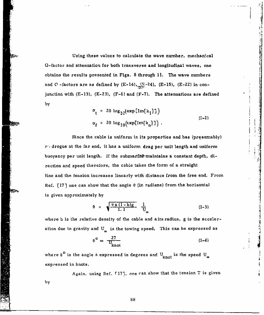
Using these values to calculate the wave number, mechanical

Q-factor and attenuation for both transverse and longitudinal waves, one

obtains the results presented in Figs. 8 through 11. The wave numbers

and 0 -factors are as defined by (E-14), ,(M-Z4), (E-15), (E-22) in con- Ijunction with (E-13), (E-23), (F-6) and (F-7). The attenuations are defined

by

O 20 Iogl 0 exp[Im(kl1)

0t 20 logl 0 (uxp[Im{ko]])

Since the cable is uniform in its properties and has (presumably)

il, drogue at the far end, it has a uniform drag per unit length and uniform Zjj

buoyancy per unit length. If the submaii,maintains a constant depth, di-

rection and speed therefore, the cable takes the form of a straight

line and the tension increases linearly with distance from the free end. From

Ref. [171 one can show that the angle 0 (in radians) from the horizontal

is given approximately byr a= -b)g 1

-.1 U (1-3)

where b is the relative density of the cable and aits radius, g is the acceler-

ation due to gravity and U is the towing speed. This can be expressed as

27 (1-4)knot

where 0 is the angle A expressed in degrees and Uknot is the speed U.

expressed in knots.

Again, using Ref. r 171, one can show that the tension T is given

by

88

T O .02 apUd, (1-5)t

where d is the distance from the tree end. This relationship is plotted

in Fig. 12.

II

/I

3} -

'1iI

11

4. J 1

p

if

i

REFE RENCES

I. R. M. Bozorth, Ferromagnetisrm (Van Nostrand, New York, 1951).

2. J. R. Wait, Electromagnetic Waves in Stratified Media (Pergarnon,New York, 1962), p. 22. *

3. A. S. Griffiths, "ELF Noise Processing," Technical Report 490,Lincoln Laboratory, M. I. T. (13 Januaryr 1972), DDC AD-739907.

7_ _ _ _ _ _ _ _ _ _ _ _ _ _ _ _ _ _ _ _ _ _ _ _

4. 0. G. Nackoney, "Design of an 'eflf~Loop Antenna Receiver,"1 T3ch-.-al Note 1972-22, Linco n-lab --atory, M. I. T; (11 July 1972),

DDC AD-902159-L.

5. M. J. Lighthill, Fourier Analysis and Gene'ralised Functions

(Cambridge, Lb;ldon, 1960), p. 51 ff.

6. M. L. Blur rows and C. W. Niessen "ELF Communication -System 7-Design" in Engineering- infthe Ocean -1nvironment (Ocean2 (I - EEE, -New York, 1972), pp. 95-109.

7. M. L. Burrows "Motion-Induced Noise in Towee. Flexible Sensors"(24 March 1969), not generally availabip..

8. H. Bittel "Noise in Ferromagnetic Materials" IEEE Trans. MAG-5,No. 3, 359-365 (September 1969).

9. P. Mazzetti and G. Montalenti "Powver Spectrum of the BarkhausenNoise of Various Magnetic Materials" J. A~P21 Phys. , Vol 34, No. 11,pp. 3223-3225 (November 1963).

10. J. E. Manning, "Vibration and Strain-Induced Noise from the ELFFlexible Loop Antenna," Technical Note 1971-51, Lincoln Laboratory,M. I. T. (15 December 1971), DDC AD-737093.

11. L. D. Landau and E. M. Lifschitz, Fluid Mechanics (Pergamon, Lon-don, 1959), Section 24.

90

1.. J'. Volt, l'r i d '. C. ,tchll tnits igl miu, )1yn1e4lch of Vibrntlone( r arrill, Columbuts, ldo, 1965), Elquitlion 4. . Z and 4. 5. 86.

13. G, ., Fran, "llighno.hii C riterla rand the RIteltionship Bletween Sur-

ri'co 1Rongiglitit) rind nF'Icn w N lise, " 7Ulh MeethnR of L1P AcounticalSoci'ty of Aiorica, Otlnwn, 21-Z-1 May 1968,

1.1. 11. 1'. 11 k'w 1tv ll, Jr. , " iirim lent Wtill.-.Presnure F luctuations on t

Blody of Revolution, " Acoustical ,so'efof ArnLri ._ Vol. 43, No. 6,pp. 1358-63 (June 1968),

15. II. rennekes und J. L. ].unilouy, A T'irst Courst in Turbulence(M, I. T. , Cufrnbridgc, 197Z), pp. tg)-2.

16. M. L,. Burrows, "Fabrication of Flexible Loop Antenna," 'TechnicalNote 1970-3t, J.incoln Laboralory, N1. I. T. (5 Oettber 1970),DDC AD-717718.

17. S. I Hocrncr. Iluid vnnmnic Dr v (Pub1 inhord hy I hr. st.-iine, lg.91p. 3-11.

18. M. \V. Waihnbsganss, Jr. smid 13. L. Botrs, "Parailcl-3-"ow-inducedVibration of a Cylindlrical R(od" An. Soc. Merli. Eng. Winter AnnualMeeting aind Energy Systevnt Expor;itioIn, New York, N. Y.1-5 December 1968.

19. It. I... Crane, "Motion Induced Noiirc inI FIexible le;Icctrode P; ir andLoop Antemaa;"- RCA David S;arujof" Reseiarch Centter Technical Memo.No. I (Tuly 197Z).

91