This DocumentReproduced From

Best Available Copy

UNCLASSIFIED

AD 289' 084

ARMED SERVICES TECHNICAL INFORMATION AGENCYARLINGTON HALL STATIONARLINGTON 12, VIRGINIA

UNCLASSIFIED

This DocumentReproduced From

Best Available Copy

NOTICE: When government or other drawings, speci-fications or other data are used for any purposeother than in connection with a definitely relatedgovernment procurement operation, the U. S.Government thereby incurs no responsibility, nor anyobligation whatsoever; and the fact that the Govern-ment may have formulated, furnished, or in any waysupplied the said drawings, specifications, or otherdata is not to be regarded by implication or other-wise as in any manner licensing the holder or anyother person or corporation, or conveying any rightsor permission to manufacture, use or sell anypatented inventi:on that may in any way be relatedthereto.

REPRODUCTION QUALITY NOTICE

This document is the best quality available. The copy furnished

to DTIC contained pages that may have the following qualityproblems:

"* Pages smaller or larger than normal.

"* Pages with background color or light colored printing.

"* Pages with small type or poor printing; and or

"* Pages with continuous tone material or colorphotographs.

Due to various output media available these conditions may ormay not cause poor legibility in the microfiche or hardcopy outputyou receive.

W If this block is checked, the copy furnished to DTICcontained pages with color printing, that when reproduced inBlack and White, may change detail of the original copy.

1'W

10 ANTENNA LAbORATORY

Techinicall Report No. 61

* ~THE -BACKFIRE, BIFILARHELICAL ANTENNA

00 by

t~JJ~Willard Thomas Patton

Contract AF331657J-8'460r 15"i~cProject No. 6278, Task No. 40572

September 1962,,nowA

Sponsored bytAERONAUTICAL SYSTEMS DIVISION

WRIGHT-PATTERSON AIR FORCE BASE, OHIO

ELECTRICAL ENGIN.EERING RESEARCH LABORATORY

ENGINEERING EXPERIMENT STATION

. UNIVERSITY Of ILLINOISURBANA, ILLINOIS

N .°'I.

Arntehna Laboratory

Technical Report No' 61

THE BACKFIRE BIFILAR HELICAL ANTENNA

-V by

Willard Thomas Patton

Contract AF33(657)-8460Project No. 6278, Task No_.40572

September 1962

Sponsored by

AERONAUTICAL SYSTEMS DIVISION

WRIGHT-PATTERSON AIR FORCE BASE9 OHIO

Electrical Engineering Research LaboratoryEngineering Experiment Station

University of IllinoisUrbana, Ill.inois

.'/ \' ,

ACKNOWLEDGEMENT

The author wishes to thank all members of the staff of the Antenna

Laboratory of the University of Illinois for their help and encouragement

during this study. The guidancdiof his adviser, Professor G. A. Desbhamps,

and the suggestions of Professor P."E. Mayes are particularly appreciated.

Thanks are also due to Samuel C. Kuo who assisted in the data

reduction and prepared the illustrations, and to Bradley Martin, Calvin

Evans, and Edward Young, who assisted in the experimental measurements.

This work was sponsored by the United States Air Force, Aeronautical

Systems Division, Wright-Patterson Air Force Base, under contract number

AF33(616)-6079 and AF33(657)-8460, for whose support the author is

grateful.

iI

I;z

) /

ABSTRACT

The backfire bifilar helical antenna, consisting of two opposed helical

wires fed with balanced currents at one end, is a new type of circularly

polarized antenna. When operated above the cutoff frequency of, the principal

mode of the helical waveguide, the bifilar helix produces a beam directed

al~ng the structure toward the feed point. The term "backfire" is used to

describe this direction of radiation in contrast with "endfire" which denotes

radiation away from-the feed point.

Radiation patterns, measured for a wide. range of. helix parametersB,

show maximum directivity slightly above the cutoff frequency. The pattern

broadens with frequency, and; for pitch angles near forty-five degrees, the

beam splits and scans toward the broadside direction.

Near field measurements show.the current decaying rapidly to a level

about twenty decibels below the input level at a rate that increases with

frequency. Phase measurements in the near field show that in the feed region

the direction of phase, progression is toward the feed point. the oppositely

directed phase progression and direction of energy flow is characteristic of

a backward wave. The direction of phase progression is consistent with the

backfire direction of the main beam observed in the radiation patterns and

the increasing rate of current decay is consistent with the broadening of

the main beam with increasing frequency.

A theoretical analysis of the bifilar helical antenna is obtained. It

is based upon"the semi-infinite motl4 using thin wire assumptions. These,

so-called, linearizing assumptions consist of replacing the current distribu-

tion on the surface of the wire with a line current ohtVthe center line of the

Y

wire and of satisfying the boundary condition along bne line on the conducting

"surface. The Fourier transform of the current.distribution on the semi-infinite

hq,lix is/deduced from)the deter4nantal equation'of the bifilar helical wave-

guide-by a Wiener-Hopf techaiqd! The relation between this Fourier transform

and theradiation pattern of the backfire bifilar helical antenna is shown.

The results predict the. patterns of the experimental study and show the effect

of wire size on antenna performance.

L.C."

2i

/. < j

K)

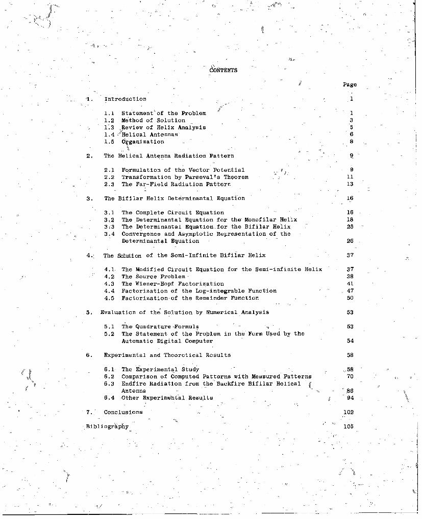
6"N'TENTS

//Page

1. Introduction 1

1.1 Statementof the Problem 11.2 Method of Solution 31.3 Review of Helix Analysis 51.4 'Helical Antennas 61.5 O4ganization 8

2. The Helical Antenna Radiation Pattern 9

2.1 Formulation of the Vector Potential 92.2 Transformation by Parseval's Theorem i12.3 The Far-Field Radiation Pattern 13

3. The Bifilar Helix Determinantal Equation 16

3.1 The Complete Circuit Equation 163.2 The Determinantal Equation for the Monofilar Helix 183;3 The Determinantal Equation for the Bifilar Helix 253.4 Convergence and Asymptotic Representation of the

Determinantal Equation 26

4. The Solution of the Semi-Infinite Bifilar Helix 37

4.1 The Modified Circuit Equation for the Semi-infinite Helix 374.2 The Source Problem 384.3 The Wiener-Hopf Factorization 414.4 Factorization of the Log-integrable Function 474.5 Factorization of the Remainder Function 50

5. Evaluation of the Solution by Numerical Analysis 53

5.1 The Quadrature-Formula 535.2 The Statement of the Problem in the Form Used by the

Automatic Digital Computer 54

6. Experimental and Theoretical Results 58

6.1 The Experimental Study "586.2 Comparison of Computed Patterns with Measured Patterns 70,

¼ 6.3 Endfire Radiation from the'Backfire Bifilar HelicalA, Antenna "86

6.4 Other Experime'htal Results 94

7. Conclusions 102

Bibliography . 105

tl . .. .'.

If',,.

CONTENTS (4pktinued)

C) Page

Appendix A. A Fourier Transform 107• /1

Appendix B. The Relation Between the Fo 'rier Spectrumof # Linear Current Distribdttion and its RadiationPattern 110

vita1

I

1

I*•" t

I.It?

--.

ILLUSTRATIONS

" .Figure Number Page

1 The Geometry of the Bifilar Helix 2

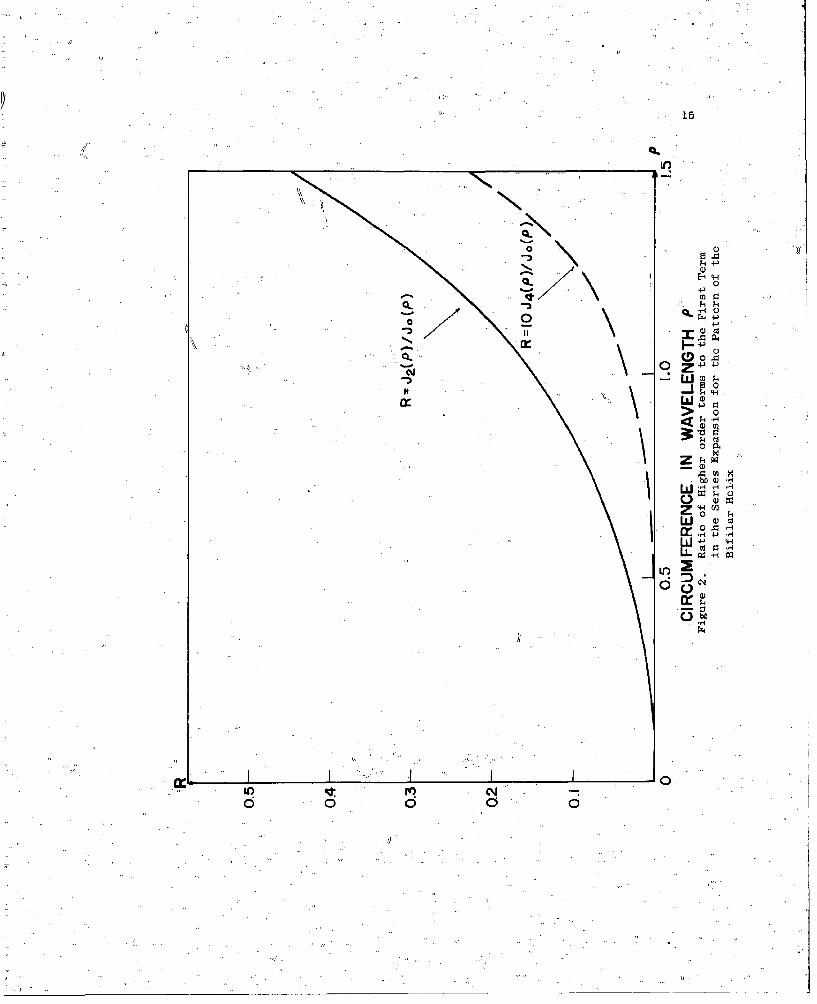
2 Ratio of Higher order termsato-the First Termin the Series Expansion for the Pattern of theBifilar Helix 15

3 Graphical Solution for the Roots of the HelixDeterminantal Equation when k 4,k 22.

. C

4 Graphical Solution for the Roots of the HelixDeterminanta~l Equation when Is i 23

5 Brillouin Diagram for a Monof.ilar HelicalWaveguide 24

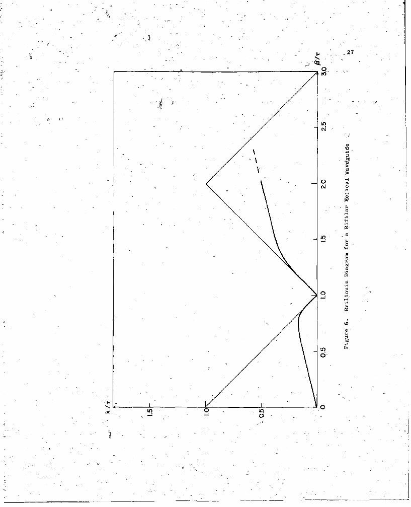
6 Brillouin Diagram for a Bifilar HelicalWaveguide 27

7 Graphical Solution for the Exponent in the'Asymptotic Form.of Z (8)" 34

8 The Bifilar Helix Determinantal Function kw k 43c

9 The Bifilar Helix Determinantal Function ki ;k i 44

10 The Zeros 'and Branch Points of (13) in theComplex B-plane "45

11 Current Amplitude Distribution on a Bifilar Helix 60

12 Measured Propagation Constapts of the PrincipalWaveguide Mode on the Bifilar Helix 61

13 Measured Values of the Principal-Mode Cut-offFrequency for the Bifilar Helix 63

14 Current Amplitude Distribution above the CriticalFrequency 66

15 Near-Field Phase Measurements for the-Bifilar HelixBBH-4 . 67

16 Measured Radiation Patterns of the Backfire BEfilarHelical Antenna 69

17 Computed. Radiation Patterns for BBH-I 71

ILLUITRATIONI (acotinue~d)

riguro- Numdber Page

is .. computed Radiation Patternsi for 80H-2 7

19 computed Radiation Patterns for 5111-3 is

20 computed Radiation Patterns for 5911-4 7

21 cow ru~td Radiation Patternsm for 9DM-5l7

22 computed Radiation Patternidg Or flfflf 7

23 Comiputed Radiation Patterns for 9911-7- 77

24*bfiaio bow@ Measured aitd Computed. -7

.go 'Comparison 'between Mevasured ad t computedPatterns for 1DBH-

29 Comhparison between Measured and ComputedPatterns for 9DMS-a 81I

27 Comparison between Measured and ComputedPatterns for 9911-4 . 8

28 . Comparison between Measured and computedPatterns for BDWf 893

go Comparison betwgien Measuried and ComputedPatternsd for Ha51kjW 84

30 Comparison between Meas~ured and ComputedPattering for flR-? 98

31i Axial Ratios for the Daukfire flifiisy 8Hlliceal Antenna 8

32 CaltuliAtd Values of the Propagation Constantof the Higher Order Waveguide Mode oni theflifilar Helix 9

33 ' Radiation -at-terna Showing the Effect ofChanginig the Length of thO Antenna go

34 trontdto-flak Ratio asm a Yunoetiori 6f Antenna,Length , 9

38 Patterns of 9911-4 With a Conduciting Coaxial Caor goat f 1.4 at

* . - .. I .

"ILLUSTRATIONS (continued)->

Figure Number Page

36 High-Gain Patterns Measured for BBH-8 97

""37 Measured Patterns for a"Long Tapered Bifilar Helix' 99

38, Radiation Patterns Measured for a BackfireMonofilar Helix 100

i.. . . . ..

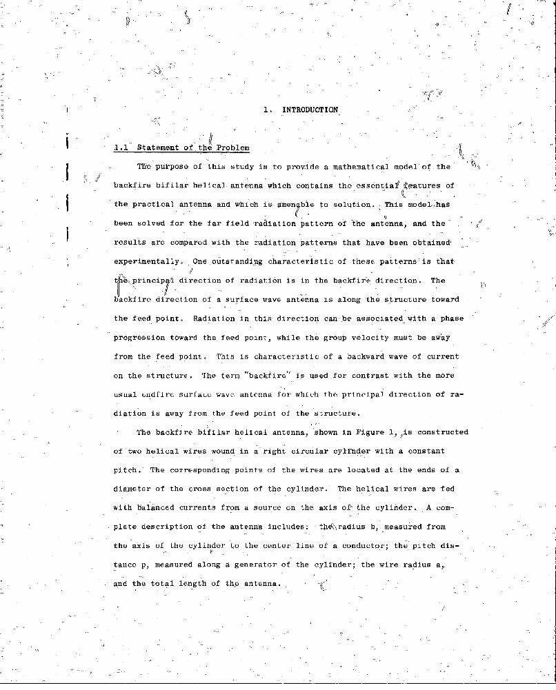
1. INTRODUCTION

1.1 Statement of the Problem

j The purpose of this study is to provide a mathematical model of the

backfire bifilar helical antenna which contains the essential leatures of

the practical antenna and which is. amenble to solution. This model,has

been solved for the far field radiation pattern of 'the antenna, and the

results are compared with the radiation patterns that have been obtained'

experimentally. One outstanding characteristic of these patterns is that

_ \principyl direction of radiation is in the backfire direction. The

backfire direction of a surface wave antenna is along the structure toward

the feed point. Radiation in this direction can be associated with a phase

progression toward the feed point, while the group velocity must be away

from the feed point. 'This is characteristic of a backward wave of current

on the structure. The term "backfire" is used for contrast with the more

usual endfire surface wave antenna for which the principal direction of ra-

diation is away from the feed point of the structure.

The backfire bifilar helical antenna, shown in Figure 1, is constructed

of two helical wires wound in a right circular cylinder with a constant

pitch. The corresponding points of the wires are located at the ends of a

diameter of the cross section of the cylinder. The helical wires are fed

with balanced currents from a source on the axis of' the cylinder. A com-

plete description of the antenna includes: thd46\radiuis b, measured from

the axis of the cylinder to the center line of a conductor; the pitch dis-

tance p, measured along a generator of the cylinder; the wire radius a,

and the total length of the antenna.,

(1, .. 'I-. M 2

"4, L

2a�fQ

tIi>,,

Figure 1. �. The Geometry of the Elf liar Helix .

\'.,�, I

ILr.

'3'I

3

1.2 Method of Solution

'A solution of ,the backfire bifilar helical antennaproblem is obtained,

first, by considering jhe basic helical geometry to be extended to infinity

in both directions, This is the helical wav,eguide"'problem which already has

an extensive literature. An exact account of the boundary conditions in this

problem involves finding a current distribution over the surface of the

conductor which makes the tangential electric intensity vanish everywhere

on the surface of the conductor. An approximation used by Sensiper. and

2.Kogan is to'require that the tangential electric intensity vanish only

along some line along the surface. This approximation is good for rela-

tively thin conductors. Sensiper, in treating the tape helix, makes a

further approximation in assuming a functional dependence for the distribution

of current across the width of the tape. Kogan makes a similar approximation

by assuming that the surface current distribution may be replaced by a

current flowing along the center line of the helical conductor. The ap-

'> proximations involved in replacing a surface current by a line current and

in satisfying the boundary conditions along only one line of the surface

have been termed linearizing approximations. A formulation of the helical

waveguide problem, similar to that of Kogan, is used in this study.

Using the above approximations, the desired current distribution

becomes a function of only one variable.. This variable may be either

distance along the helix or distance along the helical axis. In this paper.

the helical axis is taken to coincide with the z-axis of a cartesian

coordinate system, and z is taken as the independent variable of the current

distribution. The integral equation-for the current on the helical waveguide

now has the form of a convolution integral. This happy circumstance related,

4!

to invariance under a one dimensional Abelian congruence'group, suggests a

solution by Fourier transformation. The determinantal equation for the

Fourier spectrum of the current distribution has three pairs of real roots

at the lower frequencies. As the frequency is increased, two pairs of roots

tend together and coalesce at the critical frequency, f . This frequencyc

marks tile lower limit of the range of frequencies of interest 'in this

study. The critical frequency depends, in a complicated way, upon the

radius of the helix, its pitch, and th-,condudtor radius, and no simple

expression is given for it.

The second step in the selution of the backfire bifilar helial antenna

problem is to obtain a solution for the current distribution on a helical

waveguide extending only along the positive z-axis of the coordintte system.

This is accomplished"by a Wiener-Hopf factorization of the tranSfprmed

solution for the helical waveguide. The boundary conditions on the factori-

zation are such that the current is identically zero for all negative z and

approaches a finite non-zero limit as z approaches zero from the right. The

discontinuity in the current at the origin is the source of energy in the

problem and corresponds to a pair of oscillating point charges separated

by the helix diameter, The result of this calculation is.the Fourier

transform of the current distribution on a semi-infinite bifilar helix" fed

by a charge dipole in the plane z = 0.

The solution obtained in this way is limited by the linearizing appro.xi-

mations described abov6. The remaining approximations in the theory

developed here are contained in equating this solution to the radiation

pattern of a finite-length bifilarhelical antenna fed from., a source on its

axis. The practical antenna differs from the mathematical model in'the

k !I

vicinity of the feed point by the addition of a current flowing along a

diameter of the cylindrical cross section. Thts 'addi.tional current element

is short in the range of helix`diamnl•rs of primary.interest in this study

and will not contribute noticeabl. to the radiated field. Measurements

of the current on several models of the bifilar helix above the critical

frequency show that the current decays rapidly with distance from the

feed point. At a level about 20 decibels below the input value, an-und-amped

wave becomes dominant, Because of the rapid attenuation of current on the

bifilar helix, the radiation pattern of the fidite"structure is expected

to be the same except for "end-fire" radiation caused by the residual

"free-mode" wave, It is well known that a finite line current distribution

and its far field radiation. pattern are Fourier transform pairs. This is

extended here to include the semi-infinite structure, and it is shown that

in this case also the radiation pattern is simply related to the transform

of the current distribution as a function of z except in the vicinity of

the current distribution at infinity.

The Fourier transform of the current distribution is obtained by

numerical techniques usingan automatic digital computer, The computed

patterns based upon this Fourier transform show good agreement with

measured patterns presented in this report, This confirms the validity

Sof the approximations used in constructing the mathematical model of the

antenna.

l".8 Review of Helix Analysis

, The study of electromagnetic wave propagation on helical conductors

through 1955 has been summarized by Sensiper and his thesis contains

..an extensive bibliogr.aphy of the literature. He obtains an exact solution

I) 6.,

of thd "tape" helix by expressing its field as a sum of sheath helix modes

and by, requiring the tangential electric. intensity to be zero on the tape.

The resulting arithmetic is found to be. intractable, and he quickly obtains

a more-manageable approximate solution by, requiring only that the tangential

electric intensity at the center of the tape be zero, When the resulting

2expression is compared with that obtained by Kogan. from a potential

integral formulation, they are found to differ principally in the fOrm of

the convergence factor introduced by the approximation, Kogan treats the

helical wire model with the null field boundary condition satisfied only at

.,the points of tangency between the helical conductor and-a cylinder with

radius equal to the outer radius to the helical wire.

The work of these authors is directed ,toward the evaluation of the

firee-mode" propagation constants for undamped traveling waves of current

1on the helical conductors. Although Sensiper does devote some space to

the source problem, his formulation of thi's, problem is for the infinite helix.

It is used to interpret the "free-mode" solutions of the source free problem.

Many authors have contributed to the literature on the helical waveguide,

Since their work has been reviewed by SensiperI' '3the bibliography is not

reproduced here.

1.l Helical Antennas

The helical antenna which most nearly approaches the backfire bifilar

helical antenna in performance is the helical beam antenna introduced by

Kraus in 1947, Kraus1s antenna is a monofilar helical wire fed at one

end against a ground screen. The properties of this antenna have been

discovered by experimental techniques. The current distribution on helical '

5structures of this type was studied by Marsh The analysis of a helical

S... ...

7.

antenna of this type suffers the same difficulties as the analysis of

'the usual end-fire surface wave antenna. For both of these the feed

region •and the terminating region are important in determining their radiation

characteristics. In contrast, the characteristics of the backfire bifilar

helical antenna are controlled by the input region.

A bifilar-version of the Kraus helix/has been reported by.Holtum6 .

This antenna is constructed of two coaxial helical wires on the diameters of

the supporting cylinder. Each conductor is fed against a ground screen with

the exciting currents in phase opposition. This differs from the backfire

bifilar helical antenna in which the conductors are fed at one end, one

against the other, without the presence of a ground screen. It is the

absence of the ground screen that distinguishes the backfire helix from

the Kraus-type helix. This fact is essential to the performance and

analysis of the backfire helical antenna.. On the other hand, the number

of helical conductors is not essential to the backfire characteristic

of the antenna. A backfire monofi ar helix is shown to have substantially

the same radiation characteristics"as the backfire bifilar helix. The

monofilar helix, however, is more difficult to feed in" the backfire mode.

Although both the Kraus helix and the backfire bifilar helix are

circularly polarized, several differences in the performance of these

antennas must be noted. The beam width of the Kraus helix decreases with

frequency while the backfire helix beam width increases with frequency.

The gain of the Kraus helix increases with length"while the gain of the

backfire helix is independent of length provided the ,length is large

"enough. Finally, "the Kraus helix is an end-fire antenna in contrast to

the backfire helix which radiates along the helical axis toward the feed

point,;.

V V9J 11

"I")I,

8

1.5 Organization

In the present section, the bac.Wf ire bifilar,)heliual antenna is described

and compared with other helical antennas of similar character. A description

of the method used to obtain a solution for the radiation pattern of the

antenna is given, and a brief review of the literature on <the helical wave-

guide is included. In Chapter 2 the relation betweeq( tv radiation pattern

of a helical antenna and the Fourier spectrum of its current distribution

is discussed. This motivates the work~of the three following chapters in

which the Fourier spectrum of the current distribution is obtainedc

Chapter 3 describes the approximate determinantal equation for the

helical waveguide as it is used in this study. This is derived from the

potential integral with a linear current approximation. The equation

describing the helical waveguide is factorized in Chapter 4 by the method

of Wiener-Hopf, and the evaluation of the resulting expression by numeri,cal

techniques is described in Chapter 5. The results of the numerical computation

are presented in Chapter 6 along with the experimental results, This Chapter

also indicates the connection between this study and the log-spiral and other

frequency-independent antennas, Chapter 7 summarizes and concludes the work.

.t,.t

9

2. THE HELICAL ANTENNA RADIATION PATTERN

2.1 Formulation of. the Vector Potential

Since the purpose of this study is to.develop a theory that is capable

'of predicting the radiation patterns of the backfire bifilar helical antenna,

and since the geometry of the problem lends itself to a solution by Fourier

transformation) a relation between the radiation pattern and the Fourier,

spectrum of the current distribution for the bifilar helix must be obtained.

This section is devoted to establishing that relation.

The radiation pattern of an antenna will be taken to mean the angular

distribution of electric intensity in spherical coordinates at a large dis-

tance from the antenna. When only those terms that vary inversely withodis-

tance are retained", the electric intensity is related to the magnetic vector

potential by

•xr = -ik Ax * (1)

where r is a unit radial vector

k =,1 is the propagation constant of free space

is the intrinsic impedance of free space

Thus the radiation pattern is related to the angular distribution of the vector

potential, and the vector potential is deduced from the current by the well

known integral formula

A6r) =JJJ G(r, r ) I(r') dv (2)

where

G-k. -A exp [-jki_ r-r& I]Gr, r )L =L

4r , -1 Ir-

• *1

is the Green's function in an unbounded homogeneous isotr6pic three.dimensional

space,'

r is the radius vector to a point of observation and

r is the radius vector to a source point.

By the method of induced sources, we may replace the conducting boundaries

at the surface of the helical wires by a surface current distribution existing

in homogeneous space. If this current distribution equals the surface current

on the helical conductors, the fields external to the conductors are unchanged

by removing the conductors from the space. If the conductors are sufficiently

thin, the field produced by the surface current distribution will not differ much

from that produced bya current distribution on the center line of the helical

wire. This approximation limits the analysis to thih wire helices, but it

has the advantage of converting,the volume integral in Equation (2) to a line

integral.

The bifilar helix then can be considered as two helical lines of current.

'Apoint on line one with axial. coordinate z will have cartesian coordinates

P1 (b cos Tz","b sin Tz/, z')

where

T 21/p

p =pitch of helix

b radius to centerline,

and the unit tangent to the helical wire at that point is given by

A. A -A I A.u -x cos 41 sin rz +y cos '4 cos Sz +z sin

where 4 is the pitch angle of the helix given by

217 b,cot -2 :b TbP

p

if .. t '

.Iq,',

IL•

At the same value of the axial coordinate z a point on line two will have

cartesian coordinates

P C-b cos Tz', -b sin Tz' z')

with unit tangent4• A -A A

u lcx COSt sin TZ - A cos SI cia +z sin +

The distance between a remote point (r, 6, ) and a point on line 1 is

given by

[= r sin 0 cos c'-b cosZ

4- '(r sin S sin K-b sin TZ )2 + (r cos 6-z)2] 1/2

or

r 2-2br sin Q cos (Tz 4- -.b2+z 1/2

Similarly, the distance between the remote point and a point on wire 2 is

given by

r 2 2I42br sin 6 cos (Tz-) +b2+zr2 =.

The currents on the helical line can be considered to be a function of

the axial variable z # alone. If the currents in the two wires are equal and

oppositely directed for the same value of z', Equation, (2) may be written

...-. ekr -jkr

(r) cos - + -- sin Tz I ( dz

x 4,\411r 1 4'1rr2 /

(r) = cos, -j l -A (r)=COSt ekj * Jz 2) COS IZ C1 dZ' (3)Ax Tr

*1(ekr 1 jr2

A(r) sn1 -y JI (a') dx'

2.2ý Transformation by Parseval's Theorem

In Equation (3), the vector potential at the point Cr, O, 4) can be related

to the Fourier spectrum of the current distribution by Parseval's theorem.

Parseval's theorem states; Given two functions, F(z) and I(z), of the

9 spatial variable z with Fourier transforms, F(P) and I(•), in the transform

variable P,

F*(z) I(z) dz =27f 0 P(P)I(f) dP

where 7(P) is related to I (z) by

I(P) = / I(z)e dz

This introduces the Fourier transform of the current distribution into the

calculations for the vector potential. In this paper the.tilde &) is used

to ,denote the Fourier transform of a function of z, and the asterisk (*) is

used to denote the complex conjugate of a function. It is now necessary to

find the Fourier transform of the remaining factor in the integrand and to

evaluate the transformed integral at a point remote from the helix. The complex

conjugate of this factor in the first integral of Equation (3) can be writteneJkr eJkr2 )JTZe-J~z

F*(z) e, %4" s + e r?)2 sin T = (g+g ) e j -j

14T 7 2' 87TJ

where gl and g2 are, the functions discussed in Appendix A2- 2 2 1/2exp (jk[A +2AB cos (db+Tz) +13 (z-d)2I/)

9• - A2 72•'.AB cos (p,_.z).+B2 +(.-d )2]1/2

where

A = r sin 6

B= b

d = r cos e

Using Equation (A-5) and the shifting theorem for Fourier transforms we obtain

: . ." A

hI

. .-..-

13

n even... ]1/2 H(1) ([k2 r(B_(n+1)T)2]l/2)

• , . J (bO[k2-8 (- ) (rsn

-e(B-(n-I)T) r cos e +ne veI.In this way, using Parseval's theorem, the fir'st equation in (3) becomes

j (b[k2-(B-(n-l)T)2]1/2)H(1) (r sin elk2-(B-(n-1)T)2] 1/2)n n

A r+C°s • sd .j(B-(n-1)T) r cos eJný

A (r)-~ d~-oB1 *een even

-Jnb[k2B-(n+ 1)T)2]/2H(l) (r sin P[k 2 -(B-(n+1)T) I )

ej(B-(n+l)T) *r cos EeJný.'

2.3 The Far-Field Radiation Pattern

The asymptotic estimation of this integral follows that given in Appendix B.

In this case the change of variables (Equation B-4) is

B -(n-l) T = k cos a

or

B -(n+l) T = k cos a

Thus we have

A (r)-+j• cos 'J G J (kb sin 0)[I(k cos B.+.(n+I)T)-T(k cos e+)(n+l)Tr)]e nýx "n vno n

neven

where-jkr 0e o

G -o 4l•r0

In this way Equation (3) becomes .'.

A (r " +j7F cos , G J (P)[ I(k cos O4(n-l)r) -T(k cos B+(n+l)T)]eojn4 (4)n even .

A ( flcos E , GJ (P)[I(k cos .+.(n-1)T) +.I(k cos 0+(n+l)T)]en even

jný, -A (r) ' 2V sin GoJ(p) I(k cos O+nT)e.. nodd

• I14 f

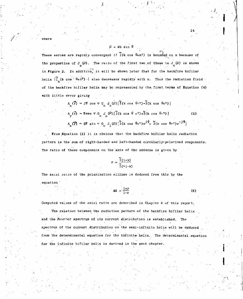
/5where

P = kb sin 8

These series are rapidly. convergent if I(k cos O+nT) is bounded on n because of

the properties of J (P). The ratio of the first two of these to J (P) is shownn 0

in Figure 2. In addition, it will be shown later that for the backfire bifilar

helix 1n (k cos, S+-T).J also decreases rapidly with n. Thus the radiation fieldn

of the backfire bifflar helix may be represented by the first terms of Equation (4)

with little error giving

A (r•) J1 cos Y G J (P)[I(k cos 0-T)-I(k cos e8+T)]x 0 0

A (r) - Woos Y.,G J (P)[I(k cos 6 +T)+I(k cos -r)] (5)y 00o

A(V M. 2W sin Y Go J 1 (p))I(k cos e+)eT e+ I(N cos G-T)e J]

From Equation (5) it is obvious that the backfire bifilar helix radiation

pattern is the sum of right-handed and left-handed circularly-polarized components.

The ratio of these components on the axis of the antenna is given by

1(1-k)I('.l-k)

The axial ratio of the polarization ellipse is deduced from this by the

equation'•' l+r

R ='-. (6)1-r

Computed values of the axial ratio are described in Chapter 6 of this report.

The relation between the radiation pattern of the backfire bifilar helix

and the Fourier spectrum of its current distribution is established. The

spectrum of the current distribution on the semi-infinite helix will be deduced

from the determinantal equation for the infinite helix. The determinantal.equation

"for the infinite bifilar helix is derived in the next chapter.

<I .

• . .,'SN

44

A a)

0000 -

E 00

16

3. THE BIFILAR HELIX DETERMINANTAL EQUATION

3.1 The Complete Circuit Equation

The electromagnetic field in an infinite homogeneous isotropic medium can

be obtained from the magnetic vector potential A and the scalar potential V

using the relations

H-= VxA

H =,-jkt A-VV

If the divergence of A is chosen to be

V-A = -jk/• V

these potentials satisfy the scalar and vector wave equations,

(7+k2 )V = _P

The solution of these equaltions can be written in terms of the Green's

function of the medium

a(•, ',) --exp[-jklr--'P{

asrr

V(r) -. JJJG(r, r )P(r) dv

A(r) f ! ) I(r-) dv (8)

Using the equation of continuity

V.T = 'jwp

in Equation (8) with Equation (7), there results

V= jXýk C (r, 'r') V'I (-:) dv (9)

7V =-E -J9kJ (rj , P) I(r) dv

which forms the basis of the complete circuit equation.

17

The circuit equation for the bifilar helix is obtained by replacing

the conducting boundaries of thehelical wires by the current. distribution

on the surface required to produce Oero tangential electric intensity there,

The equatipn is simplified by tlinearizing the boundary condition., This is

based on two thin wire approximations; first, it is assumed that the current

distributiop on the surface of the wires can be replaced with a line current

distribution at the center of the wire, and, second, it is assumed that, if

the electric field is zero along only.one line of"the surface, the resulting

p solution will be a reasonable approximation to the exact solution. These

--assumptions are good if'the wires are sufficiently thin.

In this analysis. the current will be assumed to exist on the line

defined in cartesian coordinates by

P1 = Cb cos Tz'[ b sin Tz', z")

P = (-b cos TzI, -b sin TzW, z')2

-and the null line will be taken as defined by

q= (b cos Tz , b'sin Tz, z)

"q= (-b' cos TZ, -b sin TZh z)

where

b =b-a

b = distance from helix axis to wire centerline

a = wire radius

Thus, the currents and potentials can be considered a function of the z

coordinate alone. Because of the constant pitch angle of, the helix,

. = cot- (2nrb/p)

an elementary displacement along the axis is related-to one along the wire by

"dz= sin W dp

S~~~~~~%-•' ,,, '.

i18 1

Thus on wire one

dI(z'),V, I (r =sindz

:VV(r") sin k •u(z) dV(z•

u (z') u (z') IIA 111where u1 =-cos sin Tz+^ cos cos 2ý sin 4

In these equations it is assumed that the pitch angle ofthe null line C'is Iequal to the pitch angle @of the centerline of the wire. The correct result is

eoa t cot otepchagecot+

where I

S=a/b

The approximation (0 =) is consistent, with the thin-wire assumption used Ithroughout this study.

3.2 The Determinantal Equation for the Monofilar Helix

Equation (9) will be applied first to a single wire helix so that the Imodification of the determinantal required for the balanced bifilar helix

will be made evident. The current is confined to the line p., and the potential I

is evaluated on the line ql" Since the electric field strength is assumed zero'

along this line, Equation (9) becomes

V(z) =j f GII(z; z) sin d dI 1 (zd

00

dVd

sin -j" GI(z z u (z).u (z Ii(z') dz' (0)dl'~ f 11 (0

If the-first equation is differentiated with respect to z, multiplied by sin 1and equated to the second equation; the result is

00 2 dG ii(Z, z) dI(z/) 2 A• fsn 2 d z d7- + k (Ul(z).u (z') G (Zý Z') ;(z')] dizjdz dz 1. 1 1 z)Iz) z (11)1

19

where

2 2_ / / + 2 .1/2(') -exp[-jk[b +b'-2bb cos T(z-z) + --i)

41[b 2+b 2-2bb' cos T(z-"z) t (z-az)2 1/2

andu I(a) o (z).= (a-a) :=cos cos r(z-z/) + sinY

are even f"•nctions of the difference in z coordinates at the source and

observation points.

Because G and C are -functions of the difference in the z coordinate,

Equation (11) is a convolution integral

-00z Zz-z') I Wz) dz' 0(i

where Z is the operator11

- -dGO (Z'Z ) dZd(a-z) z -k G ((Z-Za) -k cot 2 'cos T(z-za) G (Z-Za)

The Fourier transform of G (Z-aZ) is deduced from the result of Appendix A by

g*(z)

11 41r

where

S exp(jk[A-2ABcos (+÷.Tz) +B2 4(z-d) ] 1/2)

91(Z) = [A 2-2AB cos ('F.Iz) +B2 4(z-d)2I1/2

and where

A b=

B =b

4=0

"d=0

S~/

I

m20

is

- 2) ( H(2n=-00n

or

o( = - I (b[(B-nT)2 -k ] 1/2) K (b[(B-pT)2-k ]1/2)41r n1o nn

For convenience we will define a new function

B (8) . n (b'[(8.-nT)2 -_k2 ]1"K (b[(8.-nT)

2 -Ik 2 ]1/2)n n n

The function, 0 (8) now has the simpler representation

N n

(13) - Er B (B)I)GI 47r n=- Do n

The Fourier transform'of Z(z) is given by

22 k2 cot 2'Fz 11(B) (B-k) G I(B) 2 [Gfl (B+T)+a11(3-T)]

This function has infinitely many branch points located at

8 = n-tk n 0, +1, -2,'

The Fourier transform of Equation (12) is

Zl(8)(8) = 0 (13)

The spectrum of the current on the infinite monofilar helical waveguide given

by Equation (13) must be a distribution of point support at the roots of

Z(8) and, therefore, is a polynomial of delta distributions there. However, by7

analytic continuation of the distribution into the complex B-plane, it can be

shown that the order of the distribution must be one less than the order of the

root. Sincethe roots of Z(8)Y are of first order, no derivatives of the delta

appear. The current distribution, therefore, .is a sum of traveling waves with

propagation constants'given by the roots of Z(8).2

In investigating the roots of U13), Xogan rearranges terms in the form

00

B nB(q3#r) + B n-r) 2

=Tan L3(_i

2n=-0o

The function on the left can~be called F2 (p) and, following Kogan , is sketched

in Figures 3, and 4, It can be seen.that F 2 (p) is approximately equal to one in

"the range

< n < 1- -k n= 0, 4-1, +2,...¶ 'r T -- -

except near T = - k where the terms B in the numeratorhave a logar'ithmicP 0

singularity contributed by the modified Hankel function of zero order or near

P= k where B (P) in the denominator is., logarithmically singular. In this

range the root of Z (P) is given approximately by

j32 2_= 1 + cot i

k2'

or

= k/sin LP

The roots of Z(•) are-at the intersection of F 2 () and the parabola

"2 2 ]7For k small it can be seen that there are three roots: one near p = k/sin .j,

one near 1 1-k, and one near l z 1,.k. Since Z(P) is an even function of P

there are also three corresponding roots'on the negative P-axis.

The functional dependence of"the roots of Z(•) on the frequency, k, is

conveniently displayed on the Brillouin diagram, als'o called the p-k diagram,

shownin Figure 5. In this figure, due to Sensiper , the variables are

normalized with .respect to T (T1T2W/p) The deviation of the curve from the

4.0

k/T k/r-

F1 /(0/r) F

F2 ()g/r;)

2.0

MODIFIED CURVE FOR

0- k/-r 0.5 * 1.0 1.,

Figure 3. Graphical Solution for the Roots of thleHelix Determinantal Equation when k < Ic

C

4.0

F220

4.0 fN F(3r

2.00

BIFLA HELIX

0kit .0.5 1.0 5

Figure A4.- G3ýaphica1 Solution for the Roots of the

He lix Determinantal Equation whei k .)P k.jI

24.

.0

ca

0

cu

00

is Cu

c;- c;

YV

25

asymptote,

k/sin

near 3 0 can be interpreted as coupling between the current wave and a-i+linearly polarized plane wave, and the deviation near =T-k can be interpreted

as coupling with circularly polarized plane waves. This coupling is indicated

by the logarithmic singularities and depends upon the wire thickness 6(6=a/b)

of F 2 (•) shown in Figure 3.

3.3 The Determinantal Equation for the fifilar Helix

When the second conductor is added to, the problem, Equation (12) becomes

00

S(z-Z') Ii(z') Z Z 2 (Z-z') I2 ( ')] dz' (14)

where

d ( )d k2 (a-ZI2(z-z') d-• GI k - (z-z') GI2(Z-z)

12 , d 12 dxz' Cjz 12 12

In this equation

2 2 ,21/2G (a-') exp(-jk[b 2b' +2bb' cos T(z-z')+(z-Zv) I/)

14T[b 2 b' 2 +.2bb' cos T(z-z')4.(z-z')

relates the potential at wire one to the current on wire two, and

A A2 '2C (z-') Z u (a) U (a') .... cos + cos T(a-a') + sin i12 1 2

is the cosine of the angle between the line element at the source point and

the line element at the observation point.

The' fourier transform of G (Z) is12

G12 (P) .-. [ Y (-l)"Bn(p)47T n"-oo

and. that of Z (Z) is12

" 22cot2

Z G - -( kc + G • .]"2 1q12 i (22,[

'• • •26

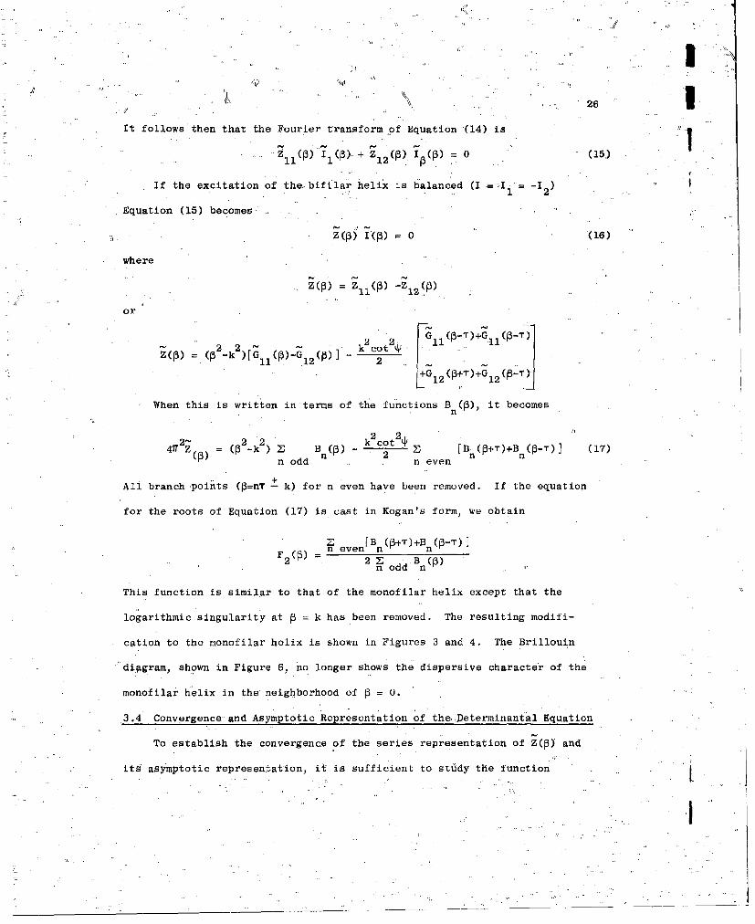
It follows then that the Fourier transform of Equation '(14) is

.z11 () TI(j) + Z12 () I(P) = 0 (15)

If the excitation of the bifilar helix is balanced (I =..I -I2)

1 2

Equation (15) becomes

Z(P) I (P) 0 (16)

where

Z(3) = 1 1 (P) -Z12 (P)

or

2)[Z k 2 ct2 1 lZ(P) =(P -k )[ 11 (f)-G 12 (P)] - 2ct1J

22 12

When this is written in terms of the functions B (P), it becomes

222_2.k 2 ct24ITZ(• = (3-k2) > Bn(I•) k~cot2l47 ) n odd 2 [B.(P+T)+Bn (P-T)] (17)

n odd n even

All branch points (P=nT+ k) for n even have been removed. If the equation

for the roots of Equation (17) is cast in Kogan's form, we obtain

n even [n (+T)+Bn(I-T)]F2 = 2 n odd Bn(P)

This function is similar to that of the monofilar helix except that the

logarithmic singularity at P = k has been removed. The resulting modifi-

cation to the monofilar helix is shown in Figures 3 and 4. The Brillouin

'diagram, shown in Figure 6, no longer shows the dispersive character of the

monofilar helix in the neighborhood of P = 0.

3.4 Convergence. and Asymptotic Representation of the..Determinantal Equation

To establish the convergence of the series representation of Z(P) and

its asymptotic representation, it is sufficient to stddy the function ...

' 2I.,

) I.,

27

0)

f eJk b. +b ý_bb,!o 13

11' 2.T -00.2+2.'2/2•11(B = • ao " 4"•[b2+b -2bb "'cos Tz+.z2/2eBd

*1ii

8o(0) + L- (Bn([3)+Bn(-13)) (18),41T2 47T2 n=l'

where '

2I,BB = (8 1 n b'N)3z( -n

2 (B-n)2 -k2

n

When k<T all the terms in the series Equation ()drepositive except* at

mostone erm It-.follows that., it the series representation of, •l(B)covre.

where tem

then GB (B) converges absolutely

8A result of Watson 00

n n2

i(X) KnX W z j2 (z) dz2 = f x2 nx

0

shows that In(x) Kn(x) is positive monotone decreasing. Since

x_---• 0 n 2n1

it follows that

then(x) Kn(X) (X) c e

for all real x. The recurrence formula for the modified Hankel function

dxn Kn(x) nzKnn-

ti -x~ KCX_1

n2

x >x it follows that

Xl~nX.L) < 3. ([r~~' (x KCx

"n2 n 2n

Thusx n nx

( n72) ~ x) .•-* x > 2,itfolo" ha

( K ,) < K (xn 2 n I , n 2 nx 2 -(2n -

£ n2->2nNx

29

But, in Equation (18),

x_2 b b-a =

b -b

so that,

1 B (1.)<n 2n

.¢•I Therefore

41r2 Gi(8 B (B) + E;0 n

n=l

or

G• (f) (Bo(8) _ n .6

where

b

is the ratio of the wire radius to the mean radius of the helix. This inequality

is vAlid where no yn(f3) is imaginary. If one is imaginary, that term may be

excluded from the series without affecting its convergence. Thus the series

representation of G 1 is convergent everywhere.

When 2 (1) is evaluated for B small, the usual small argument approximation

for the large order terms of the series does not apply because the argument of

the Bessel functions 3 ,

b[ (C3-nT) 2 +k 2 ]1/2

increases with the order of the function. In this case, Debye approximations

9.are more- appropriate.. These are

expll2( 1/2 3sih1 n

" exp([n 2 +(b yn) 2 ]/ n snh-In(b *N )bh

n

'+ N

'N/

, , •,•N

" " I

30

exp (n 2 +(bn)2/2 -n sinh|

K n(by bn

- K ~ b ~ ) 2 [ 2 + b n 2 ] ý I 4!

In +(by,)23(

The term

2 _ n (bT)2+ 2 2)2_m k 2 2 1/2(i

can be approximated for large n by

2+ n)2 1/2 1n7 'cot 2

Sn B cos2TTi sin

where the relation

bT =cot

has been used. The term

n sinh- n n n i n + n. 2 1/2bn byn byn

can be written

/L,2co2 B o 2Y ' (.k 2ct,212n sinh, n inn+no 2 C)coYnj1

and approximated

/ n c cosl 13

n sinh-- n in li+sin C. 8 os B,'n7

. nis--n-' sin q)

n In ( ._1 III-, , '- .

•-)•o"' . T

31

Thus the mo /fied Handel function can be approximated by

I/n • °• 1n

K n(byn) +"n--r-i sin,')

but since,Bf3 sin =ex 13 sin

rlim 1. nT exp 'n--400

we have

K(by) [ITSin sinexp n

Similarly, using

b T cot P = (1-5) cot

we have

ncos ex

).Si sin

Thus the Bessel function product in Equation (18) can be approximated for n

"large by S' • n

(13) "' (13) OS exp -(n-.) (-1-i2n [SO- T T-11* -ino• exp -(F s -i n )

The rate of convergence of the series representation of g11 (B) can be increased

by using.K pnmer's transformation . Since the terms B (B) can be summed, the

Vresult is

((03) Vsi 7-A .niTTq cosbh 31 - )11 47r 2 sn -i-i-

in [1 cos ' (1+sin ) p - ....co ..s -) e- sin .0(19)

+B (8) . 7 [B (13)-B n()+Bn (-13)-Bn(-B)

n=l

Equation (19) is in the form used in the numeiical calculations of this

study.. The expressions in the f irst term are somewhat complicated, and it

S. ...2 .•

(

32is interesting to apply further approximations based on the assumption of

small relative wire size 6. The algebra involved is straightforward but

tedious. The result for the first'term is

-sin4 ' in s (20)

This term controls the "sharpness" of the corners of the Brillouin diagram.

It determines, in effect, the degree of coupling between the current wave on

the helical, wire and the axial plane waves of linear and circular polari-

zation, As this term becomes larger, the corrars become sharper. When it is

small, the corners will be Well rounded, and the coupling can be considered 1large. The magnitude of this factor is controlled by the relative wire size,

and the sine of the pitch angle. As the wire size increases and also as Ithe pitch angle decreases, coupling is increased, and the Brillouin diagram

will depart considerably from the asymptote

(3= k/sin ' fOn the other hand, when the wire is thin and the pitch angle is large, coupling

is small and the asymptotic form of the Brillouin diagram well approximates the

current distribution,

-It proves to be quite difficult to obtain anasymptdtic estimation of'

CS13) for large B from the series representation. It can, however, be obtained

rather easily from the integral representation in Equation (18). The integrand

has branch points at the roots of.the denominator

2 12 -'2

b +b -2bb cos 7Z4.Z 0

This equation has no real roots. If z = xtjy, the real and imaginary parts

of this equation become

I

33

bo2.bJ2-2bb/ cosh Ty COS TX4X-y 2 Q(21)

bb sinh Ty sin TX = ýXy

The first of these equations is satisfied when

f(x, y)= g(x, y)

wheref(x, y) = 2bb cosh 2y COS x+.y2

g(x., y) = b 2+b'+ x2 2

The functions f(o,) and g(o, y) are shown in Figure 7 where q = Ty. Since

f(x, y) < f(o,.. y)

g(x, y) > g(e, y)

it is obvious that the imaginary parts of the roots at

f(o, y) = g(o, y)

have the smallest magnitude, since the second equation in (21) is satisfied

for all y when x = 0. This root. then is the' solution of the transcendental

equation

S4.b " 2-2bb/ cosh Ty-y2 = 0

If this equation isi.multiplied byT 2 and the substitutions

b (l- 6 )b

1/' 17= Ty

Cot t Tb

are used, the result is

£2 . 2k+(1-6)-2(1-6) cosh 7 (07 Tan LP)

Where 6 is small 77 is given approximately by

77 & cost, , .-

The integral in Equation (18) is evaluated by deformning the contour

upward and along branch cuts extending 'from the branch points parallel to

/.,

~34

4 '4

0, 0

00

'4-J

as 0)

P4~

wo 040

35 1

the y axis. The contribution of the branch point at z = j ?7/T is evaluated

by the method of van der WaerdenI. According to this method

S = j(jz+n/T)l/2

is chosen as a local uniformizet and a Laurent expansion of the integrand about

S =,O is obtained.

exp(-jk[b 2+b 22bb cos Tz+z2]1/2) a--

[b 2+b 2-2bbt cos Tz+z2]I/2 =0 + a 1

where

1 -- J---

-----

--l .-2(Tbb' sink 11-+.) 'D/2/T[(1-6) cot2P sink 7T+1]]

The integral of the first term is

2ja_ e ds

or

2j a_- e--

van der Waerden shows that'the remainder of the integral at this branch

point is of order *

--- 3/2R =O(e T -3/)

The exponent at the remaining branch points are larger than fl/T, and the

contribution of these terms may be neglected for B large. Thus, we'have the *

result

1.1... (22)

r'• [ (1-) oo- 2Y sinhl+.2]T . _6, . . -h

36

and (_ 83/2

- _ - T e - -

'/8,r[ i1b) cot24J sinh 1411] (03)

and the exponent is approximately

za sin~

The factor A( 6 ),

AC6 ) =I8nL(1-6) cotfl sinh &+iJ] (24) Iis given approximately by

1 /P sin

A(8 ) = a

d I

3.7

4. THE.. SOLUTION OF THE SEMI-INFINITE BIFILAH HELIX

4.1 The Modified Circuit Equation for the Semi-infinite Helix

The semi-infinite bifilar helix will be taken as two helical conducting

wires originating.'in the z-= 0 plane, of a car tesian coordinate System and

*extending in the positive z direction. There will be no conducting structure

for negative values of the z coordinate, and the structure will be considered

to be coincident with that. described in the preceeding section for positive

values of the z poordinate. The lack of conducting structure in the nega-

tive half-space forces the current distribution, I"(z), to be identically

zero there. Since there is no conducting boundary in the negative half-space,

the electric field strength tangent to the null line in this space, E (z), need

no longer be zero. However, E (z) mugst be identica.lly zero for positive z.

The positive subscript is used to indicate"a function of z, identically

zero for all negative z. The negative subscript denotes a function which

vanishes for positive z.

Equation (10); in this case, becomes

V(z) j Ik Gl(z, z') sin d 1 (z. d.

-00

dV~zAdJsint da =E (z) -jký S 1 z ' z Z(

where only one wire is considered. The potential V(z) is eliminated by

multiplying the derivative of the first equation by sin N and equating to the

second equation. The result. after a siinp.,e algebraic manipulation is

.- A E (z) fZ(z-z/) I (Z') d•'1 .... ! +"-0•,. +

-. J/

/ .... - ... ....

38

This is the modified circuit equation for the semi-infinite helix. The

circuit equation for the semi-infinite"bifilar helix is obtained from this by

including the contribution of the second wire as was 'done in Chapter 3.

. Rk6piacing ,.the expression on the left with.V (z) givyps the-..result

•V (Z) . Z (z-z') I (z') dz' (25)

for the circuit equation of the semi-infinite bifilar helix.

4.2 The Source Problem

The Fourier. transform of the convolution integral Equation (15) is

V (B) =Z(13)'I (B) (26)

This equation contains two unknown functions of 3. Since the support of

V ,(z) is the negative z axis, its transform,Do

V (13) z)e dz

is regular in the lower half of the complex B-plane; and since the support

of I (z) is the positive axis, its transform+

S(S)-_I S T (z) e dz

is regular in the upper half of the comp•eý& t--plane.. It will be assumed

that V (z) 11and I (z) are of decaying exponential order at infinity so that

their regions of regularity include the real 3-axis. The procedure for

solving Equation (26) used in.this study 'depends upon factorizing. Z(B) in

the form . /.

S- I. (27)

where Z (f3) is regular in the upper half-plane and Z (B3) is regular in the

loweri half-plane. By the Wiener-Hopf technique,(2), -Equation (26) can be

/1

39

written

vU 03) z (B) =. (B), Z (,B) = J(1) X, (28)- . 4 4.

If the factors of Z(1) have a common strip of regularity including the real

B-axis, then each side of Equation (28).must be the analyti6 continuation of

the Other in its region of regularity, and it follows that each side is an entire

function, J(B). If this function has polynomial growth at infinity, it is' a

polynomial, say P (B), by Liouville's* theorem. The factorization.-of Z(Q) isn

not unique because, Z (B) and Z (B) may be multiplied by the same polynomial,

Q (B), without changingEquation.(27).

To obtain a unique solution of Equation (28) it is necessary to determine

the asymptotic behavior of the factors at large Values of B. This is equi-

valent to determining the behavior of 4(z) near the origin. In this problem,4.

this determines the source conditions on the current distribution.

The backfire bifilar helical antenna will be fed at z = 0 from a balanced

transmission line on its axis. In the mathematical model considered here, the

transmission line and the wires connecting it to the helix will be neglected,

and the current dilsibution I (z) will start from some finite value at the origin.

This discontinuity in the current at the origin implies an oscillating point

,charge distribution at the end of the wire. An infinitely long thin straight

wire driven by an oscillating point charge at its end has been discussed by

13Schelkunoff1. The point charges can be considered as tir source of the currents

flowing in the .helical wires. They will be replaced in the physical antenna by

the transmission line and the connecting wires.

The discontinuity .in the current distribution at the origin implies that

the transform 1 () behaves as I/B.at' infinity. The current distribdtlion

C-'

-. .. I/

S•,, •'l: I N'

U!

40I

I+ (z):c be represented as the sum of• 'a decaying exponential on the positive

z-axis starting from,.I (0) and ,a function which vanishes with some power of4,

z for z small and vanishes exponentially for z large

I (z) = I.(0) e- #Z f(z) I'4. 4..

.The Fourier transform of the first term is (13i÷ja) and, hence, decays as

I/B. Since f(z) is of order zn with n positive for small z, its transform must UI

decay as B- n for 3 large and may be neglected for large B when compared with

the transform of-the first term. Now, since

.(13)-- B/B -I

and

-B A (9 ) 3 / 2z(B) ~A e_ -r

from Equation (23), it follows that

-BiB 81/2V (B) I I(R) 2cB)- -AB e- -

Thus if 2(O) is factorized so that

Z (6B ) B.4.

Z (B) e"'8I/T

Equation (28) becomes

V (B) Z(1 = I (1) Z (B) =B. (29)

and the solution for ' (8) is given by

B4- Z ( (30)

As mentioned before, the factorization of i(s) ts not unique, and the factors

obtained here could be multiplied by d polynomial Q (B). This would multiplyn

each expression in Equation (29) by the same polynomial. The result 'then would

be f

i

41

n BQ(P)B

Thus, althbugh the factOrizat'ion of Z(P1 is not unique, the solution for

I(p) 1 based upon the source condition

I (z)--I (0)

+ +

is uni.que,

4.3 The Wiener-Hopf Factorization

A function K(0) can be factorized by. theorem C of Noble12 in the form

K(P) =K (P) xP.

provided that K(P) is regular and non-zero in a strip containing the real

P-axis and further that K(0) tends to +1 as the magnitude of P becomes large

on the axis. The required factors then are given by Cauchy's integral formula

as

in dx , $m(P) > 0K (P)= exp dx,, $m (P •. 0

-00

K_ =) exp [T7-..7f x~ d] '<0-.00

These functions are bounded and non-zero in their regions of regularity, and

they tend asymptotically to +1 along the real ,axis. This theorem will be

used to factorize Z(P) after it has been properly conditioned.

Some typical graphs of the function

= *2 2[F-) - k- (k/T cot ý)4 Z() Z B (P) - E [Bn 3 vr+T)+B (P-T)] (32)T n 2 -" n

2/ T nodd n even (

d . . , .

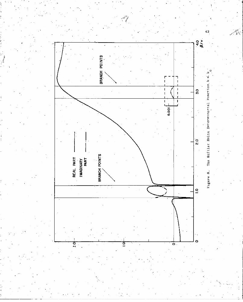
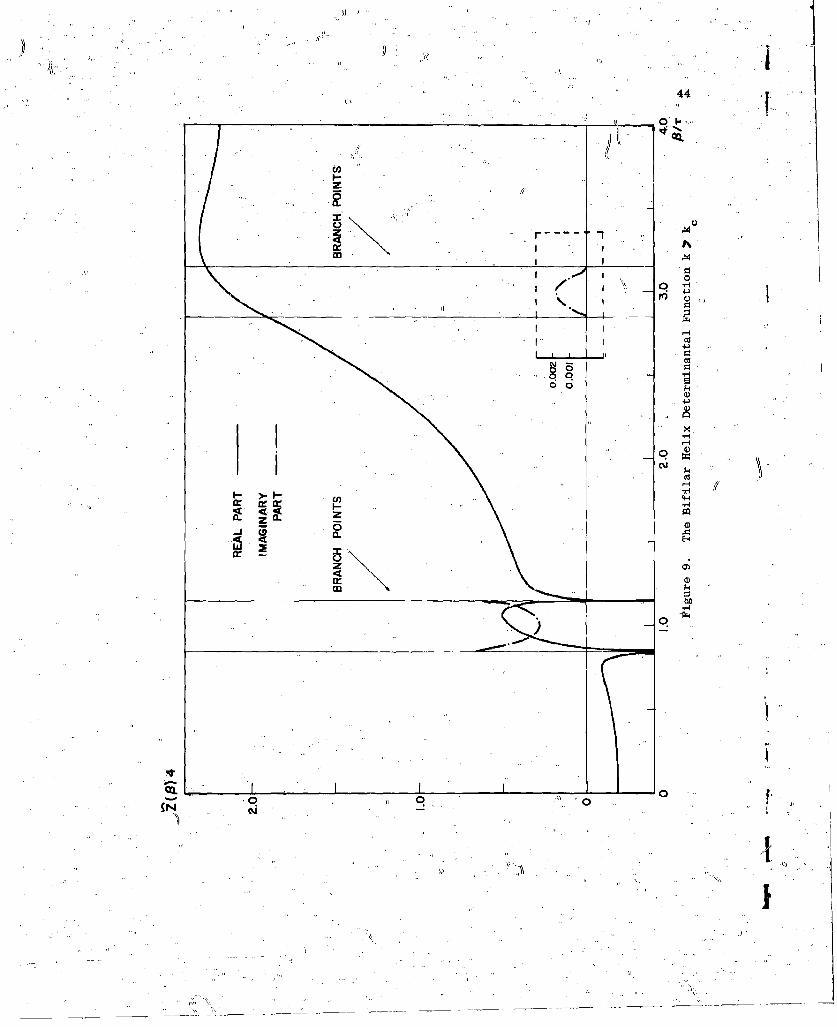
. 42 1'for real" values of B are plotted in Figures 8-and 9. In, Figure 8 the frequency

isbelow the critical frequency (k<k), and in Figure 9 the frequency is abovec

the critical frequency (k>k). In the first instance there are three roots ofc

Z(B) on the positive 3-axis, and, of course, three corresponding roots on the

-negative B-axis since Z(B) is an even function of B. The analysis given here

will be restricted to the second case, where the frequency is above the critical

value k. and where there is only one real root, B on the. positive B-axis.0

The reason for this restriction is the experimentally observed fact that

below the critical frequency a current traveling wave corresponding to the

smallest root of 2(8) dominates the current distribution. This result is shown

in Figure 11 of Chapter 6. The dominance of the contribution of this root is

explained by considering the residue of the inverse of Z(B) at these roots.

The residues are inversely proportional to the derivatives of Z(B) at its roots.

The derivative at the smallest root is always smaller since the function is

logarithmic in the vicinity of the two larger roots) and therefore, its residue

is the largest. Above the criti.cal frequency this root has vanished and only

the relatively weak root at B remains.0

The branch points of Z(B) at

B nT 4. k (n = , + 3, .

all lie on the real axis. This makes it impossible tofactorize the

function Z(B) into factors with a common strip of regularity including

the real axis. This difficulty can be surmounted by assuming that the

medium is slightly dissipative

k.=k -ja~-s0 2.•

The location in the complex,,B-plane of the branch points and zeros of

Z(8) for a dissipative medium is shown in Figure 1Q. The branch cuts

'AI

431 M

I-i

00

ca

la.

10

ft' �

''ft.

44

_____________________ 0I-

ft. ICoI- Iz

UM

I *. I

I I

I I 0

I 10 U,

-4-------* I

* I. I

Os0000 -400

-4-4

* N I�

U) p4-41- -4

L z Os

5

-4

I. I 0

0 0 0N -

ft * 1

'-ft

I,

45

.V1

0

0

Figre 0. TheZerosandB~nc Pint o

inth Cmle Ppbn

i

-46

"shown are chosen to satisfy the condition

e((B -nT)2-k21/2) = 0

If B = g +j 7 the equation of the branch line is

nT)• 7= -k

This provides a strip of. regularity of Z(B) of width 2a including the real axis.

The function 2(3) can be written as the product of two factors

2(B).= R(B) K(S) (33)

such that K(S) is non-zero in the strip and tends to 41 as B becomes large.

The factor K(B) is chosen so that it can be factored by Equation (31).

It is particularly chosen so that its function values are real over as much of

the real B-axis as possible. This allows a relatively simple estimate Tor the

magnitude of K (3) to be obtained as shown in Equation (41). The factor

R(S) remiining will be factored by-a variety of devices. These factors are IB28 B •2 -k2

R(S) =A----o-- a 1'R ([3 A 2_8)I/4 e T(34)

(13 -_B) 22 4.

K( S) 2(5) .en / V' 8 k 2 1/4 1

= 2 2 (13 +k2) (35)(S -S ) A

0

S is the root of Z(S) and the factor ([2-32) removes the zeros from K(B) "o o

satisfying one of the requirements of Theorem C.. The exponential factor

12is chosen to give the correct asymptotic form and to be easily factorizable

2 21/4 k 1/2The factor (S +k ) is chosen to give asymptotic behavior like I.

This factor is chosen because it is 'real on the real S-axis. The term k in

the factor is arbitrary as any other constant larger than a would make this fac-

tor regular inside the strip of width 2a. With this choice of factors K(S) is

real for real k everywhere on the real axis except in the segments I S-nTl< k.

J" . ' ,

47"

These segments will be called the "visible regions" of the rdal P-axis since

only this part of the, Fourier spectrum contributes to 'the radiation pattern as

is shown in Equation (4).

The functici K(P) is well behaved except a l6garithmic singularity at

+ =_l+k

This singularity is integrable in Equation (21), and K(P) can be factorized

by Noble's Theorem C.

4.4 Factorization ofthe Log-integrable Function

If K(3). is represented in polar form

wK(e) = M(P) exp [jI(P)]

we may write

00

K (P) =exp ~ r in M(x) + jd4 (X) dx (36)+ 27 e j x-(-. 00

The integral may be separated into its real and imaginary parts;

00 0 MX

in K(x) dx = -(p) dxx-• x-•

-. 0-0

(37)00

+j (7T In M(P) + ý(x-) dx)

The' imaginary part of this integral gives the magnitude of K+(P),

oo

IK4-( P)I ,m 4Th e x p f dx] (38)

-.00

and the real part gives the phase. The computation o' phase involves the

evaluation of an infinite integral while the magnitude is given by asum

of integrals over the visible range only

" *'

... . ' -'

48

. •. "nT+kr Ptx) r° n *_Cx) dx -"',x-•- dx =s x-83 I

... X_ n - o ; k ,-

where the integral over the range containing B is understood in the sense of

the cauchy principal value.

To show that the contribution to the phase integral of all terms except

for n --- 1, the following.estimate of the phase is obtained. The relative size,

of the phase values for n=l and n=2 can be obtained from Figures 8 and 9.

The function Z(B) may be written

4n 2z(3) =nodd

where(B 2-k2)T (b'y.)K (by n)n(B (39)y

?k 2 cot2J[I n- .n )n- n n+l )n n+( n

If B is in the n-th visible range the n-th term of this series .will be complex

(B)= (B -k )Jn(b/yn) [Nn(byn)jJn(bn

Jn b/ y)[Ng.(byn)•JJ (b'y)]

+1rk2cot 241 (40)

J (b/y'[N (by) IjJ (byn)* n1 n ni-i n ni-1

where

k 2 [ 2- ( nT) 2] 1/2I

For large values of n the first term dominates, and the phase of is given *.

by

1l J (by)%3) tan -n(byn) j(I-nTl c k)"N n (by n)

which is well approximated with the small argument form of the Bessel functions4*

49

when

k cot '< Cn

The result is [n~(P n!in-~t n (k) 2 j cot2ý'/ •nq(p) n. (n-1) 'o4

which tends toward zero very rapidly when n increases. The 'remaining terms

of the series, being positive real increase the real part of the function in

the visible range, thus making the phase of the function even smaller than the

phase of the, complex term.

The phase of K(P) is the same as that of Z(0) except for p1 <p Here0

division by P2 -P 2 makes K(i) positive where is negative. Only in the

range (3) < k is there a non-zero phase contributed to K(P) by the exponential

factor. Therefore, the phase integral will be approximated by

00 n +k

dxnZ Jdx n=-1, 0, 1

0- n -k

If P is in the range (T-k, T+k) the integral in that range is written

T+k T+k

d + )(P) dx+ P)- dx

T-k T-k.

or

T+k

f' P(x), dx + i T+k-3) 1 n('t))"

T-k

Thus the magnitude of K (P) is given, approximately by+

K (T tP) k expx dx + dx+(1 X) ,... •",,. 'T-k ... k

S(41).

,0'50

The magnitude of K (3) is given by two integrals over a finite range

while the computation of phase involves the. evaluation of an infinite integral.

The integrals of these functions are *not known in closed;-•orm, and they must

be evaluatedby numerical tenchiques. It was decided to evaluate only the

magnitude of Z (3) for this reason, and-also because this is sufficient to

determine the magnitude of the radiation pattern.

4.5 Factorization of the Remainder Function

Siqce K (8)..tends toward +i for large 13 the remainder function.

S. ,R(B) = -2B.k2 nyli exp7 (-

A2 2 1/4 ex

must be factorized to give the desired asymptotic behavior,

R (B) AB/! 4'

In addition, R, R_ and their inverses must be regular in the indicated half

planes.

The zeros (4-B ) of R can be assigned to the appropriate half plane by

considering the medium to be slightly dissipative

k = k -3a

The root k° a function of k and can ,be expanded in a Taylor series about

k . The change in B due to the assumption of a small loss, correct to the0 0

first order in a) is given by

0 + 0

Since B3 ipcreases with k, as seen in Figure 6, the root at +B3 is shifted0 0

to the lower half plane by a small loss, and thus,, belongs to R+. Similarly,

the root, at. -3 is a root of R0

The exP•nential factor of R may be factorized by a method due to

%..

S. " .."

I

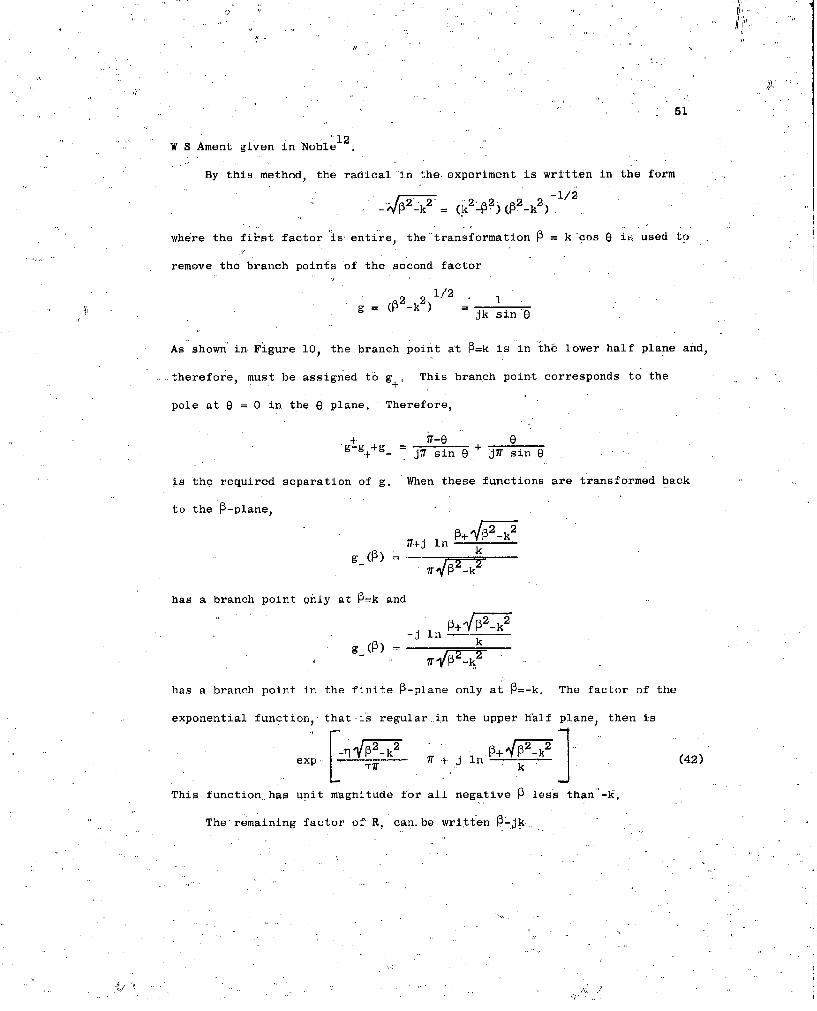
51

12W S Ament given in Noble

By this method, the radical in the experiment is written in the form

_d 2-P cP2 -k2 -1/2

where the first factor is entire, the transformation P = k cos e is used to

remove the branch points of the second factor

1/2g=(2_2) 1jk sine

As shown in Figure 10, the branch point at P=k is in the lower half plane and,

therefore, must be assigned t6 g . This branch point corresponds to the

pole at e 0 in the e plane. Therefore,

____+g_ + 0

+ jI sin 9 jF sin 9

is the required separation of g. When these functions are transformed back

to the P-plane,

Wi-+j ln

g(P) k

has a branch point only at P=k and

-j In k

g(P) = k

has a branch point in the finite P-plane only at P=-k. The factor of the

exponential function, that is regular-in the upper half plane, then is

exp I2 ln k ] (42)

This function, has unit magnitude for all negative P less than"-k.

The remaining factor of R, can.. be written P-jk

tlA' I

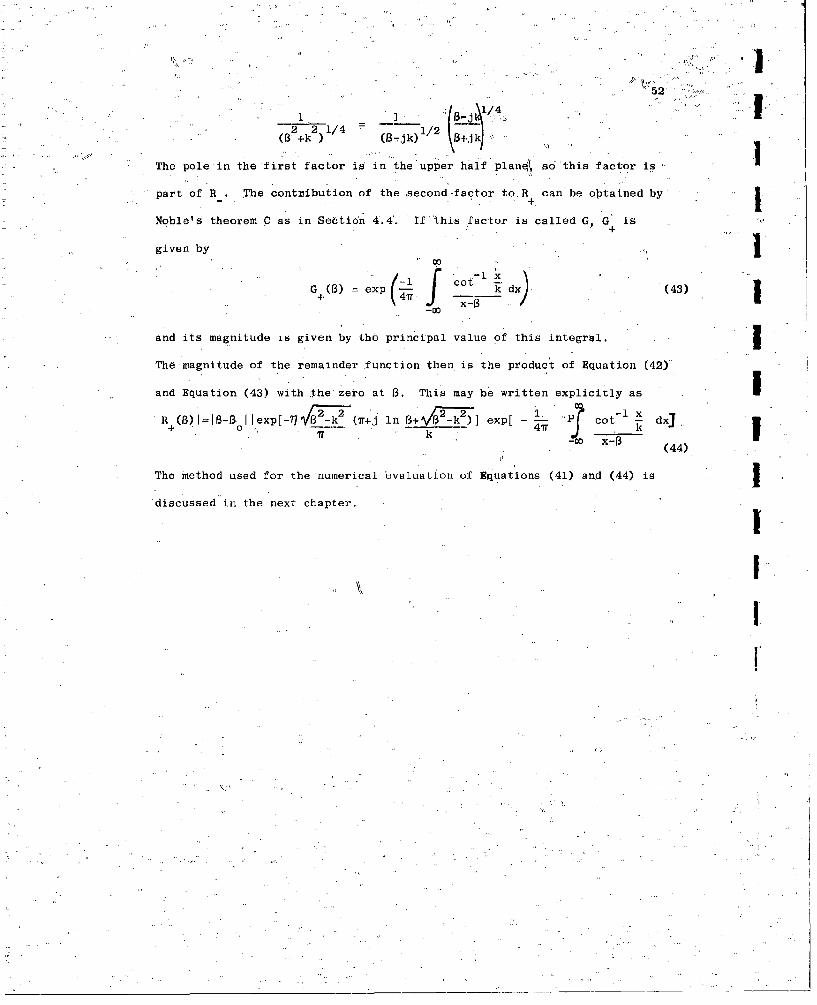
S' .... . - ~ ~52 ",. .. -.

2 2 1/4 = 1/2(B ÷k )(13-ik) X84 jiq "I~

The pole in the first factor is in the upper half plan41 so this factor is

part of R . The contribution of the-second-factor to-R can be obtained by jNoble's theorem C as in Section 4.4'.' If this factor is called G, G is

+

given by j00

G()= exp - cot ki dx (43)+ 4,f X-5

and its magnitude is given by the principal value of this integral. l

The magnitude of the remainder function then is the product of Equation (42)'

and Equation (43) with the zero at B. This may be written explicitly as i"R+ (B) .=IB-r 0 Iexp[•- f•l 7+JV - n ln 13+ •-- exk [ - c. o dxj

-0 X-S(44)

The method used for the numerical evaluation of Equations (41) and (44) is

"discussed in the next chapter.

I

KSI'

"Ji , ,

53

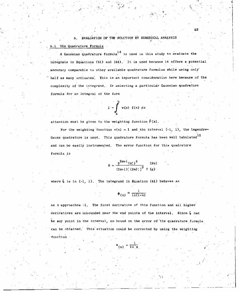
5. EVALUATION OF THE SOLUTION BY NUMERICAL ANALYSISIA

5.1 The Quadrature Formula

14A Gaussian quadrature formula is used in this study to evaluate the

integrals in Equations (41) and (44). It is used because it offers a potential

accuracy comparable to other available quadrature formulas while using only'

half as many ordinates. This is an important consideration here because of the

complexity of the integrand. Ir selecting a particular Gaussian quadrature

formula for an integral of the form

b

= w(x) f(x) dx

a

attention must be given to the weighting function P(x).

For the weighting'function w(x) =.1 and the interval (-i, 1), the Legendre-

Gauss quadrature is used, This quadrature formula has been well 'tabulated1 5

and can.be easily instrumented, The error function for this quadrature

formula is

2 2m+ (mI)4 (2m)

(2m+-l)[(2m)]3 f (g)

where • is in (-1, 1). The integrand in Equation (41) behaves as

1

oKx) in(l-x)

as x'approaches -1. The first derivative of this function and all higher

derivatives are unbounded near the end points of the interval, Since.; can

be any point in the interval, no bound on the error of"the quadrature formula

can be obtained.' This situation could be corrected by using the weighting

function /

"W (x) in x

S4 '

N'.

. .6 : /

54 3.. in a small reg.on near the endpoints of the interv'l (1-k, l+k).

SThe use of a logarithmic weighting function near the end points of theinterval would require the construction of a new set of ortnogonal polynomials

on the interval of integration. This involves the moments of the weighting

function which must be evaluated in terms of the exponential-integral functions.

Since this difficulty is caused by the behavior of the integrand near the endpoints

of integration, and since the contribution of the end regions to the integral

is obviously small, it was decided to use a. sixteen point Legendrq7Gauss luadra-

ture. Although no bound can he set for the error of this quadrature formulait is reasonable to expect that the error will be small. I

5.2 The Statement of the Problem in the Form Used by the Automatic Digital Computer

In preparing a problem for Automatic digital computation, greatest attention

must be given to the most frequent computations in the program. The Legendre- jGauss quadrature of the integral in Equation (41) can be considered as controlling

the program from the point of view of running time. This is caused by the

comparatively long time required to calculate the eighteen Bessel function

values required for each ordinate point. Since the quadrature points do not

depend on the particular values of 1 for which the integral is evaluated, it

was ,decided to compute the ordinate values in a separate program called the

"table generator". This program computes the function in Equation (17) subject

to the approximation in Equation (19) at each of the sixteen quadrature points

and at the thirty-six observation points given by,

1 = r+k cos 6

where 0 takes on increments of 5 from 5 to 180°0. If F(w) = 2 Z(B) is usedT) iu2

to represent the approximate form of thebifilar helix determinantal equationthen

, .<

", ,.. •:":

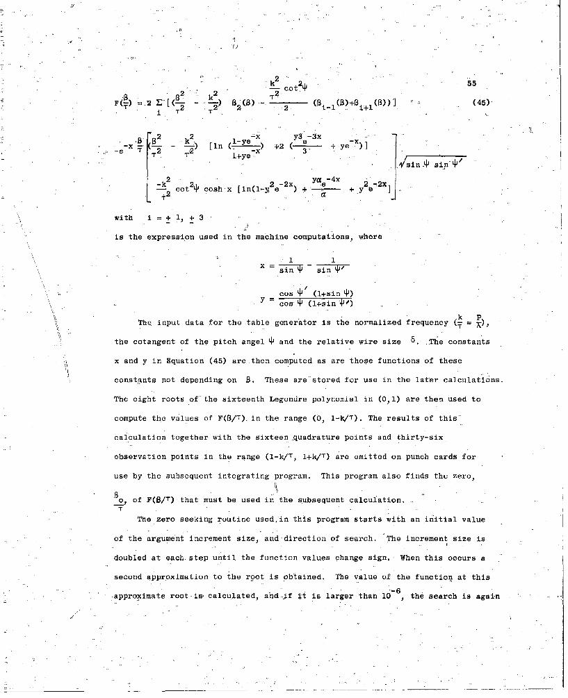
22

2 k2 55

F( 2 13 (B) - (.i (B)Bi+B (B))] (45)72 T72 2 2 i-i i

iK

-e- 1) [in (-Ye) +2y3 + yee.e T2 _ý+ye-x7. (L -)[nC+y

-k2 ya-4x 2-e.2xcotN cosh-x [ln(1-y e-) + - + y

with i =+ l + 3

is the expression used in the machine computations, where

*1 1

x= sin sJ- int/

cos 4 (l+sin Y)cos qj (l+sin N")

k PThe input data for the table generator is the normalized frequency (• = ),

the cotangent of the pitch angel NJ and the relative wire size 6. The constants

x and y in Equation (45) are then computed as are those functions of these

constmnts not depending on B. These are stored for use in the later calculations.

The eight roots of the sixteenth Legendre polynomial in (0,1) are then used to

compute the values of F(B/T).in the range (0, 1-k/T). The results of this

calculation together with the sixteen .quadrature points and thirty-six

observation points in the range (1-k/T, l+k/T) are emitted on punch cards for

use by the subsequent integrating program. This program also finds the zero,

o, of F(B/T) that must be used in the subsequent calculation.T

The zero seeking routine used,'in this program starts with an initial value

of the argument increment size, and direction of search. The increment size is

doubled at each step until the function values change sign. When this occurs a

second approximation to the root is obtained. The value of the function at this

-6.approximate root-ise calculated, andi.f it is larger than 10 , the search is again

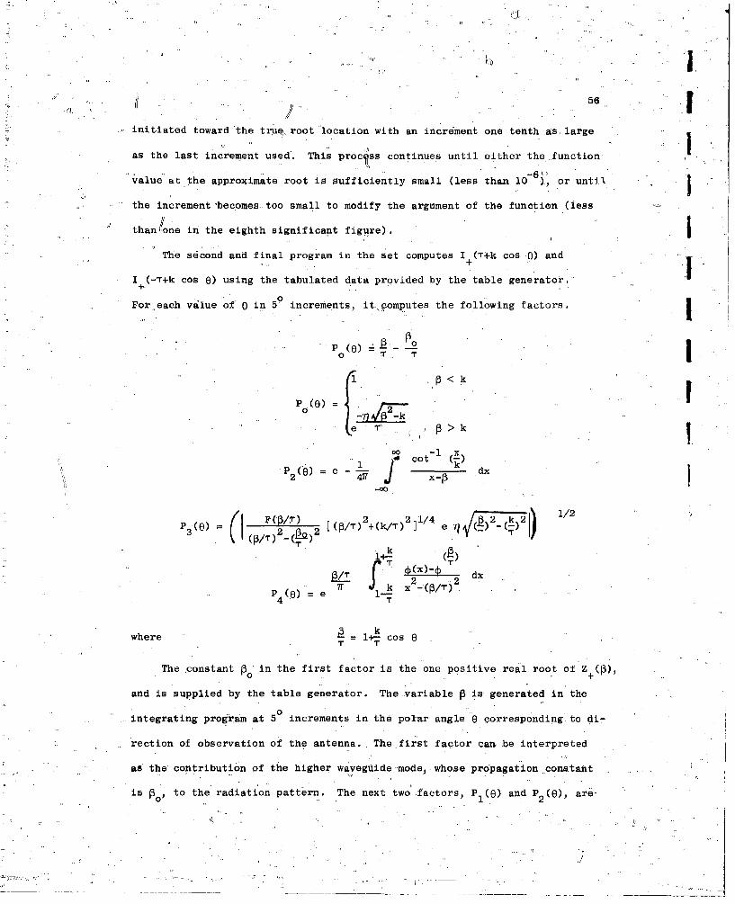
2>56 1

initiated toward the true root location with an increment one tenth as large

as the last increment used. This proc ss continues until either the function

value at the approximate root is sufficiently small (less than 10-)., or until

the increment becomes too small to modify the argument of the function (less

thanione in the eighth significant figure).

The second and final program in the set computes I (T4k cos 0) and

I (-T+k cos 0) using the tabulated data provided by the table generator,

For-each value of e in 50 increments, it, 9omputes the following factors.

P (e) • 0

Po(8) = f_13<_k0

< >k

P 2 (O)=e - j dx

C. d(x).c(kk

P 0 dx

1/(0),0 = PT (/r e i•)

where T = 1- cos T

The constant poin the first factor is the one positive rea'l root of Z+(13),

T T

and is supplied by the table generator. The variable 13 is generated in the

Sintegrating program at 5° increments in the polar angle e corresponding, to di-

:, rection of observation of the antenna. The first factor can. be interpreted

• ~~as the contribution of the higher waveguide. mode, whose propagation constant ,

is 1o, to the radiati'on patt'ern. The next two'.factors, Pl(O) and P 2 (8), are.

4 T

aU

57

included to insure the prQper asymptotic behavior of Z (B)' and consequently of

The values are generated in the integrating program independently of the

functton values of F (y) supplied by the table generator. These factors have

relatively little effect on the value of T (8) in the visible range.+

The last two factors, P3 (e) ando 4 (O• exercise primary control over the

shape of the radiation pattern. The fac t'6r P 3 (8) depends primarily upon the

Bmagnitude of F(-) at the observation points. P'((8) 'depends upon the phase at

T 4

the observation points as well as the phase at the quadrature points. The

integrating routine obtains the real and,%imaginary parts of FC-) from the tableT

supplied by the table generator and converts them to polar form. The magnitude

is then used to compute P while the phase is integrated to obtain the value of.3

P4"

The product,-of these factors is taken for the magnitude of Z (8). The+

inverse of the product is then interpreted as the magnitude of the Fourier

spectrum of the current distribution The vector potential for the backfire

bifilar helix results when the current spectrum is multiplied by the functionk

Jo( kcot 4 sin 0)

as indicated in Equation (5). The radiation pattern can be deducedfrom this

as indicated in Chapter 2. Radiation patterns were computed for a range Gt

pitch angles, relative frequency k/T, and relative wire sizes 5. The results

of these computations are discussed in the next section wherethey are compared

with experimental results.

> . ....

58.(.EXPERI 7/AL!ANDITHEORETICAL RESULTS

6.1 The Experimental Study

the study of the bifilar back fire helical antenna was start 1ed as pa.r t

of a,,larger investigation of the properties 6f periodic .radiating structure~s.

This investigation in turn was started in an effort to learn more ..about the

16-1 19

behavior of log-periodic antennas16 18 i this connection it is suggested9

that the properties of a log-periodic structure, as a function of distance

,. from the apex, are related to those of a periodic structure whose period is

given by the local pec'i-ld of the log-periodic structure. In this sense the

hifilar helix is an analog oY the two arm equiangular spiral antenna18

The portion of a log-periSu ic antenna, nearest the feed point at or near

thehapex of the structure, acts as a transmission line aarryng the energy to

the larger portion. The energy is carried to the so-called "active region"

of the st))ructure whose position and size varies linearly with frequconcy. This

region is thought to be primarily responsible for the radiation from the antenna.

Beyond this region, ..the current decays rapidly'. These characteristics of the

blog-periodic antenna are observed for the bifilar helix when the variation of

distance from te apex is replaced with a pvriation of frequency.

The operation of the helix as a waoeguide is discussed in Chapter 3.

Theieit is seen that the propagation constant is given approximately by

B k/sinuntil the sedge of the visible range is approai hed. That is until runy T

S....k = T -k',:sin 4

This equation defines the cutoff frequency or critical frequency of the

principal waveguide moe vof an infgnisely thin helical conductor. This critical

k I) I

59

frequency, normalized with respect, to Tr is calledX to avoid conxusiodl. with

the critical frequency for a finite size helicai, copductor. It is giv9n .,

explicitly by

DC sin (46)l+sin Y

The critical frequency marks the boundary between the frequencies for which

the helical structure is primarily a waveguide and the frequencies for which

it iS. a useful antenna.

Sevejal models of the bifilar helical antenna were constructed for a

range of)Cbetween 0.05 and 0.4. The physical dimensions of these models

are given in Table I. These are based upon a frequency of 1.5 Gc, The

pitch of the helix is determined from the wavelength at the base frequency by

p )(A (47)

The pitch angle is given by

= sin- 1(1 ) (48)

and the mean radius of the helix is given by

b =L -j.T236 (49)27r

The waveguide operation of these models was.studied by sampling the fieLds

near the antenna with a current loop moving parallel with the axis of-the helix,.

A typical amplitude response of this loop as a function of distance from the

feed point is shown in Figure 11. The antenna was fed by a balanced two wire

line. Below the critical frequency, the propagation c6nstant of the waveguide

mode can be easily determined by the standing wave on the structure. The propa-

gation constants measured in this way are slhown in Figure 12. It is noted that

"the cutoff frequency for each of-these models is somewhat below due to the

finite wire thickness. The cutoff frequency for the models tested in this'investi-

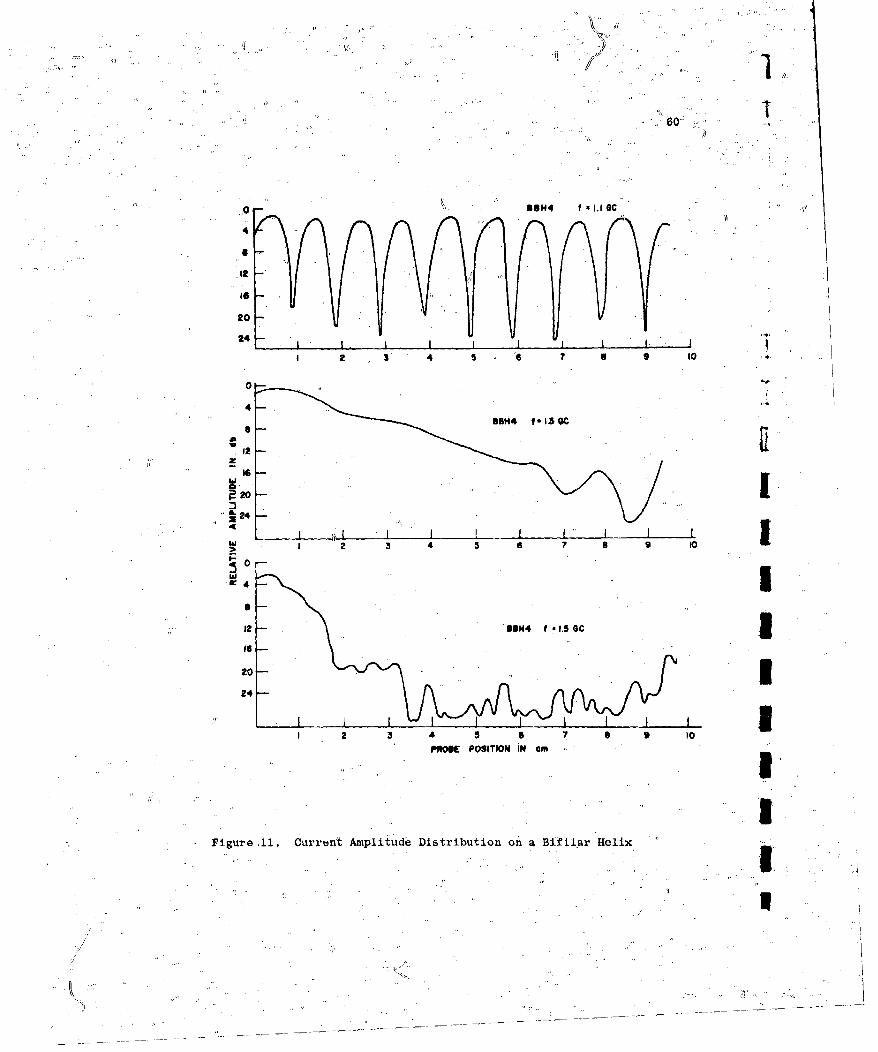
* 60

5@H394 f .1.1 OC

4

20

24

I 2 3 4 5 .. 9 10 *.

4-

20

24

IsI20 324

I 2 3 4 5 S 9 10

PROE POSITON I M.

Figure .11. Current Amplitude Distribution on a Bi Ifil~ar Heli,X

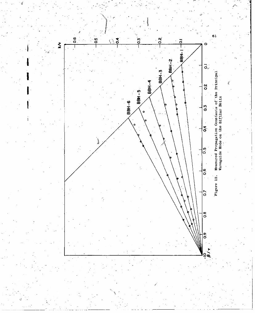
-Q

. I, I

U)~4 -HJ

0~~~ 006 o

10) '-,

1-4

(0

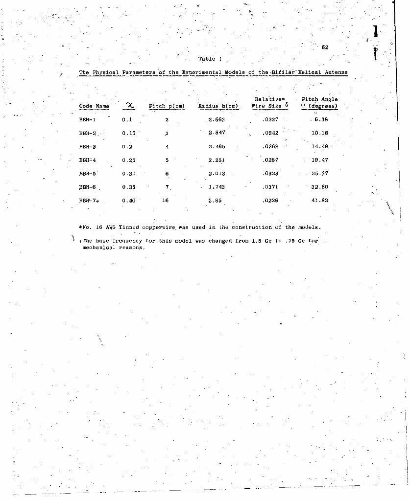
62

Table I

The Physical Parameters of the Experimental Models of the.Bifilar Helical Antenna

Relative* Pitch AngleCode Name 'X. Pitch p(cm) Radius b(cm) Wire Size & 4 (degrees)

BBH-l 0.1 2 2.663 °0227 6.38

BBH-2 0.15 3 2.847 .0242 A 10.18

BBH-3 0.2 4 2.465 .0262 14.49

BBHL4 0.25 5 2.251 0287 19.47

BBH-5' 0.30 6 2.013 .0323 25.37

,BBH-6 0.35 7 1.743 .0371 32.60

BBH-7+ 0.40 16 2.85 .0226 41.82

*No. 16 AWG Tinned copperwire was used in the construction of the models.

4+The base frequency for this model was changed from 1.5 Gc to .75 Gc formechanical reasons.

*:• G 3'-, *-

63

gation is plotted as g function of the pitch angle t in Figure 13, where it is

4 compared witht. , the normalized cutoff frequency for an infinitely thin wire

model. K

An uhusudl feature of the standing wave pattern of the waveguide mode on

the bifilar helix was noted during the course of the measurements. The apparent

guide wavelength increases with frequency from a minimum at zero frequency equal

to the pitch-of the helix to a maximum at the cutoff frequency, the max*mum

-being somewhat less than the free space wave length. This indicates that the

principal wavegulde mode on the bifilar helix is a backward wave. The phase

constant decreases with increasing frequency, and therefore, the phase velocity

and the group velocity must have opposite signs. The group velocity must be

directed away from the feed point (i.e. in the positive direction), gherefore the

phase velocity is in the negative direction as indicated in Figure 12,-

Thu measured results in Figure 12 do not seem to agree with the calculated

results'showr.,in Figure 6. However, Figure 6 gives the phase progression of the

current along the helical conductor, while Figure 12 gives the phase progression

of the near fields of the hifilar helix. The results of Figure 6 agree with the

5results of Marsh for phase measurements along the wire. When measurements

along the helix parallel"rto the axis are made, an additional phase ehift of 2ir

radians per turn is observed. This is the expected result since the test

probe is now moving from one conductor to the other as it travels along the

helix. At zero frequency therefore, the phase changes by 7T radians as each

conductor is crossed. From another point of view, the additional 21T radians

of phase shift results from the rotation of a tangent to the helical conductor

as it moves along a turn of the helix,

'It is seen in Figure 11, that above the cutoff frequency, the standing wave

3 **,, ..

47w " l

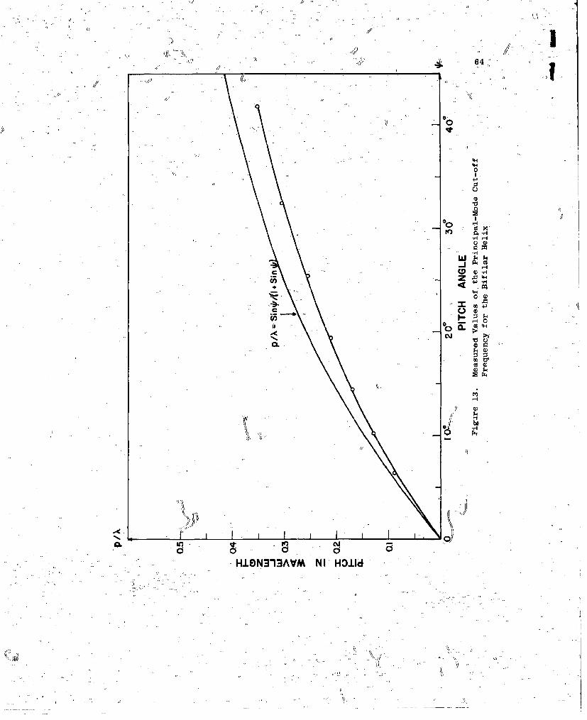
(1' 64:

00

0 .)

1-4 0-

A COO)

06 S

H.1DN,313AVM NI'HO.Lld

65

has vanished and is replaced by a decaying amplitude distribution. As frequency

is increased further the rate of decay increases. This is shown in greater detail

in Figure 14. At these higher frequencies, a standing wave distribution again

appears with a maximum amplitude about twenty decibels below the input level. This

is the higher order helical waveguide mode. The excitation of this mode increases

with frequency from a negligible level near the cutoff frequency of the principal

mode. The development of this mode places an upper limit on the frequencies for

which the bifilar helix behaves as a backfire antenna.

Phase measurements made in the near field above the cutoff frequency are

shown in Figure 15. In this figure the phase is normalized to the free"space

propagation constant and is plotted in centimeters. The first curve shows that

the phase is leading as the probe moves away from the feedpoint. The first

curve, slightly above the cutoff frequency, kc, "shows leading phase over most of

the length of the structure. As frequency is increased, the direction of phase

progression near the end of the structure changes and is away from the feedpoint.

The point at which the phase progression changes from leading to lagging moves

near to the feed point as frequency is increased. This corresponds to the

point at which the feed region currents have decayed to the level of the higher

order helical waveguide mode.

The near field phase measurements indicate that, although they do not

correspond to a proper mode, the feed region currents have a backward wave

character above the critical frequency, k This leading phase characteristic

persists as-long as the feed region currents are dominant on the"structure.

On the remainder of'ose structure the higher order waveguide mode,' with its

lagging phase or forward wave characteristic, dominates the current distri-

bution. The fact that in the feed 'region the direction of chase progression

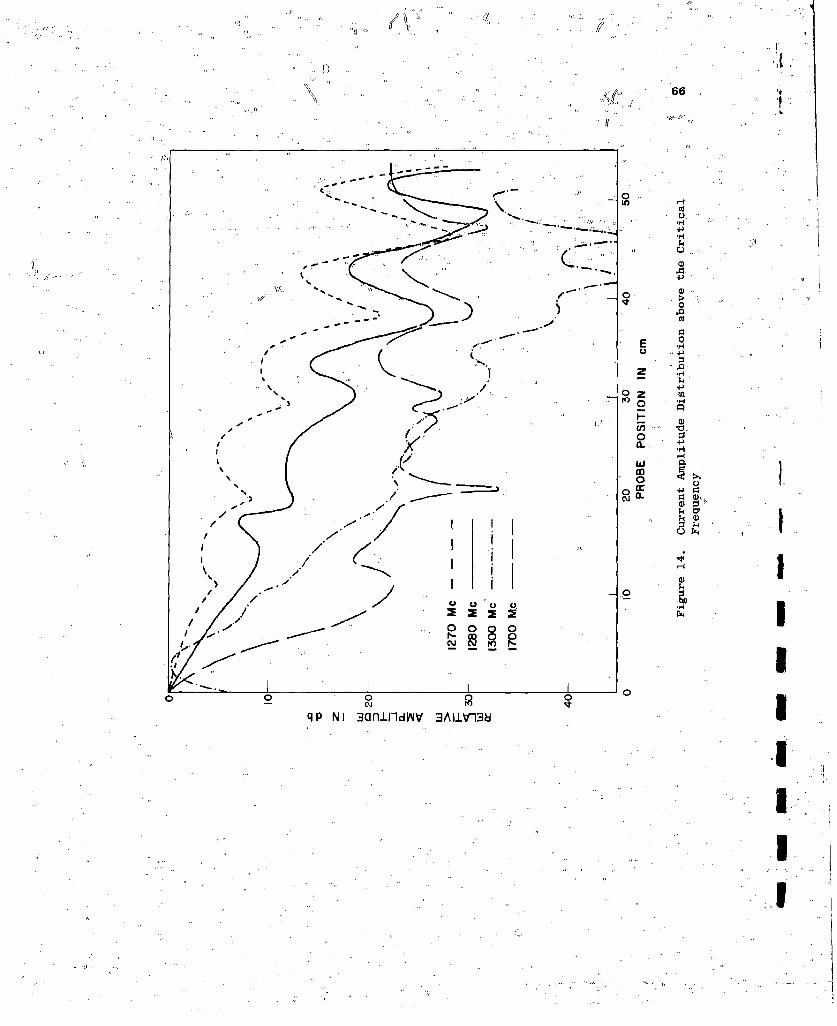
66

4.)

~'1 0

.- ,

- -~. - E .

0 v,1' :

* .L2 - -~ -

qP NI 3o lItV3AI.I

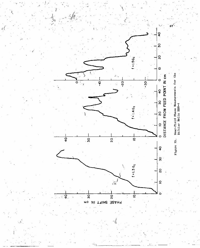
N6

0

0 $4

It)H

(0 . 0

LU

UU0 0

r-40L

C' H

0 0

0

0

0 0 00

WO NI .LJIHS 3SVHdl

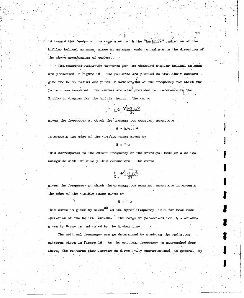
. ... •2

,, //68

is toward thi4 feedpoint, is copsist~ent with the "backfire. radiation of the

bifilar helical antenna, since an antenna tends to radiate in the direction of

the phage prog )ession of cu:ttent..

The. measured radia.titdn patterns for the backi.ire bi nliar helical antenna

are presented in Figure 16. The patt.erns.are plotted so that their centers

give the helix radius and pitch in wavelengths at. the frequency for which the

pattern was measured. Two curves are also provided for reference,,tq the

Brillouin diagram for the biffilar helix, The curve

bA' -2rp/X" b/k

2"7"

gives the frequency at which the propagation constant; asymptote

Sik/ysin n.i

intersects the edge of the visible range given by

8 =T-k

This corresponds to the cutoff frequency of the principal mode on a helical

waveguide with inf.ini.tely thnn conductors The curve

K' Igives the frequency at. which the-propagati.on constant asymptote intersects

the •edge of the visible ranke given by . 520

This curve is given by Kraus2 as the upper frequency limit for beam mode 3operation of the helical antenna. The range of parameters for this antenna

given by .Kraus is indicated by the broken line

The critical frequency can be determi~ned by studying the radiation ,3

patterns shown in' Figure 16. As the critical frequency is approached from

above, the patterns show increasing direcrivity characterized, i n general. ,

" ~I

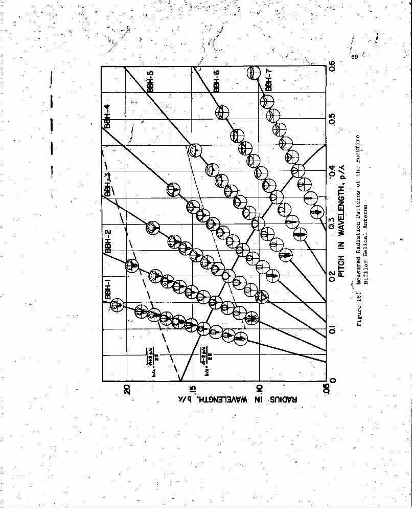
69

I, 0

0604

"0

Z IId C,

b0

In o-

y/ q HIONMAVM I .. nicv

m7G

"/dl'io r baklobe. Below 70e Va single) lobe with little or no e dZ41r e radiation back the

critical frequency,,the patterns have many lobes and the pattern shape changes

"rapidly with frequency. This indicates the standing wave current distribution

on the antenna. As the frequency is increased the patterns t~end to broaden and, -..

for larger pitch angles', tend -to form a split beam. This is due td two.,efýeqts:

first, the phase progression in the feed region tends to become fastetý than light,

and second,- the rate of current decay in the fee'd region increases, decreasing

the effective aperture.. The splitting of the main beam is not observed for

smaller pitch angles because the effective aperture is too small to formt uistinct

beams. For the larger pitch angles, the rate of current decay is smaller, and

the larger effective aperture can produce a well-defined beam. This result is

consistent with Equation (20) where it was shown that the coupling of the

antenna current to the radiated field is controlled by 6 /sin ', Since the

relative wire. size 'does not change apprecial:ly over the range of models tested,

the decreasing pitch angle serves to increase the coupling'and hence the rate of

current decay. "

6.2 Comparison of Computed Patterns with Measured Patterns

The effect of wire size is not shown in the experimental results of this

study, but it is illustrated in the computed patterns shown'in Figures 17-23.

The patterns for the' largest wire size (0 = 0.2)"show the least variation with

. fiequency. The patterns for the smallest wire size (6 = 0.002) have the,greatest /

directivity near the critical frequency, but tend to broaden faster with frequency.

It chn also be seen from the computed results that a change in wire size is,,mor%

effective in changing the shapeof the radiation pattern for larger pitch angles.

(,This again indicates the dependence of the performance of the backfire bifilar

'hlical antenna on 5/sin ..

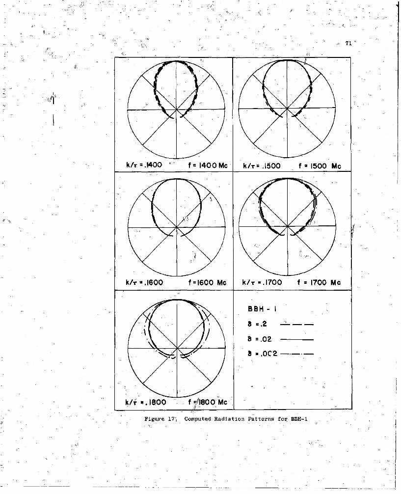
71'

*k/Ta.1400 f 1400Mc k/Tum.1500 f 1500 Mc

411

k/r m.1600 f 1600 Mc k/r -.1700 f =1700 M c

BBH-I

8 Z0

k/Si 100 fiI0Mc'_ _________

Figure. 1T.; Computed Radiation Patterns for BBH'-1

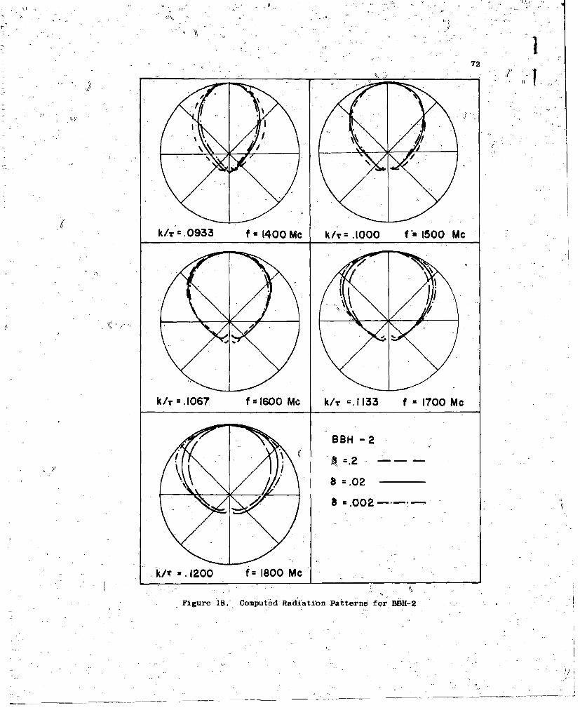
72

k/r.0933, f' 1400 Me k/Tc .1000 fu 1500 Mc

k/r .1067 f 1600 Mc k/r '1133 f 1700 Mc

a c.02

a -. 002---

k/rx. 1200 fa 1800 Me

Figure 18. Computed Ra'dflatibnPatterns forBBH-2

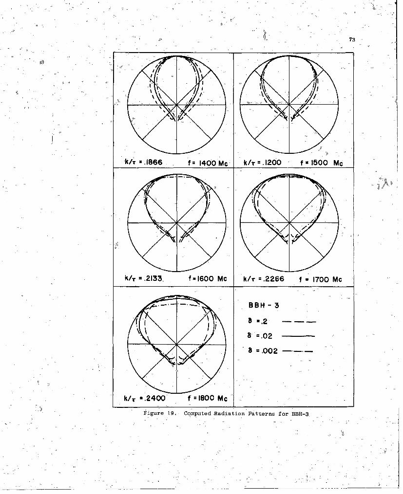
73

k/T.166f= 1400 Mc k/r .1200 f 1500 Mc

k/T .2133, f=1600 Mc k/r =.2266 f 1700 Mc

BBH- 3

z..2

a. .02

a -. 002

k/r z.2400 f 1800 Mc

F~igure, 19.. computed Radiation Patterns for BBH-3

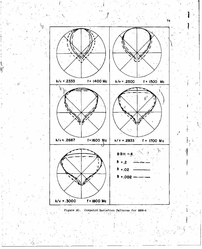
74

tv,.,

~ki.

*k/r F(2633 f 1400 Mc kl/rz.2803 fl 1700 Mc

5.2.

B=.02

j 8=.002

k/T=m.3000 ýf 1I00 Mc

Figur~e 20. Compute'd Radiation Patterns for BBHw-4 .

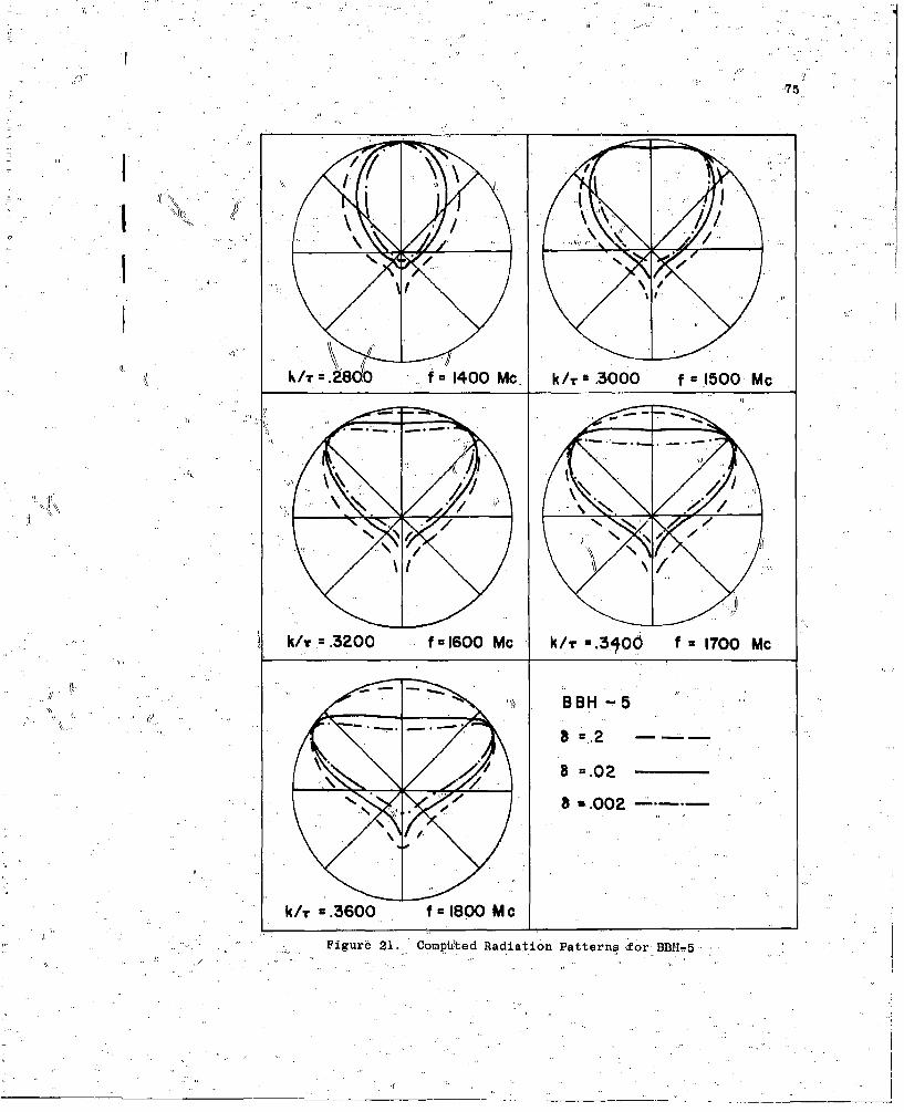
75

I It

/T f=I 400 Mc k /.r.3000 f ýI5OO Mc

k/i u.3200 f c 1600 Mc k/ir z.3400 f a 1700 Mc

=.0

B .002

k/T -.3600 f aI800 Mc

Figure 21. Comptited Radiation Patterns '.or BBH...5

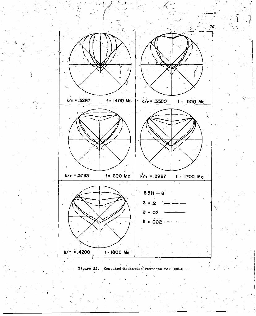
A v!

wk/r r-3267 fz 1400 Mc k /r .3500 fu 1500 Mc

k/r =.3733 f x1600 M c Or m.3967 f 1700 Mc

BBH-6

m..2

.8w.02

a z .002

k/v w.4200 f 9 800 Mc

Figure 22. Computed Radiation"Patterns for BBH-6

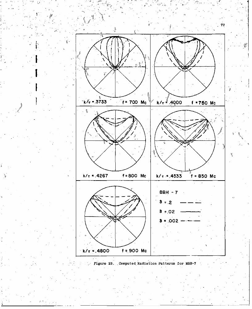
77

k/T m.26 f /80M /,, 3 f 80M

a .002

"k/ .34800 fa 7.00 Mc ~kT 40 70M

piur 23., -.optd.aitinPten o Bý-

. .. *ii

.• 78

freque pattern was computed for each' of the antenna models for the normiializedf requency/ '

T

Th i.s corresponds to the model frequency. of 1.5 Gc. One pattern was computed

for a frequency one hundred megacycles below this frequency,-and three were

computpd in increments of one hundred megacycles above this frequency. It

was considered desirable for uniformLty to use the same wire sizes for the entire

range e. antenna parametets. The value (6 = 0.02) was chosen as a convenient

number near the values obtained for the experimental models. Wire sizes of

,one tenth and ten times this value were used to show the effect of wire size

ton the,-performance of the antenna.

The computed patterns for the wire size & = (0,02) are compared with

measured patterns in Figures 24-30.. The agreement between the measured patterif

and the computed patterns is good in the main beam. There is a considerable

difference in the shape•' of the computed and measured patterns in, the direction

of the structure (back ,lobe), The radiation in this direction is controlled

by the length of the helical antenna in the manner described in the next

chapter. In this chapter we will limit our discussion to a comparison

betwepp the main beams of the computed and measured patterns.

In the patterns for BBH-I, Figure 24, the agreement between the computed

and measured patterns is quite good. The relative wire size of the experimental

model & = 0.0227. This does not differ much from the value (6 0,.02)' used in

the computation. In addition it can be seen in Figure 18 that the shape of

the radiation is little dependent on the relative wire size. For BBH-2 through

BBH-6 the relative wire-size increses, and the agreement between the measured

pattern and the patterns computed for 6 0.02 becomes poorer. The agreement is

VI

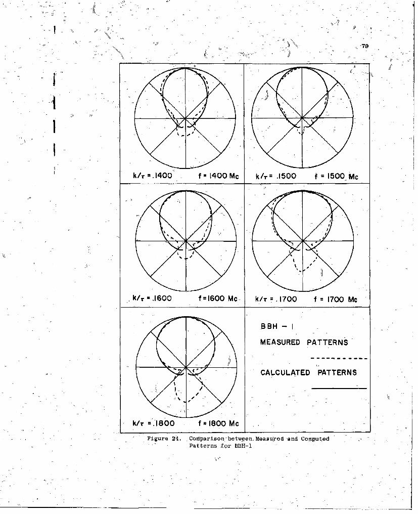
1~. v 79

k/T m.1400 f 1400 Mc k/T= .1500 f 1500 Mc

k/T =.1600 f=1600mcý k/-r:1700 f~ 1700 Mc

B BH-

MEASURED PATTERNS'

CALCULATED PATTERNS

*k/TK'-1800 f=1800 Mc

Figure 2:4. *Coniparison- be twee r, Meas ure d and ComputedPatterns for BBH-1

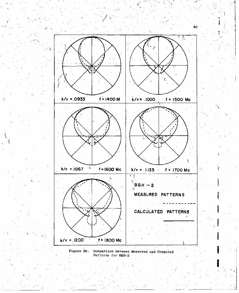
80

k/r *.0933 f 1400 M k/r- .1000 f~ 1500 Mc

k/r =.1067 f 1600 Mc k/T:.1133 f= 170 0M c

BBH -2

ffiMEASURED ,PATTERNS

CALCULATED PATTERNS

k/T =.1200' f: 1800 Mc

Figure 25. -Comlparison between Measured apd. ComputedPatterns for BBH-2

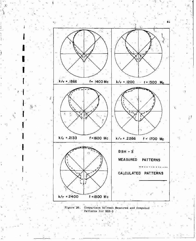
IkIT =1866 fm 1400 Mc k/T =1200. f 1500 Mc

k k/r -.2133 f =1600 Mc k/T .2266 f =~1700 Mc

MEASURED PATTERNS

CALCULATED PATTERNS

k/r m.2400 f m 1800,N Mc

Figure' 26. Comparison bet wee'n Measured and ComputedPatterns for: BBH-3

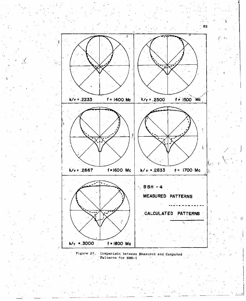
82

k/i a.2233 f= 1400. Mc k/T .2500 f1500 M

k/iT .2-667 f c1600 Me k'/T. .2833 f 1700 Mc

- . BBH -4

MEASURED PATTERNS.

CALCULATED PATTERNS..

k/.r w.3000 fuI800 Mc

Figre27 Copaisn etween Measured and ,Computed .

"patterns for BBH-4

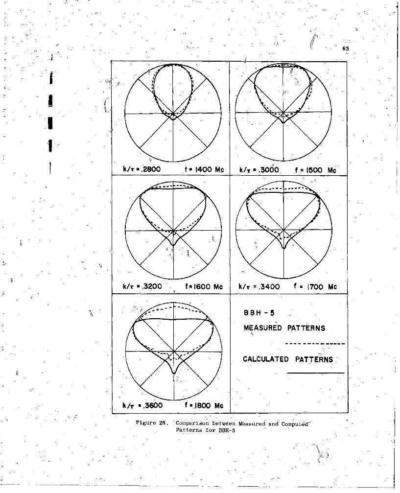
83

k/i m.2860 f a 1400 Mc k/i Z.3000 f,= 1500 Mc

k/-r P.3200 f x 1600 Mc k/i = .3400 f =1700 MC:

'~ <~ .BBH -5

MgLASURED PATTERNS

CALCULATED PATTERNS.

Figure 28-. Coprsnbetween.Moasured and Compute&'Pa~tterns for BBH75

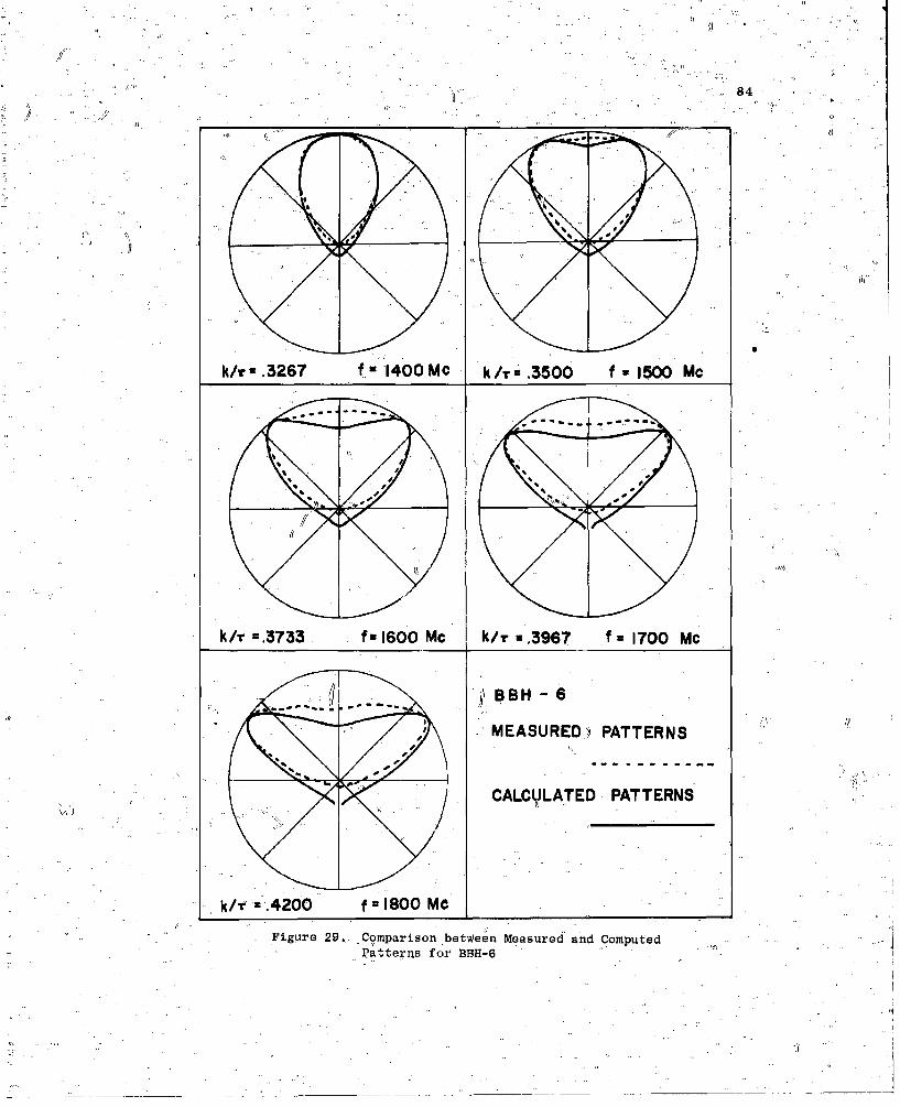
r 84

k/r a.3267 f.1400 Me k /-r.3500 fu 1500 Mc

k/-r c.3733 f a 1600 Me k/T =.3967 f=1700 Mc

MEASURED), PATTERNS

CALCYLAITED PATTERNS

k/T -. 4200 fals800Me

Figure 29. -. Comparison betWeen Measured'and ComputedP7atterns for BBH-6

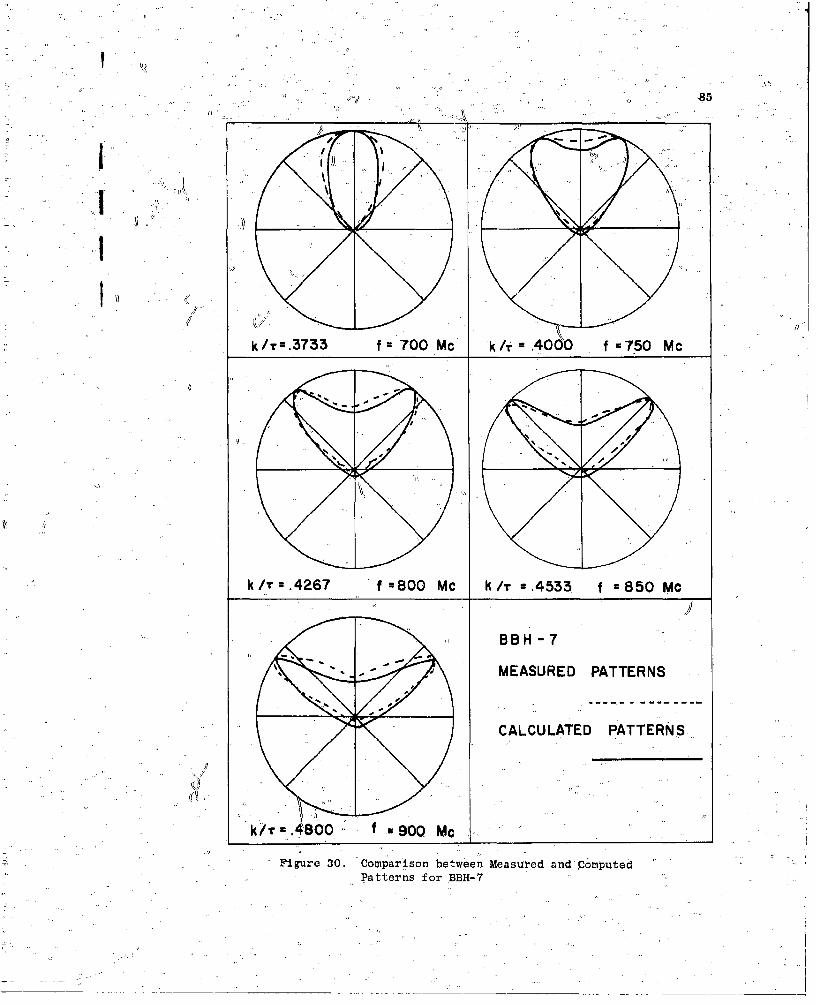
AlJ

kT2375 f. 700 Mc k/i .4000 f :750 Mc

k /T .4267 f =800 Mc k/T -.4533 f =850 Mc

- - -MEASURED PATTERNS

CALCULATED PATTERNS

k/Tu,80 f =900 Me

Figure 30. Comparison between Measui-ed and',omputod "C

Patterns for BBH-7

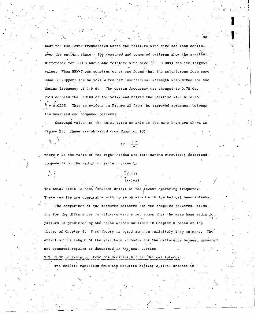
*''t1

"xx Sd86-

best for the lower frequencies where the relative wire size has less control

over the pat~ern shape. Tr measured and computted patterns show the greatest

difference for BBH-6 where the relat~ive wire size (: 0.037) has its largest

value. When BaH-7 was constructed .i; was found that. the polystyrene foam core

used to support the helical wires had insufficient. strength when sized'for the

design frequency of 1,5 Go The design frequency was changed to 0.75 Gc,

This doubled the radius of the helix and halved the relative wire size to

= 0.0226. This is evident, in kigure 30 from the improved agreement between

the measured and computed patterns,

Computed values' of the axial ratio on axis in the main beam are shown in

Fiugie-31." These are obtained from Equation (6)

I+t-r

where r is the ratio of the right-handed and left-handed circularly polarized

components of the radi-ation pattern given by

I 1(1-k)

The axial ratio is best. (nearest unit-y) at the lowest operating frequency.

These results are comparable with those obtained with the helical beam antenna.

The comparison of, the measured patterns and the computed paLi.erns, allow-

ing for the differences in relative wire size. snows that The main beam radiation

pattern is predicted by the caicultations outlined in Chapter 5 based on the

theory of Chapter 4. This theoxy is b.sed upon an infinitely long antenna, The

effect'.of the length of the structure accounts for the difference between measured

and computed, results as dtscribed.in the next section.

6.3 Endfire Radiat.•on from the Backfnr4.Blfilar Helical Antenna

The endf ire radiation from the backfire bifila;y helical antenna is --

VA

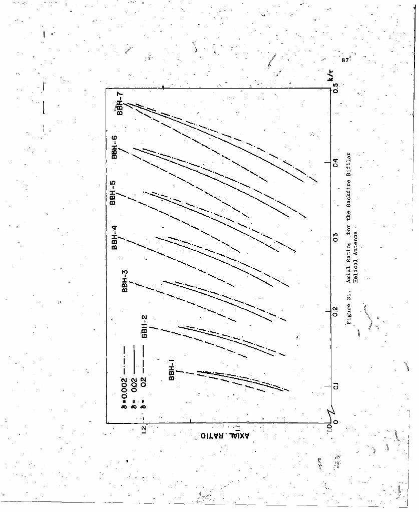
,ST,

IH

c.)('S

AMC

LD0

0H 0

00 do d

4c

OjjV8,IVI X

controlled by the root B of the determinantal equation. Values of this root

for the parameters used in the pattern calculations are shown in Figure 32.

In' this figure the normalized values of the root 1 have been

shifted to the right one unit to account for.-the difference between the

apparent phase constant as one travels along the wire and as one travels along

the helical axis. Thus zero corresponds to a circularly polarized traveling

wave of current traveling along' the positive z-axis from the origin.

Se Jo + a)z z <0

'The pattern produced by this distriv.tion is

00

B3-k cos 6-ja

In this equati'on I is proportional to the residue of I (B) at B = B . This.

T~, hecae orItoer , heslpeofZ() t i v~yIage ad 0iresidue is inversely proport~ional to the slope of •,(B) at- 8 =` B •Figure 10

/, h s . Iv

At the same time, (B -k) is very large when k is near k and decreases rapidly

as k increases. The computed patterns for BBH-l and BBH-2 show no radiation due

to B because (B -k) is too large. At the other end of the range of parameters,20 . 0

d . ..

N. . .. "V

/

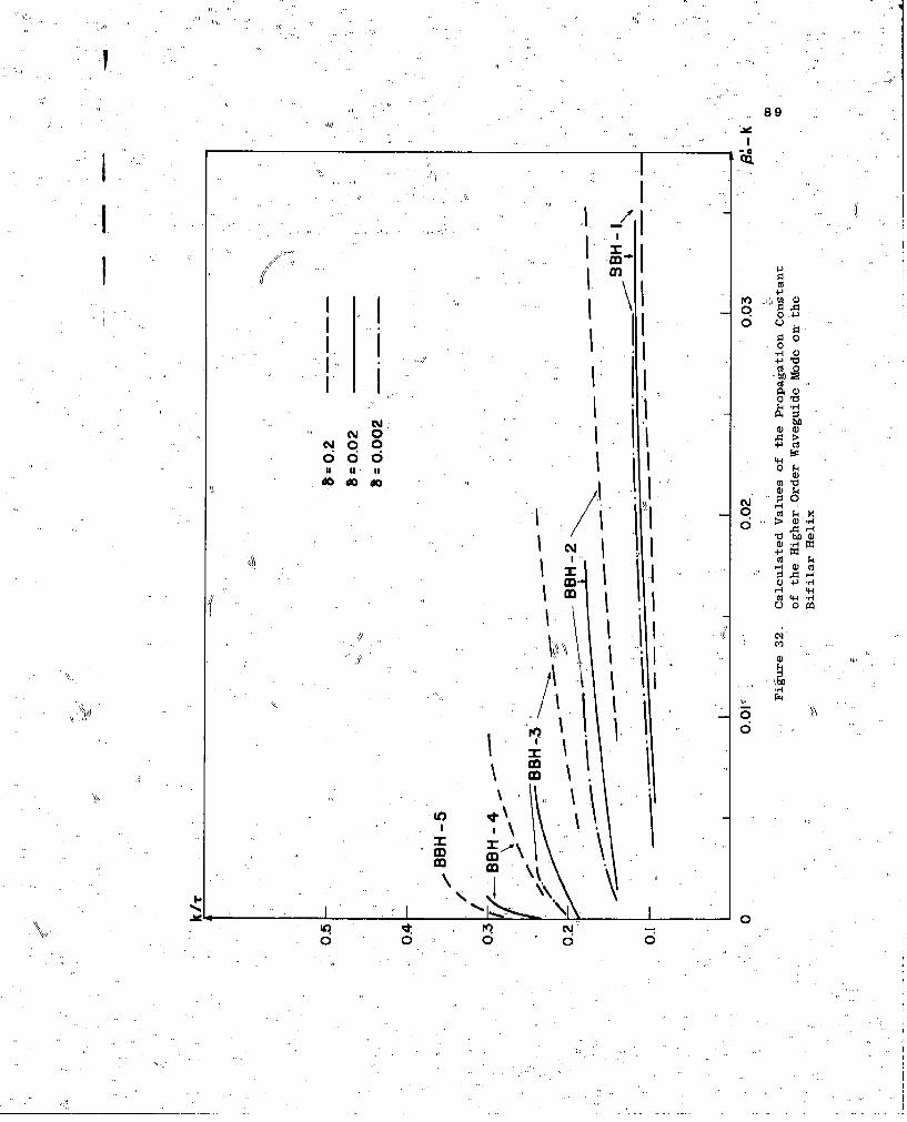
89

4-C

O4-

-P VIt '-a

I I'

I4 CO RC1,

r- 0)

90

BBH-7 shows little radiat'on due to S becauseI smal. 'The effect of0

relative wire size on this phenoenon is shown.din the patterns for BBH-3,

Figure 19. IA this figure the curve for the largest wiresie (8 =0..2) does

not have rsa4ation due to B "while the smallest wire (8"= 0.002) does., Endfire

~f. radiation due to B is also evident .in the paltterns for the.,bt4er models.

If the bifilar helical antenna is long. enough to support the feed

region current, the shape of the main beam is' not affent-oYd by truncation of

the structure. The radiation due to B is, however, controlled by .theA0

length, L, of the antenna. Considering only the incident wave, Equation (50)

must be modified for the finite antenna as follows

f•-j(B'-k~ees O).+t]z

P (6) = I j e)o C ) Zdz

0(51)

-[0(C/-k cos 0)+a]Le -i

= Io -[j-B'-k cos ).•a0

For vanishing a, the magnitude of P (0) at 0- i•

sin (13'-k)PL(0) =2 1Iv/2 - -k

0

Thus when(Bo -k) L/2 is small the radiation \4.n the endfire direction is reduced

by the factor (B -k)L. ý

P L(0) (B 0-k)L P(O) (52)

The magnitude of P (6) at other angles is given by

PL(6) = IL sin x (53)

"L 0 X

where

x = (B'-k cos 0) L/2o

',N,

' ..-

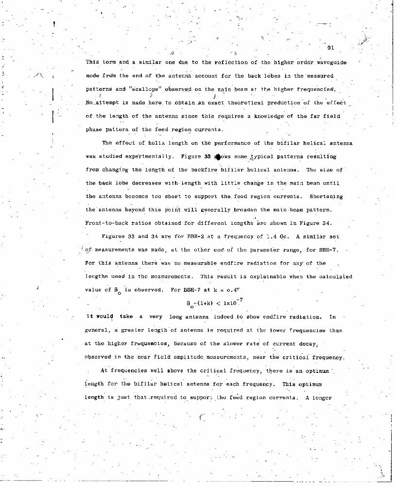
191

This term and a similar one due to the reflection of the higher order waveguide

mode from the end of the antenna account for the back lobes in the measured

patterns and "scallops" pbserved on the main beam at the higher frequeneiel.

.No.-attempt is made here to obtatn an exact theoretical preduction of the effebt

of the length of the antenna since this requires a knowledge of the far field

phase pattern of the feed region currents,

The effect of helix length on the performance of the bifilar helical antenna

was studied experimentally. Figure 33 Aows some ,jypical patterns resulting

from changing the length of the backfire bifilar helical antenna. The size of

the back lobe decreases with length with little change in the main beam until

the antenna becomes too short to support the feed region currents. Shortening

the antenna beyond this point will generally broaden the main beam pattern.

Front-to-back ratios obtained for different lengths are shown in Figure 34.

Figures 33 and 34 are for BBH-2 at a frequency of 1.4 Gc. A similar set

o9f measurements was made, at the other end of the parameter range, for BBH-7.

For this antenna there was no measurable endfire radiation for any of the

lengths used in the measurements. This result is explainable when the calculated

value of B "is observed. For BBH-7 at.k = o.4T0

-7B -(l+k) < 1xl0

it would take a very long antenna indeed to show endfire radiation. In

general, a greater length of antenna is required at the lower frequencies than

at the higher frequencies, because of the slower rate of current decay,

observed in the near field amplitude measurements, near the critical frequency.

At frequencies well above the critical frequency, there is an optimum

length for the bifilar helical antenna for each frequency. This optimum

length is just that-required to support the feed region currents. A longer

( *1_

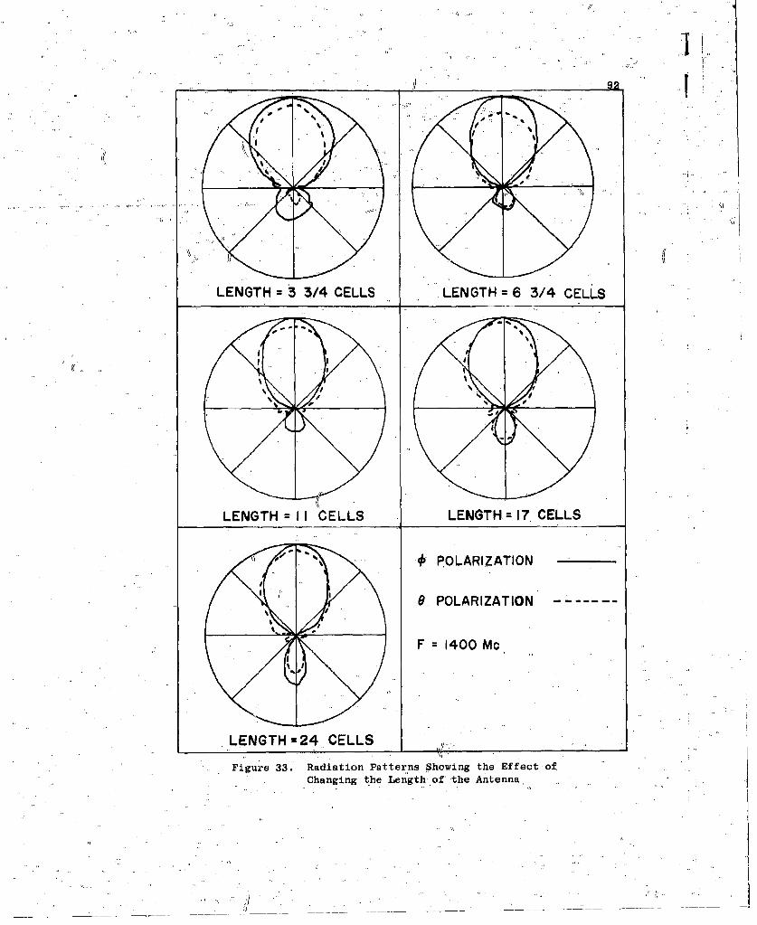
_ _ _ __ I]92

LENGTH: 3 3/4 CELLS LENGTH = 6 3/4 CELLS

LEGT= I CEL EGH 7 EL

0. PO.RIZTIO

F 1 400 Mc

LENGTH2r24 CELLS _________

Figure 33. Radiation Patterns Showing the Effect ofChanging the Length 'of' the Antenna,

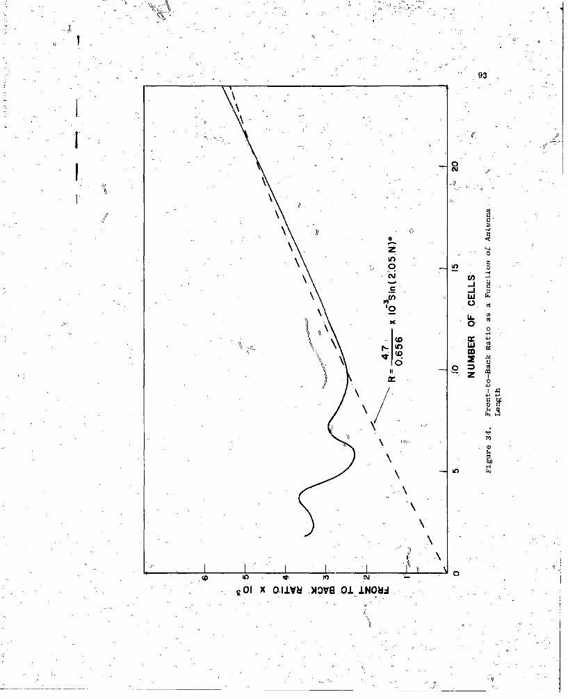
93

II

0

MCI 6

L.6

0:46

Lc)C

0 LLO Ck

0~~~~~ li oe01 N8

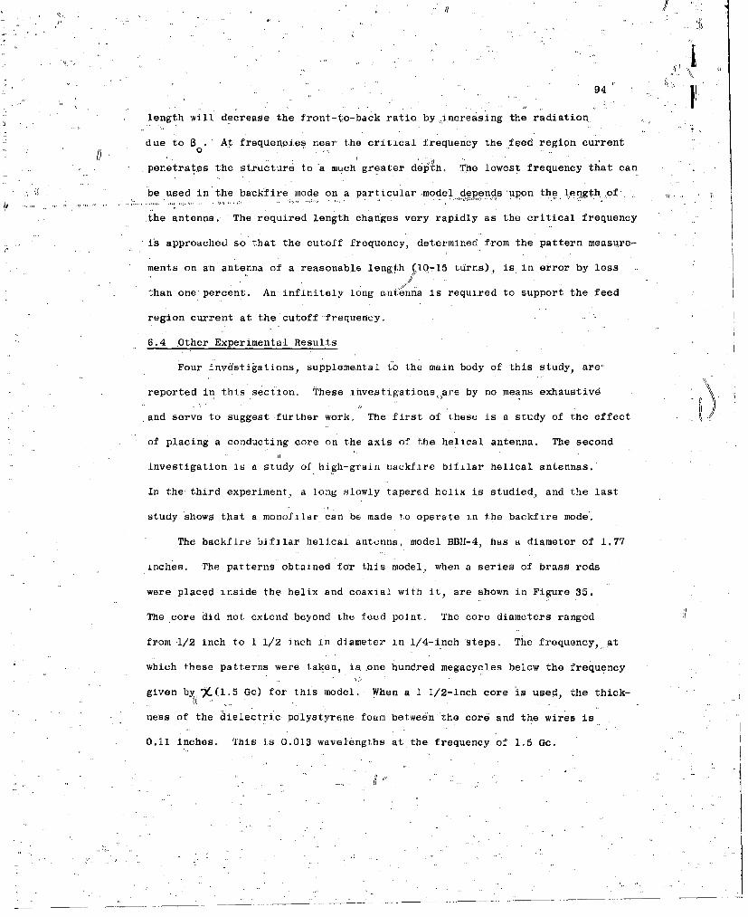
94

length will decrease the front-to-back ratio by ,increasing the radiation

due to B . At frequencies near the critical frequency the feed region currentf) o. 0

-penetrates the structure to a much greater de$#h. The lowest frequency that can

be used in the backfire mode on a particular model dependsupon the length of

the antenna. The required length changes very rapidly as the critical frequency

is approached so that the cutoff frequency, determined from the pattern measure-

ments on an antenna of a reasonable lengt;h 710-15 tUrns), is in error by less

than one percent. An infinitely long antenna is required to support the feed

region current at the cutoff frequency.

6.4 Other Experimental Results

Four invdstigations, supplemental to the main body of this study, are-

reported in this section. These investigations pare by no means exhaustive

and serve to suggest further work. The first of these is a study of the effect

of placing a conducting core on the axis of the helical antenna. The second

investigation is a study of high-grain backfire b1f.ilar helical antennas.

In the third experiment, a long slowly tapered helix is studied., and the last

study shows that a monofilar can be made to operate i.n the backfire mode.

The backfire bitfilar helical antenna, model BBH-4, has a diameter of 1.77

inches. The patterns obtained for this model, when a series of brass rods

were placed inside the helix and coaxial with it, are shown in Figure 35.

The core did not, extend beyond the feed point. The core diameters ranged

from 1/2 inch to 1 1/2 inch in diameter in 1/4-inch steps. The frequency, at

which these patterns were taken, is-one hundred megacycles below the frequency

given by %(l.5 Gc) for thi.'s model. When a I 1/2-inch core is used, the thick-

ness of the dielectric polystyrene, foam between 'the core and the wires is

0.11 inches. This is 0.013 wavelengths at the frequency of 1.5 Gc.

, , / ,,

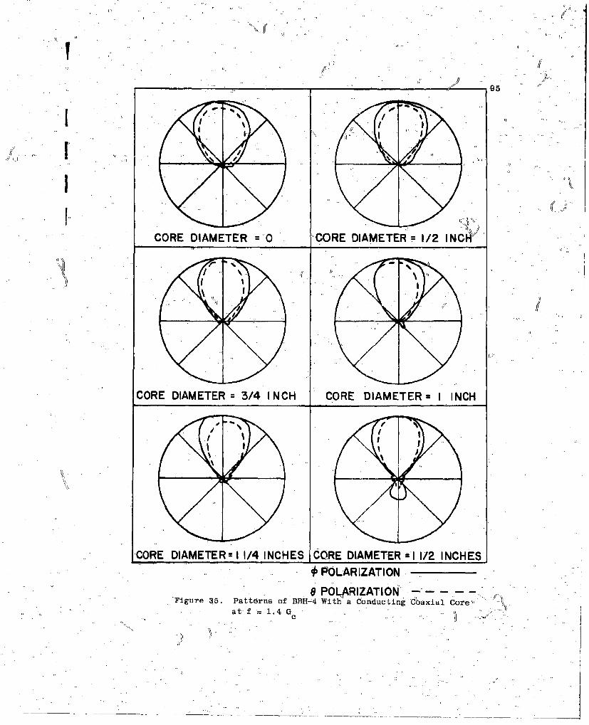
S.95

II

CORE DIAMETER = 0 CORE DIAMETER 1/2 1lNCI4

CORE DIAMETER: 3/4 I NCH CORE DIAMETER= I I NCH

CORE DIAMETER= 1 1/4 INCHES CORE DIAMETER = 1 1/2 INCHESSPOLARIZATION

8 POLARIZATION ---

Figure 3-5. Patterns of I3BH-4 With a conducting Cd~axial Core'ýat f =1.4 G 0..

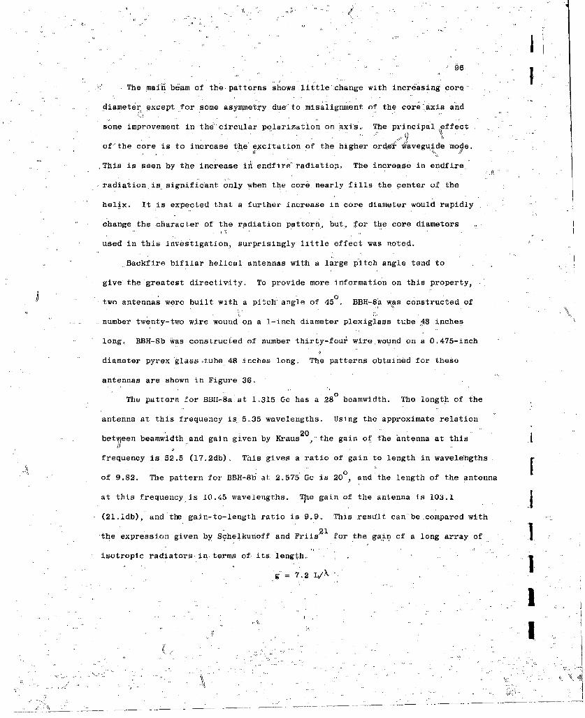
96

The ma in beam of the patterns shows li.ttle'change with increasing core

diameter except for some asymmetry dueS'to misalignment of the core .axis and

some improvement in the'circular polarization on axis. The principal effect

of"the core is to increase the 'ecitation of the higher or~d Waveguiýdb mode.

"This is seen by the increase iil endfire'radiation. The increase in endfire

radiation is significant'only when the core. nearly fills the center of the

helix. It is expected that a further increase in core diameter would rapidly

change the character of the radiation pattern, but, for the core diameters

used in this investigation, surprisingly little effect was noted.

Backfire bifilar helical antennas with a large pitch angle tend to

give the greatest directivity. To provide more information on this property,

0two antennas were built with a pitch angle of 45 . BBH-Sa yas constructed of

number twenty-two wire wound on a 1-inch diameter plexiglass tube ,48inches

long. BBH-8b was constructed of number thirty-four wire wound on a 0.475-inch

diameter pyrex klasstube 48 inches long. The patterns obtained for these

antennas are shown in Figure 36.

0The pattern for BBH-Ba.at 1.315 Gc has a 28 beamwidth. The length of the

antenna at this frequency is 5.35 wavelengths, Using the approximate relation

20betyeen beamwidth and gain given by Kraus ",the gain of. the antenna at this

frequency is 52,5 (17.2db), This gives a ratio of gain to length in wavelehgths

of 9.82. The pattern for BBH-86' at 2.575 Gc is 20 , and the length of the antenna

at this frequency is 10.45 wavelengths. 'Pe gain of the antenna is 103.14

(21.1db), and the gain-to-length ratio is 9.9. This result can be.compared with

the expression given by Schelkunoff and Friis 2 1 for the ga~in.of a long array of

isotropic radiatorsin terms of its length,. '

g"= 7.2 L/

I N'I!

'1 . .. . .. . __ _ ? . . . . . . .. . . . . .

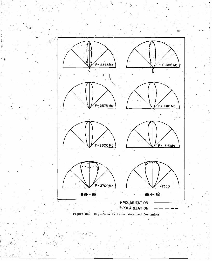
.F2575 Mc Fu 131OM c

Fm 27 350

BBH- BB BBH-_8A

*POLARIZATION8 POLARIZATION ----

Figure_ 36. High-Gain Patterns Measured,.for BBH-8

9

uI

ThiS gain results when Hansen-Woodyard excess phase shift is useddin the array.

The backfire bifilar helix provided a gain about 1.375-timts. g9rat without

side lobes. If side lobes were permitted as shown for'the lowei 'frequencies,

the gain is increased 1.7 times. The backfire bifilar helices are ,obviotislyj

supergain antennas when operated near-the critical frequency. The usual.

instability associated with supergain atitennas takes the form of A very rapid

widening of the beam with inoreasing frequency. One half percent increase in

0frequency increases the beam width 2 .

In an attempt to retain some part of the high-gain performance of the

antenna described above 'and at the same time increase the band width, a 8-foot

long antenna was built, tapered from one-half inch diameter at one end to

one-inch diameter at the other end. A Rexolite number 1422 core was used with

0number thirty-two.wire wound at a pitch angle of 45°. The patterns obtained

for this antenna are shown in Figure 37. This antenna has an average gain of

36(15.5db) in a 'five percent ban4 width. Thus tapering the helix slows the

rate with which its patterns vary with frequency and at the same time reduces

the maximum gain that can be achieved. This is the result expected since this

antenna corresponds to a conical log-spiral antenna with a very small cone angle.

A backfire monofilar. helix was constructed"to show that the nomofilar

helix will also operate in the backfire mode. This'model used the parameters

of BBH-2. The conductor in this case was a Microdot cable, which was also

used to carry energy from the feedpoint to the receiver. At the feedpoint,

the Microdot cable was brought radially from the parameter of 'the helix to

the. axis. The center conductor of the cable was connected to the center of a

straight wire ten-centimeters long placed on the axis of the helix. The patterns

obtained for the monofilar helix are shown in Figure 38. These patterns are very

Jr

'I,. .

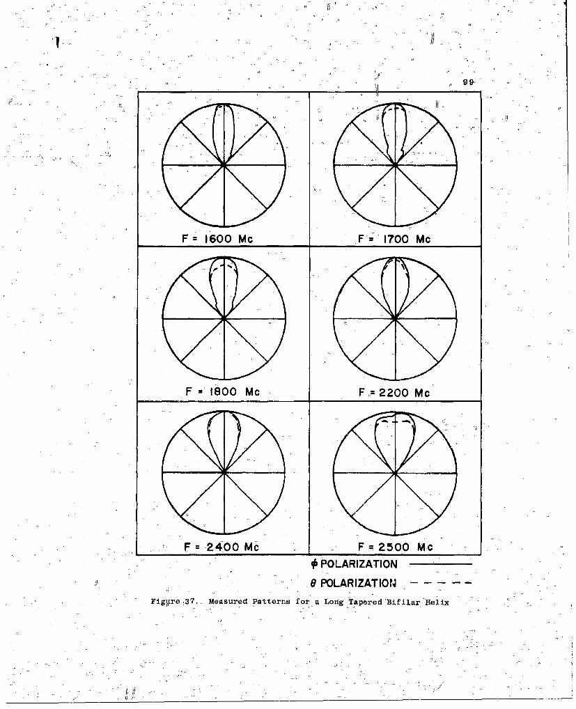
) ,,99,

F~ 1600 M~c Fw 1700 Mc

Fm 1800 Mc F,.= 2200 Mc

F2400.Mc F 2500M-C*POLARIZATION

* '1 ~~.9 POLARIZATION- ---

* Figp re .37., Measured Patterns for a Long Tapered ",3f liar "Helix

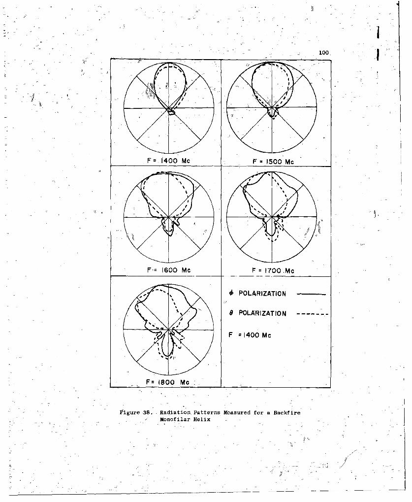
.. 100,

A ( *A

F= 1400 Mc F =1500 Mc

Fý= 1600 Mc F 1700.Mc.

SPOLARIZATION

8 POLARIZATION --- --

F 1400 Me

F 1=800M c-

Figure 38.. Radiation Patterns, Measured for a, Backf'ire'Monofilar Helix

To,

l101

similar to those obtained for the bif ilar aptenna, BBH-2. This demonstrates

that the monofilar helix, will operate in the backfirt6 mode, although it is

more difficult to feed than the bifilar helix.

gA

II'

" . (1

/I

. .,, 102

I 7. CONCLUSION

The object of this research was to provi.de ,,an,,rtica' model of thebakfr biia rdc

backfire bifilar . hekical- antenna that could be used to predic 4 -he radiation 1"charecteristics of thiss ýntenna. The model described here was shown to fulfill

this objective. ¶the jstudy went beyond this objective i"'providing a detailed

Sexperimental study of the radiation patterns of the antenna.

In this research the radiation patterns were obtained using the known

determinantal equation for the helical waveguide. This equation wasfactorized

by the Wiener-Hopf technique- to provide the Fourier transform of the current

distribution on the semi-infinito helix. The radiation pattern was related to

this Fourier spectrury I A

Two regions in the frequency spectrum of the backfire bifi'ar helix were

shown totbe important. It was shown that at the lower frequencies the bifilar

helix operates as awaveguide. Above the cutoff frequency of the principal

waveguide mode, the bifilar helix operates as a circularly polarized backfire

antenna.

The radiation characteristics of this antenna were shown to be determined

by the feed region current. This current decays with distance along the

structure. The near field has a phase progression directed toward the:,feedpoint.

The distance to which the feed region current penetrates the structure was shown

to decrease with frequency.

The phase pattern of the antenna was not obtained in the calculations

because of the"long numerical integration involved in its computation. This

prevented a more accurate accounting of the endfire radiation from the antenna.

The good agreement between measured and computed results reaffirmed the validity

"",of the approximations used in the beginning of the analysis.

,. '..

.... t . *,. ,

IIV

),"103

This study of the backfire bifilar helical antenna is important for

several reasons. Not 4the least of these is the fact thatthe antenna is a

useful, practical device in itself. It provides ciicularly polarized-fields

,with a single lobed pattern of almost any desired gain, When jitch angles0..

near 45° are used, the antenna can provide circularly polarized fields with a

pattern that is omnidirect'ional"in azimuth with high vertical directivity.

if i is inconvenient to provide a balanced feed for this antenna, it can be

fed from a coaxial line run inside one of the helical conductors to the0

feedpoint on the axis. The decay of the feed region current,,will keep antenna

.currents from flowing on the unbalanced feed line.

This study provides further ihsight into the operation of the conical

log-spiral antenna, and it is the firsts,.simply periodic backward wave or

backfire antenna for which a theoretical solution has been obtained. The

study of other typei of periodic antenna structures that operate in the

backfire mode will aid in understanding the operation of known log-periodic

antennas"and will suggest new ones. These structures are important in

themselves for their unidirectional single lobe patterns and their frequency

scanning characteristics, as well as for the insight they give in the operation

of log-periodic antennas.

"The existence of a decaying.backward wave current in the feed reginn

suggests"That the patterns of the backfire helix can be explained in terms

of improper (decaying) helical waveguide modes. An investigation along these

lines is now in progress.by another investigator. The results of such an

analysis may be simpler in interpretation than the present analysis.

Another line of inquiry-suggested by this work concerns the effect of a.

"conducting core on the axis of the helical antenna. In this study it was shown

- 104

that the helical conductors could be.ýlaced remarkably. close to the conducting,

ore with little degradation of performance. This study should be extended.to

other helix parameters. Tbh effect of extending the conducting core beyond the

feedpoint should be investigated. A backfire monofilar helix fed against a

conIucting central core should also be investigated.

* (The study of long slowly tapered bifiiar helices should be extended. The

results of this study.combined with results obtained for the conical log-spjral

antenna would establish The relation between •ain, band width, and size over

the entire spectrum of helical or conical log-spiral parameters. The conical

log-spiral antenna is known to have practically constant characteristics over

ten-to-one or greater band widths. This antenna in theusual range of parameters

hps considerably less gain than can be obtained by a sl Oly tapered hel'ix, while

the slowly tapered helix has .a relatively smaller band width.

It is characteristic of a study of a new device that many diverging courses

of investigation are suggested. A few of these, that were suggested during the

study of the backfire bifilar helical antenna, are described above. However,

the major effort in this investigation was concentrated on the study of the

radiation patterntof the antenna. In this wqy it has been possible to provide

information on this aspect of the problem over on extensive range of parameters.

. ,, , -j

;ii

105

B7BIBLIOGRAPHY¥,

1.i . S. Sensiper, Electronmagnetic Wave 'Propagation on Helical Cpnductors,Ph.D. Thesis, Massachusetts Institute of Technology, 1951.

2. S. AK. Kngan, "The Propagation of Waves Along an Endless Helix, Compt.Rend. Acad. Sci. (USSR), Vol. 66, June 1949; p. 867.

3. S. Sensiper, "Electrpmagnetic Wave Propagation on Helical Structures,"Proceedings of the IRE, Vol. 43, No. 2, February, 1955; pp. 149-161.

4. J. D. Kraus, "Helical Beam Antenna," Electronics, Vol. !aO, April, 1947,pp. 109-111,

5. J. A. Marsh, "Measured Current Distributions on Helical Antennas,"Proceedings of the IRE, Vol. 39, June, 1960, pp. 668-675.

6. A. G. Holtum, Jr., "Improving the Helical Beam Antenna," Electronics,Vol. 33, April 29, 1960; p. 99-101.

7. H. J. Bremermarin and L. Durland, "On Analytic Continuation, Multipli-cation, and Fourier Transformations of Schwartz Distributions," Journalof Math. Physics., Vol. 2, No. 2, 1961; pp. 240-258.

8. G. N. Watson, Theory of Bessel Functions, Second Edition, CambridgeUniver~ity Press, 1952; p. 429.

9. A. Erdelyi, et. al. Higher Transcendental Functions, Vol. 2, McGraw-Hill,New York, 1953; p. 86.

10. K. Knopp, Infinite Sequences and Series, Dover, 1956; p. 171.

11'. B.'L. Van der Vaerden, "On the Method of Seddle Points," Appl. Sci.Res., Vol. B2; pp.. 33-45. "N

12. B. Noble, "'The Wiener-Hopf Technique, Pergamon Press., J58.

13. S. A. Schelkunc.ff, Advanced Antenna Theory. John Wiley and Sons, New York,

1952, p. 102.

14. F. B. Hiilaerbrand, Introduction to Numerical Analysis, McGraw-Hill, NewYork, 1.956.

15. Lowan, Davids,. and Levenson, "Tables of the Zeros of the Legendre Poly-.nomials of Order 1-16 and the Weight Coefficients for Gauss' MechanicalQuadrature Formula," Tables of Functions and Zeros of Functions, NBS,"AppliedMath. Series, No. 37, 1953..

316. D. E. Isbell, "Non-Planar Logarithmically Periodic Antenna Structures,Antenna Laboratory, University of Illinois, Urbana, Tech. Rept. No. 30,Contract AF33(616)-3220, February, 1958.

/

'/ 'N/I....

106.

17. R. H. DuiHame I and.. F. R. Ore, "Logarithmically Periodic Antenna Designs,IRE National Convention Record, pt. 1, 1958; pp. 139-151.

18. _J.' D.' Dyson, The. Unidirectional Equiangular Spiral Antenna",IRE Trans. on Antennas and Propagation, Vol. AP-7, Oct. 1959,,,pp. 329-334.

19.. PW.E. Mayes, G. A. Desi'hiamps,' and W. T. Patton, "Backward-Wave Radiation,from Periodic Structureskand Application to the. Design of Frequency-Independent Antennas," Proce e10dings of the IRE, Vol. 49, May, 1961;pp. 962-961.*

20. J. *D. Kraus, Antennas, McGraw-rHill1, New Yqrk, 195,1, p. 176.

21. S. A. Schelkunoff and H. T. Friis, "Antenna Theory and Practice, John.

Wiley and Sons, New York, 1952; p. 559.

22. W. Magnus and P. Oberhettinger, Formulas and Theorems for the Functions .

of Mathematic ,al Physics 'Chelsea, New York, 1954; p. 118.

23. R. S. Phillips, "The Electromagnetic~ Field Produced by.s Helix,"Quarterly of Appl. Math., Vol. 8, No". 3, October., 1950; pp. 2'29-246.

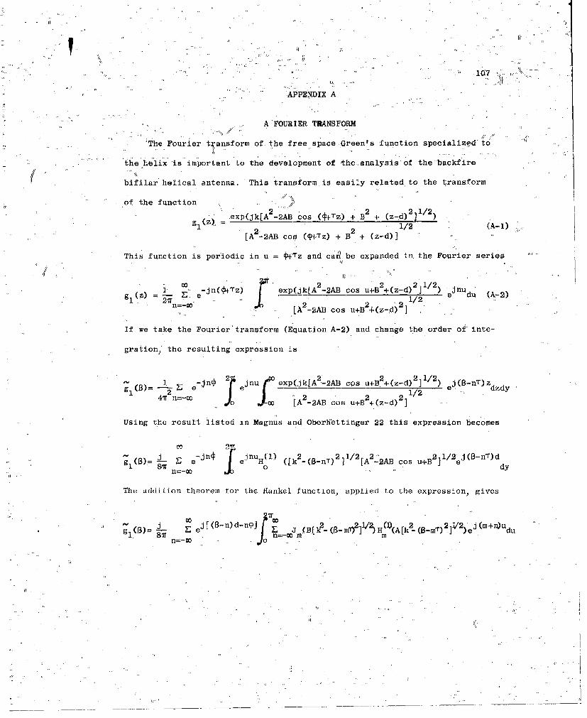
V..l

107'

APPENDIX A

A FOURIER TRANSFORM

'The Fourier t ansform of the free space Green's function specializd: to

'the L1iix is important to, the development of the..analysis of the backfire

bifilar helical antenna, This transform is easily related to the transform

of the function .

•exp(jk[A2-2 AB cos (hITz) + B2 + (z-d)2]I/2)

2 (Z) 1/2 (A-1)[A 2-2AB cos (4PTz) + B + (z-d)]

This function is periodic in u = 4lTz and car•l be expanded in, the Fourier series

() jn( z) exp(jk[A 2-2AB cos u+B2 +(z-d) du (A-2)

91 2T =0 2 2 *2 2JA -2AB cos u+B (-d21)

If we take the Fourier transform (Equation A-2) and change the order of inte-

gration, the resulting expression is

-i6) 1 -jn' 2o jnnT exp(jk[A2 -2AB cos u+B 2 +(z-d) 2 ] 1 / 2) j(B-nT)z2- 2 1/2 ej (nT.Zdzdy'

47 2 n=- [A2_ -2AB cos u+B2 +(z-d) 2 ]

Using the result listed in Magnus and Oberlhettinger 22 this expression becomes

S e- jn ejnuH(l) ([k 2 (B-nT)2 1/ 2 [A2 -2AB cos u+B2 1 1/2ej(B-nT)d

1 n=-S o o dy

Thu addition theorem for the Hankel function, applied to the expression, gives

CO1 (B- n) d- noo 0. (mS L eJ[-n)d-n J (B[k22(B-m]/H()(A[2- 2]/2 j(m+n)u8o' n0'

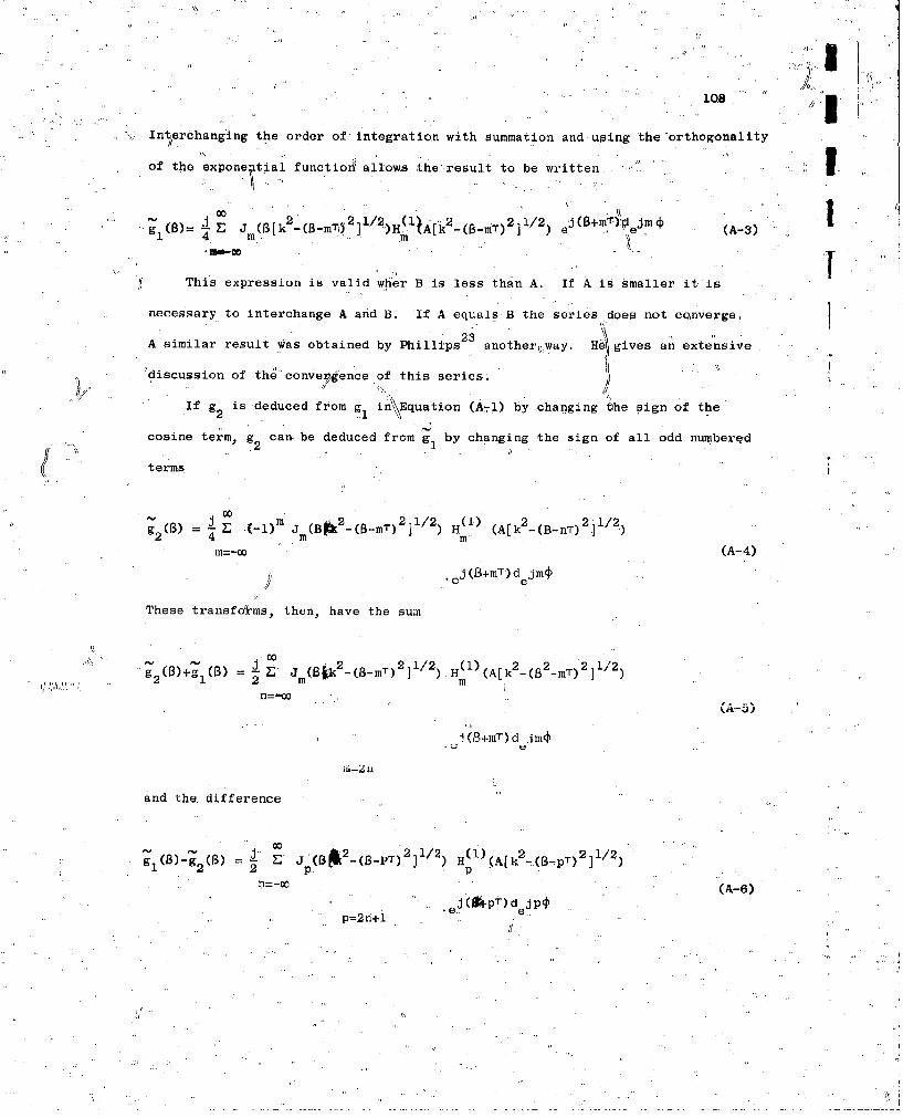
108 '

Int)erchanging the order of integration with summation and using the orthogonality

of the expone tial function allows the result to be written

2k 2 H l/2(l1'221 ej (B+MT)ý"0jMc9l (B)= E Jm (Bk- (B-mT(r• 2(1A-(3A) L Bm)2]12 'J(+'.;• m

This expression is valid wfier B is less than A. If A is smaller it is

necessary to interchange A and B. If A equals B the series does not converge.

A similar result was obtained by Phillips2 3 another,.way, H gives an extensive

discussion of the conveygence of this series.. /v .

If g2 is deduced from g \ in\\Equation (A-l) by changing the sign of the

cosine term, g2 can, be deduced from g by changing the sign of all odd numbered21

terms

B- 00 )2 l/2 (1) 2 1/292(B) L (-l)m Jm(B -(-m)2/) H(') (A[k2(B-nT) /)

M=-00 (A-4)

C ej(B+mT) deJ jm

These transfdi'ms, then, have the sum

""21• 1 -- (B• 2 (BT)2 l1/2) H(1) (Ak 2 2 2 2

Z2(B)+gl (B) =2 L'i ] inj -(-T I HmnAk( T)]l)

1(53+mT)d .ira4

and the. difference

* 2_ 2 1/2 (1) 2_ /g1 (B)- 2(B) _- 1 • (B(3 _(S3_PT)] ) H (A[k (_3ýpT)2 p p

(A-6)• .j(g•pt)d jpýp=2n1+l

.e

/1J

109

Finally, the Fourier transform of the complex conjugate of g(z) is deduced from

g(5) by replacing the Hankel funct'f6n of the first kind, H with the Hankel. •'(2)

function of the second kindH

//

A/

J\

_ _ __ _ _ I i/

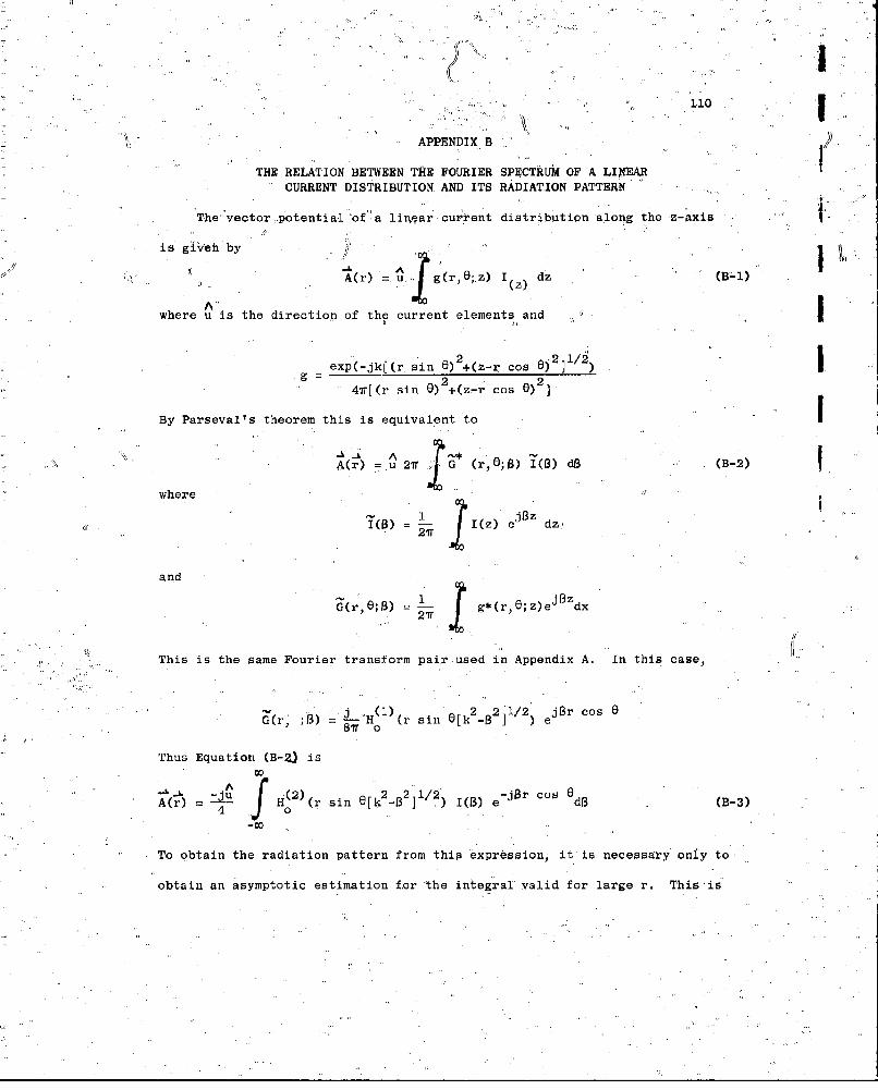
1.10

11i0 1*.

APPENDIX B 2THE RELATION BETWEEN THE FOURIER SPECTRUM OF A LINEAR

CURRENT DISTRIBUTION.AND ITS RADIATION PATTERN

The vector potential'of a linfar curient distribution along the-a-axis

is giveh by

A(r) g (r, Z) I dZ (B-i)

where u is the direction of the current elements and .

exp(-jk((r sin 6) 2 +(z-r cos )2] 1/2

2 2414(r sin 6)2+(z-r cos 6)2]

By Parseval's theorem this is equivalent to

AjA A(r) = U 271 G (r, 8B) T(B) dB (B-2)

where1 ejBz

6(3) - • I(z) dz

and

r, E);. = f g* (r, E; z) eJBZdx

' H"

This is the same Fourier transform pair used in Appendix A. In this case,

.... ,(1) 2. 2./ jfr COS 6

G(r ;3) JL"H C r sin 0[k2-32] /2) ej~r

Thus Equation (B-a) is00

fjC F (2) 2_2i -j~r cos 6A(r) - H sin [k-]/) B I(1) e d3 (B-3)

-co

To obtain the radiation pattern from this expression, it is necessaryonly to

obtain an asymptotic estimation f.or the integral valid for large r. This'is

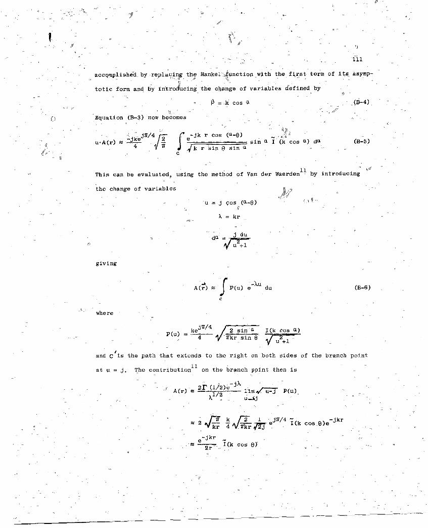
311

accomplished by replacing the Hankel':4lnction with the first term of its asymp-

totic form and by initrodkcing the change of variables defined by

:k cos a (B-4)

Equation (B-3) now becomes

J7/4 • -Jk r cos (U-0)u.ir -ike 2i e 'Asin a I (k cos a) da (B-5)

S •~k rsin esin a

This can be evaluated, using the method of Van der Waerden1 I by introducing

the change of variables

U =j os (aC-) , 3

= kr

j du

giving

e-uA(r) z P(u) e du (B-6)

c

where

P(u) kej/4 2 sin . I(k cos L.)4 /'kr sin 8

and C is the path that extends to the right on both sides of the branch point

at u,= j. The contribution on the branch ppint then is

• A(r) 2 (i2-j liraM'/' U-3' •. u-uPu

2 Tkl/ u--• "J"/ (

k7 1r J7/-k

-j'kre~'- 1 .(k cos O)

We have deduced by a lo'g-amnd complicated argument the..well kno.wn result that

'N.[

the current distribution of a line source and its radiat'ion patte'rf are Fouri er

transform pairs. This result is more easily obtained by assuming thqat r is much

•.larger than.,zin.Equation (B-1) giving.

11-jkr 01

A Or) - 9" 11k co '(z)' d

This more direct approanhg however, is valid only when the current has finite

€11

.Theorem X of 9Paley and Wiener* s~tates that Its Fo~rier spect-rum is entire..

The current spectrum then will contribute no s'ingularities,,of its own to P(u)

in Equation (dt-6)b If the current distribution is not finitep its spectrum

may have singularities of its own that must be considered in the evaluation r fi,

Equation (B-6)i

.Mathematically, such additional singul~arities can be handled by the method

of Van der Waerdenll Physically., they are usually interpreted as surface

waves guided by the structure, The contribution of the branch point at u = j

might be called the "spa~e wave" of the distributilon. It is t.llis "square wave"

that wmovediridentified with the radiation patterns of a current distribution

in this study.

• . ',ifo

Thoe o ae adWeer tts htis ore'setu i nie

Thurn setu.thnwl onrbt.o.iglrtis'fisw oPu

AF31657 )-8460 . '

"DISTRIBUTION LIST

-One copy each unless,,otherwise indicated

Armed Services Technical Information DirectorAgency Ballistics Research Laboratory

Attn: TIP-DR Attn: Ballistics Measu~ement Lab.Arlington Hall Station Aberdeen Provi~ng Ground, MarylandArlington 12, ;Virginia (10 copies) ,;

1 , iNational Aeronautics & Space Adm.,

Aeronuatical Systems Division Attn: LibrarianAttn: (ASRNRE-4) Langley Field, VirginiaWright-Pa.tterson Air Force BaseOhio (3 copies) Rome Air Development Center

'Attn: RCLTM

Aeronautical Systems.Division Griffiss Air Force BaseAttn: ASDSED, Mr. Mulligan New YorkWright-Patt1erson Air Force BaseOhio Research & Development Command

Hq. USAF (ARDRD-RE)Aeronau~tichl Systems Dividion Washington 25, D. C.Attn: AFCIN-4BlAWright-ýatterson Air Force Base Office of Chief Signal OfficerOhio Engineering & Technical Division

Attn: SIGNET-5

Air Force Cambridge Research Washington 25, D. C.Laboratory

Attn: CRRD CommanderLaurence G. Hanscom"iField U. S. Army White Sands Signal AgencyBedford, Massachusetts Attn: SIGWS-FC-02

White Sands, New MexicoCommanderAir Force Missile Test Center DirectorPatrick Air Force Base Surveillance DepartmentFlorida Evans Ares

Attn: Technical Document CenterCommander Belman, New JerseyAir Force Missile Development.CenterAttn: Technical Library CommanderHolloman Air Force Base U. S. Naval Air Test CenterNew Mexico Attn: WST-54, Antenna Sectio~n

Patuxent River,,MarylandAir Force Ballistic Missile Division . .Attn: Technical Library, Air Force Material Laboratory, Code 932

Uni t Post Office New York, Naval ShipyardLos Angeles, California Brooklyn 1, New York

2

Commanding Officer Boding Airplane CompanyDiamond Ordnance Fuse Laboratories Aero Space DivisionAttn:" 240 Attn: Technicgl LibraryWashington .25., D. C.- M/F Antenna & Radomes Unit

V U- *., . , ~Seattle ah~gpDirectorU. 3. Navy Electronics Laboratory Boeing Airplane CompanyAttn: Library Attn: Technical Library ,

San Diego 52, California M/F Antenna Systems Staff Unit"Wichita, Kansas 2

Adams-Russell Company .200 Sixth Street Chance Vought Aircraft Inc.Attn: Library (Antenna Section) THRU: BU AER RepresentativeCambridge, Massachusetts Attn: Technical Library

M/F Antenna SectionAero Gen Astro P.. O. Box 5907Attn:- Security Officer Ballas 22, Texas1200 Duke StreetAlexandria, Virginia Collins Radio'Company

Attn: Technical Library (AntennaNASA Goddard Space Flight Center Section)Attn: Antenna Section, Code 523 Dallas, TexasCreenbelt, Maryland

ConvairAirborne Instruments Labs., Inc. Ft. Worth DivisionAttn: Librarian (Antenna Section) Attn: Technical Library (AntennaWalt Whitman Road Section)Melville, L. I., New York Grants Lane

Fort Worth, TexasAmerican Electronic LabsBox 552 (Antenna Section) ConvairLansdale, Pennsylvania Attn: Technical Library (Antenna

Section)Andrew Alfred Consulting"Engineers P.. 0. Box 1050Attn: Librarian (Antenna Section) San Diego 12, California299 Atlantic Ave.Boston 10, Massachusetts Dalmo Victor Company

Attn: Technital Library (AntennaAmpheol-Borg Electronic Corporation Section)Attn: Librarian (Antenna Section) 1515 industrial Way2801 S. 25th Avenue Belmont, CaliforniaBroadview, Illinois

Dorne & Margolin, Inc.Bell Aircraft Corporation Attn: Technical Library (AntennaAttn: Technical.Library Section).

(Antenna Section) ,30 Sylvester StreetBuffalo'5, New York. Westbury, L. I., New York

Bendix Radio Division of . Dynatronics Inc,Bendix Aviation Corporation Attn: Technical Library (Antenna

Amtn: Technical Library Section)(For -Dept. 462-4) Orlandoy Florida

Ba'ltimore 4, Maryland

1/ 4?

.• 3"

" Electronic .Communicatio ns, Inc. . Grumman Aircraft Engineering Corp.Research Division Attn: Technical Library,.

A, Attn: Technical Library M/F Avionics Engineering1830-York Road.. ', Bethpage, New York ,,

Timonium, Maryland' , . The',Hallicrafters Company

/. irchi-ldEngine & Airplane Corporation Attn: Technical Library (Antenna

i(Fairchild, Aircrafp & Missiles Division Section)Attn: Tekhnical/library (Antenna" 4401 W. Fifth Avenue

I" Section)• 'Chicago 24, IllinoisHagerstown 10, Maryland

Hoffman Laboratories Inc..Georgia Institute of Technology Attn: Technical Library (AntennaEngineering Experiment Station Section)Attn: Technical Library Los Angeles 7, California

M/F Electronics"DivisionAtlanta 13, Georgia John Hopkins University

Applied Physics'LaboratoryGeneral Electric Company 8621 Georgia AvenueElectronics Laboratory Silver Springs, MarylandAttn: Technical Library-Electronics Park Hughes Aircraft CorporationSyracuse, New York Attn: Technical Library (Antenna

Section)

General Electronic Labs., Inc. Florence & Teal StreetAttn: Technical Library (Antenna Culver City, California

Section)18 Ames Street ITT LaboratoriesCambridge 42, Massachusetts Attn: Technical Library (Antenna

Section)General Precision Lab., Division of 500 Washington Avenue

General Precisioh Inc. Nutley 10, New JerseyAttn: Technical Library (Antenna

SSection) .. , U. S. Naval Ordnance Lab.

63 Bedford Road Attn: Technical LibraryPleasantville, New York Corona, California

Goodyear Aircraft Corporation Lincoln LaboratoriesAttn: Technical Library Massachusetts Institute of Technology

M/F Dept. 474 Attn: Document Room1210 Massilon Road P. 0. Box. 73Akron 15, Ohio Lexington 73, Massachusetts

Granger Asso6iates Litton Industries'Attn: Technical Library (Antenna .,Attn: Technical Library (Antenna

Section) Section)974.Commercial Stredt 4900 Calvert' RoadPalo.-Alto, California College Park, Maryland

1i /

j

44

Lockheed Missile & Space Division North American Aviation Inc.Attn: Technical Library (M/F Dept- Attn: Technical Library (14/F

58-40, Plant 1, Bldg. 130) Engineering Dept.)Sunnyvale, California . 4300 W Fifth Avenue

Colu usg6, OhioThe Martin Company .'. \

Attn: Trchnical Library TAntenna North Americant'Aviation Inc.Section) Attn: Technical Library

P. 0. Box 179 S (M/F Dept. 56)Denver 1, Colorado International Air4ort

Los Angeles, CaliforniaThe Iartin.CompanyAtt,: Tephnical Library (Antienna Northrop Corporation

Section) ENORAIR DivisionaBaltimore 3, Maryland 1001 East Broadway

Attn: Technical Information (3924-3)

The Martin Company. Hawthorne, CaliforniaAttn: Technical Library (M/F

Microwave Laboratory) Ohio State University ResearchBox 5837 FoundationOrlando, Florida Attn: Technical Library

(M/F Antenna Laboratory)

W. L. Maxson Corporation 1314 Ki~near RoadAttn: Technical Library (Antenna Columbus- 12, Ohio

Section)460. West 44th Street Philco CorporationNew VoIK I. New Ynrk Govcrnmcnt & Industrial Division

Attn: Technical Library

McDonnell Aircraft Corporation (M/F Antenna Section)Attn: Te cphnical Library (Antenna 4700 Wissachickon Avenue

Section) Philadelphia 44, PennsylvaniaBox 516St. Louij 66, Missouri Westinghouse Electric Corporation

Air Arms DivisionMelpar, Inc. Attn: Librarian (Antenna Lab)Attn: Technical Library (Antenna P. 0. Box 746

Section) Baltimore 3, Maryland3000 Arlington Blvd.Falls Church, Virginia Wheeler Laboratories' #

Attn: Librarian (Antenna Lab)

University of Michigan Box 561

Radiation Laboratory Smithtown, New YorkWillow Run201 Catherine'Street Electrical Engineering ResearchAnn Arbor, Michiigan Laboratory 1i

University of Texas

"Mitre Corporation Box 8026, Univ. StationAttn: Tqchnical Library (M/F Elect- Austin, Texas

ironic Warfare Dept. D-21)

Middlesex Turnpike University of Michigan ResearchBedford, Massachusetts, Institute..

. . Electronic Defense Group »,"Attn-: Dr. J. A., _M. Jyons

Ann'.Arbor, Michigan "3

X,

" 5

Radio Corporation of America H. R. B. Singer Corporation" RCA Laboratories Division Ai'tn: Librarian (Antenna Lab)

Attn: Technical LibrarV State College, Pennsylvania(M/F Antenna Section)

J Princeton, New Jersey Sperry Microwave Electronics CompanyAttn: Librarian (Antenna Lab)

Radiation, Inc. P. 0. Box 1828-Attn: Technical Library (M/F) Clearwater, Florida ,7k 'K

Antnna SectionDrawer 37 Sperry Gyroscope CompanyMelbourne, Florida Attn: Librarian (Antenna Lab)

Great Neck, L. I., New YorkRadioplane Company,.Attn: Librarian (M/F Aerospace Lab) Stanford Electronic Laboratory8000 Woodly Avenue Attn"Att.:Librarian (Antenna Lab)Van Nuys, California Stanford, California

Ramo-Wooldridge Corporation Stanford Research InstituteAttn: Librarian (Antcnna 4 Lab) Attn; Librarian (Antenna Lab)Conoga Park, California Menlo Park) California

Rand Corporation Sylvania Electronic SystemAttn: Librarian (Antenna Lab) Attnm Librarian (M/F Antenna &1700 Main Street Microwave Lab)Santa Monica, California 100 First Street

Waltham 54, Massachusettskantec CorporationAttn: Librarian (Antenna Lab) Sylvania Electronic System23999 Ventura Blvd. Attn: Librarian (Antenna Lab)Calabasas, California P, 0. Box 188

. .Mountain View, Oalifnrnia%4 Raytheon Electronics. Corporation

Attn: Librarian (Antenna Lab) Technical Research Group1089 Washington Street Attn: Librarian (Antenna Section)Newton, Massachusetts 2. Aerial Way

Syosset, New YorkRepublic Aviation CorporationApplied Research & Development Ling Temco Aircraft Corporation

Division Temco Aircraft DivisionAttn: Librarian (Antenna Lab) Attn: Librarian (Antenna Lab)Farmingdale, New York ,Garland, Texas

Sanders Associates Texas Instruments, Incd.Attn: Librarian (Antenna Lab) Attn: Librarian (Antenna Lab.)95 Canal street 6000 Lemmon Ave.Nashua, New Hampshire .Dallas 9,.Texas

Southwest Research Institute A. S. Thomas, Inc.Attn: Librarian (Antenna Lab),, Attn: Librarian (Antenna Lab)8500 Culebra Road 355 Providence Highway"San Antonio, Texas " Westwood, Massachusetts

"' .. ,.. , ,...

,.. ,,, •,, , . xv

j I6

New Mexico State University Aeronautical Systems DivisionHead Antenna Department Attn: ASAD - LibraryPhysical Science Laboratory Wright-Patterson Air Force BaseUniversity Park, New Mexico Ohio >.

Bell Telephone Laboratories, Inc. National Bureau of StandardsWhippany Laboratory Department of CommerceWhippany, NewdJersey Attn: Dr. A. G. McNishAttn: Technical Reports Librarian Washington 25, D. C.

Room 2A-165

Robert C. HansenAerospace Corporation.Box 95085Los Angeles 45, California

Dr. Richard C. Becker10829 BerkshireWestchester, Illinois

Dr. Harry Letaw, Jr.Raytheon CompanySurface Radar and Navigation

OperationsState Road WestWayland, Massachusetts

Dr. Frank Fu FangIBM Research LaboratoryPoughkeepsie, New York

Mr. Dwight Isbell1422 11th WpstSeattle 99, Washington

Dr. Robert L. CarrelCollins Radio CorporationAntenna SectionDallas, Texas

Dr; A. K. ChatterjeeVice Principal & Head of the Department

•of ResearchBirla Institute of TechnologyP. O. MesraDiptrict-Ranchi (Bihar) India

Iiv

I .. , . .. . .

II

TECSUI1CAL REPORT3 AND NRWRAMD IUUSD

Contract"A733(610)-310

"Synthesis of Aperture Antennas," TechnAcal Report Do. 1, c.T.A. Jo"xu,October, 1954.e

I "A Synthesis Method for Broad-band Atýna Impedance Xatching etormk, t

Technical Report No. 2, Nicholas Taori ( I February 1085.* AD 61049.

I "The Aesym•e.trically Excited Spherical eunio," Teohtilcal Report go. 3,

Robert C. Hansen, 30 April 1955.*

"Analysis of an Airborne Homing System," Technical Report No.4, Pill a.I Mayes, 1 June 1955 (CONFIDENTIAL).

"Coupling of Antenna Elements to a Circular Surfece Isveguide," TechnicalReport No. 5, K. I. Zing and a. H. DeHamal, 30 Jww 1965..

"Axi-lly Excited iurtoco Wave Antennas," technical Report No. 7, D. a. &)"a,10 October 1955.*

"Homing Antennas mor the 1-86F Aircraft (450-2800 sc),* ;Technical 2eort no.P. X. Mayes, R. F. Hyneman, and R. C. Becker, 20 February 1957, (CObJlD9XT~i£).

"Ground Screen PatternlRange," Techqical Memorandum No. 1, Roger 2. Trpp,10 July 1955,*

Contract AF33(6l6)-3ja0

"ET•ective Permeability of Spheroidal Shells," Technical Report No. 9, 3. J.Scott and R. H. DuHamel, 16 April 1958.

"An Analytical Study of Spaced Loop ADF Antenna Systimns," Technical RepmortNo. 10, D. G. Berry end J. B. treer, 10 May 1956. AD 98615

"A Technique for Controlling the Radiation from Dielectric Rod Vaveguiden,"Technical Report No. 11, J._.W Duwnan and R. 5. Dusamel, 15 July 1956.,

"Directional Charactertstics of a U-fShaped Slot Antenna," Technical ReportNo. 12, Richard C. Becker, 30 September 1956.0*

"Impedarpce of Ferrite Loop Antennas," Technical Report No. 13,V. ¥.X., Romseyand W. L. Weeks, 15 Oci'ober 1958. AD 119780

"Closely Spaced Transverse Slots In Rectangular Iaveguide," Technical ReportNo. 14, Richard;?F. Hyneman, .30 December 1956.

... ,,: I iI ___ __ _

*Diatr'ibulted Coupling, to Surf ace Wave A .nte . nas," Technical Report.No. 15,Ralph R~ehard Hodges.ý jr,, 5 January' 51.5',

'1The Characte6risti&.'Tmpcdafim of the Fin Antenna of Infinite "Length," TechnicalReprt o. 6,Robeý,t L.Carre4, '15 January 11)87.* '/

"On the Istl~nation o f Fe,'rrito Loop Ant enna Impeda~ice, 61.1chnical Report No. 17?Walter L, Weeks, 10 April 1l957.* AD 143989

"A Note Concerning a Mechanical Scanning Syslehi f or a Plush .Mounted Line SourceAntenna." TehialRpr No.. 18. Walter TL. Weeks. 20 April 1957.

"."Broadband Loga~itkinically Periodic Antenna Structures," Technical Report'No. 10,R, H. DuHamel and D. E. Isbell,. 1 May-19571. 'AD 14073'4

"*"Frequency Independent Antennas," Technical Report No.. 2.0, V. H. )Humsey, 25*October 19,57

"The Equiangulay''Spiral, Antenna," Technical Report No. 21 J. 13. J)yson, 15_September 195.7. AD 145019. I

"Experimental Investigation of the Conical Spiral Antenna," Technical- ReportNo,, 22.! R L; Carrel, 2P "May 1957. ** AD 144.021.

"LvuJJlizig between 4 PareillelkPlate waveguide and a Surface Waveguide," TechnicaiReport No 23, E J. Scott, 10 August 1957,

"'Launching Efficiency of Wires and Slots for- a Dielec.tric Rod Waveguide,"Technical Report No 24.. J-W. Duncan and R H. Dullamel, August. 1951.

"The Characteristic Impedance of an infinite Biconical Antenna of ArbitraryCross Section," Technical Repovt Nu 25, Robert L. qarrel, Augusrt 1957.

"*"Cavity-.Backed Slot Antennas.." Technical Report No, 26, R, J. Teeter .20October Q95'7

"Coupled Waveguide Excitation of Traveling Wave Slot Antennas," 1!2hnic.~lRep6'rt No 2?, W. L. Weeks, 1 December 1957.

"J.'hase Velocities In Rct~ogular Waveguide Partially Filled,,with Dielectric,"Technical Report No' 28ý V L Woek-'. 20 Deccombur 1957,

"Mea._uring the Capacitance per UnIt Length of IBiconical structures of ArbitraryCrossa Se~tion,.." Technical Report No. 29. J. D, Dyson,,, 10 January 1958.

"Noti-P)anAr Lcgaorilthaically Periodic. Antenna Struc~ture,," Technical Report No. dD B. & labell. 20 Februarv 1958 AD 156203

"Elect romag'netic. 1Yi-eld@. in Ie."..tan'gulai r lots'"ý0 Technical Report No. 31,, N. J.Kuhn and P, E,. Masi. _10 Ma rch 1958

Th• DocumentIReproduced From

Elest Available Cop

"The Efficiency of Excitation of a Surface Wave on a Dielectric Cylinder,"Technical Report No. 32, J, W, Duncan, 25 May 1958.

"A Unidirectional Equiangular Spiral Antenna," Technical Report No. 33,J. D. Dyson, 10 July 19580 AD 201138

"Dielectric Coated Spheriodil laadiatova," Techntral Report •o• _34, 1. L.Weeks, 12 September 1958. AD 204547

"A Theoretical Study of the Equiangular Spiral Antenna," Technical ReportNo. 35, P, E. Mast, 12 September 1958. AD 204548

Contract A733(616)-6079

"Use of Coupled Waveguldes in a Traveling Wave Scanning Antenna," TechnicalReport No. 36, R. H_ Ma-cPhie, 30 April 1959o AD 210558

"On the Solution of a Class of Wiener-Hopf Integral Equations in Finite andInfinite Ranges," Technical Report No. 37, Raj Mittra, 15 May 1959.

"Prolate Spheroidal Wave Functions for Electromagnetic Theory," TechnicalReport No. 38, W_ L. Weeks, 5 June 1959.

"Log Periodic Dipole Arrays," Technical Report No. 39, D0 9, Zabel2, I June 1959.AD 220651

"A Study of the Come-Corrected Zoned Mirror by Diffraction Theory," TechnicalReport No, 40, S. Dasgupta and Y. T. Lo, 17 July 1959,

"The Radiation Pattern of a Dipole on a Finite Dielectric Sheet," TechnicalReport No. 41, K. G. Balmain, I August 1959.

"The Finite Range Wiener-Hopf Integral Equation and a Boundary Value Problemin a Waveguide," Technical Report No. 42. Raj Mittra, 1 October 1959.

ip,,,• ... roperti.s of Cemp ,n ~ary Multi eriminal Planar Structuresp,.Technical Report No 43, G. A. neschsmps, 11 November 1959.

"On the Synthesis of Strip Sources," Technical Report No. 44, Raj Mittra,4 December 1959,

"Numerical Analysis of the Eigenvalue Problem of Waves in Cylindrical Waveguidos,"Technical Report. Wo 45. C. He Tang and Y, T. Lo, 11 March 1960.

"New Circulai'ly Polý.rized Frequency Independent Antennas with Conical Beam orOmnidirectional Patterns," Tecbnical Report No. 46, J. D. Dyson and P. E. Mayes,20 June 1960, AD 241321

"LPcg~rithmtcally Periodic Resonant-V Arrayt.." Technical Report No. 47, F. E. Mayes,and R L. Carrel, 15 July 1960. AD 24630O

ZThis Docum

aftt A, OCiued prl

"A Study of Chromatic Aberration of a Co-na-Corrected Zoned Mirror," TechnicalReport No, 48, Y, To Le, June 1960

"Evaluation of Cross-Correlation Methods in the Utilization of Antenna Systems,"

Technical Report No. 49, R. H. MacPhie, 23 January 1961

"Synthesis of Antenna Product Patterns Obtained from a Single Array," TechnicalReport No.. 6 00 R. H,.WacPhie, 25 January 1961l

"On the Solution of a Class of Dual Integral Equations," Technical Report No. 51,Ro Mittra•, I October 1961, AD 264557

"Analysis and Design of the Log-Periodic Dipole Antenna," Technical Report No. 52,Robert L, Carrel, 1 October 1961o* AD 264558

"A Study of the Non-Uniform Convergence of the Inverse of a Doubly-InfiniteMatrix Associated with a Boundary Value Problem in a Waveguide," Technical ReportNo, 53, R. Mittra, 1 October 1961. AD 264556

*Copies available for a three-week loan period,

* Copies no longer avaIlable.

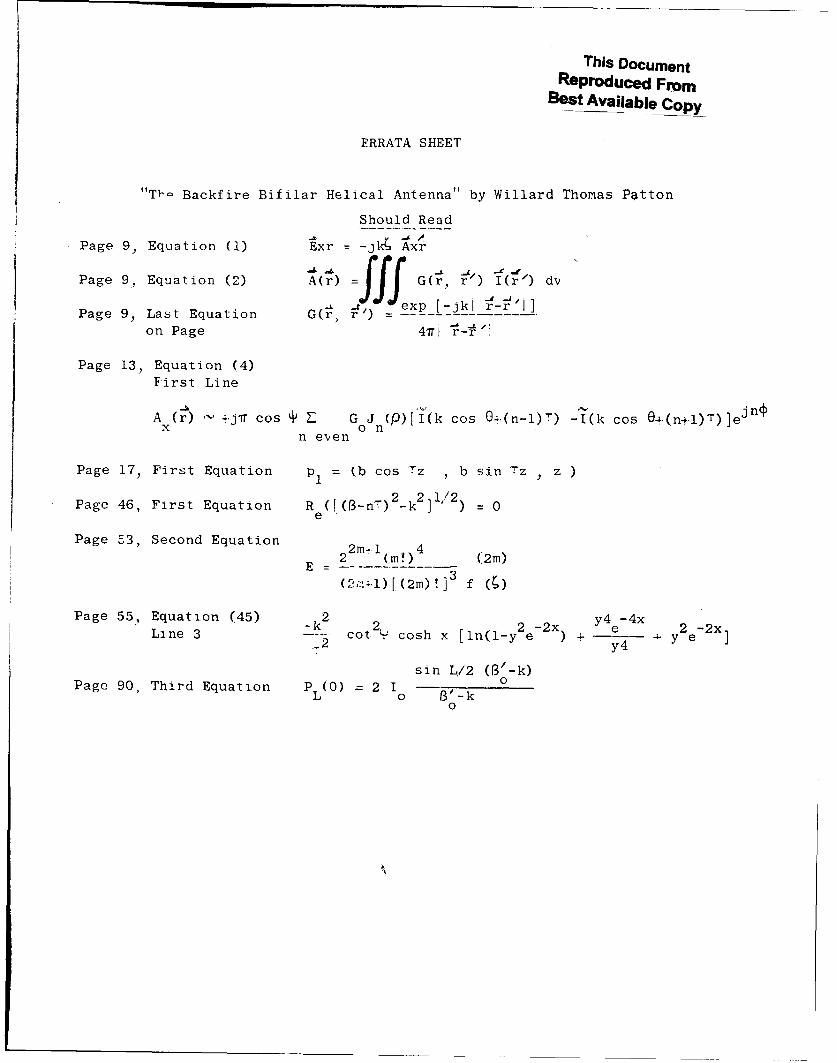
This DocumentReProduce, From

Best Available Copy

ERRATA SHEET

"TI'- Backfire Bifilar Helical Antenna" by Willard Thorias Patton

Should ReadPage 9, Equation (1) Exr =- k- Axr

Page 9, Equation (2) A(r) ff G(r, /) I( ') dv

Page 9, Last Equation G(r ) xp [-jkl )- '-]

on Page 47 •r-•I'

Page 13, Equation (4)First Line

A (r) ,- +JIT cos % G J (p)[I(k cos 04.(n-l)T) -I(k cos e4.(n4.1) )ejnýx o n

n even

Page 17, First Equation pl = (b cos rz ., b sin Tz , z )

Page 46, First Equation R ([(-nf) 2 2 1-/2 0

Page 53, Second Equation

2 (m.) (2m)(,,z .l[(2m) .]3 f ( )

Page 55, Equation (45) 2 Y4e-4X-k ct 2''csx 2 -2x y4e-4 2 -2xLine 3- cot2 cosh x [ln(l-y e- ) + _ - y e72 y4

sin L/2 (B'-k)Page 90., Third Equation P L(0) = 2 1 0 0

L o 3- k0