Embed Size (px)
Citation preview

HAL Id: tel-00931853https://tel.archives-ouvertes.fr/tel-00931853v2
Submitted on 20 Feb 2018
HAL is a multi-disciplinary open accessarchive for the deposit and dissemination of sci-entific research documents, whether they are pub-lished or not. The documents may come fromteaching and research institutions in France orabroad, or from public or private research centers.
L’archive ouverte pluridisciplinaire HAL, estdestinée au dépôt et à la diffusion de documentsscientifiques de niveau recherche, publiés ou non,émanant des établissements d’enseignement et derecherche français ou étrangers, des laboratoirespublics ou privés.
Active self-diagnosis in telecommunication networksCarole Hounkonnou
To cite this version:Carole Hounkonnou. Active self-diagnosis in telecommunication networks. Other [cs.OH]. UniversitéRennes 1, 2013. English. �NNT : 2013REN1S086�. �tel-00931853v2�

ANNÉE 2013
THÈSE / UNIVERSITÉ DE RENNES 1sous le sceau de l’Université Européenne de Bretagne
pour le grade de
DOCTEUR DE L’UNIVERSITÉ DE RENNES 1
Mention : Informatique
Ecole doctorale Matisse
présentée par
Carole HounkonnouPréparée à l’unité de recherche INRIA
Institut National de Recherche en Informatique et AutomatiqueComposante universitaire ISTIC
Active self-diagnosis in telecommunication networks.
Auto-diagnostic actif dans les réseaux de télécommunications.
Thèse soutenue à Rennesle 12 Juillet 2013
devant le jury composé de :
Francine KRIEFProfesseur, IPB, Université de Bordeaux 1 / rapporteur
Yacine GHAMRI-DOUDANEMaître de Conférences (HDR), Université de Paris Est / rapporteur
Xavier LAGRANGEProfesseur, Télécom Bretagne / examinateur
Christian DESTRÉDirecteur de projet, Orange Labs / examinateur
Laurent CIAVAGLIADirecteur de projet, Alcatel-Lucent Bell Labs / examinateur
Éric FABREDirecteur de recherche, INRIA / directeur de thèse

1

Acknowledgements
First and above all, I praise God, the almighty for providing me this opportunity andgranting me the ability to proceed successfully in spite of many challenges faced.
It would not have been possible to complete this doctoral thesis without the helpand support of the kind people around me, to only some of whom it is possible to giveparticular mention here.
I would like to express my sincere thanks to Eric Fabre, my supervisor, for his warmencouragement, critical comments, and thoughtful guidance throughout the course ofthis thesis. I also reserve special thanks to Samir Ghamri-Doudane for his time, valu-able inputs and contributions to this work.
I would also like to thank the members of my thesis committee. I place on recordmy sincere gratitude to Francine Krief and Yacine Ghamri-Doudane for spendingtime reviewing my thesis. I am also grateful to Xavier Lagrange, Christian Destre,and Laurent Ciavaglia for acting as examiners of my thesis. I want to thank you allfor letting my defence be an enjoyable moment, and for your brilliant comments andsuggestions, thanks to you.
There were many people who gave interesting feedback and valuable suggestions,for which I would like to thank them: my colleagues at INRIA and the members ofthe High Manageability joint research group of Alcatel-Lucent Bell Labs and INRIA. Aspecial thanks to Cesar Viho whose advice and support have been invaluable on bothan academic and a personal level. I am also very thankful to Nathalie Bertrand andLoıc Helouet for helping me practicing my presentation and for providing constructivefeedback. All these people have been a source of friendship as well as good advice andcollaboration.
Last but not least, a special thought is devoted to my family. Words can not expresshow grateful I am to my parents, Anastasie and Oussou Hounkonnou, and my brothers,Orens, Oswald and Bernard, for all of the sacrifices that you’ve made on my behalf.Your prayers for me was what sustained me thus far. God bless you all.

2
Abstract
While modern networks and services are continuously growing in scale, complexity andheterogeneity, the management of such systems is reaching the limits of human capa-bilities. Technically and economically, more automation of the classical managementtasks is needed. This has triggered a significant research effort, gathered under theterms self-management and autonomic networking.
The aim of this thesis is to contribute to the realization of some self-managementproperties in telecommunication networks. We propose an approach to automatize themanagement of faults, covering the different segments of a network, and the end-to-end services deployed over them. This is a model-based approach addressing the twoweaknesses of model-based diagnosis namely: a) how to derive such a model, suited toa given network at a given time, in particular if one wishes to capture several networklayers and segments and b) how to reason with a potentially huge model, if one wishesto manage a nation-wide network, for example.
To address the first point, we propose a new concept called self-modeling thatformulates off-line generic patterns of the model, and identifies on-line the instancesof these patterns that are deployed in the managed network. The second point isaddressed by an active self-diagnosis engine, based on a Bayesian network formalism,that consists in reasoning on a progressively growing fragment of the network model,relying on the self-modeling ability: more observations are collected and new tests areperformed until the faults are localized with sufficient confidence.
This active diagnosis approach has been experimented to perform cross-layer andcross-segment alarm management on an IP Multimedia Subsystem (IMS) network.

Chapter1Resume en francais
Contents
1.1 Contexte . . . . . . . . . . . . . . . . . . . . . . . . . . . . . . . 3
1.2 Introduction . . . . . . . . . . . . . . . . . . . . . . . . . . . . 4
1.3 Structure des reseaux IMS . . . . . . . . . . . . . . . . . . . . 6
1.4 L’auto-modelisation: support de la localisation de pannes . 8
1.5 Raisonnement avec les reseaux Bayesiens generiques . . . . 13
1.6 Resultats . . . . . . . . . . . . . . . . . . . . . . . . . . . . . . 15
1.7 Conclusion . . . . . . . . . . . . . . . . . . . . . . . . . . . . . 17
1.1 Contexte
Les reseaux de telecommunications deviennent de plus en plus complexes, notammentde par la multiplicite des technologies mises en œuvre, leur couverture geographiquegrandissante, la croissance du trafic en quantite et en variete, mais aussi de par l’evolutiondes services fournis par les operateurs. Tout ceci contribue a rendre la gestion de cesreseaux de plus en plus lourde, complexe, generatrice d’erreurs et donc couteuse pourles operateurs. On place derriere le terme � reseaux autonomiques � l’ensemble dessolutions visant a rendre la gestion de ce reseau plus autonome.
L’objectif de cette these est de contribuer a la realisation de certaines fonctionsautonomiques dans les reseaux de telecommunications. Nous proposons une strategiepour automatiser la gestion des pannes tout en couvrant les differents segments dureseau et les services de bout en bout deployes au-dessus. Il s’agit d’une approche baseemodele qui adresse les deux difficultes du diagnostic base modele a savoir: a) la facond’obtenir un tel modele, adapte a un reseau donne a un moment donne, en particulier sil’on souhaite capturer plusieurs couches et segments reseau et b) comment raisonner surun modele potentiellement enorme, si l’on veut gerer un reseau national par exemple.
Pour repondre a la premiere difficulte, nous proposons un nouveau concept : l’auto-modelisation qui consiste d’abord a construire les differentes familles de modeles generiques,puis a identifier a la volee les instances de ces modeles qui sont deployees dans le reseaugere. La seconde difficulte est adressee grace a un moteur d’auto-diagnostic actif, basesur le formalisme des reseaux Bayesiens et qui consiste a raisonner sur un fragment
3

4 Resume en francais
du modele du reseau qui est augmente progressivement en utilisant la capacite d’auto-modelisation: des observations sont collectees et des tests realises jusqu’a ce que lesfautes soient localisees avec precision.
Cette approche de diagnostic actif a ete experimentee pour realiser une gestionmulti-couches et multi-segments des alarmes dans un reseau IMS (IP Multimedia Sub-system).
1.2 Introduction
Plusieurs approches pour la gestion des pannes utilisent des methodes de type � boitenoire � ou des methodes d’apprentissage: reseaux de neurones, cartes auto adaptatives,apprentissage statistique (Kavulya et al., 2011), techniques de dictionnaire (Reali andMonacelli, 2009), decouverte de chroniques (Dousson, 1996; Dousson and Duong, 1999;Kavulya et al., 2012). De telles strategies souffrent generalement d’un manque dedonnees classifiees reliant les pannes aux symptomes observes. Ces strategies resistentmal aux phenomenes de familles de symptomes complexes dus aux fautes multiples, al’asynchronisme ou a la perte des observations. Par ailleurs, ces methodes sont difficilesa maintenir lorsque le reseau evolue. De telles methodes sont donc appropriees pour descorrelations d’alarmes simples, a petite echelle sur des topologies fixes, ou la convergencedu processus d’apprentissage est assuree.
Pour atteindre les objectifs mentionnes plus haut, nous devons adopter une strategiebasee modele, qui consiste tout d’abord a construire un modele du reseau gere, a etablirles relations entre le fonctionnement correct ou incorrect et les symptomes ou signauxobserves, et ensuite a deriver des algorithmes de gestion d’evenements bases sur cemodele. C’est la strategie adoptee par plusieurs contributions (voir les techniquesde traversee de modele dans (Steinder and Sethi, 2004a), et leur generalisation enmethodes theoriques graphiques). D’autres contributions assemblent la connaissanceexperte a propos des disfonctionnements et de leur consequences, ou des symptomes etde leur causes, dans des graphes causaux qui forment le support pour un raisonnementautomatique (eventuellement distribue) (Lu et al., 2011; Grosclaude, 2008). Une autreapproche majeure modelise ou decouvre a partir des donnees, les dependances (logiquesou statistiques) entre les ressources, les pannes initiales et les symptomes observables,puis, les assemble en reseaux Bayesiens ou en objets similaires (Bouloutas et al., 1994,1995; Fabre et al., 2004). Les moteurs d’inference sur de telles structures sont standardset prets a l’usage. En effet, ce sujet ainsi que la distribution de ces techniques sont desthemes bien couverts par la litterature (Fabre et al., 2004, 2005).
Cependant, comme en temoigne les contributions ci-dessus, les techniques baseesmodele soulevent toujours deux difficultes majeures: a) comment obtenir un tel modeleadapte a un reseau donne a un moment donne, en particulier si l’on souhaite cap-turer plusieurs couches et segments reseau, et b) comment raisonner sur un modelepotentiellement enorme, si l’on veut gerer un reseau national par exemple. Cette thesepropose une contribution a ces deux difficultes.
Obtenir un modele du reseau gere est loin d’etre trivial, surtout si l’on souhaite

Introduction 5
capturer les propagations de pannes inter-couche et inter-segment. La premiere sourced’information que l’on doit utiliser est bien sur la topologie du reseau, qui a ete con-sideree dans plusieurs contributions (par exemple (Bouloutas et al., 1994)), y comprisles outils professionnels dedies a des technologies reseau specifiques. Cependant, l’on de-vrait aller plus loin et agreger differentes sources d’information, generalement trouveesdans les normes, dans les descriptions de protocoles, et dans la connaissance experte sicelle-ci est disponible.
S’appuyant sur l’experience de notre equipe dans la modelisation des propaga-tions de fautes et d’alarmes (Fabre et al., 2004), nous proposons ici un nouveau con-cept: l’auto-modelisation. L’auto-modelisation consiste tout d’abord a identifier lesdifferentes familles de ressources reseau qui doivent etre gerees, et la facon dont cesressources sont structurees et liees les unes aux autres, en suivant la constructionhierarchique habituelle des reseaux. Cela donne une collection de modeles generiques,de ressources et de dependances entre celles-ci, concus selon une grammaire specifique.Ensuite, en explorant le reseau gere, on peut alors creer des instances de ces modelesgeneriques autant de fois que celles-ci sont decouvertes dans la topologie du reseau.Comme ces instances partagent certaines ressources, cette construction se traduit parune structure a grande echelle ou des tendances similaires sont dupliquees et se chevauchentpartiellement. Le modele obtenu de cette maniere correspond parfaitement a un reseaudonne et peut etre utilise pour le diagnostic.
En ce qui concerne le moteur de diagnostic, nous proposons de traduire le modele desressources reseau et de leur dependances dans le formalisme des reseaux Bayesiens, quisemble faire l’objet d’un consensus au sein de la communaute de gestion de reseau. Lesreseaux Bayesiens peuvent facilement meler dependances statistiques et contraintes/logique,tout en permettant un apprentissage statistique limite (indentification des parametres)quand les donnees sont disponibles. Ils peuvent aussi s’adapter aux reseaux de systemesdynamiques (Fabre, 2007; Fabre et al., 2004; Fabre and Hadjicostis, 2006). Le raison-nement probabiliste sur les reseaux Bayesiens est tres bien documente et permet d’associerdes observations ou des resultats de test a l’etat de variables pertinentes cachees.
Neanmoins, les reseaux Bayesiens s’averent inappropries lorsqu’il s’agit de faire facea des modeles potentiellement enormes. Par consequent, nous proposons d’adapter leformalisme des reseaux Bayesiens pour a) explorer seulement une partie du modele,en commencant par les ressources impliquees dans une panne donnee qui doit etreexpliquee, et b) introduire/reveler progressivement plus de ressources (variables) pourobtenir plus d’observations et realiser de nouveaux tests, dans le but de localiser l’originede la panne avec plus de precision.
Pour appuyer ces deux directions de recherche, la these considere la gestion despannes dans les reseaux IMS, tout en capturant plusieurs segments reseau (access,metro et core), et les services de bout en bout deployes au-dessus (Bertin et al., 2007).

6 Resume en francais
1.3 Structure des reseaux IMS
Trois couches multi-resolution
En partant des descriptions classiques des reseaux IMS, l’objectif ici est d’identifierles ressources impliquees dans de tels reseaux, et la facon dont ces ressources sontstructurees et dependent les unes des autres. Cette connaissance sera utilisee pourdiagnostiquer les dysfonctionnements.
IP
CPE DSLAM BRAS A-SBC Session Controller
Media Server
User Profile Server
Core NetworkMedia
GatewayI-SBC
First Mile Aggregation Metro-coreOther IP networks
Metro-access
Access Network
NASSARF, AMF, PDBF,
UAAF, NACF, CLF
RACSA-RACF, C-BGF, SPDF,
I-BGF, RCEF, L2TF
Core IMSP/S/I-CSCF, HSS, SLF, MRFC,
MRFP, IWF, IBCF
RegistrationStage 1, stage 2
SIP Register, Diameter UAR, etc.
Basic session setupStage 1, stage 2, etc.
SIP Invite, Diameter LIR, etc.
...
Physical Layer
Functional Layer
Procedural Layer
Supported by
Supported by
ARF AMF PDBF
UAAF NACF
L2TF RCEF
CLF SPDF A-RACF
C-BGFP-CSCF
SPDF
I-BGF
IWF
I-BCF
MRFC
MRFP
UPSF
SLFBGCF
I/S-CSCF
MGCFSGF
T-MGF
Media Gateway
Controller
PSTN/ISDN
Executed before
Figure 1.1: Les reseaux IMS sont organises de facon hierarchique.
La Figure 1.1 illustre l’architecture generique d’un reseau IMS, qui peut etre or-ganise en trois couches, chacune regroupant les ressources d’une nature specifique.Le terme � ressource � couvre a la fois les equipements physiques, les logiciels quis’executent a l’interieur, mais aussi les procedures permettant d’acceder aux services.
La couche physique comprend un access network et un core network. L’accessnetwork est constitue des segments metro-access et metro-core. Le segment metro-access se decompose en segments plus petits: first mile et aggregation. Les segmentsaggregation et metro-core sont connectes via un ou plusieurs Broadband Remote AccessServer (BRAS). Le segment metro-core est connecte au core network, contenant laplateforme de service IMS, via des routeurs comme le Session Border Controller (SBC).L’architecture de la couche physique est essentiellement hierarchique: cette coucheest constituee d’equipements specifiques connectant differents segments reseau, ceux-ci etant decomposables en d’autres equipements physiques connectant des segmentsreseau plus petits.
La couche fonctionnelle fait reference a l’architecture fonctionnelle IMS et est con-stituee de trois sous-systemes. Le sous-systeme d’attachement au reseau, NetworkAttachment Subsystem (NASS) (TISPAN, 2010a) fournit l’enregistrement au niveauacces et l’initialisation du terminal utilisateur (User Equipment, UE) pour accederaux services multimedia. Le sous-systeme de reservation des ressources et de controle

Structure des reseaux IMS 7
d’admission, Resource and Admission Control Subsystem (RACS) (TISPAN, 2006)est en charge des fonctions de controle, des reservations de ressources et du controled’admission. Enfin, le sous-systeme core IMS (TISPAN, 2007) est en charge de fournirles services multimedia destines aux terminaux utilisateur. Les sous-systemes sont desobjets hierarchiques, comprenant plusieurs fonctions listees a l’interieur de chaque blocdans l’architecture fonctionnelle de la Figure 1.1. Ces fonctions communiquent entreelles via des interfaces (egalement appelees des points de reference). Diverse solutionsexistent pour implementer ces fonctions dans les equipements/nœuds physiques et lesauteurs dans (Darvishan et al., 2009) comparent differentes implementations.
La Figure 1.1 reflete un exemple d’implementation avec un reseau d’acces xDSL.Cette implementation est modelisee par une relation � is-supported-by � entre unefonction et un equipement physique. C’est un premier exemple de dependances entreressources puisque la panne d’un equipement a en general un impact sur les fonc-tions qu’il heberge. La couche procedurale decrit les procedures impliquees dans lesoperations permettant d’acceder aux services IMS. Ces procedures, decrites dans lesnormes, ont une structure multi-resolution: elles se decomposent en phases, qui sedecomposent a leur tour en sequences (ou ordre partiel) de requetes/reponses entreles elements fonctionnels du NASS, du RACS et du core IMS (voir Figure 1.3 parexemple). Chaque requete/reponse se traduit par des echanges au-dessus d’interfacesqui obeissent a des protocoles tels que DHCP, SIP ou Diameter. L’execution d’uneprocedure positionne des variables d’etat, certaines d’entre elles sont observables oupeuvent etre testees. Par exemple, l’acquisition d’une adresse IP correcte prouve quel’attachement de l’UE au reseau (via le NASS) s’est bien deroule (voir Figure 1.3). Lesprocedures, les phases, et leur composants dependent les uns des autres, dans le sensou ils sont (partiellement) ordonnes en temps, ce que nous notons par la relation � is-preceded-by �. Par ailleurs, ils sont aussi supportes par (relation � is-supported-by �)les fonctions et les interfaces de la couche fonctionnelle qui executent ces procedures.Cette information est facilement accessible a partir des normes et revele une autre formede dependances entre ressources.
L’auto-modelisation: Modele generique et Instance reseau
Le modele en trois couches decrit ci-dessus est generique puisqu’il definit les differentstypes de ressources reseau et la facon dont celles-ci interagissent et dependent les unesdes autres. Cette description provient principalement des informations contenues dansles normes et des pratiques courantes des operateurs telecoms. Neanmoins, certainesinformations doivent etre definies par un expert. Ce travail est facilite par la taillerelativement petite de ce modele generique, par l’existence d’une grammaire definissantla facon dont les objets peuvent etre lies les uns aux autres, et par la nature hierarchiquedu modele. Cette hierarchie permet de modeliser chaque couche a differents niveauxde detail (d’abstraction), et ainsi de selectionner la granularite la plus fine a laquelleon souhaite gerer le reseau. Le modele generique definit les composants de base d’unreseau, du point de vue de l’activite de gestion. Cependant, le reseau que l’on doit gerercontient plusieurs instances de ces composants. Par analogie avec la programmation

8 Resume en francais
CPE#1
DSLAM#1 BRAS#1 A-SBC#1
Core Network
I-SBC#1
First Mile#1
Aggregation#1 Metro-core#1
Metro-access#1
Access Network#1
ARF#1
AMF#1
RCEF#1L2TF#1CLF#1
UAAF#1
PDBF#1NACF#1
P-CSCF#1SPDF#1C-BGF#1
A-RACF#1 SPDF#1I-BGF#1IWF#1
I-BCF#1
Other IP networks
Jane
Laurie
DSLAM#2
First Mile#2CPE#2
ARF#2
First Mile#3
CPE#3
AliceAlice
PSTN/ISDN
Media Gateway Controller#1
MGCF#1SGF#1
User Profile
Server#1SLF#1
UPSF#1
Media Gateway#1
T-MGF#1
Media Server#1
MRFP#1MRFC#1
IP Session Controller#1
BGCF#1I/S-CSCF#1
Figure 1.2: Une instance de reseau IMS: la couche physique et les fonctions de la couchefonctionnelle hebergees sont illustrees.
orientee objet, le modele generique est un diagramme de classes tandis que l’on doitgerer un diagramme d’objets. Le reseau peut etre represente comme une structure agrande echelle ou les instances des patterns decrits dans le modele generique partagentcertaines ressources et se chevauchent partiellement. Cela est illustre sur la Figure 1.2ou plusieurs utilisateurs d’un reseau d’acces ont des ressources privees (CPE et Firstmile), mais peuvent partager ou non un DSLAM, un segment aggregation, etc.
Obtenir le modele de l’instance reseau a gerer signifie creer autant d’instances deressources reseau (equipements, fonctions, etc) que celles-ci sont decrites dans le modelegenerique. Cela signifie aussi structurer ou connecter ces instances conformement auxpatterns permis par le modele generique. Une telle construction garantit a la foisl’adequation du modele obtenu avec les normes, et permet d’obtenir un modele adapte aun reseau specifique, ce qui est d’une importance capitale pour capturer les architecturesevolutives. Nous appelons ce processus l’auto-modelisation. Cette tache peut en effetetre automatisee a condition que l’architecture de gestion fournisse les outils permettantd’explorer le reseau et de reveler son architecture. Un tel � service � ou une telle� propriete de reflexivite � du reseau, est l’une des fonctions essentielles que l’ondoit attendre d’une architecture de gestion autonomique, de meme que la capacited’interroger les elements geres dans le but de verifier leur variables d’etat ou de realiserdes tests.
1.4 L’auto-modelisation: support de la localisation de pannes
Methodologie
La section precedente a illustre un trait typique de la conception des reseaux: desressources de bas niveau sont assemblees pour construire des ressources de niveausuperieur. Le terme ressource fait reference a des composants de la couche physique,

L’auto-modelisation: support de la localisation de pannes 9
fonctionnelle ou procedurale. Les relations de dependances illustrees dans la sec-tion precedente nous ont naturellement oriente vers une formalisation en termes dereseaux Bayesiens. Ceux-ci conviennent particulierement pour representer a la foisdes contraintes et des dependances statistiques. Par ailleurs, ils encodent les relationsd’independance conditionnelle sur lesquelles reposent les algorithmes d’inference, unsujet traite par plusieurs travaux de recherche. Dans ce contexte, l’inference consistea inferer la valeur de certaines variables d’etat etant donne la valeur observee chezd’autres variables.
Cependant, ce contexte a besoin d’adaptations, et ce, dans plusieurs directions.Tout d’abord, le reseau gere evolue avec le temps (les utilisateurs s’attachent au reseau,s’enregistrent, se deconnectent, de nouveaux equipements sont ajoutes, etc.) et peutne pas etre connu entierement et dans tous ses details. Donc, le reseau Bayesien utilisepour l’inference devrait etre construit sur demande, capturant l’etat du reseau, pourrepondre a une requete de diagnostic donnee.
Par ailleurs, toutes les ressources reseau ne sont pas impliquees dans le dysfonc-tionnement d’un service. Donc, seulement une partie du reseau devrait etre prise encompte.
Ensuite, cette construction du modele de reseau Bayesien devrait etre coupleeavec le moteur d’inference. Les utilisateurs partagent certaines ressources reseau, parconsequent ils transportent de l’information au sujet de l’etat de celles-ci, ce qui peutetre utile pour le raisonnement. Donc, l’on doit concevoir une construction dynamiquedu reseau Bayesien modelisant le reseau, ou, de facon similaire, une exploration dy-namique du reseau, pour collecter progressivement des informations et repondre a unerequete de diagnostic donnee.
Enfin, voyons ce qu’est une requete de diagnostic. Supposons que l’etat d’unecertaine ressource est observee comme etant en panne (par exemple la configuration IPest defectueuse pour un terminal utilisateur specifique), l’on doit decouvrir l’origine (lacause primaire) de cette panne. Cette cause primaire se trouve necessairement dansles ressources de couches inferieures qui sont assemblees pour construire la ressourcedefectueuse. Ceci peut etre vu comme un probleme d’inference d’etat etant donne lesvaleurs observees sur les autres variables d’etat.
Par extension, on pourrait imaginer interroger l’etat de toutes les variables d’un typedonne, etant donne des observations. Un exemple de requete serait alors la suivante:etant donne la panne d’un segment first mile, quelle est la probabilite qu’un UE (nonspecifie) soit capable d’effectuer des appels. Ce type de requete d’inference generiqueest nouveau dans le formalisme des reseaux Bayesiens, et constitue de toute evidenceune approche pour evaluer l’impact des pannes.
La methodologie que nous proposons pour localiser l’origine d’un dysfonctionnementobserve au niveau d’une ressource est la suivante:
1. Retrouver et/ou assembler (a un niveau de granularite donne) le modele generique(ou reseau Bayesien generique) qui decrit les ressources utilisees par la ressourcedefectueuse.
2. Localiser l’instance de ce reseau Bayesien generique dans l’instance du reseau IMS

10 Resume en francais
et obtenir ainsi une instance de reseau Bayesien, que nous appelons pattern.
3. Au sein du reseau Bayesien actuel (l’instance), alimenter le moteur d’inferenceavec les observations disponibles pour localiser la ressource defectueuse.
4. Si les observations recoltees ne sont pas suffisantes, etendre le reseau Bayesienactuel en explorant d’autres patterns (d’autres instances) qui partagent des ressourcesavec le reseau Bayesien actuel. Dans ce reseau Bayesien etendu, collecter les nou-velles observations disponibles pour ameliorer la precision sur localisation de lapanne.
5. Repeter l’extension jusqu’a ce que l’origine de la panne soit localisee avec precision.
Exemple
Pour illustrer cette methodologie sur un cas pratique, supposons que nous souhaitonsexpliquer pourquoi la configuration IP a echoue pour l’utilisateur Laurie dans l’instancereseau de la Figure 1.2. Comme le montre la Figure 1.3, le service de configuration IP sedecompose en deux phases successives, declenchees par l’UE. Dans la couche fonction-
UE
�������������������������� ARF
�������������������������� NACF∗
�������������������������� CLF∗
��������������������������
1. DHCP Discover //
2. DHCP Discover //
3. DHCP Offeroo
4. DHCP Request //
5. Bind IP-Address request//
6. NASS User profile requestoo
7. NASS User response //
8. Bind IP-Address answeroo
9. DHCP Ack (IP address and P-CSCF address)oo
Figure 1.3: Diagramme de sequence de la configuration IP en utilisant le protocoleDHCP (couche procedurale). Cette configuration se traduit par un dialogue entre l’UE(a gauche) et les fonctions du NASS (a droite).
nelle, la granularite choisie distingue une ressource individuelle notee � NACF* � quiregroupe les fonctions AMF (Access Management Function), NACF (Network AccessConfiguration Function), UAAF (User Access Authorization Function), et les interfacesentre elles. De la meme facon, le niveau de granularite choisi distingue une ressource

L’auto-modelisation: support de la localisation de pannes 11
individuelle notee � CLF* � qui regroupe les fonctions CLF (Connectivity session Lo-cation and repository Function) et A-RACF (Access-Resource and Admission ControlFunction), et l’interface entre ces deux fonctions.
En suivant la methodologie decrite ci-dessus, nous commencons par retrouver lemodele generique qui decrit les ressources utilisees par le service de configuration IP(Figure 1.4). Ce graphe de dependances entre ressources peut etre vu comme un reseauBayesien, avec des dependances statistiques si ces statistiques sont disponibles, oudes dependances logiques sinon. Il traduit, par exemple, le fait que le resultat de laprocedure de configuration IP depende de l’issue du � Stage 1 � qui depend lui-memede l’etat de l’interface entre les fonctions UE et ARF (notee ici � int UE-ARF �). Cetetat depend a son tour du lien physique entre l’UE et l’ARF, c’est-a-dire du segmentfirst-mile. Dans ce reseau Bayesien generique, la variable d’etat � IP configuration � estobservable puisqu’on peut facilement tester si l’UE a obtenu une adresse IP correcte.
Stage 1 Stage 2
UE Int UE - ARF ARF Int ARF - NACF* NACF* Int UE - NACF* Int NACF* - CLF* CLF*
CPE First Mile DSLAM Aggregation BRAS SBC Metro Core
Executed before
Supported by
Supported by
IP Configuration
Figure 1.4: Reseau Bayesien generique pour le service de configuration IP d’un terminalutilisateur.
Dans un deuxieme temps, nous localisons parmi plusieurs instances de ce reseauBayesien generique, l’instance qui concerne l’utilisateur Laurie. Cette instance dereseau Bayesien est montree a la Figure 1.5 ou les ressources privees de Laurie sontaffichees en orange. Dans l’instance du reseau Bayesien relative a Laurie, l’etat de lavariable observable � IP configuration � est � down � c’est-a-dire defectueux. Chacun
Laurie’s Stage 1 Laurie’s Stage 2
UE#1 Int UE#1 - ARF#1 ARF#1 Int ARF#1 - NACF*#1 NACF*#1 Int UE#1 - NACF*#1 Int NACF*#1 - CLF*#1 CLF*#1
CPE#1 First Mile#1 DSLAM#1 Aggregation#1 BRAS#1 SBC#1 Metro Core#1
Laurie’s IP Configuration
Figure 1.5: L’instance du reseau Bayesien relative a Laurie
des nœuds dans le reseau bayesien de Laurie peut etre une explication pour la panne
12 Resume en francais
observee chez Laurie.La troisieme etape consiste a collecter les observations disponibles sur toutes ces
ressources, et a executer une inference bayesienne pour essayer de localiser l’origine dela panne. Notons que toutes les ressources ne peuvent pas fournir d’observables surleur etat et, que certaines observations peuvent ne pas etre totalement discriminantes.
Dans un quatrieme temps, on peut decider de verifier les explications possiblesdecouvertes jusque-la en interrogeant d’autres utilisateurs qui partagent certaines ressourcesavec Laurie. Par exemple, nous avons choisi de verifier l’etat de la configurationIP de Jane. Par consequent, nous augmentons l’etendue du reseau Bayesien actuel(l’instance de reseau Bayesien relative a Laurie) en ajoutant l’instance de Jane. La Fig-ure 1.6 montre l’etendue du reseau Bayesien, qui contient a present plus de variablesobservables. Supposons que l’etat de la configuration IP de Jane est � up �, c’est-a-dire fonctionne correctement. Cette observation implique que toutes les ressourcesque Laurie partage avec Jane fonctionnent correctement, ce qui aurait ete revele parune inference Bayesienne sur ce reseau etendu. Par consequent, l’ensemble des causes(ressources defectueuses) possibles dans l’instance de Laurie est reduit au sous ensemblede ressources qui ne sont pas partagees avec Jane.
Laurie’s Stage 1 Laurie’s Stage 2
UE#1 Int UE#1 - ARF#1 ARF#1 Int ARF#1 -
NACF*#1 NACF*#1 Int UE#1 - NACF*#1
Int NACF*#1 - CLF*#1
CLF*#
1
CPE#1 First Mile#1 DSLAM#1 Aggregation#1 BRAS#1
Jane’s Stage 2 Jane’s Stage 1
UE#3Int UE#3 - ARF#2ARF#2Int ARF#2 -
NACF*#1Int UE#3 - NACF*#1
CPE#3First Mile#3DSLAM#2SBC#1 Metro Core#1
Laurie’s IP Configuration Jane’s IP Configuration
Figure 1.6: L’instance de Jane est ajoutee; ses ressources privees sont representees enbleu.
Ce processus peut etre itere (point 5): on peut interroger un autre utilisateur, acondition qu’il ou elle partage des ressources soit avec Laurie, soit avec Jane. Mais, lechoix de l’utilisateur a interroger devrait dependre de la valeur informative des nou-velles observations pour localiser la ressource defectueuse qui a cause le probleme deLaurie. Si nous choisissons d’interroger Alice, qui a plus de ressources en communavec Laurie qu’avec Jane, le reseau Bayesien actuel doit encore etre etendu pour in-corporer l’instance, du modele generique de configuration IP, relative a Alice. La Fig-ure 1.7 montre le reseau Bayesien etendu (les ressources privees de Jane n’ont pasete montrees). Supposons que la configuration IP d’Alice est � up �, c’est-a-direfonctionne correctement. Cette observation implique que toutes les ressources queLaurie partage avec Alice fonctionnent bien. Un fois de plus, dans l’instance de Lau-rie, l’ensemble des ressources defectueuses possibles est reduit au sous-ensemble desressources qui ne sont pas partagees avec Alice ou Jane. Par contre, supposons que laconfiguration IP pour Alice est � down �. Cette observation augmente notre certitudedans l’etat � down � pour les ressources que Laurie partage avec Alice et non avec

Raisonnement avec les reseaux Bayesiens generiques 13
Jane. L’explication de la panne observee chez Laurie se trouve probablement parmi cesressources partagees.
Laurie’s Stage 1 Laurie’s Stage 2
UE#1 Int UE#1 - ARF#1 ARF#1 Int ARF#1 -
NACF*#1 NACF*#1 Int UE#1 - NACF*#1
Int NACF*#1 - CLF*#1 CLF*#1
CPE#1 First Mile#1 DSLAM#1 Aggregation#1 BRAS#1
Alice’s Stage 2 Alice’s Stage 1
UE#2Int UE#2 - ARF#1
Int UE#2 - NACF*#1
CPE#3First Mile#3SBC#1 Metro Core#1
Laurie’s IP Configuration Alice’s IP Configuration
Figure 1.7: L’instance du reseau Bayesien relative a Alice est ajoutee; ses ressourcesprivees sont representees en vert. Les ressources privees de Jane ne sont pas montrees.
1.5 Raisonnement avec les reseaux Bayesiens generiques
Les sections precedentes ont montre comment les ressources reseau dependent les unesdes autres, formant un grand graphe de dependances. Ce graphe est modelise commeun reseau Bayesien ou plusieurs parties sont isomorphes, c’est-a-dire que ce grapheest obtenu en connectant des fragments qui sont des copies de modeles generiques.Dans cette section, nous formalisons la construction du reseau Bayesien et expliquonscomment realiser l’inference au-dessus de ce reseau, en explorant seulement la portiondu reseau Bayesien qui est la plus informative vis-a-vis d’une requete de diagnosticdonne.
Formalisation
Definition 1.1 Un reseau Bayesien X = (V,E,PX) est forme d’un graphe orienteacyclique G = (V,E), avec V l’ensemble des sommets, E ⊆ V × V l’ensemble des arcs,et une collection de variables aleatoires (Xv)v∈V indexees par V avec une distributionde probabilite PX . En notant •v = {u ∈ V : (u, v) ∈ E} les parents du nœud v ∈ Vdans le graphe (V,E), la distribution de X s’exprime comme suit: PX = ⊗v∈V PXv |X•v ,ou XU = (Xu, u ∈ U) represente un vecteur de variable aleatoires, U ⊆ V .
Comme c’est le cas habituellement, un morphisme φ : G1 → G2 entre graphesorientes acycliques Gi = (Vi, Ei) est une fonction partielle de V1 vers V2 preservant lesarcs: ∀u, v ∈ Dom(φ) = V ′
1 ⊆ V1, (u, v) ∈ E1 ⇔ (φ(u), φ(v)) ∈ E2. φ est appeleeinsertion of G2 dans G1 si et seulement si φ restreint a son domaine est bijective,i.e. φ|V ′
1est un isomorphisme entre G1|V ′
1= (V ′
1 , E1 ∩ V ′1 × V ′
1) et G2.
Definition 1.2 Un reseau Bayesien generique est un ensemble fini de reseaux Bayesiensordinaires (W k)1≤k≤K , ou chaque reseau Bayesien W k = (Vk, Ek,PWk) est aussi ap-

14 Resume en francais
pele un pattern. Une instance X = (V,E,PX , (φk,i)k≤K, i∈Ik) de ce reseau Bayesiengenerique est un reseau Bayesien standard (V,E,PX) ou
1. chaque φk,i est une insertion du pattern (Vk, Ek) dans (V,E), et le graphe orienteacyclique (V,E) est couvert par de telles instances de pattern: V = ∪k,iDom(φk,i),∀(u, v) ∈ E, ∃φk,i : u, v ∈ Dom(φk,i).
2. la probabilite PX est heritee des patterns Wk a travers les insertion-morphismes (φk,i)k≤K, i∈Ik :∀v ∈ V , on a
a) si •v = ∅, alors ∀k, i : φk,i(v) = u ⇒ PXv ≡ PWku
b) si •v 6= ∅, alors ∀k, i : φk,i(v) = u, •v∩Dom(φk,i) 6= ∅ ⇒ •v ⊆ Dom(φk,i), PXv |X•v ≡PWk
u |Wk•u
En d’autres termes, pour construire X on prend plusieurs copies de differents patternsW k, et on les agrege en partageant certaines variables aleatoires. Pour assurer lacoherence de cette construction, chaque variable Xv appartenant a differentes instancesde pattern doit etre definie par la meme probabilite conditionnelle. La Figure 1.8 donneun exemple d’un reseau Bayesien generique avec un seul pattern de cinq variables, etune instance de ce reseau Bayesien generique avec six copies du pattern se chevauchantde differentes facons. La localisation de pannes dans une instance de reseau Bayesien
s
E
A B C
D
X
Figure 1.8: Un reseau Bayesien generique (a gauche) avec un pattern unique, et uneinstance de ce reseau (a droite) avec six instances de ce pattern se chevauchant.
generique peut etre traduite en un probleme d’inference classique de la facon suivante.Supposons qu’une variable, par exemple Xs dans la Figure 1.8, est declaree/observeecomme defectueuse. Cette ressource Xs depend d’autres ressources, a savoir X••s ou••s designe tous les ancetres du nœud s. Soit la panne de Xs est spontanee, soit,elle resulte d’un pattern de propagation de pannes dans X••s. L’objectif est doncd’estimer la valeur de XZ , avec Z = ••s ∪ {s} (en gris dans la Figure 1.8). A defauton pourrait construire une localisateur de cause primaire L, comme une fonction deXZ qui contraint la presence d’une unique cause primaire au sein de XZ . L’objectif estalors d’estimer la valeur de L.
Il existe des variables observables au sein de (ou directement attachees a) de XZ ,en particulier l’observation indiquant la valeur defectueuse de Xs. Designons par

Resultats 15
Y0 = y0 ce vecteur observe. La loi conditionnelle PXZ |Y0=y0 donne une premiere in-formation de ce qui a cause la panne de Xs: par maximum de vraisemblance, onobtient une explication (c’est-a-dire un schema de propagation de pannes), la valeurXZ = arg maxx PXZ |Y0=y0(x). On peut evaluer a quel point cette explication est fiableen calculant l’entropie conditionnelle de XZ etant donne Y0 = y0 :
H(XZ |Y0 = y0) =∑x
−PXZ |Y0=y0(x) · log2 PXZ |Y0=y0(x)
Une grande valeur d’entropie conditionnelle signifie que les observations Y0 = y0 sontinsuffisantes pour choisir parmi plusieurs explications. On peut par consequent cherchera collecter plus d’observations dans le but d’obtenir plus d’information sur XZ , c’est-a-dire reduire l’entropie conditionnelle. Plus cette entropie tend vers zero, plus l’estimationde XZ est fiable. L’idee est d’explorer une zone plus large de l’instance du reseauBayesien dans le but de collecter plus d’observations, comme l’illustre l’exemple dela section precedente. A partir de l’ensemble de nœuds explores U0 = Z, on passe aU1 ⊇ U0 tel que U1 soit ferme pour la relation d’ancetre: •U1 ⊆ U1. Cela definit unnouvel ensemble d’observations Y1 = y1, a partir duquel XZ peut etre estime a condi-tion que H(XZ |Y0 = y0, Y1 = y1) soit suffisamment faible. Sinon, on poursuit avec uneautre extension.
S’agissant de la Figure 1.8, on peut etendre la partie exploree de l’instance dureseau Bayesien pour capturer des observations soit dans l’instance de pattern verte,ou dans celle de couleur violet. Designons par Y1 et Y2 ces deux ensembles possiblesd’observations. L’ensemble le plus informatif est obtenu en comparant H(XZ |Y0 =y0, Y1) a H(XZ |Y0 = y0, Y2): la valeur la plus faible indique l’ensemble le plus informatifen moyenne. Cette valeur est calculee au prealable, sans interroger/tester la valeureffective de l’observable Yi selectionnee. Supposons que Y1 est la plus prometteuse.Cela definit une nouvelle zone U1 prise en compte dans l’instance du reseau Bayesien,ou on peut collecter la valeur observee Y1 = y1. Apres une inference classique, on obtientla distribution a posteriori PXZ |Y0=y0,Y1=y1 et par consequent l’entropie conditionnelleH(XZ |Y0 = y0, Y1 = y1). Notons que H(XZ |Y0 = y0, Y1 = y1) peut en fait etre pluspetit ou plus grand que la valeur moyenne H(XZ |Y0 = y0, Y1) utilisee pour determinerl’observation la plus prometteuse.
L’introduction de nouvelles mesures se poursuit soit jusqu’a ce que l’entropie con-ditionnelle devienne suffisamment faible, soit jusqu’a ce qu’il n’y ait plus d’observationdisponible.
1.6 Resultats
Pour demontrer la pertinence de la strategie d’exploration ci-dessus, nous avons realisedes tests sur une grande instance de reseau Bayesien generique en forme d’arbre.L’unique pattern correspond a celui de la Figure 1.8 ou les variables XD et XE sontobservables. L’instance est illustree a la Figure 1.9, ou chaque sommet representeune instance du pattern (donc 5 variables). Deux instances de patterns connectees se

16 Resume en francais
chevauchent en partageant 1, 2 ou 3 des variables parmi les nœuds {A,B,C}, ce qui sereflete par l’epaisseur de l’arrete connectant ces patterns. Dans l’instance de patternX1, les variables X1,A, X1,B, X1,C sont des variables binaires uniformes independantes.Dans tous les autres patterns Xi, i > 1, les variables Xi,A, Xi,B ou Xi,C nouvellementcrees ont une distribution (p, 1−p) avec p = 0.9, dans le but de garantir une correlationa longue portee entre les instances de pattern presentees a la Figure 1.9. Dans le pat-tern Xi, les observations Yi correspondent aux variables Xi,D, Xi,E . D est plus sensiblea une panne de B qu’a une panne de A. De meme, E reagit plus a C qu’a B. Pour lesdeux capteurs, le taux de faux positif et le taux de faux negatif est de 5%. L’experience
226
13
14
11
12
20
19
9
17
8
18
3
7
15
5 21
1
16
4
2
10
Figure 1.9: Une instance de reseau Bayesien generique avec 22 instances de pattern.L’epaisseur de la ligne reliant deux instances reflete le nombre de variables partagees.Pour estimer le pattern central X1, les observations sont introduites par zones, encommencant par la zone la plus foncee et en poursuivant vers les zones plus pales.
consiste a tirer un echantillon aleatoire du processus decrit par cette instance de reseauBayesien generique, et a calculer la distribution conditionnelle PX1|YU=yU du patterncentral etant donne un ensemble de mesures croissant U . Cet ensemble de mesurespart de U = {1} jusqu’a U = {1, 2, ..., 22}. Entre temps, la mesure la plus informativeest incorporee a chaque etape. Pour chaque echantillon, l’evolution de H(X1|YU = yU )a ete calculee. L’experience a ete menee un millier de fois. En moyenne, on observeque H(X1|YU = yU ) decroit (Figure 1.10) et converge rapidement. Cependant, pourun echantillon donne, cette courbe peut ne pas decroissante, en effet, meme si uneobservable est tres informative en moyenne, la valeur reelle observee peut mener a unerevision des hypotheses courantes, par consequent a une augmentation temporaire del’incertitude. Autre detail interessant, nous avons realise des statistiques de rang surla facon dont les mesures sont introduites. En moyenne, le meilleur ordre s’avere etre1, 3, 4, 2, 7, 10, 8, 9, 21, 22, 17, 6, 16, 5, 13, 15, 20, 18, 19, 12, 14, 11, ce qui est refletepar les zones grandissantes autour de X1 dans la Figure 1.9. Les patterns fortementcouples ont tendance a etre favorises, mais cela n’est pas toujours le cas.
Nous avons egalement demontre la pertinence de cette approche pour resoudre unscenario typique de panne dans une architecture IMS. Ce scenario ainsi que les resultatscorrespondants sont decrits au chapitre 8 de cette these.

Conclusion 17
0 5 10 15 20 250.4
0.6
0.8
1
1.2
1.4
1.6
1.8
2
2.2
2.4
k = number of observations taken into account to estimate X1
H(X
1|Y1,..
.,Yk)
Decrease of uncertainty on the value of X1
Figure 1.10: Evolution en moyenne de l’entropie conditionnelle du pattern central X1
au fur et a mesure que le nombre d’observations augmente.
1.7 Conclusion
Les techniques basees modele sont la cle pour gerer de facon ambitieuse et autonomeles pannes survenant dans un reseau. Elles s’adaptent a des instances reseau, offrentun large eventail de techniques de raisonnement, suggerent des methodes pour analyserl’impact des pannes et peuvent aller plus loin en suggerant des mesures de reparation.Leur talon d’Achille reside dans l’obtention d’un modele precis du reseau gere. Nousavons propose un nouveau concept: l’auto-modelisation qui reduit la difficulte de laconstruction du modele a la definition d’un nombre limite de patterns generiques dumodele, en exploitant la connaissance disponible dans les normes. Le modele reelcorrespondant a une instance reseau donnee est ensuite construit en connectant autantde copies (c’est-a-dire d’instances) de ces patterns generiques que necessaire. Tout cela,dans le but de reproduire la structure de dependances entre les ressources deployeesdans cette instance de reseau.
Nous avons propose un formalisme base sur la notion de reseau Bayesien generique:un reseau Bayesien compose d’un certain nombre de copies de patterns. Meme sil’instance du modele est large, on a seulement besoin d’explorer la partie de cette in-stance necessaire pour expliquer/diagnostiquer un disfonctionnement observe. En effetles variables trop eloignees transportent peu d’information au sujet d’un dysfonction-nement observe. Cependant, ce formalisme a besoin d’etre complete pour capturer laconstruction hierarchique intrinseque aux reseaux, c’est-a-dire le fait qu’un segmentreseau se decompose generalement en une structure de segments reseaux plus petits,et cela, de facon recursive. De tels reseaux Bayesiens generiques et multi-resolutionn’existent pas encore, mais semblent etre cruciaux pour la gestion des reseaux. Uneautre direction de recherche serait le traitement simultane et/ou successif de plusieurs

18 Resume en francais
requetes de diagnostic. Une autre direction encore consisterait a realiser ce raison-nement de facon distribuee pour capturer le fait que les segments reseau sont generalementgeres par differentes unites operationnelles. Enfin, le calcul d’impact des pannes, peutetre realise en evaluant l’impact d’une panne donnee sur toutes les variables d’un certaintype dans un pattern generique donne du reseau Bayesien.
Liste des publications
• (Hounkonnou and Fabre, 2012) Carole Hounkonnou and Eric Fabre. EmpoweringSelf-diagnosis with Self-modeling. In 8th international conference on Network andService Management (CNSM), CNSM 2012, pages 364–370, 22–26 October 2012in Las Vegas.
• (Hounkonnou and Fabre, 2013) Carole Hounkonnou and Eric Fabre. EnhancedOSPF graceful restart. In IFIP/IEEE International Symposium on IntegratedNetwork Management (IM), IM 2013, 27–31 May 2013 in Belgium.
• (Hounkonnou et al., 2012) Carole Hounkonnou, Samir Ghamri-Doudane, and EricFabre. Detection et correction de boucles de routage dans un reseau de routeursutilisant un protocole de routage de type SPF. Europeean Patent, 2012.

Contents
1 Resume en francais 3
1.1 Contexte . . . . . . . . . . . . . . . . . . . . . . . . . . . . . . . . . . . . 3
1.2 Introduction . . . . . . . . . . . . . . . . . . . . . . . . . . . . . . . . . . 4
1.3 Structure des reseaux IMS . . . . . . . . . . . . . . . . . . . . . . . . . . 6
1.4 L’auto-modelisation: support de la localisation de pannes . . . . . . . . 8
1.5 Raisonnement avec les reseaux Bayesiens generiques . . . . . . . . . . . 13
1.6 Resultats . . . . . . . . . . . . . . . . . . . . . . . . . . . . . . . . . . . 15
1.7 Conclusion . . . . . . . . . . . . . . . . . . . . . . . . . . . . . . . . . . 17
2 Introduction 21
2.1 Scope . . . . . . . . . . . . . . . . . . . . . . . . . . . . . . . . . . . . . 21
2.2 Objective . . . . . . . . . . . . . . . . . . . . . . . . . . . . . . . . . . . 24
2.3 Thesis structure . . . . . . . . . . . . . . . . . . . . . . . . . . . . . . . . 25
3 Enhanced OSPF Graceful Restart 27
3.1 Normal and Graceful restarts in OSPF . . . . . . . . . . . . . . . . . . . 28
3.2 Properties of routing graphs . . . . . . . . . . . . . . . . . . . . . . . . . 30
3.3 Prediction of routing loops . . . . . . . . . . . . . . . . . . . . . . . . . . 32
3.4 Correction of a routing loop . . . . . . . . . . . . . . . . . . . . . . . . . 33
3.4.1 Severity Degree of Routing Loops . . . . . . . . . . . . . . . . . . 33
3.4.2 Correction of a Routing Loop . . . . . . . . . . . . . . . . . . . . 35
3.4.3 Scheduling of Backup Routings . . . . . . . . . . . . . . . . . . . 36
3.5 Correction of multiple routing loops . . . . . . . . . . . . . . . . . . . . 38
3.6 Evaluation of the enhanced graceful restart . . . . . . . . . . . . . . . . 39
3.7 Discussion . . . . . . . . . . . . . . . . . . . . . . . . . . . . . . . . . . . 41
4 State of the art 43
4.1 Rule-based Expert systems . . . . . . . . . . . . . . . . . . . . . . . . . 46
4.2 Model-based Expert systems . . . . . . . . . . . . . . . . . . . . . . . . 51
4.3 Case-based Reasoning systems . . . . . . . . . . . . . . . . . . . . . . . 54
4.4 Knowledge discovery and data mining . . . . . . . . . . . . . . . . . . . 56
4.5 Fault-symptom graphs and the codebook approach . . . . . . . . . . . . 64
4.6 Dependency/causality graphs . . . . . . . . . . . . . . . . . . . . . . . . 68
4.7 Chronicles: patterns of timed events . . . . . . . . . . . . . . . . . . . . 73
4.8 Bayesian Networks . . . . . . . . . . . . . . . . . . . . . . . . . . . . . . 78
4.9 Summary . . . . . . . . . . . . . . . . . . . . . . . . . . . . . . . . . . . 87
19

20 Contents
5 Structure of IMS networks 895.1 Physical layer of the IMS Architecture . . . . . . . . . . . . . . . . . . . 895.2 Functional layer of the IMS architecture . . . . . . . . . . . . . . . . . . 90
5.2.1 Core IMS subsystem . . . . . . . . . . . . . . . . . . . . . . . . . 915.2.2 RACS subsystem . . . . . . . . . . . . . . . . . . . . . . . . . . . 955.2.3 NASS subsystem . . . . . . . . . . . . . . . . . . . . . . . . . . . 97
5.3 Procedural layer of the IMS Architecture . . . . . . . . . . . . . . . . . 1015.3.1 NASS procedures . . . . . . . . . . . . . . . . . . . . . . . . . . . 1025.3.2 RACS procedures . . . . . . . . . . . . . . . . . . . . . . . . . . . 1045.3.3 Core IMS procedures . . . . . . . . . . . . . . . . . . . . . . . . . 105
5.4 Contributions: Relevant structural properties . . . . . . . . . . . . . . . 111
6 Network model describing resource dependencies 1136.1 Different types of resources and their relationships . . . . . . . . . . . . 113
6.1.1 Physical resources and their relationships . . . . . . . . . . . . . 1146.1.2 Functional resources and their relationships . . . . . . . . . . . . 1156.1.3 Procedural resources and their dependencies . . . . . . . . . . . . 1176.1.4 Inter-layer relationships . . . . . . . . . . . . . . . . . . . . . . . 118
6.2 Contributions: Models of network dependencies . . . . . . . . . . . . . . 1206.2.1 Network model class hierarchy . . . . . . . . . . . . . . . . . . . 1206.2.2 Causal graph of network dependencies . . . . . . . . . . . . . . . 1216.2.3 Generic model vs network instance: self-modeling . . . . . . . . . 123
7 Self-Modeling as Support for Fault Localization 1257.1 Methodology . . . . . . . . . . . . . . . . . . . . . . . . . . . . . . . . . 1267.2 Generic Bayesian Networks . . . . . . . . . . . . . . . . . . . . . . . . . 1317.3 Fault localization in a GBN instance . . . . . . . . . . . . . . . . . . . . 132
8 Experimental results 1358.1 Entropy, relative entropy and mutual information . . . . . . . . . . . . . 135
8.1.1 Entropy and conditional entropy . . . . . . . . . . . . . . . . . . 1358.1.2 Relative entropy and mutual information . . . . . . . . . . . . . 1368.1.3 Gain function for fault localization . . . . . . . . . . . . . . . . . 138
8.2 Implementation and evaluation . . . . . . . . . . . . . . . . . . . . . . . 1398.2.1 Entropy reduction as more measurements are collected . . . . . . 1398.2.2 Fault localization in an IMS network . . . . . . . . . . . . . . . . 141
9 Conclusion 151
Bibliography 164
Table des figures 165
Glossary 169

Chapter2Introduction
Contents
2.1 Scope . . . . . . . . . . . . . . . . . . . . . . . . . . . . . . . . . 21
2.2 Objective . . . . . . . . . . . . . . . . . . . . . . . . . . . . . . 24
2.3 Thesis structure . . . . . . . . . . . . . . . . . . . . . . . . . . 25
2.1 Scope
Telecom operators are going through a technological and business revolution. In ad-dition to existing services such as telephony or leased line services, spread of the In-ternet, the Internet Protocol (IP) phone, and new communications services like IPTVare making great progress with the development of digital subscriber lines (DSL) andhigh-speed communications technologies like Fiber-to-the-home (FTTH). Furthermore,with the deployment of Next Generation Networks (NGNs), development of still newerservices is anticipated. Communications networks developed over the last two decadeshave profoundly changed the way we carry out our everyday lives—how we exchangeinformation, engage in commerce, form relationships, entertain ourselves, protect our-selves, create art, learn, and work. The emerging world is pervasive and strives towardsintegrating people, technology, environment and knowledge. This emerging vision setsthe users at the core of the networks. From passive end-points, they became perma-nent active components of layered and meshed networks and sources of informationtransferred or accessed worldwide.
Besides these technology and usage revolutions, a change in the rules of the gameand in regulations have also led to a mutation in the value chain. Competition, onlineservice and content providers, the apparent free access and use of services, and ad-vertising dispatched over the networks, etc., have created new businesses and businessmodels. This context has incited operators (but also suppliers and others actors) toexplore new territories at the boundary of their core business in order to follow thevalue, the end customer.
At the technical level, historical bottlenecks disappear. Broadband fixed and mobiletechnologies are now implemented on subscriber connection and are today providingexceptional opportunities for Telecom operators to transform their business and their
21

22 Introduction
infrastructures. These services require closer network and IT, bringing together fixedand mobile infrastructures in order to get new innovative services and cost savingsthrough common service enablers. To reach this goal, network operators have studiedand set-up multimedia broadband infrastructures based on a completely new frame-work. IP has become the universal and common transport protocol for any type ofdigitalized information. New architecture principles, like the Next Generation Network(NGN) principle of separation of transport and control functions and the IP Multi-media Subsytem (IMS) principle of common control for mobile and fixed services, areenabling control and transport of data flows of any nature and origin. This includes themore stringent ones, i.e., those coming from conversational or real-time TV services.
One can notice new access characteristics: the increasing symmetry of user flowson fixed services, from xDSL over copper to optics, and on mobile services, from Uni-versal Mobile Telecommunications Services (UMTS) to 4th Generation (4G) access aswell as widespread implementation of always-on connected user equipment. This tech-nical revolution provides a great opportunity for Telecom operators to share networkinfrastructures between fixed, mobile, Internet, and content services. It provides theopportunity for separation from legacy networks (PSTN, X25, PDH), thus contributingto medium term cost savings and complexity reduction, even though mass migrationsfrom legacy to new technologies may be costly, painful, and risky. Triple play is voice,Internet, and TV services access. Quadruple play adds mobile services. Tomorrowthere will be multiple play services. These are made possible through a single genericbroadband access. This is the challenge.
Besides proposing higher access throughputs at home, on the move, and at theoffice, Telecom operators also have a fundamental imperative: to bring a continuousflow of innovation into their networks, services, and IS. This will lead, for instance, toenhancements in content offers (HDTV, 3DTV, mobile TV, etc.) and the daily oper-ation of services, such as health and security. It will support the development of usergenerated content and social networks to insure better experiences on existing services(VoIP, TV, VoD, etc.) and provide, for a given service, continuity and fluidity abilitieson different devices (multi-screen strategy) and access (fixed and mobile). This profu-sion of technologies and usage has resulted in a tremendous amount of complexity. Theneed to simplify has become more than evident. This is the reason why convergence,mutualization, architectural efforts and so on, are essential tools to obtain simplicityfor service usage as well as service and network operation.
In summary, Telecom operators have a number of challenges to face.
The commercial challenge is that historical business models, based mainly on voicetransport, are no longer sustainable. In a world of abundance, protecting a viablebusiness model by driving a broadband-everywhere strategy, while taking advantage ofassets and traditional strength, is an essential issue. This includes the use of capabilitiessuch as billing (useful for billing third-party services), business intelligence (profiling, lo-calization, and so on) based on knowledge of their customers, Quality-of-Service (QoS),and customer experience. Historical know-how and lessons are important, pulled fromdozens of years of real-time applications delivered to millions of customers.
The technical challenge is to select the best-of-breed of new technologies whose

Scope 23
arrival rate has never been so rapid. The technical challenge is to maintain agilityand secure robustness and scalability for new innovative services in a complete IP-based world of transformation. Agility means the ability to evolve service platformsand IT to support faster service rollouts. To secure robustness and scalability meansthe ability for network and IT architecture and design and implementation to face thegrowth of traffic and number of customers generated by new services. And last, but notleast, to improve customer experience. Triple play/quadruple play is currently underdeployment in conjunction with a “broadband everywhere” strategy in fixed and mobiledomains (FTTx, HSPA, LTE, WIMAX, etc.). This is going to have deep consequencesall along the technical/network chain, from the customer premises (home network),network access, backhaul and aggregation, transport backbone, service and networkcontrol, service platform, and finally to IT.
The technical challenge cannot be successfully achieved if network and IT operationschallenges, e.g., new operations models and processes, are not addressed and achieved.The key differentiator will be the ability to ensure, day-after-day, the QoS and competi-tive cost expected by customers. This will have the ability to hide (from customers) theoverall complexity. A number of quality problems with triple and quadruple play exist,such as dropped VoIP calls, bad audio or video quality, long IPTV channel zappingdelay, and others. In the end, what matters is the quality of experience, the quality asperceived by the customer. This challenge should be pursued while keeping operatingexpenses (OPEX) under control. This is critical in triple play operation and is validfor service provision, network operation, after sale processes, etc.
The existing network and IT architecture, methods of operation, delivery process(commercial and technical aspects), and operational structure need to be adapted tobetter fit with the characteristics of new services and business challenges. Unfortu-nately, network and system management solutions are no more capable to deal withthe increasing complexity; they still rely on very expensive and rare human expertsto solve problems, which themselves are beyond the capacities of the experts. Manyproblems also arise from these experts’ intervention, such as misconfigurations (wrongconfiguration, tuning). These misconfigurations are among the most complex problemsto solve; they are very difficult both to understand and locate and therefore to fix.Operators now understand that it is vital for them to master this increased, uncontrol-lable operational cost (OPEX) (including the deployment cost) by deploying breakingapproaches.
The only response to this unsustainable situation is innovation in the way networksare managed and controlled. It is necessary to develop new networks that are able toautomatically adapt their configurations to the increases and changing requirementsof end users and service providers. Soon, we’ll see drastic developments in the endusers’ services with the introduction of high-speed access networks that are either fixedwith the deployment of FTTH or wireless with LTE and WiMAX technologies. Fu-ture networks need to be more flexible, capable of reorganizing in an autonomic waywhen new types of equipment or services are introduced, reducing the need for humanintervention and consequently the associated costs. Future networks should be able toimprove their performances when needed to respond to unusual changes in the traffic

24 Introduction
pattern. The innovation should help to design new types of equipments, protocols, andnetwork architectures and even services that are able to be self-managed, to reducethe operational burden on the operators by themselves making decisions in terms ofconfiguration, optimization, and the like.
If networks and services are able to exhibit some level of autonomy that will allowthem to themselves solve their problems in any context, then the operator will be ableto reduce the need for intervention by human experts and therefore reduce their oper-ational costs (OPEX). It is time that significant progress be made in how to manageand control these complex infrastructures at the early stage of their design. Manyinitiatives have been launched to push toward innovations in this area. These initia-tives have different names, but all converge to the emergence of a new generation ofintelligent equipment, networks, and services that are able to exhibit self-* properties.These initiatives are variously named—for example, Autonomic Communication (AC),Autonomic Networks (AN), Automatic Network Management (ANM), Self-ManagedNetworks (SFN), Situated Networks (SN). Differences in the focus of the various ap-proaches can explain roughly the differences in the terminology, but all of them have onething in common: they all seek to introduce self-adaptive capabilities in the network,avoiding human interventions as much as possible.
2.2 Objective
We address the challenge of contributing to the realization of some self-managementproperties in telecommunication networks. Our strategy to achieve this goal is to usea dependency model describing the structure of the network, the relationships betweennetwork components/functions, as well as their typical behaviours.
As a first step, we have looked at the maintenance of Modern Open Shortest PathFirst (OSPF) routers in IP transport networks. These routers can preserve their packetforwarding activity while they reboot. This enables maintenance operations in thecontrol plane with minimum impact on the data plane, such as the Graceful Restart(GR) procedure. This of course assumes the stability of the network topology, since arebooting router is unable to adapt its forwarding table and may cause routing loops.The Graceful Restart standard thus recommends to revert to a normal OSPF restartas soon as a topological change is advertised. We propose to be less conservative andto take full advantage of the separation between the control and forwarding functions.This is achieved by new specific functionalities:
• the prediction of routing loops caused by a restarting router;
• the determination of the minimal number of temporary backup forwarding actionsthat should be applied to prevent these loops, without reverting back to a normalOSPF restart;
• the design of action plans to set and remove these temporary backups in order toavoid micro-loops when the restarting router goes back to a normal functioning.

Thesis structure 25
Besides being useful for planning maintenance operations, a model of resource de-pendencies can be used as a fault propagation model. Based on this observation, in asecond phase, we have proposed an approach to automatise the management of faults,covering the different segments of a network, and the end-to-end services deployed overthem. This is a model-based approach addressing the two weaknesses of model-baseddiagnosis namely deriving an accurate model and dealing with huge models. We pro-pose:
• a solution called self-modeling that formulates off-line generic patterns of themodel, and identifies on-line the instances of these patterns that are deployed inthe managed network;
• an active (self-)diagnosis engine, based on a Bayesian network formalism, thatconsists in reasoning on a progressively growing fragment of the network model,relying on the self-modeling ability: more observations are collected and new testsare performed until the faults are localized with sufficient confidence.
This active diagnosis approach is experimented to perform cross-layer and cross-segmentalarm management on an IMS network.
2.3 Thesis structure
The rest of the thesis is organized as follows.
• Chapter 3 presents the enhancements we propose to the standardized GracefulRestart procedure. First, it illustrates the normal and graceful restarts of OSPFand explains how routing loops can occur during a graceful restart. Then, thenotions of source and destination graphs are introduced. These graphs are centralfor the detection of routing loops. Next, the severity of such routing loops ischaracterized, using coloring properties of destination graphs. It is then explainedhow to correct such loops by temporary reroutings. Finally, we evaluate, on atypical network topology, the proposed enhanced OSPF GR.
• Chapter 4 reviews some of the numerous contributions to the topic of fault andalarm management. It does not aim to be exhaustive, but rather tries to samplethe domain in order to give an overview of the techniques that were proposed andexperimented, before discussing their advantages, drawbacks and positioning theambition of this thesis.
• Chapter 5 starts from standard descriptions of IMS networks, and identifies thenetwork resources involved in such networks, their structuring and above all theirdependencies, which will be the knowledge used to diagnose malfunctions. Themain idea is that the failure of a resource is either spontaneous, or results fromthe failure of a second resource that is necessary to the first one. We proposeto represent an IMS network by a dependency model of three multi-resolutionlayers.

26 Introduction
• Chapter 6 uses object oriented paradigm to represent IMS network resourcesand their relationships. The three-layer model described in the previous chapteris generic, in the sense that it defines the different types of network resourcesinvolved, how they depend on each other and how they interact. But the actualnetwork one has to manage contains many instances of these elements. Thisactual network can be represented as a large collection of instances of the patternsdescribed in the generic model, and these instances overlap on some commonresources.
• Chapter 7 demonstrates how the resources involved in a network and its servicesdepend on each other, thus forming a huge dependency graph. This graph can bemodeled as a Bayesian network (BN) where many parts are isomorphic, i.e. thisgraph is obtained by connecting tiles that are copies of a limited family of genericpatterns. Then, we formalize this construction of a possibly large Bayesian net-work, and explain how to perform inference over it, by exploring only the portionof the BN that is the most informative to a given diagnosis query. Finally, faultlocalization in a Generic Bayesian Network (GBN) instance is translated into astandard BN inference.
• Chapter 8 aims at demonstrating the relevance of the exploration strategy ex-plained in the previous chapter. We review some standard results and definitionsrelated to Entropy, Relative Entropy, Mutual Information and Gain Function forfault localization. These concepts and their properties are useful to analyse theexperimental results that will be presented.
The final part concludes this thesis and outlines directions for future work.
List of publications
• (Hounkonnou and Fabre, 2012) Carole Hounkonnou and Eric Fabre. EmpoweringSelf-diagnosis with Self-modeling. In 8th international conference on Network andService Management (CNSM), CNSM 2012, pages 364–370, 22–26 October 2012in Las Vegas.
• (Hounkonnou and Fabre, 2013) Carole Hounkonnou and Eric Fabre. EnhancedOSPF graceful restart. In IFIP/IEEE International Symposium on IntegratedNetwork Management (IM), IM 2013, 27–31 May 2013 in Belgium.
• (Hounkonnou et al., 2012) Carole Hounkonnou, Samir Ghamri-Doudane, and EricFabre. Detection et correction de boucles de routage dans un reseau de routeursutilisant un protocole de routage de type SPF. Europeean Patent, 2012.

Chapter3Enhanced OSPF Graceful Restart
Contents
3.1 Normal and Graceful restarts in OSPF . . . . . . . . . . . . 28
3.2 Properties of routing graphs . . . . . . . . . . . . . . . . . . . 30
3.3 Prediction of routing loops . . . . . . . . . . . . . . . . . . . . 32
3.4 Correction of a routing loop . . . . . . . . . . . . . . . . . . . 33
3.4.1 Severity Degree of Routing Loops . . . . . . . . . . . . . . . . 33
3.4.2 Correction of a Routing Loop . . . . . . . . . . . . . . . . . . 35
3.4.3 Scheduling of Backup Routings . . . . . . . . . . . . . . . . . 36
3.5 Correction of multiple routing loops . . . . . . . . . . . . . . 38
3.6 Evaluation of the enhanced graceful restart . . . . . . . . . . 39
3.7 Discussion . . . . . . . . . . . . . . . . . . . . . . . . . . . . . . 41
OSPF (Open Shortest Path First) (Moy, 1998b,a) is a widely used link state routingprotocol in the Internet. Modern router architectures separate the data plane, and thusthe forwarding function, from the control plane, that runs the routing protocols such asOSPF. This creates a possibility to keep forwarding packets while the control plane isbeing restarted. This so-called Graceful Restart procedure has been standardized (Moyet al., 2003) and is available in commercial routers (Juniper, 2013; Cisco, 2012). Grace-ful Restart requires the cooperation of all routers neighboring the restarting one. Theirrole is to keep up the adjacency with the restarting router as long as the topologyremains static. In case of any change in the topology, one must immediately stop thegraceful restart and return to the standard OSPF behavior, which thus fully removesthe restarting router from the topology. This intends to avoid the possible creation ofrouting loops resulting in packet losses and unreachable destinations.
Such an abrupt change of behavior can be temporarily harmful to the network.And, strictly speaking, it may not be necessary: not every topological change willresult into a routing loop, so the forwarding activity of the restarting router could bemaintained. Furthermore, even if routing loops are created, they can be temporarilyfixed. We study the possibility of such smoother changes of behavior.
Since the standardization of the graceful restart procedure, few papers have exam-ined its practical consequences. (Ghamri-Doudane and Ciavaglia, 2010) examined howa general reboot of all routers could be organized, taking into account that a helper
27

28 Enhanced OSPF Graceful Restart
node cannot reboot until the node it is helping has completed its own reboot. To thebest of our knowledge, however, the issue of preventing routing loops during the grace-ful restart of OSPF routers has only been tackled by Shaikh et al. in (Shaikh et al.,2002) and more recently in (Shaikh et al., 2006). These contributions detail necessaryconditions to the existence of routing loops, in the case of several restarting routers,and propose to remove the restarting routers from the forwarding path as soon as theseconditions are detected. We follow a similar approach for the detection, but relies ona necessary and sufficient condition for the existence of routing loops, in the case ofa single restarting router. The developments then go further by proposing minimaltemporary corrections to such loops, and by correcting simultaneously multiple prob-lematic destinations. In our approach, when a routing loop is detected, only a fewnodes are informed and apply a correction, rather than broadcasting a global warningto all nodes and returning to a standard OSPF behavior. As a result, the restartingrouter is maintained in the topology for all destinations to which it is not dangerous.
The chapter is organized as follows. Section 3.1 illustrates the normal and gracefulrestarts of OSPF and explains how routing loops can occur during a graceful restart.Section 3.2 introduces the notions of source and destination graphs. These graphs arecentral for the detection of routing loops (Section 3.3). Section 3.4 characterizes theseverity of such routing loops, using coloring properties of destination graphs. It thenexplains in detail how to correct such loops by temporary reroutings, in the case of asingle problematic destination. Section 3.5 extends the problem to several problematicdestinations to correct simultaneously. Finally, Section 3.6 evaluates, on a typicalnetwork topology, the proposed enhanced OSPF Graceful Restart.
3.1 Normal and Graceful restarts in OSPF
OSPF runs on a simple abstract vision of the network: a weighted and directed graph(Figure 3.1), that we call the topological graph.
Figure 3.1: An example of OSPF network
At the core of the OSPF routing protocol is a distributed, replicated link statedatabase that describes the collection of routers in the domain, how they are intercon-nected, and the quality of each link. Each router in the routing domain is responsiblefor describing its local piece of the routing topology in link-state advertisements, orLSAs. These LSAs are then reliably distributed to all the other routers in the routingdomain in a process called flooding. Taken together, the collection of LSAs generated

Normal and Graceful restarts in OSPF 29
by all of the routers is called the link-state database. So each node knows the fulltopological graph at any time. Given the link state database, and assuming this is areliable description of the network state, each node/router runs Dijkstra’s algorithm toderive the shortest paths to all other nodes. The shortest paths originating from (andcalculated by) some router R organize as a shortest-paths tree (SPT) rooted at R thatwe call the source graph for router R. Figure 3.2 displays this source graph for node Cin the network of Figure 3.1. The SPT defines the routing table, associating a ‘nexthop’ to each destination: for example, at node C, packets to destinations D,F or Gwill be forwarded to D.
E C D F G
B A
1 1
11
1 1
Figure 3.2: Shortest paths from C to all destinations (the source graph of C).
During a normal router restart, the router’s neighbors break adjacency with therestarting one, i.e. they generate new LSAs that are flooded throughout the networkand cause all routers to update their forwarding tables in order to avoid the rebootingnode. A few minutes later, once the restart is completed, the router’s neighbors re-establish adjacency with the rebooted one and the whole sequence of LSA floodingsand forwarding tables updates is repeated.
With a graceful restart, a router, whose control plane is about to restart and whoseforwarding plane functions normally, sends a grace LSA to its neighbors, declaring itsintention to perform a graceful restart within a specified grace period. The neighbornodes (known as helpers) continue to list the restarting router as fully adjacent intheir LSAs during the grace period, but only if the network topology remains static.Once the control plane restarts, the restarting router goes through a normal adjacencyestablishment procedure with all the helpers, at the end of which the restarting routerand the helpers regenerate their LSAs.
Any change in the network topology during the grace period would cause the helpersto abort the graceful restart and generate their LSAs showing the breakdown of adja-cency with the restarting router. Indeed, the latter is unable to adjust its forwardingtable in a timely manner when the network topology changes. Its forwarding table issaid to be frozen. Since this table may no longer be consistent with the new networktopology, routing loops can occur. Fig. 3.3 illustrates this routing loop creation for thenetwork of Figure 3.1, assuming link D → F fails while node C is restarting.
To prevent such routing loops, (Moy et al., 2003) takes a conservative approachand recommends to revert to a normal OSPF restart when a change in the networktopology occurs. However, not every topological change will result into a routing loopeven if the restarting router is unable to adjust its forwarding table. This observationunderlines the need for a solution able to detect beforehand the creation of loops while

30 Enhanced OSPF Graceful Restart
A B D F G
C E
1 1 1 1
21
(a) before failure of D → F
A B D F G
C E
1 1
1
1
21
(b) after failure of D → F
Figure 3.3: Destination graphs to F before and after failure of link D → F .
a graceful restart is in progress, and possibly to temporarily fix them, in order to avoidthe burden of several complete OSPF reconvergences and possible perturbations in theload balancing.
3.2 Properties of routing graphs
Definition 1 The topological graph of an OSPF network is a weighted directed graphG = (V,E,w) where the finite set V denotes vertices (or ‘nodes’ or ‘routers’), E ⊆V × V \ {(v, v), v ∈ V } denotes the arcs (or ‘links’), and w : E → R+ is the weight (orcost) function on links. It is assumed that any node is reachable from any other in G(see below).
Definition 2 A path from u to v in G = (V,E,w) is a sequence of vertices p =(v0, v1, ..., vn) of V such that v0 = u, vn = v, and each (vi, vi+1) ∈ E for 0 ≤ i < n.When such a path p exists from u to v, v is said to be reachable from u through p,denoted u
p; v (or simply u; v). v is called descendant of u and u is called ancestor
of v. A circuit in G is a path such that u = v. The weight/cost of path p is the sumof the weights/costs of its arcs: w(p) =
∑ni=1w(vi−1, vi). The distance between u and
v is then d(u, v) = min{w(p) : up; v}, and a shortest path between u and v is a path
reaching this bound.
We use two types of routing graphs in the sequel, source and destination graphs,attached to any node of G = (V,E,w).
Definition 3 A source graph Hσ = (V,E′) is a directed graph such that every nodehas a unique predecessor for E′, except a unique node σ ∈ V (the source), which hasnone: ∀v ∈ V \ {σ}, |{u : (u, v) ∈ E′}| = 1 (and 0 for v = σ). Hσ is said to be correctiff it contains no circuit. In G = (V,E,w), the source graph Gσ∗ = (V,Eσ∗) of a nodeσ ∈ V is obtained by gathering consistent shortest paths from σ to all other nodes inG: Eσ∗ ⊆ E, and ∀v ∈ V \ {σ} the unique path p such that σ
p; v in Gσ∗ satisfies
w(p) = d(σ, v) in G.
Definition 4 A destination graph Hδ = (V,E′) is a directed graph such that every nodehas a unique successor for E′, except a unique node δ ∈ V (the destination), which hasnone: ∀u ∈ V \ {δ}, |{v : (u, v) ∈ E′}| = 1 (and 0 for u = δ). Hδ is said to be correct

Properties of routing graphs 31
iff it contains no circuit. In G = (V,E,w), the destination graph G∗δ = (V,E∗δ ) of anode δ ∈ V is obtained by gathering consistent shortest paths to δ from all other nodesin G: E∗δ ⊆ E, and ∀u ∈ V \ {δ} the unique path p such that u
p; δ in G∗δ satisfies
w(p) = d(u, δ) in G.
Source and destination graphs naturally appear in OSPF: by connecting the for-warding rules to destination δ in all nodes of topology G, one gets a destination graphGδ. Ideally, each Gδ coincides with the true G∗δ if all nodes have an accurate and up-to-date knowledge about G. However, during a graceful restart, the Gδ in use may differfrom the expected G∗δ , due to frozen forwarding tables, and thus may contain circuits.Similarly, one could build the source graphs Gσ actually used by OSPF for topologyG: for each source σ, u is the unique predecessor of v if a packet originating from σand addressed to v reaches it through u. Ideally again, Gσ should coincide with Gσ∗,but this may not hold during a graceful restart. Observe that source and destinationgraphs are dual notions: inverting the orientation of edges in a source graph yields adestination graph.
As destination graphs encode the effective forwarding rules applied by OSPF, theyare instrumental in the prediction of routing loops. These simple objects have numerousproperties that can help for this task.
Definition 5 In a directed graph G = (V,E), the ‘connected to’ relation on vertices,denoted by u ∼ v, is defined as the equivalence relation on V generated by u;v ⇒ u ∼ v(this amounts to dropping the orientation of edges). A connected component of G is asubgraph G|V ′ = (V ′, E|V ′×V ′) of G such that V ′ ⊆ V is an equivalence class of verticesfor ∼.
Proposition 1 Let Hδ be a destination graph, each connected component of Hδ eithercontains δ or contains a unique circuit. Therefore, if Hδ contains p circuits, then itcontains p+ 1 connected components.
Proof: If a connected component contains two circuits, there must exist a ‘path’ re-lating these two circuits, where the notion of path here ignores the direction of edges.Then necessarily there exists a node on this path that has two successors, which violatesthe definition of a destination graph. Then observe that in a connected component con-taining a circuit, the number of edges is equal to the number of vertices. By definition,the number of edges in Hδ is equal to the number of vertices minus 1. So there isexactly one connected component in Hδ with no circuit at all. And it must contain avertex that has no successor, which can only be δ. �
As an example, the destination graph GF in Figure 3.3(b) contains two connectedcomponents. All destination graphs have a similar shape, with connected componentsmade of a single circuit and directed trees descending towards it, plus one last treedirected toward the destination node.

32 Enhanced OSPF Graceful Restart
Corollary 1 Let G∗δ = (V,E∗δ ) be the destination graph gathering the shortest paths toδ in G = (V,E,w). Let Gδ be a perturbed version of G∗δ where k nodes have modifiedtheir successor. Then Gδ contains at most k circuits, and k+ 1 connected components.
The perturbations above model the fact that k routers are not using the forwarding tablethey should follow on topology G, but rely on an outdated one. As a consequence, ifthe topology changes while k routers are operating a graceful restart, at most k routingloops can be created for each destination δ. And as shown in Section 3.5, the sameloop can alter several destinations at a time. This suggests that few ‘problems’ shouldactually appear and require fixing.
3.3 Prediction of routing loops
Let G0 = (V,E0, w0) denote the topology with which a restarting router r computedits last forwarding table, and let Gr be the source graph of node r in this topology. InGr, node r has h1, ..., hK as successors, which are also helper nodes by design of thegraceful restart procedure. Let Dr(hk) = {v : hk;v in Gr} denote the descendantsof hk in Gr, 1 ≤ k ≤ K. As Gr is a correct source graph, the Dr(hk) ∪ {hk} form apartition of V \ {r}.
Let G1 = (V,E1, w1) denote the actual network topology. We assume that the links(r, hk) ∈ E0 are still present in E1. Let Ghk be the source graph of node hk in this newtopology, for 1 ≤ k ≤ K (Figure 3.4). Let Dhk(r) = {v : r;v in Ghk} denote thedescendants of r in Ghk (Dhk(r) contains u and all nodes below u in Figure 3.4).
Finally, for a node δ ∈ V , let Gδ be the actual destination graph to δ when all nodesuse topology G1 except r that uses topology G0.
Proposition 2 There exists a (unique) routing loop in the destination graph Gδ iffthere exists a (unique) k such that δ ∈ Dr(hk) ∩ Dhk(r).
Proof: If δ ∈ Dr(hk) ∩ Dhk(r), then node r will forward a message addressed to δto its neighbor hk. And similarly, hk will direct this message on a path that meets rbefore δ, whence the creation of a routing loop, containing both r and its successor hk.
Conversely, a routing loop in Gδ must go through r, the only node performingan inappropriate routing. A packet addressed to δ will leave r through some hk, soδ ∈ Dr(hk), and hk is also on the rooting loop. Since the packet will ultimately comeback to r before reaching its destination, one must have that r is on the unique pathfrom hk to δ in Ghk , so δ ∈ Dhk(r).
The unicity of the routing loop, when it exists, comes from Corollary 1. And theunicity of the helper node hk revealing this loop comes from the fact that the Dr(hk)are disjoint. �

Correction of a routing loop 33
r
u v
s t
w
δ
h
δ
k
Figure 3.4: The expected source graph Ghk of hk, and its misbehavior for packets addressed to δ.Instead of correctly forwarding such packets to u, node r selects a wrong neighbor and actually sendthem back to hk, thus creating a circuit.
This defines a simple practical test for discovering destinations δ at risk, i.e. un-reachable due to the presence of a routing loop. All neighbors of r are advertised thatr initiates a graceful restart, and they act as helpers, so they can store the frozen Gr
used by r all along the grace period. Each successor hk of r can then determine andannounce the contents of Dr(hk) ∩ Dhk(r) if the topology changes.
3.4 Correction of a routing loop
Let Gδ = (V,Eδ) be a destination graph over topology G = (V,E,w), so Eδ ⊆ E. IfGδ is correct (i.e. contains no circuit), it can reliably be used to forward packets to δ,but it may not use the shortest paths of G. Assume that k routers r1, ..., rk ∈ V areperforming a graceful restart in G. As seen above, the actual Gδ used for forwardingpackets to δ differs from the optimal G∗δ by at most k arcs: the arcs originating fromrouters r1, ..., rk (assuming they differ from δ) can point to any node in V . ThereforeGδ contains at most k circuits, that each contain at least one node of {r1, ..., rk}.Given that these nodes cannot change their forwarding rule, is it possible to modifythe routing choices of other nodes to turn Gδ into a correct destination graph ? Whatis the minimal number of nodes that should be rerouted, and where are they ?
3.4.1 Severity Degree of Routing Loops
Definition 6 Let Gδ = (V,Eδ) and G′δ = (V,E′δ) be two destination graphs in G suchthat r has the same successor in Gδ and in G′δ. Let us denote by C(Gδ, G
′δ) = |Eδ\E′δ| =
34 Enhanced OSPF Graceful Restart
|E′δ \Eδ| the number of arcs that distinguish them. The color of node v in Gδ is definedas Cδ(v) = min{C(Gδ, G
′δ) : v;δ in G′δ}.
So Cδ(v) is the minimal number of reroutings that should take place in Gδ in orderto correctly forward packets from v to destination δ. Note that Cδ(v) can be infinite ifno correction is possible, and Cδ(v) = 0 iff v is in the connected component of Gδ thatcontains δ.
Proposition 3 Let Gδ be a destination graph in topology G. If u;v in Gδ, thenCδ(u) ≤ Cδ(v). And if the arc (u, v) exists in G, then Cδ(u) ≤ Cδ(v) + 1.
Proof: Assume up; v in Gδ (path p is unique). Let G′δ be obtained by rerouting
Cδ(v) vertices of Gδ, in such a way that vp′; δ in G′δ (again path p′ is unique in G′δ).
If no vertex of path p has been rerouted, then path p still exists in G′δ, and connectingit to p′ yields a path from u to δ, so Cδ(u) ≤ Cδ(v). Otherwise, some nodes of path phave been rerouted in G′δ, so p does not exist anymore in G′δ. This means that path p′
uses nodes of path p, so the path originated at u in G′δ goes to δ, and Cδ(u) ≤ Cδ(v).
For the second part, consider G′δ defined above, where vp′; δ. If path p′ does not
go through vertex u, let G′′δ be obtained by rerouting u to v in G′δ. Then u;δ in G′′δ ,so Cδ(u) ≤ Cδ(v) + 1. If path p′ goes through u, then u;δ in G′δ, so Cδ(u) ≤ Cδ(v). �
As a consequence, the color of nodes in each connected component of Gδ augmentsas one progresses towards the circuit, and it is constant on this circuit. There cannotbe gaps in series of colors: vertices of color n exist only if there exist vertices of colorn− 1.
Corollary 2 Gδ contains a circuit which color is infinite iff this routing loop cannotbe corrected. The color of a circuit in Gδ is the number of reroutings that is necessaryto redirect to δ all nodes of the connected component containing this circuit. If Gδcontains a unique circuit, its color is the minimal (and sufficient) number of reroutingsto transform Gδ into a correct destination graph.
Figure 3.5 illustrates the vertex coloring on the destination graph GF , for our run-ning example. Vertices E,F,G are located in the same connected component as thedestination F , therefore their color is 0 (displayed in green). One has CF (A) = 1 (yel-low), because edge (A,E) exists in topology G, and CF (E) = 0. A can easily reach Fby rerouting packets through E instead of B in GF . Finally, vertices B,C,D in thecircuit all have color 2 (red). C is the frozen restarting router, so it cannot be rerouted,and neither B nor D could be directly rerouted to E,F or G (recall that link (D,F )failed). However, B can be rerouted to A, and the latter to E. These two modificationsare sufficient to guarantee that all packets addressed to F actually reach it.
Proposition 3 reveals a simple coloring algorithm over Gδ. Nodes of color 0 areeasily obtained by back-tracking from δ. For any remaining (uncolored) node u, if arc(u, v) exists in G and v has color 0, then u takes color 1. And one can recover all nodes

Correction of a routing loop 35
F G
E
A B D
C
1 1
1
1
21
Figure 3.5: Vertex colors on the destination graph GF : green=0, yellow=1, red=2.
of color 1 on Gδ by backtracking from such u nodes. Similarly, nodes of color 2 are theuncolored predecessors u in G of a node v of color 1, or the uncolored ancestors in Gδof such u nodes. And so on, until no more coloring rule is applicable. The remaininguncolored nodes take ∞ as color. This algorithm has a linear complexity, similar toDijkstra’s algorithm, and it can also be distributed. It allows one to decide if routingloops can be corrected.
3.4.2 Correction of a Routing Loop
The remainder of the chapter focuses on the case of a single restarting router in G.Therefore, if destination graph Gδ is incorrect, there is a single routing loop to repair.
Corollary 3 Let the incorrect destination graph Gδ contain a unique circuit p of colorn. At least one node of this circuit (different from the frozen node r) can be reroutedto a node of color n− 1. Performing this rerouting yields the destination graph G′δ thatagain contains a unique circuit p′, of color n− 1.
This result derives simply again from Proposition 3. Its interest is to reveal a simpleprocedure to determine the n reroutings that can turn Gδ into a correct destinationgraph. Figure 3.6 illustrates these two steps for the GF in Figure 3.5: B is first reroutedfrom C to A, then A is rerouted from B to E.
F G
E
A B D
C
11
1
1
21
(a) New vertex colors once B is rerouted fromC to A.
F G
E
A B D
C
15
11 1
21
(b) New vertex colors once A is also reroutedfrom B to E.
Figure 3.6: Successive reroutings to correct destination graph GF .
In summary, when a topological change occurring during a (single) graceful restartcreates a routing loop for some destination δ, a simple procedure can determine theminimal number n of reroutings that could correct it, and the location of these rerout-ings. There generally exist several such temporary ‘patches’ of n reroutings, and onecould wonder which one is the most efficient in terms of average cost, if link weightsare taken into account. We conjecture that this problem is NP hard. One may wonder

36 Enhanced OSPF Graceful Restart
about situations where the color of the circuit is infinite. In that case, there is no so-lution to reroute messages to δ around r. Therefore a standard restart of OSPF wouldalso be useless to resolve the problem.
3.4.3 Scheduling of Backup Routings
Assume one has determined a sequence s1, ..., sn of vertices that should be rerouted tocorrect a destination graph Gδ, where the index i in si represents the color Cδ(si). Inwhich ordering should these temporary reroutings be performed ? One possibility isillustrated in Figure 3.6, where s2 = B is rerouted before s1 = A in GF . The reverseorder is illustrated in Figure 3.7. As one can notice, this second option offers a bettertransient mode: nodes are progressively rerouted correctly to δ = F , whereas in theprevious option all nodes suffer from the loop until the last rerouting is performed.
F G
E
A B D
C
15
1
1
1
21
(a) New vertex colors in GF once A is reroutedfrom B to E.
F G
E
A B D
C
15
11 1
21
(b) New vertex colors in GF once B is thenrerouted from C to A.
Figure 3.7: Successive reroutings to correct destination graph GF .
Proposition 4 Let s1, ..., sn be a minimal sequence of vertices that should be reroutedto correct Gδ, where Cδ(si) = i in Gδ, and n = Cδ(r). Rerouting only si to its ap-propriate new successor yields G′δ where the new node colors satisfy C ′δ(s) = Cδ(s) ifCδ(s) < i, and C ′δ(s) = Cδ(s)− 1 if Cδ(s) ≥ i.
Proof: Each si will be rerouted toward a vertex of color i−1 in Gδ, and in particularto an ancestor of si−1. Performing this rerouting decreases by one the color of si inG′δ, since it is now a predecessor of a node of color i− 1. Similarly, all nodes that wereat distance j ≥ i now have one less rerouting to perform to reach δ. The rerouting ofsi cannot help node of color strictly lower than i, since by definition of the color theyhave a shorter path to δ in number of reroutings. �
A consequence of this result is that one should start rerouting nodes in the orders1, ..., sn, in order to maximize the color decrease in Gδ, i.e. to maximize at each stepthe number of nodes that can correctly reach δ.
Assume now that the restarting router r has finished its graceful restart. Can itsafely switch to its new forwarding table (corresponding to the actual topology G1) ?And how should one remove the temporary rerouting patches ? Figure 3.8 illustratesthe return in function of r = C, now correctly connected to E, and a removal ofthe rerouting patches following order s1 = A, s2 = B. As one can notice, this may

Correction of a routing loop 37
recreate forwarding loops, whereas the converse ordering is safe. A similar phenemenonwas already observed in standard OSPF convergence, and led to the developement ofordered updates of forwarding tables, known as OFIB (Francois and Bonaventure, 2005,2007; Hock et al., 2011).
F G
E
A B D
C
15
11 1
2
1
(a) C recovers its normal routing to F throughE in G′δ.
F G
EC
A B D
11
1
1
2
1
(b) Vertex colors once A recovers its normalroute through B in G′F .
F G
E
A B D
C
1 1
1
1
2
1
(c) Vertex colors once B then recovers its nor-mal route through C in G′F .
Figure 3.8: Successive removals of the temporary reroutings into the corrected destination graph G′F ,after node C returns to function.
Proposition 5 Let s1, ..., sn be a minimal sequence of vertices that have been reroutedto correct the loop created by r in Gδ, where Cδ(si) = i in Gδ, and n = Cδ(r). Once rreturns to function, it can safely switch to its expected forwarding table without recre-ating a loop. And removing the temporary reroutings starting from sn to finish by s1
guarantees that no transient routing loop appears.
Proof: Consider Gδ, before rerouting s1, ..., sn, and G′δ its corrected version afters1, ..., sn have been rerouted. Before correction, Gδ contains a unique circuit, dueto the erroneous routing of r, and nodes s1, ..., sn are ancestors of this circuit. Thesecond connected component of Gδ is a directed tree where each node has a path toδ. Rerouting r to its correct (expected) neighbor for topology G1 and destination δwould turn Gδ into the correct and expected destination tree to δ for topology G1.Therefore the correct successor of r cannot be in the connected component containingthe circuit (otherwise packets would come back to r), and is necessarily in the connectedcomponent containing δ. Performing this rerouting of r in G′δ is thus harmless: itsimply establishes a more direct path to δ for ancestors of r (see Figure 3.8(a), withr = C, s1 = A, s2 = B, δ = F ).
For the second statement, consider again Gδ, before reroutings of s1, ..., sn. Assumeonly nodes s1, ..., sk, k < n are rerouted. This yields a new destination graph G′δ,k,which remains incorrect because it still contains a loop going through r, but whereall node colors have decreased by k, by Prop. 4. In particular, nodes that still have

38 Enhanced OSPF Graceful Restart
a strictly positive color in G′δ,k have r as a descendant, i.e. their outgoing path isdirected towards the remaining circuit (See Figure 3.7(a) for an example of G′δ,1, withr = C, s1 = A, s2 = B and δ = F ). Of course, G′δ,n coincides with the corrected G′δmentioned above. Consider now G′δ,k. If one reroutes r to its correct neighbor fortopology G1 and destination δ, then one gets a new destination graph G′′δ,k where thecircuit has vanished (all color nodes go down to 0). To conclude, observe that thiscorrect destination graph G′′δ,k can be obtained by starting from G′δ, rerouting r to itscorrect successor, and by reassigning to sk+1, ..., sn their original successors in Gδ. Inother words, removing the rerouting patches starting from sn and terminating by s1
does not create routing loops. However, selecting a different order can create loops,as proved by Figure 3.8(b) where the patch at s1 = A was removed before the one ats2 = B. �
3.5 Correction of multiple routing loops
Assuming a single router r has a frozen forwarding table while the network topologyevolves, we have shown how to detect a routing loop for some destination and how tocorrect it with minimal effort. This leaves open the burden of fixing all problematicdestinations, which we address now. The idea is that fixing a problematic destinationmay help resolving others. Consider again the setting of Section 3.3, where all nodesestablished their forwarding table according to topology G1 excepted node r, whichused topology G0. We rely on the criterion of Proposition 2.
Proposition 6 Let δ1, δ2 be two destinations in Dr(hk) ∩ Dhk(r) where hk is one ofthe successors of r in its source graph Gr. Consider the source graph Ghk of node hk(in topology G1). If δ1;δ2 in Ghk , then the routing loop to δ1 and to δ2 goes throughthe same nodes. The node reroutings that correct the destination graph Gδ1 can be usedto correct as well Gδ2 (see Figure 3.9).
Proof: As δ1, δ2 are in Dr(hk), their packets are forwarded to hk when they reach r.Consider the unique path relating hk to δ2 in the source graph Ghk . This path decom-poses as the concatenation of three segments p0 · p1 · p2 where path p0 relates hk to r,path p1 relates r to δ1, and path p2 relates δ1 to δ2. The path p0 · p1 from hk to δ1
goes through r, so the (unique) routing loop to δ1 in the destination graph Gδ1 to δ1 isdefined by arc (r, hk) followed by path p0. It is thus the same routing loop as the oneappearing in Gδ2 to δ2.
To correct the routing loop to δ1, one must reroute at least one node on segmentp0 (excepted r itself), and possibly other nodes elsewhere in Gδ1 . After this correction(see Section 3.4), Cδ1(r) nodes have changed their successor for destination δ1. Let G′δ1be the corrected destination graph to δ1, and p the new path from hk to δ1 in G′δ1 . Twosituations can occur. If p1 uses no node of path p2, then no node along path p2 changedtheir rerouting to help hk reach δ1, therefore in the new source graph of hk, G
hk ′, pathp2 relating δ1 to δ2 of Ghk has been preserved. Therefore the concatenation of pathsp1 ·p2 relates hk to δ2. In other words, if the Cδ1(r) nodes that changed their forwarding

Evaluation of the enhanced graceful restart 39
rule for destination δ1 adopt the same rule for destination δ2, the forwarding circuit toδ2 is repaired. In the second case, path p1 does use some node(s) of path p2 relatingδ1 to δ2 in Ghk . The remark above still holds: packets addressed to δ2 can follow thesame modified path p1 as those addressed to δ1, until they reach a node of path p2. Inthat case they can safely follow the rest of this path down to δ2. �
This also proves that the color Cδ2(r) of the routing loop (to δ2) in Gδ2 is lower thanthe color Cδ1(r) of the routing loop (to δ1) in Gδ1 . But as illustrated by the secondcase discussed above, it can be strictly lower.
δh
r
u v
s t
w
r
u v
ts
w
k hk
δ1
δ2
δ12δ
1δδ2
δ2δ1
δ2
δ1
1δ δ1δ2
2δδ1
δ12
Figure 3.9: Rerouting packets addressed to δ1 with a minimal number of hops in order to go aroundr (and thus avoid the circuit). This rerouting path can also be (partly) used to correct the circuit onthe path to δ2 when δ1;δ2 in GHk .
3.6 Evaluation of the enhanced graceful restart
To illustrate the potential gains of the proposed enhanced graceful restart, we considerthe NSFNET (Figure 3.10(a)), a US network based on a former NSF network topologyused in many studies, e.g. (Hulsermann et al., 2004).
In the destination graph GI (Figure 3.10(b)), router L is supposed to be restartingand thus has a frozen forwarding table. If any link in {A−B,A−C,B−D,D−K,E−G,K −M,F − L,N − L} fails, no routing loop will occur for destination I if L keepsits frozen routing table instead of adopting the new one expected from it. Therefore,removing L from the forwarding path as it is recommended by the standardised gracefulrestart is unnecessary. L can safely update its routing table (towards destination I) afterit completes its restart and re-establishes adjacency with its neighbors. By contrast,graceful restart is pessimistic and demands to advertise the disconnection of L, and laterto announce its return in the topology, which incurs an extra round of flooding, routing

40 Enhanced OSPF Graceful Restart
A
B
C
DE
F
G H
J
KN
M
L
I
1136
683
1702
959
2049
573732
706
718
1976
1128
839
246
385
596
2349366
1450
451
7892838
(a) 14-node NSFNET topology (link distances in km).
A
B
C
DE
F
G H
J
KN
M
L
I
683
2049
573706
718
1128
839
246
385
596
366
1450
451
2838
(b) Destination graph GI .
A
B
C
DE
F
G H
J
K
N
M
L
I
683
1702
2049
573732 718
1128
246
2349
1450
706 451
366
(c) New destination graph G′I , loop avoided using stan-dardised GR.
A
B
C
DE
F
G H
J
K
N
M
L
I
683
2049
573732
706
718
1128
246
385
1450
451
596
1702
(d) New destination graph G′′I , loop avoided using en-hanced GR. Colors are 0=green, 1=yellow, 2=red.
Figure 3.10: Evaluation on the NSFNET network

Discussion 41
table calculations and forwarding table updates, besides some unnecessary temporaryreroutings. Our proposal can avoid this second round by detecting that no routing loopis about to occur, even if the rebooting router does not behave exactly as expected forsome short period of time.
Now suppose that link I − J fails while router L is restarting. The new shortestpaths to destination I require that nodes J,K,M,N route their packets through L, thelatter being expected to forward them to F . Keeping L in the topology with its frozenrouting table would create the loop M → L → M . The standardized graceful restartavoids this by removing L from the topology, which results in the destination graphG′I (Figure 3.10(c)). Observe that J routes its traffic to I through H instead of Mand L; and K routes its traffic through D instead of N and L. Once L completes itsrestart, J,K,M,N will reorient their traffic for I through L. This represents in totalsix modifications in their routing tables.
With our proposal, the loop M → L → M is detected and temporarily patched,resulting in destination graph G′′I (Figure 3.10(d)). Observe that routers K and Nare directly set to their correct final routing. Only M and J are temporarily reroutedto patch the routing loop. Once L returns in function and updates its table, M,Jcan safely adopt their final value. This represents a total of four modifications in therouting tables of J,M,N , since two of them are directly positioned to their final value.
3.7 Discussion
This work shows that it is possible, at low complexity, to preserve the graceful restartprocedure of OSPF routers even if the topology changes during this operation. To thisend, the helper nodes of the rebooting router simply have to check if routing loops willappear, and in that case to compute the optimal patches (temporary reroutings) forall problematic destinations. They then ask the selected nodes to apply these patches,and later to remove them when the rebooting router is back, all this in an appropriateordering. Helper nodes are also in charge of moving from one set of temporary patchesto another set, in case the topology evolves again during the reboot. This is thus a min-imal extension to the existing graceful restart standard, which incurs smoother trafficperturbations since no massive rerouting is involved to bypass the potentially danger-ous router. These ideas extend to several simultaneous graceful restart operations: nfrozen routers can cause at most n loops toward some destination. However, patchingoptimally these loops will require the coordination of the n sets of helper nodes. Thiswill be examined in a forthcoming work, together with an extensive evaluation of thisenhanced graceful restart.
Modern IP networks implement fast corrective mechanisms, as IP Fast ReRoute(IPFRR) (Gjoka et al., 2007), that precompute bypassses for all single link or singlenode failures, and then rely on ordered updates of forwarding tables (OFIB) to moveto the new routing rules computed by OSPF (Francois and Bonaventure, 2005, 2007;Hock et al., 2011). These fast protection ideas are of course compatible with the workpresented here, provided their computations take into account the frozen routing table

42 Enhanced OSPF Graceful Restart
of a rebooting router, and the patches that have been applied. Notice however that theyserve a different purpose since their scope is to quickly and harmlessly isolate a faultyor dead element, while an enhanced graceful restart aims specifically at maximallyexploiting a not yet dead element, despite its non optimal behavior.

Chapter4State of the art
Contents
4.1 Rule-based Expert systems . . . . . . . . . . . . . . . . . . . 46
4.2 Model-based Expert systems . . . . . . . . . . . . . . . . . . 51
4.3 Case-based Reasoning systems . . . . . . . . . . . . . . . . . 54
4.4 Knowledge discovery and data mining . . . . . . . . . . . . . 56
4.5 Fault-symptom graphs and the codebook approach . . . . . 64
4.6 Dependency/causality graphs . . . . . . . . . . . . . . . . . . 68
4.7 Chronicles: patterns of timed events . . . . . . . . . . . . . . 73
4.8 Bayesian Networks . . . . . . . . . . . . . . . . . . . . . . . . . 78
4.9 Summary . . . . . . . . . . . . . . . . . . . . . . . . . . . . . . 87
The last decade has witnessed a spectacular development of telecommunicationnetworks. They are no longer distinguished from computer networks, and connect ahuge variety of equipment, ranging from “smart” wireless mobile devices to data cen-ters. They also support increasingly diverse services and applications, ranging fromreal time communications (voice, streaming, conferencing, gaming) to data storageand access (social networks, cloud services, online businesses) and to intensive dis-tributed/networked applications.
This evolution has impacted network structures in their size, complexity and het-erogeneity, while the demand for availability, reliability and quality of service was si-multaneously becoming prominent. Network management is thus becoming a majorconcern for operators, which has triggered intensive research about autonomic net-working, the network counterpart of the concept of autonomic computing advocatedby IBM in 2001. Autonomic networking aims at designing networks where most ofthe classical management operations would be automatized as much as possible, inorder to program the network by high-level objectives or policies, and let the networkimplement the best answer to these requirements. One objective being to relieve opera-tors from numerous tedious and error prone micro-management operations, and at thesame time to shorten the time to market of new services. Autonomic networking is alsocalled self-management, and decomposes the classical FCAPS management functions(faults, configuration, accounting, performance, security) into a collection of self-* func-
43

44 State of the art
tions, going beyond these 5 historical objectives: self-configuration, self-optimization,self-diagnosis, self-healing, etc.
This thesis focuses on the management of faults, and thus aims at contributing tothe design of self-diagnosis and self-healing methods. Besides, it advocates the newconcept of self-modelling: the ability to automatically build an abstract model of thenetwork that will be the support of diagnosis and healing algorithms.
Faults, also called failures, root causes, or primary causes, represent malfunctionsin network equipment or software that have an impact on the expected service(s) fromthis network. Given the very design of networks as a hierarchical assembling of interde-pendent functions and components, faults naturally propagate, i.e. generate a cascadeof secondary failures or malfunctions. For example a broken link cuts an end to endcommunication; a missing message can make a protocol fail an important step, that inturn may prevent the establishment of a connection, whence the impossibility to use aservice, etc. Network equipment, protocols and services are equipped with elementarymonitoring indicators that check their health and raise alarms when a malfunction ora breakdown is detected. Alarms are primarily directed to the management layer fordisplay in dashboards, from which the operator will decide which mitigation, recoveryor maintenance operation is necessary. Some alarms have also an operational role: theycan be directed to client functions in the network, for example to automatically switchprotection mechanisms (as the automatic rerouting in case of link failure), or simply fora simple informative purpose of that client, which may itself trigger a new alarm. Theconsequence of both fault and alarm propagations is that a single root cause may resultin a complex and distributed pattern of subsequent failures and of their correspondingalarms.
The first expectation from a fault management system is the ability to detect (Bouloutaset al., 1994) the occurrence of primary faults, and then to localize/isolate them (Bouloutaset al., 1995; Katker and Geihs, 1997). This consists in processing the various alarms ormalfunction indicators (such as customer complaints) in order to identify the possibleroot cause(s). This task is sometimes referred to as fault localization, alarm/event cor-relation, or root cause analysis. Event correlation was primarily performed by humanoperators, in response to customer complaints, before mitigation or corrective actionscould be envisioned. The current practice in management rooms has long been to ignorethe numerous non severe alarms, as they may result from non advertised maintenanceoperations on the network, or of temporary reconfigurations, with little impact on theusers. But even for the few selected cases, fault management was soon identified astoo complex for humans, who can keep track of only few hypotheses in their reason-ing, and who need a long training to fully master their network segment. Besides, therequirements of fault management have been considerably reinforced: it should now
• capture several layers and segments of the network at a time, and correlateevents/alarms horizontally (within the same layer, but over several network seg-ments) but also vertically (cross-layer correlation),
• be tailored to a specific network instance, and adaptive as the network architec-ture/configuration evolves,

State of the art 45
• be not only reactive, to deal with faults that have already occurred, but also beproactive, i.e. early detect failures that yet do not have serious consequences, butwhich may degenerate,
• classify accurately the different malfunctions, and evaluate their impact on theservices (with a specific focus on the services to customers),
• provide the human operator with clear explanations about what (can have) hap-pened,
• suggest corrective/repair actions, and possibly perform them automatically (withor without a human in the loop), with explanation/verification of their expectedeffect,
• extend beyond a passive procedure reasoning on the collected alarms, and becomean active procedure able to poll components or perform tests in order to collectthe most relevant information for the current state of the reasoning process,
• be designed as a distributed procedure, to coordinate the management teamsin charge of different network segments or layers within the same operator, butalso extend to multi-operator cooperation to address cross-domain malfunctions(which immediately triggers confidentiality issues).
Besides these strong expectations, fault management is facing difficulties that arespecific to the networking context. They mostly relate to a) the quality of the in-formation that is collected, b) the difficulty to reason about a very complex system.Considering the alarm side first, one is far from the familiar setting where a dynamicalsystem produces a sequence of observable events, as in hidden Markov models (HMMs)for example. Several new phenomena must be captured, such as
• the multiplication of alarms, due to repetitive failed attempts to use a service,or the intermittent/repetitive alarms (for example those reacting to thresholdcrossings);
• missing alarms, due to their loss (for example in case of inband signalling) or dueto their masking (incomplete propagation of faults), to their filtering by someintermediate equipment, to the fact that the supervisor did not register to sometype of alarms, or to their too late arrival;
• the inconsistency of alarms, due to different perceptions of the state of somenetwork resource;
• ambiguous alarms, when several underlying phenomena are loosely gathered intoa single type of default indication (this is frequent when low-level failure indicatorsare reported to an upper layer);
• transient alarms due to temporary states of the network, during reconfigurationor maintenance operations;

46 State of the art
• delayed alarms, reordered alarms or more generally the fact that a single failuregenerates alarms at different locations in the network, which results in a partiallyordered pattern of alarms rather than a nice sequence,
• the interferences and/or interleaving of alarm patterns in case of multiple primaryfailures;
• the necessity to take the timestamps of alarms into account;
• the difficulty to define the relevant range of alarms to consider among the numer-ous types raised by the different network components.
This last item introduces the second difficulty: how to reason about alarms in suchlarge complex systems ? This immediately raises several questions:
1. What type of knowledge should one use to support his reasoning?
2. How should this knowledge be modeled or formalized?
3. Which centralized and/or distributed algorithms can exploit this knowledge, atleast to recover primary failures from alarms in the first place?
Surprisingly, while alarm processing clearly falls within the scope of automatics, thecomplexity of the problem has rather attracted the artificial intelligence community.The problem was addressed with numerous techniques in the past two decades, rangingfrom expert systems that try to mimic human expertise, to machine learning techniques(neural networks, statistical inference, case-based reasoning), and to model based rea-soning.
The rest of this chapter reviews some of the numerous contributions to the topicof fault and alarm management. It does not aim at exhaustivity, but rather tries tosample the domain in order to give an overview of the techniques that were proposedand experimented, before discussing their advantages, drawbacks and positioning theambition of this thesis. For an excellent survey of various fault localization techniquesand algorithms the reader is referred to (Steinder and Sethi, 2004a).
4.1 Rule-based Expert systems
The application of expert systems in network operations and management softwaredevelopment has been a growing phenomenon (Cronk et al., 1998). Diagnostic ex-pert systems attempt to infer the cause of a problem from symptoms recognized insensor data. An expert system is a problem-solving software that embodies special-ized knowledge in a narrow task domain to do work usually performed by a trained,skilled human. Expert knowledge in the task domain must lend itself to a formalizedrepresentation to be implemented in a knowledge base. Various types of knowledge rep-resentation schemes can be employed: rules, frames, semantic networks, lists of facts,logic predicates, etc. The complexity of diagnostic systems make knowledge represen-tation a critical issue—see (PAU, 1986) for an evaluation of knowledge representation

Rule-based Expert systems 47
schemes. However, an expert system will often require a combination of the previoustypes. With regard to the inference mechanism for expert systems, the various optionsinclude: forward-backward chaining (still the most common), generate/test methods,heuristic search, and meta-rules (PAU, 1986). As with the knowledge representation,a combination of the above inference mechanisms is common.
Surveys of the first diagnostic expert systems of technological processes are pro-vided by (PAU, 1986) and (Scherer and White, 1987). The first successful diagnosticexpert systems (also called “first generation” expert systems) were rule-based and usedempirical reasoning. Since then, numerous systems have been built. Expert systemsare organized around three levels: data, control, and task knowledge. Depending uponthe type of rule-based system, these three levels become, architecturally: working mem-ory or global database (data), knowledge base (task knowledge), and inference engine(control) (Cronk et al., 1998). This architecture is shown in Figure 4.1. At the control
Figure 4.1: Organization of rule-based expert systems, taken from (Cronk et al., 1998)
level, an inference engine is a program which determines how to apply knowledge con-tained in a knowledge base to current facts and premises described in working memoryin order to infer new data, which can then be used for further inferences. In a rule-based system environment, the inference engine determines which rules are applicableand which of these candidate rules should be the one to use in a given situation. Inrule-based systems, rules are expressed in the form:
IF <condition> THEN <action>
The inference engine of a rule-based system implements the following concept: beforewe take an action, we want to consider all possible choices, and make a decision onwhich choice is best. The control mechanism is a ‘recognize-act cycle’ (see Figure 4.1).The cycle has the following three components (Cronk et al., 1998):
• Matching—finds all the rules that are satisfied by current contents of workingmemory. These matches are collectively called the ‘conflict set’.

48 State of the art
• Selection, or conflict resolution—determines which one of the matches in theconflict set is the best to invoke at this time.
• Rule invocation (execution)—is the process of applying the matches specified bythe chosen rule. These actions typically change data so that new patterns areformed. In some systems, rules themselves are added, removed, or modified.
The cycle is repeated until there are no more matches to invoke (or an explicit halt isissued). Therefore, program control is the repeated evaluation of rule conditions basedon changing data rather than on static structure of the program. Thus, the strategy iscalled data-driven control, or forward-chaining.
Reasoning by the exercising of inference rules can proceed in different ways accord-ing to different control procedures. As explained above, the strategy of forward-chainingis to start with a set of facts or given data and to look for rules in the knowledge basethe ‘IF’ portion of which matches the data. When such rules are found, one of them isselected based upon an appropriate conflict resolution criterion and executed or ‘fired’.This generates new facts and data in the knowledge base which in turn causes otherrules to fire. The reasoning operation stops when no more new rules can fire. It is il-lustrated in Figure 4.2. An alternative approach is to begin with the goal to be proved
Knowledge Base(Initial State)
Fact :F1 – A Ford Sierra is a SaloonRules :R1 – If X is a Car Then X has an EngineR2 – If X is a Saloon Then X has Four DoorsR3 – If X is a Saloon Then X is a Car
F1 & R2 Match
Knowledge Base(Intermediate State)
Facts :F1 – as beforeF2 – A Ford Sierra has Four DoorsRules :R1 –R2 –R3 –
F1 & R3 Match
Knowledge Base(Intermediate State)
Facts :F1 –F2 –F3 – A Ford Sierra is a CarRules :R1 –R2 –R3 –
F3 & R1 Match
Knowledge Base(Final State)
Facts :F1 – A Ford Sierra is a SaloonF2 – A Ford Sierra has Four DoorsF3 – A Ford Sierra is a CarF4 – A Ford Sierra has an EngineRules :R1 – If X is a Car Then X has an EngineR2 – If X is a Saloon Then X has Four DoorsR3 – If X is a Saloon Then X is a Car
as before
as before
as before
Figure 4.2: An example of forward chaining (taken from (Pham, 1988))
and try to establish the facts needed to prove it by examining rules with the desiredgoal as the ‘THEN’ portion. If such facts are not available in the knowledge base, theyare set up as sub goals. The process continues until all required facts are found, inwhich case the original goal is proved, or the situation is reached when one of the subgoals cannot be satisfied, in which case the original goal is disproved. This method ofreasoning is called ‘backward chaining’ or ‘goal directed-inferencing’.

Rule-based Expert systems 49
Several difficulties are to be taken into account while designing an expert sys-tem (David and Krivine, 1987):
1. it is difficult to formalize the problem: what knowledge is useful, how should itbe represented and how should it be used;
2. it is difficult to acquire knowledge;
3. it is difficult to validate an expert system.
Furthermore, network troubleshooting presents characteristics like incomplete data,high rate of events, simultaneous presence of several problems, which raise interestingproblems in the development of an expert system. (Mathonet et al., 1987) stressesthe development issues that are peculiar to network troubleshooting. Of particularimportance are performance of inference in real-time, multi-problem handling, andconsideration of time in reasoning and revision of belief. Dealing with such issues isprimarily a question of system design. This has implications for the knowledge baseorganization, reasoning mechanism, and recording of deductions. The above challengesand difficulties have been addressed in the literature.
Lor et al. (Lor, 1993) developed an expert system to diagnose multiplexer networks.The diagnostic expertise is classified into general expertise and customized expertise.Their Network Diagnostic Expert System keeps a database containing certain networkinformation, both static and dynamic, needed during the diagnostic process. Infor-mation stored include the relationships between the logical entities (channel groups)and the physical entities (nodes or links) like routing information, attributes of thephysical entities, and node/link incident relationship, etc. The diagnostic process is bi-directional between the core expertise and the customized expertise. A specific failureinvokes a rule in the customized knowledge, which in turn invokes a rule in the genericknowledge. The generic rules offer a general diagnosis and recovery plan for such afailure. The customized expertise is then invoked again to implement this plan. In anordinary diagnostic session with more than one network faults, the diagnostic systemgoes back and forth between customized and general expertise many times, at leastonce for each failure encountered.
Sinergia (Brugnoni et al., 1993) is an expert system for the isolation and diagno-sis of faults in the Italian Telecommunications Network. They introduce the notionof ‘reduced Fault Influence Area’ (RIA) defining the set of equipment in the networkaffected by a fault. The signals belonging to the RIA are close in time (i.e. occurwithin few milliseconds). This principle denoted as temporal locality is the main the-oretical support of the real time diagnostic technique implemented in Sinergia. Theoverall methodology exploited by Sinergia is built up of two main reasoning steps thatimplement a sort of generate and test paradigm. The first step is based on a set of ruleswhich instantiate fault hypotheses, while the second is a classical AI heuristic searchto determine the best solution among the hypotheses.
DANTES (Mathonet et al., 1987) is an expert system designed to provide real-timeassistance to network supervisors in carrying out their troubleshooting activities. It

50 State of the art
uses three kinds of knowledge: structural knowledge, deductions, and problem detec-tion/diagnosis knowledge. The structural knowledge uses a structured object formalismcomprising two hierarchies: network component and network event. Properties asso-ciated with network components serve to represent the object current situation or torepresent the relationships between objects. As for properties associated with networkevents, they serve to identify an event in time and space and to define event treat-ment characteristics. Deductions can be symptoms, hypotheses or results. Problemdetection and diagnosis knowledge specifies how to interpret network events, how torecognize problem situations and how to isolate faulty components. The heuristic na-ture of this knowledge led naturally to a production rule representation. The rule basein DANTES (Mathonet et al., 1987) is not flat: rules are grouped by object class. Thisorganization allows a distribution of expertise among the different object types of thenetwork representation. DANTES has the ability to deal with time aspects of inference(i.e. time correlation between events and belief revision with time) and present severalfeatures which are typical of traditional real-time systems.
ANSWER (Weiss et al., 1998b) is an expert system used by surveillance techniciansat AT&T’s two network control centres to monitor and maintain the 4ESS switchingelements in the AT&T network. In addition to using rule-based programming, AN-SWER uses object-oriented technology and models the 4ESS as a collection of devices.The model implicitly contains information about the structure and behavior of the4ESS. Much of the reasoning in ANSWER is accomplished by using ‘affective’ rela-tions. Affective relations express aspects of the design at a level of abstraction thatexpert troubleshooters use to link symptoms to faults, and hence are easily acquired.These relations are maintained and used by rules. The sub-part relation serves to iso-late faults. For example, ANSWER has a rule that states that if many of device A’ssub-parts fail, then the fault is most likely located in device A (not in its sub-parts).The model of the 4ESS switch is dynamically built from the information sent to itfrom the 4ESS. The first advantage of such a dynamic model is flexibility: no up-frontconfiguration information is required. The second advantage is efficiency: it is possibleto model only the components which have abnormal activity, thereby reducing the sizeof the model and thus realizing time and space savings.
Discussion Expert systems have been applied extensively within the telecommuni-cations industry, but not without problems. Early (or first generation) expert systemsrequired a knowledge engineer to acquire knowledge from the domain experts and en-code this knowledge in a rule-based expert system. These rules were very “ad-hoc”and as the number of rules increased, the expert system became more difficult to un-derstand and modify. The procedure for constructing a rule-based expert system is(a) to define a description language that represents the problem domain, (b) to extractexpertise from multiple domain experts and/or trouble-shooting documents, and (c) torepresent the expertise in the rule-based reasoning format. The procedure can requireseveral iterations of an interview/implement/test cycle in order to achieve a correctsystem (Lewis, 1993). If the knowledge does not change very often, little maintenanceis necessary. However if the diagnostic expert system is used to solve faults in un-
Model-based Expert systems 51
predictable or rapidly changing domains, two problems inevitably occur (Lewis, 1993).The first one is the system brittleness, which means that the system will fail when it ispresented with a novel problem. The counterpart of the brittleness problem is the sys-tem’s lack of ability to adapt existing knowledge to a novel situation or to learn fromexperience. The second problem is the knowledge acquisition bottleneck. It happenswhen a knowledge engineer tries to devise rules and control procedures that will coverunforeseen situations. When this happens, the system typically becomes unwieldy,unpredictable, and unmaintainable. With rapidly changing domains, the system canbecome obsolete quickly. The alternatives at this stage are to limit the coverage of therule-based system or to search for other approaches.
4.2 Model-based Expert systems
Second generation expert systems attempted to solve the limitations of rule-based sys-tems by using stronger methods, such as model-based reasoning. Model-based Systems(MBS) are knowledge-based systems which reason about a system from an explicitrepresentation of its structure and functional behaviour. For the telecommunicationnetworks management, the structural representation involves the description of net-work elements (NEs) and of the network topology (see Figure 4.3 for an example).The representation of functional behavior describes the processes of event propagationand event correlation (Jakobson and Weissman, 1995). As the real plants tend to becomplex, so are the models used in this technique (Penido et al., 1999). Model-basedSystems (MBS) have been mainly used in industry for the automation of engineer-ing tasks such as simulation, design, monitoring and diagnosis (Isermann, 1997, 2005;Angeli, 2010). However the same principles can be extended into real-time fault man-agement in a telecommunications network, where the network structure (NE types andtopology, containment constraints) and behavior (dynamic process of alarm correlation)are modelled (Gardner and Harle, 1996).
The complexity on building a diagnostic system for Network Management resideson the following facts: a regular network can have a variety of types of hardware com-ponents and a large number of them; there are different types of software components(protocols, operating systems, services, applications); the equipment and connectionsmay be changed, and yet some network protocols are based on dynamic configuration.The construction of network models to build management tools involves the identifica-tion of all necessary knowledge and its organization in such way that the managementtask can be automatically performed as an activity of exchanging behavioral, structuraland control information (Barros and Lemos, 1999). Several researchers proposed theapplication of model-based reasoning techniques to solve diagnosis problems.
Kehl et al. (Kehl et al., 1992) presented a generic maintenance system (GMS) forthe telecommunication networks (e.g. broadband ISDN networks). The knowledgebase of this GMS is divided into two parts: a functional and a physical model, with thefunctional model being he most important part of it (see Figure 4.3). The functionalmodel consists of structural information and behavioural knowledge. It is built out

52 State of the art
Figure 4.3: Structure of the knowledge sources
of functional entities (FEs) corresponding to specific functionalities of the modelledtelecommunication network. There is a mapping between the FEs of the functionalmodel and the elements of the physical model. A functional entity consists out ofinternal attributes and ports. Such ports connect FEs to each other. The FEs to-gether with these port-to-port connections are building the structural model. FEs havebeen organized on four different levels of granularity which are connected via a has-subfunctions/is-subfunction-of relation. The reasoning is done on the level which hasthe finest granularity. Furthermore, a classification hierarchy has been set up over thefunctional entities: while the upper part of the hierarchy reflects generic telecom classi-fications, the lower part introduces network-specific classes. The behavioural knowledgeis a description of how the network behaves in terms of functional entities and theirports. This generic maintenance system presents the typical characteristics of a model-based system, using an explicit model of the telecommunication network as well asa model of its behavior. It therefore exhibits the advantages of model-based systemsincluding easy maintenance, reconfiguration and extension.
Frohlich et al. (Frohlich et al., 1997) introduced a model-based solution to theproblem of alarm correlation in cellular phone networks. They proposed a model calledthe system description (SD) that consists of a set of axioms characterizing the behaviorof system components of certain types while the topology is modeled separately by aset of facts. A set of predicate logic formulas is used to specify the alarm messages aswell as their type. And another set of formulas describes the alarm behavior as well asthe alarm propagation. The strengths of this alarm correlation system rely on the factthat is is based on: a) a small and maintainable model of the system called the systemdescription (SD) that separates structural or topological knowledge from behavioralknowledge and thus makes changes of the network topology easy; b) a propagationmodel which allows to correctly diagnose unforeseen errors as well as multiple faults;c) failure probability estimates, which lead to correct diagnoses even on noisy data,where alarm messages have been lost or suppressed.
For building network models, Barros et al. (Barros and Lemos, 1999) specified aCommunication Fault Diagnostic System to support the network administrator task.This system is based on the construction of models that represent the network in its

Model-based Expert systems 53
multiple aspects, such as: configuration model, performance model, fault-states causalmodel, equipment models, and others. In particular, the Configuration Model con-struction is facilitated by a system, called Network Discovery System, able to collectand gather information about the configuration levels. Since the network configurationis the result of human activity, errors can be embedded in the discovered configurationmodel. For that reason they have also developed another system called the Config-uration Diagnosis System, which can detect a set of configuration errors during theacquisition and construction of the network models.
Dupuy et al. (Dupuy et al., 1991) described a generic network management system(Netmate) to address the management of large, heterogeneous and complex networks.They proposed a model for network management information which emphasizes thedefinition of generic network objects and relationships. Netmate Structure for Manage-ment Information (SMI) defines four object classes and five relationships: 1) is-in-layerrepresents the fact that a node, a link, or a group may belong to a single layer; 2) is-connected-to represents the notion that a node (link) may connect to more than onelink (node) in the same layer; 3) is-member-of represents the collection of groups, nodesand links into a group; 4) is-part-of represents the collection of (sub)nodes into a node,or of (sub)links into a link, or of (sub)layers into a layer; 5) is-implemented-in-terms-ofrepresents the notion that elements in one layer use the services of elements in otherlayers, and therefore, are functionally dependent on the well-being of elements in theother layers. These object classes and relationships are able to support various man-agement operations in a number of management scenarios. This object-oriented modelis extensible and well suited to accommodate current as well as future heterogeneousnetworks and protocols.
Miyazawa et al. (Miyazawa and Nishimura, 2011) addressed the issue of the in-creased time required to identify the root cause of a failure resulting from the increasednumber and type of alarms caused by network or service failures. They proposed aroot cause analysis (RCA) mechanism which classifies types of alarms based on a hier-archical alarm identification type of failure (resource, performance or service failure),but also execute a root cause analysis based on alarm types.
Discussion The model-based approach is easy to deploy and modify and is appropri-ate for a large-scale network if the network resource information is available (Miyazawaand Nishimura, 2011). Model based systems have the potential to solve novel prob-lems and their performance tends to degrade gracefully when confronted with problemsoutside their expertise. They also lend themselves well to providing explanations fortheir decisions and conclusions since each stage in an analysis can be followed and un-derstood. MBSs can be constructed in a modular fashion with different aspects of aphysical system being modelled separately, if required, and hence they cater well forexpandable, upgradable systems. Also, a model of a system may be used for purposesother than alarm correlation and take different ‘views’ of the contained knowledge ac-cording to the needs of the user or task. However, the application of a model basedapproach to many systems is often hindered by problem solving complexity. This canbe solved, in part, by using more efficient problem-solving algorithms and adopting

54 State of the art
the correct system model or sub-models for the the tasks in hand. Selecting the cor-rect level of abstraction for the model is important and the relevant functional, causal,compositional, and structural semantics of the working of the device should be cap-tured (Gardner and Harle, 1996). While these expert systems seem preferable to firstgeneration systems, they have not seen the same level of commercial success. In the fieldof telecommunications, this is because it is often too difficult to specify a behaviouralor functional model at a sufficiently high level to make the model practical and yethave it to be useful (Weiss et al., 1998a).
4.3 Case-based Reasoning systems
Some of the limitations in ‘first-generation’ expert system technology are addressesin ‘second-generation’ and ‘third-generation’ expert programs. The second-generationexpert systems use model-based reasoning. This use for network management suffershowever, for the difficulty in modeling a complete network, with its interactions in anapplication (Goyal, 1991). Third-generation expert systems use case-based reasoningand have the capacity to learn naturally with the experience and to avoid the excessivemaintenance (Lewis, 1993).
The main idea of case-based reasoning is to recover, adapt, and execute past episodesof problems solution in the evaluation of present problems (Penido et al., 1999). Pastepisodes are represented in the form of cases in a case library. The experience acquiredwith the solution proposed is stored in the case library for future references.
Cases contain registers with the most relevant characteristics of past episodes andare stored, retrieved, adapted, and utilized in the solution of new problems. Theexperience obtained from the solution to these new problems constitutes new cases,which are added to the database for future use.
An important feature of case-based reasoning is its association with learning. Whena problem is successfully solved, the parts of the solution which are likely to be usefulin the future are stored. When an attempt to solve a problem fails, then the reasonfor the failure is identified and ‘remembered’ in order to avoid a recurrence of such amistake (Gardner and Harle, 1996).
A case generally consists of information about the situation, the solution, the resultsof using that solution and some attributes that may be used in the searching for similarattributes of other cases. A case-based reasoning system may be described by a cyclicsystem comprising of four processes (Figure 4.4): retrieve the closest matching cases inthe past, reuse the information in these cases to suggest a solution to the new problem,revise the suggested solution in light of testing and retain the parts of this experiencewhich may be useful in the future.
Since the development of case-based reasoning systems, several challenges havestimulated the researchers’ creativity: how to represent the cases; how to index themto allow their retrieval when necessary; how to adapt an old case to a new situation togenerate an original solution; how to test a proposed solution and identify it as eithera success or a failure; and how to explain and repair the fault of a suggested solution

Case-based Reasoning systems 55
Figure 4.4: Case-Based Reasoning Cycle
to originate a new proposal.
The problem of case adaptation is studied in (Lewis and Dreo, 1993). It describeda technique named parametrized adaptation, which is based on the existence in atrouble ticket, of a certain relationship among the variables that describe a problemand the variables that specify the corresponding solution. A CBR system takes intoaccount the parameters of this relationship in the proposition of a solution for thecase under analysis. To represent the parameters, the use of linguistic variables (i.e.,the ones that assume linguistic values, instead of numeric values) and the provision offunctions is proposed, so that the parameters’ numeric values are translated into gradesof membership in a fuzzy set.
Lewis (Lewis, 1993) reviewed case-based reasoning (CBR) techniques for retriev-ing, adapting, and embedding knowledge in a case library and described CRITER, aCBR trouble ticketing system for managing an resolving, network faults. The problemof fault management in large and heterogeneous networks is expensive and hard tosolve. According to (Lewis, 1993), the solution to this problem includes a) a fault de-tection system, b) a trouble ticketing management system, c) a representation of faultresolution expertise.
ACS (Penido et al., 1999) is much like CRITER as it has case-based reasoning andit is integrated to the fault management system. However, ACS’s approach is to add acase-based component to an alarm collection agent, what makes a decision making ina much earlier stage of fault management. The structure of the database is designed inorder to decrease the time it takes to search the cases library by grouping the cases withrespect to the kind of the NE and to the category of the problem. ACS’s approach triesto reduce the number of alarms the operators can see by correcting faults before sendingthem to the operators. It is has proved to be greatly helpful for the organization, as itimmediately decreased the mean time to repair the faults.
Weiner et al. (Weiner et al., 1995) proposed FIXIT a system for encoding fault man-

56 State of the art
agement experience and making it available to operators confronting similar anomaloussituations. Its architecture relies on two levels of abstraction to organize fault man-agement information, and on the concept of symptomatic search for retrieving cases.Nevertheless, it presents the disadvantage of typical case-based reasoning systems: it isdomain-specific. The semantics of a specific set of fault management experiences andwhole-part decompositions do not generalize, except in concept, outside the applicationfor which they were developed. Besides, it does not correct faults.
Melchiors et al. (Melchiors and Tarouco, 1999) proposed DUMBO a system incorpo-rating case-based reasoning paradigm into traditional Trouble Ticket Systems (TTS),that already accumulate knowledge derived from previous problems, to help managersin the diagnosis of a new similar situation. The way DUMBO requests actions andpresents solutions is less structured than CRITER. Besides, DUMBO’s adaptation isbased on the mechanism of context refinement, while CRITER acquires adaptationstrategies for the exact solutions. The advantages of DUMBO are its flexibility. Prob-lem types are defined in order to include most of the situations that can be found inthe domain. Maintenance and learning are simplified.
Discussion Case-based reasoning (CBR) is an alternative approach to problem-solvingthat offers potential solutions to the problem of brittleness and knowledge acquisitionbottleneck. The goals of CBR systems are (i) to learn from experience, (ii) to offersolutions to novel problems based on past experience, and (iii) to avoid extensive main-tenance. The basic idea of CBR is to recall, adapt, and execute episodes of formerproblem-solving in attempt to deal with a current problem (Lewis, 1993). The tech-nology of case-based systems directly addresses problems found in rule-based systems:First is knowledge acquisition. The unit of knowledge is the case, not the rule. Itis easier to articulate, examine, and evaluate cases than rules. Second is performanceexperience. A case-based system can remember its own performance and modify its be-haviour to avoid repeating prior mistakes. Third are adaptive solutions. By reasoningfrom analogy with past cases, a case-based system should be able to construct solutionsto novel problems (Slade, 1991). However, case based reasoning methods suffer fromthe problem that they must be closely tailored to the domain of application—thereare no universal CBR methods. Also, despite the emphasis on the learning process,experience plays a minimal role in refining the method of reasoning; instead they relyon static pre-defined procedures. The time efficiency of the CBR process may alsopose problems when it coma to real-time alarm correlation situations. The process-ing required is potentially complex and time consuming but once up and running, afast and effective system may evolve which is resilient to changes in network size andconfiguration (Gardner and Harle, 1996).
4.4 Knowledge discovery and data mining
For many years the telecommunication industry has relied on intelligent solutions tohelp manage telecommunication networks. Building such applications involved acquir-

Knowledge discovery and data mining 57
ing valuable telecommunication knowledge from human experts and then applying thisknowledge typically by embedding it in an expert system. This knowledge acquisitionprocess is so time-consuming that it is referred to as the “knowledge acquisition bot-tleneck”. Data mining techniques can be applied to industrial applications to breakthis bottleneck by replacing the manual knowledge acquisition process with automatedknowledge discovery. Telecommunication networks which routinely generate tremen-dous amounts of data, are ideal candidates for data mining (Weiss et al., 1998a).
Knowledge discovery is the nontrivial process of identifying valid, novel, potentiallyuseful, and ultimately understandable patterns in data (Fayyad et al., 1996). Here, dataare a set of facts (for example, cases in a database), and pattern is an expression in somelanguage describing a subset of the data or a model applicable to the subset. Hence,here, extracting a pattern also designates fitting a model to data; finding structurefrom data; or in general, making any high-level description of a set of data. The termprocess implies that knowledge discovery comprises many steps, which involves:
• data preparation (selecting, cleaning and preprocessing the data e.g., filling inmissing values and transforming it so that it is suitable for data mining);
• data mining (searching for patterns of interest in a particular representationalform or a set of such representations, including classification rules or trees, re-gression, and clustering);
• interpretation and evaluation (interpreting and evaluating the patterns producedby data mining).
The term nontrivial means that some search or inference is involved; that is, it isnot a straightforward computation of predefined quantities like computing the averagevalue of a set of numbers. The step in the knowledge discovery process which typicallyrequires the most work for telecommunication applications is the transformation step,which involves identifying useful features to represent the data. This step is complicatedby the fact that telecommunication networks produce sequences of alarms, where it isnot the individual alarms which are of importance but the behavior over time of thenetwork (Weiss et al., 1998a).
Since most data mining methods do not directly operate on temporal sequences,these sequences must be transformed so that these methods can be used. The Scout (Sasisekha-ran et al., 1993, 1996) application and the forecasting application (Weiss et al., 1998a)both take this approach. An alternative approach is to develop a data mining methodwhich can reason about temporal relationships. The TASA (Hatonen et al., 1996)application follows this alternative approach.
In our brief overview of data mining tasks we use Figure 4.5 as an example. Thisfigure shows a simple two-dimensional artificial data set consisting of 23 cases. Eachpoint on the graph represents a person who has been given a loan by a particular bankat some time in the past. The horizontal axis represents the income of the person; thevertical axis represents the total personal debt of the person (mortgage, car payments,and so on). The data have been classified in two classes: (1) the x’s represent persons

58 State of the art
Figure 4.5: A simple data set with two classes used for illustrative purposes (taken from (Fayyadet al., 1996)).
who have defaulted on their loans and (2) the o’s represent persons whose loans arein good status with the bank. Thus, this simple artificial data set could represent ahistorical data set that can contain useful knowledge from the point of view of the bankmaking the loans. Note that in knowledge discovery applications there are typicallymany more dimensions (as many as several hundreds) and many more data points(many thousands or even millions).
A typical data mining application from the telecommunications industry is to pre-dict the failure of a network component based on past alarm history. Data mining canbe used to solve many tasks, including the following:
• Classification: learning a function that maps (classifies) a data item into one orseveral predefined classes. Figure 4.6 shows a simple partitioning of the loan datainto two class regions. The shaped region denotes class no loan. The bank mightwant to use the classification regions to automatically decide whether future loanapplicants will be given a loan or not.
Figure 4.6: A simple linear classification boundary for the loan data set (taken from (Fayyad et al.,1996)).
• Regression: learning a function that maps a data item to a real-valued predictionvariable. Figure 4.7 shows the result of simple linear regression where total debt

Knowledge discovery and data mining 59
is fitted as a linear function of income: The fit is poor because only a weakcorrelation exists between the two variables.
Figure 4.7: A Simple Linear Regression for the Loan Data Set (taken from (Fayyad et al., 1996)).
• Clustering : identifying a finite set of categories or clusters to describe the data.Figure 4.8 shows a possible clustering of the loan data set into three clusters;note that the clusters overlap, allowing data points to belong to more than onecluster. The original class labels (denoted by x’s and o’s in the previous figures)have been replaced by a + to indicate that the class membership is no longerassumed known.
Figure 4.8: A Simple Clustering of the Loan Data Set into Three Clusters (taken from (Fayyad et al.,1996)). Note that original labels are replaced by a +.
• Dependency modeling : finding a model that describes significant dependenciesbetween variables. Dependency models exist at two levels: (1) the structurallevel of the model specifies (often in graphic form) which variables are locallydependent on each other and (2) the quantitative level of the model specifies thestrengths of the dependencies using some numeric scale. For example, probabilis-tic dependency networks use conditional independence to specify the structuralaspect of the model and probabilities or correlations to specify the strengths ofthe dependencies.
• sequential and temporal pattern detection deals with the problem of mining pat-terns from temporal data, which can be either symbolic sequences or numerical

60 State of the art
time series. It has the capability to look for interesting correlations or rules inlarge sets of temporal data, which might be overlooked when the temporal com-ponent is ignored or treated as a simple numeric, attribute.
The above tasks can be associated with real telecommunication problems. Applica-tions such as Scout (Sasisekharan et al., 1996), the forecasting application (Weiss et al.,1998a), TASA (Hatonen et al., 1996), and Trouble locator (Chen et al., 1996) can beconsidered classification tasks (e.g. is a network element faulty or not). While thetrouble locator builds dependency models, TASA and to a lesser degree the forecastingapplication are both example of temporal pattern detection.
AT&T’s Scout system proactively identifies recurring transient faults (Sasisekha-ran et al., 1996). It identifies patterns of chronic problems directly from the data byexamining the network behavior over periods of days and weeks. To do this, featureswhich summarize time-varying historical data are extracted from the data so that stan-dard machine learning algorithms can be used (i.e., algorithms which are not capableof explicit temporal reasoning). This featurization is accomplished by using two fixedconsecutive time windows, W1 and W2. The objective is to use the measurements fromW1 to predict problems in W2. One way of summarizing these measurements is tocount the number of times each feature occurs within the window. Scout then usedSwap-1 (Weiss and Indurkhya, 1993) to learn rules that predict recurring transientfaults.
The main objective of the forecasting application (Weiss et al., 1998a) is to identifypatterns of messages that identifies the pending arrival of crucial events namely thosecorresponding to catastrophic failure of switching equipment. The (initial) time-seriesdata are expressed in a standard case-based representation, where each case includes aset of feature variables and a single class variable. This transformation is accomplishedby using two fixed consecutive time windows, a monitor window M and a predictivewindow P . The objective is to observe the count of each message type in M then lookforward some fixed unit of time and observe in P whether the crucial event occurred.Each case is represented by a monitor window, M , and a prediction window, P . Oncetime-series data are transformed into cases, standard machine learning classificationmethods such as neural nets or decision trees, can then be applied to the transformeddata. Predictive performance is maximized by varying a sampling period window anda prediction period window during the data transformation.
The Telecommunication Network Alarm Sequence Analyzer (TASA) (Hatonen et al.,1996) is a system for locating regularities in the alarm sequences in order to filter redun-dant alarms, locate problems in the network and predict future faults. TASA operatesin two phases. In the first phase, specialized algorithms are used to find rules thatdescribe frequently occurring alarm episodes from the sequential alarm data (Mannilaet al., 1995). An episode describes a set of alarm sequences over a given time periodand this set can include alarm sequences in which the specific order of alarms does notmatter. In the second phase, collections of episodes are interactively manipulated bythe user so that interesting episodes from the original set can be found. TASA supportsthis process by providing operations to prune uninteresting episodes, order the set of

Knowledge discovery and data mining 61
episodes and group similar episodes.
Pacific Bell has an intelligent system which determines the location of troubles in alocal telephone cable network (Chen et al., 1996). This system uses data generated bya nightly automated test to help narrow down potential cables or network equipmentwhich may be faulty; however, the test results are not sufficient to determine the exactcause. The Trouble Locator uses a Bayesian network and Bayesian inference (Pearl,1988) to solve this problem. The system begins by generating a local plant topologygraph and then from this generates a Bayesian network, where each node in the networkcontains state information (belief of failure) of a plant component. This network alsotakes into account historical information about the components and the data fromthe overnight test. The belief of failure is then propagated throughout the networkuntil equilibrium is reached, at which point a ranked list of faulty components canbe generated. This system is used by preventative maintenance analysts as a decisionsupport system.
Data mining methods for solving the various data mining tasks vary in several ways,including: the time they require for learning, their tolerance of noise, the expectedformat of the data and the concepts they are capable of expressing. Rule induction(used in Scout (Sasisekharan et al., 1996)) and Bayesian networks (used in (Chen et al.,1996)) are two data mining methods used extensively within the telecommunicationsindustry. Other data mining methods, such as neural networks can also be used tosolve data mining tasks. Indeed, non linear regression and classification methods are afamily of techniques for prediction that fit linear and non-linear combinations of basisfunctions to combinations of the input variables, and examples of such methods includefeed forward neural networks. Figure 4.9 illustrates the type of nonlinear decisionboundary that a neural network might find for the loan data set.
Figure 4.9: An Example of Classification Boundaries Learned by a Nonlinear Classifier (Such as aNeural Network) for the Loan Data Set (taken from (Fayyad et al., 1996)).
An Artificial Neural Network (ANN) is a system comprising a number of mutuallyconnected elements (neurons) having a simple input-output. Conceptually, each neu-ron may be considered as an autonomous processing unit, provided with local memoryand with unidirectional channels for the communication with other neurons. The func-tioning of an input channel in an ANN is inspired by the operation of a dendrite inbiological neurons. In an analog way, an output channel has an axon as its model. A

62 State of the art
neuron has only one axon, but it may have an arbitrary number of dendrites. Theoutput “signal” of a neuron may be utilized as the input for an arbitrary number ofneurons. In its simplest form, the processing carried out in a neuron consists of affect-ing the weighted sum of the signals present in their inputs and of generating an outputsignal if the result of the sum surpasses a certain threshold.
Feedforward neural networks have already been proven effective in medical diagno-sis, target tracking from multiple sensors, and image/data compression. It is thereforeplausible that NNs would be effective for the similar problem of alarm correlation, foundin fault diagnosis. In a feedforward neural net, shown in Figure 4.10, the neurons arearranged into layers, with the outputs of each layer feeding into the next layer. Thismodel has a single input layer, a single output layer, and zero, one, or more hiddenlayers. As the name suggests, all connections are in the forward direction where thereis no feedback. Feedforward networks are useful because of their ability to approxi-mate any function, given enough neurons, and their ability to learn (generalize) fromsamples of input-output pairs. Learning is accomplished by adjusting the connectionweights in response to input-output pairs, and training can be done either off-line, oron-line during actual use. Depending on how the training is done, these NNs can becharacterized as being trained by supervised methods or by unsupervised methods.
Supervised NNs training data consists of correct input vector/output vector pairs asexamples, used to adjust the neural net connection weights. An input vector is appliedto the NN, the output vector obtained from the NN is compared with the correctoutput vector, and the connection weights are changed to minimize the difference. Awell trained neural net can successfully generalize what it has learned from the trainingset (i.e., given an input vector not in the training set, it produces the correct outputvector most of the time).
In unsupervised training there is no training data based on known input/outputpairs. The NN discovers patterns, regularities, correlations, or categories in the inputdata and accounts for them in the output. For example, an unsupervised neural netwhere the variance of the output is minimized could serve as a categorizer which clustersinputs into various groups. Unsupervised training is typically faster than supervisedtraining and provides the opportunity to present patterns to operations personnel whocan identify new output relations. For these reasons unsupervised training is used evenin situations where supervised training is possible. However, for the domain of alarmcorrelation, input/output pairs can be easily produced, making supervised trained NNsa plausible choice for alarm correlation.
A different neural net approach for alarm correlation (Patton et al., 1994) usesthe ability of neural networks to predict future behavior of general nonlinear dynamicsystems. In this approach, a neural network predicts normal system behavior based onpast observations and the current state of the system. A residual signal is generatedbased on a comparison between the actual and predicted behavior, and a second neuralnetwork is trained to detect and classify the alarms based on characteristics of theresidual signal. This method can be used to identify basic categories for the alarms.
An additional approach is to cast the pattern recognition problem into an optimiza-tion problem, making Hopfield NNs an appropriate tool for alarm correlation. This type

Knowledge discovery and data mining 63
of NN operates by using gradient methods to find a local minimum of a quadratic energyfunction that represents an optimization problem, and whose coefficients depend on thenetwork’s interconnection strengths. Methods such as mean-field annealing, repeatedtrials with random initial states, and tabu learning (Beyer and Ogier, 1991) can beused to find a local minimum that is nearly optimal. For example, in alarm correlation,the optimization problem is to identify the hypothesis that best explains the observeddata. (Goel et al., 1998) propose a neural network model based on Hopfield nets forsolving a special case of this problem. In this case, the neural net would be designedso that states corresponding to the most likely hypotheses have the lowest energy.
Figure 4.10: Model of a feedforward neural network.
Discussion The difficulties of using knowledge discovery and data mining includeconsiderations such as the availability of sufficient data (cases). In general, the morefields there are and the more complex the patterns being sought, the more data areneeded. Another consideration is the relevance of attributes. It is important to havedata attributes that are relevant to the discovery task; no amount of data will allowprediction based on attributes that do not capture the required information. Further-more, low noise levels (few data errors) are another consideration. High amounts ofnoise make it hard to identify patterns unless a large number of cases can mitigate ran-dom noise and help clarify the aggregate patterns. Finally, and perhaps one of the mostimportant considerations, is prior knowledge. It is useful to know something about thedomain—what are the important fields, what are the likely relationships, what is theuser utility function, what patterns are already known, and so on (Fayyad et al., 1996).
The following properties of multilayer feedforward neural networks make them apowerful tool for alarm correlation.
• NNs can recognize conditions similar to previous conditions for which the solutionis known (i.e., pattern matching).
• They can approximate any function, given enough neurons, including booleanfunctions and classifiers. This gives NNs great flexibility in being able to be

64 State of the art
trained for different alarm patterns.
• They can generalize well and learn an approximation of a given function, withoutrequiring a deep understanding of the knowledge domain.
• They provide a fast and efficient method for analyzing incoming alarms.
• They can handle incomplete, ambiguous, and imperfect data.
They have been used for the purpose of fault localization in (Gardner and Harle, 1997,1998; Wietgrefe, 2002). Nevertheless neural networks have the disadvantage that theyrequire intensive training before being able to associate an output pattern with a giveninput pattern (Gardner and Harle, 1996; Wu et al., 1998). Although this learningprocess must occur, it is not always convenient in a telecommunications environmentwhere all the alarm signatures of fault occurrences may not be known or are not readilyavailable.
4.5 Fault-symptom graphs and the codebook approach
The codebook approach to event correlation consists in associating the n different prob-lems p1, ..., pn one wishes to recognize to patterns of k observable symptoms s1, ..., sk.Each problem pi is thus characterized by an alarm vector, checking the presence/absenceof all the selected symptoms. If the symptoms are numerous enough and correctly cho-sen, they allow not only to discriminate between problems p1, ..., pn, but also to resistto a number of observation errors, either false alarms (spurious symptoms) or misdetec-tions (missing symptoms or lost alarms). This technique has been popular in a numberof problems for its robustness properties (Reali and Monacelli, 2009; Tang et al., 2008;Frohlich et al., 1997); it generally proceeds by analysing the alarms within a sliding timewindow. There exists a probabilistic version of this approach, and several techniqueshave been proposed to automatically build a model relating problems to symptoms andto optimally select the relevant sets of symptoms. Some contributions also explain howto adapt the codebook to network changes (Yemini et al., 1996).
2s3
s4
p3
p1
p2
p3
s1
s2
s4
s3
1
p
1 1 0
1 1 0
0 1 1
0 01
p2
s1
s
Figure 4.11: A problem-symptom graph and its associated codebook.
The principle. Consider problems p1, ..., pn to be diagnosed, and the observablesymptoms s1, ..., sk. A codebook is a binary matrix C ∈ {0, 1}k×n, where Ci,j = 1 iff

Fault-symptom graphs and the codebook approach 65
problem pj can produce symptom si. Each column C.,j is thus the signature (or thecodeword) of problem pj , and each row Ci,. represents the sensitivity of symptom sito the different problems. Equivalently, one can view this matrix as a simple bipartitecausality graph relating problems to symptoms (see Figure 4.11).
A minimum of k = dlog2 ne symptoms (bits) is sufficient to distinguish the n dif-ferent problems, but k is generally larger because: a) one does not fully master thesensitivity of symptoms, and some selection should be made (see below), b) and havingmore symptoms than necessary ensures some robustness to errors in the values of thesymptoms. There is actually a straightforward analogy with error correcting codes: thecodeword C.,i of problem pi should be as far apart as possible from that of problem pj ,j 6= i, where the distance can be chosen as the Hamming distance dH , which countsthe number of different bits. With minimal distance dmin = mini6=j dH(C.,i, C.,j) be-tween codewords, one can correct at most r = (dmin − 1)/2 observation errors. Let(o1, ..., ok) ∈ {0, 1}k be an observation vector (oi = 1 iff symptom si is present), thenany observation vector within the ball of radius r around codeword C.,i will be “de-coded” as problem pi. The analogy stops here, however: by construction, the codebookdoes not correspond to a linear code, so all usual (fast) decoding strategies are unavail-able. One is thus bound to decoding an element of {0, 1}k by table lookup, minimizingthe (Hamming) distance to the different codewords.
This approach is most often presented as a fast and robust single problem identifi-cation method. It extends to multiple problems provided one can reasonably assumethat symptoms accumulate (i.e. one can add up the codewords bit by bit, with the rule1+1=1). The problem then becomes that of finding the minimal number of problemsthat best explains/fits the observed vector of alarms.
Codebook construction. This point covers three aspects:
1. the derivation of a causality graph connecting problems to symptoms,
2. its adaptation to network changes, and
3. the selection of the relevant symptoms in order to ensure robustness.
A starting point to derive the problem-symptom relations is a causality graph rep-resenting the propagation of failures from the root causes to the observable alarms (seealso the section dedicated to causality graphs). This causality graph contains muchmore information/knowledge than necessary to the codebook approach, in particularit encodes problem dependencies, the presence of intermediary consequences, and nu-merous possible symptoms. The causal graph can thus be considered as a relevantmodel for inference (see causal graph inference, and the Bayesian networks section),that would moreover provide an explanation to the collected observations. Here, onerather looks for a fast and robust technique to quickly diagnose a problem. It thusproceeds by extracting characteristic alarm patterns from this graph. The first stepconsists in removing all intermediary nodes, i.e. those not identified as a problem or asan alarm/symptom, by taking the transitivity closure of the causality relation (assumed

66 State of the art
acyclic). The causal relations between problems are dropped: problems are assumedindependent. And redundant symptoms are also discarded (i.e. symptoms that dupli-cate the behavior of other symtoms). Figure 4.12 illustrates a causal graph that couldlead to the problem-symptom graph in Figure 4.11.
4
p3
f1
s6
s5
p1
p2
s1
s2
s3
s
Figure 4.12: A causal graph explaining the propagation of failures from the problems(top) to the symptoms (bottom). This causal graph yields the problem-symptom graphof Figure 4.11 by transitivity closure, after removal or intermediate nodes and dupli-cated symptoms.
This construction brings the problem back to the derivation of a relevant causal-ity graph for a given network, a richer structure than the problem-symptom graph.The latter can derive from expert knowledge (see the section dedicated to causalitygraphs). For example, it can result from an in depth analysis of failure scenariosand the attached alarm logs. In other words, it can be identified or learnt from acollection of actual network data. Alternately, some contributions have proposed toderive a causality graph from the very structure of the network, which resembles thefirst step of model-based approaches. In (Yemini et al., 1996), the authors propose tomodel several network layers as a collection of connected objects. The ideas presentedthere are quite appealing, despite a weak formalization. They proceed by identifyingthe relevant classes of managed objects (physical objects, logical objects, links, nodes)and their relationships (consists of, contains, belongs-to-layer, layer-over/layer-below,provides/consumes, serves/served-by, connected-to/connected-via, etc.), following theNetmate class hierarchy. A given network is then composed of instances of such ob-jects and of their relations, which gives a first topological structure of the managedobject dependencies and relations. Within each class, one then identifies the eventsthat can appear, either as problems that can propagate to connected objects, or asalarms that can be reported to the manager. One also needs to model how objectsreact to events in their neighbors. For example, the event (problem) SyncLoss in anobject of class WAN-Interface can propagate to the objects of class link through theconnected-to relation, and produce an event BitErrorRate-above-threshold in these links.The last step consists in labeling the events in the causal graph either as problems, in-termediary events or symptoms, and proceed to the extraction of the problem-symptomgraph. The main advantage of this approach is that it can adapt the knowledge usedfor diagnosis to the evolution of the network topology, one of the few contributions withthis much desirable property.

Fault-symptom graphs and the codebook approach 67
Building an adequate problem-symptom graph is not sufficient to ensure the effi-ciency and the robustness of the diagnosis engine. A trade-off is necessary betweenthe selection of the most discriminant symtoms (efficiency) and the preservation of asufficient level of redundancy (robustness). This is generally performed in a two-stagemanner. The selection first isolates a subset of symptoms (at least k = dlog2 ne) thatbest discriminate the n problems p1, ..., pn. This consists in building a coding for thesen symbols. The approach is essentially empirical, and relies on the successive selectionof symptoms si that have a balanced number of 0 and 1 in their sensitivity pattern Ci,..One has to guarantee that any added bit (or symptom) in the coding maximally reducesthe entropy of the “problem” variable P that takes its values in the set {p1, ..., pn}. Forexample, a symptom reacting to a single problem is of little interest. Unfortunately,the problem is never stated as a source compression question, which would definitelybe useful there, in particular to take problem likelihoods into account. Once a validminimal coding is available, the issue of robustness is also addressed by heuristics. Theidea is to incorporate extra symptoms in order to maximize the minimal (or average)Huffman distance between codewords.
Probabilistic version. Causal graphs have a direct extension as Bayesian networks.However, this is not the clean track that has been followed by the codebook approach.A first difference lies in the definition of problem likelihoods, which is generally ignored.This translates the fact that there is an ambiguity between the identification of a singleproblem, which would mean assigning a distribution over the set {p0, p1, ..., pn} wherep0 represents the “no failure” case, and the identification of a multiple independentproblems, which would mean assigning a distribution to a n-uple of binary variablesP1, ..., Pn. This second case corresponds to a classical Bayesian network approach.
The probabilistic version of the codebook approach rather focuses on modelingthe likelihood of the different symptoms conditionally to the problems (Kliger et al.,1995). When there exists a connection between problem pj and symptom si, the modelspecifies P(si = 1|pj = 1) = di|j , i.e. the probability of detection (or misdetection, bycomplement). False alarms are thus not assumed... If a symptom depends on severalproblems, the assembling of these specifications is performed by the noisy OR technique.For example, assume si depends on pj , pk, pl, one then states 1− P(sj = 1|pj = 1, pk =1, pl = 0) = (1 − di|j)(1 − di|k), and similarly for other values of the triple (pj , pk, pl).This models the fact that only misdetections can occur, and that these misdetectionsare independent when several problems are present. Such likelihoods are then used tocompute distances from codewords to problems. In addition, one can incorporate extraprobabilities for erroneous detections of symptoms, and to account for false alarms.The decoding is then performed by a minimal distance criterion, i.e. on the basis of amaximum a priori principle.
As one can notice, this randomization of the model is ad hoc and rather question-able on many points. The derivation of a probabilistic problem-sympton graph froma probabilistic causal graph also suffers from several weaknesses: it ignores the dis-tribution of problems and their correlations, it also ignores the correlation betweensymptoms introduced by intermediary malfunctions such as f1 in Figure 4.12: one can

68 State of the art
not anymore assume that symptoms (as s2 and s3) are conditionally independent giventhe problems, as it is erroneously presented in (Kliger et al., 1995). Bayesian networksprovide a more appropriate framework to encode such causality models and to performa more rigorous estimation of the problems causing the observed symptoms.
Discussion. The codebook approach is a rather fast and flexible pattern recognitiontechnique that identifies problems from the characteristic patterns of symptoms thatthey produce. Its strong points are the simplicity and the adjustable robustness. Somecontributions have proposed a methodology to tailor the codebook to a specific networkinstance, and to adjust it as the network evolves.
However, this technique suffers from numerous drawbacks. The most obvious onesare that it focuses on the identification of a single problem, and that it provides noexplanation to what happened in the network. This is a little bothering since the veryconstruction of the problem-symptom graph uses an elaborate object, namely a causalgraph, that partly has this explanation capability and a more powerful descriptionpower. On the formal side, both the construction and optimization of the codebookand the decoding rely on heuristics. The probabilistic version of the model is tooweak, just like the handling of time. It seems that model-based approaches usingdirectly causal graphs, or Bayesian networks for their probabilistic version, are muchmore elegant. For the same modeling effort, they provide explanations about failurepropagations, deal with multiple failures, capture false or missed alarms, and rely onsome inference algorithms.
4.6 Dependency/causality graphs
Fault-symptom graphs can be considered as the basic level of model-based approachesto event correlation. By contrast, causality graphs, and their close siblings dependencygraphs, make a step further towards a more accurate modeling of network structuresand behaviors. And as mentioned above, their construction is a natural prerequisite tothe derivation of an accurate fault-symptom graph. So it seems natural to directly workwith causal graphs, and take advantage of their sparsity, which mechanically vanishesonce intermediary faults are removed.
The principle of causal graphs is to represent not only the initial failures (rootcauses) and the symptoms that they generate, but also to model the complex chainsof intermediate faults and failures that relate them (Katker and Paterok, 1997). Thisknowledge derives from several types of information: expert knowledge about the mech-anisms of fault propagation and alarm production, but also the dependency relationsbetween softwares and equipment, which are inherent to the very design of such com-plex systems as networks. By contrast with codebook approaches, the inference consistsin guessing the state of all relevant nodes in a causality graph, once some observationnodes (alarms) are positioned to true or false. This is again a static approach to eventmanagement, in the sense that it operates on a snapshot of the network state, as op-posed to dynamic approaches that track the evolution of this state.

Dependency/causality graphs 69
Causal graphs and their variations. Several formalisms of causal graphs havebeen proposed in the literature. We focus first on the work of (Lu et al., 2010, 2011)which is quite exemplary. In this setting, a causal graph is first of all an oriented graphG = (V,E), and specifically a DAG (Directed Acyclic Graph). Vertices (or nodes) inV represent events, and arrows in E ⊆ V × V stand for causality relations. A node isminimal iff it has no predecessor for E, and maximal iff it has no successor.
Vertices can be of several types: minimal nodes (for the partial defined by the edges)are generally called primary causes and represent the failures one wishes to identify,nodes both with predecessors and with successors are simply intermediate faults, andmaximal nodes represent observable events. The latter can be further divided into im-mediately observable nodes (i.e. alarms), test nodes (which provide an observation onlyif they are triggered), or display nodes. These display nodes are purely indicative andplay no part in the semantics of the graph: they are there to express a diagnosis hypoth-esis, and/or to suggest a repair action. The latter could then be triggered automaticallyif such a node assumes value true, but its effect on the causal graph is unspecified. Aconfiguration of the graph is a function c : V → {false, suspect, true, unknown} thatassociates a status to each node: true (resp. suspect, resp. false) represents the pres-ence (resp. suspected presence, resp. absence) of a root cause or of an intermediatefault. The value suspect is forbidden for terminal nodes (i.e. alarms, tests and dis-plays), since they represent the presence or absence of an alarm, or the fact that thisobservation is simply not known.
The edges of E represent causality relations between events, and can assume dif-ferent modalities, as in modal automata. For example, one can partition E intoE = Emust ] Emay. Edge (a, b) ∈ Emust means that the failure of a causes the failureof b, whereas (a, b) ∈ Emay means that the failure a can be the cause of the failure ofb, but this is not mandatory: the propagation can stop. In other words, configurationswhere a = true and b 6= true are not allowed in the first case. A configuration c issaid to be consistent (see Figure 4.13) iff edge modalities are satisfied, and for all nonminimal node a such that c(a) = true, at least one of its predecessors assumes valuetrue (i.e. there is a cause to the failure at a).
a3
f1 f2 f3 f4suspect
true
must cause
may cause
false
unknown
p1
p2
p3
a1 t3a2 t1 t2
Figure 4.13: A causal graph and a configuration over it. Edges describe two propagationmodalities: “must cause” (solid arrows) and “may cause” (dashed arows). Test nodesare represented as parallelograms, alarm nodes as ovals.
By definition, observable nodes are always terminal. Nothing prevents having them

70 State of the art
at any place in the graph; this simply translates the fact that the consequences of anobservable node (i.e. alarms resulting from other alarms) can only trigger redundantalarms. Which implicitly assumes that (intermediate) alarms cannot be lost, an as-sumption that is not made in fault-symptom graphs, nor in Bayesian networks, theprobabilistic version of causal graphs.
The literature proposes numerous variations around causal graphs. One can actu-ally play with node types, with propagation modalities, and with the possible valuesthat each node can take. Some contributions have considered causal graphs as a rep-resentation of logical constraints on the values that nodes can assume, i.e. on validconfigurations. Implicitly, in the above setting, the edges going out of a node representan AND on the consequences of that node, while the incoming edges represent an ORon the possible causes of that node. (Hasan et al., 1999) goes further by allowing anylogical constraint relating a node to its offsprings, in the binary case. For example, onecan encode the relation a⇒ b OR ( c AND d ) when b, c, d are the offsprings of a. Onecould go further in this direction and consider a more general formalism where nodesrepresent variables (taking values in any domain), and the graph encodes constraintsrelating these variables. Specifically, a constraint between variables of W ⊆ V makesW a clique in the (non-oriented) graph, that is all pairs of nodes in W are connected.This setting is a degenerated case of Bayesian networks, which allows to recycle theirinference algorithms (Dechter, 2003).
Inference procedures. The diagnosis proceeds as follows. For a given time window,and thus for a given snapshot of the network state, one positions the observed alarmsto true in the causal graph. Negative symptoms may also be observed (for example thefact that some connectivity or service is still alive) and thus positioned to false. Allother terminal nodes are positioned to unknown. The objective is to compute the set Cof all configurations c explaining the observed nodes. One is only interested in the rootcauses, i.e. in the minimal nodes of configurations c that take value true: this is calleda possible diagnosis for the observed malfunctions. For example, in Figure 4.13, onehas a2 = true and a1 = false as observations, plus the result of test t2 which returnedt2 = true. A possible diagnosis is the initial failure p2 = true. Among all elements of c,some may contain numerous root causes that generate the same observations. In thatcase, Occam’s razor applies and one selects the configurations with the minimal numberof root causes positioned to true, and proposes them as the most likely explanations.
The algorithm proceeds recursively, in a bottom-up manner, starting from the ob-served symptoms and trying to guess what are the possible causes of the observedalarms (there must be at least one, by construction). The value suspect is used forthat purpose, to keep track of the opened hypotheses about possible causes. The algo-rithm is thus a simple constraint propagation procedure, which branches when severalpossibilities appear. Consequently, when the value of a node is determined (either trueor false), it can not be reconsidered. Observe that the effects of failures are “additive”by construction: the initial failure b can only add to the consequences observed for theinitial failure a. This simplifies much the inference: one does not have to explore com-plex patterns of failures that would make some symptom disappear (inference would
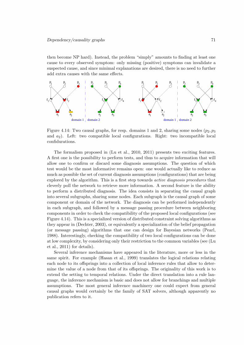
Dependency/causality graphs 71
then become NP hard). Instead, the problem “simply” amounts to finding at least onecause to every observed symptom: only missing (positive) symptoms can invalidate asuspected cause, and since minimal explanations are desired, there is no need to furtheradd extra causes with the same effects.
p4
f4f3
a3
p2
p3
p1
p2
p3
f1 f2
a1 a2 a2
p
domain 1 domain 2 domain 1 domain 2
4
f4f3
a3
p2
p3
p1
p2
p3
f1 f2
a1 a2 a2
Figure 4.14: Two causal graphs, for resp. domains 1 and 2, sharing some nodes (p2, p3
and a2). Left: two compatible local configurations. Right: two incompatible localconfidurations.
The formalism proposed in (Lu et al., 2010, 2011) presents two exciting features.A first one is the possibility to perform tests, and thus to acquire information that willallow one to confirm or discard some diagnosis assumptions. The question of whichtest would be the most informative remains open: one would actually like to reduce asmuch as possible the set of current diagnosis assumptions (configurations) that are beingexplored by the algorithm. This is a first step towards active diagnosis procedures thatcleverly poll the network to retrieve more information. A second feature is the abilityto perform a distributed diagnosis. The idea consists in separating the causal graphinto several subgraphs, sharing some nodes. Each subgraph is the causal graph of somecomponent or domain of the network. The diagnosis can be performed independentlyin each subgraph, and followed by a message passing procedure between neighboringcomponents in order to check the compatibility of the proposed local configurations (seeFigure 4.14). This is a specialized version of distributed constraint solving algorithms asthey appear in (Dechter, 2003), or equivalently a specialization of the belief propagation(or message passing) algorithms that one can design for Bayesian networks (Pearl,1988). Interestingly, checking the compatibility of two local configurations can be doneat low complexity, by considering only their restriction to the common variables (see (Luet al., 2011) for details).
Several inference mechanisms have appeared in the literature, more or less in thesame spirit. For example (Hasan et al., 1999) translates the logical relations relatingeach node to its offsprings into a collection of local inference rules that allow to deter-mine the value of a node from that of its offsprings. The originality of this work is toextend the setting to temporal relations. Under the direct translation into a rule lan-guage, the inference mechanism is basic and does not allow for branchings and multipleassumptions. The most general inference machinery one could expect from generalcausal graphs would certainly be the family of SAT solvers, although apparently nopublication refers to it.

72 State of the art
Interestingly, (Grosclaude, 2008) proposes a slightly different approach, when testnodes are more numerous than alarm nodes. The idea is to compile the causal graphinto a diagnosis procedure, that selects the most relevant tests to perform and theirordering, in view of quickly identifying the origin of a failure. This results into a decisiondiagram driven by tests, as the ones that are used by hotline operators. Apparently,the research direction has not been fully formalized nor explored.
Graph construction. The major bottleneck of this approach is clearly the derivationof the causal graph: given this graph, the design of the inference engine is rathereasy and is a well paved road. Unfortunately, the difficulties on the modeling sidehave received much less attention. From the few papers that address them, there areessentially two sources of information that can be used.
1. Dependency graphs, or modeling how things work. This consists in selecting theset of network resources that will appear in the model, together with their possiblefailures and the symptoms they produce (Houck et al., 1995). One then representsthe dependencies that relate these resources. In (Gruschke et al., 1998), these re-sources are split into 3 categories: services (connectivity, access to a data-base,etc.), the physical equipment, under the form of end-systems, and the networkdevices, that guarantee the physical connectivity between end-systems. The de-pendency relations between these resources derive from the network topology, theMIBs (Management Information Bases) of the equipment and of the applications,or the inventory systems. An important concern is the definition of the appropri-ate granularity for the model. Interestingly, this paper advocates the design of auser interface allowing an expert to partially build and refine this model. It alsoadvocates the construction at runtime of the appropriate dependency graph, inorder to track topological changes in the network. In the same spirit, (Grosclaude,2008) (in French) makes use of operational models, at the service level, that cap-ture some of the resources (or prerequisites) necessary to a service, for exampleHiFi VoIP. These dependencies describe both structural requirements as well astemporal requirements. Temporal requirements express for example the correctexecution of protocols or procedures that are necessary to launch a service (e.g.establishing a connection, obtaining an IP address, having internet connectivity,etc.). As another source of information, dependency relations can also be derivedfrom the information models that define how the managed objects are structured,connected and related (Choi et al., 1999; Yemini et al., 1996; Houck et al., 1995).
2. Failure graphs, or modeling why things may not work. This is the dual approach,that consists in examining failure cases. This information generally comes fromexperienced situations (as in Cased Based Reasoning) compiled by experts intofailure scenarios. It provides partial fault propagation examples that can be di-rectly translated into a causal graph (Grosclaude, 2008). This model can beenriched with test scenarios or simple information retrieval that can enrich theobservations (for example asking the user the color of a led on his equipment).However, it is by essence incomplete, limited to/by the interpretation of experts

Chronicles: patterns of timed events 73
and sometimes erroneous, limited to the experienced failures, and it can also betoo much specialized to a given network topology.
Discussion. Compared to fault-symptom graphs, causal graphs offer several inter-esting advantages: beyond the detection of the modeled failures (root causes), theyalso explain what happened in the network as consequences of these failures. This isa valuable information for the operator that can then check the validity of these au-tomatic interpretations of alarms, and further check the relevance of the fault model.Moreover, causal graphs are generally a prerequisite to the derivation of fault-symptomgraphs, but they have a sparser structure which is beneficial to inference algorithms.
Several formalisms have been proposed for causal graphs, that encode various kindsof logical relations between causes and effects. As they are designed for snapshots on thenetworks (i.e. for events collected within a time window), they grab both strict causal-ities, but also precedence, possibly with time constraints. The expressivity level of thedifferent formalisms varies, which results in inference problems of different complexi-ties. But overall, all can be captured under the umbrella of SAT problems. Inferenceis well understood for this family of problems, and even admits distributed/modularversions. In particular, one can consider systems defined by local (logical) constraintsas specific cases of Bayesian networks, for which exact and approximate inference al-gorithms are available and rather well understood. Interestingly, some contributionshave highlighted that the possibility to perform tests was raising new problems, like theoptimal selection of these tests, which is a first step towards active diagnosis. Further,one can also compile offline a causal graph into organized test plans that would helpresolve some observed malfunctions, and that could be used, for example, as a supportfor hotline operators.
While algorithmic resources are well mastered for these problems, the more demand-ing (but necessary) modeling stage has been much less explored. Some contributionshave proposed to use and compile the available knowledge that can be derived fromtopological considerations: managed objects definitions and structures (informationmodels), network resources dependencies (MIBs), protocols and procedures necessaryto the establishment of services, etc. Some contributions have suggested that thiscould open the way to “modelling at runtime”, in order to fit the model to the man-aged network. Two important questions remain open: the selection of the appropriategranularity for the model, and the definition of an interactive modeling framework thatwould help an operator or an expert check and refine the current version of the model.
4.7 Chronicles: patterns of timed events
Principle. This approach proposes to monitor a continuous flow of timed eventsa1, a2, ..., an, ..., and to look for known patterns of events within this flow that charac-terize a specific malfunction (Dousson, 1996; Dousson and Maigat, 2007).
The flow is made of the observable events that reach the network manager, andeach event an is characterized by some event type τ(an) denoting the nature of the

74 State of the art
observed problem (for example “excessive BER on equipment E”) and by a date δ(an)at which this alarm was produced. These dates assume the existence of a global clockin the netwok.
The patterns one is looking for in this flow are called chronicles. A chronicle isa labeled oriented graph of events G = (V,E, τ, α, β). Vertices V represent events,and τ associates an event type to each of them. Edges E ⊆ V × V encode temporaldependencies between the events they connect, by means of functions α, β : E → R.To the edge e = (v, v′) ∈ E, better denoted v → v′, one associates the time intervalI(e) = [α(e), β(e)] which means that event v′ must appear at least α(e) time unitsand at most β(e) time units after v. Equivalently, if events v and v′ appear at dates tand t′ respectively, then one must have α(e) ≤ t′ − t ≤ β(e). Observe that one couldvery well reverse the orientation of an edge e = (v, v′) without changing this semantics,by taking I(v′ → v) = −I(v → v′) = [−β(e),−α(e)]. So the oriented graph G neednot be acyclic. Observe also that the time intervals I(e) may contain both negativeand positive values, therefore a chronicle does not necessarily encode causality relationsbetween events, although this is generally the case in practice.
a
b
c
d
(a,1) (a,2) (c,3) (b,4) (a,4) (c,5) (b,5) (d,5) (c,6) (d,6)
[0,1][1,2
]
[0,1][1
,2]
Figure 4.15: An timed event flow (top) and a chronicle (bottom). The arrows indicatea chronicle instance within the event flow.
An instance of chronicle G = (V,E, τ, α, β) into the alarm flow (an)n>0 is a mappingφ : V → {an, n > 0} that preserves event types and such that event dates satisfythe time contraints of the chronicle (Figure 4.15). Specifically, one must have ∀v ∈V, τ(φ(v)) = τ(v), and ∀e = (v, v′) ∈ E, δ(φ(v′))− δ(φ(v)) ∈ I(e).
For simplicity here, we consider the basic language of chronicles, that only considersevent occurrences. The formalism extends to capture the absence of events within agiven time interval, the continuous presence of a phenomenon within some period, orto count the number of events of a certain type within some period.
Chronicle consistency. We have mentioned above that G needs not be acyclic.Nevertheless, the set of time contraints that it defines must be consistent. This veri-fication can be performed by propagating the time constraint of each edge to the restof the graph, until stability. One starts by completing G with all missing edges v → v′
(provided v′ → v does not already exist), setting I(v → v′) =]−∞,+∞[. The propa-gation rule is local (Figure 4.16): let e0 = v → v′′ be an edge, and let e1 = v → v′ ande2 = v′ → v′′ be an alternate path of length 2 relating v to v′′ in G. One then updates

Chronicles: patterns of timed events 75
I(e0) by
I(e0) := I(e0) ∩ [I(e1) + I(e2)]
or equivalently
α(e0) := max[α(e0), α(e1) + α(e2)]β(e0) := min[β(e0), β(e1) + β(e2)]
If some I(e0) becomes empty, the chronicle is invalid or inconsistent: no date on eventscan satisfy these constraints. Moreover, the local consistency that the above propaga-tion rule enforces can be proved to be equivalent to the global consistency. Thereforethe ‘if’ is actually also an ‘only if’. The propagation rule must be applied to every tripleof edges (up to reversing some of them), which results in a complexity in O(|V |3). Fig-ure 4.17 illustrates a graph of temporal constraints before and after propagation ofconstraints.
[2,4][0,5
]
[0,6]
[0,5
] [2,4]
v
v’
v" v
v’
[2,6]=[0,6] {[0,5]+[2,4]}v"U
Figure 4.16: The constraint propagation rule in a chronicle.
e2
e3
e4
[5,20]
[10,2
5]
[5,20]
[5,25][0
,5]
[5,2
5]
[15,30]
[10,3
0]
[0,30]
e
[0,5
]
1
e2
e3
e4
e1
Figure 4.17: A time constraint graph before (left) and after (right) constraint propa-gation.
Recognition algorithm. The procedure maintains a set of partially recognizedchronicles, i.e. partial mappings φ from G to the event set (Dousson, 1996; Dous-son and Maigat, 2007). This is initiated as soon as a minimal event in the chronicle isidentified in the flow. As this imposes a date to a vertex of G, the constraint propa-gation algorithm can be used to determine intervals for the arrival dates of the otherevents. If such an expected successive event appears in the flow, with correct type andcorrect time, the partial instance φ gives birth to two partial instances: an extension φ′
of φ including the new observed event a, followed by a propagation of the constraintsimposed by the date δ(a), and a copy of φ to prepare the ground for another event a′
with the same type as a that may appear later.
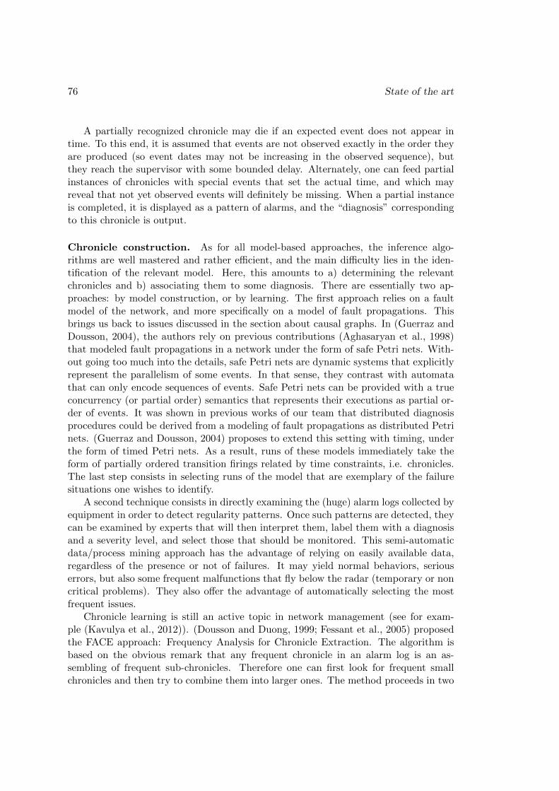
76 State of the art
A partially recognized chronicle may die if an expected event does not appear intime. To this end, it is assumed that events are not observed exactly in the order theyare produced (so event dates may not be increasing in the observed sequence), butthey reach the supervisor with some bounded delay. Alternately, one can feed partialinstances of chronicles with special events that set the actual time, and which mayreveal that not yet observed events will definitely be missing. When a partial instanceis completed, it is displayed as a pattern of alarms, and the “diagnosis” correspondingto this chronicle is output.
Chronicle construction. As for all model-based approaches, the inference algo-rithms are well mastered and rather efficient, and the main difficulty lies in the iden-tification of the relevant model. Here, this amounts to a) determining the relevantchronicles and b) associating them to some diagnosis. There are essentially two ap-proaches: by model construction, or by learning. The first approach relies on a faultmodel of the network, and more specifically on a model of fault propagations. Thisbrings us back to issues discussed in the section about causal graphs. In (Guerraz andDousson, 2004), the authors rely on previous contributions (Aghasaryan et al., 1998)that modeled fault propagations in a network under the form of safe Petri nets. With-out going too much into the details, safe Petri nets are dynamic systems that explicitlyrepresent the parallelism of some events. In that sense, they contrast with automatathat can only encode sequences of events. Safe Petri nets can be provided with a trueconcurrency (or partial order) semantics that represents their executions as partial or-der of events. It was shown in previous works of our team that distributed diagnosisprocedures could be derived from a modeling of fault propagations as distributed Petrinets. (Guerraz and Dousson, 2004) proposes to extend this setting with timing, underthe form of timed Petri nets. As a result, runs of these models immediately take theform of partially ordered transition firings related by time constraints, i.e. chronicles.The last step consists in selecting runs of the model that are exemplary of the failuresituations one wishes to identify.
A second technique consists in directly examining the (huge) alarm logs collected byequipment in order to detect regularity patterns. Once such patterns are detected, theycan be examined by experts that will then interpret them, label them with a diagnosisand a severity level, and select those that should be monitored. This semi-automaticdata/process mining approach has the advantage of relying on easily available data,regardless of the presence or not of failures. It may yield normal behaviors, seriouserrors, but also some frequent malfunctions that fly below the radar (temporary or noncritical problems). They also offer the advantage of automatically selecting the mostfrequent issues.
Chronicle learning is still an active topic in network management (see for exam-ple (Kavulya et al., 2012)). (Dousson and Duong, 1999; Fessant et al., 2005) proposedthe FACE approach: Frequency Analysis for Chronicle Extraction. The algorithm isbased on the obvious remark that any frequent chronicle in an alarm log is an as-sembling of frequent sub-chronicles. Therefore one can first look for frequent smallchronicles and then try to combine them into larger ones. The method proceeds in two
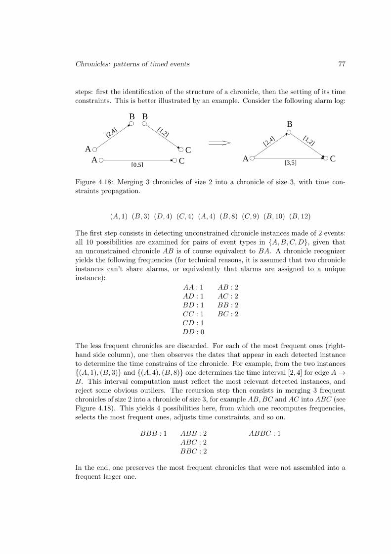
Chronicles: patterns of timed events 77
steps: first the identification of the structure of a chronicle, then the setting of its timeconstraints. This is better illustrated by an example. Consider the following alarm log:
[2,4
]
A
B
[0,5]A C
[2,4
] [1,2]
[3,5]
B
CA
C
[1,2]
B
Figure 4.18: Merging 3 chronicles of size 2 into a chronicle of size 3, with time con-straints propagation.
(A, 1) (B, 3) (D, 4) (C, 4) (A, 4) (B, 8) (C, 9) (B, 10) (B, 12)
The first step consists in detecting unconstrained chronicle instances made of 2 events:all 10 possibilities are examined for pairs of event types in {A,B,C,D}, given thatan unconstrained chronicle AB is of course equivalent to BA. A chronicle recognizeryields the following frequencies (for technical reasons, it is assumed that two chronicleinstances can’t share alarms, or equivalently that alarms are assigned to a uniqueinstance):
AA : 1 AB : 2AD : 1 AC : 2BD : 1 BB : 2CC : 1 BC : 2CD : 1DD : 0
The less frequent chronicles are discarded. For each of the most frequent ones (right-hand side column), one then observes the dates that appear in each detected instanceto determine the time constrains of the chronicle. For example, from the two instances{(A, 1), (B, 3)} and {(A, 4), (B, 8)} one determines the time interval [2, 4] for edge A→B. This interval computation must reflect the most relevant detected instances, andreject some obvious outliers. The recursion step then consists in merging 3 frequentchronicles of size 2 into a chronicle of size 3, for example AB,BC and AC into ABC (seeFigure 4.18). This yields 4 possibilities here, from which one recomputes frequencies,selects the most frequent ones, adjusts time constraints, and so on.
BBB : 1 ABB : 2 ABBC : 1ABC : 2BBC : 2
In the end, one preserves the most frequent chronicles that were not assembled into afrequent larger one.

78 State of the art
Discussion. The chronicle method belongs to pattern recognition approaches, andrelies on rather efficient detection algorithms. They offer the nice feature of processingalarms on the fly, taking their date into account, which is a clean way to go beyonda plain reasoning based on a sliding time window. In the currently available settings,however, chronicles are sensitive to alarm losses, and there is no probabilistic versionof chronices. Their explanation power is limited to the interpretation made by expertsfor each chronicle inserted into the recognition engine.
On the modeling side, chronicles can again be derived from fault propagation mod-els, but most interestingly, there exist semi-automatic learning algorithms that candiscover chronicles from alarm logs, an abundant resource which is rarely exploited.However, the unability of chronicles to adapt to changing networks, and the presenceof an expert in the loop, remain important drawbacks.
4.8 Bayesian Networks
Bayesian networks are another possible choice for alarm correlation due to their abilityto handle uncertainty and represent cause and effect relationships. A Bayesian Network(BN) is a directed acyclic graph (traditionally abbreviated DAG) whose nodes repre-sent random variables, the edges denote existence of direct causal influences betweenthe linked variables and the strengths of these influences are expressed by forward con-ditional probabilities (see Figure 4.19). In the context of fault diagnosis, the randomvariables represent states of network objects or the occurrence of network events. An
Figure 4.19: A Bayesian network for IP paths diagnosis
important advantage that Bayesian networks offer is the avoidance of building hugejoint probability distribution tables that include permutations of all the nodes in thenetwork. Rather, only the possible states of a node’s immediate predecessors and their

Bayesian Networks 79
effects on the node are necessary.
Definition 7 A Bayesian network consists of the following:
• a set of variables and a set of directed edges between variables;
• each variable has a finite set of mutually exclusive states;
• the variables together with the directed edges form a DAG, a directed graph isacyclic if there is no directed path X1 → · · · → Xn so that X1 = Xn;
• to each variable X with parents W1, ...,Wn, a conditional probability distribution(CPD) P (X|W1, ...,Wn) is attached; if X has no parents, then the table reducesto the unconditional probability table P (X).
Conditional probability distributions can be described in a variety of ways. A common,but not necessarily compact representation for a CPD is a table which contains a rowfor each possible set of values for the parents of the node describing the probability ofdifferent values for X. These are often referred to as table CPDs and are tables of multi-nomial distributions. Other possibilities are to represent the distributions via a treestructure (called, tree-structured CPDs), or using an even more compact representationsuch as a noisy-OR or noisy-MAX.
A Bayesian network is made up of various types of nodes. A root node has noparents, and a leaf node has no children. An evidence node, also known as a findingnode, instantiated node, or observed node represents a variable with a single value thathas been observed with probability one. Such a node is said to have been instantiatedwith specific or hard evidence. The set of all evidence variables is denoted E with valuese. The conditional and prior probabilities are part of the design of the network anddo not change during inference. The dynamic values of the node probabilities shall bedenoted Bel(x). This latter value reflects the overall belief in the proposition X = xgiven all the evidence, that is,
Bel(x) , p(x|e) (4.1)
As such, the belief values represent the posterior probabilities. The posterior probabilityof any variable may be obtained through marginalisation. A vector of belief values forall possible states of X is denoted Bel(X).
Belief propagation
A Bayesian network represents a complete probabilistic model of all the variables ina specific domain. Therefore, it contains all the information required to answer anyprobabilistic question about any variable in that domain. These questions are usuallyrestricted to determining the most likely hypothesis or, more specifically, the beliefin, or probability of, each possible hypothesis, given the available observations or ev-idence. The application of evidence is ongoing as the observations continue to arriveover a period of time. Therefore, the Bayesian network is dynamic and the most likelyhypotheses, and their probabilities, are likely to change.

80 State of the art
To ascertain the effect of the available evidence on any variable (hypothesis), eachnode updates the posterior probabilities for each of its hypotheses on the receipt ofdata messages from its immediate neighbours. The effect of evidence is transmittedthroughout the network by allowing each variable to continually update its state bycomparing the state of its neighbours against local constraints; if the local constraintsare satisfied, no activity takes place, otherwise action is taken to correct the constraintviolation and messages are sent to the immediate neighbours of that variable.
The posterior probability, or belief, for variable X = x is Bel(x) , p(x|e). Theevidence influencing X is separated into two disjoint subsets, e−X denoting the evidenceintroduced through the arcs between X and its children, and e+
X denoting the evidenceintroduced through the arcs between X and its parents. These may be further dividedinto e−XYi for the evidence introduced through the arc to child Yi, and e+
WjXas that
introduced through the arc from parent Wj . Applying Bayes’ rule conditioned on e+X ,
and since e−X and e+X are independent given X, the belief may be written
Bel(x) = p(x|e−X , e+X) =
p(e−X |x, e+X) p(x|e+
X)
p(e−X |e+X)
=p(e−X |x) p(x|e+
X)
p(e−X |e+X)
. (4.2)
Defining π(x) = p(x|e+X) and λ(x) = p(e−X |x), the belief becomes
Bel(x) = α π(x) λ(x), (4.3)
where α represents a normalizing constant.Variable λ(x) is the likelihood representing diagnostic or retrospective support for
the proposition X = x. Vectors or messages λ(X), where each element of λ(X) corre-sponds to a different state of X, are passed up the network in the opposite directionto the arrows on the arcs i.e. from the children of X to X. Conversely, π(x) may beconsidered as the prior certainty of x given the prior evidence e+
X , and it represents thecausal or predictive support for X = x. Messages π(x), also representing each possiblestate of X, are passed down the network in the direction of the arrows i.e. from Xto its children. For simplicity, it is assumed that all evidence is introduced into thenetwork through leaf nodes, that is, all evidence on non-leaf nodes is represented byadding child leaf nodes.
The following description of the propagation in chains, trees and polytrees is takenfrom (Krieg, 2001). Note that the product F (X)G(X) of two such vectors will standfor term-by-term multiplication while the dot symbol · will be used to indicate matrixproducts.
Propagation in Chains
Consider the serial or chain network in Figure 4.20, where λ(Y ) = p(e−Y |Y ). Now,
λ(x) = p(e−X |x) =∑y
p(y|x) p(e−Y |y)⇒ λ(X) = λ(Y ) · p(Y |X). (4.4)
Similarly, λ(W ) = λ(X) · p(X|W ). Note that λ(X) is calculated from the probability

Bayesian Networks 81
Figure 4.20: Propagation in a chain network (taken from (Krieg, 2001))
table p(Y |X) attached to node Y and is calculated at node Y . To complete the beliefpropagation, consider the propagation of the π messages, starting at node W . NodeW is a root node and its only evidence is its prior probability distribution. Therefore,π(w) = p(w|e+
W ) = p(w), and
π(x) = p(x|e+X) =
∑w
p(x|w)p(w|e+W )⇒ π(X) = π(W ) · p(X|W ). (4.5)
Similarly, π(Y ) = π(X) · p(Y |X). The π messages are propagated as illustrated inFigure 4.20, and the belief at each node can be calculated using (4.3). The appropriateλ and π messages are re-propagated if evidence is added or changed.
Propagation in Trees
Now, consider a case of multiple child nodes, as illustrated in Figure 4.21. The addi-tional problems introduced here are combining the λs as they are propagated up thetree and separating the πs as they are propagated down the tree. Starting with the
Figure 4.21: Propagation in a tree (taken from (Krieg, 2001))
λs, the evidence on the sub-tree at X is partitioned into the disjoint sets e−Y1 and e−Y2 .

82 State of the art
Therefore,
λ(x) = p(e−Y1 |x) p(e−Y2 |x) , λY1(x) λY2(x)⇒ λ(X) = λY1(X) λY2(X). (4.6)
Node X then transmits λX(W ) = λ(X) · p(X|W ) to node W . Assuming we haveπ(X) = πX(W ) · p(X|W ), it is now necessary to split π(X) into individual messagesfor each child of X, that is Y1 and Y2. Consider the predictive support for X = x thatis passed to node Y1, namely,
πY1(x) = p(x|e+X , e
−Y2
). (4.7)
Using Bayes’ rule,
πY1(x) = α p(e−Y2 |x)p(x|e+X) = α λY2(x)π(x). (4.8)
More generally, for the kth child of K children of X,
πYk(x) = αK∏
j=1\k
λYj (x)π(x) = αBel(x)
λYk(x)⇒ πYk(X) = α
Bel(X)
λYk(X), (4.9)
allowing the same message to be passed to all children, namely Bel(X), for determi-nation of πk(X) at each child.
Propagation in Polytrees
Causal polytrees are singly connected trees in which each node may have multipleparents. They may be thought of as collections of causal trees, fused at the nodeswhere the arrows converge. To illustrate the propagation in this type of network,
Figure 4.22: Propagation in a causal polytree network
consider the example in Figure 4.22. The additional problems introduced by this typeof structure are combining the π messages from multiple parent nodes and splitting

Bayesian Networks 83
the λ messages between multiple parent nodes. Consider the variable X that has twoparents, W1 and W2, and two children, Y1 and Y2. The evidence obtained from thesub-tree rooted at X is the union of evidence obtained from each arc connecting it to itschildren, that is, e−XY1 and e−XY2 . Similarly, the evidence from the rest of the networkcan be separated into that obtained from each arc linking X to each of its parents,namely e+
W1Xand e+
W2X(Pearl, 1988).
The λ messages, λ(X) = λY1(X) λY2(X) must be split for transmission to theparents of X, namely λX(W1) for W1 and λX(W2) for W2. Therefore, we denoteλX(w1) = p(e−W1X
|w1) and separate the evidence e−W1Xinto disjoint sets, namely that
associated with the sub-tree rooted at X, e−X , and that associated with all other parentsof X, in this case e+
W2X. Then,
λX(w1) = p(e−W1X|w1) = p(e−X , e
+W2X|w1), (4.10)
and conditioning on X and W2 and applying Bayes’ Rule gives
λX(w1) = β∑x
p(e−x |x)∑w2
p(w2|e+W2X
)p(x|w1, w2), (4.11)
where β is an arbitrary constant. In general, for n parents:
λX(wi) = β∑x
λ(x)∑
wk:k 6=ip(x|w1, w2, ..., wn)
n∏k=1\i
πXwk, (4.12)
where πX(wk) = p(wk|e+WkX
). The predictive support is provided through the arcs
from the parents of X, that is, π(x) = p(x|e+X) = p(c|e+
W1X, e+W2X
). Conditioning onW1 and W2, this becomes
π(x) =∑w1
∑w2
p(x|w1, w2)πX(w1)πX(w2). (4.13)
In general, for n parents, this may be written,
π(x) =∑
w1,w2,...,wn
p(x|w1, w2, ..., wn)
n∏i=1
πX(wi). (4.14)
Application of Bayesian Networks for fault management
Several applications of Bayesian networks for fault management have been reported.(Deng et al., 1993) investigated the application of probabilistic reasoning to fault di-agnosis in Linear Lightwave Networks (LLN’s). The basic network components areLDC’s (linear divider/combiner). The observable messages are the LDC input andoutput power values. If an LDC has failed or some part of it has failed, all its outputpower values will be incorrect (outside the specified range) but its input power valuesremain unaffected. The LLN routes/connections determine the internal connections

84 State of the art
between the input and the output ports of every LDC. The inference model is con-structed as follows. A power value, say Fip, is assumed to be in one of the two states,within the expected range or outside it. A binary-valued random variable Fi is definedfor power value Fip: Fi = 1 if the power value Fip is within the expected range, and0 otherwise. Similarly, for each LDC a binary-valued random variable Lj is defined:Lj = 1 if LDCj is under normal operation, and 0 otherwise. Furthermore, the Lj ’s areassumed to be mutually independent. The dependence relations among these randomvariables can be graphically represented as a DAG. For a non-root random variable Xin the DAG, X and its parents U1, ..., Un, are related by X = U1 ∧ U2 ∧ ... ∧ Un. Theconditional probability P (x|u1, ..., un) = 1 if x = u1 ∧ ... ∧ un and 0 otherwise. By theDAG and the defined probability distributions, the LLN inference model is representedby a Bayesian network. An inference algorithm capable of conducting fault diagnosiswith incomplete evidence and on an interactive basis is then proposed.
(Steinder and Sethi, 2002) proposed a layered system model that represents rela-tionships between services and functions offered between neighboring protocol layers.These relationships form a bipartite probabilistic dependency graph where each node isassociated with multiple failure modes F1, ..., Fk, which represent availability and per-formance problems pertaining to the service or function represented by the node. Thechosen BN structure represents a model of conditional probabilities known as noisy-ORgates. This simplified model contains binary-valued random variables. A mapping fromthe above dependency graph to the BN is performed as follows. For every node of thedependency graph and for every failure mode associated with this node, a random vari-able is created, whose domain is {true, false} (1 and 0 are also used to represent valuestrue and false, respectively). Let Vi be a belief network node created for failure modeFj of the dependency graph node representing a service or a function. AssignmentVi = true (V i = false) indicates that the service/the function is (is NOT) in conditionFj . For every dependency graph edge X → Y and for every failure mode of node Y ,Fi,the corresponding failure mode of node X, Fj is determined. Let Vi be the belief net-work node corresponding to Y and Fi. Let Vj be the belief network node correspondingto X and Fj . A belief network edge is inserted from Vi to Vj . A probability matrixassociated with dependency link X → Y . A symptom is defined as an observation thata dependency graph node X is in condition Fj (negative symptom), or is NOT in con-dition Fj (positive symptom). If Vi is the belief network node corresponding to X andits failure mode Fi, then the negative symptom and positive symptom are interpretedas an instantiation of Vi with value true and false, respectively. As a result of thismapping, the set of all observed symptoms becomes the evidence set e. The problemof finding the subset of (all possible) faults is equivalent to computing the MPE querybased on the evidence set e.
(Steinder and Sethi, 2004b) presents a probabilistic event-driven fault localizationtechnique, which uses the so-called probabilistic symptom-fault map as a fault prop-agation model. With every fault fi ∈ F a probability of its independent failure isassociated, which is denoted by p(fi). The edge between fi ∈ F and sj ∈ S indi-cates that fi may cause sj . The edge is weighted with the probability of the causalimplication, p(sj |fi). A noisy-OR model of probability distribution is considered. A

Bayesian Networks 85
subset of symptoms observed is denoted by SO. The purpose of fault localization is tofind FD ⊆ F that maximizes the probability that (1) all faults in FD occur and (2)each symptom in SO is explained by at least one fault from FD. A fault localizationtechnique called Incremental Hypothesis Updating (IHU) is proposed. Its basic versioncreates a set of hypotheses, each of which is a subset of F that explains all symptomsin SO. Hypothesis hj ⊆ F explains symptom si ∈ SO if it contains at least one faultthat explains si. The hypotheses are ranked using a belief metric, b, which expressesthe confidence associated with a given hypothesis relative to other hypotheses. Thealgorithm is triggered by an observation of the ith symptom, si, and creates a set ofhypotheses, Hi, each explaining symptoms s1 through si. Set Hi is created by updatingHi−1 with an explanation of symptom si. Set Hsi is defined as a set {fk ∈ F} suchthat fk may cause si. To incorporate the explanation of symptom si into a set of faulthypotheses, in the ith iteration of the algorithm, each hj ∈ Hi−1 is analysed. If hj isable to explain symptom si, hj is put into Hi. Otherwise, hj has to be extended byadding to it a fault from Hsi . Fault fl ∈ Hsi may be added to hj ∈ Hi−1 only if thesize of hj , |hj |, is smaller than µ(fl), defined as the minimal size of a hypothesis inHi−1 that contains fl and explains symptom si. The proposed solution allows multiplesimultaneous independent faults to be identified and is then extended to deal with lossand spurious symptoms.
(Khanafer et al., 2008) presented an automated diagnosis system for UMTS net-works using Bayesian Network approach. Two components of the automatic diagnosissystem have been distinguished, i.e. the diagnosis model and the inference method.The elements of the model are causes and symptoms. Causes are modeled as dis-crete random variables with two states (absent / present). Two types of symptomsare considered: Alarms and KPIs. Alarms are also modeled as discrete random vari-ables with two states (on / off ). KPIs can be modeled as discrete random variableswith two, three, or more states, each representing a subset of the continuous range ofthe KPI. The chosen BN structure is a so-called Naive Bayes Model (NBM), which isalso known as a Simple Bayes Model or Naive Bayesian Classifier. The NBM (Fig-ure 4.23) consists of a parent node C, whose states are the possible fault causes, andthe children nodes S1, ..., SN , which represent the symptoms and may have any dis-crete number of states. This model assumes that there can only be one fault happening
Figure 4.23: NBM
at the same time. The impact of this simplification on the diagnosis performance isconsidered minor while the simplicity of this type of model is a clear benefit. The re-quired probabilities for this model are the following: p(C = ck) for each fault cause ck;

86 State of the art
p(Si = si,j |C = ck) for each state si,j of Si and each fault cause ck. Thus, with theNBM structure, the desired conditional probabilities of the fault causes given the ob-served symptoms can be calculated as
p(C = ck|E) =p(C = ck)
∏Ni=1 p(Si = si,j |C = ck)
p(E).
This equations assumes that the symptoms Si are independent given the fault causeC. According to the independence properties of a BN, this is exactly what the NBMstructure indicates. To further enhance automation and performance of the BN model,the automated learning of both KPI thresholds and model probabilities has beenthouroughly investigated.
Discussion Due to Bayesian network’s form of knowledge representation, large amountsof interconnected and causally linked data can be represented. Generally speaking:Bayesian networks can represent deep knowledge by modeling the functionality of thetransmission network in terms of cause and effect relationships between element andnetwork behavior and faults.
Bayesian networks can provide guidance in diagnosis. Calculations over the sameBN can determine both the precedence of alarms and the areas that need furtherclarification in order to provide a finer grained diagnosis. They can handle noisy,transient, and ambiguous data due to their grounding in probability theory. They havea modular, compact, and easy to understand representation, when compared to otherprobabilistic methods. They provide a compact and well-defined problem space becausethey use an exact solution method for any combination of evidence or set of faults.
Bayesian networks are appropriate for automated diagnosis because of their deeprepresentations and precise calculations. A concise and direct way to represent a sys-tem’s diagnostic model is as a Bayesian Network constructed from relationships betweenfailure symptoms and underlying problems. A Bayesian Network represents cause andeffect between observable symptoms and the unobserved problems so that when a setof symptoms are observed the problems most likely to be the cause can be determined.In practice, the network is built from descriptions of the likely effects for a chosen fault.In use as a diagnostic tool, the system reasons from effects back to causes.
The difference of Bayesian Networks, in comparison with other classical methods, istheir polyvalence. They allow dealing with issues such as prediction or diagnosis, opti-mization, data analysis of feedback experience, deviation detection and model updating.The graphical representation is interesting since the model complexity is understand-able in a single view. In the case of large size model, object oriented representationOOBN or probabilistic relational descriptions (PRM) provide manageable models.
The development of a diagnostic Bayesian Network requires a deep understandingof the cause and effect relationships in a domain, provided by domain experts. Thisis both an advantage and disadvantage. An advantage is the knowledge is not rep-resented as a black box, as are the Neural Networks. Thus, humanly understandableexplanations of diagnoses can be given. The disadvantage is that the realm of the con-

Summary 87
sidered system/network can be technologically immature and as a result expertise infault diagnosis may be hard to find and to implement.
4.9 Summary
Many approaches to fault management rely on black-box or learning methods (neuralnetworks, self-organizing maps, statistical learning (Kavulya et al., 2011), codebooktechniques (Reali and Monacelli, 2009), chronicle discovery (Dousson, 1996; Doussonand Duong, 1999; Kavulya et al., 2012)). Such strategies generally suffer from a lack ofclassified data relating failures to some observed symptoms. They also poorly resist tophenomena like complex symptom patterns due to multiple faults, or to the asynchro-nism or loss of observations, and they are difficult to maintain as the network evolves.Such approaches are thus appropriate for simple and small scale event correlation overfixed topologies, where training can safely converge.
To progress towards the more ambitious objectives mentioned above, one mustadopt a model-based strategy, which consists first in building a model of the man-aged network, establishing relations between correct/incorrect functioning and observedsignals/symptoms, and then in deriving event management algorithms based on thismodel. This is the track adopted by several contributions (see the ‘model traversal’techniques in (Steinder and Sethi, 2004a), and their generalization into ‘graph theo-retic’ techniques). One trend compiles expert knowledge about malfunctions and theirconsequences, or symptoms and their causes, into causal graphs that form the supportof automatic (possibly distributed) reasoning (Lu et al., 2011) and (Grosclaude, 2008)(in French). Another important trend models or learns from data the (logical or sta-tistical) dependencies between resources, initial faults and observable symptoms, andcompile them into Bayesian networks or related objects (Bouloutas et al., 1994, 1995;Fabre et al., 2004). The inference engines on such structures can then be taken offthe shelf, since this is a well understood and much covered topic, and the distributionof these techniques is also a well paved trail (Fabre et al., 2004, 2005). As witnessedby the above contributions, however, model-based techniques always raise two majordifficulties: a) how to derive such a model, suited to a given network at a given time,in particular if one wishes to capture several network layers and segments (see openproblems 1, 4 and 6 in (Steinder and Sethi, 2004a)) and b) how to reason on a poten-tially huge model, if one wishes to manage a nation-wide network for example. Thisthesis proposes a contribution to these two issues.
Obtaining a model of the managed network is far from simple, especially if onewishes to capture inter-layer and inter-segment fault propagations. The first infor-mation source one should use is of course the topology of the network, which manycontributions considered (for e.g. (Bouloutas et al., 1994)), including professional toolsdedicated to specific network technologies. But one should go further and aggregatedifferent sources of information, generally found in the standards, in protocol descrip-tions, and in expert knowledge if available. Relying on the past experience of ourteam in the modeling of fault and alarm propagations (Fabre et al., 2004), we propose

88 State of the art
here a self-modeling approach. This consists first in identifying the different familiesof network resources that should be managed, and how these resources are structuredand rely on each other, following the usual hierarchical construction of networks. Thisyields a collection of generic patterns of resources and their dependencies, designedaccording to a specific grammar. Secondly, by exploring the managed network, one canthen create as many instances of these generic patterns as discovered in the networktopology. As these instances share some resources, this construction results in a largescale structure where similar patterns are duplicated and partially overlap. The modelobtained in that way perfectly matches a given network, and can be used for diagnosis,root-cause analysis, and possibly for failure impact analysis.
Regarding the diagnosis engine, we propose to translate the model of network re-sources and their dependencies into the Bayesian network (BN) formalism, which seemsto reach some consensus in the network management community. Bayes nets can easilymix statistical dependencies and constraints/logics, while enabling limited statisticallearning (parameter identification) when data are available. They can also accommo-date networks of dynamic systems (Fabre, 2007; Fabre et al., 2004; Fabre and Hadji-costis, 2006). Probabilistic reasoning on BN is well understood, and allows one to relateobservations or test results to the state of hidden variables of interest. But dealing withpossibly huge models may make them inappropriate. Therefore we propose to adaptthe BN formalism to explore only part of the model, starting by the resources involvedin a given malfunction to be explained, and progressively introducing/revealing moreresources (i.e. variables) to reach new observations and making new tests, in order tolocate the origin of the malfunction with more precision. Extra extensions would alsobe necessary, in particular to deal with the intrinsic hierarchical description of networks,but they will be examined in a forthcoming work.
As a support to these two research directions, the thesis considers the managementof failures in IMS networks, capturing several network segments (access, metropolitanand core), and the end-to-end services running on top of them (Bertin et al., 2007).
Chapter5Structure of IMS networks
Contents
5.1 Physical layer of the IMS Architecture . . . . . . . . . . . . 89
5.2 Functional layer of the IMS architecture . . . . . . . . . . . 90
5.2.1 Core IMS subsystem . . . . . . . . . . . . . . . . . . . . . . . 91
5.2.2 RACS subsystem . . . . . . . . . . . . . . . . . . . . . . . . . 95
5.2.3 NASS subsystem . . . . . . . . . . . . . . . . . . . . . . . . . 97
5.3 Procedural layer of the IMS Architecture . . . . . . . . . . . 101
5.3.1 NASS procedures . . . . . . . . . . . . . . . . . . . . . . . . . 102
5.3.2 RACS procedures . . . . . . . . . . . . . . . . . . . . . . . . . 104
5.3.3 Core IMS procedures . . . . . . . . . . . . . . . . . . . . . . . 105
5.4 Contributions: Relevant structural properties . . . . . . . . 111
Starting from standards descriptions of IMS networks, our objective in this chap-ter is to identify the network resources involved in such networks, their structuringand above all their dependencies, which will be the knowledge used to diagnose mal-functions. The main idea is that the failure of a resource is either spontaneous, orresults from the failure of a second resource that is necessary to the first one. The term‘resource’ covers both physical equipment in charge of transport, pieces of softwarerunning over them, but also procedures (that must be completed in order to accessIMS services). We represent an IMS network by a dependency model of three multiresolution layers.
5.1 Physical layer of the IMS Architecture
The physical layer1 displayed in Figure 5.1 comprises an access network and a corenetwork. The access network is made of two segments: the metro-access, and themetro-core. The former itself decomposes into smaller segments: access (first/lastmile) and aggregation. The first mile stretches from the Customer Premise Equipment(CPE) up to the Access Node (AN). As for the aggregation segment, it aggregates
1The one considered here corresponds to a possible realization of the TISPAN NGN IMS functionalarchitecture (TISPAN, 2009) with an xDSL-based access network.
89

90 Structure of IMS networks
traffic from different users, located behind different ANs, and connects them to themetro-core segment. Aggregation and metro-core segments are connected via one ormore IP edge routers. In configurations where the access segment uses the DigitalSubscriber Line (DSL) technology, the AN is known as a DSL Access Multiplexer(DSLAM) and the IP Edge router as a BRAS. The metro-core segment is connectedto the core network, containing the IMS service platform, via routers such as the SBC.The Point of Presence (PoP) of Internet (IP) is generally at the SBC, while routing inthe access network mostly uses Ethernet. Notice that the internal components of thecore network and of the metro aggregation have not been detailed.
IP
CPE DSLAM BRAS A-SBC Session Controller
Media Server
Media Gateway
Controller
User Profile Server
Core Network Media Gateway
I-SBC
First Mile Aggregation Metro-coreOther IP networks
Metro-access
Access Network
PSTN/ISDN
Figure 5.1: The generic IMS physical architecture
Properties of the physical layer
The physical layer architecture is made of specific equipment connecting various net-work segments. Such a connection is modelled by a ‘connected-to’ relationship betweenan equipment and a segment. Besides, the physical layer architecture is essentiallyhierarchical: network segments being decomposable into other physical equipment con-necting smaller network segments.
5.2 Functional layer of the IMS architecture
IMS is defined in the form of a reference architecture to enable delivery of next-generation communication services over an IP network. It is considered a subsystembecause it exists as part of a complete network. It is considered a reference archi-tecture, because the implementers build the functional elements conforming to thesespecifications. The IMS architecture is defined in terms of functional elements, theirinteraction, which is termed as reference points, and the protocols that carry out theseinteractions. All functional elements within the IMS architecture communicate with IP-based protocols. Session Initiation Protocol (SIP) (Rosenberg et al., 2002) is the mostprominent, as it provides the capability to establish and control multimedia sessions.One reason why SIP is important, is that IMS is seen to provide a uniform protocol forsignaling with the endpoints. Besides SIP, other protocols support vital functions aswell. Diameter (Calhoun et al., 2003) is the enabler for subscriber, policy, and chargingfunctions. Megaco/H.248 (Cuervo et al., 2000; ITU-T, 2013) and Real-Time Protocol

Functional layer of the IMS architecture 91
(RTP) (Schulzrinne et al., 2003) provide the media-related support. Common OpenPolicy Service (COPS) (Durham et al., 2000) was used in the earlier IMS releases forpolicy functions, but has now given way to Diameter.
We now look at some of the functions provided by the various elements in thearchitecture. The functional architecture is made of three main subsystems. TheNASS (TISPAN, 2010a) provides registration at the access level (identification andauthentication) and initialization of the User Equipment (UE) (in particular IP addressallocation) for accessing to the multimedia services. The RACS (TISPAN, 2006) is incharge of policy control, in particular resource reservation and admission control inthe access and aggregation segments of the network. Finally the Core IP MultimediaSubsystem (TISPAN, 2007) (core IMS) is in charge of session initiation, provisioningand termination (SIP) for multimedia services directed to terminal users. Subsystemsare hierarchical objects, comprising several functions (see below) that communicatewith each other via interfaces (reference points).
5.2.1 Core IMS subsystem
The Core IP Multimedia Subsystem (TISPAN, 2007, 2009) displayed in Figure 5.2comprises the the following functions.
Figure 5.2: Core IP Multimedia Subsystem architecture (taken from (TISPAN, 2007))
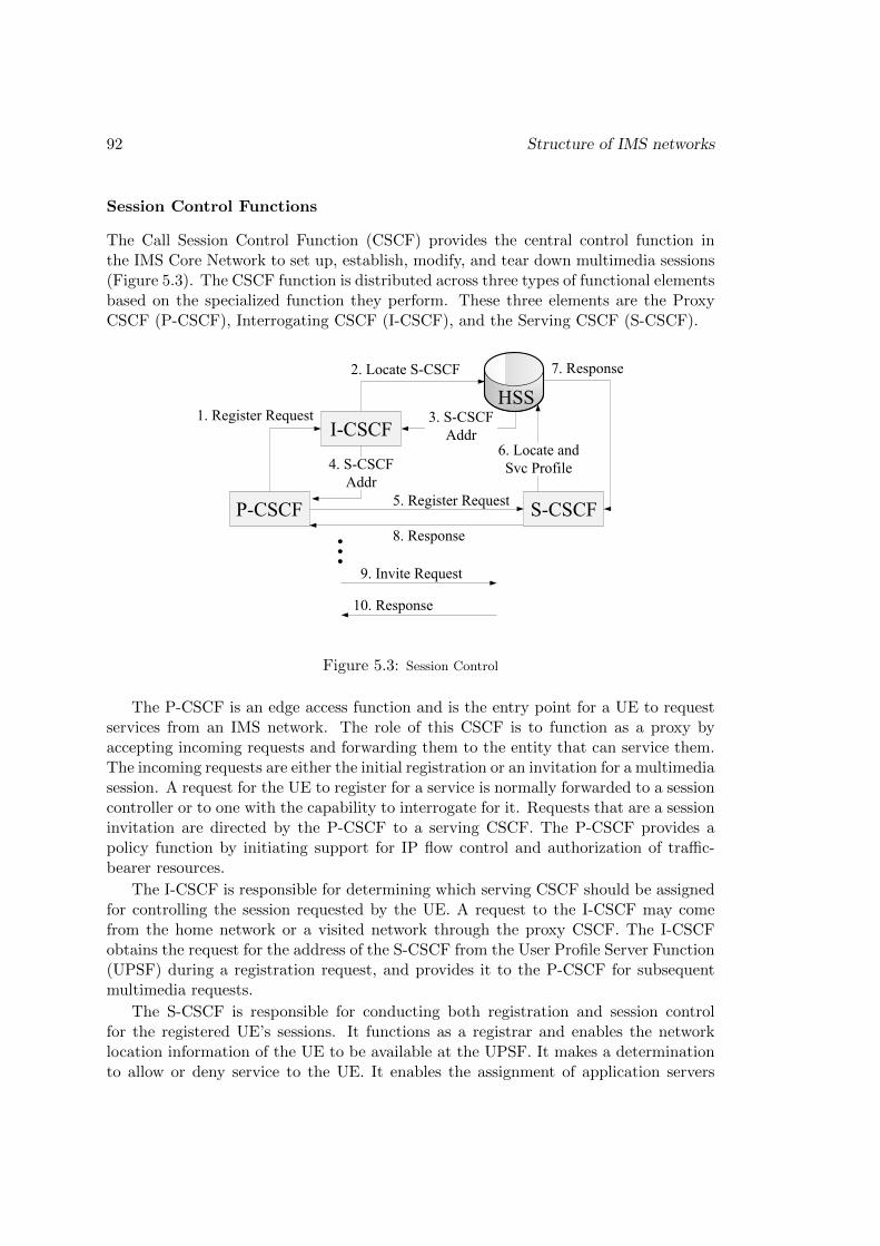
92 Structure of IMS networks
Session Control Functions
The Call Session Control Function (CSCF) provides the central control function inthe IMS Core Network to set up, establish, modify, and tear down multimedia sessions(Figure 5.3). The CSCF function is distributed across three types of functional elementsbased on the specialized function they perform. These three elements are the ProxyCSCF (P-CSCF), Interrogating CSCF (I-CSCF), and the Serving CSCF (S-CSCF).
HSS
P-CSCF S-CSCF
I-CSCF
2. Locate S-CSCF
3. S-CSCF
Addr
4. S-CSCF
Addr
1. Register Request
7. Response
6. Locate and
Svc Profile
5. Register Request
8. Response
10. Response
9. Invite Request
Figure 5.3: Session Control
The P-CSCF is an edge access function and is the entry point for a UE to requestservices from an IMS network. The role of this CSCF is to function as a proxy byaccepting incoming requests and forwarding them to the entity that can service them.The incoming requests are either the initial registration or an invitation for a multimediasession. A request for the UE to register for a service is normally forwarded to a sessioncontroller or to one with the capability to interrogate for it. Requests that are a sessioninvitation are directed by the P-CSCF to a serving CSCF. The P-CSCF provides apolicy function by initiating support for IP flow control and authorization of traffic-bearer resources.
The I-CSCF is responsible for determining which serving CSCF should be assignedfor controlling the session requested by the UE. A request to the I-CSCF may comefrom the home network or a visited network through the proxy CSCF. The I-CSCFobtains the request for the address of the S-CSCF from the User Profile Server Function(UPSF) during a registration request, and provides it to the P-CSCF for subsequentmultimedia requests.
The S-CSCF is responsible for conducting both registration and session controlfor the registered UE’s sessions. It functions as a registrar and enables the networklocation information of the UE to be available at the UPSF. It makes a determinationto allow or deny service to the UE. It enables the assignment of application servers

Functional layer of the IMS architecture 93
to the session, if required. Its role is to execute the session request by locating thedestination endpoint and conducting the signaling toward it.
All three CSCF functions are responsible for generating the Session Details or theCall Detail Records. The interface to the P-CSCF from the UE is the Gm interfacethat carries SIP or Session Description Protocol (SDP) signaling. The P-CSCF com-municates to the interrogating and serving CSCF using SIP over the Mw interface.
Subscription Functions
The User Profile Server Function (UPSF) is a large database containing the completesubscription information about an IMS user. This information is accessible to all theIMS core elements needing information about the subscriber’s profile, subscribed ser-vices, or authentication data. The UPSF supports the CSCF functions by: a) identify-ing the address of the CSCF that should be handling the session; b) storing the user’sregistration and location information; c) supporting the authentication and authoriza-tion by providing the integrity and ciphering data; d) and providing an access to aservice profile, for which the subscriber has been provisioned. The UPSF also extendsfunctionality to the application servers to determine service authorization, and alsogrants the capability to update subscriber profile data to application servers with pro-visioning capability. The CSCF communicates with the UPSF using Diameter over theCx interface. The application servers use the Diameter Sh interface. A large networkmay require provisioning the subscribers set into more than one UPSF. This requiresan intelligent entity to guide the requested CSCF or application server to the rightUPSF. The Subscriber Locator Function (SLF) provides this support to the I-CSCF,the S-CSCF, and the application servers as well. The CSCFs request the UPSF deter-mination from the SLF over the Diameter Dx interface. The application servers usethe Diameter Dh interface.
Media Functions
Having examined the elements in the control plane, we now examine the functionalelements responsible for processing the multimedia stream in the media plane (Fig-ure 5.4). The Multimedia Resource Function (MRF) encompasses the functionality tocontrol the media stream and provide resources for processing it. The MRF comprisesthe Multimedia Resource Function Controller (MRFC) and the Multimedia ResourceFunction Processor (MRFP). The bearer represents the actual multimedia stream car-rying voice, data, and video. The MRFP provides the control of the bearer, which in theIMS core network is an RTP stream. It provides the necessary resources for processingthe media stream. To support multimedia conferencing, it provides the capability tomix multiple media streams and manage access to shared resources.
The function of the MRFC is to control the resource pool of the MRFP. The MRFCand MRFP have a master-slave relationship. The MRFC controls the MRFP withan H.248 model over the Mp interface. The MRFC accepts the requests from theserving CSCF or an Application Server and controls the resources for the media stream

94 Structure of IMS networks
SIP A/S
S-CSCF
MRFC
MRFP
MGCF
IMS-MGW
BGCF
MGCF
BGCF
Circuit
Switched
Network
Outbound Request to CS
Network
Inbound Request from
CS Network
Request Tones,
Announcement,
ConferencingResource
Control
Media Stream
to UE
Resource
Control
Breakout to CS
- different network
Breakout to CS
- same network
Figure 5.4: The media functions
accordingly. The serving CSCF and the application servers can request media resourcesand services using SIP over the Mr interface.
The second set of elements in the media plane provides the capability to inter-workwith the legacy Circuit Switched (CS) network. Traffic is carried out on Time DivisionMultiplexing (TDM) streams. Media conversion between TDM and IP is performedby an IMS Media Gateway (IMS-MGW). The control function has functionality splitinto a Breakout Gateway Control Function (BGCF) and a Media Gateway ControlFunction (MGCF) based on whether a call has to go outbound to the CS networkor it is an inbound call from the CS network. Similar to the MRFP, it provides thenecessary Digital Signal Processing (DSP) resources for this function. In addition, ithas to provide processing of the payload, which involves codecs, echo cancellation, anda bridge for conferencing. The MGCF, similar to the MRFC, provides control of theMGW resources. In addition, it has to handle an inbound call from a CS network. Ittherefore needs to identify the right serving CSCF based on the routing number of theincoming call. The MGCF is also responsible for protocol conversion between the CSnetwork ISDN User Part (ISUP) signaling and SIP.
The serving CSCF requests the BCGF for determining, from the IMS network,which CS network the call needs to be directed to. If the CS network is managedwithin the same operator domain, the BGCF will direct the request to the MGCF.Otherwise, the BGCF will forward the signaling to the BGCF in that network. TheS-CSCF communicates with the BGCF using SIP over the Mi interface. The BCGFcommunicates with the MGCF using SIP over the Mj interface. The BGCF also com-municates with a BGCF in another IMS network over the Mk interface. The MGCFcontrols the IMS-MGW with Megaco/H.248 over the Mp interface.

Functional layer of the IMS architecture 95
Service Functions
The service plane in the IMS is designed to support the next generation of applicationwith SIP, and to be able to work with the Legacy service platforms. The service planeelements, referred to as the application servers, have the capability to support fullservice logic for an application. They can additionally function as a gateway or providethe inter-working function to a legacy server or a non-SIP server. Or the elements couldcoordinate service logic between multiple servers.
Regardless of their role, all types of service elements communicate with the S-CSCFusing SIP on the IMS Service Control (ISC) interface. They also have access to thesubscriber information stored in the UPSF. The SIP Application Server (AS) is a SIPserver platform providing the value-added service logic to the IMS session control. TheSIP AS can support services for call control, presence, and messaging to name a few.The SIP AS can also be used to inter-work with a non-SIP service, such as Web-basedservices.
Border Functions
The Signaling Gateway (SGW) is a border function that provides the signaling con-version between IP-based protocols and the legacy SS7 networks. The Inter WorkingFunction (IWF) provides the necessary support between different SIP profiles and be-tween SIP and H323 systems. The Interconnection Border Control Function (IBCF)provides the edge function specific to the service provider network. It supports SessionBorder Control, interfacing for bandwidth control with RACS and invokes the IWFwhen necessary.
5.2.2 RACS subsystem
RACS subsystem (see Figure 5.5) provides
• Admission control. Performs admission of Quality of Service (QoS) resource re-quests based on the user profile, operator-specific policy rules, and resource reser-vation provided by NASS.
• Resource reservation. Verifies if the QoS resource request is within the permittedbandwidth in the access network, and reserves the resource.
• Gate control. Provides Network Address Port Translation (NAPT) control andpriority traffic control, and performs gate control of the edge router based on theapproved QoS resource request.
The elements in the RACS use Diameter to communicate the policy-related infor-mation. The RACS provides the support for guaranteed QoS by resource reservation.It also supports relative QoS with diffserv. RACS consists of the following functionblocks:

96 Structure of IMS networks
Figure 5.5: Resource and Admission Control Subsystem architecture (taken from (TISPAN, 2006))
• Service Policy Decision Function (SPDF) communicates with the ApplicationFunction (AF), a P-CSCF for instance. The AF provides the resource require-ments from the session descriptor. The SPDF can take the decision to authorizethe QoS resources, which are communicated to the A-RACF or the C-BGF.
• Access Resource and Admission Control Function (A-RACF) is located in theaccess network and is responsible for directing the SPDF decisions in the RCEF.Depending upon the mode—Guaranteed QoS or diffserv—it sets the appropriateLayer 2/Layer 3 policies or diffserv markers, respectively in the RCEF.
• Resource Control Enforcement Function (RCEF) is located in the access networkand can apply the gating function on the Layer 2 termination.
• Border Gateway Function (BGF) supports border control functionality at theIP packet level in the access, core, or inter-core network. The BGF supportsthe functions for IPv4/IPv6 conversion, NAPT and Network Address Translation(NAT) traversal, traffic screening, and topology hiding. Function Core BorderGateway Function (C-BGF) is an edge router located at the border of the corenetwork. The SPDF can take the decisions to apply a gating function to theIP-flows at the C-BGF.
Figure 5.6 shows the network components associated with QoS control and the controlprocedure. The control procedure is described as follows.
< 1 > In the access authentication when starting the access to the network from aterminal, RACS receives and retains the QoS profile from NASS.

Functional layer of the IMS architecture 97
Access NW Core NW Access NW
Edge router Core router Edge router
RACSNASS
CSCF
· Secures the bandwith and determines control information such as priority control for each service used by the user, and secures End-to-End QoS by performing QoS control for the network equipment such as core router and edge router
· Gives higher priority to the more important services such as urgent calls
<4> Calculates the bandwith value that is required for guarantee of the service based on the various actions such as the requested bandwith, network equipment statuses, delay, packet loss, etc.)
<2> Session start by SIP <5> Bandwith priority control
<1> Cooperation with NASS(Sending QoS profile)
<3> Sending bandwith priority information for each service
<6> Response for resource allocation
CSCF: Call Session Control FunctionRACS: Resource and Admission Control SubsystemNASS: Network Attachment Subsystem
SIP terminal SIP terminalSecuring End-to-End QoS
Figure 5.6: Network components and control flow for QoS
< 2 > The originating terminal sends a session initiation request (SIP message) toCSCF.
< 3 > CSCF sends a QoS resource request to RACS together with the information suchas the bandwidth required for service execution, service class, and reservationpriority.
< 4 > After receiving the QoS resource request, RACS collates the requested condi-tions with the retained user profile and edge router information, and performsadmission control. RACS also calculates the bandwidth value required for guar-anteeing the service quality.
< 5 > RACS performs gate control for the edge router based on the calculated band-width value.
< 6 > RACS responds about the securing of the QoS resource to CSCF.
< 7 > CSCF sends a session initiation request to the terminating terminal.
5.2.3 NASS subsystem
NASS subsystem (see Figure 5.7) performs IP address distribution and authentication.Network attachment is provided based on either implicit or explicit user identification

98 Structure of IMS networks
credentials stored in its database (respectively, physical or logical Layer 2 addresses, oruser name and password).
Figure 5.7: Network Attachment Subsystem architecture (taken from (TISPAN, 2010a))
NASS consists of the following functions blocks:
• Network Access Configuration Function (NACF) is responsible for the IP addressallocation to the user equipment and it may provide some additional parameters.This service can be provided by a Dynamic Host Configuration Protocol (DHCP)server.
• Access Relay Function (ARF) is a relay between the CNG and the NASS thatinserts local configuration information.
• Access Management Function (AMF) translates the network access requests sentby the User Equipment (UE) and forwards requests for allocation of an IP addressand possibly additional network configuration parameters to/from the NACF.The AMF also forwards requests to the UAAF to authenticate the user, autho-rize or deny the network access, and retrieve user-specific access configurationparameters.
• Connectivity Session Location Function (CLF) is used to associate the user IP ad-dress to the physical location information and to transfer QoS profile informationcontaining the IP address and QoS information to RACS.
• Profile Database Function (PDBF) stores the user profiles and authenticationdata, manages user profile information such as subscriber ID and subscribedservices.
• User Access Authorization Function (UAAF) performs authentication for networkaccess, based on the user profile stored in the PDBF.
• Customer Network Gateway Configuration Function (CNGCF) is used to config-ure the Customer Network Gateway (CNG) when necessary.

Functional layer of the IMS architecture 99
NASS RACS
CSCF
· Authenticates the network access level based on the user profile.· Manages IP addresses of terminals and network information to be set in the terminals,and provides the information to the terminal whose connection is permitted (DHCPserver function).
· Manages QoS profile information that is required for RACS bandwidth managementand provides the information to RACS.
CSCF: Call Session Control FunctionRACS: Resource and Admission Control SubsystemNASS: Network Attachment Subsystem
Subscriber terminal
Unauthorized terminal
<1> Connection andauthentication requests
<4> IP addresssassignment
UnregisteredNot notifying networkconfiguration information
<2> Access authorizationauthorized
<5> IP addressInformationUser Profile
Figure 5.8: Network components and procedure for authentication
Figure 5.8 shows the authentication procedure and related network components.The authentication procedure is described as follows:
< 1 > Terminal requests access authentication to NASS when initiating the access tothe network.
< 2 > NASS verifies the profile information such as the subscriber ID, physical accessID, and logical access ID for the terminal connection request, and performsauthentication.
< 3 > The authenticated terminal requests IP address assignment to NASS by sendinga DHCP request.
< 4 > NASS assigns an IP address to the terminal through DHCP.
< 5 > When interacting with RACS, NASS sends the QoS profile information to RACStogether with the subscriber ID and the IP address. (See<1> of the QoS controlprocedure.
Properties of the functional layer
Figure 5.9 displays the TISPAN IMS functional architecture with NASS, RACS andCore IMS functions connected via interfaces. Such a connection is modelled by a‘connected-to’ relationship between a function and an interface. Besides, the func-tional layer architecture is essentially hierarchical: it is made of subsystems beingdecomposable into other functions connected via interfaces.

100 Structure of IMS networks
PSTN
/ISD
N
UserE
quipment
ARF AMF
CLF
UAAF NACF
CNGCF PDBF
RCEF C-BGF
A-RACF SPDF
P-CSCF
I/S-CSCF
SLFUPSF
I-BGF
MRFC MGCF
MRFP T-MGF
BGCFSGF
SPDF
IBCF
IWF
OtherIP
Networks
Application Server(SIP, OSA, IN)
e3
Ut
Gm
e1
e5
e1
a1 a2
a3 a4
e2
e4
e2
Re IaRq
Gq’
Gq’e2
Sh ISC Dh
Cx DxMx
MiMx Mx
Ib
Iw
Ic
Gq’
IaMp Mn
Mr Mg Mj
Mw
Ie
NASS RACS RACSCore IMS
Figure 5.9: TISPAN NGN IMS functional architecture
Mapping between functional and physical layers
In a real network, the IMS functions or logical servers need to be implemented on phys-ical nodes. How to map logical servers located in a functional architecture to physicalnodes located in a physical architecture is not standardized, but is of great interestto the network providers. Network providers may choose different mapping strategiesto achieve their own objectives. For example, an industry-leading network providermay want a mapping strategy that provides high reliability and high expandability.Moreover, each mapping strategy has its own advantages and disadvantages. Networkproviders select a mapping strategy with the best performance results according totheir needs and actual network conditions, including the number of users, the capacityof physical nodes, the budget plan, and so forth. This requires the providers to considerboth advantages and disadvantages of each mapping strategy, in order to determine theone that is satisfied by themselves and their users.
For example, (Xiao et al., 2010) presents a generic mapping strategy and two specialmapping strategies. The Generic Mapping Strategy is a method that allows for themapping of a logical entity into any physical node. In this case, any physical nodecan host one or more logical server(s). On the other hand, two or more physical nodescan host one or more identical logical servers. Any two or more physical nodes canbe identical, which means that they can host the same logical servers. The genericmapping strategy includes all possible mapping ways.
When using the first special mapping strategy (Customized Mapping Strategy 1)presented in (Xiao et al., 2010) to map logical servers to the physical nodes, eachphysical node only hosts one type of logical server. This mapping strategy is desiredwhen the loads of two or more logical servers exceed the capacity of a physical node.This is often the case for network providers with a large number of users. Overall,

Procedural layer of the IMS Architecture 101
there are three advantages by using this mapping strategy. First, it is easier to create abackup physical node and upgrade capacity for the future. Second, this strategy bringsa small impact to the system when the failure occurs on the physical nodes, becauseeach physical node only takes care of one type tasks. Third, it is easy to implementand maintain the physical nodes. The main disadvantages of this mapping strategyis cost. The remaining capacity of the physical nodes which host one type of logicalserver cannot be allocated to other logical servers and therefore will be wasted.
The second special mapping strategy (Customized Mapping Strategy 2) presentedin (Xiao et al., 2010) fits small carriers who try to pack different logical servers intothe same physical nodes to save footprint and cost. In this strategy, physical nodes aredivided into different groups. One logical server can be hosted by the physical nodeslocated in one group only. One group of physical nodes can host one or more than onelogical servers. Furthermore, it is assumed that a message traversing the logical serversthat belong to the same group will be processed by one physical node only in the group.This constraint can reduce the travelling time within a group. In the extreme case, ifeach group hosts only one logical server, this becomes the customized strategy 1. Themain disadvantage of this mapping strategy over the previous one is the complexityrunning these servers. When a physical node hosts more than one logical server, thephysical node has to handle more types of tasks which may interfere with each other.The maintenance cost will clearly be higher.
Figure 5.10 reflects a possible implementation of functions over physical equipment.This embedding is modelled by a ‘supported-by’ relation between a function and aphysical equipment. This is a first example of resource dependency since the failure ofan equipment generally impacts the functions running over it.
IP
CPE DSLAM BRAS A-SBC Session Controller
Media Server
Media Gateway
Controller
User Profile Server
Core Network Media Gateway
I-SBC
First Mile Aggregation Metro-coreOther IP networks
Metro-access
Access Network
ARF AMF PDBF
UAAF NACF
L2TF
RCEF
CLF
SPDF A-RACF
C-BGFP-CSCF
SPDF
I-BGF
IWF
I-BCF
MRFC
MRFP
UPSF
SLF BGCF
I/S-CSCF
MGCFSGF
T-MGF
PSTN/ISDN
Figure 5.10: Mapping functions to physical equipment
5.3 Procedural layer of the IMS Architecture
Before an IMS terminal starts any IMS-related operation there are a number of pre-requisites that have to be met. First, the IMS terminal needs to get access to an IPConnectivity Access Network (IP-CAN) such as Asymmetric Digital Subscriber Line(ADSL). As part of this prerequisite the IMS terminal needs to acquire an IP address.

102 Structure of IMS networks
Second, the IMS terminal needs to discover the IP address of the P-CSCF that will beacting as an outbound/inbound SIP proxy server. When these two prerequisites arefulfilled the IMS terminal registers at the SIP application level to the IMS network.This is accomplished by regular SIP registration. IMS terminals need to register withthe IMS before initiating or receiving any other SIP signaling. The IMS registrationprocedure allows the IMS network to locate the user (i.e. the IMS obtains the termi-nal’s IP address). It also allows the IMS network to authenticate the user, establishsecurity associations, and authorize the establishment of sessions.
The procedures required to meet the above prerequisites are defined in standards.Some procedures involve interactions between NASS functions (e.g. network attach-ment procedures (TISPAN, 2010a)), others RACS functions (e.g. resource reservationand resource release (TISPAN, 2006)) and others Core IMS functions (e.g. registra-tion (TISPAN, 2010c,b), call origination (TISPAN, 2008a,b).
5.3.1 NASS procedures
The Network attachment procedure (TISPAN, 2010a) is composed of several procedure-stages: authentication and authorization, IP configuration, CNG configuration and Lo-cation Management. Depending on the protocols (e.g. Point-to-Point Protocol (PPP),DHCP, etc.) and deployment scenarios used, these procedure-stages can be applied ina different order. Though for security reasons it needs to be ensured that the authen-tication procedure-stage is always successfully completed first.
Network attachment using DHCP Figure 5.11 shows the network attachmentprocedure using DHCP with a focus on procedure-stages 1 and 2a of the network at-tachment process (i.e. authentication and IP address allocation). Note that procedure-stages 2b (P-CSCF IP address discovery), 3 (CNG configuration), and 4 (LocationManagement) are not considered here.
< 1 > The UE initiates the IP address allocation and implicit authentication procedureby sending a DHCP Discover message.
< 2 > ARF receives the message, adds additional information to the DHCP Discover(e.g. line identification), and forwards the message on to AMF.
< 3 > AMF receives the DHCP Discover and sends an access request to the UAAFto authorize the NASS User associated with the UE which sent the DHCP Dis-cover. The association of NASS User profile and UE is facilitated by the lineidentification information.
< 4 > UAAF responds with an access accept in case a NASS User profile could suc-cessfully be associated with the supplied line identification information.
< 5 > AMF sends the DHCP Discover to NACF, which operates as a DHCP server.
< 6-7 > NACF responds with a DHCP Offer to the UE.

Procedural layer of the IMS Architecture 103
UE
����������������������������������������� ARF
����������������������������������������� AMF
����������������������������������������� NACF
����������������������������������������� UAAF
����������������������������������������� CLF
����������������������������������������� RACS
�����������������������������������������
1. DHCP Discover //
2. DHCP Discover //
3. Access request //
4. Access acceptoo
5. DHCP Discover //
6. DHCP Offeroo
7. DHCP Offeroo
8. DHCP request // //
9. Bind IP-Address request //
10. NASS User profile requestoo
11. NASS User profile response//
12. NASS User profile pushed to RACS//
13. Bind IP-Address answeroo
oo14. DHCP ACK (IP-address and P-CSCF address)
oo
Figure 5.11: Network attachment procedure using DHCP (taken from (TISPAN, 2010a))

104 Structure of IMS networks
< 8 > The UE sends a DHCP Request to request an IP address and through DHCPoption 120 the address of a P-CSCF. This request is relayed by the AMF to theNACF.
< 9 > The NACF informs the CLF that an IP address is allocated to the UE.
< 10-11 > The CLF retrieves the NASS User profile from UAAF and associates it withthe IP address received.
< 12 > The CLF pushes the NASS User profile along with the associated IP addressingand location information to RACS via the e4 reference point.
< 13 > CLF acknowledges to NACF the successful binding of IP address to NASSUser profile. This message may contain address information of the TISPAN NGNService/Applications Subsystems contact point.
< 14 > NACF provides the allocated IP address as well as the Fully Qualified DomainName (FQDN) or IP address of the P-CSCF, which is relayed by the AMF to theUE.
5.3.2 RACS procedures
This subsection describes the RACS interactions for notifying the A-RACF when asubscriber attaches to the network and for resource reservation.
Notification to the RACS during network attachment The NASS is responsi-ble for notifying the A-RACF when a subscriber attaches to the network. The NASSprovides to A-RACF an association between Subscriber ID/IP address, the bearer usedin the access network and additional subscriber access information. Figure 5.12 presentsthe associated procedure:
Figure 5.12: Notification sent to the RACS when a user attaches to the network (takenfrom (TISPAN, 2006))

Procedural layer of the IMS Architecture 105
< 1 > The NASS accepts a request from a customer equipment device to obtain bearerresources to attach to the access network or a modification on a subscriber’s accessprofile that has been previously pushed to the RACS by NASS occurs.
< 2 > The NASS sends Access-Profile-Push to inform A-RACF.
< 3 > Based on Local Policies in the A-RACF and the information received from theNASS, the A-RACF decides if any traffic policy need to be installed, changedor removed. The application of the new local policies will apply to new SPDFrequests whereas the current reservations are optionally handled according toprevious local policies.
< 4 > The A-RACF requests the RCEF to install traffic policies (depending on step< 3>).
< 5 > The RCEF confirms the installation of the traffic policies (depending on step< 4>).
5.3.3 Core IMS procedures
IMS-level registration is accomplished by a SIP REGISTER request. SIP registrationis the procedure whereby a user binds his public Uniform Resource Identifier (URI) to aURI that contains the host name or IP address of the terminal where the user is loggedin. Registration with the IMS is mandatory before the IMS terminal can establish asession.
IMS registration Figure 5.13 illustrates the registration procedure during which theuser is authenticated and authorized to access the IMS network. The goal is achievedand the procedure completes after two round trips. The registration is composed of twoprocedure-stages. In the first procedure-stage, the network challenges the user whilein the second procedure-stage, the user responds to the challenge and completes theregistration.
< 1 > The IMS terminal creates a SIP REGISTER request including the user publicURI (SIP address) and the IP address of the terminal where the user is loggedin. Then, the IMS terminal sends this request to its P-CSCF.
< 2 > The P-CSCF needs to locate an entry point into the user IMS network byexecuting some DNS procedures. These procedures provide the P-CSCF with theSIP URI of an I-CSCF. The P-CSCF forwards the SIP REGISTER request tothis I-CSCF.
< 3 > The I-CSCF does not keep any state associated to registration so it is not awareof whether an S-CSCF is allocated to the user and what the address of suchan S-CSCF would be. In order to discover whether there is an S-CSCF alreadyallocated to the user, the I-CSCF sends a Diameter User-Authentication-Request(UAR) to the UPSF.

106 Structure of IMS networks
UE
��������������������������������������������������������� P − CSCF
�������������������������������������������������������� I − CSCF
�������������������������������������������������������� UPSF
��������������������������������������������������������� S − CSCF
��������������������������������������������������������
1. Register //
2. Register //
3. Diameter UAR //
4. Diameter UAAoo
5. Register //
6. Diameter MARoo
7. Diameter MAA //
8. 401 Unauthorizedoo
9. 401 Unauthorizedoo
10. 401 Unauthorizedoo
11. Register //
12. Register //
13. Diameter UAR //
14. Diameter UAAoo
15. Register //
16. Diameter SARoo
17. Diameter SAA //
18. 200 OKoo
19. 200 OKoo
10. 200 OKoo
Figure 5.13: IMS-level registration procedure

Procedural layer of the IMS Architecture 107
< 4 > The UPSF answers with a Diameter User-Authentication-Answer (UAA). Thisanswer contains a set of S-CSCF capabilities that are the input for the I-CSCFwhen selecting the S-CSCF. After performing the S-CSCF selection, the I-CSCFcontinues with the process by proxying the SIP REGISTER request to the chosenS-CSCF.
< 5 > The S-CSCF receives the REGISTER request and is in charge of authenticatingthe user.
< 6 > The S-CSCF then contacts the UPSF for a double purpose. On the one hand,the S-CSCF needs to download authentication data to perform authenticationfor this particular user. On the other hand, the S-CSCF needs to save the S-CSCF URI in the UPSF, so that any further query to the UPSF for the sameuser will return routing information pointing to this S-CSCF. For this purpose,the S-CSCF creates a Diameter Multimedia-Auth-Request (MAR) message andsends it to the UPSF.
< 7 > The UPSF stores the S-CSCF URI in the user data and answers in a DiameterMultimedia-Auth-Answer (MAA) message. Users are authenticated by the S-CSCF with authentication vectors provided by the UPSF. The UPSF includesone or more authentication vectors in the Diameter MAA message, so that theS-CSCF can properly authenticate the user.
< 8-10 > Then, the S-CSCF creates a SIP 401 Unauthorized response. This responseincludes a challenge that the IMS terminal should answer. The SIP 401 Unautho-rized response is forwarded, according to regular SIP procedures, via the I-CSCFand P-CSCF.
< 11 > When the IMS terminal receives the SIP 401 Unauthorized response, it realizesthat there is a challenge included and produces an appropriate response to thatchallenge. The response to the challenge (sometimes known as credentials) isincluded in a new SIP REGISTER request sent to the P-CSCF.
< 12 > The P-CSCF does the same operation as for the first REGISTER request; thatis, it determines the entry point in the network and finds an I-CSCF.
< 13 > The I-CSCF sends a new Diameter UAR message, for the same reasons asexplained before.
< 14 > The difference in this situation is that the Diameter UAA message includesthe SIP URI of the S-CSCF allocated to the user. The UPSF stored this URIwhen it received a Diameter MAR message (6).
< 15 > The S-CSCF receives the REGISTER request that includes the user creden-tials. It then validates these credentials against the authentication vectors pro-vided by the UPSF in a Diameter MAA message (7).

108 Structure of IMS networks
< 16-17 > If authentication is successful, then the S-CSCF sends a Diameter SARmessage to the UPSF to inform the UPSF that the user is now registered and todownload the user profile. At this stage, the S-CSCF has stored the IP addressfor this user, as it was present in the SIP REGISTER request. It has also storedthe P-CSCF URI. Later, the S-CSCF will route initial SIP requests addressed tothe user via this P-CSCF.
< 18 > The S-CSCF sends a 200 OK response to the REGISTER request, to indicatethe success of the REGISTER request. The 200 OK response also contains theaddress of the S-CSCF of the user. Future SIP requests (excluding REGISTERrequests, which are always routed according to the instructions received from theUPSF) that the IMS terminal sends will be routed via this S-CSCF, in additionto the outbound proxy (P-CSCF).
< 19-20 > The 200 OK response traverses the same I-CSCF and P-CSCF that theREGISTER request traversed. Eventually, the IMS terminal gets the 200 OKresponse. At this stage the registration procedure is complete.
IMS call origination Figure 5.14 shows the origination procedure for a UE locatedin the home network.
< 1 > UE sends the SIP INVITE request, containing an initial SDP, to the P-CSCFaddress determined with P-CSCF discovery mechanism. The initial SDP mayrepresent one or more media for a multimedia session.
< 2 > A connection is reserved in the C-BGF with optional NAT binding list retrieval.
< 3 > P-CSCF remembers (from the registration procedure) the next hop CSCF forthis UE. In this case it forwards the INVITE to the S-CSCF in the home network.
< 4 > S-CSCF validates the service profile, and invokes any origination service logicrequired for this user. This includes authorisation of the requested SDP based onthe user’s subscription for multimedia services.
< 5 > S-CSCF forwards the request, as specified by the S-S procedures.
< 6 > The media stream capabilities of the destination are returned along the sig-nalling path, per the S-S procedures.
< 7-9 > S-CSCF forwards the Offer Response message to the P-CSCF which triggersRACS. RACS performs admission control based on the Offer and Answer param-eters. RACS configures the connections in the C-BGF based on the SDP answerand optionally requests a NAT binding list.
< 10 > UE decides the offered set of media streams for this session, confirms receiptof the Offer Response and sends the Response Confirmation to P-CSCF. TheResponse Confirmation may also contain SDP. This may be the same SDP as in

Procedural layer of the IMS Architecture 109
UE C-BGF RACS P-CSCF S-CSCF
1. INVITE (SDP offer)
2. Reserve Connection3. INVITE (SDP offer)
4. Service Control
5. INVITE (SDP offer)
6. Offer Response
7. Offer Response
8. Resource Admission &Connection Configuration
9. Offer Response
10. Resp. Conf (Opt SDP)
11. Resp. Conf (Opt SDP)12. Resp. Conf (Opt SDP)
13. Conf Ack
14. Conf Ack
15. Conf Ack 16. Ringing
17. Ringing
18. Ringing
Ringing
19. 200 OK
20. 200 OK
21. Approval of QoS Commit &Open Gates
22. 200 OK
23. Start media
24. Ack
25. Ack
26. Ack
Figure 5.14: Call origination procedure (taken from (TISPAN, 2008a))

110 Structure of IMS networks
the Offer Response received in Step 9 or a subset. If new media are defined bythis SDP, a new connection configuration shall be performed following Step 2.The originating UE is free to continue to offer new media in this request or insubsequent requests using the Update method. Each offer/answer exchange willcause the P-CSCF to repeat the RACS interactions again.
< 11 > P-CSCF forwards this message to S-CSCF.
< 12 > S-CSCF forwards this message to the terminating endpoint, as per the S-Sprocedure.
< 13 > The terminating end point responds to the originating end with an acknowl-edgement. If Optional SDP is contained in the Response Confirmation, theConfirmation Acknowledge will also contain an SDP response. If the SDP haschanged, the admission control and configure connection flows are repeated.
< 14-15 > S-CSCF and P-CSCF forward the answered media towards the UE.
< 16-18 > The destination UE may optionally perform alerting. If so, it signals thisto the originating party by a provisional response indicating Ringing. This mes-sage is sent to S-CSCF per the S-S procedure. It is sent from there toward theoriginating end along the signalling path. UE indicates to the originating userthat the destination is ringing.
< 19-20 > When the destination party answers, the terminating endpoint sends a SIP200-OK final response along the signalling path to the originating endpoint, asspecified by the termination procedures and the S-S procedures.
< 21 > P-CSCF performs the approval of QoS Commit procedure which triggers theOpen Gates procedures if required.
< 22 > P-CSCF passes the 200-OK response back to UE
< 23 > UE starts the media flow(s) for this session.
< 24-26 > UE responds to the 200 OK with an ACK message which is sent to P-CSCFand passed along the signaling path to the terminating endpoint.
Properties of the procedural layer
The procedures above have a multi-resolution structure: they decompose into stages orphases, that themselves decompose into sequences (or partial orders) of request/responsebetween functional elements of the NASS, RACS and Core IMS. Each such request/answerdecomposes further into exchanges over interfaces that obey standard protocols, such asDHCP, SIP or Diameter. The execution of a procedure positions state variables, someof which are observable or can be tested. For example, the correct obtention of an IPaddress proves that the network attachment of the User Equipment (via the NASS) wascorrectly performed. Procedures, phases, and their smaller elements depend on each

Contributions: Relevant structural properties 111
other, in the sense that they are (partially) ordered in time, which we denote by an‘executed before’ relation. But they are also ‘supported by’ the functions and interfacesof the functional layer that run these procedures. This information is easily accessiblein the standards, and reveals another form of dependency between resources.
Our approach has focused essentially on the signalling part of an IMS network, asmuch information is available in the standards and can be used for diagnosing mal-functions. The transport plane could be partly addressed in that manner, but lessinformation is available on the different problems one may encounter, on their causesand their consequences. For example, scarse (expert) knowledge exists relating the useof an incompatible vocoder and the perceived quality on the user side. But one maybe able to discover that a RACS policy prevents one of the end users to make hifi VoIPcalls.
5.4 Contributions: Relevant structural properties
Figure 5.15 illustrates the generic architecture of an IMS network, which we organizedinto three layers, each one gathering resources of a specific nature. This architectureexhibits some structural properties that are relevant and general enough to be takeninto account in the design of the dependency model that will serve as basis for diagnosisoperations.
IP
CPE DSLAM BRAS A-SBC Session Controller
Media Server
User Profile Server
Core NetworkMedia
GatewayI-SBC
First Mile Aggregation Metro-coreOther IP networks
Metro-access
Access Network
NASSARF, AMF, PDBF,
UAAF, NACF, CLF
RACSA-RACF, C-BGF, SPDF,
I-BGF, RCEF, L2TF
Core IMSP/S/I-CSCF, HSS, SLF, MRFC,
MRFP, IWF, IBCF
RegistrationStage 1, stage 2
SIP Register, Diameter UAR, etc.
Basic session setupStage 1, stage 2, etc.
SIP Invite, Diameter LIR, etc.
...
Physical Layer
Functional Layer
Procedural Layer
Supported by
Supported by
ARF AMF PDBF
UAAF NACF
L2TF RCEF
CLF SPDF A-RACF
C-BGFP-CSCF
SPDF
I-BGF
IWF
I-BCF
MRFC
MRFP
UPSF
SLFBGCF
I/S-CSCF
MGCFSGF
T-MGF
Media Gateway
Controller
PSTN/ISDN
Executed before
Figure 5.15: IMS networks are hierarchically organized structures
The physical layer architecture is made of specific equipment connecting variousnetwork segments. We represent such a connection by a ‘connected-to’ relationshipbetween an equipment and a segment. Besides, the physical layer architecture is hi-erarchical, in the sense that network segments are decomposable into other physicalequipment connecting smaller network segments.

112 Structure of IMS networks
The functional layer architecture is made of functions connected via interfaces. Werepresent such a connection by a ‘connected-to’ relationship between a function andan interface. Besides, the functional layer architecture is also hierarchical, in the sensethat it is made of subsystems being decomposable into other functions connected viainterfaces.
We represent the fact that a function is implemented into a physical equipmentby a ‘supported-by’ relation between the function and the equipment. This is a firstexample of resource dependency since the failure of an equipment generally impactsthe functions running over it.
The procedures in the procedural layer have a multi-resolution structure: theydecompose into stages or phases, that themselves decompose into sequences (or partialorders) of request/response between functional elements.
Each such request/response describes exchanges or interactions over interfaces thatobey standard protocols. Procedures, phases, and their smaller elements depend oneach other, in the sense that they are (partially) ordered in time, which we denote byan ‘executed before’ relation.
Furthermore, procedures and phases are also ‘supported by’ the functions and in-terfaces of the functional layer that run these procedures.

Chapter6Network model describing resource
dependencies
Contents
6.1 Different types of resources and their relationships . . . . . 113
6.1.1 Physical resources and their relationships . . . . . . . . . . . 114
6.1.2 Functional resources and their relationships . . . . . . . . . . 115
6.1.3 Procedural resources and their dependencies . . . . . . . . . . 117
6.1.4 Inter-layer relationships . . . . . . . . . . . . . . . . . . . . . 118
6.2 Contributions: Models of network dependencies . . . . . . . 120
6.2.1 Network model class hierarchy . . . . . . . . . . . . . . . . . 120
6.2.2 Causal graph of network dependencies . . . . . . . . . . . . . 121
6.2.3 Generic model vs network instance: self-modeling . . . . . . . 123
The three-layer model described in the previous chapter is generic, in the sensethat it defines the different types of network resources involved (for a given range oftechnologies), how they depend on each other and how they interact. The genericmodel defines the building blocks of a network, from a management perspective, butthe actual network one has to manage contains many instances of these elements.The actual network can be represented as a large collection of instances of the patternsdescribed in the generic model, and these instances overlap on some common resources.In this chapter, we use object oriented paradigm to represent IMS network resourcesand their relationships.
6.1 Different types of resources and their relationships
Our representation of IMS resources and dependencies is based on six important objectclasses: Equipment, Link, Function, Interface, Procedure, and Message such that eachIMS resource inherits from (i.e. is a subclass of) one of the above classes; and fourimportant relationships: is-connected-to, is-composed-of, is-supported-by, is-preceded-by.
113

114 Network model describing resource dependencies
6.1.1 Physical resources and their relationships
The physical layer contains physical resources that belongs to two classes/types: equip-ment or link. We use Figure 6.1(a) and Figure 6.1(b) to describe these resources andillustrate the relationships between them.
IPCPE DSLAM BRAS A-SBC Session
Controller
Media Server
Media Gateway
Controller
User Profile Server
Core Network Media Gateway
I-SBC
First Mile Aggregation Metro-coreOther IP networks
Metro-access
Access Network
PSTN/ISDN
(a) The generic IMS physical architecture
CPE#1 DSLAM#1
BRAS#1 A-SBC#1
Core Network#1
I-SBC#1
First Mile#1
Aggregation#1 Metro-core#1
Metro-access#1Access Network#1
Other IP networks
DSLAM#2
First Mile#5
CPE#5
PSTN/ISDN
Media Gateway Controller#1
User Profile
Server#1
Media Gateway#1
Media Server#1
IPSession
Controller#1First
Mile#4
CPE#4
First
Mile#3
CPE#3
First Mile#2CPE#2
AliceC
Alice
Peggy CPEPeggy
Jane TrudyTrudy
C
Mary
(b) An instance of the generic IMS physical architecture
Figure 6.1: The generic IMS physical architecture and its instance
• Equipment . An instance of the Equipment class within the physical layer repre-sents a physical box. For example, CPE, displayed in Figure 6.1(a), is one of thesubclasses inheriting from Equipment. Other subclasses include DSLAM, BRAS,SBC, etc. In Figure 6.1(b), five instances CPE#1, CPE#2, CPE#3, CPE#4,CPE#5 of CPE have been displayed.
• Link . An instance of the Link class within the physical layer represents a networksegment. For instance, First mile, displayed in Figure 6.1(a), is one of the sub-classes inheriting from Link. Other subclasses include Aggregation, Metro-access,Metro-core, Access-network, Core-network, etc. In Figure 6.1(b), five instances:first-mile#1, first-mile#2, first-mile#3, first-mile#4, first-mile#5 of this subclasshave been displayed.
• is-connected-to. This relationship denotes the fact that an equipment (resp.link) may connect to more than one link (resp. equipment). For example, DSLAM

Different types of resources and their relationships 115
is connected to first-mile in Figure 6.1(a), while in Figure 6.1(b) DSLAM#1 isconnected first-mile#3.
• is-composed-of . This relationship denotes the fact that a link (or an equipment)is composed of other links and equipment. If a physical resource X is composed ofseveral physical resources X1, X2, · · · , Xn, the set {X1, X2, · · · , Xn} is called theset of descendants of X which is said to be the ancestor of each Xi, i = 1 · · ·n.For example, in Figure 6.1(a), Metro-access is composed of first-mile, DSLAMand Aggregation. As for Figure 6.1(b), it shows that Metro-access#1 is com-posed of five instances of first-mile (first-mile#1, first-mile#2, first-mile#3, first-mile#4, first-mile#5), two instances of DSLAM (DSLAM#1 and DSLAM#2)and one instance of Aggregation (Aggregation#1). This relationship enables toorganize/analyse/view the physical IMS architecture on different levels of granu-larity. By a refinement operation we go from a coarse view of the architecture toa finest (more detailed) one.
• is-connected-to and is-composed-of . When (a) a physical resource X is con-nected to another physical resource Y and (b) X has a non-empty set of descen-dants X1, X2, · · · , Xn, then at least one descendant of X is connected to Y . Forexample, in Figure 6.1(a) where Metro-access is connected to BRAS and com-posed of first-mile, DSLAM, and Aggregation, the latter descendant is also con-nected to BRAS. Similarly, in Figure 6.1(b) Metro-access#1 and its descendantAggregation#1 are connected to BRAS#1. The connectivity between equipmentand links is preserved by the refinement and abstraction operations.
6.1.2 Functional resources and their relationships
The functional layer contains functional resources that are either functions or interfaces.We use Figure 6.1(a) and Figure 6.1(b) to describe these resources and illustrate therelationships between them.
• Function . An instance of the Function class within the functional layer rep-resents a logical entity. For example, ARF displayed in Figure 6.2(a) is one ofthe subclasses inheriting from Function. Other subclasses include AMF, NACF,NASS, A-RACF, RACS, P-CSCF, Core-IMS, etc. In Figure 6.2(b), two instancesARF#1 and ARF#2 of ARF have been displayed.
• Interface . An instance of the Interface class within the functional layer repre-sents a reference point whereby functions can interact. For instance, e1 (betweenUE and ARF) displayed in Figure 6.2(a) is one of the subclasses inheriting Inter-face. Other subclasses include Gm (between UE and P-CSCF), e2 (between CLFand Core-IMS), Gq’ (between Core-IMS and RACS), etc. In Figure 6.2(b) twoinstances of e1 (between UE and ARF) have been displayed: e1#1 and e1#2.
• is-connected-to. This relationship denotes the fact that a function (interface)may connect to more than one interface (function). For example, in Figure 6.2(a),

116 Network model describing resource dependencies
PSTN
/ISD
N
UserE
quipment
ARF AMF
CLF
UAAF NACF
CNGCF PDBF
RCEF C-BGF
A-RACF SPDF
P-CSCF
I/S-CSCF
SLFUPSF
I-BGF
MRFC MGCF
MRFP T-MGF
BGCFSGF
SPDF
IBCF
IWF
OtherIP
Networks
Application Server(SIP, OSA, IN)
e3
Ut
Gm
e1
e5
e1
a1 a2
a3 a4
e2
e4
e2
Re IaRq
Gq’
Gq’e2
Sh ISC Dh
Cx DxMx
MiMx Mx
Ib
Iw
Ic
Gq’
IaMp Mn
Mr Mg Mj
Mw
Ie
NASS RACS RACSCore IMS
(a) The generic IMS functional architecture
PSTN
/ISD
N
UserE
quipment#1
ARF#1
AMF#1
CLF#1
UAAF#1
NACF#1
CNGCF#1
PDBF#1
RCEF#1
C-BGF#1
A-RACF#1
SPDF#1
P-CSCF
I/S-CSCF
SLFUPSF
I-BGF#1
MRFC MGCF
MRFP T-MGF
BGCF
SGF
SPDF#1
IBCF
IWF
OtherIP
Networks
Application Server(SIP, OSA, IN)
e3#1
Ut#1
Gm#1
e1#1
e5#1
e1#1
a1#1 a2#1
a3#1 a4#1
e2#1
e4#1e2#1
Re#1 Ia#1Rq#1
Gq’#1
Gq’#1e2#1
Sh ISC Dh
Cx DxMx
MiMx Mx
Ib
Iw
Ic
Gq’#1
Ia#1Mp Mn
Mr Mg Mj
Mw
UserE
quipment#2
ARF#2
AMF#2
CLF#2
UAAF#2
NACF#2
CNGCF#2
PDBF#2
RCEF#2
C-BGF#2
A-RACF#2
SPDF#2
I-BGF#2
SPDF#2
Ut#2
Gm#2
e1#2
e5#2
e1#2
a1#2 a2#2
a3#2 a4#2
e2#2
e4#2
e2#2
Re#2 Ia#2Rq#2
Gq’#2
e2#2
Gq’#2
Ia#2
Ie
Core IMSNASS#1
NASS#2
RACS#1
RACS#2
RACS#1
RACS#2
(b) An instance of the generic IMS functional architecture
Figure 6.2: The generic IMS functional architecture and its instance

Different types of resources and their relationships 117
UE is connected to e1 (between UE and ARF) while in Figure 6.2(b), UE#2 isconnected to e1#2 (between UE#2 and ARF#2).
• is-composed-of . This relationship denotes the fact that a function (interface) iscomposed of other functions and interfaces. When a functional resource X is com-posed of several functional resources X1, X2, · · · , Xn. The set {X1, X2, · · · , Xn}is called the set of descendants of A which is then said to be the ancestor of eachAi, i = 1 · · ·n. For example, in Figure 6.2(a) NASS is composed of CNGCF,ARF, AMF, PDBF, UAAF, NACF, and CLF. As for Figure 6.2(b), it shows thatNASS#2 is composed of CNGCF#2, ARF#2, AMF#2, PDBF#2, UAAF#2,NACF#2, and CLF#2. This relationship enables to organize/analyse/view thefunctional IMS architecture on different levels of granularity. By a refinementoperation we go from a coarse view of the architecture to a finest (more detailed)one.
• is-connected-to and is-composed-of . When (i) a functional resource X isconnected to another functional resource Y and (ii) X has a non-empty set ofdescendants X1, X2, · · · , Xn, then at least one descendant of X is connected toY . For example, in Figure 6.2(a) where NASS is connected to A-RACF and iscomposed of CNGCF, ARF, AMF, PDBF, UAAF, NACF, and CLF. The latterdescendant is connected to A-RACF. Similarly in Figure 6.2(b), NASS#1 andits descendant CLF#1 are connected to A-RACF#1. The connectivity betweenfunctions and interfaces is preserved by the refinement and abstraction operations.
6.1.3 Procedural resources and their dependencies
The procedural layer contains resources that are either procedures or messages. Belowwe present these resources and the relationships between them.
• Procedure . An instance of the Procedure class within the procedural layer rep-resents a procedure, a procedure-stage defined either by the standards or a morecomplex high-level service capability defined by the human expert. Examples ofsubclasses inheriting from Procedure are network attachment, IMS registration,IMS call origination, etc.
• Message . An instance of the Message class within the procedural layer repre-sents a request or a response sent from a function to another one via a refer-ence point. Examples of subclasses inheriting from Message are DHCP Discover,DHCP Offer, Register, Diameter UAR, Invite, 200 OK, etc. Sometimes, receivinga specific message or not receiving a message in time can be an explanation foran observed failure.
• is-preceded-by . This relationship denotes the fact that the execution of a proce-dure (message) requires to have, previously, successfully executed some prerequi-sites: other procedures or messages. For instance, the IMS registration procedure

118 Network model describing resource dependencies
is required before a terminal can execute the IMS call origination procedure. An-other example is the network attachment procedure, where CNG configurationis preceded by IP configuration. In the same manner, DHCP Offer is precededby DHCP Discover. When a procedural resource Y is preceded by a proceduralresource X, we say that X is a predecessor of Y that is then said to be a successorof X.
• is-composed-of . This relationship denotes the fact that a procedure is com-posed of other procedures and messages. Suppose that a functional resourceX is composed of the following functional resources X1, X2, · · · , Xn. The set{X1, X2, · · · , Xn} is the set of descendants of X which is then said to be theancestor of each Ai, i = 1 · · ·n. For example, the Network attachment procedureas composed of three ordered procedures: IP configuration, CNG configurationand Location Management (TISPAN, 2010a) where IP configuration, displayedin Figure 6.3(a), is composed of procedure 1 and procedure 2. As illustrated inFigure 6.3, this relationship enables to organize/analyse/view a procedure on dif-ferent levels of granularity. By a refinement operation we go from a coarse viewof the procedure to a finest (more detailed) one.
• is-preceded-by and is-composed-of . When (i) a procedural resource Y ispreceded by another procedural resource X and (ii) Y has a non-empty set ofdescendants Y1, Y2, · · · , Yn, then each descendant of Y is preceded by X. Forexample, within IP configuration procedure displayed in Figure 6.3(b), proce-dure 2 (composed of message (8) . . . messages (14)) is preceded by procedure 1(composed of message (1) . . . message (7)). Each descendant of procedure 2 ispreceded by procedure 1.
6.1.4 Inter-layer relationships
The mapping between the generic physical and functional architectures of an IMSnetwork describes how functions and interfaces are implemented into equipment andlinks. Figure 6.4 displays an example of mapping. Note that interfaces have not beendisplayed.
• is-supported-by .
– is-supported-by from the physical layer to the functional one. This rela-tionship denotes the fact that a functional resource (a function or an in-terface) is hosted into a physical resource (an equipment or a link). Forexample, in Figure 6.4, Core-IMS is supported by Core-network, NACF issupported by BRAS, e1 (between ARF and AMF) is supported by Aggre-gation.
– is-supported-by from the functional layer to the procedural one. This rela-tionship denotes the fact that the execution of a procedural resource (proce-dure or message) requires interactions of functions via interfaces connecting

Different types of resources and their relationships 119
UE ARF
1. DHCP Discover
2. DHCP Discover
NACF* CLF*
4. DHCP Request
3. DHCP Offer
5. Bind IP-Address request
6. NASS User profilerequest
7. NASS User response
8. Bind IP-Address answer5. DHCP Ack (IP address and
P-CSCF address)
Procedure 1
Procedure 2Procedure 1A
Procedure 2A
(a) Coarse granularity of the IP configuration procedure
UE ARF
1. DHCP Discover
2. DHCP Discover
AMF UAAF
7. DHCP Offer
Procedure 1
3. Access request
4. Access accept
NACF
5. DHCP Discover
6. DHCP Offer
Procedure 1A
CLF RACS
8. DHCP Request9. Bind IP-Address request
10. NASS User profilerequest
11. NASS User response
13. Bind IP-Address answer
12. NASS User profilepushed to RACS14. DHCP Ack
(IP address andP-CSCF address)
Procedure 2A
Procedure 2
(b) Finest granularity of the IP configuration procedure
Figure 6.3: Two different levels of granularity for IP configuration procedure. The coarse granularitydistinguishes a single resource denoted ‘NACF*’ that groups the ‘AMF’, the ‘NACF’, the ‘UAAF’, thecommunication interface between ‘AMF’ and ‘NACF’ ( ‘int AMF-NACF’) and the one between ‘NACF’and ‘UAAF’ ( ‘int NACF-UAAF’). In the same manner, the chosen granularity distinguishes a singleresource denoted ‘CLF*’ that groups the ‘CLF’, the ‘A-RACF’ and the communication interface ( ‘intCLF-A-RACF’) between these two functions.

120 Network model describing resource dependencies
IP
CPE DSLAM BRAS A-SBC Session Controller
Media Server
Media Gateway
Controller
User Profile Server
Core Network Media Gateway
I-SBC
First Mile Aggregation Metro-coreOther IP networks
Metro-access
Access Network
ARF AMF PDBF
UAAF NACF
L2TF
RCEF
CLF
SPDF A-RACF
C-BGFP-CSCF
SPDF
I-BGF
IWF
I-BCF
MRFC
MRFP
UPSF
SLF BGCF
I/S-CSCF
MGCFSGF
T-MGF
PSTN/ISDN
Figure 6.4: A mapping between the physical and the functional architecture (interfaces have notbeen displayed)
them. As an example, consider Figure 6.3(b) where the IP configuration pro-cedure is supported by NACF and message DHCP discover (2) is supportedby e1 (between ARF and AMF).
• is-supported-by and is-composed-of .
– When (i) a functional (procedural) resource Y is supported by a physi-cal (functional) resource X and (ii) Y has a non-empty set of descendantsY1, Y2, · · · , Yn, Then, at least one descendant of Y is supported by X. Forexample, in Figure 6.4 where Core-IMS is supported by A-SBC, one cansee that P-CSCF is supported by A-SBC. Similarly, in Figure 6.3(b) whereIP configuration procedure is supported by CLF, one can see that proce-dure 2 (started with DHCP request (8) and ended with DHCP ack (14)) issupported by CLF.
– When (i) a functional (procedural) resource Y is supported by a physi-cal (functional) resource X and (ii) X has a non-empty set of descendantsX1, X2, · · · , Xn, then Y is supported by at least one descendant of X. Forinstance, in Figure 6.4 where NASS is supported by Metro-network, one cansee that NASS is supported by DSLAM. Similarly, the IP configuration pro-cedure displayed in Figure 6.3(a) and supported NACF*, is also supportedby NACF (see Figure 6.3(b)).
6.2 Contributions: Models of network dependencies
We used object-oriented paradigm to represent IMS network resources and their rela-tionships. Our model class hierarchy is shown in the class diagram of Figure 6.5.
6.2.1 Network model class hierarchy
Any Network resource, no matter the layer to which it belongs, may be broken downinto more than one resource within the same layer. This breakdown is expressed by
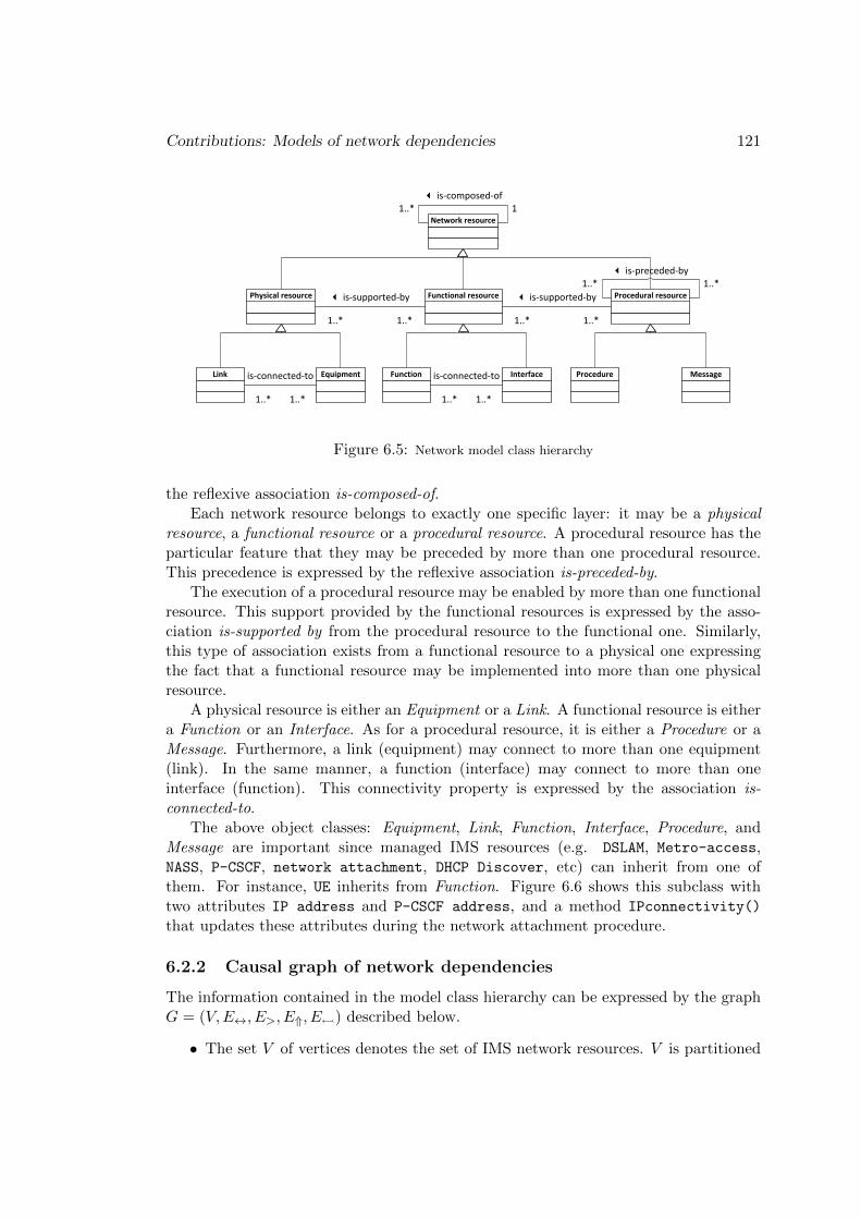
Contributions: Models of network dependencies 121
Network resource
Physical resource Functional resource Procedural resource
Link Equipment
1..* 1..*
is-connected-to Function Interface
1..* 1..*
is-connected-to Procedure
1..* 1..*
3 is-supported-by
1..* 1..*
3 is-supported-by
1..* 13 is-composed-of
1..* 1..*3 is-preceded-by
Message
Figure 6.5: Network model class hierarchy
the reflexive association is-composed-of.Each network resource belongs to exactly one specific layer: it may be a physical
resource, a functional resource or a procedural resource. A procedural resource has theparticular feature that they may be preceded by more than one procedural resource.This precedence is expressed by the reflexive association is-preceded-by.
The execution of a procedural resource may be enabled by more than one functionalresource. This support provided by the functional resources is expressed by the asso-ciation is-supported by from the procedural resource to the functional one. Similarly,this type of association exists from a functional resource to a physical one expressingthe fact that a functional resource may be implemented into more than one physicalresource.
A physical resource is either an Equipment or a Link. A functional resource is eithera Function or an Interface. As for a procedural resource, it is either a Procedure or aMessage. Furthermore, a link (equipment) may connect to more than one equipment(link). In the same manner, a function (interface) may connect to more than oneinterface (function). This connectivity property is expressed by the association is-connected-to.
The above object classes: Equipment, Link, Function, Interface, Procedure, andMessage are important since managed IMS resources (e.g. DSLAM, Metro-access,NASS, P-CSCF, network attachment, DHCP Discover, etc) can inherit from one ofthem. For instance, UE inherits from Function. Figure 6.6 shows this subclass withtwo attributes IP address and P-CSCF address, and a method IPconnectivity()
that updates these attributes during the network attachment procedure.
6.2.2 Causal graph of network dependencies
The information contained in the model class hierarchy can be expressed by the graphG = (V,E↔, E>, E⇑, E�) described below.
• The set V of vertices denotes the set of IMS network resources. V is partitioned

122 Network model describing resource dependencies
Function
IPconnectivity()
IP addressP-CSCF address
UE
Figure 6.6: Class UE inherits from class Function
into three subsets V1, V2, and V3 where V1 is the set of physical resources (equip-ment and links), V2 the set of functional resources (functions and interfaces), andV3 the set of procedural resources (procedures and messages).
• The set E↔ ⊆ (V1 × V1) ∪ (V2 × V2) of edges represents the relationship is-connected-to. ∀(u, v) ∈ (V1 × V1) ∪ (V2 × V2), u is-connected-to v is written asu↔ v.
• The set E> ⊆ (V1 × V1) ∪ (V2 × V2) ∪ (V3 × V3) of arcs represent the relationshipis-composed-of. ∀(u, v) ∈ (V1 × V1) ∪ (V2 × V2) ∪ (V3 × V3), u is-composed-of v iswritten as u > v. The set E> defines three directed acyclic graphs: one on V1, oneon V2 and another one on V3. For all u ∈ V , we denote ε(u) = {u′ ∈ V, u > u′}the set of descendants of u.
• The set E⇑ ⊆ (V1×V2)∪(V2×V3) of arcs represents the relationship is-supported-by. ∀(u, v) ∈ (V1 × V2) ∪ (V2 × V3), u is-supported-by v is written u ⇑ v. The setE⇑ defines a directed acyclic graph (DAG) on V .
• The set E� ⊆ (V3×V3) of arcs represents the relationship is-preceded-by. ∀(u, v) ∈(V3 × V3), u is-preceded-by v is written as u� v. The set E� defines a directedacyclic graph (DAG) on V3.
• Consistency between the relationship is-composed-of (refinement operation) andthe three other relationships is-connected-to, is-supported-by and is-preceded-by :∀(u, v) ∈ (V1×V1)∪ (V2×V2), [u↔ v∧ ε(u) 6= ∅ ↔ ∃u′ ∈ ε(u) : u′ ↔ v∧v /∈ ε(u)]
∀(u, v) ∈ (V1 × V2) ∪ (V2 × V3), [u ⇑ v ∧ ε(v) 6= ∅ ↔ ∃ v′ ∈ ε(v) : u ⇑ v′]∀(u, v) ∈ (V1 × V2) ∪ (V2 × V3), [u ⇑ v ∧ ε(u) 6= ∅ ↔ ∃ u′ ∈ ε(u) : u′ ⇑ v]
∀(u, v) ∈ (V3 × V3), [u� v ∧ ε(v) 6= ∅ ↔ ∀v′ ∈ ε(v), u� v′]
∀(u, v) ∈ (V3 × V3), [u� v ∧ ε(u) 6= ∅ ↔ ∀u′ ∈ ε(u), u′� v]
The relationships is-supported-by and is-preceded-by are used to express causal re-lations between failure events occurring in the IMS network. From graph G, above

Contributions: Models of network dependencies 123
a causal graph H = (V,E↑) where E↑ = E⇑ ∪ E� can be constructed. In graph H,it suffices to define the strength of the causal links, represented as conditional prob-abilities, in order to obtain a Bayesian network for reasoning under uncertainty. Therelationship is-connected-to serves to identify a specific network resource instance. Asfor the relationship is-composed-of, it can be useful to obtain a hierarchical representa-tion of the causal graph, each level corresponds to a particular level of abstraction forthe network resources. Nevertheless, as a first step we ignore the refinement operationand choose to reason with a single level of granularity.
6.2.3 Generic model vs network instance: self-modeling
The three-layer model described in the previous chapter is generic, in the sense that itdefines the different types of network resources involved (for a given range of technolo-gies), how they depend on each other and how they interact. Most of it derives fromthe standards or best practices of an operator, but part of it must be designed by anexpert. This work is facilitated by the relatively small size of this generic model, bythe existence of a grammar defining how objects can be related, and by the hierarchicalnature of the model. This allows one to model each layer by progressive refinements,thus selecting the finest granularity at which one wishes to manage the network.
The generic model defines the building blocks of a network, from a managementperspective, but the actual network one has to manage contains many instances ofthese elements. Borrowing to object oriented programming, the generic model is aclass diagram, while one has to monitor an object diagram, with many objects of thesame class. The actual network can be represented as a large collection of instancesof the patterns described in the generic model, and these instances overlap on somecommon resources. This is illustrated in Figure 6.7, where several users of an accessnetwork have private parts (CPE and first mile), but may or not share a DSLAM, mayor not be connected to the same aggregation segment, etc.
CPE#1 DSLAM#1
BRAS#1 A-SBC#1
Core Network#1
I-SBC#1
First Mile#1
Aggregation#1 Metro-core#1
Metro-access#1Access Network#1
Other IP networks
First Mile#5
CPE#5
PSTN/ISDN
Media Gateway Controller#1
User Profile
Server#1
Media Gateway#1
Media Server#1
IPFirst
Mile#4
CPE#4
First
Mile#3
CPE#3
First Mile#2CPE#2
AliceC
Alice
PeggyPE#3
Peggy
Jane TrudyCPE#5
Trudy
C
Mary
ARF#1
AMF#1
RCEF#1L2TF#1CLF#1
UAAF#1
PDBF#1NACF#1
P-CSCF#1SPDF#1C-BGF#1
A-RACF#1 SPDF#1I-BGF#1IWF#1
I-BCF#1
ARF#2
MGCF#1SGF#1
SLF#1UPSF#1
T-MGF#1
MRFP#1MRFC#1
BGCF#1I/S-CSCF#1
DSLAM#2Session
Controller#1
Figure 6.7: An IMS network instance: physical layer, with mention of the supported functions of thefunctional layer.
124 Network model describing resource dependencies
Deriving the model of the actual network instance to be managed means creatingas many instances as necessary of the network resources (equipment, functions, etc), asthey are described in the generic model. It also means structuring or connecting themin accordance with the patterns allowed by the generic model. Such a constructionguarantees both the adequacy of the resulting model with the standards, and allowsone to fit a model to a specific network, which is of great interest to track evolvingarchitectures. We call this process the self-modeling. This task can indeed be automa-tised provided the management framework provides tools to explore the network andreveal its architecture. Such a ‘service,’ or this ‘reflectivity property’ of the network,is one of the essential functions one should expect from a self-management framework,together with the ability to query the managed elements in order to check some of theirstate variables or to perform tests.
The network model obtained by this approach may be huge, in particular if onehas to capture all private equipment of all users. But it is not necessary to build itbeforehand as a necessary input to an adequate monitoring/diagnosis algorithm. Suchan approach would not scale up. We therefore adopt a strategy where only part of themodel is built on the fly, in order to solve a specific malfunction. The next chapterformalizes this approach and illustrates it on a simple example.

Chapter7Self-Modeling as Support for Fault
Localization
Contents
7.1 Methodology . . . . . . . . . . . . . . . . . . . . . . . . . . . . 126
7.2 Generic Bayesian Networks . . . . . . . . . . . . . . . . . . . 131
7.3 Fault localization in a GBN instance . . . . . . . . . . . . . . 132
The previous chapter illustrated a typical feature of network design: low-level re-sources are assembled to build a higher level resource, where the term ‘resource’ rangesfrom physical component to high-level capabilities. These complex dependency rela-tions naturally orient us to a formalization in terms of Bayesian networks (BN), whichare particularly suited to represent both constraints and statistical dependencies. Atthe same time they encode conditional independence relations, which constitute the ba-sis of efficient inference algorithms, a topic covered by a vast body of literature. In thiscontext, inference means to infer the value of some state variables given the observedvalue of other variables.
The framework needs adaptations however, in several directions. Firstly, the man-aged network evolves in time (users attach, register, de-register, new equipment orfunctionalities are added, etc.) and may not be known entirely and in full details. Sothe BN used for inference should be built on request, capturing the state of the network,to answer a given diagnosis query.
Secondly, not all network resources are involved in the malfunction of say some highlevel capability. So only part of the network should be taken into account.
But, thirdly, this BN model construction should be coupled with the inferenceengine. Users share some of the network resources, therefore they carry informationabout their state, which can be useful to the reasoning. So one must design a dynamicconstruction of the BN modeling the network, or equivalently a dynamic explorationof the network, to collect more information and solve a given diagnosis query.
Finally, let us clarify what this diagnosis query means. Assuming some networkresource is observed as down (e.g. IP configuration down for a specific UE), one has todiscover the root cause of this failure, which necessarily lies in the lower level resourcesthat are assembled to build the damaged one. This can be understood as a state
125

126 Self-Modeling as Support for Fault Localization
inference problem given the values observed on other state variables. By extension, onecould imagine querying the state of all variables of a given type, given some observations.This corresponds to a questions like, for example, given access segment failure, what isthe probability that a non specified UE be not able to make calls. This type of genericinference query is new in the BN formalism, and is clearly an approach to perform faultimpact analysis.
7.1 Methodology
Our approach to troubleshoot an observed malfunctioning resource is based on thefollowing methodology:
1. Find and/or assemble (at some level of abstraction) the generic model (or genericBN) that describes the resources used by the malfunctioning resource. The mal-functioning resource is the entry point of the fault localization query and is gen-erally a capability. But, it can also be any other IMS resource.
2. Locate the instance of this generic BN in the IMS network instance, thus derivinga BN instance, that we call a pattern.
3. Within the current BN (instance), feed the inference engine with available obser-vations to locate the faulty resource.
4. If the collected observations are not sufficient, expand the current BN by exploringother patterns (BN instances) that share resources with the current BN. In thisexpanded BN, or expanded neighborhood of the malfunction in the network,collect the new available observations to improve fault location.
5. Repeat the expansion until confidence in the explanation becomes sufficient.
To illustrate this methodology on a simple practical case, suppose that we want toexplain why the IP configuration failed for the user Laurie in the network instance ofFigure 7.1.
IP configuration comprises the IP address allocation to the UE, and the discoveryof addressing information to the Proxy-Call Session Control Function (P-CSCF). Asshown by Figure 7.2, the IP configuration capability is broken down into two successivestages, initiated by the UE.
For clarity, let us select a single granularity of description within each layer. In thefunctional layer, this granularity distinguishes a single resource denoted ‘NACF*’ thatgroups the Access Management Function (AMF), the Network Access ConfigurationFunction (NACF), the User Access Authorization Function (UAAF), the communi-cation interface between AMF and NACF (int AMF - NACF) and the one betweenNACF and UAAF (int NACF - UAAF). In the same manner, the chosen granularitydistinguishes a single resource denoted ‘CLF*’ that groups the Connectivity sessionLocation and repository Function (CLF), the Access-Resource and Admission Control

Methodology 127
CPE#1
DSLAM#1 BRAS#1 A-SBC#1
Core Network
I-SBC#1
First Mile#1
Aggregation#1 Metro-core#1
Metro-access#1
Access Network#1
ARF#1
AMF#1
RCEF#1L2TF#1CLF#1
UAAF#1
PDBF#1NACF#1
P-CSCF#1SPDF#1C-BGF#1
A-RACF#1 SPDF#1I-BGF#1IWF#1
I-BCF#1
Other IP networks
Jane
Laurie
DSLAM#2
First Mile#2CPE#2
ARF#2
First Mile#3
CPE#3
AliceAlice
PSTN/ISDN
Media Gateway Controller#1
MGCF#1SGF#1
User Profile
Server#1SLF#1
UPSF#1
Media Gateway#1
T-MGF#1
Media Server#1
MRFP#1MRFC#1
IP Session Controller#1
BGCF#1I/S-CSCF#1
Figure 7.1: An IMS network instance: physical layer, with mention of the supported functions of thefunctional layer.
UE
������������������������������ ARF
������������������������������ NACF∗
������������������������������ CLF∗
������������������������������
1. DHCP Discover ��
2. DHCP Discover ��
3. DHCP Offer��
4. DHCP Request ��
5. Bind IP-Address request��
6. NASS User profile request��
7. NASS User response ��
8. Bind IP-Address answer��
9. DHCP Ack (IP address and P-CSCF address)��
Figure 7.2: Sequence diagram of IP configuration using DHCP (procedural layer). It consists in adialog between the User Equipment (left) and functions of the NASS (right).

128 Self-Modeling as Support for Fault Localization
Function (A-RACF) and the communication interface (int CLF - A-RACF) betweenthese two functions.
The UE behaves as a DHCP client and during the first stage, it broadcasts a DHCPDiscover message (1) to locate available DHCP servers. The message is received by theNACF* that behaves as a DHCP server, via the ARF that acts as a DHCP relay. Next,the UE receives a DHCP Offer message (3) with an offer of configuration parameters.During the second stage, the UE requests offered parameters with a DHCP Requestmessage (4). This message is relayed towards the NACF* that commits binding andresponds with a DHCP Ack message.
Following the methodology described above, we first retrieve the generic modelthat describes the resources used by the IP configuration capability (Figure 7.3). Thisdependency graph between resources can be regarded as a generic BN, with statisticaldependencies if statistics are available, or logical dependencies otherwise. It encodes, forexample, that the outcome of the ‘IP configuration’ procedure demands that ‘Stage 1’ beproperly performed, which depends on the state of the interface between the functionsUE and ARF denoted here as ‘int UE-ARF’, which in turn uses the communicationchannel between the UE and the ARF, that is the first mile segment. In this genericBN, the state variable ‘IP configuration’ is observable, since one can easily test whetherthe UE obtained a correct IP address.
Stage 1 Stage 2
UE Int UE - ARF ARF Int ARF -
NACF* NACF* Int UE - NACF*
Int NACF* - CLF* CLF*
CPE First Mile DSLAM Aggregation BRAS SBC Metro Core
Executed before
Supported by
Supported by
IP Configuration
Figure 7.3: Generic BN for the IP configuration capability of a User Equipment.
As a second step, we locate among multiple instances of this generic BN, the instancethat refers to the user Laurie. This BN instance is shown in Figure 7.4. The otherBN instances refer to the other users: Jane and Alice. In Lauries’s BN instance, someresources are private to Laurie. Such resources are displayed in orange to distinguishthem from the resources that are shared with other users. The state of the observablevariable ‘IP configuration’ in the BN instance attached to Laurie is set to ‘down,’i.e. not functioning correctly.
Any node in Laurie’s BN instance can be an explanation for the observed mal-function. The third step consists in collecting the available observations on all theseresources, and running a BN inference, to try and locate the origin of the malfunction.

Methodology 129
Laurie’s Stage 1 Laurie’s Stage 2
UE#1 Int UE#1 - ARF#1 ARF#1 Int ARF#1 -
NACF*#1 NACF*#1 Int UE#1 - NACF*#1
Int NACF*#1 - CLF*#1 CLF*#1
CPE#1 First Mile#1 DSLAM#1 Aggregation#1 BRAS#1 SBC#1 Metro Core#1
Laurie’s IP Configuration
Figure 7.4: Laurie’s BN instance
Not all resources may provide observable state information. And some observation maynot be fully discriminant. For example, one may observe that the Aggregation segmentis in state ‘loaded’, but may not be certain that this is the origin of the failure. Thereis simply some probability that this caused a crash of the IP configuration, for examplebecause of the time-outs in the DHCP protocol.
As a fourth step, one may decide to cross-check the possible explanations discoveredso far by querying other users that share some resources with Laurie. For example, wechoose to check the state of Jane’s IP configuration. Thus, we extend the scope of theBN under study (Laurie’s BN instance) by adding Jane’s BN instance. Figure 7.5 showsthe extended BN, which now incorporate more observable variables. Suppose that thestate of Jane’s IP configuration is ‘up’, functioning correctly. This observation impliesthat all the resources Laurie shares with Jane are working properly (which would havebeen revealed by a BN inference on this extended BN). As a consequence, the set ofpossible faulty resources in Laurie’s BN instance is reduced to the subset of resourcesthat are not shared with Jane.
This process can be iterated (point 5 in Section 7.1): one may query another user,provided he/she shares resources with either Laurie or Jane. But the choice of theuser to query should depend on how informative the new observations will be to locatethe faulty resource that caused Laurie’s problem. If we choose to query Alice, whohas more resources in common with Laurie than Jane has, the current BN must againbe extended to incorporate Alice’s BN instance of the IP configuration generic model.Figure 7.6 shows the extended BN (due to space limitation Jane’s private resourcesare not displayed). Suppose that Alice’s IP configuration is ‘up’. This observationimplies that all the resources Laurie shares with Alice are functioning. Once more,the set of possible faulty resources in Laurie’s BN instance is reduced to the subset ofresources that are not shared with Alice or Jane. By contrast, suppose that Alice’s IPconfiguration is ‘down’. This observation increases our confidence in the state ‘down’

130 Self-Modeling as Support for Fault Localization
Laurie’s Stage 1 Laurie’s Stage 2
UE#1 Int UE#1 - ARF#1 ARF#1 Int ARF#1 -
NACF*#1 NACF*#1 Int UE#1 - NACF*#1
Int NACF*#1 - CLF*#1 CLF*#1
CPE#1 First Mile#1 DSLAM#1 Aggregation#1 BRAS#1
Jane’s Stage 2 Jane’s Stage 1
UE#3Int UE#3 - ARF#2ARF#2Int ARF#2 -
NACF*#1Int UE#3 - NACF*#1
CPE#3First Mile#3DSLAM#2SBC#1 Metro Core#1
Laurie’s IP Configuration Jane’s IP Configuration
Figure 7.5: Jane’s BN instance is added; her private resources are represented in blue
Laurie’s Stage 1 Laurie’s Stage 2
UE#1 Int UE#1 - ARF#1 ARF#1 Int ARF#1 -
NACF*#1 NACF*#1 Int UE#1 - NACF*#1
Int NACF*#1 - CLF*#1 CLF*#1
CPE#1 First Mile#1 DSLAM#1 Aggregation#1 BRAS#1
Alice’s Stage 2 Alice’s Stage 1
UE#2Int UE#2 - ARF#1
Int UE#2 - NACF*#1
CPE#3First Mile#3SBC#1 Metro Core#1
Laurie’s IP Configuration Alice’s IP Configuration
Figure 7.6: Alice’s BN instance is added; her private resources are represented in green. Jane’sprivate resources are not shown.

Generic Bayesian Networks 131
for the resources in Laurie’s BN instance that are shared with Alice, and not sharedwith Jane. The cause of Laurie’s IP configuration failure is likely to be found amongthese shared resources.
7.2 Generic Bayesian Networks
The previous section has demonstrated how the resources involved in a network and itsservices depend on each other, thus forming a huge dependency graph. This graph canbe modeled as a Bayesian network where many parts are isomorphic, i.e. this graph isobtained by connecting tiles that are copies of a limited family of generic patterns. Thissection formalizes this construction of a possibly large Bayesian network, and explainshow to perform inference over it, by exploring only the portion of the BN that is themost informative to a given diagnosis query.
Definition 8 A Bayesian network (BN) X = (V,E,PX) is formed of a finite directedacyclic graph (DAG) G = (V,E), with V as vertex set and E ⊆ V ×V as edge set, anda collection of random variables (Xv)v∈V indexed by V and with probability distributionPX . Denoting •v = {u ∈ V : (u, v) ∈ E} the parents of node v ∈ V in the DAG (V,E),the distribution of X factorizes as PX = ⊗v∈V PXv |X•v , where XU = (Xu, u ∈ U)denotes a vector of random variables, U ⊆ V .
As usual, a morphism φ : G1 → G2 between DAGs Gi = (Vi, Ei) is a partialfunction from V1 to V2 preserving the edges: ∀u, v ∈ Dom(φ) = V ′1 ⊆ V1, (u, v) ∈E1 ⇔ (φ(u), φ(v)) ∈ E2. φ is said to be an insertion of G2 into G1 iff φ restricted toits domain is bijective, i.e. φ|V ′1 is an isomorphism between G1|V ′1 = (V ′1 , E1 ∩ V ′1 × V ′1)and G2.
Definition 9 A Generic Bayesian network (GBN) is a finite collection of ordinaryBNs (W k)1≤k≤K , where each BN W k = (Vk, Ek,PWk) is also called a pattern. Aninstance X = (V,E,PX , (φk,i)k≤K, i∈Ik) of this GBN is a standard BN (V,E,PX) where
1. each φk,i is an insertion of pattern (Vk, Ek) into (V,E), and the DAG (V,E) iscovered by such pattern instances: V = ∪k,iDom(φk,i), ∀(u, v) ∈ E, ∃φk,i : u, v ∈Dom(φk,i).
2. probability PX is inherited from patterns Wk through the insertion morphisms(φk,i)k≤K, i∈Ik : ∀v ∈ V , one has
a) if •v = ∅, then ∀k, i : φk,i(v) = u ⇒ PXv ≡ PWku
b) if •v 6= ∅, then ∀k, i : φk,i(v) = u, •v∩Dom(φk,i) 6= ∅ ⇒ •v ⊆ Dom(φk,i), PXv |X•v ≡PWk
u |Wk•u
In other words, to build X one takes many copies of the different patterns W k, andaggregates them by sharing some of the random variables. To ensure consistency of thisconstruction, each variable Xv (with parents) appearing in several pattern instances

132 Self-Modeling as Support for Fault Localization
must be defined by the same conditional probability. So either Xv comes alone inan instance, or it comes with all its parents, and in this case the same PXv |X•v isobtained from the different patterns. A similar condition holds when Xv has no parent.Figure 7.7 gives an example of a GBN with a single pattern of five variables, andan instance of this GBN with six copies of the pattern, overlapping in different ways.Observe that a given variable may play different ‘roles’ according to the pattern instancewhere it is considered.
s
E
A B C
D
X
Figure 7.7: A GBN (left) with a single pattern, and an instance of this GBN (right) with sixoverlapping instances of this pattern.
7.3 Fault localization in a GBN instance
Fault localization in a GBN instance can be translated into a standard BN inference asfollows. Assume some variable, for example Xs in Figure 7.7, is declared/observed asfaulty. This resource Xs depends on other resources, namely X••s where ••s denotesall the ancestors of node s. Either the failure of Xs is spontaneous, or it results from afault propagation pattern in X••s. The objective is thus to estimate the value of XZ ,with Z = ••s ∪ {s} (in gray in Figure 7.7). Alternatively, one can build a root-causelocalizer L, as a function of XZ that constrains the presence of a single root-causewithin XZ . The objective is then to estimate the value of L.
There exist observable variables within (or directly attached to) XZ , in particularthe observation indicating the faulty value of Xs. Let us denote by Y0 = y0 thisobserved vector. The conditional law PXZ |Y0=y0 gives a first information of what causedthe failure of Xs: by maximum likelihood estimation, one gets an explanation (i.e. afault propagation scheme) as the value XZ = arg maxx PXZ |Y0=y0(x). How reliable thisexplanation is can be determined by computing the conditional entropy of XZ givenY0 = y0 :
H(XZ |Y0 = y0) =∑x
−PXZ |Y0=y0(x) · log2 PXZ |Y0=y0(x)
A large conditional entropy means that the observations Y0 = y0 are insufficientto discriminate among several explanations. One may therefore seek to collect more

Fault localization in a GBN instance 133
observations in order to increase more information about XZ , that is reduce the con-ditional entropy: the closer to zero, the most reliable the estimation of XZ . The ideais the to explore a larger area of the BN instance in order to collect more observations.From the explored set of nodes U0 = Z one thus goes to U1 ⊇ U0 such that U1 is closedfor the ancestor relation: •U1 ⊆ U1. This defines a new set of observations Y1 = y1,from which XZ can be estimated provided H(XZ |Y0 = y0, Y1 = y1) is small enough.Otherwise one proceeds to another extension.
What is the rationale governing the BN instance exploration ? Referring to Fig-ure 7.7, one may extend the explored part of the BN instance to capture observations ineither the green pattern instance, or those in the magenta one. Let us denote Y1 and Y2
these two possible sets of observations. The most informative one is obtained by com-paring H(XZ |Y0 = y0, Y1) to H(XZ |Y0 = y0, Y2): the smaller one wins, which selectsthe set of observations that is the most informative on the average. This is computedbeforehand, without querying/testing the actual value of the selected Yi. Assume Y1
was the most promising set of measurements, this defines the new area U1 taken intoaccount in the BN instance, where one may collect the observed value Y1 = y1. Afterstandard inference, this yields the new posterior distribution PXZ |Y0=y0,Y1=y1 and thusthe conditional entropy H(XZ |Y0 = y0, Y1 = y1). Notice that H(XZ |Y0 = y0, Y1 = y1)may actually be either smaller or larger than the averaged value H(XZ |Y0 = y0, Y1)used to determine the most promising set of observations.
The introduction of new measurements proceeds until either the conditional entropyis small enough, or no more observations are available. Notice that by construction ofBN, the exploration is necessarily performed by exploring pattern instances that sharevariables with the explored section of the BN. Measurements lying in disconnectedareas are independent of XZ , and thus of no help to estimate it. Observe also thatsuch a recursive exploration approach opens the way to a tradeoff when the collectionof new observations incurs some cost, for example if tests must be performed. Onecan therefore balance the amount of information that can be gained with the cost ofcollecting it.

134 Self-Modeling as Support for Fault Localization

Chapter8Experimental results
Contents
8.1 Entropy, relative entropy and mutual information . . . . . . 135
8.1.1 Entropy and conditional entropy . . . . . . . . . . . . . . . . 135
8.1.2 Relative entropy and mutual information . . . . . . . . . . . 136
8.1.3 Gain function for fault localization . . . . . . . . . . . . . . . 138
8.2 Implementation and evaluation . . . . . . . . . . . . . . . . . 139
8.2.1 Entropy reduction as more measurements are collected . . . . 139
8.2.2 Fault localization in an IMS network . . . . . . . . . . . . . . 141
The aim of this chapter is to demonstrate the relevance of the exploration strategyexplained in the previous chapter. We review some standard results and definitionsrelated to entropy, relative entropy, mutual information and gain function for faultlocalization. These concepts and their properties are useful to analyse the experimentalresults that will be presented.
8.1 Entropy, relative entropy and mutual information
For any probability distribution, we recall the definition of a quantity called the entropy,which has many properties that agree with the intuitive notion of what a measure ofinformation should be. This notion is extended to define mutual information, which isa measure of the amount of information one random variable contains about another.Entropy then becomes the self-information of a random variable. Mutual informationis a special case of a more general quantity called relative entropy, which is a measureof the distance between two probability distributions. All these quantities are closelyrelated and share a number of simple properties that are presented below.
8.1.1 Entropy and conditional entropy
We will first introduce the concept of entropy, which is a measure of uncertainty of arandom variable. Let X be a discrete random variable with alphabet X and probabilitymass function p(x) = Pr(X = x), X ∈ X . We denote the probability mass functionby p(x).
135

136 Experimental results
Definition 10 The entropy H(X) of a discrete random variable X is defined by
H(X) = −∑X∈X
p(x)log p(x). (8.1)
Note that H(X) ≥ 0.
We also recall the conditional entropy of a random variable given another as theexpected value of the entropies of the conditional distributions, averaged over the con-ditioning random variable.
Definition 11 If (X,Y ) ∼ p(x, y), then the conditional entropy H(Y |X) is defined as
H(Y |X) =∑X∈X
p(x)H(Y |X = x) (8.2)
= −∑X∈X
p(x)∑Y ∈Y
p(y|x) log p(y|x) (8.3)
= −∑X∈X
∑Y ∈Y
p(x, y) log p(y|x). (8.4)
The naturalness of the definition of joint entropy and conditional entropy is exhibitedby the fact that the entropy of a pair of random variables is the entropy of one variableplus the conditional entropy of the other.
Theorem 1 (Chain rule for entropy)
H(X,Y ) = H(X) +H(Y |X). (8.5)
Let X1, X2, ..., Xn be drawn according to p(x1, x2, ..., xn). Then
H(X1, X2, ..., Xn) =
n∑i=1
H(Xi|Xi−1, ..., X1). (8.6)
8.1.2 Relative entropy and mutual information
Here, we review two related concepts: relative entropy and mutual information.
Definition 12 The relative entropy or Kullback Leibler distance between two probabil-ity mass functions p(x) and q(x) is defined as
D(p‖q) =∑X∈X
p(x)logp(x)
q(x). (8.7)

Entropy, relative entropy and mutual information 137
Definition 13 Consider two random variables X and Y with a joint probability massfunction p(x, y) and marginal probability mass function p(x) and p(y). The mutual in-formation I(X;Y ) is the relative entropy between the joint distribution and the productdistribution p(x)p(y):
I(X;Y ) =∑X∈X
∑Y ∈Y
p(x, y) logp(x, y)
p(x)p(y)(8.8)
= D(p(x, y)‖p(x)p(y)) (8.9)
= H(X)−H(X|Y ). (8.10)
Thus, the mutual information I(X;Y ) is the reduction in the uncertainty of X dueto the knowledge of Y . Using Jensen’s inequality and its consequences (Cover andThomas, 1991) some of the properties of entropy and relative entropy can be proved.
Theorem 2 (Information inequality) Let p(x), q(x), x ∈ X , be two probabilitymass functions. Then,
D(p‖q) ≥ 0 (8.11)
Corollary 4 (Non-negativity of mutual information) For any two random vari-ables, X, Y :
I(X;Y ) ≥ 0, (8.12)
Theorem 3 (Conditioning reduces entropy)
H(X|Y ) ≤ H(X) (8.13)
Intuitively, the theorem says that knowing another random variable Y can onlyreduce the uncertainty in X. Note that this is true only on the average. Specifically,H(X|Y = y) may be greater or lower than H(X), but on the average H(X|Y ) =∑
y p(y)H(X|Y = y) ≤ H(X). For example, in a court case, specific new evidencemight increase uncertainty, but on the average evidence decreases uncertainty.
Example. Let (X,Y ) have the following joint distribution. Then, H(X) = H(18 ,
78) =
X=1 X=2
Y=1 0 34
Y=2 18
18
0.544 bits, H(X|Y = 1) = 0 bits and H(X|Y = 2) = 1 bit. We calculate H(X|Y ) =34H(X|Y = 1) + 1
4H(X|Y = 2) = 0.25 bits. Thus, uncertainty in X is increased ifY = 2 is observed and decreased if Y = 1 is observed, but uncertainty decreases onthe average. Notice again that this information reduction H(X|Y ) ≤ H(X) is on theaverage. For a given sample, one may have H(X|Y = y) ≥ H(X|Y ) and even ≥ H(X).

138 Experimental results
Theorem 4 (Chain rule for information)
I(X;Y1, Y2, ..., Xn) = I(X;Y1) + I(X;Y2|Y1) + I(X;Y3|Y1Y2) + .... (8.14)
In particular,
H(X|Z = z, Y = y) = −∑x
p(x|y, z)logp(x|y, z). (8.15)
H(X|Z, Y = y) =∑z
p(X|Z = z, Y = y)p(z|y). (8.16)
so that, to select the next measurement Z, we need p(z|y) and p(x|y, z) or equivalentlyp(x, z|y) (i.e. P (X,Z|Y = y), the full law for X,Z and fixed y).
8.1.3 Gain function for fault localization
Suppose the state of a system is denoted by a vector X = (X1, X2, ..., Xn) of randomvariables, where Xi represents the state of a node. A probabilistic model is a jointprobability distribution (a prior distribution) over all the random variables Xi. Henceit assigns, a probability p(x) to each realization x. Given observations Y of the systemstate, a fault diagnosis algorithm identifies the Most Probable Explanation (MPE) ofthe underlying system responsible for observed outage, i.e.:
x∗ = arg maxx
p(x|y)
Observations reduce uncertainty of the system. Before we observe Y , the uncer-tainty about system state can be quantified by the Shannon entropy:
H(X) = −∑x
p(x) log p(x).
If the system state is doubtless, H(X) = 0. As uncertainty goes up, H(X) increases.The purpose of making observations is just to reduce this uncertainty. Given proberesponses Y = (Y1, Y2, ..., Yn), the probability of the system state changes into P (X|Y ),consequently the average uncertainty of the system state is:
H(X|Y ) = −∑x,y
p(x, y) log p(x|y).
(Lindley, 1956) proposed a method to measure the average information providedby an experiment. Suppose the probe Yi is defined on system state X.
Definition 14 The average amount of information gain from Yi, with prior probabilitydistribution P (X), is:
G(Yi) = I(X;Yi) = H(X)−H(X|Yi) =∑x,yi
p(x, yi) logp(x, yi)
p(x)P (yi). (8.17)

Implementation and evaluation 139
In some situations, as the one we examine below, one may not be able to usedirectly the full observation set Y = (Y1, Y2, ..., Yn) and may have to select a subset ofk observations to collect. In order to select an optimal set of k probes among variablesY1, ..., Yn, for fault localization, the target is to find a subset E ⊆ {1, ..., n}, |E| = k,which maximizes the reduction of Shannon entropy i.e.:
E∗ = arg maxE
G(YE), for YE = {Yi, i ∈ E}. (8.18)
The problem stated in (8.18) is NP-hard (Brodie et al., 2003), hence efficient exactsolutions are likely not possible. An alternative, widely used in the literature, is theheuristic greedy approach, which iteratively adds to E the probe that reduces the max-imum entropy of the system, among those that were not selected yet. When problemsare detected, a greedy algorithm repeatedly selects, given E, the new observation Yi tocollect by:
i∗ = arg maxi/∈ E
I(X;Yi|YE). (8.19)
Actually i /∈ E can be simplified into i ∈ E because I(X;Yi|YE) ≥ 0 and I(X;Yi|YE) =0 for i ∈ E. Besides, note that this solution uses P (X,Yi|YE). Not only the mutualinformation of X and Yi is measured, but the impact of previously selected probes onYi is also calculated, which provides a “global view”, better than the techniques whichonly consider system state X and the candidate probe Yi.
8.2 Implementation and evaluation
Kevin Murphy’s Bayes Net Toolbox (Murphy et al., 2001) is an open-source Matlabpackage for directed acyclic graph (DAG) models, also known as Bayesian or beliefnetworks. It has proved to be very popular and it is widely used throughout the worldfor teaching and research. Bayes Net Toolbox (BNT) supports many kind of nodes(probability distributions) and offers a variety of exact and approximate inference algo-rithms. We use the junction tree inference engine in BNT to implement our explorationstrategy.
8.2.1 Entropy reduction as more measurements are collected
We have first performed some tests on a large tree-shaped GBN instance. The (unique)pattern corresponds to Figure 8.1 where variables XD and XE are observable. Theinstance is depicted in Figure 8.2, where each vertex represents a pattern instance (thus5 variables). Two connected pattern instances overlap by 1, 2 or 3 of the {A,B,C}nodes, which is reflected by the thickness of the edge relating these patterns. In pattern(instance) X1, variables X1,A, X1,B, X1,C are (independent) uniform binary variables.In all other patterns Xi, i > 1, the newly created variables Xi,A, Xi,B or Xi,C havedistribution (p, 1−p) with p = 0.9, in order to guarantee long-range correlation betweenpatterns in the net of Figure 8.2. In pattern Xi, the observations Yi correspond tovariables Xi,D, Xi,E . D is more sensitive to a failure of B than to a failure of A, and

140 Experimental results
similarly E reacts more to C than to B. Both sensors have a misdetection rate and afalse alarm rate of 5%.
s
E
A B C
D
X
Figure 8.1: A GBN (left) with a single pattern, and an instance of this GBN (right) with sixoverlapping instances of this pattern.
226
13
14
11
12
20
19
9
17
8
18
3
7
15
5 21
1
16
4
2
10
Figure 8.2: A GBN instance with 22 pattern instances. The thickness (and length) of the line relatingtwo patterns reflects the number of shared variables. To estimate the central pattern X1, observationsare introduced by zones, starting by the dark zones first and progressing towards the pale ones.
The experiment consists in drawing a random sample of the process described by thisGBN instance, and in computing the conditional distribution PX1|YU=yU of the centralpattern X1 given a growing set U of measurements collected on X1 and on distantpatterns. The measurement set starts from U = {1} up to U = {1, 2, ..., 22} where Uis the index set of the patterns where observation are collected. In between, the mostinformative measurement is incorporated at each step. For each sample, the evolutionof H(X1|YU = yU ) was computed. The experiment was conducted one thousand times.On the average, one observes that H(X1|YU = yU ) does decrease (Figure 8.3), andquickly converges. However, for a given sample, this curve may not always decrease:even if an observable node is very informative on the average, its actual observedsample may lead to a revision of the current assumptions, thus increasing temporarily

Implementation and evaluation 141
the uncertainty. An example of such a non-decreasing behaviour is presented later inthis chapter.
0 5 10 15 20 250.4
0.6
0.8
1
1.2
1.4
1.6
1.8
2
2.2
2.4
k = number of observations taken into account to estimate X1
H(X
1|Y1,..
.,Yk)
Decrease of uncertainty on the value of X1
Figure 8.3: Average evolution of the conditional entropy of the central pattern X1 as the number ofobservations increases.
More interestingly, we have performed rank statistics on the way measurements areintroduced. On the average, the best order appears to be 1, 3, 4, 2, 7, 10, 8, 9, 21, 22, 17, 6,16, 5, 13, 15, 20, 18, 19, 12, 14, 11, which is reflected by the growing zones around X1 inFigure 8.2. Strongly coupled patterns tend to be favored, but not always.
8.2.2 Fault localization in an IMS network
We have then performed another experiment on a more realistic GBN instance. Thenetwork instance considered is shown in Figure 8.4.
Description of the failure scenario
Suppose that we want to explain why the IP connectivity is down for the user Mary inthe network instance of Figure 8.4.

142 Experimental results
CPE#1 DSLAM#1
BRAS#1 A-SBC#1
First Mile#1
Aggregation#1 Metro-core#1
Metro-access#1Access Network#1
DSLAM#2
First Mile#5
CPE#5
First Mile#4
CPE#4
First
Mile#3
CPE#3
First Mile#2CPE#2
AliceC
Alice
Peggy CPEPeggy
Jane TrudyTrudy
C
Mary
ARF#2
ARF#1 NACF* CLF*
Figure 8.4: Network instance example: the physical and functional layers at a given resolution.
As shown by Figure 8.5, the IP connectivity procedure is broken down into two suc-cessive procedures, initiated by the UE. In the functional layer, the chosen granularity
UE ARF
1. DHCP Discover
2. DHCP Discover
NACF* CLF*
4. DHCP Request
3. DHCP Offer
5. Bind IP-Address request
6. NASS User profilerequest
7. NASS User response
8. Bind IP-Address answer5. DHCP Ack (IP address and
P-CSCF address)
Procedure 1
Procedure 2
Procedure 1A
Procedure 2A
Figure 8.5: Sequence diagram of IP connectivity using DHCP (procedural layer). It consists in adialog between the User Equipment, functions of the NASS and the RACS.
of description distinguishes a single resource denoted ‘NACF*’ that groups the AccessManagement Function ‘AMF’, the Network Access Configuration Function ‘NACF’,the User Access Authorization Function ‘UAAF’, the communication interface between‘AMF’ and ‘NACF’ (‘int AMF-NACF’) and the one between ‘NACF’ and ‘UAAF’ (‘intNACF-UAAF’). In the same manner, the chosen granularity distinguishes a single re-source denoted ‘CLF*’ that groups the Connectivity session Location and repositoryFunction ‘CLF’, the Access-Resource and Admission Control Function ‘A-RACF’ and
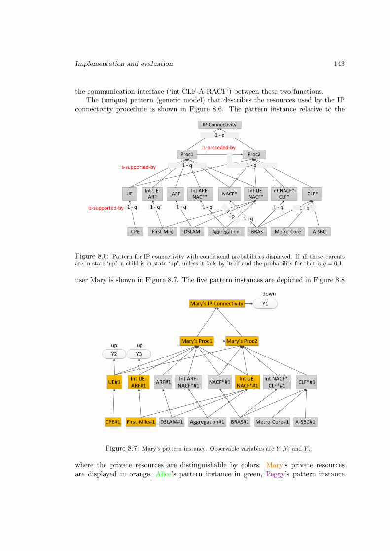
Implementation and evaluation 143
the communication interface (‘int CLF-A-RACF’) between these two functions.
The (unique) pattern (generic model) that describes the resources used by the IPconnectivity procedure is shown in Figure 8.6. The pattern instance relative to the
Proc1
UE Int UE-ARF ARF Int ARF-
NACF* NACF* Int NACF*-CLF* CLF*
CPE First-Mile DSLAM Aggregation BRAS A-SBCMetro-Core
Int UE-NACF*
Proc2
IP-Connectivity
is-preceded-by
is-supported-by
1 - q 1 - q 1 - q 1 - q 1 - q 1 - qis-supported-by
1 - q
1 - q
1 - q
1 - q
1 - q
Figure 8.6: Pattern for IP connectivity with conditional probabilities displayed. If all these parentsare in state ‘up’, a child is in state ‘up’, unless it fails by itself and the probability for that is q = 0.1.
user Mary is shown in Figure 8.7. The five pattern instances are depicted in Figure 8.8
Mary’s Proc1
UE#1 Int UE-ARF#1 ARF#1 Int ARF-
NACF*#1 NACF*#1 Int NACF*-CLF*#1 CLF*#1
CPE#1 First-Mile#1 DSLAM#1 Aggregation#1 BRAS#1 A-SBC#1Metro-Core#1
Int UE-NACF*#1
Mary’s Proc2
Mary’s IP-Connectivity
up
down
Y2
Y1
upY3
Figure 8.7: Mary’s pattern instance. Observable variables are Y1,Y2 and Y3.
where the private resources are distinguishable by colors: Mary’s private resourcesare displayed in orange, Alice’s pattern instance in green, Peggy’s pattern instance

144 Experimental results
in purple, Jane’s pattern instance in blue, Trudy’s pattern instance in red. Sharedresources are displayed in gray.
Experimental setup
The parameters for this experiment are described below.
• All variables are binary with states 1 meaning ‘down’ and 2 meaning ‘up’.
• Some of them are observable:
– Y1, Y2, and Y3 in Mary’s pattern instance
– Y4 and Y5 in Alice’s pattern instance
– Y6 and Y7 in Peggy’s pattern instance
– Y8 and Y9 in Jane’s pattern instance
– Y10 and Y11 in Trudy’s pattern instance
They are displayed in rounded boxes in Figure 8.8.
• Variables ‘CPE’, ‘First-Mile’, ‘DSLAM’, ‘Aggregation’, ‘BRAS’, ‘Metro-Core’, ‘A-SBC’ (and their corresponding instances) have no parent, they are (independent)variables with distribution (0.1, 0.9) where 0.1 is the probability of the variablebeing in state 1 (‘down’).
• Variables ‘UE’, ‘Int UE-ARF’, ‘ARF’, ‘Int ARF-NACF*’, ‘NACF*’, ‘Int NACF*-CLF*’ (and their corresponding instances) have one parent. See Figure 8.6 fortheir distribution and Table 8.1 below as an example.
CPE=1 CPE=2
UE=1 1 0.1UE=2 0 0.9
Table 8.1: P(UE|CPE)
• Variables ‘Int UE-NACF*’ and ‘CLF*’ (and their corresponding instances) havethree parents. See Figure 8.6 for their distribution and Table 8.2 below as anexample.
A-SBC=1 A-SBC=2Metro-Core=1 Metro-Core=2 Metro-Core=1 Metro-Core=2
BRAS=1 (1,0) (1,0) (1,0) (1,0)BRAS=2 (1,0) (1.0) (1,0) (0.1,0.9)
Table 8.2: P(CLF* | BRAS, Metro-Core, A-SBC). The numbers (x,y) in the tablerepresent (CLF*=1,CLF*=2)

Implementation and evaluation 145
Mar
y’s
Pro
c1
UE#
1In
t UE-
ARF#
1 A
RF#1
Int A
RF-
NAC
F*#1
NAC
F*#1
Int N
ACF*
-CL
F*#1
CLF
*#1
CPE#
1Fi
rst-
Mile
#1DS
LAM
#1Ag
greg
atio
n#1
BRAS
#1A-
SBC#
1M
etro
-Cor
e#1
Int U
E-N
ACF*
#1
Mar
y’s
Pro
c2
Mar
y’s
IP-C
onne
ctiv
ity
Alic
e’s
Pro
c1
UE#
2In
t UE-
ARF#
2
CPE#
2Fi
rst-
Mile
#2
Int U
E-N
ACF*
#2
Alic
e’s
Pro
c2
Alic
e’s
IP-C
onne
ctiv
ity
Peg
gy’s
Pro
c1
UE#
3In
t UE-
ARF#
3
CPE#
3Fi
rst-
Mile
#3
Int U
E-N
ACF*
#3
Peg
gy’s
Pro
c2
Peg
gy’s
IP-C
onyn
ectiv
ity
Jan
e’s
Pro
c1
UE#
4In
t UE-
ARF
#4 A
RF#2
Int A
RF-
NAC
F*#2
CPE#
4Fi
rst-
Mile
#4DS
LAM
#2
Int U
E-N
ACF*
#1
Jan
e’s
Pro
c2
Jan
e’s
IP-C
onne
ctiv
ity
Tru
dy’
s P
roc1 U
E#5
Int U
E-AR
F#5
CPE#
5Fi
rst-
Mile
#5Int U
E-N
ACF*
#5
Tru
dy’
s P
roc2
Tru
dy’
s IP
-Con
nect
ivity
updo
wn
up
dow
nup
dow
n
up
updo
wn
Y5
Y2
Y9
Y6Y4
Y1Y8
Y10
Y7
dow
n
Y11
up Y3
Figure 8.8: The whole model.

146 Experimental results
• Variables ‘Proc1’ and ‘Proc2’ (and their corresponding instances) have six par-ents. Their distribution is such that if at least one parent is in state down, thenthey are certainly in state 1 (‘down’). When all parents are in state 2 (‘up’),these variables can be in the state 1 (‘down’) with probability 0.1 or in the state2 (‘up’) with probability 0.9.
• Variable ‘IP-Connectivity’ (and its corresponding instance) See Figure 8.6 fortheir distribution and Table 8.3 below as an example.
proc1=1 proc1=2
proc2=1 (1,0) (1,0)proc2=2 (1,0) (0.1,0.9)
Table 8.3: P(IP-Connectivity|Proc1,Proc2). The numbers (x,y) in the table represent(IP-Connectivity=1,IP-Connectivity=2)
• All variables representing observations have one parent and distribution (1, 0.02, 0, 0.98).This is the case for Y1, Y2, Y3, Y4, Y5, Y6, Y7, Y8, Y9, Y10, Y11. As an example seeTable 8.4 below.
Mary’s IP connectivity=1 Mary’s IP connectivity=2
Y1=1 1 0.02Y1=2 0 0.98
Table 8.4: P(Y1 |Mary’s IP connectivity)
• The variable Z (not shown here) has 15 parents: all variables in Mary’s patterninstance corresponding to a physical or functional resource. Z can take 15 values,each value pointing toward the failed resource in Mary’s pattern instance (seeTable 8.5). Note that, we could have chosen sixteen values for Z, the sixteenthvalue meaning that there is no failure. Furthermore, we could have chosen to addtwo more states for Z : 17 and 18 to denote the fact that ‘proc1’ and ‘proc2’ canfail by themselves i.e. even their underlying functional resources are all in state‘up’. For simplicity, here we use only 15 values.
Results
We observed the distribution of Z and its entropy H(Z) when observations (displayedin rounded boxes in Figure 8.8) are progressively added.
1. When the set of observations {Y1 = 1, Y2 = 2, Y3 = 2} in Mary’s pattern instanceis entered and propagated, we have H(Z) = 3.3186 (see Figure 8.9(a) for Z’sdistribution).
2. Observation Y7 in Peggy’s pattern instance is selected as the most informative one.Peggy’s pattern instance is considered and observations Y6 = 1 and Y7 = 1 are

Implementation and evaluation 147
Z’s value Meaning
1 CPE#1 failed2 First-Mile#1 failed3 DSLAM#1 failed4 Aggregation#1 failed5 BRAS#1 failed6 Metro-Core#1 failed7 A-SBC#1 failed8 UE#1 failed9 Int UE-ARF#1 failed10 ARF#1 failed11 Int ARF#1-NACF*#1 failed12 NACF*#1 failed13 Int UE#1-NACF*#1 failed14 Int NACF*#1-CLF*#1 failed15 CLF*#1 failed
Table 8.5: Possible values of Z and their respective meaning
entered and propagated. The uncertainty (about the faulty resource) decreased:H(Z) dropped to 3.2575 (see Figure 8.9(b) for Z’s distribution).
3. Observation Y11 in Trudy’s pattern instance is selected as the most informa-tive one. Trudy’s pattern instance is considered and observations Y10 = 1 andY11 = 1 are entered and propagated. The uncertainty (about the faulty resource)increased: H(Z) went up to 3.2776 (see Figure 8.9(c) for Z’s distribution).
4. Observation Y8 in Jane’s pattern instance is selected as the most informativeone. Jane’s pattern instance is considered and observations Y8 and Y9 are enteredand propagated. The uncertainty (about the faulty resource) decreased: H(Z)dropped to 1.8529 (see Figure 8.9(d) for Z’s distribution).
5. Observation Y4 in Alice’s pattern instance is selected as the most informativeone. Finally, Alice’s pattern instance is considered and observations Y4 and Y5
are entered and propagated. H(Z) becomes null meaning that the state of Z i.e.the information about the guilty resource is now doubtless (see Figure 8.9(e) forZ’s distribution).
We conduct another experiment consisting in drawing a random sample of theprocess described by this GBN instance, and in computing the conditional distributionPZ|Yi=yi of the variable Z given the set Y1...Y11 of measurements. The measurementset starts from V = {Y1, Y2, Y3} up to V = {Y1, ..., Y11}. For each sample, the evolutionof H(Z|YV = yV ) was computed. The experiment was conducted one thousand times.On the average, one observes that H(Z|YV = yV ) does decrease (Figure 8.10).
However, for a given sample, this curve may not always decrease, as mentionedabove: even if an observable node is very informative on the average, its actual observedsample may lead to a revision of the current assumptions, thus increasing temporarilythe uncertainty. For example, this situation happens with the following two samples.

148 Experimental results
0 0.05 0.1 0.15 0.2
CPE#1First-Mile#1
DSLAM#1Aggregation#1
BRAS#1Metro-core#1
A-SBC#1UE#1
int UE-ARF#1ARF#1
int ARF#1-NACF*#1NACF*#1
int UE#1-NACF*#1int NACF*#1-CLF*#1
CLF*#1
Z's distribution when only Mary's pattern instance is considered
(a) Mary’s pattern instance is considered.
0 0.05 0.1 0.15 0.2 0.25
CPE#1First-Mile#1
DSLAM#1Aggregation#1
BRAS#1Metro-core#1
A-SBC#1UE#1
int UE-ARF#1ARF#1
int ARF#1-NACF*#1NACF*#1
int UE#1-NACF*#1int NACF*#1-CLF*#1
CLF*#1
Z's distribution when Peggy's pattern instance is added
(b) Peggy’s pattern instance is added.
0 0.05 0.1 0.15 0.2
CPE#1
First-Mile#1
DSLAM#1
Aggregation#1
BRAS#1
Metro-core#1
A-SBC#1
UE#1
int UE-ARF#1
ARF#1
int ARF#1-NACF*#1
NACF*#1
int UE#1-NACF*#1
int NACF*#1-CLF*#1
CLF*#1
Z's distribution when Trudy's pattern instance is added
(c) Trudy’s pattern instance is added.
0 0.1 0.2 0.3 0.4
CPE#1First-Mile#1
DSLAM#1Aggregation#1
BRAS#1Metro-core#1
A-SBC#1UE#1
int UE-ARF#1ARF#1
int ARF#1-NACF*#1NACF*#1
int UE#1-NACF*#1int NACF*#1-CLF*#1
CLF*#1
Z's distribution when Jane's pattern instance is added
(d) Jane’s pattern instance is added.
0 0.2 0.4 0.6 0.8 1
CPE#1First-Mile#1
DSLAM#1Aggregation#1
BRAS#1Metro-core#1
A-SBC#1UE#1
int UE-ARF#1ARF#1
int ARF#1-NACF*#1NACF*#1
int UE#1-NACF*#1int NACF*#1-CLF*#1
CLF*#1
Z's distribution when Alice's pattern instance is added
(e) Alice’s pattern instance is added.
Figure 8.9: Evolution of H(Z) while pattern instances are added

Implementation and evaluation 149
1 1.5 2 2.5 3 3.5 4 4.5 52.7
2.8
2.9
3
3.1
3.2
3.3
3.4
3.5
k=number of pattern instances taken into account to estimate Z
H(Z
|Y1...
Y11
)
Decrease of uncertainty on the value of Z
Figure 8.10: Average evolution of the conditional entropy of Z as the number of pattern instancesincreases.
The first one (sample 1) is characterised by {Y1 = 1, Y2 = 2, Y3 = 2, Y4 = 1, Y5 = 1,Y6 = 1, Y7 = 1, Y8 = 1, Y9 = 2, Y10 = 1, Y11 = 1} (see Figure 8.11(a) for the relativeentropy evolution). The second one (sample 2) is characterised by {Y1 = 1, Y2 = 1,Y3 = 1, Y4 = 1, Y5 = 2, Y6 = 1, Y7 = 1, Y8 = 1, Y9 = 2, Y10 = 1, Y11 = 1} (see Fig-ure 8.11(b) for the relative entropy evolution).
1 1.5 2 2.5 3 3.5 4 4.5 53.25
3.26
3.27
3.28
3.29
3.3
3.31
3.32
k=number of pattern instances taken into account to estimate Z
H(Z
|Y1...
Y11
)
Non-decreasing of uncertainty on the value of Z
(a) Sample 1
1 1.5 2 2.5 3 3.5 4 4.5 53.45
3.5
3.55
3.6
3.65
3.7Increase of uncertainty on the value of Z
k=number of pattern instances taken into account to estimate Z
H(Z
|Y1...
Y11
)
(b) Sample 2
Figure 8.11: Examples of non-decreasing behavior of H(Z) while pattern instances are added

150 Experimental results

Chapter9Conclusion
The first part of the thesis address the problem of the Graceful Restart procedure inOSPF networks. We propose to be less conservative as the standardized procedure bytaking full advantage of the separation between the control and forwarding functions.We have shown that it was possible at low complexity to preserve the graceful restartprocedure of OSPF routers even if the topology changes during this operation. Sucha possibility avoids an abrupt return to a normal OSPF restart, which could disruptthe network by large scale (possibly useless) reroutings. The proposed approach yieldsa softer transition of behavior, where possible routing loops are detected beforehand,and temporarily patched, until the restarting routers return in function. The case ofa single restarting router was completely solved: we have characterized the minimalnumber of reroutings necessary to correct forwarding loops, and have shown where toplace them, all this with low complexity and distributable algorithms.
Future work will address the case of several simultaneous reboots, and examine howto deal with successive topological changes, i.e. how to move from a set of temporaryreroutings to another one.
In the second part of the thesis, we address the self-diagnosis problem with a model-based approach that aims at managing both the access network, the core network, thefunctional architecture on top of them and the end-to-end services or the use of theseservices. Diagnosis here isolating the root cause of symptoms whether they are locatedin the physical, functional or service layer. The existing management solutions handleseparately the service layer, the access and the core network segment, which prevents asmart and automatic analysis of the situation, and blocks any correlation of observedevents in these domains. Correlating events of these domains may however require somecoordination of the dedicated management resources, that may not be always possible,so single layer versions may also be considered.
Model-based techniques are the key to an ambitious and autonomous managementof network malfunctions. They are adaptable to network instances, offer accurate andwide range reasoning techniques, suggest methods to analyse the impact of failures andcan certainly go as far as suggesting the best mitigation actions. Nevertheless, theyhave two weaknesses, namely deriving an accurate model and dealing with huge models.
We have proposed a self-modeling principle that limits the burden of model con-struction to the design of generic patterns of the model, exploiting knowledge availablein the standards. The actual model matching a given network instance is then built
151

152 Conclusion
by connecting as many copies/instances as necessary of these generic patterns, in orderto reproduce the dependency structure between the resources deployed in this networkinstance. This guarantees a perfect fit of the model.
However, this model instance may not be known entirely once for all and in fulldetails, for example, if it is supposed to represent the full national network of someoperator. First of all because the model evolves in time (users appear, connect, register,disconnect, equipment are added, reconfigured, etc.). But also, one rather needs toknow or discover only part of the model, the part that is necessary and sufficient toanswer a given diagnosis like “explain why this user cannot make calls”. So, the ideais to determine the scope and granularity of the model on which inference will beperformed, assuming the model is stationary during the time the query is examined.This means that the network configuration is assumed to change very slowly (e.g.connections that are established remain up for a long time) when compared with thetime required to carry out the fault diagnosis. Then, the model instance is progressivelybuilt/extended, on the fly, to satisfy the needs of the reasoning/diagnosis process. Thisexploration scope evolves simultaneously with the inference procedure, which will haveto determine whether it is relevant to extend the visible part of the model in order tocollect more information about a diagnosis query.
We have proposed a formalism to match this self-modeling principle. It is basedon a notion of generic Bayesian network: a BN composed of many copies of a fewpatterns. Even if the model instance is large, one only needs to explore part of it toexplain/diagnose some local observation, since variables located far away carry littleinformation about the observed malfunction.
This formalism is not yet complete however, since it does not yet capture the in-trinsic hierarchical construction of networks, that is the fact that a network componentgenerally decomposes into a structure of smaller sub-components, and recursively. Suchgeneric and multi-resolution BN do not exist yet, but seem crucial to network man-agement. Indeed, the large number of dependencies among network components (bothphysical, functional or procedural) makes it reasonable to perform fault localizationin a hierarchical fashion. Fault localization would then be performed starting from amacro-view (high level or abstract view) of the problem to select a potential spot ofthe problem, an then it should focus on the micro-view (low-level or detailed view) ofthe chosen spot.
Other new and exciting research directions are opened by this approach, for examplethe simultaneous or successive processing of multiple diagnosis requests.
Another one is the distribution of the reasoning to capture the fact that networksegments are generally managed by different operational units. Expliciting distributedreasoning (which is almost ‘built in’ the BN formalism) would indicate when theseunits should communicate and what kind of information. Finally, impact analysis canbe performed by checking the influence of a given malfunction of all variables of a giventype in a given generic pattern of the BN.
The next step of this work will of course be to demonstrate the relevance of thisapproach on typical failure scenarios in a realistic IMS architecture.

Conclusion 153
List of publications
• (Hounkonnou and Fabre, 2012) Carole Hounkonnou and Eric Fabre. EmpoweringSelf-diagnosis with Self-modeling. In 8th international conference on Network andService Management (CNSM), CNSM 2012, pages 364–370, 22–26 October 2012in Las Vegas.
• (Hounkonnou and Fabre, 2013) Carole Hounkonnou and Eric Fabre. EnhancedOSPF graceful restart. In IFIP/IEEE International Symposium on IntegratedNetwork Management (IM), IM 2013, 27–31 May 2013 in Belgium.
• (Hounkonnou et al., 2012) Carole Hounkonnou, Samir Ghamri-Doudane, and EricFabre. Detection et correction de boucles de routage dans un reseau de routeursutilisant un protocole de routage de type SPF. Europeean Patent, 2012.

154 Conclusion

Bibliography
Armen Aghasaryan, Eric Fabre, Albert Benveniste, Renee Boubour, and Claude Jard.Fault Detection and Diagnosis in Distributed Systems: An Approach by PartiallyStochastic Petri Nets. Discrete Event Dynamic Systems, 8:203–231, 1998.
C. Angeli. Diagnostic Expert Systems: From Expert’s Knowledge to Real-Time Sys-tems. Advanced Knowledge Based Systems (Model, Applications & Search), 1:50–73,2010.
Leliane Nunes De Barros and Marilza Lemos. Model based diagnosis for networkcommunication faults. In International Workshop on Artificial Intelligence for Dis-tributed Information Networking, AIDIN ’99, pages 57–62. AAAI Press, 1999.
Emmanuel Bertin, Imen Ben Yahia, and Noel Crespi. Modeling IMS services. Journalof Mobile Multimedia, 3(2):150–167, 2007.
David Beyer and Richard Ogier. Tabu learning: a neural network search method forsolving nonconvex optimization problems. In IEEE International Joint Conferenceon Neural Networks, pages 953–961. IEEE, 1991.
Anastasios Bouloutas, Seraphin Calo, and Allan Finkel. Alarm correlation and faultidentification in communication networks. IEEE Transactions on Communications,42:523–533, 1994.
Anastasios T. Bouloutas, Seraphin B. Calo, Allan J. Finkel, and Irene Katzela. Dis-tributed Fault Identification in Telecommunication Networks. Journal of Networkand Systems Management, 3:295–312, 1995.
Mark Brodie, Irina Rish, Sheng Ma, and Natalia Odintsova. Active Probing Strategiesfor Problem Diagnosis in Distributed Systems. In Proceedings of the EighteenthInternational Joint Conference on Artificial Intelligence, IJCAI 2003, 2003.
Simona Brugnoni, Guido Bruno, Roberto Manione, Enrico Montariolo, Elio Paschetta,and Luisella Sisto. An Expert System for Real Time Fault Diagnosis of the Ital-ian Telecommunications Network. In Proceedings of the IFIP TC6/WG6.6 ThirdInternational Symposium on Integrated Network Management with participation ofthe IEEE Communications Society CNOM and with support from the Institute forEducational Services, pages 617–628, 1993.
P Calhoun, J Loughney, E Guttman, and G Zorn. RFC 3588: Diameter Base Protocol,2003.
155

156 Bibliography
Chuxin Chen, Teresa L. Hollidge, and D. D. Sharma. Localization of troubles in tele-phone cable networks. In Proceedings of the eighth annual conference on Innovativeapplications of artificial intelligence, IAAI ’96, pages 1461–1470. AAAI Press, 1996.
Jaesung Choi, Myungwhan Choi, and Sang-Hyuk Lee. An alarm correlation and faultidentification scheme based on OSI managed object classes. In IEEE InternationalConference on Communications, pages 1547–1551, 1999.
Cisco. NSF-OSPF (RFC 3623 OSPF Graceful Restart), 2012. URL http://cisco.
com/en/US/docs/ios/12_0s/feature/guide/gr_ospf.html.
Thomas M. Cover and Joy A. Thomas. Elements of Information Theory. Wiley-Interscience, 1991.
Robert N Cronk, Paul H Callahan, and Lawrence Bernstein. Rule-based expert systemsfor network management and operations: an introduction. Network, IEEE, 2:7–21,1998.
F Cuervo, N Greene, A Rayhan, C Huitema, B Rosen, and J Segers. RFC 3015: MegacoProtocol Version 1.0, 2000.
A. Darvishan, H. Yeganeh, K. Bamasian, and P. Eghtedari. A Practical NGN ModelBy Evaluation of Various NGN Solutions and its Conformance with IMS-TISPAN.In Proceedings of the 4th International Conference on Ubiquitous Information Tech-nologies Applications, 2009., ICUT ’09, 2009.
JM David and JP Krivine. Three artificial intelligence issues in fault diagnosis: declar-ative programming, expert systems, and model-based reasoning. In Fault detectionand reliability: knowledge based and other approaches, pages 19–27, 1987.
Rina Dechter. Constraint processing. Morgan Kaufmann, 2003.
Robert H. Deng, Aurel A. Lazar, and Weiguo Wang. A Probabilistic Approach to FaultDiagnosis in Linear Lightwave Networks. In Proceedings of the IFIP TC6/WG6.6Third International Symposium on Integrated Network Management with participa-tion of the IEEE Communications Society CNOM and with support from the Institutefor Educational Services, pages 697–708, 1993.
Christophe Dousson. Alarm driven supervision for telecommunication network: Ii -on-line chronicle recognition. Annals of telecommunications, 51:501–508, 1996.
Christophe Dousson and Thang Vu Duong. Discovering chronicles with numerical timeconstraints from alarm logs for monitoring dynamic systems. In Proceedings of the16th international joint conference on Artifical intelligence - Volume 1, IJCAI 1999,pages 620–626, 1999.
Christophe Dousson and Pierre Le Maigat. Chronicle recognition improvement usingtemporal focusing and hierarchization. In Proceedings of International Joint Confer-ence on Artificial Intelligence (IJCAI), 324–329, 2007.

Bibliography 157
Alexander Dupuy, Er Dupuy, Soumitra Sengupta, Ouri Wolfson, and Yechiam Yemini.Design of the netmate network management system. In Zimmer (Eds.), IntegratedNetwork Management II, North-Holland, pages 639–650, 1991.
David Durham, Jim Boyle, Ron Cohen, Shai Herzog, Raju Rajan, and Arun Sastry.RFC 2748: The COPS (Common Open Policy Service) protocol, 2000.
Eric Fabre. Bayesian Networks of Dynamic Systems. Technical report, HabilitationThesis in Computer Science, University of Rennes 1, June 2007.
Eric Fabre and Christoforos Hadjicostis. A Trellis Notion for Distributed System Diag-nosis with Sequential Semantics. In 8th International Workshop on Discrete EventsSystems, pages 294–300, 2006.
Eric Fabre, Albert Benveniste, Stefan Haar, Claude. Jard, and Armen Aghasaryan.Algorithms for Distributed Fault Management in Telecommunications Networks. InTelecommunications and Networking, volume 3124 of ICT 2004. Springer Berlin Hei-delberg, 2004.
Eric Fabre, Albert Benveniste, Stefan Haar, and Claude Jard. Distributed Monitoringof Concurrent and Asynchronous Systems. Discrete Event Dynamic Systems, 15:33–84, 2005.
Usama M. Fayyad, Gregory Piatetsky-Shapiro, and Padhraic Smyth. From Data Miningto Knowledge Discovery: An Overview. In Advances in Knowledge Discovery andData Mining, 1996.
Francoise Fessant, Fabrice Clerot, and Christophe Dousson. Mining of an Alarm Logto Improve the Discovery of Frequent Patterns. In Advances in Data Mining, pages144–152. Springer Berlin Heidelberg, 2005.
Pierre Francois and Olivier Bonaventure. Avoiding transient loops during IGP conver-gence in IP networks. In 24th Annual Joint Conference of the IEEE Computer andCommunications Societies, volume 1 of INFOCOM 2005, pages 237–247, 2005.
Pierre Francois and Olivier Bonaventure. Avoiding transient loops during the conver-gence of link-state routing protocols. IEEE/ACM Transactions on Networking, 15:1280–1292, 2007.
Peter Frohlich, Wolfgang Nejdl, Klaus Jobmann, and Hermann Wietgrefe. Model-basedalarm correlation in cellular phone networks. In Proceedings of the 5th InternationalWorkshop on Modeling, Analysis, and Simulation of Computer and Telecommunica-tions Systems, MASCOTS 1997, pages 197–204, 1997.
Robert D Gardner and David A Harle. Methods and systems for alarm correlation. InGlobal Telecommunications Conference. Communications: The Key to Global Pros-perity, GLOBECOM 1996, 1996.
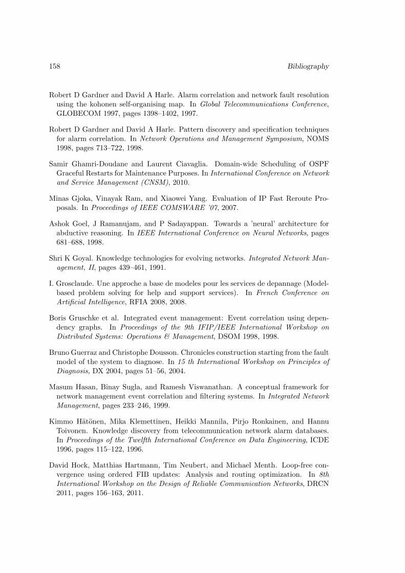
158 Bibliography
Robert D Gardner and David A Harle. Alarm correlation and network fault resolutionusing the kohonen self-organising map. In Global Telecommunications Conference,GLOBECOM 1997, pages 1398–1402, 1997.
Robert D Gardner and David A Harle. Pattern discovery and specification techniquesfor alarm correlation. In Network Operations and Management Symposium, NOMS1998, pages 713–722, 1998.
Samir Ghamri-Doudane and Laurent Ciavaglia. Domain-wide Scheduling of OSPFGraceful Restarts for Maintenance Purposes. In International Conference on Networkand Service Management (CNSM), 2010.
Minas Gjoka, Vinayak Ram, and Xiaowei Yang. Evaluation of IP Fast Reroute Pro-posals. In Proceedings of IEEE COMSWARE ’07, 2007.
Ashok Goel, J Ramanujam, and P Sadayappan. Towards a ’neural’ architecture forabductive reasoning. In IEEE International Conference on Neural Networks, pages681–688, 1998.
Shri K Goyal. Knowledge technologies for evolving networks. Integrated Network Man-agement, II, pages 439–461, 1991.
I. Grosclaude. Une approche a base de modeles pour les services de depannage (Model-based problem solving for help and support services). In French Conference onArtificial Intelligence, RFIA 2008, 2008.
Boris Gruschke et al. Integrated event management: Event correlation using depen-dency graphs. In Proceedings of the 9th IFIP/IEEE International Workshop onDistributed Systems: Operations & Management, DSOM 1998, 1998.
Bruno Guerraz and Christophe Dousson. Chronicles construction starting from the faultmodel of the system to diagnose. In 15 th International Workshop on Principles ofDiagnosis, DX 2004, pages 51–56, 2004.
Masum Hasan, Binay Sugla, and Ramesh Viswanathan. A conceptual framework fornetwork management event correlation and filtering systems. In Integrated NetworkManagement, pages 233–246, 1999.
Kimmo Hatonen, Mika Klemettinen, Heikki Mannila, Pirjo Ronkainen, and HannuToivonen. Knowledge discovery from telecommunication network alarm databases.In Proceedings of the Twelfth International Conference on Data Engineering, ICDE1996, pages 115–122, 1996.
David Hock, Matthias Hartmann, Tim Neubert, and Michael Menth. Loop-free con-vergence using ordered FIB updates: Analysis and routing optimization. In 8thInternational Workshop on the Design of Reliable Communication Networks, DRCN2011, pages 156–163, 2011.

Bibliography 159
K. Houck, S. Calo, and A. Finkel. Towards a practical alarm correlation system. InProceedings of the fourth international symposium on Integrated network managementIV, pages 226–237, 1995.
Carole Hounkonnou and Eric Fabre. Empowering Self-diagnosis with Self-modeling.In 8th international conference on Network and Service Management, CNSM 2012,pages 364–370. IEEE, 22–26 October 2012.
Carole Hounkonnou and Eric Fabre. Enhanced OSPF Graceful Restart. In IFIP/IEEEInternational Symposium on Integrated Network Management - TechSessions, IM2013, 27-31 May 2013.
Carole Hounkonnou, Samir Ghamri-Doudane, and Eric Fabre. Detection et correctionde boucles de routage dans un reseau de routeurs utilisant un protocole de routagede type SPF. Europeean Patent, 2012.
R. Hulsermann, S. Bodamer, M. Barry, A. Betker, M. Jager, J. Spath, C.M. Gauger,and M. Kohn. A Set of Typical Transport Network Scenarios for Network Modelling.In Beitrage zur 5. ITG-Fachtagung Photonische Netze, pages 65–72, May 2004.
Rolf Isermann. Supervision, fault-detection and fault-diagnosis methods — an intro-duction. Control Engineering Practice, 5:639–652, 1997.
Rolf Isermann. Model-based fault-detection and diagnosis — status and applications.Annual Reviews in Control, 29:17–85, 2005.
ITU-T. Gateway control protocol: Version 3, ITU-T Recommendation H. 248.1, 2013.
Gabriel Jakobson and Mark Weissman. Real-time telecommunication network man-agement: extending event correlation with temporal constraints. In Proceedings ofthe fourth international symposium on Integrated network management IV, pages290–301, 1995.
Juniper. Configuring Graceful Restart for OSPF, 2013. URL http://juniper.net/
techpubs/en_US/junos/topics/topic-map/ospf-graceful-restart.html.
S. Katker and M. Paterok. Fault isolation and event correlation for integrated faultmanagement. In Proceedings of the fifth IFIP/IEEE international symposium onIntegrated network management V : integrated management in a virtual world: inte-grated management in a virtual world, pages 583–596, 1997.
Stefan Katker and Kurt Geihs. A Generic Model for Fault Isolation in IntegratedManagement Systems. Journal of Network and Systems Management, 5:109–130,1997.
Soila P Kavulya, Kaustubh Joshi, Matti Hiltunen, Scott Daniels, Rajeev Gandhi, andPriya Narasimhan. Draco: Top-down statistical diagnosis of large-scale voip net-works, 2011.

160 Bibliography
Soila P. Kavulya, Kaustubh Joshi, Matti Hiltunen, Scott Daniels, Rajeev Gandhi, andPriya Narasimhan. Practical experiences with chronics discovery in large telecom-munications systems. ACM SIGOPS Operating Systems Review, 45:23–30, 2012.
Walter Kehl, Heiner Hopfmuller, Traytcho Koussev, and Mark Newstead. Applicationof model-based reasoning to the maintenance of telecommunication networks. InIndustrial and Engineering Applications of Artificial Intelligence and Expert Systems,pages 79–88. Springer Berlin Heidelberg, 1992.
Rana M Khanafer, Beatriz Solana, Jordi Triola, Raquel Barco, Lars Moltsen, ZwiAltman, and Pedro Lazaro. Automated diagnosis for UMTS networks using Bayesiannetwork approach. IEEE Transactions on Vehicular Technology, 57:2451–2461, 2008.
Shmuel Kliger, Shaula Yemini, Yechiam Yemini, David Ohsie, and Salvatore Stolfo.A coding approach to event correlation. In Proceedings of the fourth internationalsymposium on Integrated network management IV, pages 266–277, 1995.
Mark L Krieg. A tutorial on Bayesian belief networks. Technical report, DTIC Docu-ment, 2001.
Lundy Lewis. A Case-Based Reasoning Approach to the Resolution of Faults in Com-munication Networks. In Integrated Network Management, pages 671–682, 1993.
Lundy Lewis and Gabi Dreo. Extending trouble ticket systems to fault diagnostics.Network, IEEE, 7:44–51, 1993.
Dennis V Lindley. On a measure of the information provided by an experiment. TheAnnals of Mathematical Statistics, 27:986–1005, 1956.
Kar-Wing Edward Lor. A Network Diagnostic Expert System for Acculink Multiplex-ers Based on a General Network Diagnostic Scheme. In Proceedings of the IFIPTC6/WG6.6 Third International Symposium on Integrated Network Managementwith participation of the IEEE Communications Society CNOM and with supportfrom the Institute for Educational Services, pages 659–669, 1993.
Jingxian Lu, Christophe Dousson, Benoit Radier, and Francine Krief. Towards anAutonomic Network Architecture for Self-healing in Telecommunications Networks.In Mechanisms for Autonomous Management of Networks and Services, volume 6155,pages 110–113. Springer Berlin Heidelberg, 2010.
Jingxian Lu, Christophe Dousson, and Francine Krief. A Self-diagnosis AlgorithmBased on Causal Graphs. In The Seventh International Conference on Autonomicand Autonomous Systems, ICAS 2011, 2011.
Heikki Mannila, Hannu Toivonen, and A Inkeri Verkamo. Discovering frequent episodesin sequences. In Proceedings of the First International Conference on KnowledgeDiscovery and Data Mining, pages 210–215, 1995.

Bibliography 161
Robert Mathonet, Herwig Van Cotthem, and Leon Vanryckeghem. DANTES: An Ex-pert System for Real-Time Network Troubleshooting. In Proceedings of the 10thinternational joint conference on Artificial intelligence - Volume 1, pages 527–530,1987.
Cristina Melchiors and Liane M. Rockenbach Tarouco. Fault Management in ComputerNetworks Using Case-Based Reasoning: DUMBO System. In Proceedings of the ThirdInternational Conference on Case-Based Reasoning and Development, pages 510–524,1999.
Masanori Miyazawa and Kosuke Nishimura. Scalable root cause analysis assisted byclassified alarm information model based algorithm. In 7th International Conferenceon Network and Service Management, CNSM 2011, pages 1–4, 2011.
J. Moy, P. Pillay-Esnault, and A. Lindem. RFC 3623: Graceful OSPF restart, Novem-ber 2003.
John Moy. OSPF: Anatomy of an Internet Routing Protocol. Addison-Wesley LongmanPublishing Co., Inc., 1998a.
John Moy. RFC 2328: OSPF Version 2, April 1998b.
Kevin Murphy et al. The Bayes Net Toolbox for Matlab. Computing science andstatistics, 33:1024–1034, 2001.
RJ Patton, J Chen, and TM Siew. Fault diagnosis in nonlinear dynamic systems vianeural networks. In International Conference on Control, volume 2, pages 1346–1351,1994.
L.F. PAU. Survey of expert systems for fault detection, test generation and mainte-nance. Expert Systems, 3:100–110, 1986.
Judea Pearl. Probabilistic reasoning in intelligent systems: networks of plausible infer-ence. Morgan Kaufmann, 1988.
Georgia C. Penido, Jose Marcos S. Nogueira, and Christiano Mata Machado. An auto-matic fault diagnosis and correction system for telecommunications management. InProceedings of the Sixth IFIP/IEEE International Symposium on Integrated NetworkManagement, pages 777–791, 1999.
Duc Truong Pham. Expert Systems in Engineering. Springer-Verlag New York, Inc.,1988.
Gianluca Reali and Luca Monacelli. Definition and performance evaluation of a faultlocalization technique for an NGN IMS network. IEEE Transactions on Network andService Management, 6(2):122–136, 2009.
J. Rosenberg, H. Schulzrinne, G. Camarillo, A. Johnston, J. Peterson, R. Sparks,M. Handley, and E. Schooler. RFC 3261: Session initiation protocol, 2002.

162 Bibliography
Raguram Sasisekharan, Yung-Kao Hsu, and David Simen. SCOUT: an approach toautomating diagnoses of faults in large scale networks. In Global TelecommunicationsConference, GLOBECOM 1993, pages 212–216, 1993.
Raguram Sasisekharan, V Seshadri, and Sholom M Weiss. Data mining and forecastingin large-scale telecommunication networks. IEEE Expert, 11:37–43, 1996.
William T Scherer and CC White. A survey of expert systems for equipment main-tenance and diagnostics. In Fault detection & reliability: knowledge based & otherapproaches, pages 3–18. Pergamon Press, 1987.
H Schulzrinne, S Casner, R Frederick, and V Jacobson. RFC 3550: RTP: A TransportProtocol for Real-Time Applications, 2003.
Aman Shaikh, Rohit Dube, and Anujan Varma. Avoiding instability during gracefulshutdown of OSPF. In Twenty-First Annual Joint Conference of the IEEE Computerand Communications Societies, volume 2 of INFOCOM 2002, pages 883–892, 2002.
Aman Shaikh, Rohit Dube, and Anujan Varma. Avoiding instability during gracefulshutdown of multiple OSPF routers. IEEE/ACM Transactions on Networking, 14(3):532 –542, 2006.
Stephen Slade. Case-based reasoning: A research paradigm. AI magazine, 12:42, 1991.
Malgorzata Steinder and Adarshpal S. Sethi. End-to-end Service Failure DiagnosisUsing Belief Networks. In Network Operations and Management Symposium, NOMS2002, pages 375–390, 2002.
Malgorzata Steinder and Adarshpal S. Sethi. A survey of fault localization techniquesin computer networks. Science of Computer Programming, 53:165–194, 2004a.
Malgorzata Steinder and Adarshpal S. Sethi. Probabilistic fault diagnosis in commu-nication systems through incremental hypothesis updating. Computer Networks, 45:537–562, 2004b.
Yongning Tang, Ehab Al-Shaer, and Raouf Boutaba. Efficient fault diagnosis usingincremental alarm correlation and active investigation for internet and overlay net-works. Network and Service Management, IEEE Transactions on, 5:36–49, 2008.
ETSI TISPAN. Telecommunications and Internet converged Services and Protocolsfor Advanced Networking (TISPAN) - Resource and Admission Control Sub-system(RACS) - Functional Architecture. ETSI ES 282 003 V1.1.1 (2006-06), June 2006.
ETSI TISPAN. Universal Mobile Telecommunications System (UMTS) - Telecommu-nications and Internet converged Services and Protocols for Advanced Networking(TISPAN) - IP Multimedia Subsystem (IMS) - Functional architecture. ETSI TS123-517 V8.0.0 (2007-12), December 2007.

Bibliography 163
ETSI TISPAN. Universal Mobile Telecommunications System (UMTS) - TISPAN -IP Multimedia Subsystem (IMS) - Stage 2 description. ETSI TS 123 506 V8.1.0(2008-10), October 2008a.
ETSI TISPAN. Universal Mobile Telecommunications System (UMTS) - TISPAN -IP Multimedia Subsystem (IMS) - Stage 2 description. ETSI TS 123 406 V7.2.0(2008-10), October 2008b.
ETSI TISPAN. Telecommunications and Internet converged Services and Protocols forAdvanced Networking (TISPAN) - NGN Functional Architecture. ETSI ES 282 001V3.4.1 (2009-09), September 2009.
ETSI TISPAN. Telecommunications and Internet converged Services and Protocols forAdvanced Networking (TISPAN) - NGN Functional Architecture - Network Attach-ment Sub-System (NASS). ETSI ES 282 004 V3.4.1 (2010-03), March 2010a.
ETSI TISPAN. Universal Mobile Telecommunications System (UMTS) - LTE - IPMultimedia Subsystem (IMS) - Stage 2. ETSI TS 123 228 V9.4.0 (2010-10), October2010b.
ETSI TISPAN. Universal Mobile Telecommunications System (UMTS) - LTE - 3Gsecurity - Access security for IP-based services. ETSI TS 133 203 V10.2.0 (2010-12),December 2010c.
Andrew J Weiner, David A Thurman, and Christine M Mitchell. Applying case-basedreasoning to aid fault management in supervisory control. In IEEE InternationalConference on Systems, Man and Cybernetics, volume 5, pages 4213–4218, 1995.
Gary Weiss, John Eddy, and Sholom Weiss. Intelligent telecommunication technologies,1998a.
Gary Weiss, Johannes P. Ros, and Anoop Singhal. ANSWER: Network MonitoringUsing Object-Oriented Rules. In Proceedings of the Tenth Conference on InnovativeApplications of Artificial Intelligence, pages 1087–1093, 1998b.
Sholom M. Weiss and Nitin Indurkhya. Optimized Rule Induction. IEEE Expert:Intelligent Systems and Their Applications, 8:61–69, 1993.
Hermann Wietgrefe. Investigation and practical assessment of alarm correlation meth-ods for the use in GSM access networks. In IEEE/IFIP Network Operations andManagement Symposium, NOMS 2002, pages 391–403, 2002.
Peng Wu, R. Bhatnagar, L. Epshtein, M. Bhandaru, and Zhongwen Shi. Alarm correla-tion engine (ACE). In IEEE/IFIP Network Operations and Management Symposium,NOMS 98, pages 733–742, 1998.
Jie Xiao, Changcheng Huang, and James Yan. IMS network deployment cost opti-mization based on flow-based traffic model. In IEEE/IFIP Network Operations andManagement Symposium, NOMS 2010, pages 232–239, 2010.

164 Bibliography
Shaula Alexander Yemini, Shmuel Kliger, Eyal Mozes, Yechiam Yemini, and DavidOhsie. High speed and robust event correlation. IEEE Communications Magazine,34:82–90, 1996.
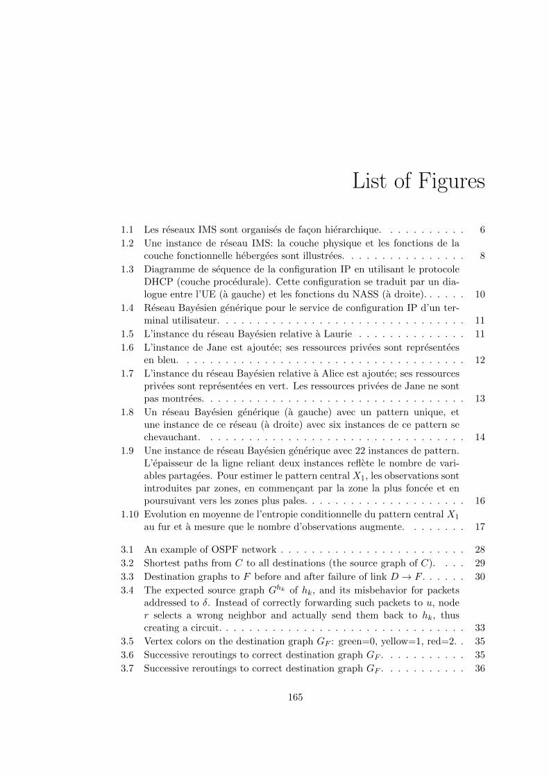
List of Figures
1.1 Les reseaux IMS sont organises de facon hierarchique. . . . . . . . . . . 6
1.2 Une instance de reseau IMS: la couche physique et les fonctions de lacouche fonctionnelle hebergees sont illustrees. . . . . . . . . . . . . . . . 8
1.3 Diagramme de sequence de la configuration IP en utilisant le protocoleDHCP (couche procedurale). Cette configuration se traduit par un dia-logue entre l’UE (a gauche) et les fonctions du NASS (a droite). . . . . . 10
1.4 Reseau Bayesien generique pour le service de configuration IP d’un ter-minal utilisateur. . . . . . . . . . . . . . . . . . . . . . . . . . . . . . . . 11
1.5 L’instance du reseau Bayesien relative a Laurie . . . . . . . . . . . . . . 11
1.6 L’instance de Jane est ajoutee; ses ressources privees sont representeesen bleu. . . . . . . . . . . . . . . . . . . . . . . . . . . . . . . . . . . . . 12
1.7 L’instance du reseau Bayesien relative a Alice est ajoutee; ses ressourcesprivees sont representees en vert. Les ressources privees de Jane ne sontpas montrees. . . . . . . . . . . . . . . . . . . . . . . . . . . . . . . . . . 13
1.8 Un reseau Bayesien generique (a gauche) avec un pattern unique, etune instance de ce reseau (a droite) avec six instances de ce pattern sechevauchant. . . . . . . . . . . . . . . . . . . . . . . . . . . . . . . . . . 14
1.9 Une instance de reseau Bayesien generique avec 22 instances de pattern.L’epaisseur de la ligne reliant deux instances reflete le nombre de vari-ables partagees. Pour estimer le pattern central X1, les observations sontintroduites par zones, en commencant par la zone la plus foncee et enpoursuivant vers les zones plus pales. . . . . . . . . . . . . . . . . . . . . 16
1.10 Evolution en moyenne de l’entropie conditionnelle du pattern central X1
au fur et a mesure que le nombre d’observations augmente. . . . . . . . 17
3.1 An example of OSPF network . . . . . . . . . . . . . . . . . . . . . . . . 28
3.2 Shortest paths from C to all destinations (the source graph of C). . . . 29
3.3 Destination graphs to F before and after failure of link D → F . . . . . . 30
3.4 The expected source graph Ghk of hk, and its misbehavior for packetsaddressed to δ. Instead of correctly forwarding such packets to u, noder selects a wrong neighbor and actually send them back to hk, thuscreating a circuit. . . . . . . . . . . . . . . . . . . . . . . . . . . . . . . . 33
3.5 Vertex colors on the destination graph GF : green=0, yellow=1, red=2. . 35
3.6 Successive reroutings to correct destination graph GF . . . . . . . . . . . 35
3.7 Successive reroutings to correct destination graph GF . . . . . . . . . . . 36
165

166 List of Figures
3.8 Successive removals of the temporary reroutings into the corrected des-tination graph G′F , after node C returns to function. . . . . . . . . . . . 37
3.9 Rerouting packets addressed to δ1 with a minimal number of hops inorder to go around r (and thus avoid the circuit). This rerouting pathcan also be (partly) used to correct the circuit on the path to δ2 whenδ1;δ2 in GHk . . . . . . . . . . . . . . . . . . . . . . . . . . . . . . . . . 39
3.10 Evaluation on the NSFNET network . . . . . . . . . . . . . . . . . . . . 40
4.1 Organization of rule-based expert systems . . . . . . . . . . . . . . . . . 47
4.2 An example of forward chaining . . . . . . . . . . . . . . . . . . . . . . . 48
4.3 Structure of the knowledge sources . . . . . . . . . . . . . . . . . . . . . 52
4.4 Case-Based Reasoning Cycle . . . . . . . . . . . . . . . . . . . . . . . . 55
4.5 A simple data set with two classes used for illustrative purposes. . . . . 58
4.6 A simple linear classification boundary for the loan data set. . . . . . . . 58
4.7 A Simple Linear Regression for the Loan Data Set. . . . . . . . . . . . . 59
4.8 A Simple Clustering of the Loan Data Set into Three Clusters. . . . . . 59
4.9 An Example of Classification Boundaries Learned by a Nonlinear Clas-sifier (Such as a Neural Network) for the Loan Data Set. . . . . . . . . . 61
4.10 Model of a feedforward neural network. . . . . . . . . . . . . . . . . . . 63
4.11 A problem-symptom graph and its associated codebook. . . . . . . . . . 64
4.12 A causal graph explaining the propagation of failures from the problems(top) to the symptoms (bottom). This causal graph yields the problem-symptom graph of Figure 4.11 by transitivity closure, after removal orintermediate nodes and duplicated symptoms. . . . . . . . . . . . . . . . 66
4.13 A causal graph and a configuration over it. Edges describe two propaga-tion modalities: “must cause” (solid arrows) and “may cause” (dashedarows). Test nodes are represented as parallelograms, alarm nodes asovals. . . . . . . . . . . . . . . . . . . . . . . . . . . . . . . . . . . . . . . 69
4.14 Two causal graphs, for resp. domains 1 and 2, sharing some nodes(p2, p3 and a2). Left: two compatible local configurations. Right: twoincompatible local confidurations. . . . . . . . . . . . . . . . . . . . . . . 71
4.15 An timed event flow (top) and a chronicle (bottom). The arrows indicatea chronicle instance within the event flow. . . . . . . . . . . . . . . . . . 74
4.16 The constraint propagation rule in a chronicle. . . . . . . . . . . . . . . 75
4.17 A time constraint graph before (left) and after (right) constraint propa-gation. . . . . . . . . . . . . . . . . . . . . . . . . . . . . . . . . . . . . . 75
4.18 Merging 3 chronicles of size 2 into a chronicle of size 3, with time con-straints propagation. . . . . . . . . . . . . . . . . . . . . . . . . . . . . . 77
4.19 A Bayesian network for IP paths diagnosis . . . . . . . . . . . . . . . . . 78
4.20 Propagation in a chain network . . . . . . . . . . . . . . . . . . . . . . . 81
4.21 Propagation in a tree . . . . . . . . . . . . . . . . . . . . . . . . . . . . . 81
4.22 Propagation in a causal polytree network . . . . . . . . . . . . . . . . . 82
4.23 NBM . . . . . . . . . . . . . . . . . . . . . . . . . . . . . . . . . . . . . . 85

List of Figures 167
5.1 The generic IMS physical architecture . . . . . . . . . . . . . . . . . . . 905.2 Core IP Multimedia Subsystem architecture . . . . . . . . . . . . . . . . 915.3 Session Control . . . . . . . . . . . . . . . . . . . . . . . . . . . . . . . . 925.4 The media functions . . . . . . . . . . . . . . . . . . . . . . . . . . . . . 945.5 Resource and Admission Control Subsystem architecture . . . . . . . . . 965.6 Network components and control flow for QoS . . . . . . . . . . . . . . . 975.7 Network Attachment Subsystem architecture . . . . . . . . . . . . . . . 985.8 Network components and procedure for authentication . . . . . . . . . . 995.9 TISPAN NGN IMS functional architecture . . . . . . . . . . . . . . . . . 1005.10 Mapping functions to physical equipment . . . . . . . . . . . . . . . . . 1015.11 Network attachment procedure using DHCP . . . . . . . . . . . . . . . . 1035.12 Notification sent to the RACS during network attachment . . . . . . . . 1045.13 IMS-level registration procedure . . . . . . . . . . . . . . . . . . . . . . 1065.14 Call origination procedure . . . . . . . . . . . . . . . . . . . . . . . . . . 1095.15 IMS networks are hierarchically organized structures . . . . . . . . . . . 111
6.1 The generic IMS physical architecture and its instance . . . . . . . . . . 1146.2 The generic IMS functional architecture and its instance . . . . . . . . . 1166.3 Different levels of granularity for IP configuration procedure . . . . . . . 1196.4 A mapping between the physical and the functional architecture . . . . 1206.5 Network model class hierarchy . . . . . . . . . . . . . . . . . . . . . . . 1216.6 Class UE inherits from class Function . . . . . . . . . . . . . . . . . . . 1226.7 An IMS network instance . . . . . . . . . . . . . . . . . . . . . . . . . . 123
7.1 An IMS network instance . . . . . . . . . . . . . . . . . . . . . . . . . . 1277.2 Sequence diagram of IP configuration using DHCP (procedural layer) . 1277.3 Generic BN for the IP configuration capability of a User Equipment. . . 1287.4 Laurie’s BN instance . . . . . . . . . . . . . . . . . . . . . . . . . . . . . 1297.5 Jane’s BN instance is added; her private resources are represented in blue1307.6 Alice’s BN instance is added. . . . . . . . . . . . . . . . . . . . . . . . . 1307.7 A GBN (left) with a single pattern, and an instance of this GBN (right). 132
8.1 A GBN (left) with a single pattern, and an instance of this GBN (right). 1408.2 A GBN instance with 22 pattern instances. . . . . . . . . . . . . . . . . 1408.3 Average evolution of the conditional entropy of the central pattern X1. . 1418.4 A Network instance example. . . . . . . . . . . . . . . . . . . . . . . . . 1428.5 IP connectivity sequence diagram. . . . . . . . . . . . . . . . . . . . . . 1428.6 Pattern for IP connectivity . . . . . . . . . . . . . . . . . . . . . . . . . 1438.7 Mary’s pattern instance. . . . . . . . . . . . . . . . . . . . . . . . . . . . 1438.8 The whole model. . . . . . . . . . . . . . . . . . . . . . . . . . . . . . . . 1458.9 Evolution of H(Z) while pattern instances are added . . . . . . . . . . . 1488.10 Average evolution of the conditional entropy of Z. . . . . . . . . . . . . 1498.11 Examples of non-decreasing behavior of H(Z) . . . . . . . . . . . . . . . 149

168 List of Figures

Glossary
4G 4th Generation 22
A-RACF Access Resource and Admission Control Function 96
ADSL Asymmetric Digital Subscriber Line 102
AF Application Function 96
AMF Access Management Function 98
AN Access Node 89
ARF Access Relay Function 98
AS Application Server 95
BGCF Breakout Gateway Control Function 94
BGF Border Gateway Function 96
BRAS Broadband Remote Access Server 90
C-BGF Core Border Gateway Function 96
CLF Connectivity Session Location Function 98
CNG Customer Network Gateway 99
CNGCF Customer Network Gateway Configuration Function 99
COPS Common Open Policy Service 91
CPE Customer Premise Equipment 89
CS Circuit Switched 94
CSCF Call Session Control Function 91
DHCP Dynamic Host Configuration Protocol 98, 102
DSL Digital Subscriber Line 90
DSLAM DSL Access Multiplexer (DSLAM) 89
169

170 Glossary
DSP Digital Signal Processing 94
FQDN Fully Qualified Domain Name 104
FTTH Fiber-to-the-home 21
I-CSCF Interrogating CSCF 91
IBCF Interconnection Border Control Function 95
IMS IP Multimedia Subsytem 2, 22, 25, 89
IMS-MGW IMS Media Gateway 94
IP Internet Protocol 21, 90
IP-CAN IP Connectivity Access Network 102
ISC IMS Service Control 95
ISUP ISDN User Part 94
IWF Inter Working Function 95
MGCF Media Gateway Control Function 94
MRF Multimedia Resource Function 93
MRFC Multimedia Resource Function Controller 94
MRFP Multimedia Resource Function Processor 94
NACF Network Access Configuration Function 98
NAPT Network Address Port Translation 96
NASS Network Attachment Subsystem 91
NAT Network Address Translation 96
NGN Next Generation Network 22, 104
OSPF Open Shortest Path First 24
P-CSCF Proxy CSCF 91
PDBF Profile Database Function 98
PoP Point of Presence 90

Glossary 171
PPP Point-to-Point Protocol 102
QoS Quality of Service 95
RACS Resource and Admission Control Subsystem 91
RCEF Resource Control Enforcement Function 96
RTP Real-Time Protocol 91
S-CSCF Serving CSCF 91
SBC Session Border Controller 90
SDP Session Description Protocol 93
SGW Signaling Gateway 95
SIP Session Initiation Protocol 90
SLF Subscriber Locator Function 93
SPDF Service Policy Decision Function 96
TDM Time Division Multiplexing 94
UAAF User Access Authorization Function 98
UE User Equipment 98
UMTS Universal Mobile Telecommunications Services 22
UPSF User Profile Server Function 91
URI Uniform Resource Identifier 105