Embed Size (px)
Citation preview

ACPN2010, Rostock, September 22nd 2010
1
Advanced solution methods for Stochastic Petri Nets
Prof.ssa Susanna DonatelliUniversita’ di Torino, [email protected]

2
Context
(System, question on system)
(Model, question on model)
(Model, answer on model)
(System, answer on system)
abstraction
model solution
backward interpretation

3
Context
System type: discrete event systems
Categories of questions: qualitative -- will system reach a deadlock? quantitative -- will system reach a deadlock before
time T? stochastic -- will system reach a deadlock before
time T with probability >0.9 ?
Corresponding classes of models: finite automata (but also Petri Nets, Process
Algebras, etc.) timed automata (continuous) time Markov chain ( SPN, GSPN, SWN,
Queueing networks, Stochastic Process algebras and stochastic processes in general)

4
Context
Typical questions/properties qualitative -- reachability, deadlock, liveness,
state/action condition, system evolution (path properties)
quantitative -- timed reachability, timed system evolution (timed path properties)
stochastic -- reachability in probability
We concentrate on stochastic properties for stochastic systems Revisit CSL for Petri Nets Go beyond CSL (not only for nets)

5
Outline
Verifying quantitative behaviour: CSL for SPN and SWN definition and model checking
Verifying quantitative behaviour: CSL for GSPN
Beyond CSL
Solving large (G)SPN: symbolic representation and tensor-based techniques
Bibliographical references

6
Outline
Verifying quantitative behaviour: CSL for SPN and SWN definition and model checking
Verifying quantitative behaviour: CSL for GSPN
Beyond CSL
Solving large (G)SPN: symbolic representation and tensor-based techniques
Bibliographical references
7
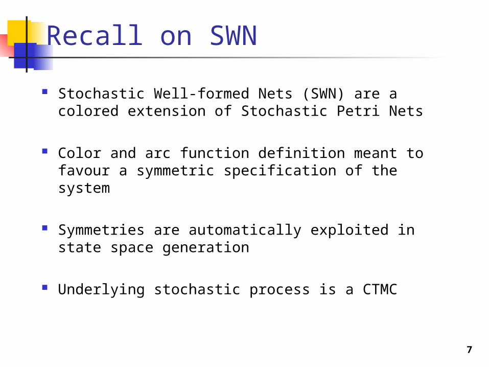
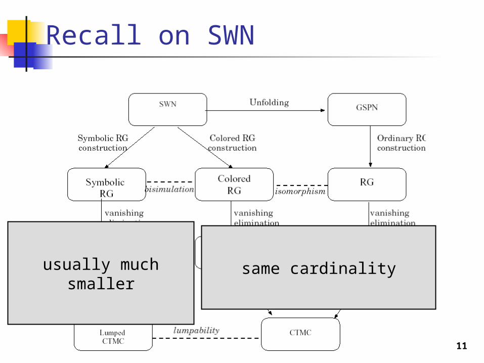
Recall on SWN
Stochastic Well-formed Nets (SWN) are a colored extension of Stochastic Petri Nets
Color and arc function definition meant to favour a symmetric specification of the system
Symmetries are automatically exploited in state space generation
Underlying stochastic process is a CTMC

8
Recall on SWN
neutral place
colored
placecolor domain
D = {d1, d2, ..}
s_srv is enabled for x = color

9
Recall on SWN
Equivalent GSPN when D = {d1, d2}

10
Recall on SWN
GSPN state: M(wait_d1)=2 SWN colored state: M(wait) = 2·d1 SWN symbolic state:
M(wait)= 2·ZD1, with |ZD1|=1
M(wait)= 1·ZD1, M(srv) = 1·ZD2, |ZD1|=1, |ZD2|
=2
equivalence class of all markings with 2 tokens of
the same color in place wait
two jobs waiting for the same device
one job waiting for a device while two jobs are
using the other two devices
11
Recall on SWN
same cardinalityusually much smaller
12
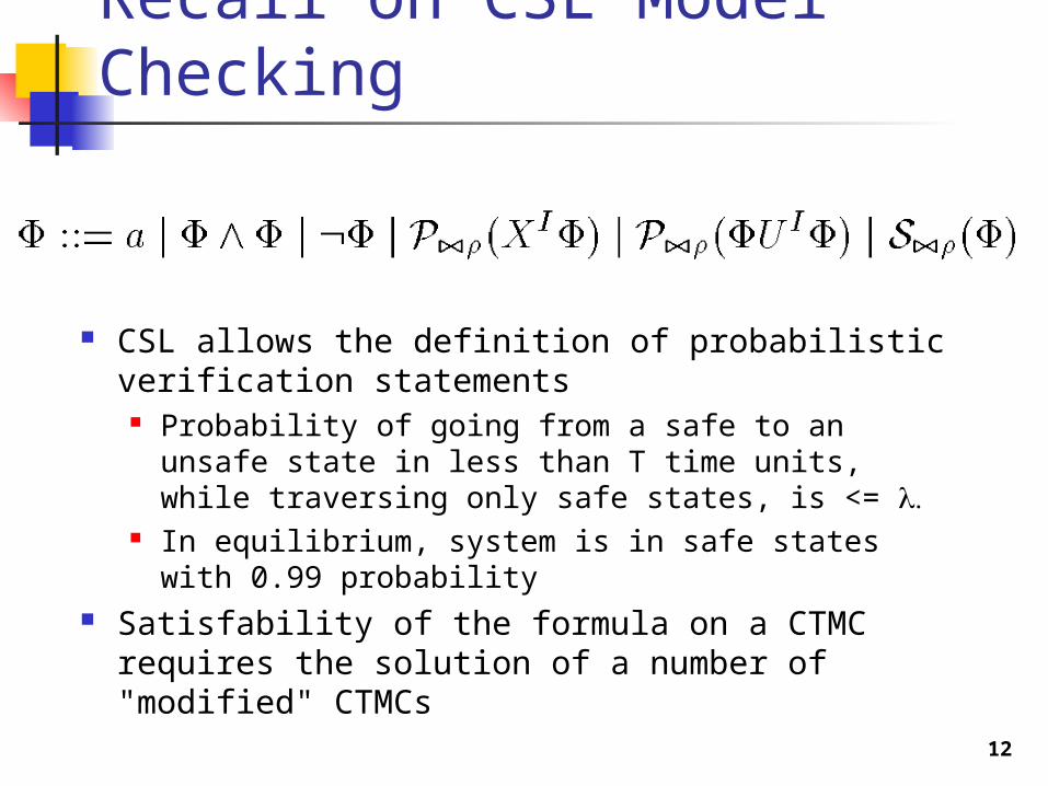
Recall on CSL Model Checking
CSL allows the definition of probabilistic verification statements
Probability of going from a safe to an unsafe state in less than T time units, while traversing only safe states, is <=
In equilibrium, system is in safe states with 0.99 probability
Satisfability of the formula on a CTMC requires the solution of a number of "modified" CTMCs
13
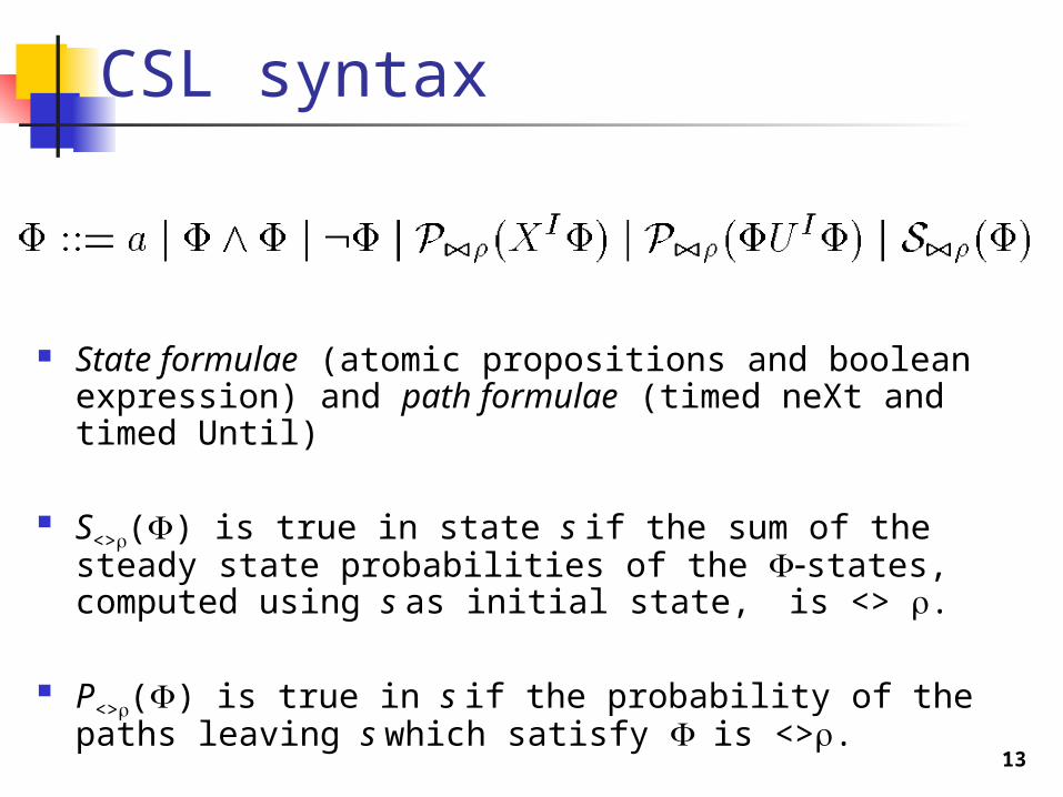
CSL syntax
State formulae (atomic propositions and boolean expression) and path formulae (timed neXt and timed Until)
S<>() is true in state s if the sum of the steady state probabilities of the states, computed using s as initial state, is <> .
P<>() is true in s if the probability of the paths leaving s which satisfy is <>.

14
Examples of CSL: P0.01(true U[10,20] a)
Satisfied in states from which the probability of reaching an a-labelled state after between 10 and 20 time units is no more than 0.01
S>0.9(a) Satisfied in states starting from which the probability of
being in an a-labelled state in the long-run is greater than 0.9
Nested formulae: e.g. P0.1(a U[10,20] S>0.9(bc))
CSL examples

15
CSL Model Checking
Ingredients of any CSL model checker:
1. A CTMC or a net model?
2. A way to define atomic properties of states
3. Efficient CSL satisfiability algorithms
As produced from an SWN
defined at the net level: symbolic, colored, or ordinary?
reuse existing tools?
16
CSL & SWN: why
Probabilistic verification of systems expressed as SWN validate system behaviour "in probability" natural way to express dependability properties
SWN model validation particular important since SWN models can be
non trivial to specify limited support is (was) available to validate
SWN models
17
CSL & SWN: how
Exploit reuse: use existing CSL model checking tools
best of the available technology, constantly updated
but does not allow to exploit the peculiarities and properties of nets
Keep simple the definition of atomic propositions
18
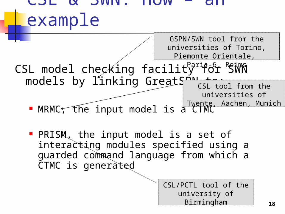
CSL & SWN: how – an example
CSL model checking facility for SWN models by linking GreatSPN to:
MRMC, the input model is a CTMC
PRISM, the input model is a set of interacting modules specified using a guarded command language from which a CTMC is generated
GSPN/SWN tool from the universities of Torino, Piemonte
Orientale, Paris-6, Reims
CSL tool from the universities of Twente,
Aachen, Munich
CSL/PCTL tool of the university of Birmingham

19
CSL & SWN: how
Language for the definition of atomic properties For SWN this task is not always
straightforward, as we may want to refer to neutral, colored and symbolic properties
Discuss the issues of the link from GreatSPN SWN solver to to MRMC and PRISM (which solution for which type of property)
20
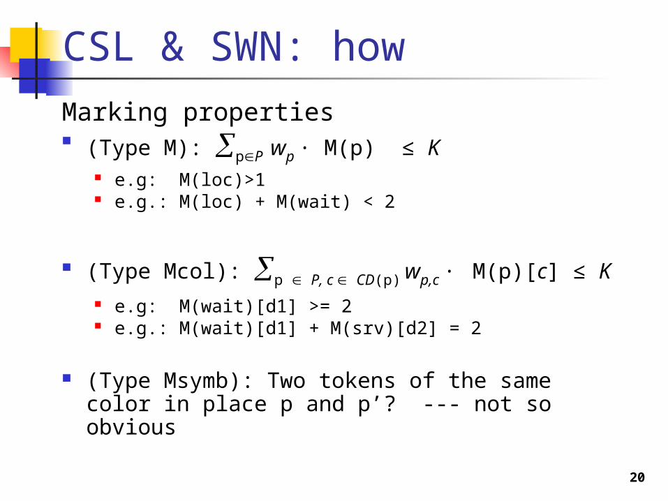
CSL & SWN: how
Marking properties (Type M): pP wp · M(p) ≤ K
e.g: M(loc)>1 e.g.: M(loc) + M(wait) < 2
(Type Mcol): p P, c CD(p) wp,c · M(p)[c] ≤ K e.g: M(wait)[d1] >= 2 e.g.: M(wait)[d1] + M(srv)[d2] = 2
(Type Msymb): Two tokens of the same color in place p and p’? --- not so obvious

21
CSL & SWN: how
Transition enabling properties (Type T): transition t is enabled
e.g.: s_srv is enabled, s_srv_d1 is enabled
(Type Tcol): transition t is enabled for a given assignment to the variables of t. e.g.: s_srv is enabled for x=d1
(Type Tsymb): transition t is enabled for x=y
22
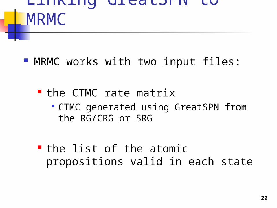
Linking GreatSPN to MRMC
MRMC works with two input files:
the CTMC rate matrix CTMC generated using GreatSPN from the
RG/CRG or SRG
the list of the atomic propositions valid in each state
23
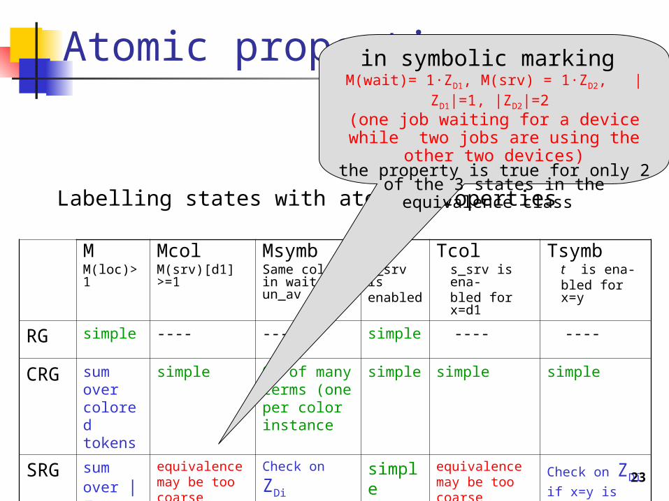
Atomic properties
Labelling states with atomic properties
M M(loc)>1
McolM(srv)[d1] >=1
MsymbSame color in wait and un_av
Ts_srv is enabled
Tcols_srv is ena-bled for x=d1
Tsymbt is ena-bled for x=y
RG simple ---- ---- simple ---- ----
CRG sum over colored tokens
simple OR of many terms (one per color instance
simple simple simple
SRG sum over |ZDi|
equivalence may be too coarse
Check on ZDisimple equivalence
may be too coarse
Check on ZDi
if x=y is not in the guard of t
in symbolic marking M(wait)= 1·ZD1, M(srv) = 1·ZD2, |ZD1|=1, |
ZD2|=2 (one job waiting for a device while
two jobs are using the other two devices)
the property is true for only 2 of the 3 states in the equivalence class
24
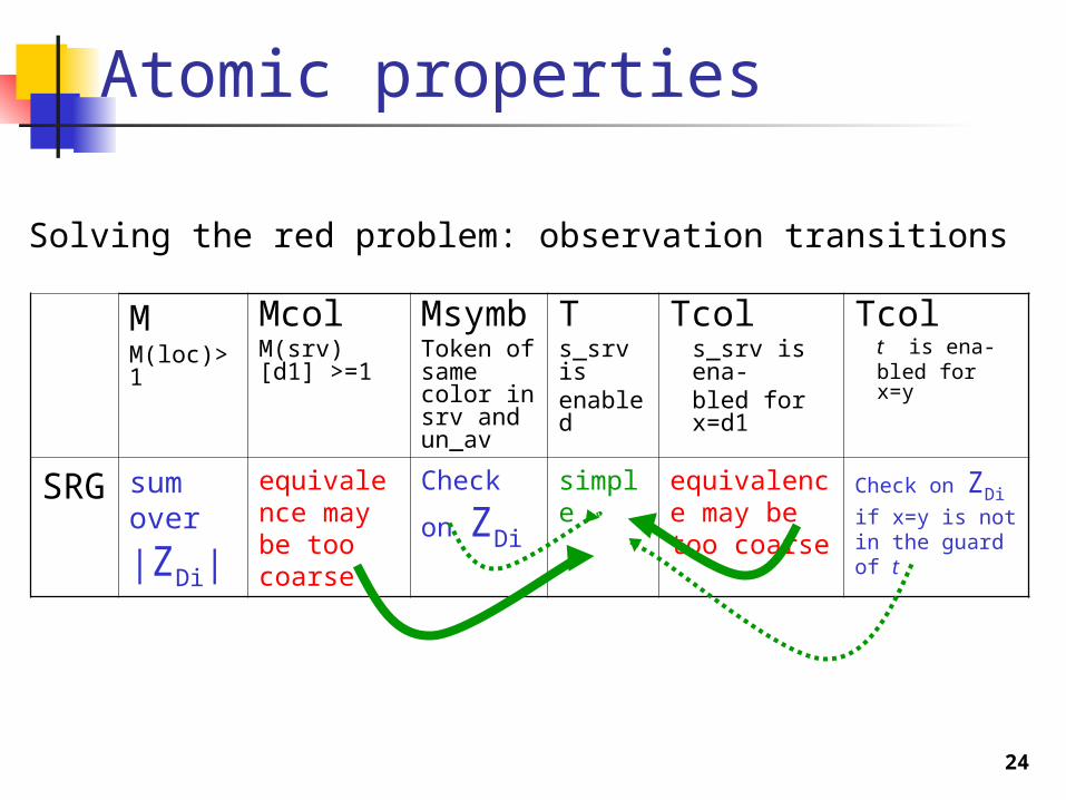
Atomic properties
Solving the red problem: observation transitions
M M(loc)>1
McolM(srv)[d1] >=1
MsymbToken of same color in srv and un_av
Ts_srv is enabled
Tcols_srv is ena-bled for x=d1
Tcolt is ena-bled for x=y
SRG
sum over |ZDi|
equivalence may be too coarse
Check
on ZDi
simple equivalence may be too coarse
Check on ZDi if
x=y is not in the guard of t

25
Atomic properties
M M(loc)>1
McolM(srv)[d1] >=1
Ts_srv is enabled
Tcols_srv is ena-bled for x=d1
SRG sum over |ZDi|
equivalence may be too coarse
simple equivalence may be too coarse
<x>
<x>a token of color d1 in place wait x = d1
test1
<x> <x>s_srv enabled for x=d1
x = d1
test2
<x>

26
Atomic properties
2<x>
2<x>
two tokens of the same color in place wait
Observation transitions can be used to define also symbolic (symmetric)
properties

27
Linking GreatSPN to MRMC
GMC2MRMC
.xlab
.tra
STATES 352TRANSITIONS 12061 2 1.0000001 3 1.0000002 4 10.000000…
1 av(1<d2>1<d1>) loc(8) tloc2 av(1<d2>1<d1>)loc(7)wait(1<d1>) s_srv_d1 ...
.net
GreatSPN.net
.apwait>=4 wait_d1>=4wait_d2>=4
user
APGenerator .lab
#DECLARATIONt_HS#END...25 wait>=4 wait_d1>=4...34 wait>=4 wait_d2>=4...
GreatSPN2MRMC
28
Linking GreatSPN to PRISM
The PRISM input language is a state-based language
State = valuation of a number of bounded variables
A set of guarded commands describes the dynamics of the system: from them PRISM derives the CTMC
Atomic propositions are implicitly defined, as a CSL formula can include any logical condition on the variables' values

29
Linking GreatSPN to PRISM
Two possible ways to connect to PRISM: produce a Prism module directly from the SWN, such
that the same CTMC (up to state numbering) is produced;
produce a Prism module directly from the CTMC of the SRG/RG definition of atomic propositions?
unfolding the SWN into an SPN, followed by the translation of the SPN into a PRISM module using the already-existing translation for SPN.
Current solution does the unfolding, since it is easier and there is already a GSPN->Prism translator.
30
Linking GreatSPN to PRISM
For GSPN place names are mapped one-to-one to variable names
no particular support is needed to translate M and Mcol atomic propositions
T and Tcol propositions have to be restated in terms of markings (variable values).
The unfolding algorithm names unfolded places using color names (e.g.: srv_d1)
31
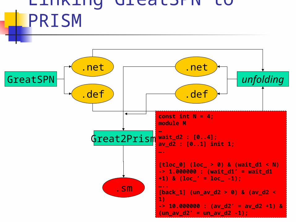
Linking GreatSPN to PRISM
GreatSPN.net
.def
Great2Prism
.sm
unfolding.net
.def
const int N = 4;module M…wait_d2 : [0..4];av_d2 : [0..1] init 1;….
[tloc_0] (loc_ > 0) & (wait_d1 < N)-> 1.000000 : (wait_d1’ = wait_d1 +1) & (loc_’ = loc_ -1);…..[back_1] (un_av_d2 > 0) & (av_d2 < 1)-> 10.000000 : (av_d2’ = av_d2 +1) & (un_av_d2’ = un_av_d2 -1);
32
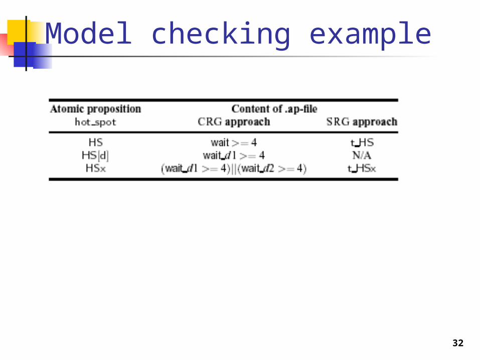
Model checking example

33
model checking example
(1) : S>0.7(hot spot) the system has a probability > 0.7 of being in an hot-
spot state
(2) : S≤0.2(P≥0.9(F[0,5]hot spot)) probability of being, in equilibrium, in “dangerous”
states is at most 0.2.
(3) : P≥0.9(F[0,5](hot spot & P≥0.7(F[0,3] ¬ hot spot))
dangerous states
good hot spot states


![Home [] · 2020-04-19 · Prof.ssa Maria Carla Re 2144510 Cell 349 6129380 Prof.ssa Paola Affanni Cell. 346 6080287 Prof.ssa Maria Eugenia Colucci Cell. 349 7786719 Dr. Andrea Crisanti](https://img.pdfslide.us/doc/110x75/5f21289f4ed94a701f03b66d/home-2020-04-19-profssa-maria-carla-re-2144510-cell-349-6129380-profssa.jpg)