Embed Size (px)
Citation preview
Acoustic Noise Suppression for SpeechSignals using Auditory Masking Effects
Joachim Thiemann
Department of Electrical & Computer EngineeringMcGill UniversityMontreal, Canada
July 2001
A thesis submitted to the Faculty of Graduate Studies and Research in partial fulfillmentof the requirements for the degree of Master of Engineering.
c© 2001 Joachim Thiemann
2001/07/26
i
Abstract
The process of suppressing acoustic noise in audio signals, and speech signals in particu-
lar, can be improved by exploiting the masking properties of the human hearing system.
These masking properties, where strong sounds make weaker sounds inaudible, are cal-
culated using auditory models. This thesis examines both traditional noise suppression
algorithms and ones that incorporate an auditory model to achieve better performance.
The different auditory models used by these algorithms are examined. A novel approach,
based on a method to remove a specific type of noise from audio signals, is presented using
a standardized auditory model. The proposed method is evaluated with respect to other
noise suppression methods in the problem of speech enhancement. It is shown that this
method performs well in suppressing noise in telephone-bandwidth speech, even at low
Signal-to-Noise Ratios.
ii
Sommaire
La suppression de bruit sonore present dans les signaux audio, et plus particulierement dans
les signaux de parole, peut etre amelioree en exploitant les proprietes de masque du systeme
de perception sonore humain. Ces proprietes, ou les sons plus intenses masquent les sons
plus faibles, c’est-a-dire qui font que ces derniers deviennent inaudibles, sont calculees en
utilisant un modele de perception sonore. Ce memoire etudie les algorithmes traditionels
de suppression de bruit et ceux qui incorporent un modele de perception afin d’obtenir de
meilleurs resultats. Une approche originale, qui utilise un modele de perception standardise,
basee sur une methode qui enleve du signal sonore un type de bruit particulier, est presentee.
Cette nouvelle methode est evaluee par rapport a d’autre methodes de suppression de bruit
pour les signaux de parole. Il est demontre que cette nouvelle approche donne de bons
resultats pour la suppression de bruit dans des signaux de paroles, et ce, meme a de bas
niveaux de rapport signal a bruit.
iii
Acknowledgments
This thesis would not have been possible without the encouragement and help from many
people.
First and foremost, I would like to thank my thesis supervisor, Professor Peter Kabal.
His guidance and support from the onset of this work was essential and key to its completion.
Thanks go out to all my friends at the Telecommunications and Signal Processing Lab,
the McGill Outing Club, and my alma mater, Concordia. They all contributed directly
or indirectly to this thesis, be it academic help, proofreading, volunteering to be a test
subject, or just generally helping me to retain my sanity.
Finally, I wish to thank my parents for their love and unwavering support that made it
all possible.
iv
Contents
1 Introduction 1
1.1 Applications of Noise Suppression . . . . . . . . . . . . . . . . . . . . . . . 1
1.2 General Noise Reduction Methods . . . . . . . . . . . . . . . . . . . . . . . 3
1.2.1 Short-time Spectral Amplitude Methods . . . . . . . . . . . . . . . 3
1.3 Auditory Models in Acoustic Noise Suppression . . . . . . . . . . . . . . . 4
1.4 Thesis Contribution . . . . . . . . . . . . . . . . . . . . . . . . . . . . . . . 4
1.5 Previous Work . . . . . . . . . . . . . . . . . . . . . . . . . . . . . . . . . 4
1.6 Thesis Organization . . . . . . . . . . . . . . . . . . . . . . . . . . . . . . . 5
2 Human Hearing and Auditory Masking 6
2.1 The Human Ear . . . . . . . . . . . . . . . . . . . . . . . . . . . . . . . . . 6
2.1.1 The Outer Ear . . . . . . . . . . . . . . . . . . . . . . . . . . . . . 7
2.1.2 The Middle Ear . . . . . . . . . . . . . . . . . . . . . . . . . . . . . 7
2.1.3 The Inner Ear . . . . . . . . . . . . . . . . . . . . . . . . . . . . . . 7
2.1.4 The Basilar Membrane and the Hair Cells . . . . . . . . . . . . . . 8
2.2 Masking . . . . . . . . . . . . . . . . . . . . . . . . . . . . . . . . . . . . . 9
2.2.1 Threshold of Hearing . . . . . . . . . . . . . . . . . . . . . . . . . . 9
2.2.2 Masking Effects . . . . . . . . . . . . . . . . . . . . . . . . . . . . . 11
2.2.3 Critical Bands and the Bark scale . . . . . . . . . . . . . . . . . . . 11
2.2.4 Excitation Patterns and the Masking Threshold . . . . . . . . . . . 13
2.3 Summary . . . . . . . . . . . . . . . . . . . . . . . . . . . . . . . . . . . . 14
3 Spectral Subtraction 15
3.1 Basic Spectral Subtraction . . . . . . . . . . . . . . . . . . . . . . . . . . . 15
3.1.1 Time to Frequency Domain Conversion . . . . . . . . . . . . . . . . 17
Contents v
3.1.2 Spectral Subtraction as a Filter . . . . . . . . . . . . . . . . . . . . 17
3.1.3 Influence of windows on spectral subtraction . . . . . . . . . . . . . 18
3.1.4 Noise estimation techniques . . . . . . . . . . . . . . . . . . . . . . 19
3.1.5 The Role of Voice Activity Detectors . . . . . . . . . . . . . . . . . 20
3.1.6 Artifacts and distortion introduced by Spectral Subtraction . . . . . 21
3.2 Related and derived methods . . . . . . . . . . . . . . . . . . . . . . . . . 23
3.2.1 The Wiener Filter . . . . . . . . . . . . . . . . . . . . . . . . . . . . 23
3.2.2 Maximum Likelihood Envelope Estimator . . . . . . . . . . . . . . 24
3.2.3 The Ephraim and Malah Noise Suppressor . . . . . . . . . . . . . . 24
3.2.4 Filter Smoothing . . . . . . . . . . . . . . . . . . . . . . . . . . . . 25
3.2.5 Signal Subspace methods . . . . . . . . . . . . . . . . . . . . . . . . 26
3.2.6 Implementation of EVRC noise reduction . . . . . . . . . . . . . . . 27
3.3 Comparison of Methods . . . . . . . . . . . . . . . . . . . . . . . . . . . . 29
3.4 Summary . . . . . . . . . . . . . . . . . . . . . . . . . . . . . . . . . . . . 31
4 Using Masking Properties in Spectral Subtraction Algorithms 32
4.1 Masking Models . . . . . . . . . . . . . . . . . . . . . . . . . . . . . . . . . 33
4.1.1 The Johnston Model . . . . . . . . . . . . . . . . . . . . . . . . . . 33
4.1.2 The Perceptual Audio Quality Measure . . . . . . . . . . . . . . . . 36
4.1.3 Soulodre’s Model . . . . . . . . . . . . . . . . . . . . . . . . . . . . 37
4.1.4 Perceptual Evaluation of Audio Quality . . . . . . . . . . . . . . . . 39
4.2 Perceptual based noise reduction . . . . . . . . . . . . . . . . . . . . . . . 42
4.2.1 Tsoukalas’ method for Speech Enhancement . . . . . . . . . . . . . 43
4.2.2 Musical Noise Suppression . . . . . . . . . . . . . . . . . . . . . . . 44
4.2.3 Virag’s method . . . . . . . . . . . . . . . . . . . . . . . . . . . . . 45
4.2.4 Tsoukalas’ method for Audio Signal Enhancement . . . . . . . . . . 46
4.2.5 Soulodre’s method . . . . . . . . . . . . . . . . . . . . . . . . . . . 46
4.3 Using the PEAQ model in noise reduction . . . . . . . . . . . . . . . . . . 47
4.3.1 Choice of Masking Model . . . . . . . . . . . . . . . . . . . . . . . 48
4.3.2 PNRF Implementation . . . . . . . . . . . . . . . . . . . . . . . . . 48
4.3.3 Implementation Issues . . . . . . . . . . . . . . . . . . . . . . . . . 49
4.3.4 Parameters and Modifications . . . . . . . . . . . . . . . . . . . . . 49
4.4 Summary . . . . . . . . . . . . . . . . . . . . . . . . . . . . . . . . . . . . 50
Contents vi
5 Results 51
5.1 Test data . . . . . . . . . . . . . . . . . . . . . . . . . . . . . . . . . . . . 51
5.2 Objective Comparisons . . . . . . . . . . . . . . . . . . . . . . . . . . . . . 52
5.3 Subjective Comparisons . . . . . . . . . . . . . . . . . . . . . . . . . . . . 55
5.4 Summary . . . . . . . . . . . . . . . . . . . . . . . . . . . . . . . . . . . . 58
6 Conclusion 59
6.1 Summary . . . . . . . . . . . . . . . . . . . . . . . . . . . . . . . . . . . . 59
6.2 Future Research Directions . . . . . . . . . . . . . . . . . . . . . . . . . . . 60
6.2.1 Iterative clean speech estimation . . . . . . . . . . . . . . . . . . . 61
6.2.2 Soft-decision VAD . . . . . . . . . . . . . . . . . . . . . . . . . . . 61
6.2.3 Application to wide-band signals . . . . . . . . . . . . . . . . . . . 61
6.2.4 Lower complexity masking model . . . . . . . . . . . . . . . . . . . 62
A Frequency bands for PEAQ 63
B Subjective testing results 68
References 70
vii
List of Figures
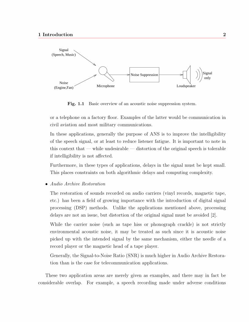
1.1 Basic overview of an acoustic noise suppression system. . . . . . . . . . . . 2
2.1 Structure of the human ear . . . . . . . . . . . . . . . . . . . . . . . . . . . 6
2.2 Cross-section of the cochlea . . . . . . . . . . . . . . . . . . . . . . . . . . 8
2.3 Threshold of hearing in quiet . . . . . . . . . . . . . . . . . . . . . . . . . 10
2.4 Masking curves for 1 kHz masking tone . . . . . . . . . . . . . . . . . . . . 12
2.5 Power spectrum, excitation pattern and masking threshold in perceptual
domain . . . . . . . . . . . . . . . . . . . . . . . . . . . . . . . . . . . . . . 14
3.1 Basic structure of spectral subtraction systems . . . . . . . . . . . . . . . . 15
3.2 Bartlett and Hanning windows . . . . . . . . . . . . . . . . . . . . . . . . . 19
3.3 Different noise estimation results . . . . . . . . . . . . . . . . . . . . . . . 21
3.4 30 frames of Musical Noise in frequency domain . . . . . . . . . . . . . . . 22
3.5 Origins of Musical Noise . . . . . . . . . . . . . . . . . . . . . . . . . . . . 23
3.6 EVRC Noise suppression structure . . . . . . . . . . . . . . . . . . . . . . 27
3.7 Gain curves of spectral subtraction algorithms . . . . . . . . . . . . . . . . 30
3.8 Gain curves of selected other methods . . . . . . . . . . . . . . . . . . . . . 31
4.1 Incorporating a perceptual model in a spectral subtraction algorithm . . . 43
4.2 Implementation of PNRF Gain Function . . . . . . . . . . . . . . . . . . . 48
5.1 Setup for obtaining SNR, SNRSEG, and SNRIMPR. . . . . . . . . . . . . . . 54
viii
List of Tables
5.1 Objective measurement results with 0 dB initial SNR . . . . . . . . . . . . 54
5.2 Objective measurement results with 6 dB initial SNR . . . . . . . . . . . . 55
5.3 Subjective results for speech segments at 0 dB SNR . . . . . . . . . . . . . 57
5.4 Subjective results for speech segments at 6 dB SNR . . . . . . . . . . . . . 58
B.1 Number of answers indicating preference of “A” at 0 dB initial SNR . . . . 68
B.2 Number of answers indicating preference of “B” at 0 dB initial SNR . . . . 68
B.3 Number of answers indicating preference of “A” at 6 dB initial SNR . . . . 69
B.4 Number of answers indicating preference of “B” at 6 dB initial SNR . . . . 69
1
Chapter 1
Introduction
When a sound is picked up by a microphone, noise — in the sense of sounds other than the
one of interest — will be picked up as well. It should be noted however, that in the context
of acoustic signals, the definition of noise is a subjective matter. For example, the sounds
made by the audience in a concert hall is usually considered to be part of the performance.
It carries information about the audience reaction to the performance.
Usually, acoustic noise that was picked up by a microphone is undesirable, especially if it
reduces the perceived quality or intelligibility of the recording or transmission. The problem
of effective removal or reduction of noise (referred to here as Acoustic Noise Suppression,
or ANS1) is an active area of research, and is the topic of this thesis.
1.1 Applications of Noise Suppression
In the general sense, noise suppression has applications in virtually all fields of communica-
tions (channel equalization, radar signal processing, etc.) and other fields (pattern analysis,
data forecasting, etc.) [1].
• Telecommunications
Perhaps the most common application of ANS is in the removal or reduction of
background acoustic noise in telephone or radio communications. Examples of the
former would be the hands-free operation of a cellular telephone in a moving vehicle,
1A distinction must be made between acoustic noise suppression and audible noise suppression. Audiblenoise suppression is discussed in Ch. 4.
2001/07/26
1 Introduction 2
Noise(Engine,Fan)
Signal(Speech, Music)
Signalonly
Microphone Loudspeaker
Noise Suppression
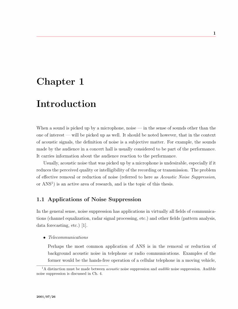
Fig. 1.1 Basic overview of an acoustic noise suppression system.
or a telephone on a factory floor. Examples of the latter would be communication in
civil aviation and most military communications.
In these applications, generally the purpose of ANS is to improve the intelligibility
of the speech signal, or at least to reduce listener fatigue. It is important to note in
this context that — while undesirable — distortion of the original speech is tolerable
if intelligibility is not affected.
Furthermore, in these types of applications, delays in the signal must be kept small.
This places constraints on both algorithmic delays and computing complexity.
• Audio Archive Restoration
The restoration of sounds recorded on audio carriers (vinyl records, magnetic tape,
etc.) has been a field of growing importance with the introduction of digital signal
processing (DSP) methods. Unlike the applications mentioned above, processing
delays are not an issue, but distortion of the original signal must be avoided [2].
While the carrier noise (such as tape hiss or phonograph crackle) is not strictly
environmental acoustic noise, it may be treated as such since it is acoustic noise
picked up with the intended signal by the same mechanism, either the needle of a
record player or the magnetic head of a tape player.
Generally, the Signal-to-Noise Ratio (SNR) is much higher in Audio Archive Restora-
tion than is the case for telecommunication applications.
These two application areas are merely given as examples, and there may in fact be
considerable overlap. For example, a speech recording made under adverse conditions
1 Introduction 3
may have a low SNR and allow for distortion, but the enhancement process will lack the
complexity constraints. It is therefore desirable to have a method that works well in either
application.
1.2 General Noise Reduction Methods
There are many ways to classify noise suppression algorithms. They may be single- or multi-
sensor. In the latter, the spatial properties of the signal and noise sources can be taken into
account. For example, beam-forming using a microphone array emphasizes sounds from a
particular direction [1]. Another example is adaptive noise cancellation (ANC), which is
a two-channel approach based on the primary channel consisting of signal and noise, and
the secondary channel consisting of only the noise. The noise in the secondary channel
must be correlated with the noise in the primary channel [3]. In the case of adaptive echo
cancellation (AEC), the primary channel is the near-end handset, which contains the near-
end signal and the reflection of the far-end signal. The secondary channel is the line from
the far-end handset.
Some noise suppression methods try to exploit the underlying production method of
the signal or the noise. In speech enhancement, this is usually done by linear prediction of
the speech signal [3]. In audio enhancement, since the signal is too general to be modeled,
the noise is modeled instead [2, 4].
1.2.1 Short-time Spectral Amplitude Methods
The noise suppression method discussed in this thesis is a single channel method based on
converting successive short segments of speech into the frequency domain. In the frequency
domain, the noise is removed by adjusting the discrete frequency “bins” on a frame-by-
frame basis, usually by reducing the amplitude based on an estimate of the noise. The
various methods (differentiated by the suppression rule, noise estimate and other details)
are collectively known as Short-Time Spectral Amplitude (STSA), Spectral Weighting, or
Spectral Subtraction methods.
1 Introduction 4
1.3 Auditory Models in Acoustic Noise Suppression
In the above sections, only properties of the source of the signal and noise were exploited
in the process of noise suppression. To further improve the performance of acoustic noise
suppression (ANS) algorithms, properties of the human ear can be taken advantage of.
Research into human auditory properties is an ongoing process. However, available
models of the human auditory system have been successfully used to improve the perfor-
mance of speech and audio coding algorithms [5]. In these coding algorithms, the purpose is
to take only as much of the signal as is perceptually relevant. This reduction of information
allows the signal to be stored or transmitted using fewer bits.
Acoustic noise suppression methods incorporating these same perceptual models have
shown significant gains in performance [4]. However, there is still room for improvements,
and research into new methods continues.
1.4 Thesis Contribution
This thesis presents an overview of noise suppression using auditory models. Different
auditory models and suppression rules are presented. The suppression methods are imple-
mented using the most recent and best-defined auditory model, and compared by objective
and subjective means. A new method, based on the generalization of a method originally
designed to remove camera noise from film soundtracks [4], is presented as a viable speech
and audio enhancement method. This new noise suppression method is shown to have a
good combination of low residual noise, low signal distortion, and low complexity when
compared to similar auditory based noise suppression methods.
1.5 Previous Work
Much of the work presented here is based on the work by Soulodre [4], where ANS methods
were evaluated for the specific problem of removing camera noise from film soundtracks.
Soulodre examined the properties of camera noise, (generated mainly by the lens shutter) in
detail, and presented a novel auditory model and an ANS method. Using a combination of
frame synchronization, sub-band processing and a novel auditory model, Soulodre achieved
noise removal at a Signal-to-Noise Ratio of up to 12 dB lower than required by traditional
1 Introduction 5
noise reduction methods, with little or no distortion of the signal.
Also, auditory-based ANS methods were developed by Tsoukalas et al, who in [6] used
an iterative approach to remove audible noise from speech signals. This method aggressively
removes all but the most audible components of the signal, resulting in almost complete
noise removal at the expense of some signal distortion. In [7], a method for reduction of
noise in audio signals is presented, based on calculating an auditory model of the noise and
removing it from an auditory model of the noisy signal.
In yet another approach, Virag [8] uses an auditory model to adjust the parameters of a
non-auditory noise suppression procedure to improve its performance and reduce artifacts.
Haulick et al [9] used a more direct approach, using the auditory masking threshold
in an attempt to identify and then suppress musical noise (a common artifact of noise
reduction algorithms).
These methods are examined and evaluated in more detail in Ch. 4 and 5.
1.6 Thesis Organization
The fundamentals of human hearing and the mechanics of the ear are explained in Chap-
ter 2. The concepts of masking and the threshold of hearing are introduced. Chapter 3
introduces algorithms to suppress noise using STSA methods that do not incorporate au-
ditory effects. In Chapter 4, some of the mathematical models of the hearing system are
presented, and noise suppression algorithms that incorporate those models. A standard
auditory model is incorporated into adapted versions of the ANS algorithms. The results
of comparing the various methods are presented in Chapter 5. Chapter 6 summarizes and
concludes the thesis.
6
Chapter 2
Human Hearing and Auditory
Masking
2.1 The Human Ear
The human auditory system consists of the ear, auditory nerve fibers, and a section of the
brain. It converts sound waves into sensations perceived by the auditory cortex.
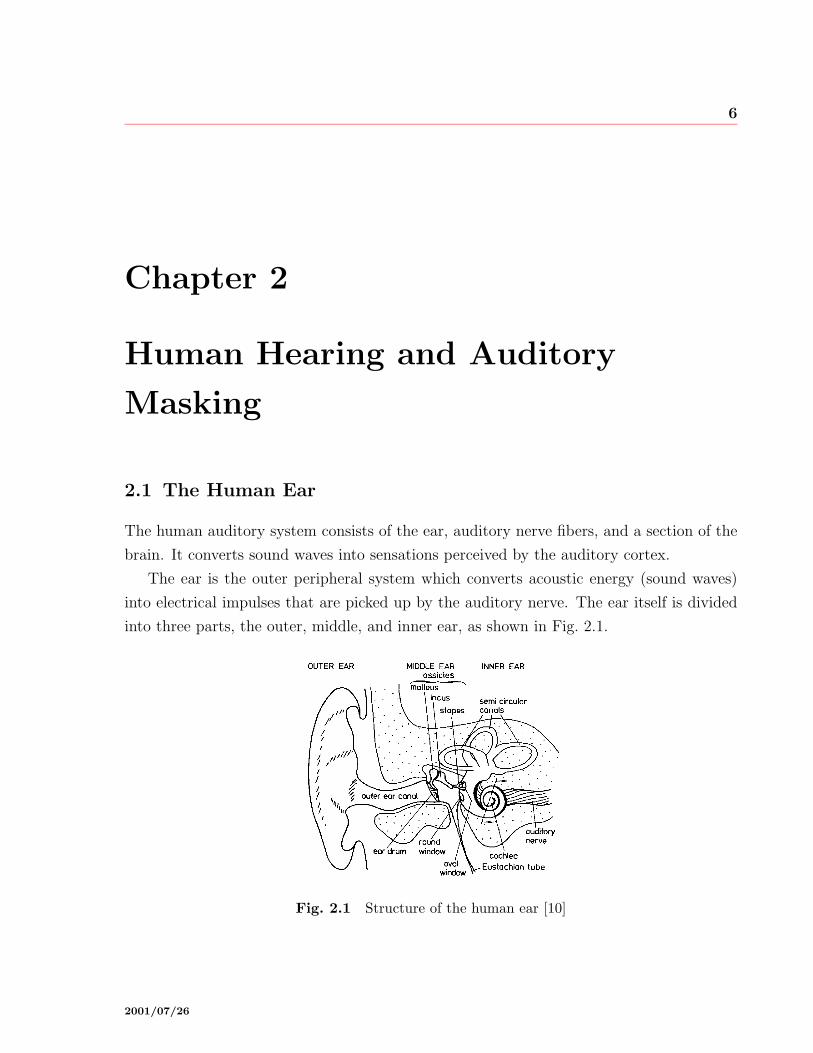
The ear is the outer peripheral system which converts acoustic energy (sound waves)
into electrical impulses that are picked up by the auditory nerve. The ear itself is divided
into three parts, the outer, middle, and inner ear, as shown in Fig. 2.1.
Fig. 2.1 Structure of the human ear [10]
2001/07/26
2 Human Hearing and Auditory Masking 7
2.1.1 The Outer Ear
The outer ear consists of the pinna (the visible part of the ear), the meatus (ear canal),
and terminates at the tympanic membrane (eardrum). The pinna collects sounds and aids
in sound localization, that is to be more sensitive to sounds coming from the front of the
listener [11].
The meatus is a tube which directs the sound to the tympanic membrane. A cavity
with one end open and the other closed by the tympanic membrane, the meatus acts as a
quarter-wave resonator with a center frequency around 3000 Hz. This particular structure
likely aids in the perception of obstruents1, which have much of their energy content in this
frequency region.
2.1.2 The Middle Ear
The middle ear is considered to begin at the tympanic membrane and contains the ossicles,
a set of three small bones. These bones are named malleus (hammer), incus (anvil), and
stapes (stirrup). Acting primarily as levers performing an impedance matching transfor-
mation (from the air outside the eardrum to the fluid in the cochlea), they also protect
against very strong sounds. The acoustic reflex activates middle ear muscles, to change
the type of motion of the ossicles when low-frequency sounds with SPL above 85–90 dB
reach the eardrum. Attenuating pressure transmission by up to 20 dB, the acoustic reflex
is also activated during voicing in the speaker’s own vocal tract [11]. Due to their mass,
the ossicles act as a low-pass filter with a cutoff frequency around 1000 Hz.
2.1.3 The Inner Ear
The inner ear is a bony structure comprised of the semicircular canals of the vestibula and
the cochlea. The vestibula is the organ that helps balancing the body and has no apparent
role in the hearing process [12]. The cochlea is a cone-shaped spiral in which the auditory
nerve terminates. It is the most complex part of the ear, wherein the mechanical pressure
waves are converted into electrical pulses.
The cochlea is a tapered tube filled with a gelatinous fluid (endolymph). At its base
this tube has a cross section of about 4 mm2, and two membrane covered openings, the
1Sounds produced by obstructing the air flow in the vocal tract, such as /s/ and /f/.
2 Human Hearing and Auditory Masking 8
Oval Window and the Round Window. The Oval Window is connected to the ossicles. The
Round Window is free to move to equalize the pressure since the endolymph is incompress-
ible.
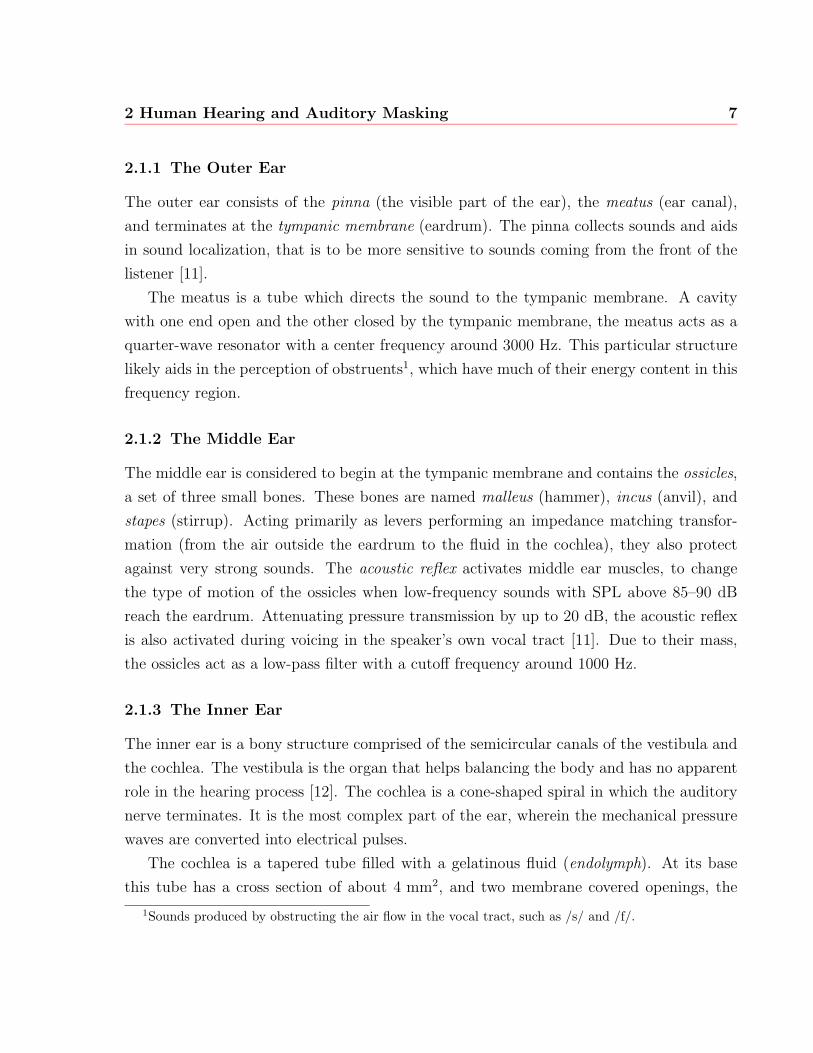
The cochlea has two membranes running along its length, the Basilar Membrane (BM)
and Reissner’s Membrane. These two membranes divide the cochlea into three channels,
as seen in Fig. 2.2.
Fig. 2.2 Cross-section of the cochlea [11]
These channels are called the Scala Vestibuli, the Scala Media, and the Scala Tympani.
Pressure waves travel from the Oval window through the Scala Vestibuli to the apex of the
cochlea. A small opening (helicotrema) connects the Scala Vestibuli to the Scala Tympani.
The sound pressure waves then travel back to the base through the Scala Tympani, termi-
nating at the Round Window. Since the velocity of sound in the cochlea is about 1600 m/s,
there is no appreciable phase delay.
2.1.4 The Basilar Membrane and the Hair Cells
The mechanics of the Basilar Membrane (BM) can explain many effects of masking (de-
scribed below). Within the BM, mechanical movements are transformed into nerve stimuli
transmitted to the brain. The BM performs a crucial part of sound perception. It is narrow
and stiff at the base of the cochlea, gradually tapering to a wide and pliable end at the apex
of the cochlea. Each point on the cochlea can be viewed as a mass-spring system with a
resonant frequency that decreases from base to apex. A frequency to place transformation
is performed, such that if a pure tone is applied to the Oval Window, a section of the
2 Human Hearing and Auditory Masking 9
BM will vibrate. The amplitude of BM vibration is dependent on distance from the oval
window and the frequency of the stimulus. The BM vertical displacement is small near the
oval window. Growing slowly, the vertical displacement reaches a maximum at a certain
distance from the oval window. The amplitude of the vertical displacement then rapidly
dies out in the direction of the helicotrema. The frequency of a signal that causes maximum
displacement at a given point of the BM is called the Characteristic Frequency (CF).
The vibration of the BM is picked up by the hair cells of the Organ of Corti. There are
two classes of hair cells, the Inner Hair Cells (IHC) and Outer Hair Cells (OHC). About
90% of afferent (ascending) nerve fibers that carry information from the cochlea to the
brain terminate at the IHC. Most of the efferent (descending) nerve fibers terminate at the
OHC, which greatly outnumber the IHC. Empirical observations suggests that the OHC,
with direct connection to the tectorial membrane, can change the vibration pattern of the
BM, improving the frequency selectivity of the auditory system [12, 13].
Measurements from afferent auditory nerves have shown further nonlinearities in the
auditory system. All IHC show a spontaneous rate of firings in the absence of stimuli. As a
stimulus (such as a tone burst at the CF for the IHC) is applied, the neuron responds with
a high rate of firings, which after approximately 20 ms decreases to a steady rate. Once
the stimulus is removed, the rate falls below the spontaneous rate for a short time before
returning to the spontaneous rate [12].
2.2 Masking
Human auditory masking is a highly complex process which is only partially understood,
yet we experience the effects in everyday life. In noisy environments, such as an airport or
a train station, noise seems to have a habit of lowering intelligibility just enough so that
you miss the last call for the flight or train you have to catch.
The American Standards Association (ASA) defines masking as the process or the
amount (customarily measured in decibels) “by which the threshold of audibility is raised
by the presence of another (masking) sound” [13]. Simply put, one sound cannot be heard
because of another (typically louder) sound being present.
2 Human Hearing and Auditory Masking 10
2.2.1 Threshold of Hearing
In order to be audible, sounds require a minimum pressure. Due in part to filtering in
the outer and middle ear, this minimum pressure (considering for now a pure tone) varies
considerably with frequency. This threshold of hearing (audibility) is unique from person
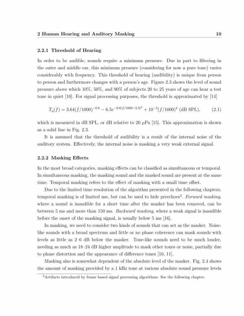
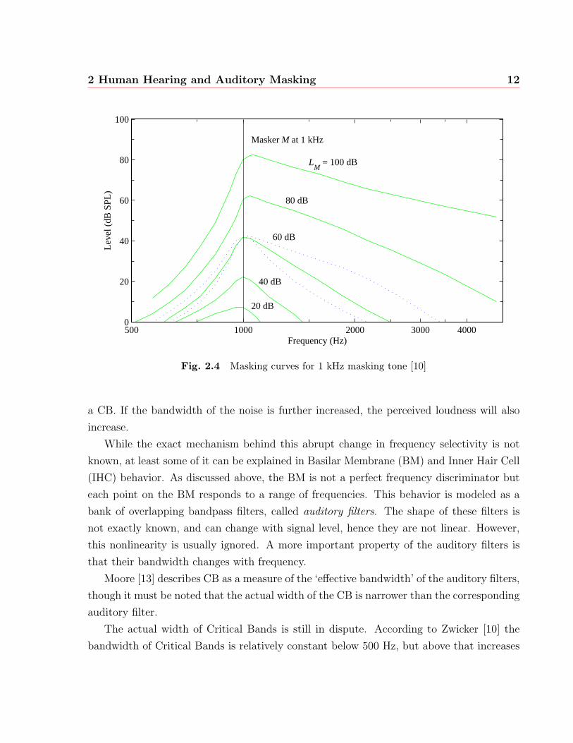
to person and furthermore changes with a person’s age. Figure 2.3 shows the level of sound
pressure above which 10%, 50%, and 90% of subjects 20 to 25 years of age can hear a test
tone in quiet [10]. For signal processing purposes, the threshold is approximated by [14]
Tq(f) = 3.64(f/1000)−0.8 − 6.5e−0.6(f/1000−3.3)2
+ 10−3(f/1000)4 (dB SPL), (2.1)
which is measured in dB SPL, or dB relative to 20 µPa [15]. This approximation is shown
as a solid line in Fig. 2.3.
It is assumed that the threshold of audibility is a result of the internal noise of the
auditory system. Effectively, the internal noise is masking a very weak external signal.
2.2.2 Masking Effects
In the most broad categories, masking effects can be classified as simultaneous or temporal.
In simultaneous masking, the masking sound and the masked sound are present at the same
time. Temporal masking refers to the effect of masking with a small time offset.
Due to the limited time resolution of the algorithm presented in the following chapters,
temporal masking is of limited use, but can be used to hide preechoes2. Forward masking,
where a sound is inaudible for a short time after the masker has been removed, can be
between 5 ms and more than 150 ms. Backward masking, where a weak signal is inaudible
before the onset of the masking signal, is usually below 5 ms [16].
In masking, we need to consider two kinds of sounds that can act as the masker. Noise-
like sounds with a broad spectrum and little or no phase coherence can mask sounds with
levels as little as 2–6 dB below the masker. Tone-like sounds need to be much louder,
needing as much as 18–24 dB higher amplitude to mask other tones or noise, partially due
to phase distortion and the appearance of difference tones [10, 11].
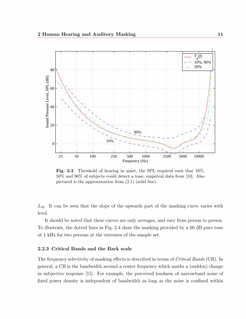
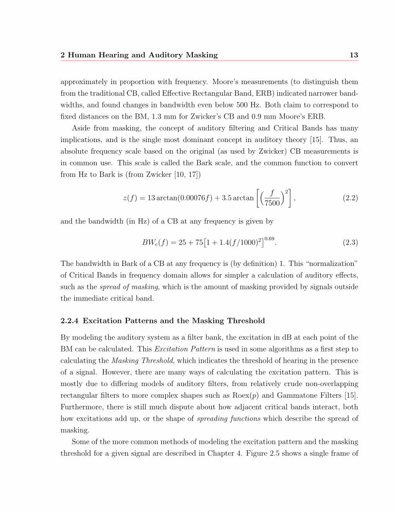
Masking also is somewhat dependent of the absolute level of the masker. Fig. 2.4 shows
the amount of masking provided by a 1 kHz tone at various absolute sound pressure levels
2Artifacts introduced by frame based signal processing algorithms. See the following chapter.
2 Human Hearing and Auditory Masking 11
25 50 100 250 500 1000 2500 5000 10000
0
20
40
60
80
Soun
d Pr
essu
re L
evel
, SPL
(dB
)
Frequency (Hz)
90%
10%
Tq(f)
10%, 90% 50%
Fig. 2.3 Threshold of hearing in quiet, the SPL required such that 10%,50% and 90% of subjects could detect a tone, empirical data from [10]. Alsopictured is the approximation from (2.1) (solid line).
LM . It can be seen that the slope of the upwards part of the masking curve varies with
level.
It should be noted that these curves are only averages, and vary from person to person.
To illustrate, the dotted lines in Fig. 2.4 show the masking provided by a 60 dB pure tone
at 1 kHz for two persons at the extremes of the sample set.
2.2.3 Critical Bands and the Bark scale
The frequency selectivity of masking effects is described in terms of Critical Bands (CB). In
general, a CB is the bandwidth around a center frequency which marks a (sudden) change
in subjective response [15]. For example, the perceived loudness of narrowband noise of
fixed power density is independent of bandwidth as long as the noise is confined within
2 Human Hearing and Auditory Masking 12
500 1000 2000 3000 40000
20
40
60
80
100
LM
= 100 dB
80 dB
60 dB
40 dB
20 dB
Masker M at 1 kHz
Frequency (Hz)
Lev
el (
dB S
PL)
Fig. 2.4 Masking curves for 1 kHz masking tone [10]
a CB. If the bandwidth of the noise is further increased, the perceived loudness will also
increase.
While the exact mechanism behind this abrupt change in frequency selectivity is not
known, at least some of it can be explained in Basilar Membrane (BM) and Inner Hair Cell
(IHC) behavior. As discussed above, the BM is not a perfect frequency discriminator but
each point on the BM responds to a range of frequencies. This behavior is modeled as a
bank of overlapping bandpass filters, called auditory filters. The shape of these filters is
not exactly known, and can change with signal level, hence they are not linear. However,
this nonlinearity is usually ignored. A more important property of the auditory filters is
that their bandwidth changes with frequency.
Moore [13] describes CB as a measure of the ‘effective bandwidth’ of the auditory filters,
though it must be noted that the actual width of the CB is narrower than the corresponding
auditory filter.
The actual width of Critical Bands is still in dispute. According to Zwicker [10] the
bandwidth of Critical Bands is relatively constant below 500 Hz, but above that increases
2 Human Hearing and Auditory Masking 13
approximately in proportion with frequency. Moore’s measurements (to distinguish them
from the traditional CB, called Effective Rectangular Band, ERB) indicated narrower band-
widths, and found changes in bandwidth even below 500 Hz. Both claim to correspond to
fixed distances on the BM, 1.3 mm for Zwicker’s CB and 0.9 mm Moore’s ERB.
Aside from masking, the concept of auditory filtering and Critical Bands has many
implications, and is the single most dominant concept in auditory theory [15]. Thus, an
absolute frequency scale based on the original (as used by Zwicker) CB measurements is
in common use. This scale is called the Bark scale, and the common function to convert
from Hz to Bark is (from Zwicker [10, 17])
z(f) = 13 arctan(0.00076f) + 3.5 arctan
[( f
7500
)2], (2.2)
and the bandwidth (in Hz) of a CB at any frequency is given by
BWc(f) = 25 + 75[1 + 1.4(f/1000)2
]0.69. (2.3)
The bandwidth in Bark of a CB at any frequency is (by definition) 1. This “normalization”
of Critical Bands in frequency domain allows for simpler a calculation of auditory effects,
such as the spread of masking, which is the amount of masking provided by signals outside
the immediate critical band.
2.2.4 Excitation Patterns and the Masking Threshold
By modeling the auditory system as a filter bank, the excitation in dB at each point of the
BM can be calculated. This Excitation Pattern is used in some algorithms as a first step to
calculating the Masking Threshold, which indicates the threshold of hearing in the presence
of a signal. However, there are many ways of calculating the excitation pattern. This is
mostly due to differing models of auditory filters, from relatively crude non-overlapping
rectangular filters to more complex shapes such as Roex(p) and Gammatone Filters [15].
Furthermore, there is still much dispute about how adjacent critical bands interact, both
how excitations add up, or the shape of spreading functions which describe the spread of
masking.
Some of the more common methods of modeling the excitation pattern and the masking
threshold for a given signal are described in Chapter 4. Figure 2.5 shows a single frame of
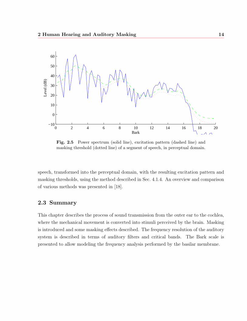
2 Human Hearing and Auditory Masking 14
0 2 4 6 8 10 12 14 16 18 20−10
0
10
20
30
40
50
60
Bark
Leve
l (dB
)
Fig. 2.5 Power spectrum (solid line), excitation pattern (dashed line) andmasking threshold (dotted line) of a segment of speech, in perceptual domain.
speech, transformed into the perceptual domain, with the resulting excitation pattern and
masking thresholds, using the method described in Sec. 4.1.4. An overview and comparison
of various methods was presented in [18].
2.3 Summary
This chapter describes the process of sound transmission from the outer ear to the cochlea,
where the mechanical movement is converted into stimuli perceived by the brain. Masking
is introduced and some masking effects described. The frequency resolution of the auditory
system is described in terms of auditory filters and critical bands. The Bark scale is
presented to allow modeling the frequency analysis performed by the basilar membrane.
15
Chapter 3
Spectral Subtraction
Spectral subtraction is a method to enhance the perceived quality of single channel speech
signals in the presence of additive noise. It is assumed that the noise component is relatively
stationary. Specifically, the spectrum of the noise component is estimated from the pauses
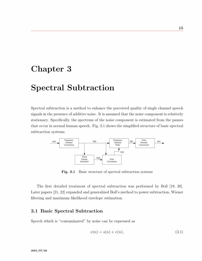
that occur in normal human speech. Fig. 3.1 shows the simplified structure of basic spectral
subtraction systems.
ConversionDomain
TimeDomain
Conversion
GainCalculation
Frequency
NoiseEnergy
Estimator
FrequencyDomain
Filter
S(f)x(n)
W(f)
G(f)
X(f) s(n)
Fig. 3.1 Basic structure of spectral subtraction systems
The first detailed treatment of spectral subtraction was performed by Boll [19, 20].
Later papers [21, 22] expanded and generalized Boll’s method to power subtraction, Wiener
filtering and maximum likelihood envelope estimation.
3.1 Basic Spectral Subtraction
Speech which is “contaminated” by noise can be expressed as
x(n) = s(n) + υ(n), (3.1)
2001/07/26
3 Spectral Subtraction 16
where x(n) is the speech with noise, s(n) is the “clean” speech signal and υ(n) is the
noise process, all in the discrete time domain. What spectral subtraction attempts to do
is to estimate s(n) from x(n). Since υ(n) is a random process, certain approximations
and assumptions must be made. One approximation is that the noise is (within the time
duration of speech segments) a short-time stationary process. Specifically, it is assumed
that the power spectrum of the noise remains constant within the time duration of several
speech segments (typically words or sentence fragments). Also, noise is assumed to be
uncorrelated to the speech signal. This is an important assumption since, as explained
in sec. 3.1.4 below, the noise is estimated from pauses in the speech signal. Finally, it is
assumed that the human ear is fairly insensitive to phase, such that the effect of noise on
the phase of s+ υ can be ignored.
If the noise process is represented by its power spectrum estimate |W (f)|2, the power
spectrum of the speech estimate |S(f)|2 can be written as
|S(f)|2 = |X(f)|2 − |W (f)|2, (3.2)
since the power spectrum of two uncorrelated signals is additive. By generalizing the
exponent from 2 to a, Eq. (3.2) becomes
|S(f)|a = |X(f)|a − |W (f)|a. (3.3)
This generalization is useful for writing the filter equation (3.6) below [1, 22].
The speech phase φS(f) is estimated directly from the noisy signal phase φX(f).
φS(f) = φX(f) (3.4)
Thus a general form of the estimated speech in frequency domain can be written as
S(f) =(
max(|X(f)|a − k|W (f)|a, 0
)) 1a · ejφX(f), (3.5)
where k > 1 is used to overestimate the noise to account for the variance in the noise
estimate, as explained below. The inner term |X(f)|a − k|W (f)|a is limitied to positive
values, since it is possible for the overestimated noise to be greater than the current signal.
3 Spectral Subtraction 17
3.1.1 Time to Frequency Domain Conversion
The statistical properties of a speech signal change over time, specifically, from one phoneme
to the next. Within phonemes, which average about 80 ms in duration [11], the statistics
of the signal are relatively constant. For this reason, the processing of speech signals is
typically done in short time sections called frames. The size of frames is typically 5 to
50 ms [1], though rarely larger than 32 ms. In these short-time segments, speech can be
considered stationary [19, 22, 23]. The frames of time domain data are windowed (the
effects of the window employed are discussed in Section 3.1.3 below) and then converted
to frequency domain using the Discrete Fourier Transform (DFT). To indicate discrete
frequency domain, the notation X(m, p)∆=X(m fs
M), where 2M is the order of the DFT and
p is the frame index, is used. The frame index p is also dropped if the operation is local
in time (that is, if the operation is memoryless, and not directly using data from previous
time frames).
Generally, when dealing with speech signals, the signal operated on is assumed to be
sampled at fs = 8000 Hz. However, until auditory effects are considered, the sampling
rate is irrelevant, as long as the length of frames is kept appropriate as mentioned in the
previous paragraph. It should be noted that the effective frequency resolution depends only
on the framesize.
3.1.2 Spectral Subtraction as a Filter
It is convenient to think of the spectral subtraction as a filter, denoted here by G(m, p),
which operates on the received signal. Specifically, the filter is implemented in the frequency
domain by
S(m) = X(m)G(m)
= X(m)
(max
(|X(m)|a − k|W (m)|a
|X(m)|a, 0
)) 1a
= X(m)
(max
(1− k |W (m)|a
|X(m)|a, 0
)) 1a
, m = 0, . . . ,M − 1. (3.6)
Equation (3.6) is the conventional spectral subtraction equation. It should be noted that
it is possible for 1 − k |W (m)|a|X(m)|a to be less than 0. In this case, G(m) is set to 0 at those
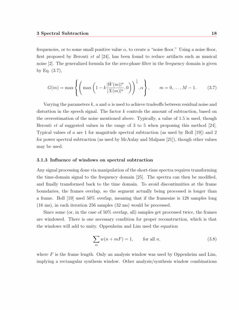
3 Spectral Subtraction 18
frequencies, or to some small positive value α, to create a “noise floor.” Using a noise floor,
first proposed by Berouti et al [24], has been found to reduce artifacts such as musical
noise [2]. The generalized formula for the zero-phase filter in the frequency domain is given
by Eq. (3.7),
G(m) = max
(
max
(1− k |W (m)|a
|X(m)|a, 0
)) 1a
, α
, m = 0, . . . ,M − 1. (3.7)
Varying the parameters k, a and α is used to achieve tradeoffs between residual noise and
distortion in the speech signal. The factor k controls the amount of subtraction, based on
the overestimation of the noise mentioned above. Typically, a value of 1.5 is used, though
Berouti et al suggested values in the range of 3 to 5 when proposing this method [24].
Typical values of a are 1 for magnitude spectral subtraction (as used by Boll [19]) and 2
for power spectral subtraction (as used by McAulay and Malpass [21]), though other values
may be used.
3.1.3 Influence of windows on spectral subtraction
Any signal processing done via manipulation of the short-time spectra requires transforming
the time-domain signal to the frequency domain [25]. The spectra can then be modified,
and finally transformed back to the time domain. To avoid discontinuities at the frame
boundaries, the frames overlap, so the segment actually being processed is longer than
a frame. Boll [19] used 50% overlap, meaning that if the framesize is 128 samples long
(16 ms), in each iteration 256 samples (32 ms) would be processed.
Since some (or, in the case of 50% overlap, all) samples get processed twice, the frames
are windowed. There is one necessary condition for proper reconstruction, which is that
the windows will add to unity. Oppenheim and Lim used the equation∑m
w(n+mF ) = 1, for all n, (3.8)
where F is the frame length. Only an analysis window was used by Oppenheim and Lim,
implying a rectangular synthesis window. Other analysis/synthesis window combinations
3 Spectral Subtraction 19
can provide improved performance [4]. Eq. (3.8) then becomes∑m
wa(n+mF )ws(n+mF ) = 1, for all n, (3.9)
where wa and ws represent the analysis and synthesis windows, respectively. It is convenient
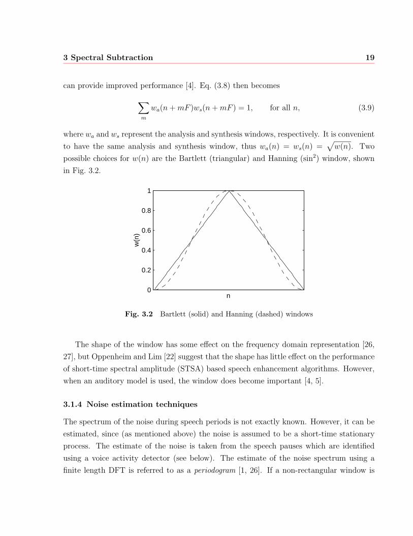
to have the same analysis and synthesis window, thus wa(n) = ws(n) =√w(n). Two
possible choices for w(n) are the Bartlett (triangular) and Hanning (sin2) window, shown
in Fig. 3.2.
0
0.2
0.4
0.6
0.8
1
n
w(n
)
Fig. 3.2 Bartlett (solid) and Hanning (dashed) windows
The shape of the window has some effect on the frequency domain representation [26,
27], but Oppenheim and Lim [22] suggest that the shape has little effect on the performance
of short-time spectral amplitude (STSA) based speech enhancement algorithms. However,
when an auditory model is used, the window does become important [4, 5].
3.1.4 Noise estimation techniques
The spectrum of the noise during speech periods is not exactly known. However, it can be
estimated, since (as mentioned above) the noise is assumed to be a short-time stationary
process. The estimate of the noise is taken from the speech pauses which are identified
using a voice activity detector (see below). The estimate of the noise spectrum using a
finite length DFT is referred to as a periodogram [1, 26]. If a non-rectangular window is
3 Spectral Subtraction 20
used, the estimator is called a modified periodogram [27]. This modified periodogram can
be obtained from the analysis section of the spectral subtraction algorithm.
To reduce the variance of the noise estimate, the Welch method of averaging modified
periodograms can be used. An alternative to the Welch method is the use of exponential
averaging. Like the Welch method, the exponential average reduces the variance, but has
greatly reduced requirements in terms of memory and computational complexity, and there-
fore are used almost exclusively in actual implementations of noise suppression algorithms.
The noise power spectrum estimate |W (m, p)|2 is updated from the power spectrum of the
current frame (|X(m, p)|2) if the current frame is considered to be noise only by
|W (m, p)|2 = λN|W (m, p− 1)|2 + (1− λN)|X(m, p)|2, m = 0, . . . ,M − 1, (3.10)
where λN is the noise forgetting factor. The value of λN determines a tradeoff between the
variance of |W (m, p)|2 (or accuracy of the noise spectrum estimate) and responsiveness to
changing noise conditions. A typical value of λN for 20 ms frames is 0.9 [1], resulting in a
time constant of about 10 frames, or 200 ms.
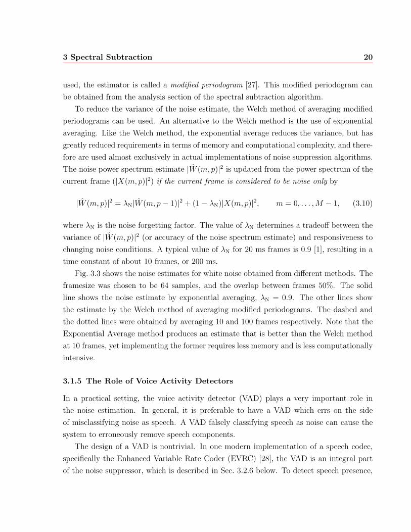
Fig. 3.3 shows the noise estimates for white noise obtained from different methods. The
framesize was chosen to be 64 samples, and the overlap between frames 50%. The solid
line shows the noise estimate by exponential averaging, λN = 0.9. The other lines show
the estimate by the Welch method of averaging modified periodograms. The dashed and
the dotted lines were obtained by averaging 10 and 100 frames respectively. Note that the
Exponential Average method produces an estimate that is better than the Welch method
at 10 frames, yet implementing the former requires less memory and is less computationally
intensive.
3.1.5 The Role of Voice Activity Detectors
In a practical setting, the voice activity detector (VAD) plays a very important role in
the noise estimation. In general, it is preferable to have a VAD which errs on the side
of misclassifying noise as speech. A VAD falsely classifying speech as noise can cause the
system to erroneously remove speech components.
The design of a VAD is nontrivial. In one modern implementation of a speech codec,
specifically the Enhanced Variable Rate Coder (EVRC) [28], the VAD is an integral part
of the noise suppressor, which is described in Sec. 3.2.6 below. To detect speech presence,
3 Spectral Subtraction 21
0 10 20 30 40 50 600
0.2
0.4
0.6
0.8
1
1.2
1.4
1.6x 10
−5
|W(m
)|
Frequency Index m
Exp. Avg.Welch10 Welch100
Fig. 3.3 Different noise estimation results. Solid line: Exponential average,dashed line: Welch Periodogram, 10 frames, dotted line: Welch Periodogram,100 frames.
a comparison of the current signal energy to the current noise estimate is performed, along
with rules based on temporal speech statistics. It should be noted that the VAD for Adap-
tive Multi-Rate (AMR) GSM coder (06.94 version 7.1.0) uses a very similar scheme [29].
The problem of reliable detection of speech in noise is beyond the scope of this thesis.
However, the influence of the VAD on the performance must be taken into account during
evaluation of noise suppression algorithms.
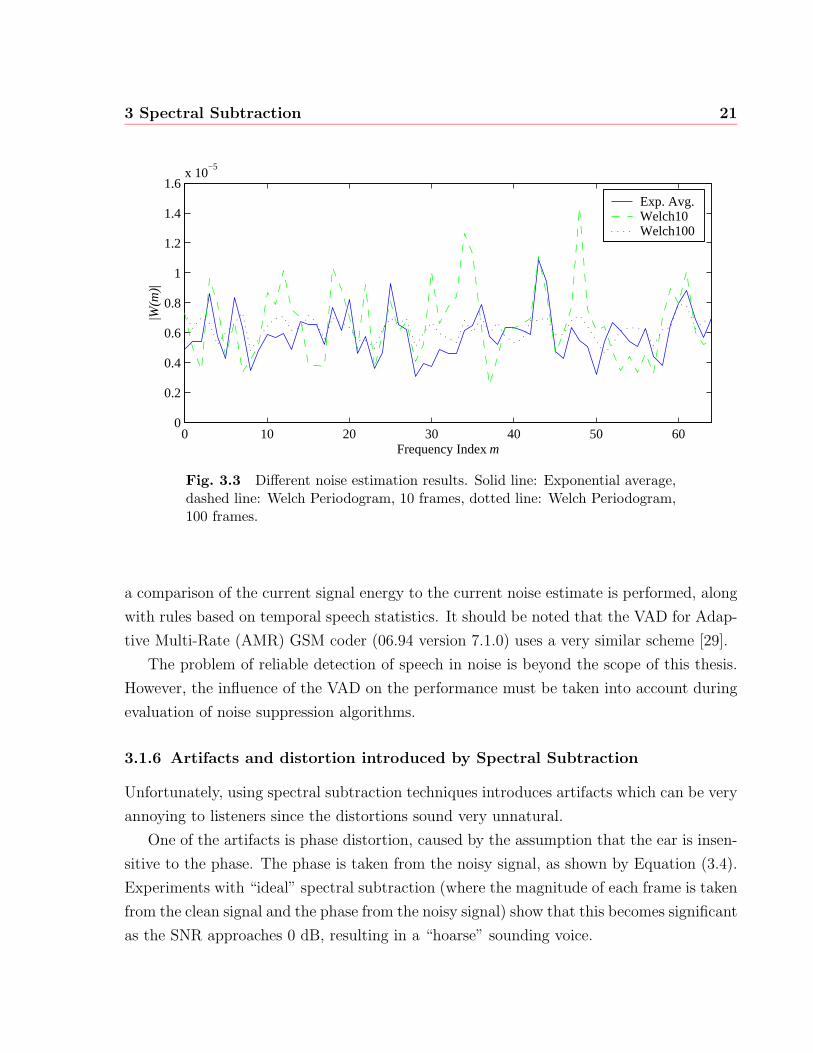
3.1.6 Artifacts and distortion introduced by Spectral Subtraction
Unfortunately, using spectral subtraction techniques introduces artifacts which can be very
annoying to listeners since the distortions sound very unnatural.
One of the artifacts is phase distortion, caused by the assumption that the ear is insen-
sitive to the phase. The phase is taken from the noisy signal, as shown by Equation (3.4).
Experiments with “ideal” spectral subtraction (where the magnitude of each frame is taken
from the clean signal and the phase from the noisy signal) show that this becomes significant
as the SNR approaches 0 dB, resulting in a “hoarse” sounding voice.
3 Spectral Subtraction 22
0 8 16 24 32 40 48 56 640
10
20
30
0
0.5
1
1.5
2
x 10−3
Frame Index p
Frequency Index m
|S(m
,p)|2
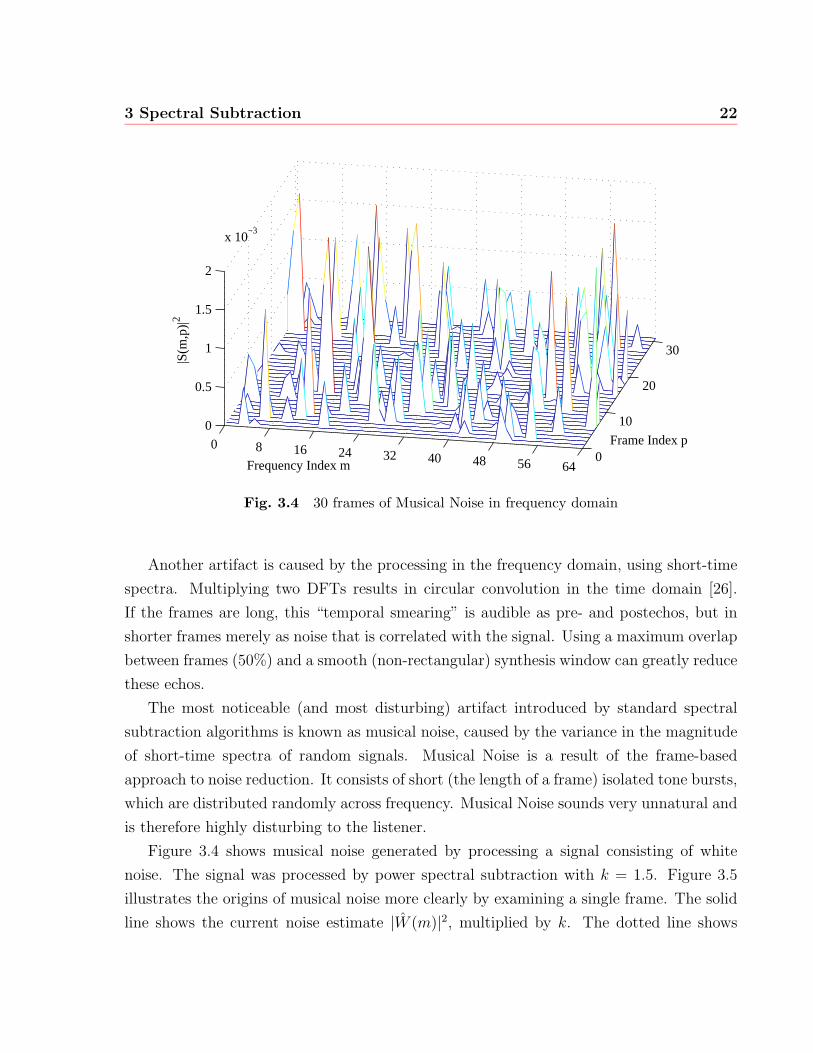
Fig. 3.4 30 frames of Musical Noise in frequency domain
Another artifact is caused by the processing in the frequency domain, using short-time
spectra. Multiplying two DFTs results in circular convolution in the time domain [26].
If the frames are long, this “temporal smearing” is audible as pre- and postechos, but in
shorter frames merely as noise that is correlated with the signal. Using a maximum overlap
between frames (50%) and a smooth (non-rectangular) synthesis window can greatly reduce
these echos.
The most noticeable (and most disturbing) artifact introduced by standard spectral
subtraction algorithms is known as musical noise, caused by the variance in the magnitude
of short-time spectra of random signals. Musical Noise is a result of the frame-based
approach to noise reduction. It consists of short (the length of a frame) isolated tone bursts,
which are distributed randomly across frequency. Musical Noise sounds very unnatural and
is therefore highly disturbing to the listener.
Figure 3.4 shows musical noise generated by processing a signal consisting of white
noise. The signal was processed by power spectral subtraction with k = 1.5. Figure 3.5
illustrates the origins of musical noise more clearly by examining a single frame. The solid
line shows the current noise estimate |W (m)|2, multiplied by k. The dotted line shows
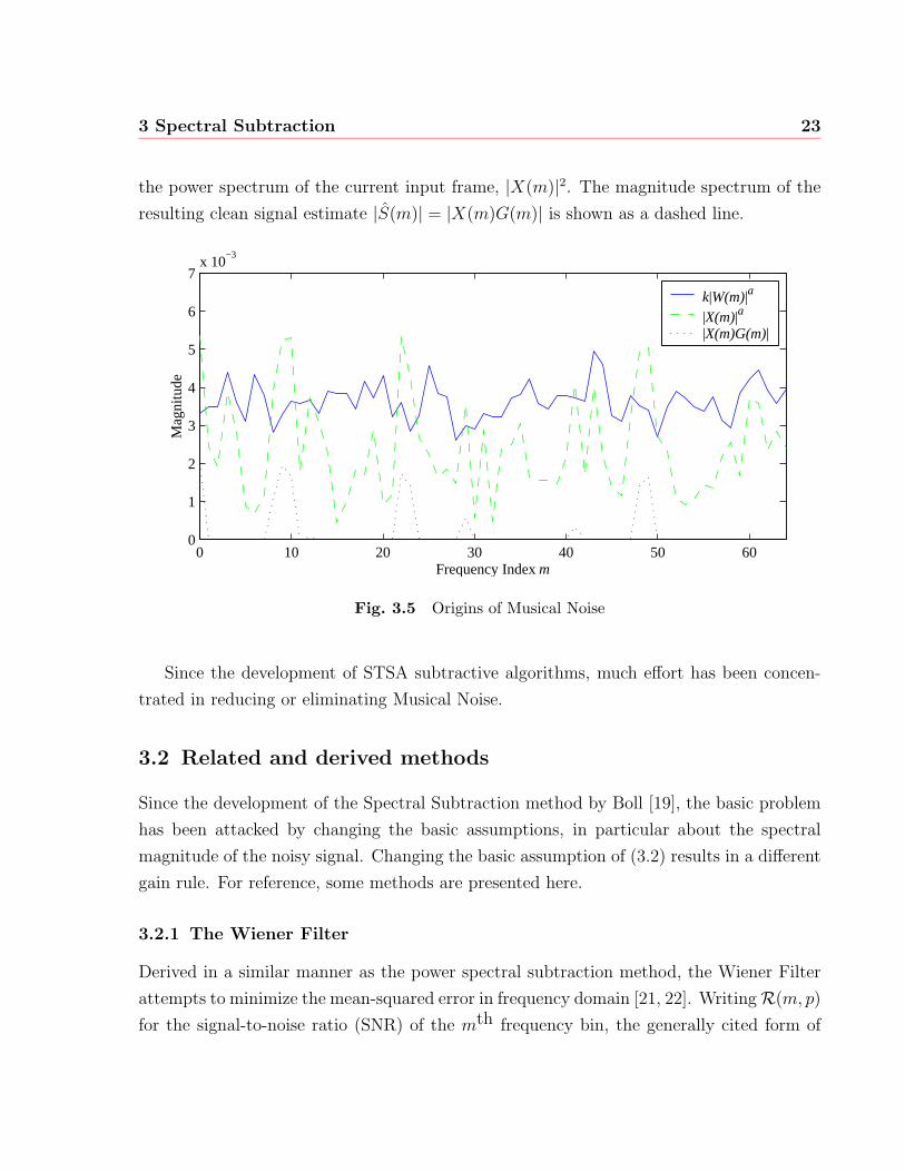
3 Spectral Subtraction 23
the power spectrum of the current input frame, |X(m)|2. The magnitude spectrum of the
resulting clean signal estimate |S(m)| = |X(m)G(m)| is shown as a dashed line.
0 10 20 30 40 50 600
1
2
3
4
5
6
7x 10
−3
Mag
nitu
de
Frequency Index m
k|W(m)|a
|X(m)|a |X(m)G(m)|
Fig. 3.5 Origins of Musical Noise
Since the development of STSA subtractive algorithms, much effort has been concen-
trated in reducing or eliminating Musical Noise.
3.2 Related and derived methods
Since the development of the Spectral Subtraction method by Boll [19], the basic problem
has been attacked by changing the basic assumptions, in particular about the spectral
magnitude of the noisy signal. Changing the basic assumption of (3.2) results in a different
gain rule. For reference, some methods are presented here.
3.2.1 The Wiener Filter
Derived in a similar manner as the power spectral subtraction method, the Wiener Filter
attempts to minimize the mean-squared error in frequency domain [21, 22]. WritingR(m, p)
for the signal-to-noise ratio (SNR) of the mth frequency bin, the generally cited form of
3 Spectral Subtraction 24
the Wiener filter is Eq. (3.11).
GW(m) =R(m)
R(m) + 1(3.11)
To compare (3.7) and (3.11), R(m) is given as
R(m) =
{|X(m)|2−|W (m)|2
|W (m)|2 , |X(m)|2 > |W (m)|2
0 otherwise,(3.12)
and substituting in Eq. (3.11), we get
GW(m) =
{1− |W (m)|2
|X(m)|2 , |X(m)|2 > |W (m)|2,0 otherwise,
(3.13)
where the similarity to Eq. (3.7) is obvious. In fact, GW(m) =√G(m) with k = 1, a = 2,
and α = 0.
3.2.2 Maximum Likelihood Envelope Estimator
The Maximum Likelihood Envelope Estimator (MLEE) is based on the assumption that
the speech signal is characterized by a deterministic waveform of unknown amplitude and
phase [21]. The MLEE is characterized by its gain function
GMLEE =
[1
2+
1
2
√1− |W (m)|2|X(m)|2
]. (3.14)
It should be notes that (3.14) was derived by estimating the a priori SNR. This leads
directly to the Ephraim and Malah Noise Suppressor below.
3.2.3 The Ephraim and Malah Noise Suppressor
In [30], Ephraim and Malah presented a modification to the MLEE Filter by adding an
estimator for the a priori SNR (Rprio) which uses exponential smoothing within the time
domain. An examination of the algorithm by Cappe [31] concluded that this smoothing
avoids the appearance of musical noise and signal distortion. However, removal of noise is
3 Spectral Subtraction 25
not complete, and due to the smoothing, the signal component is incorrectly attenuated
following signal transients.
Cappe summarized the Ephraim and Malah Suppression Rule (EMSR) by
GEMSR =
√π
2
√(1
1 +Rpost
)(Rprio
1 +Rprio
)M
[(1 +Rpost)
(Rprio
1 +Rprio
)], (3.15)
where M stands for the function
M [θ] = exp
(−θ
2
)[(1 + θ)I0
(θ
2
)+ θI1
(θ
2
)]. (3.16)
In the above equation, I0 and I1 represent the modified Bessel functions of zero and first
order. Time and frequency indices have been omitted for clarity. The a priori SNR is
calculated by
Rprio(p) = (1− α)Rpost(p) + α|G(p− 1)X(p− 1)|2
|W |2, (3.17)
while the a posteriori SNR is the same as R(m, p) given by (3.12). The value of α deter-
mines the time smoothing of the a priori SNR estimate, which on the basis of simulations
was set to about 0.98.
The a priori SNR is the dominant parameter, while the a posteriori SNR acts as a
correction parameter when the a priori SNR is low.
In [32], Scalart and Filho examined the use of a priori SNR estimation with standard
(Boll, Wiener and MLEE) methods and also reported reduction in the amount of musical
noise. This suggests that the smoothing operation plays a more significant role in the
reduction of musical noise than the gain rule.
3.2.4 Filter Smoothing
A simpler method which achieves results comparable with the Ephraim and Malah Sup-
pression Rule is filter smoothing. The EMSR uses exponential averaging to smooth the a
priori SNR, the dominant parameter. Since it is assumed that the noise estimate changes
slowly over time, the resulting filter will also change slowly over time. A similar effect may
therefore be achieved by adding exponential averaging to the filter. Using G(m, p) from
3 Spectral Subtraction 26
Eq. (3.7), this gives
GS(m, p) = λFGS(m, p− 1) + (1− λF)G(m, p). (3.18)
In this equation, λF is used to achieve a tradeoff between the amount of musical noise
and attenuation of signal transitions. As λF approaches 1, the amount of musical noise
disappears, but signal at the onset of speech segments is lost. To overcome this effect,
McAulay and Malpass described a modified form of the above in [21], where λF is chosen
to be 0 or 0.5 depending on a comparison of the current SNR estimate to the filter gain.
Similarly, the above equation can be modified to
GS(m, p) = max(λFGS(m, p− 1) + (1− λF)G(m, p), G(m, p)
), (3.19)
resulting in a one-sided smoothing that responds immediately to speech onset, but has
a hangover dependent on λF. The resulting signal will sound as if originating from a
reverberant space. This effect is caused by the slower decay of the filter gain after the
end of the speech segment, and can be perceptually annoying. Other approaches include
adapting the averaging parameter based on the spectral discrepancy measure, as proposed
by Gustafsson et al [33].
The advantage the Filter Smoothing technique has over the EMSR is that Filter Smooth-
ing is easier to understand and implement. Also it can be modified to take advantage of
temporal auditory masking effects, as discussed in the following chapter.
3.2.5 Signal Subspace methods
A new approach to noise reduction has been discussed by Ephraim and Van Trees [34],
whereby the noisy signal is decomposed into a signal-plus-noise subspace and a noise sub-
space. The noise subspace is removed and the signal is generated from the remaining
subspace by means of a linear estimation. Ephraim and Van Trees suggested the Dis-
crete Cosine Transform (DCT) and Discrete Wavelet Transforms as approximations to the
optimal, but computationally intensive Karhunen-Loeve Transform (KLT).
Subjective tests showed that some distortion was introduced to the signal, which listen-
ers found disturbing. Partially for this reason, the attention Signal Subspace approaches
have received in literature was mainly in automatic speech recognition problems.
3 Spectral Subtraction 27
3.2.6 Implementation of EVRC noise reduction
The Enhanced Variable Rate Coder (EVRC) is the standard coder for use with the IS-95x
Rate 1 air interface (CDMA) [28, 35]. It employs an adaptive noise suppression filter, which
is used as a baseline reference for the algorithm presented in this paper. Since it is a widely
used “real-world” implementation of a noise reduction algorithm, it is worth examining
in some detail. Some simplification for brevity was done to illustrate the algorithm more
clearly, but as much as possible, the symbols used in the standard document are used.
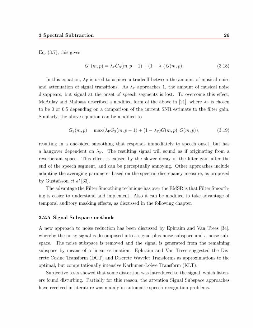
Conceptually, the EVRC’s noise suppression is accomplished by summing the outputs
of a bank of adaptive filters that span the frequency band of the input signal. The widths
of the bands roughly approximate the ear’s critical bands.
ConversionDomain
Frequency Time
Channel
DomainConversion
EnergyEstimator
ChannelGain
Calculation
BackgroundNoise
Estimator
ChannelSRN
Modifier
ChannelSNR
Estimator
NoiseUpdate
Decision
VoiceMetric
Calculation
SpectralDeviationEstimator
update_flag
Fig. 3.6 EVRC Noise suppression structure, redrawn from [28]
The EVRC noise suppressor works on 10 ms sections of speech data, using the overlap-
add method [26], to obtain 104 sample vectors. These vectors are then zero-padded to 128
sample points and transformed using a 128-point Fast Fourier Transform (FFT), windowed
by a smoothed trapezoidal window. The result of the transform is denoted here as Ec.
Reconstruction is done using the overlap-add method, with no windowing.
The 128 bins are grouped into 16 channels, approximating non-overlapping critical
bands. The energy present in each channel is estimated by calculating the mean magnitude
3 Spectral Subtraction 28
for all frequency bins within the channel, and using a exponential average of the form
Ec(m, ch) =1
fH − fL + 1
fH∑k=fL
Gm(k) (3.20)
E(m, ch) = 0.45E(m− 1, ch) + 0.55Ec(m, ch) (3.21)
where m is the index of the time frame, and fL and fH are the lowest and highest bin
respectively of that particular channel. Gm(k) is the kth bin of the FFT of time frame m.
Additionally, the channel energy estimate E(m, ch) is constrained to a minimum of 0.0625
to prevent conditions where a division by zero occurs.
The channel energy estimate is then combined with the channel noise energy estimate
(see below) to calculate the channel SNR estimate in dB units. The channel SNR values
are also used to calculate a voice metric for each frame, which is used to determine if
the current frame is noise only. If the frame is considered noise only, the current channel
energy estimates are used to update the channel noise estimate EN, again using exponential
averaging. The channel noise estimate is constrained to a minimum of 0.0625.
EN(m+ 1, ch) = 0.9EN(m, ch) + 0.1E(m, ch) (3.22)
For the final channel gain calculation, an overall gain is calculated based on the total noise
energy estimate.
γN = −10 log10
(15∑ch=0
EN(m, ch)
)(3.23)
which is constrained to the range γN = −13 . . . 0. A quantized channel SNR is generated
by
σ′′Q(ch) = round
(10 log10
(E(m, ch)
EN(m, ch)
)/0.375
)(3.24)
the result of which is constrained to be between 6 and 89. Now the individual channel
gains γ(ch) can be computed.
γdB(ch) = 0.39(σ′′Q(ch)− 6) + γN (3.25)
γ(ch) = min(1, 10γdB(ch)/20) (3.26)
These channel gains are then applied to the FFT bins belonging to their respective channels,
3 Spectral Subtraction 29
before the inverse FFT is performed.
However, while the EVRC noise suppressor has a concept of critical bands, it does not
make use of any other perceptual properties. There is no calculation of masking thresholds,
all channels are calculated independently from each other.
It should also be noted that the EVRC noise suppressor (and hence the entire coder)
is preceded by a highpass filter whose 3 dB cutoff is at about 120 Hz and has a slope of
about 80 dB/oct. This removes a large amount of noise which is commonly encountered in
mobile applications (like car noise) while not greatly affecting speech quality.
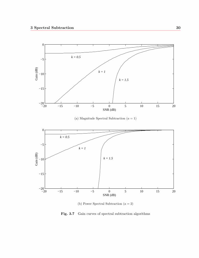
3.3 Comparison of Methods
To compare short-time spectral amplitude (STSA) subtractive methods, the gain curve is
the primary point of comparison. The gain curve shows the attenuation of any frequency
bin for any given a posteriori SNR, that is the value of G(m) given R(m) from Eq. (3.12).
Figures 3.7(a) and 3.7(b) show the gain curves for magnitude and power spectral sub-
traction respectively. From the plots, it can be seen that the parameter k is dominant in
determining the slope of the curve. For small k the attenuation remains small even for very
low SNR values. For k = 1.5 (in general, for k > 1), the spectral subtraction algorithm
(for either value of a) acts more as a noise gate, cutting off completely (assuming α = 0) if
the SNR drops below
Roff = 10 log10(ka2 − 1) (dB), k > 1. (3.27)
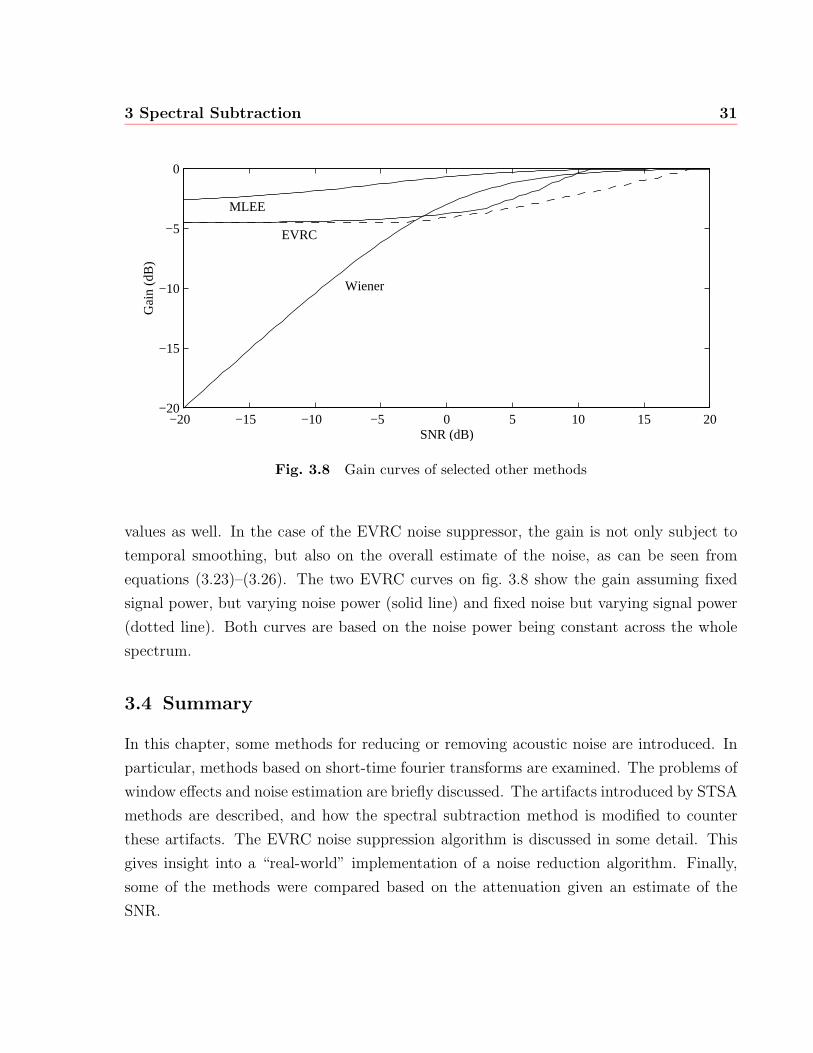
Figure 3.8 shows the gain curves of some of the other methods described in the previous
section. As expected the curve for the Wiener filter is very similar to the power spectral
subtraction with k = 1. It is an interesting feature of the Wiener filter that as the SNR
decreases, the filter gain becomes equal to the SNR.
The other curves on Fig. 3.8 show the gain curves for the MLEE method and the EVRC
noise suppressor. The MLEE curve provides very little attenuation, with a maximum
attenuation of 3 dB. It is therefore of little use if the intent is to provide significant noise
removal.
For reference, the EVRC noise suppressor was included. Like the Ephraim and Malah
Noise Suppressor, the gain is dependent not only on the (a posteriori) SNR, but on other
3 Spectral Subtraction 30
−20 −15 −10 −5 0 5 10 15 20−20
−15
−10
−5
0
Gai
n (d
B)
SNR (dB)
k = 0.5
k = 1
k = 1.5
(a) Magnitude Spectral Subtraction (a = 1)
−20 −15 −10 −5 0 5 10 15 20−20
−15
−10
−5
0
Gai
n (d
B)
SNR (dB)
k = 0.5
k = 1
k = 1.5
(b) Power Spectral Subtraction (a = 2)
Fig. 3.7 Gain curves of spectral subtraction algorithms
3 Spectral Subtraction 31
−20 −15 −10 −5 0 5 10 15 20−20
−15
−10
−5
0
Gai
n (d
B)
SNR (dB)
MLEE
EVRC
Wiener
Fig. 3.8 Gain curves of selected other methods
values as well. In the case of the EVRC noise suppressor, the gain is not only subject to
temporal smoothing, but also on the overall estimate of the noise, as can be seen from
equations (3.23)–(3.26). The two EVRC curves on fig. 3.8 show the gain assuming fixed
signal power, but varying noise power (solid line) and fixed noise but varying signal power
(dotted line). Both curves are based on the noise power being constant across the whole
spectrum.
3.4 Summary
In this chapter, some methods for reducing or removing acoustic noise are introduced. In
particular, methods based on short-time fourier transforms are examined. The problems of
window effects and noise estimation are briefly discussed. The artifacts introduced by STSA
methods are described, and how the spectral subtraction method is modified to counter
these artifacts. The EVRC noise suppression algorithm is discussed in some detail. This
gives insight into a “real-world” implementation of a noise reduction algorithm. Finally,
some of the methods were compared based on the attenuation given an estimate of the
SNR.
32
Chapter 4
Using Masking Properties in Spectral
Subtraction Algorithms
Auditory masking is aggressively exploited by algorithms used for the lossy compression of
audio signals. In compression of audio signals, the intent is to hide the noise introduced
by the coding below the masking threshold, thus making the noise inaudible. This will
then render the coding process transparent, enabling better compression without audible
degradation of the signal. A comprehensive review of perceptual audio coding was published
by Painter and Spanias [5].
More recently, masking properties of the ear have also been used to improve the quality
of noise reduction algorithms. Specifically, instead of attempting to remove all noise from
the signal, these algorithms attempt to attenuate the noise below the audible threshold. In
the context of short-time spectral magnitude (STSM) subtractive algorithms, this reduces
the amount of modification to the spectral magnitude, reducing artifacts. This is of great
importance where the resulting signal needs to be of very high quality. The methods
developed by Soulodre [4] to remove camera noise from film soundtracks were used as a
starting point for the method presented in this chapter. In fact, it may be regarded as an
application of Soulodre’s methods to more general noise reduction.
For the design of audio coders, an estimate of the masking threshold must be calculated.
In this chapter, some of the masking models (or perceptual models) will be examined. Also,
it will be shown how these models are used in noise suppression algorithms.
2001/07/26
4 Using Masking Properties in Spectral Subtraction Algorithms 33
4.1 Masking Models
4.1.1 The Johnston Model
A perceptual model was developed by Johnston for coding of audio sampled at 32 kHz
in [36]. This model was used by Tsoukalas et al in [6] for speech enhancement and is de-
scribed below. Johnston’s method calculates the auditory masking threshold to determine
how much noise the coder can add before it becomes audible.
Johnston uses the following steps to calculate the masking threshold;
• Critical band analysis of the signal
• Applying the spreading function to the critical band spectrum
• Calculating the spread masking threshold
• Relating the spread masking threshold to the critical band masking threshold.
• Accounting for absolute thresholds
Johnston’s coder operates on 32 kHz sampled signals, and transforms 2048 samples (64 ms)
in each frame. This results in an internal frequency resolution of 15.625 Hz. A Hanning
window is used to overlap the frames, which are 1920 samples long (6.25% overlap between
frames).
Critical Band Analysis
The first step calculates the energy present in each critical band, assuming discrete nonover-
lapping critical bands. This is similar to the method used by the EVRC Noise Suppressor
as discussed in Section 3.2.6. The summation
B(i) =
bh(i)∑m=bl(i)
|X(m)|2, i = 1, . . . , imax, (4.1)
where bl(i) and bh(i) are the lower and upper boundaries of the ith critical band, differs
from Eq. (3.21) only by not including a normalization for the number of DFT bins summed.
The value of imax depends on the sampling frequency.
4 Using Masking Properties in Spectral Subtraction Algorithms 34
Johnston notes that a true critical band analysis would calculate the power within one
critical band at every frequency m. This would create a higher resolution critical band
spectrum. In the context of the coder, (4.1) represents an adequate approximation.
Spreading Function
To calculate the excitation pattern, Johnston uses the spreading function as proposed
by Schroeder et al in [37]. The spreading function S(i) has lower and upper skirts of
+25 dB/Bark and −10 dB/Bark respectively. It is a reasonable approximation (at inter-
mediate speech levels) to the experimental data given by Zwicker [10], as shown in Fig. 2.4.
This spreading function is then convolved with the bark spectrum, to give
C(i) = S(i) ∗B(i), (4.2)
where C(i) denotes the spread critical band spectrum.
Calculation of the Noise Masking Threshold
Two masking thresholds are used, one for a tone masking noise and another for noise
masking a tone. Tone-masking-noise is estimated at 14.5+i dB below C(i). Noise-masking-
tone is estimated as being a uniform 5.5 dB below C(i) across the whole critical band
spectrum.
To determine if the signal is tonelike or noiselike, the Spectral Flatness measure (SFM)
is used. The SFM (in decibels) is defined as
SFM dB = 10 log10
Gm
Am
, (4.3)
where Gm and Am represent the geometric and arithmetic mean of the power spectrum
respectively. From this value, a totality coefficient α is generated, by
α = min
(SFM dB
SFM dBmax
, 1
), (4.4)
where SFM dBmax = 60 dB represents the SFM of an entirely tonelike signal, resulting in a
tonality coefficient of α = 1. Conversely, an entirely noiselike signal would have SFM dB = 0
and thus α = 0.
4 Using Masking Properties in Spectral Subtraction Algorithms 35
Using α, the offset in decibels for each band is calculated as
O(i) = α(14.5 + i) + (1− α)5.5. (4.5)
This offset is then subtracted from the spread critical band spectrum in the dB domain by
T (i) = 10log10(C(i))−(O(i)/10). (4.6)
To reduce complexity, Virag [8] uses a simplified method proposed by Sinha and Tewfik
in [38]. The simplified model is based on the idea that the speech signal has a tonelike
nature in lower critical bands and a noiselike nature in higher bands.
Converting the Spread Threshold back to the Bark Domain
This step attempts to undo the convolution of B(i) with the spreading function. Due to the
shape of the spreading function this process is very unstable, and thus a renormalization
is used instead. The spreading function increases the energy estimates in each band. The
renormalization multiplies each T (i) by the inverse of the energy gain, assuming a uniform
energy of 1 in each band. The renormalized T (i) is denoted T ′(i).
Including the Absolute Threshold
The final step is to compare T ′(i) to the absolute threshold of hearing. Since the actual
playback level is not known, it is assumed that the playback level is set such that the
quantization noise is inaudible. Specifically, it is assumed that a signal of 4 kHz with peak
magnitude of ±1 least significant bit of a 16 bit integer value is at the absolute threshold
of hearing (−5 dB SPL at 4 kHz). Thus, the final threshold is computed as
TJ(m) = max(T ′(z(fs
m
M)), Tq(fs
m
M)), (4.7)
where z(f) is a function to convert from linear frequency to Bark, as defined by Eq. (2.2).
Tq(f) is the threshold of hearing as defined by Eq. (2.1), and fsmM
is the center frequency
of the mth frequency bin.
4 Using Masking Properties in Spectral Subtraction Algorithms 36
4.1.2 The Perceptual Audio Quality Measure
A more detailed model of the auditory system was developed by Beerends and Stemerdink
in [39] to measure the quality of audio devices. Interestingly this model was also applied
by Tsoukalas et al in [7] for audio signal enhancement. The following describes the imple-
mentation by Tsoukalas et al.
The primary differences between the Perceptual Audio Quality Measure (PAQM) and
Johnston’s method (described above) are the inclusion of temporal masking estimates,
more detailed spreading functions, and a calculation of compressed loudness. There is
no calculation of tonality of the signal. The difference in masking between tonelike and
noiselike sounds is instead accounted for by the compressed loudness function.
The implementation by Tsoukalas et al is actually a greatly simplified version of PAQM
and can be summarized in two steps. The first step is the conversion to Bark domain, as
in the Johnston model by Eq. (4.1). Restating (4.1) with time indices added, we get
B(i, p) =
bh(i)∑m=bl(i)
|X(m, p)|2, i = 1, . . . , imax. (4.8)
The second step is to calculate the (noncompressed) excitation pattern by
Xf(i, p) =imax∑ν=0
{SS(ν, i)a0(ν)
p∑k=0
[T p−kf (ν)B(ν, k)]
}, i = 1, . . . , imax. (4.9)
In the above equation, a0(i) represents an outer-to-inner ear transformation, and Tf(i) is
an exponential function given by
Tf(i) = e−d/τ(i), (4.10)
which accounts for time-domain spreading. In (4.10), d is the time distance between ad-
jacent short-time frames and τ(i) is derived from time-domain masking experiments. The
function SS(ν, i) is defined as
SS(ν, i) =
S2(ν, i− ν) ν < i,
S1(ν − i) ν ≥ i,(4.11)
where S1 is the lower spreading function and S1 the upper spreading function. Beerends
4 Using Masking Properties in Spectral Subtraction Algorithms 37
and Stemerdink used
S1 = 31 dB/Bark, (4.12)
S2 = 22 + min(230/f, 10)− 0.2L dB/Bark, (4.13)
with f the frequency of the masker in hertz and L the level in dB SPL. Tsoukalas et al
dropped the level dependence.
4.1.3 Soulodre’s Model
For the purpose of removing camera noise from soundtracks, Soulodre [4] developed a model
which operates in the linear frequency domain, thus retaining the high frequency resolution
of the DFT.
The modeling of the outer and middle ear is performed by
AS = −6.5e−0.6(f−3.3)2
+ 0.001f 4 + 3.64f−0.8 − 80.64e−4.712f0.5
(dB), (4.14)
where f is in kHz, and the internal noise of the auditory system is modeled by
Nint = 80.64e−4.712f0.5
(dB). (4.15)
It should be noted that by adding these two equations, the absolute threshold of hearing
as stated in (2.1) is modeled.
The auditory filter model is based on the research of Patterson and Moore, but the
complete model is original to [4]. This model uses the Roex(p) (rounded exponential) filter
shapes for the auditory filter approximations. The response is described by
W (g) = (1 + pg)e−pg, (4.16)
where g is the normalized distance from the center frequency f0 of the filter evaluation
point,
g =|f − f0|f0
. (4.17)
The parameter p determines the slopes of the filter and thus its bandwidth. To find the
value of p, the Roex(p) filters are expressed in terms of their effective rectangular bandwidth
4 Using Masking Properties in Spectral Subtraction Algorithms 38
(ERB). The ERB’s for auditory filters are given by the expression [13]
ERB = 24.7(4.37f + 1), (4.18)
where f is in kHz. By equating the area under the curves of the Roex(p) and rectangular
filters, it is possible to derive p as
p =4f0
24.7(4.37f0 + 1). (4.19)
Thus, the excitation pattern across frequency due to a signal at frequency fc is obtained
by
J (fc, f) =(
1 +4|fc − f |
24.7(4.37f + 1)
)e
4|fc−f |24.7(4.37f+1) . (4.20)
To account for variations in the shape of the auditory filter with level, the parameter p
for the low-frequency skirt of the filter is adjusted by
pl(X) = pl(51) − 0.38( pl(51)
pl(51,1k)
)(X − 51), (4.21)
where pl(51) is the value of p at the center frequency for an equivalent noise level of
51 dB/ERB and pl(51,1k) is the value of pl at 1 kHz for a noise level of 51 dB/ERB. The
parameter X denotes the equivalent input noise level in dB/ERB.
To predict nonsimultaneous masking, the model
FM(Lm) = a(b− log ∆t)(Lm − c) dB SL (4.22)
is used, where a, b, and c are made to fit experimental data, ∆t is the length of the delay
between the masker and the signal, and Lm is the level of the masker in terms of sensation
level (SL). As with other model described in this chapter, backward masking is ignored.
To simplify the calculating process, ∆t was fixed and the experimental data was fit to
FM(f, L) = α(L) + β(L)e−fγ(L) ,
100 Hz ≤ f ≤ 20 kHz,
10 dB SPL ≤ L ≤ 100 dB SPL.(4.23)
For frequencies below 100 Hz, the value predicted at 100 Hz should be used, and for masker
levels below 10 dB SPL, a value of 0 should be assigned to FM(f, L).
4 Using Masking Properties in Spectral Subtraction Algorithms 39
The masking components, both simultaneous and non-simultaneous, are added using a
modified power-law. It can be expressed as
M = 10 log
[([ N∑i=1
(10Mi/10
)ρ]− (10Tq/10)ρ)1/ρ
], (4.24)
where Mi = 1, 2, . . . , N are the levels of the various masking components, Tq is the absolute
threshold of hearing, and ρ is the compression factor. Setting ρ = 0.3 was found to give a
good fit to the experimental data when predicting masking thresholds.
4.1.4 Perceptual Evaluation of Audio Quality
A new psychoacoustic model was developed by the International Telecommunications Union
(ITU) for use in a standard for objective measurement of perceived audio quality (adopted
as ITU-R BS.1387) [16, 40]. An evaluation of this method performed by Treurniet and
Soulodre [41] found that this measure produced results that correlate well with subjective
ratings obtained in formal listening tests. As with the PAQM above, the full model is not
described here. The following description covers only the parts that are necessary in the
context of noise reduction algorithms. However, since this masking model is implemented
for use by the noise reduction methods described in the following sections, the calculation
of the excitation pattern and the masking threshold will be covered in detail.
The Perceptual Evaluation of Audio Quality (PEAQ) model consists of two versions: one
that is intended for applications requiring high processing speed, called the basic version,
and another for applications requiring highest achievable accuracy, called the advanced
version. The basic version only uses an FFT-based ear model, whereas the advanced
version uses an FFT-based model to determine the masking threshold and a filter bank
based ear model to compare internal representation. Only the basic version (specifically,
the estimation of the masking threshold thereof) is used in the proposed noise suppression
algorithm. The basic version of PEAQ is very similar to PAQM.
The steps involved in computing the excitation pattern in the basic version are as
follows.
• Time to Frequency conversion
• Frequency-dependent weighing
4 Using Masking Properties in Spectral Subtraction Algorithms 40
• Mapping into perceptual (Bark) domain
• Adding internal noise
• Applying the spreading function
• Applying nonlinear superposition
• Temporal Spreading
Time to Frequency Conversion
PEAQ was designed for the comparison of audio devices over the the whole audible spec-
trum, and therefore operates on signals sampled at 48 kHz. The transform size is 2048
samples with 50% overlap, thus working on 0.021 s time increments. This results in a
frequency resolution of ∆f = 23.4375 Hz. Following the transform, the level is scaled to a
level assuming the maximum level to be 92 dB SPL.
Frequency-dependent weighting function
The outer and middle ear are modeled by the frequency dependent weighting function
A(f) = −0.6 · 3.64f−0.8 + 6.5e(f−3.3)2 − 10−3f 3.6 (dB), (4.25)
where f is in kHz. Using X(m) as the transformed input signal, the weighted spectrum is
Xw(m) = |X(m)| · 10A(f(m))
20 , (4.26)
where f(m) = (m∆f)/1000 is the center frequency (in kHz) of the mth frequency bin.
Mapping into perceptual domain
The weighted power spectrum, |Xw(m, p)|2, is transformed into the perceptual domain.
Specifically, the energy is grouped into 0.25 Bark bands. It should be noted that PEAQ
uses a slightly different frequency warping function than Eq. (2.2), and instead uses [37]
z = 7 · arcsinh
(f
0.65
)(Bark), (4.27)
4 Using Masking Properties in Spectral Subtraction Algorithms 41
where f is in kHz. The resulting frequency bands are listed in Appendix A.
Adding internal noise
With the signal in perceptual domain (denoted PE(k)), the internal auditory noise NI(k)
is added. The noise is modeled by
P (k) = PE(k) +NI(k) = PE(k) + 100.4 · 0.364 · (fc(k))−0.8
, (4.28)
where fc(k) represents the center frequency (in kHz) of the kth perceptual band. This noise
floor will also account for the absolute threshold of hearing.
Spreading function
A spreading function is applied to the perceptual spectrum, similar to PAQM. The slopes
are slightly different, with
S1(k, L(k)) = 27 dB/Bark, and (4.29)
S2(k, L(k)) = 24 +0.23
f(k)− 0.2L(k) dB/Bark, (4.30)
where L(k) represents the signal power (in dB SPL) in the kth perceptual band.
Nonlinear superposition
The spread perceptual bands are added in a nonlinear normalized summation (described
in [40], section 2.1.7, here denoted by the operation normk)
E2(k) = normk
(∑i
(ES(i, k)
)α)1/α
, (4.31)
where ES(i, k) represents the energy spread of the ith band to the kth band. The parameter
α was chosen to be 0.4 following an experimental optimization process [16]. E2 is called
the unsmeared excitation pattern.
4 Using Masking Properties in Spectral Subtraction Algorithms 42
Temporal spreading
The final step in calculating the excitation pattern is taking account of temporal spreading.
As mentioned in Sec. 2.2.2, only forward masking is taken into account. The time constants
depend on the center frequency of each band and are calculated by
τ(k) = τmin +0.1
f(k)(τ100 − τmin), (4.32)
where τ100 = 0.030 s and τmin = 0.008 s. As above, f(k) is in kHz. The spreading is applied
to the unsmeared excitation pattern E2 by the exponential averaging
Ef(k, p) = a(k)Ef(k, p− 1) +(1− a(k)
)E2(k, p) and (4.33)
E(k, p) = max(Ef(k, p), E2(k, p)
), (4.34)
where p is the frame (time) index, and
a(k) = e−4
187.5τ(k) . (4.35)
E(k, p) is the excitation pattern, which is sufficient for some methods. A masking
threshold can be computed from the excitation pattern by applying the weighing function
m(k) =
3.0 k ≤ 12
0.125k k > 12,(4.36)
(noting that k = 0.25 Bark) yielding
M(k, p) =E(k, p)
10m(k)/10, (4.37)
which is the mask pattern.
4.2 Perceptual based noise reduction
The use of perceptual models in acoustic noise suppression was already proposed by Petersen
and Boll in [42]. Although a simplistic model (by modern standards) for estimating the
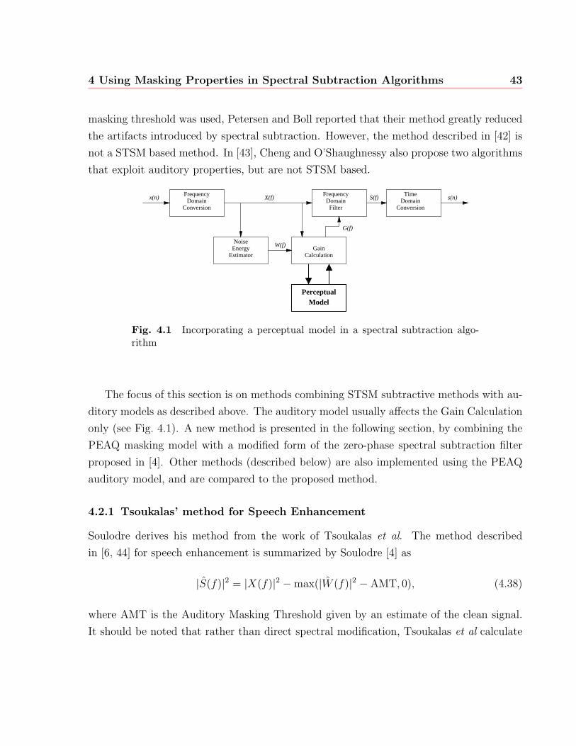
4 Using Masking Properties in Spectral Subtraction Algorithms 43
masking threshold was used, Petersen and Boll reported that their method greatly reduced
the artifacts introduced by spectral subtraction. However, the method described in [42] is
not a STSM based method. In [43], Cheng and O’Shaughnessy also propose two algorithms
that exploit auditory properties, but are not STSM based.
ConversionDomain
TimeDomain
Conversion
GainCalculation
Frequency
NoiseEnergy
Estimator
FrequencyDomain
Filter
S(f)x(n)
W(f)
G(f)
X(f) s(n)
PerceptualModel
Fig. 4.1 Incorporating a perceptual model in a spectral subtraction algo-rithm
The focus of this section is on methods combining STSM subtractive methods with au-
ditory models as described above. The auditory model usually affects the Gain Calculation
only (see Fig. 4.1). A new method is presented in the following section, by combining the
PEAQ masking model with a modified form of the zero-phase spectral subtraction filter
proposed in [4]. Other methods (described below) are also implemented using the PEAQ
auditory model, and are compared to the proposed method.
4.2.1 Tsoukalas’ method for Speech Enhancement
Soulodre derives his method from the work of Tsoukalas et al. The method described
in [6, 44] for speech enhancement is summarized by Soulodre [4] as
|S(f)|2 = |X(f)|2 −max(|W (f)|2 − AMT, 0), (4.38)
where AMT is the Auditory Masking Threshold given by an estimate of the clean signal.
It should be noted that rather than direct spectral modification, Tsoukalas et al calculate
4 Using Masking Properties in Spectral Subtraction Algorithms 44
the parameters of the nonlinear gain function
GT(m, p) =|X(m, p)|2v(m,p)
av(m,p)(m, p) + |X(m, p)|2v(m,p), (4.39)
where a(m, p) and v(m, p) are the time-frequency varying parameters. This nonlinear gain
function is based on a function proposed by Eger et al in [45], and was further developed
by Clarkson and Bahgat [46]. In the above method, a(m, p) is a threshold below which all
frequency components are highly suppressed, and v(m, p) controls the rate of suppression.
Tsoukalas et al found the influence of v(m, p) negligible and fixed it at v(m, p) = v = 1.
The parameter a(m, p) is constrained to be constant within a critical band, and Tsoukalas
et al present various ways of calculating aCB(i, p), such as
aCB(i, p) =(WCB(i) + TJ(i)
)(WCB(i)
TJ(i)
)1/v
, (4.40)
where WCB(i) represents the noise in the ith critical band and TJ(i) represents the AMT
(using Johnston’s method) in the ith critical band. To obtain a good estimate of the AMT
Tsoukalas et al suggest an iterative approach, at the expense of computational efficiency.
Essentially, the first AMT is obtained using standard power spectral subtraction, and S
is obtained using (4.39). The AMT is calculated using S, and (4.39) is applied to S.
The parameter aCB(i, p) will decrease with each iteration, converging towards zero, thus
indicating no more suppression is needed.
Tsoukalas et al report that to begin the iterative process, even the noisy signal can
be used to find the AMT. However, more iterations must be performed for aCB(i, p) to
converge.
4.2.2 Musical Noise Suppression
A more direct method for suppressing the musical noise that is generated by STSM sub-
tractive methods was presented by Haulick et al in [9]. Conceptually, this algorithm acts
as a postprocessor to conventional spectral subtraction. The masking thresholds for the
noisy signal and the output signal are computed. Components that are audible (above the
masking threshold) in the output but not the input are candidates for suppression. To
avoid suppressing previously inaudible unvoiced speech segments, a short-time stationarity
4 Using Masking Properties in Spectral Subtraction Algorithms 45
and bandwidth criterion is applied. In order to be classified as musical, noise must have a
bandwidth of less than about 300 Hz. If two successive filter coefficients fulfill the condition
min(GH(m, p− 1), GH(m, p)
)≥ 0.55, (4.41)
the corresponding spectral component is assumed be speech and is not suppressed. Audible
spectral components that meet the criteria for musical noise are suppressed by setting the
corresponding filter coefficient to the noise floor β.
4.2.3 Virag’s method
A method developed by Virag [8] can be viewed as a lower complexity version of the speech
enhancement method by Tsoukalas et al, though it is not directly derived from it. Virag
uses the masking threshold estimate (obtained using power spectrum subtraction) to adjust
the spectral subtraction parameters k and α of Eq. (3.7) on a per-band and per-frame basis.
The adaption of the subtraction parameters is performed with
k(m) = Fk[kmin, kmax, T (m)] (4.42)
α(m) = Fα[αmin, αmax, T (m)], (4.43)
where kmin, kmax, αmin, and αmax constrain k and α, and T (m) is the masking threshold
estimate. The functions Fk and Fα lead to maximal residual noise reduction for minimal
masking threshold and vice versa, such that Fk = kmax if T (m) = T (m)min and Fk = kmin
if T (m) = T (m)max. T (m)min and T (m)max are the minimal and maximal values of the
masking threshold respectively, updated from frame to frame. To avoid discontinuities in
the gain function, a smoothing function is applied.
Virag found that kmin = 1, kmax = 6, αmin = 0, and αmax = 0.02 gives a good tradeoff
between residual noise and speech distortion.
Earlier, a similar approach was taken by Lorber and Hoeldrich in [47], for use in audio
restoration. However, a very simplified auditory model (consisting of only an approximation
of the spreading function) was used, to smooth an estimate of the SNR. The SNR estimate
was then used to calculate α in a similar fashion to Virag’s method.
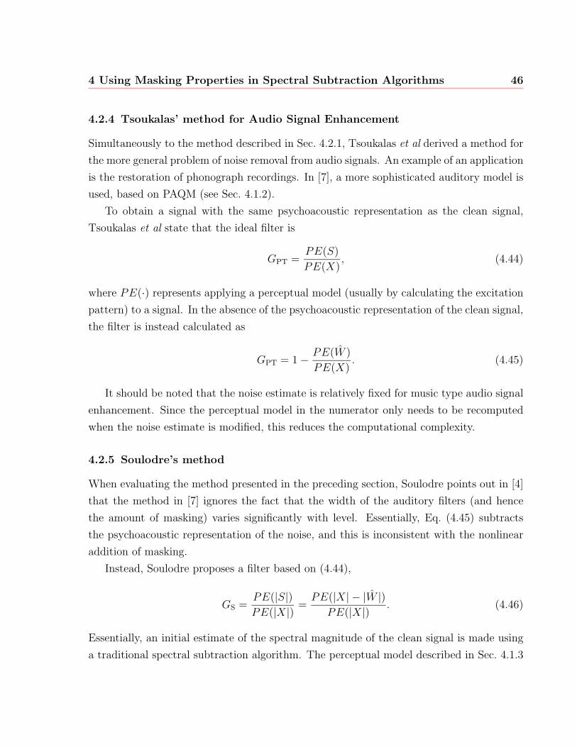
4 Using Masking Properties in Spectral Subtraction Algorithms 46
4.2.4 Tsoukalas’ method for Audio Signal Enhancement
Simultaneously to the method described in Sec. 4.2.1, Tsoukalas et al derived a method for
the more general problem of noise removal from audio signals. An example of an application
is the restoration of phonograph recordings. In [7], a more sophisticated auditory model is
used, based on PAQM (see Sec. 4.1.2).
To obtain a signal with the same psychoacoustic representation as the clean signal,
Tsoukalas et al state that the ideal filter is
GPT =PE(S)
PE(X), (4.44)
where PE(·) represents applying a perceptual model (usually by calculating the excitation
pattern) to a signal. In the absence of the psychoacoustic representation of the clean signal,
the filter is instead calculated as
GPT = 1− PE(W )
PE(X). (4.45)
It should be noted that the noise estimate is relatively fixed for music type audio signal
enhancement. Since the perceptual model in the numerator only needs to be recomputed
when the noise estimate is modified, this reduces the computational complexity.
4.2.5 Soulodre’s method
When evaluating the method presented in the preceding section, Soulodre points out in [4]
that the method in [7] ignores the fact that the width of the auditory filters (and hence
the amount of masking) varies significantly with level. Essentially, Eq. (4.45) subtracts
the psychoacoustic representation of the noise, and this is inconsistent with the nonlinear
addition of masking.
Instead, Soulodre proposes a filter based on (4.44),
GS =PE(|S|)PE(|X|)
=PE(|X| − |W |)
PE(|X|). (4.46)
Essentially, an initial estimate of the spectral magnitude of the clean signal is made using
a traditional spectral subtraction algorithm. The perceptual model described in Sec. 4.1.3
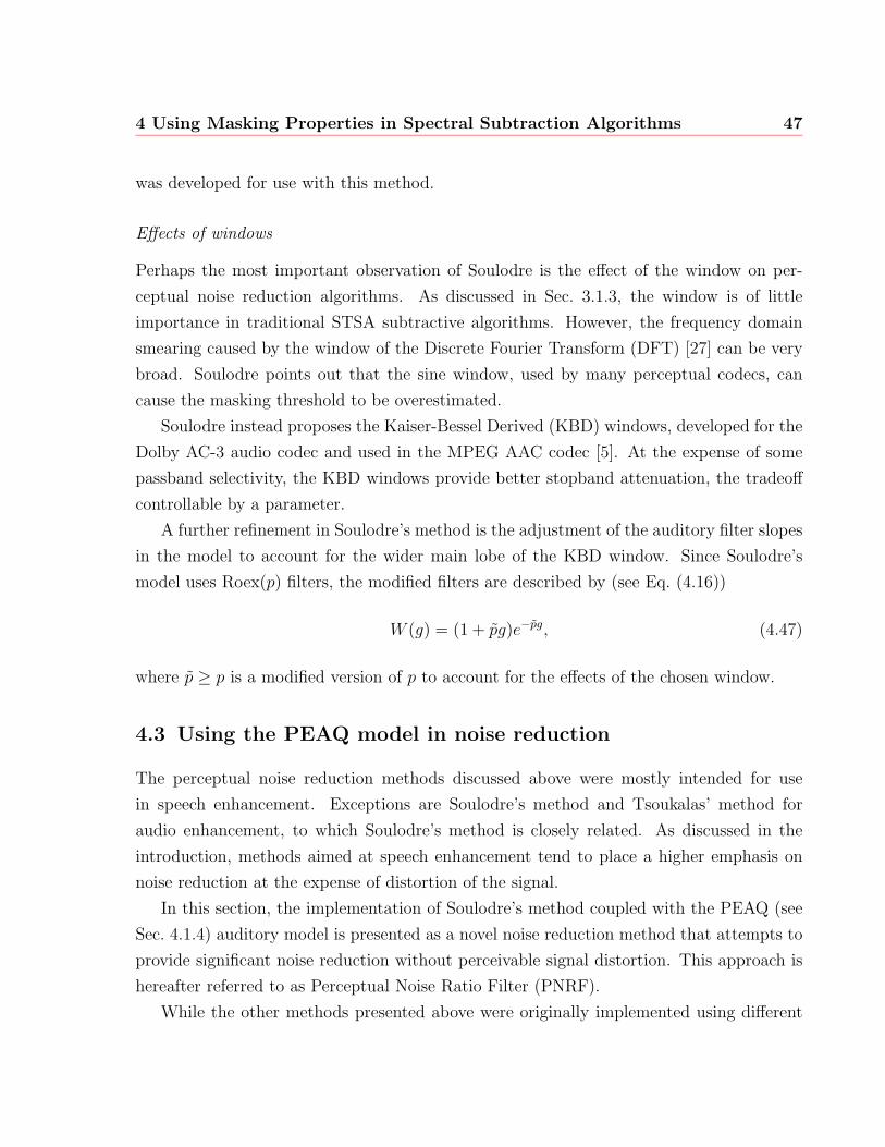
4 Using Masking Properties in Spectral Subtraction Algorithms 47
was developed for use with this method.
Effects of windows
Perhaps the most important observation of Soulodre is the effect of the window on per-
ceptual noise reduction algorithms. As discussed in Sec. 3.1.3, the window is of little
importance in traditional STSA subtractive algorithms. However, the frequency domain
smearing caused by the window of the Discrete Fourier Transform (DFT) [27] can be very
broad. Soulodre points out that the sine window, used by many perceptual codecs, can
cause the masking threshold to be overestimated.
Soulodre instead proposes the Kaiser-Bessel Derived (KBD) windows, developed for the
Dolby AC-3 audio codec and used in the MPEG AAC codec [5]. At the expense of some
passband selectivity, the KBD windows provide better stopband attenuation, the tradeoff
controllable by a parameter.
A further refinement in Soulodre’s method is the adjustment of the auditory filter slopes
in the model to account for the wider main lobe of the KBD window. Since Soulodre’s
model uses Roex(p) filters, the modified filters are described by (see Eq. (4.16))
W (g) = (1 + pg)e−pg, (4.47)
where p ≥ p is a modified version of p to account for the effects of the chosen window.
4.3 Using the PEAQ model in noise reduction
The perceptual noise reduction methods discussed above were mostly intended for use
in speech enhancement. Exceptions are Soulodre’s method and Tsoukalas’ method for
audio enhancement, to which Soulodre’s method is closely related. As discussed in the
introduction, methods aimed at speech enhancement tend to place a higher emphasis on
noise reduction at the expense of distortion of the signal.
In this section, the implementation of Soulodre’s method coupled with the PEAQ (see
Sec. 4.1.4) auditory model is presented as a novel noise reduction method that attempts to
provide significant noise reduction without perceivable signal distortion. This approach is
hereafter referred to as Perceptual Noise Ratio Filter (PNRF).
While the other methods presented above were originally implemented using different
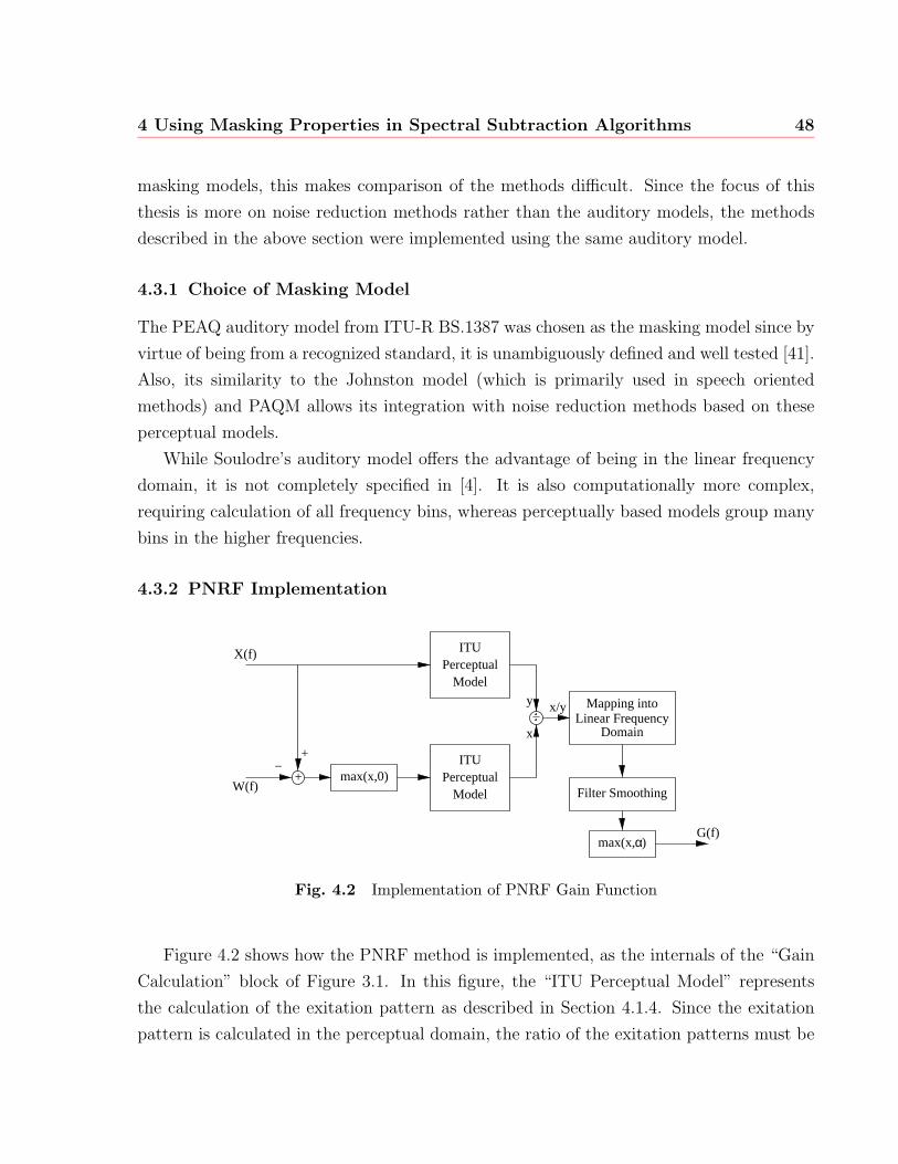
4 Using Masking Properties in Spectral Subtraction Algorithms 48
masking models, this makes comparison of the methods difficult. Since the focus of this
thesis is more on noise reduction methods rather than the auditory models, the methods
described in the above section were implemented using the same auditory model.
4.3.1 Choice of Masking Model
The PEAQ auditory model from ITU-R BS.1387 was chosen as the masking model since by
virtue of being from a recognized standard, it is unambiguously defined and well tested [41].
Also, its similarity to the Johnston model (which is primarily used in speech oriented
methods) and PAQM allows its integration with noise reduction methods based on these
perceptual models.
While Soulodre’s auditory model offers the advantage of being in the linear frequency
domain, it is not completely specified in [4]. It is also computationally more complex,
requiring calculation of all frequency bins, whereas perceptually based models group many
bins in the higher frequencies.
4.3.2 PNRF Implementation
max(x,0)+ITU
PerceptualModel
ITUPerceptual
Model
Mapping intoLinear Frequency
Domain
max(x, )α
+−
X(f)
W(f)
y
x
Filter Smoothing
G(f)
x/y
Fig. 4.2 Implementation of PNRF Gain Function
Figure 4.2 shows how the PNRF method is implemented, as the internals of the “Gain
Calculation” block of Figure 3.1. In this figure, the “ITU Perceptual Model” represents
the calculation of the exitation pattern as described in Section 4.1.4. Since the exitation
pattern is calculated in the perceptual domain, the ratio of the exitation patterns must be
4 Using Masking Properties in Spectral Subtraction Algorithms 49
converted back into the linear domain, as described below1. The resulting filter is smoothed
with λF = 0.01, and constrained to a minimum of α = 0.1 to further reduce musical noise.
4.3.3 Implementation Issues
All methods were implemented using the same time- to frequency-domain conversion, based
on the requirements for the PEAQ model. The size of the DFT is chosen such that the bin
spacing (fs/M , see Sec. 3.1.1) does not exceed the bandwidth of the smallest group in the
auditory model (in the case of PEAQ, 23.445 Hz). Also, the order of the DFT should be
a power of 2, such that the more efficient Fast Fourier Transform (FFT) can be used [26].
Overlap between frames is set at 50%, using a Hanning window, as specified by the PEAQ
model.
When used at a sampling frequency of fs = 8000 Hz, frames are spaced 256 samples
(32 ms) apart. For audio processing, sampling frequency being either fs = 44100 Hz or
fs = 48000 Hz, frames are spaced 1024 samples (23.22 ms and 21.33 ms respectively) apart.
Since for testing the clean signal was available, the problem of accurate speech detection
(by use of a VAD, see Sec. 3.1.5) could be avoided. Instead, the clean signal was used to
determine periods of speech activity, though the noise estimate was obtained from the
noisy signal. For the noise estimate, a forgetting factor of λN = 0.97 (equivalent to a time
constant of about 33 frames, or about 1 s) was used.
4.3.4 Parameters and Modifications
For methods with adjustable parameters, it was attempted to achieve a reasonable tradeoff
between musical noise, residual noise, and signal distortion.
Boll’s noise suppression method, required by the algorithm proposed by Haulick et
al, also serves as a good reference point for evaluation of auditory based methods. The
parameters used are a = 2 for power spectral subtraction, an oversubtraction factor k = 1.5,
and a spectral floor α = 0.1. Of note is especially the high value of α = 0.1, which is based
on preliminary testing, where the musical noise was deemed to be more disturbing than
the original noise.
The parameters for Virag’s method are given in [8], and were kept as given. However,
1Note that the exitation patterns are never zero due to the internal noise, and thus the division is alwaysdefined
4 Using Masking Properties in Spectral Subtraction Algorithms 50
the “smoothing function” of G(m, p) is not specified explicitly and was omitted in this
implementation.
The noise suppression scheme of Tsoukalas et al was implemented with some modifi-
cations. The most significant modification made was to fix the number of iterations to 4.
One reason for using a fixed number of iterations was partially for computing efficiency,
since this allowed all frames to be processed at once. Also, it was found that the value
of aCB does not always converge to zero, or do so extremely slowly, possibly due to the
different auditory model. Additionally, throughout every iteration, the resulting filter was
constrained to the minimum noise floor (as with Boll’s method above, α = 0.1) to avoid
the signal distortion that is otherwise present. Finally, the exponent v was set to 1, as used
by Tsoukalas et al.
Mapping from perceptual into linear domain
Most perceptually motivated methods require a mapping from the perceptual domain (in
the PEAQ model, each group represents 0.25 Bark) back to the linear frequency domain.
Since the denoised signal is created by use of an inverse DFT, the filter G must ultimately
be in linear frequency domain. The PEAQ model was intended for the comparison of two
signals, and thus there is no provision for inverse mapping the masking threshold back to
SPL levels in linear domain.
At issue is if the masking threshold value calculated by the PEAQ model should be
regarded as an absolute level constant within the critical band group, or if the value rep-
resents the total energy that the masked signal has to exceed within that group in order
to be audible. Informal testing suggested that the former interpretation would yield better
results, and thus was used in the implementation of the methods.
4.4 Summary
This chapter has presented various ways of modeling the human hearing system, most of
which were intended for coding of speech or audio signals. It was shown how these auditory
models were incorporated in noise suppression or speech enhancement algorithms. A new
method, based on a noise suppressor originally developed for a specific problem is proposed
as a good general noise suppression method. Finally, it is described how this method, and
others for comparison, is implemented with one of the auditory models.
51
Chapter 5
Results
This chapter presents an evaluation of the enhancement techniques described in the pre-
vious chapters. Ideally, an evaluation of all the presented noise reduction methods and
comparison with the proposed PNRF by formal subjective listening tests should be con-
ducted. However, due to the complexity, time and resources required, formal testing is not
feasible within the scope of this thesis. Instead, the informal testing as presented in this
chapter is intended to show the potential of the methods in a real-world application.
5.1 Test data
The test data, used for both objective and subjective testing, was chosen to represent
a typical application of a noise suppression system for speech enhancement. The signal
consisted of four sentences, two spoken by a male and two by a female. The sentences
were originally recorded separately under controlled conditions at a sampling frequency
of 48 kHz, using linear 16-bit encoding. For the testing, the signal was downsampled to
8000 Hz, and the selected sentences were concatenated with a 1 s pause between each
sentence.
The noise was taken from the SPIB (Signal Processing Information Base) at Rice Uni-
versity [48]. It consist of a recording of the interior of a automobile driving at 120 km/h,
in rainy conditions. The original was sampled at 19.98 kHz using 16-bit linear encoding,
and for this experiment was also downsampled to 8000 Hz.
Before adding the two signals, both were filtered by a 120 Hz highpass filter, as used
by the EVRC noise suppressor. The test signals were created with SNRs of 0 dB and
2001/07/26
5 Results 52
6 dB, which represents comparatively high noise levels (in contrast, the objective measures
to assess SNR improvement for the AMR noise suppressor (GSM 06.78, annex E) specify
test signals using car noise in the range of 3 dB to 15 dB SNR [49]). For the purposes of
calculating the level at which noise is added to the speech, the speech level was calculated
according to ITU-T recommendation P.56 [50].
5.2 Objective Comparisons
Objective quality comparisons of speech are intended to predict the preference a human lis-
tener would indicate. The results of an ideal objective measure would be indistinguishable
from those obtained from human observers. This means the objective comparison method
would require knowledge of all levels of human speech processing, such as psychoacoustics,
acoustic-phonetics, syntax, semantics, etc. Since most speech processing systems (either
coders or noise reduction systems) do not produce distortions in the higher levels of percep-
tion (such as syntax or semantics), these aspects can generally be ignored when comparing
signals produced from the same initial unprocessed signal [51].
While there are objective measures incorporating psychoacoustic models (the mask-
ing models described in Sections 4.1.2 and 4.1.4 are from such methods), in this chapter
only basic objective quality measures are used. Basic objective measures, such as the
Signal-to-Noise Ratio (SNR) and the Segmental SNR (SNRSEG) used below, are compactly
computable functions that can be uniformly applied to all forms of speech distortion in
order to estimate subjective quality [51].
SNR measures are generally applicable only in sample-by-sample based processing sys-
tems, and while not good at comparing dissimilar distortions, generally perform well when
ranking similar distortions. SNR measures are not able to provide fine distinctions.
In the following evaluations, three noise measures are used, SNR, SNRSEG, and SNR
Improvement (SNRIMPR). Of these, the first two are commonly used to evaluate waveform
coders, while the last is specific to evaluating noise reduction methods. The SNR is defined
as
SNR = 10 log10
∑n
|s(n)|2∑n
|s(n)− s(n+ ∆p)|2(dB), (5.1)
where s(n) and s(n) represent the clean and estimated clean speech, respectively. The
5 Results 53
offset ∆p accounts for the process delay of the noise reduction algorithm. However, the
SNR measure has specific shortcomings where strong signal sections affect the measure
more than weak signal sections [11]. The SNRSEG, defined as
SNRSEG =10
P
∑p
log10
N−1∑n=0
|s(n+Np)|2
N−1∑n=0
|s(n+Np)− s(n+Np+ ∆p)|2(dB), (5.2)
averages the SNR of segments of length N samples long, usually around 16 ms. Since in
the case of quantized signals∑
n |s(n)|2 or∑
n |s(n) − s(n + ∆p)|2 can be zero over short
sections, the following alternate form is used in the presented results. Using
SNRSEG = 10 log10
(10∑pSS(p)P − 1
)(dB), (5.3)
where
SS(p) = log10
(1 +
N−1∑n=0
|s(n+Np)|2
η +N−1∑n=0
|s(n+Np)− s(n+Np+ ∆p)|2
), (5.4)
η is a small value to prevent division by zero, and the addition of the unity term prevents
a log(0) condition. Also, due to the addition of the unity term, segments with SNR below
0 dB are discounted. This results in a measure that balances the strong and weak sections
of the signal.
The third basic noise measure used is the SNRIMPR, which is used to evaluate the
performance of noise suppression algorithms [8, 52]. It is given by the difference between
the input and output segmental SNR:
SNRIMPR =1
P
∑p
10 log10
N−1∑n=0
|υ(n+ pN)|2
N−1∑n=0
|s(n+Np)− s(n+Np+ ∆p)|2(dB), (5.5)
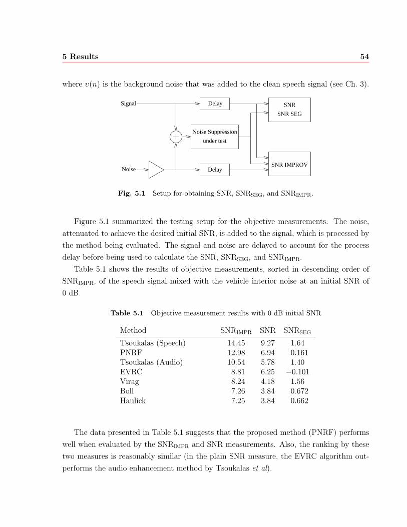
5 Results 54
where υ(n) is the background noise that was added to the clean speech signal (see Ch. 3).
Signal
Noise Delay
Delay
Noise Suppression
under test
SNR
SNR SEG
SNR IMPROV
Fig. 5.1 Setup for obtaining SNR, SNRSEG, and SNRIMPR.
Figure 5.1 summarized the testing setup for the objective measurements. The noise,
attenuated to achieve the desired initial SNR, is added to the signal, which is processed by
the method being evaluated. The signal and noise are delayed to account for the process
delay before being used to calculate the SNR, SNRSEG, and SNRIMPR.
Table 5.1 shows the results of objective measurements, sorted in descending order of
SNRIMPR, of the speech signal mixed with the vehicle interior noise at an initial SNR of
0 dB.
Table 5.1 Objective measurement results with 0 dB initial SNR
Method SNRIMPR SNR SNRSEG
Tsoukalas (Speech) 14.45 9.27 1.64PNRF 12.98 6.94 0.161Tsoukalas (Audio) 10.54 5.78 1.40EVRC 8.81 6.25 −0.101Virag 8.24 4.18 1.56Boll 7.26 3.84 0.672Haulick 7.25 3.84 0.662
The data presented in Table 5.1 suggests that the proposed method (PNRF) performs
well when evaluated by the SNRIMPR and SNR measurements. Also, the ranking by these
two measures is reasonably similar (in the plain SNR measure, the EVRC algorithm out-
performs the audio enhancement method by Tsoukalas et al).
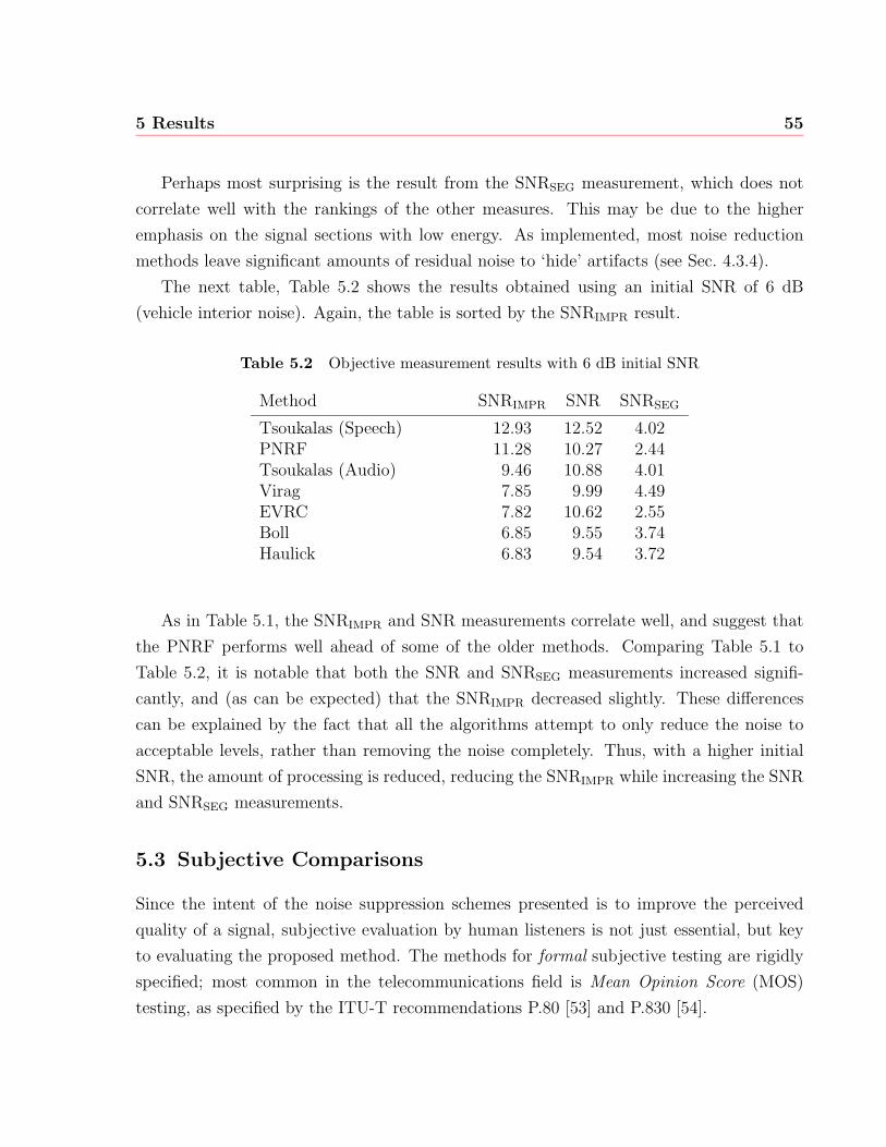
5 Results 55
Perhaps most surprising is the result from the SNRSEG measurement, which does not
correlate well with the rankings of the other measures. This may be due to the higher
emphasis on the signal sections with low energy. As implemented, most noise reduction
methods leave significant amounts of residual noise to ‘hide’ artifacts (see Sec. 4.3.4).
The next table, Table 5.2 shows the results obtained using an initial SNR of 6 dB
(vehicle interior noise). Again, the table is sorted by the SNRIMPR result.
Table 5.2 Objective measurement results with 6 dB initial SNR
Method SNRIMPR SNR SNRSEG
Tsoukalas (Speech) 12.93 12.52 4.02PNRF 11.28 10.27 2.44Tsoukalas (Audio) 9.46 10.88 4.01Virag 7.85 9.99 4.49EVRC 7.82 10.62 2.55Boll 6.85 9.55 3.74Haulick 6.83 9.54 3.72
As in Table 5.1, the SNRIMPR and SNR measurements correlate well, and suggest that
the PNRF performs well ahead of some of the older methods. Comparing Table 5.1 to
Table 5.2, it is notable that both the SNR and SNRSEG measurements increased signifi-
cantly, and (as can be expected) that the SNRIMPR decreased slightly. These differences
can be explained by the fact that all the algorithms attempt to only reduce the noise to
acceptable levels, rather than removing the noise completely. Thus, with a higher initial
SNR, the amount of processing is reduced, reducing the SNRIMPR while increasing the SNR
and SNRSEG measurements.
5.3 Subjective Comparisons
Since the intent of the noise suppression schemes presented is to improve the perceived
quality of a signal, subjective evaluation by human listeners is not just essential, but key
to evaluating the proposed method. The methods for formal subjective testing are rigidly
specified; most common in the telecommunications field is Mean Opinion Score (MOS)
testing, as specified by the ITU-T recommendations P.80 [53] and P.830 [54].
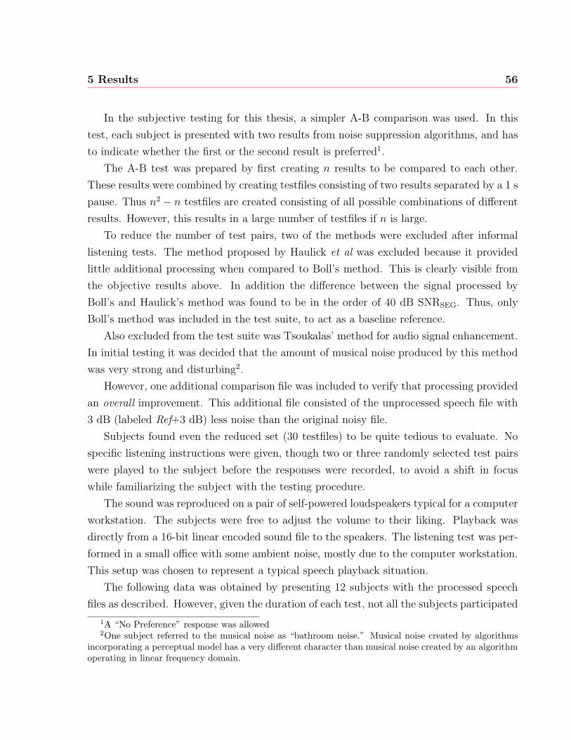
5 Results 56
In the subjective testing for this thesis, a simpler A-B comparison was used. In this
test, each subject is presented with two results from noise suppression algorithms, and has
to indicate whether the first or the second result is preferred1.
The A-B test was prepared by first creating n results to be compared to each other.
These results were combined by creating testfiles consisting of two results separated by a 1 s
pause. Thus n2 − n testfiles are created consisting of all possible combinations of different
results. However, this results in a large number of testfiles if n is large.
To reduce the number of test pairs, two of the methods were excluded after informal
listening tests. The method proposed by Haulick et al was excluded because it provided
little additional processing when compared to Boll’s method. This is clearly visible from
the objective results above. In addition the difference between the signal processed by
Boll’s and Haulick’s method was found to be in the order of 40 dB SNRSEG. Thus, only
Boll’s method was included in the test suite, to act as a baseline reference.
Also excluded from the test suite was Tsoukalas’ method for audio signal enhancement.
In initial testing it was decided that the amount of musical noise produced by this method
was very strong and disturbing2.
However, one additional comparison file was included to verify that processing provided
an overall improvement. This additional file consisted of the unprocessed speech file with
3 dB (labeled Ref+3 dB) less noise than the original noisy file.
Subjects found even the reduced set (30 testfiles) to be quite tedious to evaluate. No
specific listening instructions were given, though two or three randomly selected test pairs
were played to the subject before the responses were recorded, to avoid a shift in focus
while familiarizing the subject with the testing procedure.
The sound was reproduced on a pair of self-powered loudspeakers typical for a computer
workstation. The subjects were free to adjust the volume to their liking. Playback was
directly from a 16-bit linear encoded sound file to the speakers. The listening test was per-
formed in a small office with some ambient noise, mostly due to the computer workstation.
This setup was chosen to represent a typical speech playback situation.
The following data was obtained by presenting 12 subjects with the processed speech
files as described. However, given the duration of each test, not all the subjects participated
1A “No Preference” response was allowed2One subject referred to the musical noise as “bathroom noise.” Musical noise created by algorithms
incorporating a perceptual model has a very different character than musical noise created by an algorithmoperating in linear frequency domain.
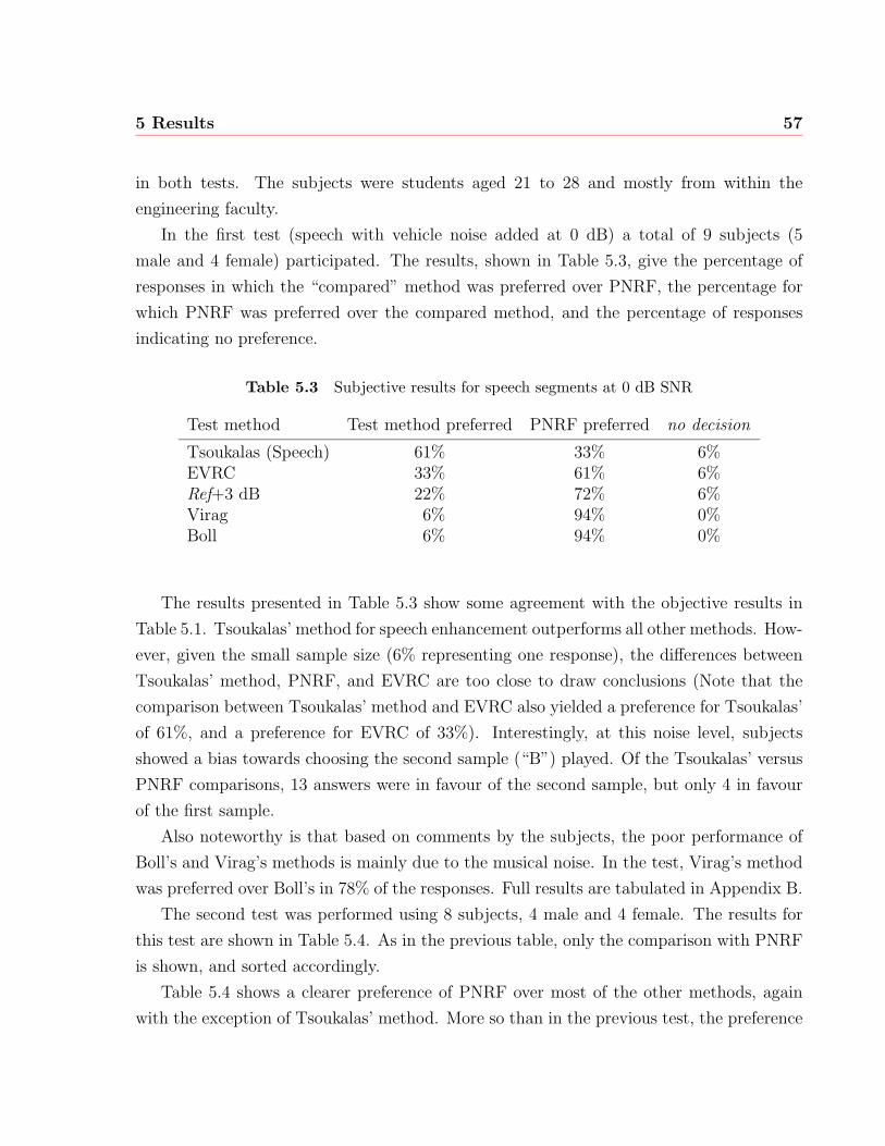
5 Results 57
in both tests. The subjects were students aged 21 to 28 and mostly from within the
engineering faculty.
In the first test (speech with vehicle noise added at 0 dB) a total of 9 subjects (5
male and 4 female) participated. The results, shown in Table 5.3, give the percentage of
responses in which the “compared” method was preferred over PNRF, the percentage for
which PNRF was preferred over the compared method, and the percentage of responses
indicating no preference.
Table 5.3 Subjective results for speech segments at 0 dB SNR
Test method Test method preferred PNRF preferred no decision
Tsoukalas (Speech) 61% 33% 6%EVRC 33% 61% 6%Ref+3 dB 22% 72% 6%Virag 6% 94% 0%Boll 6% 94% 0%
The results presented in Table 5.3 show some agreement with the objective results in
Table 5.1. Tsoukalas’ method for speech enhancement outperforms all other methods. How-
ever, given the small sample size (6% representing one response), the differences between
Tsoukalas’ method, PNRF, and EVRC are too close to draw conclusions (Note that the
comparison between Tsoukalas’ method and EVRC also yielded a preference for Tsoukalas’
of 61%, and a preference for EVRC of 33%). Interestingly, at this noise level, subjects
showed a bias towards choosing the second sample (“B”) played. Of the Tsoukalas’ versus
PNRF comparisons, 13 answers were in favour of the second sample, but only 4 in favour
of the first sample.
Also noteworthy is that based on comments by the subjects, the poor performance of
Boll’s and Virag’s methods is mainly due to the musical noise. In the test, Virag’s method
was preferred over Boll’s in 78% of the responses. Full results are tabulated in Appendix B.
The second test was performed using 8 subjects, 4 male and 4 female. The results for
this test are shown in Table 5.4. As in the previous table, only the comparison with PNRF
is shown, and sorted accordingly.
Table 5.4 shows a clearer preference of PNRF over most of the other methods, again
with the exception of Tsoukalas’ method. More so than in the previous test, the preference
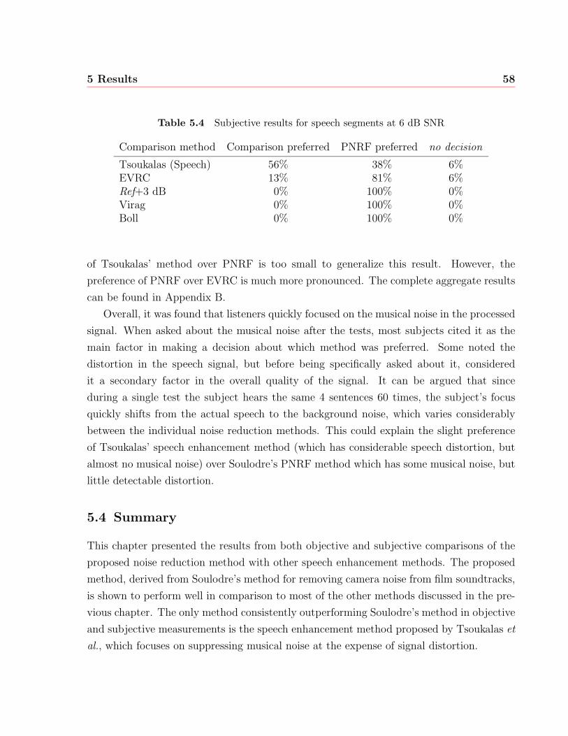
5 Results 58
Table 5.4 Subjective results for speech segments at 6 dB SNR
Comparison method Comparison preferred PNRF preferred no decision
Tsoukalas (Speech) 56% 38% 6%EVRC 13% 81% 6%Ref+3 dB 0% 100% 0%Virag 0% 100% 0%Boll 0% 100% 0%
of Tsoukalas’ method over PNRF is too small to generalize this result. However, the
preference of PNRF over EVRC is much more pronounced. The complete aggregate results
can be found in Appendix B.
Overall, it was found that listeners quickly focused on the musical noise in the processed
signal. When asked about the musical noise after the tests, most subjects cited it as the
main factor in making a decision about which method was preferred. Some noted the
distortion in the speech signal, but before being specifically asked about it, considered
it a secondary factor in the overall quality of the signal. It can be argued that since
during a single test the subject hears the same 4 sentences 60 times, the subject’s focus
quickly shifts from the actual speech to the background noise, which varies considerably
between the individual noise reduction methods. This could explain the slight preference
of Tsoukalas’ speech enhancement method (which has considerable speech distortion, but
almost no musical noise) over Soulodre’s PNRF method which has some musical noise, but
little detectable distortion.
5.4 Summary
This chapter presented the results from both objective and subjective comparisons of the
proposed noise reduction method with other speech enhancement methods. The proposed
method, derived from Soulodre’s method for removing camera noise from film soundtracks,
is shown to perform well in comparison to most of the other methods discussed in the pre-
vious chapter. The only method consistently outperforming Soulodre’s method in objective
and subjective measurements is the speech enhancement method proposed by Tsoukalas et
al., which focuses on suppressing musical noise at the expense of signal distortion.
59
Chapter 6
Conclusion
In this thesis, the problem of acoustic noise suppression is explored, using properties of the
human hearing system in an attempt to improve performance. It was shown that using
masking properties of the hearing system allows for improved noise reduction. A novel
method for noise reduction in speech signals has been proposed. This method was shown
to outperform non-auditory based methods, and compared well with other perceptually
motivated noise reduction methods. It was found that the proposed method, Soulodre’s
PNRF combined with the ITU’s PEAQ auditory model, had more musical noise but less
signal distortion that a method proposed by Tsoukalas et al, which obtained marginally
better results in informal subjective testing.
6.1 Summary
The problem of noise reduction in speech signals and audio signals was introduced. Noise
reduction is used in the telecommunication field to improve intelligibility or perceived qual-
ity of the signal. Another area where noise reduction is applied is in the process of audio
archive restoration. These different fields have distinct requirements, that cannot always be
simultaneously satisfied, and thus various methods for noise reduction have been developed.
Widely used in the problem of noise reduction in speech signals are methods based on the
processing of short-time spectral amplitudes. These methods have been further improved
by using an auditory model to reduce the amount of processing applied to the signal while
maintaining the perceived level of noise suppression.
Chapter 2 presents an overview of the human hearing system. The human auditory
2001/07/26
6 Conclusion 60
system converts sound waves into signals that are received by the brain. The acoustic
signal is transformed into a displacement of the basilar membrane, which causes nerve cells
to react. Nonlinearities in this system, such as interaction between nerve cells and the
behavior of the basilar membrane, give rise to masking effects. These masking effects cause
some sounds to be inaudible in the presence of other sounds. Auditory models are used to
predict these masking effects.
In Chapter 3 some non-auditory noise reduction methods are introduced. Spectral
subtraction is a common method, and is based on modifying the short-time spectral shape of
the signal. It is assumed that the spectrum of the noise is relatively stationary, and that the
power spectra of the clean signal and the noise are additive. However, spectral subtraction
and related methods create artifacts in the estimated signal, such as musical noise and
distortion. These artifacts are disturbing to the listener, and should be avoided. Other
methods for noise reduction have been developed that attempt to increase performance to
reduce residual noise, musical noise, and signal distortion.
Models for estimating the masking threshold and their application in noise reduction
methods are described in Chapter 4. Different auditory models were developed for speech
coding methods, audio coding methods, objective perceptual quality measures, and noise
reduction. These models are used in noise reduction methods to iteratively estimate the
clean signal, estimate the clean signal psychoacoustic representation, or identify audible
musical noise. A novel noise reduction method is proposed, based on an auditory model
from a standardized perceptual quality assessment method, and a noise reduction rule
designed to remove a specific type of noise from audio signals. For comparison, other
perceptual noise reduction methods have been implemented using the same auditory model.
An evaluation of the proposed method (PNRF), and a comparison with the other meth-
ods is presented in Chapter 5. Objective and informal subjective results show that the
PNRF compares favorably to other perceptual noise reduction methods. Only one method,
exhibiting less musical noise at the expense of higher signal distortion, is rated as being
slightly better in the objective and subjective results.
6.2 Future Research Directions
Many issues are unresolved in the problem of noise reduction. The noise reduction method
presented in this thesis shows that effective noise reduction with little or no perceivable
6 Conclusion 61
distortion is attainable. This section addresses some issues that may further improve the
performance of the proposed method, and areas other than narrowband speech enhance-
ment where the PNRF could be effectively applied as well.
6.2.1 Iterative clean speech estimation
In the objective and subjective results presented in Chapter 5, Tsoukalas’ method outper-
forms PNRF by fairly small margins. The good performance of Tsoukalas’ method may
in part be attributed to its iterative nature. Using the result of one iteration of the noise
reduction process as estimate of the clean speech signal for the next, the clean speech es-
timate is successively improved. A similar approach can be used with the PNRF, since it
uses an initial clean speech estimate based simply on Boll’s method. Since PNRF achieves
good results with only one iteration, a much smaller number of iterations than used by
Tsoukalas’ method would be necessary to match results with Tsoukalas’ method.
6.2.2 Soft-decision VAD
As mentioned in Chapter 5, test subjects focused on the musical noise that was audible in
the speech pauses of the processed signal. Since for the noise estimation it is necessary to
identify the active speech segments using a Voice Activity Detector, this information may be
used to modify the parameters of the algorithm dynamically. Care should be taken to avoid
sudden changes, which would sound unnatural. One method to work around this problem
would be to use a VAD that provides more information than a simple speech/silence de-
cision. What kind of information a VAD should generate and how this would be used by
the algorithm are issues that need to be addressed.
6.2.3 Application to wide-band signals
While briefly discussing the applications of noise reduction in other areas, the focus of this
thesis has mainly been on the enhancement of speech signal sampled at telephone band-
width. However, since both the suppression rule and the auditory model were originally
developed for use in wideband (48000 Hz sampling rate) systems, the PNRF should be
applicable equally well to wideband speech (typically sampled at 16000 Hz) and audio sig-
nal enhancement. The biggest obstacle in the latter application is reliable signal/silence
detection, to obtain a good noise spectrum estimate.
6 Conclusion 62
6.2.4 Lower complexity masking model
The evaluation of auditory models and noise suppression algorithms in this thesis was
focused primarily on performance. The issue of computational complexity has been men-
tioned only briefly. However, in a practical setting, this issue can be very important if the
processing must be performed on a portable device, or on a fixed device that processes
several hundred channels independently. Thus, reducing the complexity of the algorithm
or the model can reduce the cost to the end-user.
One target for optimization would be the nonlinear normalized summation step of the
PEAQ model. This step was found to be one of the slowest parts of the masking threshold
calculation. It would be worth investigating if this step can be simplified without affecting
the performance of the overall noise suppression algorithm.
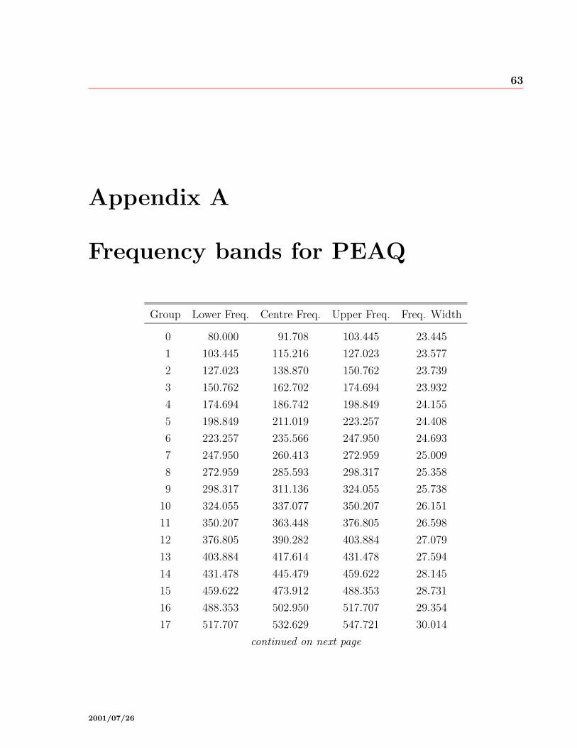
63
Appendix A
Frequency bands for PEAQ
Group Lower Freq. Centre Freq. Upper Freq. Freq. Width
0 80.000 91.708 103.445 23.445
1 103.445 115.216 127.023 23.577
2 127.023 138.870 150.762 23.739
3 150.762 162.702 174.694 23.932
4 174.694 186.742 198.849 24.155
5 198.849 211.019 223.257 24.408
6 223.257 235.566 247.950 24.693
7 247.950 260.413 272.959 25.009
8 272.959 285.593 298.317 25.358
9 298.317 311.136 324.055 25.738
10 324.055 337.077 350.207 26.151
11 350.207 363.448 376.805 26.598
12 376.805 390.282 403.884 27.079
13 403.884 417.614 431.478 27.594
14 431.478 445.479 459.622 28.145
15 459.622 473.912 488.353 28.731
16 488.353 502.950 517.707 29.354
17 517.707 532.629 547.721 30.014
continued on next page
2001/07/26
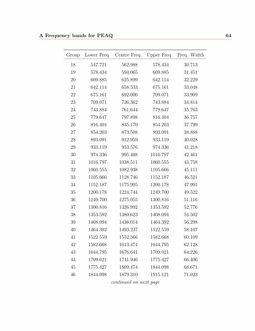
A Frequency bands for PEAQ 64
Group Lower Freq. Centre Freq. Upper Freq. Freq. Width
18 547.721 562.988 578.434 30.713
19 578.434 594.065 609.885 31.451
20 609.885 625.899 642.114 32.229
21 642.114 658.533 675.161 33.048
22 675.161 692.006 709.071 33.909
23 709.071 726.362 743.884 34.814
24 743.884 761.644 779.647 35.763
25 779.647 797.898 816.404 36.757
26 816.404 835.170 854.203 37.799
27 854.203 873.508 893.091 38.888
28 893.091 912.959 933.119 40.028
29 933.119 953.576 974.336 41.218
30 974.336 995.408 1016.797 42.461
31 1016.797 1038.511 1060.555 43.758
32 1060.555 1082.938 1105.666 45.111
33 1105.666 1128.746 1152.187 46.521
34 1152.187 1175.995 1200.178 47.991
35 1200.178 1224.744 1249.700 49.522
36 1249.700 1275.055 1300.816 51.116
37 1300.816 1326.992 1353.592 52.776
38 1353.592 1380.623 1408.094 54.502
39 1408.094 1436.014 1464.392 56.298
40 1464.392 1493.237 1522.559 58.167
41 1522.559 1552.366 1582.668 60.109
42 1582.668 1613.474 1644.795 62.128
43 1644.795 1676.641 1709.021 64.226
44 1709.021 1741.946 1775.427 66.406
45 1775.427 1809.474 1844.098 68.671
46 1844.098 1879.310 1915.121 71.023
continued on next page
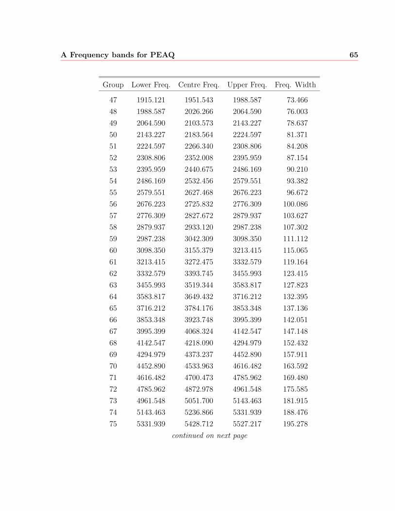
A Frequency bands for PEAQ 65
Group Lower Freq. Centre Freq. Upper Freq. Freq. Width
47 1915.121 1951.543 1988.587 73.466
48 1988.587 2026.266 2064.590 76.003
49 2064.590 2103.573 2143.227 78.637
50 2143.227 2183.564 2224.597 81.371
51 2224.597 2266.340 2308.806 84.208
52 2308.806 2352.008 2395.959 87.154
53 2395.959 2440.675 2486.169 90.210
54 2486.169 2532.456 2579.551 93.382
55 2579.551 2627.468 2676.223 96.672
56 2676.223 2725.832 2776.309 100.086
57 2776.309 2827.672 2879.937 103.627
58 2879.937 2933.120 2987.238 107.302
59 2987.238 3042.309 3098.350 111.112
60 3098.350 3155.379 3213.415 115.065
61 3213.415 3272.475 3332.579 119.164
62 3332.579 3393.745 3455.993 123.415
63 3455.993 3519.344 3583.817 127.823
64 3583.817 3649.432 3716.212 132.395
65 3716.212 3784.176 3853.348 137.136
66 3853.348 3923.748 3995.399 142.051
67 3995.399 4068.324 4142.547 147.148
68 4142.547 4218.090 4294.979 152.432
69 4294.979 4373.237 4452.890 157.911
70 4452.890 4533.963 4616.482 163.592
71 4616.482 4700.473 4785.962 169.480
72 4785.962 4872.978 4961.548 175.585
73 4961.548 5051.700 5143.463 181.915
74 5143.463 5236.866 5331.939 188.476
75 5331.939 5428.712 5527.217 195.278
continued on next page
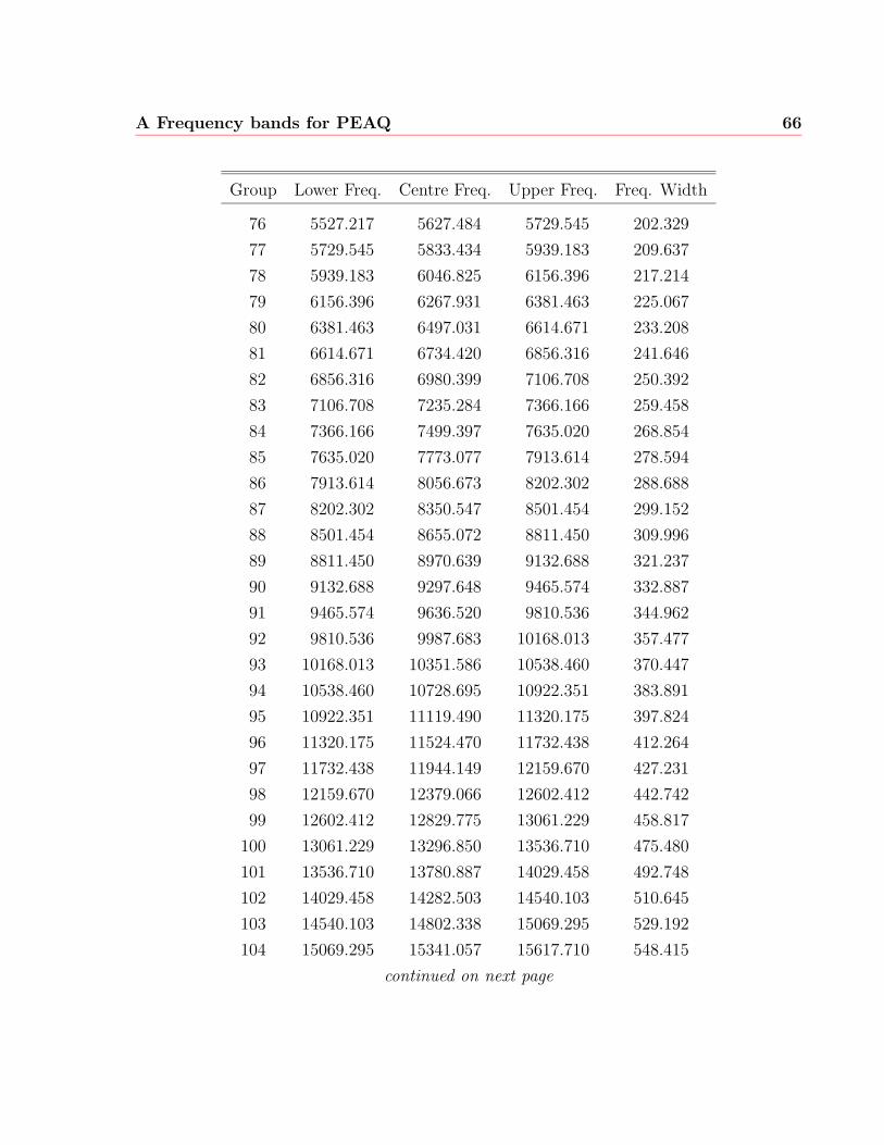
A Frequency bands for PEAQ 66
Group Lower Freq. Centre Freq. Upper Freq. Freq. Width
76 5527.217 5627.484 5729.545 202.329
77 5729.545 5833.434 5939.183 209.637
78 5939.183 6046.825 6156.396 217.214
79 6156.396 6267.931 6381.463 225.067
80 6381.463 6497.031 6614.671 233.208
81 6614.671 6734.420 6856.316 241.646
82 6856.316 6980.399 7106.708 250.392
83 7106.708 7235.284 7366.166 259.458
84 7366.166 7499.397 7635.020 268.854
85 7635.020 7773.077 7913.614 278.594
86 7913.614 8056.673 8202.302 288.688
87 8202.302 8350.547 8501.454 299.152
88 8501.454 8655.072 8811.450 309.996
89 8811.450 8970.639 9132.688 321.237
90 9132.688 9297.648 9465.574 332.887
91 9465.574 9636.520 9810.536 344.962
92 9810.536 9987.683 10168.013 357.477
93 10168.013 10351.586 10538.460 370.447
94 10538.460 10728.695 10922.351 383.891
95 10922.351 11119.490 11320.175 397.824
96 11320.175 11524.470 11732.438 412.264
97 11732.438 11944.149 12159.670 427.231
98 12159.670 12379.066 12602.412 442.742
99 12602.412 12829.775 13061.229 458.817
100 13061.229 13296.850 13536.710 475.480
101 13536.710 13780.887 14029.458 492.748
102 14029.458 14282.503 14540.103 510.645
103 14540.103 14802.338 15069.295 529.192
104 15069.295 15341.057 15617.710 548.415
continued on next page
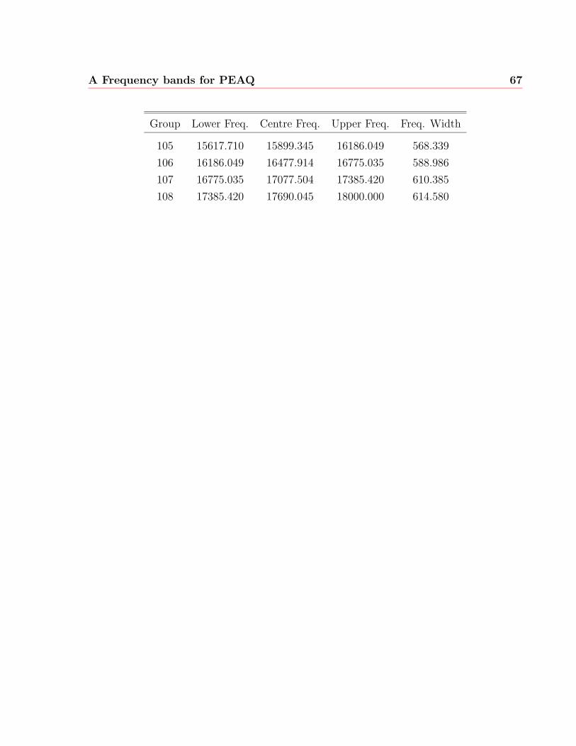
A Frequency bands for PEAQ 67
Group Lower Freq. Centre Freq. Upper Freq. Freq. Width
105 15617.710 15899.345 16186.049 568.339
106 16186.049 16477.914 16775.035 588.986
107 16775.035 17077.504 17385.420 610.385
108 17385.420 17690.045 18000.000 614.580
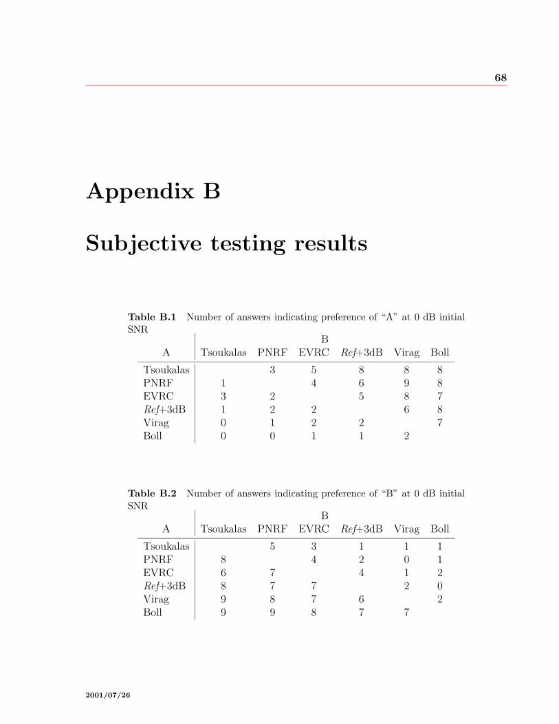
68
Appendix B
Subjective testing results
Table B.1 Number of answers indicating preference of “A” at 0 dB initialSNR
BA Tsoukalas PNRF EVRC Ref+3dB Virag Boll
Tsoukalas 3 5 8 8 8PNRF 1 4 6 9 8EVRC 3 2 5 8 7Ref+3dB 1 2 2 6 8Virag 0 1 2 2 7Boll 0 0 1 1 2
Table B.2 Number of answers indicating preference of “B” at 0 dB initialSNR
BA Tsoukalas PNRF EVRC Ref+3dB Virag Boll
Tsoukalas 5 3 1 1 1PNRF 8 4 2 0 1EVRC 6 7 4 1 2Ref+3dB 8 7 7 2 0Virag 9 8 7 6 2Boll 9 9 8 7 7
2001/07/26
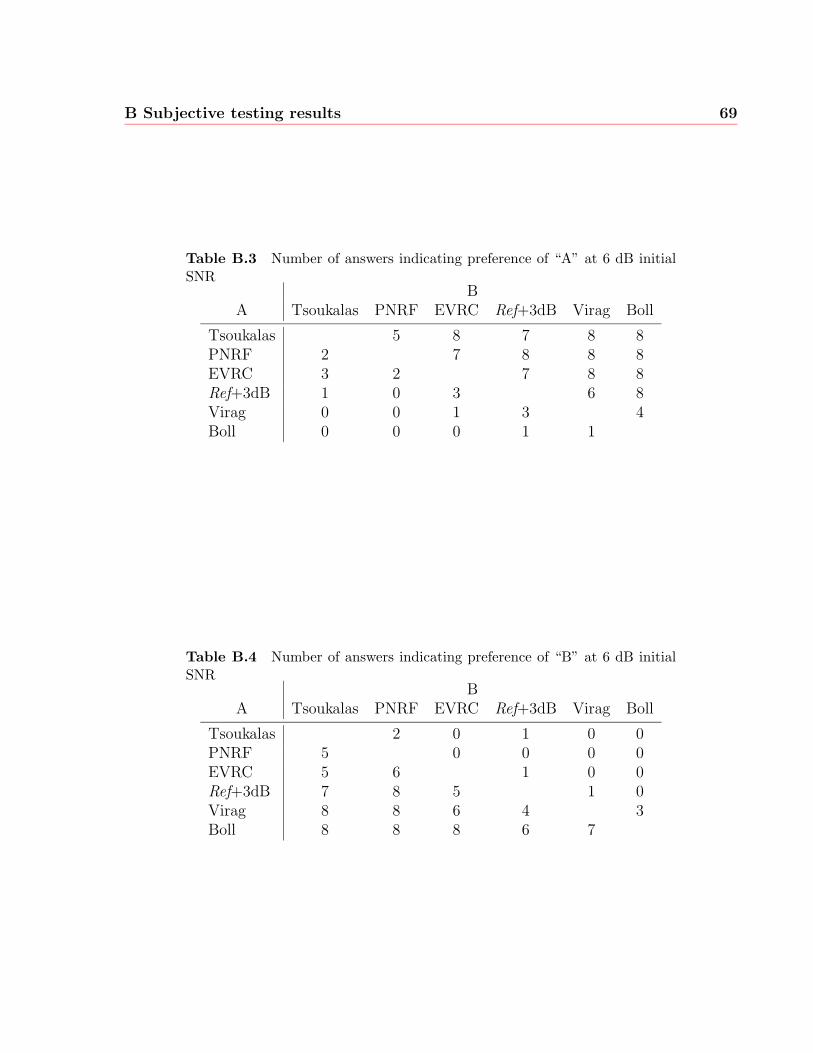
B Subjective testing results 69
Table B.3 Number of answers indicating preference of “A” at 6 dB initialSNR
BA Tsoukalas PNRF EVRC Ref+3dB Virag Boll
Tsoukalas 5 8 7 8 8PNRF 2 7 8 8 8EVRC 3 2 7 8 8Ref+3dB 1 0 3 6 8Virag 0 0 1 3 4Boll 0 0 0 1 1
Table B.4 Number of answers indicating preference of “B” at 6 dB initialSNR
BA Tsoukalas PNRF EVRC Ref+3dB Virag Boll
Tsoukalas 2 0 1 0 0PNRF 5 0 0 0 0EVRC 5 6 1 0 0Ref+3dB 7 8 5 1 0Virag 8 8 6 4 3Boll 8 8 8 6 7
70
References
[1] S. V. Vaseghi, Advanced Signal Processing and Digital Noise Reduction. Wiley Teub-ner, 1996.
[2] S. J. Godsill and P. J. W. Rayner, Digital Audio Restoration. Springer Verlag, 1998.
[3] J. John R. Deller, J. H. L. Hansen, and J. G. Proakis, Discrete-Time Processing ofSpeech Signals. New York: IEEE Press, 2000.
[4] G. Soulodre, Adaptive Methods for Removing Camera Noise from Film Soundtracks.PhD thesis, McGill University, Montreal, Canada, 1998.
[5] T. Painter and A. Spanias, “Perceptual coding of digital audio,” Proc. IEEE, vol. 88,pp. 451–513, Apr. 2000.
[6] D. E. Tsoukalas, J. N. Mourjopoulos, and G. Kokkinakis, “Speech enhancement basedon audible noise suppression,” IEEE Trans. Speech and Audio Processing, vol. 5,pp. 497–514, Nov. 1997.
[7] D. E. Tsoukalas, J. N. Mourjopoulos, and G. Kokkinakis, “Perceptual filters for audiosignal enhancement,” J. Audio Eng. Soc., vol. 45, pp. 22–35, Jan/Feb 1997.
[8] N. Virag, “Single channel speech enhancement based on masking properties of thehuman auditory system,” IEEE Trans. Speech and Audio Processing, vol. 7, pp. 126–137, Mar. 1999.
[9] T. Haulick, K. Linhard, and P. Schrogmeier, “Residual noise suppression using psy-choacoustic criteria,” in Eurospeech 97, (Rhodes, Greece), pp. 1395–1398, Sept. 1997.
[10] E. Zwicker and H. Fastl, Psychoacoustics. Springer Verlag, 2nd ed., 1999.
[11] D. O’Shaughnessy, Speech Communications: Human and Machine. IEEE Press,2nd ed., 2000.
[12] B. Gold and N. Morgan, Speech and Audio Signal Processing: Processing and Percep-tion of Speech and Music. John Wiley & Sons, 1999.
References 71
[13] B. C. J. Moore, An Introduction to the Psychology of Hearing. Academic Press, 4th ed.,1997.
[14] E. Terhardt, G. Stoll, and M. Seewann, “Algorithm for extraction of pitch and pitchsalience from complex tonal signals,” J. Acoust. Soc. Am., vol. 71, Mar. 1982.
[15] W. M. Hartmann, Signals, Sound, and Sensation. Springer Verlag, 1997.
[16] T. Thiede, W. C. Treurniet, R. Bitto, C. Schmidner, T. Sporer, J. G. Beerends,C. Colomes, M. Keyhl, G. Stoll, K. Brandenburg, and B. Feiten, “PEAQ - the ITUstandard for objective measurement of perceived audio quality,” J. Audio Eng. Soc.,vol. 48, Jan. 2000.
[17] E. Zwicker and E. Terhardt, “Analytical expressions for critical-band rate and criticalbandwidth as a function of frequency,” J. Acoust. Soc. Am., vol. 68, Nov. 1980.
[18] S. Voran, “Observations on auditory exitation and masking patterns,” in Applicationsof Signal Processing to Audio and Acoustics, IEEE ASSP Workshop on, pp. 206–209,Oct. 1995.
[19] S. F. Boll, “Suppression of acoustic noise in speech using spectral subtraction,” IEEETrans. Acoustics, Speech, Signal Processing, vol. ASSP-27, Apr. 1979.
[20] S. F. Boll, “A spectral subtraction algorithm for suppression of acoustic noise inspeech,” in Proc. IEEE Int. Conf. on Acoustics, Speech, Signal Processing, (Wash-ington, DC), pp. 200–203, Apr. 1979.
[21] R. J. McAulay and M. L. Malpass, “Speech enhancement using a soft-decision noisesuppression filter,” IEEE Trans. Acoustics, Speech, Signal Processing, vol. ASSP-28,Apr. 1980.
[22] J. S. Lim and A. V. Oppenheim, “Enhancement and badwidth compression of noisyspeech,” Proc. IEEE, vol. 67, Dec. 1979.
[23] A. S. Spanias, “Speech coding: A tutorial review,” Proc. IEEE, vol. 82, pp. 1541–1582,Oct. 1994.
[24] M. Berouti, R. Schwartz, and J. Makhoul, “Enhancement of speech corrupted byacoustic noise,” in Proc. IEEE Int. Conf. on Acoustics, Speech, Signal Processing,(Washington, DC), pp. 208–211, Apr. 1979.
[25] R. E. Crochiere, “A weighted overlap-add method of short-time fourier analy-sis/synthesis,” IEEE Trans. Acoustics, Speech, Signal Processing, vol. 28, Feb. 1980.
References 72
[26] J. G. Proakis and D. G. Manolakis, Digital Signal Processing: Principles, Algorithmsand Applications. Prentice-Hall, 3rd ed., 1996.
[27] A. V. Oppenheim and R. W. Schafer, Discrete-time Signal Processing. Prentice-Hall,1989.
[28] “Enhanced variable rate codec, speech service option 3 for wideband spread spectrumdigital systems,” Jan. 1996. TR-45, PN-3292 (to be published as IS-127).
[29] “Digital cellular telecommunications system (Phase 2+); Voice Activity Detector(VAD) for Adaptive Multi-Rate (AMR) speech traffic channels; General description(GSM 06.94 version 7.1.0 Release 1998),” 1998.
[30] Y. Ephraim and D. Mahlah, “Speech enhancement using a minimum mean-squareerror short-time spectral amplitude estimator,” IEEE Trans. Acoustics, Speech, SignalProcessing, vol. 32, pp. 1109–1121, Dec. 1984.
[31] O. Cappe, “Elimination of the musical noise phenomenon with the Ephraim and Malahnoise suppressor,” IEEE Trans. Speech and Audio Processing, vol. 2, pp. 345–349, Apr.1994.
[32] P. Scalart and J. V. Filho, “Speech enhancement based on a priori signal to noise esti-mation,” in Proc. IEEE Int. Conf. on Acoustics, Speech, Signal Processing, (Atlanta,GA), pp. 629–632, May 1996.
[33] H. Gustafsson, S. Nordholm, and I. Claesson, “Spectral subtraction with adaptiveaveraging of the gain function,” in Eurospeech 99, (Budapest, Hungary), pp. 2599–2602, Sept. 1999.
[34] Y. Ephraim and H. L. Van Trees, “A signal subspace approach for speech enhance-ment,” IEEE Trans. Speech and Audio Processing, vol. 3, July 1995.
[35] M. C. Reccione, “The enhanced variable rate coder: Toll quality speech for CDMA,”Int. J. of Speech Technology, pp. 305–315, 1999.
[36] J. D. Johnston, “Transform coding of audio signals using perceptual noise criteria,”IEEE J. Selected Areas in Comm., vol. 6, pp. 314–323, Feb. 1988.
[37] M. R. Scroeder, B. S. Atal, and J. L. Hall, “Optimizing digital speech coders byexploiting masking properties of the human ear,” J. Acoust. Soc. Am., vol. 66, Dec.1979.
[38] D. Sinha and A. H. Tewfik, “Low bit rate transparent audio compression using adaptedwavelets,” IEEE Trans. Signal Processing, vol. 41, pp. 3463–3479, Dec. 1993.
References 73
[39] J. G. Beerends and J. A. Stemerdink, “A perceptual audio quality measure based ona psychoacoustic sound representation,” J. Audio Eng. Soc., vol. 40, Dec. 1992.
[40] “Method for objective measurements of percieved audio quality,” 1998. Recommen-dation ITU-R BS.1387.
[41] W. C. Treurniet and G. Soulodre, “Evaluation of the ITU-R objective audio qualitymeasurement method,” J. Audio Eng. Soc., vol. 48, Mar. 2000.
[42] T. L. Petersen and S. F. Boll, “Acoustic noise suppression in the context of a perceptualmodel,” in Proc. IEEE Int. Conf. on Acoustics, Speech, Signal Processing, (Atlanta,Georgia), pp. 1086–1088, Apr. 1981.
[43] Y. M. Cheng and D. O’Shaughnessy, “Speech enhancement based conceptually onauditory evidene,” IEEE Trans. Signal Processing, vol. 39, Sept. 1991.
[44] D. Tsoukalas, M. Paraskevas, and J. Mourjopoulos, “Speech enhancement using psy-choacoustic criteria,” in Proc. IEEE Int. Conf. on Acoustics, Speech, Signal Processing,(Minneapolis, MN), pp. II-359–II-362, Apr. 1993.
[45] T. E. Eger, J. C. Su, and L. W. Varner, “A nonlinear spectrum processing techniquefor speech enhancement,” in Proc. IEEE Int. Conf. on Acoustics, Speech, Signal Pro-cessing, (San Diego, CA), pp. 18A.1.1–18A.1.4, Mar. 1984.
[46] P. M. Clarkson and S. F. Bahgat, “Envelope expansion methods for speech enhance-ment,” J. Acoust. Soc. Am., vol. 89, pp. 1378–1382, Mar. 1991.
[47] M. Lorber and R. Hoeldrich, “A combined approach for broadband noise reduction,”in Proc. IEEE Workshop on Audio and Acoustics, (Mohonk, NY), Oct. 1997.
[48] “Signal Processing Information Base.” Located at http://spib.rice.edu/spib.html,URL current as of March 2001.
[49] “Digital cellular telecommunication system (phase 2+); results of the AMR noisesuppression selection phase,” June 2000. GSM 06.78 version 0.5.0.
[50] “Objective measurement of active speech level,” 1993. Recommendation ITU-T P.56.
[51] S. R. Quackenbush, T. P. Barnwell III, and M. A. Clements, Objective Measures ofSpeech Quality. Prentice-Hall, 1988.
[52] “Digital cellular telecommunications system (Phase 2+); Minimum Performance Re-quirements for Noise Suppressor; Application to the AMR Speech Encoder (GSM 06.77version 1.3.0),” 2000.
References 74
[53] “Methods for subjective determination of transmission quality,” 1993. Recommenda-tion ITU-T P.80.
[54] “Method for objective and subjective assessment of telephone-band and widebanddigital codecs,” 1996. Recommendation ITU-T P.830.