· ACKNOWLEDGMENTS I never thought that one day I would be writing these acknowledgments as part of my dissertation. Being from a small place and rural background I hardly ever imagi

Some Aspects of Hadron HadronCollisions in High Energy Interactions(B0

s mixing oscillations in semileptonicdecay at DØ Experiment)

THESIS SUBMITTED TO THE UNIVERSITY OF DELHIFOR THE DEGREE OF

DOCTOR OF PHILOSOPHY

MD. NAIMUDDIN

SUPERVISOR: PROF. R. K. SHIVPURIPROF. D. S. KULSHRESHTHA

DEPARTMENT OF PHYSICS & ASTROPHYSICSUNIVERSITY OF DELHI

DELHI 110 007INDIA

2006

Dedicated ToMy Parents and family of which I am an integral

part & to my late brother-in-law Md. Shaifuzzama

whom we all miss

ii

ACKNOWLEDGMENTS

I never thought that one day I would be writing these acknowledgments as part

of my dissertation. Being from a small place and rural background I hardly ever

imagined that some day I would be working in one of the best lab and with best

minds in the world and that I would be scratching my head to find the answers to

the most fundamental questions that we have in front of us today.

And the one person who got me into this business is my mentor, teacher and

supervisor Prof. R. K. Shivpuri. I wish to express my heartfelt thanks to him. At

each and every stage of my M.Sc. days he always encouraged and motivated me to

join the research and he was always there to help me out with any problem. I learned

the basics of high energy and nuclear physics from him. I was really impressed by his

deep understandings of the subject and his magnificent style of teaching. His way of

explaining the most difficult and complicated things in simple and lucid way surprises

everyone. There used to have a Que of students in front of his office to get a chance

to work in his lab and I consider myself lucky that I got the opportunity to work with

him. I have seen very few people who work so selflessly and always think best for

his students. I seldom have seen the parallels of the magnanimous character that he

possesses. I am inspired by his tremendous energy, patience and utmost care for his

students. And above all he is a marvelous human being and a great soul. I share a

special relationship and a great bond of trust with him. I am also grateful to him for

reading and correcting my thesis.

I would also like to express my sincere thanks to my thesis adviser Prof. D. S.

Kulshreshtha. Without his help and support this thesis would not have completed.

He is the person from whom I have always learned something new. His relationship

with me is more than that of teacher and a student. I do not find the words to thank

him as it is simply impossible to return his favors in thanks. Good times, bad times

he was always a call away and has patience to listen to my complicated problems and

then to solve them. It was a privilege and pleasure to work with him as he has given

me the complete freedom to do my research. I had even the privilege to disturb him

at his home whenever I needed him. I consider myself fortunate to have him as my

supervisor.

I wish to express my special thanks to the Head of the Department of Physics,

Prof. M. P. Srivastava for providing the necessary facilities in the department. I met

and worked with many wonderful people during my stay at Fermilab. It would not

be possible to thank everyone of them individually here and I just wish that I could

reciprocate whatever I earned from them.

iv

First and foremost my sincere thanks to my local supervisor at Fermilab, Dr.

Gene Fisk. He is one person who never let me felt away from home. From the first

day, he took care of all my needs and always motivated me to work hard and excel

in life. It was his motivation and unconditional support that I was able to contribute

whatever little I could in so less time. Despite being incredibly busy, the doors of

his office was always open to me and I had the privilege to bother him anytime. He

always has time to listen to my problems and trying to find the solutions. I greatly

benefited from the long discussions we used to have on my analysis, detector, etc. I

am really fortunate that I found Gene as my local supervisor at Fermilab. Thanks a

lot Gene for all your help and personal care.

The other person who was not less than my supervisor at DØ is Prof. Jerry Blazey.

He always encouraged and motivated me to take the challenges and got me involved

in the interesting and right projects. It was his personal care that I got a chance to

work on hardware and software projects along with my physics analysis which helped

me develop myself as a complete high energy physicists. Thank you very much Jerry

for all your guidance and care and for reading the proofs of my thesis and correcting

the same despite being incredibly busy those days.

I also consider myself fortunate to have Prof. Brajesh Choudhary as my local

guardian during my stay at Fermilab. His support, help and care for me was invalu-

able. I remember how worried he was when I had to go for the US visa and how

happy he felt when I got it. I share a great relationship with him and he is more like

an elder brother and a friend. Thank you very much sir for all your help and care all

along these years and for the long discussions we used to have on variety of topics.

I would also like to thank Prof. Feroz Ahmed for his guidance and support during

the troubled days and always encouraging me to do best in life. A special thanks to

Prof. Brad Abbott for working with me all along my stay at Fermilab and guiding

me through my analysis and always taking care of my interests. I would also like to

thanks Vivek Jain who encouraged me to work on B0s mixing and also for motivating

me to work on the development of electron tagging. Many thanks to B physics

group conveners Brendan Casey and Guennadi Borissov for working with me on mass

fitting and always encouraging me to get the results and present in the meetings. I

always used to turn to Brendan for basic B physics questions and to clear my doubts.

Working with Guennadi was a wonderful and enriching experience for me. He is

full of new ideas and tremendous energy. I also owe lot of thanks to the previous B

Physics convener Rick Van Kooten for providing me the opportunity, freedom and

infrastructure in the group to carry out my analysis. My sincere thanks to Mixing

v

convener Sergey Burdin for his help throughout the mixing analysis. I would also like

to thank Tania Moulik for working with me on electron tagging and helping me out

with the softwares during my initial days at DØ. I am grateful to Prof. Terry Wyatt

for his continuous support and motivation in all my work.

I am very thankful to Hal Evans and Nikos Varelas for supporting and encouraging

me during my stunt with L1 calorimeter upgrade project. I really enjoyed and learned

a lot while working on l1cal upgrade. I am thankful to Mike Mulhearn and Sabine

Lammers for providing a wonderful and stimulating environment during l1cal work

and for the extraordinary understanding we had in carrying out our task so efficiently

and also for assisting me in my testings of the systems even in the middle of night

or in the early morning. I am also thankful to Darien Wood and George Ginther

for their encouraging words because of which we could finish our l1cal work in time.

Thanks also to Alan Stone, Lyn Bagby, Dan Edmonds, Dean Schamberger and Todd

Adams for the useful discussions we had on various l1cal issues.

I would also like to thank my Global Monitoring colleagues who always helped

me running the GM efficiently. A lot of thanks to Elliott Cheu for sharing the

responsibility of GM with me. Thanks also to Michiel Sanders for helping me get

acquainted with the GM tools. I also owe thanks to Matthew Ford and Dennis

Mackin for helping me in keeping GM running without problems. I would also like to

thank DØ run coordinators Bill Lee and Taka Yasuda for their cooperation in proper

running of GM.

A big thanks to my Delhi colleagues Kirti and Ashish for a wonderful and memo-

rable time we had during our stay at Delhi House. For their consistent encouragement

and support in all my endeavors and for never letting me feel bored and away from

home. And also for the useful and stimulating physics discussions we used to have in

our leisure time.

I owe a lot of thanks to my friend and colleague Burair for getting me acquainted

with the DØ data structure during my initial days and helping me whenever I had

any problem with my Linux box. And also for the long overnight discussions we had

on physics and beyond which sometimes used to end only with the beginning of the

day. I am also thankful to B physics colleagues and friends Cano and Dan for working

with me on mixing and the useful discussions we used to have on the various analysis

issues. Thanks to my friend Ralf for the wonderful time we had at Moriond and for

taking care of my Monte Carlo samples. I would also like to express my thanks to my

B physics colleagues Rick jesik, Alberto, Dmitri and others for the useful discussions.

I would also like to thank Shekhar and Tanuja Mishra for the continuous en-

vi

couragement and the wonderful dinners. Thanks also to Vishnu Zutshi and family,

Mrinmoy and Barnali, Harpareet and Geeti and Shailesh and Vandana for their invi-

tations for dinners, meaningful discussions and classical jokes.

Many thanks to Mr. P.C. Gupta ji for his consistent support and care. He is a

great soul with extraordinary conviction and utmost humility. Thanks to my Delhi

Colleagues Ashutosh Bhardwaj, Namrata, Sudeep, Manoj, Ajay, Ashutosh Srivastava,

Sushil and Pooja for a wonderful time and company during my Delhi days. Thanks

also to Mr. G.D. Sharma, Rajendra, Yunus and Dinesh for their continuous assistance.

Many thanks to my friends at DØ Avdhesh, Venkat, Tulika, Wade, Miruna, Peter,

Piyali, Jyotsana, Supriya, Subhendu, Prolay and Miroslav. Thanks also to Ariel,

Christos, Peier Petroff, Laurent Duflot for helping me out in need. A special thanks

to Jan Stark for taking interest in my electron tagging analysis and for helping me

with em-ID and softwares and for the stimulating and long discussions we had on

variety of physics and detector issues.

I am also thankful to my old friends Ehtesham, Nadeem, Hema, Pradeep, Kopal,

Pranav, Arijeet, Raksha, Hemant, Ravi, Mrinal, Noor Rahman, Riyaz, Ashraf, Asad,

Farhat and Riyaz Hashmi for their continuous love and support.

I would also like to thank Council of Scientific and Industrial Research (CSIR),

Govt. of India for the financial support. Thanks also to Universities Research Asso-

ciation (Fermilab) for their support during my stay at Fermilab.

And finally I would like to express my gratitude to my parents and family who

were always with me in my bad and good times and for their unconditional love.

They are the source of inspiration and the reason for me to do good in life. My Abba

being raised in difficult times and having spent most of his life in hardship has never

let me felt the hardships and did everything to help me achieve my goals. My Amma

always wanted me to go for higher studies and inculcated in me whatever good values

I possess. My parents are my ideals and I am nothing without them. Even If I adopt

half the good values they possesses I would consider my life to be successful. I would

also like to thank my elder sister for her continuous prayers and utmost support and

love for me. I thank to my other sisters, brothers and nieces for all the support and

happiness they provided me during these years.

MD. NAIMUDDIN

vii

LIST OF PUBLICATIONS

1. “Direct Limits on the B0s Oscillation Frequency”, DØ Collaboration (V. M.

Abazov, ..., Md. Naimuddin, et. al.), Phys. Rev. Lett. 97, 021802

(2005).

2. “Study of B0s Mixing at the Tevatron”, Md. Naimuddin, Proceedings of 41st

Moriond QCD Conference (2006), hep/ex-0605057.

Conference & DØ Notes

1. “B-Flavor Tagging with Soft electrons”, Md. Naimuddin et. al., DØ Note 4713

(2005).

2. “Bd Mixing measurement using semileptonic sample and combined opposite side

tagging”, G. Borrisov, ..., Md. Naimuddin, et al., DØ Note 4828 (2005), Sub-

mitted to PRD.

3. “B0s mixing in semileptonic Bs decays using D−

s → φπ−decay mode”, C. Ay, ...,

Md. Naimuddin, et. al., DØ Note 4842 (2005).

4. “B-Flavor tagging with opposite-side soft electrons”, Md. Naimuddin et al., DØ

Note 4848, (2005) (Conference Note for 2005 Summer Conferences).

5. “Study of Trilepton triggers”, Md. Naimuddin et al., DØ Note 4849 (2005).

6. “A search for B0s oscillations at DØ using B0

s → D−s µ

+X (D−s → K∗0K− )” C.

Ay, ..., Md. Naimuddin, et. al. DØ Note 4863 (2005).

7. “Combined Opposite-side Flavor Tagging”, C. Ay, ..., Md. Naimuddin, et. al.,

DØ Note 4875 (2005) (Conference Note for 2005 Summer Conferences).

8. “A search for B0s oscillations at DØ using B0

s → D−s µ

+X (D−s → K∗0K− ) ”,

C. Ay, ..., Md. Naimuddin, et. al., DØ Note 4878 (2005) (Conference Note

for 2005 Summer Conferences).

9. “Mixing in the B0s System Using B0

s → D−s µ

+X , D−s → φπ−decay mode and

opposite side flavor tagging”, C. Ay, ..., Md. Naimuddin, et al., DØ Note 4881

(2005) (Conference Note for 2005 Summer Conferences).

10. “B0s Mixing measurement at DØ Using B0

s → D−s µ

+X (D−s → K∗0K− )”, B.

Abbott, ..., Md. Naimuddin, et al., DØ Note 5015 (2006).

viii

11. “Global Monitoring at DØ”, Md. Naimuddin et. al., DØ Note 5141 (2006).

12. “B0s mixing studies in Semileptonic B0

s decays with D−s → K∗0K− and Unbinned

fit”, B. Abbott, ..., Md. Naimuddin, et. al., DØ Note 5149 (2006)

13. “B0s mixing studies in Semileptonic B0

s decays with D−s → K∗0K− and Unbinned

fit ”, B. Abbott, ..., Md. Naimuddin, et. al., DØ Note 5172 (2006) (Conference

Note for 2006 Summer Conferences).

14. “A combination of B0s Oscillations Results from DØ”, G. Borrisov, ..., Md.

Naimuddin, et. al., DØ Note 5207 (2006) (Conference Note for 2006 Sum-

mer Conferences).

ix

Contents

1 Introduction 1

2 Theoretical Overview 5

2.1 The Standard Model . . . . . . . . . . . . . . . . . . . . . . . . . . . 5

2.1.1 The Electroweak Theory . . . . . . . . . . . . . . . . . . . . . 7

2.1.2 The b Quark . . . . . . . . . . . . . . . . . . . . . . . . . . . 7

2.1.3 bb Production Mechanism . . . . . . . . . . . . . . . . . . . . 8

2.2 Heavy Flavor Hadrons . . . . . . . . . . . . . . . . . . . . . . . . . . 11

2.3 Quark Mixing . . . . . . . . . . . . . . . . . . . . . . . . . . . . . . . 12

2.4 CKM Matrix . . . . . . . . . . . . . . . . . . . . . . . . . . . . . . . 14

2.5 Neutral BB Mixing . . . . . . . . . . . . . . . . . . . . . . . . . . . . 19

2.6 Experimental Technique . . . . . . . . . . . . . . . . . . . . . . . . . 26

2.6.1 Event Selection . . . . . . . . . . . . . . . . . . . . . . . . . . 27

2.6.2 Flavor Tagging . . . . . . . . . . . . . . . . . . . . . . . . . . 28

2.6.3 Proper time resolution . . . . . . . . . . . . . . . . . . . . . . 30

2.6.4 Overview of the Mixing Analysis . . . . . . . . . . . . . . . . 32

2.6.5 The Amplitude Method . . . . . . . . . . . . . . . . . . . . . 35

3 Experimental Apparatus 39

3.1 Experimental Framework . . . . . . . . . . . . . . . . . . . . . . . . . 39

3.1.1 The Tevatron . . . . . . . . . . . . . . . . . . . . . . . . . . . 41

3.2 The DØ Detector . . . . . . . . . . . . . . . . . . . . . . . . . . . . 43

3.3 Coordinate system . . . . . . . . . . . . . . . . . . . . . . . . . . . . 44

3.4 Central Tracking System . . . . . . . . . . . . . . . . . . . . . . . . . 47

3.4.1 Silicon Microstrip Tracker (SMT) . . . . . . . . . . . . . . . . 49

3.4.2 Central Fiber Tracker . . . . . . . . . . . . . . . . . . . . . . . 51

3.4.3 Solenoid . . . . . . . . . . . . . . . . . . . . . . . . . . . . . . 53

3.4.4 Preshower Detectors . . . . . . . . . . . . . . . . . . . . . . . 53

3.5 The Calorimeter . . . . . . . . . . . . . . . . . . . . . . . . . . . . . . 55

i

3.5.1 DØ Calorimeter . . . . . . . . . . . . . . . . . . . . . . . . . . 57

3.5.2 Electromagnetic Calorimeter . . . . . . . . . . . . . . . . . . . 59

3.5.3 Hadronic Calorimeter . . . . . . . . . . . . . . . . . . . . . . . 59

3.5.4 Intercryostat and Massless Gaps Detectors . . . . . . . . . . . 62

3.6 Muon System . . . . . . . . . . . . . . . . . . . . . . . . . . . . . . . 62

3.7 Trigger . . . . . . . . . . . . . . . . . . . . . . . . . . . . . . . . . . . 65

3.8 Level 1 Trigger Elements . . . . . . . . . . . . . . . . . . . . . . . . . 66

3.8.1 Track Triggers . . . . . . . . . . . . . . . . . . . . . . . . . . . 66

3.8.2 L1 Calorimeter Trigger . . . . . . . . . . . . . . . . . . . . . . 67

3.8.3 Motivations for Upgradation . . . . . . . . . . . . . . . . . . . 71

3.8.4 New L1 Cal Trigger System . . . . . . . . . . . . . . . . . . . 71

3.8.5 ADF to TAB Data Transmission . . . . . . . . . . . . . . . . 72

3.8.6 TAB to L2/L3 Data Transmission . . . . . . . . . . . . . . . . 74

3.8.7 Full System Tests . . . . . . . . . . . . . . . . . . . . . . . . . 74

3.8.8 Muon Triggers . . . . . . . . . . . . . . . . . . . . . . . . . . . 75

3.8.9 Level 1 Calorimeter-Track Matching . . . . . . . . . . . . . . 76

3.8.10 Trigger Framework . . . . . . . . . . . . . . . . . . . . . . . . 76

3.9 L2 Trigger . . . . . . . . . . . . . . . . . . . . . . . . . . . . . . . . . 77

3.10 L3 Trigger . . . . . . . . . . . . . . . . . . . . . . . . . . . . . . . . . 77

4 Initial State Tagging 79

4.1 Introduction . . . . . . . . . . . . . . . . . . . . . . . . . . . . . . . . 79

4.2 Soft Electron Tagging . . . . . . . . . . . . . . . . . . . . . . . . . . . 79

4.3 B± → J/ψK± decay reconstruction . . . . . . . . . . . . . . . . . . . 80

4.4 Soft electron selection . . . . . . . . . . . . . . . . . . . . . . . . . . . 81

4.5 Electron tagging . . . . . . . . . . . . . . . . . . . . . . . . . . . . . . 83

4.5.1 Electron tagging in Monte Carlo . . . . . . . . . . . . . . . . . 85

4.5.2 Electron tagging in data . . . . . . . . . . . . . . . . . . . . . 87

4.6 Conclusion . . . . . . . . . . . . . . . . . . . . . . . . . . . . . . . . . 89

4.7 Fit Cross checks . . . . . . . . . . . . . . . . . . . . . . . . . . . . . . 89

4.8 B0d mixing with electron tagging . . . . . . . . . . . . . . . . . . . . . 90

4.8.1 Untagged sample Reconstruction . . . . . . . . . . . . . . . . 90

4.8.2 Tagged Sample . . . . . . . . . . . . . . . . . . . . . . . . . . 93

4.9 Experimental Observables . . . . . . . . . . . . . . . . . . . . . . . . 95

4.10 Fitting procedure and results . . . . . . . . . . . . . . . . . . . . . . 97

4.11 A study of systematic uncertainties . . . . . . . . . . . . . . . . . . . 99

4.12 Conclusions . . . . . . . . . . . . . . . . . . . . . . . . . . . . . . . . 102

ii

4.13 Combined Tagging . . . . . . . . . . . . . . . . . . . . . . . . . . . . 103

4.13.1 Discriminating Variables . . . . . . . . . . . . . . . . . . . . . 104

4.13.2 The Combined Tagger . . . . . . . . . . . . . . . . . . . . . . 107

4.14 Results . . . . . . . . . . . . . . . . . . . . . . . . . . . . . . . . . . . 107

4.15 Conclusions . . . . . . . . . . . . . . . . . . . . . . . . . . . . . . . . 114

5 B0s Mixing Analysis 117

5.1 Introduction . . . . . . . . . . . . . . . . . . . . . . . . . . . . . . . . 117

5.2 Event Selection . . . . . . . . . . . . . . . . . . . . . . . . . . . . . . 118

5.3 Mass Fitting Procedure . . . . . . . . . . . . . . . . . . . . . . . . . . 121

5.4 Initial State Flavor Tagging . . . . . . . . . . . . . . . . . . . . . . . 128

5.5 Unbinned Likelihood Fit Method . . . . . . . . . . . . . . . . . . . . 129

5.5.1 pdf for µDs Signal . . . . . . . . . . . . . . . . . . . . . . . . 132

5.5.2 pdf for µD± (D± → K∗0K±) Signal . . . . . . . . . . . . . . . 135

5.5.3 pdf for Combinatorial Background . . . . . . . . . . . . . . . 136

5.6 Inputs to the Fit . . . . . . . . . . . . . . . . . . . . . . . . . . . . . 138

5.6.1 Sample Composition . . . . . . . . . . . . . . . . . . . . . . . 138

5.6.2 K Factor . . . . . . . . . . . . . . . . . . . . . . . . . . . . . 140

5.6.3 Reconstruction Efficiencies . . . . . . . . . . . . . . . . . . . . 142

5.6.4 Resolution Scale Factor . . . . . . . . . . . . . . . . . . . . . . 145

5.7 Results of the Lifetime Fit . . . . . . . . . . . . . . . . . . . . . . . . 146

5.8 Fitting Procedure for ∆ms Limit . . . . . . . . . . . . . . . . . . . . 146

5.9 Results . . . . . . . . . . . . . . . . . . . . . . . . . . . . . . . . . . . 148

5.10 Cross Checks and Systematics . . . . . . . . . . . . . . . . . . . . . . 148

5.10.1 Dilution . . . . . . . . . . . . . . . . . . . . . . . . . . . . . . 149

5.10.2 Mass fitting procedure . . . . . . . . . . . . . . . . . . . . . . 149

5.10.3 Resolution . . . . . . . . . . . . . . . . . . . . . . . . . . . . . 151

5.10.4 Sample Composition . . . . . . . . . . . . . . . . . . . . . . . 151

5.10.5 K factor . . . . . . . . . . . . . . . . . . . . . . . . . . . . . . 151

5.11 Conclusions . . . . . . . . . . . . . . . . . . . . . . . . . . . . . . . . 152

6 Combination and Results 155

6.1 Introduction . . . . . . . . . . . . . . . . . . . . . . . . . . . . . . . . 155

6.2 Combination . . . . . . . . . . . . . . . . . . . . . . . . . . . . . . . . 155

6.3 Log Likelihood Scan . . . . . . . . . . . . . . . . . . . . . . . . . . . 157

6.4 Conclusion . . . . . . . . . . . . . . . . . . . . . . . . . . . . . . . . . 158

iii

List of Figures

2.1 Leading order diagrams for bb production. . . . . . . . . . . . . . . . 9

2.2 Next-to-Leading order diagrams for bb production. . . . . . . . . . . . 10

2.3 Feynman diagrams for B− decays in the spectator model. . . . . . . . 12

2.4 The rescaled Unitarity Triangle. . . . . . . . . . . . . . . . . . . . . . 18

2.5 Leading order box diagrams for B mixing. . . . . . . . . . . . . . . . 19

2.6 A diagram showing the tagging details. . . . . . . . . . . . . . . . . . 29

2.7 Schematic of a B → DµνX decay. . . . . . . . . . . . . . . . . . . . . 31

2.8 On the left is the mixing amplitude in ideal case and effect on mixing

amplitude due to finite decay length resolution is shown on right. . . 33

2.9 Effect on amplitude due to flavor mis-tagging (left) and combining all

the effects (right) . . . . . . . . . . . . . . . . . . . . . . . . . . . . . 33

2.10 World average amplitude for B0s which includes all the published results

up to 2004. . . . . . . . . . . . . . . . . . . . . . . . . . . . . . . . . 36

2.11 Fit to the CKM triangle using all the results up to summer 2005. . . 37

3.1 Fermilab Accelerator Complex . . . . . . . . . . . . . . . . . . . . . . 40

3.2 Side view of the DØ detector [26]. . . . . . . . . . . . . . . . . . . . 45

3.3 DØ coordinate system. . . . . . . . . . . . . . . . . . . . . . . . . . 46

3.4 Difference between Detector and Physics η. . . . . . . . . . . . . . . . 47

3.5 Schematic of the central tracking system. . . . . . . . . . . . . . . . 48

3.6 Isometric view of SMT. . . . . . . . . . . . . . . . . . . . . . . . . . 49

3.7 Schematic diagram of a silicon microstrip detector . . . . . . . . . . . 51

3.8 Cross Section view of the CFT detector . . . . . . . . . . . . . . . . . 52

3.9 Cross section view of the Preshower detector. . . . . . . . . . . . . . 55

3.10 Overall view of the DØ calorimeter system [26]. . . . . . . . . . . . . 58

3.11 A quarter of the calorimeter in the r− z plane of the detector showing

the tower geometry. . . . . . . . . . . . . . . . . . . . . . . . . . . . 60

3.12 Unit Cell in the Calorimeter. . . . . . . . . . . . . . . . . . . . . . . 61

3.13 Exploded view of the muon wire Chambers. . . . . . . . . . . . . . . 63

v

3.14 Schematic of the DØtrigger system . . . . . . . . . . . . . . . . . . . 66

3.15 Block diagram of L1 calorimeter trigger . . . . . . . . . . . . . . . . . 68

3.16 Block Diagram of TAB . . . . . . . . . . . . . . . . . . . . . . . . . . 73

3.17 Comparison plots for L1Cal2b trigger tower energies with L1Cal2a and

precision measurement using the test run data . . . . . . . . . . . . . 75

4.1 Total number of B candidates using nseg(µ) ≥ 0 . . . . . . . . . . . . 82

4.2 B candidates where kaon PT > 1.0 GeV (L) and kaon PT < 1.0 GeV (R) 82

4.3 P relT distribution for the tag electron . . . . . . . . . . . . . . . . . . 84

4.4 ∆η and ∆φ between EM object track and the generator level electron

(| η |< 1.1) . . . . . . . . . . . . . . . . . . . . . . . . . . . . . . . . . 86

4.5 EP

and EMF of EM object track matched to generator level electron

(| η |< 1.1) . . . . . . . . . . . . . . . . . . . . . . . . . . . . . . . . . 87

4.6 B mass distribution in the MC sample . . . . . . . . . . . . . . . . . 88

4.7 Right sign and wrong sign tagged candidates in MC sample using cen-

tral electrons . . . . . . . . . . . . . . . . . . . . . . . . . . . . . . . 88

4.8 Right sign and wrong sign tagged events in data using central electrons 89

4.9 The invariant mass of the Kπ system for µ+K+π− candidates before

electron tagging. . . . . . . . . . . . . . . . . . . . . . . . . . . . . . 91

4.10 The mass difference M(D0π)−M(D0) for events with 1.75 < M(D0) <

1.95 GeV/c2. . . . . . . . . . . . . . . . . . . . . . . . . . . . . . . . 92

4.11 Minimum CPS Single Layer Cluster energy of electrons (from photon

conversions) and pions (from K0S decays) . . . . . . . . . . . . . . . . 94

4.12 . . . . . . . . . . . . . . . . . . . . . . . . . . . . . . . . . . . . . . . 95

4.13 . . . . . . . . . . . . . . . . . . . . . . . . . . . . . . . . . . . . . . . 100

4.14 . . . . . . . . . . . . . . . . . . . . . . . . . . . . . . . . . . . . . . . 100

4.15 . . . . . . . . . . . . . . . . . . . . . . . . . . . . . . . . . . . . . . . 108

4.16 . . . . . . . . . . . . . . . . . . . . . . . . . . . . . . . . . . . . . . . 109

4.17 The asymmetries obtained in the D∗ and D0 sample with the result

of the fit superimposed for the Muon and electron tagger. For the

individual taggers, |d| > 0.3 was required. . . . . . . . . . . . . . . . . 110

4.18 The asymmetries obtained in the D∗ and D0 sample with the com-

bined tagger for bin |d| > 0.6. The result of the fit is superimposed . 111

5.1 Distribution of the mass of D−s → K∗0K− candidates. Both “right-

sign” (red) and “wrong-sign” (black) combinations are shown. . . . . 121

vi

5.2 Distribution of the reflection variable R for both signal (red) and D+

reflection (green) MC. . . . . . . . . . . . . . . . . . . . . . . . . . . 123

5.3 Distribution of (Kπ)K mass in three different bins of the variable R

with the fit results overlayed. The individual histograms at the bottom

show the different components separately. . . . . . . . . . . . . . . . . 123

5.4 Distribution of C(R). . . . . . . . . . . . . . . . . . . . . . . . . . . . 125

5.5 Distribution of M0(R). . . . . . . . . . . . . . . . . . . . . . . . . . . 125

5.6 Distribution of (Kπ)K mass for R < 0.22. The background shape is

quite different in this region. . . . . . . . . . . . . . . . . . . . . . . . 126

5.7 Fit to the total untagged sample, dots represents the data points and

histogram is the fit result.In this plot, dark blue histogram shows the

signal component, light blue is the D± reflection, magenta is the cab-

bibo D± decay and golden color is for the component due to Λc re-

flection. The red crosses are the signal subtracted background and the

green line is the fit to the combinatoric background. . . . . . . . . . . 127

5.8 Fit to the total tagged sample, dots represents the data points and

histogram is the fit result. . . . . . . . . . . . . . . . . . . . . . . . . 128

5.9 Distributions of VPDL errors for signal and combinatorial background. 131

5.10 Distributions of predicted dilution for signal and combinatorial back-

ground. . . . . . . . . . . . . . . . . . . . . . . . . . . . . . . . . . . 131

5.11 Distributions of selection variable for signal and combinatorial back-

ground. . . . . . . . . . . . . . . . . . . . . . . . . . . . . . . . . . . 131

5.12 Dilution calibration. . . . . . . . . . . . . . . . . . . . . . . . . . . . 133

5.13 . . . . . . . . . . . . . . . . . . . . . . . . . . . . . . . . . . . . . . . 133

5.14 . . . . . . . . . . . . . . . . . . . . . . . . . . . . . . . . . . . . . . . 141

5.15 . . . . . . . . . . . . . . . . . . . . . . . . . . . . . . . . . . . . . . . 142

5.16 . . . . . . . . . . . . . . . . . . . . . . . . . . . . . . . . . . . . . . . 143

5.17 . . . . . . . . . . . . . . . . . . . . . . . . . . . . . . . . . . . . . . . 143

5.18 . . . . . . . . . . . . . . . . . . . . . . . . . . . . . . . . . . . . . . . 143

5.19 . . . . . . . . . . . . . . . . . . . . . . . . . . . . . . . . . . . . . . . 144

5.20 . . . . . . . . . . . . . . . . . . . . . . . . . . . . . . . . . . . . . . . 144

5.21 . . . . . . . . . . . . . . . . . . . . . . . . . . . . . . . . . . . . . . . 144

5.22 . . . . . . . . . . . . . . . . . . . . . . . . . . . . . . . . . . . . . . . 144

5.23 . . . . . . . . . . . . . . . . . . . . . . . . . . . . . . . . . . . . . . . 145

5.24 . . . . . . . . . . . . . . . . . . . . . . . . . . . . . . . . . . . . . . . 145

vii

5.25 Distribution of events on VPDL in right band region (2.15 < MDs<

2.25 GeV)(left plot) and signal peak region (1.91 < MDs< 2.03 GeV)(right

plot) on log scale. Points represent experimental data and histogram

— fitting function. . . . . . . . . . . . . . . . . . . . . . . . . . . . . 146

5.26 Distribution of events on VPDL in right band region (2.15 < MDs<

2.25 GeV)(left plot) and signal peak region (1.91 < MDs< 2.03 GeV)

(right plot) on linear scale.Points represent experimental data and his-

togram — fitting function. . . . . . . . . . . . . . . . . . . . . . . . . 147

5.27 B0s oscillation amplitude with statistical and systematic errors. . . . . 148

5.28 Bd − Bd oscillation amplitude. . . . . . . . . . . . . . . . . . . . . . . 150

5.29 Bd−Bd oscillation amplitude (detailed view of the Bd oscillation region).150

5.30 Fit to the M(Kπ)K distribution for M(Kπ) > 1 GeV . Tiny blue

histogram at the bottom is the D−s → K∗0K− signal, light blue is the

D± reflection, golden color is the Λ±c reflection and green curve is the

fit to the combinatoric background. . . . . . . . . . . . . . . . . . . . 150

6.1 B0s oscillation amplitude with statistical and systematic errors forB0

s → D−s µ

+νX,

(D−s → K∗K−) decay mode. . . . . . . . . . . . . . . . . . . . . . . . 156


s → D−s µ

+νX,

(D−s → φπ−) decay mode. . . . . . . . . . . . . . . . . . . . . . . . . 156


s →D−

s e+νX, (D−

s → φπ−) decay mode. . . . . . . . . . . . . . . . . . . 156


s →D−

s e+νX and B0

s → D−s µ

+νX (D−s → φπ−) decay modes. . . . . . . . 156


s →D−

s µ+νX (D−

s → φπ− and D−s → K∗K−) decay modes. . . . . . . . . 157


s →D−

s e+νX (D−

s → φπ−) and B0s → D−

s µ+νX (D−

s → φπ− and D−s →

K∗K−) decay modes. . . . . . . . . . . . . . . . . . . . . . . . . . . . 157

6.7 Log likelihood scan for B0s → D−

s µ+νX (D−

s → φπ−) decay mode ob-

tained from the fitting procedure. . . . . . . . . . . . . . . . . . . . . 158

6.8 Log likelihood scan for B0s → D−

s µ+νX (D−

s → φπ−) decay mode ob-

tained from the amplitude scan using the total errors (stat.⊕

syst.). 158

6.9 Log likelihood scan obtained from the combined amplitude scan using

the total errors. The horizontal solid line indicates the 90% C.L. (two-

sided) log likelihood difference. The horizontal dashed line indicates

the value of ∆ logL at ∆ms = ∞. . . . . . . . . . . . . . . . . . . . . 159

viii

6.10 The effect on CKM triangle. The reduced uncertainty in the band due

to ∆ms and ∆md can be seen in this fit. . . . . . . . . . . . . . . . . 160

ix

List of Tables

1.1 Different forces and their relative strengths. . . . . . . . . . . . . . . 3

2.1 Particles that transmit forces. . . . . . . . . . . . . . . . . . . . . . . 6

2.2 Particles that make up matter. . . . . . . . . . . . . . . . . . . . . . 6

2.3 Properties of some baryons and mesons [1]. . . . . . . . . . . . . . . . 12

3.1 Tevatron Operating Parameters. . . . . . . . . . . . . . . . . . . . . . 43

3.2 Layer depths in the calorimeter. . . . . . . . . . . . . . . . . . . . . . 60

4.1 Table summarizing contributions to tag electrons . . . . . . . . . . . 86

4.2 Table summarizing tagging results for simulated events . . . . . . . . 87

4.3 Summary of electron tagging results in the data. . . . . . . . . . . . . 88

4.4 Table summarizing the soft electron cuts. . . . . . . . . . . . . . . . . 94

4.5 Definition of the seven bins in VPDL. For each bin the measured num-

ber of D∗ for the opposite sign and same sign of muon tagNnon−osci , Nosc

i ,

its statistical error σ(Nnon−osci ); σ(N osc

i ), all determined from the fits

of corresponding mass difference M(D0π)−M(D0) distributions, mea-

sured asymmetry Ai, its error σ(Ai) and expected asymmetry Aei cor-

responding to ∆md = 0.545 ps−1 (the fit result) are given. . . . . . . 96

4.6 Systematic uncertainties. . . . . . . . . . . . . . . . . . . . . . . . . . 102

4.7 . . . . . . . . . . . . . . . . . . . . . . . . . . . . . . . . . . . . . . . 111

4.8 . . . . . . . . . . . . . . . . . . . . . . . . . . . . . . . . . . . . . . . 112

4.9 Measured value of ∆md and fcc for different taggers and subsamples. 112

5.1 Fit parameters from the mass fit . . . . . . . . . . . . . . . . . . . . . 128

5.2 Parameters for background slope and signal fraction parameterization 128

5.3 Sample composition. . . . . . . . . . . . . . . . . . . . . . . . . . . . 140

5.4 Systematic uncertainties on the amplitude. The shifts of both the

measured amplitude, ∆A, and its statistical uncertainty, ∆σ, are listed 153

xi

5.5 Systematic uncertainties on the amplitude. The shifts of both the

measured amplitude, ∆A, and its statistical uncertainty, ∆σ, are listed

(cont’d) . . . . . . . . . . . . . . . . . . . . . . . . . . . . . . . . . . 154

xii

Chapter 1

Introduction

From the very beginning of their existence, human beings have tried to understand

and explore the things surrounding them. This is the unique feature of human beings

which makes them an altogether completely different and superior species. In order to

understand any natural phenomenon, a systematic study is needed. As an example,

If we are trying to understand the cause of a certain problem in the human body

then a systematic study of the human body is required. Similarly if we are trying to

understand the nature and surroundings around us then we need to explore it right

at its roots. This is what we do at a high energy physics lab like Fermilab. Aided

with big machines and state of the art technology we try to understand fundamental

questions: How did the Universe came to its present form. What happened at the

time of Big Bang. Where has all the anti-matter has gone.

The concept of a ’particle’ is a natural idealization of our everyday observation of

matter. Dust particles or baseballs, under ordinary conditions, are stable objects that

move as a whole and obey simple laws of motion. However, neither of these is actually

a structureless object. That is, if sufficiently large forces are applied to them, they can

readily be broken into smaller pieces. The idea that there must be some set of smallest

constituent parts, which are the building blocks of all matter, is a very old one. In the

1930s, it seemed that protons, neutrons, and electrons were the smallest objects into

1

which matter could be divided and they were termed “elementary particles”. The

word elementary then meant “having no smaller constituent parts”, or “indivisible”

– the new “atoms”, in the original sense.

Again, later knowledge changed our understanding as physicists discovered yet

another layer of structure within the protons and neutrons. It is now known that

protons and neutrons are made of quarks. Over 100 other ”elementary” particles

were discovered between 1930 and the present time. These elementary particles are

all made from quarks and/or antiquarks.

Once quarks were discovered, it was clear that all these so called “elementary

particles” particles were no longer elementary but were composite objects. Leptons,

on the other hand, still appear to be structureless. Today, quarks and leptons, and

their antiparticles, are the natural candidates for the fundamental building blocks

from which all else is made. Particle physicists call them the ”fundamental” or ”el-

ementary” particles – both names denoting that, as far as current experiments can

tell, they have no substructure.

Elementary particle physics

There are four kinds of forces in nature, strong, weak, electromagnetic and grav-

itational. Elementary particle physics is governed by the strong, weak and electro-

magnetic forces. The important numbers for comparing these three forces are called

coupling constants, whose value measures the strength of the respective force. For

electromagnetism, the coupling constant is called the fine structure constant αEM

and is formed by the electron charge, Planck’s constant and the speed of light. For

example αEM can be obtained as,

αEM =e2

hc=

1

137.04= 7.3 × 10−3 (1.1)

Notice this constant ends up being just a plain number. That is what is meant by

2

a dimensionless coupling constant. The combination of Planck’s constant with the

speed of light and the electron charge reveals something about the quantum relativis-

tic physics of electromagnetism, that is, it tells us something about electromagnetism

at distance scales where quantum mechanics and special relativity are both impor-

tant. There are also dimensionless coupling constants for the strong and weak nuclear

interactions. The table below compares their relative strengths and ranges.

Table 1.1: Different forces and their relative strengths.Force Symbol Strength RangeStrong nuclear force αs 1/3 10−15 mWeak nuclear force αW 1/30 10−16 mElectromagnetic force αEM 7 × 10−3 ∞

The weak nuclear force isn’t actually that weak when measured by αW , but it has

the shortest range, because the gauge bosons are very heavy and have short lifetimes,

so they can’t travel very far without decaying into lighter particles. The strong nuclear

force binds quarks into neutrons, protons and other hadrons, and binds protons and

neutrons into the nuclei of atoms, but because of quark confinement, the strong force

has a very small range as well. At the DØ experiment at Fermilab, we are trying to

understand the behavior of these elementary particles and the forces acting between

them.

In this thesis, we report the study on one such particle called the B0s meson made

up of a bottom and a strange quark. B0s mesons are currently produced in a great

numbers only at the Tevatron and we report a study done to measure the mixing

parameter ∆ms between the B0s meson and its anti-particle B

0

s. Mixing is the ability

of a very few neutral mesons to change from their particle to their antiparticle and

vice versa. Until recently there existed only a lower limit on this measurement, here

we report an upper bound and a most probable value for the mixing parameter. In

the following chapter, we discuss the theoretical motivation behind this study. The

measurement technique and the different factors that effect the measurement are

3

also given. In Chapter 3, we provide an overview of the experimental setup needed

to perform the study. In Chapter 4, we present a new initial state flavor tagging

algorithm using electrons and measurement of the B0d mixing parameter ∆md with

the new technique. Details of the combined initial state tagging used in the B0s mixing

study are also given. A detailed description of the B0s mixing analysis and the results

are covered in Chapter 5. And finally the results from all the three channels and a

bound on the mixing parameter are presented in Chapter 6.

4

Chapter 2

Theoretical Overview

2.1 The Standard Model

The Standard Model is a theory that explains physical phenomena with quite remark-

able precision. It is the only theory to date which explains almost all the physical

phenomena that we observe at the quantum level. It is a simple and comprehensive

theory that explains all the hundreds of particles and complex interactions among the

fundamental particles. Experiments have verified predictions to incredible precision,

and almost all the particles predicted by this theory have been found. But it does

not explain everything. For example, gravity is not included in the Standard Model.

According to the Standard Model, elementary particles can be grouped into two

classes: bosons (particles that transmit forces) and fermions (particles that make

up matter). The bosons have particle spin that is either 0, 1 or 2. The fermions

have spin 1/2. Table 2.1 lists the elementary particles in the Standard Model that

transmit the four forces observed in Nature [1]. The graviton isn’t technically part

of the Standard Model and has not been observed. The Standard Model is from a

technical standpoint incompatible with gravity, and that’s one reason string theory

became an active field of theoretical physics.

When we say that quarks and gluons are observed “indirectly”, we mean that

5

evidence of their existence inside hadrons exists but these particles have not been

observed singly. In the theory of quarks and gluons, they are believed to be confined

inside hadrons and unobservable as single particles, except possibly at extremely high

temperatures (or energies) such as could be found very early in the Big Bang.

Table 2.1: Particles that transmit forces.Name Spin Electric charge Mass Observed?Graviton 2 0 0 Not yetPhoton 1 0 0 YesGluon 1 0 0 IndirectlyW+ 1 +1 80 GeV YesW- 1 -1 80 GeV YesZ0 1 0 91 GeV YesHiggs 0 0 > 114 GeV Not yet

In the Standard Model, fermions are particles that make up matter, seem to be

grouped into three generations. Notice in Table 2.2 that the quarks with charge 2/3

come in a group of three, as do the quarks with charge -1/3, as do the electron,

muon and tau, and the electron, muon and tau neutrinos. Theoretical physics has

not explained why there are three generations of particles.

Table 2.2: Particles that make up matter.Name Spin Electric charge Mass Observed?Electron 1/2 -1 0.0005 GeV YesMuon 1/2 -1 0.10 Gev YesTau 1/2 -1 1.8 Gev YesElectron neutrino 1/2 0 0? YesMuon neutrino 1/2 0 < .00017 GeV YesTau neutrino 1/2 0 < .017 GeV YesUp quark 1/2 2/3 0.005 GeV IndirectlyCharm quark 1/2 2/3 1.4 GeV IndirectlyTop quark 1/2 2/3 174 GeV IndirectlyDown quark 1/2 -1/3 0.009 GeV IndirectlyStrange quark 1/2 -1/3 0.17 GeV IndirectlyBottom quark 1/2 -1/3 4.4 GeV Indirectly

We know of four fundamental forces in the universe: gravitational, electromag-

6

netic, weak and strong. Forces in gauge theories [2, 3] arise from certain local

symmetry invariances in the Lagrangian, and are each proportional to a constant,

or “charge”. In the electromagnetic interaction, this is the usual Coulomb electric

charge, whereas in the strong interaction it is called “color”. Each quark carries one of

three colors, conventionally called “red”, “green”, “blue”. Quantum Chromodynam-

ics (QCD) and the Electroweak Theory (EWK), which unifies the electromagnetic

and the weak interactions, constitute the Standard Model of particle interactions.

The remaining force is gravity, which is mediated by the graviton. The gravitation

is described by the classical general theory of relativity [4] and, at present, there is

no quantum version. However, since gravity is much weaker than all the other three

forces, it can be ignored in high energy experiments.

2.1.1 The Electroweak Theory

Electroweak theory is a unified field theory that describes two of the fundamen-

tal forces of nature, electromagnetism and the weak interaction. In the Standard

Model, electroweak interactions are described by a local gauge theory based on the

SU(2)L × U(1)Y symmetry group, with four interaction mediators, or gauge bosons:

the photon, W−, W+ and Z boson. Quarks and leptons, which transform as specific

representations under SU(2)L, are mass-ordered into three generations of two parti-

cles each. The bottom and top quark belong to the most massive quark generation.

2.1.2 The b Quark

The b quark, also referred to as the “beauty” or “bottom” quark is the second heaviest

quark among the six quarks. It was discovered in 1977 at Fermilab, in a fixed target

experiment [5]. The experiment showed an enhancement in the rate of µ+µ− pair

production with an invariant mass ∼ 9.5 GeV/c2 which was interpreted as a bb bound

state called ψ, now known to be the first of a family of the bottonium bb bound states,

7

the strong force analog of the electromagnetically bound positronium.

2.1.3 bb Production Mechanism

The b quarks in pp collisions are produced predominantly in pairs, as a result of

the strong interaction between one parton from proton and another from anti-proton.

The cross section for producing a b quark in a pp collision is calculated by convoluting

the perturbative parton cross section with the proton distribution functions:

d2σ

dpTdη(pp→ bX) =

∑

ij

∫

dxidxjfpi (xi ,µF

)f pi (xj ,µF

)d2σ(ij → bX , µF )

dpTdη(2.1)

where i and j are the incoming partons, f p,pi ,j the proton and anti-proton parton dis-

tribution functions (PDFs), and d2σ(ij → bX , µF )/dpTdη is the parton-level cross

section for the ij → bX process. The cross section is calculated perturbatively in

powers of the strong coupling constant αs(µR) at renormalization and factorization

scales µR and µF , usually chosen of the order of the energy scale of the event. Fig-

ure 2.1 shows the leading order (LO) Feynman diagram for bb pair production and

Fig 2.2 illustrates some of the processes entering the next-to-leading order (NLO)

QCD calculations.

The contribution to the total bb cross section from higher order production mech-

anisms is comparable to that of direct production. This can be qualitatively under-

stood because, for instance, the gg → gg cross section is about a factor 100 larger

than gg → bb, and the rate of gluon splitting to bottom quarks (g → bb) is propor-

tional to αs, which is of the order of 0.1. The gluon-gluon initial states dominate the

bb production cross section since the gluon PDF is higher than the quark PDF at low

momentum fractions. In hadron colliders, the bb production mechanism have been

traditionally grouped into three categories: direct production, flavor excitation, and

gluon splitting. In perturbation theory, the three processes are not independent due

8

Figure 2.1: Leading order diagrams for bb production.

to interference between them. At next-to-leading order, direct production is basically

a 2 → 2 parton subprocess with the addition of gluon radiation in the final state.

Flavor excitation consists of an initial state gluon splitting into a bb pair before inter-

acting with a parton from the other hadron. In gluon splitting, a gluon in the final

state splits into a bb pair.

In the Monte Carlo, direct production, flavor excitation and gluon splitting, are

defined by the number of b quarks entering and leaving the leading-order matrix

element. Direct production has no b quarks in the initial state and two of them are

in the final state. Flavor excitation has one b quark in both the initial and final

states. The initial b quark belongs to the proton sea and is described by the parton

distribution function. Gluon splitting has no b quarks in neither the initial nor final

9

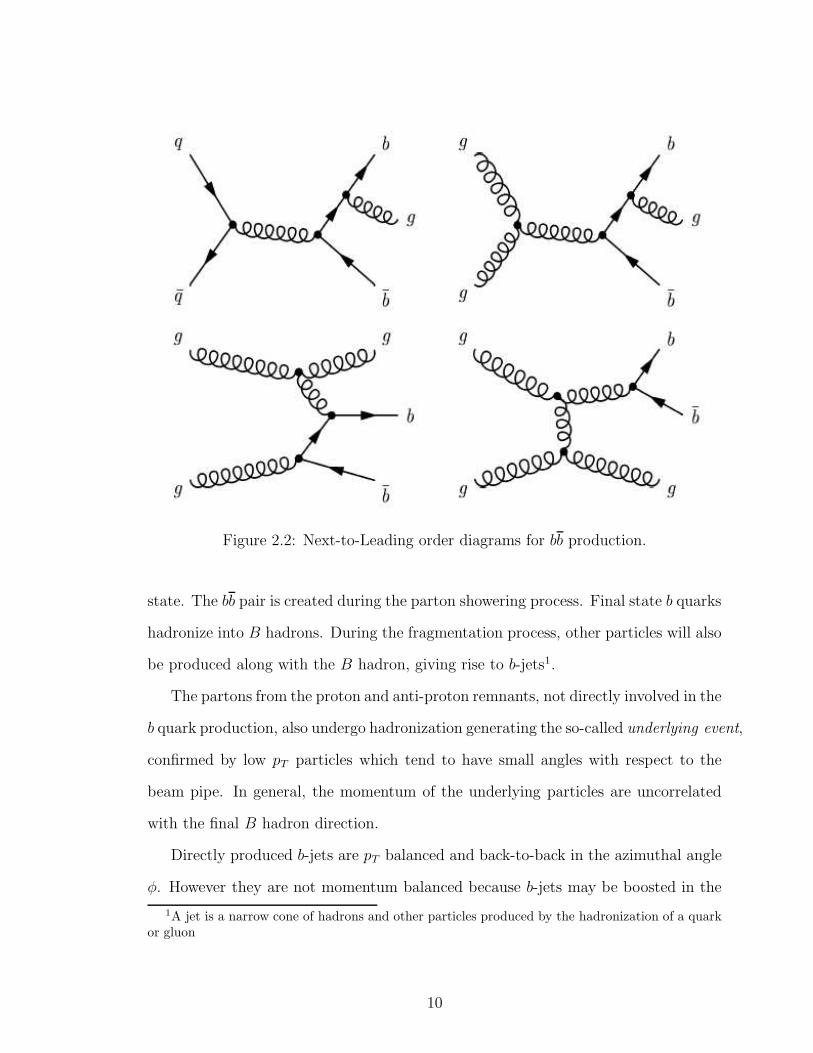
Figure 2.2: Next-to-Leading order diagrams for bb production.

state. The bb pair is created during the parton showering process. Final state b quarks

hadronize into B hadrons. During the fragmentation process, other particles will also

be produced along with the B hadron, giving rise to b-jets1.

The partons from the proton and anti-proton remnants, not directly involved in the

b quark production, also undergo hadronization generating the so-called underlying event,

confirmed by low pT particles which tend to have small angles with respect to the

beam pipe. In general, the momentum of the underlying particles are uncorrelated

with the final B hadron direction.

Directly produced b-jets are pT balanced and back-to-back in the azimuthal angle

φ. However they are not momentum balanced because b-jets may be boosted in the

1A jet is a narrow cone of hadrons and other particles produced by the hadronization of a quarkor gluon

10

z direction due to the different proton momentum fractions carried by the initial

partons. In the flavor excitation process, the b quark which does participate in the

hard scattering belongs to the underlying event, resulting in a forward (large η) b-

jet. The angular ∆φ separation between the two b-jets is therefore expected to be

flat. Gluon splitted b-jets are expected to be collinear since they originate from

the splitting of a gluon and will tend to be identified as as same hadronic jet. The

azimuthal separation between the two gluon splitted b-jets thus peaks at small angles.

2.2 Heavy Flavor Hadrons

B hadrons are produced as a result of the hadronization process of b quarks. Since

the probability for quark-antiquark creation from the vaccum depends on the quark-

antiquark mass, the most common B hadrons are B+(bu) and B0(bd) which involve

light quarks. Each comprises approximately 38% of the produced B hadrons. B0s(bs)

is the next most common B meson, comprising about 10% of the cases. The B+c

meson is made of a c and a b quark and, the c quark being much more massive than

the u − d − s, they amount to only about ∼ 0.001% of the B hadrons produced

in pp collisons. The remaining hadrons are basically comprised of Λb baryons. The

hadronization process for the c quark is similar to that of the b quark, the resulting

mesons are generically called D mesons Λc being the most common baryon. Table 2.3

summarizes the important B and D hadrons with some of their properties.

B hadrons decay via the weak interaction. The simplest decay description is

provided by the spectator model, in which the heavy quark decays via an electroweak

diagram into a virtual W and a c quark, and the lighter quark (the spectator) plays

no role, see Fig. 2.3. B hadron decays are classified as semileptonic or hadronic

depending on the W decay, which can respectively give rise to a charged lepton and

its associated neutrino, or a quark-antiquark pair.

11

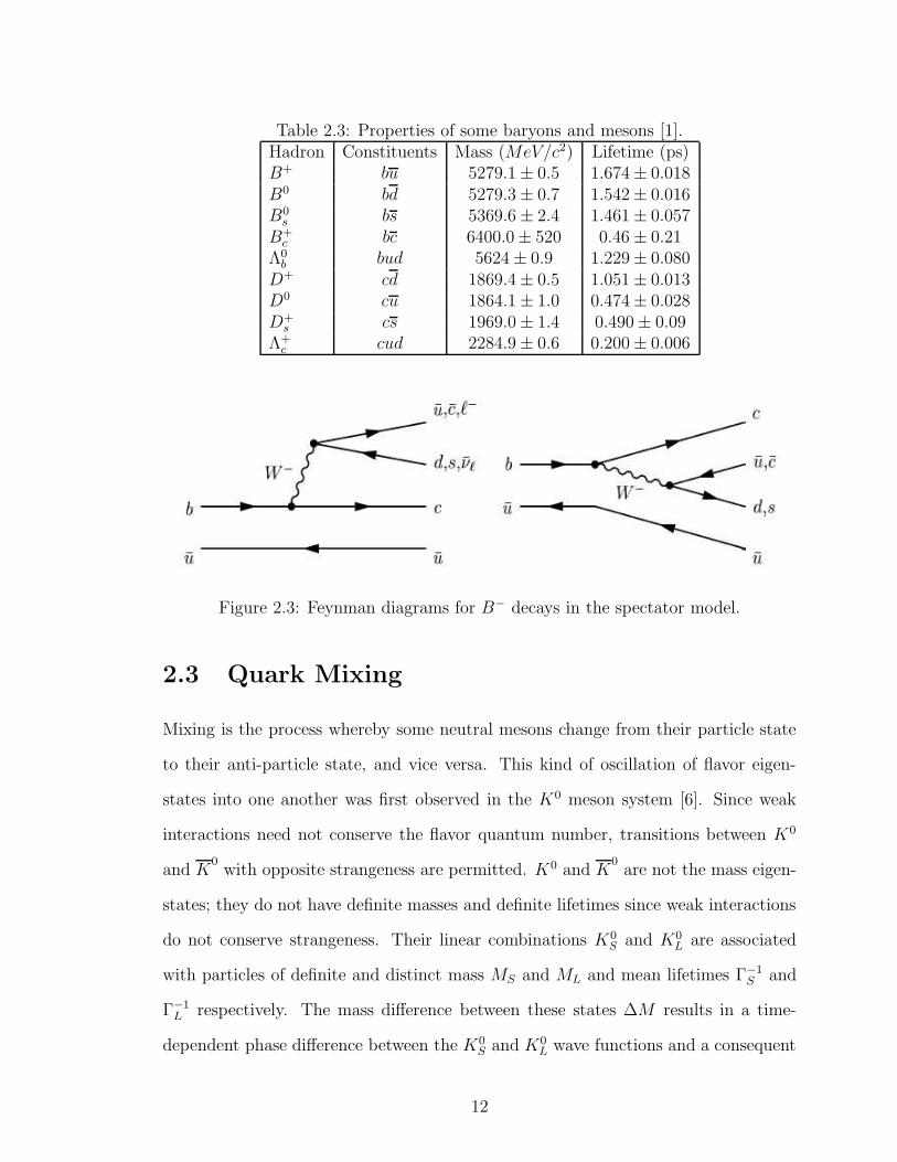
Table 2.3: Properties of some baryons and mesons [1].Hadron Constituents Mass (MeV/c2) Lifetime (ps)B+ bu 5279.1 ± 0.5 1.674 ± 0.018B0 bd 5279.3 ± 0.7 1.542 ± 0.016B0

s bs 5369.6 ± 2.4 1.461 ± 0.057B+

c bc 6400.0 ± 520 0.46 ± 0.21Λ0

b bud 5624 ± 0.9 1.229 ± 0.080D+ cd 1869.4 ± 0.5 1.051 ± 0.013D0 cu 1864.1 ± 1.0 0.474 ± 0.028D+

s cs 1969.0 ± 1.4 0.490 ± 0.09Λ+

c cud 2284.9 ± 0.6 0.200 ± 0.006

Figure 2.3: Feynman diagrams for B− decays in the spectator model.

2.3 Quark Mixing

Mixing is the process whereby some neutral mesons change from their particle state

to their anti-particle state, and vice versa. This kind of oscillation of flavor eigen-

states into one another was first observed in the K0 meson system [6]. Since weak

interactions need not conserve the flavor quantum number, transitions between K0

and K0

with opposite strangeness are permitted. K0 and K0

are not the mass eigen-

states; they do not have definite masses and definite lifetimes since weak interactions

do not conserve strangeness. Their linear combinations K0S and K0

L are associated

with particles of definite and distinct mass MS and ML and mean lifetimes Γ−1S and

Γ−1L respectively. The mass difference between these states ∆M results in a time-

dependent phase difference between the K0S and K0

L wave functions and a consequent

12

periodic variation of the K0 and K0

components [7]. Thus the K0 and K0

oscillations

are observed with a period given by 2π/∆M . The short-lived K0S only decays signif-

icantly to π+π− and π0π0, each with CP eigenvalue equal to +1. The K0L particle

decays into many modes including π+π−π0, all of which are eigenstates of CP with

eigenvalue equal to -1.

Cross-generational coupling (in the quark sector) was first introduced in 1963 by

Cabibbo [8]. He suggested that the d → u + W− vertex carries a multiplicative

factor of cos θc, whereas the s → u + W− vertex carries a factor of sin θc. The second

one is weaker and hence θc is small (θc = 12.70 experimentally). This was a fairly

successful model except for the fact that it allowed the K0 → µ+µ− decay. According

to Cabibbo’s model, the width should be Γ(K0 → µ+µ−) ≈ sin θc cos θc. However,

this was considerably larger than the experimentally set limit. Glashow, Iliopolos

and Maiani came to the rescue of the Cabibbo model in 1970 by postulating the

GIM mechanism [9]. This was an extension of the Cabibbo model and included the

fourth quark called the charm (or c− quark) that formed a doublet with the strange

quark. In this model the d→ c+W− and s→ c+W− vertices were associated with

factors of − sin θc and cos θc, respectively, such that the superposition of the Feynman

diagrams with the virtual u and c quarks cancel, and the width Γ(K0 → µ+µ−) ≈ 0.

In general, the GIM mechanism suggested that instead of the physical quarks d and

s, the states to use for weak interactions are d′ and s′, given by

d′ = (cos θc)d+ (sin θc)s, (2.2)

s′ = (− sin θc)d+ (cos θc)s. (2.3)

The phenomena is called quark mixing and Eqs. 2.2 and 2.3 can then be rewritten

using the so called “mixing” matrix which is simply a rotation of the quark basis by

13

the Cabibbo angle θc:

d′

s′

=

cos θc sin θc

− sin θc cos θc

d

s

(2.4)

The W’s then couple to the “Cabibbo rotated” states

u

d′

and

c

s′

, (2.5)

and decays that involve a factor of sin θc are known as ’Cabibbo suppressed’ decays.

2.4 CKM Matrix

In the Standard Model quarks and leptons are coupled to the W-boson field via the

charged current Jµcc. The Lagrangian for charged current processes is given by

Lcc = − g√2(Jµ

ccW+µ + Jµ†

cc W−µ ) (2.6)

where

Jµcc =

∑

k

νkγµ 1

2(1 − γ5)ek +

∑

i,j

uiγµ 1

2(1 − γ5)Vijdj (2.7)

and the sums (i, j, k) are over the 3 generations. The 3 × 3 unitary matrix V is the

so called CKM matrix [8] which describes the coupling of the charge 2/3 quarks with

the charge −1/3 quarks and is given as:

V =

Vud Vus Vub

Vcd Vcs Vcb

Vtd Vts Vtb

(2.8)

14

The CKM matrix is typically parameterized in some specific way to incorporate uni-

tary constraints. In general an n× n complex matrix has 2n2 parameters. However,

unitary requires V †V = 1 which halves the number of independent parameters. There-

fore, only n2 free parameters are left. As the phases are arbitrary, 2n-1 of them can

be absorbed by phase rotations. We are then left with (n−1)2 physically independent

parameters. Furthermore, a unitary matrix is a complex extension of an orthogonal

matrix, therefore n(n-1)/2 parameters are identified with rotation angles, leaving (n-

2)(n-1)/2 complex phases. Hence, for three generations (n=3), the CKM matrix has

four independent parameters. Three of them are identified with the real Euler angles,

leaving a single complex phase. This complex phase allows for the accommodation of

CP violation. Note that if n < 3, as in the original GIM model, there is no phase left

in the matrix and consequently no CP violation. This was the original motivation

behind Kobayashi and Maskawa’s [10] proposals for a third generation of quarks.

It should also be noted that CP is not necessarily violated in the three generation

SM. If two quarks of the same charge have equal masses, one mixing angle and

phase could be removed from CKM matrix. This leads to a condition on quark mass

differences being imposed for CP violation:

Fu 6= 0; and Fd 6= 0, (2.9)

where

Fu = (m2u −m2

c)(m2c −m2

t )(m2t −m2

u),

Fd = (m2d −m2

s)(m2s −m2

b)(m2b −m2

d). (2.10)

Another useful way of representing the above is by re-writing the commutator of the

15

mass matrices, C = [ MuM†u,MdM†

d], as

C = U †uL[(mu)

2, V (md)2V †]UuL (2.11)

which shows that det C depends on the physical masses and V.

The determinant det C illustrates several essential features of CP violation in the

SM:

• det C is imaginary, implying that CP violation originates from a complex cou-

pling.

• There is no CP violation unless Fu and Fd are non-zero.

• Non-zero Fu and Fd impose conditions on the quark masses. (Eq. 2.10).

The CKM matrix has four quantities having physical significance with three mixing

angles and one CP violating phase. These can be parameterized in many different

ways. The Particle Data Group favors the Chau-Keung parameterization[11]:

V =

c12c13 s12c13 s13e−iδ13

−s12c23 − c12s23s13eiδ13 c12c23 − s12s23s13e

iδ13 s23c13

s12c23 − c12c23s13eiδ13 −c12s23 − s12c23s13e

iδ13 c23c13

(2.12)

where cij = cos θij and sij = sin θij control the mixing between the families and δ13 is

the CP violating phase also called the KM phase.

A convenient parameterization of the CKM matrix was developed by Wolfen-

stein [12]. He exploited the hierarchy observed in the measured values of the matrix,

with diagonal elements close to one, and progressively smaller elements away from

the diagonal. This hierarchy was formalized by defining λ, A, ρ and η such that

λ ≡ s12, A ≡ s23/λ2, ρ− iη ≡ s13e

−iδ13/Aλ3

. (2.13)

16

From experiment λ ≈ 0.22, A ≈ 0.90 ± 0.12, and√ρ2 + η2 ≈ 0.39 ± 0.07, so every

element of the CKM matrix, V, was expanded as a power series in the small pa-

rameter λ = |Vus|. Neglecting terms of o(λ4) resulted in the famous “Wolfenstein

parameterization”:

V =

1 − 12λ2 λ Aλ3(ρ− iη)

−λ 1 − 12λ2 Aλ2

Aλ3(1 − ρ− iη) −Aλ2 1

+ o(λ4). (2.14)

λ, A and√ρ2 + η2 are real while the phase in question is given by arg(ρ, η). This pa-

rameterization allows for CP violation if η 6= 0. The experimentally allowed values [13]

for the matrix elements, allowing for the possibility of more than three generations

are

0.9720 − 0.9752 0.217 − 0.223 0.002 − 0.005 ...

0.199 − 0.234 0.818 − 0.975 0.036 − 0.046 ...

0 − 0.11 0 − 0.52 0 − 0.9993 ...

. . . .

. . . .

. . . .

(2.15)

Using the unitarity property of the CKM matrix one obtains the following six equa-

tions:

VudV∗us + VcdV

∗cs + VtdV

∗ts = 0, (2.16)

VusV∗ub + VcsV

∗cb + VtsV

∗tb = 0, (2.17)

VudV∗ub + VcdV

∗cb + VtdV

∗tb = 0, (2.18)

VudV∗cd + VusV

∗cs + VubV

∗cb = 0, (2.19)

17

VcdV∗td + VcsV

∗ts + VcbV

∗tb = 0, (2.20)

VudV∗td + VusV

∗ts + VubV

∗tb = 0, (2.21)

where the first three relations express the orthogonality of two different columns,

and the last three express the orthogonality of two different rows. These relations

can be geometrically represented in the complex plane as “unitarity” triangles with

rather different shapes. Aligning VcdV∗cb with the real axis and dividing all sides by

its magnitude |VcdV∗cb| (or Aλ3), one obtains a rescaled Unitarity Triangle. Fig. 2.4

shows the rescaled unitarity triangle. Two vertices of the rescaled unitarity triangle

are thus fixed at (0,0) and (1,0) while the coordinates of the third vertex is denoted

by the Wolfenstein parameters (ρ,η). The three angles of the triangle are given by:

α = arg[− VtdV∗tb

VudV ∗ub

], β = arg[−VcdV∗cb

VtdV ∗tb

], γ = arg[−VudV∗ub

VcdV ∗cb

]. (2.22)

where by reconstruction α + β + γ = π.

Figure 2.4: The rescaled Unitarity Triangle.

18

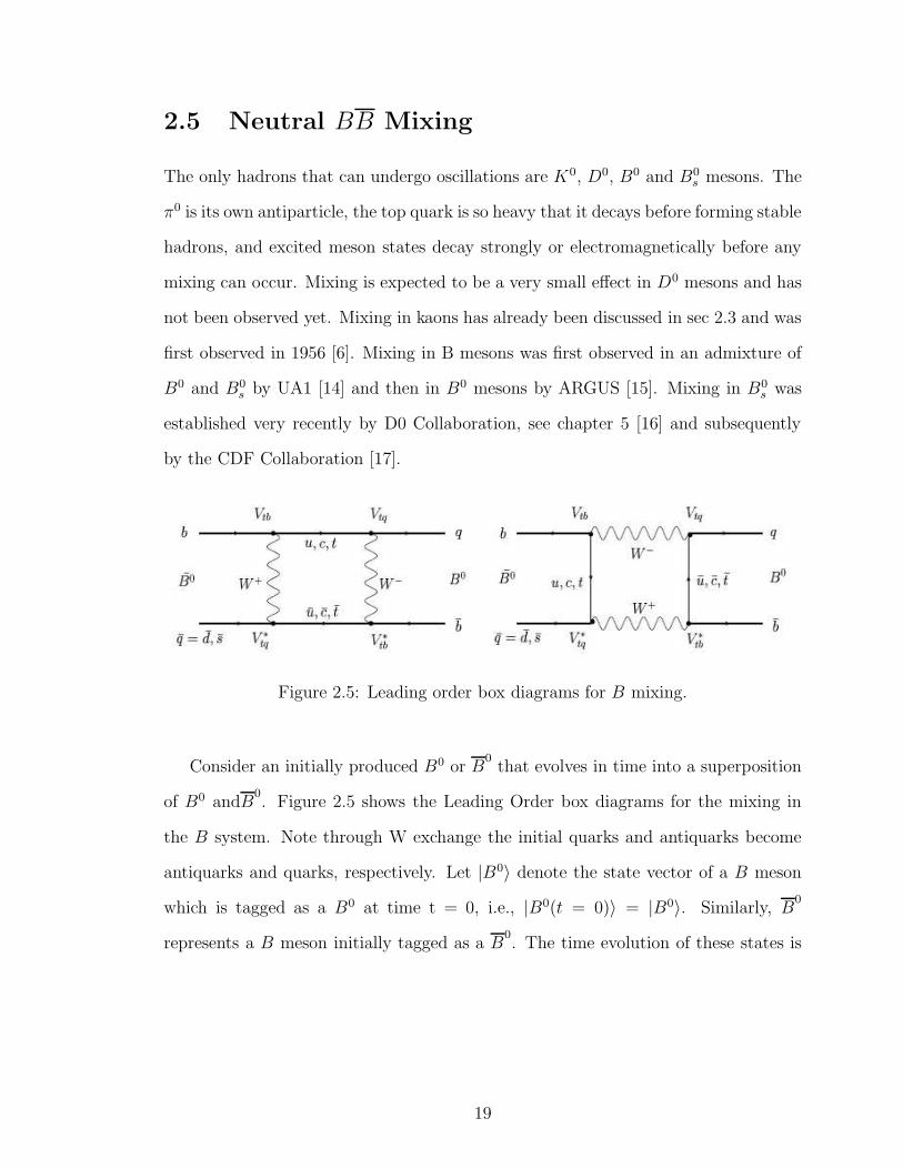
2.5 Neutral BB Mixing

The only hadrons that can undergo oscillations are K0, D0, B0 and B0s mesons. The

π0 is its own antiparticle, the top quark is so heavy that it decays before forming stable

hadrons, and excited meson states decay strongly or electromagnetically before any

mixing can occur. Mixing is expected to be a very small effect in D0 mesons and has

not been observed yet. Mixing in kaons has already been discussed in sec 2.3 and was

first observed in 1956 [6]. Mixing in B mesons was first observed in an admixture of

B0 and B0s by UA1 [14] and then in B0 mesons by ARGUS [15]. Mixing in B0

s was

established very recently by D0 Collaboration, see chapter 5 [16] and subsequently

by the CDF Collaboration [17].

Figure 2.5: Leading order box diagrams for B mixing.

Consider an initially produced B0 or B0

that evolves in time into a superposition

of B0 andB0. Figure 2.5 shows the Leading Order box diagrams for the mixing in

the B system. Note through W exchange the initial quarks and antiquarks become

antiquarks and quarks, respectively. Let |B0〉 denote the state vector of a B meson

which is tagged as a B0 at time t = 0, i.e., |B0(t = 0)〉 = |B0〉. Similarly, B0

represents a B meson initially tagged as a B0. The time evolution of these states is

19

given by the following Schrodinger equation:

id

dt

|B0(t)〉

|B0(t)〉

=

M11 − i2Γ11 M12 − i

2Γ12

M∗12 − i

2Γ∗

12 M22 − i2Γ22

(2.23)

where the mass and decay matrices (M and Γ) are 2 × 2 t-independent Hermitian

matrices. CPT invariance requires that M11 = M22 and Γ11 = Γ22 so that the particle

and anti-particle have the same mass and lifetime. B0 − B0

transitions are induced

by non-zero off-diagonal elements where M12 represents the virtual transitions and

Γ12 represents the real transitions through common decay modes. These common

modes are Cabibbo suppressed so that the B0 − B0

mixing amplitude is dominated

by virtual transitions. Diagonalization of the Hamiltonian matrix yields the mass

eigenstates that can be expressed in terms of the flavor eigenstates as

|BL〉 = p|B0〉 + q|B0〉, (2.24)

|BH〉 = p|B0〉 − q|B0〉, (2.25)

then,

q

p=

√

√

√

√

M∗12 − i

2Γ∗

12

M12 − i2Γ12

(2.26)

where BL and BH are the light and heavy mass eigenstates, respectively, and the

complex coefficients p and q obey the normalization condition |p|2 + |q|2 = 1. The

two eigenvalues are

ωL = ML − iΓL/2, (2.27)

ωH = MH − iΓH/2, (2.28)

where MH,L and ΓH,L are the masses and widths of the physical states BH and BL.

The mass difference , ∆m, and the width difference, ∆Γ, between the neutral B

20

mesons are defined using the convention:

∆ω ≡ ωH − ωL = ∆m− i

2∆Γ, (2.29)

∆m ≡MH −ML = <e(∆ω), (2.30)

∆Γ ≡ ΓH − ΓL = −2=m(∆ω). (2.31)

The eigenvalue problem

det|M − i

2Γ − ω| = 0 (2.32)

results in the condition

∆ω = 2√

(M∗12 − iΓ∗

12/2)(M12 − iΓ12/2) (2.33)

The real and imaginary parts of this equation give

(∆m)2 − 1

4(∆Γ)2 = 4|M12|2 − |Γ12|2, (2.34)

and ∆m∆Γ = 4<e(M12Γ∗12)

Using above two equations, Eqs. 2.30 and 2.31 can be re-written in terms of the

matrix elements M12 and Γ12 as:

∆m =√

2

|M12|2 −1

4|Γ12|2 +

√

(|M12|2 −1

4|Γ12|2)2 + [<e(M12Γ

∗12)]

2

12

, (2.35)

∆Γ = 2√

2

√

|M12|2 −1

4|Γ12|2 + [<e(M12Γ

∗12)]

2 − (|M12|2 −1

4|Γ12|2)

12

(2.36)

solving for the eigenvalues gives

q

p=

−∆ω

2(M12 − i2Γ12)

= −2(M∗12 − i

2Γ∗

12)

∆m− i2∆Γ

(2.37)

21

The time evolution of the mass eigenstates is then governed by the two eigenvalues

MH − iΓH/2 and ML − iΓL/2 such that

|BH,L(t)〉 = e−(iMH,L+ΓH,L/2)t|BH,L〉, (2.38)

where |BH,L〉 denotes the mass eigenstates at time t = 0 (i.e. |BH,L〉 = |BH,L(t = 0)〉).

Now, inverting Eq. 2.5 to express |B0〉 and |B0〉 in terms of the mass eigenstates and

using their time evolution in Eq. 2.37, we get:

|B0(t)〉 =1

2p[e−iMLt−ΓLt/2|BL〉 + e−iMHt−ΓH t/2|BH〉], (2.39)

|B0(t)〉 =

1

2q[e−iMLt−ΓLt/2|BL〉 − e−iMH t−ΓH t/2|BH〉] (2.40)

Eliminating the mass eigenstates in Eqs. 2.39 and 2.40 in favor of the flavor eigenstates

we get:

|B0(t)〉 = g+(t)|B0〉 + g−(t)q

p|B0〉, (2.41)

|B0(t)〉 = g−(t)

p

q|B0〉 + g+(t)|B0〉,

where

g±(t) ≡ 1

2e−iMte−

Γ2t(

e∆Γ4

tei∆m2

t ± e−∆Γ4

te−i∆m2

t)

(2.42)

and M ≡ 12(MH +ML) while Γ ≡ 1

2(ΓH + ΓL).

The above equation indicates that for t > 0 there is a finite probability that a

|B0〉 can be observed as a |B0〉 and vice versa.

Let PBm (t) denote the probability that a particle produced as a B oscillated (mixed)

and decayed as a B. Let PBu (t) denote the conjugate probability that this particle

did not oscillate, that is, it remained unmixed. Then Eqs. 2.41 and 2.42 give the

22

following:

PBu (t) =

e−Γt

Γ(

1+|q/p|2

Γ2−∆Γ2/4+ 1−|q/p|2

Γ2+∆m2

)(cosh∆Γ

2t + cos ∆mt), (2.43)

PBm (t) =

|q/p|2e−Γt

Γ(

1+|q/p|2

Γ2−∆Γ2/4+ 1−|q/p|2

Γ2+∆m2

)(cosh∆Γ

2t− cos ∆mt), (2.44)

PBu (t) =

|q/p|2e−Γt

Γ(

1+|q/p|2

Γ2−∆Γ2/4− 1−|q/p|2

Γ2+∆m2

)(cosh∆Γ

2t+ cos ∆mt), (2.45)

PBm (t) =

e−Γt

Γ(

1+|q/p|2

Γ2−∆Γ2/4− 1−|q/p|2

Γ2+∆m2

)(cosh∆Γ

2t− cos ∆mt), (2.46)

Note that these equations are not symmetric between B and B states.

These equations have two limiting cases: Neglecting CP violation in the mixing,

and neglecting lifetime difference ∆Γ (which also in general implies there is no CP

violation in the mixing).

Equation 2.5 can then be written as

|BL〉 =p+ q

2

[

(|B〉 + |B〉) +1 − q/p

1 + q/p(|B〉 − |B〉)

]

, (2.47)

and similar equation for |BH〉. So, here (1 − q/p)/(1 + q/p) ≡ εB is a measure of

the amount by which |BL〉 and |BH〉 differ from CP eigenstates. εB is expected to be

very small in the standard model, o(10−3). The limit of no CP violation in mixing is

thus q/p = 1. In this limit B and B symmetry is regained, and we obtain unmixed

and mixed decay probabilities for both B and B of:

Pu,m(t) =1

2Γe−Γt

(

1 − ∆Γ2

4Γ2

)

(cos h∆Γ

2t± cos ∆mt), (2.48)

where the + sign corresponds to Pu. This form is appropriate for B0s mesons which

are not expected to be subject to large CP-violating effects.

On the other hand, even in the presence of CP violation, a simple form can be

obtained. The lifetime difference between the heavy and light states is expected to

23

be small, ∆Γ/Γ ≤ 1% for the B0 and perhaps as large as 25% for the B0s [18].

From Eq. 2.34, ∆Γ = 0 in general only if Γ12 = 0. In this case

q

p=

√

√

√

√

M∗12 − i

2Γ∗

12

M12 − i2Γ12

=

√

M∗12

M12= e−iφ, (2.49)

thus |q/p| = 1. In this ∆Γ = 0 limit, the time evolutions from Eqs. 2.39 and 2.40

become

|B(t)〉 = e−iMte−Γ2t(

cos∆m

2t|B〉 + ie−iφ sin

∆m

2t|B〉

)

, (2.50)

|B(t)〉 = e−iMte−Γ2t(

cos∆m

2t|B〉 + ie+iφ sin

∆m

2t|B〉

)

. (2.51)

The mixed and unmixed decay probabilities again become equal for the B and B

mesons:

Pu,m(t) =1

2Γe−Γt(1 ± cos ∆mt). (2.52)

This form is expected to be appropriate for B0

mesons, for which a large phase φ (the

source of mixing-induced CP violation) is possible.

The time-integrated versions, expressing the probability that a B decays as a B,

of Eqs. 2.48 and 2.52, are

χ =∫ ∞

0Pm(t) =

1

2

x2 + 14

∆Γ2

Γ2

1 + x2(2.53)

and in the ∆Γ = 0 limit,

χ =1

2

x2

1 + x2(2.54)

where x ≡ ∆m/Γ. Oscillations observed by any experiment are oscillations in space

and not in time, therefore, one has a source creating a pure B or a B meson, which

may have oscillated by the time it reaches the detector. In this spatial picture, we

have a source, very small compared to the oscillation wavelength, which emits a

pure B meson. The boundary condition that must be imposed, then, is that the

24

probability of finding a B meson at source must vanish at all time, otherwise a pure

B would not be emanating. The |BL〉 and |BH〉 components propagate with phase

ei(EL,H t−pL,Hx), where x denotes the direction of motion. At the origin, the only way to

ensure the wavefunction does not change the relative |BL〉 − |BH〉 phase and develop

a B component is the condition EL = EH . That is, the B meson has a definite

energy. The components |BL〉 and |BH〉 will have the same energy but different

momenta pL,H =√

E2 −m2L,H respectively. This induces spatial oscillations that go

as ei(pH−pL)x.

In the Standard Model, the lowest order contribution to B mixing is given by

the box diagrams in Fig. 2.5. The dominant contribution is due to the exchange of

the virtual top quark and hence using an effective field theory, the mass difference

between heavy and light states can be written as:

∆mq = 2|M q12| =

G2F

6π2ηBmBq

BBqf 2

BqM2

WS

(

m2t

m2W

)

|VtbV∗tq|2, (2.55)

with q = s or d, and where GF is the Fermi constant and (at lowest order ) is given

by

GF√2

=g2

8M2W

(2.56)

ηB is a perturbative QCD correction factor, mBqis the B meson mass, and mt is the

top quark mass. The parameters fBqand Bq are the Bq decay constant and the “Bag

parameter”, respectively. S(

m2t

M2W

)

is the Inami-Lim function, given by

S(xq) = xq

(

1

4+

9

4(1 − xq)− 3

2(1 − xq)2

)

− 3

2

x3qlogxq

(1 − xq)3(2.57)

with xq ≡ m2t /M

2W .

Eq. 2.55 suggests that a measurement of ∆md should allow the extraction of the

CKM matrix element Vtd. Moreover, ∆md has been precisely measured and the world

25

average is [1]:

∆md = 0.502 ± 0.007ps−1. (2.58)

Unfortunately, large theoretical uncertainties in the non-perturbative QCD factors,

fBqand BBq

dominate the extraction of Vtd from ∆md. At present, Lattice QCD

calculations give about 15−20% uncertainty [1]. This difficulty, however, is overcome

if the B0s mass difference, ∆ms is also measured. The CKM matrix element, |Vtd|,

can then be extracted from the ratio of the oscillations frequencies of the B0s and B0

d

mesons as:

∆ms

∆md=mB0

s

mB0d

ξ2|Vts

Vtd|2 (2.59)

where mB0s

andmB0d

are the B0s and B0

d masses, respectively, and ξ2 ≡ f 2BsBBs

/f 2BdBBd

.

Many of the theoretical uncertainties cancel out in the ratio and ξ has been estimated

from Lattice QCD calculations to be 1.21±0.022+0.035−0.014 [19]. Therefore, the ratio Vts/Vtd

can be extracted from the measurements of ∆ms and ∆md with a relatively small

uncertainty of about 5%.

2.6 Experimental Technique

In general, a measurement of the time dependence of the neutral B meson oscillations

requires knowledge of:

• Final state reconstruction of the decay products.

• The flavor of the B meson at its production time (Flavor tagging).

• The proper decay time t of the B meson.

26

2.6.1 Event Selection

The large bb production cross section at the Tevatron (∼ 100µb) provides a very large

sample of B mesons. Since leptons are often produced in the decay of B mesons,

either directly through the semileptonic decay chain (b→ clν, where l is a lepton) or

indirectly through sequential decays (b→ c→ slν), the presence of high momentum

muons or electrons can be used to obtain datasets enriched with events from bb

production. Another characteristic of the B mesons which helps in differentiating

between the signal and background is the relatively long lifetime of the B mesons:

τ(B+) = 1.671 ± 0.018 ps, τ(B0d) = 1.536 ± 0.014 ps and τ(B0

s ) = 1.461 ± 0.057 ps

[1]. This coupled with the Lorentz boost from the initial momentum of the b quark

permits the B hadrons to travel several millimeters before decaying. Reconstructing

the B decay point or “secondary vertex” and requiring it to be separated from the

pp interaction point or “primary vertex” further enriches the data with events from

bb production.

AB0s meson can decay either semileptonically (B0

s → D(∗)s lνX) or through hadronic

decay (B0s → D(∗)

s nπ where n is number of pions in the final state). Note that a B0s

meson almost always decays to a D(∗)s meson since the branching ratio B(B0

s →

D(∗)s X) ∼ 100%. The notation D(∗)

s here is used to represent both Ds mesons and

their excited states such as D∗s and D∗

s0. Semileptonic decays have larger branching

ratios in comparison to hadronic decays and are used in the analysis presented in this

thesis. Semileptonic decays have an additional advantage that the lepton in the final

state can be used to select or trigger on the event. However, these decays do suffer

from the fact that they cannot be fully reconstructed since there is a neutrino in the

final state which escapes detection. This leads to poorer proper time resolution as

dicussed in the section 2.6.3.

At present three semileptonic decays of B0s mesons are used at DØ for the ∆ms

search. These are B0s → D−

s µ+X with D−

s → φπ− and D−s → K∗K− and B0

s →

27

D−s e

+νX with D−s → φπ−. The decay D−

s → K∗K− is primarily discussed in this

thesis. Results from all the three channels and their combination are also presented.

2.6.2 Flavor Tagging

In order to know whether a B meson has oscillated or not we need to know its flavor

at production time, this is called “initial state tagging”. The methods for tagging the

initial state can be grouped into two categories: tagging the initial charge of the b

quark in the B0s candidate itself (same side tag) and tagging the flavor of the b quark

in the event (opposite side tag). Only opposite side tagging has been used in the

current analysis.

The opposite side tagger makes use of the fact that the dominant mode of B

quark production at the Tevatron is back-to-back bb or that the b/b quark of interest

(reconstructed B meson) is always produced along with another b/b quark of opposite

charge. The other b/b in the event is called the opposite side b. Determining the

flavor of the opposite side B mesons allows us to infer the flavor of the reconstructed

B meson. The opposite side lepton tagger, for example, relies on identifying the flavor

of the other B in the event using the sign of the lepton it decayed to - a negative lepton

corresponds to a b quark, and vice versa. For reconstructed B0s → D−

s µ+X decays

both leptons having the same sign would indicate that one B hadron has oscillated

while opposite signs would indicate that neither (or both) has oscillated.

Another tagging technique determines the flavor of the opposite-side b hadron by

analyzing the jet associated with it. A momentum-weighted charge distribution of

all the tracks in the jet is used to form a variable to discriminate between b and b

quarks. Figure 2.6 shows the schematic of the tagging.

The figure of merit typically used to compare different tagging algorithms is the

“tagging power” or εD2 where ε is the tagging efficiency (or rate) and D is the

28

Figure 2.6: A diagram showing the tagging details.

“dilution” given by:

ε ≡ Ncorrect +Nwrong

Ncorrect +Nwrong +Nnotagand D ≡ Ncorrect −Nwrong

Ncorrect +Nwrong(2.60)

where Ncorrect (Nwrong) is the number of events that have been correctly (incorrectly)

tagged and Nnotag is the number of events that do not have a tag.

Eq. 2.60 indicates that a tagging algorithm with large dilution characterizes a

more powerful tagging method than one with a smaller dilution. A large dilution is,

therefore, desirable. This makes the term “dilution” counter-intuitive and its use can

sometimes be misleading. It is, therefore, better to use the purity, ηs, of the tagging

technique instead:

ηs ≡ Ncorrect/Ntotal tagged events (2.61)

where ηs is related to the dilution, D, using the simple formula D ≡ 2ηs − 1. A new

tagging method with electron as the tag lepton was developed and is discussed in

detail in chapter 4. The other taggers used in this analysis are described in detail in

the same Chapter.

29

2.6.3 Proper time resolution

The proper lifetime of the B0s meson, ctB0

s, is obtained from the measurement of the

distance, LB, between its production vertex and its decay vertex such that

ctB0s

=LB

βγ= LB MB0

s

p(B0s)

(2.62)

where β is the speed of the B0s meson, γ is the Lorentz boost factor, and MB0

sand pB0

s

are the mass and momentum of the B0s meson, respectively. The above is projected

in the plane transverse to the beam line since the transverse distance, LBxy, and the

transverse momentum, pT (B0s), are measured more accurately than LB and p(B):

ctB0s

= LBxy

MB0s

pT (B0s )

(2.63)

In the case of semileptonic decays the full momentum of the B0s meson cannot be

reconstructed since the neutrino in undetected. Instead, the combined momentum of

the Dsµ pair, pT (Dsµ), is used to calculate the Visible Proper Decay Length (VPDL)

or xM given by

xM ≡ LBxy

MB0s

pT (Dsµ), (2.64)

where LBxy is the measured decay length and is defined as the displacement ~XB

xy in

the transverse plane between the secondary B0s vertex (VB in Fig. 2.7) in the primary

vertex (VP in the Fig. 2.7) projected onto the transverse momentum of the Dµs system

such that

LBxy ≡

~XBxy · ~pT (Dsµ)

|~pT (Dsµ)| (2.65)

Using Eqs. 2.64 and 2.65 the VPDL is expressed as

xM =~XB

xy · ~pT (Dsµ)

pT (Dsµ)· MB0

s

pT (Dsµ)(2.66)

30

Figure 2.7: Schematic of a B → DµνX decay.

The actual proper lifetime is then obtained using Eq. 2.66 and a correction factor

such that

ctB0s

= xM ·K (2.67)

K ≡ pT (Dsµ)/pT (B0s ) and is known as the K-factor. It is essentially a correction

factor used in semileptonic decays to account for the missing neutrino (and other

neutral or non-reconstructed charged particles). K-factor distributions are obtained

from Monte Carlo simulations and are further discussed in Chapter 5.

The uncertainty on the proper decay time, σt, can be expressed as:

σt = σ(LBxy) ⊕ t · σ(K)

K(2.68)

where σ(LBxy) is the uncertainty due to vertexing resolution and σ(K)/K is the K-

factor resolution. Note that the latter uncertainty scales with the decay time t, while

the vertexing resolution is independent of t and only adds a constant uncertainty.

In order to resolve the fast B0s oscillations σt should be smaller than the oscillation

31

period. Moreover, since the K-factor resolution is significant for semileptonic decays

(owing to undetected neutrino), events with small decay time are the most sensitive

to oscillations.

2.6.4 Overview of the Mixing Analysis

In a B mixing measurement, the oscillation frequency ∆mq (q = s,d) is extracted

from the data using a maximum likelihood method. In the following, we discuss

the essential steps for a B0s mixing analysis determining ∆ms. We start with a pure

sample of B0s mesons and assume that the lepton tag is always correct. In this case, an

event with an opposite-sign lepton pair signals an unmixed event, while a same-sign

lepton pair indicates a mixed event. In this case the probabilities for an opposite-sign

event POS and a same-sign event PSS are directly related to the mixing probabilities:

PSS(t) = Pmix(t) and POS(t) = Punmix(t) (2.69)

The mixing probabilities are obtained from Equation 2.48 by neglecting the width

difference between the heavy and light mass eigenstates:

Punmix/mix(t) =1

2Γe−Γt(1 ± cos ∆mt) (2.70)

The observable asymmetry Amix is defined as:

Amix(t) =Punmix(t) − Pmix(t)

Punmix(t) + Pmix(t)= cos ∆mt. (2.71)

Next we introduce several effects that we will have to include in a realistic mixing

analysis. First, we consider the mixing asymmetry Amix as a function of the decay

time assuming an ideal case with a perfect tagging, ideal proper time resolution, and

no background, as shown in Fig. 2.8 (left). Then, we introduce a vertexing resolution

32

Figure 2.8: On the left is the mixing amplitude in ideal case and effect on mixingamplitude due to finite decay length resolution is shown on right.

function G which smears the decay time measurement and effectively reduce the

amplitude of the oscillation,as shown in Fig. 2.8 (right). The oscillation amplitude

is also reduced by mistag effects and the resulting amplitude is proportional with

the tagging dilution D. The effect of mis-tagging is exemplified in Fig. 2.9 (left).

The effect of introducing a momentum resolution, for example through a K-factor

distribution F(K) is also considered and shown in Fig. 2.9 (right).

Figure 2.9: Effect on amplitude due to flavor mis-tagging (left) and combining all theeffects (right)

33

The event selection efficiency might not be constant as a function of the decay

time. We account for the the lifetime distribution bias by introducing an acceptance

function ε. Including all these effects, the opposite/same-sign probability would be

modified as

POS/SS(t∗) ∼∫

dKKε(Kt∗)∫

1

2Γe−Γt(1 ±D cos(∆mst))G(t′ − t, σ)dt|t′=Kt∗. (2.72)

In real measurement there will be background such as combinatorial background

under a charm signal. We define PsigSS and Psig

OS as PSS and POS in Eq. 2.72 and

obtain

PSS(t) = (1 − fbkg)PsigSS (t) + fbkgfSSPbkg(t), (2.73)

POS(t) = (1 − fbkg)PsigOS(t) + fbkgfOSPbkg(t)

where fbkg is the fraction of the background in a given sample, fSS is the fraction of

the same-sign events in the background, while P bkg is the probability function that

describes the proper time t distribution of the background events. To extract the value

∆ms of the oscillation frequency, the following likelihood function is minimized:

L = −∑

SS

lnPSS(t∗) −∑

OS

lnPOS(t∗). (2.74)

The statistical significance S of a B0s oscillation signal can be approximated [20] as,

S ≈√

1

2fsigDe−(∆mσt)2/2 =

√

εD2

2

S√S +B

e−(∆mσt)2/2, (2.75)

where N and fsig are the number of tagged candidates and the fraction of the signal

in the selected sample and σt is the resolution on proper decay time. S and B are

the the numbers of signal and background events. The sensitivity S decreases rapidly

as ∆m increases. This dependence is controlled by σt which means that excellent

34

proper time resolution is needed to explore high frequencies of B0s oscillations. The

sensitivity time increases with the tagging power εD2, the signal fraction and the

total number of events.

2.6.5 The Amplitude Method

The amplitude method [20] is used in the B0s mixing analysis to set limits on ∆ms.

This method is also very handy when combining the results from the different ex-

periments. Though both the amplitude method and the likelihood method is being

used in the current analysis to search for B0s mixing signal, here only the amplitude

method is discussed. An amplitude A is introduced in the expressions describing the

mixed and unmixed probabilities:

PB0s

unmix =1

2Γe−Γt(1 + A cos ∆mst) (2.76)

, and similarly for the mixed sample:

PB0s

mix =1

2Γe−Γt(1 −A cos∆mst). (2.77)

In the amplitude method, a B0s oscillation amplitude A and its error σA are expected

as a function of a fixed test value of ∆ms using a likelihood method in analogy to

Eq. 2.74 based on the physics functions defined in Eqs. 2.76 and 2.77. To a very good

approximation, the statistical uncertainty on A is Gaussian and equal to the inverse

of the significance 1/S defined in Equation 2.75. If ∆ms equals its true value ∆mtrues ,

the amplitude method expects A = 1 within the total uncertainty σA. If ∆ms is

tested far from its true value, a measurement consistent with A = 0 is expected. A

value of ∆ms can be excluded at 95% Confidence Level if A + 1.645σA ≤ 1.

Because of proper time resolution, the quantity σA(∆ms) is an increasing func-

tion of ∆ms. It is therefore expected that individual values of ∆ms can be ex-

35

cluded upto ∆msenss , where ∆msens

s is called the sensitivity of the analysis defined

by 1.645σA(∆msenss ) = 1. If no signal is observed, a lower limit is set with 95%

Confidence Level at the mixing frequency for which A + 1.645σA = 1.

An interesting feature of the amplitude methods is that the result from different

analysis and experiments can be combined by simple avearging of different amplitude

spectra (after accounting for correlations between the systematic errors). The com-

-1.5

-1

-0.5

0

0.5

1

1.5

2

2.5

0 2.5 5 7.5 10 12.5 15 17.5 20 22.5 25

∆ms (ps-1)

Am

plitu

de

data ± 1 σ 95% CL limit 14.4 ps-1

1.645 σ sensitivity 17.8 ps-1

data ± 1.645 σdata ± 1.645 σ (stat only)

Average for PDG 2004

Figure 2.10: World average amplitude for B0s which includes all the published results

up to 2004.

bined measurements of the B0s oscillation amplitude as a function of ∆ms, including

all published results excluding the results from RunII of the Tevatron provide a lower

limit on the B0s mixing frequency of ∆ms > 14.4 ps−1 at 95% Confidence Level with

a sensitivity of 17.8 ps−1 as shown in Fig. 2.10 and the fit to the CKM triangle can

be seen in Fig. 2.11. This picture has changed completely after including the results

from the RunII of the Tevatron and is discussed in detail in Chapter 5 and Chapter

36

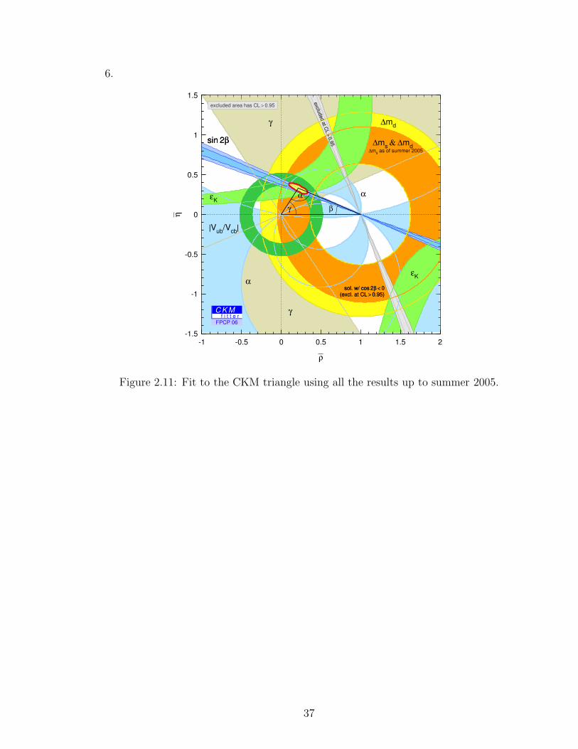
6.

-1.5

-1

-0.5

0

0.5

1

1.5

-1 -0.5 0 0.5 1 1.5 2

sin 2β

sol. w/ cos 2β < 0(excl. at CL > 0.95)

excluded at CL > 0.95

γ

γ

α

α

∆md

∆ms & ∆md

εK

εK

|Vub/Vcb|

sin 2β



α

βγ

∆ms as of summer 2005

ρ

η

excluded area has CL > 0.95

C K Mf i t t e r

FPCP 06

Figure 2.11: Fit to the CKM triangle using all the results up to summer 2005.

37

Chapter 3

Experimental Apparatus

3.1 Experimental Framework

Fermilab is the home of the world’s most powerful particle accelerator at present,

the Tevatron. The protons and antiprotons inside the Tevatron collide head on at

two collision points. The DØ detector is situated at one of these collision points

and the Collider Detector at Fermilab (CDF) being at the other point. The Fermilab

accelerator complex has a chain of accelerators to produce the world’s highest energy

particle beams.

The Tevatron accelerator first started colliding 900 GeV proton and antiproton

beams in 1985. Run I was undertaken between 1992 and 1996 and produced many

important results including the discovery of the top quark [21]. Between 1997 and

2001, both the accelerator complex (see Fig. 3.1) and the two detectors underwent

major upgrades, mainly aimed at increasing the luminosity of the accelerator and

gathering data sample of the order of 8 fb−1 or more, known as RunII of the Tevatron.

In RunII, the Tevatron is operating at a center of mass energy of 1.96 TeV. At present,

the Tevatron accelerates 36 bunches of protons and antiprotons, whereas the previous

version of the accelerator operated with only 6 bunches. Consequently, the time

between bunch crossings has decreased from 3.5 µs for the previous version to 396 ns

39

for the current machine. The instantaneous luminosity was ∼ 1 − 2 × 1031cm−2s−1

for Run I, with DØ collecting around 120 pb−1 of data. Despite the success of Run

I, the limited integrated luminosity coupled with the low production cross sections

for interesting processes limited the physics capability. Here we describe the main

components of the upgraded accelerator complex in brief and then we describe the

components used to identify and measure properties of the particles produced as a

result of collision in the Tevatron.

Figure 3.1: Fermilab Accelerator Complex.

40

3.1.1 The Tevatron

Tevatron is presently the world’s highest energy particle accelerator. The first stage of

the acceleration is provided by the Cockroft-Walton preaccelerator. Inside this device,

gaseous hydrogen is ionized to create H− ions, which are accelerated to 750 keV

energy. These H− ions then enter a linear accelerator, the Linac [22], approximately

500 feet long, where they are accelerated to 400 MeV . A series of ”kicks” from

Radio Frequency (RF) cavities produce the acceleration in the Linac. The oscillating

electric field of the RF cavities groups the ions into bunches. The next stage is the

Booster, but before that, these ions pass through a carbon foil which removes the two

electrons, leaving only the protons.

The Booster, a circular synchrotron [22] 74.5 m in diameter is located approxi-

mately twenty feet below the ground and uses magnets to bend the beam of protons in

circular path. The intensity of the proton beam is increased by injecting new protons

into the same orbit as the circulating ones. The protons travel around the Booster

about 20,000 times, acquiring about 500 keV of Kinetic energy each time and so the

protons are finally accelerated to an energy of 8 GeV . Protons are then injected into

Main Injector [23], which operates at 53 MHz. It accelerates protons from 8 GeV to

150 GeV to be injected into the Tevatron. It also produces 120 GeV protons which

are used for antiproton production and then it receives the antiprotons from antipro-

ton source and accelerates them to 150 GeV before they are finally injected into the

Tevatron.

Antiprotons are produced by hitting the nickel target with the 120 GeV protons

from the Main Injector. In the collisions, about 20 antiprotons are produced per one

million protons, with a mean kinetic energy of 8 GeV . The antiprotons are focused

by a lithium lens and separated from other particle species by a pulsed magnet.

Before the antiprotons can be used in the narrow beams needed in the collider, the

differences in the kinetic energy between the different particles need to be reduced.

41

Since this process reduces the spread of the kinetic energy spectrum of the beam, it

is referred to as ”cooling” the beam. New batches of antiprotons are initially cooled

in the Debuncher synchrotron, collected and further cooled using stochastic cooling

[24] in the 8 GeV Accumulator synchrotron.

The principle of stochastic cooling is to sample particle motion with a pickup

sensor and correct its trajectory later with a kicker magnet. In reality, the pickup

sensor samples the average motion of particles in the beam and corrects for the

average. Integrated over a long period of time, this manifests itself as a damping

force applied onto individual particles which evens out the kinetic energies.

The antiprotons are then stored in the Accumulator ring and when a sufficient

number (”stack”) has been obtained, they are sent to the Main Injector for further

acceleration before being fed into the Tevatron. It takes about 15-20 hours to build

up a stack of 100E30 antiprotons. The availability of the antiprotons is the limiting

factor for attaining high luminosities. Recently, a new technique ”Electron cooling”

[25] for cooling the antiprotons has been adopted which is supposed to increase the

stacking ability.

Not all the antiprotons in a given store are used up by the collisions at the end

of the store. An Antiproton Recycler is used to recycle the unused antiprotons and

reusing them in the next store and thus significantly reducing the stacking time. The

task of the Recycler is to receive the leftover antiprotons from a Tevatron store, cool

them and re-integrate them into the stack. The last and final stage of the accelerator

chain is the Tevatron. It receives 150 GeV protons and antiprotons from the Main

Injector and accelerates them to 980 GeV .

The protons and antiprotons accelerate in opposite directions inside the Tevatron.

There are typically 36 bunches of protons and antiprotons arranged in three groups

of 12 super bunches separated by 2 µs. The beams are brought to collisions at two

collision points, B0 and DØ. At these two points, the two collider detectors, the

42

Parameters ValuesEnergy pp (GeV) 980Proton bunches 36Protons/bunch 2.7 ×1011

Antiproton bunches 36Antiprotons/bunch ×1010

Bunch spacing (ns) 396Peak luminosity (cm−2s−1) 1.5 ×1032

Table 3.1: Tevatron Operating Parameters.

Collider Detector at Fermilab (CDF) and DØ detector are located. Quadrupole

magnets squeeze the beams into a cross sectional area of σa ∼ 5× 10−5cm2 such that

the beams collide in the geometrical center of the two detectors. The instantaneous

luminosity can be expressed as

L =frevNBNpNp

2π(σ2p + σ2

p)F (σl/β

∗), (3.1)

where frev is the revolution frequency, NB is the number of bunches, Np(p) is the

number of protons(antiprotons) per bunch, and σp(p) is the protons(antiprotons) rms

beam size at the interaction point. F is a form factor which corrects for the bunch

shape and depends on the ratio of σl, the bunch length to β∗, the beta function,

at the interaction point. The beta function is a measure of the beam width, and it

is proportional to the beam’s x and y extent in phase space. Table 3.1 lists some

important operating parameters for the Tevatron.

3.2 The DØ Detector

The DØ detector [26] is a general multipurpose collider detector. It has a typical

cylindrical structure common to many modern high energy physics experiments. The

overview of the detector is shown in Fig. 3.2. Because the beams in the Tevatron are

equal in energy, the detector is symmetrical about the interaction point and covers

43

nearly all 4π surrounding the interaction region. The detector consists of three major

subsystems:

• Central tracking detectors.

• The Calorimeter.

• The Muon Detector.

Figure 3.2 shows a schematic view of the Run II DØ detector. The tracking detectors

are positioned closest to the interaction point and have the finest segmentation. They

are designed to measure the three dimensional trajectories of the charged particles

passing through them. The magnetic field bends the trajectory of the charged par-

ticles and allows a measurement of their momenta. The tracking detectors are built

out of low Z material to introduce as little interaction as possible while still detecting

their presence. The tracker is surrounded by the Calorimeter. This detector measures

the energy of the particles and is constructed out of high Z material to absorb most

of the particles entering it. Since muons have much more penetrating power and can

escape the calorimeter, another detector has been put outside the calorimeter.

3.3 Coordinate system

We use a right handed coordinate system in which the z-axis is along the proton

direction and y-axis points vertically upward and x-axis points horizontally towards

the center of the ring, as shown in Fig. 3.3. The angles φ and θ are azimuthal and polar

angles, respectively, with θ = 0 along the beam pipe. Because of the approximate

axial symmetry of the detector, it is convenient to define the cylindrical coordinates

r and φ.

r =√

(x2 + y2) (3.2)

44

Figure 3.2: Side view of the DØ detector [26].

φ = tan(y

x) (3.3)

The r coordinate denotes the perpendicular distance from the z axis. Since most of

the particles of interest are ultra-relativistic it is convenient to use η, or the pseudo-

rapidity, in place of θ. The pseudo-rapidity η is related to the polar angle by:

η = − ln[tan(θ

2)], (3.4)

and approximates the true rapidity,

y =1

2ln[E + pz

E − pz

] (3.5)

45

Figure 3.3: DØ coordinate system.

for infinite angles in the limit that (mc2

E) → 0, where E is the energy of the particle

and Pz its longitudinal momentum. Rapidity is convenient for two regions: Rapidity

intervals are Lorentz invariant and particle multiplicity is approximately constant in

rapidity. Since some particles escape down the beam pipe and the initial momentum

of the interacting particles are not known, we measure the momentum and energy

in the direction perpendicular to the beam axis, i.e. transverse momentum (pT ) and

transverse energy (ET ), defined by

pT = p sin θ, and ET = E sin θ. (3.6)

Collisions do not always occur at the center of the detector because of the long

46

bunch length ∼ 30 cm in Z, so when reconstructing the direction and transverse

momentum of the final state objects a correction in the Z position is applied, see

Fig. 3.4. However, for discussing the position of the detector it is most convenient to

speak of the detector η. Unless otherwise noted, when discussing detector elements

the η referred to will be the detector η. Similarly, when referring to the reconstructed

physics objects such as electrons, jets, and muons the η referred to is the physics η

which is simply the η of the object with respect to the hard scattering event vertex.

Figure 3.4: Difference between Detector and Physics η.

3.4 Central Tracking System

Excellent tracking in the central region is necessary for studies of b physics, top

quark, etc. The tracking system is the backbone of the b physics program at DØ.

The central tracking system consists of the Silicon Microstrip Tracker (SMT) and

the Central Fiber Tracker (CFT) surrounded by a solenoidal magnet. A schematic

47

view of the central tracking system is shown in the figure 3.5. Working together, the

Figure 3.5: Schematic of the central tracking system.

two detectors locate the primary interaction vertex with a resolution of about 35 µm

along the beamline.

Charged particles interact with the tracking detectors and leave a pattern of hits

in the various layers of the detectors. From these hits, a track can be reconstructed

representing the trajectory of the charged particle. Since the entire tracking region is

inside a highly uniform magnetic field, the trajectories of charged particles are curved.

By measuring the curvature of the track, it’s momentum can be precisely estimated.

There is another detector called Preshower located between inner tracking system

and calorimeter. Preshower detectors function as calorimeters as well as tracking

detectors. These detectors aid in electron identification and background rejection

during both online triggering and offline reconstruction.

48

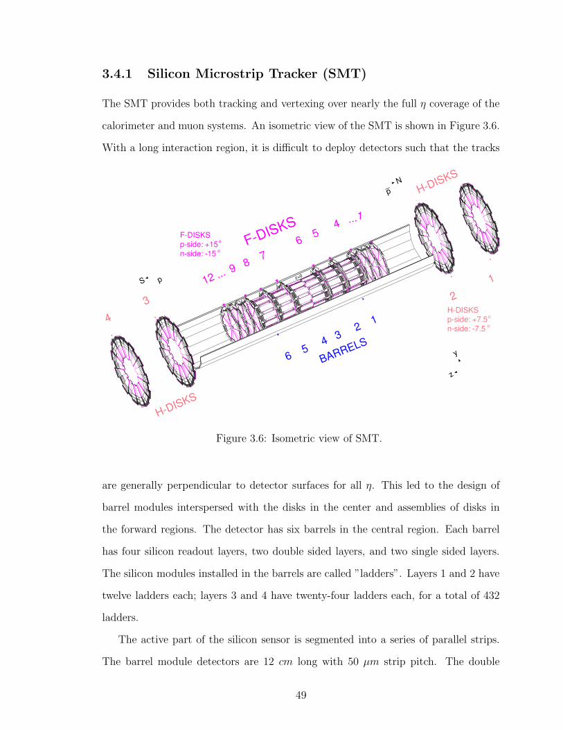
3.4.1 Silicon Microstrip Tracker (SMT)

The SMT provides both tracking and vertexing over nearly the full η coverage of the

calorimeter and muon systems. An isometric view of the SMT is shown in Figure 3.6.

With a long interaction region, it is difficult to deploy detectors such that the tracks

H-DISKS

BARRELS

14 ...

12 ... 9 8 7

6

5

6 5 4

3 2 1

4

3 2

1

F-DISKS

H-DISKS

F-DISKS p-side: +15 n-side: -15

o

o

H-DISKS p-side: +7.5 n-side: -7.5

o

o

y

z

z=0S

N

p

p_

Figure 3.6: Isometric view of SMT.

are generally perpendicular to detector surfaces for all η. This led to the design of

barrel modules interspersed with the disks in the center and assemblies of disks in

the forward regions. The detector has six barrels in the central region. Each barrel

has four silicon readout layers, two double sided layers, and two single sided layers.

The silicon modules installed in the barrels are called ”ladders”. Layers 1 and 2 have

twelve ladders each; layers 3 and 4 have twenty-four ladders each, for a total of 432

ladders.

The active part of the silicon sensor is segmented into a series of parallel strips.

The barrel module detectors are 12 cm long with 50 µm strip pitch. The double

49

sided detectors have axial strips parallel to the beam on one side while the strips on

the other side are placed at an angle (either at 20 or 900) with respect to the beam.

The pitch strips are chosen so that the position resolution would be approximately

10 microns. The length of the barrel region is dictated by the fact that the bunches

have a wide distribution along the beam axis with σz = 30 cm.

The detectors are fabricated on n-type silicon wafers that are 300 µm thick as

shown in Fig. 3.7. The strips are formed by p+ implants along the length of the

detector. A thin dielectric layer between the strips and an aluminium coating forms a

capacitor which AC couples the detector to the readout electronics. A radiation hard

polysilicon resistor is used to bias the sensor. The sensors operate essentially as reverse

biased diodes. When a charged particle passes through the sensor, electron/hole pairs

are created. The electrons are then accelerated toward the positive voltage. The p+

silicon is separated from the aluminium readout strip by a silicon oxide layer which

forms a capacitor. As electrons rush towards the p+ region, an image charge is formed

on the aluminium which is collected and stored in an analog pipeline in a readout

chip in an array of switched capacitors. The signal is buffered, digitized, and readout

by a chip which is bonded onto the sensor.

The detector is read out by 128-channel readout chips. These chips are called

SVXIIe chips and are designed to work with double sided detectors and can accept

both positive and negative currents as input signals. The chips are mounted on a

high density interconnect or HDI. Data from HDIs are sent from the sequencers to

VME readout buffer (VRB) memories via optical link fibers. The VRB controller

(VRBC) receives trigger data from the SCL and uses that information to control the

operation of the VRBs. A single board computer is resident in the readout crate to

collect and process detailed diagnostic information.

50

Figure 3.7: Schematic diagram of a silicon microstrip detector.

3.4.2 Central Fiber Tracker

The CFT consists of scintillating fibers mounted on eight concentric support cylinders

and occupies the radial space from 20 to 52 cm from the center of the beampipe.

Figure 3.8 shows a cross section of the CFT. The two innermost cylinders are 1.66

m long; the outer six cylinders are 2.52 m long. Each cylinder supports one doublet

layer of fibers oriented along the beam direction (z) and a second doublet layer at

a stereo angle of +30 (u) or −30 (v). Doublet layers with the fibers oriented along

the beam axis are referred to as the axial layers, while the doublet layers oriented

at small angles are referred to as the stereo layers. The scintillating fibers are 860

microns thick and between 1.7 - 2.6 meters long. They are organized and mounted in

128 fiber ribbons which consists of two singlet layers. Scintillating fibers are coupled

to clear fibers waveguides which carry the scintillation light to visible light photon

counters (VLPCs) for read out.

51

CPS

SOLENOID

CFT

SMT

1#2#

3#4#5#6#7# 8#

stereoaxial

stereoaxial

MAGNIFIED END-VIEW

CENTRAL CALORIMETER CRYOSTAT WALL

Be BEAM PIPE

a.) b.)

LEVEL 0

FPS

i barrel

j barrel

th

thH-disk & Enclosure

Be BEAM PIPE

+ Z

+ y

+ x

where i, j = 1,...,8 i = j

Figure 3.8: Cross Section view of the CFT detector.

The scintillating fibers, including cladding, are 835µm in diameter and 1.66 or

2.52 m in length. The fibers are 99% polystyrene (by weight) and contain two or-

ganic scintillating dyes: Paraterphenyl (PHP) and 3-hydroxyflavone (3HF) [27]. The

polystyrene absorbs energy from the ionizing radiation incident upon it. The relax-

ation time of polystyrene absorbs energy from the ionizing radiation incident upon

it. The relaxation time of polystyrene is slow so the organic dye PHP is added to the

fiber. Through dipole interactions the PHP molecules are excited which then decay

promptly back to their ground state radiating a photon within a few nanoseconds.

However, since the PHP emits light with a very short wavelength (∼ 340 mm) the

optical path length is very short, on the order of a few hundred microns. Therefore,

a second dye (3HF) is used as wavelength shifter to absorb the light from the de-

excitation of the PHP molecules and emit photons with a longer wavelength of ∼

530 nm. This second dye was chosen since the optical path length in polystyrene is

maximized in this region and is on the order of several meters. The long optical path

length allows the scintillation light to travel the necessary distance to be detected.

The light from the scintillating fiber is observed only at one end while the other

52

end of the fiber is coated with a reflecting material providing a reflectivity of 85 to

90%. The light generated by the passage of charged particles through the scintillating

fibers is converted into electrical signals by the VLPCs. These VLPCs are capable

of detecting a single photon, provide fast response, have excellent qantum efficiency

greater than 75%, and have high gain.

3.4.3 Solenoid

The superconducting solenoidal magnet was designed to optimize momentum reso-

lution, ∆pT

pT, and tracking pattern recognition. It surrounds the tracking region and

creates a highly uniform axial magnetic field of 2 Tesla. The solenoid is wound with

two layers of superconductor and is 2.73 m in length and 1.42 m in diameter. Both

conductors are made up of superconducting Rutherford-type cable of multifilamen-

tary Cu:NbTi strands stabilized with pure aluminium and operates at 4.7 K. They

run at a current of 4749A. The magent stores 5.3MJ of energy. To maximize the field

uniformity inside the bore of the magnet, current density in the windings is larger

at the ends of the coil. The magnet polarity is reversed from time to time using a

5000A DC mechanical motorized polarity reversing switch and a switch controller.

This is being done to run the detector for equal amount of time in each polarity and

maintaining the charge asymmetry distribution.

3.4.4 Preshower Detectors

Particles to loose significant amount of energy in the solenoid magnet. It is convenient

to describe the amount of material in terms of the amount of energy a particle looses

as it passes through it. The radiation length X0 is defined as the mean distance

over which an electron loses all but 1e

of its energy [1]. The material in the solenoid

amounts to about 0.8 to 2.0 X0 depending on the incident angle of the particles. The

particles coming out at large η will have to traverse a longer path and hence would

53

interact with more matter than the particle at normal incidence or smaller η.

To take into account the effect of the extra material of the solenoid, preshower

detectors are installed in the space between the magnet and calorimeter. Preshower

detectors aid in electron identification and background rejection during both online

triggering and offline reconstruction. They function as calorimeters as well as track-

ing detectors, enhancing the spatial matching between tracks and calorimeter showers

[28]. The detectors can be used offline to correct the electromagnetic energy mea-

surement of the central and end calorimeters for losses in the solenoid and upstream

materials, such as cables and supports.

The Central Preshower detector (CPS) covers the region |η| < 1.3 and is located

between the solenoid and central calorimeters. The two Forward Preshower Detectors

(FPS) cover 1.5 < |η| < 2.5 and are attached to the faces of the end calorimeters.

The detectors consist of lead absorbers and triangular strips of plastic scintillator.

Since the triangles are interleaved, there is no dead space between strips and most

tracks traverse more than one strip, allowing for strip-to-strip interpolations and hence

improved position measurement. Additional lead of varying thickness surrounds the

solenoid to make the radiation length approximately 2.0X0 for all particle trajectories.

Embedded at the center of each triangular strip is a wavelength-shifting fiber which

collects and carries the light to the end of the detector. At the readout end, the

fibers are grouped into bunches of sixteen and potted into connectors for transition

to clear light-guide fibers. Light is transmitted via the clear fibers to VLPC pixels

for readout.

The CPS consists of three concentric cylindrical layers of triangular scintillator

strips and is located in the nominal 5 cm gap between the solenoid and the central

calorimeter. Between the solenoid and the CPS is a lead radiator of approximately

1 radiation length thickness and 96” long, covering |η| < 1.31. One layer is oriented

parallel to the beam while the other two layers are oriented at a stereo angle of

54

+23.770 and −24.010. Each layer contains 1280 strips.

Figure 3.9: Cross section view of the Preshower detector.

The FPS detectors are made up of two layers, at different z , of a double layer

of scintillator strips. A 2 X0 thick lead stainless steel absorber separates the two

layers. The upstream layers are known as the minimum ionizing particle, or MIP,

layers while the downstream layers behind the absorbers are called the shower layers.

All charged particles passing through the detector will register a minimum ionizing

hit in the MIP layer, allowing measurement of the location of the track.

3.5 The Calorimeter

Calorimeter detectors are designed to accurately measure the energies of the electro-

magnetic and hadronic objects. They are crucial for the identification of electrons,

photons and jets as well as for inferring the presence of neutrinos and other non-

interacting particles from the transverse momentum imbalance. This measurement is

made by inducing interactions with incident particles via the material of the calorime-

ter, creating showers of secondary particles which lose energy (through ionization,

excitation etc.) in the calorimeter’s active medium. A measurement of a particle’s

55

total energy is made when the showering process is fully contained.

Electromagnetic (EM) and Hadronic (HAD) objects shower differently in the

calorimeter, allowing for their identification and as well as an energy measurement.

For EM objects (electrons and photons), the energy loss is dominated via two pro-

cesses : pair production (γ → e+e−) and bremsstrahlung1 (e → eγ). As a result of

successive interactions2 of these two processes, an electromagnetic shower develops.

For each successive interaction the number of secondary particles increases while the

average energy per particle decreases. Collecting and measuring these secondary par-

ticles gives insight into the original EM object’s energy (E0) since the energy of the

original particle drops exponentially:

E(x) = E0e−x/X0 (3.7)

where x is the distance traveled and X0 is the radiation length.

Calorimeters fall into two categories :

• Electromagnetic (EM) Calorimeters

• Hadronic (HAD) Calorimeters

It has to be noted here that although the hadronic showers are dominated by nuclear

interactions, they also contain EM shower components, making the determination

of hadronic showers more complicated, since the EM part has to be accounted for

differently. These two types of showers differ also in relative size. For a given energy

of an incident particle, a hadronic shower tends to be larger than the EM.

The different depth (in the radially outward direction) for the two types of showers

is reflected in the designs of the calorimeters for a general purpose collider detector.

1Emission of a photon due to the interaction between the Coulomb field surrounding a nucleus acharged particle

2For instance, an incident electron loses energy by emitting a photon. The photon converts intoan e+e− pair, which in turn will lose energy by emitting photons.

56

The calorimeter consists of two subdetectors : the EM and the HAD calorimeter.

The EM calorimeter is the innermost calorimeter and more compact; it encloses the

volume closer to the interaction point, while the hadronic calorimeter covers the outer

region of the detector.

Although the design of the calorimeter is optimized for both types of showers,

there are still some difficulties affecting the energy measurement of showers. The first

is that the EM component of the hadronic shower fluctuates in energy. The second is

that most of the hadronic energy is converted into excitation or break-up of the nuclei,

from which only a fraction will result in detectable (“visible”) energy. The above two

difficulties affect the ratio of EM and HAD response (e/h), and as a result this ratio

is not equal to one. To improve calorimeter performance, attempts have been made

to make e/h as close to one as possible by means of compensation. The main idea

was to use uranium as the absorber material; this would contribute an additional ,

i.e., compensating signal due to nuclear fission caused by nuclear excitations. The

DØ calorimeter is a compensating calorimeter with e/h=1±0.02.

3.5.1 DØ Calorimeter

The DØ calorimeter [29] is a compensating, sampling calorimeter with fine segmen-

tation. In a sampling calorimeter, the shower development of the incident particles

is periodically sampled via the ionization of an active medium or the use of a scin-

tillator. The DØ Calorimeter uses liquid argon (LAr) as active medium and 238U,

stainless steel/copper plates as absorber materials. For the active material, LAr was

chosen for several reasons : a) it provides uniform gain over the entire calorimeter,

allowing for a channel-to-channel response stable over time and dependent on gap

and absorber thickness, b) is highly flexible in segmenting the calorimeter volume

into readout cells, c) is radiation hard, and d) is easy to calibrate. For the absorber

material uranium was chosen because its high density allows for a compact detector

57

that contains almost all shower energy while reducing cost. It also improves the e/h

ratio.

The need to operate the calorimeter at liquid argon temperatures, along with

construction and installation needs (access to the Central Detectors), dictates that

the Central Calorimeter (CC) must exist as a separate module from each of the two

End Calorimeters (EC-North and EC-South). Each of the three modules (CC, EC-

North and EC-South), is placed inside a separate cryostat, which is a vessel containing

the calorimeter and the cooling apparatus to maintain the liquid argon at a constant

temperature, and is shown in Figure 3.10.

Figure 3.10: Overall view of the DØ calorimeter system [26].

The Central Calorimeter (CC) covers roughly the |ηd| < 1.1 region and each of

the End Calorimeters (EC North and EC South) extend the coverage out to large ηd

regions (1.5 < |ηd| < 4.2) . The CC weighs about 330 tons; each of the EC modules

weighs about 240 tons. The calorimeter modules themselves are further segmented

into three distinct sections. In order of increasing radius, these are

• electromagnetic (EM) section with relatively thin uranium absorber plates.

• fine-hadronic (FH) with thick uranium plates.

58

• coarse-hadronic (CH) with thick copper or stainless steel plates.

3.5.2 Electromagnetic Calorimeter

Because EM objects tend to shower over a shorter distance than hadrons, the inner-

most layers of both the CC and EC are the electromagnetic layers. The electromag-

netic calorimeter is 21 radiation lengths deep and it is arranged in four readout layers

(EM1 through EM4). These layers extend radially in the CC and along the z-axis

in the EC. Each layer uses 3(4) mm thick uranium (238U) absorber plates in the CC

(EC). In the central cryostat, the transverse segmentation of the EM calorimeter is

∆η×∆φ = 0.1×0.1 in all layers except the third. The third layer (EM3) is expected

to receive the maximum of electromagnetic showers and hence is segmented twice as

finely into cells with ∆η × ∆φ=0.05 × 0.05, to allow for more precise location of the

EM shower centroid. With this fine segmentation the azimuthal position resolution

for electrons with energy above 50 GeV is about 2.5 mm. In the endcap cryostat, the

segmentation is 0.1× 0.1 except for |ηd| > 3.2, where the pad becomes too small and

the segmentation is increased to 0.2 × 0.2.

3.5.3 Hadronic Calorimeter

The hadronic calorimeter surrounds the EM calorimeter in both the CC and EC

cryostats and are 7-9 interaction lengths deep. The transverse segmentation of all

hadronic modules is around 0.1× 0.1. It consists of 3 (4) fine hadronic layers (FH) in

CC (EC). These use slightly thicker uranium absorber plates, 6 mm thick. Finally,

the coarse hadronic layer uses 46.5 mm thick copper (CC) or stainless steel (EC)

absorbers. There is one CH layer in CC and three CH layers in EC.

The calorimeter layer depths in terms of their radiation (X0) and nuclear interac-

tion (λ0) lengths are summarised in the Table 3.2 .

From the readout point of view, each layer represents a discrete set of readout

59

EM (X0) FH (λ0) CH (λ0)EM1 EM2 EM3 EM4 FH1 FH2 FH3 FH4 CH1 CH2 CH3

CC 2 2 7 10 1.3 1.0 0.9 3EC 0.3 2.6 7.9 9.3 1.2 1.2 1.2 1.2 3 3 3

Table 3.2: Layer depths in the calorimeter.

cells. These readout cells (one from each layer) are grouped radially along the out-

ward direction (approximate direction of a shower development) to form a ∆η × ∆φ

0.2 × 0.2 readout geometry referred to as a tower. The readout tower geometry is

shown in Figure 3.11. This is a “pseudo-projective” geometry. The term “pseudo-

projective” refers to the fact that the centers of cells of increasing shower depth lie

on the rays projecting from the center of the detector, but the cell boundaries are

aligned perpendicular to the absorber plates.

CC

Figure 3.11: A quarter of the calorimeter in the r − z plane of the detector showingthe tower geometry.

Each layer consists of alternating layers of absorber plates and signal boards filled

with LAr as shown in Figure 3.12. A cell (readout cell) is a combination of several

60

adjacent unit cells. The signal boards are made of copper readout pad sandwiched

by two 0.5 mm thick G-10 insulators. The outer surfaces of the boards are coated

with a highly resistive epoxy.

An electric field is created by applying a positive high voltage of 2.0-2.5 keV

between the resistive surfaces of the signal boards and the grounded absorber. When a

particle enters the calorimeter, it showers inside the absorber plate, and the secondary

particles from the shower ionize the argon atoms. The ionization electrons drift toward

the signal boards inducing a signal on the copper pad. The gap between the absorber

plates is 2.3 mm, and the electron drift time across the gap is about 450 ns.3 Readout

electronics sample the charge on the pad, converting it to an analog signal proportional

to the ionization energy recorded. To detect signals that can be very small, signals

from several boards in the same η and φ regions are grouped together in depth to

form a readout cell. The pattern and sizes of the readout cells were determined from

Figure 3.12: Unit Cell in the Calorimeter.

several considerations.

The transverse sizes of the cells were chosen to be comparable to the transverse

sizes of showers : ∆R ∼0.2 for EM showers and ∆R ∼0.5 for hadronic showers.

3The gap thickness was chosen to be large enough to observe minimum ionizing particles(MIP)signals and to avoid fabrication difficulties.

61

Segmentation finer than this is useful in measuring the shape of electrons and jets.

Longitudinal subdivision within the EM, fine hadronic and coarse hadronic sections

is also useful since the longitudinal shower profiles help distinguish EM objects and

hadron jets.

3.5.4 Intercryostat and Massless Gaps Detectors

As evident in Fig. 3.10 and 3.11 there is an uninstrumented region between the CC and

EC cryostats (1.1 < |ηd| < 1.4). The material in this region (cryostat walls, support

structures, cabling ...) can participate in shower evolution, and thus can impact jet

measurements. To augment the shower sampling in this region, scintillator detectors

have been mounted on the EC cryostat walls facing the gap. Each intercryostat

detector (ICD) consists of 384 scintillator tiles of the same size as the calorimeter

cells (∆η × ∆φ=0.1 × 0.1), which are read out by photomultiplier tubes. Massless

gap detectors are made of a sampling LAr layer and are installed in the gap region

to make further measurements of shower formation. These detectors compensate for

the uninstrumented region, however, they do not have the energy resolution of the

CC and EC.

3.6 Muon System

Most of the particles are absorbed in the calorimeter but muons do not interact

strongly with the matter and hence escape the calorimeter system with very little

energy loss. In order to detect these high energy muons, a muon detector is located

outside the calorimeter. The muon detector consists of the central muon system

proportional drift tubes (PDTs) and toroidal magnets, central scintillation counters,

and a forward muon system. In the muon detector, a tracking system is used to

provide position and momentum measurements.

62

The muon detectors consists of three layers (labeled A, B and C) at increasing

distance from the interaction point. These provide position measurements with a

combination of drift chambers and scintillating pixels. A toroid magnet between the

A and B layers allows a measurement of momentum through the curvature of the

muon track.

The muon system has a different geometry than the rest of the DØ detector, with

a cuboid rather than cylindrical shape. In the central muon system, covering the

range |η| < 1, detectors are arranged in the planes of x and y. The two forward muon

systems consists of detectors in planes of Z, extending the coverage to |η| < 2.2.

Figure 3.13: Exploded view of the muon wire Chambers.

The central toroid is a square cuboid annulus 109 cm thick whose inner surface is

about 318 cm from the tevatron beamline. It covers the region |η| ≤ 1. The magnet

is wound using twenty coils of ten turns each. The two end toroids are located at

454 ≤ |z| ≤ 610 cm. The end toroid windings are eight coils of eight turns each. The

magnet is being operated at a current of 1500A and the fields in the central magnet

are approximately 1.8 T and those in the end magnets are approximately 1.9 T .

Three layers of the drift chambers are located inside and outside of the toroidal

63

magnet. The position of the particles are measured by collecting electrons from gas

ionized by the passage of the charge particles. Typically the gas is kept in a sealed

volume, with one or more high voltage sense wires used to collect the charge. The

arrival time of the signal coupled with the drift velocity of free electrons in the gas,

gives a measurement of the radial distance from the wire at which the charge was

created. This is called the drift distance.

The PDTs outside of the magnet have three decks of drift cells. The cells are

10.1 cm across; each chamber is 24 cells wide and typically contains 72 or 96 cells

and an anode wire at the center of the cell. The wires are grouped together in pairs

within a deck and then read out by the electronics located at one end of each chamber.

For each PDT hit, the following information is recorded: the electron drift time, the

difference ∆T in the arrival time of the hit between a hit cell and the neighbor

connected to it, and the charge deposition on the inner and outer vernier pads.

To reduce the number of bunch crossings which occur during one maximum drift

time interval, a fast mixture of gas is being used. The mixture is 84% argon, 8%

methane and 8% CF4. The operating high volatge is 2.3 kV for the pads and 4.7 kV

for the wires. The drift velocity is approximately 10 cm/µs, for a maximum drift

time of about 500 ns. The forward muon system operates in a significantly higher

radiation environment due to scattered proton and antiproton fragments that interact

with the end of the calorimeter or due to the beam remnants or halo.

The muon system also contains scintillating pixel detectors. The basic pixel design

consists of a slab of scintillator, the surface of which has grooves which holds wave-

length shifting readout fibers. A photomultiplier tube is attached to each pixel which

collects the light from the readout fibers. Time resolutions of around 2.5 ns are ex-

pected depending in the pixel size. The pixels also provide the position measurement

along the sense wires of the drift chambers.

64

3.7 Trigger

There are about 1.7M collisions taking place at the DØ interaction point every second.

Due to limited infrastructure and electronics speed, its almost impossible to write all

the events to the tape for the offline analysis. Fortunately, not all the events are of

physics interest and hence does not be written to tape. Out of 1.7M collisions, most of

them are inelastic pp scattering and the interesting elastic events occur at much lower

rate. These interesting events are selected using a technique known as ”triggering”,

which proceeds by matching event properties to a predefined set of patterns which

are characteristics of the physics process of interest.

DØ has three level trigger system. Level-1 is the hardware-based trigger system

which uses Field Programmable Gate Arrays (FPGAs) microchips, Level-2 uses FP-

GAs and microprocessors, and Level-3 is a completely software based system. For a

trigger to fire, trigger conditions for all the levels must be satisfied.

Many different triggers are defined for use in data taking with each one designed

to fire on a specific type of event. All triggers used in data taking period are grouped

together into a “trigger list”. The L1 trigger provides the largest reduction in rate

as it has to make decisions on every beam crossing to determine whether the event

should proceed in the trigger chain. The L1 system can support a total of 128 separate

L1 triggers or trigger bits. Each bit is programmed to require a specific combination

of trigger terms (or trigger decisions) and the logic is determined by custom hardware

and firmware. Each of the L1 trigger elements report their findings to the Trigger

Framework (TFW) upon each bunch crossing. The TFW then issues either an L1

”Accept” or ”Reject” to process the event further or reject it. If an L1 accept is

issued by the TFW then the event data is digitized and moved into a series of 16

event buffers for analysis at Level 2.

The L2 trigger uses both FPGAs and microprocessor chips. L2 reduces the trigger

rate by a factor of about two and has an accept rate of about 1.5 kHz. It has 100

65

µs to either accept or reject the event. On a L2 Accept events are moved into a

set of L2 buffers where they await transfer to Level 3. L3 is a fully software based

programmable trigger. Standard PCs running the Linux operating system refine the

physics objects created by the L2 trigger and do a simple reconstruction of the whole

event. The trigger has up to 100 ms to make the decision and the rate is reduced to

about 100 Hz.

Figure 3.14: Schematic of the DØtrigger system.

3.8 Level 1 Trigger Elements

3.8.1 Track Triggers

The L1 central track trigger (CTT) is based on the reconstruction of the trajectories

of charged particles using fast discriminator data provided by the three scintillator-

based detectors: the central fiber tracker and the central and forward preshower

66

detectors. The CTT trigger is based upon r − φ hit patterns in 4.50 sectors of the

CFT. A decision is based on the hit pattern being consistent with a track of one of

four software programmable pT thresholds. There may also be energy deposition in

the CPS consistent with the track trigger. The FPS requires a special match between

hits in the MIP and shower layers. The digitized signals from all fibers are fed into

VME cards with FPGA’s that search for tracks via pre-programmed look up tables

(LUTs). Each track candidate is identified by its trigger sector, relative φ within a

trigger sector, momentum, and direction of curvature. While the CTT is optimized

for making fast L1 trigger decisions, the electronics also store more-detailed event

data for later L2 or L3 readout.

3.8.2 L1 Calorimeter Trigger

The calorimeter tower segmentation in η×φ is 0.1×0.1, which results in towers whose

transverse size is larger than the expected sizes of the EM showers but, considerably

smaller than the typical sizes of the jets. For triggering purposes, four adjacent

calorimeter towers are added to form a trigger tower (TT) with a segmentation of

0.2 × 0.2 in η × φ. This yields an array that is 40 in η and 32 in φ or a total of

1280 EM and 1280 Hadronic tower energies as inputs to the L1 calorimeter trigger.

Since the L1 calorimeter trigger system has been upgraded and completely replaced

for the Run IIb of the Tevatron so it is being discussed here in somewhat more detail.

Fig. 3.15 shows the block diagram of the L1 calorimeter trigger.

• Run IIa Calorimeter electronics:

The charge from the calorimeter is integrated in the charge sensitive preampli-

fiers located on the calorimeter. The signals are then transmitted (single ended)

on terminated twisted-pair cable to the baseline subtractors cards (BLS) that

shape the signal to an approximately unipolar pulse. The signal on the trigger

path is further differentiated by the trigger pickoff to shorten the pulse width.

67

Figure 3.15: Block diagram of L1 calorimeter trigger.

The signal from the different depths in the electromagnetic and hadronic sec-

tions are added with appropriate weights to form the analog trigger tower sums.

These analog sums are output to the L1 calorimeter trigger after passing through

the trigger sum drivers.

• Pickoff :

The trigger pickoff captures the preamplifier signal before any shaping. The

preamplifier signal is differentiated and passed through an emitter follower to

attempt to restore the original charge shape (a triangular pulse with a fast rise

and a linear fall over 400 ns). This circuitry is located on a small hybrid that

plugs into the BLS motherboard. There are 48 such hybrids on a motherboard,

and a total of 55,296 for the complete detector.

• Trigger summers

The trigger pickoff signals for the EM and HAD sections in individual towers

68

are routed in the BLS board to another hybrid plug-in that forms the analog

sums with the correct weighting factors for the different radial depth signals

that form a single tower. A single 48 channel BLS board has 8 trigger summer

hybrid ( 4 EM and 4 HAD towers). There are a total of 9,216 hybrid trigger

summers made up of 75 species.

• Trigger sum Driver:

The outputs of the 4 EM trigger summers and the 4 HAD trigger summers on a

single BLS board are summed separately (except at large η) once more by the

trigger sum drivers circuit where a final over all gain can be introduced. There

are a total of 2,560 such drivers in 8 species.

Once the analog trigger tower signals from the detector platform reaches the L1

calorimeter trigger located in the first floor moving counting house (MCH1), the

first step is to scale these signals to represent the ET of the energy deposited in

each trigger and then digitize these signals at the beam-crossing rate (396 ns)

with fast analog to digital converters. The digital output of these 2,560 con-

verters is used by the subsequent trigger logic to form the level 1 calorimeter

trigger decision for each beam crossing. The converter outputs are also buffered

and made available for the readout to both the level 2 trigger system and the

level 3 trigger DAQ system.

The digital logic used in the L1 cal trigger is arranged in a ”pipe-lined” design.

Each step in the pipe-line is completed at the beam crossing rate and the length

of the pipe-line is less than the maximum DØ level 1 trigger latency for Run IIa

which is 3.3 µs. The digital logic is used to calculate a number of quantities that

are useful in triggering on specific physics processes. Among these are quantities

such as the total transverse energy and the missing transverse energy, which we

designate as ”global” and information relating to ”local” or cluster aspects of

the energy deposits in the calorimeter.

69

• Global Trigger

The interesting global quantities are:

(EEMT )Total =

1280∑

i=1

(EEMT )i (3.8)

(EHT )Total =

1280∑

i=1

(EHT )i (3.9)

and

(ET )Total = (EEMT )Total + (EH

T )Total (3.10)

The missing transverse energy:

MpT=√

(E2x + E2

y) (3.11)

where Ex =∑1280

i=1

[

(EEMT )i + (EH

T )i

]

cos(φi) and

Ey =∑1280

i=1

[

(EEMT )i + (EH

T )i

]

sin(φi).

Any of these global quantities can be used in constructing triggers. Each quan-

tity is compared to a number of thresholds and the result of these comparisons

is passed to the trigger framework where upto 128 different Level 1 triggers can

be formed.

• Cluster Trigger

In the calorimeter, electrons and photons will manifest themselves as localized

EM energy deposits and the quarks and gluons as hadron-like clusters. Energy

deposited in a trigger tower is called EM-like if it exceeds one of the EM ET

thresholds and if it is not vetoed by the Hadronic energy behind it. Up to four

EM ET thresholds and their associated H veto thresholds may be programmed

for each of the 1280 trigger towers. Hadronic energy deposits are detected by

calculating the EM ET + H ET of each trigger tower and comparing each of

70

these 1280 sums to four programmable thresholds.

3.8.3 Motivations for Upgradation

Due to an increase in the luminosity and the decrease in bunch spacing (132 ns) for

Run IIb, there is a heavy load on the L1 Calorimeter trigger. Also, the Run IIb L1

Cal trigger performance improvements allow increased rejection of backgrounds from

QCD jet production and new tools for recognition of interesting signatures. In order

to achieve these things, we need

1. An improved capability to correctly assign the calorimeter energy deposits to the

correct bunch crossing via digital filtering.

2. A significantly sharper turn-on for jet triggers, thus reducing the trigger rates.

3. Improved trigger turn-on for electromagnetic objects.

4. The ability to match tracks to energy deposition in calorimeter trigger towers,

leading to reduced trigger rates.

3.8.4 New L1 Cal Trigger System

Architectural overview of the new system:

The main elements of the new system are:

1. ADC-Digital-Filter Boards (ADF) that receive analog TT signals, from the BLS

cards, digitize them, convert from energy to transverse energy and perform the digital

filtering to associate energy with correct bunch crossing. There are a total of 80 such

boards and each of these deals with signals from 16 EM TTs and 16 HAD TTs.

2. ADF Timing Fanout Boards (ATF) that send timing signals coming from the

trigger framework to the ADF cards.

3. Trigger Algorithm Boards (TAB) that receive TT transverse energies from the

ADF boards. Each of the 80 ADF cards will send three copies of data from 16 EM

TTs and 16 HAD TTs to the TAB bit-serially in 8-bit words. Data transmission

71

between the ADF and TABs are accomplished using LVDS links. The TAB produces

EM and jet cluster ET s using a sliding windows algorithm and begins the global

summing process that will yield scalar summed transverse energy (ET , total) and

missing transverse energy (6ET ). Outputs are also provided at this level for data

transmission to L2/L3 and the Cal-track match system. TAB also allows transmission

of fake data, by computer, directly after the inputs to test system functionality and

debugging purposes. A block diagram of TAB is shown in Fig. 3.16.

4. A Global Algorithm Board (GAB) that receives data from the TABs and produces

the final ET , Etotal and missing ET , as well as providing an interface to the DØ trigger

framework and a timing fanout. The data consists of trigger terms derived from counts

of clusters over threshold and global sums and sends these to the trigger framework.

The GAB receives timing and control information from the trigger framework over

the Serial Command Link (SCL) via an SCL Receiver Mezzanine card (SCLR) and

fans this out to the ADF and TAB as necessary. It sends data to L2 and L3.

3.8.5 ADF to TAB Data Transmission

Each ADF outputs 16 8-bit trigger towers and 4 8-bit control words. The control

words are the Bunch Crossings (BC) number, the frame bit signifying the least sig-

nificant bit (i.e. it is always ”1”), the parity, and a spare word. These 20 words are

8-bit serial on the ADF, requiring a 60 MHz clock. These 20 words are sent to LVDS

channel link serializers, which multiplex the 20 words using a higher frequency. On

the TAB, the channel link receiver steps this data down back to 20 words of 8-bit

serial data clocked at 60 MHz.

The data from the ADF is written into a dual port memory using a 60 MHz clock.

It is read out by the TAB using a 90 MHz clock, with the additional four bits available

due to the higher speed set to zero. These additional bits are not needed for the input

data, but are used by the output of the sliding windows algorithm.

72

Figure 3.16: Block Diagram of TAB.

Once taken from the dual port memory, the TAB can be directed to save the data

in diagnostic memory for readout over VME. In this way, the data can be checked

offline for parity errors. The TAB also calculates the parity on board and latches a

parity error if it does not agree with parity reported by the ADF.

The ADF can be directed to send pseudo-random data, that is, data that appears

random but can in fact be calculated from a simple algorithm. The TAB is equipped

73

to check that the pseudo-random data from the ADF is exactly as expected.

3.8.6 TAB to L2/L3 Data Transmission

Upon a L1 accept, the TAB global chip assembles data from all ten sliding windows

algorithm chips and sends it to a glink transmitter. It is transmitted through a fiber

optic cable and received on a VTM. There, a glink receiver decodes the data and

sends it on to a VRB for L3 or a FIC for L2. The glink receiver reports sync lost

if the phase locked loop (PLL) on the receiver loses lock with the incoming data. It

reports a word error if the reconstructed data is not a valid word according to the

glink protocol.

The data is clocked in at 53MHz, which is stepped up by the glink for serial

transmission. On the receiving end, the clock is reconstructed by a phase locked

loop. Increasing the size of the loop filter capacitor, which makes the receiver more

sluggish to respond to jitter in the transmitter clock, has been shown to make the

transmission more robust.

Even though the glink protocol allows for separate data words (DAV) and control

words (CAV) the VRB/FIC design requires CAV is never sent. Instead, in 20 bit

mode, the upper four bits are treated as an in band control word. A value of 1010

signals begin of event while 0101 signals end of event.

3.8.7 Full System Tests

Before installing the full system in MCH1, a part of the system was setup at the side

walk test stand. The ADFs cards were connected to the BLS cables coming from

MCH1 using the splitters for the four trigger towers. The system was setup so that

TAB can send data to L2 and L3 using the fibers and can be operated using the

current DØ DAQ system. Once the system was installed at sidewalk, the system

was tested with real data coming from the collisions in the Tevatron. To check the

74

functionality of the system, data was written to tape and was reconstructed using a

newly written unpacker for Run IIb. The outcome from the new system was compared

to the precision measurement. The comparison plot for four EM and HAD trigger

towers can be seen in the fig. 3.17. After the confirmation that the new system was

functioning as it was expected to function and after some other latency and bit error

tests, the whole system was finally moved to the MCH1 and has been integrated into

the DØ trigger and DAQ system.

0 10 20 30 40 50

0

10

20

30

40

50

EM precision vs 2bTT (GeV)

0 10 20 30 40 50

0

10

20

30

40

50

HAD precision vs 2bTT (GeV)

0 10 20 30 40 50

0

10

20

30

40

50

EM 2bTT vs 2aTT (GeV)

0 10 20 30 40 50

0

10

20

30

40

50

HAD 2bTT vs 2aTT (GeV)

Figure 3.17: Comparison plots for L1Cal2b trigger tower energies with L1Cal2a andprecision measurement using the test run data

.

3.8.8 Muon Triggers

L1Muon triggers look for patterns consistent with muons using hits from muon wire

chambers, muon scintillation counters, and tracks from the L1CTT. The segmentation

75

of the muon scintillator was chosen to match that of the trigger sectors of the CFT.

FPGAs are used to perform combinatorial logic on roughly 60,000 muon channels and

up to 480 tracks from L1CTT for every bunch crossing. Because of the cosmic rays

passing the DØ detector, high pT tracks are also required to pass cosmic ray veto

scintillation counters. Cosmic rays are rejected based on their timing information

relative to the beam crossing. Since the majority of the cosmic rays pass through

the detector at oblique angles they do not pass through the center of the interaction

region. When an L1 or L2 Accept is received, the pointer is used to read the data for

a particular event.

3.8.9 Level 1 Calorimeter-Track Matching

The L1CalTrack trigger look for matches in the φ position of tracks from the L1CTT

trigger with that of EM and jet objects from the L1Cal trigger in order to reduce the

L1 trigger rates of EM and track triggers. Information from the central preshower

and forward preshower detectors is also used. The implementation of the L1CalTrack

trigger uses the existing L1Muon architecture (discussed in section 3.8.8) with small

modifications.

3.8.10 Trigger Framework

The L1 trigger framework (TFW) gathers digital information from each of the specific

L1 trigger devices and chooses whether a particular event is to be kept for further

examination. In addition, it coordinates various vetoes that can inhibit triggers,

provides the prescaling4 of triggers too copious to pass on without rate reduction,

and correlates the trigger and readout functions. The framework also manages the

4Some triggers are designed to fire on more common physics events which occur too often to keepeach of them. Prescales are defined to lower the event rate of these triggers. Prescaled triggers areonly tested once out of every ’prescale’ number of events. For example, if a trigger is prescaled by10 then only 1 out of 10 events will be considered for triggering purpose. The prescale values arehighly dependent on the luminosity and hence changes from run to run.

76

communication tasks with the front-end electronics and the trigger control computers

(TCC) and a large number of scalars that allow accounting of trigger rate deadtimes.

3.9 L2 Trigger

The L2 trigger system can handle input rates of upto 10 KHz with a maximum

accept rate of 1 KHz. The L2 trigger provides detector-specific preprocessing engines

and a global stage (L2Global) to test for correlations in physics signatures across

detector subsystems. L2 preprocessors collect data from the front-ends and L1 trigger

processors and analyze these data to form physics objects. For each L1 trigger bit

there is a corresponding L2 trigger bit.

The L2 trigger consists of L2CAL, L2CTT, L2STT, L2PS and L2MU preproces-

sors for the individual subdetector system and a global processor (L2Global) which

makes the trigger decisions. The preprocessors handle data specific to the individ-

ual subdetectors, and in general, prepare lists of physics objects (such as electrons,

muons) to be sent to L2Global. L2Global then makes trigger decisions based on the

objects found by the preprocessors. This may involve the correlation of objects in

different subdetectors (such as calorimeter and track matching), the calculation of

kinematic variables from multiple objects. When L2Global makes a decision, the de-

cision is returned to the TFW which in turns issues a L2 Accept or L2 Reject. Events

passing the L2 are tagged for full readout and sent to L3 for further analysis.

3.10 L3 Trigger

The Level-3 trigger is a high level, software based, fully programmable trigger. It

refines the physics objects created at Level-2, creates new, more sophisticated objects,

finds relations between objects and makes the final decision to keep the event. There

is full access to the detector readout and limited reconstruction of each event is

77

performed. It has approximately 50-100 ms in order to do this. The software runs on

a farm of standard PC computers running Linux Operating system. Each individual

PC is known as a Level-3 node and runs an independent instance of the Level-3

software. There are about 200 nodes.

The Level-3 nodes run essentially two programs: an event builder and an event

filter. The event builder is told by the L3 supervisor from which readout crates to

expect data. If the event builder does not get a full event from each crate then the

event is rejected. The second program runs the event reconstruction and an event

filter. The event filter is a list of filters, each of which place requirements on the event.

If the event passes any of the event filters, the event is passed on to the datalogger

where it is sent to tape for the offline analysis. The L3 acceptance is about 100 Hz.

78

Chapter 4

Initial State Tagging

4.1 Introduction

In this chapter we describe a method to identify the initial flavor of a B meson

using opposite side flavor tagging technique. First we discuss a method in which

we use low energy electrons to tag the initial flavor of B. We describe the selection

for B± → J/ψK± in section 4.3. Then we describe the soft electron selection in

section 4.4 and give the results on electron tagging in section 4.5. We then test the

electron tagger on the semileptonic sample by measuring the mixing parameter for

B0d mixing and the details are given in section 4.8. We also give a brief description of

the combined tagging used for the B0s mixing analysis in section 4.13.

4.2 Soft Electron Tagging

Electrons fromB decays often have low PT and the standard clustering with additional

isolation requirements is not efficient for selecting these electrons. For this analysis we

use track based road electrons to flavor tag a sample of B± → J/ψK± decays using

∼ 460 pb−1 of data collected with the DØ experiment. Determining the B flavor

at production is required for B mixing and CP asymmetry measurements. At the

79

Tevatron, we produce bb pairs and so the flavor of one b is strongly correlated to the

flavor of the b on the opposite side. One can flavor tag the B, using its semileptonic

decay into a lepton b(b) → l−(l+)ν(ν)X on the opposite side, where ’l’ could be an

electron or a muon. The details of this technique can be found in [30, 31].

4.3 B± → J/ψK± decay reconstruction

For this study, we have used the d0root framework to select and vertex tracks. We

reconstruct J/ψ → µ+µ− following cuts listed in [32]. We consider all events having

at least two well identified muons. Muons are identified by extrapolating tracks and

matching them with the muon track segments formed from the hits in the muon

system. We applied the following cuts on the two muons in reconstructing J/ψ’s:

• Two loose certified muons of opposite charge.

• For muons with nseg > 0, PT > 1.5 GeV/c

• PT > 1.0 for nseg(µ) = 0. Cuts on calorimeter quantities, consistent with a

MIP.

– nmtc() ≥ 0

– CalEsig() > 0.015 · CalNLayer()

– PT > 2.5GeV for second muon.

• At least 1 muon with nseg=3.

• number of CFT & SMT hits > 0 for each track.

• M(µ+µ−) > 2.5GeV/c2.

The two muons are vertexed to form the J/ψ candidate. To reconstruct the decay

B± → J/ψK±, only J/ψ′s in the mass region 2.8-3.35 GeV are considered. The cuts

for the kaon track are summarized below,

80

• PT > 0.5 GeV , Ptot > 0.7 GeV

• > 1 SMT hits

• If the PT of the kaon is < 1.0 GeV , it is required to be in the same jet as the

J/ψ.

• The 3D impact parameter significance of the kaon, relative to the primary vertex

dca2

σ2dca

+ zdca2

σ2zdca

> 3

The B candidate is required to satisfy additional criteria as follows :

• PT (J/ψ) > 5.0 GeV .

• At least 2 of the three tracks should have ≥ 2 hits in the SMT.

• The χ2 of the three track vertex should be < 16 or < 9 (if kaon PT < 1.0 GeV ).

• The decay length significance LσL

of the B candidate is required to be > 4.5 (is

increased to > 5.5, if (PT (kaon) < 1.0).

• cos(α) > 0.9 where α is the angle between the B candidate and the direction

from the primary vertex to the B± vertex.

We find a total of 6361± 135 signal B candidates shown in Figure 4.1. 5639± 119

are signal B candidates where the kaon PT > 1 GeV and 722 ± 61 signal candidates

where the kaon PT < 1 GeV . So we find approximately a ∼ 10% increase in statistics

by including tracks below 1 GeV, but the S/B is lower. (see Figure 4.2).

4.4 Soft electron selection

The details of the track based EM clusters is described in [40]. In short, the EM

cluster is comprised of the η rings and φ slices that the track hit and a neighboring φ

slice is included if it is within a certain dismerge parameter. The dismerge parameter

81

)2B Mass Untagged(GeV/C4.8 4.9 5 5.1 5.2 5.3 5.4 5.5 5.6

/20M

eVev

ents

N

0

200

400

600

800

1000

1200

1400

1600

1800

Figure 4.1: Total number of B candidates using nseg(µ) ≥ 0


/20M

eVev

ents

N

0200400600800

100012001400


/20M

eVev

ents

N

050

100150200250300350

Figure 4.2: B candidates where kaon PT > 1.0 GeV (L) and kaon PT < 1.0 GeV (R)

82

is defined as the difference between the hit position and the nearest φ slice divided

by the slice width. A neighboring η ring is included if both entrance and exit points

lie within the dismerge zone of the hit ring. The ratio of energy contained in the road

cluster to the total energy deposited in the first three floors is 89% on an average. The

energy deposited in the first three floors in the calorimeter is 90% of the total energy

deposited by the electron, so we expect E/P ∼ 80% for road electrons. Therefore we

do not see a peak at ∼ 1.0 for the E/P distribution for road electrons. The definition

of E/P and Energy fraction(EMF) in the EM calorimeter is as follows,

EMF =

∑

floornumberi=1,2,3 ET (i)∑

allfloors ET (i), (4.1)

E/P =

∑

floornumberi=1,2,3 ET (i)

PT (track), (4.2)

where ET (i) is the transverse energy within the road in floor i . The above defined

EMF does not include the energy in the fourth floor. The road clustering algorithm

calculates these variables for three different values of the dismerge parameter for the

central region, 0.25, 0.125, 0.0. For this analysis, we chose to use the value 0.25.

4.5 Electron tagging

We have optimized the cuts using simulated B+ → J/ψK+ events, and studied

expectations for efficiency and dilution. We first give numbers obtained from the

Monte Carlo simulation in subsection 4.5.1 and then in subsection 4.5.2 we summarize

the results obtained from data. We require the tag electron to satisfy the following

selection criteria. As stated earlier this is a road electron.

• PT > 2.0 GeV

• EMF > 0.7

• Central region(| η |< 1.1) : 0.6 < E/P < 1.2.

83

(GeV)relTP

0 0.5 1 1.5 2 2.5 3 3.5 4 4.5 50

50

100

150

200

250

300

Figure 4.3: P relT distribution for the tag electron

• | ∆φ | between electron and the B candidate should be > 2.5 rad(144◦).

If we find more than one non isolated EM candidate, we choose the electron with

the maximum P relT . P rel

T is the relative PT of the electron with respect to the nearest

jet, i.e. closest in ∆R =√

(∆η2 + ∆φ2) where ∆η is the difference in pseudorapidity

between electron and jet and ∆φ is the difference in azimuthal angle between electron

and jet. We require ∆Re−jet < 0.7. If no non-isolated electron is found, we take the

electron with the maximum PT . 5.7 % of the events have more than 1 EM candidate.

The P relT distribution of the tag electron is shown in Figure 4.3.

We fit both the untagged and the tagged B mass distributions to a single Gaussian

and a second order polynomial to obtain the number of events in the signal Gaussian.

We fix the background shape of the tagged mass plots from the total untagged fit

and let the rms float for all the fits. The efficiency (ε) and dilution (D) of the tag

is defined in equation 3. The tagging power (εD2) quantifies the performance of the

tag. The higher this value, the better is the tag performance.

ε =R +W

ND =

R−W

R +W(4.3)

84

The uncertainties on ε, D and εD2 are given in equations 4.4 - 4.6.

σ2ε =

1

N2(σR

2 + σW2), (4.4)

σ2D =

4W 2

(R +W )4σR

2 +4R2

(R +W )4σW

2, (4.5)

σ2εD2 = (εD2)2(

(R + 3W )2σ2R + (W + 3R)2σ2

W

(R2 −W 2)2), (4.6)

where R and W are the number of right sign, i.e. the tag electron is oppositely

charged to the kaon used in the B+ reconstruction, and wrong sign, i.e. where the tag

electron has the same charge as the opposite kaon, and σR and σW are their respective

errors. N is the total number of reconstructed B candidates.

4.5.1 Electron tagging in Monte Carlo

From the simulation, we study the contribution to the dilution and also the recon-

struction efficiency of our electron cuts. Some of the sources which contribute to right

and wrong sign electrons are listed in Table 4.1. We obtain a branching fraction of

9.5± 0.2% for direct b to electron decays and we find an acceptance of 4.5± 0.1% in

the central (η < 1.1) region and an acceptance of 3.3 ± 0.1% in the forward region

(1.4 < η < 3.2).

We evaluate numbers for generator level expectations, assuming we can remove

conversions where the second leg PT goes down to 0.2 GeV. We estimate a maximum

expected εD2 ∼ 1.06%. Most of the dilution comes from the central region. We get

an efficiency of about 4.05 ± 0.14% in the central region after requiring tag electron

PT > 1.8 GeV and ∆φeB > 144◦ at the generator level. We find a tagging power of

0.88 ± 0.12% in the central and 0.18% in the forward region. This gives us an upper

limit on the expected εD2 and efficiency in data.

We study the reconstruction efficiency of road electrons by matching generator

85

Source Type of Tag %’age fractionb → e− R 65.8 %

b→ b→ e+ (Mixed) W 8.4 %b→ c→ e+ W 9.3 %b→ c→ e− R 1.8 %

b→ b→ c→ e+ W 1.3 %b→ b→ c→ e− R 0.4 %J/ψ → e+e− Both 0.9 %

τ → e Both 1.8%π0 → e+e− Both 1.4%

π0 → e+e−γ(Dalitz) Both 2.2%Unseen conversions Both 4.0%

Table 4.1: Table summarizing contributions to tag electrons

level electrons with the track which seeded the road cluster. For each generator level

electron we find the closest road cluster, .i.e. whose track is closest, defined by a

minimum in χ2 = (∆η)2 + (∆φ)2. Requiring | ∆φ |< 0.02 rad and | ∆η |< 0.02,

we find 588 matched road cluster tracks out of 796 generated electrons, giving a

reconstruction efficiency of 73.8 ± 1.5%. The ∆φ and ∆η distributions are shown in

Fig. 4.4. The E/P and the EMF distribution for these electron matched tracks is

shown in Fig. 4.5.

/ ndf 2χ 1.99088 / 7

Constant 4.50286± 72.39999

Mean 0.00006± -0.00011

Sigma 0.00006± 0.00103

η ∆-0.02 -0.015 -0.01 -0.005 0 0.005 0.01 0.015 0.020

1020304050607080

/ ndf 2χ 1.99088 / 7

Constant 4.50286± 72.39999

Mean 0.00006± -0.00011

Sigma 0.00006± 0.00103

Deta - electron and matched track / ndf 2χ 19.00435 / 7

Constant 5.87752± 86.92462

Mean 0.00004± -0.00019

Sigma 0.00005± 0.00084

(rad)φ ∆-0.02 -0.015 -0.01 -0.005 0 0.005 0.01 0.015 0.020

20

40

60

80

100

120

/ ndf 2χ 19.00435 / 7

Constant 5.87752± 86.92462

Mean 0.00004± -0.00019

Sigma 0.00005± 0.00084

Dphi - electron and matched track

Figure 4.4: ∆η and ∆φ between EM object track and the generator level electron(| η |< 1.1)

The results of electron tagging in the simulation at the reconstructed level, is

summarized in table 4.2. NRS is the number of right sign tags, i.e. the opposite

86

0 0.2 0.4 0.6 0.8 1 1.2 1.4 1.6 1.8 2010203040506070

E/P electron

0.5 0.55 0.6 0.65 0.7 0.75 0.8 0.85 0.9 0.95 10

5

10

15

20

25

EMF electron

Figure 4.5: EP

and EMF of EM object track matched to generator level electron(| η |< 1.1)

side electron is oppositely charged to the kaon used for the B candidate and NWS

is number of wrong sign tags, i.e where the electron has the same charge as the

kaon in the B candidate. We find a low dilution in the forward region and therefore

concentrate only in the central region. Out of a total of 5393 ± 74 B candidates, we

select 133 tagged events. The number of events is obtained from a fit to the B mass

distribution. We used the MC sample number 12603 listed on the B group Monte

carlo page [34]. The B mass distribution before and after tagging is shown in Figures

4.6 and 4.7.

NRS NWS Efficiency Dilution εD2 (%)98 35 2.5 ± 0.2% 47.4 ± 7.7% 0.56 ± 0.18%

Table 4.2: Table summarizing tagging results for simulated events

4.5.2 Electron tagging in data

It was found that the forward region contributes little to the dilution and more studies

are needed in the forward region. Due to the poor dilution in the forward region, we

use electrons only in the central region (| η |< 1.1). Out of a total of 6361 ± 135,

we find a total of 126 ± 16 tagged events. Table 4.3 summarizes the results for the

87

/ ndf 2χ 188.502 / 44

p0 21.460± 1125.687

p1 0.001± 5.281

p2 0.001± 0.038

p3 3.986± -1577.901

p4 1.156± 599.763

p5 0.142± -56.465

4.84.9 5 5.15.25.35.45.55.65.75.80

200

400

600

800

1000

1200

/ ndf 2χ 188.502 / 44

p0 21.460± 1125.687

p1 0.001± 5.281

p2 0.001± 0.038

p3 3.986± -1577.901

p4 1.156± 599.763

p5 0.142± -56.465

B+ mass (GeV)

Figure 4.6: B mass distribution in the MC sample

/ ndf 2χ 15.598 / 19

p0 2.110± 16.587

p1 0.004± 5.276

p2 0.003± -0.038

4.8 4.9 5 5.1 5.2 5.3 5.4 5.5 5.602468

101214161820

/ ndf 2χ 15.598 / 19

p0 2.110± 16.587

p1 0.004± 5.276

p2 0.003± -0.038

B+ mass - RS tags / ndf 2χ 10.123 / 13

p0 1.861± 7.776

p1 0.005± 5.278

p2 0.005± 0.029

4.8 4.9 5 5.1 5.2 5.3 5.4 5.5 5.60

2

4

6

8

10

12

/ ndf 2χ 10.123 / 13

p0 1.861± 7.776

p1 0.005± 5.278

p2 0.005± 0.029

B+ mass - WS tags

Figure 4.7: Right sign and wrong sign tagged candidates in MC sample using centralelectrons

tagging and Figure 4.8 shows the B candidates for right sign and wrong sign tags.

NRS NWS Efficiency (%) Dilution (%) εD2(%)89 ± 12 37 ± 10 2.0 ± 0.2 41.2 ± 12 0.34 ± 0.19

Table 4.3: Summary of electron tagging results in the data.

88

2B Mass(rs)GeV/C4.8 4.9 5 5.1 5.2 5.3 5.4 5.5 5.6

/40M

eVev

ents

N

05

1015202530354045

2B Mass (ws)GeV/C4.8 4.9 5 5.1 5.2 5.3 5.4 5.5 5.6

/40M

eVev

ents

N

05

1015202530354045

Figure 4.8: Right sign and wrong sign tagged events in data using central electrons

4.6 Conclusion

We find a tagging power of 0.34 ± 0.19% from data and a tagging power of 0.56 ±

0.18% from simulation for electrons. The efficiency is about 2.5% in the Monte Carlo

simulation and 2.0 ± 0.2% in data.

As noted in section 4.5.1 the tagging efficiency in the central region for generator

level electrons is ∼ 4.0%. Including the electron reconstruction efficiency of 70% and

the 90% efficient cuts on E/P and EMF, we predict an overall tagging efficiency of

2.5% which gives an estimate of the upper limit on efficiency we can achieve.

4.7 Fit Cross checks

In order to test the stability of our mass fitting procedure, we performed various fits

with different options. When both the background and width is fixed from the fit

to the total untagged sample, we obtain an efficiency of 1.94 ± 0.22% and dilution

of 41.9 ± 11.5%, giving a tagging power of 0.34 ± 0.18%. When the background is

fixed from fit to the total tagged sample and width is fixed from fit to total untagged

sample then we get an efficiency of 1.77±0.22%, dilution of 43.3±12.6% and tagging

power of 0.33 ± 0.18%. Hence, we confirm the robustness of our default fit.

89

4.8 B0d mixing with electron tagging

Now that we have demonstrated the feasibility of using an initial state electron tagger,

we now turn to the measurement of ∆md using B0d → µ+νD∗−X events.

4.8.1 Untagged sample Reconstruction

For this analysis, muons were required to have transverse momentum P µT > 2 GeV/c

as measured in the central tracker, pseudo-rapidity |ηµ| < 2 and total momentum

pµ > 3 GeV/c. All charged particles in a given event were clustered into jets using

the DURHAM clustering algorithm [39]. Events with more than one identified muon

in the same jet were rejected, as well as events with identified J/ψ → µ+µ− decays.

The D0 candidate was constructed from two particles of the opposite charge be-

longing to the same jet as the reconstructed muon. Both particles are required to

have transverse momentum PT > 0.7 GeV/c, and pseudo-rapidity |η| < 2. They were

required to form a common D-vertex with good fit χ2. For each particle, the axial

(plane perpendicular to the beam direction) εT and stereo (plane parallel to the beam

direction) εL projections of the track impact parameter with respect to the primary

vertex together with the corresponding errors (σ(εT ), σ(εL)) were computed. The

combined significance√

(εT/σ(εT ))2 + (εL/σ(εL))2 was required to be greater than 2.

The distance dDT between the primary and D vertices in the axial plane was required

to exceed 4 standard deviations: dDT /σ(dD

T ) > 4. The accuracy of the distance dDT

determination was required to be better than 500 µm. The angle αDT between the

D0 momentum and the direction from the primary to the D0 vertex in the axial plane

was required to satisfy the condition: cos(αDT ) > 0.9.

The tracks of muon and D0 candidate were required to form a common B-vertex

with good fit χ2. The momentum of the B-candidate was computed as the sum of

the momenta of the µ and D0. The mass of the (µ+D0) system was required to fall

90

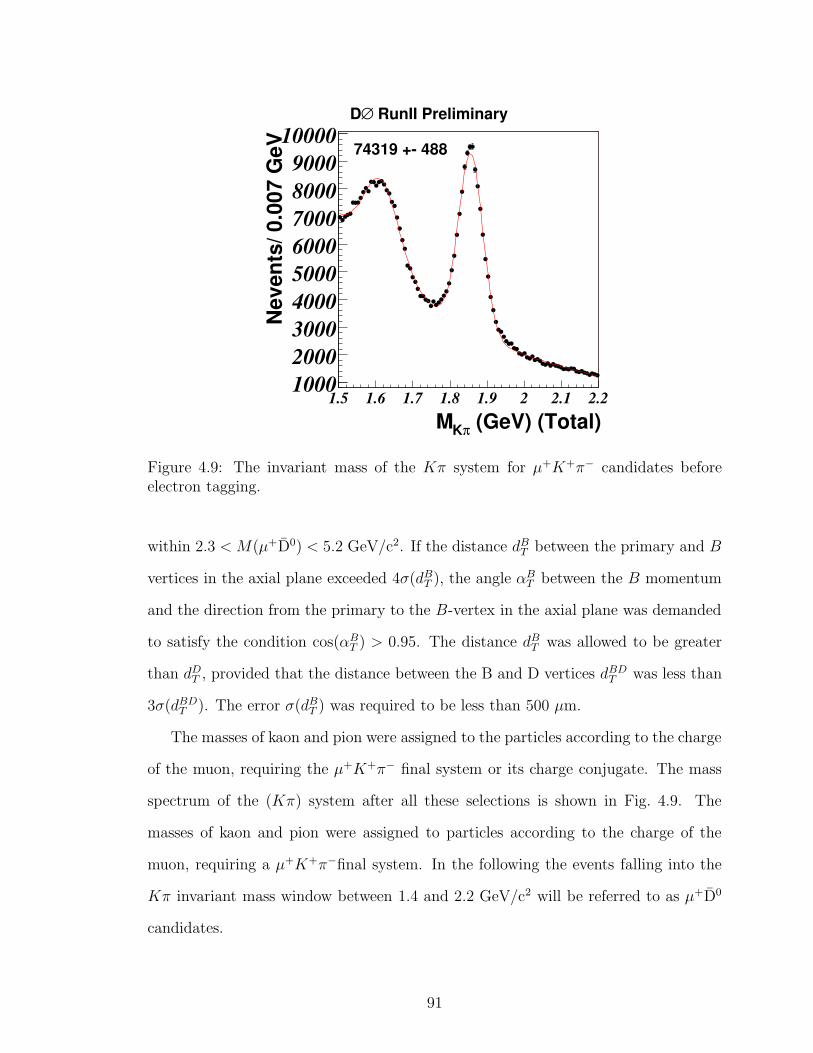
(GeV) (Total)πKM1.5 1.6 1.7 1.8 1.9 2 2.1 2.2

Nev

ents

/ 0.0

07 G

eV

100020003000400050006000700080009000

1000074319 +- 488

RunII Preliminary∅D

Figure 4.9: The invariant mass of the Kπ system for µ+K+π− candidates beforeelectron tagging.

within 2.3 < M(µ+D0) < 5.2 GeV/c2. If the distance dBT between the primary and B

vertices in the axial plane exceeded 4σ(dBT ), the angle αB

T between the B momentum

and the direction from the primary to the B-vertex in the axial plane was demanded

to satisfy the condition cos(αBT ) > 0.95. The distance dB

T was allowed to be greater

than dDT , provided that the distance between the B and D vertices dBD

T was less than

3σ(dBDT ). The error σ(dB

T ) was required to be less than 500 µm.

The masses of kaon and pion were assigned to the particles according to the charge

of the muon, requiring the µ+K+π− final system or its charge conjugate. The mass

spectrum of the (Kπ) system after all these selections is shown in Fig. 4.9. The

masses of kaon and pion were assigned to particles according to the charge of the

muon, requiring a µ+K+π−final system. In the following the events falling into the

Kπ invariant mass window between 1.4 and 2.2 GeV/c2 will be referred to as µ+D0

candidates.

91

(GeV)πK - MππKM0.135 0.14 0.145 0.15 0.155 0.16 0.165 0.17

Nev

ents

/ 0.0

007

GeV

0

2000

4000

6000

8000

1000036086 +- 254


Figure 4.10: The mass difference M(D0π)−M(D0) for events with 1.75 < M(D0) <1.95 GeV/c2.

The curve in Fig.4.9 shows the result of the fit of the K+π− mass distribution with

a Gaussian signal peak and polynomial background. The total number of D0 can-

didates in the peak is 74319 ± 488. The peak at lower masses corresponds to the

partially reconstructed decay D → K+π−X where typically a π0 is not detected.

With the tagging criteria described in the next section, the total number of electron

tagged events is 1790 ± 96 which gives a tag rate of (2.4 ± 0.1%).

For µ+D0 candidates, we search for an additional pion with charge opposite to the

charge of muon and with PT > 0.18 GeV/c. The mass difference ∆M = M(D0π) −

M(D0) for all such pions when 1.75 < M(D0) < 1.95 GeV/c2 is shown in Fig.4.10.

The peak, corresponding to the production of µ+D∗− is clearly seen. The total number

of D∗ candidates in the peak is equal to 36086 ± 254. The signal and the background

have been modelled by a sum of two Gaussian functions and by the sum of exponential

and first-order polynomial functions, respectively.

92

4.8.2 Tagged Sample

We now apply the electron tagging algorithm described in Section 4.5 to the semi-

leptonic final state. Since the semi-leptonic final state are primarily found in events

collected with the inclusive single muon triggers, the event environment is likely to be

different than in events with the J/ψ final state, which are collected with the dimuon

trigger, we re-visit the electron selection criteria. The J/ψ events are less affected by

noise, background etc. and tend to be “cleaner”.

The requirements for the electron tag are summarized below:

• Electron |η| < 1.1 and PT > 2.0 GeV/c.

• The track associated with the electron has to have at least one hit in the Silicon

detector.

• To separate the tag electron from the decaying B candidate, we require (a)

the electron is not from the same jet as the B candidate, and (b) cos(φ angle

between B and tag electron) < 0.5.

• Electron does not come from a photon conversion or from a mis-identified pion

(where the latter comes from KS decay).

• The electron is well reconstructed in the preshower sub-detector. Reconstruc-

tion involves combining clusters in each of its three layers to form a 3D cluster.

Fig. 4.11 shows the minimum single layer cluster (SLC) energy of a CPS cluster

for electrons and pions. We have included a cut on this variable for tagging the

semileptonic decays.

• The electron satisfies criteria described in Table 4.4. To improve electron

identification, we have divided up the sample in 2 PT bins and cuts are chosen

to keep the pion rejection at the same level. This was studied using a sample

of pions from KS decays and conversions to e+e−.

93

Variable P eT < 3.5 GeV/c P e

T > 3.5 GeV/cE/P > 0.55 & < 1.0 > 0.5 & < 1.1EMF > 0.8 > 0.7

Min CPS SLCE (MeV) > 4.0 > 2.0

Table 4.4: Table summarizing the soft electron cuts.

As described in Section 4.4, if more than one non-isolated electron candidate per

event is found the candidate with the maximum P relT is selected. If no non-isolated

electron is found, then the maximum PT isolated electron is chosen.

CPS Min SLC E(MeV)0 10 20 30 40 50 60 70 80 90 100

Arb

itrar

y U

nits

0

0.05

0.1

0.15

0.2

0.25

0.3

0.35Conversion electrons

Ks pions


Figure 4.11: Minimum CPS Single Layer Cluster energy of electrons (from photonconversions) and pions (from K0

S decays)

Fig. 4.12 shows the mass difference M(D0π) −M(D0) after tagging. It is found

to be equal to 904 ± 36 and thus the tagging rate is determined to be (2.5 ± 0.1%).

As will be described in Sec.4.9 the measurement of the Bd oscillations is performed

using the ratio of D∗ events with right and wrong tags. We also use the fits to the

D0 sample and do a simultaneous fit to obtain the mixing parameter. We use the

same algorithm as the one used in the analysis with muons as the inital state flavor

tag [37].

94

/ ndf 2χ 22.40430 / 22

(GeV)πK - MππKM0.135 0.14 0.145 0.15 0.155 0.16 0.165

Nev

ents

/ 0.0

01 G

eV

050

100150200250300350 / ndf 2χ 22.40430 / 22

Ns = 904 +- 36


Figure 4.12: The mass difference M(D0π) −M(D0) for tagged events with 1.75 <M(D0) < 1.95 GeV/c2.

4.9 Experimental Observables

For a mixing analysis, we need to know the production and decay points of the B

hadron, so that we can measure its decay length. The transverse decay length of a B-

hadron Lxy was defined as the distance in the axial plane between the primary vertex

and vertex produced by the muon and D0 . The vertexing algorithm is described in

detail in [42].

The transverse momentum of a B-hadron P µD0

T was defined as the vector sum of

transverse momenta of muon and D0. The sign of the decay length was set positive,

if the angle αBT was less than π/2, otherwise it was set negative. The measured visible

proper decay length (VPDL) was defined as

xM = Lxy ·MB · c/P µD0

T (4.7)

95

Events were divided into 7 bins according to the measured VPDL. The number of

µ+D∗ events with same-sign (“oscillated”) and opposite-sign (“non-oscillated”) tags,

Nosci and Nnon−osc

i , in each bin i of VPDL were determined from a fit of the D∗ peak

in the mass difference M(D0π) −M(D0) distribution.

Bin VPDL (cm) Ntot Nnon−osci Nosc

i εi Ai Aei

1 −0.025-0.000 2154 ±61 29±6 14±5 2.00± 0.30 0.359 ± 0.170 0.3402 0.000-0.025 9974 ±212 159±14 88±10 2.48±0.16 0.286 ± 0.067 0.3313 0.025-0.050 8832 ±137 125±12 59±9 2.09± 0.15 0.355 ± 0.078 0.2874 0.050-0.075 6156 ±121 76±9 46±8 1.98± 0.18 0.245 ± 0.096 0.2075 0.075-0.100 4163 ±88 51±8 49±7 2.39± 0.24 0.025 ± 0.109 0.1046 0.100-0.125 2930 ±140 27±6 25±6 1.77± 0.24 0.034 ± 0.157 −0.0037 0.125-0.250 4735 ±111 49±8 67±9 2.45± 0.23 −0.163 ± 0.104 −0.151

Table 4.5: Definition of the seven bins in VPDL. For each bin the measured number ofD∗ for the opposite sign and same sign of muon tag Nnon−osc

i , Nosci , its statistical error

σ(Nnon−osci ); σ(N osc

i ), all determined from the fits of corresponding mass differenceM(D0π)−M(D0) distributions, measured asymmetry Ai, its error σ(Ai) and expectedasymmetry Ae

i corresponding to ∆md = 0.545 ps−1 (the fit result) are given.

The experimental observables, asymmetry Ai in each VPDL bin, for this measure-

ment were defined as:

Ai =Nnon−osc

i −Nosci

Nnon−osci +Nosc

i

(4.8)

The number of “non-oscillated” and “oscillated” events, the asymmetries and the

corresponding errors derived from the fit in each VPDL bin are given in Table 4.5.

For comparison, we show the expected asymmetry obtained from the best fit to the

data (described in Section 4.10). Fig. 4.13 shows the asymmetry as a function of the

visible proper decay length.

96

4.10 Fitting procedure and results

The D∗ sample is composed mostly of B0d mesons with some contributions from Bu

and Bs mesons. Different species of B mesons behave differently with respect to

oscillations. Neutral B0d and Bs mesons do oscillate while charged Bu mesons do not

oscillate. In the following it was assumed that the oscillations of Bs mesons have

infinite frequency. Possible contributions from b-baryons to the sample were also

neglected.

The purity of the tagging method was defined as

ηs = Ncorrectly tagged events/Ntotal tagged events. It was assumed that the tagging purity is

the same for all reconstructed B mesons because the opposite-side tagging information

has little correlation with the reconstructed B meson candidate.

For a given type of reconstructed B-hadron (i.e. d, u, s), the distribution of the

visible proper decay length x is given by:

nnon−oscd (x,K) =

K

cτBd

exp(− Kx

cτBd

) · 0.5 · (1 + (2ηs − 1) cos(∆m ·Kx/c)); (4.9)

noscd (x,K) =

K

cτBd

exp(− Kx

cτBd

) · 0.5 · (1 − (2ηs − 1) cos(∆m ·Kx/c)); (4.10)

nnon−oscu (x,K) =

K

cτBu

exp(− Kx

cτBu

) · ηs, (4.11)

noscu (x,K) =

K

cτBu

exp(− Kx

cτBu

) · (1 − ηs), (4.12)

nnon−oscs (x,K) = nosc

s (x,K) =K

cτBs

exp(− Kx

cτBs

) · 0.5. (4.13)

where K = P µD0

T /PBT is a K-factor reflecting the difference between the ob-

servable and true momentum of the B-hadron and τ is the lifetime of B-hadrons

taken from [1]. The K-factors were determined from the simulation using generator-

97

level information for the computation of pBT and P µD0

T . The following decay chan-

nels of B mesons were considered: B0d → µ+νD∗−, B0

d → µ+νD∗∗− → µ+νD∗−X,

B+ → µ+νD∗∗0 → µ+νD∗−X and B0s → µ+νD∗−X. Here and in the following the

symbol “D∗∗” denotes both narrow and wide D∗∗ resonances, together with non-

resonant Dπ and D∗π production. The slow pion from D∗−decay was not included

in the PT (µD0) computation for the K-factors. The K-factors for all considered de-

cays were combined into 3 groups: B → µ+νD∗X, B → µ+νD∗∗X → µ+νD∗X and

Bs → µ+νD∗X.

Translation to the measured VPDL, xM is achieved by integration over K-factors

and resolution functions:

Nosc, non−osc(d,u,s), j (xM) =

∫

dx Resj(x−xM )·Effj(x)∫

dK Dj(K)·θ(x)·nosc, non−osc(d,u,s), j (x,K).

(4.14)

Here Resj(x − xM) is the detector resolution of the VPDL and Effj(x) is the

reconstruction efficiency for a given decay channel j of this type of B meson. Both

are determined from the simulation. The decay length resolution was parameterised

by the sum of 3 Gaussians with the following parameters: widths 26, 56 and 141

microns; relative normalizations 0.423, 0.505 and 0.072 respectively. The step function

θ(x) takes into account that only positive values of x are possible (xM can have

negative values due to resolution effects). The function Dj(K) gives the normalized

distribution of the K-factor in a given channel j.

The expected number of oscillated/non-oscillated events in the i-th bin of VPDL

is equal to

Ne,osc/non−osci =

∫

idxM (

∑

f=u,d,s

∑

j

(Brj ·Nosc/non−oscf, j (xM )) (4.15)

Here the integration∫

i dxM is taken over a given interval i, the sum

∑

j is taken

over all decay channels B → µ+νD∗−X and Brj is the branching ratio of a given

98

channel j.

The latest PDG values [1] were used for the B decay branching fractions. Ex-

ploiting the fact that semileptonic B decays are saturated by decays to D, D∗ and

D∗∗ , and isotopical invariance it was determined that the B0d ( 85%) and B+ ( 15%)

decays give the main contributions to the sample. The Bs contribution is small but

it was taken into account.

Finally, the expected value Aei for interval i of the measured VPDL is given by

equation (4.8), and substituting Nnon−osci and Nosc

i by N e,non−osci and N e,osc

i .

The fit values of ∆m and ηs were determined from the minimization of a χ2(∆m,ηs)

defined as:

χ2(∆m, ηs) =∑

i

(Ai − Aei (∆m, ηs))

2

σ2(Ai). (4.16)

We perform a simultaneous fit to the B0 and B+ samples. The result of the

minimization is:

∆md = 0.545 ± 0.085 (stat) ps−1 ηs = (66.9 ± 1.5)% (4.17)

The values of Aei obtained in each bin are given in Table 4.5. Fig. 4.13 shows the

asymmetry as function of VPDL together with the result of the fit1.

4.11 A study of systematic uncertainties

We studied various sources of systematic uncertainties and the more important ones

are described in this section, and results are summarized in Table 4.6.

The B meson branching rates and lifetimes used in the fit of the asymmetry were

taken from [1] and were varied by 1σ. The VPDL resolution, obtained in simulation,

was multiplied by a large factor from 0.2 to 2, significantly exceeds the estimated

1As a check the fit was performed by allowing different values of purity for the B0and B+

dominated samples. In this case, we obtain η0s

and η+s

to be (67.4 ± 2.8)% and (66.8 ± 2.0)%,respectively, which is consistent with the main result in the text

99

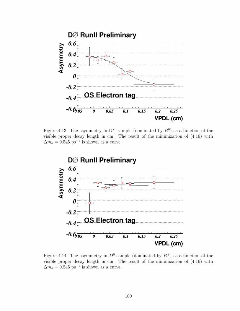
VPDL (cm)-0.05 0 0.05 0.1 0.15 0.2 0.25

VPDL (cm)-0.05 0 0.05 0.1 0.15 0.2 0.25

Asy

mm

etry

-0.6

-0.4

-0.2

0

0.2

0.4

0.6

OS Electron tag


Figure 4.13: The asymmetry in D∗ sample (dominated by B0) as a function of thevisible proper decay length in cm. The result of the minimization of (4.16) with∆md = 0.545 ps−1 is shown as a curve.

VPDL (cm)-0.05 0 0.05 0.1 0.15 0.2 0.25

VPDL (cm)-0.05 0 0.05 0.1 0.15 0.2 0.25

Asy

mm

etry

-0.6

-0.4

-0.2

0

0.2

0.4

0.6

OS Electron tag


Figure 4.14: The asymmetry in D0 sample (dominated by B+) as a function of thevisible proper decay length in cm. The result of the minimization of (4.16) with∆md = 0.545 ps−1 is shown as a curve.

100

difference in the resolution between data and simulation.

The variation of K-factors with the change of B momentum was neglected in this

analysis. To check the impact of this assumption on the final result, their computation

was repeated without the cut on PT (D0) or by applying an additional cut on PT of

muon, PT > 4 GeV/c. The change of average value of K-factors did not exceed 2%,

which was used as the estimate of the systematic uncertainty in their values. This

was propagated into the variation of ∆md and tagging purity by repeating the fit

with the K-factor distributions shifted by 2%.

The reconstruction efficiency in different B-meson decay channels depends only

on the kinematic properties of corresponding decays and can therefore be reliably

estimated in the simulation. The ISGW2 model [45] was used to describe semileptonic

B decays. The uncertainty of the reconstruction efficiency, set at 12%, was estimated

by varying kinematic cuts on PT of the muon and D0 in a wide range. Changing the

model describing semileptonic B decay from ISGW2 to HQET [46] produces a smaller

variation. The fit to extract ∆md was repeated with the efficiencies to reconstruct

B → µ+νD∗∗− and B → µ+νD∗∗0 channels modified by 12%, and the difference was

taken as the systematic uncertainty from this source.

Possible background contribution into events with small lifetime, e.g. the cc con-

tamination of the sample or the misidentification of the muon, can bias the oscillation

wave at small values of VPDL. The contribution of this background was varied from

3.5% to 10% and the difference in the result was taken as the systematic uncertainty

from this source.

We also investigated the systematic uncertainty of measuring the number of

D∗ and D0 candidates in each VPDL bin. This we call systematics due to fit

procedure. We changed the background parametrization for the D0 mass fit from the

exponent to a second degree polynomial and varied the background shape by ±1σ.

For the D∗ candidates, we performed cross-checks using other functions, but

101

the chosen background parametrization gives the best description. Since we fix the

background shape, we varied the background shape by ±1σ. Also, the default bin

width for the fits in individual VPDL bins is 1.40 MeV. We lowered the binwidth to

1.05 MeV, and increased the binwidth 1.75 MeV, and include it in our systematics.

variation δ(∆md) δ(D(B0)) δ(D(B+)) δ(D)Br(B0 → D∗−µ+ν) 5.53 ± 0.023% 0.002 ps−1 0.001 0.001 0.001Br(B → D∗πµνX) 1.07 ± 0.17% 0.008 ps−1 0.002 0.001 0.001

B lifetime ±1σ 0.001 ps−1 0.000 0.000 0.000Resolution function ×[0.2 ÷ 2] 0.006 ps−1 0.002 0.000 0.000

Alignment ±10µm 0.007 ps−1 0.004 0.000 0.004K-factor ± 2% 0.009 ps−1 0.000 0.000 0.000

cc Background [0.035 ÷ 0.1] 0.002 ps−1 0.002 0.000 0.002Efficiency ±12% 0.006 ps−1 0.001 0.001 0.001

Fit procedure Overall 0.010 ps−1 0.006 0.006 0.008

Total 0.019 ps−1 0.008 0.006 0.009

Table 4.6: Systematic uncertainties.

4.12 Conclusions

We use both fully reconstructed B± events as well as a large semileptonic sample

corresponding to about 36086 (µ+D∗X) candidate events.

Using the latter sample, the B0 meson oscillation frequency was measured to be

consistent with the world average. We also obtained a tag rate, purity and dilution

of,

ε = (2.5 ± 0.1)%, ηs = (66.9 ± 1.5 ± 0.5)%, D = (34.0 ± 3.0 ± 0.9)%

and tagging power, εD2 = (0.29 ± 0.05 ± 0.03)%.

102

4.13 Combined Tagging

In this section, we discuss how we combined the different tagging algorithms into a

single tagging variable to be finally used in our B0s mixing analysis. Many different

properties can be used to identify the original flavor – b or b – of a heavy quark

producing a reconstructed B meson. Some of them perform well by themselves; other

properties give a weak separation between flavors. In all cases, their combination into

a single tagging variable gives a significantly better result [47, 48] . We obtain such

a combination with the likelihood ratio method described below.

It is assumed that a set of discriminating variables x1, ...xn can be constructed

for a given event. The discriminating variable, by definition, should have a different

distribution for b and b flavors. For the initial b quark, the probability density function

(PDF) for a given variable xi is denoted as f bi (xi), while for the initial b quark it is

denoted as f bi (xi). The combined tagging variable y is defined as:

y =n∏

i=1

yi; yi =f b

i (xi)

f bi (xi)

(4.18)

Given variable xi can be undefined for some events. For example, there are events

which don’t contain an identified muon from the opposite side. In this case, the

corresponding variable yi is set to 1. The initial b flavor is more probable if y < 1,

and b flavor is more probable if y > 1. Correspondingly, an event with y < 1 is tagged

as b quark and the event with y > 1 is tagged as b quark. For an oscillation analysis,

it is more convenient to define the tagging variable as:

d =1 − y

1 + y. (4.19)

The variable d changes between -1 and 1. An event with d > 0 is tagged as b quark

and with d < 0 as b quark. Higher |d| value corresponds to a higher tagging purity.

103

For uncorrelated variables x1, ...xn, and perfect modeling in the PDF, d gives the best

possible tagging performance and its absolute value gives a dilution of a given event.

Very often analyzed events are divided into samples with significantly different

discriminating variables and tagging performance. This division would imply making

a separate analysis for each sample and combining results at a later stage. On the

contrary, the tagging variable d defined by (4.18-4.19) provides a “calibration” of

all events regardless of their intrinsic differences. Since its value is proportional to

the dilution of the flavor tagging, events from different categories but with a similar

value of d can be treated in the same way. Thus, another important advantage of the

proposed method of the flavor tagging is a possibility to build a single variable having

the same meaning for all kinds of events. It allows to classify all events according to

their tagging performance and use them simultaneously in the analysis.

4.13.1 Discriminating Variables

All our discriminating variables are constructed using properties of the b quark oppo-

site to the reconstructed B meson (“opposite side tagging”). It is assumed that every

event with b quark also contains a b quark. Therefore, the b flavor at the opposite

side determines the b flavor at the reconstruction side. An important property of

the opposite side tagging is the independence of its performance on the type of the

reconstructed B meson, since the hadronization of two b quark is not correlated in

pp interactions. Therefore, the flavor tagging algorithm can be calibrated in data by

applying it to the events with the B0 and B+ decays. The measured performance

then can be used to study Bs meson oscillations.

Another set of variables, which exploits properties of hadronization b → B at the

reconstruction side, can also be defined (“same side tagging”). The tagging with these

variables depends on the type of B meson. Its performance can only be obtained from

the simulation and is therefore model dependent. Currently, it is not used for the Bs

104

mixing measurement and is not discussed here.

The probability density function for each discriminating variable discussed below

was constructed using events from D0 sample with the visible proper decay length

greater than 0 and less than 500 µm. The B0d → µ+νD∗+ events give 16% con-

tribution and due to the cut on the visible proper decay length contain mainly the

non-oscillating B0d decays. Therefore, the initial flavor of a b-quark is determined by

the charge of the muon. According to the MC estimates, the purity of such identifica-

tion of the initial flavor in the selected sample is 0.98± 0.01, where the error reflects

the uncertainty in branching ratios of B decays.

For each discriminating variable, the signal band containing all events with 1.80 <

M(Kπ) < 1.92 , and the background band containing all events with 1.94 < M(Kπ) <

2.2 were defined. The PDF distribution was constructed as the difference of dis-

tribution for the signal band and for the background band multiplied by 0.74. The

coefficient 0.74 was chosen so that the number of events in the background band

corresponds to the estimated number of background events events in the signal band.

In each analyzed event, an additional muon was searched for. This muon was

required to have at least one hit in the muon chambers, and to have cosφ(pµ,pB) <

0.8, where pB is a three-momentum of the reconstructed B meson. If more than one

muon was found, the muon with the highest number of hits in the muon chambers

was used. If more than one muon with the same number of hits in the muon chambers

was found, the muon with the highest transverse momentum pT was used. For this

muon, a muon jet charge QµJ was constructed as:

QµJ =

∑

i qipi

T∑

i piT

.

The sum was taken over all charged particles, including the muon, satisfying the

condition ∆R =√

(∆φ)2 + (∆η)2 < 0.5. ∆φ and ∆η were computed with respect to

the muon direction. Daughters of the reconstructed B meson were explicitly excluded

105

from the sum. In addition, any charged particle with cosφ(p,pB) > 0.8 was excluded.

An additional identified electron [40] was used for the flavor tagging if cosφ(pe,pB) <

0.8. For this electron, an electron jet charge QeJ was constructed as:

QeJ =

∑

i qipi

T∑

i piT

.

The sum was taken over all charged particles, including the electron, satisfying the

condition ∆R =√

(∆φ)2 + (∆η)2 < 0.5. ∆φ and ∆η were computed with respect

to the electron direction. Daughters of the reconstructed B meson were explicitly

excluded from the sum. In addition, any charged particle with cosφ(p,pB) > 0.8 was

excluded.

A secondary vertex corresponding to the decay of B mesons was searched for

using all charged particles in the event. The secondary vertex should contain at

least 2 particles with the axial impact parameter significance greater than 3. The

distance lxy from the primary to the secondary vertex should satisfy the condition:

lxy > 4σ(lxy). The details of the secondary vertex search can be found in [42].

The momentum of the secondary vertex pSV was defined as the sum of all mo-

menta of particles included in the secondary vertex. The secondary vertex with

cosφ(pSV ,pB) < 0.8 was used for the flavor tagging. A secondary vertex charge QSV

was defined as the third discriminating variable:

QSV =

∑

i (qipi

L)k

∑

i (piL)k

.

where the sum was taken over all particles included in the secondary vertex. Daugh-

ters of the reconstructed B meson were explicitly excluded from the sum. In addition,

any charged particle with cosφ(p,pB) > 0.8 was excluded. The piL is the longitudinal

momentum of a given particle with respect to the direction of the secondary vertex

momentum. The value of k = 0.6 was used. It was taken from the previous studies

106

at LEP [44]. We found that this value of k results in an optimal performance of the

QSV variable, as can be seen in Fig. 4.15.

Finally, the event charge QEV was constructed as:

QEV =

∑

i qipi

T∑

i piT

.

The sum was taken over all charged particles with 0.5 < pT < 50 and having

cosφ(p,pB) < 0.8. Daughters of the reconstructed B meson were explicitly excluded

from the sum.

4.13.2 The Combined Tagger

For each event with an identified muon, the muon jet charge QµJ and the secondary

vertex charge QSV were used to construct a muon tagger. For each event without a

muon but with an identified electron, the electron charge QeJ and the secondary vertex

charge QSV were used to construct an electron tagger. Finally, for events without a

muon or an electron but with reconstructed secondary vertex, the secondary vertex

charge QSV and the event jet charge QEV were used to construct a secondary vertex

tagger. The resulting distribution of the tagging variable d for the combination of all

three taggers, called the combined tagger, is shown in Fig. 4.16.

4.14 Results

For any sample of tagged events, the observed and expected asymmetries were deter-

mined using the flavor asymmetry given as

A =Nnos −Nosc

Nnos +Nosc, (4.20)

107

κ0.2 0.4 0.6 0.8 1 1.2 1.4 1.6 1.8 2

Dilu

tion

0.12

0.14

0.16

0.18

0.2

0.22

0.24

0.26

0.28

0.3µwith

µwithout

Figure 4.15: Dilution of events tagged by QSV versus the coefficient k. Statisticalerrors shown are correlated.

and the expected value Aei for interval i of the measured VPDL given as:

Aei (∆m, fcc,Dd,Du) =

N e,nosi −N e,osc

i

N e,nosi +N e,osc

i

(4.21)

in all VPDL bins. The values of ∆md, fcc, Du and Dd were obtained from the

simultaneous χ2 fit:

χ2(∆md, fcc,Dd,Du) = χ2D∗(∆md, fcc,Dd,Du) + χ2

D0(∆md, fcc,Dd,Du)(4.22)

χ2D∗(∆md, fcc,Dd,Du) =

∑

i

(Ai,D∗ − Aei,D∗(∆md, fcc,Dd,Du))

2

σ2(Ai,D∗)

χ2D0(∆md, fcc,Dd,Du) =

∑

i

(Ai,D0 − Aei,D0(∆md, fcc,Dd,Du))

2

σ2(Ai,D0).

Here∑

i is the sum over all VPDL bins. Examples of the fit of the flavor asymmetry

with (Eq.4.22) is shown in Fig. 4.17-4.18.

The performance of the flavor tagging was studied separately for the muon, elec-

tron and secondary vertex taggers using events with |d| > 0.3. Results are given in

Tables 4.7-4.9. All errors are statistical and do not include systematic uncertainties.

108

DØ RunII Preliminary

0

500

1000

1500

2000

-1 -0.5 0 0.5 1Combined tagging variable

q(brec) < 0

q(brec) > 0

Figure 4.16: Normalized distributions of the combined tagging variable. The q(brec)is the charge of the b quark from the reconstruction side.

The tagging efficiencies shown in Tables 4.7, 4.8 were computed using events with the

VPDL=[0.025,0.250]. This selection reduces the contribution from cc → µ+νD0X

events, since they have a VPDL distribution with zero mean and σ ∼ 150µm accord-

ing to our study.

It can be seen from Tables 4.7,4.8 that the dilution of the individual taggers

with the same cut on |d| is similar. This is a direct consequence of the chosen tagging

method which defines the tagging variable through the ratio of probabilities. It allows

a very simple and transparent combination of different taggers into a single variable

with a significantly larger tagging power. All taggers give a compatible value of

∆md and fcc, as can be seen in Table 4.9. For the combined tagger the following

109

VPDL (cm)-0.05 0 0.05 0.1 0.15 0.2 0.25

VPDL (cm)-0.05 0 0.05 0.1 0.15 0.2 0.25-0.6

-0.4

-0.2

0

0.2

0.4

0.6 dil: 0.473 +/-0.027, eff: 0.066 +/-0.001 µ D*→B


(Muon Tag)

dil: 0.473 +/-0.027, eff: 0.066 +/-0.001 µ D*→B

VPDL (cm)-0.05 0 0.05 0.1 0.15 0.2 0.25

VPDL (cm)-0.05 0 0.05 0.1 0.15 0.2 0.25-0.6

-0.4

-0.2

0

0.2

0.4

0.6 dil: 0.444 +/-0.015, eff: 0.071 +/-0.001 µ0 D→B


(Muon Tag)

dil: 0.444 +/-0.015, eff: 0.071 +/-0.001 µ0 D→B

VPDL (cm)-0.05 0 0.05 0.1 0.15 0.2 0.25

VPDL (cm)-0.05 0 0.05 0.1 0.15 0.2 0.25-0.6

-0.4

-0.2

0

0.2

0.4

0.6 dil: 0.341 +/-0.057, eff: 0.018 +/-0.001 µ D*→B


(Electron Tag)

dil: 0.341 +/-0.057, eff: 0.018 +/-0.001 µ D*→B

VPDL (cm)-0.05 0 0.05 0.1 0.15 0.2 0.25

VPDL (cm)-0.05 0 0.05 0.1 0.15 0.2 0.25-0.6

-0.4

-0.2

0

0.2

0.4

0.6 dil: 0.445 +/-0.032, eff: 0.019 +/-0.000 µ0 D→B


(Electron Tag)

dil: 0.445 +/-0.032, eff: 0.019 +/-0.000 µ0 D→B

Figure 4.17: The asymmetries obtained in the D∗ and D0 sample with the result ofthe fit superimposed for the Muon and electron tagger. For the individual taggers,|d| > 0.3 was required.

110

VPDL (cm)-0.05 0 0.05 0.1 0.15 0.2 0.25

VPDL (cm)-0.05 0 0.05 0.1 0.15 0.2 0.25

Asy

mm

etry

-0.6

-0.4

-0.2

0

0.2

0.4

0.6 dil: 0.599 +/-0.058, eff: 0.011 +/-0.001µ D*→B


(Combined |d|>0.6)

dil: 0.599 +/-0.058, eff: 0.011 +/-0.001µ D*→B

VPDL (cm)-0.05 0 0.05 0.1 0.15 0.2 0.25

VPDL (cm)-0.05 0 0.05 0.1 0.15 0.2 0.25

Asy

mm

etry

-0.6

-0.4

-0.2

0

0.2

0.4

0.6 dil: 0.488 +/-0.035, eff: 0.012 +/-0.000µ D0→B


(Combined |d|>0.6)

dil: 0.488 +/-0.035, eff: 0.012 +/-0.000µ D0→B

Figure 4.18: The asymmetries obtained in the D∗ and D0 sample with the combinedtagger for bin |d| > 0.6. The result of the fit is superimposed

results were obtained:

εD2d = (2.19 ± 0.22)(%) (4.23)

∆md = 0.513 ± 0.023

fcc = (3.3 ± 1.3)(%)

Tagger ε(%) Dd εD2d(%)

Muon (|d| > 0.3) 6.61 ± 0.12 0.473 ± 0.027 1.48 ± 0.17Electron (|d| > 0.3) 1.83 ± 0.07 0.341 ± 0.058 0.21 ± 0.07SVCharge (|d| > 0.3) 2.77 ± 0.08 0.424 ± 0.048 0.50 ± 0.11Combined (|d| > 0.3) 11.14 ± 0.15 0.443 ± 0.022 2.19 ± 0.22Multidim (|d| > 0.37) 10.98 ± 0.15 0.395 ± 0.022 1.71 ± 0.19Combined(0.10< |d| <0.20) 4.63 ± 0.10 0.084 ± 0.031 0.03 ± 0.02Combined(0.20< |d| <0.30) 5.94 ± 0.12 0.236 ± 0.027 0.33 ± 0.08Combined(0.30< |d| <0.45) 3.89 ± 0.09 0.385 ± 0.034 0.58 ± 0.10Combined(0.45< |d| <0.60) 4.36 ± 0.10 0.512 ± 0.032 1.14 ± 0.14Combined(0.60< |d| <1.00) 1.13 ± 0.05 0.597 ± 0.058 0.40 ± 0.08

Table 4.7: Tagging performance for events with recosntructed B0 for different taggersand subsamples.

One of the goals of this measurement is to verify the assumption of independence

111

Tagger ε(%) Du εD2u(%) D′

d

Muon (|d| > 0.3) 7.10 ± 0.09 0.444 ± 0.015 1.400 ± 0.096 0.463 ± 0.028Electron (|d| > 0.3) 1.88 ± 0.05 0.445 ± 0.032 0.372 ± 0.054 0.324 ± 0.060SVCharge (|d| > 0.3) 2.81 ± 0.06 0.338 ± 0.026 0.320 ± 0.050 0.421 ± 0.049Combined (|d| > 0.3) 11.74 ± 0.11 0.419 ± 0.012 2.058 ± 0.121 0.434 ± 0.023Multidim (|d| > 0.37) 11.67 ± 0.11 0.363 ± 0.012 1.540 ± 0.106 0.384 ± 0.023Combined(0.10< |d| <0.20) 4.59 ± 0.08 0.104 ± 0.017 0.050 ± 0.016 0.079 ± 0.029Combined(0.20< |d| <0.30) 6.10 ± 0.09 0.234 ± 0.014 0.335 ± 0.042 0.212 ± 0.024Combined(0.30< |d| <0.45) 3.98 ± 0.07 0.361 ± 0.018 0.519 ± 0.052 0.364 ± 0.032Combined(0.45< |d| <0.60) 4.77 ± 0.07 0.504 ± 0.016 1.211 ± 0.077 0.489 ± 0.030Combined(0.60< |d| <1.00) 1.17 ± 0.04 0.498 ± 0.031 0.290 ± 0.038 0.572 ± 0.056

Table 4.8:Tagging performance for events with recosntructed B+ for different taggers and sub-samples. For comparison, the dilution D′

d measured in the D∗ sample with additionof wrong sign µ+νD0π+ events is also shown.

Tagger ∆md fcx

Muon 0.502 ± 0.028 0.013 ± 0.010Electron 0.481 ± 0.067 0.058 ± 0.045SV Charge 0.553 ± 0.053 0.096 ± 0.050Multidim 0.502 ± 0.026 0.031 ± 0.014Combined(|d| > 0.3) 0.513 ± 0.023 0.033 ± 0.013Combined(0.10 < |d| < 0.20) 0.506 ± 0.209 0.495 ± 0.505Combined(0.20 < |d| < 0.35) 0.523 ± 0.064 0.021 ± 0.025Combined(0.35 < |d| < 0.45) 0.531 ± 0.042 0.063 ± 0.038Combined(0.45 < |d| < 0.60) 0.510 ± 0.032 0.010 ± 0.010Combined(0.60 < |d| < 1.00) 0.456 ± 0.049 0.032 ± 0.026

Table 4.9: Measured value of ∆md and fcc for different taggers and subsamples.

112

of the opposite-side flavor tagging on the type of the reconstructed B meson. It

can be seen from Tables 4.7,4.8 that the measured flavor tagging performance for

B0 events is slightly better than for B+ events, both for individual and combined

taggers. This difference can be explained by a better selection of µ+νD∗− events due

to an additional requirement of the charge correlation between muon and pion from

D∗− → D0π− decay. The D0sample can contain events with a wrongly selected muon.

Since the charge of the muon determines the flavor asymmetry, such a background

can reduce the measured B+ dilution. The charge correlation between the muon and

the pion can suppress this background and result in a better measurement of the

tagging performance.

To test this hypothesis, a special sample of events satisfying all conditions for

D∗ sample, except the requirement of the charge correlation between the muon and

the pion, was selected. The dilution D′d for such sample is shown in Table 4.8. It

can be seen that D′d is statistically compatible with Dufor all samples and all taggers.

The χ2 for the difference in dilutions is found to be 1.06 to be compared to 1.27 in

the case where only RS events are considered for the D∗ sample.

This result confirms the assumption of the same performance of the opposite-side

flavor tagging for B+ and B0 events. It also shows that unaccounted contribution

of background in the D0 sample reduces the measured dilution for B+ events. This

background is suppressed by the requirement of the charge correlation between the

muon and the pion. Thus, the dilution measured in the D∗ sample can be used for

the Bs mixing measurement, where a similar charge correlation between the muon

and Ds is required.

By construction of the combined tagging, the dilution for any event should strongly

depend on the magnitude of the variable d. This property becomes important in the

Bs mixing measurement, since in this case the dilution of each event can be estimated

using the value of d and can be included in the likelihood function, improving the

113

sensitivity of the measurement. To test the dependence of dilution on d, all tagged

events were divided into subsamples with 0.1 < |d| < 0.2, 0.2 < |d| < 0.35, 0.35 <

|d| < 0.45, 0.45 < |d| < 0.6, and |d| > 0.6. The overall efficiency of this sample

is (19.95 ± 0.21)(%). The obtained dilutions are shown in Table 4.7. Their strong

dependence on the value of the tagging variable is clearly seen. The overall tagging

power, computed as the sum of tagging powers of all subsamples is:

εD2d = (2.48 ± 0.21)(%) (4.24)

The measured oscillation parameter ∆md for all considered taggers and subsam-

ples is given in Table 4.9. It is compatible with the world average value ∆md =

0.509 ± 0.004 ps−1.

Finally, the mixing parameter ∆md was obtained from the simultaneous fit of the

flavor asymmetry in the above defined subsamples. The fraction fcc was constrained

to be the same for all subsamples. The obtained result is:

∆md = 0.506 ± 0.020 (4.25)

fcc = (2.2 ± 0.9)(%)

The statistical precision of ∆md from the simultaneous fit is about 10% better

than that from the fit of events with |d| > 0.3. This improvement is directly related

with a better overall tagging power (4.24) for the sum of subsamples as compared to

the result (4.23) for the sample with |d| > 0.3.

4.15 Conclusions

A study of the likelihood-based opposite-side tagging algorithm in B0 and B+ samples

was performed. The dilutions D(B+) and D(B0) are consistent within their statistical

114

errors.

Splitting the sample into bins, according to the tagging variable |d| and measuring

the tagging power as the sum of individual tagging power in all bins we obtained

εD2 = (2.48 ± 0.21 (stat.)+0.08−0.06 (syst)) (%)

From a simultaneous fit to events in all |d| bins we measured the mixing parameter

∆md parameter: ∆md = 0.506 ± 0.020 (stat) ± 0.016 (syst) ps−1 which is in good

agreement with the world average value of ∆md = 0.509 ± 0.004 ps−1 [49].

115

Chapter 5

B0s Mixing Analysis

5.1 Introduction

In this chapter, we discuss the mixing analysis done in B0s → D−

s µ+X with Ds de-

caying to D−s → K∗0K− (K∗0 → K+π−) final state with ∼ 1.2 fb−1 of data col-

lected with the DØ detector during Run II of the Fermilab Tevatron [51, 52]. At

DØ, we already have set a two sided bound on the mixing parameter using our

large semileptonic data sample which was later confirmed by the CDF experiment.

The recent double sided bound on Bs mixing by the DØ collaboration [16] and its

confirmation later by CDF collaboration [17] has led to a lot of excitement and

enthusiasm in the Flavor Physics sector. This has provided a very good oppor-

tunity to these experiments to measure the Bs oscillations as precisely as possible

before the LHC comes into operation. DØ put a double sided bound on the Bs

mixing oscillation between 17.0 < ∆ms < 21.0 ps−1 at the 90% confidence level

with a most probable value of ∆ms = 19 ps−1. CDF measures this oscillation as

∆ms = 17.31+0.33−0.18(stat.)±0.07(sys) ps−1. It is an important test of the CKM formal-

ism of the Standard Model, and combining it with a measurement of ∆md will allow

us to reduce the theoretical error on the CKM matrix element Vtd. If the Standard

Model is correct, then ∆ms = 18.3+6.5−1.5 ps−1 from global fits to the unitarity triangle

117

if the current experimental limits on ∆ms are included in the fit. If information from

B0s oscillations limits are not included, global fits give ∆ms = 20.9+4.5

−4.2 ps−1 [50]. The

current measurements indicate a value well within the SM allowed range and small

enough to allow us to measure ∆ms with semileptonic decays.

5.2 Event Selection

All tracks in an event were clustered into jets using the DURHAM clustering algo-

rithm [53] with the cutoff parameter of 15 GeV/c. The following requirements were

made to identify the B0s → D−

s µ+X , D−

s → K∗0K− , K∗0 → K+π− decay chain. The

muon was identified using the standard DØ algorithm [54]. It was required to have

pT > 2 GeV/c and p > 3 GeV/c, to have hits in both the CFT and SMT and to have

at least 2 measurements in the muon chambers. Particles were assigned the masses

of kaons (K1 and K2) and pion requiring the charge combination µ+K+1 K

−2 π

− or its

charge conjugate. For the Ds → K∗K channel, transverse momenta were required to

be: pT (K1) > 0.9 GeV/c, pT (K2) > 1.8 GeV/c and pT (π) > 0.5 GeV/c, assuming

that K1 comes from the K∗0 → K+π− decay.

For each particle, the transverse1 εT and longitudinal2 εL projections of track

impact parameter with respect to the primary vertex together with the correspond-

ing errors (σ(εT ), σ(εL)) were computed. The combined significance (εT/σ(εT ))2 +

(εL/σ(εL))2 was required to be greater than 4 for K1 and K2, while there was no cut

on the significance of the pion.

Three charged particles were required to come from the same D−s vertex with

the χ2 of the vertex fit satisfying χ2 < 16. The D−s candidate produced by their

combination was required to have a common B vertex with the muon with the χ2 of

the vertex fit such that χ2 < 9. The mass of the µ+D−s system was required to be

1in the plane perpendicular to the beam direction.2parallel to the beam direction.

118

2.6 < M(µ+D−s ) < 5.4 GeV/c2. The distance dD

T in the axial plane between the D−s

vertex and the primary interaction point was required to satisfy dDT /σ(dD

T ) > 4. The

angle αDT between the momentum direction of the D−

s candidate and the direction

from the primary to the D−s vertex in the axial plane was required to fulfill the

condition: cos(αDT ) > 0.9.

If the distance dBT between the primary and B0

s vertex in the axial plane exceeded

4·σ(dBT ), the angle αB

T between the B0s momentum and the direction from the primary

to B0s vertex in the axial plane was required to satisfy the condition: cos(αB

T ) > 0.95.

The distance dBT was allowed to be greater than dD

T , provided that the distance between

the B0s and D−

s vertices dBDT was less than 2 · σ(dBD

T ).

Additionally, for the D−s → K∗0K− channel, the condition 0.82 < M(K1π) < 0.95

was applied. The final event samples were selected using the likelihood ratio method,

described below.

It is assumed that a set of discriminating variables x1, ...xn can be constructed for

a given event. It is also assumed that the probability density functions f s(xi) for the

signal and f b(xi) for the background can be built for each variable xi. The combined

tagging variable y is defined as:

y =n∏

i=1

yi; yi =f b

i (xi)

f si (xi)

. (5.1)

The selection of the signal is obtained by applying the cut on y < y0. For uncorrelated

variables x1, ...xn, the selection using the combined variable y gives the best possible

tagging performance, i.e., maximal signal efficiency for a given background efficiency.

The following discriminating variables were used:

• Helicity angle, defined as the angle between the D−s and K1 momenta in the

(K1π) center of mass system,

• Isolation, computed as Iso = ptot(µDs)/(ptot(µDs) +

∑

ptoti ). The sum

∑

ptoti

119

was taken over all charged particles in the cone√

(∆φ)2 + (∆η)2 < 0.5, where

∆η and ∆φ are the pseudorapidity and the azimuthal angle with respect to the

(µDs) direction. The µ+, K1, K2 and π− were not included in the sum,

• pT (K2),

• Invariant mass, M(µ+D−s ),

• χ2 of the D−s vertex fit,

• M(K1π).

The probability density functions were constructed using real data events. For

each channel, three bands B1, B2 and S were defined as:

B1 : 1.75 < M(D−s ) < 1.79 GeV/c2

B2 : 2.13 < M(D−s ) < 2.17 GeV/c2

S : 1.92 < M(D−s ) < 2.00 GeV/c2

The background probability density function for each variable was constructed using

events from the B1 and B2 bands. The signal probability density function was con-

structed by subtracting the background, obtained as a sum of distributions in the B1

and B2 bands, from the distribution of events in band S. The final selection of events

for the analysis was done by applying a cut on the combined variable log10 y < 0.16.

This cut was selected by requiring the maximal value of S/√S +B1 +B2.

Figure 5.1 shows the K∗0K− invariant mass distribution after all the selection

cuts. Distributions for both the “right-sign” D−s µ

+ combinations (Qµ ∗Qπ < 0) and

the “wrong-sign” D−s µ

− combinations (Qµ ∗Qπ > 0) are shown.

120

)2)K (GeV/cπMass (K1.8 1.85 1.9 1.95 2 2.05 2.1 2.15 2.2 2.25

)2E

vent

s/(7

.6 M

eV/c

0

1000

2000

3000

4000

5000

6000

7000

8000

9000D0 RunII Preliminary

Figure 5.1: Distribution of the mass of D−s → K∗0K− candidates. Both “right-sign”

(red) and “wrong-sign” (black) combinations are shown.

5.3 Mass Fitting Procedure

In the decays D− → K+π−π−, when the pion is mis-identified as a kaon it peaks

right under the D−s → K∗0K− signal peak and this peak strongly overlaps. The

final state KKπ mass spectrum could be a mixture of many different decays so the

shape of reflection D− → K+π−π− strongly depends on kinematical properties of

events and changes for different selections. Due to large reflections coming from the

mis-identification of pion track as a kaon track, extracting the signal becomes very

difficult in D−s → K∗0K− decays. In order to separate the signal from the large

reflection we developed an event-by-event fit based on the kinematic properties of the

events. The details of the unbinned mass fitting procedure is as follows:

Consider the decay D− → K+π−π−. The mass of Kππ system is given as:

M2D = (EKπ + Eπ)2 − (~PKπ + ~Pπ)2 (5.2)

where EKπ is the energy of (K−π+) and Eπ, Pπ is the energy and momentum of the

121

second pion respectively. Eπ =√

P 2Tr +M2

π , is the energy of track assuming the pion

mass hypothesis,

When this pion is assigned the mass of Kaon, the shifted mass of Kπ”K” system is

M2R = (EKπ + EK)2 − (~PKπ + ~PK)2 (5.3)

~PK = ~Pπ = ~PTr (5.4)

where, EK =√

P 2Tr +M2

K is the energy of the track assuming the kaon mass hypoth-

esis.

We can express MR as:

M2R = M2

D + (EKπ + EK)2 − (EKπ + Eπ)2 (5.5)

M2R = M2

D + (M2K −M2

π) + 2EKπ(EK − Eπ) (5.6)

M2R = M2

D + (1 + 2R)(M 2K −M2

π) (5.7)

where,

R =EKπ(EK − Eπ)

(M2K −M2

π)(5.8)

is the reflection variable.

A similar equation can be written for reflection due to Λc → K+π−P+, where the

proton can be mis-identified as kaon. From equation 5.8, we see that the shifted mass

depends on kinematic properties of the events but for a given EKπ and PTr, the shift

is constant. Also, for a given EKπ and PTr the mass distribution of the reflection is

determined only by the detector resolution and can be approximated by a Gaussian.

Figure 5.2 shows the distribution of the R variable for signal and reflection MC

samples. From the figure we can see that the shape of R variable for signal and

reflection are very similar. Figure 5.3 shows the distribution of (Kπ)K mass system

122

in different bins of R variable. From these plots, it can be seen that the shape of the

combinatoric background changes significantly with R.

0 0.5 1 1.5 2 2.5 3 3.5 40

0.02

0.04

0.06

0.08

0.1

0.12

--- Signal

--- Reflection

R

Arb

itrar

y un

its

Figure 5.2: Distribution of the reflection variable R for both signal (red) and D+

reflection (green) MC.

Figure 5.3: Distribution of (Kπ)K mass in three different bins of the variable R withthe fit results overlayed. The individual histograms at the bottom show the differentcomponents separately.

The (Kπ)K mass range of Mmin = 1.79 GeV to Mmax = 2.25 GeV was chosen

for fit. Four decay channels which include two signal and two physics background

channels and combinatoric background were considered as follows:

• D−s → K∗0K− (The signal) with fraction fsig.

123

• D+ → Kππ or D+ → K∗0π(K∗0 → K+π−) (Reflection) with fraction fDr.

• Λ+c → K+π−P+ (Reflection) with fraction fLr.

• D+ → K∗0K+(K∗0 → K+π−) (Cabbibo suppressed decay) with fraction fDp.

• Combinatorial background with fraction (1 − fsig − fDr − fLr − fDp).

For each event i with given value of R, the pdf of a given channel j is given as:

P ji (M) =

1√2πσj

· exp

−(

M −M ji (Ri)

)2

2σ2j

(5.9)

where M ji is the shifted mass defined in equation 5.7.

The fraction of each channel is given by

f ji = f j

0 · C(R) ·N ji (5.10)

We introduce the term C(R) to allow the change of channel fraction f ji with R. C(R)

is parameterized as

C(R) = 1.0 +R · p0 +R2 · p1 (5.11)

Here p0 and p1 are parameters returned by the fit. See table 5.2 for the values of these

parameters. The distribution of C(R) is given in Fig. 5.4. Normalization coefficient

N ji takes into account that for a given event i and given channel j , a part of pdf P j

i

can be outside the selection range 1.79 < M(KπK) < 2.25 and hence renormalizes

the pdf as,

N ji =

∫ Mmax

Mmin

dM P ji (M). (5.12)

The background pdf is given as exponential

Pbkg(M) =1

Nbkg· exp

(

− M

M0(R)

)

(5.13)

124

R0.4 0.6 0.8 1 1.2 1.4

C(R

)

1

1.2

1.4

1.6

1.8

2

2.2

2.4

2.6

2.8


Figure 5.4: Distribution of C(R).

where we allow the slope M0(R) to change with R. Here Nbkg is the normalization

constant. We parameterize this variation by a polynomial

M0(R) = p2 · (1.0 +R · p3 +R2 · p4 +R3 · p5 +R4 · p6) (5.14)

where, p2, p3, p4, p5 and p6 are the free parameters in the fit (see table 5.2 for the

values of these parameters). The distribution of M0(R) is given in Fig. 5.5. The total

R0.5 1 1.5 2 2.5 3 3.5 4

M(R

)

0

0.2

0.4

0.6

0.8

1

1.2

1.4

D0 RunII Preliminary

Figure 5.5: Distribution of M0(R).

125

likelihood is given as

Ln = Πi

∑

j

f ji · P j

i + fbkg · Pbkg

(5.15)

where,

fbkg = (1 −∑

j

f ji ) (5.16)

The following form is being minimized using the MINUIT program:

L = −2 · lnLn. (5.17)

For small values of R the kinematical threshold distort the shape of the background

)2)K (GeV/cπM(k1.8 1.85 1.9 1.95 2 2.05 2.1 2.15 2.2 2.25

2/7

.6 M

eV/c

even

tsN

0

200

400

600

800

1000

Figure 5.6: Distribution of (Kπ)K mass for R < 0.22. The background shape is quitedifferent in this region.

and it can not be described by an exponential any more as can be seen in Fig. 5.6.

That is why in this analysis we use events with R > 0.22 only. We checked that for

R > 0.22 the distortion of the background by threshold effects is negligible. Unless

stated otherwise, all the figures sensitive to the R variable and final results in this

analysis were obtained for R > 0.22.

126

The fitting program was run for all the untagged events and allowing all the

parameters to float. The resulting fit can be seen in the Figure 5.7. We obtain

12647 ± 740 signal candidates, 35937 ± 1856 D+ reflection candidates, 3232 ± 258

Cabbibo suppressed candidates and 5820± 397 Λc candidates. Once we obtained the

yields for the total untagged sample we then fix all the parameters except the fraction

of events in different components and parameter p2 in order to estimate the yields

for the tagged, unmixed and mixed candidates. We observe that the ratio of events

in Cabbibo suppressed decay to D+ reflection is constant within errors for untagged,

tagged, mixed and unmixed samples. This is another cross check of the validity of the

fit as this ratio is supposed to be constant irrespective of the sample. We fix this ratio

from the total untagged sample in the fit for the tagged sample. Table 5.1 shows

the masses, widths and fractions obtained from the mass fit for the total untagged

sample.

)2)K (GeV/cπM(k1.7 1.8 1.9 2 2.1 2.2 2.3

2/1

0.0

MeV

/cE

vent

sN

0

1000

2000

3000

4000

5000

6000

7000

8000


dots - data--- total fit--- Signal

Reflection+--- D

Cabibbo+--- D

ReflectioncΛ---

Figure 5.7: Fit to the total untagged sample, dots represents the data points and his-togram is the fit result.In this plot, dark blue histogram shows the signal component,light blue is the D± reflection, magenta is the cabbibo D± decay and golden coloris for the component due to Λc reflection. The red crosses are the signal subtractedbackground and the green line is the fit to the combinatoric background.

127

)2)K GeV/cπM(k1.7 1.8 1.9 2 2.1 2.2 2.3

2/1

0.0

MeV

/cE

vent

sN

0

200

400

600

800

1000

1200

1400

1600

1800

2000

D0 RunII Preliminary

dots - data--- total fit--- signal

Reflection+--- D

Cabibbo+--- D

ReflectioncΛ--- --- Background

Figure 5.8: Fit to the total tagged sample, dots represents the data points and his-togram is the fit result.

Table 5.1: Fit parameters from the mass fit

.

Decay Channel Mass (GeV/c2) Width (MeV/c2) FractionsD−

s → K∗0K− 1.9647 ± 0.0006 25.76 ± 0.05 0.036 ± 0.0021D+ → K+π−π+ 1.8603 ± 0.0002 23.34 ± 0.62 0.105 ± 0.0054D+ → K∗0K+ 1.8688 ± 0.0013 18.77 ± 1.15 0.009 ± 0.0007Λ+

c → K+π−P+ 2.2779 ± 0.0009 22.81 ± 0.92 0.020 ± 0.0013

5.4 Initial State Flavor Tagging

In order to measure the mixing oscillations, we need to determine whether a B0s has

mixed or not. To know the initial flavor of the B0s mesons, an Initial State Flavor

Tagging technique was used as described in Chapter 4. The second B meson (or

Table 5.2: Parameters for background slope and signal fraction parameterization

.

Parameter ValueP0 2.332 ± 0.279p1 −0.987 ± 0.149P2 0.781 ± 0.012P3 −1.087 ± 0.006P4 0.772 ± 0.003P5 −0.270 ± 0.001P6 0.037 ± 0.0005

128

baryon) in the event was used to tag the initial flavor of the reconstructed B0 meson.

The tagging technique utilized information from identified leptons (muons and elec-

trons) and reconstructed secondary vertices. For reconstructed B0s → D−

s µ+X decays

both leptons having the same sign would indicate that one B hadron had oscillated

while opposite signs would indicate that neither (or both) had oscillated. The flavor

taggings discussed in Chapter 4 has been used for the B0s mixing analysis and the

details can be found in reference [57].

An important property of opposite-side tagging is the independence of its perfor-

mance on the type of the reconstructed B meson, since the hadronization of the two

b quarks is not correlated in pp interactions. Therefore, the flavor tagging algorithm

can be calibrated in data by applying it to the events with the B0 and B+ decays.

The measured performance can then be used in the study of Bs meson oscillations.

This tagging method was tested and calibrated extensively on both Monte Carlo and

real B → µ+νD∗− events, as discussed in Chapter 4. Fits to the asymmetry distri-

bution, in various ranges of |d| for these events show clear Bd oscillations with ∆md

values consistent with the world average value [1]. Figure 5.8 shows the fit for the

total B0s tagged sample. We obtain a total of 2997 ± 146 tagged signal candidates,

8208± 145 tagged D+ reflection candidates, 1261± 89 tagged Λc events and and 732

Cabbibo suppressed candidates.

5.5 Unbinned Likelihood Fit Method

An event-by-event fit was developed to perform the Bs amplitude scan analysis. For

the details of the unbinned method, see [56]. All tagged events in the mass range of

1.79 < M(KK)π < 2.25 GeV/c2 were used in the unbinned likelihood fitting procedure.

The likelihood for an event to arise from a specific source in the sample depends

on the xM , its error (σxM ), the mass of the D−s meson candidate (m) and the predicted

129

dilution (dpr). All these quantities are known on an event-by-event basis. The pdf

for each source can be expressed by the following formula:

fi = P xM

i (xM , σxM , dpr)Pσ

xM

i Pmi P

dpr

i P yi . (5.18)

The function Pσ

xM

i is the pdf for Visible Proper Decay Length (VPDL) uncer-

tainty, Pmi is the mass pdf obtained from the mass fitting procedure, P

dpr

i is the pdf

for the dilution and P yi is the selection variable y pdf. The function P xM

i (xM , σxM , dpr)

will be defined later.

The following sources were considered for the entire mass region:

• µDs(→ K∗0K) signal with fraction FrµDs.

• µD±(→ K∗0K) signal with fraction FrµD± .

• µD±(→ Kππ) reflection with fraction FrµD±

refl.

• µΛ±(→ KπP ) reflection with fraction FrµΛ±

refl.

• Combinatorial background with fraction (1 − FrµDs− FrµD± − FrµD±

refl−

FrµΛ±

refl).

The fractions FrµDs, FrµD±, FrµD±

refland FrµΛ±

reflwere determined from the mass

fit (see Fig. 5.8). The total pdf for a B candidate has the form:

Fn = FrµDsfµDs

+ FrµD±fµD± + FrµD±

reflfµD±

refl+ FrµΛ±

reflfµΛ±

refl+ (5.19)

(

1 − FrµDs− FrµD± − FrµD±

refl− FrµΛ±

refl

)

fbkg

The following form is being minimized using the MINUIT program:

L = −2Ncandidates∑

n=1

lnFn (5.20)

130

Error on VPDL (cm)0 0.005 0.01 0.015 0.02 0.025 0.03 0.035 0.04 0.045 0.05

0

200

400

600

800

1000

1200

1400

Error on VPDL (cm)0 0.005 0.01 0.015 0.02 0.025 0.03 0.035 0.04 0.045 0.05

0

200

400

600

800

1000

1200

1400

Figure 5.9: Distributions of VPDL errors for signal and combinatorial background.

Predicted dilution0 0.1 0.2 0.3 0.4 0.5 0.6 0.7 0.8 0.9 1

0

100

200

300

400

500

Predicted dilution0 0.1 0.2 0.3 0.4 0.5 0.6 0.7 0.8 0.9 1

0

50

100

150

200

250

300

350

400

450

Figure 5.10: Distributions of predicted dilution for signal and combinatorial back-ground.

The distributions for the VPDL error, (Fig. 5.9), mass (Fig. 5.8), dilution (Fig. 5.10)

and Ctag (Fig. 5.11) are taken from experimental data (here, Ctag is the selection

variable y defined in equation 5.1). The pdfs for these quantities were obtained by nor-

malizing the above distributions. The signal pdfs were also used for the µD±(→ Kππ)

y0 0.5 1 1.5 2 2.5 3

0

50

100

150

200

250

300

350

400

450

y0 0.5 1 1.5 2 2.5 3

0

100

200

300

400

500

600

Figure 5.11: Distributions of selection variable for signal and combinatorial back-ground.

131

signal, the µD±(→ Kππ) reflection and µΛ±c → (KπP ) reflection.

5.5.1 pdf for µDs Signal

The µDs sample is composed mostly of B0s mesons with some contributions from

Bu and Bd mesons. Different species of B mesons behave differently with respect to

oscillations. Neutral Bd and Bs mesons do oscillate (with different frequencies) while

charged Bu mesons do not.

For a given type of B hadron (i.e., d, u, s) or b-baryon, the distribution of the

visible proper decay length x is given by:

pnoss (x,K, dpr) =

K

cτBs

exp(− Kx

cτBs

) · 0.5 · (1 + D(dpr) cos(∆ms ·Kx/c)) (5.21)

poscs (x,K, dpr) =

K

cτBs

exp(− Kx

cτBs

) · 0.5 · (1 −D(dpr) cos(∆ms ·Kx/c)) (5.22)

poscDsDs(x,K) =

K

cτBs

exp(− Kx

cτBs

) · 0.5 (5.23)

pnosDsDs(x,K) =

K

cτBs

exp(− Kx

cτBs

) · 0.5 (5.24)

pnosu (x,K, dpr) =

K

cτBu

exp(− Kx

cτBu

) · 0.5 · (1 −D(dpr)) (5.25)

poscu (x,K, dpr) =

K

cτBu

exp(− Kx

cτBu

) · 0.5 · (1 + D(dpr)) (5.26)

pnosd (x,K, dpr) =

K

cτBd

exp(− Kx

cτBd

) · 0.5 · (1 −D(dpr) cos(∆md ·Kx/c)) (5.27)

poscd (x,K, dpr) =

K

cτBd

exp(− Kx

cτBd

) · 0.5 · (1 + D(dpr) cos(∆md ·Kx/c)) (5.28)

pnosΛ (x,K, dpr) =

K

cτΛexp(−Kx

cτΛ) · 0.5 · (1 −D(dpr)) (5.29)

poscΛ (x,K, dpr) =

K

cτΛexp(−Kx

cτΛ) · 0.5 · (1 + D(dpr)) (5.30)

132

where K = P µD−s

T /PBT , (5.31)

D(dpr)∣

∣

∣dpr<0.6 = 0.457 · |dpr| + 2.349 · |dpr|2 − 2.498 · |dpr|3, (5.32)

D(dpr)∣

∣

∣dpr>0.6 = 0.6 (see Fig. 5.12).

Here τ is the lifetime of the B hadron and or b baryon and K is the Kfactor, which

D RunII Preliminary

0

0.2

0.4

0.6

0 0.2 0.4 0.6 0.8 1

1.837 / 2A0 −0.8918E−03A1 0.4570A2 2.349A3 −2.498

dpr

D

Figure 5.12: Dilution calibration.

/ ndf 2χ 56.2 / 20p0 17.7± 246.4 p1 1.699e-04± -9.682e-05 p2 0.000279± 0.003028 p3 10.26± 59.58 p4 0.00116± 0.01324

VPDL, cm-0.05 -0.04 -0.03 -0.02 -0.01 0 0.01 0.02 0.03 0.04 0.050

50

100

150

200

250

300

/ ndf 2χ 56.2 / 20p0 17.7± 246.4 p1 1.699e-04± -9.682e-05 p2 0.000279± 0.003028 p3 10.26± 59.58 p4 0.00116± 0.01324

Figure 5.13: VPDL distribution for thepeaking background.

reflects the difference between the observable and true momenta of the B-hadron.

Note that there is a sign swap in Eq. 5.25–5.28 with respect to 5.21 and 5.22 due to

anti-correlation of charge for muons from B → DDs; D → µX processes.

The translation to the measured VPDL, xM is achieved by a convolution of the

K factors and resolution functions as specified below.

P osc, nos(d,u,s,Λ), j(x

M , σxM , dpr) =∫ Kmax

Kmin

dK Dj(K) · Effj(xM)

Nj(K, σxM , dpr)(5.33)

∫ ∞

0dx G(x− xM , σxM ) · posc, nos

(d,u,s,Λ), j(x,K, dpr).

Here G(x− xM , σxM ) =1√

2πσxM

exp

(

−(x− xM )2

2σ2xM

)

(5.34)

133

is the detector resolution of the VPDL and σxM is given as

σxM = (fg1 · SF1 · σxM + (1 − fg1) · SF2 · σxM ) (5.35)

where fg1 is the number of events in the first Gaussian, SF1 and SF2 are the resolution

scale factors for first and second Gaussians respectively as discussed in Section 5.6.4.

Effj(x) is the reconstruction efficiency for a given decay channel j of this type of B

meson as a function of VPDL. The function Dj(K) gives the normalized distribution

of the K-factor in a given channel j. The normalization factor Nj is calculated by

integration over the entire VPDL region:

Nj(K, σxM , dpr) =∫ ∞

−∞dxM Effj(x

M )∫ ∞

0dx G(x− xM , σxM ) (5.36)

·(

posc(d,u,s,Λ), j(x,K, dpr) + pnos

(d,u,s,Λ), j(x,K, dpr))

The total VPDL pdf for the µDs signal is a sum of all the contributions which give

the Ds mass peak:

P osc, nosµDs

(xM , σxM , dpr) =

∑

j

Brj · P osc, nosd, j (xM , σxM , dpr) (5.37)

+∑

j

Brj · P osc, nosu, j (xM , σxM , dpr)

+∑

j

Brj · P osc, noss, j (xM , σxM , dpr)

+∑

j

Brj · P osc, nosΛ, j (xM , σxM , dpr)

·(1 − Frcc) + Frcc · P osc, noscc (xM)

where,

P osc, noscc (xM) =

1

N·(

exp

(

−xM2

2σ21

)

+ exp

(

−xM2

2σ22

))

, (5.38)

134

is the pdf for the cc peaking background. σ1 and σ2 are the widths of the Gaussians

fitted to the cc distribution. The sum∑

j is taken over all decay channels B →

µ+νD−s X and the Brj is the sample composition for a given channel j. In addition

to the long-lived B candidates, there is a contribution of the “peaking background”

which consists of combinations of Ds meson and muon originating from different c or

b quarks. The direct c production gives the largest contribution to this background

therefore the function P osc, noscc (xM) was determined from cc MC (see Fig. 5.13). We

assume that this background is not sensitive to opposite-side tagging.

The branching rates Brj were taken from the PDG [1]. The functions Dj(K) were

taken from the MC simulation and is in the form of histograms as an input to the fit.

Uncertainties in all these inputs will contribute to the systematic uncertainties.

The B meson lifetimes and efficiencies Effj(x) are highly correlated. The ef-

ficiencies determined using MC do not take into account the trigger selection and

therefore measurements of the B meson lifetimes with such efficiencies give biased

results. It is necessary to mention that the lifetime does not directly influence the

measurements of the Bs oscillation frequency though error on oscillation frequency

can be sensitive to the modeling of the background. Therefore, the Bs lifetime was

determined from data using the efficiencies measured in MC. Deviation of the Bs

lifetime from the PDG value is included into the systematic error. As a cross-check

we also determine the efficiency from the data by fixing the Bs lifetime and releasing

the efficiency parameters.

5.5.2 pdf for µD± (D± → K∗0K±) Signal

The µD± signal which forms a small peak on the left of the signal peak, See section

5.3, were also considered in the final fit. This peak is mainly due to decays from Bd

135

and has been modeled with the pdf

posc/nosBd

(xM , σxM , dpr) =Eff(xM)

N

∫ ∞

0dx G(x− xM , sBd

σxM ) · exp(

− Kx

cτBd

)

(5.39)

·(1 ±D(dpr) cos(∆md ·Kx/c))

where, τBdis the lifetime of the Bd meson, G(x−xM , sBd

σxM ) is the detector resolution

defined in equation 5.34 and Eff(xM) is the reconstruction efficiency for B0d →

µD±X decay as a function of VPDL.

5.5.3 pdf for Combinatorial Background

The following contributions into the combinatorial background were considered:

1. Prompt background with the µDs vertex coinciding with the PV (described as

a Gaussian with width determined by resolution; fraction in the background:

F0).

2. Background with quasi-vertices distributed around the PV (described as a Gaus-

sian with constant width σcc; fraction in the background: Fcc).

3. Long-lived background (exponential with constant decay length cτlong convo-

luted with resolution; Fraction in the background: Flong).

4. A negative exponential to take into account the outliers at negative tail. Frac-

tion in the background: FrNegExp.

5. A positive exponential convoluted with resolution with constant decay length

cτPosExp to take into account the outliers on positive tail.

The Long-lived background was further divided into three subsamples:

1. insensitive to the tagging (fraction in the long-lived background: (1 − Ftsens));

136

2. sensitive to the tagging and non-oscillating (fraction in the background sensitive

to the tagging: (1 −Fosc));

3. sensitive to the tagging and oscillating with frequency ∆md (fraction in the

background sensitive to the tagging: Fosc).

The fractions of these contributions and their parameters were determined from

the data sample. It was expected that the combinatorial background had a constant

mixed/unmixed asymmetry dbkg. The background pdf was expressed in the following

form:

Pbkg(xM , σxM , dpr) = FccG(0 − xM , σcc) + FNegExp ·

−1

cτNegExpexp

(

− x

cτNegExp

)

(5.40)

+(1 − Fcc − FNegExp) · P resbkg (xM , σxM ),

P resbkg (xM , σxM , dpr) =

Eff(xM)

N

∫ ∞

0dx(

F0G(x− xM , sbkgσxM )δ(x) + (5.41)

(1 −F0) ·G(x− xM , σxM )

(

Flong · plongbkg + (1 −Flong) ·

1

cτlongexp

(

− x

cτlong

))

,

plong,osc/nosbkg (x, dpr) =

1

cτbkgexp

(

− x

cτbkg

)

((1 − Ftsens) + Ftsens ((1 ±D)(1 − Fosc)(5.42)

+(1 ±D cos (∆md · x/c)) · Fosc,

where N is the normalization constant and the fit parameters are Fcc, σcc, F0, Ftsens,

Flong, FNegExp, Fosc, cτNeg, cτlong and cτbkg. As an efficiency Eff(xM), the efficiency

for the B0d → D−µ+νX channel was used.

137

5.6 Inputs to the Fit

5.6.1 Sample Composition

To determine the composition of the selected µDs sample, the following decay chan-

nels of B mesons were considered :

• B0s → µ+νD−

s ;

• B0s → µ+νD−

s∗ → µ+νD−

s ;

• B0s → µ+νD∗−

s0 → µ+νD−s ;

• B0s → µ+νD

′−s1 → µ+νD−

s ;

• B0s → τ+νD−

s X, τ → µνX;

• B0s → D+

s D−s X; D−

s → µνX;

• B0s → DsDX;D → µνX;

• B+ → DD−s X;D → µνX;

• B0 → DD−s X;D → µνX;

The latest PDG values[1] were used to determine the branching fractions of decays

contributing to the D−s sample. EvtGen [59] inputs were used for the branching

fractions which are not given in PDG.

• Br(B0s → µ+νD−

s X) = (7.9±2.4)%, total semileptonic Br was taken from PDG,

fractions of exclusive channels were taken from EvtGen;

– Br(B0s → µ+νD−

s ) = 2.0%;

– Br(B0s → µ+νD−

s∗) = 5.3%;

– Br(B0s → µ+νD∗−

s0 ) = 0.19%;

138

– Br(B0s → µ+νD

′−s1 ) = 0.35%;

• Br(B0s → τ+νD−

s X) = 2.9%, from Evtgen;

• Br(τ+ → µνν) = (17.36 ± 0.06)%, from PDG;

• Br(B0s → D+

s D−s X) = 23+21

−13%, from PDG;

• Br(B0s → DD−

s X) = 15.4%, from EvtGen;

• Br(B+ → DD−s X) = 10.5 ± 2.6%, from PDG;

• Br(B0 → DD−s X) = 10.5 ± 2.6%, from PDG;

• Br(D−s∗ → D−

s X) = 100%;

• Br(D∗−s0 → D−

s X) = 100%;

• Br(D′−s1 → D−

s X) = 100%;

• Br(D−s → µνX) = (6.3 ± 0.8)%, from PDG, assuming the same partial width

as for D0 and D+;

• Br(D0 → µνX) = (6.5 ± 0.8)%, from PDG;

• Br(D+ → µνX) = (17.2 ± 1.9)%, from PDG;

• Br(b→ B0) = 39.7 ± 1.0%, from PDG;

• Br(b→ B+) = 39.7 ± 1.0%, from PDG;

• Br(b→ B0s ) = 10.7 ± 1.1%, from PDG;

To determine the uncertainties, we varied the branching fractions used as inputs

by their corresponding uncertainties one by one and used the maximum deviation as

an estimate of the sample composition uncertainty. The MC statistical uncertainty

139

Table 5.3: Sample composition.Process pt muon > 2 GeV pt muon > 6 GeVB0

s → µ+νD−s (19.35 ± 1.37)% 19.64%

B0s → µ+νD−

s∗ → µ+νD−

s X (59.00 ± 4.19)% 63.57%B0

s → µ+νD∗−s0 → µ+νD−

s X (1.97 ± 0.14)% 1.87%

B0s → µ+νD

′−s1 → µ+νD−

s X (2.16 ± 0.36)% 2.00%B0

s → τ+νD−s → µ+νD−

s X (2.01 ± 0.41)% 1.75%B0

s → D+s D−

s X; D−s → µνX (2.04+1.07

−2.54)% 0.76%B0

s → DD−s X;D → µνX (0.90 ± 0.3)% 0.697%

B+ → DD−s X;D → µνX (6.03 ± 2.02)% 4.79%

B0 → DD−s X;D → µνX (6.48 ± 2.18)% 4.88%

was not taken into account. For the DD branching fractions estimated from the

EvtGen generator, we used 25% relative uncertainty.

The relative fractions of the signal B0s → µ+νD−

s X were not varied for the sample

composition since this contribution to the systematic error is taken into account by

the variation of the corresponding K factors. The B0s → DD−

s X;D → µνX branching

fraction was varied from its PDG value (23%) to its EvtGen value (4.5%). For most

of the contributions, the maximum deviation occurs when the signal Br is varied

within its uncertainty (7.9± 2.4)%. The reconstruction efficiency did not include any

lifetime cuts at this point.

To determine how sensitive the sample composition was to the muon pT cut we

increased the cut from 2 GeV/c to 6 GeV/c and recalculated the sample composition,

see table 5.3. The total contribution of the signal (sum of the first four channels)

increased from 82.54% to 87.10%. This was expected as the muon pT spectra of the

processes where the muon originates from a secondary decay are softer and therefore

take an additional hit after the harder pT cut.

5.6.2 K Factor

Semileptonic B decays necessarily have an undetected neutrino present in the decay

chain, making a precise determination of the B meson kinematics impossible. In

140

addition, other neutral or non-reconstructed charged particles can be present in the

decay chain of the B meson. This leads to a bias towards smaller values of the

momentum of the B meson calculated using reconstructed particles only. A common

practice to correct this bias is to scale the measured momentum of the B meson by

a K factor, which takes into account the effect of the neutrino and other lost (or

unreconstructed) particles. The K factor was estimated from the MC simulation.

For this analysis, it was defined as

K = pT (µD−s )/pT (B), (5.43)

where pT denotes the absolute value of the transverse momentum.

For the computation of pT , the generator level information was used. We also

checked that using the reconstructed values for pT did not cause any bias. Following

the definition (5.43), the K factors for B0s → µ+νD−

s and B0s → µ+νD∗−

s → µ+νD−s

decays were calculated after the lifetime cuts. Addition of the lifetime cuts does not

bias the K factors.

0.3 0.4 0.5 0.6 0.7 0.8 0.9 1 1.1 1.2 1.30

50

100

150

200

250

300

350

400

K-factor distribution D0 RunII Preliminary

= 0.836s > Df< K

= 0.830*s > Df< K

= 0.796*0s > Df< K

= 0.794*1s > Df< K

Figure 5.14: K factors for B0s → µ+νD−


s → µ+νD−s processes.

Figure 5.14 shows the distributions of the K factors for the semileptonic decays

B0s → µ+νD−


s → µ+νD−s . As expected, the K factor for D∗−

s

141

decays had a lower mean value because more decay products are missing. Note that

since the K factors in (5.43) were defined as the ratio of transverse momenta, they

can exceed 1.

The K factor distributions are divided into four mass(D−s µ) bins for the likelihood

fit. The mass bins are: mass(D−s µ) < 3.5 GeV/c2, 3.5 < mass(D−

s µ) < 4.0 GeV/c2,

4.0 < mass(D−s µ) < 4.5 GeV/c2, and mass(D−

s µ) > 4.5 GeV/c2. The K factor

distributions for the four mass(D−s µ) bins for B0

s → µ+νD−s decays are shown in

Fig. 5.15. Figure 5.16 shows the distributions for B0s → µ+νD∗−

s → µ+νD−s decays.

h1Entries 350Mean 0.8057RMS 0.1641

0.3 0.4 0.5 0.6 0.7 0.8 0.9 1 1.1 1.2 1.30

5

10

15

20

25

30


2)<3.5GeV/cµsmass(D h3Entries 319Mean 0.8146RMS 0.1444

0.3 0.4 0.5 0.6 0.7 0.8 0.9 1 1.1 1.2 1.30

5

10

15

20

25


2)<4.0GeV/cµs3.5<mass(D


0.3 0.4 0.5 0.6 0.7 0.8 0.9 1 1.1 1.2 1.30

5

10

15

20

25

30


2)<4.5GeV/cµs4.0<mass(D h7Entries 218Mean 0.907RMS 0.08715

0.3 0.4 0.5 0.6 0.7 0.8 0.9 1 1.1 1.2 1.30

5

10

15

20

25

30


2)>4.5GeV/cµsmass(D

Figure 5.15: K factor versus mass(D−s µ) for B0

s → µ+νD−s decays.

These K factor distributions were used in the equation 5.33 in the form of his-

tograms.

5.6.3 Reconstruction Efficiencies

The reconstruction efficiency of different modes contributing to the Bs was determined

using the MC simulations. The efficiency strongly depends on the decay length due

to the lifetime biased selections for the sample. We determined the efficiency as a

142


0.3 0.4 0.5 0.6 0.7 0.8 0.9 1 1.1 1.2 1.30

20

40

60

80

100

120


2)<3.5GeV/cµ*smass(D h4Entries 1186Mean 0.8201RMS 0.1274

0.3 0.4 0.5 0.6 0.7 0.8 0.9 1 1.1 1.2 1.30

20

40

60

80

100


2)<4.0GeV/cµ*s3.5<mass(D


0.3 0.4 0.5 0.6 0.7 0.8 0.9 1 1.1 1.2 1.30

20

40

60

80

100

120


2)<4.5GeV/cµ*s4.0<mass(D h8Entries 557Mean 0.883RMS 0.1131

0.3 0.4 0.5 0.6 0.7 0.8 0.9 1 1.1 1.2 1.30

10

20

30

40

50

60

70

80

90


2)>4.5GeV/cµ*smass(D

Figure 5.16: K factor versus mass(D−s µ) for B0

s → µ+νD∗−s → µ+νD−

s decays.

function of the reconstructed VPDL. The fit function is

Eff(xM) = p0 · (1− (p2 + p3 ·xM + p4 · (xM )2 + p5 · (xM)3) · exp(−(xM )2/p1)); (5.44)

This function was selected because it allows analytical calculation of the normalization

integral (see Eq. 5.37).

Figure 5.17 shows the efficiency as function of VPDL for the decay Bs → µ+νD−s X.

All semileptonic modes were considered together.

/ ndf 2χ 22.83 / 27

p0 0.0044± 0.9879

p1 0.000384± 0.001757

p2 0.015± 0.476

p3 1.49± -14.28

p4 68.4± 117.4

p5 924.7± 385.9

-0.05 0 0.05 0.1 0.15 0.20

0.2

0.4

0.6

0.8

1

1.2

/ ndf 2χ 22.83 / 27

p0 0.0044± 0.9879

p1 0.000384± 0.001757

p2 0.015± 0.476

p3 1.49± -14.28

p4 68.4± 117.4

p5 924.7± 385.9

mu Xs->DsEfficiency vs. VPDL (cm) for B

Figure 5.17: Efficiency as function ofVPDL for Bs → µ+νD−

s X.

/ ndf 2χ 23.76 / 28p0 0.0313± 0.9427 p1 0.003482± 0.005318 p2 0.0337± 0.3982 p3 2.01± -12.87 p4 54.5± 120.8 p5 538.7± -226.4

-0.05 0 0.05 0.1 0.15 0.20

0.2

0.4

0.6

0.8

1

1.2

/ ndf 2χ 23.76 / 28p0 0.0313± 0.9427 p1 0.003482± 0.005318 p2 0.0337± 0.3982 p3 2.01± -12.87 p4 54.5± 120.8 p5 538.7± -226.4

s Ds->DsEfficiency vs. VPDL (cm) for B

Figure 5.18: Efficiency as function ofVPDL for Bs → D+

s D−s X.

143

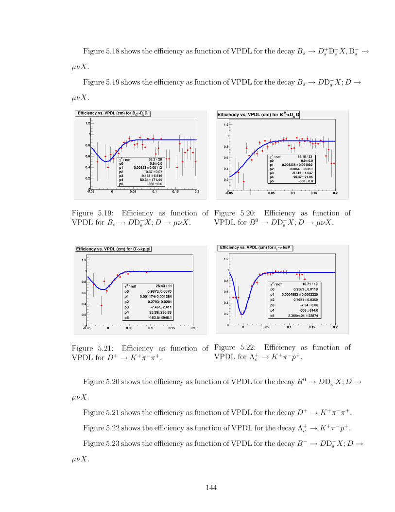
Figure 5.18 shows the efficiency as function of VPDL for the decay Bs → D+s D−

s X,D−s →

µνX.

Figure 5.19 shows the efficiency as function of VPDL for the decay Bs → DD−s X;D →

µνX.

/ ndf 2χ 36.2 / 28p0 0.0± 0.9 p1 0.00112± 0.00123 p2 0.07± 0.37 p3 6.616± -9.161 p4 171.44± 80.34 p5 0.0± -360

-0.05 0 0.05 0.1 0.15 0.20

0.2

0.4

0.6

0.8

1

1.2

/ ndf 2χ 36.2 / 28p0 0.0± 0.9 p1 0.00112± 0.00123 p2 0.07± 0.37 p3 6.616± -9.161 p4 171.44± 80.34 p5 0.0± -360

Ds->DsEfficiency vs. VPDL (cm) for B

Figure 5.19: Efficiency as function ofVPDL for Bs → DD−

s X;D → µνX.

/ ndf 2χ 54.15 / 33p0 0.0± 0.9 p1 0.004092± 0.006236 p2 0.0319± 0.3064 p3 1.647± -9.613 p4 21.06± 95.47 p5 0.0± -360

-0.05 0 0.05 0.1 0.15 0.20

0.2

0.4

0.6

0.8

1

1.2

/ ndf 2χ 54.15 / 33p0 0.0± 0.9 p1 0.004092± 0.006236 p2 0.0319± 0.3064 p3 1.647± -9.613 p4 21.06± 95.47 p5 0.0± -360

Ds->D0Efficiency vs. VPDL (cm) for B

Figure 5.20: Efficiency as function ofVPDL for B0 → DD−

s X;D → µνX.

/ ndf 2χ 26.43 / 11p0 0.0070± 0.9873 p1 0.001284± 0.001174 p2 0.0201± 0.2793 p3 2.411± -7.461 p4 236.83± 35.39 p5 4946.1± -163.8

-0.05 0 0.05 0.1 0.15 0.20

0.2

0.4

0.6

0.8

1

1.2

/ ndf 2χ 26.43 / 11p0 0.0070± 0.9873 p1 0.001284± 0.001174 p2 0.0201± 0.2793 p3 2.411± -7.461 p4 236.83± 35.39 p5 4946.1± -163.8

->kpipi-Efficiency vs. VPDL (cm) for D

Figure 5.21: Efficiency as function ofVPDL for D+ → K+π−π+.

/ ndf 2χ 10.71 / 19p0 0.0118± 0.9561 p1 0.0002220± 0.0004882 p2 0.0359± 0.7921 p3 6.06± -7.54 p4 614.0± -508 p5 22874± 2.368e+04

0 0.05 0.1 0.15 0.20

0.2

0.4

0.6

0.8

1

1.2

/ ndf 2χ 10.71 / 19p0 0.0118± 0.9561 p1 0.0002220± 0.0004882 p2 0.0359± 0.7921 p3 6.06± -7.54 p4 614.0± -508 p5 22874± 2.368e+04

Pπ -> kcΛEfficiency vs. VPDL (cm) for

Figure 5.22: Efficiency as function ofVPDL for Λ+

c → K+π−p+.

Figure 5.20 shows the efficiency as function of VPDL for the decay B0 → DD−s X;D →

µνX.

Figure 5.21 shows the efficiency as function of VPDL for the decayD+ → K+π−π+.

Figure 5.22 shows the efficiency as function of VPDL for the decay Λ+c → K+π−p+.

Figure 5.23 shows the efficiency as function of VPDL for the decay B− → DD−s X;D →

µνX.

144

/ ndf 2χ 23.46 / 26p0 0.00± 0.95 p1 0.000423± 0.001214 p2 0.047± 0.485 p3 3.43± -15.96 p4 89.4± 144.4 p5 0.0± -360

-0.05 0 0.05 0.1 0.15 0.20

0.2

0.4

0.6

0.8

1

1.2

/ ndf 2χ 23.46 / 26p0 0.00± 0.95 p1 0.000423± 0.001214 p2 0.047± 0.485 p3 3.43± -15.96 p4 89.4± 144.4 p5 0.0± -360

Ds->D-Efficiency vs. VPDL (cm) for B

Figure 5.23: Efficiency as function ofVPDL for B− → DD−

s X;D → µνX.

/ ndf = 2χ 24.08 / 21

-6 -4 -2 0 2 4 60

1000

2000

3000

4000

5000 / ndf = 2χ 24.08 / 21

PDLσPDL/

DØ Run II Preliminary

Figure 5.24: Pull of J/ψ vertex distribu-tion with respect to the Primary Vertex.

5.6.4 Resolution Scale Factor

The VPDL error was estimated by the vertex fitting procedure. A resolution scale

factor SF was introduced to take into account a possible bias. The SF was deter-

mined using the J/ψ sample (see Fig. 5.24). The negative tail of the pull of J/ψ

vertex distribution with respect to the PV should be a Gaussian with a sigma of 1

if errors assigned to the vertex coordinates were correct. For this J/ψ decay muons

from the PV were excluded . The positive side of the pull distribution was ignored

as that tends to be biased towards the larger value due to J/ψ mesons from the real

B meson decays. It is known that the scale factor depends on track transverse mo-

menta, therefore, the scale factor was also determined for J/ψ candidates with the

leading muon ptµ1> 6 GeV/c to estimate the contribution to the systematic error.

The corresponding scale factor increased by 2.5%.

The resulting pull distribution was fitted with a double Gaussian. The fit returns

a narrow Gaussian with width σnarrow = 0.998 comprising 72% of the events, and a

wide Gaussian with σwide = 1.775 comprising the rest of the events (28%).

145

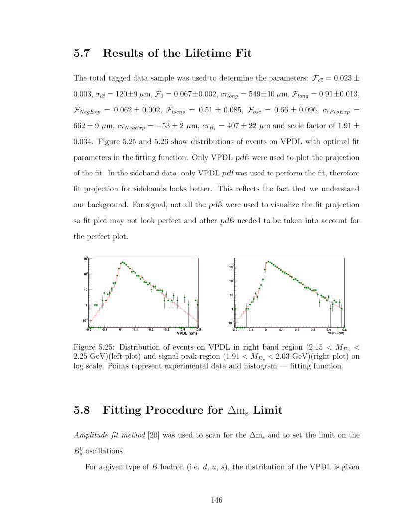
5.7 Results of the Lifetime Fit

The total tagged data sample was used to determine the parameters: Fcc = 0.023 ±

0.003, σcc = 120±9 µm, F0 = 0.067±0.002, cτlong = 549±10 µm, Flong = 0.91±0.013,

FNegExp = 0.062 ± 0.002, Ftsens = 0.51 ± 0.085, Fosc = 0.66 ± 0.096, cτPosExp =

662 ± 9 µm, cτNegExp = −53 ± 2 µm, cτBs= 407 ± 22 µm and scale factor of 1.91 ±

0.034. Figure 5.25 and 5.26 show distributions of events on VPDL with optimal fit

parameters in the fitting function. Only VPDL pdfs were used to plot the projection

of the fit. In the sideband data, only VPDL pdf was used to perform the fit, therefore

fit projection for sidebands looks better. This reflects the fact that we understand

our background. For signal, not all the pdfs were used to visualize the fit projection

so fit plot may not look perfect and other pdfs needed to be taken into account for

the perfect plot.

-0.2 -0.1 0 0.1 0.2 0.3 0.4 0.5

-110

1

10

210

310

VPDL (cm) VPDL (cm)-0.2 -0.1 0 0.1 0.2 0.3 0.4 0.5

-110

1

10

210

310

Figure 5.25: Distribution of events on VPDL in right band region (2.15 < MDs<

2.25 GeV)(left plot) and signal peak region (1.91 < MDs< 2.03 GeV)(right plot) on

log scale. Points represent experimental data and histogram — fitting function.

5.8 Fitting Procedure for ∆ms Limit

Amplitude fit method [20] was used to scan for the ∆ms and to set the limit on the

B0s oscillations.

For a given type of B hadron (i.e. d, u, s), the distribution of the VPDL is given

146

-0.2 -0.1 0 0.1 0.2 0.3 0.4 0.50

100

200

300

400

500

600

VPDL (cm)-0.2 -0.1 0 0.1 0.2 0.3 0.4 0.50

500

1000

1500

2000

2500

VPDL (cm)

Figure 5.26: Distribution of events on VPDL in right band region (2.15 < MDs<

2.25 GeV)(left plot) and signal peak region (1.91 < MDs< 2.03 GeV) (right plot) on

linear scale.Points represent experimental data and histogram — fitting function.

by:

pnoss (x) =

K

cτBs

exp(− Kx

cτBs

) · 0.5 · (1 + A · D cos(∆ms ·Kx/c)) (5.45)

poscs (x) =

K

cτBs

exp(− Kx

cτBs

) · 0.5 · (1 −A · D cos(∆ms ·Kx/c)) (5.46)

where τ is the lifetime of B hadron, K is the K factor and A is a fit parameter.

Different choices of ∆ms are used as input and the fitted value of A is returned. By

plotting the fitted value of A as a function of the input value of ∆ms, one searches

for a peak of A=1 to obtain a measurement of ∆ms. For any value of ∆ms not equal

to the “true” value of Bs oscillation frequency, the amplitude A should be zero. If no

peak is found, limits can easily be set on ∆ms using this method. The sensitivity of a

measurement is determined by calculating the probability that at a non-”true”value

of ∆ms, the amplitude could fluctuate to A=1. This occurs at the lowest value of

∆ms for which 1.645 σ∆ms = 1 for a 95% CL, where σ∆ms is the uncertainty on the

value of A at the point ∆ms. The limit is determined by calculating the probability

that a fitted value of A could fluctuate to A = 1. This occurs at the lowest value of

∆ms for which Adms + 1.645σdms = 1.

147

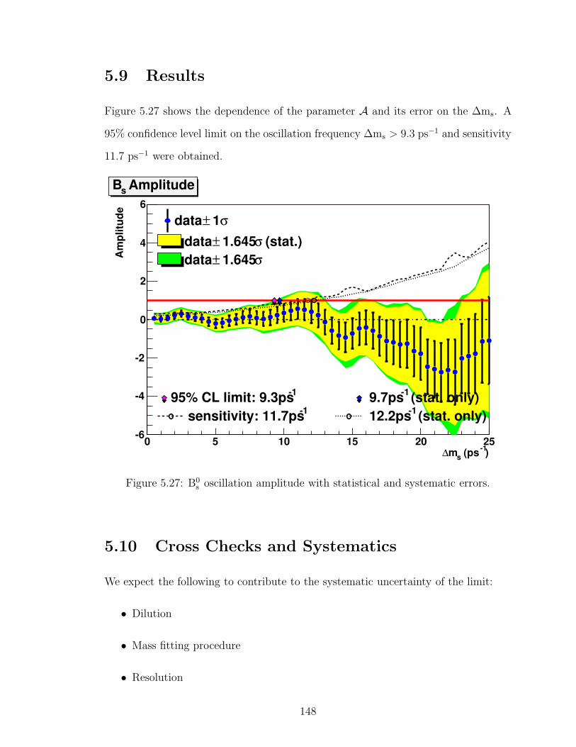
5.9 Results

Figure 5.27 shows the dependence of the parameter A and its error on the ∆ms. A

95% confidence level limit on the oscillation frequency ∆ms > 9.3 ps−1 and sensitivity

11.7 ps−1 were obtained.

)-1 (pssm∆0 5 10 15 20 25

Am

plitu

de

-6

-4

-2

0

2

4

6

(stat.)σ 1.645 ±data σ 1.645 ±data

σ 1 ±data

(stat. only)-1 9.7ps -195% CL limit: 9.3ps (stat. only)-1 12.2ps -1sensitivity: 11.7ps

AmplitudesB

Figure 5.27: B0s oscillation amplitude with statistical and systematic errors.

5.10 Cross Checks and Systematics

We expect the following to contribute to the systematic uncertainty of the limit:

• Dilution

• Mass fitting procedure

• Resolution

148

• Sample composition

• K factor

• Efficiency

The contribution to the systematic error from the uncertainties of the input fit

parameters can be estimated using the formula [20]:

σsysA = ∆A + (1 −A)

∆σAσA

(5.47)

5.10.1 Dilution

A test of the flavor tagger performance was done using µD± events from the reflection

peak in the (Kπ)K mass spectrum (see Fig. 5.8) which originates mainly from the

decays Bd → XµD±. Using these events a scan was performed for ∆Md as a cross

check. This scan is more sensitive to the description of the combinatorial background

and, therefore, the original description has been changed to take into account oscilla-

tions in the Bd contribution. The resulting amplitude scan is shown in Figures 5.28

and 5.29. The amplitude at ∆Md = 0.5 ps−1 is in agreement with 1, which confirms

that the dilution calibration was performed correctly. This cross-check also shows the

ability of the method to detect an oscillation signal.

5.10.2 Mass fitting procedure

As a cross check for mass fitting procedure we fit the M(Kπ)K distribution for

M(Kπ) > 1 GeV. It is expected that for this cut all the D−s → K∗0K− signal would

be rejected and what is left would all be D+ → Kππ reflection. We apply the fitting

technique to this distribution and the fit returns almost zero D−s → K∗0K− signal

candidates and rest everything is coming from D± reflection in the peak, fit is shown

in Fig. 5.30.

149

)-1 (pssm∆0 1 2 3 4 5 6 7 8 9 10

Am

plitu

de

-3

-2

-1

0

1

2

3


σ 1 ±data

(stat. only)-1 0.2ps -195% CL limit: 0.2ps -195% CL limit: 0.2ps -195% CL limit: 0.2ps

AmplitudesB

Figure 5.28: Bd − Bd oscillation ampli-tude.

)-1 (pssm∆0 0.2 0.4 0.6 0.8 1 1.2 1.4 1.6 1.8 2

Am

plitu

de

-3

-2

-1

0

1

2

3


σ 1 ±data

(stat. only)-1 0.2ps -195% CL limit: 0.2ps (stat. only)-1 13.0ps -1sensitivity: 13.0ps

AmplitudesB

Figure 5.29: Bd − Bd oscillation ampli-tude (detailed view of the Bd oscillationregion).

mkpikEntries 28199Mean 1.988RMS 0.1149

2M(kpik) in GeV/C1.7 1.8 1.9 2 2.1 2.2 2.3

2/1

0.0

MeV

/Cev

ents

N

0

200

400

600

800

1000

1200

mkpikEntries 28199Mean 1.988RMS 0.1149

mds

Figure 5.30: Fit to the M(Kπ)K distribution for M(Kπ) > 1 GeV . Tiny bluehistogram at the bottom is the D−

s → K∗0K− signal, light blue is the D± reflec-tion, golden color is the Λ±

c reflection and green curve is the fit to the combinatoricbackground.

Since this channel is dominated by the reflection from the D± decays so in order

to take the effect due to modeling of the mass fitting procedure we increased the

fraction of the D± reflection by 1σ and fixed it. We then re-did the entire mass fitting

procedure for the tagged sample and obtained the fractions of the signal, Cabbibo D±

and Λc reflection fractions. We used these new fractions to estimate the systematic

error due to mass fitting procedure. Also, the masses of the D± and Ds were varied

by one σ and found to be within the uncertainty on the fractions obtained from the

150

above stated procedure hence a separate systematics were not estimated for this.

5.10.3 Resolution

We use SF = 1.205 to estimate systematic errors. This value of the scale factor was

motivated by the scale factor obtained by applying a 6 GeV cut on the PT of the

muon to account for the trigger efficiencies as described in section 5.6.4. After this

cut, though the scale factor increases only by about 2.5% but to be conservative we

vary the scale factor by 3.5%.

5.10.4 Sample Composition

The Bs → DsDs branching ratio was changed from 10% to 4.7% (EvtGen value) and

23% (PDG value). The branching ratio Bs → DsµX was also changed from 7.9%

to 5.5% (PDG uncertainty). The variation of the branching ratio Bs → DsµX gives

the largest change in the signal fraction. Other systematics for sample composition

is listed in the systematics table 5.4.

The sample composition was also determined with the muon pT cut 6 GeV/c (see

Section 5.6.1). The corresponding contribution to the systematic error was deter-

mined and assigned to the MC efficiency uncertainty.

5.10.5 K factor

Four additional sets ofK-factor distributions were generated to estimate contributions

to the systematic error.

In one set, the K factor defined in Eqn. 5.43 was scaled up by 2% (i.e., multiplied

by 1.02). In the second set of K-factor distributions, the K factor was scaled down

by 2% (i.e., multiplied by 0.98). In the third set, the distributions were smoothed

using the ROOT function “Smooth” (with argument 1, which applies the smoothing

151

algorithm once). The final set of histograms was generated using the definition

K = precoT (µD−

s )/pMCT (B). (5.48)

The resulting systematic errors were obtained using the formula (5.47) and summed

in quadrature. The result is shown on the Figure 5.27.

5.11 Conclusions

Using a signal of 12.6k B0s → µ+νD−

s X decays where D−s → K∗0K− , K∗0 → K+π−

and an opposite side flavor tagging algorithm we performed a search for B0s − B0

s

oscillations. We obtained a 95% confidence level limit on the oscillation frequency

∆ms > 9.3 ps−1 and a sensitivity of 11.7 ps−1.

152

Table 5.4: Systematic uncertainties on the amplitude. The shifts of both the measured amplitude, ∆A, and its statisticaluncertainty, ∆σ, are listed

Osc. frequency 1 ps−1 2 ps−1 3 ps−1 4 ps−1 5 ps−1 6 ps−1 7 ps−1 8 ps−1 9 ps−1 10 ps−1 11 ps−1 12 ps−1 13 ps−1

A 0.035 0.235 0.174 0.053 −0.199 −0.049 0.115 0.089 0.129 0.346 0.563 0.409 −0.120Stat. uncertainty 0.137 0.158 0.176 0.207 0.236 0.268 0.313 0.362 0.411 0.456 0.525 0.595 0.658

PDG cτBs∆A −0.020 −0.006 −0.004 +0.002 −0.011 +0.003 +0.011 +0.003 +0.007 +0.012 +0.027 +0.021 +0.002∆σ +0.001 +0.002 +0.002 +0.004 +0.005 +0.006 +0.008 +0.009 +0.011 +0.013 +0.016 +0.019 +0.021

Signal SF variation ∆A +0.002 +0.003 +0.001 +0.002 −0.003 −0.001 +0.005 +0.009 +0.017 +0.031 +0.036 +0.030 +0.015by 3.5% ∆σ +0.000 +0.001 +0.001 +0.002 +0.003 +0.005 +0.006 +0.008 +0.010 +0.012 +0.015 +0.018 +0.022

D+

Reflfraction ∆A −0.011 +0.006 +0.007 +0.001 −0.006 −0.006 +0.000 +0.005 +0.004 +0.008 +0.017 +0.016 +0.003

+ 1σ ∆σ +0.002 +0.002 +0.003 +0.003 +0.004 +0.004 +0.005 +0.005 +0.006 +0.006 +0.008 +0.009 +0.010

D+

Reflfraction ∆A +0.037 −0.020 −0.023 −0.007 +0.015 +0.010 −0.009 −0.019 −0.017 −0.028 −0.052 −0.046 −0.012

- 1σ ∆σ −0.007 −0.008 −0.009 −0.010 −0.012 −0.013 −0.015 −0.018 −0.020 −0.022 −0.025 −0.030 −0.032Ds signal ∆A −0.018 +0.011 +0.011 +0.005 −0.003 +0.003 +0.013 +0.014 +0.010 +0.013 +0.020 +0.021 +0.009

- 1σ ∆σ +0.004 +0.004 +0.004 +0.005 +0.006 +0.007 +0.008 +0.010 +0.011 +0.012 +0.015 +0.017 +0.019Signal cc fraction changed ∆A +0.024 +0.039 +0.032 +0.026 +0.008 +0.015 +0.029 +0.028 +0.029 +0.043 +0.064 +0.055 +0.002

to 6% ∆σ +0.004 +0.004 +0.005 +0.006 +0.008 +0.009 +0.012 +0.015 +0.018 +0.021 +0.027 +0.033 +0.037Br(DsDs) = 4.7% ∆A +0.001 −0.003 −0.002 −0.001 +0.002 +0.000 −0.002 −0.001 −0.002 −0.004 −0.006 −0.005 +0.001

∆σ −0.001 −0.002 −0.002 −0.002 −0.002 −0.003 −0.003 −0.004 −0.004 −0.005 −0.006 −0.006 −0.007K-factor decreased ∆A +0.003 −0.012 +0.017 +0.021 +0.010 −0.027 −0.032 +0.034 −0.045 −0.028 −0.043 +0.037 +0.176

by 2% ∆σ −0.001 −0.000 −0.001 −0.002 −0.003 −0.003 −0.006 −0.007 −0.008 −0.008 −0.017 −0.014 −0.015Br(µDs) = 5.5% ∆A +0.022 +0.005 +0.004 −0.009 −0.021 −0.015 −0.005 −0.006 +0.001 +0.013 +0.026 +0.025 −0.005

∆σ +0.008 +0.009 +0.011 +0.012 +0.014 +0.016 +0.019 +0.022 +0.026 +0.028 +0.032 +0.037 +0.041Oscillated and Mixed fraction ∆A +0.033 −0.000 −0.009 −0.012 −0.012 −0.011 −0.011 −0.012 −0.010 −0.009 −0.008 −0.006 −0.008

varied in bkg ∆σ +0.000 +0.000 +0.000 +0.000 +0.000 +0.000 +0.000 +0.000 +0.000 +0.000 +0.000 +0.000 +0.000Br(µDs) = 10.8% ∆A −0.011 −0.003 −0.003 +0.004 +0.011 +0.008 +0.002 +0.003 −0.001 −0.008 −0.015 −0.015 +0.003

∆σ −0.005 −0.005 −0.006 −0.007 −0.008 −0.009 −0.011 −0.013 −0.014 −0.016 −0.018 −0.021 −0.023Br(DsDs) = 23% ∆A −0.002 +0.007 +0.006 +0.003 −0.004 −0.001 +0.004 +0.003 +0.004 +0.010 +0.016 +0.012 −0.003

∆σ +0.004 +0.004 +0.005 +0.005 +0.006 +0.007 +0.008 +0.009 +0.011 +0.012 +0.014 +0.016 +0.017K-factor increased ∆A +0.011 +0.011 +0.018 −0.042 +0.012 +0.023 +0.019 −0.052 +0.088 +0.149 −0.006 −0.158 −0.310

by 2% ∆σ +0.002 +0.004 +0.008 +0.012 +0.017 +0.021 +0.028 +0.034 +0.039 +0.048 +0.055 +0.057 +0.067Bkg SF changed ∆A +0.001 +0.001 −0.000 −0.001 −0.001 −0.002 −0.003 −0.003 −0.004 −0.004 −0.004 −0.005 −0.004

to 2.0 ∆σ −0.000 −0.000 −0.000 −0.000 −0.000 −0.000 −0.000 −0.000 −0.000 −0.000 −0.000 −0.000 −0.000Bkg cc changed ∆A +0.018 +0.009 +0.007 +0.004 −0.001 −0.005 −0.011 −0.014 −0.011 −0.001 +0.009 +0.001 −0.018

to 10.23% ∆σ −0.000 −0.000 −0.001 −0.001 −0.000 −0.000 +0.000 +0.001 +0.002 +0.002 +0.003 +0.005 +0.005PT (µ) ∆A −0.014 −0.005 −0.005 +0.005 +0.014 +0.009 +0.001 +0.004 −0.002 −0.012 −0.021 −0.019 +0.007

> 6 GeV ∆σ −0.006 −0.007 −0.008 −0.009 −0.011 −0.012 −0.014 −0.017 −0.019 −0.022 −0.025 −0.028 −0.031Generator level ∆A +0.004 +0.011 +0.014 −0.019 −0.006 −0.002 +0.001 +0.023 +0.030 −0.018 −0.013 −0.010 +0.014

K factor ∆σ +0.001 +0.002 +0.003 +0.005 +0.006 +0.009 +0.011 +0.014 +0.017 +0.020 +0.023 +0.026 +0.032Smoothed K factor ∆A +0.004 +0.013 +0.014 −0.016 −0.004 −0.001 +0.003 +0.028 +0.031 −0.020 −0.005 −0.012 −0.005

∆σ +0.001 +0.002 +0.004 +0.006 +0.008 +0.010 +0.012 +0.015 +0.018 +0.022 +0.025 +0.028 +0.034

Total syst. σsystot

0.132 0.128 0.141 0.116 0.152 0.164 0.175 0.164 0.247 0.263 0.173 0.198 0.304

Total σtot 0.191 0.203 0.226 0.237 0.280 0.314 0.359 0.398 0.479 0.526 0.552 0.627 0.725

153

Table 5.5: Systematic uncertainties on the amplitude. The shifts of both the measured amplitude, ∆A, and its statisticaluncertainty, ∆σ, are listed (cont’d)

Osc. frequency 14 ps−1 15 ps−1 16 ps−1 17 ps−1 18 ps−1 19 ps−1 20 ps−1 21 ps−1 22 ps−1 23 ps−1 24 ps−1 25 ps−1

A −0.828 −0.721 −0.405 −0.865 −1.185 −1.252 −1.777 −2.581 −2.634 −2.024 −1.774 −1.093Stat. uncertainty 0.729 0.809 0.890 1.004 1.130 1.251 1.377 1.484 1.613 1.817 2.058 2.266

PDG cτBs∆A −0.033 −0.025 +0.005 −0.004 −0.022 +0.007 −0.039 −0.094 −0.090 +0.001 −0.065 +0.011∆σ +0.024 +0.028 +0.030 +0.036 +0.043 +0.047 +0.055 +0.059 +0.062 +0.070 +0.081 +0.087

Signal SF variation ∆A −0.019 −0.021 −0.030 −0.057 −0.072 −0.051 −0.063 −0.112 −0.164 −0.219 −0.273 −0.314by 3.5% ∆σ +0.026 +0.031 +0.036 +0.043 +0.052 +0.061 +0.071 +0.080 +0.091 +0.106 +0.124 +0.144

D+

Reflfraction ∆A −0.012 −0.008 −0.001 +0.005 +0.018 +0.030 +0.024 +0.010 +0.018 +0.031 +0.046 +0.059

+ 1σ ∆σ +0.011 +0.011 +0.012 +0.013 +0.016 +0.018 +0.019 +0.020 +0.021 +0.024 +0.027 +0.030

D+

Reflfraction ∆A +0.035 +0.027 +0.002 −0.008 −0.033 −0.055 −0.027 +0.020 −0.007 −0.053 −0.091 −0.129

- 1σ ∆σ −0.036 −0.039 −0.041 −0.047 −0.054 −0.061 −0.067 −0.070 −0.074 −0.083 −0.094 −0.105Ds signal ∆A −0.014 −0.013 +0.002 −0.005 −0.013 −0.019 −0.046 −0.083 −0.073 −0.046 −0.035 −0.012

- 1σ ∆σ +0.021 +0.023 +0.026 +0.030 +0.035 +0.039 +0.044 +0.047 +0.049 +0.054 +0.062 +0.067Signal cc fraction changed ∆A −0.081 −0.074 −0.034 −0.098 −0.153 −0.168 −0.267 −0.424 −0.444 −0.355 −0.342 −0.213

to 6% ∆σ +0.044 +0.051 +0.057 +0.071 +0.087 +0.101 +0.118 +0.133 +0.148 +0.176 +0.219 +0.245Br(DsDs) = 4.7% ∆A +0.009 +0.007 +0.004 +0.009 +0.012 +0.013 +0.020 +0.028 +0.029 +0.022 +0.019 +0.012

∆σ −0.008 −0.009 −0.010 −0.011 −0.012 −0.014 −0.015 −0.016 −0.017 −0.020 −0.022 −0.025K-factor decreased ∆A +0.125 −0.151 −0.011 +0.201 +0.160 −0.017 +0.266 +0.158 +0.004 −0.508 −0.033 −0.547

by 2% ∆σ −0.018 −0.023 −0.025 −0.036 −0.040 −0.043 −0.041 −0.038 −0.053 −0.095 −0.104 −0.081Br(muDs) = 5.5% ∆A −0.050 −0.055 −0.040 −0.070 −0.087 −0.092 −0.110 −0.164 −0.176 −0.148 −0.135 −0.137

∆σ +0.046 +0.050 +0.054 +0.060 +0.067 +0.075 +0.083 +0.088 +0.096 +0.109 +0.122 +0.134Oscillated and Mixed fraction ∆A −0.011 −0.012 −0.011 −0.010 −0.007 −0.004 +0.000 +0.001 −0.006 −0.012 −0.013 −0.014

varied in bkg ∆σ +0.000 +0.000 −0.000 −0.001 −0.001 −0.002 −0.002 −0.003 −0.002 −0.001 −0.001 −0.001Br(µDs) = 10.8% ∆A +0.029 +0.031 +0.022 +0.040 +0.049 +0.051 +0.062 +0.094 +0.101 +0.083 +0.074 +0.075

∆σ −0.026 −0.028 −0.031 −0.034 −0.038 −0.043 −0.047 −0.050 −0.055 −0.062 −0.069 −0.076Br(DsDs) = 23% ∆A −0.021 −0.018 −0.008 −0.021 −0.029 −0.032 −0.048 −0.070 −0.070 −0.054 −0.046 −0.028

∆σ +0.019 +0.021 +0.023 +0.027 +0.030 +0.033 +0.037 +0.039 +0.043 +0.048 +0.055 +0.060K-factor increased ∆A −0.003 +0.412 −0.211 −0.235 −0.685 −0.352 −0.557 −0.126 +0.461 −0.023 +0.121 −0.344

by 2% ∆σ +0.073 +0.085 +0.110 +0.119 +0.107 +0.143 +0.133 +0.143 +0.219 +0.235 +0.212 +0.226Bkg SF chnaged ∆A −0.003 −0.004 −0.004 −0.004 −0.004 −0.004 −0.003 −0.001 −0.001 −0.003 −0.004 −0.007

to 2.0 ∆σ −0.001 −0.001 −0.001 −0.001 −0.001 −0.001 −0.002 −0.002 −0.003 −0.003 −0.003 −0.003Bkg cc changed ∆A −0.038 −0.023 −0.012 −0.031 −0.041 −0.040 −0.061 −0.099 −0.108 −0.094 −0.104 −0.079

to 10.23% ∆σ +0.007 +0.008 +0.010 +0.012 +0.015 +0.017 +0.019 +0.020 +0.022 +0.027 +0.033 +0.036PT (µ) ∆A +0.042 +0.038 +0.027 +0.048 +0.070 +0.074 +0.084 +0.124 +0.135 +0.112 +0.103 +0.088

> 6 GeV ∆σ −0.035 −0.038 −0.042 −0.046 −0.052 −0.058 −0.064 −0.068 −0.074 −0.085 −0.095 −0.105Generator level ∆A +0.085 −0.028 −0.160 +0.125 −0.132 −0.280 −0.144 +0.112 +0.086 −0.275 −0.095 −0.492

K factor ∆σ +0.033 +0.037 +0.045 +0.050 +0.050 +0.056 +0.060 +0.074 +0.089 +0.087 +0.092 +0.096Smoothed K factor ∆A +0.076 −0.018 −0.132 +0.064 −0.088 −0.279 −0.163 +0.099 −0.002 −0.252 −0.182 −0.634

∆σ +0.036 +0.040 +0.049 +0.054 +0.055 +0.061 +0.066 +0.079 +0.093 +0.097 +0.102 +0.106

Total syst. σsystot

0.335 0.644 0.181 0.341 0.520 0.359 0.413 0.524 1.054 0.820 0.526 0.981

Total σtot 0.802 1.034 0.909 1.060 1.244 1.302 1.438 1.574 1.926 1.994 2.124 2.469

154

Chapter 6

Combination and Results

6.1 Introduction

Besides D−s → K∗0K− channel there are other two channels used to search for the

B0s mixing oscillations. Therefore, we produced results on B0

s − B0s oscillations using

three B0s decay modes [60]:

• B0s → D−

s µ+νX, D−

s → K∗K− [51] (Fig. 6.1).

• B0s → D−

s µ+νX, D−

s → φπ− [16] (Fig. 6.2).

• B0s → D−

s e+νX, D−

s → φπ− [61] (Fig. 6.3).

6.2 Combination

The program “combos” [62] developed at LEP to combine the results with statistical

and systematic uncertainties with different correlations has been used to perform the

combination of different decay modes. Figures 6.4, 6.5, 6.6 show combinations of µφπ

and µK∗K; µφπ and eφπ; and all three decay modes. Uncertainties in the following

parameters were considered as correlated:

• Br(Bs → XµDs).

155

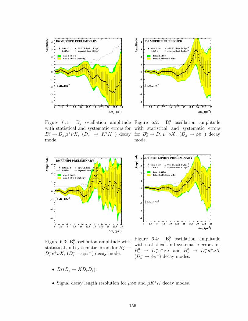
-4

-3

-2

-1

0

1

2

3

4

0 2.5 5 7.5 10 12.5 15 17.5 20 22.5 25

∆ms (ps-1)

Am

plitu

dedata ± 1 σ 95% CL limit 9.3 ps-1

1.645 σ expected limit 11.8 ps-1


D0 MUKSTK PRELIMINARY

D∅ Run II preliminary

∫ Ldt=1fb-1

Figure 6.1: B0s oscillation amplitude

with statistical and systematic errors forB0

s → D−s µ

+νX, (D−s → K∗K−) decay

mode.

-4

-3

-2

-1

0

1

2

3

4

0 2.5 5 7.5 10 12.5 15 17.5 20 22.5 25

∆ms (ps-1)

Am

plitu

de




D0 MUPHIPI PUBLISHED

∫ Ldt=1fb-1


with statistical and systematic errorsfor B0

s → D−s µ

+νX, (D−s → φπ−) decay

mode.

-6

-4

-2

0

2

4

6

0 2.5 5 7.5 10 12.5 15 17.5 20 22.5 25

∆ms (ps-1)

Am

plitu

de




D0 EPHIPI PRELIMINARY

∫ Ldt=1fb-1

Figure 6.3: B0s oscillation amplitude with

statistical and systematic errors for B0s →

D−s e

+νX, (D−s → φπ−) decay mode.

-4

-3

-2

-1

0

1

2

3

4

0 2.5 5 7.5 10 12.5 15 17.5 20 22.5 25

∆ms (ps-1)

Am

plitu

de




D0 (MU+E)PHIPI PRELIMINARY


∫ Ldt=1fb-1



s → D−s e

+νX and B0s → D−

s µ+νX

(D−s → φπ−) decay modes.

• Br(Bs → XDsDs).

• Signal decay length resolution for µφπ and µK∗K decay modes.

156

• ∆Γ/Γ.

Although some degree of correlation is expected between the systematic uncertainty

due to dilution uncertainty of the different channels, the way this systematic is cur-

rently assessed makes it difficult to quantify the correlation. Tests including or ex-

cluding this systematic uncertainty in individual channels indicate that ignoring this

one correlation leads to negligible differences in the combined results.

-4

-3

-2

-1

0

1

2

3

4

0 2.5 5 7.5 10 12.5 15 17.5 20 22.5 25

∆ms (ps-1)

Am

plitu

de




D0 MU(PHIPI+K*K) PRELIMINARY


∫ Ldt=1fb-1

Figure 6.5: B0s oscillation amplitude with

statistical and systematic errors for B0s →

D−s µ

+νX (D−s → φπ− and D−

s → K∗K−)decay modes.

-4

-3

-2

-1

0

1

2

3

4

0 5 10 15 20 25 30

∆ms (ps-1)

Am

plitu

de




D0 ALL PRELIMINARY

∫ Ldt=1fb-1



s → D−s e

+νX (D−s → φπ−) and B0

s →D−

s µ+νX (D−

s → φπ− and D−s → K∗K−)

decay modes.

6.3 Log Likelihood Scan

An amplitude scan can be transformed to a log likelihood scan using the following

formula [20, 63]:

−∆ log(L) =

1

2

(

1 − AσA

)2

− 1

2

(

AσA

)2

(6.1)

This formula can be tested using the B0s → D−

s µ+νX, D−

s → φπ− decay mode where

the log likelihood scan was obtained directly from the fitting procedure. Figures 6.7

157

and 6.8 show the log likelihood scans obtained in two different ways.

−∆lo

g(L)

0

2

4

6

2622181410[ps ]sm∆

30−1

D Run II, 1 fb−1

90% C.L.

(two-sided)

Figure 6.7: Log likelihood scan for B0s →

D−s µ

+νX (D−s → φπ−) decay mode ob-

tained from the fitting procedure.

]-1 [pss m∆10 12 14 16 18 20 22 24

]-1 [pss m∆10 12 14 16 18 20 22 24

log(

L)∆-

0

1

2

3

4

5

6

Figure 6.8: Log likelihood scan for B0s →

D−s µ

+νX (D−s → φπ−) decay mode ob-

tained from the amplitude scan using thetotal errors (stat.

⊕

syst.).

A log likelihood scan obtained from the combined amplitude scan (Fig. 6.6) is

shown in Fig. 6.9. The combined likelihood curve has a preferred value of the oscil-

lation frequency ∆ms = 19 ps−1, with a 90% confidence level interval of 17 < ∆ms <

21 ps−1, assuming Gaussian uncertainties.

In the previous analysis [16], the probability of a background fluctuation to give

a minimum of equal or greater depth in this interval was determined to be 5% using

ensemble tests. Comparing the change in likelihood at ∆ms = 19 ps−1 and the

likelihood at ∆ms = ∞ [63] also yields a 5% expectation for a background fluctuation.

For the current combined result, comparison of the change in likelihood between

∆ms = 19 ps−1 and ∆ms = ∞ yields an 8% expectation for a background fluctuation.

6.4 Conclusion

The combined amplitude scan allows the setting of a 95% C.L. limit on the B0s − B0

s

oscillation frequency ∆ms > 14.9 ps−1 with the corresponding expected limit at

16.5 ps−1. The combined likelihood curve has a preferred value of ∆ms = 19 ps−1,

158

]-1 [pssm∆10 12 14 16 18 20 22 24 26 28 30

log(

L)∆-

0

1

2

3

4

5

6

7DØ Run II Preliminary

-11 fb

90% C.L.

(two-sided)

Figure 6.9: Log likelihood scan obtained from the combined amplitude scan usingthe total errors. The horizontal solid line indicates the 90% C.L. (two-sided) loglikelihood difference. The horizontal dashed line indicates the value of ∆ logL at∆ms = ∞.

with a 90% confidence level interval of 17 < ∆ms < 21 ps−1, assuming Gaussian

uncertainties. The probability for a background fluctuation to give a similar dip in

the same interval is estimated to be approximately 8%. The effect of these results on

CKM fit can be seen in Fig. 6.10.

159

-1.5

-1

-0.5

0

0.5

1

1.5

-1 -0.5 0 0.5 1 1.5 2

sin 2β



γ

γ

α

α

∆md

∆ms & ∆md

εK

εK

|Vub/Vcb|

sin 2β



α

βγ

∆ms as of Moriond 2006

ρ

η

excluded area has CL > 0.95

C K Mf i t t e r

FPCP 06

Figure 6.10: The effect on CKM triangle. The reduced uncertainty in the band dueto ∆ms and ∆md can be seen in this fit.

160

Bibliography

[1] S. Eidelman et al ., Phys. Lett. B592, 1 (2004).

[2] S.L. Glashow, Murray Gell-Mann, Gauge theories of Vector Particles, AnnalsPhys. 15 437-460, (1961).

[3] Gauge theories of elementary interactions, A. Salam and J.C. ward, Phys. Rev.136, B763-768 (1964).

[4] A. Eienstein, The foundation of the General Theory of Relativity, Annalen Phys.14, 517-571 (1905); Annalen Phys. 49, 769-822 (1916).

[5] Observation of a Dimuon Resonance at 9.5 GeV in 400-GeV Proton-NucleusCollisions, S.W. Herb, et al ., Phys. Rev. Lett. 39, 252-255 (1977).

[6] K. Lande, et al ., Phys. Rev. 103 1901 (1956).

[7] M. Gell-Mann, A. Pais, Phys. Rev. 97, 1387 (1955).

[8] N.Cabibbo, Phys. Rev. Lett. 10, 531 (1963).

[9] S.L. Glashow, J. Iliopoulos, and L. Maiani, Phys. Rev. D2 1585 (1970).

[10] M. Kobayashi and T. Maskawa, Progr. Theor. Phys. 49 652 (1973).

[11] L.L. Chau and W.Y. Keung, Phys. Rev. Lett. 53 1802 (1984).

[12] L. Wolfenstein, Phys. Rev. Lett. 51 1945 (1983).

[13] R.M. Barnett et al ., Review of Particle Properties, Phys. Rev. D54 1 (1996).

[14] C. Albajar, et al ., (UA1 Collaboration) Phys. Lett. B187, 247 (1987).

[15] H. Albrecht, et al ., (ARGUS Collaboration) Phys. Lett. B192, 245 (1987)

[16] V. Abazov, et al , Phys.Rev.Lett. 97 021802 (2006).

[17] [CDF Collaboration] Measurement of B0s - Anti-B0

s Oscillation Frequency, Sub-mitted in Physical Review Letters, arXiv:hep-ex/0606027.

[18] M. Beneke, G. Buchalla, I. Dunietz, Phys. Rev. D54 4419 (1996).

161

[19] I. Stewart, QCD effects in Weak Decays, Plenary talk at the 22nd InternationalSymposium on Lepton-Photon Interactions at High Energy (LP 2005), Uppsala,Sweden (2005).

[20] H.-G. Moser and A. Roussarie,Nucl. Instrum. Methods A 384, 1997 (491).

[21] DØ Collaboration, “Observation of the Top Quark”, Phys. Rev. Lett. 74, 2632(1995).

[22] C. W. Schmidt, The Fermilab 400 − MeV Linac upgrade, FERMILAB-CONF-93-111 (1993).

[23] Fermilab Beams Division, Run II Handbook ,http://www-bd.fnal.gov/runII/index.html

[24] J. Marriner, stochastic Cooling Overview , FERMILAB-CONF-03-158 (2003).

[25] G.L. Budkar, Atomnaya Energiya, 22, 346-8 (1996).

[26] DØ Collaboration, The upgraded DØ detector, Accepted in NIM .

[27] R. Ruchti, Ann. Rev. Nucl. Part. Sci. 46 (1996) 281.

[28] P. Baringer, et al ., Nucl. Instrum. Methods A 469, 2001 (295)

[29] S. Abachi et al., The DØ Collaboration : The DØ detector , Nucl. Instrum.Methods A 338, 1994 (185).

[30] Md. Naimuddin, et al., DØ Note 4713 , B-Flavor Tagging with Soft electrons.

[31] Md. Naimuddin, et al., DØ Note 4848 , B-Flavor Tagging with Soft electrons.

[32] Reconstruction of B Hadron Signals at DØ, Guennadi Borissov, Sergey Bur-din, Eduard de la Cruz-Burelo, Vivek Jain, Andrei Nomerotski, Pedro Podesta-Lerma, Rick Van Kooten, June 24 2004.

[33] http://www-d0.fnal.gov/Run2Physics/ckm/d0 private/computing/new data files onDISK.html

[34] http://www-d0.fnal.gov/Run2Physics/ckm/d0 private/computing/mc files.html

[35] Z. Ligetti “Introduction to heavy meson decays and CP asymmetries”, hep-ph/0302031.

[36] E. Berger et al., Phys. Rev. Lett. 86, 4231 (2001).

[37] DØ Collaboration, “Flavor oscillations in B0d mesons with opposite-side muon

tags”. D0 Note 4370, Mar, 2004.

[38] S. Abachi et al.,NIMA 338, 1994 (185).

[39] S. Catani et al., Phys. Lett. B269 (1991) 432.

162

[40] F. Beaudette and J.-F. Grivaz, “The Road Method (an algorithm for the identi-fication of electrons in jets)”, DØ Note 3976, Nov 4 2002.

[41] Reconstruction of B hadron signals at D0: http://www-d0.fnal.gov/Run2Physics/WWW/results/prelim/B/B00/B00.pdf.

[42] DELPHI Collab., b−tagging in DELPHI at LEP , Eur. Phys. J. C32 (2004),185-208.

[43] P. Abreu et al., DELPHI Collaboration, Phys. Lett. B 475, 407 (2000).

[44] DELPHI Collab., Euro. Phys. J. C35, 35 (2004).

[45] D. Scora and N. Isgur, Phys. Rev. D 52, 2783 (1995).

[46] M. Neubert, Phys. Rep. 245, 259 (1994).

[47] G. Borrisov, et al., DØ Note 4828 , Bd Mixing measurement using semileptonicsample and combined opposite side tagging.

[48] C. Ay, et al., DØ Note 5029 , Bd mixing measurement using Opposite-side FlavorTagging.

[49] Heavy Flavor Averaging Group, http://www.slac.stanford.edu/xorg/hfag/index.html

[50] CKM Fitter Group, http : //www .slac.stanford .edu/xorg/ckmfitter/ckm welcome.html

[51] B. Abbott et al ., DØ Note 5149 , B0s mixing studies in Semileptonic B0

s decayswith D−

s → K∗0K− and Unibinned fit.

[52] B. Abbott et al ., DØ Note 5172 , B0s mixing studies in Semileptonic B0

s decayswith D−

s → K∗0K− and Unibinned fit.

[53] S. Catani, Yu.L. Dokshitzer, M. Olsson, G. Turnock, B.R. Webber, Phys. Lett.B269 (1991) 432.

[54] http://www-d0.fnal.gov/computing/algorithms/muon/muon algo.html.

[55] B. Abbott et al., DØ Note 4842 , Bs mixing in semileptonic Bs decays using Dsto Phi Pi decay mode.

[56] M. Anzelc et al., DØ Note 5017 , Bs mixing in semileptonic Bs decays using Dsto Phi Pi decay mode.

[57] G. Borissov et al., DØ Note 4991 , Bd mixing measurement using Opposite-sideFlavor Tagging.

[58] T. Sjostrand et al., arXiv:hep-ph/0108264.

[59] D.J. Lange,Nucl. Instrum. Methods A 462, 2001 (152); for details seehttp://www.slac.stanford.edu/˜ lange/EvtGen.

163

[60] G. Borrisov et al., D0Note 4701 , A combination of B0s Oscillations Results from

DØ.

[61] The DØ Collaboration, DØ Note 5174 , “Bs mixing in Bs → DseνX, Ds → φπdecay mode”

[62] http://lepbosc.web.cern.ch/LEPBOSC/combos/.

[63] D. Abbaneo, G. Boix, JHEP 08 (1999) 004.

164

Documents

· ACKNOWLEDGMENTS I never thought that one day I would be writing these acknowledgments as part of my dissertation. Being from a small place and rural background I hardly ever imagi