Acknowledgment

First of all, I thank my wife, Alex, for listening and supporting in the lastcouple of years.I deeply thank my advisor, Prof. Abraham Neyman, whose help, advice andsupervision was invaluable.I also thank Janos Flesch, with whom I discussed three-player games, threeanonymous referees of Mathematics of Operations Research, whose commentssubstantially improved the presentation of the results in section 4, and Nico-las Vieille, who commented on the presentation of the results in section 5.Finally, I would like to thank the Center of Rationality and Interactive Deci-sion Theory, Sergiu Hart and Hana Shemesh. Their hospitality and supportduring the period this research took place is greatly acknowledged.

1

Contents

1 Introduction 41.1 The Model . . . . . . . . . . . . . . . . . . . . . . . . . . . . . 41.2 The Discounted Equilibrium . . . . . . . . . . . . . . . . . . . 61.3 The Uniform Equilibrium . . . . . . . . . . . . . . . . . . . . 6

1.3.1 Uniform Equilibrium Payoff . . . . . . . . . . . . . . . 61.3.2 Special Classes of Stochastic Games . . . . . . . . . . . 71.3.3 Zero-Sum Games . . . . . . . . . . . . . . . . . . . . . 81.3.4 Non Zero-Sum Games . . . . . . . . . . . . . . . . . . 9

1.4 Application . . . . . . . . . . . . . . . . . . . . . . . . . . . . 111.5 The Present Monograph . . . . . . . . . . . . . . . . . . . . . 12

1.5.1 Two-Player Repeated Games with Absorbing States . . 121.5.2 n-Player Repeated Games with Absorbing States . . . 131.5.3 Two-Player Recursive Games with the Absorbing Prop-

erty . . . . . . . . . . . . . . . . . . . . . . . . . . . . 14

2 Preliminaries 162.1 On Puiseux Functions . . . . . . . . . . . . . . . . . . . . . . 162.2 Semi-Algebraic Sets . . . . . . . . . . . . . . . . . . . . . . . . 172.3 Notations . . . . . . . . . . . . . . . . . . . . . . . . . . . . . 17

3 Stochastic Games 193.1 The Model . . . . . . . . . . . . . . . . . . . . . . . . . . . . . 193.2 The Discounted Payoff . . . . . . . . . . . . . . . . . . . . . . 203.3 The Uniform MinMax Value . . . . . . . . . . . . . . . . . . . 213.4 The Uniform Equilibrium Payoff . . . . . . . . . . . . . . . . . 223.5 On Perturbed Equilibrium . . . . . . . . . . . . . . . . . . . . 22

4 Repeated Games with Absorbing States 264.1 An Equivalent Formulation . . . . . . . . . . . . . . . . . . . . 264.2 Different Types of Equilibria . . . . . . . . . . . . . . . . . . . 27

4.2.1 The Structure of the Proofs . . . . . . . . . . . . . . . 284.2.2 An ‘Almost’ Stationary Non-Absorbing Equilibrium . . 304.2.3 An ‘Almost’ Stationary Absorbing Equilibrium . . . . 324.2.4 Average of Perturbations . . . . . . . . . . . . . . . . . 344.2.5 A Cyclic Equilibrium . . . . . . . . . . . . . . . . . . . 40

2

4.2.6 A Generalization . . . . . . . . . . . . . . . . . . . . . 464.3 On the Discounted Game . . . . . . . . . . . . . . . . . . . . . 474.4 The Auxiliary Game . . . . . . . . . . . . . . . . . . . . . . . 504.5 Puiseux Stationary Profiles . . . . . . . . . . . . . . . . . . . . 544.6 A Preliminary Result . . . . . . . . . . . . . . . . . . . . . . . 564.7 Three Players Repeated Games with Absorbing States . . . . 594.8 More Than Three Players . . . . . . . . . . . . . . . . . . . . 604.9 Repeated Team Games with Absorbing States . . . . . . . . . 624.10 Proof of Lemma 4.24 . . . . . . . . . . . . . . . . . . . . . . . 64

5 Recursive Games with the Absorbing Property 715.1 An Equivalent Formulation . . . . . . . . . . . . . . . . . . . . 715.2 An Example . . . . . . . . . . . . . . . . . . . . . . . . . . . . 735.3 Sufficient Conditions for Existence of an Equilibrium Payoff . 755.4 Preliminary Results . . . . . . . . . . . . . . . . . . . . . . . . 815.5 The ε-Approximating Game . . . . . . . . . . . . . . . . . . . 82

5.5.1 The Game . . . . . . . . . . . . . . . . . . . . . . . . . 825.5.2 Existence of a Stationary Equilibrium . . . . . . . . . . 825.5.3 Properties as n→ 0 . . . . . . . . . . . . . . . . . . . . 83

5.6 Existence of an Equilibrium Payoff . . . . . . . . . . . . . . . 865.6.1 Exits from a State . . . . . . . . . . . . . . . . . . . . 875.6.2 The Main Result . . . . . . . . . . . . . . . . . . . . . 90

5.7 More Than Two Non-Absorbing States . . . . . . . . . . . . . 93

3

1 Introduction

The present monograph deals with uniform equilibria in stochastic games.In the Introduction we review informally the basic definitions and the knownresults in this topic. We begin by introducing the model, continue with theknown results for the discounted and the uniform equilibria, and finally wereview the main results and ideas presented in the monograph.

1.1 The Model

A stochastic game is played in stages. At every stage the game is in somestate of the world, and each player, given the whole history (including thecurrent state), chooses an action in his action space. The action combinationthat was chosen by all the players, together with the current state, determinethe daily payoff that each player receives and the probability distributionaccording to which the new state of the game is chosen.

The results that appear in this monograph are for stochastic games wherethe number of players, states and available actions are finite.

One may consider a finite t-stage game — the game terminates aftert stages, and the payoff for the players is their average payoff. Anotherstandard version is the infinite discounted game, where the infinite sequenceof payoffs (ri1, r

i2, . . .) of player i is evaluated by the discounted sum

(1− β)∞∑t=1

βt−1rit,

and β ∈ [0, 1) is the discount factor.It is fairly easy to prove (i) the existence of a stationary equilibrium profile

for the discounted case (stationary, in the sense that the mixed action that ischosen by each player at every stage depends only on the current state, ratherthan on the whole history), and (ii) the existence of an equilibrium profile(which usually depends on the stage of the game, as well as on the currentstate) for finite t-stage games. However, the equilibrium profiles in both casesusually depend on the exact discount factor or on the exact duration of thegame; an equilibrium profile for one discount factor might yield some playersa low payoff if the discount factor is slightly changed and the equilibriumprofiles for finite t-stage games differ for every t.

4

A strategy profile is a uniform ε-equilibrium if no player can profit morethan ε by deviating in any sufficiently long game, or in any discounted game,for discount factor sufficiently close to 1. Moreover, no player can profit morethan ε in the infinite game as well (a precise definition is given in section 3.4).

Aumann and Maschler [2] mention several reasons to study the uniformequilibrium:

1. A uniform ε-equilibrium profile is an ε-equilibrium profile in any finitegame whose duration is sufficiently long, as well as in any discountedgame, when the discount factor is sufficiently close to 1. Thus, theuniform equilibrium can be used

• if the game is “long”, but its the exact duration is not known, or ifthe players are sufficiently patient, but the exact discount factor,is not known,

• or when the players have bounded rationality, and taking the stageof the game into account is too complex.

2. Uniform ε-equilibrium profiles are usually simple to describe, and theplayers follow rules that make use only of fairly simple statistics of thepast history. Thus, uniform equilibria lead to simple “rules of thumb”for the players.

3. To study optimal behavior for the players in games that continue in-definitely, and the payoff of any finite number of stages is negligible.

4. Since uniform ε-equilibrium profiles depend only on the structure ofthe game (rather than on its duration or the discount factor), one cancompare optimal behavior of different games — how does an additionalplayer changes the optimal behavior, or the addition of states or actionsfor the players.

In the following two subsections we introduce the discounted and theuniform equilibria, and the results concerning these two types of equilibria.The proofs in the monograph make use of the discounted equilibria, ratherthen equilibria in finite t-stage games. However, bearing in mind the resultsof Bewley and Kohlberg [4], one could use finite games instead of discountedgames.

5

1.2 The Discounted Equilibrium

Let 0 ≤ β < 1. In the β-discounted game each player i evaluates a profile σby

viβ(s, σ) = Es,σ

((1− β)

∞∑t=1

βt−1rit

)

where s is the initial state and rit is the daily payoff that player i receives atstage t.

A strategy profile σ is a β-discounted (Nash) equilibrium if viβ(s, σ) ≥viβ(s, σ−i, τ i) for every player i and every strategy τ i of player i, where σ−i =(σj)j 6=i. The payoff vector vβ(·, σ) is a β-discounted equilibrium payoff. It iseasy to verify that if the equilibrium payoff of a two-player zero-sum gameexists, then it is unique. In this case, the unique equilibrium payoff of player1 is the discounted value of the game.

Shapley [26] introduced the model of stochastic games and proved thatevery two-player zero-sum discounted stochastic game has a discounted value.Moreover, there are stationary equilibrium profiles. Fink [12] generalized thisresult for n-player stochastic games.

Bewley and Kohlberg [4] proved that the value of a two-player zero-sumdiscounted game, as a function of the discount factor, is a Puiseux function(that is, it has an expansion as a Laurent series in fractional powers). In par-ticular, it follows that the limit of the discounted value, as the discount factortends to 1, exists. Moreover, they proved that there exists a Puiseux func-tion that assigns to every discount factor a stationary equilibrium profile inthe corresponding discounted game. Following similar lines it can be proven(see, e.g., Mertens, Sorin and Zamir [21]) that for every n-player stochasticgame there exists a Puiseux function that assigns for every discount factor anequilibrium payoff and an equilibrium strategy profile in the correspondingdiscounted game. As we will see, this result is used extensively for provingresults on the uniform equilibrium payoff.

1.3 The Uniform Equilibrium

1.3.1 Uniform Equilibrium Payoff

A payoff vector g = (gis) is a uniform ε-equilibrium payoff if there exists astrategy profile σ and a finite horizon te ∈ N such that for every player i,

6

every strategy τ i of player i and every initial state s

• If the players follow the profile σ, then the expected average dailypayoff for player i in every finite t stage game (for t > te), as well asthe expected lim inf of the average daily payoffs, is at least gis − ε.

• If the players follow the profile (σ−i, τ i), then the expected averagepayoff of player i in every finite t stage game (for t > te), as well as theexpected lim sup of the average daily payoffs, is at most gis + ε.

The strategy profile σ is an ε-equilibrium profile.It can easily be proven that σ is also an ε-equilibrium profile in the dis-

counted game, for discount factors sufficiently close to 1.A payoff vector g is a uniform equilibrium payoff if it is a uniform ε-

equilibrium payoff for every ε > 0. If the game is two-player zero-sum andit has a uniform equilibrium payoff, then the uniform equilibrium payoff isunique. In this case the unique equilibrium payoff of player 1 is the (uniform)value of the game.

Many authors used the undiscounted equilibrium (the players evaluate astream of payoffs by its lim inf, lim sup or some other Banach limit) ratherthan the uniform equilibrium. Several results that were proved for undis-counted equilibria hold for uniform equilibria as well, with minor modifica-tions in the proofs. In the sequel we mention these results as proved foruniform equilibria.

1.3.2 Special Classes of Stochastic Games

A state is absorbing if once it is reached, the probability to leave it, whateverthe players play, is 0.

A recursive game is a stochastic game where the payoff for the playersin all the non-absorbing states is identically 0, whatever actions the playersplay.

A repeated game with absorbing states is a stochastic game where all thestates but one are absorbing.

A stochastic game is of perfect information if in every state only oneplayer has a non-degenerate action space (that is, only one player has morethan one possible action), and of switching control if in every state only oneplayer controls the transitions.

7

An irreducible game is a stochastic game where the game reaches everystate infinitely often, whatever the players play.

Stochastic team games are stochastic games where the players are dividedinto two teams, and the players of each team have the same payoff function.Since different players in the same team cannot correlate their actions, thestrategy space of a team, viewed as a single player, is strictly larger than theproduct of the strategy spaces of the players of that team (provided that theteam consists of at least two players). Therefore one cannot deduce triviallyresults on team games from the corresponding results on two-player games.

1.3.3 Zero-Sum Games

The study of the undiscounted evaluation has begun by Everett [10] andGillette [15].

Everett [10] proved that for two-player zero-sum recursive games the valueexists, and there are stationary ε-equilibrium profiles.

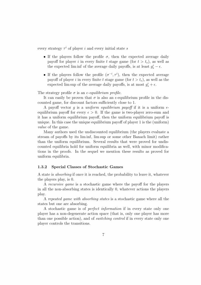
Gillette [15] studied games of perfect information and irreducible games,and proved the existence of stationary equilibrium profiles in both cases.Gillette introduced the following example of the “Big Match” which is atwo-player zero-sum repeated game with absorbing states.

Example 1 The “Big Match”

B

T

L R

1,−1

−1, 1 ∗

−1, 1

1,−1 ∗

Player 1 is the row player, while player 2 is the column player. The dailypayoff is as indicated by the cell. An cell marked with an asterisk means thatonce this cell is reached, then the game moves to an absorbing state, wherethe payoff for the players is as indicated by the cell. If an unmarked cell ischosen, then the game remains at the same state.

Gillette proves that in this game there is no stationary equilibrium profile.

Nevertheless, Blackwell and Ferguson [5] proved that the value of the“Big Match” is 0 (that is, the value of the non-absorbing state), and they

8

constructed ε-equilibrium profiles. In the ε-equilibrium profile, player 2 playsat every stage with equal probability his two actions, and player 1 plays ahistory-dependent strategy. An ε-equilibrium strategy that Blackwell andFerguson suggest for player 1 is to play T at stage t with probability 1

1/ε+kt,

where kt is the number of times that player 2 played R until stage t, minusthe number of times that player 2 played L until stage t. It can easily beproven that a 0-equilibrium profile for player 1 does not exist, and there areneither stationary nor Markovian ε-equilibrium profiles.

Kohlberg [16] generalized the result of Blackwell and Ferguson, and provedthat every zero-sum repeated game with absorbing states has a value.

Mertens and Neyman [20] generalized this result further, and provedthat every two-player zero-sum stochastic game has a value. Moreover, theyproved that the limit of the β-discounted value is equal to the uniform value.Their proof relies on the result of Bewley and Kohlberg [4] that was men-tioned before, that the value of the β-discounted game is a Puiseux functionin β.

1.3.4 Non Zero-Sum Games

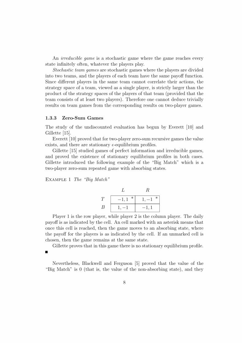
The study of non zero-sum games turns out to be much more difficult. Sorin[30] introduced the following example of a two-player non zero-sum repeatedgame with absorbing states:

Example 2

B

T

L R

1, 0

0, 2 ∗

0, 1

1, 0 ∗

The unique β-discounted equilibrium payoff of this game is (1/2, 2/3),and the points on the interval (1/2, 1) − (2/3, 2/3) are the only uniformequilibrium payoffs. Since the limit of the β-discounted equilibrium payoffsis not on this interval, it follows that the approach of Mertens and Neyman[20] cannot be used for non zero-sum games.

By studying Sorin’s example, Vrieze and Thuijsman [36] were able toprove that every two-player repeated game with absorbing states has a uni-form equilibrium payoff. Though stationary uniform ε-equilibrium profiles

9

need not exist in two-player repeated games with absorbing states, one canprove that ‘almost’ stationary ε-equilibrium strategies do exist. A profile ofstrategies is ‘almost’ stationary if it is given by a stationary profile and astatistical test; the players follow the stationary profile as long as no playerfails the statistical test. Once a player has failed the test, he is punishedwith an ε-min-max strategy forever. (an ε-min-max strategy against player1 is the strategy of player 2 in an ε-equilibrium profile of the zero-sum gamethat is defined by the payoffs of player 1).

Rogers [25] and Sobel [28] proved that stationary uniform equilibriumprofiles exist in every irreducible game and Thuijsman and Raghavan [31]prove the same result for switching control games.

By carefully analyzing the proof of Vrieze and Thuijsman [36], Vieille [32]proved that every stochastic game with three states has a uniform equilibriumpayoff.

Vieille [33, 34] proved that a uniform equilibrium payoff exists in everytwo-player (non zero-sum) stochastic game if and only if a uniform equi-librium payoff exists in every two player positive recursive games with theabsorbing property. These games are recursive games where the payoff forplayer 2 in absorbing states is positive, and satisfy the following absorbingproperty: for every fully mixed stationary strategy of player 2, the gameeventually reaches an absorbing state with probability 1, whatever player 1plays. Existence of a uniform equilibrium payoff for this class of games wasgiven only recently by Vieille [35].

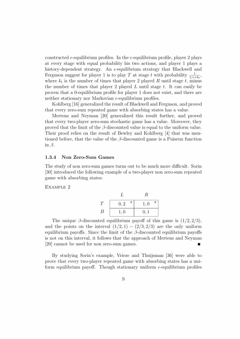
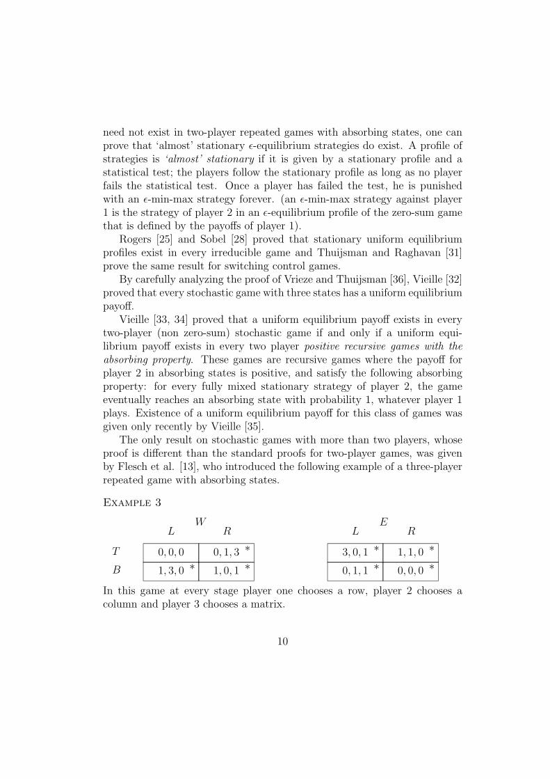
The only result on stochastic games with more than two players, whoseproof is different than the standard proofs for two-player games, was givenby Flesch et al. [13], who introduced the following example of a three-playerrepeated game with absorbing states.

Example 3

B

T

L R L RW E

1, 3, 0 ∗0, 0, 0

1, 0, 1 ∗0, 1, 3 ∗

0, 1, 1 ∗3, 0, 1 ∗

0, 0, 0 ∗1, 1, 0 ∗

In this game at every stage player one chooses a row, player 2 chooses acolumn and player 3 chooses a matrix.

10

Flesch et al. proved that there is no stationary uniform ε-equilibriumprofile in this game, but nevertheless a uniform equilibrium payoff does exist.The equilibrium strategy profile has a cyclic nature: the mixed action thatplayer i plays at stage t is equal to the mixed action that player i+ 1 mod 3plays at stage t+ 1. For more details, see section 4.2.5.

1.4 Application

Stochastic games have many applications in economy, biology, political sci-ences and other fields. Bargaining between agents, interactions between dif-ferent species, the behavior of political parties and political alliances can bemodeled by stochastic games.

Shubik and Whitt [27] modeled an economy with one non-durable good,where the money is valued only as a means to obtain more real goods, as astochastic game. The state variable in this case is the vector of amounts ofmoney each player possesses.

Winston [38] gave a model of an arm race as a stochastic game. In hismodel there is a weapon development competition between two countries,and the difference between the level of development between the countries isthe state variable.

Filar [11] studied a traveling inspector model: an inspector should in-spect some facilities, who can profit by violating the regulations. The aim ofthe inspector is to minimize the cost for the society, due to inspection andviolations. In this model the state variable is the current facility that theinspector inspects.

Levhari and Mirman [19], Amir [1], Dutta and Sundaram [9] and othersconsider a common property resource model. Two agents simultaneouslyexploit a productive asset (or resource). Any amount of the resource left overafter consumption in a given period forms the investment for that period,and is transformed into the available stock for the next period through aproduction function.

Team games were studied in [6, 7, 8] for understanding interactions be-tween players of the same team, and more precisely, the “free rider” phe-nomenon in team games.

Kohlberg and Zamir [17] proved that if every two player zero-sum re-peated game with absorbing states has a uniform equilibrium payoff then ev-

11

ery repeated game with symmetric incomplete information and deterministicsignaling has a uniform equilibrium payoff. This result was generalized byNeyman and Sorin for existence of a uniform equilibrium payoff in n-playerrepeated games with symmetric incomplete information and deterministicsignaling [23] and for non-deterministic signaling [24].

1.5 The Present Monograph

The goal of the present monograph is to shed more light on the existenceof the uniform equilibrium payoff in n-player stochastic games, and on thestructure of the uniform ε-equilibrium profiles.

We consider both n-player repeated games with absorbing states, andtwo-player stochastic games, and we prove existence of a uniform equilibriumpayoff in classes of stochastic games, where existence was unknown before.

In this section we outline the main ideas of the monograph. We firstconcentrate on n-player repeated games with absorbing states, and then ontwo-player stochastic games.

1.5.1 Two-Player Repeated Games with Absorbing States

Since a basic idea of our approach was presented by Vrieze and Thuijsman[36] in their proof for existence of a uniform equilibrium payoff in two-playernon zero-sum repeated games with absorbing states, we give a sketch of theirproof.

Vrieze and Thuijsman consider a sequence of β-discounted equilibria inthe game that converges to a limit as β → 1, and they construct differenttypes of uniform ε-equilibrium profiles according to various properties of thissequence. Denote by x = (x1, x2) the limit of the β-discounted equilibriumprofiles, and by g = (g1, g2) the limit of the corresponding β-discountedequilibrium payoffs. Note that x can be viewed as a stationary profile aswell.

Vrieze and Thuijsman prove that three cases can occur. (i) The stationaryprofile x is absorbing, and then, by adding threat strategies to x, one canconstruct a uniform ε-equilibrium profile. (ii) The stationary profile x isnon-absorbing, but the expected non-absorbing payoff for the players if theyfollow the profile x is at least g. Then, by adding threat strategies to x,one can devise a uniform ε-equilibrium profile. (iii) The stationary profile

12

x is non-absorbing, but the non-absorbing payoff for one player, say player1, if the players follow the profile x, is strictly less then g1. In this case, asVrieze and Thuijsman prove, player 2 has an action a2 (or a perturbation)such that by playing the stationary profile (x1, a2) the game will be eventuallyabsorbed, and the payoff for both players is at least g. Using x, a2 and threatstrategies, one can construct a uniform ε-equilibrium profile.

It turns out that for more than two players, if the first two cases do notoccur then it might be the case that neither the payoff that the players receiveby the stationary profile x nor any absorbing perturbation of any subset ofthe players (or a convex combination of some perturbations), yield all theplayers a payoff which is at least g.

1.5.2 n-Player Repeated Games with Absorbing States

In order to overcome this difficulty, we define an auxiliary game, where thenon-absorbing payoff is bounded by the min-max value of the players in theoriginal game. We prove that for every player, the discounted value of theauxiliary game converges, as the discount factor tends to 1, to his uniformvalue in the original game.

Consider a sequence of discounted equilibria in the auxiliary game. De-note by x the limit of the discounted stationary equilibrium profiles, and byg the limit of the corresponding discounted equilibrium payoffs. It turns outthat the first two cases of Vrieze and Thuijsman yield an ‘almost’ stationaryε-equilibrium profile as above, and, if they do not hold, then there exists aconvex combination of some perturbations that yields each player i a payoffwhich is at least gi. When there are three players, or in team games, one canconstruct, using this convex combination, a uniform ε-equilibrium profile forevery ε > 0.

In all the uniform ε-equilibrium profiles that we construct, the playersplay mainly the limit of the discounted stationary equilibrium profiles, andperturb to other actions with a very small probability, while checking statisti-cally whether the other players do not deviate. Once a deviation is detected,the deviator is punished with an ε-min-max profile forever. Such a profile iscalled a perturbed profile.

Unfortunately, our approach cannot be generalized for more than threeplayers. In section 4.8 we give an example of a four player repeated gamewith absorbing states where there exists a sequence of discounted equilibrium

13

profiles in the auxiliary game that converges to a limit, but one cannot con-struct a uniform ε-equilibrium profile where the players play mainly the limitmixed-action. Recently Solan and Vieille [29] found an example of a fourplayer repeated game with absorbing states that has no perturbed uniformequilibrium payoff. It is currently not known whether a uniform equilib-rium payoff exists in every n-player repeated game with absorbing states, forn ≥ 4.

The uniform equilibrium payoff that we construct is not necessarily equalto g, the limit of the discounted equilibrium payoffs of the auxiliary game.The reason is that the discounted payoff is a convex combination of the non-absorbing payoff and the absorbing payoff, whereas the undiscounted payoffof an absorbing mixed-action combination depends only on the absorbingpart.

For this reason we could not generalize the construction for stochasticgames with more than one non-absorbing state — if there is an equality be-tween the uniform equilibrium payoff and the limit of the discounted payoffs,then one can turn all non-absorbing states but one into absorbing states,which yield the players a payoff equal to this limit, and get a repeated gamewith absorbing states. By our result, this game has an equilibrium payoff,which would be equal (by the hypothesis) to the original limit of the dis-counted payoffs. Thus, one could construct an equilibrium payoff by working“state after state”.

However, since the hypothesis is incorrect, and the limit of the discountedpayoff is not necessarily equal to the constructed equilibrium payoff, such anapproach fails.

1.5.3 Two-Player Recursive Games with the Absorbing Property

To overcome this problem we consider the undiscounted payoff instead of thediscounted payoff, that is, a player evaluates a stationary profile x by

Ex,s

limt→∞

1

t

t∑j=1

rij

.Since the undiscounted payoff is not continuous over the space of stationarystrategies (with the maximum norm), we cannot use standard fixed pointtheorems.

14

In order to “make” the undiscounted payoff continuous, we use a resultof Vieille [34]. As mentioned above, Vieille proved that for two player games,it is sufficient to prove the existence of an equilibrium payoff for positiverecursive games with the absorbing property.

If we consider such a game, and restrict player 2 to a compact subset of thefully mixed stationary strategies, then the undiscounted payoff is continuousover the strategy space. We define ε-approximating games where player 2must play every action with a positive probability, which is greater than somefunction of ε. We consider a sequence of stationary undiscounted equilibriain the ε-approximating games as ε→ 0, and, as in Vrieze and Thuijsman [36],if there are at most two non-absorbing states then we construct, accordingto various properties of the sequence, uniform ε-equilibrium profiles.

Unfortunately, the uniform equilibrium payoff that we construct neednot be equal to the limit of the sequence of the equilibrium payoffs of theε-approximating games, hence we cannot generalize the proof for stochasticgames with more than two non-absorbing states.

15

2 Preliminaries

2.1 On Puiseux Functions

Denote by F the collection of all Puiseux series, that is, the collection of allthe formal sums

∑∞k=K ak(1− θ)k/M where K ∈ Z, M ∈ N, (ak)

∞k=K are real

numbers and there exists θ0 ∈ (0, 1) such that∑∞k=K ak(1− θ)k/M converges

for every θ ∈ (θ0, 1).We use θ both as an abstract symbol and as a real number. This dual

use should not confuse the reader.It is well known (see, e.g. Walker [37] or Bewley and Kohlberg [4]) that F

is an ordered field, when addition and multiplication are defined in a similarway to the same operations on power series, and

∑∞k=K ak(1 − θ)k/M > 0 if

and only if∑∞k=K ak(1− θ)k/M > 0 for every θ sufficiently close to 1.

We define the degree of any non-zero Puiseux series by:

deg

( ∞∑k=K

ak(1− θ)k/M)

def=

min{k | ak 6= 0}M

and deg(0) =∞.

Definition 2.1 A function f : [0, 1) → R is a Puiseux function if thereexists a Puiseux series

∑∞k=K ak(1 − θ)k/M and θ0 ∈ (0, 1) such that f(θ) =∑∞

k=K ak(1− θ)k/M for every θ ∈ (θ0, 1).

As a rule, Puiseux functions are denoted with a hat.The degree of a Puiseux function is the degree of the corresponding

Puiseux series, and the order on F induce an order on Puiseux functions.Note that f(θ) = o((1 − θ)deg(f)−c) for every c > 0. If deg(f) ≥ 0 then

limθ→1 f(θ) is finite. In this case define f(1)def= limθ→1 f(θ). Note also that

deg(f g) = deg(f) + deg(g). (1)

Clearly we have:

Lemma 2.2 Let f , g be two Puiseux functions such that f , g > 0. limθ→1f(θ)g(θ)∈

(0,∞) if and only if deg(f) = deg(g), and limθ→1f(θ)g(θ)

= 0 if and only if

deg(f) > deg(g).

16

2.2 Semi-Algebraic Sets

Definition 2.3 For every d ≥ 1, let Cd be the collection of all subsets ofRd of the form {x ∈ Rd | p(x) = 0} or {x ∈ Rd | p(x) > 0}, where p is anarbitrary polynomial.

A set C ⊆ Rd is semi-algebraic if it is in the finitely generated algebrawhich is spanned by Cd.

By Theorem 8.14 in Forster [14] we have

Lemma 2.4 If the graph of a real valued function defined on (0, 1) is a semi-algebraic set, then the function is a Puiseux function.

By Lemma 2.4 and Theorem 2.2.1 in Benedetti and Risler [3] we have,by induction on d:

Theorem 2.5 Let C ⊆ Rd be a semi-algebraic set, whose projection overits first coordinate includes the interval (0, 1). Then there exists a vector ofPuiseux functions f = (f i)d−1

i=1 : (0, 1) → Rd−1 such that (θ, f(θ)) ∈ C forevery θ ∈ (0, 1).

2.3 Notations

For every finite set I, we denote by ∆(I) the set of all probability distributionsover I.

Let I be a finite set, J ⊆ I, µ ∈ ∆(I) a probability distribution such that∑i∈J µ(i) > 0, and L = {L1, . . . , Ln} a partition of J (that is, {Lj}nj=1 are

disjoint sets, whose union in J). The conditional probability induced by µover L, µL, is a probability distribution over L that is defined by:

µL(Lj) =

∑i∈Lj µ(i)∑i∈J µ(i)

.

For every a, b ∈ Rd, a ≥ b if ai ≥ bi for every i = 1, . . . , d, and a > bif a ≥ b and a 6= b. Whenever we use a norm, it is the maximum norm. If‖ a− b ‖≤ ε, we say that a is ε-close to b. For every ε > 0 let

B(a, ε) = {a′ ∈ Rd | ‖ a− a′ ‖≤ ε}.

17

We identify each a0 ∈ A with α ∈ ∆(A) that is defined by

αa =

{1 a = a0

0 a 6= a0

By convention, a sum over an empty set of indices is 0.

18

3 Stochastic Games

3.1 The Model

A stochastic game is a 5-tuple G = (N,S, (Ai)i∈N , h, w) where

• N is a finite set of players.

• S is a finite set of states.

• For every i ∈ N , Ai is a finite set of actions available for player i ineach state s. Denote A = ×i∈NAi.

• h : S × A → R is the daily payoff function, hi(s, a) being the dailypayoff for player i in state s when the action combination a is played.Let R ≥ 1 be a bound on |h|.

• w : S × A→ ∆(S) is the transition function.

Note that since the state space is finite, the assumption that the availableset of actions is independent of the state is not restrictive.

Let Hn = S × (A × S)n be the space of all histories of length n, H0 =∪n∈NHn be the space of all finite histories and H = S × (A× S)N be thespace of all infinite histories. For every finite history h0 ∈ H0, L(h0) is itslength and sL(h0) is its last stage.

We define a partial order on H0. Let h0 = (s0, a1, s1, . . . , at, st) andh′0 = (s′0, a

′1, s′1, . . . , a

′t′ , s

′t′) be two histories. h′0 ≤ h0 if and only if t′ ≤ t

and (s′0, a′1, . . . , s

′t′) = (s0, a1, . . . , st′), that is, h′0 is a beginning of h0. Define

h′0 < h0 if and only if h′0 ≤ h0 and h′0 6= h0. If h0 ∈ H0 and h ∈ H,we say that h0 < h if h = (s0, a1, s1, . . .), h0 = (s′0, a

′1, s′1, . . . , a

′t, s′t) and

(s′0, a′1, . . . , s

′t) = (s0, a1, . . . , st), that is, h0 is a beginning of h.

For every i ∈ N , let X i = ∆(Ai), the set of all mixed-action combinationsof player i. We denote X = ×i∈NX i, X−i = ×j 6=iX i and XL = ×i∈LX i forevery L ⊆ N . The multi-dimensional extensions of h and w to X are denotedalso by h and w.

Definition 3.1 A behavioral strategy of player i is a function σi : H0 →X i. A strategy σi is stationary if σi(h0) depends only on sL(h0).

19

A strategy profile (or simply a profile) is a vector of strategies, one for eachplayer. Every profile σ and finite history h0 induce a probability measure overH (equipped with the σ-algebra generated by all the finite cylinders). Theprobability measure is the measure that is induced by σ given that the historyh0 has occurred (regardless of the probability of h0 under σ). We denote thismeasure by Prh0,σ, and expectation according to it by Eh0,σ. If h0 = (s) wedenote the expectation by Es,σ.

For every strategy σ and finite history h0 = (s0, a1, s1, . . . , at, st) we definethe strategy σ|h0 by:

σ|h0(h′0) = σ(s0, a1, s1, . . . , at, s

′0, a′0, . . . , a

′t′ , s

′t′)

where h′0 = (s′0, a′0, . . . , a

′t′ , s

′t′).

Every xi ∈ X i can be viewed as a stationary strategy of player i. Everysuch strategy is identified with a vector in R|S|·|A

i|

3.2 The Discounted Payoff

We denote by rit the daily payoff that player i receives at stage t.Let σ be a strategy profile, s ∈ S, β ∈ [0, 1) and i ∈ N . The expected

β-discounted payoff for player i if the initial state is s and the players followthe profile σ is given by:

viβ(s, σ) = (1− β)∞∑t=1

βt−1Es,σrit,

where rit is the payoff of player i at stage t.

Definition 3.2 Let i ∈ N and β ∈ [0, 1). The vector (cis(β))s∈S is theβ-discounted min-max value of player i if the following two conditions hold:

• For every strategy profile σ−i of players N \ {i} there exists a strategyσi of player i such that viβ(s, σ) ≥ cis(β) for every s ∈ S.

• There exists a strategy profile σ−i of players N \{i} such that for everystrategy σi of player i, viβ(s, σ) ≤ cis(β) for every s ∈ S.

Since the discounted payoff is continuous over the strategy space, and thesetup is finite, it follows that the β-discounted min-max value exists.

20

Definition 3.3 The strategy profile σ is a β-discounted equilibrium if forevery player i, every strategy τ i of player i and every initial state s,

viβ(s, σ) ≥ viβ(s, σ−i, τ i).

The payoff vector (vβ(s, σ))s∈S is a β-discounted equilibrium payoff.

Fink [12] has proved the following:

Theorem 3.4 For every β ∈ [0, 1) there exists a β-discounted stationaryequilibrium profile in every stochastic game.

3.3 The Uniform MinMax Value

Definition 3.5 Let i ∈ N . The vector (cis)s∈S ∈ RS is the uniform min-max value of player i if for every ε > 0 there exists tc ∈ N and a profile σ−iεof players N \ {i} such that for every initial state s ∈ S:

• For every strategy σi of player i

Es,σ−iε ,σi

(lim supt→∞

ri1 + ri2 + · · ·+ ritt

)≤ cis + ε

and for every t ≥ tc

Es,σ−iε ,σi

(ri1 + ri2 + · · ·+ rit

t

)≤ cis + ε.

• For every strategy profile σ−i of players N \ {i} there exists a strategyσi of player i such that

Es,σ

(lim inft→∞

ri1 + ri2 + · · ·+ ritt

)≥ cis − ε

and for every t > tc,

Es,σ

(ri1 + ri2 + · · ·+ rit

t

)≥ cis − ε.

The profile σ−iε is a uniform ε-min-max profile against player i.

21

Lemma 3.6 For every player i, the min-max value ci exists. Moreover, ci =limβ→1 c

i(β), the limit of the discounted min-max value of player i.

This result was proved by Mertens and Neyman [20] for two-player stochas-tic games, and an unpublished proof of Neyman [22] that follows similar linesproves the result for n-player stochastic games.

3.4 The Uniform Equilibrium Payoff

Definition 3.7 The payoff vector (g(s))s∈S ∈ RN×S is a uniform ε-equilibriumpayoff if there exist a strategy profile σε and te ∈ N such that for every playeri, every strategy τ i of player i, every initial state s and every t ≥ te

Es,σε

(ri1 + ri2 + · · ·+ rit

t

)≥ gi(s)− ε, (2)

Es,σε

(lim inft→∞

ri1 + ri2 + · · ·+ ritt

)≥ gi(s)− ε, (3)

Es,σ−iε ,τ i

(ri1 + ri2 + · · ·+ rit

t

)≤ gi(s) + ε and (4)

Es,σ−iε ,τ i

(lim supt→∞

ri1 + ri2 + · · ·+ ritt

)≤ gi(s) + ε. (5)

The profile σε is a uniform ε-equilibrium profile. The payoff vector g ∈ RN×S

is a uniform equilibrium payoff if it is an ε-equilibrium payoff for every ε > 0.

3.5 On Perturbed Equilibrium

In order to be able to implement the ε-equilibrium profile, we need the profileto be “simple”. In example 1, one cannot construct ε-equilibrium profileswhich are stationary or Markovian. For some classes of stochastic gamesexistence of ‘almost’ stationary ε-equilibrium profiles was established. Fleschet al. proved that in the game presented in example 3 there are no ‘almost’stationary ε-equilibrium profiles.

In this section we define a broader class of profiles, called perturbed pro-files. A profile in this class is given by a stationary strategy, small perturba-tions and statistical tests. The players play mainly the stationary strategies,

22

but perturb to other actions with small probability. All along, the actions ofeach player are screened by a statistical test, and the first player who failsthe test is punished forever.

We later prove that different classes of stochastic games admit equilibriumpayoffs, whose corresponding ε-equilibrium profiles are perturbed.

The importance of perturbed strategies are that the distribution of theactions almost resembles stationary strategies. Thus, if the players are dif-ferent species, and the actions stand for various types of this specie, thenan equilibrium where at even stages half the population should consists ofmales and half of females, while at odd stages two thirds should be females,is clearly undesirable.

Note that perturbed equilibrium profiles may be complex: we say nothingabout the complexity of the perturbations, or on the statistical test.

For every function f : H0 → {0, 1}, let Z(f) ⊆ H0 be the set of all finitehistories h0 such that f(h0) = 0, but f(h′0) = 1 for every h′0 < h0.

Every function f : H0 → {0, 1} can represent a statistical test — iff(h0) = 1 then the player does not fail the test, while if f(h0) = 0 then theplayer fails the test. Z(f) is the set of all finite histories in which the playerfails the test for the first time.

For every vector function f : H0 → {0, 1}N we define Z(f) ⊆ H0 to bethe set of all finite histories h0 such that h0 ∈ Z(f i) for some i ∈ N , buth′0 6∈ Z(f j) for every h′0 < h0 and every j ∈ N . For every h0 ∈ Z(f), theindex of h0 is the minimal i such that h0 ∈ Z(f i).

Every vector function f : H0 → {0, 1}N can represent a vector of statis-tical tests, one test for each player. Z(f) is the set of finite histories wherea failure of some player is observed for the first time, and the index of thehistory is the identity of the first player who failed his test.

We denote by G(f) the set of all finite histories h0 such that f i(h′0) = 1for every i ∈ N and h′0 ≤ h0. G(f) is the set of “good” histories, where nofailure of the test has ever occurred.

DefineG?(f) = {h ∈ H | h0 ∈ G(f) ∀h0 < h}

andZ?(f) = H \G?(f).

G?(f) is the set of all infinite histories where no failure is detected along thewhole game, and Z?(f) is the set of all infinite histories where a failure of

23

some player is detected at some point.Formally, the new class of equilibrium payoffs is defined as follows:

Definition 3.8 Let x ∈ X and ε > 0. A profile σ is (x, ε)-perturbed ifthere exist

• a function f : H0 → {0, 1}N

• and for every i ∈ N , an ε-min-max strategy τ−iε against player i

such that

• For every history h0 ∈ G(f) we have ‖ σ(h0)− x ‖< ε.

• For every history h0 ∈ Z(f) with index i0 we have σ−i0|h0= τ−i0ε .

Finally

Definition 3.9 Let x ∈ X. The payoff vector g ∈ RN×S is a uniform(x, ε)-perturbed equilibrium payoff if it is an ε-equilibrium payoff, and thereexists an ε-equilibrium profile for g which is (x, ε)-perturbed. x is the baseof the ε-equilibrium payoff. The payoff vector g ∈ RN×S is a uniform x-perturbed equilibrium payoff (or a perturbed equilibrium payoff) if it is an(x, ε)-perturbed equilibrium payoff for every ε > 0.

In all the classes of stochastic games for which existence of the undis-counted equilibrium payoff was proven, there exists a perturbed equilibriumpayoff. These classes, apart of the classes that admit stationary equilibria,are two-player non zero-sum repeated games with absorbing states (Vriezeand Thuijsman [36]), and positive recursive games with the absorbing prop-erty (Vieille [35]). Recall that for two-player zero-sum stochastic games,there exists an ε-equilibrium profile σ such that ‖ σ(h0) − x ‖< ε for everyfinite history h0 ∈ H0, where x is a fixed mixed action combination (thelimit of the discounted stationary equilibria). Moreover, the expected payoffthat these profiles yield converge, as ε tends to 0, to the value of the game(Mertens and Neyman [20]).

However, Solan and Vieille [29] show that stochastic games in generalneed not admit perturbed equilibrium payoffs.

In the present paper we prove existence of a uniform perturbed equilib-rium payoff in the following three classes of stochastic games: three-player

24

repeated games with absorbing states, repeated team games with absorbingstates and two player stochastic games with two non-absorbing states.

Since the results in this monograph refer to uniform equilibria, when-ever we write equilibrium payoff, ε-equilibrium profiles and min-max value,we mean the uniform equilibrium payoff, uniform ε-equilibrium profile anduniform min-max value respectively. Whenever we refer to the discountedversion of these notion, we explicitly mention the word discounted.

25

4 Repeated Games with Absorbing States

In this section we prove that every three-player repeated game with absorb-ing states, as well as every repeated team game with absorbing states, hasan equilibrium payoff. We begin by introducing an equivalent formulation ofrepeated games with absorbing states (section 4.1). We then give five sets ofsufficient conditions for existence of a perturbed equilibrium payoff (section4.2). We derive some preliminary results in sections 4.3-4.6, including thedefinition of an auxiliary game (section 4.4), which is the core of the proof.Afterwards we prove that every three-player repeated game with absorbingstates has an equilibrium payoff (section 4.7), and we explain why our ap-proach cannot be used for games with more than three players (section 4.8).We finally prove that every repeated team game with absorbing states hasan equilibrium payoff (section 4.9), and prove a geometric result, which isused along the section (section 4.10).

4.1 An Equivalent Formulation

Recall that a repeated game with absorbing state is a stochastic game whereall the states but one are absorbing. Since every absorbing state is a standardrepeated game, we can choose for each such state one equilibrium payoff, andassume that once this state is reached, all future payoffs are equal to thisequilibrium payoff.

Thus, an equivalent representation of a repeated game with absorbingstates is by a 5-tuple G = (N, (Ai, hi, ui)i∈N , w) where:

• N is a finite set of players.

• For every player i ∈ N , Ai is a finite set of pure actions available toplayer i. Denote A = ×i∈NAi.

• For every player i, hi : A→ R is a function that assigns to each actioncombination a ∈ A a non-absorbing payoff for player i.

• For every action combination a ∈ A, w(a) is the probability that thegame is absorbed if this action combination is played. If the game isabsorbed, ui(a) is the payoff that player i receives, at each future stage.

26

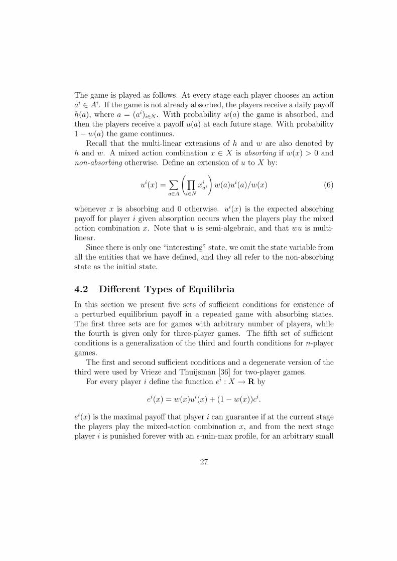
The game is played as follows. At every stage each player chooses an actionai ∈ Ai. If the game is not already absorbed, the players receive a daily payoffh(a), where a = (ai)i∈N . With probability w(a) the game is absorbed, andthen the players receive a payoff u(a) at each future stage. With probability1− w(a) the game continues.

Recall that the multi-linear extensions of h and w are also denoted byh and w. A mixed action combination x ∈ X is absorbing if w(x) > 0 andnon-absorbing otherwise. Define an extension of u to X by:

ui(x) =∑a∈A

(∏i∈N

xiai

)w(a)ui(a)/w(x) (6)

whenever x is absorbing and 0 otherwise. ui(x) is the expected absorbingpayoff for player i given absorption occurs when the players play the mixedaction combination x. Note that u is semi-algebraic, and that wu is multi-linear.

Since there is only one “interesting” state, we omit the state variable fromall the entities that we have defined, and they all refer to the non-absorbingstate as the initial state.

4.2 Different Types of Equilibria

In this section we present five sets of sufficient conditions for existence ofa perturbed equilibrium payoff in a repeated game with absorbing states.The first three sets are for games with arbitrary number of players, whilethe fourth is given only for three-player games. The fifth set of sufficientconditions is a generalization of the third and fourth conditions for n-playergames.

The first and second sufficient conditions and a degenerate version of thethird were used by Vrieze and Thuijsman [36] for two-player games.

For every player i define the function ei : X → R by

ei(x) = w(x)ui(x) + (1− w(x))ci.

ei(x) is the maximal payoff that player i can guarantee if at the current stagethe players play the mixed-action combination x, and from the next stageplayer i is punished forever with an ε-min-max profile, for an arbitrary small

27

ε. DefineEi(x) = max

ai∈Aiei(x−i, ai).

Ei(x) is the maximal payoff that player i can guarantee by “deviating” whenthe mixed action combination x should be played, and then be punished withan ε-min-max strategy, for an arbitrary small ε.

4.2.1 The Structure of the Proofs

With every set of sufficient conditions we give an example that illustrates thecorresponding ε-equilibrium profile, a formal definition of the ε-equilibriumprofile, and a proof that the profile is indeed an ε-equilibrium.

Since the proofs in all the different cases have the same structure, we willnow sketch the structure of the proofs.

In all the cases, we will be given a mixed action combination x ∈ X anda payoff vector g ∈ RN such that gi ≥ Ei(x) for every player i ∈ N . We willfix ε > 0 and proceed as follows.

Step a: Definition of a profile σWe will define a profile σ such that ‖ σ(h0)− x ‖≤ ε for every finite historyh0 ∈ H0. The profile σ will always be cyclic, but the length of the cycle maydepend on ε, and its exact nature is derived from the conditions we impose.Therefore the limit limt→∞(ri1 + · · ·+rit)/t exists a.s. w.r.t. σ. We will defineσ in such a way that∣∣∣∣Eσ

(limt→∞

(ri1 + · · ·+ rit)/t)− gi

∣∣∣∣ < ε. (7)

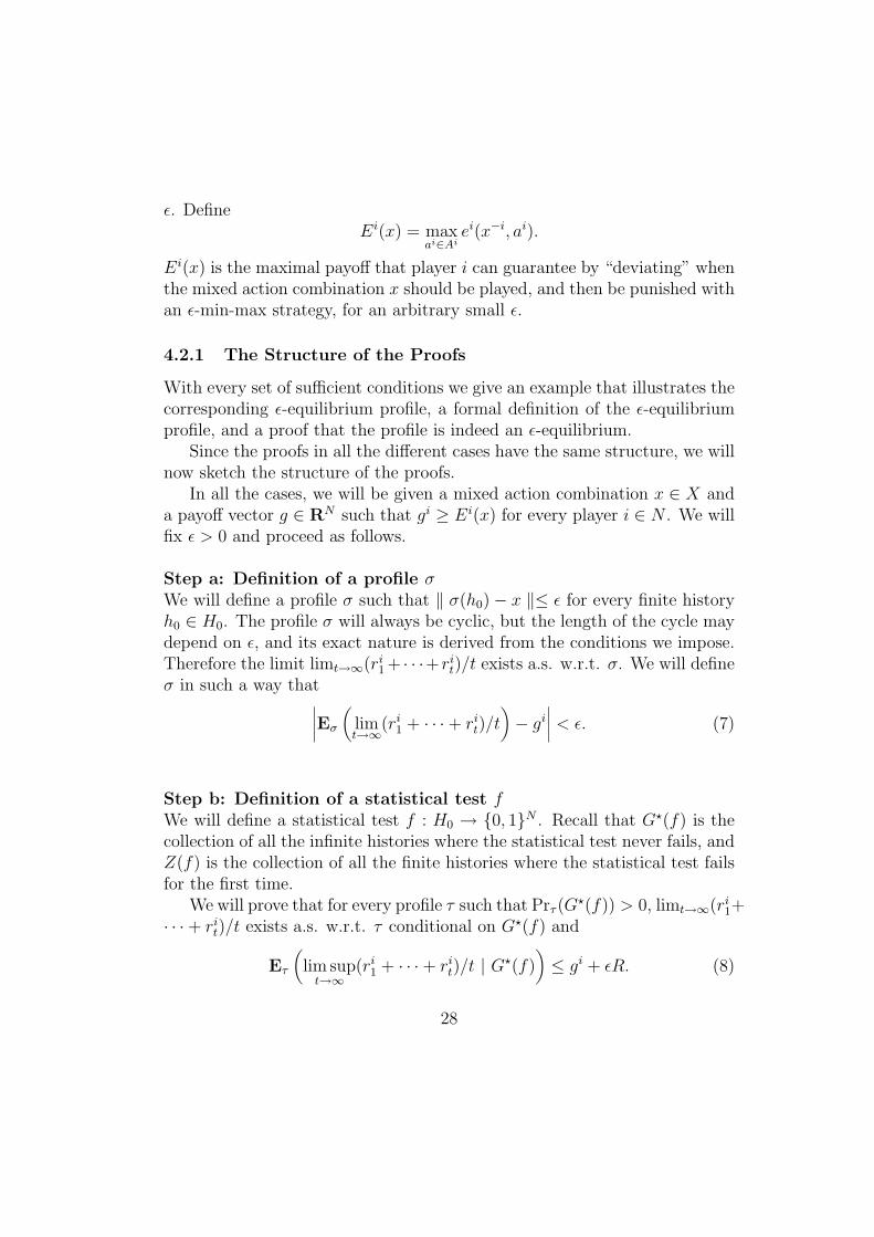
Step b: Definition of a statistical test fWe will define a statistical test f : H0 → {0, 1}N . Recall that G?(f) is thecollection of all the infinite histories where the statistical test never fails, andZ(f) is the collection of all the finite histories where the statistical test failsfor the first time.

We will prove that for every profile τ such that Prτ (G?(f)) > 0, limt→∞(ri1+

· · ·+ rit)/t exists a.s. w.r.t. τ conditional on G?(f) and

Eτ

(lim supt→∞

(ri1 + · · ·+ rit)/t | G?(f))≤ gi + εR. (8)

28

That is, as long as no “deviation” is detected, the expected payoff for anyplayer i cannot exceed gi + εR.

Step c: False Detection of DeviationNext we will prove that if the players follow σ, then the probability of falsedetection of deviation is smaller than ε, that is:

Prσ(G?(f)) > 1− ε. (9)

Step d: Definition of a Profile σfFor every profile σ and statistical test f , we define an (x, ε)-perturbed profileσf as follows. The players follow σ as long as no player fails the statisticaltest. The first player who fails the statistical test is punished with an ε-min-max profile forever. Formally, σf (h0) = σ(h0) for every h0 ∈ G(f), andσf |h0 = τ−iε for every h0 ∈ Z(f) with index i, where τ−iε is any ε-min-maxstrategy against player i.

In all the cases, we define σ and f in such a way that the profile σf is a3εR-equilibrium for g.

In the following steps we show how we will prove that σf is a 3εR-equilibrium profile.

Step e: Eqs. (2) and (3) in Definition 3.7 holdWe shall now see that from the above steps it follows that Eqs. (2) and (3)in Definition 3.7 hold w.r.t. σf . Indeed, by (7), (9) and since the payoffs arebounded by R ≥ 1 it follows that

Eσf

(lim inft→∞

(ri1 + · · ·+ rit)/t)≥ gi − 2εR.

Assume that te is sufficiently large such that for every t ≥ te

Eσ

((ri1 + · · ·+ rit)/t

)≥ gi − 2ε ∀i ∈ N. (10)

It follows from (9) and (10) that for every t ≥ te

Eσf((ri1 + · · ·+ rit)/t

)≥ gi − 3εR ∀i ∈ N.

29

Step f: Eqs. (4) and (5) in Definition 3.7 holdThis part of the proof is different for each set of sufficient conditions. Sincethe limit limt→∞(ri1 + · · ·+ rit)/t exists a.s. w.r.t. σ, there exists te ∈ N suchthat for every t ≥ te

Eτ

((ri1 + · · ·+ rit)/t | G?(f)

)≤ gi + ε. (11)

By (8) and (11) it is left to verify that for every player i, every strategy τ i

of player i and every finite history h0 ∈ Z(f) with index i,

Eh0,σ−if,τ i

(lim supt→∞

(ri1 + · · ·+ rit)/t)≤ gi + εR

and for every t ≥ te

Eh0,σ−if,τ i

((ri1 + · · ·+ rit)/t

)≤ gi + εR.

To summarize, for each set of sufficient conditions we need to define a profileσ that satisfies (7), a statistical test f that satisfies (8), and to prove (9)and Step f. Along the different proofs we will refer to these steps as ourguidelines.

4.2.2 An ‘Almost’ Stationary Non-Absorbing Equilibrium

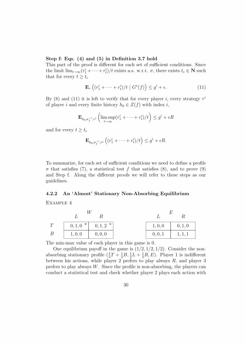
Example 4

B

T

L R L RW E

1, 0, 0

0, 1, 0 ∗

0, 0, 0

0, 1, 2 ∗

0, 0, 1

1, 0, 0

1, 1, 1

0, 1, 0

The min-max value of each player in this game is 0.One equilibrium payoff in the game is (1/2, 1/2, 1/2). Consider the non-

absorbing stationary profile (12T + 1

2B, 1

2L + 1

2R,E). Player 1 is indifferent

between his actions, while player 2 prefers to play always R, and player 3prefers to play always W . Since the profile is non-absorbing, the players canconduct a statistical test and check whether player 2 plays each action with

30

probability close to 1/2. If the distribution of the realized actions of player2 is not sufficiently close to (1/2, 1/2), then the other two players punishhim with a min-max profile forever. A deviation of player 3 is detectedimmediately, and, given the game is not absorbed, can be punished with amin-max profile.

It is easy to verify that the stationary non-absorbing profile, supplementedwith these threat strategies, is an ε-equilibrium profile for h(x), where the εcomes from the probability of false detection of deviation in the statisticaltest.

Lemma 4.1 Let x ∈ X be a non-absorbing mixed action combination suchthat hi(x) ≥ Ei(x) for every player i ∈ N . Then h(x) is an equilibriumpayoff.

Note that by the assumption it follows that hi(x) ≥ ci for every player i.Proof: Let ε > 0 be fixed, and denote g = h(x). Define a stationary profileσ by:

σ(h0) = x ∀h0 ∈ H0.

It is clear that σ satisfies (7).Define a statistical test as follows.

1. Each player i is checked if his strategy is compatible with σ (that is,he does not play an action outside supp(xi)).

2. At every stage t ≥ t1 (where t1 is defined below), each player i ischecked whether the distribution of his realized actions is ε-close to xi.

Formally, the statistical test is given by a function f : H0 → {0, 1}N that isdefined as follows. f i(a1, a2, . . . , at) = 0 if and only if ait 6∈ supp(xi) or t ≥ t1

and∣∣∣∣∣∣∣∣ai1+···+ait

t− xi

∣∣∣∣∣∣∣∣ > ε. It is clear that (8) holds.

The constant t1 ≥ 1/ε is chosen sufficiently large such that the probabilityof false detection of deviation is bounded by ε, that is, for every i ∈ N

Pr(‖ X i

t − xi ‖< ε ∀t > t1)> 1− ε/|N | (12)

where X it = 1

t

∑tj=1 X

ij and {X i

j} are i.i.d. r.v. with distribution xi. Hence(9) holds.

31

We shall now verify that (4) and (5) in Definition 3.7 hold. As remarkedin Step f, we fix a player i, a strategy τ i of player i and a history h0 ∈ Z(f)with index i.

We assume that t1 is sufficiently large such that:

t1hi(x) + tcR

t1 + tc≤ hi(x) + ε ∀i ∈ N. (13)

Let t2 ≥ tc be sufficiently large such that

t1R + t2ci

t1 + t2≤ ci + ε ∀i ∈ N. (14)

If L(h0) ≤ t1 then by (14) and the condition, for every t ≥ t1 + t2,

Eh0,σ−if,τ i

(ri1 + · · ·+ rit

t

)≤ hi(x) + 2εR (15)

and

Eh0,σ−if,τ i

(lim inft→∞

ri1 + · · ·+ ritt

)≤ hi(x) + εR. (16)

If, on the other hand, L(h0) > t1 then it follows by (13) and the conditionthat (15) and (16) hold.

Thus σf is a 3εR-equilibrium profile for h(x), and h(x) is an x-perturbedequilibrium payoff.

4.2.3 An ‘Almost’ Stationary Absorbing Equilibrium

Consider the game in example 4. Another equilibrium payoff in this game is(0, 1, 1), and an equilibrium profile is to play the stationary profile (T, 1

2L+

12R,W ), while checking for a deviation of players 1 and 3. Once a deviation is

detected, the deviator is punished with a min-max strategy profile. Note thatplayer 2 is indifferent between his actions, hence the fact that his deviationscannot be checked (since the game is absorbed after the first stage, whateverhe plays) does not affect this equilibrium.

Lemma 4.2 Let x ∈ X be an absorbing mixed action combination that sat-isfies the following two conditions:

32

1. ui(x) ≥ Ei(x) ∀i ∈ N .

2. ui(x) = ui(x−i, ai) for every i ∈ N and every ai ∈ supp(xi) such thatw(x−i, ai) > 0.

Then u(x) is a perturbed equilibrium payoff.

Proof: Denote g = u(x). We will consider the profile that was defined inthe proof of Lemma 4.1, but assume that the constant t1 is sufficiently largeto satisfy an additional requirement. We will then prove, as in Lemma 4.1,that this profile is an ε-equilibrium for g.

It is clear that if the players follow the stationary profile σ that wasdefined in the proof of Lemma 4.1 then (7) holds, and that (8) holds as well.

Let η > 0 be fixed. Let ε ∈ (0, η) be sufficiently small such that everyy ∈ B(x, ε) satisfies that w(y) > w(x)/2 and ‖ u(y)− u(x) ‖< η.

Consider the statistical test f that was defined in the proof of Lemma 4.1,but assume that the constant t1 is sufficiently large such that if no deviationis detected then absorption occurs before stage t1 with probability greaterthan 1− ε, that is, (1− w(x)/2)t1 < ε.

By the choice of t1, (9) holds.Fix a player i, a strategy τ i of player i and a history h0 ∈ Z(f) with

index i. If L(h0) ≤ t1 then by (14) and the conditions, for every t ≥ t1 + t2(where t2 is defined in the proof of Lemma 4.1)

Eh0,σ−if,τ i

(ri1 + · · ·+ rit

t

)≤ t1u

i(x) + (t− t1)(Ei(x) + ε)

t≤ ui(x) + ε (17)

and

Eh0,σ−if,τ i

(lim inft→∞

ri1 + · · ·+ ritt

)≤ ui(x) + ε. (18)

SincePrσ (h ∈ H | ∃h0 < h s.t. h0 ∈ Zf and L(h0) ≥ t1) < ε

it follows that

Eσ−if,τ i

(ri1 + · · ·+ rit

t

)≤ ui(x) + 3εR

and

Eσ−if,τ i

(lim inft→∞

ri1 + · · ·+ ritt

)≤ ui(x) + 2εR.

33

Thus σf is a 3εR-equilibrium profile for u(x), and u(x) is an x-perturbedequilibrium payoff.

4.2.4 Average of Perturbations

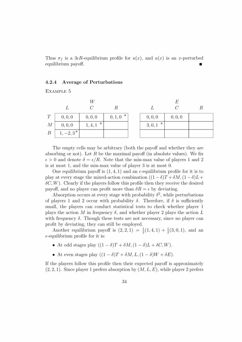
Example 5

B

M

T

L C R L C R

W E

1,−2, 3∗0, 0, 0

0, 0, 0

1, 4, 1 ∗0, 0, 0 0, 1, 0 ∗

3, 0, 1 ∗0, 0, 0 0, 0, 0

The empty cells may be arbitrary (both the payoff and whether they areabsorbing or not). Let R be the maximal payoff (in absolute values). We fixε > 0 and denote δ = ε/R. Note that the min-max value of players 1 and 2is at most 1, and the min-max value of player 3 is at most 0.

One equilibrium payoff is (1, 4, 1) and an ε-equilibrium profile for it is toplay at every stage the mixed-action combination ((1− δ)T + δM, (1− δ)L+δC,W ). Clearly if the players follow this profile then they receive the desiredpayoff, and no player can profit more than δR = ε by deviating.

Absorption occurs at every stage with probability δ2, while perturbationsof players 1 and 2 occur with probability δ. Therefore, if δ is sufficientlysmall, the players can conduct statistical tests to check whether player 1plays the action M in frequency δ, and whether player 2 plays the action Lwith frequency δ. Though these tests are not necessary, since no player canprofit by deviating, they can still be employed.

Another equilibrium payoff is (2, 2, 1) = 12(1, 4, 1) + 1

2(3, 0, 1), and an

ε-equilibrium profile for it is:

• At odd stages play ((1− δ)T + δM, (1− δ)L+ δC,W ).

• At even stages play ((1− δ)T + δM,L, (1− δ)W + δE).

If the players follow this profile then their expected payoff is approximately(2, 2, 1). Since player 1 prefers absorption by (M,L,E), while player 2 prefers

34

absorption by (M,C,W ), the players should conduct statistical tests andcheck whether each of them follows this profile, and punish a deviator withan ε-min-max profile.

Yet a third equilibrium payoff is (1, 1, 2) = 12(1, 4, 1) + 1

2(1,−2, 3), and an

ε-equilibrium profile for it is:

• At odd stages play ((1− δ)T + δM, (1− δ)L+ δC,W ).

• At even stages play ((1− δ2)T + δ2B,L,W ).

If the players follow this profile then their expected payoff is approximately(1, 1, 2). In this case the players cannot check whether player 1 plays ateven stages the action B in frequency δ2, since once he plays this action thegame terminates with probability 1 − δ, and there is a probability of 1/2that he never plays B. Nevertheless player 1 has no incentive to deviate, andtherefore such a check is not needed. However. the players do need to checkwhether player 2 perturbs at odd stages as he should.

Actually, every convex combination (g1, g2, g3) of the four absorbing cells(1,−2, 3), (1, 4, 1), (0, 1, 0) and (3, 0, 1) in which g1, g2 ≥ 1, g3 ≥ 0 that satis-fies:

• If (1,−2, 3) has a positive weight in this combination then g1 = 1.

• If (0, 1, 0) has a positive weight in this combination then g2 = 1.

is an equilibrium payoff.

Definition 4.3 Let x ∈ X be a non-absorbing mixed-action combinationand L ⊆ N . An action combination bL ∈ ×i∈LAi is an absorbing neighborof x by L if

• w(x−L, bL) > 0.

• w(x−L′, bL

′) = 0 for every strict subset L′ of L.

If L = {i} then the absorbing neighbor is called a single absorbing neighborof player i.

We denote by B(x) the set of all absorbing neighbors of x, and by Bi(x)the set of all single absorbing neighbors of player i. Note that B(x) is neverempty (as long as there is an absorbing action combination), but Bi(x) maybe empty.

35

Lemma 4.4 Let x ∈ X be a non-absorbing mixed action combination. Letµ ∈ ∆(B(x)) and denote g =

∑bL∈B(x) µ(bL)u(x−L, bL). Assume the following

conditions hold:

1. gi ≥ Ei(x) ∀i ∈ N .

2. ui(x−i, ai) = gi for every player i and every action ai ∈ Bi(x)∩supp(µ).

Then g is an equilibrium payoff.

Proof: Let ε > 0 be sufficiently small, T ∈ N sufficiently large, and m :[1, . . . , T ]→ supp(µ) such that∣∣∣∣∣#{j | m(j) = bL}

T− µ(bL)

∣∣∣∣∣ < ε/3, ∀bL ∈ supp(µ). (19)

That is, m is a discrete approximation of µ. Extend the domain of m to Nby m(t) = m(t mod T ) for every t > T . Let L(t) be the set of players forwhich m(t) is an absorbing neighbor of x.

In the sequel, δ ∈ (0, ε) is sufficiently small, such that

(1− δ)T > 1− ε/3 (20)

and t1, t2 ∈ N are sufficiently large. For every bL ∈ supp(µ), let δ(bL) =(δ/w(x−L, bL))1/|L|. Define a cyclic profile σ as follows:

• At stage t the players play the mixed action combination (1−δ(m(t)))x+δ(m(t))(x−L(t),m(t)).

If the players follow σ then the probability of absorption at each staget is δ(m(t))|L(t)|w(x−L(t),m(t)) = δ. Fix consecutive T stages. By (19) and(20), the probability that the game is absorbed by a neighbor bL ∈ supp(µ),given absorption occurs in these T stages, is ε-close to µ(bL). It follows that(7) holds.

Let η ∈ (0, ε/3) be sufficiently small such that for every bL ∈ supp(µ) andy ∈ B(x, η) we have ‖ u(x−L, bL)− u(y−L, bL) ‖< ε. Define a statistical testf as follows. Each player i is checked for the following:

1. Whether his realized actions are compatible with σ.

36

2. For every bL ∈ supp(µ) such that i 6∈ L, whether the distribution of hisrealized actions, restricted to stages j such that m(j) = bL, is η-closeto xi. This check is done only after stage t1T .

3. For every bL ∈ supp(µ) such that i ∈ L, whether player i plays theaction bi during stages j such that m(j) = bL with probability δ(bL)(that is, the realized probability p should satisfy 1−η/|N | < p/δ(bL) <1 + η/|N |). This check is done only after stage t2T .

4. If supp(µ) ⊆ Bi(x), whether the game was absorbed before stage t0(where t0 is defined below).

The second test checks whether the players play mainly the mixed actioncombination x, and the third test checks whether the players perturb toabsorbing neighbors bL such that |L| ≥ 2 in the pre-specified frequencies. Bythe second condition, it is not necessary to check whether players perturb tosingle absorbing neighbors in the pre-specified frequencies. Moreover, sucha check cannot be done. However, if all the absorbing neighbors in µ aresingle absorbing neighbors of player i, then it might be in the interest ofplayer i never to perturb to his single absorbing neighbors, and to receivethe non-absorbing payoff forever. The last test takes care of this type ofdeviation.

Formally, f i(a1, . . . , at) = 0 if and only if at least one of the followingholds:

• i 6∈ L(t) and ait 6∈ supp(xi).

• i ∈ L(t) and ait 6∈ supp(xi) ∪ {mi(t)}.

• t ≥ t1T , i 6∈ L(t) and∣∣∣∣∣∣∣∣xi − ∑

j<t | m(j)=m(t)aij

t

∣∣∣∣∣∣∣∣ > η.

• t ≥ t2T , i ∈ L(t) and∣∣∣1−#{j < t | m(j) = m(t) and aij = mi(t)}/δ(m(t))∣∣∣ < η/|N |.

• If supp(µ) ⊆ Bi(x) and t ≥ t0, where t0 ∈ N satisfies that (1 −δ(m(1)))t0 < ε.

37

Note that if no deviation is ever detected, then the game is bounded to beeventually absorbed. By (19), (20), the second condition and the definitionsof η and f it follows that (8) holds.

It is left to prove that (9) holds, and that no player can gain too muchby deviating.

We claim that it is sufficient to prove the following:

a) If the game is absorbed before a deviation is detected, while player iplays an action ai ∈ Bi(x)∩ supp(µ), then player i’s expected payoff isat most gi + ε.

b) If player i deviates, by altering the probability in which he plays actionswithin supp(xi), or the action mi(t) at stage t with |L(t)| ≥ 2, thenthe probability of absorption before the statistical test is employed isat most ε.

c) By a detectable deviation no player can profit more than 2εR.

d) The probability of false detection of deviation is bounded by ε (that is,(9) holds).

Indeed, (a)-(c) imply that Step f holds. Note that (a) holds by the secondcondition and the definition of σ, and (c) holds by the first condition and thedefinition of σ.

Let us now see how to choose the constants δ,t1 and t2 such that (b) and(d) will hold. To insure (d) we need for the second test that

Pr(‖ X i

t − xi ‖< η ∀t > t1T)> 1− ε/2|N | ∀i ∈ N (21)

where X it = 1

t

∑tj=1 X

ij and {X i

j} are i.i.d. r.v. with distribution xi. For thethird test we need that

Pr(‖ Y i

t /δ(m(t))− 1 ‖< η ∀t > t2T)> 1− ε/2|N | ∀i ∈ N (22)

where Y it = 1

t

∑tj=1 Y

ij and {Y i

j } are i.i.d. Bernoulli r.v. with P (Y ij = 1) =

δ(m(t)). To insure (b) we need for the first test that

(1− δ)t1T > 1− ε (23)

38

and for the third test that(1− δ(|L(t)|−1)/|L(t)|

)t2T ≥ (1− δ1/2)t2T > 1− ε ∀t = 1, . . . , T. (24)

We claim that there exist δ, t1 and t2 such that (21), (22), (23) and (24)hold. We need the following lemma:

Lemma 4.5 Let ε > 0, p = 1/n for some n ∈ N and (Xt)t∈N be i.i.d.Bernoulli random variables with P (Xt = 1) = p. There exists t? ∈ N suchthat

P

(∣∣∣∣∣∑tj=1 Xj

tp− 1

∣∣∣∣∣ < 2ε ∀t > t?p

)> 1− ε. (25)

Proof: Let λ ∈ (1, 1 + ε) and t? = λ/ε3(λ− 1). By Kolmogorov’s Inequality(see, e.g., Lamperti [18], p. 46), for every k ∈ N

Pr

maxλkt?/p<t≤λk+1t?/p

∣∣∣∣∣∣t∑

j=1

(Xj − p)

∣∣∣∣∣∣ < ελk+1t?p

≤ λk+1t?p(1− p)ε2λ2(k+1)t2?p

2

<1

ε2λk+1t?p(26)

Summing (26) over all k ≥ 0 yields

Pr

maxt?/p<t

∣∣∣∣∣∣t∑

j=1

(Xj − p)

∣∣∣∣∣∣ < 2εt

<λ

ε2t?(λ− 1)≤ ε

and (25) follows.

Let t1 ∈ N be sufficiently large to satisfy (21). Let ρ0 > 0 be such thatfor every ρ ∈ (0, ρ0)

(1− ρ)ρ−1/2

=((1− ρ)1/ρ

)ρ1/2> 1− ε. (27)

Let δ ∈ (0, ρ20) be sufficiently small such that (23) holds. Denote t2 = 1/Tδ1/4.

We assume δ is sufficiently small such that t? = t2T satisfies Lemma 4.5.Since δ1/2 < ρ0, it follows by (27) that (24) holds, and since t2T satisfiesLemma 4.5, (22) holds.

39

4.2.5 A Cyclic Equilibrium

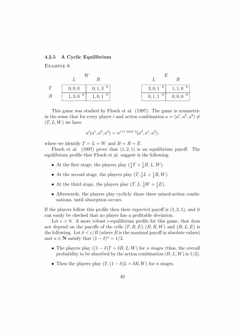
Example 6

B

T

L R L RW E

1, 3, 0 ∗0, 0, 0

1, 0, 1 ∗0, 1, 3 ∗

0, 1, 1 ∗3, 0, 1 ∗

0, 0, 0 ∗1, 1, 0 ∗

This game was studied by Flesch et al. (1997). The game is symmetricin the sense that for every player i and action combination a = (a1, a2, a3) 6=(T, L,W ) we have

ui(a1, a2, a3) = ui+1 mod 3(a3, a1, a2),

where we identify T = L = W and B = R = E.Flesch et al. (1997) prove that (1, 2, 1) is an equilibrium payoff. The

equilibrium profile that Flesch et al. suggest is the following.

• At the first stage, the players play (12T + 1

2B,L,W ).

• At the second stage, the players play (T, 12L+ 1

2R,W ).

• At the third stage, the players play (T, L, 12W + 1

2E).

• Afterwards, the players play cyclicly those three mixed-action combi-nations, until absorption occurs.

If the players follow this profile then their expected payoff is (1, 2, 1), and itcan easily be checked that no player has a profitable deviation.

Let ε > 0. A more robust ε-equilibrium profile for this game, that doesnot depend on the payoffs of the cells (T,R, E), (B,R,W ) and (B,L,E) isthe following. Let δ < ε/R (where R is the maximal payoff in absolute values)and n ∈ N satisfy that (1− δ)n = 1/2.

• The players play ((1− δ)T + δB, L,W ) for n stages (thus, the overallprobability to be absorbed by the action combination (B,L,W ) is 1/2).

• Then the players play (T, (1− δ)L+ δR,W ) for n stages.

40

• Then the players play (T, L, (1− δ)W + δE) for n stages.

• Afterwards, the players play cyclicly those three phases, until absorp-tion occurs.

Definition 4.6 Let a, b, c ∈ R3. The three vectors (a, b, c) are left-cyclic ifb1 > a1 > c1, c2 > b2 > a2 and a3 > c3 > b3, and right-cyclic if b1 < a1 < c1,c2 < b2 < a2 and a3 < c3 < b3. They are cyclic if they are either left-cyclicor right-cyclic. They are positive cyclic if they are cyclic and

det

0 b1 − a1 c1 − a1

a2 − b2 0 c2 − b2

a3 − c3 b3 − c3 0

> 0.

Whenever we say that three vectors are cyclic, it should be understood thatthe first vector serves as the a in the above definition, the second vectorserves as the b, and the third serves as the c.

Note that if (a, b, c) are left-cyclic, then ((a1, a3, a2), (c1, c3, c2), (b1, b3, b2))are right-cyclic.

Lemma 4.7 If (a, b, c) are positive right-cyclic vectors then the system ofequations

a1 =βb1 + (1− β)γc1

β + (1− β)γ(28)

b2 =γc2 + (1− γ)αa2

γ + (1− γ)α(29)

c3 =αa3 + (1− α)βb3

α + (1− α)β(30)

has a unique solution. Moreover, this solution satisfies α, β, γ ∈ (0, 1).

Proof: Assume w.l.o.g. that a1 = b2 = c3 = 0. Since the vectors are cyclic, itfollows that a2, a3, b1, b3, c1, c2 6= 0. Note that every solution (α, β, γ) satisfiesthat α, β, γ 6∈ {0, 1}.

41

We are going now to calculate β. By (29) and (30) we have

α =−γc2

(1− γ)a2

=βb3

βb3 − a3

, (31)

and by (28) we have

γ =−βb1

(1− β)c1

. (32)

Substituting (32) in (31) and dividing by β yields

b1c2

c1 − βc1 + βb1

=b3a2

βb3 − a3

.

Hence

β =a2b3c1 + a3b1c2

b3b1c2 + a2b3c1 − a2b3b1

is uniquely determined. Since (a, b, c) are right-cyclic it follows that thedenominator is positive, while since they are positive cyclic, the numeratoris also positive. Hence β > 0. To prove that β < 1 it is sufficient to provethat b3b1c2 − a2b3b1 − a3b1c2 > 0, which holds since (a, b, c) are right-cyclic.

In a similar way we prove that α, γ ∈ (0, 1).

The following sufficient condition is given only for three-player repeatedgames with absorbing states, hence we assume that N = {1, 2, 3}.

Lemma 4.8 Let x ∈ X be a non-absorbing mixed action combination andfor every i ∈ N let yi ∈ X i such that

1) For every i ∈ N , w(x−i, yi) > 0 and ui(x−i, yi) ≥ Ei(x).

2) (u(x−1, y1), u(x−2, y2), u(x−3, y3)) are positive cyclic vectors.

3) For every player i and every action ai ∈ supp(yi), w(x−i, ai) > 0 andui(x−i, ai) = ui(x−i, yi).

Then there exists an equilibrium payoff.

Proof: Assume w.l.o.g. that (u(x−1, y1), u(x−2, y2), u(x−3, y3)) are right-cyclic (otherwise, change the names of players 2 and 3, and recall the remark

42

after Definition 4.6). By condition 2 and Lemma 4.7 there exist α, β, γ ∈(0, 1) such that

u1(x−1, y1) =βu1(x−2, y2) + (1− β)γu1(x−3, y3)

β + (1− β)γ, (33)

u2(x−2, y2) =γu2(x−3, y3) + (1− γ)αu2(x−1, y1)

γ + (1− γ)αand (34)

u3(x−3, y3) =αu3(x−1, y1) + (1− α)βu3(x−2, y2)

α + (1− α)β. (35)

Let ε > 0 be fixed. Let δ1, δ2, δ3 ∈ (0, ε) be sufficiently small andn1, n2, n3 ∈ N satisfy the following

(1− δ1w(x−1, y1))n1 = 1− α(1− δ2w(x−2, y2))n2 = 1− β (36)

(1− δ3w(x−3, y3))n3 = 1− γ.

Define a profile σ as follows:

• Phase 1: The players play the mixed action combination (1 − δ1)x +δ1(x−1, y1) for n1 stages.

• Phase 2: The players play the mixed action combination (1 − δ2)x +δ2(x−2, y2) for n2 stages.

• Phase 3: The players play the mixed action combination (1 − δ3)x +δ3(x−3, y3) for n3 stages.

• The players repeat cyclicly these three phases until absorption occurs.

If the players follow σ then the probability that the game is absorbedduring the first phase is 1−(1−δ1w(x−1, y1))n1 = α. Similarly, the probabilitythat the game is absorbed during the second and third phases are β and γrespectively. Hence the game will be eventually absorbed with probability 1.

We first calculate the expected payoff for the players if they follow σ. Theexpected payoff for player 1 is, by (33),

αu1(x−1, y1) + (1− α)βu1(x−2, y2) + (1− α)(1− β)γu1(x−3, y3)

1− (1− α)(1− β)(1− γ)= u1(x−1, y1).

43

Moreover, for every j ≤ n1 his expected payoff given absorption has notoccurred in the first j stages is u1(x−1, y1).

Similarly, the expected payoff of player 2 given absorption has not oc-curred during the first n1 stages is u2(x−2, y2). By condition 2, u2(x−1, y1) >u2(x−2, y2), and therefore the expected payoff of player 2 is

αu2(x−1, y1) + (1− α)u2(x−2, y2) ≥ u2(x−2, y2).

Moreover, for every j ≤ n1 the expected payoff for player 2 given absorptionhas not occurred in the first j stages is at least u2(x−2, y2).

In a similar way, the expected payoff of player 3 given absorption hasnot occurred during the first n1 + n2 stages is u3(x−3, y3). Since the profileis cyclic, it follows that his expected payoff at the beginning of the gameis u3(x−3, y3). By condition 2, u3(x−1, y1) < u3(x−3, y3), and therefore forevery j ≤ n1 his expected payoff given absorption has not occurred duringthe first j stages is at least u3(x−3, y3).

Denote g = (u1(x−1, y1), αu2(x−1, y1) + (1 − α)u2(x−2, y2), u3(x−3, y3)).Then (7) holds. Since (u(x−1, y1), u(x−2, y2), u(x−3, y3)) are right-cyclic andby the first assumption, it follows that

gi ≥ ui(x−i, yi) ≥ Ei(x) ∀i ∈ N.

Let η ∈ (0, ε) sufficiently small such that for every z ∈ B(x, η) we havew(z−i, yi) > w(x−i, yi)/2 and ‖ u(x−i, yi)− u(z−i, yi) ‖< ε.

Define a statistical test f as follows. Each player i is checked for thefollowing:

• Whether his realized action is compatible with σ.

• Let t0 = k(n1 + n2 + n3) be the first stage of phase 1 at the k + 1stcycle. At each stage t such that t0 + t1 ≤ t ≤ t0 + n1 (where t1 isdefined below) players 2 and 3 are checked whether the distribution oftheir realized actions at stages t0, t0 + 1, . . . , t − 1 is η-close to x2 andx3 respectively.Analogous checks are done in phases 2 and 3.

Formally, the statistical test is defined as follows. Let t, k ∈ N satisfy thatk(n1 + n2 + n3) ≤ t < k(n1 + n2 + n3) + n1. f i(a1, a2, . . . , at) = 0 if and onlyif at least one of the following holds:

44

• i 6= 1 and ait 6∈ supp(xi).

• i = 1 and a1t 6∈ supp(x1) ∪ supp(y1).

• i 6= 1, t ≥ t0 + t1, where t0 = k(n1 + n2 + n3), and

∣∣∣∣∣∣∣∣∣∣∑t−1

j=t0aij

t−t0 − xi∣∣∣∣∣∣∣∣∣∣ > η.

The function f is defined analogously for every t that satisfies k(n1 + n2 +n3) + n1 ≤ t < (k + 1)(n1 + n2 + n3) for some k ∈ N. By condition 3 andthe definitions of f and η, (8) holds.

We choose the various constants in the following way. Let k0 ∈ N besufficiently large such that if no deviation is detected in σf , and at least oneof the players follows σf , then absorption occurs during the first k0 cycleswith probability greater than 1− ε/2. Formally,

(1− α/2)k0 , (1− β/2)k0 , (1− γ/2)k0 < ε/2. (37)

Let t1 ∈ N be sufficiently large such that

Pr(‖ X i

t − xi ‖< η ∀t > t1)> 1− ε/6k0 ∀i ∈ N (38)

where X it = 1

t

∑tj=1 X

ij and {X i

j} are i.i.d. r.v. with distribution xi. By (37)and (38) it follows that (9) holds.

Let δ1, δ2, δ3 > 0 be sufficiently small such that

(1− δi)t1 > 1− ε ∀i ∈ N. (39)

Moreover, we choose {ni} and {δi} in such a way that (36) holds.Let t3 = k0(n1 + n2 + n3). If no deviation is detected then absorption

occurs before stage t3 with probability greater than 1 − ε/2. Let t4 ∈ N besufficiently large such that

t3R + (t4 − t3)ci

t4≤ ci + ε ∀i ∈ N. (40)

We will show that in phase 1 no player can deviate and profit more than2εR. The proofs for the other phases is analogous.

Fix a player i, a strategy τ i of player i and a history h0 ∈ Z(f) with indexi such that L(h0) < n1. If in h0 player i fails the second test then by (39)

45

the probability of absorption before the statistical test is employed is smallerthan ε, and by the first condition and the choice of t4, for every t ≥ t4:

Eh0,σ−if,τ i

(ri1 + · · ·+ rit

t

)≤ t3R + (t− t3)(Ei(x) + ε)

t≤ gi + 2ε (41)

and

Eh0,σ−if,τ i

(lim inft→∞

ri1 + · · ·+ ritt

)≤ Ei(x) + ε ≤ gi + ε. (42)

If, on the other hand, player i fails the first test, then by the first condi-tion, Eqs. (41) and (42) hold.

Thus σf is a 2εR-equilibrium profile for g, and g is an x-perturbed equi-librium payoff.

4.2.6 A Generalization

We now generalize the third and fourth sufficient conditions to a single suf-ficient condition, that holds for an arbitrary number of players.

Lemma 4.9 Let x be a non-absorbing mixed-action combination. For everyj ∈ N, let µj ∈ ∆(B(x)) and αj ∈ (0, 1] such that

∑j∈N αj =∞. Let (rj)j∈N

be the unique solution of the following system of linear equation:

rj = αj

∑bL∈B(x)

µj(bL)u(x−L, bL)

+ (1− αj)rj+1 ∀j ∈ N. (43)

Assume that the following conditions hold:

1) rij ≥ Ei(x) for every i, j ∈ N.

2) For every j ∈ N and every player i ∈ N such that there exists a singleabsorbing perturbation bi ∈ supp(µj) of player i we have:

rij+1 = ui(x−i, bi) = rij.

Then for every j ∈ N, rj is an x-perturbed equilibrium payoff.

46

Note that since∑j∈N αj =∞ it follows that the system of linear equations

(43) has a unique solution.The ε-equilibrium profile is constructed in phases: in phase j, the players

play an ε/2j-equilibrium profile as defined in the proof of Lemma 4.4 forµj, either until the game is absorbed, or a deviation is detected, or untilthe overall probability of absorption during phase j is at least αj − ε/2j. Ifthe players follow this profile then the overall probability of false detectionof deviation is bounded by ε, and since

∑j∈N αj = ∞, if no deviation is

detected then the game will eventually be absorbed with probability 1. Asin the proof of Lemma 4.4, no player can profit more than ε by deviating.

Note that this equilibrium can be generalized to equilibrium profiles whichare not perturbed, by using at stage j a (possibly) different mixed-actioncombination xj, instead of the same x always.

4.3 On the Discounted Game

Recall that viβ(x) is the expected β-discounted payoff for player i if the playersfollow the stationary profile x.

In this section we recall a fundamental formula that is already derived byVrieze and Thuijsman [36] for the discounted payoff that is used later, andwe prove that for every ε > 0 there exists an interval (β(ε), 1) such that forevery mixed action x−i of the players N \ {i}, player i has a reply which isε-good in every β-discounted game (where β ∈ (β(ε), 1)).

The function vβ(x) satisfies the recursion formula:

vβ(x) = (1− β)h(x) + βw(x)u(x) + β(1− w(x))vβ(x). (44)

Since h and uw are multi-linear, it follows that vβ is quasi-concave. Indeed,assume that for x, y ∈ X

(1− β)h(x) + βw(x)u(x)

1− β + βw(x),(1− β)h(y) + βw(y)u(y)

1− β + βw(y)≥ c.

Then

vβ(λx+ (1− λ)y) =

=λ ((1− β)h(x) + βw(x)u(x)) + (1− λ) ((1− β)h(y) + βw(y)u(y))

λ(1− β + βw(x)) + (1− λ)(1− β + βw(y))

≥ c. (45)

47

The solution of (44) is:

vβ(x) =(1− β)h(x) + βw(x)u(x)

1− β + βw(x).

Let

αβ(x) =1− β

1− β + βw(x)(46)

thenvβ(x) = αβ(x)h(x) + (1− αβ(x))u(x). (47)

In other words, vβ(x) is a convex combination of the non-absorbing payoffh(x) and the absorbing payoff u(x). The weight of each factor depends onthe absorbing probability w(x) and on the discount factor β.

αβ(x) is defined only for β ∈ [0, 1), but whenever w(x) > 0 we can defineit continuously for β = 1.

If w(x) = 0 then αβ(x) = 1 for every β, and therefore vβ(x) = h(x) —if the strategy is non-absorbing then the expected discounted payoff for theplayers is equal to the non-absorbing payoff, whatever the discount factor is.

For every fixed x, if w(x) > 0 then limβ→1 αβ(x) = 0, which means thatif x is absorbing then limβ→1 vβ(x) = u(x).

For every ε > 0, define

β(ε) = inf{β′ ∈ [0, 1) | |ci(β)− ci| ≤ ε ∀β ∈ (β′, 1)}.

By Lemma 3.6, β(ε) < 1 for every ε > 0.For every ε > 0, every player i ∈ N , every action ai ∈ Ai and every

stationary profile x−i ∈ X−i, let

Γε(x−i, ai) = {β ∈ (β(ε), 1) | viβ(x−i, ai) ≥ ci − ε}.

That is, the set of all discount factors β, such that ai is an ε-good reply ofplayer i against x−i in the β-discounted game.

By the definition of β(ε),

∪ai∈AiΓε(x−i, ai) = (β(ε), 1). (48)

By (47), if Γε(x−i, ai) 6= ∅ then at least one of the following inequalities

hold:hi(x−i, ai) ≥ ci − ε or (49)

48

ui(x−i, ai) ≥ ci − ε. (50)

Clearly if for a given pair (x−i, ai) both (49) and (50) hold, then Γε(x−i, ai) =

(β(ε), 1). If Γε(x−i, ai) 6= ∅, w(x−i, ai) > 0 and hi(x−i, ai) < ci − ε then

ui(x−i, ai) > ci−ε and vice versa, if ui(x−i, ai) < ci−ε then hi(x−i, ai) > ci−ε.By the continuity of vβ(x), as a function of β for every fixed x, Γε(x

−i, ai) isrelatively closed in (β(ε), 1).

Lemma 4.10 Let ε > 0, i ∈ N , x−i ∈ X−i and ai ∈ Ai. The set Γε(x−i, ai)

is either empty, or has the form (β(ε), β1], [β2, 1) or (β(ε), 1).

Proof: For every fixed x ∈ X, the function

αβ(x) = 1− βw(x)

1− β + βw(x)

is monotonic decreasing in β.Assume that β′ ∈ Γε(x

−i, ai). Since αβ(x−i, ai) is monotonic decreasing inβ, if (49) holds then every β ∈ (β(ε), β′) is also in Γε(x

−i, ai). Symmetrically,if (50) holds then every β ∈ (β′, 1) is also in Γε(x

−i, ai). Since Γε(x−i, ai) is

relatively closed in (β(ε), 1) the result follows.

Since limβ→1 αβ(x) = 0 whenever w(x) > 0 and by the continuity of wand ui we get:

Lemma 4.11 Let ε > 0, i ∈ N , x−i ∈ X−i and ai ∈ Ai such that w(x−i, ai) >0. If there exists β′ ∈ (β(ε), 1) such that [β′, 1) ⊆ Γε(x

−i, ai) then ui(x−i, ai) ≥ci − ε, whereas if Γε(x

−i, ai) = (β(ε), β′] for some β′ < 1 then ui(x−i, ai) <ci − ε.

The result that we need in the next section is the following.

Lemma 4.12 Let ε > 0, i ∈ N and x−i ∈ X−i. Assume that there is noaction ai ∈ Ai such that Γε(x

−i, ai) = (β(ε), 1). Then there exists yi ∈ X i

such that hi(x−i, yi) = ci − ε and ui(x−i, yi) ≥ ci − ε.

Proof: Let x−i ∈ X−i satisfy the assumptions. Since Ai is finite, by (48) andLemma 4.10, there exist actions ai and bi of player i such that Γε(x

−i, ai) =(β(ε), β1], Γε(x

−i, bi) = [β2, 1) and β1 ≥ β2. Indeed, let ai be an action thatmaximizes β1 among all actions a′ ∈ Ai such that Γε(a

′, x−i) = (β(ε), β1],

49

and let bi be an action that minimizes β2 among all actions a′ ∈ Ai such thatΓε(a

′, x−i) = [β2, 1). It follows from Lemma 4.10 and (48) that β1 ≥ β2, asdesired.

Note that w(x−i, ai) > 0, otherwise hi(x−i, ai) ≥ ci − ε, which impliesthat Γε(x

−i, ai) = (β(ε), 1). Similarly, w(x−i, bi) > 0.By Lemma 4.11, ui(x−i, bi) ≥ ci − ε and ui(x−i, ai) < ci − ε. By (47) and

the assumption it follows that hi(x−i, bi) < ci − ε and hi(x−i, ai) > ci − ε.Let q ∈ (0, 1) solve the equation

qhi(x−i, ai) + (1− q)hi(x−i, bi) = ci − ε.

Let yi be the mixed action of player i where he plays the action ai withprobability q and the action bi with probability 1− q.

Clearly

hi(x−i, yi) = qhi(x−i, ai) + (1− q)hi(x−i, bi) = ci − ε (51)

andw(x−i, yi) = qw(x−i, ai) + (1− q)w(x−i, bi) > 0. (52)

Since both viβ(x−i, ai) ≥ ci − ε and viβ(x−i, bi) ≥ ci − ε we get by the quasi-concavity of viβ that viβ(x−i, yi) ≥ ci − ε. By (47), (51) and (52) we get thatui(x−i, yi) ≥ ci − ε, as desired.

4.4 The Auxiliary Game

In this section we associate with every repeated game with absorbing statesG and a continuous quasi-concave function h : X → RN a new game G(h),similar to the original game, but with a different way to calculate the dailypayoff — the daily payoff for the players in G(h) is given by h, instead ofh. We then define a specific function h and we prove that the β-discountedmin-max value of each player in the G(h) exists, its limit, as β tends to 1,is equal to the min-max value of that player in the original game, and thatstationary β-discounted equilibrium profiles in the auxiliary game exist.

Let G = (N, (Ai, hi, ui)i∈N , w) be a repeated game with absorbing statesand h : X → RN be continuous and quasi-concave. The auxiliary gameG(h), is played in the same way as G, but the non-absorbing payoff at stage

50

t is h(xt), where xit is the mixed action that the strategy of player i indicateshim to play at stage t.

We denote by vβ(x) the expected β-discounted payoff in G given a purestationary profile x is played.

Formally, for every profile σ : H0 → X and β ∈ [0, 1), the expectedβ-discounted payoff in G is given by:

vβ(σ) = (1− β)∞∑t=1

βt−1Eσ

(1t?≥th(xt) + 1t?<tu(xt?)

)where t? is the stage in which absorption occurs.

An equivalent definition for G(h) is that we consider a game with a largerstrategy space. Each player chooses at every stage a mixed action rather thana pure action, and the non-absorbing payoff is given by the function h. Thegame G is given by this larger game, when the players are restricted to purestrategies (that is, at every stage each player chooses one mixed action, andhe cannot lotter between some mixed actions).

Example 7

Consider the following two-player zero-sum repeated game with absorbingstates:

1− xx

y 1− y

−1, 1

1,−1

0, 0 ∗0, 0 ∗

The min-max value of both players in this game is 0. Any stationaryprofile (x, y) where x ∈ [1/2, 1] and y = 0 is a discounted equilibrium profile(for every discount factor).

Define the function h : X → R by

hi(x) = min{h(x), 0}

where h(x) is the non-absorbing payoff. In the auxiliary version G(h) thereis one more stationary discounted equilibrium, (x = 1/2, y = 1/2), since ifplayer 1 plays x = 1 then his expected payoff in the auxiliary game is 0. Note,

51

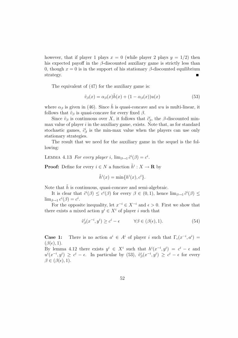
however, that if player 1 plays x = 0 (while player 2 plays y = 1/2) thenhis expected payoff in the β-discounted auxiliary game is strictly less than0, though x = 0 is in the support of his stationary β-discounted equilibriumstrategy.

The equivalent of (47) for the auxiliary game is:

vβ(x) = αβ(x)h(x) + (1− αβ(x))u(x) (53)

where αβ is given in (46). Since h is quasi-concave and wu is multi-linear, itfollows that vβ is quasi-concave for every fixed β.

Since vβ is continuous over X, it follows that ciβ, the β-discounted min-max value of player i in the auxiliary game, exists. Note that, as for standardstochastic games, ciβ is the min-max value when the players can use onlystationary strategies.

The result that we need for the auxiliary game in the sequel is the fol-lowing:

Lemma 4.13 For every player i, limβ→1 ci(β) = ci.

Proof: Define for every i ∈ N a function hi : X → R by

hi(x) = min{hi(x), ci}.

Note that h is continuous, quasi-concave and semi-algebraic.It is clear that ci(β) ≤ ci(β) for every β ∈ (0, 1), hence limβ→1 c

i(β) ≤limβ→1 c

i(β) = ci.For the opposite inequality, let x−i ∈ X−i and ε > 0. First we show that

there exists a mixed action yi ∈ X i of player i such that

viβ(x−i, yi) ≥ ci − ε ∀β ∈ (β(ε), 1). (54)

Case 1: There is no action ai ∈ Ai of player i such that Γε(x−i, ai) =

(β(ε), 1).By lemma 4.12 there exists yi ∈ X i such that hi(x−i, yi) = ci − ε andui(x−i, yi) ≥ ci − ε. In particular by (53), viβ(x−i, yi) ≥ ci − ε for everyβ ∈ (β(ε), 1).

52

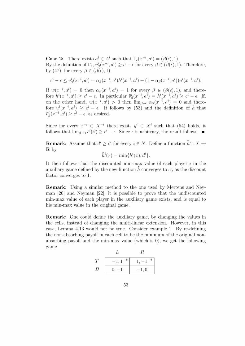
Case 2: There exists ai ∈ Ai such that Γε(x−i, ai) = (β(ε), 1).

By the definition of Γε, viβ(x−i, ai) ≥ ci− ε for every β ∈ (β(ε), 1). Therefore,

by (47), for every β ∈ (β(ε), 1)

ci − ε ≤ viβ(x−i, ai) = αβ(x−i, ai)hi(x−i, ai) + (1− αβ(x−i, ai))ui(x−i, ai).

If w(x−i, ai) = 0 then αβ(x−i, ai) = 1 for every β ∈ (β(ε), 1), and there-fore hi(x−i, ai) ≥ ci − ε. In particular viβ(x−i, ai) = hi(x−i, ai) ≥ ci − ε. If,on the other hand, w(x−i, ai) > 0 then limβ→1 αβ(x−i, ai) = 0 and there-fore ui(x−i, ai) ≥ ci − ε. It follows by (53) and the definition of h thatviβ(x−i, ai) ≥ ci − ε, as desired.

Since for every x−i ∈ X−i there exists yi ∈ X i such that (54) holds, itfollows that limβ→1 c

i(β) ≥ ci − ε. Since ε is arbitrary, the result follows.

Remark: Assume that di ≥ ci for every i ∈ N . Define a function hi : X →R by

hi(x) = min{hi(x), di}.It then follows that the discounted min-max value of each player i in theauxiliary game defined by the new function h converges to ci, as the discountfactor converges to 1.

Remark: Using a similar method to the one used by Mertens and Ney-man [20] and Neyman [22], it is possible to prove that the undiscountedmin-max value of each player in the auxiliary game exists, and is equal tohis min-max value in the original game.

Remark: One could define the auxiliary game, by changing the values inthe cells, instead of changing the multi-linear extension. However, in thiscase, Lemma 4.13 would not be true. Consider example 1. By re-definingthe non-absorbing payoff in each cell to be the minimum of the original non-absorbing payoff and the min-max value (which is 0), we get the followinggame

B

T

L R

0,−1

−1, 1 ∗

−1, 0

1,−1 ∗

53

but the min max value of both players in this game is −13, which is less than

their min max value in the original game.

Since vβ is quasi concave and continuous for every fixed β, and X is compact,it follows that:

Lemma 4.14 For every β ∈ [0, 1) there exists a stationary β-discounted equi-librium in G, i.e. there exists a mixed action combination x ∈ X such thatfor every player i and mixed action yi ∈ X i of player i,

viβ(x) ≥ viβ(x−i, yi).

4.5 Puiseux Stationary Profiles

Definition 4.15 Let I be a finite set. A vector f = (fi)i∈I of Puiseuxfunctions is called a Puiseux probability distribution if fi ≥ 0 for every i ∈ Iand

∑i∈I fi = 1.

Clearly we have:

Lemma 4.16 Let I be a finite set and f a Puiseux probability distributionover I. Then f(1) is a probability distribution over I.

Definition 4.17 A vector of Puiseux functions x = (xiai)i∈N,ai∈Ai is a Puiseuxstationary profile if xiai is a Puiseux function for every i ∈ N and ai ∈ Ai,and x(θ) = (xiai(θ))i∈N,ai∈Ai is a stationary profile for every θ ∈ (0, 1).

The following lemma, which follows from Lemma 2.2, connects the degreeof the probability of absorption to Equation (53).

Lemma 4.18 Let x be a Puiseux stationary profile. deg(w(x)) = 1 if andonly if limθ→1 αθ(x(θ)) ∈ (0, 1). deg(w(x)) < 1 if and only if limθ→1 αθ(x(θ)) =0. deg(w(x)) > 1 if and only if limθ→1 αθ(x(θ)) = 1.

Lemma 4.19 Let x be a Puiseux stationary profile such that limθ→1 αθ(x(θ)) ≤1. Let i ∈ N and ai ∈ Ai such that deg(w(x−i, ai)) < deg(w(x)). Then

limθ→1

vθ(x−i(θ), ai) = lim

θ→1u(x−i(θ), ai).

54

Proof: By the assumption and Lemma 4.18 it follows that deg(w(x−i, ai)) <deg(w(x)) ≤ 1. By a second use of Lemma 4.18 it follows that limθ→1 αθ(x

−i(θ), ai) =0. The result follows by (53).

By (53) and since αβ(x) is continuous at β = 1 for any absorbing mixedaction combination x it follows that:

Corollary 4.20 If w(x(1)) > 0 then

limθ→1

viθ(x(θ)) = ui(x(1)) =

∑ai∈supp(xi(1)) x

iai(1)w(x−i(1), ai)ui(x−i(1), ai)

w(x(1)).

A Puiseux stationary profile x is absorbing if for every θ sufficiently closeto 1, x(θ) is an absorbing stationary profile.

Let x be an absorbing Puiseux stationary profile. For every L ⊆ N andbL ∈ AL we define the Puiseux function xbL by:

xbL = Πi∈Lxibi .

Define the probability distribution µx over B(x(1)) as follows:

µx(bL) = lim

θ→1

xbL(θ)w(x−L(1), bL)∑aT∈B(x(1)) xaT (θ)w(x−T (1), aT )

.

Lemma 4.21 If x is absorbing but x(1) is non-absorbing then

limθ→1

u(x(θ)) =∑

bL∈B(x(1))

µx(bL)u(x−L(1), bL).

Proof: Define

x?−L(θ) = Πi 6∈L

∑ai∈supp(xi(1))

xiai(θ)

.x?−L(θ) is the probability that the realized action of every player i ∈ N \ Lis in supp(xi(1)), given the players N \L play the mixed action combinationx−L(θ).

For every mixed action combination x, let

B0(x) = {bL ∈ AL | L ⊆ N,w(x−L, bL) > 0}.

55

Note that B0(x) ⊇ B(x) for every x ∈ X. By the definition of B, if bL ∈B0(x(1))\B(x(1)) then there exists aT ∈ B(x(1)) such that limθ→1

w(x−L(θ),bL)w(x−T (θ),aT )

=0.

By re-ordering the summation in (6)

u(x(θ)) =∑

bL∈B0(x(1))

xbL(θ)x?−L(θ)w(x−L(1), bL)u(x−L(1), bL)∑aT∈B0(x(1)) xaT (θ)x?−T (θ)w(x−T (1), aT )

.

Since x?−L(1) = 1 for every L ⊂ N , taking the limit as θ → 1, and usingLemma 2.2, yields

limθ→1

u(x(θ)) = limθ→1

∑bL∈B(x(1))

xbL(θ)w(x−L(1), bL)u(x−L(1), bL)∑aT∈B(x(1)) xaT (θ)w(x−T (1), aT )

=∑

bL∈B(x(1))

µx(bL)u(x−L(1), bL)

as desired.

4.6 A Preliminary Result

In this section we prove that there exists a mixed action combination thatsatisfies some “nice” properties. This mixed action combination is used in thefollowing sections to construct perturbed equilibria in three player repeatedgames with absorbing states, and in repeated team games with absorbingstates.

Lemma 4.22 There exist x ∈ X, g ∈ RN , µ ∈ ∆(B(x)) and d : ∪iAi →[0,∞) that satisfy:

a) gi ≥ Ei(x) for every player i ∈ N .

b) At least one of the following holds:

i) w(x) = 0 and h(x) ≥ g.

ii) w(x) > 0, u(x) = g and ui(x−i, ai) = gi for every player i andevery action ai such that w(x−i, ai) > 0.

iii) 1) w(x) = 0.

56

2)∑bL∈B(x) µ(bL)u(x−L, bL) ≥ g.

3) For every player i and every action ai 6∈ supp(xi)

∑bL | i∈L,bi=ai

µ(bL)ui(x−L, bL) =

∑bL | i∈L,bi=ai

µ(bL)

gi.4) If there is strict inequality in (b).iii(2) then

∑i∈L d(bi) = 1 for

every bL ∈ supp(µ).

Note that the second condition in (b).ii follows from the third condition in(b).ii.

Condition (a) states that g is a “good” payoff vector, that is, no playercan profit by deviating and being punished forever from the second stage.Condition (b).i states that x is non-absorbing and the non-absorbing payoffis “good” for all the players. Condition (b).ii states that x is absorbing, theabsorbing payoff is “good” for all the players and the players are indifferentbetween their actions. Condition (b).iii states that x is non-absorbing, theaverage of the payoff in the absorbing neighbors of x is “good”, while thisaverage is equal to the average given any player i plays an action which is notone of his “main” actions. The last condition in (b).iii, which is technical, isessential for later results.Proof: The idea is to consider a sequence of β-discounted stationary equi-libria in the auxiliary game G, that converges to a limit. The values of x,g, µ and d are derived from this sequence, and conditions (a) and (b) areproven using various inequalities that discounted equilibria satisfy, and bytaking the limit β → 1.

Step 1: Definition of a Puiseux stationary profile xConsider the set

E ={

(β, x) ∈ (0, 1)×X | viβ(x) ≥ viβ(x−i, yi) ∀i ∈ N, yi ∈ X i}. (55)

(β, x) ∈ E if and only if x is a β-discounted stationary equilibrium profile inG.

Note that E is semi-algebraic. Indeed, using the recursive formula of thediscounted payoff (44) the condition a = vβ(x) (as vectors) is a system ofequations between polynomials in β, a and x. Therefore E is a projection

57

of a semi-algebraic set, and in particular it is semi-algebraic (Benedetti andRisler [3]).

By Lemma 4.14 the projection of E over the first coordinate is the interval(0, 1). By Theorem 2.5 there exists a Puiseux stationary profile x such that(β, x(β)) ∈ E for every β ∈ (0, 1).

Step 2: Definition of x, g, µ, dDefine x = x(1), g = limβ→1 vβ(x(β)), µ = µx and d(ai) = deg(xiai) for everyai ∈ ∪iAi.

Since viβ(x(β)) is a Puiseux function, g is well defined. By Lemmas 3.6and 4.13

g = limβ→1

vβ(x(β)) ≥ limβ→1

c(β) = c. (56)

Step 3: Assertion (a) holdsFix a player i and an action ai ∈ Ai. If w(x−i(1), ai) = 0 then (a) follows from(56). If, on the other hand, w(x−i(1), ai) > 0 then limβ→1 αβ(x−i(β), ai) = 0.Since xi(β) is a best reply against x−i(β), by (53) and the continuity of u atabsorbing mixed action combinations, it follows that

gi = limβ→1

viβ(x(β)) ≥ limβ→1

viβ(x−i(β), ai) = limβ→1

ui(x−i(β), ai) = ui(x−i(1), ai).

(57)Assertion (a) follows from (56), (57) and the definition of Ei.

Step 4: The distinction between the possibilities in (b)Denote q = limβ→1 αβ(x(β)). Substituting x(β) instead of x in (53) andtaking the limit as β → 1 yields, by the continuity of h and (56),

c ≤ g = limβ→1

vβ(x(β)) = qh(x(1)) + (1− q) limβ→1

u(x(β)). (58)

If q = 1 then h(x(1)) ≥ h(x(1)) = g and w(x(1)) = 0. Therefore (b).iholds.

If w(x(1)) > 0 then q = 0 and the second claim in (b).ii holds. In Step 5we prove that in this case (b).ii holds.

Otherwise q < 1 and w(x(1)) = 0. Therefore x is absorbing. Sinceh(x) ≤ c, it follows by (58) that limβ→1 u(x(β)) ≥ g, and by Lemma 4.21,

58

(b).iii(2) holds. We shall later see that in this case (b).iii holds.

Step 5: If w(x(1)) > 0 then assertion (b).ii holdsLet i ∈ N and ai ∈ supp(xi) such that w(x−i, ai) > 0. Then limβ→1 αβ(x−i(β), ai) =1 and, by the optimality of xi(β),

ui(x−i, ai) = limβ→1

viβ(x−i(β), ai) ≤ limβ→1

viβ(x(β)) = gi. (59)

By corollary 4.20 there is an equality in (59), as desired.

From now on we assume that q < 1 and w(x(1)) = 0.

Step 6: Assertion (b).iii(3) holdsLet i ∈ N be fixed. For every ai ∈ Ai, denote B(µ, ai) = {bL ∈ supp(µ) | i ∈L, bi = ai}.

By Lemma 4.19 it follows that

gi = lim viβ(x(β))

= α limβ→1

viβ(x−i(β), xi(1)) +∑

ai 6∈supp(xi(1))

αai limβ→1

viβ(x−i(β), ai) (60)

where αai = (1 − q)∑bL∈B(µ,ai) µ(bL), and α = 1 − ∑

ai 6∈supp(xi(1)) αai . Bythe optimality of xi(β) it follows that viβ(x−i(β), ai) = gi for every ai 6∈supp(xi(1)).

Step 7: Assertion (b).iii(4)If there is strict inequality in (b).iii(3) then q ∈ (0, 1). Hence, by Lemma4.18, deg(w(x(β))) = 1. Therefore, for every bL ∈ supp(µ),∑

i∈Ld(bi) =

∑i∈L

deg(xibi) = deg(w(x(β))) = 1.

4.7 Three Players Repeated Games with AbsorbingStates

The main result of this section is:

59

Theorem 4.23 Every three-player repeated game with absorbing states hasa perturbed equilibrium payoff.

Recall that Bi(x) is the set of single absorbing neighbors of player i w.r.t.x.

For the proof we need the following lemma:

Lemma 4.24 Let x ∈ X, g ∈ RN , µ ∈ ∆(B(x)) and d : ∪iAi → [0,∞)satisfy condition 4.22(b).iii. At least one of the following hold.

a) There exists a probability distribution ν ∈ ∆(B(x)) such that supp(ν) ⊆supp(µ), for every player i∑

bL∈supp(ν)

ν(bL)ui(x−L, bL) ≥ gi (61)

and for every player i such that Bi(x)∩supp(ν) 6= ∅ there is an equalityin (61).

b) For every player i there exists yi ∈ ∆(Bi(x)) such that supp(yi) ⊂supp(µ) and (u(x−1, y1), u(x−2, y2), u(x−3, y3)) are positive cyclic vec-tors.

The proof of the lemma is postponed to section 4.10.

Proof of Theorem 4.23:Theorem 4.23 is an immediate consequence of Lemmas 4.1, 4.2, 4.4, 4.8, 4.22and 4.24.

Indeed, 4.22(b).i and 4.22(a) imply that the conditions of Lemma 4.2 hold.4.22(b).ii and 4.22(a) imply that the conditions of Lemma 4.1 hold. 4.24(b)and 4.22(a) imply that the conditions of Lemma 4.4 hold, while 4.24(a) and4.22(a) imply that the conditions of Lemma 4.8 hold.

4.8 More Than Three Players

Unfortunately, our approach cannot be generalized for more than three play-ers. In our proof we construct for every ε > 0 and a sequence of discountedequilibria in the auxiliary game that converges to a mixed action combina-tion x, an (x, ε)-perturbed equilibrium profile. Such a construction need not

60

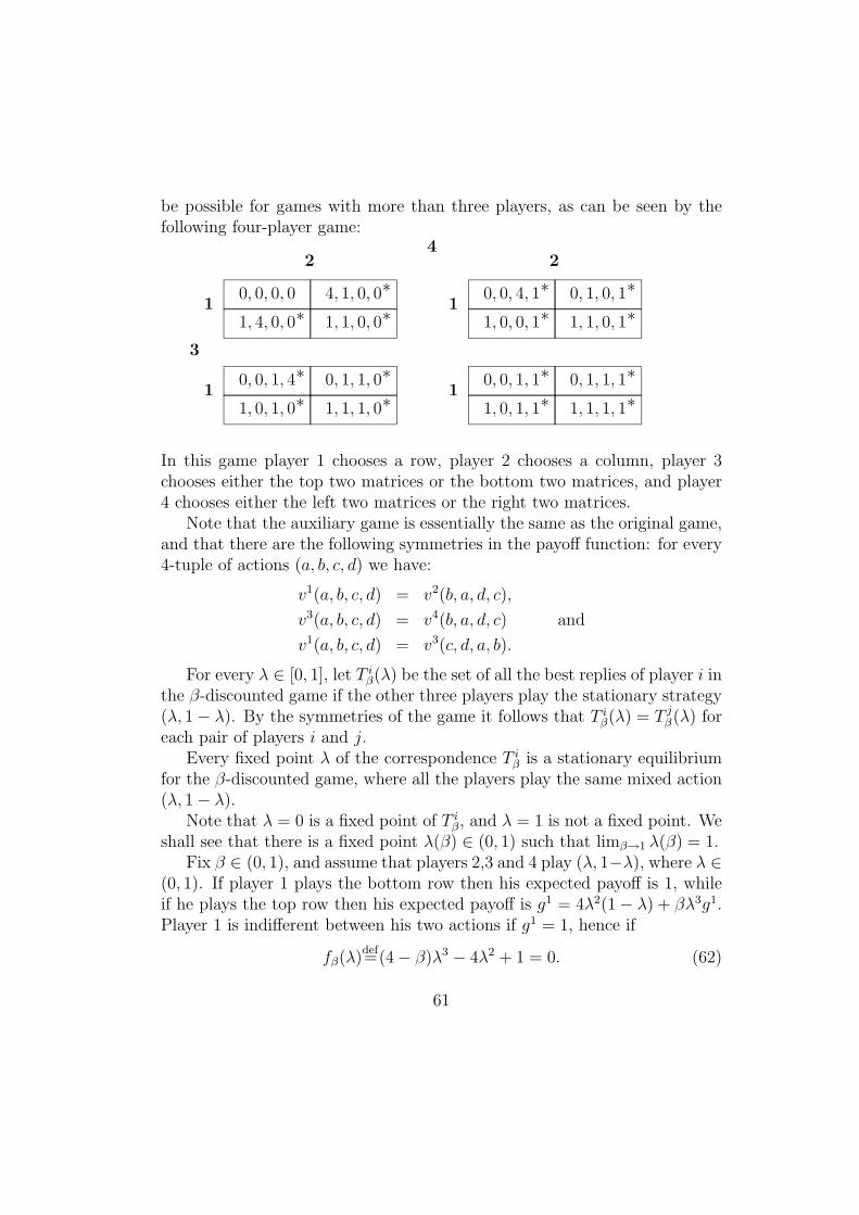
be possible for games with more than three players, as can be seen by thefollowing four-player game:

1

1

1

1

22

3

4

1, 4, 0, 0∗0, 0, 0, 0

1, 1, 0, 0∗4, 1, 0, 0∗

1, 0, 0, 1∗0, 0, 4, 1∗

1, 1, 0, 1∗0, 1, 0, 1∗

1, 0, 1, 0∗0, 0, 1, 4∗

1, 1, 1, 0∗0, 1, 1, 0∗

1, 0, 1, 1∗0, 0, 1, 1∗

1, 1, 1, 1∗0, 1, 1, 1∗

In this game player 1 chooses a row, player 2 chooses a column, player 3chooses either the top two matrices or the bottom two matrices, and player4 chooses either the left two matrices or the right two matrices.

Note that the auxiliary game is essentially the same as the original game,and that there are the following symmetries in the payoff function: for every4-tuple of actions (a, b, c, d) we have:

v1(a, b, c, d) = v2(b, a, d, c),

v3(a, b, c, d) = v4(b, a, d, c) and

v1(a, b, c, d) = v3(c, d, a, b).

For every λ ∈ [0, 1], let T iβ(λ) be the set of all the best replies of player i inthe β-discounted game if the other three players play the stationary strategy(λ, 1− λ). By the symmetries of the game it follows that T iβ(λ) = T jβ(λ) foreach pair of players i and j.

Every fixed point λ of the correspondence T iβ is a stationary equilibriumfor the β-discounted game, where all the players play the same mixed action(λ, 1− λ).

Note that λ = 0 is a fixed point of T iβ, and λ = 1 is not a fixed point. Weshall see that there is a fixed point λ(β) ∈ (0, 1) such that limβ→1 λ(β) = 1.

Fix β ∈ (0, 1), and assume that players 2,3 and 4 play (λ, 1−λ), where λ ∈(0, 1). If player 1 plays the bottom row then his expected payoff is 1, whileif he plays the top row then his expected payoff is g1 = 4λ2(1− λ) + βλ3g1.Player 1 is indifferent between his two actions if g1 = 1, hence if

fβ(λ)def=(4− β)λ3 − 4λ2 + 1 = 0. (62)

61

We claim that (62) has a solution λ(β) ∈ (0, 1) such that limβ→1 λ(β) = 1.Indeed, fβ(1) > 0 for every β ∈ (0, 1), and fβ(β2) < 0 for β sufficiently closeto 1. The claim follows since fβ is continuous and limβ→1 β

2 = 1.However, the conditions of Lemmas 4.1, 4.2, 4.4 and 4.8 are not satisfied

for the non-absorbing cell. Moreover, the conditions of Lemma 4.9 are notsatisfied as well. It is clear that the condition of Lemma 4.1 is not satisfiedfor the non-absorbing cell, and Lemma 4.2 is irrelevant for this cell.

It is easily checked that the only convex combinations z of the four vectorsa1 = (1, 4, 0, 0), a2 = (4, 1, 0, 0), a3 = (0, 0, 1, 4) and a4 = (0, 0, 4, 1) such thatzi = 1 if ai has a positive weight in the combination are the four combinationsthat include only a single vector ai. Therefore the conditions of Lemma 4.4are not satisfied for the non-absorbing cell. Moreover, if the conditions ofLemma 4.9 hold, then at every phase only a single player perturbs (ratherthan a subset of the players).

We now prove that the conditions of Lemma 4.9 do not hold when a singleplayer perturbs in every phase.

Assume to the contrary that g = (g1, g2, g3, g4) ≥ (1, 1, 1, 1) is such anequilibrium payoff, that player 1 is the first player to perturb, γ > 0 isthe overall probability in which player 1 perturbs in the first phase, andf = (f 1, f 2, f 3, f 4) is the expected payoff for the players given player 1 didnot perturb in the first phase.

Clearly g = γ(1, 4, 0, 0)+(1−γ)f , hence f 3, f 4 > 1 and f 1 = 1. Thereforethe only player that can perturb after player 1 has finished his perturbationsis player 2. Let y = (y1, y2, y3, y4) be the expected payoff for the players afterplayer 2 has finished his phase of perturbations. Since f 1 = 1 it follows thaty1 < 1, a contradiction to the individual rationality of the strategy.

It is a little more technical to show that such a construction is not possibleif the future expected payoff of the players should be at least 1 − ε at eachstage (given absorption has not occurred) instead of 1.Remark: Recently Solan and Vieille [29] found an example of a four-playerrepeated game with absorbing states that has no perturbed equilibrium pay-off.

4.9 Repeated Team Games with Absorbing States

Definition 4.25 An n+m-player repeated game with absorbing states is arepeated team game with absorbing states if hi = hj and ui = uj whenever

62

1 ≤ i, j ≤ n or n+ 1 ≤ i, j ≤ n+m.

Let G be a repeated team game with absorbing states. We denote by Nand M the two sets of players in each team, hence n = |N | and m = |M |.

Let

di =

{maxj∈N c

j i ∈ Nmaxj∈M cj i ∈M

It is clear that for any equilibrium payoff g = (gi)i∈N∪M , gi = gj wheneveri, j ∈ N or i, j ∈ M . Moreover, gi ≥ ci for every i ∈ N ∪M , and thereforegi ≥ di for every i ∈ N ∪M .

The main result of this section is:

Theorem 4.26 Every repeated team game with absorbing states has a per-turbed equilibrium payoff.

Proof: For every i ∈ N , define hi : X → R by

hi(x) = min{hi(x), di}.

By the remark following the proof of Lemma 4.13, it follows that Lemma4.22 holds for G. Let (x, g, µ, d) satisfy the conclusion of Lemma 4.22. Weprove that x is a base of a perturbed equilibrium.

Note that since hi(x) = hj(x) whenever 1 ≤ i, j ≤ n or n + 1 ≤ i, j ≤n+m, it follows that gi = gj whenever 1 ≤ i, j ≤ n or n+ 1 ≤ i, j ≤ n+m.

We have 4 cases:

1) x is absorbing.

2) x is non-absorbing and h(x) ≥ g.

3) x is non-absorbing, and there exists a single absorbing neighbor bi0 ∈B(x) such that u(x−i0 , bi0) ≥ g.

4) Non of the first three cases hold.

In case 1, condition 4.22(b).ii holds, and, together with condition 4.22(a)implies that the conditions of Lemma 4.2 hold.

In case 2, condition 4.22(b).i holds, and, together with condition 4.22(a)implies that the conditions of Lemma 4.1 hold.

63

In case 3, the assumption and condition 4.22(a) imply that the conditionsof Lemma 4.4 hold w.r.t. the probability distribution that gives probability1 to bi0 .

Assume now that neither case 1 nor cases 2 or 3 hold. We prove that inthis case the conditions of Lemma 4.4 hold.

Since cases 1 and 2 do not hold it follows that condition 4.22(b).iii holds.Let bi0 ∈ supp(µ) be any single absorbing neighbor. By condition 4.22(b).iii(3),

ui0(x−i0 , bi0) = gi0 , and since the game is a team game, ui(x−i0 , bi0) = gi forevery player i of the same team as i0. Since case 3 does not hold, there existsa player i of the opposing team such that ui(x−i0 , bi0) < gi, and thereforeui(x−i0 , bi0) < gi for every player i in the opposing team. In particular, if∩iBi(x) ∩ supp(µ) 6= ∅ then∑

∩iBi(x)∩supp(µ)

µ(bL)ui(x−L, bL) ≤ gi for every i ∈ N ∪M (63)

and ∑∩iBi(x)∩supp(µ)

µ(bL)u(x−L, bL) 6= g. (64)

Let C = {bL ∈ supp(µ) | |L| ≥ 2}. By condition 4.22(b).iii(2), (63) and(64), it follows that C 6= ∅ and

∑bL∈C µ(bL) > 0.

Let ν be the induced probability distribution of µ over C. By condition4.22(b).iii(2), (63) and (64) we have:∑

bL∈Cν(bL)ui(x−L, bL) ≥ gi for every i ∈ N ∪M. (65)

Since |L| ≥ 2 for every bL ∈ supp(ν), condition 4.22(a) and (65) imply thatthe conditions of Lemma 4.4 hold w.r.t. C and ν.

4.10 Proof of Lemma 4.24

In this section we prove Lemma 4.24. The proof is technical, and its generalidea is as follows. Let r be the number of players that have single absorbingneighbors of x with positive weight according to µ. We divide the proof into4 cases, according to the value of r. If r = 0 then 4.24(a) holds trivially. Ifr is positive and 4.24(b) does not hold, we need to construct the probabilitydistribution ν. The method is to different when r = 1 and when r > 1.

64

When r = 2, by changing the weights of the single absorbing neighbors ofthe various players in a certain way, we can obtain a probability distributionν over B(x) that satisfies 4.24(a).

When r = 3, there can be two sub-cases. Either 4.24(b) holds, or, aswhen r = 2, by changing the weights of the single absorbing neighbors of thevarious players in a certain way, we can obtain a probability distribution νover B(x) that satisfies 4.24(a).

When r = 1 one constructs the desired probability distribution ν in adifferent manner, by changing the weights of all the absorbing neighbors ofx.

The rest of the section is arranged as follows. We first deal with the caser = 1. Then we prove two lemmas, that show how one can change the weightsof single absorbing neighbors in order to get a new probability distributionfor which there is an equality in (61) for one more player. These two lemmasare then applied to prove the case r = 2, and finally, the case r = 3.

For the rest of the section we fix x ∈ X and g ∈ R3 for which there existµ ∈ ∆(B(x)) and d : ∪Ai → [0,∞) such that 4.22(b).iii holds for (x, g, µ, d).

For every vector 0 < λ ∈ R3+, the normalization of λ, denoted by λ, is

defined by:

λi =λi∑3j=1 λj

.

Let z ∈ R3. The signed form of z is the vector of the signs of the valuesof (z1− g1, z2− g2, z3− g3). If zi− gi = 0 then the ith coordinate of the signvector is 0.

LetMD = {(µ, d) | µ ∈ B(x), d : ∪iAi → [0,∞) and 4.22(b).iii holds for(x, g, µ, d)}. We denote byM the projection ofMD over the first coordinate.By the assumption, MD 6= ∅. From now on we fix a pair (µ, d) ∈MD suchthat µ has a minimal support among the elements in M.

Let R = {i ∈ N | Bi(x) ∩ supp(µ) 6= ∅}. R is the set of players thathave single absorbing neighbors in supp(µ). We denote r = |R|. The proofof Lemma 4.24 is divided into several cases, according to the value of r.

If r = 0 or there is an equality in 4.22(b).iii(2) then 4.24(a) holds trivially.From now on we assume that

∑i∈L d(bi) = 1 for every bL ∈ supp(µ). In

particular, d(ai) = 1 for every player i ∈ N and single absorbing neighborai ∈ Bi(x) ∩ supp(µ).

65

For every i ∈ R we define yi ∈ X i as follows:

yiai =

0 d(ai) 6= 1µ(ai)∑

bi∈Bi(x)µ(bi)

d(ai) = 1

Note that for every ai ∈ supp(yi), w(x−i, ai) > 0 and, by 4.22(b).iii(3),ui(x−i, ai) = gi.

If 1 ∈ R and the signed form of u(x−1, y1) is (0,+,+) then y1, viewed asa probability distribution over B(x), satisfies 4.24(a). By the minimality ofµ, it follows that u(x−1, y1) does not have the signed form (0,−,−). Hencewe assume that if 1 ∈ R then u(x−1, y1) has the signed form (0,+,−) or(0,−,+). Symmetric assumptions are made for players 2 and 3.

For every function ρ : B(x) → [0,∞) and player j ∈ N we define

supp(ρ)def= {bL ∈ B(x) | ρ(bL) 6= 0} and

〈ρ, uj〉 =∑

bL∈B(x)

ρ(bL)uj(x−L, bL).

Recall that B(ρ, ai) = {bL ∈ B(x)∩supp(ρ) | i ∈ L, bi = ai} for every ai ∈ Ai.Denote

〈ρ, uj, ai〉 =∑

bL∈B(ρ,ai)

ρ(bL)uj(x−L, bL).

Note that for every i ∈ N , 〈ρ, uj〉 =∑ai∈Ai〈ρ, uj, ai〉.

Lemma 4.27 If r = 1 then assertion 4.24(a) holds.

Proof: Assume that R = {1}. Clearly if there exists ν ∈ ∆(B(x)) such thatsupp(ν) ⊂ supp(µ), supp(ν)∩Bi(x) = ∅ and 〈ν, uj〉 ≥ gj for j = 2, 3 then thelemma holds. Indeed, if such ν exists then by the minimality of µ it followsthat 〈ν, u1〉 < g1, and therefore there exists a convex combination of µ andν that satisfies 4.24(a).

By 4.22(b).iii(3),

〈µ, u2, a2〉 = g2∑

bL∈B(µ,a2)

µ(bL) ∀a2 6∈ supp(x2). (66)

By the above discussion it follows that for every a2 6∈ supp(x2) with B(µ, a2) 6=∅

〈µ, u3, a2〉 < g3∑

bL∈B(µ,a2)

µ(bL). (67)

66

Similarly,

〈µ, u3, a3〉 = g3∑

bL∈B(µ,a3)

µ(bL) ∀a3 6∈ supp(x3) (68)

and if B(µ, a3) 6= ∅ we have

〈µ, u2, a3〉 < g2∑

bL∈B(µ,a3)

µ(bL). (69)

Define

ν(bL) =

{d(b1)µ(bL) bL ∈ B(x) and 1 ∈ L0 Otherwise.

Since supp(µ)∩B1(x) 6= ∅ it follows that∑bL∈B(x) ν(bL) > 0. By 4.22(b).iii(2)

and 4.22(b).iii(4)

gi ≤∑

bL∈B(x)

µ(bL)ui(x−L, bL)

=∑

bL∈B(x)

µ(bL)ui(x−L, bL)∑j∈L

d(bj)

=∑a1∈A1

〈ν, ui〉+∑a2∈A2

d(a2)〈µ, ui, a2〉+∑a3∈A3

d(a3)〈µ, ui, a3〉

=∑a1∈A1

〈ν, ui〉+∑

a2 6∈supp(x2)

d(a2)〈µ, ui, a2〉+∑

a3 6∈supp(x3)

d(a3)〈µ, ui, a3〉

where the last equality holds since d(ai) = 0 whenever ai ∈ supp(xi). By(66), (67), (68) and (69) it follows that 〈ν, ui〉 ≥ gi for i = 2, 3, where ν isthe normalization of ν.

Moreover,〈ν, u1〉 =

∑a1∈A1

d(a1)〈µ, u1, a1〉.

By condition 4.22(b).iii(3), 〈µ, u1, a1〉 = g1 whenever d(a1) > 0. Therefore〈ν, u1〉 = g1, and ν is the desired probability distribution.

The following two lemmas assert that if 2 ∈ R then we can assume w.l.o.g.that 〈µ, u3〉 = g3.

67

Lemma 4.28 If 2 ∈ R and u(x−2, y2) has the signed form (−, 0,+) then thereexists ν ∈M such that supp(µ) = supp(ν) and 〈ν, u3〉 = g3. Furthermore, if〈µ, u2〉 = g2 then 〈ν, u2〉 = g2.

Proof: For every t ∈ [0, 1] define:

νt(bL) =

{tµ(bL) bL ∈ supp(B2(x))µ(bL) Otherwise

i.e. as t decreases we decrease the weight of the single absorbing neighborsof player 2. Clearly ν1 = µ, for every t ∈ [0, 1] conditions 4.22(b).iii(3) and4.22(b).iii(4) hold w.r.t. νt and 4.22(b).iii(2) holds w.r.t. νt for i = 1, 2.For every t such that 〈νt, u3〉 ≥ g3 condition 4.22(b).iii(2) holds w.r.t. νtfor i = 3 too. Since µ has a minimal support, there is t0 ∈ (0, 1] such that〈νt0 , u3〉 = g3. For every t, 〈µ, u2〉 = 〈νt, u2〉 and therefore νt0 is the desiredvector.

Lemma 4.29 If 2 ∈ R and u(x−2, y2) has the signed form (+, 0,−) Thenthere exists a vector ν ∈ M such that supp(µ) = supp(ν) and 〈ν, u3〉 = g3.Furthermore, if 〈µ, u2〉 = g2 then 〈ν, u2〉 = g2.

Proof: For every t ∈ [1,∞) define:

νt(bL) =

{tµ(bL) bL ∈ supp(B2(x))µ(bL) Otherwise

i.e. as t increases we increase the weight of the single absorbing neighborsof player 2. Clearly ν1 = µ, for every t ∈ [1,∞) conditions 4.22(b).iii(3)and 4.22(b).iii(4) hold w.r.t. νt and 4.22(b).iii(2) holds w.r.t. νt for i = 1, 2.For every t such that 〈νt, u3〉 ≥ g3 condition 4.22(b).iii(2) holds w.r.t. νt fori = 3 too. Since u(x−2, y2) has the signed form (+, 0,−), for t sufficientlylarge 〈νt, u3〉 < g3. Therefore there is t0 ∈ [1,∞) such that 〈νt0 , u3〉 = g3.For every t, 〈µ, u2〉 = 〈νt, u2〉 and therefore νt0 is the desired vector.

Lemma 4.30 If r = 2 then there exists ν ∈M such that 4.24(a) holds.

68

Proof: Assume w.l.o.g. that R = {2, 3}. By either Lemma 4.28 or Lemma4.29, according to the signed form of u(x−3, y3), we can assume that 〈µ, u2〉 =g2. By a second use of either Lemma 4.28 or Lemma 4.29, according to thesigned form of u(x−2, y2), we can assume w.l.o.g. that 〈µ, ui〉 = gi for i = 2, 3,as desired.

Lemma 4.31 If r = 3 and (u(x−1, y1), u(x−2, y2), u(x−3, y3)) are not positivecyclic vectors, then there exists ν ∈M such that 4.24(a) holds.

Proof: Up to symmetries we can assume that u(x−1, y1) has the signed form(0,+,−) and u(x−2, y2) has the signed form (−, 0,+).

Using Lemma 4.28 twice, once with u(x−1, y1) and then with u(x−2, y2),we can assume that 〈µ, ui〉 = gi for i = 2, 3. If 〈µ, u1〉 = g1 we are done.Hence assume 〈µ, u1〉 > g1.

Case 1: 〈µ, u3〉 has the signed form (+,−, 0).Let α, β > 0 solve the equations

u3(x−1, y1) + αu3(x−2, y2) = (1 + α)g3

u2(x−1, y1) + βu2(x−3, y3) = (1 + β)g2. (70)

Since (u(x−1, y1), u(x−2, y2), u(x−3, y3)) are not positive cyclic it follows that

αu1(x−2, y2) + βu1(x−3, y3) ≤ (α + β)g1. (71)

Let ν : B(x)→ [0,∞) be defined as follows:

ν(bL) =

µ(bL) bL ∈ B1(x) ∩ supp(µ)αµ(bL) bL ∈ B2(x) ∩ supp(µ)βµ(bL) bL ∈ B3(x) ∩ supp(µ)0 Othewise.

By (70), 〈ν, ui〉 = gi for i = 2, 3. If there is an equality in (71) then〈ν, u1〉 = g1, and ν is the desired vector. Otherwise 〈ν, u1〉 < g1. Let ρbe the convex combination of µ and ν that satisfies 〈ρ, u〉 = g. Then ρ sat-isfies 4.24(a), as desired.

Case 2: u(x−3, y3) has the signed form (−,+, 0).

69

Let α, β > 0 solve the equations

u3(x−1, y1) + αu3(x−2, y2) = g3

u2(x−1, y1) = βu2(x−3, y3). (72)

For every t ≥ 0 define

νt(bL) =

µ(bL) + t bL ∈ B1(x) ∩ supp(µ)µ(bL) + tα bL ∈ B2(x) ∩ supp(µ)µ(bL) + tβ bL ∈ B3(x) ∩ supp(µ)µ(bL) Otherwise.

Note that∑bL∈B(x) νt(b

L) = 1 + tq, where

q =∑

bL∈B1(x)

µ(bL) + α∑

bL∈B2(x)

µ(bL) + β∑

bL∈B3(x)

µ(bL).

For every t ≥ 0 we have by (72):

〈νt, u3〉 = 〈µ, u3〉+ t(u3(x−1, y1) + αu3(x−2, y2)) + tβg3∑

bL∈B3(x)

µ(bL) =

g3(1 + tq)

〈νt, u2〉 = 〈µ, u2〉+ t(u2(x−1, y1) + βu2(x−3, y3)) + tαg2∑

bL∈B2(x)

µ(bL) =

g2(1 + tq)

〈νt, u1〉 = 〈µ, u1〉+ t(αu1(x−2, y2) + βu1(x−3, y3)) + t∑

bL∈B1(x)

µ(bL).

Clearly 〈ν0, u1〉 = 〈µ, u1〉 > g1. Since u1(x−i, yi) < gi for i = 1, 2, there

exists t0 > 0 such that 〈νt0 , u1〉 = g1. Then νt0 is the desired probabilitydistribution.

70

5 Recursive Games with the Absorbing Prop-

erty

In this section we prove that every two-player stochastic game with two non-absorbing states has an equilibrium payoff. We use Vieille’s reduction [33, 34]that claims that it is sufficient to prove the existence for positive recursivestochastic games with the absorbing property.

We begin by an equivalent formulation of recursive games (section 5.1),provide an example of such a game, and show some of the equilibrium payoffsand the corresponding ε-equilibrium profiles (section 5.2). We then introducetwo sufficient conditions for existence of an equilibrium payoff in recursivegames (section 5.3), and after proving some preliminary results (section 5.4),we introduce the approximating games and derive several results on thesegames (section 5.5). We end by proving the main result (section 5.6) andby explaining why our approach cannot be generalized for games with morethan two non-absorbing states (section 5.7).

5.1 An Equivalent Formulation

Let G = (N,S, (Ai)i∈N , h, w) be a two-player stochastic game, that is, |N | =2. For simplicity we denote by A and B the sets of actions available for thetwo players, and by X and Y the spaces of stationary strategies. Strategiesof the two players are denoted by σ and τ .

Let T ⊆ S be the set of all the absorbing states.

Definition 5.1 The game is positive if h2(s, a, b) > 0 for every absorbingstate s ∈ T and every pair of actions (a, b) ∈ A×B. It is recursive ifhi(s, a, b) = 0 for every non-absorbing state s 6∈ T , every pair of actions(a, b) ∈ A×B and every player i = 1, 2. It satisfies the absorbing propertyif for every fully mixed stationary strategy y of player 2, every strategy σ ofplayer 1 and every initial state s ∈ S,

Prs,σ,y (∃t ∈ N s.t. st ∈ T ) = 1

where st is the state of the game at stage t.

In [34] Vieille proves that in order to prove existence of an equilibriumpayoff in every two-player stochastic game, it is sufficient to prove the exis-

71

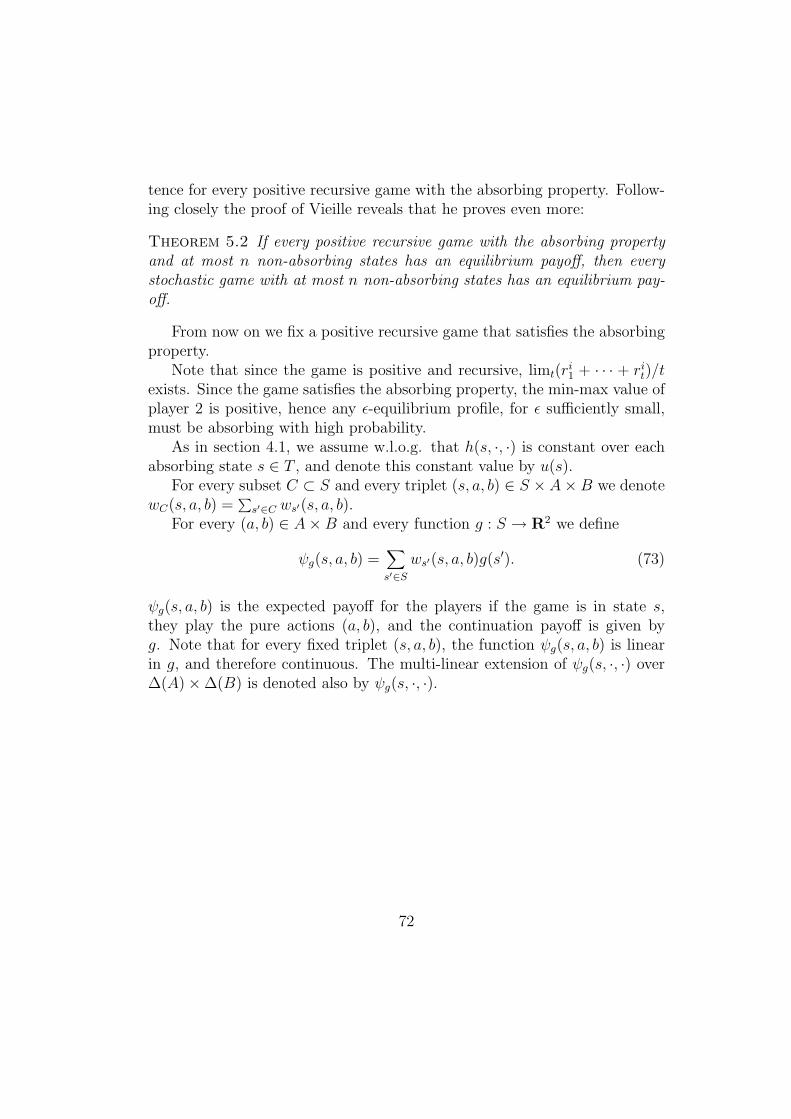
tence for every positive recursive game with the absorbing property. Follow-ing closely the proof of Vieille reveals that he proves even more:

Theorem 5.2 If every positive recursive game with the absorbing propertyand at most n non-absorbing states has an equilibrium payoff, then everystochastic game with at most n non-absorbing states has an equilibrium pay-off.

From now on we fix a positive recursive game that satisfies the absorbingproperty.

Note that since the game is positive and recursive, limt(ri1 + · · · + rit)/t

exists. Since the game satisfies the absorbing property, the min-max value ofplayer 2 is positive, hence any ε-equilibrium profile, for ε sufficiently small,must be absorbing with high probability.

As in section 4.1, we assume w.l.o.g. that h(s, ·, ·) is constant over eachabsorbing state s ∈ T , and denote this constant value by u(s).

For every subset C ⊂ S and every triplet (s, a, b) ∈ S × A×B we denotewC(s, a, b) =

∑s′∈C ws′(s, a, b).

For every (a, b) ∈ A×B and every function g : S → R2 we define

ψg(s, a, b) =∑s′∈S

ws′(s, a, b)g(s′). (73)

ψg(s, a, b) is the expected payoff for the players if the game is in state s,they play the pure actions (a, b), and the continuation payoff is given byg. Note that for every fixed triplet (s, a, b), the function ψg(s, a, b) is linearin g, and therefore continuous. The multi-linear extension of ψg(s, ·, ·) over∆(A)×∆(B) is denoted also by ψg(s, ·, ·).

72

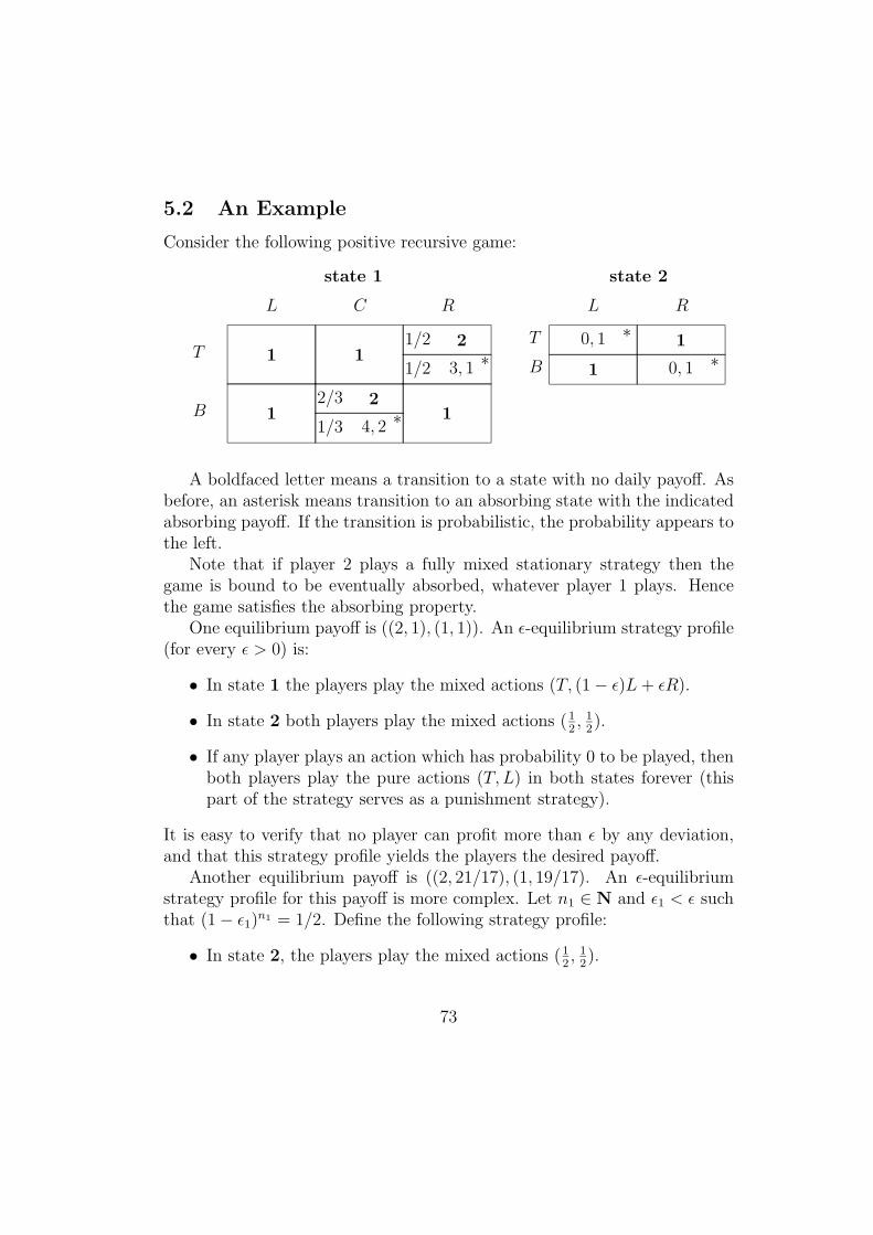
5.2 An Example

Consider the following positive recursive game:

B

T

L C R

B

T

L R

state 1 state 2

1

1

4, 21/3

22/3∗

1

1

3, 11/2

21/2∗

1

0, 1 ∗

0, 1 ∗1

A boldfaced letter means a transition to a state with no daily payoff. Asbefore, an asterisk means transition to an absorbing state with the indicatedabsorbing payoff. If the transition is probabilistic, the probability appears tothe left.

Note that if player 2 plays a fully mixed stationary strategy then thegame is bound to be eventually absorbed, whatever player 1 plays. Hencethe game satisfies the absorbing property.

One equilibrium payoff is ((2, 1), (1, 1)). An ε-equilibrium strategy profile(for every ε > 0) is:

• In state 1 the players play the mixed actions (T, (1− ε)L+ εR).

• In state 2 both players play the mixed actions (12, 1

2).

• If any player plays an action which has probability 0 to be played, thenboth players play the pure actions (T, L) in both states forever (thispart of the strategy serves as a punishment strategy).

It is easy to verify that no player can profit more than ε by any deviation,and that this strategy profile yields the players the desired payoff.

Another equilibrium payoff is ((2, 21/17), (1, 19/17). An ε-equilibriumstrategy profile for this payoff is more complex. Let n1 ∈ N and ε1 < ε suchthat (1− ε1)n1 = 1/2. Define the following strategy profile:

• In state 2, the players play the mixed actions (12, 1

2).

73

• Assume the game moves to state 1 at stage t0. The players play asfollows:

– The players play the mixed actions ((1−ε1)T+ε1B, (1−ε1)L+ε1C).The players play these mixed actions until player 2 played theaction C for n1 times since stage t0, or until both players played(B,C) at the same stage (and the game leaves state 1).

– If player 2 played the action C for n1 times since stage t0, thenthe players play the mixed actions (T, (1− ε)L+ εR) until player2 plays the action R (and the game leaves state 1).

– If any player plays an action which has probability 0 to be played,the players play the pure actions (T, L) in both states forever.

Note that if the players follow this profile, then the probability that thegame leaves state 1 through (B,C) is 1/2, as is the probability that thegame leaves state 1 through (T,R). In particular the game is bound to beeventually absorbed.

Assume that the players follow the above profile, and let g = (gis) be thepayoff that the players receive. Clearly no player can deviate and gain instate 2, and gi2 = 1

2(0, 1) + 1

2gi1 for i = 1, 2.

Moreover, we have:

g1 =1

2

(1

3(4, 2) +

2

3g2

)+

1

2

(1

2(3, 1) +

1

2g2

)and therefore g1 = (2, 21/17).

We shall now verify that no player can profit more than ε by deviatingin state 1. Indeed, if player 2 deviates in state 1, then his expected payoff isbounded by 1 (since after the punishment begins, his expected payoff is atmost 1). Given the players follow the above profile, the initial state is 1, andthe first time the game leaves state 1 is through (B,C), the expected payofffor player 1 is 2

3+ 1

3· 4 = 2, where if the first time the game leaves state 1

is through (T,R), the expected payoff of player 1 is 12

+ 12· 3 = 2 as well.

Hence player 1 cannot profit by any deviation whenever the game is in state1. Therefore this strategy profile is an ε-equilibrium, as desired.

74

5.3 Sufficient Conditions for Existence of an Equilib-rium Payoff

In this section we give two sets of sufficient conditions for existence of anequilibrium payoff in positive recursive games with the absorbing property.

Definition 5.3 Let (x, y) be a stationary profile. A set C ⊆ S is stableunder (x, y) if wC(s, x, y) = 1 for every s ∈ C.

In the example presented in section 5.2, {s1} is stable, for example, under((T, L), (·, ·)), and {s1, s2} is stable under ((T, L), (T,R)) and ((T, L), (B,L)),as well as under ((1

2T + 1

2B,L), (T,R)).

Definition 5.4 Let (x, y) be a stationary profile and ε > 0. An ε-perturbationis a stationary profile (x′, y′) such that ‖ x − x′ ‖< ε, ‖ y − y′ ‖< ε,supp(x′s) ⊇ supp(xs) and supp(y′s) ⊇ supp(ys).

Note that if C is stable under an ε-perturbation (x′, y′) of (x, y), then inparticular C is stable under (x, y).

Definition 5.5 Let (x, y) be a stationary profile. A set C ⊆ S is commu-nicating w.r.t. (x, y) if for every s ∈ C there exists an ε-perturbation (x′, y′)of (x, y) such that C is stable under (x′, y′) and

Prs′,x′,y′(∃t ∈ N s.t. st = s) = 1 ∀s′ ∈ C.

In the example presented in section 5.2, {s1} is communicating w.r.t. ((T, L), (·, ·)),((T,C), (·, ·)), ((B,L), (·, ·)) and ((B,R), (·, ·)).

A set C is communicating if the players, by changing their stationarystrategies a little, can reach from any state in C any other state in C, with-out leaving the set. Note that if there exists an ε-perturbation (x′, y′) thatsatisfies definition 5.5, then for every ε′ > 0 there exists an ε′-perturbationthat satisfies it.

Clearly every absorbing state defines a communicating set, that includesonly this state. We denote by C(x, y) the collection of all communicating setsw.r.t. (x, y). Define for every communicating set C ∈ C(x, y) and s ∈ C

A1s(C, y) = {a ∈ A | wC(s, a, ys) < 1} and (74)

B1s (C, x) = {b ∈ B | wC(s, xs, b) < 1}.

75

In the example presented in section 5.2, denote by (x?, y?) = ((T, L), (T, L)).Then A1

s1(s1, y

?) = ∅ and B1s1

(s1, x?) = {L}.

Definition 5.6 Let (x, y) be a stationary profile and C ∈ C(x, y). Everytriplet (s, x′s, ys), where s ∈ C and x′s ∈ ∆(A1

s(C, y)) is an exit of player 1from C. Every triplet (s, xs, y

′s), where s ∈ C and y′s ∈ ∆(B1

s (C, x)) is anexit of player 2 from C. Every triplet (s, x′s, y

′s) ∈ C × ∆(A)×∆(B) such

that supp(xs) ∩ supp(x′s) = supp(ys) ∩ supp(y′s) = ∅ is a joint exit from C ifwC(s, x′s, y

′s) < 1 while wC(s, xs, y

′s) = wC(s, x′s, ys) = 1.

In the example presented in section 5.2, {s1} ∈ C(x?, y?), (s1, T, R) is an exitof player 2 from {s1} and (s1, B, C) is a joint exit from {s1}.

A joint exit (s, x′s, y′s) is pure if |supp(x′s)| = |supp(y′s)| = 1. An exit

(s, x′s, ys) of player 1 is pure if |supp(x′s)| = 1. Pure exits of player 2 aredefined analogously.

We denote by E1C(x, y), E2

C(x, y) and E1,2C (x, y) the sets of exits of player

1, player 2 and the joint exits from C respectively. Let

EC(x, y) = E1C(x, y) ∪ E2

C(x, y) ∪ E1,2C (x, y)

be the set of all exits from C and E0C(x, y) be the set of all pure exits from

C. We denote by s(e), x(e) and y(e) the three coordinates of any exit e.For any exit e, we define the support of e by:

supp(e) = supp(x(e))× supp(y(e)).

Note that any two exits e1, e2 ∈ E0C(x, y) have disjoint supports.

For simplicity we write s ∈ C(x, y) whenever {s} ∈ C(x, y). In this casewe write Es(x, y) instead of E{s}(x, y).

Let R = S \T be the set of non-absorbing states, and recall that c = (cis)is the min-max value of the players.

Lemma 5.7 Let (x, y) be a stationary profile such that R ∈ C(x, y). Assumethat there exists an exit e ∈ ER(x, y) and g = (gs)s∈S ∈ R2|S| such that

1) gs is constant over R, gs = u(s) for every absorbing state s ∈ T , andgs = ψg(e) for every non-absorbing state s ∈ R.

2) g1s ≥ ψ1

c (s, a, ys) for every s ∈ R and a ∈ A.

76

3) g2s ≥ ψ2

c (s, xs, b) for every s ∈ R and b ∈ B.

4) If e ∈ E1R(x, y) then g1 = ψ1

g(s(e), a, ys(e)) for every a ∈ supp(x(e)).

5) If e ∈ E2R(x, y) then g2 = ψ2

g(s(e), xs(e), b) for every b ∈ supp(y(e)).

Then g is an equilibrium payoff.

Note the similarity between the conditions of Lemma 5.7 and Lemma 4.4.Proof: Fix ε > 0. As in section 4.2, the ε-equilibrium profile that weconstruct (both here and in the proof of the next sufficient condition) isdefined by a profile σ that satisfies ‖ σ(h0) − (x, y) ‖≤ ε for every finitehistory h0 ∈ H0, supplemented with a statistical test.

Let δ ∈ (0, ε) be sufficiently small, and (x′, y′) be an ε-perturbation of(x, y) such that

Prs′,x′,y′(∃t ∈ N s.t. st = s(e)) = 1 ∀s′ ∈ R.

Since R ∈ C(x, y), such a perturbation exists.Define a profile σ as follows:

• Whenever the game is in state s(e) the players play the mixed actioncombination ((1− δ)xs(e) + δx(e), (1− δ)ys(e) + δy(e)).

• Whenever the game is in a state s 6= s(e) the players play the mixedaction combination (x′s, y

′s).

If the players follow σ then the game is bound to exit R through e, andto be absorbed. Hence, by condition 1, the expected payoff for the players isgs, where s is the initial state.

In order to prevent the players from deviating, we choose t1 ∈ N suf-ficiently large and define the following statistical test. At each stage t theplayers check the following.

1) Both players check whether the realized action of their opponent iscompatible with σ.

2) If e ∈ E2R(x, y) and the game visited the state s(e) at least t1 times, then

player 2 checks whether the distribution of the realized actions of player1, whenever the game is in s(e), is δ-close to xs(e). If e ∈ E1

R(x, y), thenplayer 1 employs a symmetric test.

77

3) If e ∈ E1,2R (x, y) and the game visited the state s(e) at least t1 times,

then player 1 checks whether the realized actions of player 2, wheneverthe game is in the state s(e), restricted to supp(y(e)), is δ-close to y(e).Player 2 employs a symmetric test.

If a player fails one of these tests, this player is punished by his opponentwith an ε-min-max strategy forever.

Since player 1 may profit by causing the game never to be absorbed, weadd one more test. Let t2 ∈ N be sufficiently large such that if no deviationis detected then absorption occurs before stage t2 with probability greaterthan 1− ε. We add the following test to σ:

4) At stage t2 both players switch to an ε-min-max strategy.

The constants δ and t1 are chosen as in the proof of Lemma 4.4, in sucha way that the probability of false detection of deviation is bounded by ε,and no player can profit more than 2εR by any kind of deviation. Thus g isan (x, y)-perturbed equilibrium payoff.

Lemma 5.8 Let (x, y) be a stationary profile, and g = (gs)s∈S ∈ R2|S|. As-sume that the following conditions hold:

1) gs = u(s) for every absorbing state s ∈ T .

2) g1s ≥ ψ1

c (s, a, ys) for every s ∈ R and a ∈ A.

3) g2s ≥ ψ2

c (s, xs, b) for every s ∈ R and b ∈ B.

4) For every s ∈ R \ C(x, y) the following hold:

a) g1s = ψ1

g(s, a, ys) for every a ∈ supp(xs).

b) g2s = ψ2

g(s, xs, b) for every b ∈ supp(ys).

5) For every s ∈ R∩C(x, y) there exist two exits e1 = e1(s) and e2 = e2(s)in Es(x, y) and α = α(s) ∈ [0, 1] that satisfy the following:

a) ψ1g(ej) = g1

s for each j = 1, 2, and g2s = αψ2

g(e1) + (1− α)ψ2g(e2).

b) If ej ∈ E1s (x, y) then g1

s = ψ1g(s, a, ys) for every a ∈ supp(x(ej)).

78

c) If ej ∈ E2s (x, y) then ψ2

g(s, xs, b1) = ψ2g(s, xs, b2) ≥ ψ2

c (s, xs, b3) forevery b1, b2 ∈ supp(y(ej)) and b3 ∈ B.

d) At most one of e1 and e2 is an exit of player 2.

6) The Markov chain over S whose transition law is induced by (xs, ys) forevery s 6∈ C(x, y) and by α(s)e1(s)+(1−α(s))e2(s) for every s ∈ C(x, y)is absorbing (i.e. for every initial state, an absorbing state is reachedwith probability 1).

Then g is an equilibrium payoff.

Proof: Let ε > 0 be given. Let t1, t2 ∈ N be sufficiently large. Thesetwo constants will be used in the statistical tests, but the profile σ that weconstruct depend on them as well.

Define a profile σ as follows:

• Whenever the game is in a state s ∈ R\C(x, y) the players play (xs, ys).

In order to define σ at states s ∈ R ∩ C(x, y), we recall that to each suchstate there exist two exits e1 = e1(s) and e2 = e2(s), and α = α(s) thatsatisfy condition 5. If one of these exits is an exit of player 2, we assume it ise2. Otherwise, we assume that ψ2

g(e1) ≤ ψ2g(e2). We fix δ = δ(s) ∈ (0, 1/t1)

and n = n(s) ∈ N such that (1 − δ)n = 1 − α if e1 is a unilateral exit and(1− δ2)n = 1− α if e1 is a joint exit.

The profile σ is defined at states s ∈ R ∩ C(x, y) as follows. Assume thegame moves to this state at stage t0.

• The players play the mixed action combination ((1−δ)xs+δx(e1), (1−δ)ys+δy(e1)) for n stages or until an action combination in the supportof e1 is played.

• If no action combination in the support of e1 was played in the first nstages, the players play ((1− δ)xs + δx(e2), (1− δ)ys + δy(e2)) until anaction combination in the support of e2 is played.

• If an action combination in the support of either e1 or e2 is played, butthe game remains in the same state, then the players act as if the gamehas left the state s, and immediately returned to it.

79

Fix an initial state s and assume that the players follow σ. By condition 6,the game is bound to be eventually absorbed. Moreover, by the definitionof δ(s) and n(s), the probability to leave a state s ∈ R ∩ C(x, y) throughan action combination in the support of e1 is α(s), and through an actioncombination in the support of e2 is 1−α(s). By conditions 1, 4 and 5(a) theexpected payoff for the players is gs.

We supplement σ with a statistical test. In order to prevent the playersfrom playing actions which are not compatible with σ, the players check, as inlemma 5.7, that the realized action combination that is played is compatiblewith σ.

Let k ∈ N be sufficiently large such that the number of times that thegame leaves a communicating state s ∈ R ∩ C(x, y) until absorption occursis smaller than k with probability of at least 1− ε.

Assume that the game moves to a state s ∈ C(x, y) at stage t0. Denotee1 = e1(s), e2 = e2(s) and n = n(s). Each player checks his opponent’sbehavior as follows. At every stage t such that t0 < t < t0 + n, or until thegame leaves s:

1) If e1 ∈ E2s (x, y) and t ≥ t0 + t1, then player 2 checks whether the

distribution of the realized actions of player 1 at stages t0, t0 +1, . . . , t−1, restricted to supp(xs), is ε-close to xs. If e1 ∈ E1

s (x, y), then player1 employs a symmetric test.

2) If e1 ∈ E1,2s (x, y) and t ≥ t0 + t2, then both players check whether

the realized actions of their opponent at stages t0, t0 + 1, . . . , t − 1,restricted to supp(x(e1)) and supp(y(e1)), is ε-close to x(e1) and y(e1)respectively.

If a player fails one of these tests at a stage t0 ≤ t < t0 + n, this player ispunished with an ε-min-max strategy forever.

If no deviation is detected before stage t0 + n, then each player begins tocheck, in a similar way, if his opponent continues to follow σ, until the gameleaves the state s (i.e. replace e1 by e2 in the statistical tests).

Let t3 be sufficiently large such that if no deviation is detected thenleaving s occurs in t3 stages with probability greater than 1− ε/k. As in theproof of Lemma 5.7, at stage t0 + t3 both players switch to an ε-min-maxstrategy.

80

By conditions 2, 3 and 4, no player can deviate in any state s 6∈ C(x, y)and profit more than εR.

The constants t1 and t2 = t2(δ) are chosen, as in the proof of Lemma 4.4,in such a way that no player can profit more than 2εR by any deviation, andthe probability of false detection of deviation is bounded by ε. Thus g is an(x, y)-perturbed equilibrium payoff.

5.4 Preliminary Results

A stationary profile (x, y) is absorbing if by playing it, the game is bound toreach an absorbing state with probability 1.

For every state s ∈ S, let

vis(x, y) = Es,x,y

(limt→∞

∞∑t=1

rit/t

)

be the expected undiscounted payoff for player i if the initial state is sand the players follow the stationary profile (x, y). The function v(x, y) =(vs(x, y))s∈S ∈ R2|S| is harmonic over S w.r.t. the transition ps,s′ = ws′(s, xs, ys).If (x, y) is absorbing then v(x, y) is the unique solution of the following systemof linear equations:

ξs = u(s) ∀s ∈ Tξs = ψξ(s, xs, ys) ∀s ∈ R. (75)

Lemma 5.9 Let (x, y) be an absorbing stationary profile. Let g : S → R2 besuch that ψ2

g(s, xs, ys) ≤ g2s for every s ∈ R and g2

s = u2(s) for every s ∈ T .Then v2

s(x, y) ≤ g2s for every s ∈ S

Proof: v2(x, y) is an harmonic function and g2 is a sub-harmonic functionover S that have the same values over T . Hence v2(x, y) − g2 is a super-harmonic function that vanishes over T . Since (x, y) is absorbing, the resultfollows.

Corollary 5.10 Let x be a stationary strategy of player 1. Let g : S → R2

satisfy for every stationary strategy y of player 2, (i) g2s ≥ ψ2

g(s, xs, ys) forevery s ∈ R and (ii) g2

s = u2(s) for every s ∈ T . Then c2s ≤ g2

s for everys ∈ S.

81

Proof: Since the game is a positive recursive game with the absorbing prop-erty, the best reply of player 2 against the stationary strategy x is a stationarystrategy y such that (x, y) is absorbing. By Lemma 5.9, v2

s(x, y) ≤ g2s for

every stationary strategy y such that (x, y) is absorbing and s ∈ S. Hencec2s ≤ g2

s .

A symmetric proof proves the following lemma:

Lemma 5.11 Let y be a fully mixed stationary strategy of player 2. Let g :S → R2 satisfy for every stationary strategy x of player 1, (i) ψ1

g(s, xs, ys) ≤g1s for every s ∈ R and (ii) g1

s = u1(s) for every s ∈ T . Then c1s ≤ g1

s forevery s ∈ S.

5.5 The ε-Approximating Game

5.5.1 The Game

Let ε? = 1|B| . For every ε ∈ (0, ε?) define the set

Ys(ε) =

ys ∈ ∆(B) |∑b∈J

ybs ≥ ε|B|−|J | ∀J ⊆ B

. (76)

Let Y (ε) = ×s∈SYs(ε). Every stationary strategy y ∈ Y (ε) is fully mixed.Since the game satisfies the absorbing property, the payoff function v(x, y) iscontinuous over X × Y (ε).

Define the ε-approximating game G′(ε) as a positive recursive game withthe absorbing property (S,A,B,w, u), where player 2 is restricted to strate-gies in which the mixed action he plays whenever the game is in state s mustbe in Ys(ε) (rather than in ∆(B)).

5.5.2 Existence of a Stationary Equilibrium

Note that X and Y (ε) (for every ε ∈ (0, ε?)) are non-empty, convex andcompact sets. Define the correspondence φ1

s,ε : X × Y (ε)→ ∆(A) by:

φ1s,ε(x, y) = argmaxx′s∈∆(A)ψ

1v(x,y)(s, x

′s, ys) (77)

that is, player 1 maximizes his payoff locally — in every state s he choosesa mixed action that maximizes his expected payoff if the initial state is s,

82

player 2 plays the mixed action ys, and the continuation payoff is given byv(x, y). Let φ1

ε = ×s∈Sφ1s,ε.

Lemma 5.12 The correspondence φ1ε has non-empty convex values and it is

upper semi-continuous.

Proof: Since ψ1v(x,y)(s, x

′s, ys) is linear in x′s for every fixed (s, x, y) and X

is convex and compact, φ1ε has non-empty and convex values. By the con-

tinuity of v1 over the compact set X × Y (ε), it follows that φ1ε is upper

semi-continuous.

Define the correspondence φ2s,ε : X × Y (ε)→ Ys(ε) by:

φ2s,ε(x, y) = argmaxy′s∈Ys(ε)ψ

2v(x,y)(s, xs, y

′s). (78)

Let φ2ε = ×s∈Sφ2

s,ε. As in Lemma 5.12, since Ys(ε) is not empty, convex andcompact whenever ε ∈ (0, ε?), and v2 is continuous over X × Y (ε), we have:

Lemma 5.13 The correspondence φ2ε has non-empty convex values and it is

upper semi-continuous.

Define the correspondence φε : X × Y (ε)→ X × Y (ε) by

φε(x, y) = φ1ε(x, y)× φ2

ε(x, y).

By Lemmas 5.12, 5.13 and by Kakutani’s fixed point Theorem we get:

Lemma 5.14 For every ε ∈ (0, ε?) there exists (x(ε), y(ε)) ∈ X × Y (ε) thatis a fixed point of the correspondence φε.

5.5.3 Properties as n→ 0

Since the state and action spaces are finite, there exists sequences {εn}n∈N ofreal numbers and {(x(n), y(n))}n∈N of stationary profiles such that εn → 0,(x(n), y(n)) is a fixed point of φεn for every n ∈ N, and (x(n), y(n)) convergeto a limit (x(∞), y(∞)). Moreover, it can be assumed that supp(xs(n))and supp(ys(n)) are independent of n. Thus, if for some fixed pair (s, a),xas(n) > 0 for one n, this inequality holds for every n ∈ N.

83

In the sequel, we need that various sequences that depend on {x(n)} and{y(n)} have a limit. The number of those sequences is finite, hence, by takinga subsequence we will assume that the limits exist.Remark: Using Theorem 2.5 it can be proven that we can choose for everyε > 0 a fixed point (x(ε), y(ε)) of φε such that x and y, as functions of ε, arePuiseux functions, hence all the limits that we take exist.

We denote for every n ∈ N and s ∈ S, gs(n) = vs(x(n), y(n)). Denotegs(∞) = limn→∞ gs(n). Define for every x ∈ X, every y ∈ Y and every(s, b) ∈ S ×B

hbs(x, y) = ψ2v(x,y)(s, xs, b).

hbs(x, y) is the expected payoff for player 2 if the initial state is s, the playersplay the mixed action combination (xs, b) and the continuation payoff is givenby v(x, y).

Lemma 5.15 Let s1 ∈ S and b1, b2 ∈ B. If limn→∞yb1s1

(n)

yb2s1

(n)<∞ then for every

n sufficiently large

hb1s1(x(n), y(n)) ≤ hb2s1(x(n), y(n)).

Proof: By definition, y(n) is a best reply in Y (εn) against x(n). If thelemma is not true, then for every n one can find a strategy y′(n) for player 2,that is in Y (εn), and, for n sufficiently large, yields player 2 a better payoffthan does y(n) — a contradiction.

Assume that the lemma is not true. Then, by taking a subsequence,hb1s1(x(n), y(n)) > hb2s1(x(n), y(n)) for every n ∈ N. Define for every n thestationary strategy y′(n) for player 2 as follows:

y′bs (n) =

yb2s (n)/2 (s, b) = (s1, b2)yb1s (n) + yb2s (n)/2 (s, b) = (s1, b1)ybs(n) Otherwise.

Let us verify that y′s(n) ∈ Ys(εn) for every n sufficiently large. Otherwise, bytaking a subsequence, there exists a set J ⊆ B such that b2 ∈ J , b1 6∈ J and∑

b∈Jy′bs (n) < ε|B|−|J |n ∀n ∈ N. (79)

84

In particular, lim yb2s (n)

ε|B|−|J|n

< ∞. By the assumption, lim yb1s (n)

ε|B|−|J|n

< ∞ as well.

Since∑b∈J y

bs(n) + yb1s (n) ≥ ε|B|−|J |−1

n it follows that there exists b ∈ J \ {b2}such that lim ybs(n)

ε|B|−|J|−1n

> 0 — a contradiction to (79).

However

ψ2g(n)(s, xs(n), y′s(n))− ψ2

g(n)(s, xs(n), ys(n))

=(ψ2g(n)(s, xs(n), b1)− ψ2

g(n)(s, xs(n), b2))yb2s1(n)/2

=(hb1s1(x(n), y(n))− hb2s1(x(n), y(n))

)yb2s1(n)/2 > 0,

which contradicts the optimality of y(n) against x(n).

By applying Lemma 5.15 in both directions, and taking the limit asn→∞ we conclude that if player 2 plays two actions with the same or-der of magnitude, then the corresponding limits of his continuation payoffsare equal. We need a weaker result:

Corollary 5.16 Let b1, b2 ∈ B and s ∈ S. If limn→∞yb1s (n)

yb2s (n)

∈ (0,∞) then

ψ2g(∞)(s, xs(∞), b1) = ψ2

g(∞)(s, xs(∞), b2).

Since all the actions in the support of ys(∞) are played with the sameorder of magnitude, we have:

Corollary 5.17 For every b ∈ supp(ys(∞))

ψ2g(∞)(s, xs(∞), b) = g2

s(∞).

Proof:

g2s(∞) = lim

n→∞g2s(n)

= limn→∞

ψ2g(n)(s, xs(n), ys(n))

= ψ2g(∞)(s, xs(∞), ys(∞))

=∑

b∈supp(ys(∞))

ybs(∞)ψ2g(∞)(s, xs(∞), b).

The result now follows from Corollary 5.16.

85

By Lemma 5.15, Corollary 5.17 and the continuity of ψ it follows that

ψ2g(∞)(s, xs(∞), b) ≤ g2

s(∞) ∀(s, b) ∈ S ×B. (80)

By Corollary 5.10 and (80) we have

g2s(∞) ≥ c2

s ∀s ∈ S. (81)

Since x(n) is a best reply against y(n),

ψ1g(n)(s, a, ys(n)) ≤ g1

s(n) ∀(s, a) ∈ S × A (82)

and equality holds whenever a ∈ supp(xs(n)). Taking a limit in (82) asn→∞ we get

ψ1g(∞)(s, a, ys(∞)) ≤ g1

s(∞) ∀(s, a) ∈ S × A (83)

and equality holds whenever xas(n) > 0 for every n.By Lemma 5.11 and (82), c1

s ≤ g1s(n) for every s ∈ S and n ∈ N, and by

taking the limit as n→∞, c1s ≤ g1

s(∞) for every s ∈ S. Therefore,

ψ1c (s, a, ys(∞)) ≤ g1

s(∞) ∀(s, a) ∈ S × A. (84)

To summarize, we have asserted that gis(∞) is greater than the min-maxvalue of player i, and that no player can receive more than gs(∞) by playingany action in any state s and then be punished with his min-max value.

5.6 Existence of an Equilibrium Payoff

In this section we prove that if there are two non-absorbing states theneither the conditions of Lemma 5.7 hold or the conditions of Lemma 5.8hold. Denote the two non-absorbing states by R = {s1, s2}.

In our proof we could have used Puiseux functions, as was done in Section4. However, whereas there the degree of the function was used extensively,here it is used only to simplify arguments. Therefore we decided to prove theresults using a convergent sub-sequence, as is done in the literature, includingthe classical paper of Vrieze and Thuijsman [36].

Before going into the details of the proof, we explain the way we areheading. The idea is, as in Section 4, to consider a sequence of stationary

86

equilibria in the ε-approximating games that converges to a limit x. Wedenote by g the limit of the equilibrium payoff in these ε-approximatinggames.

If there is no communicating set w.r.t. x, it is easy to see that x is astationary absorbing equilibrium profile.

Assume now that there is a communicating set w.r.t. x that contains asingle state s. The idea is to find a pair of exits from the communicating set{s} such that the continuation payoff of player 1 by both is equal to g1

s (thatis, the limit of the expected payoff for player 1 in the ε-approximating gameif the play leaves s through each of these exits), and the expected payoffof player 2 if the first exit is used is more than g2

s , while if the second exitis used is less than g2

s . Since there are only two non-absorbing states, theother state either forms another communicating set, and we apply the sameargument, or it is transient w.r.t. x. Thus, we can apply Lemma 5.8, andconstruct an equilibrium payoff. The problem arises when both states forma single communicating set. In this case, there need not exist a pair of exitsas above. However, there always exists an exit that yields both player anexpected continuation payoff of at least gs (for any non-absorbing state s).Since there is a unique communicating set, one can apply Lemma 5.7, andconstruct an equilibrium payoff.

5.6.1 Exits from a State

Fix a state s ∈ S such that ws(s, xs(∞), ys(∞)) = 1. In particular, s ∈C(x(∞), y(∞)). Since the game satisfies the absorbing property, Es(x(∞),y(∞))6=∅.

Let

U ={

(a, b) ∈ A×B | (a, b) ∈ supp(e) for some e ∈ E0s (x(∞), y(∞))

}.

U is the set of all pairs of actions that take part in one of the absorbingneighbors of (x(∞), y(∞)). Note that not necessarily ws(s, a, b) < 1 forevery (a, b) ∈ U , and that E0

s (x(∞), y(∞)) induces naturally a partition onU .

For every n ∈ N, the mixed action (xs(n), ys(n)) induces a probabilitydistribution over A×B. Since the game satisfies the absorbing property,this probability distribution gives positive probability to the set U . Let ρn be

87

the conditional probability induced by (xs(n), ys(n)) over E0s (x(∞), y(∞)).

Define ρ∞def= limn ρn.

We define two additional subsets of A×B:

U1 = {(a, b) ∈ (A×B) \ U | ws(s, a, b) < 1}

andU2 = {(a, b) ∈ (A×B) \ U | ws(s, a, b) = 1}.

U1 is the set of pairs where exiting {s} occurs with positive probability,while U2 is the set of pairs that cause the play to stay in s with probability1.

Any pair in U1 is dominated by a pair of actions in U : for every (a, b) ∈ U1

there exists a pair (a0, b0) ∈ U such that limnxas (n)ybs(n)

xa0s (n)y

b0s (n)

= 0. Clearly, if

(a, b) ∈ U2 then gs(n) = ψg(n)(s, a, b). Therefore

gs(n) =∑

(a,b)∈A×Bxas(n)ybs(n)ψg(n)(s, a, b) =

∑e∈E0

s (x(∞),y(∞))

ρn(e)ψg(n)(e) + o(1),

where o(1) means a function that converges to 0 as n→∞. The elementsin U contribute the first term on the right hand side, and the elements inU1 contribute the second term. The elements in U2 are absorbed on the lefthand side.

By taking the limit as n→∞ we have:

gs(∞) =∑

e∈E0s (x(∞),y(∞))

ρ∞(e)ψg(∞)(e). (85)

This equation is the equivalent of Lemma 4.21 for communicating sets.For every a ∈ supp(xs(n)) \ supp(xs(∞)) \ A1

s(s, y(∞)) we define

B(a) = {b ∈ B | (s, a, b) ∈ E0s (x(∞), y(∞))}.

B(a) is the collection of the elements in U whose first coordinate is a. Notethat if b ∈ B(a) then (s, a, b) is a joint exit from s.

If∑b∈B(a) ρ∞(s, a, b) > 0 then we define an exit ea ∈ Es(x(∞), y(∞)) by:

ea =

(s, a,

∑b∈B(a) ρ∞(s, a, b) · b∑b∈B(a) ρ∞(s, a, b)

).

88

ea is not necessarily a pure exit. It is, in a sense, an exit that includes all theexits from s where player 1 plays a.

Since for every n ∈ N and action a ∈ supp(xs(n)), ψ1g(n)(s, a, ys(n)) =

g1s(n), one can show as above that

ψ1g(∞)(ea) = g1

s(∞). (86)

Recall that B1s (s, x(∞)) is the set of all actions of player 2 that cause

the game to leave s with positive probability, given player 1 plays xs(∞). If∑b∈B1

s (s,x(∞)) ρ∞(s, xs(∞), b) > 0, we define an exit e0 ∈ Es(x(∞), y(∞)) by:

e0 =

(s, xs(∞),

∑b∈B1

s (s,x(∞)) ρ∞(s, xs(∞), b) · b∑b∈B1

s (s,x(∞)) ρ∞(s, xs(∞), b)

).

As above, since ψ1g(n)(s, xs(∞), ys(n)) = g1

s(n) for every n ∈ N, one can showthat

ψ1g(∞)(e0) = g1

s(∞). (87)

For every a ∈ A1s(s, x(∞)) for which ρ∞(s, a, ys(∞)) > 0 define an exit

ea ∈ Es(x(∞), y(∞)) by:

ea = (s, a, ys(∞)).

By (83) we haveψ1g(∞)(ea) = g1

s(∞). (88)

The following lemma states that there always exists a pair of exits thatsatisfy various properties, as described in the beginning of this section.

Lemma 5.18 There exist two exits e1, e2 ∈ Es(x(∞), y(∞)) and α ∈ [0, 1]such that

1. g1s(∞) = g1

s(ej) for j = 1, 2.

2. g2s(∞) = αψ2

g(∞)(e1) + (1− α)ψ2g(∞)(e2).

3. At most one of e1, e2 is a unilateral exit of player 2.

4. If there exists e ∈ supp(ρ∞) such that wT (e) > 0, then wT (e1) > 0.

89

Proof: Consider the set E ′ that contains the exits e0 and {ea} that weredefined above. Note that the supports of these exits form a partition of U ,which is coarser than the partition E0

s (x(∞), y(∞)). Thus, for every e′ ∈ E ′,

ρ∞(e′) =∑{ρ∞(e) | e ∈ E0

s (x(∞), y(∞)) and supp(e) ⊆ supp(e′)}.

By 85,gs(∞) =

∑e′∈E′

ρ∞(e′)ψg(∞)(e′). (89)

Note that by (86), (87) and (88), g1s(∞) = ψ1

g(∞)(e′) for every e′ ∈ E ′.

We will now distinguish between two cases.Case 1: If there exists e′ ∈ E ′ with wT (e′) > 0, we choose e1 to satisfywT (e1) > 0. If ψg(∞)(e1) = gs(∞) we are done (choose α = 1 and e2 = e1).Otherwise, assume w.l.o.g. that ψ2

g(∞)(e1) > g2s(∞). by (89) there exists

e2 ∈ E ′ with ψ2g(∞)(e2) < g2

s(∞). α in, then, the unique number that satisfiescondition (2).Case 3: Otherwise, by (89) it follows that there exist two exits e1, e2 ∈ E ′and α ∈ [0, 1] such that condition (2) holds. By (86), (87) and (88) condition(1) holds, by assumption condition (4) holds, and by the construction of E ′

condition (3) holds.

5.6.2 The Main Result

The proof of the main result is divided into two cases: whether R is commu-nicating under (x(∞), y(∞)) or not.

Consider the following two conditions:

A.1. R is communicating under (x(∞), y(∞)).

A.2. For every s ∈ R such that s ∈ C(x(∞), y(∞)), and every e ∈ Es(x(∞), y(∞))such that ρ∞(e) > 0 we have wT (e) = 0.

We shall prove that if conditions A hold then the conditions of Lemma5.7 hold, while if they do not hold then the conditions of Lemma 5.8 hold.

Lemma 5.19 If conditions A hold then the conditions of Lemma 5.7 holdw.r.t. (x(∞), y(∞)).

90

Proof: By taking a subsequence and exchanging the names of s1 and s2 ifnecessary, we can assume that exactly one of the following holds:

B.1. Either g2s1

(n) > g2s2

(n) for every n ∈ N.

B.2. Or, g2s1

(n) = g2s2

(n) and g1s1

(n) > g1s2

(n) for every n ∈ N.

B.3. Or, g2s1

(n) = g2s2

(n), g1s1

(n) = g1s2

(n) and wT (s1, xs1(n), ys1(n)) > 0 forevery n ∈ N.

Step 1: Construction of an exit.Note that wT (s1, xs1(n), ys1(n)) > 0 for every n ∈ N. Otherwise, it followsthat gs1(n) = gs2(n) for every n ∈ N, which contradicts all of the assumptionsB.

Let A? be the set of all actions a ∈ A such that

i) wT (s1, a, ys1(n)) > 0 for every n.

ii) limn→∞wT (s1,a,ys1 (n))

wT (s1,a′,ys1 (n))> 0 for every a′ such that wT (s1, a

′, ys1(n)) > 0

for every n.

i.e. the actions of player 1 that are absorbing with highest order of magnitudeagainst ys1(n). Let B? be the set of all actions b ∈ B such that

• wT (s1, xs1(n), b) > 0 for every n.

• limybs1 (n)

yb′s1

(n)> 0 for every b′ such that wT (s1, xs1(n), b′) > 0 for every n.

i.e. the actions of player 2 that are absorbing against xs1(n) and player 2plays with highest order of magnitude.

Since wT (s1, xs1(n), ys1(n)) > 0 for every n it follows that A?, B? 6= ∅.Let x?s1(n) and y?s1(n) be the conditional probability distribution that is in-

duced by xs1(n) and ys1(n) overA? andB? respectively. Denote (x?s1(∞), y?s1(∞)) =limn→∞(x?s1(n), y?s1(n)).

Let e = (s1, x?s1

(∞), y?s1(∞)). By the definition of A? and B? it followsthat supp(x?s1(∞)) = supp(x?s1(n)) and supp(y?s1(∞)) = supp(y?s1(n)) for ev-ery n ∈ N. Therefore e is an exit from R.

Step 2: g2s1

(∞) ≤ ψ2g(∞)(e).

91

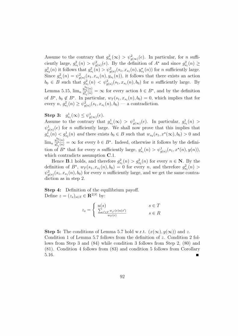
Assume to the contrary that g2s1

(∞) > ψ2g(∞)(e). In particular, for n suffi-

ciently large, g2s1

(n) > ψ2g(n)(e). By the definition of A? and since g2

s1(n) ≥

g2s2

(n) it follows that g2s1

(n) > ψ2g(n)(s1, xs1(n), y?s1(n)) for n sufficiently large.

Since g2s1

(n) = ψ2g(n)(s1, xs1(n), ys1(n)), it follows that there exists an action

b0 ∈ B such that g2s1

(n) < ψ2g(n)(s1, xs1(n), b0) for n sufficiently large. By

Lemma 5.15, limnyb0s1

(n)

ybs1 (n)= ∞ for every action b ∈ B?, and by the definition

of B?, b0 6∈ B?. In particular, wT (s1, xs1(n), b0) = 0, which implies that forevery n, g2

s1(n) ≥ ψ2

g(n)(s1, xs1(n), b0) — a contradiction.

Step 3: g1s1

(∞) ≤ ψ1g(∞)(e).

Assume to the contrary that g1s1

(∞) > ψ1g(∞)(e). In particular, g1

s1(n) >

ψ1g(n)(e) for n sufficiently large. We shall now prove that this implies that

g1s1

(n) < g1s2

(n) and there exists b0 ∈ B such that ws2(s1, x?(∞), b0) > 0 and

limnyb0s1

(n)

ybs1 (n)= ∞ for every b ∈ B?. Indeed, otherwise it follows by the defini-

tion of B? that for every n sufficiently large, g1s1

(n) > ψ1g(n)(s1, x

?(n), y(n)),which contradicts assumption C.1.

Hence B.1 holds, and therefore g2s1

(n) > g2s2

(n) for every n ∈ N. By thedefinition of B?, wT (s1, xs1(n), b0) = 0 for every n, and therefore g2

s1(n) >

ψ2g(n)(s1, xs1(n), b0) for every n sufficiently large, and we get the same contra-

diction as in step 2.

Step 4: Definition of the equilibrium payoff.Define z = (zs)s∈S ∈ R2|S| by:

zs =

u(s) s ∈ T∑s′∈T ws′ (e)u(s′)

wT (e)s ∈ R

Step 5: The conditions of Lemma 5.7 hold w.r.t. (x(∞), y(∞)) and z.Condition 1 of Lemma 5.7 follows from the definition of z. Condition 2 fol-lows from Step 3 and (84) while condition 3 follows from Step 2, (80) and(81). Condition 4 follows from (83) and condition 5 follows from Corollary5.16.

92

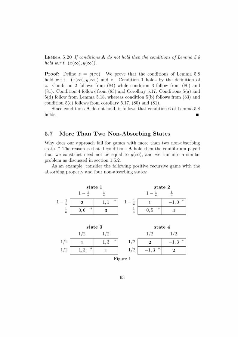
Lemma 5.20 If conditions A do not hold then the conditions of Lemma 5.8hold w.r.t. (x(∞), y(∞)).

Proof: Define z = g(∞). We prove that the conditions of Lemma 5.8hold w.r.t. (x(∞), y(∞)) and z. Condition 1 holds by the definition ofz. Condition 2 follows from (84) while condition 3 follow from (80) and(81). Condition 4 follows from (83) and Corollary 5.17. Conditions 5(a) and5(d) follow from Lemma 5.18, whereas condition 5(b) follows from (83) andcondition 5(c) follows from corollary 5.17, (80) and (81).

Since conditions A do not hold, it follows that condition 6 of Lemma 5.8holds.

5.7 More Than Two Non-Absorbing States

Why does our approach fail for games with more than two non-absorbingstates ? The reason is that if conditions A hold then the equilibrium payoffthat we construct need not be equal to g(∞), and we run into a similarproblem as discussed in section 1.5.2.

As an example, consider the following positive recursive game with theabsorbing property and four non-absorbing states:

state 3

1/2

1/2

1/2 1/2

1, 3 ∗1

1

1, 3 ∗

state 4

1/2

1/2

1/2 1/2

−1, 3 ∗2

2

−1, 3 ∗

state 1

1n

1− 1n

1− 1n

1n

0, 6 ∗2

3

1, 1 ∗

state 2

1n

1− 1n

1− 1n

1n

0, 5 ∗1

4

−1, 0 ∗

Figure 1

93

Let (x(n), y(n)) be the stationary profile indicated in Figure 1. First letus verify that (x(n), y(n)) is a fixed point of the correspondence φ1/n de-fined in section 5.5. Indeed, both players are indifferent between their ac-tions in states 3 and 4, and in states 1 and 2 player 2 must play each ac-tion with a probability of at least 1/n. It can be checked that player 2prefers to play in these two states L, hence his strategy is a best reply inY (1/n). The expected payoff for player 1 by this stationary strategy profile

is g1(n) = ( 1/n2−1/n

, −1/n2−1/n

, 12−1/n

, −12−1/n

). One can check that player 1 is indif-ferent between his actions in states 1 and 2, and therefore his strategy is abest reply against y(n).

Let C = {s1, s2}. Note that C is communicating w.r.t. (x(∞), y(∞)), andthat the exits from C w.r.t. (x(∞), y(∞)) are (s1, B, L), (s1, T, R), (s2, B, L)and (s2, T, R). It turns out that ρ∞ is the uniform distribution over thesefour exits and therefore

g1(∞) = g2(∞) =1

4(0, 6) +

1

4(1, 1) +

1

4(0, 5) +

1

4(−1, 0) = (0, 3).

However, there does not exist any way to exit from C in such a way thatis individually rational for both players and yields the players an expectedpayoff (0, 3).

The proof given by Vieille [35] for the existence of an equilibrium payoff inpositive recursive games with the absorbing property and arbitrary numberof non-absorbing states, uses different approximating games and best replycorrespondence. Moreover, after proving that the approximating game has astationary equilibrium, a lot of work is needed to construct an ε-equilibriumprofile in the original game. We hope that one can prove the existence ofan equilibrium payoff for an arbitrary number of non-absorbing states bytaking our approach, and finding another payoff function for player 2 orother constraints on his strategy space (or both).

94

References

[1] Amir R. (1987) Sequential Games of Resource Extraction: Existence ofNash Equilibrium, Cowles Foundation D.P. #825

[2] Aumann R.J. and Maschler B.M. (1995) Repeated Games with Incom-plete Information, The MIT Press

[3] Benedetti R. and Risler J.J. (1990) Real Algebraic and Semi-AlgebraicSets, Hermann

[4] Bewley T. and Kohlberg E. (1976) The Asymptotic Theory of StochasticGames, Math. Oper. Res., 1, 197-208

[5] Blackwell D. and Ferguson T. S. (1968) The Big Match, The Annals ofMath. Stat., 39, 159-163

[6] Bornstein G., Budescu D. and Zamir S. (1996) Cooperation in Inter-group, N -Person and Two-Person Games of Chicken, D.P. #96, Cen-ter for Rationality and Interactive Decision Theory, Hebrew University,Jerusalem

[7] Bornstein G., Erev I. and Goren H. (1994) The Effect of Repeated Playin the IPG and IPD Team Games, J. of Conflict Resolution, 38, 690-707

[8] Bornstein G., Goren H. and Winter E. (1996) Experimental Study ofRepeated Team-Games, European J. Political Economy, 12, 629-639

[9] Dutta P. and Sundaram R. (1993) How Different can Strategic ModelsBe?, J. Econ. Theory, 60, 42-61

[10] Everett H. (1957) Recursive Games, Contributions to the theory ofGames, 3, 47-78, Princeton, N.J. Annals of Mathematical Studies, 39,Princeton University Press.

[11] Filar J.A. (1985) Player Aggregation in the Traveling Inspector Model,IEEE Trans. Automated Control, AC-30, 723-729

[12] Fink A.M. (1964) Equilibrium in a Stochastic n-Person Game, J. Sci.Hiroshima Univ.,28, 89-93

95

[13] Flesch J., Thuijsman F. and Vrieze K. (1997) Cyclic Markov Equilibriain Stochastic Games, Int. J. Game Th., 26, 303-314

[14] Forster O. (1981) Lectures on Riemann Surfaces, Graduate Texts inMathematics, Springer Verlag

[15] Gillette D. (1957) Stochastic Games with Zero Stop Probabilities, Con-tributions to the Theory of Games, 3, Princeton University Press

[16] Kohlberg E. (1974) Repeated Games with Absorbing States, Ann. Stat.,2, 724-738

[17] Kohlberg E. and Zamir S. (1974) Repeated Games of Incomplete Infor-mation: The Symmetric Case, Ann. Stat., 2, 1040-1041

[18] Lamperti J.W. (1996) Probability, John Wiley and sons

[19] Levhari D. and Mirman L. (1980) The Great Fish War: An ExampleUsing a Dynamic Cournot-Nash Solution, Bell J. Econ., 11(1), 322-334

[20] Mertens J.F. and Neyman A. (1981) Stochastic Games, Int. J. GameTh., 10, 53-66

[21] Mertens J.F., Sorin S. and Zamir S. (1994) Repeated Games, COREDiscussion Paper 9421

[22] Neyman A. (1996) Lecture Notes of a course in “Stochastic Games”,The Hebrew University, Jerusalem.

[23] Neyman A. and Sorin S. (1995) Equilibria in Repeated Games of In-complete Information: The Deterministic Symmetric Case, D.P. #82,Center for Rationality and Interactive Decision Theory, Hebrew Uni-versity, Jerusalem

[24] Neyman A. and Sorin S. (1995) Equilibria in Repeated Games of In-complete Information: The General Symmetric Case, D.P. #86, Cen-ter for Rationality and Interactive Decision Theory, Hebrew University,Jerusalem

96

[25] Rogers P.D. (1969) Non-Zerosum Stochastic Games, Ph.D. Thesis, re-port ORC 69-8, Operations Research Center, University of California,Berkeley

[26] Shapley L.S. (1953) Stochastic Games, Proc. Nat. Acad. Sci. U.S.A.,39, 1095-1100

[27] Shubik M. and Whitt W. (1973) Fiat Money in an Economy with oneNondurable Good and No Credit: a Noncooperative Sequential Game.In Topics in Differential Games, Blaquiere A. (ed), 401-448

[28] Sobel M.J. (1971) Noncooperative Stochastic Games, Ann. MAth. Stat.,42, No. 6, 1930-1935

[29] Solan E. and Vieille N. (1998), Quitting Games. In preparation

[30] Sorin S. (1986) Asymptotic Properties of a Non-zerosum StochasticGames, Int. J. Game Theory, 15, 101-107

[31] Thuijsman F. and Raghavan T.E.S. (1997) Perfect Information Stochas-tic Games and Related Classes, Int. J. Game Theory, (forthcoming)

[32] Vieille N. (1993) Solvable States in Stochastic Games, Int. J. GameTheory, 21, 395-404

[33] Vieille N. (1994) On Equilibria in Undiscounted Stochastic Games, D.P.9446, CEREMADE

[34] Vieille N. (1997) Equilibrium in 2-Person Stochastic Games I: A Re-duction, preprint

[35] Vieille N. (1997) Equilibrium in 2-Person Stochastic Games II: The Caseof Recursive Games, preprint

[36] Vrieze O.J. and Thuijsman F. (1989) On Equilibria in Repeated GamesWith Absorbing States, Int. J. Game Th., 18, 293-310

[37] Walker R.J. (1950) Algebraic Curves, Princeton University Press

[38] Winston W. (1978) A Stochastic Game Model of a Weapons Develop-ment Competition, Siam J. Control and Optimization, 16, 411-419

97