Embed Size (px)
Citation preview

INFORMATION TO USERS
This manuscript has been reproduced frorn the microfilm master. UMI films the
text directly from the criginal or copy submitted. Thus, some thesis and
dissertation =$es are in typewriter face, while others may be from any type of
cornputer printer.
The quality of this reproduction is dependent upon the quality of the copy
submitted. Broken or indistinct print, colored or poor quality illustrations and
photographs, print bleedthrough, substandard margins, and improper alignrnent
can adversely affect reproduction.
In the unlikely event that the author did not send UMI a complete manuscript and
there are missing pages, thesa wili be noted. Also, if unauthofized copyright
material had to be removed, a note will indicate the deletion.
Oversize materials (e.g., maps, drawings, charts) are reproduœd by sedioning
the original, beginning at the upper lefthand corner and continuing from left to
right in equal sections with small overlaps. Each original is also photographed in
one exposure and is inciuded in reduced fom at the back of the book
Photographs inciuded in the original manuscript have been reproduced
xerographically in this copy. Higher quality 6" x 9" black and white photographie
pnnts are available for any photographs or illustrations appeanng in this copy for
an additional charge. Contact UMI directiy to order.
Bell & Howell Information and Leaming 300 North Zaeb Road, Ann Abor. MI 481061346 USA
8001521-0600

VARIABLE FREQUENCY CURRENT DENSITY IMAGING
Aaron P hillip Weinrot h
A thesis submit ted in conformiw with the requirements for the degree of Master of Applied Science
Graduate Department of Electricd and Computer Engineering University of Toronto
@ Copyright by Aaron Phillip Weinroth 1998

National Library l*l of Canada Bibliothéque nationale du Canada
Acquisitions and Acquisitions et Bibliographie Services services bibliographiques
395 Wellington Street 395, rue Wellington OttawaON K1A ON4 OttawaON K1AON4 Canada Canada
The author has granted a non- exclusive Licence allowing the National Library of Canada to reproduce, loan, distribute or seii copies of this thesis in microform, paper or electronic formats.
The author retains ownership of the copyright in this thesis. Neither the thesis nor substantial extracts fiom it may be printed or othemise reproduced without the author's permission.
L'auteur a accordé une licence non exclusive permettant à la Bibiiothèque nationale du Canada de reproduire, prêter, distribuer ou vendre des copies de cette thèse sous la forme de microfiche/nlm, de reproduction sur papier ou sur format électronique.
L'auteur conserve la propriété du &oit d'auteur qui protège cette thèse. Ni la thèse ni des extraits substantiels de celle-ci ne doivent être imprimés ou autrement reproduits sans son autorisation.
Variable F'requency Current Density Imaging
Department of Electrical Engineering and Institute of Biomedical Engineering
University of Toronto
Abstract
Current density imaging (CDI) is a technique in magnetic resonance imaging
(MRI) in which the MR imager is used to produce a spatial map of the electric
current density in a subject. Typically, the current is externally applied. Variable
fiequency current density imaging (VF-CDI) is a new CD1 technique in which the
fiequency of the externally applied current is not restricted to a single fixed fiequency
as in previous CD1 techniques.
This thesis describes the theory of VF-CD1 and an implementation of the VF-CD1
technique on a clinical MR imager. A series of experiments were perfomed using this
implementation and the results are presented and analyzed.
The results of the experllnents confirm the theoretical predictions of VF-CD1 and
show that there are a number of limitations to the technique. The performance of
VF-CD1 is compared to other CD1 techniques and some suggestions for improvements
to the technique are made.

Acknowledgment s
1 would like to thank my supervisor Dr. Michael Joy for giving me the opportunity
to work on this project and for his assistance and encouragement along the way. 1
wodd also like to express my gratitude to aU those who have made my research pas-
sible by working on current density imaging before me and especidy to the graduate
students who helped teach me what it was all about.
While working on this thesis 1 have benefited greatly bom the knowledge of John
Simpson on electrical design and £rom the talents of F'ranz Schuh in the mechanical
workshop. Special thanks also to members of the magnetic resonance imaging research
goup at the Sunnybrook Health Science Centre for the use of their facilities and their
advice along the way.
Here at the Institute of Biomedical Engineering 1 have been very fortunate to
have many hiends who made my time so much more enjoyable and relaxed. 1 must
also recognize the work of Anne Mitchell and the rest of the administrative staff for
making sure that the only thing 1 had to worry about was my reseaîch.
My academic life would not have been nearly as successful or enthusiastic without
the encouragement and support of my family and fnends. 1 am especidy grateful to
my proofieader for her patience and understandhg when there was work that had to
be done.
Last, but certainly not least, 1 would Iike to acknowledge the hancial support
provided by the N a t d Sciences and Engineering Research Council of Canada for
this project.

Contents
Abstract
Acknowledgments iii
List of Tables viii
List of Figures ix
List of Abbreviations and Symbols xi
1 Introduction 1
1.1 Objective . . . . . . . . . . . . . . . . . . . . . . . . . . . . . . . . . 2
1.2 A Brief History of Current Density Irnaging . . . . . . . . . . . . . . 2
1.3 Motivation and Applications . . . . . . . . . . . . . . . . . . . . . . . 3
1.4 Outline. . . . . . . . . . . . . . . . . . . . . . . . . . . . . . . . . . . 5
2 Theory 8
2.1 Magnetic Resonance Imaging . . . . . . . . . . . . . . . . . . . . . . 8
2.1.1 Rotating fiame of Reference . . . . . . . . . . . . . . . . . . . 9
2.2 Current Density Imaging . . . . . . . . . . . . . . . . . . . . . . . . . 10
2.2.1 Electric Current Density in Heterogeneous Media . . . . . . . 10
2.2.2 Application of Maxwell's Equations . . . . . . . . . . . . . . . 11
Contents
. . . . . . . . . . . . . . . . . . . . . . . . . 2.3 Vaxiable Frequency CD1 12
. . . . . . . . . . . . . . . . . . . . . . . . . . . 2.3.1 Current Field 12
. . . . . . . . . . . . . . . . . . . . . 2.3.2 Requency Tuning Pulse 15
2.3.3 Double Rotating Ftame of Reference . . . . . . . . . . . . . . 16
2.3.4 Determining the Effective Field in P . . . . . . . . . . . . . . 18
. . . . . . . . . . . . . . . . . . . . . . . . . . . . 2.3.5 Implications 22
. . . . . . . . . . . . . . . . . . . . . . . 2.3.6 Cornputer Simulation 24
. . . . . . . . . . . . . . . . . . . . . . . . . 2.4 PracticalConsiderations 24
. . . . . . . . . . . . . . . . . . . . . 2.4.1 RCP Cornponent of B, 25
. . . . . . . . . . . . . . . . . . . . . . . . . . . 2.4.2 Off-Resonance 32
. . . . . . . . . . . . . . . . . . . . . . . . . 2.4.3 Bo Inhomogeneity 35
. . . . . . . . . . . . . . . . . . . . . . . . . 2.4.4 BI Inhomogeneity 36
. . . . . . . . . . . . . . . . . . . . . . . . . . . . . 2.4.5 Relaxation 37
. . . . . . . . . . . . . . . . . . . . . . . . . . 2.4.6 Phase Wrapping 37
. . . . . . . . . . . . . . . . . . . . . . . . . 2.4.7 Fkequency Range 37
. . . . . . . . . . . . . . . . . . . . . . . . . . . 2.4.8 Current Phase 38
. . . . . . . . . . . . . . . . . . . . . . 2.5 Imaging System Requirements 38
. . . . . . . . . . . . . . . 2.5.1 Data and Processing Requirements 39
. . . . . . . . . . . . . . . . . . . . . . . . . . 2.5.2 Applied Curent 41
3 BI Homogeneity 42
. . . . . . . . . . . . . . . . . . . . . . . . . . . . . . . . . . 3.1 Method 42
. . . . . . . . . . . . . . . . . . . . . . . . . . 3.1.1 Pulse Sequence 44
. . . . . . . . . . . . . . . . . . . . . . . . . . 3.1.2 Post-Processing 46
. . . . . . . . . . . . . . . . . . . . . . . . . . . . . . . . . . . 3.2 Results 47
. . . . . . . . . . . . . . . . . . . . . . . . . . . . . . . . . 3.3 Discussion 49
. . . . . . . . . . . . . . . . . . . . . . . . . . . . . . . . 3.4 Conclusions 50
4 Method 51
. . . . . . . . . . . . . . . . . . . . . . . . . . . . . 4.1 Hardware Design 52
. . . . . . . . . . . . . . . . . . . . . . . . . . . 4.1.1 StartingPoint 52
. . . . . . . . . . . . . . . . . . . . . . . . . 4.1.2 Circuit Operation 53

Contents
4.1.3 PhantornSetup . . . . . . . . . . . . . . . . . . . . . . . . . . 55
. . . . . . . . . . . . . . . . . . . . . . . . . . . . . 4.2 haging Sequence 56
4.2.1 ImagingParameters . . . . . . . . . . . . . . . . . . . . . . . 59
. . . . . . . . . . . . . . . . . . . . . . . . . . . . . . 4.3 Post-Processing 59
. . . . . . . . . . . . . . . . . . . . . . . . . 4.3.1 Phase Correction 60
. . . . . . . . . . . . . . . . . . . 4.3.2 Magnetization Components 60
. . . . . . . . . . . . . . . 4.3.3 Quatemion Least Squares Rotation 61
. . . . . . . . . . . . . . . . . . . . . . . . 4.3.4 Vector Unwrapping 62
. . . . . . . . . 4.3.5 Converting the Rotation into a Magnetic Field 63
. . . . . . . . . . . . . . . . . 4.3.6 Computing the Current Density 64
. . . . . . . . . . . . . . . . . . . . . . . . . . . . . . 4.3.7 Filtering 64
. . . . . . . . . . . . . . . . . . . . . . . . . . 4.3.8 Region Analysis 64
5 Results 65
. . . . . . . . . . . . . . . . . . . . . . . . . . 5.1 Problems Encountered 65
. . . . . . . . . . . . . . . . . . . 5.1.1 Magnetohydrodynamic Flow 66
. . . . . . . . . . . . . . . . . . . . . . 5.1.2 Rotation of the Subject 67
. . . . . . . . . . . . . . . . . . . . . . . . . . . 5.1.3 Slice Selection 67
. . . . . . . . . . . . . . . . . . . . . . . 5.1.4 Return Wire Artifact 68
. . . . . . . . . . . . . . . . . . . . . . . . . . . . . . 5.2 500 Hz Current 68
. . . . . . . . . . . . . . . . . . . 5.2.1 Magnetization Components 68
. . . . . . . . . . . . . . . . . . . . . . . 5.2.2 Rotation Ms/Angle 71
. . . . . . . . . . . . . . . . . . . . . . . . . . 5.2.3 Magnetic Fields 71
. . . . . . . . . . . . . . . . . . . . . . . . . . 5.2.4 Curent Density 72
. . . . . . . . . . . . . . . . . . . . . . . . . . . . . . 5.3 100 Hz Current 75
. . . . . . . . . . . . . . . . . . . . . . . . . . 5.4 Off Resonance Current 75
. . . . . . . . . . . . . . . . . . . . . . . . . . . 5.5 Performance Analysis 75
6 Discussion and Conclusions 79
. . . . . . . . . . . . . . . . 6.1 Cornparison With Other CD1 Techniques 80
. . . . . . . . . . . . . . . . . . . . . . . 6.1.1 Technical Limitations 80
. . . . . . . . . . . . . . . . . . . . . . . 6.1.2 Practical Limitations 81

Contents
. . . . . . . . . . . . . . . . . . . . . . 6.1.3 Biophysical Limitations 81
. . . . . . . . . . . . . . . . . . . . . . . . . . . . . . . . 6.2 Future Work 82
. . . . . . . . . . . . . . . . . . . . . . . . . . . . . . . 6.3 Other Insights 83
. . . . . . . . . . . . . . . . . . . . . . . 6.3.1 Extension of LF-CD1 83
. . . . . . . . . . . . . . . . . . . . . . . . . . . . . 6.3.2 Hannonics 85
. . . . . . . . . . . . . . 6.3.3 Currents Near the Larmor F'requency 85
. . . . . . . . . . . . . . . . . . . . . . . . . . . . 6.3.4 Tlplmaging 85
. . . . . . . . . . . . . . . . . . . . . . . . . . . . . . . . 6.4 Conclusions 86
Bibliograp hy
A Mathematical Derivation 91
. . . . . . . . . . . . . . . . . . . . . . . . . . . . . . A.1 Bloch Equation 91
A. l . l Derivative in Time of the Axes of the Double Rotating Rame 94
. . . . . . . . . . . . . . . . . . . A.2 Sarnple Effective Field Calculation 95
B Schematic Drawings 98
C System Operating Instructions 102
. . . . . . . . . . . . . . . . . . . . . . . . . . . . . . C.l Hardware Setup 102
. . . . . . . . . . . . . . . . . . . . . . C . 1.1 Switches and Controls 104
. . . . . . . . . . . . . . . . . . . . . . . . . . . C.2 GE Signa Operation 105

List of Tables
3.1 B Field Inhomogeneity . . . . . . . . . . . . . . . . . . . . . . . . . 47
4.1 Measured Phantom Resistance . . . . . . . . . . . . . . . . . . . . . . 56
4.2 Pulse Settings for Data Acquisition . . . . . . . . . . . . . . . . . . . 57
5.1 Current Density Statistics for Figure 5.5a . . . . . . . . . . . . . . . . 73
. . . . . . . . . . . . . . . . 5.2 Current Density Statistics for Figure 5.5b 73
5.3 Curent Density Statistics for Figure 5.7a . . . . . . . . . . . . . . . . 76
. . . . . . . . . . . . . . . . 5.4 Current Density Statistics for Figure 5.7b 76
C . 1 Operator Prescription Input for ufcdiU2 . e . . . . . . . . . . . . . . . . 106
C.2 Prescan Setup and CV Entry for ufcdi02.e . . . . . . . . . . . . . . . 107
List of Figures
. . . . . . . . . . . . . . . . . . . . . . . . . . . 1.1 Outline of the Thesis 7
. . . . . . . . . . . . . . . . . . . 2.1 Precession of the Net Magnetization 9
. . . . . . . . . . . 2.2 Magnetic Field Generated by the Applied Current 13
. . . . . . 2.3 Effectofthecurrent'smagneticfieldonthemagnetization 14
. . . . . . . . . . . . . . . . . . . . . . . . . 2.4 VF-CD1 Timing Diagram 15
. . . . . . . . . . . . . 2.5 Magnetic Fields with Curent and Bi Applied 16
2.6 Effect of the current's magnetic field on the magnetization with the
. . . . . . . . . . . . hequency tuning pulse applied (rotating hame) 17
2.7 Effect of the current's magnetic field on the magnetization with the
. . . . . . . . . . . . . . . . âequency tuning putse applied (P hame) 19
2.8 Decomposition of a linearly polarized field into circdarly polarized
. . . . . . . . . . . . . . . . . . . . . . . . . . . . . . . . components 20
. . . . . . 2.9 Logical conversion to the double rotating fiame of reference 21
. . . . . . . . . . . . . . . . 2.10 Analogy between basic MRI and W-CD1 23
2.11 Simulation including the effects of the RCP component of & (ji frame) 26
2.12 Cornparison of precession phase for ideal and RCP included cases . . 27
2.13 Cornparison of precession phase for ideal and RCP included cases as
. . . . . . . . . . . . . . . . . . the fkequency of the current changes 29
List of Figures
2.14 Comparison of precession phase for ideal and RCP included cases as
the amplitude of the current changes . . . . . . . . . . . . . . . . . . 30
2.15 Comparison of precession phase for ideal and RCP included cases with
. . . . . . . . . . the current amplitude and frequency both increased 31
2.16 Simulation showing an off-resonance effect in the rotating frame . . 33
2.17 Simulation in ii with a s m d AB^ off-resonance field . . . . . . . . . . 34
2.18 Cornparison of precession phase for a AB^ off-resonance error . . . . 35
2.19 Required measurements with no off-resonance error and the phase of
. . . . . . . . . . . . . . . . . . . . . . . . . . . . . the curent known 39
. . . . . . . . . . 2.20 Required measurements with no assumptions made 40
. . . . . . . . . . . . . . . . . . . . . . 3.1 Tri-Concentric Tube Phantom 44
. . . . . . . . . . . . . 3.2 Pulse sequence for measuiing Bi homogeneity 45
. . . . . . . . . . . . . . . . 3.3 Phase images encoding BI field strength 48
. . . . . . 4.1 Pulse sequence for VF-CD1 experirnents (symbolic pulses) 57
. . . . . . . . 4.2 Pulse sequence for VF-CD1 experiments (actual puises) 58
. . . . . . . . . . . . . . . . . . 5.1 Measured magnetization components 69
. . . . . . . . . . 5.2 Magnitudes of the measured magnetization vectors 70
5.3 Rotation axis and angle plots for BI and the current both applied . . 71
. . . . . . . . . 5.4 Measured B~ for Bi and current pulses both applied 72
. . . . . . . . . . . . . 5.5 Current Density Magnitude Images at 500 Hz 73
. . . . . . . . . . . . . . . . 5.6 Phase Image of Current Fields at 500 Hz 74
. . . . . . . . . . . . . 5.7 Current Density Magnitude Images at 100 Hz 76
. . . . . . . . . . . . . . . . 5.8 Phase Image of Current Fields at 100 Hz 77
6.1 Cornparison of VF-CD1 and Extended LF-CD1 . . . . . . . . . . . . . 84
. . . . . . . . . . . . . . . . . . . . . . . . . . . . B.1 Schematic Drawing 100
. . . . . . . . . . . . . . . . . . . . . . . . . . . . . . . B.2 Board Layout 101
. . . . . . . . . . . . . . . . . . . . . . . . C.l Hardware Setup Schematic 103

List of Abbreviations & Symbols
ABBREVIATIONS
CD1 CGB DC EEG FOV IC LCP LF MHD M N PLL RCP RF SNR VF VFCG
current density imaging current generation box direct current electroencephalogram field of view integra ted circuit left circuiady polarized low kequency magnetohydrodynamic magnetic resonance imaging phase locked loop right circularly polarized radio bequency signal to noise ratio variable frequency variable fiequency current generator
For the symbols listed below and in the text, bold indicates a vector quantity and regular type is used for scalars or a vector magnitude. Individual components of a vector are denoted with the subscript x, y, or z. Quantities in the rotating frame are shown as Ü and quantities in the double rotating frame are shom as Ô.
B magnetic field [Tl l3 symmetric rnatrix for quaternion computation Bo main static magnetic field in the MR imager [Tl BI RF transmit field in the MR imager [TI

List of Abbreviations & Symbols
ideal effective magnetic field in fi [Tl effective magnetic field [TI magnetic field due to the applied current [TI Bo off-resonance error term [Tl BI off-resonance error terru [TI initial magnetization orientation matrix hd magnetization orientation matrix electric field [V/rnJ force [NI Frequency [Hz1 Larmor frequency [Hz] frequency of the applied current [Hz] magnetic field [Alml magnetic field due to the applied curent [A/ml elect ric current [Al electric current density [A/m2] tangentid electric current density [A/m2] net nuclear magnetization vector [Alml axis of magnetization precession rnatrix of orthonormal bai s vectors quaternion rotation matrix time [SI longitudinal and transverse relaxation times [SI current pulse duration [SI echo t h e [s] repetition t h e [SI coordhate system axes coordinate system unit vecton gyromagnetic ratio [rad/Tsj electric permittivity [F/mj electric permittivity of kee space [F/mj relative electric permittivity [£?/ml phase [rad], [degreesl magnetic permeabiüty of £ree space [H /ml double rotating hame of reference conductivity [S/ml complex conductivity [S /ml angular fiequency [rad/s] anpuiar fiequency vector [rad/sj mgulax frequency of the applied current [rad/sj Larmor aggular fiequency [rad/sl
CHAPTER 1
Introduction
Current density imaging (CDI) is a technique in magnetic resonance imaging
(MRI) in which the kfR imager is used to produce a spatial map of the electric current
density in a subject resulting hom an externdy applied electric current . The contrast
in a current density image is dependent on the variations in complex conductivity (a
hequency dependent electrical property) between tissues within the subject . This
differs from traditional MRI in which the cantrast is a function of the relaxation times
and proton density of the tissues. The change in contrast mechanism rnakes CD1 a
novel imaging modality since tissues which are indistinguishable in MRI may appear
to be different in CDI. As a result, MRI and CD1 used together can provide a more
effective diagnostic tool than either one alone. CD1 on its own can be used to obtain
information on electric curent pathways in the body as well as detect disease in soft
tissue. CD1 may be effective for functional imaging of muscle and brain activity since
research has shown that the conductivity of both change when active [Il. h o , CD1
could possibly provide more insight into such issues as electroencephalogram (EEG)
source localization.
'Placement of the eiectrodes for injecting the m e n t can also have an effeet on the current density image contrast .
Chapter 1 o Introduction 2
This thesis presents the theory and a first implementation of variable frequency
current density imaging (VF-CDI), a new CD1 technique in which the frequency of the
extemally applied current is not restricted to a single fixed frequency as in previous
CD1 techniques. The development of such a method for imaging currents over a wider
frequency range gives more flexibility and venatility to CD1 and makes many new
applications possible.
1.1 Objective
The objective of this thesis is to examine the feasibility of VF-CDI. This will be
accomplished by:
Clearly describing the theoretical basis for VF-CDI.
Investigating the practical limitations of the technique.
a Developing the hardware and software necessary to implement VF-CDI.
Analyzing the results of the implementation.
The task of optimizing the VF-CD1 technique, M y characterizing the system perfor-
mance, and preparing VF-CD1 for clinical use will be left to other researchers.
1.2 A Brief History of Current Density Imaging
The motivation and approach for developing a new CD1 technique will be better
understood in the histoncal context of past CD1 evolution. Research into CD1 at the
University of Toronto began in 1987 with experiments to measure uniform current
density in a cylinder. These experiments assumed planar current BOW so that the
required measurements could be reduced to one component of the magnetic field [2].
The restriction of planar current flow was eliminated with the development of low
frequency CD1 (LF-CDI) [3, 41. One limitation of LF-CDI was that it could not
be used on live subjects due to the biological effects of the DC curxents it required.
Another was the need to rotate the subject to orthogonal positions. This led to errors
Chapter 1 O Introduction 3
caused by inaccurate rotation and restricted the size of the subject to what could be
rotated within the imager bore [5, 61.
The technique of radio frequency CD1 (RF-CDI) was developed to overcome the
biological effects of the DC currents and the need to rotate the subject. Two RF-CD1
techniques were developed; the first was the polar decornposition method [3, 71 and
the second was the rotating hame method [6j.
AU of the experiments performed up to that point were carried out using a General
Electric CS1 2.0 Tesla (T) imager with a 30 cm bore. The rotating frame method of
RF-CD1 has since been implemented on a General Electric Signa 1.5 T clinical imager
[5, 81 as has the polar decomposition method [91. Most recently, the rotating kame
method has been implemented using a fast, spiral-scan MM sequence 1101.
The lessons learned and knowledge developed about CD1 kom all this past work
in tems of theory as well as hardware and software tools will contribute to the
development of VF-CD1 in this thesis.
1.3 Motivation and Applications
Although CD1 has great potential, the existing techniques of CD1 are both limited
in that they are restricted to a single frequency of current which they can image. LF-
CD1 is restricted to near DC cunents. Such currents have a limit to the magnitude
which can be applied to live subjects, set by the physiological reaction to the current
which involves depolarization of nerves leading to muscle twitch and pain. Also, with
DC currents there is no tissue contrast fkom the tissue capacitances. RF-CD1 provides
significant improvernent over LF-CD1 as it does not stimulate a biological response
to the ~ur ren t .~ However, it is restricted to currents at the Larmor fiequency which
is the resonant fkequency of magnetic resonance imaging. At such a high fiequency
the capacitive effects of the tissues are easier to observe, but the dinaences in the
capacitive effects is decreased [31. Given these limitations, it is desirable to develop
a new technique in which the fiequency of the m e n t is not restricted to a single
value and in which the fiequency of the current can be chosen to be a fiequency of
2The upper magnitude Mt for RF-CD1 is set by tissue heating constraints instead.
Cha~ter 1 O Introduction 4 -- -
"biological interest".
The main benefits of VF-CD1 are derived from the frequency dependence of tissue
conductivity (and therefore the hequency dependence of the tissue appearance and
contrast) and these two unique features:
The frequency of operation is not predetermined by the technique itself.
m Images can be obtained at different current frequencies.
Since the curent density distribution, and therefore the contrast in the image, is
determined by fiequency dependent electricai properties of the tissues in the subject,
the ability to select the current's frequency presents a sigdicant benefit. The fre-
quency of the current can be selected to enhance a particulax biological response or
to maximize current density contrast between tissues in the same way that echo and
repetition times are selected in MRI to enhance relaxation time contrast. Because
more than one hequency can be used, a set of images can be obtained at different
current frequencies, a cornparison between these images can be performed, and the
change in the images with fkequency can be used as an additional diagnostic tool
which would be mavailable if only a single frequency could be used.
The most obvious application of VF-CD1 is its use in obtaining MR-iike images but
with a different contrast mechanism. It c m be used in the same situations and under
the same conditions as MRI but could provide contrast between tissues which appear
identical in MRI or other CD1 techniques. VF-CD1 also has potential applications
in areas where M M or other CD1 techniques cannot be used. For example, W-CD1
could be the first step towards an MR mapping of the naturd electncal activity in the
body if synchronization problems can be overcome. It is also possible that VF-CD1
d have non-medical, spectroscopic type applications.
The VF-CD1 implementation resulting fkom this thesis has a number of limita-
tions. The k t is that due to hardware (power) restrictions it is not possible to
image currents outside the kequency range of DC to slightly higher than 1 kHz 3.
3This is due to Limitations on the strength of the RF field whieh ean be produced by the MR imager hardware. However, tissue heating d also present a Limit to current puise duration at high field strengths.
Chapter 1 O Introduction 5 - - --- -
This will lirnit the initial use of VF-CD1 on iive subjects due to the biological effects
of electric cursents in this frequency range. Also, since the fkequency range is not very
large, the changes in tissue conductivity over this frequency range will rely mostly on
a-dispersion effects. An ideal VF-CD1 system wodd be capable of imaging currents
in a frequency range from DC to over 100 kHz. The second limitation is that the
proposed technique can only measure one component of the magnetic field in a given
orientation of the subject and physical rotation of the subject wiU be required in order
to calculate any one component of the current density. It is expected that this first
implernentation of VF-CD1 will act as a stepping Stone for another method which will
overcome these limitations while still providing the benefits of VF-CDI.
1.4 Outline
The theory of the VF-CD1 technique is presented in chapter 2 dong with some
results £rom a cornputer simulation used to v e e , investigate, and demonstrate the
theory. This chapter aiso examines a number of practical considerations for VF-
CD1 and discusses the requirements of a VF-CD1 system. Appendix A contains a
mathematical derivation of part of the theory contained in chapter 2.
Chapter 3 describes a series of experiments performed to test the homogeneity of
the RF transmit field in the MR imager. The results of these experiments are needed
to determine the exact data requirements of W-CD1 and complgte the background
work for the VF-CD1 implementation.
The method used for preparing and conducting the VF-CD1 experiments is found
in chapter 4. The method includes the design of haxdware for generating the curent
(additional details and schematic drawings are in appendix B), softwaze for ninning
the imaging sequence, and software for processing the data and forming the current
demie images. Specific operating instructions for the VF-CD1 system are given in
appendix C.
The r e d t s of the experiments and some analysis of the results are located in
chapter 5. This chapter also includes details of some of the problems encountered
and the changes made to the experimental procedure. Chapter 6 discusses the results

Chapter 1 o Introduction 6
of this thesis, compares the performance of VF-CD1 to other CD1 techniques, and
makes a number of suggestions for future work on VF-CDI.
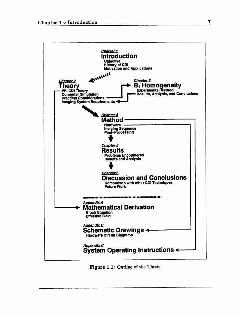
A graphical outline of the basic structure and content of the thesis is shown in
figure 1.1.
Chapter l O Introduction 7
- Introduction
Objective tlistory of CD1 Motivation and Applications -
Theox B1 Homo eneity - VF-CDI eory Experimentrrl 1 ethod Cornputer Simulation Results, Analysis, and Conclusions Practical Considerations lmaging System Requirements
- -
Mëthod
I
1
Figure 1.1: Outline of the Thesis.
Hardware Imaging Sequence Post-Processing -
Results Problems Encountered Hesults and Analysis
CheaterG Discussion and Conclusions
Cornparison wlth other COI Techniques Future Work - - Mathematical Derivation
Bloch Equdon Effectfve Field
dwmWXB Schematic Drawings s
Hardwam Circuit Diagrams
AmMdkG System Operating Instructions t
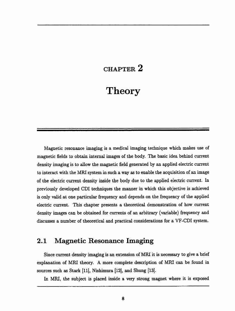
CHAPTER 2
Theory
Magnetic resonance imaging is a medical imaging technique which makes use of
magnetic fields to obtain intemal images of the body. The basic idea behind current
density imaging is to d o w the magnetic field generated by an applied electric current
to interact with the MRI system in such a way as to enable the acquisition of an image
of the electric current density inside the body due to the applied electric current. In
previously developed CD1 techniques the manner in which this objective is achieved
is only valid at one paxticular fkequency and depends on the fkequency of the applied
electric current. This chapter presents a theoretical demonstration of how current
density images c m be obtained for currents of an arbitrary (variable) frequency and
discusses a number of theoretical and practical considerations for a VF-CD1 system.
2.1 Magnetic Resonance Imaging
Since current density imaging is an extension of MRI it is necessary to give a brief
explanation of MRI theory. A more complete description of MRI can be found in
sources such as Stark [III, Nishimura [12j, and Shung [13].
In MRI, the subject is placed inside a very strong magnet where it is exposed
Chapter 2 O Theory 9
to a large, uniform magnetic field (Bo) l which defines the z axis. Spinning protons
within the subject give rise to magnetic dipoles and Bo causes these dipoles to align
and create a net nuclear magnetization (M) pardel to Bo. The basic MRI technique
involves using an RF pulse to tip M away fkom Bo and into the transverse (x-y) plane.
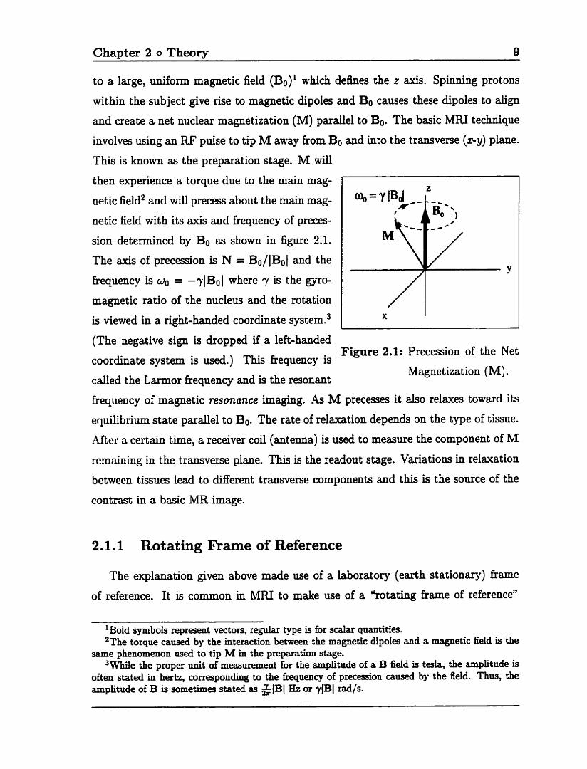
This is knom as the preparation stage. M will
then experience a torque due to the main mag-
netic field2 and will precess about the main mag-
netic field with its axis and fiequency of preces-
sion determined by Bo as shown in figure 2.1.
The axis of precession is N = Bo/ IBO 1 and the
fiequency is wo = -71Bo 1 where 7 is the gyro-
magnetic ratio of the nucleus and the rotation
is viewed in a right-handed coordinate ~ y s t e m . ~
(The negative sign is dropped if a left-haaded Figure 2.1: Precession of the Net
coordinate system is used.) This fiequency is Magnetization (M) .
c d e d the Larmor fiequency and is the resonant
Eiequency of magnetic resonance imaging. As M precesses it also relaxes toward its
equihb~um state pardel to Bo. The rate of relaxation depends on the type of tissue.
After a certain tirne, a receiver coil (antenna) is used to measure the cornponent of M
remaining in the transverse plane. This is the readout stage. Variations in relaxation
between tissues lead to different tramerse components and this is the source of the
contrast in a basic MR image.
2.1.1 Rotating Rame of Reference
The explmation given above made use of a laboratory (earth stationary) fiame
of reference. It is cornmon in MRI to make use of a "rotating hame of referencen
'Bold symbols represent vecton, regular type is for scalar quantities. *The torque caused by the interaction between the magnetic dipoles and a magnetic field is the
same phenornenon used to tip M in the pteparation stage. 3 W e the proper unit of measurement for the amplitude of a B field is tesla, the amplitude is
often stated in hertz, correspondhg to the frequency of precession caused by the field. Thus, the amplitude of B is sometimes stated as &IBI Hz or 7iBI rad/$.
Chapter 2 o Theory 10
which is obtained by rotating the x-y plane about t at the Larmor fiequency in a
Mt-handed (clockwise) direction. The rotating h m e compensates for the precession
of M due to Bo and therefore Bo and the resulting precession of M are effectively
eliminated. The situation in figue 2.1 would appear in the rotating hame as a
stationary magnetization (with the same angle to z) and no Bo field. If there is a
change in the magnitude of the static field such that IBO 1 f 7 then there will be an
"off-resonance" error term in the rotating bame parallel to the original Bo field and
having a magnitude of ABo = Bo - 7 .
2.2 Current Density Imaging
Current density imaging takes advantage of the dependence of an MR image on
magnetic fields and the fact that an externally applied electric current (J) generates
its own magnetic field (Hj = WBJ) which will cause a spatially varying distortion
of the standard MR image. When the electric current is applied in CD1 between the
preparation and readout stages, the total field changes fkom Bo to Bo + BJ and the
axis and fiequency of precession change accordingly. This results in a change in the
expected orientation of M and distortion of the MR images. The key to any CD1
technique is to develop an imaging sequence such that an image is obtained which,
when distorted by the application of the electric current, will encode information
about the curent's magnetic field in the phase and/or magnitude of the resulting MR
image. (How this is done for VF-CD1 will be explained later.) Once the magnetic
field information is extracted, the current density can be cdculated with the aid of
Maxwell's equations (section 2.2.2).
2.2.1 Electric Current Density in Heterogeneous Media
A current density image can be a diagnostically useful tool due to the fact that
the electric current density in the subject depends on the tissue and fkequency de-
pendent conductivity (O) and permittivity ( E ) of the tissues within the subject. The
relationship between a sinusoida1 electric field E and current density (conduction and
displacement current) is:
Chapter 2 O Theory 11
in which c = ~ ~ € 0 . At the boundary of dissimilar media, the tangentid component of
the electric field must be continuous and the ratio of tangential current density must
sat is@:
Therefore, the tangentid components of current density display contrast based on the
cornplex conductivities (O* = o + jwcrc0 S/m) of the media (4, 7, 14, 151.
While images obtained at any hequency will exhibit a* contrast between tissues,
variations in d with fiequency are greatest in the under 10 H z range due to a-
dispersion effects and in the 100 kHz to 10 MHz range due to ,&dispersion effects [16,
17, 181. A VF-CD1 technique which cannot accommodate currents in these frequency
ranges would still be useful for showing tissue contrast but no t for determinhg changes
in tissue complex conductivity with kequency.
2.2.2 Application of Maxwell's Equat ions
Using the differential form of Maxwell's equations the current density can be
calculated from the magnetic field as:
Once the magnetic field is measured using a magnetic resonance imaging technique,
the current density can be computed and an image in which the contrast is a function
of complex conductivity can be obtained. The curl operation c m be broken down
into separate calculations for each of the three components of J:
In order to calculate any one component of J the two perpendicular components of
Bj are required. Thus, if the m e n t is hown to be in a single direction only two
Chapter 2 O Theory 12
components of Bj rnust be measured.
2.3 Variable Fkequency CD1
The only magnetic fields which normaIly have a significant effect on the magne-
tization axe DC fields paralle1 to Bo and fields rotating at the Larmor frequency in
the transverse plane. Other fields which are present tend to cause oscillations of the
rnagnetization but have no net effect. The focus of this section is to describe how
to establish a resonance of the magnetization at the frequency of the applied current
in addition to the resonance at the Larmor Erequency. This resonance will enable
the component of the curent's field parallel to Bo (a magnetic field at the frequency
of the applied current rather than DC) to have a predictable and measurable effect
on the rnagnetization. The amplitude and phase of this field component can then
be calcdated from appropriate data which encodes changes in the orientation of the
magnetization.
The magnetization preparation requirements of VF-CD1 will be determined once
the theory of operation has been e.uplained. The presentation of the VF-CD1 theory
which follows will assume that M is positioned parallel to Bo when the current is fbst
applied unless otherwise stated.
2.3.1 Current Field
The applied current WU give rise to a spatially varying magnetic field (Bj) which
can be described at any point in the subject by three sinusoidal cornponents in the
laboratory (lab) kame of reference:
B. = 6, cos(w,t + 9,)
B, = b, COS(W,~ + 8,)
B, = b, cos (w,t + O,)
These field components are show in figure 2.2a at a given instant in time dong with
M and the static Bo field of the imager. The hequency of the field will be equal to the
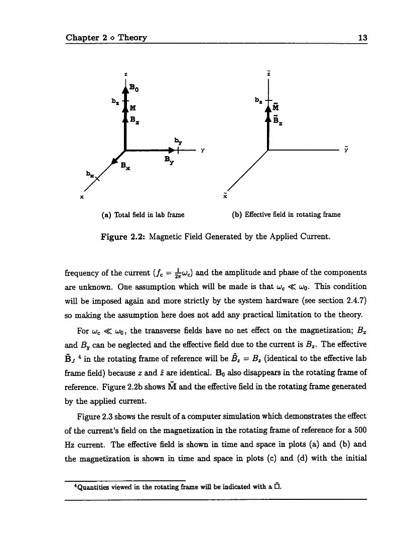
Chapter 2 O Tbeory 13
(a) Total field in lab frame (b) Effective field in rotating frame
Figure 2.2: Magnetic Field Generated by the Applied Current.
frequency of the current (f, = &oc) and the amplitude and phase of the components
are unknown. One assumption which will be made is that w, « wo. This condition
will be imposed again and more strictly by the system hardware (see section 2.4.7)
so making the assumption here does not add any practical limitation to the theory.
For w, « wo, the transverse fields have no net effect on the magnetization; B,
and By can be neglected and the effective field due to the cment is B,. The effective
BJ in the rotating frame of reference wiU be B, = Bz (identical to the eEective lab
frarne field) because z and Z are identical. Bo &O disappears in the rotating frame of
reference. Figure 2.2b shows M and the effective field in the rotating frame generated
by the applied current.
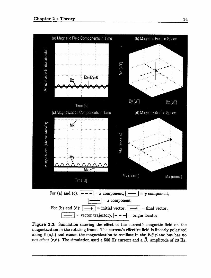
Figure 2.3 shows the result of a computer simulation which demonstrates the effect
of the current's field on the magnetization in the rotating frame of reference for a 500
Hz current. The effective field is shown in time and space in plots (a) and (b) and
the magnetization is shown in t h e and space in plots (c) and (d) with the initial
'Quantities viewed in the rotating fiame will be indicated with a O.
Chapter 2 o Theory 14
For (a) and (c): [-l= 2 component, = # component,
1 - 1 = Z component
For (b) and (d): = initial vector, = h d vector,
= vector trajectory, 1-1 = origin locator
Figure 2.3: Simulation showing the eEect of the current's magnetic field on the magnetization in the rotating frame. The current 's effective field is linearly polarized dong 5 (a,b) and causes the magnetization to oscillate in the 2 4 plane but has no net effect (c,d). The simulation used a 500 Hz current and a B= amplitude of 20 Hz.
Chapter 2 O Theory 15
(RF) BI
I I .
Magnetization Cuvent Image Preparation Encoding Acquisition
Current
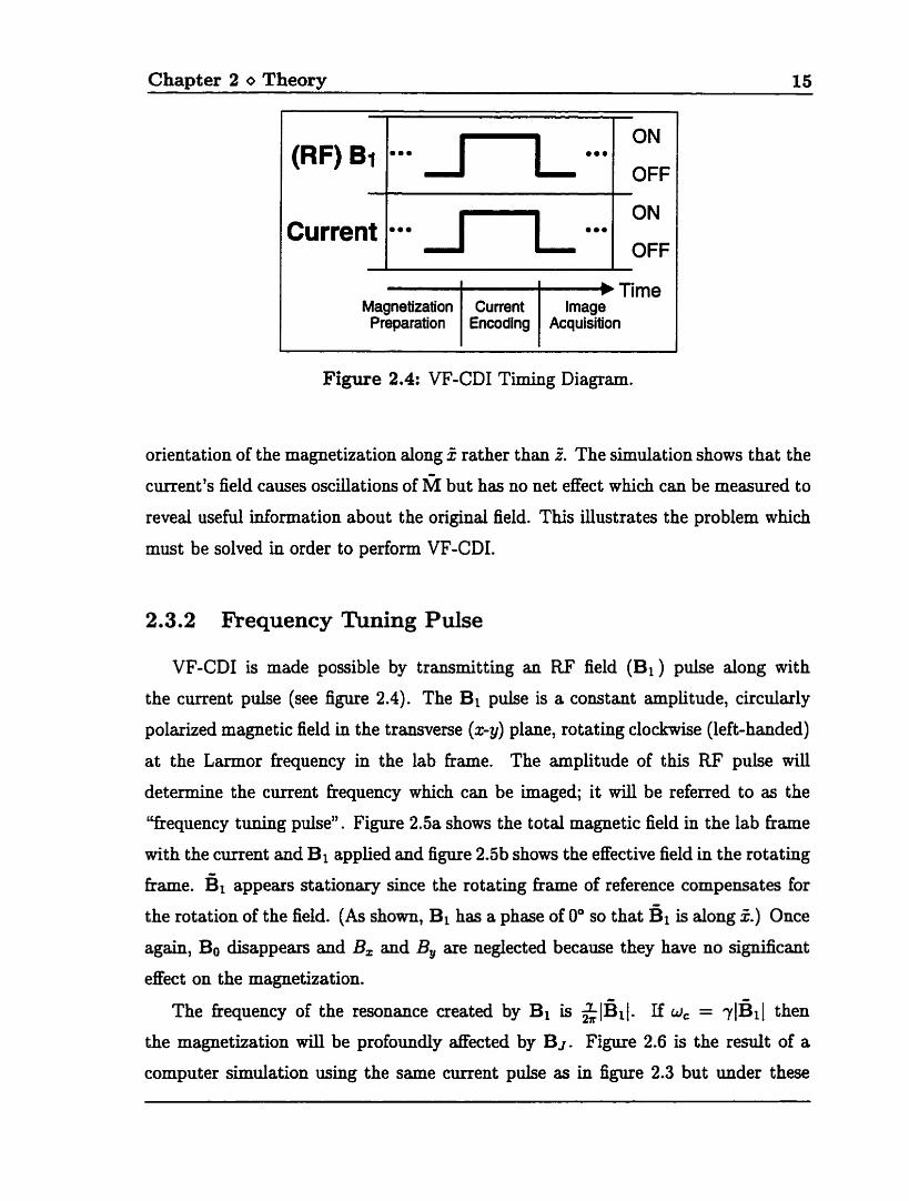
Figure 2.4: VF-CD1 Timing Diagram.
.a. 1 - o..
orientation of the magnetization dong 2 rather than i. The simulation shows that the
current's field causes oscillations of M but has no net effect which can be measured to
reveal usefd information about the original field. This illustrates the problem which
must be solved in order to perform VF-CDI.
ON
OFF
1-1
2.3.2 Frequency Tuning Pulse
ON
OFF
VF-CD1 is made possible by transmitting an RF field (BI ) pulse dong with
the current pulse (see figure 2.4). The Bi pulse is a constant amplitude, circularly
polarized magnetic field in the transverse (x-y) plane, rotating clockwise (left-handed)
at the Larmor fiequency in the lab hame. The amplitude of this RF pulse will
determine the curent fkequency which can be imaged; it will be referred to as the
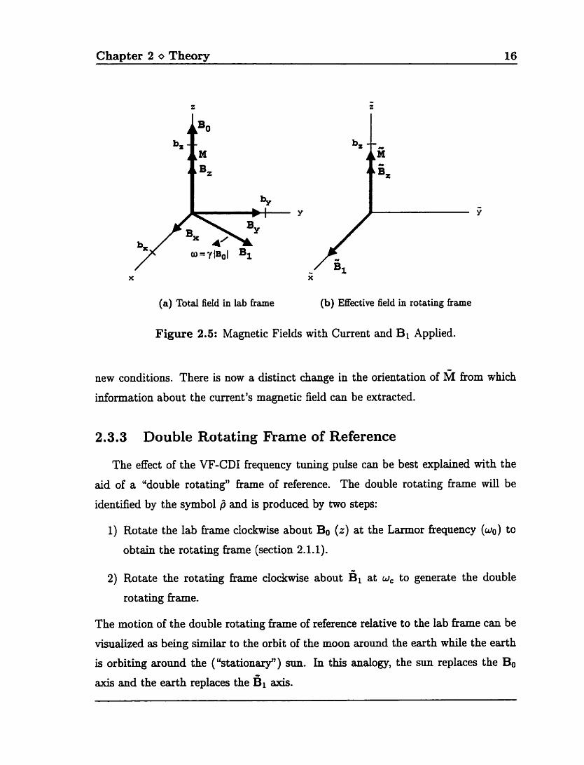
"fiequency tuning pulse". Figure 2.5a shows the total magnetic field in the lab Bame
with the current and Bi applied and figure 2.5b shows the effective field in the rotating
£rame. & appears stationary since the rotating Bame of reference compensates for
the rotation of the field. (As shown, Bi has a phase of O" so that is dong 2) Once
again, Bo disappears and B, and B, are neglected because they have no significmt
effect on the magnetization.
The fkequency of the resonance created by Bi is $16~1. If w, = rlBll then
the magnetization will be profoundly affected by Bj. Figure 2.6 is the r e d of a
cornputer simulation using the same m e n t pulse as in figure 2.3 but under these
Chapter 2 o Theory 16
(a) Total field in lab trame (b) Effective field in rotating kame
Figure 2.5: Magnetic Fields with Current and Bi Applied.
new conditions. There is now a distinct change in the orientation of M fkom which
information about the curent's magnetic field can be extracted.
2.3.3 Double Rotating Frame of Reference
The effect of the VF-CD1 frequency tunllig pulse can be best explained with the
aid of a "double rotating" hame of reference. The double rotating hame wiU be
identified by the symbol j and is produced by two steps:
1) Rotate the lab frame clockwise about Bo (2) at the Larmor frequency (wo) to
obtain the rotating frame (section 2.1.1).
2) Rotate the rotating frame clockwise about at LI, to generate the double
rot ating hame.
The motion of the double rotating frame of reference relative to the lab fiame can be
visualized as being similar to the orbit of the moon around the earth while the earth
is orbiting around the ("stationary") sun. In this analogy, the sun replaces the Bo
axis and the earth replaces the B~ iuris.
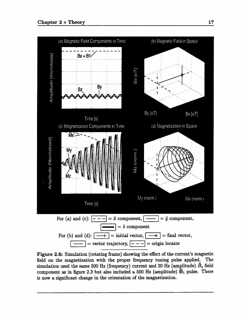
Chapter 2 Q Theory 17
For (a) and (c): = 5 component, [=I = component,
[- 1 = Z component
For (b) and (d): = initial vector, IYI = final vector,
= vector trajectory, FI= origin locator
Figure 2.6: Simulation (rotating hame) showing the efSect of the current's magnetic field on the magnetization with the proper frequency tuning pulse applied. The simulation used the same 500 Hz (fkequency) cwent and 20 Hz (amplitude) fiz field cornponent as in figure 2.3 but also included a 500 Hz (amplitude) pulse. There is now a sigdicant change in the orientation of the magnetization.

Chapter 2 o Theory 18
The j kame will compensate for the left-handed rotation of fields and rnagneti-
zation about Bi at w, and for the field pardel to Ë1 with a magnitude equd to 7 in the rotating fiame. This is identical to the rotating frame's compensation for the
left-handed rotation of fields and magnetization about Bo at wo and for the Bo field
in the lab frame. If 1 B~ 1 is exactly equd to 7 then B will disappear completely from
p. Otherwise there will be a AB^ off-resonance field in 6 equd to El - 7 , similar
to the AB, off-resonance field in the rotating fiame.
An important feature of @ is that the second rotation (rotation of the rotating
frame) does not interfere with the h s t (rotation of the lab kame) so fields and
rotations which are eliminated in the rotating kame do not reappear in P. For
example, f i experiences the same rotation at wo relative to the lab hame as does the
rotating hame. Therefore, the Bo field which disappears in the rotating came is not
present in either.
The usefulness of the double rotating £rame can be seen in figure 2.7 which shows
the case of figure 2.6 when viewed in P. The spiral motion of M is converted to a
circular arcing of M which is the result of an effective j j field. This ci field will be
determined next.
2.3.4 Determining the Effective Field in @
There are three approaches which will be presented for deriving the B~ field.
These are:
a Logical Derivation
a Mathematical Derivation
Andogy With Basic MRI
Each of these methods ends with the same r d t but ail are presented in order to
give a more complete understanding of how and why VF-CD1 works.
SQuantities viewed in the f i fiame will be indicated wïth a Ô. 6 ~ e E consists of an ideal & component and a possible A& off-resonance term.
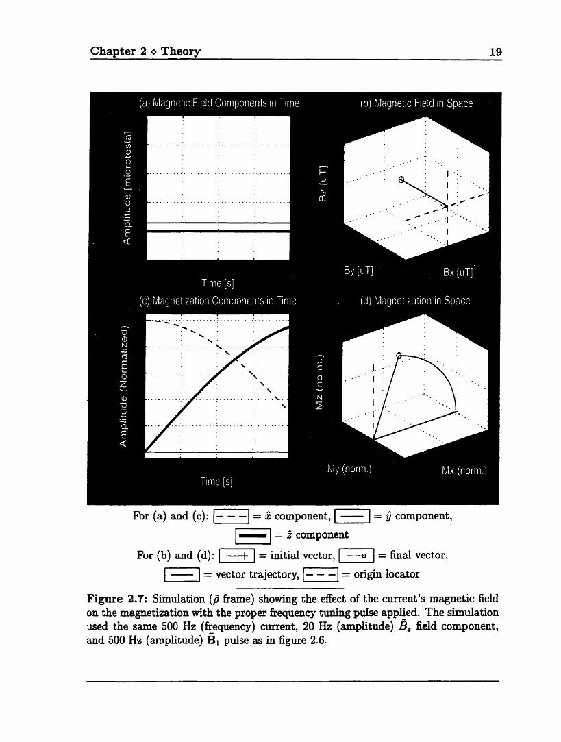
Chapter 2 O Theory 19
For (a) and (c): (-1 = I component, = y component,
= î component
For (b) and (d): (1 = initial vector, = £inal vector,
F] = vector trajectory, 1-1 = origin locator
Figure 2.7: Simulation (P fiame) showing the effect of the cunent's magnetic field on the magnetization with the proper £requency hining pulse applied. The simulation used the same 500 Hz (kequency) m e n t , 20 Hz (amplitude) field component, and 500 Hz (amplitude) fi1 pulse as in figure 2.6.
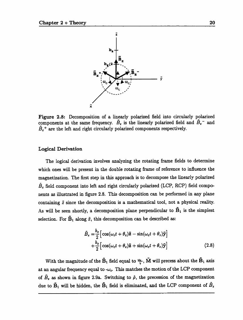
Chapter 2 O Theory 20
Figure 2.8: Decomposition of a linearly polarized field into circularly polarized components at the same fkequency. B~ is the linearly polarized field and fiz- and B, + are the left and right circularly polarized components respectively.
Logical Derivation
The logicd derivat ion involves analyzing the rot ating fiame fields t O det ermine
which ones will be present in the double rotating kame of reference to influence the
magnetization. The first step in this approach is to decompose the linearly polarized
B= field component into left and right circularly polarized (LCP, RCP) field compo-
nents as illustrated in figure 2.8. This decomposition can be performed in any plane
containing t since the decomposition is a mathematical tool, not a physical reality.
As will be seen shortly, a decornposition plane perpendicular to Bi is the simplest
selection. For BI dong 2, this decomposition can be described as:
With the magnitude of the B~ field equal to y, M wi l l precess about the ~1 a i s
at an angular fiequency equal to -w, This matches the motion of the LCP component
of 9 as shown in figure 2.9a. Switching to $, the precession of the magnetization
due to Ë1 will be hidden, the field is eliminated, and the LCP component of B,
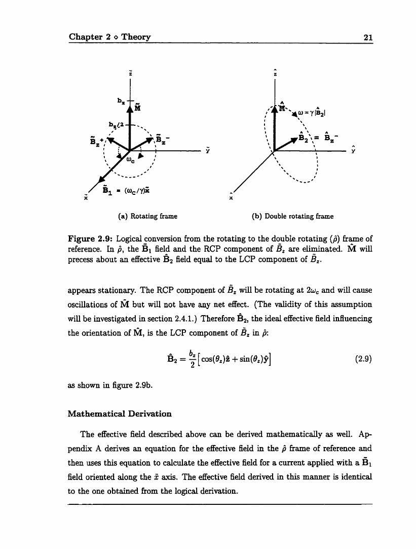
Chapter 2 o Theory 21
(a) Rotating frame (b) Double rotating frame
Figure 2.9: Logical conversion from the rotating to the double rotating (/î) fiame of reference. In p, the field and the RCP component of BZ are eliminated. M d l precess about an effective Êj2 field equal to the LCP component of fi,.
appears stationary. The RCP component of B~ will be rotating at 2uc and will cause
oscillations of but d l not have any net effect. (The validity of this assumption
will be investigated in section 2.4.1.) Therefore Ê2, the ided effective field infiuencing
the orientation of M, is the LCP component of È, in fi:
as shown in figure 2.9b.
Mat hematicd Derivat ion
The effective field described above can be derived mathematically as well. A p
pendix A derives an equation for the effective field in the kame of reference and
then uses this equation to calculate the effective field for a current applied with a fi1 field oriented dong the 5 The effective field derived in this manner is identical
to the one obtained fiom the logical derîvation.
Chapter 2 o Theory 22
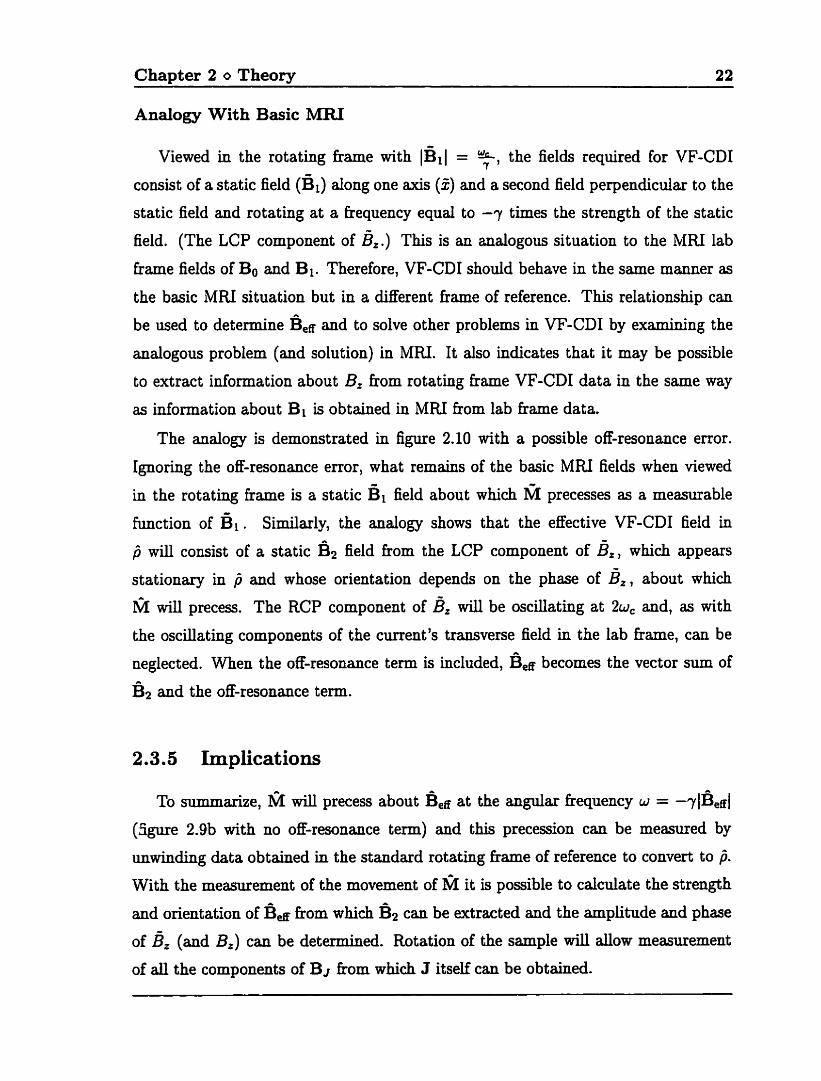
Analogy With Basic MRI
Viewed in the rotating kame with I& ( = 7 , the fields required for VF-CD1
consist of a static field (B~) dong one axis (5) and a second field perpendicular to the
static field and rotating at a fiequency equal to -7 times the strength of the static
field. (The LCP component of B, .) This is an analogous situation to the MRI lab
k a m e fields of Bo and Bi. Therefore, VF-CD1 should behave in the same manner as
the basic MRI situation but in a different fiame of reference. This relationship can
be used to detennine Ber and to solve other problems in VF-CD1 by exitmiring the
analogous problem (and solution) in MRI. It also indicates that it may be possible
to extract information about Bz fiom rotating frame VF-CD1 data in the same way
as information about Bi is obtained in MRI from lab frame data.
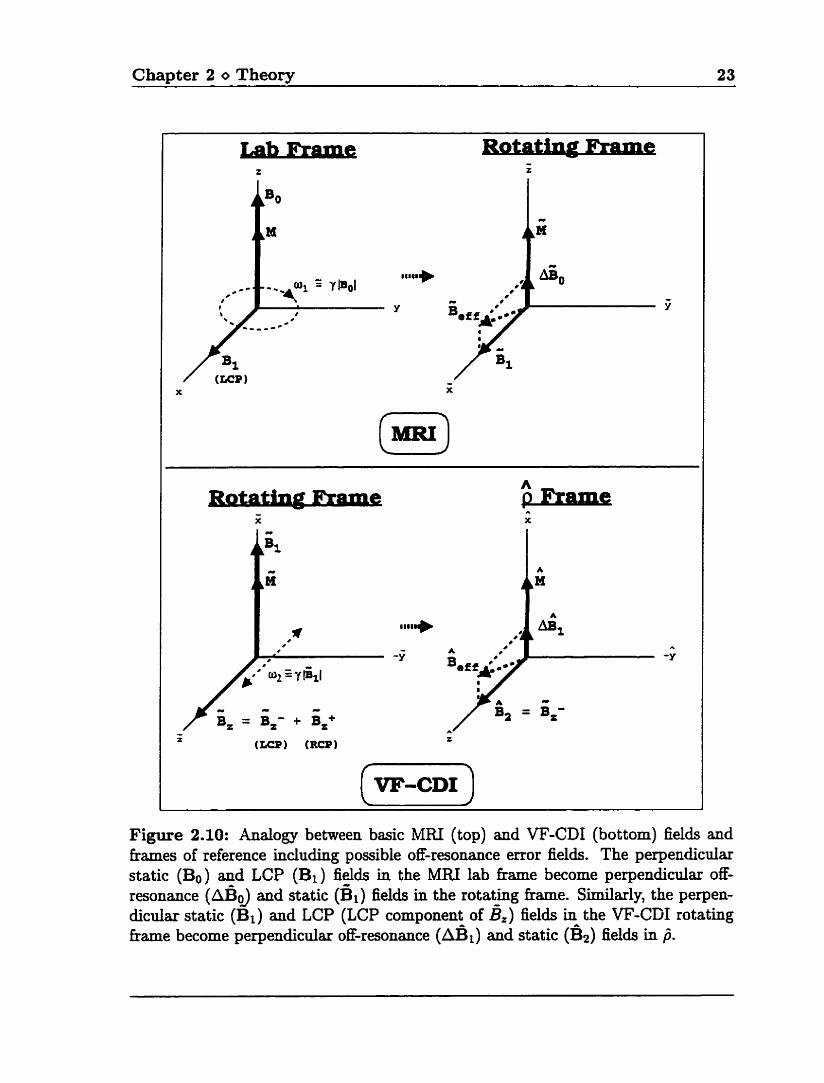
The analogy is demonstrated in figure 2.10 with a possible off-resonance error.
Ignoring the off-resonance error, what remains of the basic MRI fields when viewed
in the rotating hame is a static Ë1 field about which 6l precesses as a measurable
hrnction of BI . Similarly, the analogy shows that the effective VF-CD1 field in
j will consist of a static B, field hom the LCP component of B,, which appeaxs
stationary in and whose orientation depends on the phase of &, about which
M 32 precess. The RCP component of BZ will be oscillating at 2wc and, as with
the oscillating components of the curent's transverse field in the lab fiame, can be
neglected. When the off-resonance t e m is included, B , ~ becornes the vector s u m of
B* and the off-resonance term.
2.3.5 Implications
To summarize, M will precess about Ê)& at the angular fiequency w = -?lÊeirl
(Sgure 2.9b with no off-resonance te=) and this precession can be measured by
unwinding data obtained in the standard rotating kame of reference to convert to 6. With the measurement of the movement of M it is possible to calculate the strength
and orientation of B~ kom which B~ can be extracted and the amplitude and phase
of B= (and Bz) can be detezmined. Rotation of the sample will allow measurement
of all the components of Br bom which J itself can be obtained.
Chapter 2 O Theory 23
Figure 2.10: Analogy between basic MRI (top) and VF-CD1 (bottom) fields and fiames of reference including possible off-resonance error fields. The perpendicular static (Bo) and LCP (Bi) fields in the MM lab kame become perpendicular off- resonance (&d and static (&) fields in the rotating fiame. Similady, the perpen- dicular static (BI) and LCP (LCP component of &) fields in the VF-CD1 rotating frame become perpendicular off-resonance AB^) and static (B,) fields in P.
Chapter 2 o Theory 24
2.3.6 Computer Simulation
The results of the computer simulation which were used to demonstrate the pre-
dictions of VF-CD1 can also be used to verify the accuracy of the theory. Consider
the case of a 500 Hz (frequency) current and a 500 Hz (amplitude) fiequency tuning
Ë1 field in the rotating hame as in figure 2.6. A 20 Hz amplitude B, field with an
initial phase of 8, = 90' would be expected to generate a 10 Hz Bz (= Ben) field
dong Y. With fi initiaüzed dong Z (M initialized dong 5) the theory predicts that
Ph wii l precess about in the 6 2 plane at a fiequency of 10 Hz. When viewed in the
rotating kame the precession would be expected to include a spiraling motion due to
the presence of el. Plot (a) shows the constant & (= BI) and sinusoidal B, fields in
t h e . Plot (b) shows the total (effective) field in space. The path traced out by the
tip of the field vector is shown dong with the initial (+) and ha1 ( O ) vectors. Plot (c)
shows the cornponents of M in tirne and confirms the predicted results. 6l is rotating
into the transverse plane at a fiequency of 10 Hz and the transverse components are
rotating about Ël at a fkequency of 500 Hz. Plot (d) shows the path traced out by
the tip of M in tirne.
The computer simulation can also be nui in b. This has been done and displayed
in figure 2.7 for the same case as figure 2.6. (For clarity, the RCP component of 4, has been removed. Its effects will be investigated in section 2.4.1.) Plot (a) shows
the 10 Hz (amplitude) B~~ dong & due to the LCP component of B,. The spiraling,
spherîcal motion of the magnetization in the rotating kame is unwound and appears
as a 10 Hz circula motion in the 2-2 plane.
2.4 Pract ical Considerat ions
Other than a bnef mention of an off-resonance error tem, the description of the
theory of VF-CD1 has so far assumed ideal conditions. However, there are a number
of practical, non-ideal issues which much be addressed such as:
0 Right circularly polarized component of &,
Chapter 2 o Theory 25
a
a
O
O
O
This
Bo and BI inhomogeneity
Relaxation
Phase wrapping
Fkequency range
Current phase
section will investigate these practicd considerations, determine their severity,
and propose solutions and compensation techniques where possible.
2.4.1 RCP Component of 8, In the initial description of VF-CDI, the transition from the rotating hame of
reference to @ assumeci that the RCP component of B, cauld be neglected in p . The reasoning was that this component would appear to be rotating at an angular
frequency of 2wc in /î and would therefore cause small oscillations in the orientatim
of Ph but would have no net effect. The vaüdity of this assumption will now be
examined.
The ideal case consists of a cosinusoidal current (and correspondhg magnetic
fields) with an initial phase of 90" and M initiaiized dong Z at the t h e when the ËI
field is applied along the I a i s . In P these fields reduce to a constant B~ field along
the y axis and M wiii precess in the 2-2 plane at a constant frequency. This situation
was shown in figure 2.7 ( f i fiame of reference).
If the RCP component is included in the P then it will have an effect on the
magnetization as shown in figure 2.11. The RCP component causes M to wobble
in the y direction as it precesses. The wobble in one direction during the first half
of the RCP component's cycle is ''undone" during the second half of the cycle. A
convenient method of measuring the orientation of the magnetization is by using the
phase of M in the ideal plane of precession. A comparison of this phase for the ideal
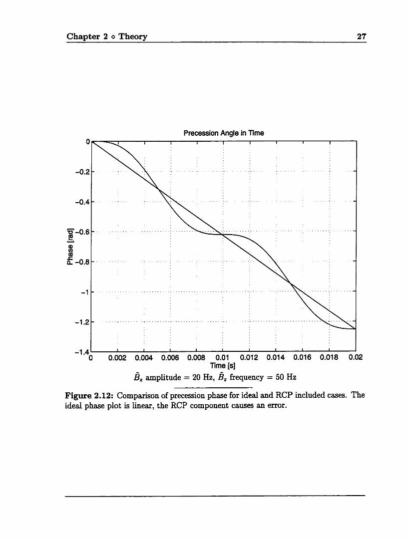
and RCP included cases (figure 2.12) shows that if the duration of the current pulse
is a multiple of & seconds (one quarter of the period of the current) then there is

Chapter 2 O Theory 26
For (a) and (c): = ii component, = 6 component,
1 - 1 = i component
For (b) and (d): = initid vector, [FI = b a l vector,
= vector trajectory, /-1- oriongin locator - - -
Figure 2.11: Simulation in j showhg the effect of the RCP component of B,. The simulation used a 50 Hz (frequency) curent, 20 Hz (amplitude) & field component and 500 Hz (amplitude) É1 pulse. hcluding the RCP component of Ëz causes a change fkom the ideal case of figure 2.7.
Chapter 2 o Theory
Precession Angle in Time 1
1 -
-
1 -
-
-
-
-1.4- O 0.002 0.004 0.006 0.008 0.01 0.012 0.014 0.016 0.018 0.02
Time [s3
amplitude = 20 Hz, kequency = 50 Hz
Figure 2.12: Cornparison of precession phase for ideal and RCP included cases. The ideal phase plot is linear, the RCP component causes an error.
Chapter 2 o Theory 28
almost no error in the phase measmement. This is true for O, = 90". In generai, the
zero error duration is a multiple of -& seconds. This leads to the conclusion that
the duration of the current pulse should be a multiple of one half of the period of the
current to rninimize the effects of the RCP component. If it is made to be a multiple
of the penod itself then an additional advantage arises because the fi and rotating
Erarnes will coincide and no post-processing will be required to unwind the fi data.
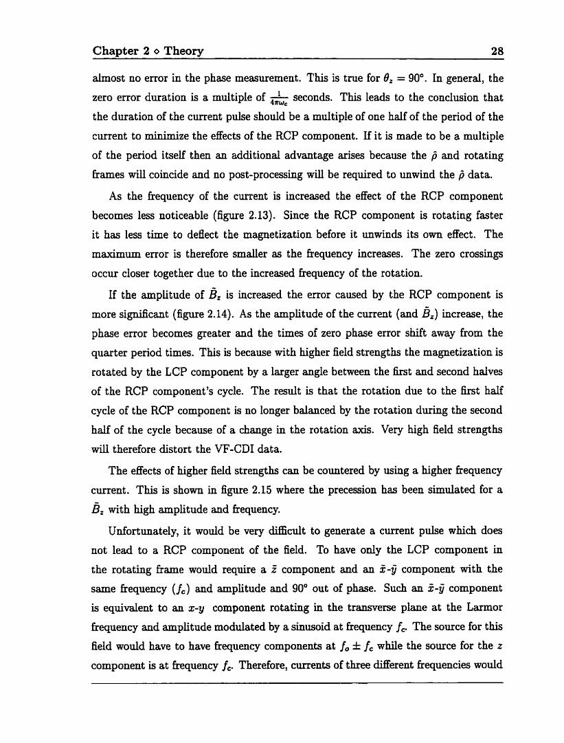
As the fiequency of the current is increased the effect of the RCP component
becomes l e s noticeable (figure 2.13). Since the RCP component is rotating faster
it has less tirne to deflect the magnetization before it unwinds its own effect. The
maximum error is therefore srnder as the fiequency increases. The zero crossings
occur closer together due to the increased kequency of the rotation.
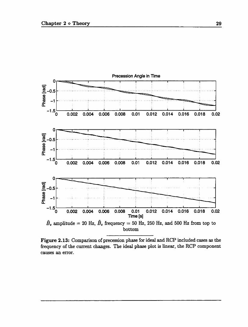
If the amplitude of B~ is increased the error caused by the RCP component is
more si&cant (figure 2.14). As the amplitude of the current (and 61,) increase, the
phase error becomes greater and the times of zero phase error shift away from the
quarter period times. This is because with higher field strengths the magnetization is
rotated by the LCP component by a larger angle between the first and second halves
of the RCP component's cycle. The result is that the rotation due to the kt half
cycle of the RCP component is no longer balanced by the rotation during the second
half of the cycle because of a change in the rotation axis. Very high field strengths
will therefore distort the VF-CD1 data.
The effects of higher field strengths can be countered by using a higher frequency
current. This is shown in figure 2.15 where the precession has been simulated for a
B, with high amplitude and frequency.
Unfortunately, it would be very diaicult to generate a current pulse which does
not lead to a RCP component of the field. To have only the LCP component in
the rotating kame would require a 2 component and an 5-jj component with the
same fiequency (f,) and amplitude and 90" out of phase. Such an 2-fj component
is equivalent to an x-y component rotating in the transverse plane at the Larmor
fiequency and amplitude modulated by a sinusoid at fkequency f, The source for this
field would have to have frequency components at f, f: f, while the source for the r
component is at frequency f,. Therefore, currents of three different fiequencies would
Chapter 2 O Theory 29
Precession Angle in Time
-1.5 ' 1 I 1 1 I 1 1 I 1 I O 0.002 0.004 0.006 0.008 0.01 0.012 0.014 0.01 6 0.018 0.02
Tirne [s] Ë, amplitude = 20 Hz, B= fiequency = 50 Hz, 250 Hz, and 500 Hz hom top to
bottom
Figure 2.13: Cornparison of precession phase for ideal and RCP hequency of the current changes. The ideal phase plot is linear, causes an error.
included cases as the the RCP component
Chapter 2 O Theow 30
Precession Angle in T h e
Dz amplitude = 40 Hz (top) and 100 Hz (bottom), BZ fiequency = 50 Hz
Figure 2.14: Cornparison of precession phase for ideal and RCP included cases as the amplitude of the current changes. The ideal phase plot is linear, the RCP cornponent causes an error.
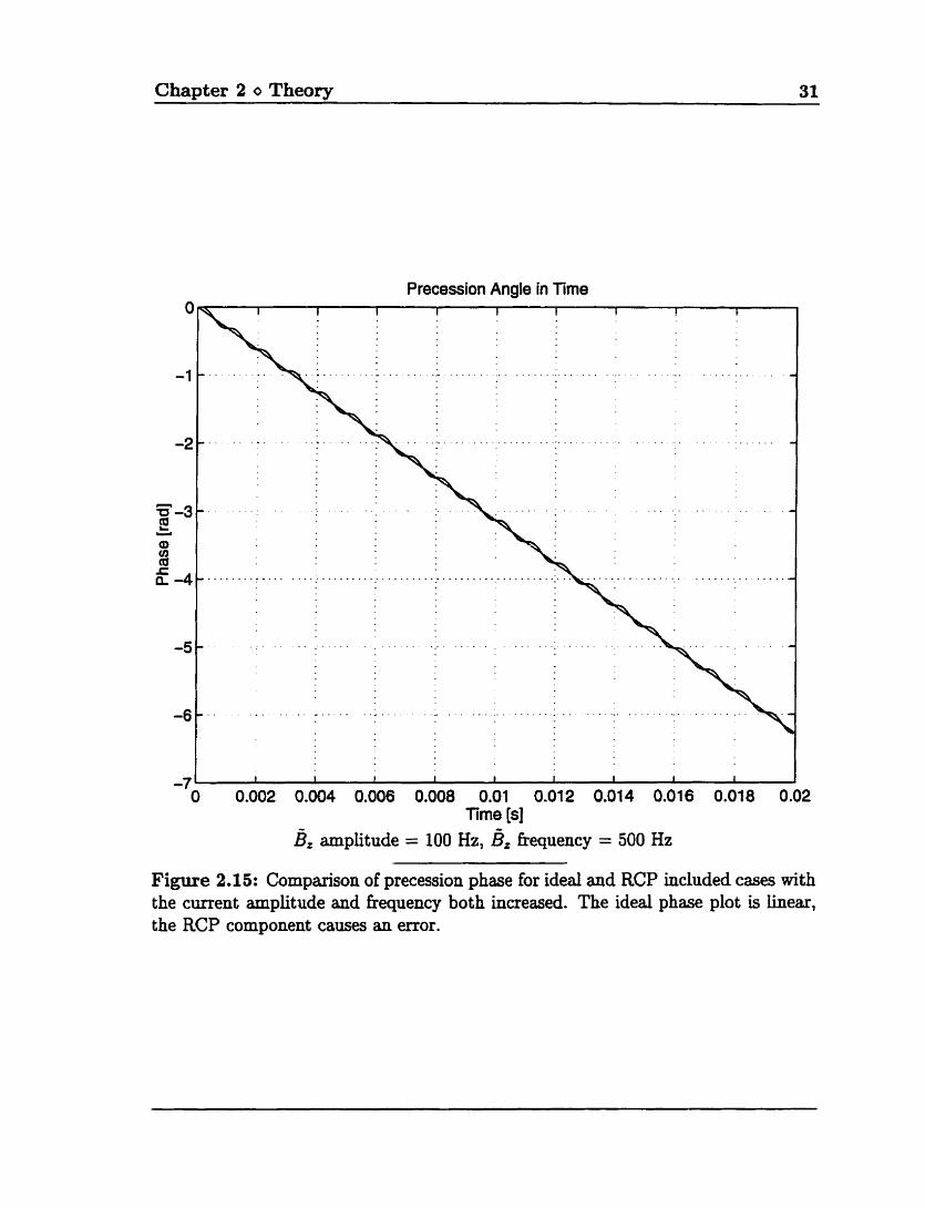
Chapter 2 O Theory 31
Precession Angle in Tirne I I I 1 1
O 0.002 0.004 0.006 0.008 0.01 0.012 0.014 0.016 0.018 0.02 Time [s]
B* amplitude = 100 Hz, frequency = 500 Hz
Figure 2.15: Cornparison of precession phase for ideal and RCP included cases with the curent amplitude and fiequency both increased. The ideal phase plot is linear, the RCP component causes an error.
Chapter 2 o Theory 32
be required but because of the frequency and tissue dependence of the amplitude and
phase of the current density it would not be possible to ensure the correct amplitude
and phase relationships between the components. Also, it would no longer be possible
to observe the current density distribution at a single frequency.
2.4.2 Off-Resonance
If the strength of Bi is not properly tuned to f, then an off-resonance effect occurs
which c m be modeled by a A& field in fi equal to the difference between the actual
and correct Bi fields. This mode1 applies regardless of whether the error is the result
of a change in either the current frequency or the amplitude of Bi. BeE becomes the
sum of B~ (the ideal effective field in f i ) and aBi and as the off-resonance becomes
greater the effective field is dominated by AB,. When this occurs, the precession of
Ph will be rnainly influenced by AB, and the effects of B~ will be masked. The exact
ratio of Ê2 to AB, at which the curent field can no longer be measured will depend
on the noise level in the imaging system and sensitivity of the VF-CD1 processing
t ethnique.
Figure 2.16 is the result of a simulation with the same parameters as in figure 2.6
but with a 600 Hz (frequency) curent. This yields a ÊeE which is the vector s u m
of the 10 Hz field dong @ and a 100 Ha AB^ field dong -2. The effective field
is orientecl 5.7' off of the -5 axis and has an amplitude of I/- = 100.5 Hz.
When viewed in the rotating frame M will appear to wobble in and out of the i - L plane at 100.5 Hz while remaining mostly dong 5.
A very large off-resonance will prevent measurement of the current's fields. The
case of a s m d off-resonance should ais0 be considered in order to determine the best
method of compensation. The effect of including a small error is demonstrated in
figure 2.17 which shows plots in the kame of reference for 10 Hz (amplitude) B* and
1 Hz (amplitude) A& fields. This is the Ê2 field generated by a 20 Hz (amplitude)
BZ field with a phase of Oz = 90' and a 1 Hz off-resonance. A cornparison with the on-
resonance case in figure 2.7 shows that the A& off-resonance field does indeed change
the expected orientation of the magnetization. In the ideal case, the magnetization
precesses in the 2-Z plane with the phase of M incleasing linearly, proportional to 82.
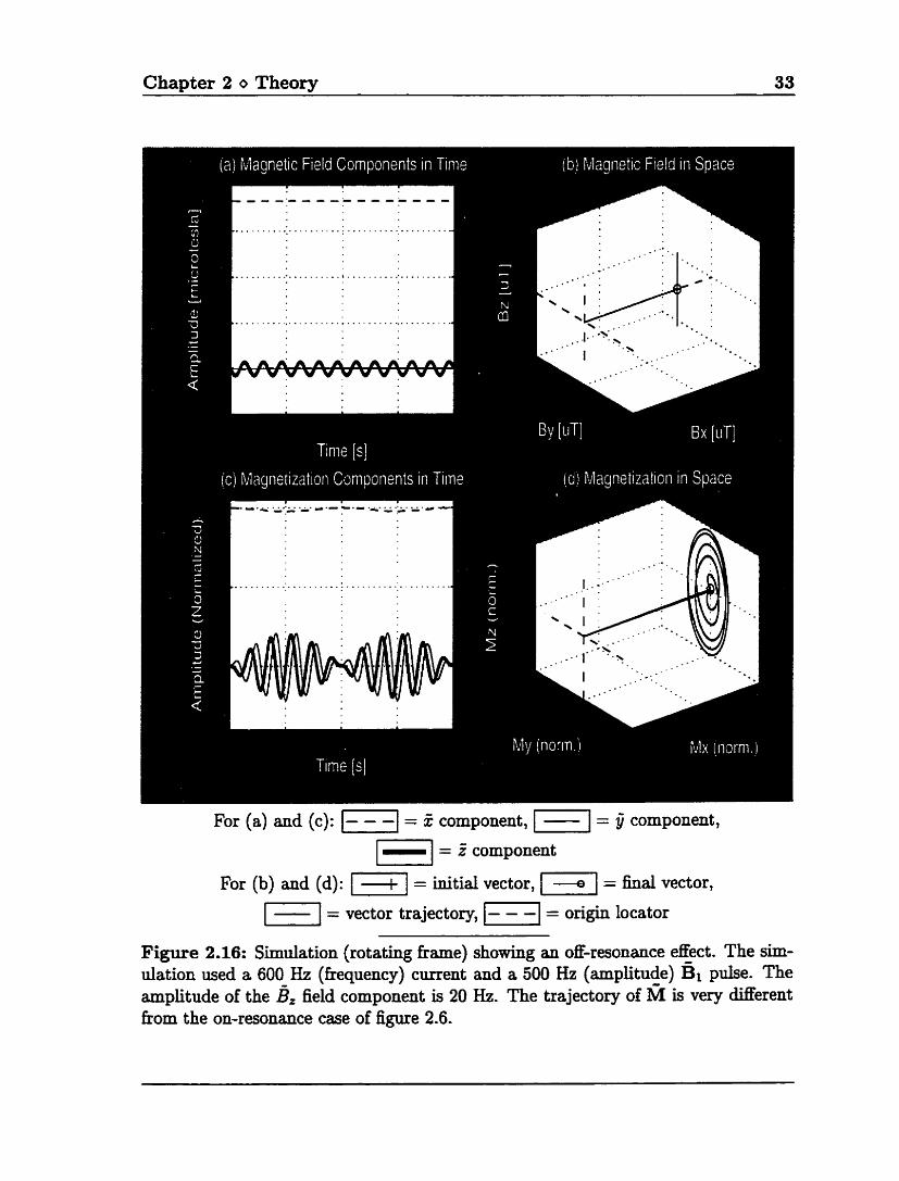
Chapter 2 o Theory 33
For (a) and (c): F I = Z component, = ij icomponent,
1 - ( = Z component
For (b) and (d): -1 = initial vector, = hd vector,
= vector trajectory, F I = orïgin locator
Figure 2.16: Simulation (rotating frame) showing an off-resonance efFect. The sim- ulation used a 600 Hz (frequency) current and a 500 Hz (amplitude) & pulse. The amplitude of the É), field component is 20 Hz. The trajectory of M is very different fiom the on-resonance case of figure 2.6.
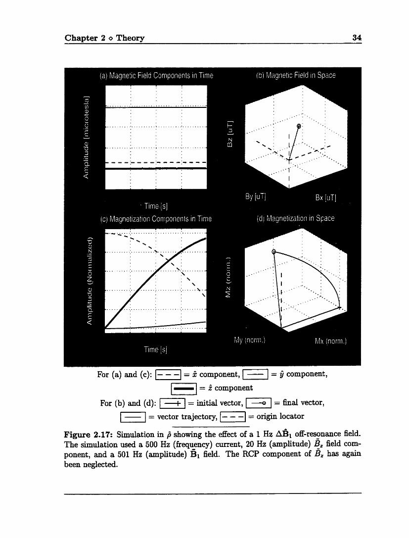
Chapter 2 o Theory 34
For (a) and (c): 1-1 = 2 component, = component,
1 - 1 = Z component
For (b) and (d): = initial vector, = final vector,
F I = vector trajectory, F I = o@n locator
Figure 2.17: Simulation in f i showing the effect of a 1 Hz A& off-resonance field. The simulation used a 500 Hz (kequency) current, 20 Hz (amplitude) B= field com- ponent, and a 501 Hz (amplitude) Bi field. The RCP component of B= has again been neglected.
Chapter 2 O Theory 35
Precession Angle in Thne
-7 l I 1 I i 1 t I I 1 J O 0.002 0,004 0.006 0.008 0.01 0.012 0.014 0.016 0.018 0.02
Time [s]
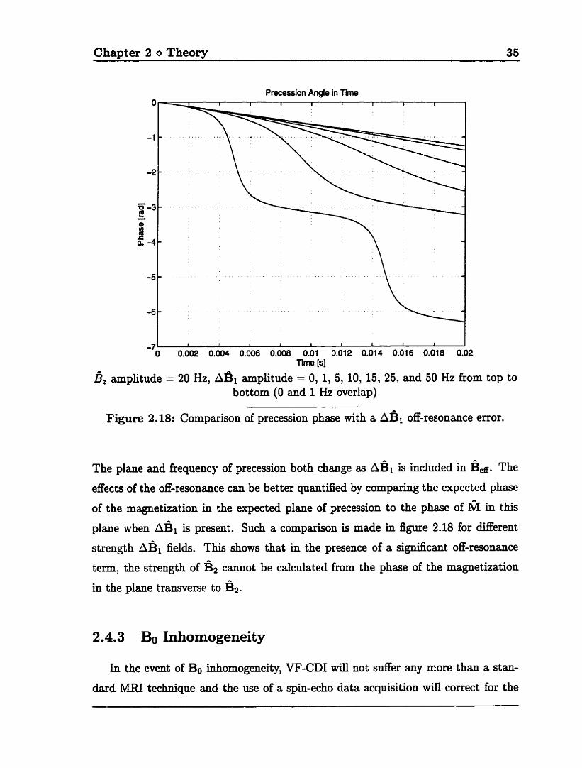
& amplitude = 20 Hz, AB^ amplitude = 0, 1, 5, 10, 15, 25, and 50 Hz from top to bottom (O and 1 Hz overlap)
Figure 2.18: Cornparison of precession phase with a A& off-resonance error.
The plane and frequency of precession both change as hB1 is included in B ~ . The
effects of the off-resonance can be better quantified by comparing the expected phase
of the magnetization in the expected plane of precession to the phase of M in this
plane when A& is present. Such a cornparison is made in figure 2.18 for different
strength A& fields. This shows that in the presence of a significant off-resonance
terrn, the strength of fi2 c w t be cdculated kom the phase of the magnetization
in the plane transverse to B2.
In the event of Bo inhomogeneity, W-CD1 will not SUffer any more than a stan-
dard MRI technique and the use of a spin-echo data acquisition wi l l correct for the
Chapter 2 O Theory 36
precession mors during the time between data preparation and acquisition. With
regard to field interactions in VF-CD1 while the current is applied, a ABo field will
appear in fi Like the RCP component of Ë, but will be oscillating at only w, instead
of 2wc. By using a current pulse with a duration of a multiple of the penod of the
current this error will dso be minimized.
2.4.4 Bi Inhomogeneity
In the ideal case, B~ will be perfectly uniform over the entire subject and the
amplitude will be tuned to the exact, on-resonance value. However, this ideal case is
unlikely in a practical imaging situation and it d l be shown in chapter 3 that Bi
amplitude inhomogeneity shodd be expected. This inhomogeneity will appear as an
off-resonance error and will have an effect as discussed in section 2.4.2. If the error is
small then it may be possible to ignore the effects of the inhomogeneity. Otherwise
it will have to be measured and taken into account. In addition to the off-resonance
effect on the fiequency tuning pulse, Bi inhomogeneity will cause errors in the effects
of the other RF pulses used and therefore in the results of VF-CDI.
The factors which contribute to BI inhomogeneity include a non-uniform transmit
field as well as penetration, eddy current, and shielding effects. Field homogeneity has
been studied extensively, including the factors which contribute to BI inhomogeneity
[191, methods of measurement [20, 21, 22, 23, 241, and ways to correct the errors
[25, 26, 27, 281. The correction methods cannot be used in VF-CD1 because VF-
CD1 requires a constant amplitude BI pulse while the correction methods require
modulated pulses. Using a 180' current phase change halfway through the pulse, as
used in other CD1 techniques, will also not work as explained below.
B~ Field Reversal
The correction techniques used for Bo inhomogeneity in LF-CD1 (spin echo) and
B1 inhomogeneity in RF-CD1 (rotary echo)? will not work to correct BI inhomogene-
?The correction technique for Bi inhomogeneity in RF-CD1 does not correct for Bo inhomogeneity and will not correct BI inhomogeneity properly in the presence of Bo inhomogeneity.
Chapter 2 o Theory 37
ity in VF-CDI. This is because the error-free field and the error field are paralle1
in the other cases, but perpendicular in VF-CDI. In LF and RF-CDI, reversal of
the error field changes the frequency but not the aJris of precession resulting in an
mwinding of the accumulated error. In VF-CDI, a reversal of the error field wodd
change the axis as well as frequency of precession and wodd therefore not accurately
unwind the phase error.
2.4.5 Relaxation
The relaxation which the magnetization experiences between the preparation and
readout stages will have an eEect on the VF-CD1 measurements made. However, by
keeping the current pulse duration and echo tirne short these relaxation effects will
be minimal. Also, the applied BI field is continuously rotating the magnetization
and exchanging the transverse and longitudinal components. This further reduces
the relaxation problem as long as the period of rotation is shorter than the relaxation
times. The effective relaxation times for magnetization undergoing Bi rotation are
calculated in Scott 131.
2.4.6 Phase Wrapping
ü the current causes the magnetization to rotate by an angle greater than 27r there
will be some uncertainty in the exact number of rotations that the magnetization
has undergone. Rotations of an exact multiple of 27r will appear identical to no
rotation at all. These problems can either be corrected by unwrapping large phase
jumps or prevented by keeping the product of current amplitude and duration srnall
enough that the rotation is always less than Zr. Depending on the post-processing
technique, it may not be possible to unwind rotations greater than 2r and the product
of amplitude and duration will have to be kept small.
2.4.7 Frequency Range
The highest kequency at which VF-CD1 can operate is limited only by the max-
imum amplitude of the Bi fkequency tuning pulse (assuming that the field is homo-

Chapter 2 o Theory 38
geneous and accurate enough so off-resonance is not a problem). The actual value
of this maximum amplitude depends on such factors as power of the RF transmit-
ter, type of transmit coi1 used, size and composition of the subject, and duty cycle
of the RF trammitter in the imaging sequence. For the imaging setup used in this
thesis, the upper limit was found to be slightly greater than 1 kHz. (There is also a
maximum acceptable product of BI amplitude and duration based on the acceptable
power deposition limit of 0.4 W/kg.)
The lower Iimit on the VF-CD1 frequency range depends on the required system
performance rather than a hardware limit. As seen in section 2.4.1, the error caused
by the RCP component of 8, increases with decreasing frequency. When this error
becomes unacceptably large the lower frequency limit is established.
2.4.8 Current Phase
Using suitable hardware, it will be possible to select the initial phase of the applied
signal with very high accuracy. However, the phase of the curent at any given point
in the subject will depend on the complex conductivities of the tissues in the subject.
(This is not a problem in a homogeneous phantom for which o* is known.) For
frequencies below 100 MHz the complex conductivity is dominated by the conductivity
rather than the dielectric constant. As a result, the phase of the curent will not
display wide vaxiations. However, the phase of the complex conductivities udl v a q
between tissues and can not be expected to be zero 131. Therefore, it will be assumed
that the phase of the cunent (and the angle of fi2) is not known.
2.5 Imaging System Requirements
The VF-CD1 system will have two main componentsa. The k t is the data ac-
quisition and processing software and the second is the hardware for generating the
variable fiequency m e n t . Using the material presented in this chapter, the basic
requirements for both these components can be outlhed.
addition to the MR imaging system.
Chapter 2 o Theory 39
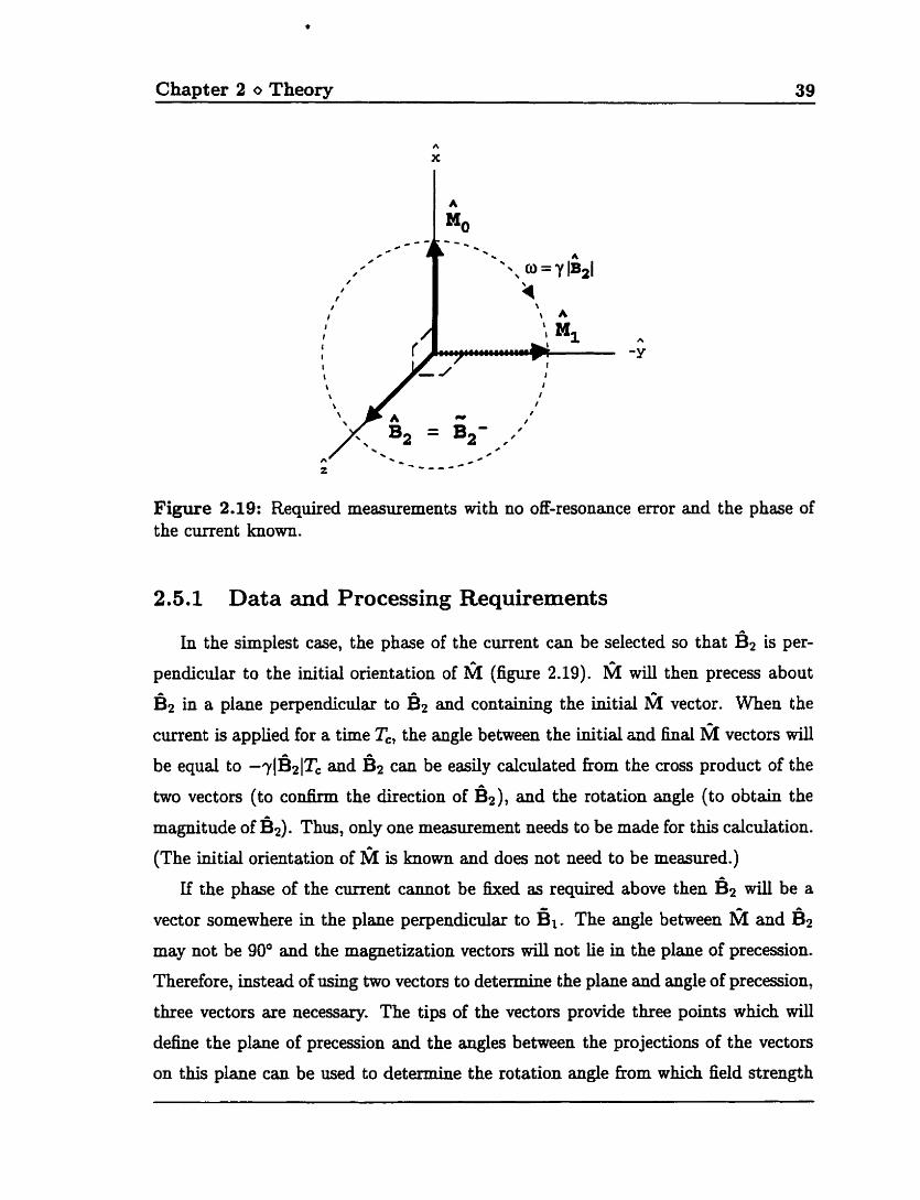
Figure 2.19: Required rneasurernents with no off-resonance error and the phase of the current known.
2.5.1 Data and Processing Requirements
In the simplest case, the phase of the current can be selected so that B~ is per-
pendicular to the initial orientation of M (figure 2.19). M will then precess about
in a plane perpendicular to Ê2 and containing the initial M vector. When the
cwent is applied for a time Tc, the angle between the initial and ha1 M vectors will
be equal to -?I&~T, and B* can be easily calculated from the cross product of the
two vectors (to c o h the direction of B ~ ) , and the rotation angle (to obtain the
magnitude of B2). Thus, only one measurement needs to be made for this cdculation.
(The initial orientation of M is known and does not need to be measured.)
If the phase of the current cannot be fked as required above then B* d be a
vector somewhere in the plane perpendicular to Ë1. The angle between M and Ê 2
may not be 90' and the magnetization vectors wîll not lie in the plane of precession.
Therefore, instead of using two vectors to determine the plane and angle of precession,
three vectors are necessary. The tips of the vectors provide three points which will
define the plane of precession and the angles between the projections of the vectors
on this plane can be used to determine the rotation angle fkom which field strength
Chapter 2 o Theory 40
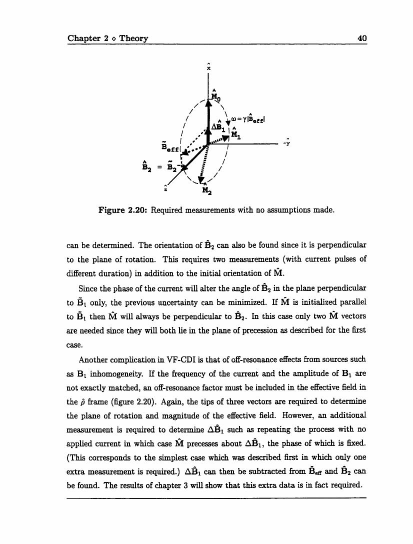
Figure 2.20: Required measurements with no a ssump t ions made.
can be deterrnined. The orientation of B* can also be found since it is perpendicular
to the plane of rotation. This requires two measurements (with current pulses of
different duration) in addition to the initial orientation of M.
Since the phase of the current will alter the angle of fi2 in the plane perpendicular
to Ë1 only, the previous uncertainty can be minimized. If M is initialized pardel
to GI then Ph w i l l always be perpendicular to B ~ . In this case o d y two M vectors
axe needed since they wi l l both lie in the plane of precession as described for the first
case.
-4nother complication in VF-CD1 is that of off-resonance effects fiom sources such
as BI inhomogeneity. If the fiequency of the current and the amplitude of BI are
not exactly matched, an off-resonance factor must be included in the effective field in
the j frame (figure 2.20). Again, the tips of three vectors are required to determine
the plane of rotation and magnitude of the effective field. However, an additional
measurement is required to determine AB^ such as repeating the process with no
applied current in which case M precesses about A&, the phase of whkh is fixed.
(This corresponds to the simplest case which was described first in which ouly one
extra measurement is required.) A& can then be subtracted kom and B~ can
be found. The results of chapter 3 will show that this extra data is in fact required.
Chapter 2 O Theory 41
In addition to the measurements described above for determining the values of the
various field parameters, data will be required in which neither the current nor the
BI field are applied. This reference information will be used to determine reference
magnitudes and phases hom which the other data will Mer. This reference data will
correct for artifacts such as offsets in k-space sarnpling, transfer hinction idueaces
of the M M transmit and receive systems, and other small systematic errors.
Quaternion Least Squares Rotation
The more cornplicated of the data requirements suggested repeating the imaging
sequence with current pulses of different lengths. However, changing the current pulse
duration while the sequence is ninning is very difncult. Instead, the same information
about axis and angle of rotation can be obtained by repeating the imaging sequence
with the initial orientation of the magnetization changed each time. The quaternion
least squares rotation algorithm 129, 301 can then be used to determine the axis and
angle of rotation fiom the sets of initial and ha1 orientations [3].
2.5.2 Applied Current
The current pulse required for VF-CD1 must interface with the MR system such
that it can be t m e d on and off dong with the fiequency tuning pulse. The pulse
must be identical each time it is turned on so that the phase encoding will be correct.
Other desired properties of the current pulse are that its Bequency, phase, amplitude,
and duration should a l l be adjustable by the operator.

CHAPTER 3
Bi Homogeneity
The previous chapter discussed the minimum data requirernents for VF-CD1 and
demonstrated that the presence of BI inhomogeneity would complicate the data ac-
quisition process for this technique. It is therefore necessary to determine the homo-
geneity of the Bi field and whether or not the extra steps must be taken to account
for errors in the field strength. Section 2.4.4 provided references giving reasons for
BI inhomogeneity and methods of measurement and correction. This chapter de-
scribes the experiments performed to characterize the Bi field and shows that the Bi
inhomogeneity cannot be neglected.
While it is possible for the BI field to be non-uniform in direction as well as in mag-
nitude, the results of the experiments reveded that direction inhomogeneity was only
present when using strong Bi fields with the extremity RF transmit coil. Therefore,
it wi l l be assumed that the direction of the field is accurate and the inhomogeneity
is in field amplitude only.
3.1 Method
The basic approach of the method to measure BI field strength is to begin by
allowing the rnagnetization to precess about a fi1 field (fkequency tuning pulse) for
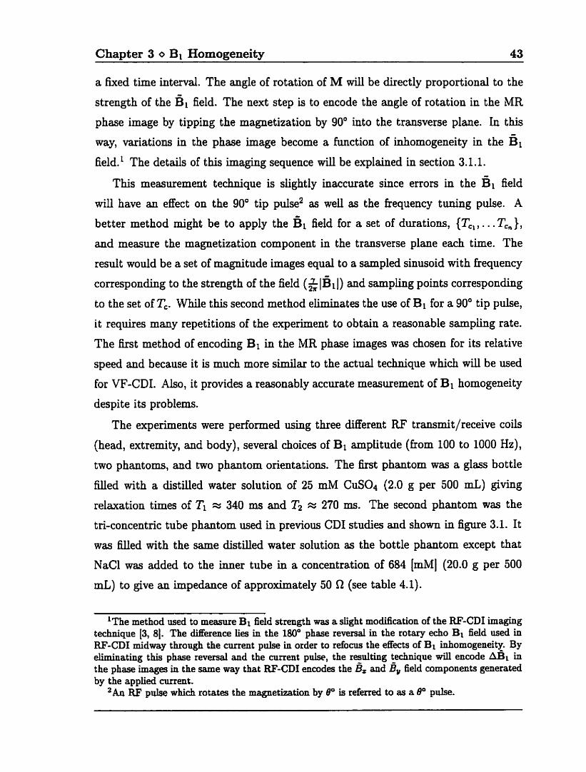
Chapter 3 o BI Homogeneity 43
a fixed time interval. The angle of rotation of M will be directly proportional to the
strength of the BI field. The next step is to encode the angle of rotation in the MR
phase image by tipping the magnetization by 90' into the transverse plane. In this
way, variations in the phase image become a huiction of inhomogeneity in the
field. The details of this imaging sequence will be explained in section 3.1.1.
This measurement technique is siightly inaccurate since errors in the Ë1 field
will have an effect on the 90" tip pulse2 as well as the frequency tuning pulse. A
better method might be to apply the ËI field for a set of durations, {Tc,, . . . Tcn), and measure the magnetization component in the transverse plane each tirne. The
result would be a set of magnitude images equal to a sampled sinusoid with frequency
corresponding to the strength of the field (& 1Ëi 1) and sampling points corresponding
to the set of Tc. While this second method eliminates the use of Bi for a 90' tip pulse,
it requires many repetitions of the experiment to obtain a reasonable sampling rate.
The first method of encoding Bi in the MR phase images was chosen for its relative
speed and because it is much more similar to the actual technique which will be used
for VF-CDI. Also, it provides a reasonably accurate measurement of Bi homogeneity
despite its problems.
The experiments were performed using three different RF transmit/receive coils
(head, extremity, and body), several choices of B1 amplitude (from 100 to 1000 Hz),
two phantoms, and two phantom orientations. The hst phantom was a glass bottle
filled with a distilled water solution of 25 mM CuS04 (2.0 g per 500 mL) giving
relaxation times of Tl 2 340 ms and T2 55: 270 ms. The second phantom was the
tri-concentric tube phantom used in preevius CD1 studies and shown in figure 3.1. It
was Wed with the same distilled water solution as the bottle phantom except that
NaCl was added to the inner tube in a concentration of 684 [IRMI (20.0 g per 500
mL) to give an impedance of approximately 50 0 (see table 4.1).
'The method used to meagure Bi field strength was a slight modification of the RF-CD1 imaging technique [3, 81. The difference Les in the 180° phase reversal in the rotary echo BI field used in RF-CD1 midway through the m e n t pulse in order to refocus the effkcts of Bi inhomogeneity. By elMinating this phase reversal and the m e n t puise, the resulting technique will encode A& in the phase images in the same way that RF-CD1 encodes the B. and $ field cornponents generated by the apphed current.
2An RF pulse whi& rotates the magnetization by e0 is referred to as a e0 pulse.
Chapter 3 O BI Homogeneity 44
ReturnWiie f l Router \
=Plexigkiss Tubes
Figure 3.1: Tri-Concentric Tube Phantom. The diameters are: inner tube = 15.9 mm, middle annular region = 19.0 - 31.8 mm, outer annular region = 34.0 - 50.4 mm. Cornpartmental cross sections are: 1.98 x m2, 5.07 x IO-^ mZ, and 1.12 x 10-~ m2 respectively.
The phantoms were oriented in one of two ways. In the first orientation the
phantom was placed wîth its principal axis parallel to the principal axis of the coi1
and an axial (transverse) image slice was obtained. In the second orientation the
principal axis of the phantom was perpendicular to the principal axis of the coi1 and
a sagittal (longitudinal) image slice was taken.
Typical irnaging parameters for the BI homogeneity experiments were: TE = 25
ms, f i = 300 ms, field of view (FOV) = 12 x 12 cm for the bottle phantom and 8
x 8 cm for the tube phantom, 10 mm slice thidmess, and k-space sampling of 256
(fkequency) x 128 (phase). The tube phantom was oriented such that the retum wire
ran beneath the phantom.
The experimental data was processed to determine the severity of the inhomo-
geneity as will be described in section 3.1.2.
3.1.1 Pulse Sequence
The pulse sequence used to encode the A& field information is shown in figure
3.2 and operates as follows. The magnetization begîm initialized dong the 2 axis
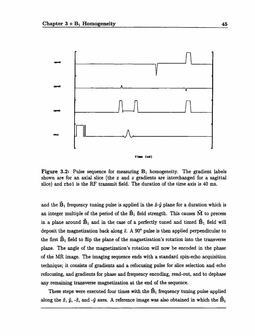
Chapter 3 O BI Homogeneity 45
Figure 3.2: Pulse sequence for measuring BI homogeneity. The gradient labels shown are for an axial slice (the x and z gradients are interchanged for a sagittal slice) and rhoi is the RF transmit field. The duration of the time axis is 40 ms.
and the fiequency tuning pulçe is applied in the 5-Y plane for a duration which is
an integer multiple of the period of the B~ field strength. This causes M to precess
in a plane around %1 and in the case of a perfectly tuned and timed B~ field wiU
deposit the magnetization back along i. A 90" pulse is then applied perpendicular to
the k t field to Bip the plane of the magnetization's rotation into the transverse
plane. The angle of the magnetization's rotation will now be encoded in the phase
of the MR image. The Maging sequence ends with a standard spin-echo acquisition
technique; it consists of gradients and a refocusing pulse for slice selection and echo
refocusing, and gradients for phase and frequency encoding, read-out, and to dephase
any remauiing transverse magnetization at the end of the sequence.
These steps were executed four times with the fi1 frequency titning pulse applied
along the Z, i, -Z, and -# axes. A reference image was also obtained in which the B~
Chapter 3 o BI Homogeneity 46
fiequency tuning pulse was not applied. For this reference image the magnetization
was tipped into the transverse plane such that the phase image represents phase due
to the 90" tip pulse, effects of the detection systern (coil, hardware) and phase due to
k-space sampling offset.
3.1.2 Post-Processing
Once the data is obtained, the post-processing is a matter or subtracting the
reference phase image from the other phase images. For a perfect field the result
wül be a phase of 0" for every pixel in the phantom. If the field is homogeneous but
incorrectly tuned or timed, the phase will be dinerent than 0" but constant across
the phantom. For an inhornogeneous field there will be a phase variation across the
phantom such that
where Tc is the duration of the hequency tuning pulse. This phase variation can
then be used to calculate the fi1 inhomogeneity. It should be noted that in cases
where the inhomogeneity inchdes direction inhomogeneity as well as magnitude
inhorcogeneity, as is the case with the extremity c d , the magnitude images also
change from being iiniform to having variations which are sinusoidally proportional
to the direction inhomogeneity. This is because the magnetization is tipped out of the
expected plane of rotation and when tipped by the 90" pulse the magnetization is only
partidy in the transverse plane. However, except for large fields in the extremity
coil this effect was not noticeably present.
In order to better illustrate the inhomogeneity and keep the same scale for all
the plots, the phase jumps hom -2r to zero were not unwrapped. This prevents
the display of AB^ magnitude images by a direct conversion from the phase images
using equation 3.1. However, the phase jumps are unwrapped for specific pixels for
the purpose of calcdating the magnitude of the inhomogeneity.
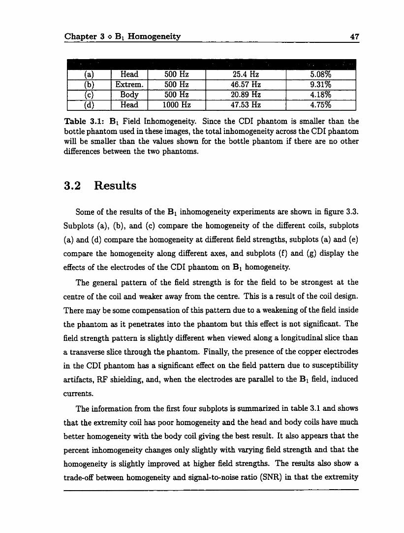
Chapter 3 O BI Homogeneity 47
(a) Head 500 Hz 25.4 Hz 508% (b) Extrem. 500 Hz 46.57 Hz 9.32% . r r I I 1
( 4 1 Body 1 500 Hz 20.89 Hz 4.18% 1
Table 3.1: BI Field uihomogeneity. Since the CD1 phantom is srnader than the bottle phantom used in these images, the total inhomogeneity across the CD1 phantom will be smaller than the values shown for the bottle phantom if there axe no other clifferences between the two phantoms.
3.2 Results
Some of the results of the Bi inhomogeneity experiments are shown in figure 3.3.
Subpiots (a), (b), and ( c ) compare the homogeneity of the different coils, subplots
(a) and (d) compare the hornogeneity at difFerent field strengths, subplots (a) and (e)
compare the hornogeneity dong different axes, and subplots ( f ) and (g) display the
effects of the electrodes of the CD1 phantom on Bi homogeneity.
The generd pattern of the field strength is for the field to be strongest at the
centre of the coil and weaker away from the centre. This is a result of the coil design.
There may be sorne compensation of this pattern due to a weakening of the field inside
the phantom as it penetrates into the phantom but this effect is not significant. The
field strength pattern is slightly different when viewed along a longitudinal slice than
a transverse slice through the phantom. Findy, the presence of the copper electrodes
in the CD1 phantom has a significant effect on the field pattern due to susceptibility
artifacts, RF shielding, and, when the electrodes are paralle1 to the BI field, induced
currents.
The information fkom the first four subplots is summarized in table 3.1 and shows
that the extremity coil has poor hornogeneity and the head and body coils have much
better homogeneity with the body coü giving the best result. It also appears that the
percent inhomogeneity changes only slightly with varying field strength and that the
homogeneity is slightly improved at higher field strengths. The results &O show a
trade-off between homogeneity and signal-to-noise ratio (SNR) in that the extremity
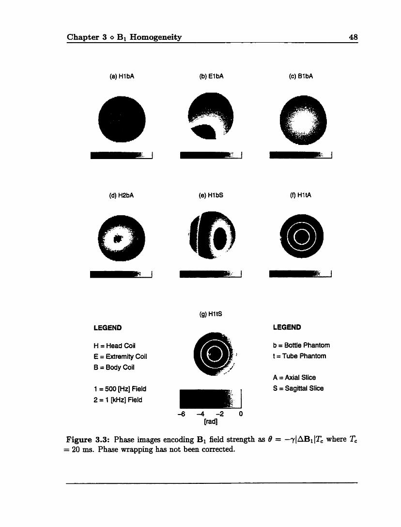
Chapter 3 O Bi Homojqeneity 48
(a) H l bA
(d) H2bA
(b) El bA
(e) H 1 bS
LEGENO
H = Head Coil E = Extremity Coil
B = Body Coil
(c) B1bA
LEGEND
b = Bottfe Phantorn t = Tube Phantom
A = Axial Slice
S = Sagittal Slice 1 = 500 [Hz] Field 2 = 1 (ld-la field
Figure 3.3: Phase images encoding Bi field strength as B = -?laBi ITc where Tc = 20 ms. Phase wrapping has not been corrected.
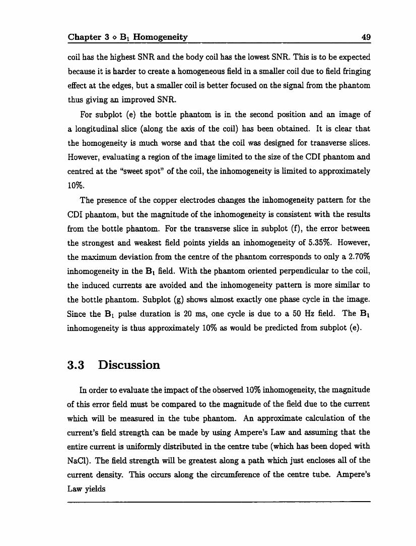
Chapter 3 o Bi Homogeneity 49
coil has the highest SNR and the body coil has the lowest SNR. This is to be expected
because it is harder to create a homogeneous field in a smder coil due to field fringing
effect at the edges, but a smaUer coi1 is better focused on the signal from the phantom
thus giving an improved SNR.
For subplot (e) the bottle phantom is in the second position and an image of
a longitudinal siice (along the axis of the coil) has been obtained. It is clear that
the homogeneity is much worse and that the coil was designed for transverse slices.
However, evaluating a region of the image Limited to the size of the CD1 phantom and
centred at the "sweet spot" of the coil, the inhomogeneity is limited to approximately
10%.
The presence of the copper electrodes changes the inhomogeneity pattern for the
CD1 phantom, but the magnitude of the inhomogeneity is consistent with the results
from the bottle phantom. For the transverse slice in subplot (f), the error between
the strongest and weakest field points yields an inhomogeneity of 5.35%. However,
the m;urimum deviation fiom the centre of the phantom corresponds to only a 2.70%
inhomogeneity in the B1 field. With the phantom oriented perpendicular to the coil,
the induced currents are avoided and the inhomogeneity pattern is more similar to
the bottle phantom. Subplot (g) shows almost exactly one phase cycle in the image.
Since the Bi pulse duration is 20 ms, one cycle is due to a 50 Hz field. The B1
inhomogeneity is thus approximately 10% as would be predicted fkom subplot (e).
3.3 Discussion
In order to evaluate the impact of the observed 10% inhornogeneity, the magnitude
of this error field must be compared to the magnitude of the field due to the current
which will be measured in the tube phantom. An approxhate caldation of the
current's field strength c m be made by using Ampere's Law and assuming that the
entire current is un i fody distributed in the centre tube (which has been doped with
NaCI). The field streength will be greatest along a path which just encloses all of the
current density. This occurs along the cirderence of the centre tube. Ampere's
Law yields
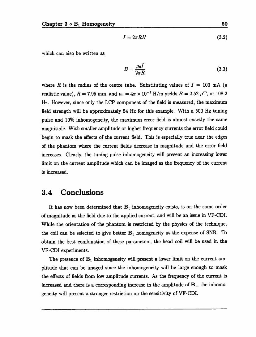
Chapter 3 o BI Homogeneity 50
which can also be written as
where R is the radius of the centre tube. Substituting values of I = 100 mA (a
realistic value), R = 7.95 mm, and po = 47r x 10-~ H/m yields B = 2.52 PT, or 108.2
Hz. However, since only the LCP component of the field is measured, the maximum
field strength will be approximately 54 Hz for this example. With a 500 Hz tuning
pulse and 10% inhomogeneity, the maximum error field is almost exactly the same
magnitude. With smaller amplitude or higher fiequency currents the error field could
begin to mask the effects of the current field. This is especially true near the edges
of the phantom where the current fields decrease in magnitude and the error field
increases. Clearly, the tuning pulse inhomogeneity will present an increasing lower
iimit on the current amplitude which can be imaged as the fiequency of the current
is increased.
3.4 Conclusions
It has now been determined that BI inhomogeneity exists, is on the same order
of magnitude as the field due to the applied current, and will be an issue in VF-CDI.
While the orientation of the phantom is restricted by the physics of the technique,
the coil can be selected to give better Bi homogeneity at the expense of SNR To
obtain the best combination of these parameters, the head coil will be used in the
VF-CD1 experiments.
The presence of BI inhomogeneity will present a lower limit on the current am-
plitude that can be imaged since the inhomogeneity will be luge enough to mask
the effects of fields from low amplitude currents. As the fiequency of the current is
increased and there is a correspondhg increase in the amplitude of BI, the inhomo-
geneity will present a stronger restriction on the sensitivity of W-CDI.
CHAPTER 4
Method
The theoretical requirements of a VF-CD1 method have been established and it
was deterrnined that an applied current and frequency tuning pulse will generate an
effective field in the double rotating kame which can be calculated by measwing the
rotation of the magnetization about the effective field. This effective field will contain
two unknown components due to the applied current and one due to Bi inhomogene-
ity. With this number of unknowns, three sets of initial and final orientation data
wil l be required. For practical reasons, it was decided that the three sets of rotation
data should be obtained using three different initial orientations rather than three
different rotation durations. Special consideration will &O be given to the timing of
the rotations in order to minimize certain mors and simplify data processing.
The steps taken to develop an actual expertmental method for the VF-CD1 theory
can be divided into three categories:
Hazdware design
Imaging sequence software
Data processing software

Chapter 4 o Method 52 - -- --
This chapter will describe the method used in each of these three areas to implement
the VF-CDI theory on a 1.5 T GE Signa imaging system at the Siinnybrook Health
Science Centre in Toronto.
4.1 Hardware Design
In order to perfom the VF-CD1 experiments, hardware was designed to generate
a current pulse which was a sinusoidal signal at a precise, operator selected frequency
and starting phase, and gated to start and stop synchronous with the frequency tuning
pulse in the imaging sequence. The remainder of this section describes the operation
of the hardware and the design procedure.
4.1.1 Starting Point
The current pulse required for VF-CD1 is very similar to that of RF-CD1 except
for the frequency of the current. It therefore seems naturd that the hardware for
VF-CD1 might incorporate the current generation box (CGB) developed by Michael
Carter for RF-CD1 [51. There were four options for making use of the CGB:
Make interna1 modifications to the CGB so it c m be used for VF-CD1 as well.
Develop hardware that could be added at the input or output of the CGB to
generate the desired current puises.
Devebp hardware that would incorporate signals fiom the CGB but would not
be in the direct signal path of the CGB.
Don't use the CGB and develop a stand-alone VF-CD1 system.
The k t option was d e d out since the CGB was stiU in use for RF-CD1 ex-
periments. Therefore, it could not be removed fiom semice for a long period while
modifications were made and the consequences of damaging the CGB while modi-
fications were made were too great. &O, in the event that VF-CD1 proved to be
unsuccessful, a permanent piece of VF-CD1 hardware inside the RF-CD1 unit would
be a waste of space and power.
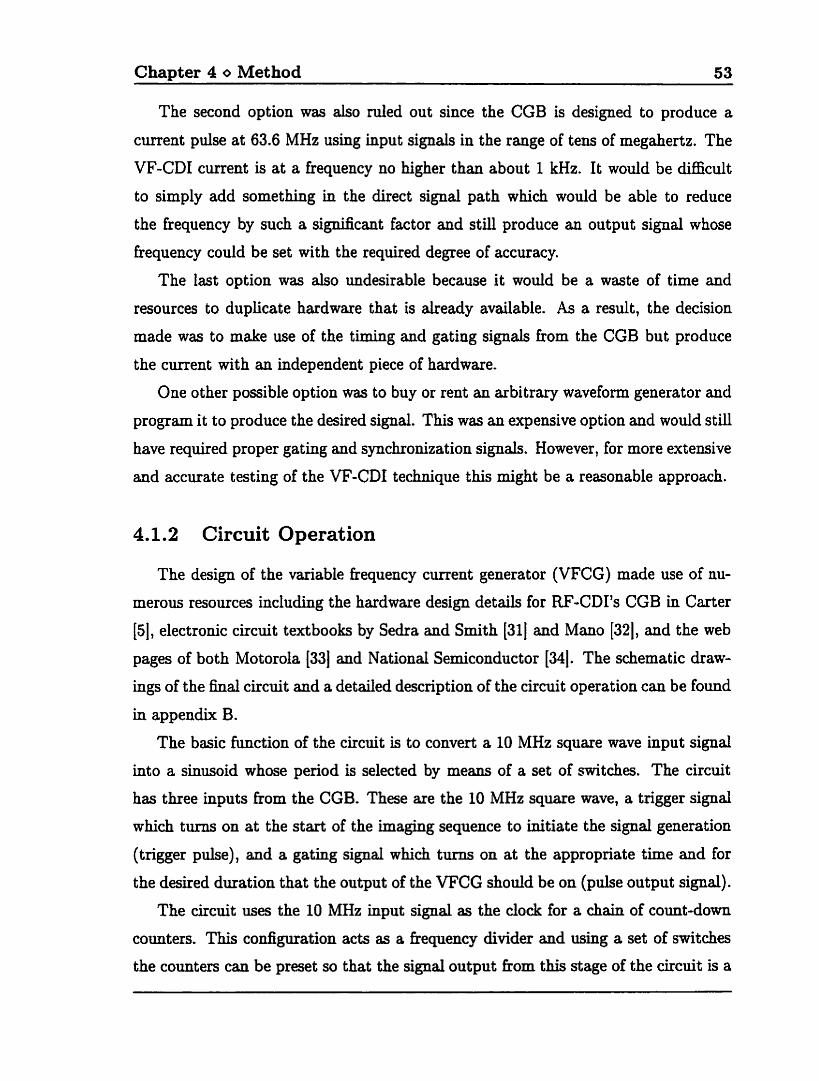
Chapter 4 O Method 53
The second option was &O d e d out since the CGB is designed to produce a
current pulse at 63.6 MHz using input signals in the range of tens of megahertz. The
VF-CD1 current is at a fiequency no higher than about 1 kHz. It would be dBicult
to simply add something in the direct signal path which would be able to reduce
the Erequency by such a significant factor and still produce an output signal whose
fiequency could be set with the required degree of accuracy.
The last option was also undesirable because it would be a waste of tirne and
resources to duplicate hardware that is already available. As a result, the decision
made was to make use of the timing and gating signals from the CGB but produce
the current with an independent piece of hardware.
One other possible option was to buy or rent an arbitrary wavefom generator and
program it to produce the desired signal. This was an expensive option and would still
have required proper gating and synchronization signals. However, for more extensive
and accurate testing of the VF-CD1 technique this might be a reasonable approach.
4.1.2 Circuit Operation
The design of the variable fiequency current generator (VFCG) made use of nu-
merous resources including the hardware design details for RF-CDI's CGB in Carter
[5j, electronic circuit textbooks by Sedra and Smith [311 and Mano 1321, and the web
pages of both Motorola (331 and National Semiconductor [34]. The schematic draw-
ings of the final circuit and a detailed description of the circuit operation can be found
in appendix B.
The basic hinction of the circuit is to convert a 10 MHz square wave input signal
into a sinusoid whose period is selected by means of a set of switches. The circuit
has three inputs kom the CGB. These are the 10 MHz square wave, a trigger signal
which turns on at the start of the imaging sequence to initiate the signal generation
(trigger pulse), and a gating signal which turns on at the appropriate time and for
the desired duration that the output of the VFCG should be on (pulse output signal).
The circuit uses the 10 MHz input signal as the clock for a chab of count-down
counters. This configuration acts as a fiequency divider and using a set of switches
the counters can be preset so that the signal output kom this stage of the circuit is a
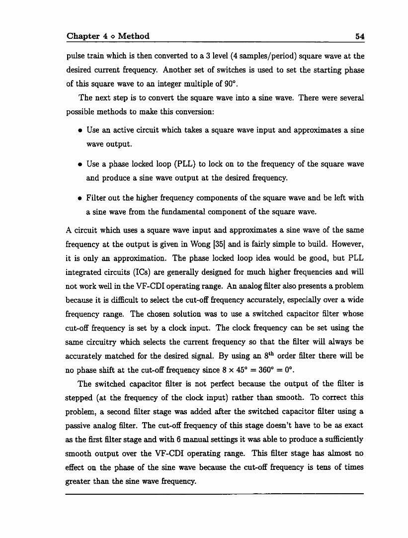
Chapter 4 o Method 54
pulse train which is then converted to a 3 level(4 sarnples/period) square wave at the
desired current fkequency. Another set of switches is used to set the starting phase
of this square wave to an integer multiple of 90".
The next step is to convert the square wave into a sine wave. There were several
possible methods to make this conversion:
Use an active circuit which takes a square wave input and approximates a sine
wave output.
Use a phase locked loop (PLL) to lock on to the frequency of the square wave
and produce a sine wave output at the desired frequency.
Filter out the higher fiequency components of the square wave and be left with
a sine wave fkom the fundamental component of the square wave.
A circuit which uses a square wave input and approximates a sine wave of the same
frequency at the output is given in Wong [35] and is fairly simple to build. However,
it is only an approximation. The phase locked loop idea would be good, but PLL
integrated circuits (ICs) are generally designed for much higher fiequencies and will
not work well in the VF-CDI operating range. An analog filter also presents a problem
because it is difEcult to select the cut-off frequency accurately, especidy over a wide
frequency range. The chosen solution was to use a switched capacitor filter whose
cut-off fkequency is set by a dock input. The clock fkequency cm be set using the
same circuitry which selects the current frequency so that the filter will always be
accurately matched for the desired signal. By using an 8th order filter there WU be
no phase shift at the cut-off frequency since 8 x 45" = 360" = 0'.
The switched capacitor filter is not perfect because the output of the filter is
stepped (at the frequency of the clock input) rather than smooth. To correct this
problem, a second filter stage waç added after the switched capacitor fdter using a
passive analog filter. The cut-off fiequency of this stage doesn't have to be as exact
as the first filter stage and with 6 manual settings it was able to produce a d c i e n t l y
smooth output over the VF-CD1 operating range. This flter stage has alrnost no
effect on the phase of the sine wave because the cut-oE fiequency is tens of times
greater than the sine wave fiequency.
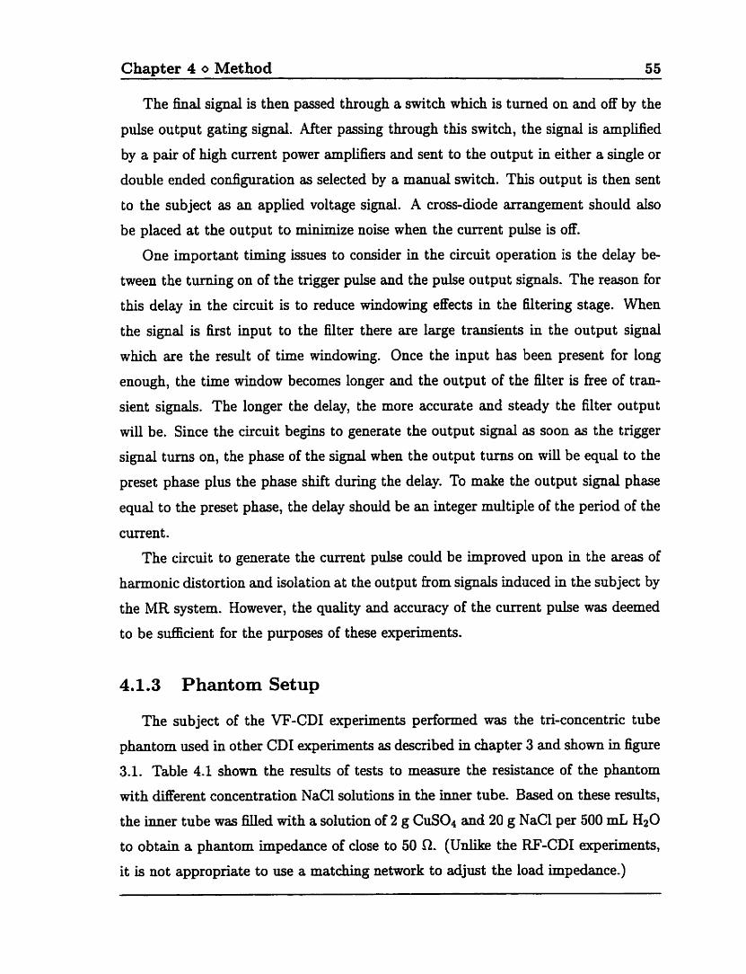
Chapter 4 o Method 55
The fininal signal is then passed through a switch which is turned on and off by the
pulse output gating signal. After passing through this switch, the signal is arnplified
by a pair of high current power amplifiers and sent to the output in either a single or
double ended configuration as selected by a manual switch. This output is then sent
to the subject as an applied voltage signal. A cross-diode arrangement should also
be placed at the output to minimize noise when the current pulse is off.
One important timing issues to consider in the circuit operation is the delay be-
tween the turning on of the trigger pulse and the pulse output signals. The reason for
this delay in the circuit is to reduce windowing effects in the filtering stage. When
the signal is first input to the filter there are large transients in the output signal
which are the result of t h e windowing. Once the input has been present for long
enough, the tirne window becomes longer and the output of the filter is fiee of tram
sient signals. The longer the delay, the more accurate and steady the filter output
will be. Since the circuit begins to generate the output signal as soon as the trigger
signal turns on, the phase of the signal when the output turns on will be equal to the
preset phase plus the phase shift during the delay. To make the output signal phase
equal to the preset phase, the delay should be an integer multiple of the period of the
current.
The circuit to generate the current pulse could be irnproved upon in the areas of
harmonic distortion and isolation at the output fkom signals induced in the subject by
the MR system. However, the quality and accuracy of the curent pulse was deemed
to be sufEcient for the purposes of these experiments.
Phantom Setup
The subject of the VF-CD1 experiments performed was the tri-concentric tube
phantom used in other CD1 experiments as described in chapter 3 and shown in figure
3.1. Table 4.1 shown the results of tests to measure the resistance of the phantom
with different concentration NaCl solutions in the inner tube. Based on these results,
the inner tube was fUed with a solution of 2 g CuS04 and 20 g NaCl per 500 mL H20
to obtain a phantom impedance of close to 50 Q. (Unlike the RF-CD1 arperiments,
it is not appropriate to use a matching network to adjust the load impedance.)
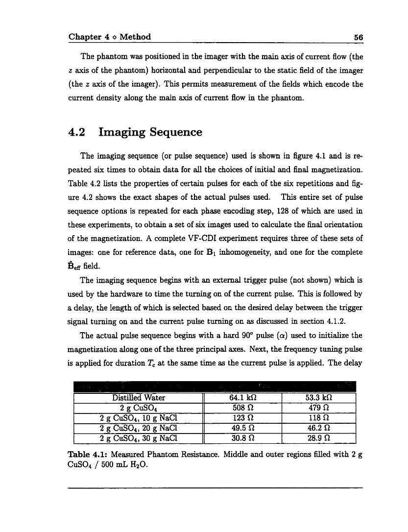
Chapter 4 O Method 56
The phantom was positioned in the imager with the main axis of current flow (the
z axis of the phantom) horizontal and perpendicular to the static field of the imager
(the r axis of the imager). This permits measurement of the fields which encode the
current density along the main axis of current flow in the phantom.
4.2 Imaging Sequence
The imaging sequence (or pulse sequence) used is shown in figure 4.1 and is re-
peated six times to obtain data for d the choices of initial and finai magnetization.
Table 4.2 lists the properties of certain pulses for each of the six repetitions and fig-
ure 4.2 shows the exact shapes of the actud pulses used. This entire set of pulse
sequence options is repeated for each phase encoding step, 128 of which are used in
these experiments, to obtain a set of six images used to calculate the final orientation
of the rnagnetization. A cornplete VF-CD1 experiment requires three of these sets of
images: one for reference data, one for Bi inhomogeneity, and one for the complete
B , ~ field.
The imaging sequence begins with an extemd trigger puise (not shown) which is
used by the hardware to time the turning on of the current pulse. This is followed by
a delay, the length of which is selected based on the desired delay between the trigger
signal turning on and the current pulse turning on as discussed in section 4.1.2.
The actual pulse sequence begins with a hard 90" pulse (a) used to initialize the
rnagnetization along one of the three principal axes. Next , the Bequency tuning pulse
is applied for duration Tc at the same t h e as the cment pulse is applied. The delay
Table 4.1: Measured Phantom Resistance. Middle and outer regions füled with 2 g CuS04 / 500 mL HzO.
53.3 k0 Distilled Water 64.1 kS1
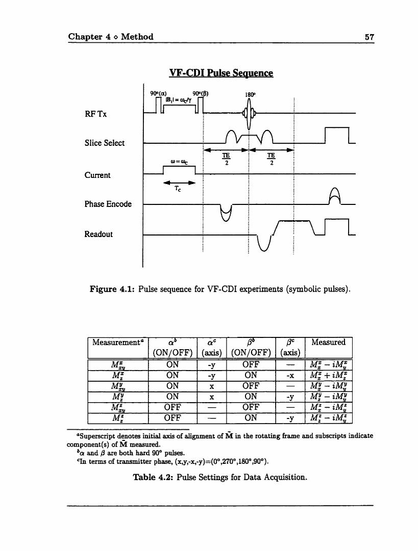
Chapter 4 o Method 57
Slice Select
Phase Encode
Readout
VF-CD1 Pulse Seauence
Figure 4.1: Pulse sequence for VF-CD1 experirnents (symbolic pulses).
aSuperscript d ~ o t e s initial axis of alignment of M in the rotating fiame and subscripts indicate component (s) of M measured.
ba and ,û are both hard 90' pulses. ?n terms of t ransmitter phase, (&y,-x,-y ) =(0°,2?00 ,180' $O0).
Measurement a
MN M: M L M! MR, Mz
Table 4.2: Pulse Settings for Data Acquisition.
,@ (axis) - -x -
-y -
-y
Measured
Mz - OM; Mg +iM: M: - iM,V Mt-ZM: M . - iMv Mf - iMv
ab (ON/OFF)
ON ON ON ON
OFF OFF
aC
(iuris) -Y -Y x x - -
Pb (ONIOFF)
OFF ON
OFF ON
OFF ON
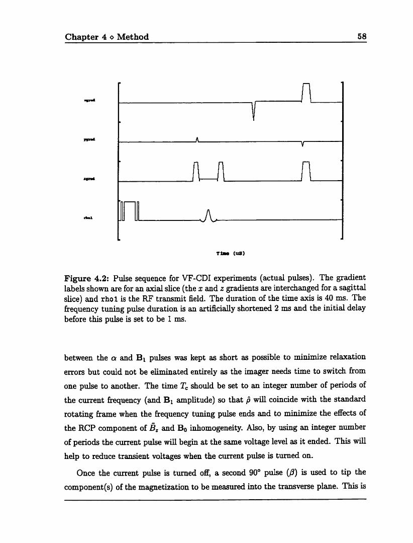
Chapter 4 o Method 58
Figure 4.2: Puise sequence for VF-CD1 experiments (actual pulses). The gradient labels shown are for an axial slice (the x and z gradients are interchanged for a sagittal slice) and rho 1 is the RF transmit field. The duration of the time axis is 40 m. The frequency tuning pulse duration is an artificidy shortened 2 ms and the initial deiay before this pulse is set to be 1 ms.
between the a and Bi pulses was kept as short as possible to minimize relaxation
errors but could not be eliminated entirely as the imager needs time to switch fkom
one pulse to another. The time Tc should be set to an integer number of periods of
the current frequency (and BI amplitude) so that fi WU coincide with the standard
rotating frame when the frequency tuning pulse ends and to minimiae the effects of
the RCP component of B~ and Bo inhomogeneity. Also, by using an integer number
of periods the current pulse will begin at the same voltage level as it ended. This will
help to reduce transient voltages when the curent pulse is turned on.
Once the m e n t pulse is turned off, a second 90" pulse (P) is used to tip the
cornponent(s) of the magnetization to be measured into the transverse plane. This is
Chapter 4 O Method 59
followed by a standard spin-echo data acquisition and large gradients to dephase any
rnagnetization remaining in the transverse plane. The phase of the 180' spin-echo
pulse is set to 0' (dong 5) for ail the repetitions of the sequence.
Current Free Sequences
For the acquisition of the reference data set, the cunent and the fiequency tuning
pulse amplitudes are both set to zero and the duration Tc is set to 10 p. This
effectively eliminates these puises and enables the use of the same pulse sequence
code for the reference data set. To eliminate those pulses entirely, a separate pulse
sequence would have to be written with no fiequency tuning pulse and with the
extemal trigger pulse t m e d off.
To obtain the BI inhomogeneity data the amplitude of the curent pulse is set to
zero while the rest of the sequence remained unchanged.
4.2.1 Imaging Parameters
While experiments were performed using many different values for the imaging
parameters, the experiments shown in the results (chapter 5 of this thesis) a.ll used
the following: head coi1 for RF transmit and receive, 8x8 cm FOV, sagittal slice
selection, 256 fiequency encoding steps in the anterior/posterior direction, 128 phase
encoding steps in the superior/inferior direction, 25 ms TE, 300 rn TR, 10 m~ Tc, and
a 4 ms delay hom the start of the sequence to the start of the curent and fiequency
tuning pulses. As mentioned above, a Tc of 10 ps was used for the reference image
data set.
4.3 Post-Processing
Once the three sets of data are obtained and Fourier transformed to form space
domain images, it is the role of the post-processing software to convert the data to a
VF-CD1 image. The steps învolved in this transformation are:
a Correct the m e n t data with the reference data.
Chapter 4 o Method 60
Calculate the magnetization components.
Calculate rotation axis/angle using the quaternion least squares rotation algo-
rithm and vector unwrapping of the results where appropriate.
a Compute B , ~ from the rotation data.
a Repeat for the AB, data and subtract from to obtain fi2.
Repeat for the data from the second o~entation of the subject.
Perform the curl operation to obtain the current density.
[Optional] Filter the data to get an enhanced image.
Analyze the regions of the phantom to measure image statistics.
Many of the processing steps are simila (or identical) to those performed in the post-
processing for RF-CD1 images using the polar decomposition method [7] and some
of the processing steps can be found described in more detail in Scott 131. AU of the
processing steps were implemented using MATLAB.
4.3.1 Phase Correction
The reference data phase images show the magnetization's phase in the transverse
plane resulting from the combinations of a and ,û pulses used in the experiments and
including errors fkom pulse imperfections and k-space sampling ofiet. These phase
images are baseline images which represent the zero phase pattern for the systern. The
first step in post-processing is to subtract these phase images from the corresponding
phase images in the B~ and aBi data sets to correct for the above mentioned errors.
4.3 .2 Magnetization Components
After the phase images are corrected, the magnitude images are multiplied by the
sine and cosine of the corrected phase images to obtain the measured components as
listed in the last column of table 4.2. This must be done with care since subtraction

Chapter 4 o Method 61
of the reference phase results in a 90' shift of some of the phase images which was
not accounted for in table 4.2. The final result is two sets of magnitude images:
one for the curent and fiequency tuning pulses both applied, and one with oniy the
fiequency tuning pulse.
4.3.3 Quaternion Least Squares Rotation
Once the initial (by choice) and final (by measurement) magnetization vectors have
been obtained, the quaternion least squares rotation algorithm is used to compute
the rotation axis and angle. This algorithm was presented in Scott [31 based on work
by Horn 1301 and Weng 1291. It will be repeated here for completeness.
For a rotation axis N = (n,, n,, n,), a rotation by the angle B can be described
by the unit quaternion:
To obtain this quaternion, the k s t step is to f o m matrices C and Zi which are 3 x 3
matrices in which the columns are the initial and corresponding final magnetization
vectors respec tively :
Next, the 4 x 4 matrix B is formed such that:
in which Bi is constmcted from the zch c o h m vectors of C and as:
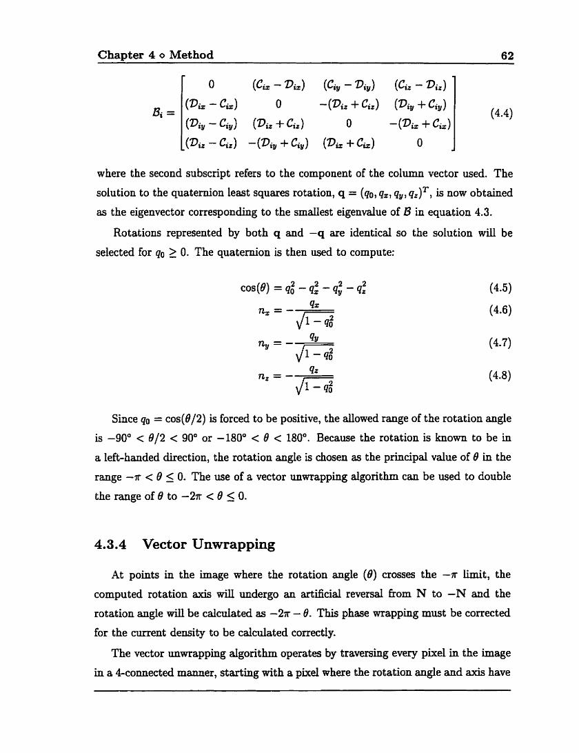
Chapter 4 O Method 62
where the second subscript refers to the component of the column vector used. The
solution to the quaternion least squares rotation, q = (qo, q,, q,, qz)T, is now obtained
as the eigenvector correspondhg to the smallest eigenvalue of B in equation 4.3.
Rotations represented by both q and -q are identical so the solution will be
selected for qo 1 O. The quaternion is then used to cornpute:
Since qo = cos(B/2) is forced to be positive, the allowed range of the rotation angle
is -90' < 012 < 90" or -180" < O c 180". Because the rotation is known to be in
a left-handed direction, the rotation angle is chosen as the principal value of û in the
range -r < 0 5 O. The use of a vector unwrapping algorithm can be used to double
the range of û to -2n < 0 5 0.
4.3.4 Vector Unwrapping
At points in the image where the rotation angle ( O ) crosses the -a limit, the
computed rotation axis WU undergo an artificial reversal Born N to -N and the
rotation angle wiU be calculated as -27r - B. This phase wrapping must be corrected
for the cment density to be calculated correctly.
The vector unwrapping algorithm operates by travershg every pixel in the image
in a C c o ~ e c t e d manner, staxting with a pixel where the rotation angle and axis have
Chapter 4 o Method 63
their correct values. (At the edges of the phantom's tubes the pixels are treated as if
they were connected to the closest pixel on the opposite side of the gap between the
tubes.) The dot product is taken between the pixel axis N and the neighbouring pixel
axis Nt. If this dot product is negative and the rotation angle is between -T and -al2
then a rotation reversal has occurred. (The reason for the angle restriction is that in
regions where the rotation angle is close to O k 2kn the rotation axis is dominated
by noise and a negative dot product does not necessarily indicate a reversal of the
rotation &S.) For the neighbouring pixel, Nt is replaced with -Nf and 0 is replaced
with -27r - O. When the pixel traversal enters a region where unwrapping has aiready
taken place there are three possible situations. First, if the dot product is negative the
above correction is repeated, regardless of the value of O. Second, if the dot product
is positive and -n < O < -al2 then the traversal has retumed to a region where the
data is already correct and no changes are made to the pixel data. Third, if the dot
product is positive and 8 is close to O f 2kr, the data should continue to be corrected
as the dot product is unreliable in such a region. This algorithm will fail if the image
contains axîs reversais corresponding to rotation angles of -3n or greater.
4.3.5 Converting the Rotation into a Magnetic Field
To convert the rotation information to magnetic field information, the rotation axis
cornponents (which are normalized) are multiplied by the magnitude of the magnetic
field vector. This magnitude is calculated using IBI = -8/(7Tc).
When this operation has been performed for both BeE and AB^, a vector subtrac-
tion of these fields yields the desired Ê2 field. The phase of the current field (and the
current) is then equal to the angle of B2 in the 9-2 plane and b, is equal to twice the
magnitude of B*. Depending on the orientation of the phantom, this z aligned field
in the imager is assigned to the appropriate field component in the phantom's frarne
of reference. Repetition with data fiom other orientations gives more components
of the field. In these experiments two orientations were used to obtain both field
components perpendicular to the direction of current flow in the phantom.
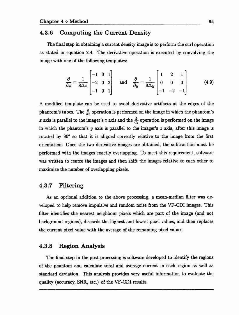
Chapter 4 o Method 64
4.3.6 Computing the Current Density
The final step in obtaining a current density image is to perform the curl operation
as stated in equation 2.4. The derivative operation is executed by convolving the
image with one of the following templates:
A modified template can be used to avoid derivative artifacts at the edges of the
phantom's tubes. The & operation is performed on the image in which the phantom's
x axis is pardel to the imager's z axis and the $ operation is performed on the image
in which the phantom's y axis is parade1 to the imager's z axis, after this image is
rotated by 90" so that it is aligned correctly relative to the image £rom the first
orientation. Once the two derivative images are obtained, the subtraction must be
performed with the images exactly overlapping. To meet this requirement, software
was written to centre the images and then shift the images relative to each other to
maximize the number of ovedapping pixels.
4.3.7 Filtering
As an optional addition to the above processing, a mean-median fdter was d e
veloped to help remove impulsive and random noise fFom the VF-CDI images. This
Nter identifies the nearest neighbour pixels which axe part of the image (and not
background regions), discards the highest and lowest pixel values, and then replaces
the current pixel value with the average of the remaining pixel d u e s .
4.3 .8 Region Analysis
The ha1 step in the post-processing is softwaxe developed to identify the regions
of the phantom and calculate total and average current in each region as well as
standard deviation. This analysis provides very useful information to evaluate the
quaüty (accuracy, SNR, etc.) of the VF-CD1 results.
CHAPTER 5
Result s
A series of experiments were performed following the method of the previous chap
ter. The results were analyzed in an iterative method in order to make modifications
and improvements to the experimental procedure and to decide on a h a l set of imag-
ing parameters. The first section of this chapter describes the problems identified by
the earlier experiments and the solutions (if any) which were implemented. A sample
of the final results of the VF-CD1 experiments is then presented.
5.1 Problems Encountered
A number of problems with the VF-CD1 method were discovered in early VF-CD1
experiments and these led to some modifications and refinements of the method. The
problems encountered included:
Magnetohydrodynamic flow
Rotation of the subject
Slice selecticn
Chapter 5 o Results 66 - -
While these problems were dealt with specificdy for the tube phantom being imaged,
the problems and solutions c m be easily extrapolated to imaging situations with other
subjects.
5.1.1 Magnetohydrodynarnic Flow
Experiments performed with very large applied currents displayed an artifact in
the phase encoding direction. This artifact was identified as being mainly the result
of rnagnetohydrodynamic (MHD) flow [361. MHD Bow is a Lorentz force phenomenon
which states that for a current (1) flowing in the presence of a magnetic field, the
charged ions which make up the cunent experience a force (F) equal to:
MHD flow is a more significant problem in VF-CD1 than in RF-CD1 techniques be-
cause the orientation of the subject is such that the current flows perpendicular to
Bo instead of pardel. Therefore, a significant MHD flow effect can be observed. As
the current is sinusoidal, the Lorentz force is also sinusoidal and causes vibrations
rather than the constant displacement which would be observed in LF-CDI. Since
the vibration does not result in the exact same fluid motion each t h e the current is
applied, an artifact is generated in the phase encoding direction.
For the rest of the experiments, this artifact was minimized by keeping the am-
plitude of the current low, by using a special platform for the phantom, and by
performing phase encoding in the direction paralle1 to Bo. The platform was heavy
and ngid so that the vibration of the phantom was minimized when the phantom
was attached to it. Also, since the Lorentz force is predicted to be perpendicular to
Bo, the vibrations were expected to introduce less significant flow artifact in the Bo direction. Phase encoding was subsequently performed in the Bo direction to take
advantage of this. Both these approaches helped to sipnincmtly reduce the phase
encoding artifact . Another method of reducing MHD flow would be to use a gel inside the phantom
rather than a liquid. Such a step was not attempted in this work. For a real biological
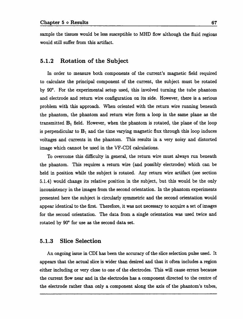
Chapter 5 o Results 67
sample the tissues would be less susceptible to MHD flow although the fluid regions
wodd still suffer fiom this artifact.
5.1.2 Rotation of the Subject
In order to measure both components of the curent's magnetic field required
to calculate the principal cornponent of the current, the subject must be rotated
by 90". For the experimental setup used, this involved tuming the tube phantom
and electrode and r e t m wire configuration on its side. However, there is a serious
problem with this approach. When oriented with the return wire running beneath
the phantom, the phantom and return wire forrn a loop in the same plane as the
transmitted B1 field. However, when the phantom is rotated, the plane of the loop
is perpendicular to BI and the tirne varying magnetic flux through this loop induces
voltages and currents in the phantom. This results in a very noisy and distorted
image which cannot be used in the VF-CD1 calculations.
To overcome this difnculty in general, the return wire m u t always run beneath
the phantom. This requires a retuni wire (and possibly electrodes) which c m be
held in position while the subject is rotated. Any return wire artifact (see section
5.1.4) would change its relative position in the subject? but this would be the only
inconsistency in the images ftom the second orientation. In the phantom experiments
presented here the subject is circularly symmetric and the second orientation would
appear identical to the tint. Therefore, it was not necessary to acquire a set of images
for the second orientation. The data £rom a single orientation was used twice and
rotated by 90' for use as the second data set.
5.1.3 Slice Selection
An ongoing issue in CD1 has been the accuracy of the slice selection pulse used. It
appears that the actual slice is widei than desired and that it often includes a region
either including or very close to one of the electrodes. This will cause errors because
the current flow near and in the electrodes has a component directed to the centre of
the electrode rather than only a component dong the axis of the phantom's tubes,
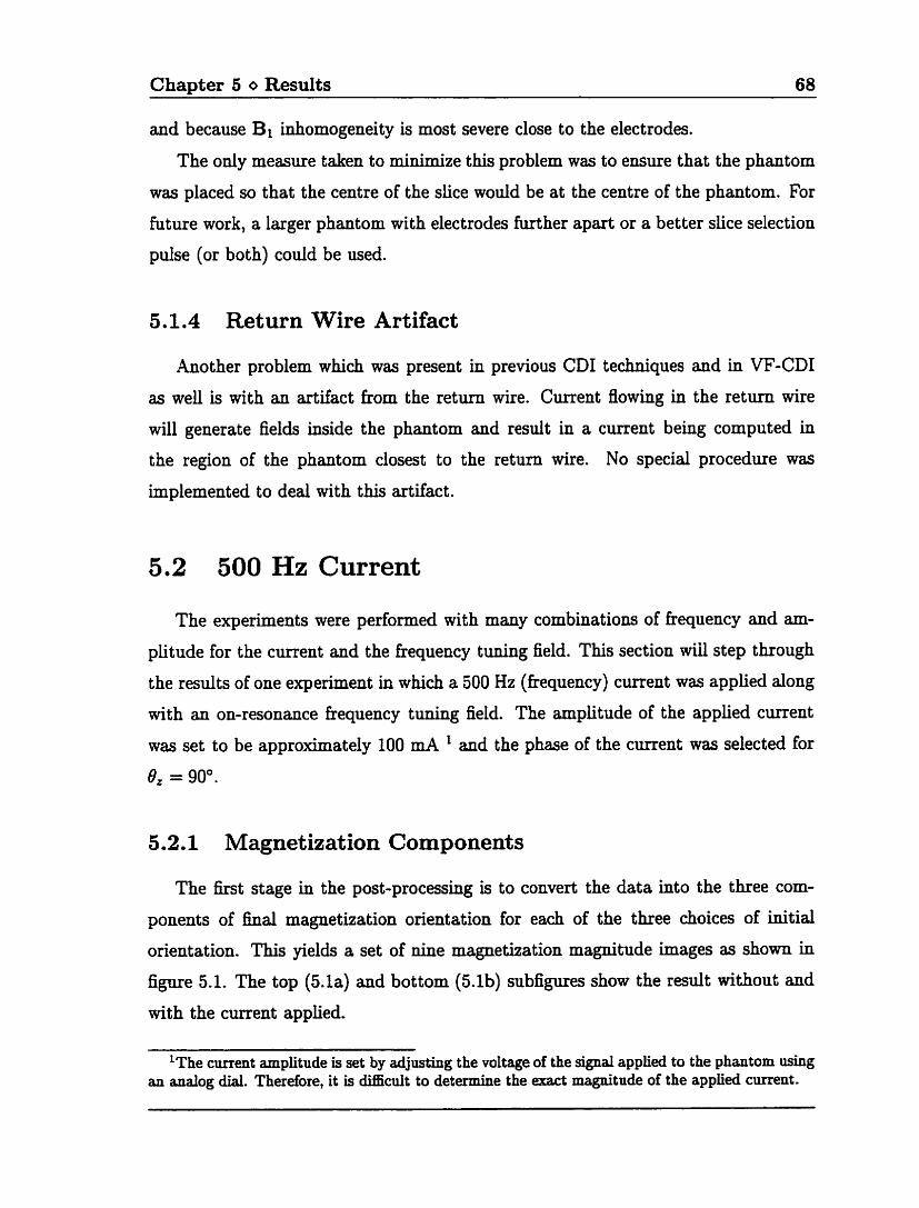
Chapter 5 o Resdts 68 --- - - -
and because Bi inhomogeneity is most severe close to the electrodes.
The only measure taken to minimize this problem was to ensure that the phantom
was placed so that the centre of the slice would be at the centre of the phantom. For
future work, a larger phantom with electrodes further apart or a better slice selection
pulse (or both) could be used.
5.1.4 Return Wire Artifact
Another problem which was present in previous CD1 techniques and in VF-CD1
as well is with an artifact £rom the return wire. Current flowing in the return wire
will generate fields inside the phantom and result in a current being computed in
the region of the phantom closest to the return wire. No special procedure was
implemented to deal with this artifact .
5.2 500 Hz Current
The experiments were performed with many combinations of kequency and am-
plitude for the current and the fiequency tunuig field. This section WU step through
the results of one experiment in which a 500 Hz (fiequency) current was applied along
with an on-resonance hequency tuning field. The amplitude of the applied current
was set to be approximately 100 mA ' and the phase of the current was selected for
8, = go0.
5.2.1 Magnetization Components
The first stage in the post-processing is to convert the data into the three com-
ponents of ha1 magnetization orientation for each of the three choices of initial
orientation. This yields a set of nine magnetization magnitude images as shown in
figure 5.1. The top (5.la) and bottom (5.lb) subfigures show the result without and
with the current applied.
=The current amplitude is set by adjusting the voltage of the signal applied to the phantom using an analog dial. Therefore, it is difiicuit to determine the exact magnitude of the applied m e n t .
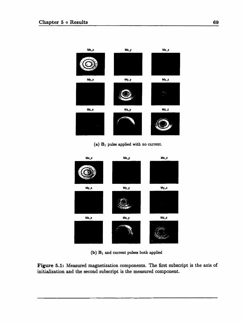
Chapter 5 O Results 69
(a) Bi pulse applied with no current.
(b) BI and current pulses both appiied
Figure 5.1: Measnred magnetization components. The first subscript is the a x k of initialkation and the second subscript is the measured component.
Chapter 5 o Results 70
Figure 5.2: Magnitudes of the measured magnetization vectors (normalized) . The subscript represent the axis of initialization. The top row is for reference data and the bottom row is with current and the Bi kequency tuning pulse both applied.
For the ideal case of B~~ = 0, the matrix of components should appear as an
identity m a t h with the measured component equal to one for the axis of initialization
and zero for the other components. The difference between this ideal case and subplot
5.la is due mainly to A& and also to errors in the other imaging sequence timing
and amplitude parameters as well as relaxation effects. Subplot 5.lb shows the added
effects of the applied current on the measured magnetization components.
Magnetization Magnitude Distortion
As a test of the imaging sequence it is usefd to calculate the magnitude of the
ha1 orientation magnetization vector ( JM;~ + Y + M'* ) and compare it to the
expected magnitude. Figure 5.2 shows the result of such a caldation. The top
row displays the expected magnitudes of the magnetization vectors for each initial
orientation using the reference data set. (As expected, this magnitude is the same
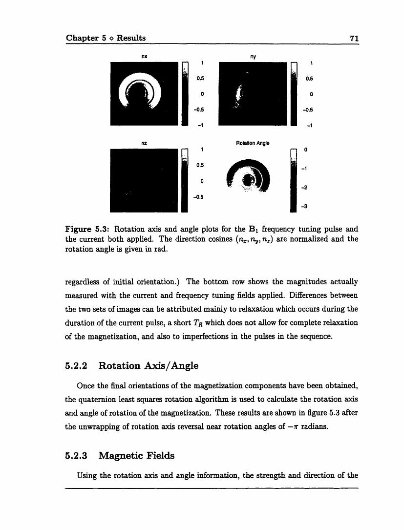
Chapter 5 O Results 71
nx Rotadon Angle
Figure 5.3: Rotation axis and angle plots for the BI fiequency tuning pulse and the curent both applied. The direction cosines (n,, %, n,) are norxnalized and the rotation angle is given in rad.
regardless of initial orientation.) The bottom row shows the magnitudes actudy
measured with the current and fiequency tuning fields applied. Differences between
the two sets of images cm be attributed rnainly to relaxation which occurs during the
duration of the current pulse, a short TR which does not d o w for complete relaxation
of the magnetization, and &O to imperfections in the pulses in the sequence.
5.2.2 Rotation Axis/Angle
Once the ha1 orientations of the magnetization components have been obtained,
the quaternion least squares rotation algorithm is used to calculate the rotation axis
and angle of rotation of the magnetization. These results are shom in figure 5.3 after
the unwrapping of rotation axis reversal near rotation angles of -T radians.
5.2.3 Magnetic Fields
Using the rotation axis and angle information, the strength and direction of the
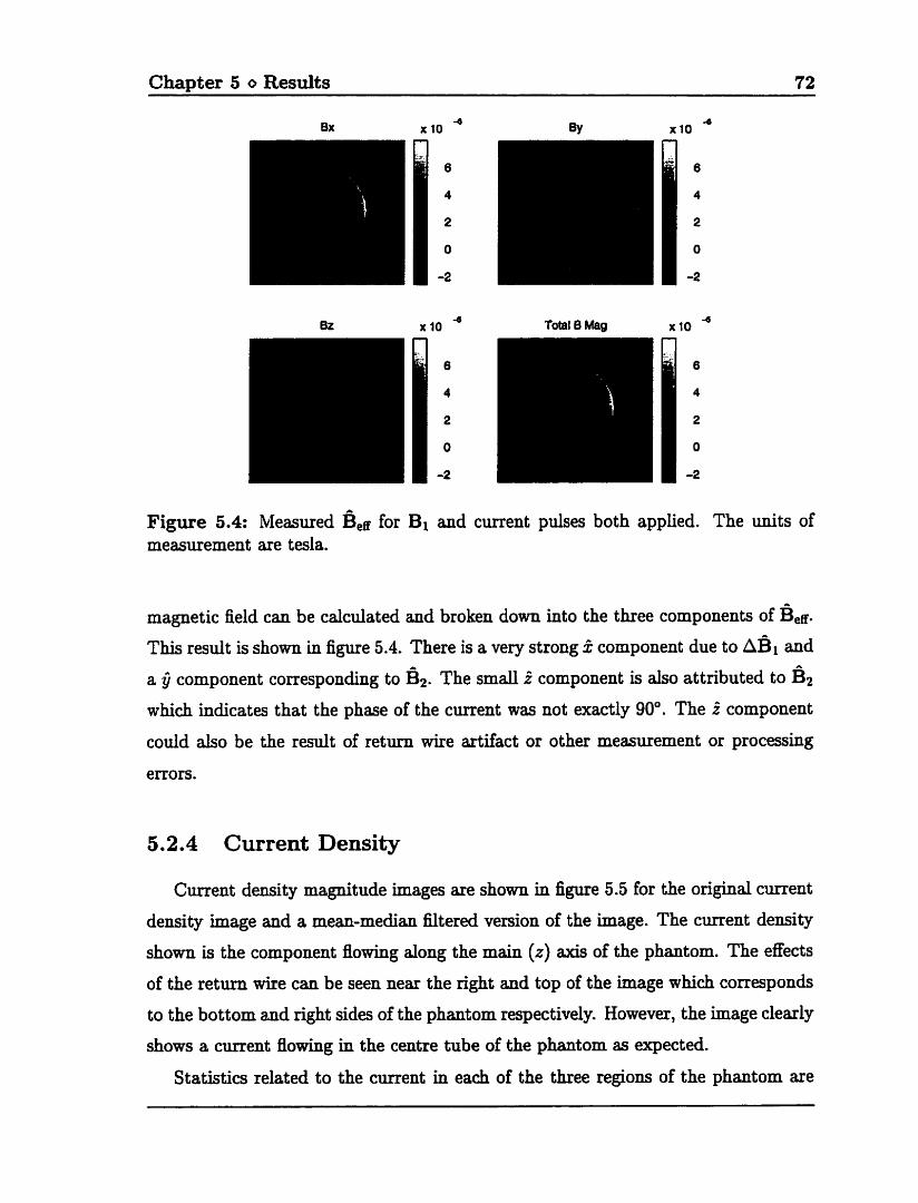
Chapter 5 O Results 72
Figure 5.4: Measured ÊeE for Bi and current pulses both applied. The units of rneasurement are tesla.
magnetic field can be calculated and broken down into the three components of fieE. This result is shown in figure 5.4. There is a very strong 3 component due to aBi and a ij component correspondhg to B*. The s m d î component is also attributed to B?
which indicates that the phase of the current was not exactly 90'. The 2 component
could also be the result of return wire artifact or other measurement or processing
errors.
5.2.4 Current Density
Current density magnitude images are shown in figure 5.5 for the original current
density image and a mean-median filtered version of the image. The cment density
shown is the component flowing almg the main (2) a x k of the phantom. The effects
of the return wire can be seen near the right and top of the image which corresponds
to the bottom and right sides of the phantom respectively. However, the image clearly
shows a curent flowing in the centre tube of the phantom as expected.
Statistics related to the current in each of the three regions of the phantom are
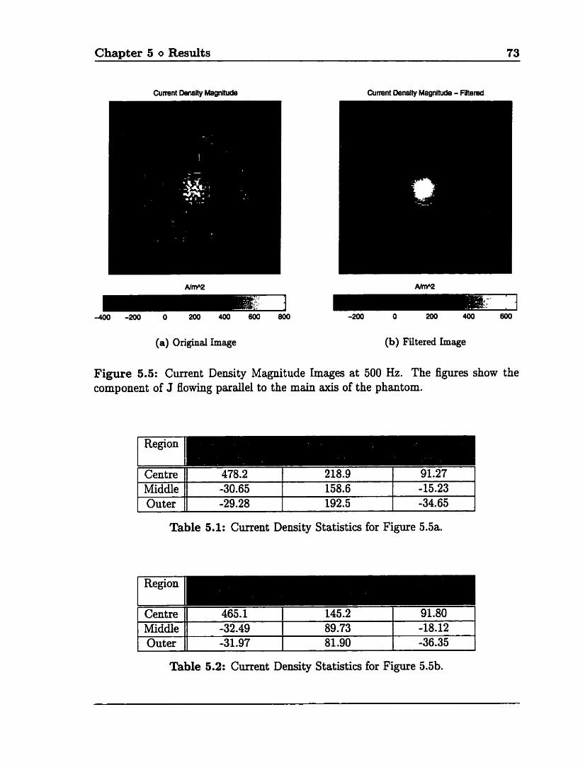
Current Density Magnitude Cumnt Density Magnitude - Rltered
(a) Original Image (b) Fitered Image
Figure 5.5: Current Density Magnitude Images at 500 Hz. The figures show the component of J Bowing parallel to the main axis of the phantom.
Middle 1 -30.65 158.6 -15.23 Outer 1 -29.28 192.5 -34.65
Table 5.1: Current Density Statistics for Figure 5.5a.
Middle -32.49 89.73 -18.12 Outer -31.97 81 .90 -36.35
Table 5.2: Current Density Statistics for Figure 5.5b.
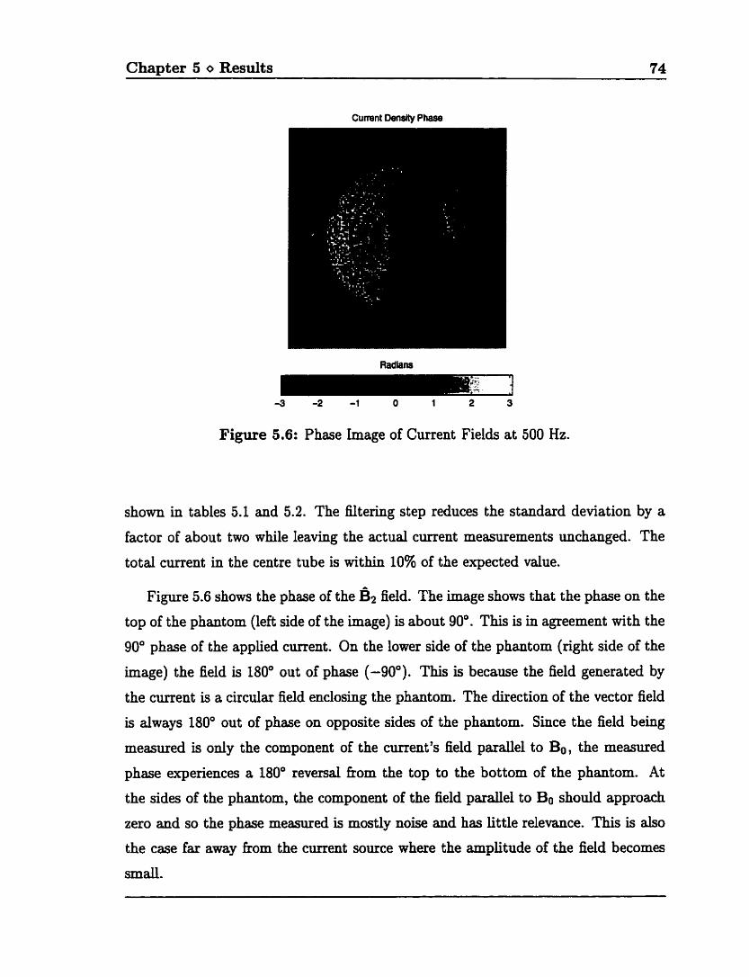
Chapter 5 o Results 74
Current Denslty Phase
Radians
-3 -2 -1 O 1 2 3
Figure 5.6: Phase Image of Current Fields at 500 Hz.
shown in tables 5.1 and 5.2. The Eltering step reduces the standard deviation by a
factor of about two while leaving the actual current measurements unchanged. The
total current in the centre tube is withh 10% of the expected value.
Figure 5.6 shows the phase of the B:, field. The image shows that the phase on the
top of the phantom (left side of the image) is about 90". This is in agreement with the
90" phase of the applied current. On the lower side of the phantom (right side of the
image) the field is 180" out of phase (-90"). This is because the field generated by
the current is a circdar field enclosing the phantom. The direction of the vector field
is always 180" out of phase on opposite sides of the phantom. Since the field being
measured is only the component of the current's field pivalle1 to Bo, the measured
phase experiences a 180" reversal kom the top to the bottom of the phantom. At
the sides of the phantom, the component of the field pardel to Bo should approach
zero and so the phase measured is mostly noise and has little relevance. This is also
the case far away hom the current source where the amplitude of the field becomes
Sm&.
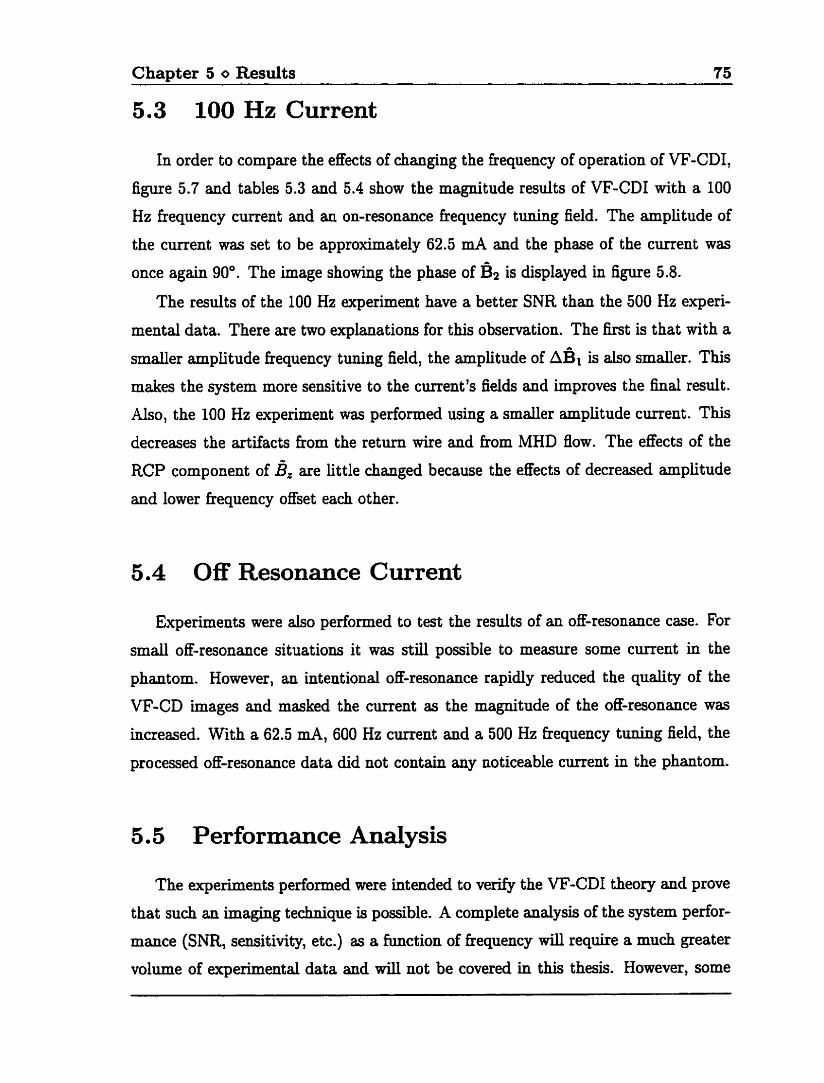
Chapter 5 o Results 75
5.3 100 Hz Current
In order to compare the effects of changing the fiequency of operation of VF-CDI,
figure 5.7 and tables 5.3 and 5.4 show the magnitude results of VF-CD1 with a 100
Hz frequency current and an on-resonance frequency tuning field. The amplitude of
the current was set to be approximately 62.5 mA and the phase of the current was
once again 90°. The image showing the phase of B~ is displayed in figure 5.8.
The results of the 100 Hz experiment have a better SNR than the 500 Hz experi-
mental data. There are two explmations for this observation. The fint is that with a
smder amplitude frequency tunllig field, the amplitude of AB, is also smder. This
makes the system more sensitive to the curent's fields and Mproves the final result.
Also, the 100 Hz experiment was performed using a smaller amplitude current. This
decreases the artifacts from the return wire and £rom MHD flow. The effects of the
RCP component of B~ are little changed because the efFects of decreased amplitude
and lower hequency offset each other.
5.4 Off Resonance Current
Experiments were also performed to test the results of an off-resonance case. For
smail off-resonance situations it was still possible to rneasure some current in the
phantom. However, an intentional off-resonance rapidly reduced the quality of the
VF-CD images and masked the current as the magnitude of the off-resonance was
increased. With a 62.5 mA, 600 Hz current and a 500 Hz frequency tuning field, the
processed off-resonance data did not contain any noticeable current in the phantom.
5.5 Performance Analysis
The experiments performed were intended to verify the VF-CD1 theory and prove
that such an imaging technique is possible. A complete analysis of the system pedor-
mance (SNR, sensitiw, etc.) a s a function of frequency will require a much greater
volume of experimental data and will not be covered in this thesis. However, some
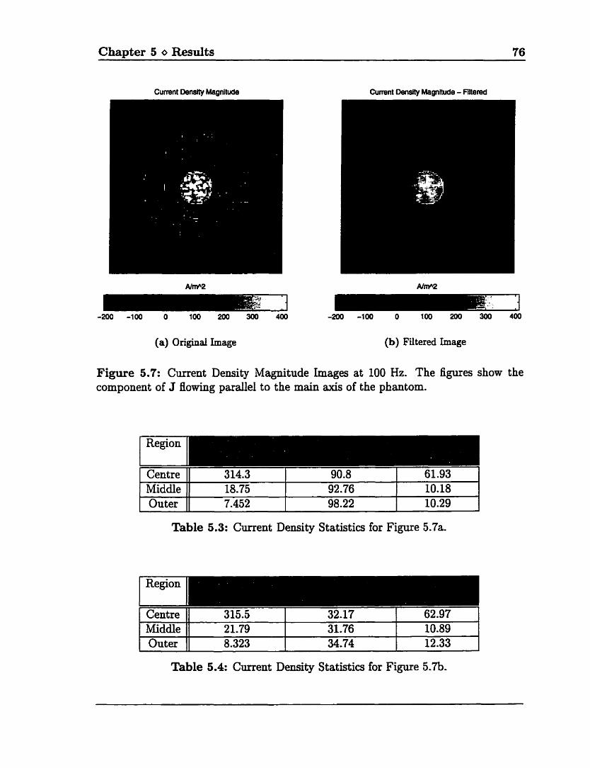
Chapter 5 o Results 76
Current Denslty Magnitude Cunent Denslîy Magnitude - mtered
(a) Original Image (b) Filtered Image
Figure 5.7: Current Density Magnitude Images at 100 Hz. The figures show the component of J flowing paxalle1 to the main a i s of the phantom.
Table 5.3: Current Density Statistics for Figure 5.7a.
Middle Outer
1 Middle il I , L
21.79 1 31.76 1 10.89 1
Table 5.4: Cunent Density Statistics for Figure 5.7b.
1
10.18 10.29
18.75 7.452
92.76 98.22
Chapter 5 o Results 77
Cumnt Densfty Phase
Figure
3 -2 -1 O 1 2 3
5.8: Phase Image of Current Fields a 100 Hz.
generd remarh on this topic can be made.
The biggest performance issue in this VF-CD1 technique is that it is highly prone
to noise. This is because of the many steps in the post-processing in which numerous
images are added, subtracted, and multiplied and in which the noise in the images is
&O added, subtracted, and multiplied. The polar decomposition rnethod of EU?-CD1
has a very similar processing algorithm and a detailed analysis of the noise in that
system can be found in Scott [31. The issue of noise can be dealt with in two ways.
The k s t is to h d a better data acquisition and processing techaique which is less
susceptible to noise. The second is to improve the SNR in the original MR images as
tbis is an improvement which will propagate throughout the post-processing stages.
h improvement in MR SM1 can be obtained by increasing pixel size, lengthening
TR (the t h e between repetitions of the pulse sequence), and averaging the results of
repeated experiments.
The sensitivity of VF-CD1 depends on the point of operation. A current with a
very high or low fiequency or amplitude will not be detected accurately. Otherwise,
the predicted and measured current density values were very close to each other as

Chapter 5 O Results 78
seen in the two sets of results presented here. VF-CD1 is &O prone to axtifacts when
currents at the limits of the system operation are being irnaged. These artifacts are the
result of MHD flow, the return wire, and the RCP component of B,. The sensitivity
could be enhanced and artifacts minimized by using a phase cycling technique to
correct for systematic errors in the data. Phase cycling involves obtaining a second
image set in which the parameters have been modified to reverse the effects of the
artifact. The images can then be averaged to remove the artifact and improve SNR.
Discussion and Conclusions
The objective of this thesis was to discover and implement a method of CD1 to
map electric currents at fiequencies other than DC and the Larmor frequency. Now
that this has been accomplished, there are three questions which must be answered
in order to determine the role of this new technique within CDI. These are:
How does VF-CD1 perform compared to the other CD1 techniques?
a What else can be done to improve on this implementation of VF-CDI?
e What are the potentiai applications of VF-CDI?
The fint two questions will be addressed here but the answers given do not exhaust
all discussion on these topics, nor are they intended to. The third question, related
to the applications of VF-CDI, was partly mwered in section 1.3 and the discovery
of any further applications will rely on the ingenuity of future research.
Along with the discussion and suggestions provoked by the above questions, some
other insights will be presented and the major conclusions of this work WU be stated.
Cha~ter 6 e Discussion and Conclusions 80
6.1 Cornparison With Other CD1 Techniques
The other CD1 techniques with which VF-CD1 is to be compared are LF-CD1 and
the two methods of RF-CDI: the polar decomposition method and the rotating h u n e
method. Of these techniques, LF-CD1 (for use with currents near DC) has the best
performance in terms of SNR and sensitivity, but requires rotation of the subject and
suffers £rom trouble with muscle twitch and pain when used on live subjects. The
RF-CD1 methods operate at the Larmor frequency. This fiequency is not of as much
biological interest but eliminates the need to rotate the subject and the problems of
muscle twitch and pain. However, the polar decomposition method has lower SNR
and sensitivity, a longer imaging time, and more complicated data processing. As a
result, it was replaced with the rotating frame method which is only slightly worse
than LF-CD1 for SNR and sensitivity, has a similar imaging time and data processing
complexîty, but causes a greater amount of tissue heating.
The performance of VF-CD1 is hampered by some of the problems encountered in
each of the previous CD1 techniques. VF-CD1 is therefore not likely to replace other
CD1 techniques for applications which can already be achieved with LF or RF-CDI.
Instead, the benefits of VI?-CD1 will corne from new applications which would not be
possible using the other CD1 techniques.
6.1.1 Technical Limitations
The main techical limitations of VF-CD1 are in the areas of noise and sensitivity.
As the method of VF-CD1 is almost identical to the polar decomposition method, it
experiences the same SNR and sensitivity problems due to the significant additive and
multiplicative noise which arises fiom the many post-processing steps and from the
phase wrapping problem. VF-CD1 has additional limitations due to BI inhomogeneity
and the RCP component of the field.
Compared to polar decomposition RF-CDI, VI?-CD1 has about the same signal to
noise ratio (SNR) and only slightly worse sensitivity. Rotating fIame RF-CDI, which
also has a Bi pulse applied with the cultrent, has similar sensitivity to VF-CD1 but
a much better SNR. LF-CD1 is better than VF-CD1 for both noise and sensitivity
Chapter 6 o Discussion and Conclusions 81
considerations.
6.1.2 Practical Limitations
Two important practical limitations in CD1 are irnaging time and the need to
rotate the subject. VF-CD1 &ers in both these areas. Rotation of the subject is
required as in LF-CD1 and the unconstrained axis of rotation and ability to measure
only one field component at a time in VF-CD1 result in much more data required and
a longer imaging time than other CD1 techniques. The imaging time is approximately
twice as long as polar decomposition RF-CD1 and roughly four times as long as the
other two techniques. In the implementation presented in this thesis the imaging
time is even longer because a less efficient method for obtaining reference and BI
inhomogeneity data was used.
6.1.3 Biophysical Limitations
One CD1 limitation which is deviated by VF-CD1 is the pain threshold and
muscle twitch of LF-CDI. The maximum current amplitude which can be applied
before muscle twitch and pain become a problem rises rapidly as the current fiequency
is increased. Therefore, VF-CD1 could be used in applications which require a lower
fiequency current but in which LF-CD1 cannot be used due to pain and/or muscle
twitch. While this biophysicd limitationis not as severe in VF-CD1 as it is in LF-CD1
it is still much more of a problem than in RF-CDI, in which the pain threshold and
muscle twitch are not present at ad.
Another biophysicd limitation is the amount of power which can be deposited in
the subject before harmful tissue heating occm. Due to the strong Bi field which is
applied in both VF and rotating kame RF-CDI, these techniques have simila tissue
heating constraints which are more of an issue than in LF-CD1 or polar decomposition
EU?-CDI.
Chapter 6 O Discussion and Conclusions 82
6.2 Future Work
This thesis is only the fkst stage in the development of W-CDI. There is still a
great deal of work to be done in improving the technique, analyzing its performance
and safety, and discovering and testing new applications. Some possible enhancements
to the implementation are already apparent. For example, some suggestions to reduce
the imaging tirne are:
Combine the M&, and Mi data acquisition steps into one excitation and TR
interval instead of two. This can be done by adding a 90" pulse and second
readout sequence after the first readout of the ML data to Bip the Mz data
into the transverse plane and rneasure it. (The Mt data would also have to be
scaled to account for relaxation.)
Use a more efficient method for obtaining the phase reference and BI inhomo-
geneity data so that not as many images are required. This will save tirne in
both data acquisition and processing.
Use an echo-planar or spiral scan readout to reduce the number of k-space
sarnpling excitations required.
and to improve the SNR and sensitivity of the technique:
Use phase cycling and/or averaging of multipte data acquisitions.
Improve the shape and location accuracy of the slice selection pulse.
Ensure accurate timing and RF pulse amplitudes in the imaging sequence and
improve the quality of the curent pulse.
Develop a method which dows for unwrapping of rotations greater than 2r.
(A larger rotation angle will be less affected (in percent) by noise and other
erron.)
There is &O the possibility of making more fundamental changes to VF-CD1 in
order to improve the technique. The following two ideas require much further study,
but may hold the key to significant improvements tu VF-CDI:
Chapter 6 O Discussion and Conclusions 83
Use a strong field to constrain the rotation axis in the double rotating hame
of reference in the same way that BI is used in the rotating frame method of
RF-CDI. The advantages of the rotating kame method over the polar decom-
position method would then be present in this new VF-CD1 technique as weU.
The difnculty lies in generating a static field in as this requires a complicated
modulation technique.
Recently, an MR coi1 has been developed which can modulate the strength of
Bo at one of a very wide range of fiequencies. Using such a modulation, it
may be possible to develop a VF-CD1 technique which can operate over a much
wider range of fiequencies and which will not require rotation of the subject.
6.3 Other Insights
There are a number of discussion topics related to the VF-CD1 theory which will
be dealt with in this section. These ideas may provide some additional insight into
the operation of, and possible improvements or modifications to, VF-CDI.
6.3.1 Extension of LF-CD1
Another way of understanding VF-CD1 is as an extension of the LF-CD1 technique.
LF-CD1 uses a bipolar DC current pulse along with a 180' Bi pulse to Bip the
magnetization by 180' when the sign of the cment changes. If this sequence is
repeated the current becomes a square wave along with a train of 180' pulses as
shown in figure 6.la. If the square wave is then replaced by a sine wave at the same
hindamentd kequency and the energy in the 180" pulses is spread out (so it will still
cause a 180" rotation every half period of the curent) then the result is identical to
the VF-CD1 sequence (figure 6.lb).
The extended LF-CD1 technique could in fact be used to image currents in the
low end of the VF-CD1 fiequency range. However, LF-CD1 has more severe require-
ments of the hardware for features such as current and RF amplifier slew rate and RF
amplifier power. The extended LF-CD1 technique also results in greater power being
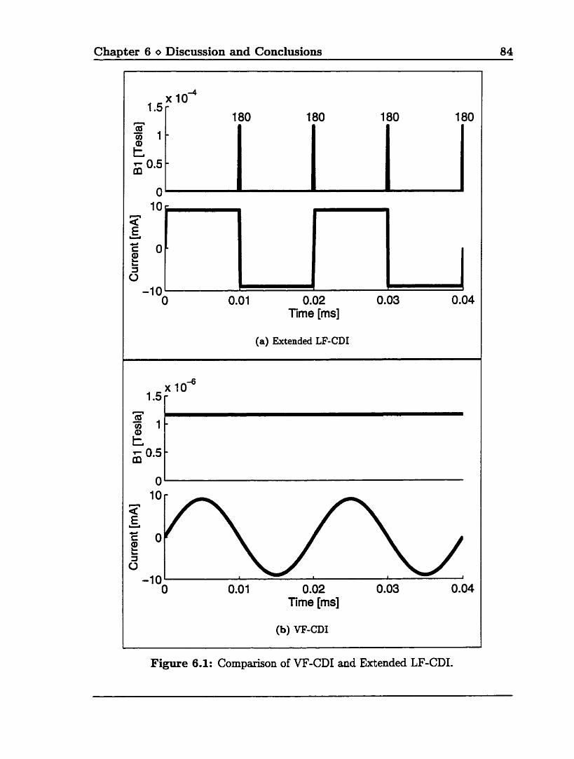
Chapter 6 o Discussion and Conclusions 84
Tirne [ms]
I (a) Extended LF-CDI
Time [ms]
I (b) w-CD1
Figure 6.1: Cornparison of VF-CD1 and Extended LF-CDI.
Chapter 6 o Discussion and Canclusions 85
absorbed by the subject since power is proportional to the square of the RF magni-
tude. One other clifference between the techniques is that the LF-CD1 method images
a current with many frequency components while VF-CD1 uses a single fiequency.
The highest frequency current which cm be imaged by VF-CD1 is limited by
the maximum strength of the frequency tuning pulse which can be applied. The
versatility of VF-CD1 would be geatly enhanced if currents with fiequencies greater
than this amplitude could also be imaged. One possible scenario would be to image
currents with kequencies that are harmonies of the tuned fiequency. Unfortunately,
this option was explored unsuccessfully. The h m o n i c fiequencies do not appear to
have any special properties to overcome the off-resonance error which they represent.
However, it is still possible that a method d l be found for irnaging the harmonic
currents.
6.3.3 Currents Near the Larmor Fkequency
The theory has shown that it is possible to image currents with angular fiequencies
ylBil away fiom DC. Based on the results of an initial investigation, it does not
appear possible to use a similar method for cunents which have fiequencies shifted
by a comparable amount £rom the Larmor fiequency. Such currents would have to be
dealt with using an RF-CD1 method and accounting for the off-resonance error which
would result. In any case, the relative ciifference between cments near the Larmor
kequency is much less than currents near DC and therefore there is no significant
diagnostic use for such a technique.
6.3.4 T l p Imaging
VF-CD1 has some similarities to Tlp irnaging [37]. In Tlp imaging M is initialized
in the transverse plane and is applied pardel to M. The rnagnetization becomes
locked to fi1 and relaxes toward thermal equilibrium along the locking field. This
relaxation is characterized by the relaxation t h e Tlp which is frequency dependent
Chapter 6 O Discussion and Conclusions 86
and sensitive to field fluctuations at hequencies close to & I B ~ 1. This is in contrast to
T l which is also frequency dependent but sensitive to the frequency IBO 1. Thus, Tlp
imaging dows measurement of relaxation time sensi tivi ty at low resonant frequencies
which is simila to VF-CD1 where a low resonant frequency is established to match
the low frequency fields generated by the applied current. In both cases the same
measurements could be obtained without Bi by using a much lower Bo field strength,
but in clinical imaging at low Bo field strengths the SNR and image quality obtained
are poor. A more in-depth investigation of Tlp imaging rnay provide further insight
into VF-CD1 as well.
6.4 Conclusions
This thesis has shown that current density imaging can be performed at current
frequencies other than DC and the Larmor fkequency. It has described the theory,
implementation, and results of a VF-CD1 method which allows imaging of currents
with fiequencies from DC up to about 1 H z . This creates the possibility of many new
and exciting applications for CD1 and while this implementation of VF-CD1 does not
perfom a s well as other CD1 techniques, future developments may lead to a VF-CD1
rnethod with better performance over a wider hequency range.
As the capabilities of current density imaging continue to expand, hirther develop-
ment will be accelerated by adopting a two streamed research approach of technique
and applications. Advances in new and/or improved CD1 techniques will give rise to
new applications while the implementation and clinical testing of new applications
will spur research into CD1 techniques. Such an approach will be the fastest way to
transform CD1 from an interesthg engineering project to a practical imaging modality
with clinical applications.

Bibliography
[II G.G. Sornjen et al. Mechanisms of spreading depression: a review of recent
findings and a hypot hesis. Canadian Journal of P h ysiology and Phamacology,
70:S248-S252, 1992.
[2l P. Pesikan, M.L.G. Joy, G.C. Scott, and R.M. Henkelman. Two dimentional cur-
rent density imaging. IEEE Ransactzons on I~tmrnentation and Mearement ,
39(6):1048-1053, December 1990.
[3] Greig Cameron Scott. NMR Imaging of Cumnt Denaity and Magnetic Fields.
PhD thesis, University of Toronto, 1993.
[41 G.C. Scott, M.L.G. Joy, R.L. Armstrong, and R.M. Henbelman. Measurement
of nonuniform current density by magnetic resonance. IEEE IBonsactions on
hiedical Imag2ng, lO(3) :362-374, 1991.
[51 Michael A. Carter. RF Current Density Imaging With a Clinical Magnetic Res-
onance Imager. MASc thesis, University of Toronto, 1995.
[61 G.C. Scott, M.L.G. JOY, R.L. Armstrong, and R.M. Henkelman. Rotating frame
RF current density imaging. Magnetic Resonance in Medicine, 33:355-369, 1995.
171 G.C. Scott, M.L.G. Joy, R.L. Armstrong, and R.M. Henkehan. RF current den-
sity imaging in homogeneous media. Magnetic Resonance in Medicine, 28:18&
201, 1992.
Bibliography 88
[8] Anthony N. Gerkis. A n Enhanced R F Curen t Desnity Imagzng Technique for
Imagzng Biological Media. MASc thesis, University of Toronto, 1996.
[91 Aaron P. Weinroth. Implementation of the Polar Decomposition Method of RF-
CDI on a Clinical MR Imager. BASc thesis, University of Toronto, 1996.
[ l O l Raymond Yan. Fast Radio-fiequency Current Density Imagzng vith Spiral Ac-
qubzt2on. MASc thesis, University of Toronto, 1997.
1111 D.D. Stark and W.G. Bradley, Jr. Magnetic Resonance Imaghg. C.V. Mosby
Company, Toronto, 1988.
Il21 D. G . Nishimura. Principles of Magnetic Resonance Irnaging. Department of
Electrical Engineering, S tanford University.
[131 K.K. Shung, M. Smith, and B. Tsui. Principles of Medical Imuging. Academic
Press, San Diego, 1992.
[141 G.C. Scott, M.L.G. Joy, and R.M. Henkelman. Current density imaging of bio-
logical media. In SMR M Eighth Annual Meeting Con ference Proceedzngs, A rns-
terdam, page 1163. Society of Magnetic Resonance in Medicine, August 1989.
[151 J.D. M. Thompson, M.L.G. Joy, and R.M. Henkelman. Current density imaging
in rabbit head and chest. In SMRM Tenth Annuol Meeting Conference Proceed-
zngs, New York, page 1274. Society of Magnetic Resonance in Medicine, August
1991.
[161 R.D. Stoy, K.R. Foster, and H.P. Schwan. Dielectric properties of mammalian
tissues from 0.1 to 100 mhz: A summary of recent data. Phys. Med. Biol.,
27(4):501-513, 1982.
[171 K.R. Foster and H.P. Schwan. Dielectric properties of tissues and biological
materials: A critical review. Cd. Rev. Biorned. Eng., 17(1):25-104, 1989.
[181 C. Polk and E. Postow, editors. CRC Handbook of BiologicBl E f f i of Electro-
magnetic Fields. CRC Press, 1986.
Bibliography 89
[191 G.H. Glover et al. Cornparison of linear and circula polarization for magnetic
resonance imaging. Journal of Magnetic Resonance, 64:255-270, 1985.
[20[ S. Topp, E. .4dalsteinsson, and D.M. Spielman. Fast multislice B1 mapping. In
Proceedings of the Fifih Annual Meeting of the ISMRM, Vancouver, page 281.
International Society of Magnetic Resonance in Medicine, April 1997.
[2 11 S .L. Talagala and J. Gillen. Experimental determination of three-dimentional
RF magnetic field distribution of nmr coils. Journal of Magnetic Resonance,
94:493-500, 1991.
[221 C.H. Oh, S.K. Hilal, Z.H. Cho, and LK. Mun. Radio frequency field intensity
mapping using a composite spin echo sequence. Magnetic Resonance Imaging,
8:21-25, 1990.
[231 E.K. lnsko and L. Bolinger. Bl mapping. In Proceedings of the Eleventh Annual
Meeting of the SMRM, Berlin, page 4302. Society of Magnetic Resonance in
Medicine, 1992.
1241 J. Lian, L. Zha, and I.J. Lowe. A NMR technique for rneasuring the RF magnetic
field distributions of NMR coils. In Proceedings of the Tenth Annual Meeting of
the SMRM, San Franslsco, page 731. Society of Magnetic Resonance in Medicine,
1991.
[251 M.R. Bendall, M. Garwood, K. Ugubril, and D.T. Pegg. Adiabatic refocusing
pulse which compensates for variable RF power and off-resonance effects. Mag-
netic Resonance in Medicine, 4:493-499, 1987.
[26] K. Ugurbil, M. Garwood, and M.R. Bendall. Amplitude and hequency modu-
lated pulses to achieve 90" plane rotations with inhomogeneous B1 fields. Journal
of Magnetic Resonance, 72: 177-185, 1987.
[271 N. Bansal and R.L. Nunnally. lmproved MR imaging in extremely inhomoge
neous radidiequency fields. Magnetic Resonance Imaging, 9:61-65, 199 1.
1281 M. Garwood and Y. Ke. Symmetric pulses to induce arbitrary Bip angles with
compensation for RF inhomogeneity and resonance offsets. Journal of Magnetic
Resonance, 94:511-525, 1991.
[291 J. Weng, T.S. Huang, and N. Ahuja. Motion and structure from two perspective
views: dgorithrns, error analysis, and error estimation. IEEE ïkansoctions on
Pattern Analysis and Machine Intelligence, 11 (5):451-476, May 1989.
1301 B.K.P. Horn. Closed fom solution of absolute orientation using unit quaternions.
Journal of the Optical Society of Americu A, 4(4):427-433, 1987.
[3 11 A.S. Sedra and K.C. Smith. Microelectronic Circuits. Saunders College Publish-
hg, Toronto, 3rd edition, 1991.
[321 M . Mano. Digital Design. Prentice Hd, Englewood Cliffs, NJ, 2nd edition, 1991.
1331 Motorola Semiconductor Products Sector Web Site. http://www.mot-sps.com.
1341 National Semiconductor Web Site. ht tp://www.national.com.
1351 Y.J. Wong and W. Ott. Functional Circuits. McGraw Hill, Toronto, 1976. pp
207-209.
[361 J.A. Shercliff. A Teztbook of Magnetohydrodynamics. Pergamon, New York,
1965.
[37j R.E. Sepponen et al. A method for T l p imaging. Jovrnal of Cornputer Assisted
Tomography, 9(6):1007-1011, 1985.
[38] H. Anton. Elementary Linear Algebra. John Wiley and Sons, Toronto, 6th
edition, 1991.
[39] GE Medical Systems. Signa Advantage Customer 5.3 EPIC Tools Users' Manual,
1551 9.3, 1993.

APPENDIX A
Mat hernatical Derivat ion
In section 2.3 the effective magnetic field in the double rotating frame of refer-
ence was derived by presenting and explaining a series of logical steps in which the
laboratory hame fields were transformed to the double rotating kame. The effective
magnetic field in the double rotating hame can also be obtained from the laboratory
or rotating kame fields using a direct mathematical calculation. The equation for the
effective field in P can be extracted hom the double rotating frame representation of
the Bloch equationl.
This chapter derives the Bloch equation in f i and performs a sample calculation
of B~ for one particular set of magnetic fields. The derivation was performed with
the aid of Nishimura 1121 and Anton [381.
A. 1 Bloch Equation in the Double Rotating Frame
of Reference
The cornponents of the magnetization (M) in the laboratory kame of reference
can be represented by the vector Ml* = [M* M, M,]* and M can be e t t e n as:
=The Bloch equation describes the behaviour of the magnetization in MRL

Appendix A o Mathematical Derivation 92
where n = [x y zIT is a matrix in which x, y, and z are the orthonormal basis
vectors of the laboratory kame of reference. The rotating and double rotating fYame
representations of the magnetization can be stated similarly and are related to the
laboratory frarne representation as:
where 7Zf«t ) is the rotation matrix for a left-handed rotation about the axis at an
angular fiequency [ (E is the magnitude of E ) and the subscripts rot and rho represent
the rotating and p fiames of reference respectively. (It d l be assumed that there are
no phase shifts between the axes of the three frames of reference at t h e t = O. Such
a shift can be accounted for by adding a constant phase tenu to the argument of the
rotation matrices.)
Similar equations can &O be written for the rotation axes wo (about which the
rotating kame is rotating clockwise) and wl (about which the double rotating fiame
is rotating clockwise) and the magnetic fields:
Taking the derivative of equation A.2 gives:
Using the relation:

Appendix A O Mathematical Derivation 93
where x is any vector stationary in time (other than the rotation) 2, it c m be shown
that:
This relationship is verified for one particular set of {wo, w 1) in section A. 1.1.
Substituting equation A.6 into equation A.4 gives:
Using the Bloch equation (M = M x TB with the relaxation te- ignored), equations
A.2 and A.3 to substitute for M and B, and noting that:
yields:
2This relation states that the time derivative of a rotating vector is tangential to the Qrcular path of rotation and is equal to the aass product between the of rotation and the position of the vector at that the.

A ~ ~ e n d i x A o Mathematical Derivation 94
Extracthg the terms matched with each double rotating fiame unit vector results in
an equation describing the behavior of the magnetization when viewed in the double
rotating hame of reference. The Bloch equation thus becomes:
(A. 10)
and the effective field is a,s shown above.
A.1.1 Derivative in Time of the Axes of the Double Rotating
Frame
As a check on equation A.6, the calculation will be carried out for the specific case
of wo = woz and wi = wll so that:
and:
cos(wot) - sin (wot) O
sin(wot) cos(wot) O
O O 1
Taking the derivative gives:

Appendix A O Mathematical Derivation 95
=x ( - wo sin(&) - wl sin(wot) sin(wlt) + wo cos(wot) cos(w t)
+ wo cos(wot) sin(wlt) + w l sin(wot) cos(# it))
+ y ( - wo cos(wot) - wo sin(wot) cos(wlt) - wi cos(wot) sin(wlt)
- wl sin(wot) sin(wit) + wl cos(wot) cos(wlt))
+ z( - W I C O S ( W ~ ~ ) - WI sin(wlt)) (A. 13)
which verifies the correctness of equation A.6 for this case.
A. 2 Sample Effective Field Calculat ion
This section will calculate the effective magnetic field in (fiefi) for the case of an
applied current and a transmitted B~ field along i. In the laboratory frame, the total
field due to the current J at any point in the subject will have sinusoida1 cornponents
dong each of the x, y, and z axes with frequency f, and unknown amplitude and
phase:
The main magnetic field and transmitted RF fields also contribute to the total mag-
aetic field which becomes:
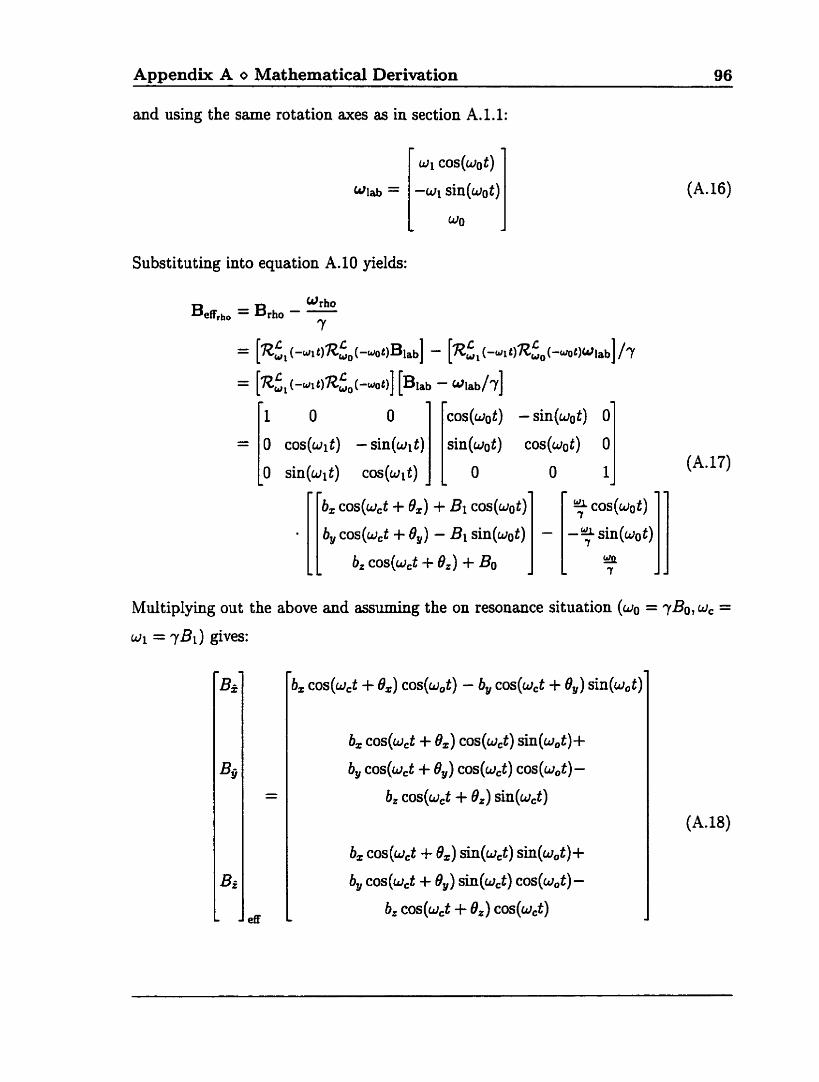
Appendix A o Mathematical Derivation 96
and using the same rotation axes as in section A. 1.1:
Substituting into equation A.10 yields:
b, cos(wct + 0,) + Bi COS (wot) Y cos(wot)
b , , c o ~ ( w ~ t + 0 , ) - B ~ ~ i n ( ~ ~ t ) - a 7 sin (wo t )
b, C O S ( W , ~ + O,) + B~ a 7Y
Multiplying out the above and assiiming the on resonance situation (wo =
b, cos(wCt + 0,) cos(w.t) - b, cos(w,t + O,) sin(wot)
(A. 16)
(A. 17)
Bo, WC =

Appendix A o Mathematical Derivation 97
Eliminating all the t h e varying tems (which will cause oscillations but have no net
effect on M) results in:
which is the same effective field as was obtained by using the analogy in section 2.3.

APPENDIX B
Schematic Drawings
An overview of the operation of the variable frequency current generator (VFCG)
circuit was given in section 4.1.2 and a more detailed explanation of the circuit oper-
ation will be given here. Full descriptions of the integrated circuits used can be found
on the web pages of rnanufacturers such as Motorola 1331 or National Semiconductor
[341 or catalogues and selection guides published by these companies. The last two
pages of this appendiv contain the schematic drawing for the variable fkequency CU-
rent generator and the board layout for the circuit. These drawings were prepared
by John Simpson from hand drawn originals by the author.
The VFCG takes 3 input signals fiom the current generator box (CGB) developed
by Carter [51. These are: the 10 MHz clock signal, the scope trigger signal, and the
pulse output signal. The scope trigger signai is passed directly fkom the imager, the
clock signal is derived £?rom the imager's 10 MHz reference signal, and the pulse output
signal is the output of the timing and gating circuitry in the CGB.
The fint stage of the circuit is a set of4 decade counters (U2-U5) chained together
and set to count down fiom a preset value determined by the thumb-wheel switches
SW1-SW4. The counters are held at their preset value until the scope trigger pulse
tunis on. When the trigger pulse is on, the counters count down using the 10 MHz
input signal as a clock. When the counters reach zero, an output pulse is produced
Appendix B o Schematic Drawings 99
(Usl3) and the counters are reset. The output pulse train has a penod of 0.1 ps times
the value on the switches. The frequency of this output signal is fa.
The U513 pulse is then used to clock another pair of counters (U7,U8) which are set
to count down from 25. The output pulse of these counters (U8i3) has a frequency of
f.125 and is used to clock binary counter U9. The lower 2 output bits of U9 are then
used to step multiplexer U11 through 4 values of a sampled sinusoid. This sampled
sinusoid has a fiequency of f a / l O O and the phase depends on the initial setting of
the counter U9, which is set to a multiple of 90' with switches 3 and 4 of U10. The
output of this stage (Ulis) is then input to a pair of 4th order switched capacitor
filters (U12,U13) connected in series.
The cut-off frequency of the switched capacitor filters is set as 1/50th of an input
dock hequency. The dock is obtained by using pulse signal U5L3 to toggle flip-flop
U17. This converts the pulse with fiequency fa to a square wave with frequency
fa/2. Therefore, the cut-off of the filters is fa/lOO which matches the fundamental
component of the signal input to the switched capacitor filters. This results in an
output fiom the filters which is a sinusoid with the same frequency and phase as the
square wave input.
The output of the switched capacitor filter stage is passed through a low-pass RC
filtering stage (input of U18) to smooth the signal. The cut-off hequency for this
stage has 6 possible setting which are chosen manually using a rotary switch. This
signal is buffered and amplified by U18 and sent to U14 which operates as a switch.
When the switch is turned on by the pulse output signal from the CGB, the signal is
passed through a variable resistor for amplitude control and is buffered and amplified
by U19. The signal then passes to a pair of high current amplifiers (U20,U21) with
equal amplitude but opposite sign gain. The final output of the circuit selects either
the signal fkom U21 in a single ended mode or the differentid signal between U21 and
U20 in a double ended mode with twice the amplitude.
Potentiometers are provided for offset nulling of the four operational amplifiers
(U18-21) and to exactly match the gains of U20 and U21. A voltage regulator (U22)
is also included to provide the -5 V power supply h m the -12 V source.
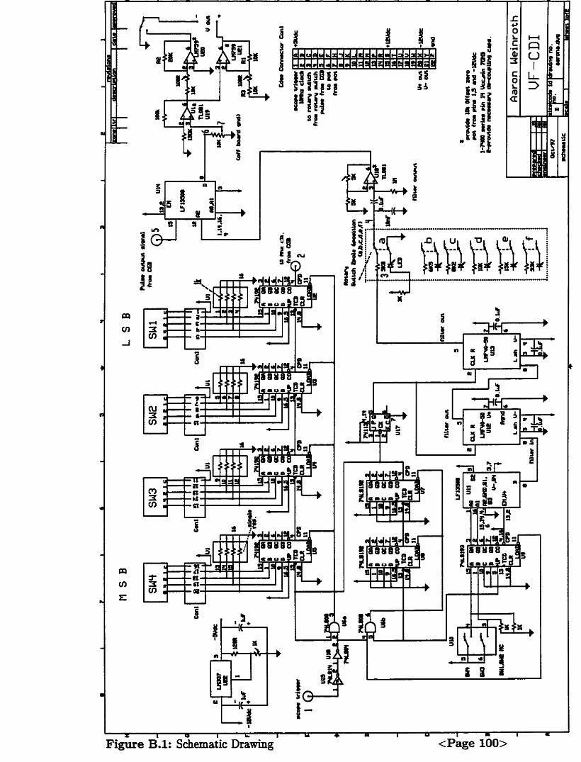
Figure B.1: Schematic Drawing <Page 100>
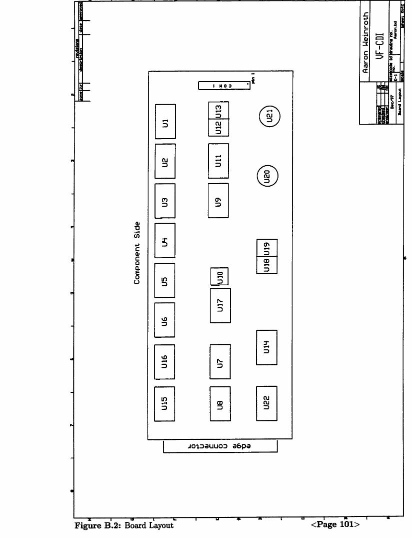
APPENDIX C
System Operating Instructions
This appendix serves as an instruction manual for the setup and operation of
the VF-CD1 imaging system on the GE Signa MR imager at the Sunnybrook Health
Science Centre in Toronto. Additional insight into the system operation can be found
in descriptions of the RF-CD1 imaging system contaioed in Gerkis (81, Carter [5j, and
Yan 1101.
C.1 Hardware Setup
The hardware setup for VF-CD1 makes use of the variable fiequency current gen-
erator (VFCG) and hardware fiom the RF-CD1 system. Due to this overlap and the
fact that the RF-CD1 setup is, at present, used more hequently than VF-CDI, the
VF-CD1 operator must understand the W-CD1 setup relative to RF-CDI.
The hardware setup schematic for RF-CD1 is shown in figure C.1. For VF-CD1
the following connections are made as shown:
10 MHz reference signal hoom the Exciter Board interconnect to the CGB
Scope trigger signal fiom the IPG to the CGB
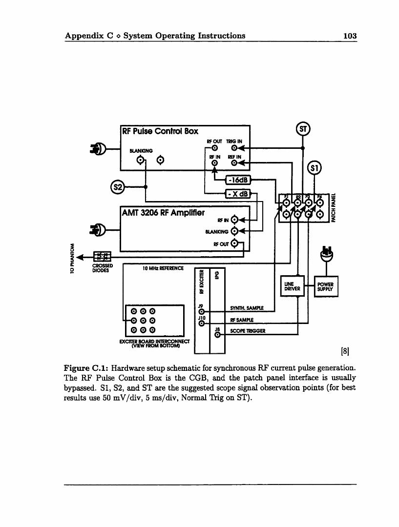
Appendix C o System Operating Instructions 103
AMT 3206 RF Amplifier
MANKING
Figure C.l: Hardware setup schematic for synchronous RF current pulse generation. The RF Pulse Control Box is the CGB, and the patch panel interface is usuaIly bypassed. SI, S2, and ST are the suggested scope signal observation points (for best results use 50 mV/div, 5 rns/div, Normal Trig on ST).
Appendix C o System Operating Instructions 104
m [Optional] RF Sample from the RF Exciter to the scope
and the following connections are modified:
.r The output signal sent to the crossed diodes and then the subject is obtained
from the output of the VFCG rather than the output of the AMT amplifier.
[Optional' Scope connected to the output of the VF'CG (using a T-connector)
rather than to the Blanking signal fkom the CG%.
All of the other connections show are not used for VF-CDI. The one additiond
connection which must be made is to attach the 3 pin connecter fiom the CGB to
the VFCG.
Before making the connections to the IPG and RF Exciter boards the TPS should
be shut off. After completing the setup, turn the power to the TPS back on and reset
the system from the operator console (select UTILITIES + OPERATOR MODE + RESET TPS).
C . l . l Switches and Controls
Once the hardware connections are made, the switches and other controls on the
hardware should be set. The CGB has thumbwheel switches for curent pulse delay
and duration. Both these settings are in units of 0.1 ps.
The VFCG has thumbwheel switches for setting the current fkequency. The fie-
quency is selected by setting the p e ~ o d of the desired m e n t in units of 10 p. For
example, to select a 500 Hz curent (period of 2 ms) the switches should be set to
200 (200 x 10 x 10-~ s = 2 x 10-~ s). The filter selection should then be made for the
appropriate fiequency range using the rotary switch. Findy, the amplitude control
dial should be set. The peak voltage of the cment pulse will be equal to the value
on the dial in single ended mode and twice this value in double ended mode. The
single/double ended mode of operation is selected using a switch located inside the
VFCG. Since the interface from the hardware room to the imager room grounds the
outer conductor of the coaxial cabie, single ended operation is standard.
Appendix C o System Operating Instructions 105
C.2 GE Signa Operation
Sub ject Placement
The head coil is first connected to the imager using the reverse polarity adapter.
The subject should then be connected to the output of the VFCG and secured to a
ngid platform such that it is located in the centre of the head coil. (A rigid platform
reduces MHD flow vibration effects.)
Sample Landmarkhg
The reference location of the subject for the imager is set using a landmarkhg
operation. On the keypad of the Signa imager select ALIGN ON, use the table
controls and/or manual adjustments to place the subject in the desired location,
select LANDMARK, and then ADVANCE TO SCAN.
Console Input
Table C.l details the input required on the Signa touch-screen console to set the
standard control variables for the imaging experiment. A detailed description of the
controi vanable names which are set by this process can be found in chapter 2 of the
Signa Advantage Custorner 5.3 EPIC Tool's User Manual [391.
Prescan Instructions
Table C.2 outlines the steps for the pre-scan sequence. Ensure that the coaxial
cable leading to the irnaging room is disconnected for this stage, and re-connected
upon completion. Once the pre-scan has completed, reset the CGB to initialize the
timing and phase cycling counters. The manual prescan step is optional and is only
meant for he-tiining the auto-prescan cdbration.
Once the pre-scan has completed, pressing the SCAN button on the operator
console W . initiate the W-CD1 sequence. If a scan is intempted due to an error,
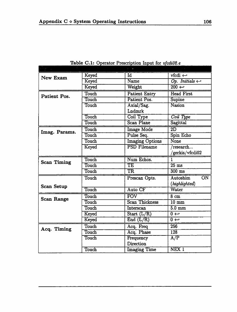
Appendix C o System Operating Instructions 106
Table C.1: Operator Prescri~tion In~ut for vfcdi02. e
New Exam Keyed Id Keyed Name Op. Initials e
1 Keyed I
1 Weight i 200 c,
1 Touch ¶ 1
1 Axial/Sag. 1 Nasion
-
Patient Pos.
Tou& Touch
Touch Touch
Lndrnrk Coi1 Type Scan Plane
I
TOU& ~maging Options Keyed 1 PSD Filename
Pa tient Entry Patient Pos .
Coi1 Type Sagittal
Image Mode Pulse Seq.
Imag. Params.
None /research.. .
Scan Timing
Head First Supine
Y
2D Spin Echo
Touch Touch
Touch Touch
Touch 1 Num Echos. Touch 1 TE
1 Scan Setup
1 Touch 1 I
1 Interscan 1 5.0 mm 1
/gerkis/vfcdiOÎ 1 25 ms
1
Scan Range
TR Prescan Opts.
Touch
300 ms Autoshim ON
Touch Touch
Keyed Keyed
Auto CF
Touch Touch Touch
Touch
(hzghlighted) Water
1
l
Start (L/R) End (L/R)
FOV Scan Thickness
O * Ow
Acq. Ekeq Acq. Phase Frequency Direction Imaging T h e
8 cm 10 mm
256 128 A/P
NEX 1
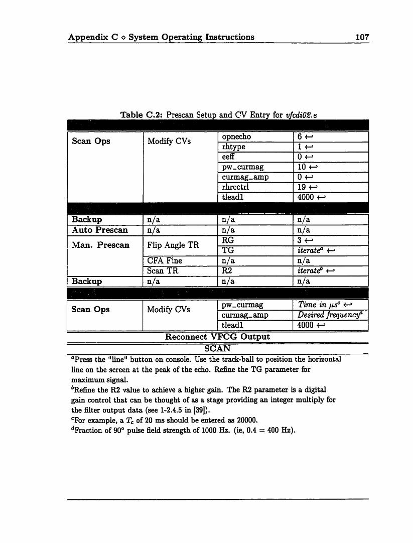
Appendix C O System Operating Instructions 107
Table C.2: Prescan Setup and CV Entry for vfcdi02. e
1 eeff I O * I Scan Ops
pw-curmag 10 t. curmag- amp O t , rhrcctrl 19 t, tleadl 4000 t,
1 Auto Prescan 1 n/a I
Modify CVs
CFA Fine 9 I
I n/a I n/a I
opnecho rhtype
Man. Prescan
I Scan TR I r I i
I R2 I iteratt? F 1
6 - I t ,
Scan Ops Modify CVs
3 - iteratd' f3
I i G
1 I I 1 I
Reconnect VFCG Output
Flip Angle TR
aPress the "line" button on console. Use the track-ball to position the horizontal line on the screen at the peak of the echo. Refme the TG parameter for maximum signal. '~efme the R2 value to achieve a higher gain. The R2 parameter is a digital gain control that can be thought of as a stage providing an integer multiply for the £ilter output data (see 1-2.4.5 in 1391). Tor example, a Tc of 20 ms should be entered as 20000. d~raction of 90" pulse field strength of 1000 Ha. (ie, 0.4 = 400 Hz).
TG
Appendix C o System Operating Instructions 108 - - -- - -- -
press the STOP SCAN button (located to the right of the operator keyboard) and
reset the CGB before initiating the next scan. Some cornmon problems are outlined
below as a trouble-shooting guide:
ERBTEC RF Amplifier Fault 81 [ E m r : 2225660/ almost always results Eiom
a BI pulse width or amplitude which exceeds the power capabilities of the
RH0 gradient amplifier. This occurs during subsequent pre-scans when the
pw-curmag is not reset to its "pre-scan" CV value fiom a previous scan. For
example, pw-curmag is set at 20000 (20 ms) for the pre-scan. Amplifier faults
will also occur if TG is too high for an given sample.
The MrMazl send of reset to IPG tzmed out [Error: 2218590/ indicates a Signa
communication problem between the IPG and TPS. Resetting the TPS will
restore system huictioning.
Data Acquisition Emor [Enor: 1 resdts kom the opnecho CV not being set to
6.
Prescan Error in IP Lib Init [Error: / occurs when the Manual Prescan entry
point cannot get access to the video console. To unlock the video console, select
the DISPLAY NORMAL button on the touch-screen.
detailed description of debugging the RF-CD1 system hardware can is outlined
in Carter [51. The VF-CD1 hardware operation was presented in appendix B.
Raw Data Retrieval
The raw data is output to the /net/signa2/usr/g/mnaw directory on the sunny-
brook.utoronto. ca Unix system. The files have the form PO1234 and can be identified
by their theldate stamp. These files should be copied or moved to a user's o w .
directory because the raw data files in .../m rmw are periodically purged.
The post-processing software for VF-CD1 was written for MATLAB and can be
found (at present) in the /rfcdi/home/wetnmt/MATLAB/CODE dîrectory on the

Appendix C o System Operating Instructions 109
Silicon Graphics Indy workstation (ibme2) at the Institute of Biomedical Engineering
at the University of Toronto. This directory also contains a text documentation file
(README) which describes how to perform the post-processing. An explanation of
the post-processing algorithm was given in section 4.3.