Embed Size (px)
Citation preview


ACKNOWLEDGEMENTS
The ALEPH experiment is a large, complicated and expensive scientific pro ject
requiring the efforts of hundreds of outstanding physicists, engineers, and techni
cians. All them have my sincere gratitude for their work, which has made ALEPH
an outstanding success.
I would like to thank my committee members Vasken Hagopian, J.F. Owens,
Paul Cottle, and Gregory Riccardi for reviewing this dissertation and overseeing
its completion. I especially want to thank my advisor, David Levinthal, for his
guidance, for teaching me some particle physics, and for the occasional bottle of
Pilsner Urquel.
I thank the Supercomputer Computations Research Institute (SCRI) at Florida
State for the use of their facilities. I particularly want to thank my SCRI colleagues
on ALEPH - Martyn Corden, Christos Georgiopoulos, and Mike Mermikides - for
explaining ALEPH event reconstruction to me, and for other things as well. I also
thank Donna Burnette of SCRI for producing a :U.'!EXstyle to meet the F.S.U.
dissertation guidelines.
Special thanks go to Andy Halley ("Och, man"), Ingrid ten Have, Alain Blondel,
and Rick St Denis for the work they did on hadronic asymmetry; to Andy Belk
for programmimg assistance and sailboard instructions; to Jolyon Martin and Peré
Mato for putting up with me; to Alessandro Miotto for guitar and FASTBUS lessons;
and particularly to John Harvey for guiding me around when 1 ~rst arrived at CERN
and knew absolutely nothing.
I suppose sometimes people have a hard time deciding to whom to dedicate their
dissertation, but not me. This work would not exist were it not for the patience,
love, and support of my wife, Carol McBride Sawyer. This dissertation is dedicated
to her, as some token that the years she sacrificed while I worked at CERN were in
fact worth something.
iii


This research was supported in part by funds from the U. S. Department of
Energy, grant number DE-FG05-87ER40319. Permission is granted to copy this
dissertation.
iv


CONTENTS
1 INTRODUCTION
1.1 The Standard Mode!
1.1.1 The Electroweak Theory.
1.1.2 Quantum Chromodynamics
1.2 Angular Dependence of the Cross Section for e+ e- ~ Z 0 ~ hadrons
1.3 Born level Values and Corrections ............. .
1.4 Measuring the Forward-Backward Asymmetry in e+ e-~ ff
1.5 Jet Charges . . . . . . . . . . . . .
1.6 Introduction to the Charge Flow
2 THE ALEPH DETECTOR
2.1 The ALEPH Subdetectors .
2.1.1 The Inner Tracking Chamber
2.1.2 The Time Projection Chamber
2.1.3 The Electromagnetic Calorimeter .
2.1.4 The Magnet . . . . . . . . . . . . . . ....
2.1.5 The Hadron Calorimeter and Muon Chambers
2.1.6 Luminosity Monitors . .
2.1. 7 Vertex Detector . .
2.2 The ALEPH Triggers
2.3 Data Acquisition . . . .
2.4 Event Reconstruction
2.4.1 Track Reconstruction
2.5 Data Quality Monitoring . .
V
1
2
3
6
7
10
12
14
17
20
22
22
23
26
28
28
30
32
33
36
39
40
42


3 DATA
3.1 Run Requirements
3.2 Definition of Hadronic Events
3.3 Track Requirements
3.4 Monte Carlo Data
4 ANALYSIS
4.1 Determination of the Quark Direction . . . .
4.2 Determination of the Charge of the Quark .
44
44
45
45
46
53
53
57
4.3 Evaluation of the Charge Flow, Q FB • • • 60
4.4 Determination of the Weighting Power K. • 61
4.5 Measurement of (QFB} and (Q} in the ALEPH Event Sample 66
4.6 Detector Systematics . . . . . . . . . . . . 69
4.6.1 Momentum Refit . . . . . . . . . 70
4.6.2 Track Losses . . .
4.6.3 Anomalously High Momentum Tracks
4.6.4 Asymmetry Due to Detector Material
4.6.5 Background From T-T Production
4.7 Final Measurement of (QFB} ••••
5 QUARK CHARGE SEPARATIONS
5.1 Relationship Between QFB and ÂFB at Parton Level
5.2 Definition of Quark Charge Separations . . . . . . .
5.3 Relationship Between QFB and ÂFB at Hadron Level.
5.4 Evaluation of <TQps ••••• • • • • • • • • • • •
5.5 Systematic Errors on the Quark Separations .
5.6 Charge Separation of c Quark Events . . . . . .
V1
72
74
79
80
81
83
83
85
87
89
94
98


6 ELECTROWEAK INTERPRETATION
6.1 Fitting QFB for sin2 (6w)
6.2 Standard Mode! Fitting .
6.3 Evaluation of Ae Using Measured Quark Couplings ..
6.4 Conclusion . . . . . . . . . . . . . . . . . . . . . . .
A QUARK FRAGMENTATION
A.1 Description of the Models
A.1.1 Perturbative QCD
A.1.2 Phenomenological Fragmentation Models
A.1.3 Hadron Decays
A.2 Fragmentation Studies . . . . . . . .
A.2.1 Parameter Variation in JETSET
BIBLIOGRAPHY
vii
100
101
108
110
113
116
117
117
118
120
121
121
124


LIST OF TABLES
1.1 The fondamental interactions
1.2 The Leptons .
1.3 The Quarks .
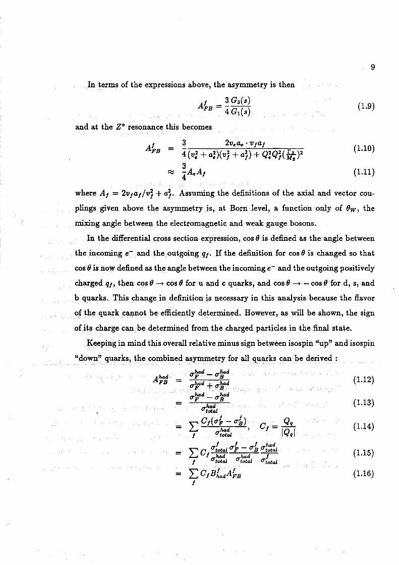
1.4 Quark Forward-Backward Asymm.etries
3.1 Number of hadronic events per LEP energy
4.1 Charge Finding Efficiencies
4.2 QFB per Energy Bin
4.3 QFB VS COS 8Thruat •••
.. • .
4.4 Occurence of Anomalously High Momentum Tracks in Data and
2
3
4
11
48
60
66
69
Monte Carlo . . . . . . . . . . . . . . . . . . . . . . . . . . . . . . . 7 4
4.5 Track Information for Anomalously High Momentum Tracks . 75
4.6 Track Information for Good Tracks . . . . . . . . . . . . . . . . 78
4. 7 Forward-Backward Asymm.etry of Anomalously High Momentum
Tracks ...... .
4.8 Summ.ary of Detector systematics .
5.1 Quark Separations . . . . . . . . .
5.2 Widths and Means of Charge Flow Quantities .
5.3 Variation of Monte Carlo Parameters . . . .
78
82
86
93
97
5.4 Charge Separations in c Quark Events 99
6.1 Peak and mean values, with errors, from the recursive calculation . 112
6.2 Values of sin2( 8w) from Various ALEPH measurements . . . . . . 113
viii


LIST OF FIGURES
1.1 Born level Feynman diagrams for the reaction e+e- --+ qq .
1.2 Hadronic Event in ALEPH
1.3 Jet Charges in Deep Inelastic Neutrino Scattering ..
1.4 Jet charge schematic ............. .
1.5 Distribution of simulated events versus QFB •
2.1 The ALEPH detector . . . .
2.2 The ITC wire arrangement
2.3 The TPC ........ .
2.4 TPC Wire Arrangement .
2.5 The ECAL
2.6 The HCAL
2. 7 The Luminosity Monitors
2.8 The Data Acquisition System
2.9 Track Fitting Parameters ...
3.1 Charged Track Multiplicity and Total Energy Distributions
3.2 Distribution of do and zo . • . • •
3.3 Monta. Carlo Event Production
3.4 Compa.rison of Data. and Monte Carlo Events
4.1 Angular Separation of Event/Jet Axes and the Parent Quark
4.2 Charge Finding Efficiency for Weighting by z, y, pz ••
4.3 The Sensitivity S = L, 51a1v1 / a'Qps ••••• • • • • •
4.4 The QFB Distributions in Data at "' = 0.5,1.0, 2.0, and 3.0.
lX
8
13
15
17
19
21
23
24
25
27
29
31
38
41
49
50
51
52
56
.... 59
63
64


4.5 Track Correlation Between Hemispheres versus "' 65
4.6 Distribution of QFB in Data and Monte Carlo . 67
4.7 Distribution of Q in Data and Monte Carlo 68
4.8 p(µ)/ Ebeam in Collinear Dimuon Events. 71
4.9 Momentum correction versus cos 8 73
4.10 Momentum Distributions in Data . 76
4.11 Distribution of the number of coordinates for good tracks and tracks
with p >50 GeV . . . . . . . . . . . . . . . . . . . . . . . . . . . . . 77
5.1 Distribution of simulated events versus QFB 84
5.2 QF versus QB for u quarks . . . . . . . . . 91
5.3 Comparison of 'Sand E1 S1g~gt between the full simulation and gen-
erator level . . . . . . . . . . . . . . . . . .
6.1 X2 parabola for the fit of sin2(8w) to (QFB)
6.2 Predicted Value of QFB vs sin2(8w)
6.3 QFB vs cos(8thru.t) •.........
6.4 Extracted Value of sin2( 8w) versus "'·
6.5 Quark ÂFB Values versus "'· ..... .
6.6 Standard Model Fit to the Energy Dependence of QFB .
6. 7 Distribution of sin2( 8w) Â 4n and 9v / 9Â values from th.e recursive com-
95
102
103
104
106
107
109
putation . . . . . . . . . . . . . . . . . . . . . . . . . . . . . . . . . . 112
6.8 Fit to the Electron Couplings Based on ru and A~B· . . . . . . . 115
A.1 Schematic Representation of Quark Fragmentation in e+ e- --+ qq. 116
X

ABSTRACT
The asymmetry in the angular distribution of hadronic events produced in the
reaction e+ e- ~ Z 0 ~ hadrons at center of mass energies near the mass of the Z 0
is studied. The data used in the analysis were taken at the European Center for
Nuclear Research (CERN) from September 1989 - August 1990.
The detector was a large multicomponent system consisting of a central Time
Projection Chamber, full electromagnetic and hadronic calorimetry, additional
trac.king near the interaction region, and luminosity monitors. It provided good
charged track reconstruction and momentum resolution.
The charge asymmetry is measured through the mean charge fl.ow, QFB averaged
over all events, where QFB= QF- QB is the difference between the momentum
weighted charges in the forward and backward hemispheres.
A fit to the value of (QFB) yields a measurement of sin20w(M~) = 0.2300 ±
0.0036( stat.) ± 0.0015( exp.sys.) ± 0.0021( theor.sys.) , which compares well with val
ues obtained by other methods. Using quark coupling measurements from previous
experiments, a value for the electron left-right asymmetry of Â: = 0.122:.!tg~: is
obtained. This result can also be expressed as a measurement of the ratio of the
electron vector and axial couplings, ~ = 0.06l!g:g~! , thus establishing that the
signs of gY, and 9Â are the same.
xi

CHAPTER 1
INTRODUCTION
The analysis in this dissertation is based on data collected by the ALEPH de
tector at the recently completed Large Electron-Positron collider (LEP) at the Eu
ropean Center for Nuclear Research (CERN), located on the Franco-Swiss border
near Geneva, Switzerland. This collider produces the highest energy collisions of
any electron-positron collider currently in operation. An initial run took place in
September, 1989, and the data described in this dissertation were taken from Oc
tober, 1989, through mid-December, 1989, and from late March, 1990, through
August, 1990.
The inauguration of LEP allows a new energy range in electron-positron ( e+ e-)
collisions to be studied, one in which the nature of the reactions differs funda
mentally from lower energies. ALEPH primarily looks at phenomena in which the
mediating force is the weak interaction, rather than the predominantly electromag
netic reactions which occur at e+e-collisions much below the mass of the Z 0• This
allows detailed tests of the Standard Model of electroweak interactions; the model
formulated by Glashow {1], Weinberg (2], Salam [3], and others to describe both the
weak and electromagnetic forces in a single theoretical framework.
The ALEPH detector is designed as a general purpose detector. In this sense
no single analysis can be construed as the primary motivation for the experiment.
However there are certain types of analyses for which it is optimized. For example,
because it has good tracking capabilities and track momentum resolution, ALEPH
is an excellent tool for studies in which the momenta of many charged tracks are
needed. As will be shown below, this is in fact the information needed for this
analysis.
1
2
1.1 The Standard Model
Physics phenomena at the most fundamental level are believed to involve fourba
sic interactions: the strong, weak, electromagnetic, and gravitational forces. These
forces act on two broad classes of particles, quarks and leptons. Quarks are sub
ject to ail four forces. Charged leptons interact via the electromagnetic, weak, and
gravitational interactions. The neutral leptons, called neutrinos, only interact via
the weak and gravitational forces.
The electromagnetic, weak, and strong interactions are described by gauge field
theories, where the force between two fermions is mediated by the exchange of
a gauge boson. The electromagnetic and weak interactions, often grouped un
der the term electroweak, are currently understood in the theoretical framework
known as the Standard Model, chiefly attributable to Glashow [1], Weinberg [2],
and Salam [3].
Table 1.1: The fondamental interactions, with characteristic strengths (in terms of
dimensionless coupling constants) and ranges, and associated exchange particle in
the theory describing the interactions. Values taken from [4]
Interaction Strength Range Exchanged Particle
electromagnetic a- 1 -m OO photon ('Y)
weak 1.02 X 10⁻⁶ 10-16 cm Intermediate Vector Bosons
(W±,z0 )
strong a.= 0.1-1.0 10-13 - 10-14 cm gluon (g)
gravitational 5.3 X 10-39 OO graviton (?)

3
Ta.ble 1.2: The three lepton pa.irs in the Standard Mode!. • Masses ta.ken from [6].
•• The ta.u neutrino ha.s not been directly observed.
Particle Na.me Symbol Charge Ma.ss (Me V)*
electron e -e = -1.602 X 10⁻¹⁹ C 0.511
electron neutrino Ve 0 < 17 X 10-6
muon µ -e 105.66
muon neutrino Vµ 0 < 0.27
ta.u T -e 1784.1
ta.u neutrino•• VT 0 < 35
1.1.1 The Electroweak Theory
The underlying symmetry of the electrowea.k theory is ba.sed on the group
SU(2)L ® U(l)y, where the subscript L indica.tes tha.t only the left-ha.nded helicity
states of the fermions enter in the wea.k interactions, a.nd the subscript Y indica.tes
tha.t the genera.tor of this group is wea.k hypercha.rge. There are four genera.tors for
this group, ta.ken to be wea.k isospin T and weak hypercharge Y. These are defined
so tha.t the charge of a. fermion in units of the electric charge is
Q y -=T3+e 2
The funda.menta.l gauge bosons forma ma.ssless triplet W"' a.nd a ma.ssless singlet
Bµ. Their interactions with a fermion field ca.n be described by the Lagra.ngia.n
density [5] g'
C = -gJ"' · W"' - 2i:B"'
where J µ a.nd J; are the isospin a.nd hypercharge currents of the fermions, a.nd g
a.nd g1 are the fermion's couplings to the W µ a.nd Bµ fields. This has the form
C = Ccc + CNc, where the subscripts "CC" a.nd "NC" denote charge-cha.nging a.nd

4
Table 1.3: The three quark pairs in the Standard Model. • Masses taken from [6].
•• The top quark has not been directly observed. Limits on the mass of the top
quark taken from [21].
Particle Name Symbol Charge Mass (Mevr
up u +1e 3 ~ 5.6
down d _le 3
~ 9.9
strange s _le 3 ~ 199
charm c +1e 3
~ 1.35 GeV
bot tom b _le 3
~5 GeV
top•• t +1e 3 120 ± 45 Ge V
neutral current interactions. The neutral current interaction is then
The physical states w;, z;, and Aµ are then mixtures of the gauge fields,
w± = _!_(w1 ± w 2) µ v'2 µ µ
zo - gW!-g'Bµ µ - y'g2 + g'2
g'wa +gB A - " "
µ - Jg2 + g'2
where ˵ is the field corresponding to the photon. This combination of fields can be
thought of as a mixing of the weak electromagnetic interactions, with an effective
mixing angle defined by g'
tanBw = -g
(1.1)
The masses of the four gauge bosons have been ignored. In fact the w± and Z 0
are qui te massive. These masses are generated in the electroweak theory through the

5
Higgs mechanism [7]. This modifies the Lagrangian in such a way that three bosons
w± and Z0 acquire mass, while one boson (Aµ) remains massless. The Lagrangian
then acquires additional terms involving interactions between the fermions and a
new scalar spin-0 field, the Higgs boson.
Electroweak phenomena are thus those processes mediated by the exchange of a
w±, z0 , or a;. This theory both incorporates Quantum Electrodynamics (QED),
the first and most successful field theory, and provides a renormalizable theory for
weak interactions [8]. It is not a truly unified theory because each the couplings g
and g1 are free parameters, and thus the value of Bw can not be predicted. Other
parameters, such as the fermion masses, are not predicted by the theory and must
be determined experimentally.
The weak interactions have long been recognized [9] as violating parity (P) and
charge conjugation (C) symmetry. This leads to the "V-A" (vector - axial-vector)
form of the weak interaction. For example, the Z 0 -f - f vertex is given by [22]
-ig;"' 2 8 (gv - 9Ais)
cos w
where gv and 9A are the vector and axial coupling strengths, and the constant g ·
is related to the Fermi coupling constant GF. The terms "vector" and "axial
vector" arise from the transformation properties of the bilinear covariants iÏJ;"''l/J
and {rya.;51/J : iÏJ;a'l/J is a vector, while the combination iÏJ;a/51/J is an axial-vector.
By contrast the electromagnetic vertex is
-iQe;"'
where Qe is the charge of the fermion.
Because of the appearance of the 1 - ; 5 operator, which has the property of
projecting helicity states (for massless fermions), only left-handed fermions (and
right-handed antifermions) couple to the w± and Z 0• Both leptons and quarks
appear as left-handed weak isospin doublets, for example (~L) or(~~). Each doublet

6
consists of a charged lepton and neutrino, or a charge ~ and a charge -l quark.
ALEPH measurements [16] have set the number of standard massless neutrinos at
3.01±0.15(exp.) ± 0.05(theor.). This number can be interpreted as the number of
weak isospin doublets.
1.1.2 Quantum Chromodynamics
The strong interactions are described in the Standard Mode! by the theory
known as quantum chromodynamics(QCD) (11). This theory assumes that hadrons
are composites of fermions, which are identified as quarks; an assumption supported
by experimental results [10]. Quark interactions proceed via the exchange of an
octet of gauge bosons known as gluons which, like the w± and zo' can also self
interact. The quarks and gluons couple via a new "charge" or quantum number,
labelled color, in analogy to the coupling to electric charge in QED. There are
fundamental differences between QCD and the electroweak gauge theory, however.
The symmetry group of the theory is SU(3), leading to three types of color (and
anticolor) charge. The color charges are carried by eight gluons. This symmetry is
believed to be exact, so that the gluons are massless.
Although quantum chromodynamics is currently unable to describe low energy
phenomena such as quarks binding to form hadrons, at high energies adequate
perturbative results exist to predict experimental results. This reflects in part the
dependence of the strong coupling constant, a., on the momentum transfer in an
interaction. This "running" of the coupling constant is not unique to QCD, and
will be discussed below for electroweak phenomena. An approximate perturbative
expression for a. as a fonction of the momentum transfered ( q) is
( 2) 121r a. q = B ln( q2 /A)

7
where A is a parameter which sets the scale of the momentum dependence, and
B = 33 - 2Ns.avoun• This decrease in a. with momentum is known as asymptotic
f.reedom.
1.2 Angular Dependence of the Cross Section for e+ e- -t Z0 -t hadrons
The reaction e+e- -t qq can be understood as the annihilation of the e+e-pair
either into a photon, to which they couple electromagnetically, or to a Z 0, to which
they couple through the weak interaction. The photon or Z 0 then produce a qq pair.
The Feynman graphs for these processes are shown in figure 1.1 . The existence
of both processes gives rise to quantum mechanical interference effects.
The differential cross section for producing quark-antiquark pairs in an e+ e
collision, for quark f with charge Q,, mass m1, and weak isospin If, is given [12]
by
where
duf
d!l
µ,
G1
-
--µ-t 0
G2 -
G3 -
xo(s) -
a2
48 Nf ..j1 - µ1[G1(s )(1 + cos2(8)) + G3(s )..jl - µ12 cos( 8)
+G2(s )4µ1 sin2(8)] (1.2) a2
48 N![G1(s )(1 + cos2 8) + G3(s )2 cos 8], (1.3)
8
Q!Q} + 2QeQ1vev1Re(xo(s)) + (v; + a!)(vj +a} - 4µ1a})lx~(s)I
Q!Q~ + 2QeQ1vev1Re(xo(s)) + (v; + a!)(vj + aj)lx~(s)I
Q!Q} + 2QeQ1vev1Re(xo(s)) + (v; + a!)vjlx~(s)I
2QeQ1aea1Re(xo(s)) + 4veaev1a1lx~(s)I s

and the Z-fermion vector and axial couplings are given by
Vf - If - 2Q1 sin2 (8w)
a1 - If
8
(1.4)
(1.5)
The contributions to this cross section due to the exchange of either a photon or
Z 0 are included in the 1 + cos2( 8) term. The asymmetric cos( 8) term is due to
the interference between these two exchange graphs and the difference between the
vector and axial vector coupling strengths in the Z 0 exchange.
q
Figure 1.1: Born level Feynman diagrams for the reaction e+e- ---+ qq
The asymmetry for a particular quark flavor f is defined experimentally as
f f AJ - <Tp - <TB
FB - f f <TF+ <TB
(1.6)
where <T~(B) is the integrated cross s~ction over the forward (backward) hemisphere,
<Tt 1 d f
- 21r J :n d( cos 8) (1.7) F 0
<T~ 0 d<Tf
- 21r J d!l d( cos 8). (1.8) -1
Forward always refers to the +z direction and backward refers to the -z direction,
where z is defined as the electron direction.
q
9
In terms of the expressions above, the asymmetry is then
(1.9)
and at the Z 0 resonance this becomes
(1.10)
(1.11)
where A1 = 2v1a1/v' +a~. Assuming the definitions of the a.xi.al and vector cou
plings given above the asymmetry is, at Born level, a fonction only of 8w, the
mixing angle between the electromagnetic and weak gauge bosons.
ln the differential cross section expression, cos 8 is defined as the angle between
the incoming e- and the outgoing ql. If the definition for cos () is changed so that
cos 8 is now defined as the angle between the incoming e- and the outgoing positively
charged q1, then cos () -+ cos () for u and c quarks, and cos 8 -+ - cos () for d, s, and
b quarks. This change in definition is necessary in this analysis because the flavor
of the quark cannot be efficiently determined. However, as will be shown, the sign
of its charge can be determined from the charged particles in the final state.
Keeping in mind this overall relative minus sign between isospin "up" and isospin
"down" quarks, the combined asymmetry for all quarks can be derived:
Ahad -FB - (1.12)
(1.13)
(1.14)
(1.15)
(1.16)

10
where Bl4 is the fraction of quarks of fl.avor f out of the total sample of hadronic
events.
A1;'3 will be referred to as the "charge asymmetry", since the definition of the
quark angle is with respect to the quark or antiquark having positive charge.
1.3 Born level Values and Corrections
The Born level expressions, including (negligible) mass effects, yield' values of
ÂFB= -0.08 for u and c quarks, and ÂFB= -0.112 for d, s, and b quarks. These
lowest order values are sub ject to corrections from two sources : 1) Initial and
final state radiative corrections, 2) Electroweak corrections to the couplings and
propagators. In addition there are QCD corrections to the final state due to gluon
radiation from the outgoing quarks. The radiative, or QED, corrections are the
largest, typically on the order of 103 of the Born level value. The electroweak
corrections, on the other hà.nd, change the value of the basic couplings and depend
on the number of fermions in the theory and their masses. All of these corrections
are usually included through a. Monte Carlo simulation of the rea.ction e+ e- ~ qij.
Results using the EXPOSTAR Monte Carlo [14] are shown in table 1.3, with the
difference between the Born level result and the corrected asymmetry of u, d, and
b quarks shown for top quark masses of 100 and 200 GeV.
Schematically most corrections can be ta.ken into account by writing an effective
expression for the asymmetry, where the bare couplings are replaced by renormalized
quantities [15]. The couplings then "run" - they gain a dependence upon the
energy scale of the process, namely the momentum tranfer. This method, known
as the lmproved Born Approzimation, includes the genuine electroweak corrections
11
Table 1.4: Quark Forward-Backward Asymmetries
Quark Type Born Level EXPOSTAR EXPOSTAR
(Mtop = 100 GeV) ( Mtop = 200 Ge V)
u 0.080 0.0582 0.0727
d 0.112 0.0892 0.1085
b 0.112 0.0893 0.1082
in a transparent manner so that
where the B indicates the Born level expression, and the * indicates the same
expression rewritten in terms of appropriately run couplings. The O(a.) QCD
corrections are included as [12]
ÂFB--+ ÂFB(l - a. (1 -2
1r JLJ )} 1r 3
where µ J is the reduced mass squared of quark f, as above. The 0( a) QED correc
tions are applied by convoluting the improved Born expression with the intial-state
radiative photon spectrum, which has the form of (13]
O'FB( S) O'T(s)
J~ dzH(s,z)uFB(sz) J~ dzH( s, z )uT( sz)
where z = energy lost to the photon
(1.17)
Final state radiation affects the asymmetry in similar manner to the QCD cor
rection for gluon radiation as given above, so that the asymmetry is reduced by a
factor of

12
1.4 Measuring the Forward-Backward Asymmetry in e+ e--+ ff
In order to understand the information needed to measure ÂFB in the reaction
e+ e- -+ Z 0 -+ hadrons, it may be helpful to consider first the case where muons
are produced (f = µ). Muon final states are characterized by low charged track
multiplicities, in which the two final state particles are the µp. pair produced in the
e+e- annihilation. Qualitatively the measurement of an asymmetry in a sample of
muons is straightforward for a detector such as ALEPH , in which the charge and
production angle of each particle are well-measured [21]. A histogram of events is
made in bins of cos fJ, where fJ is the polar angle formed by the identified µ. This
distribution is then fit to a polynomial in cos fJ. The fit coefficient of the cos fJ term
is interpreted as being proportional to A~B· There is no ambiguity in determining
which track was formed by the muon or antimuon.
For e+ e- -+ qq events the situation is complicated by the fragmentation of
quarks into collimated, high multiplicity final states, known as jet&(18]. The quarks
produced in the e+e-collision are never seen. Information on the quarks has to
be derived from the observed particles, primarily pions and kaons, in the jets.
Hadronic events are characterized by high mean particle multiplicities. ALEPH
has measured (17] a mean charged multiplicity of 21.3 ± 0.1 ± 0.6 , with a similar
number of neutrals. A typical event in ALEPH , with two jets in the final state, is
shown in figure 1.2. This high multiplicity final state is understood to be a result of
quark fragmentation (see App. A), the process by which bare quarks evolve toward
hadronic final states. Because the information concerning the original quarks is
hidden in the high multiplicity hadronic final state, determining the quark charge
and direction is not a trivial task.

-Il .., Il > .Q l:..J'-'
Cii Q
o .... NO
"'""' CO N
Il "' c:o ::S CO a:
0
"' 1 r-0 1
0
°' ..., 1
"' 1 c z ..... .... O"IO . "' "'°' -Il Il '11E-< .c.c
!:..JE-<
O"IO ..... CO-
""' n n ......... 31 >
l:..Jl:..J
o .... ..... °'°' CO
" Il .-l "' ..... > l:..Jl:..J
CO CO ..... "'°' ln
ff Il .c-o> P.,l:..J
ln
"' Il .c 0 z
"' Ill! ..... ...:! < Q
e 0
0 OO <ni\
c: l:..J
.... 1\ E-< -"' V 0 c
0
~~~~~~~J..!~~~~~==~~U!Jo-ro_._...--.----.---'r---t----.----,....--.--.....---.r-' uooos a
uu ::cw >> CllCll
C><.!> oc-
TI
0 wooos- .... z~
0 woos-
.... A --V 0 N
XX
0 1\ c:
l:..J
13
Figure 1.2: Display of a hadronic event in the ALEPH detector. The final state is
characterised by two highly collimated jets.

14
1.5 Jet Charges
The method of jet charges is used in this analysis to reconstruct the charge of
the quark from the charges of the final state particles. This method relies on certain
a.ssumptions concerning the way the multiparticle final state evolves. In particular,
it is a.ssumed that the probability of a charged particle in a jet reta.ining the charge
of the parent quark is proportional to its momentum component along the direction
of the jet.
In 1978, Field and Feynman [19] proposed that there is a high probability of
the original quark being conta.ined in one of the higher momentum hadrons near
the a.xis of the jet. This ha.s been experimenta.lly confirmed in deep inela.stic lepton
scattering experiments [23] [24].
In deep inela.stic neutrino scattering, the charge of the scattered quark is inferred
from the charge of the outgoing lepton [23]. Results for scattering of neutrinos off u
quarks and d quarks are shown in figure 1.3. Here the jet charge is Ql'v = l:i zr·5qi,
where z = pif pqt.14,.,, and the sum is over charged hadrons moving in the forward
direction in the hadronic center-of-ma.ss frame. Results from deep inela.stic muon
scattering [24] and e+ e- experiments at lower energies [25] also suggest that the
primary quark-antiquark pa.ir are to be found predominantly in the fa.ster particles.
This leading charge effect is exploited in constructing jet charges from the the
final state hadrons in this analysis. Jet charges a.re in general formed by summing .
a.11 charges in a jet, weighted by some discriminating variable to a power K (K being
tuned to optimize jet charge finding sensitivity) :
(1.18)
where X is the discriminator variable used to give greater weight in the sum to
particles more likely to discern the parent quark charge.

15
1.2 (b.) Cii)
"~ N 1.0 r•QS LO ·-·~} .. . .
~fias f 1
d-quark : 0.8 ~ • • f . 1
-IJQ.6 • • o . . 1 • 1 . . • OA • 1
• Q4 • • Q2 0.2
OQ3 -2 2 30.0 -3 ·2 -1 0 2 3 a: Figure 1.3: Jet charges in deep inelastic neutrino scattering. The flavor of the
scattered quark is inferred from the charge of the outgoing lepton. Figure taken
from [23].
The first experiment to look for the forward-backward asymmetry in the produc
tion of hadrons was the MAC experiment at the PEP collider [26]. The technique
used is considered typical and was employed as well by the JADE experiment at
PETRA [54] and the AMY and Topaz experiments at KEK (63][29]. The analysis
involves dividing the final state into jets, selecting two-jet events, and forming the
sum
Qjet = L q X PÎ ' jet
where Pl is the longitudinal component of the particle's momentum relative to the
jet axis, q is its charge, K. is used to give higher weights to leading tracks, and the
sum runs over the particles in a jet. This jet charge is then used as an estimate
of the charge of the parent quark of the jet. No attempt is made to identify the
flavour of quark originally produced. The jet axis is given the sign of the jet charge,
and the distribution of signed jet axes is fit to a polynomial in cos 8.

16
The JADE experiment also employed a discriminant analysis technique [30), in
addition to an analysis similar to that of MAC, using the quantities
qiPti Zi=--
E&eam
of the three leading charged particles in each jet as the discriminant variables, where
pz is the longitudinal momentum of the particle with respect to the sphericity axis
of the event. An expectation value for the number of jets with a positive parent
quark is derived and binned as a function of cos 8, and the resulting distribution is
fit for the asymmetry.
The value obtained from the fit to the jet axis distribution must be corrected
for misidentification of the quark charge before it can be compared to theoretical
expectations. Alternatively it can be compared with a full Monte Carlo simulation
of the underlying process and detector effects. In either case the connection between
the measured quantity and its physics content is through the Monte Carlo simulation
of the data. This Monte Carlo correction is subject to systematic uncertainties due
to the modelling of both the experimental apparatus and the underlying physical
processes.
ln this thesis, the charge asymmetry will be studied using a new technique. Here
the charge difference between the forward and backward hemispheres will be used to
determine how often a postive charged quark was produced in .the forward direction.
This quantity, called the charge flow, will be shown to be directly proportional to
the quark asymmetries and will be used to extract the same information as a fit to
the angular distributions.

17
1.6 Introduction to the Charge Flow
Figure 1.4 illustrates the geometry of two possible events, one in which the quark
is produced in the forward direction, and another in which the quark is produced in
the backward direction, with the antiquark recoiling in each case. The jet produced
by the quark or antiquark in the forward direction will be called the forward jet,
even though there may be particles associated with it which 'have p · z < 0 ( see
figure 1.4). Similarly, the jet produced by the quark or antiquark in the backward
direction will be called the backward jet.
The quantities QF and Qs are the jet charges formed from the tracks in each
hemisphere. The charge flow for the event is then defined as
A) Forward Direction
B) Forward Directi on
.
~ . ' .
e·~e· OrisWI Quult • Dilo<liœ
Backward Direction Backward Direction
Figure 1.4: Schematic of e+e- -+ qij collisions showing the event directions. A)
Quark in the forward direction, B) Antiquark in the forward direction.
Consider a single e+ e- -+ qq event, and assume that the quarks do not fragment.
Then the charge of each quark could be measured as accurately as for a muon. For

18
the case of au quark produced in the forward direction, the value for QFBwouid
be ±t- (Charge Forward - Charge Backward = ~ - -;2 = +i). For the case of an
antiquark produced in the forward direction, QFB would be -i. Now assume that the quarks fragment in some manner so as to produce the typi
cal multiparticle final state associated with hadronic events. The charge flow is now
the difference between the forward and backward jet charges, and not necessarily
equal to the value for the unfragmented quarks.
Figure 1.5 shows a distribution of QFB from simulated events, for the following
cases : 1) a u quark in the forward direction (hatched), 2) a ü antiquark in the
forward direction (solid), and 3) the sum of these two samples (unshaded). This
distribution is necessary to an understanding of the charge flow method and will be
examined again in Cha,pter 6. For now the gross features will be considered. The
value for QFB in the case where only the unfragmented quarks were considered are
represented by the histograms labeled "+2q!" and "-2q!". The effect of fragmen
tation is manifested in the spreading of the distributions and the shift of the mean
to an absolute value less than 2q! = 1 . An asymmetry is still visible from the
difference in height of the two distributions. This difference in height will cause a
shift in the combined sample of the mean value of QFB averaged over ail events.
This mean value of the charge flow will be denoted (QFB)· This shift can be seen
in figure 1.5, where the mean value for unshaded distribution (u or ü forward) is
{QFB)u+a = 0.0294 ± 0.0033.

1400
1200
1000
800
600
400
200
~uquorks
-2q:
-1.5 -1
<O,."> • 0.0290:i:0.0036
-0.5 0.5
DaJD u quarks
+2q."
1.5 2 o.
19
Figure 1.5: Simulated distribution of events for : 1) a u quark in the forward
direction (hatched), 2) a il antiquark in the forward direction (solid), and 3) the
quark in the forward direction is either u or il (unshaded). Single bins at ±~ show
values of QFB expected if the quarks were observed directly. The mean value (QFB)
for case 3) is shown by the line at 0.029.
CHAPTER 2
THE ALEPH DETECTOR
The ALEPH detector [32] is a large general purpose detector designed to accu
rately measure most of the phenomena associated with e+ e-collisions. In particular
it has highly accurate charged particle tracking capability, good electron and muon
identification, and nearly full solid angle coverage about the interaction region.
The detector is shown in a cut-away diagram in figure 2.1 This detector is con
structed in an onion-like fashion of increasingly absorptive detectors. At the center
of the detector surrounding the interaction region outside the beam pipe is a sili
con strip mini-vertex detector (VDET), which was only partially instrumented for
the 1989-1990 data taking. Surrounding the VDET is the Inner Tracking Chamber
(ITC). Outside the ITC is the main tracking detector, a Time Projection Cham
ber {TPC). The TPC is fully enclosed, along with the electromagnetic calorimeter
(ECAL), within a solenoid magnet. The return yoke of the solenoid is instrumented
to perform as a hadron calorimeter {HCAL) and muon identifier. Outside the steel
of the return yoke there is an additional set of wire chambers for further muon
identification.
The luminosity is monitored by electromagnetic calorimeters (LCAL) at each
end of the detector, near the beam pipe. The LCALs measure the rate of Bhabha
events ( e+ e- -+ e+ e-) at small scattering angles, where the cross section is domi
nated by known QED processes.
Trlggering, the real time recognition and selection of interactions, is done both in
hardware and software. The two levels of trigger validation are designed to keep the
rate of events written to disk at 1 - 2 Hz, with maximal trigger efficiency for a wide
number of physics processes. Data acquisition proceeds via a tree-like structure of
20

21
Figure 2.1:. The ALEPH detector. 1) Luminosity Calorimeters and Small Angle
Tracking devices 2) The Inner Tracking Chamber 3) The Time Projection Chamber
4) The Electromagnetic Calorimeter 5) The superconducting solenoidal magnet 6)
Magnet return yoke and hadron calorimeter 7) Muon Chambers 8) The focusing
quadropole magnets

22
FASTBUS devices controlled by a. cluster of VAX computers. Event reconstruction
proceeds "qua.si online", in a. farm of VAX worksta.tions.
2.1 The ALEPH Subdetectors
2.1.1 The Inner Tracking Chamber
The ITC provides charged track information to the first level of the ALEPH
trigger, indicating that "something" ha.s pa.ssed into the detector. It also augments
the tracking information from the TPC by providing up to 8 r-</> coordinates. The
ITC is a cylindrical drift chamber, with 960. sense wires arranged in 8 concentric
layers. The r-</> coordinate is obtained by mea.suring the drift time for the ionization
to arrive at the sense wire, while the z coordinate is obtained by using the difference
in the time of arriva! of signals at each end of a sense wire. The sense wires are
a.rranged in the center of hexagonal drift cells of six field wires. The chamber
wa.s operated with either a 50%/50% mixture of argon and ethane, or a. 80%/20%
mixture of argon and carbon dioxide. The 2m long cylindrical chamber covers 97%
of 41"' steradians.
Two signals determined by the front-end electronics are used later in the trigger
system : an r-</> signal per wire which is used to search for tracks, and an r-</>-z
signal used to find tracks in space. The first trigger signal is formed in 60 segments
in </> by a set of r-</> processors, which search for tracks in radial patterns. At this
point a track is simply a coïncidence of signals in at lea.st 5 wire planes out of 8 in an
azimuthal segment. The second trigger signal is mapped onto the trigger segments,
which are described below. The number of wire signals per layer and the number
of tracks per azimuthal segment found by the r-</> processors is generated for each
interaction and made available to the trigger in less than 3 µs.

. . ... • • .··a·o.o.o
• 0 0 0 • • • •
0 • • • • • • • • • • • • • • • 0 0 0 ••• 0 • 0 •••••••
0 • • • ••••••• . ~ . . . . . ..... • • • • • • 0 0 0 • •o o.~·.···· 0 • • • • • • ••••• • • • • • • 0 0 0 •o o.o •••• •.• . . .
~-- . . . ..... ~-- ::====-::-. . • • • • - • • • 0 0
• • 0 • ~ ••••
~-· <! •••••••• --- • •o o.o. : ~ . ~ : : . : . . . : . . . . . • • 0 : 0 • ~ • ~ s....-----o •.••.
• • • • • 0 • 0 • ,.. ....... -----~ 0 • ~ •••••
•• ----Scale I cm
• 0.5 l 1.5 2 2.5 J
23
Q Sen.se Wire
e Field Wire
o Calibration wire
- Calibration 'zigzag'
Figure 2.2: A section of the lnner Tracking Cham.ber, showing the arrangement of
wires into hexagonal drift cells.
2.1.2 The Time Projection Chamber
The TPC is a cylindrical chamber 4.8 m long, filled with a mixture of 91 % argon
and 9% methane, and divided into two parts by a central high voltage plane. The
electric field due to the 27 kV central high voltage plane is about 115 V /cm. This
field is parallel or antiparallel to the magnetic field of the large solenoid, depending
on the half of the TPC. A charged particle entering the TPC ionizes the gas, and the
liberated electrons drift along the electric field lines to the instrumented endplates,
while restrained from diffusing in the gas by the magnetic field.
The ionization produced in the TPC is detected at the endplates by wire cham
bers. Each endplate is instrumented by 21 concentric circles of radial pads 30 mm
in length and 6.5 mm wide for detecting the three dimensional coordinate of the
ionization. The circular endplates are constructed from 18 sectors. The ground and
sense wires are strung above and perpendicular to the cathode pads, and above the

,,/ ./· /'
./ /' ./·
WIRE OR1l:R st.PPœT
24
Figure 2.3: The ALEPH Time Projection Cham.ber, shown in relation to the su
perconducting solenoid coil. The central high voltage membrane, field cages, and
endplates are labelled.

25
ground wires is a plane of wires called the "gating grid", as shown in figure 2.4
There are 20,502 pads on an endplate, and 3168 proportional wires, for a total of
47,340 TPC electronic channels.
The ionization electrons drift into the high electric field region near the anode
sense wires, inducing signais on the cathode pads. The TPC is continuously sensi
tive, but the gating grid operates as a shutter, "opening" at the occurrence of an
appropriate trigger signal and allowing drift electrons to reach the detection plane
of the TPC. The grid is opened by applying a voltage bias to all the grid wires such
that the drift field is not disturbed. When the gating grid is "closed", by putting
opposing voltages on neighboring· grid wires, the drifting ionization terminates on
the grid wires without forming an avalanche. This gating system also removes pos
itive ions produced in the avalanches near the sense wires. This charge tends to
migrate toward the central high voltage plane and could alter the drift field or cause
tracking distortions.
Cathode rid
Sens /field ri
10mm
Figure 2.4: The arrangement of wires in a section of a TPC endcap. The sense,
field, and gating grid wires are shown above the cathode pads.

26
Information about the trajectories of ionizing particles is obtained by reading
the signal from both the proportional wires and the induced charge on the cathode
pads. The electronics determine both the time of arriva! and pulse height of these
signals by recurrent sampling with flash ADCs during the 35-45µs drift time. The r</>
coordinate·is determined by the pulse height centroid induced on the cathode pads.
The z coordinate is found by extrapolating the electron drift time. The proportional
wires provide a measure of ionization density along the projected track at a spacing
of 4 mm (the wire spacing). This measurement of ionization loss is translated into
a difl'erential energy loss dE / d:z:, which is used in particle identification.
2.1.3 The Electromagnetic Calorimeter
The electromagnetic calorimeter, ECAL, is a lead/wire-chamber sampling
calorimeter placed inside the solenoid. The detector is arranged in three parts
- a barrel section closed at each end by end-caps, as shown in figure 2.5. Both
the barrel and endcaps of the electromagnetic calorimeter are composed of twelve
modules each covering 30° in azimuthal angle. The modules are a 'sandwich' of
45 layers of lead sheets and wire chambers with a total thickness of 22 radiation
lengths.
The wire chamber cells are constructed from three sided extruded aluminum
channels with 25 µm tungsten wires running down the center of each channel. The
fourth side is made of graphite coated Mylar. The chamber is filled with xenon
(803) and carbon dioxide (20%). The high Z gas is used to minimize energy
fluctuations caused by ionization electrons ( 6-rays) scattered parallel to the chamber
axis which would spiral down the magnetic field lines. On the other side of the
graphite-coated mylar is a sheet of PVC, mounted with copper cathode pads, with
each pad approximately 3 cm by 3 cm. The tungsten anode wire amplifies the gas

27
Figure 2.5: The ALEPH Electromagnetic Calorimeter (ECAL ), showing the barrel
and endcap modules.
ionization resulting from showers developed in the lead sheets. The avalanche of
chà.rge on the anode wires then induces a charge on the copper pads.
The pads are arranged in geometrically projective towers, appro:ximately 1° x
1° sin 8 of solid angle in the barrel modules. The signais from the pads are summed
to form 3 energy samples in the direction of the shower development; the first
consisting of 10 layers of 2mm lead sheets, the second of 23 layers of 2mm lead
sheets, and the third of 12 layers of 4mm lead sheets. These energy samples, or
storeys, correspond to thicknesses by radiation length Xo of 4X0 , lOXo, and 9X0 •
The longitudinal shower .profile, characterised by the energy deposited in each of
these storeys, is used for particle identification.
The wire signais from each plane are read out together and summed by alter
nating planes. These wire signais are used for triggering and as a crosscheck to the
energy measurement derived from the pad signais. In total 221,000 pad channels
and 1620 wire channels are read out.

28
2.1.4 The Magnet
The solenoid is designed to produce a homogeneous magnetic field of 1.5 T in
the central detector. The solenoid coils are composed of superconducting NbTi clad
in aluminum. The coils are encased in an annular vacuum tank and cooled with
liquid helium. The return yoke of the solenoid not only shapes the longitudinal field
but also acts as the hadron calorimeter and muon fil ter, and as the main mechanical
support for the detector.
The homogeneity of the magnetic field can be expressed as an integral of the
radial deviation of the field over the length of the coil :
{2.2m
lo B,./Br.dz <.2mm (2.1)
This implies that the radial component of the field is typically less than 0.1 % The
detailed knowledge of the field is needed to understand the ionization drift path in
the TPC, and hence the particle trajectory reconstruction.
2.1.5 The Hadron Calorimeter and Muon Chambers
The return yoke of the magnet is instrumented to serve as a sampling detector.
It is constructed from 23 layers of steel plates. The outer layer is 10 cm thick and all
others are 5 cm thick, and the layers of steel are interspersed with planes of limited
streamer tubes. In this manner the return yoke can serve as a hadron calorimeter,
HCAL, and a muon tracking and identification device. The barrel of the HCAL is
divided azimuthally into 12 modules, each of which are split into two 7m long half
modules. In the endcap tubes of decreasing length are arranged in the sextants of
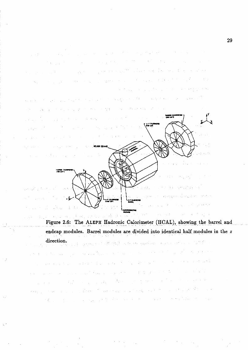
the iron structure. The HCAL is shown in figure 2.6.
There are 55,776 tubes in the barrel and 76,800 tubes in the endcaps for a total
of 132,576 streamer tubes in the hadron calorimeter. The tubes are plastic, filled
with argon, carbon dioxide, and n-pentane in a 1:2:1 ratio. The inner walls of
the tubes are coated with graphite, and a lOOµm wire runs 4 mm above the lower
29
,. ;. ........ .... ~lL_ 11...... -
=--Figure 2.6: The ALEPH Hadronic Calorimeter (HCAL), showing the barrel and
endcap modules. Barrel modules are divided into identical half modules in the z
direction.

30
wall. Each tube layer is equipped with pads on one sicle for integrated energy flux
measurements, as in the ECAL. Strips on the other sicle of each tube layer allow
reconstruction of individual tracks. This information is used for the identification of
muons. As with the electromagnetic calorimeter, the pads are arranged in projective
towers pointing to the interaction vertex.
Outside the return yoke of the magnet are two double layers of steamer tubes
used to identify muons and measure their angle. The double layers are separated
by 50 cm, and the readout strips in each layer are arranged in two orthogonal
projections in the barrel and at a relative angle of 60° in the endcaps. The layers
around the barrel are built in 12 modules, while the endcap layers are built in
quadrants rather than sextants, as is the case with the calorimeters. A layer of
slanted chambers are placed over the outer edges of the encaps to insure full coverage
in the barrel-endcap overlap region.
2.1.6 Luminosity Monitors
The luminosity for the experiment is monitored by calorimeters (LCAL) placed
close to the beampipe at each end of the detector, approximately 2.7 m from the
interaction point. At a center of mass energy of 100 Ge V and the design luminosity
of 1031 cm-2s-1 , the rate of Bhabha events detected by the luminosity calorimeters
is around 0.3 Hz.
As the solid angle of the luminosity calorimeter is not covered by either the ITC
or TPC, a small angle tracking device (SATR) is located between the interaction
region and the luminosity calorimeter to better define the acceptance of the LCAL.
This device defines an angular acceptance domain between 45 and 90 mrad relative
to the beam axis. The tracking device consists of nine layers of separated brass tube
chambers arranged into three groups of three layers each. These are structured in
eight 45° sectors. The second group is rotated by 15° with respect to the first group,
and the third group by 30°. The LCAL and SATR are shown in figure 2. 7.

31
Figure 2. 7: The luminosity system, showing the luminosity calorimeter (LCAL) and
the small angle tracking device (SATR).
The design of LCAL is similar to the endcap electromagnetic calorimeter, the
only differences being due to the ge6metry and available space. The LCAL consists
of 38 layers of proportional wire tubes separated by lead sheets 2.8 mm thick in the
first 29 layers and 5.6 mm thick in the last 9 layers. The induced signals on the cath
ode pads are transported by strip lines to the edge of the calorimeter and read out.
As in the ECAL, the cathode pads are arranged in projective towers, and the signals
from the fi.rst 9, middle 20, and last 9 pads inside the towers are read separately
to improve 7r - e separation by measuring the longitudinal shower development. In
the LCAL the cathode pads are smaller than in the ECAL, aproximately 30 x 30
mm2• The angular coverage of LCAL is between 45 and 155 mrad relative to the
beam axis, so that the overlap with the SATR is in the region between 45 and 90
mrad. The systematic uncertainty on the luminosity measurment is estimated to
be below 23.

32
A forward luminosity monitor, known as the Bhabha calorimeter (BCAL), mea
sures the rate of Bhabha events in the region between 5 mrad and 12 mrad for online
luminosity monitoring and for periods when LEP is running below the design lumi
nosity. This luminosity monitor is a small tungsten and scintillator calorimeter. A
layer of tungsten, 4 radiation lengths thick, is located at the front of BCAL to pro
tect it from synchrotron photons. This is followed by layers of tungsten 2 radiation
lengths thick alternating with 3 mm thick scintillators read in pairs by small (1 cm
diameter) photomultiplier tubes. After the first 8 radiation lengths there is a layer
of vertical silicon strips, which provide additional shower position information. A
final thick layer of tungsten protects the BCAL from synchrotron radiation entering
from the back of the device. Since Bhabha scattering drops as sin-4 (6/2) , the rate
of events in the forward luminosity monitor is two orders of magnitude greater than
in the primary luminosity monitors. As the backgrounds are also much higher, the
information from the BCAL is used mainly for online estimates of the luminosity,
while the LCAL is used for the detailed offi.ine analysis.
2.1. 'T Vertex Detector
A silicon-strip minivertex detector (VDET) was only partially installed during
the 1989 - 1990 running period. Information from this detector was not used in this
analysis. However, as the amount of silicon in place around the interaction region
was somewhat different in 1990 than in 1989, the effect of this detector on the
analysis must be considered. The detector configuration for 1989 will be referred
to as the "1989 geometry" and the configuration for 1990 as "1990 geometry". The
net difference between the two geometries is that the number of photon conversion
into e+e- pairs was seen to increase in 1990 as compared to 1989. When fully
operational the VDET will provide additional tracking information for the region
between the interaction point and the ITC.

33
2.2 The ALEPH Triggers
The ALEPH detector is designed to look at a variety of physics topics, and as
such is not triggered by one speci:fic type of event. The trigger electronics are
designed to initiate the readout of the detector whenever activity indicative of a
beam.-beam. interaction is detected. These good events are referred to as the signal.
The signal events are interspersed with other uninteresting events which are referred
to as background. The main sources of background are
1. Beam.-wall or beam.-collimator interactions from off-momentum particles,
which mostly affect the endcap calorimeters and ITC,
2. Beam.-gas interactions, which produce low energy tracks in the tracking cham.
bers.
3. Synchrotron radiation, which should not affect the calorimeters but will pro
duce random hits in the tracking chambers.
4. Cosmic rays, which could mimic dilepton events.
The aim of the trigger then is to sift out as many background events as possible
while keeping all signal events. At the design luminosity and running on the zo peak, the rate of beam.-beam. events, i.e. Z 0 interactions, is about 1 Hz. Background
levels can change dram.atically with the param.eters of the accelerator.
The trigger system has three levels of increasingly restrictive requirements, each
requiring longer decision times. The Level 1 triggers require one of the following
conditions be met:
1. At least two minimum ionizing tracks,
2. One minimum ionizing track and one energy cluster,

34
3. A total electromagnetic or hadron energy above a certain threshold,
4. A luminosity event.
The ITC, electromagnetic and hadron calorimeters, and the luminosity monitor
are used in the Level 1 triggers. A track candidate in the ITC is defined as a wire
signal in at least 5 out of 8 planes in one of the 60 </> segments. The wire and
tower signals from the ECAL and HCAL are also summed in 60 trigger segments,
with segmentation closely following the modular structure of the calorimeters. The
ITC trigger signals are mapped on the trigger segments by an 0 R of appropriate
azimuthal segments. ln general signals from different physical modules must be
mixed in order to produce the correct segmentation in both 8 and</>. The LCAL
tower signals are grouped into 24 trigger segments, 12 in each end of the detector.
A Level 1 trigger may initiate the subsequent higher level triggering and digiti
zation of signals every time its conditions are met, or be prescaled by some preset
factor. An 0 R of the enabled triggers determines a Level 1 YES or N 0. If the Level
1 trigger conditions are met, the Level 1 trigger opens the TPC gate and initializes
the Level 2 trigger logic. Up to 32 Level 1 triggers may be defined for a run; in the
1989-1990 running period the following trigger conditions were used :
1. Based on the ITC and ECAL wire information:
- Greater than 6.5 Ge V of energy in the ECAL barrel, No ITC requirement.
- Greater than 3.8 GeV of energy in one of the ECAL endcaps, No ITC
requirement.
- Greater than 1.6 Ge V of energy total in the two ECAL end caps in coïn
cidence, No ITC requirement.
- Coïncidence of an ITC track candidate and an ECAL module with greater
than 1.3 Ge V of energy, in the same azimuthal region

35
2. Based on the ITC and HCAL wire information:
- Coïncidence of an ITC track candidate with four out of twelve double
planes of an HCAL module, in the same azimuthal region. (This is
sensitive to penetrating particles such as muons.)
3. Based on the LCAL tower information:
- Greater than 31 Ge V in either of the two calorimeters.
- Greater than 20 GeV in one calorimeter and greater than 16 GeV in the
other, with no azimuthal correlation required.
- Greater than 16 GeV in either calorimeter. (prescaled)
- Greater than 20 GeV in either calorimeter. (prescaled)
The two prescaled luminosity triggers are used to estimate the beam related back
ground to the luminosity measurement. These general trigger requirements are
translated into specific trigger electronics configurations.
The Level 2 trigger requires that at least one track in the TPC points to the
bunch crossing region, by reconstructing tracks using microprocessors in the readout
chain. There are 24 such processors, which use information from special pad rows
located between the standard pad rows. The long trigger pads are 6 mm wide and
subtend an arc of 15° in </>.
The Level 2 track search is done progressively during the 40 µs TPC drift time. If
the event is accepted, control is passed to the data acquisition system, otherwise the
readout is cleared to accept the next event. The total delay for the Level 1 trigger
from bunch crossing to opening the TPC gate is about 1.5 µs and introduces no
dead time. The Level 2 trigger decision is available a few microseconds after the
end of the TPC drift time, around 50 µs after the Level 1 YES. This introduces

36
a dead time on the order of a few percent for typical running conditions. Bunch
crossing occurs every 23 µs for a four bunch mode.
The Level 3 trigger is in fact an event reconstruction program. which analyses the
digitizations for evidence of tracks. This is done in a set of single board microvaxes
attached to the main data acquisition computer. Reconstruction is only done on
those parts of the detector showirig activity in the Level 1 or Level 2 triggers. The
Level 3 trigger was not allowed to reject "false" triggers since the trigger rate with
just the Level 1 and Level 2 triggers was acceptable in the 1989 and 1990 data runs.
The trigger efficiency is ea.Sily measured, since most events trigger more than
one trigger. The efficiency for triggering on hadronic events in the fiducial region
of the detector is 99.96±0.02 %, for triggering on leptonic events 99.9±0.1 %, and
for triggering on luminosity 99.7±0.2 % (21].
2.3 Data Acquisition
The data acquisition for such a large detector as ALEPH (the number of chan
nels is approximately 500,000) is necessarily a complicated problem. The ALEPH
Data Acquisition System {DAQ) is designed to support the independent collection
of data from di:fferent subdetectors, so many users can work independently on dif
ferent parts of the experiment at the same time. A subdetector is any one of the
major ALEPH components - the ITC, the TPC, the electromagnetic calorimeter,
the hadron calorimeter {including the muon cham.bers), the small-angle tracker, the
luminosity calorimeter, the Bhabha calorimeter, and the mini-vertex detector. The
typical readout system for any of these subdetectors is based on the FASTBUS
protocol, and is organized in a branching "tree" structure (see figure 2.8). The base
of the tree is a Motorola 68020-based microprocessor known as an Event Builder.

37
This device controls the readout of information from the "front-end" electronics -
devices connected to the subdetectors which convert the subdetector analog signals
into digital information. Pieces of the event (blocks of 32 bit data words) from the
subdectector Event Builders are passed to a Main Event Builder, which assembles
the entire event data buffer and passes it via an optical :fi.ber link to the main data
acquisition host computer in the control room.
The FASTBUS tree can be separated into branches, each of which can be config
ured as an independent data acquisition stream. This concept, known as partioning,
allows the individual subdetectors to debug, calibrate, or take data independently.
The whole mechanism is handled in software, through the use of databases speci
fying the data acquistion tree, enabling triggers, data ouput destination ( disk file,
no output, etc.), and monitoring tasks, for the partition being used. The utility of
this approach was particularly appreciated near the end of the 1989 run, when a
hardware failure crippled the main data acquisition Host Computer. The partition
which corresponded to the readout of the entire detector was rede:fi.ned so that the
data stream passed through the TPC subdetector computer, and data acquisistion
continued.
The necessary elements of a read-out partition are 1) The host computer, 2) A
Main Event builder to control the Event Builder-to-Host exchange, 3) A subdetector
Event Builder in which the local data consumer and producer tasks run, and 4) A
Trigger Supervisor. The FASTBUS elements of a partition are assigned a unique
broadcast class, and will only respond to FASTBUS instructions (service requests)
of that class. Readout elements toward the detector obey instructions from the
elements toward the host computer. Components on the same level of the readout
hierarchy do not communicate.
During real data-taking conditions, the timing signal from the LEP machine
indicates beam bunch crossings. This signal enables the digitization of the front-

1 1 1 1 1 1
TPC (108 FASTBUS crates) 1 . ,....,...,,..., : .......... ..... . ,... ..... ,.... •. ,...,,...,r-' ,...r-',... .......... ............... ,....,:...,.... ,....,....,.... ,...,.... ..... .......... ,.... ..........
............ : .... ......... ............ , ............. ........ .._.. --. .... : 1 .._. .._. .._.: .... .._..._., ...,.._..._., ...,._.._.. .... .._..._. . .._....,: 1 1 ,....,....,... ...,.._...., 1
1 ,.... ,.... ,.... .._. .._...., 1
BCAL ,----.., : . ..., 1 .__..
MVER .... 1 .._. 1
L::...J rrc ~ 1 ...... 1
LCAL
.._. : .____:.;
ECAL
I ~ ..... ::: :::0 .... 1 ....... ~
: 7 1
Î 1 1 1 1 1 1 1 1 . ,....,....,.... .............. : : ,....,_,,... ................ . , ,...,_,,... ............ :
1 .... 1
1 .... l ~=~---: ,_ 1
1f ,_. ,_.1 r. .._. ._,f 1 HCAL Trigger r----; r-:--,
i rf" 111;f_J! !~~! L ___ . · ...... · ~~---·_: _l .... 1 __ 1c~;; ~ J
f .---·--------• 1
- --n 1 1 1
Event l'l!CO!!.!!!l.E'.2.'!._ 1 1 1 1 1 1
1~1~1 ... ~1 1 1
1 l 1 1 1 1 1 1 1 1 1
'--·----- l 12 limes VAX3100 l
38
Figure 2.8: The ALEPH data acquisition system, show the tree-like structure of the
readout hierarchy.
39
end electronics of the subdetectors. Level 1 and 2 NO triggers cause a reset, while
a level 1 YES trigger permits data acquisition to continue and a level 2 YES trigger
validates the event digitized in the front-end. During the time that the event is
being digitized or read-out by the FASTBUS Read-Out Controller (ROC), a Main
Trigger Supervisor inhibits the acceptance of new triggers. Digitized information
from the ROCs is read by the subdetector Event Builders on a "first ready, first
read" basis, and the contents of the subevent in the Event Builders are available
to subdetector computers for monitoring. The subdetector Event Builders format
the data, buffer the subevents to equalize data flow rate, and signal the next level
in the readout. Acceptable events are passed from the subdetector Event Builders
through the Main Event Builder to the Host Computer, where the event is written
to disk. The Main Event builder insures that ail the data buffers belong to the same
event, and are not fragmented.
2.4 Event Reconstruction
Event reconstruction proceeds in a "quasi-online" manner in a farm of DEC
workstations, each running the reconstruction software. This farm is known as
FALCON I [33], FALCON II and FALCON III referring to later data transfer and
offilne analysis facilities. Datais taken in sets of events known as "runs". The length
a run is defined by the amount of data which can fit on an IBM 3480 cartridge.
Runs are often eut short because of loss of beam, or because of operator intervention
due to a problem with the detector, readout, or beam conditions. After a run is
completed, the disk on which the events were written is made available to the
FALCON cluster. Each processor accesses a distinct set of events and the track
finding and energy clustering algorithms translate the raw detector information into
quantities suitable for physics analysis.

40
2.4.1 Track Reconstruction
Tracks in ALEPH are reconstructed based on information from the ITC and
TPC. Because of the parallel E and B fields charged particle trajectories are helices,
with a circular projection on the nearest endplate of the TPC.
The tracking in the TPC is done in the following manner [34] : First, "chains" of
radially ordered TPC coordinates are found. These chains consist of at least three
points which satisfy the hypothesis of lying on a helix. Second, chains which may
be formed by the same particle are combined to form tracks candidates. Third, the
track candidates are fitted to form TPC tracks.
The five parameters of the helix fit are chosen to be
- w = the signed inverse radius of curvature, thereby including the particle
charge.
- tan À = ddz = tangent of the dip angle . .. , - <Po = emission angle in the :z:, y plane at the point of closest approach to the
z a.xis.
- do = signed distance in the :z:, y of closest approach to the z axis. The sign
indicates whether the helix encompasses the z axis.
•t• . t 2 + 2 J2 - Z0 = pOSl lOn ln Z a :Z: y = ao•
These quantities are illustrated schematically in figure 2.9 .
. The momentum resolution in the TPC can be expressed in terms of the error
on the sagitta of the fitted helix;
ê:,.pT D.s PT = 0.021pT L2 B
where L is the length of the trajectory in meters, and B is the magnetic field in
Tesla. In order to reduce this error, the TPC was built with largest lever arm that

41
y z
. 6,.Z
} z
X s
Figure 2.9: The parameters used to fit tracks in the TPC. The dip angle À is defined
by tan.X= /z . ., .. .,

42
was practical, so that L = 1.4 m for a track at 0 = 90°. A 0.13 resolution in the
momentum of 45 Ge V tracks produced at 90° th us requires a sagitta error below
3 µm. Systematic shifts in the sagitta due to imprecise knowledge of the field can
lead to an error in the momentum measurement. The overall momentum resolution
for the TPC, obtained by measuring the ratio of momentum to beam energy for
collinear dimuon events, is found to be [35]
When ITO and TPC coordinates are used to together to determine the trajectory
and momentum, the momentum resolution improves to
2.5 Data Quality Monitoring
The quality of the data taken during a particular run depends on the condi
tions of the accelerator, detector, data acquisition, and event reconstruction facil
ity. Futhermore data ma.y be judged acceptable for one analysis, and rejected by
· another. The final decision on which runs to use must in the end be made by the
physicists performing the particular analyses. However, many of the criteria which
go into this decision can be coded in data quality assessment software.
During the initial 1989 runs, data quality monitoring was done "by hand"; that
is, obvious errors were noted as they occured. Inconsistencies which could be de
tected during data acquisition (bank corruption during data transmission, trigger
errors, missing pieces of an event) were written to bank headers. Inconsistencies
detected during processing, such as corrupted or unreadable data, were written out

43
in run summaries. This proved to be satisfactory for the amount of data taken.
For the small amount of data, statistical errors on the luminosity dominated all
systematic errors due to data quality and uniformity.
For the 1990 running an automated system for monitoring data quality was de
veloped. This system centered around a run quality database which accepted input
from several sources. Information on data quality directly obtainable from the run
database, such as missing subdetectors, was added automatically to the database
by a server task which ran parallel to, but independent of, the data acquisition.
Additional information was added by hand, making the database in practice a form
of electronic logbook. Information was also collected during the run by individual
subdetector monitoring tasks, and during event reconstruction by the reconstruc
tion software. Finally all this information was collated and a list made of runs which
were good, questionable, or not good for particular sets of analyses.
The labels given to a run were : PERF if the run was considered perfect for
analysis; MAYB if there were problems which might hinder certain analyses; and
DUCK if the run should be avoided in general. MAYB runs had information in the
database suggesting for which analyses the runs would or would not be acceptable.
Because there .were nearly 3000 runs taken in the 1990 data taking period, this
automated procedure was essential in determining the subset of runs which were
suitable for physics analysis. The automated run quality system resulted in an
assessment for the entire running period being available within hours of the end of
the last data run. Later, as data was reprocessed, run assessments for many runs
were changed, with several runs being upgraded from MAYB to PERF.

CHAPTER 3
DATA
The charge flow analysis, to be discussed in detail in the next chapter, is based on
190,656 hadronic events recorded by the ALEPH detector in the two running periods
from September 1989, to August, 1990. The events were taken predominantly at
center of mass energies near the mass of the Z 0, but other energy values were also
used.· Table 3 shows the number of events per nominal energy bin. The actual energy
varies due to slight differences in the beam orbits, effects which are magnified by
the large circumference of the LEP machine.
Computer simulated hadronic events are also studied. There were 236, 700
hadronic events with full detector simulation in this sample. These events were
also predominantly at the peak energy, specifically 92.2 Ge V, with a small fraction
of the events at off-peak energies. Other Monte Carlo event samples were generated
without the detector simulation, and were used for specific studies.
3.1 Run Requirements
Data were selected from all runs of good data quality. For the purposes of this
analysis, this means runs in 1989 in which the TPC high voltage was on, all TPC
sectors were functioning, and in which no problems effecting track reconstruction
were noted. For runs in 1990 this means a Run Quality stamp of MAYB or PERF,
as all runs were labelled DUCK in which the TPC was not functioning adequately.
There are some events known to have been lost; as short runs, in which 10 or less
44

45
probable hadronic events were recorded, were labelled DUCK. These were for the
most part runs which were aborted prematurely or stopped in order to change the
output file destination.
3.2 Deflnition of Hadronic Events
As already discussed, hadronic events are characterised by the high particle
multiplicities of the final state. Thus the main criteria for selecting hadronic events
are : 1) At least 5 :fi.ve· good charged tracks, and 2) total charged energy Ech >
0.1 x y'S. The distribution of charged track multiplicity and total charged energy for
all events is shown in figure 3.1. Also shown are the cuts made on each distribution
in order to select hadronic events.
The main background to the hadronic event selection is from tau decays which
are largely eliminated by both cuts, and from two photon interactions, which are
largely eliminated by the total energy eut. The background from tau production
is estimated to be 0.13 % relative to the hadronic event sample. The background
from two-photon interactions is :hegligible.
3.3 Track Requirements
The requirements for considering a track good for analysis are important and a
possible source of systematic error. Tracks are reconstructed primarily from infor
mation from the TPC. The numbers of possible "hits" (three dimensional coordi
nates) in the TPC is 21 for a track produced around 90° relative to the beam line,
but decreases with polar angle. The requirement for a good track is that it have

46
at least 4 hits in the TPC, and a polar angle of at least 8 = 18.2°, corresponding
to six pad rows in the TPC. Good tracks are also expected to originate from the
interaction region. Define for each track do as the distance of closest approach in the
x-y plane, and z0 as the distance of closest approach along the z-axis. A good track
is required to have do < 2.0 cm and lzol < 10 cm. Figure 3.2 shows the distribution
of do and z0 for ail tracks, with the good track cuts indicated.
3.4 Monte Carlo Data
The simulated events, usually referred to as "Monte Carlo" data, were produced
in the following manner. Bare events consisting of the colliding e+e- pair, the
exchange boson, the quark pair, and initial and/or final state radiative photons
were generated by the DYMU [36] generator. These generator events were evolved
into hadrons (fragmented) using the LUND [39] Monte Carlo of jet fragmentation,
with some modifications by the ALEPH group for heavy flavor decays, Dalitz decays,
and updates of branching fractions and decay rates. For some studies this level of
simulation, in which the parent quarks have evolved into a multiparticle final state
and the unstable particles have decayed, is sufficient. For studies requiring the
inclusion of detector effects, the simulated event is passed through a simulation of
the ALEPH detector. This simulation program, named GALEPH, is based on the
GEANT [37] simulation package, and produces simulated tracking and calorimeter
responses. A unique feature of the ALEPH simulation is precise simulation of the
passage of tracks through the TPC. This simulation program, called TPCSIM[38],
takes track segments produced by GEANT and propagates them through the TPC,
simulating drift electron trajectories and endcap sector responses. These simulated
raw data are then fed through the event reconstruction program JULIA, the same

47
program used to reconstruct real events. This chain of simulation packages and
event reconstruction is shown schematically in figure 3.3.
The Monte Carlo programs are tuned to provide the closest agreement possible
with real data. Sorne example plots which will be of importance to this analysis
are shown in figure 3.4; these are the distribution of the transverse and longitudinal
components of the track momenta relative to the beam axis, the charged track
multiplicities of the events, and the angular distribution of the leading charged
track in each event. The Monte Carlo events are shown as a histogram, data events
as closed circles.

48
Table 3.1: Number of hadronic events seem at each nominal LEP center of mass
energy value. True energy values deviate from the nominal values by at most ±50
MeV.
Nominal LEP Energy True -Energy Range N umber of Events
(Ge V) (Ge V) zo -+hadrons
88.250 88.216 - 88.280 2865
89.250 89.214 - 89.312 5100
90.250 90.216 - 90.312 12054
91.000 91.030 - 91.062 5099
91.250 91.204 - 91.312 126136
91.500 91.526 - 91.530 4829
92.250 91.214 - 91.304 16168
92.500 92.562 86
93.250 93.212 - 93.316 8497
94.250 94.216 - 94.278 5874
95.000 95.036 95

49
NCH distribution
10 t track eut
0 10 20 30 40 50
EcH distribution
., ., 102
b.1.Js eut
'•. 1
'·. 1
i
0 20 40 60 80 1 OO
Figure 3.1: 1) Distribution of eharged traek multiplicity a) for ail event, and b) for
events passing the eut on EcH > O.ly's 2) Distribution of total eharged energy a)
for ail events, and b) for events passing the eut on N CH > 4.

-·.6 -•• _,. i 1 1
. .. -, 1
dO distribution
L---------------------------1Q3,__..__.._....._.._....__.__.__..__.__.__,__.__.___.._...__,.__,__.__..__...__.....__.__._~ -10 -7.5 -5 -2.5 0
-15 -10 -5 0
2.5
. '•
1
5
5 7.5 10
zO distribution
10 15 20
50
Figure 3.2: Distribution of track d0 and z0 for ail tracks. The arrows indicate the
cuts made for good tracks originating from the interaction region. The dashed
distributions shows the resulting d0 and z0 for tracks passing the selection cuts.
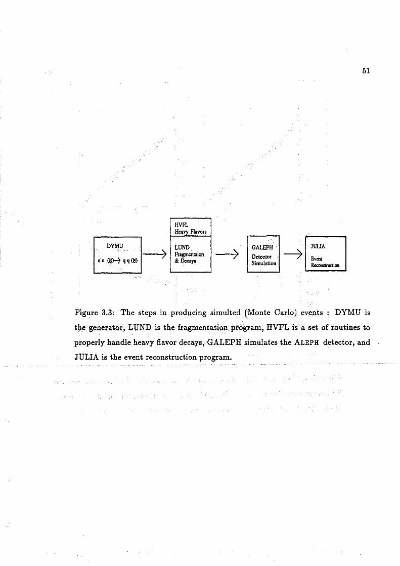
HVFL Hcavy Flavors
DYMU --~' LUND
7 Fragmcntaion & Dccays c c (lS)~ q q (21)
1 GAI.EPH
Dctcctor Simulation
.__ __ ....
51
---7'=1 ~
Figure 3.3: The steps in producing simulted (Monte Carlo) events : DYMU is
the generator, LUND is the fragmentation program, HVFL is a set of routines to
properly handle heavy flavor decays, GALEPH simulates the ALEPH detector, and
JULIA is the event reconstruction program.

52
-1 -1 10 10
-2 10
-3 10
-4 10
-5 10
0 20 40 0 20 40 Pr (GeV) Pi (GeV)
0.08 0.035 0.07 0.03 1/N dN/dcos(~)
0.06 0.025
0.05 0.02
0.04
0.03 0.015
0.02 0.01
0.01 0.005
0 0 0 0.25 0.5 0.75 cos(1't)
Figure 3.4: Comparison of data and Monte Carlo events. A) Tranverse momenta,
B) Longitudinal Momenta, C) Charged track multiplicity, D) Angular distribution
of the thrust axis. Data is shown as closed circles, Monte Carlo as histograms.

CHAPTER 4
ANALYSIS
As briefly explained in the introduction, an asymmetry measurement needs an
experimental determination of the direction and charge of the particles produced in
the e+ e- collisions. In this chapter the methods used for detemining these values
in hadronic events are discussed. These methods are then used to define the charge
flow. The mean value obtained for the charge flow in the total hadronic sample is
presented, along with statistical and systematic measurement errors on the value.
The interpretation of the measured quantity is presented in the subsequent chapter.
4.1 Determination of the Quark Direction
The process of fragmentation obscures not only the charge of the parent quark,
but also its direction. Various methods are used to determine the parent quark
direction; jet finding algorithms, sphericity, and thrust.
Jet finding algorithms work along the following principles. Tracks are ordered by
momenta. High momentum tracks are selected as the starting point for finding jets.
Neighboring tracks are joined with the starting track to form clusters or minijets.
These clusters are then joined to form larger clusters. The joining process ends
when the remaining jets are separated in phase space by more than some cutoff
value.
The particular jet finding algorithm used (41] had the feature that tracks are
joined to a cluster on the basis of their transverse momenta with respect to the net
53

54
momentum of the cluster,
2 (p • PJ(Pchu • Pclu•) - (p • Pclu• )(p • Pclu•) PT= ( -+ - ) (-+ - ) P Pclu• • P Pclu•
(4.1)
A track is joined to a cluster if p~ < 0.25 (Ge V/ c) 2• Clusters are then joined
to form jets based on the value of the invariant mass of the two clusters scaled by
the visible energy in the event (taken to be the charged energy in this analysis),
y = M 2 / E! •. If y < Ycut the clusters are merged. Various Ycut values were compared.
Both the sphercity and thrust axes are global for the event, in that they are
based on ail the tracks in the event rather those judged as belonging to a particular
cluster. The starting point for the sphericity axis is the momentum matrix (42]
1 n
Mi;= - 2:P•(k)p;(k) n k=l
( 4.2)
where i,j = z, y, z directions, and n is the number of tracks in the final state. The
normalized eigenvectors of the matrix are
( 4.3)
If the eigenvalues are defined so that 1 A1 > A2 > A3 , then ii1 is the sphericity axis,
while ii1 and ii2 define the event plane. ii3 is the direction in which the sum of the
square of the momenta projections are minimized. The scalar quantity sphericity,
S = HA2 + A3) = ~(1 - A1), is a measure of the "jettiness" of the event; it is 0 for
collinear jets.
The thrust axis is the direction ii for which the quantity
T = 2L:P(k)-n>o.P(k) · ii E1el.P(k)I
( 4.4)
is maximized. The thrust, T, is another scalar measure of the jet-like nature of the
event; it is equal to 1 for collinear jets.
1This is the definition used in ALEPH • Other definitions, with A1 < A, < A3, are common,
cf.[43).

55
The effi.ciency with which these jet quantities approximate the original quark
direction can be estimated in the Monte Carlo simulation. Define a as the angle
between the original quark and the nearest jet, or between the quark and the event
(sphericity or thrust) axis. A plot of sina is shown in figure 4.1 for jet axis with
Ycut =0.02,0.04, and 0.06; sphericity axis; and thrust axis. The event axes show an
advantage over jet axes, but all lead to an error on the quark direction of a few
degrees. Furthermore there are problems involved in using jet finding, due to the
artificial nature of the Ycu.t or similar eut-off parameter. Ultimately in this analysis
the thrust axis will be used to approximate the quark direction.

56
0.06 0.06 0.06
0.05 Y.,.= 0.02 0.05 Y.,.= 0.04 0.05 Y_.= 0.06
0.04 0.04 0.04
0.03 0.03 0.03
0.02 0.02 0.02
0.01 0.01 0.01
0.5 0.5 1 0.5 sin(11) sin(11) sin(11)
0.32 0.32
0.28 Sphericity 0.28 Thrust 0.24
0.24 0.2
0.2 0.16 :.:::
)~ 0.16 ·:; 0.12 0.12
0.08 0.08
0.04
0.25 0.5 0.75 0.25 0.5 0.75 sin( a) sin{ a)
Figure 4.1: sin a, the sine of the angle between the quark and the jet or event axis,
for jet axis with Ycut =0.02,0.04, and 0.06; sphericity axis; and thrust axis.

57
4.2 Determination of the Charge of the Quark
In order to reconstruct the charge of the parent quark of a final state jet of
charged particles, the assumption is made (19] that the hadrons in the final state
with a higher value of z = 2LEP will have a greater probablility of retaining the ....... charge of the parent quark. This leading charge effect is incorporated in the Monte
Carlo simulation of quark fragmentation. The results of this simulation canin turn
be used to estimate the effi.ciency of various weighting methods in reconstructing
the quark charge from the charged particles in the final state.
Jet charges are in general formed by summing all charges in a jet weighted by
some discriminating variable to a power "' ("' being tuned to optimize jet charge
finding sensitivity) :
Q L:jet IXI" q; jet = L:jet IXI" ' ( 4.5)
where X is the discriminator variable used to give greater weight in the sum to
particles more likely to discern the parent quark charge.
The discriminators studied were :
• longitudinal momentum with respect to the jet axis1,
• rapidity with respect to a jet axis 1,
• longitudinal momentum with respect to the thrust axis,
• rapidity, y =ln( ~~!D where Pl is measured with respect to the thrust axis,
• the total momentum fraction carried by the charged particle, z = 7. Generally no significant superiority was demonstrated of one discriminator over all
others at their optimum "' values. Clearly this not unexpected, as the only free
variable is Pl in ·all but the last discriminator. Also the assumption is that the
11n each case various values of Ycui were used to define the jets

58
tracks with a greater projection of momentum in the original quark direction would
be more likely to retain the charge of the quark; thus Pl would be expected to be a
better estimator than the total momentum.
The charge finding effi.ciency is defined as
Ncorrect €total= N
total
where Ncorrect is the number of events in which the sign of the quark was correctly
reconstructed, and Ntotal the total number of events in the sample. A large difference
in the charge finding effi.ciency is seen when only events with oppositely charged jets
are considered. This quantity,
Ncorreci €opp. charged jeta = N
opp. charged jets
is shown in table 4.2. This definition assumes that only two charges are recon
structed per event. For the case where the event axis (thrust axis) is used this
means reconstructing the weighted charge in each hemisphere. For the cases where
jet axes are used, this means limiting the study to those events in which the.jet find
ing algorithm reconstructed only two jets. The effi.ciencies for these discriminators
are given in table 4.2 below.
The fourth discriminator is thus chosen, Pl = P.f.T , where f.T is defined as the
direction of the thrust axis. The direction of the thrust axis is always taken as
forward, that is, €.z > O. This discriminator showed a marginally better charge find
ing effi.ciency than z weighting, has a clearer optimum effi.ciency than y weighting,
and avoided uncertainties associated with jet-finding algorithms, e.g. dependence
of Qjet on Ycut• Plots of €total and €opp. charged jets for z, y, PÎhrust weighting are shown
in figure 4.2.
In the rest of this analysis, each event is divided into two hemispheres as defined
by the thrust axis, and the Pl-weighted charge is computed for each hemisphere.
These weighted charges are referred to as the "hemisphere charges".
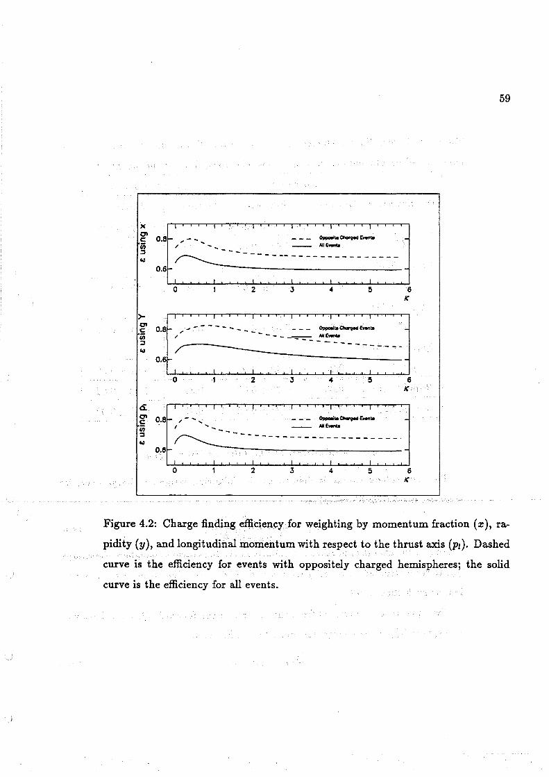
)(
g' 0.8 (ij :::1
"' 0.6
>-g' 0.8 (ij :::s
"' 0.6
ci g' 0.8 (;; :::1
"'
,,,,,.- ........ " --- ----~ - -- - - - - - - - - - - - - - - -
0
;
" ------
2
---
3 4 5
- - - ~ .. Chor9'ld Ewftle - - - - --=-=-:., _,.. E"9nta ---------- ------
0 2 3 5
- ... ; ... I
--------------------~ ~--0.6 ---------------
0 2 3 4 5
6 /(
6 /(
6 /(
59
Figure 4.2: Charge finding effi.ciency for weighting by momentum fraction ( z ), ra
pidity (y), and longitudinal momentum with respect to the thrust axis (pi). Dashed
curve is the efficiency for events with oppositely charged hemispheres; the solid
curve is the efficiency for ail events.

60
Table 4.1: Charge finding efficiencies for the various discrim.inator variables tested,
based on ail events and events with oppositely charged jets or hem.ispheres.
Ail Events Opposite Charges
Discrim.inator Optimum Efficiency Optimum Efficiency
K, at Optimum 1<. K, at Optimum "'
Piet 0.45 0.65 ± 0.02 0.35 0.82 ± 0.02
(Yc:ut = 0.02)
Piet 0.45 0.64 ± 0.02 0.50 0.82 ± 0.02
(Yc:ut = 0.04)
Piet 0.55 0.64 ± 0.02 0.35 0.81±0.02
(Yc:ut = 0.06)
P1brust 0.25 0.69 ± 0.02 0.35 0.81±0.02
Rapidity (y) 0.60 0.70 ± 0.02 0.80 0.83 ± 0.02
z =p/Ecm 0.25 0.63 ± 0.02 0.40 0.81±0.02
4.3 Evaluation of the Charge Flow, QFB
The hem.isphere charge is defined as the following weighted charge over, for
example, the forward hem.isphere :
Q - EPi.ii>O IPï·fil" qi (4.6) F - '°' , - -1" ' 4-p1.ii>O Pi•ft
where ~ is the charge of particle i. Sim.ilarly in the backward hem.isphere the charge,
QB, is reconstructed using ail particles with Pi·Ëi < O. The thrust axis is always
defined such that f:: > O.
Two quantities are formed from the charges in the forward ( Q F) and backward
hem.isphere (QB): the charge flow between the hem.ispheres,
(4.7)

61
and the total event charge
(4.8)
This charge evaluation is done on an event-by-event basis, with the results stored
in histograms. Finally the mean value of QFB and of the event charge Q are com
puted. The statistical errors on these mean values are evaluated by assuming Guas
sian distributions. These errors are ilQFB = u(QFB)/VN and llQ = u(Q)/VN,
where u( z) is the square root of the variance, u( :z: )2 = * :l:ï( i - Zi )2
, where i is
the mean of the distribution, and N is the number of events.
4.4 Determination of the Weighting Power "'
In the definition of hemisphere charges (Eq. 4.6) the exponent "' was included
as a tuning parameter used to maximize the effectiveness of the measurement. The
criteria will now be considered for picking a value of "' to be used in the final
measurement.
Previous experiments set "' by optimizing the fraction of events in which Q F
and QB were oppositely charged. As shown in figure 4.2, this would yield a weak
optimum value near "' = 0.4 , and the opposite charge fraction per quark type
decreases monotonically .
The following were considered in making a choice of "' :
• Sensitivity of the measurement to the underlying physics.
• Minimizing detector induced effects
• The shape of the distribution ( since many of the results used in interpreting
the measurement will depend on approximâting the distributions as Gaus
sian ).

62
• Correlations between hemispheres
Of these, the sensitivity is the most unambiguous, and the choice of "' for this
measurement has been made primarily on the basis of this indicator.
ln defining a quantity with which to express the sensitivity of the measurement,
the following result is used: The expected quark asymmetry is e:ffectively contained
in the term L. S1afVf as will be shown in the next chapter. Here the quantity 81 is
the mean value of the QFB distribution for Monte Carlo events in which a quark of
:flavor f was produced in the forward hemisphere. The five values of SI are taken
from the full Monte Carlo simulation, and will be discussed in more detail in the
next chapter. The sensitivity is then defined as the quantity to be measured divided
by the error on the measurement. This is proportional to
Figure 4.3 shows a plot of S as function of "' . There is a clear optimum at "' = 1.0 .
Generally, low values of "' correspond to nearly equal weight being given to all
charged tracks. As "' increases more weight is given to higher momentum tracks
until, for "' --+- oo , only the leading track in the event is given any appreciable
weight.
As"'--+- oo the QFB and Q distributions develop additional peaks at ±2.0 as well
as the approximately Gaussian peak at O. This is shown in figure 4.4, where the QFB
distributions at "' = 0.5,1.0, 2.0, and 3.0 are plotted. Eventually the distribution
collapses into three spikes at -2, O, and +2 , when only the leading charges forward
and back are e:ffectively used in forming the hemisphere charges. We therefore do
not consider values of "' past 2.0 except for the special case of "' = oo (leading
charges only ).
For low values of"' the contribution from low momentum tracks is greater. For
a perfect detector the fraction of oppositely charged jets would be 1003 at "'= O,

63
(/)
0.45 oD 0
0 0.4 0 0
0.35 0
0.3
0.25
0.2
0.15
0.10 0.5 1.5 2 2.5 3 3.5 ... K
Figure 4.3: The sensitivity s = E s,a,v,/ O'Qps where O'Qps is the width of the QFB
distribution in data.

64
16000
14000 9000 K=1.0 8000
12000 7000 10000 6000
8000 5000
6000 4000 3000
4000 2000
2000 1000
0 2 0
-2 0 2
9000 6000 8000 K=3.0
5000 7000
6000 4000
5000 3000 4000
2000 3000
2000 1000 1000
0 2 0 2
Figure 4.4: The QFB distributions in data at K = 0.5,1.0, 2.0, and 3.0.

65
due to conservation of charge. This is not the case, since there are tracks which
are not detected, particularly very low momenta tracks (PT < 150 Me V) which
produce helices of radii smaller than the sixth pad row in the TPC. Other low
momentum tracks (PT = 150 - 200 Me V) are not well reproduced by the simulation.
In order to minimize the effect these tracks, which tend to lead to correlations
between hemispheres due to spill over effects, values of K. < 0.8 are not considered.
Figure 4.5 shows the hemisphere correlation, C , defined as the difference between
the number of events with oppositely signed hemisphere charges and the number
of oppositely signed events expected based on the charge finding efficiency. This
correlation quickly becomes negligible as K. increases from zero.
ü 0.2
0.175
0.15
0.125
0.1
0.075
0.05
0.025 0 ....... _..__..._._....._. ..................... _.__ ......... _.._ .......... ~ ......... _._.._._ .......... ._._...._._.._ ......... ~
0.4 0.8 1.2 1.6 2 2.4
Figure 4.5: Track correlation between hemispheres versus K.
Taken together these considerations lead to the choice of K = 1.0 for the final
measurement.
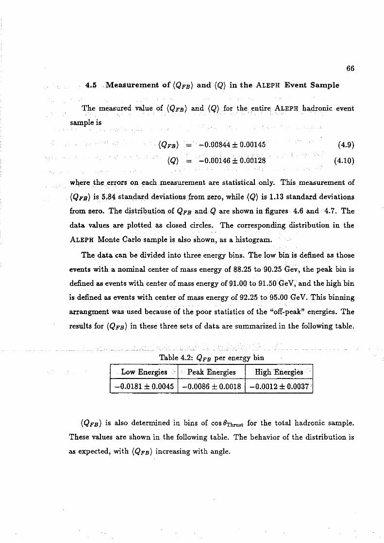
66
4.5 Measurement of (QFB} and (Q} in the ALEPH Event Sample
The measured value of (QFB} and (Q} for the entire ALEPH hadronic event
sample is
(QFB} - -0.00844 ± 0.00145
(Q} - -0.00146 ± 0.00128
( 4.9)
( 4.10)
where the errors on each measurement are statistical only. This measurement of
(QFB} is 5.84 standard devia.tions from zero, while (Q} is 1.13 standard devia.tions
from zero. The distribution of QFB and Q are shown in figures 4.6 and 4.7. The
da.ta values are plotted as closed circles. The corresponding distribution in the
ALEPH Monte Carlo sample is also shown, as a histogram.
The data can be divided into three energy bins. The low bin is defi.ned as those
events with a nominal center of mass energy of 88.25 to 90.25 Gev, the peak bin is
defi.ned as events with center of mass energy of 91.00 to 91.50 Ge V, and the high bin
is defi.ned as events with center of mass energy of 92.25 to 95.00 Ge V. This binning
arrangment was used beca.use of the poor statistics of the "off-peak" energies. The
results for (QFB) in these three sets of data. are summa.rized in the following table.
Table 4.2: QFB per energy bin
Low Energies Peak Energies High Energies
-0.0181 ± 0.0045 -0.0086 ± 0.0018 -0.0012 ± 0.0037
( Q FB} Îs also determined in bins of cos 0Thrust for the total hadronic sample.
These values are shown in the following table. The behavior of the distribution is
as expected, with {QFB} increasing with angle.

& "O ......... ~0.05 z .........
0.04
0.03
0.02
0.01
I Monte Carlo
0 Dota
0 ~laer:.L...i..i-i...L.i...i. ....... L..i....i....WL.....i.......1..i-i...a....W. ....... 1....1-L.:!::9~
-2 -1.5 -1 -0.5 0 0.5 1 1.5 2 a,.,
67
Figure 4.6: Distribution of QFB in data and Monte Carlo. Quantities are evaluated
at K.= 1.0.

0 -0
' ~ 0.06 z
' 0.05
0.04
0.03
0.02
0.01
J Monte Carlo
0 Dota
0 l!ee~tw...J...L...l..i....i...i'-1...i..i....1-1.....L-'--l-U....l...l...l....l....i...~~~
-2 -1.5 -1 -0.5 0 0.5 1 1.5 2 a
68
Figure 4. 7: Distribution of Q in data and Monte Carlo. Quantities are evaluated
at K.= 1.0.

69
Table 4.3: QFB vs cos OThrust
Central cos OThrust (QFB)
0.075 -0.00148 ± 0.00394
0.225 -0.00116 ± 0.00386
0.375 -0.01310 ± 0.00374
0.525 -0.00468 ± 0.00357
0.675 -0.01586 ± 0.00342
0.825 -0.01030 ± 0.00325
4.6 Detector Systematics
Estimates can be made of experimental systematic errors which might arise from
asymmetries in the detector material, track lasses, background processes or poorly
fitted tracks. In general this measurement will be affected by processes which are
both forward-backward and charge asymmetric.
The measurements of (QFB) and (Q) are sensitive to track reconstruction errors,
due to strong reliance on the reconstructed momentum in calculating these weighted
charges. These errors include track fitting errors due to imprecise knowedge of
the magnetic field, electric field, or detector alignment. Also poorly fitted tracks
caused by,e.g. randomly associated coordinates may lead to erroneous momentum
measurements which could affect the momentum-weighted charges.
Tracks lasses, which lead to a loss of charged track information, could potentially
reduce the accuracy of the charge flow measurement. ln addition false asymmetries
arising from processes not associated with the original e+ e- ~ qq reaction, including
asymmetries in the conversion of photons into e+ e- pairs, can affect the charge flow
measurement. Production of r -'f pairs, which are the only appreciable background

70
in the hadronic event sample, is also forward-backward asymmetric and can affect
the (QFB) measurement.
4.6.1 Momentum Refit
The error on the momentum reconstruction can be estimated by studying
dimuon events in which the acollinearity angle between the muons is less than
0.3° [35]. In such an event each muon is expected to carry the beam momentum, so
that the quantity p/ Ebeam is expected to equal one. The overall value of p(µ)/ Ebeam
for positive and negative muons is shown in figure 4.8 before any correction to the
fitted tracks.
A phenomenological momentum refit per cos 8 bin was performed, based on the
E/p distributions for muons. This refit corresponds to a constant sagitta shift,
where the constant is determined for a bin in the polar angle. The size of the the
correction factor Pc is plotted versus cos 8 in figure 4.9 for both positive and negative
tracks. The refitted momentum of a track with charge Q and momentum pis then
given by
p"efit - pold _ Q X Pc( 8) X (pold)2 (4.11)
Ere fit - Eold - Q X Pc( 8) X ( Eold)2 ( 4.12)
refit prefit
( 4.13) PJ. - ( pcld )p~d prefit
p:efit - (-)pold (4.14) pold z
refit p;efit - (E.L_ )pold ( 4.15)
p°}_d :1:
refit p~efit - (E.L_ )pold ( 4.16)
p°}_d y
where in this case PJ. is measured with respect to the beam axis. The unreffitted
values of (Q) and (QFB) are slightly different from the measured values with the

450 400
350
300
250 200
150
100
50
0 0.5
. . . . . . . . . 0 ...........
1 ................ ~ .............. T .............. .
............. ~ ............... : ............... t·····--···--·· ••oo•ouoou~ouoo••••••••• f ouooooouout•u••o•onooo
::::::::::::r::::::::::.:r.··::·::::::::r·:·::::::·: ............ ~ ... . . . . .... . --1· ........... j· ...... ····· .. . ············;-····----·· ···~· ........... T ............. . ............ ! .......... '"[" .......... t ............ .. ............ r ......... ···1 .. ·· ·· .. ·····r·····--······
0.75 1.25 1 .5
p/E, a - + 1, .o < cos(0) < .95
450 400 350 300
250
200 150 100
50
0.75 1.25 1.5
p/E. a= +1, -.95 < cos(0) < .o
500
400
300
200
100
0 0.5
. . .
::::::::::::1:::::::::::::··'.·::::::::::::::::::::::::::::
: l::~· 1 ·::~ :
.. ··········~··········· .. ·1 ··
~ i 0.75 1.25 1.5
p/E, a • - 1, .o < cos(0) < .95
400
350
300
250
200
150
100
50
·······--···j···········-- ;···········--·t········--···· ············r·······H··· ~ ···········-·r··············
···--·······r--········· -~ ·············r ............. . o•o•uou•••1••0000000000 ••~ •••••••••••t••n•••oonuo
····· ······· ~-··········· ··t· ·············r ·············· ............ ~ ............ ···r·· ........... l ............. .. ............ ~--·.... ... . ··~ .. . ........ ·1· .. ··- ........ .
···········-~········ ···-~ .. -· ········t·········· .. ··
0.75 1.25 1 .5
p/E, Q = -1.-.95 < cos(0) < .O
Figure 4.8: p(µ)/ Ebeam in collinear dimuon events.
71
72
momentum correction,
(QFB)(unrefitted) - -0.00888 ± 0.00145
- 1.048 x (QFB)(refitted)
(Q)(unrefitted) -0.00126 ± 0.00128
- 0.875 x {Q}(refitted)
The sagitta correction shifts the value of ( Q FB) by 4.1 ± 2.0 x 10⁻⁴ • The sys
tematic error associated with this momentum refit reflects the error on the sagitta
correction itself, propagated through the QFB calculation.
4.6.2 Track Losses
· The number of charged parti de tracks not reconstructed is very low. A quanti
tative estimate of the level track loss has been made (44] by scanning 5519 tracks in
404 events and looking for good unused coordinates which might constitute a track
and which seemed to originate from the interaction region. Only three such tracks
were found. The total number of lost tracks which had marginal track parameters
(distance of closest appraoch to the interaction region, number of coordinates in the
TPC) was 50. Taking this second number as an upper limit, the track loss is then
0.93±1.33.
The track loss is translated into an error on Q FB by considering the effect of a
lost track on the charge flow in a typical event. Assume that the typical momentum
of a lost track is 0.5 ± 0.1 Ge V, and that the mean total momentum in a hemisphere
is 25 ± 5 Ge V. The effect on QFB of losing one track is then 0.5/25 = 0.02 ± 0.006.
The mean charged track multiplicity in the events surveyed was 13.7 ± 0.7. The
overall effect of the three lost tracks is then estimated as 0.02x3x13.6/5519 = 1.5±
1.2 x 10⁻⁴• The systematic error on ( Q FB) due to track loss is then conservatively
estimated to be 3 x 10⁻⁴ •

73
o.. X 103
<I ..; 0.2 • Positive Tracks "-0 (.) 0.1 E • ::l 0 • • -c • 4' -0.1 • E • 0 ~ -0.2 • •
-1 -0.75 -0.5 -0.25 0 0.25 0.5 0.75 1 X 10³ cos(1')
o.. Il <I
..; ... Il 0 Il (.)
Ill [Il E Il ::l - m c -0.1 m 4' E -0.2 Ill Negotive T rock 0 ~
-0.3
-1 -0.75 -0.5 -0.25 0 0.25 0.5 0.75 1 cos(1')
Figure 4.9: Momentum correction versus cos() for positve tracks (top) and negative
tracks tracks (bottom).

74
4.6.3 Anomalously High Momentum Tracks
The number of poorly fit tracks can be estimated by looking at tracks in hadronic
events with anomalously high momenta. These are defined as tracks which meet
the criteria for good tracks, namely number of TPC coordinates 2: 4, ldOI ::=; 2.0
cm, lzOI ::=; 10.0 cm, and Pl. > 200 MeV; but which have p > Peut , where Peut =
30 or 50 Ge V. In other words these tracks appear to have momenta greater than
expected or, for Peut = 50 Ge V, greater than one half of the center of mass energy.
As the charge flow measurement gives greater weight to high momentum tracks, the
influence of these tracks on the the Q FB measurement has been investigated.
The number of anomalously high momentum tracks out of the sample of good
tracks, for each Peut value, found in the data and Monte Carlo, is given in the '
following table. Out of the sample of events containing 1 or more such tracks, the
a.vera.ge multiplicity is 1.0127 tracks with Peut = 30 Ge V and 1.0035 tracks with
Peut = 50 Ge V At Peut = 50 Ge V there are two data. events with two such tracks;
there are no data events and one Monte Carlo event with three such tracks.
Table 4.4: Occurence of anomalously high momentum tracks in data and Monte
Carlo
Peut> 30 GeV Peut> 50 GeV
No. Tracks with p > Peut - Data 4294 573
% Tracks with p >Peut - Data 0.129% 0.017%
% Tracks with p > Peut - M C 0.1293 0.0193
The momenta of all tracks, and tracks with p > Peut, in data are shown in
figure 4.10. The number of ITC and TPC coordinates used in fitting these tracks
is shown in figure 4.11 and compared to the same distributions for ail tracks. The
number of coordinates used in the fit, the x2 value per degree of freedom, and the

75
relative error on the momentum for these tracks are given in the following table.
Note that for the highest momenta tracks (Peut= 50 Ge V) the mean of the fractional
error distribution ( { ~}) is almost one.
Table 4.5: Track information for anomalously high momentum tracks
Data Monte Carlo
Peut= 30 GeV Peut= 50 GeV Peut= 30 GeV Peut> 30 GeV
{NTPC} 15.69 9.28 15.59 9.50
{NITc} 4.67 1.28 4.47 1.47
x2/v 2.24 5.69 2.67 5.87
{~} 0.19 0.90 0.20 0.85
By comparison, for good tracks with p <Peut ; {NTPc} = 16. 76 in data and 17.18
in Monte Carlo, {NITc} = 4.95 in data and 5.16 in Monte Carlo, x2 /v = 1.56 for data
and 1.54 for Monte Carlo, and {~} = 0.05 in data and Monte Carlo. The values
of the fit parameters for good tracks in events with at least one anomalously high
momentum track are somewhat worse than the average for al! good tracks. This is
consistent with the hypothesis that these tracks are due to misassociated hits. The
fit values for ail good tracks, and for good track in events with anomalously high
momentum tracks, is given in the following·table.
There is no correlation between these tracks and the overall multiplicity. The
mean charged multiplicity for events with an anomalously high momentum track is
the same, within errors, as for ail other events.
Since the effect is well reproduced in the Monte Carlo, the matching Monte
Carlo truth information for these tracks can be considered. This is done by finding
the particle in the generated event which is most likely to correspond to a track

76
0 20 40 60 80 100
p distr - oil good trocks
10 p...,=30 GeV
0 20 40 60. 80 100
p distr - Hi p trocks
10
p...,"'50 GeV
0 20 40 60 80 100
p distr - Hi p tracks
Figure 4.10: Momentum distributions in data. Top plot is for ail good tracks, with
the values of Peut shown. The middle plot is the momentum distribution for tracks
with p >30 GeV; the bottom plot for p >50 GeV.

77
X 10 2 90
5000 80
70 p ... =50 GeV 4000
60
3000 50
40 2000 JO
1000 20
10
10 20 10 20
No. TPC hits No. TPC hits - hi p tks
9000 500
8000 7000 400
6000 300 p ... =50 GeV
5000 4000 200 3000 2000 100 1000
2.5 5 7.5 10 0 0 2.5 5 7.5 10
No. ITC hils No. ITC hils - hi p tks
Figure 4.11: Distribution of the number of coordinates in the TPC (top) and ITC
(bottom) for good tracks (left) and tracks with p >50 GeV (right).

78
Table 4.6: Track information for good tracks. Ail numbers based on events in the
data.
Ail Good Tracks Good Tracks in Good tracks in
in Good Events High p Events High p Events
Peut= 30 GeV Peut= 50 GeV
(NTPC) 16.76 16.80 11.26
(NITc) 4.95 5.12 4.16
x2/v 1.56 1.57 1.80
(~) 0.05 0.05 0.14
reconstructed from the information produced by the GALEPH detector simulation.
The lead Monte Carlo "truth " track is a candidate to match an anomalously high
momentum track in 20.31 3 of the cases for Peut> 30 Ge V, and in only 8.42 3 of
the cases for Peut > 50 Ge V.
No appreciable forward-backward asymmetry is seen in the tracks, except pos
sibly for the highest momentum tracks. The forward-backward asymmetry of these
tracks is given in the foilowing table.
Table 4.7: Forward-backward asymmetry of anomalously high momentum tracks
Peut> 30 Ge V Peut> 30 GeV
Data 1.8 ± 1.13 8.8 ± 3.63
MC 1.1±1.53 3.3 ± 4.23
The .effect of these tracks on the measurement of the charge flow is estimated
by excluding events with anomalously high momentum tracks. The resulting shift

79
is l:l.QFB = 0.6 x 10⁻⁴ and represents a "worst case" estimate since some of these
tracks do accurately reflect the charge of the parent quark. Therefore these tracks
are a small source of systematic error in the QFB measurement.
4.6.4 Asymmetry Due to Detector Material
Based on a study of photon conversions (45], the material asymmetry was found
to be
Amat = -2.0 ± 1.23
The effect of this asymmetry on Q FB can be estimated from the difference of ( Q}
from zero, so that l:l.QFB = Amat X (Q}.
To see this, consider only one quark of type f. Let E>F(B) be the cross-section for
producing charged tracks in the material in the forward (backward) direction, and
d1(/) be the change in the weighted charge for a f (f) quark, due to this material.
This change in QF or QB can be due to photon conversions in the material, for
example. Then, if there are N f events produced, the number of f quarks in the
forward direction is
Nt= !N1(1 + A~B) 2
and the shift in QFB and Q due the material is
(QFB} = (QFB) 0 + ~0Fd1(l + A~B) - ~E>Bdt(l - A~B) 1 J 1 J
+2E>Fd1(l - AFB) - 2E>Bd1(l + AFB)
- (QFB) 0 + ~(E>F - 0B)(dt + df)
1 J +2(0F + E>B)(dt - d1)AFB
(Q} - (Q} 0 + ~E>Fdf(l + A~B) + ~E>Bdt(l -A~B) 1 J 1 J
+2E>Fd1(1 -AFB) + 2E>Bd1(l + AFB)
- (Q} 0 + ~(0F + E>B)(dJ + d1)
( 4.17)

80
( 4.18)
where the superscript o denote the values of (QFB) and (Q) in the absence of
any detector material. Making the assumption (based on isospin symmetry) that
d1 = db then
(QFB) - (QFs) 0 + (E>F - E>B)d1
(Q) - (Q)0 + (0F + 0B)dt
(4.19)
( 4.20)
The change in each quantity with respect to the value in the absence of detector
material is sQFB _ (E>F - eB) fiQ - (0F + E>B)
But this is simply the measured material asymmetry,
(0F - 0s) Amat = --------( 0 F + E>B)
( 4.21)
(4.22)
Extending this argument to ail :flavors, assuming that ail the shift of (Q) is due
to t-he detector material, and taking the upper limit of the error range, the resulting
systematic error on the charge :flow is
fiQFB - Amat X {Q}
- 0.5 X 10⁻⁴
4.6.5 Background From T-f" Production
(4.23)
( 4.24)
As discussed in chapter 3, the major background process in the hadronic event
sample is due to e+e-~ TT. In particular those events in which both tau's decay
into three or more charged particles would pass the hadronic event selection cuts.
As this represents only a smail fraction of tau decay channels, only a smail amount
contamination from taus fs expected. Monte Carlo studies show the tau background
to be 0.133 of the hadronic event sample.

81
Performing the same QFB analysis on a sample of tau events yields
(QFB).,. = -0.02776 ± 0.02130
Out of a asmaple of 60,000 r- events only 2971 passed the same analysis cuts used
for hadronic events. Thus the selection efficiency is
E.,. = 4.95 ± 8.253
A background correction can then be performed on the measured value of (QFB) in
the hadronic sample :
(QFB)(corrected) u( 7")
- (QFB)(uncorrected) - (QFB).,. x e.,. x u(hadron)
- -0.00844 + 0.00006 = -0.00838
The shift is (0.6 ± 0.6) X 10-4 and is a negligible effect. The systematic error on the
(QFB) measurement is taken as the error on the tau subtraction,
.ô..(QFB) = 0.6 X 10⁻⁴
4.7 Final Measurement of (QFB}
A summary of detector related systematic errors is given in the table below.
Overall the total systematic error, taken by ad ding ail the en tries linearly, is
D.QFB = 6.2 x 10⁻⁴• Thus the measurement of the charge flow is
(QFB) = -0.00844 ± 0.00145(stat) ± 0.00062(syst)

82
Table 4.8: Summery of the sources and magnitudes of detector related systematic
errors on the measurement of(QFB)· ,~--S-o_u_r-ce_o_f_E_r_r-or---.-1 ~--(Q--FB_)_(_x_1_0 __ 4-)~,
Sagitta Corrections 2.0
Track Losses 3.0
Anomalously High < 0.6
Momentum Tracks
Material Asymmetry 0.5
T Background 0.6
Subtraction
Total 6.2

CHAPTER 5
QUARK CHARGE SEPARATIONS
The connection between the charge flow measurement and the underlying physics
is through the quantity S1 , defined as the mean charge flow for a quark of type f
in the forward direction. These five quantities (one per quark flavor) are referred to
as the quark charge separations. A phenomenological mode! for connecting {QFB)
to ÀFB via the quark charge separations is presented in this chapter.
In order to understand the relation between QFB and ÀFB , figure 5.1 shows
a histogram of simulated events versus QFB of the event, for the following cases :
1) a u quark in the forward direction (hatched), 2) a ü antiquark in the forward
direction (solid), and 3) the sum of these two samples (unshaded). This is the same
figure used in Chapter 1 to introduce the concept of the charge flow.
5.1 Relationship Between QFB and ÀFB at Parton Level
Consider the forward-backward asymmetry at parton level. In the hypothetical
case that the event sample consists of only one quark flavour there are two possi
bilities: the quark can go into the forward hemisphere and the antiquark into the
backward hemisphere or vice versa. Recall that
QFB - QF-QB (5.1)
L: ,- - ,~ QF
p;.€-r>O Pï·f.T qi (5.2) -L: ,- - 1~ p;.iT>O Pi·f.T
83

<J ~600 z "D
1400
1200
1000
800
600
200
~ uquorks
<O,."> • 0.0290:1:0.0036
accc u quarks
+2q:
1.5 2 o ..
84
Figure 5.1: Simulated distribution of events for : 1) a u quark in the forward
direction (hatched), 2) a ü antiquark in the forward direction (solid), and 3) the
quark in the forward direction is either u or ü (unshaded). Single bins at ±~ show
values of QFBexpected if the quarks were observed directly.

85
(5.3)
{5.4)
This results in two discrete values of Q FB for that specific quark flavour: Q~B =
+2qlor- 2ql (ql being the quark charge). In figure 5.1 the two parton level expec
tation values of Q~8 for the cases where an u- or an fi-quark went into the forward
hemisphere are indicated by the two bins at +4/3 and -4/3 respectively. The fact
that the two delta functions are well separated means one can distinguish between
a quark or an antiquark going into the forward hemisphere. The presence of a
forward-backward charge asymmetry is reflected by the difference in height of the
two bins. The average Q~B in an event sample with quarks of flavour fis given by:
(5.5)
5.2 Definition of Quark Charge Separations
As the quarks are not observed directly, their charges have to be reconstructed
from the resulting hadronic final states. The quantity for the final state correspond
ing to the quark charges will be the quark charge separation 5, the mean value of
QFs for a sample of simulated events in which the quark is known to be produced
in the forward direction. At the parton level this would mean 51 = 2q1.
In Monte Carlo studies the nature of the initial quark is known, and will be
·either (approximately) along fT or opposite. We label with an f quantities for
which the quark of flavor f went into the forward hemisphere, and label with an
f those quantities for which the antiquark went into the forward hemisphere. The
quark charge separations for ail five flavors are given in table 5.2. The mean quark

86
separations, which will be used to extract physics parameters from the QFB mea
surement, are evaluated as Hc51 - 61), in order to minimize the statistical error on
the separations. For example, the mean values of QFB for the the d quark and the
d antiquark distributions are
(QFB)d - -0.2086 ± 0.0034
(QFB)J - 0.2069 ± 0.0038
The quark charge separation would be evaluated as
1 d J 6a - 2((QFB) - (QFB) )
- -0.2078 ± 0.0025
where the errors are due to statistics.
Table 5.1: The quark separations taken from the full Monte Carlo simulation. The
value 6 = (61 - 61)/2 is taken as the mean quark sepa~ation.
Quark s, 61 6
d -0.2086 ± 0.0034 0.2069 ± 0.0038 -0.2078 ± 0.0025
'U 0.4265 ± 0.0039 -0.4159 ± 0.0042 0.4212 ± 0.0029
s -0.2906 ± 0.0034 0.2784 ± 0.0038 -0.2845 ± 0.0025
c 0.1656 ± 0.0039 -0.1756 ± 0.0041 0.1706 ± 0.0028
b -0.2183 ± 0.0032 0.2151 ± 0.0035 -0.2167 ± 0.0024
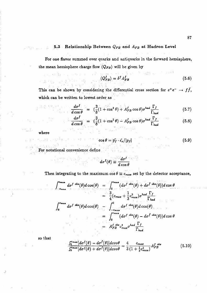
87
5.3 Relationship Between QFB and ÂFB at Hadron Level
For one flavor summed over quarks and antiquarks in the forward hemisphere,
the mean hemisphere charge flow {QFB) will be given by
(5.6)
This can be shown by considering the differential cross section for e+ e- -+ f f, which can be written to lowest order as
where
dO'I
dcos fJ dO'l
dcos fJ
- ( ~(1 + cos2 fJ) + A~B cos fJ)O'ha.d _!.L 8 rha.d
- ( ~(1 + cos2 fJ) - A~B cos fJ)O'ha.d _!.L 8 rha.d
cos e = pj · t.z/IPil
For notational convenience define
dO'I dO'' ( fJ) = d () cos
(5.7)
(5.8)
(5.9)
Then integrating to the maximum cos fJ = Cma:i: set by the detector acceptance,
J.::: .. dO'I ob• ( fJ) d COS ( fJ) foc.,.,.. ( dO'I oba ( fJ) + dO'J ob• ( fJ)) d COS 0
a 13 ha.dr, - 4( Cma:i: + 3cma:i:)O' fha.d
foc.,,. .. d0'1 00•( fJ)d cos( fJ) J.:m .... d0'1 00
•( fJ)d cos( fJ)
_ foc.,...., ( dO'I ob• ( fJ) - dO'f ob• ( 0) )d COS 0
Al obi c2 O'had _!.L FB ma:i: f ha.d
so that J;""••[dO'l(O) - dO'f(fJ)]dcosfJ _ i Cma:i: Al ob• J;m ... [dO'l(fJ) + dO'f(fJ)JdcosfJ - 3 (1 + ~C~a:i:) FB
(5.10)

88
Define P1(QFB) and Pf(QFB) as the probability density of QFB for a sample of
f quarks and f antiquarks, respectively. These are normalized so that
(5.11)
Then the average charge flow for a given flavor as a function of angle is
f f!.°:[dO'f(O)Pf(QFB) + dO'l(O)Pl(QFB)]QFBdQFB (Q~ÎJ )lcos(S) = J!.°:[dO'l(O)Pl(QFB) + dO'f(O)Pf(QFB)]dQFB
(QFB)fdO'f(O) + (QFB)f dO'f(O) dO'l(O) + dO'f(O)
(QFB)1 + (QFB)l ((QFB)1 - (QFB)l)cos(O)A~B 2 + ~(1 + cos2( 0))
Isospin invariance of the strong interactions implies, Q~B = -Q~B = 81 . Then
!+! 4 cos( 0) 1 {QFB) lcos(8) = 3 (l + cos2(0)) 28tAFB (5.12)
In a similar fashion, the average charge over a range of cosO is calculated to be:
{Q~t{)j~"'·• = J;"' .. dcos 0 J!.°:[dO'f(O)Pf(QFB) + dO'l(O)Pf(QFB)]QFBdQFB J;"'•• dcosO f!.°:[dO'l(O)Pl(QFB) + dO'f(O)Pf(QFB)]dQFB
{QFB)f + {QFB)f ({QFB)f - {QFB)1)7A~B 2 + ~(1 + ic~G:zJ
4 Cmaz f - 31 1 2 81AFB + 3cmaz
Taking Cmaz = 1.0, this reduces to
which was to be shown.
For the sum of all flavors this becomes
4 Cma:i: I: t r1 - 1 2 81A1b-3 1 + 3cma:i: I rhad
4 Cma:i: I: 3 r1 - 1 2 81-AeA1-3 1 + 3cmaz I 4 rhad
Cmaz Âe Lf 281v1a1 1 + ic~G:I: 'L1(v] + a1)
(5.13)
(5.14)
(5.15)
(5.16)

89
5.4 Evaluation of O'QFs
From the widths of the QFB and Q distributions a significant measure of the
mean overall charge separation for ail the quark flavors can be derived. In the
following we use the observed relations
u Q F - u Q 8 ( uncorrelated)
J ! (J'QP'B - (J'QP'B
which reflects the isospin invariance of the strong interactions. Also
J (J'J (5.17) (J' Q P'B - Q
J (J'f (5.18) O'qP'B - q
J (J'J+f (5.19) (J'QP'B - q
The last relation is particularly important. The width of the QFB distribution for a
quark is equal to the width of the event charge distribution when either the quark
or antiquark is in the forward direction. In principle the width of an unmeasurable
quantity (the charge flow when the direction of the quark is known) can be obtained
from a measurable quantity, the width of the mean weighted charge of ail events.
For a particular quark species, it can be shown that the width of the QFB
distribution for quark and antiquark events is approximately equal to the width of
the QFB distribution which occurs when only the quark goes in the forward direction
plus the mean of that distribution added in quadrature; that is,
( J+f )2 - ( J )2 (Q )2 (J'QP'B - O'qP'B + FB J (5.20)
Consider the definition of the variance of a distribution, which can be written as
u 2 = (~2 ) - (~) 2 • Then
(5.21)

and
(Q~B) J+f - (QFB)~+f
~ (Q~B)!+f
90
(5.22)
(5.23)
(5.24)
The mean squared value of QFB for either quarks or antiquarks in the forward
direction can be written as 1
2 ) N1 ( 2 ) N1( 2 ) (QFB J+f - N QFB J + N QFB f
(Q~B)!+f - (Q~B)J + ~ ((Q~B)r- (Q~B)J)
and by isospin symmetry
(Q~B)J+f - (Q~B)J
- (u6PB)2 + s; and therefore
and using the relation in equation 5.19 ,
( 17/+/)2 = (u')2 +c52 Qps Q J
(5.25)
(5.26)
(5.27)
(5.28)
(5.29)
(5.30)
(5.31)
This relation is based on the assumption that c51 + 81 ~ 0 , which is indeed
observed in the Monte Carlo, as shown in table 5.2. In other words, O"Qps(f + f) is
1Here the forward-backward asymmetry is ignored, so that Nt= Ni is assumed. Including Aps
the relation becomes
(<TJ+f )2 =(<Tt )2 + é2(l _ A2 ). Qra Qra J FB

91
broadened due to the fact that QFB(/) and QFB(f) are centered around fit and fi1
, rather than zero. This is illustrated in figure 5.2, where the 1 u contour lines for
(QFB)u, (QFB)fl, and (QFB)u+fl are shown on a QF - QB plot.
ô 0.8
-0.4
-0.8
-1 0 1
Os
ô 0.8
-1 0 1
Os
d
Figure 5.2: QF versus QB for u quarks. The contours correspond to a one u width
for each distribution. The contours on the left are the QFB distributions for u or ü
quarks forward. The contour on the left is the combined QFB distribution.
The sum of the charges is independent of whether the quark went forward or
backward, and nearly zero on average; (Q)f = (Q)l = (Q) = 0 . Any deviation
from zero of the total charge is due to detector imperfection, lost low momentum
tracks, and limited statistics.
The distribution of QFB in the total hadronic sample will be broadened relative
the the Q distribution. Then
(5.32)

92
(5.33)
Define the mean charge separation 6 such that
(5.34)
since for a particular flavor f,
(5.35)
That such a mean separation in the data is observed, is a strong test of the
validity of this technique. The measured value of 6 in the data, for qQps = 0.6077,
qq = 0.5350, and K. = 1.0, is
s = 0.2882 ± 0.0054 (5.36)
For comparison, the mean charge separation in the Monte Carlo is
SMc = 0.2911 ± 0.0043.
and " S2(a2 + v2) ~1 J 2 J 2 J = 0.2698 EJ(a1 + v1)
The comparison of S in data and Monte Carlo provides the only check of the
quark charge separations with the data. The close agreement between the two quan
tities is an validation of the assumptions made in connecting the QFB measurement
with the quark asymmetries.
The widths and means of QFB and Q distributions are presented in table 5.4 for
the full Monte Carlo simulation, and for data.

93
Table 5.2: The widths and means of the charge flow quantities, by quark flavor and
summed for ail flavors, in the full simulation and in the data. Errors on the quark
separations are 0.0026 to 0.0034, errors on the (QFB} values are 0.0010 to 0.0022,
and errors on the (Q} values are 0.0006 to 0.0016
1 quark 1 5+ us+ 5- <rs- (QFB} UQps (Q} trq
FUll Monte Carlo
d 0.2068 0.5532 -0.2085 0.5560 -0.0213 0.5920 0.0051 0.5459
u 0.4269 0.5515 -0.4157 0.5570 0.0290 0.6957 0.0017 0.5343
s 0.2783 0.5544 -0.2907 0.5572 -0.0343 0.6239 0.0044 0.5426
c 0.1654 0.5442 -0.1759 0.5484 0.0038 0.5722 0.0055 0.5394
b 0.2148 0.5134 -0.2181 0.5128 -0.0214 0.5566 0.0000 0.5062
Sum Over All Flavors
ALL o.2568 0.5506 -0.2565 0.5511 -0.0112 0.6076 0.0013 0.5336
DATA -0.0084 0.6077 0.0015 0.5350

94
5.5 Systematic Errors on the Quark Separations
The knowledge of the quark separations S f is based on the Monte Carlo simu
lation of e+ e- -+ Z 0 -+ hadrons and therefore limited by the uncertainties in this
simulation. These uncertainties can be estimated by varying the parameters of the
simulation and comparing observables related to the charge retention in the final
state.
In order to vary a large number of parameters in the simulation, only results at
the generator level of simulation were used. This was necessary as the detector sim
ulation requires much larger amounts of computer processing time. By comparison,
tens of thousands of generator level events can produced in a few hours.
Because the detector related effects are small, the results obtained from the
studies at the generator-level can be extended to the values for the full simulation.
For example, at "'= 1.0, the ratio of the values of Sin the full simulation compared
to the generator particles is 1.023 ± 0.022, while the ratio of sum of Ôfg~gt in the
full simulation and at the generator level is 1.12±0.027. These ratios are dependent
upon the value of "'' as shown in figure 5.3.
A detailed survey of quark fragmentation models is given in an appendix. Also
included in this appendix is a discussion of the parameters varied in the study of
fragmentation-related systematic errors. The parameters were:
- AQcD, the QCD renormalization scale. This parameter in turn effects the rate
of gluon emission in the earlier stages of fragmentation.
- Mmin, the minimum invariant mass needed to continue fragmenting the system.
This effects the final state multiplicity and momentum distribution.
- a and b, the parameters in the LUND symmetric fragmentation fonction.
These parameters effect the longitudinal momentum distribution. As they
are not independent, a was left at its "best fit" value, and only b was varied.

95
-1.4
ô 1.3 GALEPH/KINGAL Ratio
1.2
1.1 0 0 0 0 0
0 0 0.9
0.8
0.7
0.6 0 0.5 1.5 2 2.5 J J.5
K
~ 1.4 0
GALEPH/KINGAL Ratio '° 1.3 w 1.2 0 1.1 0 0 0 0
0 0
0.9
0.8
0.7
0.6 0 0.5 1.5 2 2.5 3 J.5
IC
Figure 5.3: Comparison of 8 and 2:1 S1g~gt between the full simulation and gener
ator level. The ratios of values between the two sets stabilize near K. = 1.0.

96
- u, the spread in transverse momenta of the fragmentation products.
- êc, the parameter in the Peterson fragmentation fonction for c quarks.
- êb, the parameter in the Peterson fragmentation function for b quarks.
- [V /(V + PS)Ju,d
- [V /(V+ PS)].
- [V /(V +PS)]c,b
These three parameters determine the frequency of producing a vector meson
state relative to the total (vector plus pseudoscalar), for u. and d quarks, for
s quarks, and for c and b quarks.
- s/u, the probability of producing ans quark relative to au. quark.
- X, the B0 - B0 mixing parameter.
The estimate of the error due to the simulation is obtained by varying these
fragmentation parameters over a range of the variation either based on measure
ments [20](58](60](61](62](63], or given by theoretical constraints. The uncertainty
is expressed in terms an error on :F = I: ô J9~9t .
The systematic errors determined from variations of eleven fragmentation pa
rameters in JETSET Version 6.3 are listed in table 5.5. The main error on :Fin
JETSET stems from the uncertainty on the s/u-ratio. The total error on :F due to
uncertainties in the fragmentation parameters of the Lund string fragmentation is
estimated to be 13.53 when added in quadrature.

97
Table 5.3: Variation in the predicted value of J=' for changes in the fragmentation
parameters. The statistical error on the uncertainties is 1.23.
parameter range t:..:F 7
(%)
AQco 0.26 - 0.40 Ge V 4.4
Mmin 1.0 - 2.0 GeV 2.2
b 0.85 - 0.93 2.8
(j 0.34-0.40 1.9
ec 0.002 - 0.071 3.7
êb 0.003 - 0.10 4.4
[V /(V+ PS)Ju,d 0.3 -0.75 3.5
[V /(V+ PS)]. 0.5 -0.75 1.0
[V /(V+ PS)]c,b 0.65 -0.8 2.8
s/u 0.27 - 0.40 8.7
X 0.11 - 0.16 4.2

98
5.6 Charge Separation of c Quark Events
Naively the quark charge separations for u and c quarks should be approximately
the same, as should the charge separations for d,s, and b quarks. Furthermore the
u-type quark charge separation should be roughly twice that of the d-type quarks.
Table 5.2 shows that this is the case, with the exception of c quarks.
The c quarks di:ffer from u quarks in the following ways : 1) The charmed mesons
have more complicated decay chains. 2) The c quark fragmentation function has
a harder momentum spectr:um than that of the u quarks (see appendix A). Both
of these features result from the constituent mass of the c being roughly five times
that of the u.
Severa! samples of c quark events were produced in order to study this e:ffect. For
one sample the LUND symmetric fragmentation function was used, instead of the
Peterson fragmentation function, which is generally thought to be more appropriate
to heavy quarks. This resulted in a statistically significant shift in Sc, but not enough
to completely ac~ount for the Sc - Su difference.
The other samples were generated using the Peterson fragmentation function,
but with charmed mesons decays selectively disabled. Suppressing only the n° decays results in Sc~ Su, while disabling other charmed meson decays causes Sc to
be larger than Su. These results are summarized in table 5.6.
These e:ffects can be understood by considering the decays of charmed mesons.
In n•± -+ 7r± n°, the pion momentum is 40 Me V/ c in the n•± rest frame. This
relativly soft pion does not give a large contribution to the jet charge, although it
correctly reflects the charge of the parent quark. For n° decays the largest decay
channel is n° -+ 7r- K+. Here the 7r- carries the "wrong" charge, but is given a
high weight in the jet charge sum.
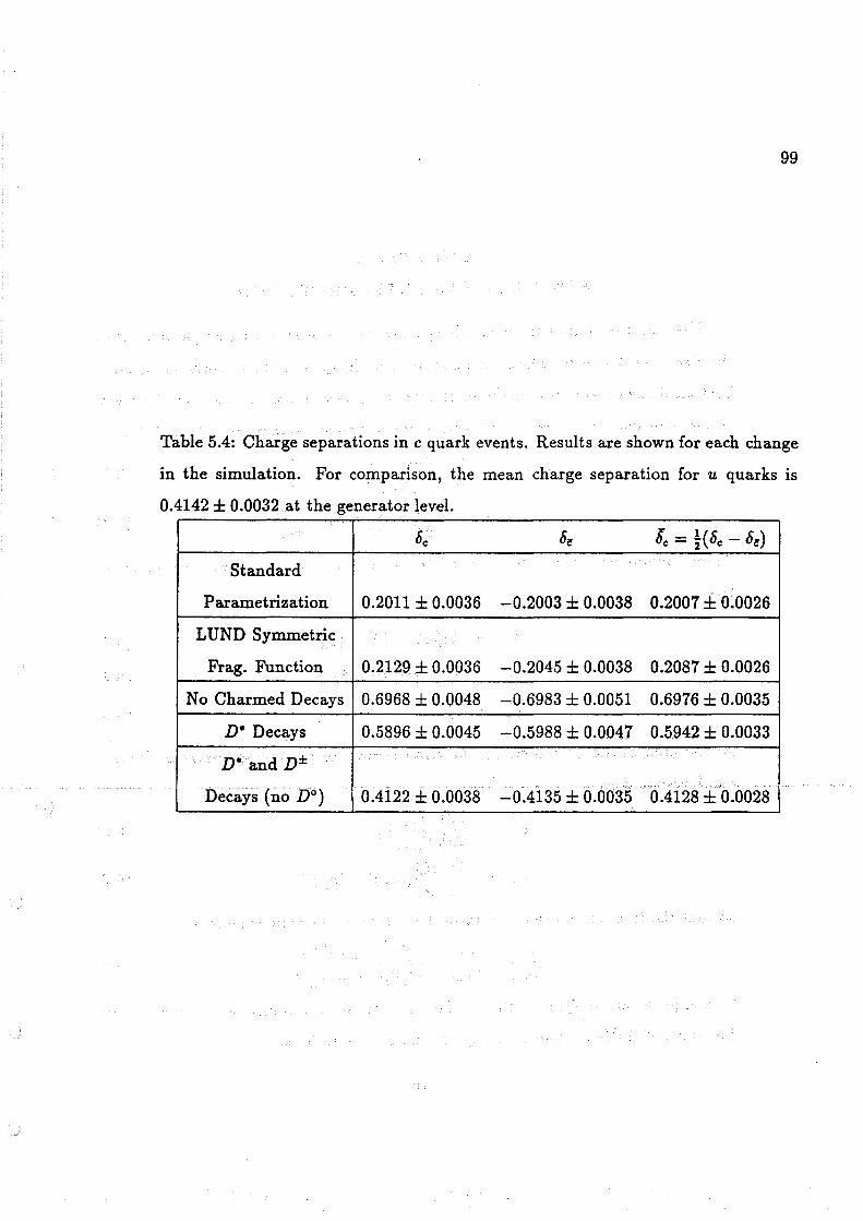
99
Table 5.4: Charge separations in c quark events. Results are shown for each change
in the simulation. For comparison, the mean charge separation for u quarks is
0.4142 ± 0.0032 at the generator level.
Ôc s~ - 1 Ôc = 2(8c - s~)
Standard
Parametrization 0.2011 ± 0.0036 -0.2003 ± 0.0038 0.2007 ± 0.0026
LUND Symmetric
Frag. Function 0.2129 ± 0.0036 -0.2045 ± 0.0038 0.2087 ± 0.0026
No Charmed Decays 0.6968 ± 0.0048 -0.6983 ± 0.0051 0.6976 ± 0.0035
D• Decays 0.5896 ± 0.0045 -0.5988 ± 0.0047 0.5942 ± 0.0033
D• and D±
Decays (no D 0) 0.4122 ± 0.0038 -0.4135 ± 0.0035 0.4128 ± 0.0028

CHAPTER 6
ELECTROWEAK INTERPRETATION
The measurement of the mean charge flow can be used to extract parameters of
the electroweak theory. The connection between (QFB} and the underlying forward
backward asymmetry was made in chapter 5. There it was shown that the mean
charge flow can be expressed in terms of the left-right asymmetries Ae and Ah
(QFB) = ~ Cma:e ~ 6 Al ...!!l_ 3 1 + 1 2 L..J I lb
3cmaz f O'had (6.1)
Cmaz ~ 6 A A ...!!l_ -1 12 L..J/e/ + 3cmaz I O'had
(6.2)
These asymmetries canin turn be written as fonctions of the fermion couplings to
the Z 0,
A1 - 2gtg~/(gt )2 + (g~)2 (6.3)
gt - If - 2Q1 sin2 (Ow) (6.4)
g~ - If (6.5)
At the peak of the Z 0 resonance, the cross section for producing quarks of flavor f can be written as
O'J - 1211" ree r, Mj I'total
(6.6)
GFM![( I 2 ( ')2] r, - 2411"y'2 9v) + 9A (6.7)
so that the fraction of events of flavor f relative to hadronic sample is
o-I r I [(gt )2 + (g~)2] o-1iaa = rhad = L:1[(gt )2 + (g~)2]
(6.8)
The expression for QFB is then a fonction of the couplings, which are in turn
fonctions of sin2( Ow ), and of the quark charge separations.
100

101
6.1 Fitting QFB for sin2(8w)
In the spirit of the Improved Born Approximation discussed in chapter 1, Born
level forms of the expressions for the fermions couplings are used in computing the
expected asymmetry for each quark type, but with sin2( Bw) interpreted as the full,
running function
This replacement incorporates the largest eledroweak corrections to the cou
plings (46]. The only other significant radiative correction is that due to photon
radiation, particularly from the initial e+e- pair. This correction is derived from the
EXPOSTAR Monte Carlo (14], and incorporated as an additive energy-dependent
correction on the value of A~B· The value of sin2(8w) can then easily be fit to
the experimental result for QFB by assuming the values of the quark separation
constants taken from the full simulation. The x2 function
(Q ) QTheory X2 _ FB - FB (6.9)
D,.(QFB)2
D._(QFB) - ./(dQi1/)2 + (dQ~~t)2, QTheory 4 Cma:i: """""" c: (Al c:Af (E)) (T f
FB - J 1 + lc2 L.JL.JUf fb + u FB ;--' 3 ma:a: E f had
is minimized for sin2( Bw) = 0.230. The error on thîs value is the range in sin2
( 8w) for
which the value of x2 changes by one unit. This corresponds to 8sin2( Bw) = 0.005.
The x2 parabola for this fit is shown in figure 6.1. The predicted value Q~'.;;°"11
is plotted as a fonction of sin2( Bw) in figure 6.2. The sum over the nine energy
points, weighted by the number of events at each point, is needed since (QFB) is
measured at nine center-of-mass energies. The individual contributions to the error
on sin2( Bw) are determined by repeating the procedure using only the statistical
error on (QFB), the detector systematic error on (QFB), and the systematic error
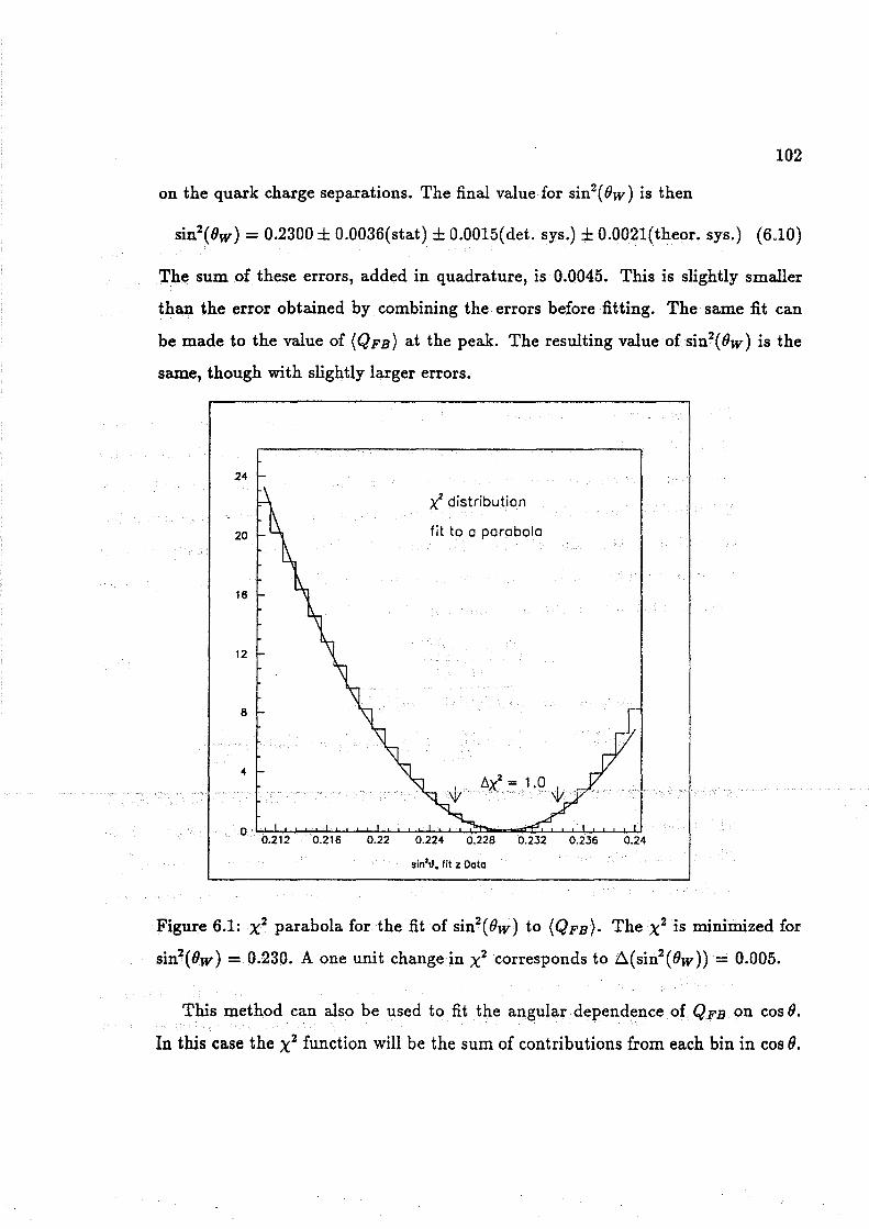
102
on the quark charge separations. The final value for sin2( Ow) is then
sin2(8w) = 0.2300 ± 0.0036(stat) ± 0.0015(det. sys.) ± 0.0021(theor. sys.) (6.10)
The sum of these errors, added in quadrature, is 0.0045. This is slightly smaller
than the error obtained by combining the errors before fitting. The same fit can
be made to the value of (QFB) at the peak. The resulting value of sin2(8w) is the
same, though with slightly larger errors.
24
20
16
12
8
x.2 distribution
fit to a parabole
sin•,,. fit z Ooto
Figure 6.1: x2 parabola for the fit of sin2(8w) to (QFB)· The x2 is minimized for
sin2( Ow) = 0.230. A one unit change in x2 corresponds to A( sin2
( Ow)) = 0.005.
This method can also be used to fit the angular dependence of QFB on cos 8.
In this case the x2 function will be the sum of contributions from each bin in cos 8.

I!! 0
0.004
0
-0.004
-0.00B
-0.012
0,. Meosurement
0.21 0.22
103
0.23 0.24 0.25 0.26 sin2(~.)
Figure 6.2: Predicted value of QFB vs sin2(Bw ). The measured value of (QFB}
is indicted by the curve, while the solid band indicates the range of the (QFB}
measurement.

104
The same value of sin2( Ow) is found: sin2
( Ow) = 0.230 ± 0.006. The plot of the
angular distribution of QFB with the fitted fonction is shown in figure 6.3. The fit
has a value of x2 per degree of freedom (v) of x2/v = 6.28/5.
0
-0.012
-0.016
Fitted sin(e,,) • 0.230±0.004
t - 6.28/5 0.0.F'.
0 0.1 0.2 0.3 0.4 0.5 0.6 0.7 0.8 0.9 cos(0r)
Figure 6.3: QFB vs cos(Othru.st), showing the measured values and best-fit theory
curve, which corresponds to sin2 Ow = 0.230 ± 0.006. The fit has x2 /v = 6.1/5
The extracted value of sin2( Ow) is relatively stable as a fonction of "'· In
figure 6.4, the value of sin2(8w) is plotted versus"' based on (QFB) for each K. value.
The top figure shows the values extracted from the measured values of (QFB)· The
bottom figure shows the values of sin2(Bw) obtained if the mean values of QFB in

105
the Monte Carlo are treated as measurements. The band in each plot shows the
combined fit for sin2 (8w) extracted from all K values, with correlations between the
distributions taken into account.
In figure 6.5, the values of the forward-backward asymmetries for each quark
type is plotted versus K, as computed from the Monte Carlo. The value of ÂFB
is evaluated from the value of (QFs) for that flavor, divided by the quark charge
separation and the angular acceptance factor (cf eq. 5.13). These plots show that
the corresponding ÂFB value stabilizes near K = 1.0, with the exception of the the
charm quarks. Also shown is (QFs) in the Monte Carlo, divided by the mean charge
separation, S. This quantity, which is roughly proportional to the hadronic charge
asymmetry, also stabilizes near K = 1.0.

106
Figure 6.4: The extracted value of sin2 (Bw) versus""· The plot on top is for (QFB)
measured in the data; the plot on bottom is for (QFB) taken from the Monte Carlo.
The solid band shows the combined fit for all values of,,.,, with correlations included.

107
0.15 ._
0.08 0.1
0.04 0.05
0 0 0 2 3 4 0 2 3 4
Qfb./6. Qfb./6.
0.15 -- 0.075
0.1 0.05
0.05 0.025 1 0 0 0 2 3 4 0 2 3 4
Qfb./6. Qfb./6.
0.15 - 0.06 -0.1 0.04 -
0.05 0.02 -0 0
0 2 3 4 0 2 3 4
Qfb./6. Qfb/·.s - MC
Figure 6.5: The quark ÂFBvalues versus"'· The final plot is (QFB) in the Monte
Carlo, d.ivided by the mean charge separation, S.

108
6.2 Standard Madel Fitting
A more rigorous approach to fitting the measured Q FB values for Standard
Model parameters would use a closed-form calculation of the photonic and elec
troweak corrections to ÂFB to as high a precision as has been calculated. Such a
fitting program has been written [47], based on the EXPOSTAR Monte Carlo.
This fitting program is based on the minimal standard model, with one Higgs
scalar and the top quark. One particle irreducible loop corrections to the Z 0 and
photon propagators are taken into account to ail orders in the couplings by Dyson
summation. Initial state radiative effects are evaluated using electron structure
functions, as discussed in chapter 1. The basic input parameters to the standard
mode! are taken to be aQED(O) (the fine structure constant in Thomson scattering),
GF from muon lifetime measurements, and the masses of the Z 0, Higgs boson, and
top quark. One or more of these three masses are fit to the data. Final state QCD
corrections are varied by fitting the number of colors. Ail other quantities, such as
sin2(8w ), are evaluated from (fitted) input parameters.
Fitting the energy distribution of (QFB) to the mass of the top quark, sin2(8w)
is evaluated to be
sin!( Ow) = 0.225 ± 0.006
calculated from the fitted value of Mtop = 325 ± 77 Ge V. This fit is shown in figure
6.6. Fitting just the peak value of (QFB) to the mass of the top quark yields
sin!(Bw) = 0.226 ± 0.006
and
Mtop = 301 ± 85GeV.
This value of sin2( Bw) is consistent with the value obtained from the improved Born
approximation fit described above.

109
0
-0.004
-0.008
-0.012
-0.016
-0.02
./s lGeVJ
Figure 6.6: Standard Model Fit to the Energy Dependence of QFB· Datais mea
sured over three energy ranges. The curve shows the expected value of QFB from
the EXPOSTAR calculation.

110
6.3 Evaluation of Ae U sing Measured Quark Couplings
As shown in Chapter l(eq. 1.10), ÀFB for each quark flavor factorizes (at ...fi=
Mz) into the product of the electron and quark left-right asymmetries. If one
of these quantities could be fixed, based on independent measurements, the other
could then be evaluated. Therefore an alternative approach to interpreting the
information contained in the charge flow measurement is to use measured values of
the quark couplings to construct the left-right quark asymmetries, then solve for
the left-right asymmetry of the electron.
The measured values used are the left- and right-handed couplings of the d
and u quarks, taken from (48]. These values represent a best fit to the results
from.many deep inelastic scattering experiments, including neutrino scattering from
both isoscalar and non-isoscalar targets, as well (v) p --+- (v) p elastic scattering and
vN __,.. V1f'0 N production. Together these results lead to a unique fit to the d- and
u- quark chiral couplings. The quoted quantities used as input in this analysis are
gi_ = 9L(u)2 + 9L(d)2 -
g~=9R(u)2 +9R(d)2 -
fh = arctan(gL(u)/gL(d)) -
()R = arctan(gR(u)/gR(d))
from which the following values are computed
0.2996 ± 0.0044
0.0298 ± 0.0038
2.47 ± 0.04
4 65+0.48 • -0.32
9L(u) - 0.34059
9R( U) - -0.17228
9L( d) - -0.42849
9R( d) - -0.01095
The chiral couplings are related to the axial and vector couplings by
9A = 9L -gR
(6.11)
(6.12)
(6.13)
(6.14)
(6.15)
(6.16)
(6.17)
(6.18)
(6.19)
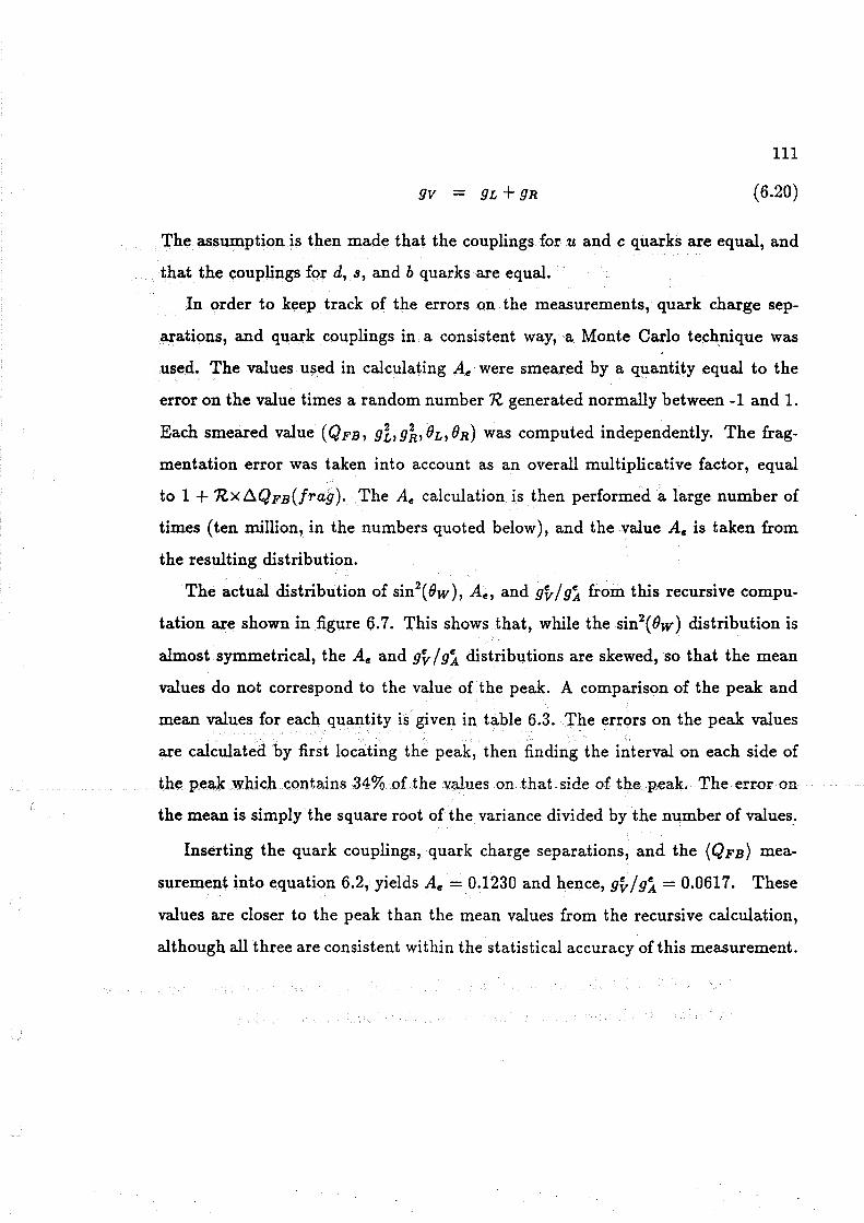
9V = 9L + 9R
111
(6.20)
The assumption is then made that the couplings for u and c quarks are equal, and
that the couplings for d, s, and b quarks are equal.
ln order to keep track of the errors on the measurements, quark charge sep
arations, and quark couplings in a consistent way, a Monte Carlo tec~nique was
used. The values used in calculating Ae were smeared by a quantity equal to the
error on the value times a random number 'R, generated normally between -1and1.
Each smeared value (QFB, gl,gh,OL,OR) was computed independent.ly. The frag
mentation error was taken into account as an overall multiplicative factor, equal
to 1 + nx~QFB(frag). The Ae calculation is then performed a large number of
times (ten million, in the numbers quoted below), and the value Ae is taken from
the resulting distribution.
The actual distribution of sin2(0w), Ae, and 9v/9Â from this recursive compu
tation are shown in figure 6.7. This shows that, while the sin2(0w) distribution is
almost symmetrical, the Ae and gy / 9Â distributions are skewed, so that the mean
values do not correspond to the value of the peak. A comparison of the peak and
mean values for each quantity is given in table 6.3. The errors on the peak values
are calculated by first locating the peak, then finding the interval on each side of
the peak which contains 34% of the values on that side of the peak. The error on
the mean is simply the square root of the variance divided by the number of values.
Inserting the quark couplings, quark charge separations, and the (QFB) mea
surement into equation 6.2, yields Ae = 0.1230 and hence, gy / 9Â = 0.0617. These
values are doser to the peak than the mean values from the recursive calculation,
although ail three are consistent within the statistical accuracy of this measurement.

112
Table 6.1: Peak and mean values, with errors, from the recursive calculation.
Peak Value (-o-) ( +o-) Mean Value Error on Mean
sin2(8w) 0.2313 -0.0050 +0.0040 0.2297 ± 0.0052
Ae 0.1289 -0.0280 +0.0440 0.1462 ± 0.0480
9v/9Â 0.0625 -0.0140 +0.0240 0.0747 ± 0.0279
0.04
sin(1'.)
0.02
0 1-1-L....L...J.....J'--L...L....L-'-..._.~-..:=-.L...J...-'-L-.J.....i..JL....U.....J.....J'--L...C::.0~...L....L-I
o. 19 0.2 0.21 0.22 0.2.3 0.24 0.25
Figure 6. 7: Distribution of sin2( Ow) Ae, and 9v / 9Â values from the recursive com
putation. Peak and mean values of each distribution are marked.

113
6.4 Conclusion
The measurement of the mean charge fl.ow yields a value of the weak mixing
angle sin 2 ( Ow)
sin2 ( Ow) = 0.230 ± 0.005 (6.21)
where the errors are due to statistical and systematic errors on the measurement of
(QFs}, and to theoretical uncertainties in the quark charge separations.
This measurement of sin2(0w) compares well with values obtained from other
analyses[50]. In table 6.4, measurements of sin2(0w) from lepton AFs, tau polariza
tion, and AFB for bb and cë events are shown, along with the value obtained from
(QFs). Combining these independent measurements yields a very precise value for
sin2(0w):
sin2( Ow) = 0.2297 ± 0.0024.
Table 6.2: Values of sin2(0w) from Various ALEPH measurements.
Measurement sin2(0w )(Mj)
Lepton F-B asymmetry 0.2295 ± 0.0038
Quark charge asymmetry (QFn) 0.2300 ± 0.0050
Tau polarization asymmetry 0.2319 ± 0.0057
bb asymmetry 0.2262 ± 0.0054
cë asymmetry 0.2310 ± 0.0110
Average 0.2297 ± 0.0024
By assuming universality among the quark families, and using the measured
u and d quark couplings, the mean charge flow measurement yields values of the
electron left-right asymmetry,
A 0 1289+0.0440 e = • -0.0280 (6.22)

114
or equivalently the ratio of the vector and axial vector couplings of the electron,
e / e 0 0625+0.0240 9v 9 A = · -0.0140' (6.23)
Figure 6.8 shows the ALEPH result (49) for 9v and 9Â, based on fitting the partial
widths and forward-backward asymmetries in Z 0 ~ z+ z-. The two lines indicate
the range of values for 9v using the measurement of 9v / 9Â presented here and the
best-fit value of 9.Â. The ALEPH value of the electron axial vector coupling based
on the full 1989 and 1990 statistics is [50] l9AI = 0.498 + / - 0.002. This yields
The fit to the leptonic partial widths p~efers values of 9v and 9Â in the negative-
9. half-plane. The QFB measurement establishes that the vector and axial vector
couplings are of the same sign, so that
0 031+0.012 gv = - · -0.001 (6.24)
is the resulting value for the electron vector coupling. By comparison, the best
fit value for 9v from the lepton ÂFs and tau polarization measurements is 9v =
-0.039 ± 0.006(50].

-0.49
-0.5
-0.51
-0.52
68% C.L.
99% C.L.
-0.53 ..................... ._._ .................... .....__.. ............................................................ _.__.__._......_..._.__.__._....__.._._.__._ ..... -o. 12 -0.08 -0.04 0 0.04 0.08 o. 12
115
Figure 6.8: Fit to the Electron Couplings Based on I'u and Ai8 • The range of 9v implied by the (QFB) measurement and the best-fit value of 9Â is indicated by the
two lines.

APPENDIX A
QUARK FRAGMENTATION
Quarks are not observed in high energy physics experiments, and no search
for free quarks has produced an unambiguous positive result. This inability to
observe quarks is understood in terms of confinement of the quarks by a force
which grows with the quark-antiquark separation. As a result, at large separations
the quarks are likely to form hadronic states with quark-antiquark pairs produced
from the vacuum. The process by which an initial qq pair evolves into a final state of
observed particles is known as fragmentation. The stages involved in fragmentation
are illustrated schematically in figure A.1 .
••
. -+----m---- (jj) - (jjj) __ .,. ( ivl
Figure A.1: Schematic representation of quark fragmentation in the process e+ e- -+
qq. i) Initial reaction and parton shower, ii) Hadronization, iii) Unstable particle
decays, iv) Final state seen in the detector.
Fragmentation has proven to be an in tractable problem to salve from first princi
ples. First the description of hadron production and gluon radiation is only solvable
in perturbative QCD at high values of the typical momentum scale of the problem,
116
117
the transferred momentum squared ( q2). At lower values of q2 the expansion pa
rameter a. approaches a value of 1. Second, the final state is a complicated mix
ture of initial fragmentation by-products and daughter particles from the decay of
short lived states (and often there are several such generations ). Because of these
complications the usual approach has been to mode! fragmentation based on some
assumptions about the manner in which quarks form hadrons, then track the result
ing hadronic states in a computer simulation (Monte Carlo), decaying particles in
accordance with observations or best theoretical estimates. The various parameters
of the mode! can then be tuned so as to agree with experimentally observed values
of final state particle momenta, multiplicities, event shapes, etc.
In the remainder of this appendix the main fragmentation models used in the
charge asymmetry study will be described, as well as the estimate of the error on
the charge asymmetry measurement due to uncertainties in these models.
A.1 Description of the Models
The parameterization of quark fragmentation is divided into three stages. In the
first stage, characterized by high momentum quarks produced in the e+ e- collision,
fragmentation begins by the emission of gluons by each the quarks. These gluons
will in turn produce pairs of gluons or quarks. In the second stage, the partons
fragment into hadrons. In the third stage, hadrons are allowed to decay.
A.1.1 Perturbative QCD
The process of fragmentation begins with the radiation of gluons from the quark
antiquark pair produced in the e+ e- collision. These gluons will in turn produce
pairs of gluons or quarks. This process is well described in QCD as long as the mo
menta transfers involved are large. The relevant parameter controlling this stage

118
of the fragmentation process is the QCD coupling constant as. The coupling is
changed by varying the renormalization scale parameter A and q2 • The two quan
tities are related by
( 2) a,(A}
a, q = 1 + Ba,(A)ln(q2/A) (A.1)
and B is a function of the number of quark flavors.
Two approaches to this stage of fragmentation are used in the Monte Carlo sim-
ulations. ln one approach, explicit matrix elements for gluon radiation, calculated
to order a;, are used to compute the probability of radiating a gluon from one of the
outgoing quarks. This approach fails to predict events with four or more jets, and
does not fit the charged pa,rticle multiplicity at LEP energies very well [20]. The
other approach, incorporated in the Monte Carlos used for this analysis, makes use
of leading-logarithm calculations, with contributions from ail orders in the strong
coupling constant. This is usually referred to as the Parton Shower approach, or
LLA (Leading Logarithm Apparoach).
A.1.2 Phenomenological Fragmentation Models
The second stage of the fragmentation process is the hadronization of quarks.
This process cannot be described by QCD and relies on phenomenological
parametrizations. ln the simulations, quark-antiquark pairs are created and
grouped with the other quarks and antiquarks in the event to form diquark systems.
At some point in the fragmentation these diquarks may identified with mesons, or
may be split and the component partons reassigned. Mode! differ in the manner
by which they group together quark-antiquark pairs and assign momenta to the re
sulting systems. The most common models are Independent Fragmentation, String
Fragmentation, and Cluster Fragmentation models. [51]
In lndependent Fragmentation models, each parton is allowed to evolve inde
pendently of the others, using an iterative ansatz. Momentum and flavor are not

119
necessarily conserved, but can be made to balence at the end of the fragmentation
process. The fragmentation procedure is also not Lorentz invariant. For these and
other reasons Independent Fragmentation models are not often used, and were not
considered in this analysis.
In String Fragmentation models, each quark pair is thought of as being connected
by a color flux tube, or string, with an energy density per unit length of ~1 Ge V /fm. As the quark and antiquark a.re separated, the color string breaks, and a new quark
antiquark pair is created at the break. This process is continued until the remaining
string fragments can be identified as hadron states. For qqg configurations, the color
string runs from the quark to the gluon to the ·antiquark, so that the gluon can be
thought of as a "kink" in the color string.
Particles are produced with longitudinal momenta given by so-called fragmen
tation fonctions, and transverse momenta sampled from a Guassian distribution of
momenta of a given width.
Many different fragmentation fonctions exist. One of the first, suggested by
Field and Feynman, was
f(z) = 1 - a+ 3a(l - z)2
where z = P11/ E is the fraction of the remaining total momentum of the system
taken by the longitudinal momentum of the hadron, and a is a small parameter
which can be tuned to the data. Further experiments (56] showed this fonction to
be too strongly peaked at z =O.
The two fragmentation fonctions used in the ALEPH Monte Carlo simulation
are the LUND symmetric fragmentation fonction b ..... 2
f(z) = z-1 (1 - z)ae-7" (A.2)
and the Peterson fragmentation fonction
1 f(z) = z(l - l _ .!9_)
z 1-z
(A.3)

120
These two fragmentation fonctions differ in their resulting mean momenta, the
Peterson fonction producing a harder momentum spectrum. The LUND symmetric
fragmentation fonction is considered appropriate for lighter ( u, d, s) quarks and the
Peterson fragmentation fonction for heavy ( c, b) quarks.
In addition there are parameters which set the probability of producing a quark
of a particular flavor when forming hadrons, as well as specifying the spin state
of the resulting system. Generally the probability of producing heavy quarks is
negligible. The relevant parameter is s/u , the relative probability of producing an
ss quark pair from the vacuum compared to producing a uü pair. The only relevant
spin states are of angular momentum L = 1 (vector meson) or L = 0 (pseudoscalar
meson). The probability of producing a vector state compared to producing all
( vector and pseudoscalar) states is Pv. There are three such probabilities in the
simulation : Pv( u, d), Pv( s ), Pv( c, b ); the vector /vector+pseudoscalar probabilities
for u and d quarks, for s quarks, and for c and b quarks.
In Cluster Fragmentation models, the partons resulting from the parton shower
are grouped together into colorless clusters, with any remaining gluons being split
into qq pairs. These clusters are then decayed to form hadronic states. The decay
sequence ends when some cluster mass cutoff is reached. Cluster Fragmentation
models have relatively fewer free parameters than String Fragmentation models,
although some parametrization remains, particularly for the assignment of quark
antiquark clusters to known meson states.
A.1.3 Hadron Decays
In the third stage of the fragmentation process, the unstable hadrons are al
lowed to decay, according to branching fractions and decay widths which are either
measured or represent the best theoretical estimates. As was shown in chapter 5,
this stage of the fragmentation process does affect the charge retention, particularly
for c quarks.

121
A.2 Fragmentation Studies
Two models were used for the fragmentation studies. Most studies were per
formed using the JETSET Monte Carlo [39], which has Parton Showers and String
Fragmentation.1 Since JETSET does not have final state photon radiation, the
DYMU generator was actually used to generate the initial e+ e-( i) ~ qëj( i) config
uration, as discussed in chapter 3 for the full Monte Carlo simulation.
The HERWIG Monte Carlo [40] was also studied, as an example of Cluster
Fragmentation. HERWIG does not fit the data as well as JETSET, and was not
interfaced with a more accurate electroweak generator. However it does verify
that the observed quark charge separations are not an artifact of the particular
fragmentation scheme chosen.
A.2.1 Parameter Variation in JETSET
The effects on the quark charge separations of eleven parameters of the JETSET
Monte Carlo was tested by varying each parameter by the limits given by previous
experiments, ALEPH data, or theoretical limits.
For AQcD the values given by the different e+e- experiments range from 0.26
[61] - 0.40 GeV [62][63].
Most experiments have determined the best value for the minimum mass in the
parton shower evolution, Mmin, to be 1.0 GeV. As the ALEPH data favour a value
around 1.50 ± 0.12 [20], Mmin for this study has been varied from 1.0 up to its
maximum, 2.0 Ge V.
For the parameters a and b in the light quark string fragmentation two sets of
preferred values exist, a :::::: 0.5, b:::::: 0.9 [20](62][63] and a :::::: 0.18, b :::::: 0.34 [60][61].
The latter setting, in combination with the ALEPH tuning for the other fragmen-
1 Both the matrix element approach and Independent Fragmentation are available as options.
ALEPH data prefer the parton shower approach, however [17] [20].
122
tation parameters, yields a charged particle multiplicity that is too high by one
track/event, therefore only the former setting is studied. As a and b are strongly
correlated it is sufficient to vary b between 0.85 and 0.93 while keeping a fixed at
0.5 [20].
The width of the transverse momentum distribution of observable particles pro
duced in the fragmentation, O', has been varied between 0.34 and 0.40 Ge V/ c. This
covers almost the full range of measured values from the various experiments [20]
[63]. The ALEPH data prefer a value of O' = 0.34[20].
The variation of the Peterson Fragmentation fonction parameters êc and êb is
based on ALEPH heavy flavor studies [58]. These favor a value of êc = -0.016 and
êb = -0.008. The parameter êc was varied from -0.002 to -0.071; eb was varied from
-0.003 to -0.010.
The values of the vector to vector plus pseudoscalar ratios are relatively poorly
known. For this study the ratios have been varied around the default values in the
Monte Carlo (39]. The maximum values are set by a theoretical constraint. For
light quarks the maximum is 3/{1+3)=0.75, while for heavy quarks the ratio can go
up to 0.8 due to mass e:ffects. The lower limits were obtained by varying the default
settings clown by the amount they differ from the maximum. As vector particles
are observed it is unphysical to reduce the vector to pseudoscalar ratio to zero.
The HRS [53] and JADE [54] experiments parametrized the pseudoscalar to vector
rate as P /V= 1/3(mv/mp)0·55
• For p0 /7r0 one obtains a vector to pseudoscalar rate
of 0.55, for K0* /K0 0.7 and for D0• /D0 0.74. ln each case the value obtained is
contained in the range over which the respective vector to pseudoscalar ratios are
varied here.
The review of measurements of the s/u-ratio given in ref. [55] sets the range to
0.27-0.37. As all these measurements were carried out at lower energies where the

123
mass suppression of s-quarks is greater, the s/u-range has been extended up to 0.40
to allow for possible increased strangeness production at LEP energies.
The influence of B 0 - ÏJ 0 mixing has also been investigated. For the charge
reconstruction, all charged fragments or decay products of the b-quark are used.
Due to the different time scales for mixing and fragmentation, the b-quark will
have fragmented to a neutral abject, a ÏJ 0, long before it mixes to a B 0
• Before
decay it is in either case a neutral abject. The only bias B 0 - ÏJ 0 mixing can give
in this analysis, therefore, cames from the difference between the contributions to
the hemisphere charge of the B 0 decay products.
The amount of mixing is expressed in terms of the parameter X· Defining th~
relative mass difference of the long- and sort-lived eigenstates Bi and B~ as
AM :z:=--
M
and assuming the resonance widths of the two states are the same, then
X= 2 + 2:z:2·
There are two types neutral B 0 mesons -
and consequently two mixing parameters, Xd and x,. The overall mixing parameter
X is a combination of these two, weighted by their production rates.
The effect of B 0 -ÏJ0 mixing has been studied by varying the mixing parameter X
between 0.11 and 0.16, which is the range presently set by the ALEPH data [58] [59].
The actual variation of X was produced by varying the mass splittings for Bd and
B: separately.

BIBLIOGRAPHY
[1] S.L. Glashow, Nucl. Phys. 22 (1961) 579.
[2] S. Weinberg, Phys. Rev. Lett. 19 (1967) 1264.
[3] A. Salam, Elementary Particle Theory, Almquist & Wiksell, Sweden (1968)
367.
[4] Perkins, Donald H., Introduction to High Energy Physics, Addison-Wesley
Publishing Co. (1982).
[5] Renton, Peter, An Introduction to the Physics of Quarks and Leptons, Cam
bridge University Press (1990).
[6] The Particle Data Group, M. Aguilar-Benitez, et al., Review of Particle Prop
erties, Phys. Lett. B239 (1990).
[7] P.W. Higgs, Phys. Rev. Lett 13 (1964) 508.
[8] G. 'tHooft, Nucl. Phys. B33 (1972) 173; G. 'tHooft, Nucl. Phys. B35 (1971)
167.
[9] C.S. Wu, E. Ambler, R. Hayward, D. Hoppes, and R. Hudson, Phys. Rev. 105
(1957) 1413.
[10] J.T. Friedman and H.W. Kendall, Ann. Rev. Nucl. Science 22 (1972) 203.
[11] H. Fritzsch, M. Gell-Mann and H. Leutwyler, Phys. Lett B47 (1973), 365.
[12) M. Bohm, W. Hollick, et al., "Forward-Backward Asymmetries", in Z Physics
at LEP 1, vol. 1, G. Alterelli, R. Kleiss, and C. Verzegnassi,eds.; CERN report
89-08 (1989) 204.
124
125
(13] O. Nicrosini and L. Trentadue, Phys. Lett. Bl85 (1987) 395.
(14] D. C. Kennedy, et al., Nucl. Phys. B321 (1989) 83-107.
[15] B. W. Lynn, M. E. Peskin, and R. G. Stuart,"Radiative Corrections in SU2 X
U1 : LEP /SLC", in Physics at LEP, vol. 1, John Ellis and Roberto Peccei eds.,
CERN report 86-02, (1986) 90-152.
(16] ALEPH Collab.,D. Decamp, et al., Phys. Lett. B235 (1990) 399-411.
(17] ALEPH Collab., D. Decamp, et al., Phys. Lett. B234 (1990) 209-218.
[18] The earliest reference to jets in e+ e- collisions appears to be B.J. Bjorken and
S.J. Brodsky, Phys. Rev. Dl (1970) 1416.
[19] R.D. Field and R.P.Feynman, Nucl. Phys. Bl36 (1978) 1.
[20] ALEPH collab., K Smith, in Proceedings of the 25th Rochester Conference,
Singapore (1990).
[21] ALEPH collab., D. Decamp, et al., Z. Phys. C48 (1990) 365.
[22] F. Mandl and G. Shaw,Quantum Field Theory, John Wiley & Sons Ltd., New
York, (1984).
(23] J. P. Berge, et al., Nucl. Phys. B184 (1981), 13.
[24] EMC collab., J. P. Albanese, et al., Phys. Lett. B144 (1984) 302.
[25] PLUTO collab., Ch. Berger, et al., Nucl. Phys. B214 (1983), 189.
[26] MAC collab., W. W. Ash, et al., Phys. Rev. Lett. 58 (1987), 1080.
(27] JADE collab., T. Greenshaw, et al., Z. Phys. C42 (1989), 1.
[28] AMY collab., D. Stuart, et al., Phys. Rev. Lett. 64 (1990), 983.

126
[29] Topaz collab., I. Adachi, et al., Phys. Lett. B255 (1991) 613.
[30] R. Barlow, Journal of Computational Physics 72 (1987) 202.
[31] TASSO collab., R. Brandelik, et al., Phys. Lett. BlOO (1981) 357.
[32] ALEPH collab., D. Decamp, et al., Nucl. Instr. and Meth. A294 (1990) 121.
[33] M. Delfino, er al; Universitat Automata di Barcelona preprint LFAE-89-01
(April 1989), submitted to 'Computing in High Energy Physics', Oxford, UK,
{1989)
[34] J. Knobloch and P. Norton, eds., ALEPH NOTE 88-46 {1988)
[35] W.B. Atwood, et al., ALEPH NOTE 91-20 (1991), submitted to Nuclear In
struments and Methods A.
[36] J.E. Campagne, Ph.D. Thesis, Paris, report LNPHEP pp 89-02; J.E. Campagne
and R. Zitoun, Z. Phys. C 43 (1989) 469.
[37] R. Brun, et al., CERN-DD/EE/84-1 (1986)
[38] A.Caldwell, et al., ALEPH NOTE PTC-85-10 (1985)
[39] M. Bengtsson and T. Sjëstrand, Phys Lett. Bl85 (1987) 435. ·
[40] G. Marchesini and B. Webber, Nucl. Phys. B310 (1988) 461; I. G. Knowles,
Nucl. Phys. B310 (1988) 571.
(41] J.M. Scarr and I. ten Have, ALEPH NOTE 89-150 (1989)
[42] J.D. Bjorken and S.J. Brodsky, Phys. Rev. Dl (1970) 1416
[43] F.M. Renard,Basics of Electron Positron Collisions, Editions Frontieres (1981)
31

127
(44] R. Johnson, S. Patton, A. Roth, and R. St. Denis, ALEPH NOTE 91-34 (1991).
(45] Traudl Hansl-Kozenici and Vivek Sharma, private communication (1990).
(46] D.C. Kenneday and B.W. Lynn, Nucl. Phys. B322 (1989) 1-54
(47] F. Bird, D. Levinthal, B.W. Lynn, R.G. stuart, and J. Thomas, CERN TH
6094/91 (1991), submitted to Z. Phys. C.
(48] U. Amaldi, et al., Phys. Rev. D36 (1987) 1385; and references therein.
(49] Andrew Halley and Elizabeth Locci, private communication (1991).
(50] ALEPH collab., D. Decamp, et al., "lmproved Measurements of Electroweak
Parameters from Z Decays into Fermion Pairs", submitted to Z. Phys. C.
[51] T. Sjostrand, et al., "QCD Generators", in Z Physics at LEP 1, vol.3, G.
Alterelli, R. Kleiss, and C. Verzegnassi,eds.; CERN report 89-08 (1989) 143.
(52] Andrew Halley, private communication (1991).
[53] HRS collab., M. Derrick, et al., Phys. Rev. Lett. 54 (1985) 2568.
(54] JADE collab., W. Bartel, et al., Phys. Lett. B145 (1985) 441.
(55} D. H. Saxon in "High Energy Electron-Positron Physics" by A. Ali and P.
Soding, (1988) 539.
[56] TASSO collab., M. Althoff, et al., Z. Phys. C26 (1984) 157.
(57] ALEPH collab., D. Decamp, et al., Phys. Lett. B250 (1990) 172.
[58] ALEPH collab., D. Decamp, et al., Phys. Lett. B244 (1990) 551.
(59] ALEPH collab., D. Decamp, et al., Phys. Lett. B244 (1990) 551; ALEPH col
lab., D. Decamp, et al., CERN-PPE/90-194 (1990).

(60] OPAL collab., M. Z. Akrawy, et al., Z. Phys. C47 (1990) 505.
[61] TASSO collab., W. Braunschweig, et al., Z. Phys. C41 (1988) 359.
(62] MARK II collab., A. Petersen, et al., Phys. Rev. D37 (1988) 1.
(63] AMY collab., Y. K. Li, et al., Phys. Rev. D41 (1990) 2675.
128