Embed Size (px)
Citation preview
Achieving Seventh-Order
Amplitude Accuracy in
Leapfrog Integrations
Paul Williams
Department of Meteorology, University of Reading, UK
Sources of uncertainty in
simulations of weather and climate
• initial conditions
• boundary conditions
• internal chaotic variability
• external forcing
• model error
– dynamical assumptions
– parameterisations of sub-gridscale processes
– numerical approximations
– discrete spatial grid or truncated spectral expansion
– discrete time stepping
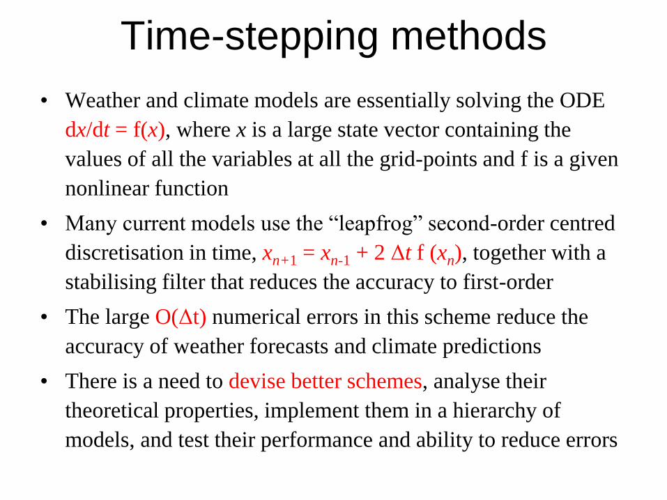
• Weather and climate models are essentially solving the ODE
dx/dt = f(x), where x is a large state vector containing the
values of all the variables at all the grid-points and f is a given
nonlinear function
• Many current models use the “leapfrog” second-order centred
discretisation in time, xn+1 = xn-1 + 2 Δt f (xn), together with a
stabilising filter that reduces the accuracy to first-order
• The large O(Δt) numerical errors in this scheme reduce the
accuracy of weather forecasts and climate predictions
• There is a need to devise better schemes, analyse their
theoretical properties, implement them in a hierarchy of
models, and test their performance and ability to reduce errors
Time-stepping methods
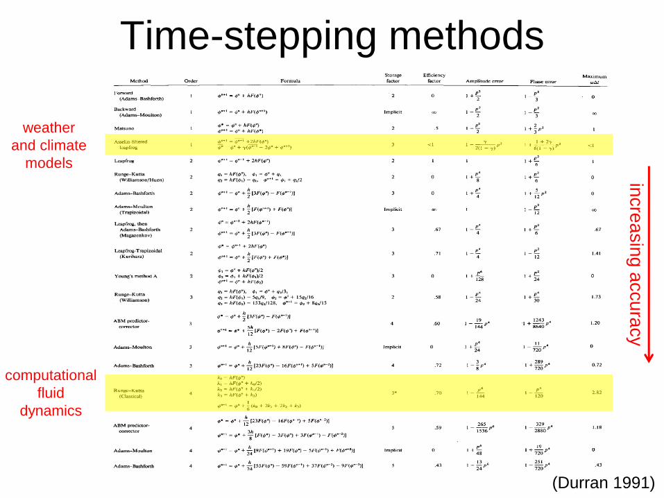
(Durran 1991)
incre
asin
g a
ccu
racy
Time-stepping methods
weather
and climate
models
computational
fluid
dynamics
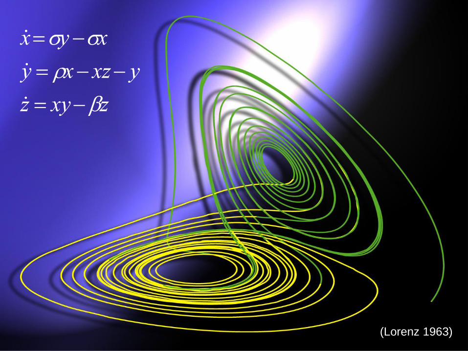
(Lorenz 1963)
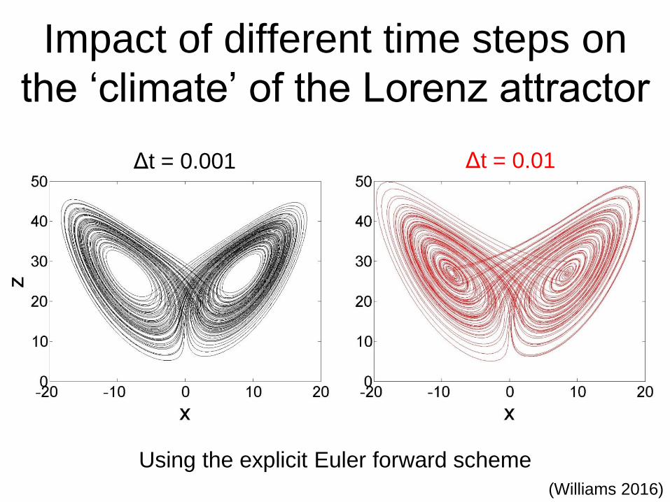
Impact of different time steps on
the ‘climate’ of the Lorenz attractor
Δt = 0.001 Δt = 0.01
Using the explicit Euler forward scheme
(Williams 2016)
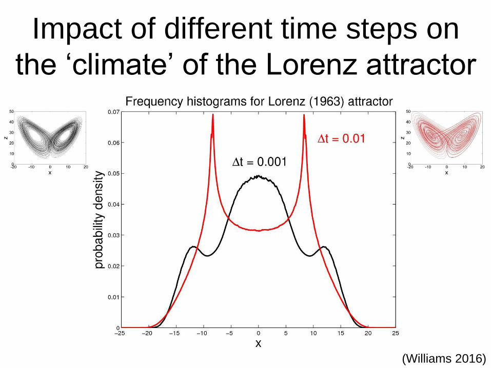
Impact of different time steps on
the ‘climate’ of the Lorenz attractor
(Williams 2016)
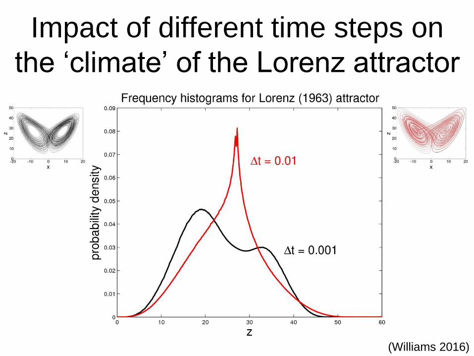
Impact of different time steps on
the ‘climate’ of the Lorenz attractor
(Williams 2016)
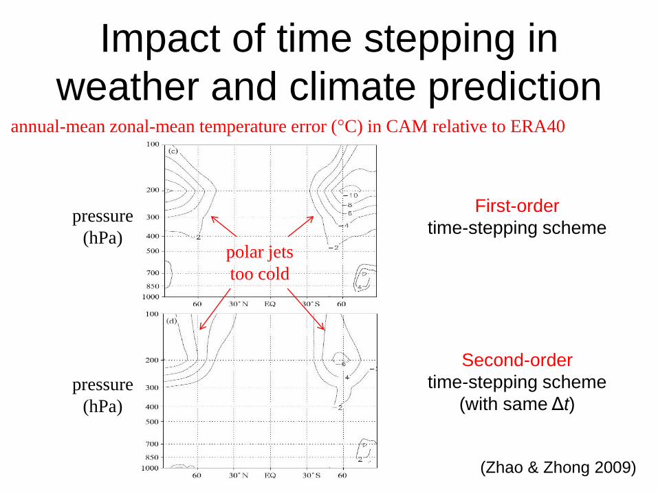
(Zhao & Zhong 2009)
annual-mean zonal-mean temperature error (°C) in CAM relative to ERA40
pressure
(hPa)
pressure
(hPa)
polar jets
too cold
Impact of time stepping in
weather and climate prediction
First-order
time-stepping scheme
Second-order
time-stepping scheme
(with same Δt)
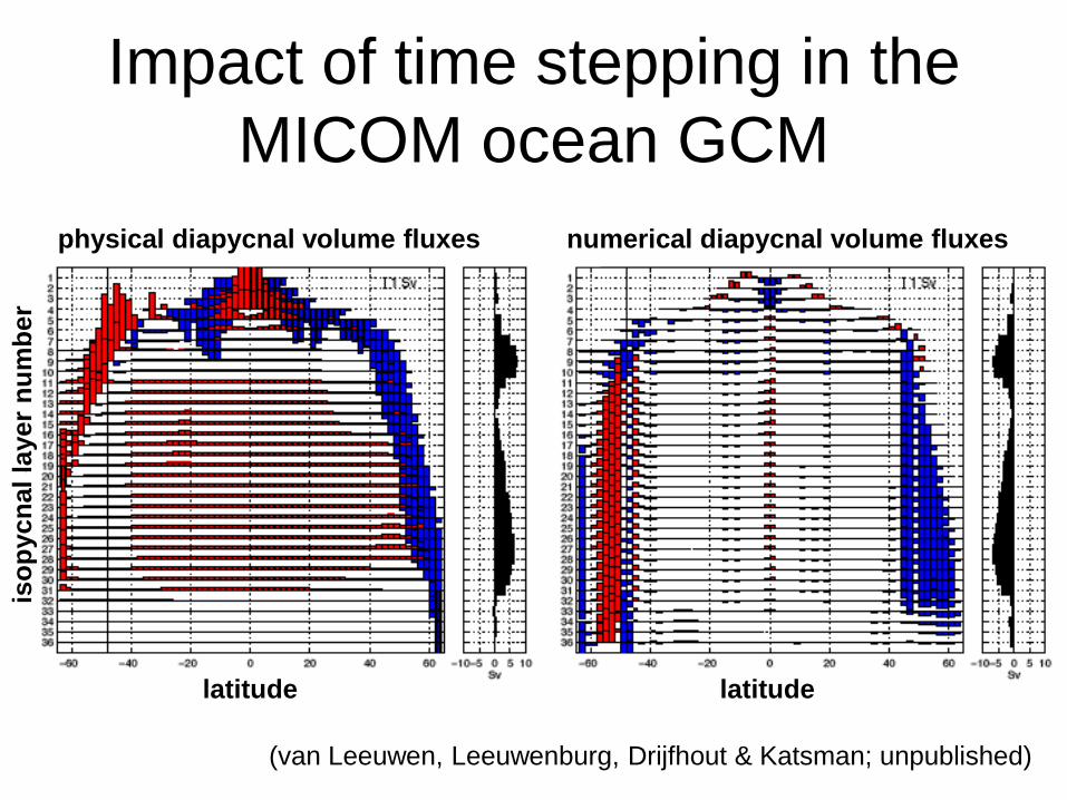
Impact of time stepping in the
MICOM ocean GCM
(van Leeuwen, Leeuwenburg, Drijfhout & Katsman; unpublished)
physical diapycnal volume fluxes numerical diapycnal volume fluxes
iso
pycn
al
layer
nu
mb
er
latitude latitude
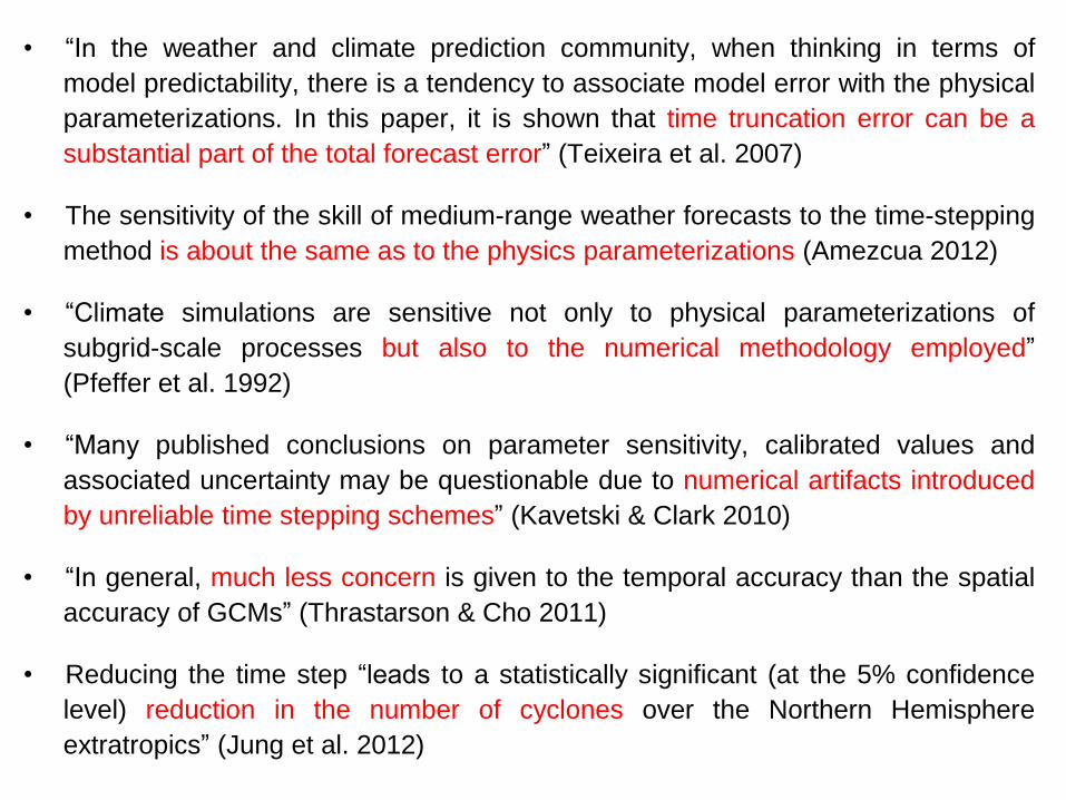
• “In the weather and climate prediction community, when thinking in terms of
model predictability, there is a tendency to associate model error with the physical
parameterizations. In this paper, it is shown that time truncation error can be a
substantial part of the total forecast error” (Teixeira et al. 2007)
• The sensitivity of the skill of medium-range weather forecasts to the time-stepping
method is about the same as to the physics parameterizations (Amezcua 2012)
• “Climate simulations are sensitive not only to physical parameterizations of
subgrid-scale processes but also to the numerical methodology employed”
(Pfeffer et al. 1992)
• “Many published conclusions on parameter sensitivity, calibrated values and
associated uncertainty may be questionable due to numerical artifacts introduced
by unreliable time stepping schemes” (Kavetski & Clark 2010)
• “In general, much less concern is given to the temporal accuracy than the spatial
accuracy of GCMs” (Thrastarson & Cho 2011)
• Reducing the time step “leads to a statistically significant (at the 5% confidence
level) reduction in the number of cyclones over the Northern Hemisphere
extratropics” (Jung et al. 2012)
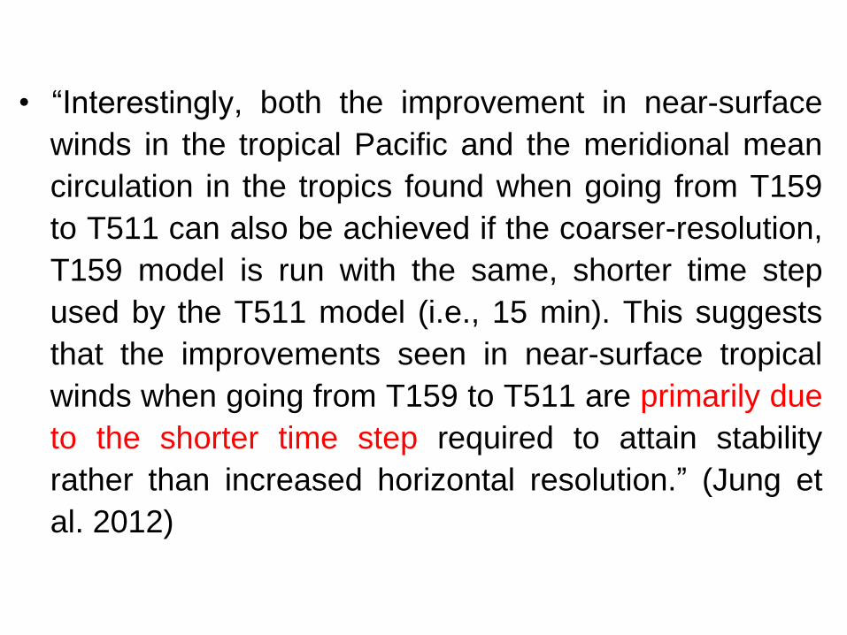
• “Interestingly, both the improvement in near-surface
winds in the tropical Pacific and the meridional mean
circulation in the tropics found when going from T159
to T511 can also be achieved if the coarser-resolution,
T159 model is run with the same, shorter time step
used by the T511 model (i.e., 15 min). This suggests
that the improvements seen in near-surface tropical
winds when going from T159 to T511 are primarily due
to the shorter time step required to attain stability
rather than increased horizontal resolution.” (Jung et
al. 2012)
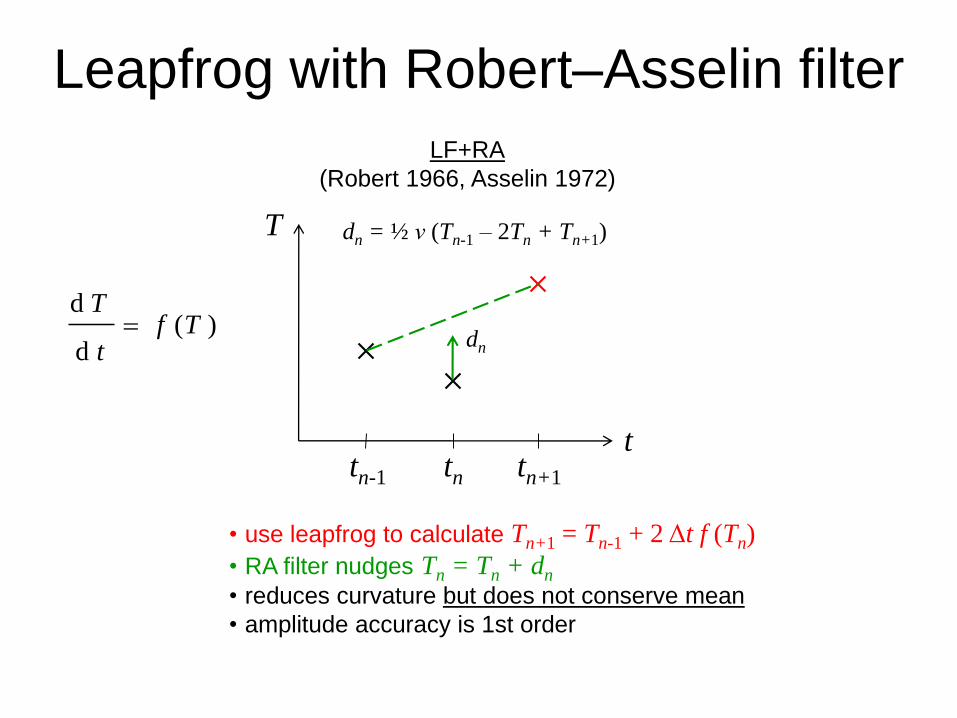
T
ttn-1 tn+1tn
• use leapfrog to calculate Tn+1 = Tn-1 + 2 Δt f (Tn)
• RA filter nudges Tn = Tn + dn
• reduces curvature but does not conserve mean
• amplitude accuracy is 1st order
LF+RA
(Robert 1966, Asselin 1972)
dn
dn = ½ ν (Tn-1 – 2Tn + Tn+1)
Leapfrog with Robert–Asselin filter
)(d
dTf
t
T
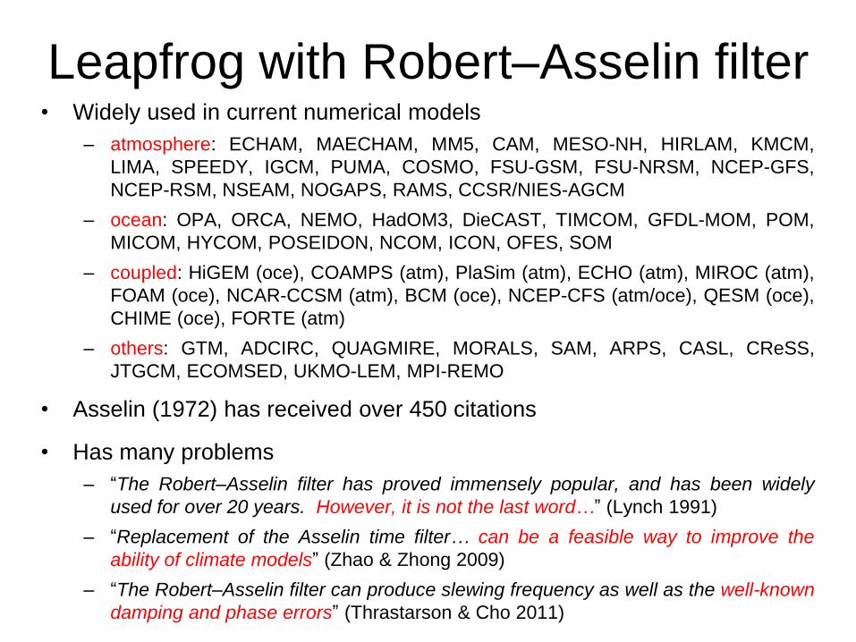
• Widely used in current numerical models
– atmosphere: ECHAM, MAECHAM, MM5, CAM, MESO-NH, HIRLAM, KMCM,
LIMA, SPEEDY, IGCM, PUMA, COSMO, FSU-GSM, FSU-NRSM, NCEP-GFS,
NCEP-RSM, NSEAM, NOGAPS, RAMS, CCSR/NIES-AGCM
– ocean: OPA, ORCA, NEMO, HadOM3, DieCAST, TIMCOM, GFDL-MOM, POM,
MICOM, HYCOM, POSEIDON, NCOM, ICON, OFES, SOM
– coupled: HiGEM (oce), COAMPS (atm), PlaSim (atm), ECHO (atm), MIROC (atm),
FOAM (oce), NCAR-CCSM (atm), BCM (oce), NCEP-CFS (atm/oce), QESM (oce),
CHIME (oce), FORTE (atm)
– others: GTM, ADCIRC, QUAGMIRE, MORALS, SAM, ARPS, CASL, CReSS,
JTGCM, ECOMSED, UKMO-LEM, MPI-REMO
• Asselin (1972) has received over 450 citations
• Has many problems
– “The Robert–Asselin filter has proved immensely popular, and has been widely
used for over 20 years. However, it is not the last word…” (Lynch 1991)
– “Replacement of the Asselin time filter… can be a feasible way to improve the
ability of climate models” (Zhao & Zhong 2009)
– “The Robert–Asselin filter can produce slewing frequency as well as the well-known
damping and phase errors” (Thrastarson & Cho 2011)
Leapfrog with Robert–Asselin filter
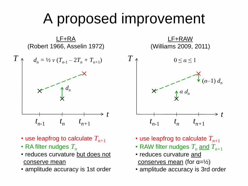
(α–1) dn
T
ttn-1 tn+1tn
• use leapfrog to calculate Tn+1
• RA filter nudges Tn
• reduces curvature but does not
conserve mean
• amplitude accuracy is 1st order
LF+RA
(Robert 1966, Asselin 1972)
T
ttn-1 tn+1tn
• use leapfrog to calculate Tn+1
• RAW filter nudges Tn and Tn+1
• reduces curvature and
conserves mean (for α=½)
• amplitude accuracy is 3rd order
LF+RAW
(Williams 2009, 2011)
A proposed improvement
dn α dn
dn = ½ ν (Tn-1 – 2Tn + Tn+1) 0 ≤ α ≤ 1
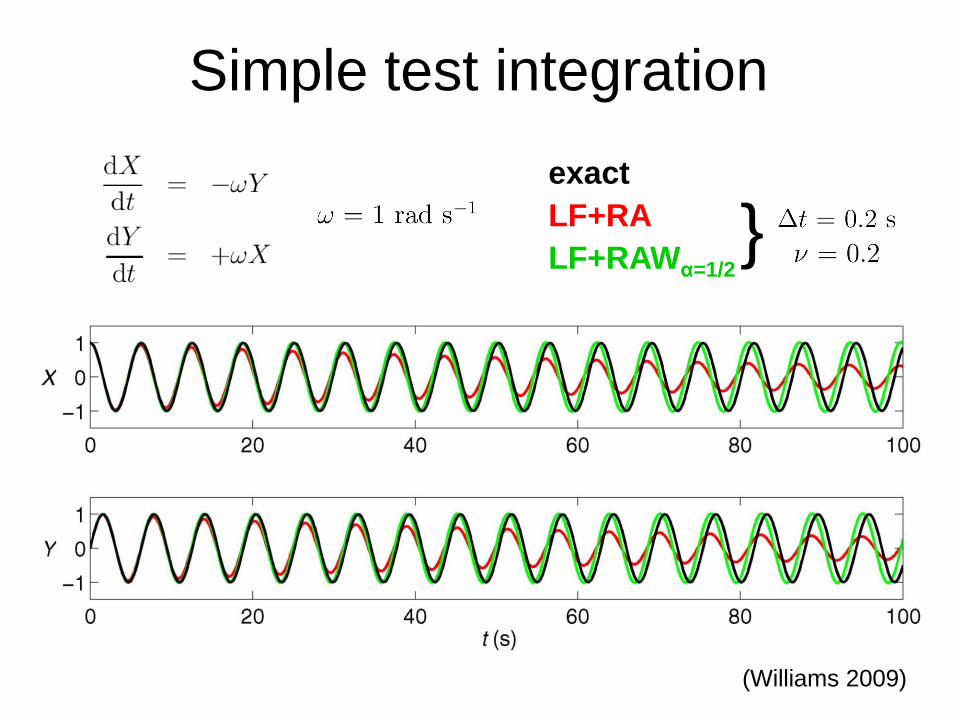
(Williams 2009)
Simple test integration
exact
LF+RA
LF+RAWα=1/2}
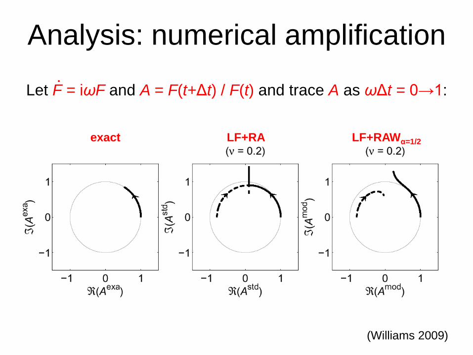
Analysis: numerical amplification
(Williams 2009)
Let F = iωF and A = F(t+Δt) / F(t) and trace A as ωΔt = 0→1:
LF+RAWα=1/2LF+RAexact
(Williams 2009)
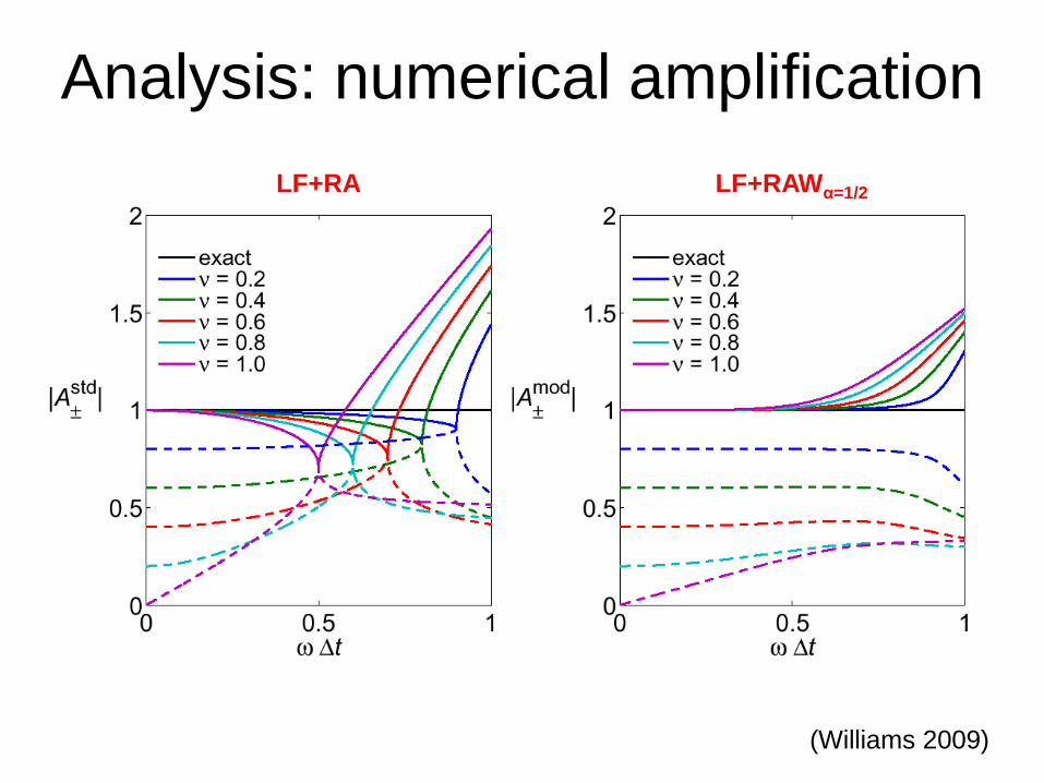
Analysis: numerical amplification
LF+RAWα=1/2LF+RA
(Williams 2009)
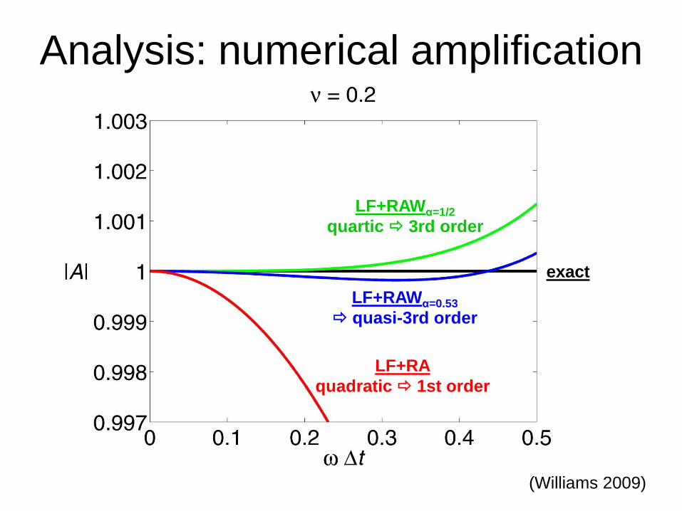
Analysis: numerical amplification
LF+RAWα=1/2
quartic 3rd order
LF+RAWα=0.53
quasi-3rd order
exact
LF+RA
quadratic 1st order
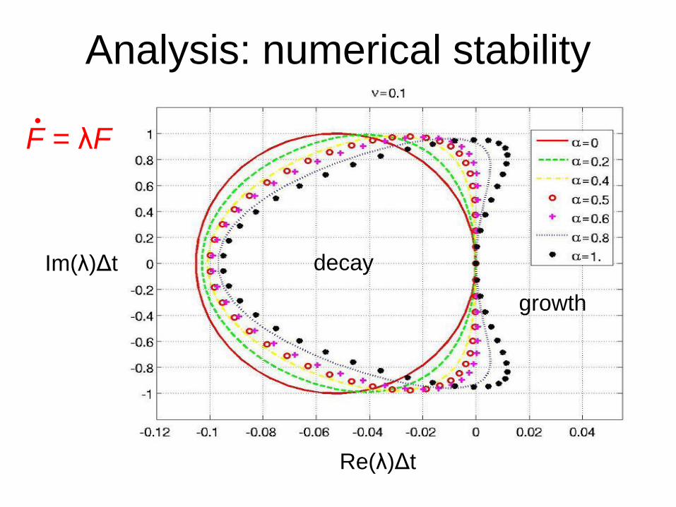
Analysis: numerical stability
decay
growth
Re(λ)Δt
Im(λ)Δt
F = λF
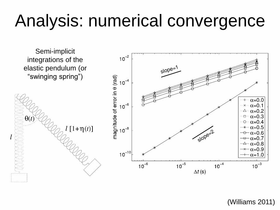
Analysis: numerical convergence
(Williams 2011)
Semi-implicit
integrations of the
elastic pendulum (or
“swinging spring”)
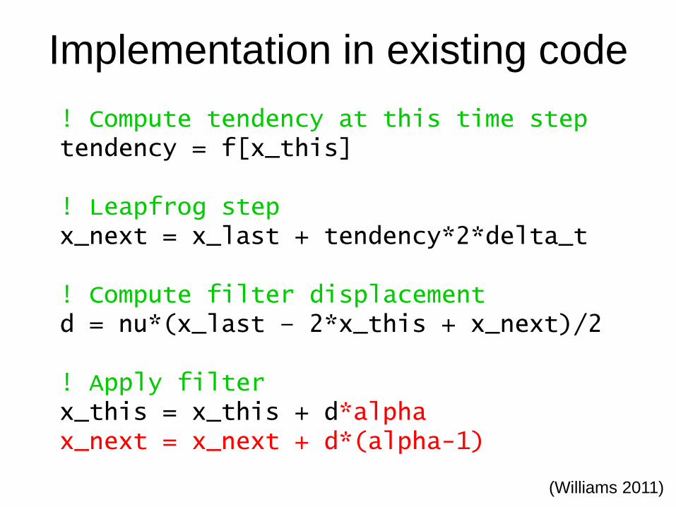
! Compute tendency at this time steptendency = f[x_this]
! Leapfrog stepx_next = x_last + tendency*2*delta_t
! Compute filter displacementd = nu*(x_last – 2*x_this + x_next)/2
! Apply filterx_this = x_this + d*alphax_next = x_next + d*(alpha-1)
Implementation in existing code
(Williams 2011)
The RAW-filtered leapfrog...
• is the default time-stepping method in the atmosphere of MIROC5, the latest
version of the Model for Interdisciplinary Research On Climate (Watanabe et
al. 2010)
• has been used in the regional climate model COSMO-CLM (CCLM) with
α=0.7, and “can lead to a significant improvement, especially for the simulated
temperatures” (Wang et al. 2013)
• is the default time-stepping method in TIMCOM, the TaIwan Multi-scale
Community Ocean Model, and gives simulations that are in better agreement
with observations (Young et al. 2014)
• has been implemented in an ice model, and improves the spin-up and
conservation energetics of the physical processes (Ren & Leslie 2011)
• has been implemented in the SPEEDY atmosphere GCM, and significantly
improves the skill of medium-range weather forecasts (Amezcua et al. 2011)
• has been found to perform well in various respects in semi-implicit integrations
(Durran & Blossey 2012, Clancy & Pudykiewicz 2013)
Some recent implementations
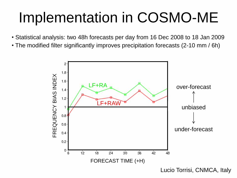
• Statistical analysis: two 48h forecasts per day from 16 Dec 2008 to 18 Jan 2009
• The modified filter significantly improves precipitation forecasts (2-10 mm / 6h)
Implementation in COSMO-ME
LF+RA
LF+RAW
FR
EQ
UE
NC
Y B
IAS
IN
DE
X
FORECAST TIME (+H)
unbiased
over-forecast
under-forecast
Lucio Torrisi, CNMCA, Italy
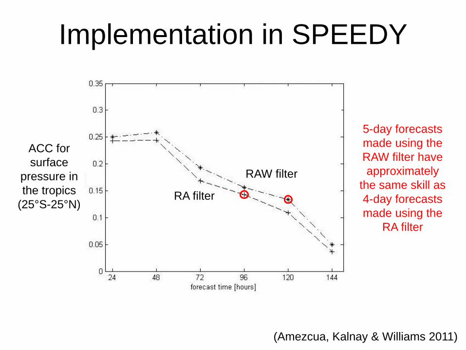
(Amezcua, Kalnay & Williams 2011)
Implementation in SPEEDY
ACC for
surface
pressure in
the tropics
(25°S-25°N)
5-day forecasts
made using the
RAW filter have
approximately
the same skill as
4-day forecasts
made using the
RA filter
RA filter
RAW filter
• The stability of the Crank–Nicolson-Leapfrog method with the
Robert–Asselin–Williams time filter has been interrogated
rigorously by Nicholas Hurl, Bill Layton, Yong Li, and Catalin
Trenchea (2014)
• A higher-order Robert–Asselin (hoRA) time filter has been
developed by Yong Li and Catalin Trenchea (2014), which is
almost as accurate, stable, and efficient as the third-order
Adams–Bashforth (AB3) method but easier to implement
Some recent developments
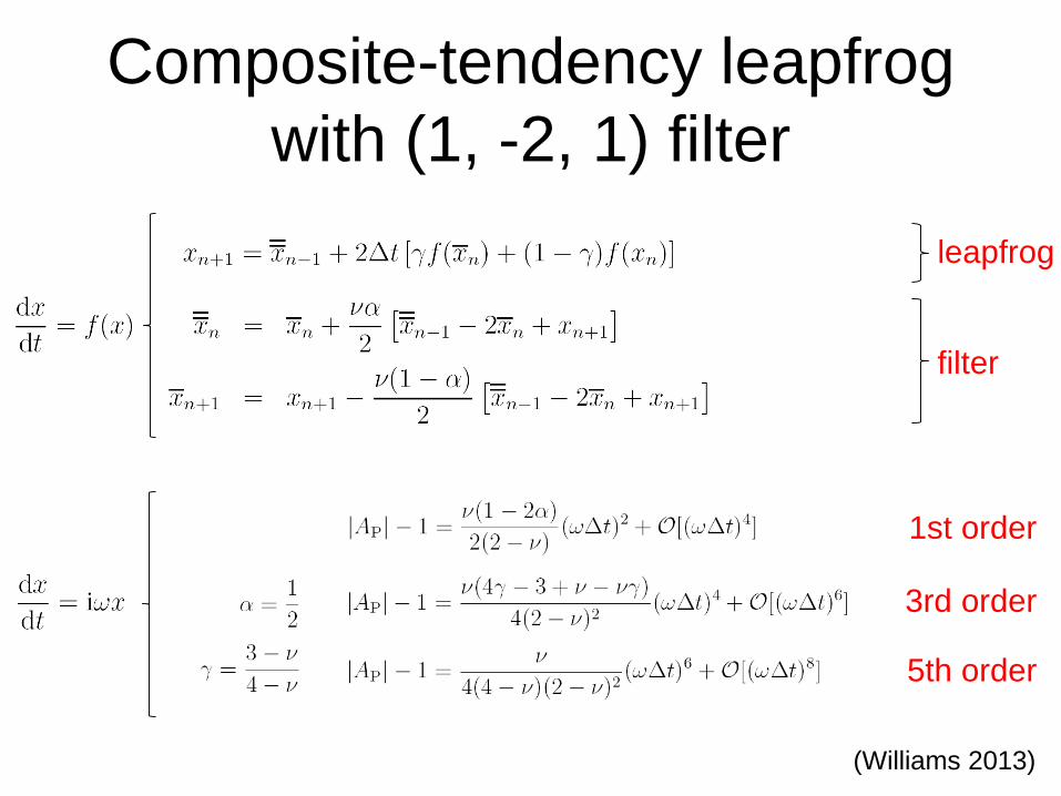
Composite-tendency leapfrog
with (1, -2, 1) filter
leapfrog
filter
1st order
3rd order
5th order
(Williams 2013)
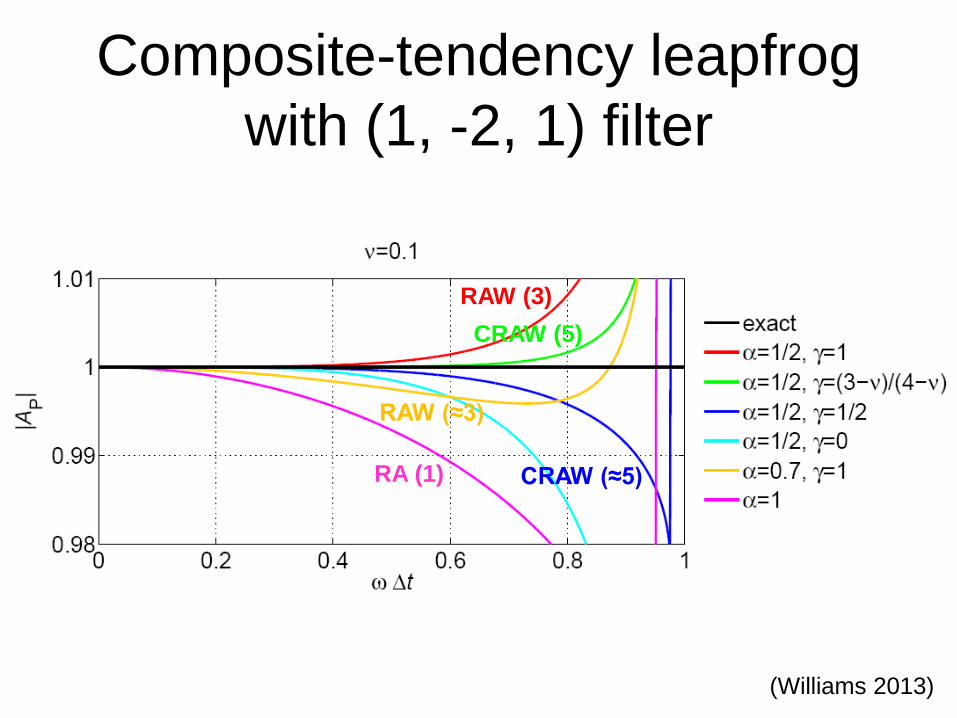
Composite-tendency leapfrog
with (1, -2, 1) filter
(Williams 2013)
RA (1)
RAW (3)
RAW (≈3)
CRAW (5)
CRAW (≈5)
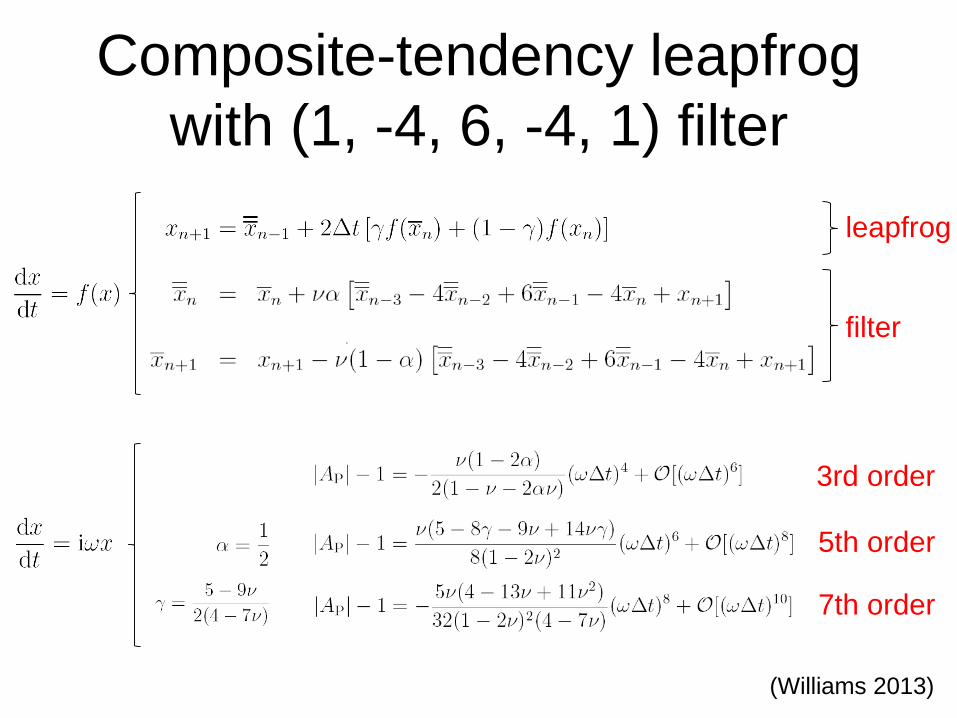
Composite-tendency leapfrog
with (1, -4, 6, -4, 1) filter
leapfrog
filter
3rd order
5th order
7th order
(Williams 2013)
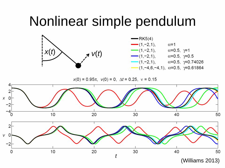
Nonlinear simple pendulum
(Williams 2013)t
x(t) v(t)
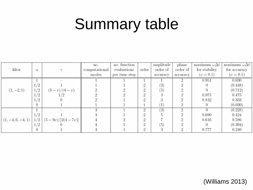
Summary table
(Williams 2013)

• Time stepping is an important contributor to model
error in today’s weather and climate models
• The Robert–Asselin filter is widely used but is
dissipative and reduces accuracy
• The RAW filter has approximately the same
stability but much greater accuracy
• Implementation in an existing code is trivial and
there is no extra computational cost
• 5th-order and even 7th-order amplitude accuracy
may be achieved, by using a composite tendency
and/or a more discriminating filter
Summary
Further information
Williams PD (2013) Achieving seventh-order amplitude accuracy in
leapfrog integrations. Monthly Weather Review 141(9), 3037-3051.
Williams PD (2011) The RAW filter: An improvement to the Robert–Asselin
filter in semi-implicit integrations. Monthly Weather Review 139(6), 1996-
2007.
Williams PD (2009) A proposed modification to the Robert–Asselin time
filter. Monthly Weather Review 137(8), 2538-2546.
twitter: @DrPaulDWilliams
www.met.reading.ac.uk/~williams