Embed Size (px)
Citation preview

Achieving Accurate Results With a CircuitSimulator
Ken Kundert and Ian Clifford
Cadence Design Systems
Analog Division
San Jose, Calif 95134
1

Outline
• Solving Nonlinear Systems of Equations
◦ Convergence Issues
◦ Solving Ordinary Differential Equations
◦ Models
◦ Examples
◦ Circuit Issues
2

Newton’s Method
A iterative methods for solving nonlinear algebraic systems of
equations.
Newton’s method is used in the DC analysis, and at each step of atransient analysis.
3

Nodal Analysis
I D D
R
R1 2
3
4 5
1 2
Write Kirchhoff’s Current Law
−I1 + Is(eV1VT − 1) +
V1 − V2
R3= 0
V2 − V1
R3+ Is(e
V2VT − 1) +
V2
R3= 0
Or f(v) = 0.
We need to find v = [V1, V2] such that f(v) = [f1(v), f2(v)] = 0
4

Newton’s Method
v
f(v)
v
v
f(v)
vv(1) (0)
f(v )(0)
v
df(v )dv
(0)
v
f(v)
vvv
(1)
(2) (1) (0)
f(v )(2)
f(v )
f(v )(0)
v
Cannot solve nonlinear equations directly.
So guess a starting point, linearize,
solve linear system, and iterate.
Algorithm for finding v̂ such that f(v̂) = 0:
Step 0: Initialize
set k ← 0
choose v(0)
Step 1: Linearize about v(k)
Jf(v(k)) = ∂f(v(k))
∂v
where Jf is the Jacobian of f .
Step 2: Solve the linearized system
v(k+1) ← v(k) − J−1f (v(k))f(v(k))
Step 3: Iterate
set k ← k + 1
if not converged, go to step 1.
5

Newton Convergence CriteriaThe Newton-Raphson algorithm is used to solve the large systems of nonlinear equations that result whenperforming DC and transient analyses. It is an iterative algorithm that terminates when the convergencecriteria are satisfied. The accuracy of the final solution is determined by the convergence criteria.
Newton’s Method:
Solve f(v) = 0 by iterating
v(k) = v(k−1) − df(v(k−1))
dxf(v(k−1))
until the following criteria are satisfied.
SPICE
|v(k)n − v(k−1)
n | < RELTOL max(|v(k)n |, |v(k−1)
n |) + VNTOL
|fnj(v(k)) − fnj(v
(k−1))| < RELTOL max(|fnj(v(k))|, |fnj(v
(k−1))|) +
ABSTOL
Spectre
|v(k)n − v(k−1)
n | < RELTOL max(|v(k)n |, |v(k−1)
n |) + VNTOL
|fn(v(k))| < RELTOL max
j(|fnj(v
(k))|) + ABSTOL
Since SPICE does not verify KCL, it is subject to falseconvergence.Unlike Spectre, SPICE never actually verifies that Kirchoff’s current law (KCL) is satisfied. This can resultin false convergence, which occurs when the iteration is terminated prematurely with KCL far from beingsatisfied because progress on one iteration is slow.
In the above, k is the iteration index, n is the node index, and j isthe branch index for node n.
6

Selecting Newton Convergence Tolerances
• RELTOL – relative Newton tolerance
Primary means of controlling accuracy In general, if you
need more accuracy, tighten RELTOL.
Controls how well KCL is satisfied, and sets how well
truncation error is controlled.• ABSTOL – absolute Newton tolerance for current
ABSTOL is called iabstol in Spectre.
Tighten if you are interested in very small currents
Loosen if your circuit exhibits very large currents
• VNTOL – absolute Newton tolerance for voltageVNTOL is called vabstol in Spectre.
Tighten if you are interested in very small voltages
Loosen if your circuit exhibits very large voltages
7

Remedies for DC Accuracy Problems
• Assume computed solution is correct
Circuit may have unanticipated problems
Debug circuit as if on lab bench
Circuit may have multiple solutions
Use NODESET to select solution
• Check topology
• Check models
• Check component values
• Check power supplies
• Tighten RELTOL
• Check GMIN
8

Outline
◦ Solving Nonlinear Systems of Equations
• Convergence Issues
Requirements for Convergence
Nodesets
Continuation Methods
Suggestions
◦ Solving Ordinary Differential Equations
◦ Models
◦ Examples
◦ Circuit Issues
9

Newton’s Method will Always Converge if . . .
• f(v) and its derivatives are continuous.
• Solutions must be isolated (Jf(v̂) is nonsingular).
• Initial guess v(0) is sufficiently close to solution v̂.
The last condition is the hardest to satisfy.
10

Nodesets
Allows user to provide a good initial guess.
• Nodesets can be used in both DC and transient analyses.
• Nodesets do not change the solutions of the circuit. However, if
the circuit has multiple solutions, nodesets may change the
solution that the simulator finds.
How SPICE forces nodesets
Step 1:
Force all set nodes with voltage source in series with 1Ω resistor.
Compute DC solution with set nodes forced.
Step 2:
Delete forcing circuits and compute DC solution using results
from step 1 as starting point.
11

Continuation Methods
Used to compute a good initial guess.
Write the circuit equations in the form
f(v(λ), λ) = 0
and choose λ as a natural or contrived parameter of you circuit
such that
• For λ = 0, the solution v(0) is known in advance or is easy to
find.
• For λ = 1, f(v(1), 1) = f(v).
• v(λ) is a continuous function of λ.
f( )
Procedure:
Slowly step λ from 0 to 1 computing v(λ) at every step. Use v(λk)
as the initial guess of the solution v(λk+1).
If |λk+1 − λk| is small, and if v(λ) is continuous, then v(λk) will be
in the region of convergence for v(λk+1) and so convergence will be
guaranteed.
Examples:Source Stepping, GMIN Stepping, and Pseudo-Transient
12

Why Continuation Methods Fail
Folds plague source stepping and GMIN stepping.f( )
Oscillations plague pseudo-transient.f( )
Bifurcations result from symmetry.f( )
Q
Q
Vcc
13

Reasons for DC Convergence Problems
• Fundamentally a hard problem.
• Degenerate circuit.
• Unreasonable parameter values.
• Excessively tight tolerances
• Errors in model equations.
14

Remedies for DC Convergence Problems
• Heed warnings
• Check topology
• Check component parameter values
• Avoid small floating resistors
Use 0-volt voltage source as current probe
Avoid small parasitic resistors
Do not set RBmin ≈ 0 on BJT
• Use Nodesets to give estimate of solution
• Loosen Tolerances (particularly ABSTOL)
• Enable continuation methods
Set ITL6 in SPICE• Simplify models
Try to eliminate second-order effects and parasitic resistors (especially nonlinear base resistors. Usethe simplified circuit to generate a nodeset file for the original circuit.
• Disable oscillators and use transient analysisAs a last resort, Spectre used a pseudo-transient analysis to compute the DC solution. This analysiswill not find the DC solution if the circuit oscillates.
15

Reasons for Transient Convergence Problems
• Instantaneous jumps in signal value
Jumps are generally caused by local positive feedback on nodes
without capacitors. Circuits that can exhibit jumps include
latches, Schmitt triggers, and relaxation oscillators.
• Errors in device charge models
16

Remedies for Transient Convergence Problems
• Avoid simplified models
Use a complete capacitance model
Specify nonzero output conductance
Specify overlap capacitors
• Specify nonzero source and drain areas for all MOSFETsThis results in the junction capacitors being modeled.
• Identify which node is having difficulties, and add a small
capacitor from that node to ground.
• With Spectre, set CMIN nonzero. CMIN causes Spectre to add
small capacitors from every node in the circuit to ground.
17

Outline
◦ Solving Nonlinear Systems of Equations
◦ Convergence Issues
• Solving Ordinary Differential Equations
Integration Methods
Truncation Error
Initial Conditions
Suggestions
◦ Models
◦ Examples
◦ Circuit Issues
18

Transient Analysis
Formulate equations using Nodal Analysis
i(v(t)) +d
dtq(v(t)) = 0
v(0) = v0
Where
i is current exiting the nodes from resistors.
q is current exiting the nodes from capacitors.
Example:
R C
v
Cv̇(t) +v(t)
R= 0
v(0) = v0
In general, it is not possible to solve explicitly a nonlinear ordinary
differential equation.
Approach:
Replace ddt operator by discrete-time approximation.
19

Integration Methods
Multistep Methods:
Form discrete time approximation to ddt by assuming trajectory is a
low order polynomial.
Assume time is discretized uniformly and that h = tk+1 − tk
Backward Euler (Linear Polynomial — One Step)
v̇(tk+1) =1
h(v(tk+1) − v(tk))
Trapezoidal Rule (Quadratic Polynomial — One Step)
v̇(tk+1) =2
h(v(tk+1) − v(tk)) − v̇(tk)
Second-order Gear (Quadratic Polynomial — Two Step)
v̇(tk+1) =1
h
⎛⎝3
2v(tk+1) − 2v(tk) +
1
2v(tk−1)
⎞⎠
Example:
Applying backward Euler to circuit equations:
q(v(tk+1)) − q(v(tk)) + hi(v(tk+1)) = 0
v(t0) = v0
20

Trapezoidal-Rule Rings
Trapezoidal Rule:
0.0
0.5
1.0
1.5
2.0
2.5
3.0
3.5
4.0
4.5
5.0
0us 50us 100us 150us
Point-to-point ringing is an artifact of the trapezoidal rule, switch
to Gear to avoid it.
21

Gear Damps
Apply various integration methods to lossless linear LC oscillator.
Trapezoidal Rule:
-1.0V
-0.5V
0.0V
0.5V
1.0V
0s 20s 40s 60s 80s 100s
Gear’s Second-Order Backward-Difference Formula:
-1.0V
-0.5V
0.0V
0.5V
1.0V
0s 20s 40s 60s 80s 100s
Backward Euler:
-1.0V
-0.5V
0.0V
0.5V
1.0V
0s 20s 40s 60s 80s 100s
Artificial numerical damping is an artifact of Gear and
backward-Euler, switch to trapezoidal to avoid it.
22

Truncation Error
Definitions:
Truncation Error:
Error made by replacing time-differentiation operator with its
discrete-time approximation. In general, the smaller the time
step, the smaller the truncation error.
Local Truncation Error (LTE):
The truncation error made at a single step assuming all
previous steps are accurate.
Global Truncation Error:
Maximum accumulated truncation error. Related to
accumulated LTE and the tendency of the circuit to accumulate
or dissipate errors.
In general, it is difficult to estimate global truncation error, so LTEis used to control the time step.
23

Circuit Determines How Errors Accumulate
Use superposition to consider effect of error separately.
Assume i represents error current injected by not satisfying KCL
exactly.
Example 1 — RC Circuit
R C
v
I
I(t)
tn
t
v(t)
tn
t
I(t)
tn
t
v(t)
tn
t
Example 2 — C Circuit
C
v
I
I(t)
tn
t
v(t)
tn
t
I(t)
tn
t
v(t)
tn
t
24

Local-Truncation Error
Integration method is exact if trajectory is low-order polynomial.
Thus, LTE is proportional to difference between actual trajectory
and low-order polynomial.
kpredV t
V(t )k
LTEk-1
V(t )
V(t )k-3
k-2
( )
V(t )
The local truncation error (LTE) is the error made on each time-step that results from discretizing time.The local truncation error is the difference between the computed solution and the polynomialextrapolation from the previous few time-steps.
Choose time step such that v(tk) − vpred(tk) < LTEmax
25

Charge-based Local-Truncation Error Criterion
SPICE — Controls Error in Charge
|q(v(t)) − q(vpred(t))| < TRTOL[RELTOL|q(v(t))| + CHGTOL]
Use of CHGTOL results in SPICE ignoring large voltage errors on
small capacitors.
CHGTOL should be reduced as device capacitances decrease.
0.0 V
0.2 V
0.4 V
0.6 V
0.8 V
1.0 V
1.2 V
0 ns 100 ns 200 ns 300 ns 400 ns 500 ns 600 ns
585 mV
590 mV
595 mV
600 mV
605 mV
350 ns 400 ns 450 ns 500 ns 550 ns 600 ns
26

Voltage-based Local-Truncation Error Criterion
Spectre — Controls Error in Voltage
|v(t) − vpred(t)| < TRTOL[RELTOL|v(t)| + VNTOL]
0.0 V
0.2 V
0.4 V
0.6 V
0.8 V
1.0 V
1.2 V
0 ns 100 ns 200 ns 300 ns 400 ns 500 ns 600 ns
590 mV
595 mV
600 mV
605 mV
610 mV
350 ns 400 ns 450 ns 500 ns 550 ns 600 ns
One can either control the local truncation error in charge or voltage. SPICE-based simulators control theerror on the charge, hence the use of the cumbersome tolerance parameter CHGTOL. Controlling thecharge error is not a good idea for two reasons. First, users are not interested in charge, and controllingcharge error does not guarantee accurate voltages. Second, charge scales with the size of the nonlineardevices. Thus, CHGTOL should be reduced every time a new smaller semiconductor process is introduced.Instead, Spectre controls error on voltage, which gives more accurate answers and avoids the charge scalingproblem.
27

Selecting Truncation Error TolerancesTruncation error tolerances only affect accuracy of transient analysis.
All Newton convergence tolerances are also used as truncation error tolerances. In addition there are thefollowing parameters.
• TRTOL – relative truncation error toleranceTRTOL is equivalent to LTERATIO in Spectre.
Sets acceptable truncation error relative to RELTOL
Allows independent control of KCL and truncation errors.Do not set TRTOL < 2.
In general, if you need more accuracy, tighten RELTOL. Tightening TRTOL is not a good ideabecause it causes the simulator to shrink the time step in order to accurately follow the errors thatresult from not completely converging the Newton iteration. Generally, TRTOL is used to allow theNewton criteria to be set much tighter than the truncation error criteria (this is useful when trying toreduce charge conservation error to negligible levels). Loosening TRTOL by the same factor thatRELTOL is tightened results in the Newton convergence criteria being tightened while keeping thetruncation error criteria the same.
• CHGTOL – absolute charge toleranceSpectre has no equivalent to CHGTOL.
Should be tightened as devices shrink.CHGTOL should be set such that roughly CHGTOL = VNTOL × Cmin where Cmin is the smallestinteresting capacitor in the circuit. If you are having problems with trapezoidal-rule ringing, tightenCHGTOL.
• TMAX – maximum time step
Use if simulator misses events or for onset of oscillation.
Should not normally be used to control error because
1. Convergence criteria not affected.2. Only shrinks large steps.
In general, tightening RELTOL is a better way to control error than tightening TMAX. TMAX is apoor way to control error for several reasons. First, tightening TMAX does not tighten the Newtonconvergence criteria. Second, tightening TMAX only shrinks large time steps. Thus tighteningTMAX only has an effect when signals are not moving much, and not when signals are movingrapidly. TMAX is the preferred way to control error if signals are very small compared to their DClevels. This happens during the build-up phase of an oscillation. In this situation, the signals aregenerally too small to produce enough truncation error to shrink the time-step.
• LVLTIM – Time-step control method selection
Can be used to disable truncation error time step control.
28

This is very dangerous and is not recommended!
29

Initial Conditions
Used in a transient analysis to start the circuit from some point
other than the DC solution.
• Initial conditions are used only in transient analysis.
• Initial conditions directly affect the computed results by
changing the starting point.
How SPICE forces initial conditions
UIC:
Set v(0) equal to initial condition and go. Any unspecified
initial conditions are taken to be zero.
No UIC:
Force all nodes with initial conditions with voltage sources in
series with 1Ω resistors.
Compute DC solution with initial conditions forced. Set v(0)
equal to result and go.
30

Remedies for Transient Accuracy Problems
• Check initial operating point.
• Check topology.
• Check models.
• Check component values.
• Check power supplies.
• Check stimulus waveforms.
• Tighten RELTOL.
• Check GMIN.
• If charge conservation problem, use charge-conserving models.
• If point-to-point ringing problem, use Gear’s method.
• If excessive loss, use trapezoidal rule.
• If simulating an oscillator, set TMAX for 10-25 time steps per
period.
31

Outline
◦ Solving Nonlinear Systems of Equations
◦ Convergence Issues
◦ Solving Ordinary Differential Equations
• Models
MOS Models
Charge Conservation in Models
◦ Examples
◦ Circuit Issues
32

Model Accuracy
Spice Current Model
Model Output Velocity Subthresh Impact
Conductance Saturation Region Ionization
MOS-1 poor none none no
MOS-2 poor poor poor no
MOS-3 poor poor poor no
BSIM-1 poor okay okay no
BSIM-2 good good good no
Spectre Current Model
Model Output Velocity Subthresh Impact
Conductance Saturation Region Ionization
MOS-1 poor none none yes
MOS-2 poor poor poor yes
MOS-3 poor poor poor yes
BSIM-1 poor okay okay yes
BSIM-2 good good good yes
33

Model Accuracy
Spice Charge Models
Charge Available Conserves Velocity
Model In Model Charge Saturation
Meyer MOS-1,2,3 no none
Ward-Dutton MOS-2 yes good
BSIM BSIM-1,2 yes good
Spectre Charge Models
Charge Available Conserves Velocity
Model In Model Charge Saturation
Modified-Meyer MOS-1,2,3, BSIM-1,2 yes none
Yang-Chatterjee MOS-1,2,3, BSIM-1,2 yes good
BSIM MOS-1,2,3, BSIM-1,2 yes good
34

Model Accuracy
Model Minimum Feature Size
Model Min Gate Min Gate Min Oxide
Length Width Thickness
MOS-1 10μm 10μm 60nm
MOS-2 2μm 2μm 30nm
MOS-3 0.8μm 2μm 20nm
BSIM-1 0.8μm 1μm 20nm
BSIM-2 0.2μm 1μm 5nm
Spectre Model Evaluation Time
Model Evaluation
Time
MOS-1 0.44ms
MOS-2 1.4ms
MOS-3 0.58ms
BSIM-1 0.59ms
BSIM-2 0.93ms
BSIM2 is the only commercially available MOS model suitable for very small feature size MOSFETs orMOSFETs used in analog circuits.
35

Charge Conservation
Capacitance-Based Models
Do not conserve charge because charge is computed from linearized
model.
q(t1)
v(t1) v
q
v(t2)
q(t2)
C(v(t1))
C(v(t0))
Charge-Based Models
q(t1)
v(t1) v
q
v(t2)
q(t2)
36

Outline
◦ Solving Nonlinear Systems of Equations
◦ Convergence Issues
◦ Solving Ordinary Differential Equations
◦ Models
• Examples
Oscillator:
Suffers from phase drift due to truncation error.
AC-Coupled Comparator:
Suffers from charge conservation problems.
Sample and Hold:
Suffers droop caused by GMIN.
◦ Circuit Issues
37

Lossless Linear LC OscillatorExample:
Accuracy determined largely by circuit.
• Resonator stores energy without loss.
• Resonator also stores error without loss.
• Small amount of error accumulates at each step.
Stimulus:
-1.0 A
-0.8 A
-0.6 A
-0.4 A
-0.2 A
0.0 A
0.0 20.0 40.0 60.0 80.0
38

Correct Response:
-30mV
-20mV
-10mV
0V
10mV
20mV
30mV
0s 20s 40s 60s 80s
Simulated Response:
-30mV
-20mV
-10mV
0V
10mV
20mV
30mV
0s 20s 40s 60s 80s
39
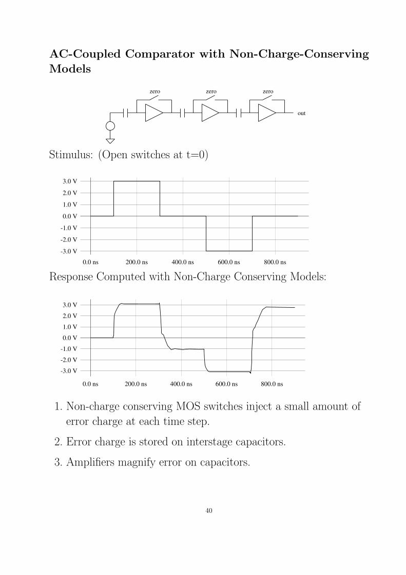
AC-Coupled Comparator with Non-Charge-Conserving
Models
zero zero zero
out
Stimulus: (Open switches at t=0)
-3.0 V
-2.0 V
-1.0 V
0.0 V
1.0 V
2.0 V
3.0 V
0.0 ns 200.0 ns 400.0 ns 600.0 ns 800.0 ns
Response Computed with Non-Charge Conserving Models:
-3.0 V
-2.0 V
-1.0 V
0.0 V
1.0 V
2.0 V
3.0 V
0.0 ns 200.0 ns 400.0 ns 600.0 ns 800.0 ns
1. Non-charge conserving MOS switches inject a small amount of
error charge at each time step.
2. Error charge is stored on interstage capacitors.
3. Amplifiers magnify error on capacitors.
40

AC-Coupled Comparator with Charge-Conserving
ModelsResponse Computed with Charge-Conserving Models:
-3.0 V
-2.0 V
-1.0 V
0.0 V
1.0 V
2.0 V
3.0 V
0.0 ns 200.0 ns 400.0 ns 600.0 ns 800.0 ns
Convergence Criteria:
|i(v(j)n ) − i(v(j−1)
n )| < RELTOL max(|i(v(j)n )|, |i(v(j−1)
n )|) + ABSTOL
Response Computed with Charge-Conserving Models and Tight
Tolerances:
-3.0 V
-2.0 V
-1.0 V
0.0 V
1.0 V
2.0 V
3.0 V
0.0 ns 200.0 ns 400.0 ns 600.0 ns 800.0 ns
41

Sample and Hold
Response Computed with GMIN = 10−12 and GMIN = 0:gmin=0
gmin=1e-12
1.5 V
1.6 V
1.7 V
1.8 V
1.9 V
2.0 V
2.1 V
2.2 V
2.3 V
2.4 V
2.5 V
0.0 us 10.0 us 20.0 us 30.0 us 40.0 us 50.0 us 60.0 us
Zoom-in to compute drift:gmin=0
gmin=1e-12
0 uV
50 uV
100 uV
150 uV
45.0 us 50.0 us 55.0 us 60.0 us
With GMIN, drift is 8.5 V/s, without GMIN, drift is 0.
42

How SPICE installs GMIN:
43

Outline
◦ Solving Nonlinear Systems of Equations
◦ Convergence Issues
◦ Solving Ordinary Differential Equations
◦ Models
◦ Examples
• Circuit Issues
Oscillators
Op-Amp Loop Gain Measurements
44

Oscillators
• Tighten RELTOLHigh-Q resonators store energy and error for long periods.Since oscillators accumulate phase error, is is a good idea to simulate oscillators with the RELTOLset tigher than you normally use on other circuits.
• Use initial conditions to start oscillation
Oscillators do not start themselves.
Initial conditions better than sources:
Less error prone.Does not require modification of circuit.
Use initial conditions to start an oscillator rather than an impulse stimulus. Initial conditions willmore reliably start an oscillator without unexpected side effects.
• Set the maximum time step (TMAX) to accurately followstart-up.When simulating the start-up phase of the oscillation, the signals are so small that they are ignoredby the time-step control algorithm and the time-step is not chosen small enough to accurately followthe signals. Generally TMAX should be set so that there are at least 10-25 time steps per period.
45

Op-Amp Loop Gain
a
f
in out
fb
where
a = open loop gain
f = feedback factor
T = af = loop gain
A =1
1 + T= closed loop gain
Conceptually, to measure loop gain, you break the loop at fb.
Difficulties:
1. You must not change the operating point.
2. You must account for loading.
46

Measuring Voltage Loop Gain
a
f
+
-vn
vpvo
Vin
vf
fb
Procedure:
1. Insert floating voltage source with 0 DC value and unity AC
magnitude at point fb.
2. Set AC magnitude of input source to 0.
3. Measure voltage loop gain as:
Tv = −vf
vn
a
f
+
-vn
vpvo
V
V
in
t
vf
Z f
Z n
T = Tv if Zn � Zf
47
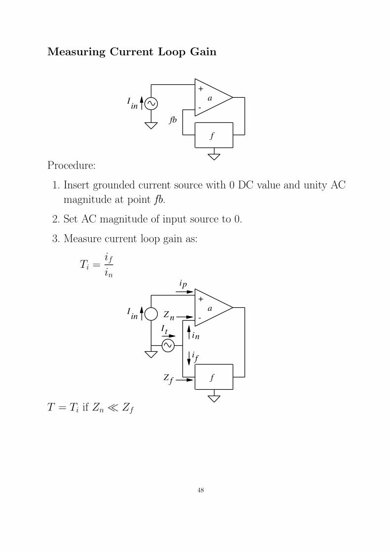
Measuring Current Loop Gain
a
f
+
-inI
fb
Procedure:
1. Insert grounded current source with 0 DC value and unity AC
magnitude at point fb.
2. Set AC magnitude of input source to 0.
3. Measure current loop gain as:
Ti =ifin
a
f
+
-
n
p
in
t
f
I
I
i
i
i
Z n
Z f
T = Ti if Zn � Zf
48

Computing Total Loop Gain
If T �= Tv because Zn � Zf ,
and T �= Ti because Zn � Zf , use
T =TvTi − 1
2 + Tv + Ti
This equation becomes inaccurate if T � 1.
49