Accuracy analysis for fifty-four clear-sky solar radiation models using routine hourly global irradiance measurements in Romania.pdf

(This is a sample cover image for this issue. The actual cover is not yet available at this time.)

This article appeared in a journal published by Elsevier. The attachedcopy is furnished to the author for internal non-commercial researchand education use, including for instruction at the authors institution

and sharing with colleagues.

Other uses, including reproduction and distribution, or selling orlicensing copies, or posting to personal, institutional or third party

websites are prohibited.

In most cases authors are permitted to post their version of thearticle (e.g. in Word or Tex form) to their personal website orinstitutional repository. Authors requiring further information

regarding Elsevier’s archiving and manuscript policies areencouraged to visit:

http://www.elsevier.com/copyright

http://www.elsevier.com/copyright

Author's personal copy

Accuracy analysis for fifty-four clear-sky solar radiation models usingroutine hourly global irradiance measurements in Romania

Viorel Badescu a,b,*, Christian A. Gueymard c, Sorin Cheval d, Cristian Oprea e, Madalina Baciu e,Alexandru Dumitrescu e,f, Flavius Iacobescu a, Ioan Milos e, Costel Rada e

aCandida Oancea Institute, Polytechnic University of Bucharest, Spl. Independentei 313, Bucharest 060042, RomaniabRomanian Academy, Calea Victoriei 125, Bucharest, Romaniac Solar Consulting Services, P.O. Box 392, Colebrook, NH 03576, USAdNational Research and Development Institute for Environmental Protection, Splaiul Independentei nr. 294, Sect. 6, 060031 Bucuresti, RomaniaeNational Meteorological Administration, 97 Sos. Bucuresti-Ploiesti, Bucharest 013686, RomaniafUniversity of Bucharest, Faculty of Geography, Bucharest, Romania

a r t i c l e i n f o

Article history:Received 15 November 2011Accepted 27 November 2012Available online

Keywords:Clear sky modelsGlobal solar radiationHourly irradiationRomania

a b s t r a c t

Fifty-four broadband clear-sky models for computation of global solar irradiance on horizontal surfacesare tested by using measured data from Romania (South-Eastern Europe). The input data to the modelsconsist of surface meteorological data, column integrated data and data derived from satellite mea-surements. The testing procedure is performed in twenty-one steps for two different sites in Romania.The models accuracy is reported for various sets of input data. No model ranked “the best” for all sets ofinput data. However, some of the models were ranked among the best for most of the testing steps, andthus performed significantly better than others. These “better” models are, on an equal footing, ESRA3,Ineichen, METSTAT and REST2 (version 8.1). The next “better” models are, on an equal footing, Bird, CEMand Paulescu and Schlett. Details about the accuracy of each model are found in the ElectronicSupplementary Content for all testing steps.

! 2012 Elsevier Ltd. All rights reserved.

1. Introduction

Although there are several world maps or datasets of solar ra-diation, they are usually not detailed enough to be used for thedetermination of available solar energy over small areas. Thesecircumstances have prompted the development of calculationprocedures to provide radiation estimates for areas where mea-surements are not carried out, or for situations when gaps in themeasurement records occurred. These procedures range from verysimple radiation models to sophisticated computing codes. Onlya minority of these models has been validated by their authors, andusually under specific geographical or climatic circumstances only.To increase the confidence inmodeled data accuracy there is a needfor validation by independent groups and at a variety of test sites inmany different climatic areas. Existing validation reports usually

refer to a small number of models being intercompared underspecific climatic environments [1e10]. The correct validation andcomparison of radiative models raise specific issues. For instance,different statistics may be used to evaluate the bias and randomdifferences between the computed and measured data series.Moreover, various ranking procedures can be used to compare themodels accuracy, yielding different results (for more detailed dis-cussions, see [9]).

Clear sky solar radiation models are traditionally used inbuilding design and simulation of solar concentration systems.Also, they are of interest for filling historical missing measurementdata. Most recent procedures to estimate ground level solar radi-ation from satellite data are associated with a specific clear skymodel. As an example, the Heliosat-2 procedure was developedwith special reference to the ESRA clear-skymodel [11]. Many otherclear sky models are now available and they may be used withinother solar radiation computing procedures based on satellite data.

The present investigation considers fifty-four clear-sky globalsolar radiation models, i.e., a much larger sample of what the lit-erature offers than in any previous study. This large sample en-compasses a large range of modeling complexity, from very simpleto sophisticated models. Some models only calculate global

* Corresponding author. Candida Oancea Institute, Polytechnic University ofBucharest, Spl. Independentei 313, Bucharest 060042, Romania. Tel.: !40 21 4029339; fax: !40 21 318 1019.

E-mail addresses: [email protected] (V. Badescu), [email protected] (C.A. Gueymard), [email protected] (S. Cheval).

Contents lists available at SciVerse ScienceDirect

Renewable Energy

journal homepage: www.elsevier .com/locate/renene

0960-1481/$ e see front matter ! 2012 Elsevier Ltd. All rights reserved.http://dx.doi.org/10.1016/j.renene.2012.11.037

Renewable Energy 55 (2013) 85e103


irradiance, whereas others also provide its direct and diffusecomponents. Most of these models have been previously tested,under a fewgeographical conditions, during different time intervalsand by using various testing procedures. How they compare inpractice under specific and identical conditions is still not known.

One frequent problem occurring in practice when one has tomake use of a radiation model is related to the input data that itrequires vs. what is actually available for the specific location andperiod under scrutiny. It is quite frequent that the potential user ofa specific model known to offer good accuracy has access to onlydatabases that do not provide all the necessary input parameters. Inthis case the user can either obtain the missing data by inter-polation, extrapolation or estimation (thus introducing larger un-certainties in the predicted irradiances), or choose another modelthat would fit the available input databases better, but would bepresumably simpler and coarser, and thus would have loweraccuracy.

Compared to the existing validation studies, the present con-tribution describes some further steps that are deemed necessaryto better validate and rank the accuracy of radiation models underthe “typical” conditions encountered by users in practice. In par-ticular, this means that the precise state of the atmosphere cannotbe obtained from collocated instruments (such as sunphotometers),whose availability is normally critical in assessing the inherentaccuracy of models, as shown in most validation studies mentionedabove.

The objectives of this investigation are twofold. First, the accu-racy of these fifty-four models is analyzed and ranked by compar-ing their predictions under identical climate conditions and usinga unique testing procedure. Second, various input datasets are usedand the accuracy of each model is reported. Reference radiometricmeasurements (used as “ground truth”) are provided here by twometeorological and radiometric stations in South-Eastern Europe(Romania). These stations have provided good-quality routine dataover many years. These are not high-end research-class stations,however, which means that the present study can be consideredrepresentative of what can be obtained at hundreds of similarstations over theworld, rather than at a few specialized sites, like insome previous studies (e.g. [9,10]). These studies considered theideal case when all the investigated models’ inputs were measuredlocally at high frequency with high-quality instruments, so as toobtain the intrinsic performance of these models by avoidingpropagation of errors. In contrast, the present investigation is muchmore pragmatic, since it uses “normal” radiation measurementsand interpolated/extrapolated input data in both space and time toevaluate the “real world” performance of models under non-idealconditions.

2. Radiation models

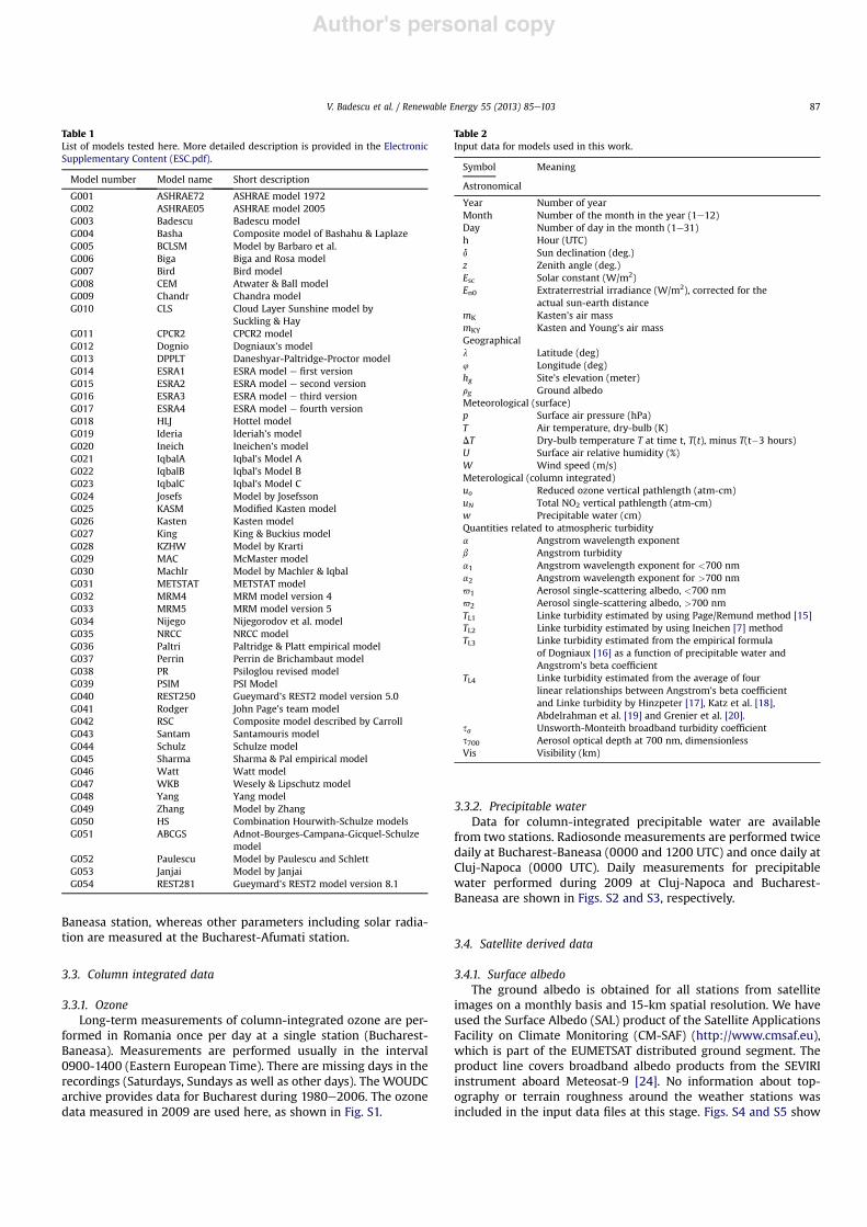
Fifty-four broadband models for the prediction of global irra-diance on horizontal surfaces have been selected for this study.These models are listed in Table 1 using a call number (G001 toG054) for further reference and are briefly described the ElectronicSupplementary Content (ESC.pdf) where Fortran routines are alsoprovided. Some of these models were already tested in [9,10,12].Others were intentionally added here for completeness. A bird’s eyeview on all models’ hierarchy has been reported in [13]. However,no detailed quantitative information about the models accuracy isprovided in [13], where the procedure was intended just to checkwhether a given model passes (or not) some accuracy criteria. Thesuccessful events were counted and the counts were used to createhierarchies. In the present paper we provide detailed, quantitativeresults, for the accuracy of each model in part. Therefore, the reader

interested in a particular model will find here specific informationwhich in [13] is missing.

3. Input data

Thefifty-four solar radiationmodels have different requirementsfor input data (Table 2). Table 3 shows the entries needed by eachmodel.

The only input variable that is common to all models is thezenith angle, Z, which characterizes the sun position. Most modelstake the solar geometry into account through the relative air mass,m, rather than Z. The specific relationship between m and Z rec-ommended by each model is used here. Computations were per-formed only for Z < 85" to avoid inaccuracies resulting frompossible horizon shading or experimental cosine errors, forinstance. For those models that refer to the solar constant, a com-mon value of 1366.1 W/m2 is used [14].

The input data have been organized in several subgroups. Themost important of these consists of measured meteorological dataat the ground surface. In Romania, meteorological stations rou-tinely measure the quantities described in Table S1 (prefix S comefrom the Electronic Supplementary Content).

3.1. Solar radiation measurements

Two types of measurement devices are used in parallel in eachRomanian station, i.e., Robitsch actinographs (which recorded dataduring a few decades) and Kipp & Zonen CM radiometers (whichstarted recording data in 2006). A CM11 radiometer is operating atBucharest-Afumati station. All other radiometric stations are pro-vided with CM6B radiometers. The measurement uncertainty is#3% for CM11 and #5% for CM6B. The temperature dependence ofsensitivity is #1% for CM11 and #2% for CM6B, on the interval $20to !40 "C. On a monthly basis the bias for CM6B ranges between e2% and !0.9% [21]. More information about definition of instru-ment uncertainty may be found in [22,23]. The radiometers arechecked twice per week and cleaned when necessary.

The measurement methodology is provided by standard pro-cedures prepared at the National Meteorological Administration.Measurements are performed as follows. Solar irradiance (units:W/m2) is measured at 1-min intervals. The series of irradiancevalues are averaged over 10 min, 60 min and 1440 min, respec-tively. Irradiation values (units: J) for 10 min, 1 h and 24 h areobtained by multiplying the appropriate average irradiance valuesby the appropriate time duration. The integration interval starts !hour before the time stamp in the files and ends ! hour after thattime stamp. Central European Time is used in the files.

The radiometers are calibrated once per year through shaded -unshaded measurements in clear sky days and through directirradiance measurements on a horizontal surface with reference tothe Linke-Feussner etalon actinometer. The Linke-Feussner etalonis calibrated with reference to the national etalon, i.e. an Angstrom702 pyrheliometer with electric compensation. The national etalonis calibrated once at five years with reference to the World Radio-metric Reference at Davos (Swiss).

In this study data provided during 2009 by CM K&Z radiometersis used. Partial sky obstructions or shading of the sensors by naturalor artificial structures is low and is not considered. There are lessthan 0.1% missing or suspicious data.

3.2. Surface meteorological data

Meteorological data measured during 2009 at the three stationsof Table 4 are used in this study. In the case of Bucharest, some ofthe meteorological variables are measured at the Bucharest-

V. Badescu et al. / Renewable Energy 55 (2013) 85e10386


Baneasa station, whereas other parameters including solar radia-tion are measured at the Bucharest-Afumati station.

3.3. Column integrated data

3.3.1. OzoneLong-term measurements of column-integrated ozone are per-

formed in Romania once per day at a single station (Bucharest-Baneasa). Measurements are performed usually in the interval0900-1400 (Eastern European Time). There are missing days in therecordings (Saturdays, Sundays as well as other days). The WOUDCarchive provides data for Bucharest during 1980e2006. The ozonedata measured in 2009 are used here, as shown in Fig. S1.

3.3.2. Precipitable waterData for column-integrated precipitable water are available

from two stations. Radiosonde measurements are performed twicedaily at Bucharest-Baneasa (0000 and 1200 UTC) and once daily atCluj-Napoca (0000 UTC). Daily measurements for precipitablewater performed during 2009 at Cluj-Napoca and Bucharest-Baneasa are shown in Figs. S2 and S3, respectively.

3.4. Satellite derived data

3.4.1. Surface albedoThe ground albedo is obtained for all stations from satellite

images on a monthly basis and 15-km spatial resolution. We haveused the Surface Albedo (SAL) product of the Satellite ApplicationsFacility on Climate Monitoring (CM-SAF) (http://www.cmsaf.eu),which is part of the EUMETSAT distributed ground segment. Theproduct line covers broadband albedo products from the SEVIRIinstrument aboard Meteosat-9 [24]. No information about top-ography or terrain roughness around the weather stations wasincluded in the input data files at this stage. Figs. S4 and S5 show

Table 1List of models tested here. More detailed description is provided in the ElectronicSupplementary Content (ESC.pdf).

Model number Model name Short description

G001 ASHRAE72 ASHRAE model 1972G002 ASHRAE05 ASHRAE model 2005G003 Badescu Badescu modelG004 Basha Composite model of Bashahu & LaplazeG005 BCLSM Model by Barbaro et al.G006 Biga Biga and Rosa modelG007 Bird Bird modelG008 CEM Atwater & Ball modelG009 Chandr Chandra modelG010 CLS Cloud Layer Sunshine model by

Suckling & HayG011 CPCR2 CPCR2 modelG012 Dognio Dogniaux’s modelG013 DPPLT Daneshyar-Paltridge-Proctor modelG014 ESRA1 ESRA model e first versionG015 ESRA2 ESRA model e second versionG016 ESRA3 ESRA model e third versionG017 ESRA4 ESRA model e fourth versionG018 HLJ Hottel modelG019 Ideria Ideriah’s modelG020 Ineich Ineichen’s modelG021 IqbalA Iqbal’s Model AG022 IqbalB Iqbal’s Model BG023 IqbalC Iqbal’s Model CG024 Josefs Model by JosefssonG025 KASM Modified Kasten modelG026 Kasten Kasten modelG027 King King & Buckius modelG028 KZHW Model by KrartiG029 MAC McMaster modelG030 Machlr Model by Machler & IqbalG031 METSTAT METSTAT modelG032 MRM4 MRM model version 4G033 MRM5 MRM model version 5G034 Nijego Nijegorodov et al. modelG035 NRCC NRCC modelG036 Paltri Paltridge & Platt empirical modelG037 Perrin Perrin de Brichambaut modelG038 PR Psiloglou revised modelG039 PSIM PSI ModelG040 REST250 Gueymard’s REST2 model version 5.0G041 Rodger John Page’s team modelG042 RSC Composite model described by CarrollG043 Santam Santamouris modelG044 Schulz Schulze modelG045 Sharma Sharma & Pal empirical modelG046 Watt Watt modelG047 WKB Wesely & Lipschutz modelG048 Yang Yang modelG049 Zhang Model by ZhangG050 HS Combination Hourwith-Schulze modelsG051 ABCGS Adnot-Bourges-Campana-Gicquel-Schulze

modelG052 Paulescu Model by Paulescu and SchlettG053 Janjai Model by JanjaiG054 REST281 Gueymard’s REST2 model version 8.1

Table 2Input data for models used in this work.

Symbol Meaning

Astronomical

Year Number of yearMonth Number of the month in the year (1e12)Day Number of day in the month (1e31)h Hour (UTC)d Sun declination (deg.)z Zenith angle (deg.)Esc Solar constant (W/m2)En0 Extraterrestrial irradiance (W/m2), corrected for the

actual sun-earth distancemK Kasten’s air massmKY Kasten and Young’s air massGeographicall Latitude (deg)4 Longitude (deg)hg Site’s elevation (meter)rg Ground albedoMeteorological (surface)p Surface air pressure (hPa)T Air temperature, dry-bulb (K)DT Dry-bulb temperature T at time t, T(t), minus T(t$3 hours)U Surface air relative humidity (%)W Wind speed (m/s)Meterological (column integrated)uo Reduced ozone vertical pathlength (atm-cm)uN Total NO2 vertical pathlength (atm-cm)w Precipitable water (cm)Quantities related to atmospheric turbiditya Angstrom wavelength exponentb Angstrom turbiditya1 Angstrom wavelength exponent for <700 nma2 Angstrom wavelength exponent for >700 nm61 Aerosol single-scattering albedo, <700 nm62 Aerosol single-scattering albedo, >700 nmTL1 Linke turbidity estimated by using Page/Remund method [15]TL2 Linke turbidity estimated by using Ineichen [7] methodTL3 Linke turbidity estimated from the empirical formula

of Dogniaux [16] as a function of precipitable water andAngstrom’s beta coefficient

TL4 Linke turbidity estimated from the average of fourlinear relationships between Angstrom’s beta coefficientand Linke turbidity by Hinzpeter [17], Katz et al. [18],Abdelrahman et al. [19] and Grenier et al. [20].

sa Unsworth-Monteith broadband turbidity coefficients700 Aerosol optical depth at 700 nm, dimensionlessVis Visibility (km)

V. Badescu et al. / Renewable Energy 55 (2013) 85e103 87


monthly albedo information for Cluj-Napoca and Bucharest-Baneasa as observed during 2009.

3.4.2. Atmospheric turbidity dataThe Ångström turbidity coefficients a and b, as well as the aer-

osol single-scattering albedo 6, are obtained for each station from

world datasets that have been published [25]. These are climato-logical (long-term monthly average) values, whereas daily valueswould ideally be necessary. These datasets actually provide theaerosol optical depth at 550 nm, sa550, rather than ß. The latter musttherefore be calculated from Ångström’s Law:

b % sa550$0:55a (1)

Data files containing values of a, sa550 and 6 are the primarydatabases that are used here to evaluate aerosol extinction in thosemodels that take it into account. Data is gridded at 1" & 1" reso-lution, and no correction for elevation is considered. Ideally, a muchfiner spatial resolution (such as 10& 10 km) would be necessary forvalidation purposes, but this is currently not available. Figs. S4 andS5 show the monthly values of a, s550 and 6 at Cluj-Napoca and

Table 4Meteorological stations involved in this study.

Geographiccode

Station Latitude(deg N)

Longitude(deg E)

Altitude (m)

430613 Bucharest-Afumati 44.50 26.21 90430608 Bucharest-Baneasa 44.50 26.13 90647334 Cluj-Napoca 46.78 23.57 417

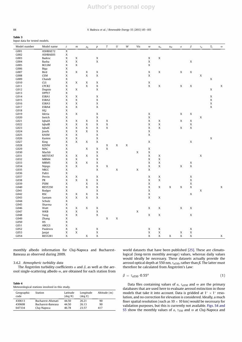
Table 3Input data for tested models.

Model number Model name z m rg p T U W Vis w uo uN a b sa TL 6

G001 ASHRAE72 XG002 ASHRAE05 XG003 Badesc X X X X XG004 Basha X X X X XG005 BCLSM X X XG006 Biga XG007 Bird X X X X X X X XG008 CEM X X X X XG009 Chandr X XG010 CLS X X X X XG011 CPCR2 X X X X X X X XG012 Dognio X X X XG013 DPPLT XG014 ESRA1 X X X XG015 ESRA2 X X X XG016 ESRA3 X X X XG017 ESRA4 X X X XG018 HLJ XG019 Ideria X X X X X XG020 Ineich X X X XG021 IqbalA X X X X X X X X XG022 IqbalB X X X X X X X XG023 IqbalC X X X X X X X X XG024 Josefs X X X X XG025 KASM X X X XG026 Kasten X X X XG027 King X X X X X XG028 KZHW X X X XG029 MAC X X X X XG030 Machlr X X X XG031 METSTAT X X X X X X XG032 MRM4 X X X X XG033 MRM5 X X X X X X XG034 Nijego X X X X X X X XG035 NRCC X X X X XG036 Paltri XG037 Perrin X X X X X XG038 PR X X X X X X XG039 PSIM X X X X XG040 REST250 X X X X X X X X XG041 Rodger X X X XG042 RSC X X X X X XG043 Santam X X X X X XG044 Schulz XG045 Sharma XG046 Watt X X X X X X X XG047 WKB X X X XG048 Yang X X X X X XG049 Zhang X X XG050 HS XG051 ABCGS XG052 Paulescu X X X X X XG053 Janjai X X X X X X XG054 REST281 X X X X X X X X X



Bucharest-Baneasa, respectively. The monthly data were smoothedto derive pseudo daily data.

A more elaborate value of the Angstrom turbidity coefficient ß isused in computation. A first mean monthly estimate of the Ang-strom turbidity (saybb) is computed by using Eq. (1). Next, themodalvalue b is calculated from [25]

b %bb!0:83212! 3:2104bb

"

1! 5:852bb0:75 (2)

Some models use a special value of ß that corresponds to ana value fixed at 1.3. It is calculated here by using Eq. (1) with a% 1.3.

These various inputs used by different models to evaluate theeffects of aerosols are shown in Table 3.

3.5. Default values

The column-integrated nitrogen dioxide content is not meas-ured. Constant values of 0.0002 atm-cm over rural areas and0.0005 atm-cm over cities are assumed. The latter value is adoptedhere for both Bucharest and Cluj-Napoca.

4. Results and discussions

The most common bulk performance statistics are the MeanBias Error (MBE) and the Root Mean Square Error (RMSE) which aredefined by, respectively

MBE %1nm

Xn

i%1ei (3a)

RMSE % 1m

#################1n

Xn

i%1e2i

vuut (3b)

where n is the number of measured and computed values, denotedmi and ci (i % 1,n), respectively, while:

eihci $mi (4)

Also, the mean value of the measured values, m, is defined by:

mh1n

Xn

i%1mi (5)

Eq. (3a,b) provide dimensionless quantities. In what follows,they are expressed in percent for clarity.

A model designed to compute hourly solar irradiation providesgood performance if the MBE, RMSE and the standard deviations %

##################################RMSE2 $MBE2

phave as low values as possible. The following

quantitative recommendations are sometimes used for computa-tion of global irradiation [9]: MBE within #10% and RMSE < 20%indicate good fitting between model results and measurements.The following criteria are used in this work to stratify the hourlyirradiation models:

' “good model” means jMBEj < 5% and RMSE < 15%;' “good enough model” means 5% < jMBEj < 10% and15% < RMSE < 20%;

' “bad model” means jMBEj > 10% and RMSE > 20%.

Two parameters are used to estimate the state of the sky,directly and indirectly, respectively. They are the cloud fraction

(between 0 and 1 e instantaneous quantity, denoted by C) and therelative sunshine (between 0 and 1, denoted by RSS). The cloudfraction C is computed by using the total cloud cover amountestimated hourly in octas by trained observers at Cluj-Napoca andBucharest-Baneasa station. The relative sunshine RSS is computedby using sunshine duration measurements. Before 2006 Campbell-Stokes devices were use to estimate the sunshine duration. After2006, the sunshine duration is calculated from solar radiation byusing the World Meteorological Organization sunshine criterion[26]. This stipulates that the “sun is shining” if the normal globalsolar irradiance exceeds 120 W/m2. Sunshine data are recordedhourly. Daily totals are also computed. Measurements are reportedin tens of an hour. In the case of Bucharest, sunshine duration is stillmeasured with a Campbell-Stokes recorder at the Bucharest-Afumati station.

Ideally, one expects that the relation C% 1$RSS is fulfilled whenlong term averages are used. However, it is a well-known issue thatdeviations exist from this relationship. At Bucharest the deviationsmay be even larger since C and RSS are estimated in two differentplaces located 10.8 km from each other (see Fig. S6). Indeed, duringcloudy days the time sequences with shining sun may be quitedifferent at Bucharest-Baneasa and Bucharest-Afumati, respec-tively. However, this study refers to clear days only. It is likely thatthe sky is clear simultaneously at both meteorological stations inBucharest. This assumption is analyzed in Section 4.1, where thecloud fraction and the relative sunshine are used as input.

The testing procedure is performed in several stages intended toprovide information about the models accuracy for various sets ofinput data. Separate analyses are performed for Cluj-Napoca andBucharest. In both cases details are first provided about the avail-able inputs while the results are reported next. Finally, an overallconclusion about models’ performance is drawn.

4.1. Accuracy analysis

A general approach for sensitivity analysis is provided in [27,28].The choice of the proper sensitivity analysis technique depends onmany factors, including (i) the computational cost, (ii) the numberof input factors, (iii) the degree of complexity, (iv) the amount ofanalyst’s time involved in the sensitivity analysis, and (v) theobjective of the analysis (such as factors’ fixing and mapping) [27].Here we prefer to use a simpler approach based on variance-typeindicators.

The purpose here is to see the models performance for differentsets of realistic input data. The input data sets are realistic in thesense that some categories of real users may have only partial ac-cess to very accurate input data (for instance, input data obtainedby very accurate measurements). The usual solution in this case isto replace the missing accurate input data with less accurate inputdata, resulting from less accurate measurements or from varioustypes of estimations.

A first test (so called Stage 1) consisted of checking the proce-dure. A large number of subsequent tests have been performed forCluj-Napoca and Bucharest by using data from 2009 only. The mostrelevant fourty-two testing stages are reported here. Stages 2e22refer to Cluj-Napoca while Stages 32e52 refer to Bucharest. Thesestages are organized in pairs, e.g. Stage 2 and Stage 32 are similar,but they refer to Cluj-Napoca and Bucharest, respectively.

4.1.1. Stage 2 (Cluj-Napoca) and Stage 32 (Bucharest)These testing stages make use of the best-quality input data

available. Only data for which C % 0 and RSS % 1 (simultaneously)are used, resulting in a total of 133 hourly records at Cluj-Napocaand 324 hourly recordings at Bucharest.



Daily radiosonde measurements of precipitable water per-formed at 0000 UTC at Cluj-Napoca and 0.00 and 12.00 UTC atBucharest-Baneasa are used. For intermediate hours, values arelinearly interpolated between two consecutive measured values.

Column integrated ozone is not measured at Cluj-Napoca, thusdaily measurements performed at Bucharest (once per day at 1200UTC) are used for both Cluj-Napoca and Bucharest. For intermediatehours, values were linearly interpolated.

Monthly-averaged satellite-derived values of ground albedo(rg), a, sa550 and 6 for Cluj-Napoca and Bucharest are used. Thesevalues are associated to the 15th day of each month. For interme-diate days, values were linearly interpolated. These parameters areassumed constant during any given day.

Table 5 shows the accuracy indicators for all models while Fig. 1shows the results for those models fulfilling the performance cri-teria indicated above at Cluj-Napoca. Models G053, G052 and G035provide the best performance. Fig. 2 shows a comparison betweenthe measured data and the results predicted by model G053.Table S2 provides the input data used by the three models fulfillingthe performance criteria.

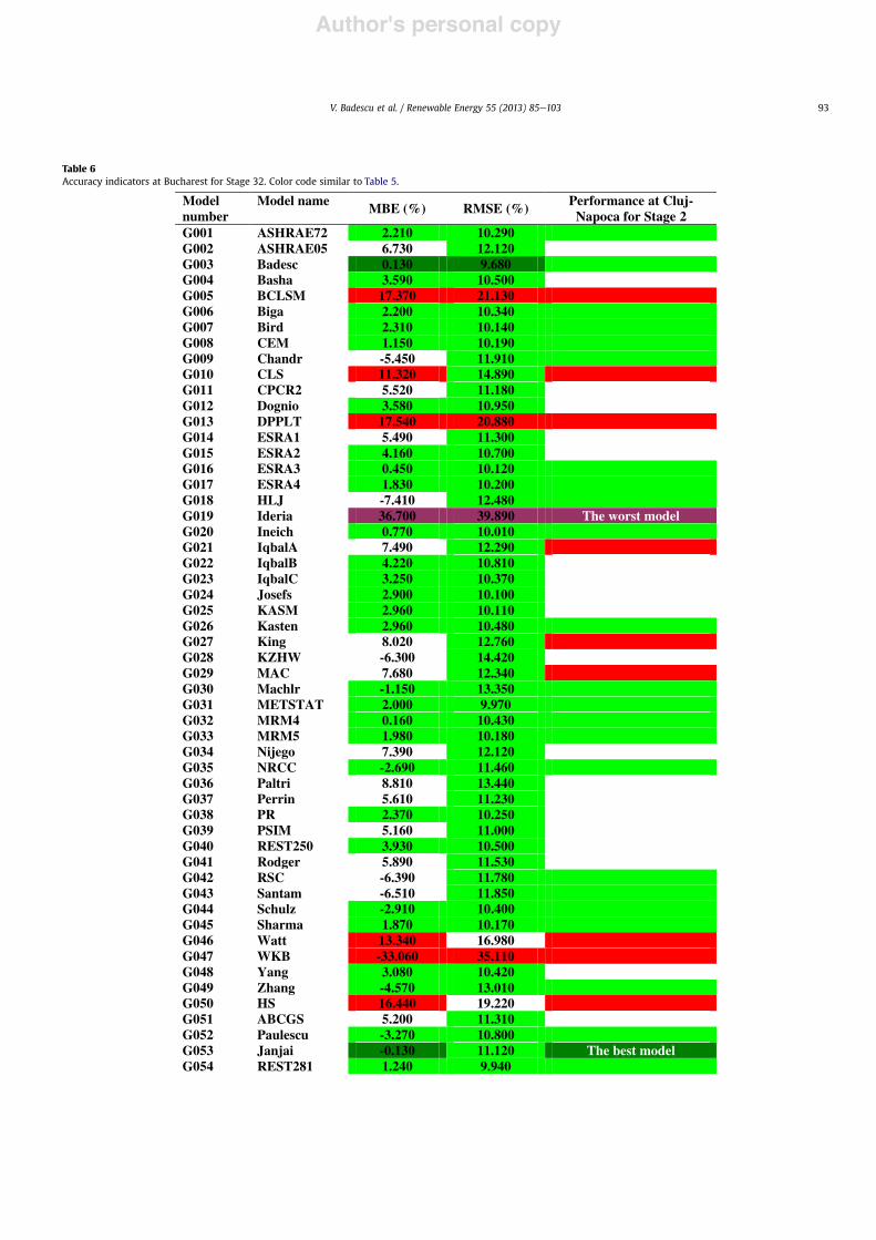
Table 6 shows the accuracy indicators for all models while Fig. 3shows the results for the models fulfilling the performance criteriaat Bucharest. Models G053, G003 and G032 have the best perfor-mance. Fig. 4 shows a comparison between the measured data andthe results predicted by model G053. Table S3 shows the input dataused by the models fulfilling the performance criteria. The accuracycriteria are not fulfilled by simplemodels but only bymore complexmodels.

4.1.2. Stage 3 (Cluj-Napoca) and Stage 33 (Bucharest)Here we tested the effect of input data quality related to visual

(direct) estimation of the state of the sky. All the data for whichC % 0 are used (while RSS is a free parameter). Other input data aresimilar to those used in Stage 2.

A total of 166 hourly recordings at Cluj-Napoca (Fig. S7) and391 hourly recordings at Bucharest (Fig. S8) fulfilled the testcondition. Only a few data associated with both C % 0 and RSS % 0exist. Such situations may occur during clear days near sunriseand sunset, i.e., when the irradiance is too low to activate thesunshine recorder.

Fig. S7 shows that Stage 3 uses input data associated to RSSlower than unity. Therefore, one expects lower model accuracy inStage 3 than in Stage 2. However, by comparing Table S4 to Table 5,it appears that models accuracy generally increase at Cluj-Napocaby using the more relaxed input data set of Stage 3. Even thoughmost models perform in Stage 3, a few models show performancedegradation (i.e. G009; G018; G035; G042; G044; G052).

Table 7 provides an easier comparison between results obtainedfor Stages 2 and 3 at Cluj-Napoca for some selected models. Gen-erally, both MBE and RMSE decrease slightly in Stage 3 compared toStage 2 while standard deviations increase for all models. Anexception is model G052. A brief explanation follows. The slightdecrease ofMBE in Stage 3may be the result of the larger number ofdata compared to Stage 2. This is the known effect of regressiontowards the mean [29]. The larger standard deviations obtained atStage 3 take into account the expected increase in error scatteringas compared to Stage 2. The decrease of RMSE is the result of thesetwo opposite effects, in which the influence of the decreasing MBEvalues is stronger. Stage 33 below provides further explanations.

Table S5 shows that models accuracy apparently increases atBucharest by using the more relaxed set of input data of Stage 33(compare with Table 6 for stage 32).

Some of the comments associated to Stage 3 for Cluj-Napocaapply here, too. For instance, both the MBE and the standard de-viation decrease in Stage 33 for most models as compared to Stage

32. However, the RMSE increases in Stage 33 for most models ascompared to Stage 32. This didn’t happen when Stage 3 was com-pared to Stage 2. A few comments follow. The decrease of MBE isthe result of the effect of regression towards the mean discussed atStage 3. The larger standard deviation in Stage 33 takes into accountthe expected increased error spreading as compared to Stage 32.The apparent increase of RMSE is the result of these two oppositeeffects, where the influence of the standard deviation decreasing isstronger. This is different from Stage 3, where the influence of MBEdecreasing is more important.

4.1.3. Stage 4 (Cluj-Napoca) and Stage 34 (Bucharest)Here we tested the effect of input data quality related to the

(indirect) estimation of the state of the sky by means of sunshinedata. The simple approximation C % 1$RSS is sometimes used inliterature when data on cloud fraction is missing. Only data asso-ciated to RSS % 1 were used here, while no constraint has beenimposed to C. Most of the cloud fraction values equal 0, as expected.However, positive values of C do also exist. This corresponds toperiods with the sun shining during the whole hourly interval,while some parts of the sky are covered by clouds. 775 hourly re-cordings were used at Cluj-Napoca (Fig. S9) and 908 hourly re-cordings were used at Bucharest (Fig. S10). Other input data aresimilar to the input data of Stage 2.

Table S6 shows that the accuracy of all models significantlydecreases at Cluj-Napoca by using this more relaxed set of inputdata (compare with Table 5). Consequently, most models do notmeet the performance criteria. This proves that using clear-skymodels under faint cloudy conditions is not recommended.

Also, the models accuracy decreases at Bucharest by using themore relaxed set of input data of Stage 34 as compared to Stage 32(compare Table S7 and Table 6).

4.1.4. Stage 5 (Cluj-Napoca) and Stage 35 (Bucharest)These testing stages intend to estimate the model accuracy

when a constant ozone value uo % 0.3 atm-cm is assumed for thewhole year. The other input data are those used for Stage 2, pro-viding 133 hourly recordings for Cluj-Napoca and 324 hourly re-cordings for Bucharest.

The models may be stratified as: (i) those not using ozone dataas input; and (ii) those using it. Models of the first category behavesimilarly in Stages 5 and 2 at Cluj-Napoca, and Stages 35 and 32 atBucharest, as expected.

Table S8 shows that the accuracy of all models of category (ii)degrades at Cluj-Napoca when using a fixed amount of ozone(compare with Table 5). Table 8 provides a summary of results forsome models of category (ii): MBE increases in comparison withStage 2, as expected. The RMSE of a few models decreases in Stage5. This may be explained by a compensation effect: even thoughinexact ozone data are used, the bias they introduce may com-pensate for other error sources. The standard deviation is larger inStage 5 than in Stage 2 for all models, since the decrease of (theabsolute values of) MBE is always larger than the decrease of RMSE.

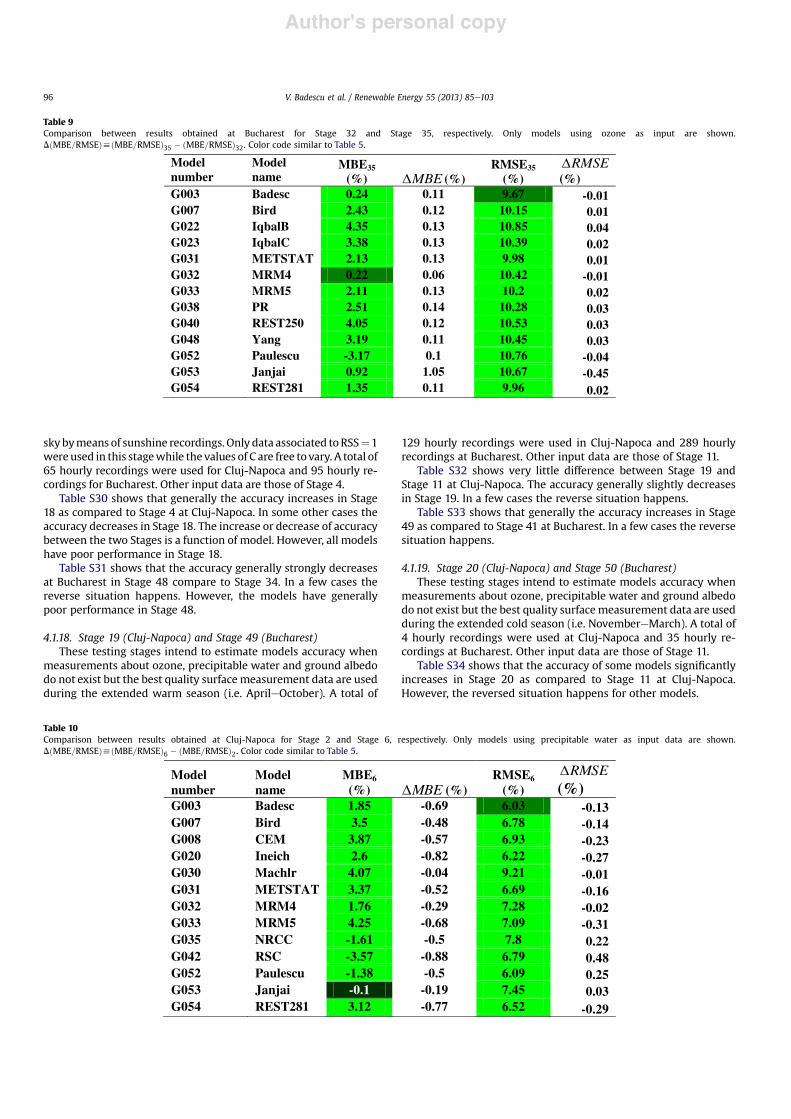
Table S9 shows that in case (ii) the models accuracy slightlydecreases at Bucharest by using a fix amount of ozone as input data(compare with Table 6). There is, however, one model (G052)whose accuracy increases. Table 9 provides an easier comparisonfor models of category (ii).

4.1.5. Stage 6 (Cluj-Napoca) and Stage 36 (Bucharest)These testing stages intend to estimate the models accuracy

when precipitable water is computed by using the formula byLeckner [30]. A total of 133 hourly recordings at Cluj-Napoca and324 hourly recordings at Bucharest are used. All other inputs arethose of Stage 2.



Table 5Accuracy indicators at Cluj-Napoca for Stage 2.

Color Meaning

Best model

Good model |MBE|<5%; RMSE<15%

Good enough model 5%<|MBE|<10%;15%<RMSE<20%

Bad model |MBE|>10%; RMSE>20%

Worst model

Model number Model name MBE2 (%) RMSE2 (%)

G001 ASHRAE72 2.850 6.560G002 ASHRAE05 7.590 9.550G003 Badesc 2.540 6.160G004 Basha 6.190 8.270G005 BCLSM 17.860 20.130G006 Biga 2.630 7.410G007 Bird 3.980 6.920G008 CEM 4.440 7.160G009 Chandr -4.150 8.570G010 CLS 14.120 15.240G011 CPCR2 7.480 9.310G012 Dognio 6.350 8.650G013 DPPLT 18.160 20.000G014 ESRA1 8.660 10.510G015 ESRA2 7.120 9.200G016 ESRA3 4.260 6.920G017 ESRA4 4.780 7.910G018 HLJ -3.550 7.230G019 Ideria 39.600 41.640G020 Ineich 3.420 6.490G021 IqbalA 10.180 11.610G022 IqbalB 6.790 8.780G023 IqbalC 5.210 7.700G024 Josefs 5.190 7.550G025 KASM 5.380 7.740G026 Kasten 4.860 7.820G027 King 10.100 11.470G028 KZHW -6.880 13.790G029 MAC 10.080 11.540G030 Machlr 4.110 9.220G031 METSTAT 3.890 6.850G032 MRM4 2.050 7.300G033 MRM5 4.930 7.400G034 Nijego 9.200 10.720G035 NRCC -1.110 7.580G036 Paltri 9.710 12.000G037 Perrin 7.020 9.350G038 PR 5.090 7.510G039 PSIM 7.840 9.520G040 REST250 6.260 8.340G041 Rodger 8.160 10.040G042 RSC -2.690 6.310G043 Santam -4.930 7.570G044 Schulz -2.390 7.160G045 Sharma 2.420 6.840G046 Watt 13.890 15.750G047 WKB -29.070 30.880G048 Yang 5.760 7.960G049 Zhang -4.710 12.640G050 HS 17.530 18.790G051 ABCGS 5.970 9.040G052 Paulescu -0.880 5.840G053 Janjai 0.090 7.420G054 REST281 3.890 6.810



Two categories of models exist: (i) those not using precipitablewater as input; and (ii) those using it. The accuracy of all themodelsof the first category is the same in Stages 6 and 2 at Cluj-Napoca andStages 36 and 32 at Bucharest.

Comparison of Table S2 and Table S10 shows that at Cluj-Napocathe accuracy of category (ii) models may increase or may decrease.This is also shown in Table 10, which provides a summary. In Stage6, most models exhibit a positive MBE, although it is less than inStage 2. This is also the case with RMSE. One may conclude thateither the use of calculated precipitable water each hour is betterthan that of interpolated daily measurements, or that, like in Stage5, there are compensations of errors. A few models (G035, G042,G052, and G053) underestimate more in Stage 6 than in Stage 2,while their RMSE increase. One may conclude that no compensa-tion of errors exist for these models at this Stage 6.

In case (ii) at Bucharest the models accuracy may increase ormay decrease by using a computed value instead of a measuredvalue of precipitable water (compare Table S11 with Table 6).

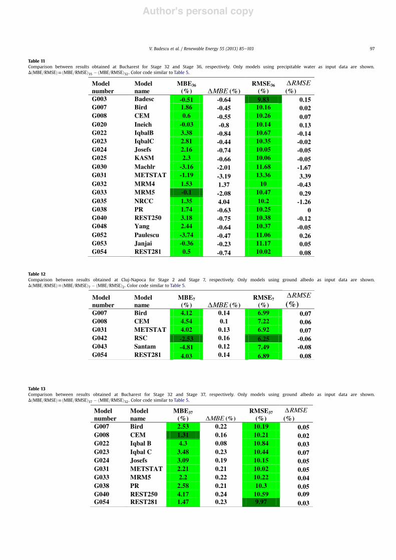
Table 11 provides an easier comparison for some models ofcategory (ii). In Stage 6 many models have positive MBE values. Thebias error decreases for these models as compared to Stage 32. Also,

the RMSE values decrease in Stage 36 for these models. Thus, theaccuracy is generally better in Stage 36.

There are a few other models (i.e. G030; G052; G053) withnegative MBE values in Stage 36 and the associated decreasing ofMBE as reported to Stage 32 means the bias error increases forthese models. The RMSE values increase in Stage 36 for some ofthese models (i.e. G052, G053). Thus, the accuracy is generallyworse for these models in Stage 36. For the other models (i.e. G030)the RMSE values decrease in Stage 36. But the decrease of RMSE issmaller than the decrease of MBE and this means the accuracy inStage 36 is worse for these models, too, as compared to Stage 32.

4.1.6. Stage 7 (Cluj-Napoca) and Stage 37 (Bucharest)These testing stages intend to estimate the models accuracy

when the conventional constant value of 0.2 is used for the groundalbedo all over the year. The other input data are those of Stage 2. Atotal of 133 hourly recordings were used at Cluj-Napoca and 324hourly recordings were used at Bucharest.

The models may be stratified as: (i) not using albedo as inputdata and (ii) using albedo data. For category (i) of models the ac-curacy at Cluj-Napoca in Stage 7 is similar to the accuracy of Stage 2while at Bucharest Stage 37 and Stage 32 have the same accuracy.

The comparison of Table 5 and Table S12 shows that, in general,using a fixed albedo value of 0.2 at Cluj-Napoca results in accuracydegradation for the models of category (ii). Table 12 providesa summary of results for some of these models. For most modelsbothMBE and RMSE slightly increase compared to Stage 2. Onemayconclude that using an observed surface albedo is recommended.

Table S13 shows that generally in case (ii) the models accuracydecreases at Bucharest by using a computed value instead ofa measured albedo value (compare with Table 6). Table 13 providesa more detailed comparison for models of category (ii). For allmodels both MBE and RMSE slightly increase in Stage 37 as com-pared to Stage 32. Thus, the accuracy is a bit better in Stage 32. Thisis to be compared with results at Cluj-Napoca where the influenceof the albedo input quality on models accuracy is less conclusive.

4.1.7. Stage 8 (Cluj-Napoca) and Stage 38 (Bucharest)Herewe tested the effect of input data quality related to both the

visual (direct) estimation of the state of the sky and ozone contentin the atmosphere. Only data for C% 0were used (i.e. the RSS valuesare free to vary). A total of 166 hourly recordings were used for Cluj-Napoca and 391 hourly recordings for Bucharest. Other input dataare those of Stage 5 (i.e. with a constant ozone value used as input).

Table S14 shows that for some models the MBE values are largerat Cluj-Napoca in Stage 8 than in Stage 5. The opposite happens forother models. The same comments may be made for the RMSEvalues.

Table S15 shows that for some “good” models the MBE valuesare larger in Stage 38 than in Stage 35 at Bucharest. However, theopposite happens for the same models in case of the RMSE values.There are other (worse performing) models whose MBE and RMSEvalues decrease in Stage 38 as compared to Stage 35.

One may conclude that no clear correlation exists between themodels accuracy and the combined effect of the quality of ozoneinput data and clear sky estimations.


visual (direct) estimation of the state of the sky and the precipitablewater content in the atmosphere. Only data for C% 0 were used (i.e.the RSS values are free to vary). A total of 166 hourly recordingswere used for Cluj-Napoca and 391 hourly recordings for Bucharest.Other input data are those of Stage 6 (i.e. with precipitable watercomputed by using Leckner (1978) formula).

Fig. 1. MBE and standard deviation for the models fulfilling the performance criteriafor computation of global hourly irradiation at Cluj-Napoca in 2009. The modelnumber is attached to the column.

Fig. 2. Comparison between results predicted by model G053 and measured data atCluj-Napoca in 2009.



Table 6Accuracy indicators at Bucharest for Stage 32. Color code similar to Table 5.

Model number

Model name MBE (%) RMSE (%) Performance at Cluj-Napoca for Stage 2

G001 ASHRAE72 2.210 10.290G002 ASHRAE05 6.730 12.120G003 Badesc 0.130 9.680G004 Basha 3.590 10.500G005 BCLSM 17.370 21.130G006 Biga 2.200 10.340G007 Bird 2.310 10.140G008 CEM 1.150 10.190G009 Chandr -5.450 11.910G010 CLS 11.320 14.890G011 CPCR2 5.520 11.180G012 Dognio 3.580 10.950G013 DPPLT 17.540 20.880G014 ESRA1 5.490 11.300G015 ESRA2 4.160 10.700G016 ESRA3 0.450 10.120G017 ESRA4 1.830 10.200G018 HLJ -7.410 12.480G019 Ideria 36.700 39.890 The worst modelG020 Ineich 0.770 10.010G021 IqbalA 7.490 12.290G022 IqbalB 4.220 10.810G023 IqbalC 3.250 10.370G024 Josefs 2.900 10.100G025 KASM 2.960 10.110G026 Kasten 2.960 10.480G027 King 8.020 12.760G028 KZHW -6.300 14.420G029 MAC 7.680 12.340G030 Machlr -1.150 13.350G031 METSTAT 2.000 9.970G032 MRM4 0.160 10.430G033 MRM5 1.980 10.180G034 Nijego 7.390 12.120G035 NRCC -2.690 11.460G036 Paltri 8.810 13.440G037 Perrin 5.610 11.230G038 PR 2.370 10.250G039 PSIM 5.160 11.000G040 REST250 3.930 10.500G041 Rodger 5.890 11.530G042 RSC -6.390 11.780G043 Santam -6.510 11.850G044 Schulz -2.910 10.400G045 Sharma 1.870 10.170G046 Watt 13.340 16.980G047 WKB -33.060 35.110G048 Yang 3.080 10.420G049 Zhang -4.570 13.010G050 HS 16.440 19.220G051 ABCGS 5.200 11.310G052 Paulescu -3.270 10.800G053 Janjai -0.130 11.120 The best modelG054 REST281 1.240 9.940



Table S16 shows that for some “good” models the MBE valuesare smaller in Stage 9 than in Stage 6 at Cluj-Napoca. The oppositehappens for other models. The same comments may be made forthe RMSE values.

Table S17 shows that for some “good” models the MBE valuesare larger in Stage 39 than in Stage 36 at Bucharest. However, theopposite happens for the same models in case of the RMSE values.There are other (worse performing) models whose MBE and RMSEvalues decrease in Stage 39 as compared to Stage 36.

One may conclude that no clear correlation exists between themodels accuracy and the combined effect of the quality of precip-itable water input data and clear sky estimations.


visual (direct) estimation of the state of the sky and the groundalbedo. Only data for C% 0were used (i.e. the values of the sunshinefraction are free to vary). A total of 166 hourly recordings were usedfor Cluj-Napoca and 391 hourly recordings for Bucharest. Otherinput data are those of Stage 7 (i.e. with fixed value of groundalbedo).

Table S18 shows that for some “good” models the MBE valuesare smaller in Stage 10 than in Stage 7 at Cluj-Napoca. The opposite

happens for other models. The same comments may be made forthe RMSE values.

Table S19 shows that for some “good” models the MBE valuesare larger in Stage 40 than in Stage 37 at Bucharest. However, theopposite happens for the other models in case of the RMSE values.There are other (worse performing) models whose MBE and RMSEvalues decrease in Stage 40 as compared to Stage 37.

One may conclude that no clear correlation exists between themodels accuracy and the combined effect of the quality of groundalbedo input data and clear sky estimations.

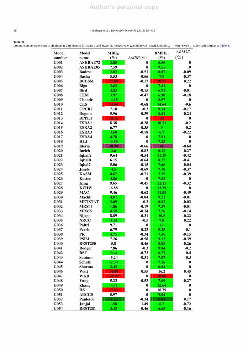
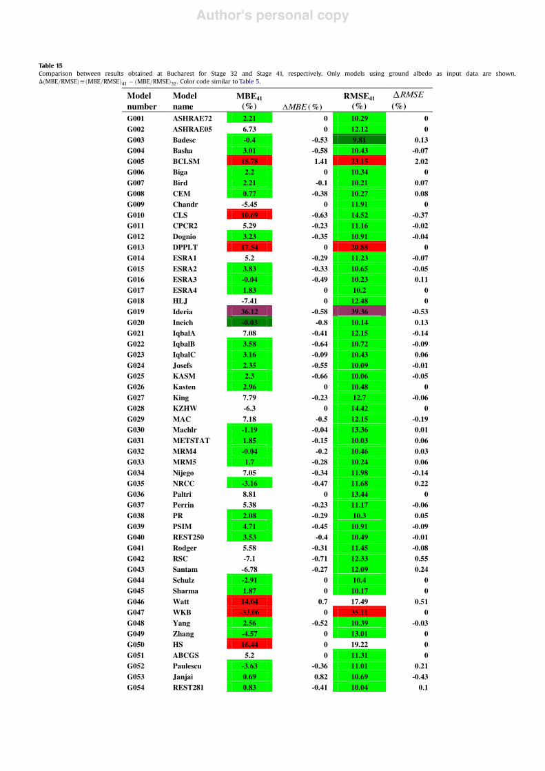
4.1.10. Stage 11 (Cluj-Napoca) and Stage 41 (Bucharest)These testing stages intend to estimate models accuracy when

measurements about ozone, precipitable water and ground albedodo not exist but the best available surface measurement data areused. A total of 133 hourly recordings were used for Cluj-Napocaand 324 hourly recordings for Bucharest. A constant ozoneamount 0.3 atm-cm has been assumed. Precipitable water has beencomputed by using Leckner formula [30]. A constant ground albedovalue (0.2) has been assumed. Other input data are those of Stage 2.

The accuracy of somemodels is unchanged at Cluj-Napocawhenpassing from Stage 2 to Stage 11 (Table 14). Similarly, the accuracyof the same models is unchanged at Bucharest when passing fromStage 32 to Stage 41 (Table 15). These models do not use as inputdata values of ozone, precipitable water and ground albedo.

Table 14 shows that for most models both the MBE and RMSEdecrease at Cluj-Napoca in Stage 11 as compared to stage 2. Table 15shows that for mostmodels theMBE slightly decreases at Bucharestin Stage 41 as compared to stage 32.


measurements about ozone, precipitable water and ground albedodo not exist but only direct (visual) information about the state ofthe sky exists. Only data for C % 0 were used (i.e. the RSS values arefree to vary). A total of 166 hourly recordings were used at Cluj-Napoca and 391 hourly recordings at Bucharest. Other input dataare those of Stage 11.

Table S20 shows that for most models both the MBE and RMSEvalues decrease at Cluj-Napoca in Stage 12 as compared to Stage 11.However, exceptions exist. Thus, the accuracy of the models isgenerally better in Stage 12.

Table S21 shows that for most models the MBE slightly de-creases at Bucharest and the RMSE slightly decreases in Stage 42 ascompared to Stage 41. This is slightly different from the resultsobtained at Cluj-Napoca.

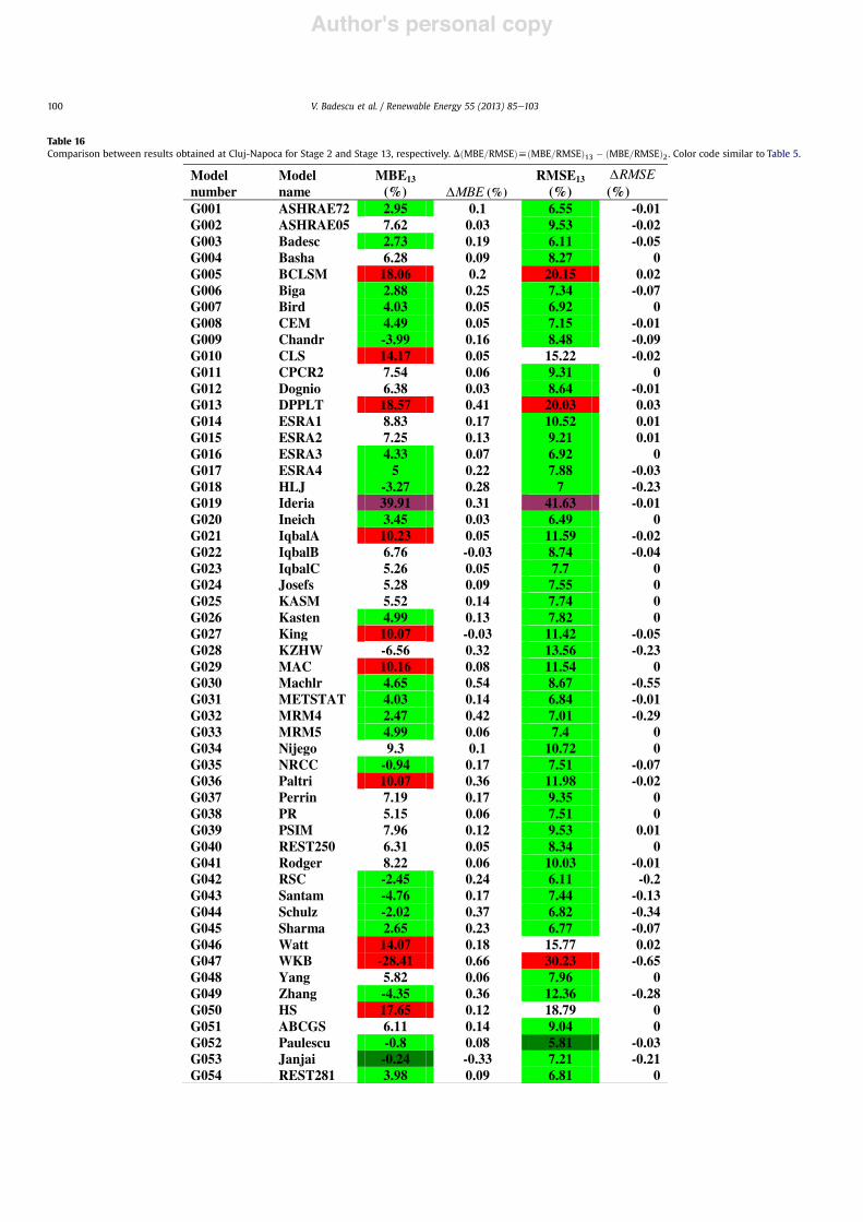
4.1.12. Stage 13 (Cluj-Napoca) and Stage 43 (Bucharest)These testing stages are associated to the best quality input data

during the extended warm season (i.e. during AprileOctober). Onlydata associated to C% 0 and RSS% 1were used. A total of 129 hourlyrecordings were used at Cluj-Napoca and 289 hourly recordings atBucharest. Other input data are those of Stage 2.

Table 16 shows that the MBE values increase while the RMSEvalues slightly decrease in Stage 13 as compared to Stage 2 at Cluj-Napoca. Thus, the accuracy is generally worse in Stage 13.

Table S22 shows that for most models the MBE values decreasewhile the RMSE values slightly increase in Stage 43 as compared toStage 42 at Bucharest. This is different from the results obtained atCluj-Napoca.

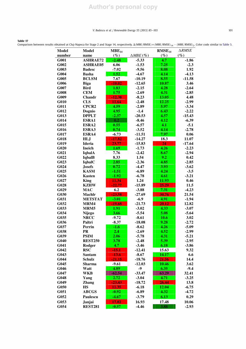
4.1.13. Stage 14 (Cluj-Napoca) and Stage 44 (Bucharest)These testing stages are associated to the best quality input data

during the extended cold season (i.e. during NovembereMarch).Only data associated to C % 0 and RSS % 1 were used. A total of 4

Fig. 3. MBE and standard deviation for the models fulfilling the performance criteriafor computation of global hourly irradiation at Bucharest in 2009. The model number isattached to the column.

Fig. 4. Comparison between results predicted by model G053 and measured data atBucharest in 2009.



hourly recordings were used at Cluj-Napoca and 289 hourly re-cordings at Bucharest. Other input data are those of Stage 2.

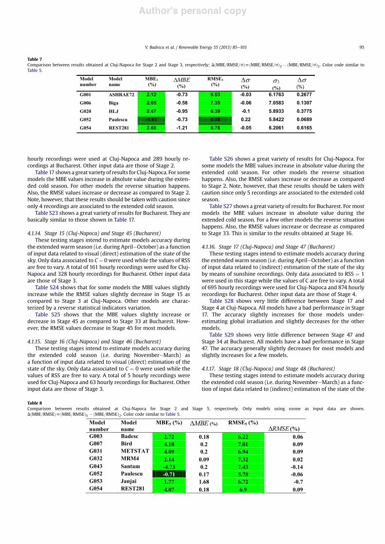
Table 17 shows a great variety of results for Cluj-Napoca. For somemodels the MBE values increase in absolute value during the exten-ded cold season. For other models the reverse situation happens.Also, the RMSE values increase or decrease as compared to Stage 2.Note, however, that these results should be takenwith caution sinceonly 4 recordings are associated to the extended cold season.

Table S23 shows a great variety of results for Bucharest. They arebasically similar to those shown in Table 17.

4.1.14. Stage 15 (Cluj-Napoca) and Stage 45 (Bucharest)These testing stages intend to estimate models accuracy during

the extended warm season (i.e. during AprileOctober) as a functionof input data related to visual (direct) estimation of the state of thesky. Only data associated to C% 0 were used while the values of RSSare free to vary. A total of 161 hourly recordings were used for Cluj-Napoca and 328 hourly recordings for Bucharest. Other input dataare those of Stage 3.

Table S24 shows that for some models the MBE values slightlyincrease while the RMSE values slightly decrease in Stage 15 ascompared to Stage 3 at Cluj-Napoca. Other models are charac-terized by a reverse statistical indicators variation.

Table S25 shows that the MBE values slightly increase ordecrease in Stage 45 as compared to Stage 33 at Bucharest. How-ever, the RMSE values decrease in Stage 45 for most models.


the extended cold season (i.e. during NovembereMarch) asa function of input data related to visual (direct) estimation of thestate of the sky. Only data associated to C % 0 were used while thevalues of RSS are free to vary. A total of 5 hourly recordings wereused for Cluj-Napoca and 63 hourly recordings for Bucharest. Otherinput data are those of Stage 3.

Table S26 shows a great variety of results for Cluj-Napoca. Forsome models the MBE values increase in absolute value during theextended cold season. For other models the reverse situationhappens. Also, the RMSE values increase or decrease as comparedto Stage 2. Note, however, that these results should be taken withcaution since only 5 recordings are associated to the extended coldseason.

Table S27 shows a great variety of results for Bucharest. For mostmodels the MBE values increase in absolute value during theextended cold season. For a few other models the reverse situationhappens. Also, the RMSE values increase or decrease as comparedto Stage 33. This is similar to the results obtained at Stage 16.


the extendedwarm season (i.e. during AprileOctober) as a functionof input data related to (indirect) estimation of the state of the skyby means of sunshine recordings. Only data associated to RSS % 1were used in this stage while the values of C are free to vary. A totalof 695 hourly recordings were used for Cluj-Napoca and 874 hourlyrecordings for Bucharest. Other input data are those of Stage 4.

Table S28 shows very little difference between Stage 17 andStage 4 at Cluj-Napoca. All models have a bad performance in Stage17. The accuracy slightly increases for those models under-estimating global irradiation and slightly decreases for the othermodels.

Table S29 shows very little difference between Stage 47 andStage 34 at Bucharest. All models have a bad performance in Stage47. The accuracy generally slightly decreases for most models andslightly increases for a few models.


the extended cold season (i.e. during NovembereMarch) as a func-tion of input data related to (indirect) estimation of the state of the

Table 7Comparison between results obtained at Cluj-Napoca for Stage 2 and Stage 3, respectively; D(MBE=RMSE=s)h(MBE=RMSE=s)3 $ (MBE=RMSE=s)2. Color code similar toTable 5.

Table 8Comparison between results obtained at Cluj-Napoca for Stage 2 and Stage 5, respectively. Only models using ozone as input data are shown.D(MBE=RMSE)h(MBE=RMSE)5 $ (MBE=RMSE)2. Color code similar to Table 5.



sky bymeans of sunshine recordings.Only data associated to RSS% 1wereused in this stagewhile the values of C are free tovary. A total of65 hourly recordings were used for Cluj-Napoca and 95 hourly re-cordings for Bucharest. Other input data are those of Stage 4.

Table S30 shows that generally the accuracy increases in Stage18 as compared to Stage 4 at Cluj-Napoca. In some other cases theaccuracy decreases in Stage 18. The increase or decrease of accuracybetween the two Stages is a function of model. However, all modelshave poor performance in Stage 18.

Table S31 shows that the accuracy generally strongly decreasesat Bucharest in Stage 48 compare to Stage 34. In a few cases thereverse situation happens. However, the models have generallypoor performance in Stage 48.


measurements about ozone, precipitable water and ground albedodo not exist but the best quality surface measurement data are usedduring the extended warm season (i.e. AprileOctober). A total of

129 hourly recordings were used in Cluj-Napoca and 289 hourlyrecordings at Bucharest. Other input data are those of Stage 11.

Table S32 shows very little difference between Stage 19 andStage 11 at Cluj-Napoca. The accuracy generally slightly decreasesin Stage 19. In a few cases the reverse situation happens.

Table S33 shows that generally the accuracy increases in Stage49 as compared to Stage 41 at Bucharest. In a few cases the reversesituation happens.


measurements about ozone, precipitable water and ground albedodo not exist but the best quality surface measurement data are usedduring the extended cold season (i.e. NovembereMarch). A total of4 hourly recordings were used at Cluj-Napoca and 35 hourly re-cordings at Bucharest. Other input data are those of Stage 11.

Table S34 shows that the accuracy of some models significantlyincreases in Stage 20 as compared to Stage 11 at Cluj-Napoca.However, the reversed situation happens for other models.

Table 9Comparison between results obtained at Bucharest for Stage 32 and Stage 35, respectively. Only models using ozone as input are shown.D(MBE=RMSE)h(MBE=RMSE)35 $ (MBE=RMSE)32. Color code similar to Table 5.

Model number

Model name

MBE35(%) MBE (%)

RMSE35(%)

RMSE(%)

G003 Badesc 0.24 0.11 9.67 -0.01G007 Bird 2.43 0.12 10.15 0.01G022 IqbalB 4.35 0.13 10.85 0.04G023 IqbalC 3.38 0.13 10.39 0.02G031 METSTAT 2.13 0.13 9.98 0.01G032 MRM4 0.22 0.06 10.42 -0.01G033 MRM5 2.11 0.13 10.2 0.02G038 PR 2.51 0.14 10.28 0.03G040 REST250 4.05 0.12 10.53 0.03G048 Yang 3.19 0.11 10.45 0.03G052 Paulescu -3.17 0.1 10.76 -0.04G053 Janjai 0.92 1.05 10.67 -0.45G054 REST281 1.35 0.11 9.96 0.02

Table 10Comparison between results obtained at Cluj-Napoca for Stage 2 and Stage 6, respectively. Only models using precipitable water as input data are shown.D(MBE=RMSE)h(MBE=RMSE)6 $ (MBE=RMSE)2. Color code similar to Table 5.

Model number

Model name

MBE6

(%) MBE (%)RMSE6

(%)RMSE

(%)G003 Badesc 1.85 -0.69 6.03 -0.13G007 Bird 3.5 -0.48 6.78 -0.14G008 CEM 3.87 -0.57 6.93 -0.23G020 Ineich 2.6 -0.82 6.22 -0.27G030 Machlr 4.07 -0.04 9.21 -0.01G031 METSTAT 3.37 -0.52 6.69 -0.16G032 MRM4 1.76 -0.29 7.28 -0.02G033 MRM5 4.25 -0.68 7.09 -0.31G035 NRCC -1.61 -0.5 7.8 0.22G042 RSC -3.57 -0.88 6.79 0.48G052 Paulescu -1.38 -0.5 6.09 0.25G053 Janjai -0.1 -0.19 7.45 0.03G054 REST281 3.12 -0.77 6.52 -0.29



Table 11Comparison between results obtained at Bucharest for Stage 32 and Stage 36, respectively. Only models using precipitable water as input data are shown.D(MBE=RMSE)h(MBE=RMSE)35 $ (MBE=RMSE)32. Color code similar to Table 5.

Model number

Model name

MBE36

(%) MBE (%)RMSE36

(%)RMSE

(%)G003 Badesc -0.51 -0.64 9.83 0.15G007 Bird 1.86 -0.45 10.16 0.02G008 CEM 0.6 -0.55 10.26 0.07G020 Ineich -0.03 -0.8 10.14 0.13G022 IqbalB 3.38 -0.84 10.67 -0.14G023 IqbalC 2.81 -0.44 10.35 -0.02G024 Josefs 2.16 -0.74 10.05 -0.05G025 KASM 2.3 -0.66 10.06 -0.05G030 Machlr -3.16 -2.01 11.68 -1.67G031 METSTAT -1.19 -3.19 13.36 3.39G032 MRM4 1.53 1.37 10 -0.43G033 MRM5 -0.1 -2.08 10.47 0.29G035 NRCC 1.35 4.04 10.2 -1.26G038 PR 1.74 -0.63 10.25 0G040 REST250 3.18 -0.75 10.38 -0.12G048 Yang 2.44 -0.64 10.37 -0.05G052 Paulescu -3.74 -0.47 11.06 0.26G053 Janjai -0.36 -0.23 11.17 0.05G054 REST281 0.5 -0.74 10.02 0.08

Table 12Comparison between results obtained at Cluj-Napoca for Stage 2 and Stage 7, respectively. Only models using ground albedo as input data are shown.D(MBE=RMSE)h(MBE=RMSE)7 $ (MBE=RMSE)2. Color code similar to Table 5.

Model number

Model name

MBE7

(%) MBE (%)RMSE7

(%)RMSE

(%)G007 Bird 4.12 0.14 6.99 0.07G008 CEM 4.54 0.1 7.22 0.06G031 METSTAT 4.02 0.13 6.92 0.07G042 RSC -2.53 0.16 6.25 -0.06G043 Santam -4.81 0.12 7.49 -0.08G054 REST281 4.03 0.14 6.89 0.08

Table 13Comparison between results obtained at Bucharest for Stage 32 and Stage 37, respectively. Only models using ground albedo as input data are shown.D(MBE=RMSE)h(MBE=RMSE)37 $ (MBE=RMSE)32. Color code similar to Table 5.

Model number

Model name

MBE37

(%) MBE (%)RMSE37

(%)RMSE

(%)G007 Bird 2.53 0.22 10.19 0.05G008 CEM 1.31 0.16 10.21 0.02G022 Iqbal B 4.3 0.08 10.84 0.03G023 Iqbal C 3.48 0.23 10.44 0.07G024 Josefs 3.09 0.19 10.15 0.05G031 METSTAT 2.21 0.21 10.02 0.05G033 MRM5 2.2 0.22 10.22 0.04G038 PR 2.58 0.21 10.3 0.05G040 REST250 4.17 0.24 10.59 0.09G054 REST281 1.47 0.23 9.97 0.03



Table 14Comparison between results obtained at Cluj-Napoca for Stage 2 and Stage 11, respectively. D(MBE=RMSE)h(MBE=RMSE)11 $ (MBE=RMSE)2. Color code similar to Table 5.

Model number

Model name

MBE11(%) MBE (%)

RMSE11(%)

RMSE(%)

G001 ASHRAE72 2.85 0 6.56 0G002 ASHRAE05 7.59 0 9.55 0G003 Badesc 2.03 -0.51 6.07 -0.09G004 Basha 5.53 -0.66 7.9 -0.37G005 BCLSM 17.69 -0.17 20.35 0.22G006 Biga 2.63 0 7.41 0G007 Bird 3.83 -0.15 6.91 -0.01G008 CEM 3.97 -0.47 6.98 -0.18G009 Chandr -4.15 0 8.57 0G010 CLS 13.44 -0.68 14.64 -0.6G011 CPCR2 7.18 -0.3 9.14 -0.17G012 Dognio 5.96 -0.39 8.41 -0.24G013 DPPLT 18.16 0 20 0G014 ESRA1 8.38 -0.28 10.31 -0.2G015 ESRA2 6.77 -0.35 9 -0.2G016 ESRA3 3.68 -0.58 6.7 -0.22G017 ESRA4 4.78 0 7.91 0G018 HLJ -3.55 0 7.23 0G019 Ideria 38.94 -0.66 41 -0.64G020 Ineich 2.6 -0.82 6.22 -0.27G021 IqbalA 9.64 -0.54 11.19 -0.42G022 IqbalB 6.15 -0.64 8.37 -0.41G023 IqbalC 5.06 -0.15 7.66 -0.04G024 Josefs 4.5 -0.69 7.18 -0.37G025 KASM 4.67 -0.71 7.35 -0.39G026 Kasten 4.86 0 7.82 0G027 King 9.65 -0.45 11.15 -0.32G028 KZHW -6.88 0 13.79 0G029 MAC 9.46 -0.62 11.05 -0.49G030 Machlr 4.07 -0.04 9.21 -0.01G031 METSTAT 3.69 -0.2 6.82 -0.03G032 MRM4 1.86 -0.19 7.29 -0.01G033 MRM5 4.59 -0.34 7.26 -0.14G034 Nijego 8.89 -0.31 10.5 -0.22G035 NRCC -1.61 -0.5 7.8 0.22G036 Paltri 9.71 0 12 0G037 Perrin 6.79 -0.23 9.25 -0.1G038 PR 4.75 -0.34 7.36 -0.15G039 PSIM 7.26 -0.58 9.13 -0.39G040 REST250 5.8 -0.46 8.08 -0.26G041 Rodger 7.86 -0.3 9.84 -0.2G042 RSC -3.41 -0.72 6.71 0.4G043 Santam -5.24 -0.31 7.87 0.3G044 Schulz -2.39 0 7.16 0G045 Sharma 2.42 0 6.84 0G046 Watt 14.44 0.55 16.2 0.45G047 WKB -29.07 0 30.88 0G048 Yang 5.23 -0.53 7.69 -0.27G049 Zhang -4.71 0 12.64 0G050 HS 17.53 0 18.79 0G051 ABCGS 5.97 0 9.04 0G052 Paulescu -1.22 -0.34 6.01 0.17G053 Janjai 1.58 1.49 6.7 -0.72G054 REST281 3.43 -0.46 6.65 -0.16



Table 15Comparison between results obtained at Bucharest for Stage 32 and Stage 41, respectively. Only models using ground albedo as input data are shown.D(MBE=RMSE)h(MBE=RMSE)41 $ (MBE=RMSE)32. Color code similar to Table 5.

Model number

Model name

MBE41(%) MBE (%)

RMSE41(%)

RMSE(%)

G001 ASHRAE72 2.21 0 10.29 0G002 ASHRAE05 6.73 0 12.12 0G003 Badesc -0.4 -0.53 9.81 0.13G004 Basha 3.01 -0.58 10.43 -0.07G005 BCLSM 18.78 1.41 23.15 2.02G006 Biga 2.2 0 10.34 0G007 Bird 2.21 -0.1 10.21 0.07G008 CEM 0.77 -0.38 10.27 0.08G009 Chandr -5.45 0 11.91 0G010 CLS 10.69 -0.63 14.52 -0.37G011 CPCR2 5.29 -0.23 11.16 -0.02G012 Dognio 3.23 -0.35 10.91 -0.04G013 DPPLT 17.54 0 20.88 0G014 ESRA1 5.2 -0.29 11.23 -0.07G015 ESRA2 3.83 -0.33 10.65 -0.05G016 ESRA3 -0.04 -0.49 10.23 0.11G017 ESRA4 1.83 0 10.2 0G018 HLJ -7.41 0 12.48 0G019 Ideria 36.12 -0.58 39.36 -0.53G020 Ineich -0.03 -0.8 10.14 0.13G021 IqbalA 7.08 -0.41 12.15 -0.14G022 IqbalB 3.58 -0.64 10.72 -0.09G023 IqbalC 3.16 -0.09 10.43 0.06G024 Josefs 2.35 -0.55 10.09 -0.01G025 KASM 2.3 -0.66 10.06 -0.05G026 Kasten 2.96 0 10.48 0G027 King 7.79 -0.23 12.7 -0.06G028 KZHW -6.3 0 14.42 0G029 MAC 7.18 -0.5 12.15 -0.19G030 Machlr -1.19 -0.04 13.36 0.01G031 METSTAT 1.85 -0.15 10.03 0.06G032 MRM4 -0.04 -0.2 10.46 0.03G033 MRM5 1.7 -0.28 10.24 0.06G034 Nijego 7.05 -0.34 11.98 -0.14G035 NRCC -3.16 -0.47 11.68 0.22G036 Paltri 8.81 0 13.44 0G037 Perrin 5.38 -0.23 11.17 -0.06G038 PR 2.08 -0.29 10.3 0.05G039 PSIM 4.71 -0.45 10.91 -0.09G040 REST250 3.53 -0.4 10.49 -0.01G041 Rodger 5.58 -0.31 11.45 -0.08G042 RSC -7.1 -0.71 12.33 0.55G043 Santam -6.78 -0.27 12.09 0.24G044 Schulz -2.91 0 10.4 0G045 Sharma 1.87 0 10.17 0G046 Watt 14.04 0.7 17.49 0.51G047 WKB -33.06 0 35.11 0G048 Yang 2.56 -0.52 10.39 -0.03G049 Zhang -4.57 0 13.01 0G050 HS 16.44 0 19.22 0G051 ABCGS 5.2 0 11.31 0G052 Paulescu -3.63 -0.36 11.01 0.21G053 Janjai 0.69 0.82 10.69 -0.43G054 REST281 0.83 -0.41 10.04 0.1



Model number

Model name

MBE13

(%) MBE (%)RMSE13

(%)RMSE

(%)G001 ASHRAE72 2.95 0.1 6.55 -0.01G002 ASHRAE05 7.62 0.03 9.53 -0.02G003 Badesc 2.73 0.19 6.11 -0.05G004 Basha 6.28 0.09 8.27 0G005 BCLSM 18.06 0.2 20.15 0.02G006 Biga 2.88 0.25 7.34 -0.07G007 Bird 4.03 0.05 6.92 0G008 CEM 4.49 0.05 7.15 -0.01G009 Chandr -3.99 0.16 8.48 -0.09G010 CLS 14.17 0.05 15.22 -0.02G011 CPCR2 7.54 0.06 9.31 0G012 Dognio 6.38 0.03 8.64 -0.01G013 DPPLT 18.57 0.41 20.03 0.03G014 ESRA1 8.83 0.17 10.52 0.01G015 ESRA2 7.25 0.13 9.21 0.01G016 ESRA3 4.33 0.07 6.92 0G017 ESRA4 5 0.22 7.88 -0.03G018 HLJ -3.27 0.28 7 -0.23G019 Ideria 39.91 0.31 41.63 -0.01G020 Ineich 3.45 0.03 6.49 0G021 IqbalA 10.23 0.05 11.59 -0.02G022 IqbalB 6.76 -0.03 8.74 -0.04G023 IqbalC 5.26 0.05 7.7 0G024 Josefs 5.28 0.09 7.55 0G025 KASM 5.52 0.14 7.74 0G026 Kasten 4.99 0.13 7.82 0G027 King 10.07 -0.03 11.42 -0.05G028 KZHW -6.56 0.32 13.56 -0.23G029 MAC 10.16 0.08 11.54 0G030 Machlr 4.65 0.54 8.67 -0.55G031 METSTAT 4.03 0.14 6.84 -0.01G032 MRM4 2.47 0.42 7.01 -0.29G033 MRM5 4.99 0.06 7.4 0G034 Nijego 9.3 0.1 10.72 0G035 NRCC -0.94 0.17 7.51 -0.07G036 Paltri 10.07 0.36 11.98 -0.02G037 Perrin 7.19 0.17 9.35 0G038 PR 5.15 0.06 7.51 0G039 PSIM 7.96 0.12 9.53 0.01G040 REST250 6.31 0.05 8.34 0G041 Rodger 8.22 0.06 10.03 -0.01G042 RSC -2.45 0.24 6.11 -0.2G043 Santam -4.76 0.17 7.44 -0.13G044 Schulz -2.02 0.37 6.82 -0.34G045 Sharma 2.65 0.23 6.77 -0.07G046 Watt 14.07 0.18 15.77 0.02G047 WKB -28.41 0.66 30.23 -0.65G048 Yang 5.82 0.06 7.96 0G049 Zhang -4.35 0.36 12.36 -0.28G050 HS 17.65 0.12 18.79 0G051 ABCGS 6.11 0.14 9.04 0G052 Paulescu -0.8 0.08 5.81 -0.03G053 Janjai -0.24 -0.33 7.21 -0.21G054 REST281 3.98 0.09 6.81 0




Model number

Model name

MBE14

(%) MBE (%)RMSE14

(%)RMSE

(%)G001 ASHRAE72 -2.48 -5.33 4.7 -1.86G002 ASHRAE05 6.06 -1.53 7.25 -2.3G003 Badesc -7.02 -9.56 8.08 1.92G004 Basha 1.52 -4.67 4.14 -4.13G005 BCLSM 7.67 -10.19 8.55 -11.58G006 Biga -10.02 -12.65 10.87 3.46G007 Bird 1.83 -2.15 4.28 -2.64G008 CEM 1.75 -2.69 4.31 -2.85G009 Chandr -12.38 -8.23 13.05 4.48G010 CLS 11.64 -2.48 12.25 -2.99G011 CPCR2 4.59 -2.89 5.97 -3.34G012 Dognio 4.95 -1.4 6.43 -2.22G013 DPPLT -2.37 -20.53 4.57 -15.43G014 ESRA1 0.2 -8.46 4.12 -6.39G015 ESRA2 0.55 -6.57 4.1 -5.1G016 ESRA3 0.74 -3.52 4.14 -2.78G017 ESRA4 -6.73 -11.51 7.97 0.06G018 HLJ -17.82 -14.27 18.3 11.07G019 Ideria 23.77 -15.83 24 -17.64G020 Ineich 1.69 -1.73 4.26 -2.23G021 IqbalA 7.76 -2.42 8.67 -2.94G022 IqbalB 8.33 1.54 9.2 0.42G023 IqbalC 2.85 -2.36 4.85 -2.85G024 Josefs 0.72 -4.47 3.93 -3.62G025 KASM -1.51 -6.89 4.24 -3.5G026 Kasten -1.92 -6.78 4.61 -3.21G027 King 11.34 1.24 11.93 0.46G028 KZHW -22.77 -15.89 25.29 11.5G029 MAC 6.2 -3.88 7.31 -4.23G030 Machlr -23.58 -27.69 30.76 21.54G031 METSTAT -3.01 -6.9 4.91 -1.94G032 MRM4 -19.68 -21.73 20.12 12.82G033 MRM5 1.91 -3.02 4.33 -3.07G034 Nijego 3.66 -5.54 5.08 -5.64G035 NRCC -9.72 -8.61 10.6 3.02G036 Paltri -8.37 -18.08 9.28 -2.72G037 Perrin -1.6 -8.62 4.26 -5.09G038 PR 2.4 -2.69 4.52 -2.99G039 PSIM 2.06 -5.78 4.31 -5.21G040 REST250 3.78 -2.48 5.39 -2.95G041 Rodger 4.7 -3.46 6.18 -3.86G042 RSC -15.1 -12.41 15.63 9.32G043 Santam -13.6 -8.67 14.17 6.6G044 Schulz -21.15 -18.76 21.56 14.4G045 Sharma -9.61 -12.03 10.46 3.62G046 Watt 4.89 -9 6.35 -9.4G047 WKB -62.54 -33.47 63.29 32.41G048 Yang 2.72 -3.04 4.71 -3.25G049 Zhang -23.43 -18.72 26.44 13.8G050 HS 11.35 -6.18 12.04 -6.75G051 ABCGS -0.92 -6.89 4.32 -4.72G052 Paulescu -4.67 -3.79 6.13 0.29G053 Janjai 17.02 16.93 17.48 10.06G054 REST281 -0.57 -4.46 3.88 -2.93



Table S35 shows that for some models the MBE values increasesignificantly at Bucharest in Stage 50 as compared to Stage 41. Ina few other cases the reverse situation happens. The RMSE valuesgenerally increase in Stage 50.


the extended warm season (i.e. AprileOctober) when measure-ments about ozone, precipitable water and ground albedo do notexist but only direct (visual) information about the state of the skyexists. Only data for C % 0 were used (i.e. the RSS values are free tovary). A total of 161 hourly recordingswere used at Cluj-Napoca and328 hourly recordings at Bucharest. Other input data are those ofStage 12.

Table S36 shows a comparable models’ accuracy at Cluj-Napocain Stage 21 as compared to Stage 12. The RMSE values generallydecrease in Stage 21.

Table S37 shows a comparable models’ accuracy at Bucharest inStage 51 as compared to Stage 42. Generally, the RMSE valuesslightly decrease in Stage 50.


the extended cold season (i.e. NovembereMarch) when measure-ments about ozone, precipitable water and ground albedo do notexist but only direct (visual) information about the state of the skyexists. Only data for C % 0 were used (i.e. the RSS values are free tovary). A total of 5 hourly recordings were used at Cluj-Napoca and63 hourly recordings at Bucharest. Other input data are those ofStage 12.

Table S38 shows that for some models the difference in models’accuracy in Stage 12 and Stage 22 is large at Cluj-Napoca. In somecases the MBE and/or RMSE values increase in Stage 22. Thereversed situation also happens. These results should be consideredwith caution since only 5 recordings are available for calculation.

Table S39 shows that for some models the difference in models’accuracy in Stage 52 and Stage 42 is large at Bucharest. In somecases the MBE values and/or RMSE values increase in Stage 22. Thereversed situation also happens.

4.2. Overview

An overview for results obtained in both localities is useful. Wehave counted the number of testing Stages permodel with accuracycriteria fulfilled for both MBE and RMSE indicators. This way ofclassification stratified the models in several accuracy groups andthe first twelve best groups are shown on Fig. 5. Sixteen modelsbelong to the first three best groups. This number is smaller thanthe similar number for Cluj-Napoca and Bucharest, respectively.Indeed, the best three groups for each of the two locations refers to18, 17 and 16 testing Stages passed by a given model, respectively,while in Fig. 5 the best three groups refer to 16, 15 and 14 testingStages passed by a given model, respectively.

Three models belonging to the first three best groups in Fig. 5(i.e. G001, G006 and G045) are very simple models (i.e. they donot require meteorological data as input). However, all the fourmodels of the best group (i.e. G016, G020, G031 and G054) arebased on rather complex algorithms.

Two models belonging to the first best group (i.e. G020 andG054) and one model belonging to the second best group (i.e.G007) were found among the five best models as a result of themore accurate analysis described in [10].

Note that the present analysis, based on variance type indicators,does not take into account the non linearity of somemodels and theinteractions between the inputs on the output. Tools proposed in the

literature are able to provide a more general and systematicapproach [27,28]. They can be used to evaluate the sensitivity ofmodels and to provide robust and understandable results. However,such sophisticated sensitivity analyses require lengthy proceduresand largeamountsof computing resources. Theyshouldbeprecededbysimpleranalyses, like thepresentone,whichallowobtaininga listof selected models, candidate for further analysis.

5. Conclusions

Fifty-four broadband models for computation of global irradi-ance on horizontal surface were selected for testing. These modelswere tested by using input data from two meteorological stationsfrom Romania (South-Eastern Europe). The input data consist ofsurface meteorological data, column integrated data and dataderived from satellite measurements. The testing procedure isperformed in fourty-two stages intended to provide informationabout the accuracy of the models for various sets of input data.

There is no model to be ranked “the best” for all sets of inputdata. However, some of themodels performed better than others, inthe sense that they were ranked among the best for most of thetesting stages. Fig. 5 shows that these models can be grouped inthree categories. The best models are G016, G020, G31 and G54. Thesecond best models are G007, G008 and G052. The third bestmodels are G001, G003, G006, G026, G032, G033, G044, G045 andG053.

Models accuracy depends on the quality of input data and site ofmeasurements. Details about the accuracy of each model can befound in the paper and in the Electronic Supplementary Content.

Acknowledgments

This work was supported in part by a grant of the RomanianNational Authority for Scientific Research, CNCS e UEFISCDI, proj-ect number PN-II-ID-PCE-2011-3-0089 and by the EuropeanCooperation in Science and Technology project COST ES1002. Theauthors thank the reviewers for useful comments and suggestions.

Fig. 5. Number of testing stages per model with accuracy criteria fulfilled for both MBEand RMSE indicators. Global solar radiation in 2009 at Cluj-Napoca and Bucharest isconsidered. The maximum number of testing stages is 21.



Appendix A. Supplementary data

Supplementary data related to this article can be found at http://dx.doi.org/10.1016/j.renene.2012.11.037.

References

[1] Davies JA, McKay DC, Luciani G, Abdel-Wahab M. Validation of models forestimating solar radiation on horizontal surfaces. Downsview, Ontario: At-mospheric Environment Service; 1988. IEA Task IX Final Report.

[2] Davies JA, McKay DC. Evaluation of selected models for estimating solar ra-diation on horizontal surfaces. Solar Energy 1989;43:153e68.

[3] Gueymard C. Critical analysis and performance assessment of clear sky solarirradiance models using theoretical and measured data. Solar Energy 1993;51:121e38.

[4] Badescu V. Verification of some very simple clear and cloudy sky models toevaluate global solar irradiance. Solar Energy 1997;61:251e64.

[5] Batlles FJ, Olmo FJ, Tovar J, Alados-Arboledas L. Comparison of cloudless skyparameterizations of solar irradiance at various Spanish midlatitude locations.Theor Appl Climatol 2000;66:81e93.

[6] Iziomon MG, Mayer H. Assessment of some global solar radiation parame-terizations. J Atmos Solar Terr Phys 2002;64:1631e43.

[7] Ineichen P. Comparison of eight clear sky broadband models against 16 in-dependent data banks. Solar Energy 2006;80:468e78.

[8] Younes S, Muneer T. Clear-sky classification procedures and models usinga world-wide data-base. Appl Energy 2007;84:623e45.

[9] Gueymard CA, Myers DR. Validation and ranking methodologies for solar ra-diation models. In: Badescu V, editor. Modeling solar radiation at the earthsurface. Berlin: Springer; 2008. p. 479e509. chap. 20.

[10] Gueymard CA. Clear-sky solar irradiance predictions for large-scale applica-tions using 18 radiative models: improved validation methodology anddetailed performance analysis. Solar Energy 2012. http://dx.doi.org/10.1016/j.solener.2011.11.011.

[11] Rigollier C, Bauer O, Wald L. On the clear sky model of the ESRAdEuropeansolar radiation atlasdwith respect to the Heliosat method. Solar Energy 2000;68:33e48.

[12] Badescu V, Cheval S, Gueymard C, Oprea C, Baciu M, Dumitrescu A, et al.Testing 52 models of clear sky solar irradiance computation under the climateof Romania, The workshop solar energy at urban scale. Compiegne, France:Universite de Technologie; May 25-26, 2010. p. 12e5.

[13] Badescu V, Gueymard CA, Cheval S, Oprea C, Baciu M, Dumitrescu A, et al.Computing global and diffuse solar hourly irradiation on clear sky. Review andtesting of 54 models. Sustainable Energy Rev 2012;16:1636e56.

[14] Gueymard CA, Kambezidis HD. Solar spectral radiation. In: Muneer T, editor.Solar radiation and daylight models. New York: Elsevier; 2004.

[15] Remund J, Wald L, Lefevre M, Ranchin T, Page J. Worldwide Linke turbidityinformation. In: Proc. ISES conf. Stockholm, Sweden: International Solar En-ergy Society; 2003.

[16] Dogniaux R. The estimation of atmospheric turbidity. Proc. advances in Eu-ropean solar radiation climatology. London, UK, U.K: Int. Sol. Energy Soc;1986. p. 3.1e3.4.

[17] Hinzpeter H. Uber Trubungsbestimmungen in Potsdam in dem Jahren 1946und 1947m Meteor, vol. 4; 1950. p. 1.

[18] Katz M, Baille A, Mermier M. Atmospheric turbidity in a semi-rural site. Part I:evaluation and comparison of different atmospheric turbidity coefficients.Solar Energy 1982;28:323e7.

[19] Abdelrahman MA, Said SAM, Shuaib AN. Comparison between atmosphericturbidity coefficients of desert and temperate climates. Solar Energy 1988;40:219e25.

[20] Grenier JC, de la Casiniere A, Cabot T. A spectral model of linke’s turbidityfactor and its experimental implications. Solar Energy 1994;52:303e14.

[21] Myers DR, Wilcox SM. Relative accuracy of 1-Minute and daily total solarradiation data for 12 global and 4 direct beam solar radiometers, Americansolar energy society annual conference buffalo. New York; May 11e16,2009.

[22] Gueymard CA, Myers DR. Evaluation of conventional and high-performanceroutine solar radiation measurements for improved solar resource, climato-logical trends, and radiative modeling. Solar Energy 2009;83:171e85.

[23] Myers DR. Terrestrial solar spectral distributions derived from broadbandhourly solar radiation data. In: Tsai BK, editor. Optical modeling and mea-surements for solar energy systems III: proceedings of SPIE conference, 2e4august 2009, San Diego, California. Proceedings of SPIE e the internationalsociety for optical engineering, paper No. 74100A, Bellingham, WA. SPIE e TheInternational Society for Optical Engineering; 2009. p. 11.

[24] Schulz J, Albert P, Behr H-D, Caprion D, Deneke H, Dewitte S, et al. Operationalclimate monitoring from space: the EUMETSAT satellite application facility onclimate monitoring (CM-SAF). Atmos Chem Phys 2009;9:1687e709, http://www.atmos-chem-phys.org/9/1687/2009/acp-9-1687-2009.pdf.

[25] Gueymard CA, Thevenard D. Monthly average clear-sky broadband irradiancedatabase for worldwide solar heat gain and building cooling load calculations.Solar Energy 2009;83(11):1998e2018.

[26] WMO. Guide to meteorological instruments and methods of observation.WMO No. 8. Ch. 8 e Measurement of sunshine duration, pp. I.8.1e1.8.11,http://www.wmo.int/pages/prog/www/IMOP/publications/CIMO-Guide/CIMO_Guide-7th_Edition-2008.html; 2008.

[27] Saltelli A, Ratto M, Tarantola S, Campolongo F. Sensitivity analysis for chemicalmodels. Chem Rev 2005;105(7):2811e28.

[28] Saltelli A, Ratto M, Andres T, Campolongo F, Cariboni J, Gatelli D, et al. Globalsensitivity analysis e the primer. Newy York: John Wiley & Sons; 2008.

[29] Stigler SM. Regression toward the mean, historically considered. Stat MethodsMed Res 1997;6(2):103e14.

[30] Leckner B. The spectral distribution of solar radiation at the Earth’s surface eelements of a model. Solar Energy 1978;20:143e50.


Documents

Accuracy analysis for fifty-four clear-sky solar radiation models using routine hourly global irradiance measurements in Romania.pdf