Accordion Drawing Guaranteed Visibilitytmm/talks/bord05/bord05.6up.pdf · • Accordion Drawing – information visualization technique • TreeJuxtaposer – tree comparison •

1

1

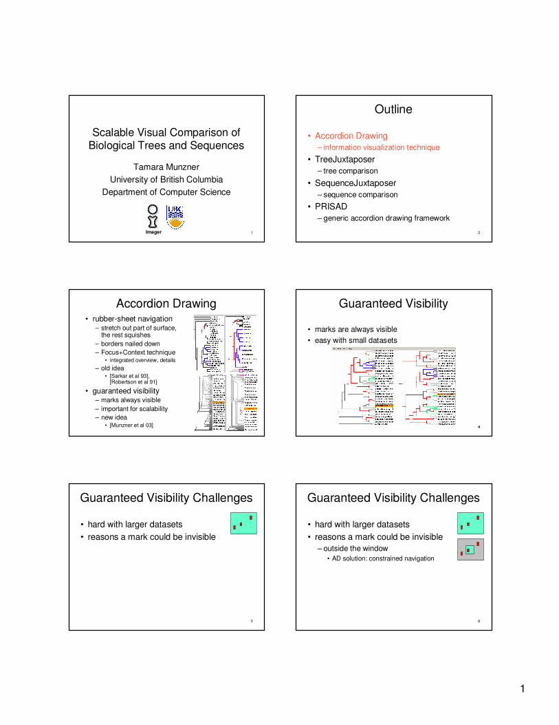
Scalable Visual Comparison of Biological Trees and Sequences

Tamara MunznerUniversity of British Columbia

Department of Computer Science

Imager 2

Outline

• Accordion Drawing– information visualization technique

• TreeJuxtaposer– tree comparison

• SequenceJuxtaposer– sequence comparison

• PRISAD– generic accordion drawing framework

3

Accordion Drawing• rubber-sheet navigation

– stretch out part of surface, the rest squishes

– borders nailed down– Focus+Context technique

• integrated overview, details– old idea

• [Sarkar et al 93], [Robertson et al 91]

• guaranteed visibility– marks always visible– important for scalability – new idea

• [Munzner et al 03] 44

Guaranteed Visibility

• marks are always visible• easy with small datasets

5

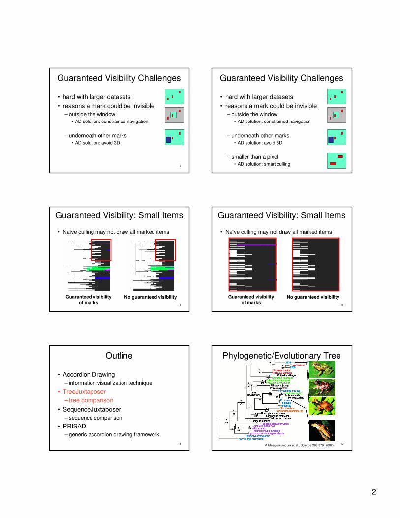
Guaranteed Visibility Challenges

• hard with larger datasets• reasons a mark could be invisible

6



– outside the window• AD solution: constrained navigation

2

7




– underneath other marks• AD solution: avoid 3D

8




– underneath other marks• AD solution: avoid 3D

– smaller than a pixel• AD solution: smart culling

9

Guaranteed Visibility: Small Items

• Naïve culling may not draw all marked items

GV no GV

Guaranteed visibilityof marks

No guaranteed visibility10

Guaranteed Visibility: Small Items

• Naïve culling may not draw all marked items

GV no GV

Guaranteed visibilityof marks

No guaranteed visibility

11

Outline





12

Phylogenetic/Evolutionary Tree

M Meegaskumbura et al., Science 298:379 (2002)

3

13

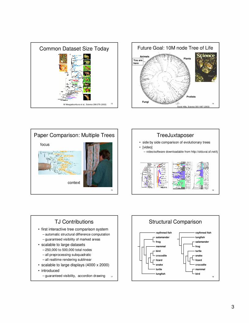
Common Dataset Size Today

M Meegaskumbura et al., Science 298:379 (2002) 14

Future Goal: 10M node Tree of Life

David Hillis, Science 300:1687 (2003)

Plants

Protists

Fungi

AnimalsYou arehere

15

Paper Comparison: Multiple Trees

focus

context

16

TreeJuxtaposer• side by side comparison of evolutionary trees • [video]

– video/software downloadable from http://olduvai.sf.net/tj

17

TJ Contributions• first interactive tree comparison system

– automatic structural difference computation– guaranteed visibility of marked areas

• scalable to large datasets– 250,000 to 500,000 total nodes– all preprocessing subquadratic– all realtime rendering sublinear

• scalable to large displays (4000 x 2000)• introduced

– guaranteed visibility, accordion drawing 18

Structural Comparison

rayfinned fish

lungfish

salamander

frog

mammal

turtle

bird

crocodile

lizard

snake

rayfinned fish

bird

lungfish

salamander

frog

mammal

turtle

snake

lizard

crocodile

4

19

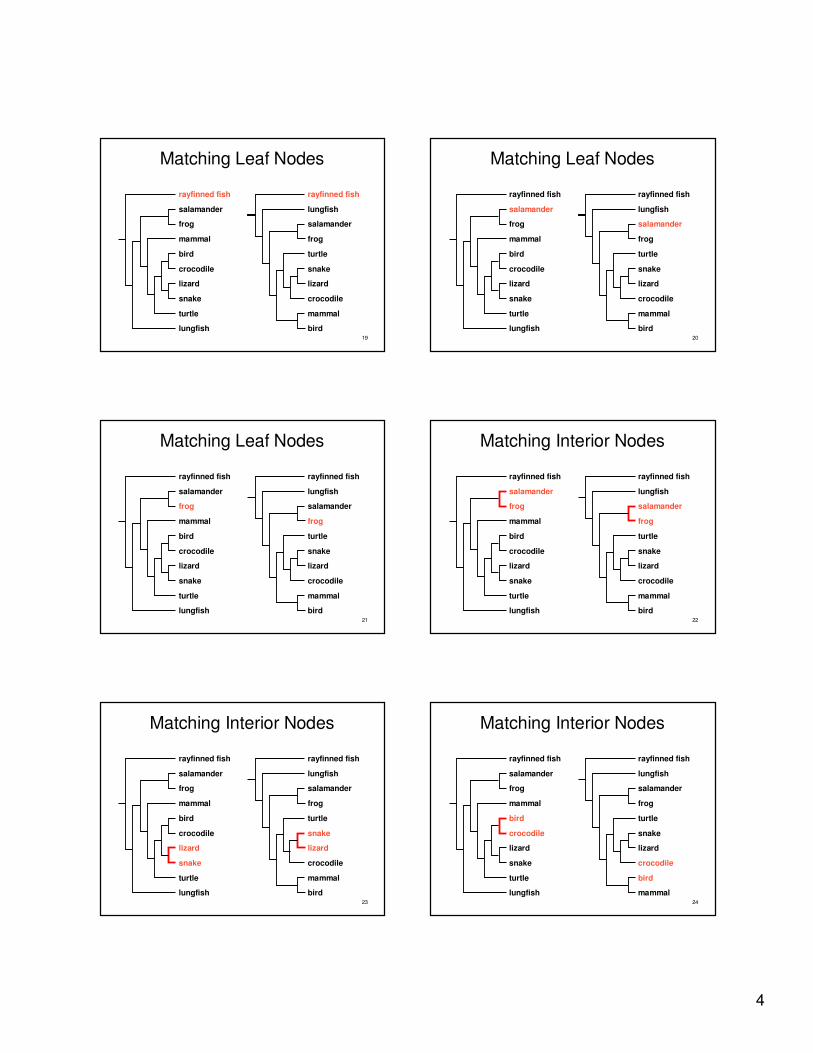
Matching Leaf Nodes

rayfinned fish

lungfish

salamander

frog

mammal

turtle

bird

crocodile

lizard

snake

rayfinned fish

bird

lungfish

salamander

frog

mammal

turtle

snake

lizard

crocodile

20

Matching Leaf Nodes

rayfinned fish

lungfish

salamander

frog

mammal

turtle

bird

crocodile

lizard

snake

rayfinned fish

bird

lungfish

salamander

frog

mammal

turtle

snake

lizard

crocodile

21

Matching Leaf Nodes

rayfinned fish

lungfish

salamander

frog

mammal

turtle

bird

crocodile

lizard

snake

rayfinned fish

bird

lungfish

salamander

frog

mammal

turtle

snake

lizard

crocodile

22

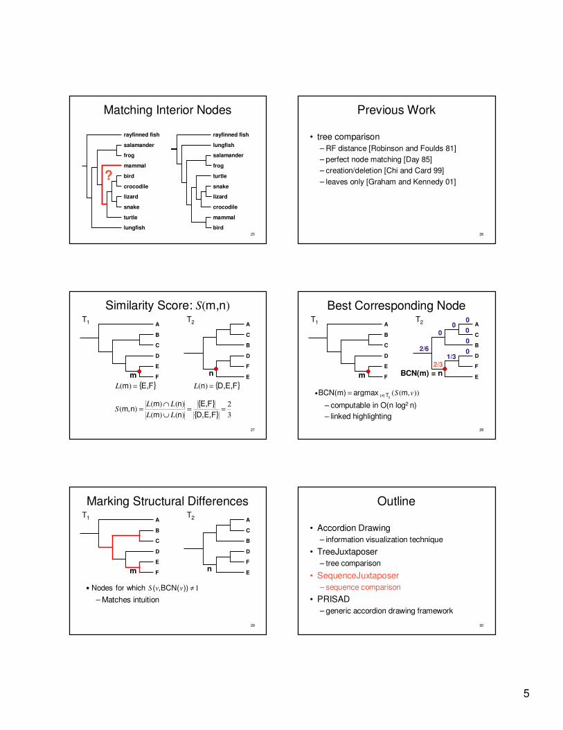
Matching Interior Nodes

rayfinned fish

lungfish

salamander

frog

mammal

turtle

bird

crocodile

lizard

snake

rayfinned fish

bird

lungfish

salamander

frog

mammal

turtle

snake

lizard

crocodile

23


rayfinned fish

lungfish

salamander

frog

mammal

turtle

bird

crocodile

lizard

snake

rayfinned fish

bird

lungfish

salamander

frog

mammal

turtle

snake

lizard

crocodile

24


rayfinned fish

lungfish

salamander

frog

mammal

turtle

bird

crocodile

lizard

snake

rayfinned fish

mammal

lungfish

salamander

frog

bird

turtle

snake

lizard

crocodile

5

25


rayfinned fish

lungfish

salamander

frog

mammal

turtle

bird

crocodile

lizard

snake

rayfinned fish

bird

lungfish

salamander

frog

mammal

turtle

snake

lizard

crocodile

?

26

Previous Work

• tree comparison– RF distance [Robinson and Foulds 81]– perfect node matching [Day 85]– creation/deletion [Chi and Card 99]– leaves only [Graham and Kennedy 01]

27

Similarity Score: S(m,n)

{ }{ } 3

2)()()()(

),( ==∪∩

=FE,D,

FE,nmnm

nmLLLL

S

{ }FE,D,n =)(L{ }FE,m =)(L

T1 T2A

B

C

D

E

F

A

C

B

D

F

Em n

28

Best Corresponding Node

•– computable in O(n log2 n)– linked highlighting

T1 T2A

B

C

D

E

F

A

C

B

D

F

Em BCN(m) = n

1/32/3

2/6

00

0000

1/21/2

)),(( vSv margmax)mBCN(2T∈=

29

•– Matches intuition

1≠))BCN(,( whichfor Nodes vvS

Marking Structural DifferencesT1 T2A

B

C

D

E

F

A

C

B

D

F

Em n

30

Outline





6

31

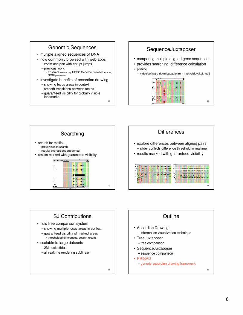
Genomic Sequences• multiple aligned sequences of DNA• now commonly browsed with web apps

– zoom and pan with abrupt jumps– previous work

• Ensembl [Hubbard 02], UCSC Genome Browser [Kent 02], NCBI [Wheeler 02]

• investigate benefits of accordion drawing– showing focus areas in context– smooth transitions between states– guaranteed visibility for globally visible

landmarks32

SequenceJuxtaposer

• comparing multiple aligned gene sequences• provides searching, difference calculation• [video]

– video/software downloadable from http://olduvai.sf.net/tj

33

Searching

• search for motifs– protein/codon search– regular expressions supported

• results marked with guaranteed visibility

34

Differences

• explore differences between aligned pairs– slider controls difference threshold in realtime

• results marked with guaranteed visibility

35

SJ Contributions• fluid tree comparison system

– showing multiple focus areas in context– guaranteed visibility of marked areas

• thresholded differences, search results

• scalable to large datasets– 2M nucleotides– all realtime rendering sublinear

36

Outline





7

37

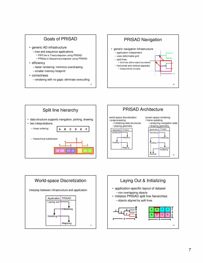
Goals of PRISAD

• generic AD infrastructure– tree and sequence applications

• PRITree is TreeJuxtaposer using PRISAD• PRISeq is SequenceJuxtaposer using PRISAD

• efficiency– faster rendering: minimize overdrawing– smaller memory footprint

• correctness– rendering with no gaps: eliminate overculling

38

PRISAD Navigation

• generic navigation infrastructure– application independent– uses deformable grid– split lines

• Grid lines define object boundaries

– horizontal and vertical separate• Independently movable

39

Split line hierarchy

• data structure supports navigation, picking, drawing• two interpretations

– linear ordering

– hierarchical subdivision

A B C D E F

40

PRISAD Architecture

world-space discretization• preprocessing

• initializing data structures• placing geometry

screen-space rendering• frame updating

• analyzing navigation state• drawing geometry

41

World-space Discretization

interplay between infrastructure and application

42

4

2

• application-specific layout of dataset– non-overlapping objects

• initialize PRISAD split line hierarchies– objects aligned by split lines

Laying Out & Initializing

A A C C

A T T T68

12

34 5

97

4

5

8

43

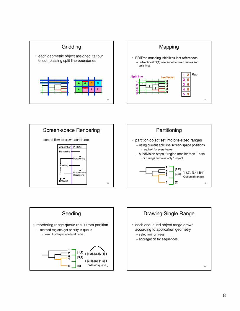
Gridding

• each geometric object assigned its four encompassing split line boundaries

A A C C

A T T T

44

Mapping

• PRITree mapping initializes leaf references– bidirectional O(1) reference between leaves and

split lines

13

468

25

973

4

12

58495

635221 Map

68

25

9

Split line Leaf index

45

Screen-space Rendering

control flow to draw each frame

46

Partitioning

• partition object set into bite-sized ranges– using current split line screen-space positions

• required for every frame

– subdivision stops if region smaller than 1 pixel• or if range contains only 1 object

1234

5

[1,2]

[3,4]

[5]

{ [1,2], [3,4], [5] }Queue of ranges

47

Seeding

• reordering range queue result from partition– marked regions get priority in queue

• drawn first to provide landmarks

1234

5

[1,2]

[3,4]

[5]

{ [1,2], [3,4], [5] }

{ [3,4], [5], [1,2] }ordered queue 48

Drawing Single Range

• each enqueued object range drawn according to application geometry– selection for trees– aggregation for sequences

9

49

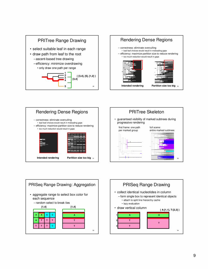
PRITree Range Drawing

• select suitable leaf in each range• draw path from leaf to the root

–ascent-based tree drawing–efficiency: minimize overdrawing

• only draw one path per range

1234

5

[3,4]{ [3,4], [5], [1,2] }

50

Rendering Dense Regions

– correctness: eliminate overculling• bad leaf choices would result in misleading gaps

– efficiency: maximize partition size to reduce rendering• too much reduction would result in gaps

Intended rendering Partition size too big

51

Rendering Dense Regions

– correctness: eliminate overculling• bad leaf choices would result in misleading gaps

– efficiency: maximize partition size to reduce rendering• too much reduction would result in gaps

Intended rendering Partition size too big 52

PRITree Skeleton• guaranteed visibility of marked subtrees during

progressive rendering

first frame: one path per marked group

full scene: entire marked subtrees

53

PRISeq Range Drawing: Aggregation

• aggregate range to select box color for each sequence– random select to break ties

A A C C

A T T T

[1,4]

A

T

[1,4]

T T T C T

54

PRISeq Range Drawing

• collect identical nucleotides in column– form single box to represent identical objects

• attach to split line hierarchy cache• lazy evaluation

• draw vertical column

A

T

TT

A

{ A:[1,1], T:[2,3] }

1

2

3

10

55

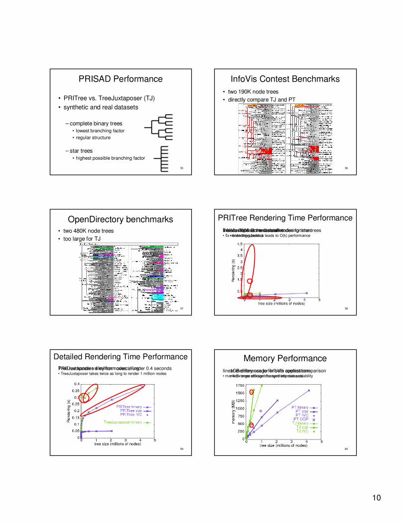
PRISAD Performance

• PRITree vs. TreeJuxtaposer (TJ)• synthetic and real datasets

– complete binary trees• lowest branching factor• regular structure

– star trees• highest possible branching factor

56

InfoVis Contest Benchmarks• two 190K node trees• directly compare TJ and PT

57

OpenDirectory benchmarks• two 480K node trees• too large for TJ

58

PRITree Rendering Time PerformanceTreeJuxtaposer renders all nodes for star trees

• branching factor k leads to O(k) performanceInfoVis 2003 Contest dataset• 5x rendering speedupa closer look at the fastest rendering times

59

PRITree handles 4 million nodes in under 0.4 seconds• TreeJuxtaposer takes twice as long to render 1 million nodes

Detailed Rendering Time PerformanceTreeJuxtaposer valley from overculling

60

Memory Performance1GB difference for InfoVis contest comparison

• marked range storage changes improve scalabilitylinear memory usage for both applications

• 4-5x more efficient for synthetic datasets

11

61

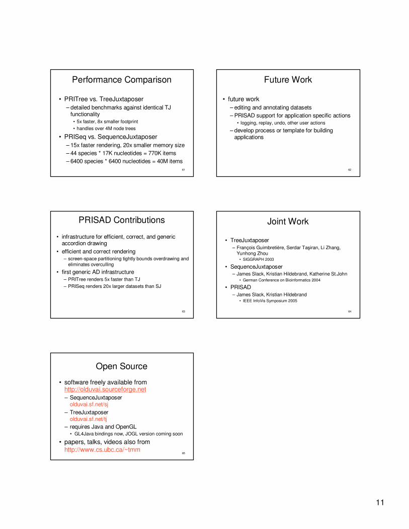
Performance Comparison

• PRITree vs. TreeJuxtaposer– detailed benchmarks against identical TJ

functionality• 5x faster, 8x smaller footprint• handles over 4M node trees

• PRISeq vs. SequenceJuxtaposer– 15x faster rendering, 20x smaller memory size– 44 species * 17K nucleotides = 770K items– 6400 species * 6400 nucleotides = 40M items

62

Future Work

• future work– editing and annotating datasets– PRISAD support for application specific actions

• logging, replay, undo, other user actions

– develop process or template for building applications

63

PRISAD Contributions

• infrastructure for efficient, correct, and generic accordion drawing

• efficient and correct rendering – screen-space partitioning tightly bounds overdrawing and

eliminates overculling

• first generic AD infrastructure– PRITree renders 5x faster than TJ– PRISeq renders 20x larger datasets than SJ

64

Joint Work

• TreeJuxtaposer– François Guimbretière, Serdar Ta�iran, Li Zhang,

Yunhong Zhou• SIGGRAPH 2003

• SequenceJuxtaposer– James Slack, Kristian Hildebrand, Katherine St.John

• German Conference on Bioinformatics 2004

• PRISAD– James Slack, Kristian Hildebrand

• IEEE InfoVis Symposium 2005

65

Open Source

• software freely available from http://olduvai.sourceforge.net– SequenceJuxtaposer

olduvai.sf.net/sj– TreeJuxtaposer

olduvai.sf.net/tj– requires Java and OpenGL

• GL4Java bindings now, JOGL version coming soon

• papers, talks, videos also from http://www.cs.ubc.ca/~tmm

Documents

Accordion Drawing Guaranteed Visibilitytmm/talks/bord05/bord05.6up.pdf · • Accordion Drawing – information visualization technique • TreeJuxtaposer – tree comparison •