Accepted Manuscript

A traffic cellular automata model based on road network grids and its spatial &

temporal resolution’s influences on simulation

Tengda Sun, Jinfeng Wang

PII: S1569-190X(07)00057-3

DOI: 10.1016/j.simpat.2007.04.010

Reference: SIMPAT 564

To appear in: Simulation Modeling Practices and Theory

Received Date: 3 November 2006

Revised Date: 22 April 2007

Accepted Date: 23 April 2007

Please cite this article as: T. Sun, J. Wang, A traffic cellular automata model based on road network grids and its

spatial & temporal resolution’s influences on simulation, Simulation Modeling Practices and Theory (2007), doi:

10.1016/j.simpat.2007.04.010

This is a PDF file of an unedited manuscript that has been accepted for publication. As a service to our customers

we are providing this early version of the manuscript. The manuscript will undergo copyediting, typesetting, and

review of the resulting proof before it is published in its final form. Please note that during the production process

errors may be discovered which could affect the content, and all legal disclaimers that apply to the journal pertain.

ACCEPTED MANUSCRIPT

1

A traffic cellular automata model based on road network grids

and its spatial & temporal resolution’s influences on simulation Tengda Sun1,2,3, Jinfeng Wang*1

1. Institute of Geographic Science & Natural Resources Research, Chinese Academy of Sciences,

Beijing 100101, P.R China 2. Graduate School of the Chinese Academy of Sciences, Beijing 100039, P.R China

3. Navigation College, Jimei University, XIAMEN, 361021, P.R China

Abstract

Microscopic Traffic Simulation Model based on Cellular Automata (CA) has become more and more popular since it was firstly introduced by Creamer and Ludwig in 1986. Cellular automata are simpler to implement on computers, provide a simple physical picture of the system and can be easily modified to deal with different aspects of traffic. However, in a traditional traffic CA model, the spatial resolution of CA and temporal resolution of simulation are low. Take TRANSIMS for example. The size of cellular automata is 7.5 meters and the time step equals 1 second. In such a case, if a vehicle drives at a speed of 4 cells per second, the speed difference between 95km/h (3.5*7.5m/s) and 121km/h (4.4999*7.5m/s) will not be distinguished by simulation models. And the temporal resolution of 1 second makes the system hard to model different drivers’ reaction time, which plays a very important role in vehicular movement models. In this paper, a microscopic traffic cellular automata model based on road network grids is proposed to overcome the low spatial and temporal resolutions of traditional traffic CA models. In our model, spatial resolution can be changed by setting different grid size for lanes and intersections before or during simulation and temporal resolution can be defined according to simulation needs to model different drivers’ reaction time, whereas the vehicular movement models are still traditional CA models. By doing so, the low spatial and temporal resolution of CA model can be overcome and the advantages of using CA to simulate traffic are preserved. The paper also presents analyses of the influences on simulation of different 1D lane grid size, 2D intersection grid size and different combinations of temporal resolution and mean drivers’ reaction time. The analysis results prove the existence of spatial and temporal resolution thresholds in traffic CA models. They also reveal that the size of grids, the combinations of different temporal resolutions and mean drivers’ reaction time do pose influences on the speed of vehicles and lane/intersection occupancy, but do not affect the volume of traffic greatly. Key Words: Microscopic traffic simulation; Cellular automata; Road network grids; Spatial resolution;

Temporal resolution; Influences on simulation

1. Introduction

Cellular automata were originally introduced by von Neumann and Ulam (under the name of “cellular spaces”) as a possible idealization of biological systems [1][2], with the particular

*Corresponding author. Tel: +86 01064888965; E-mail address: wangjf@lreis.ac.cn

ACCEPTED MANUSCRIPT

2

purpose of modeling biological self-reproduction. Since then, they have been used in physics applications such as particle transport simulations and thermodynamics studies. In the field of traffic study, cellular automata were firstly introduced by Creamer and Ludwig in 1986 [3]. They used a cellular automaton model in the form of a boolean simulation of traffic flow. The boolean model represents individual vehicles by 1-bit variables that are placed in computer memory locations analogous to the locations of vehicles on the roadway. More recently, since the introduction of the Nagel-Schreckenberg model in 1992 [4], cellular automata have become a well-established method of traffic flow modeling. In traffic cellular automata model, the roadway is represented by a uniform cell lattice in which each cell belongs to a discrete set of states. The state of the cells is updated at discrete time steps with a set of update rules that combine a few vehicle motion models that are governed by a small set of parameters. This means that both time and space are discrete variables, and physical quantities take on a finite set of discrete values. Therefore, CA models are simpler to implement on computers, provide a simple physical picture of the system and can be easily modified to deal with different aspects of traffic [5][6][7]. For these reasons, traffic cellular automata models are getting more and more popular.

In microscopic traffic simulation models based on CA, the size of CA and the time step of the simulation, i.e., the spatial & temporal resolution of simulation are two key parameters while running simulations. However, till now, there are few relevant papers discussing such issues. For many microscopic traffic simulation system based on CA, the selection of size of CA and time step of simulation is somewhat a bit arbitrary. In TRANSIMS [8], the size of cellular automata is 7.5 meters, while time step equals 1 second. In [7], the size of CA is set as 5 meters, and time step equals 1 second as well. Apparently, both of the two spatial and temporal resolutions are low, for the velocity gap which the simulation system cannot distinguish from vehicles to vehicles is large. For instance, in TRANSIMS, if a vehicle drives at a speed of 4 cells per second, the speed difference between 95km/h (3.5*7.5m/s) and 121km/h (4.4999*7.5m/s) will not be distinguished by simulation models. All vehicles with the speed within such range will move at the same speed without any differences. For temporal resolution, if the time step is set uniformly as 1 second, simulation models are hardly able to depict accurately such differences among drivers as reaction time, intersection start-up delay and so forth. From most of the recent papers regarding traffic simulation models based on CA, we can find that many of these models are for highway traffic rather than for urban traffic. When using traditional CA models (traditional CA models denote those CA models whose spatial and temporal resolutions are invariable before or while running simulations) to simulate urban traffic, the spatial resolution and temporal resolution is not enough to make a good simulation result. Therefore, a more subtle simulation model based on CA is needed.

In this paper, a microscopic traffic cellular automata model based on road network grids is proposed to overcome the low spatial and temporal resolutions of traditional traffic CA models mentioned above. In this model, spatial resolution can be changed by setting different grid size for lanes and intersections before or during simulation and temporal resolution can be defined according to simulation needs to model different drivers’ reaction time, whereas vehicular movement models are still traditional CA models. By doing so, the low spatial and temporal resolution of CA model can be overcome and the advantages of using CA to simulate traffic are preserved.

The following section will discuss the road network data model designed for the revised CA

ACCEPTED MANUSCRIPT

3

model and the gridization process of one-dimensional traffic lanes and two-dimensional nodes.

2. Road Network Model and Gridization

2.1 Data Structure of Road Network

The data model for road network in this paper is still a traditional “Node-Link-Segment-Lane” relationship which is shown in Fig. 1. However, considering different spatial resolution in road network, we add a new data element “grid” for both lanes (one-dimensional, 1D) and nodes (two dimensional, 2D). The new relationship for the data model is illustrated in Fig. 2[9]. And the gridization processes of nodes and traffic lanes are described in the remaining part of this section.

Fig. 1 Basic Elements of Road Network Model

Fig.2 Node-Link-Segment-Lane-Grid Data Model: a Node may have some incoming and outgoing links. A link is composed of road segments which are made up of one or several traffic lanes. For

each node, it is divided into a grid matrix whose spatial resolution is defined by 2D grid size (Length and Width), see Fig. 5. Similarly, a traffic lane can be divided into a series of 1D grids (in

terms of Length, see Fig. 3 and Fig. 4), which correspond to cells in the traditional CA model

ACCEPTED MANUSCRIPT

4

2.2 One-Dimensional Lanes Gridization

The first step of 1D lanes gridization is to determine the grid counts for traffic lanes. The quantity of grids for a lane is determined by equation (1):

1/__ += GridSizeLengthLaneGridsLane 1

where: Lane Grids=The quantity of grids in a lane Lane_Length=length of a lane; GridSize=length of a grid, also known as 1D spatial resolution.

The grid count occupied by a vehicle is determined by equation (2):

1/__ += GridSizeLengthVehGridsVeh 2

where: Veh_Grids=number of grids occupied by a vehicle; Veh_Length=length of a vehicle.

The width of a grid in a traffic lane is defined as the width of the traffic lane. The traffic lane status is represented by the lane grids’ status string. Each lane has a grids’

status string. The string indicates which grids in the lane are occupied by vehicles. The status of a grid in the lane is represented by two characters, 0 for idle grid and 1 for occupied one. The length of the status string equals the number of lane grids. The 0-1 status string is similar to the binary string of traditional CA models. The major difference between traditional CA models and our CA model is that in traditional CA models, a vehicle can occupy only one grid (cell), however, in this model, a vehicle can occupy more than one grids and the grid count that a vehicle occupies at one time is proportional to the vehicle’s length. Fig. 3 and Fig. 4 present two examples of lane grid status string, one for a one lane segment and the other for a three lane segment. Fig. 4 also presents subject vehicle’s gap from other vehicles in the same traffic lane and neighboring lanes. These gap parameters are essential for car following and lane changing models.

Fig. 3 Lane Grids’ Status String for one Lane Segment (traffic moves from west to east)

Fig. 4 Lane Grids’ Status String for three Lane Segment (The subject vehicle is the second vehicle in the middle lane, and traffic moves from west to east)

2.2 Two-Dimensional Intersections Gridization

ACCEPTED MANUSCRIPT

5

In 1D lane’s gridization, the grid count for a traffic lane is calculated according to lane length and grid size. Similarly, in case of 2D intersections gridization, the grid count is determined by intersection size and grid size. However, the intersection grid size is defined by a rectangle with length and width instead of only by grid length. The status for one grid point is “1” and “0”, which indicate that the grid is occupied by a vehicle or not respectively. Just as in the 1D lane situation, a vehicle in the intersection can occupy more than one grid. The grid count that a vehicle can occupy at one time is proportional to the size of its bounding rectangle. If a grid is within or intersects the bounding rectangle of a vehicle, the status character for this grid is set as “1” (black color), otherwise “0” (grey color), See Fig. 5.

Fig. 5 Intersection grid statuses (black for occupied grids, grey for idle ones)

The movements of vehicles which have been within or are ready to enter intersections are constrained by the intersection grid matrix status. If a vehicle decides to move forward in the next time step, it has to check if the statuses of all grids from its current position to target position, which will be occupied by its bounding rectangle, are available or not. If the grids between them are all idle, it will move forward as expected; otherwise, it will stop or decelerate. In Fig. 6, Vehicle A (near the junction) will make a right turn in next time step. Before it moves forward, it has to check if some of the grids in the intersection occupied by Vehicle B are available or not. If negative, it has to stop and wait until those grids become cleared.

Fig. 6 Grid Status Check before entering intersections or moving within intersections

ACCEPTED MANUSCRIPT

6

The mechanism mentioned above makes sure that all vehicles to the same target link from the same source link will not “pass through” each other. However, when vehicles move within intersections, they may be “deadlocked” by each other for some reasons. A deadlock is a situation wherein two or more vehicles are unable to proceed because each is waiting for one of the others to move forward. We can often find this phenomenon in real traffic, especially in intersections without signal control. Two or more vehicles move at the same time to the same place and none of them would like to give way to others. The only solution to the problem is that one or more of the vehicles back off to make room for other vehicles. However, in the simulation model, vehicles are seldom modeled to be able to move backward. To make the process of handling such problem easy, we allow at random one of the vehicles to “pass through” other vehicles until it waits for a reasonable time after the deadlock occurs. The “reasonable time” becomes one of the model parameters of the vehicular movement model and will be calibrated in the calibration process.

In this section, we mainly focus on the process of dividing 1D traffic lanes and 2D intersections into grids. The key issue of this process is the selection of the spatial resolution. As mentioned earlier, in traditional CA models, the spatial and temporal resolutions are coarse and invariable when running simulations. Therefore, we need a new CA model whose spatial and temporal resolution can be changed according to simulation needs and hardware performance. This means that the grid size can be less. But how less is enough to make a good simulation? What are the influences of grid size on simulation output? Can it be infinitesimal? These are very interesting questions when using CA model to simulate real traffic.

In the following sections, we will discuss these issues by making simulations and then comparing simulation output from volume, average lane/intersection occupancy and speed. Before the presentation of the simulation output, it is necessary for us to explain some of the terms used below for clarification. The first one is volume, including lane volume and intersection volume. Lane volume denotes the count of vehicles that reach the end of lane and leave from the same. Intersection volume includes vehicles from all incoming links that enter the intersection. Volume here is an accumulative variable, and is recalculated after a specified period of time (in our model, 15 minutes). The second term is lane/intersection occupancy. The term occupancy here is different from the term “occupancy” in traffic engineering. It is the percentage of the lane/intersection grids which are occupied by vehicles. The lane/intersection average speed in this paper is the average speed of vehicles within the lanes/intersections. Occupancy and speed data are calculated at an interval of 5 seconds and averaged every 15 minutes.

The remaining sections are organized as follows. Section 3 discusses the influences of spatial and temporal resolutions on simulation output. For the sake of better understanding, in this section, we firstly propose directly the simulation conditions; then the results of numerical simulations are presented in the form of plots and tables; finally, analysis findings of these data are given for these numerical simulations. Section 4 concludes this paper.

3. Influences of Spatial and Temporal Resolution on Simulation Output

3.1 Influences of Spatial Resolution on Simulation Output

3.1.1 Influences of 1D lane grid size on Simulation Output

Simulation Conditions: Road network is a one lane segment and a two lane segment. The length of the two segments is 1000 meters. The arriving rate distribution of vehicles is a Poisson

ACCEPTED MANUSCRIPT

7

distribution with a mathematic expectation of 300 vehicles per 15 minutes. The combinations of different types of vehicles are: 70% for small vehicles (length=4.5m), 22% for medium vehicles (length=7.5m) and 8% for large vehicles (length=12m). The initial speed for all vehicles is 30km/h, and the maximum desired speed for all vehicles is 100km/h. The record interval of volume, speed and occupancy is 5 seconds. The horizontal axis in the following curves is for record time counter. The simulation models such as car following model and lane changing model are based on TRANSIMS models. For detailed information about the models, see [8]. To avoid errors incurred by random factors, we ran simulation five times, each lasting 15 minutes.

The simulation outputs are given by Fig.7-12 and Table 1. Figures7-12 give the detailed information regarding speed, occupancy and volume of each record from one of the five times. The average speed and occupancy for each simulation are shown by Table1.

40

60

80

100

1 31 61 91 121 151

Spee

d/(k

m/h

)

GridSize=2 GridSize=5 GridSize=7.5

Fig. 7 speed comparison of one lane segment with different grid sizes (The horizontal axis represents time; each

value on the axis represents one record. There are about 180 records, lasting 900 seconds, i.e., 15 minutes.)

40

60

80

100

1 31 61 91 121 151

Spee

d/(k

m/h

)

GridSize=2 GridSize=5 GridSize=7.5

Fig. 8 speed comparison of two lane segment with different grid sizes

0

0.05

0.1

0.15

0.2

0.25

0.3

1 31 61 91 121 151

Occ

upan

cy

GridSize=2 GridSize=5 GridSize=7.5

Fig. 9 occupancy comparison of one lane segment with different grid sizes

ACCEPTED MANUSCRIPT

8

0

0.05

0.1

0.15

1 31 61 91 121 151

Occ

upan

cy

GridSize=2 GridSize=5 GridSize=7.5

Fig. 10 occupancy comparison of two lane segment with different grid sizes

0

50

100

150

200

250

300

1 31 61 91 121 151

Vol

ume

GridSize=2 GridSize=5 GridSize=7.5

Fig. 11 volume comparison of one lane segment with different grid sizes

0

50

100

150

200

250

300

1 31 61 91 121 151

Vol

ume

GridSize=2 GridSize=5 GridSize=7.5

Fig. 12 volume comparison of two lane segment with different grid sizes

Table 1 Average Speed and Occupancy of Lanes by different lane grid sizes (Speed in km/h)

Size=2 Size=5 Size=7.5 Size=2 Size=5 Size=7.5 Times

single lane segment two lane segment

Spd 72.9 73.4 58.9 83.1 80.4 71.7 1

Occu 0.097 0.102 0.160 0.046 0.043 0.068

Spd 72.8 74.5 60.4 82.1 79.2 69.1 2

Occu 0.102 0.093 0.167 0.047 0.045 0.074

Spd 73.1 73.2 60.7 83.1 80.3 73.4 3

Occu 0.098 0.099 0.164 0.045 0.043 0.069

Spd 74.7 74.6 59.3 83.5 81.6 73.4 4

Occu 0.096 0.097 0.170 0.043 0.043 0.066

Spd 73.1 74.2 62.3 82.6 79.5 70.7 5

Occu 0.102 0.097 0.156 0.044 0.045 0.069

ACCEPTED MANUSCRIPT

9

Analyses of simulation output: (1) Speed of the two lane segment is faster than one lane segment, but occupancy of the two

lane segment is lower than one lane segment. The conclusion is apparent. For in a two lane segment, vehicles can change lanes to move faster when there is a slower vehicle ahead. Given the same vehicle arriving rate, occupancy in a lane from a two lane segment is definitely lower than the lane from a one lane segment.

(2) The more the grid size is, the lower the average speed will be, and the higher the lane occupancy will be. In other words, vehicles will move more slowly in the case of lower spatial resolution than in the case of higher spatial resolution; however, the lane occupancy becomes higher. This is attributed to the low precision in measuring the grid count that a vehicle can occupy when the grid size is big. It reduces the chance of a vehicle to move forward. Contrary, when the lane grid size is small, the grids that a vehicle occupies in a lane can be depicted more accurately and there will be more areas left empty when compared with bigger grids. Therefore possibilities for vehicles to move forward will be higher.

(3) The value of different spatial resolution of lane grids seems not to affect the volume output greatly.

(4) There exists a spatial resolution threshold. The “spatial resolution threshold” is a spatial resolution over which, the differences of simulation output between two spatial resolutions can be negligible. To determine the spatial resolution threshold, we assume that distribution of simulation output from simulation tests is a normal distribution and perform the two-sample t-test ([10]) based on the simulation outputs. Table 2 shows the final result of the test with significance level alpha of 0.05. From Table 2, we find that, sample data from grid size being 2 meters and 5 meters passed the two-sample t-test. Therefore, we can make the conclusion that the difference between the two situations is small. However, in the case of two lane segment, the p value(0.001) for speed data is less than alpha (0.05). This means that the null hypothesis can be rejected although it passed the t-test. Considering the fact that computation resource required will increase if spatial resolution is set higher and t-tests for other sample data have passed, we still take 5 meters as the spatial resolution threshold. However, this spatial resolution threshold is only applied to the specified simulation conditions. In other simulation conditions, it may be different.

Table 2 T-Test for 1D Spatial Resolution simulations (alpha=0.05)

single lane segment two lane segment

Samples(x,y) (Size=2,Size=5) (Size=5,Size=7.5) (Size=2,Size=5) (Size=5,Size=7.5)

Spd Yes* No Yes No

p value 0.183 - 0.001 -

Occu Yes No Yes No

p value 0.491 - 0.200 -

(*: “Yes” denotes that the sample data have passed the t-test, “No” for otherwise; calculation is performed by the

function ttest2 from Matlab 6.5)

3.1.2 Influences of 2D intersection grid size on Simulation Output

Simulation Conditions: road network is given by Fig. 13. Distances from nodes 1,2,3 and 4 to intersection node 0 are all 1000 meters. All segments have 3 lanes, the left most for left turn; the other two for through. Right turn vehicles share the right most lanes with through vehicles. The

ACCEPTED MANUSCRIPT

10

movements of vehicles after passing intersection are governed by intersection turn percentage: 25% for left turn, 25% for right turn and 50% for through traffic. The distributions of vehicles arriving rate for all nodes (except node 0) are Poisson distributions with a mathematical expectation of 500 vehicles per 15 minutes. The combinations of different types of vehicles are: 70% for small vehicles (length=4.5m), 22% for medium vehicles (length=7.5m) and 8% for large vehicles (length=12m). The initial speed for all vehicles is 30km/h, and the maximum desired speed for all vehicles is 100km/h. The 1D lane grid size is 5 meters for all lanes. The intersection is an intersection without signal control and speed limit in the intersection is 50km/h. The record interval of volume, speed and occupancy is 5 seconds. The horizontal axis in the following curves is for record time counter. Simulation models such as car following model and lane changing model are based on TRANSIMS models. To avoid errors incurred by random factors, we ran simulation five times, each lasting 15 minutes.

Fig. 13 Road Network of 2D intersection spatial resolution simulation

The simulation outputs are given by Figures 14-16 and Table 3. Figures 14-16 give the detailed information regarding speed, occupancy and volume of each record from one of the five simulations. The average values of each of five simulations are given by Table 3.

0

15

30

45

1 31 61 91 121 151 181

Spee

d/(k

m/h

)

NodeSize=0.5 NodeSize=1 NodeSize=2

Fig. 14 Average Speed of vehicles within the intersection of different grid sizes

ACCEPTED MANUSCRIPT

11

0

0.05

0.1

0.15

0.2

0.25

1 31 61 91 121 151 181

Occ

upan

cy

NodeSize=0.5 NodeSize=1 NodeSize=2

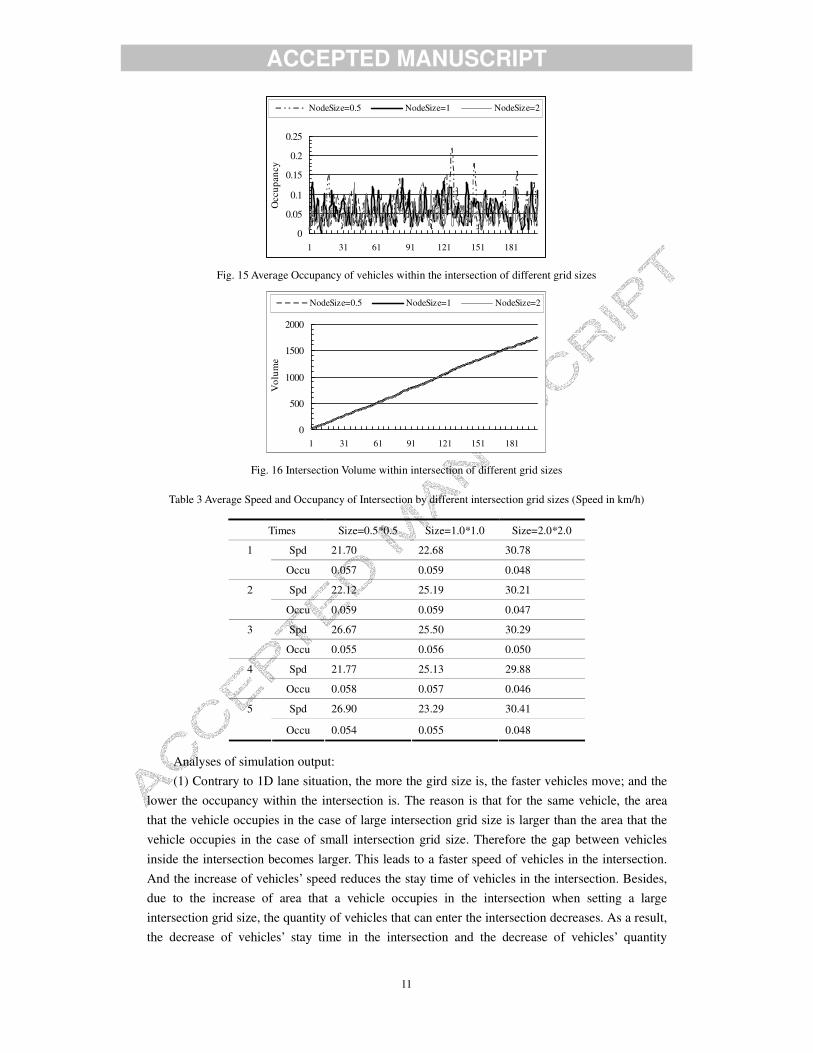
Fig. 15 Average Occupancy of vehicles within the intersection of different grid sizes

0

500

1000

1500

2000

1 31 61 91 121 151 181

Vol

ume

NodeSize=0.5 NodeSize=1 NodeSize=2

Fig. 16 Intersection Volume within intersection of different grid sizes

Table 3 Average Speed and Occupancy of Intersection by different intersection grid sizes (Speed in km/h)

Times Size=0.5*0.5 Size=1.0*1.0 Size=2.0*2.0

Spd 21.70 22.68 30.78 1

Occu 0.057 0.059 0.048

Spd 22.12 25.19 30.21 2

Occu 0.059 0.059 0.047

Spd 26.67 25.50 30.29 3

Occu 0.055 0.056 0.050

Spd 21.77 25.13 29.88 4

Occu 0.058 0.057 0.046

Spd 26.90 23.29 30.41 5

Occu 0.054 0.055 0.048

Analyses of simulation output: (1) Contrary to 1D lane situation, the more the gird size is, the faster vehicles move; and the

lower the occupancy within the intersection is. The reason is that for the same vehicle, the area that the vehicle occupies in the case of large intersection grid size is larger than the area that the vehicle occupies in the case of small intersection grid size. Therefore the gap between vehicles inside the intersection becomes larger. This leads to a faster speed of vehicles in the intersection. And the increase of vehicles’ speed reduces the stay time of vehicles in the intersection. Besides, due to the increase of area that a vehicle occupies in the intersection when setting a large intersection grid size, the quantity of vehicles that can enter the intersection decreases. As a result, the decrease of vehicles’ stay time in the intersection and the decrease of vehicles’ quantity

ACCEPTED MANUSCRIPT

12

entering the intersection at one time lead to a decrease of occupancy in the intersection. (2) The value of different spatial resolution of intersection grids seems not to affect the

volume output greatly. The conclusion is the same as in the case of 1D lane grids. (3) Likewise, there exists a spatial resolution threshold. Table 4 gives the t-test result for

simulation output. From Table 4, when intersection grid size is set as 0.5*0.5 and 1.0*1.0, the difference between the two situations is minor. Therefore, 2D spatial resolution threshold in the case is 1.0*1.0. Table 4 T-Test for 2D Spatial Resolution Simulations (alpha=0.05)

Samples(x,y) Size(0.5*0.5, 1.0*1.0) Size (1.0*1.0, 2.0*2.0)

Spd Yes No

p value 0.704 -

Occu Yes No

p value 0.637 -

3.2 Influences of Temporal Resolution on Simulation Output

As mentioned before, the influence of temporal resolution on simulation is mainly from drivers’ reaction time. The drivers’ reaction time is the interval between the instant that the driver recognizes the situation in the roadway ahead and the instant that the driver makes decision. This response time is frequently referred to as the "perception-reaction time" in traffic engineering literatures. The assumption of a reaction time value for drivers responding to road situations is fundamental for many microscopic traffic simulation models. However, in traffic simulation models based on CA, drivers’ reaction time is seldom modeled.

Generally speaking, the lower the temporal resolution of simulation system is, the more difficult it is to distinguish different drivers’ reaction time. In some literatures (such as [11]), the maximum drivers’ reaction time is 1.5 seconds. Therefore, if the temporal resolution is lower than the threshold, for instance, 2 seconds, it cannot distinguish all drivers’ reaction time. In this paper, the simulation model uses a parameter called “Mean Reaction Time (MRT)” to model drivers’ reaction time. The distribution of all drivers’ reaction time is a normal distribution with a mathematical expectation of MRT. When the driver feels necessary to take actions to change the vehicle’s status, such as accelerate, decelerate or change lanes, the system starts counting from time step to time step. Only when the accumulative action time is larger than the driver’s reaction time does the vehicle change its status. Considering that it is impossible to set the temporal resolution too high, the range for the temporal resolution in our model is between 0.1s and 1s.

3.2.1 Simulation Conditions

Simulation road network is a two lane segment with segment length 1000 meters. The arriving rate distribution of vehicles is a Poisson distribution with a mathematic expectation of 400 vehicles per 15 minutes. The combinations of different types of vehicles are: 70% for small vehicles (length=4.5m), 22% for medium vehicles (length=7.5m) and 8% for large vehicles (length=12m).The initial speed for all vehicles is 30km/h, and the maximum desired speed for all vehicles is 100km/h. The record interval of volume, speed and occupancy is 5 seconds. The simulation models such as car following model and lane changing model are based on TRANSIMS models. To avoid errors incurred by random factors, we ran simulation five times continuously, each time lasting 15 minutes. Temporal resolution is set as 0.1s, 0.25s, 0.5s and 1.0s

ACCEPTED MANUSCRIPT

13

respectively. MRT for drivers include 0.75s, 1.0s and 1.25s.

3.2.2 Simulation Output and Discussion

Table 5 gives the values of volume, speed and occupancy of each numerical simulation for different combinations of temporal resolution and mean reaction time. The average values of volume, speed and occupancy of each time are also listed. The extent that temporal resolution can describe drivers’ reaction time is given by Table 6. The number inside the parentheses denotes the step count that is needed for vehicles to change from original status to desired status. The number before the parentheses is the time difference between the accumulative action time and reaction time. The less the time difference is, the more accurate the temporal resolution describes drivers’ reaction time. When the time difference equals zero, the temporal resolution can depict reaction time fully. In table 6, when both the temporal resolution and reaction time is 1 second, the time difference is nothing; the only difference for different temporal resolution is that the time steps needed to change vehicles’ status are different.

Table 5 Volume (veh), Speed (km/h) and Occupancy for different combinations of temporal resolution and mean

reaction time

MRT=0.75s MRT=1.0s MRT=1.25s Temporal

Resolution Volume Spd Occu Volume Spd Occu Volume Spd Occu

1 371 43.34 0.130 369 43.25 0.135 367 44.26 0.124

2 383 45.61 0.124 391 45.14 0.120 386 44.55 0.128

3 398 44.61 0.132 393 43.23 0.136 412 42.63 0.130

4 389 45.71 0.121 386 44.41 0.128 389 42.09 0.125

5 422 43.17 0.140 434 42.67 0.145 416 45.29 0.134

0.1s

Average 393 44.49 0.129 395 43.74 0.133 394 43.76 0.128

1 372 44.52 0.132 359 45.78 0.137 380 47.32 0.127

2 384 48.71 0.123 401 44.10 0.142 382 45.03 0.135

3 394 45.61 0.133 392 45.65 0.142 396 46.45 0.133

4 397 48.11 0.129 386 47.10 0.131 390 44.35 0.137

5 413 44.05 0.154 425 42.45 0.159 420 47.50 0.135

0.25s

Average 392 46.20 0.134 393 45.02 0.142 394 46.13 0.133

1 370 48.21 0.134 362 48.75 0.133 358 44.33 0.146

2 382 46.55 0.135 391 44.95 0.144 395 48.34 0.134

3 400 45.42 0.147 405 46.43 0.142 410 47.94 0.141

4 395 46.59 0.139 382 46.71 0.141 374 44.82 0.151

5 420 45.99 0.149 427 47.23 0.149 429 45.04 0.155

0.50s

Average 393 46.55 0.141 393 46.81 0.142 393 46.09 0.145

1 352 49.08 0.151 370 52.68 0.136 329 48.47 0.155

2 401 49.61 0.162 388 52.62 0.156 424 45.41 0.187

3 400 54.07 0.145 376 46.95 0.162 399 42.34 0.185

4 401 47.08 0.161 415 48.35 0.174 373 44.52 0.160

5 412 49.51 0.175 391 43.90 0.180 445 43.65 0.183

1.0s

Average 393 49.87 0.159 388 48.90 0.162 394 44.88 0.174

ACCEPTED MANUSCRIPT

14

Table 6 Time difference for different combinations of temporal resolution and mean reaction time

Temporal Resolution

0.1s 0.25s 0.5s 1.0s

MRT=0.75s 0.05s(8) 0.0s(3) 0.25s(2) 0.25(1)

MRT=1.0s 0.0s(10) 0.0s(4) 0.0s(2) 0.0s(1)

MRT=1.25s 0.05s(13) 0.0s(5) 0.25s(3) 0.75s(2)

Figures 17-19 present the information regarding average speed, average occupancy and volume of five simulations for different combinations of temporal resolution and mean reaction time. Number 1, 2, 3 and 4 in horizontal axis represent different temporal resolutions of 0.1s, 0.25s, 0.5s and 1.0s respectively.

40

45

50

1 2 3 4

Spe

ed(k

m/h

)

MRT=0.75s MRT=1.0s MRT=1.25s

Fig. 17 Average Speed comparisons for different combinations of temporal resolution and mean reaction time

0

0.05

0.1

0.15

0.2

1 2 3 4

Occ

upan

cy

MRT=0.75s MRT=1.0s MRT=1.25s

Fig. 18 Average Occupancy comparisons for different combinations of temporal resolution and mean reaction time

300

350

400

1 2 3 4

Vol

ume(

Veh

)

MRT=0.75s MRT=1.0s MRT=1.25s

Fig. 19 Average Volume comparisons for different combinations of temporal resolution and mean reaction time

Analyses of simulation output:

ACCEPTED MANUSCRIPT

15

(1) Given a temporal resolution, the more the MRT is, the higher the occupancy will be. The reason is apparent. The increase of MRT leads to the increase of the time taken for vehicles to move from upstream intersection to downstream intersection. As a result, occupancy is proportional to MRT provided that other simulation conditions keep.

(2) The difference between the volume, average speed and average occupancy for MRT=0.75 and MRT=1.0 when the temporal resolution is set as 1.0s is small. It proves that if both reaction times are less than (or equal) the temporal resolution, the simulation model is not able to distinguish them from each other. This means that the case of MRT=0.75s and temporal resolution=1.0s will be the same as the case of MRT=1.0s and temporal resolution=1.0s.

(3) The time difference between accumulative action time and reaction time affects speed greatly. The more the time difference is, the more vehicles’ speed decreases. The case when MRT is 1.25s and temporal resolution is 1.0s is the most obvious case. The time difference here amounts to 0.75s. According to conclusion (1), this case is similar to the case that MRT is 2.0s and temporal resolution is 1.0s. Such a large reaction time makes vehicles to accelerate have to wait for a long time. Therefore, a decrease of speed occurs. When the time difference is nothing, the speed will increase along with the decrease of temporal resolution, for instance, the case of MRT=1.0s.

(4) Volume is not greatly affected by the temporal resolution and reaction time. This can be seen from Fig. 19.

(5) Like spatial resolution, there exists a temporal resolution threshold. From the t-test result shown in Table 7, the volume, average speed and average occupancy are almost the same for the case of temporal resolution being 0.25s and the case of temporal resolution being 0.5s (Although in the case of MRT=1.25s, t-test for occupancy failed, we still hold the opinion that they are almost the same because MRT=1.25s case is rare). Even when the temporal resolution is set as high as 0.1s, simulation outputs such as volume, speed and occupancy do not change much. Therefore, 0.5s is the temporal resolution threshold. However, this temporal resolution threshold is only applied to the specified simulation conditions. In other conditions, it may be different.

Table 7 T-Test for Temporal Resolution Simulations (alpha=0.05)

MRT=0.75s MRT=1.0s MRT=1.25s Temporal Resolution

Sample(x, y) Volume Spd Occu Volume Spd Occu Volume Spd Occu

T Test Yes Yes Yes Yes Yes Yes Yes No Yes (0.1s,0.25s)

p value 0.958 0.153 0.461 0.898 0.201 0.172 0.973 - 0.070

T Test Yes Yes Yes Yes Yes Yes Yes Yes No (0.25s,0.50s)

p value 0.901 0.746 0.309 0.960 0.112 0.942 0.979 0.974 -

T Test Yes No No Yes Yes No Yes Yes No (0.50s,1.0)

p value 0.989 - - 0.698 0.280 - 0.974 0.389 -

4 Conclusions and final remarks

Large scale microscopic traffic simulation using CA is simpler to implement on computers, provides a simple physical picture of the system and can be easily modified to deal with different aspects of traffic. However, in traditional traffic CA models, the spatial resolution of CA and temporal resolution of simulation are low. In this paper, we proposed a new CA model based on road network grids, in which, the spatial resolution can be changed by setting different grid size for lanes and intersections before or during simulation and the temporal resolution can be defined

ACCEPTED MANUSCRIPT

16

according to simulation needs to model different drivers’ reaction time, whereas the vehicular movement model is still a traditional CA model. As a result, the low spatial and temporal resolution of CA models can be overcome and the advantages of using CA to simulate traffic are preserved. The analyses of simulation output of different 1D lane grid size, 2D intersection grid size and different combinations of temporal resolution and mean drivers’ reaction time revealed that the spatial and temporal resolution of simulation models do pose influence on simulation result, but do not affect the volume of traffic greatly.

The main contribution of this paper is that it is a useful attempt to study the spatial and temporal resolutions of CA because in the fields of research by using CA, such as traffic engineering, geography and so on, few papers discussed such topic. The conclusion from our simulation outputs also convey us such information that a proper selection of spatial and temporal resolutions is recommended while simulating urban traffic using CA. It is difficult to give an exact mathematical equation to depict the relationship between CA spatial & temporal resolutions and their influences on simulation outputs for it depends on the simulation precision requirements, hardware performance, and also the output indicators that engineers concern most. For instance, one of the conclusions from this paper is that volume is not greatly affected by CA spatial and temporal resolution. Hence, if volume is the most concerned output, the spatial and temporal resolution can be a bit lower than in the case of speed and occupancy being the most interested so that simulation can be completed more efficiently. The suggestion from this paper is that before we run simulations based on CA formally, it is necessary to make a resolution test (no matter spatial or temporal, or both) to find the threshold. The final threshold is the lower one from the two resolutions configured in which little variances in simulation outputs are found. The purpose of the spatial & temporal threshold is, on the one hand, to prevent the occurrence of errors incurred by a coarse resolution; on the other hand, to make good advantage of hardware resource since a higher resolution will not lead to a more accurate simulation results.

Acknowledgements

The research is supported by the Beijing Nature Science Foundation (No. 8033015), NSFC (No. 70571076, 40471111) and MOST (No. 2006AA12Z215).

The authors would also like to thank the anonymous reviewers for their valuable suggestions and contributions to this paper.

References:

[1] Von Neumann, J.. The general and logical theory of automata, in J. von Neumann, Collected Works, edited by A. H. Taub, 5,1963: 288. [2] Von Neumann, J.Theory of Self-Reproducing Automata, edited by A. W. Burks (University of Illinois, Urbana), 1966. [3] Creamer, M. and J. Ludwig. A fast simulation model for traffic flow on the basis of Boolean operations. Mathematical and Computers in Simulation, 1986(Vol 28): 297-303. [4] K. Nagel and M. Shreckenberg. A cellular automaton model for freeway traffic. J. Phisique I. 1992, 2(12):2221-2229. [5] T. Nagatani, Phys. Rev. E 48, 3920 (1993). [6] S.C. Benjamin, N.F. Johnson, P.M. Hui, J. Phys. A 29, 3119 (1996). [7] E.G. Campari1 and G. Levi, A cellular automata model for highway traffic. THE EUROPEAN

ACCEPTED MANUSCRIPT

17

PHYSICAL JOURNAL. 2000, B 17:159-166 [8] Kai Nagel, Paula Stretz, et al. TRANSIMS traffic flow characteristics. 1997,http://arxiv.org/abs/adap-org/9710003. [9] ZOU Zhi-jun, YANG Dong-yuan. Simulation Models for Road Network Representation. Journal of Xi�an Highway University. 2001(10):33-35 [10] Snedecor, George W. and Cochran, William G., Statistical Methods, Eighth Edition, Iowa State University Press ,1989. [11] WANG Wuhong, SUN Fengchun, Cao Qi and LIU Shuyan. Driving Behavior Theory and Its Application in Road Traffic System. Beijing: Science Press. 2001:266