Acceleration of a Dynamically PackedOblique Sparse Projection Random Forest

by

James Browne

A dissertation submitted to The Johns Hopkins University

in conformity with the requirements for the degree of

Doctor of Philosophy

Baltimore, Maryland

May, 2019

© 2019 by James Browne

All Rights Reserved

Abstract

The proliferation of scientific and industrial sensors is causing an accelerating

deluge of data, the processing of which into actionable knowledge requires

fast and accurate machine learning methods. A class of algorithms suited to

process these large amounts of data is decision forests, widely used methods

known for their versatility, state of the art inference, and fast model training.

Oblique Sparse Projection Forests — OSPFs — are a subset of decision forests,

which provide data inference superior to other methods. Despite providing

state of the art inference and having a computational complexity similar to

other popular decision forests, there are no OSPF implementations that scale

beyond trivially sized datasets.

We explore whether OSPF training and inference speeds can compete with

other popular decision forest variants despite an algorithmic incompatibility

which prevent OSPFs from using traditional forest training optimizations.

First, using R, we implement a highly extensible proof of concept version

of a recently conceived OSPF, Randomer Forest, shown to provide state of

the art results on many datasets and provide this system for general use via

CRAN. We then develop and implement a postprocessing method, Forest

Packing, to pack the nodes of a trained forest into a novel data structure and

ii

modify the ensemble traversal method to accelerate forest based inferences.

Finally, we develop FastRerF, an optimized version of Randomer Forest which

dynamically performs forest packing during training.

The initial implementation in R provided training speeds inline with other

decision forest systems and scaled better with additional resources, but used

an excessive amount of memory and provided slow inference speeds. The

development of Forest Packing increased inference throughput by almost an

order of magnitude as compared to other systems while greatly reducing pre-

diction latency. FastRerF model training is faster than other popular decision

forest systems when using similar parameters and trains Random Forests

faster than the current state of the art. Overall, we provide data scientists a

novel OSPF system with R and Python front ends, which trains and predicts

faster than other decision forest implementations.

iii

Thesis Committee

Primary Readers

Randal Burns (Primary Advisor)ProfessorDepartment of Computer ScienceJohns Hopkins Whiting School of Engineering

Carey E. PriebeProfessorDepartment of Applied Mathematics and StatisticsJohns Hopkins Whiting School of Engineering

Joshua T. VogelsteinAssistant ProfessorDepartment of Biomedical EngineeringJohns Hopkins Whiting School of Engineering

iv

Acknowledgments

I thank Dr. Randal Burns for making this journey through exploration and self

doubt manageable and rewarding. He would let me branch off in directions I

thought were interesting, but would pull me back when I would wander off

track. His anecdotes and experiences always reminded me of why I chose this

pursuit.

I thank Joshua Vogelstein, Jovo, for his can-do attitude, belief that anything

is possible, and ability to share his vision. You are who I will forever think of

when I think of difficult but attainable goal setting. You truly do make the

world a better place.

I thank Carey Priebe for opening my eyes to what machine learning is.

Before his class I thought ML was just a manipulation of ones and zeroes.

Now I understand ML is a manipulation of ones and zeroes with a little math

involved.

I would like to thank my HSSL mates Disa, Kunal, Da, Stephen, Alex,

Meghana, and Brian. Our diverse backgrounds provided possible research

directions, solutions to problems, and a greater understanding of our different

cultures and how they help shape American culture.

Thank you Tyler, Ben, and Jesse. Working with all of you was fun and

v

rewarding. I felt like our product improved after every interaction.

And of course I couldn’t have done this without the patience of my wife,

Cheree, and children Jocelyn and Jimmy. For the last couple of years I wasn’t

really there, even when I was. I can’t wait to get back to normal.

This work was supported by NSF grants IOS-1707298 and ACI-1649880;

DARPA grants HR001117S0016-L2M-FP-054 and N66001-15-C-4041; and NIH/NINDS

grants 1R01NS092474-01 and 1U01NS090449-01.

vi

Table of Contents

List of Tables xi

List of Figures xii

1 Introduction 1

1.1 Random Forest IO . . . . . . . . . . . . . . . . . . . . . . . . . . 2

1.2 R-RerF . . . . . . . . . . . . . . . . . . . . . . . . . . . . . . . . 3

1.3 Forest Packing . . . . . . . . . . . . . . . . . . . . . . . . . . . . 3

1.4 Dynamic Forest Packing . . . . . . . . . . . . . . . . . . . . . . 4

1.5 List of contributions . . . . . . . . . . . . . . . . . . . . . . . . . 5

2 Background 6

2.1 Decision Trees . . . . . . . . . . . . . . . . . . . . . . . . . . . . 6

2.2 Decision Forests . . . . . . . . . . . . . . . . . . . . . . . . . . . 7

2.2.1 Forest Growing . . . . . . . . . . . . . . . . . . . . . . . 7

2.2.2 Inference . . . . . . . . . . . . . . . . . . . . . . . . . . . 7

2.3 Forest Variants . . . . . . . . . . . . . . . . . . . . . . . . . . . . 8

vii

2.3.1 Random Forest . . . . . . . . . . . . . . . . . . . . . . . 8

2.3.2 Boosted Forests . . . . . . . . . . . . . . . . . . . . . . . 9

2.3.3 Oblique Forests . . . . . . . . . . . . . . . . . . . . . . . 9

2.3.4 Oblique Sparse Projections Forest . . . . . . . . . . . . 10

2.4 Discussion . . . . . . . . . . . . . . . . . . . . . . . . . . . . . . 11

3 Decision Forest IO 13

3.1 Memory Access Patterns of Random Forests . . . . . . . . . . 13

3.1.1 Node Processing Order . . . . . . . . . . . . . . . . . . 13

3.1.2 Data Traversal: Training . . . . . . . . . . . . . . . . . . 14

3.1.3 Data Traversal: Inference . . . . . . . . . . . . . . . . . 15

3.2 Multithreaded Forest Training . . . . . . . . . . . . . . . . . . . 15

3.3 Decision Forest Training Acceleration . . . . . . . . . . . . . . 16

3.3.1 Feature Loading Optimization . . . . . . . . . . . . . . 17

3.3.2 Sorting Optimization . . . . . . . . . . . . . . . . . . . . 18

3.3.3 Split Search Optimization . . . . . . . . . . . . . . . . . 20

3.4 Conclusion . . . . . . . . . . . . . . . . . . . . . . . . . . . . . . 20

4 R-RerF 22

4.1 Introduction . . . . . . . . . . . . . . . . . . . . . . . . . . . . . 22

4.2 R-RerF Implementation . . . . . . . . . . . . . . . . . . . . . . 23

4.3 System Complexity . . . . . . . . . . . . . . . . . . . . . . . . . 24

4.3.1 Theoretical Time Complexity . . . . . . . . . . . . . . . 24

viii

4.3.2 Theoretical Space Complexity . . . . . . . . . . . . . . . 25

4.3.3 Theoretical Storage Complexity . . . . . . . . . . . . . . 26

4.4 Experimental Results . . . . . . . . . . . . . . . . . . . . . . . . 27

4.5 Conclusion . . . . . . . . . . . . . . . . . . . . . . . . . . . . . . 28

5 Forest Packing 32

5.1 Introduction . . . . . . . . . . . . . . . . . . . . . . . . . . . . . 32

5.2 Methods and Technical Solutions . . . . . . . . . . . . . . . . . 33

5.2.1 Memory Layout Optimization . . . . . . . . . . . . . . 34

5.2.2 Tree Traversal Modification . . . . . . . . . . . . . . . . 40

5.3 Empirical Evaluation . . . . . . . . . . . . . . . . . . . . . . . . 43

5.3.1 Experimental Setup . . . . . . . . . . . . . . . . . . . . . 43

5.3.2 Layout Contributions . . . . . . . . . . . . . . . . . . . 46

5.3.3 Algorithm Contributions . . . . . . . . . . . . . . . . . 47

5.3.4 Parallel Evaluation to Reduce Latency . . . . . . . . . . 48

5.3.5 Comparison to Popular Tools . . . . . . . . . . . . . . . 50

5.4 Conclusions . . . . . . . . . . . . . . . . . . . . . . . . . . . . . 52

6 Dynamic Forest Packing 54

6.1 fastRerF Optimizations . . . . . . . . . . . . . . . . . . . . . . . 55

6.1.1 Memory Reduction . . . . . . . . . . . . . . . . . . . . . 55

6.1.2 Node Level Stratified Subsampling . . . . . . . . . . . 57

6.1.3 Parallelism . . . . . . . . . . . . . . . . . . . . . . . . . . 58

ix

6.1.4 Dynamic Forest Packing . . . . . . . . . . . . . . . . . . 58

6.2 System Evaluation . . . . . . . . . . . . . . . . . . . . . . . . . 60

6.2.1 Experimental Setup . . . . . . . . . . . . . . . . . . . . . 60

6.2.2 Training Time and Scalability . . . . . . . . . . . . . . . 61

6.2.3 Dataset Characteristics Effects . . . . . . . . . . . . . . 63

6.2.4 Effects of Node Level Subsampling . . . . . . . . . . . 65

6.2.5 Effects of Dynamic Forest Packing . . . . . . . . . . . . 66

6.3 Conclusion . . . . . . . . . . . . . . . . . . . . . . . . . . . . . . 68

7 Discussion and Conclusion 71

References 74

Vita 80

x

List of Tables

5.1 Dataset and Resulting Forest Information . . . . . . . . . . . . 40

5.2 Execution Statistics for 25,000 Higgs Observations, Single Thread 47

xi

List of Figures

2.1 Stair Step Boundary between classes is characteristic of axis

aligned splits. . . . . . . . . . . . . . . . . . . . . . . . . . . . . 10

2.2 Sparse Oblique Boundary is able to better discriminate be-

tween class boundaries . . . . . . . . . . . . . . . . . . . . . . . 12

4.1 R-RerF Training Time as a function of cores used as compared

to similar systems. Three datasets were used: MNIST, Higgs,

and p53. . . . . . . . . . . . . . . . . . . . . . . . . . . . . . . . 29

4.2 R-RerF Strong Scaling compared to similar systems. Three

datasets were used: MNIST, Higgs, and p53. . . . . . . . . . . 30

4.3 R-RerF Inference Times on hold-out test observations com-

pared to similar systems. Test set sizes: Higgs 25,000; MNIST

10,000; p53 400. . . . . . . . . . . . . . . . . . . . . . . . . . . . 31

xii

5.1 The representation of trees as arrays of nodes in memory for

breadth-first (BF), depth-first (DF), depth-first with class nodes

(DF-), statistically ordered depth-first with leaf nodes replaced

by class nodes (Stat), and root nodes interleaved among mul-

tiple trees (Bin). Colors denote order of processing, where like

colors are placed contiguously in memory. . . . . . . . . . . . 35

5.2 Prediction time as a function of the number of trees in each

bin and their interleaved depths. Ideal bin parameters are forest

dependent. Interleaving trees beyond a certain depth becomes

detrimental to performance. . . . . . . . . . . . . . . . . . . . . 38

5.3 Forest packing with the Bin memory layout given four trees

and varying setting. We show different parameterizations of

number of trees per bin and depth of interleaving. Colors of

internal nodes denote node level in the tree. Levels Interleaved

denotes the highest level of each tree interleaved. . . . . . . . 39

5.4 Encoding contributions to runtime reduction. Optimized breadth

first (BF) layout serves as a baseline for all performance gains.

Bin shows performance gains based on all memory layout op-

timizations. Bin+ is the combination of Bin with efficient tree

traversal methods. This experiment uses a single thread. . . . 45

5.5 Multithread characteristics of inference techniques. Bin+ per-

formance with one thread is superior to the other encodings

and scales better with additional resources. . . . . . . . . . . . 50

xiii

5.6 Effects of bin size on multithread performance for a 2048 tree

forest. Increasing bin size allows for more intra-thread paral-

lelism but limits thread level parallelism. . . . . . . . . . . . . 51

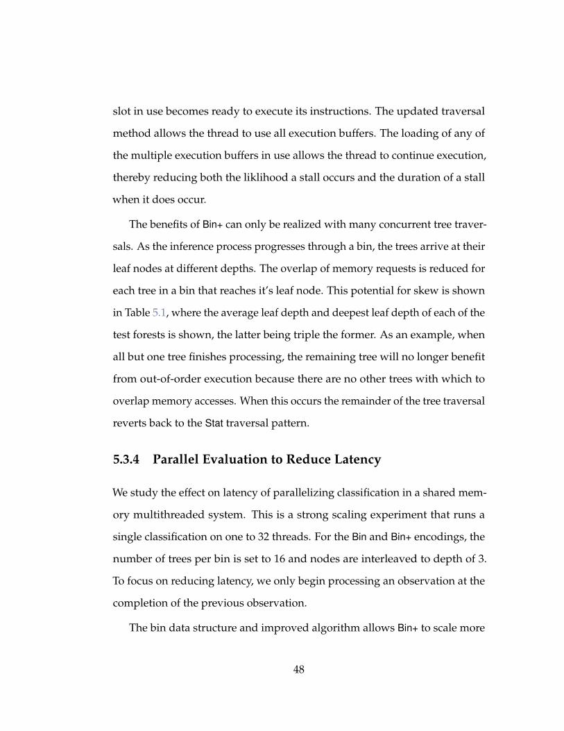
5.7 Inference throughput when varying number of trees in for-

est (defined above the chart) and tree depth. Forests were

created using the MNIST dataset. Experiment uses multiple

threads and batch size of 5000 where applicable. . . . . . . . . 52

6.1 Multicore performance comparing fastRF and fastRerF train-

ing times to those of popular decision forest variants. Forests

contain 96 trees. . . . . . . . . . . . . . . . . . . . . . . . . . . . 62

6.2 Multicore speed-up of fastRF and fastRerF compared with

other popular decision forest variants. Forests contain 96 trees. 63

6.3 Affect of number of classes in dataset on fastRF and fastR-

erF training times. 60000 observations, 1024 features, and 16

threads, 128 trees. . . . . . . . . . . . . . . . . . . . . . . . . . . 64

6.4 Affect of number of features in dataset on fastRF and fas-

tRerF training times. 60000 observations, 5 Classes, and 16

threads, 128 trees. All systems set to use√

d features at each

node. . . . . . . . . . . . . . . . . . . . . . . . . . . . . . . . . . 65

6.5 Affect of number of observations in dataset fastRF and fas-

tRerF training times. 60000 observations, 1024 features, and 16

threads, 128 trees. . . . . . . . . . . . . . . . . . . . . . . . . . . 66

xiv

6.6 Effects of subsampling size on training time. MNIST dataset,

128 trees. . . . . . . . . . . . . . . . . . . . . . . . . . . . . . . . 67

6.7 Effects of subsampling size on test set accuracy. MNIST dataset,

128 trees. . . . . . . . . . . . . . . . . . . . . . . . . . . . . . . . 68

6.8 Affects on training time of dynamically binning fastRF. MNIST

dataset. . . . . . . . . . . . . . . . . . . . . . . . . . . . . . . . . 69

6.9 Effects of dynamic binning on inference time. MNIST dataset. 70

xv

Chapter 1

Introduction

In order to leverage the growing amount of data being created today, re-

searchers are continuously developing machine learning techniques and sys-

tems to process data faster and better. For example, deep networks classify

gravitational waves more accurately and orders of magnitude faster than

matched filtering in LIGO simulations [1]. Using reinforcement learning to

drive parameter exploration has transformed mapping protein-ligand interac-

tions, reducing simulation time from hours to minutes [2]. On smaller scales,

suites of tools like Scikit-learn and MLkit provide scalable implementations

of many machine learning tools including neural nets, SVMs, and decision

forests [3, 4].

Decision forests are a popular group of ensemble machine learning tech-

niques which provide superior accuracy, interpretable models, and are robust

to parameter selection. It can be shown that decision forests are equivalent to

weighted nearest neighbor classifiers and, as such, continually improve with

additional training observations [5] and the use of multiple weak learners

further improves accuracy by reducing variance. Good results are normally

1

obtainable with default parameter settings, but, when optimized, decision

forests can provide state of the art accuracy which has made them a dominant

tool used to win multiple Kaggle competitions [6, 7]. Another positive as-

pect of decision forests are their easily interpreted and visualized dimension

partitioning hyper-planes [8].

Of the many decision forest variants, many prior works have shown that

oblique hyper-planes are capable of superior predictive performance [9, 10, 11,

12]. The non-axial splits of these forests are able to model the boundaries be-

tween classes more accurately, which allows them to perform better than other

forest variants. The drawback to these oblique forests are their long training

times. A recent framework — Oblique Sparse Projection Forests (OSPF) —

overcomes this limitation by using sparse oblique projections, thereby allow-

ing oblique forests to have computational complexities similar to other forest

variants.

This work explores the evolution of the first scalable OSPF implementation.

We start with a scalable system written in R, which suffered from poor training

and inference speeds. We describe and implement a post-training process to

reduce inference latency, call Forest Packing. And we finish with an OSPF that

rivals traditional forest training times, while simultaneously packing a forest

for reduced inference latency.

1.1 Random Forest IO

Decision tree variants all share the same slow IO bound properties, with

over 80% of typical implementation training time spent determining node

2

splits. Node splitting is a difficult task to optimize because of erratic memory

accesses compounded with runtime characteristics that change from the top of

the tree to the leaf nodes. We analyze several node splitting optimizations and

determine they are not practical for many oblique forest techniques including

OSPFs.

1.2 R-RerF

Breiman first hypothesized that oblique forests could provide superior infer-

ence as compared to forests relying solely on axial splits. Subsequent studies

have agreed with Breiman’s hypothesis, showing obliqe forests are capable

of outperforming the current state of the art on many datasets. Despite the

benefits, there was no scalable system that produces oblique forests. We cre-

ated R-RerF, an implementation of Randomer Forest in R, a scalable and easily

modifiable OSPF system and test it using several popular large datasets. R-

RerF training times are comparable to other forest variants, but is able to scale

more efficiently with additional resources. Two weaknesses are identified in

the system, which motivates the subsequent chapters.

1.3 Forest Packing

A negative aspect of decision forests, and an untenable property for many real

time applications, is their high inference latency caused by the combination

of large model sizes with random memory access patterns. We present mem-

ory packing techniques and a novel tree traversal method to overcome this

3

deficiency. The result of our system is a grouping of trees into a hierarchical

structure. At low levels, we pack the nodes of multiple trees into contiguous

memory blocks so that each memory access fetches data for multiple trees.

At higher levels, we use leaf cardinality to identify the most popular paths

through a tree and collocate those paths in contiguous cache lines. We extend

this layout with a re-ordering of the tree traversal algorithm to take advantage

of the increased memory throughput provided by out-of-order execution and

cache-line prefetching. Together, these optimizations increase the performance

and parallel scalability of classification in ensembles by a factor of ten over an

optimized C++ implementation and a popular R-language implementation.

1.4 Dynamic Forest Packing

The idea for most machine learning techniques is to train on a test set of

data once and perform inference on new data for the life time of the system.

There is often a disconnect between training a model and the ideal format

to use the model. For this reason there are several post training systems

which will rearrange a decision forest model to optimize the inference stage

of the models use [13, 14, 15]. These optimizations can perform inference

an order of magnitude or more faster than naive models. We show that we

can pack the nodes of a decision forest during model training in a manner

that optimizes inference with minimal effect on training times. The resulting

system uses the OSPF framework to quickly train oblique forests, packs nodes

for fast inference speeds, and provides extensibility for future sparse forest

implementations.

4

1.5 List of contributions

This work explores techniques to overcome the poor computational prop-

erties of oblique forest ensembles and extends the findings to improve the

performance of a well performing but, until now, poorly scaling machine

learning class, oblique decision forests. We show that oblique forests using

sparse projections, OSPFs, are similar to the training times and scalability

of other forest variants and provide the system through CRAN. Traditional

optimizations are incompatible with oblique forests including OSPFs so we

provide several forest optimizations that reduce IO and greatly improve the

scalability of these oblique forests. We describe and implement Forest Packing,

a post processing method that re-arranges forest models to greatly reduce

inference latencies. We describe a method to grow forests so the resulting

forest models closely conform to the models produced via Forest Packing post

processing. Together these contributions result in the creation of fastRerF, an

OSPF with training speeds and inference latencies superior to the current state

of the art.

5

Chapter 2

Background

Forest ensemble training and use have several inherent challenges that limit

the practical dataset size used to create a model. The choice of specific en-

sembles, such as the focus of this document on supervised sparse projection

forests, further exacerbates these challenges. This chapter briefly describes the

following: decision forest overview, the general training and inference algo-

rithms used by these ensembles, and the data access pattern design choices

typical of these algorithms.

2.1 Decision Trees

A decision tree is a collection of hyperplanes that partition a dataset into

informative cells. The root of each tree symbolizes the whole of the training

set and each subsequent level of the tree is a partitioning of the data into

subsets. Leaf nodes represent cells in the dataset space where observations

have similar properties. The properties of unlabeled data can then be inferred

by traversing the observation from root to leaf and assuming properties are

6

shared among all observations in the leaf node.

2.2 Decision Forests

Decision Forests are a popular category of machine learning techniques, pop-

ular for their discriminating properties and natural extensions. These forests

are composed of multiple decision trees each of which contribute to the in-

ference provided by the model. By combining these multiple weak learners,

the forests are able to reduce inference variance without affecting model bias.

Devroye and Gyiorfi show the isometry of Random Forests with nearest neigh-

bor classification, a universally consistent classifier [16]. Simple extensions

of the forest ensembles can provide popular machine learning goals such as

feature importance, model accuracy estimates, regression, nearest neighbor

search, unsupervised Learning, and many others [10, 8]

2.2.1 Forest Growing

Forest models consist of one or more decision trees, which are independently

grown from their roots to their leaves in a recursive process. Although the

process itself is independent, initial input of a tree can be influenced by

previously grown trees and a tree’s output may be considered by subsequent

trees [17].

2.2.2 Inference

The purpose of a supervised decision forest is to infer properties of obser-

vations not present in the training set. It is assumed that the properties of

7

a new observation will be similar to the closest observations in the training

set. The nearest neighbors of an observation are determined by traversing

the observation through a decision tree from the root to a leaf, where, either

the nearest neighbor indices or their properties are stored. This work only

considers classification forests which store class labels in leaf nodes. A forest

uses multiple decision trees and combines their predictions to come up with

an overall prediction.

2.3 Forest Variants

The many decision forest variants typically differ by input — how to populate

the root node, splitting criteria — how to determine the best split at each

node, and stopping criteria — when to make an internal node a leaf. Random

Forests and Boosted Forests are popular variants with many implementations

[6, 7, 18, 19, 3]. Oblique forests are a less studied and used variant lauded for

providing superior class discrimination, but has no scalable implementation.

2.3.1 Random Forest

Random Forest is the prototypical forest variant first described by Leo Breiman

in 1999 [10]. Independent decision trees are grown with multiple forms of

randomness in order to de-correlate trees, leading to a lower variance in

predictions. The first form of randomness comes from bagging where each

tree is grown with a subset of the N training observations. The second form

of randomness comes from choosing a random subset of features to explore at

each node. The feature used to split a node and the value at which to split is

8

chosen by the minimization of impurity or the maximization of information

gain. When performing inference on a test observation, each individual tree

infers a class label for the observation and the final prediction is the class that

receives a plurality of votes.

2.3.2 Boosted Forests

Boosted forests consist of sequentially grown trees where each subsequent

tree learns from the error induced by the previously grown tree. There are

two main types of boosted forest: Adaptive and Gradient. Adaptive boosted

forests give more credence to trees that do well on held out samples and

is more likely to use mislabeled data in subsequent tree growing iterations.

Gradient boosted forests use the prediction error of all observations in the

current tree to refine predictions of the subsequent tree. Inference in boosted

forests is performed by summing the predictions of all trees rather than using

the plurality vote used by many forest variants. This forest variant is popular

due to its accuracy and efficient training implementations.

2.3.3 Oblique Forests

Oblique forests consist of decision trees that create non axis aligned splits.

Compared to axis split decision forests, forests using oblique splits are capable

of better defining class boundaries, resulting in superior inference perfor-

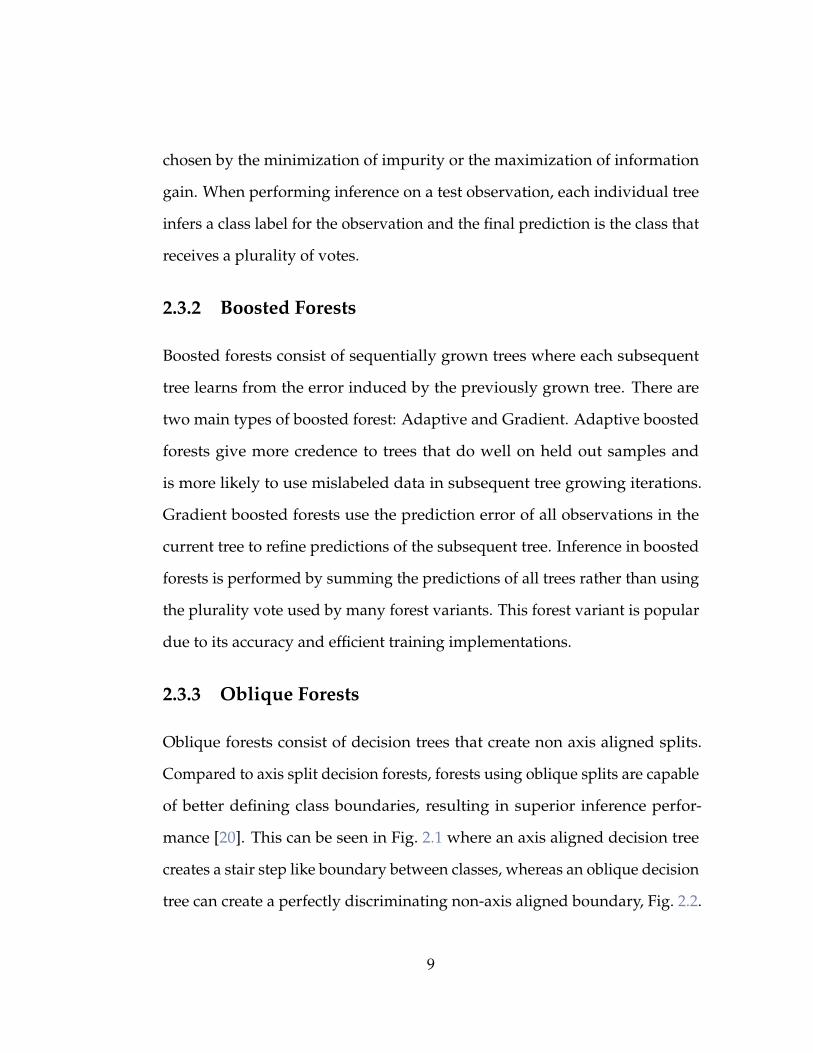
mance [20]. This can be seen in Fig. 2.1 where an axis aligned decision tree

creates a stair step like boundary between classes, whereas an oblique decision

tree can create a perfectly discriminating non-axis aligned boundary, Fig. 2.2.

9

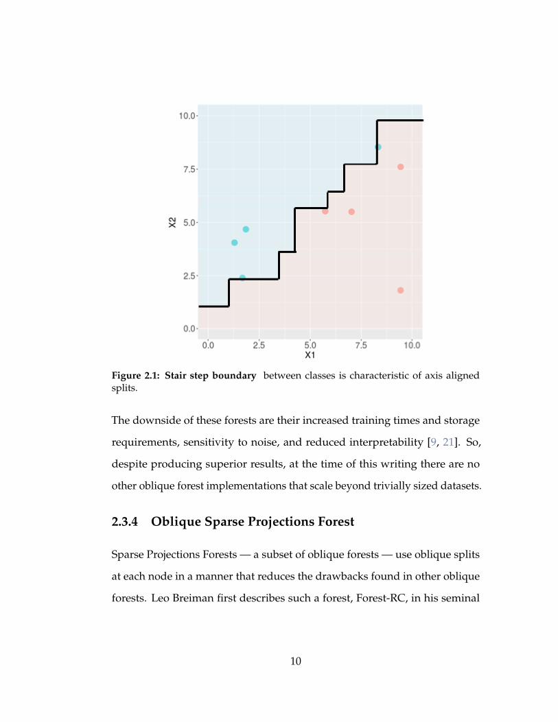
Figure 2.1: Stair step boundary between classes is characteristic of axis alignedsplits.

The downside of these forests are their increased training times and storage

requirements, sensitivity to noise, and reduced interpretability [9, 21]. So,

despite producing superior results, at the time of this writing there are no

other oblique forest implementations that scale beyond trivially sized datasets.

2.3.4 Oblique Sparse Projections Forest

Sparse Projections Forests — a subset of oblique forests — use oblique splits

at each node in a manner that reduces the drawbacks found in other oblique

forests. Leo Breiman first describes such a forest, Forest-RC, in his seminal

10

work on Random Forests [10]. The sparse projections of Forest-RC are cre-

ated by linearly combining multiple weighted features to create a single new

feature. Many of these features are created at each node and searched for an

impurity minimizing split.

Randomer Forest (RerF) is an oblique sparse projection forest that limits

feature weights to +1 and −1 resulting in d! possible feature combinations,

where d is the number of features in a dataset. Using sparse projections, rather

than completely rotated data, allows RerF to reduce training times, sensitivity

to noise, and model complexity as compared to other oblique techniques. RerF

outperforms other forest variants including Random Forest, XGBoost, and

Random-Rotation Random Forests on a large proportion of the UCI datasets

[22].

2.4 Discussion

Decision forests are a broad class of robust machine learning algorithms com-

posed of ensembles of weak learners. Two of the most widely used and

studied variants are Random Forests and gradient boosted forests. Another

variant, oblique forests, provides class discrimination superior to other deci-

sion forests. Despite this highly beneficial quality, oblique forests have not

been widely adopted and there are currently no implementations that scale

beyond small datasets.

11

Figure 2.2: Sparse Oblique boundary is able to better discriminate between classboundaries.

12

Chapter 3

Decision Forest IO

The random nature of decision forests and their applicability to many dataset

types makes optimization difficult. Often, optimizing techniques will benefit

node splitting either near the tops of trees or for nodes near the base of

trees, but not both. We detail here the various methods to grow trees and

their implications on memory use and processing time. Several methods to

accelerate forest growing are described, followed by a discussion on why

these methods are incompatible with oblique sparse projection forests.

3.1 Memory Access Patterns of Random Forests

3.1.1 Node Processing Order

There are two methods to recursively grow a tree structure: breadth first

and depth first. In breadth first traversal, all nodes at level L are processed

before processing any nodes at level L + 1. This requires the storage of 2L

unprocessed nodes at each level, with a maximum of 2D nodes at maximum

depth D. The use of breadth first traversal when growing forests is widely

13

recommended [23, 8, 24] because it allows for several space-time trade-off

optimizations, see 3.3.

In depth first traversal, child nodes are placed on a stack as they are created.

Nodes are popped from the stack and processed, either placing resulting child

nodes on the stack or creating new leaf nodes. This method requires the

storage of at most D unprocessed nodes at any time. Depth first traversal

requires less memory than breadth first traversal.

3.1.2 Data Traversal: Training

Data consisting of N observations each with d features is an Nxd structure,

stored in memory either in row major or column major formats. Each of the N

observations are placed contiguously in memory when using the row major

format. This format is useful when multiple features in a single observation

are accessed closely in time. This is contrasted by the column major format,

which stores each of the d features contiguously, a useful method when the

same feature in multiple observations are accessed closely in time.

The choice of which format to prefer depends on a system’s cache size

and the algorithm’s data access pattern. In Random Forest, when N is large,

typically near the top of a tree, it is beneficial to use the column major for-

mat, where N is the number of observations in a node. As tree growing

progresses, N shrinks and the row major format becomes preferable. This

switch over occurs when cache pollution is unlikely to evict required data

(N × cachelinesize < cachesize) and when a cache load is likely to fetch multi-

ple useful data elements (N/N < mtry/d).

14

3.1.3 Data Traversal: Inference

Like training data, the data presented to a decision forest model for clas-

sification can be formatted in either row major — where an observation’s

features are contiguous in memory — or column major — where features

are stored contiguously. The choice of which to use depends on whether

inference is performed on individual observations or on multiple observations

in a batch. The row major format is preferable when performing inference

on single observations because each cache line request of the inference data

provides data potentially useful by subsequently traversed nodes in the forest.

This is contrasted by column major storage where each cache line request is

only guaranteed to provide one useful data element and all other elements in

the remainder of the cache line will be cache pollution. Contrarily, batched

processing can benefit from a column major formatting because, at each node,

a single feature of multiple observations is tested, allowing a single cache

line request to potentially load multiple useful data elements. When batching

inferences a row major format guarantees a load of one useful element and

multiple cache pollution elements.

3.2 Multithreaded Forest Training

There are multiple locations within the decision forest training process where

multiple threads can be used to accelerate training. The most fine grained

parallelism will process each feature using multiple threads to find the best

split. Both the sorting and best split searching sub-tasks are cache efficient

and not easily divisible, so neither would benefit from multithreading. In the

15

case where histogram bins are well defined, multiple threads could populate

thread specific bins — a slow random read process — then merge bin tallies

with other threads prior to the exhaustive split search sub-task. This form of

parallelism is typical of histogram accelerated decision forests.

Another location within the forest training process where multiple threads

could be employed is over each of the mtry features in a node. This method

would be inefficient when mtry is less than the number of threads and when N

is small because little work would be done by each thread. A third location for

parallelism is at each node. This form of parallelism is easily implemented but

is inefficient when the number of nodes waiting to be processed is less than

the number of threads (i.e. at the tops of trees) and when N is small because

little work would be done by each thread. The final location to perform

parallelism is at the tree level, where a single thread processes an entire tree.

This method duplicates all tree growing structures, thereby resulting in a

per thread O(N) memory increase roughly equivalent to the size of a single

feature. This method is also inefficient when the number of trees to process is

less than the available number of threads.

3.3 Decision Forest Training Acceleration

Testing shows many forest implementations spend greater than 80% of forest

growing time determining the cut feature and cut value for each node, making

this sub-task the target for most optimizations in decision forest systems. The

most simplest way to reduce node splitting time is using hyper-parameter

selection to reduce the number of nodes a tree creates or reduce the number

16

of features explored at each node. Three parameters are typically available in

decision forests to reduce the number of nodes created in each tree: minimum

parent size, maximum depth, and maximum number of nodes. There is

also a parameter to change the number of features explored at each node,

mtry, which ranges from 1 to d, where d is the number of features in a dataset.

Reducing training time through parameter selection can reduce model efficacy,

so it is important to make the node splitting function, see Alg. 1, as efficient as

possible.

The sub-tasks of the node split algorithm, Alg. 1, which require the most

time are: feature loading (line 6), feature sorting (line 7), and the exhaustive

split search (line 8). The complexities of these sub-tasks are respectively O(N),

O(Nlog((N)), and O(NC, where C is the number of unique labels in the

dataset. Run time analysis shows each of the sub-tasks take nearly the same

operating time despite the range of complexities.

3.3.1 Feature Loading Optimization

Feature loading consists of loading the target feature from each of a node’s N

resident observations into a temporary vector. This is an inherently inefficient

gather operation, which suffers from cache misses due to the random memory

reads induced by the splitting of observations at each node. Thus, at the top

of a tree each gather operation tends to be efficient because the bagging of

observations results in roughly 63% of the training set observations being

resident in the root node. The efficiency at this level of a tree is realized

because each cache load is likely to result in multiple cache hits. At each level

17

Algorithm 1 Basic Find Best Split Location

1: ▷ n: a set of observations2: ▷ mtry: the number of features to consider for each split3: procedure FIND BEST SPLIT(n)4: test f eatures← randomly select mtry features to test5: for all i in testFeatures do6: load all ni into tempFeature vector7: sort(tempFeature)8: splitIn f o ← exhaustiveSplitSeach(tempFeature)9: if splitIn f o.Score > bestSplit.Score then

10: bestSplit.Score← splitIn f o.Score11: bestSplit.Feature← i12: bestSplit.Value← splitIn f o.Value13: end if14: end for15: return bestSplit16: end procedure

of the tree, N is reduced by half, which reduces the chance the loading of a

feature into cache will result in subsequent cache hits.

The typical means to accelerate the feature loading sub-task is through

software prefetching. Modern Processors perform hardware prefetching when

memory accesses form a simple pattern (e.g. loading every fourth memory

location) and so is unlikely to be triggered when training forests due to the

random splitting of observations. The software prefetcher is able to inform

the processor to load memory locations regardless of access pattern, thereby

reducing the load latency that would otherwise be experienced.

3.3.2 Sorting Optimization

Feature sorting entails sorting a vector of feature values while maintaining

a mapping between each observation’s feature value and class label. The

18

typical alternative to per node feature sorting is to sort all features prior

to forest training, maintaining a two way mapping between feature values

and observation indices, and rearranging the training data in memory as

observations are split between children nodes [25, 19]. In addition to removing

the need to sort, this technique also removes the need to gather feature values

at each node. The algorithm instead searches for the best split point by

streaming over each of the mtry features. The downside of this method is

a large memory footprint and the need to relocate observations in memory

after each node split, which requires accessing every feature of every resident

observation in a random manner. The number of memory accesses grows

linearly with d, the number of features in a dataset, irrespective of hyper-

parameter settings.

Another method to remove per node sorting is to define sorted accumula-

tion bins. Some systems define bins based on the unique values of each feature

[18], whereas other systems implement a histogram method [6], or a similar

reduced precision method [7]. The predefinition of the number and size of

bins is a trade-off between processing time and best split accuracy. When

using bins, the gathering step of the splitting function changes to incrementing

a bin’s tally when its specific feature value is encountered. An added benefit

of this technique is the possible reduction of split locations when the number

of bins is smaller than N. A downside of this method is the increase of split

locations when the number of bins is greater than N.

Each of these binning optimizations requires increased memory usage due

to the storage of bin properties and mappings between features and bins. In

19

addition, the determination of value to bin can become a costly function due

to a random read pattern.

3.3.3 Split Search Optimization

The exhaustive search for an optimal split entails traversing the ordered

feature vector from least to greatest value and calculating the impurity of

each side assuming all values less than the current traversal location would

go to the left node and all greater values would go to the right node. Splits

between equal feature values are not possible and need not be considered.

Thus a weighted bin for each unique feature value reduces the possible split

points from N to U, where U is the number of unique feature values. This

is beneficial when U is less than N and detrimental otherwise. When using

histogram bins split are only possible between bins. This reduces the required

search space, but, as a heuristic method, does not guarantee the best possible

split and so may affect model efficacy.

3.4 Conclusion

Decision Forests algorithms are difficult to efficiently process because the

random IO of the algorithm is a product of the random splits that occur in

each node of the forest. Optimizations in sorting and searching have been

developed to minimize this lack of cache coherence, but are not practical for

sparse projection forests. For OSPFs to realize the gains of these optimizations

all potential oblique features would need to be materialized, which is unfeasi-

ble. Thus, implementations of oblique sparse projection forests cannot rely on

20

many of the optimizations employed by axis aligned forests.

21

Chapter 4

R-RerF

4.1 Introduction

Randomer Forest (RerF) is a recently conceived decision forest variant with

superior accuracy and complexities, both training and inference, similar to

those of Random Forest. RerF and Random forest are both considered sparse

random projection forests. The algorithms differ by their choice of sparse

projections, Random Forest node splitting only considers very sparse pro-

jections, whereas RerF node splitting also considers linear combinations of

sparse projections.

At each node in a Random Forest a random subset of features are exhaus-

tively tested to determine which feature and cut value minimizes impurity

when resident observations are split into two subsets. When class boundaries

are not axis aligned this splitting method potentially leads to deep trees, in-

creased variance, and over-fitting. This is contrasted by RerF, which, considers

oblique features created by linearly combining multiple features in addition

to the axial splits considered by Random Forest.

22

We implement R-RerF in the R programming language using the Oblique

Sparse Projection Forest (OSPF) framework. Including this framework in the

system allows for easy extension of R-RerF to other oblique sparse projection

forests.

4.2 R-RerF Implementation

RerF was originally implemented in matlab and was ported to R in order to

increase speed and flexibility. This new system was branded R-RerF. Accel-

eration of R-RerF was accomplished through multithreading and execution

analysis. Multithreading in R is realized by forking the R process, which

limits the fine grained interactions possible with threads. To overcome this

limitation, R-RerF processes a single tree per forked process, thereby trading

memory efficiency for processing efficiency. Execution profiling was used

to further improve processing efficiency, helping us avoid slow R functions

and identifying the slowest portions of our system: sorting and split finding.

We were unable to improve upon R’s c++ optimized quick sort function. The

splitting function was rewritten in C++, but still remained our function with

the highest execution time.

Writing the code in R allowed for quick modification and testing of im-

plementation details and allowed for custom tailoring of the algorithm to

suit novel problems. To accomplish this level of extensibility required two

key insights. First, we realized that the rotation of training data need not be

completely materialized, instead the sparse projections can be materialized

as needed in a computationally efficient sparse vector multiplication. The

23

second realization was that by allowing a data scientist to provide their own

sparse rotation matrix would allow for easily implementable data specific

custom projections. Thus, at the core of R-RerF’s novelty is a sparse projection

matrix which efficiently rotates the data at each node to increase the number

of potential split features, thereby facilitating the rapid integration of other

forest variants such as patch detectors, random forest, Random Rotation Ran-

dom Forest, and Forest-RC. This ease of code manipulation coupled with

the package management system provided in R, CRAN, minimizes the effort

required by data scientists to use and contribute to the system.

4.3 System Complexity

The complexity of a system shows how a runtime characteristic of an algorithm

changes with input size.

4.3.1 Theoretical Time Complexity

The time complexity of an algorithm characterizes how the theoretical pro-

cessing time for a given input relies on both the hyper-parameters of the

algorithm and the characteristics of the input. Let T be the number of trees, N

the number of training samples, d the number of features in the training data,

and mtry the number of features sampled at each split node. The average

case time complexity of constructing a Random Forest is O(mtryTN log2 N)

[24]. The mtryN log N accounts for the sorting of mtry features at each node.

The additional log N accounts for both the reduction in node size at lower

24

levels of the tree and the average number of nodes produced. Random For-

est’s near linear complexity shows that a good implementation will scale

nicely with large input sizes, making it a suitable algorithm to process big

data. RerF’s average case time complexity is similar to Random Forest’s, the

only difference being the addition of a term representing a sparse matrix

multiplication which is required in each node. This makes RerF’s complexity

O(mtryT log N(N log N + λd)), where λ is the fraction of nonzeros in the

d×mtry random projection matrix. We generally let λ be close to 1/d, giving

a complexity of O(mtryTN log2 N), which is the same as for Random Forest.

Of note, in Random Forest mtry is constrained to be no greater than d, the

dimensionality of the data. RerF, on the other hand, does not have this restric-

tion on mtry. Therefore, if mtry is selected to be greater than d, RerF may take

longer to train. However, mtry > d often results in improved classification

performance.

4.3.2 Theoretical Space Complexity

The space complexity of an algorithm describes how the theoretical maximum

memory usage during runtime scales with the inputs and hyperparameters.

Let C be the number of classes and T, d, and N be defined as in Section

4.3.1. Building a single tree requires the data matrix to be kept in memory,

which is O(Nd). During an attempt to split a node, two C-length arrays

store the counts of each class to the left and to the right of the candidate

split point. These arrays are used to evaluate the decrease in Gini impurity

or entropy. Additionally, a series of random sparse projection vectors are

25

sequentially assessed. Each vector has less than d nonzeros. Therefore this

term is dominated by the Nd term. Assuming trees are fully grown, meaning

each leaf node contains a single data point, the tree has 2N nodes in total. This

term gets dominated by the Nd term as well. Therefore, the space complexity

to build a RerF model is O(T(Nd + C)). This is the same as that of Random

Forest.

4.3.3 Theoretical Storage Complexity

We define storage complexity as the dependency of disk space required to

store a forest on the inputs and hyperparameters. Assume that trees are fully

grown. For each leaf node, only the class label of the training data point

contained within the node is stored, which is O(1). For each split node, the

split dimension index and threshold are stored, which are also both O(1).

Therefore, the storage complexity of a RF is O(TN).

For RerF, the only aspect that differs is that a (sparse) vector projection

along which to split is stored at each split node rather than a single split

dimension index. Let z denote the number of nonzero entries in a vector

projection stored at each split node. Storage of this vector at each split node

requires O(z) memory. Therefore the storage complexity of a RerF model

is O(TNz). z is a random variable whose prior is governed by λ, which is

typically set to 1/d. The posterior mean of z is determined also by the data;

empirically it is close to z = 1. Therefore, in practice, the storage complexity

of RerF is close to that of Random Forest.

26

4.4 Experimental Results

The performance of decision tree implementations typically entail a thorough

exploration of accuracy – how well models classify test data – and training

times; inference speed is another important measure but is not commonly

discussed for many popular systems. The measure of performance used here

is training time, scalability, and inference throughput; system performance

as it relates to accuracy can be found in other RerF literature [22]. We test

our system with three datasets commonly used to measure training time

performance: MNIST consists of 60000 images of digits (0-9) each containing

784 features; Higgs consists of 250,000 observations of two classes, either

signal or background, each containing 28 features; and p53 consists of 16,772

observations of protein mutations, either active or inactive, each containing

5409 features. We compare our system to what we consider the most popular

decision forest implementation, XGBoost, and the fastest Random Forest

implementation, Ranger. All experiments were run on a 64-bit Ubuntu 16.04

platform with four Intel Xeon E7-4860V2 2.6 GHz processors, with 1TB RAM.

Initially it was assumed that an implementation primarily written in R

would be significantly slower than its C++ counterparts. Surprisingly, R-RerF

outperformed XGBoost in two of three experiments, Fig. 4.1. R-RerF performs

worst on Higgs, the largest dataset, because the size of resulting trees in R

combined with memory inefficiencies inherent in R exacerbates the memory

bottleneck. As resources are added, the additional cache and separation of

growing trees into separate processes allows R-RerF to more efficiently use

memory resulting in improved scalability on the Higgs dataset, Fig. 4.2.

27

When performing inference, R-RerF batches test observations in order to

accelerate the process. Batching allows for a regular traversal of trees and

multiple reuse of fetched memory. This inference technique is found in most

decision forest implementations including Ranger and XGBoost. It can be seen

in Fig. 4.3 that R-RerF’s inference speed is far slower than XGBoost. R-RerF’s

inference speed is slow when compared to traditional decision forests because

determining a traversal path requires combining multiple features, requiring

an additional memory indirection. Despite this penalty, R-RerF is still able to

outperform Ranger in two out of three tests.

4.5 Conclusion

R-RerF is the first scalable and easily accessible, via CRAN, oblique forest

implementation. The system provides state of the art discriminating perfor-

mance and scales well with additional resources. In addition, because it is

written in R, R-RerF can easily be tailored to a given dataset through its use

of an easily modifiable sparse projection matrix or by taking advantage of

R packages of popular enhancements such as external memory, distributed

computing, or sparse processing. Unfortunately, R-RerF suffers from a large

memory footprint, poor single core performance, large model size, and poor

inference speeds; deficiencies we address in subsequent chapters. Despite

these shortcomings R-RerF’s performance remains competitive with other

highly optimized decision forest variants.

28

Figure 4.1: R-RerF Training Time as a function of cores used as compared to similarsystems. Three datasets were used: MNIST, Higgs, and p53.

29

Figure 4.2: R-RerF Strong Scaling compared to similar systems. Three datasets wereused: MNIST, Higgs, and p53.

30

Figure 4.3: R-RerF Inference Times on hold-out test observations compared to simi-lar systems. Test set sizes: Higgs 25,000; MNIST 10,000; p53 400.

31

Chapter 5

Forest Packing

5.1 Introduction

R-RerF was the first scalable oblique forest system, but the implementation

suffered because of high latency and low throughput inferences, Ref. 4. This

poor inference speed, particularly latency, is endemic to decision forests and

thus makes the systems unusable for many real-time applications such as

computer vision and spam detection. Poor inference speeds are caused by

the combination of large model sizes combined with random memory access

patterns. As an ensemble classifier, decision forests are composed of many

weak classifiers, each of which may have a size on order with the training set,

leading to a large overall memory footprint. When the model size is larger

than a system’s cache, typically KBytes for fast cache and low MBytes for slow

cache, the inference operation relies on the order of magnitude slower main

memory. The paths through a decision forest are purposefully uncorrelated,

which leads to random accesses throughout the model for each inference task,

making common acceleration tools—such as GPUs—unusable for general

32

forest inference.

Decision forest research typically focuses on model training systems with-

out mention of run time operation. Application of these powerful tools is

hindered by this oversight, which has lead to increased research into forest

inference acceleration and development of several third-party post training

optimizations [14, 15]. Current solutions either place structure limiting re-

quirements on the forests, e.g. maximum node depth, or focus on increas-

ing throughput at the cost of increased inference latency, e.g. batching. The

method described here, Forest Packing, extends previous research on this topic

by introducing several tree storage memory optimizations and a reordering of

the tree traversal process to take advantage of modern CPU enhancements.

5.2 Methods and Technical Solutions

Attempts to increase the speed of decision forest inference falls into two cate-

gories: memory access optimizations and inference algorithm modifications.

Our proposed improvement to forest based inference, Forest Packing, takes

advantage of both improvement types. We use inference latency, specifically

classification latency, to indicate model performance (training time is a popu-

lar complementary topic that we do not consider here). Other decision forest

variants such as regression or distance learning forests are not specifically

discussed here, but the techniques we describe should extend to these tools.

The input to forest packing is a trained forest, F, that consists of decision trees,

t. Each internal node of the trees describes a splitting condition on the data

and has two children. Each leaf node contains a single class label; a criteria

33

typical of random forests [10, 26], but not true for all variants. One of the

novel optimizations that we present relies on the single class assumption.

Forest Packing, the system presented here, reorganizes the trees in a forest

to minimize cache misses, allow for use of modern CPU capabilities, and

improve parallel scalability. The system outputs ⌈T/B⌉ bins, where T is the

number of trees in the forest and B is the bin size—a user provided parameter

defining the number of trees in a bin. A bin is a grouping of at most B trees

into a contiguous memory structure. Most bins will contain B trees while

one bin may contain between 1 and B-1 trees. Within each bin, we interleave

low-level nodes of multiple trees to realize memory parallelism in each cache

line access. We decrease cache misses by using split cardinality information to

store popular paths contiguously in memory. During inference, each bin is

assigned to an OpenMP thread (for shared memory). Forest packing includes

a runtime system that prefetches data and evaluates tree nodes out-of-order

as data is ready, leveraging the memory layout to maximize performance.

5.2.1 Memory Layout Optimization

We describe our memory layout as a progression of improvements over the

breadth-first layout, BF, typically used in random forests, with each improve-

ment reducing cache misses or encoding parallelism. Fig. 5.1 describes this

evolution with each panel displaying a tree in which the nodes are numbered

breadth-first and the resulting layout in memory is shown as an array at the

bottom of the panel. Breadth-first layouts are typical in decision forests be-

cause they provide the sequential traversal through all nodes used by batched

34

inference processing. The depth-first (DF) layout is preferred for single ob-

servation inference because it allows for the possible reuse of a memory load.

We will use aspects of both breadth- and depth-first layouts in our ultimate

design.

Figure 5.1: The representation of trees as arrays of nodes in memory for breadth-first (BF), depth-first (DF), depth-first with class nodes (DF-), statistically ordereddepth-first with leaf nodes replaced by class nodes (Stat), and root nodes interleavedamong multiple trees (Bin). Colors denote order of processing, where like colors areplaced contiguously in memory.

Our first optimization reduces the duplication of information contained in

leaf nodes thereby reducing the number of nodes in the forest almost in half.

In many classification forest variants, each leaf node provides both a signal

that the tree traversal is complete and a class label determined during training

by the plurality observation class in a leaf node. Rather than pointing parent

nodes to their own unique children, parent nodes instead point to communal

35

leaf nodes which provide the functionality of a typical leaf node without the

duplication. We call this encoding DF-. We are unaware of other literature

recommending this encoding, which reduces the size of a tree from n nodes to

n/2 + C nodes, where C is the number of classes present in a dataset.

In most datasets, the number of distinct classes are many orders of magni-

tude smaller than the number of nodes in the tree and so we expect the DF-

trees to be nearly half the size of DF trees. Removing these nodes has the dual

benefit of allowing more useful nodes to be loaded by each memory fetch (a

fact we exploit in the Stat layout) and also greatly reduces cache pollution. The

class nodes that replace leaf nodes are placed at the end of each tree’s block

of contiguous memory. The DF- panel of Fig. 5.1 shows the resulting layout

when building a decision tree for a two-class (α, β) problem. DF- indicates

depth-first with leaf nodes removed.

The next improvement encodes paths through trees sequentially in mem-

ory based on the number of observations used to create the nodes during

training. This statistical redefinition of the BF- layout is called Stat. We use

the leaf cardinalities collected during training to determine the likelihood

that any given data point routes to a specific leaf. If cardinality information

is unavailable, these statistics can be inferred after training using a suitably

large set of observations. We then enumerate depth first paths based on their

probability of access. The Stat panel of Fig. 5.1 illustrates this process with “+”

indicating a more likely path, leading to the decision to enumerate the path to

node 3 prior to node 4. The statistical ordering applies to nodes from the root

to the leaf parents, because class nodes that replace leaf nodes are at the end

36

of the block of memory and so are not considered for statistical ordering.

In more detail, Stat considers each parent node and its two children. The

child that is accessed most often is placed adjacent to the parent node in

memory while the less accessed child is placed later in the block of memory.

If a parent node has a leaf node child and an internal node child, the internal

child node is always placed adjacent to the parent while the leaf node is

shared among all leaf nodes of the same class at the end of the memory block.

Similar optimizations have been recommended in one form or another by

other researchers [27].

Our final memory optimization, Bin, interleaves the nodes of multiple trees

into a single block of memory, called a bin, to both reduce memory latency

and to allow for the encoding of parallel memory accesses. This layout takes

advantage of the fact that a parent node is accessed about twice as often as

each of it’s children and so nodes at lower levels of a tree are accessed far more

often then nodes at higher levels. This is similar to the hot (often used nodes)

and cold (rarely used nodes) memory model recommended by Chilimbi et al.

[28]. By interleaving the lower level nodes from multiple trees in a bin, we are

increasing the density of “likely to be used” nodes which allows a single cache

line fetch to be more useful while also reducing cache pollution. The Bin panel

of Fig. 5.1 shows the root (level 0) nodes interleaved in the layout and all higher

level nodes are stored one tree at a time using the Stat method. A similar

recommendation was proposed by Ren et al. where trees are interleaved by

level for the entirety of the tree [29]. In our testing, interleaving trees past a

certain depth results in an increase of inference latency, Fig. 5.2.

37

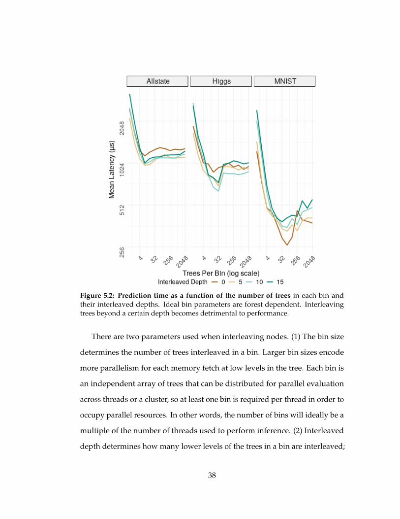
Figure 5.2: Prediction time as a function of the number of trees in each bin andtheir interleaved depths. Ideal bin parameters are forest dependent. Interleavingtrees beyond a certain depth becomes detrimental to performance.

There are two parameters used when interleaving nodes. (1) The bin size

determines the number of trees interleaved in a bin. Larger bin sizes encode

more parallelism for each memory fetch at low levels in the tree. Each bin is

an independent array of trees that can be distributed for parallel evaluation

across threads or a cluster, so at least one bin is required per thread in order to

occupy parallel resources. In other words, the number of bins will ideally be a

multiple of the number of threads used to perform inference. (2) Interleaved

depth determines how many lower levels of the trees in a bin are interleaved;

38

the remaining levels of each tree are stored according to the Stat encoding.

Interleaving too many levels results in breadth-first like behavior resulting in

degraded performance.

The Bin layout combines binned interleaving for the top levels of a tree

and statistical depth-first layout, Stat, for the bottom levels in a tree. A more

in depth example of this layout can be found in Fig. 5.3, which demonstrates

the layout for a forest of 4 trees and 3 classes with varying bin sizes and

depths interleaved. A design experiment helps choose the bin size that makes

sense in light of the properties of the processor memory hierarchy and forest

characteristics. Fig. 5.2 explores the effects bin size and interleaved depth

has on a trained forest. The figure displays average prediction time (lower is

better) for an observation given varying values of bin size. The characteristics

of the datasets and their resulting forests can be seen in Table 5.1.

Figure 5.3: Forest packing with the Bin memory layout given four trees and varyingsetting. We show different parameterizations of number of trees per bin and depth ofinterleaving. Colors of internal nodes denote node level in the tree. Levels Interleaveddenotes the highest level of each tree interleaved.

39

Table 5.1: Dataset and Resulting Forest Information

Allstate Higgs MNIST

Observations 500000 250000 60000Test Observations 50000 25000 10000Features in Dataset 33 30 784Trees in Forest 2048 2048 2048Internal Nodes (avg) 90020 23964 5008Avg Leaf Depth 25 21 17Deepest Leaf Depth 74 65 50

Fig. 5.4 shows performance comparisons between the memory optimiza-

tions described above. The first three performance improvements (DF, DF-,

and Stat) are purely reorganizations of nodes within memory. In addition to

reorganizing nodes, Bin groups trees into bins and interleaves the nodes of

trees within a bin.

5.2.2 Tree Traversal Modification

The inference algorithm includes the traversal of trees from root to leaf using

a path determined by a simple comparison of data stored in each node to

the test observation, Algorithm 2. The most common modification of this

traversal processes multiple test observations through a tree simultaneously in

batches. This optimization results in much higher throughput of classification

inference [15, 13]. Although groups of observations are processed faster, the

latency of each inference task is increased. Other methods have been used

to accelerate forest based inference using GPUs, SIMD operations, traversal

unrolling, and branch prediction [14, 15, 29]. Many of these optimizations

place restrictions on forest structure such as a maximum depth or require a

40

full tree [30].

The binned forest memory optimization, Bin, described in 5.2.1 allows us

to efficiently modify the processing order of trees (Algorithm 3) to simulta-

neously traverse multiple trees in a manner that takes advantage of modern

CPU enhancements while also allowing us to use intra-observation threaded

parallelism. Forest Packing, our acceleration technique, is the use of the culmi-

nation of memory improvements, Bin, with this efficient tree traversal method

described below. For brevity, we will refer to Forest Packing, the combination

of memory improvements and efficient tree traversal, as Bin+.

Our binning strategy adds an additional layer of hierarchy within the

forest (i.e. the bins) which provides for multiple levels of parallelism. The first

level of parallelism, inter-bin parallelism, takes advantage of the embarrass-

ingly parallel nature of trees, allowing each bin to be processed by a thread

independent of work done in other bins. This form of parallelism was always

available within forests using individual trees rather than bins.

Intra-bin parallelism realizes performance improvements through fine-

grained, low-level prefetching and scheduling provided inherently in modern

CPUs. Bin+ takes advantage of this capability by evaluating all trees in a

bin using a round-robin order, thereby giving a single thread additional

non-blocking avenues of work. This has the dual benefit of using more of

each thread’s processing capability and gives us an opportunity to explicitly

prefetch the upcoming node prior to it being required (line 17, Algorithm 3).

We use simple policies to encode execution overlap because more complex

policies incur scheduling overheads that exceed gains. Overlap happens

41

Algorithm 2 Single Tree Traversal

1: procedure TREEPREDICTION(t, o[])2: ▷ Tree, t, an array of nodes3: cn← 0 ▷ start at tree root4: while t[cn] is internal node do5: ▷ get split feature of node cn6: s f ← t[cn].splitFeature7: ▷ compare observation’s feature to split value8: if o[s f ] < t[cn].splitValue then9: cn← t[cn].le f tChild

10: else11: cn← t[cn].rightChild12: end if13: end while14: return t[cn].classNumber15: end procedure

among tens of memory accesses and hundreds to thousands of instructions.

Trying to control this fine-grained process in software is not practical. Instead,

we assign a single thread to each interleaved bin which evaluates the bin’s

trees in round-robin order. For each node that we evaluate, we issue a prefetch

instruction for the memory address of the resulting child node, with the idea

that useful work from other trees can be performed while the resulting child

node is being loaded into cache. We proceed navigating through the levels

of the tree in the same order that we processed the root nodes. This round-

robin scheduling submits independent instructions for each tree. In practice,

the processor executes these independent instructions out-of-order as data

becomes available.

42

5.3 Empirical Evaluation

We evaluate Forest Packing in order to quantify the benefits from memory

layout and scheduling optimizations. We start with a breakdown of the

contributions of each optimization, applying them incrementally. An overview

experiment using CPU performance counters demonstrates the improvement

of Forest Packing versus other layouts. We explore the scalability of each of

the optimizations across a shared-memory multithread system to minimize

inference latency. We finish our evaluation by comparing the inference latency

of Forest Packing to two commonly used forest systems.

5.3.1 Experimental Setup

We implement all of the optimizations described in Section 5.2 and apply

them successively. We start with BF as our baseline implementation because

it performs similarly to a popular decision forest implementation, XGBoost.

Thus, comparative evaluations are against our re-implementation, BF. We

focus on standard decision forests that create deep trees with a single class per

leaf node. We infer the class of each test observation sequentially, only starting

the inference of an observation at the completion of the previous observation

in order to measure test latency.

All experiments were run on a 64-bit Ubuntu 16.04 platform with four Intel

Xeon E7-4860V2 2.6 GHz processors, with 1TB RAM. gcc 5.4.1 compiled the

project using -fopenmp, -O3, and -ffast-math compiler flags.

We perform all experiments against three common machine-learning

datasets that are widely used in competitions and benchmarks. Training

43

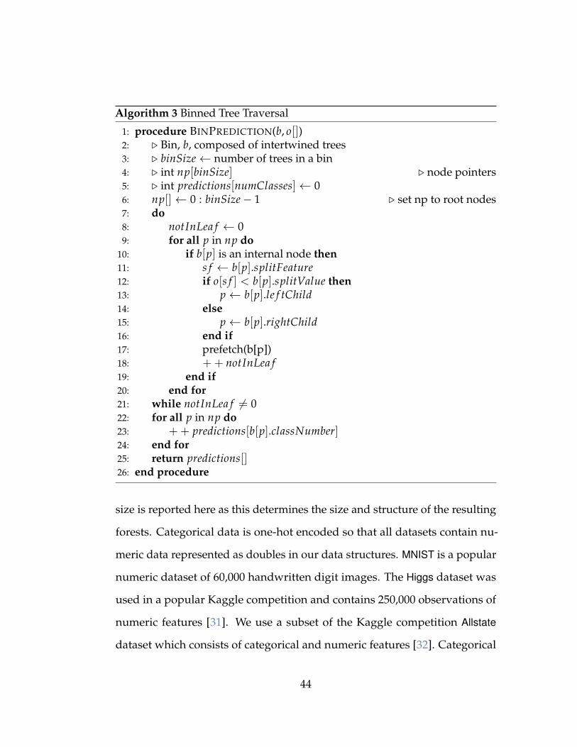
Algorithm 3 Binned Tree Traversal

1: procedure BINPREDICTION(b, o[])2: ▷ Bin, b, composed of intertwined trees3: ▷ binSize← number of trees in a bin4: ▷ int np[binSize] ▷ node pointers5: ▷ int predictions[numClasses]← 06: np[]← 0 : binSize− 1 ▷ set np to root nodes7: do8: notInLea f ← 09: for all p in np do

10: if b[p] is an internal node then11: s f ← b[p].splitFeature12: if o[s f ] < b[p].splitValue then13: p← b[p].le f tChild14: else15: p← b[p].rightChild16: end if17: prefetch(b[p])18: ++ notInLea f19: end if20: end for21: while notInLea f = 022: for all p in np do23: ++ predictions[b[p].classNumber]24: end for25: return predictions[]26: end procedure

size is reported here as this determines the size and structure of the resulting

forests. Categorical data is one-hot encoded so that all datasets contain nu-

meric data represented as doubles in our data structures. MNIST is a popular

numeric dataset of 60,000 handwritten digit images. The Higgs dataset was

used in a popular Kaggle competition and contains 250,000 observations of

numeric features [31]. We use a subset of the Kaggle competition Allstate

dataset which consists of categorical and numeric features [32]. Categorical

44

features are converted to numeric features by the forest growing system (RerF

or XGBoost). The principles shown are independent of the system used to

grow the forest, but for benchmarking purposes RerF is used to create our

forests which are then post-processed into packed forests. Further information

about these datasets and resulting trained forests can be found in Table 5.1.

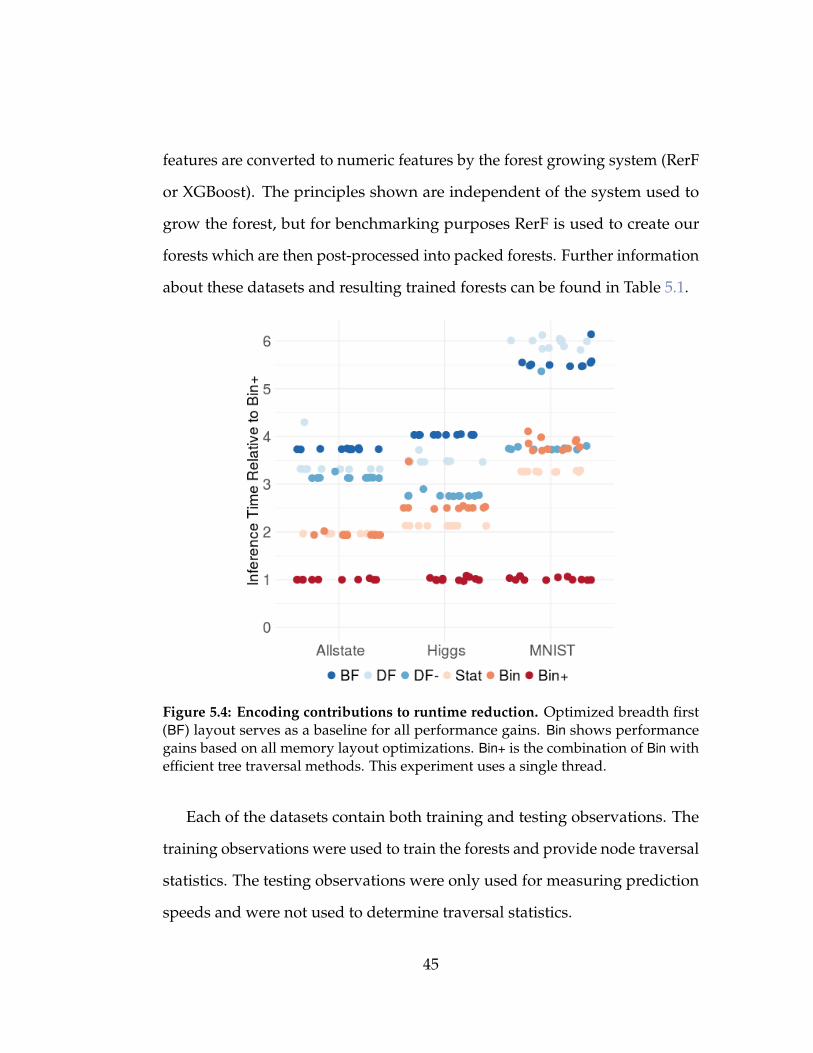
Figure 5.4: Encoding contributions to runtime reduction. Optimized breadth first(BF) layout serves as a baseline for all performance gains. Bin shows performancegains based on all memory layout optimizations. Bin+ is the combination of Bin withefficient tree traversal methods. This experiment uses a single thread.

Each of the datasets contain both training and testing observations. The

training observations were used to train the forests and provide node traversal

statistics. The testing observations were only used for measuring prediction

speeds and were not used to determine traversal statistics.

45

5.3.2 Layout Contributions

We now turn to a detailed study of the effects of layout optimizations on

runtime performance. Tab. 5.2 shows the incremental improvement of run-

time statistics for the optimizations. The high ratio of wasted cycles of each

of the encodings shows that runtimes are dominated by CPU stalls which

are typically caused by slow memory accesses or high numbers of branch

mispredictions. Because the runtime is nearly cut in half between the BF

and Bin with little change in the numbers of instructions executed, branches,

and branch mispredictions, we conclude that stalls occur mainly because of

slow memory accesses. This is corroborated by greater than one Cycles Per

Instruction (CPI), which indicates an application is memory bound.

We attribute the improvement of run times for DF, DF-, and Stat to reduc-

tions in the level at which cache misses are resolved. Average stall duration is

reduced by finding required memory lower in the cache hierarchy, which is

shown in “Avg Stall (cycles)” column of Tab. 5.2. The Bin optimization sees a

slight increase in stall duration which we attribute to interleaving trees. This

happens because “likely to be used” nodes, those near the roots, of several

trees are stored together. This makes the access of a needed node in one

tree likely to also load a soon to be useful node from another tree. Whereas

other encodings quickly recover from stalls due to cache misses for often used

nodes, the Bin encoding avoids these stalls altogether. In other words, the

Bin optimization avoids quickly resolved stalls which increases the overall

average stall duration.

46

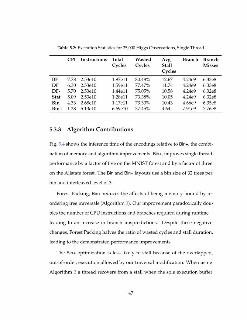
Table 5.2: Execution Statistics for 25,000 Higgs Observations, Single Thread

CPI Instructions TotalCycles

WastedCycles

AvgStallCycles

Branch BranchMisses

BF 7.78 2.53e10 1.97e11 80.48% 12.67 4.24e9 6.33e8DF 6.30 2.53e10 1.59e11 77.47% 11.74 4.24e9 6.33e8DF- 5.70 2.53e10 1.44e11 75.05% 10.58 4.24e9 6.32e8Stat 5.09 2.53e10 1.28e11 73.38% 10.05 4.24e9 6.32e8Bin 4.33 2.68e10 1.17e11 73.30% 10.43 4.66e9 6.35e8Bin+ 1.28 5.13e10 6.69e10 37.45% 4.64 7.91e9 7.76e8

5.3.3 Algorithm Contributions

Fig. 5.4 shows the inference time of the encodings relative to Bin+, the combi-

nation of memory and algorithm improvements. Bin+, improves single thread

performance by a factor of five on the MNIST forest and by a factor of three

on the Allstate forest. The Bin and Bin+ layouts use a bin size of 32 trees per

bin and interleaved level of 3.

Forest Packing, Bin+ reduces the affects of being memory bound by re-

ordering tree traversals (Algorithm 3). Our improvement paradoxically dou-

bles the number of CPU instructions and branches required during runtime—

leading to an increase in branch mispredictions. Despite these negative

changes, Forest Packing halves the ratio of wasted cycles and stall duration,

leading to the demonstrated performance improvements.

The Bin+ optimization is less likely to stall because of the overlapped,

out-of-order, execution allowed by our traversal modification. When using

Algorithm 2 a thread recovers from a stall when the sole execution buffer

47

slot in use becomes ready to execute its instructions. The updated traversal

method allows the thread to use all execution buffers. The loading of any of

the multiple execution buffers in use allows the thread to continue execution,

thereby reducing both the liklihood a stall occurs and the duration of a stall

when it does occur.

The benefits of Bin+ can only be realized with many concurrent tree traver-

sals. As the inference process progresses through a bin, the trees arrive at their

leaf nodes at different depths. The overlap of memory requests is reduced for

each tree in a bin that reaches it’s leaf node. This potential for skew is shown

in Table 5.1, where the average leaf depth and deepest leaf depth of each of the

test forests is shown, the latter being triple the former. As an example, when

all but one tree finishes processing, the remaining tree will no longer benefit

from out-of-order execution because there are no other trees with which to

overlap memory accesses. When this occurs the remainder of the tree traversal

reverts back to the Stat traversal pattern.

5.3.4 Parallel Evaluation to Reduce Latency

We study the effect on latency of parallelizing classification in a shared mem-

ory multithreaded system. This is a strong scaling experiment that runs a

single classification on one to 32 threads. For the Bin and Bin+ encodings, the

number of trees per bin is set to 16 and nodes are interleaved to depth of 3.

To focus on reducing latency, we only begin processing an observation at the

completion of the previous observation.

The bin data structure and improved algorithm allows Bin+ to scale more

48

efficiently than the other encodings. Binning allows us to statically pin an

execution thread to a subset of bins which allows a thread to process a subset

of trees using out-of-order execution, maintain usefulness of all levels of cache,

and reduce skew. Without the optimizations provided by binning, we can pin

trees to threads and experience degraded parallelism due to skewed execution,

or, we can allow threads to dynamically process trees and experience degraded

parallelism due to poor use of cache. In neither case can we take advantage of

out-of-order processing.

Shared-memory parallelism reduces latency effectively for each of the

encodings (except Bin), but, despite being embarrassingly parallel, scaling is

sublinear, Fig. 5.5. We expected this suboptimal scaling due to both increased

contention in the memory subsystem and the skewed nature of observation

traversal depths (Table 5.1). Multithread Bin performs poorly because threads

receive extraneous nodes with each memory request because of the interleaved

trees. This adds cache pollution, reduces cache locality, and requires multiple

requests for cache lines with interleaved nodes.

To realize the full benefit of both threaded parallelism and the intra-thread

parallelism provided by out-of-order execution, it is necessary that the number

of trees in the forest be at least 16 to 32 times the number of threads used.

This limitation can be seen in Fig. 5.6 where intra-thread parallelism is shown

to work well with at least 16 to 32 trees per bin. In addition, the number

of bins in a forest should be a multiple of the intended number of threads

used for parallelism in order to ensure equal workloads are provided to

each thread. In general, larger bin sizes perform better during multithread

49

(a) Per observations prediction time. The Y axis is log10 scale.

(b) Speed-up with additional threads.

Figure 5.5: Multithread characteristics of inference techniques. Bin+ performancewith one thread is superior to the other encodings and scales better with additionalresources.

operation, but increasing bin sizes reduces the number of bins available for

threaded parallelism.

5.3.5 Comparison to Popular Tools

We found no forests implementations that specifically target the reduction

of inference latency, so instead comparisons will be made to two popular

decision tree systems: XGBoost and RerF. Because both of these systems

typically process observations in batches, we chose to use throughput as a

measurement of comparison despite our system being optimized to reduce

latency. We vary the size of forests in both the number of trees and size of

50

Figure 5.6: Effects of bin size on multithread performance for a 2048 tree forest.Increasing bin size allows for more intra-thread parallelism but limits thread levelparallelism.

trees (using max depth) to show the efficacy of Forest Packing for a variety of

forest sizes, Fig. 5.7. We set the batch size to 5000 for XGBoost and RerF. All

systems except Forest Packing use all 96 threads of our machine—XGBoost

uses forest characteristics to dynamically choose how many of the 96 threads

to use. We limit Forest Packing to use only 16 threads in order to maximize

intra-thread parallelism, a limitation described in Sec. 5.3.4. The use of 16

threads requires the use of at least 16 bins, which, for 2048 trees, limits the bin

size to 128 trees. For a forest of 128 trees, the use of 16 threads limits the bin

size to 8 trees. Despite the limitation on thread use, Forest Packing continues

to outperform all other systems.

51

Figure 5.7: Inference throughput when varying number of trees in forest (definedabove the chart) and tree depth. Forests were created using the MNIST dataset.Experiment uses multiple threads and batch size of 5000 where applicable.

5.4 Conclusions

The two major contributions provided by Forest Packing are the reduced

memory footprint of a forest model and the novel tree traversal process made

possible by tree binning. The removal of redundant leaf nodes halves decision

forest memory requirements, which is a critical improvement for machine

learning applications on memory limited devices such as mobile devices

or stand-alone sensors. The tree traversal modification provides a faster,

more scalable, system with multithread performance more than an order of

magnitude faster than the naive solution. This reduced latency can make

52

decision forests a more competitive option for real-time vision, recommender,

and anomaly detection systems. Using Forest Packing to process trained

decision forests such as those created by R-RerF allows for state of the art

inference speeds.

53

Chapter 6

Dynamic Forest Packing

In Chapter 4 we described R-RerF which produced state of the art accuracy

when used on many popular datasets. This system suffered from poor in-

ference speed performance, which we addressed in Chapter 5 with the post

processing step we called Forest Packing. This chapter outlines fastRerF, a

system that fixes the final deficiency of R-RerF — slower than state-of-the-art

training speeds — while also performing forest packing simultaneously with

training.

We describe several training optimization alternatives to typical decision

forest implementations, introduce a node level subsampling, and dynamically

pack forests to reduce inference time. The benefits of these improvements are

shown using several widely used datasets to compare our memory efficient

systems, fastRF and fastRerF, against other popular forest implementations.

The resulting system provides state-of-the-art accuracy, training speeds, and

inference speeds.

54

6.1 fastRerF Optimizations

The most popular training time optimization used in decision forest systems

entails presorting each feature, which is not a feasible enhancement for RerF.

Presorting features in RerF would entail materializing all possible features,

sorting them, and storing pointer data to required observation properties

such as class label and weight. This is not feasible because there are on the

order of d! possible linear combinations that would each form a new feature,

where d is the number of features in a dataset. This would grow the memory

requirements of the algorithm beyond a system’s available resources for all

but the smallest datasets. With the presorting optimization unavailable for

our system, we instead focused on memory reduction techniques, node level

subsampling, and efficient parallelism.

6.1.1 Memory Reduction

Randomer Forest, like typical decision forests, is a memory bound algorithm

that suffers from the high load latencies experienced when performing random

reads from memory. Criminisi et al recommends storing a tree’s mapping from

observation indices to node in a single vector rather than node specific index

vectors [8]. Indices are rearranged within this data structure as observations

are split into children nodes. The importance of this technique increases

when performing functions such as determining observation distances, which

require maintaining index locations for the duration of the tree growing

process, rather than just indices in the frontier nodes. This method only

requires storing a vector iterator for the first and last location of each node’s

55

indices, which defines a subregion of the vector which also encompasses all

descendant node indices.

The fastRF system processes nodes in a memory efficient order. Most

decision forest systems process nodes at a per level processing order, allowing

them to quickly process an entire level of a tree by streaming over each feature

in a single pass. As the number of nodes doubles at each level, so too does the

memory required to store the unprocessed node data. For this reason fastRF

uses a depth first traversal order which requires storing at most L unprocessed

nodes vs the 2L nodes stored when processing in a breadth first order, where

L is the maximum depth of a tree.

Another memory reducing method is a suggestion from Criminisi to main-

tain a tree wide vector to map observation indices to nodes [8]. A naive

decision forest implementation will maintain a per node vector of resident

observations, thereby duplicating data at each level of a tree. Rather than

duplicating data, the use of a single N length vector can be used, where ob-

servation indices are moved within the vector according to node residency.

This in-place tracking of observations reduces the allocation of node track-

ing vectors. Movement of indices within the vector is an efficient operation

commonly employed in the quicksort algorithm.

The final memory optimization employed by fastRF is the use of C index

vectors, where C is the number of classes in a dataset, to store the location

of observations in a tree. This serves two purposes, first, it reduces memory

by tying an observation’s class label to the entire vector rather than storing a

class label for each observation. The second benefit is an increase in cache load

56

efficiency due to processing observations in class order, which increases the

likelihood a cache load is used multiple times prior to eviction. This secondary

benefit is only realized when a training set is ordered by class label.

6.1.2 Node Level Stratified Subsampling

There are several approximation techniques used to reduce the amount of

work required at each node. For instance, XGBoost reduces the number of

potential splitting points to explore at each node when N is above a user

defined cutoff value. When N is large all observation values are binned and

only splits between these bins are considered. Louppe detailed a subsampling

method that subsamples both observations and features from the training

data for each tree and uses this reduced subset of observations and features

for training [24]. This method reduces the number of features explored at

each node and reduces the number of observations resident in each node,

thereby reducing training time but also reducing the efficacy of a tree. Our

subsampling method is inspired by these two techniques.

FastRerF employs a stratified subsampling of observations at each node

when N surpasses a user defined threshold. Whereas XGBoost’s method loads

all observations into a histogram, FastRerF only loads the subsampled obser-

vations, which reduces gathering, sorting, and searching time. In addition,

Louppe’s subsampling may select poor features and thus have a poorly per-

forming tree, FastRerF chooses a subset at each node and so a bad sampling

of uninformative features only affects a single node rather than an entire tree.

57

6.1.3 Parallelism

FastRerf uses tree level parallelism, the most coarse grained form of paral-

lelism available in forests. This choice almost completely removes both false

sharing between threads and all thread synchronization, but duplicates tree

growing structures in each thread. We tolerate this small memory duplica-

tion because the structures are duplicated in independent caches and so the

increased memory use is tempered by a high cache coherency.

6.1.4 Dynamic Forest Packing

Forest Packing showed the node representation in memory and traversal

method through trees could result in an order of magnitude difference in

inference times as compared to non optimized methods, Chapter 5. As a

post processing step forest packing is an inconvenience to data scientists

and so would, in all likelihood, be relegated to use only in forest deployment

scenarios, such as in embedded sensors. But, by modifying both the processing

order of nodes and rearranging the forest data structure, it is possible to closely

replicate the implementation of Packed Forests during forest growing. An

enhancement we call Dynamic Forest Packing.

fastRF uses a depth first traversal order, sect. 6.1.1, in order to minimize

memory use. This is implemented via a stack of unprocessed nodes, where

nodes are popped after processing, which results in either two children nodes

being pushed onto the stack or nodes becoming leaf nodes within the forest

structure. Placing the right child on the stack followed by the left child results

in the traditional depth first creation of a forest. Forest Packing requires nodes

58

to reside in the forest adjacent to the child which is most likely to be traversed,

the child node whose set of observations has the higher cardinality. To achieve

this order within the resulting forest structure, the nodes must be processed

in order of cardinality, where the sibling with higher cardinality must be

processed first, which results from the lower cardinality node being placed on

the processing stack first.

The trees within the forest must also be binned in order to gain the full

benefits of Forest Packing. The bin structure of Forest Packing consists of T

trees combined into a single data structure where roots are adjacent, the first

several levels of each tree are intertwined, per-tree nodes are stored according

to cardinality, and leaf nodes are stored at the end of the structure. fastRerF

is unable to completely match this formatting because the final bin size in

memory is unknown until the training process is complete. So instead, during

fastRerF training, the number of trees per bin is calculated and the initial forest

structure is created with leaf nodes stored at the beginning of the contiguous

memory structure rather than at the end. Trees within the bin are grown

sequentially with the nodes in the intertwined layers being placed in their

predefined position and later nodes are placed sequentially at the end of the

growing data structure.

Parallelism is also modified to be on a bin per thread basis rather than

the previously used tree per thread basis. Each bin uses an independent

number generator, seeded by a forest level number generator, to maintain

reproducibility and reduce synchronization among threads. The number of

bins used in a forest should be a multiple of the number of threads used to

59

train the forest in order to maximize thread use.

6.2 System Evaluation

We evaluate FastRerF and FastRF against other popular and well performing

decision forest systems. Ideally, FastRerF would be compared against other

OSPFs but there are no implementations that scale beyond trivially large

datasets. We explore the scalability of our system as it pertains to number of

cores and training dataset characteristics. We also isolate dataset characteris-

tics to demonstrate the effects these particular characteristics have on training

time. Finally, we show the effects of stratified subsampling on training time

and test accuracy.

6.2.1 Experimental Setup

We compare FastRerF and FastRF to Ranger, LightGBM, and XGBoost. Ranger

is one of the fastest Random Forest implementations, particularly on datasets

with few unique feature values. LightGBM and XGBoost are boosted systems

which are popular due to their fast training speed and successes in Kaggle

competitions. The algorithms employed by these forests are similar in that

they are decision forests that split nodes based on some minimization criteria.

Similar parameters are used when comparing forests and defaults are used

for forest specific parameters not used by the other variants.

Four commonly used real world and simulated datasets are used to demon-

strate performance: Higgs, MNIST, p53, and SVHN. The Higgs dataset was

used in a popular Kaggle competition, is composed of simulated background

60

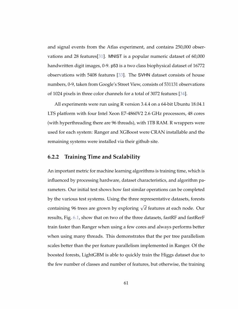
and signal events from the Atlas experiment, and contains 250,000 obser-

vations and 28 features[31]. MNIST is a popular numeric dataset of 60,000

handwritten digit images, 0-9. p53 is a two class biophysical dataset of 16772

observations with 5408 features [33]. The SVHN dataset consists of house

numbers, 0-9, taken from Google’s Street View, consists of 531131 observations

of 1024 pixels in three color channels for a total of 3072 features [34].

All experiments were run using R version 3.4.4 on a 64-bit Ubuntu 18.04.1

LTS platform with four Intel Xeon E7-4860V2 2.6 GHz processors, 48 cores

(with hyperthreading there are 96 threads), with 1TB RAM. R wrappers were

used for each system: Ranger and XGBoost were CRAN installable and the

remaining systems were installed via their github site.

6.2.2 Training Time and Scalability

An important metric for machine learning algorithms is training time, which is

influenced by processing hardware, dataset characteristics, and algorithm pa-

rameters. Our initial test shows how fast similar operations can be completed

by the various test systems. Using the three representative datasets, forests

containing 96 trees are grown by exploring√

d features at each node. Our

results, Fig. 6.1, show that on two of the three datasets, fastRF and fastRerF

train faster than Ranger when using a few cores and always performs better

when using many threads. This demonstrates that the per tree parallelism

scales better than the per feature parallelism implemented in Ranger. Of the

boosted forests, LightGBM is able to quickly train the Higgs dataset due to

the few number of classes and number of features, but otherwise, the training

61

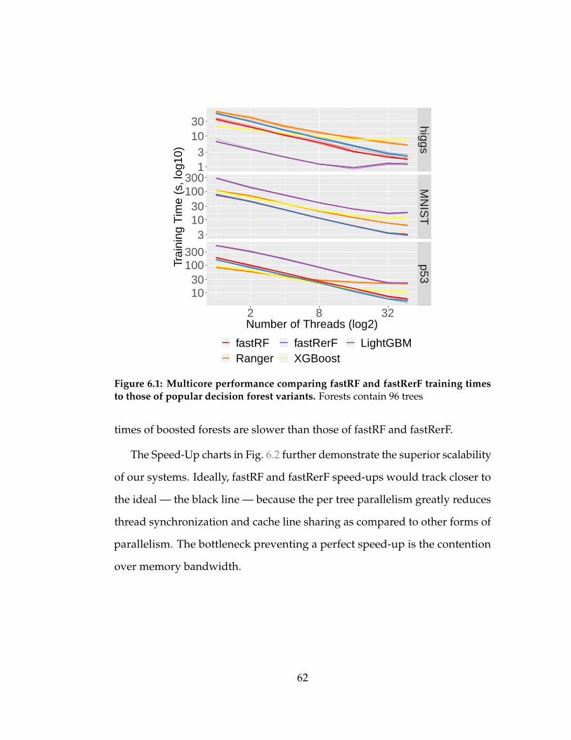
higgsM

NIS

Tp53

2 8 32

13

1030

31030

100300

1030

100300

Number of Threads (log2)

Trai

ning

Tim

e (s

, log

10)

fastRF fastRerF LightGBMRanger XGBoost

Figure 6.1: Multicore performance comparing fastRF and fastRerF training timesto those of popular decision forest variants. Forests contain 96 trees

times of boosted forests are slower than those of fastRF and fastRerF.

The Speed-Up charts in Fig. 6.2 further demonstrate the superior scalability

of our systems. Ideally, fastRF and fastRerF speed-ups would track closer to

the ideal — the black line — because the per tree parallelism greatly reduces

thread synchronization and cache line sharing as compared to other forms of

parallelism. The bottleneck preventing a perfect speed-up is the contention

over memory bandwidth.

62

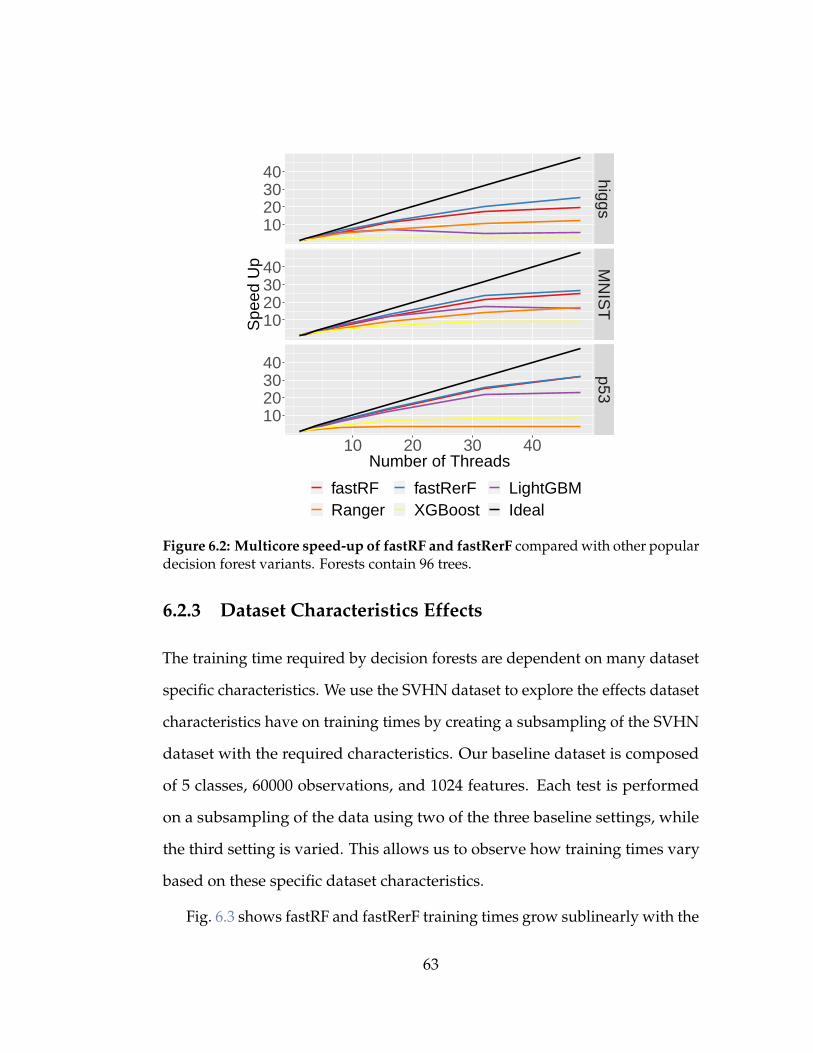
higgsM

NIS

Tp53

10 20 30 40

10203040

10203040

10203040

Number of Threads

Spe

ed U

p

fastRF fastRerF LightGBMRanger XGBoost Ideal

Figure 6.2: Multicore speed-up of fastRF and fastRerF compared with other populardecision forest variants. Forests contain 96 trees.

6.2.3 Dataset Characteristics Effects

The training time required by decision forests are dependent on many dataset

specific characteristics. We use the SVHN dataset to explore the effects dataset

characteristics have on training times by creating a subsampling of the SVHN

dataset with the required characteristics. Our baseline dataset is composed

of 5 classes, 60000 observations, and 1024 features. Each test is performed

on a subsampling of the data using two of the three baseline settings, while

the third setting is varied. This allows us to observe how training times vary

based on these specific dataset characteristics.

Fig. 6.3 shows fastRF and fastRerF training times grow sublinearly with the

63

number of classes. This is expected because only one third of node splitting,

the exhaustive search, is effected by the number of classes, Sect. 4.3.1. Boost-

ing algorithms scale linearly with the number of classes because boosting

algorithms require a forest to be created for each class.

25

50

75

2 4 6 8 10Number of Classes

Trai

ning

Tim

e (s

)

fastRF fastRerF LightGBMRanger XGBoost

Figure 6.3: Affect of number of classes in dataset on fastRF and fastRerF trainingtimes. 60000 observations, 1024 features, and 16 threads, 128 trees.

Fig. 6.4 shows fastRF and fastRerF training times grow sublinearly with

the number of features. All systems were set to search√

d features at each

node. Training time as a function of d is an important metric as forest variants

differ in recommended values for mtry:√

d for Random Forests, d for boosted

forests, and between 2d and d2 for OSPFs.

Fig. 6.5 shows fastRF and fastRerF training times grow linearly with the

64

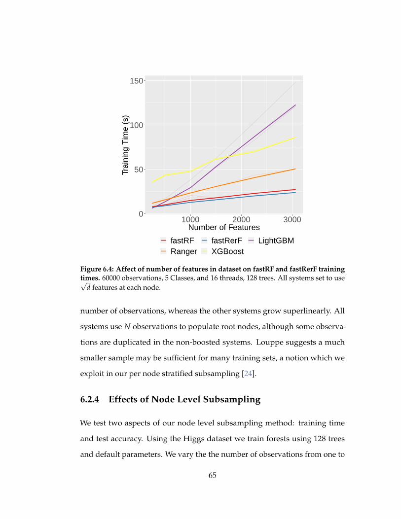
0

50

100

150

1000 2000 3000Number of Features

Trai

ning

Tim

e (s

)

fastRF fastRerF LightGBMRanger XGBoost

Figure 6.4: Affect of number of features in dataset on fastRF and fastRerF trainingtimes. 60000 observations, 5 Classes, and 16 threads, 128 trees. All systems set to use√

d features at each node.

number of observations, whereas the other systems grow superlinearly. All

systems use N observations to populate root nodes, although some observa-

tions are duplicated in the non-boosted systems. Louppe suggests a much

smaller sample may be sufficient for many training sets, a notion which we

exploit in our per node stratified subsampling [24].

6.2.4 Effects of Node Level Subsampling

We test two aspects of our node level subsampling method: training time

and test accuracy. Using the Higgs dataset we train forests using 128 trees

and default parameters. We vary the the number of observations from one to

65

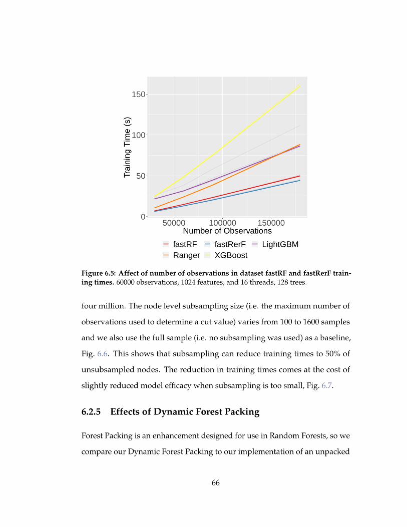
0

50

100

150

50000 100000 150000Number of Observations

Trai

ning

Tim

e (s

)

fastRF fastRerF LightGBMRanger XGBoost

Figure 6.5: Affect of number of observations in dataset fastRF and fastRerF train-ing times. 60000 observations, 1024 features, and 16 threads, 128 trees.

four million. The node level subsampling size (i.e. the maximum number of

observations used to determine a cut value) varies from 100 to 1600 samples

and we also use the full sample (i.e. no subsampling was used) as a baseline,

Fig. 6.6. This shows that subsampling can reduce training times to 50% of

unsubsampled nodes. The reduction in training times comes at the cost of

slightly reduced model efficacy when subsampling is too small, Fig. 6.7.

6.2.5 Effects of Dynamic Forest Packing

Forest Packing is an enhancement designed for use in Random Forests, so we

compare our Dynamic Forest Packing to our implementation of an unpacked

66

50

100

300

500

1 2 3 4Number of Observations (millions)

Trai

ning

Tim

e (s

, log

10)

Subsample Size 100200

400800

1600Full Sample

Figure 6.6: Effects of subsampling size on training time. MNIST dataset, 128 trees.

forest; Ranger is also included in the comparisons as a baseline. We first show

the effects of Dynamic Forest Packing on forest training times, Fig. 6.8, using

the MNIST dataset with its accompanying 10000 observation test set. The

difference between our nonpacked and dynamically packed forest is small,

with changes only in node placement because our nonpacked version uses the

cardinality based processing order. Our Dynamically Packed Forest is slightly

faster due to the reduction in tree size caused by sharing leaf nodes.

We then compare inference times using MNIST’s test set, Fig. 6.9. Inference

times grow as expected with the addition of trees to the forest. The use of

binning can be seen when comparing the fastRF and fastRF(binned) results.

Overall, binning reduces inference times an order of magnitude as compared

67

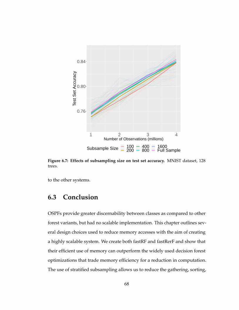
0.76

0.80

0.84

1 2 3 4Number of Observations (millions)

Test

Set

Acc

urac

y

Subsample Size 100200

400800

1600Full Sample

Figure 6.7: Effects of subsampling size on test set accuracy. MNIST dataset, 128trees.

to the other systems.

6.3 Conclusion

OSPFs provide greater discernability between classes as compared to other

forest variants, but had no scalable implementation. This chapter outlines sev-

eral design choices used to reduce memory accesses with the aim of creating

a highly scalable system. We create both fastRF and fastRerF and show that

their efficient use of memory can outperform the widely used decision forest

optimizations that trade memory efficiency for a reduction in computation.

The use of stratified subsampling allows us to reduce the gathering, sorting,

68

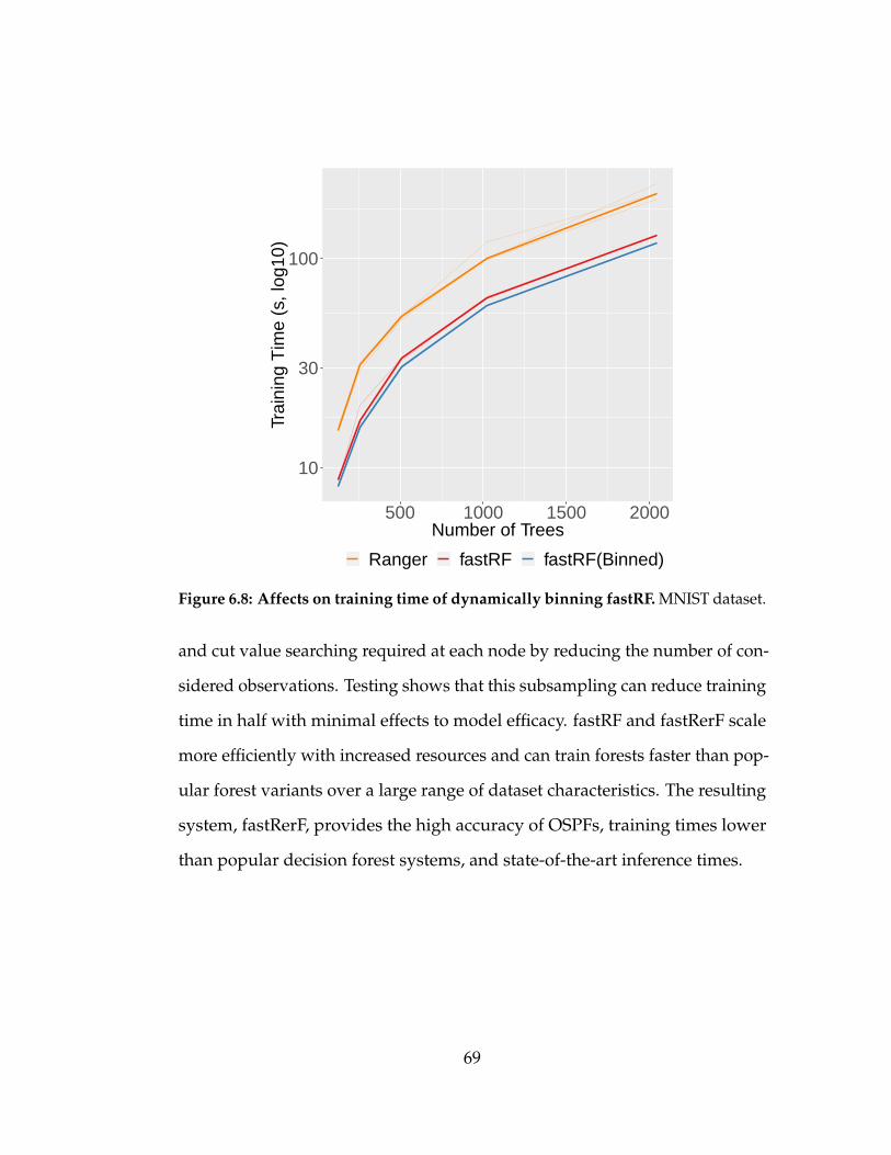
10

30

100

500 1000 1500 2000Number of Trees

Trai

ning

Tim

e (s

, log

10)

Ranger fastRF fastRF(Binned)

Figure 6.8: Affects on training time of dynamically binning fastRF. MNIST dataset.

and cut value searching required at each node by reducing the number of con-

sidered observations. Testing shows that this subsampling can reduce training

time in half with minimal effects to model efficacy. fastRF and fastRerF scale

more efficiently with increased resources and can train forests faster than pop-

ular forest variants over a large range of dataset characteristics. The resulting

system, fastRerF, provides the high accuracy of OSPFs, training times lower

than popular decision forest systems, and state-of-the-art inference times.

69

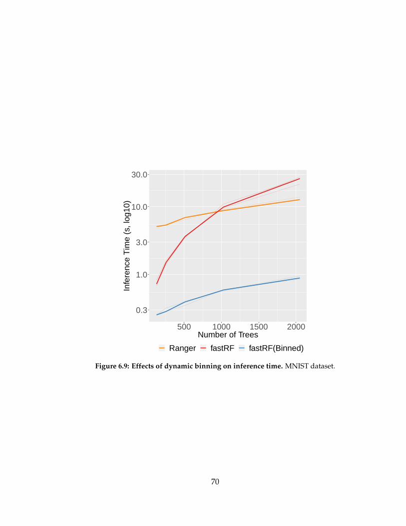
0.3

1.0

3.0

10.0

30.0

500 1000 1500 2000Number of Trees

Infe

renc

e T

ime

(s, l

og10

)

Ranger fastRF fastRF(Binned)

Figure 6.9: Effects of dynamic binning on inference time. MNIST dataset.

70

Chapter 7

Discussion and Conclusion

The purpose of this dissertation was to explore the feasibility of designing and

implementing a scalable Oblique Sparse Projection Forest (OSPF). The benefits

of these forests have been known since the conception of decision forests over

two decades ago, but no scalable implementation has ever been developed,

despite computational complexities similar to that of other popular forest

variants. The reason for this oversight is not definitively known, but this

researcher contends, after delving into many decision forest implementations,

that typical forest acceleration techniques cannot extend to sparse projection

forests and thus, without the use of the typical optimizations, oblique forests

were computationally untenable.

This exploration started with the development of R-RerF, a mostly R ver-

sion of Tyler Tomita’s sparse projection forest, Randomer Forest (RerF). The

implementation was highly optimized, scaled similarly to state of the art

forest implementations, and provided an easily extensible framework that al-

lowed for easy implementation of other sparse projection forests. We showed

R-RerF’s training speeds were similar to the speeds found in other forest

71

variants and R-RerF’s ability to scale with increased resources surpassed other

implementations. In addition we provided a CRAN package that implements

RerF, Random Forest, Random-Rotation Random Forest and S-RerF, a patch

processing OSPF used for image classification. Although this implementation

scaled well, it suffered from excessive memory use and slow inference speeds.

The slow inference speeds of decision forest algorithms was an interesting

problem that others had explored before. Prior to our investigation though,

solutions focused on data representations of trees in memory and batched

processing of test observations. We were able to improve upon the state-of-

the-art inference speeds by intertwining trees in a bin structure, removing

duplicate leaf nodes, relocating leaf nodes to the end of bins so that multiple

trees would share nodes, and changing the traversal order of trees in the

forest to take advantage of modern CPU architectures. Our overall product,

Forest Packing, reduced tree memory requirements in half, provided single

core inference faster than a many threaded naive implementation, scaled

better with additional resources, and increased throughput while reducing

per inference latencies as compared to other popular forest implementations.

The realization of these benefits required data scientists to perform an offline,

multistep process to save the forest to disk, analyze the forest, rewrite the

forest in an optimized format, and reload the forest into memory.

The final contribution of this dissertation was to create an optimized ver-

sion of RerF that would dynamically pack a forest’s nodes for fast inference.

Prior to implementing our system we analyzed several fast decision forests

with the aim of finding optimizations for our new system, but instead we

72

found the typical forest optimizations were not extendable to OSPFs. We

instead focused on several memory reduction design choices and introduced

a per node subsampling method inspired by similar well performing methods.

Our final product is more memory efficient than other state of the art decision

forests, trains faster on many datasets, scales better with additional resources,

and provides state-of-the-art inference speeds.

The culmination of our efforts is available with front end interfaces for both

R and Python, with packages available via CRAN and pip. There are plans

to extend fastRerF beyond the RerF and Random Forest algorithms currently

provided to include unsupervised methods such as U-RerF and other OSPFs

such as S-RerF. In addition to added algorithms, we also plan to make the

current implementations feature rich with support for common Random

Forest features such as observation proximity and feature importance.

73

References

[1] Daniel George and EA Huerta. “"Deep Learning for Real-Time Grav-itational Wave Detection and Parameter Estimation: Results with Ad-vanced LIGO Data"”. In: Physics Letters B (2017).

[2] Daniel Lecina, Joan F Gilabert, and Victor Guallar. “"Adaptive Simu-lations, Towards Interactive Protein-Ligand Modeling"”. In: ScientificReports 7.1 (2017), p. 8466.

[3] Fabian Pedregosa, Gaël Varoquaux, Alexandre Gramfort, Vincent Michel,Bertrand Thirion, Olivier Grisel, Mathieu Blondel, Peter Prettenhofer,Ron Weiss, Vincent Dubourg, et al. “Scikit-learn: Machine learning inPython”. In: Journal of machine learning research 12.Oct (2011), pp. 2825–2830.

[4] Martin Elsman, Philip Munksgaard, and Ken Friis Larsen. “ExperienceReport: Type-Safe Multi-Tier Programming with Standard ML Mod-ules”. In: (2018).

[5] L. Devroye, L. Györfi, and G. Lugosi. A Probabilistic Theory of PatternRecognition. Stochastic Modelling and Applied Probability. SpringerNew York, 1997. ISBN: 9780387946184. URL: https://books.google.com/books?id=uDgXoRkyWqQC.

[6] Tianqi Chen and Carlos Guestrin. “XGBoost: A Scalable Tree BoostingSystem”. In: Proceedings of the 22Nd ACM SIGKDD International Con-ference on Knowledge Discovery and Data Mining. KDD ’16. New York,NY, USA: ACM, 2016, pp. 785–794. ISBN: 978-1-4503-4232-2. DOI: 10.1145/2939672.2939785. URL: http://doi.acm.org/10.1145/2939672.2939785.

[7] Guolin Ke, Qi Meng, Thomas Finley, Taifeng Wang, Wei Chen, WeidongMa, Qiwei Ye, and Tie-Yan Liu. “Lightgbm: A highly efficient gradient

74

boosting decision tree”. In: Advances in Neural Information ProcessingSystems. 2017, pp. 3146–3154.

[8] Antonio Criminisi, Jamie Shotton, Ender Konukoglu, et al. “Decisionforests: A unified framework for classification, regression, density esti-mation, manifold learning and semi-supervised learning”. In: Founda-tions and Trends® in Computer Graphics and Vision 7.2–3 (2012), pp. 81–227.

[9] Bjoern H Menze, B Michael Kelm, Daniel N Splitthoff, Ullrich Koethe,and Fred A Hamprecht. “On oblique random forests”. In: Joint EuropeanConference on Machine Learning and Knowledge Discovery in Databases.Springer. 2011, pp. 453–469.

[10] Leo Breiman. “Random Forests”. In: Machine Learning 45.1 (2001), pp. 5–32. ISSN: 1573-0565. DOI: 10.1023/A:1010933404324. URL: https://doi.org/10.1023/A:1010933404324.

[11] Le Zhang, Jagannadan Varadarajan, Ponnuthurai Nagaratnam Sugan-than, Narendra Ahuja, and Pierre Moulin. “Robust visual tracking usingoblique random forests”. In: Proceedings of the IEEE Conference on Com-puter Vision and Pattern Recognition. 2017, pp. 5589–5598.

[12] Junshi Xia, Nicola Falco, Jón Atli Benediktsson, Peijun Du, and JocelynChanussot. “Hyperspectral image classification with rotation randomforest via KPCA”. In: IEEE Journal of Selected Topics in Applied EarthObservations and Remote Sensing 10.4 (2017), pp. 1601–1609.

[13] Ting Ye, Hucheng Zhou, Will Y Zou, Bin Gao, and Ruofei Zhang. “Rapid-Scorer: Fast Tree Ensemble Evaluation by Maximizing Compactness inData Level Parallelization”. In: Proceedings of the 24th ACM SIGKDDInternational Conference on Knowledge Discovery & Data Mining. ACM.2018, pp. 941–950.

[14] N. Asadi, J. Lin, and A. P. de Vries. “"Runtime Optimizations for Tree-Based Machine Learning Models"”. In: IEEE Transactions on Knowledgeand Data Engineering 26.9 (2014), pp. 2281–2292. ISSN: 1041-4347. DOI:10.1109/TKDE.2013.73.

[15] Hyunsu Cho and Mu Li. “Treelite: toolbox for decision tree deployment”.In: (2018). URL: http://hyunsu-cho.io/preprints/treelite_sysml.pdf.

[16] Luc Devroye, László Györfi, and Gábor Lugosi. A probabilistic theory ofpattern recognition. Vol. 31. Springer Science & Business Media, 2013.

75

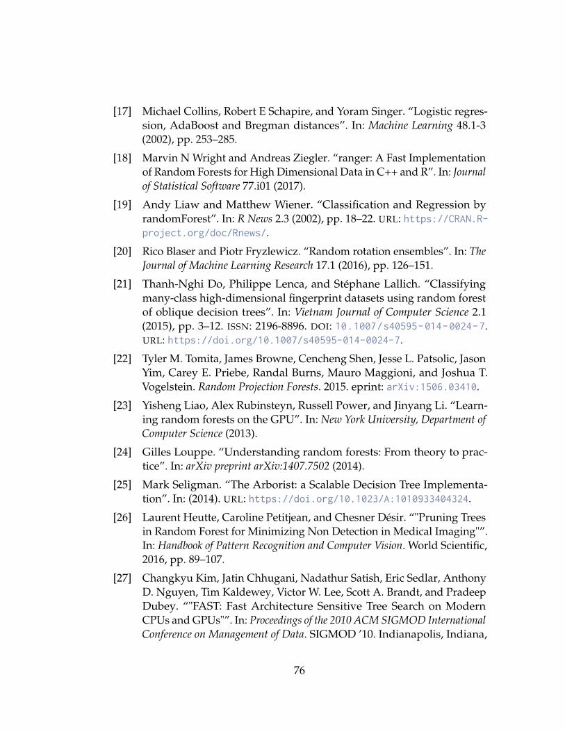
[17] Michael Collins, Robert E Schapire, and Yoram Singer. “Logistic regres-sion, AdaBoost and Bregman distances”. In: Machine Learning 48.1-3(2002), pp. 253–285.

[18] Marvin N Wright and Andreas Ziegler. “ranger: A Fast Implementationof Random Forests for High Dimensional Data in C++ and R”. In: Journalof Statistical Software 77.i01 (2017).

[19] Andy Liaw and Matthew Wiener. “Classification and Regression byrandomForest”. In: R News 2.3 (2002), pp. 18–22. URL: https://CRAN.R-project.org/doc/Rnews/.

[20] Rico Blaser and Piotr Fryzlewicz. “Random rotation ensembles”. In: TheJournal of Machine Learning Research 17.1 (2016), pp. 126–151.

[21] Thanh-Nghi Do, Philippe Lenca, and Stéphane Lallich. “Classifyingmany-class high-dimensional fingerprint datasets using random forestof oblique decision trees”. In: Vietnam Journal of Computer Science 2.1(2015), pp. 3–12. ISSN: 2196-8896. DOI: 10.1007/s40595-014-0024-7.URL: https://doi.org/10.1007/s40595-014-0024-7.

[22] Tyler M. Tomita, James Browne, Cencheng Shen, Jesse L. Patsolic, JasonYim, Carey E. Priebe, Randal Burns, Mauro Maggioni, and Joshua T.Vogelstein. Random Projection Forests. 2015. eprint: arXiv:1506.03410.

[23] Yisheng Liao, Alex Rubinsteyn, Russell Power, and Jinyang Li. “Learn-ing random forests on the GPU”. In: New York University, Department ofComputer Science (2013).

[24] Gilles Louppe. “Understanding random forests: From theory to prac-tice”. In: arXiv preprint arXiv:1407.7502 (2014).

[25] Mark Seligman. “The Arborist: a Scalable Decision Tree Implementa-tion”. In: (2014). URL: https://doi.org/10.1023/A:1010933404324.

[26] Laurent Heutte, Caroline Petitjean, and Chesner Désir. “"Pruning Treesin Random Forest for Minimizing Non Detection in Medical Imaging"”.In: Handbook of Pattern Recognition and Computer Vision. World Scientific,2016, pp. 89–107.

[27] Changkyu Kim, Jatin Chhugani, Nadathur Satish, Eric Sedlar, AnthonyD. Nguyen, Tim Kaldewey, Victor W. Lee, Scott A. Brandt, and PradeepDubey. “"FAST: Fast Architecture Sensitive Tree Search on ModernCPUs and GPUs"”. In: Proceedings of the 2010 ACM SIGMOD InternationalConference on Management of Data. SIGMOD ’10. Indianapolis, Indiana,

76

USA: ACM, 2010, pp. 339–350. ISBN: 978-1-4503-0032-2. DOI: 10.1145/1807167 . 1807206. URL: http : / / doi . acm . org / 10 . 1145 / 1807167 .1807206.

[28] T. M. Chilimbi, M. D. Hill, and J. R. Larus. “Making Pointer-Based DataStructures Cache Conscious”. In: Computer 33.12 (2000), pp. 67–74. ISSN:0018-9162. DOI: 10.1109/2.889095.

[29] B. Ren, G. Agrawal, J. R. Larus, T. Mytkowicz, T. Poutanen, and W.Schulte. “"SIMD Parallelization of Applications that Traverse IrregularData Structures"”. In: Proceedings of the 2013 IEEE/ACM InternationalSymposium on Code Generation and Optimization (CGO). 2013, pp. 1–10.DOI: 10.1109/CGO.2013.6494989.

[30] B. Van Essen, C. Macaraeg, M. Gokhale, and R. Prenger. “"Accelerat-ing a Random Forest Classifier: Multi-Core, GP-GPU, or FPGA?"”. In:2012 IEEE 20th International Symposium on Field-Programmable CustomComputing Machines. 2012, pp. 232–239. DOI: 10.1109/FCCM.2012.47.

[31] "Higgs Boson Machine Learning Challenge". https://www.kaggle.com/c/higgs-boson.

[32] "Allstate Claim Prediction Challenge". https://www.kaggle.com/c/ClaimPredictionChallenge.

[33] Samuel A Danziger, S Joshua Swamidass, Jue Zeng, Lawrence R Dearth,Qiang Lu, Jonathan H Chen, Jianlin Cheng, Vinh P Hoang, Hiroto Saigo,Ray Luo, et al. “Functional census of mutation sequence spaces: theexample of p53 cancer rescue mutants”. In: IEEE/ACM transactions oncomputational biology and bioinformatics 3.2 (2006), pp. 114–125.

[34] Yuval Netzer, Tao Wang, Adam Coates, Alessandro Bissacco, Bo Wu,and Andrew Y Ng. “Reading digits in natural images with unsupervisedfeature learning”. In: (2011).

[35] Chao Chen, Andy Liaw, and Leo Breiman. “Using random forest tolearn imbalanced data”. In: University of California, Berkeley 110 (2004),pp. 1–12.

[36] Piotr Indyk and Rajeev Motwani. “Approximate nearest neighbors:towards removing the curse of dimensionality”. In: Proceedings of thethirtieth annual ACM symposium on Theory of computing. ACM. 1998,pp. 604–613.

[37] Sung-Hyuk Cha. “Comprehensive survey on distance/similarity mea-sures between probability density functions”. In: City 1.2 (2007), p. 1.

77

[38] Andy Liaw, Matthew Wiener, et al. “Classification and regression byrandomForest”. In: R news 2.3 (2002), pp. 18–22.

[39] Matthew Schultz and Thorsten Joachims. “Learning a distance metricfrom relative comparisons”. In: Advances in neural information processingsystems. 2004, pp. 41–48.

[40] Jiong Zhang and Mohammad Zulkernine. “Anomaly based networkintrusion detection with unsupervised outlier detection”. In: Communi-cations, 2006. ICC’06. IEEE International Conference on. Vol. 5. IEEE. 2006,pp. 2388–2393.

[41] Prasanta Gogoi, DK Bhattacharyya, Bhogeswar Borah, and Jugal KKalita. “A survey of outlier detection methods in network anomalyidentification”. In: The Computer Journal 54.4 (2011), pp. 570–588.

[42] Ziawasch Abedjan, Xu Chu, Dong Deng, Raul Castro Fernandez, Ihab FIlyas, Mourad Ouzzani, Paolo Papotti, Michael Stonebraker, and NanTang. “Detecting data errors: Where are we and what needs to be done?”In: Proceedings of the VLDB Endowment 9.12 (2016), pp. 993–1004.

[43] Andy Liaw and Matthew Wiener. “Classification and Regression byrandomForest”. In: R News 2.3 (2002), pp. 18–22. URL: https://CRAN.R-project.org/doc/Rnews/.

[44] L. Torgo. Data Mining with R, learning with case studies. Chapman andHall/CRC, 2010. URL: http://www.dcc.fc.up.pt/~ltorgo/DataMiningWithR.

[45] Katherine R Gray, Paul Aljabar, Rolf A Heckemann, Alexander Ham-mers, and Daniel Rueckert. “Random forest-based manifold learning forclassification of imaging data in dementia”. In: International Workshop onMachine Learning in Medical Imaging. Springer. 2011, pp. 159–166.

[46] Antonio Criminisi, Ender Konukoglu, and Jamie Shotton. Decision Forestsfor Classification, Regression, Density Estimation, Manifold Learning andSemi-Supervised Learning. Tech. rep. 2011. URL: https://www.microsoft.com/en-us/research/wp-content/uploads/2016/02/decisionForests_MSR_TR_2011_114.pdf.

[47] Joshua B Tenenbaum, Vin De Silva, and John C Langford. “A global ge-ometric framework for nonlinear dimensionality reduction”. In: science290.5500 (2000), pp. 2319–2323.

[48] Sam T Roweis and Lawrence K Saul. “Nonlinear dimensionality reduc-tion by locally linear embedding”. In: science 290.5500 (2000), pp. 2323–2326.

78

[49] Fei Tony Liu, Kai Ming Ting, and Zhi-Hua Zhou. “Isolation forest”. In:2008 Eighth IEEE International Conference on Data Mining. IEEE. 2008,pp. 413–422.

[50] Marius Muja and David Lowe. “Flann-fast library for approximate near-est neighbors user manual”. In: Computer Science Department, Universityof British Columbia, Vancouver, BC, Canada (2009).

[51] Alexander Radovic, Mike Williams, David Rousseau, Michael Kagan,Daniele Bonacorsi, Alexander Himmel, Adam Aurisano, Kazuhiro Terao,and Taritree Wongjirad. “Machine learning at the energy and intensityfrontiers of particle physics”. In: Nature 560.7716 (2018), p. 41.

[52] Danfeng Zhu, Rui Wang, Zhongzhi Luan, Depei Qian, Han Zhang,and Jihong Cai. “Memory Centric Hardware Prefetching in Multi-coreProcessors”. In: Trustworthy Computing and Services. Ed. by Lu Yueming,Wu Xu, and Zhang Xi. Berlin, Heidelberg: Springer Berlin Heidelberg,2015, pp. 311–321. ISBN: 978-3-662-47401-3.

[53] Shaoqing Ren, Xudong Cao, Yichen Wei, and Jian Sun. “Global Refine-ment of Random Forest”. In: The IEEE Conference on Computer Vision andPattern Recognition (CVPR). 2015.

[54] Cheng Tang, Damien Garreau, and Ulrike von Luxburg. “When do ran-dom forests fail?” In: Advances in Neural Information Processing Systems.2018, pp. 2987–2997.

[55] Yunming Ye, Qingyao Wu, Joshua Zhexue Huang, Michael K. Ng, andXutao Li. “Stratified sampling for feature subspace selection in randomforests for high dimensional data”. In: Pattern Recognition 46.3 (2013),pp. 769 –787. ISSN: 0031-3203. DOI: https://doi.org/10.1016/j.patcog.2012.09.005. URL: http://www.sciencedirect.com/science/article/pii/S0031320312003974.

[56] George Marsaglia. “Random number generators”. In: Journal of ModernApplied Statistical Methods 2.1 (2003), p. 2.

[57] Q. Wu, Y. Ye, Y. Liu, and M. K. Ng. “SNP Selection and Classification ofGenome-Wide SNP Data Using Stratified Sampling Random Forests”.In: IEEE Transactions on NanoBioscience 11.3 (2012), pp. 216–227. ISSN:1536-1241. DOI: 10.1109/TNB.2012.2214232.

79

[58] Sam Ainsworth and Timothy M. Jones. “Software Prefetching for In-direct Memory Accesses”. In: Proceedings of the 2017 International Sym-posium on Code Generation and Optimization. CGO ’17. Piscataway, NJ,USA: IEEE Press, 2017, pp. 305–317. ISBN: 978-1-5090-4931-8. URL: http://dl.acm.org/citation.cfm?id=3049832.3049865.

[59] Joshua T Vogelstein, Eric Perlman, Benjamin Falk, Alex Baden, WilliamGray Roncal, Vikram Chandrashekhar, Forrest Collman, Sharmishtaa Se-shamani, Jesse L Patsolic, Kunal Lillaney, et al. “A community-developedopen-source computational ecosystem for big neuro data”. In: Naturemethods 15.11 (2018), p. 846.

[60] Joshua D Cohen, Lu Li, Yuxuan Wang, Christopher Thoburn, BahmanAfsari, Ludmila Danilova, Christopher Douville, Ammar A Javed, FayWong, Austin Mattox, et al. “Detection and localization of surgicallyresectable cancers with a multi-analyte blood test”. In: Science 359.6378(2018), pp. 926–930.

[61] Tom Rainforth and Frank Wood. “Canonical correlation forests”. In:arXiv preprint arXiv:1507.05444 (2015).

[62] Tianqi Chen, Ignacio Cano, and Tianyi Zhou. “RABIT : A Reliable Allre-duce and Broadcast Interface”. In: vol. 3. 2015, p. 2. URL: https://pdfs.semanticscholar.org/cc42/7b070f214ad11f4b8e7e4e0f0a5bfa9d55bf.pdf.

80

Vita

James D. Browne was born in 1980 in Nuremberg, Ger-

many. He received a Bachelors degree in Computer Sci-

ence from the United States Military Academy at West

Point in 2002. In 2012 he received a dual Masters of

Science Degree in Computer Science and Applied Mathe-

matics from the Naval Postgraduate School in Monterey,

California, where he received the Rear Admiral Grace

Murray Hopper Computer Science Award for excellence

in computer science research. He enrolled in the Com-

puter Science Ph.D. program at Johns Hopkins Univer-

sity in 2016 and, after graduation, will become an instructor in the Electrical

Engineering and Computer Science Department at the United States Military

Academy.

81