Embed Size (px)
Citation preview
7Oblique Incidence
7.1 Oblique Incidence and Snel’s Laws
With some redefinitions, the formalism of transfer matrices and wave impedances fornormal incidence translates almost verbatim to the case of oblique incidence.
By separating the fields into transverse and longitudinal components with respectto the direction the dielectrics are stacked (the z-direction), we show that the transversecomponents satisfy the identical transfer matrix relationships as in the case of normalincidence, provided we replace the media impedances η by the transverse impedancesηT defined below.
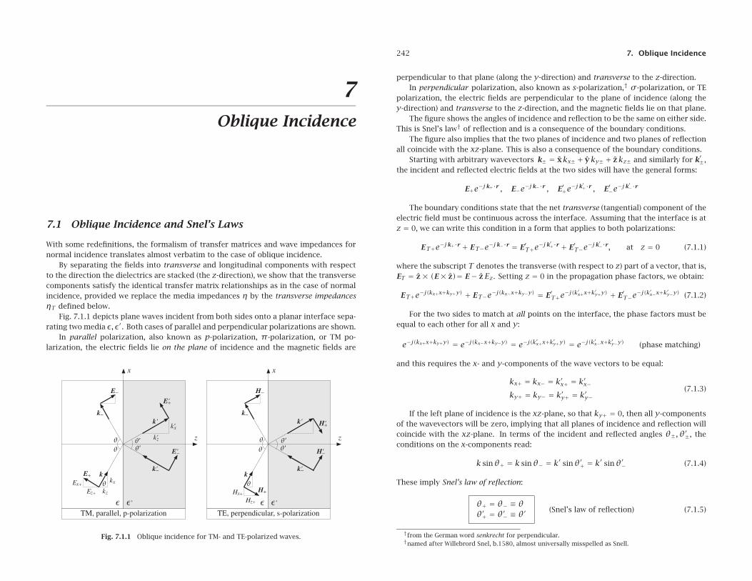
Fig. 7.1.1 depicts plane waves incident from both sides onto a planar interface sepa-rating two media ε, ε′. Both cases of parallel and perpendicular polarizations are shown.
In parallel polarization, also known as p-polarization, π-polarization, or TM po-larization, the electric fields lie on the plane of incidence and the magnetic fields are
Fig. 7.1.1 Oblique incidence for TM- and TE-polarized waves.
242 7. Oblique Incidence
perpendicular to that plane (along the y-direction) and transverse to the z-direction.In perpendicular polarization, also known as s-polarization,† σ-polarization, or TE
polarization, the electric fields are perpendicular to the plane of incidence (along they-direction) and transverse to the z-direction, and the magnetic fields lie on that plane.
The figure shows the angles of incidence and reflection to be the same on either side.This is Snel’s law† of reflection and is a consequence of the boundary conditions.
The figure also implies that the two planes of incidence and two planes of reflectionall coincide with the xz-plane. This is also a consequence of the boundary conditions.
Starting with arbitrary wavevectors k± = xkx± + yky± + zkz± and similarly for k′±,the incident and reflected electric fields at the two sides will have the general forms:
E+e−j k+·r , E−e−j k−·r , E′+e−j k′+·r , E′−e−j k′−·r
The boundary conditions state that the net transverse (tangential) component of theelectric field must be continuous across the interface. Assuming that the interface is atz = 0, we can write this condition in a form that applies to both polarizations:
ET+e−j k+·r + ET−e−j k−·r = E′T+e−j k′+·r + E′T−e
−j k′−·r, at z = 0 (7.1.1)
where the subscript T denotes the transverse (with respect to z) part of a vector, that is,ET = z× (E× z)= E− zEz. Setting z = 0 in the propagation phase factors, we obtain:
ET+e−j(kx+x+ky+y) + ET−e−j(kx−x+ky−y) = E′T+e−j(k′x+x+k′y+y) + E′T−e
−j(k′x−x+k′y−y) (7.1.2)
For the two sides to match at all points on the interface, the phase factors must beequal to each other for all x and y:
e−j(kx+x+ky+y) = e−j(kx−x+ky−y) = e−j(k′x+x+k′y+y) = e−j(k
′x−x+k′y−y) (phase matching)
and this requires the x- and y-components of the wave vectors to be equal:
kx+ = kx− = k′x+ = k′x−ky+ = ky− = k′y+ = k′y−
(7.1.3)
If the left plane of incidence is the xz-plane, so that ky+ = 0, then all y-componentsof the wavevectors will be zero, implying that all planes of incidence and reflection willcoincide with the xz-plane. In terms of the incident and reflected angles θ±, θ′±, theconditions on the x-components read:
k sinθ+ = k sinθ− = k′ sinθ′+ = k′ sinθ′− (7.1.4)
These imply Snel’s law of reflection:
θ+ = θ− ≡ θθ′+ = θ′− ≡ θ′ (Snel’s law of reflection) (7.1.5)
†from the German word senkrecht for perpendicular.†named after Willebrord Snel, b.1580, almost universally misspelled as Snell.
7.2. Transverse Impedance 243
And also Snel’s law of refraction, that is, k sinθ = k′ sinθ′. Setting k = nk0, k′ = n′k0,and k0 =ω/c0, we have:
n sinθ = n′ sinθ′ ⇒ sinθsinθ′
= n′
n(Snel’s law of refraction) (7.1.6)
It follows that the wave vectors shown in Fig. 7.1.1 will be explicitly:
k = k+ = kxx+ kzz = k sinθ x+ k cosθ z
k− = kxx− kzz = k sinθ x− k cosθ z
k′ = k′+ = k′xx+ k′zz = k′ sinθ′ x+ k′ cosθ′ z
k′− = k′xx− k′zz = k′ sinθ′ x− k′ cosθ′ z
(7.1.7)
The net transverse electric fields at arbitrary locations on either side of the interfaceare given by Eq. (7.1.1). Using Eq. (7.1.7), we have:
ET(x, z)= ET+e−j k+·r + ET−e−j k−·r = (ET+e−jkzz + ET−ejkzz
)e−jkxx
E′T(x, z)= E′T+e−j k′+·r + E′T−e
−j k′−·r = (E′T+e
−jk′zz + E′T−ejk′zz
)e−jk
′xx
(7.1.8)
In analyzing multilayer dielectrics stacked along the z-direction, the phase factore−jkxx = e−jk′xx will be common at all interfaces, and therefore, we can ignore it andrestore it at the end of the calculations, if so desired. Thus, we write Eq. (7.1.8) as:
ET(z)= ET+e−jkzz + ET−ejkzz
E′T(z)= E′T+e−jk′zz + E′T−e
jk′zz(7.1.9)
In the next section, we work out explicit expressions for Eq. (7.1.9)
7.2 Transverse Impedance
The transverse components of the electric fields are defined differently in the two po-larization cases. We recall from Sec. 2.10 that an obliquely-moving wave will have, ingeneral, both TM and TE components. For example, according to Eq. (2.10.9), the waveincident on the interface from the left will be given by:
E+(r) =[(x cosθ− z sinθ)A+ + yB+
]e−j k+·r
H+(r) = 1
η[yA+ − (x cosθ− z sinθ)B+
]e−j k+·r
(7.2.1)
where the A+ and B+ terms represent the TM and TE components, respectively. Thus,the transverse components are:
ET+(x, z) =[xA+ cosθ+ yB+
]e−j(kxx+kzz)
HT+(x, z) = 1
η[yA+ − xB+ cosθ
]e−j(kxx+kzz)
(7.2.2)
244 7. Oblique Incidence
Similarly, the wave reflected back into the left medium will have the form:
E−(r) =[(x cosθ+ z sinθ)A− + yB−
]e−j k−·r
H−(r) = 1
η[−yA− + (x cosθ+ z sinθ)B−
]e−j k−·r
(7.2.3)
with corresponding transverse parts:
ET−(x, z) =[xA− cosθ+ yB−
]e−j(kxx−kzz)
HT−(x, z) = 1
η[−yA− + xB− cosθ
]e−j(kxx−kzz)
(7.2.4)
Defining the transverse amplitudes and transverse impedances by:
AT± = A± cosθ , BT± = B±
ηTM = η cosθ , ηTE = ηcosθ
(7.2.5)
and noting that AT±/ηTM = A±/η and BT±/ηTE = B± cosθ/η, we may write Eq. (7.2.2)in terms of the transverse quantities as follows:
ET+(x, z) =[xAT+ + yBT+
]e−j(kxx+kzz)
HT+(x, z) =[yAT+ηTM
− xBT+ηTE
]e−j(kxx+kzz)
(7.2.6)
Similarly, Eq. (7.2.4) is expressed as:
ET−(x, z) =[xAT− + yBT−
]e−j(kxx−kzz)
HT−(x, z) =[−y
AT−ηTM
+ xBT−ηTE
]e−j(kxx−kzz)
(7.2.7)
Adding up Eqs. (7.2.6) and (7.2.7) and ignoring the common factor e−jkxx, we find forthe net transverse fields on the left side:
ET(z) = xETM(z)+ yETE(z)
HT(z) = yHTM(z)− xHTE(z)(7.2.8)
where the TM and TE components have the same structure provided one uses the ap-propriate transverse impedance:
ETM(z) = AT+e−jkzz +AT−ejkzz
HTM(z) = 1
ηTM
[AT+e−jkzz −AT−ejkzz
] (7.2.9)
ETE(z) = BT+e−jkzz + BT−ejkzz
HTE(z) = 1
ηTE
[BT+e−jkzz − BT−ejkzz
] (7.2.10)
7.2. Transverse Impedance 245
We summarize these in the compact form, where ET stands for either ETM or ETE :
ET(z) = ET+e−jkzz + ET−ejkzz
HT(z) = 1
ηT
[ET+e−jkzz − ET−ejkzz
] (7.2.11)
The transverse impedance ηT stands for either ηTM or ηTE :
ηT =⎧⎨⎩
η cosθ , TM, parallel, p-polarizationη
cosθ, TE, perpendicular, s-polarization
(7.2.12)
Because η = ηo/n, it is convenient to define also a transverse refractive indexthrough the relationship ηT = η0/nT. Thus, we have:
nT =⎧⎨⎩
ncosθ
, TM, parallel, p-polarization
n cosθ , TE, perpendicular, s-polarization(7.2.13)
For the right side of the interface, we obtain similar expressions:
E′T(z) = E′T+e−jk′zz + E′T−e
jk′zz
H′T(z) =
1
η′T
(E′T+e
−jk′zz − E′T−ejk′zz
) (7.2.14)
η′T =⎧⎪⎨⎪⎩
η′ cosθ′ , TM, parallel, p-polarization
η′
cosθ′, TE, perpendicular, s-polarization
(7.2.15)
n′T =⎧⎪⎨⎪⎩
n′
cosθ′, TM, parallel, p-polarization
n′ cosθ′ , TE, perpendicular, s-polarization(7.2.16)
where E′T± stands for A′T± = A′± cosθ′ or B′T± = B′±.For completeness, we give below the complete expressions for the fields on both
sides of the interface obtained by adding Eqs. (7.2.1) and (7.2.3), with all the propagationfactors restored. On the left side, we have:
E(r)= ETM(r)+ETE(r)
H(r)= HTM(r)+HTE(r)(7.2.17)
where
ETM(r) = (x cosθ− z sinθ)A+e−j k+·r + (x cosθ+ z sinθ)A−e−j k−·r
HTM(r) = y1
η(A+e−j k+·r −A−e−j k−·r)
ETE(r) = y(B+e−j k+·r + B−e−j k−·r)
HTE(r) = 1
η[−(x cosθ− z sinθ)B+e−j k+·r + (x cosθ+ z sinθ)B−e−j k−·r]
(7.2.18)
246 7. Oblique Incidence
The transverse parts of these are the same as those given in Eqs. (7.2.9) and (7.2.10).On the right side of the interface, we have:
E ′(r)= E ′TM(r)+E ′TE(r)
H ′(r)= H ′TM(r)+H ′
TE(r)(7.2.19)
E ′TM(r) = (x cosθ′ − z sinθ′)A′+e−j k′+·r + (x cosθ′ + z sinθ′)A′−e−j k′−·r
H ′TM(r) = y
1
η′(A′+e−j k′+·r −A′−e−j k′−·r)
E ′TE(r) = y(B′+e−j k′+·r + B′−e−j k′−·r)
H ′TE(r) =
1
η′[−(x cosθ′ − z sinθ′)B′+e−j k′+·r + (x cosθ′ + z sinθ′)B′−e−j k′−·r]
(7.2.20)
7.3 Propagation and Matching of Transverse Fields
Eq. (7.2.11) has the identical form of Eq. (5.1.1) of the normal incidence case, but withthe substitutions:
η→ ηT , e±jkz → e±jkzz = e±jkz cosθ (7.3.1)
Every definition and concept of Chap. 5 translates into the oblique case. For example,we can define the transverse wave impedance at position z by:
ZT(z)= ET(z)HT(z)
= ηTET+e−jkzz + ET−ejkzz
ET+e−jkzz − ET−ejkzz(7.3.2)
and the transverse reflection coefficient at position z:
ΓT(z)= ET−(z)ET+(z)
= ET−ejkzz
ET+e−jkzz= ΓT(0)e2jkzz (7.3.3)
They are related as in Eq. (5.1.7):
ZT(z)= ηT1+ ΓT(z)1− ΓT(z)
� ΓT(z)= ZT(z)−ηTZT(z)+ηT (7.3.4)
The propagation matrices, Eqs. (5.1.11) and (5.1.13), relating the fields at two posi-tions z1, z2 within the same medium, read now:
[ET1+ET1−
]=
[ejkzl 0
0 e−jkzl
][ET2+ET2−
](propagation matrix) (7.3.5)
[ET1
HT1
]=
[coskzl jηT sinkzl
jη−1T sinkzl coskzl
][ET2
HT2
](propagation matrix) (7.3.6)
7.3. Propagation and Matching of Transverse Fields 247
where l = z2− z1. Similarly, the reflection coefficients and wave impedances propagateas:
ΓT1 = ΓT2e−2jkzl , ZT1 = ηTZT2 + jηT tankzlηT + jZT2 tankzl
(7.3.7)
The phase thickness δ = kl = 2π(nl)/λ of the normal incidence case, where λ isthe free-space wavelength, is replaced now by:
δz = kzl = kl cosθ = 2πλ
nl cosθ (7.3.8)
At the interface z = 0, the boundary conditions for the tangential electric and mag-netic fields give rise to the same conditions as Eqs. (5.2.1) and (5.2.2):
ET = E′T , HT = H′T (7.3.9)
and in terms of the forward/backward fields:
ET+ + ET− = E′T+ + E′T−
1
ηT
(ET+ − ET−
) = 1
η′T
(E′T+ − E′T−
) (7.3.10)
which can be solved to give the matching matrix:
[ET+ET−
]= 1
τT
[1 ρTρT 1
][E′T+E′T−
](matching matrix) (7.3.11)
where ρT,τT are transverse reflection coefficients, replacing Eq. (5.2.5):
ρT = η′T − ηTη′T + ηT
= nT − n′TnT + n′T
τT = 2η′Tη′T + ηT
= 2nTnT + n′T
(Fresnel coefficients) (7.3.12)
where τT = 1 + ρT. We may also define the reflection coefficients from the right sideof the interface: ρ′T = −ρT and τ′T = 1 + ρ′T = 1 − ρT. Eqs. (7.3.12) are known as theFresnel reflection and transmission coefficients.
The matching conditions for the transverse fields translate into corresponding match-ing conditions for the wave impedances and reflection responses:
ZT = Z′T � ΓT = ρT + Γ′T1+ ρTΓ′T
� Γ′T =ρ′T + ΓT
1+ ρ′TΓT(7.3.13)
If there is no left-incident wave from the right, that is, E′− = 0, then, Eq. (7.3.11) takesthe specialized form:
[ET+ET−
]= 1
τT
[1 ρTρT 1
][E′T+
0
](7.3.14)
which explains the meaning of the transverse reflection and transmission coefficients:
248 7. Oblique Incidence
ρT = ET−ET+
, τT = E′T+ET+
(7.3.15)
The relationship of these coefficients to the reflection and transmission coefficientsof the total field amplitudes depends on the polarization. For TM, we have ET± =A± cosθ and E′T± = A′± cosθ′, and for TE, ET± = B± and E′T± = B′±. For both cases,it follows that the reflection coefficient ρT measures also the reflection of the totalamplitudes, that is,
ρTM = A− cosθA+ cosθ
= A−A+
, ρTE = B−B+
whereas for the transmission coefficients, we have:
τTM = A′+ cosθ′
A+ cosθ= cosθ′
cosθA′+A+
, τTE = B′+B+
In addition to the boundary conditions of the transverse field components, there arealso applicable boundary conditions for the longitudinal components. For example, inthe TM case, the component Ez is normal to the surface and therefore, we must havethe continuity condition Dz = D′z, or εEz = ε′E′z. Similarly, in the TE case, we musthave Bz = B′z. It can be verified that these conditions are automatically satisfied due toSnel’s law (7.1.6).
The fields carry energy towards the z-direction, as well as the transverse x-direction.The energy flux along the z-direction must be conserved across the interface. The cor-responding components of the Poynting vector are:
Pz = 1
2Re
[ExH∗
y − EyH∗x], Px = 1
2Re
[EyH∗
z − EzH∗y]
For TM, we have Pz = Re[ExH∗y ]/2 and for TE, Pz = −Re[EyH∗
x ]/2. Using theabove equations for the fields, we find that Pz is given by the same expression for bothTM and TE polarizations:
Pz = cosθ2η
(|A+|2 − |A−|2), or,cosθ
2η(|B+|2 − |B−|2) (7.3.16)
Using the appropriate definitions for ET± and ηT, Eq. (7.3.16) can be written in termsof the transverse components for either polarization:
Pz = 1
2ηT
(|ET+|2 − |ET−|2) (7.3.17)
As in the normal incidence case, the structure of the matching matrix (7.3.11) impliesthat (7.3.17) is conserved across the interface.
7.4 Fresnel Reflection Coefficients
We look now at the specifics of the Fresnel coefficients (7.3.12) for the two polarizationcases. Inserting the two possible definitions (7.2.13) for the transverse refractive indices,we can express ρT in terms of the incident and refracted angles:
7.4. Fresnel Reflection Coefficients 249
ρTM =n
cosθ− n′
cosθ′n
cosθ+ n′
cosθ′
= n cosθ′ − n′ cosθn cosθ′ + n′ cosθ
ρTE = n cosθ− n′ cosθ′
n cosθ+ n′ cosθ′
(7.4.1)
We note that for normal incidence, θ = θ′ = 0, they both reduce to the usualreflection coefficient ρ = (n− n′)/(n+ n′).† Using Snel’s law, n sinθ = n′ sinθ′, andsome trigonometric identities, we may write Eqs. (7.4.1) in a number of equivalent ways.In terms of the angle of incidence only, we have:
ρTM =
√(n′
n
)2
− sin2 θ−(n′
n
)2
cosθ√(n′
n
)2
− sin2 θ+(n′
n
)2
cosθ
ρTE =cosθ−
√(n′
n
)2
− sin2 θ
cosθ+√(
n′
n
)2
− sin2 θ
(7.4.2)
Note that at grazing angles of incidence, θ→ 90o, the reflection coefficients tend toρTM → 1 and ρTE → −1, regardless of the refractive indices n,n′. One consequence ofthis property is in wireless communications where the effect of the ground reflectionscauses the power of the propagating radio wave to attenuate with the fourth (insteadof the second) power of the distance, thus, limiting the propagation range (see Exam-ple 22.3.5.)
We note also that Eqs. (7.4.1) and (7.4.2) remain valid when one or both of the mediaare lossy. For example, if the right medium is lossy with complex refractive index n′c =n′r − jn′i , then, Snel’s law, n sinθ = n′c sinθ′, is still valid but with a complex-valued θ′
and (7.4.2) remains the same with the replacement n′ → n′c. The third way of expressingthe ρs is in terms of θ,θ′ only, without the n,n′:
ρTM = sin 2θ′ − sin 2θsin 2θ′ + sin 2θ
= tan(θ′ − θ)tan(θ′ + θ)
ρTE = sin(θ′ − θ)sin(θ′ + θ)
(7.4.3)
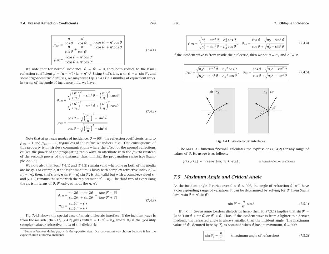
Fig. 7.4.1 shows the special case of an air-dielectric interface. If the incident wave isfrom the air side, then Eq. (7.4.2) gives with n = 1, n′ = nd, where nd is the (possiblycomplex-valued) refractive index of the dielectric:
†Some references define ρTM with the opposite sign. Our convention was chosen because it has theexpected limit at normal incidence.
250 7. Oblique Incidence
ρTM =√n2d − sin2 θ− n2
d cosθ√n2d − sin2 θ+ n2
d cosθ, ρTE =
cosθ−√n2d − sin2 θ
cosθ+√n2d − sin2 θ
(7.4.4)
If the incident wave is from inside the dielectric, then we set n = nd and n′ = 1:
ρTM =√n−2d − sin2 θ− n−2
d cosθ√n−2d − sin2 θ+ n−2
d cosθ, ρTE =
cosθ−√n−2d − sin2 θ
cosθ+√n−2d − sin2 θ
(7.4.5)
Fig. 7.4.1 Air-dielectric interfaces.
The MATLAB function fresnel calculates the expressions (7.4.2) for any range ofvalues of θ. Its usage is as follows:
[rtm,rte] = fresnel(na,nb,theta); % Fresnel reflection coefficients
7.5 Maximum Angle and Critical Angle
As the incident angle θ varies over 0 ≤ θ ≤ 90o, the angle of refraction θ′ will havea corresponding range of variation. It can be determined by solving for θ′ from Snel’slaw, n sinθ = n′ sinθ′:
sinθ′ = nn′
sinθ (7.5.1)
If n < n′ (we assume lossless dielectrics here,) then Eq. (7.5.1) implies that sinθ′ =(n/n′)sinθ < sinθ, or θ′ < θ. Thus, if the incident wave is from a lighter to a densermedium, the refracted angle is always smaller than the incident angle. The maximumvalue of θ′, denoted here by θ′c, is obtained when θ has its maximum, θ = 90o:
sinθ′c =nn′
(maximum angle of refraction) (7.5.2)
7.5. Maximum Angle and Critical Angle 251
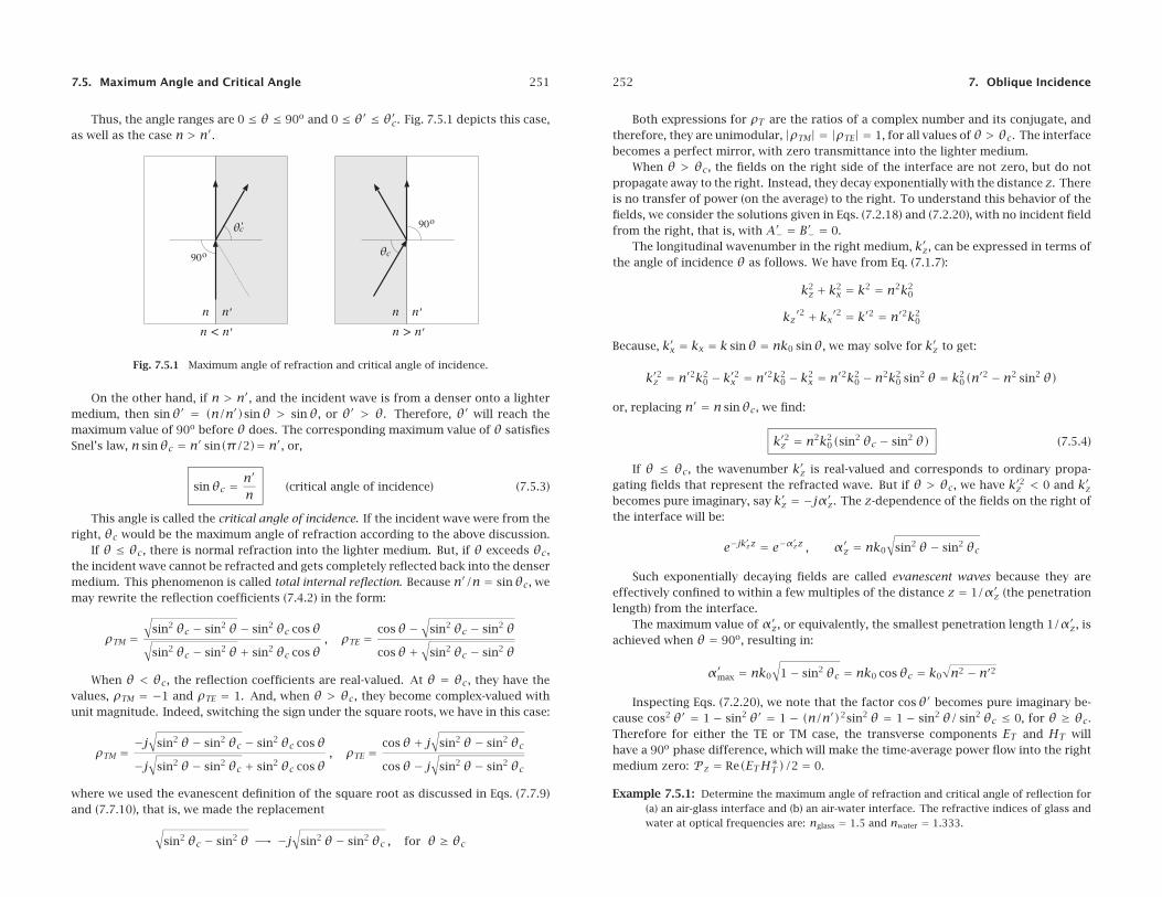
Thus, the angle ranges are 0 ≤ θ ≤ 90o and 0 ≤ θ′ ≤ θ′c. Fig. 7.5.1 depicts this case,as well as the case n > n′.
Fig. 7.5.1 Maximum angle of refraction and critical angle of incidence.
On the other hand, if n > n′, and the incident wave is from a denser onto a lightermedium, then sinθ′ = (n/n′)sinθ > sinθ, or θ′ > θ. Therefore, θ′ will reach themaximum value of 90o before θ does. The corresponding maximum value of θ satisfiesSnel’s law, n sinθc = n′ sin(π/2)= n′, or,
sinθc = n′
n(critical angle of incidence) (7.5.3)
This angle is called the critical angle of incidence. If the incident wave were from theright, θc would be the maximum angle of refraction according to the above discussion.
If θ ≤ θc, there is normal refraction into the lighter medium. But, if θ exceeds θc,the incident wave cannot be refracted and gets completely reflected back into the densermedium. This phenomenon is called total internal reflection. Because n′/n = sinθc, wemay rewrite the reflection coefficients (7.4.2) in the form:
ρTM =√
sin2 θc − sin2 θ− sin2 θc cosθ√sin2 θc − sin2 θ+ sin2 θc cosθ
, ρTE =cosθ−
√sin2 θc − sin2 θ
cosθ+√
sin2 θc − sin2 θ
When θ < θc, the reflection coefficients are real-valued. At θ = θc, they have thevalues, ρTM = −1 and ρTE = 1. And, when θ > θc, they become complex-valued withunit magnitude. Indeed, switching the sign under the square roots, we have in this case:
ρTM =−j
√sin2 θ− sin2 θc − sin2 θc cosθ
−j√
sin2 θ− sin2 θc + sin2 θc cosθ, ρTE =
cosθ+ j√
sin2 θ− sin2 θc
cosθ− j√
sin2 θ− sin2 θc
where we used the evanescent definition of the square root as discussed in Eqs. (7.7.9)and (7.7.10), that is, we made the replacement
√sin2 θc − sin2 θ −→ −j
√sin2 θ− sin2 θc , for θ ≥ θc
252 7. Oblique Incidence
Both expressions for ρT are the ratios of a complex number and its conjugate, andtherefore, they are unimodular, |ρTM| = |ρTE| = 1, for all values ofθ > θc. The interfacebecomes a perfect mirror, with zero transmittance into the lighter medium.
When θ > θc, the fields on the right side of the interface are not zero, but do notpropagate away to the right. Instead, they decay exponentially with the distance z. Thereis no transfer of power (on the average) to the right. To understand this behavior of thefields, we consider the solutions given in Eqs. (7.2.18) and (7.2.20), with no incident fieldfrom the right, that is, with A′− = B′− = 0.
The longitudinal wavenumber in the right medium, k′z, can be expressed in terms ofthe angle of incidence θ as follows. We have from Eq. (7.1.7):
k2z + k2
x = k2 = n2k20
kz′2 + kx′2 = k′2 = n′2k20
Because, k′x = kx = k sinθ = nk0 sinθ, we may solve for k′z to get:
k′2z = n′2k20 − k′2x = n′2k2
0 − k2x = n′2k2
0 − n2k20 sin2 θ = k2
0(n′2 − n2 sin2 θ)
or, replacing n′ = n sinθc, we find:
k′2z = n2k20(sin2 θc − sin2 θ) (7.5.4)
If θ ≤ θc, the wavenumber k′z is real-valued and corresponds to ordinary propa-gating fields that represent the refracted wave. But if θ > θc, we have k′2z < 0 and k′zbecomes pure imaginary, say k′z = −jα′z. The z-dependence of the fields on the right ofthe interface will be:
e−jk′zz = e−α
′zz , α′z = nk0
√sin2 θ− sin2 θc
Such exponentially decaying fields are called evanescent waves because they areeffectively confined to within a few multiples of the distance z = 1/α′z (the penetrationlength) from the interface.
The maximum value of α′z, or equivalently, the smallest penetration length 1/α′z, isachieved when θ = 90o, resulting in:
α′max = nk0
√1− sin2 θc = nk0 cosθc = k0
√n2 − n′2
Inspecting Eqs. (7.2.20), we note that the factor cosθ′ becomes pure imaginary be-cause cos2 θ′ = 1 − sin2 θ′ = 1 − (n/n′)2sin2 θ = 1 − sin2 θ/ sin2 θc ≤ 0, for θ ≥ θc.Therefore for either the TE or TM case, the transverse components ET and HT willhave a 90o phase difference, which will make the time-average power flow into the rightmedium zero: Pz = Re(ETH∗
T)/2 = 0.
Example 7.5.1: Determine the maximum angle of refraction and critical angle of reflection for(a) an air-glass interface and (b) an air-water interface. The refractive indices of glass andwater at optical frequencies are: nglass = 1.5 and nwater = 1.333.
7.5. Maximum Angle and Critical Angle 253
Solution: There is really only one angle to determine, because if n = 1 and n′ = nglass, thensin(θ′c)= n/n′ = 1/nglass, and if n = nglass and n′ = 1, then, sin(θc)= n′/n = 1/nglass.Thus, θ′c = θc:
θc = asin(
1
1.5
)= 41.8o
For the air-water case, we have:
θc = asin(
1
1.333
)= 48.6o
The refractive index of water at radio frequencies and below is nwater = 9 approximately.The corresponding critical angle is θc = 6.4o.
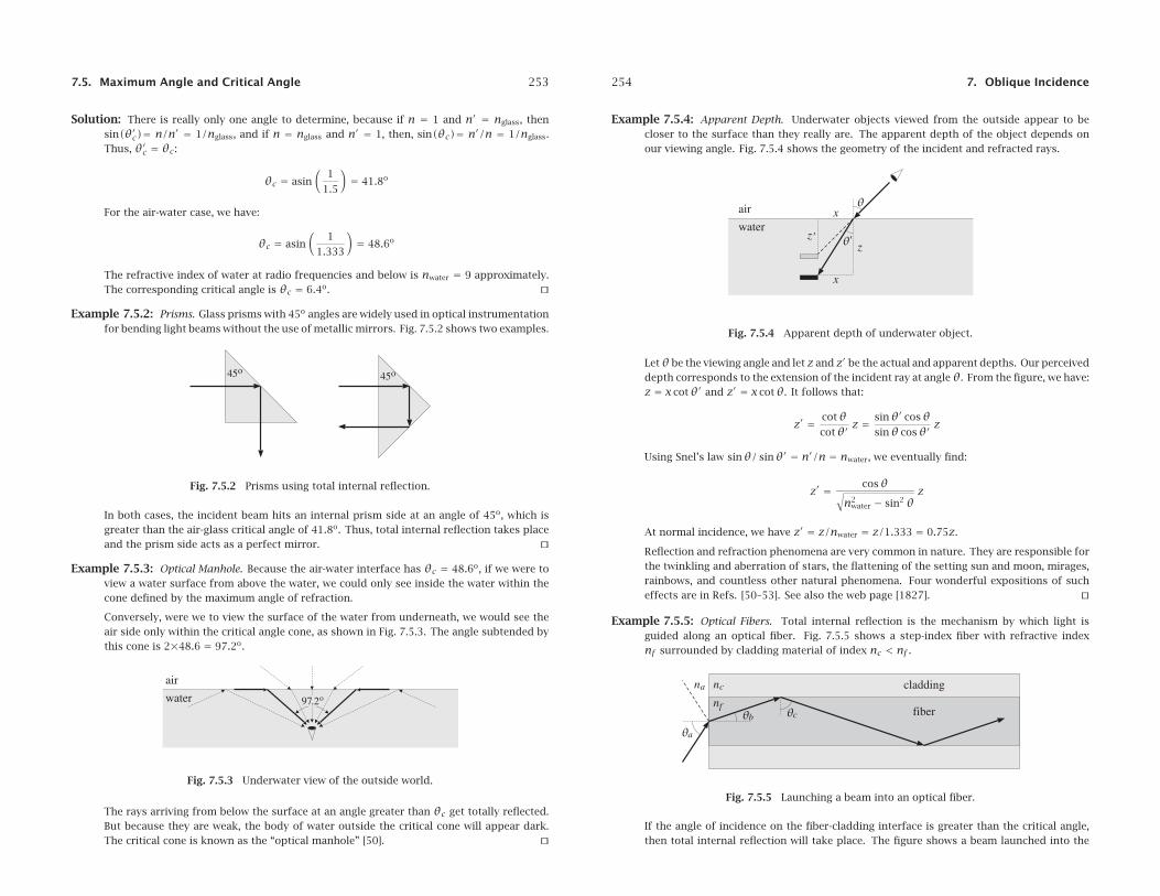
Example 7.5.2: Prisms. Glass prisms with 45o angles are widely used in optical instrumentationfor bending light beams without the use of metallic mirrors. Fig. 7.5.2 shows two examples.
Fig. 7.5.2 Prisms using total internal reflection.
In both cases, the incident beam hits an internal prism side at an angle of 45o, which isgreater than the air-glass critical angle of 41.8o. Thus, total internal reflection takes placeand the prism side acts as a perfect mirror.
Example 7.5.3: Optical Manhole. Because the air-water interface has θc = 48.6o, if we were toview a water surface from above the water, we could only see inside the water within thecone defined by the maximum angle of refraction.
Conversely, were we to view the surface of the water from underneath, we would see theair side only within the critical angle cone, as shown in Fig. 7.5.3. The angle subtended bythis cone is 2×48.6 = 97.2o.
Fig. 7.5.3 Underwater view of the outside world.
The rays arriving from below the surface at an angle greater than θc get totally reflected.But because they are weak, the body of water outside the critical cone will appear dark.The critical cone is known as the “optical manhole” [50].
254 7. Oblique Incidence
Example 7.5.4: Apparent Depth. Underwater objects viewed from the outside appear to becloser to the surface than they really are. The apparent depth of the object depends onour viewing angle. Fig. 7.5.4 shows the geometry of the incident and refracted rays.
Fig. 7.5.4 Apparent depth of underwater object.
Letθ be the viewing angle and let z and z′ be the actual and apparent depths. Our perceiveddepth corresponds to the extension of the incident ray at angleθ. From the figure, we have:z = x cotθ′ and z′ = x cotθ. It follows that:
z′ = cotθcotθ′
z = sinθ′ cosθsinθ cosθ′
z
Using Snel’s law sinθ/ sinθ′ = n′/n = nwater, we eventually find:
z′ = cosθ√n2
water − sin2 θz
At normal incidence, we have z′ = z/nwater = z/1.333 = 0.75z.
Reflection and refraction phenomena are very common in nature. They are responsible forthe twinkling and aberration of stars, the flattening of the setting sun and moon, mirages,rainbows, and countless other natural phenomena. Four wonderful expositions of sucheffects are in Refs. [50–53]. See also the web page [1827].
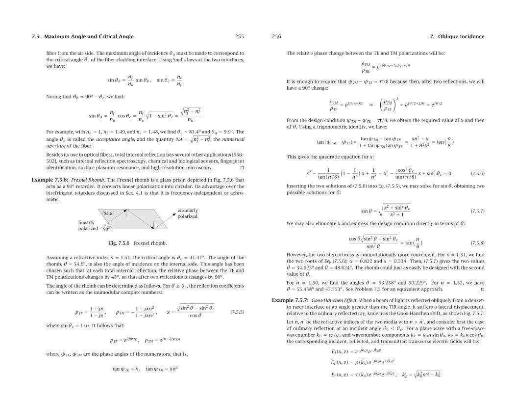
Example 7.5.5: Optical Fibers. Total internal reflection is the mechanism by which light isguided along an optical fiber. Fig. 7.5.5 shows a step-index fiber with refractive indexnf surrounded by cladding material of index nc < nf .
Fig. 7.5.5 Launching a beam into an optical fiber.
If the angle of incidence on the fiber-cladding interface is greater than the critical angle,then total internal reflection will take place. The figure shows a beam launched into the
7.5. Maximum Angle and Critical Angle 255
fiber from the air side. The maximum angle of incidenceθa must be made to correspond tothe critical angle θc of the fiber-cladding interface. Using Snel’s laws at the two interfaces,we have:
sinθa = nfna
sinθb , sinθc = ncnf
Noting that θb = 90o − θc, we find:
sinθa = nfna
cosθc = nfna
√1− sin2 θc =
√n2f − n2
c
na
For example, with na = 1, nf = 1.49, and nc = 1.48, we findθc = 83.4o andθa = 9.9o. The
angle θa is called the acceptance angle, and the quantity NA =√n2f − n2
c , the numericalaperture of the fiber.
Besides its use in optical fibers, total internal reflection has several other applications [556–592], such as internal reflection spectroscopy, chemical and biological sensors, fingerprintidentification, surface plasmon resonance, and high resolution microscopy.
Example 7.5.6: Fresnel Rhomb. The Fresnel rhomb is a glass prism depicted in Fig. 7.5.6 thatacts as a 90o retarder. It converts linear polarization into circular. Its advantage over thebirefringent retarders discussed in Sec. 4.1 is that it is frequency-independent or achro-matic.
Fig. 7.5.6 Fresnel rhomb.
Assuming a refractive index n = 1.51, the critical angle is θc = 41.47o. The angle of therhomb, θ = 54.6o, is also the angle of incidence on the internal side. This angle has beenchosen such that, at each total internal reflection, the relative phase between the TE andTM polarizations changes by 45o, so that after two reflections it changes by 90o.
The angle of the rhomb can be determined as follows. Forθ ≥ θc, the reflection coefficientscan be written as the unimodular complex numbers:
ρTE = 1+ jx1− jx
, ρTM = −1+ jxn2
1− jxn2, x =
√sin2 θ− sin2 θc
cosθ(7.5.5)
where sinθc = 1/n. It follows that:
ρTE = e2jψTE , ρTM = ejπ+2jψTM
where ψTE, ψTM are the phase angles of the numerators, that is,
tanψTE = x , tanψTM = xn2
256 7. Oblique Incidence
The relative phase change between the TE and TM polarizations will be:
ρTM
ρTE= e2jψTM−2jψTE+jπ
It is enough to require that ψTM −ψTE = π/8 because then, after two reflections, we willhave a 90o change:
ρTM
ρTE= ejπ/4+jπ ⇒
(ρTM
ρTE
)2
= ejπ/2+2jπ = ejπ/2
From the design condition ψTM −ψTE = π/8, we obtain the required value of x and thenof θ. Using a trigonometric identity, we have:
tan(ψTM −ψTE)= tanψTM − tanψTE
1+ tanψTM tanψTE= xn2 − x
1+ n2x2= tan
(π8
)
This gives the quadratic equation for x:
x2 − 1
tan(π/8)(1− 1
n2
)x+ 1
n2= x2 − cos2 θc
tan(π/8)x+ sin2 θc = 0 (7.5.6)
Inserting the two solutions of (7.5.6) into Eq. (7.5.5), we may solve for sinθ, obtaining twopossible solutions for θ:
sinθ =√x2 + sin2 θc
x2 + 1(7.5.7)
We may also eliminate x and express the design condition directly in terms of θ:
cosθ√
sin2 θ− sin2 θcsin2 θ
= tan(π
8
)(7.5.8)
However, the two-step process is computationally more convenient. For n = 1.51, we findthe two roots of Eq. (7.5.6): x = 0.822 and x = 0.534. Then, (7.5.7) gives the two valuesθ = 54.623o and θ = 48.624o. The rhomb could just as easily be designed with the secondvalue of θ.
For n = 1.50, we find the angles θ = 53.258o and 50.229o. For n = 1.52, we haveθ = 55.458o and 47.553o. See Problem 7.5 for an equivalent approach.
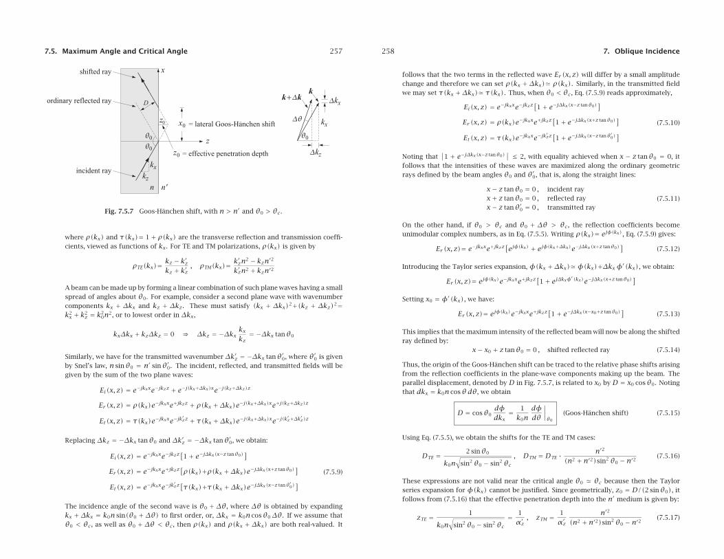
Example 7.5.7: Goos-Hanchen Effect. When a beam of light is reflected obliquely from a denser-to-rarer interface at an angle greater than the TIR angle, it suffers a lateral displacement,relative to the ordinary reflected ray, known as the Goos-Hanchen shift, as shown Fig. 7.5.7.
Let n,n′ be the refractive indices of the two media with n > n′, and consider first the caseof ordinary reflection at an incident angle θ0 < θc. For a plane wave with a free-spacewavenumber k0 = ω/c0 and wavenumber components kx = k0n sinθ0, kz = k0n cosθ0,the corresponding incident, reflected, and transmitted transverse electric fields will be:
Ei(x, z) = e−jkxxe−jkzz
Er(x, z) = ρ(kx)e−jkxxe+jkzz
Et(x, z) = τ(kx)e−jkxxe−jk′zz , k′z =
√k2
0n′2 − k2x
7.5. Maximum Angle and Critical Angle 257
Fig. 7.5.7 Goos-Hanchen shift, with n > n′ and θ0 > θc.
where ρ(kx) and τ(kx)= 1+ ρ(kx) are the transverse reflection and transmission coeffi-cients, viewed as functions of kx. For TE and TM polarizations, ρ(kx) is given by
ρTE(kx)= kz − k′zkz + k′z
, ρTM(kx)= k′zn2 − kzn′2
k′zn2 + kzn′2
A beam can be made up by forming a linear combination of such plane waves having a smallspread of angles about θ0. For example, consider a second plane wave with wavenumbercomponents kx + Δkx and kz + Δkz. These must satisfy (kx + Δkx)2+(kz + Δkz)2=k2x + k2
z = k20n2, or to lowest order in Δkx,
kxΔkx + kzΔkz = 0 ⇒ Δkz = −Δkx kxkz = −Δkx tanθ0
Similarly, we have for the transmitted wavenumber Δk′z = −Δkx tanθ′0, where θ′0 is givenby Snel’s law, n sinθ0 = n′ sinθ′0. The incident, reflected, and transmitted fields will begiven by the sum of the two plane waves:
Ei(x, z) = e−jkxxe−jkzz + e−j(kx+Δkx)xe−j(kz+Δkz)z
Er(x, z) = ρ(kx)e−jkxxe+jkzz + ρ(kx +Δkx)e−j(kx+Δkx)xe+j(kz+Δkz)z
Et(x, z) = τ(kx)e−jkxxe−jk′zz + τ(kx +Δkx)e−j(kx+Δkx)xe−j(k
′z+Δk′z)z
Replacing Δkz = −Δkx tanθ0 and Δk′z = −Δkx tanθ′0, we obtain:
Ei(x, z) = e−jkxxe−jkzz[1+ e−jΔkx(x−z tanθ0)
]Er(x, z) = e−jkxxe+jkzz
[ρ(kx)+ρ(kx +Δkx)e−jΔkx(x+z tanθ0)
]Et(x, z) = e−jkxxe−jk
′zz[τ(kx)+τ(kx +Δkx)e−jΔkx(x−z tanθ′0)
](7.5.9)
The incidence angle of the second wave is θ0 + Δθ, where Δθ is obtained by expandingkx + Δkx = k0n sin(θ0 + Δθ) to first order, or, Δkx = k0n cosθ0 Δθ. If we assume thatθ0 < θc, as well as θ0 + Δθ < θc, then ρ(kx) and ρ(kx + Δkx) are both real-valued. It
258 7. Oblique Incidence
follows that the two terms in the reflected wave Er(x, z) will differ by a small amplitudechange and therefore we can set ρ(kx + Δkx)� ρ(kx). Similarly, in the transmitted fieldwe may set τ(kx +Δkx)� τ(kx). Thus, when θ0 < θc, Eq. (7.5.9) reads approximately,
Ei(x, z) = e−jkxxe−jkzz[1+ e−jΔkx(x−z tanθ0)
]Er(x, z) = ρ(kx)e−jkxxe+jkzz
[1+ e−jΔkx(x+z tanθ0)
]Et(x, z) = τ(kx)e−jkxxe−jk
′zz[1+ e−jΔkx(x−z tanθ′0)
](7.5.10)
Noting that∣∣1 + e−jΔkx(x−z tanθ0)
∣∣ ≤ 2, with equality achieved when x − z tanθ0 = 0, itfollows that the intensities of these waves are maximized along the ordinary geometricrays defined by the beam angles θ0 and θ′0, that is, along the straight lines:
x− z tanθ0 = 0 , incident rayx+ z tanθ0 = 0 , reflected rayx− z tanθ′0 = 0 , transmitted ray
(7.5.11)
On the other hand, if θ0 > θc and θ0 + Δθ > θc, the reflection coefficients becomeunimodular complex numbers, as in Eq. (7.5.5). Writing ρ(kx)= ejφ(kx), Eq. (7.5.9) gives:
Er(x, z)= e−jkxxe+jkzz[ejφ(kx) + ejφ(kx+Δkx)e−jΔkx(x+z tanθ0)
](7.5.12)
Introducing the Taylor series expansion, φ(kx +Δkx)� φ(kx)+Δkx φ′(kx), we obtain:
Er(x, z)= ejφ(kx)e−jkxxe+jkzz[1+ ejΔkxφ
′(kx)e−jΔkx(x+z tanθ0)]
Setting x0 = φ′(kx), we have:
Er(x, z)= ejφ(kx)e−jkxxe+jkzz[1+ e−jΔkx(x−x0+z tanθ0)
](7.5.13)
This implies that the maximum intensity of the reflected beam will now be along the shiftedray defined by:
x− x0 + z tanθ0 = 0 , shifted reflected ray (7.5.14)
Thus, the origin of the Goos-Hanchen shift can be traced to the relative phase shifts arisingfrom the reflection coefficients in the plane-wave components making up the beam. Theparallel displacement, denoted by D in Fig. 7.5.7, is related to x0 by D = x0 cosθ0. Notingthat dkx = k0n cosθdθ, we obtain
D = cosθ0dφdkx
= 1
k0ndφdθ
∣∣∣∣θ0
(Goos-Hanchen shift) (7.5.15)
Using Eq. (7.5.5), we obtain the shifts for the TE and TM cases:
DTE = 2 sinθ0
k0n√
sin2 θ0 − sin2 θc, DTM = DTE · n′2
(n2 + n′2)sin2 θ0 − n′2(7.5.16)
These expressions are not valid near the critical angle θ0 � θc because then the Taylorseries expansion for φ(kx) cannot be justified. Since geometrically, z0 = D/(2 sinθ0), itfollows from (7.5.16) that the effective penetration depth into the n′ medium is given by:
zTE = 1
k0n√
sin2 θ0 − sin2 θc= 1
α′z, zTM = 1
α′zn′2
(n2 + n′2)sin2 θ0 − n′2(7.5.17)
7.6. Brewster Angle 259
where α′z =√k2x − k2
0n′2 = k0
√n2 sin2 θ0 − n′2 = k0n
√sin2 θ0 − sin2 θc . These expres-
sions are consistent with the field dependence e−jk′zz = e−α
′zz inside the n′ medium, which
shows that the effective penetration length is of the order of 1/α′z .
7.6 Brewster Angle
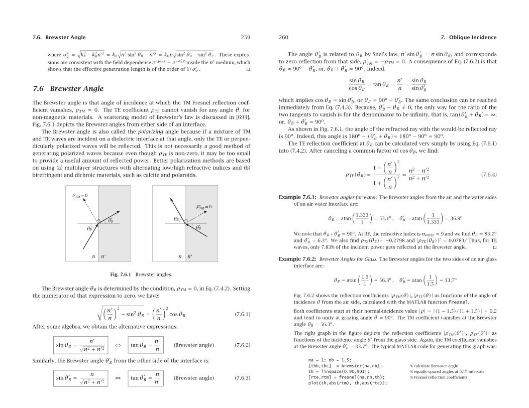
The Brewster angle is that angle of incidence at which the TM Fresnel reflection coef-ficient vanishes, ρTM = 0. The TE coefficient ρTE cannot vanish for any angle θ, fornon-magnetic materials. A scattering model of Brewster’s law is discussed in [693].Fig. 7.6.1 depicts the Brewster angles from either side of an interface.
The Brewster angle is also called the polarizing angle because if a mixture of TMand TE waves are incident on a dielectric interface at that angle, only the TE or perpen-dicularly polarized waves will be reflected. This is not necessarily a good method ofgenerating polarized waves because even though ρTE is non-zero, it may be too smallto provide a useful amount of reflected power. Better polarization methods are basedon using (a) multilayer structures with alternating low/high refractive indices and (b)birefringent and dichroic materials, such as calcite and polaroids.
Fig. 7.6.1 Brewster angles.
The Brewster angle θB is determined by the condition, ρTM = 0, in Eq. (7.4.2). Settingthe numerator of that expression to zero, we have:
√(n′
n
)2
− sin2 θB =(n′
n
)2
cosθB (7.6.1)
After some algebra, we obtain the alternative expressions:
sinθB = n′√n2 + n′2
� tanθB = n′
n(Brewster angle) (7.6.2)
Similarly, the Brewster angle θ′B from the other side of the interface is:
sinθ′B =n√
n2 + n′2� tanθ′B =
nn′
(Brewster angle) (7.6.3)
260 7. Oblique Incidence
The angle θ′B is related to θB by Snel’s law, n′ sinθ′B = n sinθB, and correspondsto zero reflection from that side, ρ′TM = −ρTM = 0. A consequence of Eq. (7.6.2) is thatθB = 90o − θ′B, or, θB + θ′B = 90o. Indeed,
sinθBcosθB
= tanθB = n′
n= sinθB
sinθ′B
which implies cosθB = sinθ′B, or θB = 90o − θ′B. The same conclusion can be reachedimmediately from Eq. (7.4.3). Because, θ′B − θB = 0, the only way for the ratio of thetwo tangents to vanish is for the denominator to be infinity, that is, tan(θ′B + θB)= ∞,or, θB + θ′B = 90o.
As shown in Fig. 7.6.1, the angle of the refracted ray with the would-be reflected rayis 90o. Indeed, this angle is 180o − (θ′B + θB)= 180o − 90o = 90o.
The TE reflection coefficient at θB can be calculated very simply by using Eq. (7.6.1)into (7.4.2). After canceling a common factor of cosθB, we find:
ρTE(θB)=1−
(n′
n
)2
1+(n′
n
)2 =n2 − n′2
n2 + n′2(7.6.4)
Example 7.6.1: Brewster angles for water. The Brewster angles from the air and the water sidesof an air-water interface are:
θB = atan(
1.333
1
)= 53.1o , θ′B = atan
(1
1.333
)= 36.9o
We note that θB+θ′B = 90o. At RF, the refractive index is nwater = 9 and we find θB = 83.7o
and θ′B = 6.3o. We also find ρTE(θB)= −0.2798 and |ρTE(θB)|2 = 0.0783/ Thus, for TEwaves, only 7.83% of the incident power gets reflected at the Brewster angle.
Example 7.6.2: Brewster Angles for Glass. The Brewster angles for the two sides of an air-glassinterface are:
θB = atan(
1.51
)= 56.3o , θ′B = atan
(1
1.5
)= 33.7o
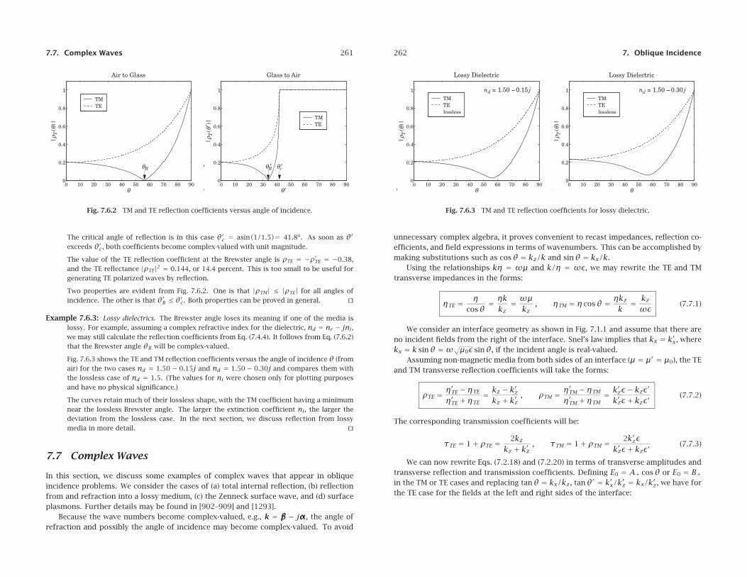
Fig. 7.6.2 shows the reflection coefficients |ρTM(θ)|, |ρTE(θ)| as functions of the angle ofincidence θ from the air side, calculated with the MATLAB function fresnel.
Both coefficients start at their normal-incidence value |ρ| = |(1 − 1.5)/(1 + 1.5)| = 0.2and tend to unity at grazing angle θ = 90o. The TM coefficient vanishes at the Brewsterangle θB = 56.3o.
The right graph in the figure depicts the reflection coefficients |ρ′TM(θ′)|, |ρ′TE(θ′)| asfunctions of the incidence angle θ′ from the glass side. Again, the TM coefficient vanishesat the Brewster angle θ′B = 33.7o. The typical MATLAB code for generating this graph was:
na = 1; nb = 1.5;[thb,thc] = brewster(na,nb); % calculate Brewster angle
th = linspace(0,90,901); % equally-spaced angles at 0.1o intervals
[rte,rtm] = fresnel(na,nb,th); % Fresnel reflection coefficients
plot(th,abs(rtm), th,abs(rte));
7.7. Complex Waves 261
0 10 20 30 40 50 60 70 80 900
0.2
0.4
0.6
0.8
1
θ θB
|ρ T
(θ)|
θ θ
Air to Glass
TM TE
0 10 20 30 40 50 60 70 80 900
0.2
0.4
0.6
0.8
1
θ θB′θ θc′
|ρ T
(θ′)|
θ θ′
Glass to Air
TM TE
Fig. 7.6.2 TM and TE reflection coefficients versus angle of incidence.
The critical angle of reflection is in this case θ′c = asin(1/1.5)= 41.8o. As soon as θ′
exceeds θ′c, both coefficients become complex-valued with unit magnitude.
The value of the TE reflection coefficient at the Brewster angle is ρTE = −ρ′TE = −0.38,and the TE reflectance |ρTE|2 = 0.144, or 14.4 percent. This is too small to be useful forgenerating TE polarized waves by reflection.
Two properties are evident from Fig. 7.6.2. One is that |ρTM| ≤ |ρTE| for all angles ofincidence. The other is that θ′B ≤ θ′c. Both properties can be proved in general.
Example 7.6.3: Lossy dielectrics. The Brewster angle loses its meaning if one of the media islossy. For example, assuming a complex refractive index for the dielectric, nd = nr − jni,we may still calculate the reflection coefficients from Eq. (7.4.4). It follows from Eq. (7.6.2)that the Brewster angle θB will be complex-valued.
Fig. 7.6.3 shows the TE and TM reflection coefficients versus the angle of incidence θ (fromair) for the two cases nd = 1.50 − 0.15j and nd = 1.50 − 0.30j and compares them withthe lossless case of nd = 1.5. (The values for ni were chosen only for plotting purposesand have no physical significance.)
The curves retain much of their lossless shape, with the TM coefficient having a minimumnear the lossless Brewster angle. The larger the extinction coefficient ni, the larger thedeviation from the lossless case. In the next section, we discuss reflection from lossymedia in more detail.
7.7 Complex Waves
In this section, we discuss some examples of complex waves that appear in obliqueincidence problems. We consider the cases of (a) total internal reflection, (b) reflectionfrom and refraction into a lossy medium, (c) the Zenneck surface wave, and (d) surfaceplasmons. Further details may be found in [902–909] and [1293].
Because the wave numbers become complex-valued, e.g., k = βββ − jααα, the angle ofrefraction and possibly the angle of incidence may become complex-valued. To avoid
262 7. Oblique Incidence
0 10 20 30 40 50 60 70 80 900
0.2
0.4
0.6
0.8
1
|ρ T
(θ)|
θ θ
Lossy Dielectric
nd = 1.50 − 0.15 j TM TE lossless
0 10 20 30 40 50 60 70 80 900
0.2
0.4
0.6
0.8
1
|ρ T
(θ)|
θ θ
Lossy Dielectric
nd = 1.50 − 0.30 j TM TE lossless
Fig. 7.6.3 TM and TE reflection coefficients for lossy dielectric.
unnecessary complex algebra, it proves convenient to recast impedances, reflection co-efficients, and field expressions in terms of wavenumbers. This can be accomplished bymaking substitutions such as cosθ = kz/k and sinθ = kx/k.
Using the relationships kη = ωμ and k/η = ωε, we may rewrite the TE and TMtransverse impedances in the forms:
ηTE = ηcosθ
= ηkkz
= ωμkz
, ηTM = η cosθ = ηkzk
= kzωε
(7.7.1)
We consider an interface geometry as shown in Fig. 7.1.1 and assume that there areno incident fields from the right of the interface. Snel’s law implies that kx = k′x, wherekx = k sinθ =ω√μ0ε sinθ, if the incident angle is real-valued.
Assuming non-magnetic media from both sides of an interface (μ = μ′ = μ0), the TEand TM transverse reflection coefficients will take the forms:
ρTE = η′TE − ηTE
η′TE + ηTE= kz − k′zkz + k′z
, ρTM = η′TM − ηTM
η′TM + ηTM= k′zε− kzε′
k′zε+ kzε′(7.7.2)
The corresponding transmission coefficients will be:
τTE = 1+ ρTE = 2kzkz + k′z
, τTM = 1+ ρTM = 2k′zεk′zε+ kzε′
(7.7.3)
We can now rewrite Eqs. (7.2.18) and (7.2.20) in terms of transverse amplitudes andtransverse reflection and transmission coefficients. Defining E0 = A+ cosθ or E0 = B+in the TM or TE cases and replacing tanθ = kx/kz, tanθ′ = k′x/k′z = kx/k′z, we have forthe TE case for the fields at the left and right sides of the interface:
7.7. Complex Waves 263
E(r) = yE0[e−jkzz + ρTE ejkzz
]e−jkxx
H(r) = E0
ηTE
[(−x+ kx
kzz)e−jkzz + ρTE
(x+ kx
kzz)ejkzz
]e−jkxx
E ′(r) = yτTE E0e−jk′zze−jkxx
H ′(r) = τTE E0
η′TE
(−x+ kx
k′zz)e−jk
′zze−jkxx
(TE) (7.7.4)
and for the TM case:
E(r) = E0
[(x− kx
kzz)e−jkzz + ρTM
(x+ kx
kzz)ejkzz
]e−jkxx
H(r) = yE0
ηTM
[e−jkzz − ρTM ejkzz
]e−jkxx
E ′(r) = τTM E0
(x− kx
k′zz)e−jk
′zze−jkxx
H ′(r) = yτTM E0
η′TMe−jk
′zze−jkxx
(TM) (7.7.5)
Equations (7.7.4) and (7.7.5) are dual to each other, as are Eqs. (7.7.1). They transforminto each other under the duality transformation E → H, H → −E, ε → μ, and μ → ε.See Sec. 18.2 for more on the concept of duality.
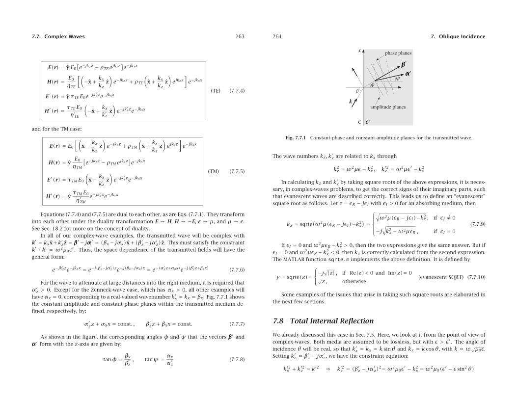
In all of our complex-wave examples, the transmitted wave will be complex withk′ = kxx+k′zz = βββ′ −jααα′ = (βx−jαx)x+(β′z−jα′z)z. This must satisfy the constraintk′ · k′ = ω2μ0ε′. Thus, the space dependence of the transmitted fields will have thegeneral form:
e−jk′zze−jkxx = e−j(β
′z−jα′z)ze−j(βx−jαx)x = e−(α
′zz+αxx)e−j(β
′zz+βxx) (7.7.6)
For the wave to attenuate at large distances into the right medium, it is required thatα′z > 0. Except for the Zenneck-wave case, which has αx > 0, all other examples willhaveαx = 0, corresponding to a real-valued wavenumber k′x = kx = βx. Fig. 7.7.1 showsthe constant-amplitude and constant-phase planes within the transmitted medium de-fined, respectively, by:
α′zz+αxx = const. , β′zz+ βxx = const. (7.7.7)
As shown in the figure, the corresponding angles φ and ψ that the vectors βββ′ andααα′ form with the z-axis are given by:
tanφ = βxβ′z
, tanψ = αx
α′z(7.7.8)
264 7. Oblique Incidence
Fig. 7.7.1 Constant-phase and constant-amplitude planes for the transmitted wave.
The wave numbers kz, k′z are related to kx through
k2z =ω2με− k2
x , k′2z =ω2με′ − k2x
In calculating kz and k′z by taking square roots of the above expressions, it is neces-sary, in complex-waves problems, to get the correct signs of their imaginary parts, suchthat evanescent waves are described correctly. This leads us to define an “evanescent”square root as follows. Let ε = εR − jεI with εI > 0 for an absorbing medium, then
kz = sqrte(ω2μ(εR − jεI)−k2
x) =
⎧⎪⎪⎨⎪⎪⎩
√ω2μ(εR − jεI)−k2
x , if εI = 0
−j√k2x −ω2μεR , if εI = 0
(7.7.9)
If εI = 0 and ω2μεR−k2x > 0, then the two expressions give the same answer. But if
εI = 0 and ω2μεR−k2x < 0, then kz is correctly calculated from the second expression.
The MATLAB function sqrte.m implements the above definition. It is defined by
y = sqrte(z)=⎧⎨⎩−j
√|z| , if Re(z)< 0 and Im(z)= 0√z , otherwise
(evanescent SQRT) (7.7.10)
Some examples of the issues that arise in taking such square roots are elaborated inthe next few sections.
7.8 Total Internal Reflection
We already discussed this case in Sec. 7.5. Here, we look at it from the point of view ofcomplex-waves. Both media are assumed to be lossless, but with ε > ε′. The angle ofincidence θ will be real, so that k′x = kx = k sinθ and kz = k cosθ, with k = ω√μ0ε.Setting k′z = β′z − jα′z, we have the constraint equation:
k′2x + k′2z = k′2 ⇒ k′2z = (β′z − jα′z)2=ω2μ0ε′ − k2x =ω2μ0(ε′ − ε sin2 θ)
7.8. Total Internal Reflection 265
which separates into the real and imaginary parts:
β′2z −α′2z =ω2μ0(ε′ − ε sin2 θ)= k2(sin2 θc − sin2 θ)
α′zβ′z = 0(7.8.1)
where we set sin2 θc = ε′/ε and k2 = ω2μ0ε. This has two solutions: (a) α′z = 0 andβ′2z = k2(sin2 θc − sin2 θ), valid when θ ≤ θc, and (b) β′z = 0 and α′2z = k2(sin2 θ −sin2 θc), valid when θ ≥ θc.
Case (a) corresponds to ordinary refraction into the right medium, and case (b), tototal internal reflection. In the latter case, we have k′z = −jα′z and the TE and TMreflection coefficients (7.7.2) become unimodular complex numbers:
ρTE = kz − k′zkz + k′z
= kz + jα′zkz − jα′z
, ρTM = k′zε− kzε′
k′zε+ kzε′= −kzε
′ + jα′zεkzε′ − jα′zε
(7.8.2)
The complete expressions for the fields are given by Eqs. (7.7.4) or (7.7.5). The prop-agation phase factor in the right medium will be in case (b):
e−jk′zze−jkxx = e−α
′zze−jkxx
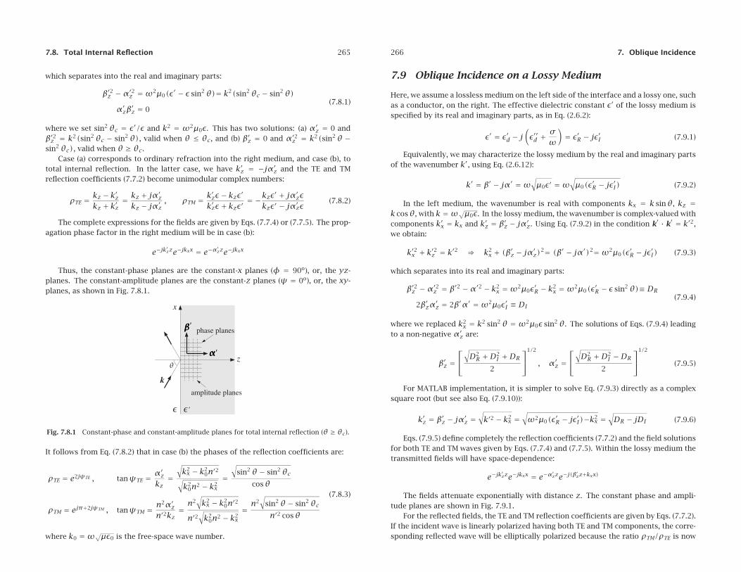
Thus, the constant-phase planes are the constant-x planes (φ = 90o), or, the yz-planes. The constant-amplitude planes are the constant-z planes (ψ = 0o), or, the xy-planes, as shown in Fig. 7.8.1.
Fig. 7.8.1 Constant-phase and constant-amplitude planes for total internal reflection (θ ≥ θc).
It follows from Eq. (7.8.2) that in case (b) the phases of the reflection coefficients are:
ρTE = e2jψTE , tanψTE = α′zkz
=√k2x − k2
0n′2√k2
0n2 − k2x=
√sin2 θ− sin2 θc
cosθ
ρTM = ejπ+2jψTM , tanψTM = n2α′zn′2kz
= n2√k2x − k2
0n′2
n′2√k2
0n2 − k2x= n2
√sin2 θ− sin2 θcn′2 cosθ
(7.8.3)
where k0 =ω√με0 is the free-space wave number.
266 7. Oblique Incidence
7.9 Oblique Incidence on a Lossy Medium
Here, we assume a lossless medium on the left side of the interface and a lossy one, suchas a conductor, on the right. The effective dielectric constant ε′ of the lossy medium isspecified by its real and imaginary parts, as in Eq. (2.6.2):
ε′ = ε′d − j(ε′′d +
σω
)= ε′R − jε′I (7.9.1)
Equivalently, we may characterize the lossy medium by the real and imaginary partsof the wavenumber k′, using Eq. (2.6.12):
k′ = β′ − jα′ =ω√μ0ε′ =ω
√μ0(ε′R − jε′I) (7.9.2)
In the left medium, the wavenumber is real with components kx = k sinθ, kz =k cosθ, with k =ω√μ0ε. In the lossy medium, the wavenumber is complex-valued withcomponents k′x = kx and k′z = β′z − jα′z. Using Eq. (7.9.2) in the condition k′ · k′ = k′2,we obtain:
k′2x + k′2z = k′2 ⇒ k2x + (β′z − jα′z)2= (β′ − jα′)2=ω2μ0(ε′R − jε′I) (7.9.3)
which separates into its real and imaginary parts:
β′2z −α′2z = β′2 −α′2 − k2x =ω2μ0ε′R − k2
x =ω2μ0(ε′R − ε sin2 θ)≡ DR
2β′zα′z = 2β′α′ =ω2μ0ε′I ≡ DI(7.9.4)
where we replaced k2x = k2 sin2 θ = ω2μ0ε sin2 θ. The solutions of Eqs. (7.9.4) leading
to a non-negative α′z are:
β′z =⎡⎣√D2R +D2
I +DR
2
⎤⎦
1/2
, α′z =⎡⎣√D2R +D2
I −DR
2
⎤⎦
1/2
(7.9.5)
For MATLAB implementation, it is simpler to solve Eq. (7.9.3) directly as a complexsquare root (but see also Eq. (7.9.10)):
k′z = β′z − jα′z =√k′2 − k2
x =√ω2μ0(ε′R − jε′I)−k2
x =√DR − jDI (7.9.6)
Eqs. (7.9.5) define completely the reflection coefficients (7.7.2) and the field solutionsfor both TE and TM waves given by Eqs. (7.7.4) and (7.7.5). Within the lossy medium thetransmitted fields will have space-dependence:
e−jk′zze−jkxx = e−α
′zze−j(β
′zz+kxx)
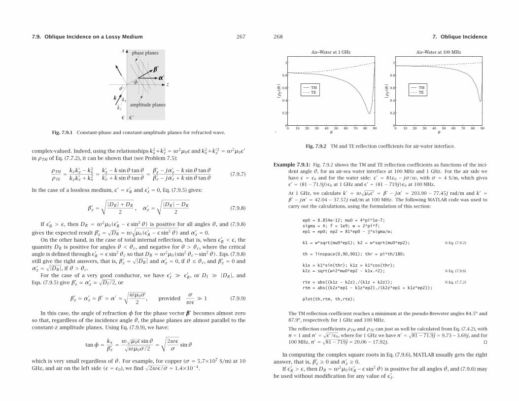
The fields attenuate exponentially with distance z. The constant phase and ampli-tude planes are shown in Fig. 7.9.1.
For the reflected fields, the TE and TM reflection coefficients are given by Eqs. (7.7.2).If the incident wave is linearly polarized having both TE and TM components, the corre-sponding reflected wave will be elliptically polarized because the ratio ρTM/ρTE is now
7.9. Oblique Incidence on a Lossy Medium 267
Fig. 7.9.1 Constant-phase and constant-amplitude planes for refracted wave.
complex-valued. Indeed, using the relationships k2x+k2
z =ω2μ0ε and k2x+k′2z =ω2μ0ε′
in ρTM of Eq. (7.7.2), it can be shown that (see Problem 7.5):
ρTM
ρTE= kzk′z − k2
xkzk′z + k2
x= k′z − k sinθ tanθk′z + k sinθ tanθ
= β′z − jα′z − k sinθ tanθβ′z − jα′z + k sinθ tanθ
(7.9.7)
In the case of a lossless medium, ε′ = ε′R and ε′I = 0, Eq. (7.9.5) gives:
β′z =√|DR| +DR
2, α′z =
√|DR| −DR
2(7.9.8)
If ε′R > ε, then DR = ω2μ0(ε′R − ε sin2 θ) is positive for all angles θ, and (7.9.8)
gives the expected result β′z =√DR =ω
√μ0(ε′R − ε sin2 θ) and α′z = 0.
On the other hand, in the case of total internal reflection, that is, when ε′R < ε, thequantity DR is positive for angles θ < θc, and negative for θ > θc, where the criticalangle is defined through ε′R = ε sin2 θc so thatDR =ω2μ0(sin2 θc−sin2 θ). Eqs. (7.9.8)still give the right answers, that is, β′z =
√|DR| and α′z = 0, if θ ≤ θc, and β′z = 0 andα′z =
√|DR|, if θ > θc.For the case of a very good conductor, we have ε′I � ε′R, or DI � |DR|, and
Eqs. (7.9.5) give β′z � α′z �√DI/2, or
β′z � α′z � β′ � α′ �√ωμ0σ
2, provided
σωε
� 1 (7.9.9)
In this case, the angle of refraction φ for the phase vector βββ′ becomes almost zeroso that, regardless of the incidence angle θ, the phase planes are almost parallel to theconstant-z amplitude planes. Using Eq. (7.9.9), we have:
tanφ = kxβ′z= ω√μ0ε sinθ√
ωμ0σ/2=
√2ωεσ
sinθ
which is very small regardless of θ. For example, for copper (σ = 5.7×10⁷ S/m) at 10GHz, and air on the left side (ε = ε0), we find
√2ωε/σ = 1.4×10⁻⁴.
268 7. Oblique Incidence
0 10 20 30 40 50 60 70 80 900
0.2
0.4
0.6
0.8
1
|ρ T
(θ)|
θ θ
Air−Water at 1 GHz
TM TE
0 10 20 30 40 50 60 70 80 900
0.2
0.4
0.6
0.8
1
|ρ T
(θ)|
θ θ
Air−Water at 100 MHz
TM TE
Fig. 7.9.2 TM and TE reflection coefficients for air-water interface.
Example 7.9.1: Fig. 7.9.2 shows the TM and TE reflection coefficients as functions of the inci-dent angle θ, for an air-sea water interface at 100 MHz and 1 GHz. For the air side wehave ε = ε0 and for the water side: ε′ = 81ε0 − jσ/ω, with σ = 4 S/m, which givesε′ = (81− 71.9j)ε0 at 1 GHz and ε′ = (81− 719j)ε0 at 100 MHz.
At 1 GHz, we calculate k′ = ω√μ0ε′ = β′ − jα′ = 203.90 − 77.45j rad/m and k′ =
β′ − jα′ = 42.04 − 37.57j rad/m at 100 MHz. The following MATLAB code was used tocarry out the calculations, using the formulation of this section:
ep0 = 8.854e-12; mu0 = 4*pi*1e-7;sigma = 4; f = 1e9; w = 2*pi*f;ep1 = ep0; ep2 = 81*ep0 - j*sigma/w;
k1 = w*sqrt(mu0*ep1); k2 = w*sqrt(mu0*ep2); % Eq. (7.9.2)
th = linspace(0,90,901); thr = pi*th/180;
k1x = k1*sin(thr); k1z = k1*cos(thr);k2z = sqrt(w^2*mu0*ep2 - k1x.^2); % Eq. (7.9.6)
rte = abs((k1z - k2z)./(k1z + k2z)); % Eq. (7.7.2)
rtm = abs((k2z*ep1 - k1z*ep2)./(k2z*ep1 + k1z*ep2));
plot(th,rtm, th,rte);
The TM reflection coefficient reaches a minimum at the pseudo-Brewster angles 84.5o and87.9o, respectively for 1 GHz and 100 MHz.
The reflection coefficients ρTM and ρTE can just as well be calculated from Eq. (7.4.2), withn = 1 and n′ = √
ε′/ε0, where for 1 GHz we have n′ = √81− 71.9j = 9.73−3.69j, and for
100 MHz, n′ = √81− 719j = 20.06− 17.92j.
In computing the complex square roots in Eq. (7.9.6), MATLAB usually gets the rightanswer, that is, β′z ≥ 0 and α′z ≥ 0.
If ε′R > ε, then DR =ω2μ0(ε′R−ε sin2 θ) is positive for all angles θ, and (7.9.6) maybe used without modification for any value of ε′I.
7.9. Oblique Incidence on a Lossy Medium 269
If ε′R < ε and ε′I > 0, then Eq. (7.9.6) still gives the correct algebraic signs for anyangle θ. But when ε′I = 0, that is, for a lossless medium, then DI = 0 and k′z =
√DR.
For θ > θc we have DR < 0 and MATLAB gives k′z =√DR =
√−|DR| = j√|DR|, which
has the wrong sign for α′z (we saw that Eqs. (7.9.5) work correctly in this case.)In order to coax MATLAB to produce the right algebraic sign for α′z in all cases, we
may redefine Eq. (7.9.6) by using double conjugation:
k′z = β′z − jα′z =(√
(DR − jDI)∗)∗
=⎧⎪⎨⎪⎩−j
√|DR| , if DI = 0 and DR < 0√
DR − jDI , otherwise(7.9.10)
One word of caution, however, is that current versions of MATLAB (ver. ≤ 7.0) mayproduce inconsistent results for (7.9.10) depending on whether DI is a scalar or a vectorpassing through zero.† Compare, for example, the outputs from the statements:
DI = 0; kz = conj(sqrt(conj(-1 - j*DI)));DI = -1:1; kz = conj(sqrt(conj(-1 - j*DI)));
Note, however, that Eq. (7.9.10) does work correctly when DI is a single scalar withDR being a vector of values, e.g., arising from a vector of angles θ.
Another possible alternative calculation is to add a small negative imaginary part tothe argument of the square root, for example with the MATLAB code:
kz = sqrt(DR-j*DI-j*realmin);
where realmin is MATLAB’s smallest positive floating point number (typically, equalto 2.2251 × 10−308). This works well for all cases. Yet, a third alternative is to useEq. (7.9.6) and then reverse the signs whenever DI = 0 and DR < 0, for example:
kz = sqrt(DR-j*DI);kz(DI==0 & DR<0) = -kz(DI==0 & DR<0);
Next, we discuss briefly the energy flux into the lossy medium. It is given by the z-component of the Poynting vector, Pz = 1
2 z ·Re(E×H∗). For the TE case of Eq. (7.7.4),we find at the two sides of the interface:
Pz = |E0|22ωμ0
kz(1− |ρTE|2
), P′z =
|E0|22ωμ0
β′z|τTE|2e−2α′zz (7.9.11)
where we replaced ηTE = ωμ0/kz and η′TE = ωμ0/k′z. Thus, the transmitted powerattenuates with distance as the wave propagates into the lossy medium.
The two expressions match at the interface, expressing energy conservation, that is,at z = 0, we have Pz = P′z, which follows from the condition (see Problem 7.7):
kz(1− |ρTE|2
) = β′z|τTE|2 (7.9.12)
Because the net energy flow is to the right in the transmitted medium, we must haveβ′z ≥ 0. Because also kz > 0, then Eq. (7.9.12) implies that |ρTE| ≤ 1. For the case of
†this has been fixed in versions > v7.0.
270 7. Oblique Incidence
total internal reflection, we have β′z = 0, which gives |ρTE| = 1. Similar conclusions canbe reached for the TM case of Eq. (7.7.5). The matching condition at the interface is now:
εkz
(1− |ρTM|2
) = Re(ε′
k′z
)|τTM|2 = ε′Rβ′z + ε′Iα′z
|k′z|2 |τTM|2 (7.9.13)
Using the constraint ω2μoε′I = 2β′zα′z, it follows that the right-hand side will againbe proportional toβ′z (with a positive proportionality coefficient.) Thus, the non-negativesign of β′z implies that |ρTM| ≤ 1.
7.10 Zenneck Surface Wave
For a lossy medium ε′, the TM reflection coefficient cannot vanish for any real incident
angle θ because the Brewster angle is complex valued: tanθB =√ε′/ε =
√(ε′R − jε′I)/ε.
However, ρTM can vanish if we allow a complex-valued θ, or equivalently, a complex-valued incident wavevector k = βββ − jααα, even though the left medium is lossless. Thisleads to the so-called Zenneck surface wave [32,902,903,909,1293].
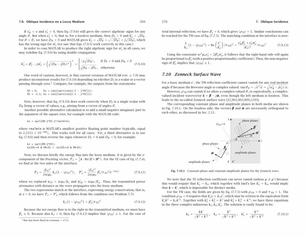
The corresponding constant phase and amplitude planes in both media are shownin Fig. 7.10.1. On the lossless side, the vectors βββ and ααα are necessarily orthogonal toeach other, as discussed in Sec. 2.11.
Fig. 7.10.1 Constant-phase and constant-amplitude planes for the Zenneck wave.
We note that the TE reflection coefficient can never vanish (unless μ = μ′) becausethis would require that k′z = kz, which together with Snel’s law k′x = kx, would implythat k = k′, which is impossible for distinct media.
For the TM case, the fields are given by Eq. (7.7.5) with ρTM = 0 and τTM = 1. Thecondition ρTM = 0 requires that k′zε = kzε′, which may be written in the equivalent formk′zk2 = kzk′2. Together with k2
x + k2z = k2 and k2
x + k′2z = k′2, we have three equationsin the three complex unknowns kx, kz, k′z. The solution is easily found to be:
kx = kk′√k2 + k′2
, kz = k2√k2 + k′2
, k′z =k′2√
k2 + k′2(7.10.1)
7.10. Zenneck Surface Wave 271
where k =ω√μ0ε and k′ = β′ − jα′ =ω√μ0ε′. These may be written in the form:
kx =ω√μ0
√εε′
ε+ ε′, kz =ω
√μ0
ε√ε+ ε′
, k′z =ω√μ0
ε′√ε+ ε′
(7.10.2)
Using k′x = kx, the space-dependence of the fields at the two sides is as follows:
e−j(kxx+kzz) = e−(αxx+αzz)e−j(βxx+βzz) , for z ≤ 0
e−j(k′xx+k′zz) = e−(αxx+α′zz)e−j(βxx+β
′zz) , for z ≥ 0
Thus, in order for the fields not to grow exponentially with distance and to be con-fined near the interface surface, it is required that:
αx > 0 , αz < 0 , α′z > 0 (7.10.3)
These conditions are guaranteed with the sign choices of Eq. (7.10.2). This can beverified by writing
ε′ = |ε′|e−jδ
ε+ ε′ = |ε+ ε′|e−jδ1
ε′
ε+ ε′=
∣∣∣∣ ε′
ε+ ε′
∣∣∣∣e−j(δ−δ1)
and noting that δ2 = δ − δ1 > 0, as follows by inspecting the triangle formed by thethree vectors ε, ε′, and ε + ε′. Then, the phase angles of kx, kz, k′z are −δ2/2, δ1/2,and −(δ2 + δ1/2), respectively, thus, implying the condition (7.10.3). In drawing thistriangle, we made the implicit assumption that ε′R > 0, which is valid for typical lossydielectrics. In the next section, we discuss surface plasmons for which ε′R < 0.
Although the Zenneck wave attenuates both along the x- and z-directions, the atten-uation constant along x tends to be much smaller than that along z. For example, in theweakly lossy approximation, we may write ε′ = ε′R(1− jτ), where τ = ε′I/ε
′R � 1 is the
loss tangent of ε′. Then, we have the following first-order approximations in τ:
√ε′ =
√ε′R
(1− j
τ2
),
1√ε+ ε′
= 1√ε+ ε′R
(1+ j
τ2
ε′Rε+ ε′R
)
These lead to the first-order approximations for kx and kz:
kx =ω√μ0
√√√ εε′Rε+ ε′R
(1− j
τ2
εε+ ε′R
), kz =ω
√μ0
ε√ε+ ε′R
(1+ j
τ2
ε′Rε+ ε′R
)
It follows that:
αx =ω√μ0
√√√ εε′Rε+ ε′R
τ2
εε+ ε′R
, αz = −ω√μ0ε√
ε+ ε′R
τ2
ε′Rε+ ε′R
⇒ αx
|αz| =√
εε′R
Typically, ε′R > ε, implying that αx < |αz|. For example, for an air-water interfacewe have at microwave frequencies ε′R/ε = 81, and for an air-ground interface, ε′R/ε = 6.
272 7. Oblique Incidence
If both media are lossless, then both k and k′ are real and Eqs. (7.10.1) yield theusual Brewster angle formulas, that is,
tanθB = kxkz= k′
k=√ε′√ε, tanθ′B =
kxk′z= kk′=√ε√ε′
Example 7.10.1: For the data of the air-water interface of Example 7.9.1, we calculate the fol-lowing Zenneck wavenumbers at 1 GHz and 100 MHz using Eq. (7.10.2):
f = 1 GHz f = 100 MHz
kx = βx − jαx = 20.89− 0.064j kx = βx − jαx = 2.1− 0.001jkz = βz − jαz = 1.88+ 0.71j kz = βz − jαz = 0.06+ 0.05jk′z = β′z − jα′z = 202.97− 77.80j k′z = β′z − jα′z = 42.01− 37.59j
The units are in rads/m. As required, αz is negative. We observe that αx � |αz| and thatthe attenuations are much more severe within the lossy medium.
7.11 Surface Plasmons
Consider an interface between two non-magnetic semi-infinite media ε1 and ε2, as shownin Fig. 7.11.1 The wavevectors k1 = xkx + zkz1 and k2 = xkx + zkz2 at the two sidesmust have a common kx component, as required by Snel’s law, and their z-componentsmust satisfy:
k2z1 = k2
0ε1 − k2x , k2
z2 = k20ε2 − k2
x (7.11.1)
where we defined the relative dielectric constants ε1 = ε1/ε0, ε2 = ε2/ε0, and the free-space wavenumber k0 =ω√μ0ε0 =ω/c0. The TM reflection coefficient is given by:
ρTM = kz2ε1 − kz1ε2
kz2ε1 + kz1ε2
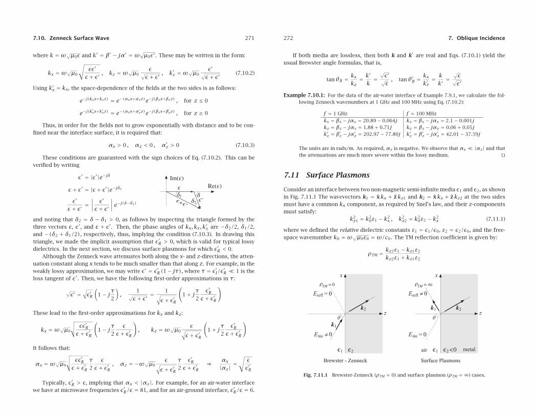
Fig. 7.11.1 Brewster-Zenneck (ρTM = 0) and surface plasmon (ρTM = ∞) cases.
7.11. Surface Plasmons 273
Both the Brewster case for lossless dielectrics and the Zenneck case were charac-terized by the condition ρTM = 0, or, kz2ε1 = kz1ε2. This condition together withEqs. (7.11.1) leads to the solution (7.10.2), which is the same in both cases:
kx = k0
√ε1ε2
ε1 + ε2, kz1 = k0ε1√
ε1 + ε2, kz2 = k0ε2√
ε1 + ε2(7.11.2)
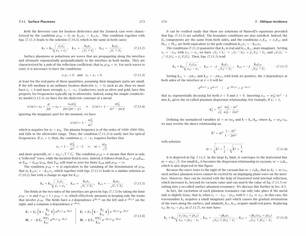
Surface plasmons or polaritons are waves that are propagating along the interfaceand attenuate exponentially perpendicularly to the interface in both media. They arecharacterized by a pole of the reflection coefficient, that is, ρTM = ∞. For such waves toexist, it is necessary to have the conditions:
ε1ε2 < 0 and ε1 + ε2 < 0 (7.11.3)
at least for the real-parts of these quantities, assuming their imaginary parts are small.If the left medium is an ordinary lossless dielectric ε1 > 0, such as air, then we musthave ε2 < 0 and more strongly ε2 < −ε1. Conductors, such as silver and gold, have thisproperty for frequencies typically up to ultraviolet. Indeed, using the simple conductiv-ity model (1.12.3), we have for the dielectric constant of a metal:
ε(ω)= ε0 + σjω
= ε0 +ε0ω2
p
jω(jω+ γ)⇒ ε(ω)= 1− ω2
p
ω2 − jωγ(7.11.4)
Ignoring the imaginary part for the moment, we have
ε(ω)= 1− ω2p
ω2
which is negative for ω <ωp. The plasma frequency is of the order of 1000–2000 THz,and falls in the ultraviolet range. Thus, the condition (7.11.3) is easily met for opticalfrequencies. If ε1 = 1, then, the condition ε2 < −ε1 requires further that
ε2 = 1− ω2p
ω2< −1 ⇒ ω <
ωp√2
and more generally, ω <ωp/√
1+ ε1. The condition ρTM = ∞means that there is onlya “reflected” wave, while the incident field is zero. Indeed, it follows from Erefl = ρTMEinc,or Einc = Erefl/ρTM, that Einc will tend to zero for finite Erefl and ρTM →∞.
The condition ρTM = ∞ is equivalent to the vanishing of the denominator of ρTM,that is, kz2ε1 = −kz1ε2, which together with Eqs. (7.11.1) leads to a similar solution as(7.10.2), but with a change in sign for kz2:
kx = k0
√ε1ε2
ε1 + ε2, kz1 = k0ε1√
ε1 + ε2, kz2 = − k0ε2√
ε1 + ε2(7.11.5)
The fields at the two sides of the interface are given by Eqs. (7.7.5) by taking the limitρTM →∞ and τTM = 1+ρTM →∞, which effectively amounts to keeping only the termsthat involve ρTM. The fields have a z-dependence ejkz1z on the left and e−jkz2z on theright, and a common x-dependence e−jkxx:
E1 = E0
(x+ kx
kz1z)ejkz1z e−jkxx
H1 = −yE0ωε1
kz1ejkz1z e−jkxx
∣∣∣∣∣∣∣∣∣E2 = E0
(x− kx
kz2z)e−jkz2z e−jkxx
H2 = yE0ωε2
kz2e−jkz2z e−jkxx
(7.11.6)
274 7. Oblique Incidence
It can be verified easily that these are solutions of Maxwell’s equations providedthat Eqs. (7.11.1) are satisfied. The boundary conditions are also satisfied. Indeed, theEx components are the same from both sides, and the conditions ε1Ez1 = ε2Ez2 andHy1 = Hy2 are both equivalent to the pole condition kz2ε1 = −kz1ε2.
The conditions (7.11.3) guarantee that kx is real and kz1, kz2 , pure imaginary. Settingε2 = −ε2r with ε2r > ε1, we have
√ε1 + ε2 = √ε1 − ε2r = j
√ε2r − ε1, and
√ε1ε2 =√−ε1ε2r = j
√ε1ε2r . Then, Eqs. (7.11.5) read
kx = k0
√ε1ε2r
ε2r − ε1, kz1 = −j k0ε1√
ε2r − ε1, kz2 = −j k0ε2r√
ε2r − ε1(7.11.7)
Setting kz1 = −jαz1 and kz2 = −jαz2, with both αs positive, the z-dependence atboth sides of the interface at z = 0 will be:
ejkz1z = eαz1z∣∣ e−jkz2z = e−αz2z
that is, exponentially decaying for both z < 0 and z > 0. Inserting ε2r = ω2p/ω2 − 1
into kx gives the so-called plasmon dispersion relationship, For example, if ε1 = 1,
k2x =
ω2
c20
ω2p −ω2
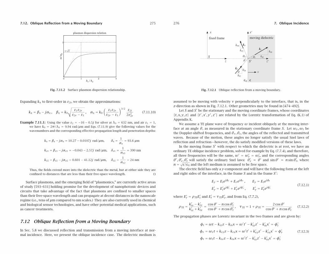
ω2p − 2ω2
Defining the normalized variables ω = ω/ωp and k = kx/kp, where kp = ωp/c0,we may rewrite the above relationship as,
k2 = ω2 1− ω2
1− 2ω2
with solution
ω =√√√√k2 + 1
2−√k4 + 1
4(7.11.8)
It is depicted in Fig. 7.11.2. In the large kx limit, it converges to the horizontal lineω =ωp/
√2. For small kx, it becomes the dispersion relationship in vacuum, ω = c0kx,
which is also depicted in this figure.Because the curve stays to the right of the vacuum line ω = c0kx, that is, kx > ω/c0,
such surface plasmon waves cannot be excited by an impinging plane wave on the inter-face. However, they can be excited with the help of frustrated total internal reflection,which increases kx beyond its vacuum value and can match the value of Eq. (7.11.7) re-sulting into a so-called surface plasmon resonance. We discuss this further in Sec. 8.5.
In fact, the excitation of such plasmon resonance can only take place if the metalside is slightly lossy, that is, when ε2 = −ε2r − jε2i, with 0 < ε2i � ε2r . In this case, thewavenumber kx acquires a small imaginary part which causes the gradual attenuationof the wave along the surface, and similarly, kz1, kz2, acquire small real parts. Replacingε2r by ε2r + jε2i in (7.11.7), we now have:
kx = k0
√ε1(ε2r + jε2i)ε2r + jε2i − ε1
, kz1 = −jk0ε1√ε2r + jε2i − ε1
, kz2 = −jk0(ε2r + jε2i)√ε2r + jε2i − ε1
(7.11.9)
7.12. Oblique Reflection from a Moving Boundary 275
0 1 2 3
1
kx /kp
ω/ω
p
1/√⎯⎯2
plasmon dispersion relation
Fig. 7.11.2 Surface plasmon dispersion relationship.
Expanding kx to first-order in ε2i, we obtain the approximations:
kx = βx − jαx , βx = k0
√ε1ε2r
ε2r − ε1, αx = k0
(ε1ε2r
ε2r − ε1
)3/2 ε2i
2ε22r
(7.11.10)
Example 7.11.1: Using the value ε2 = −16 − 0.5j for silver at λ0 = 632 nm, and air ε1 = 1,we have k0 = 2π/λ0 = 9.94 rad/μm and Eqs. (7.11.9) give the following values for thewavenumbers and the corresponding effective propagation length and penetration depths:
kx = βx − jαx = 10.27− 0.0107j rad/μm, δx = 1
αx= 93.6 μm
kz1 = βz1 − jαz1 = −0.043− 2.57j rad/μm, δz1 = 1
αz1= 390 nm
kz2 = βz2 − jαz2 = 0.601− 41.12j rad/μm, δz2 = 1
αz2= 24 nm
Thus, the fields extend more into the dielectric than the metal, but at either side they areconfined to distances that are less than their free-space wavelength.
Surface plasmons, and the emerging field of “plasmonics,” are currently active areasof study [593–631] holding promise for the development of nanophotonic devices andcircuits that take advantage of the fact that plasmons are confined to smaller spacesthan their free-space wavelength and can propagate at decent distances in the nanoscaleregime (i.e., tens of μm compared to nm scales.) They are also currently used in chemicaland biological sensor technologies, and have other potential medical applications, suchas cancer treatments.
7.12 Oblique Reflection from a Moving Boundary
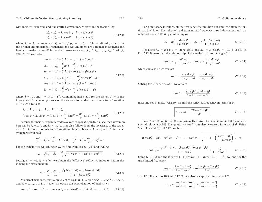
In Sec. 5.8 we discussed reflection and transmission from a moving interface at nor-mal incidence. Here, we present the oblique incidence case. The dielectric medium is
276 7. Oblique Incidence
Fig. 7.12.1 Oblique reflection from a moving boundary.
assumed to be moving with velocity v perpendicularly to the interface, that is, in thez-direction as shown in Fig. 7.12.1. Other geometries may be found in [474–492].
Let S and S′ be the stationary and the moving coordinate frames, whose coordinates{t, x, y, z} and {t′, x′, y′, z′} are related by the Lorentz transformation of Eq. (K.1) ofAppendix K.
We assume a TE plane wave of frequency ω incident obliquely at the moving inter-face at an angle θ, as measured in the stationary coordinate frame S. Let ωr,ωt bethe Doppler-shifted frequencies, and θr,θt, the angles of the reflected and transmittedwaves. Because of the motion, these angles no longer satisfy the usual Snel laws ofreflection and refraction—however, the do satisfy modified versions of these laws.
In the moving frame S′ with respect to which the dielectric is at rest, we have anordinary TE oblique incidence problem, solved for example by Eq. (7.7.4), and therefore,all three frequencies will be the same, ω′ = ω′
r = ω′t, and the corresponding angles
θ′, θ′r, θ′t will satisfy the ordinary Snel laws: θ′r = θ′ and sinθ′ = n sinθ′t, where
n = √ε/ε0 and the left medium is assumed to be free space.
The electric field has only a y-component and will have the following form at the leftand right sides of the interface, in the frame S and in the frame S′:
Ey = Eiejφi + Erejφr , Ey = Etejφt
E′y = E′i ejφ′i + E′rejφ
′r , E′y = E′tejφ
′t
(7.12.1)
where E′r = ρTEE′i and E′t = τTEE′i , and from Eq. (7.7.2),
ρTE = k′iz − k′tzk′iz + k′tz
= cosθ′ − n cosθ′tcosθ′ + n cosθ′t
, τTE = 1+ ρTE = 2 cosθ′
cosθ′ + n cosθ′t(7.12.2)
The propagation phases are Lorentz invariant in the two frames and are given by:
φi =ωt − kizz− kixx =ω′t′ − k′izz′ − k′ixx
′ = φ′i
φr =ωrt + krzz− krxx =ω′t′ + k′rzz′ − k′rxx′ = φ′r
φt =ωtt − ktzz− ktxx =ω′t′ − k′tzz′ − k′txx′ = φ′t
(7.12.3)
7.12. Oblique Reflection from a Moving Boundary 277
with incident, reflected, and transmitted wavenumbers given in the frame S′ by:
k′iz = k′rz = k′i cosθ′ , k′tz = k′t cosθ′tk′ix = k′rx = k′i sinθ′ , k′tx = k′t sinθ′t
(7.12.4)
where k′i = k′r = ω′/c and k′t = ω′√εμ0 = nω′/c. The relationships betweenthe primed and unprimed frequencies and wavenumbers are obtained by applying theLorentz transformation (K.14) to the four-vectors (ω/c, kix,0, kiz), (ωr, krx,0,−krz),and (ωt/c, ktx,0, ktz):
ω = γ(ω′ + βck′iz)=ω′γ(1+ β cosθ′)
kiz = γ(k′iz +βcω′)= ω′
cγ(cosθ′ + β)
ωr = γ(ω′ − βck′rz)=ω′γ(1− β cosθ′)
−krz = γ(−k′rz +βcω′)= −ω
′
cγ(cosθ′ − β)
ωt = γ(ω′ + βck′tz)=ω′γ(1+ βn cosθ′t)
ktz = γ(k′tz +βcω′)= ω′
cγ(n cosθ′t + β)
(7.12.5)
where β = v/c and γ = 1/√
1− β2. Combining Snel’s laws for the system S′ with theinvariance of the x-components of the wavevector under the Lorentz transformation(K.14), we have also:
kix = krx = ktx = k′ix = k′rx = k′tx
ki sinθ = kr sinθr = kt sinθt = ω′
csinθ′ = ω′
csinθ′r = n
ω′
csinθ′t
(7.12.6)
Because the incident and reflected waves are propagating in free space, their wavenum-bers will be ki =ω/c and kr =ωr/c. This also follows from the invariance of the scalar(ω/c)2−k2 under Lorentz transformations. Indeed, because k′i = k′r = ω′/c in the S′
system, we will have:
ω2
c2− k2
i =ω′2
c2− k′2i = 0 ,
ω2r
c2− k2
r =ω′2
c2− k′2r = 0
For the transmitted wavenumber kt, we find from Eqs. (7.12.5) and (7.12.6):
kt =√k2tz + k2
tx = ω′
c
√γ2(n cosθ′t + β)2+n2 sin2 θ′t (7.12.7)
Setting vt = ωt/kt = c/nt, we obtain the “effective” refractive index nt within themoving dielectric medium:
nt = cvt= ckt
ωt=
√γ2(n cosθ′t + β)2+n2 sin2 θ′t
γ(1+ βn cosθ′t)(7.12.8)
At normal incidence, this is equivalent to Eq. (5.8.6). Replacing ki =ω/c, kr =ωr/c,and kt =ωtnt/c in Eq. (7.12.6), we obtain the generalization of Snel’s laws:
ω sinθ =ωr sinθr =ωtnt sinθt =ω′ sinθ′ =ω′ sinθ′r =ω′n sinθ′t (7.12.9)
278 7. Oblique Incidence
For a stationary interface, all the frequency factors drop out and we obtain the or-dinary Snel laws. The reflected and transmitted frequencies are θ-dependent and areobtained from (7.12.5) by eliminating ω′:
ωr =ω1− β cosθ′
1+ β cosθ′, ωt =ω
1+ βn cosθ′t1+ β cosθ′
(7.12.10)
Replacing kiz = ki cosθ = (ω/c)cosθ and krz = kr cosθr = (ωr/c)cosθr inEq. (7.12.5), we obtain the relationship of the angles θ,θr to the angle θ′:
cosθ = cosθ′ + β1+ β cosθ′
, cosθr = cosθ′ − β1− β cosθ′
(7.12.11)
which can also be written as:
cosθ′ = cosθ− β1− β cosθ
= cosθr + β1+ β cosθr
(7.12.12)
Solving for θr in terms of θ, we obtain:
cosθr = (1+ β2)cosθ− 2β1− 2β cosθ+ β2
(7.12.13)
Inserting cosθ′ in Eq. (7.12.10), we find the reflected frequency in terms of θ:
ωr =ω1− 2β cosθ+ β2
1− β2(7.12.14)
Eqs. (7.12.13) and (7.12.14) were originally derived by Einstein in his 1905 paper onspecial relativity [474]. The quantity n cosθ′t can also be written in terms of θ. UsingSnel’s law and Eq. (7.12.12), we have:
n cosθ′t =√n2 − sin2 θ′ =
√n2 − 1+ cos2 θ′ =
√√√√n2 − 1+(
cosθ− β1− β cosθ
)2
, or,
n cosθ′t =√(n2 − 1)(1− β cosθ)2+(cosθ− β)2
1− β cosθ≡ Q
1− β cosθ(7.12.15)
Using (7.12.15) and the identity (1 + β cosθ′)(1 − β cosθ)= 1 − β2 , we find for thetransmitted frequency:
ωt =ω1+ βn cosθ′t1+ β cosθ′
=ω1− β cosθ+ βQ
1− β2(7.12.16)
The TE reflection coefficient (7.12.2) may also be expressed in terms of θ:
ρTE = cosθ′ − n cosθ′tcosθ′ + n cosθ′t
= cosθ− β−Qcosθ− β+Q
(7.12.17)
7.13. Geometrical Optics 279
Next, we determine the reflected and transmitted fields in the frame S. The simplestapproach is to apply the Lorentz transformation (K.30) separately to the incident, re-flected, and transmitted waves. In the S′ frame, a plane wave propagating along the unitvector k
′has magnetic field:
H ′ = 1
ηk′ × E ′ ⇒ cB ′ = cμ0H ′ = η0
ηk′ × E ′ = n k
′ × E ′ (7.12.18)
where n = 1 for the incident and reflected waves. Because we assumed a TE wave andthe motion is along the z-direction, the electric field will be perpendicular to the velocity,that is, βββ · E ′ = 0. Using the BAC-CAB rule, Eq. (K.30) then gives:
E = E⊥ = γ(E ′⊥ −βββ× cB ′⊥)= γ(E ′ −βββ× cB ′)= γ(E ′ −βββ× (n k
′ × E ′))
= γ(E ′ − n(βββ · E′)k′ + n(βββ · k
′)E′
) = γE ′(1+ nβββ · k′)
(7.12.19)
Applying this result to the incident, reflected, and transmitted fields, we find:
Ei = γE′i (1+ β cosθ′)Er = γE′r(1− β cosθ′)= γρTEE′i (1− β cosθ′)Et = γE′t(1+ nβ cosθ′t)= γτTEE′i (1+ nβ cosθ′t)
(7.12.20)
It follows that the reflection and transmission coefficients will be:
ErEi= ρTE
1− β cosθ′
1+ β cosθ′= ρTE
ωr
ω,
EtEi= τTE
1+ nβ cosθ′t1+ β cosθ′
= τTEωt
ω(7.12.21)
The case of a perfect mirror corresponds to ρTE = −1 and τTE = 0. To be interpretableas a reflection angle, θr must be in the range 0 ≤ θr ≤ 90o, or, cosθr > 0. This requiresthat the numerator of (7.12.13) be positive, or,
(1+ β2)cosθ− 2β ≥ 0 � cosθ ≥ 2β1+ β2
� θ ≤ acos( 2β
1+ β2
)(7.12.22)
Because 2β/(1+ β2)> β, (7.12.22) also implies that cosθ > β, or, v < cz = c cosθ.Thus, the z-component of the phase velocity of the incident wave can catch up with thereceding interface. At the maximum allowed θ, the angle θr reaches 90o. In the above,we assumed that β > 0. For negative β, there are no restrictions on the range of θ.
7.13 Geometrical Optics
Geometrical optics and the concepts of wavefronts and rays can be derived from Maxwell’sequations in the short-wavelength or high-frequency limit.
We saw in Chap. 2 that a uniform plane wave propagating in a lossless isotropicdielectric in the direction of a wave vector k = k k = nk0 k is given by:
E(r)= E0 e−jnk0 k·r , H(r)= H0 e−jnk0 k·r , k · E0 = 0 , H0 = nη0
k× E0 (7.13.1)
280 7. Oblique Incidence
where n is the refractive index of the medium n = √ε/ε0, k0 and η0 are the free-space
wavenumber and impedance, and k, the unit-vector in the direction of propagation.The wavefronts are defined to be the constant-phase plane surfaces S(r)= const.,
where S(r)= n k · r. The perpendiculars to the wavefronts are the optical rays.In an inhomogeneous medium with a space-dependent refractive index n(r), the
wavefronts and their perpendicular rays become curved, and can be derived by consid-ering the high-frequency limit of Maxwell’s equations. By analogy with Eqs. (7.13.1), welook for solutions of the form:
E(r)= E0(r) e−jk0S(r) , H(r)= H0(r) e−jk0S(r) (7.13.2)
where we will assume that k0 is large and that E0,H0 are slowly-varying functions of r.This means that their space-derivatives are small compared to k0 or to 1/λ. For example,|∇∇∇× E0| � k0.
Inserting these expressions into Maxwell’s equations and assuming μ = μ0 and ε =n2ε0, we obtain:
∇∇∇× E = e−jk0S(∇∇∇× E0 − jk0∇∇∇S× E0
) = −jωμ0H0 e−jk0S
∇∇∇×H = e−jk0S(∇∇∇×H0 − jk0∇∇∇S×H0
) = jn2ωε0E0 e−jk0S
Assuming |∇∇∇×E0| � |k0∇∇∇S×E0|, and similarly for H0, and dropping the commonphase factor e−jk0S, we obtain the high-frequency approximations:
−jk0∇∇∇S× E0 = −jωμ0H0
−jk0∇∇∇S×H0 = jn2ωε0E0
Replacing k0 =ω√μ0ε0, and defining the vector k = 1
n∇∇∇S, we find:
H0 = nη0
k× E0 , E0 = −η0
nk×H0 (7.13.3)
These imply the transversality conditions k ·E0 = k ·H0 = 0. The consistency of theequations (7.13.3) requires that k be a unit vector. Indeed, using the BAC-CAB rule, wehave:
k× (k× E0)= k(k · E0)−E0(k · k)= −E0(k · k)= η0
nk×H0 = −E0
Thus, we obtain the unit-vector condition, known as the eikonal equation:
k · k = 1 ⇒ |∇∇∇S|2 = n2 (eikonal equation) (7.13.4)
This equation determines the wavefront phase function S(r). The rays are the per-pendiculars to the constant-phase surfaces S(r)= const., so that they are in the directionof∇∇∇S or k. Fig. 7.13.1 depicts these wavefronts and rays.
The ray passing through a point r on the surface S(r)= SA, will move ahead by adistance dr in the direction of the gradient ∇∇∇S. The length of dr is dl = (dr · dr)1/2.
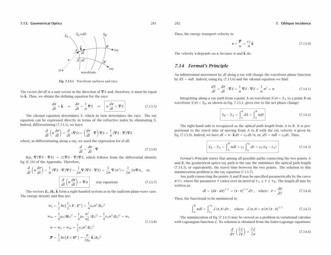
7.13. Geometrical Optics 281
Fig. 7.13.1 Wavefront surfaces and rays.
The vector dr/dl is a unit vector in the direction of∇∇∇S and, therefore, it must be equalto k. Thus, we obtain the defining equation for the rays:
dr
dl= k ⇒ dr
dl= 1
n∇∇∇S ⇒ n
dr
dl=∇∇∇S (7.13.5)
The eikonal equation determines S, which in turn determines the rays. The rayequation can be expressed directly in terms of the refractive index by eliminating S.Indeed, differentiating (7.13.5), we have:
ddl
(ndr
dl
)= ddl
(∇∇∇S)=(dr
dl·∇∇∇
)∇∇∇S = 1
n(∇∇∇S ·∇∇∇)∇∇∇S
where, in differentiating along a ray, we used the expression for d/dl:
ddl= dr
dl·∇∇∇ (7.13.6)
But, ∇∇∇(∇∇∇S · ∇∇∇S) = 2(∇∇∇S · ∇∇∇)∇∇∇S, which follows from the differential identity
Eq. (C.16) of the Appendix. Therefore,
ddl
(ndr
dl
)= 1
n(∇∇∇S ·∇∇∇)∇∇∇S = 1
2n∇∇∇(∇∇∇S ·∇∇∇S) = 1
2n∇∇∇(n2)= 1
2n2n∇∇∇n , or,
ddl
(ndr
dl
)=∇∇∇n (ray equation) (7.13.7)
The vectors E0,H0, k form a right-handed system as in the uniform plane-wave case.The energy density and flux are:
we = 1
2Re
[1
2εE · E∗
] = 1
4ε0n2|E0|2
wm = 1
4μ0|H0|2 = 1
4μ0
n2
η20|E0|2 = 1
4ε0n2|E0|2 = we
w = we +wm = 1
2ε0n2|E0|2
PPP = 1
2Re
[E×H∗
] = n2η0
k |E0|2
(7.13.8)
282 7. Oblique Incidence
Thus, the energy transport velocity is:
v = PPPw= c0
nk (7.13.9)
The velocity v depends on r, because n and k do.
7.14 Fermat’s Principle
An infinitesimal movement by dl along a ray will change the wavefront phase functionby dS = ndl. Indeed, using Eq. (7.13.6) and the eikonal equation we find:
dSdl= dr
dl·∇∇∇S = 1
n∇∇∇S ·∇∇∇S = 1
nn2 = n (7.14.1)
Integrating along a ray path from a point A on wavefront S(r)= SA to a point B onwavefront S(r)= SB, as shown in Fig. 7.13.1, gives rise to the net phase change:
SB − SA =∫ B
AdS =
∫ B
Andl (7.14.2)
The right-hand side is recognized as the optical path length from A to B. It is pro-portional to the travel time of moving from A to B with the ray velocity v given byEq. (7.13.9). Indeed, we have dl = v · kdt = c0 dt/n, or, dS = ndl = c0dt. Thus,
SB − SA =∫ B
Andl = c0
∫ tB
tAdt = c0(tB − tA) (7.14.3)
Fermat’s Principle states that among all possible paths connecting the two points Aand B, the geometrical optics ray path is the one the minimizes the optical path length(7.14.3), or equivalently, the travel time between the two points. The solution to thisminimization problem is the ray equation (7.13.7).
Any path connecting the pointsA and Bmay be specified parametrically by the curver(τ), where the parameter τ varies over an interval τA ≤ τ ≤ τB. The length dl may bewritten as:
dl = (dr · dr
)1/2 = (r · r
)1/2 dτ , where r = dr
dτ(7.14.4)
Then, the functional to be minimized is:
∫ B
Andl =
∫ τB
τAL(r, r)dτ , where L(r, r)= n(r)
(r · r
)1/2(7.14.5)
The minimization of Eq. (7.14.5) may be viewed as a problem in variational calculuswith Lagrangian function L. Its solution is obtained from the Euler-Lagrange equations:
ddτ
(∂L∂r
)= ∂L
∂r(7.14.6)
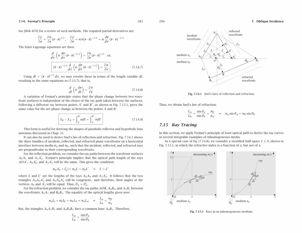
7.14. Fermat’s Principle 283
See [868–870] for a review of such methods. The required partial derivatives are:
∂L∂r
= ∂n∂r
(r · r
)1/2 ,∂L∂r
= n r(r · r
)−1/2 = ndr
dτ(r · r
)−1/2
The Euler-Lagrange equations are then:
ddτ
(ndr
dτ(r · r
)−1/2)= ∂n
∂r
(r · r
)1/2or,
(r · r
)−1/2 ddτ
(ndr
dτ(r · r
)−1/2)= ∂n
∂r(7.14.7)
Using dl = (r · r
)1/2 dτ, we may rewrite these in terms of the length variable dl,resulting in the same equations as (7.13.7), that is,
ddl
(ndr
dl
)= ∂n
∂r(7.14.8)
A variation of Fermat’s principle states that the phase change between two wave-front surfaces is independent of the choice of the ray path taken between the surfaces.Following a different ray between points A′ and B′, as shown in Fig. 7.13.1, gives thesame value for the net phase change as between the points A and B:
SB − SA =∫ B
Andl =
∫ B′
A′ndl′ (7.14.9)
This form is useful for deriving the shapes of parabolic reflector and hyperbolic lensantennas discussed in Chap. 21.
It can also be used to derive Snel’s law of reflection and refraction. Fig. 7.14.1 showsthe three families of incident, reflected, and refracted plane wavefronts on a horizontalinterface between media na and nb, such that the incident, reflected, and refracted raysare perpendicular to their corresponding wavefronts.
For the reflection problem, we consider the ray paths between the wavefront surfacesA0A1 and A1A′2. Fermat’s principle implies that the optical path length of the raysAOA′, A0A′0, and A2A′2 will be the same. This gives the condition:
na(la + l′a)= naL = naL′ ⇒ L = L′
where L and L′ are the lengths of the rays A0A0 and A2A′2. It follows that the twotriangles A0A2A′2 and A0A′0A′2 will be congruent. and therefore, their angles at thevertices A0 and A′2 will be equal. Thus, θa = θ′a.
For the refraction problem, we consider the ray pathsAOB,A0B0, andA1B1 betweenthe wavefronts A0A1 and B0B1. The equality of the optical lengths gives now:
nala + nblb = nbLb = naLa ⇒ LaLb= nbna
But, the triangles A0A1B1 and A0B0B1 have a common base A0B1. Therefore,
LaLb= sinθa
sinθb
284 7. Oblique Incidence
Fig. 7.14.1 Snel’s laws of reflection and refraction.
Thus, we obtain Snel’s law of refraction:
LaLb= sinθa
sinθb= nbna
⇒ na sinθa = nb sinθb
7.15 Ray Tracing
In this section, we apply Fermat’s principle of least optical path to derive the ray curvesin several integrable examples of inhomogeneous media.
As a special case of Eq. (7.14.8), we consider a stratified half-space z ≥ 0, shown inFig. 7.15.1, in which the refractive index is a function of z, but not of x.
Fig. 7.15.1 Rays in an inhomogeneous medium.
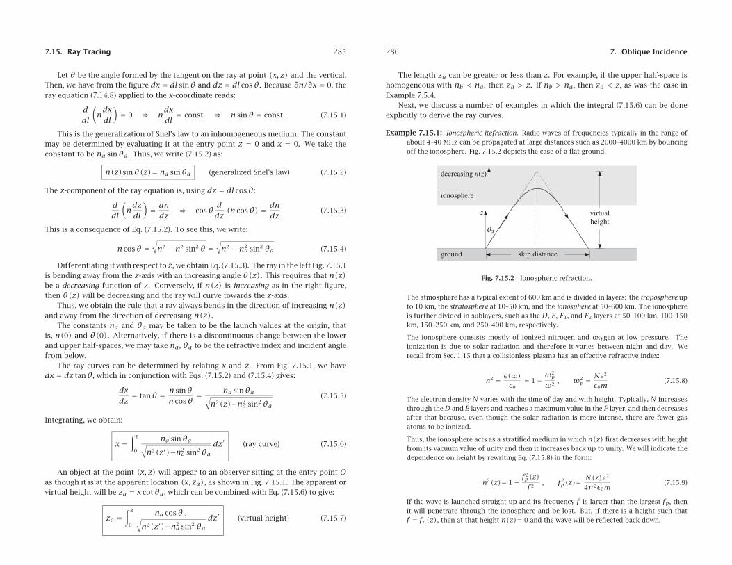
7.15. Ray Tracing 285
Let θ be the angle formed by the tangent on the ray at point (x, z) and the vertical.Then, we have from the figure dx = dl sinθ and dz = dl cosθ. Because ∂n/∂x = 0, theray equation (7.14.8) applied to the x-coordinate reads:
ddl
(ndxdl
)= 0 ⇒ n
dxdl= const. ⇒ n sinθ = const. (7.15.1)
This is the generalization of Snel’s law to an inhomogeneous medium. The constantmay be determined by evaluating it at the entry point z = 0 and x = 0. We take theconstant to be na sinθa. Thus, we write (7.15.2) as:
n(z)sinθ(z)= na sinθa (generalized Snel’s law) (7.15.2)
The z-component of the ray equation is, using dz = dl cosθ:
ddl
(ndzdl
)= dndz
⇒ cosθddz
(n cosθ) = dndz
(7.15.3)
This is a consequence of Eq. (7.15.2). To see this, we write:
n cosθ =√n2 − n2 sin2 θ =
√n2 − n2
a sin2 θa (7.15.4)
Differentiating it with respect to z, we obtain Eq. (7.15.3). The ray in the left Fig. 7.15.1is bending away from the z-axis with an increasing angle θ(z). This requires that n(z)be a decreasing function of z. Conversely, if n(z) is increasing as in the right figure,then θ(z) will be decreasing and the ray will curve towards the z-axis.
Thus, we obtain the rule that a ray always bends in the direction of increasing n(z)and away from the direction of decreasing n(z).
The constants na and θa may be taken to be the launch values at the origin, thatis, n(0) and θ(0). Alternatively, if there is a discontinuous change between the lowerand upper half-spaces, we may take na, θa to be the refractive index and incident anglefrom below.
The ray curves can be determined by relating x and z. From Fig. 7.15.1, we havedx = dz tanθ, which in conjunction with Eqs. (7.15.2) and (7.15.4) gives:
dxdz
= tanθ = n sinθn cosθ
= na sinθa√n2(z)−n2
a sin2 θa(7.15.5)
Integrating, we obtain:
x =∫ z
0
na sinθa√n2(z′)−n2
a sin2 θadz′ (ray curve) (7.15.6)
An object at the point (x, z) will appear to an observer sitting at the entry point Oas though it is at the apparent location (x, za), as shown in Fig. 7.15.1. The apparent orvirtual height will be za = x cotθa, which can be combined with Eq. (7.15.6) to give:
za =∫ z
0
na cosθa√n2(z′)−n2
a sin2 θadz′ (virtual height) (7.15.7)
286 7. Oblique Incidence
The length za can be greater or less than z. For example, if the upper half-space ishomogeneous with nb < na, then za > z. If nb > na, then za < z, as was the case inExample 7.5.4.
Next, we discuss a number of examples in which the integral (7.15.6) can be doneexplicitly to derive the ray curves.
Example 7.15.1: Ionospheric Refraction. Radio waves of frequencies typically in the range ofabout 4–40 MHz can be propagated at large distances such as 2000–4000 km by bouncingoff the ionosphere. Fig. 7.15.2 depicts the case of a flat ground.
Fig. 7.15.2 Ionospheric refraction.
The atmosphere has a typical extent of 600 km and is divided in layers: the troposphere upto 10 km, the stratosphere at 10–50 km, and the ionosphere at 50–600 km. The ionosphereis further divided in sublayers, such as the D, E, F1, and F2 layers at 50–100 km, 100–150km, 150–250 km, and 250–400 km, respectively.
The ionosphere consists mostly of ionized nitrogen and oxygen at low pressure. Theionization is due to solar radiation and therefore it varies between night and day. Werecall from Sec. 1.15 that a collisionless plasma has an effective refractive index:
n2 = ε(ω)ε0
= 1− ω2p
ω2, ω2
p =Ne2
ε0m(7.15.8)
The electron density N varies with the time of day and with height. Typically, N increasesthrough theD and E layers and reaches a maximum value in the F layer, and then decreasesafter that because, even though the solar radiation is more intense, there are fewer gasatoms to be ionized.
Thus, the ionosphere acts as a stratified medium in which n(z) first decreases with heightfrom its vacuum value of unity and then it increases back up to unity. We will indicate thedependence on height by rewriting Eq. (7.15.8) in the form:
n2(z)= 1− f2p(z)f2
, f2p(z)=
N(z)e2
4π2ε0m(7.15.9)
If the wave is launched straight up and its frequency f is larger than the largest fp, thenit will penetrate through the ionosphere and be lost. But, if there is a height such thatf = fp(z), then at that height n(z)= 0 and the wave will be reflected back down.
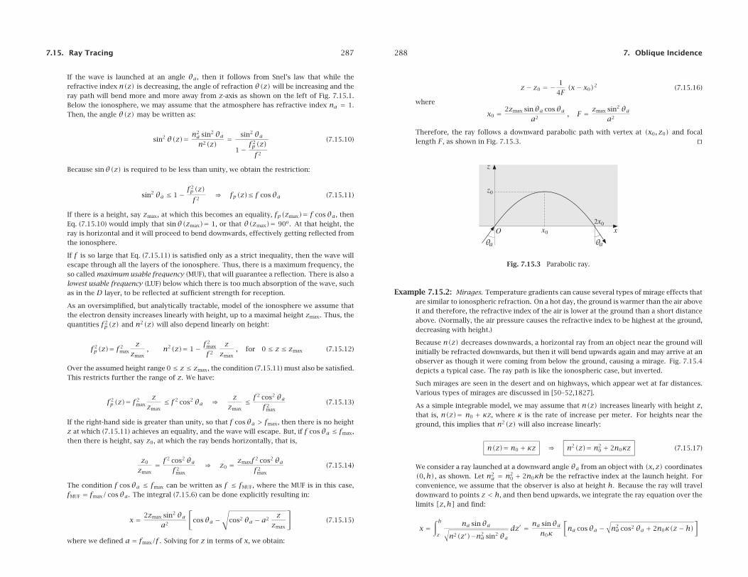
7.15. Ray Tracing 287
If the wave is launched at an angle θa, then it follows from Snel’s law that while therefractive index n(z) is decreasing, the angle of refraction θ(z) will be increasing and theray path will bend more and more away from z-axis as shown on the left of Fig. 7.15.1.Below the ionosphere, we may assume that the atmosphere has refractive index na = 1.Then, the angle θ(z) may be written as:
sin2 θ(z)= n2a sin2 θan2(z)
= sin2 θa
1− f2p(z)f2
(7.15.10)
Because sinθ(z) is required to be less than unity, we obtain the restriction:
sin2 θa ≤ 1− f2p(z)f2
⇒ fp(z)≤ f cosθa (7.15.11)
If there is a height, say zmax, at which this becomes an equality, fp(zmax)= f cosθa, thenEq. (7.15.10) would imply that sinθ(zmax)= 1, or that θ(zmax)= 90o. At that height, theray is horizontal and it will proceed to bend downwards, effectively getting reflected fromthe ionosphere.
If f is so large that Eq. (7.15.11) is satisfied only as a strict inequality, then the wave willescape through all the layers of the ionosphere. Thus, there is a maximum frequency, theso called maximum usable frequency (MUF), that will guarantee a reflection. There is also alowest usable frequency (LUF) below which there is too much absorption of the wave, suchas in the D layer, to be reflected at sufficient strength for reception.
As an oversimplified, but analytically tractable, model of the ionosphere we assume thatthe electron density increases linearly with height, up to a maximal height zmax. Thus, thequantities f2
p(z) and n2(z) will also depend linearly on height:
f2p(z)= f2
maxz
zmax, n2(z)= 1− f2
max
f2
zzmax
, for 0 ≤ z ≤ zmax (7.15.12)
Over the assumed height range 0 ≤ z ≤ zmax, the condition (7.15.11) must also be satisfied.This restricts further the range of z. We have:
f2p(z)= f2
maxz
zmax≤ f2 cos2 θa ⇒ z
zmax≤ f2 cos2 θa
f2max
(7.15.13)
If the right-hand side is greater than unity, so that f cosθa > fmax, then there is no heightz at which (7.15.11) achieves an equality, and the wave will escape. But, if f cosθa ≤ fmax,then there is height, say z0, at which the ray bends horizontally, that is,
z0
zmax= f2 cos2 θa
f2max
⇒ z0 = zmaxf2 cos2 θaf2
max(7.15.14)
The condition f cosθa ≤ fmax can be written as f ≤ fMUF, where the MUF is in this case,fMUF = fmax/ cosθa. The integral (7.15.6) can be done explicitly resulting in:
x = 2zmax sin2 θaa2
[cosθa −
√cos2 θa − a2
zzmax
](7.15.15)
where we defined a = fmax/f . Solving for z in terms of x, we obtain:
288 7. Oblique Incidence
z− z0 = − 1
4F(x− x0)2 (7.15.16)
where
x0 = 2zmax sinθa cosθaa2
, F = zmax sin2 θaa2
Therefore, the ray follows a downward parabolic path with vertex at (x0, z0) and focallength F, as shown in Fig. 7.15.3.
Fig. 7.15.3 Parabolic ray.
Example 7.15.2: Mirages. Temperature gradients can cause several types of mirage effects thatare similar to ionospheric refraction. On a hot day, the ground is warmer than the air aboveit and therefore, the refractive index of the air is lower at the ground than a short distanceabove. (Normally, the air pressure causes the refractive index to be highest at the ground,decreasing with height.)
Because n(z) decreases downwards, a horizontal ray from an object near the ground willinitially be refracted downwards, but then it will bend upwards again and may arrive at anobserver as though it were coming from below the ground, causing a mirage. Fig. 7.15.4depicts a typical case. The ray path is like the ionospheric case, but inverted.
Such mirages are seen in the desert and on highways, which appear wet at far distances.Various types of mirages are discussed in [50–52,1827].
As a simple integrable model, we may assume that n(z) increases linearly with height z,that is, n(z)= n0 + κz, where κ is the rate of increase per meter. For heights near theground, this implies that n2(z) will also increase linearly:
n(z)= n0 + κz ⇒ n2(z)= n20 + 2n0κz (7.15.17)
We consider a ray launched at a downward angle θa from an object with (x, z) coordinates(0, h), as shown. Let n2
a = n20 + 2n0κh be the refractive index at the launch height. For
convenience, we assume that the observer is also at height h. Because the ray will traveldownward to points z < h, and then bend upwards, we integrate the ray equation over thelimits [z, h] and find:
x =∫ h
z
na sinθa√n2(z′)−n2
a sin2 θadz′ = na sinθa
n0κ
[na cosθa −
√n2a cos2 θa + 2n0κ(z− h)
]
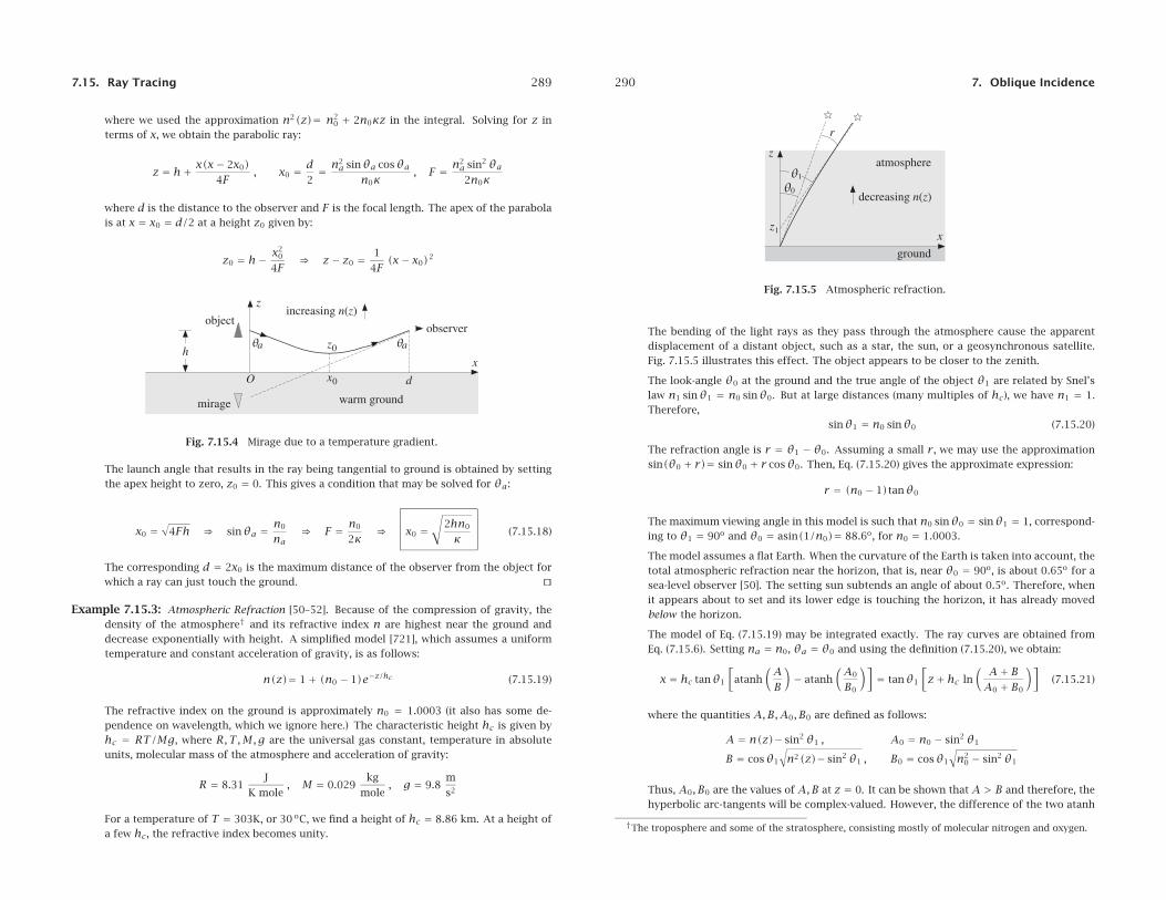
7.15. Ray Tracing 289
where we used the approximation n2(z)= n20 + 2n0κz in the integral. Solving for z in
terms of x, we obtain the parabolic ray:
z = h+ x(x− 2x0)4F
, x0 = d2= n2
a sinθa cosθan0κ
, F = n2a sin2 θa2n0κ
where d is the distance to the observer and F is the focal length. The apex of the parabolais at x = x0 = d/2 at a height z0 given by:
z0 = h− x20
4F⇒ z− z0 = 1
4F(x− x0)2
Fig. 7.15.4 Mirage due to a temperature gradient.
The launch angle that results in the ray being tangential to ground is obtained by settingthe apex height to zero, z0 = 0. This gives a condition that may be solved for θa:
x0 =√
4Fh ⇒ sinθa = n0
na⇒ F = n0
2κ⇒ x0 =
√2hn0
κ(7.15.18)
The corresponding d = 2x0 is the maximum distance of the observer from the object forwhich a ray can just touch the ground.
Example 7.15.3: Atmospheric Refraction [50–52]. Because of the compression of gravity, thedensity of the atmosphere† and its refractive index n are highest near the ground anddecrease exponentially with height. A simplified model [721], which assumes a uniformtemperature and constant acceleration of gravity, is as follows:
n(z)= 1+ (n0 − 1)e−z/hc (7.15.19)
The refractive index on the ground is approximately n0 = 1.0003 (it also has some de-pendence on wavelength, which we ignore here.) The characteristic height hc is given byhc = RT/Mg, where R,T,M,g are the universal gas constant, temperature in absoluteunits, molecular mass of the atmosphere and acceleration of gravity:
R = 8.31J
K mole, M = 0.029
kg
mole, g = 9.8
m
s2
For a temperature of T = 303K, or 30 oC, we find a height of hc = 8.86 km. At a height ofa few hc, the refractive index becomes unity.
290 7. Oblique Incidence
Fig. 7.15.5 Atmospheric refraction.
The bending of the light rays as they pass through the atmosphere cause the apparentdisplacement of a distant object, such as a star, the sun, or a geosynchronous satellite.Fig. 7.15.5 illustrates this effect. The object appears to be closer to the zenith.
The look-angle θ0 at the ground and the true angle of the object θ1 are related by Snel’slaw n1 sinθ1 = n0 sinθ0. But at large distances (many multiples of hc), we have n1 = 1.Therefore,
sinθ1 = n0 sinθ0 (7.15.20)
The refraction angle is r = θ1 − θ0. Assuming a small r, we may use the approximationsin(θ0 + r)= sinθ0 + r cosθ0. Then, Eq. (7.15.20) gives the approximate expression:
r = (n0 − 1)tanθ0
The maximum viewing angle in this model is such that n0 sinθ0 = sinθ1 = 1, correspond-ing to θ1 = 90o and θ0 = asin(1/n0)= 88.6o, for n0 = 1.0003.
The model assumes a flat Earth. When the curvature of the Earth is taken into account, thetotal atmospheric refraction near the horizon, that is, near θ0 = 90o, is about 0.65o for asea-level observer [50]. The setting sun subtends an angle of about 0.5o. Therefore, whenit appears about to set and its lower edge is touching the horizon, it has already movedbelow the horizon.
The model of Eq. (7.15.19) may be integrated exactly. The ray curves are obtained fromEq. (7.15.6). Setting na = n0, θa = θ0 and using the definition (7.15.20), we obtain:
x = hc tanθ1
[atanh
(AB
)− atanh
(A0
B0
)]= tanθ1
[z+ hc ln
(A+ BA0 + B0
)](7.15.21)
where the quantities A,B,A0, B0 are defined as follows:
A = n(z)− sin2 θ1 , A0 = n0 − sin2 θ1
B = cosθ1
√n2(z)− sin2 θ1 , B0 = cosθ1
√n2
0 − sin2 θ1
Thus, A0, B0 are the values of A,B at z = 0. It can be shown that A > B and therefore, thehyperbolic arc-tangents will be complex-valued. However, the difference of the two atanh
†The troposphere and some of the stratosphere, consisting mostly of molecular nitrogen and oxygen.
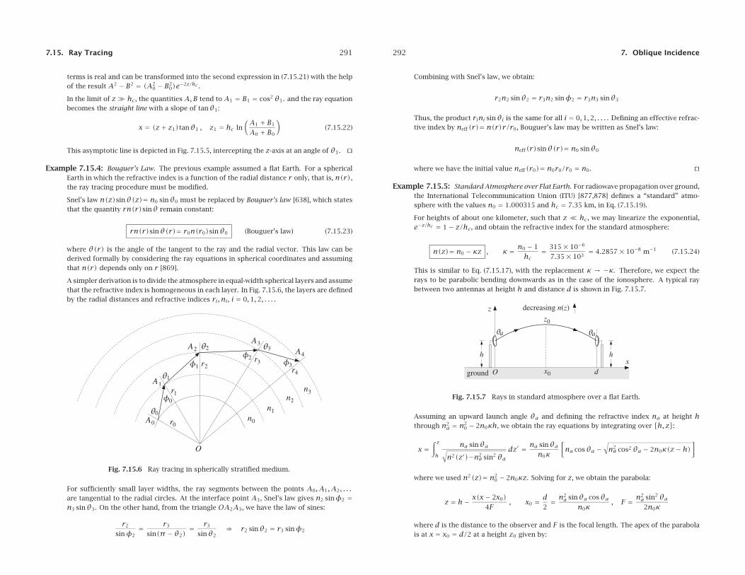
7.15. Ray Tracing 291
terms is real and can be transformed into the second expression in (7.15.21) with the helpof the result A2 − B2 = (A2
0 − B20)e−2z/hc .
In the limit of z� hc, the quantities A,B tend to A1 = B1 = cos2 θ1. and the ray equationbecomes the straight line with a slope of tanθ1:
x = (z+ z1)tanθ1 , z1 = hc ln(A1 + B1
A0 + B0
)(7.15.22)
This asymptotic line is depicted in Fig. 7.15.5, intercepting the z-axis at an angle of θ1.
Example 7.15.4: Bouguer’s Law. The previous example assumed a flat Earth. For a sphericalEarth in which the refractive index is a function of the radial distance r only, that is, n(r),the ray tracing procedure must be modified.
Snel’s law n(z)sinθ(z)= n0 sinθ0 must be replaced by Bouguer’s law [638], which statesthat the quantity rn(r)sinθ remain constant:
rn(r)sinθ(r)= r0n(r0)sinθ0 (Bouguer’s law) (7.15.23)
where θ(r) is the angle of the tangent to the ray and the radial vector. This law can bederived formally by considering the ray equations in spherical coordinates and assumingthat n(r) depends only on r [869].
A simpler derivation is to divide the atmosphere in equal-width spherical layers and assumethat the refractive index is homogeneous in each layer. In Fig. 7.15.6, the layers are definedby the radial distances and refractive indices ri, ni, i = 0,1,2, . . . .
Fig. 7.15.6 Ray tracing in spherically stratified medium.
For sufficiently small layer widths, the ray segments between the points A0,A1,A2, . . .are tangential to the radial circles. At the interface point A3, Snel’s law gives n2 sinφ2 =n3 sinθ3. On the other hand, from the triangle OA2A3, we have the law of sines:
r2
sinφ2= r3
sin(π− θ2)= r3
sinθ2⇒ r2 sinθ2 = r3 sinφ2
292 7. Oblique Incidence
Combining with Snel’s law, we obtain:
r2n2 sinθ2 = r3n2 sinφ2 = r3n3 sinθ3
Thus, the product rini sinθi is the same for all i = 0,1,2, . . . . Defining an effective refrac-tive index by neff(r)= n(r)r/r0, Bouguer’s law may be written as Snel’s law:
neff(r)sinθ(r)= n0 sinθ0
where we have the initial value neff(r0)= n0r0/r0 = n0.
Example 7.15.5: Standard Atmosphere over Flat Earth. For radiowave propagation over ground,the International Telecommunication Union (ITU) [877,878] defines a “standard” atmo-sphere with the values n0 = 1.000315 and hc = 7.35 km, in Eq. (7.15.19).
For heights of about one kilometer, such that z � hc, we may linearize the exponential,e−z/hc = 1− z/hc, and obtain the refractive index for the standard atmosphere:
n(z)= n0 − κz , κ = n0 − 1
hc= 315× 10−6
7.35× 103= 4.2857× 10⁻⁸ m−1 (7.15.24)
This is similar to Eq. (7.15.17), with the replacement κ → −κ. Therefore, we expect therays to be parabolic bending downwards as in the case of the ionosphere. A typical raybetween two antennas at height h and distance d is shown in Fig. 7.15.7.
Fig. 7.15.7 Rays in standard atmosphere over a flat Earth.
Assuming an upward launch angle θa and defining the refractive index na at height hthrough n2
a = n20 − 2n0κh, we obtain the ray equations by integrating over [h, z]:
x =∫ z
h
na sinθa√n2(z′)−n2
a sin2 θadz′ = na sinθa
n0κ
[na cosθa −
√n2a cos2 θa − 2n0κ(z− h)
]
where we used n2(z)= n20 − 2n0κz. Solving for z, we obtain the parabola:
z = h− x(x− 2x0)4F
, x0 = d2= n2
a sinθa cosθan0κ
, F = n2a sin2 θa2n0κ
where d is the distance to the observer and F is the focal length. The apex of the parabolais at x = x0 = d/2 at a height z0 given by:
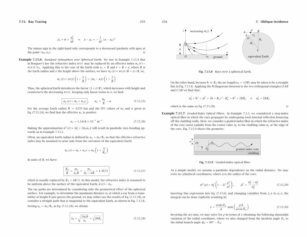
7.15. Ray Tracing 293
z0 = h+ x20
4F⇒ z− z0 = − 1
4F(x− x0)2
The minus sign in the right-hand side corresponds to a downward parabola with apex atthe point (x0, z0).
Example 7.15.6: Standard Atmosphere over Spherical Earth. We saw in Example 7.15.4 thatin Bouguer’s law the refractive index n(r) may be replaced by an effective index ne(r)=n(r)r/r0. Applying this to the case of the Earth with r0 = R and r = R + z, where R isthe Earth radius and z the height above the surface, we have ne(z)= n(z)(R+ z)/R, or,
ne(z)= n(z)(
1+ zR
)= (n0 − κz)
(1+ z
R
)
Thus, the spherical Earth introduces the factor (1+z/R), which increases with height andcounteracts the decreasing n(z). Keeping only linear terms in z, we find:
ne(z)= n0 + κez , κe = n0
R− κ (7.15.25)
For the average Earth radius R = 6370 km and the ITU values of n0 and κ given inEq. (7.15.24), we find that the effective κe is positive:
κe = 1.1418× 10⁻⁷ m−1 (7.15.26)
Making the approximation n2(z)= n20 + 2n0κez will result in parabolic rays bending up-
wards as in Example 7.15.2.
Often, an equivalent Earth radius is defined by κe = n0/Re so that the effective refractiveindex may be assumed to arise only from the curvature of the equivalent Earth:
ne(z)= n0 + κez = n0
(1+ z
Re
)
In units of R, we have:
Re
R= n0
κeR= n0
n0 − κR= 1.3673 (7.15.27)
which is usually replaced by Re = 4R/3. In this model, the refractive index is assumed tobe uniform above the surface of the equivalent Earth, n(z)= n0.
The ray paths are determined by considering only the geometrical effect of the sphericalsurface. For example, to determine the maximum distance x0 at which a ray from a trans-mitter at height h just grazes the ground, we may either use the results of Eq. (7.15.18), orconsider a straight path that is tangential to the equivalent Earth, as shown in Fig. 7.15.8.
Setting κe = n0/Re in Eq. (7.15.18), we obtain:
x0 =√
2n0hκe
=√
2hRe (7.15.28)
294 7. Oblique Incidence
Fig. 7.15.8 Rays over a spherical Earth.
On the other hand, because h� Re the arc length x0 = (OB)may be taken to be a straightline in Fig. 7.15.8. Applying the Pythagorean theorem to the two orthogonal triangles OABand CAB we find that:
x20 + h2 = d2 = (h+Re)2−R2
e = h2 + 2hRe ⇒ x20 = 2hRe
which is the same as Eq. (7.15.28).
Example 7.15.7: Graded-Index Optical Fibers. In Example 7.5.5, we considered a step-indexoptical fiber in which the rays propagate by undergoing total internal reflection bouncingoff the cladding walls. Here, we consider a graded-index fiber in which the refractive indexof the core varies radially from the center value nf to the cladding value nc at the edge ofthe core. Fig. 7.15.9 shows the geometry.
Fig. 7.15.9 Graded-index optical fiber.
As a simple model, we assume a parabolic dependence on the radial distance. We maywrite in cylindrical coordinates, where a is the radius of the core:
n2(ρ)= n2f
(1−Δ2 ρ2
a2
), Δ2 = n2
f − n2c
n2f
(7.15.29)
Inserting this expression into Eq. (7.15.6), and changing variables from z, x to ρ, z, theintegral can be done explicitly resulting in:
z = a sinθaΔ
asin(
ρΔa cosθa
)(7.15.30)
Inverting the arc-sine, we may solve for ρ in terms of z obtaining the following sinusoidalvariation of the radial coordinate, where we also changed from the incident angle θa tothe initial launch angle φ0 = 90o − θa:
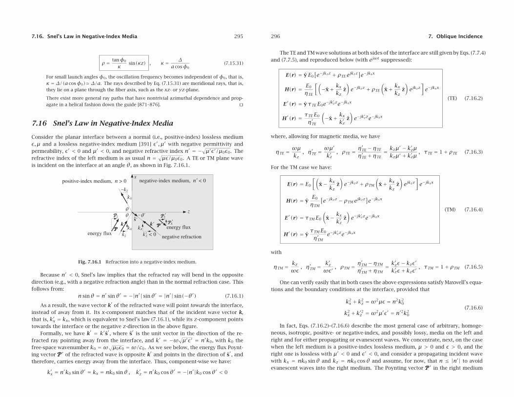
7.16. Snel’s Law in Negative-Index Media 295
ρ = tanφ0
κsin(κz) , κ = Δ
a cosφ0(7.15.31)
For small launch angles φ0, the oscillation frequency becomes independent of φ0, that is,κ = Δ/(a cosφ0)� Δ/a. The rays described by Eq. (7.15.31) are meridional rays, that is,they lie on a plane through the fiber axis, such as the xz- or yz-plane.
There exist more general ray paths that have nontrivial azimuthal dependence and prop-agate in a helical fashion down the guide [871–876].
7.16 Snel’s Law in Negative-Index Media
Consider the planar interface between a normal (i.e., positive-index) lossless mediumε, μ and a lossless negative-index medium [391] ε′, μ′ with negative permittivity andpermeability, ε′ < 0 and μ′ < 0, and negative refractive index n′ = −√μ′ε′/μ0ε0. Therefractive index of the left medium is as usual n = √
με/μ0ε0. A TE or TM plane waveis incident on the interface at an angle θ, as shown in Fig. 7.16.1.
Fig. 7.16.1 Refraction into a negative-index medium.
Because n′ < 0, Snel’s law implies that the refracted ray will bend in the oppositedirection (e.g., with a negative refraction angle) than in the normal refraction case. Thisfollows from:
n sinθ = n′ sinθ′ = −|n′| sinθ′ = |n′| sin(−θ′) (7.16.1)
As a result, the wave vector k′ of the refracted wave will point towards the interface,instead of away from it. Its x-component matches that of the incident wave vector k,that is, k′x = kx, which is equivalent to Snel’s law (7.16.1), while its z-component pointstowards the interface or the negative z-direction in the above figure.
Formally, we have k′ = k′s′, where s′ is the unit vector in the direction of the re-fracted ray pointing away from the interface, and k′ = −ω√
μ′ε′ = n′k0, with k0 thefree-space wavenumber k0 =ω√μ0ε0 =ω/c0. As we see below, the energy flux Poynt-ing vectorPPP′ of the refracted wave is opposite k′ and points in the direction of s′, andtherefore, carries energy away from the interface. Thus, component-wise we have:
k′x = n′k0 sinθ′ = kx = nk0 sinθ , k′z = n′k0 cosθ′ = −|n′|k0 cosθ′ < 0
296 7. Oblique Incidence
The TE and TM wave solutions at both sides of the interface are still given by Eqs. (7.7.4)and (7.7.5), and reproduced below (with ejωt suppressed):
E(r) = yE0[e−jkzz + ρTE ejkzz
]e−jkxx
H(r) = E0
ηTE
[(−x+ kx
kzz)e−jkzz + ρTE
(x+ kx
kzz)ejkzz
]e−jkxx
E ′(r) = yτTE E0e−jk′zze−jkxx
H ′(r) = τTE E0
η′TE
(−x+ kx
k′zz)e−jk
′zze−jkxx
(TE) (7.16.2)
where, allowing for magnetic media, we have
ηTE = ωμkz
, η′TE =ωμ′
k′z, ρTE = η′TE − ηTE
η′TE + ηTE= kzμ′ − k′zμkzμ′ + k′zμ
, τTE = 1+ ρTE (7.16.3)
For the TM case we have:
E(r) = E0
[(x− kx
kzz)e−jkzz + ρTM
(x+ kx
kzz)ejkzz
]e−jkxx
H(r) = yE0
ηTM
[e−jkzz − ρTM ejkzz
]e−jkxx
E ′(r) = τTM E0
(x− kx
k′zz)e−jk
′zze−jkxx
H ′(r) = yτTM E0
η′TMe−jk
′zze−jkxx
(TM) (7.16.4)
with
ηTM = kzωε
, η′TM =k′zωε′
, ρTM = η′TM − ηTM
η′TM + ηTM= k′zε− kzε′
k′zε+ kzε′, τTM = 1+ ρTM (7.16.5)
One can verify easily that in both cases the above expressions satisfy Maxwell’s equa-tions and the boundary conditions at the interface, provided that
k2x + k2
z =ω2με = n2k20
k2x + k′2z =ω2μ′ε′ = n′2k2
0
(7.16.6)
In fact, Eqs. (7.16.2)–(7.16.6) describe the most general case of arbitrary, homoge-neous, isotropic, positive- or negative-index, and possibly lossy, media on the left andright and for either propagating or evanescent waves. We concentrate, next, on the casewhen the left medium is a positive-index lossless medium, μ > 0 and ε > 0, and theright one is lossless with μ′ < 0 and ε′ < 0, and consider a propagating incident wavewith kx = nk0 sinθ and kz = nk0 cosθ and assume, for now, that n ≤ |n′| to avoidevanescent waves into the right medium. The Poynting vector PPP′ in the right medium
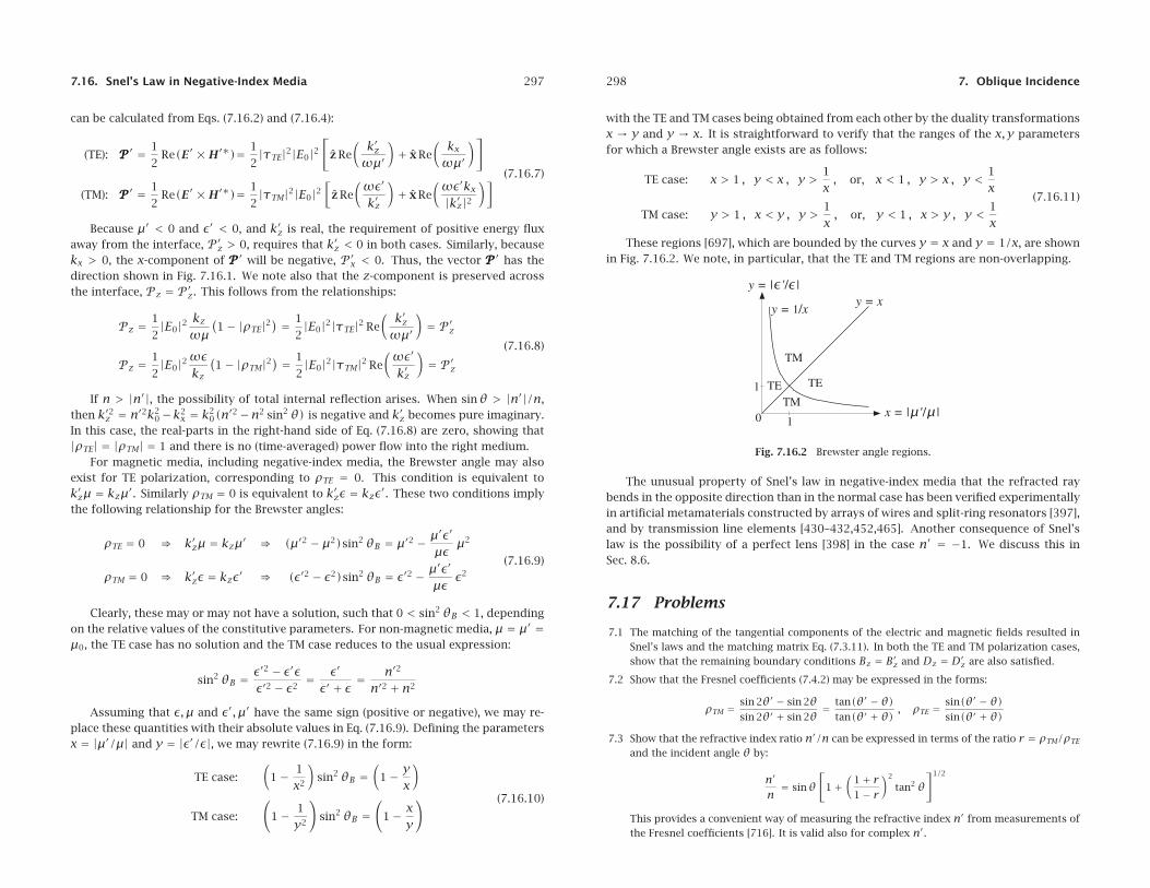
7.16. Snel’s Law in Negative-Index Media 297
can be calculated from Eqs. (7.16.2) and (7.16.4):
(TE): PPP′ = 1
2Re(E ′ ×H ′∗)= 1
2|τTE|2|E0|2
[z Re
( k′zωμ′
)+ x Re
(kxωμ′
)]
(TM): PPP′ = 1
2Re(E ′ ×H ′∗)= 1
2|τTM|2|E0|2
[z Re
(ωε′
k′z
)+ x Re
(ωε′kx|k′z|2
)] (7.16.7)
Because μ′ < 0 and ε′ < 0, and k′z is real, the requirement of positive energy fluxaway from the interface, P′z > 0, requires that k′z < 0 in both cases. Similarly, becausekx > 0, the x-component of PPP′ will be negative, P′x < 0. Thus, the vector PPP′ has thedirection shown in Fig. 7.16.1. We note also that the z-component is preserved acrossthe interface, Pz = P′z. This follows from the relationships:
Pz = 1
2|E0|2 kz
ωμ(1− |ρTE|2
) = 1
2|E0|2|τTE|2 Re
( k′zωμ′
)= P′z
Pz = 1
2|E0|2ωε
kz
(1− |ρTM|2
) = 1
2|E0|2|τTM|2 Re
(ωε′
k′z
)= P′z
(7.16.8)
If n > |n′|, the possibility of total internal reflection arises. When sinθ > |n′|/n,then k′2z = n′2k2
0−k2x = k2
0(n′2−n2 sin2 θ) is negative and k′z becomes pure imaginary.In this case, the real-parts in the right-hand side of Eq. (7.16.8) are zero, showing that|ρTE| = |ρTM| = 1 and there is no (time-averaged) power flow into the right medium.
For magnetic media, including negative-index media, the Brewster angle may alsoexist for TE polarization, corresponding to ρTE = 0. This condition is equivalent tok′zμ = kzμ′. Similarly ρTM = 0 is equivalent to k′zε = kzε′. These two conditions implythe following relationship for the Brewster angles:
ρTE = 0 ⇒ k′zμ = kzμ′ ⇒ (μ′2 − μ2)sin2 θB = μ′2 − μ′ε′
μεμ2
ρTM = 0 ⇒ k′zε = kzε′ ⇒ (ε′2 − ε2)sin2 θB = ε′2 − μ′ε′
μεε2
(7.16.9)
Clearly, these may or may not have a solution, such that 0 < sin2 θB < 1, dependingon the relative values of the constitutive parameters. For non-magnetic media, μ = μ′ =μ0, the TE case has no solution and the TM case reduces to the usual expression:
sin2 θB = ε′2 − ε′εε′2 − ε2
= ε′
ε′ + ε= n′2
n′2 + n2
Assuming that ε, μ and ε′, μ′ have the same sign (positive or negative), we may re-place these quantities with their absolute values in Eq. (7.16.9). Defining the parametersx = |μ′/μ| and y = |ε′/ε|, we may rewrite (7.16.9) in the form:
TE case:(
1− 1
x2
)sin2 θB =
(1− y
x
)
TM case:
(1− 1
y2
)sin2 θB =
(1− x
y
) (7.16.10)
298 7. Oblique Incidence
with the TE and TM cases being obtained from each other by the duality transformationsx → y and y → x. It is straightforward to verify that the ranges of the x, y parametersfor which a Brewster angle exists are as follows:
TE case: x > 1 , y < x , y >1
x, or, x < 1 , y > x , y <
1
x
TM case: y > 1 , x < y , y >1
x, or, y < 1 , x > y , y <
1
x
(7.16.11)
These regions [697], which are bounded by the curves y = x and y = 1/x, are shownin Fig. 7.16.2. We note, in particular, that the TE and TM regions are non-overlapping.
Fig. 7.16.2 Brewster angle regions.
The unusual property of Snel’s law in negative-index media that the refracted raybends in the opposite direction than in the normal case has been verified experimentallyin artificial metamaterials constructed by arrays of wires and split-ring resonators [397],and by transmission line elements [430–432,452,465]. Another consequence of Snel’slaw is the possibility of a perfect lens [398] in the case n′ = −1. We discuss this inSec. 8.6.
7.17 Problems
7.1 The matching of the tangential components of the electric and magnetic fields resulted inSnel’s laws and the matching matrix Eq. (7.3.11). In both the TE and TM polarization cases,show that the remaining boundary conditions Bz = B′z and Dz = D′z are also satisfied.
7.2 Show that the Fresnel coefficients (7.4.2) may be expressed in the forms:
ρTM = sin 2θ′ − sin 2θsin 2θ′ + sin 2θ
= tan(θ′ − θ)tan(θ′ + θ)
, ρTE = sin(θ′ − θ)sin(θ′ + θ)
7.3 Show that the refractive index ratio n′/n can be expressed in terms of the ratio r = ρTM/ρTE
and the incident angle θ by:
n′
n= sinθ
[1+
(1+ r1− r
)2
tan2 θ]1/2
This provides a convenient way of measuring the refractive index n′ from measurements ofthe Fresnel coefficients [716]. It is valid also for complex n′.
7.17. Problems 299
7.4 It is desired to design a Fresnel rhomb such that the exiting ray will be elliptically polarizedwith relative phase difference φ between its TE and TM components. Let sinθc = 1/n bethe critical angle within the rhomb. Show that the rhomb angle replacing the 54.6o angle inFig. 7.5.6 can be obtained from:
sin2 θ = cos2 θc ±√
cos4 θc − 4 sin2 θc tan2(φ/4)
2 tan2(φ/4)+ cos2 θc ±√
cos4 θc − 4 sin2 θc tan2(φ/4)
Show φ is required to satisfy tan(φ/4)≤ (n− n−1)/2.
7.5 Show the relationship (7.9.7) for the ratio ρTM/ρTE by first proving and then using the fol-lowing identities in the notation of Eq. (7.7.4):
(k′z ± kz)(k2x ± kzk′z)= k2k′z ± k′2kz
Using (7.9.7), show that when both media are lossless, the ratio ρTM/ρTE can be expresseddirectly in terms of the angles of incidence and refraction, θ and θ′:
ρTM
ρTE= cos(θ+ θ′)
cos(θ− θ′)
Using this result argue that |ρTM| ≤ |ρTE| at all angles θ. Argue also that θB + θ′B = 90o,for the Brewster angles. Finally, show that for lossless media with ε > ε′, and angles ofincidence θ ≥ θc, where sinθc =
√ε′/ε, we have:
ρTM
ρTE= j
√sin2 θ− sin2 θc + sinθ tanθ
j√
sin2 θ− sin2 θc − sinθ tanθ
Explain how this leads to the design equation (7.5.8) of the Fresnel rhomb.
7.6 Let the incident, reflected, and transmitted waves at an interface be:
E+(r)= E+e−j k+·r , E−(r)= E−e−j k−·r , E′(r)= E′0e−j k′·r
where k± = kx x ± kz z and k′ = kx x + k′z z. Show that the reflection and transmissioncoefficients defined in Eqs. (7.7.1)–(7.7.5) can be summarized compactly by the followingvectorial relationships, which are valid for both the TE and TM cases:
k± × (E′0 × k±)k2
= 2kzkz ± k′z
E±
7.7 Using Eqs. (7.7.4), derive the expressions (7.9.11) for the Poynting vectors. Derive similarexpressions for the TM case.
Using the definitions in Eqs. (7.3.12), show that if the left medium is lossless and the rightone lossy, the following relationship holds:
1
ηT
(1− |ρT|2
) = Re
(1
η′T
)|τT|2
Then, show that Eqs. (7.9.12) and (7.9.13) are special cases of this result, specialized to theTE and TM cases.
300 7. Oblique Incidence
7.8 A light ray enters a glass block from one side, suffers a total internal reflection from the topside, and exits from the opposite side, as shown below. The glass refractive index is n = 1.5.
a. How is the exit angle θb related to the entry angle θa? Explain.
b. Show that all rays, regardless of the entry angle θa, will suffer total internal reflectionat the top side.
c. Suppose that the glass block is replaced by another dielectric with refractive index n.What is the minimum value of n in order that all entering rays will suffer total internalreflection at the top side?
7.9 An underwater object is viewed from air at an angle θ through a glass plate, as shown below.Let z = z1+z2 be the actual depth of the object from the air surface, where z1 is the thicknessof the glass plate, and let n1, n2 be the refractive indices of the glass and water. Show thatthe apparent depth of the object is given by:
z′ = z1 cosθ√n2
1 − sin2 θ+ z2 cosθ√
n22 − sin2 θ
7.10 An underwater object is viewed from air at an angle θ through two glass plates of refractiveindices n1, n2 and thicknesses z1, z2, as shown below. Let z3 be the depth of the objectwithin the water.
7.17. Problems 301
a. Express the apparent depth z of the object in terms of the quantities θ, n0, n1, n2, n3
and z1, z2, z3.
b. Generalize the results of the previous two problems to an arbitrary number of layers.
c. Consider also the continuous limit in which the body of water is inhomogeneous witha refractive index n(z) given as a function of the depth z.
7.11 As shown below, light must be launched from air into an optical fiber at an angle θ ≤ θa inorder to propagate by total internal reflection.
a. Show that the acceptance angle is given by:
sinθa =√n2f − n2
c
na
b. For a fiber of length l, show that the exiting ray, at the opposite end, is exiting at thesame angle θ as the incidence angle.
c. Show that the propagation delay time through this fiber, for a ray entering at an angleθ, is given as follows, where t0 = l/c0:
t(θ)= t0n2f√
n2f − n2
a sin2 θ
d. What angles θ correspond to the maximum and minimum delay times? Show that thedifference between the maximum and minimum delay times is given by:
Δt = tmax − tmin = t0nf(nf − nc)nc
Such travel time delays cause “modal dispersion,” that can limit the rate at which digitaldata may be transmitted (typically, the data rate must be fbps ≤ 1/(2Δt) ).
302 7. Oblique Incidence
7.12 You are walking along the hallway in your classroom building wearing polaroid sunglassesand looking at the reflection of a light fixture on the waxed floor. Suddenly, at a distance dfrom the light fixture, the reflected image momentarily disappears. Show that the refractiveindex of the reflecting floor can be determined from the ratio of distances:
n = dh1 + h2
where h1 is your height and h2 that of the light fixture. You may assume that light fromthe fixture is unpolarized, that is, a mixture of 50% TE and 50% TM, and that the polaroidsunglasses are designed to filter out horizontally polarized light. Explain your reasoning.†
7.13 Prove the effective depth formulas (7.5.17) of the Goos-Hanchen effect by directly differen-tiating the reflection coefficient phases (7.8.3) with respect to kx, noting that the lateral shiftis x0 = 2dψ/dkx where ψ is either ψTE or ψTM.
7.14 First, prove Eq. (7.12.13) from Eqs. (7.12.11). Then, show the following relationships amongthe angles θ,θr, θ′:
tan(θ/2)tan(θ′/2)
=√
1− β1+ β
,tan(θr/2)tan(θ′/2)
=√
1+ β1− β
,tan(θr/2)tan(θ/2)
= 1− β1+ β
7.15 A TM plane wave is incident obliquely on a moving interface as shown in Fig. 7.12.1. Showthat the Doppler-shifted frequencies of the reflected and transmitted waves are still givenby Eqs. (7.12.14) and (7.12.16). Moreover, show that the Brewster angle is given by:
cosθB = 1+ β√n2 + 1
β+√n2 + 1
†See, H. A. Smith, “Measuring Brewster’s Angle Between Classes,” Physics Teacher, Febr. 1979, p.109.


![Oblique-incidence radio transmission and the Lorentz ...nvlpubs.nist.gov/nistpubs/jres/26/jresv26n2p105_A1b.pdf · Smith] Radio Transmission and Lorentz Term 107 The method of calculating](https://img.pdfslide.us/doc/110x75/5ab715837f8b9ab7638e6f29/oblique-incidence-radio-transmission-and-the-lorentz-radio-transmission-and.jpg)