Acceleration Data Structures

for Ray Tracing

Most slides are taken from Fredo Durand

Shadows

• one shadow ray per

intersection per point

light source

no shadow rays

one shadow ray

Soft Shadows

• multiple shadow rays

to sample area light

source

one shadow ray

lots of shadow rays

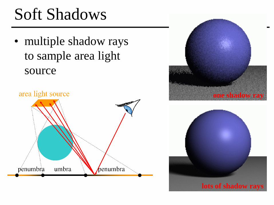
Antialiasing – Supersampling

• multiple

rays per

pixel

point light

area light

jaggies w/ antialiasing

• one reflection ray per intersection

perfect mirror

Reflection

θ θ

Glossy Reflection

• multiple reflection

rays

polished surface θ θ

Justin Legakis

Motion Blur

• Sample objects

temporally

Rob Cook

Algorithm Analysis

• Ray casting

• Lots of primitives

• Recursive

• Distributed Ray

Tracing Effects

– Soft shadows

– Anti-aliasing

– Glossy reflection

– Motion blur

– Depth of field

cost ≤ height * width *

num primitives *

intersection cost *

num shadow rays *

supersampling *

num glossy rays *

num temporal samples *

max recursion depth *

. . .

can we reduce this?

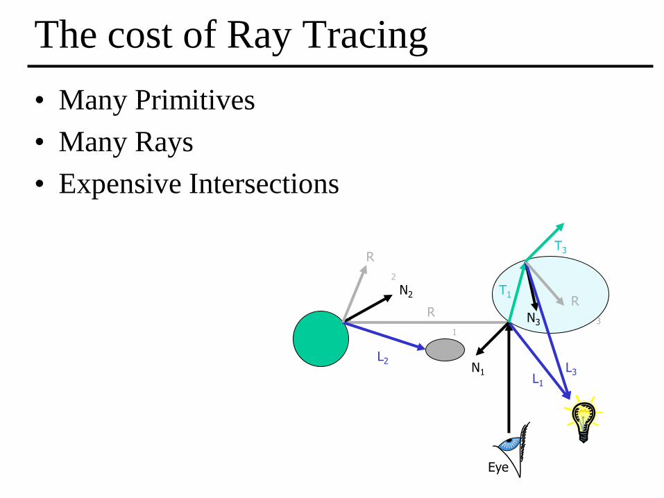
The cost of Ray Tracing

• Many Primitives

• Many Rays

• Expensive Intersections

R

2

R

1

R

3

L2

L1 L3 N1

N2

N3

T1

T3

Eye

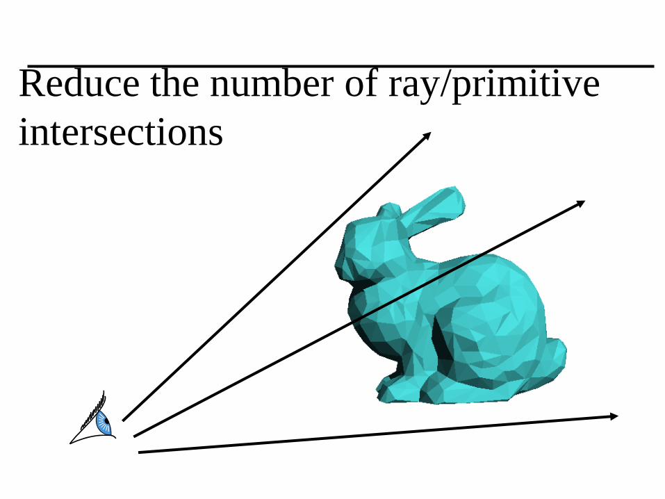
Reduce the number of ray/primitive

intersections

Bounding Volumes

• Idea: associate with each object a simple bounding volume. If a ray misses the bounding volume, it also misses the object contained therein.

• Effective for additional applications:

– Clipping acceleration

– Collision detection

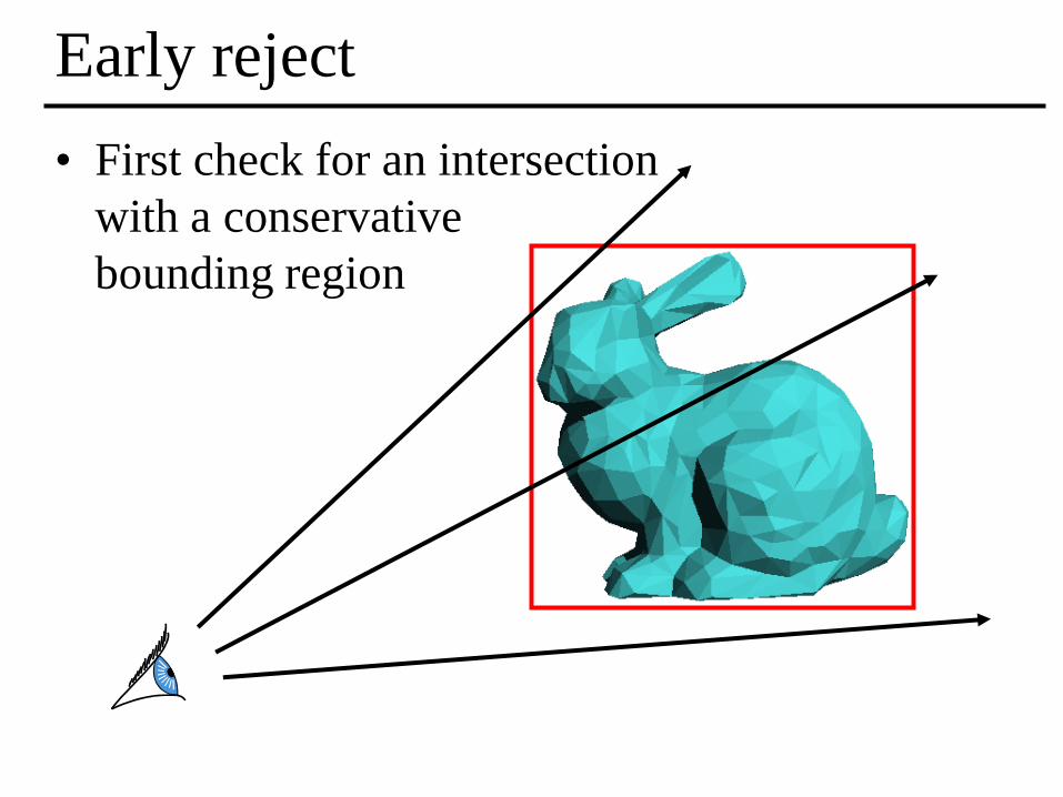
Early reject

• First check for an intersection

with a conservative

bounding region

Conservative Bounding Regions

axis-aligned

bounding box

non-aligned

bounding box

bounding

sphere

arbitrary convex region

(bounding half-spaces)

What is a good bounding volume?

arbitrary convex region

(bounding half-spaces)

• tight → avoid false positives

• fast to intersect

• easy to construct

Bounding Volumes

Bounding Volumes

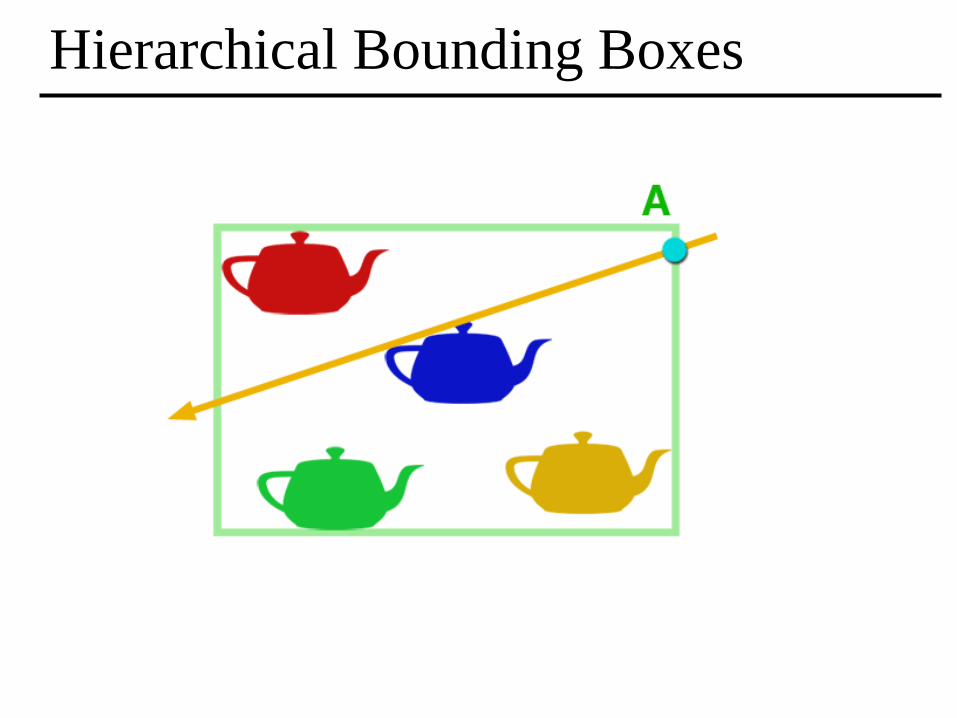
Hierarchical Bounding Boxes

Intersection with Axis-Aligned Box

• For all 3 axes,

calculate the intersection

distances t1 and t2

• tnear = max (t1x, t1y, t1z)

tfar = min (t2x, t2y, t2z)

• If tnear> tfar,

box is missed

• If tfar< tmin,

box is behind

• If box survived tests,

report intersection at tnear

y=Y2

y=Y1

x=X1 x=X2

tnear

tfar

t1x

t1y

t2x

t2y

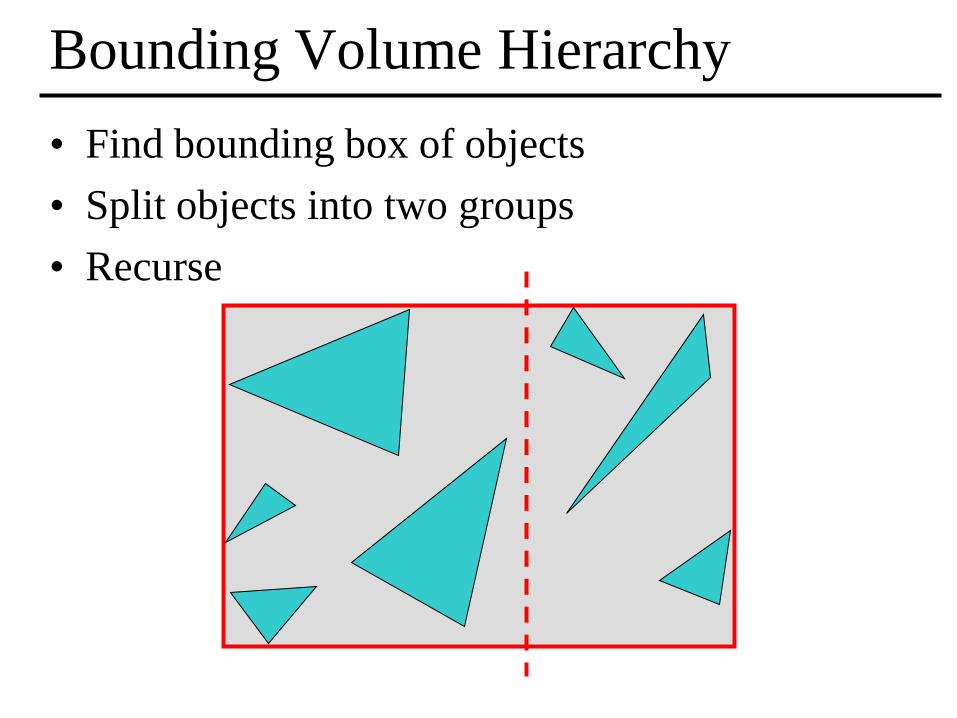
Bounding Volume Hierarchy

• Find bounding box of objects

• Split objects into two groups

• Recurse

Bounding Volume Hierarchy

• Find bounding box of objects

• Split objects into two groups

• Recurse

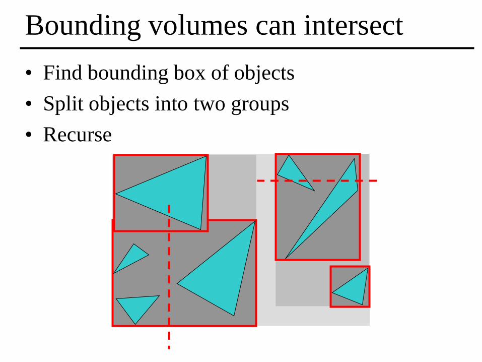
Bounding volumes can intersect

• Find bounding box of objects

• Split objects into two groups

• Recurse

Bounding Volume Hierarchy

Bounding Volume Hierarchy

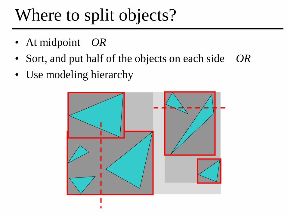
Where to split objects?

• At midpoint OR

• Sort, and put half of the objects on each side OR

• Use modeling hierarchy

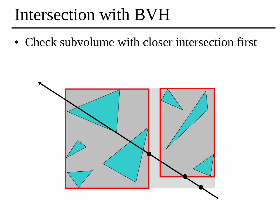
Intersection with BVH

• Check subvolume with closer intersection first

Intersection with BVH

• Don't return intersection immediately if the

other subvolume may have a closer intersection

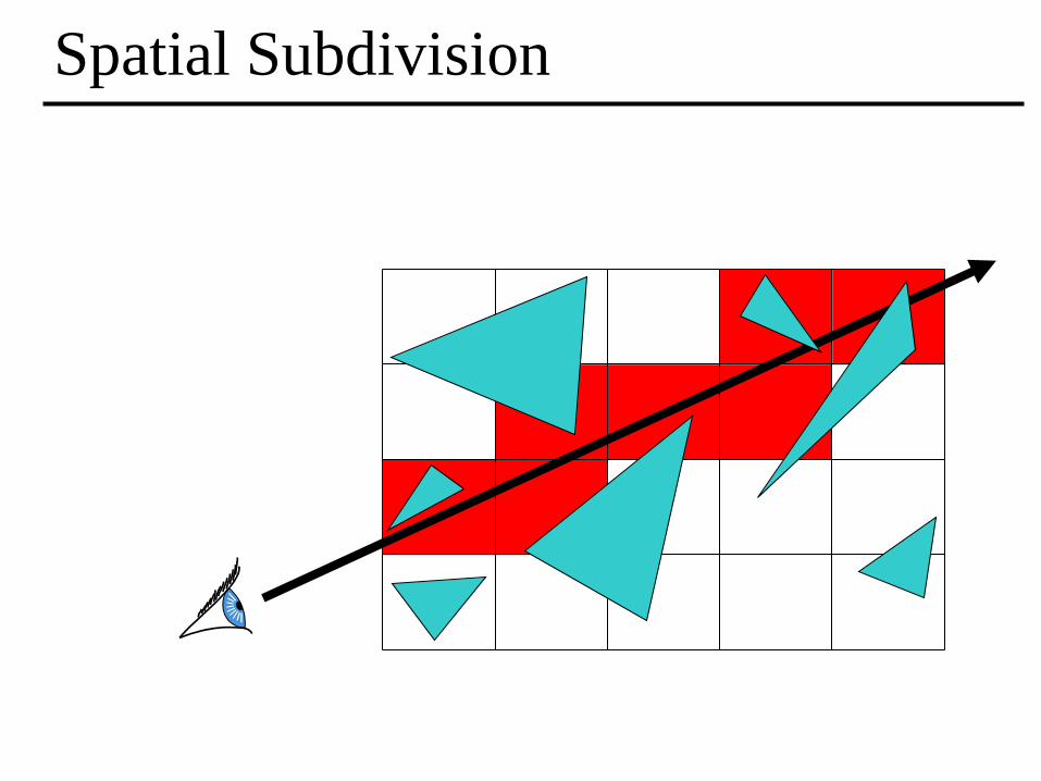
Spatial Subdivision

Spatial Subdivision

• Uniform spatial subdivision:

– The space containing the scene is subdivided into a

uniform grid of cubes “voxels”.

– Each voxel stores a list of all objects at least partially

contained in it.

– Given a ray, voxels are traversed using a 3D variant

of the 2D line drawing algorithms.

– At each voxel the ray is tested for intersection with

the primitives stored therein

– Once an intersection has been found, there is no need

to continue to other voxels.

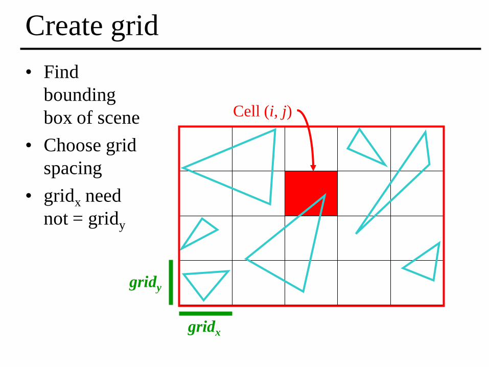
Cell (i, j)

Create grid

• Find

bounding

box of scene

• Choose grid

spacing

• gridx need

not = gridy

gridy

gridx

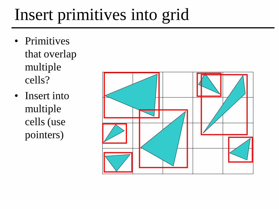
Insert primitives into grid

• Primitives

that overlap

multiple

cells?

• Insert into

multiple

cells (use

pointers)

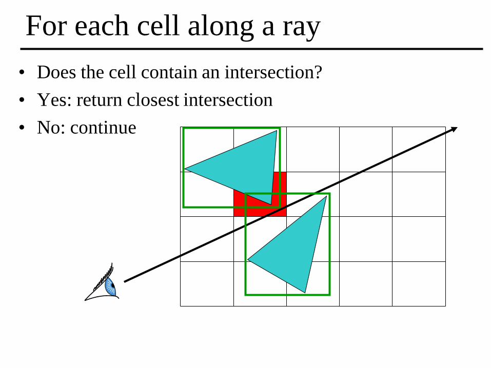
For each cell along a ray

• Does the cell contain an intersection?

• Yes: return closest intersection

• No: continue

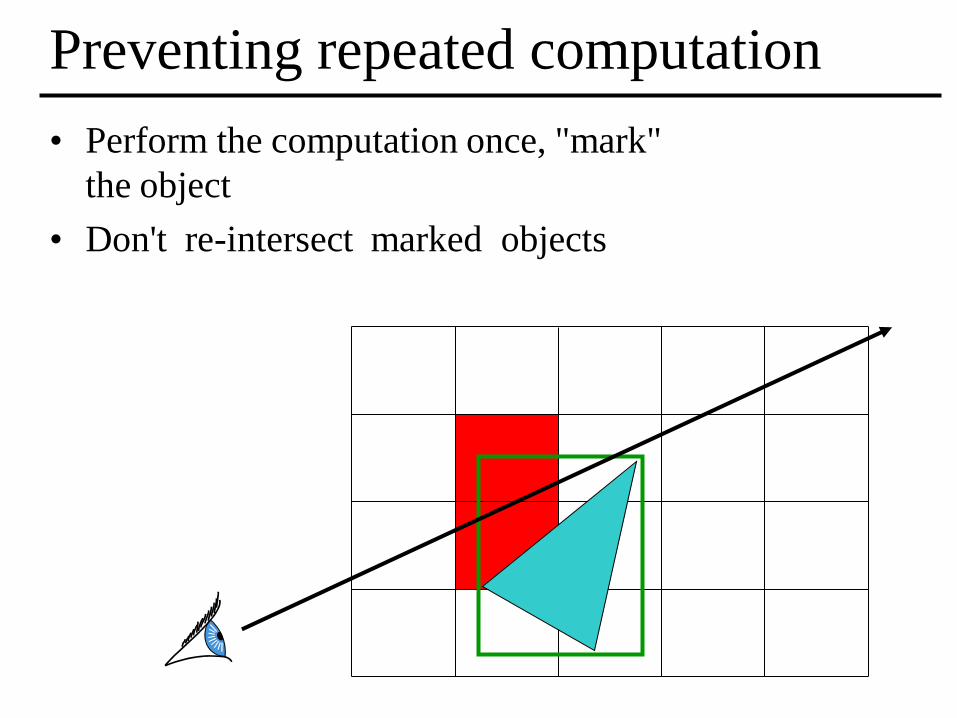
Preventing repeated computation

• Perform the computation once, "mark"

the object

• Don't re-intersect marked objects

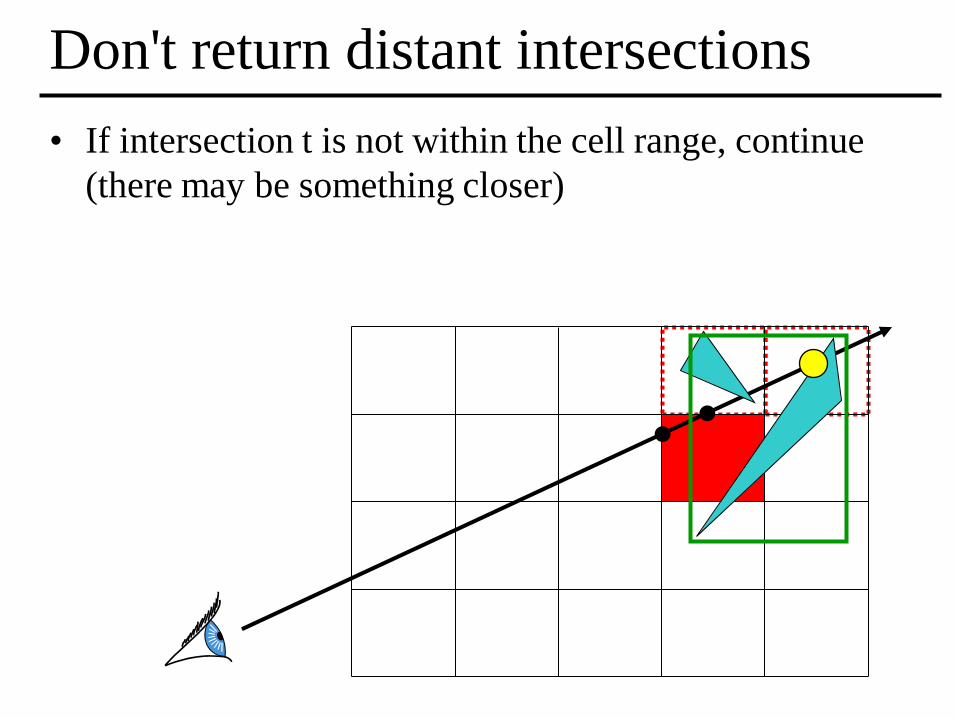
Don't return distant intersections

• If intersection t is not within the cell range, continue

(there may be something closer)

Is there a pattern to cell crossings?

• Yes, the

horizontal

and vertical

crossings

have regular

spacing

dtv = gridy / diry

dth = gridx / dirx

gridy

gridx

(dirx, diry)

Where do we start?

• Intersect ray

with scene

bounding box

• Ray origin

may be inside

the scene

bounding box

tmin

tnext_v

tnext_h

tmin

tnext_v tnext_h

Cell (i, j)

What's the next cell?

dtv dth

Cell (i, j)

if tnext_v < tnext_h

i += signx

tmin = tnext_v

tnext_v += dtv

else

j += signy

tmin = tnext_h

tnext_h += dth

tmin

tnext_v

tnext_h

Cell (i+1, j)

(dirx, diry)

if (dirx > 0) signx = 1 else signx = -1

if (diry > 0) signy = 1 else signy = -1

What's the next cell?

• 3DDDA – Three

Dimensional Digital

Difference Analyzer

• We'll see this

again later, for

line rasterization

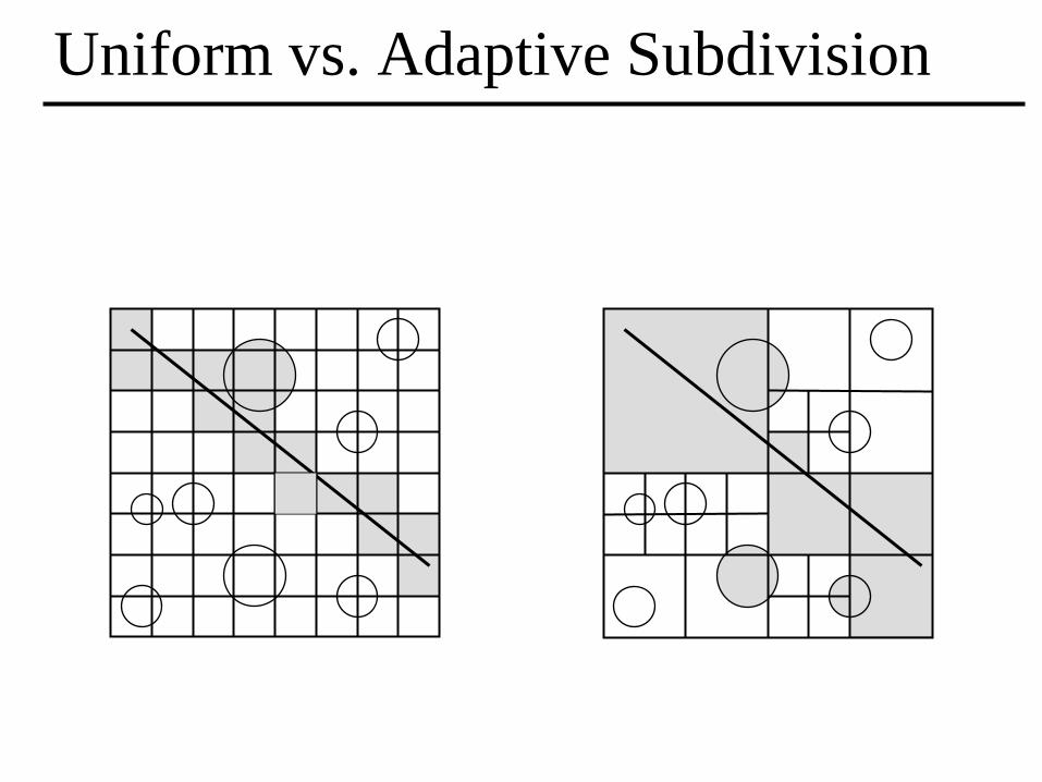
Uniform vs. Adaptive Subdivision

Regular Grid Discussion

• Advantages?

– easy to construct

– easy to traverse

• Disadvantages?

– may be only sparsely filled

– geometry may still be clumped

Adaptive Grids

Nested Grids Octree/(Quadtree)

• Subdivide until each cell contains no more than

n elements, or maximum depth d is reached

Primitives in an Adaptive Grid

• Can live at intermediate levels, or

be pushed to lowest level of grid

Octree/(Quadtree)

Bottom Up traversal

Step from cell to cell.

Intersect current cell and add an

epsilon into the next cell.

Then search for the cell in the

tree.

A naïve search starts from the

root.

Otherwise, try an intelligent

guess…

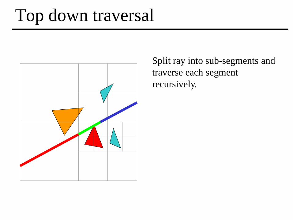
Top down traversal

Split ray into sub-segments and

traverse each segment

recursively.

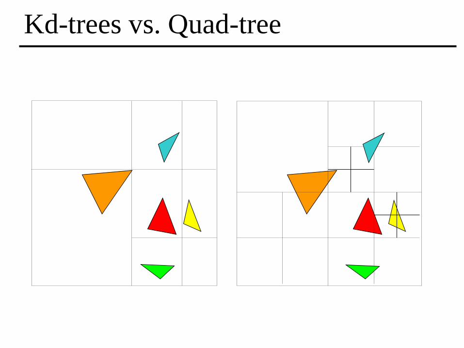
Kd-trees vs. Quad-tree

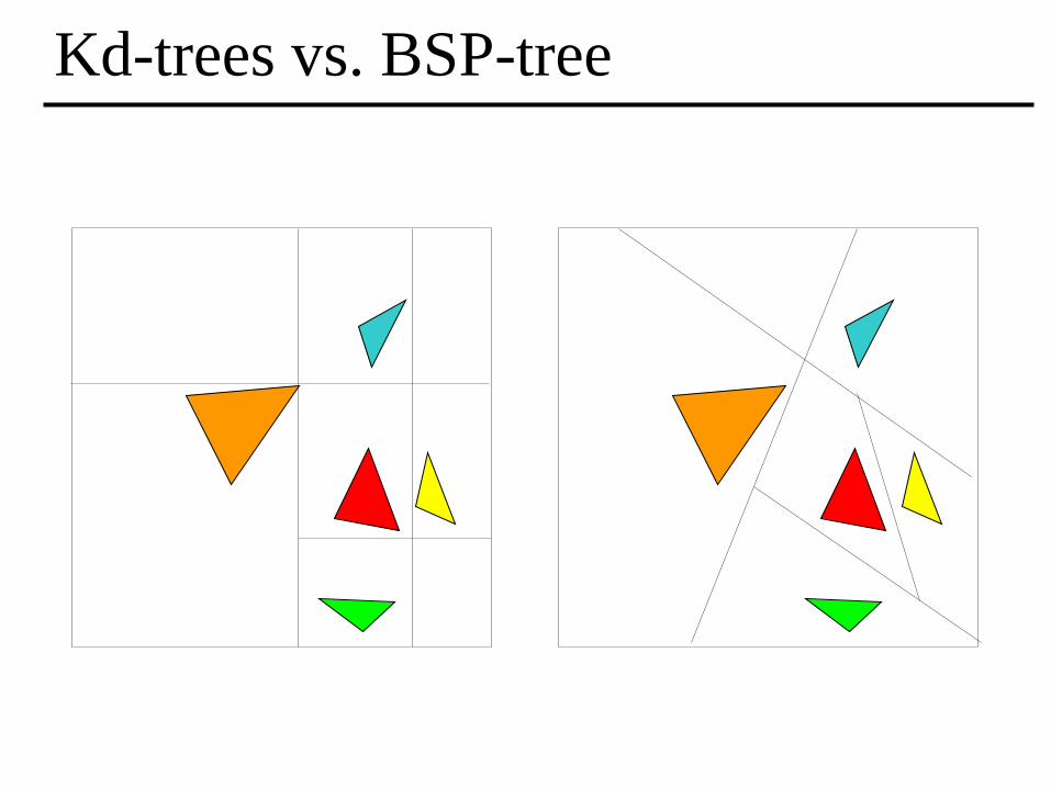
Kd-trees vs. BSP-tree

Adaptive Spatial Subdivision

• Disadvantages of uniform subdivision:

– requires a lot of space

– traversal of empty regions of space can be slow

– not suitable for “teapot in a stadium” scenes

• Solution: use a hierarchical adaptive spatial

subdivision data structure

– octrees

– BSP-trees

• Given a ray, perform a depth-first traversal of the

tree. Again, can stop once an intersection has

been found.

Uniform vs. Adaptive Subdivision

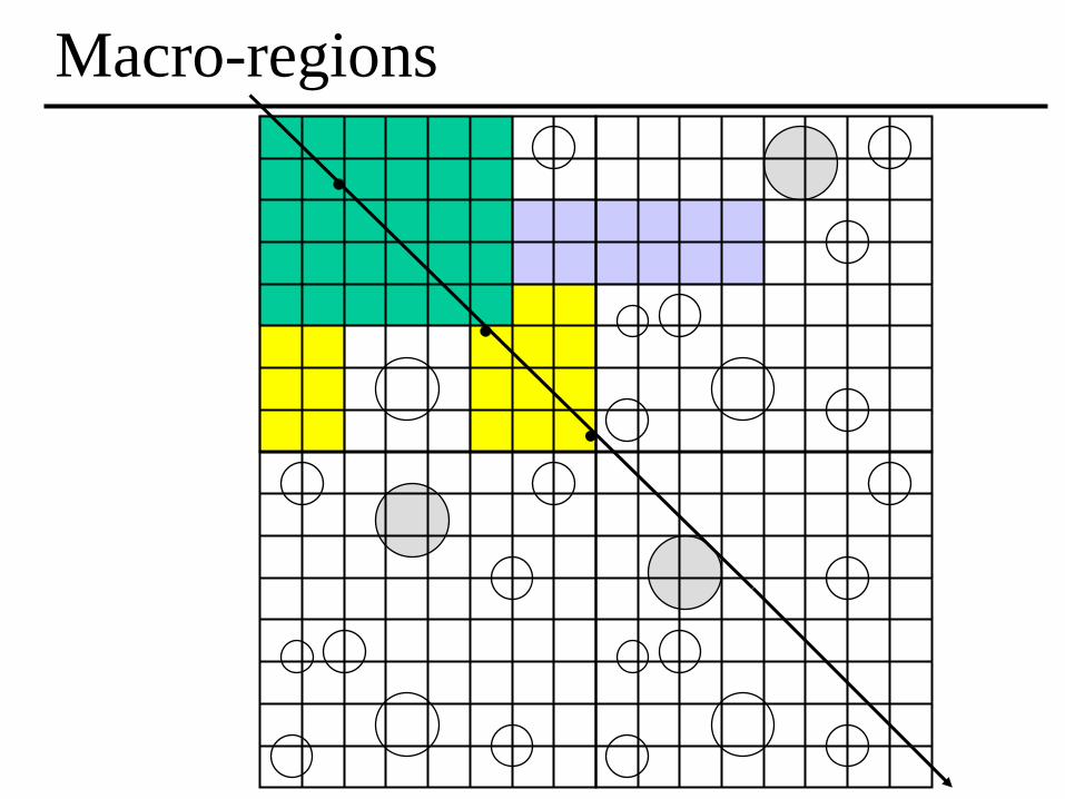
Macro-regions

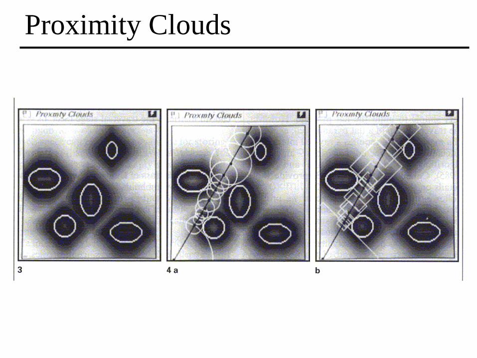
Proximity Clouds

Parallel/Distributed RT

• Two main approaches:

– Each processor is in charge of tracing a subset of the

rays. Requires a shared memory architecture,

replication of the scene database, or transmission of

objects between processors on demand.

– Each processor is in charge of a subset of the scene

(either in terms of space, or in terms of objects).

Requires processors to transmit rays among

themselves.

Directional Techniques

• Light buffer: accelerates shadow rays.

– Discretize the space of directions around each

light source using the direction cube

– In each cell of the cube store a sorted list of

objects visible from the light source through that

cell

– Given a shadow ray locate the appropriate cell of

the direction cube and test the ray with the

objects on its list

Directional Techniques

• Ray classification (Arvo and Kirk 87):

– Rays in 3D have 5 degrees of freedom: (x,y,z,q,f)

– Rays coherence: rays belonging to the same small 5D

neighborhood are likely to intersect the same set of objects.

– Partition the 5D space of rays into a collection of 5D

hypercubes, each containing a list of objects.

– Given a ray, find the smallest containing 5D hypercube, and

test the ray against the objects on the list.

– For efficiency, the hypercubes are arranged in a hierarchy: a

5D analog of the 3D octree. This data structure is constructed

in a lazy fashion.