1

Visible Surface Detection (Chapt. 15 in FVD, Chapt. 13 in Hearn & Baker)

2

• Given a set of 3D objects and a viewing specifications, determine which

lines or surfaces of the objects should be visible.

• A surface might be occluded by other objects or by the same object

(self occlusion)

• Two main approaches:

– Image-precision algorithms: determine what is visible at each pixel.

– Object-precision algorithms: determine which parts of each object are visible.

3

Hidden Lines Removal

4

Coherence • Most methods use coherence features in the surface:

– Object coherence.

– Face coherence.

– Edge coherence.

– Scan-line coherence.

– Depth coherence.

– Frame coherence.

5

Back-face Culling

6

Back-face Culling

7

Back-face Culling

8

Back-face Culling

9

Depth Sort (Painter Algorithm)

• Sort all of the polygons in the scene by their depth.

• Draw them back to front.

• Question: Does a depth ordering always exist?

• Answer: Unfortunately, no!

• For polygons with constant Z value, this sorting clearly works.

10

Z x

x

x

• Given two polygons P and Q, an order may

be determined between them, if at least

one of the following holds:

• Z values of P and Q do not overlap.

• The bounding rectangle in the x,y plane

for P and Q do not overlap.

• P is totally on one side of Q’s plane.

• Q is totally on one side of P’s plane.

11

P is totally on one side of Q’s plane

12

• How to quickly determine which polygon to draw

first?

13

• How to quickly determine which polygon to draw

first?

14

• How to quickly determine which polygon to draw

first?

Simply sorting back-to-front all polygons based on their mid-points doesn’t always work

15

• In addition to the frame buffer (keeping the pixel values), keep a Z-buffer containing the depth value of each pixel.

• Surfaces are scan-converted in an arbitrary order. For each pixel (x,y), the Z-value is computed as well. The (x,y) pixel is overwritten only if its Z-values is closer to the viewing plane than the one already written at this location.

Z-buffer Algorithm

Penetrating Triangle

Z-buffer Algorithm

Incremental Scanline

0

0

CC

DByAxz

DCzByAx

,)(

xC

Azz

C

xxAzz

C

DBjAx

C

DBjAxzz

)(

)(

)()(

1

11

11

, since x = 1,

C

Azz 1

18

Scan-line Algorithm

19

Scan-line Algorithm

20

BSP-Tree Algorithm

Virtual Reality Applications

The user “walks” interactively in a virtual polygonal environment. Examples: model of a city, museum, mall, architectural design

Large and complex - hundreds thousands or even millions of polygons

The goal: to render an updated image for each view point and for each view direction in interactive frame rate

The Visibility Problem

Selecting the (exact?) set of polygons from the model which are visible from a given viewpoint

The Visibility Problem is important

Average number of polygons, visible from a viewpoint, is much smaller than the model size

Indoor scene

25

Oil-tanker ship

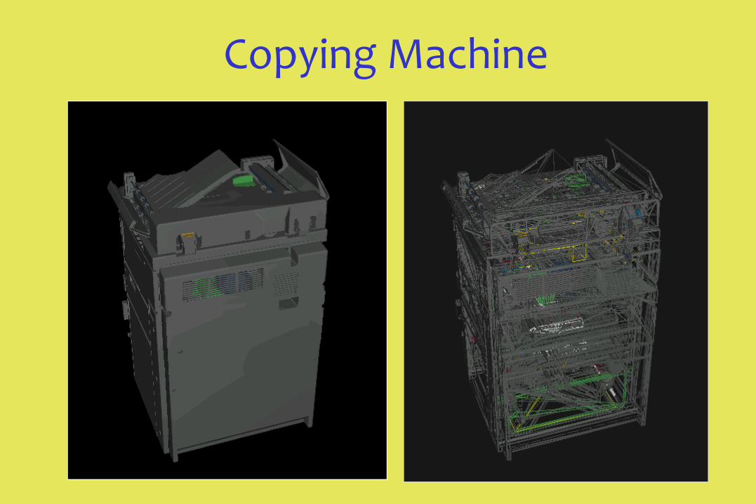
Copying Machine

27

Outdoor scenes

The Visibility Problem is not easy...

A small change of the viewpoint might causes large changes in the visibility

29

The Visibility Problem is not easy...

A small change of the viewpoint might

causes large changes in the visibility

30

31

Close details Far details

Culling

A primitive can be culled by:

View Frustum Culling

Occlusion Culling

Back Face Culling

Avoid processing polygons which contribute nothing to the rendered image

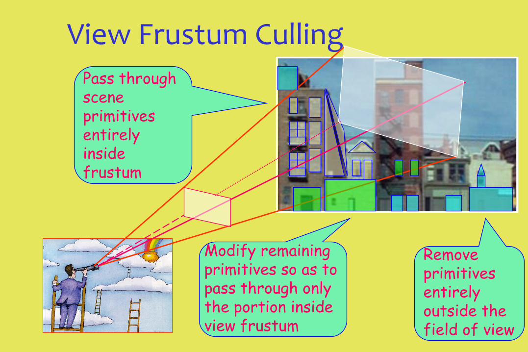
View Frustum Culling

Remove primitives entirely outside the field of view

Modify remaining primitives so as to pass through only the portion inside view frustum

Pass through scene primitives entirely inside frustum

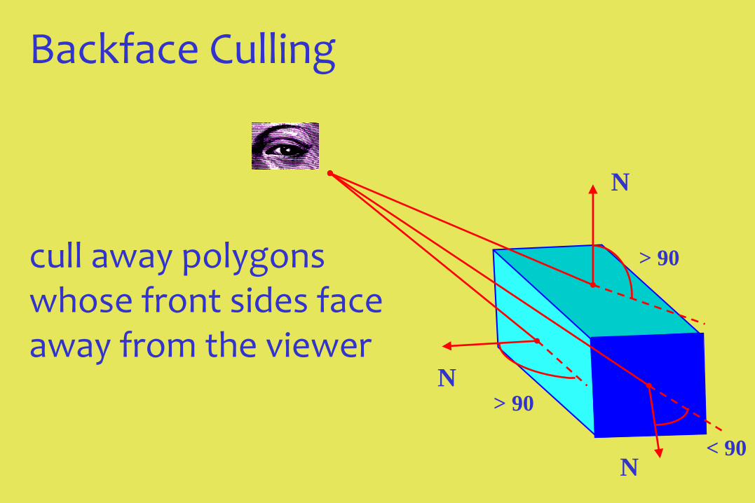
Backface Culling

N

N

N

> 90

> 90

< 90

cull away polygons whose front sides face away from the viewer

35

Occlusion Culling Cull the polygons occluded by other objects in the scene

Very effective in densely occluded scenes

Global: involves interrelation between the polygons

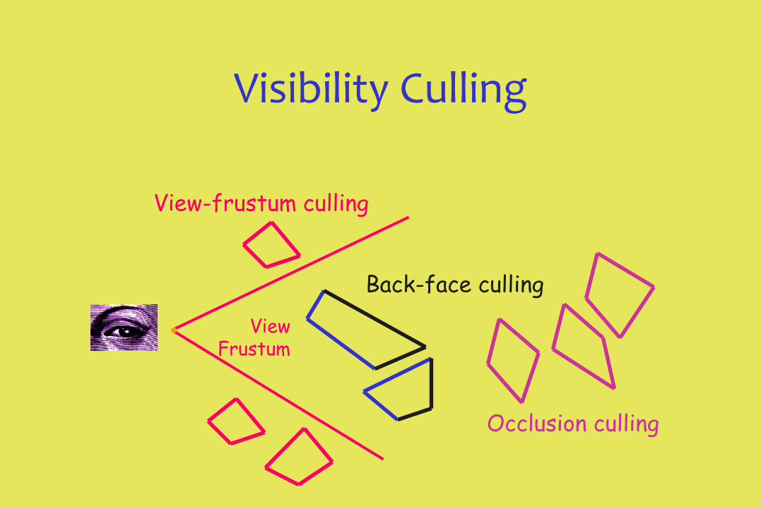
Visibility Culling

View-frustum culling

Back-face culling

Occlusion culling

View Frustum

Hidden Surface Removal

Polygons overlap, so somehow, we must

determine which portion of each

polygon to draw (is visible to the eye)

Output sensitive algorithms

39

Visibility in real-time rendering

• interactively walk through a large model

• large model millions of polygons acceleration necessary (e.g., visibility)

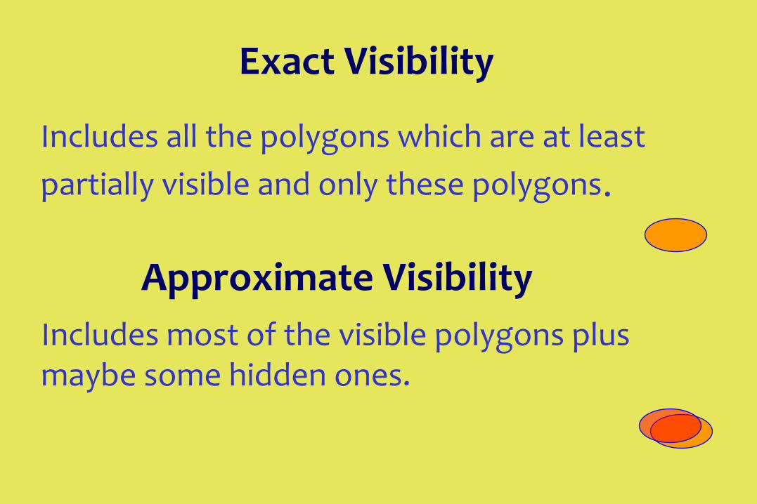
Exact Visibility

Approximate Visibility

Includes all the polygons which are at least

partially visible and only these polygons.

Includes most of the visible polygons plus maybe some hidden ones.

May classify invisible object as visible but may never classify visible object as invisible

Conservative Visibility

Includes at least all the visible objects plus maybe some additional invisible objects

48

What is visible?

What is Occluded?

49

From this point only the red objects are visible

Point Visibility

50

From this cell the red objects are visible as well as orange ones

Cell Visibility Compute the set of all

polygons visible from every possible viewpoint from a region (view-cell)

51

The Aspect Graph

Isomorphic graphs

The Aspect Graph ISG – Image Structure graph

The planner graph, defined by the outlines of an image, created by projection of a polyhedral object, in a certain view direction

The Aspect Graph (Cont.) Aspect

Two different view directions of an object have the same aspect iff the corresponding Image Structure graphs are isomorphic

The Aspect Graph (Cont.) VSP – Visibility Space Partition

Partitioning the viewspace into maximal connected regions in which the viewpoints have the same view or aspect

Visual Event A boundary of a VSP region called a VE for it marks a change in visibility

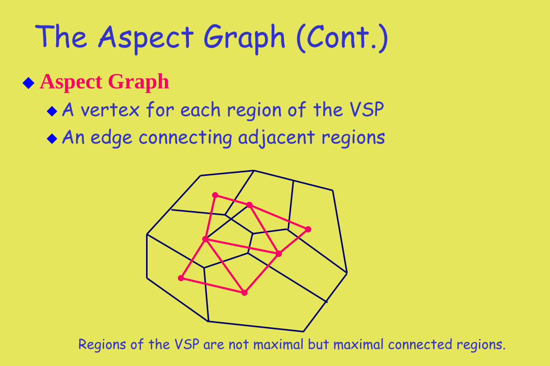
The Aspect Graph (Cont.)

Aspect Graph

A vertex for each region of the VSP

An edge connecting adjacent regions

Regions of the VSP are not maximal but maximal connected regions.

Aspect graph (Cont.)

2 polygons - 12 aspect regions

Aspect graph (Cont.)

3 polygons - “many” aspect regions

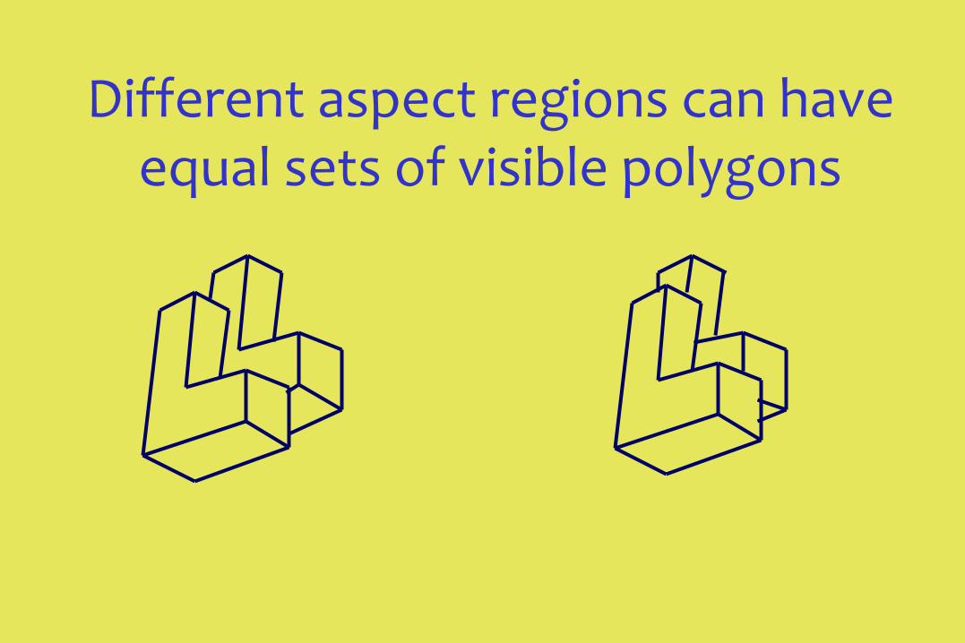
Different aspect regions can have equal sets of visible polygons

Supporting & Separating Planes

3

2

2

1

1 Supporting

Separating

Supporting

Separating

A

T is not occluded in region 1 T is partially occluded in region 2 T is completely occluded in region 3

A - occluder

T - occludee

T

Visibility from the light source

The Art Gallery Problem

See: ftp://ftp.math.tau.ac.il/pub/~daniel/pg99.pdf

Classification of visibility algorithms

•Exact vs. Approximated •Conservative vs. Exact •Precomputed vs. Online •Point vs. Region •Image space vs. Object space •Software vs. Hardware •Dynamic vs. Static scenes