Accelerating Stochastic Optimization - Tel Aviv Universitywolf/deeplearningmeeting/pdfs/FastStochastic.pdf · Accelerating Stochastic Optimization Shai Shalev-Shwartz School of CS

Accelerating Stochastic Optimization

Shai Shalev-Shwartz

School of CS and Engineering,The Hebrew University of Jerusalem

andMobileye

”Master Class at Tel-Aviv”,Tel-Aviv University, November 2014

Shalev-Shwartz (HUJI&Mobileye) Fast Stochastic TAU’14 1 / 34

Learning

Goal (informal): Learn an accurate mapping h : X → Y based onexamples ((x1, y1), . . . , (xn, yn)) ∈ (X × Y)n

Deep learning: Each mapping h : X → Y is parameterized by a weightvector w ∈ Rd, so our goal is to learn the vector w


Learning

Goal (informal): Learn an accurate mapping h : X → Y based onexamples ((x1, y1), . . . , (xn, yn)) ∈ (X × Y)n

Deep learning: Each mapping h : X → Y is parameterized by a weightvector w ∈ Rd, so our goal is to learn the vector w


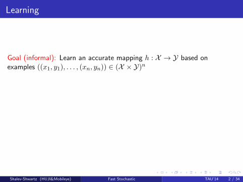
Regularized Loss Minimization

A popular learning approach is Regularized Loss Minimization (RLM)with Euclidean regularization:

Sample S = ((x1, y1), . . . , (xn, yn)) ∼ Dn and approximately solvethe RLM problem

minw∈Rd

1

n

n∑i=1

φi(w) +λ

2‖w‖2

where φi(w) = `yi(hw(xi)) is the loss of predicting hw(xi) when thetrue target is yi


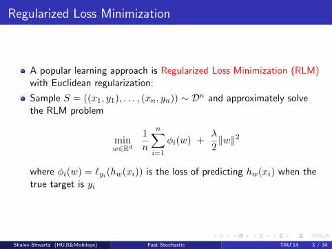
How to solve RLM for Deep Learning?

Stochastic Gradient Descent (SGD):

Advantages:Works well in practicePer iteration cost independent of n

Disadvantage: slow convergence

0 0.1 0.2 0.3 0.4 0.5 0.6 0.7 0.8 0.9 1 1.1 1.2 1.3 1.4 1.5

·107

10−2

10−1

100

# of backpropagation

obje

ctiv

e






0 0.1 0.2 0.3 0.4 0.5 0.6 0.7 0.8 0.9 1 1.1 1.2 1.3 1.4 1.5

·107

10−2

10−1

100


obje

ctiv

e






0 0.1 0.2 0.3 0.4 0.5 0.6 0.7 0.8 0.9 1 1.1 1.2 1.3 1.4 1.5

·107

10−2

10−1

100


obje

ctiv

e


How to improve SGD convergence rate?

1 Stochastic Dual Coordinate Ascent (SDCA):

Same per iteration cost as SGD... but converges exponentially faster

Designed for convex problems... but can be adapted to deep learning

2 SelfieBoost:

AdaBoost, with SGD as weak learner, converges exponentially fasterthan vanilla SGDBut yields an ensemble of networks — very expensive at prediction timeI’ll describe a new boosting algorithm that boost the performance ofthe same networkI’ll show faster convergence under some “SGD success” assumption


How to improve SGD convergence rate?

1 Stochastic Dual Coordinate Ascent (SDCA):

Same per iteration cost as SGD... but converges exponentially faster

Designed for convex problems... but can be adapted to deep learning

2 SelfieBoost:

AdaBoost, with SGD as weak learner, converges exponentially fasterthan vanilla SGDBut yields an ensemble of networks — very expensive at prediction timeI’ll describe a new boosting algorithm that boost the performance ofthe same networkI’ll show faster convergence under some “SGD success” assumption


SDCA vs. SGD

On CCAT dataset, shallow architecture

5 10 15 20 2510

−6

10−5

10−4

10−3

10−2

10−1

100

SDCA

SDCA−Perm

SGD


SelfieBoost vs. SGD

On MNIST dataset, depth 5 network

0 0.1 0.2 0.3 0.4 0.5 0.6 0.7 0.8 0.9 1 1.1 1.2 1.3 1.4 1.5

·107

10−4

10−3

10−2

10−1

100


erro

r

SGDSelfieBoost


Gradient Descent vs. Stochastic Gradient Descent

Define: PI(w) = 1|I|∑

i∈I φi(w) + λ2‖w‖

2

GD SGD

rule wt+1 = wt − η∇P (wt) wt+1 = wt − η∇PI(wt)for random I ⊂ [n]

per iteration cost O(n) O(1)

convergence rate log(1/ε) 1/ε


Hey, wait, but what about ...

Decaying learning rate

Nesterov’s momentum


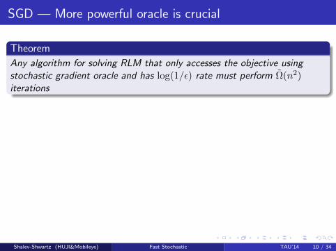
SGD — More powerful oracle is crucial

Theorem

Any algorithm for solving RLM that only accesses the objective usingstochastic gradient oracle and has log(1/ε) rate must perform Ω(n2)iterations

Proof idea:

Consider two objectives (in both, λ = 1): for i ∈ ±1

Pi(w) =1

2n

(n− 1

2(w − i)2 +

n+ 1

2(w + i)2

)A stochastic gradient oracle returns w ± i w.p. 1

2 ±12n

Easy to see that w∗i = −i/n, Pi(0) = 1/2, Pi(w∗i ) = 1/2− 1/(2n2)

Therefore, solving to accuracy ε < 1/(2n2) amounts to determiningthe bias of the coin


SGD — More powerful oracle is crucial

Theorem

Any algorithm for solving RLM that only accesses the objective usingstochastic gradient oracle and has log(1/ε) rate must perform Ω(n2)iterations

Proof idea:

Consider two objectives (in both, λ = 1): for i ∈ ±1

Pi(w) =1

2n

(n− 1

2(w − i)2 +

n+ 1

2(w + i)2

)A stochastic gradient oracle returns w ± i w.p. 1

2 ±12n

Easy to see that w∗i = −i/n, Pi(0) = 1/2, Pi(w∗i ) = 1/2− 1/(2n2)

Therefore, solving to accuracy ε < 1/(2n2) amounts to determiningthe bias of the coin


Outline

1 SDCADescription and analysis for convex problemsSDCA for Deep LearningAccelerated SDCA

2 SelfieBoost


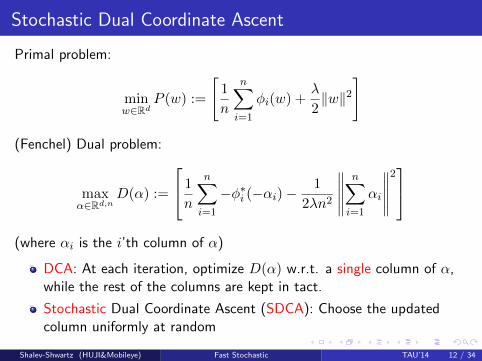
Stochastic Dual Coordinate Ascent

Primal problem:

minw∈Rd

P (w) :=

[1

n

n∑i=1

φi(w) +λ

2‖w‖2

]

(Fenchel) Dual problem:

maxα∈Rd,n

D(α) :=

1

n

n∑i=1

−φ∗i (−αi)−1

2λn2

∥∥∥∥∥n∑i=1

αi

∥∥∥∥∥2

(where αi is the i’th column of α)

DCA: At each iteration, optimize D(α) w.r.t. a single column of α,while the rest of the columns are kept in tact.

Stochastic Dual Coordinate Ascent (SDCA): Choose the updatedcolumn uniformly at random


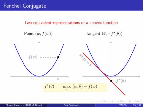
Fenchel Conjugate

Two equivalent representations of a convex function

Point (w, f(w))

w

f(w)

Tangent (θ,−f?(θ))

slope=θ

−f?(θ)f?(θ) = max

w〈w, θ〉 − f(w)


SDCA Analysis

Theorem

Assume each φi is convex and smooth. Then, after

O

((n+

1

λ

)log

1

ε

)iterations of SDCA we have, with high probability, P (wt)− P (w∗) ≤ ε.

GD SGD SDCA

iteration cost nd d d

convergence rate 1λ log(1/ε) 1

λε

(n+ 1

λ

)log(1/ε)

runtime nd · 1λ d · 1λε d ·

(n+ 1

λ

)runtime for λ = 1

n n2d ndε nd


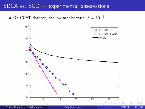
SDCA vs. SGD — experimental observations

On CCAT dataset, shallow architecture, λ = 10−6

5 10 15 20 2510

−6

10−5

10−4

10−3

10−2

10−1

100

SDCA

SDCA−Perm

SGD


SDCA vs. DCA — Randomization is crucial

0 2 4 6 8 10 12 14 16 1810

−6

10−5

10−4

10−3

10−2

10−1

100

SDCADCA−Cyclic

SDCA−PermBound


Outline


2 SelfieBoost


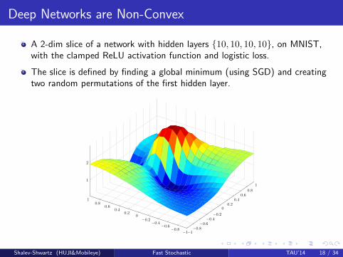
Deep Networks are Non-Convex

A 2-dim slice of a network with hidden layers 10, 10, 10, 10, on MNIST,with the clamped ReLU activation function and logistic loss.

The slice is defined by finding a global minimum (using SGD) and creatingtwo random permutations of the first hidden layer.

−1−0.8−0.6−0.4−0.2

00.2

0.40.6

0.8

1

−1−0.8

−0.6−0.4

−0.20

0.20.4

0.60.8

1

1

2


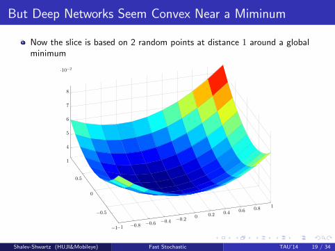
But Deep Networks Seem Convex Near a Miminum

Now the slice is based on 2 random points at distance 1 around a globalminimum

−1 −0.8 −0.6 −0.4 −0.20 0.2 0.4 0.6 0.8 1

−1

−0.5

0

0.5

1

4

5

6

7

8

·10−2


SDCA for Deep Learning

For φi being non-convex, the Fenchel conjugate often becomesmeaningless

But, our analysis implies that an approximate dual update suffices,that is,

α(t)i = α

(t−1)i − ηλn

(∇φi(w(t−1)) + α

(t−1)i

)The relation between primal and dual vectors is by

w(t−1) =1

λn

n∑i=1

α(t−1)i

and therefore the corresponding primal update is:

w(t) = w(t−1) − η(∇φi(w(t−1)) + α

(t−1)i

)These updates can be implemented for deep learning as well and donot require to calculate the Fenchel conjugate


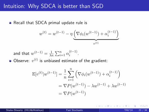
Intuition: Why SDCA is better than SGD

Recall that SDCA primal update rule is

w(t) = w(t−1) − η(∇φi(w(t−1)) + α

(t−1)i

)︸︷︷︸

v(t)

and that w(t−1) = 1λn

∑ni=1 α

(t−1)i .

Observe: v(t) is unbiased estimate of the gradient:

E[v(t)|w(t−1)] =1

n

n∑i=1

(∇φi(w(t−1)) + α

(t−1)i

)= ∇P (w(t−1))− λw(t−1) + λw(t−1)

= ∇P (w(t−1))



Recall that SDCA primal update rule is

w(t) = w(t−1) − η(∇φi(w(t−1)) + α

(t−1)i

)︸︷︷︸

v(t)

and that w(t−1) = 1λn

∑ni=1 α

(t−1)i .

Observe: v(t) is unbiased estimate of the gradient:

E[v(t)|w(t−1)] =1

n

n∑i=1

(∇φi(w(t−1)) + α

(t−1)i

)= ∇P (w(t−1))− λw(t−1) + λw(t−1)

= ∇P (w(t−1))



The update step of both SGD and SDCA is w(t) = w(t−1) − ηv(t)where

v(t) =

∇φi(w(t−1)) + λw(t−1) for SGD

∇φi(w(t−1)) + α(t−1)i for SDCA

In both cases E[v(t)|w(t−1)] = ∇P (w(t))

What about the variance?

For SGD, even if w(t−1) = w∗, the variance of v(t) is still constant

For SDCA, we’ll show that the variance of v(t) goes to zero asw(t−1) → w∗


SDCA as variance reduction technique (Johnson & Zhang)

For w∗ we have ∇P (w∗) = 0 which means

1

n

n∑i=1

∇φi(w∗) + λw∗ = 0

⇒ w∗ =1

λn

n∑i=1

(−∇φi(w∗)) =1

λn

n∑i=1

α∗i

Therefore, if α(t−1)i → α∗i and w(t−1) → w∗ then the update vector

satisfies

v(t) = ∇φi(w(t−1)) + α(t−1)i → ∇φi(w∗) + α∗i = 0


Issues with SDCA for Deep Learning

Needs to maintain the matrix α

Can significantly reduce storage if working with mini-batches

Another approach is the SVRG algorithm of Johnson and Zhang


Accelerated SDCA

Nesterov’s Accelerated (deterministic) Gradient Descent (AGD):combine 2 gradients to accelerate the convergence rate

AGD runtime: O(dn 1√

λ

)SDCA runtime: O

(d(n+ 1

λ

))Can we accelerate SDCA ?

Yes! The main idea is to iterate

Use SDCA to approximately minimize Pt(w) = P (w) + κ2 ‖w− y

(t−1)‖2Update y(t) = w(t) + β(w(t) − w(t−1))

Accelerated SDCA runtime: O(d(n+

√nλ

))


Experimental Demonstration

Smoothed hinge-loss with `1, `2 regularization, λ = 10−7:

astro-ph cov1 CCAT

0 20 40 60 80 1000

0.1

0.2

0.3

0.4

0.5 AccProxSDCAProxSDCA

FISTA

0 20 40 60 80 100

0.3

0.35

0.4

0.45


FISTA

0 20 40 60 80 100

0.1

0.2

0.3

0.4


FISTA


Outline


2 SelfieBoost


SelfieBoost Motivation

0 0.1 0.2 0.3 0.4 0.5 0.6 0.7 0.8 0.9 1 1.1 1.2 1.3 1.4 1.5

·107

10−2

10−1

100


obje

ctiv

e

Why SGD is slow at the end?

High variance, even close to the optimum

Rare mistakes: Suppose all but 1% of the examples are correctlyclassified. SGD will now waste 99% of its time on examples that arealready correct by the model


SelfieBoost Motivation

For simplicity, consider a binary classification problem in the realizablecase

For a fixed ε0 (not too small), few SGD iterations find a solution withP (w)− P (w∗) ≤ ε0However, for a small ε, SGD requires many iterations

Smells like we need to use boosting ....


First idea: learn an ensemble using AdaBoost

Fix ε0 (say 0.05), and assume SGD can find a solution with error < ε0quite fast

Lets apply AdaBoost with the SGD learner as a weak learner:

At iteration t, we sub-sample a training set based on a distribution Dt

over [n]We feed the sub-sample to a SGD learner and gets a weak classifier htUpdate Dt+1 based on the predictions of htThe output of AdaBoost is an ensemble with prediction

∑Tt=1 αtht(x)

The celebrated Freund & Schapire theorem states that ifT = O(log(1/ε)) then the error of the ensemble classifier is at most ε

Observe that each boosting iteration involves calling SGD on arelatively small data, and updating the distribution on the entire bigdata. The latter step can be performed in parallel

Disadvantage of learning an ensemble: at prediction time, we need toapply many networks


Boosting the Same Network

Can we obtain “boosting-like” convergence, while learning a singlenetwork?

The SelfieBoost Algorithm:

Start with an initial network f1

At iteration t, define weights over the n examples according toDi ∝ e−yift(xi)

Sub-sample a training set S ∼ DUse SGD for approximately solving the problem

ft+1 ≈ argming

∑i∈S

yi(ft(xi)− g(xi)) +1

2

∑i∈S

(g(xi)− ft(xi))2


Analysis of the SelfieBoost Algorithm

Lemma: At each iteration, with high probability over the choice of S,there exists a network g with objective value of at most −1/4

Theorem: If at each iteration, the SGD algorithm finds a solutionwith objective value of at most −ρ, then after

log(1/ε)

ρ

SelfieBoost iterations the error of ft will be at most ε

To summarize: we have obtained log(1/ε) convergence assuming thatthe SGD algorithm can solve each sub-problem to a fixed accuracy(which seems to hold in practice)


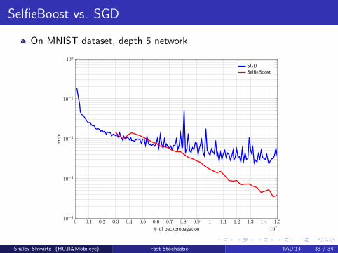
SelfieBoost vs. SGD

On MNIST dataset, depth 5 network

0 0.1 0.2 0.3 0.4 0.5 0.6 0.7 0.8 0.9 1 1.1 1.2 1.3 1.4 1.5

·107

10−4

10−3

10−2

10−1

100


erro

r

SGDSelfieBoost


Summary

SGD converges quickly to an o.k. solution, but then slows down:1 High variance even at w∗

2 Wastes time on already solved cases

There’s a need for stochastic methods that have similar per-iterationcomplexity as SGD but converge faster

1 SDCA reduces variance and therefore converges faster2 SelfieBoost focuses on the hard cases

Future Work and Open Questions:

Evaluate the empirical performance of SDCA and SelfieBoost forchallenging deep learning tasks

Bridge the gap between empirical success of SGD and worst-casehardness results


Summary

SGD converges quickly to an o.k. solution, but then slows down:1 High variance even at w∗

2 Wastes time on already solved cases

There’s a need for stochastic methods that have similar per-iterationcomplexity as SGD but converge faster

1 SDCA reduces variance and therefore converges faster2 SelfieBoost focuses on the hard cases

Future Work and Open Questions:

Evaluate the empirical performance of SDCA and SelfieBoost forchallenging deep learning tasks

Bridge the gap between empirical success of SGD and worst-casehardness results


Documents

Accelerating Stochastic Optimization - Tel Aviv Universitywolf/deeplearningmeeting/pdfs/FastStochastic.pdf · Accelerating Stochastic Optimization Shai Shalev-Shwartz School of CS