Embed Size (px)
Citation preview
Qiyuan Tian and Haomiao Jiang
Department of Electrical Engineering
Stanford University
GPU Technology Conference, San Jose
March 17, 2015
Accelerating a learning–based image processing pipeline for digital cameras Local, Linear and Learned (L3) pipeline
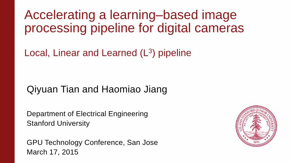
Digital camera sub-systems
Focus
control
Exposure
control
Lens, aperture and
sensor
Pre-processing • dead pixel removal
• dark floor subtraction
• structured noise reduction
• quantization
• etc.
RAW image Display image
Image
processing
pipeline
Transform the
sensor data
into a display image
CFA
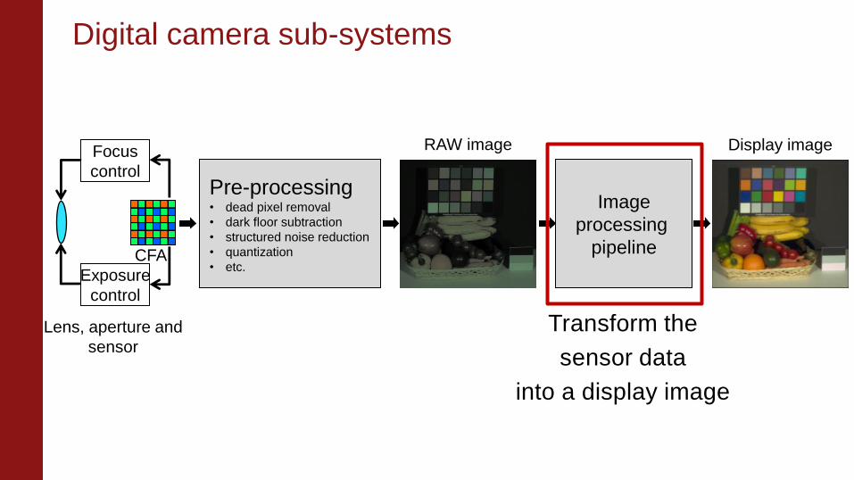
Standard image processing pipeline
RAW image Display image
CFA
interpolation
Sensor
conversion
Illuminant
correction
Tone
scale
Noise
reduction
− Requires multiple algorithms
− Each algorithm requires optimization
− Optimized only for Bayer (RGB) color filter array (CFA)
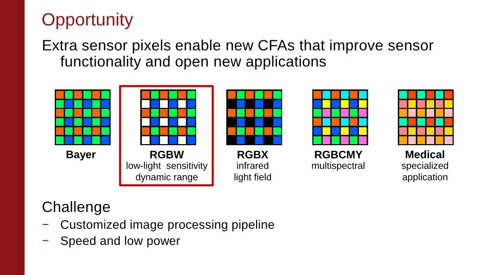
Opportunity
Extra sensor pixels enable new CFAs that improve sensor functionality and open new applications
Challenge − Customized image processing pipeline
− Speed and low power
Bayer
RGBX
infrared
light field
RGBW
low-light sensitivity
dynamic range
Medical
specialized
application
RGBCMY
multispectral
Sensor
conversion
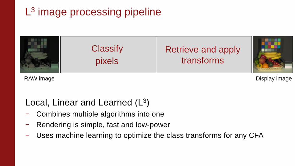
L3 image processing pipeline
Local, Linear and Learned (L3)
− Combines multiple algorithms into one
− Rendering is simple, fast and low-power
− Uses machine learning to optimize the class transforms for any CFA
RAW image Display image
CFA
interpolation
Illuminant
correction
Tone
scale
Noise
reduction
Classify
pixels Retrieve and apply
transforms
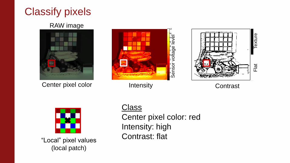
Classify pixels
Se
nso
r vo
lta
ge
leve
l
Intensity
Fla
t
Te
xtu
re
Contrast
Class
Center pixel color: red
Intensity: high
Contrast: flat
Center pixel color
RAW image
“Local” pixel values
(local patch)
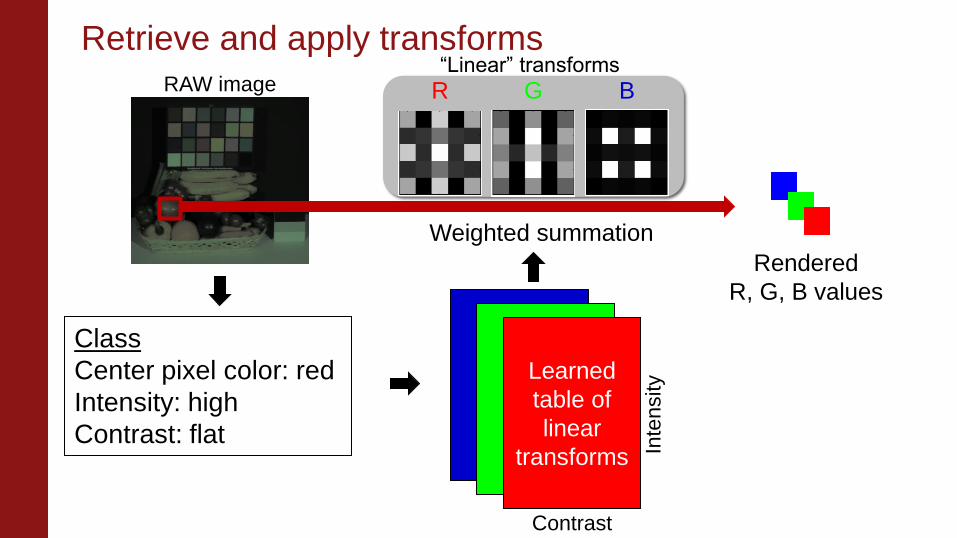
Retrieve and apply transforms
Class
Center pixel color: red
Intensity: high
Contrast: flat
Contrast
Inte
nsity Learned
table of
linear
transforms
Weighted summation
Rendered
R, G, B values
RAW image R G B “Linear” transforms
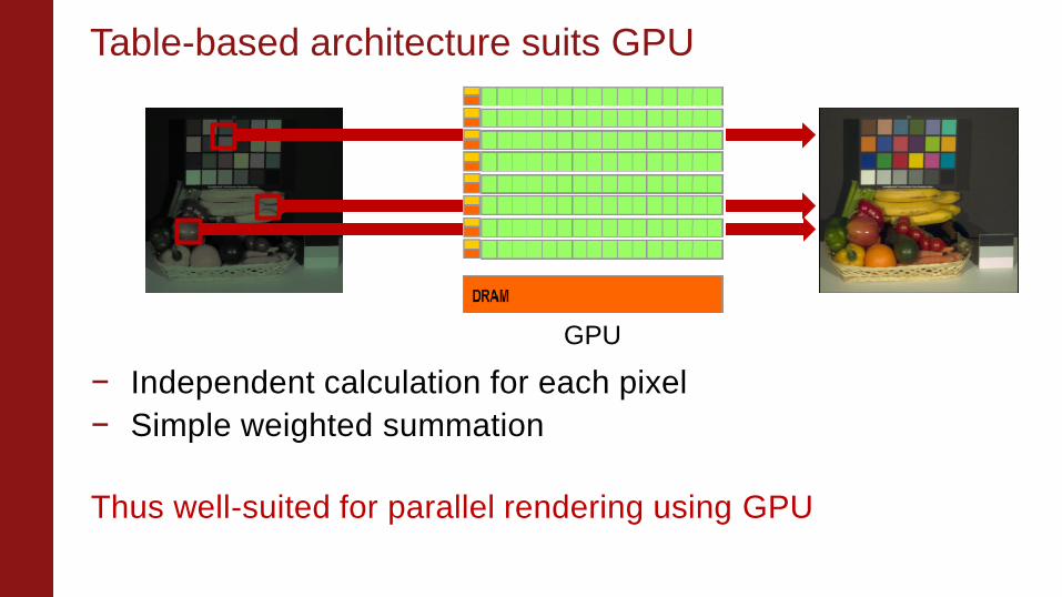
Table-based architecture suits GPU
Weighted summation Weighted summation
− Independent calculation for each pixel
− Simple weighted summation
Thus well-suited for parallel rendering using GPU
GPU
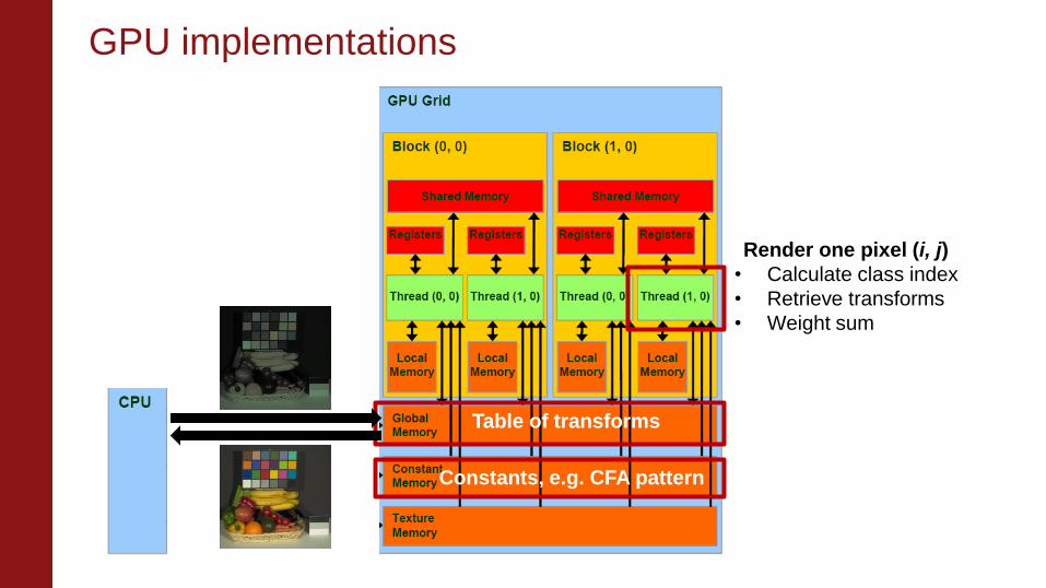
GPU implementations
Table of transforms
Render one pixel (i, j)
• Calculate class index
• Retrieve transforms
• Weight sum
Constants, e.g. CFA pattern
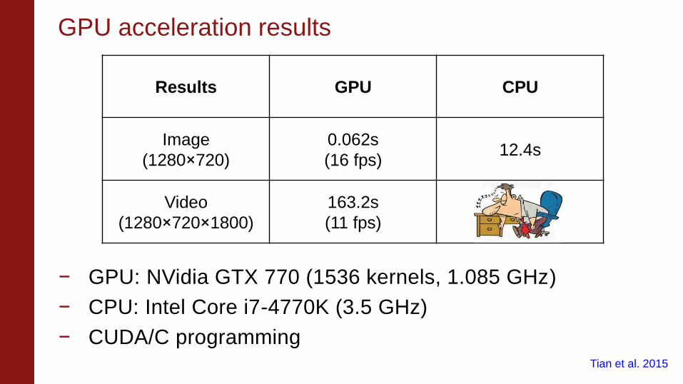
GPU acceleration results
− GPU: NVidia GTX 770 (1536 kernels, 1.085 GHz)
− CPU: Intel Core i7-4770K (3.5 GHz)
− CUDA/C programming
Results CPU GPU
Image
(1280×720) 12.4s
0.062s
(16 fps)
Video
(1280×720×1800)
163.2s
(11 fps)
Tian et al. 2015
Potential speed improvement
Use shared memory and registers
Specialized image signal processor (ISP)
L3 ISP
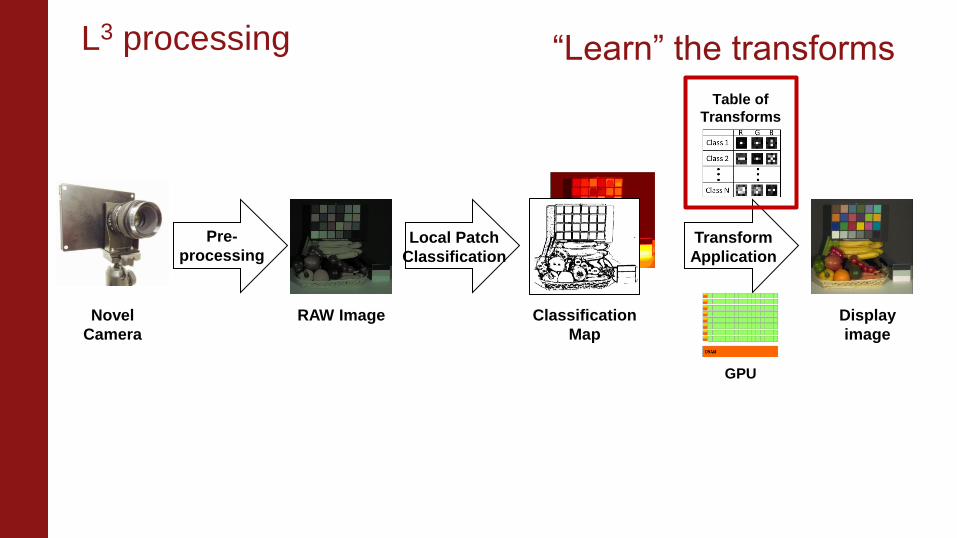
Novel
Camera
Pre-
processing Local Patch
Classification
Transform
Application
RAW Image Classification
Map
Display
image
Table of
Transforms
GPU
“Learn” the transforms L3 processing
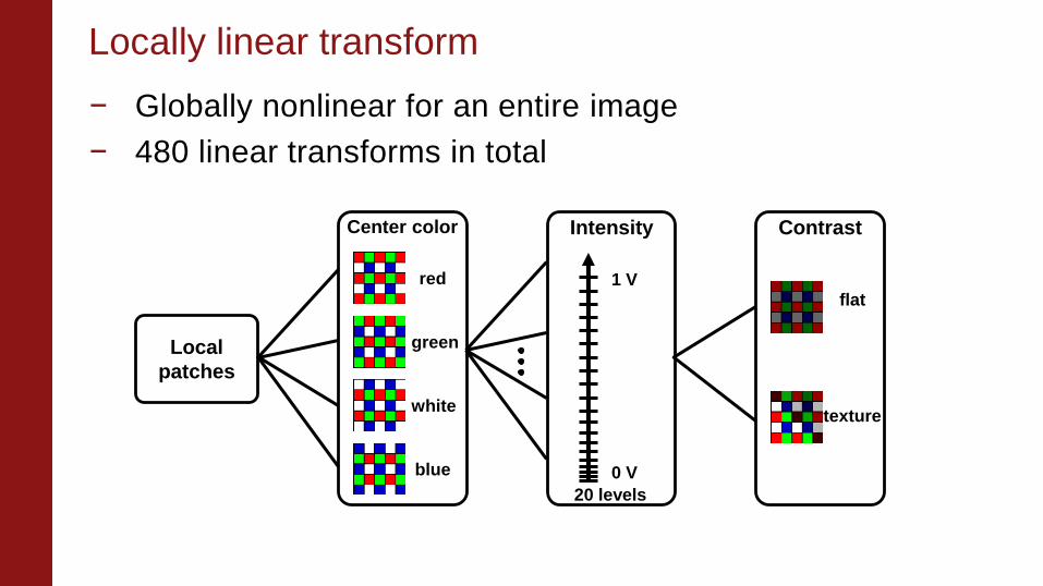
Locally linear transform
Contrast Center color Intensity
Local
patches
red
white
green
blue
flat
texture
0 V
1 V
20 levels
− Globally nonlinear for an entire image
− 480 linear transforms in total
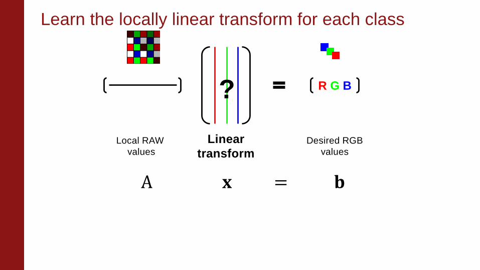
Learn the locally linear transform for each class
R G B
Linear
transform Local RAW
values
Desired RGB
values
A 𝐱 = 𝐛
?
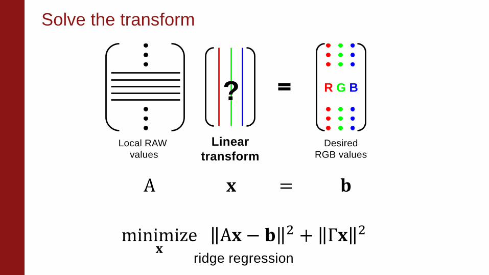
Solve the transform
R G B
Local RAW
values
Desired
RGB values
minimize𝐱
A𝐱 − 𝐛 2 + Γ𝐱 2
Linear
transform
?
ridge regression
A 𝐱 = 𝐛
?
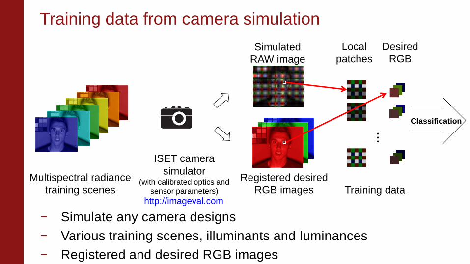
Training data from camera simulation
Multispectral radiance
training scenes
ISET camera
simulator (with calibrated optics and
sensor parameters)
Simulated
RAW image
Registered desired
RGB images
…
Training data
Classification
Local
patches
Desired
RGB
− Simulate any camera designs
− Various training scenes, illuminants and luminances
− Registered and desired RGB images
http://imageval.com
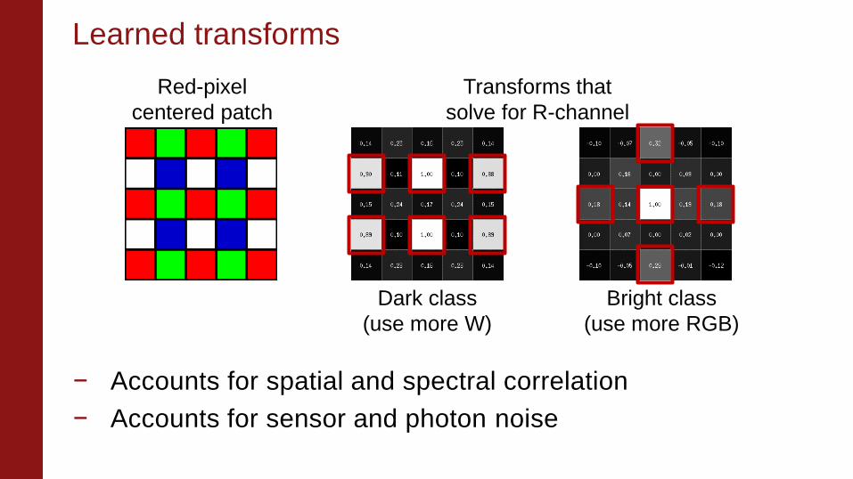
Dark class
(use more W)
Learned transforms
Red-pixel
centered patch
Transforms that
solve for R-channel
Bright class
(use more RGB)
− Accounts for spatial and spectral correlation
− Accounts for sensor and photon noise
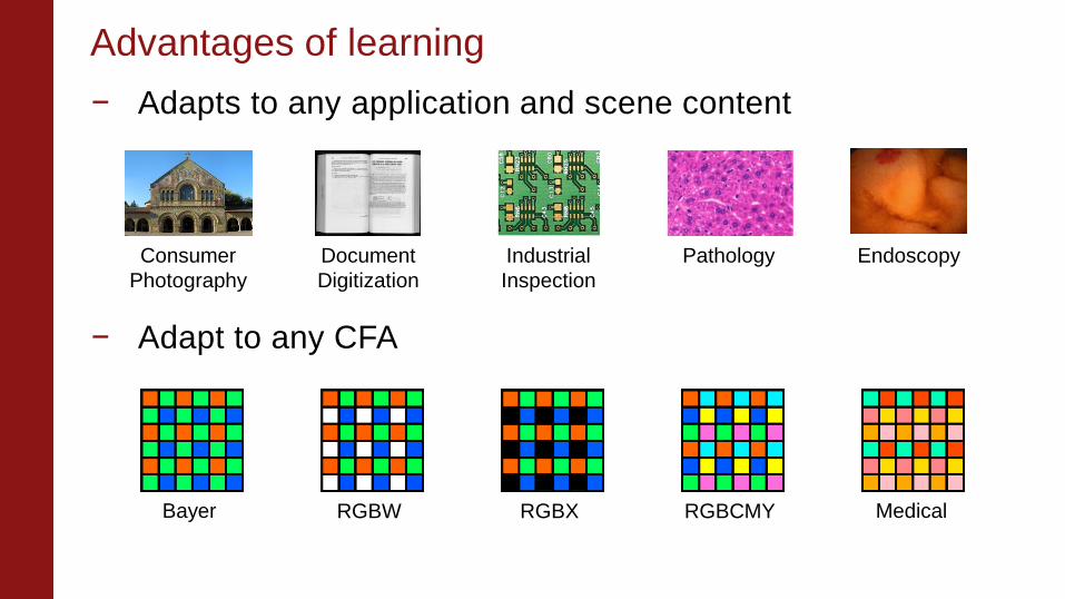
Advantages of learning
− Adapts to any application and scene content
− Adapt to any CFA
Consumer
Photography
Industrial
Inspection
Document
Digitization
Endoscopy Pathology
Bayer
RGBX
RGBW
Medical
RGBCMY
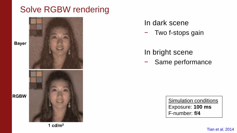
In dark scene
− Two f-stops gain
In bright scene
− Same performance
Solve RGBW rendering
Simulation conditions
Exposure: 100 ms
F-number: f/4
Tian et al. 2014
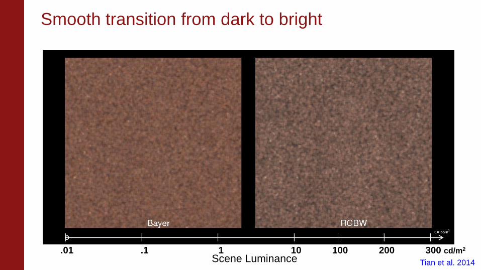
Smooth transition from dark to bright
.01 .1 1 10 100 200 300 cd/m2
Scene Luminance Tian et al. 2014
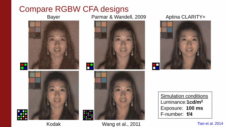
Compare RGBW CFA designs Bayer Parmar & Wandell, 2009 Aptina CLARITY+
Kodak Wang et al., 2011
Simulation conditions
Luminance:1cd/m2
Exposure: 100 ms
F-number: f/4
Tian et al. 2014
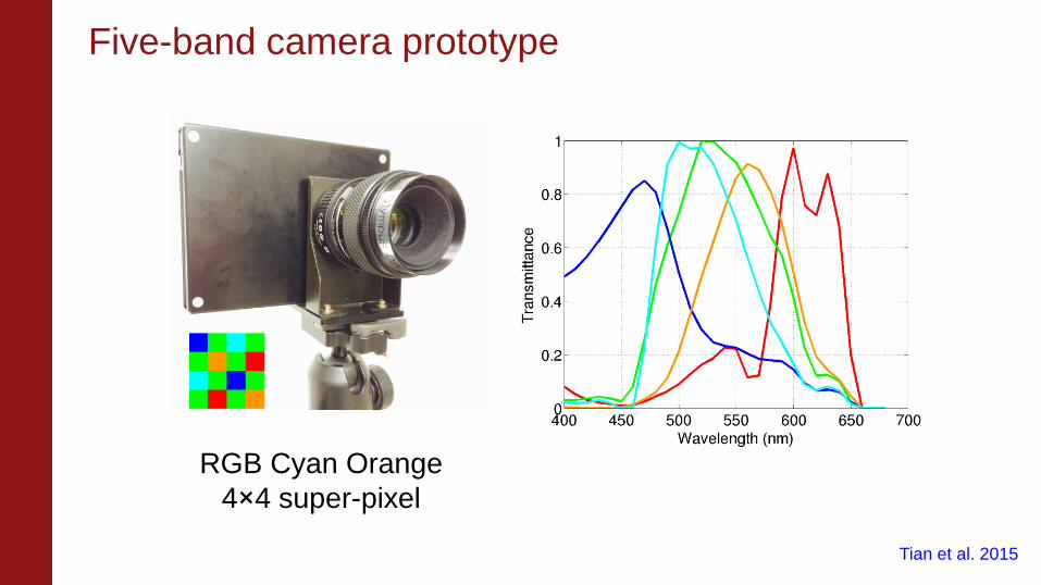
Five-band camera prototype
RGB Cyan Orange
4×4 super-pixel
Tian et al. 2015
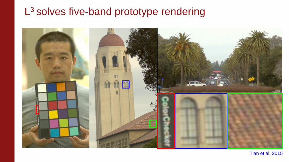
L3 solves five-band prototype rendering
Tian et al. 2015
GPU acceleration results
− GPU: NVidia GTX 770 (1536 kernels, 1.085 GHz)
− CPU: Intel Core i7-4770K (3.5 GHz)
− CUDA/C programming
Results GPU CPU
Image
(1280×720)
0.062s
(16 fps) 12.4s
Video
(1280×720×1800)
163.2s
(11 fps)
Tian et al. 2015
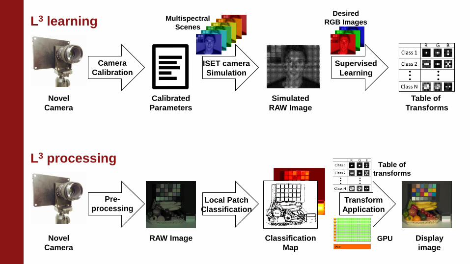
Simulated
RAW Image
Desired
RGB Images
Calibrated
Parameters
Camera
Calibration
Table of
Transforms
Multispectral
Scenes
ISET camera
Simulation
Supervised
Learning
L3 learning
Novel
Camera
Novel
Camera
Pre-
processing Local Patch
Classification
Transform
Application
RAW Image Classification
Map
Display
image
Table of
transforms
L3 processing
GPU
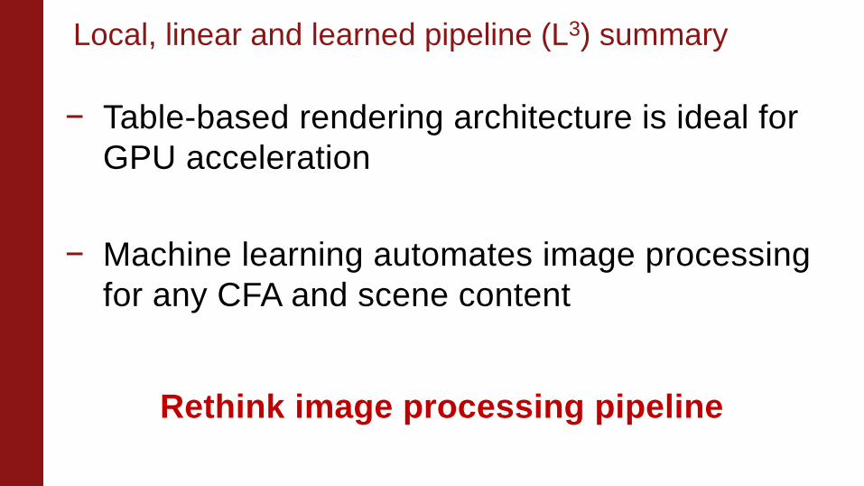
Local, linear and learned pipeline (L3) summary
− Table-based rendering architecture is ideal for
GPU acceleration
− Machine learning automates image processing
for any CFA and scene content
Rethink image processing pipeline

Acknowledgement
Advisors
Brian Wandell, Joyce Farrell
Group members
Henryk Blasinski, Andy Lin
Stanford collaborators
Francois Germain, Iretiayo Akinola
Olympus collaborators
Steven Lansel, Munenori Fukunishi
References
Tian, Q., Lansel, S., Farrell, J. E., and Wandell, B. A., “Automating the design of image
processing pipelines for novel color filter arrays: Local, Linear, Learned (L3)
method,” in [IS&T/SPIE Electronic Imaging], 90230K–90230K, International Society
for Optics and Photonics (2014).
Tian, Q., Blasinski, H., Lansel, S., Jiang, H., Fukunishi, M., Farrell, J. E., and Wandell,
B. A., “Automatically designing an image processing pipeline for a five-band
camera prototype using the local, linear, learned (L3) method,” in [IS&T/SPIE
Electronic Imaging], 940403-940403-6, International Society for Optics and
Photonics (2015).
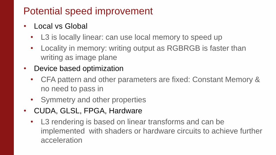
Potential speed improvement
• Local vs Global
• L3 is locally linear: can use local memory to speed up
• Locality in memory: writing output as RGBRGB is faster than
writing as image plane
• Device based optimization
• CFA pattern and other parameters are fixed: Constant Memory &
no need to pass in
• Symmetry and other properties
• CUDA, GLSL, FPGA, Hardware
• L3 rendering is based on linear transforms and can be
implemented with shaders or hardware circuits to achieve further
acceleration