Embed Size (px)
Citation preview

ACCELERATED TESTS OF ENVIRONMENTAL
DEGRADATION IN IN COMPOSITE MATERIALS
by
Tom George Reynolds
B.Eng (Hons), Aeronautical EngineeringUniversity of Bristol, United Kingdom (1995)
Submitted to the Department of Aeronautics andin Partial Fulfillment of
the Requirements for the Degree of
Astronautics
Master of Sciencein Aeronautics and Astronautics
at the
Massachusetts Institute of Technology
September 1998
© 1998 Massachusetts Institute of TechnologyAll rights reserved
Signature of AuthorDepartment of Aeronaudcs and Astronautics
14 August 1998
Certified byProfessor Hugh L. McManus
Associate Professori Thesis Supervisor
Accepted by
Chainan, DiMASSACHUSETS INSTITUTE Ch , DOF TECHNOLOGY
SEP 2 2 1998
LIBRARIES
l I Jaime PeraireAssociate Professor
epartment Graduate Committee
- ,,
I

ACCELERATED TESTS OF ENVIRONMENTALDEGRADATION IN COMPOSITE MATERIALS
by
Tom G. Reynolds
Submitted to the Department of Aeronautics and Astronauticson 14 August 1998 in Partial Fulfillment of the Requirements for the
Degree of Master of Science in Aeronautics and Astronautics
ABSTRACT
High temperature polymer matrix composites are key candidates for the structuralcomponents of proposed supersonic transport aircraft. The operational environment ofthese vehicles exposes the airframe to harsh conditions, including temperature extremes andmoisture. These environments have been seen to cause visible damage in polymer matrixcomposites in timescales much less than the lifetime of the vehicle. Therefore, there is anurgent requirement for accelerated testing of the key components of the environment. Afirst step to this goal is to identify the components of the environment responsible for thedamage. The effects of a realistic moisture and thermal environment on two hightemperature polymer matrix composites (PETI-5 and PIXA-M) have been investigated inthis work. An extensive test program was developed to test the response of the materials tothis baseline environment and its individual components: time at moisture, moisturecycling, time at temperature and thermal cycling. Mechanism-based models were used todesign accelerated moisture cycles and acceler ed thermal cycles in an attempt to speed upthe response to these environmental factors. These accelerated cycles were also used in thetest program. The results showed visible damage in the form of cracking in both r.terials.The PIXA-M material was found to show more damage than the PETI-5. Cracking wasconfined to a thin layer of material next to the exposed edge. This suggests that theenvironmental exposure is reducing the effective fracture toughness of the material in thislayer more than in the interior. Analysis suggests that this layer is exposed to more of theenvironmental components and fluctuations than the material in the interior. The individualcomponents of time at moisture and thermal cycling were seen to cause cracking, whiletime at temperature did not, and moisture cycling did not appear to accelerate moisturedamage. The combined environments in the baseline cycle caused more damage than anyone component of the cycle on its own. Evidence points to the combined effects of time atmoisture and thermal cycling as being the dominant parameters causing damage, whilemoisture cycling controls the extent of the damaged region. Although the designedaccelerated cycles were not successful in accelerating the damage from the baseline cycle,they were instrumental in establishing what were the dominant parameters. It is suggestedthat a promising way of accelerating the damage observed under the realistic conditions isby combining an isomoisture environment with a cyclical stress environment, which can beachieved either thermally or mechanically.
Thesis Supervisor: Hugh L. McManusTitle: Associate Professor
Department of Aeronautics and AstronauticsMassachusetts Institute of Technology
2

ACKNOWLEDGEMENTS
It is not often that you are forced to sit down and think about who you want to thank when
work such as this is complete. It was only when I did that I realised just how many people
have influenced and supported me, both professionally and personally. This is my humble
attempt at recording my gratitude to those people.
Firstly, I would like to thank my advisor, Prof. Hugh McManus. He has an enviable ability
to find the important results in a sea of data and always pointed me in the right direction. I
will also be eternally grateful to him for having the faith to hire me as a Research Assistant
in TELAC two years ago, which provided the financial support which enabled me to come
to MIT. My sincere thanks to Prof. Paul Lagace and Prof. Mark Spearing for their
constructive inputs to my work and for always supporting me in my educational
endeavours. It means a great deal to have two people I admire so much on my side. Thanks
also to Prof. Carlos Cesnik and Prof. John Dugundji for always finding the right questions
to ask during presentations (or the wrong ones if you are the one having to answer!) and
for their support. Of course, I am also extremely grateful to Deb for all her help (and wise
comments!) and to Ping for making sure my accounts were in order.
It is often said that UROPs are key elements of many of the research programs here at MIT.
My UROPs were no exception and it has been a privilege to work with four extremely
bright people. In the early days, Phil Ogston toiled for hours on the polishers to track the
progress of damage. Ryan Peoples counted about as many cracks as I did and, believe me,
that's too many for any sane person! In the latter stages of the work, I was very ably
assisted by Thad Matuszeski, who has a unique ability to solve any problem you throw at
3

him. The final round of testing and the really fun job of preparing this thesis was made a
whole lot more pleasant and efficient thanks to the help of Kim Murdoch. My sincerest
gratitude goes to them all.
My thanks to Eric Sager of The Boeing Company in Renton for being my point of contact
and coordinating the testing conducted there. It made my job a whole lot easier. Thanks are
also due to Ron Zabora at Boeing for his support in this work. Invaluable technical
assistance was provided primarily by John Kane of TELAC. Thanks also to Lenny Rigione
of DMSE and Don Weiner of the Aero/Astro workshop.
Before I came to MIT, I was told that the people I would meet would be as important as the
technical knowledge that I gained. And so it has turned out to be. Thanks to all the graduate
students in TELAC for creating a very friendly atmosphere in the lab. Particular thanks go
to my 'second big sister' Lauren for always lending me an ear for my whining (and
pretending to care!) and to my throwing buddy Mike. Maybe one day I'll be able to throw a
consistent tight spiral. In the greater Aero/Astro community I have made some good
friends. But I particularly look forward to 'working' with Cyrus and Paulo over the next x
years (x=3??) since we all went through the hell they call the Doctoral Qualifying exam and
managed to come out the other side smiling.
Finally, none of this would have been possible without the love and support of my family.
My brother Jim and sister Kate have always blazed a trail for me to follow and taught me
that second best was never good enough. There are not enough words to express my
gratitude and love to my parents. They have sacrificed so much to enable their children to
have the best possible opportunities in life. This is all thanks to them.
4

FOREWORD
This work was conducted in the Technology Laboratory for Advanced Composites
(TELAC) of the Department of Aeronautics and Astronautics at the Massachusetts Institute
of Technology.
The program manager for the funding was Ron Zabora of the High Speed Civil Transport
Structures Group, The Boeing Company, Renton, WA, and was conducted under the
Hygrothermal Microcracking Research Program.
Partial financial assistance for the academic year 196/7 was provided by a Fulbright
Scholarship sponsored by the British-American Foundation of the British-American
Chamber of Commerce. Their support is gratefully acknowledged.
5

TABLE OF CONTENTS
ABSTRACT .................. ................... ................... 2..........ACKNOWLEDGEMENTS ......... ......... ................... 3....3FOREWORD ......... .................................................................... 5LIST OF FIGURES ..................................................................... 10
LIST OF TABLES ................................................................ 12
NOMENCLATURE ........................... 3...................................13
1. INTRODUCTION ............................................................... 141.1 THE PROBLEM .................................... ......................... 14
1.2 THIS WORK .................................... 5..................
1.3 THESIS OUTLINE .............................................. ..........19
2. BACKGROUND ................................................................. 202.1 SUPERSONIC TRANSPORTS AND THEIR OPERATIONAL
ENVIRONMENT ......... .......... ........................................202.2 MOISTURE ......... ......... ......... ..........................................23
2.2.1 Behavior of PMCs exposed to moisture environments ............ 23
2.2.2 Moisture diffusion . ........ ......... ................... 242.2.3 Degradation and damage from moisture .......................... 25
2.3 TEMPERATURE .............................................................. 26
2.3.1 Diffusion of temperature ......... ......... ............................26
2.3.2 Degradation and damage from temperature and oxygen ........... 27
2.4 MICROCRACKING ......... ....................................... 29
2.5 MECHANISM-BASED MODELS ........................................... 30
2.5.1 Physics .................................................................. 30
2.5.2 Modeling framework .............................................. 32
2.5.3 Implementation of models ........................... 32.............. 32
2.6 SUMMARY ................................................................. 33
3. PROBLEM STATEMENT & APPROACH .............................. 35
6

4. ANALYSIS .............................. ....................................... 3 74.1 MECHANISM-BASED MODELING FRAMEWORK ................... 37
4.2 MOISTURE DISTRIBUTION MODELING ............................... 37
4.2.1 Analytical development . ............... ..... ....................................37
4.2.2 Modeling the effects of the baseline environment . ........ 43
4.3 DESIGNING ACCELERATED MOISTURE CYCLES WITH
MODCOD ................................................................. 46
4.3.1 Parametric studies ................................................... 46
4.3.1.1 Warm/wet hold temperature ................................ 47
4.3.1.2 Warm/wet hold time ......................................... 47
4.3.1.3 Relative humidity of warm/wet hold ....................... 50
4.3.1.4 Dry hot and cold hold times ................................ 50
4.3.1.5 Ramp rates between segments .............................. 54
4.3.2 Accelerated moisture cycle design .................................... 56
4.4 THERMAL EFFECTS MODELING ........................................ 60
4.5 DESIGNING ACCELERATED THERMAL CYCLES WITH
CRACKOMATIC ......... ........................................... 664.5.1 Parametric studies ...................................................... 66
4.5.2 Accelerated thermal cycle design ..................................... 68
5. EXPERIMENTAL PROCEDURES ........................................ 7 0
5.1 TEST MATRIX DESIGN ..................................................... 70
5.1.1 Stage I testing ........................................................... 70
5.1.2 Stage II testing .......................................... 72
5.2 MANUFACTURE AND TESTING PROCEDURES ..................... 75
5.2.1 Material manufacture ......... ...................................... 75
5.2.2 Baseline environmental testing ....................................... 76
5.2.3 Accelerated moisture testing ................... 7....................... 76
5.2.4 Accelerated thermal cycling ........................................... 78
5.2.5 Isothermal aging ......................................................... 79
5.3 DAMAGE ASSESSMENT TECHNIQUE . ................................ 79
5.3.1 .Iefining damage ....................................................... 79
5.3.2 Measuring edge damage ............................................... 81
5.3.3 Tracking internal damage ..............................................82
5.4 DATA REDUCTION .......................................................... 85
5.4.1 Crack count data ......... .......................................... 85
7

5.4.1.1 Research layup ....................................... 85
5.4.1.2 Crossply and quasi-isotropic layups ....... ........86
5.4.2 CRACKOMATIC fits ................................................. 86
6. RESULTS ............................... .......... 8.................. 8 8
6.1 STAGE I TESTING ....................... .................................... 88
6.2 STAGE II TESTING - EDGE DAMAGE .................. 93
6.2.1 General ...................................... .. . .........................93
6.2.2 Baseline, isolated thermal and accelerated moisture edge data.... 93
6.2.2.1 PETI-5 results ................... .. ...........................93
6.2.2.2 PIXA-M results ..................... ......................... 94
6.2.3 Accelerated thermal 1 and 2 edge data .............................. 106
6.2.3.1 PETI-5 results .................................................... 106
6.2.3.2 PIXA-M results ....................................... 106
6.2.4 Isothermal aging edge data .... . ... ..... .. ............... 113
6.2.4.1 PETI-5 results .............................. 1................. 113
6.2.4.2 PIXA-M results ................ .............................. 113
6.2.5 Accelerated thermal testing of isothermal specimens ............. 113
6.2.5.1 PETI-5 results ................................... 113
6.2.5.2 PIXA-M results .................................... 113
6.3 STAGE II TESTING - INTERIOR DAMAGE ............................. 117
6.3.1 General . ... .. ...... ... .................................................. 117
6.3.2 PETI-; results ................... .. . .................................... 117
6.3.2. Research specimens ......................................... 117
6.3.2.2 Crossply specimens ......................................... 118
6.3.3 PIXA-M results ................... 1..................................... 18
6.3.3.1 Research specimens ........................................ 118
6.3.3.2 Crossply specimens ........................................ 119
7. DISCUSSION ................... 1...................2..............................
7.1 INTRODUCTION & GENERAL OBSERVATIONS ..................... 120
7.2 MOISTURE CYCLING ................... ................................... 122
7.3 EXTENDED TIME AT MOISTURE ....................................... 123
7.4 THERMAL CYCLING . ................................... 127
7.5 EXTENDED TIME AT TEMPERATURE ................................. 131
7.6 COMBINATIONS OF ENVIRONMENTS ................. ... 131
8
8. CONCLUSIONS .................................... ................... 0........1408.1 GENERAL ............................................................... 140
8.2 INDIVIIUAL ENVIRONMENT COMPONENT EFFECTS ............ 141
8.3 COMBINED ENVIRONMENT EFFECTS ................................ 141
8.4 ACCELERATED CYCLES .................................................. 142
8.5 FURTHER ACCELERATED TESTING ................... 1.............. 142
REFERENCES ................................................................... 143
APPENDIX A - STAGE II TESTING EDGE DAMAGE ................ 148
APPENDIX B - STAGE I TESTING EDGE DAMAGE ................. 175
APPENDIX C - CRACKOMATIC & MODCOD INPUTS .............. 176
9

LIST OF FIGURES
1.1 An artist's impression of Boeing's High Speed Civil Transport (HSCT) .. 151.2 Baseline test cycle for material evaluation ....................................... 161.3 Edge damage in a cross-ply laminate exposed to 500 baseline cycles ....... 171.4 1 mm below exposed edge of a material where damage does not progress
beyond a thin layer ................................................................. 171.5 Interior of a material that exhibits through-cracks away from the exposed
edge .................................................................... 18
2.1 Events leading to degraded performance ......... 1......... .................312.2 Mechanism-based modeling framework ........................................ 32
4.1 Representative moisture profile .............................................. 404.2 Representative temperature profile ............................................ 404.3 MODCOD algorithm ......... ......... ......... ......... 424.4 Moisture absorption through the material at different points of the cycle
after 100 baseline cycles .......................................................... 444.5 Moisture distribution metrics ..................................................... 454.6 Effect of varying warm/wet hold temperature .................................. 484.7 Effect of varying warm/wet hold time ......... .......................... 494.8 Effect of varying warm/wet relative humidity ......... ...................... 514.9 Effect of varying hot dry hold time .......... ........................... 524.10 Effect of varying cold dry hold time ................................... .. 534.11 Effect of varying heating and cooling ramp rates .............................. 554.12 Temperature/time plot for the baseline and accelerated moisture cycles ..... 584.13 Comparison of material response to baseline and accelerated moisture
environments in cold/dry phase after 100 cycles ............................... 594.14 Laminate and crack geometry ......... .. ......... .................................604.15 Geometry of microcracking problem ............................................ 614.16 Shear lag stress model ............................................................ 614.17 Stress distribution around cracks ................................................ 624.18 CRACKOMATIC code algorithm ............................................... 644.19 Effect of varying cold temperature .............................................. 674.20 Accelerated thermal cycle design plot ............................................ 69
5.1 Moisture response from actual and desired accelerated moisture cycle ...... 775.2 Accelerated thermal cycling equipment setup ................................... 785.3 Crack types at the edge of 'research' layup ..................................... 805.4 Cracking at the edge of the 'real' crossply layup ............................... 805.5 Cracking at the edge of the 'real' quasi-isotropic layup ....................... 815.6 Crack-counting stereoscope equipment setup .................................. 825.7 Grinding and polishing technique ......... ................................. 84
6.1 Edge damage in the [03/9031] R1-16 laminate subjected to 500 baselinecycles . ................................................................90
6.2 Damage at a depth of 0.25 mm from the original edge ........................ 906.3 Damage at a depth of 0.5 mm from the original edge .......................... 916.4 Damage at a depth of 0.8 mm from the original edge .......................... 916.5 Comparison of classical thermal microcracking prediction with internal
damage data in the K3B laminate subjected to the baseline environment .... 92
10

6.6 Group crack density at the edge in the 904 ply group for PETI-5research specimens exposed to the baseline, isolated thermal andaccelerated moisture environments .......... .................................... 98
6.7 Aggregate crack density at the edge in the 904 ply group for PETI-5research specimens exposed to the baseline, isolated thermal andaccelerated moisture environments ......... ........... ........... 99
6.8 Averaged crack density at the edge for PETI-5 crossply specimensexposed to the baseline, isolated thermal and accelerated moistureenvironments .............................. ............................... 100
6.9 Averaged crack density at the edge for PETI-5 quasi-isotropicspecimens exposed to baseline, isolated thermal and accelerated moistureenvironments ..................................................... 01
6.10 Group crack density at the edge in the 904 ply group for PIXA-Mresearch specimens exposed to the baseline, isolated thermal andaccelerated moisture environments ............................................. 102
6.11 Aggregate crack density at the edge in the 904 ply group for PIXA-Mresearch specimens exposed to the baseline, isolated thermal andaccelerated moisture environments...............................................103
6.12 Averaged crack density at the edge for PIXA-M crossply specimensexposed to the baseline, isolated thermal and accelerated moistureenvironments ........................................................ ........... 104
6.13 Averaged crack density at the edge for PIXA-M quasi-isotropicspecimens exposed to baseline, isolated thermal and accelerated moistureenvironments ........................... ......................................... 105
6.14 Aggregate crack density at the edge in the 904 ply group for PETI-5research specimens exposed to the isolated thermal and acceleratedthermal environments ....... ...................................................... 108
6.15 Group crack density at the edge in the 904 ply group for PIXA-Mresearch specimens exposed to the isolated thermal and acceleratedthermal environments .............................................................. 109
6.16 Aggregate crack density at the edge in the 904 ply group for PIXA-Mresearch specimens exposed to the isolated thermal and acceleratedthermal environments .............................................................. 110
6.17 Averaged crack density at the edge for PIXA-M crossply specimensexposed to the isolated thermal and accelerated thermal environments ...... 111
6.18 Averaged crack density at the edge for PIXA-M quasi-isotropicspecimens exposed to the isolated thermal and accelerated thermalenvironments ...... ................... 12.. ........................... 112
6.19 Comparison of aggregate crack density for virgin and isothermally-exposedPIXA-M research specimens exposed to the accelerated thermal
environment (to -1800 C) .......... ...................................... 1146.20 Comparison of crack density for virgin and isothermally exposed
PIXA-M crossply specimens exposed to the accelerated thermalenvironment (to -180C) .......................................................... 115
6.21 Comparison of crack density for virgin and isothermally-exposedPIXA-M quasi-isotropic specimens exposed to the accelerated thermalenvironment (to -180C) .......................................................... 116
7.1 Corrected accelerated moisture aggregate crack data in PETI-5 researchlaminates ........... .......... .. ..........................125
7.2 Corrected accelerated moisture crack data in PETI-5 crossply laninates .... 1257.3 Corrected accelerated moisture group crack data in PIXA-M research
laminates ..................................... ....................................... 126
11

7.4 Corrected accelerated moisture aggregate crack data in PIXA-M researchlaminates .............................................................. 126
7.5 Fit of CRACKOMATIC output to accelerated thermal cycle data inPIXA-M crossply ............................................... ......... 129
7.6 Fit of CRACKOMATIC output to the -180°C accelerated thermal cycledata in PIXA-M quasi-isotropic .................. ................................ 130
7.7 Fit of CRACKOMATIC output to baseline cycle group crack data inPETI-5 research laminates ........................................................ 134
7.8 G-N curve used in Figure 7.7 ........... ................................. 1357.9 Fit of CRACKOMATIC output to baseline cycle group crack data in
PIXA-M research laminates ...................................................... 1367.10 G-N curve used in Figure 7.9 .................. .............................. 1377.11 Combined G-N curves for PETI-5 & PIXA-M baseline environment
exposure and isomoisture exposure of a similar polyimide material ......... 139
LIST OF TABLES
4.1 Moisture diffusion properties for PETI-5 . ........ .................. 394.2 Baseline vs. accelerated moisture cycle parameters ............................ 57
5.1 Stage I test program matrix .715.2 Stage II test program matrix ...................................................... 74
A. 1 Baseline environment damage data (PETI-5) .................................. 149A.2 Baseline environment damage data (PIXA-M) .............................. 151A.3 Isolated thermal environment damage data (PETI-5) .......................... 153A.4 Isolated thermal environment damage data (PIXA-M) ........................ 155A.5 Accelerated moisture environment damage data (PETI-5) .................. 157A.6 Accelerated moisture environment damage data (PIXA-M) .................. 159A.7 Accelerated thermal environment 1 (-180°C) damage data (PETI-5) ........ 161A.8 Accelerated thermal environment 1 (-180°C) damage data (PIXA-M) ...... 162A.9 Accelerated thermal environment 2 (-150C) damage data (PETI-5) ........ 165A. 10 Accelerated thermal environment 2 (-150°C) damage data (PIXA-M) ...... 166A. 11 Accelerated thermal environment 1 damage data (PETI-5 isothermal
specimens) ................ .......................................... 169A. 12 Accelerated thermal environment 1 damage data (PIXA-M isothermal
specim ens).......................................................................... 172
12

NOMENCLATURE
CLPT Classical Laminated Plate TheoryHSCT High Speed Civil TransportHSR High Speed ResearchPMC Polymer Matrix Composite
a thicknessesA constant fit to dataAni amplitude of each mode at time ic (subscript) cracking ply groupCo(z) initial state of moisture through laminateCeq internal equilibrium moisture concentrationCm concentration of moisture in laminateCJt) ambient far field condition of moisture concentrationd depth of 'thrashed zone'D moisture diffusivityD anisotropic diffusivity tensor for moistureDom moisture diffusivity constantDfz component of moisture diffusivity corresponding to ze depth from exposed edge
f material constantg material constantGc effective critical strain energy release rate (toughness)Go initial toughnessh thickness of laminateE material stiffness in x' directionEA m moisture activation energyI length of exposed depth gagen index of the modeN number of cycleso (subscript) entire laminater (subscript) smeared properties of the laminateR universal gas constantRH relative humidityT absolute temperatureTO stress free temperatureXi, xj material directionsx', y', z' local coordinate system of crackz through thickness direction
a coefficient of thermal expansion in the x' directionAt* modified time stepAT maximum difference between environment temperature and To
p crack densityapplied stress to laminateshear lag parameter
13

CHAPTER 1
INTRODUCTION
1.1 THE PROBLEM
Polymer matrix composite materials (PMCs) are well suited to the aerospace industry,
primarily because of their high specific strength and stiffness. Reduced structural weight
equates to better performance, greater payload or increased range. The usage of composites
is increasing for primary aircraft structures: the Boeing 777 airframe is about 10%
composite (compared to only 3% for the 767) while the F-22 airframe is 30% composite.
Future applications are proposing extensive use of composite materials to meet demanding
performance requirements. Examples include gas turbine engine structures, reusable launch
vehicles (such as the X-33) and supersonic commercial aircraft. In all of these applications,
the material is exposed to harsh cyclic environments (including moisture, thermal,
mechanical and chemical components) for extended periods of time. These environments
have been shown to cause degradation and damage to polymer matrix composites.
It is the latter application, that of the supersonic commercial airliner, which is the focus of
this study. Boeing has established the High Speed Civil Transport (HSCT) program with
the goal of developing a 300 passenger, 5000+ nautical mile range, Mach 2.4 aircraft
within the next two decades (see Figure 1.1). The program goals require an advanced
airframe to be developed which significantly outperforms (in terms of mass fraction) the
conventional aluminum skin-stringer designs we see today. It is likely that advanced
polymer matrix composites will be used extensively in the airframe of the HSCT to meet
the challenging performance requirements. In order to choose suitable materials for the
14

airframe, an understanding of the effects of the harsh environment on candidate materials
needs to be gained.
Figure 1.1: An artist's impression of Boeing's High Speed Civil Transport (HSCT)[courtesy of The Boeing Company]
1o2 THIS WORK
The focus of this work is the environmental response of potential PMCs for the airframe of
the HSCT. The airframe material is exposed to high temperatures (up to 350°F at Mach 2.4
cruise) and low temperatures (down to -650 F in subsonic flight), moisture and a spectrum
of mechanical stresses over the entire design lifetime of 20,000 flight cycles. These
environmental factors have been seen to significantly degrade even advanced high
temperature PMCs. To assess the suitability of a material to the HSCT application, a
'baseline' test cycle has been defined by Boeing (Figure 1.2). Although it is not identical to
the conditions that the airframe will encounter during a flight, the baseline cycle captures
the main elements of the actual environment. A short 'cold/dry' segment represents a
subsonic phase of flight, while a longer 'hot/dry' segment represents a typical supersonic
15

cruise phase. Moisture is introduced via a 'warm/wet' segment. Moisture is encountered by
the airframe in a number of different operational environments, such as low altitude flight,
maintenance and airport gate times.
Temp1
'Warm/wet'
= 3 hoursTime
-540C (-65oF)10 mins
Figure 1.2: Baseline test cycle for material evaluation
Degradation in the form of edge crazing and through-laminate microcracking is observed
when some materials are exposed to this baseline environment (Figure 1.3). However,
different materials show different damage responses. For some materials, the observed
damage is restricted to a very thin edge layer (about 1 mm in depth - Figure 1.4), while
others show damage (particularly through-thickness 'microcracks') to much deeper levels
(Figure 1.5).
16
'IUiht/r n'
Figure 1.3: Edge damage in a cross-ply laminate exposed to 500 baseline cycles
Figure 1.4: 1 mm below exposed edge of a material where damage does not progress=_ : beyond a thin layer
17
Figure 1.5: Interior of a material that exhibits through-cracks away from the exposed edge
Different materials respond in different ways when exposed to the same environment.
There are a number of different components of the environment which could be responsible
for the different types of damage observed, including moisture cycling, thermal cycling,
time at moisture, time at temperature or interactions of any of these. Since the airframe has
a service life of twenty thousand cycles, it is unrealistic to test the environmental response
of candidate materials in real tire. The baseline cycle is approximately 3 hours in length, so
20,000 cycles equates to almost 7 years of continuous testing. Hence, it is highly desirable
to use accelerated test methods which expose the materials to environmental conditions
which bring the same degradation response from the material as the baseline cycle (or some
other, more realistic test environment), but in a much shorter time. To do this, it is
necessary to understand which mechanisms are causing the observed damage.
In this work, previously-developed mechanism-based models (see Section 2.5) are used to
investigate the mechanisms believed to be behind the observed degradation phenomena. An
18

experimental test matrix was designed to isolate each of the mechanisms to determine which
was responsible for the damage behavior of each material under investigation. The models
were used to devise accelerated test methods for moisture cycling and thermal cycling, two
of the possible mechanisms causing the damage. Baseline hygrothermal, accelerated
hygrothermal and isothermal testing were carried out at Boeing. Accelerated thermal cycling
tests and all damage assessment and data reduction were conducted at MIT. These tests
provided a wealth of data on the response of two candidate materials to different
components (and combination of components) of the service environment and enabled
identification of the most important mechanisms causing damage.
When the overall damage mechanisms have been isolated, it is possible to design
accelerated tests which enable more timely evaluation of materials for the HSCT
application. This should also produce significant savings in both cost and manpower.
1.3 THESIS OUTLINE
Background for this research in terms of relevant prior work in enviromnental effects on
PMCs is given in Chapter 2. Chapter 3 provides a focused problem statement and the
approach for its solution. A review of the models used in this work and the design of the
accelerated tests is given in Chapter 4. The experimental test matrix and procedures are
outlined in Chapter 5, with results and discussions given in Chapters 6 and 7 respectively.
Conclusions from this work are given in Chapter 8.
19
CHAPTER 2
BACKGROUND
2.1 SUPERSONIC TRANSPORTS AND THEIR OPERATIONAL
ENVIRONMENT
Supersonic transports were first developed in the 1960s in the USA (SST), USSR (Tu-
144) and Britain/France (Concorde). The SST program was canceled following significant
weight and environmental problems with preliminary designs. The Tu-144 was the first
supersonic transport to fly commercially, but service soon ceased and it is now used only
as a research vehicle. Only the Concorde has survived in commercial service, but it is an
economic and environmental failure. Not until recently has technology evolved sufficiently
to solve most of the shortcomings of these 'first generation' designs. Active research is
ongoing around the world, particularly in America (HSCT), Europe (Alliance) and Japan
[1].
Supersonic transports are only permitted to fly above Mach 1.0 when over water. Alnost
three quarters of international routes are 85% or more over water. Over half of the current
international routes are in excess of 2000 nautical miles. As a result, more than 300
potential HSCT city pairs exist, and traffic is predicted to at least double by 2015. All these
factors combined have led to market forecasts for supersonic transports ranging from 900
to 1300 aircraft through 2025. This is far in excess of the minimum market size of 300-500
aircraft required for a program launch. The potential returns include 140,000 new jobs and
an estimated $500 billion in positive trade [2].
20

NASA's High Speed Research (HSR) program is directing 'focused technology
development' [3], the results of which should enable the aerospace industry to develop a
high speed commercial airplane. The HSR program has a stated vision to "establish the
technology foundation by 2002 to support the US transport industry's decision for a 2006
production of an environmentally acceptable, economically viable, 300 passenger, 5000
nautical mile range, Mach 2.4 cruise speed aircraft". The 5000 nautical mile range was
chosen as being the minimum necessary for the high volume Los Angeles/Tokyo trans-
Pacific route.
Many challenges still exist, particularly in the areas of propulsion (supersonic and subsonic
efficiency with low noise and emissions), aerodynamics (sonic boom mitigation) and
structures. This study is focused on the structural problems. The required structural mass
fraction (compared to operating weight empty) for a supersonic commercial transport is
much smaller (<20%) than that for a subsonic aircraft (25%), requiring innovative
structural concepts to be developed and advanced materials to be used.
One of the biggest challenges faced by the structural designers is the selection of the
materials to withstand the aerothermal loads (particularly aerodynamic heating) experienced
by the aircraft [4]. The skin of the aircraft will be exposed to temperatures as high as 350°F
at Mach 2.4 [5] and as low as -65°F in subsonic flight, while moisture both in flight and
while on the ground is also experienced. The structure will be exposed to these
environments for extended periods of time-the HSCT has a design life of 20,000 flight
cycles or over 60,000 flight hours. By setting a cruise speed of Mach 2.4, the HSR
program is pushing the state of the art of materials technology. Different families of
materials are required for use at sustained temperatures above 250°F (which is the skin
temperature at Mach 2.2) than for use at below 250°F. Aluminum is suitable below 250°F,
21

but titanium or high temperature PMCs are required for sustained use above this
temperature.
Over 140 different materials have been analyzed to assess their suitability to the HSCT
application. Unlike aluminum alloys, titanium alloys are stable up to 3500 F and are not
susceptible to environmental degradation at these temperatures. But an all-titanium HSCT
structure would be too heavy to be economically viable. It is likely that titanium will be
used in parts of the structure (particularly for high temperature areas such as the wing and
tail leading edges) but not throughout. New hybrid materials made out of alternating layers
of titanium and graphite composite material (TiGr) show significant promise as they
combine the attractive properties of both materials. The titanium provides compressive
strength and protection from the environment, while the graphite composite provides
stiffness, tensile strength and fatigue resistance [6]. However, from a materials technology
viewpoint, there are still major obstacles to overcome with regard manufacturability,
maintainability and repairability.
Hence, it is likely that more conventional (but advanced, high temperature-capable)
polymer matrix composites will be used extensively in the airframe of the HSCT. It is,
therefore, necessary to investigate the behavior of PMCs when exposed to conditions they
will meet in service. The environment includes cyclical exposure to moisture and
temperature, and the impact of these on PMCs is reviewed next.
22
2.2 MOISTURE
2.2.1 Behavior of PMCs exposed to moisture environments
A great deal of work has been performed in the last few decades on various aspects of
moisture effects on PMCs. Reviews are included in Weitsman [71 and Wolff [8]. Much of
the early work established the fundamental behavior of PMCs exposed to moisture. When
moisture and temperature are constant throughout a test, it was found that the maximum
moisture content depends primarily on the ambient relative humidity, while the speed of
diffusion of moisture into the laminate is controlled by temperature and not humidity
[9,10]. Investigations into transient cyclic moisture conditions concluded that the moisture
content of the material approaches a steady state after prolonged exposure, while most of
the moisture distribution changes occurred in a narrow 'boundary layer' near the exposed
surface [10]. A complete transient analysis needed to be performed before equivalent
constant conditions could be substituted to accelerate the transient effects. An early attempt
at simulating a 'realistic' supersonic service environment was made by McKague et al.
[11]. They used a cycle comprising -65F 'subsonic' and 300°F 'supersonic dash'
components, together with simulated periods of rainfall. They found that the supersonic
dash component constituted a thermal spike which significantly increased the moisture
diffusivity (measured by weight increase) over the materials not experiencing the spike.
This phenomenon was later analyzed in more detail to investigate the effect of spike
temperature and material layup [12]. It was suggested that the enhanced moisture
absorption was due to the increase in the free volume of the matrix at the spiking
temperature.
DeIasi, et al., [13] attempted to simulate operational environments by incorporating
'realistic' tropical and temperate climates, plus periods of typical sub- and supersonic flight
conditions. They compared the material response in these use environments to those under
23

simpler environmental conditions (plain thermal and moisture cycling). They found that the
latter tests gave much insight into the observed anomalies in the results from the full tests.
Based on these observations, they concluded that good prospects existed for the
substitution of accelerated tests for real time tests to predict the response of materials to the
service environment.
Experiments performed by immersing material in various kinds of liquids [14] showed that
moisture uptake depended on time and temperature for immersion in distilled water and salt
water. This was not the case for diesel fuel, jet oil and aviation oil, where only time seemed
to be important. Techniques for tracking moisture distribution through a laminate with a
nuclear probe were demonstrated by Whiteside et al. [15] using labeled hydrogen atoms
(in heavy water, D2 0). Effects of the composite manufacturing techniques [16] were
shown to have a significant effect on moisture uptake. Oven cured composites were shown
to have more voids than those autoclave cured, leading to greater moisture
absorption/diffusivity and a concomitant reduction in glass transition temperature and
properties. In the same work, kevlar fiber was shown to be strongly hygroscopic,
providing an easy route for moisture ingress.
2.2.2 Moisture diffusion
Models of moisture (and oxygen) diffusion based on Fick's law have been widely used to
describe the process [17]. The diffusivity of the material is usually assumed to be
exponentially temperature dependent and may also depend on degradation and damage. A
review of the applicability of Fick's equation to diffusion of moisture in PMCs is given in
Shirrell & Halpin [18]. Significant deviation from Fickian diffusion occurs primarily when
damage such as microcracking provides alternative mechanisms for moisture ingress into
the material. Fick's equation is generally used as the exclusive governing equation for
24

moisture diffusion into a material. Highly efficient numerical schemes have been developed
to compute moisture distributions with Fick's law under time-varying ambient conditions
of temperature and relative humnidity [19]. Truncated infinite series solutions obtained
extremely high accuracy with only a small number of terms. Similar schemes have been
incorporated into computer codes, such as W8GAIN [20] which simplify the process of
predicting the moisture (and temperature) distribution in a laminate. It is the code developed
by Foch [21,53] called MODCOD which is the foundation for the moisture study in this
work. It will be fully described in Chapter 4. These codes predict that in a transient
moisture environment, much of the moisture level fluctuations occur in a thin boundary
layer near the surface. The interior moisture concentration is shielded from the moisture
transients and approaches an equilibrium level (depending on the ambient conditions) as the
number of cycles increases.
2.2.3 Degradation and damage from moisture
Long term moisture exposure, especially at elevated temperatures and extreme high or low
pH, has been shown to cause both reversible and irreversible degradation effects [22].
Short exposures to moisture at low temperatures tends to only cause effects which are
reversed on drying. However, long term moisture exposure, especially at temperatures
above the glass transition temperature for the material, is seen to irreversibly degrade a
composite material.
Water plasticizes epoxy resins by interruption of the Van de Waals bonds in the matrix [8].
This reduces the glass transition temperature of the matrix material by as much as 10-20°C
for every 1% weight gain due to moisture [23], which has a significant effect on the
mechanical properties. Humid environments have been seen to cause reductions in
25

transverse and shear strengths [24] and decreases in mode II fracture toughness of the
material [25].
Moisture and elevated temperatures over extended periods of time can cause viscoelastic
response changes [26]. Moisture causes the matrix to swell, which can introduce
significant stresses into a material with wet surface plies and dry interior [18]. When the
stresses exceed the matrix in situ strength, cracking can occur. Moisture also causes
mechanical damage from moisture-induced swelling affecting the fiber/matrix interface
region [27]. This can cause fiber debonds, thus reducing the mechanical properties [7].
Initial crescent-shaped fiber debonds coalesce on drying and/or cyclic moisture exposure to
form discrete continuous cracks [28,29]. This introduces new pathways for moisture to
enter the material, altering the moisture uptake and making the diffusion non-Fickian. Since
the moisture diffusivity is low, only the material immediately surrounding a crack will
experience noticeably non-Fickian diffusion. The bulk of the material still sees diffusion
which is close to being Fickian, at least until cracking becomes very extensive or long
periods of time have elapsed allowing significant moisture ingress from cracked areas.
2.3 TEMPERATURE
2.3.1 Diffusion of temperature
The temperature distribution in a material is controlled by conduction, with the rate of heat
flow being governed by Fourier's law. Typically, the in-plane conductivity along the fibers
is greater than the through-thickness conductivity, leading to increased heat flow to/from
the edges of specimens. This often makes a one dimensional heat flow analysis inadequate,
requiring two and three dimensional analyses to be performed [30]. Parametric studies by
26

Crews [31] have developed metrics for when one dimensional analyses of heat flow are
adequate. These metrics can also be applied to moisture and oxygen diffusion. Typically,
though, heat conductivities are orders of magnitude greater than moisture diffusivities.
Hence specimens reach thermal equilibrium long before they reach moisture equilibrium. It
is valid when studying moisture diffusion, therefore, to assume that temperature in a
specimen is everywhere equal to the current ambient temperature. Linear theory of coupled
heat and moisture effects has verified that coupling becomes significant only as the ratio of
thermal conductivity to moisture diffusivity approaches unity [32]. Hence, only moisture
transients are considered in this work.
2.3.2 Degradation and damage from temperature and oxygen
Elevated temperatures over long periods of time will degrade PMCs, either directly or via
enhanced temperature-dependent diffusions of moisture, oxygen or other substances.
Direct degradation includes thermally-driven reactions which chemically and physically
alter the properties of the material [33], physical aging [34] and burning/charring when
exposed to very high temperatures [31]. Models of these phenomena have been developed,
and are presented in the references cited. A coupled diffusion-reaction model has been
incorporated into the same code as used in the moisture analysis [21]. Used to analyze
material susceptible to oxygen at high temperatures, it shows severe degradation can
happen near the edge of the material in certain environments. This damage grows slowly
inwards with time.
Effects of these degraded matrix states, plus laminate geometry, loads, temperature and
moisture states, have been used to find stresses, strains and deformations in laminates and
to see if failure occurs [36]. Degraded surface layers are often quite highly stressed due to
matrix shrinkage [21,33]. The effect of degraded surface layers on overall laminate material
27

properties is somewhat harder to determine. In work by Tsuji [37], mechanical and thermal
bend tests have been used to extract material properties. The radii of curvature of specimens
with thin degraded layers were used to quantify the shrinkage and mechanical property
changes of material in the surface layer.
Promising work with protective coatings has been conducted [e.g. 35]. In this work,
silicon nitride was applied to the surface of the composite material by chemical vapor
deposition (CVD). The material was protected from oxidation for 500 hours at 371 °C, but
the effectiveness was found to be highly dependent on surface finish. Complex coating
technologies (e.g. CVD) are expensive, and cheaper coatings (such as spreadable
polymers) have similar problems to the composite resins themselves.
New, high temperature-resistant resin systems are being developed which are capable of
surviving (and being usable) at high temperatures for extended periods of time [38,39].
Many of these developmental materials, although having impressive high temperature
properties, have major disadvantages that reduce their potential for operational use.
Problems include manufacturability, cost and toxicity concerns. However, a number of
new materials do show significant promise, such as PETI-5, PIXA, PIXA-M and K3B.
These are the focus for much of the HSR work, and Boeing is particularly interested in
PETI-5 and PIXA-M for the HSCT application. The chemistry, synthesis and behavior of
the NASA Langley-developed PETI (phenylethynyl-terminated imide) family of polyimide
materials is fully described in Hou et al. [40]. PETI-5 is a new variant which combines the
excellent thermo-oxidative stability and mechanical performance at elevated temperatures of
a polyimide, together with superior processability [41]. PIXA-M is an amorphous form of
the thermoplastic polyimide PIXA material, which promises thermal and chemical
resistance, toughness, good processability and cost-effectiveness [42].
28

2.4 MICROCRACKING
Microcracks are cracks that appear in the matrix and run parallel to the fibers, often through
the entire laminate. They are generally confined to ply groups (a number of plies together
with the same orientation). Microcracks are often the most obvious form of damage seen in
PMCs.
'Classical thermal microcracking' arises due to the mismatch in the coefficient of thermal
expansion (CIE) between plies in a laminate when exposed to a temperature other than the
stress free (nominally the cure) temperature. This mismatch induces stresses in the plies,
which cause matrix cracks when these stresses exceed the strength of the matrix material.
The physical mechanism is explained more fully in Chapter 4. A thorough review of
thermal microcracking literature is given in Maddocks [43]. A large experimental database
of thermally-induced microcracking for a number of material systems and laminate
configurations has been developed [e.g. 44,45]. The prediction of thermal microcracking,
usually based on a shear lag analysis and simple fracture mechanics crack formation
criteria, is well established and incorporated into a computer code known as
CRACKOMATIC [46,47]. This will be discussed in the next section and Chapter 4.
A number of extensions to the basic code have also been developed. Reduced ;;tresses at
free edges for certain ply angles have been analyzed [48] and used to explain some of the
observed cracking behaviors. An extension by Michii, which incorporates a Monte Carlo
simulation method [49], accounts for much of the observed statistical nature of
microcracking. The method 'seeds' effecdve flaws at random places on the edge of the
specimen to act as crack initiation sites, while material property variations are modeled to
vary about a mean value. The gradual appearance of cracks, data scatter, partial through-
29

cracks and delayed appearance of cracking seen in thick ply groups have all been captured
with this method.
Microcracking can also be caused by factors other than temperature and temperature
cycling. Degraded layers due to oxidation have been observed to microcrack [33]. Moisture
and solvents (such as dye penetrants [50]) have also been shown to cause or accelerate
microcracking.
2.5 MECHANISM-BASED MODELS
The models which will be used in this study, incorporated into the MODCOD and
CRACKOMATIC codes, are two of a group of mechanism-based models which have been
developed in the Technology Laboratory for Advanced Composites (TELAC) at MIT. A
summary of the overall modeling effort is provided in MivcManus et al. [51]. Mechanism-
based models attempt to directly capture the relevant isolated physical mechanisms. Simple
models are developed based on these mechanisms and tests are conducted to confirm the
applicability of each individual model. The simple models for each mechanism are
combined in order to replicate the complex behavior seen when a material is exposed to a
realistic environment.
2.5.1 Physics
The environmental factors which lead to degraded performance were described in the
preceding sections: they are shown schematically in Figure 2.1.
30

LaminateStructure
Loads
DiffusionHeat Oxvaen HI20
Chemical , Therma,Reactions ,erma
Other?
Material Composite
Figure 2.1: Events leading to degraded performance
Moisture enters the material as described by Fickian diffusion at a speed determined by the
material's moisture diffusivity. Moisture affects the composite material both physically
(e.g. swelling and fiber/matrix bond interference) and chemically (e.g. plasticization).
Cyclic variations in the moisture environment are mirrored by significant variations in the
moisture content in a very thin layer of material next to the edge or surface which is
exposed. The interior of the specimen, on the other hand, slowly approaches an
equilibrium moisture concentration determined by the ambient relative humidity.
Heat enters the material governed by Fourier's law. Temperature affects the composite both
physically (e.g. shrinkage and thermal mismatch in plies leading to microcracking) and
chemically (e.g. thermal reactions and oxidation coupled with oxygen diffusion i-to the
material). Temperature conductivity for the materials under consideration are typically
orders of magnitude higher than the moisture diffusivities. Hence, temperature gradients
can generally be ignored when studying moisture effects.
Temperature and moisture can affect the properties of the material, either reversibly or
irreversibly via chemical reactions. Figure 2.1 shows microdamage such as fiber-matrix
debonding (due to stresses created by all of the above combined with material property
31

changes), and ply cracking (also caused by stresses and possibly aided by microdamage).
Most discussion here will concentrate on the thermal and moisture states, as these are
believed to be the drivers of the observed damage.
2.5.2 Modeling framework
The framework for the mechanism-based modeling effort in TELAC is shown in Figure
2.2. Environmental inputs of both temperature and moisture affect the thermal response and
diffusion/reaction processes. Physical and chemical changes which result change the
properties of the composite and hence its response to loads. Damage may occur depending
on this response, which in turn affects the thermal/diffusion behaviors. Hence the model is
coupled as seen in Figure 2.2.
Figure 2.2: Mechanism-based modeling framework
2.5.3 Implementations of models
The diffusion and reaction chemistry elements are part of the MODCOD code, while
thermomechanical response and damage mechanisms are incorporated into
32

CRACKOMATIC. The other components of the framework are complemented by other
models as described in McManus et al. [51]. When combined together, they form a set of
models which can realistically analyze most complex environments to which a material can
be exposed.
MODCOD uses an efficient modal solution to the governing Fickian diffusion equation to
model the moisture distribution through the laminate both within and between any number
of cycles of a predefined moisture and thermal environment. It is fully described in Section
4.2.
CRACKOMATIC predicts crack density (number of cracks per unit length) and the
resulting degradation in elastic material properties (stiffness and CTE) for both
monotonically decreasing temperatures and temperature fatigue cycling. Thermal fatigue
(cycling) effects have been modeled in CRACKOMATIC using an effective material
toughness reduction criterion. Material toughness is assumed to decrease with number of
cycles. This technique has been utilized elsewhere for related fatigue work [52]. The
CRACKOMATIC code is used extensively in this work and so is discussed more fully in
Section 4.4.
2.6 SUMMARY
As composite materials find wider application in the aerospace industry, more and more
effort is being expended on characterizing their long term behavior in the environments to
which they are exposed. It has been established that transient moisture environments cause
fluctuating moisture conditions for a thin layer of material just below the surface which is
exposed, while the interior approaches an equilibrium level as more cycles are experienced.
This response has been modeled in efficient computer codes based on Fickian diffusion.
33

Moisture can cause both temporary and permanent material property changes, as well as
inducing stresses. This combination can cause damage, which can in turn cause
complications in establishing the moisture distribution within a laminate by making the
diffusion non-Fickian.
Temperature effects include oxidation, aging, enhanced moisture diffusion and
microcracking. The primary temperature concerns in this study are the enhanced moisture
diffusion effects and thermally-induced microcracking. Models handle both effects.
This work utilizes the MODCOD and CRACKOMATIC models (which are based on much
of the work included in this section) to better understand the environmental effects that are
observed when candidate HSCT materials are subjected to the baseline and accelerated
conditions.
34
CHAPTER 3
PROBLEM STATEMENT & APPROACH
Given that the operational environment of the HSCT causes damage to PMCs, there is a
need to characterize and quantify this damage to assess the suitability of any given material
for the HSCT application over the lifetime of the aircraft. This requires that the nature and
causes of damage are thoroughly understood. It also requires that accelerated tests be
developed so that data on material suitability can be obtained in a much shorter time frame
than real time testing would allow.
Different materials may be damaged by different components of the use environment. A list
of 'suspect' mechanisms has been developed from previous work: moisture cycling,
temperature cycling, time at moisture, time at temperature, mechanical stress and
interactions of some or all of these.
It was suspected prior to this work that it is the moisture cycling component of the baseline
cycle which is responsible for observed surface damage, and the thermal cycling
component which is responsible for observed interior cracking. Design of accelerated test
cycles for moisture and thermal cycling environments is achieved by using two of the
mechanism-based models developed in TELAC: the moisture effects code MODCOD and
the thermal microcracking code CRACKOMATIC. An accelerated moisture cycle is
designed which is predicted to cause a very similar moisture response in the material as the
baseline environment, but in a much shorter time. Similarly, the accelerated thermal cycle is
35

predicted to cause thermal microcracking damage equivalent to that caused by the baseline
environment in a much smaller number of more severe thermal cycles.
An experimental test program is designed which subjects the candidate materials to the
baseline environment, the individual components of that environment and the accelerated
moisture and thermal environments just discussed. This experimental program allows us to
establish whether (and which of) the 'suspect list' of individual mechanisms is causing the
damage for each material and to confirm whether the accelerated tests do indeed accelerate
the damage mechanisms, as postulated. The test program allows us to rule out those
mechanisms shown not to be responsible for the damage in the materials under
investigation. This will also allow us to direct future studies in acceleration testing to the
true causes of damage.
36

CHAPTER 4
ANALYSIS
4.1 MECHANISM-BASED MODELING FRAMEWORK
As discussed in Section 2.5, a group of mechanism-based models have been developed in
TELAC over the last few years. These simple models are combined together into a
framework (Figure 2.2) which can analyze many complex environments. The two models
which we used in this work were the moisture code MODCOD and the thermal
microcracking code CRACKOMATIC. These models will be reviewed in detail in the
following sections, along with how the models were used in this study. Complete
descriptions of the development of the models are given in [53] and [43] respectively.
4.2 MOISTURE DISTRIBUTION MODELING
4.2.1 Analytical development
This analytical development is the work of Foch [53]. Moisture effects have been modeled
assuming Fickian diffusion, which is described by the equation:
at ( D dC a (4.1)
where C,m is the concentration of moisture in the laminate, xi and x denote material
directions and Dijmis the anisotropic diffusivity tensor for moisture. The assumed geometry
is of an infinitely long/wide flat plate, subjected to the same environment on the top and
bottom surfaces. Given this, only through-thickness moisture gradients need be considered
37

and the further assumption of orthotropic diffusivity reduces the above equation to its one-
dimensional form:
adCt dz (Dm a-') (4.2)=t -Z -
where z represents through-thickness direction and D m is the corresponding component of
moisture diffusivity. This is assumed to increase exponentially with temperature as
described by an Arrhenius equation:
Dz = Do exp[ T (4.3)
Dom is the moisture diffusivity constant, EA the moisture activation energy, R the universal
gas constant and Tthe absolute temperature. All of these are taken as constant in z, so the
rate of moisture ingress can be described by (dropping the z and m):
dC a2C0 D 7 = D-~~~~~iF ~(4.4)
Initial and boundary conditions to solve Eqn. 4.4 are given by:
C(z) = C(z) for t < O (4.5)
C(O) = C(h) C(t) for t > 0 (4.6)
The value of Co(z) is simply the initial state of moisture through the laminate, while Cft) is
the ambient far field condition of moisture concentration. Here, h is the thickness of the
laminate. The boundary conditions are set by the assumption that the exposed edge or
surface is always in equilibrium with the environment, and that the equilibrium can be
expressed by the relation
Coo = f(RH) g (4.7)
where RH is the relative humidity and f and g are material constants. The material
properties used for all analyses are given in Table 4.1. They are taken from PETI-5 data
[21].
38

Table 4. 1: Moisture diffusion properties for PETI-5 [21]
D EA f g 1(mm/s) (1dJ/mol)0.8 42 0.018 1
A very efficient modal solution to the above system of equations for cyclic environments
has been obtained, as fully described in [53]. Cyclic environment profiles that include
relative humidity segments that remain constant over time (Figure 4.1) and temperatures
that remain constant or change at a constant ate (Figure 4.2) can be analyzed.
A modal solution to Eqn. 4.4 in the time interval starting at t is:
n .; ~nnz -n2 Ir2DAt]C(z t) = Ci - AniSnt h ex p 2 (4.8)
where the change in time At = t - ti, and C., is calculated from RHj with Eqn. 4.7. In Eqn.
4.8, Ani represents the amplitude of each mode at time i, and n the index of each mode. In
order to find the first set of modal amplitudes from the initial conditions, use is made of a
Fourier series expansion:
A 2 h Co(z))sin(- irz, (4.9)
where the subscript 1 represents values at the first time step. The first set of calculations for
Ani can be performed and these values used in Eqn. 4.8 to find the concentration levels in
the first time interval, C(z,t). In order to calculate subsequent modal amplitudes, An(+,), and
thus new concentrations, substitute C(z,ti ) (from Eqn. 4.8) for Co(z) and C.,+) for C, in
Eqn. 4.9, simplify, integrate, and exploit the orthogonality of the sine function to get the
general form:,
A,(+) =- (C=ci,, -C ar ) + Aniexp{ni h2 (4.10)Anail = Ftl17
39

RH
L
to t1 t2t3
Figure 4.1: Representative moisture profile
Temp
to ti t2 t3 t4
Figure 4.2: Representative temperature profile
40
RH3
RH2
RH1 I _
t4
Time
Time
- -I - l- -
- -
" '" lI ,, Y I
T 3

where Ati = (ti+, - ti). For the geometry of interest, only odd values of n need to be
calculated. This form is useful in that it does not require the evaluation of the integrals of
the form of Eqn. 4.9 except at the initial time step.
This development is appropriate for periods of constant temperature, as the moisture
diffusivity, D, is constant, and can be calculated via Eqn. 4.3. For the segments with
ramped temperature changes, however, this calculation is complicated by the time
dependence of temperature. The resulting variation in D invalidates the solutions above.
This problem is solved by substituting Eqn. 4.3 into 4.8 and defining a modified time step,
At*. This yields a new form of Eqn. 4.8 for the calculation of the current moisture
concentration following a temperature ramp:
C(z,t)= Co - XAnisin( exp , _ 2 (4.11)n=O ~ h h(
where
At* = expRT dt (4.12)
If the moisture and temperature profiles are repeated (cycled), the values of Ati * can be
calculated for each segment prior to doing the cyclical calculations.
At=.*t exp[ RT(At (4.13)
and Eqn. 4.10 becomes
An(i+l) - o (Cai+,) - + AiexpC 2 J (4.14)
This allows repeated calculations of moisture concentration for each segment. The
coefficients Ani are found by progressive application of Eqn. 4.14, and then the
41

concentration at any time can be found from Eqn. 4.11. The calculations are repeated for as
many cycles as desired. The mathematical procedure just outlined was coded into a
FORTRAN program known as MODCOD (MOisture Diffusion, Chemical reactions and
Oxygen Diffusion). Similar procedures were developed to analyze oxidative diffusion and
reactions as well (see [53]). An algorithm giving the computation sequence is shown in
Figure 4.3.
INPUT CYCLE PROFILE,MATERIAL PROPERTIES
CONVERT RAMPED
TIME/TEMP TO At*'s
CALCULATECONCENTRATION FROM
INITIAL CONDITIONS
_ NEW CONCENTRATION)
l CALCULATION I-'-~ (from At or At*)
A~~~~~~~~~_
NEW An CALCULATION
FROM OLD An J
END OF CYCLE?
4yes
END OF RUN? Yes
- STORE OUTPUTCvs. t Cvs. z
C C
t
Figure 4.3: MODCOD algorithm (from Foch [53])
42
£
T
. ..
-
,,~~rI

4.2.2 Modeling the effects of the baseline environment
Figure 4.4 shows the model output for a 16 ply laminate exposed to the baseline
environment (shown in Figure 1.2). During the warm/wet part of the baseline cycle,
moisture is driven into the exposed edge of the material but the absorbed moisture drops off
quickly away from the edge due to the low moisture diffusivity of the material. The
moisture 'spike' is confined to a volume of material about one ply thickness from the
exposed surface. As the cycle goes to the cold/dry segment, the exposed surface dries out,
but the cold temperature does not provide enough energy to drive the moisture out from just
below the surface, and a 'moisture bubble' results. However, the temperature of the
hot/dry part of the cycle is sufficient to drive the moisture out of this spike, most being
removed out of the material but some being driven into the center of the material. This is the
origin of the internal equilibrium moisture concentration.
This modeled behavior is confirmed indirectly in two ways: the overall moisture uptake of
the entire laminate is correctly predicted by this model, and the depth of the observed
damaged zones (Figures 1.3 and 1.4) in most materials exposed in the screening tests
corresponds to the predicted depth over which the moisture concentration varies greatly
with each cycle (the so-called 'moisture-thrashed' zone).
It is observed that two metrics are relevant in analyzing the moisture distribution in the
material: depth of this 'thrashed zone', d and the internal equilibrium moisture
concentration, Ceq (see Figure 4.5). These metrics were used when designing the
accelerated moisture cycle, as discussed later in this chapter.
43

0.012 -
0.01 -
0.008 -
' OiarL VI W aWIII/WUt L
----- End of warm/wetIt Cold/dry, -.--- Start of hot/dryI ---- .End of hot/dry
z
I-n.--
IllW-p-3 . Q 3L
I I I I I I I I I I I I I I I I I I I
0.1 0.2 0.3 0.4 0.5z/h
Figure 4.4: Moisture absorption through the material at different points of the cycle after
100 baseline cycles
44
§o
00Cc)o.3
E00Q
Cl
0.006
0.004
0.002
00
_ __ I
__ �
n

nf An4 U. IL
0
,o 0.008o
e 0.006C._
C 0.00400T 0.002
a)
CD O0 �0.1 0.2 0.3 0.4 0.5
0 -0.1 0.2 0.3 0.4 0.5z/h
Figure 4.5: Moisture distribution metrics
45

4.3 DESIGNING ACCELERATED MOISTURE CYCLES WITH
MODCOD
4.3.1 Parametric studies
There are a number of components of the baseline environmental cycle which can be varied
to accelerate the cycle and which affect the moisture response to the environment. These
include:
* warm/wet hold temperature
* warm/wet hold time
* relative humidity of warm/wet hold
* dry hot and cold hold times
* ramp rates between segments
It was desired to keep the temperature extremes in the accelerated cycle the same as in the
baseline cycle, so hot and cold dry temperature variations were not investigated.
Parametric studies were undertaken to investigate the sensitivity of the moisture response of
the material to each of these components. Each of the above were altered in the cycle
separately, while all other parameters were kept as in the baseline cycle. The following
studies compare the response of the material at the cold/dry part of the cycle after 100
cycles. The cold/dry part of the cycle was chosen here as it captures both d and Ceq
characteristics and the moisture concentration at the peak of the moisture bubble trapped
beneath the surface at the exposed edge of material.
46

4.3. 1. 1 Warm/wet hold temperature
The effect of varying the warm/wet hold temperature is shown in Figure 4.6. This
parameter has the largest effect on the moisture response of the material. A 50C (90°F)
increase in the warm/wet temperature significantly increases both Ceq (up about 200%) and
d (up about 67%). A 50°C decrease in the temperature reduces Ceq to virtually zero (the
modality of the moisture distribution solution becomes visible at these very low moisture
values), while d is also significantly reduced (by about 50%).
Increasing the temperature increases the moisture diffusivity of the material in an
exponential manner (Eqn. 4.3). Hence, more moisture enters the material in a given time at
increased temperatures, and thus cause the increases in Ceq and d seen in the response.
4.3.1.2 Warm/wet hold time
The effect of varying the warm/wet hold time is shown in Figure 4.7. The effect of this
parameter on Ceq is linear. Increasing the hold time by 50% increases Cq by 50% (and d by
20%), while decreasing the hold time by 50% causes an equal and opposite effect on Ceq
and d. As we have assumed that the temperature through the laminate is the same as the
ambient temperature, doubling the hold time allows double the amount of moisture to
diffuse into the material.
47

0.008
0.007 '
0.006
0.005
0.004:
0.003
0.002
0.001 _
00
I \
,; I % -ilm r
! I
I
.I
--132 0C (2700 F)- Baseline (82°C/1800F).... 320C (900F)
_ -
I' ' ' I I' I I I I I I I I I I
0.1 0.2 0.3 0.4 lz/h
Figure 4.6: Effect of varying warm/wet hold temperature
48
§0o
,-
co
4-0
Ca)C0
I _ __
-
=_ - . ·_ . _ __
I
I. ". , ."." . - .. .% .. · I-- - 1.- I .. 0% . -. .. -.. - . . ,_ " . . ... "
0.5

n Anaa0· 0.007
c, 0.006CQo 0.0050- 0.004
o 0.003
. 0.002
0OC/) 0
0 0.1 0.2 0.3 0.4 0.5
z/h
Figure 4.7: Effect of varying warm/wet hold time
49

4.3.1.3 Relative humidity of warm/wet hold
The effect of varying the relative humidity by 10% above and below the baseline value of
85% is show in Figure 4.8. The effect is linear due to the g parameter in Eqn. 4.7 being
unity. A higher ambient relative humidity allows more moisture to diffuse into the material
in a given amount of time.
4.3.1.4 Dry hot and cold hold times
Changing the hot dry hold times has an effect as seen in Figure 4.9. A 50% increase or
decrease in the hot hold time has a minor effect on d, but a somewhat larger effect on Ceq.
The hot dry segment of the cycle provides thermal energy which indirectly affects the
moisture distribution in the material. When the hold time is increased, the elevated
temperature has more time to cause enhanced diffusion out of the surface, hence reducing
Ceq. The reverse is the case when the hold time is decreased.
The effect of changing the cold dry hold time is not noticeable (Figure 4.10). This is
because virtually no diffusion occurs when the temperature is at the low point of the cycle
(at least in the time frame of minutes to hours). The curves of moisture responses with hold
times of 5, 10 and 30 minutes sit on top of each other (the 30 mins curve is just
distinguishable at low z/h values).
50

r nnl
0C 0.007
a 0.006
o 0.0050'- 0.004Cn'o 0.003E._ 0.002
a) 0.001
oo00 0.1 0.2 0.3 0.
z/h
Figure 4.8: Effect of varying warm/wet relative humidity
4 0.5
51

A nn7C0X 0.006
a) 0.005
O 0.004
._ 0.003
E 0.002e0
0.00103C) 00O .1 . .
0 0.1 0.2 z/h 0.3z/h
Figure 4.9: Effect of varying hot dry hold time
0.4 0.5
52

A AC17V.SuV/ -
* 0.006-
.005o o 0.0045 C=0
.co 0.003-
0.002-
0a) 0.001 -
--
0
- - 30 mineBaselin
---- 5 mins
; cold dry holde (10 mins cold dry hold)cold dry hold
- - . 0
0.1 0.2 h 0.3 0.4 0.5
Figure 4.10: Effect of varying cold dry hold time
53
I I I I' I I I I I I I I I I' I I I I I
_ __ _ _ _
I
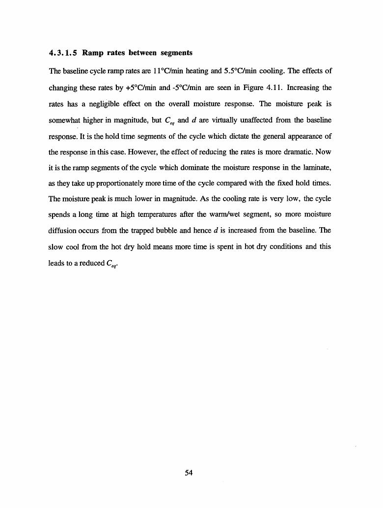
4.3.1.5 Ramp rates between segments
The baseline cycle ramp rates are 1 1C/min heating and 5.5°C/min cooling. The effects of
changing these rates by +5°C/min and -5°C/min are seen in Figure 4.11. Increasing the
rates has a negligible effect on the overall moisture response. The moisture peak is
somewhat higher in magnitude, but Ceq and d are virtually unaffected from the baseline
response. It is the hold time segments of the cycle which dictate the general appearance of
the response in this case. However, the effect of reducing the rates is more dramatic. Now
it is the ramp segments of the cycle which dominate the moisture response in the laminate,
as they take up proportionately more time of the cycle compared with the fixed hold times.
The moisture peak is much lower in magnitude. As the cooling rate is very low, the cycle
spends a long time at high temperatures after the warm/wet segment, so more moisture
diffusion occurs from the trapped bubble and hence d is increased from the baseline. The
slow cool from the hot dry hold means more time is spent in hot dry conditions and this
leads to a reduced Ceq.
54

0.008
0.007 -
0.006 -
0.005 -
0.004 -
0.003
0.002 -
0.001 -
,,U
0
4
I I'
I
-Iq
- -- HE- Ba
eat 16°C/min, cool 10.50C/min
Lseline (heat 1 1°C/min, cool 5.50C/min)
- - - - - Heat 6°C/min, cool 0.5°C/min
I0.10.1
I I I Ir I II I I I
0.2 z/h0.3z/h
I I I I
0.4 0.5
Figure 4.11: Effect of varying heating and cooling ramp rates
55
O-
-C1)
0
-o(c)L.
a)0CD
w _ __
w
3
L -·P
. . . . .. . . . . . . . . . . . . . . . . . . . .
-I1 I I

4.3.2 Accelerated moisture cycle design
The objective in designing a good accelerated test cycle is to match the metrics of d and Ceq
as closely as possible to the metrics for the baseline cycle, both throughout and between
cycles, but doing so in a cycle which takes less time.
Based on the results of the parametric studies, it is possible to design accelerated cycles to
match these two metrics very closely. This can be achieved by varying the parameters in a
number of different ways, although the response is more sensitive to changes in some
parameters than others.
Most time saving can be achieved by increasing the ramp rates between the hold points and
by using slightly more aggressive conditions in the warm/wet phase. It is desirable not to
change the conditions too drastically so as not to enter a new type of damage response.
The accelerated cycle which was used had the following philosophy behind its design. The
heating rate of 11 C/min was the maximum rate that the testing equipment could achieve,
so could not be increased. However, the cooling rate was increased from the -5.5C/min in
the baseline cycle to -140 C/min in the accelerated cycle. This value was chosen as it was
not so great that any thermal shock effects would be encountered, but was a significant
increase over the baseline cooling rate. This rate is also consistent with similar successful
cooling experiments which have been carried out in the laboratory. It was decided that the
warm/wet phase relative humidity should be maintained at 85% for ease of equipment setup
relative to the baseline apparatus. It is difficult to maintain RH values much greater than this
for the extended periods of time which were required for these tests, and a 5-10% increase
does not have a dramatic effect on the moisture response in any case (Figure 4.8). To
shorten the cycle, the warm/wet temperature was made more aggressive (increased by 11°C
56

(20°F) to 93°C (200°F)), and thus enabling the warm/wet hold time to be reduced from 60
minutes to 30 minutes. Temperatures higher than 930C were avoided as the conditions
become very hard to maintain for extended periods of time as 100°C is approached in a
humid envirrcnment. With these warm/wet conditions, the dry hot and cold hold times were
adjusted by trial and error to get a best fit. It was found that the Ceq and d metrics were very
closely matched to the baseline response when the hot dry and cold dry times were 20
minutes and 5 minutes respectively (compared with 30 minutes and 10 minutes respectively
for the baseline cycle).
These comparative conditions are summarized in Table 4.2 and Figure 4.12. The
accelerated cycle cuts the total cycle time from 160 minutes for the baseline cycle, to 90
minutes for the accelerated cycle, a saving of 44%.
Table 4.2: Baseline vs. accelerated moisture cycle parameters
Cycle Ramp rates Dry hot/cold hold Warm/wet hold Cycleheat/cool times conditions time°C/min (mins) (mins)(°F/min)
Baseline +11/-5.5 30/10 60 mins 160(20/-10) 820C (180OF)
RH 85%
Accelerated +11/-14 20/5 30 mins 90moisture (+20/-25) 930C (2000 F)
RH 85%
57

15
o 1C
5
EQ)
-5
-100 20 40 60 80 100 120 140 1)
Time (mins)
Figure 4.12: Temperature/time plot for the baseline and accelerated moisture cycles
A comparison of the theoretical material response to the baseline and accelerated moisture
environments after 100 cycles is shown in Figure 4.13. As can be seen, the Ceq and d
metrics are very similar for the two environments. Hence, the moisture history through the
material should be equivalent for both cycles after any number of cycles. Since the
accelerated moisture cycle is significantly shorter, the objective of duplicating the moisture
response in the material in a shorter amount of time should be met.
58
nff~n

oA 0.007CZ
.-- 0.0043
o 0.003
o 0.0020Coa) 0.001
0LU) 0
0 0.1 0.2 0.3 0.4 0z/h
Figure 4.13: Comparison of material response to baseline and accelerated moisture
environments in cold/dry phase after 100 cycles
59
.5
B\ MDA

4.4 THERMAL EFFECTS MODELING
A simple shear lag solution of the stresses around a crack was used by McManus and
Maddocks [47] combined with a strain energy release model of crack appearance. Much of
this analytical development can be found in this reference, and in Maddocks [43]. A ply or
ply group (stack of plies with the same orientation) embedded in a laminate is considered.
Cracks form parallel to the fibers with geometry as shown in Figure 4.14.
GlobalCoordinate
SvstemLocal Coordinate System
of Shaded Crack
y
Figure 4.14: Laminate and crack geometry
The laminate is modeled as being made up of two regions: a cracking ply group (subscript
c) and the rest of the laminate (subscript r): see Figure 4.15.
60
PIGro

ao
Z'
Iar/2-j
layer CI
I] a1
II
I.ar/2I
1/p-I
Figure 4.15: Geometry of microcracking problem
A one dimensional shear lag model is used to determine the stress and displacements in the
vicinity of a crack in its local x'y'z' coordinate system: see Figure 4.16.
ATLh
Oa 4
zI
LX'
ar + (darl dx ') dx'--o
ac + (dac/dx) dx'
ar + (dar/dx9) dx'
I dx' -
Figure 4.16: Shear lag stress model
Figure 4.17 shows the stress distribution around two crack configurations. The stresses
cause strain energy to be stored in the material due to elastic deformation. A new crack
forms when the strain energy released due to new crack formation is greater than the critical
strain energy release rate (the energy required to form the new crack surfaces).
61
-. ·.-ar/
.? F, ' .,; -;,~,~'~ -' ~ '~ ;' ~ ~ ~ ~ :^ >:-:i ~
'.~ ~ ,.l~~~~~~~~~.·:·,,p d·i~c.7! ~ ~ '·: iii ii ii i
-I--.4
| x c� f ^ w - U A 5
i - - --- -- --5 - --
-
I -I -
Or

Existing cracks
/1 \RA
Existing stress distribution
Figure 4.17: Stress
Stress released by crack
distribution around cracks
A complete analysis of the model is not duplicated here, but can be found in [47]. This
method allows the following relation to be derived for the cracking of a ply or ply group
within a laminate under thermal stresses:
(4.15)Gc=2aEE a-Ec (ac-aO)T x 2tanhA - ,-tanh2
Here, a's are thicknesses, Es are the stiffnesses in the x' direction of Figure 4.14, and a's
are the x' coefficients of thermal expansion (CTE's), with the subscripts identifying
properties of the cracking ply group (c), the smeared properties of the rest of the laminate
(r) or the entire laminate (o). Gc is the effective critical strain energy release rate (toughness)
62
New crackNew crack
a
Id --I LI I LI -� I�-J·- I Y

of the material when microcracking, AT is the maximum difference between the
environmental temperature and the effective stress free temperature T, is a shear lag
parameter, and p is the crack density, expressed in cracks/unit length, in the cracking ply
group. a is the applied stress to the laminate, which is zero in this case. The stiffnesses
and CTE's used in Eqn. 4.15 are calculated by classical laminated plate theory (CLPT).
The relation is an implicit one; the desired quantity p must be solved for numerically or
graphically.
As fully described in [43] and [47], thermal loads (and mechanical if they are being
considered also) are considered incrementally. At every temperature/oad increment, the
crack formation analysis is carried out for all ply groups. A numerical solution of Eqn.
4.15 is used to determine the crack density in the cracking ply group under consideration.
The properties of the ply group under consideration and the properties of the rest of the
laminate are calculated using CLPT relations. Cracking which does occur degrades the
properties of the laminate, and this is accounted for by the use of 'knockdown factors'
applied to those properties affected once all of the ply groups have been examined at this
load increment.
The above process is repeated for each load increment until the entire load history has been
completed. This iterative damage progression model is implemented by the computer code
CRACKOMATIC. This code utilizes material properties, laminate geometry, and
thermomechanical load history and outputs crack densities and degraded laminate
properties: see Figure 4.18.
63

Start at T = To
o-a =0
?
Repeat untilload historycompleted
Next Load Increment(Temperatuie and Stress) Iy Done
Repeat forall plies
! _
Compute Material Propertiesat Teperature
LFor Ply i
, ect Coordinate Systemalculate Stiffness Constants
Calculae NewCmrack Density
Done
Calculate New Larminate PropertiesUpdate Knockdown Factors
Figure 4.18: CRACKOMATIC code algorithm (from Maddocks [43])
64

If the material undergoes numerous thermal cycles, the material gets progressively more
damaged. This 'thermal fatigue' is accounted for by an effective toughness reduction
method. The effective toughness is assumed to drop with cycles according to the following
(strictly empirical) relation:
G, = G(N) (4.16)
where N is the number of cycles. For convenience in reducing data, the G-N relation is
sometimes expressed as:
Gc = GoAl °g °O(N) (4.17)
where Go is the initial toughness and A is a constant fit to data. This relation has been used
by other researchers [52] and experimental evidence exists to justify its application to this
problem [54]. On running the code, the user inputs the (empirical) shear lag factor, , the
greatest AT (which is the temperature difference between the cure temperature and the
lowest temperature in the cycle) and a 'G-N curve', in addition to the mechanical properties
required by CLPT (Appendix C).
Some of the material properties are very difficult to obtain for the materials under
investigation and only approximate values are known. This is particularly true for the zero
cycle and degraded fracture toughness properties. Hence, it is necessary to fit these
parameters to existing data for a given material and layup, and then use these 'backed-out'
parameters to predict other damage behaviors for the same material.
65

4.5 DESIGNING ACCELERATED THERMAL CYCLES WITH
CRACKOMATIC
4.5.1 Parametric studies
The only component of the baseline environment which strongly affects the thermal
microcracking response of the material is the low temperature point in the cycle. The lower
this temperature, the greater the AT is from the stress free (cure) temperature in the
laminate. This directly affects the thermal load in the composite: the greater the AT, the
greater the thermal load. As the low temperature is decreased, microcracking initiates
sooner and is more severe for a given number of cycles: see Figure 4.19. These curves
were produced using parameters in CRACKOMATIC which were consistent with
microcracking data found from the first round of testing with the high temperature material
K3B. Input requirements for the CRACKOMATIC code and input values used in these
analyses can be found in Appendix C.
This kind of microcracking response is typical: cracking is suppressed until a certain
number of cycles have been experienced (when the fracture toughness of the material has
fallen below the critical value for cracking). The onset of cracking is sudden and crack
density rises rapidly. As more cycles are experienced, the crack density approaches an
equilibrium value determined by the low temperature in the cycle. The rate of increase of
microcrack density is reduced after the initial onset because stress in the material is reduced
as cracks form (see Figure 4.17).
66

P% Aft
E 15--01-
2 10-- 50o 5-
-
0 200 400 600 800 1000Number of Cycles
Figure 4.19: Effect of varying cold temperature
67
_ _-
Baseline'/1 _____ ~~ -790C low
l'I I - -1040C lowJII -129 0C low
... - -1540C lowIII, _____i , I I I ii,/iii

4.5.2 Accelerated thermal cycle design
When designing the accelerated moisture cycle, the two metrics of d and Ceq were matched
to get the same moisture distribution in the material after a certain number of cycles, but
those cycles took much less time to complete compared to the baseline. For the design of
the accelerated thermal cycle, the same predicted level of microcracking damage was
obtained in a smaller number of more severe cycles.
The more severe cycles actually take more time than an equivalent baseline thermal cycle
because lower temperatures have to be reached, but cracking is predicted to occur in fewer
cycles and hence time is saved for a given amount of damage.
A 'target' crack density was established after a certain number of the baseline cycles (taken
as 1000 cycles in our case). As can be seen in Figure 4.20, an equivalent amount of 'target'
damage is predicted to occur in a much smaller number of more severe cycles, as shown by
the thin horizontal line in Figure 4.20. For example, 1000 cycles which have a low
temperature of -54°C (the baseline cycle) produce the same level of damage as about 250
cycles to a -150°C low, and only 150 cycles for a cycle with a low of -180°C. Hence,
theoretically accelerated thermal cycles can produce the same damage after as little as 15%
of the number of baseline cycles.
The accelerated thermal cycles used in this study went down to -180°C and -150°C: see
Figure 4.20. These will be referred to as Accelerated thermal cycle 1 and Accelerated
thermal cycle 2 respectively throughout the rest of this document. They were chosen as
they were the most severe cycles that could be easily generated. They also had the largest
theoretical affect on the thermal response of the material of any of the family of curves
shown in Figure 4.19.
68

0 200 400 600 800 1000Number of Cycles
Figure 4.20: Accelerated thermal cycle design plot
69
mu
15E
-10
(.,
_ 5
0
r% ^

CHAPTER 5
EXPERIMENTAL PROCEDURES
5.1 TEST MATRIX DESIGN
5.1.1 Stage I testing
A first phase of testing was undertaken by The Boeing Company. Specimens of four
different materials with various layups were tested, as shown in Table 5.1. The materials
chosen were those which were of prime interest to high temperature flight applications. For
these initial tests, the layups were arbitrary and inconsistent between materials. This phase
of testing was performed in order to show what range of damage responses could be
expected from this class of materials.
Specimens were subjected to 0, 25, 100, 200, 500 and 1000 cycles of the baseline and
isolated thermal environments. Crack damage was counted at Boeing and reduced at MIT.
Some interior damage assessment was undertaken by cutting the specimens after exposure
and polishing an interior surface which was well below the exposed edge during the test.
However, this was only undertaken for one specimen at each cycle number.
The results of this set of tests are given in Appendix B.
70

Table 5.1: Stage I test program matrix (Boeing)
71
Material Layups Test types
R1-16 [45/0/-45/90]s
[03/9 03]s Baseline environment
[45 /-45 2/45/04/90] s Isolated thermal environment
[45/-45/0:/90/0 2/-45/45]s
PETI-5 [4 5/0/- 4 5/90]2s
[90 /0 /9 0 12s Baseline environment
[4 5/- 4 5 2/4 5/0 4/90 ]s Isolated thermal environment
[45/-45/02/90/02/-45/45]s
K3B [45/-45/90/014s Baseline environment
[-45/45/90/0]4S Isolated thermal environment
PIXA [90/0/ 90 12s Baseline environmentIsolated thermal environment

5.1.2 Stage II testing
The second stage of testing was the main experimental program for this work. The testing
was conducted both at The Boeing Company in Renton, WA and in the Technology
Laboratory for Advanced Composites (TELAC) at MiT in Cambridge, MA.
Two materials which show promise for the application were tested: PETI-5 and PIXA-M.
More details and references for these materials are given in Section 2.3.2. Three layups
were chosen for testing:
* a 'research' layup of [902/04/902]s
* a 'real' crossply layup of [0/90/0]2s
* a 'real' quasi-isotropic layup of [45/90/-45/0]2s
These layups will be referred to as 'research', 'crossply' and 'quasi-isotropic' respectively
throughout the remainder of this document. Cracking from environmental (and other)
damage is generally confined to a ply group (i.e. a number of plies stacked together with
the same angle). The research layup was chosen because it contains thick 904 ply groups
which had been shown in previous studies to damage more easily than thinner ply groups.
This generated more data for this study. The two 'real' layups were chosen by Boeing as
being realistic laminate layups which could be used for a flight application.
Specimens of each material and layup were exposed to a number of different conditions,
designed to isolate one or more components of the baseline environment which potentially
could be responsible for causing the damage. These components include:
* moisture cycling
· extended time at moisture
* thermal cycling
72

* extended time at temperature
* combinations of the above.
Tests were designed to expose specimens to the baseline environment and to isolate the
exposure to the above mechanisms from the baseline environment. Parallel tests were also
conducted which used the accelerated moisture and accelerated thermal cycles, the designs
of which were discussed in the previous chapter. The tests performed exposed specimens
to:
* full baseline cycle (combined response to all components)
* isolated thermal component of the baseline cycle (response to thermal only)
* isothermal aging (response to time at temperature)
· accelerated moisture cycling (to speed up response to pure moisture cycling)
* accelerated thermal cycling (to speed up response to pure thermal cycling)
* accelerated thermal cycling of previously isothermally-exposed specimens
(to speed up visible damage to possibly degraded material)
This test program is summarized in the test matrix shown in Table 5.2.
Tests conducted by other researchers [55] investigated the effect of isomoisture exposure
which showed response to long duration exposure to moisture.
In the operational environment, many other factors may be important, including mechanical
stresses, chemical solvents, impacts, etc. The effect of mechanical stresses on these
materials, both in isolation and coupled with moisture and temperature effects (so-called
'hygrothermomechanical' testing) are also being investigated [56] as an extension to this
study.
73

Table 5.2: Stage II test program matrix
Material Layups Test types No. of cycles I Notes
Baseline 0, 50, 200, 500, 2 different1000, 1500 specimens at each
cycle countIsolated thermal 0, 50, 200, 500, 2 different
'Research' 1000, 1500 specimens at each[902/04/902] cycle count
Isothermal 4250 hrs at 350°F Research: 8 spcmnsonly Crossply: 4 spcmns
'Crossply' Quasi: 7 spcmnsPETI-5 [0/90/012 S , Accel. moisture 0, 288, 500, 1000, 2 different
1500, 1960 specimens at each'Quasi' cycle count
[45/90/-45/0]2S Accel. thermal 1 0, 65, 100, 180, same 3 specimens300, 400, 540, 750 used throughout
Accel. thermal 2 0, 80, 170, 280, same 3 specimens410, 560, 750 used throughout
Accel. thermal 0, 50, 150, 300, same 3 isothermal(isothermal 400 specimens usedspecimens) throughoutBaseline 0, 50, 200, 500, 2 different
1000, 1500 specimens at eachcycle count
Isolated thermal 0, 50, 200, 500, 2 different'Research' 1000, 1500 specimens at each
[902/04/9021] s cycle countIsothermal 4250 hrs at 350°F Research: 8 spcmns
only Crossply: 5 spcmns'Crossply' Quasi: 7 spcmns
PIXA-M [0/90/012 S Accel. moisture 0, 288, 500, 1000, 2 different1500, 1960 specimens at each
'Quasi' cycle count[45/90/-45/0]2s Accel. thermal 1 0, 65, 100, 180, same 3 specimens
300, 400, 540, 750 used throughoutAccel. thermal 2 0, 80, 170, 280, same 3 specimens
410, 560, 750 used throughoutAccel. thermal 1 0, 50, 150, 300, same 3 isothermal
(isothermal 400 specimens usedspecimens) I throughout
74

5.2 MANUFACTURE AND TESTING PROCEDURES
5.2.1 Material manufacture (Boeing)
The plies were laid up into 12" by 12" flat plates according to the laminate configurations
outlined above. The laminates were laid on a plate, vacuum-bagged and a 27" Hg vacuum
was maintained during the cure. The PETI-5 material was cured at 7500 F in an autoclave
pressurized to 100 psi. The PIXA-M was cured at 7000 F with 100 psi positive pressure.
Exact dwell times and ramp rates were unavailable (proprietary data). After curing, the
plates had 0.5" cut from all edges to remove resin-starved material, leaving plates of 11"
square. These were then cut on a water-cooled diamond saw into specimens 2" long by 1"
wide. The specimens were subsequently polished on all sides using Struers automatic
polishers down to a 5grm finish. The specimens were then dried in a Blue-M electric oven
for 5 days at 300°F to remove any internal moisture prior to testing.
5.2.2 Baseline environmental testing (Boeing)
A Thermotron Model F-7-CHM-5-5 environmental chamber was used with a Model 4800
microcontroller. This was pre-programmed to run the exact conditions of the baseline
cycle. Wet and dry bulbs created the appropriate moisture environments, while electric
heaters, forced-air mechanical refrigeration units and cryogenic attachments maintained the
desired temperatures in the oven. Specimens were held in the oven in a rack assembly, with
a controller feedback thermocouple situated next to these specimens. The specimens which
were designated to experience only the thermal component of the cycle were wrapped in
aluminum foil. This was to protect these specimens from the moisture in the environment
without affecting the thermal exposure. However, there was evidence to suggest that this
procedure did not actually shield the specimens from all of the moisture in the environment,
the implications of which are discussed in Chapter 7.
75

5.2.3 Accelerated moisture cycling (Boeing)
A similar environmental chamber was used as for the baseline testing. It was programmed
to conduct the accelerated moisture cycle as defined in the previous chapter. Unfortunately,
equipment error meant that the actual cycle which the materials saw was different from the
desired accelerated moisture cycle. All parameters were as detailed in Table 4.2, except the
warm/wet hold temperature was 82°C (180°F) rather than the desired 93C (200°F). This
difference in warm/wet hold temperature had a non-trivial effect on the theoretical moisture
distribution (see Figure 5.1). Of the two metrics, Ceq was 20% less and d was 25% less
compared to the baseline cycle due to the error in the accelerated cycle parameters.
Although the response to the accelerated moisture environment is further than desired from
the baseline response, the Ceq and d parameters are sufficiently close as to not invalidate the
usefulness of the tests. The moisture-thrashed peak is as high as in the baseline response,
and hence the extreme edge layer sees a moisture environment similar to the baseline. The
moisture-thrashed zone is a little less thick, so any moisture-thrashing-induced damage may
not be expected to progress quite as far as in the material exposed to the baseline cycles.
Equipment failure during the course of the accelerated moisture cycling experiments left the
specimens under unknown ambient conditions for several days. It is difficult to quantify
the effect that this had on the response of the specimens (if any), but it is unlikely that this
would significantly alter the damage response.
76
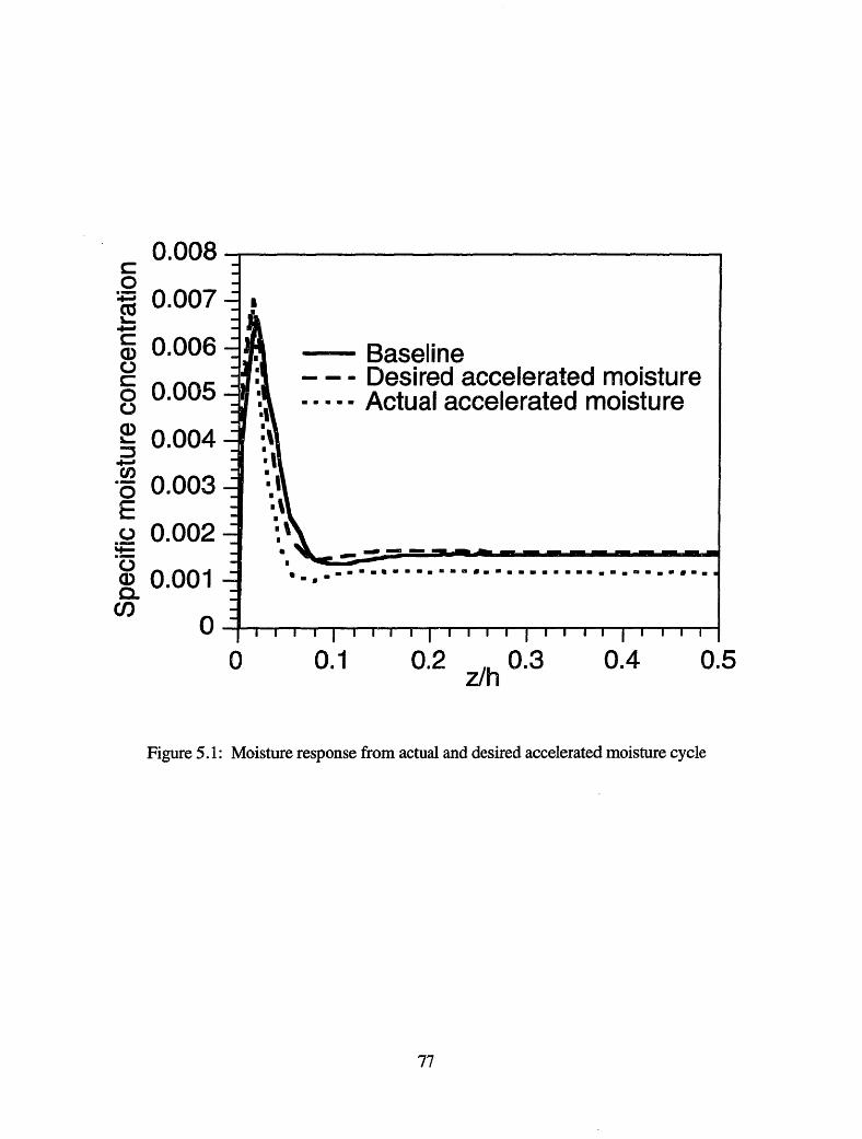
n AQvJ. J''JC0* 0.007
c 0.006
o 0.005
2 0.004
o 0.003
.) 0.002
O 0.0010.001
00 0.1 0.2 0.3 0.4 (
z/h
Figure 5.1: Moisture response from actual and desired accelerated moisture cycle
77
).5
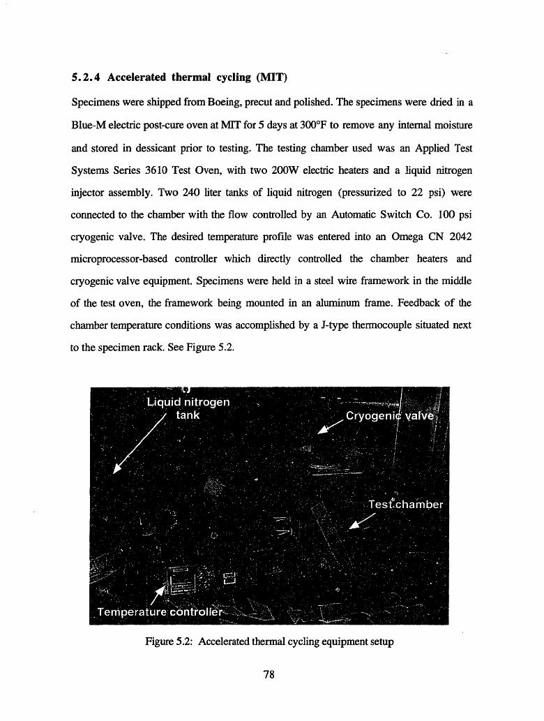
5.2.4 Accelerated thermal cycling (MIT)
Specimens were shipped from Boeing, precut and polished. The specimens were dried in a
Blue-M electric post-cure oven at MIT for 5 days at 300°F to remove any internal moisture
and stored in dessicant prior to testing. The testing chamber used was an Applied Test
Systems Series 3610 Test Oven, with two 200W electric heaters and a liquid nitrogen
injector assembly. Two 240 liter tanks of liquid nitrogen (pressurized to 22 psi) were
connected to the chamber with the flow controlled by an Automatic Switch Co. 100 psi
cryogenic valve. The desired temperature profile was entered into an Omega CN 2042
microprocessor-based controller which directly controlled the chamber heaters and
cryogenic valve equipment. Specimens were held in a steel wire framework in the middle
of the test oven, the framework being mounted in an aluminum frame. Feedback of the
chamber temperature conditions was accomplished by a J-type thermocouple situated next
to the specimen rack. See Figure 5.2.
Figure 5.2: Accelerated thermal cycling equipment setup
78

5.2.5 Isothermal aging (Boeing)
Specimens were placed on a rack in a Blue-M electric oven. The oven was held at a
constant temperature of 350°F and specimens were removed after 4250 hours of exposure.
5.3 DAMAGE ASSESSMENT TECHNIQUE (MIT)
5.3.1 Defining damage
The impact of the environment on the materials was measured by the amount of cracking
damage that was visible on the polished edge of the specimens. In the research layup of
[9 0 /0 4/9 0 2]s, it was the center 904 ply group which was chosen as the group of interest in
this study as it was thick. A number of different crack configurations are possible: see
Figure 5.3. A 'group' crack is defined as one which traverses the entire 904 ply group.
'Triple', 'double' and 'single' cracks traverse three, two and one ply from the group
respectively. A crack was designated as a single if it traversed from half to one and a half
plies, a double if it traversed one and a half to two and a half plies and as a triple if it
traversed between two and a half and three and a half plies.
In the 'real' layups, the plies of interest were the single 90's (the other plies did not show
significant damage). Hence, the only damage seen was of cracks spanning one ply: see
Figures 5.4 and 5.5.
79

04 plygroup
904 plygroup
04 plygroup
Figure 5.3: Crack types at the edge of the 'research' layup
Figure 5.4: Cracking at the edge of the 'real' crossply layup
80

Figure 5.5: Cracking at the edge of the 'real' quasi-isotropic layup
5.3.2 Measuring edge damage
The edge damage was measured by counting the number of cracks in the ply groups of
interest. For the research layup, the number of group, triple, double and single cracks on
the entire length of each 2" side of all specimens were counted. For the real crossply and
quasi-isotropic layups, the number of single cracks in each of the four 90 ° plies on each
side were counted. The 450 plies were checked, but very few cracks were observed and
were not useful for analysis purposes. Cracks were counted by viewing the specimens
under an Olympus SZ stereoscope (see Figure 5.6), with a magnification of 20-40x as
required. Light was brought onto the specimen using a 150W dual fiber optic halogen
lamp. The polished surfaces of the specimen were cleaned with a water-soaked cotton-
tipped applicator prior to viewing. Crack numbers were recorded using a hand tally counter
as the specimen was moved across the field of view.
81
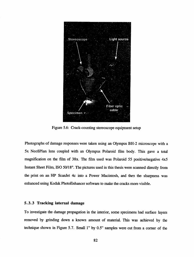
Figure 5.6: Crack-counting stereoscope equipment setup
Photographs of damage responses were taken using an Olympus BH-2 microscope with a
5x NeoSPlan lens coupled with an Olympus Polaroid film body. This gave a total
magnification on the film of 38x. The film used was Polaroid 55 positive/negative 4x5
Instant Sheet Film, ISO 50/18°. The pictures used in this thesis were scanned directly from
the print on an HP ScanJet 4c into a Power Macintosh, and then the sharpness was
enhanced using Kodak PhotoEnhancer software to make the cracks more visible.
5.3.3 Tracking internal damage
To investigate the damage propagation in the interior, some specimens had surface layers
removed by grinding down a known amount of material. This was achieved by the
technique shown in Figure 5.7. Small 1" by 0.5" samples were cut from a comer of the
82

original 2" by 1" specimens using a Dremel Moto-Tool with No. 49 cut-off wheels. The
polished edge whose damage depth was to be investigated was on the 1" side. A metal
'depth gage' was glued to the specimen with Ducco multipurpose cement such that the tip
of the gage was directly in line with the polished edge of the specimen under investigation.
It was very important to ensure that the gage was accurately aligned such that the two
parallel edges of the gage were perpendicular to the polished edge. These procedures were
achieved by viewing through the stereoscope and carefully positioning the metal gage while
the cement was still compliant. The specimen was then stabilized with a Buehler stainless
steel 'Sampl-Klip' support spring before placing in a Buehler 1.25" diameter plastic mold
with the side to be polished facing down. 15g of Buehler Epo-Kwik resin was added to 3g
of hardener and stirred slowly until the solution was clear. This was then added to the mold
around the specimen and left to cure overnight. The result was the specimen mounted in a
clear cylinder of epoxy resin, with the specimen at one end of the cylinder ready for
grinding and polishing. Polishing was achieved on a Struers Rotopol-l automatic polisher
with Pedemat power heads capable of applying a predetermined force on up to 6 specimens
simultaneously. Grinding took place with 500, 1200 and 2400 grit silicon carbide paper
mounted on the wheels of the machine. Most grinding took place on the 500 grit paper,
which was found to remove about 1 mm of material from the surface of the specimen with
a force of 55N over 10 minutes. The other grit papers were used to remove the scratches
left after the 500 grit was used. Final polishing to a suitable finish for photographic
purposes was achieved with a force of 60N for 45 minutes using 4000 grit paper.
The depth, e, from the edge was found by measuring the length, 1, of exposed 'depth gage'
left on the new polished surface: see Figure 5.7. By knowing the angle at the tip of the
depth gage (which is level with the initial surface prior to polishing), and the length, 1, the
depth below the initial exposed edge could easily be found. By performing a number of
grinds, a three dimensional map of damage from the edge could be obtained.
83

I 1"
A
0.5"
A&
Polished edgeunder investigation
1~~~~~1 ~ ~Removed material
Removed material
Metal 'depth gage'glued to specimen
so tip is in line with thepolisnea eage
Grinding or polishing paper
Depthgage
e ...... ..-
Known angle = 760such that I= 4e
Measure under microscope andhence get depth of grind from
original edge, e
Figure 5.7: Grinding and polishing technique
84
/L
Specimen
Specimen placedin cylindrical mold
and filled with epoxyresin
I/ r
I I .
r
-4
, /I

5.4 DATA REDUCTION
5.4. 1 Crack count data
The data obtained from these statistical methods is displayed in Appendix A.
5.4.1.1 Research layup
For the research layups, the number of group cracks were counted in the 904 group on both
2" sides of all three specimens at each condition. The average group crack density was
calculated as:
E (Group crack count)across
sides and
Average group crack density (/cm)= specimens3 specimens x 2 sides x 5.08 cm/side
(5.1)
Counts of triple, double and single cracks were also taken and averaged in the same way.
An 'aggregate' crack density was used as a measure of the overall level of cracking in these
thick ply groups. The aggregate crack count in a given ply group was found from:
(4 x #ofgroups)+(3 x #oftriples) + (2 x #of doubles) + (#of singles)
The average aggregate crack density was then calculated using:
I (Aggregate crack count)across
sides and.
Average aggregate crack density (/cm) = specimens3 specimens x 2 sides x 5.08 cm/side
(5.3)
Standard deviations for a given crack type were calculated using the equation:
85

_: (crack count - average)2Standard deviation = (#c count aluves -) (5.4)
(#ofcount values -I)
where 'crack count' is the number of cracks of a given type in each ply or ply group.
5.4.1.2 Crossply and quasi-isotropic layups
For these layups, the number of ply cracks were recorded for all four 90 plies on each 2"
side of the three specimens at a given test condition. The average crack density was
calculated using:
(# of cracks in each ply)across plies,
sides and
Average crack density (/cm) =specimens3 specimens x 2 sides x 4 plies/side x 5.08 cm/side
(5.5)
Standard deviations were calculated as in Eqn. 5.4.
5.4.2 CRACKOMATIC fits
Fits to select data sets were made using the CRACKOMATIC code. The fit to a G-N curve
eliminates geometric and laminate effects and hence should reveal the material response to
environmental cycling.
Material properties are input into the code (Appendix C). In all case, the shear lag parameter
was taken as ,=0.6 (consistent with that used in [43]). Assuming the material toughness
drops as in Eqn. 4.17, a fit was obtained by adjusting Go and A and repeatedly running the
analysis until cracking onset and growth rate were successfully simulated. The Go
parameter has a dominant effect on the onset of cracking, while A dictates how quickly
crack density increases thereafter. In some cases, Eqn. 4.17 was unsuitable and a more
86

general G-N curve (Eqn. 4.16) was determined by repeated analytical fits to the
microcracking data.
The values obtained are representative of the properties of the material near the edges of the
material which is cracking and not necessarily the material as a whole. But these values do
give an indication as to the toughness of the material in the damaged layer and the
susceptibility of the material to environmental cycling degradation. In cases where Eqn.
4.17 was usable, Go indicates the initial toughness of the material in the cracking area,
while A reflects its sensitivity to the environment. A value of A close to 1 indicates a
material which is resistant to degradation, while a value closer to zero indicates a material
which is vulnerable to environmental damage.
87

CHAPTER 6
RESULTS
6.1 STAGE I TESTING
The first stage of testing (as outlined in Section 5.1.1) yielded some interesting qualitative
data. Cracking which was observed on the edges was tracked into the specimen interior by
the method described in Section 5.3.3. Figure 6.1 shows significant edge damage in the
thick 06 ply group of the [03/903]S layup of the R1-16 material subjected to 500 baseline
cycles. The smaller cracks were seen to disappear only a very short distance into the
interior - Figure 6.2 shows the crack state 0.25 mm below the original edge. At 0.5 mm
below the original edge, only 3 or 4 cracks were still visible (Figure 6.3), while at 0.8 mm
virtually all the damage was gone (Figure 6.4). The same technique revealed that the more
severe (group) cracking in this material was visible up to 2 mm below the original edge.
Similar results were obtained for the other materials (except K3B) subjected to 500 baseline
cycles, with no damage progressing further into the material than a very thin edge layer,
with a depth of less than 2 mm.
Cutting and polishing of an interior surface (0.5" from the exposed edge) only revealed
cracks in the 90° plies of the K3B quasi-isotropic specimens (see Figure 1.5). All the other
specimens showed no damage at this internal location. The behavior displayed by the K3B
material was consistent with that due to classical thermal microcracking. From the very
limited amount of data available for K3B (only one specimen at each cycle number), an
assessment with the classical thermal microcracking code CRACKOMATIC (see Section
4.4 and 5.4) was undertaken. An approximate fit to the data was obtained as shown in
88

Figure 6.5. The crack density variation is typical of thermal microcracking: delayed crack
initiation followed by a rapid increase in the crack growth rate. The fracture toughness of
these high temperature resin systems is proprietary, but it is generally believed to be around
1000 J/m2. A value of 950 J/m2 was suitable for capturing the onset of cracking at around
100 cycles, while a very low value of A (see Eqn. 4.17) was required to capture the level
of cracking displayed thereafter. In order to achieve this, a value of 0.57 was needed for A,
implying a 43% reduction in the fracture toughness of the material for each factor of ten
increase in the number of exposure cycles.
The fit of the observed interior cracking behavior data to a classical thermal microcracking
prediction suggests that the K3B material is more sensitive to the hygrothermal
environment than the other materials tested. Even though the exact values may be
approximate, using a realistic initial fracture toughness requires a very low value of A in
order to fit to the data, suggesting that this material is very sensitive to hygrothermal
fatigue. This is one of the reasons this material was not considered further for this
application.
The data produced from this testing in contained in Appendix B.
89

Figure 6.1: Edge damage in the [03/903]s R1-16 laminate subjected to 500 baseline cycles
Figure 6.2: Damage at a depth of 0.25 mm from the original edge
90

Figure 6.3: Damage at a depth of 0.5 mm from the original edge
Figure 6.4: Damage at a depth of 0.8 mm from the original edge
91

15E-0
(Dn 10a)
0 5
O 4
0 200 400 600 800 1000 1200Cycles
Figure 6.5: Comparison of classical thermal microcracking prediction with internal damage
data in the K3B laminate subjected to the baseline environment
92
CRACKOMATIC prediction
o K3B data
, -IIII
M o. : 0 _ _ _ _ _ _ _ _ _ _ _ _ _ _ _
f%^
I
6.2 STAGE II TESTING - EDGE DAMAGE
6.2.1 General
Group, triple, double and single cracks were counted and recorded for all the 904 ply
groups of the research specimens. The single crack counts were also taken for all the 90 ply
groups of both the quasi-isotropic and crossply layups (see Appendix A). The data
produced was reduced as discussed in Section 5.4.
The average crack densities and error bars showing one standard deviation from the
average are plotted in the Figures which follow.
6.2.2 Baseline, isolated thermal and accelerated moisture edge data
6.2.2. 1 PETI-5 results
The data for these tests can be found in Tables A. 1, A.3 and A.5. Plots of the reduced data
for the three tests for a given crack type (group and aggregate) and laminate are shown in
Figures 6.6-6.9.
Figure 6.6 shows the number of group cracks in the 904 ply group of the PETI-5 research
laminates for these three test conditions. Very little cracking is evident under any condition
before 500 cycles have elapsed. Thereafter, the baseline cycle causes a rapid increase in
group crack density after 1000 cycles. An additional 500 cycles causes no significant
further increase in the group crack density average from that at 1000 cycles, but there is
significant scatter in the 1500 cycle data. The data for specimens subjected to the isolated
thermal environment shows a similar increase after 500 cycles to 30-50% of the baseline
environment group crack values, but again there is a large amount of scatter in the 1500
93

cycle data. The data for specimens subjected to the accelerated moisture environment shows
no group cracking occurs until after 1500 cycles have elapsed, and even then to only about
20% of the value caused by the baseline cycle after 1000 cycles.
Figure 6.7 shows the aggregate crack data for the same layup, ply group and conditions.
Aggregate crack densities are uniformly higher than the corresponding group crack
densities, by about a factor of 10. This indicates that there is extensive partial cracking, in
addition to the large group cracks (see Eqn. 5.2 and Figure 5.3). The baseline environment
causes a slow but steady increase in aggregate crack density up to 500 cycles. After this,
the increase is more rapid until a pseudo-equilibrium level appears to be reached after 1000
cycles (at about 35 cracks/cm), much like that seen in the group crack data for the baseline
environment. The isolated thermal environment causes a similar affect on the specimen's
aggregate crack density as on the group cracks. Little response is shown up to 500 cycles,
after which crack density rises steadily. The average crack density at 1000 cycles is about
50% of the value for the baseline environment, while the densities after 1500 cycles are
almost identical (although there is much more scatter in the isolated thermal data). Again,
the accelerated moisture environment causes little cranking until after 1500 cycles, although
by 2000 cycles, the aggregate crack density has reached about 15 cracks/cm (albeit with a
lot of scatter), which is about 50% of the 'pseudo-equilibrium' baseline value after 1000
cycles.
Similar behavior for all three environments is shown by the crossply laminate specimens
(see Figure 6.8). The average cracking response of the specimens subjected to the baseline
environment again displays a rapid increase to a pseudo-equilibrium level after 1000 cycles.
Again, the response of specimens subjected to the isolated thermal environment is
somewhat less severe than that due to the baseline environment before 1000 cycles.
However, by 1500 cycles the averages are very similar and well within the scatter of data
94

from both environments. The cracking response of specimens subjected to the accelerated
moisture cycle shows a more steady rise than before, but the values are about 30% of the
corresponding baseline environment response, and much scatter is evident for the higher
cycle counts.
The quasi-isotropic laminate response to the baseline and isolated thermal environments
show similar trends (see Figure 6.9) as seen for the crossply specimens, although the crack
densities are somewhat lower (final value of about 15/cm compared to about 25/cm in the
crossply baseline response). However, the accelerated moisture environment now causes
very little cracking, even after 2000 cycles.
6.2.2.2 PIXA-M results
The data for these tests can be found in Tables A.2, A.4 and A.6, and plotted in Figures
6.10-6.13.
Figure 6.10 shows the density of group cracks in the PIXA-M research specimens
(compare with Figure 6.6). The baseline environment causes a steady rise in the group
crack density average up to 1000 cycles, followed by a curious drop in the 1500 cycle
average (although the scatter still encompasses all of the 1000 cycle data average and
spread). Specimens exposed to the isolated thermal environment show similar behavior as
seen in PETI-5: delayed crack initiation (to 500 cycles) followed by a steady increase
thereafter, approaching the baseline values after 1500 cycles. Note that the baseline and
isolated group crack densities are higher than the equivalent values in PETI-5 by
approximately a factor of 2. The group data for specimens subjected to the accelerated
moisture environment is also different from the PETI-5 response. Group cracking starts
95

immediately and produces crack densities comparable to those produced by the isolated
thermal environment. Data scatter was very low for these specimens.
The trends for the aggregate crack densities in the research laminate (Figure 6.11) are
remarkably similar to those displayed for the group crack densities for all three
environments. Not surprisingly given the definition, the magnitudes are higher by a factor
of about 7. Comparison of Figure 6.11 with Figure 6.7 shows that the response to the
baseline cycle is somewhat more severe in the PIXA-M, but the response to the isolated
thermal cycle is remarkably similar for the two materials, both having approximately 40
cracks/cm by the 1500 cycle point. The response to the accelerated moisture environment is
much more severe in the PIXA-M than PETI-5, with aggregate crack density rising to
about 30/cm by 1500 cycles, compared to only about 15/cm after 2000 cycles in the PETI-
5.
Figure 6.12 shows the response of the PIXA-M crossply specimens to the three
environments. Exposure to the baseline environment causes a fairly steady increase in crack
density to 1500 cycles. Response to the isolated thermal environment shows the same
delayed crack growth followed by an approach to the baseline environment values for 1500
cycles, as seen before for the other layups. Exposure to the accelerated moisture cycle
causes cracking to a level of only about 50% of the response to the isolated thermal
environment. Comparison with the PETI-5 response (Figure 6.8) shows the crack densities
under all conditions are only slightly higher in PIXA-M than in PETI-5.
The behavior of the quasi-isotropic specimens is shown in Figure 6.13. The crack densities
are very similar to those displayed by the crossplies for all environments up to 1000 cycles.
However, after 1000 cycles the cracking from exposure to the baseline and isolated thermal
environments show no further increase in average crack density. In fact, the response to the
96

baseline cycle to 1500 cycles shows a decrease in average crack density which cannot be
fully explained by data scatter, which is relatively low in this case. Specimens subjected to
the accelerated moisture environment show a similar slowing down of crack growth at
larger cycle numbers. Comparison with the equivalent PETI-5 specimen results (Figure
6.9) show the baseline response gives very slightly more cracking in PIXA-M than PETI-
5. The isolated thermal responses are very similar in behavior and crack density magnitude,
while the accelerated moisture cracking response is much more significant in PIXA-M than
in PETI-5.
97
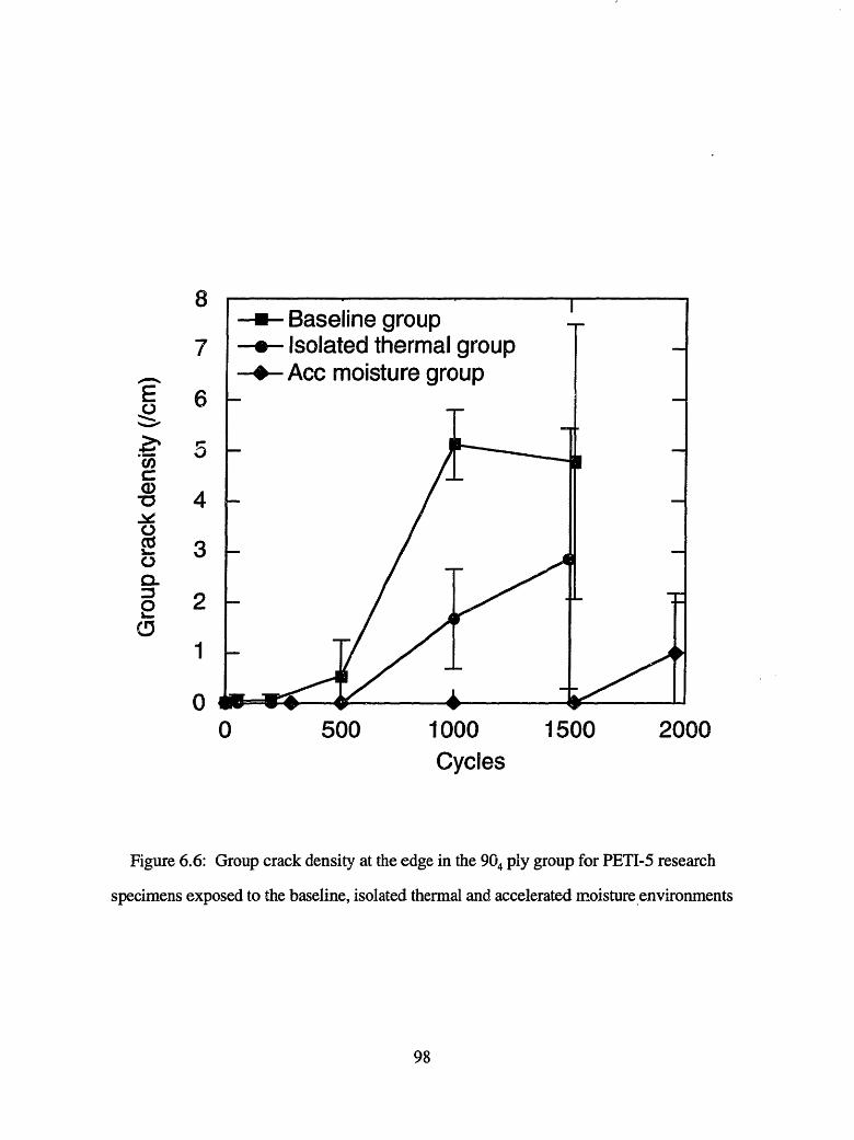
8
7
E 6
Cn
0aa 4
E5 3
o:5
2 2
1
00 500 1000 1500 2000
Cycles
Figure 6.6: Group crack density at the edge in the 904 ply group for PETI-5 research
specimens exposed to the baseline, isolated thermal and accelerated moisture environments
98
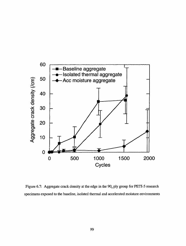
/n_'
g 50
040
is 30CD
a)
m 10
O
0 500 1000 1500 2000Cycles
Figure 6.7: Aggregate crack density at the edge in the 904 ply group for PETI-5 research
specimens exposed to the baseline, isolated thermal and accelerated moisture environments
99

50
40
E30(/3 o
D 20
0IO
00 500 1000 1500 2000
Cycles
Figure 6.8: Averaged crack density at the edge for PETI-5 crossply specimens exposed to
the baseline, isolated thermal and accelerated moisture environments
100
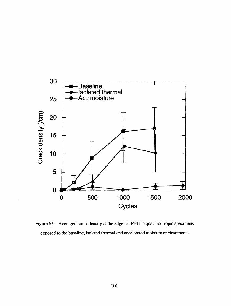
;.U
25
E 20
.) 15
. 5
5
00 500 1000 1500 2000
Cycles
Figure 6.9: Averaged crack density at the edge for PETI-5 quasi-isotropic specimens
exposed to the baseline, isolated thermal and accelerated moisture environments
101

A14
12
E- 10
Cl)
a)
O 6
040
2
00 500 1000 1500 2000
Cycles
Figure 6.10: Group crack density at the edge in the 904 ply group for PIXA-M research
specimens exposed to the baseline, isolated thermal and accelerated moisture environments
102

80
CI)E
a>)0 60
a)co20C-030
00 500 1000 1500 2000
Cycles
Figure 6.11: Aggregate crack density at the edge in the 904 ply group for PIXA-M research
specimens exposed to the baseline, isolated thermal and accelerated moisture environments
103

50
40
Ev 30
CICc-
' 20c0
10
00 500 1000 1500 2000
Cycles
Figure 6.12: Averaged crack density at the edge for PIXA-M crossply specimens exposed
to the baseline, isolated thermal and accelerated moisture environments
104

50
40
E
30._n
c-
0
10
00 500 1000 1500 2000
Cycles
Figure 6.13: Averaged crack density at the edge for PIXA-M quasi-isotropic specimens
exposed to the baseline, isolated thermal and accelerated moisture environments
105

6.2.3 Accelerated thermal 1 and 2 edge data
6.2.3.1 PETI-5 results
Data for these tests is contained in Tables A.7 and A.9. PETI-5 shows virtually zero
cracking for all layups and crack types for both of the accelerated thermal cycles. The only
non-zero readings were for the research aggregate crack counts for the accelerated thermal
cycle to -180 0C (Figure 6.14) and even these counts were trivially small.
6.2.3.2 PIXA-M results
Data for these tests is included in Tables A.8 and A. 10, and presented in Figures 6.15-
6.18.
Figure 6.15 shows the group crack response in the 904 ply group of PIXA-M research
laminates subjected to both of the accelerated thermal cycles (down to -180C and -150°C)
and to the isolated thermal environment. Group cracking is very low in both accelerated
environments up to 750 cycles (as it is for the isolated environment), and the more severe
thermal environments do not appear to accelerate the group crack damage at this number of
cycles.
Figure 6.16 shows the aggregate crack response in the research specimens. This time,
exposure to the more severe accelerated cycle (Acc thermal 1 to -1 800 C) caused about 50%
more average cracks than the isolated thermal environment up to 600 cycles, but the amount
of scatter is non-trivial. The less severe accelerated cycle (Acc thermal 2 to -150°C) causes
no more or less damage to the specimens than the isolated thermal environment up to 750
accelerated cycles.
106

Figure 6.17 shows the response for the crossply specimens. The response of the
specimens exposed to the -180°C environment is more promising, with a rapid jump in
average crack density at 100 cycles to a level which is not reached from exposure to the
isolated thermal environment until about 700 cycles have elapsed. Up until about 500
cycles have elapsed, crack density due to the accelerated thermal 1 environment is about 3
times higher than that for the isolated thermal environment for a given number of cycles.
The crack density rise after about 300 cycles is at a rate lower than for the isolated thermal
environment. The damage response due to the -1500 C environment does not show the
rapid rise in average crack density seen for the more severe environment. However, the
crack levels are about two times higher than the isolated environment response before the
two responses converge at 750 cycles. It should be noted, however, that the scatter in the
cracking responses for ALL environments is significant, thus making interpretation of the
data difficult.
Figure 6.18 shows the equivalent graph for the quasi-isotropic specimens. Again the more
severe accelerated environment causes a rapid rise in average crack density to a level after
100 cycles equivalent to 700 cycles of the isolated thermal environment (note: same as
before). The responses to the accelerated thermal cycles and the baseline cycle converge
after 800 cycles of both. This time the less severe accelerated cycle gives no benefit in
shortening the number of cycles to duplicate the isolated thermal damage response, but it
may still save time as the cycle is shorter. Again, the high scatter in the data should be
noted.
107

70
EU
mw
coC"
'c)3
CD
C)
CD
60
50
40
30
20
10
oJ 0 500 1000
Cycles1500 2000
Figure 6.14: Aggregate crack density at the edge in the 904 ply group for PETI-5 research
specimens exposed to the isolated thermal and accelerated thermal environments
108
-e--Isolated thermal aggregate
-- Acc thermal 1 aggregate (to -180°C)
_ - - - I I
5_ _
I _ __ __ P �· · _
A
A_

4 ^Ilu
8E
'n 6
c-
00"
0O
0 500 1000 1500 2000Cycles
Figure 6.15: Group crack density at the edge in the 904 ply group for PIXA-M research
specimens exposed to the isolated thermal and accelerated thermal environments
109
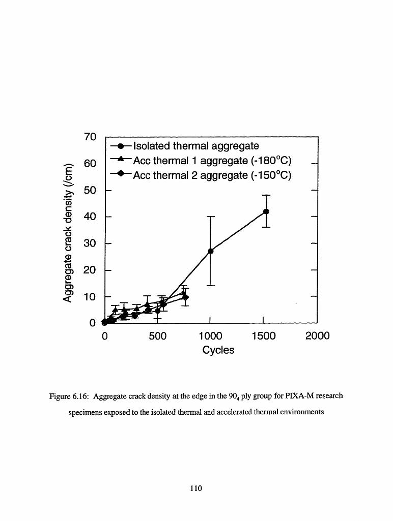
70
60E
, 50cnC
a) 40
0, 300
.i -.m 2U
$0o
0 500 1000 1500 2000Cycles
Figure 6.16: Aggregate crack density at the edge in the 904 ply group for PIXA-M research
specimens exposed to the isolated thermal and accelerated thermal environments
110
- Isolated thermal aggregatem,. _ A _ 1 4 ___.. _ _ 1 _ / .. - " n 1a \
-Acc nermai I aggregate - I u-- )-- Acc thermal 2 aggregate (-1 50°C)
II/_ /I
I I
-

F- fr3U
40
:v 30._
0J 20
010
00 500 1000 1500 2000
Cycles
Figure 6.17: Averaged crack density at the edge for PIXA-M crossply specimens exposed
to the isolated thermal and accelerated thermal environments
111
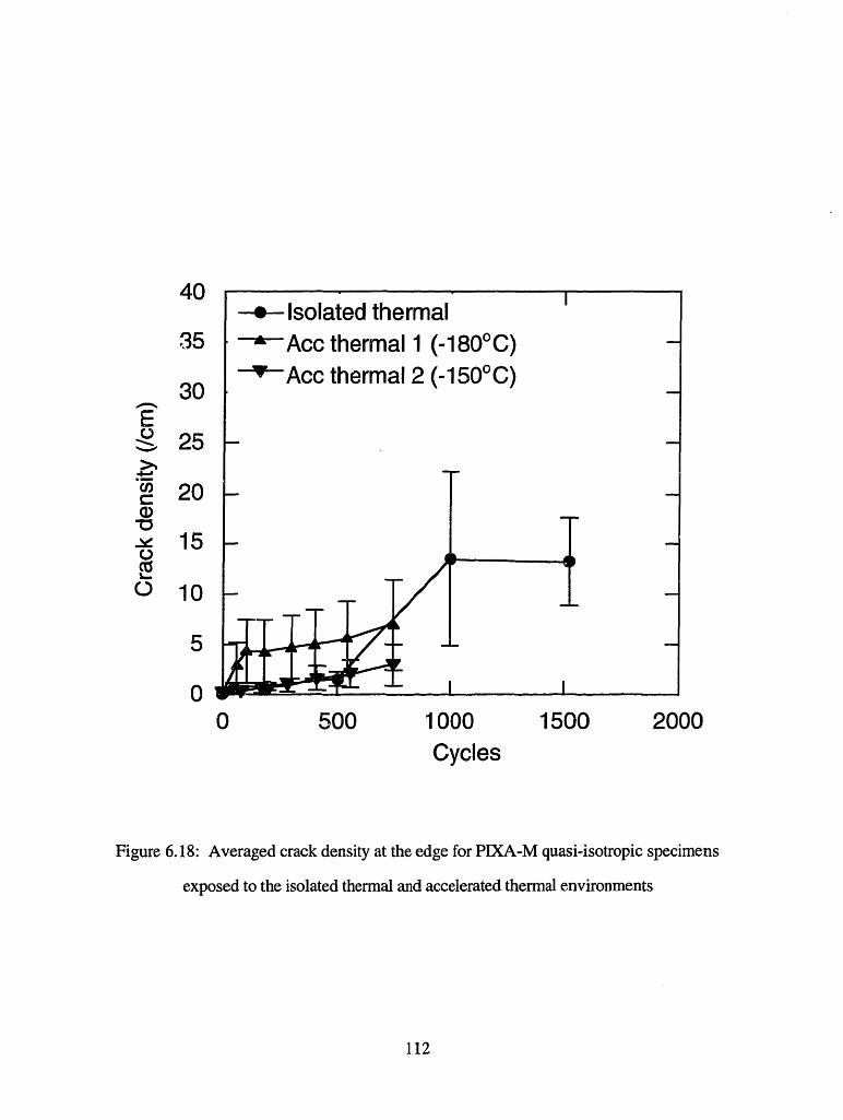
A £_V
35
30Eg 25
t 20a0
- 151_
o 10
5
00 500 1000 1500 2000
Cycles
Figure 6.18: Averaged crack density at the edge for PIXA-M quasi-isotropic specimens
exposed to the isolated thermal and accelerated thermal environments
112

6.2.4 Isothermal aging edge data
6.2.4.1 PETI-5 results
The PETI-5 specimens aged for 4250 hours at 3500 F showed no cracking for any of the
layups (see data under 0 cycle column of Table A. 11).
6.2.4.2 PIXA-M results
The PIXA-M specimens aged for 4250 hours at 350°F showed minimal cracking for all of
the layups (see data under 0 cycle column of Table A. 12).
6.2.5 Accelerated thermal testing of isothermal specimens
6.2.5.1 PETI-5 results
The results of the PETI-5 isothermal specimens which were subsequently subjected to the
accelerated thermal cycle down to -1800 C are shown in Table A.11. These specimens did
not show any significant damage as a result of the accelerated thermal testing.
6.2.5.2 PIXA-M results
The results of the PIXA-M isothermal specimens which were subsequently subjected to the
accelerated thermal cycle down to -1800C are shown in Table A.12 and in Figures 6.19-
6.21. These figures show a comparison of the response of the 'virgin' specimens and the
specimens previously exposed to the isothermal environment to the accelerated thermal 1
cycle. Unlike the PETI-5 specimens, the PIXA-M material does crack when subjected to
the accelerated thermal environment. In all cases, the isothermal specimens show a reduced
tendency to crack compared to the virgin specimens, although as noted earlier, scatter in the
data for the virgin specimens makes detailed interpretation difficult.
113

15
ErO
a,e-
C0 5
0 100 200 300 400 500 600 700 800Cycles
Figure 6.19: Comparison of aggregate crack density for virgin and isothermally-exposed
PIXA-M research specimens exposed to the accelerated thermal environment (to -1800C)
114

I""r-
20
E)
15CnCD
0
05
n0 100 200 300 400 500 600 700 800
Cycles
Figure 6.20: Comparison of crack density for virgin and isothermally-exposed PIXA-M
crossply specimens exposed to the accelerated thermal environment (to -1800 C)
115

12
10
E 8
o 6
as 4
2
n
0 100 200 300 400 500 600 700 800Cycles
Figure 6.21: Comparison of crack density for virgin and isothermally-exposed PIXA-M
quasi-isotropic specimens exposed to the accelerated thermal environment (to -180°C)
116
6.3 STAGE II TESTING - INTERIOR DAMAGE
6.3. 1 General
The internal damage state was investigated as described in Section 5.3.3. The Stage I
interior damage assessment tracked the damage at very small incremental steps (of about
0.1 mm) below the original edge (see Section 6.1). This investigation showed that, for
most of the materials under investigation (except K3B), the damage only progressed a very
small distance below the original edge (generally less than 1-2 mm). For the Stage II
interior damage assessment, measurements weie taken at 0.5-1 mm intervals until no more
damage was visible. The process of grinding material away to take interior measurements is
very time consuming, so minimizing the number of grinds is desirable. This gave a clear
indication of whether damage was confined to an edge layer or went deeper, but did not
provide enough resolution to establish how deep the damage went to the nearest tenth of a
millimeter (as was achieved in Stage I).
6.3.2 PETI-5 results
6.3.2.1 Research specimens
Three PETI-5 research specimens were potted in epoxy and polished: one each of
specimens subjected to 1500 cycles of the baseline and isolated thermal environments and
1000 cycles of the accelerated moisture environments. For all specimens, cracking other
than group cracks were not visible after a grind to 1 mm below the original edge, while all
group cracking subsequently disappeared when the grind was taken to 2 mm below the
original edge. To investigate further depths, other samples were potted and polished but
this time the interior edge was polished, rather than the exposed edge. This 'interior'
surface (as it will be referred to throughout this section) would have been about 10 mm
117

from the exposed edge at the time of exposure. This is considered to be out of the region of
influence of any edge effects. No damage was observed at the interior for any of these
specimens.
6.3.2.2 Crossply specimens
One specimen from each of the baseline (1500 cycles), isolated thermal (1500 cycles) and
accelerated thermal cycle 1 (to 750 cycles) were examined. The specimen subjected to the
baseline environment showed some visible cracks at a depth of 0.7 mm, but these
disappeared on subsequent grinding to a depth of 1.3 mm. The specimen subjected to the
isolated thermal environment showed no damage deeper than 0.6 mm from the edge. The
accelerated thermal cycling specimen showed no damage at any depth. No damage was
seen at the interior for any of these specimens.
6.3.3 PIXA-M results
6.3.3. 1 Research specimens
Three PIXA-M research specimens were potted in epoxy and polished: one each of
specimens subjected to 1500 cycles of the baseline and isolated thermal and 1000 cycles of
the accelerated moisture environments. In all cases, any damage less severe than a group
crack disappeared after a grind to 1 mm. Group cracks, however, persisted to a depth of at
least 3 mm. The baseline and isolated thermal environment specimens showed no damage
after polishing the interior surface, implying that even the group cracks disappear at a depth
between 3-10 mm below the original edge. However, two group cracks were faintly visible
in the interior of the specimen subjected to the accelerated moisture cycle. This result is
considered to be an anomaly with little significance since the accelerated moisture cycle was
118

not as severe as some of the other environments which universally caused zero internal
damage.
6.3.3.2 Crossply specimens
One specimen from each of the baseline (1500 cycles), isolated thermal (1500 cycles) and
accelerated thermal cycle 1 (to 750 cycles) were examined. For the specimen exposed to the
baseline environment, crack were still clearly visible at 0.9 mm below the original edge, but
they had disappeared at a depth of 1.5 mm. The isolated thermal environment specimen had
cracks visible (although only barely) at a depth of 0.9 mm, but they had also disappeared at
a depth of 1.5 mm. The accelerated thermal specimen showed no damage even on the first
grind to 0.8 mm. Polishing of interior surfaces revealed no damage.
119

CHAPTER 7
DISCUSSION
7.1 INTRODUCTION & GENERAL OBSERVATIONS
In Section 5.1.2, the components of the baseline environment which were candidates for
causing the observed damage were listed as:
* moisture cycling
* extended time at moisture
* thermal cycling
* extended time at temperature
* combinations of the above
The Stage II experimental program was designed to provide evidence as to the damage
caused by each of the above. The results of this program were presented in Chapter 6, and
are discussed here in the context of the list of candidates.
It is worth highlighting some of the more general observations of these results. One of the
most striking observations is that the damage in all cases (bar only one specimen) was
confined to a thin layer near the edge of specimens, usually less than 2 mm in depth.
Cracking was also mainly seen in the 90° plies and only rarely in the 45° plies. Previous
work [48] has shown that the transverse stresses responsible for microcracking are
approximately the same near the edges in 90° plies as in the interior of a laminate. For 45 °
plies, the transverse stresses are lower near edges. Hence, the edge stress state can help
explain the absence of cracks in 450 plies, but not the presence of cracks only near the
120

edges in the 90° plies. Therefore, the observation of damage only in this region suggests
that the material near the edges has different properties from that in the interior of the
specimen.
Since the cracks do not run all the way through the laminate, they cannot be considered as
'classical' microcracks. However, the cracks generally run to a depth about 5-10 times
greater than their height within the edge layer zone. As a result, the theory used to
understand microcrack behavior is valid if applied to these observed cracks. It is therefore
reasonable to use microcracking analyses (CRACKOMATIC) to assess the cracking
behavior in this region.
There is a large amount of scatter in the data, and this can be attributed to a number of
different factors. Prior work [49] has shown that classical microcracking analyses predict
considerable data scatter if one considers factors such as material variations. The current
study was also limited in the number of specimens available for testing at each condition.
Only three specimens were ultimately used for each test condition. The tests conducted at
MIT tracked damage in the same specimens as they became progressively more damaged at
each condition. In the Boeing tests, different specimens were used for each condition,
adding more variation to the scatter. Overall, although the scatter is high, the trends in the
data discussed here were all more significant than the data scatter.
Finally, some problems arose with the experimental setup, the effects of which are difficult
to quantify. There was some evidence to suggest that the specimens subjected to the
'isolated' thermal environment were not actually fully isolated from the moisture
component of the environment. The specimens subjected to the baseline environment had to
be thoroughly cleaned prior to damage assessment to remove edge layers of dirt and
mineral deposits. This contamination was presumed to be as a result of exposure to the
121

humid environment in the warm/wet phase of the cycle. Similar (although less pronounced)
deposits were also found on many of the 'isolated' thermal specimens, leading to the
suggestion that they did in fact encounter some of the moisture environment (i.e. the
thermal blankets were not fully sealed). It is likely that the presence of the thermal blankets
did lessen the impact of the moisture environment on these specimens. The blankets could
have reduced the humidity inside the blanket, or shielded one side of the specimen from
most of the moisture. The suggestion of a reduced humidity inside the blanket could
account for the fact that the isolated thermal environment data generally mirrors the trends
seen under the baseline environment, only at a lower level of damage (e.g. Figures 6.8,
6.9, 6.12 and 6.13). High data scatter would be a consequence of one edge being shielded
from moisture while the other side was exposed.
Equipment failures and shutdowns (see Section 5.2.3) are an inevitable part of long term
tests such as these. These problems also added to the overall uncertainty as to the
environment that the specimens encountered.
7.2 MOISTURE CYCLING
The effect of moisture cycling can be seen by comparing the results of the baseline and
accelerated moisture cycle. As discussed in Section 4.3.2, the accelerated moisture cycle
was designed to give an almost identical theoretical moisture distribution in the material as
the baseline cycle, only in a shorter cycle time. In particular, the characteristics of the
'moisture-thrashed' zone were matched between the two cycles. The actual accelerated
cycle was subtly different from that designed (see Section 5.2.3), but the effect on
changing the moisture distribution within the material was minimal (see Figure 5.1).
122

If moisture cycling had been the dominant parameter in causing the edge damage, the
results from the two cycles would be expected to be very similar. The results for PET-5
shown in Figures 6.6-6.9 show that this is clearly not the case. In all cases shown, the
damage from the accelerated moisture cycle is very much lower than that seen under the
baseline environment.
The equivalent results for the PIXA-M material are shown in Figures 6.10-6.13. Again,
these plots show that the accelerated moisture cycling does not produce the same level of
edge damage in PIXA-M as the baseline cycle. However, the damage levels are generally
up to 50% of the damage due to the baseline environment. These crack levels are much
greater than those displayed in PETI-5 under the same conditions. This indicates that the
PIXA-M is more susceptible to one (or more) component of the accelerated moisture cycle
than the PETI-5.
These results for both materials indicate that the moisture cycling component of the baseline
cycle is unlikely to be the dominant factor responsible for the observed edge damage.
7.3 EXTENDED TIME AT MOISTURE
Extended time at moisture has been observed in previous studies to have very significant
effects on the toughness of polymer matrix composites [55]. Moisture effects on K3B were
seen to reduce the effective toughness of the resin to zero after only 500 hours of
immersion in 80°C water. Immersion in 76% humidity air at 80°C was found to have a
comparable effect. PETI-5 was seen to be less susceptible to isomoisture effects, but it too
showed clear signs of decline in its fracture toughness before 2000 hours of exposure. The
conditions used in [55] were very similar to those in the warm/wet segment of both the
baseline and accelerated moisture cycles used in this study.
123

Although extended time under isomoisture conditions was not investigated directly in this
study, insight into its effects can be gleaned from the data collected. In particular,
comparison of the baseline and accelerated moisture cycle data reveals some interesting
observations. The major difference in the accelerated cycle parameters from the baseline
parameters was a 50% reduction in the warm/wet hold time-see Table 4.2. As noted in
Section 5.2.3, the accelerated cycle parameters which were seen by the specimens were
different from those detailed in Table 4.2: the warm/wet temperature was 82°C rather than
the 93°C which was specified. This resulted in the specimens seeing exactly the same
warm/wet conditions as the baseline, but only for half the time per cycle.
The accelerated moisture and baseline data are compared based on the time exposed to
warm/wet conditions in Figures 7.1-7.4. This basis of comparison does not account for the
depth of the zone affected by moisture, or the time moisture takes to diffuse into it. These
considerations also tend to work against the accelerated cycle.
Figures 7.1 and 7.2 show this comparison for some PETI-5 specimens. Even corrected for
time exposed to moisture, the accelerated cycles do less damage than the baseline, perhaps
for some of the reasons given above. The correction works well for PIXA-M specimens,
as can be seen in Figures 7.3 and 7.4. These results suggest that time at moisture may be
more important than moisture cycling. Further evidence on this matter will be discussed in
Section 7.6.
124

60
E
C.
an
.)cm
50
40
30
20
10
00 500 1000 1500
Time at moisture (hrs)
Figure 7.1: Corrected accelerated moisture aggregate crack data in PET r 5 research
laminates
50
40
E0
-(1)"0'a
.e
0o
30
20
10
00 500 1000
Time at moisture (hrs)1500
Figure 7.2: Corrected accelerated moisture crack data in PETI-5 crossply laminates
125

14
12
E10
-,)'o
en0
.o
10
8
6
4
2
0 500 1000 1500Time at moisture (hrs)
Figure 7.3: Corrected accelerated moisture group crack data in PIXA-M research laminates
E
a)C
L.CD)
80
60
40
20
00 500 1000 1500
Time at moisture (hrs)
Figure 7.4: Corrected accelerated moisture aggregate crack data in PIXA-M research
laminates
126

7.4 THERMAL CYCLING
The isolated thermal and the accelerated thermal environments were designed to isolate and
accelerate respectively the effects of thermal cycling. As discussed in Section 7.1, there
was evidence to suggest that the 'isolated' thermal environment specimens were not fully
sealed from the moisture component of the environment. As a result, the only thermal
cycling data discussed here will be from the accelerated thermal cycling experiments.
The results for PETI-5 (Section 6.2.3.1 and Figure 6.14) showed effectively zero damage
up to 750 cycles under even the most severe accelerated thermal cycle (down to -1800C) for
all specimens. This suggests that PETI-5 is not susceptible to damage from this severe
thermal cycle up to 750 cycles. No evidence is available at this point to comment on its
behavior beyond this number of cycles, but it should be noted that the accelerated thermal
environment is much more severe than the thermal conditions in the baseline environment.
The results of the accelerated thermal cycle testing with PIXA-M (Section 6.2.3.2, Figures
6.15-6.18) shows that this material is more susceptible to thermal cycling effects than
PETI-5. The damage is confined to a thin edge layer rather than behaving like classical
thermal microcracks which propagate throughout the entire laminate. However, these edge
cracks in the crossply laminates generally have aspect ratios (length/height) of about 10.
This value is high enough for an evaluation with CRACKOMATIC to be viable. Figure 7.5
shows the result of best fit CRACKOMATIC plots to the data from the accelerated thermal
1 cycle (down to -1800C) and the accelerated thermal 2 cycle (down to -1500C) for the
crossply layup.
A so-called 'G-N curve' (Eqn. 4.17) was fit to the data using the procedure outlined in
Section 5.4. It illustrates how the material's effective fracture toughness is reduced by
127

cyclic exposure. For this plot, the parameters for the G-N curves are initial fracture
toughness, Go = 508 J/m2 , A = 0.97 for Accelerated thermal 1 and Go = 508 J/m2, A =
0.967 for Accelerated thermal 2. The other parameters were as for PETI-5 (see Appendix
C). Only the A parameter had to be changed slightly (to 0.98) in order to get a best fit to the
quasi-isotropic PIXA-M data-see Figure 7.6. On the other hand, the research layup did
not microcrack in a classic fashion. Very few cracks were seen in the 904 ply group.
Hence, no fit using CRACKOMATIC was attempted.
Given the scatter in the data (see Figure 7.6; error bars omitted from 7.5 for clarity), the fits
are quite good in all cases, capturing the trends seen. In particular, the acceleration of
damage at -180C compared to -150 °C (Figure 7.5) occurs as predicted. However, these
fits apply only to the material near the edge of the specimens, where cracking was
observed. The interior material is not damaged by thermal cycling. The reason why the
edge material is vulnerable to damage is not known. Given that the transverse stresses in
this region are no worse than in other parts of the laminate [48] and the susceptibility of the
material to moisture already discussed, ambient moisture and/or some other environmental
condition during cycling or in storage before the tests began is suspected.
128

25
20
15
10
5
00 200 400 600
Cycles800 1000
Figure 7.5: Fit of CRACKOMATIC output to accelerated thermal cycle data in 'ILXA-M
crossply
(Acc thermal 1: Go = 508 J/m2, A = 0.97, Acc thermal 2: Go = 508 J/m2 , A = 0.967)
129
' Acc thermal 1 (-180°C)-- - CRACKOMATIC prediction to -180°C,-v Acc thermal 2 (-150C).- - CRACKOMATIC prediction to -150°C
I
O
-'
C
L.0;
-- --
l.I
11-10-1-- - - - - - - - , , -
m _ _ I
II
II
I III

4 C'Il
E 10
V)-0.0c N
n
0 250 500 750 1000Cycles
Figure 7.6: Fit of CRACKOMATIC output to the -180 °C accelerated thermal cycle data in
PIXA-M quasi-isotropic (Go = 508 J/m2 , A = 0.98)
130

7.5 EXTENDED TIME AT TEMPERATURE
The isothermal experiments directly tested the effects of extended time at temperature. After
4250 hours at 350°F, none of the laminates of either of the two materials showed any
significant damage. This time at elevated temperature was considerably longer than any of
the cycled specimens experienced. Therefore, the effect of time at temperature can be
discounted as a direct causal factor in the observed damage behaviors in both materials.
Subsequent accelerated thermal cycling of these specimens resulted in no cracks in PETI-5
and a smaller number of cracks than seen in unaged specimens for a given number of
cycles in PIXA-M (see Figures 6.19-6.21). This implies that the elevated temperature aging
affected the edge layer of the material, making it less prone to cracking. This could be
accounted for by either the aging reducing the laminate stresses at the edge, or the aging
having a toughening effect on the edge layer.
7.6 COMBINATIONS OF ENVIRONMENTS
The results from the moisture cycling section shows that PETI-5 is not severely damaged
by the moisture cycling component of the baseline environment. Accelerated moisture
cycling produces less damage than the baseline environment. The level of damage which is
observed can be partly explained by the time at moisture arguments. No damage was
observed (either on the edge or internally) due to even the most severe accelerated thermal
cycle. Similarly, extended time at elevated temperature was not seen to cause any damage.
Hence, it is the time at moisture which seems to be the dominant environmental factor for
PETI-5. However, it is not the only factor; the combined hygrothermal environment seems
to have effects not accounted for simply by time at moisture.
131

CRACKOMATIC can be used to analyse the results of the baseline hygrothermal cycling
since the cracks in the edge layer of the research laminates have an aspect ratio of at least 4.
An 'effective' G-N curve for the hygrothermal environment can be developed based on
fitting a CRACKOMATIC prediction to the baseline environment damage data for the
research laminate.
The crossply and quasi-isotropic specimens had cracks that were very shallow (most
cracking disappeared in these specimens on grinding off a very small amount of edge
material). Therefore, CRACKOMATIC was not used to analyze these laminates.
The result for the research laminate is shown in Figure 7.7, with the G-N curve used to
generate this plot illustrated in Figure 7.8. This is one of the 'general' G-N curves (Eqn.
4.16) discussed in Section 5.4.2. The Go value of around 1200 J/m2 is consistent with
other discussions, but the rapid drop off in G beyond 1000 cycles is interesting.
Experiments (Section 6.2.3.1) proved that PETI-5 did not display this rapid decline in G
when subjected to the pure thermal environment (or it would have cracked). This fit to the
data indicates that the combined baseline environment is having a detrimental effect on the
fracture toughness.
Similar arguments concerning moisture effects hold true for PIXA-M. Accelerated moisture
cycling does not replicate the observed baseline damage, so moisture cycling is not the
dominant environmental factor. Correcting the accelerated moisture data for time at
moisture brings the data very much into line with the baseline damage data. Thermal
cycling down to -180 0 C and -150 °C does have an effect on edge material. But, using the
CRACKOMATIC fit parameters from Section 7.4 to predict the response to the baseline
thermal environment (which only went down to -540 C) indicates that even in the edge
132
zone, thermal cycling should not have a big effect at -540C until at least 5000 cycles. As
was the case for PETI-5, the prolonged exposure to elevated temperatures did not damage
the material. This suggests that, for PIXA-M, the dominant environmental factor again is
the time at moisture, but again this time at moisture may not be the only factor.
The best fit CRACKOMATIC plot to the research laminate baseline cycle group crack data
is shown in Figure 7.9, with the associated G-N curve used to generate this plot shown in
Figure 7.10. The initial toughness of the material for the combined environment is greater
than that used in the thermal cycling fits (Section 7.4) and here it is more in line with the
accepted value for PETI-5. This figure shows that the drop in G for PIXA-M after 100
cycles is more severe than it was in PETI-5. As was the case for PETI-5, this indicates that
the combined environment degrades the effective fracture toughness of this material. Time
at moisture and thermal cycling are the prime candidates for the combined effect.
133

8
7
E
.?C)
CD0C-
6
5
4
3
2
1
00 500 1000
Cycles1500 2000
Figure 7.7: Fit of CRACKOMATIC output to baseline cycle group crack data in PETI-5
research laminates
134
* Baseline group data
- CRACKOMATIC prediction
- a , t …__ a__
I.P
I= I
B'I
L
I -r - · ·
I.
.
I
!I
I I

c -4 AMAAE I UUU
1400CD
(c 1200CD
c 1000
800
2 600
E 400
>e 20005cI),D
1 10 100 1000 104
Cycles
Figure 7.8: G-N curve used in Figure 7.7
135

4 AI1+
12
E?, 10
8Q)
o 60C
0
2
00 500 1000 1500 2000
Cycles
Figure 7.9: Fit of CRACKOMATIC output to baseline cycle group crack data in PIXA-M
research laminates
136

c_ 1 rAnE I UUt,-
2 1400(D
c( 1200C,aD
-c 1000
o 800
2 600
c 400
.> 200
0? n
1 10 100 1000 104
Cycles
Figure 7.10: G-N curve used in Figure 7.9
137

Pure time at moisture studies are being carried out by Nairn as part of the HSR program.
These differ from current studies in the fact that specimens are soaked, so all material is
exposed to moisture and not just a thin surface/edge zone. There is no thermal cycling
component in these tests, so no cyclic stresses are present. Mechanical loading is used to
induce microcracking and data reduction similar to that in Section 5.4 was used to find the
effects of time at moisture on the fracture toughness of the material.
Figure 7.11 shows the two G-N curves for hygrothermally-cycled PETI-5 and PIXA-M
laminates, along with the experimental values obtained for a similar polyimide material after
extended time under isomoisture conditions, as discussed in [55]. This data suggests that
the combined environment degrades the edge material even more rapidly than simple time
at moisture. PIXA-M seems to have a greater reduction in its toughness with the combined
environment than PETI-5. The drop-off in effective fracture toughness occurs much sooner
for the combined environment than in the isomoisture environment (100 cycles vs. 1500
cycles).
138

C60cr
:30co
.t
a>
LI
1400
1200
1000
800
600
400
200
01 10 100 1000
Cycles
Figure 7.11: Combined G-N curves for PETI-5 & PIXA-M baseline environment
exposure and isomoisture exposure of a similar polyimide material
139
I I I
----- PETI5
----- PIXAM
polyimide isomoisture exposure (Nairn [55])
104
_·_

CHAPTER 8
CONCLUSIONS
8.1 GENERAL
The effects of a realistic moisture and thermal environment on two high temperature
polymer matrix composites (PETI-5 and PIXA-M) have been investigated. The response of
the materials to this baseline environment and its individual components of time at
moisture, moisture cycling, time at temperature and temperature cycling were studied.
Models were used to design accelerated moisture cycles and accelerated thermal cycles in an
attempt to speed up the response to these environmental factors.
The baseline environment was found to cause visible damage in the form of cracking in
both materials. Some of the individual components of the environment also caused
cracking, while other components caused no visible damage. When damage did occur, it
was found to exist only in a thin layer of material next to the exposed edge, and did not
progress beyond a few millimeters from that edge. This was the case for both materials.
This suggests that the environmental exposure is reducing the effective fracture toughness
of the material in this thin layer of material next to the exposed edge more than the material
at the interior.
PIXA-M was seen to show more visible environmental damage than PETI-5. When
cracking occurred in both materials at a given condition, PIXA-M displayed higher crack
densities than PETI-5. In other cases, PIXA-M displayed cracking when exposed to
environments which caused no visible damage in PETI-5.
140

8.2 INDIVIDUAL ENVIRONMENT COMPONENT EFFECTS
Time at temperature causes no visible damage in either material and appears to alter the
material properties such that subsequent thermal cycling causes less damage in PIXA-M.
Severe thermal cycling (to -1800 C and -150°C) has no effect on PETI-5. PIXA-M showed
damage due to this severe thermal cycling, but not due to 'realistic' thermal cycling to the
baseline cycle low of -54°C.
Time at moisture seems to be a dominant factor in damage of both materials.
Moisture cycling does not seem to be a principle component causing damage, as evidenced
indirectly by the fact that the accelerated moisture cycling tests did not accelerate damage.
However, it is believed to play an important role in setting up the depth of the damaged
surface layer since it significantly affects the moisture distribution.
8.3 COMBINED ENVIRONMENT EFFECTS
The combined environments in the baseline cycle cause more visible damage to both
materials than any one component of that cycle on its own. Time at moisture appears to be
the dominant factor for both materials. Thermal cycling is known to cause cyclic internal
stresses which can cause damage (and did in this case in PIXA-M). The mechanism by
which moisture cycling affects the material is not fully understood, but evidence does not
show it to be as large a factor in causing cracking as the thermal cycling component. Time
at temperature is not seen to be a significant contributor to visible damage.
141

These observations point to the combined effects of time at moisture and thermal cycling as
being the dominant parameters causing the visible damage in the baseline environment.
8.4 ACCELERATED CYCLES
The accelerated thermal cycles which were designed did cause some increased damage at
low cycle numbers in the PIXA-M material and the more severe the cycle, the greater the
observed damage. The accelerated moisture cycle was not seen to cause any acceleration of
visible damage in either material. The goal of using these accelerated cycles to expedite the
damage seen from the baseline environment was not achieved since they were not
accelerating the dominant damage components of that cycle. However, the accelerated
cycles were instrumental in providing data to establish what were the dominant parameters.
8.5 FURTHER ACCELERATED TESTING
The accelerated cycles which were used in this study did not accelerate the dominant parts
of the baseline environment causing damage. In the light of the findings of the study, it is
proposed that an isomoisture (extended time at moisture) environment combined with a
thermal (or mechanical) cycling component would be a viable option for accelerating
damage. Isomoisture exposure would expose specimens to the maximum amount of time at
moisture for a given test time. The thermal or mechanical cycling component would
introduce cyclic stresses throughout the laminate which are believed to play a role in
causing visible damage when combined with isomoisture.
142

REFERENCES
1. Noor, A. K. and S. L. Venneri (Eds.), Future Aeronautical and Space Systems,AIAA Progress in Astronautics and Aeronautics, Vol. 172, AIAA, 1997, pp. 173-210.
2. Wilhite, A. W. and R. J. Shaw, "HSCT research picks up speed", AerospaceAmerica, AIAA, August 1997, pp. 24-29, 41.
3. National Research Council, U.S. Supersonic Commercial Aircraft: AssessingNASA's High Speed Research Program, National Academy Press, 1997.
4. Thornton, E. A., Thermal Structures for Aerospace Applications, AIAAEducation Series, AIAA, 1996, pp. 1-20.
5. Johnson, B., "Temperature Issues for a Mach 2.4 High Speed Civil Transport",SAE Technical Paper 942160, AEROTECH '94, Los Angeles, CA, October 1994.
6. Burianek, D., "Fatigue Damage in Titanium-Graphite Hybrid Laminates", AIAA-98-1965, 39th Structures, Structural Dynamics and Materials Conference, LongBeach, CA, April 1998.
7. Weitsman, Y., "Moisture in Composites: Sorption and Damage", Fatigue inComposite Materials, Elsevier Science Publishers, 1990, pp. 385-428.
8. Wolff, E. G., "Moisture Effects on Polymer Matrix Composites", SAMPEJournal, Vol. 29, No. 3, May/June 1990, pp. 11-19.
9. Shen, Chi-Hung and G. S. Springer, "Moisture Absorption and Desorption ofComposite Materials", Journal of Composite Materials, Vol. 10, No. 1, 1976,pp. 2-20.
10. Springer, G. S., "Moisture Content of Composites Under Transient Conditions",Journal of Composite Materials, Vol. 11, No. 1, 1977, pp. 107-122.
11. McKague, Jr., E. L., J. E. Halkias and J. D. Reynolds, "Moisture in Composites:The Effect of Supersonic Service on Diffusion", Journal of Composite Materials,Vol. 9, No. 1, 1975, pp. 2-9.
12. Xiang, Z. D. and F. R. Jones, "Thermal-Spike-Enhanced Moisture Absorption byPolymer-Matrix Carbon-Fibre Composites", Composites Science and Technology,Vol. 57, 1997, pp. 451-461.
13. DeIasi, R. J., J. B. Whiteside and W. Wolter, "Effects of Varying HygrothermalEnvironments on Moisture Absorption in Epoxy Composites", FibrousComposites in Structural Design, E. M. Lenoe et al. (Eds.), Plenum Press, 1980,pp. 809-818.
143

14. Loos, A. C. and G. S. Springer, "Moisture Absorption of Graphite-EpoxyComposites Immersed in Liquids and in Humid Air", Journal of CompositeMaterials, Vol. 13, April 1979, pp. 131-147.
15. Whiteside, J. B., R. J. DeIasi and R. L. Schulte, "Distribution of AbsorbedMoisture in Graphite/Epoxy Laminates After Real-Time Environmental Cycling",Long-Term Behavior of Composites, STP 813, ASTM, 1983, pp. 192-205.
16. Akay, M., S. Kong Ah Mun and A. Stanley, "Influence of Moisture on theThermal and Mechanical Properties of Autoclaved and Oven-Cured Kevlar-49/Epoxy Laminates", Composites Science and Technology, Vol. 57, 1997, pp.565-571.
17. Springer, G. S., "Environmental Effects on Epoxy Matrix Composites",Composite Materials: Testing and Design, STP 674, ASTM, 1979, pp. 291-312.
18. Shirrell, C. D. and J. Halpin, "Moisture Absorption and Desorption in EpoxyComposite Laminates", Composite Materials: Testing and Design, STP 617,ASTM, 1997, pp. 514-528.
19. Weitsman, Y., "A Rapidly Convergent Scheme to Compute Moisture Profiles inComposite Materials Under Fluctuating Ambient Conditions", Journal ofComposite Materials, Vol. 15, July 1981, pp. 349-358.
20. Springer, G. S., Environmental Effects on Composite Materials, TechnomicPublishing, Lancaster, PA, Vols. 1 and 2, 1981.
21. Foch, B. and H. L. McManus, "Modeling of Environmentally Induced Damage inPolymer Matrix Composites", 11th International Conference on CompositeMaterials, Gold Coast, Australia, July 1997.
22. Antoon, M. K. and J. L. Koenig, "Irreversible Effects of Moisture on the EpoxyMatrix in Glass-Reinforced Composites", Journal of Polymer Science: PolymerPhysics Edition, Vol. 19, 1981, pp. 197-212.
23. Zhou, J. and J. P. Lucas, "Effects of Water on a Graphite/Epoxy Composite",Journal of Thermoplastic Composite Materials, Vol. 9, October 1996, pp. 316-328.
24. Upadhyay, P. C. and J. Prucz, "Parametric Damage Modeling of Composites dueto Moisture Absorption", Journal of Reinforced Plastics and Composites, Vol.11, 1992, pp. 198-210.
25. Davies, P. F. Pomies and L. A. Carlsson, "Influence of Water Absorption onTransverse Tensile Properties and Shear Fracture Toughness ofGlass/Polypropylene", Journal of Composite Materials, Vol. 30, No. 9, 1996,pp. 1004-1019.
26. Flaggs, D. L. and F. W. Crossman, "Analysis of the Viscoelastic Response ofComposite Laminates during Hygrothermal Exposure", Journal of CompositeMaterials, Vol. 15, January 1981, pp. 21-40.

27. Lee, Myung Cheon and N. A. Peppas, "Models of Moisture Transport andMoisture-Induced Stresses in Epoxy Composites", Journal of CompositeMaterials, Vol. 12, No. 12, 1993, pp. 1146-1171.
28. Harper, B. D. and Y. Weitsman, "On the Effects of Environmental Conditioning onResidual Stresses in Composite Laminates", Int. Journal Solids Structures, Vol.21, No. 8, 1985, pp. 907-926.
29. Weitsman, Y., "Coupled Damage and Moisture-Transport in Fiber-Reinforced,Polymeric Composites", Int. Journal Solids Structures, Vol. 23, No. 7, 1987, pp.1003-1025.
30. Milke, J. A. and A. J. Vizzini, "Thermal Response of Fire-Exposed Composites",Journal of Composites Technology and Research, Vol. 13, No. 3, pp. 145-151.
31. Crews, L. K. and H. L. McManus, "Modeling the High-Temperature Degradationof Graphite/Epoxy", Proceedings of the American Society for Composites 12thTechnical Conference on Composite Materials, Detroit, MI, October 1997, pp.1123-1132.
32. Chang, Win-Jin, Tei-Chen Chen and Cheng-I Weng, "Transient HygrothermalStresses in an Infinitely Long Annular Cylinder: Coupling of Heat and Moisture",Journal of Thermal Stresses, Vol. 14, 1991, pp. 439-454.
33. Cunningham, R. A. and H. L. McManus, "Coupled Diffusion-Reaction Models forPredicting the Distribution of Degradation in Polymer Matrix Composites", 1996AMSE International Mechanical Engineering Congress and Exposition, Symposiumon Composite Materials.
34. Nelson, J. B., "Thermal Aging of Graphite/Polyimide Composites", Long-TermBehavior of Composites, ASTM STP 813, T. K. O'Brien (Ed.), ASTM, 1983,pp. 206-221.
35. Harding, D. R., J. K. Sutter and D. S. Papadopoulos, "Protective Coatings forHigh Temperature Polymer Matrix Composites", 25th International SAMPEConference, October 1993, pp. 514-527.
36. McManus, H. L. and C. C. Chamis, "Stress and Damage in Polymer MatrixComposite Materials due to Material Degradation at High Temperatures", NASATechnical Memorandum 4682, January 1996.
37. Tsuji, L. C., H. L. McManus and K. J. Bowles, "Mechanical Properties ofDegraded PMR-15 Resin", ASTM Symposium on Time Dependent and Non-lineareffects in Polymers and Composites, STP 1357, Atlanta, GA, May 1998.
38. Lo, Ying-Jin, Chung-Ho Liu, Diing-Guey Hwang, Jin-Fu Chang, Jong-ChengChen, Wen-Yin Chen and Shu-En Hsu, "High Temperature Behaviors of anInnovative Polymeric Matrix Composite", High Temperature and EnvironmentalEffects on Polymeric Composites, STP 1174, C. E. Harris and T. S. Gates(Eds.), ASTM, 1993, pp. 66-77.
145

39. Meador, M. A., P. J. Cavano and D. C. Malarik, "High Temperature PolymerMatrix Composites for Extreme Environments", Structural Composites: Designand Processing Technologies, Proceedings of the 6th Annual ASM/ESD AdvancedComposites Conference, Detroit, MI, October 1990, pp. 529-539.
40. Hou, T. H., B. J. Jensen and P. M. Hergenrother, "Processing and Properties ofIM7/PETI Composites", Journal of Composite Materials, Vol. 30, No. 1, 1996,pp. 109-122.
41. Rommel, M. L., L. Konopka and P. M. Hergenrother, "Process Development andMechanical Properties of IM7/LaRC PETI-5 Composites", 28th InternationalSAMPE Technical Conference Proceedings, November 1996, pp. 1-13.
42. Hartness, J. T., "The Characterisation of a Thermoplastic Polyimide Composite",28th International SAMPE Technical Conference, Vol. 28, 1996, pp. 48-62.
43. Maddocks, J. R., "Microcracking in Composite Laminates under Thermal andMechanical Loading", Master of Science Thesis, Massachusetts Institute ofTechnology, 1995.
44. Tompkins, S. S. and S. L. Williams, "Effects of Thermal Cycling on MechanicalProperties of Graphite Polyimide", Journal of Spacecraft, Vol. 21, No. 3, 1984,pp. 274-280.
45. Adams, D. S., D. E. Bowles and C. T. Herakovich, "Thermally-InducedTransverse Cracking in Graphite-Epoxy Cross-Ply Laminates", Journal ofReinforced Plastics and Composites, Vol. 5, July 1986, pp. 152-169.
46. McManus, H. L., D. E. Bowles and S. S. Tompkins, "Prediction of ThermalCycling Induced Matrix Cracking", Journal of Reinforced Plastics andComposites, Vol. 15, February 1996, pp. 124-140.
47. McManus, H. L. and J. R. Maddocks, "On Microcracking in Composite LaminatesUnder Thermal and Mechanical Loadings", Polymers & Polymer Composites,Vol. 4, No. 5, 1996, pp. 305-314.
48. Park, C. H. and H. L. McManus, '"Thermally Induced Damage in CompositeLaminates: Predictive Methodology and Experimental Investigation", CompositesScience and Technology, Vol. 56, 1996, pp. 1209-1219.
49. Michii, Y. and H. L. McManus, "Prediction of Microcracking Distributions inComposite Laminates Using a Monte Carlo Simulation Method", Journal ofReinforced Plastics and Composites, Vol. 16, No. 13, pp. 1220-1230.
50. Clifton Furrow, A. P., D. A. Dillard, T. L. St. Clair and J. Hinkley, "DyePenetrant Induced Microcracking in High Performance Thermoplastic PolyimideComposites", Journal of Composite Materials, Vol. 32, No. 1, 1998, pp. 31-48.
51. McManus, H. L., B. J. Foch and R. A. Cunningham, "Mechanism-basedModeling of Long-term Degradation", DURACOSYS 97: Progress in DurabilityAnalysis of Composite Systems, Blacksburg, VA, September 1997.
146

52. Sriram, P., Y. Khourchid, S. J. Hooper and R. H. Martin, "ExperimentalDevelopment of a Mixed-Mode Fatigue Delamination Criterion", CompositeMaterials Fatigue and Fracture, STP 1230, ASTM, 1995, pp. 3-18.
53. Foch, B. J., "Integrated Degradation Models for Polymer Matrix Composites",Master of Science Thesis, Massachusetts Institute of Technology, May 1997.
54. Bradai, M., "Microcracking in Composite Laminates Under Thermal Cycling",Technology Laboratory for Advanced Composites, TELAC Report 97-9,Massachusetts Institute of Technology, March 1997.
55. Nairn, J., Polyimide isomoisture data, personal communication with R.Cunningham, The Boeing Co., October 1997.
56. Hygrothermomechanical testing document, in preparation, TELAC, MIT.
147

APPENDIX A
STAGE II TESTING EDGE DAMAGE DATA
A.1 DEFINITIONS
Laminate/Material typeP5 = PETI-5
PMf PIXA-M
side of specimenunder consideration
cycle number
i
ply group underconsideration
specimen mber
number of cracks:g = group(3) = triple
(2) = double(1) = single
148
PS-R -1 -2 - -3 L 4 -5 1 -6 -7 1-8 -9 L -10
902 0 0 16g 6g 18g 21g 45g 44g 36g 38ggroup 8(1) 9(1) 3(1) 4(1) 6 2(1) 2(1)
side 1 2(2) 0 ig 2(3) 2g Ig 24g 26g 12g 33g904 4(2) 3(2) 2(3) 1(3) 8(3) 8(3) 1(3) 5(3)
group 50(1) 27(1) 3(2) 4(2) 9(2) 17(2) 10(2) 12(2)47(1) 38(1) 52(1) 44(1)
902 0 0 6g 2g 32g 12g 45g 47g 37g 42ggroup 14(1) 5(1) 2(1) 4(1) 6(1)
side 2 0 ig 15(1) 2(2) 8g 1(2) 31g 23g 39g 13g
904 4(1) 2(3) 5(1) 9(3) 9(3) 4(3) 6(3)group 14(2) 19(2) 20(2) 10(2) 16(2)
_______,_____ ______ _____ 22(1) _ 55(1) i 37(1) 60(1

A.2 DATA
Table A. 1: Baseline environment damage data (PETI-5)
RESEARCH 50 I I00cycles 20cycls es 11520cycesP5-R -1 -2 -3 I -4 -5 1 -6 -7 1 -8 -9 1 -10
902 0 0 16g 6g 18g 21g 45g 44g 36g 38ggroup . 8(1) 9(1) 3(1) 4(1) 6(1) 2(1) 2(1)
side 1 2(2) 0 lg 2(3) 2g ig 24g 26g 12g 33g904 4(2) 3(2) 2(3) 1(3) 8(3) 8(3) 1(3) 5(3)
group 50(1) 27(1) 3(2) 4(2) 9(2) 17(2) 10(2) 12(2)47(1) 38(1) 52(1) 44(1)
902 0 0 6g 2g 32g 12g 45g 47g 37g 42ggroup 14(1) 5(1) 2(1) 4(1) 6(1)
side 2 0 ig 15(1) 2(2) 8g 1(2) 31g 23g 39g 13g
904 4(1) 2(3) 5(1) 9(3) 9(3) 4(3) 6(3)
group 14(2) 19(2) 20(2) 10(2) 16(2)22(1) 55(1) 37(1) 60(1)
Group Avg. 0.05 0.05 0.54 5.12 4.77Group SD 0.10 0.10 0.71 0.70 2.72
Aggr. Avg. 0.39 6.10 10.58 34.60 35.68Aggr. SD 0.45 4.84 6.76 9.20 9.38
CROSSPL 150 cycles 1200 cycles 500 cycles 1000 cycles I 1520 cyclesP5-C -1 -2 -31 -4 -51 -6 -7 -8 -9 -10
90 0 0 3 bp 55 25 57 171 157 173side 1 90 0 0 3? b 21 8bp 8 159 121 115
90 5 0 ? bp 27 bp 109 162 166 13190 6 0 5 bp 50 25 157 127 158 146
90 bp 0 10 10 77 102 158 102 196
side 2 90 bp 0 3 1 21 62 121 50 184
90 1 0 8 4 92 106 129 bp 54 18390 0 0 8 14 86 137 147 bp 65 195
Average 0.17 1.23 12.46 26.00 27.02SD 0.39 0.79 7.40 6.75 9.63
149

Table A. 1 (cont.)
QUASI 50 cycles 200 cycles 500 cycles 1000 cycles 1520 cyclesP5-Q -1 1-2 -3 1 -4 -5 -6 -7 -8 -9 I -10
90 0 0 24 22 69 72 41 109 124
side 1 90 0 0 10 16 40 28 b 48 3990 0 0 6 26 77 56 94 67 92 6390 0 6 15 28 77 35 87 65 99 6690 0 0 0 2 29 80 65 123 103 156
side 2 90 1 0 1 0 7 24 57 bp47 8490 0 0 4 1 19 38 112 bp 80 8490 3 0 7 8 26 45 106 bp 93 89
Average 0.12 2.09 8.88 16.08 16.93SD 0.32 1.95 4.64 5.26 5.92
150

Table A.2: Baseline environment damage data (PIXA-M)
RESEARCH 50 cycles 200 cycles 500 cycles 1000cycles 1520cyclesPM-R -1 -2 -3 -4 1 -5 -6I -7 -8 1 - -10
902 2g 3(1) 8g 9g 19g 19g 42g 38g 39g 33ggroup 6(1) 2(1) 15(1) 16(1) 20(1) 24(1) 25(1) 13(1)
1(1) 6(1) 5g 1 lg 29g 20g 36g bp 45g 48gside 1 904 2(3) 2(3) 6(3) 10(3) 17(3) 4(3) 6(3)
group 5(2) 12(2) 13(2) 8(2) 15(2) 7(2) 9(2)12(1) 32(1) 28(1) 28(1) 54(1) 33(1) 18(1)
902 5g 4g 12g 16g 24g 27g 46g 40g 41g 39ggroup 4(1) 3(1) 8(1) 12(1) 12(1) 9(1) 27(1) 18(1) 17(1) 3(1)
902 0 lg Ig 2g 8g 47g 43g 19g 32ggroup 0(1) 1(1) 20(1) 14(1) 8(1) 8(1)
1(1) 3(1) 1(1) 2(3) 3g ig 43g 51g 1 g 23gside 2 904 1(2) 4(3) 1(2) 6(3) 8(3) 2(2) 6(3)
group 4(1) 6(2) 1(1) 3(2) 22(2) 19(1) 6(2)15(1) 52(1) 54(1) 26(1)
902 ig 0 5g 12g 31g 20g 44g 43g 37g 40ggroup 3(1) 3(1) 12(1) 2(1) 19(1) 16(1) 4(1) 5(1)
Group Avg. 0.00 0.79 2.61 8.53 6.25Group SD 0.00 1.03 2.66 1.48 3.50Aggr. Avg. 0.54 8.22 19.69 55.97 34.45Aggr. SD 0.47 9.31 16.75 7.73 16.68
CROSSPL cle 200 cycles 500 cycles 1000 cycles 1520 cyclesPMI-C 1 , -26 --7 -8 -9 1 -10
90 6 9 70 70 98 119 149 143 187 189
side 1 90 0 0 25 24 21 59 150 131 152 169
90 0 2 39 50 35 73 146 142 121 182
90 14 18 73 115 86 96 138 163 210 197
90 5 5 20 16 101 70 166 144 bp 186
side 2 90 0 2 5 2 14 18 103 137 144 144
90 0 4 5 2 11 40 128 122 167 7790 13 12 27 18 47 48 148 179 218 180
Average 1.11 6.90 11.52 28.16 33.11SD 1.16 6.36 6.81 3.53 7.15
151
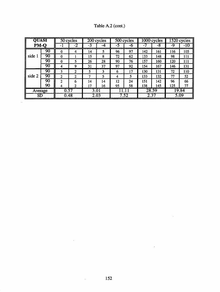
Table A.2 (cont.)
QUASI IL50cycles 200 cycles 500 cycles 1000 cycles 1520 cyclesPM-Q 5 -1 -2 -3 ] -4 1 -5 -6 -7 1 -8 -9 I -10
90 0 4 14 5 96 97 142 161 116 105
side 1 90 0 1 15 8 72 62 133 148 98 111
90 0 5 26 28 90 76 157 160 120 11190 4 9 31 37 97 92 154 167 146 131
90 3 2 5 3 6 17 130 131 72 110
side 2 90 2 2 7 5 4 5 133 132 77 52
90 2 6 14 14 12 24 151 142 96 6690 4 2 17 16 95 58 138 145 125 77
Average 0.57 3.01 11.11 28.59 19.84SD 0.48 2.03 7.52 2.37 5.09
152

Table A.3: Isolated thermal environment damage data (PETI-5)
RESEARCH Ii 50 cycles 1 200cycles 500 cycles I 1000cycles 1520 cycesP5-R -1 1 -12 -13 1 -14 -15 1-16 1 -17 1 -18 -19 1-20
902 0 0 2(1) Ig 7g 7g 35g 29g 27g 48ggroup 6(1) 8(1) 4(1) 17(1) 14(1) 5(1) 8(1)
side 1 6g 0 0 0 2(1) 1(2) 14g 8g 12g 33g904 1(3) 11(1) 5(3) 3(3) 8(3) 9(3)
group 2(2) 19(2) 11(2) 9(2) 29(2)
56(1) 111(1) 108(1)902 0 Ig Ig 2(1) 3g 58g 34g 30g 34g 20g
group 2(3) 3(1) 6(1) 6(1) 5(1) 10(1) 4(1) 6(1)1(2)
1(1)
side 2 0 0 0 0 6(1) 2(1) 2g log 11g 2g904 4(3) 6(3) 5(3) 2(3)
group 5(2) 19(2) 11(2) 5(2)39(1) 89(1) 68(1)
Group Avg. 0.00 0.00 0.00 1.67 2.85Group SD 0.00 0.00 0.00 0.98 2.58Aggr. Avg. 0.00 _ .00 1 .13 19.34 38.78Agr. SD 0.00 0.00 _ _1.02 9.20 19.07
CROSSPLY 50 les 200 cles 500 cycles 1000 cycles 1520 cyclesPS-C -11 -12 -13 I -14 -15 I -16 -17 1 -18 -19 -20
90 0 0 1 0 47 bp 195 166side 1 90 0 0 0 0 14 bbp 130 81
90 0 0 8 0 16 bp p 129 7690 0 0 17 4 35 bp bp 123 52
90 0 0 0 0 31 16 130 125 bp
side 2 90 0 0 0 0 9 4 57 49 bp90 0 26 0 4 20 22 81 85 bp bp90 0 20 9 9 37 24 88 153 bp bp
Average 0.57 0.64 4.51 18.90 23.43SD 1.56 0.99 2.47 7.21 9.41
153

Table A.3 (cont.)
QUASI 1150 cycles 200 cycles 500 cycles 1000 cycles 1520 cyclesP5-Q _ -11 1 -12 -13 1 -14 1 -15 -16 1 -17 I -18 -19 -20
90 0 0 1 0 36 28 46 51 119 99side 1 90 0 0 1 0 6 13 52 19 45 48
90 0 0 0 1 19 13 51 51 68 52
90 7 1 0? 3 24 21 63 59 48 46
90 0 0 1 0 4 5 113 60 52 50
side 2 90 0 0 0 0 0 0 61 38 27 1890 0 0 0 0 2 4 81 84 30 2290 1 0 1 3 9 11 91 b 44 63
Average 0.11 0.14 2.40 12.07 10.22SD 0.34 0.20 2.11 4.54 5.19
154-------2~~~~~- ---

Table A.4: Isolated thermal environment damage data (PIXA-M)
SEARCHl 50 cycles 200 cycles 500 cycls 1000 cycles 1520 cyclesPM-R --11 -12 -13 1 -14 -15 1-16 -17 1-18 -19 1-20
902 2g Ig 2g 3g 5g 5g 33g 31g 27g 33ggroup 3(1) 2(1) 3(1) 3(1) 3(1) 8() 22(1) 9(1)
Ig 6(1) ig ig ig 2g 27g 28g 32g 25gside 1 904 1(1) 1(3) 4(3) 2(2) 1(3) 3(3) 10(3) 6(3) 11(3)
group 3(2) 2(2) 7(1) 5(1) 6(2) 13(2) 21(2) 14(2)4(1) 8(1) 31(1) 27(1) 47(1) 37(1)
902 6g 2g 3g 7g 13g 13g 38g 44g 48g 40ggroup 4(1) 5(1) 5(1) 7(1) 20(1) 22(1) 8(1) 9(1)
902 0 0 ig 1(1) 4g 4g 29g 8g 27g 19ggroup 1(1) 5(1) 6(1) 17(1) 11(1) 14(1) 16(1)
1(2) 5(1) 2(3) 1(2) ig 4g 19g 3g 24g 30gside 2 904 6(1) 3(2) 3(1) 3(2) 2(3) 9(3) 3(3) 4(3) 10(3)
group 6(1) 8(1) 5(2) 13(2) 2(2) 15(2) 17(2)13(1) 23(1) 17(1) 41(1) 58(1)
902 1(1) ig 7g ig 16g 12g 26g 27g 30g 40g.group 1(1) 1(1) 3(1) 8(1) 9(1) 15(1) 6(1) 18(1) 12(1)
Group Avg. 0.05 0.10 0.39 3.79 5.46Group SD 0.10 0.11 0.28 2.28 0.76Aggr. Avg. 1.18 3.35 4.63 27.02 42.03Aggr. SD 0.28 1.85 2.83 13.03 5.91
CROSSPLY 50cycles 200 cycles 500 cycles 1000 cycles 1520 cyclesPM-C -11 -12 -13 -14 -15 -16 -17 -18 -19 -20
90 6 7 6 9 33 24 139 131 217 206side 1 90 0 0 1 8 5 7 101 60 133 153
90 2 1 3 2 24 8 117 117 134 126
90 9 21 21 26 41 14 153 104 196 189
90 5 5 5 3 47 13 83 67 215 146
side 2 90 1 2 0 2 8 2 23 30 57 84
90 0 4 0 2 9 16 22 31 92 7190 8 14 7 12 41 48 i01 107 156 166
Average 1.05 1.32 4.18 17.05 28.80SD 1.13 1.47 3.13 8.46 10.08
155

Table A.4 (cont.)
QUASI 50 es 200 cles 500 cycles 1000 cycles 1520 clesPM-Q -11 1 -12 -13 -14 -15 1 -16 -17 1 -18 -19 -20
90 2 2 5 4 11 12 98 114 64 75side 1 90 1 4 3 3 7 4 61 93 50 73
90 3 1 4 1 6 3 104 117 36 39
90 3 2 8 6 6 6 120 147 58 59
90 3 1 6 5 12 13 34 15 70 110
side 2 90 2 0 4 2 6 12 17 12 59 10790 7 4 0 6 8 2 30 28 44 8290 9 6 5 4 12 9 62 47 55 91
Average 0.62 0.81 1.59 13.52 13.19SD 0.48 0.40 0.71 8.74 4.34
156

Table A.5: Accelerated moisture environment damage data (PETI-5)
RESEARCH 288 cycles I500cycles I 1000cycles 1500cyclesl 1960cyclesP5-R 7 33 -34 -35 1 -36_1 -37 1 -38 1 -39 -40 -41 -42
902 5(1) Ig Ig 3g ig 4(1) 18g 5g 34g loggroup 4(1) 8) 6(1) 1 4 _1) 8(1) 7(1) 16(1) 2(1)
side 1 6(1) 5(1) 20(1) 6(1) 16(1) 1(1) 4(2) 1(3) 8g 2(3)
904 37(1) 4(3) 6(1)group 16(2)
59(1)
· 902 ig 5(1) 7(1) 3(1) lg ig 4g 14g 14g 18ggroup 6(1) 10(1) 3(1) 16(1) 2(1) 4(1)
side 2 2(1) 1(2) 2(1) 4(1) 2(1) 6(1) 0 1(3) 4(1) 12g904 10(1) 3(2) 4(3)
group 24(1) 12(2)G.roup~~ -I~ -_~~ -- - - - - - 55(1)
Group Avg. 0.00 0.00 0.00 0.00 0.98Group SD 0.00 0.00 0.00 0.00 1.18Aggr. Avg. 1.23 1.57 1.23 3.99 14.27Aggr. SD 0.83 J 1.61 1.35 4.38 14.68
CROSSPY 288 cycles 500 cycles 1000 cycles 1500 cycles 1960 cyclesP5-C -38 -39 -40 -41 -42 -43 -44] -45 -46 j -47
90 bp 0 1 11 11 25 46 78 137 29
side 1 90 0 0 0 1 8 12 9 23 56 890 3 1 1 3 6 15 21 47 80 8
90 12 5 0 23 9 44 65 62 120 2790 bp b bp bp bp bp 101
side 2 90 bp bp bp bbp bp
90 o? bp bp bp bp bp bp bp bp bp90 2? bp bp bp bp bp bp bp 43
Average 0.50 0.98 3.20 8.64 12.38SD 0.78 1.60 2.49 4.78 9.60
, ,~~~~~~~~~~~~~~
157

Table A.5 (cont.)
QUSI 288 cycles 00 cles 1000 cles 1500 cycles 1960 cyclePS-Q -2 1 -3 -4 -5 -39 -40 -42 1-43 -44 1 -45
90 1 0 18 3 1 0 6 4 13 13side 1 90 0 0 2 0 0 2 3 3 5 0
90 1 0 1 1 0 0 5 17 17 290 4 7 14 5 0 d 4 11 14 790 1 0 7 d 0 3 4 2 8 4
side 2 90 0 0 1 d 0 0 2 0 2 090 0 0 2 d 0 1 9 2 3 490 6 6 5 d 0 1 8 5 4 4
Average 0.32 0.97 0.10 1.05 1.23SD 0.50 1.11 0.18 0.83 1.04
158

Table A.6: Accelerated moisture environment damage data (PIXA-M)
RESEARCH II 288 cycles I 500 cycles [ 1000 cycles 1500 cycles 1960 cyclesPM-R -36 -37 -38 1-39 -40 -41 1 -42 -43 -44 1-45
902 3g 6g 8g 6g 12g 9g 16g 18g 24g 20ggroup 3(1) 6(1) 3(1) 3(1) 6(1) 3(1) 12(1) 4(1) 13(1) 6(1)
Ig 8g 6g 6g llg 13g 22g 30g 24g 24gside 1 904 2(3) 2(3) 3(2) 1(3) 3(3) 6(3) 6(3) 6(3) 1(3) 2(3)
group 4(2) 4(2) 13(1) 3(2) 9(2) 5(2) 11(2) 7(2) 4(2) 6(2)3(1) 20(1) 7(1) 16(1) 15(1) 44(1) 23(1) 30(1) 20(1)
902 lOg 1 lg 18g 20g 24g 21g 27g 23g 29g 24ggroup 5(1) 3(1) 4(1) 4(1) 7(1) 11(1) 18(1) 6(1) 17(1) 8(1)
902 ig 9g 8g 8g 12g 13g 15g llg 23g 15ggroup 3(1) ) 4( 1 ) 2(1) 2(1) 7(1) 5(1) 9(1) 7(1) 14(1) 5(1)
3g 3g 2g 3g 13g lOg 16g 22g 26g 26gside 2 904 9(1) 1(3) 1(3) 3(3) 10(3) 3(3) 6(3) 4(3) 1(3) 6(3)
group 5(2) 5(2) 1(2) 8(2) 6(2) 4(2) 6(2) 7(2) 2(2)18(1) 17(1) 9(1) 21(1) 14(1) 20(1) 20(1) 23(1) 29(1)
902 8g 11 g 18g 23g 20g 18g 20g 23g 24g 22ggroup 4(1 ) 7 1) 3(1) 7(1) 5(1) 5(1) 9(1) 8(1) 7(1
Group Avg. 0.74 0.84 2.31 4.43 4.92Group SD 0.59 0.41 0.30 1.13 0.23Aggr. Avg. 7.43 7.53 18.50 28.99 28.05Aggr. SD 4.23 0.91 _ 3.66 6.23 1.84
CROSSPLYi 288 cycles 500 cycles 1000 cycles 1500 cycles 1960 cyclesPM-C j -38 -39 -40 -41 -42 -43 -44 -45 -46 -47
90 10 14 21 19 54 41 132 159 153 180
side 1 90 3 2 1 4 15 14 68 48 45 32
90 1 1 1 1 14 28 46 49 61 58
90 16 9 24 35 69 71 128 173 168 156
90 9 7 23 30 63 41 148 bp 115 135
side 2 90 4 0 5 4 4 15 29 bp bp 23 61
90 0 1 4 7 9 14 36 bp 55 4890 9 4 25 27 62 40 169 bp 124 166
Average 1.11 2.84 6.82 19.43 19.44SD 0.10 2.37 4.61 10.63 10.95
159

Table A.6 (cont.)
QUASI 11 288 cycles 500 cycles 100 cycles 1500 cycles 1960 cyclesPM-Q -36 1[-37 -38 1 -39 -40 1 -41 -42 1 -43 -44 -45
90 6 6 14 12 9 16 40 44 32 42side 1 90 4 5 7 7 4 9 28 28 28 29
90 3 8 12 11 13 8 42 41 23 30
90 5 16 26 14 26 25 74 64 67 5390 7 0 6 3 15 20 24 31 61
side 2 90 1 2 0 3 3 4 12 79 13 38
90 4 9 4 11 6 1 7 65 13 3290 7 5 6 14 29 17 32 67 41 56
Average 1.09 1.85 2.52 8.49 7.25SD 0.73 1.24 1.73 4.39 3.12
160

Table A.7: Accelerated thermal environment 1 (-180°C) damage data (PETI-5)
RESEARCH 0 cycles 65 cycles 100 cycles 180 cyclesP5-R -22 -24 -25 -22 -24 -25 -22 I -241 -25 -22 1-24 1 -25
902 3(1) 2(1) 3(1) ig 13(1) 3g 2g 2g 4g 2g 5g 5gside group 3 80) 7(1 3side group I 5(1) 3(1) 3(1) 8(1) 4(1) 5(1) 7(1) 3(1)
1 904 0 0 0 0 0 1(1) 0 1(1) 1(1) 0 0 1(1)group
902 0 0 0 2(1) 2(1) 4(1) ig 4g ig ig 4g lgside group 1(1) 4(1) 5(1) 2(1) 3(1) 3(1)
2 904 o o 0 0 1(1) 0 0 1(1) 0 0 2(1) 0group
Group Av. 0.00 0.00 0.00 0.00Group SD 0.00 0.00 0.00 0.00AggrAv. 0.00 0.07 0.10 0.10Aggr.SD 0.00 0.10 0.11 0.16
RESEARCH 300 cycles 1 400 cycles 540 cycles 750 cyclesP5-R -22 -24 -25 -22 -24 -25 -22 -24 -25 -22 1-24 | -25
902 3g 5g 6g 4g 7g 5g 4g 8g 8g 6g lOg 8gside -group 4(1) 7(1) 1(1) 4(1) 1 8(1) 2(1) 3(1) 6(1) 4(1) 2(1)
1 904 0 0 1(1) 1(1) 1(1) 1(1) 0 1(1) 1(1) 1(1) 1(1) 1(2)group
902 2g 7g 3g 2g 10g 3g 3g 10g 5g 3g 12g 10gside group 3(1) 2(1) 3(1) 1(1) 1(1) 3(1) 4(1) 3(1) 3(1) 5(1) 2(1) 1(1)
2 904 0 2(1) 0 0 1(1) 0 0 1(1) 0 0 1(1) 0roup
Group Av. 0.00 0.00 0.00 0.00Group SD 0.00 0.00 0.00 0.00Aggr. Av. 0.10 0. 16 0.16Aggr. SD 0.16 0.15 0.15 0.15
P5-C and P5-Q all zeros.
161

Table A.8: Accelerated thermal environment 1 (-180°C) damage data (PIXA-M)
RESEARCH 0|_O ycles 65 cycles 100 cycles 1 180 cyclesPMR -23 -24 -25 -23 -24 - -231-24 25 -23 -24 -25
902 1(1) 0 0 lg 4g Ig 3g 7g Ig 3g 7g 3ggroup 1(1) ()21 ) 1() 1(1) 2(1) 2(1) 1(1) 2(1) 1(1)
904 4(1) 1(1) 1(2) 3(2) 1(2) 3(2) 3(3) 3(2) 4(2) ig 2(2) 4(2)side group 1(1) 9(1) 9(1) 10(1) 5(2) 11(1) 15(1) 4(3) 12(1) 12(1)
1 I21(1) 5(2)_1~~~~~ ~25(1)
902 3(1) 0 1(1) 1Og 3g 6g lg 7g 9g 12g 9g 9ggroup 2(1) 7(1) 3(1) 31 51 ( 1) 2(1) 1(1)
902 0 1(1) 2(1) 2g ig 2g 3g 3g 3g 3g 3g 3ggroup 1(1) 4 (1) i 1(1)
904 3(1) 1(2) 5(1) 10(1) 2(2) 11(1) ig 2(3) 3(2) ig 3(3) 1(3)side group 2(1) 6(1) 2(3) 4(2) 18(1) 2(3) 4(2) 3(2)
2 3(2) 5(1) 3(2) 3(1) 11(1)
17(1) 17(1)902 0 0 2(1) 3g Ig 2g 1 lg 3g 3g 13g 6g 3ggroup 3(1) 4(1) 3(1) 4 (1 ) 41 ) 41 2(1) 3(1) 4(1)
Group Av. 0.00 0.00 0.03 0.07Group SD 0.00 0.00 0.08 0.10Aggr. Av. 0.66 2.40 5.12 5.25Aggr. SD 0.27 0.52 1.73 2.76
RESEARCH 300 cycles 400 cycles 540 cycles 750 cyclesPM-R -23 1 -24 1 -25 -23 1 -24 1 -25 -23 1 -24 1 -25 -23 1 -24 -25
902 3g 7g 3g 3g 7g 3g 4g 8g 3g 7g 12g 4ggroup 1(1) 2(1) 1(1) 12 (1 ) 1 1(1)
904 2g 2(3) 5(2) 4g Ig ig 4g Ig Ig 6g 2g 8gside group 3(3) 1(2) 13(1) 2(3) 1(3) 1(3) 3(3) 1(3) 6(3) 4(3) 1(3) 2(3)
1 5(2) 14(1) 5(2) 2(2) 3(2) 6(2) 6(2) 3(2) 8(2) 11(2) 6(2)22(1) 33(1) 17(1) 15(1) 22(1) 16(1) 17(1) 23(1) 15(1) 151)
902 12g 9g 9g 12g 9g 10g 14g 12g 10lg 13g 13g 13ggroup 1(1) 3(1) 1(1) 4(1) 3(1) 1(1) 2(1 ) 2(1) 5(1) 1 ) 3(1 )
902 3g 3g 3g 4g 3g 3g 5g 4g 5g 7g 5g 4ggroup 1) 2(1) 1(1) 1(1) 1(1) 5(1) 2(1) 2(1 ) 1 1 (1)
904 lg 3(3) 2(3) Ig 2g 3(3) ig 3g 3g 6g 5g 5gside group 2(3) 3(2) 2(2) 4(3) 3(3) 1(2) 4(3) 2(3) 1(3) 4(3) 1(3) 5(3)
2 5(2) 5(1) 30(1) 4(2) 1(2) 23(1) 6(2) 2(2) 4(2) 4(2) 3(2) 4(2)15(1) 15(1) 12(1) 15(1) 11(1) 16(1) 16(1) 12(1) 20(1)
902 14g 8g 6g 14g 8g 6g 16g 1 lg 9g 18g 13g lOggroup 2 1 1(1 4(1) 3 ( 1) 3(1) 1 2(1 ) - 3(1)
Group Av. 0.10 0.30 0.43 1.05Group SD 0.16 0.27 0.26 0.39Aggr. Av. 5.48 7.38 8.33 11.55Aggr. SD 1.57 2.77 1.84 2.42
162

Table A.8 (cont.)
CROSSPLY 0 cycles 65 cycles 100 cycles 180 cyclesPM-C -23 -24 1-25 1-23 -24 -25 -23 1-24 1-25 -23 1-24 -25
90 0 1 0 22 15 47 31 50 67 30 50side 90 1 0 0 7 4 9 10 8 18 10 6
1 90 1 0 1 8 1 10 14 5 18 12 5
90 1 2 0 52 50 67 82 82 85 79 76
90 0 1 0 29 12 44 43 34 68 40 32side 90 0 0 0 7 2 6 13 7 14 13 62 90 0 0 0 8 3 6 13 6 9 12 5
90 2 6 2 65 28 40 88 73 65 89 62
Average 0.15 4.45 7.41 8.48SD 0.26 4.19 5.99 5.64
CR OSSPLY 300 cycles 400 cyles 540 cycles 750 cyclesPM-C 23 -24 -25 -23 -24 -25 -23 1-24 -25 1-23 -241-25
90 34 65 79 38 61 85 46 74 93 60 118 103
side 90 13 12 28 17 12 24 23 19 30 29 31 38
1 90 14 8 24 20 11 25 23 14 27 36 18 43
90 88 80 89 101 92 87 99 95 92 118 127 109
90 53 41 78 74 45 82 78 54 81 94 65 104
side 90 16 11 17 18 10 19 21 16 25 26 24 38
2 90 15 6 14 19 7 19 19 11 27 25 15 39
90 106 113 78 115 82 85 109 78 94 125 112 I 122
Average 8.87 9.42 10.24 13.28
SD 6.94 6.97 6.72 8.16
163
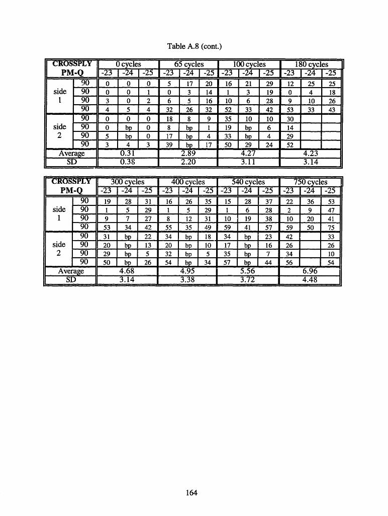
Table A.8 (cont.)
C SSPLY i 0 cycles 1 65 ccles 100 cycles 180 cyclesPM-Q -23 1-24 1-25 -23 1-24 1-25 -23 1-24 1-25 -23 1-24 1-25
90 0 0 0 5 17 20 16 21 29 12 25 25side 90 0 0 1 0 3 14 1 3 19 0 4 181 90 3 0 2 6 5 16 10 6 28 9 10 26
90 4 5 4 32 26 32 52 33 42 53 33 43
90 0 0 0 18 8 9 35 10 10 30side 90 0 bp 0 8 bp 1 19 bp 6 14
2 90 5 bp 0 17 4 33bp 4 2990 3 4 3 39 bp 17 50 29 24 52
Average 0.31 2.89 4.27 4.23SD 0.38 2.20 3.11 3.14
CROSSPL I 300 cycles 400cycles 540 cycles 750 cyclesPM-Q -23 1-24 1-25 -23 1-24 1-25 -23 1-24 1-25 1-23 1-24 1-25
90 19 28 31 16 26 35 15 28 37 22 36 53side 90 1 5 29 1 5 29 1 6 28 2 9 47
1 90 9 7 27 8 12 31 10 19 38 10 20 4190 53 34 42 55 35 49 59 41 57 59 50 7590 31 bp 22 34 bp 18 34 bp 23 42 33
side 90 20 b 13 20 bp 10 17 bp 16 26 262 90 29 bp 5 32 bp 5 35 bp 7 34 10
90 50 26 5 4 b 34 57 b 44 56 54Average 4.68 4.95 5.56 6.96
SD 3.14 3.38 3.72 4.48
164

Table A.9: Accelerated thermal environment 2 (-150°C) damage data (PETI-5)
RESEARCH 0 cycles 80 cycles 1 170 cycles 1 280 cyclesP5-R -26 -271-28 -261-27-28 -261-271-28 -26 1-271 -28
902 2(1) 3(1) 1(1) 3(1) 3(1) 1(1) 3(1) 3(1) lg 3(1) lgside group 1(1)
1 904 0 0 0 0 0 0 0 0 0 0 0group
902 0 l(1) 0 2(1) 2(1) 0 2(1) 4(1) lg 1(1)side group 3(1)
2 904 0 0 0 0 0 0 0 0 0 0group
Group Av. 0.09 0.00 0.00 0.00Group SD 0.00 0.00 0.00 0.00Aggr. Av. 0.00 0.00 0.00 0.00Aggr. SD 0.00 0.00 0.00 0.00
RESEARCH 410 cycles 560 cycles 750 cyclesP5-R -26 -27 1-28 -26 -27 1-28 -26 -271 -28
902 ig 2g ig 2g 2g Ig 3g 2g 2gside group 4(1) 1(1) 1(1) 1 1(1 1(1) 1(1) 2(1)
1 904 0 0 0 0 0 0 0 0 0group
902 ig 2g ig 2g 2g Ig 4g 4g 4gside group 5(1) 3(1) 1(1) 4(1) 3(1) 1(1) 4(1) 2(1) 1(1)2 904 0 0 0 0 0 0 0 0 0
group
Group Av. 0.00 0.00 0.00Group SD 0.00 0.00 0.00Aggr. Av. 0.00 0.00 0.00Aggr. SD 0.00 0.00 0.00
F~~~~~~~F ~ i i i
P5-C and P5-Q all zeros.
165

Table A.10: Accelerated thermal environment 2 (-1500 C) damage data (PIXA-M)
RESEARCH 0cycles 80 cycles 170 cycles I 280 cyclesPMR -27 -28 1-29 -27 1-28 1-29 -271 -28 -29 -27 -28 -29
902 3(1) 0 2(1) lg 1(1) 3(1) lg 4(1) 2g lg 3(1) 3ggroup 12(1) 1(1) 2(1 )
side 904 2(1) 6(1) 2(1) 2(1) 8(1) 4(1) 2(2) 1(3) 5(1) 2(3) 2(3) 9(1)1 group 3(1) 1(2) 7(1) 2(2)------__ 10(1) 9(1)
902 d 0 1(1) d lg lg 6g 3g 6g 7g 6g 7ggroup 1( 3(1 ) 1 2(1) 2(1) 2(1) 1(1)
902 0 3(1) 1(1) 0 Ig Ig ig 2g ig Ig 3g 2ggroup 2(1) 1(1) 1(1) 2(1)
side 904 3(1) 4(1) 2(1) 4(1) 6(1) 7(1) ig 10(1) 3(2) lg 1(2) 2(3)2 group 1(2) 6(1) 3(2) 12(1) 1(2)
3(1) 2(1) 12(1)
902 0 Ig 3(1) 1(1) 2g 5g 6g 5g lOg 6g 9g 12ggroup _ ___- 4(1) 4(1) 6(1) 2(1) 2(1) 1(1)
Group Av. 0.00 0.00 0.03 0.03Group SD 0.00 0.00 0.08 0.08Aggr. Av. 0.62 1.02 2.26 2.72Aggr. SD 0.32 0.44 1.13 0.98
RESEARCH 410 cycles 560 cycles J 750 cyclesPM-R [-27 1 28 -29 1 -271-281-29 -271-28 1 -29
902 3g 2g 4g 4g 4g 7g 4g 8g 10ggroup II | 4(1) 2(1) 5(1) 2(1) 2(1) 4(1) 3(1)
904 2g 2g 1(3) 3g 6g Ig 3g 8g 5gside group 1(3) 3(3) 3(2) 2(2) 1(3) 2(3) 3(2) 1(3) 1(3)
1 i 11 1(2) 3(2) 13(1) 6(1) 3(2) 4(2) 9(1) 5(2) 9(2)7(1) 1 8(1) 1 1 9(1) 1 16(1) 1 9(1) 1 12(1)
902 8g 8g 8g 10g 9g 10lOg 13g 14g 13ggroup 2) 4(1 1) 1 8(1) 2(1) 5(1) 3(1)
902 2g 5g 2g 2g 7g 3g 3g 9g 4ggroup 11 3(1) 2(1) 1(1) 3(1 ) 1(1) 1 (1 ) 1 2(1)
904 2g lg 2g 4g 2g 2g 4g 6g 7gside group 2(3) 1(3) 3(2) 7(1) 4(3) 4(3) 1(3) 3(3) 4(3)
2 4(1) 3(2) 15(1) 6(2) 4(2) 2(2) 11(2) 3(2)
20(1) 23(1) 10(1) 8(1) 16(1) 14(1)902 7g 15g 14g 8g 14g 14g 1 g 16g 18ggroup 6(1) 4(1) 6(1) 5(1) 2(1) 2(1) 4(1) 4(1)
Group Av. 0.30 0.59 1.08Group SD 0.16 0.35 0.37Aggr. Av. 11 3.84 4.66 5.38Aggr. SD 1.41 2.95 2.45
166

Table A. 10 (cont.)
coSPLY les 80 les 170 cyles 280yesPM-C -26 1-27 1-28 -26 -27 -28 -261-27 1-28 -26 1 -27 -28
90 0 0 0 3 d 1 10 10 10 19 22 25
side 1 90 0 3 1 1 6 5 2 13 8 6 16 17
90 1 1 3 1 9 14 3 13 15 6 24 20
90 2 3 0 6 28 48 15 55 71 25 78 100
90 0 0 0 2 0 5 7 9 11 11 6 33side 2 90 0 0 0 2 3 0 2 7 2 5 12 4
90 0 0 1 1 4 1 4 6 1 7 7 1
90 1 1 6 2 9 37 11 20 49 16 36 74
Average 0.19 1.56 2.90 4.68SD 0.29 2.42 3.51 4.99
CROSSPLY 1 410 cyles 560 cycles 750 cyclesPM-C -26 -27 -28 -26 -27 -28 -26 -27 -28
90 29 41 53 51 62 78 57 76 90
side 1 90 11 34 26 16 49 32 25 66 34
90 15 34 35 23 55 38 30 67 46
90 35 99 125 42 113 139 54 121 140
90 20 17 42 34 26 51 45 51 66
side 2 90 7 18 10 10 28 14 10 41 22
90 11 13 5 14 19 7 16 21 8
90 25 54 97 33 70 110, 45 90 130
Average 7.02 9.14 11.08SD 6.12 , 6.81 7.22
167

Table A. 10 (cont.)
2ROSSPLY ! cys 80 cles I 170 c 280PM-Q -26 -27 1-29 -26 -27 -29 -26 -27 1-29 -26 -27 -29
90 0 0 0 0 0 1 1 1 2 1 3 6side 1 90 0 0 0 1 1 2 1 2 3 1 3 5
90 2 2 0 2 2 1 1 3 2 2 4 390 0 0 0 1 0 2 4 4 6 6 6 9
90 0 0 1 0 0 0 0 0 3 1 0 5side 2 90 0 0 0 0 0 0 2 1 4 4 1 5
90 4 1 1 4 1 0 4 2 3 7 3 6
90 2 1 4 4 3 6 8 5 11 13 5 12
Average 0.15 0.25 0.60 0.91SD 0.24 0.32 0.50 0.65
cRtossPLYW l 410 cycles 560 cycles 750 cyclesPM-Q -26 -27 1-29 -26 1-27 1-29 -26 1 -27 1-29
90 2 4 10 5 9 15 7 14 18
side 1 90 2 3 6 5 3 9 6 4 11
90 4 5 8 5 6 11 6 11 17
90 12 15 19 16 22 24 17 33 35
90 2 1 12 4 1 15 9 4 21
side 2 90 4 2 6 7 3 8 10 3 12
90 8 4 9 9 3 11 10 6 15
90 17 14 23 20 16 25 34 21 34
Average 1.57 2.07 2.94SD 1.20 1.39 1.99
168

Table A. 11: Accelerated thermal environment 1 damage data (PETI-5 isothermalspecimens)
RESEARCHII O cycles 50 cycles 150 cycles 1 300 clesP5-R -43 -44 1 -45 -43 -44 -45 -43 1-44 1 -45 -43 -44 -45
side 904 0 Ig 0 2(2) 0 0 2(2) 5(1) 1(1) 1(3) 5(1) 1(1)
1 group 2(1) 4(1) 1(2)6(1)
side 904 0 0 0 0 i(2) 0 2(1) 1(3) 2(1) 3(1) lg 3(1)2 group _- -Group Av. 0.00 0.00 0.00 0.00 0.03Group SD 0.00 0.00 0.00 0.08Aggr. Av. 0.13 0.26 0.33 ' _ 0.89Aggr. SD 0.32 0.48 0.63 0.68
RESEARCH I 400 cyclesPS-R -43 -44 -45
side 904 ig 1(2) 1(1)1 group 1(2) 3(1)
6(1)
side 904 6(1) ig 3(1)2 groupGroup Av. 0.07Group SD 0.10Aggr. Av. 1.02Aggr. SD 0.74
169

Table A. 11 (cont.)
CROSSPLY [L 0 cycles 50cycles 1 150 cyces 300 cyclesP5-C -34 -35 1-36 --34 1-35 1-36 -34 1-35 1-36 1-34 1-35 1-36
90 o 0 0 0 0 0 4 1 0 5 0 0side 1 90 0 0 0 0 0 0 0 0 0 0 0
90 o o o 0 o o 1 0 0 0 0 090 d d d d d d d d d d d d90 0 0 0 0 0 0 3 0 1 2 0 0
side 2 90 o o o 1 0 0 1 0 0 1 0 090 0 0 0 2 0 0 3 1 0 3 2 090 d d d d d d d d d d d d
Average 0.00 0.02 0.12 0.11SD 0.00 0.09 0.22 0.22
CIOSSPLY 400 cyclesP5-C -34 -35 1-36
90 4 0 0side 90 0 0 0
90 1 0 0
90 d d d90 2 0 3
side2 90 1 o o90 5 1 090 d d d
Average 0.17SD 0.28
170

Table A. 11 (cont.)
QUASI 0 cles 1 50 cles 1 150 cles 1 300 clesP5-Q -36 -37 1-38 -36 1-37 1-38 -36 1-37 1-38 -36 1-37 1-38
90 0 0 0 1 0 1 0 0 1 0 0 2side 1 90 0 o o o o o o o o o o o
90 o 0 o o 1 o o 2 o o 2 o90 0 d 0 0 d 0 0 d 0 0 d 190 0 0 0 0 1 1 0 3 0 0 3 0
side 2 90 0 0 0 0 0 0 0 2 0 0 1 090 0 0 0 0 o 0 0 0 0 0 0 090 o o 0 1 o 0 1 2 o 1 5 0
Average 0.00 0.05 0.09 0.12SD 0.00 0.09 0.17 0.24
QUASI H 400 cyclesP5-Q 36 -37 1-38
90 3 0 4
side 1 90 0 o o90 0 0 290 1 d 1
90 0 3 1
side 2 90 0 2 090 0 0 090 1 d 2
Average - 0.12SD 0.24
171

Table A.12: Accelerated thermal environment 1 damage data (PIXA-M isothermalspecimens)
RESEARCH Ocycles 50 es 150c cls 300 cyclesPM-R -33 -34 -33 -34 -35 -33 -34 -35 -33 -34 -35
35side 904 0 1(2) 0 7(1) 1(2) 4(1) 12(1) 1(2) 1(2) 14(1) 1(3) 1(2)
1 group 4(1) 11(1) 13(1) 8(1) 26(1) 10(1)
side 904 1(1) 0 0 6(1) 5(1) 3(1) 11(1) 10(1) 6(1) 1(2) 1(2) 1(2)2 group 14(1) 18(1) 81
Group Avg. 0.00 0.00 0.00 0.00Group SD 0.00 0.00 0.00 0.00Aggr. Avg. 0.23 1.25 2.10 3.31Aggr. SD 0.47 0.70 0.58 1.35
RESEARCH 400 cyclesPM-R -33 -34 1 -35
side 904 2(2) 2(3) 2(3)1 group 19(1) 1(2) 8(1)
23(1)
side 904 Ig 6(2) lg2 group 1(2) 26(1) 1(2)
14(1) 7(1)
Group Avg. 0.07Group SD 0.10Aggr. Avg. 4.56Aggr. SD 1.93
172

Table A. 12 (cont.)
CROSSPLY cyc les 50 cycles 150 cycles 300 cyclesPM-C -33 -34 -34 5 1-33 -34 -35 -- 33 1-34 -35
90 0 1 7 7 18 21 19 46 24 24 53 27side 1 90 0 1 1 6 4 10 13 8 11 15 10 9
90 1 1 1 6 4 4 7 6 5 8 6 590 4 10 4 16 33 18 44 57 37 57 78 36
90 2 2 4 9 16 15 26 34 24 34 30 23side 2 90 0 1 3 4 6 5 9 15 7 10 12 7
90 3 1 0 4 2 0 7 4 3 9 3 590 12 4 3 32 27 22 62 62 52 82 43 47
Average 0.54 2.37 4.77 5.19SD 0.61 1.89 3.93 4.56
CROSSPLY 400 cyclesPM-C 33 -34 1 -35
90 37 62 41side 1 90 15 9 16
90 9 6 890 73 75 50
90 45 53 41side 2 90 13 22 13
90 10 6 10
90 93 72 78Average 7.38
SD 5.50
173

Table A. 12 (cont.)
QUASI 0 cycles 50 cycles 150 cycles 300 cyclesPM-Q -34 -35 -X1 -34 -Xl -35 4 1-35 -Xl
90 0 1 0 2 3 0 2 4 1 2 5 3side 1 90 1 1 1 1 1 0 1 3 3 2 8 3
90 1 3 1 4 7 2 7 16 6 7 15 11
90 0 3 1 4 5 4 7 16 9 9 16 1490 2 0 2 3 1 1 4 1 3 4 1 6
side 2 90 o 1 0 3 1 1 3 1 4 4 4 5
90 1 0 4 5 0 5 6 2 7 6 2 890 0 2 3 2 2 14 4 7 24 5 12 28
Average 0.23 0.58 1.16 1.48SD 0.23 0.59 1.10 1.20
QUASI 400 cyclesPM-Q -34 -35 -X
90 5 14 6side 1 90 4 18 6
90 11 28 16
90 12 24 31
90 7 4 6side 2 90 4 4 7
90 7 4 1790 14 15 32
Average 2.15SD 1 1.74
174

APPENDIX B
STAGE I TESTING EDGE DAMAGE DATA
Material Layup Ply Group Crack density (/cm) at number of cycles shown25 i 50 100 200 _ 500 ! 1000
R1-16 Quasi 902 0 - 0 0.4 0.4 9.4
Rl-16 [03/903]s 906 0.4 - 15.7 9.4 9.4 13
Rl-16 [+45/ 902 0 - 18.5 9.8 15.7 33.5
-452/+45/04/
90]s
R1-16 [+45/ avg. 90's 0 - 0 1.4 0.8 21.3
-45/02/90/02/
-45/+45]s
PETI-5 Quasi 902 0 0 0 0.4 0.8 5.1
PETI-5 [0/90/012S avg. 90's 0 0 0 0 0 0.4
PETI-5 [+45/ 902 0 0 2.8 2.4 8.3 18.1
-452/+45/04/
90]s
PETI-5 [+45/ avg. 90's 0 0 0 3.0 16.1 17.3
-45/02/90/02/
-45/+45],
K3B [+45/ 902 1.9 1.9 0.8 1.57 12.2 12.2
-45/90/014s
PIXA [0/90/012s avg. 90's 0.6 7.1 4.4 0 0.6 1.0__________________________________ ___ ImI_ _
175

APPENDIX C
CRACKOMATIC & MODCOD INPUTS
C.1 CRACKOMATIC INPUTS (PETI-5 & PIXA-M)
E, longitudinal ply modulus (157.3 GPa)
Ey transverse ply modulus (9.7 GPa)
v major Poisson's ratio (0.33)
Gxy shear modulus (4.20 GPa)
al longitudinal ply CTE (-0.7 ,g/K)
a 2 transverse ply CTE (36.9 ge/K)
To laminate stress free temperature (400°C)
shear lag factor (0.6)
C.2 MODCOD INPUTS (based on PETI-5 data)
t ply thickness (0.125 mm)
Di moisture diffusivity (1.108 mm2/s)
Temperature Profile Description (time, temperature, RH)
176

THESIS PROCESSING SLIP
FIXED FIELD: ill.
index
, COPIE: rrcv;)(!3Lindgren Music
TITLE VARIES: E
Dewey E
Rotch Sc
name
biblio
!ng Hum
:ience
NAME VARIES: 4"j
IMPRINT: (COPYRIGHT)
COLLATION: /76 -
,ADD: DEGREE: , DEPT.:
SUPERVISORS:
NOTES:
cat'r: date:page:
pDEPT: r1,S35,YEAR: KJ9& "DEGREE:
NAME:1EY1Vo/DH%2 TC-e 6 C4 C'-
I


![Accelerated Degradation Tests Planning With Competing ... · accelerated tests. Bai and Chun [13] discussed the optimal simple step-stress ALT (SSALT) plans with independent competing](https://img.pdfslide.us/doc/110x75/5ec5928fa51e9b1376067df5/accelerated-degradation-tests-planning-with-competing-accelerated-tests-bai.jpg)