Embed Size (px)
Citation preview
ACCELERATED COMPOSITE DISTRIBUTION FUNCTION METHODS FOR COMPUTATIONAL FLUID DYNAMICS USING GPU
Prof. Matthew Smith, Yen-Chih Chen
Mechanical Engineering, NCKU
MOTIVATION
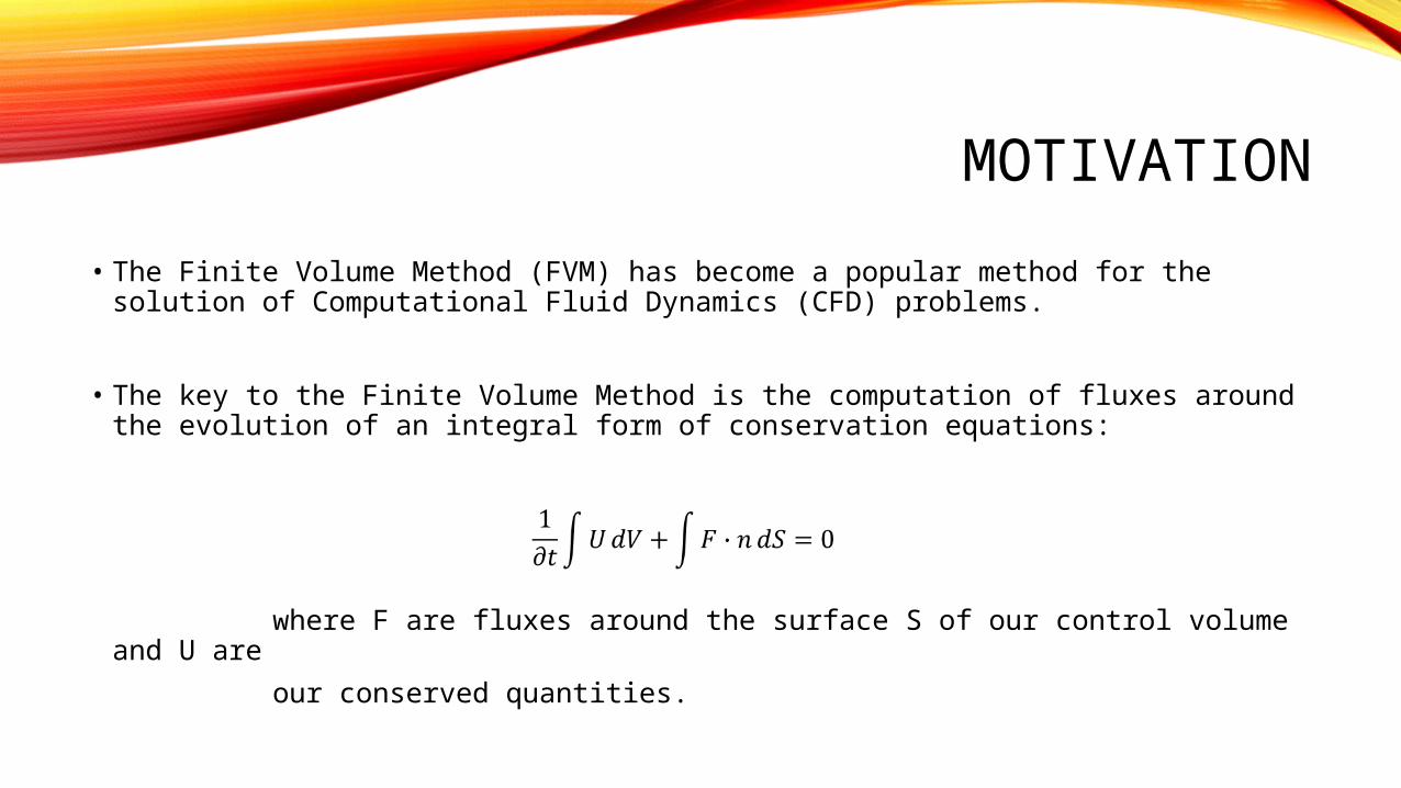
• The Finite Volume Method (FVM) has become a popular method for the solution of Computational Fluid Dynamics (CFD) problems.
• The key to the Finite Volume Method is the computation of fluxes around the evolution of an integral form of conservation equations:
where F are fluxes around the surface S of our control volume and U are
our conserved quantities.

MOTIVATION
• By introducing the average value of U over the cell volume:
• We can reformulate the governing equations as:
• For a simple 1D problem on a regular spaced grid, we might discretize this in the explicit form:

MOTIVATION
• The fundamental problem is the computation of the fluxes across each cell surface, in this case and .
• There are a large number of approaches available for the computation of these fluxes:
• Exact or approximate Riemann solvers,
• Integral Balance techniques,
• Algebraic techniques, etc.
MOTIVATION
• Regardless of the method, there are several challenges to the use of the FVM in real-life problems:
• The scheme must possess a suitably small amount of numerical (artificial) dissipation such that the physical dissipation present (if any) is correctly captured.
• The solution itself must lend itself to the application – in many real-life multi-scale applications, the scale of the problem is very large.
Hence (i) knowledge of the dissipative qualities of the solver must be understood, and
(ii) the computational complexity cannot be too great to prohibit practical application.

PARALLEL AND GPU COMPUTING
• Due to these restrictions, many real-life applications require parallel computing to obtain a solution in a realistic amount of time.
• Nowadays, there are a large number of architecture options available for researchers and engineers whom need to perform parallel computation:
(For connecting these devices)
PARALLEL AND GPU COMPUTING
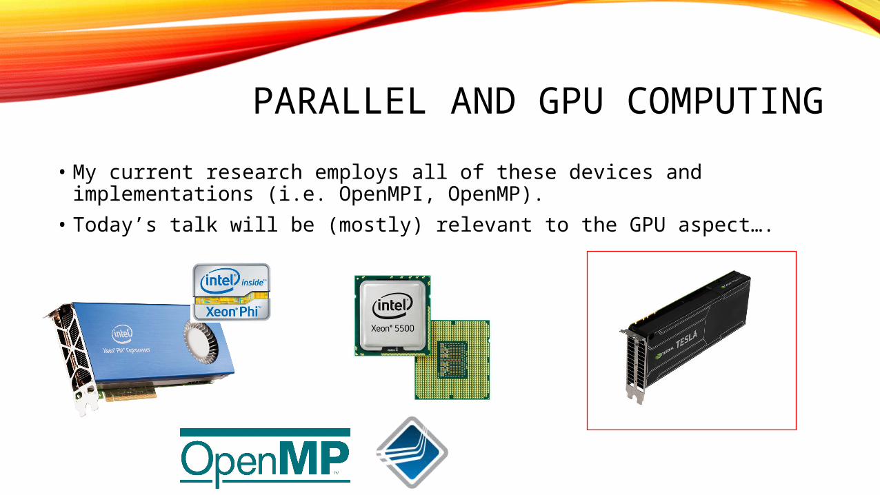
• My current research employs all of these devices and implementations (i.e. OpenMPI, OpenMP).
• Today’s talk will be (mostly) relevant to the GPU aspect….
PARALLEL AND GPU COMPUTING
• The GPU device does provide an attractive architecture for the parallel computation of FVM CFD applications.
• It’s (now semi) unique architecture provides us with additional “restraints”, however, to our Finite Volume Method approach
– I won’t cover these restraints here in the hope that someone with more time will talk about them.
• We will revisit this idea, however, in upcoming slides.

VECTOR SPLIT FVM COMPUTATION
• One particular approach which is very well suited to GPU computation is the vector splitting of the fluxes at cell surfaces, for example:
• The high degree of locality of these schemes results in an increased capacity to take advantage of vectorization – this is good for every parallel architecture.
• A very large family of these methods exist:• Mach Number split solvers (i.e. van Leer, (S)HLL, AUSM to name a few)• Kinetic theory based splitting (EFM / KFVS, EIM, TDEFM, UEFM to name a few)
VECTOR SPLIT FVM COMPUTATION
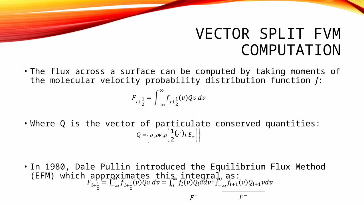
• The flux across a surface can be computed by taking moments of the molecular velocity probability distribution function f:
• Where Q is the vector of particulate conserved quantities:
• In 1980, Dale Pullin introduced the Equilibrium Flux Method (EFM) which approximates this integral as:
inEvvQ 2
2
1,,
VECTOR SPLIT FVM COMPUTATION
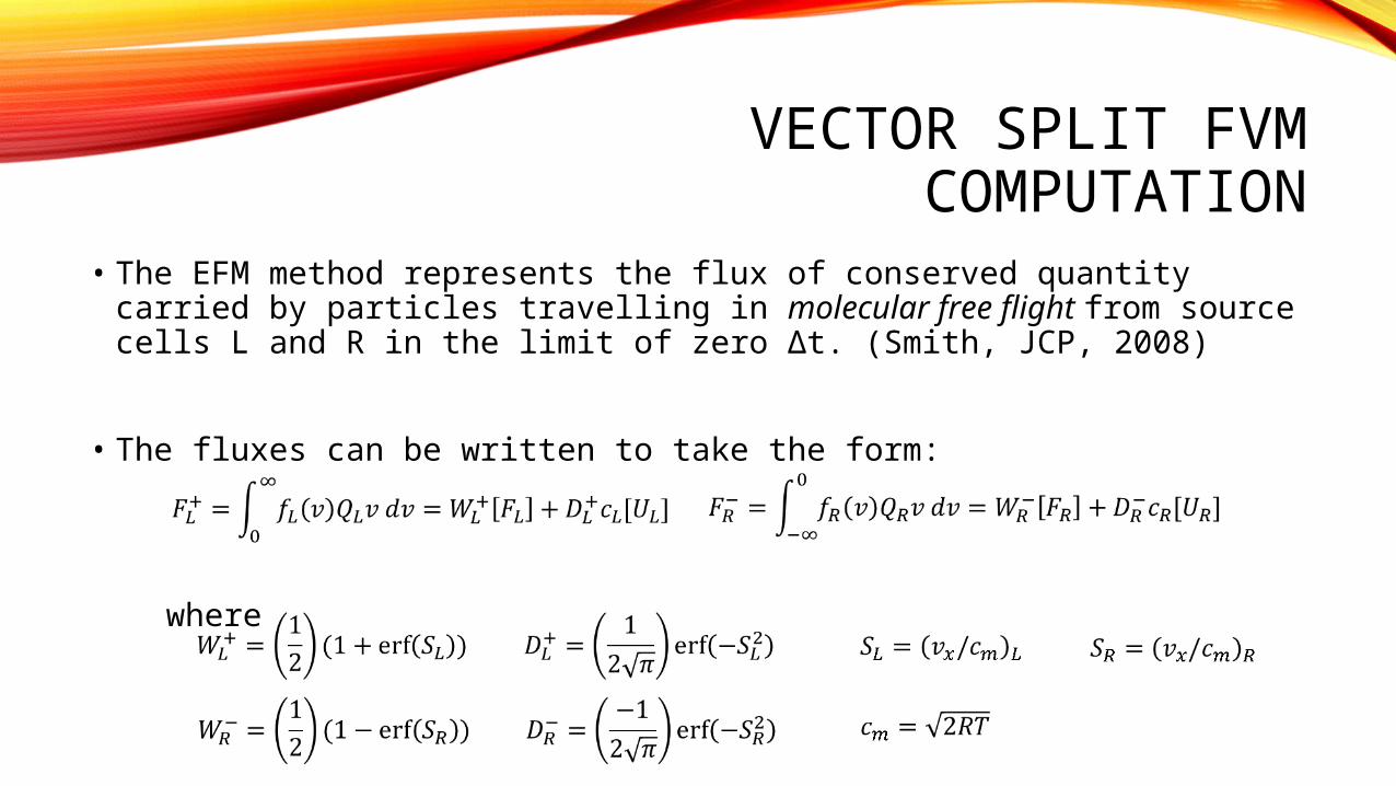
• The EFM method represents the flux of conserved quantity carried by particles travelling in molecular free flight from source cells L and R in the limit of zero Δt. (Smith, JCP, 2008)
• The fluxes can be written to take the form:
where
VECTOR SPLIT FVM COMPUTATION
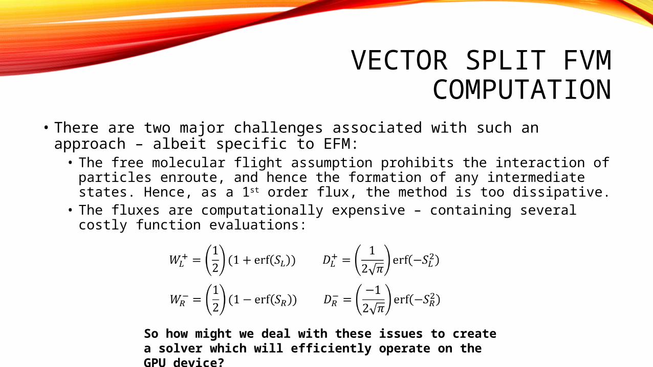
• There are two major challenges associated with such an approach – albeit specific to EFM:• The free molecular flight assumption prohibits the interaction of particles
enroute, and hence the formation of any intermediate states. Hence, as a 1st order flux, the method is too dissipative.
• The fluxes are computationally expensive – containing several costly function evaluations:
So how might we deal with these issues to create a solver which will efficiently operate on the GPU device?
QDS
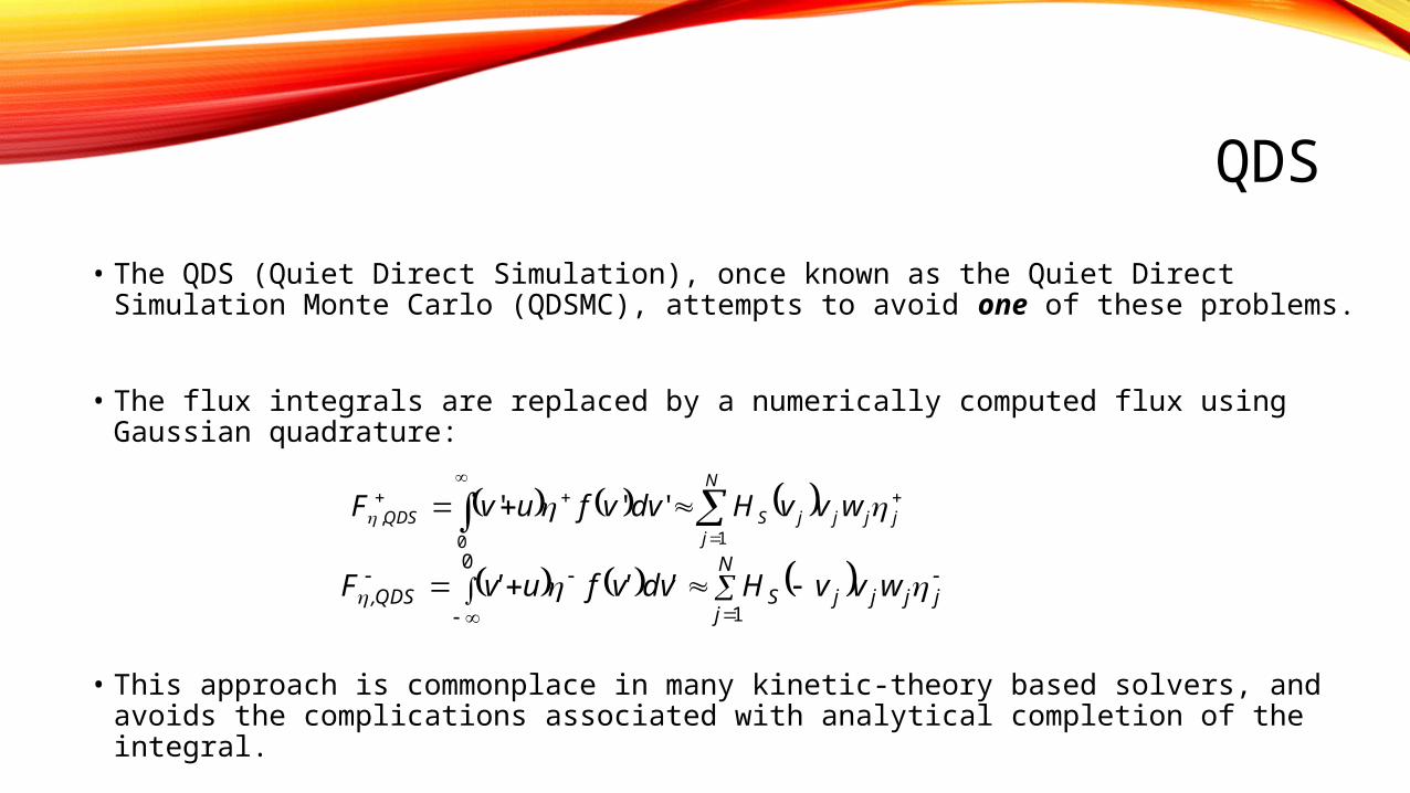
• The QDS (Quiet Direct Simulation), once known as the Quiet Direct Simulation Monte Carlo (QDSMC), attempts to avoid one of these problems.
• The flux integrals are replaced by a numerically computed flux using Gaussian quadrature:
• This approach is commonplace in many kinetic-theory based solvers, and avoids the complications associated with analytical completion of the integral.
N
jjjjjSQDS wvvHdvvfuvF
10
, '''
N
jjjjjSQDS, wvvH'dv'vfu'vF
1
0

QDS
• Together with Fang-An Kuo (who will speak later in the week) his supervisor (Prof. J.-S. Wu), we extended the method to higher order accuracy and applied it to multiple GPU computation:

NUMERICAL DISSIPATION
• However, despite the success of the QDS method, there were still several issues:
• A finite number of discrete “ordinates” (velocities) resulted in an error in the thermal (diffusive) flux, causing problems in regions where this is important.
• The basic numerical dissipation present in EFM, while modified as a result of the velocity discretization, is still very much present.
• A good starting point might be to quantify the numerical dissipation present in the EFM method.

NUMERICAL DISSIPATION
• A flux commonly used in FVM CFD for over 50 years is the “Rusanov Flux”
where alpha (in this case) is a characteristic speed associated with the system.
• One attractive feature of this form is that – through direct discretization of the governing equations and substitution, we can show that we are calculating:
Sub in
Re-arrange
NUMERICAL DISSIPATION
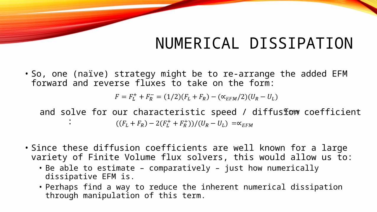
• So, one (naïve) strategy might be to re-arrange the added EFM forward and reverse fluxes to take on the form:
and solve for our characteristic speed / diffusion coefficient :
• Since these diffusion coefficients are well known for a large variety of Finite Volume flux solvers, this would allow us to:• Be able to estimate – comparatively – just how numerically dissipative EFM is.• Perhaps find a way to reduce the inherent numerical dissipation through
manipulation of this term.
NUMERICAL DISSIPATION
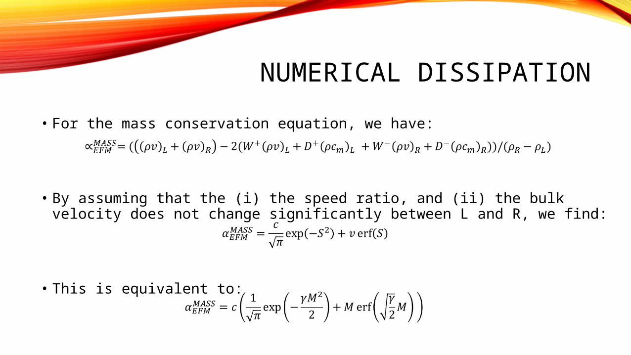
• For the mass conservation equation, we have:
• By assuming that the (i) the speed ratio, and (ii) the bulk velocity does not change significantly between L and R, we find:
• This is equivalent to:
NUMERICAL DISSIPATION
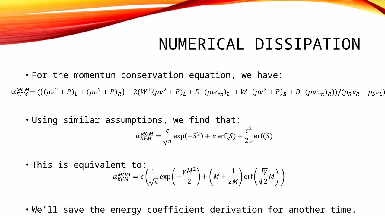
• For the momentum conservation equation, we have:
• Using similar assumptions, we find that:
• This is equivalent to:
• We’ll save the energy coefficient derivation for another time.
NUMERICAL DISSIPATION
• We’ve determined that the numerical dissipation for EFM is:
• Closely coupled with Δx,
• A strong function of the Mach number.
• We can use this result as a benchmark for the next step.
• Instead of using a finite set of discrete velocities for the approximation of the integral itself, we can use a finite set of continuous distribution functions which can approximate our original function and add the discrete fluxes.
UEFM AND TEFM
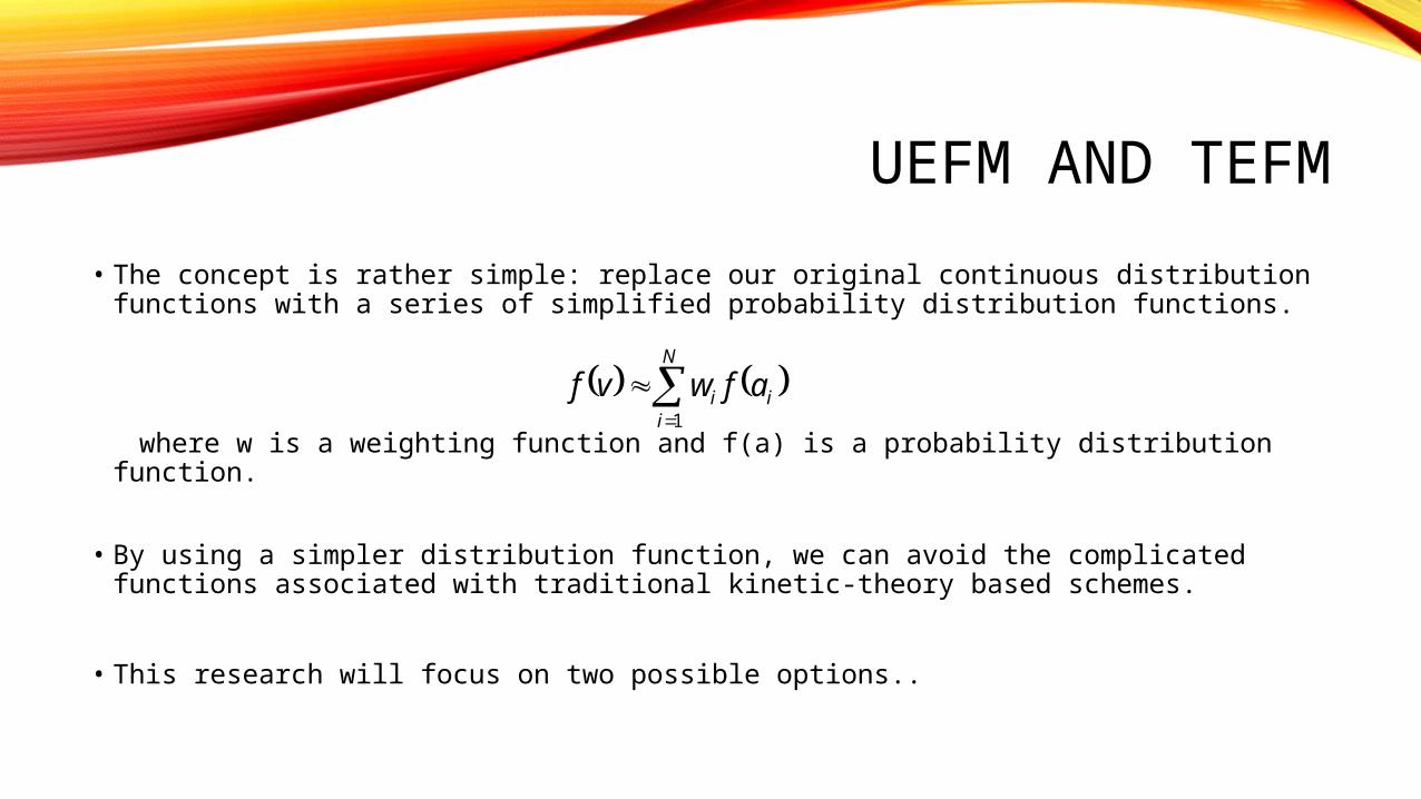
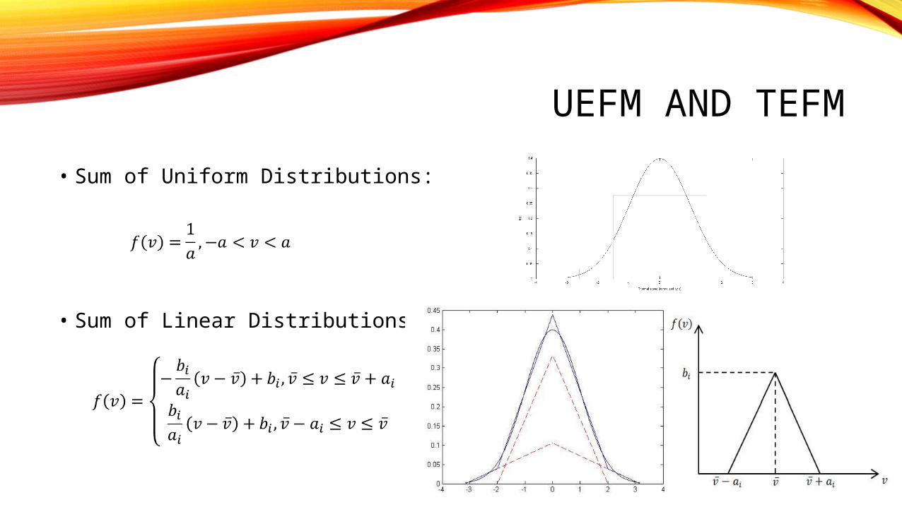
• The concept is rather simple: replace our original continuous distribution functions with a series of simplified probability distribution functions.
where w is a weighting function and f(a) is a probability distribution function.
• By using a simpler distribution function, we can avoid the complicated functions associated with traditional kinetic-theory based schemes.
• This research will focus on two possible options..
N
iii afwvf
1
UEFM AND TEFM
• Sum of Uniform Distributions:
• Sum of Linear Distributions:
UEFM AND TEFM
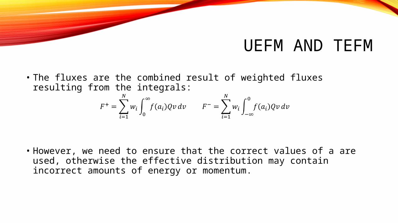
• The fluxes are the combined result of weighted fluxes resulting from the integrals:
• However, we need to ensure that the correct values of a are used, otherwise the effective distribution may contain incorrect amounts of energy or momentum.
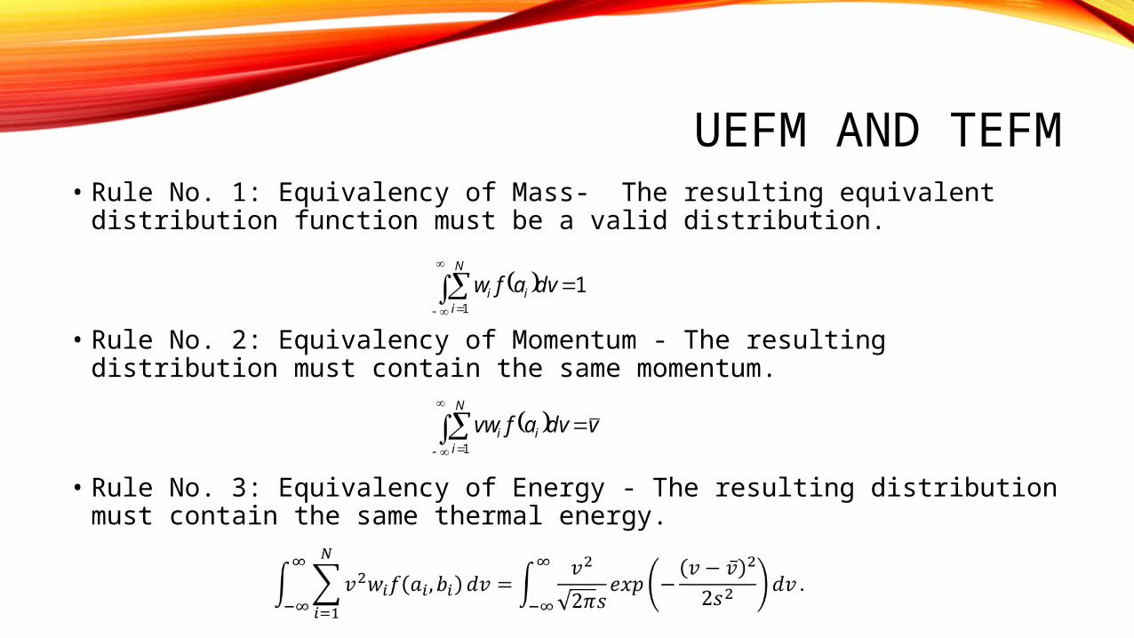
UEFM AND TEFM• Rule No. 1: Equivalency of Mass- The resulting equivalent distribution
function must be a valid distribution.
• Rule No. 2: Equivalency of Momentum - The resulting distribution must contain the same momentum.
• Rule No. 3: Equivalency of Energy - The resulting distribution must contain the same thermal energy.
11
dvafwN
iii
vdvafvwN
iii
1
UEFM AND TEFM
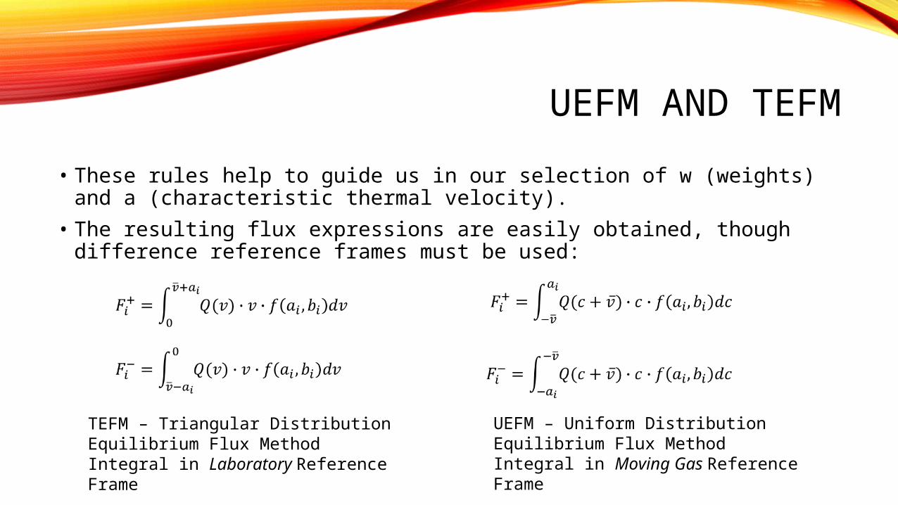
• These rules help to guide us in our selection of w (weights) and a (characteristic thermal velocity).
• The resulting flux expressions are easily obtained, though difference reference frames must be used:
TEFM – Triangular Distribution Equilibrium Flux MethodIntegral in Laboratory Reference Frame
UEFM – Uniform Distribution Equilibrium Flux MethodIntegral in Moving Gas Reference Frame

UEFM AND TEFM
• The resulting flux expressions are as we expected – lacking of complex exp() and erf() functions. The 1D forward fluxes are (for each distribution):
i
iini
i
i
i
iii a
vaEva
a
va
a
vvawF
16
4
624
2232
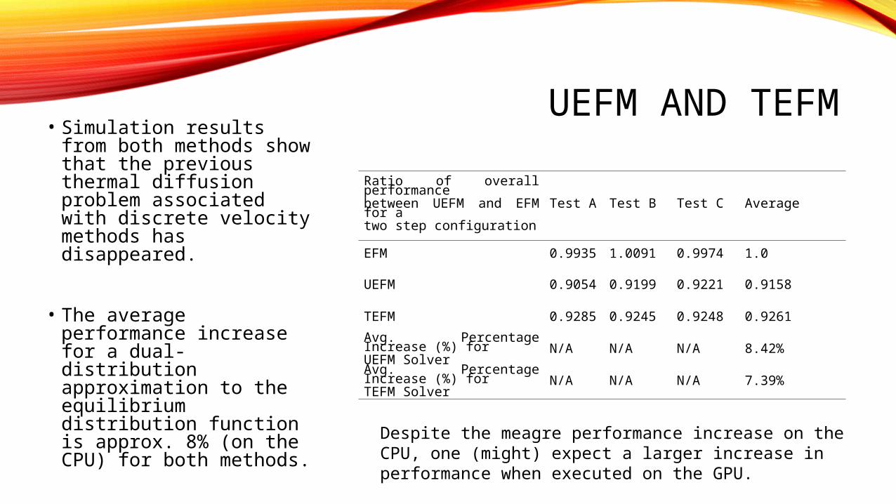
UEFM AND TEFM• Simulation results from
both methods show that the previous thermal diffusion problem associated with discrete velocity methods has disappeared.
• The average performance increase for a dual-distribution approximation to the equilibrium distribution function is approx. 8% (on the CPU) for both methods.
Ratio of overall performancebetween UEFM and EFM for a two step configuration
Test A Test B Test C Average
EFM 0.9935 1.0091 0.9974 1.0
UEFM 0.9054 0.9199 0.9221 0.9158
TEFM 0.9285 0.9245 0.9248 0.9261
Avg. Percentage Increase (%) for UEFM Solver N/A N/A N/A 8.42%
Avg. Percentage Increase (%) for TEFM Solver N/A N/A N/A 7.39%
Despite the meagre performance increase on the CPU, one (might) expect a larger increase in performance when executed on the GPU.

UEFM AND TEFM• 1D Shock Tube results – UEFM
• The kink present in the QDS result has disappeared (as per our goal).
• However, there is additional numerical dissipation present, especially in the contact surface.
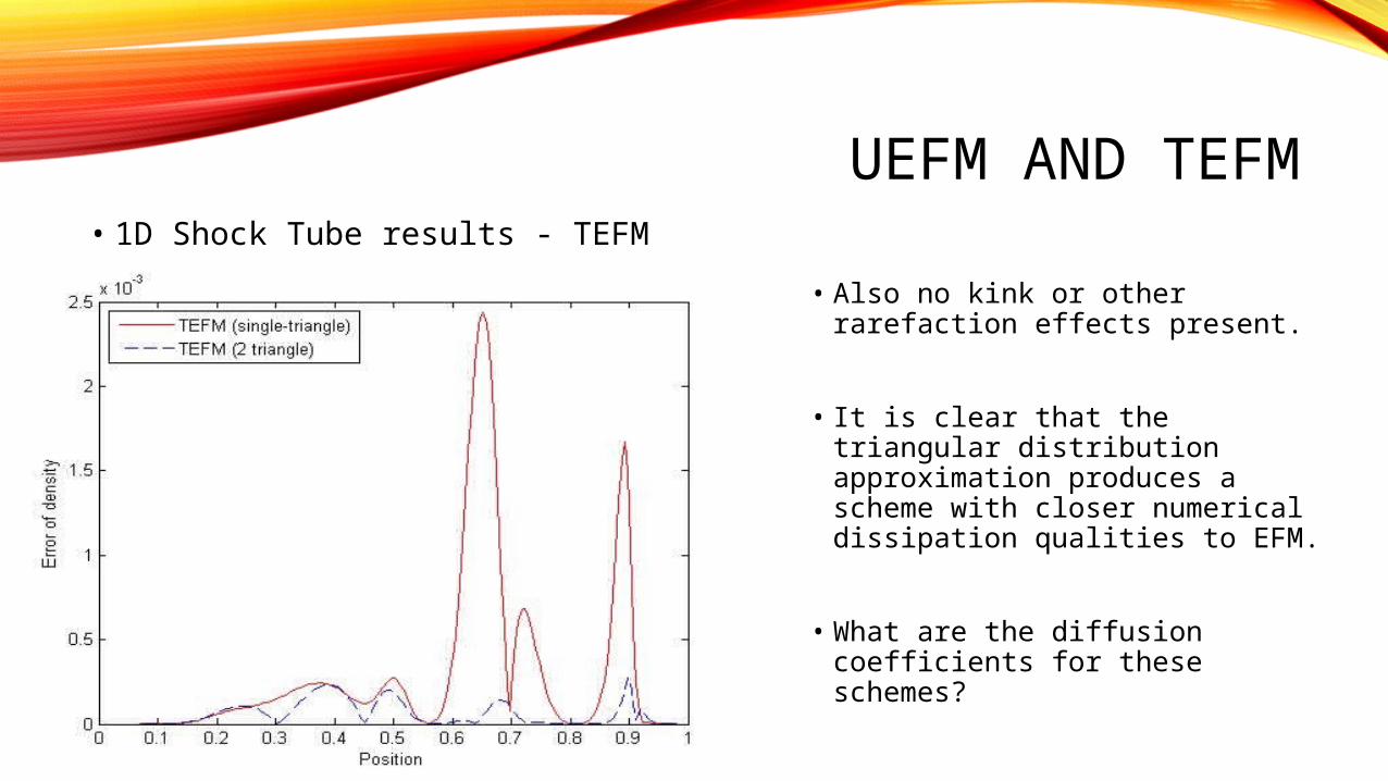
UEFM AND TEFM• 1D Shock Tube results - TEFM
• Also no kink or other rarefaction effects present.
• It is clear that the triangular distribution approximation produces a scheme with closer numerical dissipation qualities to EFM.
• What are the diffusion coefficients for these schemes?
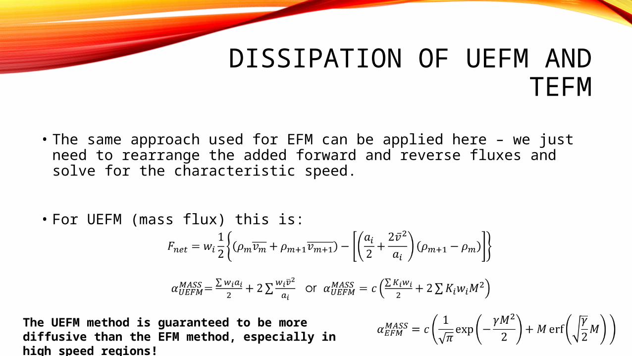
DISSIPATION OF UEFM AND TEFM
• The same approach used for EFM can be applied here – we just need to rearrange the added forward and reverse fluxes and solve for the characteristic speed.
• For UEFM (mass flux) this is:
The UEFM method is guaranteed to be more diffusive than the EFM method, especially in high speed regions!
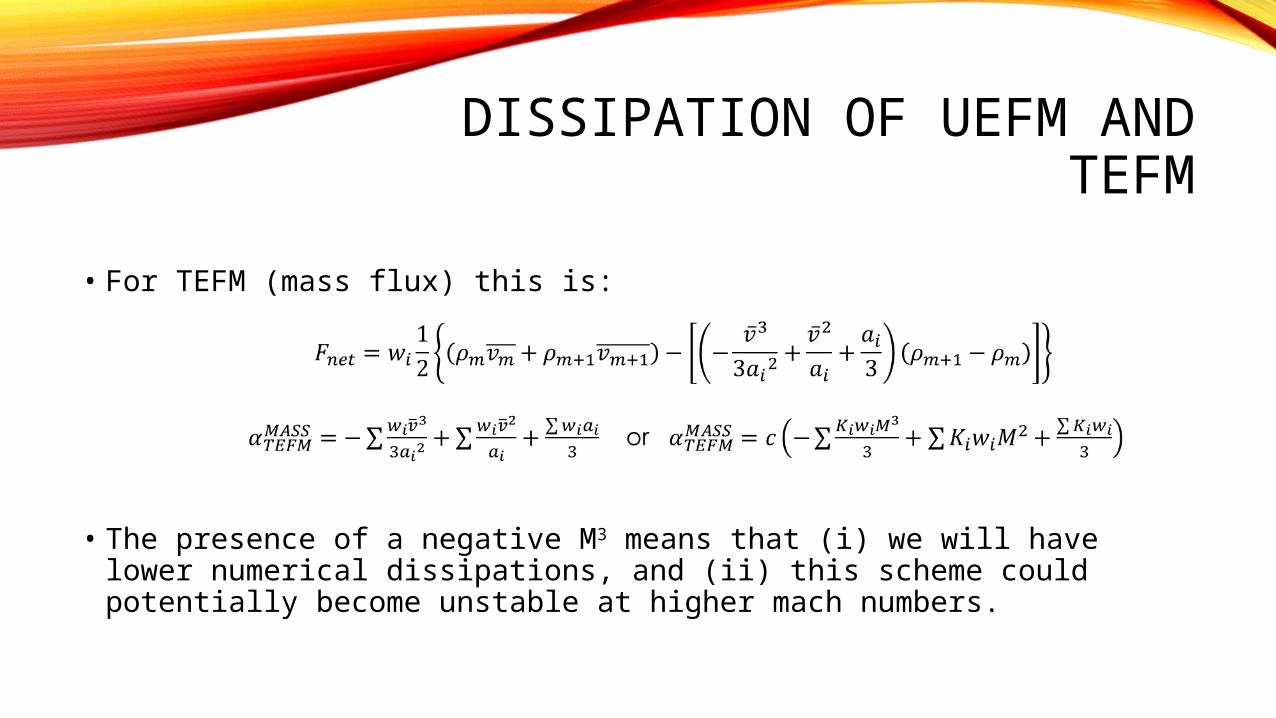
DISSIPATION OF UEFM AND TEFM
• For TEFM (mass flux) this is:
• The presence of a negative M3 means that (i) we will have lower numerical dissipations, and (ii) this scheme could potentially become unstable at higher mach numbers.

DISSIPATION OF UEFM AND TEFM
• Without any modification, the UEFM solver has a lower dissipation that EFM.
• This is more than likely due to the reduced tail of the velocity probability distribution function.
• But do we have stability at higher mach numbers?

DISSIPATION OF UEFM AND TEFM
• We can test this out – high speed shock – bubble interaction.
• We can employ a higher order scheme through expansion each flux component:
DISSIPATION OF UEFM AND TEFM
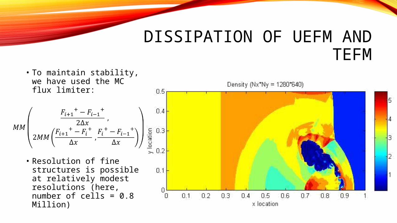
• To maintain stability, we have used the MC flux limiter:
• Resolution of fine structures is possible at relatively modest resolutions (here, number of cells = 0.8 Million)
DISSIPATION OF UEFM AND TEFM
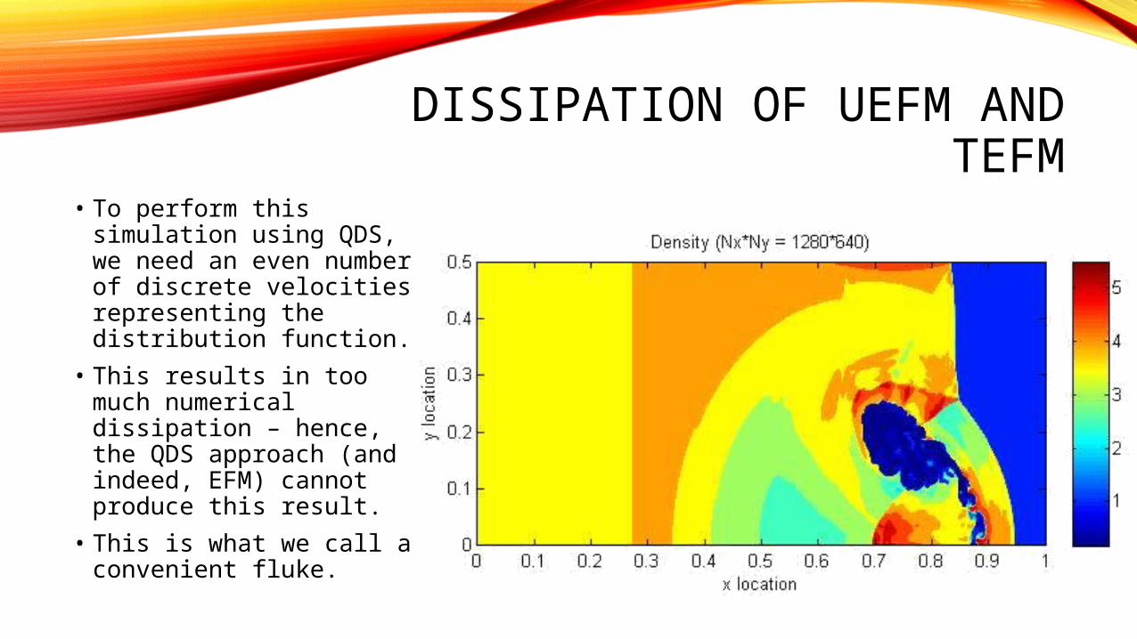
• To perform this simulation using QDS, we need an even number of discrete velocities representing the distribution function.
• This results in too much numerical dissipation – hence, the QDS approach (and indeed, EFM) cannot produce this result.
• This is what we call a convenient fluke.
GPU PERFORMANCE (STRUCTURED)
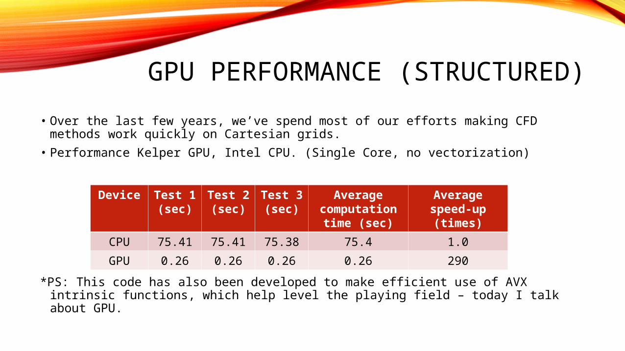
• Over the last few years, we’ve spend most of our efforts making CFD methods work quickly on Cartesian grids.
• Performance Kelper GPU, Intel CPU. (Single Core, no vectorization)
*PS: This code has also been developed to make efficient use of AVX intrinsic functions, which help level the playing field – today I talk about GPU.
Device Test 1(sec)
Test 2(sec)
Test 3(sec)
Average computation
time (sec)
Average speed-up (times)
CPU 75.41 75.41 75.38 75.4 1.0
GPU 0.26 0.26 0.26 0.26 290
APPLICATION
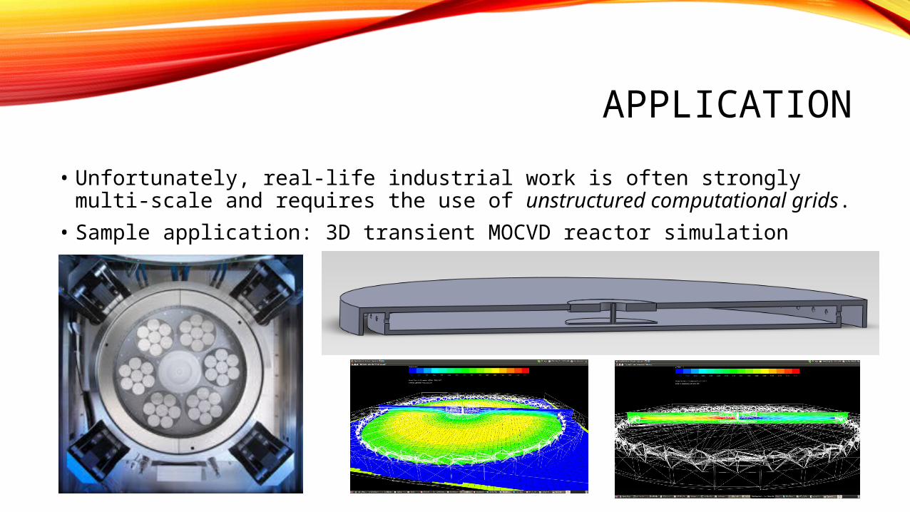
• Unfortunately, real-life industrial work is often strongly multi-scale and requires the use of unstructured computational grids.
• Sample application: 3D transient MOCVD reactor simulation
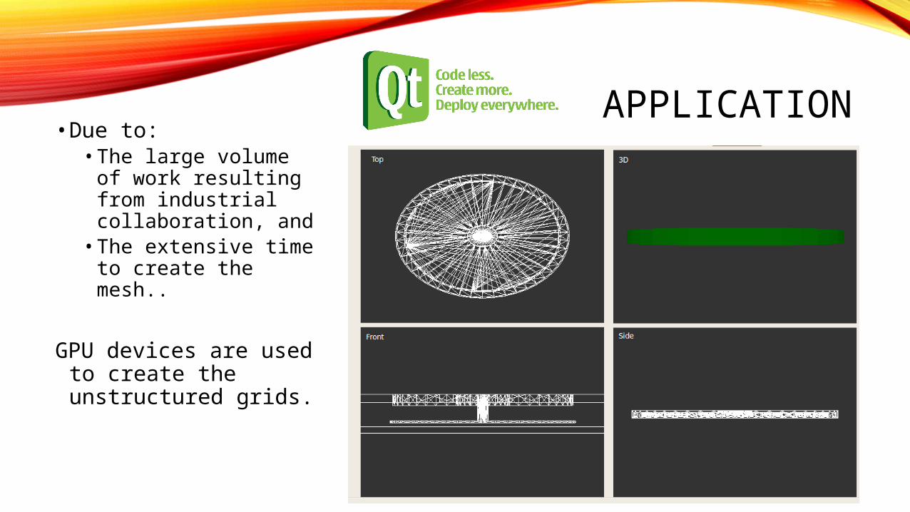
APPLICATION• Due to:• The large volume of
work resulting from industrial collaboration, and• The extensive time
to create the mesh..
GPU devices are used to create the unstructured grids.
GPU
Calc_Intercept GPU Kernel
CPU
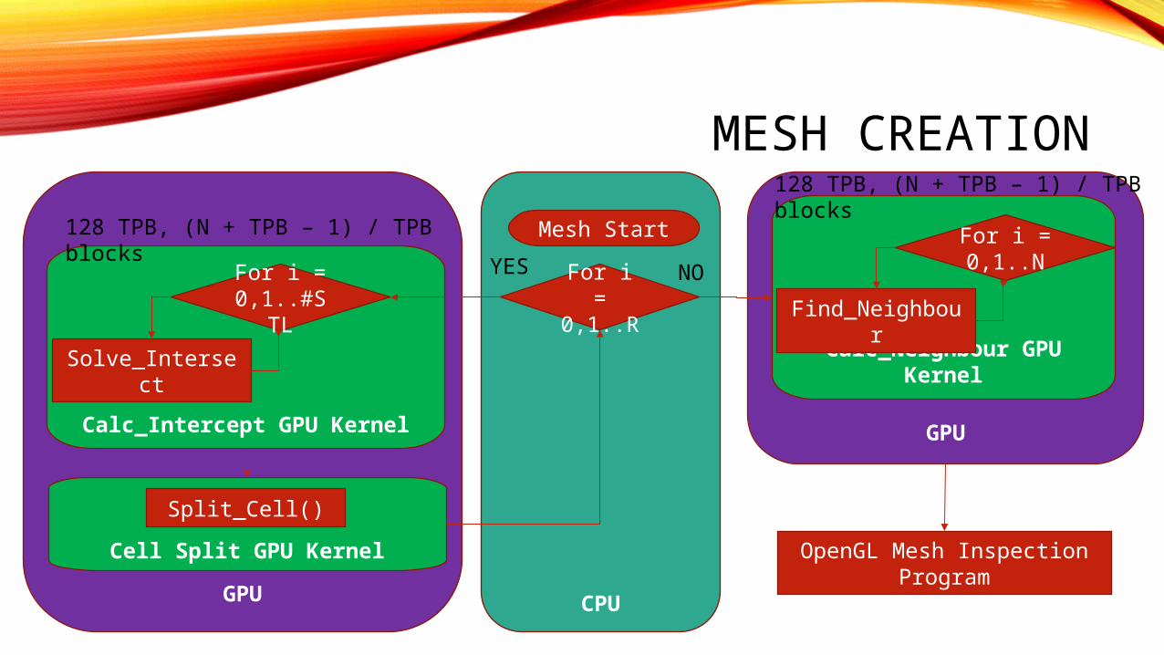
MESH CREATION
Mesh Start
For i = 0,1..R
For i = 0,1..#S
TL
Solve_Intersect
128 TPB, (N + TPB – 1) / TPB blocks
Cell Split GPU Kernel
Split_Cell()
GPU
Calc_Neighbour GPU Kernel
For i = 0,1..N
Find_Neighbour
YES NO
128 TPB, (N + TPB – 1) / TPB blocks
OpenGL Mesh Inspection Program
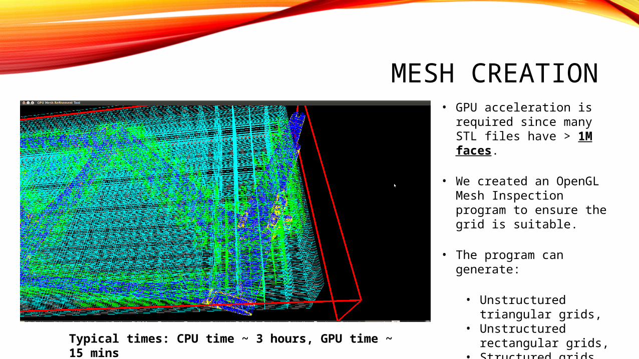
MESH CREATION• GPU acceleration is
required since many STL files have > 1M faces.
• We created an OpenGL Mesh Inspection program to ensure the grid is suitable.
• The program can generate:
• Unstructured triangular grids,
• Unstructured rectangular grids,
• Structured grids.Typical times: CPU time ~ 3 hours, GPU time ~ 15 mins
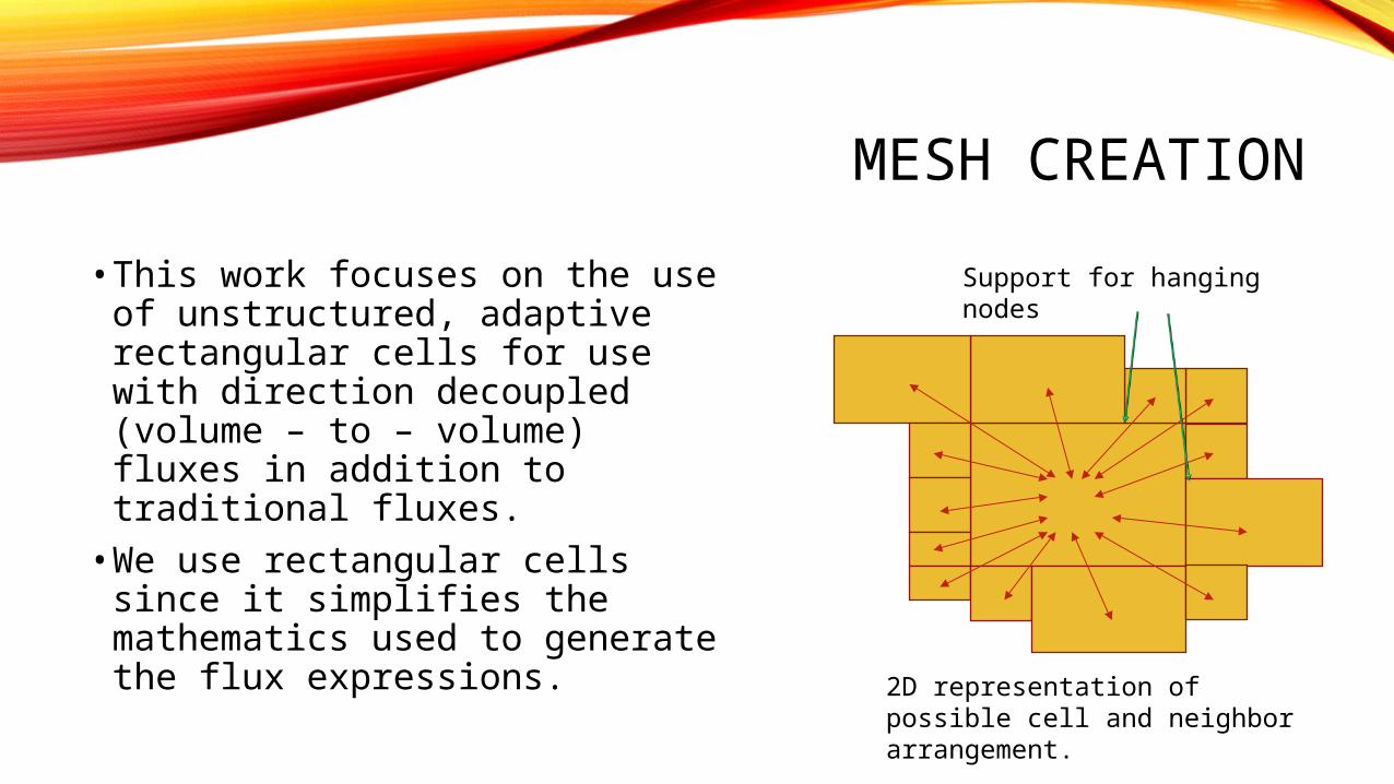
MESH CREATION
• This work focuses on the use of unstructured, adaptive rectangular cells for use with direction decoupled (volume – to – volume) fluxes in addition to traditional fluxes.• We use rectangular cells since
it simplifies the mathematics used to generate the flux expressions. 2D representation of possible
cell and neighbor arrangement.
Support for hanging nodes
SOLVER
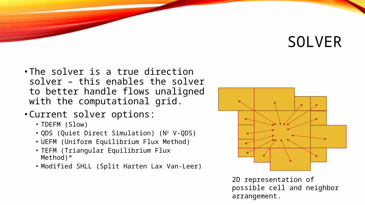
• The solver is a true direction solver – this enables the solver to better handle flows unaligned with the computational grid.• Current solver options:
• TDEFM (Slow)• QDS (Quiet Direct Simulation) (N2 V-QDS)• UEFM (Uniform Equilibrium Flux Method)• TEFM (Triangular Equilibrium Flux
Method)*• Modified SHLL (Split Harten Lax Van-Leer) 2D representation of possible
cell and neighbor arrangement.
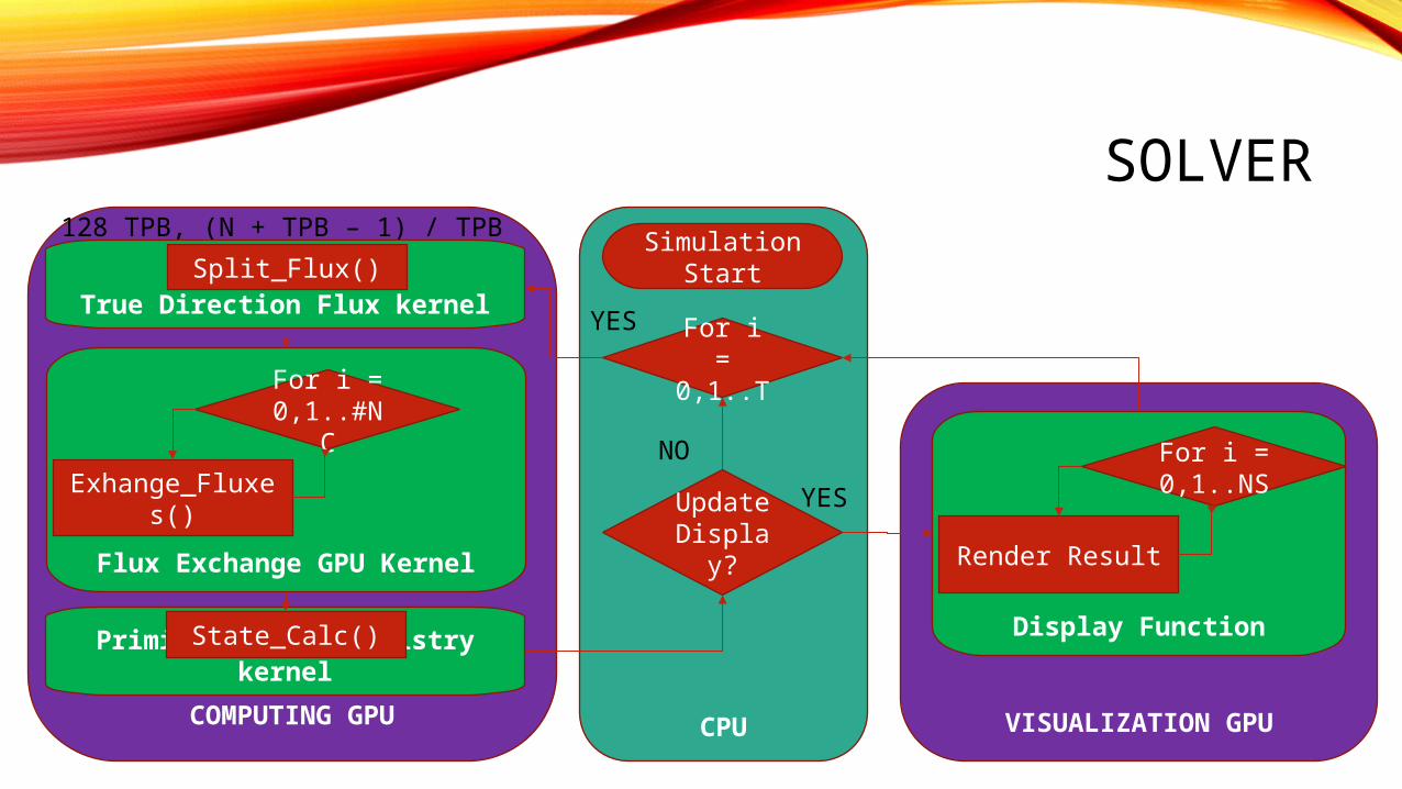
COMPUTING GPU
Flux Exchange GPU Kernel
CPU
SOLVERSimulation
Start
For i = 0,1..TFor i =
0,1..#NC
Exhange_Fluxes()
128 TPB, (N + TPB – 1) / TPB blocks
True Direction Flux kernelSplit_Flux()
VISUALIZATION GPU
Display Function
For i = 0,1..NS
Render Result
YES
NO
Primitives and Chemistry kernel
State_Calc()
Update Display
?
YES
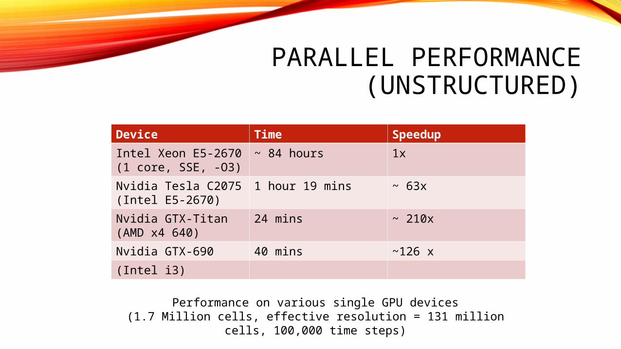
PARALLEL PERFORMANCE (UNSTRUCTURED)
Performance on various single GPU devices(1.7 Million cells, effective resolution = 131 million cells, 100,000 time
steps)
Device Time Speedup
Intel Xeon E5-2670(1 core, SSE, -O3)
~ 84 hours 1x
Nvidia Tesla C2075 (Intel E5-2670)
1 hour 19 mins ~ 63x
Nvidia GTX-Titan(AMD x4 640)
24 mins ~ 210x
Nvidia GTX-690 40 mins ~126 x
(Intel i3)
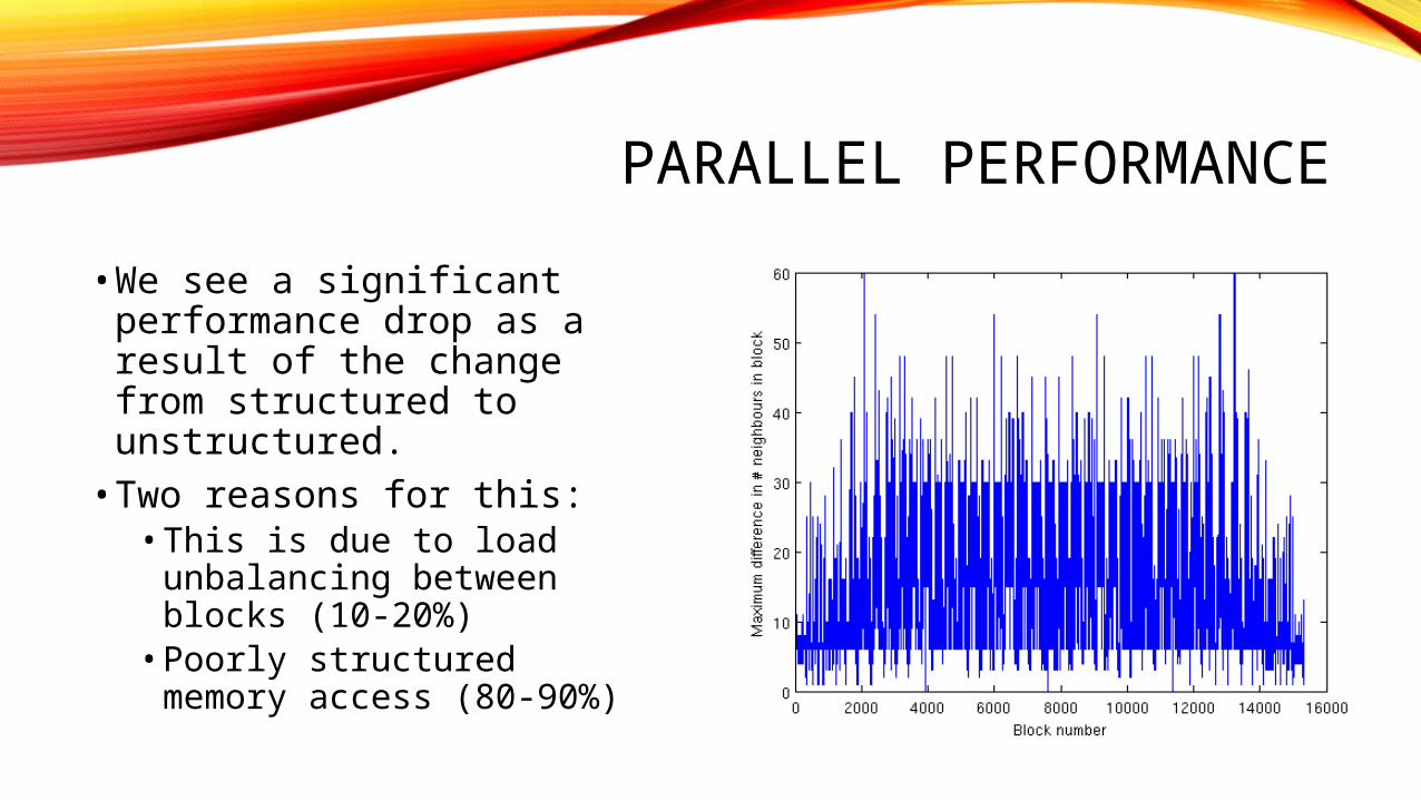
PARALLEL PERFORMANCE
• We see a significant performance drop as a result of the change from structured to unstructured.• Two reasons for this:• This is due to load
unbalancing between blocks (10-20%)• Poorly structured memory
access (80-90%)
CONCLUSIONS
• Many challenges remain for the future of unstructured grid CFD on multiple GPU devices.
• Despite the challenges, we have still created a solver which improves upon the accuracy of previous implementations while still being fast enough to apply to practical problems.
• Currently, the libraries for this solver are written to support OpenCL, CUDA and efficient vectorization on newer Xeon cores and the Intel Phi device (results not discussed here).
• Future work (with regard to the GPU device) will lie in optimization of memory access for unstructured grids and load balancing across multiple devices.
I’d like to thank the following companies for their valuable support.