ACase(Study(Analysis(of(Inventory( Cost(and(Practices(for ......risk cost, total inventory capital cost, total on hand material cost and total inventory related labor cost. The carrying

October 2013

A Case Study Analysis of Inventory Cost and Practices for Operating Room

Medical/Surgical Items CENTER FOR INNOVATION IN HEALTHCARE LOGISTICS

Dr. Manuel D. Rossetti Dr. Vijith M. Varghese Dr. Edward A. Pohl Payam Parsa

University of Arkansas, Center for Innovation in Healthcare Logistics 4207 Bell Engineering Center -‐ Fayetteville, AR, 72701 http://cihl.uark.edu -‐ (479) 575 6033

Copyright (c) 2013 No part of this report may be quoted or used without express permission of the authors.

1

TABLE OF CONTENTS

Overview ............................................................................................................................................. 2

Item identification, data collection, and data scrubbing ..................................................................... 4

Holding and ordering cost estimation ................................................................................................. 5

Inventory pareto analysis and demand classification ......................................................................... 6

Forecasting analysis ............................................................................................................................ 7

Single-echelon optimization ................................................................................................................ 8

Multi-echelon optimization ................................................................................................................. 9

Results and sensitiviy analysis .......................................................................................................... 10

Summary .......................................................................................................................................... 15

Acknowledegement ........................................................................................................................... 16

Bibliography ..................................................................................................................................... 16

2

OVERVIEW

Health care expenditures in the United States reached $2.6 trillion in 2010, nearly ten times the $256 billion spent in 1980. (Centers for Medicare and Medicaid Services, Office of the Actuary, National Health Statistics Group, 2012) The rate of growth has decreased slightly recently, but is expected to grow faster than national income levels over the foreseeable future. (Robert Wood Johnson Foundation, October 2008) Hospital care and clinical services account for 51% of the nation’s health expenditure. (Martin, et al., 2012) These facts motivate the need to put more attention on cost efficiency in the health care industry. (Centers for Medicare and Medicaid Services, Office of the Actuary, National Health Statistics Group, 2012) According to a research study, supply chain costs may account for as much as 40% of the cost of providing care (Haavik, 2000) and it is estimated that if demand and inventory are better managed, the cost savings could range from 6% to 13.5% of total healthcare costs. (Chandra & Kachhal, 2004)

A recent survey on the cost and quality of the health care supply chain (Nachtmann & Pohl, 2009) provides information on the average amount in each cost category that large health care providers spend as a percentage of annual operating expenses. Figure 1 illustrates how much each cost would be if $100 million were spent on supply chain activities, which take approximately 31% of total costs. The two cost categories of main interest to this paper are “Inventory Management” and “Order Management,” which account for 61% of the supply chain costs, or $61 million per year for a typical large health care provider.

FIGURE 1: TYPICAL ANNUAL OPERATING EXPENSES OF A LARGE HEALTH CARE PROVIDER

(NATCHMANN AND POHL, 2009)

Through an industry-wide analysis involving the retail and health care sectors, the Center for Innovation in Healthcare Logistics (CIHL) at the University of Arkansas has identified three supply chain practices that can have a significant impact on the healthcare value chain:

$223 million

$29 million

$32 million

$10 million $13 million $16 million

$100 million

Typical Annual Operating Expenses ($323 million total)

Non-‐Supply Chain Inventory Mgmt Order Mgmt Transportation Shipping/Receiving Other

3

collaborative planning, forecasting and replenishment (CPFR), education and training for materials management, and improved inventory management practices. A case study for the Mercy Health System indicated that significant cost savings are possible by applying improved inventory management practices to pharmaceutical items. The development and adoption of the methodologies used within the case study by the healthcare industry can result in higher fill rates, fewer back orders, higher inventory turns, and decreased overall healthcare inventory costs. Covidien, Inc. as a global healthcare products provider, committed to innovative medical solutions, improved world health, and delivering value through healthcare leadership and excellence, partnered with CIHL to replicate the findings of CIHL’s previous case study (Sisters of Mercy Health System) on products within their system.

This project evaluates the potential for cost savings by applying advanced inventory management practices driven by actual usage data. The focus of the study is on medical/surgical (medsurg) items used in the operating rooms within Mercy hospitals at Fort Smith, AR (FTSM), Oklahoma City, OK (OKLC) and Springfield, MO (SPRG). The medsurg items included 143 items at FTSM, 115 at OKLC and 152 at SPRG all manufactured by Covidien, Inc. The effectiveness of using standard data identifiers is also demonstrated.

This case study attempts to reduce the two main costs of inventory/order management, which are holding costs and ordering costs. The case study used the (r, Q) inventory policy to develop a more cost-effective system. Figure 2 summarizes the steps involved in creating a better inventory management strategy. These steps are explained in detail throughout the rest of the paper.

FIGURE 2: STEPS FOR INVENTORY ANALYSIS

The first stage is data collection and cleansing of the actual usage data and receipt data for the commodities. The effectiveness of using data standards such as GTIN numbers will be discussed. The second stage consists of estimating the holding rate and ordering cost associated with each item. In the next step, actual usage data is further analyzed using a Pareto analysis and demand classification analysis. This permits an understanding of the different approaches that must be taken for items in each of these categories. This is followed by forecasting analysis, in which forecasts are made and the best forecast techniques are selected for each item. In the fifth stage, an optimal (r, Q) policy will be determined for unique items at each location and in the sixth stage another optimal (r, Q) policy will be proposed for pooled items. Finally, a sensitivity

Data Collection, and Data Cleansing

Holding and Ordering Cost Estimation

Inventory Pareto

Analysis and Demand

ClassiKication

Forecasting Analysis

Minimum Cost Inventory Analysis by Location

Multi-‐Echelon Minimum Cost Inventory Analysis

Sensitivity Analysis and Cost Savings Projections

4

analysis will be performed in which current policies will be compared to the proposed policies in several aspects, and the projected cost savings will be discussed.

ITEM IDENTIFICATION, DATA COLLECTION AND CLEANSING

Mercy provided the research team with the actual usage data for Covidien products in Operating Rooms (OR) across their health system. The actual usage data was extracted from the clinical software, Epic® across a time span of 578 days (from October 1st, 2010 to April 30th, 2012). The daily actual usage was aggregated by Site ID. Fort Smith (FTSM), Oklahoma City (OKLC), Springfield (SPRG), and St. Louis (STLO) have a very high volume of transactions. FTSM, OKLC and SPRG were selected because of their high transaction volume and each of these sites employs perpetual inventory. Each of the 3 locations has 192 Covidien items. At each location, the following item counts were used in the study, Fort Smith: 143 items, Oklahoma City: 115 items and Springfield: 152 items

The format of the available dataset was not useful for the analysis in the succeeding tasks which involves Pareto analysis, demand characteristics analysis, etc. The dataset needed to be in a format where demand data for each item at the 3 locations can be read as a time series (with 578 time indices). The available dataset was exported into a Microsoft Access database and queries were run, resulting in a time series format that is useful for the remaining analysis. The receipt data was extracted across a time span of 366 days (from May 1st, 2010 to April 30th, 2011). The receipt data was also organized into a time series as in the case of the actual usage data in order to do further analysis. The receipt data for the SPRG location that orders for the CSC was removed from this data set so as to not bias the analysis.

The usage data from the clinical records software as well as the Purchase Order (PO) data from the Electronic Data Interchange (EDI) system posed a number of challenges with respect to item identification. Items are identified by IDs, namely ABC Item Nbr and User Nbr; ABC Item Nbr is specified by the vendor and User Nbr (the internal ID) by Mercy. We found that it is possible to report the same items from different vendors, using the same internal item ID. For instance, the usage data consisted of 210 unique ABC Item Nbr and 212 unique User Nbr, i.e. there was no one to one mapping between the 2 identifiers. This led to inaccuracy while reporting usage and makes the analysis complicated.

For some items, the order and the usage of the same items are reported at different units of measures from various locations, i.e. item usage at SPRG and FTSM can be reported in different units of measure. Also, items from the same location can be reported using different units of measurement at different points in time. These discrepancies can lead to inaccuracies in the amount ordered and used. However, the analysts ensured that these discrepancies were eliminated.

In order to avoid data inaccuracy and to have consistency in item identification, we recommend the use of data standards, universal, unambiguous and unique item identifiers. This should ensure data accuracy within an analysis. The use of standardized item identifiers is a recommended best practice for improving inventory and order management. The Global Trade

5

Item Number (GTIN) developed by GS1 standards is one of the most widely used item identifiers by the healthcare industry leaders. By using GTINs, the discrepancies related to multiple item identifiers, as in this case, ABC Item Nbr and User Nbr, can be eliminated. Each item has a different GTIN for each unit of measures and hence, discrepancies related to units of measurement can also be avoided.

Research on the use of data standards within the healthcare supply chain and the implementation of data standards in the healthcare supply chain has shown the benefits of data standards at an operational level. This study illustrates the operational benefits of data standards at strategic and tactical level decision-making. GTIN helps to streamline the view between trading partners and also improve the data quality, which is vital in any analysis.

HOLDING AND ORDERING COST ESTIMATION

A spreadsheet was created to collect the various cost components of total inventory cost at each of the 3 locations: total inventory service cost, total inventory space cost, total inventory risk cost, total inventory capital cost, total on hand material cost and total inventory related labor cost. The carrying charge rate (holding cost rate) is estimated in $/$ per year at each location. A rate of 32% and a rate of 17% were estimated for SPRG and for the CSC respectively. For the analysis, models are tested at 3 levels of the holding cost rate: a minimum value, the most likely value and the maximum value. The Mercy team advised us to adopt the following levels (Table 1) for holding cost rate.

TABLE 1: LEVELS OF CARRYING CHARGE

Carrying Charge ($/$/yr) Min Most likely Max FTSM/OKLC/SPRG 25% 30% 35%

CSC 15% 20% 25%

An activity based costing approach was used to estimate the ordering cost at each location. A number of key activities were identified at each location. Then, the Mercy team collected a minimum estimate, most likely estimate and maximum estimate for the following metrics related to each activity: Time spent for each activity per day (in hours/day), Cost associated with each activity per hour (in dollars/hour) and activity quantity for each activity per day (lines or SKUs/day). The cost of placing and processing orders are computed and tabulated in Table 2.

TABLE 2: LEVELS OF ORDERING COST

Ordering Cost ($/order) Min Most Likely Max FTSM $4.55 $5.05 $5.57 OKLC $4.55 $5.04 $5.56 SPRG $4.53 $5.04 $5.54 CSC $4.56 $5.07 $5.58

6

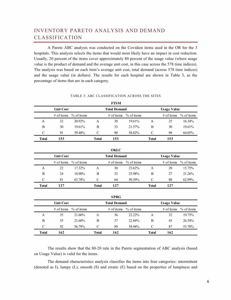
INVENTORY PARETO ANALYSIS AND DEMAND CLASSIFICATION

A Pareto ABC analysis was conducted on the Covidien items used in the OR for the 3 hospitals. This analysis selects the items that would most likely have an impact in cost reduction. Usually, 20 percent of the items cover approximately 80 percent of the usage value (where usage value is the product of demand and the average unit cost, in this case across the 578 time indices). The analysis was based on each item’s average unit cost, total demand (across 578 time indices) and the usage value (in dollars). The results for each hospital are shown in Table 3, as the percentage of items that are in each category.

TABLE 3: ABC CLASSIFICATION ACROSS THE SITES

The results show that the 80-20 rule in the Pareto segmentation of ABC analysis (based on Usage Value) is valid for the items.

The demand characteristics analysis classifies the items into four categories: intermittent (denoted as I), lumpy (L), smooth (S) and erratic (E) based on the properties of lumpiness and

# of items % of items # of items % of items # of items % of itemsA 32 20.92% A 30 19.61% A 25 16.34%B 30 19.61% B 33 21.57% B 30 19.61%C 91 59.48% C 90 58.82% C 98 64.05%

Total 153 Total 153 Total 153





FTSM

OKLC

SPRGUnit Cost Total Demand Usage Value

Unit Cost Total Demand Usage Value

Unit Cost Total Demand Usage Value

7

intermittence. Intermittent, Lumpy and Erratic demands are hard to forecast and hard to model and hence it is harder to manage products that exhibit these type of characteristics. Table 4 illustrates the percentage of items under each of the classes.

TABLE 4: DEMAND CLASSIFICATION ACROSS THE SITES

The observations suggest that 70% of the items are intermittent in nature and 20%

are lumpy. (Table 4) The traditional forecasting approaches such as simple exponential smoothing and moving average are often not appropriate for these items.

FORECASTING ANALYSIS

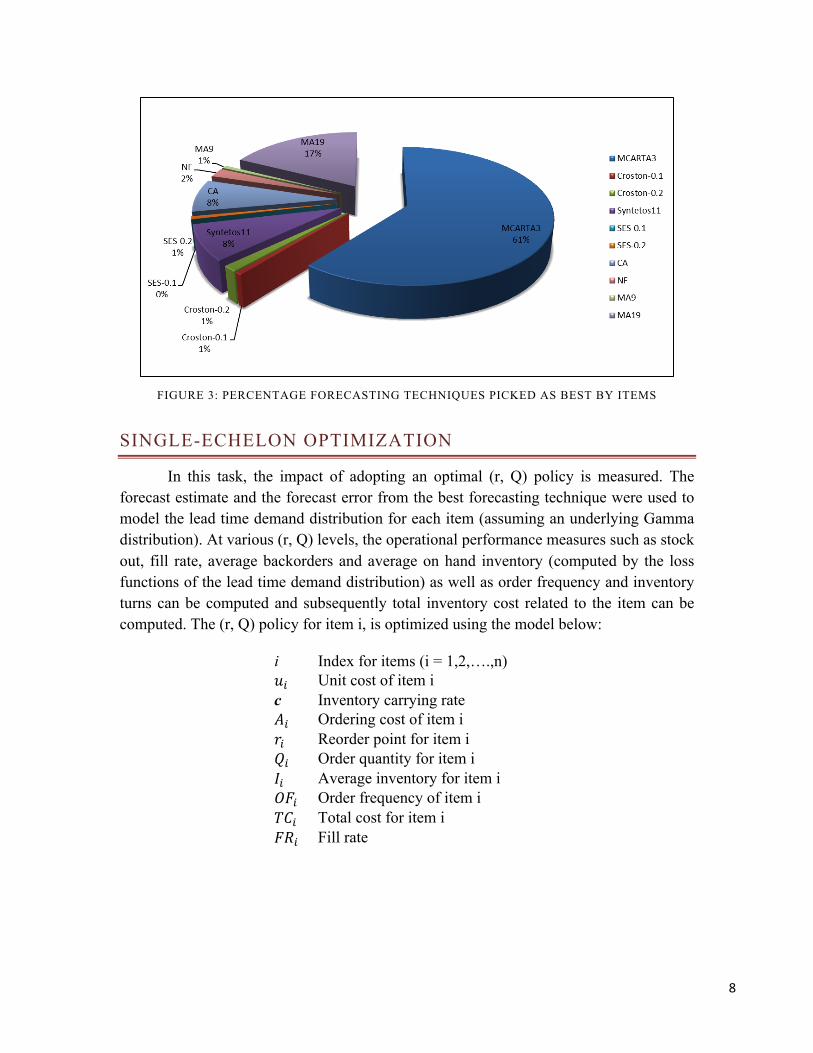
The goal of this task is to select the best forecasting techniques for each item at each location. We selected the Mean Absolute Scaled Error as the performance measure because it is appropriate for demand series which are intermittent or lumpy. The following forecasting techniques were considered for the analysis: MCARTA (an intermittent demand forecasting technique developed by the U of A researchers), Croston (0.1), Croston (0.2), Syntetos (0.1) (Boylan, et al., 2008), Simple Exponential Smoothing (0.1), Simple Exponential Smoothing (0.2), Moving Average (19) and Moving Average (9). The values used as the forecasting parameters are selected from range of 0 to 1 based on common industry practices. Figure 3 shows the percentage of time that each technique was selected as best at FTSM. MCARTA was selected as the best for the majority of items at each location: 61% at FTSM, 65% at OKLC and 71% at SPRG.

# of items % of items # of items % of items # of items % of itemsE 1 0.65% E 1 0.79% E 4 2.47%I 112 73.20% I 88 69.29% I 114 70.37%L 36 23.53% L 32 25.20% L 32 19.75%S 4 2.61% S 6 4.72% S 12 7.41%Total 153 Total 127 Total 162

FTSM OKLC SPRG

8

FIGURE 3: PERCENTAGE FORECASTING TECHNIQUES PICKED AS BEST BY ITEMS

SINGLE-ECHELON OPTIMIZATION

In this task, the impact of adopting an optimal (r, Q) policy is measured. The forecast estimate and the forecast error from the best forecasting technique were used to model the lead time demand distribution for each item (assuming an underlying Gamma distribution). At various (r, Q) levels, the operational performance measures such as stock out, fill rate, average backorders and average on hand inventory (computed by the loss functions of the lead time demand distribution) as well as order frequency and inventory turns can be computed and subsequently total inventory cost related to the item can be computed. The (r, Q) policy for item i, is optimized using the model below:

i Index for items (i = 1,2,….,n) 𝑢! Unit cost of item i c Inventory carrying rate 𝐴! Ordering cost of item i 𝑟! Reorder point for item i 𝑄! Order quantity for item i 𝐼! Average inventory for item i 𝑂𝐹! Order frequency of item i 𝑇𝐶! Total cost for item i 𝐹𝑅! Fill rate

9

𝑀𝑖𝑛𝑖𝑚𝑖𝑧𝑒 𝑇𝐶! = 𝐼! ∗ 𝑢! ∗ 𝑐 + 𝑂𝐹! ∗ 𝐴! 𝑆𝑢𝑏𝑗𝑒𝑐𝑡 𝑡𝑜: 𝐹𝑅! ≤ 1.00 [𝑈𝑝𝑝𝑒𝑟 𝑏𝑜𝑢𝑛𝑑 𝑓𝑜𝑟 𝑡ℎ𝑒 𝑓𝑖𝑙𝑙 𝑟𝑎𝑡𝑒] 𝐹𝑅! ≥ 0.985 [𝐿𝑜𝑤𝑒𝑟 𝑏𝑜𝑢𝑛𝑑 𝑓𝑜𝑟 𝑡ℎ𝑒 𝑓𝑖𝑙𝑙 𝑟𝑎𝑡𝑒] 𝑄! ≥ 1 [𝑀𝑖𝑛𝑖𝑚𝑢𝑚 𝑜𝑟𝑑𝑒𝑟 𝑞𝑢𝑎𝑛𝑡𝑖𝑡𝑦] 𝑄! , 𝑟! ≥ 0 [𝑁𝑜𝑛 − 𝑛𝑒𝑔𝑎𝑡𝑖𝑣𝑖𝑡𝑦]

MULTI-ECHELON OPTIMIZATION

Multi-echelon optimization allows for analysis of the pooling effect of inventory by allowing the stocking policy at the sites to depend on the stocking policy at the CSC. This allows for possible cost savings as a result of the pooling effect at the CSC. The algorithm aggregates demands from bottom to top (sites to CSC). This involves calculating replenishment interval and replenishment size at the sites as well as calculating demand interval and demand size at the CSC. Followed by that, the algorithm solves for single inventory at the CSC and then obtains waiting time due to the backorders at the CSC. The waiting time due to the backorders at the CSC is added to the lead time at the sites and then the model solves for the single inventory at the individual sites. The optimization model is as follows:

𝑀𝑖𝑛𝑖𝑚𝑖𝑧𝑒 𝑇𝑜𝑡𝑎𝑙 𝐶𝑜𝑠𝑡 (𝑟!,𝑄! , 𝑟!,𝑄! , 𝑟!,𝑄! , 𝑟!,𝑄!) 𝑆𝑢𝑏𝑗𝑒𝑐𝑡 𝑡𝑜 𝐹𝑅! 𝑟!,𝑄! , 𝑟!,𝑄! , 𝑟!,𝑄! , 𝑟!,𝑄! ≥ 0.985 𝑟! ’𝑠 𝑎𝑟𝑒 𝑛𝑜𝑛 − 𝑛𝑒𝑔𝑎𝑡𝑖𝑣𝑒 𝑖𝑛𝑡𝑒𝑔𝑒𝑟𝑠 𝑄! ’𝑠 𝑎𝑟𝑒 𝑝𝑜𝑠𝑖𝑡𝑖𝑣𝑒 𝑖𝑛𝑡𝑒𝑔𝑒𝑟𝑠

Since only 45 items are used across all three sites and replenished by the CSC, these items alone are used in the multi-echelon model. The majority of the items studied have low total usage value (Table 5) and hence savings will be lower than the savings from the single-echelon analysis.

TABLE 5: ITEMS INCLUDED IN MULTI-ECHELON ANALYSIS BY ABC/DEMAND CLASSIFICATION-45 ITEMS

FTSM OKLC SPRGA 10 7 6 23B 9 7 14 30C 26 31 25 82Total 45 45 45 135

FTSM OKLC SPRGE 0 1 2 3I 33 29 23 85L 8 12 12 32S 4 3 8 15Total 45 45 45 135

10

RESULTS AND SENSITIVIY ANALYSIS

In the single-echelon optimization, there were some discrepancies between the actual usage data set and the receipt data set. Some items used (actual usage data) were not reported in the receipt data set. For efficiency and accuracy, these items were excluded from the study. Thus, the items contained in the final study where reduced from 153 to 119 at FTSM, from 127 to 103 at OKLC, from 162 to 148 at SPRG. For some items, total annual usage exceeded total ordered and therefore assumptions were made on the initial inventory level ( I!!!). The I!!! value for each item was initialized by 𝐼!!! =𝑆𝑢𝑚 𝐷! − 𝑆𝑢𝑚 𝑄! +𝑀𝑎𝑥(𝐷!)1.

This time series for the daily on hand inventory was used to compute the average fill rate and the average on hand inventory for each item. We observed that 37% of items at FTSM, 60% at OKLC and 48% at SPRG have been backordered at least once during the 366-day time horizon. It is possible that demands for these items might have been met through a rush delivery or a substitute item, for which we do not have the records. The average fill rate across all the items is 94.7% at FTSM, 91.9% at OKLC and 93.7% at SPRG which is lower than the desired 98.5%. Meanwhile, the total of daily average on hand inventory across the items within a location is considerably high: 10,118.9 units at FTSM, 9,039.4 at OKLC and 20,359.5 at SPRG. The daily average on hand inventory for an item within a location is 85.0 units at FTSM, 87.8 at OKLC and 137.6 at SPRG.

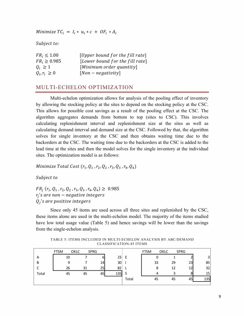
Figure 4 compares the fill rate and average on hand inventory of the current method with the proposed model. The current average inventory is considerably higher than the average inventory for the proposed inventory model. Meanwhile the fill rate for the current inventory model is usually lower than the proposed fill rates.

1 Real-time observations of on-hand inventory were not available; therefore, we adopted this approach. To initialize the approach, we have to make an estimate for the initial on hand inventory and hence we arbitrarily set it as the maximum number of units used for the item. Since, it is not possible for total annual usage to exceed total ordered, we assumed that the initial on hand served towards the excess demand.

11

FIGURE 4: DAILY AVERAGE INVENTORY AND FILL RATE BY SORTED SKU

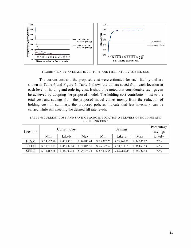
The current cost and the proposed cost were estimated for each facility and are shown in Table 6 and Figure 5. Table 6 shows the dollars saved from each location at each level of holding and ordering cost. It should be noted that considerable savings can be achieved by adopting the proposed model. The holding cost contributes most to the total cost and savings from the proposed model comes mostly from the reduction of holding cost. In summary, the proposed policies indicate that less inventory can be carried while still meeting the desired fill rate levels.

TABLE 6: CURRENT COST AND SAVINGS ACROSS LOCATION AT LEVELS OF HOLDING AND ORDERING COST

Location Current Cost Savings Percentage

savings Min Likely Max Min Likely Max Likely

FTSM $ 34,872.96 $ 40,833.31 $ 46,843.64 $ 25,362.25 $ 29,760.22 $ 34,206.12 73%

OKLC $ 38,611.87 $ 45,287.84 $ 52,015.38 $ 26,627.52 $ 31,311.05 $ 36,058.93 69%

SPRG $ 73,187.66 $ 86,300.94 $ 99,489.33 $ 57,336.65 $ 67,789.20 $ 78,322.44 79%

12

FIGURE 5: COMPARING TOTAL COST ACROSS THE LOCATIONS The current cost and the proposed cost for the multi-echelon optimization model

were estimated for each facility and are shown in Figure 6. It has to be noted that both single-echelon and multi-echelon optimization has considerable savings at each location by driving down the holding cost. As mentioned before the savings for single-echelon is greater than that of multi-echelon analysis because the majority of items selected as the pooling items have low unit costs and low usage values.

FIGURE 6: COMPARING TOTAL COST ACROSS THE LOCATIONS -‐ 45 ITEMS

13

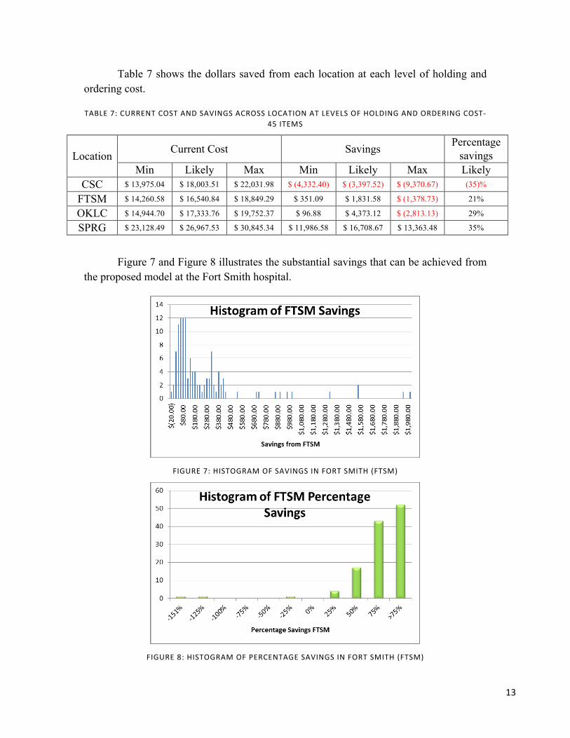
Table 7 shows the dollars saved from each location at each level of holding and ordering cost.

TABLE 7: CURRENT COST AND SAVINGS ACROSS LOCATION AT LEVELS OF HOLDING AND ORDERING COST-‐45 ITEMS

Location Current Cost Savings Percentage savings

Min Likely Max Min Likely Max Likely CSC $ 13,975.04 $ 18,003.51 $ 22,031.98 $ (4,332.40) $ (3,397.52) $ (9,370.67) (35)%

FTSM $ 14,260.58 $ 16,540.84 $ 18,849.29 $ 351.09 $ 1,831.58 $ (1,378.73) 21%

OKLC $ 14,944.70 $ 17,333.76 $ 19,752.37 $ 96.88 $ 4,373.12 $ (2,813.13) 29%

SPRG $ 23,128.49 $ 26,967.53 $ 30,845.34 $ 11,986.58 $ 16,708.67 $ 13,363.48 35%

Figure 7 and Figure 8 illustrates the substantial savings that can be achieved from the proposed model at the Fort Smith hospital.

FIGURE 7: HISTOGRAM OF SAVINGS IN FORT SMITH (FTSM)

FIGURE 8: HISTOGRAM OF PERCENTAGE SAVINGS IN FORT SMITH (FTSM)

14

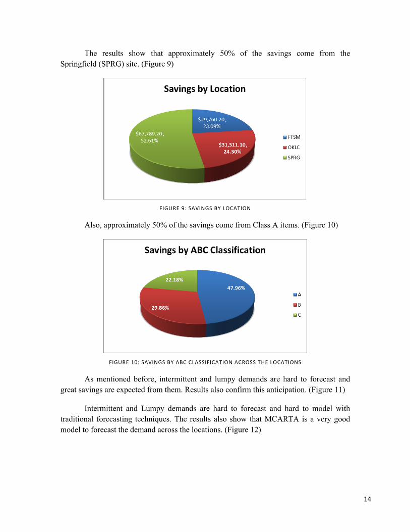
The results show that approximately 50% of the savings come from the Springfield (SPRG) site. (Figure 9)

FIGURE 9: SAVINGS BY LOCATION

Also, approximately 50% of the savings come from Class A items. (Figure 10)

FIGURE 10: SAVINGS BY ABC CLASSIFICATION ACROSS THE LOCATIONS

As mentioned before, intermittent and lumpy demands are hard to forecast and great savings are expected from them. Results also confirm this anticipation. (Figure 11)

Intermittent and Lumpy demands are hard to forecast and hard to model with traditional forecasting techniques. The results also show that MCARTA is a very good model to forecast the demand across the locations. (Figure 12)

15

FIGURE 11: SAVINGS BY DEMAND CHARACTERISTICS ACROSS THE LOCATIONS

FIGURE 12: SAVINGS BY FORECAST TECHNIQUE ACROSS THE LOCATIONS

SUMMARY

The analysis shows that high on hand inventories are carried across the locations in the Mercy hospital network, especially at Fort Smith (FTSM) and hence considerable savings are possible by better managing the items using the proposed inventory policies. These savings are predicted from both single-echelon optimization and multi-echelon optimization models that are discussed in detail. In addition, despite the lower on-hand inventory, the proposed model achieves the desired fill rate.

It is to be noted that the majority of the items have intermittent or lumpy demand and therefore modeling and forecasting the demand using the traditional methods is not sufficiently effective. Therefore, we selected MCARTA as the best forecasting technique

16

for most of the items through an analysis which shows 61% of items at FTSM, 65% at OKLC and 71% at SPRG are better forecasted using this technique. Furthermore, the 80-20 rule is valid in this system in terms of unit cost, demand and actual usage value. The implication is that vital items are fewer in nature and adoption of inventory best practices on these items may generate considerable savings. Future work should investigate the allocation of the inventory from the central store of the hospitals to localized units within the hospital in order to understand the effect on service of the new inventory policies.

ACKNOWLEDEGEMENT

This material is based upon work supported in part by the Center for Innovation in Healthcare Logistics at the University of Arkansas via a grant from Covidien, Inc.. Any opinions, findings, and conclusions or recommendations expressed in this material are those of the author(s) and do not necessarily reflect the views of Covidien, Inc.

BIBLIOGRAPHY

Boylan, J. E., Syntetos, A. A. & Karakostas, J. E., 2008. Classification for Forecasting and Stock Control: A Case Study. Journal of Operational Research Society , pp. 473-481.

Centers for Medicare and Medicaid Services, Office of the Actuary, National Health Statistics Group, 2012. National Health Care Expenditures Data. s.l.:s.n.

Chandra, C. & Kachhal, S. K., 2004. Managing Helth Care Supply Chain: Trends, Issues, and Solutions from a Logistics Perspective. Orlando, Florida, s.n.

Haavik, S., 2000. Building a Demand-Driven, Vendor-Managed Supply Chain. Healthcare Financial Management.

Martin, A. B., Lassman, D., Washington, B. & Catlin, A., 2012. Growth In US Health Spending Remained Slow In 2010; Health Share Of Gross Domestic Product Was Unchanged From 2009. Health Affairs.

Nachtmann, H. & Pohl, E. A., 2009. The State of Healthcare Logistics: Cost and Quality Improvement Opportunities, s.l.: Center for Innovation in Healthcare Logistics, University of Arkansas.

Robert Wood Johnson Foundation, October 2008. High and rising health care costs: Demystifying U.S. health care spending. s.l.:s.n.

Documents

ACase(Study(Analysis(of(Inventory( Cost(and(Practices(for ......risk cost, total inventory capital cost, total on hand material cost and total inventory related labor cost. The carrying