Page | 1

Academic Resource Center Math Lab Lo Angeles Valley College

Final Review Workshop Outcomes:

Our final review workshop cannot cover all the topics in chapter 1-12.

• You will be able to identify what you will need to cover in each chapter briefly.

• You will be able to become a problem solver which you comfortably tackle a problem by using a right

formula/definition.

• You will be able to build up your confidence in confidence interval and hypothesis testing.

• You will be able to get a set of sample problems to prepare for your final.

• You will be able to obtain all the necessary formula to prepare for your comprehensive final.

Here is the table of the content: Pg. 1-4 ……..Brief Topics from Each Chapter Pg. 5-9 ……..Final Review Topics Pg. 10-11 ……Useful Formula

Page | 2

Stat Final Review—Important Topic for the Final Exam Chapter 1 Introduction to Statistics • Distinguish between a population and a sample as well between a parameter and a statistic.

• Different types of data: qualitative, quantitative, continuous, discrete, sample, population, random sample, and simple random sample.

• Categorize different levels of measurement: nominal, ordinal, interval, and ratio.

• Differentiate random, simple random, systematic, convenience, stratified, and cluster sampling.

• Know observational studies and experiment and identify different observational studies and experiment.

• Be able to identify the experiment and figure out explanatory variable and response variables.

Chapter 2 Summarizing and Graphing Data • Frequency distribution: class, upper and lower limits, class boundaries, class midpoints, frequency, relative

frequency, cumulative frequency and construct a histogram

• Construct graphs of data using a frequency polygon, dot plot, stem plot, bar graph, multiple bar graph, Pareto charter, pie chart, scatter plot, and time-series graphs

Calculator Key for Box Plot

• To input data: Stat → Edit→input your data To calculate 5 number summary: min, Q1, Median, Q3, max:

Stat→Calc→1-Var Stats (your list)

Chapter 3 Statistics for Describing, Exploring and Comparing Data

• Mean, median, mode, standard deviation, variance, range (sample / population)

• Compare data values by using z scores, quartiles, or percentiles.

Calculator Key for this Chapter:

• To input data: Stat → Edit→input your data

• To calculate the mean, standard deviation and so on: Stat→Calc→1-Var Stats (your list)

• To sort your data in ascending or descending order:

• 2nd→0→variance (your list)

Chapter 4 Probability

• Probability: fundamental, addition rule, multiplication rule, and complements

• Mutually exclusive events/ independent events.

• Counting: fundamental counting rule, combination and permutation

Calculator Key for this Chapter: • Math→PRB→select 2: nPr (permuation), 3: nCr (combination), and 4: !

• To find the number of combinations of r many items out of n distinct items (order does not matter) o Math→PRB→nCr

• To find the number of permutations of r many items out of n distinct items (order does matter) o Math→PRB→nPr o Factorial: Math→PRB→!

➢ Probability Example Factorial ! ==8! (Punch your number) →Math→PRB→! Combination nCr = 5C3 (punch n = 5) →Math→PRB→nCr→(punch r =3) →ENTER Permutation nPr = 5P3 (punch n = 5) →Math→PRB→nPr→(punch r =3) →ENTER

Page | 3

Chapter 5 Random Variables

• Random variable and its probability distribution (add up to 1), standard deviation, and expected value (mean).

• Binomial distribution (requirements), using A-1 table or TI 83/84 Plus Calculator

• Poisson distribution

• Unusual Outcomes using the range rule of thumb to find minimum and maximum

Calculator Key for this Chapter:

• To find the binomial probability. Probability of getting x many successes out of n many binomial trials o For exactly x many successes: 2nd

→dist→binompdf(n,p,x) o For x or less (up to x) many successes: 2nd

→dist→binomcdf(n,p,x)

• To find the Poisson probability: Probability of getting x many occurrences (customers) in a given period (µ is the average number of occurrences)

o For exactly x many occurrences: 2nd→dist→Poissonpdf (µ,x)

o For x or less (up to x) many occurrences: 2nd→dist→Poissoncdf (µ,x)

Chapter 6 Normal Probability Distribution

• Uniform distribution

• Normal distribution versus standard normal distribution: finding area (probability), finding z-score formula

• Sampling -- DSM, Central Limit Theorem Calculator Key for this Chapter:

• To find the area (probability) under normal distribution: o For standard normal (µ=0, σ=1): 2nd→dist→normalcdf(left end point, right end point)

o For just normal: 2nd→dist→normalcdf(left end pt, right end pt, µ, σ)

• To find the z-score (or the value) when the probability is given for normal distribution. o For standard normal: 2nd

→dist→InvNorm(cumulative probability) o For just normal: 2nd

→dist→InvNorm(cumulative probability, µ, σ) Chapter 7 Estimates and Sample Sizes

• Basic Methods of finding estimate of population proportions, means, and variance.

• Calculate margin of error, construct Confidence level and Estimate sample sizes for proportion and mean (µ known using z-score or µ unknown using t-distribution), and variance using Chi-Square Distribution

• Know 4 different types of confidence interval: calculating the sample size from the margin of error, understand 5 step procedure for this type of problem

Calculator Key for this Chapter:

• To construct confidence interval for proportion

Stat→Cal→1-PropZInterval • To construct confidence interval for mean when µ is known

Stat→Cal→ZInterval • To construct confidence interval for mean when µ is unknown

Stat→Cal→TInterval

Page | 4

Chapter 8 Hypothesis Testing • 4 different types of hypothesis testing

• Identify three methods for testing hypothesis testing: The P-value method, the traditional method, and confidence intervals, understand 6-step procedure for each method.

Calculator Key for this Chapter:

• To input data: Stat → Edit→input your data

• To find hypothesis test for proportion

Stat→Cal→1-PropZTest • To find hypothesis test for mean when µ is known

Stat→Cal→Z-Test • To find hypothesis test for mean when µ is unknown

Stat→Cal→T-Test

• To find the area or p-value (probability) under t-distribution: 2nd→dist→tcdf(left end pt, right end pt, degrees of freedom)

• To find the area or p-value (probability) under χ-square-distribution: 2nd→dist→ χ^2 cdf(left end pt, right end pt, degrees of freedom)

Chapter 9 Inferences from Two Samples

• Construct confidence interval estimates of population parameters

• Using methods of hypothesis testing to test claims about population, understand how to use 6-step procedure for this type of problem.

Calculator Key for this Chapter:

• To input data: Stat → Edit→input your data on L1, L2, and/or L3

• To find hypothesis test and construct confidence interval for two samples of proportion

Stat→Test→2-PropZTest and 2PropZInterval • To find hypothesis test for independent populations means and construct confidence interval for

Stat→Test→2-SampleTTest and 2-SampleTInterval (Be aware of standard deviation σ1 and σ2 are equal or unequal) To find the hypothesis test for population variance Stat→Test→2-SampleFTest

• To find the area or p-value (probability) under t-distribution: 2nd→dist→tcdf(left end pt, right end pt, degrees of freedom)

• To find the area or p-value (probability) under χ-square-distribution: 2nd→dist→ χ^2 cdf(left end pt, right end pt, degrees of freedom)

Chapter 10 Correlation (Page 575 Review)

• Methods of using scatter plots for linear correlation coefficient between 2 variables and using A-6 table to find critical values, testing a hypothesis

• Find regression equation and find predicted value Calculator Key for this Chapter:

• To input data: Stat → Edit→input your data on L1

• To find linear correlation coefficient or the regression equation

Stat→TESTS→LinRegTTest or Stat→Cal→LineReg (ax+b)

Page | 5

Chapter 11 Goodness of Fit and Contingency Table

• Method using frequency counts from different categories for testing goodness-of-fit

• Find test statistics for one-way frequency table, contingency table, and McNemar’s tests and know the degree of freedom.

Calculator Key for this Chapter:

• To find test statistic and p-value for good of fit, using Stat→TESTS→X^2-GOF-Test (for TI-84 Calculator users only)

• To find test statistic and p-value for the contingency Table, enter the matrix 2nd x^-1 → EDIT Matrix and adjust the row and column Then go Stat→TESTS→X^2-Test

Chapter 12 Analysis of Variance • Understand one way of Analysis of Variance and set up the hypothesis testing for three or more population

means. Calculator Key for this Chapter:

• To find test statistic and p-value for three or more population means: Then go Stat→TESTS→ANNOVA (L1, L2 or L3)

Sample Final Problems for Statistics

Page | 6

1. The weekly salaries of teachers in a state are normally distributed with a mean of $490 and a standard deviation of $45.

a. What is the probability that a randomly selected teacher earns more than $525 a week?

b. What is the probability that 10 randomly selected teachers will earn more than $525 a week?

2. In a batch of 8,000 clock radios, 5% are defective. A sample of 14 clock radios is randomly selected

without replacement from the 8,000 and tested. The entire batch will be rejected if at least one of those

tested is defective. What is the probability that the entire batch will be rejected?

3. The National Traffic Safety Administration publishes a report about motorcycle fatalities and helmet

use. The proportion of fatalities by location of injury includes: Head - 31%, Neck – 3%, Thorax – 6%,

Abdomen/Spine 3%, Multiple Locations – 57%. The following data show the location of injury and fatalities for 2068 riders not wearing a helmet. Use a 0.025 significance level to test the claim that the distribution of fatal injuries for riders not wearing a helmet is the same as for all riders.

Location of Injury Head Neck Thorax Abdomen/Spine Multiple Locations

Number 864 38 83 47 1036

Page | 7

4. How many weeks of data must be randomly sampled to estimate the mean weekly sales of a new line

of athletic footwear? We want 99% confidence that the sample mean is within $200 of the population mean,

and the population standard deviation is known to be $1100.

5. The paired data below consist of the costs of advertising (in thousands of dollars) and the number of

products sold (in thousands).

a. Use a 0.05 significance level to test whether there is a linear correlation between advertising and the

number of products sold.

b. Predict the number of products sold if a company spends $12,000 in advertising.

6. Suppose that 11% of people are left-handed. If 8 people are selected at random, what is the probability that

exactly 2 of them are left-handed? What is the probability that at least 4 are left-handed?

7. A supplier of digital memory cards claims that no more than 1% of the cards are defective. In a random

sample of 600 memory cards, it is found that 3% are defective, but the supplier claims that this is only a

sample fluctuation. At the 0.01 level of significance, test the supplier's claim that no more than 1% are

defective.

Page | 8

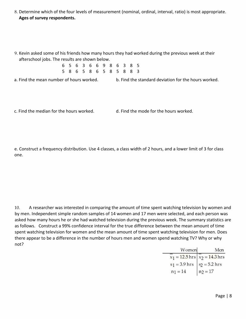
8. Determine which of the four levels of measurement (nominal, ordinal, interval, ratio) is most appropriate.

Ages of survey respondents.

9. Kevin asked some of his friends how many hours they had worked during the previous week at their

afterschool jobs. The results are shown below.

6 5 6 3 6 6 9 8 6 3 8 5 5 8 6 5 8 6 5 8 5 8 8 3

a. Find the mean number of hours worked. b. Find the standard deviation for the hours worked.

c. Find the median for the hours worked. d. Find the mode for the hours worked.

e. Construct a frequency distribution. Use 4 classes, a class width of 2 hours, and a lower limit of 3 for class one.

10. A researcher was interested in comparing the amount of time spent watching television by women and

by men. Independent simple random samples of 14 women and 17 men were selected, and each person was

asked how many hours he or she had watched television during the previous week. The summary statistics are

as follows. Construct a 99% confidence interval for the true difference between the mean amount of time

spent watching television for women and the mean amount of time spent watching television for men. Does

there appear to be a difference in the number of hours men and women spend watching TV? Why or why

not?

Page | 9

11. A survey was given out to our college students asking about their main plans for the summer. The

following table summarizes their answers. Give answers as an unsimplifed fraction and as a decimal rounded

to the correct number of significant digits.

Attend summer session at our

college

Travel Work a summer job

Male 55 39 72

Female 65 42 53

If a student from the survey was picked at random, what is the probability that they:

a)are a female?

b) are a male who plans to travel this summer?

If two students are chosen, what is the probability that they

c) are two males?

d) are two females to plan to travel this summer?

Given that one student randomly chosen plans to work a summer job, what is the probability that they are

e) female?

f) Given that one student randomly chosen is male, what is the probability that they are going to work a summer job?

Page | 10

Probability

• 1 event? • More Than 1 event? Other Formulas…

Simple 𝑃(𝐴) =𝐴

𝑇𝑜𝑡𝑎𝑙

If independent…

𝑃(𝐴 and 𝐵) = 𝑃(𝐴) ⋅ 𝑃(𝐵)

If dependent…

𝑃(𝐴 and 𝐵) = 𝑃(𝐴) ⋅ 𝑃(𝐵|𝐴)

For “at least 1”…

𝑃(At least 1 𝐴) = 1 − 𝑃(none 𝐴)

Complement 𝑃(�̅�) = 1 − 𝑃(𝐴)

And 𝑃(𝐴 and 𝐵) =

𝐴 and 𝐵

𝑇𝑜𝑡𝑎𝑙

To check for “independent

events”…

If 𝑃(𝐴) = 𝑃(𝐴|𝐵),

Then 𝐴 and 𝐵 are independent

Or 𝑃(𝐴 𝑜𝑟 𝐵) = 𝑃(𝐴) + 𝑃(𝐵) − 𝑃(𝐴 and 𝐵)

Conditional 𝑃(𝐴|𝐵) =𝐴 and 𝐵

𝐵

Discrete Probability Distributions

Rules for a Probability Model

1. ( ) 1P x = 2. 0 ( ) 1P x

( )x P x = ➔ “expected value”

2 2 2( )x P x = − and 2 2( )x P x = −

Features of a Binomial Experiment

1. Fixed number of trials, n.

2. Trials are independent.

3. Exactly two outcomes for each trial.

Success or Failure

4. Probability of success is fixed, p.

𝑃(success) = 𝑝 and 𝑃(failure) = 𝑞

Exact Probability

𝑃(𝑋 = 𝑥) =nCx ⋅ 𝑝𝑥 ⋅ (1 − 𝑝)𝑛−𝑥

OR

𝑃(𝑋 = 𝒙) =binomialpdf(𝑛, 𝑝, 𝒙)

Inequality Probability

𝑃(𝑋 ≤ 𝒂) =binomialcdf(𝑛, 𝑝, 𝒂). 𝑃(𝑋 ≥ 𝑏) = 1 −binomialcdf(𝑛, 𝑝, 𝒂)

Mean Value for Binomial Variance for Binomial Standard Deviation for

Binomial

Formula:

n p =

“expected value”

Formula:

2 n p q =

Formula:

n p q =

𝒂 𝒃 𝒂 𝒃

Page | 11

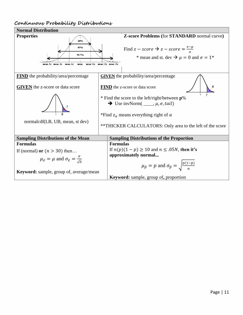
Continuous Probability Distributions

Normal Distribution

Properties

Z-score Problems (for STANDARD normal curve)

Find 𝑧 − 𝑠𝑐𝑜𝑟𝑒 → 𝑧 − 𝑠𝑐𝑜𝑟𝑒 =𝑥−𝜇

𝜎

* mean and st. dev → 𝜇 = 0 and 𝜎 = 1*

FIND the probability/area/percentage

GIVEN the z-score or data score

normalcdf(LB, UB, mean, st dev)

GIVEN the probability/area/percentage

FIND the z-score or data score

* Find the score to the left/right/between p%

➔ Use invNorm( ____, 𝜇, 𝜎, 𝑡𝑎𝑖𝑙)

*Find 𝑧𝛼 means everything right of 𝛼

**THICKER CALCULATORS: Only area to the left of the score

Sampling Distributions of the Mean Sampling Distributions of the Proportion

Formulas

If (normal) or (𝑛 > 30) then…

𝜇�̅� = 𝜇 and 𝜎�̅� =𝜎

√𝑛

Keyword: sample, group of, average/mean

Formulas

If 𝑛(𝑝)(1 − 𝑝) ≥ 10 and 𝑛 ≤ .05𝑁, then it’s

approximately normal...

𝜇𝑝 = 𝑝 and 𝜎𝑝 = √𝑝(1−𝑝)

𝑛

Keyword: sample, group of, proportion

?

#

?

#

Page | 12

Confidence Intervals

Working Backwards to Find Sample Size

For �̂�

For �̅�

If given �̂�, 𝐸, and 𝐶 − 𝑙𝑒𝑣𝑒𝑙

If no prior estimates,

Just 𝐸 and 𝐶 − 𝑙𝑒𝑣𝑒𝑙 Given 𝑠, 𝐸 & 𝐶 − 𝑙𝑒𝑣𝑒𝑙

2

2

2

ˆ ˆ[ ]z p qn

E

=

𝑛 =[𝑧𝛼 2⁄ ]

2(. 5)(. 5)

𝐸2

2

2zn

E

=

ONE PARAMETER HYPOTHESIS TEST

Estimating 𝑝 Estimating 𝜇

Scenario Qualitative Variables

(2 outcomes)

Average of Quantitative Variable

Requirements 1) 𝑛 ≤ 0.05𝑁

AND

2) 𝑛�̂�(�̂�) ≥ 10

1) Simple Random Sample

AND

2) 𝑥 is normal OR 𝑛 > 30

Calculation 1st: �̂� =𝑥

𝑛 (decimal first)

2nd: Need 𝑧𝛼

2

3rd: Find the margin of error

�̂� ± 𝑧𝛼2

√�̂�(�̂�)

𝑛

1st: Need �̅� and 𝑠

2nd: Need 𝑡𝛼

2

�̅� ± 𝑡𝛼2

(𝑠

√𝑛)

ONE PARAMETER?

𝐻0: 𝑝𝑎𝑟𝑎𝑚𝑒𝑡𝑒𝑟0 = #

𝑝 𝜇

𝜎

REQUIREMENTS MET?

1) 𝑛 ≤ .05𝑁 AND

2) 𝑛𝑝0𝑞0 ≥ 10

REQUIREMENTS MET?

1) 𝑋 is normal OR 𝑛 > 30

REQUIREMENTS MET?

1) Simple Random Sample

2) 𝑋 is normal

First find…

𝑛 and �̂� =𝑥

𝑛 and 𝑝0

Then find the TEST STATISTIC

𝑧0 =�̂� − 𝑝0

√𝑝0𝑞0)𝑛

First Find…

*𝑛, �̅�, 𝑠 , and 𝜇0

Then find the TEST STATISTIC

𝑡0 =�̅� − 𝜇0

𝑠

√𝑛

First Find…

* 𝑛, 𝑠, and 𝜎0

Then find the TEST

STATISTIC

𝑋20 =

(𝑛 − 1)𝑠2

𝜎02

Page | 13

Critical Region Approach

invNorm(___, 0,1) invT(_____, df) or CHART CHART

P-value Approach

normalcdf(LB, UB, 0,1) tcdf(LB, UB, df) 𝑋2cdf(LB, UB, df)

TWO PARAMETERS?

𝐻0: 𝑝𝑎𝑟𝑎𝑚𝑒𝑡𝑒𝑟1

= 𝑝𝑎𝑟𝑎𝑚𝑒𝑡𝑒𝑟 𝑝 𝜇

𝜎

DEPENDENT?

𝐻 : 𝜇 = 0

REQUIREMENTS MET?

1) 𝑛1 ≤ .05𝑁1 & 𝑛2 ≤.05𝑁2

2) 𝑛1�̂�1�̂�1 ≥ 10 and. REQUIREMENTS MET?

1)Normal OR 𝑛1 ≥ 30 &

𝑛2 ≥ 30

2) Simple Random Sample

REQUIREMENTS

MET?

1) Simple Random

Sample

First Find…

�̅� =𝑥1 + 𝑥2

𝑛1 + 𝑛2

Then find the TEST

STATISTIC

𝑧0

=(�̂�1 − �̂�2) − (𝑝1 − 𝑝2)

√�̅� ∙ 𝑞ത𝑛1

+�̅� ∙ 𝑞ത𝑛2

First Find…

* Subtract ALL of the

data to obtain the

difference data

*Find �̅� and 𝑠𝑑

Then find the TEST

STATISTIC

𝑡0 =�̅� − 𝜇𝑑

𝑠𝑑

√𝑛

*𝑑𝑓 = 𝑛 – 1

First Find…

*�̅�1 and 𝑠1 then �̅�2

and 𝑠2

Then find the TEST

STATISTIC

𝑡0

=(�̅�1 − �̅�2) − (𝜇1 − 𝜇2)

√𝑠1

2 𝑛1

+𝑠2

2

𝑛2

*𝑑𝑓 = "𝑠𝑚𝑎𝑙𝑙𝑒𝑟 𝑛" – 1

First Find…

* 𝑠1 and 𝑠2

Then find the TEST

STATISTIC

𝐹0 =𝑠1

2

𝑠22

*p-value approach only!

𝐹𝑐𝑑𝑓(𝐿𝐵, 𝑈𝐵, 𝑑𝑓𝑁𝑈𝑀, 𝑑𝑓𝐷𝐸𝑁)

INDEPEND

ENT?