AC RL and RC Circuits - The University of Texas at Dallas

Erik Jonsson School of Engineering and Computer Science

The University of Texas at Dallas

© N. B. Dodge 09/10

AC RL and RC Circuits

• When a sinusoidal AC voltage is applied to an RL or RC circuit, the relationship between voltage and current is altered.

• The voltage and current still have the same frequency and cosine-wave shape, but voltage and current no longer rise and fall together.

• To solve for currents in AC RL/RC circuits, we need some additional mathematical tools: – Using the complex plane in problem solutions. – Using transforms to solve for AC sinusoidal currents.

EE 1202 Lab Briefing #5 1



© N. B. Dodge 09/10

Imaginary Numbers • Solutions to science and

engineering problems often involve .

• Scientists define . • As we EE’s use i for AC current,

we define . • Thus technically, j = ‒i, but that

does not affect the math. • Solutions that involve j are said to

use “imaginary numbers.” • Imaginary numbers can be

envisioned as existing with real numbers in a two-dimensional plane called the “Complex Plane.”


Real Axis

Imaginary Axis

−3 −2 −1 1 2 3 4

3j

2j

j

−j

−2j

−3j

1st Quadrant

2nd Quadrant

4th Quadrant

3rd Quadrant

The Complex Plane

1−1i = − −

1j = + −



© N. B. Dodge 09/10

The Complex Plane

• In the complex plane, imaginary numbers lie on the y-axis, real numbers on the x-axis, and complex numbers (mixed real and imaginary) lie off-axis.

• For example, 4 is on the +x axis, ‒8 is on the ‒x axis, j6 is on the + y axis, and ‒j14 is on the ‒y axis.

• Complex numbers like 6+j4, or ‒12 ‒j3 lie off-axis, the first in the first quadrant, and the second in the third quadrant.


Real Axis

Imaginary Axis

−3 −2 −1 1 2 3 4

3j

2j

j

−j

−2j

−3j

1st Quadrant

2nd Quadrant

4th Quadrant

3rd Quadrant



© N. B. Dodge 09/10

Why Transforms?

• Transforms move a problem from the real-world domain, where it is hard to solve, to an alternate domain where the solution is easier.

• Sinusoidal AC problems involving R-L-C circuits are hard to solve in the “real” time domain but easier to solve in the ω-domain.


Real-world domain

Problem-solving domain



© N. B. Dodge 09/10

The ω Domain

• In the time domain, RLC circuit problems must be solved using calculus.

• However, by transforming them to the ω domain (a radian frequency domain, ω = 2πf), the problems become algebra problems.

• A catch: We need transforms to get the problem to the ω domain, and inverse transforms to get the solutions back to the time domain!


Time Domain

ω Domain

Transform Equations Inverse

Transform Equations



© N. B. Dodge 09/10

A Review of Euler’s Formula

• You should remember Euler’s formula from trigonometry (if not, get out your old trig textbook and review): .

• The alternate expression for e±jx is a complex number. The real part is cos x and the imaginary part is ± jsin x.

• We can say that cos x = Re{e±jx} and ±jsin x =Im{e±jx}, where Re = “real part” and Im = “imaginary part.”

• We usually express AC voltage as a cosine function. That is, an AC voltage v(t) and be expressed as v(t) =Vp cos ωt, where Vp is the peak AC voltage.

• Therefore we can say that v(t) =Vp cos ωt = Vp Re{e±jωt}. This relation is important in developing inverse transforms.


cos sinjxe x j x± = ±



© N. B. Dodge 09/10

Transforms into the ω Domain

• The time-domain, sinusoidal AC voltage is normally represented as a cosine function, as shown above.

• R, L and C are in Ohms, Henrys and Farads. • Skipping some long derivations (which you will get in EE 3301),

transforms for the ω domain are shown above. • Notice that the AC voltage ω-transform has no frequency information.

However, frequency information is carried in the L and C transforms. EE 1202 Lab Briefing #5 7

Element Time Domain ω Domain Transform

AC Voltage V p cos ωt V p Resistance R R Inductance L jωL Capacitance C 1/jωC



© N. B. Dodge 09/10

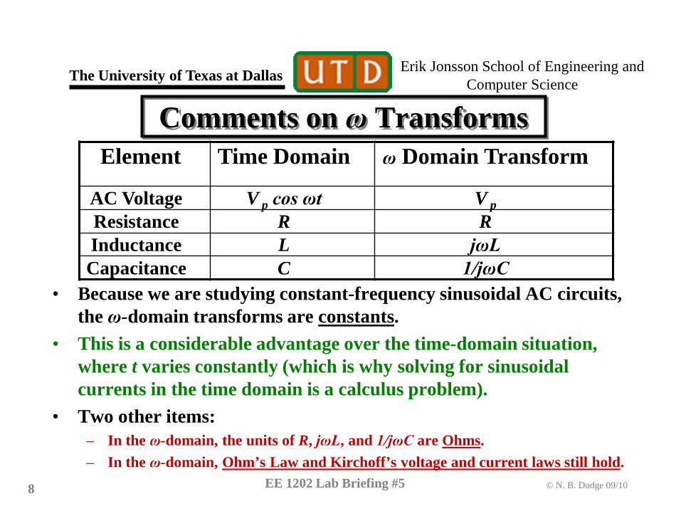
Comments on ω Transforms

• Because we are studying constant-frequency sinusoidal AC circuits, the ω-domain transforms are constants.

• This is a considerable advantage over the time-domain situation, where t varies constantly (which is why solving for sinusoidal currents in the time domain is a calculus problem).

• Two other items: – In the ω-domain, the units of R, jωL, and 1/jωC are Ohms. – In the ω-domain, Ohm’s Law and Kirchoff’s voltage and current laws still hold.


Element Time Domain ω Domain Transform

AC Voltage V p cos ωt V p Resistance R R Inductance L jωL Capacitance C 1/jωC



© N. B. Dodge 09/10

Solving for Currents in the ω Domain • Solving problems in the frequency

domain: – Given a circuit with the AC voltage

shown, and only a resistor in the circuit, then the transform of the voltage is 10. R transforms directly as 100.

– Solving for the circuit current, I=V/R, or I=10/100 = 0.1 A.

– This current is the ω-domain answer. It must be inverse-transformed to the time domain to obtain a usable answer.


AC Voltage Source =10 cos (1000t)

100 Ω

ω-domain voltage = Vp = 10

ω-domain current = Vp /R = 10/100 = 0.1 ampere



© N. B. Dodge 09/10

An ω Domain Solution for an L Circuit • The ω-domain voltage is still 10. • The ω-domain transform of L = jωL =

j(1000)10(10)‒3. = j10. • The units of the L transform is in Ohms

(Ω), i.e., the ω-domain transform of L is j10 Ω.

• The value ωL is called inductive reactance (X). The quantity jωL is called impedance (Z).

• Finding the current: I = V/Z = 10/j10 = 1/j = ‒j (rationalizing).

• Time-domain answer in a few slides! EE 1202 Lab Briefing #5 10

AC Voltage =10 cos (1000t)

10 mH


ω-domain current = Vp /jωL = 10/j10 = ‒j1 = ‒j ampere



© N. B. Dodge 09/10

An ω Domain Solution for a C Circuit

• The ω-domain voltage still = 10. • The ω-domain transform of C = 1/jωC

=1/ j(1000)100(10)‒6. = 1/j0.1= ‒j10. • The units of the C transform is in Ohms

(Ω), i.e., the ω-domain transform of C is ‒j10 Ω.

• The value 1/ωC is called capacitive reactance, and 1/jωC is also called impedance (here, capacitive impedance).

• Finding the current: I = V/Z = 10/‒j10 = 1/‒j = j1 (rationalizing) = j.

• Time-domain answer coming up!



100 μF


ω-domain current = Vp /(1/jωC) = 10/‒j10 = j1 = j amperes



© N. B. Dodge 09/10

An RL ω-Domain Solution • The ω-domain voltage still = 10. • The ω-domain impedance is 10+j10 . • Resistance is still called resistance in

the ω-domain. The R and L transforms are called impedance, and a combination of resistance and imaginary impedances is also called impedance.

• Note: all series impedances add directly in the ω-domain.

• Finding the current: I = V/Z = 10/(10+j10) = (rationalizing) (100‒j100)/200 = 0.5‒j0.5.

• Time-domain answers next! EE 1202 Lab Briefing #5 12


10 mH


ω-domain current = Vp /(R+jωL) = 10/(10+j10) = 0.5‒j0.5 ampere

10 Ω



© N. B. Dodge 09/10

Inverse Transforms

• Our ω-domain solutions do us no good, since we are inhabitants of the time domain.

• We required a methodology for inverse transforms, mathematical expressions that can convert the frequency domain currents we have produced into their time-domain counterparts.

• It turns out that there is a fairly straightforward inverse transform methodology which we can employ.

• First, some preliminary considerations.




© N. B. Dodge 09/10

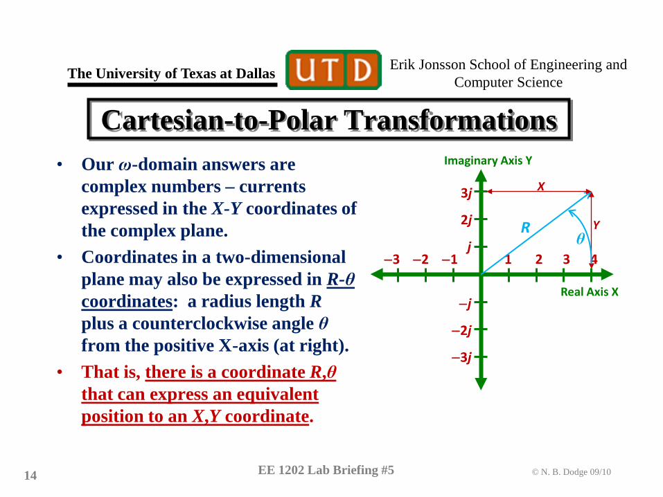
Cartesian-to-Polar Transformations • Our ω-domain answers are

complex numbers – currents expressed in the X-Y coordinates of the complex plane.

• Coordinates in a two-dimensional plane may also be expressed in R-θ coordinates: a radius length R plus a counterclockwise angle θ from the positive X-axis (at right).

• That is, there is a coordinate R,θ that can express an equivalent position to an X,Y coordinate. EE 1202 Lab Briefing #5 14

Real Axis X

Imaginary Axis Y

−3 −2 −1 1 2 3 4

3j

2j

j

−j

−2j

−3j

X

Y R θ



© N. B. Dodge 09/10

Cartesian-to-Polar Transformations (2) • The R,θ coordinate is equivalent to

the X,Y coordinate if θ = arctan(Y/X) and .

• In our X-Y plane, the X axis is the real axis, and the Y axis is the imaginary axis. Thus the coordinates of a point in the complex plane with (for example) X coordinate A and Y coordinate +B is A+jB.

• Now, remember Euler’s formula:


Real Axis X

Imaginary Axis Y

−3 −2 −1 1 2 3 4

3j

2j

j

−j

−2j

−3j

X

Y R θ

2 2R X Y= +

cos sinjxe x j x± = ±



© N. B. Dodge 09/10

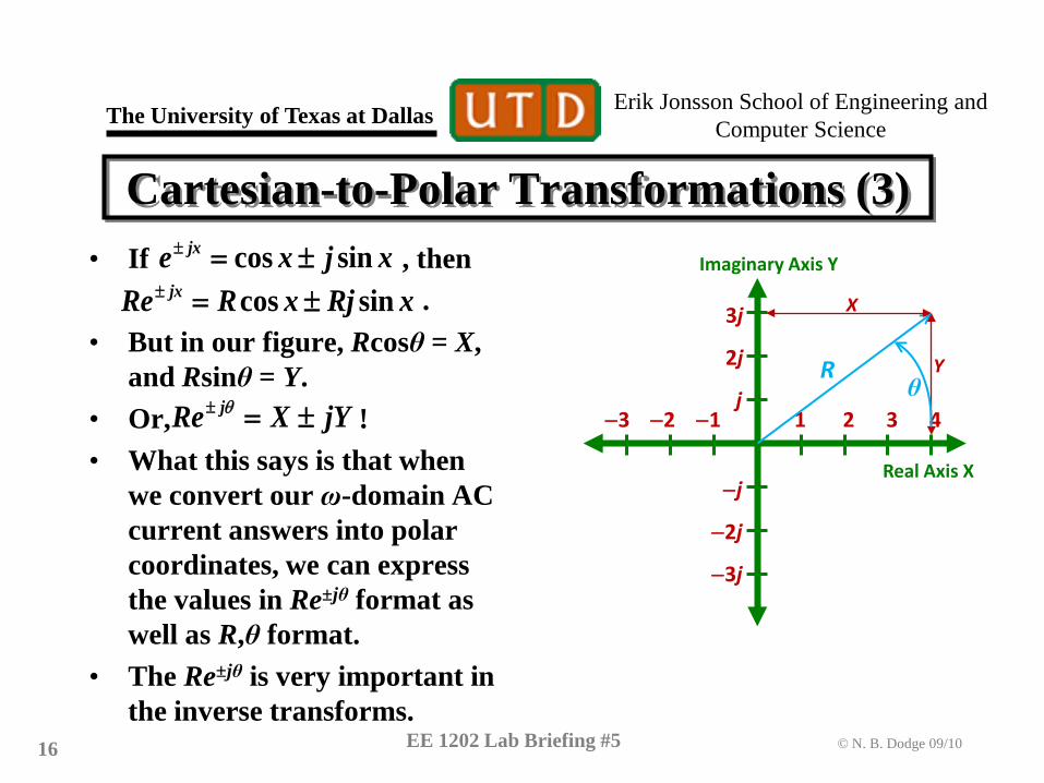
Cartesian-to-Polar Transformations (3) • If , then . • But in our figure, Rcosθ = X,

and Rsinθ = Y. • Or, ! • What this says is that when

we convert our ω-domain AC current answers into polar coordinates, we can express the values in Re±jθ format as well as R,θ format.

• The Re±jθ is very important in the inverse transforms.


Real Axis X

Imaginary Axis Y

−3 −2 −1 1 2 3 4

3j

2j

j

−j

−2j

−3j

X

Y R θ

cos sinjxe x j x± = ±cos sinjxRe R x Rj x± = ±

jRe X jYθ± = ±



© N. B. Dodge 09/10

Inverse Transform Methodology

• We seek a time-domain current solution of the form i(t) = Ipcos(ωt). where Ip is some peak current.

• This is difficult to do with the ω-domain answer in Cartesian (A±jB) form.

• So, we convert the ω-domain current solution to R,θ format, then convert that form to the Re±jθ form, where we know that θ = arctan (Y/X), and .

• Once the ω-domain current is in Re±jθ form (and skipping a lot of derivation), we can get the time-domain current as follows:


2 2R X Y= +



© N. B. Dodge 09/10

Inverse Transform Methodology (2)

• Given the Re±jθ expression of the ω-domain current, we have only to do two things: – Multiply the Re±jθ expression by ejωt . – Take the real part.

• This may seem a little magical at this point, but remember, Re (ejωt) is cos ωt, and we are looking for a current that is a cosine function of time.

• We can see examples of this methodology by converting our four ω-domain current solutions to real time-domain answers.




© N. B. Dodge 09/10

Transforming Solutions

• In the resistor case, our ω-domain current is a real number, 0.1 A. Then X=0.1, Y=0.

• Then , and θ = arctanY/X = arctan 0 = 0.

• Thus current = Re {0.1 ejωtej0} = 0.1Re {0.1 ejωt} = 0.1 cos1000t A.

• Physically, this means that the AC current is cosinusoidal, like the voltage. It rises and falls in lock step with the voltages, and has a maximum value of 0.1 A (figure at right).


2 2 2(0.1) 0.1R X Y= + = = ω-domain current = Vp /R = 10/100 = 0.1 ampere

Voltage Current



© N. B. Dodge 09/10

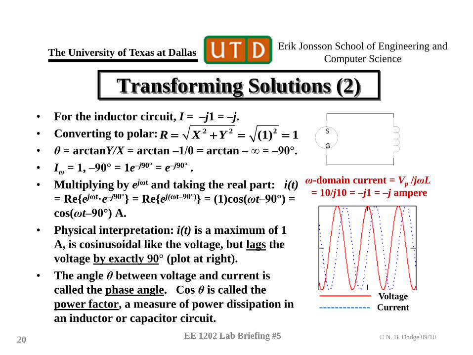
Transforming Solutions (2) • For the inductor circuit, I = ‒j1 = ‒j. • Converting to polar: • θ = arctanY/X = arctan ‒1/0 = arctan ‒ ∞ = ‒90°. • Iω = 1, ‒90° = 1e‒j90° = e‒j90° . • Multiplying by ejωt and taking the real part: i(t)

= Re{ejωt·e‒j90°} = Re{ej(ωt‒90°)} = (1)cos(ωt‒90°) = cos(ωt‒90°) A.

• Physical interpretation: i(t) is a maximum of 1 A, is cosinusoidal like the voltage, but lags the voltage by exactly 90° (plot at right).

• The angle θ between voltage and current is called the phase angle. Cos θ is called the power factor, a measure of power dissipation in an inductor or capacitor circuit.


ω-domain current = Vp /jωL = 10/j10 = ‒j1 = ‒j ampere

2 2 2(1) 1R X Y= + = =

Voltage Current



© N. B. Dodge 09/10

Transforming Solutions (3) • For the capacitor circuit, I = ‒j A. • Converting to polar: . • θ = arctanY/X = arctan 1/0 = arctan ∞

= 90°, so that Iω = 1, 90° = ej90°. • Multiplying by ejωt and taking the real

part: i(t) = Re{ejωt ·ej90°} = Re{ej(ωt +90°)} = cos(ωt+90°) A.

• Physically, i(t) has a maximum amplitude of 1 A, is cosinusoidal like the voltage, but leads the voltage by exactly 90° (figure at right).


ω-domain current = Vp /(1/jωC) = 1/‒j0.1 = j10 amperes

2 2 2( 1) 1R X Y= + = − =

Voltage Current



© N. B. Dodge 09/10

Transforming Solutions (4) • For the RL circuit, I = 0.5‒j0.5 ampere. • Converting to polar: . • And θ = arctanY/X = arctan ‒0.5/0.5 = arctan

‒1= ‒45°; Iω = 0.707, ‒90° = 0.707e‒j45° . • Multiplying by ejωt and taking the real part:

i(t) = Re{0.707ejωt ·e‒j45°} = 0.707Re{ej(ωt ‒45°)} = 0.707cos(ωt‒45°) = 0.707cos(ωt‒45°) A.

• Note the physical interpretation: i(t) has a maximum amplitude of 0.707 A, is cosinusoidal like the voltage, and lags the voltage by 45°. Lagging current is an inductive characteristic, but it is less than 90°, due to the influence of the resistor.


ω-domain current = Vp /(R+jωL) = 10/(10+j10) = 0.5‒j0.5 ampere

2 2 2 2(0.5) ( 0.5) 0.707R X Y= + = + − ≈



© N. B. Dodge 09/10

Summary: Solving for Currents Using ω Transforms • Transform values to the ω-domain: • Solve for Iω, using Ohm’s and Kirchoff’s laws.

– Solution will be of the form A±jB (Cartesian complex plane). • Use inverse transforms to obtain i(t).

– Convert the Cartesian solution (A±jB) to R,θ format and thence to Re±jθ form.

– Multiply by e±jωt and take the real part to get a cosine-expression for i(t).


Element Time Domain ω Domain Transform AC Voltage V p cos ωt V p Resistance R R Inductance L jωL

Capacitance C 1/jωC



© N. B. Dodge 09/10

Measuring AC Current Indirectly • Because we do not have current probes for the

oscilloscope, we will use an indirect measurement to find i(t) (reference Figs. 11 and 13 in Exercise 5).

• As the circuit resistance is real, it does not contribute to the phase angle of the current. Then a measure of voltage across the circuit resistance is a direct measure of the phase of i(t).

• Further, a measure of the Δt between the i,v peaks is a direct measure of the phase difference in seconds.

• We will use this method to determine the actual phase angle and magnitude of the current in Lab. 5.




© N. B. Dodge 09/10

Discovery Exercises • Lab. 5 includes two exercises that uses inductive and capacitive

impedance calculations to allow the discovery of the equivalent inductance of series inductors and the equivalent capacitance of series capacitors.

• Question 7.6 then asks you to infer the equivalent inductance of parallel inductors and the equivalent capacitance of parallel capacitors.

• Although you are really making an educated guess at that point, you can validate your guess using ω-domain circuit theory, with one additional bit of knowledge not covered in the lab text: – In the ω-domain, parallel impedances add reciprocally, just like

resistances in a DC circuit. – (Remember that in the ω-domain, series impedances add directly).


Documents

AC RL and RC Circuits - The University of Texas at Dallas