Electric-dipole, electric-quadrupole, magnetic-dipole, andmagnetic-quadrupole transitions in the neon isoelectronic

sequence

U.I. Safronova1,2, C. Namba1, I. Murakami1, W.R. Johnson2, and M.S. Safronova21National Institute for Fusion Science, Toki, Gifu, 509-5292, Japan

2Department of Physics, University of Notre Dame, Notre Dame, IN 46556, USA

(April 12, 2001)

Abstract

Excitation energies for 2l − 3l′ hole-particle states of Ne-like ions are deter-mined to second order in relativistic many-body perturbation theory (MBPT).

Reduced matrix elements, line strengths, and transition rates are calculated

for electric-dipole (E1), magnetic-quadrupole (E2), magnetic-dipole (M1), and

magnetic-quadrupole (M2) transitions in Ne-like ions with nuclear charges

ranging from Z = 11 to 100. The calculations start from a 1s22s22p6 closed-

shell Dirac-Fock potential and include second-order Coulomb and Breit-

Coulomb interactions. First-order many-body perturbation theory (MBPT)

is used to obtain intermediate-coupling coefficients and second-order MBPT

is used to determine the matrix elements. Contributions from negative-energy

states are included in the second-order E1, M1, E2, and M2 matrix elements.

The resulting transition energies are compared with experimental values and

with results from other recent calculations. Trends of E1, E2, M1, and M2

transition rates as functions of nuclear charge Z are shown graphically for all

transitions to the ground state.

PACS Numbers: 32.70.Cs, 31.25.Jf, 31.15.Md

Typeset using REVTEX

1

I. INTRODUCTION

Excitation energies, line strengths, and transition probabilities for 2s22p53l and 2s2p63lstates along the neon isoelectronic sequence have been studied theoretically and exper-imentally during the past 30–40 years. Z-expansion [1–3], model potential (MP) [4–7],configuration-interaction (CI) [8–12], multi-configuration Hartree-Fock (MCHF) [13–15], R-matrix [16], multi-configuration Dirac-Fock (MCDF) [17], and relativistic many-body per-turbation theory (MBPT) [18–20] are among the methods that have been used to calculatethese quantities for Ne-like ions.Nonrelativistic perturbation theory was used in Refs. [1–3] to calculate energy levels of

2s22p53l and 2s2p63l states in Ne-like ions. In those papers, contributions from the Coulomband Breit interactions were represented in powers of 1/Z. Accurate transition energies andrates were obtained for ions with nuclear charges Z from 20 to 60 by introducing screeningconstants and including radiative and higher-order relativistic effects. The technique usedin [1–3] is referred to as the MZ method. Results obtained by the MZ method and twoversions of the model potential method [4–7] were compared in Ref. [21] for the 2l − 3l′electric-dipole transition energies in Ne-like ions with Z = 36− 92. Correlation correctionsfor Ne-like ions were studied empirically by Quinet et al. in Ref. [17], where uncorrectedMCDF energies were given and differences between the experimental and uncorrected MCDFenergies were treated by least-squares fitting. The resulting adjusted energies for 2s22p53lstates were given for ions with Z = 28− 92. A similar idea was used by Hibbert et al. [11],where accurate adjusted energies for 2s22p53l and 2s2p63l states were presented for ionswith Z = 10− 36. At a more sophisticated level, relativistic MBPT was used to determineenergies of four 2s22p53s levels and three 2s22p53d levels for ions with Z = 10 − 92 byAvgoustouglou et al. in Refs. [19,20], where second-order MBPT for the Coulomb and Breitcorrelation corrections was supplemented by all-order hole-core corrections.Accurate measurements along the Ne isoelectronic sequence have been made using a

variety of light sources. Most accurate wavelength measurements come from plasma lightsources, both magnetic-fusion plasmas and laser-produced plasmas. Early wavelength mea-surements for high-Z ions were made by Aglitskii et al. [2], Boiko et al. [22], Gordon etal. [23,24], Jupen et al. [25], Gauthier et al. [26], Beiersdorfer et al. [27], and Buchet et al.[28]. Some of the work was summarized by Aglitskii et al. [21] in a report on measure-ments of Kr26+-Nd50+ spectra observed in low-inductance vacuum spark-produced plasmas[21]. Beiersdorfer et al. [29] reported results in Ne-like Xe, La, Nd, and Eu obtained atthe Princeton Tokamak. Some years later, Beiersdorfer et al. [30,31] presented spectra ofNe-like Yb and Th obtained in an electron-beam ion trap (EBIT). Beam-foil spectra of2l− 3l′ transitions in highly-stripped gold and bismuth was reported by Chandler et al. [32]and Dietrich et al. [33]. Recently, accurate wavelengths measurements of lasing and nonlas-ing lines in a laser-produced germanium plasma were reported by Yuan et al. in Ref. [34].Wavelengths of x-ray transitions in Ne-like I43+, Cs45+, and Ba46+ were measured with a flatcrystal spectrometer at the Tokyo EBIT by Nakamura et al. in Ref. [35].In the present paper, relativistic many-body perturbation theory (MBPT) is used to

determine energies of 2s22p53l(J) and 2s2p63l(J) states of Ne-like ions with nuclear chargesZ = 11 − 100. Energies are calculated for the 16 even-parity excited states and the 20odd-parity excited states. The calculations are carried out to second order in perturbation

2

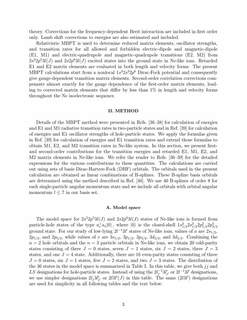
theory. Corrections for the frequency-dependent Breit interaction are included in first orderonly. Lamb shift corrections to energies are also estimated and included.Relativistic MBPT is used to determine reduced matrix elements, oscillator strengths,

and transition rates for all allowed and forbidden electric-dipole and magnetic-dipole(E1, M1) and electric-quadrupole and magnetic-quadrupole transitions (E2, M2) from2s22p53l(J) and 2s2p63l(J) excited states into the ground state in Ne-like ions. RetardedE1 and E2 matrix elements are evaluated in both length and velocity forms. The presentMBPT calculations start from a nonlocal 1s22s22p6 Dirac-Fock potential and consequentlygive gauge-dependent transition matrix elements. Second-order correlation corrections com-pensate almost exactly for the gauge dependence of the first-order matrix elements, lead-ing to corrected matrix elements that differ by less than 1% in length and velocity formsthroughout the Ne isoelectronic sequence.

II. METHOD

Details of the MBPT method were presented in Refs. [36–38] for calculation of energiesand E1 and M1 radiative transition rates in two-particle states and in Ref. [39] for calculationof energies and E1 oscillator strengths of hole-particle states. We apply the formulas givenin Ref. [39] for calculation of energies and E1 transition rates and extend those formulas toobtain M1, E2, and M2 transition rates in Ne-like system. In this section, we present first-and second-order contributions for the transition energies and retarded E1, M1, E2, andM2 matrix elements in Ne-like ions. We refer the reader to Refs. [36–39] for the detailedexpressions for the various contributions to these quantities. The calculations are carriedout using sets of basis Dirac-Hartree-Fock (DHF) orbitals. The orbitals used in the presentcalculation are obtained as linear combinations of B-splines. These B-spline basis orbitalsare determined using the method described in Ref. [40]. We use 40 B-splines of order 8 foreach single-particle angular momentum state and we include all orbitals with orbital angularmomentum l ≤ 7 in our basis set.

A. Model space

The model space for 2s22p53l(J) and 2s2p63l(J) states of Ne-like ions is formed fromparticle-hole states of the type a+v aa|0〉 , where |0〉 is the closed-shell 1s21/22s21/22p21/22p43/2ground state. For our study of low-lying 2l−13l′ states of Ne-like ions, values of a are 2s1/2,2p1/2, and 2p3/2, while values of v are 3s1/2, 3p1/2, 3p3/2, 3d3/2, and 3d5/2. Combining then = 2 hole orbitals and the n = 3 particle orbitals in Ne-like ions, we obtain 20 odd-paritystates consisting of three J = 0 states, seven J = 1 states, six J = 2 states, three J = 3states, and one J = 4 state. Additionally, there are 16 even-parity states consisting of threeJ = 0 states, six J = 1 states, five J = 2 states, and two J = 3 states. The distribution ofthe 36 states in the model space is summarized in Table I. In this table, we give both jj andLS designations for hole-particle states. Instead of using the 2l−1j 3l′j′ or 2l

−13l′ designations,we use simpler designations 2lj3l

′j′ or 2l3l

′(J) in this table. The same (2l3l′) designationsare used for simplicity in all following tables and the text below.

3

B. Example: energy matrix for Mo32+

In Table II, we give various contributions to the second-order energies for the specialcase of Ne-like molybdenum, Z = 42. In this table, we show the one-body and two-bodysecond-order Coulomb contributions to the energy matrix labeled E

(2)1 and E

(2)2 , respectively.

The corresponding Breit-Coulomb contributions are given in columns headed B(2)1 and B

(2)2

of Table II. The one-body second-order energy is obtained as a sum of the valence E(2)v and

hole E(2)a energies with the later being the dominant contribution. The values of E(2)1 and

B(2)1 are non-zero only for diagonal matrix elements. Although there are 36 diagonal and142 non-diagonal matrix elements for (2l3l′) (J) hole-particle states in jj coupling, we listonly the subset with J=0 in Table II. Both even-parity states and odd-parity states arepresented. It can be seen from the table that second-order Breit-Coulomb corrections arerelatively large and, therefore, must be included in accurate calculations. The values of non-diagonal matrix elements given in columns headed E

(2)2 and B

(2)2 are comparable with values

of diagonal two-body matrix elements. However, the values of one-body contributions, E(2)1

and B(2)1 , are larger than the values of two-body contributions, E

(2)2 and B

(2)2 , respectively. As

a result, total second-order diagonal matrix elements are much larger than the non-diagonalmatrix elements, which are shown in Table III.In Table III, we present results for the zeroth-, first-, and second-order Coulomb contri-

butions, E(0), E(1), and E(2), and the first- and second-order Breit-Coulomb corrections, B(1)

and B(2). It should be noted that corrections for the frequency-dependent Breit interaction[41] are included in the first order only. The difference between the first-order Breit-Coulombcorrections calculated with and without frequency dependence is less than 1%. As one cansee from Table III, the ratio of non-diagonal and diagonal matrix elements is larger for thefirst-order contributions than for the second-order contributions. Another difference in thefirst- and second-order contributions is the symmetry properties: the first-order non-diagonalmatrix elements are symmetric and the second-order non-diagonal matrix elements are notsymmetric. The values of E(2)[a′v′(J), av(J)] and E(2)[av(J), a′v′(J)] matrix elements differin some cases by a factor 2–3 and occasionally have opposite signs.We now discuss how the final energy levels are obtained from the above contributions. To

determine the first-order energies of the states under consideration, we diagonalize the sym-metric first-order effective Hamiltonian, including both the Coulomb and Breit interactions.The first-order expansion coefficient CN [av(J)] is the N -th eigenvector of the first-ordereffective Hamiltonian and E(1)[N ] is the corresponding eigenvalue. The resulting eigenvec-tors are used to determine the second-order Coulomb correction E(2)[N ], the second-orderBreit-Coulomb correction B(2)[N ] and the QED correction ELamb[N ].In Table IV, we list the following contributions to the energies of 36 excited states

in Mo32+: the sum of the zeroth and first-order energies E(0+1) = E(0) +E(1)+B(1), thesecond-order Coulomb energy E(2), the second-order Breit-Coulomb correction B(2), theQED correction ELAMB, and the sum of the above contributions Etot. The QED correctionis approximated as the sum of the one-electron self energy and the first-order vacuum-polarization energy. The self-energy contribution is estimated for s, p1/2, and p3/2 orbitalsby interpolating the values obtained by Mohr [42] using Coulomb wavefunctions. For thispurpose, an effective nuclear charge Zeff is obtained by finding the value of Zeff required togive a Coulomb orbital with the same average 〈r〉 as the DHF orbital.

4

When starting calculations from relativistic DHF wavefunctions, it is natural to use jjdesignations for uncoupled transition and energy matrix elements; however, neither jj norLS coupling describes the physical states properly, except for the single-configuration state2p3/23d5/2(4) ≡ 2p3d 3F4. Both designations are used in Table IV.

C. Z-dependence of eigenvectors and eigenvalues in Ne-like ions

In Figs. 1 and 2, we show the Z-dependence of the eigenvectors and eigenvalues of the2lj 3l′j′ (J) states for the example of odd-parity states with J=1. We refer to a set ofstates of the same parity and the same J as a complex of states. This particular J=1odd-parity complex includes seven states which are listed in Table I. Using the first-orderexpansion coefficients CN [av(J)] defined in the previous section, we can present the resultingeigenvectors as

Φ(N) = CN [2p3/23s1/2(1)]Φ[2p3/23s1/2(1)] + CN [2p1/23s1/2(1)]Φ[2p1/23s1/2(1)] +

CN [2p3/23d3/2(1)]Φ[2p3/23d3/2(1)] + CN [2p3/23d5/2(1)]Φ[2p3/23d5/2(1)] +

CN [2p1/23d3/2(1)]Φ[2p1/23d3/2(1)] + CN [2s1/23p1/2(1)]Φ[2s1/23p1/2(1)] +

CN [2s1/23p3/2(1)]Φ[2s1/23p3/2(1)] . (2.1)

As a result, 49 CN [av(J)] coefficients are needed to describe the seven eigenvalues. Thesecoefficients are often called mixing coefficients. For simplicity, we plot only four of the mixingcoefficients for the level N=2p3d 3D1 in Fig. 1. These coefficients are chosen to illustratethe mixing of the states; the remaining mixing coefficients give very small contributionsto this level. We observe strong mixing between 2p1/23s1/2(1) and 2p3/23d5/2(1) states forZ = 54− 55 which results in the dramatic changes in their values.Energies, relative to the ground state, of odd-parity states with J=1, divided by (Z−7)2,

are shown in Fig. 2. We plot the four energy levels within the odd-parity J=1 complex whichare involved in the mixing of states illustrated in Fig. 1. We use LS designations for smallZ and jj designations for large Z in the figure. It should be noted that the LS designationsare chosen by comparing our results with available experimental data for low-Z ions. It wasalready shown in Fig. 1 that the largest mixing coefficient contributing to the 2p3d 3D1 levelis not the same for Z ≤ 54 and Z ≥55. This change is seen in Fig. 2. The first and thirdcurves almost cross for Z=55; the difference in energy values at Z=55 is equal to just 0.27%of the total energy values. Strong mixing also occurs for other levels, for example, between[2p1/23d3/2(1)] and [2s1/23p1/2(1)] states for Z = 69 − 70 and between [2p3/23d5/2(2)] and[2p3/23d3/2(2)] states for Z = 36− 37.

D. Electric-dipole and electric-quadrupole matrix elements

We calculate electric-dipole (E1) matrix elements for the transitions between the sevenodd-parity 2s1/23pj(1), 2pj3s1/2(1), and 2pj3dj′(1) excited states and the ground stateand electric-quadrupole (E2) matrix elements between the five even-parity 2pj3pj′(2) and2s1/23dj(2) excited states and the ground state for Ne-like ions with nuclear chargesZ = 11 − 100. The evaluation of the reduced E1 matrix elements for neon-like ions fol-lows the corresponding calculation for nickel-like ions described in Ref. [39]. The calculation

5

of the reduced E2 matrix elements is carried out using the same MBPT formulas given inRef. [39] and replacing the one-particle E1 matrix elements by the one-particle E2 matrixelements given in Ref. [43]. The first- and second-order Coulomb corrections and second-order Breit-Coulomb corrections to reduced E1 and E2 matrix elements will be referred toas Z(1), Z(2), and B(2), respectively, throughout the text. These contributions are calculatedin both length and velocity gauges. In this section, we show the importance of the differentcontributions and discuss the gauge dependence of the E1 and E2 matrix elements.In Fig. 3, differences between length and velocity forms are illustrated for the various

contributions to uncoupled 0 − 2p3/23d3/2(1) matrix element, where 0 is the ground state.In the case of E1 transitions, the first-order matrix element Z(1) is proportional to 1/Z,the second-order Coulomb matrix element Z(2) is proportional to 1/Z2, and the second-order Breit-Coulomb matrix element B(2) is almost independent of Z (see [37]) for high Z.Therefore, we plot Z(1)×Z, Z(2)×Z2, and B(2)×104 in Fig. 3. As one can see from Fig. 3, allthese contributions are positive, except for the second-order matrix elements Z(2) in lengthform which becomes negative for Z >21.The difference between length- and velocity-forms for the E2 uncoupled 0−2p3/23p1/2(2)

matrix element is illustrated in Fig. 4. In the case of E2 transitions, the first-order matrixelement Z(1) is proportional to 1/Z2, the second-order Coulomb matrix element Z(2) is pro-portional to 1/Z3, and the second-order Breit-Coulomb matrix element B(2) is proportionalto 1/Z for high Z. Taking into account these dependencies, we plot Z(1) × Z2, Z(2) × Z3,and B(2) × Z × 104 in Fig. 4. The second-order Breit-Coulomb correction to the E2 matrixelement B(2) is much smaller in velocity form than in length form, as seen in the figure.The differences between results in length- and velocity-forms shown in Figs. 3 and 4

are compensated by additional second-order terms called “derivative terms” P (derv); theyare defined by Eq. (2.16) in Ref. [39]. The derivative terms arise because transition am-plitudes depend on the energy, and the transition energy changes order-by-order in MBPTcalculations.In Table V, we list values of uncoupled first- and second-order E1 and E2 matrix elements

Z(1), Z(2), B(2), together with derivative terms P (derv), for Ne-like molybdenum, Z=42. Welist values for the seven E1 transitions between odd-parity states with J=1 and the groundstate and the five E2 transitions between even-parity states with J=2 and the ground state,respectively. Matrix elements in both length (L) and velocity (V ) forms are given. We can

see that the first-order matrix elements, Z(1)L and Z

(1)V , differ by 5–10%; however, the L–V

differences between second-order matrix elements are much larger for some transitions. Itcan be also seen from Table V that for the E1 transitions the derivative term in length form,P(derv)L , is almost equal to Z

(1)L but the derivative term in velocity form, P

(derv)V , is smaller

than Z(1)V by three to four orders of magnitude. For the E2 transition, the value of P

(derv)

in velocity form almost equals Z(1) in velocity form and the P (derv) in length form is largerby factor of two than Z(1) in length form.Values of E1 and E2 coupled reduced matrix elements in length and velocity forms are

given in Table VI for the transitions considered in Table V. Although we use an intermediate-coupling scheme, it is nevertheless convenient to label the physical states using the jj scheme.The first two columns in Table VI show L and V values of coupled reduced matrix elementscalculated in first order. The L − V difference is about 5–10%. Including the second-ordercontributions (columns headed MBPT in Table VI) decreases the L−V difference to 0.002-

6

0.2%. This extremely small L−V difference arises because we start our MBPT calculationsusing a non-local Dirac-Fock (DF) potential. If we were to replace the DF potential by alocal potential, the differences would disappear completely. It should be emphasized thatwe include the negative energy state (NES) contributions to sums over intermediate states(see Ref. [37] for details). Neglecting the NES contributions leads to small changes in theL-form matrix elements but to substantial changes in some of the V -form matrix elementswith a consequent loss of gauge independence.

E. Magnetic-dipole and magnetic-quadrupole matrix elements

We calculate magnetic-dipole (M1) matrix elements for the transitions between the sixeven-parity 2s1/23s1/2(1), 2s1/23d3/2(1), and 2pj3pj′(1) excited states and the ground stateand magnetic-quadrupole (M2) matrix elements for the transitions between the six odd-parity 2s1/23p3/2(2), 2p3/23s1/2(2), and 2pj3dj′(2) excited states and the ground state for Ne-like ions with nuclear charges Z = 11− 100. We calculate first- and second-order Coulomb,second-order Breit-Coulomb corrections, and second-order derivative term to reduced M1and M2 matrix elements Z(1), Z(2), B(2), and P (derv), respectively, using the method describedin Ref. [39]. In this section, we illustrate the importance of the relativistic and frequency-dependent contributions to the first-order M1 and M2 matrix elements. We also show theimportance of the taking into account the second-order MBPT contributions to M1 and M2matrix elements and we subsequently discuss the necessity of including the negative-energycontributions to sums over intermediate states.The differences between first-order M1 uncoupled matrix elements, calculated in nonrel-

ativistic, relativistic frequency-independent, and relativistic frequency-dependent approxi-mations are illustrated for the 0−2p1/23p1/2(1) matrix element in Fig. 5. The correspondingmatrix elements are labeled Z(1)(NR), Z(1)(R), and Z(1)(RF). Formulas for non-relativisticand relativistic frequency-dependent first-order M1 matrix elements are given in Ref. [38].We also plot the second-order Coulomb contributions, Z(2), and the second-order Breit-Coulomb contributions, B(2), in the same figure. As we observe from Fig. 5, the values ofZ(1)(NR) are twice as small as the values of Z(1)(R) and Z(1)(RF). Therefore, relativisticeffects are very large for M1 transitions. The frequency-dependent relativistic matrix ele-ments Z(1)(RF) differ from the relativistic frequency-independent matrix elements Z(1)(R)by 5–10%. The differences between other first-order matrix elements calculated with andwithout frequency dependence are also on the order of a few percent. Uncoupled second-order M1 matrix elements Z(2) are comparable to first-order matrix elements Z(1)(RF) forsmall Z but the relative size of the second-order contribution decreases for high Z. This isexpected since second-order Coulomb matrix elements Z(2) are proportional to Z for highZ while first-order matrix elements Z(1)(RF) grow as Z2. The second-order Breit-Coulombmatrix elements B(2) are proportional to Z3 and become comparable to Z(2) for very highZ.In Fig. 6, we illustrate the Z-dependence of the line strengths of M1 transition from the

2p3p 3D1 excited state to the ground state. In this figure, we plot the values of the first-order line strengths S(1)(NR) , S(1)(R), and S(1)(RF) calculated in the same approximationsas the M1 uncoupled matrix elements: nonrelativistic, relativistic frequency-independent,and relativistic frequency-dependent approximations, respectively. The total line strengths

7

S(tot), which include second-order corrections, are also plotted. Strong mixing inside of theeven-parity complex with J=1 between 2p3/23p1/2 and 2p3/23p3/2 states occurring for smallZ leads to the sharp features in the line strengths seen in the graphs. The deep minimumon Fig. 6 shifts when different approximations are used for the calculation of line strengths.This shift in the placement of the minimum leads to difficulties in comparison of data forM1 transitions obtained in nonrelativistic and relativistic approximations. We discuss thisquestion further in Section III.Ab initio relativistic calculations require careful treatment of negative-energy states (vir-

tual electron-positron pairs). In second-order matrix elements, such contributions explicitlyarise from those terms in the sum over states for which εi < −mc2. The effect of the NEScontributions to M1-amplitudes has been studied recently in Ref. [38]. The NES contribu-tions drastically change the second-order Breit-Coulomb matrix elements B(2). However, thesecond-order Breit-Coulomb correction contributes only 2–5% to uncoupled M1 matrix ele-ments and, as a result, negative-energy states change the total values of M1 matrix elementsby a few percent only.In Table VII, we list values of uncoupled first- and second-order M2 matrix elements

Z(1), Z(2), B(2), together with derivative terms P (derv), for Ne-like molybdenum, Z=42. Welist values for the six M2 transitions between odd-parity states with J=2 and the groundstate. We note that the first-order M2 matrix element 0 − 2p3/23p3/2(2) vanishes becausethe corresponding factor (κa + κv), where κi is a relativistic angular momentum quantumnumber of a state i, in equation for Z(1) equals zero for this transition. Differences betweenfirst-order uncoupled M2 matrix elements calculated with and without frequency dependenceare shown in first two columns of Table VII labeled Z(1)(R) and Z(1)(RF). As one can seefrom Table VII, the difference between Z(1)(R) and Z(1)(RF) is about 1%.The importance of negative-energy states (NES) is illustrated for the second-order Breit-

Coulomb matrix elements B(2). In Table VII, we compare the values of B(2)(pos) andB(2)(neg) calculated with positive and negative part of spectra, respectively. The ratio ofB(2)(neg) to B(2)(pos) is about 10%.In Table VIII, we present results of line strengths S for M2 lines in Ne-like ions. In this

table, the values of S for Z=20-100 in steps of 10 are given. The S-values are obtained inthe intermediate-coupling scheme; nevertheless, both LS and jj designations are shown inthis table. Among the six transitions presented in Table VIII, there is one transition withzero first-order uncoupled matrix element, 0 − 2p3/23p3/2(2). The non-zero S-value of thistransition results from the non-vanishing second-order contribution. It can be seen fromTable VIII that the S-value of this transition is the smallest of the six for high Z.

III. COMPARISON OF RESULTS WITH OTHER THEORY AND EXPERIMENT

A. Transition energies

In Table IX, we compare our MBPT results for energies with experimental measurementsfrom [21] and with theoretical results from Refs. [19,20]. We list only comparisons for ionswith Z= 42, 48, 54, and 60. A comparison of our results with data from Refs. [19–21] forall ions from Z=39 to Z=60 is available as supplementary data in Ref. [44]. Our resultsare seen to be in close agreement with theoretical calculations from Refs. [19,20] and with

8

experimental measurements from Ref. [21]. In Refs. [19,20], all virtual orbitals were gen-erated in the field of the hole state, i.e. in 1s22s22p5 V (N−1) potential. The choice of suchpotential is very convenient if only one hole state is being considered, which was the case inRefs. [19,20], where only 2p3l(J) states were investigated. The influence of the 2s3l(J) statescan be taken into account by summing all-order diagrams. In the present paper, the V (N)

(1s22s22p6) potential, which allows one to treat 2s3l(J) and 2p3l(J) states simultaneously, ischosen. The calculations in Refs. [19,20] included third-order corrections that are omitted inour work. However, third-order corrections are small for the high Z considered in Table IXand do not significantly affect the results for high-Z ions. It was shown in Refs. [19,20] thatthe third-order hole-core Coulomb correlation energy E(3+) is about 0.1 a.u. for Ne I. Thiscorrection decreases rapidly with Z; the value of E(3+) is less than 0.007 a.u. for Zr30+.Energies of 2s2p63p 1,3P1 levels are given in Table X for selected high-Z ions. Our results

are compared with measurements from Ref. [21] and results for Ag37+, Xe44+, Yb60+, Au69+,and Bi73+ reported by Beiersdorfer et al. [27,29,30], Chandler et al. [32], and Dietrich et al.[33]. The experimental results for Ag37+ in Refs. [21,27] and Xe44+ in Refs. [21,29] disagreeby 0.03–0.07 a.u.; our MBPT results lie between these two experimental measurements.A complete tabulation of our data for 2s1/23pj(1) energies for ions with Z=39-94 and acomparison of those energies with all available experimental results is given as supplementarydata in Ref. [44].Our MBPT data are compared with measurements from Beiersdorfer et al. in

Refs. [27,29–31], Chandler et al. [32], and Dietrich et al. [33] in Table XI and found tobe in excellent agreement with experimental measurements. Our theoretical data for othercases will be useful as benchmark data for future experiments. Results for the energies ofall 36 2l3l′(J) levels for ions with Z=47, 54, 57, 60, 63, 70, 79, 83, and 90 are available assupplementary data in Ref. [44].

B. The E1, E2, M1, and M2 transition probabilities

The E1, E2, M1, and M2 transition probabilities A for the transitions between the groundstate and 2lj3l′j′(J) states are obtained using the relations

A(E1) =2.1420× 1010(2J + 1)

(∆E)3 S(E1) s−1,

A(M1) =2.8516× 105(2J + 1)

(∆E)3 S(M1) s−1,

A(E2) =5.7032× 104(2J + 1)

(∆E)5 S(E2) s−1,

A(M2) =7.5926× 10−1(2J + 1)

(∆E)5 S(M2) s−1, (3.1)

where ∆E is the transition energy in atomic units and S(E1), S(M1), S(E2), and S(M2)are the corresponding line strengths in atomic units.We present the resulting transition probabilities in Figs. 7-10. Transition rates for the

seven E1 2p3s 3P1,1P1, 2p3d

3P1,3D1,

1P1 and 2s3p3P1,

1P1 lines are plotted in Fig. 7.The curves describing 2p3s 3P1 and 2s3p

1P1 transition rates smoothly increase with Z

9

without any sharp features. However, the curves representing other transitions containdeep minima due to mixing of states. We already mentioned the strong mixing between[2p1/23s1/2(1)]+[2p3/23d3/2(1)]+[2p3/23d5/2(1)] states in the interval Z = 51−55. This mixingcauses the exchange of 2p3d 3P1 and 2p3d

3D1 labels and the sharp minimum in the 2p3s1P1

transition rate graph for Z=52. There are also minima in the curves describing the 2p3d 3P1(Z=45), 2p3d 3D1 (Z=58), and 2s3p

3P1 (Z=66) transition rates. We also compare ourMBPT calculations with E1 transition rates calculated by using superstructure code inRefs. [8,9,12] and civ3 code in Ref. [11]. All results agree at the level of 10-20%, except forcases with singularities in the curves of transition rates. In these cases, (for example, the2p3d 3P1 transition rates for Z=42) our MBPT data are in better agreement with data fromRef. [5] than with data from Ref. [12].Disagreement between our results and the theoretical calculations presented in Refs.

[8,9,12] is much larger for M1 transition rates than for E1 transition rates. This differenceis explained by large contribution of relativistic effects partly omitted in Refs. [8,9,12] buttaken into account in our calculations. In the previous section, we compared results forM1 uncoupled matrix elements (see Fig. 5) and M1 line strengths (see Fig. 6) calculatedusing nonrelativistic, relativistic and frequency-dependent relativistic first-order matrix el-ements. The relativistic effects modify uncoupled matrix elements by a factor of two anddrastically change the Z-dependence of coupled matrix elements. In the superstructurecode [8,9,12], the wavefunctions were determined by diagonalizing the nonrelativistic Hamil-tonian using orbitals calculated in a scaled Thomas-Fermi-Dirac-Amaldi (TFDA) potential.These nonrelativistic functions were used to calculate M1 matrix elements. Our MBPTresults and results from superstructure given in [8,9,12], differ by 20-30% for 2p3p 3P1transition rates and by a factor of 2–3 for 2p3p 3S1,

3D11P1 transition rates. Much better

agreement was found between our results and results obtained in Ref. [5], where a relativisticapproach was used. The differences with nonrelativistic calculations are especially large forthe transition rates in the interval of Z around the minima of line strength curves, such asthose shown in Fig. 6. As we discussed in Section II E, the minima occur for different valuesof Z in nonrelativistic and relativistic approximations. Since the transition rates are calcu-lated using these line strengths, they change rapidly with Z around the minima, leading tolarge disagreements between our relativistic calculations and the nonrelativistic calculationsof Refs. [8,9,12]. For example, our result for 2p3p 3D1 transition rates in Cu

19+, where theminimum illustrated in Fig. 8 occurs, differs from the result of the superstructure codegiven in Ref. [12] by three orders of magnitude. The same minimum is seen in the curvedescribing the corresponding line strengths in Fig. 6.The E2 transition rates are less sensitive to relativistic effects than the M1 transition

rates. In Fig. 9, transition rates for the six E2 2p3p 3D2,3P2,

1D2 and 2s3d3D2,

1D2lines are shown. It should be noted that there are the very small differences between the2p3p 3D2,

3 P2,1D2 transition rates which is seen from Fig. 9. All six E2 transition rates

increase smoothly with Z.A similar smooth Z-dependence for M2 rates is shown in Fig. 10. In this figure, the

transition rates for the six M2 2p3s 3P2, 2p3d3P2,

3F2,1D2,

1D2, and 2s3p3P2 lines are

presented. The curve describing the 2p3d 3P2 transition rate crosses the five curves describingother M2 transitions rates and becomes the smallest one for Z >54. Such a decrease in the2p3d 3P2 transition rates can be explained by the fact that the jj coupling scheme is more

10

suitable than LS coupling scheme for high Z. The value of uncoupled 0−2p3/23d3/2(2) matrixelement is non-vanishing only because of the second-order contribution. Mixing inside theodd-parity complex with J=2 becomes less important with the increase of Z. The coupled0− 2p3d 3P2 matrix element is approximately equal to uncoupled 0− 2p3/23p3/2(2) matrixelement. This is a very interesting example of the case where intermediate-coupling convertsto pure jj coupling.Finally, we discuss some small singularities for low Z in Figs. 7-10. These singularities

are caused by the second-order uncoupled matrix elements already discussed in the previoussection. The 2s1/23s1/2 (1), 2s1/23pj (J), and 2s1/23dj (J) states are autoionizing for the2pj-hole threshold in the Z = 11 − 20 range. In this case, the singularity arises from thecontribution of the continuous part of spectra in the sum over states for Z(2) (see Ref. [39]).

IV. CONCLUSION

We have presented a systematic second-order relativistic MBPT study of excitation en-ergies, reduced matrix elements, line strengths, and transition rates for ∆n=1 electric- andmagnetic-dipole and quadrupole transitions in Ne-like ions with nuclear charges Z=11–100.Our calculation of the retarded E1, E2, M1, and M2 matrix elements include correlationcorrections from both Coulomb and Breit interactions. Contributions from virtual electron-positron pairs were also included in the second-order matrix elements. Both length and ve-locity forms of the E1 and E2 matrix elements were evaluated and small differences, causedby the non-locality of the starting HF potential, were found between the two forms. Second-order MBPT transition energies were used to evaluate oscillator strengths and transitionrates. Good agreement of our MBPT data with other accurate theoretical results leads usto conclude that the MBPT method provides accurate data for Ne-like ions. Results fromthe present calculations provide benchmark values for future theoretical and experimentalstudies of the neon isoelectronic sequence.

ACKNOWLEDGMENTS

The work of WRJ and MSS was supported in part by National Science FoundationGrant No. PHY-99-70666. UIS acknowledges partial support by Grant No. B503968 fromLawrence Livermore National Laboratory. UIS would like to thank the members of the Dataand Planning Center, the National Institute for Fusion Science for their hospitality, friendlysupport and many interesting discussions.

11

REFERENCES

[1] L. A. Bureeva and U. I. Safronova, Phys. Scripta, 20, 81 (1979).[2] E. V. Aglitskii, E. Ya. Golts, Yu. A. Levykin, A. M. Livshits, S. L. Mandelshtam andU. I. Safronova, Opt. Spectrosc. 46, 590 (1979).

[3] U.I. Safronova, M. S. Safronova and R. Bruch, Phys. Scripta, 49, 446 (1994).[4] E. P. Ivanova and A. V. Glushkov, Journ. Quant. Spectr. Rad. Transf., 36, 127 (1986).[5] E. P. Ivanova and A. V. Gulov, Atomic Data and Nucl. Data Tables 49, 1 (1991).[6] U. I. Safronova and J.-F. Wyart, Phys. Scripta, 46, 134 (1992).[7] E. P. Ivanova and I. P. Grant, J. Phys. B, 31, 2671 (1998).[8] A. K. Bhatia, U. Feldman and J. F. Seely, Atomic Data and Nucl. Data Tables 32, 435(1985).

[9] A. K. Bhatia and G. A. Doschek, Atomic Data and Nucl. Data Tables 52, 1 (1992).[10] Y. Kagawa, Y. Honda and S. Kiyokawa, Phys. Rev. A, 44, 7092 (1991).[11] A. Hibbert, M. Le Dourneuf, and M. Mohan, Atomic Data and Nucl. Data Tables 53,23 (1993).

[12] M. Cornille, J. Dubau and S. Jacquemot, Atomic Data and Nucl. Data Tables 58, 1(1994).

[13] W. Fielder, Jr., D. L. Lin and D. Ton-That, Phys. Rev. A, 19, 741 (1979).[14] A. K. Das, Astr. J.,468, 445 (1996).[15] C. Hongshan, D. Chenzhong and Z. Xiaoxin, Journ. Quant. Spectr. Rad. Transf., 61,143 (1999).

[16] A. Hibbert and M. P. Scott, J. Phys. B, 27, 1315 (1994).[17] P. Quinet, T. Gorilia and E. Biemont, Phys. Scripta, 44, 164 (1991).[18] E. Avgoustoglou, W. R. Johnson, D. R. Plante, J. Sapirstein, S. Sheinerman and S. A.Blundell, Phys. Rev. A 46, 5478 (1992).

[19] E. Avgoustoglou, W. R. Johnson and J. Sapirstein, Phys. Rev. A 51, 1196 (1995).[20] E. Avgoustoglou and Z. W. Liu, Phys. Rev. A 54, 1351 (1996).[21] E. V. Aglitskii, E. P. Ivanova, S. A. Panin, U. I. Safronova, S.I. Ulitin, L. A., Vainshteinand J.-F. Wyart, Phys. Scripta, 40, 601 (1989).

[22] V. A. Boiko, A. Ya. Faenov and S. A. Pikuz, Journ. Quant. Spectr. Rad. Transf., 19,11 (1979).

[23] H. Gordon, M. G. Hobby, N. J. Peacock and R. D. Cowan, J. Phys. B, 12, 881 (1979).[24] H. Gordon, H. G. Hobby and N. J. Peacock, J. Phys. B, 13, 1985 (1980).[25] C. Jupen and U. Litzen, Phys. Scripta, 30, 112 (1984).[26] J.-C. Gauthier, J.-P. Geindre, P. Monier, E. Luc-Koenig and J.-F. Wyart, J. Phys. B,19, L391 (1986).

[27] P. Beiersdorfer, M. Bitter, S. von Goeler, S. Cohen, K. W. Hill, J. Timberlake, R. S.Walling, M. H. Chen, P. L. Hagelstein and J. H. Scofield, Phys. Rev. A 34, 1297 (1986).

[28] J. P. Buchet, M. C. Buchet-Poulizac, A. Denis, J. Desesquelles, M. Druetta, S. Martin,D. Leclerc, E. Luc-Koenig, and J.-F. Wyart, Nucl. Instrum. Methods Phys. Res. B, 31,177 (1988).

[29] P. Beiersdorfer, S. von Goeler, M. Bitter, E. Hinnov, R. Bell, S. Bernabei, J. Felt, K. W.Hill, R. Hulse, J. Stevens, S. Suckewer, J. Timberlake, A. Wouters, M.H. Chen, J. H.Scofield, D. D. Dietrich, M. Gerassimenko, E. Silver, R. S. Walling and P. L. Hagelstein,Phys. Rev. A 37, 4153 (1988).

12

[30] P. Beiersdorfer, M. H. Chen, R. E. Marrs and M. A. Levine, Phys. Rev. A 41, 3453(1990).

[31] P. Beiersdorfer, Nucl. Instrum. Methods Phys. Res. B, 56, 1144 (1991).[32] G. A. Chandler, M. H. Chen, D. D. Dietrich, P. O. Egan, K. P. Ziock, P. H. Mokler, S.Reusch and D. H. H. Hoffmann, Phys. Rev. A 39, 565 (1989).

[33] D. D. Dietrich, A. Simionovici, M. H. Chen, G. Chandler, C. J. Hailey, P. O. Egan, P.H. Mokler, S. Reusch and D. H. H. Hoffmann, Phys. Rev. A 41, 1450 (1990).

[34] G. Yuan, Y. Kato, R. Kodama, K. Murai and T. Kagava, Phys. Scripta, 53, 197 (1996).[35] N. Nakamura, D. Kato and S. Ohtani, Phys. Rev. A 61, 052510 (2000).[36] M. S. Safronova, W. R. Johnson and U. I. Safronova, Phys. Rev. A 53, 4036 (1996).[37] U. I. Safronova, W. R. Johnson, M. S. Safronova and A. Derevianko, Phys. Scr. 59, 286(1999).

[38] U. I. Safronova, W. R. Johnson, and A. Derevianko, Phys. Scr. 60, 46 (1999).[39] U. I. Safronova, W. R. Johnson and J.R. Albritton, Phys. Rev. A 62, 052505 (2000).[40] W. R. Johnson, S. A. Blundell and J. Sapirstein, Phys. Rev. A37, 2764 (1988).[41] M. H. Chen, K. T. Cheng, and W. R. Johnson, Phys. Rev. A47, 3692 (1993).[42] P. J. Mohr, Ann. Phys. (N.Y.) 88, 26 (1974); Ann. Phys. (N.Y.) 88, 52 (1974); Phys.Rev. Lett. 34, 1050 (1975).

[43] W. R. Johnson, D. R. Plante and J. Sapirstein, Advances in Atomic, Molecular, andOptical Physics 35, 255 (1995).

[44] See AIP Document No. E-PAPS-AAAAAAA-00-0000 including four tables: Table I.Energies (a.u.) for the 2p3s (1) and 2p3d (1) levels in Ne-like ions given relative to theground state. Comparison of MBPT data (a) with theoretical results (b) presented inRefs. [19,20] and experimental data (c) given in Ref. [21]. Table II. Energies (a.u.) for the2s1/23pj (1) levels in Ne-like ions given relative to the ground state. Comparison of ourMBPT results with experimental data given in Refs. [21]-(a), [33]-(b), [32]-(c), [30]-(d),[27]-(e), and [29]-(f). Table III. Energies (a.u.) for the 2l3l′ (J) levels in Ne-like ions givenrelative to the ground state. Comparison of our MBPT results with experimental datagiven in Refs. [27]-(a), [29]-(b), [30]-(c), [32]-(d), [33]-(e), and [31]-(f). This documentmay be retrieved via the EPAPS homepage (http://www.aip.org/pubservs/epaps.html)or from ftp.aip.org in the directory /epaps/. See the EPAPS homepage for more infor-mation.

13

FIGURES

10 20 30 40 50 60 70 80 90 100Nuclear charge Z

0.0

0.1

0.2

0.3

0.4

0.5

0.6

0.7

0.8

0.9

1.0

Mix

ing

coef

ficie

nts C[2p1/23s1/2(1)]

C[2p3/23d3/2(1)]C[2p3/23d5/2(1)]C[2p1/23d3/2(1)]

2p3d 3D1

FIG. 1. Mixing coefficients for the 2p3d 3D1 level as functions of Z.

0 10 20 30 40 50 60 70 80 90 100Nuclear charge Z

15

17

19

21

E/(

Z−7

) 2 (

103 c

m−

1 )

2p3s1P1

2p3d 1,3

P1,3D1

2p3/23d5/2(1)

2p1/23s1/2(1)

2p1/23d3/2(1)

2p3/23d3/2(1)

FIG. 2. Energies (E/(Z − 7)2 in 103 cm−1) of 2l3l′ odd-parity states with J=1 as functions of Z.

14

0 20 40 60 80 100Nuclear charge Z

−2

0

2

4

6

8

10

E1

unco

uple

d m

atrix

ele

men

t

Z(1)

ZZ

(2)Z

2

B(2)

104

0

2

4

6

8

10

Z(1)

ZZ

(2)Z

2

B(2)

104

2p3/23d3/2(1)

velocity form

length form

FIG. 3. Contributions to E1 uncoupled matrix element (a.u.) for the transition from the

2p3/23d3/2(1) state to the ground state calculated in length and velocity forms in Ne-like ions.

0 20 40 60 80 100Nuclear charge Z

0

20

40

60

80

100

E2

unco

uple

d m

atrix

ele

men

t

Z(1)

Z 2

Z(2)

Z 3

B(2)

Z104

20

40

60

80

100Z

(1)Z

2

Z(2)

Z 3

B(2)

Z104

2p3/23p1/2(2)

velocity form

length form

FIG. 4. Contributions to E2 uncoupled matrix element (a.u.) for the transition from the

2p3/23p1/2(1) state to the ground state calculated in length and velocity forms in Ne-like ions.

15

0 20 40 60 80 100Nuclear charge Z

10−8

10−6

10−4

10−2

M1

unco

uple

d m

atrix

ele

men

tZ

(1)(NR)

Z(1)

(R)Z

(1)(RF)

Z(2)

B(2)

2p1/23p1/2(1)

FIG. 5. Contributions to M1 uncoupled matrix elements (a.u.) from 2p1/23p1/2(1) state to the

ground state in Ne-like ions as functions of Z.

0 20 40 60 80 100Nuclear charge Z

10−8

10−6

10−4

10−2

M1

line

stre

ngth

s

S(1)

(NR)S

(1)(R)

S(1)

(RF)S

(tot)

2p3p3D1

FIG. 6. Line strengths (a.u.) for magnetic-dipole transition from 2p3p 3D1 state to the ground

state in Ne-like ions as functions of Z.

16

10 20 30 40 50 60 70 80 90 100Nuclear charge Z

108

1010

1012

1014

1016

E1

tran

sitio

n pr

obab

ilitie

s (s

−1 )

2p3s 3P1

2p3s 1P1

2p3d 3P1

2p3d 3D1

2p3d 1P1

2s3p 3P1

2s3p 1P1

FIG. 7. E1 transition probabilities (s−1) for Ne-like ions as functions of Z.

10 20 30 40 50 60 70 80 90 100Nuclear charge Z

102

104

106

108

1010

1012

M1

tran

sitio

n pr

obab

ilitie

s (s

−1 )

2p3p 3S1

2p3p 3D1

2p3p 1P1

2p3p 3P1

2s3s 3S1

2s3d 3D1

FIG. 8. M1 transition probabilities (s−1) for Ne-like ions as functions of Z.

17

10 20 30 40 50 60 70 80 90 100Nuclear charge Z

103

105

107

109

1011

1013

E2

tran

sitio

n pr

obab

ilitie

s (s

−1 )

2p3p 3D2

2p3p 3P2

2p3p 1D2

2s3d 3D2

2s3d 1D2

FIG. 9. E2 transition probabilities (s−1) for Ne-like ions as functions of Z.

10 20 30 40 50 60 70 80 90 100Nuclear charge Z

103

105

107

109

1011

M2

tran

sitio

n pr

obab

ilitie

s (s

−1 )

2p3s 3P2

2p3d 3P2

2p3d 3F2

2p3d 1D2

2p3d 3D2

2s3p 3P2

FIG. 10. M2 transition probabilities (s−1) for Ne-like ions as functions of Z.

18

TABLES

TABLE I. Possible hole-particle states in the 2lj 3l′j′ complexes; jj and LS coupling schemes.

Even-parity states Odd-parity states

jj coupling LS coupling jj coupling LS coupling

2p3/23p3/2 (0) 2p3p 3P0 2p1/23s1/2 (0) 2p3s 3P02p1/23p1/2 (0) 2p3p 1S0 2p3/23d3/2 (0) 2p3d 3P02s1/23s1/2 (0) 2s3s 1S0 2s1/23p1/2 (0) 2s3p 3P0

2p3/23p1/2 (1) 2p3p 3S1 2p3/23s1/2 (1) 2p3s 3P12p3/23p3/2 (1) 2p3p 3D1 2p1/23s1/2 (1) 2p3s 1P12p1/23p1/2 (1) 2p3p 1P1 2p3/23d3/2 (1) 2p3d 3P12p1/23p3/2 (1) 2p3p 3P1 2p3/23d5/2 (1) 2p3d 3D12s1/23s1/2 (1) 2s3s 3S1 2p1/23d3/2 (1) 2p3d 1P12s1/23d3/2 (1) 2s3d 3D1 2s1/23p1/2 (1) 2s3p 3P1

2s1/23p3/2 (1) 2s3p 1P1

2p3/23p1/2 (2) 2p3p 3D2 2p3/23s1/2 (2) 2p3s 3P22p3/23p3/2 (2) 2p3p 3P2 2p3/23d5/2 (2) 2p3d 3P22p1/23p3/2 (2) 2p3p 1D2 2p3/23d3/2 (2) 2p3d 3F22s1/23d3/2 (2) 2s3d 3D2 2p1/23d3/2 (2) 2p3d 1D22s1/23d5/2 (2) 2s3d 1D2 2p1/23d5/2 (2) 2p3d 3D2

2s1/23p3/2 (2) 2s3p 3P2

2p3/23p3/2 (3) 2p3p 3D3 2p3/23d3/2 (3) 2p3d 3F32s1/23d5/2 (3) 2s3d 3D3 2p3/23d5/2 (3) 2p3d 3D3

2p1/23d5/2 (3) 2p3d 1F3

2p3/23d5/2 (4) 2p3d 3F4

19

TABLE II. Second-order contributions to the energy matrices (a.u.) for even- and odd-parity

states with J=0 in the case of Ne-like molybdenum, Z = 42. One-body and two-body second-order

Coulomb and Breit-Coulomb contributions are given in columns labeled E(2)1 , E

(2)2 , B

(2)1 , and B

(2)2 ,

respectively.

(a) - Coulomb Interaction: (b) - Breit-Coulomb Correction:

2l1j1 3l2j2, 2l3j3 3l4j4 E(2)1 E

(2)2 B

(2)1 B

(2)2

Even parity states, J=0

2p3/23p3/2, 2p3/23p3/2 -0.093121 -0.021694 0.023048 0.000666

2p1/23p1/2, 2p1/23p1/2 -0.104719 -0.004136 0.023404 0.002373

2s1/23s1/2, 2s1/23s1/2 -0.137890 -0.010115 0.018779 0.001201

2p3/23p3/2, 2p1/23p1/2 0 0.027015 0 0.001622

2p1/23p1/2, 2p3/23p3/2 0 0.026980 0 0.001518

2p3/23p3/2, 2s1/23s1/2 0 0.000692 0 -0.000444

2s1/23s1/2, 2p3/23p3/2 0 0.000541 0 -0.000327

2p1/23p1/2, 2s1/23s1/2 0 -0.000528 0 0.000571

2s1/23s1/2, 2p1/23p1/2 0 -0.000985 0 0.000624

Odd parity states, J=0

2p1/23s1/2, 2p1/23s1/2 -0.097297 0.007555 0.024669 0.002590

2p3/23d3/2, 2p3/23d3/2 -0.098824 -0.005758 0.023456 0.004385

2s1/23p1/2, 2s1/23p1/2 -0.145320 0.003364 0.017514 0.003414

2p1/23s1/2, 2p3/23d3/2 0 0.003797 0 -0.000034

2p3/23d3/2, 2p1/23s1/2 0 0.003868 0 -0.000150

2p1/23s1/2, 2s1/23p1/2 0 -0.009976 0 -0.000284

2s1/23p1/2, 2p1/23s1/2 0 -0.007312 0 -0.000382

2p3/23d3/2, 2s1/23p1/2 0 -0.018302 0 -0.000842

2s1/23p1/2, 2p3/23d3/2 0 -0.018404 0 -0.001147

20

TABLE III. Contributions to energy matrices (a.u.) for even- and odd-parity states with J=0

before diagonalization in the case of Ne-like molybdenum, Z = 42.

2l1j1 3l2j2, 2l3j3 3l4j4 E(0) E(1) B(1) E(2) B(2)

Even parity states, J=0

2p3/23p3/2, 2p3/23p3/2 94.31412 -2.14875 -0.11363 -0.11482 0.02371

2p1/23p1/2, 2p1/23p1/2 97.42414 -2.69622 -0.17075 -0.10885 0.02578

2s1/23s1/2, 2s1/23s1/2 102.94272 -2.60244 -0.10796 -0.14801 0.01998

2p3/23p3/2, 2p1/23p1/2 0 -0.72929 -0.00262 0.02702 0.00162

2p1/23p1/2, 2p3/23p3/2 0 -0.72929 -0.00262 0.02698 0.00152

2p3/23p3/2, 2s1/23s1/2 0 0.18869 0.00465 0.00069 -0.00044

2s1/23s1/2, 2p3/23p3/2 0 0.18869 0.00465 0.00054 -0.00033

2p1/23p1/2, 2s1/23s1/2 0 -0.14649 -0.00145 0.00053 0.00057

2s1/23s1/2, 2p1/23p1/2 0 -0.14649 -0.00145 0.00098 0.00062

Odd parity states, J=0

2p1/23s1/2, 2p1/23s1/2 94.83453 -3.21316 -0.19463 -0.08974 0.02726

2p3/23d3/2, 2p3/23d3/2 97.71474 -3.87933 -0.11784 -0.10458 0.02784

2s1/23p1/2, 2s1/23p1/2 105.53232 -3.27937 -0.08679 -0.14196 0.02093

2p1/23s1/2, 2p3/23d3/2 0 -0.05389 0.00241 0.00380 -0.00003

2p3/23d3/2, 2p1/23s1/2 0 -0.05389 0.00241 0.00387 -0.00015

2p1/23s1/2, 2s1/23p1/2 0 0.43065 0.00145 -0.00998 -0.00028

2s1/23p1/2, 2p1/23s1/2 0 0.43065 0.00145 -0.00731 -0.00038

2p3/23d3/2, 2s1/23p1/2 0 0.43608 -0.00470 -0.01830 -0.00084

2s1/23p1/2, 2p3/23d3/2 0 0.43608 -0.00470 -0.01840 -0.00115

21

TABLE IV. Energies (a.u.) of Ne-like molybdenum, Z=42, relative to the ground state.

E(0+1) ≡ E(0) + E(1) +B(1).LS-coupling jj-coupling E(0+1) E(2) B(2) ELAMB Etot2p3p 3P0 2p3/23p3/2(0) 91.8510 -0.1012 0.0246 -0.0047 91.7698

2p3p 1S0 2p1/23p1/2(0) 94.7484 -0.1225 0.0249 0.0006 94.6514

2s3s 1S0 2s1/23s1/2(0) 100.2417 -0.1480 0.0199 -0.0674 100.0462

2p3p 3S1 2p3/23p1/2(1) 89.7840 -0.0860 0.0270 -0.0068 89.7182

2p3p 3D1 2p3/23p3/2(1) 90.8239 -0.0899 0.0258 -0.0052 90.7545

2p3p 1P1 2p1/23p1/2(1) 93.8402 -0.0956 0.0271 0.0010 93.7728

2p3p 3P1 2p1/23p3/2(1) 94.8700 -0.0968 0.0267 0.0023 94.8022

2s3s 3S1 2s1/23s1/2(1) 99.7699 -0.1338 0.0207 -0.0667 99.5900

2s3d 3D1 2s1/23d3/2(1) 106.2204 -0.1649 0.0209 -0.0880 105.9883

2p3p 3D2 2p3/23p1/2(2) 89.8803 -0.0835 0.0264 -0.0067 89.8165

2p3p 3P2 2p3/23p3/2(2) 91.0273 -0.0802 0.0256 -0.0051 90.9677

2p3p 1D2 2p1/23p3/2(2) 94.9325 -0.0932 0.0259 0.0027 94.8679

2s3d 3D2 2s1/23d3/2(2) 106.2738 -0.1516 0.0196 -0.0879 106.0539

2s3d 1D2 2s1/23d5/2(2) 106.7656 -0.1609 0.0202 -0.0875 106.5376

2p3p 3D3 2p3/23p3/2(3) 90.8176 -0.0863 0.0255 -0.0051 90.7518

2s3d 3D3 2s1/23d5/2(3) 106.4321 -0.0544 -0.0033 -0.0874 106.2871

2p3s 3P0 2p1/23s1/2(0) 91.4073 -0.0888 0.0273 0.0213 91.3670

2p3d 3P0 2p3/23d3/2(0) 93.6979 -0.1031 0.0279 -0.0071 93.6156

2s3p 3P0 2s1/23p1/2(0) 102.2052 -0.1443 0.0208 -0.0875 101.9942

2p3s 3P1 2p3/23s1/2(1) 87.5287 -0.0801 0.0262 0.0136 87.4884

2p3s 1P1 2p1/23s1/2(1) 91.4753 -0.0904 0.0266 0.0213 91.4329

2p3d 3P1 2p3/23d3/2(1) 93.8092 -0.0939 0.0260 -0.0070 93.7344

2p3d 3D1 2p3/23d5/2(1) 94.8970 -0.1000 0.0263 -0.0062 94.8171

2p3d 1P1 2p1/23d3/2(1) 98.4600 -0.1067 0.0263 0.0003 98.3799

2s3p 3P1 2s1/23p1/2(1) 102.2493 -0.1383 0.0203 -0.0873 102.0441

2s3p 1P1 2s1/23p3/2(1) 103.3370 -0.1392 0.0195 -0.0860 103.1313

2p3s 3P2 2p3/23s1/2(2) 87.3861 -0.0802 0.0263 0.0136 87.3459

2p3d 3P2 2p3/23d5/2(2) 94.0298 -0.0948 0.0262 -0.0068 93.9544

2p3d 3F2 2p3/23d3/2(2) 94.1939 -0.0960 0.0259 -0.0064 94.1174

2p3d 1D2 2p1/23d3/2(2) 97.9568 -0.1087 0.0264 0.0009 97.8754

2p3d 3D2 2p1/23d5/2(2) 98.1817 -0.1072 0.0260 0.0013 98.1018

2s3p 3P2 2s1/23p3/2(2) 103.2248 -0.1421 0.0196 -0.0858 103.0165

2p3d 3F3 2p3/23d3/2(3) 93.9594 -0.0989 0.0255 -0.0069 93.8790

2p3d 3D3 2p3/23d5/2(3) 94.3546 -0.0905 0.0256 -0.0062 94.2835

2p3d 1F3 2p1/23d5/2(3) 98.2537 -0.1051 0.0260 0.0016 98.1761

2p3d 3F4 2p3/23d5/2(4) 94.0797 -0.0995 0.0251 -0.0062 93.9990

22

TABLE V. Contributions to E1 and E2 uncoupled reduced matrix elements (a.u.) in length L

and velocity V forms for transitions from av(J) states into the ground state in Mo32+.

av(J) Z(1)L Z

(1)V Z

(2)L Z

(2)V B

(2)L B

(2)V P

(derv)L P

(derv)V

E1 uncoupled reduced matrix elements

2p3/23s1/2(1) -0.039269 -0.037253 -0.001920 -0.001694 -0.000093 -0.000020 -0.038945 0.000031

2p1/23s1/2(1) -0.024205 -0.022987 -0.001469 -0.001262 -0.000111 -0.000048 -0.023881 0.000214

2p3/23d3/2(1) 0.060681 0.057688 -0.000580 0.000595 0.000101 -0.000022 0.060625 0.000296

2p3/23d5/2(1) 0.181119 0.172191 -0.001765 0.001839 0.000254 -0.000065 0.179768 -0.001475

2p1/23d3/2(1) -0.129576 -0.123282 0.001442 -0.001070 -0.000281 0.000036 -0.128916 0.000399

2s1/23p1/2(1) 0.055251 0.052692 0.000859 0.001187 0.000003 -0.000069 0.054858 -0.000027

2s1/23p3/2(1) 0.072600 0.069291 0.001306 0.001650 0.000066 -0.000036 0.071730 -0.000672

E2 uncoupled reduced matrix elements

2p3/23p1/2(2) 0.016820 0.016077 0.000319 0.000392 0.000023 0.000002 0.033582 0.016077

2p3/23p3/2(2) 0.016157 0.015372 0.000334 0.000405 0.000030 0.000008 0.032213 0.015372

2p1/23d3/2(2) 0.014794 0.014005 0.000345 0.000412 0.000044 0.000015 0.029449 0.014005

2s1/23d3/2(2) -0.028815 -0.027526 -0.000636 -0.000962 -0.000046 -0.000012 -0.057507 -0.027526

2s1/23d5/2(2) -0.035170 -0.033255 -0.000878 -0.001292 -0.000047 -0.000007 -0.070016 -0.033255

TABLE VI. E1 and E2 coupled reduced matrix elements (a.u.) in length L and velocity V

forms for transitions from av(J) states to the ground state in Mo32+.

First order MBPT

av(J) L V L V

E1 coupled reduced matrix elements

2p3/23s1/2(1) 0.046140 0.043791 0.048063 0.047973

2p1/23s1/2(1) -0.036248 -0.034441 -0.037756 -0.037685

2p3/23d3/2(1) -0.004052 -0.003851 -0.003992 -0.003992

2p3/23d5/2(1) 0.172035 0.163554 0.170333 0.170226

2p1/23d3/2(1) -0.157792 -0.150125 -0.156141 -0.156054

2s1/23p1/2(1) -0.039214 -0.037421 -0.040111 -0.040065

2s1/23p3/2(1) 0.065087 0.062157 0.066582 0.066509

E2 coupled reduced matrix elements

2p3/23p1/2(2) 0.017202 0.016422 0.016832 0.016846

2p3/23p3/2(2) -0.016568 -0.015830 -0.016269 -0.016281

2p1/23d3/2(2) -0.015765 -0.015074 -0.015550 -0.015560

2s1/23d3/2(2) 0.010784 0.010309 0.010632 0.010634

2s1/23d5/2(2) -0.043530 -0.041617 -0.043257 -0.043255

23

TABLE VII. Contributions to M2 uncoupled reduced matrix elements (a.u.) for transitions

from odd-parity states with J=2 into the ground state in Mo32+.

av(J) Z(1)(R) Z(1)(RF) Z(2) B(2)(pos) B(2)(neg) P (derv)

2p3/23s1/2(2) -0.153944 -0.152793 -0.002071 -0.000283 -0.000027 -0.303282

2p3/23d5/2(2) 0.799284 0.796894 0.021865 0.001083 0.000034 1.589006

2p3/23d3/2(2) 0.000000 0.000000 -0.001750 0.000008 0.000030 0.000000

2p1/23d3/2(2) -0.099421 -0.099668 -0.001187 -0.000258 0.000010 -0.199831

2p1/23d5/2(2) -0.326342 -0.325136 -0.012417 -0.000669 0.000025 -0.647860

2s1/23p3/2(2) 0.283552 0.281548 0.005763 0.000031 0.000027 0.559088

TABLE VIII. Line strengths (a.u.) for magnetic-quadrupole lines as functions of Z in Ne-like

ions.

LS designations Z=20 Z=30 Z=40 Z=50 Z=60 Z=70 Z=80 Z=90 Z=100 jj designations

2p3s 3P2 1.96[-1] 5.99[-2] 2.93[-2] 1.81[-2] 1.31[-2] 1.06[-2] 9.40[-3] 8.92[-3] 8.96[-3] 2p3/23s1/2(2)

2p3d 3P2 2.99[0] 1.06[0] 2.24[-1] 1.97[-2] 2.76[-3] 5.83[-4] 1.57[-4] 4.96[-5] 1.75[-5] 2p3/23d3/2(2)

2p3d 3F2 3.28[-1] 3.26[-1] 5.02[-1] 4.22[-1] 2.91[-1] 2.07[-1] 1.53[-1] 1.16[-1] 9.02[-2] 2p3/23d5/2(2)

2p3d 3D2 2.83[-1] 5.00[-2] 1.53[-2] 7.45[-3] 4.34[-3] 2.74[-3] 1.79[-3] 1.17[-3] 8.32[-4] 2p1/23d3/2(2)

2s3d 3D2 1.05[-2] 1.07[-1] 9.39[-2] 6.50[-2] 4.39[-2] 2.97[-2] 2.02[-2] 1.37[-2] 8.52[-3] 2p1/23d5/2(2)

2s3d 1D2 2.00[-1] 9.71[-2] 5.91[-2] 3.83[-2] 2.52[-2] 1.65[-2] 1.05[-2] 5.67[-3] 3.51[-3] 2s1/23p3/2(2)

24

TABLE IX. Energies (a.u.) for the 2p3s (1) and 2p3d (1) levels in Ne-like ions given relative

to the ground state. Comparison of the present MBPT data (a) with theoretical results from

Avgoustoglou et al. [19,20] (b) and with experimental data from Aglitskii et al. [21] (c).

2p3/23s1/2(1) 2p1/23s1/2(1) 2p3/23d3/2(1) 2p3/23d5/2(1) 2p1/23d3/2(1)

2p3s 3P1 2p3s 1P1 2p3d 3P1 2p3d 3D1 2p3d 1P1Z=42

(a) 87.4885 91.4330 93.7344 94.8171 98.3800

(b) 87.4933 91.4384 93.7406 94.8167 98.3837

(c) 87.506 91.441 94.821 98.356

Z=48

(a) 118.9269 126.0972 127.0644 128.5289 135.0259

(b) 118.9323 126.1035 127.0774 128.5219 135.0293

(c) 118.933 126.155 126.963 128.489 134.978

Z=54

(a) 154.9060 166.9707 165.4626 167.5019 178.4834

(b) 154.9124 166.9801 165.4835 167.4993 178.4917

(c) 154.856 166.929 165.426 167.365 178.400

Z=60

(a) 195.2675 214.8141 208.9688 211.5009 229.3971

(b) 195.2755 214.8249 208.9978 211.4833 229.4005

(c) 195.174 211.432 229.215

TABLE X. Energies (a.u.) of the 2s1/23pj (1) levels in Ne-like ions given relative to the ground

state. Comparison of our MBPT results with experimental data.

2s1/23p1/2(1) 2s1/23p1/2(1) 2s1/23p3/2(1) 2s1/23p3/2(1)

MBPT Expt. MBPT Expt.

Z=47 132.1937 132.198a 133.983 133.962a

132.23 e 133.99 e

Z=54 181.8632 181.824a 185.194 185.134a

181.875f 185.209f

Z=57 205.9817 210.231 210.163a

210.25f

Z=70 332.1460 343.264 343.29d

Z=79 443.7867 443.62c 463.150 463.05c

Z=83 500.8355 500.77b 525.348

aAglitskii et al. [21].bDietrich et al. [33].cChandler et al. [32].dBeiersdorfer et al. [30].eBeiersdorfer et al. [27].fBeiersdorfer et al. [29].

25

TABLE XI. Energies (a.u.) of 2l3l′ (J) levels in Ne-like ions given relative to the ground state.Comparison of our MBPT results with experimental data.

2l3l′ LSJ Z=47 Z=54 Z=57 Z=60 Z=63 Z=70 Z=79 Z=83 Z=90 2lj3l′j′(J)2p3s 3P1 113.37 154.91 174.55 195.27 217.03 271.70 349.31 386.10 453.23 2p3/23s1/2(1)

113.38a 154.91b 174.57b 195.29b 217.07b 349.36d 386.15e 453.44f

2p3s 1P1 119.89 165.46 186.58 208.97 232.64 292.90 380.77 423.61 504.24 2p1/23s1/2(1)

380.65d

2p3d 3P1 121.16 166.97 188.76 211.50 235.56 296.94 386.84 430.86 514.03 2p3/23d3/2(1)

121.19a 166.97b 188.75b 211.50b 386.59d 430.78e

2p3d 3D1 122.55 167.50 190.10 214.81 241.38 311.01 418.15 473.07 581.83 2p3/23d5/2(1)

122.55a 167.49b 190.12b 214.86b 418.01d 473.11e

2p3d 1P1 128.46 178.48 202.96 229.40 257.89 332.15 443.79 500.83 613.58 2p1/23d3/2(1)

128.47a 178.50b 443.62d 500.77e

2s3p 3P1 132.19 181.86 205.98 231.90 259.72 333.42 450.80 511.78 634.10 2s1/23p1/2(1)

132.23a 181.87b 333.53c 450.58d

2s3p 1P1 133.98 185.19 210.23 237.26 266.39 343.26 463.15 525.35 649.99 2s1/23p3/2(1)

133.99a 185.21b 210.25b 343.2c 463.05d

2p3s 3P2 113.20 154.71 174.34 195.04 216.78 271.41 348.96 385.73 452.81 2p3/23s1/2(2)

113.21a 154.72b 174.35b 195.06b 216.81b 453.03f

2p3p 3D2 116.08 158.20 178.10 199.09 221.13 276.50 355.10 392.37 460.40 2p3/23p1/2(2)

116.08a 158.21b 178.12b 355.24d 393.52e

2p3p 3P2 117.96 161.64 182.48 204.60 227.99 287.58 374.57 417.02 496.94 2p3/23p3/2(2)

117.96a 161.65b 374.48d

2p3p 1D2 124.44 173.74 197.91 224.04 252.23 326.77 443.28 503.83 625.38 2p1/23p3/2(2)

124.45a 173.77b 197.93b

2s3d 1D2 138.03 190.29 215.84 243.42 273.17 351.72 474.40 538.12 665.88 2s1/23d5/2(2)

190.32b 215.86b 351.73c 474.42d

aBeiersdorfer et al. [27].bBeiersdorfer et al. [29].cBeiersdorfer et al. [30].dChandler et al. [32].eDietrich et al. [33].fBeiersdorfer et al. [31].

26

TABLE I. Energies (a.u.) for the 2p3s (1) and 2p3d (1) levels in Ne-like ions given relative to the ground state. Comparisonof MBPT data (a) with theoretical results (b) presented by E. Avgoustoglou, W. R. Johnson and J. Sapirstein, Phys. Rev. A51, 1196 (1995) and E. Avgoustoglou and Z. W. Liu, Phys. Rev. A 54, 1351 (1996) and experimental data (c) given by E. V.Aglitskii, E. P. Ivanova, S. A. Panin, U. I. Safronova, S.I. Ulitin, L. A., Vainshtein and J.-F. Wyart, Phys. Scripta, 40, 601(1989).

2p3/23s1/2(1) 2p1/23s1/2(1) 2p3/23d3/2(1) 2p3/23d5/2(1) 2p1/23d3/2(1)2p3s 3P1 2p3s 1P1 2p3d 3P1 2p3d 3D1 2p3d 1P1

Z=39(a) 73.5118 76.3377 78.9650 79.8848 82.4453(c) 82.432

Z=40(a) 78.0402 81.2078 83.7481 84.7205 87.5857(b) 78.0450 81.2131 83.7521 84.7224 87.5894(c) 84.706 87.570

Z=41(a) 82.6993 86.2390 88.6711 89.6979 92.8966(c) 89.693 92.878

Z=42(a) 87.4885 91.4330 93.7344 94.8171 98.3800(b) 87.4933 91.4384 93.7406 94.8167 98.3837(c) 87.506 91.441 94.821 98.356

Z=43(a) 92.4073 96.7910 98.9379 100.0786 104.0380(c) 92.426 96.817 100.075 104.012

Z=44(a) 97.4552 102.3147 104.2819 105.4825 109.8727(c) 97.474 102.355 105.488 109.844

Z=45(a) 102.6317 108.0055 109.7663 111.0291 115.8865(c) 102.650 108.057 111.033 115.855

Z=46(a) 107.9362 113.8652 115.3914 116.7188 122.0817(b) 107.9413 113.8711 115.4021 116.7138 122.0853(c) 107.955 113.923 116.712 122.046

Z=47(a) 113.3681 119.8952 121.1574 122.5519 128.4606(b) 113.3733 119.9012 121.1692 122.5459 128.4642(c) 113.381 119.954 122.528 128.420

Z=48(a) 118.9269 126.0972 127.0644 128.5289 135.0259(b) 118.9323 126.1035 127.0774 128.5219 135.0293(c) 118.933 126.155 126.963 128.489 134.978

Z=49(a) 124.6119 132.4722 133.1132 134.6503 141.7800(c) 124.616 132.521 133.020 134.584 141.734

Z=50(a) 130.4224 139.0194 139.3062 140.9167 148.7258(b) 130.4281 139.0258 139.3226 140.9078 148.7291(c) 130.416 139.057 139.227 140.828 148.671

Z=51(a) 136.3579 145.7737 145.6099 147.3294 155.8661(b) 136.3637 145.7815 145.6217 147.3197 155.8692(c) 136.344 145.598 145.737 147.221 155.804

Z=52(a) 142.4175 152.6665 152.0933 153.8906 163.2038(b) 142.4234 152.6736 152.1118 153.8804 163.2067(c) 142.390 152.605 152.070 153.764 163.134

1

2p3/23s1/2(1) 2p1/23s1/2(1) 2p3/23d3/2(1) 2p3/23d5/2(1) 2p1/23d3/2(1)2p3s 3P1 2p3s 1P1 2p3d 3P1 2p3d 3D1 2p3d 1P1

Z=53(a) 148.6004 159.7425 158.7078 160.6065 170.7418(b) 148.6065 158.7507 158.7274 160.5970 170.7444(c) 148.560 158.680 159.714 160.463 170.668

Z=54(a) 154.9060 166.9707 165.4626 167.5019 178.4834(b) 154.9124 166.9801 165.4835 167.4993 178.4917(c) 154.856 166.929 165.426 167.365 178.400

Z=55(a) 161.3334 174.2316 172.3588 174.6980 186.4318(c) 161.269 174.158 172.334 186.338

Z=56(a) 167.8818 182.2736 179.3966 181.4493 194.5904(b) 167.8886 182.2894 179.4200 181.4331 194.5978(c) 167.802 182.217 179.411 181.345 194.482

Z=57(a) 174.5511 190.0994 186.5772 188.7563 202.9626(b) 174.5575 190.1113 186.6011 188.7392 202.9693(c) 174.465 186.629 188.636 202.837

Z=58(a) 181.3381 198.1346 193.8982 196.1942 211.5520(c) 181.246 196.022 211.411

Z=59(a) 188.2441 206.3728 201.3623 203.7749 220.3623(c) 188.146 203.535 220.198

Z=60(a) 195.2675 214.8141 208.9688 211.5009 229.3971(b) 195.2755 214.8249 208.9978 211.4833 229.4005(c) 195.174 211.432 229.215

2

TABLE II. Energies (a.u.) for the 2s1/23pj (1) levels in Ne-like ions given relative to the ground state. Comparison of ourMBPT results with experimental data.

2s1/23p1/2(1) 2s1/23p1/2(1) 2s1/23p3/2(1) 2s1/23p3/2(1) 2s1/23p1/2(1) 2s1/23p3/2(1)MBPT Expt. MBPT Expt. MBPT MBPT

Z=39 85.9738 85.957a 86.759 86.744a Z=60 231.9030 237.2592Z=40 91.1661 91.190a 92.043 92.030 a Z=61 240.9588 246.7296Z=41 96.5224 96.512a 97.500 97.491 a Z=62 250.2282 256.4375Z=42 102.0441 102.039a 103.139 103.122a Z=63 259.7168 266.3887Z=43 107.7333 107.730a 108.939 108.930a Z=64 269.4290 276.5867Z=44 113.5907 113.587a 114.926 114.917a Z=65 279.3742 287.0378Z=45 119.6188 119.620a 121.094 121.082a Z=66 289.5646 297.7464Z=46 125.8192 125.824a 127.445 127.428a Z=67 300.0247 308.7151Z=47 132.1937 132.198a 133.983 133.962a Z=68 309.9935 319.9571

132.23 e 133.99 e Z=69 320.9804 331.4692Z=48 138.7444 138.743a 140.710 140.684a Z=70 332.1460 343.2645Z=49 145.4731 145.468a 147.628 147.597a Z=71 343.5218 355.3432Z=50 152.3819 152.376a 154.741 154.704a Z=72 355.1332 367.7158Z=51 159.4730 159.457a 162.050 162.009a Z=73 366.9937 380.3897Z=52 166.7485 166.728a 169.560 169.513a Z=74 379.1092 393.3688Z=53 174.2115 174.185a 177.274 177.213a Z=75 391.4915 406.6652Z=54 181.8632 181.824a 185.194 185.134a Z=76 404.1440 420.2834

181.875f 185.209f Z=77 417.0715 434.2296Z=55 189.7074 189.650a 193.325 193.253a Z=78 430.2839 448.5158Z=56 197.7458 197.672a 201.669 201.599a Z=84 515.8963 541.8660Z=57 205.9817 210.231 210.163a Z=85 531.2878 558.7893

210.25f Z=86 547.0191 576.1301Z=58 214.4177 219.014 218.960a Z=87 563.1098 593.9118Z=59 223.0571 228.022 227.976a Z=88 579.5593 612.1370

Z=70 332.1460 343.264 343.29d Z=89 596.3846 630.7702Z=79 443.7867 443.62c 463.150 463.05c Z=90 613.5816 649.9861Z=80 457.5848 478.139 Z=91 631.1831 669.6440Z=81 471.6890 493.496 Z=92 649.1720 689.7912Z=82 486.1033 509.229 Z=93 667.5909 710.4783Z=83 500.8355 500.77b 525.348 Z=94 686.4203 731.6814

a E. V. Aglitskii, E. P. Ivanova, S. A. Panin, U. I. Safronova, S.I. Ulitin, L. A., Vainshtein and J.-F. Wyart, Phys. Scripta, 40,601 (1989).b D. D. Dietrich, A. Simionovici, M. H. Chen, G. Chandler, C. J. Hailey, P. O. Egan, P. H. Mokler, S. Reusch and D. H. H.Hoffmann, Phys. Rev. A 41, 1450 (1990).c G. A. Chandler, M. H. Chen, D. D. Dietrich, P. O. Egan, K. P. Ziock, P. H. Mokler, S. Reusch and D. H. H. Hoffmann, Phys.Rev. A 39, 565 (1989).d P. Beiersdorfer, M. H. Chen, R. E. Marrs and M. A. Levine, Phys. Rev. A 41, 3453 (1990).eP. Beiersdorfer, M. Bitter, S. von Goeler, S. Cohen, K. W. Hill, J. Timberlake, R. S. Walling, M. H. Chen, P. L. Hagelsteinand J. H. Scofield, Phys. Rev. A 34, 1297 (1986).f P. Beiersdorfer, S. von Goeler, M. Bitter, E. Hinnov, R. Bell, S. Bernabei, J. Felt, K. W. Hill, R. Hulse, J. Stevens, S.Suckewer, J. Timberlake, A. Wouters, M.H. Chen, J. H. Scofield, D. D. Dietrich, M. Gerassimenko, E. Silver, R. S. Wallingand P. L. Hagelstein, Phys. Rev. A 37, 4153 (1988).

3

TABLE III. Energies (a.u.) for the 2l3l′ (J) levels in Ne-like ions given relative to the ground state. Comparison of ourMBPT results with experimental data.

2l3l′ LSJ Z=47 Z=54 Z=57 Z=60 Z=63 Z=70 Z=79 Z=83 Z=90 2lj3l′j′(J)2p3s 3P0 119.8243 165.2662 186.3611 208.7323 232.3873 292.5985 380.4162 423.2362 503.8333 2p1/23s1/2(0)2p3d 3P0 121.0107 166.9877 189.9624 214.6947 241.2607 310.8860 418.0313 472.9449 581.7111 2p3/23d3/2(0)2s3p 3P0 132.1357 181.7921 205.9025 231.8109 259.5977 332.2730 443.8077 500.8610 613.6337 2s1/23p1/2(0)2p3s 3P1 113.3681 154.9060 174.5511 195.2675 217.0305 271.6996 349.3058 386.1023 453.2289 2p3/23s1/2(1)

113.38a 154.91b 174.57b 195.29b 217.07b 349.36d 386.15e 453.44f

2p3s 1P1 119.8952 165.4626 186.5772 208.9688 232.6444 292.9026 380.7736 423.6135 504.2382 2p1/23s1/2(1)

380.65d

2p3d 3P1 121.1574 166.9707 188.7563 211.5009 235.5622 296.9380 386.8416 430.8568 514.0343 2p3/23d3/2(1)

121.19a 166.97b 188.75b 211.50b 386.59d 430.78e

2p3d 3D1 122.5519 167.5019 190.0994 214.8141 241.3779 311.0059 418.1543 473.0673 581.8277 2p3/23d5/2(1)

122.55a 167.49b 190.12b 214.86b 418.01d 473.11e

2p3d 1P1 128.4606 178.4834 202.9626 229.3971 257.8856 332.1460 443.7867 500.8355 613.5816 2p1/23d3/2(1)

128.47a 178.50b 443.62d 500.77e

2s3p 3P1 132.1937 181.8632 205.9817 231.9030 259.7168 333.4211 450.7984 511.7832 634.0970 2s1/23p1/2(1)132.23a 181.87b 333.53c 450.58d

2s3p 1P1 133.9836 185.1947 210.2313 237.2592 266.3887 343.2645 463.1498 525.3476 649.9861 2s1/23p3/2(1)133.99a 185.21b 210.25b 343.2c 463.05d

2p3s 3P2 113.2020 154.7057 174.3356 195.0363 216.7833 271.4132 348.9643 385.7343 452.8123 2p3/23s1/2(2)113.21a 154.72b 174.35b 195.06b 216.81b 453.03f

2p3d 3P2 121.4152 165.7617 186.8875 209.2895 232.9745 293.2522 381.1478 423.9995 504.6473 2p3/23d5/2(2)2p3d 3F2 121.7022 166.3760 187.7072 210.3606 234.3489 295.5713 385.2934 429.2313 512.2778 2p3/23d3/2(2)2p3d 1D2 127.9008 177.8523 202.3058 228.7212 257.2068 332.4364 449.8699 510.8412 633.1404 2p1/23d3/2(2)2p3d 3D2 128.2939 178.6188 203.2958 229.9808 258.7880 335.0078 454.3341 516.4245 641.1849 2p1/23d5/2(2)2s3p 3P2 133.8535 185.0428 210.0698 237.0881 266.2076 343.0587 462.9070 525.0838 649.7353 2s1/23p3/2(2)2p3d 3F3 121.3050 165.6076 186.7144 209.0968 232.7614 292.9874 380.8057 423.6184 504.1901 2p3/23d3/2(3)2p3d 3D3 121.9073 166.6273 187.9769 210.6482 234.6540 295.9166 385.6893 429.6495 512.7344 2p3/23d5/2(3)2p3d 1F3 128.3810 178.7211 203.4035 230.0934 258.9049 335.1320 454.4624 516.5527 641.3112 2p1/23d5/2(3)2p3d 3F4 121.5734 166.2220 187.5401 210.1792 234.1523 295.3359 385.0008 428.9106 511.9033 2p3/23d5/2(4)2p3p 3P0 119.8473 165.3416 186.4373 208.8124 292.7069 292.7069 380.5905 423.4599 504.1876 2p3/23p3/2(0)2p3p 1S0 121.0890 166.9820 189.9413 214.6568 310.7837 310.7837 417.8620 472.7452 581.4620 2p1/23p1/2(0)2s3s 1S0 132.3858 182.1220 206.2776 232.2392 332.9500 332.9500 444.8342 502.0943 615.3271 2s1/23s1/2(0)2p3p 3S1 115.9920 158.1122 178.0202 199.0086 276.4273 276.4273 355.0453 392.3346 460.3836 2p3/23p1/2(1)2p3p 3D1 117.7044 161.3371 182.1548 204.2464 287.1541 287.1541 374.0687 416.4745 496.3290 2p3/23p3/2(1)2p3p 1P1 122.6299 170.3720 193.6125 218.6176 315.7872 315.7872 423.9170 479.3027 588.9376 2p1/23p1/2(1)2p3p 3P1 124.3562 173.6320 197.7867 223.8938 326.1776 326.1776 437.5113 494.0844 605.9099 2p1/23p3/2(1)2s3s 3S1 129.3252 178.3842 202.2290 227.8691 327.7359 327.7359 443.3871 503.9024 625.4330 2s1/23s1/2(1)2s3d 3D1 137.2833 189.1259 214.4380 241.7444 348.7010 348.7010 469.4722 532.0699 657.3906 2s1/23d3/2(1)2p3p 3D2 116.0854 158.1997 178.1050 199.0905 276.4962 276.4962 355.0962 392.3749 460.4015 2p3/23p1/2(2)

116.08a 158.21b 178.12b 355.24d 393.52e

2p3p 3P2 117.9568 161.6428 182.4832 204.5977 287.5844 287.5844 374.5754 417.0173 496.9387 2p3/23p3/2(2)117.96a 161.65b 374.48d

2p3p 1D2 124.4371 173.7383 197.9083 224.0370 326.7711 326.7711 443.2845 503.8348 625.3802 2p1/23p3/2(2)124.45a 173.77b 197.93b

2s3d 3D2 137.3732 189.2517 214.5782 241.8981 348.8891 348.8891 469.6742 532.2717 657.6142 2s1/23d3/2(2)2s3d 1D2 138.0336 190.2871 215.8360 243.4240 351.7236 351.7236 474.4025 538.1211 665.8846 2s1/23d5/2(2)

190.32b 215.86b 351.73c 474.42d

2p3p 3D3 117.7051 161.3384 182.1551 204.2452 287.1447 287.1447 374.0479 416.4475 496.2901 2p3/23p3/2(3)2s3d 3D3 137.7376 189.9326 215.4570 243.0204 351.2358 351.2358 473.8353 537.5178 665.2597 2s1/23d5/2(3)

a P. Beiersdorfer, M. Bitter, S. von Goeler, S. Cohen, K. W. Hill, J. Timberlake, R. S. Walling, M. H. Chen, P. L. Hagelsteinand J. H. Scofield, Phys. Rev. A 34, 1297 (1986).b P. Beiersdorfer, S. von Goeler, M. Bitter, E. Hinnov, R. Bell, S. Bernabei, J. Felt, K. W. Hill, R. Hulse, J. Stevens, S.Suckewer, J. Timberlake, A. Wouters, M.H. Chen, J. H. Scofield, D. D. Dietrich, M. Gerassimenko, E. Silver, R. S. Wallingand P. L. Hagelstein, Phys. Rev. A 37, 4153 (1988).c P. Beiersdorfer, M. H. Chen, R. E. Marrs and M. A. Levine, Phys. Rev. A 41, 3453 (1990).d G. A. Chandler, M. H. Chen, D. D. Dietrich, P. O. Egan, K. P. Ziock, P. H. Mokler, S. Reusch and D. H. H. Hoffmann, Phys.Rev. A 39, 565 (1989).

4

e D. D. Dietrich, A. Simionovici, M. H. Chen, G. Chandler, C. J. Hailey, P. O. Egan, P. H. Mokler, S. Reusch and D. H. H.Hoffmann, Phys. Rev. A 41, 1450 (1990).f P. Beiersdorfer, Nucl. Instrum. Methods Phys. Res. B, 56, 1144 (1991).

5