Embed Size (px)
Citation preview
ABSTRACT
Title of Dissertation: Fuzzy Predicate Product Logic
and Embeddings of Ordered Abelian Groups
Shirin Minoo Malekpour, Doctor of Philosophy, 2004
Dissertation directed by: Professor Michael C. Laskowski
Department of Mathematics
We show the embedding provided by the Hahn Embedding Theorem of an
ordered Abelian group into a lexicographic functions space is coinitiality pre-
serving. From this we strengthen Hajek’s Completeness theorem for predicate
product logic. We conclude that the set of tautologies for a lexicographic func-
tion space over a set S which is not initially scattered is recursively enumerable.
By contrast we conclude that the set of tautologies for a lexicographic function
space over a set S which is initially scattered is not arithmetical.

Fuzzy Predicate Product Logic
and Embeddings of Ordered Abelian Groups
by
Shirin Minoo Malekpour
Dissertation submitted to the Faculty of the Graduate School of theUniversity of Maryland, College Park in partial fulfillment
of the requirements for the degree ofDoctor of Philosophy
2004
Advisory Committee:
Professor Michael C. Laskowski, Chairman/AdvisorProfessor David KuekerProfessor E.G.K. Lopez-EscobarProfessor Donald PerlisProfessor Lawrence Washington
c© Copyright by
Shirin Minoo Malekpour
2004

DEDICATION
To my beautiful daughters:
Neeloufar and Faranak
ii

ACKNOWLEDGEMENTS
They say “it takes a village to raise a child”. In my case, “it takes a
village to write a thesis”. I owe so many thanks to so many people.
The lion share of that goes to my advisor, Dr.Chris Laskowski. With-
out any doubt, I would not have accomplished what I have, had it not
been for him. His enthusiasm for Mathematics and new discoveries
inspires me. He stuck by me when things were not going well and
always had a cheerful outlook. He answered every one of my “quick”
questions. There are no words that can express my gratitude to him.
So I am just going to keep it simple and say: Chris, thank you from
the bottom of my heart.
It would have been nearly impossible for me to finish my dissertation,
if I did not have my father’s support. He took care of my girls from
infancy. He took over 3 a.m. feedings so I could get a good night
sleep. His daily (if not hourly) pep talks kept me going. Dad, I don’t
think any father or grandfather has ever done what you have done for
iii

my family. Thank you.
Dr. Yvonne Shahshoua not only introduced me to the field of fuzzy
logic but also let me borrow her books and papers. She helped me
enormously with studying for the logic qualification exam. My thesis
builds on her dissertation work in conjunction with Dr. Laskowski. I
owe her a big debt of gratitude.
I would like to thank Dr.David Kueker who first introduced me to
the field of logic. He answered all my questions patiently when I was
taking his course and also when I was preparing for the logic quali-
fication exam. He has also graciously accepted to be on my defense
committee. I also owe Dr. Bill Adams many thanks. He has been a
wonderful mentor throughout my years at Maryland. It has been a
privilege learning and working with him. I wish to express my grati-
tude to Dr. E.G.K Lopez-Escobar, Dr. Donald Perlis and Dr. Larry
Washington for kindly accepting to be on my defense committee.
There are numerous friends at Maryland, whose friendship over the
years have meant a lot to me, especially, Joe Kolesar, Jarad Schofer,
Angela Grant, Ju-Yi Yen, Joe McMahon and Ru Chen. I have special
thanks for two special friends: Joe Kolesar and Jarad Schofer. Joe
has been a wonderful friend in every possible way. He taught for me
when I was on bed rest, answered all my TEXquestions and always
listened when I wanted to talk. Joe, you are a good man. Jarad has
been a great friend throughout the years. He always has something
smart to say and makes me laugh. He made the long hours we spent
in the library studying for the qualification exams go much faster. It
iv

has been a privilege to be friends with you.
I would also like to thank my mother, sister and brother for their on-
going support and letting me borrow my father for a couple of years.
Last but not least are my husband and two daughters. Peiman, thank
you for being there for me, encouraging me and holding me when I
needed it. I love you very much. Girls, nothing I ever accomplish
in life compares to the joy I felt when I first held you. Your smiles
inspired me to keep going. You are the sunshine of my life.
v
TABLE OF CONTENTS
1 Introduction 1
2 Preliminaries for Linear Orderings 5
2.1 Linear Orderings . . . . . . . . . . . . . . . . . . . . . . . . . . . 5
2.2 Countable Linear Orderings . . . . . . . . . . . . . . . . . . . . . 9
3 Ordered Abelian Groups 13
3.1 Ordered Abelian Groups . . . . . . . . . . . . . . . . . . . . . . . 13
3.2 Embeddings of Ordered Abelian Groups . . . . . . . . . . . . . . 16
3.3 Hahn Embedding of G into an RT . . . . . . . . . . . . . . . . . . 20
4 Fuzzy Logic 25
4.1 Classification of BL-chains . . . . . . . . . . . . . . . . . . . . . . 25
4.2 Fuzzy Predicate Logic . . . . . . . . . . . . . . . . . . . . . . . . 29
5 Predicate Product Logic 37
5.1 Classification of Π∀-Chains . . . . . . . . . . . . . . . . . . . . . . 37
5.2 Closed Structures . . . . . . . . . . . . . . . . . . . . . . . . . . . 41
5.3 Some Results for Π∀ . . . . . . . . . . . . . . . . . . . . . . . . . 42
5.4 Completeness Theorem For Π∀ . . . . . . . . . . . . . . . . . . . 47
5.5 Transfer Results to RQ or R1+Q . . . . . . . . . . . . . . . . . . . 53
vi
6 L(RS)-Tautologies When S Is Not Initially Scattered 58
6.1 Main Result . . . . . . . . . . . . . . . . . . . . . . . . . . . . . . 58
7 L(RS)-Tautologies When S Is Initially Scattered 64
7.1 Preliminaries . . . . . . . . . . . . . . . . . . . . . . . . . . . . . 64
7.2 Montagna’s Technique . . . . . . . . . . . . . . . . . . . . . . . . 67
7.3 Main Result . . . . . . . . . . . . . . . . . . . . . . . . . . . . . . 70
8 Scattered Subsets of Ordered Abelian Group 78
8.1 Main Result . . . . . . . . . . . . . . . . . . . . . . . . . . . . . . 78
Bibliography 87
vii
Chapter 1
Introduction
In every day life we are used to properties which can not be dealt with satisfac-
torily on a simple yes or no basis. Whether a house is “small” for example is
perhaps best indicated by a shade of gray rather than by the black or white of a
simple dichotomy. In 1965 Lotfi Zadeh [Zad65] suggested a modified set theory
in which an individual could have a degree of membership which ranged over a
continuum of values rather than being 0 or 1. He showed how set operations such
as union and intersection could be defined for these “fuzzy sets” and developed a
consistent framework for dealing with them. His system allows fuzzy sets to be
manipulated in a consistent and reasonable intuitive way.
In [Haj98] Hajek presents a systematic treatment of deductive aspect and struc-
ture of fuzzy logic. He gives a set of axioms for fuzzy predicate logic which he
calls BL∀-axioms and defines a BL-chain to be a residuated lattice L = 〈L,+,⇒
,≤, 0, 1〉〉. In particular, the framework is general enough to include all three
“classical” fuzzy predicate logics, namely Lukawsiewicz, Godel and product log-
ics. In [LS02], Shashoua and Laskowski algebraically classified BL-chains to be
an ordinal sum of certain ‘basic forms’ derived from ordered Abelian groups.
In this paper we investigate the interplay between fuzzy predicate product logic
1

Π∀ and embeddings of ordered Abelian groups. In the context of predicate fuzzy
logic, for a fixed BL-chain L and countable relational language L, an L-structure
M consists of a non-empty universe M together with functions rp : Mn → L
for each P ∈ L. We define truth evaluation by ||p(~a)||LM = rp(~a) for atomic for-
mulas, ||ϕ&ψ||LM = ||ϕ||LM + ||ψ||LM, ||ϕ→ ψ||LM = ||ϕ||LM ⇒ ||ψ||L
M and ||∀xϕ||LM =
inf{||ϕ(a)||LM | a ∈M}, ||∃xϕ||L
M = sup{||ϕ(a)||LM | a ∈M} provided the infimum
and supremum exist. A L-structure, M, is called safe, if ||ϕ||LM is defined for all
ϕ. α is called an L-tautology if and only if ||α||LM = 1L for all safe L-structures
M. Hajek’s Completeness Theorem (Theorem 4.2.17) says:
If T is a theory over any extension of BL∀ by finitely many axioms,
then a sentence α is provable from T if and only if ||α||LM = 1L for all
BL-chain L and safe L-structure M.
In this paper we strengthen Hajek’s Completeness Theorem for predicate
product logic, Π∀, substantially. Let L(RQ) be the BL-chain consisting of the
extended negative cone of RQ followed by a single point. We proved (Theorem
6.1.6):
Let T be a theory over Π∀ and α a sentence. Then T proves α if and
only if ||α||L(RQ)M = 1L(RQ), for all closed L(RQ)-structures M.
A closed L-structure is a structure where ||∃xϕ||LM = ||ϕ(c)||LM for some c ∈M
and ||∀xϕ||LM = ||ϕ(d)||LM for some d ∈ M , provided ||∀xϕ||LM 6= 0. We were
actually able to strengthen this result even further. Let L(RS) be a BL-chain
consisting of the extended negative cone of RS, where S is not initially scattered
(see Definition 2.1.18, followed by a single point. Then for T a theory over Π∀
and α a sentence we have (Theorem 6.1.7):
2
T proves α if and only if ||α||L(RS)M = 1L(RS), for all closed L-structures
M.
That is the set of sentences provable from Π∀ is the same as the set of tau-
tologies for any L = L(RS), where S is not initially scattered. Hence, this set
of tautologies are recursively enumerable. On the other hand, in Chapter 7 we
extend Montagna’s result for L(R1) tautologies [Mon01] and we show that if S is
initially scattered, then the set of L(RS)-tautologies is not arithmetical (Theorem
7.3.9).
In order to get our results we show that if L is a Π∀-chain then L consists of an
extended negative cone of an ordered Abelian group followed by a single point,
L(G) (Theorem 5.1.6). Therefore we concentrate on ordered Abelian groups. To
prove the above results, we extensively use coinitiality preserving embeddings of
ordered Abelian groups. We show that the embedding provided by the Hahn
Embedding Theorem (Theorem 3.3.6) f : (G,≤,+) → (RS,≤,+), where S is
the set of Archimedean classes of N(G), the negative cone of G, is coinitiality
preserving. On one hand, we prove that if S is countable, then there exists a coin-
tiality preserving embedding or RS either into RQ or R1+Q. On the other hand,
we show that if S is initially scattered then there exists a coinitiality preserving
embedding h : RQ → RS. It is also proved that if f : (G,≤,+)→ (H,≤,+) is a
coinitiality preserving embedding of ordered Abelian groups, then if α is not an
L(G)-tautology then α is not an L(H)-tautology (Theorem 5.5.3).
Our Completeness Theorems for fuzzy predicate product logic by combining
a modification of Henkin’s method with our results on embeddings of ordered
Abelian groups We conclude that if S, the set of Archimedean classes of N(G),
is initially scattered then L(RS)-tautologies are not arithmetical. If S is not ini-
3

tially scattered then L(RS)-tautologies coincide with consequences of Π∀ and are
recursively enumerable.
Only the notion of initially scattered and Lemmas 2.2.4, 2.2.5, 2.2.6, 2.2.7, 2.2.8
in Chapter 2 are original. In Chapter 3, only the lemmas concerning coinitiality
preserving embeddings are original. Material in Chapter 4 is all due to Hajek,
Laskowski and Shashoua. The bulk of the original results are in Chapter 5 which
is the heart of the thesis. The material in Chapters 6 and 7 follow from Chapter
5 and illustrate the difference between the two cases. Chapter 8 is self contained
and is not used anywhere else in the paper.
4
Chapter 2
Preliminaries for Linear Orderings
In this chapter we will first go over some preliminary definitions and results
about linear orderings. Then we will give some specific results for countable
linear orderings. The majority of the material in section 2.1 comes from [Ros82].
2.1 Linear Orderings
Definition 2.1.1 (Definition 1.1 of [Ros82]). A linear ordering of the set A
is a binary relation R on A satisfying the conditions
1. if (x, y) ∈ R and (y, z) ∈ R then (x, z) ∈ R;
2. if x 6= y, then either (x, y) ∈ R or (y, x) ∈ R, but not both;
3. (x, x) /∈ R.
Example 2.1.2. Here are some examples of linear orderings.
1. An = {0, 1, 2, . . . , n− 1} and RAn= {(i, j) | i < j}.
2. ω the set of natural numbers and Rω = {(i, j) | i < j}, the natural ordering.
3. ω the set of natural numbers and Rω∗ = {(i, j) | i > j}, the backward
ordering.
5
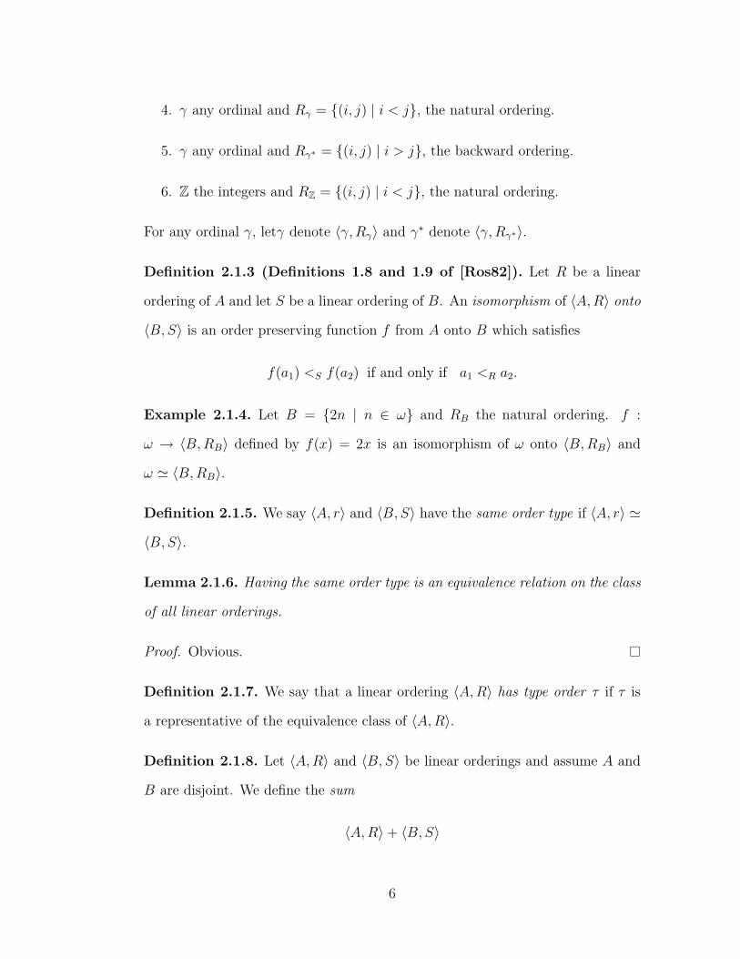
4. γ any ordinal and Rγ = {(i, j) | i < j}, the natural ordering.
5. γ any ordinal and Rγ∗ = {(i, j) | i > j}, the backward ordering.
6. Z the integers and RZ = {(i, j) | i < j}, the natural ordering.
For any ordinal γ, letγ denote 〈γ,Rγ〉 and γ∗ denote 〈γ,Rγ∗〉.
Definition 2.1.3 (Definitions 1.8 and 1.9 of [Ros82]). Let R be a linear
ordering of A and let S be a linear ordering of B. An isomorphism of 〈A,R〉 onto
〈B,S〉 is an order preserving function f from A onto B which satisfies
f(a1) <S f(a2) if and only if a1 <R a2.
Example 2.1.4. Let B = {2n | n ∈ ω} and RB the natural ordering. f :
ω → 〈B,RB〉 defined by f(x) = 2x is an isomorphism of ω onto 〈B,RB〉 and
ω ≃ 〈B,RB〉.
Definition 2.1.5. We say 〈A, r〉 and 〈B,S〉 have the same order type if 〈A, r〉 ≃
〈B,S〉.
Lemma 2.1.6. Having the same order type is an equivalence relation on the class
of all linear orderings.
Proof. Obvious.
Definition 2.1.7. We say that a linear ordering 〈A,R〉 has type order τ if τ is
a representative of the equivalence class of 〈A,R〉.
Definition 2.1.8. Let 〈A,R〉 and 〈B,S〉 be linear orderings and assume A and
B are disjoint. We define the sum
〈A,R〉+ 〈B,S〉
6

to be the linear ordering 〈C, T 〉, where C = A ∪B and
c1 <T c2 if and only if (c1 ∈ A and c2 ∈ B) or
(c1 ∈ A and c2 ∈ A and c1 <R c2) or
(c1 ∈ B and c2 ∈ b and c1 <S c2).
It is easily verified that 〈C, T 〉 is a linear ordering. Intuitively adding 〈B,S〉
to 〈A,R〉 means to place the entire linear ordering 〈B,S〉 to the right of the linear
ordering 〈A,R〉.
Example 2.1.9. 1. Z has the order type ω∗ + ω.
2. 1 + Q is a linear ordering with a first element followed by a copy of Q (the
rational numbers ordered naturally).
We now turn to the definition of generalized sums of linear orderings.
Definition 2.1.10 (Definition 1.38 of Rosenstein). Let 〈I, R〉 be a linear
ordering and for each i ∈ I let 〈Ai, Ri〉 be a linear ordering. We assume that
{Ai | i ∈ I} are pairwise disjoint. We define the generalized sum∑{Ai | i ∈ I}
to be the linear ordering 〈C, T 〉 where C = ∪{Ai | i ∈ I} and
x <T y if (for some i ∈ I, x ∈ Ai and y ∈ Ai and x <Riy) or
(for some i 6= j, x ∈ Ai and y ∈ Aj and i <R j).
Intuitively, imagine I stretched out as a line. Replace each element i ∈ I by
a miniature version of Ai. The resulting linear ordering is∑{Ai | i ∈ I}.
Definition 2.1.11. Let A be a linear ordering with more than 1 element. We
say A is dense if and only if, given any two elements a1, a2 ∈ A such that a1 < a2,
then there exists a3 ∈ A such that a1 < a3 < a2.
7

Example 2.1.12. Q, the rational numbers are dense and Z, the integers are not.
Definition 2.1.13. Let A be a linear ordering and let X be a subordering of A.
1. We say X is cofinal in A if and only if for all a ∈ A there is an x ∈ X such
that a ≤ x.
2. We say X is coinitial in A if and only if for all a ∈ A there is an x ∈ X
such that x ≤ a.
Example 2.1.14. 1. Z is both cofinal and coinitial in R.
2. N is cofinal and not coinitial in R.
Definition 2.1.15. Let A and B be two linear orderings and f : A → B be an
order preserving map. We say f is cofinality (coinitiality) preserving if and only
if f(X) is cofinal (coinitial) in B when X is cofinal (coinitial) in A.
Definition 2.1.16. A linear ordering S is called scattered if it does not contain
a dense subset.
Example 2.1.17. 1. ω, ω∗ are scattered.
2. Q,R are not scattered.
Definition 2.1.18. Let (T,<) be a linear ordering. We say T is initially scattered
if and only if there exists t ∈ T such that {s ∈ T | s ≤ t} is scattered.
Example 2.1.19. 1. Any scattered set is initially scattered.
2. Q is not initially scattered but 1 + Q is.
8

2.2 Countable Linear Orderings
In this section we will focus on countable linear orderings and obtain a few results.
For the rest of this section we assume (T,<) is a countable ordered set and let Q
denote the ordered set of the rational numbers.
Definition 2.2.1. Let X and Y be ordered sets. Let f : X → Y be any
order preserving map. We say f preserves cofinality (coinitiality) or is cofinality
(coinitiality) preserving if and only if whenever {xi | i ∈ I} is cofinal (coinitial)
in X then {f(xi) | i ∈ I} is cofinal (coinitial) in Y .
Example 2.2.2. 1. Let f : (R,≤) → (R2,≤) defined by f(x) = (x, 0) (R2 is
ordered lexicographically). Then f is cofinality (coinitiality) preserving.
2. Let f : (R,≤)→ (R2,≤) defined by f(x) = (0, x). Then f is not cofinality
preserving.
The following lemma is a well known result that any countable linear ordering
may be embedded into Q.
Lemma 2.2.3. There exists f : T → Q which is order preserving.
Proof. Let {tn | n ∈ ω} be an enumeration of T . We will define f inductively.
Let f(t0) = 0. Suppose we have decided f(t0), . . . , f(tn) in an order preserving
fashion. We need to decide f(tn+1). Observe the the relation of tn+1 to t0, . . . , tn.
Since Q is dense and without end points, there exist a ∈ Q \ {f(t0), . . . , f(tn)}
such that a has the same relation to f(t0), . . . , f(tn) as tn+1 has to t0, . . . , tn. Let
f(tn+1) = a. By construction f is order preserving.
The following lemmas gives criteria for existence of cointiality preserving maps
between countable linear orderings.
9
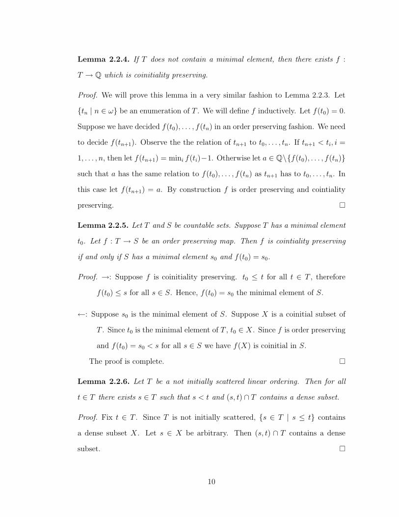
Lemma 2.2.4. If T does not contain a minimal element, then there exists f :
T → Q which is coinitiality preserving.
Proof. We will prove this lemma in a very similar fashion to Lemma 2.2.3. Let
{tn | n ∈ ω} be an enumeration of T . We will define f inductively. Let f(t0) = 0.
Suppose we have decided f(t0), . . . , f(tn) in an order preserving fashion. We need
to decide f(tn+1). Observe the the relation of tn+1 to t0, . . . , tn. If tn+1 < ti, i =
1, . . . , n, then let f(tn+1) = mini f(ti)−1. Otherwise let a ∈ Q\{f(t0), . . . , f(tn)}
such that a has the same relation to f(t0), . . . , f(tn) as tn+1 has to t0, . . . , tn. In
this case let f(tn+1) = a. By construction f is order preserving and cointiality
preserving.
Lemma 2.2.5. Let T and S be countable sets. Suppose T has a minimal element
t0. Let f : T → S be an order preserving map. Then f is cointiality preserving
if and only if S has a minimal element s0 and f(t0) = s0.
Proof. →: Suppose f is coinitiality preserving. t0 ≤ t for all t ∈ T , therefore
f(t0) ≤ s for all s ∈ S. Hence, f(t0) = s0 the minimal element of S.
←: Suppose s0 is the minimal element of S. Suppose X is a coinitial subset of
T . Since t0 is the minimal element of T , t0 ∈ X. Since f is order preserving
and f(t0) = s0 < s for all s ∈ S we have f(X) is coinitial in S.
The proof is complete.
Lemma 2.2.6. Let T be a not initially scattered linear ordering. Then for all
t ∈ T there exists s ∈ T such that s < t and (s, t) ∩ T contains a dense subset.
Proof. Fix t ∈ T . Since T is not initially scattered, {s ∈ T | s ≤ t} contains
a dense subset X. Let s ∈ X be arbitrary. Then (s, t) ∩ T contains a dense
subset.
10
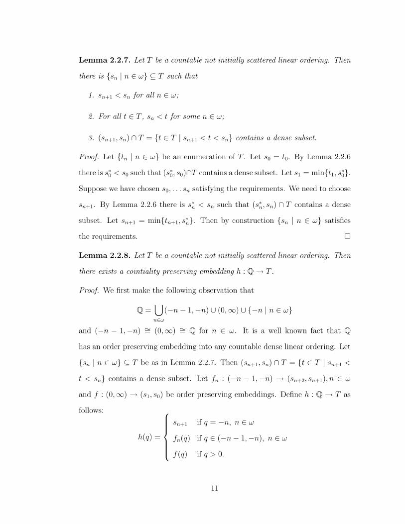
Lemma 2.2.7. Let T be a countable not initially scattered linear ordering. Then
there is {sn | n ∈ ω} ⊆ T such that
1. sn+1 < sn for all n ∈ ω;
2. For all t ∈ T , sn < t for some n ∈ ω;
3. (sn+1, sn) ∩ T = {t ∈ T | sn+1 < t < sn} contains a dense subset.
Proof. Let {tn | n ∈ ω} be an enumeration of T . Let s0 = t0. By Lemma 2.2.6
there is s∗0 < s0 such that (s∗0, s0)∩T contains a dense subset. Let s1 = min{t1, s∗0}.
Suppose we have chosen s0, . . . sn satisfying the requirements. We need to choose
sn+1. By Lemma 2.2.6 there is s∗n < sn such that (s∗n, sn) ∩ T contains a dense
subset. Let sn+1 = min{tn+1, s∗n}. Then by construction {sn | n ∈ ω} satisfies
the requirements.
Lemma 2.2.8. Let T be a countable not initially scattered linear ordering. Then
there exists a cointiality preserving embedding h : Q→ T .
Proof. We first make the following observation that
Q =⋃
n∈ω
(−n− 1,−n) ∪ (0,∞) ∪ {−n | n ∈ ω}
and (−n − 1,−n) ∼= (0,∞) ∼= Q for n ∈ ω. It is a well known fact that Q
has an order preserving embedding into any countable dense linear ordering. Let
{sn | n ∈ ω} ⊆ T be as in Lemma 2.2.7. Then (sn+1, sn) ∩ T = {t ∈ T | sn+1 <
t < sn} contains a dense subset. Let fn : (−n − 1,−n) → (sn+2, sn+1), n ∈ ω
and f : (0,∞) → (s1, s0) be order preserving embeddings. Define h : Q → T as
follows:
h(q) =
sn+1 if q = −n, n ∈ ω
fn(q) if q ∈ (−n− 1,−n), n ∈ ω
f(q) if q > 0.
11
By construction, h is cointiality preserving and this completes the proof.
12

Chapter 3
Ordered Abelian Groups
In this chapter we will investigate different notions of embedding of ordered
Abelian groups. We will show that any ordered Abelian group may be embedded
into RT , a lexicographic function space, in a coinitiality preserving manner. But
first we will discuss some properties of countable ordered sets which we will utilize
in our embedding discussions.
3.1 Ordered Abelian Groups
Definition 3.1.1. An ordered Abelian semigroup (G,≤,+) is a linear ordering
(G,≤) with a commutative and associative operation + which satisfies
x ≤ y implies x+ z ≤ y + z.
for all x, y and z ∈ G.
Definition 3.1.2. (G,≤,+) is said to be an ordered Abelian group if and only if
(G,+) is an Abelian group, (G,≤) is a linear ordering and for all x, y and z ∈ G
x ≤ y implies x+ z ≤ y + z.
13
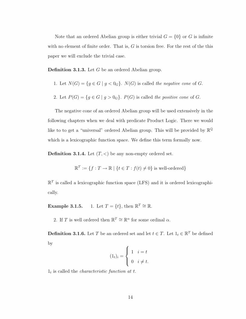
Note that an ordered Abelian group is either trivial G = {0} or G is infinite
with no element of finite order. That is, G is torsion free. For the rest of the this
paper we will exclude the trivial case.
Definition 3.1.3. Let G be an ordered Abelian group.
1. Let N(G) = {g ∈ G | g < 0G}. N(G) is called the negative cone of G.
2. Let P (G) = {g ∈ G | g > 0G}. P (G) is called the positive cone of G.
The negative cone of an ordered Abelian group will be used extensively in the
following chapters when we deal with predicate Product Logic. There we would
like to to get a “universal” ordered Abelian group. This will be provided by RQ
which is a lexicographic function space. We define this term formally now.
Definition 3.1.4. Let (T,<) be any non-empty ordered set.
RT := {f : T → R | {t ∈ T : f(t) 6= 0} is well-ordered}
RT is called a lexicographic function space (LFS) and it is ordered lexicographi-
cally.
Example 3.1.5. 1. Let T = {t}, then RT ∼= R.
2. If T is well ordered then RT ∼= Rα for some ordinal α.
Definition 3.1.6. Let T be an ordered set and let t ∈ T . Let 1t ∈ RT be defined
by
(1t)i =
1 i = t
0 i 6= t.
1t is called the characteristic function at t.
14

Definition 3.1.7. Let (G,+,≤) be an ordered Abelian group and let a, b ∈ G.
1. We write a � b if and only if a ≤G nb for some n ∈ ω \ {0}.
2. We say a ∼ b if and only if a � b and b � a.
3. For ease of notation we write a≪ b if and only if a � b and a ≁ b.
Definition 3.1.8. Let G be an ordered Abelian group
1. Let [a] = {b ∈ G | a ∼ b}. [a] is called the Archimedean class of a.
2. Let T be the collection of Archimedean classes of G. We define order on T
by t < s if and only if a≪ b, for some a ∈ t and b ∈ s. (This is well defined
by basic properties of ≪.)
Example 3.1.9. 1. (1, 1) � (1, 0) and (1, 0) � (1, 1), hence they belong to
the same Archimedean class of R2.
2. (0, 1)≪ (1, 0), hence they belong to different Archimedean classes of R2.
Definition 3.1.10. Let (G,+,≤) be an ordered Abelian group. We say G is
Archimedean if and only if N(G) consists of a single Archimedean class.
Example 3.1.11. 1. (R,+,≤) is an Archimedean ordered Abelian group.
2. (R2,+,≤) where ≤ is the lexicographic order is not Archimedean; n·(0, 1) <
(1, 0) for all n ∈ ω.
It is easy to see that, for an ordered Abelian group G, the set of Archimedean
classes with ≪ form a linear ordering.
Lemma 3.1.12. Let G and H be ordered Abelian groups. Let f : G→ H be an
order preserving group homomorphism. If [g1] < [g2], then [f(g1)] < [f(g2)].
15
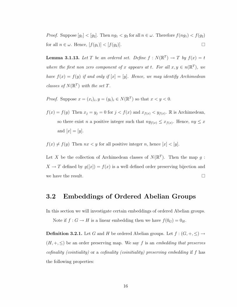
Proof. Suppose [g1] < [g2]. Then ng1 < g2 for all n ∈ ω. Therefore f(ng1) < f(g2)
for all n ∈ ω. Hence, [f(g1)] < [f(g2)].
Lemma 3.1.13. Let T be an ordered set. Define f : N(RT ) → T by f(x) = t
where the first non zero component of x appears at t. For all x, y ∈ n(RT ), we
have f(x) = f(y) if and only if [x] = [y]. Hence, we may identify Archimedean
classes of N(RT ) with the set T .
Proof. Suppose x = (xi)i, y = (yi)i ∈ N(RT ) so that x < y < 0.
f(x) = f(y) Then xj = yj = 0 for j < f(x) and xf(x) < yf(x). R is Archimedean,
so there exist n a positive integer such that nyf(x) ≤ xf(x). Hence, ny ≤ x
and [x] = [y].
f(x) 6= f(y) Then nx < y for all positive integer n, hence [x] < [y].
Let X be the collection of Archimedean classes of N(RT ). Then the map g :
X → T defined by g([x]) = f(x) is a well defined order preserving bijection and
we have the result.
3.2 Embeddings of Ordered Abelian Groups
In this section we will investigate certain embeddings of ordered Abelian groups.
Note if f : G→ H is a linear embedding then we have f(0G) = 0H .
Definition 3.2.1. Let G and H be ordered Abelian groups. Let f : (G,+,≤)→
(H,+,≤) be an order preserving map. We say f is an embedding that preserves
cofinality (cointiality) or a cofinality (coinitiality) preserving embedding if f has
the following properties:
16
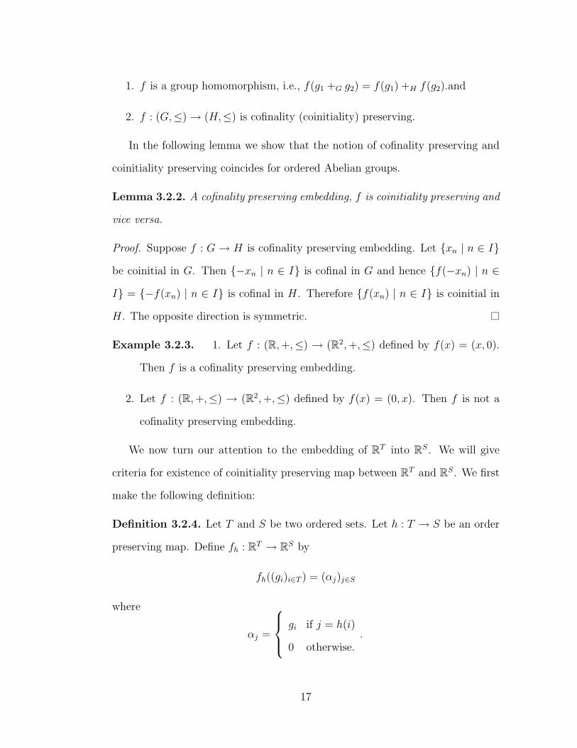
1. f is a group homomorphism, i.e., f(g1 +G g2) = f(g1) +H f(g2).and
2. f : (G,≤)→ (H,≤) is cofinality (coinitiality) preserving.
In the following lemma we show that the notion of cofinality preserving and
coinitiality preserving coincides for ordered Abelian groups.
Lemma 3.2.2. A cofinality preserving embedding, f is coinitiality preserving and
vice versa.
Proof. Suppose f : G→ H is cofinality preserving embedding. Let {xn | n ∈ I}
be coinitial in G. Then {−xn | n ∈ I} is cofinal in G and hence {f(−xn) | n ∈
I} = {−f(xn) | n ∈ I} is cofinal in H. Therefore {f(xn) | n ∈ I} is coinitial in
H. The opposite direction is symmetric.
Example 3.2.3. 1. Let f : (R,+,≤) → (R2,+,≤) defined by f(x) = (x, 0).
Then f is a cofinality preserving embedding.
2. Let f : (R,+,≤) → (R2,+,≤) defined by f(x) = (0, x). Then f is not a
cofinality preserving embedding.
We now turn our attention to the embedding of RT into RS. We will give
criteria for existence of coinitiality preserving map between RT and RS. We first
make the following definition:
Definition 3.2.4. Let T and S be two ordered sets. Let h : T → S be an order
preserving map. Define fh : RT → RS by
fh((gi)i∈T ) = (αj)j∈S
where
αj =
gi if j = h(i)
0 otherwise..
17
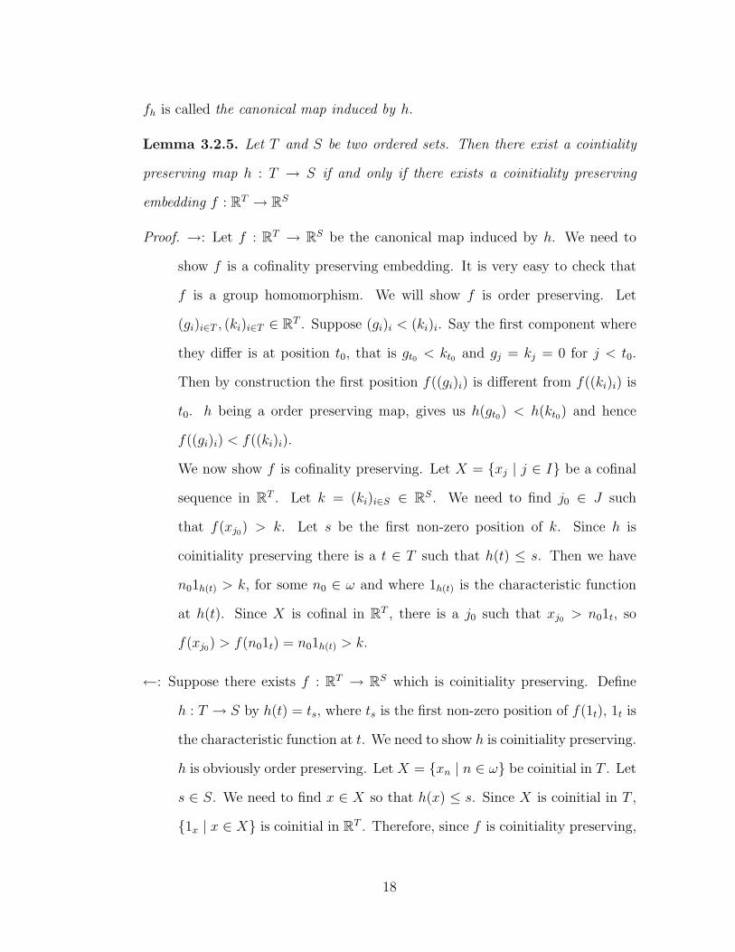
fh is called the canonical map induced by h.
Lemma 3.2.5. Let T and S be two ordered sets. Then there exist a cointiality
preserving map h : T → S if and only if there exists a coinitiality preserving
embedding f : RT → RS
Proof. →: Let f : RT → RS be the canonical map induced by h. We need to
show f is a cofinality preserving embedding. It is very easy to check that
f is a group homomorphism. We will show f is order preserving. Let
(gi)i∈T , (ki)i∈T ∈ RT . Suppose (gi)i < (ki)i. Say the first component where
they differ is at position t0, that is gt0 < kt0 and gj = kj = 0 for j < t0.
Then by construction the first position f((gi)i) is different from f((ki)i) is
t0. h being a order preserving map, gives us h(gt0) < h(kt0) and hence
f((gi)i) < f((ki)i).
We now show f is cofinality preserving. Let X = {xj | j ∈ I} be a cofinal
sequence in RT . Let k = (ki)i∈S ∈ RS. We need to find j0 ∈ J such
that f(xj0) > k. Let s be the first non-zero position of k. Since h is
coinitiality preserving there is a t ∈ T such that h(t) ≤ s. Then we have
n01h(t) > k, for some n0 ∈ ω and where 1h(t) is the characteristic function
at h(t). Since X is cofinal in RT , there is a j0 such that xj0 > n01t, so
f(xj0) > f(n01t) = n01h(t) > k.
←: Suppose there exists f : RT → RS which is coinitiality preserving. Define
h : T → S by h(t) = ts, where ts is the first non-zero position of f(1t), 1t is
the characteristic function at t. We need to show h is coinitiality preserving.
h is obviously order preserving. Let X = {xn | n ∈ ω} be coinitial in T . Let
s ∈ S. We need to find x ∈ X so that h(x) ≤ s. Since X is coinitial in T ,
{1x | x ∈ X} is coinitial in RT . Therefore, since f is coinitiality preserving,
18

there exists x ∈ X such that f(1x) ≤ 1s. Now h(x) = the first non-zero
position of f(1x), hence h(x) ≤ s and the proof is complete.
Lemma 3.2.6. Let T be a countable linear ordering. Then T does not contain
a minimal element if and only if there exist a coinitiality preserving embedding
f : RT → RQ.
Proof. →: If T does not contain a minimal element then by Lemma 2.2.4, there
exists h : T → Q which is coinitiality preserving and by Lemma 3.2.5, the
canonical map induced by h is cofinality preserving.
← If T contains a minimal element, then by Lemma 2.2.5, there are no coinitial
preserving map h : T → Q since Q has no least element. Hence there is no
coinitiality preserving map f : RT → RQ.
Lemma 3.2.7. Let T be a countable linear ordering with a minimal element.
Then there exists a cointiality preserving embedding f : RT → R1+Q.
Proof. Let t0 be the minimal element of T and let h : T \ {t0} → Q be order
preserving. Let g : T → 1 + Q be defined by g(x) = f(x) if x 6= t0 and g(t0) = 1.
Then g is coinitiality preserving.
Lemma 3.2.8. Let T be a countable linear ordering. Then either there exist
f : RT → RQ or f : RT → R1+Q which is coinitiality preserving.
Proof. This is a direct corollary to Lemmas 3.2.6 and 3.2.7.
Example 3.2.9. Let T = {1} and S = {1, 2}.
19

1. Define h : T → S by h(1) = 1. Then h is cointiality preserving and the
corresponding map f : R → R2 defined by f(x) = (x, 0) is order and
cofinality preserving.
2. Note if we define h : T → S by h(1) = 2, then the corresponding map
f : RT → RS defined by f(x) = (0, x) is not cofinality preserving.
3.3 Hahn Embedding of G into an RT
The Hahn Embedding Theorem asserts that any ordered Abelian group (G,+,≤)
can be embedded into a lexicographic function space (RT ,+,≤), where T is set of
Archimedean classes of N(G). This embedding is taken place in two steps. First
G is embedded into a ordered vector space and then the ordered vector space is
mapped into a lexicographic function space. We will state the results and give
references for their proofs. We will show that at each step the embedding is
coinitiality preserving. Hence, (G,+,≤)→ (RT ,+,≤) is cointiality preserving.
Definition 3.3.1. Let G be an ordered Abelian group. Let VG = {(x, n)|x ∈
G, n a positive integer}. We define equality by
(x,m) ≈ (y, n) if and only if nx = my,
and addition and Q-scalar multiplication by
(x,m) + (y, n) ≈ (nx+my,mn)
q
p· (x,m) ≈ (px, qm).
Proposition 3.3.2. Let G be an ordered Abelian group. Then
20

1. VG is a vector space over the rational numbers, Q. Furthermore, if we
define
(x,m) > (y, n) if and only if nx > my
then VG becomes an ordered vector space.
2. VG is divisible as an ordered Abelian group, i.e., for any v ∈ VG and
positive integer n, there exists x ∈ VG such that nx = v.
3. VG is dense.
Proof. 1. Showing VG is an ordered vector space over Q is a routine exercise.
We just note that 0V = (0, 1) and −(x,m) ≈ (−x,m).
2. First note that n(x,m) ≈ (nmn−1x,mn) for (x,m) ∈ VG and n a positive
natural number. Let v = (g, k) ∈ V and n ∈ N. Let x = (g, kn). Hence
nx ≈ (n(kn)n−1g, (nk)n) ≈ (nnkn−1g, nnkn) ≈ (g, k).
3. Any ordered divisible Abelian group is dense. Let v1, v2 ∈ VG such that
v1 < v2. Since VG is divisible, v1+v2
2∈ VG and furthermore v1 <
v1+v2
2< v2.
Hence, VG is dense.
We now show that there exists a natural embedding of G → VG which is
coinitiality preserving.
Theorem 3.3.3. Let G be an ordered Abelian group. Let f : G→ VG be defined
by x 7→ (x, 1). Then f is a coinitiality preserving embedding.
Proof. 1. f(x+ y) = (x+ y, 1) = (x, 1) + (y, 1) = f(x) + f(y), for all x, y ∈ G.
21
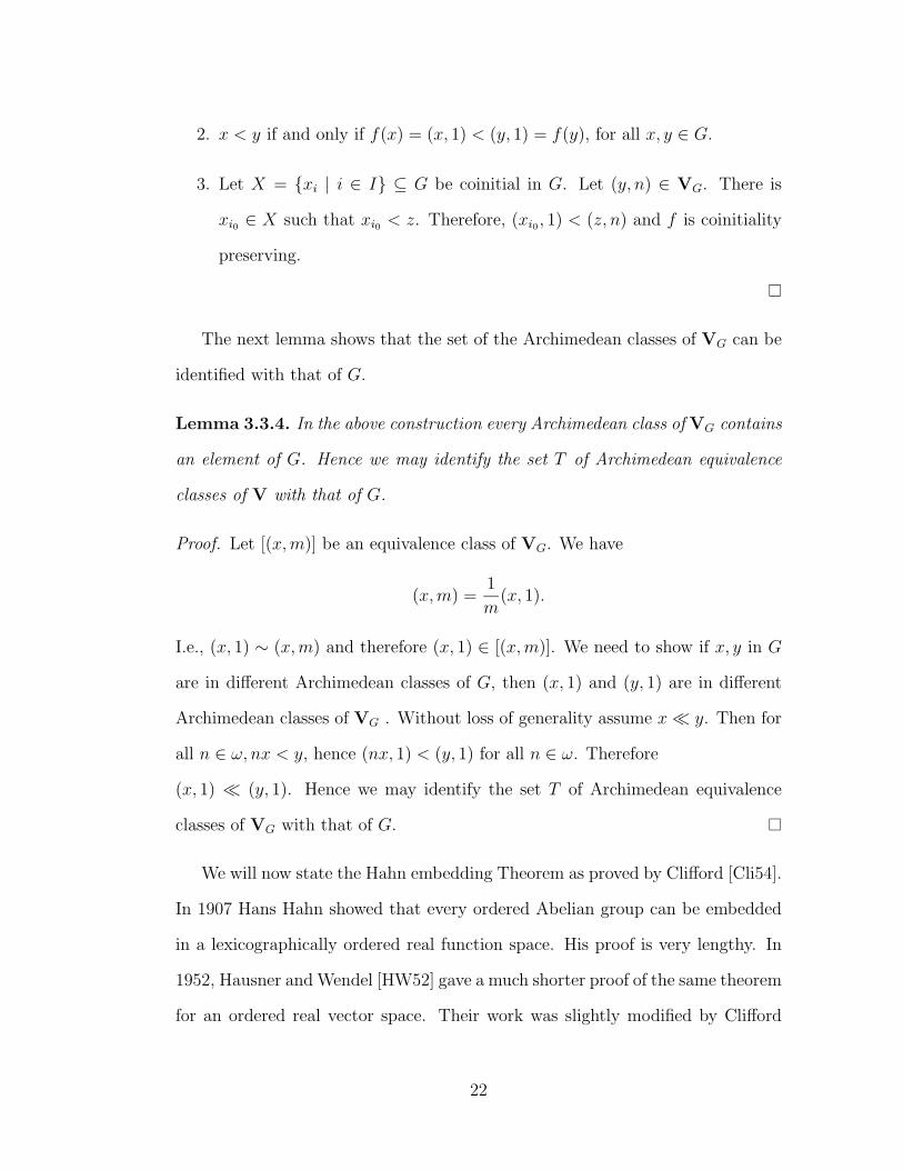
2. x < y if and only if f(x) = (x, 1) < (y, 1) = f(y), for all x, y ∈ G.
3. Let X = {xi | i ∈ I} ⊆ G be coinitial in G. Let (y, n) ∈ VG. There is
xi0 ∈ X such that xi0 < z. Therefore, (xi0 , 1) < (z, n) and f is coinitiality
preserving.
The next lemma shows that the set of the Archimedean classes of VG can be
identified with that of G.
Lemma 3.3.4. In the above construction every Archimedean class of VG contains
an element of G. Hence we may identify the set T of Archimedean equivalence
classes of V with that of G.
Proof. Let [(x,m)] be an equivalence class of VG. We have
(x,m) =1
m(x, 1).
I.e., (x, 1) ∼ (x,m) and therefore (x, 1) ∈ [(x,m)]. We need to show if x, y in G
are in different Archimedean classes of G, then (x, 1) and (y, 1) are in different
Archimedean classes of VG . Without loss of generality assume x≪ y. Then for
all n ∈ ω, nx < y, hence (nx, 1) < (y, 1) for all n ∈ ω. Therefore
(x, 1) ≪ (y, 1). Hence we may identify the set T of Archimedean equivalence
classes of VG with that of G.
We will now state the Hahn embedding Theorem as proved by Clifford [Cli54].
In 1907 Hans Hahn showed that every ordered Abelian group can be embedded
in a lexicographically ordered real function space. His proof is very lengthy. In
1952, Hausner and Wendel [HW52] gave a much shorter proof of the same theorem
for an ordered real vector space. Their work was slightly modified by Clifford
22
[Cli54]to get the same result for an ordered rational vector space. This provides
a more accessible proof of Hahn’s fundamental theorem. We will show that the
embedding provided in the Hahn embedding Theorem is cofinality preserving.
We first need to make a definition so we can give the statement of the Hahn
embedding Theorem in full.
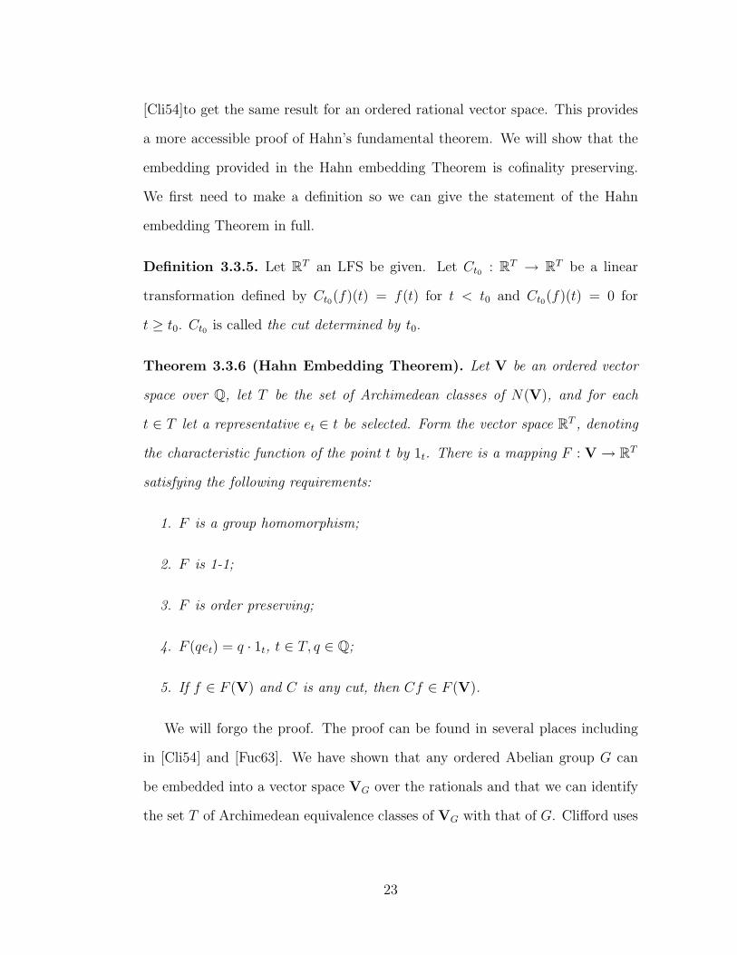
Definition 3.3.5. Let RT an LFS be given. Let Ct0 : RT → RT be a linear
transformation defined by Ct0(f)(t) = f(t) for t < t0 and Ct0(f)(t) = 0 for
t ≥ t0. Ct0 is called the cut determined by t0.
Theorem 3.3.6 (Hahn Embedding Theorem). Let V be an ordered vector
space over Q, let T be the set of Archimedean classes of N(V), and for each
t ∈ T let a representative et ∈ t be selected. Form the vector space RT , denoting
the characteristic function of the point t by 1t. There is a mapping F : V→ RT
satisfying the following requirements:
1. F is a group homomorphism;
2. F is 1-1;
3. F is order preserving;
4. F (qet) = q · 1t, t ∈ T, q ∈ Q;
5. If f ∈ F (V) and C is any cut, then Cf ∈ F (V).
We will forgo the proof. The proof can be found in several places including
in [Cli54] and [Fuc63]. We have shown that any ordered Abelian group G can
be embedded into a vector space VG over the rationals and that we can identify
the set T of Archimedean equivalence classes of VG with that of G. Clifford uses
23
these facts in [Cli54] and modifies the proof of the Theorem 3.3.6 to get Hahn’s
embedding Theorem for rational vector spaces, hence he has the fundamental
Theorem of Hahn that any ordered Abelian group may be embedded into a
lexicographically ordered, real function space.
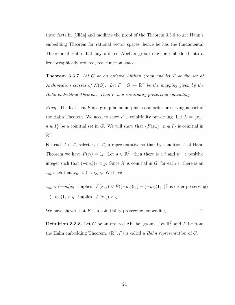
Theorem 3.3.7. Let G be an ordered Abelian group and let T be the set of
Archimedean classes of N(G). Let F : G → RT be the mapping given by the
Hahn embedding Theorem. Then F is a coinitiality preserving embedding.
Proof. The fact that F is a group homomorphism and order preserving is part of
the Hahn Theorem. We need to show F is coinitiality preserving. Let X = {xn |
n ∈ I} be a coinitial set in G. We will show that {F (xn) | n ∈ I} is coinitial in
RT .
For each t ∈ T , select et ∈ T , a representative so that by condition 4 of Hahn
Theorem we have F (et) = 1t. Let g ∈ RT , then there is a t and m0 a positive
integer such that (−m0)1t < g. Since X is coinitial in G, for each et there is an
xn0 such that xn0 < (−m0)et. We have
xn0 < (−m0)et implies F (xn0) < F ((−m0)et) = (−m0)1t (F is order preserving)
(−m0)1t < g implies F (xn0) < g.
We have shown that F is a coinitiality preserving embedding.
Definition 3.3.8. Let G be an ordered Abelian group. Let RT and F be from
the Hahn embedding Theorem. (RT , F ) is called a Hahn representation of G.
24
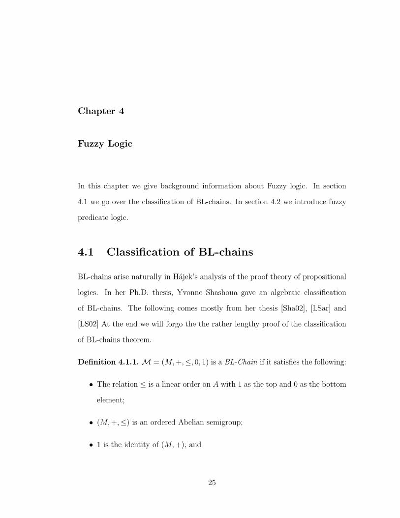
Chapter 4
Fuzzy Logic
In this chapter we give background information about Fuzzy logic. In section
4.1 we go over the classification of BL-chains. In section 4.2 we introduce fuzzy
predicate logic.
4.1 Classification of BL-chains
BL-chains arise naturally in Hajek’s analysis of the proof theory of propositional
logics. In her Ph.D. thesis, Yvonne Shashoua gave an algebraic classification
of BL-chains. The following comes mostly from her thesis [Sha02], [LSar] and
[LS02] At the end we will forgo the the rather lengthy proof of the classification
of BL-chains theorem.
Definition 4.1.1. M = (M,+,≤, 0, 1) is a BL-Chain if it satisfies the following:
• The relation ≤ is a linear order on A with 1 as the top and 0 as the bottom
element;
• (M,+,≤) is an ordered Abelian semigroup;
• 1 is the identity of (M,+); and
25

• For all y ≤ x, there is a largest z such that x+ z = y.
In particular, this means that BL-algebras form an elementary class.
Definition 4.1.2. Let M = (M,+,≤) be given. Let x, y ∈ M , then we define
x ⇒ y := z, where z is the largest element of M such that x + z = y if y < x
and x ⇒ y := 1 if x ≤ y. Hence ⇒ is definable from + and ≤. We will use ⇒
extensively in our work. It makes the notation and discussions to come have a
smoother flow.
Example 4.1.3. The following are the three main examples of BL-chains:
1. Lukasiewicz Logic [0, 1] L
x+ y = max{0, x+ y − 1}
x⇒ y =
1 if x ≤ y
1− x+ y if x > y
2. Godel Logic [0, 1]G
x+ y = min{x, y}
x⇒ y =
1 if x ≤ y
y if x > y
3. Product logic [0, 1]Π
x+ y = x+ y
x⇒ y =
1 if x ≤ y
y/x if x > y
Definition 4.1.4. Let (G,+,≤) be any ordered Abelian group.
26
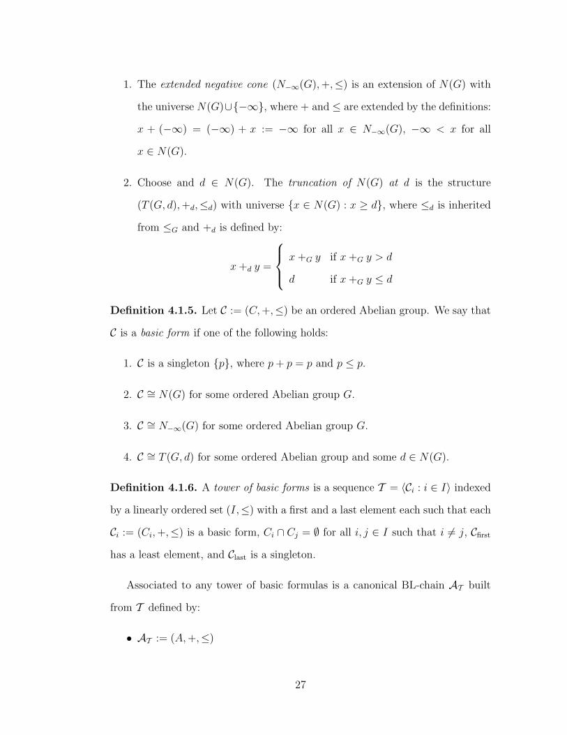
1. The extended negative cone (N−∞(G),+,≤) is an extension of N(G) with
the universe N(G)∪{−∞}, where + and ≤ are extended by the definitions:
x + (−∞) = (−∞) + x := −∞ for all x ∈ N−∞(G), −∞ < x for all
x ∈ N(G).
2. Choose and d ∈ N(G). The truncation of N(G) at d is the structure
(T (G, d),+d,≤d) with universe {x ∈ N(G) : x ≥ d}, where ≤d is inherited
from ≤G and +d is defined by:
x+d y =
x+G y if x+G y > d
d if x+G y ≤ d
Definition 4.1.5. Let C := (C,+,≤) be an ordered Abelian group. We say that
C is a basic form if one of the following holds:
1. C is a singleton {p}, where p+ p = p and p ≤ p.
2. C ∼= N(G) for some ordered Abelian group G.
3. C ∼= N−∞(G) for some ordered Abelian group G.
4. C ∼= T (G, d) for some ordered Abelian group and some d ∈ N(G).
Definition 4.1.6. A tower of basic forms is a sequence T = 〈Ci : i ∈ I〉 indexed
by a linearly ordered set (I,≤) with a first and a last element each such that each
Ci := (Ci,+,≤) is a basic form, Ci ∩ Cj = ∅ for all i, j ∈ I such that i 6= j, Cfirst
has a least element, and Clast is a singleton.
Associated to any tower of basic formulas is a canonical BL-chain AT built
from T defined by:
• AT := (A,+,≤)
27

• A :=⋃{Ci : i ∈ I};
• For x ∈ Ci, y ∈ Cj,
x ≤T y if and only if [i ≤I j or (i = j and x ≤Ciy)]
• 0T := the least element of Cfirst, and 1T := the unique element of Clast;
• For x, y ∈ A
x+T y =
x+Ciy for x, y ∈ Ci for some i ∈ I
min{x, y} for x ∈ Ci, y ∈ Cj, i 6= j
Theorem 4.1.7 (Classification of BL-Chains). For any tower T of basic
forms, the structure AT constructed as above is a BL-chain. And every BL-chain
is isomorphic to AT for some tower T of basic forms.
Here is the application of the classification theorem to the three “classical” BL-
chains.
Example 4.1.8. 1. [0, 1] L ∼= AT L, where T L = 〈C0, C1〉, where (C0,+,≤) ∼=
(T (R,−1),+,≤) and C1 is a singleton.
2. [0, 1]G ∼= ATG, where TG = 〈Ci : i ∈ [0, 1]〉, where Ci is a singleton.
3. [0, 1]Π ∼= ATΠ, where TΠ = 〈C0, C1〉 where (C0,+,≤) ∼= (N−∞(R),+,≤) and
C1 is a singleton.
Shahshoua shows that there is only obstruction to the uniqueness of a de-
composition. Specifically, whenever a singleton is followed by a copy of N(G)
we may “fuse” them together and have N−∞(G) instead. Hence, we may assume
that whenever a singleton is the first component of a tower it is either followed
28
by another singleton or a copy of T (G, d) for some ordered Abelian group. This
will be crucial when we investigate models of predicate product logic.
4.2 Fuzzy Predicate Logic
We would like to investigate fuzzy predicate logic. Most of the following material
come from Hajek [Haj98].
Definition 4.2.1. A predicate language contains the following:
• Predicates: P,Q,R, . . . each together with a positive natural number, its
arity
• Object constants: c, d, . . .
• Object variables: x, y, z, . . .
• Connectives: &,→
• The truth constants: 0, 1
• Quantifiers ∀,∃.
Definition 4.2.2. Terms and formulas of predicate logic are defined in the fol-
lowing way:
• Object variables and object constants are terms .
• P (t1, t2, . . . tn) where P is a predicate of arity n and t1, . . . tn are terms is
an atomic formula.
• If ϕ, ψ are formulas, then so are ϕ&ψ and ϕ→ ψ.
29
• if ϕ is a formula and x is an object variable, then (∀x)ϕ(x) and (∃x)ϕ(x)
are formulas.
• 0 and 1 are formulas.
We will assume that predicate languages that we work with are countable
and contain only relation symbols and constants. The only place we will deal
with the cardinality of L is when we consider a single sentence in the context
of completeness theorem. Since a sentence has finitely many symbols from the
language we may already have assumed that L is countable.
Definition 4.2.3. We define other connectives as follows:
• ϕ ∧ ψ denotes ϕ&(ϕ→ ψ).
• ϕ ∨ ψ denotes ((ϕ→ ψ)→ ψ) ∧ ((ψ → ϕ)→ ϕ).
• ¬ϕ denotes ϕ→ 0.
• ϕ ≡ ψ denotes (ϕ→ ψ)&(ψ → ϕ).
• ϕn denotes ϕ& . . .&ϕ︸ ︷︷ ︸
n times
.
Definition 4.2.4. Let L be a predicate language and let L be a BL-chain. An
L-structure M = 〈M, (rP )P , (mc)c〉 for L contains the following:
• Non-empty domain M ;
• rP : Mn → L, for each n-ary predicate P ;
• mc ∈M for each constant object c.
30
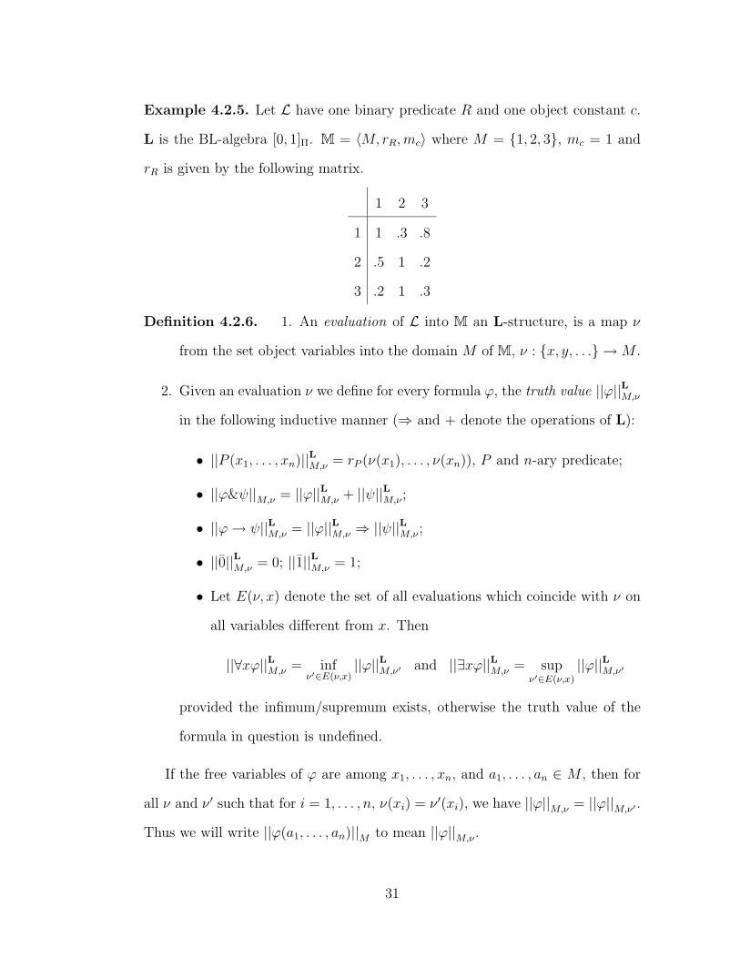
Example 4.2.5. Let L have one binary predicate R and one object constant c.
L is the BL-algebra [0, 1]Π. M = 〈M, rR,mc〉 where M = {1, 2, 3}, mc = 1 and
rR is given by the following matrix.
1 2 3
1 1 .3 .8
2 .5 1 .2
3 .2 1 .3
Definition 4.2.6. 1. An evaluation of L into M an L-structure, is a map ν
from the set object variables into the domain M of M, ν : {x, y, . . .} →M .
2. Given an evaluation ν we define for every formula ϕ, the truth value ||ϕ||LM,ν
in the following inductive manner (⇒ and + denote the operations of L):
• ||P (x1, . . . , xn)||LM,ν = rP (ν(x1), . . . , ν(xn)), P and n-ary predicate;
• ||ϕ&ψ||M,ν = ||ϕ||LM,ν + ||ψ||LM,ν ;
• ||ϕ→ ψ||LM,ν = ||ϕ||LM,ν ⇒ ||ψ||L
M,ν ;
• ||0||L
M,ν = 0; ||1||L
M,ν = 1;
• Let E(ν, x) denote the set of all evaluations which coincide with ν on
all variables different from x. Then
||∀xϕ||LM,ν = infν′∈E(ν,x)
||ϕ||LM,ν′ and ||∃xϕ||LM,ν = supν′∈E(ν,x)
||ϕ||LM,ν′
provided the infimum/supremum exists, otherwise the truth value of the
formula in question is undefined.
If the free variables of ϕ are among x1, . . . , xn, and a1, . . . , an ∈ M , then for
all ν and ν ′ such that for i = 1, . . . , n, ν(xi) = ν ′(xi), we have ||ϕ||M,ν = ||ϕ||M,ν′ .
Thus we will write ||ϕ(a1, . . . , an)||M to mean ||ϕ||M,ν .
31

Definition 4.2.7. The structure M is L-safe if all the needed infima and suprema
exist, i.e. ||ϕ||LM,ν is defined for all ϕ, ν.
In particular, each finite structure (with finite domain) is safe. Every L-
structure M where L = [0, 1] L, [0, 1]G, [0, 1]Π is safe, since [0, 1] contains the
limit points of every monotone sequence.
Example 4.2.8. We verify that in example 4.2.5
||∀xR(x, c)||M,ν = 0.2
and
||∃x¬R(c, x)||M,ν = 0.
In his work, [Haj98], Hajek uses safe models. In this paper we define a new
class of models which has more restrictions than the class of safe models.
Definition 4.2.9. 1. ||ϕ||LM = inf{||ϕ||LM,ν | ν M − evaluation}
2. A formula ϕ of a language L is an L-tautology if and only if ||ϕ||LM = 1 for
all M safe L-model. That is, ||ϕ||LM,ν = 1 for each safe L-structure M and
each M-valuation ν of object variables. Let LL-TAUT denote the set of
L-tautologies for the language L.
We will drop the subscript L from L-TAUT, whenever the language is clear
from the context.
Example 4.2.10. ∀xϕ(x) → ∃xϕ(x) is an LL-tautology for any L and L. This
is true since for all M safe L-structures we have
infai∈M
||ϕ(ai)||M ≤ supai∈M
||ϕ(ai)||M.
32
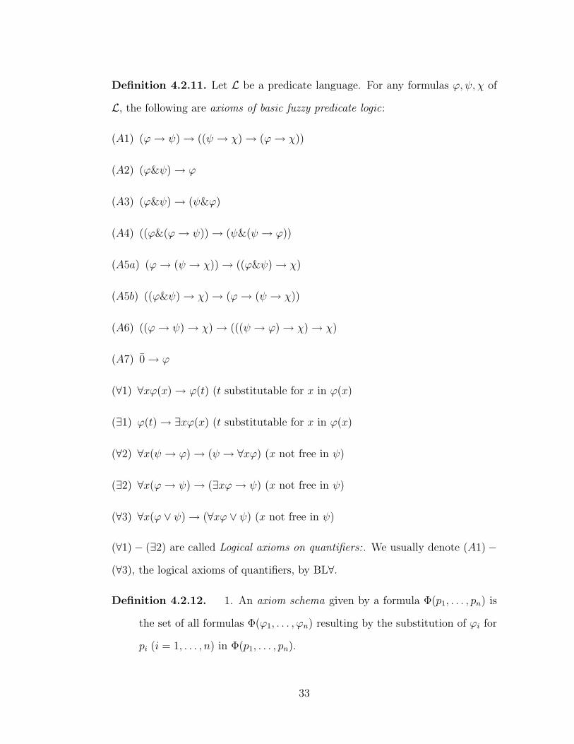
Definition 4.2.11. Let L be a predicate language. For any formulas ϕ, ψ, χ of
L, the following are axioms of basic fuzzy predicate logic:
(A1) (ϕ→ ψ)→ ((ψ → χ)→ (ϕ→ χ))
(A2) (ϕ&ψ)→ ϕ
(A3) (ϕ&ψ)→ (ψ&ϕ)
(A4) ((ϕ&(ϕ→ ψ))→ (ψ&(ψ → ϕ))
(A5a) (ϕ→ (ψ → χ))→ ((ϕ&ψ)→ χ)
(A5b) ((ϕ&ψ)→ χ)→ (ϕ→ (ψ → χ))
(A6) ((ϕ→ ψ)→ χ)→ (((ψ → ϕ)→ χ)→ χ)
(A7) 0→ ϕ
(∀1) ∀xϕ(x)→ ϕ(t) (t substitutable for x in ϕ(x)
(∃1) ϕ(t)→ ∃xϕ(x) (t substitutable for x in ϕ(x)
(∀2) ∀x(ψ → ϕ)→ (ψ → ∀xϕ) (x not free in ψ)
(∃2) ∀x(ϕ→ ψ)→ (∃xϕ→ ψ) (x not free in ψ)
(∀3) ∀x(ϕ ∨ ψ)→ (∀xϕ ∨ ψ) (x not free in ψ)
(∀1)− (∃2) are called Logical axioms on quantifiers:. We usually denote (A1)−
(∀3), the logical axioms of quantifiers, by BL∀.
Definition 4.2.12. 1. An axiom schema given by a formula Φ(p1, . . . , pn) is
the set of all formulas Φ(ϕ1, . . . , ϕn) resulting by the substitution of ϕi for
pi (i = 1, . . . , n) in Φ(p1, . . . , pn).
33

2. A logical calculus C∀ is a schematic extension of BL∀ if it results from BL∀
by adding some (finitely or infinitely many) axiom schemata to its axioms.
3. Let C∀ be schematic extension of BL∀ and let L be a BL-chain. L is a
C∀-chain if all axioms of C∀ are L-tautologies.
Definition 4.2.13. Let C∀ be a schematic extension of BL∀.
1. A theory over C∀ is a set of formulas. Elements of T are axioms of T .
2. The deduction rules of Basic Predicate Fuzzy Logic are
- modus ponens : From ϕ and ϕ→ ψ infer ψ.
- generalization (from ϕ infer ∀xϕ).
3. A proof from theory T (over C∀) is a finite sequence of formulas ϕ0, . . . , ϕn
such that for each i = 0 to n, ϕi is either an element of T ∪ C∀ or follows
from some earlier ϕj and ϕk (j, k < i) by modus ponens or ϕi = ∀xϕj for
some earlier ϕj.
4. A formula ϕ is provable from T if there exists a proof from T : ϕ0, . . . ϕn
with ϕ = ϕn, the last line of the proof.
5. Let M be a safe L-structure. M is called an L-model of T if ||ϕ||LM = 1L
for each ϕ ∈ T .
Example 4.2.14. The following are three examples of theories:
L∀ := {BL∀-axioms} ∪ {¬¬ϕ : ϕ is a formula of BL∀}
G∀ := {BL∀-axioms} ∪ {ϕ→ (ϕ&ϕ) : ϕ is a formula of BL∀}
Π∀ := {BL∀-axioms} ∪ {(ϕ ∧ ¬ϕ)→ 0) : ϕ is a formula of BL∀}
∪ {¬¬χ→ ((ϕ&χ→ ψ&χ)→ (ϕ→ ψ)) : ϕ, ψ, χ are formulas of BL∀}
34
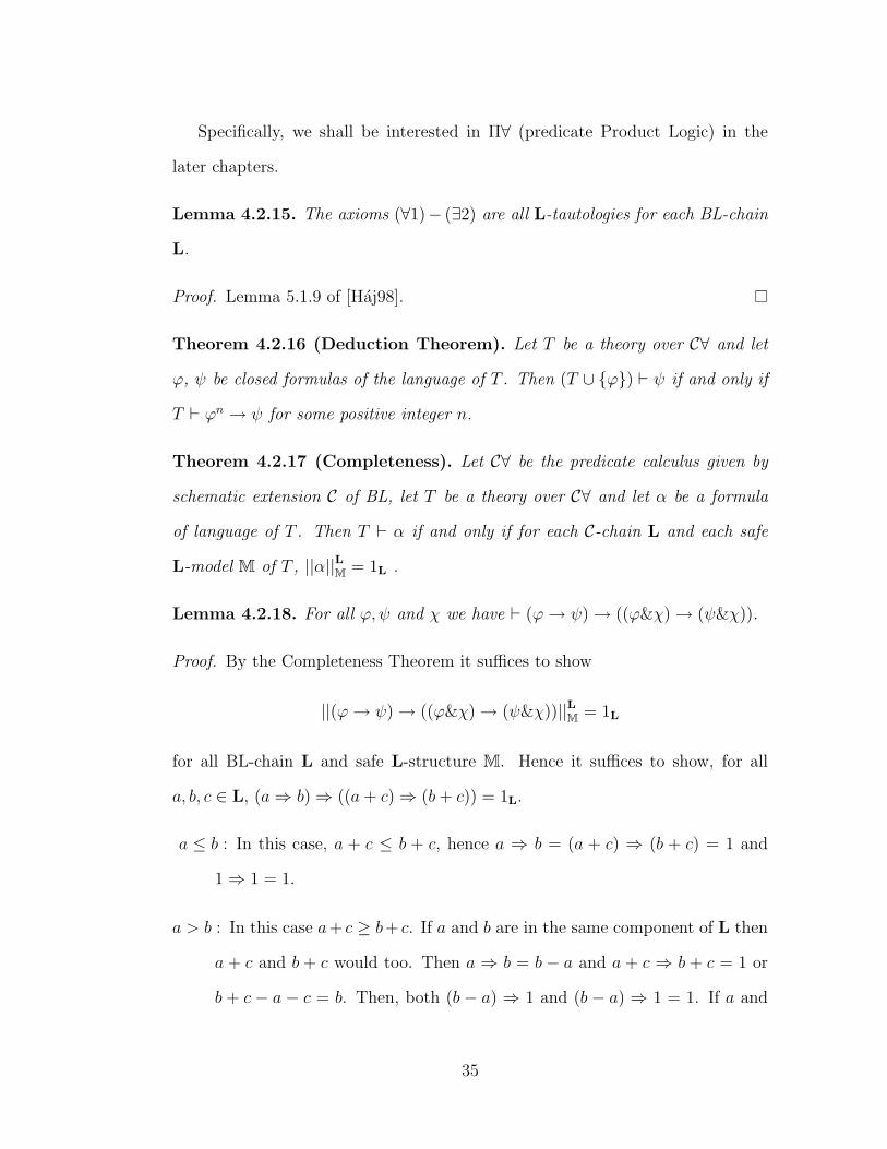
Specifically, we shall be interested in Π∀ (predicate Product Logic) in the
later chapters.
Lemma 4.2.15. The axioms (∀1)− (∃2) are all L-tautologies for each BL-chain
L.
Proof. Lemma 5.1.9 of [Haj98].
Theorem 4.2.16 (Deduction Theorem). Let T be a theory over C∀ and let
ϕ, ψ be closed formulas of the language of T . Then (T ∪ {ϕ}) ⊢ ψ if and only if
T ⊢ ϕn → ψ for some positive integer n.
Theorem 4.2.17 (Completeness). Let C∀ be the predicate calculus given by
schematic extension C of BL, let T be a theory over C∀ and let α be a formula
of language of T . Then T ⊢ α if and only if for each C-chain L and each safe
L-model M of T , ||α||LM = 1L .
Lemma 4.2.18. For all ϕ, ψ and χ we have ⊢ (ϕ→ ψ)→ ((ϕ&χ)→ (ψ&χ)).
Proof. By the Completeness Theorem it suffices to show
||(ϕ→ ψ)→ ((ϕ&χ)→ (ψ&χ))||LM = 1L
for all BL-chain L and safe L-structure M. Hence it suffices to show, for all
a, b, c ∈ L, (a⇒ b)⇒ ((a+ c)⇒ (b+ c)) = 1L.
a ≤ b : In this case, a + c ≤ b + c, hence a ⇒ b = (a + c) ⇒ (b + c) = 1 and
1⇒ 1 = 1.
a > b : In this case a+ c ≥ b+ c. If a and b are in the same component of L then
a + c and b + c would too. Then a ⇒ b = b − a and a + c ⇒ b + c = 1 or
b + c − a − c = b. Then, both (b − a) ⇒ 1 and (b − a) ⇒ 1 = 1. If a and
35
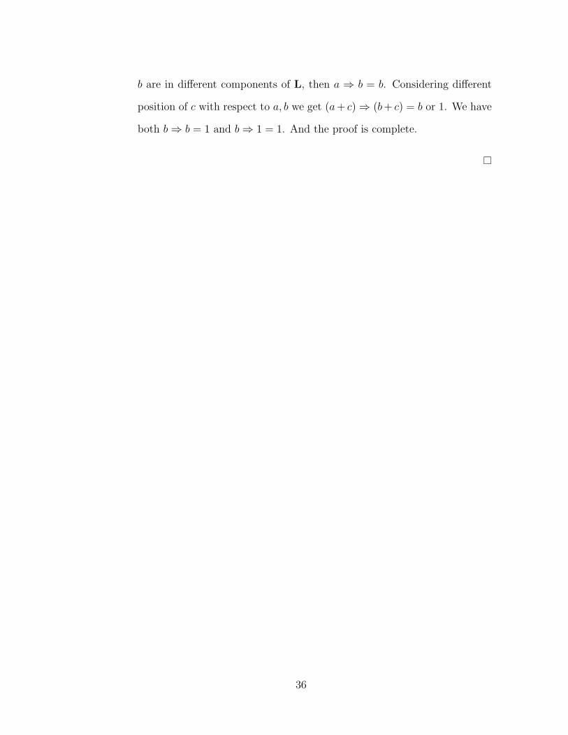
b are in different components of L, then a ⇒ b = b. Considering different
position of c with respect to a, b we get (a+ c)⇒ (b+ c) = b or 1. We have
both b⇒ b = 1 and b⇒ 1 = 1. And the proof is complete.
36
Chapter 5
Predicate Product Logic
In this chapter we will focus on predicate Product Logic. We will use Shashoua’s
Classification of BL-Chains extensively. Her algebraic classification of BL-chains
lets us focus on ordered Abelian groups and their properties. In his work [Haj98],
Hajek uses safe structures. We would like to define a new class of structures
(called closed) with more restraints. The Completeness Theorem for Π∀ as stated
by Hajek (Theorem 4.2.17) says Π∀ ⊢ α if and only if for each Π∀-chain L, and
M safe L-structure ||α||LM = 1. We will be able to improve this theorem to get
L = L(RS) a lexicographic function space and M a closed L-model. We will
actually improve the theorem so that S is Q. We will first classify Π∀-chains and
then define closed structures and motivate their definition.
5.1 Classification of Π∀-Chains
In this section we will investigate the possible Π∀-chains. As noted by Laskowski
and Shashoua BL-chains are a sequence of basic forms (singleton, extended neg-
ative cone of an ordered Abelian group and T (G, d) for some ordered Abelian
group). We will show that if L is a Π∀-chain then L consists of an extended neg-
ative cone of an ordered Abelian group and a singleton. Remember from chapter
37
4 that
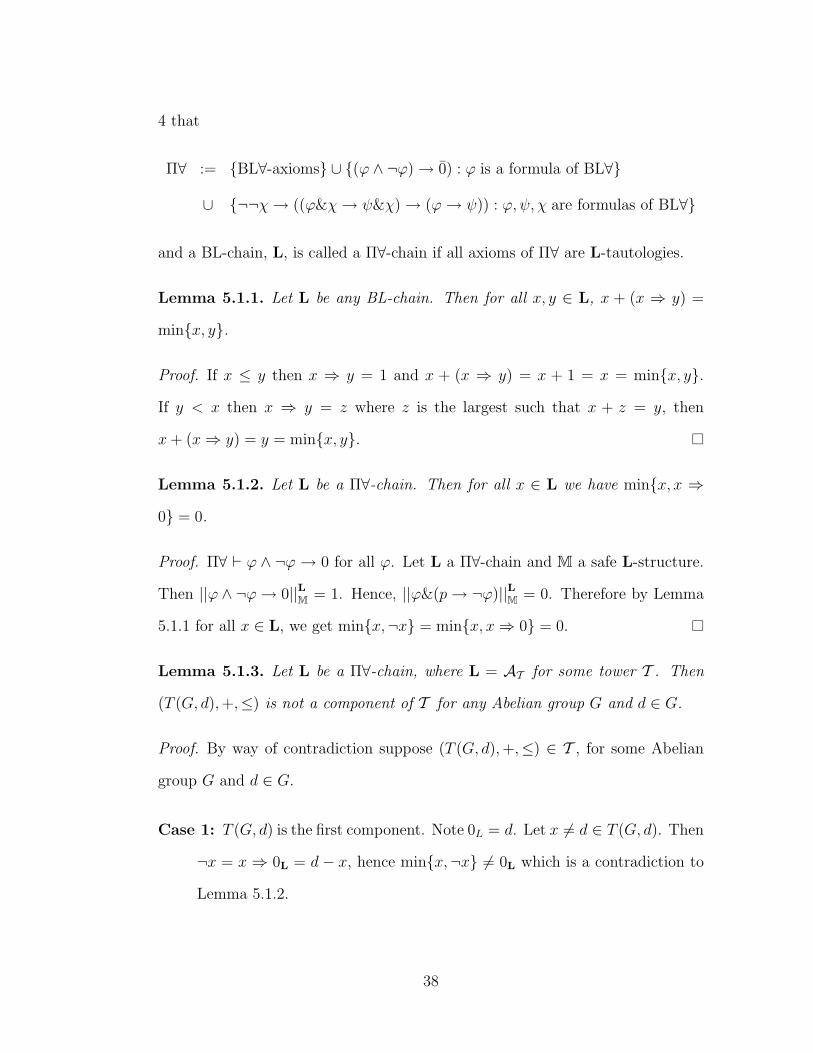
Π∀ := {BL∀-axioms} ∪ {(ϕ ∧ ¬ϕ)→ 0) : ϕ is a formula of BL∀}
∪ {¬¬χ→ ((ϕ&χ→ ψ&χ)→ (ϕ→ ψ)) : ϕ, ψ, χ are formulas of BL∀}
and a BL-chain, L, is called a Π∀-chain if all axioms of Π∀ are L-tautologies.
Lemma 5.1.1. Let L be any BL-chain. Then for all x, y ∈ L, x + (x ⇒ y) =
min{x, y}.
Proof. If x ≤ y then x ⇒ y = 1 and x + (x ⇒ y) = x + 1 = x = min{x, y}.
If y < x then x ⇒ y = z where z is the largest such that x + z = y, then
x+ (x⇒ y) = y = min{x, y}.
Lemma 5.1.2. Let L be a Π∀-chain. Then for all x ∈ L we have min{x, x ⇒
0} = 0.
Proof. Π∀ ⊢ ϕ ∧ ¬ϕ → 0 for all ϕ. Let L a Π∀-chain and M a safe L-structure.
Then ||ϕ ∧ ¬ϕ→ 0||LM = 1. Hence, ||ϕ&(p→ ¬ϕ)||LM = 0. Therefore by Lemma
5.1.1 for all x ∈ L, we get min{x,¬x} = min{x, x⇒ 0} = 0.
Lemma 5.1.3. Let L be a Π∀-chain, where L = AT for some tower T . Then
(T (G, d),+,≤) is not a component of T for any Abelian group G and d ∈ G.
Proof. By way of contradiction suppose (T (G, d),+,≤) ∈ T , for some Abelian
group G and d ∈ G.
Case 1: T (G, d) is the first component. Note 0L = d. Let x 6= d ∈ T (G, d). Then
¬x = x ⇒ 0L = d− x, hence min{x,¬x} 6= 0L which is a contradiction to
Lemma 5.1.2.
38

Case 2: T (G, d) ∈ T but it is not the first component. Let a > b > d ∈ T (G, d).
We have that a + d = b + d = d. Since L is a ϕ-chain we have ¬¬χ →
((ϕ&χ→ ψ&χ)→ (ϕ&ψ)) is an L-tautology.
¬¬d⇒ ((a+ d→ b+ d)⇒ (a⇒ b)) = 1
1⇒ ((d⇒ d)⇒ (a⇒ b)) = 1
1⇒ (a⇒ b) = 1
a⇒ b = 1.
But a⇒ b = b− a < 1 and we have a contradiction.
Lemma 5.1.4. Let L be a Π∀-chain, where L = AT for some tower T . Then
none of the components are singletons except for possibly the first and last ones.
Proof. Suppose {p} ∈ T is neither the first or last component. Then ¬¬p = 1
and p+p = p. Since L is a Π∀-chain, we have ¬¬χ→ ((ϕ&χ→ ψ&χ)→ (ϕ&ψ))
is an L-tautology. Hence
¬¬p⇒ ((1 + p⇒ p+ p)⇒ (1⇒ p)) = 1
1⇒ ((p⇒ p)⇒ p) = 1
(p⇒ p)⇒ p = 1
1⇒ p = 1
p = 1.
But p < 1 and we have a contradiction.
Lemma 5.1.5. Let L be a Π∀-chain, where L = AT for some tower T . If Ci, Cj
are components of T and neither is the last component, then i = j.
39

Proof. Without loss of generality, assume j < i. By Lemma 5.1.4, we know Ci
and Cj are not singleton. Let a, b ∈ Ci so that a > b and let c 6= 0 ∈ Cj. Since
L is a Π∀-chain, we have ¬¬χ → ((ϕ&χ → ψ&χ) → (ϕ&ψ)) is an L-tautology.
Hence
¬¬c⇒ ((a+ c⇒ b+ c)⇒ (a⇒ b)) = 1
1⇒ ((c⇒ c)⇒ (a⇒ b)) = 1
(c⇒ c)⇒ (a⇒ b) = 1
1⇒ (a⇒ b) = 1
a⇒ b = 1.
But a⇒ b = b− a < 1L which is a contradiction. Therefore i = j.
Theorem 5.1.6. Let L be a Π∀-chain, where L = AT for some tower T . Then
T = 〈C0, C1〉 where C0∼= (N−∞(G),+,≤), for some ordered Abelian group G and
C1 is a singleton.
Proof. This is a direct corollary of the preceding lemmas. If the first component is
a singleton by the decomposition theorem it has to be followed either by another
singleton or an T (G, d). Lemmas 5.1.4 and 5.1.3 imply that this can not happen.
Now Lemma 5.1.5 gives us that T has two components 〈C0, C1〉, where C0∼=
(N−∞(G),+,≤), for some ordered Abelian group G and C1 is a singleton.
In order to make the notation easy to follow we make the following definition.
Definition 5.1.7. Let G be an ordered Abelian group. Let L = AT , where
T = 〈C0, C1〉 and C0∼= (N−∞(G),+,≤). We write L(G) for L.
Corollary 5.1.8. Let L be a Π∀-chain. Then L = L(G) for some ordered Abelian
group G.
40
Proof. Theorem 5.1.6.
5.2 Closed Structures
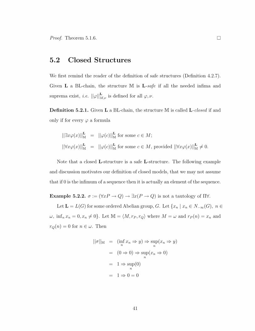
We first remind the reader of the definition of safe structures (Definition 4.2.7).
Given L a BL-chain, the structure M is L-safe if all the needed infima and
suprema exist, i.e. ||ϕ||LM,ν is defined for all ϕ, ν.
Definition 5.2.1. Given L a BL-chain, the structure M is called L-closed if and
only if for every ϕ a formula
||∃xϕ(x)||LM = ||ϕ(c)||LM for some c ∈M ;
||∀xϕ(x)||LM = ||ϕ(c)||LM for some c ∈M , provided ||∀xϕ(x)||LM 6= 0.
Note that a closed L-structure is a safe L-structure. The following example
and discussion motivates our definition of closed models, that we may not assume
that if 0 is the infimum of a sequence then it is actually an element of the sequence.
Example 5.2.2. σ := (∀xP → Q)→ ∃x(P → Q) is not a tautology of Π∀.
Let L = L(G) for some ordered Abelian group, G. Let {xn | xn ∈ N−∞(G), n ∈
ω, infn xn = 0, xn 6= 0}. Let M = 〈M, rP , rQ〉 where M = ω and rP (n) = xn and
rQ(n) = 0 for n ∈ ω. Then
||σ||M = (infnxn ⇒ y)⇒ sup
n
(xn ⇒ y)
= (0⇒ 0)⇒ supn
(xn ⇒ 0)
= 1⇒ supn
(0)
= 1⇒ 0 = 0
41
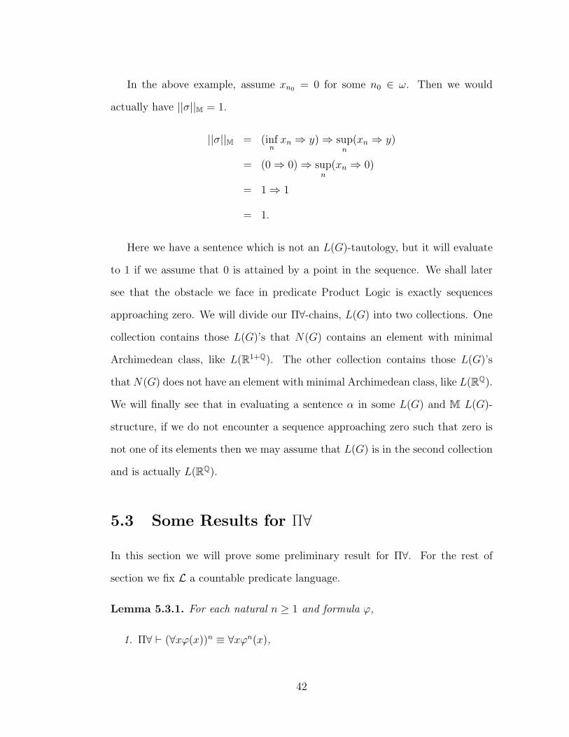
In the above example, assume xn0 = 0 for some n0 ∈ ω. Then we would
actually have ||σ||M = 1.
||σ||M = (infnxn ⇒ y)⇒ sup
n
(xn ⇒ y)
= (0⇒ 0)⇒ supn
(xn ⇒ 0)
= 1⇒ 1
= 1.
Here we have a sentence which is not an L(G)-tautology, but it will evaluate
to 1 if we assume that 0 is attained by a point in the sequence. We shall later
see that the obstacle we face in predicate Product Logic is exactly sequences
approaching zero. We will divide our Π∀-chains, L(G) into two collections. One
collection contains those L(G)’s that N(G) contains an element with minimal
Archimedean class, like L(R1+Q). The other collection contains those L(G)’s
that N(G) does not have an element with minimal Archimedean class, like L(RQ).
We will finally see that in evaluating a sentence α in some L(G) and M L(G)-
structure, if we do not encounter a sequence approaching zero such that zero is
not one of its elements then we may assume that L(G) is in the second collection
and is actually L(RQ).
5.3 Some Results for Π∀
In this section we will prove some preliminary result for Π∀. For the rest of
section we fix L a countable predicate language.
Lemma 5.3.1. For each natural n ≥ 1 and formula ϕ,
1. Π∀ ⊢ (∀xϕ(x))n ≡ ∀xϕn(x),
42

2. Π∀ ⊢ (∃xϕ(x))n ≡ ∃xϕn(x).
Proof. 1. Theorem 4.2.17 implies Π∀ ⊢ (∀xϕ(x))n ≡ ∀xϕn(x) if and only if for
all Π∀-chains L and L-safe structure M, we have ||(∀xϕ(x))n ≡ ∀xϕn(x)||LM =
1L. We have shown that if L is a Π∀-chain then L = L(G) for some or-
dered Abelian group. Let L(G) and M an L(G)-safe structure be given.
Let ||ϕ(mi)||M = ai, for each mi ∈ M and some ai ∈ N(G). Then since +
is continuous in L(G) we have
infinai = n(inf
iai).
so ||(∀xϕ(x))n ≡ ∀xϕn(x)||L(G)M = 1L.
2. We have the same proof as above, replacing infimum with supremum.
Lemma 5.3.2. For each natural n ≥ 1 and formulas ϕ and ψ,
1. Π∀ ⊢ (ϕ→ ψ)n ≡ (ϕn → ψn),
2. Π∀ ⊢ (ϕ&ψ)n ≡ (ϕn&ψn).
Proof. Again we will use the technique of Lemma 5.3.1. We need to show
||(ϕ→ ψ)n ≡ (ϕn → ψn)||L(G)M = 1 and ||(ϕ&ψ)n ≡ (ϕn&ψn)||
L(G)M = 1 for all or-
dered Abelian groups, G and all L(G)-safe structures M. Fix n ≥ 1, a, b ∈ N(G)
for G an ordered Abelian group. We need to show n(a ⇒ b) = na ⇒ nb and
n(a+ b) = na+ nb.
1. If a ≤ b then we have na ≤ nb, hence n(a⇒ b) = n1 = 1 and na⇒ nb = 1.
If a > b, then n(a ⇒ b) = n(b − a) = nb − na = na ⇒ nb. In both cases,
n(a⇒ b) = na⇒ nb.
43

2. Trivial.
Lemma 5.3.3. Let ϕ be an arbitrary formula, ν a formula not containing x,
then
1. ⊢ ∀x(ϕ(x)→ ν) ≡ (∃xϕ(x)→ v),
2. Π∀ ⊢ ∃x(ν → ϕ(x)) ≡ (ν → ∃xϕ(x)).
Proof. 1. (→) is (∃2).
(←), ⊢ ϕ(x)→ ∃xϕ(x);
∴ ⊢ (∃xϕ(x)→ ν)→ (ϕ(x)→ ν; )
∴ ⊢ ∀x((∃xϕ(x)→ ν)→ (ϕ(x)→ ν)) (generalization);
∴ ⊢ (∃xϕ(x)→ ν)→ ∀x(ϕ(x)→ ν) by ∀2.
2. (→), ⊢ (ν → ϕ(x))→ (ν → ∃xϕ(x));
∴ ⊢ ∀x((ν → ϕ(x))→ (ν → ∃xϕ(x))), (generalization);
∴ ⊢ ∃x(ν → ϕ(x))→ (ν → ∃xϕ(x)) by applying (∃2).
(←), Let L(G) be a Π∀-chain, where G is an ordered Abelian group. It
suffices to show a ⇒ supi bi ≤ supi(a ⇒ bi), for a, bi, sup bi ∈ N(G). If
there is a j such that a ≤ bj then a ≤ supi bi. Therefore we get, a ⇒
supi bi = 1 = a⇒ bj = supi(a ⇒ bi). On the other hand, if a ≥ bi for all i
we get a⇒ supi bi = supi bi − a = supi(bi − a) = supi(a⇒ bi).
Lemma 5.3.4. For each theory T and closed formulas α, ϕ, ψ, if T 0 α then
either T ∪ {ϕ→ ψ} 0 α or T ∪ {ψ → ϕ} 0 α.
44
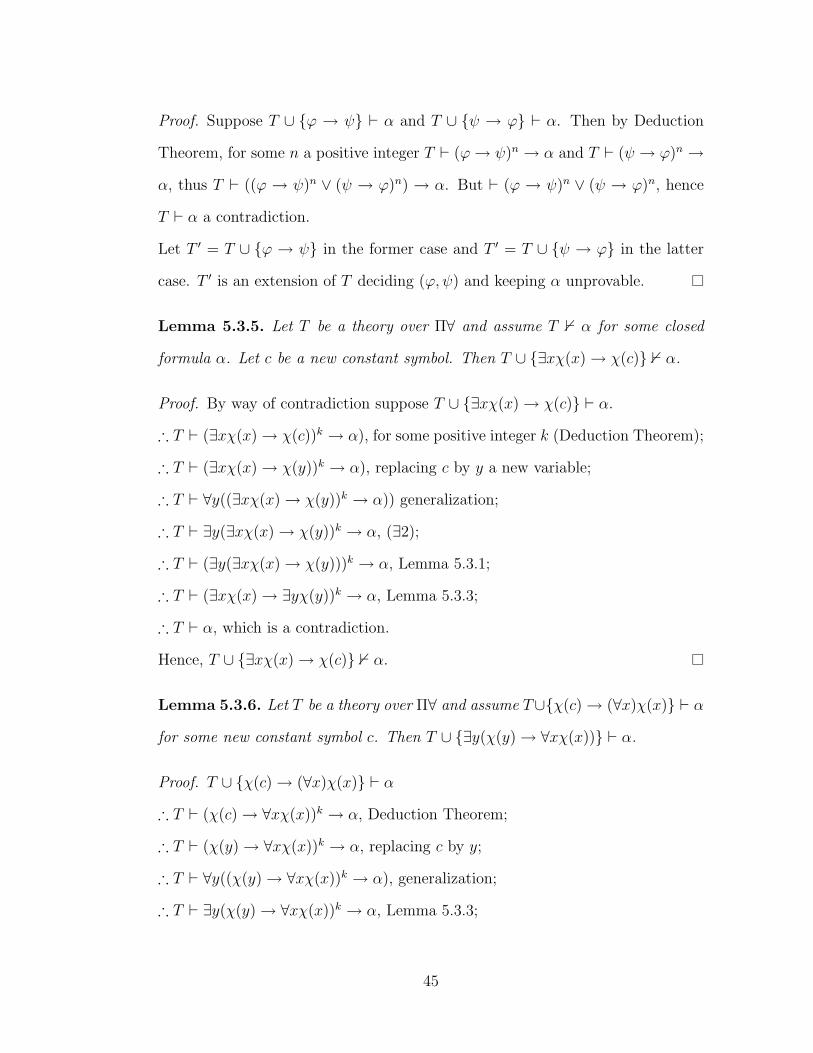
Proof. Suppose T ∪ {ϕ → ψ} ⊢ α and T ∪ {ψ → ϕ} ⊢ α. Then by Deduction
Theorem, for some n a positive integer T ⊢ (ϕ→ ψ)n → α and T ⊢ (ψ → ϕ)n →
α, thus T ⊢ ((ϕ → ψ)n ∨ (ψ → ϕ)n) → α. But ⊢ (ϕ → ψ)n ∨ (ψ → ϕ)n, hence
T ⊢ α a contradiction.
Let T ′ = T ∪ {ϕ → ψ} in the former case and T ′ = T ∪ {ψ → ϕ} in the latter
case. T ′ is an extension of T deciding (ϕ, ψ) and keeping α unprovable.
Lemma 5.3.5. Let T be a theory over Π∀ and assume T 0 α for some closed
formula α. Let c be a new constant symbol. Then T ∪ {∃xχ(x)→ χ(c)} 0 α.
Proof. By way of contradiction suppose T ∪ {∃xχ(x)→ χ(c)} ⊢ α.
∴ T ⊢ (∃xχ(x)→ χ(c))k → α), for some positive integer k (Deduction Theorem);
∴ T ⊢ (∃xχ(x)→ χ(y))k → α), replacing c by y a new variable;
∴ T ⊢ ∀y((∃xχ(x)→ χ(y))k → α)) generalization;
∴ T ⊢ ∃y(∃xχ(x)→ χ(y))k → α, (∃2);
∴ T ⊢ (∃y(∃xχ(x)→ χ(y)))k → α, Lemma 5.3.1;
∴ T ⊢ (∃xχ(x)→ ∃yχ(y))k → α, Lemma 5.3.3;
∴ T ⊢ α, which is a contradiction.
Hence, T ∪ {∃xχ(x)→ χ(c)} 0 α.
Lemma 5.3.6. Let T be a theory over Π∀ and assume T∪{χ(c)→ (∀x)χ(x)} ⊢ α
for some new constant symbol c. Then T ∪ {∃y(χ(y)→ ∀xχ(x))} ⊢ α.
Proof. T ∪ {χ(c)→ (∀x)χ(x)} ⊢ α
∴ T ⊢ (χ(c)→ ∀xχ(x))k → α, Deduction Theorem;
∴ T ⊢ (χ(y)→ ∀xχ(x))k → α, replacing c by y;
∴ T ⊢ ∀y((χ(y)→ ∀xχ(x))k → α), generalization;
∴ T ⊢ ∃y(χ(y)→ ∀xχ(x))k → α, Lemma 5.3.3;
45

∴ T ⊢ (∃y(χ(y)→ ∀xχ(x))k → α, Lemma 5.3.1;
T ∪ {∃y(χ(y)→ ∀xχ(x))} ⊢ α, Deduction Theorem.
Theorem 5.3.7. Let T be a theory over Π∀ and suppose T ∪ {∀xχ(x)→ 0} ⊢ α
and T ∪ {χ(c)→ (∀x)χ(x)} ⊢ α (c a new constant symbol). Then T ⊢ α.
Proof. Let L be a BL-chain and let M be a L-model of T .We need to show
||α||M = 1.
Case 1: ||∀xχ(x)||LM = 0. Then ||∀xχ(x)→ 0||LM = 1. Therefore, M |= T ∪
{∀xχ(x)→ 0} and ||α||LM = 1.
Case 2: ||∀xχ(x))||LM 6= 0. Therefore, ||∃y(χ(y)→ ∀xχ(x))||LM = 1 On the other
hand T ∪{χ(c)→ (∀x)χ(x)} ⊢ α which implies T ∪{∃y(χ(y)→ ∀xχ(x))} ⊢
α (Lemma 5.3.6).
∴ T ⊢ (∃y(χ(y)→ ∀xχ(x)))k → α (Deduction Theorem).
∴ ||(∃y(χ(y)→ ∀xχ(x)))k → α||L
M = 1. But
||(∃y(χ(y)→ ∀xχ(x)))k → α||L
M = ||1→ α||LM
= ||α||LM = 1L.
In both cases we have shown that ||α||LM = 1 and this completes the proof of the
theorem.
Corollary 5.3.8. Let T be a theory over Π∀ and suppose T 0 α. Let χ(x)
be a formula of the language of T and c a new constant symbol. Then either
T ∪ {∀xχ(x)→ 0} 0 α or T ∪ {χ(c)→ (∀x)χ(x)} 0 α .
46
5.4 Completeness Theorem For Π∀
In this section we will strengthen Hajek’s Completeness Theorem for predicate
product logic. We will use techniques used in [Haj98]. We will expand our
language and go through a Henkinization process. We then provide a closed
L-model for T which is the collection of classes of T -equivalent closed formulas.
Definition 5.4.1. ([Haj98]) Let T be a theory over C∀ a schematic extension of
BL∀.
1. T is consistent if there is formula ϕ unprovable in T .
2. T is complete if for each pair ϕ, ψ of closed formulas, T ⊢ (ϕ → ψ) or
T ⊢ (ψ → ϕ).
3. T is Henkin if for each closed formula of the form ∀xϕ(x) unprovable in T
there is a constant c in the language of T such that ϕ(c) is unprovable in
T .
Definition 5.4.2. Let C∀ be a schematic extension of BL∀. Let T be a theory
over C∀. For each closed formula ϕ let [ϕ]T = {ψ | T ⊢ ϕ ≡ ψ}. Let LT be the
set of all the classes [ϕ]T . We define
[ϕ]T + [ψ]T := [ϕ&ψ]T .
[ϕ]T ⇒ [ψ]T := [ϕ→ ψ]T
Lemma 5.4.3. 1. If T is complete then LT is a BL-chain.
2. If T is Henkin then for each formula ϕ(x) with just one free variable x,
[∀xϕ]T = infc
[ϕ(c)]T
47
[∃xϕ]T = supc
[ϕ(c)]T
(c running over all constants of T ).
Proof. 1. We order LT by
[ϕ]T ≤ [ψ]T if and only if T ⊢ ϕ→ ψ.
(a) Since T is complete the definition of ≤ is well defined on LT and
[1]T = 1LTand [0]T = 0LT
.
(b) It is a very straightforward application of the definitions to show
(LT ,+) is a semigroup ([ϕ&ψ]T = [ψ&ϕ]T ). We now need to show
for all ϕ, ψ and χ formula the following holds.
[ϕ]T ≤ [ψ]T if and only if [ϕ]T + [χ]T ≤ [ψ]T + [χ]T .
Suppose [ϕ]T ≤ [ψ]T , then T ⊢ ϕ→ ψ. But by Lemma 4.2.18 we have
⊢ (ϕ → ψ) → ((ϕ&χ) → (ψ&χ)), therefore T ⊢ (ϕ&χ) → (ψ&χ).
Hence [ϕ]T + [χ]T ≤ [ψ]T + [χ]T .
Now suppose [ϕ]T � [ψ]T . Then [ψ]T < [ϕ]T . A symmetric argument
shows that [ψ]T + [χ]T ≤ [ϕ]T + [χ]T .
(c) [ϕ]T + [ϕ→ ψ]T = [ψ]T by definition.
Therefore LT is a BL-chain.
2. Obviously, [ϕ(c)]T ≤ [∃xϕ(x)]T for all c. Assume [ϕ(c)]T ≤ [γ]T for all c.
We need to show [∃xϕ(x)]T ≤ [γ]T .
By way of contradiction, suppose [∃xϕ(x)]T � [γ]T . ∴ T 0 (∃xϕ(x))→ γ.
∴ T 0 ∀x(ϕ(x)→ γ).
∴ T 0 ϕ(c)→ γ (T is Henkin).
48
∴ [ϕ(c)]T � [γ]T a contradiction. Therefore [∃xϕ]T = supc[ϕ(c)]T . A
similar argument shows that [∀xϕ]T = infc[ϕ(c)]T .
Lemma 5.4.4. For each theory T over Π∀ and each closed formula α, if T 0 α
then there is theory T such that
1. T ⊆ T ;
2. T is Henkin and complete;
3. {∃xχ(x)→ χ(cχ)} ∈ T for all χ formula and some constant cχ;
4. Either {∀xχ(x) → 0} ∈ T or {χ(dχ) → (∀x)χ(x)} ∈ T for all χ formula
and some constant dχ;
5. T 0 α.
Proof. We first extend the language L of T to L′ = L ∪ {ci | i ∈ ω}, where ci’s
are new constant symbols. In our construction we need to ensure four properties:
completeness, the Henkin property, the ∃ and ∀ properties. Fix a countable
enumeration {(ϕ, ψ) | ϕ, ψ formulas of L′} of pairs of L′-formulas. For n ∈ ω, at
4n steps we will decide on (ϕ→ ψ) and (ψ → ϕ) (completeness). At 4n+1 steps
we will take care of formulas of the form ∀xχ(x), at 4n+ 2 steps we will process
the ∃ property and at 4n+ 3 we will process the ∀ property.
Let T0 = T, α0 = α. Assume Tn, αn have been constructed so that T0 ⊆ Tn, Tn ⊢
α → αn, Tn 0 αn. We want to construct Tn+1, αn+1 so that Tn+1 ⊢ αn → αn+1,
Tn+1 0 αn+1 and Tn+1 satisfies the nth task.
Case 1: The nth task is deciding (ϕ, ψ). By Lemma 5.3.4 let Tn+1 be the exten-
sion of Tn deciding (ϕ, ψ), keeping αn unprovable. Let αn+1 = αn.
49

Case 2: The nth task is deciding ∀xχ(x). Let c be one of the new constant
symbols of L′ not appearing in Tn.
Subcase (a) Tn 0 αn ∨ χ(c), then Tn 0 χ(c), hence Tn 0 ∀xχ(x). In this
case, let Tn+1 = Tn and αn+1 = αn ∨ χ(c).
Subcase (b) Tn ⊢ αn ∨ χ(c).
∴ Tn ⊢ αn ∨ χ(x) (c does not appear in Tn).
∴ Tn ⊢ ∀x(αn ∨ χ(x)) (generalization).
∴ Tn ⊢ (αn ∨ ∀xχ(x)) ((∀3)).
But (αn ∨ ∀xχ(x)) ≡ [(αn → ∀xχ(x))→ ∀xχ(x)] ∧ [(∀xχ(x)→ α)→
∀xχ(x)].
∴ T ∪ {∀xχ(x)→ αn} ⊢ αn (Deduction Theorem).
∴ T ∪ {αn → ∀xχ(x)} 0 αn (Lemma 5.3.4) and
T ∪ {αn → ∀xχ(x)} ⊢ ∀xχ(x).
In this case, we let Tn+1 = T ∪ {αn → ∀xχ(x)} and αn+1 = αn.
Case 3: The nth task is deciding ∃ property. Let Tn+1 = Tn∪{∃xχ(x)→ χ(cχ)}
and αn+1 = αn. Note Tn+1 0 αn+1 by Lemma 5.3.5.
Case 4: The nth task is deciding between {∀xχ(x)→ 0} and {χ(dχ)→ (∀x)χ(x)}.
Then by corollary 5.3.8 either Tn ∪ {∀xχ(x) → 0} 0 α or Tn ∪ {χ(c) →
(∀x)χ(x)} 0 α . In the former case let Tn+1 = Tn ∪ {∀xχ(x) → 0} and in
the latter case let Tn+1 = Tn ∪ {χ(c)→ (∀x)χ(x)}.
Let T =⋃
n Tn. We show T has the desired properties.
T is complete: By construction (ϕ, ψ) was decided at one of the steps. Hence
either ϕ→ ψ ∈ T or ψ → ϕ ∈ T .
50
T is Henkin: Suppose T 0 ∀xχ(x) and suppose ∀xχ(x) was handled in step n.
Then Tn+1 0 ∀xχ(x), so we can apply subcase (2a) and Tn+1 0 αn ∨ χ(c).
So, T 0 χ(c).
T 0 α: Suppose T ⊢ α. Then Tn ⊢ α for some n. But Tn ⊢ α → αn. Therefore
Tn ⊢ αn, a contradiction.
We have {∃xχ(x) → χ(cχ)} ∈ T for all χ formula and some constant cχ by
construction;
Similarly by construction, either {∀xχ(x)→ 0} ∈ T or {χ(dχ)→ (∀x)χ(x)} ∈ T
for all χ formula and some constant dχ;
Theorem 5.4.5. For each theory T over Π∀ satisfying the conditions (2) − (4)
of Lemma 5.4.4 and each closed formula α such that T 0 α, there is a Π∀-chain
L and closed L-model M of T such that ||α||LM < 1L.
Proof. Let L be the language of T . Let L = LT Which is a BL-chain by Lemma
5.4.3 . Let M = 〈M, (rP )P , (mc)c〉, where M is the set of all constant symbols of
L, mc = c and for each predicate P define rP (~c) = [P (~c)]T .
Claim 1: ||ϕ||LM = [ϕ]T .
Proof of the claim 1: We will prove this by induction on the formulas. If ϕ is an
atomic formula the claim follows from definition.
||ϕ ◦ ψ||LM = ||p||LM ⋄ ||ψ||L
M
= [ϕ]T ⋄ [ψ]T
= [ϕ ◦ ψ]T
51
where ◦ = &,→ and ⋄ = +,⇒.
||∀xϕ(x)||LM = infc||ϕ(c)||LM
= infc
[ϕ(c)]T , induction
= [∀xϕ(x)]T , Lemma 5.4.3.
||∃xϕ(x)||LM = supc
||ϕ(c)||LM
= supc
[ϕ(c)]T , induction
= [∃xϕ(x)]T , Lemma 5.4.3.
This completes the proof of the claim 1.
Claim 2: M is a closed L-model. Let χ(x) be a formula with one free variable
we need to show:
1. ∃c such that ||∃xχ(x)||LM = ||χ(c)||LM;
2. If ||∀xχ(x)||LM 6= 0 then ∃d such that ||∀xχ(x)||LM = ||χ(d)||LM.
Proof of claim 1:Since {∃χ(x) → χ(cχ)} ∈ T , we have ||∃xχ(x)→ χ(cχ)||LM
= 1.
That is ||∃xχ(x)||LM ≤ ||χ(cχ)||LM
. On the other hand, ||χ(cχ)||LM≤ ||∃xχ(x)||LM
hence we have ||χ(cχ)||LM
= ||∃xχ(x)||LM.
Either {∀xχ(x) → 0} ∈ T or {χ(dχ) → (∀x)χ(x)} ∈ T . If ||∀xχ(x)||LM 6= 0, we
have {χ(dχ)→ (∀x)χ(x)} ∈ T . We have
||χ(dχ)→ (∀x)χ(x)||LM
= 1.
Then
||χ(dχ)||LM≤ ||(∀x)χ(x)||LM.
But ||(∀x)χ(x)||LM ≤ ||χ(dχ)||LM
. Therefore, ||(∀x)χ(x)||LM = ||χ(dχ)||LM
. Hence M
is a closed L-model and the proof of claim 2 is complete.
52
We have shown that M is a closed model of T , i.e., for every axiom ϕ of T we
have ||ϕ||LM = [ϕ]T = 1L. However, ||α||LM = [α]T 6= [1]T = 1L. This completes
the proof of the theorem.
Notice in the above theorem by construction M and L are countable since we
are working with countable languages. We are now ready to tackle Completeness
Theorem.
Theorem 5.4.6 (Completeness Theorem for Π∀ (A)). Let T be a theory
over Π∀. Let ϕ be a formula of the language of T . Then T ⊢ ϕ if and only if
||ϕ||LM = 1L for every countable L a Π∀-chain and every countable closed L-model
M.
Proof. This follows immediately from Theorem 5.4.5 and Lemma 5.4.4.
Theorem 5.4.7 (Completeness Theorem for Π∀ (B)). Let T be a theory
over Π∀. Let ϕ be a formula of the language of T . Then T ⊢ ϕ if and only if
||ϕ||LM = 1L(G) for every countable ordered Abelian group, G, and every countable
closed L(G)-model M of T .
Proof. The proof follows from Theorem 5.4.6 and the fact that if L is a Π∀-chain
then L = L(G) for some ordered Abelian group.
5.5 Transfer Results to RQ or R1+Q
In this section we will show Π∀ ⊢ α if and only if for all M closed L-structures
||α||LM = 1, where L = L(RQ) or L(R1+Q). This will be done in several steps.
We will first show that if α is not an L(G)-tautology then α is not an L(RS)-
tautology, where (F, S) is a Hahn representation of G. This will be done using
53
the fact that F is cointiality preserving. We will then show that α is either not
an L(R1+Q)-tautology or not an L(RQ)-tautology. This will be achieved using
the fact that for any ordered set S there is a coinitiality preserving embedding of
RS into either RQ or R1+Q.
Definition 5.5.1. Let G and H be two ordered Abelian groups and let f : G→
H be a coinitiality preserving embedding (hence f : N(G) → N(H)) . Let
f : L(G)→ L(H) be defined by f(−∞) = −∞ f ⇂N(G)= f and f(1) = 1.
Theorem 5.5.2. Let G and H be two ordered Abelian groups and let f : G→ H
be a coinitiality preserving embedding. Let M = 〈M, (rP )P , (mc)c〉 be a closed
L(G)-model. Let f be from Definition 5.5.1 and let M = 〈M, (rP )P , (mc)c〉,
where rP (~m) = f(rP (~m)) and mc = mc. Then
||ϕ||LM,ν = f(||ϕ||LM,ν)
for all ν evaluation and ϕ a formula and M is a closed L(H)-structure.
Proof. . We prove this by induction on the formulas.
||x||M,ν = ν(x) = ||x||M,ν ;
||c||M,ν = mc = mc = ||c||M,ν ;
||P (~t)||L
M,ν = rP (||~t||L
M,ν) = f(rP (||~t||L
M,ν)) = f(||P (~t)||L
M,ν);
For connectives we have
||ϕ ◦ ψ||LM,ν = ||ϕ||L
M,ν ⋄ ||ψ||L
M,ν ,
= f(||ϕ||LM,ν) ⋄ f(||ψ||LM,ν) (induction)
= f(||ϕ ◦ ψ||LM,ν)
54
where ◦ = &,→ and ⋄ = +,⇒.
For quantifiers we have
f(||∃xϕ||LM,ν) = f(||ϕ(c)||LM,ν) for some c (M is a closed model)
= ||ϕ(c)||LM,ν (induction)
= supν′∈E(ν,x)
||ϕ(x)||LM,ν′
The last equality holds since f(||ϕ(c)||LM,ν) ≥ f(||ϕ(d)||LM,ν) (f is order pre-
serving) and supν′∈E(ν,x) ||ϕ(x)||LM,ν′ = sup f(||ϕ(d)||LM,ν). Hence ||∃xϕ||L
M,ν =
f(||∃xϕ||LM,ν).
If ||∀xϕ||LM,ν 6= 0, then
f(||∀xϕ||LM,ν) = f(||ϕ(c)||LM,ν) for some c (M is a closed model)
= ||ϕ(c)||LM,ν (induction)
= infν′∈E(ν,x)
||ϕ||LM,ν′
The last equality holds since f(||ϕ(c)||LM,ν) ≤ f(||ϕ(d)||LM,ν) (f is order preserving)
and infν′∈E(ν,x) ||ϕ(x)||LM,ν′ = inf f(||ϕ(d)||LM,ν). Hence ||∀xϕ||L
M,ν = f(||∀xϕ||LM,ν).
If ||∀xϕ||LM,ν = 0, then since f is coinitiality preserving we have ||∀xϕ||LM,ν = 0.
This complete the proof of the claim and that M is a closed L(H)-model.
Corollary 5.5.3. Suppose f : G→ H is a coinitiality preserving embedding. Let
M be a closed L(G)-model such that ||ϕ||L(G)M < 1. Then ||ϕ||
L(H)
M< 1.
Proof. This is a direct corollary of Theorem 5.5.2.
Corollary 5.5.4. Let G be a countable ordered Abelian group and let M be a
closed L(G)-structure. Suppose ||ϕ||L(G)M < 1. Then there exist an ordered set S
such that ||ϕ||L(RS)
M< 1
55

Proof. Let (RS, F ) be a Hahn representation of G. We have shown that F is
coinitiality preserving. Therefore by corollary 5.5.3, ϕ is not an L(RS)-tautology.
Lemma 5.5.5. Let S be a countable linear ordering and let M be a closed L(RS)-
structure. Suppose ||ϕ||L(RS)M < 1 Then either ||ϕ||
L(RQ)
M< 1 or ||ϕ||
L(R1+Q)
M< 1.
Proof. By Lemma 3.2.8, we have that for any countable ordered set S, RS there
exists a coinitiality preserving embedding f : RS → RQ or R1+Q. This gives the
desired result.
So far we have shown that if α is not an L(G)-tautology for some countable
G, then either α is not an L(RQ)-tautology or α is not an L(R1+Q)-tautology.
The next two Completeness Theorems follow directly from our earlier versions of
Completeness Theorem and the results in section 5.5.
Theorem 5.5.6 (Completeness Theorem for Π∀ (C)). Let T be a theory
over Π∀. Let ϕ be a formula of the language of T . Then T ⊢ ϕ if and only if
||α||LM = 1L where L = L(RS) for all lexicographic function space RS (S countable)
and every countable closed RS-model M of T .
Proof. (→) Suppose T ⊢ α then for every L, a Π∀-chain and every closed L-
model M, ||ϕ||LM = 1L. We have shown that L = L(G) for some countable
ordered Abelian group. And certainly, RS is an ordered Abelian group.
(←) Suppose T 0 α. Then there is an L(G) for some ordered Abelian group and
a closed L(G)-model M such that ||α||L(G)M 6= 1. Now by corollary 5.5.4 we may
assume that L = L(RS), where (RS, F ) is a Hahn representation for G. And the
proof is complete.
56
Theorem 5.5.7 (Completeness Theorem for Π∀ (D)). Let T be a theory
over Π∀. Let ϕ be a formula of the language of T . Then T ⊢ ϕ if and only if
||α||LM = 1L where L = L(RQ) or L(R1+Q) and every countable closed L-model M
of T .
Proof. The result directly follows from Theorem 5.5.6 and Lemma 5.5.5.
57

Chapter 6
L(RS)-Tautologies When S Is Not Initially Scattered
In this chapter will show that if α is not provable from Π∀, then α is not an
L(RS)-tautology, where S is not initially scattered. We will go through a very
similar Henkenization process as in 5.4. We will conclude that L(RS)-TAUT is
recursively enumerable if S is not initially scattered.
6.1 Main Result
Again for the rest of this section let L be a countable predicate language. We
need to deal with sequences that approach but do not equal 0 in evaluation of
sentences.
Lemma 6.1.1. Let T be a theory over Π∀ and α a sentence of L, the language
of T . Let L be a Π∀-chain and M a closed L-model of T such that ||α||LM < 1.
Let χ(x) be an L-formula with one single variable and let c ∈ M . Suppose there
exists b∗ ∈M such that ||χ(b∗)||LM ≤ m||χ(c)||LM for all m ∈ ω. Then
T ∪ {χ(e)→ χm(c) : m ∈ ω} 0 α,
where e is a new constant symbol.
58
Proof. Note by assumption we have T 0 α. By way of contradiction suppose
T ∪ {χ(e) → χm(c) : m ∈ ω} ⊢ α. Since proofs have finite length, we may
assume there is a single m such that T ∪{χ(e)→ χm(c)} ⊢ α. Now by Deduction
theorem T ⊢ (χk(e) → χmk(c)) → α, for some positive k. Since e is a constant
not appearing in T we may replace it by x and get T ⊢ (χk(x) → χmk(c)) → α.
Hence by generalization we get ||(χk(b∗)→ χmk(c))→ α||L
M = 1. However, we
have ||χk(b∗)→ χmk(c)||L
M = 1. Therefore, ||α||LM = 1 a contradiction and we
have the result.
Lemma 6.1.2. Let T be a complete Henkin theory over Π∀, where L is the
language of T . Suppose T 0 α. Then there exists L′ ⊇ L and T ′ ⊇ T such that
1. T ′ is a complete Henkin theory over L′;
2. T ′ 0 α;
3. For all L-formulas χ(x) with one free variable, there exist c ∈ L′ such that
{∃xχ(x)→ χ(c)} ∈ T ′;
4. For all L-formulas χ(x) with one free variable, either there is d ∈ L′ such
that {χ(d) → ∀xχ(x)} ∈ T ′ or for all c ∈ L there is dc ∈ L′ such that
{χ(dc)→ χ(c)n | n ∈ ω} ∈ T ′.
Proof. We first extend the language L of T to L′ = L ∪ {ci | i ∈ ω}, where ci’s
are new constants. The proof of this theorem is almost identical to the proof of
Lemma 5.4.4. The only slight difference is in ensuring property 4. This is how
we do it. If the nth task is deciding between {χ(d) → ∀xχ(x)} and {χ(dc) →
χ(c)n | n ∈ ω}. By corollary 5.3.8 we have either Tn ∪ {∀xχ(x) → 0} 0 α or
Tn∪{χ(c)→ (∀x)χ(x)} 0 α . In the former case let Tn+1 = Tn∪{χ(dc)→ χ(c)n |
n ∈ ω} and in the latter case let Tn+1 = Tn ∪ {χ(d)→ (∀x)χ(x)}.
59

Let T ′ =⋃
n Tn. Verifying T ′ has the desired properties is identical to the
proof of Lemma 5.4.4.
Theorem 6.1.3. Let T be a theory over Π∀ in the language L. Suppose T 0 α,
α an L-sentence. Then there is L∗ ⊇ L, L a Π∀-chain, M a closed L-structure
such that
1. M is an L-model of T , i.e., ||σ||M = 1L for all σ ∈ T .
2. M is super-closed, i.e.,
(a) For all L∗-formula ϕ(x) with one free variable there is c ∈ L∗ such
that ||ϕ(c)||M ≥ ||∃xϕ(x)||M (hence we have equality);
(b) For all L∗-formula ϕ(x) with one free variable such that ||∀xϕ(x)||M 6=
0, there is d ∈ L∗ such that ||ϕ(d)||M ≤ ||∀xϕ(x)||M (hence we have
equality).
(c) For all L∗-formula ϕ(x) with one free variable such that ||∀xϕ(x)||M =
0, but ||ϕ(c)||M > 0 for all c ∈ L∗, there exists dc ∈ L∗ such that
||ϕ(dc)||M ≤ ||ϕ(c)n||M for all n ∈ ω and c ∈ L∗.
Proof. Given T,L and α let L0 ⊇ L ∪ Henkin constants. Let T0 be a complete
Henkin theory in L0 such that T0 0 α. Iterate Lemma 6.1.2 ω times. At step n
let Tn+1 = (Tn)′. αn+1 = α. Let L∗ = ∪{Ln : n ∈ ω} and T ∗ ∪ {Tn : n ∈ ω}.
Claim: T ∗ is a complete Henkin theory in L∗ such that
1. T ∗ 0 α;
2. For all L-formulas ϕ(x) with one free variable, there exist c ∈ L′ such that
{∃xϕ(x)→ ϕ(c)} ∈ T ′;
60

3. For all L-formulas ϕ(x) with one free variable, either there is d ∈ L′ such
that {ϕ(d) → ∀xϕ(x)} ∈ T ′ or for all c ∈ L there is dc ∈ L′ such that
{ϕ(dc)→ ϕ(c)n | n ∈ ω} ∈ T ′.
Proof of the claim: The completeness and Henkin properties of T ∗ is proved
exactly as in 6.1.2. By way of contradiction suppose T ∗ ⊢ α, then Tn ⊢ α for
some n ∈ ω a contradiction to Lemma 6.1.2. By construction we have the other
3 properties involving quantifiers.
Let L be the Π∀-chain and M be the closed L-model we produced in theorem
5.4.5. We claim that M has the properties needed by the theorem.
By construction M is a model of T ∗. Again by construction ||α||M < 1.
Let ϕ(x) be an L∗ formula with one free variable. Since ϕ has finitely many
symbols we may assume ϕ is an Ln-formula for some n ∈ ω. Then by
Lemma 6.1.2, there exists c ∈ Ln+1 ⊆ L∗ such that {∃xϕ(x) → ϕ(c)} ∈
Tn+1 ⊆ T ∗. Hence ||∃xϕ(x)→ ϕ(c)||M = 1, that is ||ϕ(c)||M ≥ ||∃xϕ(x)||M.
Let ϕ(x) be an L∗ formula with one free variable. Again we may assume ϕ
is an Ln-formula for some n ∈ ω. Then by Lemma 6.1.2, either there is
d ∈ Ln+1 ⊆ L∗ such that {ϕ(d) → ∀xϕ(x)} ∈ Tn+1 ⊆ T ∗ or for all c ∈ Ln
there is dc ∈ Ln+1 such that {ϕ(dc) → ϕ(c)n | n ∈ ω} ∈ Tn+1 ⊆ T ∗. In
the former case ||ϕ(d)→ ∀xϕ(x)||M = 1, hence ||ϕ(d)||M ≤ ||∀xϕ(x)||M. In
the latter case ||ϕ(dc)→ ϕ(c)n||M = 1 for all n ∈ ω, hence ||ϕ(dc)||M ≤
||ϕ(c)n||M = n||ϕ(c)||M for all n ∈ ω.
And the proof is complete.
Definition 6.1.4. Let L be a predicate language. Let L be a Π∀-chain and let
M be a closed L-structure over L. We say there is a threat present at M if and
61
only if for some L-formula with one free variable, ϕ(x), ||∀xϕ(x)||LM = 0, but
||ϕ(c)||LM 6= 0 for all c ∈ L.
Now we would like to show if ||α||L(RS)M < 1 then ||α||
L(RQ)M < 1. We will
use Theorem 5.5.2 which requires a coinitiality preserving embedding. However,
we note that if there are no threats present at M, it suffices to have an order
preserving embedding f : S → Q.
Lemma 6.1.5. Let T be a theory over Π∀. Suppose T 0 α for some sentence α.
Then α is not an L(RQ)-tautology.
Proof. There exist S an ordered set and M an L(RS)-structure such that
||α||L(RS)M < 1.
There are two cases. Either there is a threat present at M or not.
Case 1: Suppose there is no threat present at M. Let h : S → Q be any order
preserving map. Let f : RS → RQ be the canonical map induced by h.
Since there are no threats present at M as in the proof of theorem 5.5.2 we
get ||α||L(RQ)M = f(||α||
L(RS)M ).
Case 2: Suppose there is a threat present at M. Hence there exists a ϕ such
that ||∀xϕ(x)||L(RS)M = 0, but ||ϕ(c)||
L(RS)M 6= 0 for all c ∈ L. Therefore by
part 2(c) of 6.1.3, we have that L(RS) does not contain a smallest non-zero
Archimedean class. Therefore S does not contain a smallest element. Let
h : S → Q be an order and cointiality preserving map given by Lemma
2.2.4. Let f : RS → RQ be the canonical map induced by h which is
coinitiality preserving. Then ||α||L(RQ)M = f(||α||L(RQ)
M ) < 1.
62
This completes the proof of the theorem.
Theorem 6.1.6 (Completeness theorem for Π∀ (E)). Let T be a theory
over Π∀. Let ϕ be a formula of the language of T . Then T ⊢ ϕ if and only if
||α||L(RQ)M = 1L(RQ), for every countable closed L(RQ)-structure M of T .
Proof. This is a direct result of Lemma 6.1.5 and our other completeness theo-
rems.
Theorem 6.1.7. Let T be a theory over Π∀. Let ϕ be a formula of the language
of T . Let S be a countable, not initially scattered linear ordering. Then T ⊢ ϕ if
and only if ||α||L(RS)M = 1L(RS), for every countable closed L(RS)-structure M of
T .
Proof. → Theorem 5.5.6.
← Suppose T 0 ϕ, then by Theorem 6.1.6 ||α||L(RQ)M < 1L(RQ), for every countable
closed L(RQ)-structure M. By Lemma 2.2.8 we have a coinitiality preserv-
ing map h : Q → S. Therefore by Theorem 5.5.2, ||α||L(RS)
M< 1L(RS), for
every countable closed L(RQ)-structure M.
Corollary 6.1.8. Let S be a countable not initially scattered linear ordering.
Then L(RS)-TAUT is recursively enumerable. In particular L(RS)-TAUT=L(RQ)-
TAUT.
Proof. σ ∈ L(RS)-TAUT if and only if Π∀ ⊢ σ if and only if σ ∈ L(RQ)-TAUT.
Hence, L(RS)-TAUT is recursively enumerable.
63
Chapter 7
L(RS)-Tautologies When S Is Initially Scattered
In [Mon01], Montagna proves that the set of L(R1)-tautologies of predicate Prod-
uct Logic is not arithmetical. We will extend his proof to show that the set of
L(RT )-tautologies is not arithmetical when T is initially scattered.
7.1 Preliminaries
Let L0 be a predicate language containing {Z, S,E, L,A, P}, and let L = L0∪{U}
where
• Z and U are unary predicates, Z(x) to be read as x = 0 and U(x) has no
arithmetical interpretation;
• S,E and L are binary relations. S(x, y) to be read x+ 1 = y, E(x, y) to be
read x = y and L(x, y) to be read x < y;
• A and P are ternary relation symbols, A(x, y, z) to be read x + y = z and
P (x, y, z) to be read x · y = z.
Definition 7.1.1. For every L0-formula ϕ(x) , we write ϕ(0) for
∀x(x = 0→ ϕ(x)),
64
and for k a positive integer , we write ϕ(x+ k) for
∀x1 . . . ∀xk((k−1∧
i=1
(xi + 1 = xi+1) ∧ (x1 = x+ 1))→ ϕ(xk)).
Definition 7.1.2. Let P denote a finitely axiomatizable system of arithmetic (in
the language L0), whose axioms are:
• The axioms of Robinson’s Q, including the axioms of equality.
– ∀x(¬S(x) = 0);
– ∀x∀y(S(x) = S(y)→ x = y);
– ∀x(x+ 0 = x);
– ∀x∀y(x+ S(y) = S(x+ y));
– ∀x(x · 0 = 0);
– ∀x∀y(x · S(y) = x · y + x);
– ∀x(¬x < 0);
– ∀x∀y(x < S(y)↔ x < y ∨ x = y);
– ∀x∀y(x < y ∨ x = y ∨ y < x);
• Axioms representing that < is a strict linear order, compatible with + and
with ·.
• The axiom ∀x(x < x+ 1 ∧ ¬∃u(x < u ∧ u < x+ 1)).
Let Θ be the conjunction of the axioms of P.
Definition 7.1.3. For every L-formula ϕ we let ϕ◦ denote the formula obtained
from ϕ by replacing every atomic formula α of the language L0 by ¬¬α and
leaving other atomic formulas unchanged.
65

The above definition basically says in a formula ϕ of the language L, replace
Z, S,E, L,A and P by ¬¬Z,¬¬S,¬¬E,¬¬L,¬¬A and ¬¬P .
Example 7.1.4. 1. (U(x)→ Z(x))◦ ≡ U(x)→ ¬¬Z(x).
2. [∀x(∃yS(x, y)→ U(x))]◦ ≡ ∀x(∃y¬¬S(x, y)→ U(x)).
In the next section we will utilize some properties of non-standard models
of Robinson’s Q. We will now go over some properties that we will need. For
the rest of this chapter let N∗ be a non-standard model of Q. A non-standard
model of Q, N∗, contains a copy of the natural numbers and an element which is
larger than all natural numbers and models axioms of Q. Note, N∗ is an ordered
Abelian semigroup. For 0 < a < b we write a ≪ b if and only if na < b for all
n ∈ ω and we write a ∼ b if there is a positive integer n such that b < na.
Lemma 7.1.5. a ∼ a+ n for all 0 < a ∈ N∗ and n ∈ ω.
Proof. By the structure of N∗, ∃m ∈ ω such that a+ n ≤ ma.
Lemma 7.1.6. For a, b ∈ N∗, if a≪ b then a+ n≪ b for all n ∈ ω.
Proof. Follows immediately from Lemma 7.1.5.
Lemma 7.1.7. For a, b ∈ N∗, if a≪ b then a≪ a+b
2≪ b.
Proof. By way of contradiction suppose there is n such that a+b2≤ na. Then
b ≤ (2n − 1)a, which is a contradiction to a < b. Hence a ≪ a+b2
. Similar
argument shows that a+b2≪ b.
Lemma 7.1.8. Let b ∈ N∗ be a non-standard element and let m be positive
integer. Then nbm+bm−1
n+1+ 1≪ bm for all n ∈ ω.
66
Proof. nbm+bm−1
n+1+ 1≪ bm if and only if nbm + bm−1 + n + 1≪ (n + 1)bm if and
only if bm−1 + n+ 1≪ bm which is always true by Lemma 7.1.6.
Lemma 7.1.9. Let b ∈ N∗ be a non-standard element and m a positive integer.
Consider the set
Bm = {bm−1, bm} ∪ {(2k − 1)bm + bm−1
2k+ 1 | k a positive integer}.
Then
bm−1 ≪bm + bm−1
2+ 1≪
3bm + bm−1
4+ 1≪
. . .≪(2k − 1)bm + bm−1
2k+ 1≪ . . .≪ bm + 1.
Furthermore, Bm is dense.
Proof. We observe that(2k
−1)bm+bm−1
2k+1+bm+1
2= (2k+1−1)bm+bm−1
2k+1 + 1. I.e., each
middle term is the average of the previous term and bm + 1. Therefore Bm is
dense and the other result follows from Lemma 7.1.7.
7.2 Montagna’s Technique
The basic idea for this section comes from [Mon01], where he focuses on L(R1).
We were able to extend his result to L(RT )’s (for initially scattered sets T ) which
are Π∀-chains. Our technique to prove theorem 7.3.5 is new. In his paper, he
basically uses the fact that any coinitial sequence in [0, 1] converges to 0. For
the rest of this section suppose T is a linear ordering and M is a closed L(RT )-
structure. For ease of notation let || · ||M = || · ||L(RT )M .
Lemma 7.2.1. 1. Let x ∈ L(RT ) such that x > 0. Then ¬¬x = 1 and
¬¬0 = 0.
67

2. Let x, y ∈ L(RT ) such that x > y, then x⇒ (y + z) ≤ z for all z ∈ L(RT ).
Proof. 1. ¬¬x = 0⇒ (0⇒ x) = 1 if x 6= 0 and ¬¬0 = 0.
2. x > y > y + z for all z. Therefore, x ⇒ (y + z) = y + z − x = z + y − x.
y − x < 0 implies z + y − x < z and x⇒ (y + z) ≤ z
Lemma 7.2.2. Let ν be an M-evaluation. Then for every formula ϕ of the
language of P
||ϕ◦||M,ν = 0 or 1.
Furthermore, ||ϕ◦||M,ν = 1 if and only if ||ϕ||M,ν > 0.
Proof. By Lemma 7.2.1, ¬¬x is either 0 or 1. Now since U does not appear in ϕ,
ϕ◦ involves atomic formulas of the form ¬¬α, whose evaluations in M is either 0
or 1. So we have
||ϕ◦||M,ν = 0 if and only if ||ϕ||M,ν = 0
and
||ϕ◦||M,ν = 1 if and only if ||ϕ||M,ν > 0.
Lemma 7.2.3. Suppose ||Θ◦||M = 1 and ||E(a, b)◦||M = 1 then ||L(a, b)◦||M = 0
and ||L(b, a)◦||M = 0.
Proof. Since ||Θ◦||M = 1, we have ||E(a, b)→ ¬L(a, b)||M > 0. By way of contra-
diction suppose ||L(a, b)||M > 0. Then ||¬L(a, b)||M = 0 and ||E(a, b)→ 0||M > 0
implies ||E(a, b)||M = 0 which is a contradiction. Therefore, ||L(a, b)||M = 0.
Switch the place of a and b and we have ||L(b, a)||M = 0.
68
Lemma 7.2.3, intuitively implies that if a and b ∈M have a positive chance of
being equal, they have zero chance of not being equal and hence we can not define
a linear ordering just yet. To remedy this problem, we define a new relation on
M .
Definition 7.2.4. Suppose ||Θ◦||M = 1. For a and b ∈M let
a ∼ b if and only if ||E(a, b)◦||M = 1
if and only if ||E(a, b)||M > 0
Lemma 7.2.5. 1. ∼ is an equivalence relation of M .
2. The ∼-equivalence classes are convex.
3. M◦ := M/ ∼, < is a linear ordering, where
[a] < [b] if and only if ||L(a, b)||M > 0.
Proof. 1. a ∼ a if and only if ||E(a, a)||M 6= 0, which is true since ||Θ◦||M = 1.
Suppose a ∼ b, we need to show b ∼ a. Again since ||Θ◦||M = 1, we
have that ||E(a, b)⇒ E(b, a)||M 6= 0. By way of contradiction suppose
||E(b, a)||M = 0 then since ||E(a, b)||M 6= 0 we would get
||E(a, b)⇒ E(b, a)||M = 0,
which is a contradiction.
Suppose a ∼ b and b ∼ c, we need to show a ∼ c. We have ||E(a, b)||M 6= 0,
||E(b, c)||M 6= 0 and ||E(a, b)&E(b, c)→ E(a, c)||M 6= 0. By way of contra-
diction suppose ||E(a, c)||M = 0. This would imply ||E(a, b)&E(b, c)||M = 0
which in turn implies either ||E(a, b)||M = 0 or ||E(b, c)||M = 0,a contradic-
tion. Hence a ∼ c. This completes the proof of part 1.
69
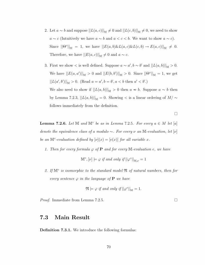
2. Let a ∼ b and suppose ||L(a, c)||M 6= 0 and ||L(c, b)||M 6= 0, we need to show
a ∼ c (Intuitively we have a ∼ b and a < c < b. We want to show a ∼ c).
Since ||Θ◦||M = 1, we have ||E(a, b)&L(a, c)&L(c, b)→ E(a, c)||M 6= 0.
Therefore, we have ||E(a, c)||M 6= 0 and a ∼ c.
3. First we show < is well defined. Suppose a ∼ a′, b ∼ b′ and ||L(a, b)||M > 0.
We have ||E(a, a′)||M > 0 and ||E(b, b′)||M > 0. Since ||Θ◦||M = 1, we get
||L(a′, b′)||M > 0. (Read a = a′, b = b′, a < b then a′ < b′.)
We also need to show if ||L(a, b)||M > 0 then a ≁ b. Suppose a ∼ b then
by Lemma 7.2.3, ||L(a, b)||M = 0. Showing < is a linear ordering of M/ ∼
follows immediately from the definition.
Lemma 7.2.6. Let M and M◦ be as in Lemma 7.2.5. For every a ∈ M let [a]
denote the equivalence class of a modulo ∼. For every ν an M-evaluation, let [ν]
be an M◦-evaluation defined by [ν](x) = [e(x)] for all variable x.
1. Then for every formula ϕ of P and for every M-evaluation e, we have
M◦, [ν] |= ϕ if and only if ||ϕ◦||M,ν = 1
2. If M◦ is isomorphic to the standard model N of natural numbers, then for
every sentence ϕ in the language of P we have
N |= ϕ if and only if ||ϕ◦||M = 1.
Proof. Immediate from Lemma 7.2.5.
7.3 Main Result
Definition 7.3.1. We introduce the following formulas:
70

• Ψ0 ≡ ¬∀xU(x).
• Ψ1 ≡ ∀x∀y∀z(((U(x)&U(z))→ (U(y)&U(z)))→ (U(x)→ U(y))).
• Ψ2 ≡ ∀x¬¬U(x).
• Ψ3 ≡ (∀x(U(x+ 1)→ (∀z((z ≤ x)→ U(z)))3))◦.
• Ψ ≡ Θ◦&Ψ0&Ψ1&Ψ2&Ψ3.
Intuitively, Ψ0 says the infimum of U(ai) is 0, Ψ1 is one of the axioms of the
Product logic. Ψ2 says no U(ai) is 0 and Ψ3 controls the speed at which U(ai)
decreases to 0.
For the rest of this section we will suppose ||Ψ||M > 0. Therefore, we have M◦ is
a model of P. So it makes sense to talk about ≤M◦
,≪M◦
.
Proposition 7.3.2. Let M be a closed L(RT )-structure such that ||Ψ||M > 0. Let
M◦ be defined as before. Then there exists b ∈ M such that for all c ∈ M , if
M◦ |= [b] ≤ [c], then
||U(c+ 1)||M ≤ 2( inf[z]≤M◦
[c]||U(z)||M)
Proof. First note that since ||Ψ||M > 0 we have ||Θ◦||M = 1. Hence M◦ |= P. Let
B = {a ∈M | ||U(a+ 1))||M > ( inf[z]≤M◦
[a]||U(z)||M)2}.
Suppose by way of contradiction that for all a ∈ M , there is b(a) ∈ B such that
[a] ≤M◦
[b(a)]. Then by Lemma 7.2.1
||U(a+ 1))||M ⇒ 3( inf[z]≤M◦
[b(a)]||U(z)||M) ≤ inf
[z]≤M◦[b(a)]||U(z)||M.
Since ||Ψ0||M = 1 we have infa∈M ||U(a)||M = 0. It follows
71
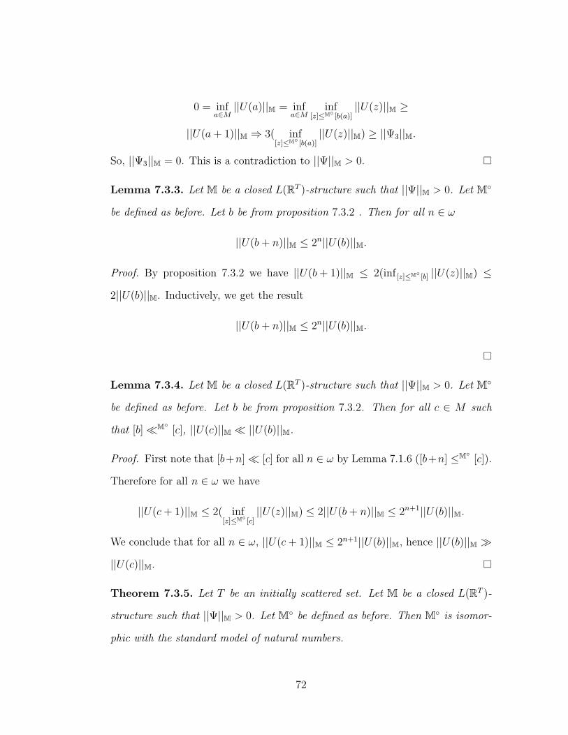
0 = infa∈M||U(a)||M = inf
a∈Minf
[z]≤M◦[b(a)]||U(z)||M ≥
||U(a+ 1)||M ⇒ 3( inf[z]≤M◦
[b(a)]||U(z)||M) ≥ ||Ψ3||M.
So, ||Ψ3||M = 0. This is a contradiction to ||Ψ||M > 0.
Lemma 7.3.3. Let M be a closed L(RT )-structure such that ||Ψ||M > 0. Let M◦
be defined as before. Let b be from proposition 7.3.2 . Then for all n ∈ ω
||U(b+ n)||M ≤ 2n||U(b)||M.
Proof. By proposition 7.3.2 we have ||U(b+ 1)||M ≤ 2(inf [z]≤M◦[b] ||U(z)||M) ≤
2||U(b)||M. Inductively, we get the result
||U(b+ n)||M ≤ 2n||U(b)||M.
Lemma 7.3.4. Let M be a closed L(RT )-structure such that ||Ψ||M > 0. Let M◦
be defined as before. Let b be from proposition 7.3.2. Then for all c ∈ M such
that [b]≪M◦
[c], ||U(c)||M ≪ ||U(b)||M.
Proof. First note that [b+n]≪ [c] for all n ∈ ω by Lemma 7.1.6 ([b+n] ≤M◦
[c]).
Therefore for all n ∈ ω we have
||U(c+ 1)||M ≤ 2( inf[z]≤M◦
[c]||U(z)||M) ≤ 2||U(b+ n)||M ≤ 2n+1||U(b)||M.
We conclude that for all n ∈ ω, ||U(c+ 1)||M ≤ 2n+1||U(b)||M, hence ||U(b)||M ≫
||U(c)||M.
Theorem 7.3.5. Let T be an initially scattered set. Let M be a closed L(RT )-
structure such that ||Ψ||M > 0. Let M◦ be defined as before. Then M◦ is isomor-
phic with the standard model of natural numbers.
72
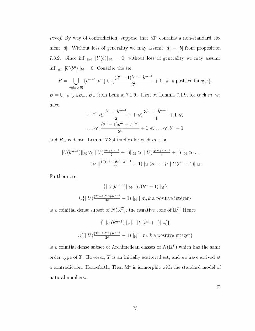
Proof. By way of contradiction, suppose that M◦ contains a non-standard ele-
ment [d]. Without loss of generality we may assume [d] = [b] from proposition
7.3.2. Since infa∈M ||U(a)||M = 0, without loss of generality we may assume
infn∈ω ||U(bn)||M = 0. Consider the set
B =⋃
m∈ω\{0}
{bm−1, bm} ∪ {(2k − 1)bm + bm−1
2k+ 1 | k a positive integer}.
B = ∪m∈ω\{0}Bm, Bm from Lemma 7.1.9. Then by Lemma 7.1.9, for each m, we
have
bm−1 ≪bm + bm−1
2+ 1≪
3bm + bm−1
4+ 1≪
. . .≪(2k − 1)bm + bm−1
2k+ 1≪ . . .≪ bm + 1
and Bm is dense. Lemma 7.3.4 implies for each m, that
||U(bm−1)||M ≫ ||U( bm+bm−1
2+ 1)||M ≫ ||U(3bm+bm−1
4+ 1)||M ≫ . . .
≫ ||U((2k−1)bm+bm−1
2k + 1)||M ≫ . . .≫ ||U(bm + 1)||M.
Furthermore,
{||U(bm−1)||M, ||U(bm + 1)||M}
∪{||U( (2k−1)bm+bm−1
2k + 1)||M | m, k a positive integer}
is a coinitial dense subset of N(RT ), the negative cone of RT . Hence
{[||U(bm−1)||M], [||U(bm + 1)||M]}
∪{[||U( (2k−1)bm+bm−1
2k + 1)||M] | m, k a positive integer}
is a coinitial dense subset of Archimedean classes of N(RT ) which has the same
order type of T . However, T is an initially scattered set, and we have arrived at
a contradiction. Henceforth, Then M◦ is isomorphic with the standard model of
natural numbers.
73

Corollary 7.3.6. Let T be an initially scattered set.
1. If Φ is a sentence of arithmetic which is true in the standard model of
natural numbers, then Ψ→ Φ◦ is an L(RT )-tautology.
2. If Φ is a sentence of arithmetic which is false in the standard model of
natural numbers, then ||Ψ&Φ◦||M 6= 1 for any M closed L(RT )-structure.
Proof. Let M be a closed L(RT )-structure.
Case 1: ||Ψ||M = 0, then ||Ψ→ Φ◦||M = 1 and ||Ψ&Φ◦||M = 0
Case 2 ||Ψ||M > 0. Then by Theorem 7.3.5 M◦ is isomorphic to the standard
model of natural numbers. So, if M◦ |= Φ◦, then ||Φ◦||M = 1 and hence
||Ψ→ Φ◦||M = 1. If M◦ 2 Φ◦, we have ||Φ◦||M = 0 and hence ||Ψ&Φ◦||M =
0.
This completes the proof.
Notice that the choice of formula Ψ is independent of the set T in corollary
7.3.6. That is we use the the same Ψ for different initially scattered sets. Hence
we have the following generalized corollary.
Corollary 7.3.7. Let {Ti | i ∈ I} be a collection of initially scattered sets.
1. If Φ is a sentence of arithmetic which is true in the standard model of
natural numbers, then Ψ→ Φ◦ is an L(RTi )-tautology, for all i ∈ I.
2. If Φ is a sentence of arithmetic which is false in the standard model of
natural numbers, then ||Ψ&Φ◦||M 6= 1 for any M closed L(RTi )-structure,
i ∈ I.
74

Theorem 7.3.8. Let T be an initially scattered set. Then there exists a closed
L(RT )-structure M such that ||Ψ||M = 1. Hence:
1. If Φ is a sentence of arithmetic which is true in the standard model of
natural numbers, then Ψ→ Φ◦ is an L(RT )-tautology.
2. If Φ is a sentence of arithmetic which is false in the standard model of
natural numbers, then ||Ψ&Φ◦||M 6= 1 for any M closed L(RT )-structure.
Proof. Let ω the set of natural numbers be the universe of M. For every atomic
L0-formula ϕ(x1, . . . , xn) and every a1, . . . , an ∈ ω let
||ϕ(a1, . . . , an)||M = 1 if and only if N |= ϕ(a1, . . . , an).
For k ∈ ω, If T is well ordered let ||U(k)||M = (γi)i∈T , where
γ0 = −3k and γi = 0, i 6= 0.
If T is not well ordered, then {t−k | k ∈ ω} ⊆ T , where t−k−1 < t−k for all k ∈ ω.
In this case let ||U(k)||M = (γi)i∈T , where
γt−k= −3k and γi = 0 otherwise.
Claim 1: ||Θ◦||M = ||Ψ0||M = ||Ψ1||M = ||Ψ2||M = ||Ψ3||M = 1.
Proof of the claim 1:
1. ||Θ◦||M = 1 by definition.
2. infk∈ω ||U(k)||M = 0, therefore ||Ψ0||M = ¬ infk∈ω ||U(k)||M = 1.
3. Ψ1 = ∀x∀y∀z(((U(x)&U(z)) → (U(y)&U(z))) → (U(x) → U(y))) is an
axiom of Π∀ hence and ||Ψ0||M = 1
75

4. ||U(k)||M > 0 for all k, hence ¬¬||U(k)||M = 1. Therefore, ||Ψ2||M =
infk∈ω(¬¬||U(k)||M) = 1
5. ||Ψ3||M = ||(∀x(U(x+ 1)→ (∀z((z ≤ x)→ U(z))3))◦||M. For l < k + 1 we
have ||U(k + 1)||M = ||U(l)||M, for both cases of T . An tedious computation
notation-wise shows that ||Ψ3||M = 1.
Claim 2: M is a closed L(RT )-structure.
Proof of claim 2: First note ||∃xU(x)||M = ||U(0)||M. By construction, M is
closed. The rest of the theorem is a direct corollary to 7.3.6.
Theorem 7.3.9. Fix L(RT ), T initially scattered. Then for every sentence Φ of
arithmetic Ψ → Φ◦ is an L(RT )-tautology if and only if N |= Φ. Hence L(RT )-
TAUT, is not arithmetical.
Proof. This is an immediate result of Theorem 7.3.8 and corollary 7.3.6.
Example 7.3.10. L(R1+Q)-TAUT is not arithmetical.
Again we have a generalized result since the choice of Ψ is uniform for all T
initially scattered set.
Theorem 7.3.11. Let {Ti | i ∈ I} be a collection of initially scattered sets. Then
⋂
i∈I
L(RTi )-TAUT
are not arithmetical.
On one hand the Completeness Theorem for Π∀ implies that L(RQ)-TAUT
∩L(R1+Q)-TAUT is recursively enumerable. On the other hand, in this chapter
we have shown that L(R1+Q)-TAUT is not arithmetical. Consider the following
example.
76
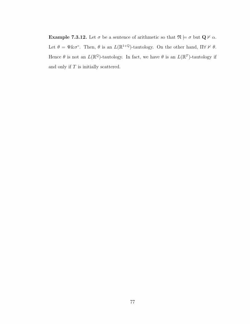
Example 7.3.12. Let σ be a sentence of arithmetic so that N |= σ but Q 0 α.
Let θ = Ψ&σ◦. Then, θ is an L(R1+Q)-tautology. On the other hand, Π∀ 0 θ.
Hence θ is not an L(RQ)-tautology. In fact, we have θ is an L(RT )-tautology if
and only if T is initially scattered.
77

Chapter 8
Scattered Subsets of Ordered Abelian Group
Remember in chapter 2 we defined a linear ordering S to be scattered if it does
not contain a dense subset. In this chapter we will show that if A and B are two
convergent and scattered subsets of an ordered Abelian group then A+B is also
convergent and scattered. We will formally define A+B and convergent later in
thin chapter.
8.1 Main Result
Definition 2.1.16 tells us what a scattered linear ordering is by telling us what it is
not. The following definition gives a more positive description of scattered linear
orderings by a providing a prescription of how to construct it from “simpler”
scattered linear orderings.
Definition 8.1.1. We define the class L of ranked linear orderings by presenting
inductively for each ordinal α a class Lα, and then by setting L = ∪Lα.
1. 0,1 ∈ L0.
2. Given a linear ordering I of type γ, γ∗ for some ordinal γ and for each i ∈ I
a linear ordering Li ∈ ∪{Lβ | β < α}, then∑{Li | i ∈ I} ∈ Lα.
78
The rank of L, a ranked linear ordering, is the smallest ordinal α such that
L ∈ Lα.
Example 8.1.2. ω, ω∗ are ranked linear orderings of rank 1.
Theorem 8.1.3 (Hausdorff). A linear ordering is in L if and only if it is
scattered.
A proof of Hausdorff Theorem may be found in [Ros82].
Definition 8.1.4. Let G be an ordered Abelian group. A scattered linear order-
ing S ⊆ G is convergent if and only if every countable increasing or decreasing
sequence of elements of S has a limit point in G.
Lemma 8.1.5. Let A and B be two convergent scattered linear orderings of G
an ordered Abelian group. Then A ∪B is also convergent and scattered.
Proof. Scattered: By way of contradiction suppose X ⊆ A ∪ B is dense. Then
we claim either X ∩ A or X ∩ B contains a dense subset. Without loss
of generality assume X ∩ A contains at least two elements a1 < a2. It
suffices to show there exists a3 ∈ X ∩ A such that a1 < a3 < a2. Let
(a1, a2) = {x ∈ X | a1 < x < a2}. By way of contradiction suppose
(a1, a2) ∩X ∩ A is empty. Then (a1, a2) is a dense subset of B which is a
contradiction to B being scattered.
Convergent: Let {xn | n ∈ ω}, without loss of generality be an increasing
sequence in A∪B. Then either {xn | n ∈ ω} ∩A or {xn | n ∈ ω} ∩B is an
infinite increasing sequence. By assumption either one has a limit point in
G. This completes the proof.
79

Definition 8.1.6. Let G be an ordered Abelian group. Let A and B be subsets
of G. Then A+B denotes
{a+ b | a ∈ A, b ∈ B}.
Example 8.1.7. Let G = R and let {qn, n ∈ ω} be an enumeration of Q∩ [0, 1].
Let A = {10n + qn | n ∈ ω} and B = {−10n | n ∈ ω}. Then {10n + qn + (−10n) |
n ∈ ω} ⊆ A+B. That is Q ∩ [0, 1] ⊆ A+B. Hence A+B is not scattered.
The above gives an example of two scattered sets where their sum is not
scattered. The problem turns out to be that A and B are not convergent. In the
next few theorems we will show that if A and B are scattered and convergent
then A+B will be scattered and convergent.
Definition 8.1.8. Let α be an ordinal. Let A =∑{Ai | i ∈ α} and B =
∑{Bj |
j ∈ β} where either β = α or β = α∗.
Let ⊙I :=
A+Bj convergent scattered for all j
Ai +B convergent scattered for all i⇒ A+B is convergent and scattered.
We will show that ⊙α holds for all ordinals α. We will show ⊙ω holds and
then prove ⊙α, (ω < α < ω1) holds by induction. But we first need a preliminary
lemma.
Lemma 8.1.9. Let α be an ordinal. Let A =∑{Ai | i ∈ α} and B =
∑{Bj |
j ∈ β} where either β = α or β = α∗. Suppose Ai +B and A+Bj are convergent
and scattered for all i ∈ α and j ∈ β. Then A and B are convergent and scattered.
Proof. We will show A is convergent and scattered. The proof for B is symmetric.
Let j ∈ β and b ∈ Bj. Then by assumption A + Bj is convergent and scattered,
80
hence A + b ⊆ A + Bj is convergent and scattered. Now A + b ∼= A, hence A is
convergent and scattered.
Note if ⊙α holds then ⊙β holds for all β ≤ α. This is true since we may
let Aj = Bj = ∅, β < j < α (∅ is assumed to be scattered and convergent).
Assume ⊙α holds and β is an initial segment of α. Suppose A =∑{Ai | i ∈ α}
and B =∑{Bj | j ∈ β} where either β = α or β = α∗. Also suppose that
Ai + B, i ∈ α and A + Bj, j ∈ ρ is convergent and scattered. Then A + B is
convergent and scattered. This is again done by inserting ∅ into B.
Lemma 8.1.10. ⊙ω holds. Hence ⊙n, n ∈ ω holds.
Proof. There are 2 cases to consider. α = ω, β = ω∗ and α = ω, β = ω.
Case 1: (α = ω, β = ω∗) Let sup(A) = a ∈ G and inf(B) = b ∈ G. Consider
the interval I = [min(A0) + b, a+ max(B0)]. We have A+B ⊆ I and
I =⋃
k∈ω
[min(Ak) + b,min(Ak+1) + b)
∪⋃
k∈ω (a+ max(Bk+1), a+ max(Bk)]
∪ {a+ b}
First we will show that the intersection of A+B with any of these disjoint
intervals is scattered.
Claim 1: Fix k. (A+B) ∩ [min(Ak) + b,min(Ak+1) + b) ⊆ ∪t≤k(At +B).
Proof of Claim 1: If t ≥ k + 1, then for all x ∈ At, x ≥ min(Ak+1). So
for all y ∈ B since y > b, we have x + y > min(Ak+1) + b. So if t ≥ k + 1
then At +B ∩ [min(Ak) + b,min(Ak+1) + b) = ∅. So we have shown that
(A+B) ∩ [min(Ak) + b,min(Ak+1) + b) ⊆ ∪t≤k(At +B).
81
∪t≤k(At +B) is a finite union of scattered sets hence it is scattered.
Claim 2: Fix k. (A+B)∩ (a+ max(Bk+1), a+ max(Bk)] ⊆ ∪t≤k(A+Bt).
Proof of Claim 2: The proof of claim 2 is symmetric to that of claim
1. So we have A + B is scattered. We need to show A + B is convergent.
Without loss of generality suppose {xn | n ∈ ω} is an increasing sequence
in A+B. Then either xn converges to a+ b or for all but finitely many xn
is in one of the above intervals. Now since the intersection of A + B with
any of those intervals is convergent, {xn} converges to a point in A+B.
Case 2: (α = ω, β = ω) Let a = sup(A), b = sup(B).
Claim Let d < a + b, then (A + B) ∩ (−∞, d) ≤ ∪i<Q(Ai + B) for some
Q ∈ ω.
Proof of the Claim Let c = a+b−d2
and choose Q ∈ ω such that if i, j ≥ Q
then
min(Ai) > a− c and min(Bj) > b− c.
So if i, j ≥ Q we have min(Ai) + min(Bj) > a− c+ b− c = d. Therefore, if
Ai +Bj intersects (−∞, d) non-trivially, at least one of the i or j is less than
Q. Without loss of generality assume i < Q. Then (A + B) ∩ (−∞, d) ≤
∪i<Q(Ai + B) which is convergent and scattered. This implies that A + B
is scattered. To show A+B is convergent is exactly the same argument as
the previous case.
Lemma 8.1.11. ⊙δ holds for all δ < ω1 .
Proof. Since we have already shown ⊙ω, it suffices to show ⊙δ, δ < ω1. There
are two cases:
82

δ is a countable limit ordinal > ω: Then δ = ∪n∈ωβn, ω < βn < δ and βn is
strictly increasing. Suppose ⊙β holds for all γ < δ . We have A =∑{Ai |
i ∈ δ} and B =∑{Bj | j ∈ δ or δ∗}. We need to show A+B is convergent
and scattered. Let γ0 = β0 and γi = βi\βi−1. Then δ is a disjoint union of
γi, i ∈ ω. We may rewrite A and B as follows:
A =∑
{Cn | n ∈ ω} where Cn =∑
{Ai | i ∈ γn}
B =∑
{Dn | n ∈ ω} where Dn =∑
{Bi | i ∈ γn}.
Now induction hypothesis applies to Cn and Dm. We have (Cn)k + B and
A+ (Dm)k convergent and scattered for all k by the induction hypothesis.
Therefore, showing A + B is convergent and scattered which has been re-
duced to showing ⊙ω, which we already have. Therefore A+B is convergent
and scattered. The case where A =∑{Ai | i ∈ δ} and B =
∑{Bj | j ∈ δ
∗}
is identical.
δ + 1 is a successor ordinal: Suppose ⊙ρ holds for all ρ < δ + 1. We have
A =∑{Ai | i ∈ δ+ 1} and B =
∑{Bj | j ∈ δ+ 1}. We may rewrite A and
B as follows
A =∑
{Ai | i ∈ δ}+ Aδ
B =∑
{Bj | j ∈ δ}+Bδ.
Now we have
A+B = (∑
{Ai | i ∈ δ}+∑
{Bj | j ∈ δ})
∪ (∑
{Ai | i ∈ δ}+Bδ)
∪ (Aδ +∑
{Bj | j ∈ δ}) ∪ (Aδ +Bδ).
83
Each part of the above decomposition is convergent and scattered by the
induction hypothesis. A + B being a finite union of convergent scattered
sets is convergent and scattered. The case where A =∑{Ai | i ∈ α} and
B =∑{Bj | j ∈ α
∗} is again identical.
Theorem 8.1.12. Let G be an ordered Abelian group and let A and B be count-
able convergent scattered subsets of G. Then A+B is countable, convergent and
scattered.
Proof. Let G be an ordered Abelian group. We call A ⊆ G ccs if and only if A
is countable, convergent and scattered. Let for α and β countable,
(∗)(α,β) := [if A is ccs of rank < α and B is ccs of rank < β]⇒
A+B is ccs;
(#)α := ∀(β < ω1)(∗)(α,β)
= (∀B ccs)(A is ccs of rank < α⇒ A+B is ccs).
To prove the theorem we need to prove (∗)(α,β) for all countable α, β which is
equivalent to showing (#)α for all countable α. We will do this by induction:
α = 0: There are no scattered sets with rank smaller than 0, so (#)0 is true
trivially.
α a limit ordinal: Assume for δ < α, (#)δ holds. Suppose rank(A) < α, then
rank(A) < rank(A) + 1 < α and by the inductive assumption (#)rank(A)+1
holds. That is (∀B)(A+B) is countable, convergent and scattered.
α + 1 a successor countable ordinal: Assume (#)δ holds for all δ < α + 1.
We need to show (#)α+1. Choose A of rank less than α+1. We may assume
84

rank(A) = α. So A has the form A =∑{Ai | i ∈ δ} where rank(Ai) < α
for all i. Note since A is countable, δ < ω1. We need to prove A + B is
convergent and scattered for all B. We will do this by induction on the
rank of B.
Let
(+)β := ∀B ccs of rank < β, A+B is ccs
β = 0: Trivially true.
β a limit ordinal: Assume for δ < β (+)δ holds. If rank of B is less than
β then rank(B) < rank(B)+1 < β. Therefore by induction hypothesis
(+)rank(B)+1 holds. Hence A+B is convergent and scattered.
β + 1 successor ordinal: Assume (+)δ holds for all δ < β + 1. we need
to show (+)β+1. Choose B of rank less than β + 1. We may assume
rank(B) = β. We need to show A + B is convergent and scattered.
Say B has the form B =∑{Bj | j ∈ γ} where rank(Bj) < β for all
j and γ < ω1. Now we have both ⊙δ and ⊙γ holds. Without loss of
generality suppose δ ≤ γ. Then by the observation from before and
inserting ∅ into A we get A+B is scattered.
This completes the proof of (+)β+1, which in turn completes the proof of
(#)α+1. This concludes the proof of the double induction and we have the theo-
rem.
We now relax the the countability requirement for A and B in Theorem 8.1.12.
Theorem 8.1.13. Let G be an ordered Abelian group and let A and B be con-
vergent scattered subsets of G. Then A+B is convergent and scattered.
85
Proof. The proof mimics the proof of Theorem 8.1.12. We first show ⊙α holds for
all ordinal α. We have previously shown that ⊙α holds if α is countable. Let α
be an uncountable ordinal. Suppose A =∑{Ai | i ∈ α} and B =
∑{Bi | i ∈ α}
satisfy the assumptions of ⊙α but A+ B is not a convergent scattered subset of
G. Let X be a dense subset of A + B. We may assume X is countable. Collect
all Ai and Bi represented in X and add all the limit points (and corresponding
factors) needed from A and B. Call these sets A′ and B′ respectively. A′ and
B′ are countable subsets of A and B respectively. Then X is a dense subset of
A′ +B′ which by the countable case is scattered. Hence we have a contradiction.
Let {xn | n ∈ ω} be an increasing sequence in A + B. Collect all Ai and Bi
represented in {xn | n ∈ ω} and add all the limit points (and corresponding
factors) needed from A and B. Call these sets A′ and B′ respectively. Since
the sequence is countable, A′ and B′ re countable and {xn | n ∈ ω} ⊆ A′ + B′.
Therefore the sequence has a limit point in A′ + B′ ⊆ A + B by the countable
case. Therefore {xn | n ∈ ω} is convergent in A+B. This completes the proof of
⊙α for all ordinal α. Now we go through the proof of Theorem 8.1.12 and leave
out any reference to countability. This shows gives the desired result.
86
BIBLIOGRAPHY
[Cli54] A. H. Clifford, Note on Hahn’s theorem on ordered abelian groups, Proc.
Amer. Math. Soc. 5 (1954), 860–863. MR 16,792b
[Fuc63] L. Fuchs, Partially ordered algebraic systems, Pergamon Press, Oxford,
1963. MR 30 #2090
[Haj98] Petr Hajek, Metamathematics of fuzzy logic, Trends in Logic—Studia
Logica Library, vol. 4, Kluwer Academic Publishers, Dordrecht, 1998.
MR 2003c:03048
[HW52] M. Hausner and J. G. Wendel, Ordered vector spaces, Proc. Amer. Math.
Soc. 3 (1952), 977–982. MR 14,566b
[LS02] Michael C. Laskowski and Yvonne V. Shashoua, A classification of
BL-algebras, Fuzzy Sets and Systems 131 (2002), no. 3, 271–282. MR
2003j:03084
[LSar] , A generalized ordinal sums and th decidability of BL-chains,
Algebra Universalis (To Appear).
[Mon01] Franco Montagna, Three complexity problems in quantified fuzzy logic,
Studia Logica 68 (2001), no. 1, 143–152, Methods for investigating self-
referential truth. MR 2003m:03038
87
[Ros82] Joseph G. Rosenstein, Linear orderings, Pure and Applied Mathematics,
vol. 98, Academic Press Inc. [Harcourt Brace Jovanovich Publishers],
New York, 1982. MR 84m:06001
[Sha02] Yvonne Shashoua, Algebras of basis logic: A classification and related
decidability results, Ph.d. dissertation, University of Maryland, College
Park, MD, 2002.
[Zad65] L. A. Zadeh, Fuzzy sets, Information and Control 8 (1965), 338–353.
MR 36 #2509
88