Embed Size (px)
Citation preview
ABSTRACT
Title of Dissertation: FORECASTING TECHNOLOGY INSERTION CONCURRENT WITH DESIGN REFRESH PLANNING FOR COTS-BASED OBSOLESCENCE SENSITIVE SUSTAINMENT-DOMINATED SYSTEMS
Pameet Singh, Doctor of Philosophy, 2004
Dissertation Directed By: Dr. Peter A. Sandborn
Department of Mechanical Engineering There are many types of products and systems that have lifecycles longer than their
constituent parts (specifically COTS - Commercial Off The Shelf parts). These lifecycle
mismatches often result in high sustainment1 costs for long field life systems (e.g., avionics,
military systems, etc.) due to part obsolescence problems. While there are a number of ways
to mitigate obsolescence, e.g., lifetime buys, aftermarket sources, etc., ultimately systems are
redesigned one or more times during their lives to update functionality and manage
obsolescence. Unfortunately, redesign of sustainment-dominated systems like those
mentioned above often entails very large non-recurring engineering and system re-
qualification costs.
1 Sustainment in this context means all activities necessary to: keep an existing system operational, and continue to manufacture and field versions of the system that satisfy the original and evolving requirements.
Ideally, a methodology that determines the best dates for design refreshes, and the
optimum mixture of actions to take at those design refreshes is needed. The goal of refresh
planning is to determine:
• When to refresh the design
• Which obsolete parts should be replaced at a specific design refresh (versus
continuing with some other obsolescence mitigation strategy)
• Which non-obsolete parts should be replaced at a specific design refresh
• Which parts should be functionally upgraded.
To address the refresh planning goals above, a methodology called MOCA (Mitigation
of Obsolescence Cost Analysis) has been developed. MOCA determines the electronic part
obsolescence impact on lifecycle sustainment costs for long field life electronic systems
based on future production projections, maintenance requirements and part obsolescence
forecasts. The methodology determines the optimal design refresh plan to be implemented
during the system’s lifetime in order to minimize the system’s lifecycle cost.
For technology insertion decision making, MOCA uses a Monte Carlo/multi-criteria
decision making hybrid computational technique in which a Monte Carlo is used to
accommodate input uncertainties and Bayesian networks are used to make part upgrade
decisions at design refreshes.
A case study is performed to demonstrate MOCA’s capabilities on a NDU (Navigation
Data Unit) that resides on a US Navy class of ships known as the LPD-17.
FORECASTING TECHNOLOGY INSERTION CONCURRENT WITH DESIGN REFRESH PLANNING FOR COTS-BASED OBSOLESCENCE
SENSITIVE SUSTAINMENT-DOMINATED SYSTEMS
by
Pameet Singh
Dissertation submitted to the Faculty of the Graduate School of the University of Maryland, College Park in partial fulfillment
of the requirements for the degree of Doctor of Philosophy
2004
Advisory Committee: Associate Professor Peter A. Sandborn, Chair Associate Professor Linda C. Schmidt Professor Shapour Azarm Assistant Professor Steven A. Gabriel Professor Thomas M. Corsi

©Copyright by
Pameet Singh
2004

DEDICATION
I dedicate this dissertation to my wife Suchitra. She is the reason why I did this PhD.
ii

ACKNOWLEDGEMENTS I’d like to thank my advisor Dr. Peter Sandborn who has been an excellent source of
inspiration for me during the past few years, and I have cherished every moment of it. I am
immensely grateful for his encouragement and guidance. I thank the Naval Surface Warfare
Center personnel, especially Bob and Cathy, who spent their valuable time to help me get
useful information about their tools and for the LPD-17 case study. I extend my thanks to Dr.
Shapour Azarm, Dr. Linda Schmidt, Dr. Steven Gabriel and Dr. Thomas Corsi for their
invaluable suggestions. I would also like to thank Bevin Etienne for being a great friend and
source of inspiration throughout my stay. Last but not the least I would like to thank my wife
Suchitra for being my best friend and for getting me through all the tough times at school and
at home.
iii
TABLE OF CONTENTS
LIST OF TABLES................................................................................................................... vi
LIST OF FIGURES ................................................................................................................ vii
Chapter 1: Introduction................................................................................................... 1 1.1 Sustainment-Dominated Systems ......................................................................... 3 1.2 Relevant Existing Work........................................................................................ 6 1.3 Obsolescence Forecasting..................................................................................... 8
1.3.1 CALCE Method of Obsolescence Prediction (Solomon et al., 2000) ........ 10 1.4 Lifecycle Cost Analysis ...................................................................................... 11 1.5 Summary ............................................................................................................. 12
Chapter 2: Event Sequence Diagram Management: A Technology Sustainment Based Design Refresh Planning Methodology (Tasks 1 and 2) ........................................................ 15
2.1 The Life Cycle Costing Problem Definition....................................................... 16 2.2 Design Refresh Planning Architecture................................................................ 17 2.3 Event Sequence Diagram (ESD)......................................................................... 20 2.4 Scheduling Design Refreshes ............................................................................. 23 2.5 Managing the Event Sequence for Cost Analysis............................................... 27
2.5.1 The Cost Analysis Process.......................................................................... 29 2.5.2 Production and Redesign Event Simulation ............................................... 30
2.6 Cost Models ........................................................................................................ 33 2.6.1 Obsolescence Cost Model........................................................................... 33 2.6.2 Life Time Buy or Last Time Buy Cost Model............................................ 34 2.6.3 Design Refresh Cost Model ........................................................................ 35 2.6.4 Re-qualification Cost Model....................................................................... 36
2.7 Miscellaneous MOCA Concepts......................................................................... 37 2.7.1 Design Refresh “look-ahead” Time ............................................................ 37 2.7.2 Data Coarsening (Time Step Fidelity) ........................................................ 37
2.8 A Tutorial Example............................................................................................. 38 2.8.1 Calculations for the Tutorial Example........................................................ 42
2.9 Comparison of MOCA and the Porter Model..................................................... 44 2.9.1 Porter Model Implemented within MOCA Tool ........................................ 47
2.10 Baseline MOCA Analysis Example................................................................ 49 2.11 Summary ......................................................................................................... 57
Chapter 3: Technology Insertion – Using Probabilistic Decision Methods to Determine Design Refresh Content (Task 3)............................................................................................ 59
3.1 Probabilistic Decision Methods .......................................................................... 59 3.1.1 External versus Intentional Approaches ..................................................... 61 3.1.2 Intentional Approaches ............................................................................... 63
3.2 Bayesian Belief Networks (BBNs) ..................................................................... 65 3.3 Technology Insertion Decision Making Using Bayesian Belief Networks ........ 68
iv
3.4 MOCA Bayesian Belief Network ....................................................................... 71 3.4.1 A Bayesian Belief Network for an Electronic Part..................................... 72 3.4.2 Node Reference for a Single Part BBN ...................................................... 73 3.4.3 BBN Chance Node Discretization .............................................................. 77 3.4.4 The Methodology used to Populate BBN Chance Node Probabilities
Tables…….. .................................................................................................................... 79 3.4.5 Coupling BBNs........................................................................................... 82
3.5 Curtailing the Network ....................................................................................... 84 3.6 Splitting the BBN (Jensen, 2002) ....................................................................... 84 3.7 The Reliability Chance Node Model .................................................................. 86 3.8 The Reliability and Performance Values Model................................................. 87 3.9 MOCA Integration with Hugin®......................................................................... 88 3.10 Case Studies .................................................................................................... 88
3.10.1 Tutorial Case Study..................................................................................... 89 3.10.2 AS900 Engine Controller Example ............................................................ 92
3.11 Summary ......................................................................................................... 94
Chapter 4: LPD-17 Case Study (Task 4) ...................................................................... 95 4.1 MOCA Solution Strategy.................................................................................... 96 4.2 Horizon (NSWC’s Design Refresh Cost Model)................................................ 98 4.3 MOCA-Horizon Integration.............................................................................. 101 4.4 Analysis Data .................................................................................................... 104
4.4.1 BBN Data.................................................................................................. 104 4.5 Retroactive Sparing Model ............................................................................... 106 4.6 Results............................................................................................................... 108 4.7 Summary ........................................................................................................... 112
Chapter 5: Contributions and Conclusions ................................................................. 113 5.1 Contributions..................................................................................................... 113
5.1.1 Discussion of Problem Scope ................................................................... 115 5.1.2 Methodology Specific Contributions........................................................ 117
5.2 Future Work ...................................................................................................... 118
Appendix A: Publications Associated With This Work ................................................. 119
Appendix B: Computer Network Example (Task 4)...................................................... 121
Appendix C: BBN Expressions Pseudo Code ................................................................ 128
References………................................................................................................................. 130
v
LIST OF TABLES Table 2-1: Average recurring cost multipliers for obsolescence resolutions in Avionics
(McDermott; MDEA, 2001) ........................................................................................... 34 Table 2-2: Tutorial example details ........................................................................................ 39 Table 2-3: Scenarios for basic MOCA tutorial example ........................................................ 42 Table 2-4: Costs incurred for scenarios in Table 2-3. X - Cost incurred, blank = No cost
incurred. .......................................................................................................................... 43 Table 2-5: Key to the abbreviations used in Table 2-4........................................................... 43 Table 2-6: Calculations and results for MOCA tutorial example ........................................... 43 Table 2-7: Sample data for the Porter model (Porter, 1998)................................................... 45 Table 2-8: Porter model calculations (plotted in Figure 2-14) ............................................... 46 Table 2-9: Predicted AS900 FADEC lifecycle costs for ~3200 units sustained for 20 years 55 Table 3-1: Calculations for conditional probability example in Figure 3-1 ........................... 68 Table 3-2: Cases explored by MOCA-BBN analysis for the tutorial example (recall, cases 1,
2, and 3 are the same as in Section 2.7, Table 2-3)......................................................... 89 Table 3-3: Comparison chart for costs incurred for all the cases explored by MOCA (with
and without BBN) ........................................................................................................... 90 Table 3-4: Calculation results for simple example using BBN analysis ................................ 90
vi
LIST OF FIGURES
Figure 1-1: Examples for lifecycle cost breakdown ................................................................. 5 Figure 2-1: MOCA architecture.............................................................................................. 18 Figure 2-2: Design refresh planning analysis time line .......................................................... 20 Figure 2-3: Design refresh scheduling.................................................................................... 24 Figure 2-4: A candidate refresh plan in defined as one or more design refreshes, and their
dates relative to production events.................................................................................. 26 Figure 2-5: Recursive design refresh scheduling algorithm ................................................... 27 Figure 2-6: Cost analysis algorithm........................................................................................ 29 Figure 2-7: Production event simulation................................................................................. 30 Figure 2-8: Redesign event simulation ................................................................................... 32 Figure 2-9: MOCA results (tutorial example) ........................................................................ 39 Figure 2-10: Lifecycle cost comparison graph for no design refresh case (dotted red line) and
MOCA “best” solution case (solid blue line) for the tutorial example........................... 41 Figure 2-11: Unit cost graphs for no design refresh case (left) and MOCA “best” solution
(right) for the tutorial example........................................................................................ 41 Figure 2-12: Simple Porter model analysis graph (calculations in Table 2-8) ....................... 46 Figure 2-13: Comparison of Porter model results (implemented within MOCA) and MOCA
analysis............................................................................................................................ 47 Figure 2-14: AS900 FADEC .................................................................................................. 49 Figure 2-15: AS900 base line MOCA design refresh planning results. The “best” solution is
selected and expanded to show the actual design refresh dates...................................... 50 Figure 2-16: Refresh plan generated for the selected point in Figure 2-17 ............................ 52 Figure 2-17: Comparison of lifecycle cost between MOCA “best” solution (solid blue line)
and no design refresh case (dotted red line), from Figure 2-15 ...................................... 53 Figure 2-18: Comparison of unit procurement cost between MOCA “best” solution (solid
blue line) and no design refresh case (dotted red line), from Figure 2-15...................... 54 Figure 2-19: Variation in lifecycle cost for AS900 as a function of the look-ahead time...... 55 Figure 2-20: Lifecycle cost distribution for 5 years look-ahead time from Figure 2-21 (AS900
case study)....................................................................................................................... 56 Figure 3-1: Example of a conditional probability table .......................................................... 67 Figure 3-2: BBN decision model within MOCA architecture ................................................ 70 Figure 3-3: MOCA single part BBN architecture................................................................... 72 Figure 3-4: MOCA-BBN part replacement decision node and part category node used for
coupling........................................................................................................................... 74 Figure 3-5: Example obsolescence probability table of the part numbered 431-7262-6152 .. 77 Figure 3-6: Data discretization................................................................................................ 78 Figure 3-7: Picture of a sample distribution equation as entered in Hugin® interface (Pseudo
code in Appendix C) ....................................................................................................... 80 Figure 3-8: Population algorithm of Part Mitigation Cost node ............................................ 81 Figure 3-9: Coupling points in MOCA BBN.......................................................................... 83 Figure 3-10: Splitting the BBN............................................................................................... 85 Figure 3-11: BBN constructed for decision analysis (tutorial example) ................................ 91 Figure 3-12: Comparison of MOCA results for non-BBN and BBN analysis (tutorial
example).......................................................................................................................... 92
vii
Figure 3-13: Picture of BBN generated in MOCA for the AS900 controller ......................... 93 Figure 3-14: Comparison of results between BBN solution and non-BBN solution for AS900
base line case................................................................................................................... 93 Figure 4-1: LPD-17 Ship ........................................................................................................ 95 Figure 4-2: NDU used in the LDP-17 (Courtesy of NSWC-Crane)...................................... 96 Figure 4-3: Desired link and the information flow between MOCA and Horizon................. 97 Figure 4-4: Steps 1 and 2 in the Horizon redesign cost analysis process ............................... 99 Figure 4-5: Steps 3 and 4 in the Horizon redesign cost analysis process ............................. 100 Figure 4-6: MOCA-Horizon integration schematic diagram................................................ 102 Figure 4-7: LPD-17 components and production events screens (MOCA).......................... 104 Figure 4-8: LPD-17 hierarchy as loaded in MOCA.............................................................. 105 Figure 4-9: Matrix representation of the set of linear equations........................................... 106 Figure 4-10: Non-BBN MOCA analysis results (LDP-17) .................................................. 108 Figure 4-11: Comparison of lifecycle cost for MOCA “best” solution (solid blue line) and no
design refresh case (dotted red line), from Figure 4-10................................................ 109 Figure 4-12: Comparison of unit procurement cost for MOCA “best” solution (solid blue
line) and no design refresh case (dotted red line), from Figure 4-10............................ 110 Figure 4-13: BBN MOCA analysis results (LPD-17)........................................................... 111 Figure 4-14: Picture of BBN constructed for decision analysis (LPD-17)........................... 112 Figure 5-1: Diagram depicting the problem size, where Pi is the i’th part; ti is the time
between (i-1)’th and i’th redesigns; L is the total lifetime of the system ....................... 116 Figure 5-2: Number of possible design refresh schedules .................................................... 116 Figure B-1: Component list for computer network case study ............................................. 123 Figure B-2: Architecture of computer network case study................................................... 124 Figure B-3: Test data for computer network case study ....................................................... 126 Figure B-4: Comparison of results between BBN solution and non-BBN solution for
computer network case study........................................................................................ 127
viii
Chapter 1: Introduction
The rapid growth of the electronics industry has spurred dramatic changes in the
electronic parts that comprise the products and systems that the public buys. Increases in
speed, reductions in feature size and supply voltage, and changes in interconnection and
packaging technologies are becoming events that occur nearly monthly. Consequently, many
of the electronic parts that compose a product have a lifecycle that is significantly shorter
than the lifecycle of the product they go into. A part becomes obsolete when it is no longer
manufactured, either because demand has dropped to low enough levels that it is impractical
for manufacturers to continue to make it, or because the materials or technologies necessary
to produce it are no longer available. Therefore, unless the system of interest has a short life
(manufacturing and field), or the product is the driving force behind the part’s market (e.g.,
personal computers driving the microprocessor market), there is a high likelihood of a
lifecycle mismatch between the parts and the product (Solomon et al., 2000).
Electronic part obsolescence began to emerge as a problem in the 1980s when the end
of the Cold War accelerated pressure to reduce military outlays and lead to an effort in the
United States military called Acquisition Reform. Acquisition reform included a reversal of
the traditional reliance on military specifications (“Mil-Specs”) in favor of commercial
standards and performance specifications (Perry, 1994). One of the consequences of the shift
away from Mil-Specs was that Mil-Spec parts that were qualified to more stringent
environmental specifications than commercial parts and manufactured over longer-periods of
1
time were no longer available, creating the necessity to use Commercial Off The Shelf
(COTS) parts that are manufactured for non-military applications and are often available for
much shorter periods of time. Although this history is associated with the military, the
problem it has created reaches much further, since many non-military applications depended
on Mil-Spec parts, e.g., avionics, oil well drilling, and automotive.
Managing the lifecycle mismatch problem requires that during design, engineers be
cognizant of which parts will be available and which parts may be obsolete during a
product’s life. Avionics and military systems may encounter obsolescence problems before
being fielded and nearly always experience obsolescence problems during field life
(Bumbalough, 1999). These problems are exacerbated by manufacturing that may take place
over long periods of time, the need to support the system for a long period of time (i.e.,
providing spares), and the high cost of system qualification and certification that make design
refreshes using newer parts an expensive undertaking. However, obsolescence problems are
not the sole domain of avionics and military systems. Consumer products, such as pagers,
naturally divide into two groups – 1) cutting edge (the latest technology and features), and 2)
workhorse, minimal feature set products (such as the pagers used to tell restaurant patrons
that their table is ready). While the first set is unlikely to encounter obsolescence problems,
the second set often does. Because original equipment manufacturers require long lifetimes
out of workhorse products, critical parts often become obsolete before the last product is
manufactured.
If a product requires a long application life, then a parts obsolescence management
strategy may be required. Many obsolescence mitigation approaches have been proposed and
are being used. These approaches include (Stogdill, 1999): lifetime or last time buys (buying
2

and storing enough parts to meet the system’s forecasted lifetime requirements or
requirements until a redesign is possible), part substitution (using a different part with
identical or similar form fit and function), and redesign (upgrading the system to make use of
newer parts). Several other mitigation approaches are also practical in some situations:
aftermarket sources (third parties that continue to provide the part after it’s original
manufacturer obsoletes it), emulation (using parts with identical form fit and function that are
fabricated using newer technologies), reclaim (salvaged parts), and up-rating (using a part
beyond the manufacturer’s specifications, usually at a higher temperature (Wright et al.,
1997)).
Redesign (or design refresh) is the ultimate obsolescence mitigation approach where
obsolete parts are designed out of the system in favor of newer, non-obsolete parts.2 Nearly
all long field life systems are redesigned one or more times in their lives. Unfortunately,
design refresh potentially has large non-recurring costs, and it may require the system to be
re-qualified, which is costly. Therefore, design refreshes are not a practical solution every
time a part becomes obsolete and must be prudently planned.
1.1 Sustainment-Dominated Systems
The relevant portion of the lifecycle of an electronic part is the duration of time it is
manufactured and available for purchase; the relevant portion of the avionics product
lifecycle is design, manufacturing, and sustainment. Consider, for example, the Boeing 777.
The Intel 80486 processor was selected for use in the 777 flight management system; Intel
2 In this dissertation the terms “redesign” and “design refresh” are used interchangeably, however, there is a difference (Herald, 2000). Design refresh is used as a reference to system changes that “Have To Be Done” in order for the system functionality to remain viable. Insertion (redesign) is used to identify the “Want To Be Done” system changes, which include both new technologies to accommodate system functional growth and new technologies to replace and better the existing functionality of the system.
3
obsoleted (discontinued the production and support of) the 80486 before the FAA even
finished certifying the 777, (Condra, 1997). Refreshing the 777 design to use a newer
processor (or even a 80486 equivalent manufactured elsewhere) is very expensive due to
qualification/certification constraints. Alternatively, buying and storing enough Intel 80486
processors to build all the 777s (“lifetime buy”) has it’s own problems. How many will you
need? How will you store them for decades so they can be installed into the product without
manufacturing problems (e.g., solderability)?
The concept of part obsolescence (e.g., the 777 example above) is straightforward.
More generally, the obsolescence of a system means that over time the system can no longer
be manufactured, can not meet the original or evolving system requirements, and/or can not
be maintained. Due to the speed of technology advancement in today’s world, complex
systems (especially systems with high informational, computational and/or electronic
component content) become obsolete very quickly if their designs are not refreshed.
With relevance to design refreshment, products can be categorized as leaders or
trailers. Leaders must watch the leading edge of the technology and adapt the newest
materials, parts, and processes in order to prevent loss of their market share to competitors
who are trying to do the same thing. For leaders, design refresh planning is a question of
balancing the risks of investing resources in new, potentially immature technologies against
potential functional or performance gains that could differentiate them from their competitors
in the market. Examples of leading edge products are high-volume consumer-oriented
electronics (e.g., mobile phones).
4
Investment30%
Sustainment70%
Investment (hardware)
21%
Investment (software)
6%
Investment (infrastructure)
11%
Investment (hardware)
21%
Investment (software)
6%
Investment (infrastructure)
11%
Sustainment62%
Business Jet (Omnijet)
Office PC Network (Shields, 2001)
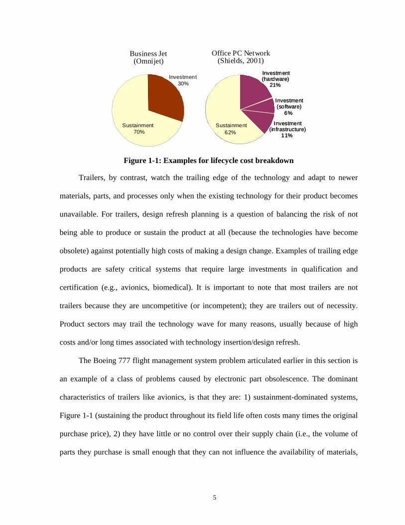
Figure 1-1: Examples for lifecycle cost breakdown
Trailers, by contrast, watch the trailing edge of the technology and adapt to newer
materials, parts, and processes only when the existing technology for their product becomes
unavailable. For trailers, design refresh planning is a question of balancing the risk of not
being able to produce or sustain the product at all (because the technologies have become
obsolete) against potentially high costs of making a design change. Examples of trailing edge
products are safety critical systems that require large investments in qualification and
certification (e.g., avionics, biomedical). It is important to note that most trailers are not
trailers because they are uncompetitive (or incompetent); they are trailers out of necessity.
Product sectors may trail the technology wave for many reasons, usually because of high
costs and/or long times associated with technology insertion/design refresh.
The Boeing 777 flight management system problem articulated earlier in this section is
an example of a class of problems caused by electronic part obsolescence. The dominant
characteristics of trailers like avionics, is that they are: 1) sustainment-dominated systems,
Figure 1-1 (sustaining the product throughout its field life often costs many times the original
purchase price), 2) they have little or no control over their supply chain (i.e., the volume of
parts they purchase is small enough that they can not influence the availability of materials,
5
technologies, and parts used to manufacture their products), and 3) the cost of redesign are
large (due to stringent qualification and certification requirements).
Sustainment includes all activities necessary to:
• Keep an existing system operational (able to successfully complete the purpose it is
intended for).
• Continue to manufacture and field versions of the system that satisfy the original
requirements.
• Manufacture and field revised versions of the system that satisfy evolving
requirements (insertion).
Part obsolescence is hardly a problem confined to just avionics. Other types of
electronic products are beginning to be affected by this problem, e.g., computer servers and
automotive electronics. Technology obsolescence also affects large computer networks,
information technology systems, and software.
1.2 Relevant Existing Work
Existing work relevant to the management of part obsolescence includes: 1) part
lifecycle characterization, 2) part obsolescence forecasting, 3) product deletion, and 4)
lifecycle planning. Lifecycle characterization is addressed in (Levitt, 1965), and
obsolescence forecasting is addressed in (TACTech; Henke and Lai, 1997; Amspaker, 1999;
Solomon et al., 2000; and MTI). The state-of-the-art in the world today is to use
obsolescence forecasting to audit the bill of materials and make part change decisions during
design only. Another relevant area is product deletion studies that address how a
manufacturer or supplier of a product makes a decision to stop offering the product, e.g.,
(Avlonitis et al., 2000). Alternatively, obsolescence (which is part of the topic of this
6
dissertation) focuses on the management of the consequences to the customer of a product
deletion decision made by others.
There are numerous research efforts that have worked on the generation of suggestions
for redesign in order to improve manufacturability, e.g., (Irani et al., 1989; and Das et al.,
1996). Design refresh planning has also been addressed outside the manufacturing area, e.g.,
general strategic replacement modeling (Meyer, 1993), re-engineering of software (Lin,
1993), capacity expansion (Rajagopalan et al., 1998), and equipment replacement strategies
(Pierskalla and Voelker, 1976; and Nair et al., 1992). All of the previous work mentioned
above represents design refresh driven by improvements in manufacturing, equipment or
technology. They do not deal with design refresh driven by technology obsolescence that
would otherwise render the product un-producible and/or un-sustainable.
The only existing work on pro-active lifecycle planning associated with part
obsolescence focuses on trading off last time buys3 versus delaying design refreshes using
Net Present Value metrics (Porter, 1998). This model is relevant to cost-plus business models
that provide incentive for the OEM (Original Equipment Manufacturer) to defer redesigns as
long as possible (thereby letting the customer pay for both the obsolescence-driven upgrade
and the performance improvements concurrently. This type of model is common for military
products. Alternatively, in a price-based (fixed price) business model the OEM is allowed to
“pocket” all or some of the recurring cost savings that are recognized on a fixed cost
subsystem, thus providing an incentive for the OEM to redesign the system as soon as it
makes economic sense. In this case a different model is needed that minimizes the lifecycle
cost of the system with respect to design refreshes.
3 Only enough parts are purchased to satisfy the product’s forecasted production and sustainment needs until the next redesign.
7
This dissertation aims at pro-active planning of the product’s lifecycle (to ultimately
reduce the overall lifecycle cost). It presents a methodology that enables determination of a
product design refresh schedule that intends to lower the lifecycle cost of the system
compared to no analysis based on forecasted years-to-obsolescence for electronic parts. The
objective function can also be to lower the lifecycle cost variance or to lower a user defined
weighted mix of the mean and the variance of the lifecycle cost. It can also incorporate
performance and reliability increase as part of the objective function. Unlike trading off only
last time buys and single design refreshes, (i.e., Porter, 1998), this methodology
accommodates a broad range of obsolescence mitigation approaches, and addresses
functional upgrade at design refreshes.
1.3 Obsolescence Forecasting
Nearly all the manufacturers and consumers of long field life sustainable systems are
concerned about part obsolescence issues. There have been issues related to obsolescence in
fast changing products like cellular phones and pagers too, but these issues are more focused
on usage and functional changes in the product and market competition behind it. It is not a
kind of product that one would repair when it does not work. Among other businesses
affected by this issue are agencies or organizations, which help manufacturers and consumers
to assess products and their cost impacts for long-term usage. Using their information the
manufacturers decide on facility planning and maintenance depot location planning etc.,
which are very important concerns. Part obsolescence dates4 make up one of the most
important inputs in the design refresh planning methodology. Due to part obsolescence, the
4 The obsolescence date is the date on which the part is expected to become obsolete. Sometimes this date is in the form of a “life code” that forecasts the part’s lifecycle stage. A life code coupled with a lifecycle model for the part can be used to produce an obsolescence date.
8
cost of the product changes during its fielded life, and therefore has a major impact on
product’s lifecycle cost. In order to plan design refreshes with the objective of reducing the
lifecycle cost of the system we need a forecasted estimate of the obsolescence dates for the
parts in the system.
The use of technological lifecycle forecasting (Meade and Islam, 1998; Young, 1993;
and Kumar and Kumar, 1992) and lifecycle demand models (Meixell and Wu, 2001;
Solomon et al., 2000; TACTech; Amspaker, 1999; Henke et al., 1997; and Kurawarwala and
Matsuo, 1996), provides an attractive alternative to technology road mapping5 for describing
the demand for technology products.
Studies indicate that most electronic parts pass through several lifecycle stages (Levitt,
1965) corresponding to changes in part sales: introduction, growth, maturity (saturation),
decline, and phase-out (Pecht et al., 2000), several additional phases have been proposed
(Sherwood, 2000) including: Introduction Pending (prior to introduction), and splitting the
Obsolescence stage into Last Shipment and Discontinued or Purged. Most electronic part
obsolescence forecasting is based on the development of models for the part’s lifecycle.
Traditional methods of lifecycle forecasting utilized in commercially available tools and
services are based “scorecard” approaches, in which the lifecycle stage of the part is
determined from an array of technological attributes (TACTech; Amspaker, 1999; Henke and
Lai, 1997). More general models based on technology trends have also appeared including a
methodology based on forecasting part sales curves (Solomon et al., 2000), and leading-
indicator approaches (Meixell and Wu, 2001).
The use of demand based models, like described in Section 1.3.1, requires that the
parameters be estimated relatively early in the product’s lifecycle and at a time when the
5 Technology road mapping means forecasting both technology availability and unavailability (obsolescence).
9
values generally can not be ascertained definitively. Additionally, new information that
becomes available over time, such as a decrease in the number of suppliers currently offering
a technology in question, needs to be folded into the demand model. In (Meixell and Wu,
2001), a Bayesian update is used with early observed sales to update the parameters of a
lifecycle model. Unfortunately, the approach in Meixell and Wu was not developed
specifically for obsolescence prediction (rather, it was developed for technology demand
modeling).6
It is to be noted that obsolescence forecasting is not a part of this dissertation. It
however, is a critical input to the methodology presented in this dissertation. To calculate this
critical input any of the existing models and part obsolescence forecasting techniques can be
used. The MOCA model discussed in Chapter 2 can use life code inputs from the TACTech
commercial forecasting tool or accept dates or date distributions generated by the CALCE
approach (Solomon et al., 2000).
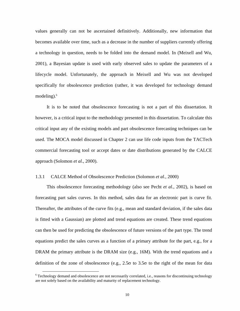
1.3.1 CALCE Method of Obsolescence Prediction (Solomon et al., 2000)
This obsolescence forecasting methodology (also see Pecht et al., 2002), is based on
forecasting part sales curves. In this method, sales data for an electronic part is curve fit.
Thereafter, the attributes of the curve fits (e.g., mean and standard deviation, if the sales data
is fitted with a Gaussian) are plotted and trend equations are created. These trend equations
can then be used for predicting the obsolescence of future versions of the part type. The trend
equations predict the sales curves as a function of a primary attribute for the part, e.g., for a
DRAM the primary attribute is the DRAM size (e.g., 16M). With the trend equations and a
definition of the zone of obsolescence (e.g., 2.5σ to 3.5σ to the right of the mean for data
6 Technology demand and obsolescence are not necessarily correlated, i.e., reasons for discontinuing technology are not solely based on the availability and maturity of replacement technology.
10
fitted with a Gaussian), the future obsolescence date for a part can be predicted. The same
sales forecasting process has to be performed on secondary attributes such as bias level (e.g.,
5V, 3.3V, etc.) and package type too, and the minimum prediction of the zone of
obsolescence is finally used for the part.
The baseline obsolescence forecasting approach uses a fixed window of obsolescence
determined as some fixed number of standard deviations from the peak sales year of the part.
An extension to this methodology that increases the accuracy of the forecasts is the
calculation of electronic part vendor-specific windows of obsolescence using historical last-
order or last-ship dates (Sandborn and Knox, 2005). The historical information is used to
create vendor-specific histograms of last-order or last ship dates mapped to the number of
standard deviations past the peak sales year for the part. In this way, the window of
obsolescence specification is dependent on manufacturer-specific business practices.
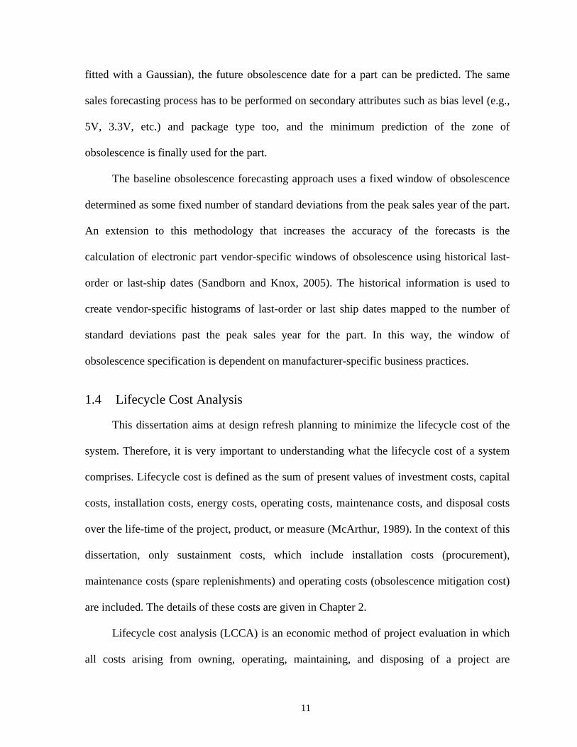
1.4 Lifecycle Cost Analysis
This dissertation aims at design refresh planning to minimize the lifecycle cost of the
system. Therefore, it is very important to understanding what the lifecycle cost of a system
comprises. Lifecycle cost is defined as the sum of present values of investment costs, capital
costs, installation costs, energy costs, operating costs, maintenance costs, and disposal costs
over the life-time of the project, product, or measure (McArthur, 1989). In the context of this
dissertation, only sustainment costs, which include installation costs (procurement),
maintenance costs (spare replenishments) and operating costs (obsolescence mitigation cost)
are included. The details of these costs are given in Chapter 2.
Lifecycle cost analysis (LCCA) is an economic method of project evaluation in which
all costs arising from owning, operating, maintaining, and disposing of a project are
11
considered. LCCA is particularly suited to the evaluation of design alternatives that satisfy a
required performance level, but that may have differing investment, operating, maintenance,
or repair costs; and possibly different life spans. LCCA can be applied to any capital
investment decision, and is particularly relevant when high initial costs are traded for reduced
future cost obligations – which is the case for sustainment-dominated systems.
1.5 Summary
Many technologies have market lifecycles that are shorter than the lifecycle of the
product they are incorporated within. Lifecycle mismatches caused by the technology
obsolescence often result in very high lifecycle costs for technology-lagging sustainment-
dominated products. Such products are characterized by: 1) field life (sustainment) costs that
are many times the original purchase price, 2) little or no control over their supply chain due
to their low production volumes, and 3) high costs associated with their redesign due to
stringent qualification/certification requirements. Examples from this product sector include:
avionics, marine electronics, traffic signals, and increasingly computer networks.
The sustainment-dominated technology obsolescence problem generalizes to: how does
one collect and measure the “utility” of domain-specific knowledge needed for making
decisions about design refresh when there are many complex inter-related variables of
varying degrees of time-dependent fidelity in such a manner that we can make rapid and
repeatable decisions that provide preferred solutions for multiple stakeholders?
Planning lifecycle management for technology-lagging sustainment-dominated
products consists of determining technology obsolescence mitigation approaches and the
quantity, timing and content of design refreshes during the product’s life. Successful
planning requires that the technology obsolescence be forecasted using disparate information
12
sources consisting of incomplete and uncertain information, and that the result be fused with
application-specific information. This dissertation demonstrates a decision-centric
information system that will allow technology refreshment to be planned so as to increase the
utility of the planned refreshment while concurrently minimizing lifecycle costs. The
problem at hand has multiple objectives to consider, however, the value of all the objectives
are eventually interpreted as cost. For this reason there is a single selection criterion for the
“best” solution, which is lowest lifecycle cost. The following tasks were performed to
achieve this objective:
Task 1. Develop a methodology for managing the obsolescence timeline including date
uncertainties, and for scheduling the design refreshes relative to planned
production events.
Task 2. Develop models for performing a lifecycle cost analysis for the events on the
timeline.
Task 3. Determine how the product changes at each of the associated design refreshes, and
evaluate the part replacement strategy for each affected part(s) using probabilistic
reasoning methods.
Task 4. Perform case studies for electronic and non-electronic systems (including expected
capability increases).
Work on the tasks has been completed in the form of a methodology and its
implementation developed for determining the electronic part obsolescence impact on
lifecycle sustainment costs for the long field life electronic systems based on future
production projections, maintenance requirements and electronic part obsolescence forecasts.
Based on a cost analysis model, the methodology determines the optimum design refresh
13
plan during the field-support-life of the product. The design refresh plan consists of the
number of design refresh activities, and their content and respective calendar dates that
intends to lower the lifecycle cost of the product compared to no analysis.
This work represents the first formal treatment of design refresh planning for
technology-lagging sustainment-dominated systems. The research incorporates: decision
making based on fusion of qualitative and quantitative information that is uncertain,
synthesizing adjusted decision recommendations.
The following chapters describe the design refresh planning process (Mitigation of
obsolescence Cost Analysis, MOCA) in detail. Chapter 2 starts off with design refresh
planning inputs and requirements. It explains the architecture of the analysis followed by an
example case study. Chapter 3 details the optimization of design refresh content along with
the design refresh schedule optimization. It lays out the input details and explains why it is
necessary to perform optimization for design refresh content. The methodology of design
refresh content selection is described in detail. Bayesian Belief Networks (BBNs) and their
applications are discussed and a general BBN model used within the MOCA tool is
explained. Issues such as node coupling and data discretization in BBN models are treated.
Chapter 4 presents a real life case study to demonstrate the capabilities of MOCA-BBN
analysis. It describes the case study system named NDU that resides in a ship called LPD-17.
This case study is provided by the Naval Surface Warfare Center (NSWC). It then goes on to
explain the way the MOCA-NSWC model is architected, and then finally results of the
analysis. The chapter finishes with a discussion of the value addition that the BBNs provide
to the basic model.
14
Chapter 2: Event Sequence Diagram Management: A Technology Sustainment Based Design Refresh Planning Methodology (Tasks 1 and 2)
Technology sustainment (as opposed to technology insertion) is often used to denote
methodologies that manage “part-for-part” level replacement during design refresh activities.
Technology sustainment targets maintaining equivalent functionality and performance rather
than increasing functionality or performance. The most straightforward approach to design
refresh planning is to use a simple rule for determining if a part is replaced at a candidate
design refresh: if the part is obsolete, replace it. Potentially this can be extended slightly to
say: if the part is obsolete or forecasted to become obsolete within some specified period of
time, replace it. The methodology developed in this chapter is technology sustainment
oriented. Chapter 3 extends the methodology using probabilistic reasoning techniques to treat
technology insertion.
This chapter describes the baseline design refresh planning process explaining the
inputs involved in the process, the cost drivers, and the outputs. Further, it explains the key
details of the process, e.g., uncertainties in the model, and re-qualification details, etc.,
followed by an example of basic design refresh planning to demonstrate the utility of the
methodology.
15
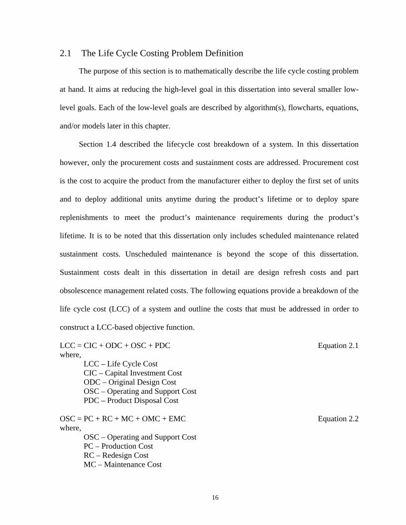
2.1 The Life Cycle Costing Problem Definition
The purpose of this section is to mathematically describe the life cycle costing problem
at hand. It aims at reducing the high-level goal in this dissertation into several smaller low-
level goals. Each of the low-level goals are described by algorithm(s), flowcharts, equations,
and/or models later in this chapter.
Section 1.4 described the lifecycle cost breakdown of a system. In this dissertation
however, only the procurement costs and sustainment costs are addressed. Procurement cost
is the cost to acquire the product from the manufacturer either to deploy the first set of units
and to deploy additional units anytime during the product’s lifetime or to deploy spare
replenishments to meet the product’s maintenance requirements during the product’s
lifetime. It is to be noted that this dissertation only includes scheduled maintenance related
sustainment costs. Unscheduled maintenance is beyond the scope of this dissertation.
Sustainment costs dealt in this dissertation in detail are design refresh costs and part
obsolescence management related costs. The following equations provide a breakdown of the
life cycle cost (LCC) of a system and outline the costs that must be addressed in order to
construct a LCC-based objective function.
LCC = CIC + ODC + OSC + PDC where,
LCC – Life Cycle Cost CIC – Capital Investment Cost ODC – Original Design Cost OSC – Operating and Support Cost PDC – Product Disposal Cost
Equation 2.1
OSC = PC + RC + MC + OMC + EMC where,
OSC – Operating and Support Cost PC – Production Cost RC – Redesign Cost MC – Maintenance Cost
Equation 2.2
16
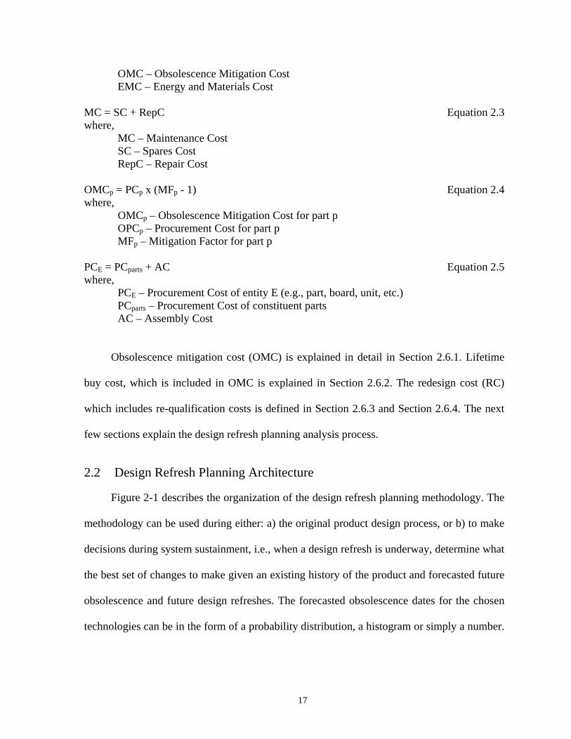
OMC – Obsolescence Mitigation Cost EMC – Energy and Materials Cost
MC = SC + RepC where,
MC – Maintenance Cost SC – Spares Cost RepC – Repair Cost
Equation 2.3
OMCp = PCp x (MFp - 1) where,
OMCp – Obsolescence Mitigation Cost for part p OPCp – Procurement Cost for part p MFp – Mitigation Factor for part p
Equation 2.4
PCE = PCparts + AC where,
PCE – Procurement Cost of entity E (e.g., part, board, unit, etc.) PCparts – Procurement Cost of constituent parts AC – Assembly Cost
Equation 2.5
Obsolescence mitigation cost (OMC) is explained in detail in Section 2.6.1. Lifetime
buy cost, which is included in OMC is explained in Section 2.6.2. The redesign cost (RC)
which includes re-qualification costs is defined in Section 2.6.3 and Section 2.6.4. The next
few sections explain the design refresh planning analysis process.
2.2 Design Refresh Planning Architecture
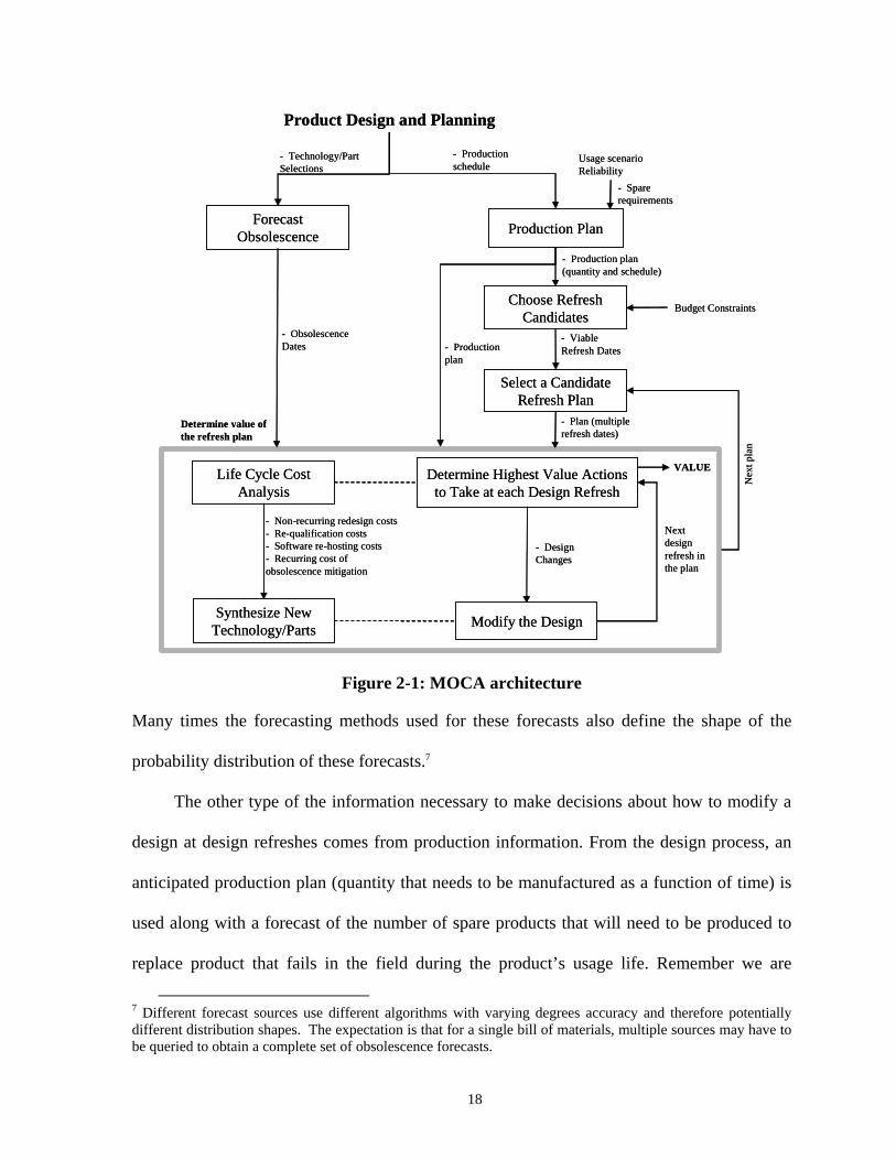
Figure 2-1 describes the organization of the design refresh planning methodology. The
methodology can be used during either: a) the original product design process, or b) to make
decisions during system sustainment, i.e., when a design refresh is underway, determine what
the best set of changes to make given an existing history of the product and forecasted future
obsolescence and future design refreshes. The forecasted obsolescence dates for the chosen
technologies can be in the form of a probability distribution, a histogram or simply a number.
17
Production Plan
Product Design and Planning
Forecast Obsolescence
- Technology/Part Selections
- Production schedule
Usage scenarioReliability
- Spare requirements
- Production plan(quantity and schedule)
Choose Refresh Candidates
- Viable Refresh Dates
Select a Candidate Refresh Plan
- Plan (multiple refresh dates)
Determine Highest Value Actions to Take at each Design Refresh
- Design Changes
- Obsolescence Dates
Budget Constraints
Modify the Design
Life Cycle Cost Analysis
Next design refresh in the plan
Synthesize New Technology/Parts
Determine value of the refresh plan
Nex
t pla
n
- Non-recurring redesign costs- Re-qualification costs- Software re-hosting costs- Recurring cost of obsolescence mitigation
- Production plan
VALUE
Figure 2-1: MOCA architecture
Many times the forecasting methods used for these forecasts also define the shape of the
probability distribution of these forecasts.7
The other type of the information necessary to make decisions about how to modify a
design at design refreshes comes from production information. From the design process, an
anticipated production plan (quantity that needs to be manufactured as a function of time) is
used along with a forecast of the number of spare products that will need to be produced to
replace product that fails in the field during the product’s usage life. Remember we are
7 Different forecast sources use different algorithms with varying degrees accuracy and therefore potentially different distribution shapes. The expectation is that for a single bill of materials, multiple sources may have to be queried to obtain a complete set of obsolescence forecasts.
18

dealing with sustainment-dominated products that will fail in the field due to wear out and
overstress, and will require replacement. The production plan associated with “spare
replenishment” will be determined from the forecasted reliability of the product’s
components and the forecasted usage profile for the system. Using a production plan,
possible locations for design refreshes can be determined (see Section 2.3 for how this is
done). With the possible design refresh dates chosen; a candidate refresh plan can be formed.
A refresh plan is a group of one or more design refreshes representing all the refreshes (and
their respective dates) that will be performed on a product during its lifetime. Thereafter,
given the obsolescence forecasts, the production plan and a candidate design refresh plan, we
now determine the lifecycle cost of the product subject to the candidate refresh plan by
traversing the timeline and costing the events as they occur. To determine the “best” design
refresh plan, multiple candidate refresh plans can be assessed. For sustainment-dominated
products, the number of discrete production events is usually relatively small. For example,
the AS900 engine built by Honeywell has 5 discrete production events (as per data collected
for the AS900 case study in Section 2.9). Therefore, checking all the possible candidate
refresh plans is often very reasonable, i.e., optimization by enumeration.
The methodology developed in this dissertation is implemented in a computational tool
called MOCA (Mitigation of Obsolescence Cost Analysis) using the Java programming
language. MOCA is available through the CALCE Electronic Products and Systems Center
and is currently installed and supported at over 20 sites worldwide. The software
implementation of the tool is documented in the MOCA 1.3 user’s guide (MOCA, 2003).8
8 The MOCA web page for software and documentation download is located at http://www.calce.umd.edu/contracts/MOCA/MOCA_Page.htm. It can only be accessed by CALCE members. If anyone else needs to access it then please email to CALCE website manager.
19
Start of Life
Part becomes obsolete
Part is not obsolete Part is obsolete short term mitigation strategy used
Design refresh
• Spare replenishment• Other planned product ion
“Short term” mitigation strategy
• Existing stock• Last time buy• Aftermarket source
• Lifetime buy
“Long term” mitigat ion strategy
• Substitute part• Emulation• Uprate simi lar part
Redesign non-recurring costs
Re-qualification?• N umber of parts changed• Individual part properties
Functionality Upgrades
Hardware and Software
Figure 2-2: Design refresh planning analysis time line
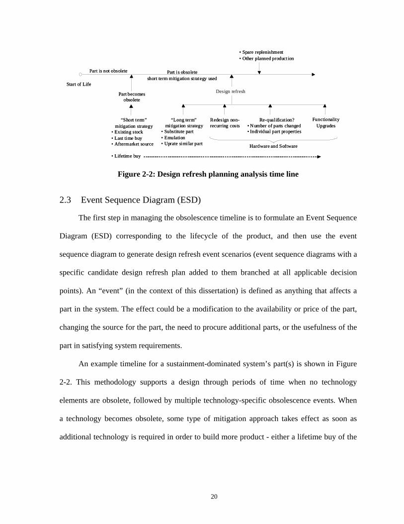
2.3 Event Sequence Diagram (ESD)
The first step in managing the obsolescence timeline is to formulate an Event Sequence
Diagram (ESD) corresponding to the lifecycle of the product, and then use the event
sequence diagram to generate design refresh event scenarios (event sequence diagrams with a
specific candidate design refresh plan added to them branched at all applicable decision
points). An “event” (in the context of this dissertation) is defined as anything that affects a
part in the system. The effect could be a modification to the availability or price of the part,
changing the source for the part, the need to procure additional parts, or the usefulness of the
part in satisfying system requirements.
An example timeline for a sustainment-dominated system’s part(s) is shown in Figure
2-2. This methodology supports a design through periods of time when no technology
elements are obsolete, followed by multiple technology-specific obsolescence events. When
a technology becomes obsolete, some type of mitigation approach takes effect as soon as
additional technology is required in order to build more product - either a lifetime buy of the
20
part is made or a short-term mitigation strategy that only applies until the next design refresh
is instituted.9
Next there are periods of time when one or more technology elements are obsolete,
lifetime buys or short-term mitigation approaches are in place on a part-specific basis. At a
design refresh a long-term obsolescence mitigation solution is applied (until the end of the
product’s sustainment life or until some future design refresh), and non-recurring, recurring,
and re-qualification costs are applied. Re-qualification (and/or re-certification) may be
required depending on the impact of the design change on the application. In some cases, if
the expense of a design refresh is to be undertaken, then functional upgrades will also occur
requiring forecasting of the system functional upgrades. Whether functional upgrades are
included or not, the lifecycle characteristics of new technology elements (that replace
obsolete ones) must be forecasted, including reliability and new obsolescence dates
(replacements become obsolete too).
The last activity appearing on the example timeline in Figure 2-2 is production. The
product often has to be produced after technology elements begin to go obsolete due to the
length of the initial design/manufacturing process, additional orders for the product, and
replenishment of spares. Production events charge recurring manufacturing costs to the
lifecycle total, and design refresh events modify the recurring cost of the product the next
time it is manufactured and charge non-recurring redesign and re-qualification costs to the
lifecycle total.
9 Possible mitigation approaches include (Stogdill, 1999): last time buys (buying enough parts to meet the system’s forecasted requirements until the next redesign), part substitution (using a different part with similar form fit and function), aftermarket sources (third party provided parts), emulation (using parts with identical form fit and function that are fabricated using newer technologies), and reclaim (parts salvaged from other products).
21
In Task 2, first the production events and scheduled design refresh events are ordered
according to their event dates starting with the earliest event. At an event, the first step is to
check the parts that are already obsolete. If the event is a production event then all the
obsolete parts are selected and their current short-term obsolescence mitigation strategy is
applied.10 Cost of acquisition of the new part or replacement parts is then calculated from the
specified mix of mitigation strategies. The total cost of acquisition of the system is calculated
and scaled up depending on the purchase order quantity. When the event is a design refresh
then all the obsolete parts are checked for replacement. Either a Bayesian belief network
(BBN) model is used to decide on the part replacement (technology insertion approach, see
Chapter 3) or simply every obsolete part or every part that is going to go obsolete in the near
future (defined by a look-ahead time) is replaced (technology sustainment approach). The
part replacement cost is calculated and then added to the total lifecycle cost of the system.
The design refresh planning process consists of obtaining system details along with the
marketing information about the system in order to schedule design refreshes relative to the
various orders/reorders in the system’s field life. Lifecycle cost analysis models are used to
assess the design refresh schedules and rank them based on economics. The process involves
uncertainties as well as time-dependent input variations.
Obsolescence events and non-recurring design refresh and qualification costs are the
main drivers of system cost during the system’s support life for many low-volume electronic
systems. On one hand, system sustainers do not wish to incur escalating recurring costs for
systems because parts are obsolete, but on the other hand, design refreshes that would
10 Mitigation strategies are independently defined for each component. Valid short-term mitigation approaches are shown in Figure 2-2. A mitigation strategy for a part might consist of several mitigation approaches that are applied depending on the date of obsolescence or the length of time between the obsolescence event and the next design refresh.
22
decrease recurring costs by removing obsolete parts that are extremely expensive.
Somewhere between the extremes of no design refresh and design refreshes for every
obsolete part when it becomes obsolete may lie a combination of obsolescence management
and design refreshing that intends to lower the lifecycle cost when compared to doing no
analysis. Part of the MOCA process is to perform sustainment cost analysis for a system and
schedule design refreshes during the system’s lifetime. The sustainment cost in this context
includes the cost due to all the orders and reorders (including spares). It also includes
maintenance activities as well as design changes performed on the system during its
sustainment lifetime. Electronic part obsolescence, which determines the part costs during
the system’s lifetime, has a major impact on the sustainment cost and is often the driving
factor behind design refresh scheduling.
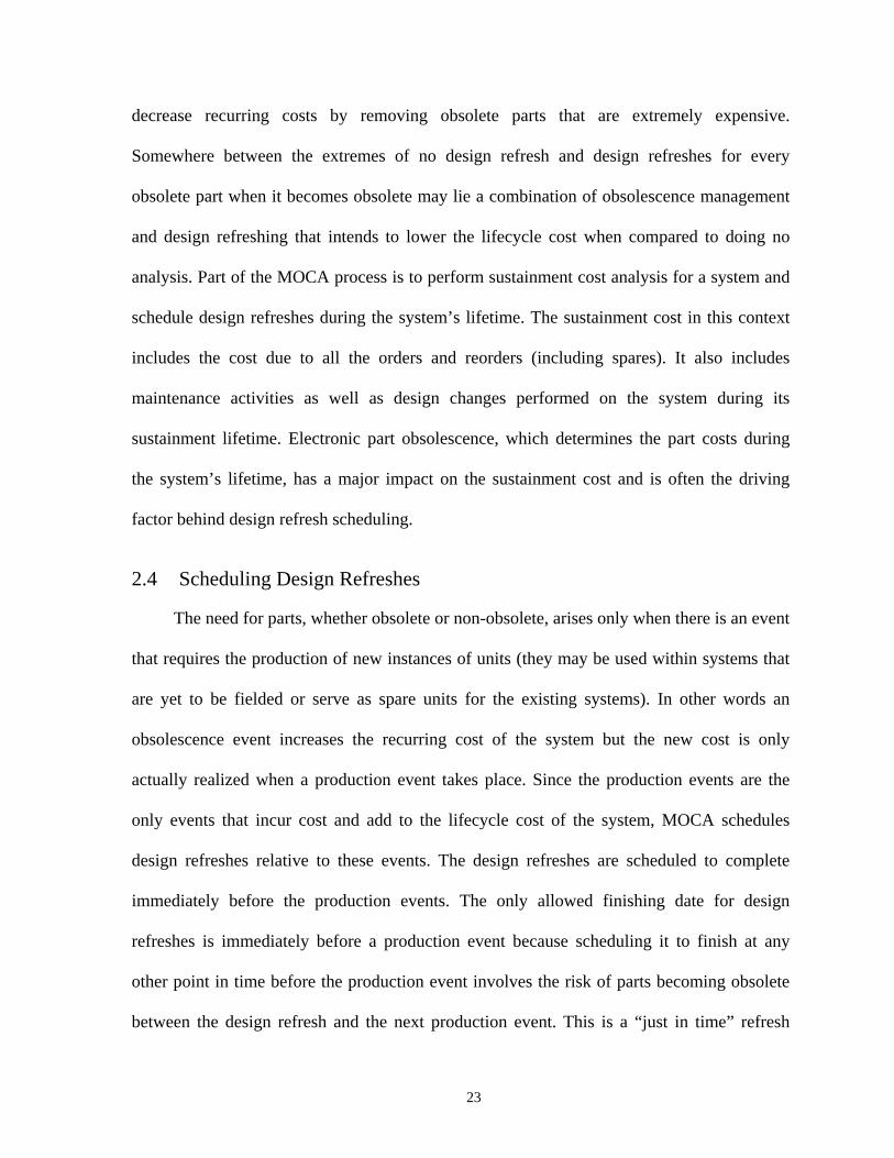
2.4 Scheduling Design Refreshes
The need for parts, whether obsolete or non-obsolete, arises only when there is an event
that requires the production of new instances of units (they may be used within systems that
are yet to be fielded or serve as spare units for the existing systems). In other words an
obsolescence event increases the recurring cost of the system but the new cost is only
actually realized when a production event takes place. Since the production events are the
only events that incur cost and add to the lifecycle cost of the system, MOCA schedules
design refreshes relative to these events. The design refreshes are scheduled to complete
immediately before the production events. The only allowed finishing date for design
refreshes is immediately before a production event because scheduling it to finish at any
other point in time before the production event involves the risk of parts becoming obsolete
between the design refresh and the next production event. This is a “just in time” refresh
23
strategy. The intention is to minimize the time span between a design refresh and the next
production event, thus eliminating the need to perform another design refresh because of any
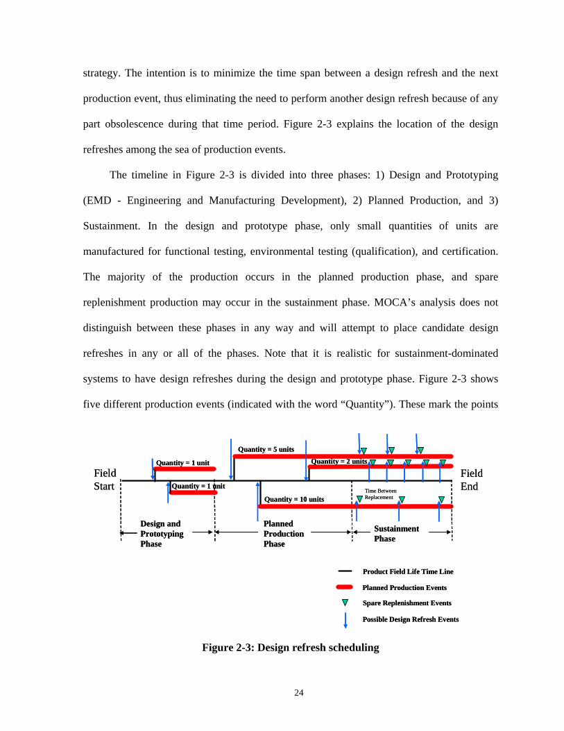
part obsolescence during that time period. Figure 2-3 explains the location of the design
refreshes among the sea of production events.
The timeline in Figure 2-3 is divided into three phases: 1) Design and Prototyping
(EMD - Engineering and Manufacturing Development), 2) Planned Production, and 3)
Sustainment. In the design and prototype phase, only small quantities of units are
manufactured for functional testing, environmental testing (qualification), and certification.
The majority of the production occurs in the planned production phase, and spare
replenishment production may occur in the sustainment phase. MOCA’s analysis does not
distinguish between these phases in any way and will attempt to place candidate design
refreshes in any or all of the phases. Note that it is realistic for sustainment-dominated
systems to have design refreshes during the design and prototype phase. Figure 2-3 shows
five different production events (indicated with the word “Quantity”). These mark the points
Time Between Replacement
Design and Prototyping Phase
Planned Production Phase
Sustainment Phase
Field Start
Field End
Planned Production Events
Quantity = 10 units
Quantity = 5 units
Quantity = 2 units
Product Field Life Time Line
Spare Replenishment Events
Quantity = 1 unit
Quantity = 1 unit
Possible Design Refresh Events
Figure 2-3: Design refresh scheduling
24
on the timeline when specific quantities of units have to be fielded. When a produced unit is
fielded, a new timeline branch is created, e.g., the “Quantity = 10 units” branch in Figure 2-3.
The fielded units may need to be repaired or replaced at some point before the end of field
life. If they need to be replaced, the replacement may occur using initial spares that where
constructed during the original manufacturing of the unit or with replenishment spares that
are manufactured at a later time. Possible replenishment spare manufacturing is shown on the
timeline in Figure 2-3 as triangles.
Design refreshes can take place at any point on the timeline, however, a design refresh
that completes at a point in time that is significantly earlier than the next production event
(whether planned production or spare replenishment) will never be as economically
advantageous as one that is completed “just in time” for the next production event.11 This
strategy for placing design refreshes has two significant advantages: obviously the number of
possible locations on the timeline for design refreshes becomes finite (limited to the number
of production events, which is a small number especially for avionics and military systems),
and this allows each design refresh candidate to be associated a specific instance of some
type of a production event which enables a probabilistic treatment of the production event
dates (see below). Possible design refresh completion points are shown in Figure 2-3.
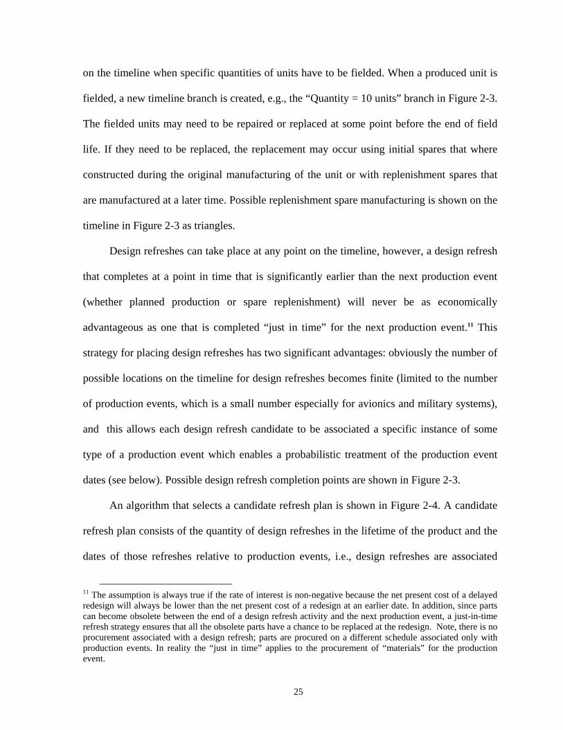
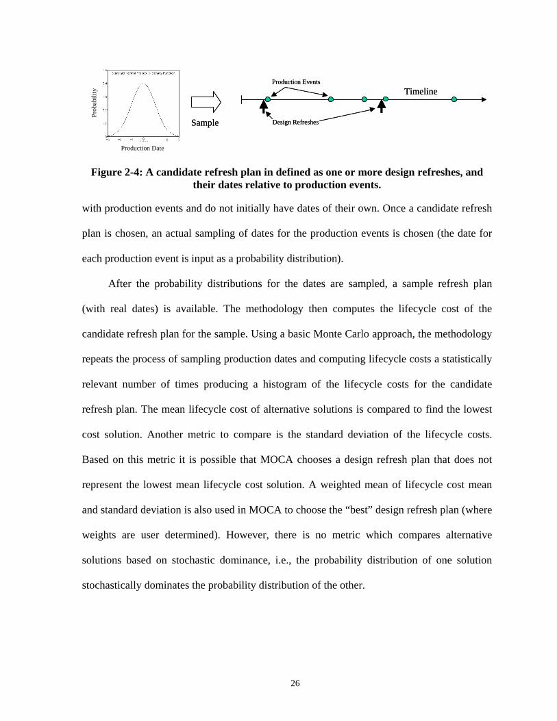
An algorithm that selects a candidate refresh plan is shown in Figure 2-4. A candidate
refresh plan consists of the quantity of design refreshes in the lifetime of the product and the
dates of those refreshes relative to production events, i.e., design refreshes are associated
11 The assumption is always true if the rate of interest is non-negative because the net present cost of a delayed redesign will always be lower than the net present cost of a redesign at an earlier date. In addition, since parts can become obsolete between the end of a design refresh activity and the next production event, a just-in-time refresh strategy ensures that all the obsolete parts have a chance to be replaced at the redesign. Note, there is no procurement associated with a design refresh; parts are procured on a different schedule associated only with production events. In reality the “just in time” applies to the procurement of “materials” for the production event.
25
Production Date
Prob
abili
ty
Sample
Timeline
Design Refreshes
Production Events
Production Date
Prob
abili
ty
Sample
Timeline
Design Refreshes
Production Events
Figure 2-4: A candidate refresh plan in defined as one or more design refreshes, and their dates relative to production events.
with production events and do not initially have dates of their own. Once a candidate refresh
plan is chosen, an actual sampling of dates for the production events is chosen (the date for
each production event is input as a probability distribution).
After the probability distributions for the dates are sampled, a sample refresh plan
(with real dates) is available. The methodology then computes the lifecycle cost of the
candidate refresh plan for the sample. Using a basic Monte Carlo approach, the methodology
repeats the process of sampling production dates and computing lifecycle costs a statistically
relevant number of times producing a histogram of the lifecycle costs for the candidate
refresh plan. The mean lifecycle cost of alternative solutions is compared to find the lowest
cost solution. Another metric to compare is the standard deviation of the lifecycle costs.
Based on this metric it is possible that MOCA chooses a design refresh plan that does not
represent the lowest mean lifecycle cost solution. A weighted mean of lifecycle cost mean
and standard deviation is also used in MOCA to choose the “best” design refresh plan (where
weights are user determined). However, there is no metric which compares alternative
solutions based on stochastic dominance, i.e., the probability distribution of one solution
stochastically dominates the probability distribution of the other.
26
Pass on the number of design refreshes remaining to be scheduled (J) and the StartPosition of the scheduling of the design refreshes among the production events and the previous design refreshes
J = N (number of design refreshes to be scheduled).StartPosition = 0
Decrement J by 1.Set counter = StartPosition
Insert design refresh at position specified by the counter
Set StartPosition = counter +2
Increment counter by 1
Write the design refresh generated into the database for future use
Remove the design refresh at position specified by the counter
Is j > 0 ?
Is counter <number ofproduction
events ?
Candidate design refresh schedules for optimization
N
Y
Y
N
J, St
artP
ositi
on
Figure 2-5: Recursive design refresh scheduling algorithm
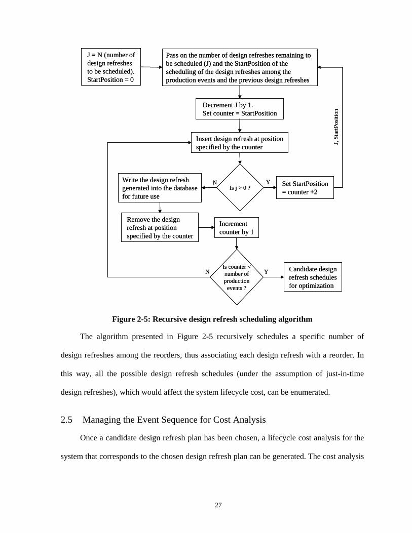
The algorithm presented in Figure 2-5 recursively schedules a specific number of
design refreshes among the reorders, thus associating each design refresh with a reorder. In
this way, all the possible design refresh schedules (under the assumption of just-in-time
design refreshes), which would affect the system lifecycle cost, can be enumerated.
2.5 Managing the Event Sequence for Cost Analysis
Once a candidate design refresh plan has been chosen, a lifecycle cost analysis for the
system that corresponds to the chosen design refresh plan can be generated. The cost analysis
27
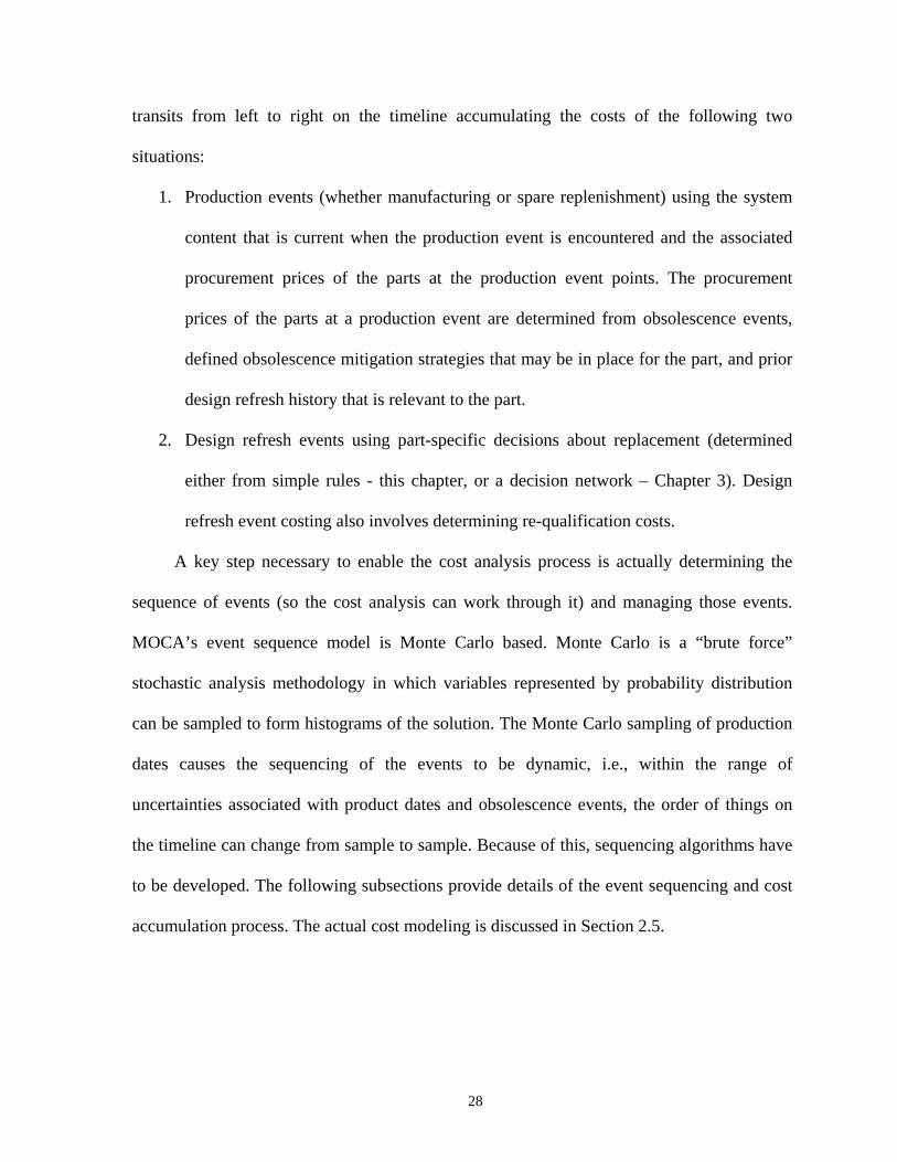
transits from left to right on the timeline accumulating the costs of the following two
situations:
1. Production events (whether manufacturing or spare replenishment) using the system
content that is current when the production event is encountered and the associated
procurement prices of the parts at the production event points. The procurement
prices of the parts at a production event are determined from obsolescence events,
defined obsolescence mitigation strategies that may be in place for the part, and prior
design refresh history that is relevant to the part.
2. Design refresh events using part-specific decisions about replacement (determined
either from simple rules - this chapter, or a decision network – Chapter 3). Design
refresh event costing also involves determining re-qualification costs.
A key step necessary to enable the cost analysis process is actually determining the
sequence of events (so the cost analysis can work through it) and managing those events.
MOCA’s event sequence model is Monte Carlo based. Monte Carlo is a “brute force”
stochastic analysis methodology in which variables represented by probability distribution
can be sampled to form histograms of the solution. The Monte Carlo sampling of production
dates causes the sequencing of the events to be dynamic, i.e., within the range of
uncertainties associated with product dates and obsolescence events, the order of things on
the timeline can change from sample to sample. Because of this, sequencing algorithms have
to be developed. The following subsections provide details of the event sequencing and cost
accumulation process. The actual cost modeling is discussed in Section 2.5.
28
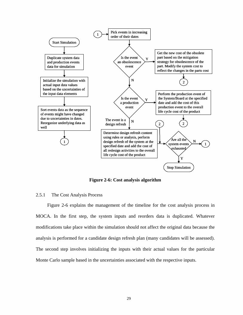
Duplicate system data and production events data for simulation
Initialize the simulation with actual input data values based on the uncertainties of the input data elements
Sort events data as the sequence of events might have changed due to uncertainties in dates. Reorganize underlying data as well
Is the eventa production
event
N
YPerform the production event of the System/Board at the specified date and add the cost of this production event to the overall life cycle cost of the product
Determine design refresh content using rules or analysis, perform design refresh of the system at the specified date and add the cost of all redesign activities to the overall life cycle cost of the product
Is the eventan obsolescence
event
N
Y
Pick events in increasing order of their dates
Get the new cost of the obsolete part based on the mitigation strategy for obsolescence of the part. Modify the system cost to reflect the changes in the parts cost
The event is a design refresh
1
1
2
2
2
Are all thesystem events
exhausted
Y
N1
Stop Simulation
Start Simulation
Figure 2-6: Cost analysis algorithm
2.5.1 The Cost Analysis Process
Figure 2-6 explains the management of the timeline for the cost analysis process in
MOCA. In the first step, the system inputs and reorders data is duplicated. Whatever
modifications take place within the simulation should not affect the original data because the
analysis is performed for a candidate design refresh plan (many candidates will be assessed).
The second step involves initializing the inputs with their actual values for the particular
Monte Carlo sample based in the uncertainties associated with the respective inputs.
29
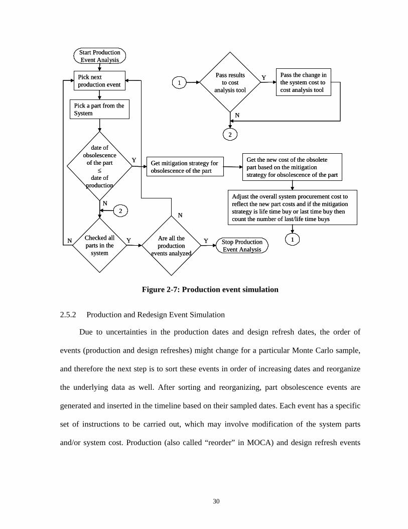
Pick a part from the System
Pick next production event
Get the new cost of the obsolete part based on the mitigation strategy for obsolescence of the part
Adjust the overall system procurement cost to reflect the new part costs and if the mitigation strategy is life time buy or last time buy then count the number of last/life time buys
date ofobsolescence
of the part≤
date ofproduction
N
Y
Checked allparts in the
system
YN
Pass the change in the system cost to cost analysis tool
Pass resultsto cost
analysis tool
N
Y1
1
2
2
Are all theproduction
events analyzed
Get mitigation strategy for obsolescence of the part
Y
N
Start ProductionEvent Analysis
Stop ProductionEvent Analysis
Figure 2-7: Production event simulation
2.5.2 Production and Redesign Event Simulation
Due to uncertainties in the production dates and design refresh dates, the order of
events (production and design refreshes) might change for a particular Monte Carlo sample,
and therefore the next step is to sort these events in order of increasing dates and reorganize
the underlying data as well. After sorting and reorganizing, part obsolescence events are
generated and inserted in the timeline based on their sampled dates. Each event has a specific
set of instructions to be carried out, which may involve modification of the system parts
and/or system cost. Production (also called “reorder” in MOCA) and design refresh events
30
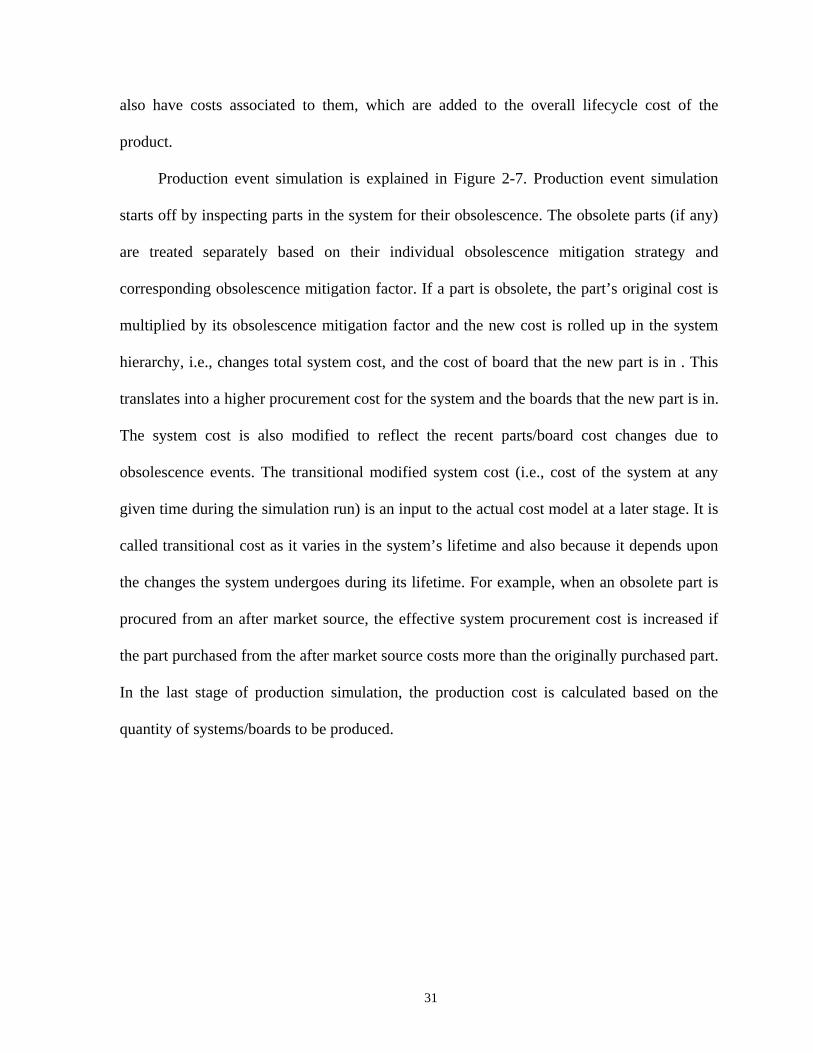
also have costs associated to them, which are added to the overall lifecycle cost of the
product.
Production event simulation is explained in Figure 2-7. Production event simulation
starts off by inspecting parts in the system for their obsolescence. The obsolete parts (if any)
are treated separately based on their individual obsolescence mitigation strategy and
corresponding obsolescence mitigation factor. If a part is obsolete, the part’s original cost is
multiplied by its obsolescence mitigation factor and the new cost is rolled up in the system
hierarchy, i.e., changes total system cost, and the cost of board that the new part is in . This
translates into a higher procurement cost for the system and the boards that the new part is in.
The system cost is also modified to reflect the recent parts/board cost changes due to
obsolescence events. The transitional modified system cost (i.e., cost of the system at any
given time during the simulation run) is an input to the actual cost model at a later stage. It is
called transitional cost as it varies in the system’s lifetime and also because it depends upon
the changes the system undergoes during its lifetime. For example, when an obsolete part is
procured from an after market source, the effective system procurement cost is increased if
the part purchased from the after market source costs more than the originally purchased part.
In the last stage of production simulation, the production cost is calculated based on the
quantity of systems/boards to be produced.
31
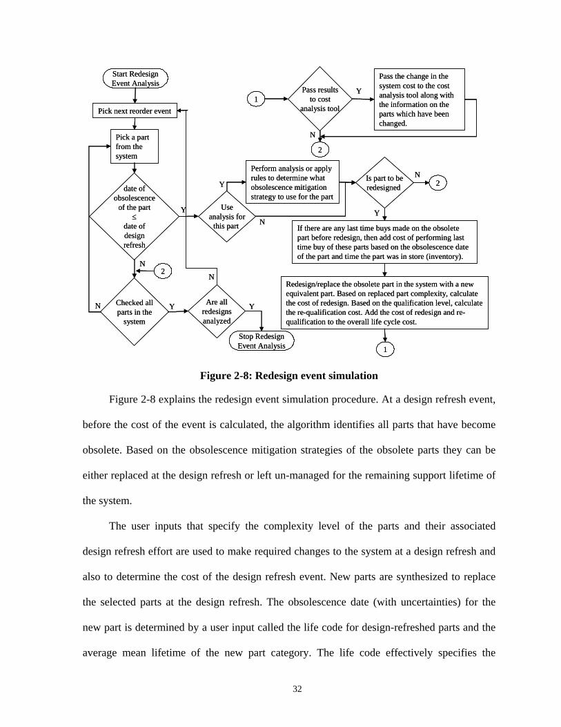
Pick a part from the system
If there are any last time buys made on the obsolete part before redesign, then add cost of performing last time buy of these parts based on the obsolescence date of the part and time the part was in store (inventory).
date ofobsolescence
of the part≤
date ofdesignrefresh
N
Y
Checked allparts in the
system
YN
Pass the change in the system cost to the cost analysis tool along with the information on the parts which have been changed.
Pass resultsto cost
analysis tool
N
Y1
1
2
2
Useanalysis for
this part N
Y
Redesign/replace the obsolete part in the system with a new equivalent part. Based on replaced part complexity, calculate the cost of redesign. Based on the qualification level, calculate the re-qualification cost. Add the cost of redesign and re-qualification to the overall life cycle cost.
Pick next reorder event
Are allredesignsanalyzed
Y
N
Start RedesignEvent Analysis
Stop RedesignEvent Analysis
Perform analysis or apply rules to determine what obsolescence mitigation strategy to use for the part
Is part to beredesigned
Y
N2
Figure 2-8: Redesign event simulation
Figure 2-8 explains the redesign event simulation procedure. At a design refresh event,
before the cost of the event is calculated, the algorithm identifies all parts that have become
obsolete. Based on the obsolescence mitigation strategies of the obsolete parts they can be
either replaced at the design refresh or left un-managed for the remaining support lifetime of
the system.
The user inputs that specify the complexity level of the parts and their associated
design refresh effort are used to make required changes to the system at a design refresh and
also to determine the cost of the design refresh event. New parts are synthesized to replace
the selected parts at the design refresh. The obsolescence date (with uncertainties) for the
new part is determined by a user input called the life code for design-refreshed parts and the
average mean lifetime of the new part category. The life code effectively specifies the
32
lifecycle stage of the replacement part that, when combined with the lifetime of the part,
enables forecasting of the obsolescence date for the synthesized part.
Another important step is to cost last time buys made for parts that are being replaced
at the design refresh. All the underlying data for the old part is modified with the values of
the new part. Cost models are used to determine the design refresh non-recurring cost during
the design refresh process.
2.6 Cost Models
This section explains the MOCA cost models. The specific cost models discussed are
the obsolescence cost model, the lifetime buy or the last time buy cost model, the design
refresh cost model and the re-qualification cost model.
2.6.1 Obsolescence Cost Model
The model for an obsolete part in MOCA is based on the fact that after obsolescence of
a particular part, the cost of procuring that part (or its equivalent) changes. There are two
situations MOCA must model. First, the part becomes obsolete and a production event is
encountered before the obsolete part is designed out (or MOCA decides not to design out the
obsolete part at a design refresh). In this case, MOCA assumes that the original part is used
for production, but a price penalty is applied commensurate with the mitigation approach that
is in effect at the time of production. MOCA uses the recurring cost factors in Table 2-1
associated with various obsolescence mitigation approaches as defaults (more accurate, part-
specific factors can be entered into MOCA if they are known).
33
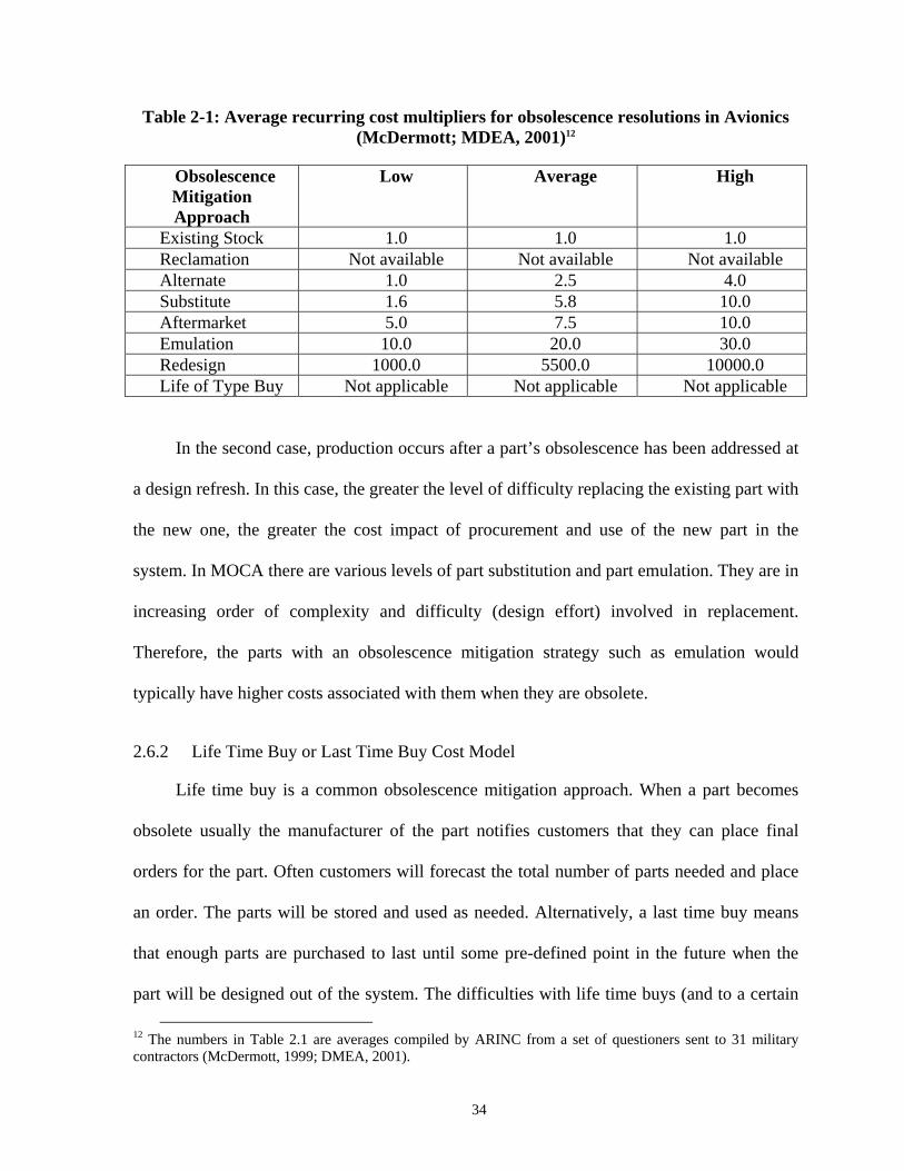
Table 2-1: Average recurring cost multipliers for obsolescence resolutions in Avionics (McDermott; MDEA, 2001)12
Obsolescence Mitigation Approach
Low Average High
Existing Stock 1.0 1.0 1.0 Reclamation Not available Not available Not available Alternate 1.0 2.5 4.0 Substitute 1.6 5.8 10.0 Aftermarket 5.0 7.5 10.0 Emulation 10.0 20.0 30.0 Redesign 1000.0 5500.0 10000.0 Life of Type Buy Not applicable Not applicable Not applicable
In the second case, production occurs after a part’s obsolescence has been addressed at
a design refresh. In this case, the greater the level of difficulty replacing the existing part with
the new one, the greater the cost impact of procurement and use of the new part in the
system. In MOCA there are various levels of part substitution and part emulation. They are in
increasing order of complexity and difficulty (design effort) involved in replacement.
Therefore, the parts with an obsolescence mitigation strategy such as emulation would
typically have higher costs associated with them when they are obsolete.
2.6.2 Life Time Buy or Last Time Buy Cost Model
Life time buy is a common obsolescence mitigation approach. When a part becomes
obsolete usually the manufacturer of the part notifies customers that they can place final
orders for the part. Often customers will forecast the total number of parts needed and place
an order. The parts will be stored and used as needed. Alternatively, a last time buy means
that enough parts are purchased to last until some pre-defined point in the future when the
part will be designed out of the system. The difficulties with life time buys (and to a certain
12 The numbers in Table 2.1 are averages compiled by ARINC from a set of questioners sent to 31 military contractors (McDermott, 1999; DMEA, 2001).
34
extent last time buys) are: 1) uncertainty in the estimation of the number of parts needed to
sustain a system after obsolescence through its proposed lifetime (when all the electronic
parts used in the avionics of Boeing 747 went obsolete in the early 1970s, could Boeing
foresee that they would be building 747s for 30 more years?); 2) it is potentially expensive to
store the parts successfully until they are needed (solder plated leads oxidize quickly making
the part un-assemblable, therefore, parts have to be stored using special facilities); 3) one has
to be able to keep track of the parts for long periods of time (they can be lost or absorbed by
another application); and 4) life time buys may represent a considerable capital investment
that management may not be willing to approve.
The original vendor, from whom parts were purchased for the current design, might
offer the parts for last time buys or lifetime buys at a different price. They could also be
discounted since the lifetime buys/last time buys are usually made in large quantities.
2.6.3 Design Refresh Cost Model
MOCA uses two models for costing design refreshes. The primary model is a linkage
to a pair of commercial parametric lifecycle cost modeling tools. In one of the primary
models, MOCA determines the changes to the system and then exports those changes to
Price H/HL (PRICE H, 2001). Price H/HL is the hardware cost modeling tool developed by
Price System Inc., L.L.C. It performs the cost modeling and exports the non-recurring re-
engineering cost back to MOCA.
MOCA also supports a secondary internal (simpler) cost model for design refreshes.
The internal design refresh cost model built upon the fact that design refresh cost is primarily
dependent upon the number of parts per board that have to be design refreshed, and the
number of boards effected. The model is described in Equation 2.6,
35
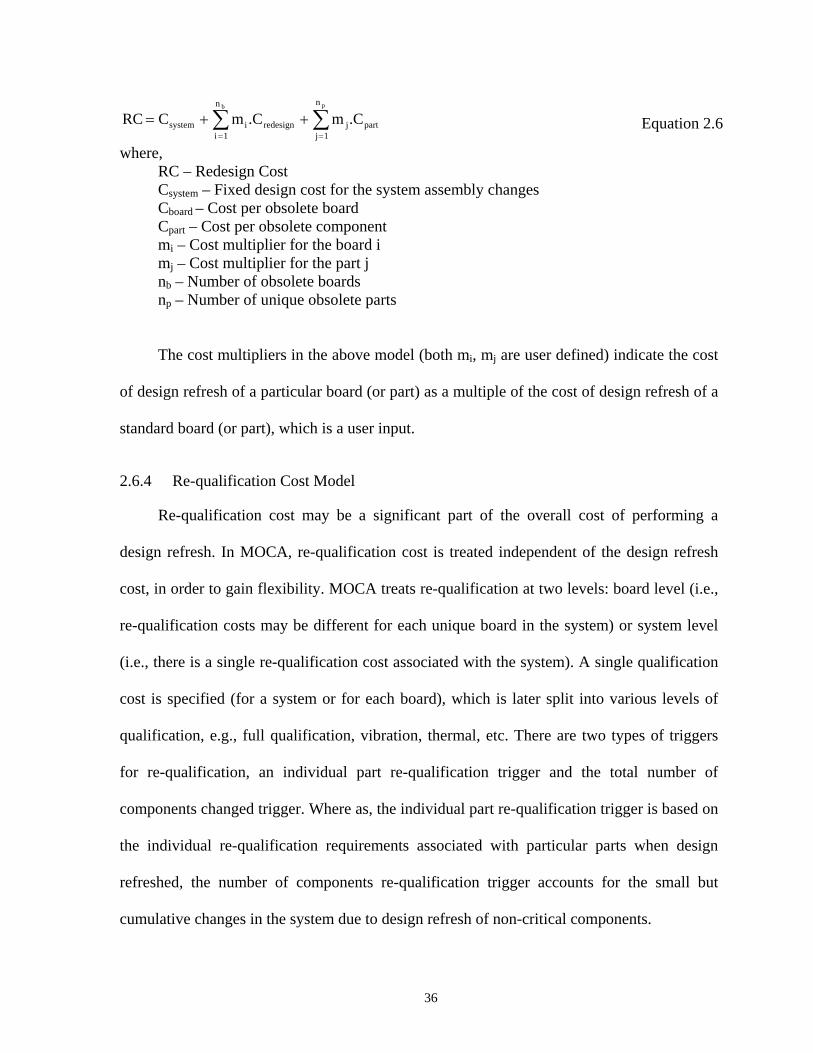
∑∑==
++=pb n
1jpartj
n
1iredesignisystem .Cm.CmC RC
where, RC – Redesign Cost Csystem – Fixed design cost for the system assembly changes Cboard – Cost per obsolete board Cpart – Cost per obsolete component mi – Cost multiplier for the board i mj – Cost multiplier for the part j nb – Number of obsolete boards np – Number of unique obsolete parts
Equation 2.6
The cost multipliers in the above model (both mi, mj are user defined) indicate the cost
of design refresh of a particular board (or part) as a multiple of the cost of design refresh of a
standard board (or part), which is a user input.
2.6.4 Re-qualification Cost Model
Re-qualification cost may be a significant part of the overall cost of performing a
design refresh. In MOCA, re-qualification cost is treated independent of the design refresh
cost, in order to gain flexibility. MOCA treats re-qualification at two levels: board level (i.e.,
re-qualification costs may be different for each unique board in the system) or system level
(i.e., there is a single re-qualification cost associated with the system). A single qualification
cost is specified (for a system or for each board), which is later split into various levels of
qualification, e.g., full qualification, vibration, thermal, etc. There are two types of triggers
for re-qualification, an individual part re-qualification trigger and the total number of
components changed trigger. Where as, the individual part re-qualification trigger is based on
the individual re-qualification requirements associated with particular parts when design
refreshed, the number of components re-qualification trigger accounts for the small but
cumulative changes in the system due to design refresh of non-critical components.
36
2.7 Miscellaneous MOCA Concepts
2.7.1 Design Refresh “look-ahead” Time
Design refresh look-ahead time means that whenever a design refresh takes place,
MOCA looks ahead for forecasted part obsolescence issues and proactively removes those
part obsolescence problems at the current design refresh opportunity. By having a long
design refresh look-ahead time the number of design refreshes can be reduced. On the other
hand, by design refreshing parts that are not yet obsolete there is a risk of incurring extra cost
for no improvement, i.e., there is a possibility that the obsolete part that was proactively
design refreshed is never required in the future. In general, there will be an optimum look-
ahead time for a specific application.
The concept of look-ahead is only applicable to the baseline version of MOCA
discussed in this chapter. In the technology insertion version of MOCA discussed in Chapter
3, look-ahead is effectively optimized on a part-by-part basis when the decision networks for
parts are coupled from refresh-to-refresh.
2.7.2 Data Coarsening (Time Step Fidelity)
MOCA is capable of simulating on an exact date basis, i.e., MOCA could produce a
design refresh plan that includes refresh dates specified to the minute. Lifecycle Cost
Analysis (LCCA) tools, however, generally operate with time increments that may be
anywhere from one month to one year. In order to interface MOCA with the Price Systems
LCCA tools, the MOCA solution must be coarsened, i.e., combined into one-year steps or
whatever time step size is used by the LCCA tool. It is important to define and understand
how data coarsening will affect the overall solution.
37
In dynamic simulation of systems, e.g., thermal, mechanical, electrical, or chemical,
choosing a smaller time step always produces a more accurate solution since physical
systems are continuous and practically accepted models for physical systems are valid as the
time step approaches zero. In the design refresh problem, smaller time steps do not
necessarily produce more accurate answers; it is critical to choose the right time step. Too
small a time step can result in just as inaccurate an answer as too large a time step. As an
example, it is impractical for most companies to procure parts on a per minute basis 24 hours
a day 7 days a week, rather, procurement happens on a courser time scale, e.g., once a month
or once a quarter. As it turns out that the one year time step assumed by most LCCA tools
(PRICE, 2001) is a reasonably accurate representation of the time scale on which
manufacturers of long field life systems plan and operate.
Two different approaches were taken to coarsen the data in MOCA. They are: 1)
combining re-order events before design refresh optimization, and 2) rounding off dated
events and associating the events with the nearest budget period. Combining production
events in MOCA mean that starting from a particular date, add up all the production events
for a time span specified by the user. The production events in that time span are then treated
as a single production event at the start date. In this way the support life of the product is
fragmented into various sections and active simulation steps taken only on these fragments.
Budgeting in MOCA means that each date input is rounded and included with in the nearest
budget period. Therefore, all the date inputs reflect budget period based inputs.
2.8 A Tutorial Example
This section presents a very simple sample system consisting of only two parts that
demonstrates the MOCA methodology. A single level hierarchy is considered for simplicity,
38
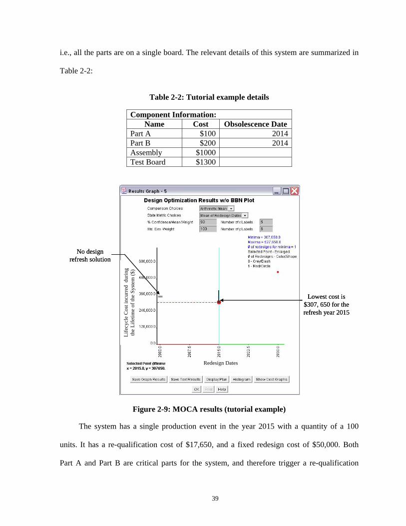
i.e., all the parts are on a single board. The relevant details of this system are summarized in
Table 2-2:
Table 2-2: Tutorial example details
Component Information: Name Cost Obsolescence Date
Part A $100 2014 Part B $200 2014 Assembly $1000 Test Board $1300
Life
cycl
e C
ost i
ncur
red
dur
ing
the
Life
time
of th
e Sy
stem
($)
Redesign Dates
Lowest cost is $307, 650 for the refresh year 2015
No design refresh solution
Life
cycl
e C
ost i
ncur
red
dur
ing
the
Life
time
of th
e Sy
stem
($)
Redesign Dates
Lowest cost is $307, 650 for the refresh year 2015
No design refresh solution
Figure 2-9: MOCA results (tutorial example)
The system has a single production event in the year 2015 with a quantity of a 100
units. It has a re-qualification cost of $17,650, and a fixed redesign cost of $50,000. Both
Part A and Part B are critical parts for the system, and therefore trigger a re-qualification
39
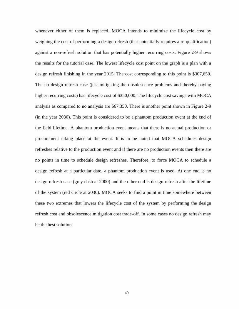
whenever either of them is replaced. MOCA intends to minimize the lifecycle cost by
weighing the cost of performing a design refresh (that potentially requires a re-qualification)
against a non-refresh solution that has potentially higher recurring costs. Figure 2-9 shows
the results for the tutorial case. The lowest lifecycle cost point on the graph is a plan with a
design refresh finishing in the year 2015. The cost corresponding to this point is $307,650.
The no design refresh case (just mitigating the obsolescence problems and thereby paying
higher recurring costs) has lifecycle cost of $350,000. The lifecycle cost savings with MOCA
analysis as compared to no analysis are $67,350. There is another point shown in Figure 2-9
(in the year 2030). This point is considered to be a phantom production event at the end of
the field lifetime. A phantom production event means that there is no actual production or
procurement taking place at the event. It is to be noted that MOCA schedules design
refreshes relative to the production event and if there are no production events then there are
no points in time to schedule design refreshes. Therefore, to force MOCA to schedule a
design refresh at a particular date, a phantom production event is used. At one end is no
design refresh case (grey dash at 2000) and the other end is design refresh after the lifetime
of the system (red circle at 2030). MOCA seeks to find a point in time somewhere between
these two extremes that lowers the lifecycle cost of the system by performing the design
refresh cost and obsolescence mitigation cost trade-off. In some cases no design refresh may
be the best solution.
40
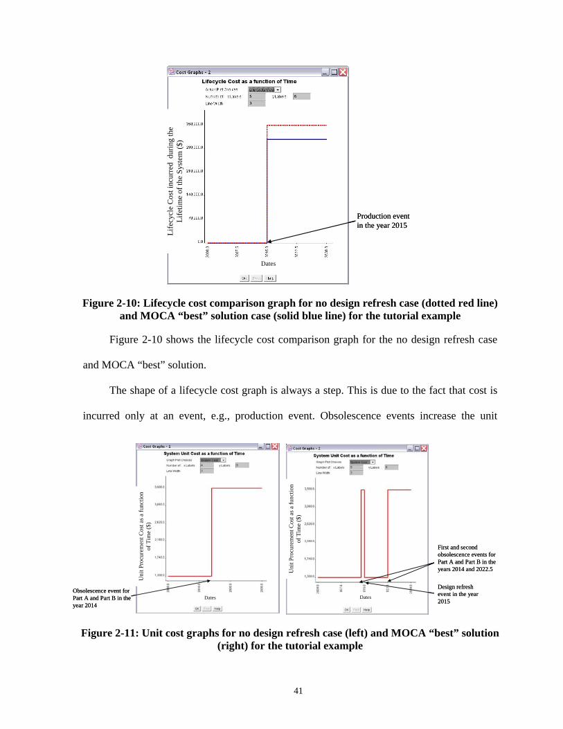
Production event in the year 2015
Life
cycl
e C
ost i
ncur
red
dur
ing
the
Life
time
of th
e Sy
stem
($)
Dates
Production event in the year 2015
Life
cycl
e C
ost i
ncur
red
dur
ing
the
Life
time
of th
e Sy
stem
($)
Dates
Figure 2-10: Lifecycle cost comparison graph for no design refresh case (dotted red line) and MOCA “best” solution case (solid blue line) for the tutorial example
Figure 2-10 shows the lifecycle cost comparison graph for the no design refresh case
and MOCA “best” solution.
The shape of a lifecycle cost graph is always a step. This is due to the fact that cost is
incurred only at an event, e.g., production event. Obsolescence events increase the unit
Obsolescence event for Part A and Part B in the year 2014
Uni
t Pro
cure
men
t Cos
t as a
func
tion
of T
ime
($)
Dates
First and second obsolescence events for Part A and Part B in the years 2014 and 2022.5
Design refresh event in the year 2015
Uni
t Pro
cure
men
t Cos
t as a
func
tion
of T
ime
($)
DatesObsolescence event for Part A and Part B in the year 2014
Uni
t Pro
cure
men
t Cos
t as a
func
tion
of T
ime
($)
Dates
First and second obsolescence events for Part A and Part B in the years 2014 and 2022.5
Design refresh event in the year 2015
Uni
t Pro
cure
men
t Cos
t as a
func
tion
of T
ime
($)
Dates
Figure 2-11: Unit cost graphs for no design refresh case (left) and MOCA “best” solution (right) for the tutorial example
41
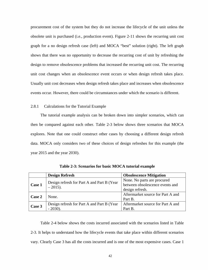
procurement cost of the system but they do not increase the lifecycle of the unit unless the
obsolete unit is purchased (i.e., production event). Figure 2-11 shows the recurring unit cost
graph for a no design refresh case (left) and MOCA “best” solution (right). The left graph
shows that there was no opportunity to decrease the recurring cost of unit by refreshing the
design to remove obsolescence problems that increased the recurring unit cost. The recurring
unit cost changes when an obsolescence event occurs or when design refresh takes place.
Usually unit cost decreases when design refresh takes place and increases when obsolescence
events occur. However, there could be circumstances under which the scenario is different.
2.8.1 Calculations for the Tutorial Example
The tutorial example analysis can be broken down into simpler scenarios, which can
then be compared against each other. Table 2-3 below shows three scenarios that MOCA
explores. Note that one could construct other cases by choosing a different design refresh
data. MOCA only considers two of these choices of design refreshes for this example (the
year 2015 and the year 2030).
Table 2-3: Scenarios for basic MOCA tutorial example
Design Refresh Obsolescence Mitigation
Case 1 Design refresh for Part A and Part B (Year – 2015).
None. No parts are procured between obsolescence events and design refresh.
Case 2 None. Aftermarket source for Part A and Part B.
Case 3 Design refresh for Part A and Part B (Year - 2030).
Aftermarket source for Part A and Part B.
Table 2-4 below shows the costs incurred associated with the scenarios listed in Table
2-3. It helps to understand how the lifecycle events that take place within different scenarios
vary. Clearly Case 3 has all the costs incurred and is one of the most expensive cases. Case 1
42
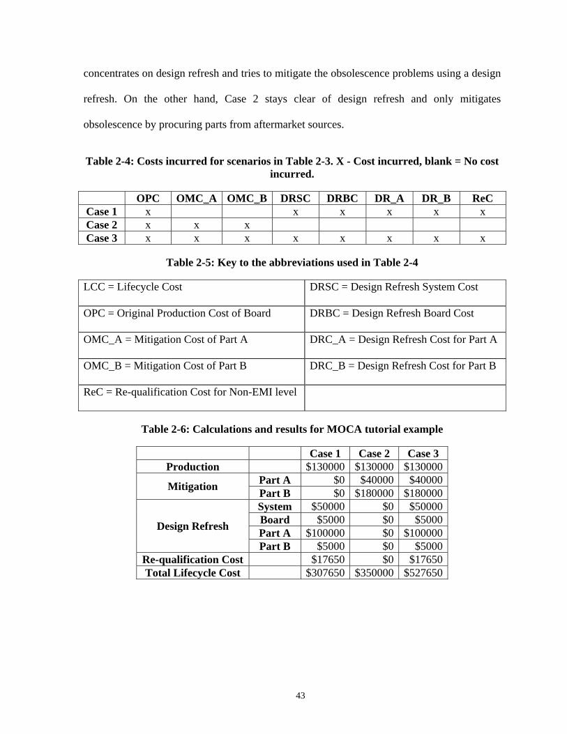
concentrates on design refresh and tries to mitigate the obsolescence problems using a design
refresh. On the other hand, Case 2 stays clear of design refresh and only mitigates
obsolescence by procuring parts from aftermarket sources.
Table 2-4: Costs incurred for scenarios in Table 2-3. X - Cost incurred, blank = No cost incurred.
OPC OMC_A OMC_B DRSC DRBC DR_A DR_B ReC Case 1 x x x x x x Case 2 x x x Case 3 x x x x x x x x
Table 2-5: Key to the abbreviations used in Table 2-4
LCC = Lifecycle Cost DRSC = Design Refresh System Cost
OPC = Original Production Cost of Board DRBC = Design Refresh Board Cost
OMC_A = Mitigation Cost of Part A DRC_A = Design Refresh Cost for Part A
OMC_B = Mitigation Cost of Part B DRC_B = Design Refresh Cost for Part B
ReC = Re-qualification Cost for Non-EMI level
Table 2-6: Calculations and results for MOCA tutorial example
Case 1 Case 2 Case 3 Production $130000 $130000 $130000
Part A $0 $40000 $40000 Mitigation Part B $0 $180000 $180000 System $50000 $0 $50000 Board $5000 $0 $5000 Part A $100000 $0 $100000 Design Refresh
Part B $5000 $0 $5000 Re-qualification Cost $17650 $0 $17650 Total Lifecycle Cost $307650 $350000 $527650
43
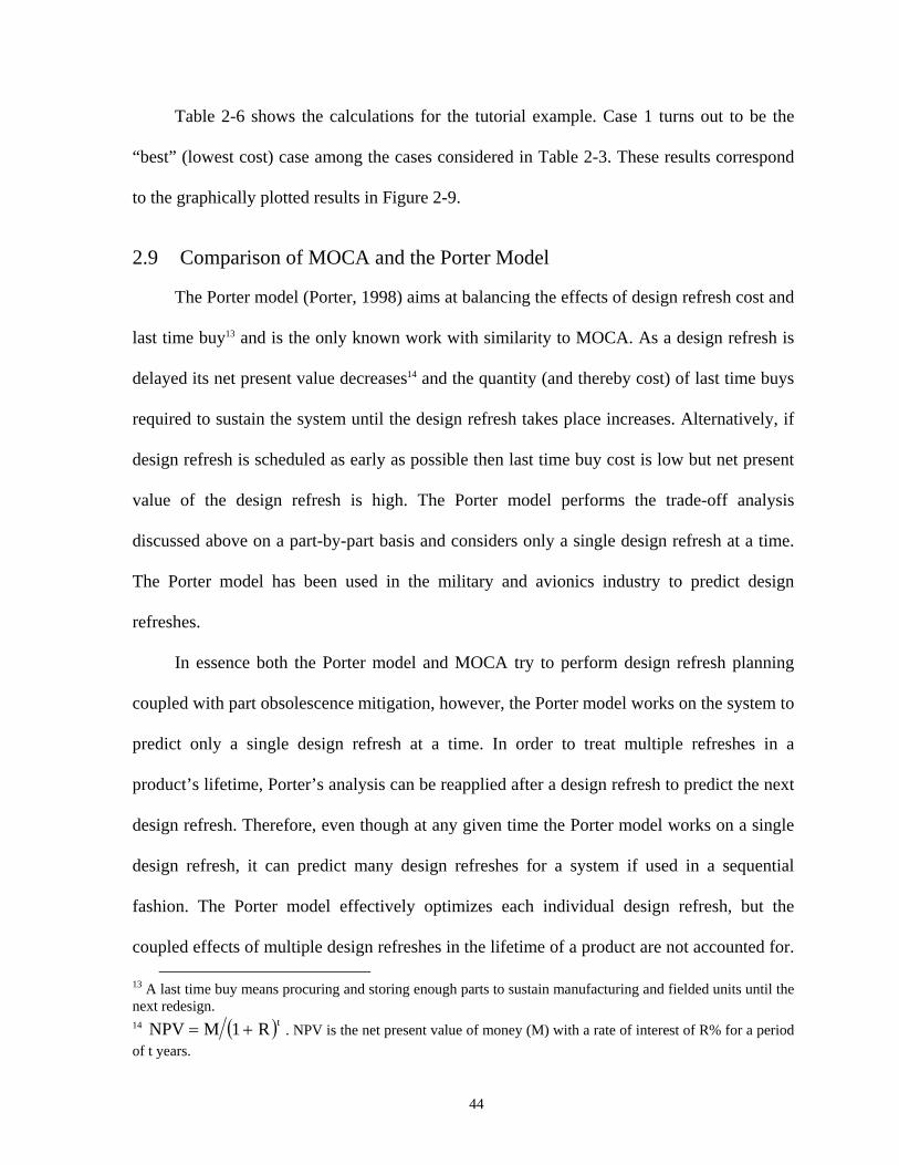
Table 2-6 shows the calculations for the tutorial example. Case 1 turns out to be the
“best” (lowest cost) case among the cases considered in Table 2-3. These results correspond
to the graphically plotted results in Figure 2-9.
2.9 Comparison of MOCA and the Porter Model
The Porter model (Porter, 1998) aims at balancing the effects of design refresh cost and
last time buy13 and is the only known work with similarity to MOCA. As a design refresh is
delayed its net present value decreases14 and the quantity (and thereby cost) of last time buys
required to sustain the system until the design refresh takes place increases. Alternatively, if
design refresh is scheduled as early as possible then last time buy cost is low but net present
value of the design refresh is high. The Porter model performs the trade-off analysis
discussed above on a part-by-part basis and considers only a single design refresh at a time.
The Porter model has been used in the military and avionics industry to predict design
refreshes.
In essence both the Porter model and MOCA try to perform design refresh planning
coupled with part obsolescence mitigation, however, the Porter model works on the system to
predict only a single design refresh at a time. In order to treat multiple refreshes in a
product’s lifetime, Porter’s analysis can be reapplied after a design refresh to predict the next
design refresh. Therefore, even though at any given time the Porter model works on a single
design refresh, it can predict many design refreshes for a system if used in a sequential
fashion. The Porter model effectively optimizes each individual design refresh, but the
coupled effects of multiple design refreshes in the lifetime of a product are not accounted for.
)
13 A last time buy means procuring and storing enough parts to sustain manufacturing and fielded units until the next redesign. 14 ( tR1MNPV += . NPV is the net present value of money (M) with a rate of interest of R% for a period of t years.
44
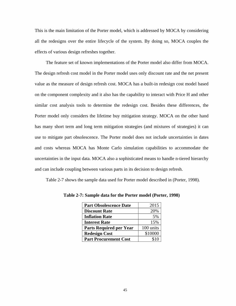
This is the main limitation of the Porter model, which is addressed by MOCA by considering
all the redesigns over the entire lifecycle of the system. By doing so, MOCA couples the
effects of various design refreshes together.
The feature set of known implementations of the Porter model also differ from MOCA.
The design refresh cost model in the Porter model uses only discount rate and the net present
value as the measure of design refresh cost. MOCA has a built-in redesign cost model based
on the component complexity and it also has the capability to interact with Price H and other
similar cost analysis tools to determine the redesign cost. Besides these differences, the
Porter model only considers the lifetime buy mitigation strategy. MOCA on the other hand
has many short term and long term mitigation strategies (and mixtures of strategies) it can
use to mitigate part obsolescence. The Porter model does not include uncertainties in dates
and costs whereas MOCA has Monte Carlo simulation capabilities to accommodate the
uncertainties in the input data. MOCA also a sophisticated means to handle n-tiered hierarchy
and can include coupling between various parts in its decision to design refresh.
Table 2-7 shows the sample data used for Porter model described in (Porter, 1998).
Table 2-7: Sample data for the Porter model (Porter, 1998)
Part Obsolescence Date 2015Discount Rate 20%Inflation Rate 5%Interest Rate 15%Parts Required per Year 100 unitsRedesign Cost $10000Part Procurement Cost $10
45
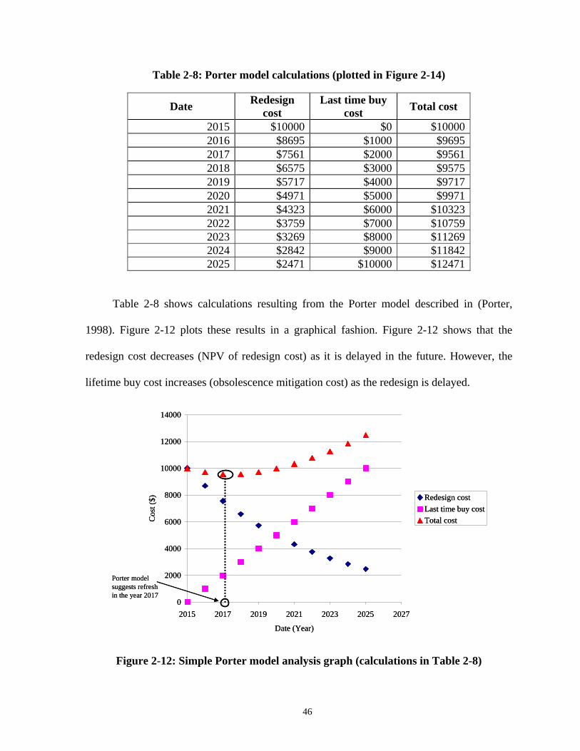
Table 2-8: Porter model calculations (plotted in Figure 2-14)
Date Redesign cost
Last time buy cost Total cost
2015 $10000 $0 $10000 2016 $8695 $1000 $9695 2017 $7561 $2000 $9561 2018 $6575 $3000 $9575 2019 $5717 $4000 $9717 2020 $4971 $5000 $9971 2021 $4323 $6000 $10323 2022 $3759 $7000 $10759 2023 $3269 $8000 $11269 2024 $2842 $9000 $11842 2025 $2471 $10000 $12471
Table 2-8 shows calculations resulting from the Porter model described in (Porter,
1998). Figure 2-12 plots these results in a graphical fashion. Figure 2-12 shows that the
redesign cost decreases (NPV of redesign cost) as it is delayed in the future. However, the
lifetime buy cost increases (obsolescence mitigation cost) as the redesign is delayed.
0
2000
4000
6000
8000
10000
12000
14000
2015 2017 2019 2021 2023 2025 2027
Date (Year)
Cos
t ($) Redesign cost
Last time buy costTotal cost
Porter model suggests refresh in the year 2017
0
2000
4000
6000
8000
10000
12000
14000
2015 2017 2019 2021 2023 2025 2027
Date (Year)
Cos
t ($) Redesign cost
Last time buy costTotal cost
Porter model suggests refresh in the year 2017
Figure 2-12: Simple Porter model analysis graph (calculations in Table 2-8)
46
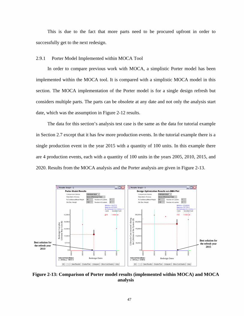
This is due to the fact that more parts need to be procured upfront in order to
successfully get to the next redesign.
2.9.1 Porter Model Implemented within MOCA Tool
In order to compare previous work with MOCA, a simplistic Porter model has been
implemented within the MOCA tool. It is compared with a simplistic MOCA model in this
section. The MOCA implementation of the Porter model is for a single design refresh but
considers multiple parts. The parts can be obsolete at any date and not only the analysis start
date, which was the assumption in Figure 2-12 results.
The data for this section’s analysis test case is the same as the data for tutorial example
in Section 2.7 except that it has few more production events. In the tutorial example there is a
single production event in the year 2015 with a quantity of 100 units. In this example there
are 4 production events, each with a quantity of 100 units in the years 2005, 2010, 2015, and
2020. Results from the MOCA analysis and the Porter analysis are given in Figure 2-13.
Life
cycl
e C
ost i
ncur
red
dur
ing
the
Life
time
of th
e Sy
stem
($)
Redesign DatesRedesign Dates
Red
esig
n C
ost p
lus
Life
time
Buy
Cos
t ($)
Best solution for the refresh year
2015
Best solution for the refresh year
2010
Life
cycl
e C
ost i
ncur
red
dur
ing
the
Life
time
of th
e Sy
stem
($)
Redesign DatesRedesign Dates
Red
esig
n C
ost p
lus
Life
time
Buy
Cos
t ($)
Life
cycl
e C
ost i
ncur
red
dur
ing
the
Life
time
of th
e Sy
stem
($)
Redesign DatesRedesign Dates
Red
esig
n C
ost p
lus
Life
time
Buy
Cos
t ($)
Best solution for the refresh year
2015
Best solution for the refresh year
2010
Figure 2-13: Comparison of Porter model results (implemented within MOCA) and MOCA analysis
47
It is to be noted that the scales of the two graphs in Figure 2-13 are different. The
Porter model graph (left) shows very low cost numbers as it considers only net present value
of the fixed design refresh cost and the lifetime buy costs of the parts. MOCA cost model
considers overall lifecycle costs. It includes design refresh cost, obsolescence mitigation cost,
and production costs. Therefore, MOCA graph (right) shows mush higher cost numbers.
While performing analysis for a single redesign refresh planning The Porter model assumes
that the part’s original obsolescence event is the only obsolescence event involving the part
in the product’s lifetime, i.e., that the part does not go obsolete again in the future. Therefore,
Porter misses the impact of a possible second obsolescence event of the same part. This is a
fundamental difference between the Porter model and the MOCA model. By design, the
Porter model is limited in its view of the lifecycle of the system. The Porter model plans for a
single obsolescence event at a time. As the field life of the systems increase, a part within the
system can possibly become obsolete multiple times over its lifetime. MOCA takes all such
obsolescence events for each of the parts in the system into account whereas the Porter model
handles each obsolescence event one at a time. In the Porter model implemented in this
dissertation it is assumed that there is no obsolescence after the part is replaced during a
design refresh. In a more complex Porter model implementation, theoretically multiple
design refreshes and multiple part obsolescence events could be handled. But, they will all by
analyzed in sequential order rather than concurrently. So, there is no link between one design
refresh and other design refreshes over the system’s life in the Porter model. Neither is there
any link between various obsolescence events. Each of these obsolescence events and design
refreshes are planned for and optimized separately. In MOCA however, all such
48
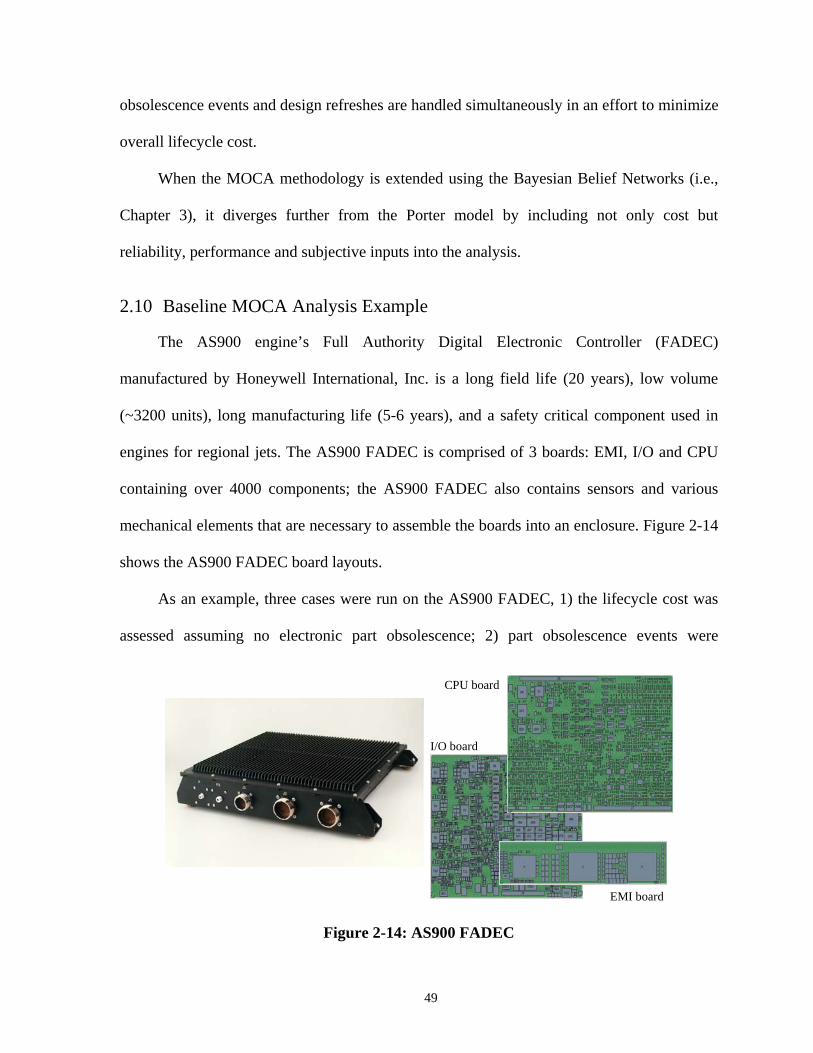
obsolescence events and design refreshes are handled simultaneously in an effort to minimize
overall lifecycle cost.
When the MOCA methodology is extended using the Bayesian Belief Networks (i.e.,
Chapter 3), it diverges further from the Porter model by including not only cost but
reliability, performance and subjective inputs into the analysis.
2.10 Baseline MOCA Analysis Example
The AS900 engine’s Full Authority Digital Electronic Controller (FADEC)
manufactured by Honeywell International, Inc. is a long field life (20 years), low volume
(~3200 units), long manufacturing life (5-6 years), and a safety critical component used in
engines for regional jets. The AS900 FADEC is comprised of 3 boards: EMI, I/O and CPU
containing over 4000 components; the AS900 FADEC also contains sensors and various
mechanical elements that are necessary to assemble the boards into an enclosure. Figure 2-14
shows the AS900 FADEC board layouts.
As an example, three cases were run on the AS900 FADEC, 1) the lifecycle cost was
assessed assuming no electronic part obsolescence; 2) part obsolescence events were
EMI board
CPU board
I/O board
Figure 2-14: AS900 FADEC
49
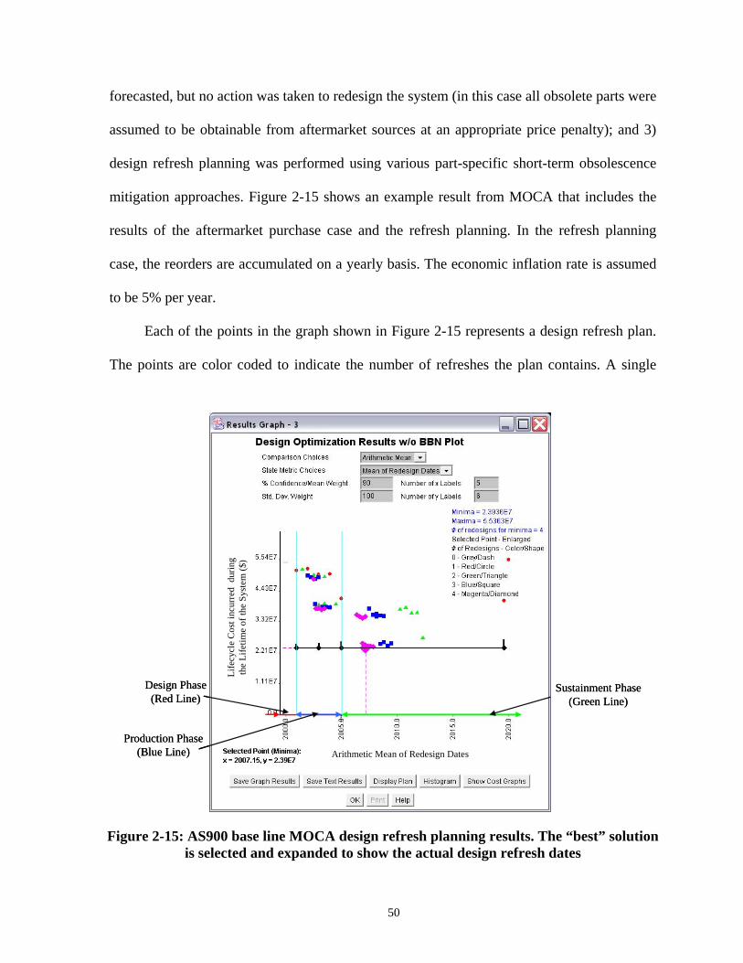
forecasted, but no action was taken to redesign the system (in this case all obsolete parts were
assumed to be obtainable from aftermarket sources at an appropriate price penalty); and 3)
design refresh planning was performed using various part-specific short-term obsolescence
mitigation approaches. Figure 2-15 shows an example result from MOCA that includes the
results of the aftermarket purchase case and the refresh planning. In the refresh planning
case, the reorders are accumulated on a yearly basis. The economic inflation rate is assumed
to be 5% per year.
Each of the points in the graph shown in Figure 2-15 represents a design refresh plan.
The points are color coded to indicate the number of refreshes the plan contains. A single
Life
cycl
e C
ost i
ncur
red
dur
ing
the
Life
time
of th
e Sy
stem
($)
Arithmetic Mean of Redesign DatesProduction Phase
(Blue Line)
Design Phase (Red Line)
Sustainment Phase (Green Line)
Life
cycl
e C
ost i
ncur
red
dur
ing
the
Life
time
of th
e Sy
stem
($)
Arithmetic Mean of Redesign DatesProduction Phase
(Blue Line)
Design Phase (Red Line)
Sustainment Phase (Green Line)
Figure 2-15: AS900 base line MOCA design refresh planning results. The “best” solution is selected and expanded to show the actual design refresh dates
50
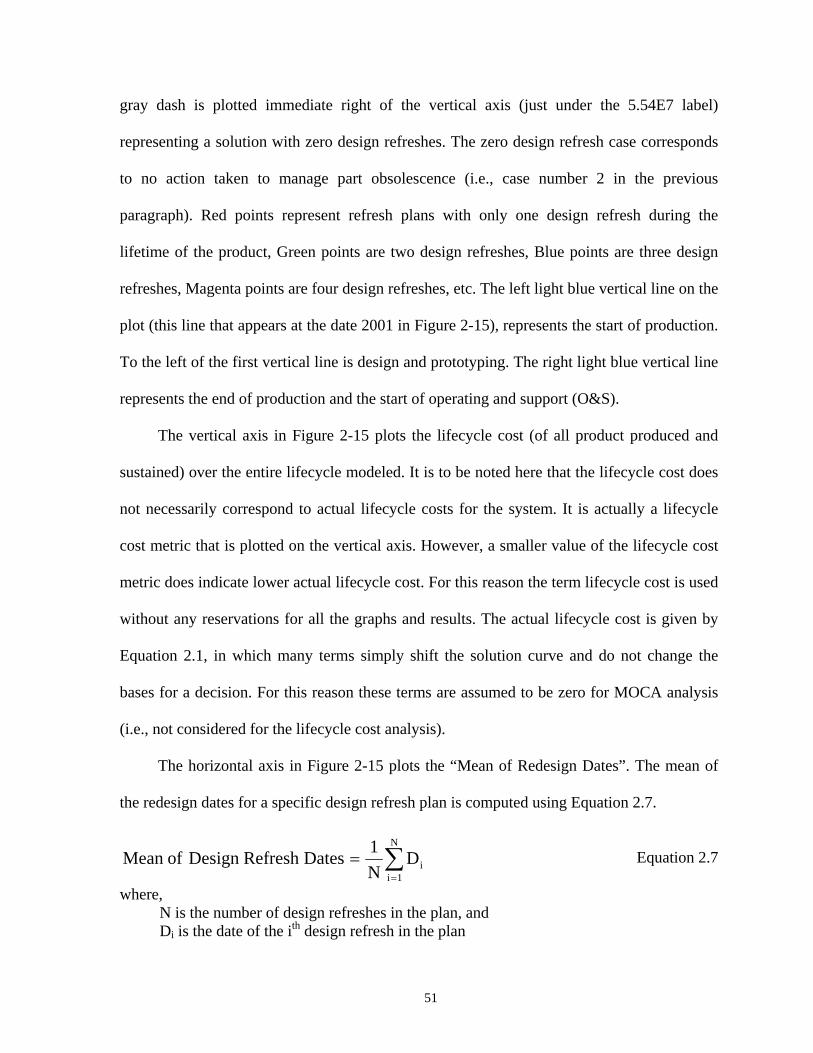
gray dash is plotted immediate right of the vertical axis (just under the 5.54E7 label)
representing a solution with zero design refreshes. The zero design refresh case corresponds
to no action taken to manage part obsolescence (i.e., case number 2 in the previous
paragraph). Red points represent refresh plans with only one design refresh during the
lifetime of the product, Green points are two design refreshes, Blue points are three design
refreshes, Magenta points are four design refreshes, etc. The left light blue vertical line on the
plot (this line that appears at the date 2001 in Figure 2-15), represents the start of production.
To the left of the first vertical line is design and prototyping. The right light blue vertical line
represents the end of production and the start of operating and support (O&S).
The vertical axis in Figure 2-15 plots the lifecycle cost (of all product produced and
sustained) over the entire lifecycle modeled. It is to be noted here that the lifecycle cost does
not necessarily correspond to actual lifecycle costs for the system. It is actually a lifecycle
cost metric that is plotted on the vertical axis. However, a smaller value of the lifecycle cost
metric does indicate lower actual lifecycle cost. For this reason the term lifecycle cost is used
without any reservations for all the graphs and results. The actual lifecycle cost is given by
Equation 2.1, in which many terms simply shift the solution curve and do not change the
bases for a decision. For this reason these terms are assumed to be zero for MOCA analysis
(i.e., not considered for the lifecycle cost analysis).
The horizontal axis in Figure 2-15 plots the “Mean of Redesign Dates”. The mean of
the redesign dates for a specific design refresh plan is computed using Equation 2.7.
∑=
=N
1iiD
N1 Dates Refresh Designof Mean
where, N is the number of design refreshes in the plan, and Di is the date of the ith design refresh in the plan
Equation 2.7
51
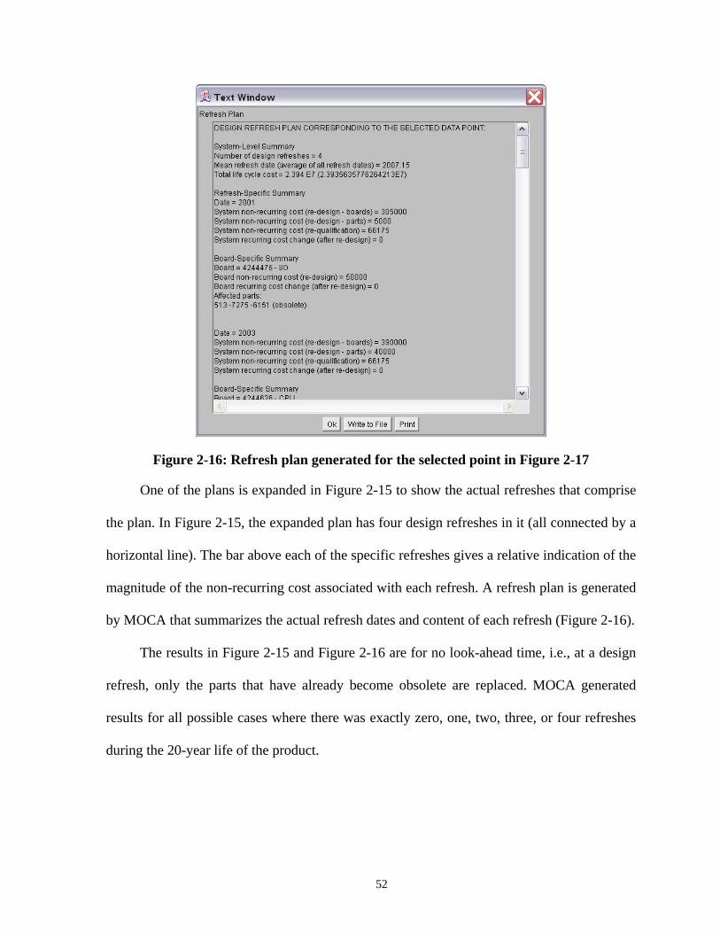
Figure 2-16: Refresh plan generated for the selected point in Figure 2-17
One of the plans is expanded in Figure 2-15 to show the actual refreshes that comprise
the plan. In Figure 2-15, the expanded plan has four design refreshes in it (all connected by a
horizontal line). The bar above each of the specific refreshes gives a relative indication of the
magnitude of the non-recurring cost associated with each refresh. A refresh plan is generated
by MOCA that summarizes the actual refresh dates and content of each refresh (Figure 2-16).
The results in Figure 2-15 and Figure 2-16 are for no look-ahead time, i.e., at a design
refresh, only the parts that have already become obsolete are replaced. MOCA generated
results for all possible cases where there was exactly zero, one, two, three, or four refreshes
during the 20-year life of the product.
52
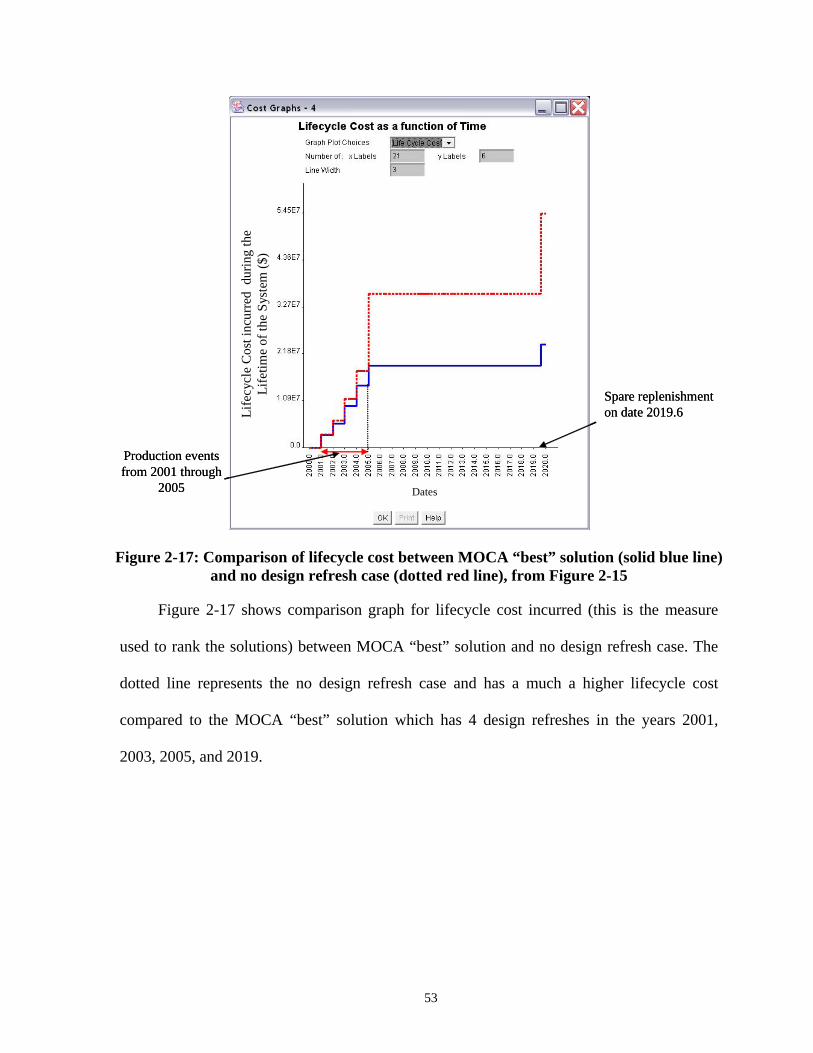
Production events from 2001 through
2005
Spare replenishment on date 2019.6Li
fecy
cle
Cos
t inc
urre
d d
urin
g th
e Li
fetim
e of
the
Syst
em ($
)
Dates
Production events from 2001 through
2005
Spare replenishment on date 2019.6Li
fecy
cle
Cos
t inc
urre
d d
urin
g th
e Li
fetim
e of
the
Syst
em ($
)
Dates
Figure 2-17: Comparison of lifecycle cost between MOCA “best” solution (solid blue line) and no design refresh case (dotted red line), from Figure 2-15
Figure 2-17 shows comparison graph for lifecycle cost incurred (this is the measure
used to rank the solutions) between MOCA “best” solution and no design refresh case. The
dotted line represents the no design refresh case and has a much a higher lifecycle cost
compared to the MOCA “best” solution which has 4 design refreshes in the years 2001,
2003, 2005, and 2019.
53
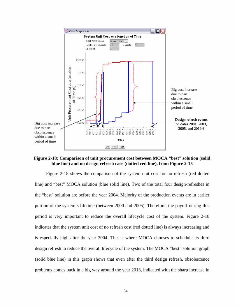
Design refresh events on dates 2001, 2003,
2005, and 2019.6
Big cost increase due to part obsolescence within a small period of time
Uni
t Pro
cure
men
t Cos
t as a
func
tion
of T
ime
($)
Big cost increase due to part obsolescence within a small period of time Dates
Design refresh events on dates 2001, 2003,
2005, and 2019.6
Big cost increase due to part obsolescence within a small period of time
Uni
t Pro
cure
men
t Cos
t as a
func
tion
of T
ime
($)
Big cost increase due to part obsolescence within a small period of time Dates
Figure 2-18: Comparison of unit procurement cost between MOCA “best” solution (solid blue line) and no design refresh case (dotted red line), from Figure 2-15
Figure 2-18 shows the comparison of the system unit cost for no refresh (red dotted
line) and “best” MOCA solution (blue solid line). Two of the total four design-refreshes in
the “best” solution are before the year 2004. Majority of the production events are in earlier
portion of the system’s lifetime (between 2000 and 2005). Therefore, the payoff during this
period is very important to reduce the overall lifecycle cost of the system. Figure 2-18
indicates that the system unit cost of no refresh cost (red dotted line) is always increasing and
is especially high after the year 2004. This is where MOCA chooses to schedule its third
design refresh to reduce the overall lifecycle of the system. The MOCA “best” solution graph
(solid blue line) in this graph shows that even after the third design refresh, obsolescence
problems comes back in a big way around the year 2013, indicated with the sharp increase in
54
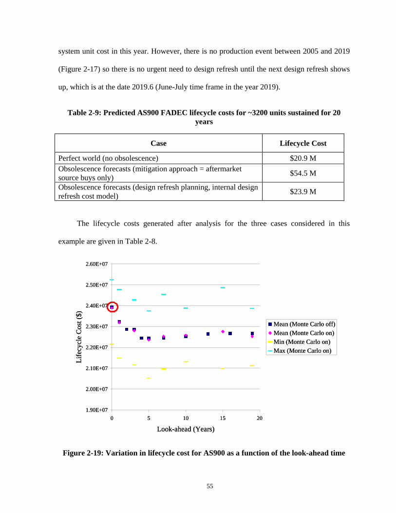
system unit cost in this year. However, there is no production event between 2005 and 2019
(Figure 2-17) so there is no urgent need to design refresh until the next design refresh shows
up, which is at the date 2019.6 (June-July time frame in the year 2019).
Table 2-9: Predicted AS900 FADEC lifecycle costs for ~3200 units sustained for 20 years
Case Lifecycle Cost
Perfect world (no obsolescence) $20.9 M Obsolescence forecasts (mitigation approach = aftermarket source buys only) $54.5 M
Obsolescence forecasts (design refresh planning, internal design refresh cost model) $23.9 M
The lifecycle costs generated after analysis for the three cases considered in this
example are given in Table 2-8.
1.90E+07
2.00E+07
2.10E+07
2.20E+07
2.30E+07
2.40E+07
2.50E+07
2.60E+07
0 5 10 15 20
Look-ahead (Years)
Life
cycl
e C
ost (
$)
Mean (Monte Carlo off)Mean (Monte Carlo on)Min (Monte Carlo on)Max (Monte Carlo on)
1.90E+07
2.00E+07
2.10E+07
2.20E+07
2.30E+07
2.40E+07
2.50E+07
2.60E+07
0 5 10 15 20
Look-ahead (Years)
Life
cycl
e C
ost (
$)
Mean (Monte Carlo off)Mean (Monte Carlo on)Min (Monte Carlo on)Max (Monte Carlo on)
Figure 2-19: Variation in lifecycle cost for AS900 as a function of the look-ahead time
55
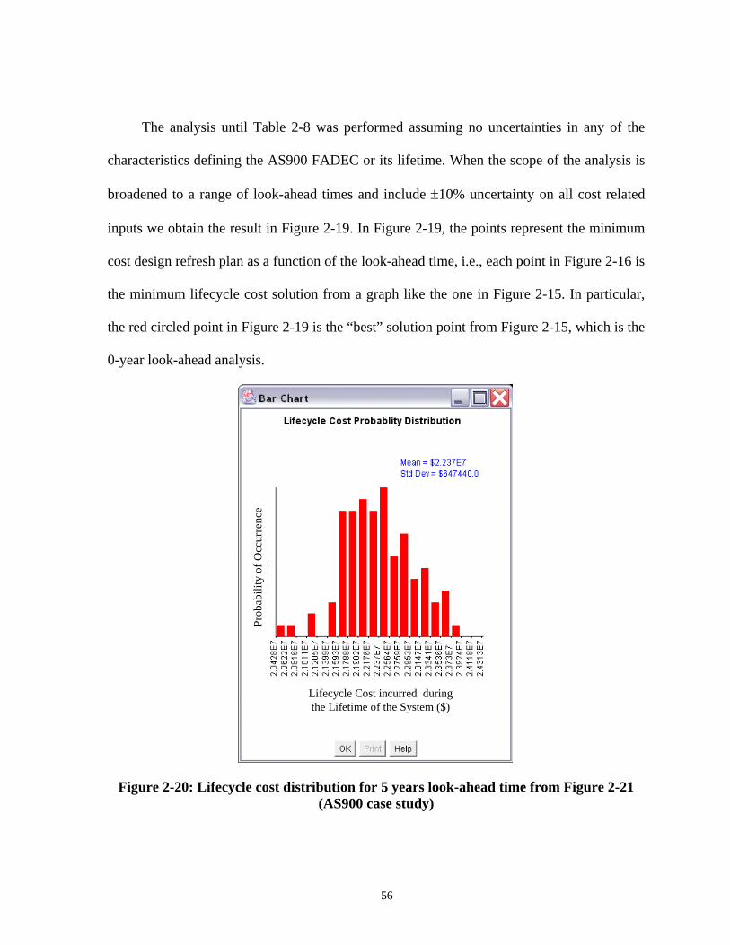
The analysis until Table 2-8 was performed assuming no uncertainties in any of the
characteristics defining the AS900 FADEC or its lifetime. When the scope of the analysis is
broadened to a range of look-ahead times and include ±10% uncertainty on all cost related
inputs we obtain the result in Figure 2-19. In Figure 2-19, the points represent the minimum
cost design refresh plan as a function of the look-ahead time, i.e., each point in Figure 2-16 is
the minimum lifecycle cost solution from a graph like the one in Figure 2-15. In particular,
the red circled point in Figure 2-19 is the “best” solution point from Figure 2-15, which is the
0-year look-ahead analysis.
Lifecycle Cost incurred during the Lifetime of the System ($)
Prob
abili
ty o
f Occ
urre
nce
Lifecycle Cost incurred during the Lifetime of the System ($)
Prob
abili
ty o
f Occ
urre
nce
Figure 2-20: Lifecycle cost distribution for 5 years look-ahead time from Figure 2-21 (AS900 case study)
56
The closed points in Figure 2-19 correspond to the means of the analysis runs that have
uncertainties. The bars represent the standard deviation for these solutions. The open points
in Figure 2-19 correspond to analysis runs with no uncertainties. The numbers next to closed
points give the number of design refreshes in the lowest lifecycle cost solution. The overall
optimal solution in Figure 2-19 is the 5 years look-ahead point. In this case, the optimal
solution remains the same with or without including uncertainties; however, this will not
generally be true. Figure 2-20 shows the lifecycle cost histogram (100 samples) for the 5
years look-ahead time case in Figure 2-19.
2.11 Summary
This chapter describes the formulation of the baseline design refresh planning process
and provides an example of basic design refresh planning to demonstrate the utility of the
methodology. The baseline design refresh process has been implemented in a software tool
called MOCA. As of Fall 2004, MOCA is installed and supported at Honeywell, Lockheed
Martin, Northrop Grumman, Caterpillar, Halliburton, QinetiQ, Boeing, Rockwell
Automation, Precience, Price Systems, Frontier Technology, Titan Systems, Raytheon,
UCLA, the Naval Surface Warfare Center (Crane), UK MOD, and the U.S. Air Force
(Wright Patterson AFB).
The baseline version of MOCA is limited to considering technology sustainment (as
opposed to technology insertion), i.e., managing “part-for-part” level replacement during
design refresh activities. Chapter 3 extends the methodology using probabilistic reasoning
techniques to treat broader technology insertion problems that consider more detail when
determining whether to change parts at design refresh opportunities. Chapter 3 also extends
57

MOCA to consider non-electronic systems where the definition of “components” is extended
beyond just hardware to include software and intellectual property.
58
Chapter 3: Technology Insertion – Using Probabilistic Decision Methods to Determine Design Refresh Content (Task 3)
Design refresh planning as described in Chapter 2 involves scheduling of redesigns
over the lifetime of the system and measuring the lifecycle impact of each candidate design
refresh plan on the system. This chapter describes the process of determining which parts to
replace during a design refresh, i.e., deciding the design refresh content. In basic MOCA
described in Chapter 2, when a design refresh is encountered, parts that are obsolete or going
to be obsolete within a specified period of time (look-ahead time) are replaced. In this
chapter, the part replacement decision is driven by a broader range of issues including
performance, reliability, and logistics, and coupled part-to-part and refresh-to-refresh
coupling.
A Bayesian Belief Network (BBN) based approach is used to determine design refresh
content. This chapter starts off by explaining the approach used to decide design refresh
content and why it is feasible. The chapter reviews Bayesian Belief Networks and how they
are used in the context of this dissertation. Sample networks are discussed and the details of
the MOCA BBN architecture follow with examples to demonstrate the utility of the BBN
analysis and design refresh content selection.
3.1 Probabilistic Decision Methods
Most problems in the real world require some simplifications to be made to define their
domain. Many facts are left unknown or incompletely defined. The domain determines the
59
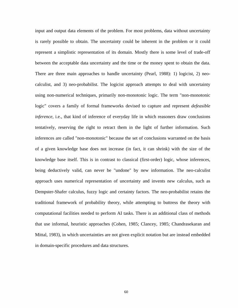
input and output data elements of the problem. For most problems, data without uncertainty
is rarely possible to obtain. The uncertainty could be inherent in the problem or it could
represent a simplistic representation of its domain. Mostly there is some level of trade-off
between the acceptable data uncertainty and the time or the money spent to obtain the data.
There are three main approaches to handle uncertainty (Pearl, 1988): 1) logicist, 2) neo-
calculist, and 3) neo-probabilist. The logicist approach attempts to deal with uncertainty
using non-numerical techniques, primarily non-monotonic logic. The term "non-monotonic
logic" covers a family of formal frameworks devised to capture and represent defeasible
inference, i.e., that kind of inference of everyday life in which reasoners draw conclusions
tentatively, reserving the right to retract them in the light of further information. Such
inferences are called "non-monotonic" because the set of conclusions warranted on the basis
of a given knowledge base does not increase (in fact, it can shrink) with the size of the
knowledge base itself. This is in contrast to classical (first-order) logic, whose inferences,
being deductively valid, can never be "undone" by new information. The neo-calculist
approach uses numerical representation of uncertainty and invents new calculus, such as
Dempster-Shafer calculus, fuzzy logic and certainty factors. The neo-probabilist retains the
traditional framework of probability theory, while attempting to buttress the theory with
computational facilities needed to perform AI tasks. There is an additional class of methods
that use informal, heuristic approaches (Cohen, 1985; Clancey, 1985; Chandrasekaran and
Mittal, 1983), in which uncertainties are not given explicit notation but are instead embedded
in domain-specific procedures and data structures.
60
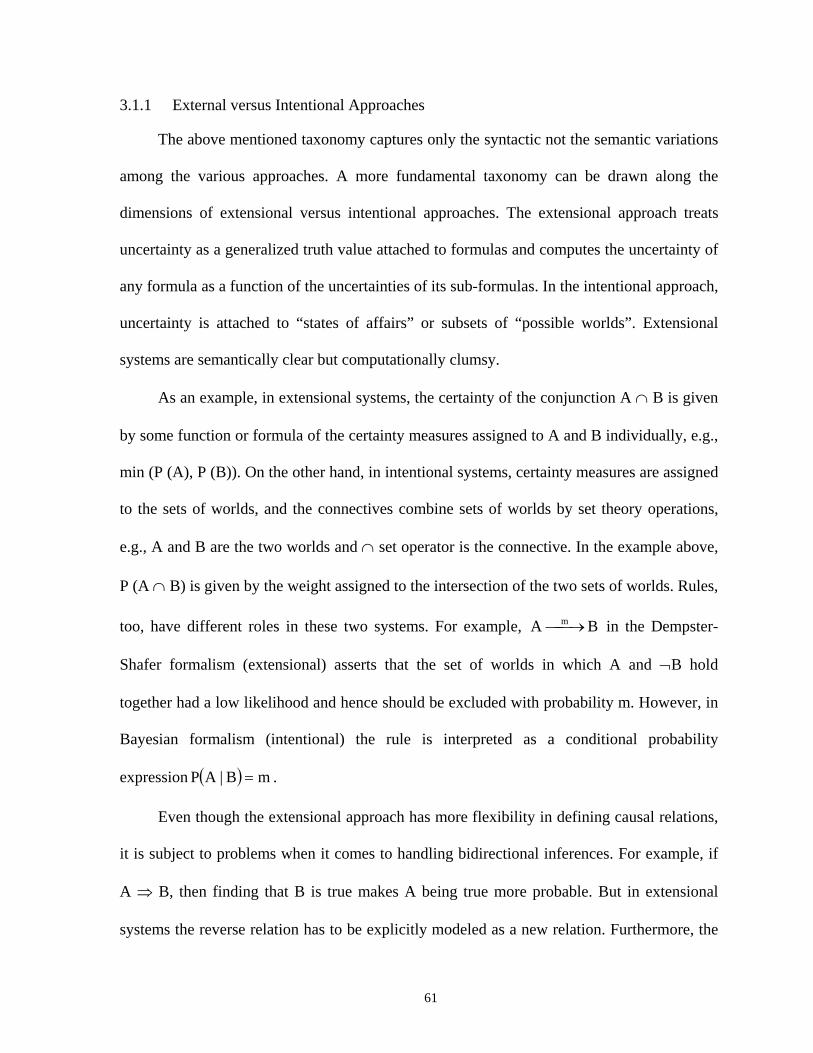
3.1.1 External versus Intentional Approaches
The above mentioned taxonomy captures only the syntactic not the semantic variations
among the various approaches. A more fundamental taxonomy can be drawn along the
dimensions of extensional versus intentional approaches. The extensional approach treats
uncertainty as a generalized truth value attached to formulas and computes the uncertainty of
any formula as a function of the uncertainties of its sub-formulas. In the intentional approach,
uncertainty is attached to “states of affairs” or subsets of “possible worlds”. Extensional
systems are semantically clear but computationally clumsy.
As an example, in extensional systems, the certainty of the conjunction A ∩ B is given
by some function or formula of the certainty measures assigned to A and B individually, e.g.,
min (P (A), P (B)). On the other hand, in intentional systems, certainty measures are assigned
to the sets of worlds, and the connectives combine sets of worlds by set theory operations,
e.g., A and B are the two worlds and ∩ set operator is the connective. In the example above,
P (A ∩ B) is given by the weight assigned to the intersection of the two sets of worlds. Rules,
too, have different roles in these two systems. For example, in the Dempster-
Shafer formalism (extensional) asserts that the set of worlds in which A and ¬B hold
together had a low likelihood and hence should be excluded with probability m. However, in
Bayesian formalism (intentional) the rule is interpreted as a conditional probability
expression
BA m⎯→⎯
( ) mB|AP = .
Even though the extensional approach has more flexibility in defining causal relations,
it is subject to problems when it comes to handling bidirectional inferences. For example, if
A ⇒ B, then finding that B is true makes A being true more probable. But in extensional
systems the reverse relation has to be explicitly modeled as a new relation. Furthermore, the
61

first relation has to be removed from the model before making the reverse relation to prevent
cycles in the model. Therefore, the extensional approach is mainly used in diagnostic
inference and not predictive inference. The extensional approach also has difficulty retracting
conclusions within the model. This causes the extensional system to have too many
exceptions to a rule. For example, if rule R1 says that if it is wet then it rained yesterday, then
once R1 is true it automatically makes inference that it rained yesterday. However, if there
was another event that the water sprinkler was on last night and was in fact responsible for
the ground being wet, then the inference that it rained yesterday should be retracted. This is
not possible in extensional systems. Another drawback of the extensional approach is the
improper treatment of the correlated sources of evidence. Extensional systems ignore the fact
the different sources of evidence may have similar or identical original sources, and therefore
treats all the sources of evidence as independent. However, the intentional approach takes
into account that if the sources of evidence have a similar or the same origin then their
cumulative effect is decreased.
In intentional systems, the syntax consists of declarative statements about states of
affairs and hence simulates the real world situations. These systems have no problems with
bidirectional analysis relations and correlated evidences. However, intentional approaches
need a mechanism to convert declarative statements into routines that answer queries. Such a
mechanism is offered by techniques based on belief networks. In particular declarative
statements are transformed into conditional probability statements which are then used in the
belief network to draw inferences.
62
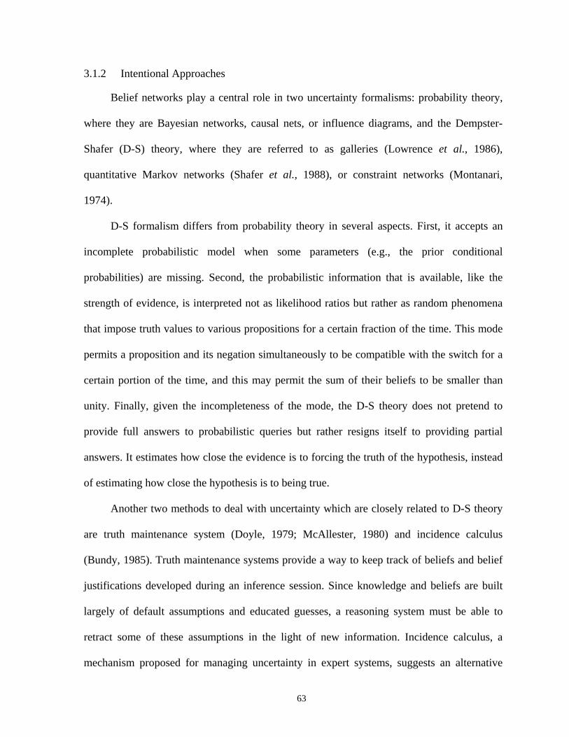
3.1.2 Intentional Approaches
Belief networks play a central role in two uncertainty formalisms: probability theory,
where they are Bayesian networks, causal nets, or influence diagrams, and the Dempster-
Shafer (D-S) theory, where they are referred to as galleries (Lowrence et al., 1986),
quantitative Markov networks (Shafer et al., 1988), or constraint networks (Montanari,
1974).
D-S formalism differs from probability theory in several aspects. First, it accepts an
incomplete probabilistic model when some parameters (e.g., the prior conditional
probabilities) are missing. Second, the probabilistic information that is available, like the
strength of evidence, is interpreted not as likelihood ratios but rather as random phenomena
that impose truth values to various propositions for a certain fraction of the time. This mode
permits a proposition and its negation simultaneously to be compatible with the switch for a
certain portion of the time, and this may permit the sum of their beliefs to be smaller than
unity. Finally, given the incompleteness of the mode, the D-S theory does not pretend to
provide full answers to probabilistic queries but rather resigns itself to providing partial
answers. It estimates how close the evidence is to forcing the truth of the hypothesis, instead
of estimating how close the hypothesis is to being true.
Another two methods to deal with uncertainty which are closely related to D-S theory
are truth maintenance system (Doyle, 1979; McAllester, 1980) and incidence calculus
(Bundy, 1985). Truth maintenance systems provide a way to keep track of beliefs and belief
justifications developed during an inference session. Since knowledge and beliefs are built
largely of default assumptions and educated guesses, a reasoning system must be able to
retract some of these assumptions in the light of new information. Incidence calculus, a
mechanism proposed for managing uncertainty in expert systems, suggests an alternative
63
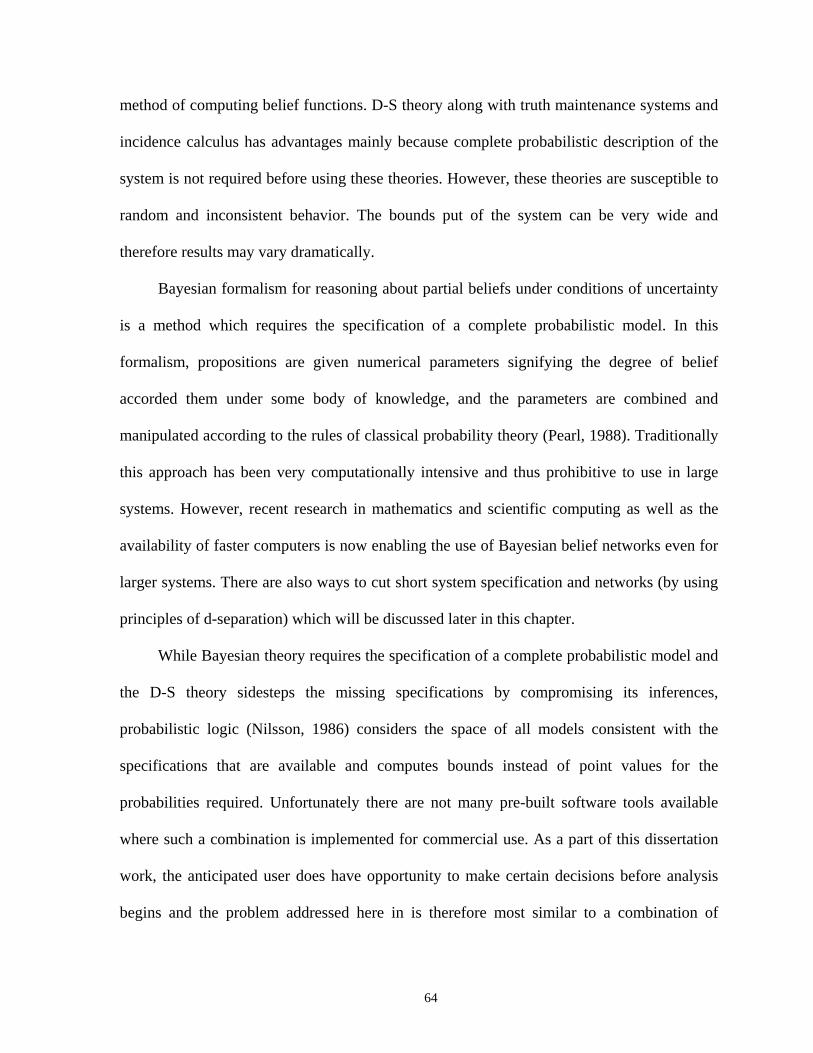
method of computing belief functions. D-S theory along with truth maintenance systems and
incidence calculus has advantages mainly because complete probabilistic description of the
system is not required before using these theories. However, these theories are susceptible to
random and inconsistent behavior. The bounds put of the system can be very wide and
therefore results may vary dramatically.
Bayesian formalism for reasoning about partial beliefs under conditions of uncertainty
is a method which requires the specification of a complete probabilistic model. In this
formalism, propositions are given numerical parameters signifying the degree of belief
accorded them under some body of knowledge, and the parameters are combined and
manipulated according to the rules of classical probability theory (Pearl, 1988). Traditionally
this approach has been very computationally intensive and thus prohibitive to use in large
systems. However, recent research in mathematics and scientific computing as well as the
availability of faster computers is now enabling the use of Bayesian belief networks even for
larger systems. There are also ways to cut short system specification and networks (by using
principles of d-separation) which will be discussed later in this chapter.
While Bayesian theory requires the specification of a complete probabilistic model and
the D-S theory sidesteps the missing specifications by compromising its inferences,
probabilistic logic (Nilsson, 1986) considers the space of all models consistent with the
specifications that are available and computes bounds instead of point values for the
probabilities required. Unfortunately there are not many pre-built software tools available
where such a combination is implemented for commercial use. As a part of this dissertation
work, the anticipated user does have opportunity to make certain decisions before analysis
begins and the problem addressed here in is therefore most similar to a combination of
64
Bayesian Belief Networks and expert systems based approach where the user provides the
expert system database.
3.2 Bayesian Belief Networks (BBNs)
A Bayesian belief network is used to model a domain containing uncertainty. This
uncertainty can be due to imperfect understanding of the domain, incomplete knowledge of
the state of the domain at the time when a task is to be performed, randomness in the
mechanisms governing the behavior of the domain, or a combination of all these. BBNs are
also called belief networks (BNs), Bayesian decision networks (BDNs) and causal
probabilistic networks (CPNs). A BBN has a network of nodes connected by acyclic directed
links and is also called a directed acyclic graph (DAG), i.e., there is no directed path starting
and ending at the same node (Jensen, 2001).
Throughout this chapter, the terms "variable" and "node" are used interchangeably. A
node represents either a discrete random variable with a finite number of states or a
continuous (Gaussian distributed) random variable. The links between the nodes represent
(causal) relationships between the nodes. If a node has no parents (i.e., it has no links
directed towards it), then the node will contain a marginal probability table. If the node is
discrete, it contains a probability distribution over the states of the variable that it represents.
If the node is continuous, it contains a probability density function for the random variable it
represents. If a node has parents (i.e., one or more links pointing towards it), the node
contains a conditional probability table (CPT). If the node is discrete, each cell in the CPT
(or, in more general terms, the conditional probability function (CPF)) of a node contains a
conditional probability for the node being in a specific state given a specific configuration of
the states of its parents. Thus, the number of cells in a CPT for a discrete node equals the
65
product of the number of possible states for the node and the product of the number of
possible states for the parent nodes.
The BBN analysis requires the network to be compiled before it is used. The
compilation process involves conversion of the BBN(s) into symmetric decision graph(s).
The decision graphs are then solved by calculating the expected values for various nodes in
the decision graph. This process is also called propagation of the causal network. The causal
network is comprised of the nodes in BBN with direction links between them. The links
describe the direction of flow of information. If any of the nodes at the top level of this
causal network are changed then the effect is propagated down to other nodes. Similarly, if
any of the nodes within the causal network (e.g., leaf nodes in a tree) are changed then the
effect is back propagated to make corresponding adjustments to the nodes at the top level
(before the changed node in precedence of causality). Simple Bayesian rules are used to
perform the above calculations.
( ) ( ) ( )BPAPBAP ×=∩ , if A and B are independent of each other Equation 3.1
( ) ( )( )BP
BAPB|AP ∩= , ( ) ( ) 1BP,AP0 ≤≤ Equation 3.2
( ) (APB|AP = )
)
)
, if A and B are independent of each other Equation 3.3
( ) ( ) ( ) (APA|BPBPB|AP = Equation 3.4
( ) ( ) ( )∑=i
ii BPB|APAP , and Equation 3.5
( ) ( ) (∑ ∩=i
ii K|BPKB|APK|AP Equation 3.6
The basic conditional probability rule is given by Equation 3.2. In Equation 3.2 both A,
and B are events. If these events are independent of each other then the equation becomes
66
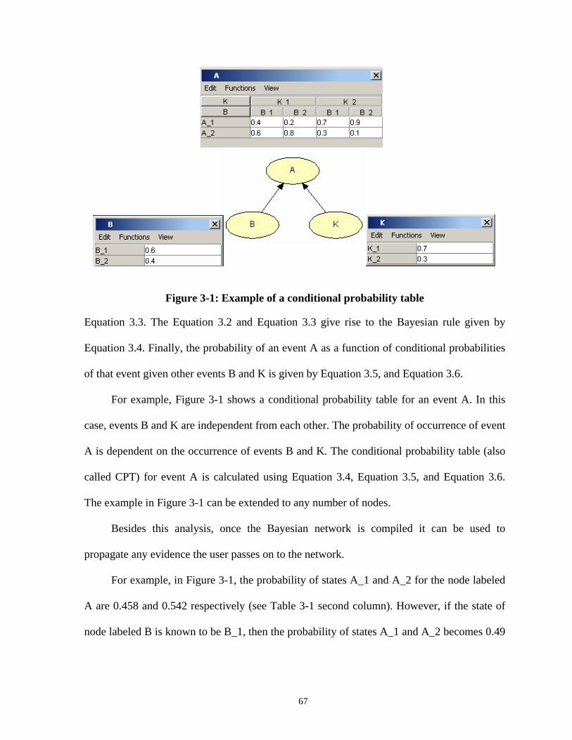
Figure 3-1: Example of a conditional probability table
Equation 3.3. The Equation 3.2 and Equation 3.3 give rise to the Bayesian rule given by
Equation 3.4. Finally, the probability of an event A as a function of conditional probabilities
of that event given other events B and K is given by Equation 3.5, and Equation 3.6.
For example, Figure 3-1 shows a conditional probability table for an event A. In this
case, events B and K are independent from each other. The probability of occurrence of event
A is dependent on the occurrence of events B and K. The conditional probability table (also
called CPT) for event A is calculated using Equation 3.4, Equation 3.5, and Equation 3.6.
The example in Figure 3-1 can be extended to any number of nodes.
Besides this analysis, once the Bayesian network is compiled it can be used to
propagate any evidence the user passes on to the network.
For example, in Figure 3-1, the probability of states A_1 and A_2 for the node labeled
A are 0.458 and 0.542 respectively (see Table 3-1 second column). However, if the state of
node labeled B is known to be B_1, then the probability of states A_1 and A_2 becomes 0.49
67
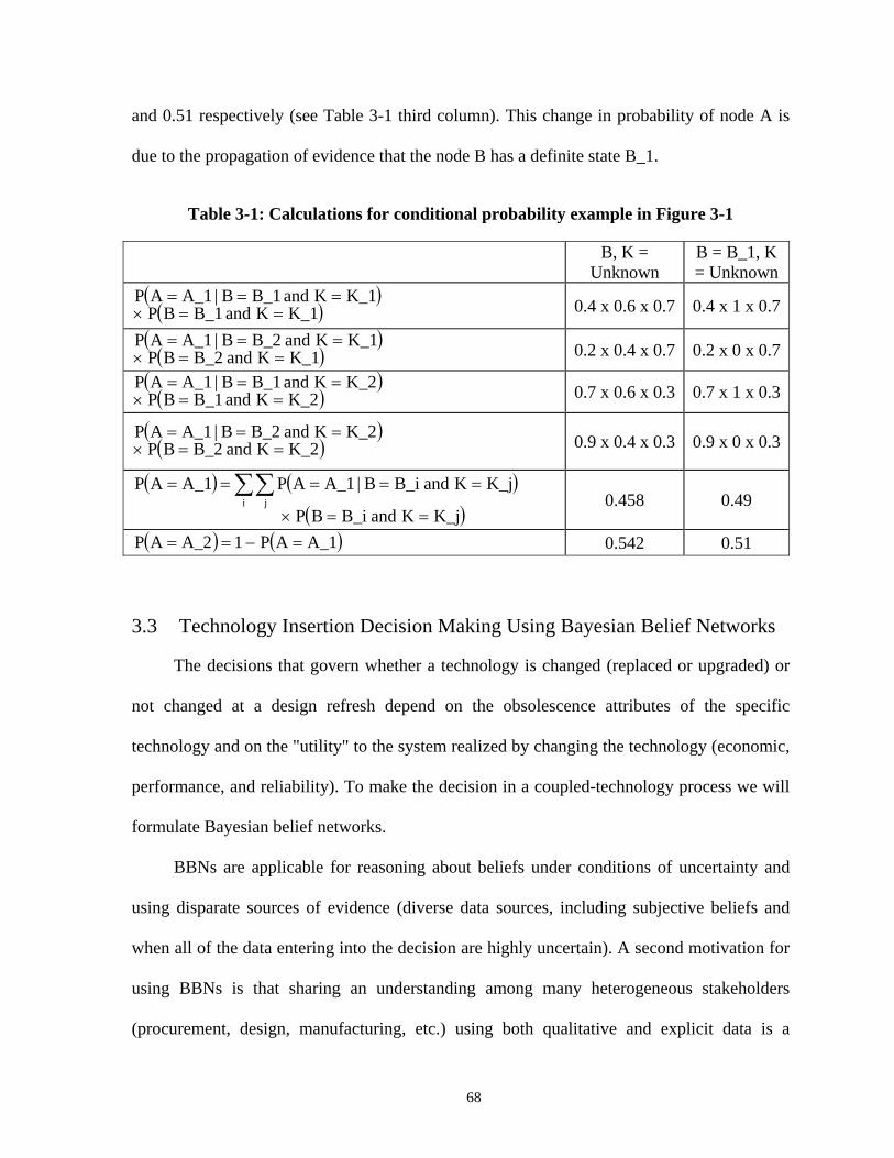
and 0.51 respectively (see Table 3-1 third column). This change in probability of node A is
due to the propagation of evidence that the node B has a definite state B_1.
Table 3-1: Calculations for conditional probability example in Figure 3-1
B, K = Unknown
B = B_1, K = Unknown
( )( )K_1KandB_1BP
K_1KandB_1B|A_1AP==×
=== 0.4 x 0.6 x 0.7 0.4 x 1 x 0.7
( )( )K_1KandB_2BP
K_1KandB_2B|A_1AP==×
=== 0.2 x 0.4 x 0.7 0.2 x 0 x 0.7
( )( )K_2KandB_1BP
K_2KandB_1B|A_1AP==×
=== 0.7 x 0.6 x 0.3 0.7 x 1 x 0.3
( )( )K_2KandB_2BP
K_2KandB_2B|A_1AP==×
=== 0.9 x 0.4 x 0.3 0.9 x 0 x 0.3
( ) (( )K_jKandB_iBP
K_jKandB_iB|A_1APA_1APi j
==×
===== ∑∑ ) 0.458 0.49
( ) ( A_1AP1A_2AP =−== ) 0.542 0.51
3.3 Technology Insertion Decision Making Using Bayesian Belief Networks
The decisions that govern whether a technology is changed (replaced or upgraded) or
not changed at a design refresh depend on the obsolescence attributes of the specific
technology and on the "utility" to the system realized by changing the technology (economic,
performance, and reliability). To make the decision in a coupled-technology process we will
formulate Bayesian belief networks.
BBNs are applicable for reasoning about beliefs under conditions of uncertainty and
using disparate sources of evidence (diverse data sources, including subjective beliefs and
when all of the data entering into the decision are highly uncertain). A second motivation for
using BBNs is that sharing an understanding among many heterogeneous stakeholders
(procurement, design, manufacturing, etc.) using both qualitative and explicit data is a
68

necessity. BBNs also have the ability to propagate decisions in multiple directions. Besides
determining the highest value action to take with regard to a technology at a redesign, it will
also potentially enable fixing a design refresh date and solving for the best technology to use
(a realistic situation for sustainment-dominated systems such as aircraft and ships).
The structure of the BBNs corresponding to an application will be created
automatically from the system description by assembling predefined network fragments. The
probability tables associated with the chance nodes will be populated automatically from
uncertain data inputs. The data associated with utility nodes represent the inputs from various
stakeholders, i.e., “customer-directed value”.
In the context of this work the BBNs are used to decide upon the design refresh
content. Decision analysis has the capability to consider all the decision affecting variables at
once in the model, e.g., availability of a new part to replace the old part, availability of the
old part already in stock, performance and reliability change due to the part replacements, re-
qualification trigger due to part replacement, etc. Figure 3-2 shows where the decision model
fits within the MOCA design refresh planning analysis architecture introduced in Figure 2-1.
This approach ensures that we consider both dimensions of optimization, i.e., date of the
design refresh along with what is changed at the design refresh. Using the technology
sustainment version of MOCA (Chapter 2) it is possible that MOCA decides to design
refresh all the parts during a design refresh simply because they are all obsolete (not a
completely unrealistic situation for avionics and military systems). However, for some of the
parts, continuation of mitigation approaches (e.g., purchase from an aftermarket source)
might have been preferable to replacement at the refresh due to the cost, reliability, and/or
performance penalties that may be associated with the replacement. For this kind of situation
69
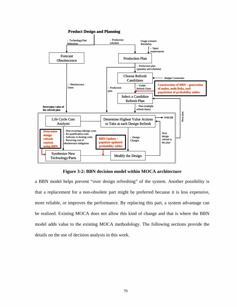
Production Plan
Product Design and Planning
Forecast Obsolescence
- Technology/Part Selections
- Production schedule
Usage scenarioReliability
- Spare requirements
- Production plan(quantity and schedule)
Choose Refresh Candidates
- Viable Refresh Dates
Select a Candidate Refresh Plan
- Plan (multiple refresh dates)
Determine Highest Value Actions to Take at each Design Refresh
- Design Changes
- Obsolescence Dates
Budget Constraints
Modify the Design
Life Cycle Cost Analysis
Next design refresh in the plan
Synthesize New Technology/Parts
Determine value of the refresh plan
Nex
t pla
n
- Non-recurring redesign costs- Re-qualification costs- Software re-hosting costs- Recurring cost of obsolescence mitigation
- Production plan
VALUE
Construction of BBN – generation of nodes, node links, and population of probability tables
BBN Update –populate updated probability tables
Determine design refresh content using BBN
Figure 3-2: BBN decision model within MOCA architecture
a BBN model helps prevent “over design refreshing” of the system. Another possibility is
that a replacement for a non-obsolete part might be preferred because it is less expensive,
more reliable, or improves the performance. By replacing this part, a system advantage can
be realized. Existing MOCA does not allow this kind of change and that is where the BBN
model adds value to the existing MOCA methodology. The following sections provide the
details on the use of decision analysis in this work.
70
3.4 MOCA Bayesian Belief Network
In the current work, BBNs are used to determine the optimal design refresh content at
each design refresh in a plan. A BBN representing the bill of materials is constructed at the
start of a MOCA design refresh planning analysis.15 At each design refresh (i.e., MOCA
generated design refresh plan candidates contain one or more design refresh), MOCA sets the
current, and the prospective future design refresh date in the BBN. When this happens, all the
part-specific and system-specific nodes are updated. Their respective probabilities are also
updated. This is called network propagation. After propagation of the network, the updated
decision node for each part contains the decision associated with design refreshing that part.
Based on that decision a list of parts affected and to be replaced during the current design
refresh is generated. The decision node is where either the user makes decisions and selects a
state, or where the network back propagates and gives a value metric to compare all the
possible choices. Depending on what the value of this metric is and how it is interpreted, a
decision regarding the state of the decision node is made. Every part is tested for replacement
at a design refresh and if the part is replaced then its obsolescence date is refreshed to a new
value. Nodes such as part obsolescence, new part availability, and parts in stock are
measured from the previous design refresh date or field start date, which ever is more recent.
These nodes are also updated at a design refresh to reflect the changes in the system due to
part replacements.
15 There are three types of nodes in a BBN, 1) chance nodes (oval shaped), 2) decision nodes (rectangular shaped), and 3) value nodes (rhombus shaped). The chance nodes have probability tables associated to them. The value nodes have a value assigned to them depending on their state. The decision node does not have probability or value assigned to it.
71
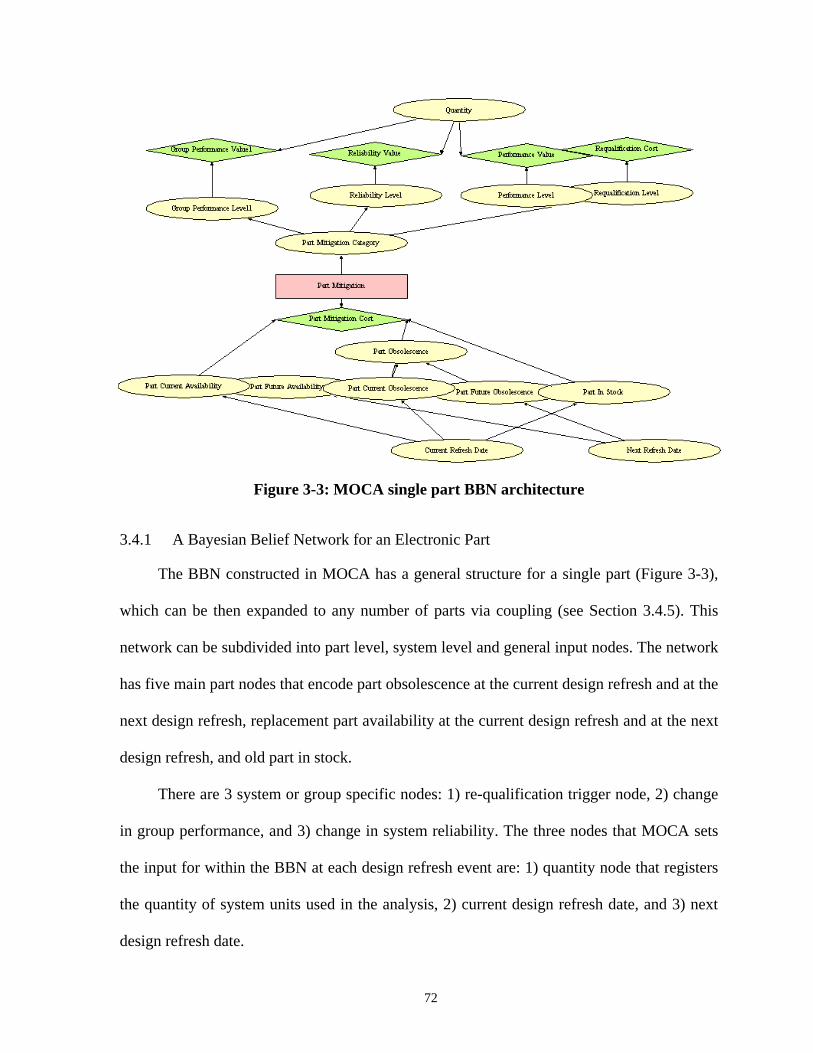
Figure 3-3: MOCA single part BBN architecture
3.4.1 A Bayesian Belief Network for an Electronic Part
The BBN constructed in MOCA has a general structure for a single part (Figure 3-3),
which can be then expanded to any number of parts via coupling (see Section 3.4.5). This
network can be subdivided into part level, system level and general input nodes. The network
has five main part nodes that encode part obsolescence at the current design refresh and at the
next design refresh, replacement part availability at the current design refresh and at the next
design refresh, and old part in stock.
There are 3 system or group specific nodes: 1) re-qualification trigger node, 2) change
in group performance, and 3) change in system reliability. The three nodes that MOCA sets
the input for within the BBN at each design refresh event are: 1) quantity node that registers
the quantity of system units used in the analysis, 2) current design refresh date, and 3) next
design refresh date.
72
3.4.2 Node Reference for a Single Part BBN
An alternative taxonomy of a single part BBN (Figure 3-3) is, a) input nodes (e.g.,
Current Design Refresh date node), b) output nodes (e.g., Part Mitigation decision node),
and c) system specification nodes (e.g., Part Obsolescence node). Each of these node types is
described below:
Input Nodes
Input nodes in a single part BBN are Current Design Refresh, Next Design Refresh,
and Quantity nodes. The Current Design Refresh and Next Design Refresh nodes have
prospective future design refreshes dates as their states. These nodes are linked to all other
nodes that are discretized based on design refresh dates (e.g., the Part Obsolescence node).
Intuitively, if the next design refresh date is far away (in time) with respect to the current
design refresh or if there is no future design refresh scheduled then there is more value added
if the system is redesigned at the current design refresh. This is caused by the possibility that
future orders (production events) that require this part may render the system unusable due to
unavailability of an obsolete part. Therefore, if there is a chance to design refresh at the
current date then the maximum benefit should be attained from it.
The Quantity node specifies the number of systems (units) deployed in the field or the
number of systems affected by the design refresh. This node links to all other nodes that have
dependency on the number of system units deployed or to be deployed. For example, system
reliability and performance value is defined on a system level, but in the BBN it is used to
find out the value gained due to change in performance after a design refresh per unit system.
The Quantity node is essential to comparing apples-to-apples, i.e., if the cost of redesign is
given per unit then other cost metrics should also be mapped to a per unit basis.
73
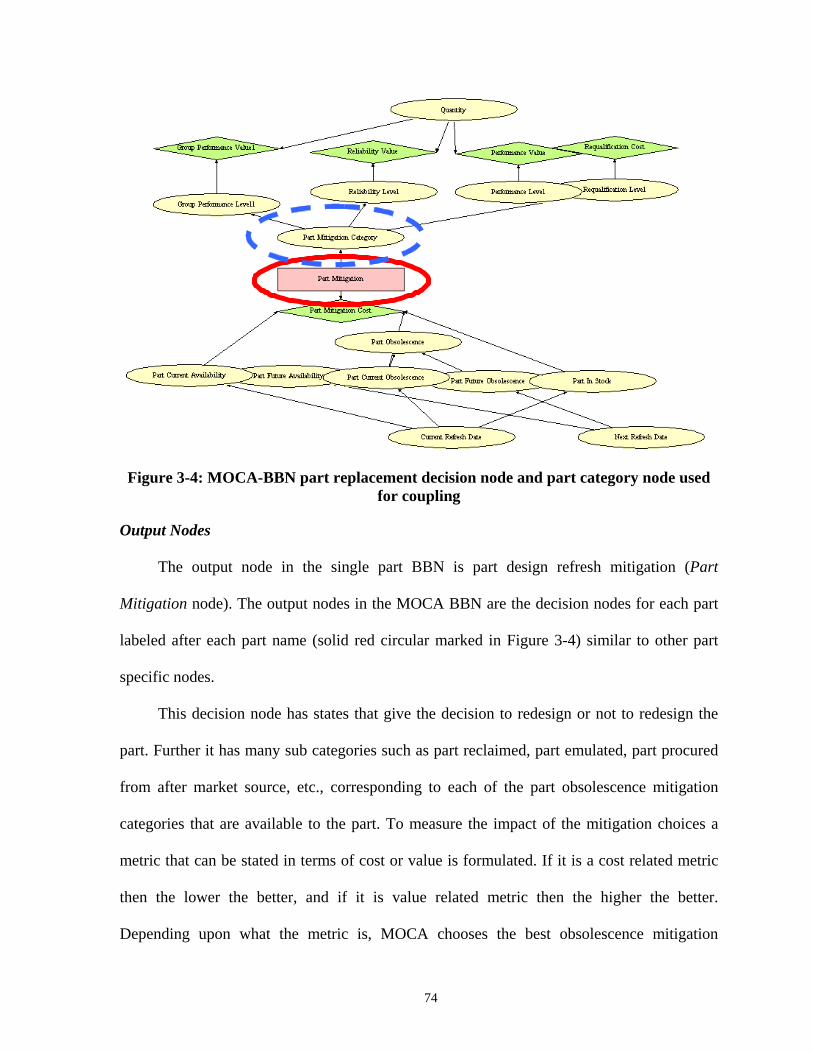
Figure 3-4: MOCA-BBN part replacement decision node and part category node used for coupling
Output Nodes
The output node in the single part BBN is part design refresh mitigation (Part
Mitigation node). The output nodes in the MOCA BBN are the decision nodes for each part
labeled after each part name (solid red circular marked in Figure 3-4) similar to other part
specific nodes.
This decision node has states that give the decision to redesign or not to redesign the
part. Further it has many sub categories such as part reclaimed, part emulated, part procured
from after market source, etc., corresponding to each of the part obsolescence mitigation
categories that are available to the part. To measure the impact of the mitigation choices a
metric that can be stated in terms of cost or value is formulated. If it is a cost related metric
then the lower the better, and if it is value related metric then the higher the better.
Depending upon what the metric is, MOCA chooses the best obsolescence mitigation
74
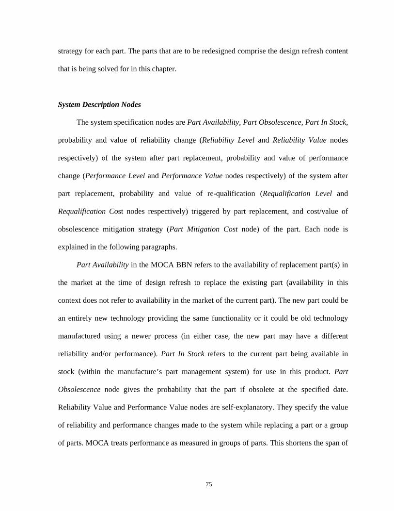
strategy for each part. The parts that are to be redesigned comprise the design refresh content
that is being solved for in this chapter.
System Description Nodes
The system specification nodes are Part Availability, Part Obsolescence, Part In Stock,
probability and value of reliability change (Reliability Level and Reliability Value nodes
respectively) of the system after part replacement, probability and value of performance
change (Performance Level and Performance Value nodes respectively) of the system after
part replacement, probability and value of re-qualification (Requalification Level and
Requalification Cost nodes respectively) triggered by part replacement, and cost/value of
obsolescence mitigation strategy (Part Mitigation Cost node) of the part. Each node is
explained in the following paragraphs.
Part Availability in the MOCA BBN refers to the availability of replacement part(s) in
the market at the time of design refresh to replace the existing part (availability in this
context does not refer to availability in the market of the current part). The new part could be
an entirely new technology providing the same functionality or it could be old technology
manufactured using a newer process (in either case, the new part may have a different
reliability and/or performance). Part In Stock refers to the current part being available in
stock (within the manufacture’s part management system) for use in this product. Part
Obsolescence node gives the probability that the part if obsolete at the specified date.
Reliability Value and Performance Value nodes are self-explanatory. They specify the value
of reliability and performance changes made to the system while replacing a part or a group
of parts. MOCA treats performance as measured in groups of parts. This shortens the span of
75
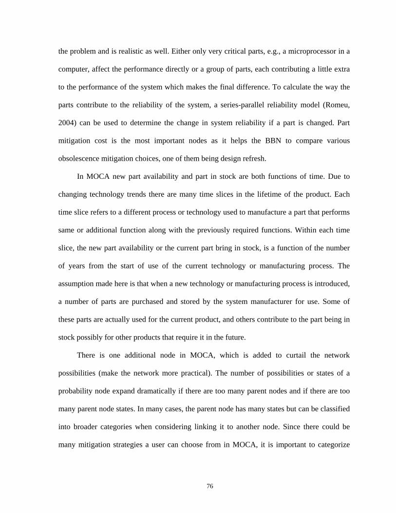
the problem and is realistic as well. Either only very critical parts, e.g., a microprocessor in a
computer, affect the performance directly or a group of parts, each contributing a little extra
to the performance of the system which makes the final difference. To calculate the way the
parts contribute to the reliability of the system, a series-parallel reliability model (Romeu,
2004) can be used to determine the change in system reliability if a part is changed. Part
mitigation cost is the most important nodes as it helps the BBN to compare various
obsolescence mitigation choices, one of them being design refresh.
In MOCA new part availability and part in stock are both functions of time. Due to
changing technology trends there are many time slices in the lifetime of the product. Each
time slice refers to a different process or technology used to manufacture a part that performs
same or additional function along with the previously required functions. Within each time
slice, the new part availability or the current part bring in stock, is a function of the number
of years from the start of use of the current technology or manufacturing process. The
assumption made here is that when a new technology or manufacturing process is introduced,
a number of parts are purchased and stored by the system manufacturer for use. Some of
these parts are actually used for the current product, and others contribute to the part being in
stock possibly for other products that require it in the future.
There is one additional node in MOCA, which is added to curtail the network
possibilities (make the network more practical). The number of possibilities or states of a
probability node expand dramatically if there are too many parent nodes and if there are too
many parent node states. In many cases, the parent node has many states but can be classified
into broader categories when considering linking it to another node. Since there could be
many mitigation strategies a user can choose from in MOCA, it is important to categorize
76
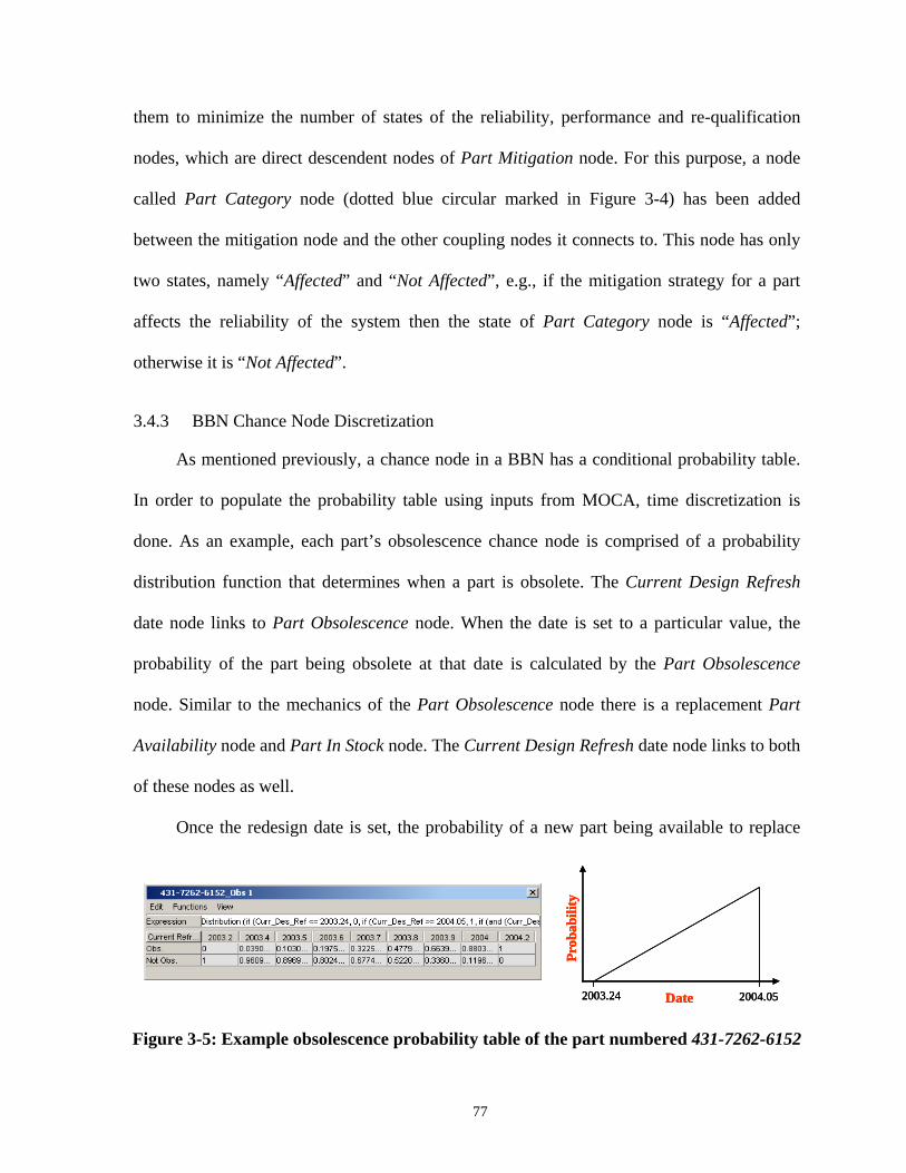
them to minimize the number of states of the reliability, performance and re-qualification
nodes, which are direct descendent nodes of Part Mitigation node. For this purpose, a node
called Part Category node (dotted blue circular marked in Figure 3-4) has been added
between the mitigation node and the other coupling nodes it connects to. This node has only
two states, namely “Affected” and “Not Affected”, e.g., if the mitigation strategy for a part
affects the reliability of the system then the state of Part Category node is “Affected”;
otherwise it is “Not Affected”.
3.4.3 BBN Chance Node Discretization
As mentioned previously, a chance node in a BBN has a conditional probability table.
In order to populate the probability table using inputs from MOCA, time discretization is
done. As an example, each part’s obsolescence chance node is comprised of a probability
distribution function that determines when a part is obsolete. The Current Design Refresh
date node links to Part Obsolescence node. When the date is set to a particular value, the
probability of the part being obsolete at that date is calculated by the Part Obsolescence
node. Similar to the mechanics of the Part Obsolescence node there is a replacement Part
Availability node and Part In Stock node. The Current Design Refresh date node links to both
of these nodes as well.
Once the redesign date is set, the probability of a new part being available to replace
Date
Prob
abili
ty
2003.24 2004.05Date
Prob
abili
ty
2003.24 2004.05Date
Prob
abili
ty
2003.24 2004.05
Figure 3-5: Example obsolescence probability table of the part numbered 431-7262-6152
77
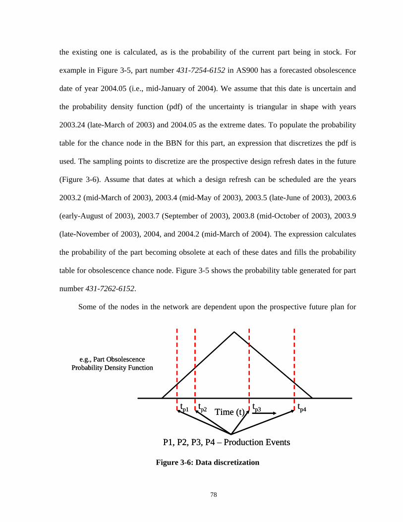
the existing one is calculated, as is the probability of the current part being in stock. For
example in Figure 3-5, part number 431-7254-6152 in AS900 has a forecasted obsolescence
date of year 2004.05 (i.e., mid-January of 2004). We assume that this date is uncertain and
the probability density function (pdf) of the uncertainty is triangular in shape with years
2003.24 (late-March of 2003) and 2004.05 as the extreme dates. To populate the probability
table for the chance node in the BBN for this part, an expression that discretizes the pdf is
used. The sampling points to discretize are the prospective design refresh dates in the future
(Figure 3-6). Assume that dates at which a design refresh can be scheduled are the years
2003.2 (mid-March of 2003), 2003.4 (mid-May of 2003), 2003.5 (late-June of 2003), 2003.6
(early-August of 2003), 2003.7 (September of 2003), 2003.8 (mid-October of 2003), 2003.9
(late-November of 2003), 2004, and 2004.2 (mid-March of 2004). The expression calculates
the probability of the part becoming obsolete at each of these dates and fills the probability
table for obsolescence chance node. Figure 3-5 shows the probability table generated for part
number 431-7262-6152.
Some of the nodes in the network are dependent upon the prospective future plan for
e.g., Part Obsolescence Probability Density Function
Time (t)tp1 tp2 tp3 tp4
P1, P2, P3, P4 – Production Events
e.g., Part Obsolescence Probability Density Function
Time (t)tp1 tp2 tp3 tp4
P1, P2, P3, P4 – Production Events
Figure 3-6: Data discretization
78
the product. Therefore, these nodes have a varying degree of effect on the decision making
process at the current design refresh. For example, if there is no future design refresh planned
and there are still five years of system life left, then at the current design refresh, replacement
part availability will have a smaller impact on the part replacement decision and the
probability that the current part is in stock will have larger impact on the decision to replace
the part. This scenario assumes that any future needs to procure the obsolete part is satisfied
by the in stock inventory, and any other alternative, e.g., get the parts from an aftermarket
source is too expensive and unpredictable. Therefore, even if the replacement part is not
available in abundance, it may be advisable to redesign the part for future needs. This is an
example of how the next redesign date node couples to the network.
The part mitigation cost node tabulates the various costs required to mitigate
obsolescence using different mitigation strategies. Similarly, the part Reliability Value and
part Performance Value nodes have values measured in a common cost metric for each
obsolescence mitigation strategy. The Requalification Cost node is independent of the
quantity of the part in the system, as it is applied to a system only once, where as, the
Reliability Value node and the Performance Value node are dependent on the quantity of the
part in the system.
3.4.4 The Methodology used to Populate BBN Chance Node Probabilities Tables
BBN conditional probability tables are populated using two methods: 1) using
mathematical expressions to describe the states of the table and 2) populating the table using
user defined values or randomly generated values if these values are not specified by the
user. The discretization of these tables is done at time steps defined by the production event
schedule given by the user. Since the production events are the only events where additional
79
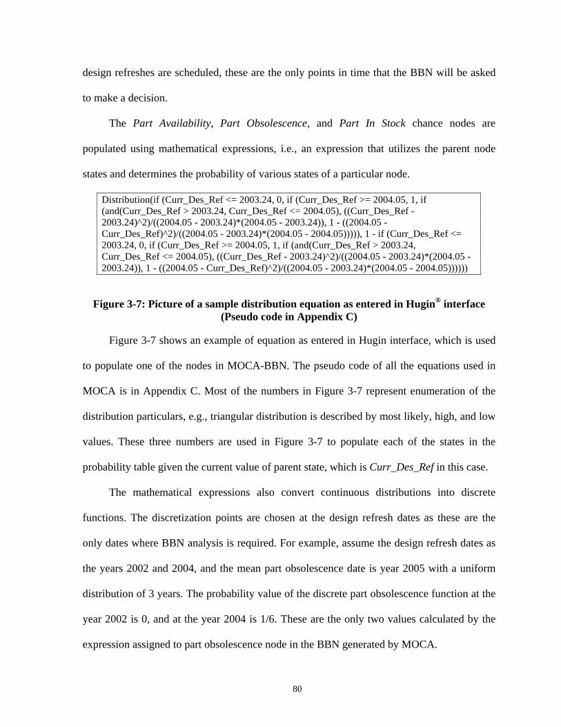
design refreshes are scheduled, these are the only points in time that the BBN will be asked
to make a decision.
The Part Availability, Part Obsolescence, and Part In Stock chance nodes are
populated using mathematical expressions, i.e., an expression that utilizes the parent node
states and determines the probability of various states of a particular node.
Distribution(if (Curr_Des_Ref <= 2003.24, 0, if (Curr_Des_Ref >= 2004.05, 1, if (and(Curr_Des_Ref > 2003.24, Curr_Des_Ref <= 2004.05), ((Curr_Des_Ref - 2003.24)^2)/((2004.05 - 2003.24)*(2004.05 - 2003.24)), 1 - ((2004.05 - Curr_Des_Ref)^2)/((2004.05 - 2003.24)*(2004.05 - 2004.05))))), 1 - if (Curr_Des_Ref <= 2003.24, 0, if (Curr_Des_Ref >= 2004.05, 1, if (and(Curr_Des_Ref > 2003.24, Curr_Des_Ref <= 2004.05), ((Curr_Des_Ref - 2003.24)^2)/((2004.05 - 2003.24)*(2004.05 - 2003.24)), 1 - ((2004.05 - Curr_Des_Ref)^2)/((2004.05 - 2003.24)*(2004.05 - 2004.05))))))
Figure 3-7: Picture of a sample distribution equation as entered in Hugin® interface (Pseudo code in Appendix C)
Figure 3-7 shows an example of equation as entered in Hugin interface, which is used
to populate one of the nodes in MOCA-BBN. The pseudo code of all the equations used in
MOCA is in Appendix C. Most of the numbers in Figure 3-7 represent enumeration of the
distribution particulars, e.g., triangular distribution is described by most likely, high, and low
values. These three numbers are used in Figure 3-7 to populate each of the states in the
probability table given the current value of parent state, which is Curr_Des_Ref in this case.
The mathematical expressions also convert continuous distributions into discrete
functions. The discretization points are chosen at the design refresh dates as these are the
only dates where BBN analysis is required. For example, assume the design refresh dates as
the years 2002 and 2004, and the mean part obsolescence date is year 2005 with a uniform
distribution of 3 years. The probability value of the discrete part obsolescence function at the
year 2002 is 0, and at the year 2004 is 1/6. These are the only two values calculated by the
expression assigned to part obsolescence node in the BBN generated by MOCA.
80
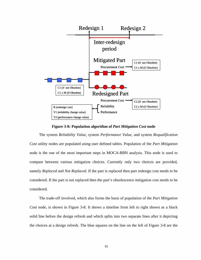
Redesign 1 Redesign 2
Inter-redesign period
Mitigated Part
Redesigned PartProcurement Cost
Reliability
Performance
Procurement Cost
C2 (if not Obsolete)
C2 x M (if Obsolete)R (redesign cost)
V1 (reliability change value)
V2 (performance change value)
C1 (if not Obsolete)
C1 x M (if Obsolete)
C1 (if not Obsolete)
C1 x M (if Obsolete)
Figure 3-8: Population algorithm of Part Mitigation Cost node
The system Reliability Value, system Performance Value, and system Requalification
Cost utility nodes are populated using user defined tables. Population of the Part Mitigation
node is the one of the most important steps in MOCA-BBN analysis. This node is used to
compare between various mitigation choices. Currently only two choices are provided,
namely Replaced and Not Replaced. If the part is replaced then part redesign cost needs to be
considered. If the part is not replaced then the part’s obsolescence mitigation cost needs to be
considered.
The trade-off involved, which also forms the basis of population of the Part Mitigation
Cost node, is shown in Figure 3-8. It shows a timeline from left to right shown as a black
solid line before the design refresh and which splits into two separate lines after it depicting
the choices at a design refresh. The blue squares on the line on the left of Figure 3-8 are the
81
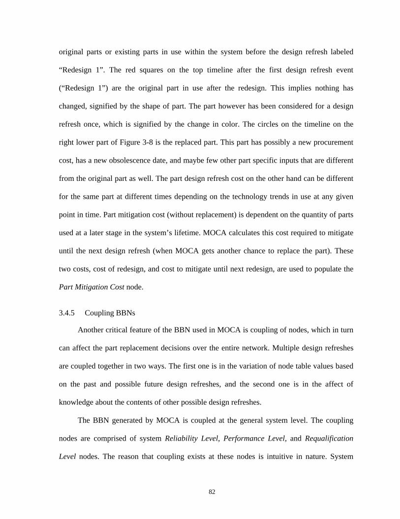
original parts or existing parts in use within the system before the design refresh labeled
“Redesign 1”. The red squares on the top timeline after the first design refresh event
(“Redesign 1”) are the original part in use after the redesign. This implies nothing has
changed, signified by the shape of part. The part however has been considered for a design
refresh once, which is signified by the change in color. The circles on the timeline on the
right lower part of Figure 3-8 is the replaced part. This part has possibly a new procurement
cost, has a new obsolescence date, and maybe few other part specific inputs that are different
from the original part as well. The part design refresh cost on the other hand can be different
for the same part at different times depending on the technology trends in use at any given
point in time. Part mitigation cost (without replacement) is dependent on the quantity of parts
used at a later stage in the system’s lifetime. MOCA calculates this cost required to mitigate
until the next design refresh (when MOCA gets another chance to replace the part). These
two costs, cost of redesign, and cost to mitigate until next redesign, are used to populate the
Part Mitigation Cost node.
3.4.5 Coupling BBNs
Another critical feature of the BBN used in MOCA is coupling of nodes, which in turn
can affect the part replacement decisions over the entire network. Multiple design refreshes
are coupled together in two ways. The first one is in the variation of node table values based
on the past and possible future design refreshes, and the second one is in the affect of
knowledge about the contents of other possible design refreshes.
The BBN generated by MOCA is coupled at the general system level. The coupling
nodes are comprised of system Reliability Level, Performance Level, and Requalification
Level nodes. The reason that coupling exists at these nodes is intuitive in nature. System
82
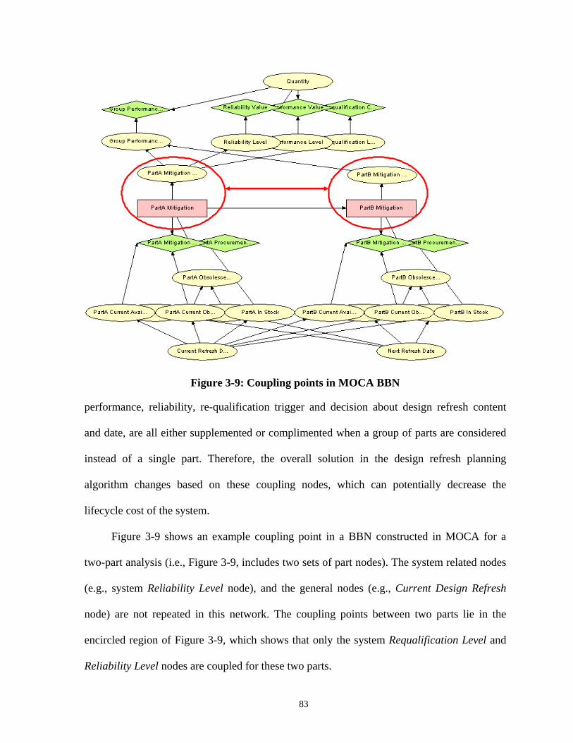
Figure 3-9: Coupling points in MOCA BBN
performance, reliability, re-qualification trigger and decision about design refresh content
and date, are all either supplemented or complimented when a group of parts are considered
instead of a single part. Therefore, the overall solution in the design refresh planning
algorithm changes based on these coupling nodes, which can potentially decrease the
lifecycle cost of the system.
Figure 3-9 shows an example coupling point in a BBN constructed in MOCA for a
two-part analysis (i.e., Figure 3-9, includes two sets of part nodes). The system related nodes
(e.g., system Reliability Level node), and the general nodes (e.g., Current Design Refresh
node) are not repeated in this network. The coupling points between two parts lie in the
encircled region of Figure 3-9, which shows that only the system Requalification Level and
Reliability Level nodes are coupled for these two parts.
83
Performance Level is used not on a system level but on a group level. User defined
groups of parts are placed in different groups and then the group performance change is dealt
with in the BBN. This also allows the user to specify special groups of parts that influence
each others decision to be replaced at a redesign.
3.5 Curtailing the Network
One of the hurdles to effectively use BBNs in MOCA is that as the problem size
increases (i.e., the total number of nodes, links, and states) and the BBNs become
computationally cumbersome as the number of parts concurrently analyzed increases and the
number of design refreshes in the plan increases. A larger network not only slows down the
analysis drastically but also requires large amounts of computer memory. Therefore, it is
imperative to curtail the network as much as possible before analysis. The solution used in
this work is to split the large network into smaller more manageable sub-networks. These
smaller networks have to be solved in succession and then their results merged to emulate the
larger network. This enables MOCA to run large models with thousands of parts. The
following sections present the methodology and a proof of principle for network splitting of
MOCA BBNs.
3.6 Splitting the BBN (Jensen, 2002)
The first step required to split a BBN is the identification of division nodes, i.e., where
the network can be split while maintaining the consistency in the solution. As described in
previous sections, the MOCA BBN consists of nodes that determine the state of each part
separately and nodes that couple various parts together (which make system or group level
inferences). The solution of the BBN is embedded in the decision nodes which are linked to
the part-specific state nodes as well as the coupling nodes. The structure of MOCA BBN
84
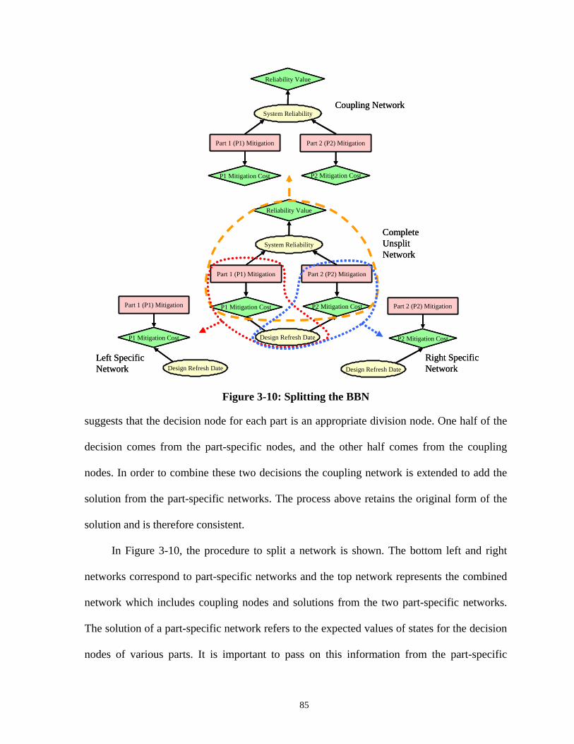
Design Refresh Date
Part 2 (P2) Mitigation
P2 Mitigation Cost
Part 1 (P1) Mitigation
Design Refresh Date
P1 Mitigation Cost
Reliability Value
Part 1 (P1) Mitigation
System Reliability
Part 2 (P2) Mitigation
P1 Mitigation Cost P2 Mitigation Cost
Reliability Value
Part 1 (P1) Mitigation
Design Refresh Date
System Reliability
Part 2 (P2) Mitigation
P1 Mitigation Cost P2 Mitigation Cost
Complete Unsplit Network
Coupling Network
Left Specific Network
Right Specific NetworkDesign Refresh Date
Part 2 (P2) Mitigation
P2 Mitigation Cost
Design Refresh Date
Part 2 (P2) Mitigation
P2 Mitigation Cost
Part 1 (P1) Mitigation
Design Refresh Date
P1 Mitigation Cost
Part 1 (P1) Mitigation
Design Refresh Date
P1 Mitigation Cost
Reliability Value
Part 1 (P1) Mitigation
System Reliability
Part 2 (P2) Mitigation
P1 Mitigation Cost P2 Mitigation Cost
Reliability Value
Part 1 (P1) Mitigation
System Reliability
Part 2 (P2) Mitigation
P1 Mitigation Cost P2 Mitigation Cost
Reliability Value
Part 1 (P1) Mitigation
Design Refresh Date
System Reliability
Part 2 (P2) Mitigation
P1 Mitigation Cost P2 Mitigation Cost
Reliability Value
Part 1 (P1) Mitigation
Design Refresh Date
System Reliability
Part 2 (P2) Mitigation
P1 Mitigation Cost P2 Mitigation Cost
Complete Unsplit Network
Coupling Network
Left Specific Network
Right Specific Network
Figure 3-10: Splitting the BBN
suggests that the decision node for each part is an appropriate division node. One half of the
decision comes from the part-specific nodes, and the other half comes from the coupling
nodes. In order to combine these two decisions the coupling network is extended to add the
solution from the part-specific networks. The process above retains the original form of the
solution and is therefore consistent.
In Figure 3-10, the procedure to split a network is shown. The bottom left and right
networks correspond to part-specific networks and the top network represents the combined
network which includes coupling nodes and solutions from the two part-specific networks.
The solution of a part-specific network refers to the expected values of states for the decision
nodes of various parts. It is important to pass on this information from the part-specific
85
networks to the coupled network anytime there is a change in state(s) in any part-specific
network.
As an example, a 28-part network was run using the splitting technique and by using
the non-split combined network. The results obtained is this case were exactly the same in
terms of cost analysis and decision analysis is concerned, i.e., the lifecycle cost of design
refresh schedule in the two solutions graph were the same along with the design refresh
content for each of the design refreshes in these design refresh schedules. However, the
improvement in run time was dramatic. The split technique ran in 7 seconds where as the
combined network ran in 56 minutes.
3.7 The Reliability Chance Node Model
The reliability model in MOCA is a probabilistic model. The reliability of a printed
circuit board (PCB) is a combination of its material-specific reliability and its constituent-
parts reliability. Similarly, a system’s reliability is a combination of its constituent boards
and parts reliability plus the systems material reliability. In the MOCA BBN, system
reliability is subject to change when any of the constituent parts/boards is replaced. This
makes it important to refresh the BBN with a new reliability value for the system. In order to
calculate the new reliability a cumulative distribution probability model described in the next
paragraph is utilized.
As an example, consider a system with a single board, “testboard”, and two parts on
the board, “part 1”, and “part 2”. Assume the MTBF (Mean Time Between Failure) for part 1
is 30,000 hrs, and the MTBF for part 2 is 50,000 hrs. Therefore, if we assume that the
reliability for the parts and the system is exponentially distributed then the testboard MTBF
would be 18,750 hrs (1/MTBFtestboard = 1/MTBFpart1 + 1/MTBFpart2). If part 2 is replaced
86
during a design refresh and its new MTBF is 40,000 hrs then the new “testboard” MTBF
would be 17,143 hrs. This amounts to ~18.6% decrease in reliability. The BBN in MOCA
divides reliability change into various levels, where each of the levels is defined by a range
of increase or decrease in reliability. After finding out the change in reliability, MOCA
determines the level to which the change belongs. This level is then labeled to be the most
likely change (highest probability) for “part 2” replacement. The other levels which are
closer to the reliability change level chosen for “part 2” replacement are also given
probability values. These values are based on the confidence on the “part 2” reliability
change.
3.8 The Reliability and Performance Values Model
Both of these value nodes are populated using similar techniques, and for this reason
they have been discussed in the same section. MOCA uses an equation to define models for
these nodes. The value of reliability and performance change varies with variation in time
between the current and next possible design refresh. The assumption is that as the time
between the current and the next design refresh increases, there is more uncertainty in the
reliability and performance requirements of the future. This uncertainty translates into
increase in value of an increase in reliability and/or performance, and vice versa. If however,
the model is constant in time, then no matter when the next design refresh is, the change in
reliability and performance is valued only at the current point in time. It loses the chance of
making an informed decision about part replacement based on impact of reliability and
performance change on the lifecycle cost incurred within the current and next possible design
refresh. Therefore, the value of reliability and performance change is assumed to be time
dependent. The MOCA tool chooses from exponential, logarithmic, power and polynomial
87
equations to specify these two nodes. However, the MOCA methodology does not limit the
reliability and performance change variables to be of these forms only. It can be a discrete set
of data points as well. It is to be noted here that this is true for all the uncertain variables
presented in this dissertation. A particular sample distribution for a variable may be shown in
this dissertation, but, the MOCA methodology does not necessarily require the variable to
have only that particular form of the uncertainty probability distribution function.
3.9 MOCA Integration with Hugin®
In order to perform BBN analysis, MOCA uses a commercial tool from HuginExpert.
MOCA uses JavaTM libraries provided with Hugin to interface with the Hugin tool. The
Bayesian network is built automatically by MOCA during its analysis. Hugin is used only as
the engine for compiling the network and performing the propagation.
3.10 Case Studies
Two case studies have been developed for demonstration of the methodology
developed in this chapter. The first case study is similar to the tutorial-level analysis in
Section 2.7 and is meant to show how the MOCA-BBN process works. The second case
study is of an electronic system, the engine controller described in Section 2.9 (consisting of
multiple printed circuit boards with chips mounted on them). This problem is chosen because
the system is familiar to the part obsolescence community and has well developed
infrastructure for determining technology obsolescence characteristics (electronic chip
obsolescence).
88
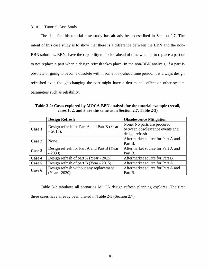
3.10.1 Tutorial Case Study
The data for this tutorial case study has already been described in Section 2.7. The
intent of this case study is to show that there is a difference between the BBN and the non-
BBN solutions. BBNs have the capability to decide ahead of time whether to replace a part or
to not replace a part when a design refresh takes place. In the non-BBN analysis, if a part is
obsolete or going to become obsolete within some look-ahead time period, it is always design
refreshed even though changing the part might have a detrimental effect on other system
parameters such as reliability.
Table 3-2: Cases explored by MOCA-BBN analysis for the tutorial example (recall, cases 1, 2, and 3 are the same as in Section 2.7, Table 2-3)
Design Refresh Obsolescence Mitigation
Case 1 Design refresh for Part A and Part B (Year – 2015).
None. No parts are procured between obsolescence events and design refresh.
Case 2 None. Aftermarket source for Part A and Part B.
Case 3 Design refresh for Part A and Part B (Year - 2030).
Aftermarket source for Part A and Part B.
Case 4 Design refresh of part A (Year - 2015). Aftermarket source for Part B. Case 5 Design refresh of part B (Year - 2015). Aftermarket source for Part A.
Case 6 Design refresh without any replacement (Year - 2020).
Aftermarket source for Part A and Part B.
Table 3-2 tabulates all scenarios MOCA design refresh planning explores. The first
three cases have already been visited in Table 2-3 (Section 2.7).
89
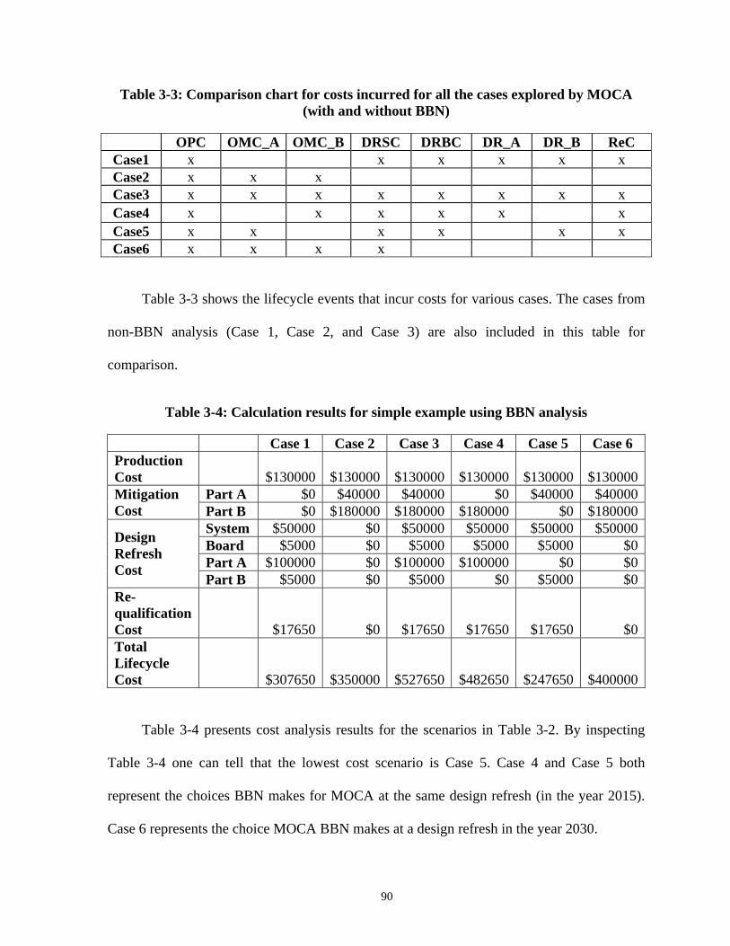
Table 3-3: Comparison chart for costs incurred for all the cases explored by MOCA (with and without BBN)
OPC OMC_A OMC_B DRSC DRBC DR_A DR_B ReC Case1 x x x x x x Case2 x x x Case3 x x x x x x x x Case4 x x x x x x Case5 x x x x x x Case6 x x x x
Table 3-3 shows the lifecycle events that incur costs for various cases. The cases from
non-BBN analysis (Case 1, Case 2, and Case 3) are also included in this table for
comparison.
Table 3-4: Calculation results for simple example using BBN analysis
Case 1 Case 2 Case 3 Case 4 Case 5 Case 6 Production Cost $130000 $130000 $130000 $130000 $130000 $130000
Part A $0 $40000 $40000 $0 $40000 $40000Mitigation Cost Part B $0 $180000 $180000 $180000 $0 $180000
System $50000 $0 $50000 $50000 $50000 $50000Board $5000 $0 $5000 $5000 $5000 $0Part A $100000 $0 $100000 $100000 $0 $0
Design Refresh Cost
Part B $5000 $0 $5000 $0 $5000 $0Re-qualification Cost $17650 $0 $17650 $17650 $17650 $0Total Lifecycle Cost
$307650 $350000 $527650 $482650 $247650 $400000
Table 3-4 presents cost analysis results for the scenarios in Table 3-2. By inspecting
Table 3-4 one can tell that the lowest cost scenario is Case 5. Case 4 and Case 5 both
represent the choices BBN makes for MOCA at the same design refresh (in the year 2015).
Case 6 represents the choice MOCA BBN makes at a design refresh in the year 2030.
90
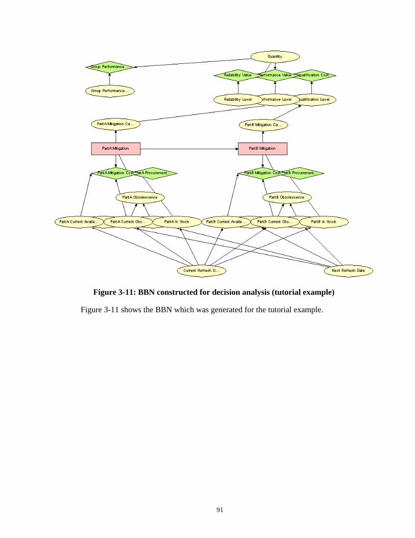
Figure 3-11: BBN constructed for decision analysis (tutorial example)
Figure 3-11 shows the BBN which was generated for the tutorial example.
91
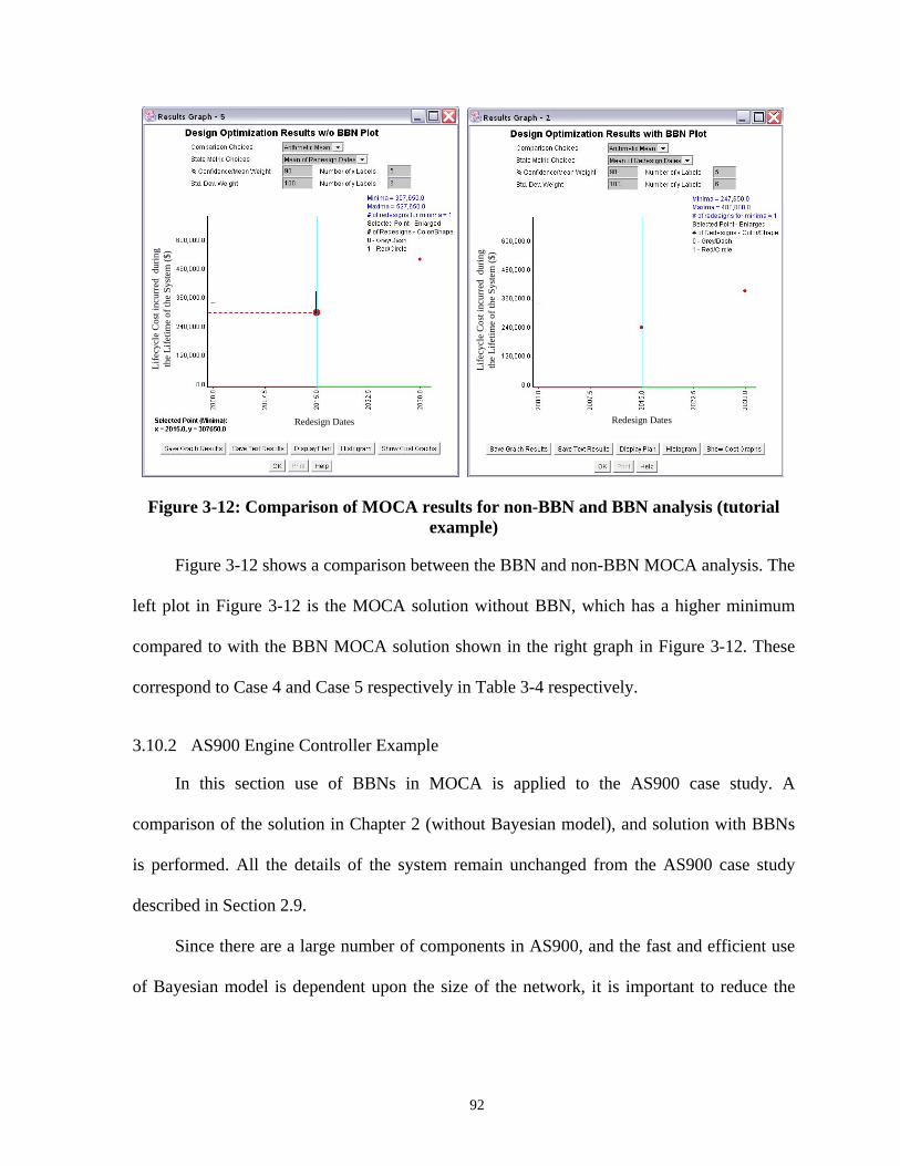
Life
cycl
e C
ost i
ncur
red
dur
ing
the
Life
time
of th
e Sy
stem
($)
Life
cycl
e C
ost i
ncur
red
dur
ing
the
Life
time
of th
e Sy
stem
($)
Redesign Dates Redesign Dates
Life
cycl
e C
ost i
ncur
red
dur
ing
the
Life
time
of th
e Sy
stem
($)
Life
cycl
e C
ost i
ncur
red
dur
ing
the
Life
time
of th
e Sy
stem
($)
Redesign Dates Redesign Dates
Figure 3-12: Comparison of MOCA results for non-BBN and BBN analysis (tutorial example)
Figure 3-12 shows a comparison between the BBN and non-BBN MOCA analysis. The
left plot in Figure 3-12 is the MOCA solution without BBN, which has a higher minimum
compared to with the BBN MOCA solution shown in the right graph in Figure 3-12. These
correspond to Case 4 and Case 5 respectively in Table 3-4 respectively.
3.10.2 AS900 Engine Controller Example
In this section use of BBNs in MOCA is applied to the AS900 case study. A
comparison of the solution in Chapter 2 (without Bayesian model), and solution with BBNs
is performed. All the details of the system remain unchanged from the AS900 case study
described in Section 2.9.
Since there are a large number of components in AS900, and the fast and efficient use
of Bayesian model is dependent upon the size of the network, it is important to reduce the
92

431-
7275
-615
2
431-
7301
-615
2
431-
7302
-615
1
431-
7306
-615
3
513-
7207
-615
1
513-
7222
-605
1
431-
7262
-615
2
513-
7273
-616
1
513-
7273
-616
2
513-
7274
-615
2
PC
431-
7328
-615
1
PC51
3-73
11-6
151
431-
7277
-615
1
513-
7260
-605
1
513-
7275
-615
1
513-
7278
-616
3
PC
513-
7211
-605
2
PC
513-
7304
-615
3
431-
7275
-615
2
431-
7301
-615
2
431-
7302
-615
1
431-
7306
-615
3
513-
7207
-615
1
513-
7222
-605
1
431-
7262
-615
2
513-
7273
-616
1
513-
7273
-616
2
513-
7274
-615
2
PC
431-
7328
-615
1
PC51
3-73
11-6
151
431-
7277
-615
1
513-
7260
-605
1
513-
7275
-615
1
513-
7278
-616
3
PC
513-
7211
-605
2
PC
513-
7304
-615
3
Figure 3-13: Picture of BBN generated in MOCA for the AS900 controller
problem size. For simplicity and problem size reduction, only the parts above $5
procurement cost in the AS900 case were included in the BBN analysis.
Figure 3-13 shows a BBN generated in MOCA for AS900 system. There are 18 parts
above $5 in AS900 and all these are considered for the BBN analysis. The sum of costs of
these 18 parts amounts to 28.34 % of the total parts cost of the system ($3031).
Replace what’s obsolete: Best solution –refresh in year 2003
With BN: Best solution – refresh in year 2005
Difference of $7,010,000
Figure 3-14: Comparison of results between BBN solution and non-BBN solution for AS900 base line case
93
A comparison between the results obtained using the MOCA model without BBN
analysis, and the results obtained using MOCA with the BBN analysis is shown in Figure 3-
14. BBN analysis is able to save around $7 Million over the life of the system as compared to
non-BBN MOCA model (i.e., replace every obsolete part within the look-ahead time at a
design refresh).
In the non-BBN MOCA model, whenever a design refresh event takes place and
MOCA identifies a part that is obsolete, it eliminates the obsolescence problem forever by
replacing it with a new part without immediate obsolescence issues. In this case a redesign
cost is incurred on behalf of this part. If this part is not required in the future (i.e., no
production events in the future which require it) or is available at reasonable cost in the
future (i.e., through other alternative sources) then MOCA should choose to let the current
part remain in the system, i.e., not change the part at a design refresh. This situation is
nothandled by the non-BBN MOCA analysis. To handle such a situation a BBN is employed
to make a more informed decision at a design refresh and decide whether to replace the part
or not.
3.11 Summary
This chapter describes a structure and architecture for determining which parts to
replace during a design refresh, i.e., deciding the design refresh content. The next chapter
applies the MOCA methodology to a specific US Navy system.
94
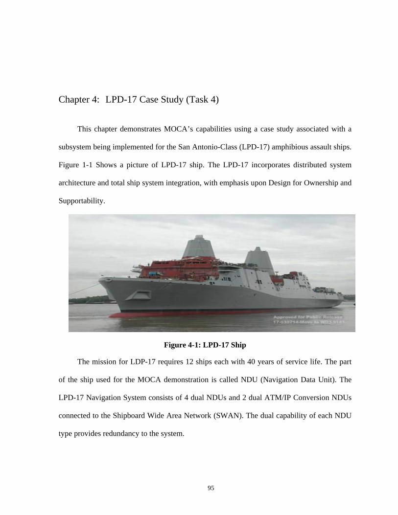
Chapter 4: LPD-17 Case Study (Task 4)
This chapter demonstrates MOCA’s capabilities using a case study associated with a
subsystem being implemented for the San Antonio-Class (LPD-17) amphibious assault ships.
Figure 1-1 Shows a picture of LPD-17 ship. The LPD-17 incorporates distributed system
architecture and total ship system integration, with emphasis upon Design for Ownership and
Supportability.
Figure 4-1: LPD-17 Ship
The mission for LDP-17 requires 12 ships each with 40 years of service life. The part
of the ship used for the MOCA demonstration is called NDU (Navigation Data Unit). The
LPD-17 Navigation System consists of 4 dual NDUs and 2 dual ATM/IP Conversion NDUs
connected to the Shipboard Wide Area Network (SWAN). The dual capability of each NDU
type provides redundancy to the system.
95
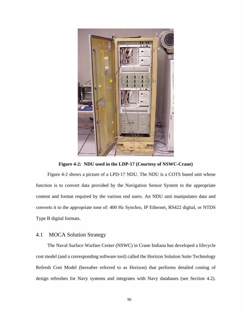
Figure 4-2: NDU used in the LDP-17 (Courtesy of NSWC-Crane)
Figure 4-2 shows a picture of a LPD-17 NDU. The NDU is a COTS based unit whose
function is to convert data provided by the Navigation Sensor System to the appropriate
content and format required by the various end users. An NDU unit manipulates data and
converts it to the appropriate tone of: 400 Hz Synchro, IP Ethernet, RS422 digital, or NTDS
Type B digital formats.
4.1 MOCA Solution Strategy
The Naval Surface Warfare Center (NSWC) in Crane Indiana has developed a lifecycle
cost model (and a corresponding software tool) called the Horizon Solution Suite Technology
Refresh Cost Model (hereafter referred to as Horizon) that performs detailed costing of
design refreshes for Navy systems and integrates with Navy databases (see Section 4.2).
96
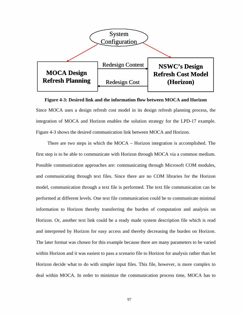
System Configuration
MOCA Design Refresh Planning
NSWC’s Design Refresh Cost Model
(Horizon)Redesign Cost
Redesign Content
System Configuration
MOCA Design Refresh Planning
NSWC’s Design Refresh Cost Model
(Horizon)Redesign Cost
Redesign Content
Figure 4-3: Desired link and the information flow between MOCA and Horizon
Since MOCA uses a design refresh cost model in its design refresh planning process, the
integration of MOCA and Horizon enables the solution strategy for the LPD-17 example.
Figure 4-3 shows the desired communication link between MOCA and Horizon.
There are two steps in which the MOCA – Horizon integration is accomplished. The
first step is to be able to communicate with Horizon through MOCA via a common medium.
Possible communication approaches are: communicating through Microsoft COM modules,
and communicating through text files. Since there are no COM libraries for the Horizon
model, communication through a text file is performed. The text file communication can be
performed at different levels. One text file communication could be to communicate minimal
information to Horizon thereby transferring the burden of computation and analysis on
Horizon. Or, another text link could be a ready made system description file which is read
and interpreted by Horizon for easy access and thereby decreasing the burden on Horizon.
The later format was chosen for this example because there are many parameters to be varied
within Horizon and it was easiest to pass a scenario file to Horizon for analysis rather than let
Horizon decide what to do with simpler input files. This file, however, is more complex to
deal within MOCA. In order to minimize the communication process time, MOCA has to
97
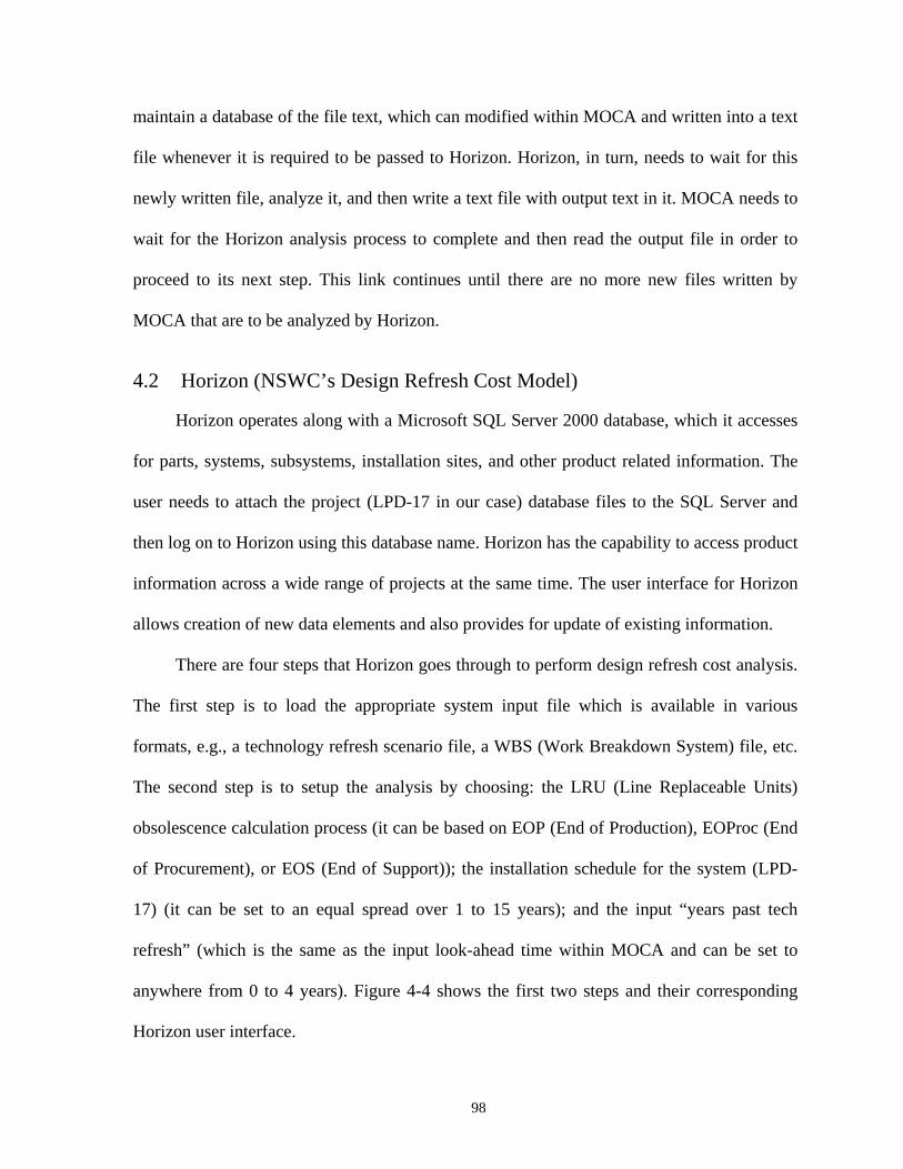
maintain a database of the file text, which can modified within MOCA and written into a text
file whenever it is required to be passed to Horizon. Horizon, in turn, needs to wait for this
newly written file, analyze it, and then write a text file with output text in it. MOCA needs to
wait for the Horizon analysis process to complete and then read the output file in order to
proceed to its next step. This link continues until there are no more new files written by
MOCA that are to be analyzed by Horizon.
4.2 Horizon (NSWC’s Design Refresh Cost Model)
Horizon operates along with a Microsoft SQL Server 2000 database, which it accesses
for parts, systems, subsystems, installation sites, and other product related information. The
user needs to attach the project (LPD-17 in our case) database files to the SQL Server and
then log on to Horizon using this database name. Horizon has the capability to access product
information across a wide range of projects at the same time. The user interface for Horizon
allows creation of new data elements and also provides for update of existing information.
There are four steps that Horizon goes through to perform design refresh cost analysis.
The first step is to load the appropriate system input file which is available in various
formats, e.g., a technology refresh scenario file, a WBS (Work Breakdown System) file, etc.
The second step is to setup the analysis by choosing: the LRU (Line Replaceable Units)
obsolescence calculation process (it can be based on EOP (End of Production), EOProc (End
of Procurement), or EOS (End of Support)); the installation schedule for the system (LPD-
17) (it can be set to an equal spread over 1 to 15 years); and the input “years past tech
refresh” (which is the same as the input look-ahead time within MOCA and can be set to
anywhere from 0 to 4 years). Figure 4-4 shows the first two steps and their corresponding
Horizon user interface.
98
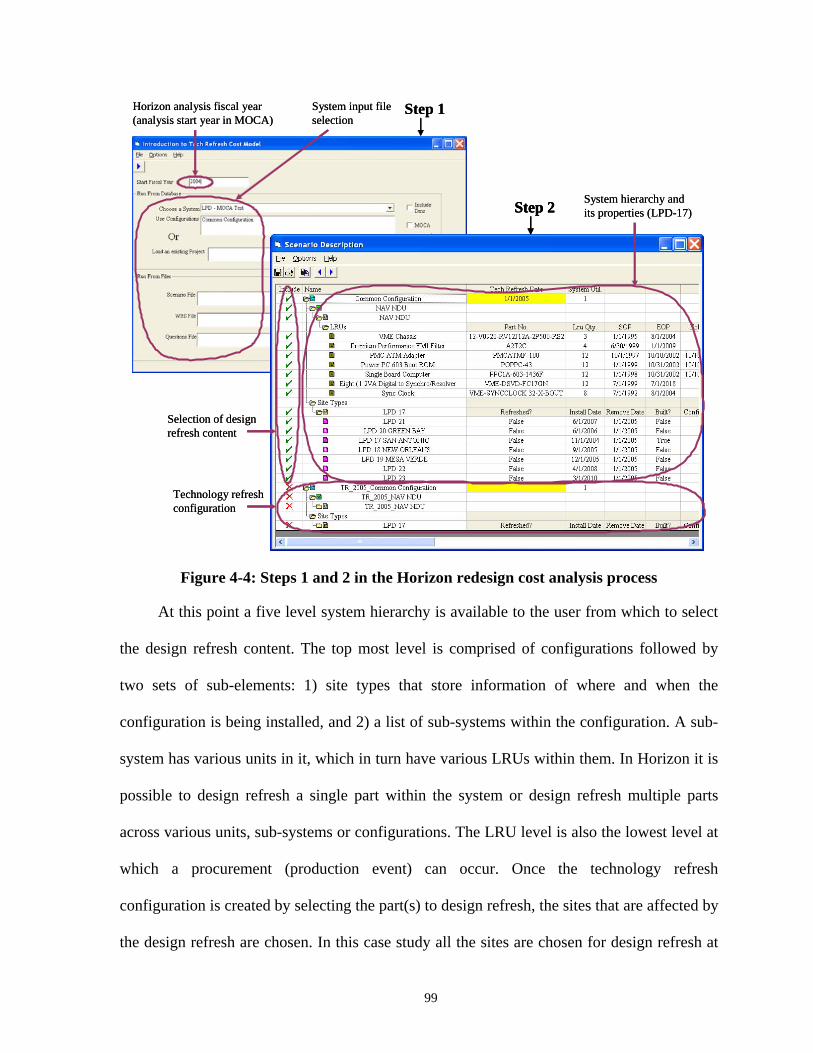
System input file selection
Horizon analysis fiscal year (analysis start year in MOCA)
Selection of design refresh content
System hierarchy and its properties (LPD-17)
Technology refresh configuration
Step 1
Step 2
System input file selection
Horizon analysis fiscal year (analysis start year in MOCA)
Selection of design refresh content
System hierarchy and its properties (LPD-17)
Technology refresh configuration
Step 1
Step 2Step 2
Figure 4-4: Steps 1 and 2 in the Horizon redesign cost analysis process
At this point a five level system hierarchy is available to the user from which to select
the design refresh content. The top most level is comprised of configurations followed by
two sets of sub-elements: 1) site types that store information of where and when the
configuration is being installed, and 2) a list of sub-systems within the configuration. A sub-
system has various units in it, which in turn have various LRUs within them. In Horizon it is
possible to design refresh a single part within the system or design refresh multiple parts
across various units, sub-systems or configurations. The LRU level is also the lowest level at
which a procurement (production event) can occur. Once the technology refresh
configuration is created by selecting the part(s) to design refresh, the sites that are affected by
the design refresh are chosen. In this case study all the sites are chosen for design refresh at
99
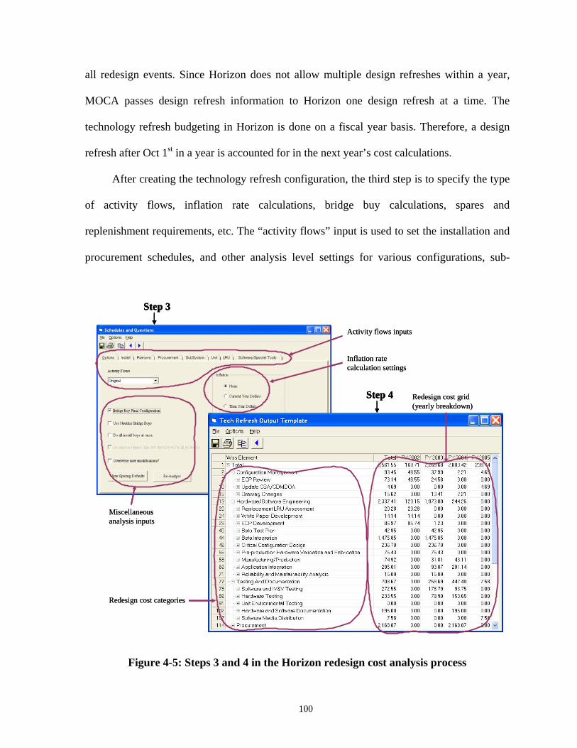
all redesign events. Since Horizon does not allow multiple design refreshes within a year,
MOCA passes design refresh information to Horizon one design refresh at a time. The
technology refresh budgeting in Horizon is done on a fiscal year basis. Therefore, a design
refresh after Oct 1st in a year is accounted for in the next year’s cost calculations.
After creating the technology refresh configuration, the third step is to specify the type
of activity flows, inflation rate calculations, bridge buy calculations, spares and
replenishment requirements, etc. The “activity flows” input is used to set the installation and
procurement schedules, and other analysis level settings for various configurations, sub-
Miscellaneous analysis inputs
Activity flows inputs
Redesign cost grid (yearly breakdown)
Redesign cost categories
Step 3
Step 4
Inflation rate calculation settings
Miscellaneous analysis inputs
Activity flows inputs
Redesign cost grid (yearly breakdown)
Redesign cost categories
Step 3Step 3
Step 4Step 4
Inflation rate calculation settings
Figure 4-5: Steps 3 and 4 in the Horizon redesign cost analysis process
100

systems, units, and LRUs. The inflation rate, bridge buy, and spare replenishment settings are
self explanatory. The fourth and final step is to run the analysis, which gives a table output
specifying costs on a yearly basis for various cost breakdown elements, e.g., procurement,
configuration management, engineering, installation, etc. These costs are saved in a
predetermined format for use in MOCA. Figure 4-5 shows steps 3 and 4.
4.3 MOCA-Horizon Integration
To perform the required MOCA-Horizon integration, a stand-alone Visual Basic (VB)
tool was created. This tool reads the scenario file written by MOCA and then calls the
Horizon DLL (Dynamically Linked Library) function(s) to analyze it. This integration
process eliminates the need to open, operate, and close Horizon via its user interface. There is
a Horizon status window that shows up while the scenario file is being read and processed; it
is the only way to check any errors that might have occurred during the analysis.
There are various steps that MOCA has to go through to include the Horizon analysis
as a part of its design refresh planning analysis. The first and foremost thing to be looked at
is the scenario file format that is readable by Horizon . As explained in Section 4.2, there are
five different levels of hierarchy available in the Horizon tool to describe a system. There are
many inputs that are specific to some of these hierarchy levels; however, they are all present
for each of the elements in the scenario file. Therefore, some of the elements of the scenario
file do not mean anything in the context of its hierarchy level and are ignored by MOCA.
There is a header at the beginning of each scenario file that gives the name of the system,
date the file was created, the analysis start and end dates, and other similar inputs. Thereafter
is the block of text that is called “Work Elements”. This block of text has many different sub-
blocks called “Work Element”. The LPD-17 hierarchy and its properties are presented in a
101
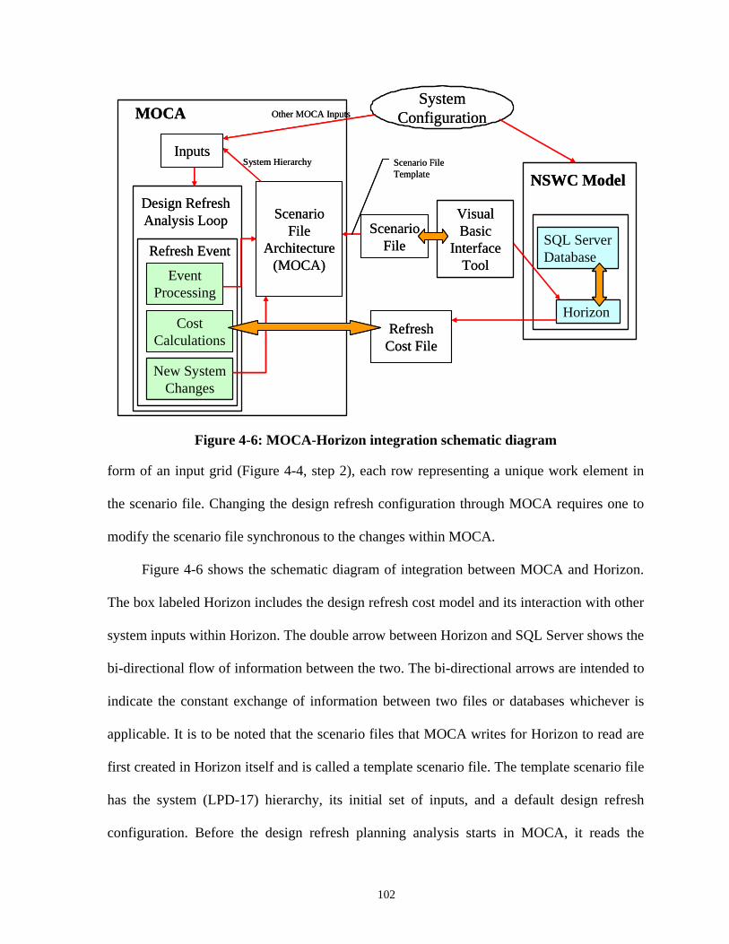
Scenario File
Architecture (MOCA)
System ConfigurationMOCA
Design Refresh Analysis Loop
NSWC Model
SQL Server Database
Horizon
New System Changes
Refresh Event
Cost Calculations
Event Processing
System HierarchyInputs
Refresh Cost File
Visual Basic
Interface Tool
Scenario File
Scenario File Template
Other MOCA Inputs
Scenario File
Architecture (MOCA)
System ConfigurationMOCA
Design Refresh Analysis Loop
NSWC Model
SQL Server Database
Horizon
New System Changes
Refresh Event
Cost Calculations
Event Processing
System HierarchyInputs
Refresh Cost File
Visual Basic
Interface Tool
Scenario File
Scenario File Template
Other MOCA Inputs
Figure 4-6: MOCA-Horizon integration schematic diagram
form of an input grid (Figure 4-4, step 2), each row representing a unique work element in
the scenario file. Changing the design refresh configuration through MOCA requires one to
modify the scenario file synchronous to the changes within MOCA.
Figure 4-6 shows the schematic diagram of integration between MOCA and Horizon.
The box labeled Horizon includes the design refresh cost model and its interaction with other
system inputs within Horizon. The double arrow between Horizon and SQL Server shows the
bi-directional flow of information between the two. The bi-directional arrows are intended to
indicate the constant exchange of information between two files or databases whichever is
applicable. It is to be noted that the scenario files that MOCA writes for Horizon to read are
first created in Horizon itself and is called a template scenario file. The template scenario file
has the system (LPD-17) hierarchy, its initial set of inputs, and a default design refresh
configuration. Before the design refresh planning analysis starts in MOCA, it reads the
102
Horizon template scenario file and stores all its information into a scenario file data structure
that resides within MOCA. This data structure within MOCA needs to be updated after every
design refresh to reflect the changes made to the original system due to part replacement.
There are several important inputs involved in MOCA-Horizon analysis. LRU level
inputs are: Cost, Mean-Time-Between-Failure (MTBF), Generic Type, Quantity, End of
Production, Start of Production, and Product Lifetime. Site level inputs are: Install Date, and
Remove Date. Configuration level inputs are: Tech Refresh Year, and Configuration
Quantity. Inputs that are common to all hierarchy levels are: Identity Number, Include Field,
and Work Element Type, and Name.
The site installation and remove dates correspond to the dates a particular configuration
is deployed in the field and removed from the field respectively. The template scenario file
has the original site install dates and remove dates. At a design refresh the old version of the
configuration is removed and the new version is installed. At the second design refresh, the
first design refreshed system is removed and the new (second) one installed. The install dates
of the sites for the first scheduled design refresh corresponds to the template scenario file’s
install dates, and the remove date of the sites for the last scheduled design refresh
corresponds to the template scenario file’s remove date.
EOP = SOP + Prod Life where,
EOP = End of Production SOP = Start of Production Prod Life = Product Lifetime
Equation 4.1
Equation 4.1 (above) gives relationship between a part’s EOP, SOP, and Lifetime. At a
design refresh a replaced part’s SOP changes and its Lifetime can change as well. MOCA
103
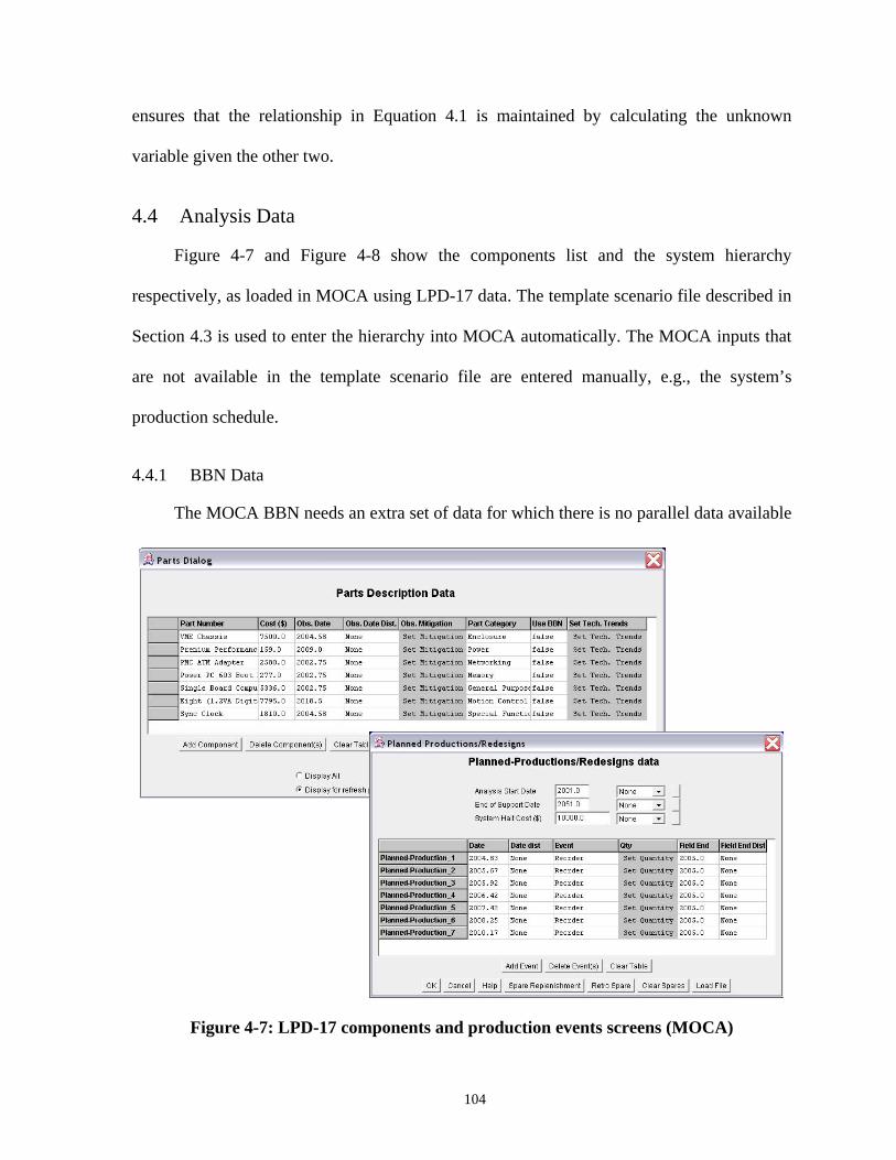
ensures that the relationship in Equation 4.1 is maintained by calculating the unknown
variable given the other two.
4.4 Analysis Data
Figure 4-7 and Figure 4-8 show the components list and the system hierarchy
respectively, as loaded in MOCA using LPD-17 data. The template scenario file described in
Section 4.3 is used to enter the hierarchy into MOCA automatically. The MOCA inputs that
are not available in the template scenario file are entered manually, e.g., the system’s
production schedule.
4.4.1 BBN Data
The MOCA BBN needs an extra set of data for which there is no parallel data available
Figure 4-7: LPD-17 components and production events screens (MOCA)
104
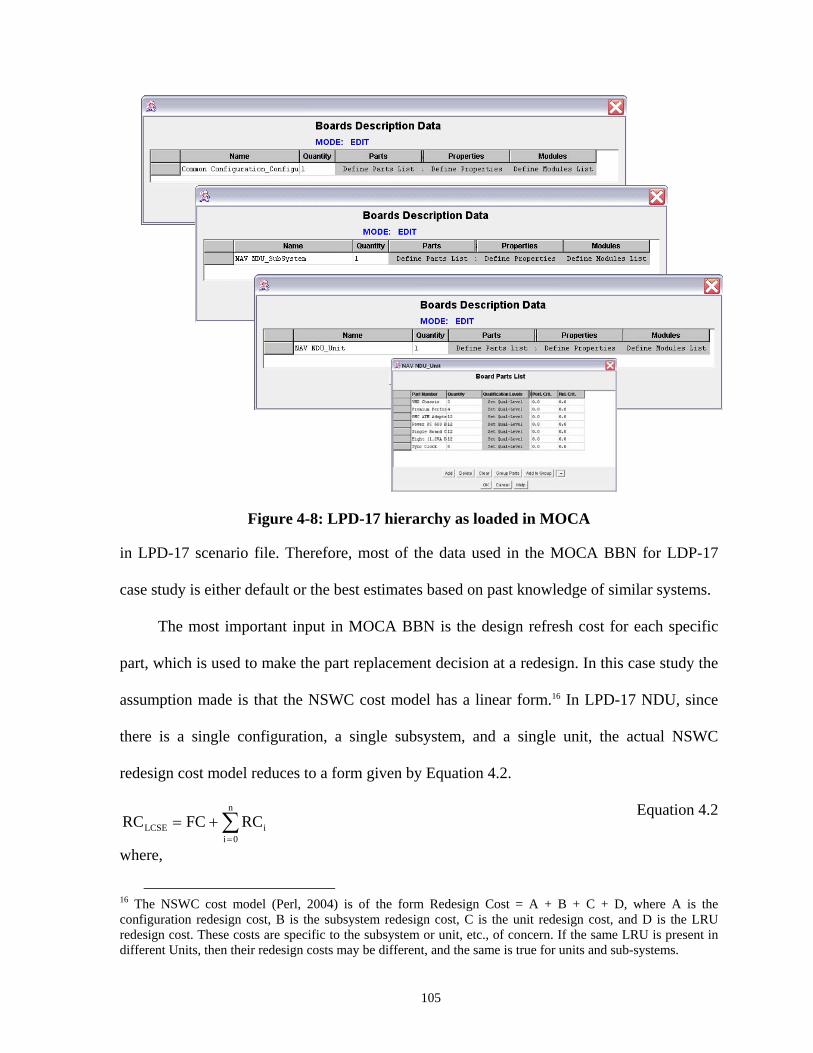
Figure 4-8: LPD-17 hierarchy as loaded in MOCA
in LPD-17 scenario file. Therefore, most of the data used in the MOCA BBN for LDP-17
case study is either default or the best estimates based on past knowledge of similar systems.
The most important input in MOCA BBN is the design refresh cost for each specific
part, which is used to make the part replacement decision at a redesign. In this case study the
assumption made is that the NSWC cost model has a linear form.16 In LPD-17 NDU, since
there is a single configuration, a single subsystem, and a single unit, the actual NSWC
redesign cost model reduces to a form given by Equation 4.2.
∑=
+=n
0iiLCSE RCFCRC
where,
Equation 4.2
16 The NSWC cost model (Perl, 2004) is of the form Redesign Cost = A + B + C + D, where A is the configuration redesign cost, B is the subsystem redesign cost, C is the unit redesign cost, and D is the LRU redesign cost. These costs are specific to the subsystem or unit, etc., of concern. If the same LRU is present in different Units, then their redesign costs may be different, and the same is true for units and sub-systems.
105
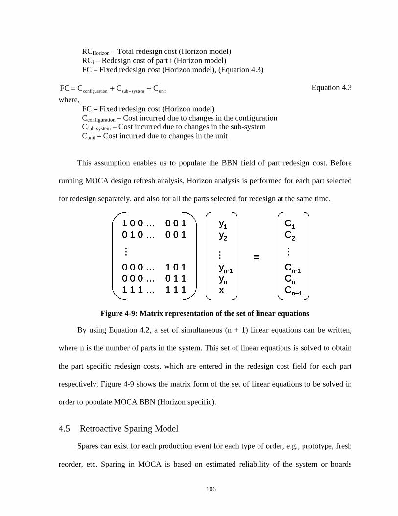
RCHorizon – Total redesign cost (Horizon model) RCi – Redesign cost of part i (Horizon model) FC – Fixed redesign cost (Horizon model), (Equation 4.3)
unitsystemsubionconfigurat CCCFC ++= −
where, FC – Fixed redesign cost (Horizon model) Cconfiguration – Cost incurred due to changes in the configuration Csub-system – Cost incurred due to changes in the sub-system Cunit – Cost incurred due to changes in the unit
Equation 4.3
This assumption enables us to populate the BBN field of part redesign cost. Before
running MOCA design refresh analysis, Horizon analysis is performed for each part selected
for redesign separately, and also for all the parts selected for redesign at the same time.
1 0 0 … 0 0 1 0 1 0 … 0 0 1
0 0 0 … 1 0 1 0 0 0 … 0 1 1 1 1 1 … 1 1 1
…=
C1C2
Cn-1 CnCn+1
…
y1y2
yn-1ynx
…
1 0 0 … 0 0 1 0 1 0 … 0 0 1
0 0 0 … 1 0 1 0 0 0 … 0 1 1 1 1 1 … 1 1 1
…
1 0 0 … 0 0 1 0 1 0 … 0 0 1
0 0 0 … 1 0 1 0 0 0 … 0 1 1 1 1 1 … 1 1 1
…=
C1C2
Cn-1 CnCn+1
…
C1C2
Cn-1 CnCn+1
…
y1y2
yn-1ynx
…
y1y2
yn-1ynx
…
Figure 4-9: Matrix representation of the set of linear equations
By using Equation 4.2, a set of simultaneous (n + 1) linear equations can be written,
where n is the number of parts in the system. This set of linear equations is solved to obtain
the part specific redesign costs, which are entered in the redesign cost field for each part
respectively. Figure 4-9 shows the matrix form of the set of linear equations to be solved in
order to populate MOCA BBN (Horizon specific).
4.5 Retroactive Sparing Model
Spares can exist for each production event for each type of order, e.g., prototype, fresh
reorder, etc. Sparing in MOCA is based on estimated reliability of the system or boards
106
within the system. The model uses the most likely reliability prediction (in operation hours)
and then generates sparing requirements in the future by adding this time to the different field
dates of the system. Each different field date needs to be managed separately as their
operational hours clock runs separate from other dates. Retroactive sparing means that some
of the production event’s units are replaced with spares that have been purchased and stored
when the system was first fielded. These spares are often based on projected maintenance
requirements and are specific to certain groups of systems, e.g., from a fleet of 20 ships only
10 may have retroactive spares. To calculate retroactive adjusted future spares one has to
deduct retroactive spares from the calculated spares thus maintaining the balance of spares
available at all times. This potentially saves inventory costs for the system.
In the LPD-17 example every time a new set of ships or NDU units are installed
originally or reinstalled after a design refresh, there is a purchase of spares equal to 20% of
the total installation quantity. These spares are equivalent to retroactive spares in the context
of this case study. MOCA includes these spares in the design refresh scheduling algorithm. If
however there is no specific date specified for these spares then MOCA does not include
them for design refresh scheduling. Instead, the cost incurred due to these spares is included
within design refresh cost along with the procurement cost of the reinstalled units at the
design refresh. The difference here between the LPD-17 case study and the examples in
Chapter 2 and Chapter 3 is that in the previous examples no reinstallation cost was taken into
account at a design refresh. Therefore, the fielded units are not addressed at a design refresh
to reinstall the redesigned part(s). These already fielded units have an opportunity of
reinstallation of new parts only at the next maintenance event, which is also called a spare
107
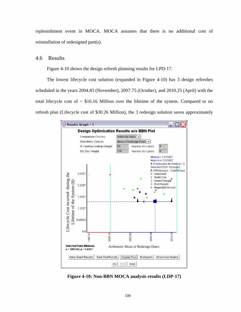
replenishment event in MOCA. MOCA assumes that there is no additional cost of
reinstallation of redesigned part(s).
4.6 Results
Figure 4-10 shows the design refresh planning results for LPD-17.
The lowest lifecycle cost solution (expanded in Figure 4-10) has 3 design refreshes
scheduled in the years 2004.83 (November), 2007.75 (October), and 2010.25 (April) with the
total lifecycle cost of ~ $16.16 Million over the lifetime of the system. Compared to no
refresh plan (Lifecycle cost of $30.26 Million), the 3 redesign solution saves approximately
Life
cycl
e C
ost i
ncur
red
dur
ing
the
Life
time
of th
e Sy
stem
($)
Arithmetic Mean of Redesign Dates
Life
cycl
e C
ost i
ncur
red
dur
ing
the
Life
time
of th
e Sy
stem
($)
Arithmetic Mean of Redesign Dates
Figure 4-10: Non-BBN MOCA analysis results (LDP-17)
108
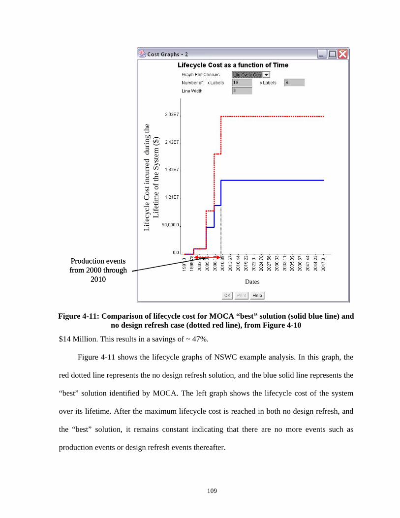
Production events from 2000 through
2010
Life
cycl
e C
ost i
ncur
red
dur
ing
the
Life
time
of th
e Sy
stem
($)
Dates
Production events from 2000 through
2010
Life
cycl
e C
ost i
ncur
red
dur
ing
the
Life
time
of th
e Sy
stem
($)
Dates
Figure 4-11: Comparison of lifecycle cost for MOCA “best” solution (solid blue line) and no design refresh case (dotted red line), from Figure 4-10
$14 Million. This results in a savings of ~ 47%.
Figure 4-11 shows the lifecycle graphs of NSWC example analysis. In this graph, the
red dotted line represents the no design refresh solution, and the blue solid line represents the
“best” solution identified by MOCA. The left graph shows the lifecycle cost of the system
over its lifetime. After the maximum lifecycle cost is reached in both no design refresh, and
the “best” solution, it remains constant indicating that there are no more events such as
production events or design refresh events thereafter.
109
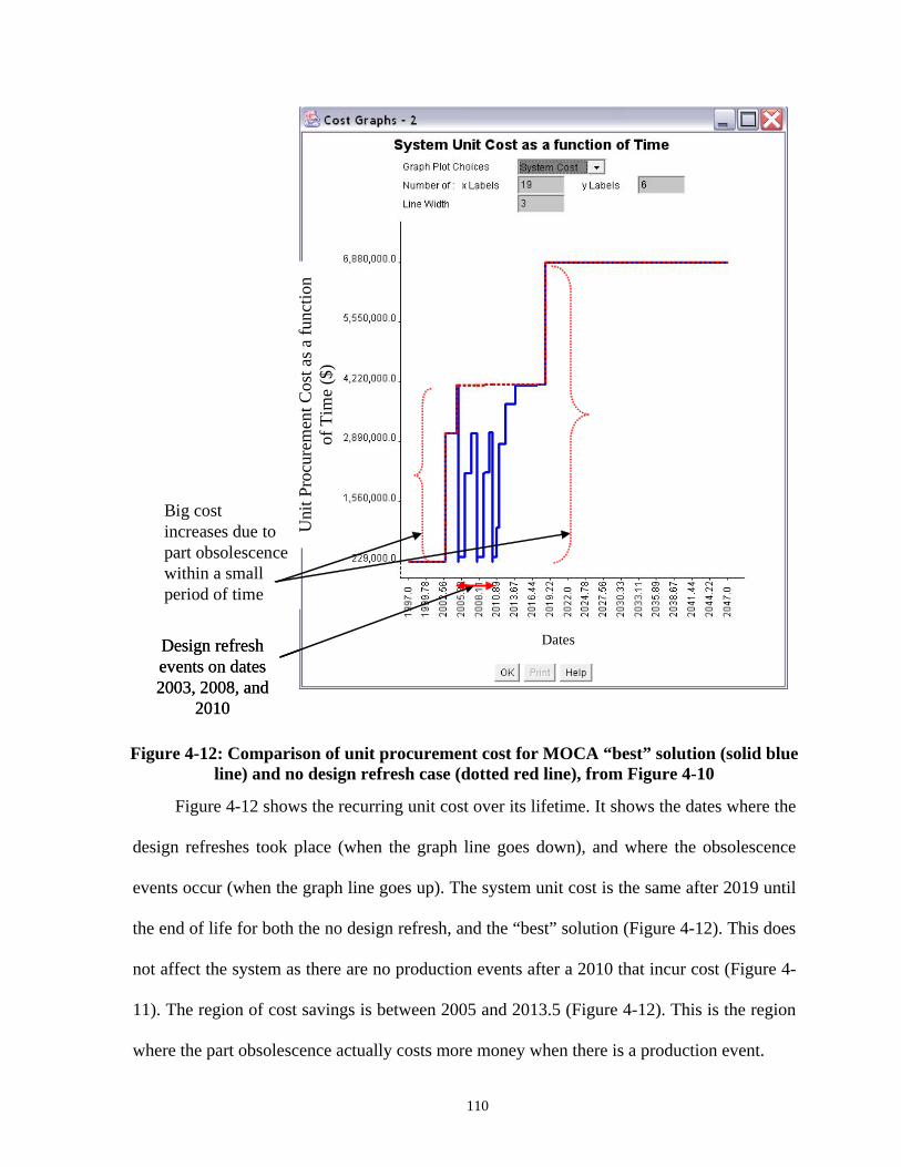
Design refresh events on dates 2003, 2008, and
2010
Big cost increases due to part obsolescence within a small period of time
Uni
t Pro
cure
men
t Cos
t as a
func
tion
of T
ime
($)
DatesDesign refresh events on dates 2003, 2008, and
2010
Big cost increases due to part obsolescence within a small period of time
Uni
t Pro
cure
men
t Cos
t as a
func
tion
of T
ime
($)
Dates
Figure 4-12: Comparison of unit procurement cost for MOCA “best” solution (solid blue line) and no design refresh case (dotted red line), from Figure 4-10
Figure 4-12 shows the recurring unit cost over its lifetime. It shows the dates where the
design refreshes took place (when the graph line goes down), and where the obsolescence
events occur (when the graph line goes up). The system unit cost is the same after 2019 until
the end of life for both the no design refresh, and the “best” solution (Figure 4-12). This does
not affect the system as there are no production events after a 2010 that incur cost (Figure 4-
11). The region of cost savings is between 2005 and 2013.5 (Figure 4-12). This is the region
where the part obsolescence actually costs more money when there is a production event.
110
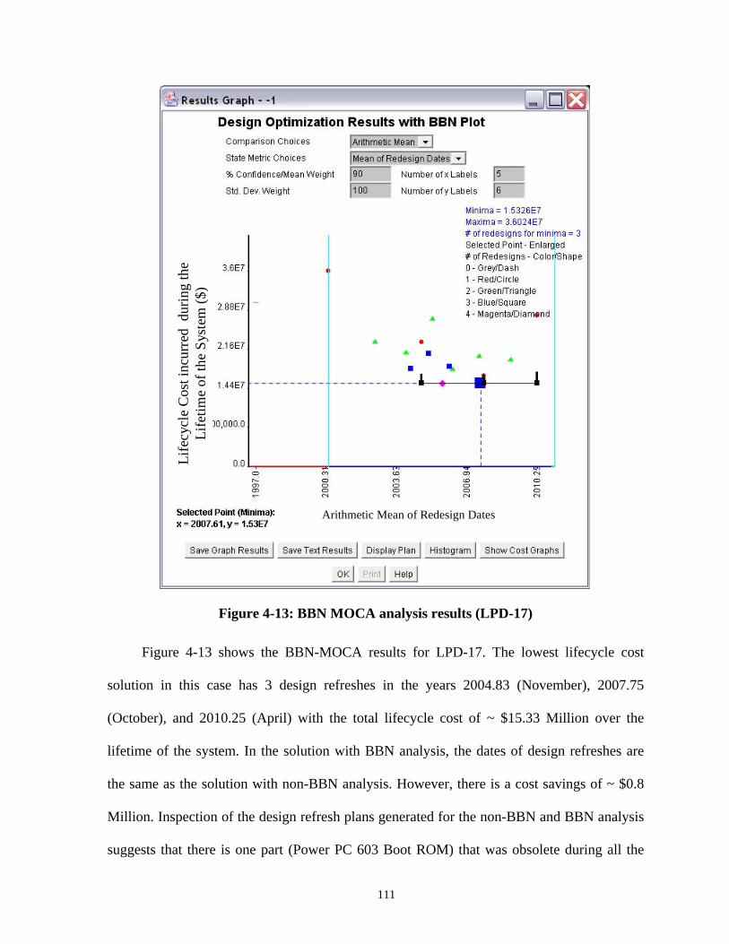
Life
cycl
e C
ost i
ncur
red
dur
ing
the
Life
time
of th
e Sy
stem
($)
Arithmetic Mean of Redesign Dates
Life
cycl
e C
ost i
ncur
red
dur
ing
the
Life
time
of th
e Sy
stem
($)
Arithmetic Mean of Redesign Dates
Figure 4-13: BBN MOCA analysis results (LPD-17)
Figure 4-13 shows the BBN-MOCA results for LPD-17. The lowest lifecycle cost
solution in this case has 3 design refreshes in the years 2004.83 (November), 2007.75
(October), and 2010.25 (April) with the total lifecycle cost of ~ $15.33 Million over the
lifetime of the system. In the solution with BBN analysis, the dates of design refreshes are
the same as the solution with non-BBN analysis. However, there is a cost savings of ~ $0.8
Million. Inspection of the design refresh plans generated for the non-BBN and BBN analysis
suggests that there is one part (Power PC 603 Boot ROM) that was obsolete during all the
111
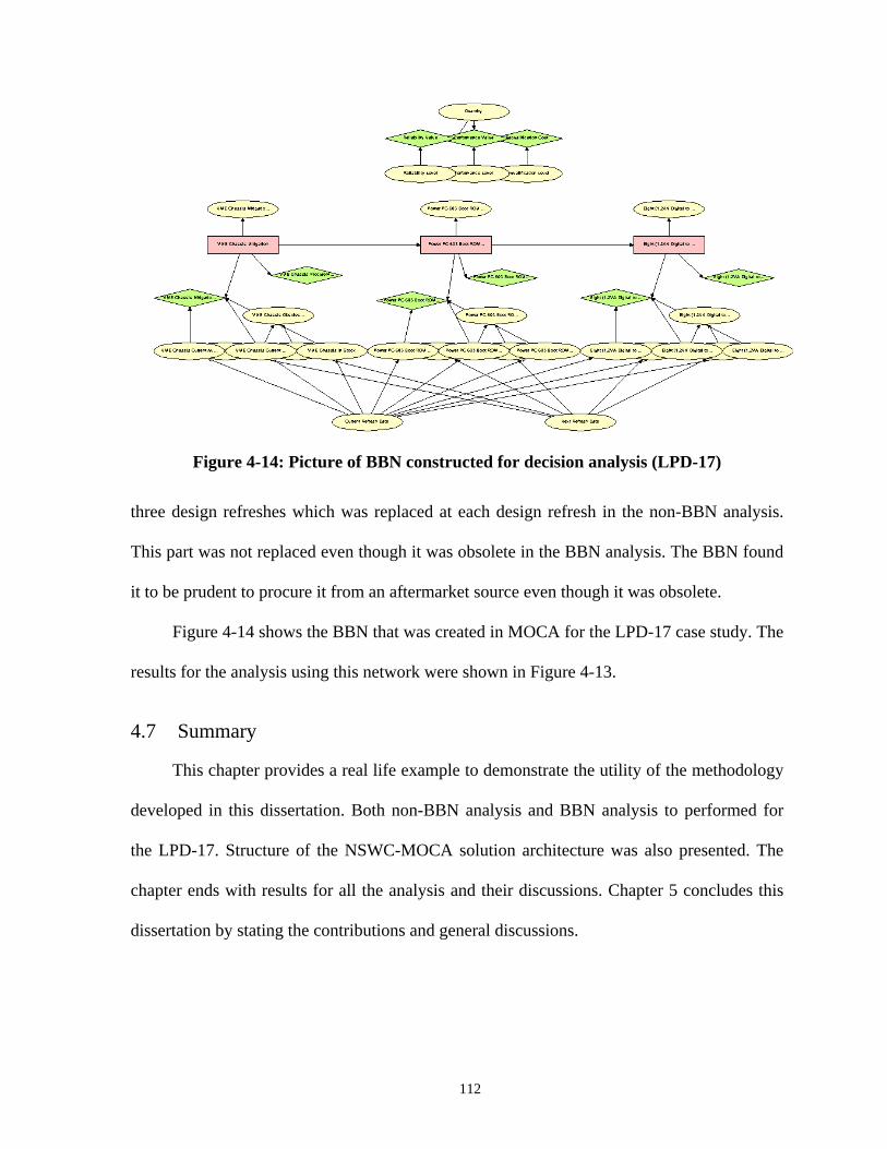
Figure 4-14: Picture of BBN constructed for decision analysis (LPD-17)
three design refreshes which was replaced at each design refresh in the non-BBN analysis.
This part was not replaced even though it was obsolete in the BBN analysis. The BBN found
it to be prudent to procure it from an aftermarket source even though it was obsolete.
Figure 4-14 shows the BBN that was created in MOCA for the LPD-17 case study. The
results for the analysis using this network were shown in Figure 4-13.
4.7 Summary
This chapter provides a real life example to demonstrate the utility of the methodology
developed in this dissertation. Both non-BBN analysis and BBN analysis to performed for
the LPD-17. Structure of the NSWC-MOCA solution architecture was also presented. The
chapter ends with results for all the analysis and their discussions. Chapter 5 concludes this
dissertation by stating the contributions and general discussions.
112
Chapter 5: Contributions and Conclusions
This dissertation presents a methodology for forecasting technology insertion
concurrent with design refresh planning for sustainment-dominated systems. This
methodology aims at minimizing the lifecycle cost of the system. The resulting analysis
provides a design refresh schedule for the system (i.e., when to design refresh) along with the
design refresh content for each of the design refreshes scheduled. The design refresh content
is determined using a hybrid analysis scheme, which utilizes Monte Carlo methods to
account for uncertainties (particularly in dates) and Bayesian Belief Networks to enable
critical decision making once candidate refresh dates are chosen. The methodology has been
demonstrated on a Full Authority Digital Electronic Controller (FADEC) from Honeywell
that is subject to electronic component obsolescence and a shipboard wide are network for
the Navy’s LPD-17 expeditionary ship.
The MOCA tool was developed to implement the methodology described in this
dissertation. It has a cost analysis engine, and an integrated design refresh planning engine.
MOCA also couples together pre-built network fragments to construct Bayesian Belief
Networks that are used in the design refresh content selection process.
5.1 Contributions
In the real world, the treatment of technology obsolescence has been exclusively
reactive in nature, i.e., people in the industry focus all their effort on mitigating the
consequences of obsolescence problems when they become a problem rather than planning
113
the product so as to minimize obsolescence problems before they arrive. For this reason, all
existing work applicable to this problem targets optimizing the reactive solution (i.e.,
enabling the best choice of mitigation approaches after obsolescence occurs). Besides the
work presented here, only one other approach proactively addresses when design refreshes
should be done as a function of technology obsolescence forecasts (Porter, 1998), an
approach that does not minimize lifecycle cost.16
This dissertation postulates that given knowledge of part obsolescence dates (albeit
uncertain), we can identify a mix of design refreshes and mitigation approaches that
minimize the impact on the product’s lifecycle cost. The methodology developed in this
dissertation can be used at the design stage of the product where the opportunity to impact
future cost avoidance is the greatest (it can also be used throughout the lifecycle of the
product, but its impact is reduced).
As an example, a realistic scenario is when the manufacturer does not mitigate a part
obsolescence problem using proactive planning but uses reactive methods only. If no
planning is done for even the reactive obsolescence management then there is increased risk
involved in design refreshing the system. The risk is due to the fact that if the reactive
redesign takes place at the wrong time it may be more expensive than mitigating the
obsolescence problem using other approaches. For example, an aftermarket source may be
able to sustain the system better than a redesign at the wrong time. Therefore, planning is
essential in obsolescence management whether we decide to do proactive management or
16 The Porter model performs a net present value trade off analysis between life time buy cost and delays in design refreshes only. The Porter model fundamentally differs from MOCA in that it treats design refreshes one at a time (serially) rather than optimizing a refresh plan consisting of potentially multiple refreshes as MOCA does. In this way, the Porter model minimizes the OEMs costs associated with cost plus type contractual arrangements – it does not minimize the lifecycle cost of the product. Therefore, the Porter model tackles a somewhat different problem than what is addressed in this dissertation.
114
reactive management. For obsolescence management to be beneficial we have to adopt some
form of a proactive approach.
The global contribution of this work is the development of a methodology that truly
targets minimization of lifecycle costs through optimal design refresh date selection and
content selection for products that are sustainment-dominated and subject to technology
obsolescence. Such a methodology could also enable, as a byproduct, optimal reactive
mitigation approach choices based on an entire lifecycle view, which would be more accurate
than existing reactive modeling methodologies. The demonstration case studies performed in
this dissertation suggest that there is a significant opportunity to save cost by planning for
obsolescence.
5.1.1 Discussion of Problem Scope
It is not the target of this dissertation to find the most efficient solution to the problem,
rather to find and demonstrate a solution to a problem that has not been solved before. If the
value of such a feasible solution can be demonstrated, there will be ample opportunity in the
future to make the computational procedure more efficient. The following paragraph
discusses a number of possibilities in the MOCA analysis.
Figure 5-1 shows the possible design refresh plans which make up the solution space.
Theoretically, there are infinite points in time where a design refresh can be schedule over a
system’s life span. However, in MOCA the life cycle of the system is impacted only during
cost incurring events. These events include all the production events, spare replenishments
event, and design refresh events. Therefore, we have finite number of points in time where a
design refresh can be scheduled.
115
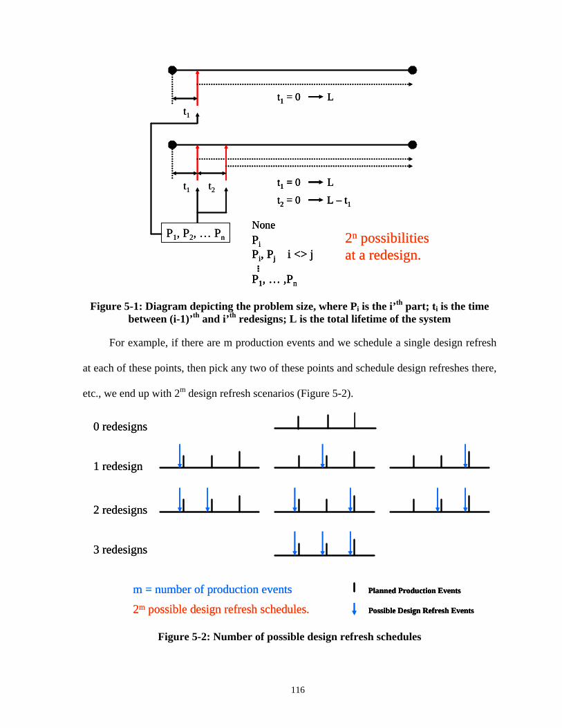
t1
t1 = 0 L
t1t1 = 0 Lt2t2 = 0 L – t1
P1, P2, … Pn PiPi, Pj i <> j
P1, … ,Pn
None2n possibilities at a redesign.
t1
t1 = 0 Lt1 = 0 L
t1t1 = 0 Lt1 = 0 Lt2t2 = 0 L – t1t2 = 0 L – t1
P1, P2, … Pn PiPi, Pj i <> j
P1, … ,Pn
NonePiPi, Pj i <> j
P1, … ,Pn
None2n possibilities at a redesign.
Figure 5-1: Diagram depicting the problem size, where Pi is the i’th part; ti is the time between (i-1)’th and i’th redesigns; L is the total lifetime of the system
For example, if there are m production events and we schedule a single design refresh
at each of these points, then pick any two of these points and schedule design refreshes there,
etc., we end up with 2m design refresh scenarios (Figure 5-2).
2m possible design refresh schedules.
m = number of production events Planned Production Events
Possible Design Refresh Events
0 redesigns
2 redesigns
1 redesign
3 redesigns
2m possible design refresh schedules.
m = number of production events Planned Production Events
Possible Design Refresh Events
Planned Production Events
Possible Design Refresh Events
0 redesigns
2 redesigns
1 redesign
3 redesigns
Figure 5-2: Number of possible design refresh schedules
116
There are 2n cases generated by the permutations of the selection choice of n parts to be
replaced at a design refresh. The two represent the options “Replace” and “Not Replace”.
Therefore, total solution space is 2m x 2n. The 2n part replacement cases are dealt with by the
BBN in the context of this work. The 2m cases of design refresh schedules are enumerated
within MOCA.
5.1.2 Methodology Specific Contributions
The primary contribution of this work is a global planning methodology for lifecycle
cost reduction for a system subject to technology obsolescence (as articulated above);
however, several more specific contributions anticipated from this work are discussed below:
• Development of decision networks that treat technology replacement, and the
identification and implementation of coupling between multiple technology’s
replacement decisions.
• Development of a Monte Carlo analysis approach that accommodates timeline
planning uncertainties, thus allowing uncertain product dates to be combined with
design refresh candidates such that independent uncertainties in both can be
accommodated in a practical manner.
• The implementation of the methodology within a design tool called MOCA that
represents the first (and currently only) design tool that treats design refresh planning
for sustainment-dominated systems that are subject to technology obsolescence.
• Development and application of obsolescence concepts to non-hardware portions of
systems (e.g., software). Coupling of non-hardware technologies with hardware
technologies in the decision replacement space (Appendix B).
117
5.2 Future Work
Some of the analysis particulars that can be dealt with in the future to make the model
more useful and clear are discussed below:
• More nodes and links may need to be added to the BBN to produce a more complete
description of the problem. As an example, part obsolescence is a possible coupling
point. A set of parts can depend upon similar technology (or be an integrated “chip
set”) and therefore become obsolete at the same time. Such a coupling can also exist
at the cost of mitigation node. A group of parts replaced at the same time can result in
lower cost impact as opposed to the cumulative cost of single parts being replaced.
• Currently some of the nodes are updated by MOCA internally where as links between
corresponding nodes in the BBN should take care of changes in the system through
network propagation, e.g., the Next Design Refresh node is not yet linked to
Performance Value and Reliability Value nodes. However, MOCA does update these
two nodes according to the possible next design refresh date internally.
• Hardware obsolescence precipitated software changes have not been addressed in the
version of MOCA discussed in this dissertation. The cost of software changes is
significant and needs to be included in the solution. Preliminary work in this area has
been done by Goswami [reference Arindam’s thesis].
• Use of MOCA as a tool for avoidance of design refresh, i.e., using MOCA to
optimally plan logistics and mitigation so that solutions with no design refreshes are
the lowest lifecycle cost solutions.
• Connection of the technology insertion attributes of MOCA to technology
roadmapping.
118
Appendix A: Publications Associated With This Work
1. Singh, P., Sandborn, P., Geiser, T., and Lorenson, D., "Electronic Part Obsolescence
Driven Design Refresh Optimization," Proc. International Conference on Concurrent
Engineering, Cranfield University, UK, p 961-970, July 2002.
2. Sandborn, P., and Singh, P., "Electronic Part Obsolescence Driven Design Refresh
Optimization," in Proc. FAA/DoD/NASA Aging Aircraft Conference, San Francisco, CA,
September 2002.
3. Singh, P., Sandborn, P., Lorenson, D., and Geiser, T., "Determining Optimum Redesign
Plans for Avionics Considering Electronic Part Obsolescence Forecasts," in Proc. World
Aviation Congress, Phoenix, AZ, (SAE Technical Paper: 2002-1-3012), November 2002.
4. Singh, P., and Sandborn, P., MOCA Software Tool – University of Maryland Invention
of the Year for 2002 in the information science category.
5. Sandborn, P., and Singh P., MOCA User’s Guide, V. 1.3, ESCML Technical Report 03-
01, June 2003.
6. Sandborn, P., Singh, P., Herald, T., and Houston, J., "Optimum technology insertion into
systems based on the assessment of viability," IEEE Transactions on Components and
Packaging Technologies, v 26, n 4, December 2003.
7. Singh, P., Sandborn, P., Geiser, T., and Lorenson, D., "Electronic Part Obsolescence
Driven Design Refresh Planning," International Journal of Agile Manufacturing, v 7, n 1,
2004.
119
8. Singh, P., and Sandborn, P., “Forecasting Technology Insertion Concurrent with Design
Refresh Planning for COTS-Based Electronic Systems”, to be published in Proc.
Reliability and Maintainability Symposium, Arlington, VA, January 2005.
9. Singh, P., Sandborn, P., and Crabtree, C., “Pro-Active Design Refresh Planning Applied
to an LPD-17 NAV NDU Subsystem,” to be published in Proceedings of the DMSMS
Conference, April 2005.
120
Appendix B: Computer Network Example (Task 4)
A second case study of a computer network, such as a university’s local area network,
consisting of multiple users, computers, and application software requirements will also be
considered. The second example is a broader and more general example than the first case
with more diverse data sources and different stakeholders. In the second case, both hardware
and software are becoming obsolete. Design refresh planning and lifecycle cost analysis used
in MOCA for electronic parts can also be used to model refresh planning for a computer
network. As an example, this dissertation presents a computer network model that consists of
three different groups of users having differing hardware and software requirements. The
groups are: 1) design group, 2) maintenance group, and 3) quality group. The design group
requires more computational power to perform analysis, and a large hard disk storage
capacity to save large amounts of data and analysis files. In addition to the hardware required
by the design group, the group needs to access analysis and development software tools. The
maintenance group needs a standard hardware unit, and access to all the application software
tools. The quality group mainly deals with hardware reliability. However, the quality group
also needs to support the final software product developed. There are 25 team members in the
design group, 10 team members in the maintenance group, and 15 team members in the
quality group. Each team member has a computer with a pre-defined hardware and software
configuration. In addition, collectively all the computers used by the various groups are
connected via a network. MOCA is used to model lifecycle environment of the network of
121
computer hardware and software, and then to determine design refresh planning schedule for
the entire system.
The MOCA tool was designed to deal with real obsolescence events, i.e., elements of a
system becoming unavailable (non-procurable). Real obsolescence will be a factor for the
computer network we are considering, however, due to technology advancements and
evolving user functional requirements, the hardware and software, also may become
functionally obsolete within few years.17 In MOCA, the part obsolescence considers only
actual unavailability of parts. It does not consider functional obsolescence. The concept of
functional obsolescence is modeled analogous to reliability. As an example, a Windows
operating system loaded on a computer that goes functionally obsolete within 4 years can be
modeled using MTBF of 4 years for that version of Windows. Creating sparing requirements
based on MTBF will require MOCA to build or procure additional (new, upgraded in the
case of software) Windows software packages approximately every 4 years. These new
procurements, although analogous to “spare replenishments”, are in actuality upgrades in the
case of software. The design refresh planning analysis takes into account these spare
requirements while scheduling redesigns during the networks lifetime. Further, each of the
groups, i.e., design, maintenance, and quality, are separated into actual obsolescence modules
and functional obsolescence modules.
As discussed earlier, functional obsolescence of a component (hardware or software)
means that the component is available for procurement in the market but it no longer satisfies
the system requirements in terms of function. For example, a component B in the system is
17 Functional obsolescence does not imply that the element is unavailable or non-operational, only that it becomes effectively unusable, e.g., you can still purchase a Windows 98 operating system, however, if the application software you need to use won’t run under Windows 98 then Windows 98 has become functionally obsolete to you.
122
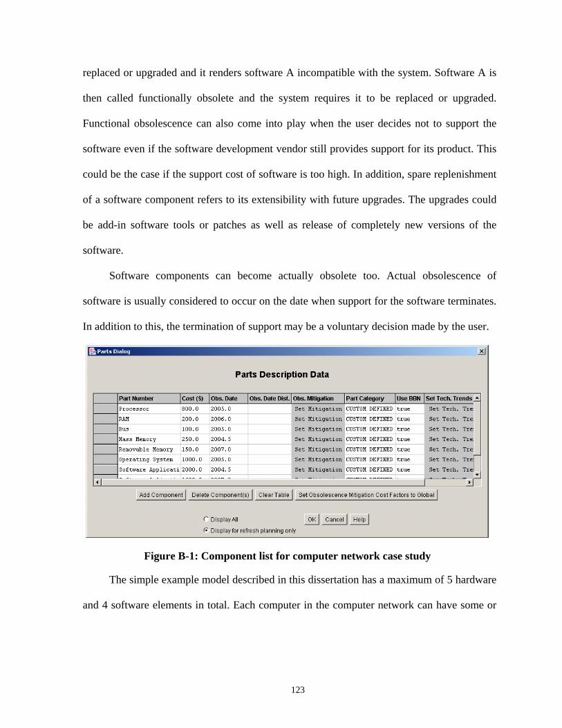
replaced or upgraded and it renders software A incompatible with the system. Software A is
then called functionally obsolete and the system requires it to be replaced or upgraded.
Functional obsolescence can also come into play when the user decides not to support the
software even if the software development vendor still provides support for its product. This
could be the case if the support cost of software is too high. In addition, spare replenishment
of a software component refers to its extensibility with future upgrades. The upgrades could
be add-in software tools or patches as well as release of completely new versions of the
software.
Software components can become actually obsolete too. Actual obsolescence of
software is usually considered to occur on the date when support for the software terminates.
In addition to this, the termination of support may be a voluntary decision made by the user.
Figure B-1: Component list for computer network case study
The simple example model described in this dissertation has a maximum of 5 hardware
and 4 software elements in total. Each computer in the computer network can have some or
123
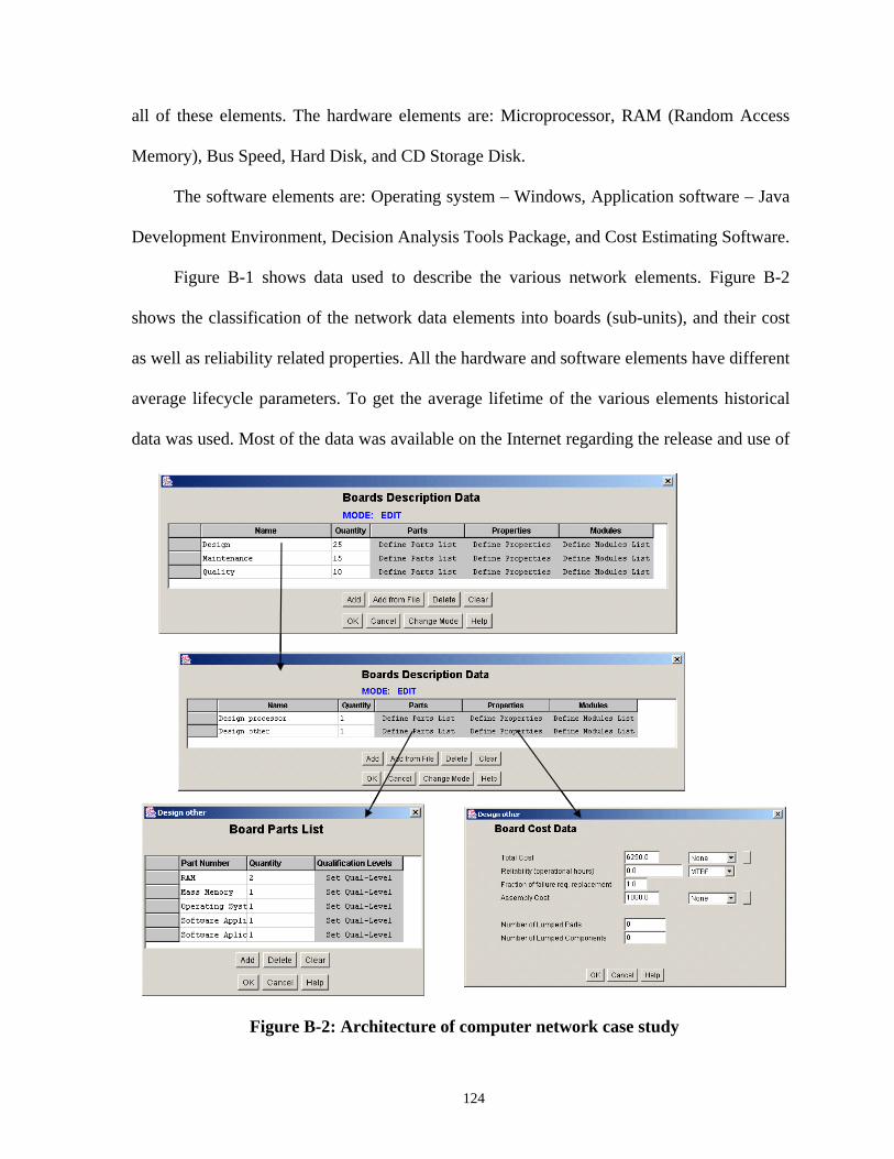
all of these elements. The hardware elements are: Microprocessor, RAM (Random Access
Memory), Bus Speed, Hard Disk, and CD Storage Disk.
The software elements are: Operating system – Windows, Application software – Java
Development Environment, Decision Analysis Tools Package, and Cost Estimating Software.
Figure B-1 shows data used to describe the various network elements. Figure B-2
shows the classification of the network data elements into boards (sub-units), and their cost
as well as reliability related properties. All the hardware and software elements have different
average lifecycle parameters. To get the average lifetime of the various elements historical
data was used. Most of the data was available on the Internet regarding the release and use of
Figure B-2: Architecture of computer network case study
124
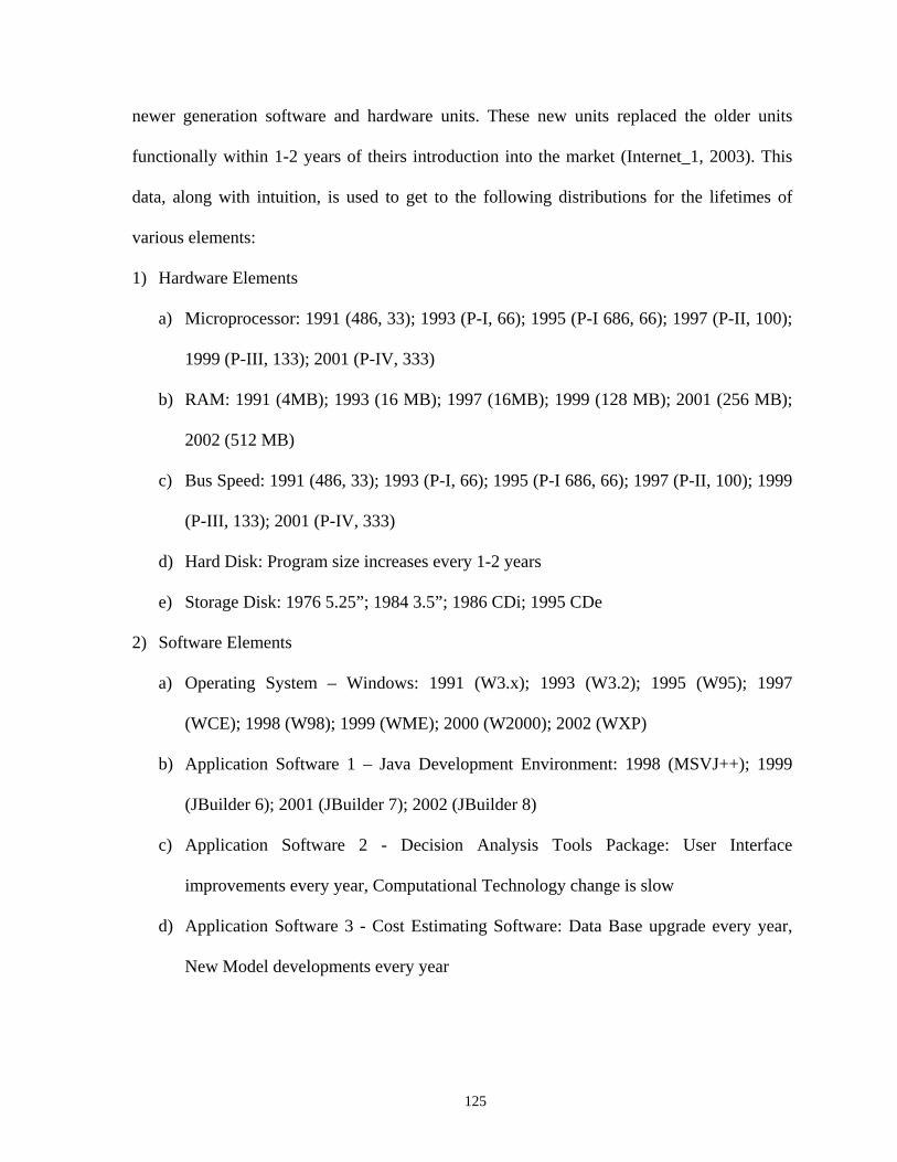
newer generation software and hardware units. These new units replaced the older units
functionally within 1-2 years of theirs introduction into the market (Internet_1, 2003). This
data, along with intuition, is used to get to the following distributions for the lifetimes of
various elements:
1) Hardware Elements
a) Microprocessor: 1991 (486, 33); 1993 (P-I, 66); 1995 (P-I 686, 66); 1997 (P-II, 100);
1999 (P-III, 133); 2001 (P-IV, 333)
b) RAM: 1991 (4MB); 1993 (16 MB); 1997 (16MB); 1999 (128 MB); 2001 (256 MB);
2002 (512 MB)
c) Bus Speed: 1991 (486, 33); 1993 (P-I, 66); 1995 (P-I 686, 66); 1997 (P-II, 100); 1999
(P-III, 133); 2001 (P-IV, 333)
d) Hard Disk: Program size increases every 1-2 years
e) Storage Disk: 1976 5.25”; 1984 3.5”; 1986 CDi; 1995 CDe
2) Software Elements
a) Operating System – Windows: 1991 (W3.x); 1993 (W3.2); 1995 (W95); 1997
(WCE); 1998 (W98); 1999 (WME); 2000 (W2000); 2002 (WXP)
b) Application Software 1 – Java Development Environment: 1998 (MSVJ++); 1999
(JBuilder 6); 2001 (JBuilder 7); 2002 (JBuilder 8)
c) Application Software 2 - Decision Analysis Tools Package: User Interface
improvements every year, Computational Technology change is slow
d) Application Software 3 - Cost Estimating Software: Data Base upgrade every year,
New Model developments every year
125
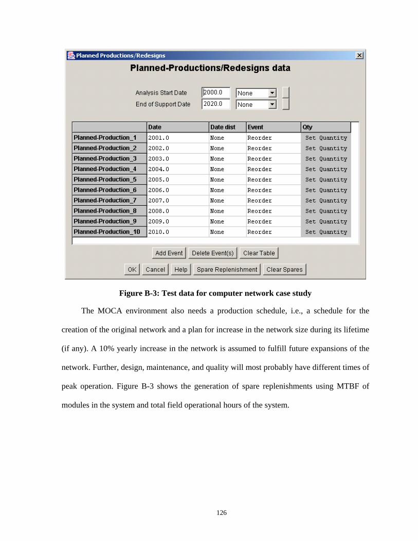
Figure B-3: Test data for computer network case study
The MOCA environment also needs a production schedule, i.e., a schedule for the
creation of the original network and a plan for increase in the network size during its lifetime
(if any). A 10% yearly increase in the network is assumed to fulfill future expansions of the
network. Further, design, maintenance, and quality will most probably have different times of
peak operation. Figure B-3 shows the generation of spare replenishments using MTBF of
modules in the system and total field operational hours of the system.
126
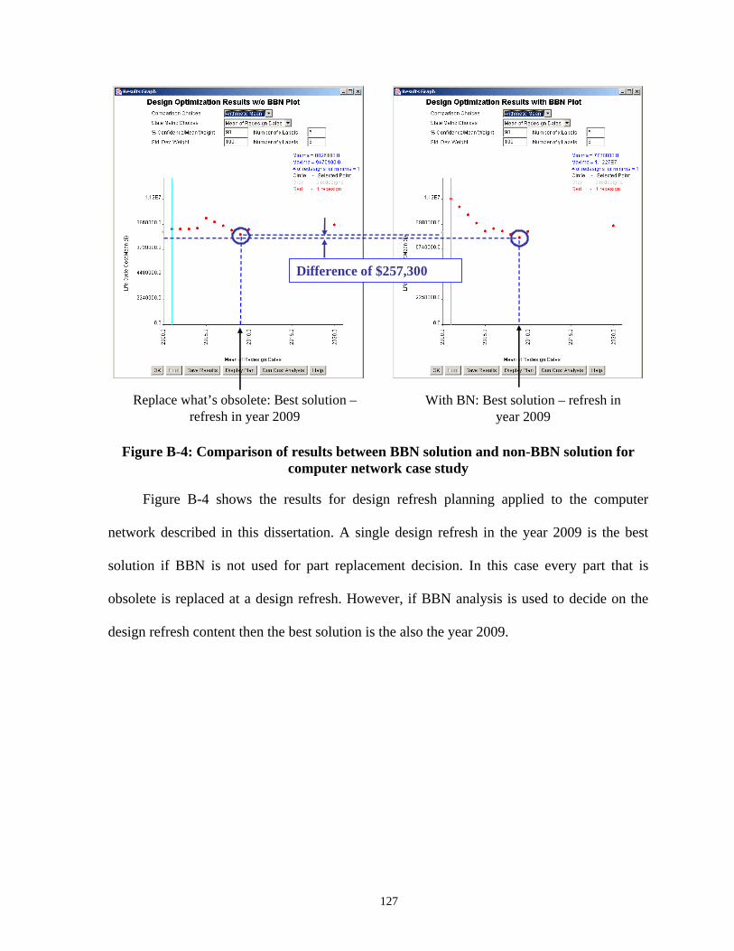
Replace what’s obsolete: Best solution –refresh in year 2009
With BN: Best solution – refresh in year 2009
Difference of $257,300
Figure B-4: Comparison of results between BBN solution and non-BBN solution for computer network case study
Figure B-4 shows the results for design refresh planning applied to the computer
network described in this dissertation. A single design refresh in the year 2009 is the best
solution if BBN is not used for part replacement decision. In this case every part that is
obsolete is replaced at a design refresh. However, if BBN analysis is used to decide on the
design refresh content then the best solution is the also the year 2009.
127
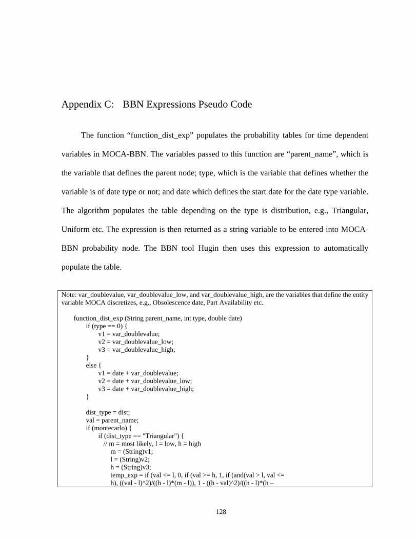
Appendix C: BBN Expressions Pseudo Code
The function “function_dist_exp” populates the probability tables for time dependent
variables in MOCA-BBN. The variables passed to this function are “parent_name”, which is
the variable that defines the parent node; type, which is the variable that defines whether the
variable is of date type or not; and date which defines the start date for the date type variable.
The algorithm populates the table depending on the type is distribution, e.g., Triangular,
Uniform etc. The expression is then returned as a string variable to be entered into MOCA-
BBN probability node. The BBN tool Hugin then uses this expression to automatically
populate the table.
Note: var_doublevalue, var_doublevalue_low, and var_doublevalue_high, are the variables that define the entity variable MOCA discretizes, e.g., Obsolescence date, Part Availability etc.
function_dist_exp (String parent_name, int type, double date) if (type == 0) {
v1 = var_doublevalue; v2 = var_doublevalue_low; v3 = var_doublevalue_high;
} else {
v1 = date + var_doublevalue; v2 = date + var_doublevalue_low; v3 = date + var_doublevalue_high;
} dist_type = dist; val = parent_name; if (montecarlo) {
if (dist_type == "Triangular") { // m = most likely, l = low, h = high
m = (String)v1; l = (String)v2; h = (String)v3; temp_exp = if (val <= l, 0, if (val >= h, 1, if (and(val > l, val <= h), ((val - l)^2)/((h - l)*(m - l)), 1 - ((h - val)^2)/((h - l)*(h –
128
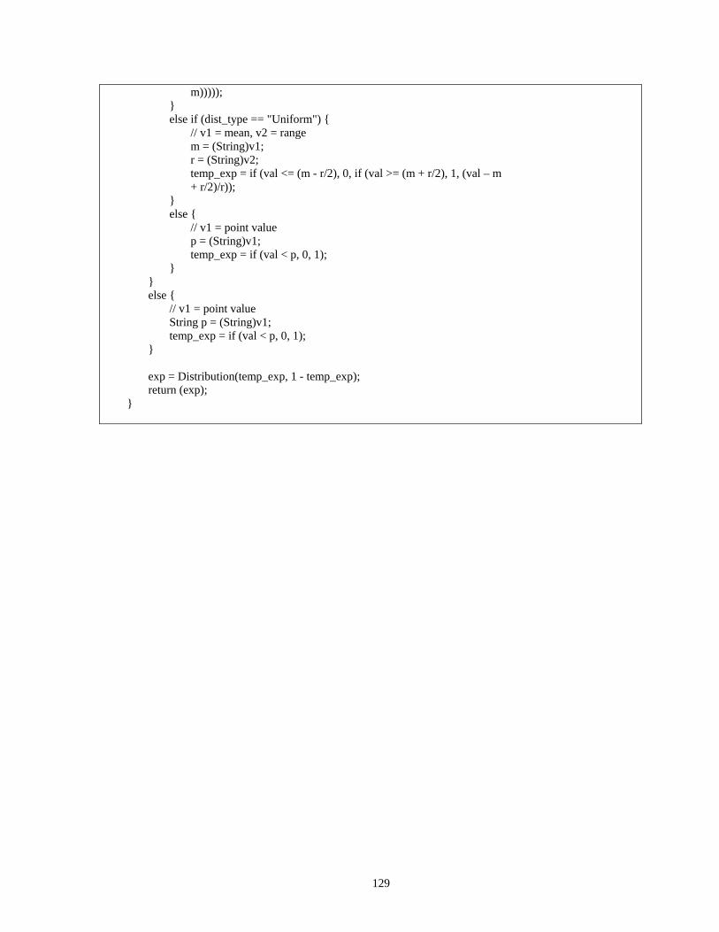
m))))); } else if (dist_type == "Uniform") {
// v1 = mean, v2 = range m = (String)v1; r = (String)v2; temp_exp = if (val <= (m - r/2), 0, if (val >= (m + r/2), 1, (val – m + r/2)/r));
} else {
// v1 = point value p = (String)v1; temp_exp = if (val < p, 0, 1);
} } else {
// v1 = point value String p = (String)v1; temp_exp = if (val < p, 0, 1);
} exp = Distribution(temp_exp, 1 - temp_exp); return (exp);
}
129
References
Amspaker, M., “Expanding Current Obsolescence Tools to Non-Electronic Areas”, Proceedings of the DMSMS Conference, http://smaplab.ri.uah.edu/dmsms98/ papers/amspaker.pdf, 1999.
Avlonitis, G.J., Hart S.J., and Tzokas, N.X., “An Analysis of Product Deletion Scenarios”, Journal of Product Innovation Management, v 17, p 41-56, 2000.
Bumbalough, A., “USAF Manufacturing Technology’s Initiative on Electronics Parts Obsolescence Management”, Proceedings of the 44th International SAMPE Symposium, p 2044-2051, 1999.
Bundy, A., “Incidence Calculus: A mechanism for probabilistic reasoning”, Journal of Automated Reasoning, v 1, p 283-83, 1985.
Chandrasekaran, B., and Mittal, S., “Conceptual representation of medical knowledge for diagnosis by computer: MDX and related systems”, Advances in Computers, v 22, p 217-93, 1983.
Clancey, W. J., “Heuristic classification”, Artificial Intelligence, v 27, n 3, p 289-350, 1985.
Cohen, P. R., Heuristic reasoning about uncertainty: An artificial intelligence approach, Pitman Publishing, Inc., 1985.
Cojazzi, G., “The DYLAM Approach to Dynamic Reliability Analysis of Systems”, Reliability Engineering and System Safety, v 52, p 279-296, 1996.
Condra L. W., Presentation to Boeing Commercial Airplane Group Electronic Component Management Program Users' Forum II, March 1997.
Das, D., Gupta, S. K., and Nau, D., “Generating Redesign Suggestions to Reduce Setup Cost: A Step Towards Automated Redesign”, Computer Aided Design, v 28, n 10, p 763-782, 1996.
130
DMEA, Resolution Cost Metrics for Diminishing Manufacturing Sources and Material Shortages, Defense Micro Electronic Activity (DMEA), Dec. 2001, (www.dmea.osd.mil/docs/cost_metrics_revision1.pdf).
Doyle, J., “A truth maintenance system”, Artificial Intelligence, v 12, n 3. p 231-72, 1979.
Henke, A. L., and Lai, S., “Automated Parts Obsolescence Prediction,” Proc. DMSMS Conference, (http://smaplab.ri.uah.edu/dmsms/laip.pdf), 1997.
Herald, T.E., “Technology Refreshment Strategy and Plan for Application in Military Systems – A ‘How-To Systems Development Process’ and Linkage with CAIV”, Proceedings of the National Aerospace and Electronics Conference (NAECON), p 729-736, 2000.
Internet_1, Data collected from various sites over the internet and through personal observation over the last few years, 2003.
Irani, R. K., Kim, B. H., and Dixon, J. R., “Integrating CAE, Features, and Iterative Redesign to Automate the Design of Injection Molds”, Proceedings of the ASME International Computers in Engineering Conference, 1989.
Jensen, F.V., Bayesian Networks and Decision Graphs – Statistics for Engineering and Information Science, Springer, 2002.
Kumar, U. and Kumar, V., “Technological Innovation Diffusion: The Proliferation of Substitution Models and Easing the User’s Dilemma,” IEEE Transactions on Engineering Management, 39(2), p 158-168, 1992.
Kurawarwala, M., and Matsuo, H., “Forecasting and inventory management of short life-cycle products,” Operations Research, 44, January-February, 1996.
Levitt, T., “Exploit the Product Lifecycle”, The Harvard Business Review, Nov-Dec 1965.
Lin, F., “Re-engineering Option Analysis for Managing Software Rejuvenation”, Information and Software Technology, v 35, n 8, p 462-467, 1993.
Lowrence, J. D., Garvey, T.D., and Strat, T.M., A framework for evidential reasoning systems. Proc. 5th National Conference on AI (AAAI-86), Philadelphia, 896-901, 1986.
131
McAllester, D., “An outlook on truth maintenance”, AI memo n 551, Artificial Intelligence Laboratory, MIT, 1980.
McArthur, C. J., and Snyder, H. M., “Lifecycle Cost – The Logistics Support Analysis Connection”, Proceedings of the IEEE National Aerospace and Electronics Conference NAECON, Vol. 3, p 1206-1209, May 1989.
McDermott, J.,Shearer, J., and Tomczykowski, W., “Resolution Cost Factors for Diminishing Manufacturing Sources and Material Shortages,” ARINC, February 1999, (www.gidep.org/data/dmsms/library/dmea3.pdf).
Meade, N., and Islam, T., “Technological Forecasting - Model Selection, Model Stability, and Combining Models”, Management Science, 44, pp. 1115-1130, August 1998.
Meixell, M. J., and Wu, S.D., “Scenario Analysis of Demands in a Technology Market Using Leading Indicators”, IEEE Transactions on Semiconductor Manufacturing, 14(1), p 65-75, Feb. 2001.
Meyer, B. C., “Market Obsolescence and Strategic Replacement Models”, The Engineering Economist, v 38, n 3, p 209-221, 1993.
Montanari, U., “Networks of constrains, fundamental properties and applications to picture processing”, Information Science, v 7, p 95-132, 1974.
MTI, http://www.mtifwb.com/static/obsolecence.shtml
Nair, S. K., and Hopp, W. J., “A Model for Equipment Replacement Due to Technology Obsolescence”, European Journal of Operations Research, v 63, p 207-221, 1992.
Nilsson, N. J., “Probabilistic logic”, Artificial Intelligence, v 28, n 1, p 71-87, 1986.
Omnijet, Investment Costs: Omni Jet Performance & Cost Database, available at http://www.omnijet.com/menu/
Pearl, J., Probabilistic Reasoning in Intelligent Systems – Networks of Plausible Inference, Morgan Kaufmann Publishers Inc., 1988.
Perl, R. J., Information provided as a part of a NSWC (at Crane) project with CALCE, University of Maryland, College Park, MD, 2004.
Pecht, M., R. Solomon, P. Sandborn, C. Wilkinson, and D. Das, Lifecycle Forecasting, Mitigation Assessment and Obsolescence Strategies, CALCE EPSC Press, 2002.
132
Perry, W., U.S. Secretary of Defense, June 1994.
Pierskalla, W., and Voelker, J., “A Survey of Maintenance Models: The Control and Surveillance of Deteriorating Systems”, Naval Research Logistics, v 23, p 353-388, 1976.
Porter, Z., “An Economic Method for Evaluating Component Obsolescence Solutions”, Boeing Corporation, 1998.
PRICE H, help manual accessed through Price H software tool, September 2001.
Rajagopalan, S., Singh, M. R., and Morton, T. E., “Capacity Expansion and Replacement in Growing Markets with Uncertain Technology Breakthroughs”, Management Science, v 44, n 1, p 12-30, 1998.
Romeu, J. L., “Understanding Series and Parallel Systems Reliability”, Selected Topics in Assurance Related Technologies (START), Department of Defense Reliability Analysis Center (DoD RAC), v 11, n 5, 2004.
Sandborn, P., and Knox, R., “Part Obsolescence Forecasting Based on Data Mining,” to be published Proceedings of the DMSMS Conference, April 2005.
Shafer, G., “Combining AI and OR”, Working paper No.195, School of Business, University of Kansas (Lawrence), 1988.
Sherwood, E., “Product Lifecycle (PLC) Code Definitions and Applications,” Proposal to EIA, 2000.
Shields, P., “Total Cost of Ownership: Why the price of the computer means so little.” http://www.thebusinessmac.com/features/tco_hardware.shtml, December 2001.
Solomon, R., Sandborn, P. and Pecht, M., “Electronic Part Lifecycle Concepts and Obsolescence Forecasting”, IEEE Transactions on Components and Packaging Technologies, v 23, n 4, p 707-713, 2000.
Stogdill, R.C., “Dealing with Obsolete Parts”, IEEE Design & Test of Computers, v 16, n 2, p 17-25, 1999.
TACTech, http://www.tactech.com
133

Wright, M., Humphrey, D., and McCluskey, P., “Uprating Electronic Components for Use Outside Their Temperature Specification Limits”, IEEE Transactions on Components, Packaging, and Manufacturing Technology, Part A, v 20, n 2, p 252-256, 1997.
Young, P., “Technological Growth Curves: A Competition of Forecasting Models,” Technological Forecasting and Social Change, 44, pp 375-389, 1993.
134