ABSTRACT

Wang, Zhi. Spectral Analysis of Protein Sequences. (Under the direction of Dr.

William R. Atchley and Dr. Charles E. Smith.)

The purpose of this research is to elucidate how to apply spectral analysis

methods to understand the structure, function and evolution of protein sequences.

In the first part of this research, spectral analyses have been applied to the basic-

helix-loop-helix (bHLH) family of transcription factors. It is shown that the periodicity

of the bHLH variability pattern (entropy profile) conforms to the classical α-helix

periodicity of 3.6 amino acids per turn. Further, the underlying physiochemical

attributes profiles (factor score profiles) are examined and their periodicities also

have significant implications of the α-helix secondary structure. It is suggested that

the entropy profile can be well explained by the five factor score variance

components that reflect the polarity/hydrophobicity, secondary structure information,

molecular volume, codon composition and electrostatic charge attributes of amino

acids.

In the second part of this research, complex demodulation (CDM) method is

introduced in an attempt to quantify the amplitude of periodic components in protein

sequences. Proteins are often considered to be “multiple domain entities” because

they are composed of a number of functionally and structurally distinct domains with

potentially independent origins. The analyses of bZIP and bHLH-PAS protein

domains found that complex demodulation procedures can provide important insight

about functional and structural attributes. It is found that the local amplitude

minimums or maximums are associated with the boundary between two structural or

functional components.

In the third part of this research, the periodicity evaluation of a leucine zipper

protein domain with a well-known structure is used to rank 494 published indices

summarized in a database (http://www.genome.jp/dbget/aaindex.html). This

application allows us to select those amino acid indices that are strongly associated

with the protein structure and hereby to promote the protein structure prediction. This

procedure can be used to reduce some redundancy of the amino acid indices.

Spectral Analysis of Protein Sequences

by Zhi Wang

A dissertation submitted to the Graduate Faculty of

North Carolina State University in partial fulfillment of the

requirements for the Degree of Doctor of Philosophy

Biomathematics and Bioinformatics

Raleigh 2005

APPROVED BY: Chair of Advisory Committee

Chair of Advisory Committee Co-Chair of Advisory Committee

Biography

I was born in Wuhan, Hubei, China on Mar 18, 1977. I attended the No. 1 Middle

School of Chinese Central Normal University, where I was intrigued by the complexity

of life. As a teenager, I became enamored with science and math and participated

contests of biological science. I attended Wuhan University in the fall of 1994 and

majored in Biology. In 1998, I was awarded the Bachelor Degree. In 2000, I was

awarded a Master Degree in Genetics. During this period, I was proud of publishing

one scientific paper on modeling of branching structures of plants and accomplishing

the computer simulation of genetic recombination project. After encouragement and

support from Youhao Guo and Qixing Yu, I decided to apply and later attend North

Carolina State University for my graduate studies on Biomathematics and

Bioinformatics. Fortunately, I begin working in William Atchley’s lab on computational

biology and I am able to do a lot exploration works on computational methods under

the guidance of Dr. Atchley and Dr. Smith. The following thesis will explain what I have

been doing during these last few years in Atchley’s lab.

ii

Acknowledgements

There are many people who have been very helpful throughout my graduate

career. First and for most I would like to thank my advisor Dr. William R. Atchley and

Dr. Charles E. Smith, for academic mentoring and for allowing me to do exploratory

research on computational biology. I would like to thank all my committee members

past and present Dr. Bruce S. Weir and Dr. Jeff L. Thorne.

For emotional support I would like to thank my fellow graduate students especially

Jieping Zhao, Andrew Fernandes, Kevin Scott, Andrew Dellinger and Jhondra

Funk-Keenan. I wish to thank my parents Dashun Wang and Yingqing Liu for their love

and financial support. Lastly, I am indebted to my wife Jing Zhang for her love and

support.

iii

Table of Contents

Page

List of Tables……………………………………………………………………..………….vi

List of Figures………………………...……………………………………………………..vii

Introduction……………………………………………………………………..……………1

Chapter 1: Spectral Analysis of Sequence Diversity in basic-Helix-Loop-Helix (bHLH) Protein Domains…………………………………………………..….9

Abstract ...………………………………………………………...…….………….11 Introduction.…………………………..……………………………….………….. 12 Methods……………………………………………………………….……………15 Results ………………………………………………………….…….……………23 Discussion…………..…………………………………………..………………… 27 Acknowledgements……………………………………………..…………………31 Supplement ……………………………………….………………….……………36 Chapter 2: Application of Complex Demodulation on bZIP and bHLH-PAS Protein Domains……………………………………………………………………….…....………………...47 Abstract. ………………………………………………………………………………………...48 Introduction ……………………………………………………………………….…....………………………………49 Methods ……………………………………………………………………………51 Results……………………………………………………………………………...56 Discussion………………………………………………………………………….61

Acknowledgements………………………………………………………….. 64

Supplement………………………………………………………………………...72 Chapter 3: Evaluation of Amino Acid Indices with Spectral Analysis .……………….……………………………………………75

Abstract ……………………………………………………………………...……..76 Introduction ……………………………………………………………...…………76 Methods …………………………..……………………..…………………………79 Results ………………………..…………………………..………………………. 79 Acknowledgements.. …………………..…………………………..…………………………………...81

iv

Summary………………………………………………………………………….………..82

Reference…………………………………………….…………………………………….84

Appendix A: Spectral Analysis Based on the Burg Method…….………………………….93

Appendix B: Critical Values for the Fisher Test of Significance.………………………….95

v

List of Tables

Page

Supplemental Table 1.1 Five groups of bHLH protein domains……….……………..36

Supplemental Table 1.2 Results of white noise tests for the entropy,

factor score means/ variances profiles…………….……………………………….38

Supplemental Table 1.3 Summary of the fundamental periods of the

entropy profiles …………………………..…………….……………………………..39

Table 2.1 Summary of the locations of local amplitude minimums and

maximums of the 3.6 aa periodic component of the Factor I profile ..…………..71

Table 3.1 Ranking of amino acid indices according to the periodicity

estimates of HsGem-LZ protein domain………….………………………………..80

Appendix Table B.1 Critical values of the proportion of variance for the

Fisher Test…………………………………………………………………………….96

vi

List of Figures

Page

Figure 1.1 Illustration of the spectral plot of the signal sin(x)+2cos(3x)

produced by Fourier Transformation……….………………….……………32

Figure 1.2 Entropy and Factor profiles of bHLH protein domains………………….…33

Figure 1.3 Plots of the spectral density distribution of entropy,

Factor score means and variances profiles produced

by the Fast Fourier transformation……………………………………….…34

Supplemental Fig. 1.1 Three-dimensional Structure of bHLH

protein domain of MYC Proto-Oncogene Protein………………………....36

Supplemental Fig.1.2 Spectral density plot of entropy profile

produced by Burg method. …………………………………………….……40

Supplemental Fig.1.3 Spectral density plot of Factor I means

profile produced by Burg method……………………………………….…..40

Supplemental Fig.1.4 Spectral density plot of Factor I variances

profile produced by Burg method. …………………………………….……41

Supplemental Fig.1.5 Spectral density plot of Factor II means

profile produced by Burg method. …………………………………….……41

Supplemental Fig.1.6 Spectral density plot of Factor II variances

profile produced by Burg method. …………………………………….……42

Supplemental Fig.1.7 Spectral density plot of Factor III means

profile produced by Burg method. ……………………………………….…42

Supplemental Fig.1.8 Spectral density plot of Factor III variances

profile produced by Burg method…………………………………………...43

Supplemental Fig.1.9 Spectral density plot of Factor IV means

profile produced by Burg method………………………………………….. 43

vii

Supplemental Fig.1.10 Spectral density plot of Factor IV variances

profile produced by Burg method…………………………………………...44

Supplemental Fig.1.11 Spectral density plot of Factor V means

profile produced by Burg method……………………………………….…..44

Supplemental Fig.1.12 Spectral density plot of Factor V variances

profile produced by Burg method…………………………………………...45

Supplemental Fig.1.13 Plot of the observed entropy profile and the

predicted entropy profile with a period of 3.68 aa…………………………45

Supplemental Fig.1.14 Plot of the observed and predicted entropy

profiles for each region……………………………………………………….46

Figure 2.1 Comparison between autoregressive power spectrum

analysis and complex demodulation (CDM) of simulated

data containing two periodic components A and B………………………..65

Figure 2.2 Transfer functions of least squares low-pass filters with

convergence factors applied………………………….…………………... 65

Figure 2.3 Entropy profile of bZIP protein domains and the

amplitude of the 3.6-aa periodic component………………………….… 66

Figure 2.4 Spectral density plot of the entropy profile of bZIP

protein domains…………………………………………………….………. 66

Figure 2.5 Factor I profile of a bZIP protein domain of

transcription factor c-fos protein …………………………………….…….66

Figure 2.6 Spectral density plot of the factor I profile of a bZIP

protein domain of transcription factor c-fos protein …………….……….67

Figure 2.7 Entropy profile of bHLH-PAS protein domains and

the amplitude of the 3.6-aa periodic component..…………………..……67

Figure 2.8 Spectral density plot of the entropy profile of

bHLH-PAS protein domains……………………………………….……… 67

Figure 2.9 Spectral density plot of the Factor I profile of Arnt protein..……….……68

viii

Figure 2.10 Factor I profile of Arnt_human protein and the amplitude

of the 3.67-aa periodic component....……………………………………69

Supplemental Fig. 2.1 Amino acid residues and base pairs that

influence DNA bending by Fos and Jun basic-Zip proteins………………..72

Supplemental Fig. 2.2 Structure-Based Sequence Alignment of PERIOD

Proteins and bHLH-PAS Transcription Factors……………….………………73

Supplemental Fig. 2.3 Domain Architecture and 3D Structure of

Drosophila PERIOD PAS protein……………………………………………….74

Figure 3.1 Organization, sequence alignment and the structure

of human geminin protein domain……………………………………….……78

ix

1

Introduction

Spectral Analysis

The broad application of genome sequencing methodology has generated a

huge amount of protein sequence data. Parallel development of sophisticated

computational and statistical methodology for analyzing sequence data has

equipped us with many tools to investigate and explore protein evolution as well as

the relationship between protein sequence and structure. Of particular importance

has been the application of methodology permitting simultaneous consideration of

many amino acid sites to elucidate “patterns” of variability over large portions of

particular proteins. Often such multivariate analyses have focused on the

multidimensional patterns of covariation among amino acid sites.

An integral part of analyzing the multidimensional nature of sequences is the

description of periodicity in the attributes among sequence elements. Periodicity of

sequence elements can reveal important structural and functional characteristics of

the molecule. A typical method for studying periodicity is spectral analysis, which

characterizes the frequency content of a measured signal. Spectral analysis has

been widely used to analyze time series data, and indeed can be used to analyze

protein sequences data if the amino acid is represented by numeric values. There

are many kinds of spectral analysis methods, including Fast Fourier Transformation

(FFT) method, Yule-Walker method, Burg method, Least Squares method and

2

Maximum likelihood method as well (Marple, 1987; Percival and Walden, 1993).

The FFT method has a number of advantages over other methods. (i) The only

assumption FFT makes is that the data are wide-sense stationary. However, the

non-classical methods require additional assumptions. Only when the non-classical

model is an accurate representation of the data, these spectral estimates can

outperform the classical spectral estimators (e.g., the periodogram) (Marple, 1987).

(ii) Statistical property of the periodogram method has been well addressed over

other methods (Percival and Walden; 1993). The FFT is more easily interpreted in

terms of partitioning of variance (Warner, 1998). (iii) The FFT algorithm is the most

computationally efficient spectral estimation method available (Marple, 1987).

The FFT method has been used to detect the residue repeat of a protein

sequence (Mclachlan,1977) and a web server designed for locating periodical

pattern of a sequence exists (Pasquier et al., 1998). In the latter case, a sequence

of N residues is represented as a linear array of N items, with each item given a

weight. The sequence of weights is used to create a “pulse”, which can be

analyzed by Fourier analysis. For example, selecting a weight of 1 for “D” and 2 for

“L”, the sequence ‘AAILVADMLIA’ is transformed into the array {0 0 0 2 0 0 1 0 2 0

0}. In Fourier theory such numeric array pattern can be decomposed into a number

of sine and/or cosine waves, consisting of integer multiples of the basic frequency.

The period is the same as the inverse of the frequency.

Other methods have been proposed because of the low-resolution limitation

of the FFT method. These include the Yule-Walker method, the Burg method, the

Least Squares method and the Maximum likelihood method. All of these methods

3

are based on parametric spectral estimation and hereby they can compensate for

the low-resolution of FFT method. They can maintain or improve high resolution

without sacrificing stability (Marple, 1987; Naidu, 1996).

Few applications of spectral analysis methods to the protein sequences have

been reported. Therefore, in Chapter 1, both the FFT method and the Burg method

are applied to conduct spectral analyses to the variability profiles of the

basic-helix-loop-helix (bHLH) protein domains. Rigorous statistical tests have been

included in this research. The Burg method was explored over other methods

because: (i) The Burg method is computationally more efficient than the Maximum

Likelihood method (Kay 1988, Percival and Walden, 1993). (ii) The Burg method

produces stable and more reasonable estimates for short data series, which is

useful in studying short protein sequences (Matlab Help 2004, Percival and Walden,

1993).

Warner (1998) recommends some preliminary data analysis on the sequence

data before the spectral analysis. First, it is recommended determining whether

there is a linear trend (change in level over residues). If a trend is present, it needs

to be removed before assessing periodic component. Second, it is recommended

that one ascertain if the data series is stationary. If the stationary assumption is

violated, an overall FFT or spectral analysis on the entire data series can be

somewhat misleading. In the latter instance, the complex demodulation method

described in the Chapter 2 is suggested. Third, it is recommended that one

determine if the data series represents white noise, i.e., observations uncorrelated

with each other. In the context of spectral analysis, white noise means no individual

4

periodic component explains a larger share of the variance than the other periodic

component. The spectrum shows a flat line under the null hypothesis. Finally, one

conducts the spectral analysis with FFT method or others to protein sequences and

analyzes the results.

Variability Profiles in Entropy and Factor Scores

To accurately and robustly define the variability of alphabetic data, we apply

tools from information theory. Specifically, we use entropy profiles to measure the

residue diversity of each amino acid in multiple alignments. Entropy profile

procedures are widely accepted in many fields of science and are frequently

employed in physics, chemistry, biology, mathematics, statistics, etc. (Atchley,

1997, 1999, 2000, 2005). Once one has accurately described differential variability

in a set of aligned sequences with entropy profile, the next step is to resolve the

origin and underlying causality of the observed sequences variability. We need to

understand the underlying physiochemical causes of sequence variability, not

simply describe them as a “molecular natural history” phenomenon.

However, there are serious statistical problems associated with analyzing the

amino acid variability in biological sequence data, the so-called “sequence metric

problem” (Atchley, 2005). Protein sequences are composed of long strings of

alphabetic letters rather than arrays of numerical values. Lack of a natural

underlying metric for comparing such alphabetic data significantly inhibits

sophisticated statistical analyses of sequences, modeling structural and functional

aspects of proteins, and related problems. For example, the amino acid leucine (L)

5

is more similar in its physiochemical properties to valine (V) than leucine is to

alanine (A). Currently, no reliable quantitative measure exists to summarize the

extent of the physiochemical divergence among amino acids. These differences

must be quantified before periodicity analysis of physiochemical variability can be

understood for protein sequences.

Previous authors circumvented sequence metric problems in different ways.

Some generated ad hoc quantitative indices to summarize amino acid variability

(Grantham, 1974; Sneath, 1966). However, ad hoc indices generally summarize

only part of the total variability in amino acid attributes. If a numerical index

approach is to be effective, indices must (i) represent the proximate causes of

amino acid variability; (ii) reflect interpretable partitions of total amino acid variation;

and (iii) resolve intercorrelations among relevant amino attributes (Atchley et al,

2005).

An on-line database (AAIndex) exists that summarizes many attributes of

amino acids (www.genome.ad.jp/dbget/aaindex.html). A total of 494 indices are

found at this website that include general attributes, such as molecular volume or

size, hydrophobicity, and charge, as well as more specific measures, such as the

amount of nonbonded energy per atom or side chain orientation angle.

However, there is much redundancy in these data making selection of

appropriate indices for analyses much more difficult Atchley et al. (2005) used the

multivariate statistical procedure of factor analysis to produce a subset of numerical

descriptors that would summarize the entire constellation of amino acid

physiochemical properties. Factor analysis is a powerful exploratory statistical

6

procedure, that can simplify high-dimensional data by generating a smaller number

of ‘‘factors’’ that describe the structure of highly correlated variables. The resultant

factors are linear functions of the original data, fewer in number than the original,

and reflect clusters of covarying traits that describe the underlying or ‘‘latent

structure’’ of the variables. High-dimensional attribute data are summarized by five

multidimensional patterns of attribute covariation that reflect polarity, secondary

structure, molecular volume, codon diversity, and electrostatic charge.

Thus, the entropy profiles and factor scores permit me to conduct spectral

analysis on the periodicity of proteins to investigate their structure, function and

evolution in this dissertation.

Complex Demodulation

Suppose that a set of data contains a perturbed periodic component

cos( )t t t tX A t zλ φ= + + where At is a slowly changing amplitude instead of a

constant, and tφ is a slowly changing phase. Complex demodulation is to extract

approximations to the series At and tφ . Description of the amplitude and the phase

of a particular frequency by rigorous mathematical tools can be very informative to

solve the puzzle of the complicated structure and function of protein sequences.

However, spectral analyses, such as those based on the FFT method, cannot be

used to assess sudden, time-dependent (i.e. amino acid site-dependent for protein

sequences) changes in the amplitude of a particular frequency.

7

The complex demodulation method (CDM) has been developed to provide a

continuous assessment of the amplitude of numeric protein sequences and thereby

identify changing events (Bloomfield, 1976). While CDM has been widely applied in

many other scientific field (Hayano, et al., 1993; Lipsitz, et al., 1998; Babkoff, et al.,

1991; Rutherford and D’Hondt, 2000), it has apparently never been applied in

computational biology and bioinformatics. I explored the application of CDM on

the entropy and factor profiles of basic-ZIP (bZIP) and basic-Helix-Loop-Helix-PAS

(bHLH-PAS) protein domains. These results are summarized in Chapter 2.

Currently there are several on-line bioinformatics tools of analyzing the

hydrophobicity profiles of protein sequences. For example, the tool at

http://arbl.cvmbs.colostate.edu/molkit/hydropathy can make plots that characterize

the hydrophobic character of protein sequences, which may be useful in predicting

membrane-spanning domains, potential antigenic sites and regions that are likely

exposed on the protein's surface. Generally, windowing techniques have been

used in analyses of the hydrophobicity profiles where window size refers to the

number of amino acids examined to determine hydrophobic characteristics.

Windowing techniques can smooth the hydrophobicity profiles and reduce

fluctuation in the original signal. Unfortunately, such procedures result in the loss of

some biological information, especially the information contained in the

high-frequency components. In other words, the removal of short-range oscillations

results in the loss of some biological information.

The CDM method is a mathematical tool that can be used to analyze the

amplitude and phase of the high-frequency components without the loss of

8

information because it does not use windowing techniques. Therefore, it can be

regarded as a complementary procedure to other computational tools of analyzing

sequence profiles. Indeed, it can also analyze low-frequency components. The

analyses of the changing amplitude of the 3.6-aa periodic component of bZIP and

bHLH-PAS protein domains in Chapter 2 prove that CDM is a sound procedure to

reveal the biological information contained in high-frequency components.

Evaluation of Amino Acid Indices

Interaction with water of the amino acid side chains is a major determinant of

protein structure. The hydrophobic scales are semiempirical quantities based on

both computation and experimental measurements that describe the interaction

between amino acid and water. The hydrophobic scales are helpful in analyzing the

protein biochemical structures because they are associated with the free energy of

folding and formation of structure (Fasman,1989). However, there are numerous

indices proposed to measure residue hydrophobicity and there is a lot of

redundancy of these indices.

In Chapter 3, periodicity evaluation is proposed as a method to make

comparison among those indices that are closely associated with the helix

formation. If the periodicity of a certain amino acid index profile conforms to the

observed periodicity of a well-known structure, then such amino acid index can be

assumed as a good one.

9

Goal of Research

The application of spectral analysis methods on protein sequences is poorly

investigated. Therefore, the goal of my dissertation work is to explore the potential

application of these methods.

This research is to demonstrate how spectral analysis methods such as FFT,

Burg method and complex demodulation can be used to analyze the biological

signals contained in protein sequences. This research is to elucidate that the

entropy profile can be decomposed into underlying physiochemical components.

This research is to elucidate that the complex demodulation method is a promising

method to quantify the amplitudes of periodic components of protein sequence

signals. And the research suggests that the amplitudes are predictors of protein

structure and function. Finally, this research presents an approach to rank the

amino acid indices based on their periodicity parameters, which is valuable to

determine the best amino acid index for computation.

10

Chapter 1

Spectral Analysis of Sequence Diversity in

basic-Helix-Loop-Helix (bHLH) Protein Domains

by

Zhi Wang1,* and William R. Atchley1,2

1Graduate Program In Biomathematics And Bioinformatics and 2Department

Of Genetics and Center For Computational Biology, North Carolina State

University, Raleigh, NC 27695-7614, USA

Key words: spectral analysis, entropy, factor, periodicity, helix

* To whom correspondence should be addressed

* CONTACT: zwang2@ ncsu.edu

11

ABSTRACT

Using the basic helix-loop-helix (bHLH) family of transcription factors as a

paradigm, we explore whether periodicity patterns of amino acid diversity have

implications of its helix secondary structure. Further we wish to ascertain whether

statistical analyses will clarify the underlying causes of periodic amino acid

variation. A Boltzmann-Shannon entropy profile was used to represent site-by-site

amino acid diversity in the bHLH domain. Spectral analysis showed that the

periodicity of the bHLH entropy profile and provided strong statistical evidence that

the amino acid diversity pattern conforms to the classical α-helix three-dimensional

structure periodicity of 3.6 amino acids per turn. Then, amino acid attribute indices

derived from multiple factor analysis of almost 500 amino acid attributes were used

to explore the underlying causal components of the bHLH variability patterns.

These five multivariate attribute indices reflect patterns in i) polarity / hydrophobicity

/ accessibility, ii) propensity for various secondary structures, iii) molecular volume,

iv) codon composition and v) electrostatic charge. The periodicity analyses of these

indices also have significant implications of the underlying helix secondary

structure. Further, multiple regression analyses of the entropy values and the

underlying physiochemical attributes represented by factor score means/variances

can decompose the variation in entropy values into their underlying structural

components. These analyses have significant implications of the statistical

estimations of important attributes of protein secondary structure.

Availability: http://www.atchleylab.org/spectral/bhlh.htm

12

Introduction

Much of contemporary research in biological, medical and agricultural

sciences focuses on complex traits. Complex traits are generally characterized as

being composed of various component parts that are interdependent, dynamic and

multi-regulated. Some classic examples include mammalian body weight,

craniofacial form, human diseases like diabetes, heart disease and cancer, human

behaviors like schizophrenia and alcohol addiction, and other important traits.

Protein molecules often fit this classification as well. Protein molecules: i) may

contain multiple structural and functional domains, ii) protein domains are

composed of many different amino acid sites with varying degrees of

intercorrelation, iii) the various amino acids contribute differentially to structure and

function, iv) the separate domains may have distinct evolutionary origins, v) they

are integrated through processes like domain shuffling, and vi) different domains

(and their constituent amino acids) may be subjected to separate selection regimes

based on their functioning. To adequately understand protein evolution and

structure requires a deeper knowledge of these component parts of proteins, their

characteristics, dynamics, integration and divergence.

In a series of papers, we have employed a computational biology approach

to exploring a number of structural and evolutionary aspects of the basic

helix-loop-helix (bHLH) family of proteins. The bHLH proteins are a collection of

important transcriptional regulators that are involved with the control of a wide

variety of developmental processes in eukaryote organisms (Murre et al., 1989,

13

1994; Sun and Baltimore, 1991; Atchley and Fitch, 1997; Ledent and Vervoort,

2001).

Our previous analyses have focused on a number of important questions

including estimating amino acid diversity, describing phylogenetic relationships

(Atchley and Fitch, 1997), elucidating networks of covarying amino acid sites

(Atchley et al., 2001; Buck and Atchley, 2005), describing the relationships

between sequence covariability and protein structure (Atchley et al., 2001),

exploring the underlying causes of sequence covariation (Wollenberg and Atchley,

2000; Atchley et al., 2001), describing sequence signatures (Atchley et al., 2000;

Atchley and Fernandes, 2005), exploring domain shuffling (Morgenstern and

Atchley, 19xx) and other fundamental questions about this important group of

proteins. In all of these analyses, we have sought to provide results and

methodology that can be incorporated in results of other types of structural and

functional analyses.

Herein, we use a battery of computational methods to explore the nature of

amino acid diversity in the bHLH proteins to better understand the underlying

causes of sequence variability and covariability. Specifically, we wish to ascertain

whether the patterns of amino acid diversity in the bHLH domain over large

numbers of sequences (as shown by Atchley et al., 2000) correspond to the

structural geometry of single proteins, as described by crystal structure studies

(e.g., Ferre-D’Amare et al., 1993; 1998 Shimizu et al., 1997). Previously, we have

used a mutual information approach to describe differential variability and

covariability among amino acid sites in large aligned sequence databases (Atchley

14

et al., 1999, 2000; Wollenberg and Atchley, 2000). In the present paper, we

evaluate the null hypothesis that the observed patterns of amino acid diversity in

the bHLH domain exhibit a systemic periodicity that corresponds to known

structural geometry.

A number of previous authors have suggested that analyses of periodicity

among sequence elements can elucidate important characteristics in molecular

structure, function and evolution (Eisenberg et al., 1984; Pasquier et al., 1998;

Leonov and Arkin, 2005). For example, an α-helix adopts an amino acids spiral

configuration of 99 7±� �

around the helical axis, generating a range in

periodocity of 3.40 - 3.91 aa per turn. The conventionally accepted average

periodocity value is about 3.60 aa per turn (Kyte, 1995). Mutations that disrupt such

structural geometry are expected to be subject to strong natural selection (Patthy,

1999). Hence, there should be significant changes in the patterns of amino acid

diversity at different positions in the α-helix that are conserved over large numbers

of evolutionarily related proteins. Indeed, our previous quantitative analyses of

the bHLH domain suggest a strong relationship between levels of amino acid

diversity and the amphipathic nature of the α-helices that comprise the bHLH

domain (Atchley et al., 2000).

Herein, we use spectral analysis, information theory and multivariate

statistical methods to examine the periodic nature in amino acid variability in the

bHLH domain. Our goal is to: 1) describe the periodicity patterns in amino acid

diversity within the highly conserved bHLH protein domain; 2) ascertain whether

the diversity in amino acid composition conforms to estimates of secondary

15

structure known from previous crystal structure analyses; and 3) decompose the

variability in entropy patterns into their underlying structural components.

Methods

Definition and Structure of the bHLH Domain

The bHLH domain is a highly conserved domain comprised of

approximately 60 amino acids (Atchley and Fitch, 1997). It is best modeled as two

separate α-helices separated by the loop (Ferre-D’Amare et al., 1993; Shimizu et

al., 1997). The domain is comprised of a basic DNA binding region (b) of about 14

amino acids that interacts with a consensus hexanucleotide E-box (CANNTG). The

basic region is followed by two amphipathic α-helices (H) separated by a variable

length loop (L). The helix regions are involved with protein-DNA contacts and

protein-protein interaction, i.e., dimerization. The loop region is of variable length

and may range from approximately 5 to 50 residues that are generally quite difficult

to homologize among different bHLH subfamilies (Morgenstern and Atchley, 1999)

The bHLH proteins are conventionally classified into 5 major DNA-binding

groups (A, B, C, D, and E) based on how the proteins bind to the consensus E-box

and other attributes (Atchley and Fitch, 1997; Ledent and Vervoort, 2001). Herein,

we analyze a total of 196 bHLH sequences chosen to reflect the diversity of the

bHLH subfamilies and DNA binding groups. These data include 83, 72, 16, 9 and

16 sequences belonging to groups A, B, C, D and E, respectively. These

sequences are part of a standard bHLH dataset used in a number of previous

16

computational analyses (Atchley and Fitch, 1997; Atchley et al., 2000; Atchley et al.,

2005).

Data preparation

The sequences were initially aligned using both local and global type

alignment algorithms and the resultant preliminary alignments then corrected by

eye when the results of the two alignment algorithms did not agree.

Representatives of the aligned subfamilies can be found in Atchley and Fitch

(1997). As is previous analyses, the break points between components follows

the structural analyses of Ferre-D’Amare et al., (1993). where the basic region

includes amino acids 1—13; helix 1 involves 14—28; the loop comprises 29—49

and helix 2 includes 50—64.

To facilitate subsequent analysis, the loop region between residues 32 and

46 was removed. The loop region is highly divergent in both length and

composition among groups of bHLH proteins making accurate decisions about

homology difficult for much of this region Atchley and Fitch, 1997; Morgenstern and

Atchley, 1999). Unless an accurate alignment can be achieved, subsequent

statistical analyses are of dubious value. Thus, much of the loop has been

removed and only 49 columns of the multiple alignments remain further spectral

and statistical analysis. Removal of the non-homologous portion before

subsequent analyses is standard procedure for such analyses. Preliminary

spectral density plots of the profile containing the whole loop region was compared

with the one used in this paper. The results were not significantly affected by

removing this highly variable portion of the loop region.

17

Additional analyses can be found at

http://www.atchleylab.org/spectral/bhlh.htm

Entropy Profiles

We use the Boltzmann-Shannon entropy E to quantify sequence variability of

amino acid residues at each aligned amino acid site as defined in Atchley et al.

(1999, 2000). It is calculated as 21

1 2( ) log ( )j j

jE p p p== −∑ , where pj is the

probability of a residue being a specific amino acid or a gap, and

0 ( ) 4.39E p≤ ≤ . An “entropy profile” is given in a histogram (Fig.1.2a) where

the height of the individual bars reflects the entropy value (residue diversity) at a

particular aligned amino acid site. Small E values indicate a high degree of

sequence conservation.

Factor Score Profiles

Atchley et al. (2005) pointed out that statistical analyses of alphabetic

sequence data are hindered by the lack of a rational underlying metric for

alphabetic codes. To resolve this “metric” problem, these authors generated a

small set of highly interpretable numerical values that summarize complex patterns

of amino acid attribute covariation. This was accomplished through multivariate

statistical analyzes of 495 separate amino acid attributes and. Using factor

analysis (Johnson and Wichern 2002), these authors defined five major patterns of

amino acid attribute covariation that summarize the most important aspects of

18

amino acid covariability. These five patterns or multidimensional indices were

interpreted as follows: Factor I = a complex index reflecting highly intercorrelated

attributes for polarity, hydrophobicity, solvent accessibility, etc. Factor II =

propensity to form various secondary structures, e.g., coil, turn or bend versus

alpha helix frequency. Factor III = molecular size or volume, including bulkiness,

residue volume, average volume of a buried residue, side chain volume, and

molecular weight. Factor IV = relative amino acid composition in various proteins,

number of codon coding for an amino acid, and amino acid composition. Factor V

= electrostatic charge including isoelectric point and net charge. A set of “factor

scores” arising from these analyses provide a multidimensional index positioning

each amino acid in these major interpretable patterns of physiochemical variation.

Herein, we transform the original alphabetic amino acid codes to these five

factor scores in the aligned sequence data. This procedure generates five sets of

numerical values that accurately reflect a broad spectrum of amino acid attributes.

The factor score transformed data is then used for many of our subsequent statistical

analyses. For simplicity, we analyze the five factor score transformed data

individually, i.e., one set of analyses for polarity/hydrophobicity, another for

molecular size, etc, rather than do an analysis of all five factors simultaneously.

To better understand the underlying causes of diversity in amino acids, we

include analyses of both the factor score means as well as the factor variances

(Fig.1.2.b-k). The former replaces alphabetic data with the average amino acid

attribute while the latter uses a multidimensional measure of attribute variability.

19

Spectral Analysis Based on Fourier Transformation

It is well known that amino acid sequences can exhibit a periodic pattern in the

occurrence of certain types of amino acids. What is not clear is whether the

diversity of site-specific amino acids similarly exhibits periodic patterns.

To explore this question, a time series model can be expressed in terms of sine

and cosine components (Bloomfield, 1976) as

1

( cos( ) sin( )) (1)m

tt i i i i

i

Y A t B t eω ω=

= + +∑

where Yt is the original variable with n observations. m=n/2 if n is even;

m=(n-1)/2 , if n is odd. ωi specifies the Fourier frequencies, 2πi/n, where i =1, 2, …,

m. Ai and Bi are the amplitude of the sine and cosine components. et is the error

term.

The sum of squares of the Ai and Bi can be plotted against frequency or against

wavelength to form periodograms. The periodogram can be interpreted as the

amount of variation in Y at each frequency. If there is a significant sinusoidal

component at a given frequency, the amplitude A or B or both will be large and the

periodogram will have a large ordinate at that given frequency. If there is no

significant sinusoidal component, then the periodogram will not have any large

ordinates at any frequencies. Hamming window is applied to produce the spectral

density plots, which is a general smoothing procedure in spectral analysis (Kendall

and Ord, 1990). The spectral density plots (Fig.1.3) of entropy, factor score means

and variances are produced by the Fast Fourier Transformation (FFT) procedure in

SAS software (PROC SPECTRA).

20

With Fourier Transformation, any waveform can be analyzed as a

combination of sine waves of various amplitude, frequency and phase. For

example, a signal which is a sum of sin(x) and 2cos(3x) can be analyzed by its

spectral plot, in which there are two bars representing these two periodic

components (Fig. 1.1).

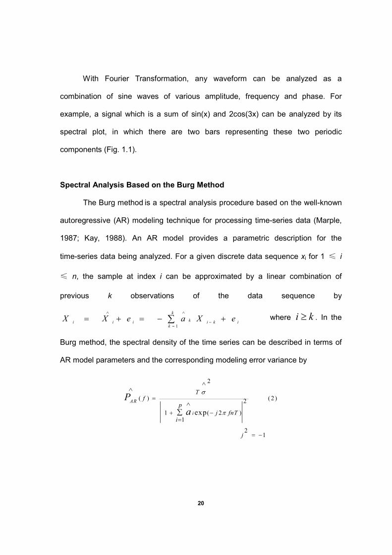
Spectral Analysis Based on the Burg Method

The Burg method is a spectral analysis procedure based on the well-known

autoregressive (AR) modeling technique for processing time-series data (Marple,

1987; Kay, 1988). An AR model provides a parametric description for the

time-series data being analyzed. For a given discrete data sequence xi for 1 ≤ i

≤ n, the sample at index i can be approximated by a linear combination of

previous k observations of the data sequence by

1

k

ki i i i k ik

X X e a X e∧ ∧

−=

= + = − +∑ where i k≥ . In the

Burg method, the spectral density of the time series can be described in terms of

AR model parameters and the corresponding modeling error variance by

2

( ) ( 2 )2

1 ( 2 )1

21

exp

AR

i

Tf

p

j fnTi

j

P

a

σ

π

∧∧

=∧

+ −=

= −

∑

21

where 2

σ� is the estimated modeling error variance, and T is the sampling

interval.

The Burg method is used to calculate the spectral density of the entropy and

factor score variance series as an alternative method to the FFT method. Readers

are referred to Marple (1987) for more details on the algorithms of the Burg

method. Similar to the Fourier transformation method, the spectral density plot can

be produced by the Burg method. The spectral density plots for entropy, factor

score means and variances profiles produced by Matlab software (version 6.5) are

very similar to those listed in Fig.1.3 produced by FFT method.

When spectral density plots are graphed, “large” peaks are generally noted,

necessitating determination of their statistical significance and accuracy. Several

follow-up analyses were conducted to gain more information out of the spectral

density plots.

Fisher’s test is a useful and conservative test for identification of “major”

periodic components (Warner, 1998). The premise behind the Fisher’s test

rejection of the null hypothesis if the periodogram contains a value significantly

larger than the average value (Brockwell and Davis, 1991; Warner, 1998). The test

statistic g, gives the proportion of the total variance that is accounted for by the

largest periodogram component. The critical values of the proportion of variance for

the Fisher’s test at α=0.05 level (N=49) are 0.240, 0.156 and 0.122 for the first,

second and third largest periodogram ordinates, respectively. The critical value

0.240 means that if there are 49 data points in the numeric sequence, then the

22

largest periodogram ordinate must account for more than 24% of the variance to by

judged significant at the 0.05 level. Note that in the special case of a constant time

series (constant numeric sequence in this paper), the p-value returned by Fisher’s

test is exactly 1 (i.e. the null hypothesis is not rejected). If the largest periodogram

ordinate is statistically significant, then it is possible to go on and test the second

and third largest periodogram ordinates for significance, and so on.

Given the major periodic components, harmonic analysis was used to fit

the data with the cyclic components (Warner, 1998). As in regression analysis,

harmonic analysis involves estimating the amplitude parameters A and B in the

formula (1) given a fixed fundamental period parameter ω. R-square (R2)

measures the goodness of fit of the predictive model and estimates the percentage

of total variance of the observations explained by the analysis. Therefore, with the

period estimate from the spectral analysis as a prior, we are able to search for the

best period estimate maximizing the R-square in a relative small range and its

confidence interval (CI).

For the entropy profile, a bootstrap simulation procedure is used to produce

1000 random samples with replacement from the original bHLH multiple

alignments. For each sample, the harmonic analysis is conducted to detect the

best period estimate with the largest R-square statistics. Assuming the 1000 period

estimates have a normal distribution, the 95% confidence interval of the mean can

be obtained.

Analysis of variance (ANOVA) is conducted to partition the total variance in

the entropy data into the variance in factor scores for Factors I-V. The null

23

hypothesis in this analysis is that there is no difference between the total variation

of the scores for Factor I-V and the error variance.

Further, multiple regression analysis is conducted (dependent variable:

entropy independent variable: five factor score variance components) to estimate

β0, β1,…, β5 of the following regression model equation.

Entropy = β0 + β1(Factor I Var) + β2(Factor II Var) + β3(Factor III Var)

+ β4(Factor IV Var) + β5(Factor V Var) + ε (3)

where ε is a normal distributed random variable with µε=0 and σε2=σ2

RESULTS

Periodicity Analyses of Entropy Profiles

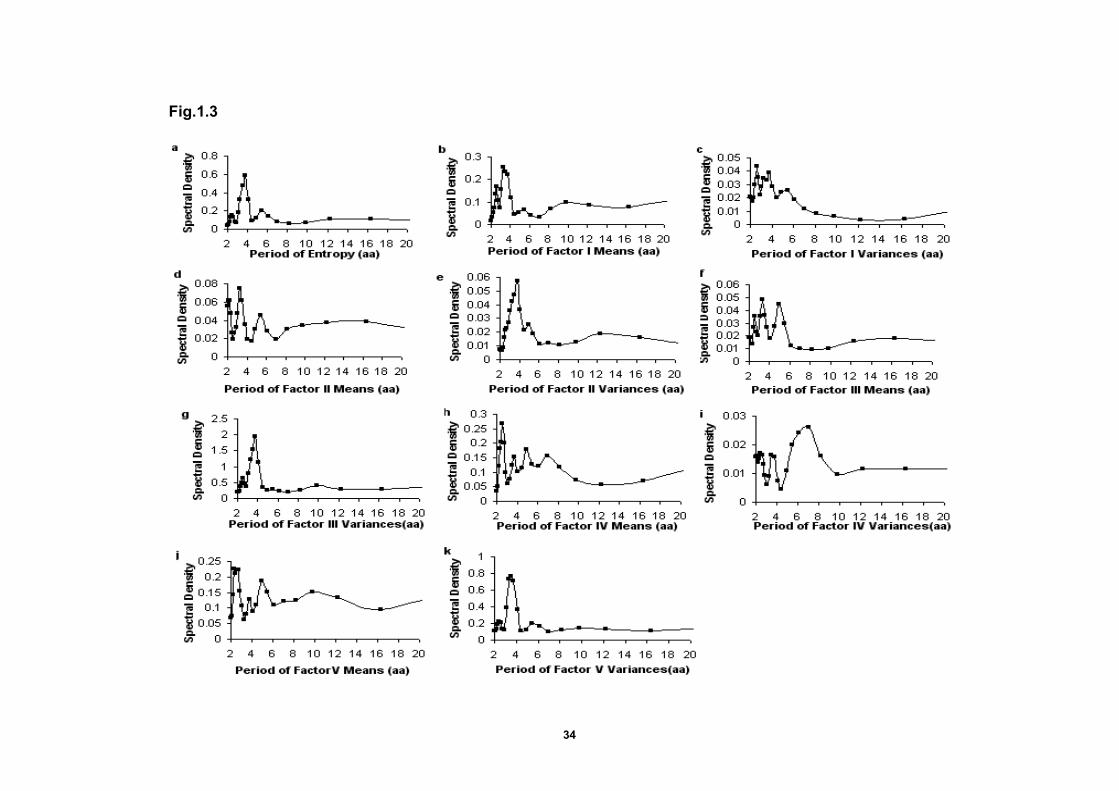
The spectral density plot produced by the Fast Fourier transformation for the

entropy profile is shown in Fig.1.3a. The largest peak corresponds to a period of

approximately 3.77 aa. The spectral density plot produced by the Burg method is

very similar. Fisher’s test indicates that the periodogram ordinate at 3.77 aa is

significantly different from the average periodogram, which confirms that the

periodic component with a period of 3.77aa is statistically significant. However, the

second and third largest periodogram ordinates are not significant. Thus, there is

one statistically significant major periodicity component in the entropy profile and it

corresponds to a value well within the range of known α-helix values.

Limitations of the Fourier frequency reported by the FFT method permit the

spectral analysis to give only an approximate periodicity estimate. Thus,

harmonic analysis was conducted to detect the best period estimate in the range

24

from 3.30 aa to 3.90 aa, with increments of 0.01. A predictive model was fitted and

the associated R-square statistics (R2) was calculated each iteration. The period

maximizing the R-square statistics was recorded as the best period estimate.

Results indicate that the entropy profile has a major periodic component of 3.6776

aa repeat and this component can explain 45.7% of total variance (R2 = 0.457 ).

A 95% confidence interval of the period estimate calculated from 1000

bootstrap entropy profiles gives an interval of (3.6773 - 3.6778). This finding

substantiates our result that there is a major periodic component in the entropy

profile of bHLH protein domain. Thus, the entropy profile of bHLH protein domain

has a periodicity estimate very similar to the conventionally accepted value (3.60

aa per turn) for the ideal α-helix.

Periodicity of Factor Score Means

The factor score means describe the average physiochemical attribute for

each amino acid site for each factor (=multidimensional physiochemical attribute

index). The spectral density plot of Factor I (polarity) means is given in Fig.1.3b.

The peaks located between 3-4 aa suggest the existence of periodic components.

The periodogram data suggests three possible periodic components of 3.27 aa,

3.77 aa and 2.58 aa. The Fisher’s test statistic g for the 3.27-aa periodic

component is 0.196, which does not exceed the critical value 0.240. However, if it

is assumed that the 3.27-aa component is significant and we continue to test the

3.77-aa component, it is found that the Fisher’s test statistics g of the 3.77-aa

periodic component is 0.176, which exceeds the critical value 0.156. These results

25

suggest that there are possible significant periodic components in the Factor I

means profile.

The spectral density plot of factor II and III means (Fig.1.3d) exhibit some

peaks in the spectral density plot and several large periodogram ordinates.

However, none are statistically significant in the Fisher’s test. The spectral density

plot of Factor IV means (Fig.1.3h) has three large periodogram ordinate at 2.58 aa,

3.27 aa 4.9 aa. The 2.58-aa component is not significant. However, the Fisher’s

test statistics g of the 3.27-aa component is significant, which indicate that there is

possible significant periodic component the Factor IV means profile. Finally,

Factor V has no statistically significant values according to the Fisher’s test.

In summary, these analyses suggest that the factors I and IV means profiles

contain periodicity components which conform to the periodicity of helix secondary

structure, although the statistical significance is not strong. Factor I is a

multidimensional attribute relating to covariation in polarity, hydrophobicity,

accessibility and free energy. Factor IV is related to relative amino acid composition

in various proteins, number of codon coding for an amino acid, and amino acid

composition (Atchley et al., 2005). Other factors have large values around 3.3 to

3.7 but the results do not reach the level of statistical significance in the Fisher’s

tests.

Periodicity Analyses of the Factor Score Variances

An entropy profile (Fig.1.2a) is a description of the total site-by-site amino

acid diversity without regard to the underlying causal physiochemical attributes.

26

Consequently, analyses relating the entropy values to the variances in factor

scores at each site should permit decomposition of the total variability at each

amino acid site into its underlying components of attribute variability.

An analysis of variance of the factor score variances has a statistically

significant F-test value =52.77 (P<0.0001) indicating that the explained variation is

large relative to unexplained variance. Hence, we can reject the null hypothesis

that there is no difference between the total variation of Factor I-V and the error

variance. A multiple regression analysis was carried out of the form:

Entropy = β0 + β1(Factor I Var) + β2(Factor II Var) + β3(Factor III Var)

+ β4(Factor IV Var) + β5(Factor V Var) + ε

This analysis gave parameter estimates of β0 = 0.564 (P<.0001), β1 = 0.470

(P=0.052), β2 = 0.468 (P=0.062), β3 = 0.154 (P=0.023), β4 = 1.263 (P< .0001)

and β5 = 0.174 (P=0.054). The proportion of the total variation explained by the

model has an R2 = 0.86 meaning that 86% of the variation in entropy values could

be explained by these five complex attribute index variables.

The spectral density plot of Factor I variances (Fig.1.3c) has peaks at three

periodogram ordinates (2.58 aa, 3.77 aa and 3.27 aa) but none are statistically

significant by the Fisher’s test. However, analyses of the Factor II variances

profile is Fig.1.3e, give a major peak at 3.77 aa, which is statistically significant in

the Fisher’s test. A follow-up harmonic analysis gives an accurate period estimate

as 3.69 aa (R2=0.285). Similarly, Factor III variances (Fig.1.3g) gave a major

peak at 3.77 aa that is also statistically significant in the Fisher’s test. The follow-up

harmonic analysis gives an accurate period estimate as 3.71 aa (R2=0.379). The

27

spectral density plot of Factor IV variances (Fig.1.3i) had three peaks at

periodogram ordinates at 7 aa, 5.44 aa and 2.13 aa but none are statistically

significant. However, the spectral density plot of Factor V variances (Fig.1.3k)

had large periodogram ordinates at 3.27 aa, 3.77 aa, and 5.44 aa. The value at

3.77 aa is statistically significant in the Fisher’s test.

Thus, Factors II, III and V variances have statistically significant

patterns of periodicity. In each instance, the peak occurs at approximately 3.6 –

3.7 aa, which is close to the conventionally accepted value for an α-helix pattern.

Factor I and IV variances profiles have no significant periodic components.

Discussion

Herein we describe the application of spectral and multivariate

statistical analyses to the patterns of amino acid periodicity in a diverse array of

bHLH domain-containing proteins. Our results suggest that these computational

techniques can be powerful estimators of important structural features in proteins.

Our analyses show that analyzing sequence elements as highly interpretable factor

score attribute indices can facilitate other quantitative analyses to explore important

evolutionary and structural phenomena in proteins.

These analyses of sequence variability give periodicity estimates that

deviate only slightly from the conventionally accepted value of 3.60 aa for an

α-helix. Indeed, they fall well within in the known range of 3.40 - 3.91 aa (Kyte,

1995).

What phenomena might be responsible for variable estimates in amino acid

28

periodicity? First, there is variability in sampling. Our analyses are based on a

single family of transcription factors containing two short amphipathic α-helices.

Thus, we might expect some variability in periodicity among different families of

proteins. For example, it has been reported that the number of residues per

α-helical turn of a leucine zipper protein is about 3.64 (Thepaut et al., 2004), a

value still very similar to that reported here.

Second, more complicated structural phenomena may be at work that adds

noise to the estimates. For example, in the basic region of the bHLH protein/DNA

complex in Pho4, there are non-regular α-helical turns and the basic region is

mostly unfolded relative to residual helical content in the absence of DNA (Cave et

al., 2000). Studies on the bHLH-leucine zipper protein Max when uncomplexed

with DNA has the first 14 residues of the basic region mostly unfolded. However,

the last four residues of the basic region form a persistent helical turn while the loop

region is observed to be flexible (Sauve et al., 2004). Therefore, the basic region

and loop regions may exhibit different periodicity values relative to helix 1 and helix

2. This topic is certainly worthy of further investigation.

The removal of some part of the highly variable loop region (such as done in

this report) may distort the long-range periodicity (low-frequency components)

evaluation of profiles of multiple alignments. However, removal of part of the loop

region has little impact on the short-range periodicity (high-frequency components)

as analyzed in this report. Thus, our short-range evaluations in this paper are

robust.

It is important to consider the stationarity property of a numeric sequence

29

profile since it can affect the periodicity evaluation. Spectral analysis has a

stationary assumption (Warner, 1998), i.e., the mean and variance of the numeric

sequence are constant over amino acid sites and structure depends only on the

relative position of two observations (Kendall and Ord, 1990). However, different

regions of a protein sequence may be subject to different selection pressures

during evolutionary divergence. As a consequence, they may display entropy and

factor score patterns that are not stationary. In the bHLH case, partitioning the

sequence into several short homogeneous regions and then investigating the

periodicity for the basic region, Helix 1 and Helix 2 separately could improve the

accuracy of the periodicity evaluation. Such findings are expected because

structurally and evolutionarily homogeneous regions intend to be more stationary

than the entire sequence. Several suggestions have been made for this problem.

For example, Warner (1998) has suggested a log transformation of the data might

reduce this heterogeneity somewhat. Also, complex demodulation methods (e.g.,

Bloomfield, 1976) make it possible to describe the change in amplitude of the

periodic component across amino acid sites more precisely for nonstationary

series.

The ANOVA and multiple regression results described here demonstrate that

the overall variation (entropy) in alphabetic amino acids can be significantly related

to variation in their major underlying physiochemical attributes. Through studying

the influence of these physiochemical components, we are able to understand and

explain the causes of the variability patterns observed in protein sequences. Based

on the simple model described in this paper, more complex models can be

30

developed that including interaction effects as well as more components.

In summary, our results demonstrate that the major periodic components in

the entropy profile and as well as data on several factor score index variances

exhibit reflect the classical α-helix periodicity of 3.6 aa. The variances of the factor

score for propensity for secondary structure (Factor II), molecular volume (Factor

III) and electrostatic charge (Factor V) are significant underlying causal

components to site-by-site amino acid diversity in the bHLH domain. Further, the

factor score means for polarity and codon composition also contain information

related to the helix secondary structure.

These results suggest that periodicity patterns in amino acid diversity reflect

significant secondary structure information. Further, entropy as a measure of

diversity at each amino acid site can be decomposed into its causal components.

These findings should facilitate formal dynamic modeling of both the variability in

sequence elements and their underlying causes. Such analyses would provide

valuable new information for structural and evolutionary biologists.

It is clear from these analyses that spectral analysis in combination with

other powerful statistical procedures can provide valuable information about the

periodicities in variability patterns of protein domains. Methods, like those

described here, can be used to significantly enhance our understanding of protein

variability, structure, function and evolution.

31

ACKNOWLEDGEMENTS

Thanks to Charles Smith, Andrew Fernandes, Kevin Scott, Andrew Dellinger and

the anonymous reviewers for their helpful suggestions. This research was

supported by a grant from the National Institutes of Health (GM45344) to WRA.

32

Fig.1.1

2cos(3x) sin(x) Signal

Spectral Plot

Frequency of 2cos(3x)

Frequency of sin(x)

33

Fig. 1.2

34

Fig.1.3

35

Figure Legends Fig.1.1 Illustration of the spectral plot of the signal sin(x)+2cos(3x) produced by Fourier Transformation. Fig.1.2 Entropy and Factor profiles of bHLH protein domains. (a) Entropy vs. Amino Acid Sites. (b) Factor I Means vs. Amino Acid Sites. (c) Factor I Variance vs. Amino Acid Sites. (d) Factor II Means vs. Amino Acid Sites. (e) Factor II Variances vs. Amino Acid Sites. (f) Factor III Means vs. Amino Acid Sites. (g) Factor III Variance vs. Amino Acid Sites. (h) Factor IV Means vs. Amino Acid Sites. (i) Factor IV Variances vs. Amino Acid Sites. (j) Factor V Means vs. Amino Acid Sites. (k) Factor V Variances vs. Amino Acid Sites. Fig.1.3 Plots of the spectral density distribution of entropy, Factor score means and variances profiles produced by the Fast Fourier transformation. (a) Spectral density plot of entropy profile. (b) Spectral density plot of Factor I means profile. (c) Spectral density plot of Factor I variances profile. (d) Spectral density plot of Factor II means profile. (e) Spectral density plot of Factor II variances profile. (f) Spectral density plot of Factor III means profile. (g) Spectral density plot of Factor III variances profile. (h) Spectral density plot of Factor IV means profile. (i) Spectral density plot of Factor IV variances profile. (j) Spectral density plot of Factor V means profile. (k) Spectral density plot of Factor V variances profile.

‘

36

Supplement

Supplemental Fig.1.1 Three-dimensional Structure of bHLH protein domain of MYC Proto-Oncogene Protein

Supplemental Table 1.1 Five groups of bHLH protein domains

Group Example Protein

Characteristics

A Myod binds to CAGCTG

B Myc binds to CACGTG

C Sim doesn’t bind directly

D Id no basic region/doesn’t bind

E Hes may bind CACGCG or CACGAG

37

White Noise Tests

In the context of spectral analysis, white noise may be defined more formally

as an equal mixture of all the frequencies. In other words, there is no individual

periodic component that can explain a larger share of the variance over other

periodic components (Warner,1996). Instead of showing peaks in the spectrum of

the signal ( e.g. the data series), white noise shows a flat straight line due the same

contribution of individual periodic components.

Therefore, two white noise tests, Fisher’s Kappa tests and Bartlett's

Kolmogorov-Smirnov (BKS) are conducted (SAS, 1992) to analyze the bHLH

protein domain. The results are shown in Table 2. Although these statistical tests

can provide statistical information about periodicity patterns, we should be cautious

when applying the results to explain the numeric sequence profile and equating

statistical and biological significance. For example, even if a periodic component is

not statistically significant by the Fisher’s test, it still may have some biological

meaning. Even if a numeric sequence profile is assumed to be white noise, the

corresponding amino acid sequence may still contain biological information about

structure, function and evolution.

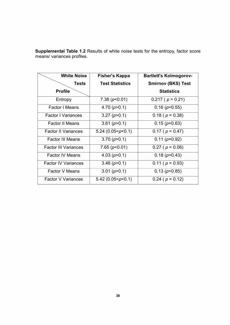
The entropy and Factor III variances profiles are rejected as white noise.

Factor II and Factor V variances profiles are also susceptible as white noise

because both p-values are less than 0.1. Other profiles are not rejected as white

noise in both statistical tests.

38

Supplemental Table 1.2 Results of white noise tests for the entropy, factor score means/ variances profiles.

White Noise

Tests

Profile

Fisher's Kappa

Test Statistics

Bartlett's Kolmogorov-

Smirnov (BKS) Test

Statistics

Entropy 7.38 (p<0.01) 0.217 ( p = 0.21)

Factor I Means 4.70 (p>0.1) 0.16 (p=0.55)

Factor I Variances 3.27 (p>0.1) 0.18 ( p = 0.38)

Factor II Means 3.61 (p>0.1) 0.15 (p=0.63)

Factor II Variances 5.24 (0.05<p<0.1) 0.17 ( p = 0.47)

Factor III Means 3.70 (p>0.1) 0.11 (p=0.92)

Factor III Variances 7.65 (p<0.01) 0.27 ( p = 0.06)

Factor IV Means 4.03 (p>0.1) 0.18 (p=0.43)

Factor IV Variances 3.46 (p>0.1) 0.11 ( p = 0.93)

Factor V Means 3.01 (p>0.1) 0.13 (p=0.85)

Factor V Variances 5.42 (0.05<p<0.1) 0.24 ( p = 0.12)

39

Supplemental Table 1.3 Summary of the fundamental periods of the entropy profiles for the whole sequence, Basic region, Helix 1 and Helix 2. The percentage of variance indicates the percentage of total variance contributed by the periodic component with major periods.

Entropy Profile

Fundamental Period

Model R2

Whole Domain

3.68 2 2Yt 2.497-0.2915 sin( ) 0.8963cos( )

3.68 t 1,2,. . . 49

t tT T

T

π π= +

= =

0.457

Basic Region

3.56 2 2Yt 2.5238+0.1713sin( ) 0.9431cos( )

3.56 t 1,2,. . . 13

t tT T

T

π π= +

= =

0.463

Helix 1 3.59 2 2Yt 2.5423 0.3335sin( ) 0.9567 cos( )

3.59 t 14,15,. . . 28

t tT T

T

π π= + +

= =

0.530

Helix 2 3.59 2 2Yt 2.3744+1.3057 sin( )+0.0028 cos( )

3.59 t 35,36,. . . 49

t tT T

T

π π=

= =

0.777

40

Spectral Density Plots Produced by Burg Methods

Supplemental Fig.1.2 Spectral density plot of entropy profile produced by Burg method.

Supplemental Fig.1.3 Spectral density plot of Factor I means profile produced by Burg method.

41

Supplemental Fig.1.4 Spectral density plot of Factor I variances profile produced by Burg method.

Supplemental Fig.1.5 Spectral density plot of Factor II means profile produced by Burg method.

42

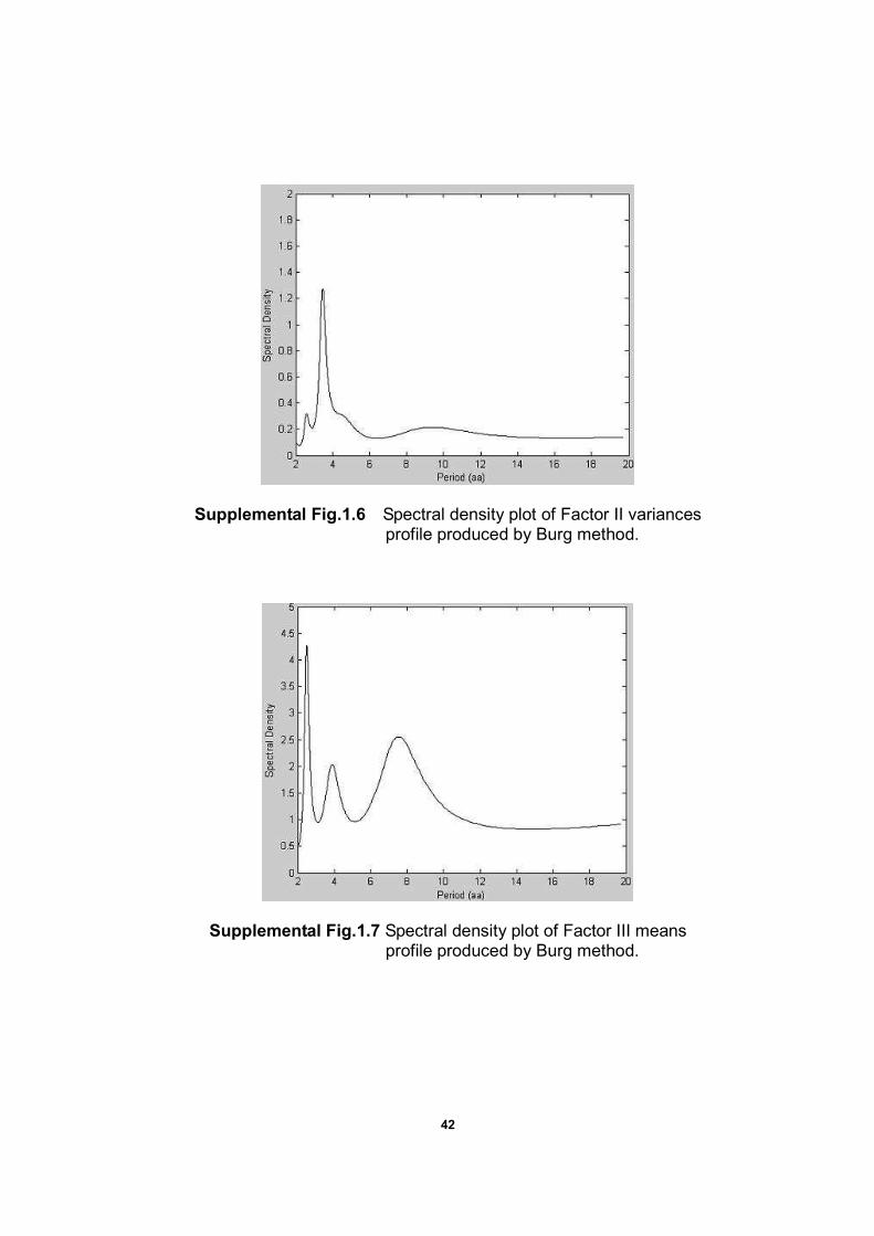
Supplemental Fig.1.6 Spectral density plot of Factor II variances profile produced by Burg method.

Supplemental Fig.1.7 Spectral density plot of Factor III means profile produced by Burg method.

43

Supplemental Fig.1.8 Spectral density plot of Factor III variances profile produced by Burg method.

Supplemental Fig.1.9 Spectral density plot of Factor IV means profile produced by Burg method.

44

Supplemental Fig.1.10 Spectral density plot of Factor IV variances profile produced by Burg method.

Supplemental Fig.1.11 Spectral density plot of Factor V means profile produced by Burg method.

45

Supplemental Fig.1.12 Spectral density plot of Factor V variances profile produced by Burg method.

Supplemental Plots of Analyses on Entropy profile

0

0.5

1

1.5

2

2.5

3

3.5

4

4.5

0 4 8 12 16 20 24 28 32 36 40 44 48

Site

entropy

Supplemental Fig.1.13 Plot of the observed entropy profile (smooth curve) and the predicted entropy profile (dotted curve) with a period of 3.68 aa.

46

0

1

2

3

4

0 2 4 6 8 10 12 14

Site

entropy

Basic Regiona

0

1

2

3

4

14 16 18 20 22 24 26 28 30

Site

entropy

Helix 1b

0

1

2

3

4

5

35 37 39 41 43 45 47 49

Site

entropy

Helix 2c

Supplemental Fig.1.14 Plot of the observed and predicted entropy profiles for each region. (a) Plot of the observed entropy profile (smooth curve) and the predicted entropy profile (dotted curve) with a period of 3.56 aa for the Basic region. (b) Plot of the observed entropy profile (smooth curve) and the predicted entropy profile (dotted curve) with a period of 3.59 aa for the Helix 1 region. (c) Plot of the observed entropy profile (smooth curve) and the predicted entropy profile (dotted curve) with a period of 3.59 aa for the Helix 2 region.

47

Chapter 2

Application of Complex Demodulation on

bZIP and bHLH-PAS Protein Domains

by

Zhi Wang1,* , William R. Atchley1,2, Charles E. Smith1

1Graduate Program In Biomathematics and 2Department Of Genetics and

Center For Computational Biology, North Carolina State University, Raleigh,

NC 27695-7614, USA

Keyword: periodicity, complex demodulation, functional region

* To whom correspondence should be addressed

* CONTACT: zwang2@ ncsu.edu

48

ABSTRACT

Proteins are built with molecular building blocks such as α-helix, β-sheet, loop

region and else, which is an economic way of constructing complex molecules.

Periodicity analysis of protein sequences has allowed us to obtain meaningful

information of their structure, function and evolution. In this work, complex

demodulation (CDM) is introduced to detect functional regions in protein

sequences data. We analyzed bZIP and bHLH-PAS protein domains and found that

complex demodulation can provide insightful information of changing amplitudes of

periodic components in protein sequences. Furthermore, it is found that the local

amplitude minimum or local amplitude maximum of the 3.6-aa periodic component

is associated with protein structural or functional information due to the observation

that they are mainly located in the boundary area of two structural or functional

regions.

49

Introduction

Recent developments in computational methodology have provided

mechanisms to statistically transform alphabetic sequence information into

biologically meaningfully arrays of numerical values (Atchley et al., 2005). Using a

multivariate statistical approach, these authors generated five multidimensional

indices (factors) of amino acid attributes that reflect polarity, secondary structure,

molecular volume, codon diversity, and electrostatic charge of sequences. This

advance will make possible a number of statistical and mathematical analyses that

will facilitate our understanding of the structure and function of biological sequence

data.

For example, it has been suggested that periodicity of a sequence can be

evaluated by Fourier transformation or spectral analysis (Pasquier et al., 1998).

Periodicity of biological sequences is an important indicator of protein structure and

DNA folding (Herzel et al., 1999; Schieg and Herzel, 2004). However, the Fourier

analysis or spectral analysis is not useful in assessing the changes in cycle

parameters, such as amplitude and phase of the periodic components over the

sequence.

Recently, the technique of complex demodulation (CDM) has been introduced

to provide a continuous assessment of the periodic amplitude and thereby identify

regions of change in structural and functional aspects of biological sequences.

Complex demodulation has been widely used in many fields such as physiology,

psychology and oceanography research (Hayano et al., 1993; Lipsitz et al., 1998;

50

Babkoff et al., 1991; Rutherford and D’Hondt 2000). However, there are obviously

no applications of CDM procedures in computational biology and bioinformatics.

Therefore, this paper is to illustrate the application of CDM method on protein

sequences with the case study of bZIP and bHLH-PAS protein domains. This paper

is also an exploratory work to ascertain if the amplitude of a certain periodic

component of a protein sequence has biological information. The bZIP and

bHLH-PAS proteins are selected because of the complexity of their function and

structure, which can represent the complex characteristics of biological signals.

In this article, we show that CDM can describe the changing amplitude of a

certain periodic component. The amplitude pattern of the 3.6-aa periodic

component is closely associated with the secondary structure of the protein

sequences. It is found that the amino acid sites with local amplitude maximums and

local amplitude minimums mostly occur at the boundaries of helices and strands.

This strongly suggests that CDM method is a new computational tool of helping us

to understand biological sequences. There are several methods available to predict

the regular secondary structure, however, the number of correctly predicted α-helix

start positions was just 38% (Wilson, 2004). This research should trigger more

interests in CDM and more exploration works to apply CDM method to analyze the

biological sequences.

51

Methods

Principle of Complex Demodulation

Not every “periodic” series has simple representation in terms of cosine or sine

functions. A perturbed periodic component may have changing amplitude and

changing phase. Therefore, the goal of complex demodulation is to quantify the

amplitude and phase as a function of time. The amplitude and phase are

determined by the data in the neighborhood of t, rather than by the whole series.

The principle of complex demodulation has been well documented by Bloomfield

(1976) so that it is briefly described here before showing the case study results on

the bZIP and bHLH-PAS proteins. Given the fundamental period of a biological

sequence, CDM can extract approximations of the changing amplitude and

changing phase as a function of the position of nucleotides or amino acid residues.

If numerical series data xt of a biological sequence is known to include a component

oscillating around a frequency of λ (the amplitude and the phase may varies), then xt

can be written as

cos( ) (1)t t t tX A t zλ φ= + +

where At and Øt are the changing amplitude and phase of the periodic component

and zt is residue including all other components and noises. Fig.2.1 is a good

illustration of power spectrum analysis and complex demodulation of simulated

52

data (Hayano et al., 1993). It is obvious from this figure that CDM is able to

extract approximations of At (amplitude) as a function of time. Øt can be also

represented as a function of time, but this phase plot hasn’t been shown here.

In factor, the real-valued time series (1) can be regarded as complex-valued

series and hereby can be easily processed in computation. With the Euler relation

cos sin exp( )i iλ λ λ+ = , the time series Xt in (1) is converted to its complex

analogue

1{exp[ ( )] exp[ ( )]} (2)

2t t t t tX A i t i t zλ φ λ φ= + + − + +

where i is a complex number and i2= -1.

We then obtain a new signal yt by shifting all the frequencies in Xt by –λ. This

procedure is called CDM and yt is expressed as

2 exp[ ] (3)t ty x i tλ= −

Inserting equation (2) into (3), equation (3) then becomes

exp( ) exp[ (2 )] 2 exp( ) (4)t t t t t ty A i A i t z i tφ λ φ λ= + − + + −

The first item of equation (4) is smooth (the frequency is around zero), the second

term oscillates at a frequency of -2λ and the third item is assumed to contain no

component around the zero frequency from the definition of zt. Therefore, when we

let Yt be the signal obtained by passing yt through a low-pass filter, we would obtain

Yt in complex version as

exp( ) (5)tt tY A iφ=

Here Yt is represented by a set of complex numbers in terms of its magnitude

53

and phase, At and Øt. The instantaneous amplitude of the periodic component is

defined as

* (6)t t t tA Y Y Y= =

where Yt* is the complex conjugate of Yt . The phase Øt can be then caculated.

The FORTRAN program of CDM was listed by Bloomfield (1976). From a

frequency-domain perspective, the power spectrum of xt has a peak around a

frequency of λ. As the result of CDM, the peak is moved leftward to around zero

frequency in the power spectrum of yt (in the PSD-frequency plot). For example in

Fig. 2.1, if CDM is applied to the low-frequency periodic component A with a

frequency around 0.09 HZ, then the Low-frequency peak will move leftward to

around zero frequency. The peaks of all other components in xt, if any, are also

moved leftward, those at an original frequency above λ do not reach zero

frequency, and those below λ move into the negative part of the frequency axis.

Thus, is is desirable for a low-pass filter to exclude all components except

the zero-frequency component and then the amplitude can be determined. The

low-pass filter is designed according to the least squares filter design method

presented by Bloomfield (1976). The transfer function of the ideal low-pass filter is

1 0( )

0

c

c

ifH

if

ω ωω

ω ω π≤ ≤

= < ≤

(7)

where ωc is the cutoff frequency. The Fourier coefficients of H(ω) are

sin1

c

u

uh u

u

ωπ

= ≥ and 0

c

hωπ

= (8)

54

We have to construct a smoothing function to approximate the ideal low-pass filter

in computation. Convergence factors are used to accelerate the convergence of

Fourier series and achieve better approximation of the transfer function H(ω) in

equation (7). According to Bloomfield, the smoothed function approximating H(ω) is

~

0

1

sin / 2( ) 2 cos

/ 2

s

s u

u

uH h h u

u

δω ω

δ== + ∑ (9)

The multiplier sin 2 /(2 1)

2 /(2 1)

u s

u s

ππ

++

is an example of convergence factor. The

smoothed transfer function, which are initially 1 and decay to smoothly 0, are a

smooth approximation to the ideal filter H(ω). Fig.2.2 shows the smoothed transfer

functions for s=5 (an 11-term filter) and s=20 (a 41-term filter), and the ideal

transfer function.

It is important to note that the amplitudes obtained with the use of complex

demodulation are relative rather than absolute measures. This is due to several

factors, including the following: (i) the signal is not exactly sinusoidal. And (ii) the

absolute measures of the amplitude represents the sum of high and low frequency

periodic components, however, complex demodulation separates out the

amplitudes at each frequency.

Computational Procedures

First, we transform the biological sequences into numeric values. In our case

study, a protein sequence is transformed into a numeric array of factor scores

55

(Atchley et al., 2005). The variability of protein multiple alignments is measures as

a numeric array of entropy values.

Second, spectral analysis is conducted to produce power spectral density

(PSD) plot (as shown in Fig.2.1). Through examining the PSD plot, certain periodic

component of interests can be selected for the following CDM procedure.

Third, given a periodic component of interests, CDM is applied to produce a

plot of instantaneous amplitude and phase of the periodic component of interests

as a function of amino acid sites.

Data Types

The data utilized in this study are basic region-leucine zipper (bZIP) protein

domain and basic region-helix-loop-helix-PAS (bHLH-PAS) protein domain. The

bZIP proteins and bHLH-PAS are both very important transcription factors. bZIP

proteins contain a basic region mediating sequence-specific DNA-binding, followed

by a leucine zipper region, which is required for dimerization (Podust et al., 2001).

Both the basic region and the leucine zipper region have a helix form. Binding to

DNA induces a coil-to-helix transition of the basic DNA-binding region. The leucine

zipper region exhibits a stable helix form. bZIP domain is one of the simplest types

of DNA-binding domains. However, the bZIP transcription factors are capable of

recognizing a diverse range of DNA sequences and regulate the gene transcription.

The collection of 321 bZIP protein sequences (clad bzip_2) was retrieved from the

database Pfam (Dec,2004).

56

The second group of proteins to be analyzed are the bHLH-PAS proteins.

They are a family of sensor proteins involved in signal transduction in a wide range

of organisms. The bHLH-PAS domains contain a structurally conserved α/β-fold.

There are basic region-helix-loop-helix motif, PAS-1 and PAS-2 motifs in the

domain. The illustration of structure-based sequence alignment and the structure of

bHLH-PAS domains can be found in Supplemental Fig.2.2 -2.3. Both PAS-1 and

PAS-2 motifs contain a five-stranded antiparallel β-sheet with one face flanked by

several α –helices (Yildiz et al., 2005). The PAS-1 and PAS-2 motifs are connected

by a short linker.

The choice of bZIP and bHLH-PAS proteins is based on their structural and

functional attributes. Since there are subtle differences among different regions of

the sequences, it is intriguing to distinguish the differences between these various

regions and to explore a novel approach to identifying the boundary of each region.

It is hypothesized that CDM can distinguish the subtle differences among the

structural and functional regions of sequences with a similar helix conformation. If

CDM is able to distinguish the subtle differences, it is expected to work better for

regions of sequences have more structural and functional differences. bHLH-PAS

contains complex α/β-fold which provides us with a complicated data set to

examine the CDM procedure.

Results

bZIP Protein Domain

An entropy profile was calculated (Fig.2.3) based on the method described by

57

Atchley et al. (2000). Such a profile is a numeric representation of the residue

diversity at each amino acid site in a set of aligned proteins. Large entropy values

represent high variability for that site while small values represents low variability.

In our aligned sequence database, the basic region in bZIP proteins ranges from

residue 1 to 27 while the leucine zipper region extends from residue 28 to 55.

There are interesting oscillations of the entropy values and the periodic component

was identified by spectral analysis (Bloomfield, 1976).

A spectral density plot (Fig.2.4) for this entropy profile was produced by the

spectral analysis method-Fast Fourier Transformation (Bloomfield, 1976) using

SAS software (PROC SPECTRA). The peak at around 3.6 aa indicates that there is

a major significant periodic component of at that point in the entropy profile.

Increases of spectral density in the period range from 13.75aa to 56 aa indicate

that there is also low-frequency periodic component, whose period estimate is

much larger. The largest period estimate can be the length of the whole numeric

sequence, but such estimate is meaningless.

We focus on the high-frequency periodic component at around 3.6aa that

conforms to the average 3.6 aa per turn for an ideal α-helix. The CDM procedure

was then used to analyze the amplitude of the 3.6-period component as a function

of amino acid sites. We are particularly interested in locating the boundary between

the basic region and the leucine zipper region.

The amplitude of the periodic component at 3.6 aa vs. residue is plotted in the

dotted line in Fig.2.3. We found there is amplitude decrease in the boundary region

between the basic and leucine zipper regions. The entropy amplitude at residue 27

58

achieved a local minimum. Structural studies indicate that residue 27 is the last

residue of the basic region and the ZIP region starts at residue 28 (Pfam, 2005)

These results indicate that the entropy amplitudes of residues located in the

end of the basic region and near the start of the ZIP region are significantly smaller

than the average values (t-test: p-value<0.05). The maximal entropy amplitude

occurs at residue 42. These latter findings indicate that some residues in leucine

zipper region are highly conserved while others are highly variable. The latter

results in large amplitude which is reflected by large fluctuations in the entropy

values.

These findings suggest that the existence of local minimum entropy

amplitude identifies the boundary of specific structural or functional regions. It is

interesting that the entropy amplitude at residue 4 has global minimal amplitude

and the amplitude increases beyond residue 4. This observation suggests a

functional and structural difference of these residues that warrants further

investigations.

Next, we investigate the Factor I profile (Atchley et al., 2005) of the bZIP

domain of the well-studied transcription factor C-fos shown in Fig.2.5. The

sequence of the domain (primary accession number: P01100; secondary accession

number: P18849, Glover, 1995) is :

139-KRRIRRERNKMAAAKCRNRRREL|TDTLQAETDQLEDEKSALQTE IANLLKEKEKLEFI LAAH-200

Basic Region | Leucine Zipper

The spectral plot of c-fos factor I profile does not reveal a significant

periodic component at around 3.6 aa (Fig.2.6). However, implemented the CMD

59

method assuming that there is a periodic component of 3.6 aa and we obtain the

amplitude of it (dotted curve in Fig.2.5).

Based on the known structure of the c-fos protein (Glover, 1995), the leucine

zipper region starts at residue 162 (labeled in Fig.2.5). However, the amplitude of

the 3.6-aa periodic component of Factor I at residue 162 is not significantly different

from the average (t-test, p>0.05) and indeed the local minimum is not at residue

162. However, the minimal amplitude of factor I occurs at residue 164, which is

close to the leucine zipper starting residue of 162. This result suggests that the

CDM method is somewhat robust to predict the start point of a new structural or

functional region, even if there is no significant 3.6-aa periodic component of Factor

I. The deviation of the leucine zipper start residue from the residue with a minimal

amplitude is possibly related to the absence of a statistical significant 3.6-aa

periodic component of Factor I. This observation provides us with an interesting

topic that may trigger further investigation.

PAS Protein Domain

Within the bHLH/PAS proteins the PAS region is involved in protein

dimerization with another protein of the same family (Ponting and Aravind, 1997;

Hefti et al., 2004; Zhulin et al., 1997). It has also been associated with light

reception, light regulation and circadian rhythm regulators (clock). In bacteria, the

PAS repeat is usually associated with the input domain of a histidine kinase, or a

sensor protein that regulates a histidine kinase. 77 bHLH-PAS protein domains

60

were obtained from PFAM database (version 17.0 May, 2005). The entropy profile

of 77 bHLH-PAS domains is shown in Fig.2.7.

The spectral density plot of the entropy profile of bHLH-PAS protein domains

is given in Fig.2.8. Only short-range periodicity (i.e. high-frequency components)

is shown in Fig.2.8. There are peaks located in the 3.40-3.91 aa range that signal

the existence of an α-helix (Kyte, 1995). Therefore, CMD method is conducted to

produce the amplitude of the 3.6-aa periodic component as a function of amino

acid site (in dotted curve in Fig. 2.7).

Further, we investigate the Factor I profile of a well-known bHLH-PAS protein

Arnt_human protein (p27540/ gi:114163) , whose secondary structure has been

determined (Hoffman et al., 1991). It is a 789 aa-length protein containing

bHLH/PAS1/PAS2 domains (Basic region: 90..102 ; Helix-loop-helix region:

103..143; PAS 1 domain: 161..235; PAS 2 domain 349..419). Regions

1-50 and 468-789 are removed because of they are included in the bHLH/PAS

domain. The estimated secondary structure of the Arnt protein is obtained via

Prediction protein web server.

The spectral density plot of the Factor I profile of Arnt protein has been

produced in Fig.2.9. There are some peaks located in the 3.40-3.91 aa range which

signals the existence of α-helix, especially there is a large peak at around 3.6 aa

(Kyte, 1995).

The Factor I profile of Arnt protein domain is show as histogram in Fig.2.10.

The CMD method produces the amplitude as a function of amino acid sites for the

3.6-aa periodic component (curve in Fig.2.10).

61

Many local amplitude minimums have implication for the boundary of the

α-helix regions or beta-sheets (Table 2.1). Local minimum residue 102 is the

ending residue of the basic region of the bHLH conserved domain. Local

minimum 158 is close to the beginning residue 161 of PAS domain 1 ranging from

residue 161 to 235. Local minimum 344 is close to the beginning residue 349 of

PAS domain 2 ranging from residue 349 to 419.

Most local amplitude maximums have implication the boundary of the α-helix

regions or beta-sheets (Table 2.1). The results are: Local maximum residue 143

is the ending residue of the 2nd helix of the HLH region. Local maximum residue

171 is the ending residue of an α-helix; local maximum residue 291 is close to the

ending residue of a predicted α-helix; local maximum residue 273 is located

between two beta-sheets; local maximum residue 313 is close to the ending

residue of a predicted beta-sheet; local maximum residue 334 is the beginning

residue of a predicted beta-sheet; local maximum residue 355 is the beginning

residue of a predicted beta-sheet; local maximum residue 397 is the 2nd beginning

residue of a predicted beta-sheet. The only exceptions are: local maximum residue

220 is located within a predicted α-helix region; local maximum residue 413 is

located in a predicted beta–sheet region.

Discussion

From the case study of well-known protein sequences of bZIP and

bHLH-PAS proteins, the amplitude of certain periodic component is proved to

contain meaningful biological information. The complex demodulation procedure is

62

able to quantify the amplitude and phase of periodic components of protein

sequences. It is the first time to introduce and illustrate the applications of complex

demodulation on biological sequences. The analyses reveal that the minimums or

maximums of amplitudes of the 3.6-aa periodic component of protein profiles (i.e.

entropy and factor I profiles) are predictors of the boundaries of helices secondary

structures. The results in the paper should trigger the scientific interests of

investigating the application of the CDM method on computational biology and

bioinformatics. Possiblely the analyses of the amplitudes or phased of periodic

components through the CDM method could reveal very important functional and

structural information. Also it may be used to improve the accuracy of the prediction

for N-termini of α-helices because the current prediction accuracy is just 38%

(Wilson, 2004).

Hayano (1993) has address three concerns of the CDM performance. 1) Is

the resolution sufficient enough to distinguish between the LF and HF components?

2) Is the estimation of amplitude robust against alterations in the frequencies of the

components? 3) What is the upper limit of rapid changes in amplitude that can be

detected by the analysis? Hayano examined a cosine wave that had a linearly

increasing frequency from 0 to 0.5 Hz during 1,000 s and had a constant amplitude

of 50. CDM calculated the Low-frequency and High-frequency amplitude only when

the instantaneous frequency was between 0.055 and 0.125 Hz and between 0.175

and 0.445 Hz, respectively. Hayano reported that the CDM can not only distinguish

the Low-frequency and High-frequency amplitudes but also exclude the influence of

the DC trends (those frequency<0.022HZ) on the Low-frequency amplitude. To

63

examine the alterations in the frequencies of the component, Hayano simulated a

signal by adding two sine waves whose frequencies were fluctuating between 0.06

and 0.12 Hz and between 0.18 and 0.44 Hz. The Low-frequency and

High-frequency amplitude are then calculated by CDM. The results showed slight

fluctuations of only 1.6 and 4.5%, whereas the power spectral plot showed

wide-based multiple peaks reflecting the fluctuating frequencies of the components.

These results indicate that the amplitude estimated by CDM is sufficiently robust

against the alterations in the frequency of the signal. Further, the simulation of

Hayano suggests that CDM provides a reliable estimate of amplitude when the

frequency of amplitude fluctuations was below 0.034 Hz for the LF component and

below at least 0.040 Hz for the HF component.

During the filtering procedure, the input signal will be truncated at both ends

because the use of the low-pass filter is analogous to the use of a data window. In

the practice of analyzing series, the standard way is to extend the input signal with

arbitrary numeric sequences like 0000000 or 1111111111 so that the original data

is not truncated. In this research, I find that this may be influence of the arbitrary

numeric sequences on the estimation of amplitudes. Therefore, the moving

average can be considered as an alternative of the arbitrary numeric sequences.

Also in this research, the phase plot produced by the CDM method is not included

because Hayano (1993) has stated that the phase alternation (i.e. the frequency

alternation) has little influence on the amplitude estimation. The results in this

research are based on case studies on the bZIP and bHLH-PAS protein domains. It

64

is expected that more representative protein sequences are examined with this

CDM method.

All in all, the CDM method is a promising computational procedure to quantify

the amplitude of the numeric profiles of protein sequences, which contains a lot of

unknown biological information and signals. A lot follow-up applications of the CDM

methods are expected to promote our understanding of the complex protein

sequences and structures.

ACKNOWLEDGEMENTS

Thanks for helpful suggestions from Andrew Fernandes. This research was

supported by a grant from the National Institutes of Health (GM45344) to WRA.

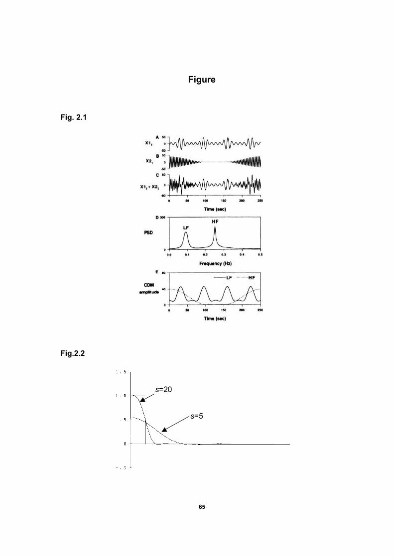
65

Figure

Fig. 2.1

Fig.2.2

s=5

s=20

66

Fig. 2.3

0

0.5

1

1.5

2

2.5

3

3.5

4

1 10 19 28 37 46 55

Amino Acid Sites (aa)

Entropy

Fig. 2.4

0

0.1

0.2

0.3

0.4

0.5

0.6

0 4 8 12 16 20 24 28 32 36 40 44 48 52 56

Period of bZIP Entropy

Spectral Density

Fig. 2.5

Leucine zipper region starts

3.6-aa Periodic Component

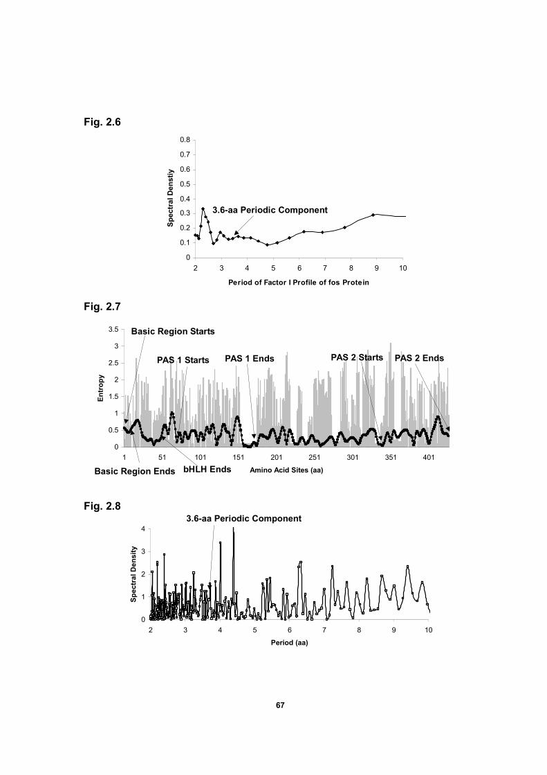
67

Fig. 2.6

0

0.1

0.2

0.3

0.4

0.5

0.6

0.7

0.8

2 3 4 5 6 7 8 9 10

Period of Factor I Profile of fos Protein

Spectral Denstiy

Fig. 2.7

0

0.5

1

1.5

2

2.5

3

3.5

1 51 101 151 201 251 301 351 401

Amino Acid Sites (aa)

Entropy

Fig. 2.8

0

1

2

3

4

2 3 4 5 6 7 8 9 10

Period (aa)

Spectral Density

Basic Region Ends bHLH Ends

PAS 1 Starts PAS 1 Ends PAS 2 Starts PAS 2 Ends

Basic Region Starts

3.6-aa Periodic Component

3.6-aa Periodic Component

68

Fig. 2.9

0

0.05

0.1

0.15

0.2

0.25

0.3

0.35

0.4

0.45

2 3 4 5 6 7 8 9 10

Period of Factor I Profile of Arnt Protein

Spectral Density

3.6-aa Periodic Component

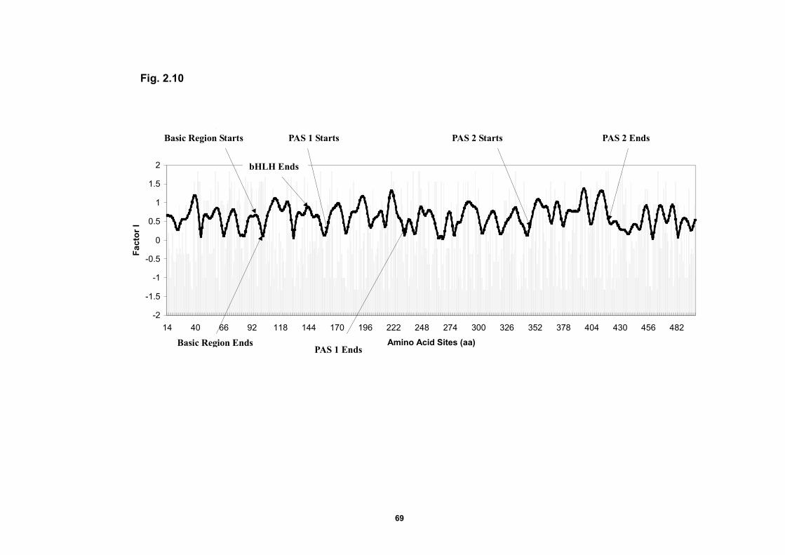
69

Fig. 2.10

-2

-1.5

-1

-0.5

0

0.5

1

1.5

2

14 40 66 92 118 144 170 196 222 248 274 300 326 352 378 404 430 456 482

Amino Acid Sites (aa)

Factor I

Basic Region Ends

Basic Region Starts PAS 1 Starts PAS 2 Starts

bHLH Ends

PAS 1 Ends

PAS 2 Ends

70

Figure Legends Fig. 2.1 Comparison between autoregressive power spectrum analysis and complex demodulation (CDM) of simulated data containing two periodic components A and B. A: simulated low-frequency (LF) component. B: simulated high-frequency (HF) component. X1t and X2t, 0.09 and 0.25 Hz sine functions with a fluctuating amplitude, respectively. C: time series generated by adding 2 sine functions (X1t +X2t). D: autoregressive power spectrum density (PSD). E: time series of instantaneous amplitude of LF and HF components obtained by CDM. (Figure from Hayano et al., 1993) Fig. 2.2 Transfer functions of least squares low-pass filters with convergence factors applied, s=5 and s=20 (Figure from Bloomfield, 1976) Fig. 2.3 Entropy profile of bZIP protein domains and the amplitude of the 3.6-aa periodic component. The entropy profile is represented by the histogram. Large entropy value represents high variation at that residue while small one represents low variation. Basic region: residue 1-27 Leucine zipper region: residue 28-55. The amplitude of the 3.6-aa periodic component vs. amino acid site is in dotted curve produced by CMD method. Fig. 2.4 Spectral density plot of the entropy profile of bZIP protein domains in the range from 2 to 10aa (the periodic component of around 3.6 aa period is labeled). Fig. 2.5 Factor I profile of a bZIP protein domain of transcription factor c-fos protein. The amplitude of the periodic component at 3.6 aa vs. amino acid site is in dotted curve produced by CMD method. Fig. 2.6 Spectral density plot of the factor I profile of a bZIP protein domain of transcription factor c-fos protein in the range from 2 to 10aa (the periodic component of around 3.6 aa period is labeled). Fig. 2.7 Entropy profile of bHLH-PAS protein domains and the amplitude of the 3.6-aa periodic component. The entropy profile is represented by the histogram. The amplitude of the 3.6-aa periodic component vs. amino acid site is in dotted curve produced by CMD method. Fig. 2.8 Spectral density plot of the entropy profile of bHLH-PAS protein domains in the range from 2 to 10aa (the periodic component of around 3.6 aa period is labeled). Fig. 2.9 Spectral density plot of the Factor I profile of Arnt protein in the range from 2 to 10 aa (the periodic component of around 3.6 aa period is labeled).

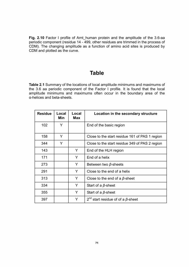
71

Fig. 2.10 Factor I profile of Arnt_human protein and the amplitude of the 3.6-aa periodic component (residue 14 - 499, other residues are trimmed in the process of CDM). The changing amplitude as a function of amino acid sites is produced by CDM and plotted as the curve.

Table

Table 2.1 Summary of the locations of local amplitude minimums and maximums of the 3.6 aa periodic component of the Factor I profile. It is found that the local amplitude minimums and maximums often occur in the boundary area of the α-helices and beta-sheets.

Close to the end of a helix Y 291

2nd start residue of of a β-sheet Y 397

Start of a β-sheet Y 355

Start of a β-sheet Y 334

Y

Y

Y

Y

Local Max

Close to the end of a β-sheet

Between two β-sheets

End of a helix

End of the HLH region

Close to the start residue 349 of PAS 2 region

Close to the start residue 161 of PAS 1 region

End of the basic region

Location in the secondary structure

Y

Y

Y

Local Min

313

273

171

143

344

158

102

Residue

72

Supplement

Supplemental Fig. 2.1 Overall Structure of Complex: DNA bended by Fos and

Jun bZIP proteins (from Glove, 1995).

73

Supplemental Fig.2.2 Structure-Based Sequence Alignment of bHLH-PAS Transcription Factors (from Yildiz, 2005).

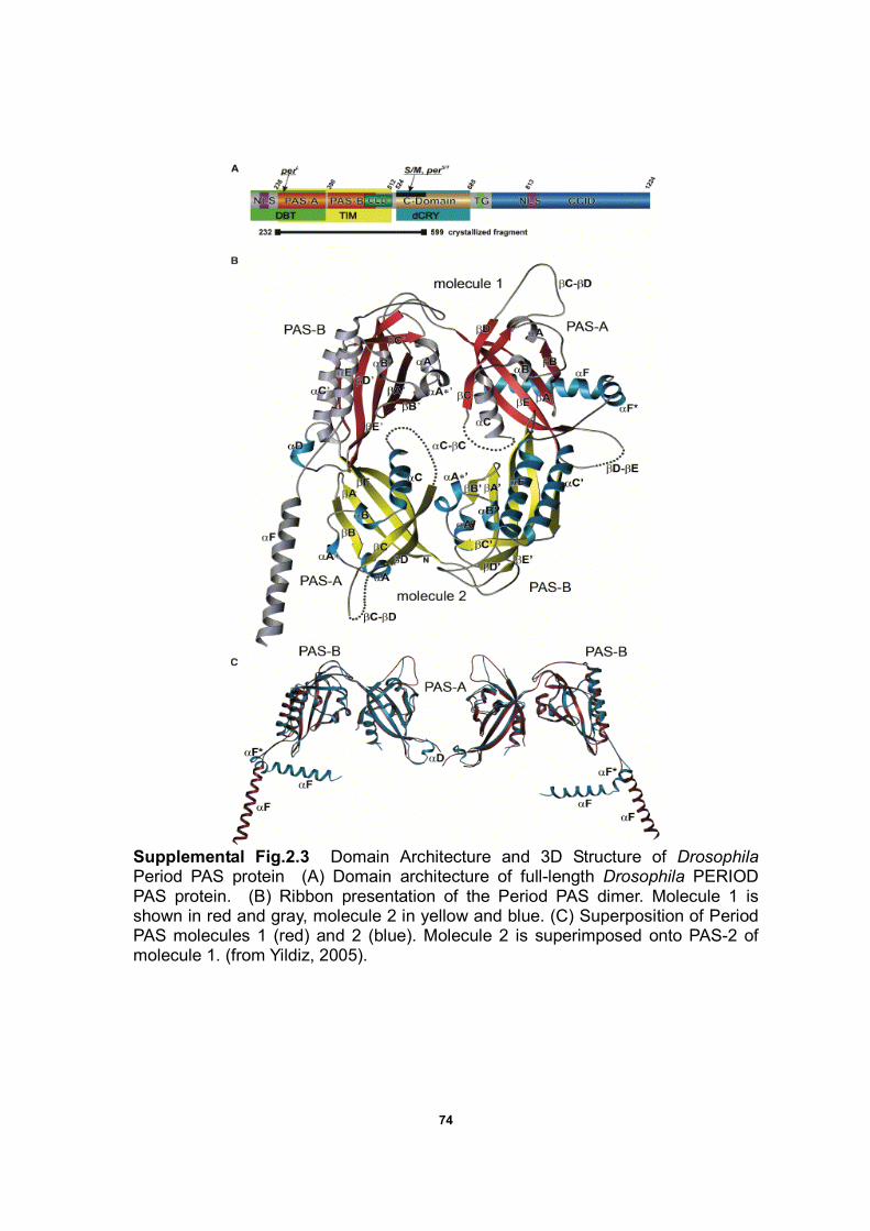
74

Supplemental Fig.2.3 Domain Architecture and 3D Structure of Drosophila Period PAS protein (A) Domain architecture of full-length Drosophila PERIOD PAS protein. (B) Ribbon presentation of the Period PAS dimer. Molecule 1 is shown in red and gray, molecule 2 in yellow and blue. (C) Superposition of Period PAS molecules 1 (red) and 2 (blue). Molecule 2 is superimposed onto PAS-2 of molecule 1. (from Yildiz, 2005).

75

Chapter 3

Evaluation of Amino Acid Indices with

Spectral Analysis

by

Zhi Wang1,* , William R. Atchley1,2, Charles E. Smith1

1Graduate Program In Biomathematics and 2Department Of Genetics and

Center For Computational Biology, North Carolina State University, Raleigh,

NC 27695-7614, USA

Keyword: periodicity, spectral analysis, amino acid index

* To whom correspondence should be addressed

* CONTACT: zwang2@ ncsu.edu

76

Abstract

It is difficult to select a proper amino acid scale to study protein secondary

structure out of the available 494 amino acid indices because some of them are

very similar. Till now, there are no comparisons and evaluations of these indices

being made. This research proposes a ranking method based on the periodicity

parameters of well-known protein sequences. We use a well-know periodicity

parameter of a Leucine zipper helix structure to rank the amino acid indices.

Introduction

An amino acid index is defined as a set of 20 numerical values representing any

of the different physicochemical and biochemical properties of amino acids. 494

published indices are summarized in a database

(http://www.genome.jp/dbget/aaindex.html). As stated in a cluster analysis of

amino acid indices for prediction of protein structure and function (Nakai, etc.

1988), all these 492 indices have been clustered into six categories: (i) Alpha and

turn propensities (ii) Beta propensity (iii) Composition (iv) Hydrophobicity (v)

Physicochemical properties (vi) Other properties. Therefore, many indices are

similar with each other or measures of the same physiochemical trait. Such

situation could raise some confusion in application. For example, it is difficult to

select the hydrophobicity scale because of too many different hydrophobicity

indices proposed in the database. Therefore, it is necessary to make evaluation

77

and comparison among those scales based on some well-known structure

information of protein sequences.

In this chapter, the α-helix periodicity property of the leucine zipper protein

domain is used to evaluate these amino acid scales, who play an important role in

the formation of secondary structure. This ranking information should be very

useful to promote our secondary structure prediction or develop better

bioinformatics tools to understand protein sequences. Those indices that have

similar periodicity as that of the secondary structure of protein sequences are

assumed as the most useful indices in protein structure prediction.

Materials

The structure of conserved leucine zipper domain of Geminin, a polypeptide of

about 25 kDa, occurs in the nuclei of higher eukaryotes and functions as both a

negative regulator of genome replication and coordinator of differentiation, has

been well studied (Thepaut, 2004). Geminin was discovered as a protein that is

degraded when cells exit from mitosis, by the large ubiquitin–ligase complex known

as the cyclosome or anaphase-promoting complex, APC.

78

Fig.3.1 Organization, sequence alignment and the structure of human geminin protein domain. (from Thepaut, et al., 2004) (A) Functional domain organization of geminin. The LZ domain is indicated by the hatched area,110–144. (B) Vertebrate geminin sequences alignment of the DNA replication inhibition domain. Letters above the sequences indicate the heptad repeat a,b,c,d,e,f,g positions assigned according to the crystal structure. Strictly conserved residues are in red and similar residues are in green. (C) The overall structure of HsGem-LZ peptide (L2-A37) in Cα trace representation. (D) Ribbon diagram of the view.

According to the crystal structure analysis (Thepaut, 2004), the structure of

the HsGem-LZ peptide is a parallel homodimer coiled coil with a typical α-helical

structure. The number of residues per α-helical turn is about 3.64 aa, a value more

79

closely related to a regular α-helix (3.6 aa) than to a classical coiled coil (3.5 aa).

Methods

The HsGem-LZ helices have an periodicity of about 3.64 aa observed from the

experimental data. We then transform the HsGem-LZ domain protein sequences

into numeric arrays by replacing the alphabetic codes with the 494 indices. Then

spectral analysis method (Burg method) has been applied to these numeric

sequences to evaluate their periodicities in Matlab. Those indices who have the

closest periodicity to 3.64 aa are listed in Table 3.1. Only those periods between

the interval (3.458, 3.822) which is within the 5% error range from 3.64 are reported

in Table 3.1.

Results

It is found that some indices have a period very close to 3.64 aa and some

indices are not. Among those indices, most are related to the formation of

secondary structure. A majority of indices falls into the hydrophobicity category,

which proved the important role the hydrophobicity plays in the formation of helical

structure. This result allows us to do comparison between different hydrophobicity

indices and helps us to determine which hydrophobicity scale is the best in terms of

secondary structure prediction.

80

Table 3.1 Ranking of amino acid indices according to the their periodicity estimate of HsGem-LZ protein domain. Only those periods between the interval (3.458, 3.822 ) which is within the 5% error range from 3.64 are reported here.

Amino Acid Index Name Series # Period

Normalized van der Waals volume (Fauchere et al., 1988) P. Physicochemical properties

80 3.6312

Activation Gibbs energy of unfolding, pH9.0 (Yutani et al., 1987) H. Hydrophobicity

396 3.6184

Frequency of the 4th residue in turn (Chou-Fasman, 1978b) A. alpha and turn propensities

52 3.6184

Radius of gyration of side chain (Levitt, 1976) P. Physicochemical properties

157 3.6056

The number of bonds in the longest chain (Charton-Charton, 1983) P. Physicochemical properties

29 3.5930

pK (-COOH) (Jones, 1975) H. Hydrophobicity

133 3.6968

Accessible surface area (Radzicka-Wolfenden, 1988) H. Hydrophobicity

319 3.7101

Optimized transfer energy parameter (Oobatake et al., 1985) H. Hydrophobicity

220 3.5679

Refractivity (McMeekin et al., 1964), Cited by Jones (1975) P. Physicochemical properties

177 3.5679

STERIMOL minimum width of the side chain (Fauchere et al., 1988) P. Physicochemical properties

82 3.5679

Optical rotation (Fasman, 1976) A. alpha and turn propensities

74 3.5556

Distance between C-alpha and centroid of side chain (Levitt, 1976) P. Physicochemical properties

154 3.5433

Residue accessible surface area in tripeptide (Chothia, 1976) H. Hydrophobicity

33 3.5433

STERIMOL length of the side chain (Fauchere et al., 1988) P. Physicochemical properties

81 3.5310

Size (Dawson, 1972) P. Physicochemical properties

63 3.7647

Optimized side chain interaction parameter (Oobatake et al., 1985) H. Hydrophobicity

222 3.5068

Flexibility parameter for two rigid neighbors (Karplus-Schulz, 144 3.7926

81

1985) C. Composition

Average relative fractional occurrence in AL(i) (Rackovsky-Scheraga, 1982) C. Composition

302 3.4949

Relative preference value at N4 (Richardson-Richardson, 1988) A. alpha and turn propensities

328 3.4830

Average interactions per side chain atom (Warme-Morgan, 1978) H. Hydrophobicity

382 3.4830

Weights for coil at the window position of -6 (Qian-Sejnowski, 1988 ) H. Hydrophobicity

284 3.4830

Percentage of exposed residues (Janin et al., 1978) H. Hydrophobicity

129 3.4712

Residue accessible surface area in folded protein (Chothia, 1976) H. Hydrophobicity

34 3.4712

Molecular weight (Fasman, 1976) P. Physicochemical properties

72 3.4712

Proportion of residues 100% buried (Chothia, 1976) H. Hydrophobicity

36 3.4595

Transfer free energy (Janin, 1979) H. Hydrophobicity

131 3.4595

Average accessible surface area (Janin et al., 1978) H. Hydrophobicity

127 3.4595

Weights for beta-sheet at the window position of -4 (Qian-Sejnowski, 1988 ) H. Hydrophobicity

273 3.4595

Side chain orientational preference (Rackovsky-Scheraga, 1977) H. Hydrophobicity

299 3.4595

ACKNOWLEDGEMENTS

Thanks to Charles Smith and Jieping Zhao for their helpful suggestions. This

research was supported by a grant from the National Institutes of Health (GM45344)

to WRA.

82

Summary

This dissertation describes several powerful computational techniques to

conduct spectral analysis on protein sequences. Spectral analysis has not been

widely used in protein sequences and it is the first time to apply it to analyze the

periodicity of variability pattern of protein domains.

In Chapter 1, spectral analysis is conducted to study the periodicity of the

variability pattern of bHLH protein domains represented by the entropy profile. It is

found that there is a significant periodic component of about 3.6 aa in the entropy

profile, which has implication of the underlying helix structure. In order to

understand the physiochemical causes of the variability, we decompose the

variability into five factor scores representing i) polarity / hydrophobicity /

accessibility, ii) propensity for various secondary structures, iii) molecular volume,

iv) codon composition and v) electrostatic charge. The periodicities of these factor

means/variances profiles also have implications of the helix structure.

In Chapter 2, complex demodulation method (CDM) is a complementary method

of the spectral analysis method used in Chapter 2 because it can describe the

changing amplitude of a certain frequency of the data. And therefore, it can provide

very meaningful information that FFT method cannot provide. Although CDM has

been widely applied into other scientific fields, it is the first report that CDM has been

introduced into computational biology. With the analysis of bZIP protein domains

83

and more complex bHLH-PAS protein domains, CDM proves to be a very useful

technique of description of the amplitude of a certain frequency. The analyses on

the amplitude of the periodic component of about 3.6 aa reveal that the local

maximums/minimums have implications of the boundary of the secondary structure

α-helix and β-sheet. For bZIP protein domain, the CDM method can separate the

basic region and ZIP region very well. And even there are no significant 3.6-aa

periodic components in the bZIP Factor I profile, CDM still shows some robustness

to indicate the boundary of the basic region and the ZIP region.

In Chapter 3, spectral analysis is conducted to evaluate and compare the amino

acid indices to see if their periodicity property conforms to the observed 3.64-aa

periodicity of a Leucine Zipper domain. It seems that the periodicity parameter can

be a criteria of selecting a proper amino acid index for the goal of studying protein

structure, function and evolution. In this way, the redundancy of the amino acid

indices can be largely reduced.

84

REFERENCE

Atchley, W. R. and Fitch, W. M. (1997) A natural classification of the basic

helix-loop-helix class of transcription Factors. Proc. Natl. Acad. Sci. USA,

94, 5172-5176.

Atchley, W. R., et al. (1999) Positional Dependence, cliques and predictive

motifs in the bHLH protein domain. J. Mol. Evol. 48:501-519.

Atchley, W.R., et al. (2000) Correlations among amino acid residues in bHLH

protein domains: An information theoretic analysis. Mol. Biol. Evol. 17,

164-178.

Atchley, W.R., et al. (2005) Solving the protein sequence “metric” problem. Proc.

Natl. Acad. Sci. USA 102, 6395-6400.

Atchley WR, Fernandes AD. (2005) Sequence signatures and the probabilistic

identification of proteins in the Myc-Max-Mad network. Proc Natl Acad Sci

102, 6401-6406.

Babkoff H, Caspy T, Mikulincer M, Sing HC. (1991) Monotonic and rhythmic

influences: a challenge for sleep deprivation research. Psychol Bull.109,

411-428

Bloomfield, P. (1976) Fourier analysis of time series: An introduction. Wiley, New

York. pp.1-150

Brockwell, P.J., and Davis, R.A. (1991). Time Series: Theory and Methods (2nd

ed). Springer Verlag. section 10.2

85

Brownlie, P., Ceska, T., Lamers, M., Romier, C., Stier, G., Teo, H. & Suck, D.

(1997) The crystal structure of an intact human Max-DNA complex: new

insights into mechanisms of transcriptional control. Structure. 5, 509-520.

Buck, M.J. (2003) Protein evolution from sequence to structure. (Ph.D. thesis)

pp.49-50, North Carolina State University, USA

Buck M.J., Atchley W.R., (2005) Networks of coevolving sites in structural and

functional domains of serpin proteins. Mol Biol Evol. 22,1627-1634

Chou, P.Y. and Fasman, G.D. (1978) Prediction of the secondary structure of

proteins from their amino acid sequence Adv. Enzymol. 47, 45-148

Charton, M. and Charton, B. (1983) The dependence of the Chou-Fasman

parameters on amino acid side chain structure J. Theor. Biol. 111,

447-450

Chothia, C. (1976) The nature of the accessible and buried surfaces in proteins

J. Mol. Biol. 105, 1-14

Wilson C. L., Boardman P. E., Doig A. J., Hubbard S. J., (2004) Improved prediction

for N-termini of -helices using empirical information Proteins: Structure,

Function, and Bioinformatics 57 ,322 – 330

Dawson, D.M. (1972) The Biochemical Genetics of Man Academic Press, New

York, pp.1-38

Eisenburg, D., et al. (1984) The hydrophobic moment detects periodicity in protein

Hydrophobicity. Proc. Natl. Acad. Sci. USA, 81, 140-144.

Fasman, G.D., (1976) "Handbook of Biochemistry and Molecular Biology", 3rd ed.,

Proteins Volume 1, CRC Press, Cleveland

86

Fasman, G.D., (1989) Prediction of protein structure and the principles of protein

conformation Plenum Press, New York pp. 625-646

Fauchere, J.L., Charton, M., Kier, L.B., Verloop, A. and Pliska, V. (1988) Amino acid

side chain parameters for correlation studies in biology and pharmacology

Int. J. Peptide Protein Res. 32, 269-278

Ferre-D’Amare A.R., Prendergast G.C., Ziff E.B., Burley S.K. (1993) Recognition by

Max of its cognate DNA through a dimeric b/HLH/Z domain. Nature

363,38–45

Glover J.N., Harrison S.C., (1995) Crystal structure of the heterodimeric bZIP

transcription factor c-Fos-c-Jun bound to DNA. Nature 373:257-261

Grantham,R., (1974) Amino acid difference formula to help explain protein

evolution. Science 185, 862-864.

Hamming, R.W. (1983) Digital filters (2nd ed.). Prentice Hall, Englewood Cliffs, New

Jersey.

Hayano J, Taylor JA, Yamada A, Mukai S, Hori R, Asakawa T, Yokoyama K,

Watanabe Y, Takata K, Fujinami T. (1993) Continuous assessment of

hemodynamic control by complex demodulation of cardiovascular

variability. Am J Physiol. 264 1229-1238.

Hefti MH, Francoijs KJ, de Vries SC, Dixon R, Vervoort J, (2004) The PAS fold: a

redefination of the PAS domain based upon structural prediction. Eur J

Biochem 271:1198-1208.

87

Herzel H., Weiss O., Trifonov E.N. (1999) 10-11 bp periodicities in complete

genomes reflect protein structure and DNA folding. Bioinformatics.

15,187-193.

Hoffman,E.C., Reyes,H., Chu,F.F., Sander,F., Conley,L.H., Brooks,B.A. and

Hankinson,O. (1991) Cloning of a factor required for activity of the Ah

(dioxin) receptor Science 252 (5008), 954-958

Janin, J., Wodak, S., Levitt, M., and Maigret, B. (1978) Conformation of amino acid

side-chains in proteins J. Mol. Biol. 125, 357-386

Janin, J. (1979) Transfer free energ Surface and inside volumes in globular

proteins Nature 277, 491-492

Johnson and Wichern (2002) Applied Multivariate Analysis, 5/e, Prentice Hall

Jones, D.D. (1975) Amino acid properties and side-chain orientation in proteins: A

cross correlation approach J. Theor. Biol. 50, 167-183

Karplus, P.A. and Schulz, G.E. (1985) Prediction of chain flexibility in proteins.

Naturwissenchaften 72, 212–213.

Kay, S. M. (1988) Modern Spectral Estimation: Theory and Application, Prentice

Hall, Englewood Cliffs, New Jersey. pp. 265-270

Kendall, M. and Ord, J.K. (1990) Time series Edward Arnold, Sevenoaks, Kent,

Great Britain pp.51-52, 170

Kyte, J. (1995) Structure in Protein Chemistry Garland Publishing, Inc., New York

and London pp.201

Ledent V, Vervoort M (2001) The basic helix-loop-helix protein family: comparative

genomics and phylogenetic analysis. Genome Res 11,754–770

88

Leonov, H. and Arkin, I.T. (2005) A periodicity analysis of transmembrane helices

Bioinformatics 21, 2604-2610

Levitt, M. (1976) A simplified representation of protein conformations for rapid

simulation of protein folding J. Mol. Biol. 104, 59-107

Lipsitz LA, Hayano J, Sakata S, Okada A, Morin RJ. (1998) Complex

demodulation of cardiorespiratory dynamics preceding vasovagal syncope.

Circulation. 98(10):977-983.

Marple, S. L. (1987) Digital Spectral Analysis with Applications, Prentice Hall,

Englewood Cliffs, New Jersey. pp.21, 164, 172-284, 379

McMeekin, T.L., Groves, M.L., and Hipp, N.J. (1964) In "Amino Acids and Serum

Proteins" (Stekol, J.A., ed.), American Chemical Society, Washington, D.C.,

p. 54

Morgenstern B, Atchley WR (1999) Evolution of bHLH transcription factors:

modular evolution by domain shuffling? Mol Biol Evol 16,1654–1663

Murre, C., et al. (1989) A new DNA binding and dimerization motif in

immunoglobulin enhancer binding, daughterless, MyoD, and myc proteins.

Cell 56, 777–783.

Murre, C, et al. (1994) Structure and function of helix-loop-helix proteins Biochim.

Biophys. Acta 1218, 129–135.

Naidu, P. S. (1996) Modern Spectrum Analysis of Time Series, pp. 161-162, 241,

CRC press, Boca Raton, Florida.

Nakai, K., Kidera, A., and Kanehisa, M.; (1988) Cluster analysis of amino acid

indices for prediction of protein structure and function. Protein Eng. 2, 93-100.

89

Oobatake, M., Kubota, Y. and Ooi, T. (1985) Optimization of amino acid parameters

for correspondence of sequence to tertiary structures of proteins Bull. Inst.

Chem. Res., Kyoto Univ. 63, 82-94

Pasquier, C.M., et al. (1998) A web server to locate periodicities in a sequence.

Bioinformatics. 14, 749-750.

Patthy, L. (1999) Protein Evolution. Blackwell Science ltd., Oxford pp.42-43

Percival, D. B.& Walden, A. T. (1993) Spectral Analysis for Physical Applications,

pp. 414, 445-449, Cambridge University Press, New York.

Podust LM, Krezel AM, Kim Y. (2001) Crystal structure of the CCAAT

box/enhancer-binding protein beta activating transcription factor-4 basic

leucine zipper heterodimer in the absence of DNA. J Biol Chem.

276(1):505-13.

Ponting C.P., Aravind L., (1997).PAS: a multifunctional domain family comes to

light. Curr. Biol. 7:R674-R677

Qian, N. and Sejnowski, T.J. (1988) Predicting the secondary structure of globular

proteins using neural network models J. Mol. Biol. 202, 865-884

Quinn, L.M., A. Herr, T.J. McGarry and H. Richardson, (2001) The Drosophila

Geminin homolog: roles for Geminin in limiting DNA replication, in anaphase

and in neurogenesis, Genes Dev. 15 pp. 2741–2754

Rackovsky, S. and Scheraga, H.A. (1977) Hydrophobicity, hydrophilicity, and the

radial and orientational distributions of residues in native proteins Proc.

Natl. Acad. Sci. USA 74, 5248-5251

Rackovsky, S. and Scheraga, H.A. (1982) Differential geometry and polymer

90

conformation. 4. Conformational and nucleation properties of individual

amino acids Macromolecules 15, 1340-1346

Radzicka, A. and Wolfenden, R. T (1988) Comparing the polarities of the amino

acids: Side-chain distribution coefficients between the vapor phase,

cyclohexane, 1-octanol, and neutral aqueous solution Biochemistry 27,

1664-1670

Richardson, J.S. and Richardson, D.C. (1988) Amino acid preferences for specific

locations at the ends of alpha helices Science 240, 1648-1652

Rutherford S, D'Hondt S., (2000) Early onset and tropical forcing of 100,000-year

Pleistocene glacial cycles. Nature. 408, 72-75.

SAS, (1992) SAS/ETS Software Application Guide 1. SAS Institute Inc., Cary, NC,

USA pp.220 http://v9doc.sas.com/sasdoc/

Sauve S, Tremblay L, Lavigne P. (2004) The NMR solution structure of a

mutant of the Max b/HLH/LZ free of DNA: insights into the specific and

reversible DNA binding mechanism of dimeric transcription factors. J Mol

Biol. 342(3): 813-32.

Schieg P., Herzel H., (2004) Periodicities of 10-11bp as indicators of the

supercoiled state of genomic DNA. J Mol Biol. 343 (4):891-901

Shannon, C.& Weaver, W. (1949) The Mathematical Theory of Communication.

University of Illinois Press, Urbana.

Sharma, D., Issac, B., Raghava, G.P. & Ramaswamy, R. (2004) Spectral Repeat

Finder (SRF): identification of repetitive sequences using Fourier

transformation. Bioinformatics. 20, 1405-1412

91

Shimizu T, Toumoto A, Ihara K, Shimizu M, Kyogoku Y, Ogawa N, Oshima Y,

Hakoshima T. (1997) Crystal structure of PHO4 bHLH domain-DNA

complex: flanking base recognition. EMBO J. 16(15): 4689-97.

Sneath P.H.A., (1966) Relations between chemical structure and biological activity.

J Theor Biol 12:157–195

Sun, X. and Baltimore, D. (1991) An inhibitory domain of E12 transcription factor

prevents DNA binding in E12 homodimers but not in E12 heterodimers. Cell

64, 459–467.

Thepaut, M., Maiorano, D., Guichou, J.F., Auge, M.T., Dumas, C., Mechali, M.,

Padilla, A. (2004) Crystal structure of the coiled-coil dimerization motif of

geminin: structural and functional insights on DNA replication regulation. J

Mol Biol. 342, 275-87

Warme, P.K. and Morgan, R.S. (1978) A survey of amino acid side-chain

interactions in 21 proteins J. Mol. Biol. 118, 289-304

Warner, R. M. (1998) Spectral Analysis of Time-Series Data, The Guilford Press,

New York, London. pp. 1-111.

Wilson, C.L., Boardman, P.E., Doig, A.J., Hubbard, S.J. (2004) Improved prediction

for N-termini of alpha-helices using empirical information. Proteins. 57,

322-330

Wollenberg, K.R. and Atchley, W.R. (2000) Separation of phylogenetic and

functional associations in biological sequences by using the parametric

bootstrap. Proc. Natl. Acad. Sci. 97,3288-3291.

Yutani, K., Ogasahara, K., Tsujita, T., and Sugino, Y. (1987) Dependence of

92

conformational stability on hydrophobicity of the amino acid residue in a

series of variant proteins substituted at a unique position of tryptophan

synthase alpha subunit Proc. Natl. Acad. Sci. USA 84, 4441-4444

Zhulin I.B., Taylor B.L., Dixon R., (1997) PAS domain S-boxes in Archaea, Bacteria

and sensors for oxygen and redox. Trends Biochem. Sci. 22:331-333

93

Appendix A: Spectral Analysis Based on the Burg Method

The procedure of Burg method is briefly described here. For more details,

please refer to the books by Kay, 1988 and Marple, 1987. Spectral analysis is

applied to determine the spectral content of a random process based on a finite set

of observations from that process. The power spectral density (PSD denoted by

Pxx(f) , of a complex wide sense stationary (WSS) random process x[n] is defined

as

1 1

( ) [ ]exp( 2 )2 2

xx xx

k

p f r k j fk fπ∞

=−∞

= − − ≤ ≤∑

Where rxx[k] is the autocorrelation function (ACF) of x[n] defined as

rxx[k] = E ( x*[n]x[n+k] )

E is expectation operator. The PSD function describes the distribution of power

with frequency of the random process.

When the autoregressive (AR) modeling assumption is valid, spectral

estimators are obtained which are less biased and have a lower variability than

conventional Fourier based spectral estimators. To estimate the PSD using an AR

model we need to estimate the parameters of the model. The theoretical PSD is

given as below

2

2( )

1 [1]exp( 2 ) ... [ ]exp( 2 )ARp f

a j f a p j f

σ

π π=

+ − + + −

94

The estimate of the PSD is obtained by replacing the theoretical AR parameters by

their estimates to yield

2

2( )

1 [1]exp( 2 ) ... [ ]exp( 2 )

ARp f

a j f a p j f

σ

π π

∧∧

∧ ∧=

+ − + + −

In order to estimate AR parameters, the basic idea is to minimize the average of

the forward and backward prediction error.

Forward predictor

^

1

[ ] [ ] [ ]f p

f

k

x n a k x n k=

= −∑

Backward predictor

^

1

[ ] [ ] [ ]b p

b

k

x n a k x n k=

= −∑

Minimization of the average errors yields an optimal estimate of Kk

1*

1 1

2 21

1 1

2 [ ] [ 1]

( [ ] [ 1] )

f bN

k k

n kk

f bN

k k

n k

e n e n

k

e n e n

− ∧ ∧

− −∧

=

− ∧ ∧

− −

=

− −=

+ −

∑

∑

where e is the prediction error

This kk∧

is used in each stage of the Levinson-recursive algorithm to produce

[1]a∧

, [2]a∧

,…, and [ ]a p∧

95

Appendix B: Critical Values for the Fisher Test of Significance

The critical values in Tables B.1 and the description of Fisher Test presented

below are from Warner (1998).

To compute the test statistic g, compute the periodogram for the time series.

Find the sum of all the periodogram ordinates, and then divide the periodogram

intensity for each frequency by this sum to yield an estimate of the proportion of

variance in the time series that is accounted for by each frequency component

represented in the periodogram. The test statistic g is simply the proportion of the

total variance in the time series that is accounted for by a particular frequency in the

periodogram analysis.

Select the largest values of this proportion, that is, the proportions of variance

that are explained by the first largest, second largest, third largest, fourth largest,

and fifth largest periodogram ordinates. The tables provided here give critical

values to test the significance of the peaks that are ranked first through fifth largest

in the proportion of variance accounted for.

To choose the appropriate critical values, you need to know N (number of

observations in the time series), and the alpha level for your significance tests.

Critical values of g are given for α = .05 in Table B.1. Within the table, the columns

headed r1, r2, r3, r4, and r5 give the critical values used to test the significance of

the peaks that are ranked first, second, …,fifth in the periodogram.

Start with the largest obtained proportion of variance and compare this to the

critical value in the r1 column (critical value of g for the largest periodogram

ordinate). If the obtained proportion of variance exceeds the critical value given in

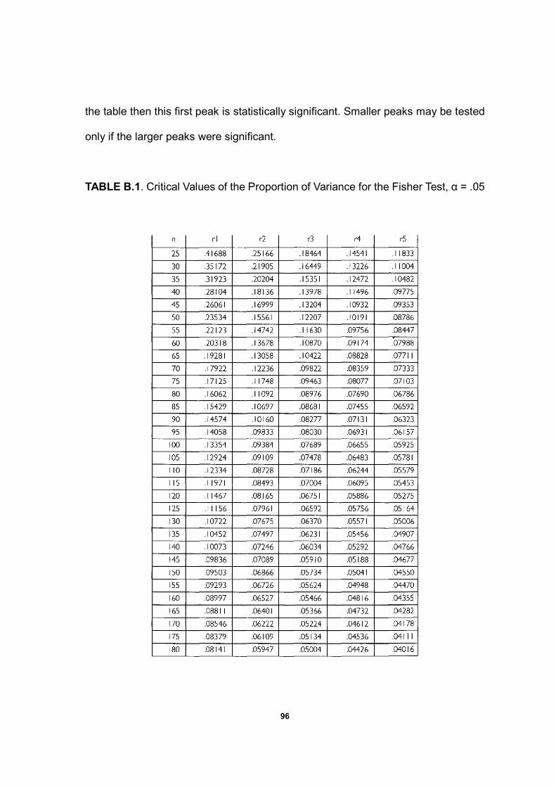
96

the table then this first peak is statistically significant. Smaller peaks may be tested

only if the larger peaks were significant.

TABLE B.1. Critical Values of the Proportion of Variance for the Fisher Test, α = .05