Embed Size (px)
Citation preview
ABSTRACT
Foam for Mobility Control in Alkaline/Surfactant
Enhanced Oil Recovery Process
by
Wei Yan
This thesis addresses several key issues in the design of foam for mobility
control in alkaline-surfactant enhanced oil recovery processes. First, foam flow in
fracture systems was studied. A theory for foam flow in a uniform fracture was
developed and verified by experiment. The apparent viscosity was found to be
the sum of contributions arising from liquid between bubbles and the resistance
to deformation of the interfaces of bubbles passing through the fracture.
Apparent viscosity increases with gas fractional flow and is greater for thicker
fractures (for a given bubble size), indicating that foam can divert flow from
thicker to thinner fractures. The diversion effect was confirmed experimentally
and modeled using the above theory for individual fractures. The amount of
surfactant solution required to sweep a heterogeneous fracture system
decreases greatly with increasing gas fractional flow owing to the diversion effect
and to the need for less liquid to occupy a given volume when foam is used. The
sweep efficiency’s sensitivity to bubble size was investigated theoretically in a
heterogeneous fracture system with log-normal distributed apertures.
Second, the foam application in forced convection of alkaline-surfactant
enhanced oil recovery processes was studied. From sand pack experiments for

II
the alkaline-surfactant-polymer process, a 0.3 PV slug of the surfactant blend
studied can recover almost all the waterflood residual crude oil when followed by
a polymer solution as mobility control agent. But this blend is a weak foamer near
its optimum salinity while one of its components, IOS, is a good foamer. Two
types of processes were tested in sand packs to study possible process
improvements and cost savings from replacing some polymer by foam for
mobility control. The first used IOS foam as drive after the surfactant slug, while
the second, which is preferred, involved injecting gas with the surfactant slug
containing polymer followed by IOS foam. It was found that foam has higher
apparent viscosity in high than in low permeability region. Thus, use of foam
should be more attractive in heterogeneous system to get better sweep
efficiency.
ACKNOWLEDGEMENTS
I have been very fortunate to study under the direction of Professors George
Hirasaki and Clarence Miller. Their wisdom and authoritative knowledge on foam,
interfacial phenomena, and flow in porous media have guided me throughout my
thesis work. I deeply appreciate their help, trust and support.
I thank Professors Mason Tomson and Walter Chapman for serving in my thesis
committee. I am also grateful to the many individuals who helped me in my
research. Professor Shi-Yow Lin, Dr, Maura Puerto and Mr. Dick Chronister
provided guidance and assistance for setting up my experimental device. Dr.
Frank Zhao helped me with the image analysis software.
I thank the United States Department of Energy (#DE-FC26-03NT15406) and
Consortium on Process in Porous Media for financial support.
Many fellow students in Dr. Hirasaki’s and Dr. Miller’s laboratories have offered
me help, support, and most important of all, their friendships. I am grateful to this
awesome group of people.
I thank my wife Yan for her constant support, love and understanding.
IV
Last but certainly not least, I am grateful and eternally indebted to my parents
Hongzhi Yan and Zhi Ling. Their love and spirit of dedication to their society,
friends, and the humanity as a whole has been a constant source of inspiration.
TABLE OF CONTENTS
Table of Contents…………………………………………………………………….VIII
List of Tables………………………………………………………………………..….IX
List of Figures………………………………………………………………..……..XVIII
Chapter 1 Introduction…………………………………..………………………….1
1.1 Enhanced oil recovery………………………………………………….1
1.2 Foam……………………………………………………………………..5
1.3 Thesis scope and organization………………………………………..8
Chapter 2 Technical background………………………………………………...11
2.1 Fundamentals of flow in porous media…………………………...…11
2.2 Surfactants……………………………………………………………..13
2.3 Fundamentals of Foam Flow in porous Media………………….....16
2.4 Mechanisms of Foam Formation and Decay…………………....….21
2.4.1 Foam formation…………………………………………………..21
2.4.2 Foam destruction………………………………………………...25
2.5 Foam stability to crude oil in porous media…………………….…...29
2.6 Foam flow in capillary tubes……………………………………….....38
2.7 Effect of heterogeneity on foam flow………………………….…….43
2.7.1 Capillary pressure’s role in bulk foams……………………….43
2.7.2 Limiting capillary pressure for foam in porous media……….44
2.7.3 Behavior of foam in low-permeability media…………………46
2.7.4 Foam flow in heterogeneous porous media………………….48

2.8 Alkaline surfactant enhanced oil recovery process……………..….51
2.9 Enhanced oil recovery in fractured carbonate reservoir……….…53
Chapter 3 Foam flow in homogeneous fracture………………………………...56
3.1 Foam apparent viscosity in homogeneous fracture………………..56
3.2 Experimental methods………………………………………………...60
3.3 Foam bubble size measurement in fractures……………………….62
3.4 Foam apparent viscosity in homogeneous fracture experiment
results…………………………………………………………………...64
3.5 Bulk foam apparent viscosity…………………………………………69
3.6 Contrary diversion effect………………………………………………73
Chapter 4 Foam diversion in heterogeneous fractures…………………….…..75
4.1 Foam apparent viscosity in heterogeneous fractures ……………...…75
4.2 Prediction of sweep efficiency in heterogeneous fractures…………...76
4.3 Fractures with log-normal distribution fractures………………………..78
4.4 Experimental methods………………………………………………...….80
4.5 Experimental results for apparent viscosity and sweep in
heterogeneous fractures………………………………………………....81
4.5.1 Apparent viscosity………………………………………………...81
4.5.2 Sweep efficiency…………………………………………………..84
4.6 Sensitivity of foam bubble size to sweep efficiency in heterogeneous
fractures…………………………………………………………………..88
4.6.1 Foam bubble size with some constant ratio (>1) to
aperture…………………………………………………………………90
VI

4.6.2 Foam bubbles at constant size (>aperture) in different
layers……………………………………………………….…...94
4.6.3 Foam bubbles at constant size (<aperture) in different
layers……………………………………………………….…...97
4.6.4 Foam bubbles at constant size (>some apertures and <
some apertures) in different layers…………………….….....99
Chapter 5 Surfactant evaluation for foam-aided alkaline/surfactant enhanced
oil recovery process……………………………………………….....104
5.1 Selection of surfactants…………………………………….……...104
5.2 Foam strength with different surfactants………………………...109
5.3 Foam stability with the presence of residual oil…………….…...112
Chapter 6 Alkaline/surfactant/polymer/foam enhanced oil recovery
process………………………………………………………………..116
6.1 Alkaline/surfactant/polymer EOR process……………………....117
6.2 Foam drive possibility in alkaline/surfactant/polymer
process……………………………………………………………...122
6.3 Foam drive in alkaline/surfactant/polymer process……….…....126
6.4 Alkaline/surfactant/polymer/foam process………………….…...133
6.4.1 40 darcy sand pack……………………………….……...134
6.4.2 200 darcy sand pack………………………………….....137
6.4.3 Comparison between the flooding in 40 darcy and 200
darcy sand packs………………………………………...140
6.5 Calculations for ASPF in heterogeneous systems…………....…145
VII

Chapter 7 Conclusions and recommendations…………………………..…..155
7.1 Conclusions……………………………………………………..…...155
7.1.1 Foam flow in homogeneous fracture…………………..155
7.1.2 Foam diversion in heterogeneous fractures……….....156
7.1.3 Surfactant evaluation………………………… ……….157
7.1.4 Foam in alkaline/surfactant/polymer/foam EOR
process… ………………………………………………..158
7.2 Recommendations for future work………………………………...159
7.2.1 Foam flow in fractures………………………………..….159
7.2.2 Surfactant…………………………………………….…...160
7.2.3 ASPF process………………………………………..…..161
References…………………………………………………………………………...162
Appendices…………………………………………………………………………...175
Appendix A……………………………………………………………….…175
Appendix B………………………………………………………………….177
Appendix C………………………………………………………………….180
VIII
LIST OF TABLES
Table 5.1 Surfactants used in the experiments for alkaline-surfactant EOR
process………………………………………………………………..…106
Table 6.1 Revenue and expense calculation for ASPF process…………….….153
Table 6.2 Revenue and expense calculation for ASP process………………….154
LIST OF FIGURES
Fig. 1.1 Three-dimensional foam consists of cells whose faces are thin films,
meeting in Plateau borders…………………………………………………..6
Fig. 1.2 Surfactant molecules stabilize thin films……………………….……………6
Fig. 1.3 In a foam the Plateau borders form a continuous network………………..7
Fig. 1.4 Examples of simulations of wet foam………………………………………..8
Fig. 2.1 Classification of surfactants…………………………………………………14
Fig. 2.2 Schematic of surfactant behavior above the CMC…………………….....15
Fig. 2.3 Cross-sectional view of cornered pores……………………………….…..17
Fig. 2.4 Pore level schematic of foam in porous media……………………….…..19
Fig. 2.5 Schematic of capillary snap-off mechanism………………………….…...22
Fig. 2.6 Schematic of lamella division mechanism………………………………...24
Fig. 2.7 Schematic of leave-behind mechanism…………………………………...25
Fig. 2.8 Disjoining pressure π curve governs the stability of a thin
Film……………………………………………………………………………26
Fig. 2.9 Foam lamella translating from left to right in a periodically constricted
tube……………………………………………………………………………28
Fig. 2.10 Foam lamella translating from left to right in a periodically constricted
tube……………………………………………………………………………29
Fig. 2.11 Photomicrograph of two-dimensional foam containing emulsified oil
drops that have drained from the foam films into the Plateau
borders………………………………………………………………….…….30
Fig. 2.12 Aqueous foam, pseudoemulsion and emulsion films and Plateau
borders containing oil drops………………………………………………...33
Fig. 2.13 Configurations of oil at the gas-aqueous solution interface…………....33
Fig. 2.14 Oil lens, definition of and unstable bridge
configurations………………………………………………………………...37
Fig. 2.15 Schematic profile of several defoaming mechanisms…………………..38
Fig. 2.16 Mechanisms affecting apparent viscosity in smooth
capillaries……………………………………………………………………..41
Fig. 2.17 Bubble configurations when the bubbles are separated and when they
are touching…………………………………………………………………..42
Fig. 2.18 Sketches of capillary-pressure and fractional-flow curves operating
during a two-phase displacement………………………………………….45
Fig. 2.19 Relationship between capillary-entry pressure, limiting capillary
pressure, and permeability……………………………………………..…..47
Fig. 2.20 Schematic of the correlation between foam mobility and
permeability………………………………………………………………..…47
Fig. 3.1 Mechanisms affecting apparent viscosity in smooth capillaries………...57
Fig. 3.2 Detailed diagram of homogeneous fracture model……………………….61
Fig. 3.3 Set –up diagram for foam mobility control experiment in fracture
model………………………………………………………………………….62
Fig. 3.4 Bubble size measurement results from image processing method and
capillary tube method match each other………………………………..…63
Fig. 3.5 Effect of flow rate and fractional flow on apparent viscosity…………….65
XII

Fig. 3.6 Effect of flow rate and fractional flow on apparent viscosity…………….66
Fig. 3.7 Effect of flow rate and fractional flow on apparent viscosity…………….66
Fig. 3.8 Effect of flow rate and fractional flow on apparent viscosity…………….67
Fig. 3.9 Effect of ratio of aperture/bubble size on apparent viscosity……………68
Fig. 3.10 Bulk foam apparent viscosity in fractures measurement and
prediction…………………………………………………………………..…72
Fig. 3.11 Apparent viscosity at different ratio of foam bubble diameter to aperture
and different gas fractional flow………………………………………….74
Fig. 4.1 Detailed diagram of heterogeneous fracture model……………………...81
Fig. 4.2 Apparent viscosity for aperture ratio of 0.1 mm/0.2 mm, bubble size = 0.4
mm and Re = 0.22…………………………………………………………..83
Fig. 4.3 Apparent viscosity for aperture ratio of 0.05 mm/0.15 mm, bubble size =
0.4 mm and Re = 0.22…………………….………………………………...83
Fig. 4.4 Surfactant solution sweeping heterogeneous fracture, Re = 0.22, fracture
aperture ratio = 0.05 mm(top)/0.15 mm(bottom)…………………….…..86
Fig. 4.5 Foam/surfactant solution sweeping heterogeneous fracture, Re = 0.22, fg
= 0.9, fracture aperture ratio = 0.05 mm(top)/0.15 mm(bottom), DB = 0.4
mm………………………………………………………………………..…..86
Fig. 4.6 Surfactant solution sweeping heterogeneous fracture at different fracture
aperture ratio (for thinner region only)…………………………………….87
XIII

Fig. 4.7 Comparison between the calculation and the experiment results for
foam/surfactant sweep in heterogeneous fractures with 1:3 aperture
ratio……………………………………………………………………………87
Fig. 4.8 Sweep efficiency by foam with bubble size 2 times aperture in each
layer…………………………………………………………………………..91
Fig. 4.9 Sweep efficiency by foam with bubble size 5 times of aperture in each
layer……………………………………………..……………………………92
Fig. 4.10 Apparent viscosity in a heterogeneous fracture system with V=0.8 when
the bubble diameter in a fixed ratio to the aperture of each layer.
………………………………………………………………………………94
Fig. 4.11 Sweep efficiency by foam with bubble size 6.4 times of the log-mean
aperture which is equal to the largest aperture in the heterogeneous
fracture system……………………………….…………………….……..95
Fig 4.12 Apparent viscosity in a heterogeneous fracture system with V=0.8 when
the bubble diameter is equal to the largest aperture in the
heterogeneous system………………………………………….….….....96
Fig. 4.13 sweep efficiency by foam with bubble size 125 times of
aperture…………………………………………………………………....97
Fig. 4.14 sweep efficiency by bulk foam………………………………………..….98
Fig. 4.15 Apparent viscosity in a heterogeneous fracture system
with V=0.8 when the bubble diameter is smaller than any
aperture…………………………………………………………………....98
XIV

Fig 4.16 sweep efficiency by foam with bubble size equal to log-mean
aperture……………………………………………………………….…..100
Fig 4.17 Apparent viscosity in a heterogeneous fracture system with V=0.8 when
the bubble diameter is equal to the log-mean
aperture…………………………………………………………….……..100
Fig 4.18 sweep efficiency by foam with bubble size 5 times log-mean
aperture…………………………………………………………………...101
Fig. 4.19 Apparent viscosity in a heterogeneous fracture system with V=0.8 when
the bubble diameter is equal to 5 times log-mean
aperture…………………………………………………………………...101
Fig. 4.20 Comparison of sweep efficiency at different bubble size………….….103
Fig. 5.1 Aqueous phase behavior of N67-7PO&IOS blends, 1% Na2CO3 +
various NaCl……………………………………………………………...108
Fig. 5.2 Aqueous phase behavior of N67-7PO&IOS blends, 1% Na2CO3 + various
CaCl2……………………………………………………………………....108
Fig. 5.3 Foam strength at different surfactant composition……………………...110
Fig. 5.4 Foam strength at different salinity………………………………………...110
Fig. 5.5 Short sand pack setup……………………………………………………..114
Fig. 5.6 Comparison of foam strength with or without residual oil by different
surfactant or surfactant blends………………………………………...….115
Fig. 6.1 Photos showing behavior during ASP flood of silica sand
pack………………………………………………………………..………...118
Fig. 6.2 Effluents for different pore volume for ASP experiment......…………..118
XV
Fig. 6.3 Measured cumulative oil recovery for ASP flood in silica sand
pack…………………………………………………………….……………119
Fig. 6.4 Time-dependence of pressure drop during ASP flood in silica sand
pack…………………………………………………………………….……119
Fig. 6.5 Photos of unsuccessful ASP flood at 4% NaCl………………………....121
Fig. 6.6 Photo of phase separation with polymer at 4% NaCl…………………..121
Fig. 6.7 Time-dependence of pressure drop during unsuccessful ASP
flood………………………………………………………………………....122
Fig. 6.8 Foam sweep the sand pack presaturated with
polymer/surfactant……………………………………………………….…124
Fig. 6.9 Apparent viscosity during the sweeping the sand pack presaturated with
polymer/surfactant……………………...………………………………….125
Fig. 6.10 Photos showing behavior during ASPF flood of silica sand
pack………………………………………………………………….………128
Fig. 6.11 Recovery history for ASPF experiment……………………………..…..128
Fig. 6.12 Effluents for different pore volume for ASPF experiment…………..…129
Fig. 6.13 Pressure history for ASPF experiment………………………………....129
Fig. 6.14 Photos showing behavior during ASPF flood of silica sand pack at
optimized condition…………………………………………………….…..131
Fig. 6.15 Recovery history for ASPF experiment at optimized
condition……………………………………………………..…………...…131
Fig. 6.16 Effluents for different pore volume for ASPF experiment at optimized
condition………………………………………………………………….…132
XVI

Fig. 6.17 Pressure history for ASPF experiment at optimized
condition………………………………………………………………..…...132
Fig. 6.18 Pictures for the displacement of residual crude oil by polymer/foam in
40 darcy sand pack………………………………………………………...135
Fig. 6.19 Pictures for effluents for polymer/foam flooding in 40 darcy sand
pack……………………………………………………………………….....135
Fig. 6.20 Recovery efficiency for polymer/foam flooding in 40 darcy sand
pack……………………………………………………………….……..…..136
Fig. 6.21 Pressure history for polymer/foam flooding in 40 darcy sand
pack……………………………………………………………………….…136
Fig. 6.22 Pictures for the displacement of residual crude oil by polymer/foam in
200 darcy sand pack……………………………………………………….138
Fig. 6.23 Pictures for effluents for polymer/foam flooding in 200 darcy sand
pack…………………………………………………………………...……..139
Fig. 6.24 Recovery efficiency for polymer/foam flooding in 200 darcy sand
pack…………………………………………………………………..……...139
Fig. 6.25 Pressure history for polymer/foam flooding in 200 darcy sand
pack………………………………………………………………………….140
Fig. 6.26 Apparent viscosity during the foam displacing oil for both 40 darcy and
200 darcy sand packs………………………………………………..……141
Fig. 6.27 Schematic description of the different regions during the ASPF process
in sand pack…………………………………………………………….…..144
Fig. 6.28 Schematic of a reservoir with 2 layers at different permeability……...146
XVII
Fig. 6.29 schematic illustration of ASPF flooding……………………………...…148
Fig. 6.30 Sweep efficiency of foam or polymer sweep in a heterogeneous system
with 5:1 permeability ratio and 1:4 thickness ratio…………………...…151
Fig. C.1 Schematic illustration of heterogeneous reservoirs…………………….180
XVIII

XIX

XX

Chapter 1
INTRODUCTION
1.1 Enhanced oil recovery
Crude oil development and production in U.S. oil reservoirs can include up to
three distinct phases: primary, secondary, and tertiary (or enhanced) recovery.
During primary recovery, the natural pressure of the reservoir or gravity drives oil
into the wellbore, and combined with artificial lift techniques (such as pumps),
brings the oil to the surface. But only about 10 percent of a reservoir's original oil
in place is typically produced during primary recovery. Shortly after World War II,
producers began to employ secondary recovery techniques to extend the
productive life of U.S. oil fields, often increasing ultimate recovery to 20 to 40
percent of the original oil in place. For the most part, these techniques have
involved injecting water to displace oil and drive it to a production wellbore. In
some cases, the reinjection of natural gas has been employed to maintain
reservoir pressure (natural gas is often produced simultaneously with the oil from
a reservoir).
According to Green and Willhite [1998], conventional oil recovery (including
primary and secondary recovery) typically recovers only 35-50% of the original
1
oil-in-place. However, with much of the easy-to-produce oil already recovered
from U.S. oil fields, producers have attempted several tertiary, or enhanced oil
recovery (EOR), techniques that offer prospects for producing more of the
reservoir's original oil in place. An estimated 377 billion barrels of oil in place
represent the “stranded” resource that could be the target for EOR applications.
Enhanced oil recovery (EOR) is oil recovery by the injection of fluids other than
water, such as steam, gas, surfactant solution, or carbon dioxide. It is important
that the injected fluid contacts as much of the reservoir as possible. EOR
includes a number of thermal, gas-injection, and chemical processes that can
substantially increase reservoir recovery beyond that of conventional oil
production. Normally, EOR processes fall into one of three categories [Lake,
1990]: thermal, chemical or solvent methods.
Thermal methods involve the introduction of heat such as the injection of steam
to lower the viscosity, or thin, the heavy viscous oil, and improve its ability to flow
through the reservoir. Because of steam’s much lower density in comparison with
the resident liquids in the reservoir, it tends to rise and accumulate at the top of
the formation. Therefore, steam flood works best only when gravity can be made
favorable to the process. This occurs when steam is injected updip and when
there is large gravity flux that drives the heated oil to the producer downdip in the
reservoir. In other words, steam works best in a reservoir with large dip angles
and/or high permeability [Hirasaki, 1989]. But in other situations, gravity
2

sometimes works against steam drive and diminishes its efficiency. In such case,
gravity override occurs as steam rises to the top of the reservoir. Together with
reservoir heterogeneity, gravity override results in early steam production and
reduced volumetric sweep efficiency.
Foam has been shown to enhance the effectiveness of steam flooding. With
foam, steam mobility is reduced and the process results in less override and
more piston-like steam drive. This approach is called “steam foam flooding”. A
very efficient lower mobility drive fluid is created by foaming the steam [Hirasaki,
1989].
Chemical methods involve the use of long-chained molecules called polymers to
increase the effectiveness of waterfloods, or the use of detergent-like surfactants
to help lower the interfacial tension that often prevents oil droplets from moving
through a reservoir. The most common chemical flooding method is polymer
flooding, which consists of adding polymer to the water of a waterflood to
decrease its mobility. The resulting increase in viscosity, as well as decrease in
aqueous phase permeability that occurs with some polymers, causes a lower
mobility ratio. This lowering increases the efficiency of the waterflood through
greater volumetric sweep efficiency and lower swept zone oil saturation. The
greater recovery efficiency constitutes the economic incentive for polymer
flooding when applicable [Lake, 1990].
3

Also, it was found that capillary forces caused large quantities of oil to be left
behind in well-swept zones of waterflooded oil reservoirs. Capillary forces are the
consequence of the interfacial tension (IFT) between the oil and water phases.
The predominant EOR technique for achieving low IFT is micellar-polymer (MP)
flooding. Lowering interfacial tension recovers additional oil by reducing the
capillary forces that leave oil behind during immiscible displacement. This
trapping is best expressed as a competition between viscous forces, which
mobilize the oil, and capillary forces, which trap the oil [Lake, 1990].
A major disadvantage of MP flooding is the high cost of the polymer. If foam
generated with the surfactant can be substituted for polymer as a mobility control
agent in MP processes, the cost would be lower. The same is true for
alkaline/surfactant processes in which much of the surfactant is soap formed in
alkaline solutions from organic acids present in the crude oil.
Solvent methods use solvent to extract oil from the permeable media. The oil
extraction can be brought about by many fluids: alcohols, refined hydrocarbons,
liquid petroleum gas (LPG), natural gas, carbon dioxide, air, nitrogen, flue gas,
and others. In the early 1960’s, LPG was used as the main solvent. With the
increase of LPG price, carbon dioxide became the leading solvent from 1980’s
although other fluids were used also [Stalkup, 1985].
4

Foam can be used in solvent method EOR processes involving gas injection:
natural gas, carbon dioxide, or nitrogen. Like steam flooding, these gas
displacement processes face the same problem of poor sweep efficiency, which
can be improved by the use of foam.
1.2 Foam
Foam is a two-phase system in which gas bubbles are enclosed by liquid. Foam
may contain more or less liquid, according to circumstances. Dry foam has little
liquid: it consists of thin films, which may be idealized as single surface. The
bubbles take the form of polyhedral cells, with these surfaces as their faces,
whose thickness are not uniform during drainage because the thinning rate at the
center of the film is much lower than the thinning rate at the periphery [Frankel
and Mysels, 1962]. The films meet in lines (the edges of the polyhedra) and the
lines meet at vertices. In two dimensions, the dry foam consists of polygonal
cells. See Fig. 1.1.
Most foam owes its existence to the presence of surfactants, that is, materials
which are surface active. They are concentrated on the surface. They reduce the
surface energy or tension associated with surfaces. More importantly, they
stabilize the thin film against rupture. In aqueous foam, surfactant molecules are
amphiphilic; their two parts are hydrophobic and hydrophilic so that they can stay
on the water surface. See Fig. 1.2.
5
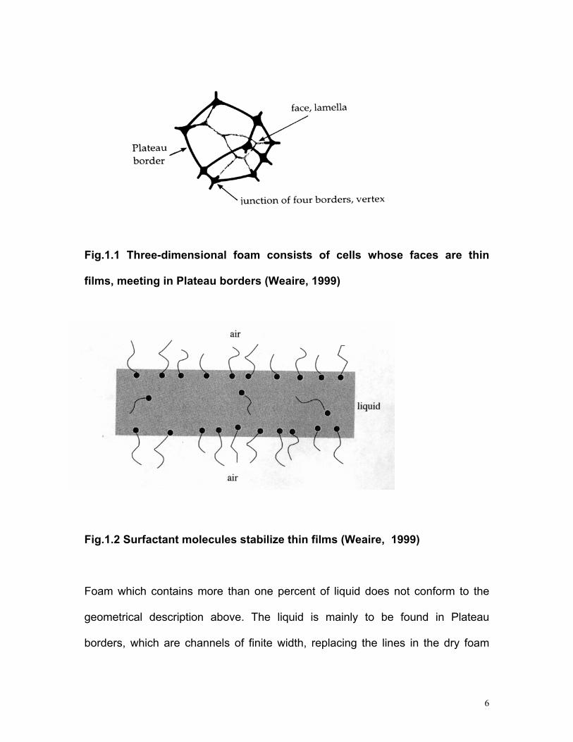
Fig.1.1 Three-dimensional foam consists of cells whose faces are thin
films, meeting in Plateau borders (Weaire, 1999)
Fig.1.2 Surfactant molecules stabilize thin films (Weaire, 1999)
Foam which contains more than one percent of liquid does not conform to the
geometrical description above. The liquid is mainly to be found in Plateau
borders, which are channels of finite width, replacing the lines in the dry foam
6
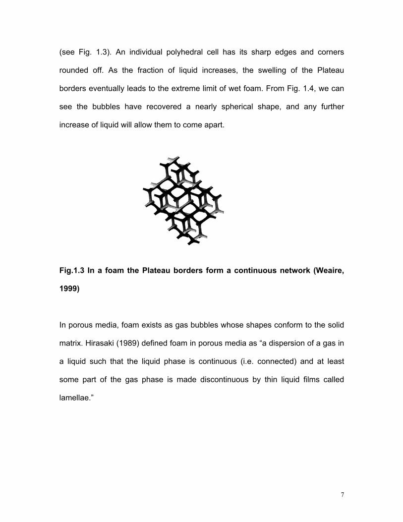
(see Fig. 1.3). An individual polyhedral cell has its sharp edges and corners
rounded off. As the fraction of liquid increases, the swelling of the Plateau
borders eventually leads to the extreme limit of wet foam. From Fig. 1.4, we can
see the bubbles have recovered a nearly spherical shape, and any further
increase of liquid will allow them to come apart.
Fig.1.3 In a foa
1999)
In porous media
matrix. Hirasaki
a liquid such th
some part of th
lamellae.”
m the Plateau borders form a continuous network (Weaire,
, foam exists as gas bubbles whose shapes conform to the solid
(1989) defined foam in porous media as “a dispersion of a gas in
at the liquid phase is continuous (i.e. connected) and at least
e gas phase is made discontinuous by thin liquid films called
7
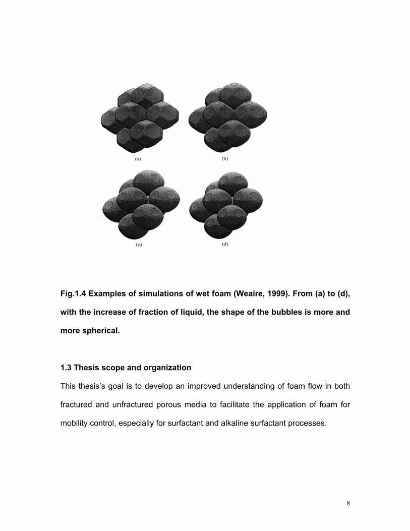
Fig.1.4 Examples of simulations of wet foam (Weaire, 1999). From (a) to (d),
with the increase of fraction of liquid, the shape of the bubbles is more and
more spherical.
1.3 Thesis scope and organization
This thesis’s goal is to develop an improved understanding of foam flow in both
fractured and unfractured porous media to facilitate the application of foam for
mobility control, especially for surfactant and alkaline surfactant processes.
8
Chapter 2 provides the technical background for the thesis. Foam flow in porous
media, mechanism of foam formation and foam decay, foam stability to crude oil
in porous media, foam flow in capillary tubes, the effect of heterogeneity on foam
flow and alkaline surfactant enhanced oil recovery in fractured carbonate
reservoir are reviewed.
Chapter 3 describes the mechanism for foam apparent viscosity when foam flows
in homogeneous fractures. Two contributions – liquid slug and foam bubble
deformation are found to be responsible for the foam apparent viscosity with
bubble diameter larger than aperture. The apparent viscosity for bulk foam can
be predicted by semi-empirical model. The contrary diversion effect is also
described.
Chapter 4 studies the foam flow in heterogeneous fractures with different
apertures. The apparent viscosity for foam with bubble diameter larger than
aperture can be calculated by the sum of the liquid slug and bubble deformation
contributions in heterogeneous fractures. The experimental results for foam flow
in two layer heterogeneous fractures fit the prediction from theory. Calculation for
foam sweep in heterogeneous fractures is expanded to parallel fractures with
apertures in log-normal distribution. The sweep efficiency sensitivity to bubble
size is discussed.
9

10
Chapter 5 investigates the surfactant work for alkaline-surfactant EOR process,
including the foaming and calcium tolerance ability of new surfactants used in
alkaline-polymer-surfactant process, surfactant stability to residual crude oil and
foam strength with different surfactants.
Chapter 6 focuses on alkaline/surfactant/polymer/foam (ASPF) enhanced oil
recovery process. Two different ASPF processes are developed – one is the
foam drive after surfactant slug and the other is foam injection from the
beginning. Higher apparent viscosity is found in sand packs with larger
permeability. The advantage of ASPF in heterogeneous reservoir is discussed.
Chapter 7 gives the conclusions for this study and recommendations for future
work.
In appendices, the derivations for the equivalent lamellae per unit length,
calculation for sweep efficiency in 2 layer fracture system and the calculation for
Dykstra-Parson’s model are given.
Chapter 2
TECHNICAL BACKGROUND
2.1 Fundamentals of flow in porous media
A porous medium is a solid matrix with interconnected holes or pores, such as
packed columns of sand, rocks, and soils. Macroscopically, Darcy’s law can
describe flow in a porous medium at a low Reynolds number:
)(→→
−∇−= gpku ρµ
(2.1)
The above equation of Darcy’s law is for a single-phase flow. It relates flow in
porous media to the pressure gradient. The term µ/k (also represented by the
symbol λ ) is the mobility of the fluid in the porous medium. It includes a
macroscopic property of the porous medium -- the permeability and a fluid-
dependent property -- the viscosity
k
µ . The superficial velocity u , also known as
the Darcy velocity, is the volumetric flow rate divided by the entire cross-sectional
area of the porous medium, Aqu /= . The actual flow, however, is limited only to
the pore spaces in the porous medium. Therefore, the actual mean velocity
within the pores, or the interstitial velocity ν , is related to the superficial velocity
by φν /u= , where φ is the porosity – another macroscopic property of the
porous medium.
11
For multiphase flow, Darcy’s law can be written for each phase i as:
)()( →→→
−∇⋅
−== gpSkk
u ii
iriii ρ
µφν (2.2)
The term k is the effective permeability of the porous medium and is a
product of the intrinsic permeability k and the relative permeability that is a
function of the fluid saturation . The mobility of phase i is expressed as
)( iri Sk⋅
rik
iS
i
rii
kkµ
λ⋅
= iS )( .
Another important concept for foam flow in porous media is capillary pressure.
For foam, capillary pressure is the difference between gas and liquid phase
pressure. From the generalized Young-Laplace equation, the capillary pressure
is:
)(2 hHP mc ∏+= σ (2.3)
Where is the capillary pressure, is the mean interfacial curvature of the
film, and
cP mH
σ is the surface tension. ∏ is first introduced by Derjaguin and co-
workers [1936], which is the film disjoining pressure. ∏ is a function of film
thickness, . Positive values of h ∏ reflect net repulsive film forces, and negative
12
values of indicate net attractive forces. The capillary pressure depends on the
liquid saturation.
∏
2.2 Surfactants
The term “surfactants” is a contraction of “surface active agents.” As the name
implies, a surfactant is a substance that is active or highly enriched at the surface
or interface between phases [Miller and Neogi, 1985]. A typical surfactant
monomer is composed of a polar (hydrophilic) moiety, and a nonpolar
(hydrophobic) moiety; the entire monomer is sometimes called an amphiphile
because of this dual nature. The monomer is represented by a “tadpole” symbol,
with the nonpolar moiety being the tail and the polar moiety being the head.
Surfactants can be divided into four categories by their polar moieties: anionic,
cationic, nonionic and amphoteric.
• Anionic. The anionic (negatively charged) surfactant ion is balanced with a
cation (usually sodium) associated with the monomer.
• Cationic. The surfactants are cationic if the polar moiety is positively charged.
The surfactant molecule contains an inorganic anion to balance the charge.
• Nonionic. Nonionic surfactants do not form ionic bonds. When they are
dissolved in aqueous solution, however, nonionic surfactants exhibit
surfactant properties. The most frequently used nonionic surfactants are
prepared by adding ethylene oxide to long-chain hydrocarbons with terminal
13

polar groups, e.g., -OH. The procedure introduces ethoxy or propoxy groups,
which are polar in nature and form hydrogen bonds with water.
• Amphoteric (Zwitterionic). This class of surfactants contains aspects of two or
more of the other classes. The ionic character or the polar group depends on
the pH of the solution.
+ -
+ -
Fig. 2.1 C
Surfactan
water wh
Consequ
polar and
tension.
As shown
oil/water
surfactan
-
c c Amphoteric
Anioniclassification of su
ts have a “head” a
ile the “tail” has
ently, surfactant m
non-polar phase
in Fig. 2.2, some s
interface and form
t molecules are
+
Cationi
rfactants (Lak
nd a “tail”, the
an affinity w
olecules tend t
s, which resul
urfactant mole
a monolayer. A
dissolved in t
Nonioni
e, 1989)
“head” prefers polar media such as
ith non-polar media like oil or air.
o adsorb at the interface between the
ts in the reduction of the interfacial
cules are adsorbed on the air/water or
t low concentration, all the rest of the
he solution as individual surfactant
14

monomers. Above a particular concentration, however, some surfactant
molecules form aggregates that are called micelles [Miller and Neogi, 1985]. The
critical concentration for micelles to be formed is called the critical micelle
concentration, or CMC. Above CMC, virtually all further increases in surfactant
concentration cause growth only in the micelle concentration.
Fig.
Surfa
inter
decr
CMC
func
beca
grou
2.2 Schematic of surfactant behavior above the CMC (Tanzil, 2001)
ctants have two important functions in EOR processes. One is to lower the
facial tension (IFT) between oil and water phase. Below CMC, IFT
eases significantly with the increase of surfactant concentration. Above
, the addition of pure surfactant does not change IFT much. The other
tion of a surfactant is to stabilize foams used for mobility control. This occurs
use it can stabilize the lamellae of foams owing to repulsive between head
ps of surfactant molecules adsorbed on the film surfaces.
15
2.3 Fundamentals of Foam Flow in porous Media
The behavior of foam in porous media is intimately related to media connectivity
and geometry. Porous media have several attributes that are important to foam
flow. First, they are characterized by the size distribution of the pore bodies
interconnected through the pore-throats of another size distribution. Foam
generation and destruction mechanisms depend strongly on the body to throat
size aspect ratio. Second, pores are not cylindrical but exhibit corners. For large
pores, the wetting fluid resides in the corners of gas-occupied pores and in thin
wetting films coating the pore walls (see Fig. 2.3). The non-wetting phase resides
in the central portion of the large pores. Small pores are completely filled with
wetting fluid. Hence, the wetting phase remains continuous. Third, when flow
rates are very low and capillary forces dominate, the capillary pressure is set by
the local saturation of the wetting phase and the value of the interfacial tension.
Local imbalances in capillary pressure tend to equalize through the interlinked,
continuous wetting phase. During biphasic flow, the nonwetting fluid flows in
interconnected large pore channels. Wetting fluid flows in interconnceted small
channels and in the corners of the nonwetting –phase occupied pores because of
pressure gradients in the aqueous phase.
When the characteristic length scale of the pore space is much greater than the
size of individual foam bubbles, the foam is called bulk foam. When the gas
fraction is low, the bulk foam is “spherical foam” which consists of well-separated,
spherical bubbles. When the gas fraction is high, the bulk foam is called
16

“polyhedral foam” which consists of polyhedral bubbles separated by surfactant-
stabilized thin liquid films called lamellae.
Fig. 2.3 Cross-sectional view of cornered pores. The wetting fluid is held in
the pore corners. (Kovscek and Radke, 1994)
On the other hand, when the characteristic pore size is comparable to or less
than the characteristic size of the dispersed gas bubbles, the bubbles and
lamellae span pores completely. At low gas fractional flow, the pore-spanning
bubbles are widely spaced, separated by thick wetting liquid lenses or bridges. At
high gas fractional flow, the pore-spanning bubbles are in direct contact,
separated by lamellae. Hirasaki and Lawson [1985] denote this direct-contact
morphology as the individual–lamellae regime.
17
Although both bulk foam and individual-lamellae foam can exist in principle,
effluent bubble sizes equal to or larger than pore dimensions are usually
reported. It is now generally accepted that single bubbles and lamellae span the
pore space of most porous media undergoing foam flow in the absence of
fractures.
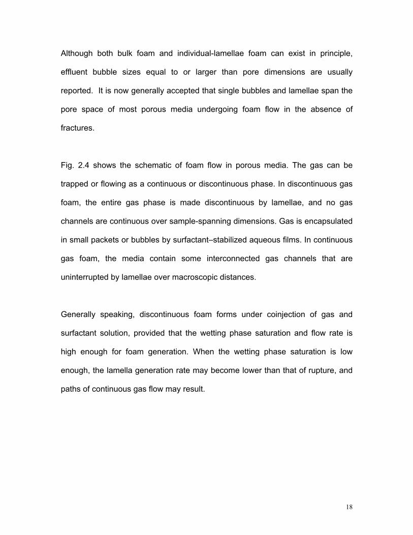
Fig. 2.4 shows the schematic of foam flow in porous media. The gas can be
trapped or flowing as a continuous or discontinuous phase. In discontinuous gas
foam, the entire gas phase is made discontinuous by lamellae, and no gas
channels are continuous over sample-spanning dimensions. Gas is encapsulated
in small packets or bubbles by surfactant–stabilized aqueous films. In continuous
gas foam, the media contain some interconnected gas channels that are
uninterrupted by lamellae over macroscopic distances.
Generally speaking, discontinuous foam forms under coinjection of gas and
surfactant solution, provided that the wetting phase saturation and flow rate is
high enough for foam generation. When the wetting phase saturation is low
enough, the lamella generation rate may become lower than that of rupture, and
paths of continuous gas flow may result.
18

Fig. 2.4 Pore level schematic of foam in porous media (Tanzil, 2001)
Fig. 2.4 is also a summary of the pore-level microstructure of foam during flow
through porous media. Because of the dominance of capillary forces, wetting
surfactant solution flows as a separate phase in the small pore spaces. Minimal
wetting liquid transports as lamellae. So the wetting-phase relative permeability is
unchanged when foam is present. When both flowing and trapped gas exist,
flowing foam transports in large pores because the resistance there is less than
in the smaller pores. Then bubble trapping can happen only in intermediate-sized
19

pores. The relative permeability of flowing-foam is solely a function of the gas
saturation of flowing bubbles and is much reduced by the trapped foam
saturation. The foam bubbles, which move in the largest backbone channels,
parade in series as trains. They are usually destroyed and recreated. Bubble-
trains usually exist in a time-averaged sense.
Thus, we can divide foam into “weak” foam and “strong” foam. For “weak foam”
with no moving lamellae, the increase in trapped gas saturation is crucial to the
behavior of foam flow as it results in the blockage of gas pathways, which
reduces the relative permeability of gas. The trapped gas reduces mobility, but
the rest of the gas flows as continuous gas.
“Strong” foam flows by a different mechanism. The lamellae make the flowing
gas discontinuous. Then the bubble trains face much higher resistance than in
continuous gas flow. The apparent viscosity of the discontinuous foam is usually
much greater than in continuous flow. The combined effect of the reduction of
gas relative permeability and the increase of apparent gas viscosity greatly
increases the mobility reduction effect of the foam.
Generally speaking, the most important factors that affect foam trapping and
mobilization are pressure gradient, gas velocity, pore geometry, bubble size, and
bubble-train length. Increasing the pressure gradient can open up new channels,
which were occupied by moving or trapped gas.
20
2.4 Mechanisms of Foam Formation and Decay
As described above, the identity of a single bubble or train is not conserved over
large distances. Bubble trains usually exist in a time-averaged sense. The
bubbles comprising these trains are usually destroyed and recreated in time. So
obviously it is necessary to discuss the mechanism of foam formation and decay.
2.4.1 Foam Formation
Until now, three fundamental pore-level foam generation mechanisms are
generally accepted: capillary snap-off, lamella-division and leave-behind.
Generally, capillary snap-off and lamella-division generate strong foam
(discontinuous gas) while leave-behind generates weak foam (continuous gas).
Capillary snap-off
Capillary snap-off can repeatedly occur during multiphase flow in porous media
regardless of the presence or absence of surfactant. It is recognized as a
mechanical process.
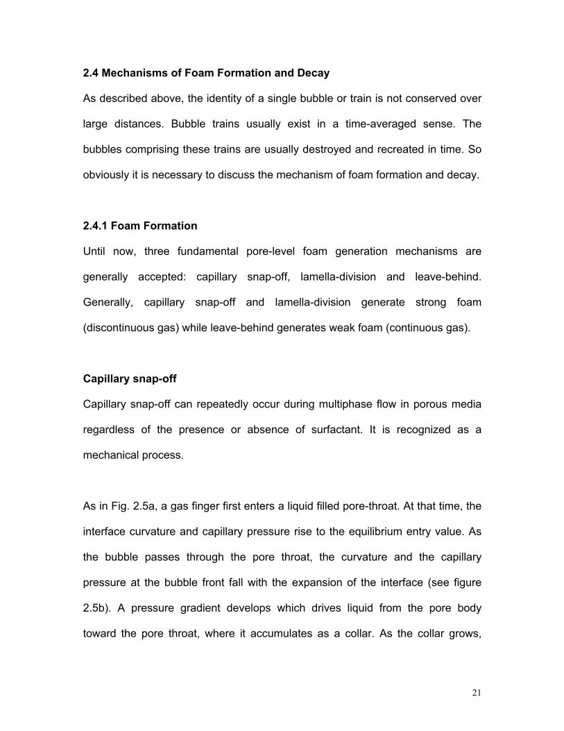
As in Fig. 2.5a, a gas finger first enters a liquid filled pore-throat. At that time, the
interface curvature and capillary pressure rise to the equilibrium entry value. As
the bubble passes through the pore throat, the curvature and the capillary
pressure at the bubble front fall with the expansion of the interface (see figure
2.5b). A pressure gradient develops which drives liquid from the pore body
toward the pore throat, where it accumulates as a collar. As the collar grows,
21

snap-off occurs. The generated foam bubble has a similar size to that of the pore
bodies (see figure 2.5c).
Fig. 2.5 Schematic of capillary snap-off mechanism showing (a) gas entry
into liquid filled pore-throat (b) gas finger and wetting collar formation prior
to breakup (c) liquid lens after snap-off (Kovscek and Radke, 1994)
There are some conditions for the snap-off to happen. First, a sufficient amount
of wetting phase is needed. Second, the pressure difference across the interface
in the throat must be greater than that at the leading surface. Or, in other words,
the liquid pressure in the throat must be smaller than that at the leading surface.
Indeed, the capillary pressure at the leading surface must be smaller than the
critical value . Form Fall et al. [1988], this critical value is about half of the
capillary entry pressure, that is
sncP
sncP
ec
snc PP
21
≈ . From hydrodynamic analysis, the pore
body radius must be at least two times of that of pore throat to create sufficient
capillary pressure reduction for snap off [Kovscek and Radke, 1994].
22
From the above description, it is evident that snap-off depends on liquid
saturation or, equivalently, on the medium capillary pressure. Except for
alteration of solution properties such as surface tension, it is essentially
independent of surfactant formulation.
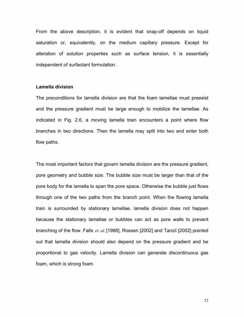
Lamella division
The preconditions for lamella division are that the foam lamellae must preexist
and the pressure gradient must be large enough to mobilize the lamellae. As
indicated in Fig. 2.6, a moving lamella train encounters a point where flow
branches in two directions. Then the lamella may split into two and enter both
flow paths.
The most important factors that govern lamella division are the pressure gradient,
pore geometry and bubble size. The bubble size must be larger than that of the
pore body for the lamella to span the pore space. Otherwise the bubble just flows
through one of the two paths from the branch point. When the flowing lamella
train is surrounded by stationary lamellae, lamella division does not happen
because the stationary lamellae or bubbles can act as pore walls to prevent
branching of the flow. Falls [1988], Rossen [2002] and Tanzil [2002] pointed
out that lamella division should also depend on the pressure gradient and be
proportional to gas velocity. Lamella division can generate discontinuous gas
foam, which is strong foam.
et .al
23

Fig. 2.6 Schematic of lamella division mechanism. A lamella is flowing from
the left to the right. (a) Lamellae approaching branch point (b) Divided
lamellae (Kovscek and Radke, 1994)
Leave-behind
Snap-off and lamella division can generate strong foam. Here we discuss the
mechanism for weak foam generation, leave-behind.
When two gas fingers invade adjacent liquid-filled pore bodies, a lamella is left
behind (see Fig. 2.7). A stationary stable lamella emerges as long as the
capillary pressure is not too high and the pressure gradient is not too large.
The lamella from leave-behind is generally oriented to the direction of flow and
can generate only continuous gas foam, which is weak foam.
24
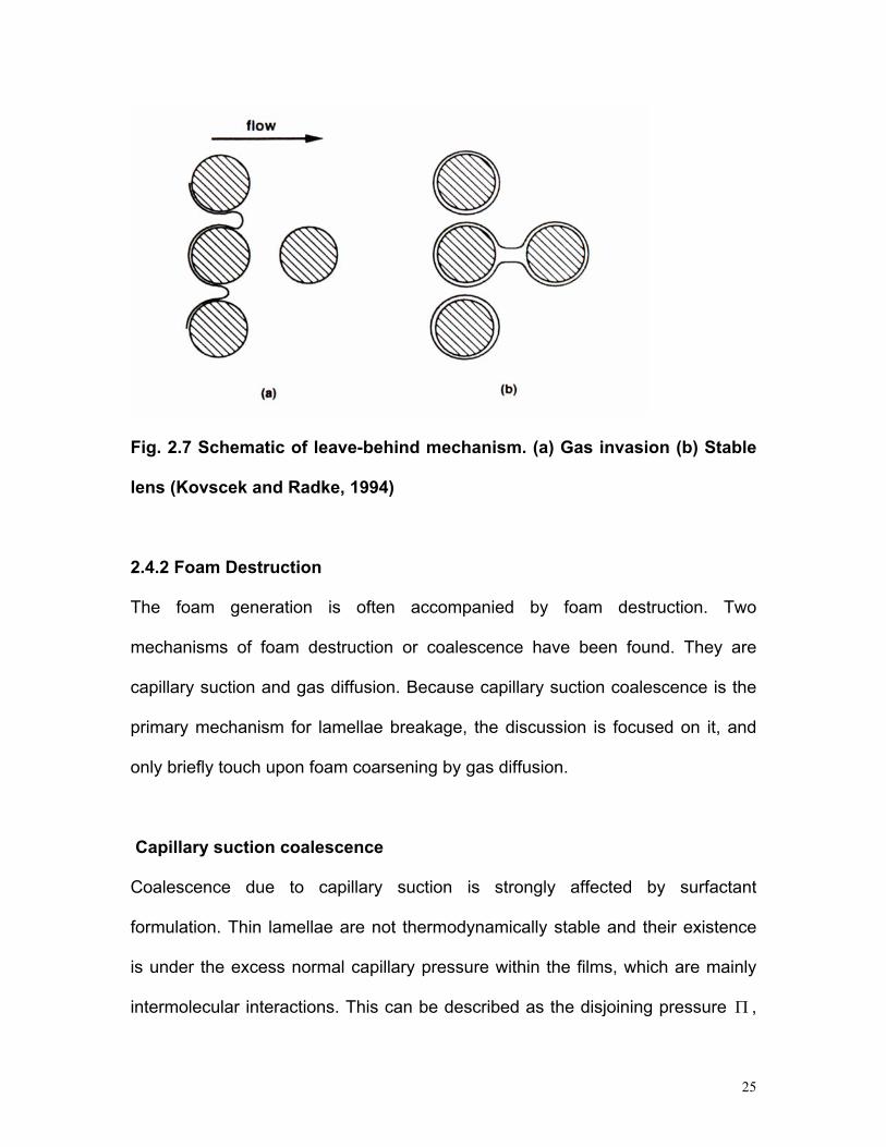
Fig. 2.7 Schematic of leave-behind mechanism. (a) Gas invasion (b) Stable
lens (Kovscek and Radke, 1994)
2.4.2 Foam Destruction
The foam generation is often accompanied by foam destruction. Two
mechanisms of foam destruction or coalescence have been found. They are
capillary suction and gas diffusion. Because capillary suction coalescence is the
primary mechanism for lamellae breakage, the discussion is focused on it, and
only briefly touch upon foam coarsening by gas diffusion.
Capillary suction coalescence
Coalescence due to capillary suction is strongly affected by surfactant
formulation. Thin lamellae are not thermodynamically stable and their existence
is under the excess normal capillary pressure within the films, which are mainly
intermolecular interactions. This can be described as the disjoining pressure Π ,
25
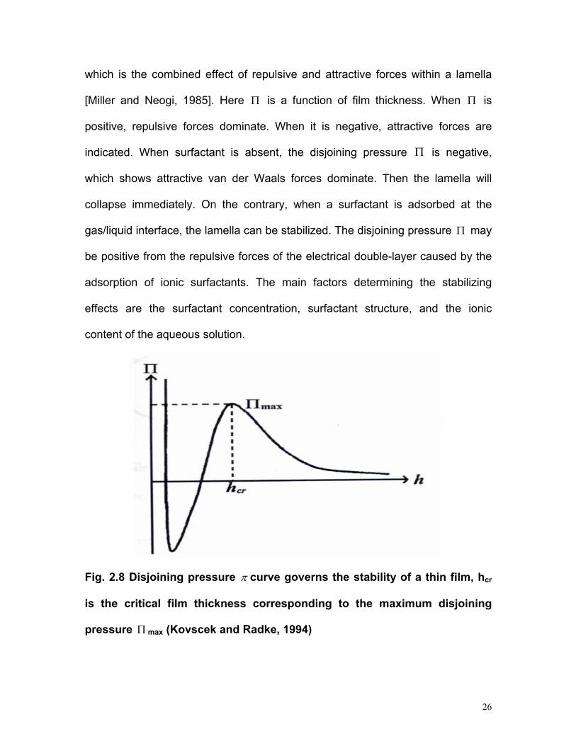
which is the combined effect of repulsive and attractive forces within a lamella
[Miller and Neogi, 1985]. Here Π is a function of film thickness. When Π is
positive, repulsive forces dominate. When it is negative, attractive forces are
indicated. When surfactant is absent, the disjoining pressure is negative,
which shows attractive van der Waals forces dominate. Then the lamella will
collapse immediately. On the contrary, when a surfactant is adsorbed at the
gas/liquid interface, the lamella can be stabilized. The disjoining pressure may
be positive from the repulsive forces of the electrical double-layer caused by the
adsorption of ionic surfactants. The main factors determining the stabilizing
effects are the surfactant concentration, surfactant structure, and the ionic
content of the aqueous solution.
Π
Π
Fig. 2.8 Disjoining pressure π curve governs the stability of a thin film, hcr
is the critical film thickness corresponding to the maximum disjoining
pressure Π max (Kovscek and Radke, 1994)
26

As shown in Fig. 2.8, from experiments, the isotherm of disjoining pressure to the
thickness of the lamella film is “S” shaped just as a pressure-volume isotherm for
real gas and liquid. When a static trapped film is in equilibrium at a flat interface,
the disjoining pressure is equal to the capillary pressure. The capillary pressure
in a foam depends on the wetting-liquid saturation. During drainage or gas
injection, the liquid saturation decreasing causes an increase of capillary
pressure. In turn, the thickness of the lamella film decreases until Π max is
reached. When the capillary pressure increases further over Π max, the film
ruptures.
Coalescence behavior of flowing foam bubbles is more complicated than that of
static lamella. In Fig. 2.9, a moving thin film undergoes squeezing and stretching
as it translates from a pore body to a throat to another pore body. It causes film
thickness to oscillate about the equilibrium film thickness established for the
static film. A thin film with mobile surface will rupture during stretching if its
thickness falls below the critical film thickness [Jimenez and Radke, 1996;
Singh , 1997]. Therefore, a moving thin film could rupture at a limiting
capillary pressure , which is less than the maximum disjoining pressure
crh
et .al
*cP maxΠ .
In other words, moving lamellae can be even less stable than static ones.
Besides the disjoining pressure Π , Marangoni effect is also a restoring and
stabilizing force in a lamella [Alvarez, 1998]. When the lamella film is stretched in
the pore space, the stretching can cause a reduction in surfactant concentration
27

and an increase in the local surface tension if the surfactant transports slowly to
the lamella surface. Then the liquid can be dragged from the low surface tension
region to the high surface tension region by surface flow. So the increased
surface tension works against lamella thinning.
Fig. 2.9 Foam lamella translating from left to right in a periodically
constricted tube (Kovscek and Radke, 1994)
Singh, Hirasaki and Miller [1997] found that Jimenez and Radke’s previous
theory could be applied only to a limited regime. They found that when the film
surface is immobilized by surfactants, moving lamellae may be more stable than
stationary lamellae. For this case, moving lamella trains will switch paths as
stationary lamellae rupture and new paths of least resistance appear. This may
be the preferred mode of foam flow when it is desired to contact as much of the
porous medium as possible with flowing continuous gas foam. When the film is
mobile, the stationary lamellae will be more stable than the moving lamellae. This
case is in qualitative agreement with Jimenez and Radke’s theory. So the choice
of a suitable surfactant is important for the stability of foam in porous media.
28

Gas diffusion
For trapped foam bubbles, the gas on the concave side of the bubble has a
higher pressure than that on the convex side. The pressure difference drives the
gas to diffuse from the concave side to the convex side through the liquid film.
Gas diffusion mechanism is less important than capillary suction mechanism in
foam coalescence in porous media.
Fig. 2.10 Gas diffusion mechanism for bubble coalescence
2.5 Foam Sensitivity to Crude Oil in Porous Media
Most experiments about foam flow in porous media were done by injecting gas
and aqueous surfactant solution or gas only. In true EOR field use, crude oil is
present. It is necessary to understand the oil’s effect on the foam stability.
When a surfactant solution comes in contact with oil during flow in a porous
medium, oil can be emulsified. Fig. 2.11 shows the presence of emulsified oil
droplets inside a capillary network. The oil has drained from the thinning foam
film and is trapped inside the Gibbs-Plateau borders. Under the capillary
pressure inside the Gibbs-Plateau border, the three phases (gas, water, and oil)
come in contact and three types of aqueous films are formed (Fig. 2.12): foam
29
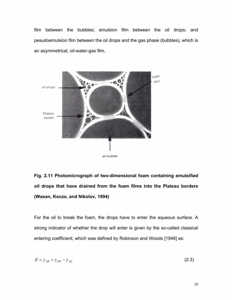
film between the bubbles; emulsion film between the oil drops; and
pesudoemulsion film between the oil drops and the gas phase (bubbles), which is
an asymmetrical, oil-water-gas film.
Fig. 2.11 Photomicrograph of two-dimensional foam containing emulsified
oil drops that have drained from the foam films into the Plateau borders
(Wasan, Koczo, and Nikolov, 1994)
For the oil to break the foam, the drops have to enter the aqueous surface. A
strong indicator of whether the drop will enter is given by the so-called classical
entering coefficient, which was defined by Robinson and Woods [1948] as:
AOOWAWE γγγ −+= (2.3)
30

where AOOWAW γγγ ,, are the air-water, oil-water, and air-oil interfacial tensions
respectively.
When E is positive, entry is expected. E may have different values for the initial
un-equilibrated fluids and the final situation after equilibrium is reached.
If the drop can enter the interface, the spreading coefficient of oil on water,
which was defined by Harkins [1941], should be considered:
S
AOOWAWS γγγ −−= (2.4)
If , the oil can spread, the interface can expand and this expansion can
result in a thinning of the film. It produces local thinning of the foam film, which
can lead to rupture.
0>S
Besides the spreading coefficient , the bridging coefficient S B is also important.
It is defined as:
222AOOWAWB γγγ −+= (2.5)
Even when , so that the oil drop forms a lens at the air-water surface
instead of spreading, the foam can become unstable once the drop has entered
its other surface so that it spans the film, provided that .
0<S
0>B
31

The effect of emulsified oil on foams is closely connected with the configuration
of oil relative to the aqueous and gas phase. From Wasan, Koczo and Nikolov
[1994], the configuration can be one of the following (figure 2.12):
a. An oil drop without interaction with the gas-liquid surface is generally the
initial oil configuration inside the foam. The entry coefficient is less than zero
(E<0). So the oil drop can retain its configuration.
b. If the oil drop interacts with the gas-liquid surface, the drop gets deformed
and separated by a pseudoemulsion film from the gas phase. The entry
coefficient can be less than zero if this is a steady state. It can also be
greater than zero if this is a meta-stable state.
c. If the pseudoemulsion film ruptures, the oil drop enters the surface, and an
oil lens is formed at the solution surface. For this state, the entry coefficient is
greater than zero but spreading coefficient is less than zero.
d. A spread oil layer or film can form from the lens on the solution surface. At
that time, the spreading coefficient is equal to zero.
32
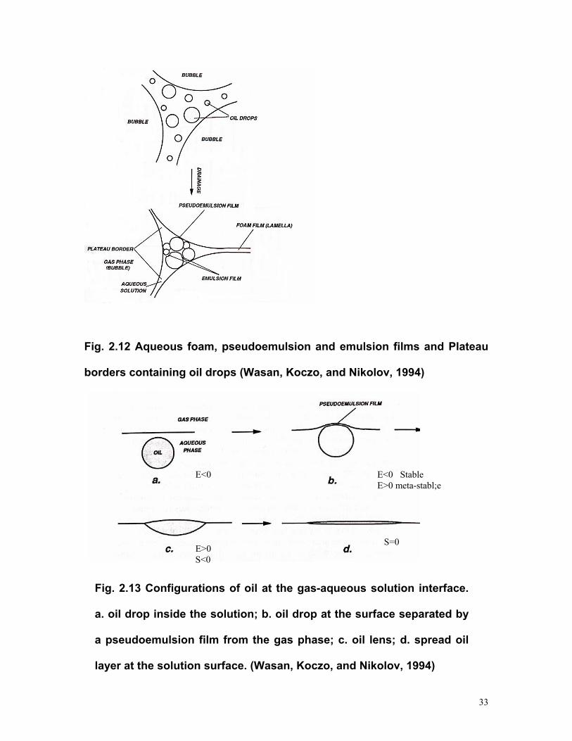
Fig. 2.12 Aqueous foam, pseudoemulsion and emulsion films and Plateau
borders containing oil drops (Wasan, Koczo, and Nikolov, 1994)
E<0
E<0 Stable E>0 meta-stabl;e
S=0 E>0
S<0
33
Fig. 2.13 Configurations of oil at the gas-aqueous solution interface.
a. oil drop inside the solution; b. oil drop at the surface separated by
a pseudoemulsion film from the gas phase; c. oil lens; d. spread oil
layer at the solution surface. (Wasan, Koczo, and Nikolov, 1994)

Entry barrier
The formation of oil bridges from pre-emulsified oil drops requires the rupture of
the pseudoemulsion film. The film may be stabilized by various surface forces,
which suppress the drop entry and impede the antifoam action of oil.
The entry coefficient E is a thermodynamic property. It determines whether the
particular configuration of the oil drop is energetically favorable or not, but can
not predict the fate of the oil drops under dynamic conditions which exist within
the draining foam film. So its application to the physical processes in porous
media is limited.
Some different parameters have been suggested to quantify the entry barriers for
oil drops, such as the modified entry coefficient by Bergeron et al [1993],
which is described as:
gE
∫Π
−=)(
0
EAS h
ASg hdE π (2.6)
where the lower limit of the integral corresponds to 0)( =∞→Π hAS , is the
equilibrium thickness of the thin film at a particular disjoining pressure. The
classical entry coefficient
Eh
E can be obtained when [Bergeron et al.,
1993].
0→Eh
34
Another possible quantity as a measure of the pseudoemulsion film is the
capillary pressure. The critical capillary pressure is the most adequate measure
of the film stability because the capillary pressure is the actual external variable
that forces the film surfaces toward each other against the repulsive forces
(disjoining pressure) stabilizing the film. Hadjiiski et al [1996] developed the film
trapping technique (FTT) to measure the critical capillary pressure.
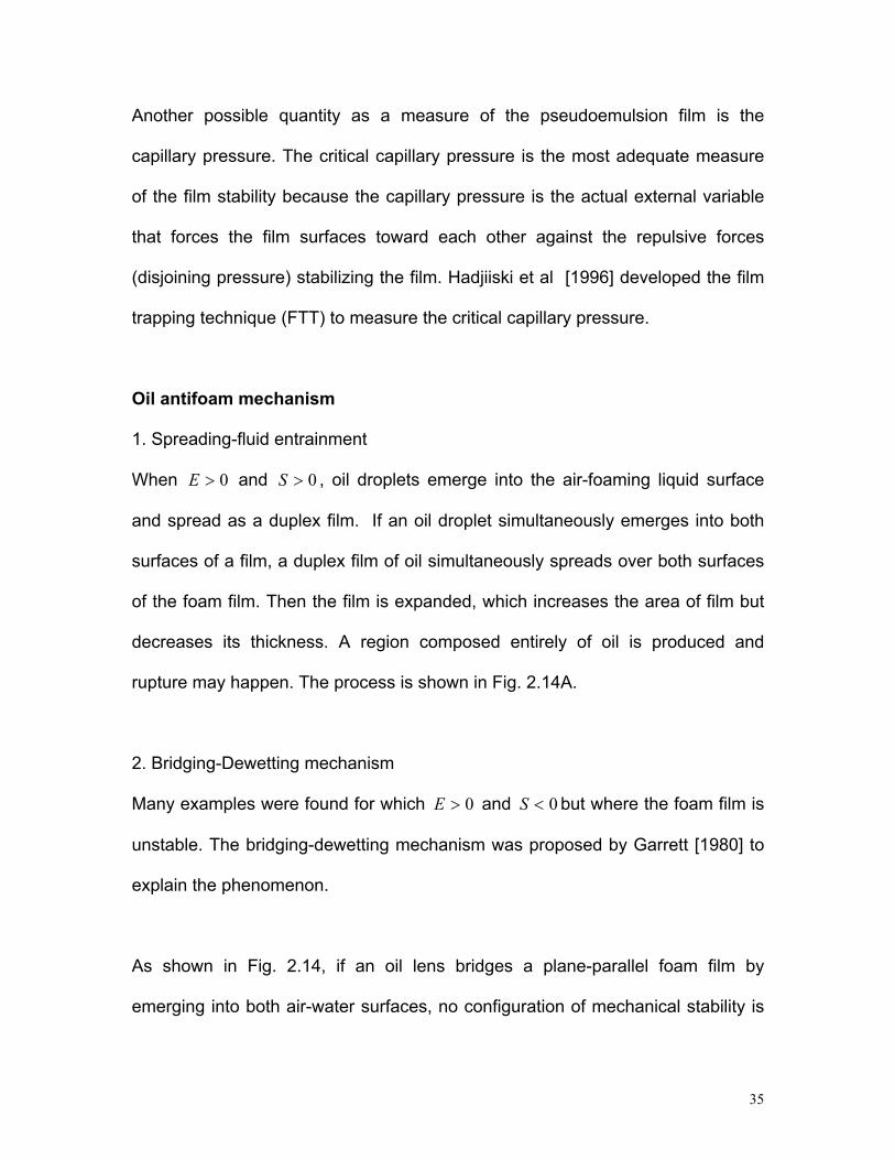
Oil antifoam mechanism
1. Spreading-fluid entrainment
When and , oil droplets emerge into the air-foaming liquid surface
and spread as a duplex film. If an oil droplet simultaneously emerges into both
surfaces of a film, a duplex film of oil simultaneously spreads over both surfaces
of the foam film. Then the film is expanded, which increases the area of film but
decreases its thickness. A region composed entirely of oil is produced and
rupture may happen. The process is shown in Fig. 2.14A.
0>E 0>S
2. Bridging-Dewetting mechanism
Many examples were found for which and 0>E 0<S but where the foam film is
unstable. The bridging-dewetting mechanism was proposed by Garrett [1980] to
explain the phenomenon.
As shown in Fig. 2.14, if an oil lens bridges a plane-parallel foam film by
emerging into both air-water surfaces, no configuration of mechanical stability is
35
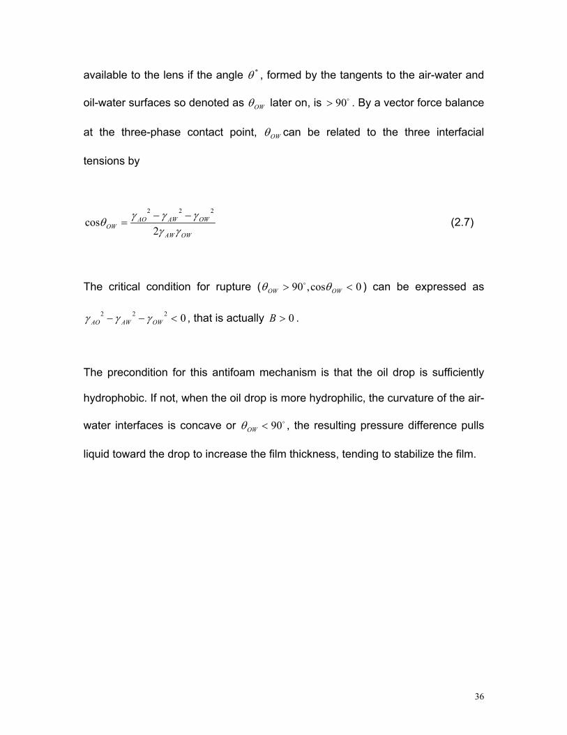
available to the lens if the angle , formed by the tangents to the air-water and
oil-water surfaces so denoted as
*θ
OWθ later on, is . By a vector force balance
at the three-phase contact point,
o90>
OWθ can be related to the three interfacial
tensions by
OWAW
OWAWAOOW γγ
γγγθ2
cos222 −−
= (2.7)
The critical condition for rupture ( ) can be expressed as
, that is actually .
0cos,90 <> OWOW θθ o
0>B0222 <−− OWAWAO γγγ
The precondition for this antifoam mechanism is that the oil drop is sufficiently
hydrophobic. If not, when the oil drop is more hydrophilic, the curvature of the air-
water interfaces is concave or , the resulting pressure difference pulls
liquid toward the drop to increase the film thickness, tending to stabilize the film.
o90<OWθ
36
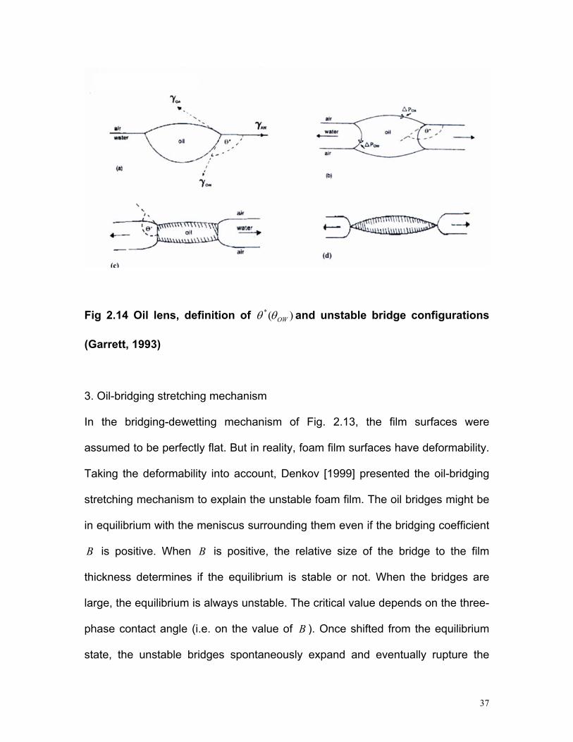
Fig 2.14 Oil lens, definition of and unstable bridge configurations
(Garrett, 1993)
)(*OWθθ
3. Oil-bridging stretching mechanism
In the bridging-dewetting mechanism of Fig. 2.13, the film surfaces were
assumed to be perfectly flat. But in reality, foam film surfaces have deformability.
Taking the deformability into account, Denkov [1999] presented the oil-bridging
stretching mechanism to explain the unstable foam film. The oil bridges might be
in equilibrium with the meniscus surrounding them even if the bridging coefficient
B is positive. When B is positive, the relative size of the bridge to the film
thickness determines if the equilibrium is stable or not. When the bridges are
large, the equilibrium is always unstable. The critical value depends on the three-
phase contact angle (i.e. on the value of B ). Once shifted from the equilibrium
state, the unstable bridges spontaneously expand and eventually rupture the
37

foam film. At negative value of B , the bridges are in stable equilibrium with the
contiguous meniscus.
Below figure 2.15 is a schematic illustration of the above three defoaming
mechanisms. For all of these mechanisms, the first step is drop entry, for which
the entry coefficient E is positive and the entry barrier is small.
Fig 2.15 Schematic profile of several defoaming mechanisms (Zhang, 2002)
(A) Spreading-fluid entrainment
(B) Bridging-dewetting mechanism
(C) Bridging-stretching mechanism
2.6 Foam flow in capillary tubes
From Hirasaki and Lawson [1985], a reasonable conceptual model of a natural
porous medium is a bundle of interconnected capillaries of different sizes and
38
containing constrictions. From their research, the apparent viscosity is the sum of
three contributions (as shown in Fig. 2.16): those resulting from slugs of liquid
between bubbles, the resistance to deforming the interface when a bubble
passes through a capillary, and the surface tension gradient as surface active
material is swept from the front of the bubble and accumulates at the back of the
bubble.
The viscosity contribution from liquid slugs in capillary tube from Hirasaki and
Lawson [1985] is:
Lsliqapp nLµµ = (2.8)
where is the length of liquid slugs and n is the number of equivalent lamellae
per unit length.
sL L
The contribution of the deformation of the foam bubble to apparent viscosity in
capillary tube was also derived. In a capillary tube, for the bubbles shown in
figure 2.17, the expression for the net dynamic pressure drop is:
]1)/[()/3)(/(26.2 23/2 +=∆ RrUrp ccdynamic σµσ (2.9)
where U is the velocity of bubble, σ is the surface tension, is the radius of
curvature of gas-liquid interface and R is the capillary radius.
cr
39

The apparent viscosity in a tube with the model above is derived from Poiseuille
flow as:
[ 1)/()/3()/()(85.0
823/1
2
+=∆
= − RrURrRn
UpRn
cc
LLshapeapp σµ
µµ ] (2.10)
From Hirasaki and Lawson [1985], the apparent viscosity resulting from surface
tension gradient is:
)1()1()/3)(( 3/1
L
L
N
N
sLgradapp e
eNURn −
−−
+−
= σµµµ (2.11)
where is the dimensionless length of the thin film portion of bubble and is
the dimensionless number for surface tension gradient effect. The value of
describes the degree of mobility of the interface. The relationship between the
two dimensionless numbers is:
LN sN
NL
scc
BL NrUP
LN3/1)/3()(
2σµ
−= (2.12)
where is a coefficient. cP)(
40
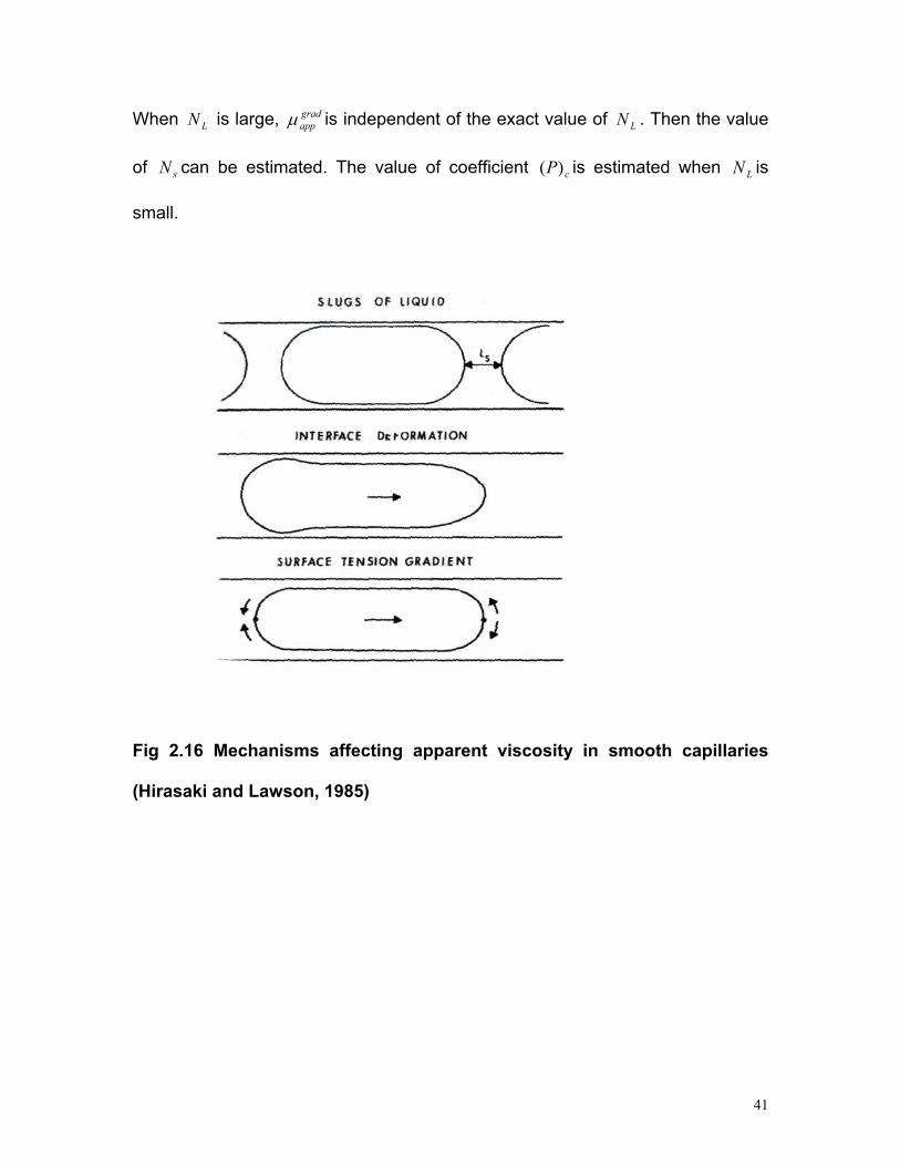
When is large, is independent of the exact value of . Then the value
of can be estimated. The value of coefficient is estimated when is
small.
LNgradappµ LN
sN cP)( LN
Fig 2.16 Mechanisms affecting apparent viscosity in smooth capillaries
(Hirasaki and Lawson, 1985)
41
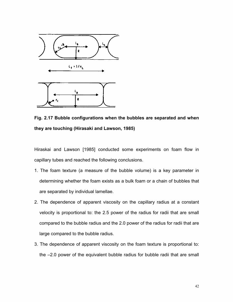
Fig. 2.17 Bubble configurations when the bubbles are separated and when
they are touching (Hirasaki and Lawson, 1985)
Hiraskai and Lawson [1985] conducted some experiments on foam flow in
capillary tubes and reached the following conclusions.
1. The foam texture (a measure of the bubble volume) is a key parameter in
determining whether the foam exists as a bulk foam or a chain of bubbles that
are separated by individual lamellae.
2. The dependence of apparent viscosity on the capillary radius at a constant
velocity is proportional to: the 2.5 power of the radius for radii that are small
compared to the bubble radius and the 2.0 power of the radius for radii that are
large compared to the bubble radius.
3. The dependence of apparent viscosity on the foam texture is proportional to:
the –2.0 power of the equivalent bubble radius for bubble radii that are small
42

compared to the capillary radius and the –3.0 power of the equivalent bubble
radius for bubble radii that are large compared to the capillary radius.
4. The dependence of apparent viscosity on the velocity is proportional to the –
1/3 power of velocity when the foam is bulk foam or the velocity is low for
individual lamellae, and to the –2/3 power of velocity for individual lamellae at
high velocity.
2.7 Effect of heterogeneity on foam flow
Foam is used in EOR process to change the mobility of gas in the reservoir. The
field situation is primarily heterogeneous and multidimensional. It is found the
mobility of gas can be reduced more in high permeability regions than in low
permeability regions. The reason is that the stability of foam is higher in high
permeability regions than low permeability regions. Khatib et proposed the
limiting capillary pressure mechanism in 1988, which is discussed below.
.al
2.7.1 Capillary pressure’s role in bulk foams
First let’s discuss capillary pressure’s role in foam stability outside porous media,
or bulk foam. From Derjaguin-Laudau-Verwey-Overbeek (DLVO) theory, when
gas/liquid interfaces are present, ionic surfactant molecules from an aqueous
solution adsorb preferentially at the interface, thereby creating charged surfaces.
The overlap of the electric fields from these charged layers imparts stability to a
foam lamella. The double layer repulsion balances the van der Waals forces plus
the capillary pressure, which acts to force the charged surfaces closer to one
43

another and destabilize the system. As the capillary pressure increases, the work
required for breaking the film decreases. Thus, the capillary pressure can play a
role in determining the stability of foams outside porous media. Khristov
[1988] presented the concept of the “critical” capillary pressure above which
the lifetime of lamellae becomes exceedingly short. The critical capillary pressure
varies with surfactant formulation-i.e., the type and concentration of surfactant
and electrolyte.
et .al
The presence of salts may be good or bad for the stability of bulk foams. From
DLVO theory, at higher electrolyte levels, the length over which the electric field
from the charged surfactant layers decay should shorten and the repulsive forces
should weaken. But this effect may be offset because salt raises the surface
concentration of surfactant at the gas/liquid interfaces [Nilsson, 1957].
2.7.2 Limiting capillary pressure for foam in porous media
The stability of foams in porous media may likewise depend on capillary
pressure. But in porous media, all lamellae do not coalesce at some “critical”
capillary pressure. Instead, because lamellae are convected or generated in situ,
the capillary pressure increases up to a limiting capillary pressure as foam
generation creates stronger foam or the gas fractional flow is raised. With further
decrease in gas mobility or increase in gas fractional flow, the capillary pressure
remains at its limiting value while the foam texture remains constant or becomes
coarser respectively.
44

Fig 2.18 Sketches of capillary-pressure and fractional-flow curves
operating during a two-phase displacement [Khatib, Hirasaki, Falls, 1988]
From Fig. 2.18, if the capillary pressure during a foam displacement can not
exceed a limiting value , because of the stability of lamellae, then the liquid
saturation must be greater than or equal to the corresponding liquid saturation,
, because the capillary pressure is a monotonic function of saturation.
Suppose that gas and liquid are flowing as a foam of constant bubble size at a
given gas velocity. As the gas fractional flow is raised, the liquid saturation
declines until the limiting value (at ) is attained. If the gas fractional flow is
*cP
*wS
*wS
*cP
45

increased further, foam texture must coarsen to keep the capillary pressure from
rising above the limiting value.
2.7.3 Behavior of foam in low-permeability media
From Khatib , Hirasaki and Falls [1988], the limiting capillary pressure is a
decreasing function of gas flow rate and of the permeability. Then below some
permeability, the limiting capillary pressure will become less than the capillary
entry pressure, as shown in Fig. 2.19. When the capillary pressure is less than
the capillary entry pressure, the implication is that flowing-foam lamellae are not
stable and will coalesce. If the flowing foam coalesces, then either the gas will
flow as a continuous phase or moving lamellae will have a short lifetime.
As shown in Fig. 2.20, Khatib and Hirasaki [1988] speculate on the
consequences of gas flowing as a continuous phase whenever the permeability
is less than the permeability at which the limiting capillary pressure is equal to the
capillary entry pressure. The limiting capillary pressure applies to the dynamic
stability of flowing lamellae. Stationary lamellae, by contrast, have zero velocity
and thus can be expected to be stable at capillary pressures in excess of the
limiting capillary pressure for a flowing film. It is presumed that that the stationary
lamellae block some fraction of the gas-saturated pore space such that the
relative gas mobility is at some reduced value and that the moving gas flows as a
continuous phase. As a consequence, the gas mobility may have a dependence
on permeability, as shown by the solid line in figure 3.5. This can explain why the
46
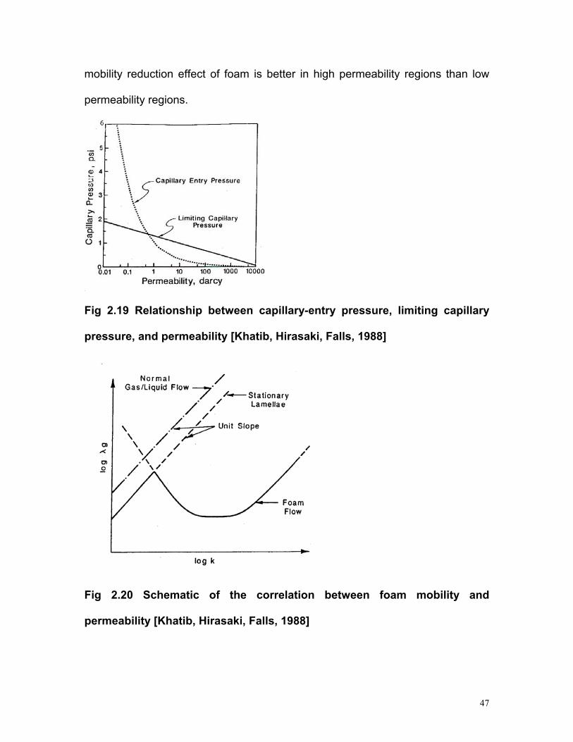
mobility reduction effect of foam is better in high permeability regions than low
permeability regions.
Fig 2.19 Relationship between capillary-entry pressure, limiting capillary
pressure, and permeability [Khatib, Hirasaki, Falls, 1988]
F
p
ig 2.20 Schematic of the correlation between foam mobility and
ermeability [Khatib, Hirasaki, Falls, 1988]
47

2.7.4 Foam flow in heterogeneous porous media
Two kinds of heterogeneous systems have been used in previous laboratory
studies to investigate the ability of foam to improve sweep efficiency in parallel
cores with differing permeabilities. The cores can be either isolated or placed in
contact wherecross flow can occur, e.g., in composite cylindrical cores. As
indicated below, some of the studies have dealt with gas injection, others with
injection of acid solutions to increase permeability.
Casteel & Djabbarah [1988] used two parallel Berea cores with a 6.4 permeability
ratio. They compared the use of foam with the water-alternating-gas process and
showed that foam was preferentially generated in the more permeable core and
could divert CO2 towards the less permeable core. Llave et al. [1990] obtained
similar results with parallel cores with a 4.6 permeability ratio. Zerhboub et al.
[1994] studied matrix acidizing in a stratified system. They also showed clearly
the effect of foam diversion. All these experiments, performed with parallel cores,
considered only the case of porous media which were not in capillary contact, so
that crossflow was prohibited.
Yaghoobi et al. [1996] used a short composite cylindrical core to study the
influence of capillary contact. They observed a reduction of mobility in the higher
permeability zone and called it “SMR”, Selective Mobility Reduction.
48

Siddiqui et al. [1997] investigated the diversion characteristics of foam in Berea
sandstone cores of contrasting permeabilities. They found that the diversion
performance strongly depended on permeability contrast, foam quality and total
flow rate.
Bertin et al. [1999] studied foam propagation in an annularly heterogeneous
porous medium having a permeability ratio of approximately 70. Experiments
were performed with and without crossflow between the porous zones. In situ
water saturations were measured continuously using X-ray computed
tomography. They observed that foam fronts moved at the same rates in the two
porous media if they were in capillary contact. On the other hand, when crossflow
was prohibited due to the presence of an impervious zone between the layers,
gas was blocked in the high permeability zone and diverted towards the low
permeability core.
Osterloh and Jante [1992] identified two distinct foam-flow regimes: a high-quality
(gas fractional flow) regime in which steady-state pressure gradient is
independent of gas flow rate, and a low-quality regime, in which steady-state
pressure gradient is independent of liquid flow rate. In each regime foam
behavior is dominated by a single mechanism: at high qualities by capillary
pressure and coalescence [Osterloh and Jante, 1992], and at low qualities by
bubble trapping and mobilization [Cheng et al., 2000]. Cheng et al. [2000] found
that foam diversion is sensitive to permeability in high quality regime and
49
insensitive to permeability in low quality regime. But in the low quality regime the
harmful effect on diversion from crossflow is much less.
Nguyen et al. [2003] conducted experiments to study foam-induced fluid
diversion in isolated and capillary-communicating double layer cores. They found
that there existed a threshold injection foam quality below which foam no longer
invaded the low permeability layer. This threshold depends on the permeability
contrast and foam strength in the high permeability layer. The use of foam below
the threshold quality is appropriate in foam acid diversion, where the presence of
foam in the high permeability layer helps control the relative acid permeability,
and acid can still penetrate the low permeability layer without resistance of foam.
Few studies have been reported of foam in fractures. Kovscek et al. [1995]
experimentally studied nitrogen, water and foam flow through a transparent
rough walled rock fracture with a hydraulic aperture of 30µm. In these
experiments, foam flow resistance was approximately 100-540 times greater than
that of nitrogen for gas fractional flow ranging from 0.60 to 0.99.
Our purpose is to understand the mechanisms of foam flow in fractures and
predict foam diversion in heterogeneous fracture systems. We derive below a
theory to predict the foam apparent viscosity, starting from the existing theory for
foam flow in capillary tubes. We made a uniform fracture model and conducted
experiments to verify the theory. Also a heterogeneous fracture model was set up
50

and used to study foam diversion. Finally, we developed a model to predict the
sweep efficiency in multiple heterogeneous fractures with log-normal distributed
apertures.
2.8 Alkaline surfactant enhanced oil recovery process
Alkaline surfactant is a kind of chemical method in enhanced oil recovery that
involves the injection of alkaline-surfactant solution into the reservoir. Both
injection of surfactants and injection of alkaline solutions to convert naturally
occurring naphthenic acids in crude oils to soaps can achieve ultralow interfacial
tensions to get oil recovered. Most of the work in the past was directed toward
developing micellar-polymer processes to recover residual oil from sandstone
formations using anionic surfactants. However, Nelson et al. [1984] recognized
that in most cases the soaps formed by injecting alkali would not be at the
"optimal" conditions needed to achieve low tensions. They proposed that a
relatively small amount of a suitable surfactant be injected with the alkali so that
the surfactant/soap mixture would be optimal at reservoir conditions. With
polymer added for mobility control the process would be an alkali-surfactant-
polymer (ASP) flood. The use of alkali also reduces adsorption of anionic
surfactants on sandstones because the high pH reverses the charge of the
positively charged clay sites where adsorption occurs.
The initial portion of a Shell field test, which did not use polymer, demonstated
that residual oil could be displaced by an alkaline/surfactant process [Falls et al.,
51
1992]. Several ASP field projects have been conducted with some success in
recent years in the US and Canada [Vargo et al., 2000, Wyatt et al.,2002]. Pilot
ASP tests in China have recovered more than 20% OOIP in some cases, but the
process has not yet been applied there on a large scale [Wang et al 1999, Qiao
et al 2000, Chang 2006].
The application of surfactant processes including ASP to carbonate reservoirs
received little attention until the last few years, probably owing to concern that the
main surfactants being considered, e.g., alkyl/aryl sulfonates, would form calcium
and magnesium sulfonates that would either precipitate or partition into the oil
phase. An exception was the work of Adams and Schievelbein [1984], who
found from laboratory experiments and two well pair tests that oil could be
displaced in a carbonate reservoir using a mixture of petroleum sulfonates and
alkyl ether sulfates or alkyl/aryl ether sulfates.
Carbonate reservoirs are typically mixed wet and often fractured as well. As a
result, considerable effort has been directed toward promoting spontaneous
imbibition of aqueous solutions by adding surfactants to alter wettability. Austad
and coworkers [2003] suggested using cationic surfactants to promote desorption
of acids on carbonate rock surfaces, making the rock more water wet. Others
have investigated the effectiveness of various surfactants in altering wettability
[Chen et al., 2001, Xie et al., 2005]. Hirasaki and Zhang [2004] showed that if
sodium carbonate was used as the alkali and injected with a suitable anionic
52

surfactant, the usual positive charge of carbonate rocks could be reversed with
the results that surfactant adsorption was greatly decreased and oil wet surfaces
were modified to intermediate wet. They found that a significant amount of oil
could be recovered from an initially oil wet carbonate core placed in an imbibition
cell containing a suitable aqueous solution of surfactant, sodium carbonate and
sodium chloride. The wettability modification allowed the surfactant solution to
enter and the resulting low interfacial tension reduced capillary forces to the point
that oil rose to the top of the core, where it was released. No oil was recovered
when a sodium chloride solution was used instead. They proposed that such
alkaline/surfactant solutions could be injected into fractured carbonate formations
to increase recovery. Seethepalli et al [2004] and Adibhatla et al. [2005] pursued
a similar approach experimentally and performed simulations of how such a
process would perform for field conditions.
2.9 Enhanced oil recovery in fractured carbonate reservoir
The formation of interest is a fractured and preferentially oil-wet carbonate,
where water flooding is not effective because water flows preferentially in the
fractures and negative capillary pressure keeps water from entering the matrix,
which results in a large amount of residual oil trapped in the matrix below oil-
water contact. The average matrix permeability is 100 md, but the fracture
permeability is greater than 1,000 md [Chen, 2000]. When water invades the
reservoir, it flows into fractures instead of matrix, which leads to a high residual
oil saturation.
53

With this background, it is evident that a cost effective enhanced oil recovery
method for the targeted reservoir is needed. In the last decade, extensive
research on alkaline/surfactant flooding has been carried out worldwide, Bahrain
[Zubari and Sivakumar, 2003], Canada [e.g. Tayor and Nasr-El-Din, 1996], China
[e.g. Han et al., 1997], France [e.g. Baviere et al., 1995], Saudi Arabia [e.g. Al-
Hashim et al., 1996], USA [e.g. Nelson, 1989], to name a few. Alkaline/surfactant
flooding combining principal technologies of two traditional chemical methods
has great prospect for increasing oil recovery.
Clark et al. [1988] estimated the ultimate recoveries of water, polymer,
alkaline/polymer, and alkaline/surfactant/polymer flooding for West Kiehl field,
and alkaline/surfactant/polymer flooding was expected to increase ultimate
recovery dramatically.
Olsen et al. [Olsen et al., 1990], too, worked on an oil-wet carbonate reservoir.
They compared oil recovery of alkaline/surfactant/polymer flooding with that of
alkaline/ polymer and polymer flooding, and found alkaline/surfactant/polymer
flooding has a much better post-water-flood recovery than the other two. They
concluded that a cost effective alkaline/surfactant/polymer flooding could be
designed for application in a carbonate reservoir.
Delshad et al. [Delshad et al., 1998] predicted oil recovery of a Chinese oil field
by computer simulation. Among water, alkaline, surfactant/polymer, and alkaline/
54

55
surfactant/polymer flooding, alkaline/surfactant/polymer flooding exhibited the
best simulation result.

Chapter 3
FOAM FLOW IN HOMOGENEOUS FRACTURE
3.1 Foam apparent viscosity in homogeneous fracture
Gas has a very low viscosity compared with oil and water. However, when gas is
a dispersed phase, as in foam, its apparent viscosity is greatly increased, i.e., its
mobility is greatly reduced. Hirasaki and Lawson [1985] described a
mathematical model for apparent viscosity in a smooth capillary tube for bubbles
large enough that they travel sequentially along the tube. They found that the
most important variable affecting foam apparent viscosity in uniform, smooth
capillaries is foam texture or bubble size, which determines the number of
interfaces per unit length. Dynamic changes at these interfaces strongly influence
apparent viscosity, which is the sum of three contributions as in Fig. 3.1:
1) Slugs of liquid between gas bubbles resist flow.
2) Viscous and capillary forces result in interface deformation against the
restoring force of surface tension. The different curvatures at the front and
rear of a moving bubble dictate the pressure drop required for bubble
motion.
3) The surfactant is swept to accumulate at the back and be depleted at the
front of the bubble, which causes a surface tension gradient that resists
flow.
56

Fig. 3.1 Mechanisms affecting apparent viscosity in smooth capillaries
(Hirasaki and Lawson, 1985)
The goal of our research is to find the optimum condition to divert the greatest
amount of surfactant solution into thinner fracture regions. For that purpose, we
first adapt the above model for capillary tubes to the case of a uniform fracture
and describe experiments to confirm the validity of the model and determine the
parameters involved. Then we extend both model and experiments to parallel
flow in fractures of different thickness.
As indicated above, there are three contributions to the apparent viscosity of
foam in a circular smooth capillary tube. The first is that from liquid between the
57

bubbles, which is given by equation (3.1). This equation is also applicable to flow
in a wide fracture of uniform thickness.
(1 )liq liqapp gfμ μ= − (3.1)
where liqμ is the viscosity of pure liquid and gf is the gas fractional flow.
The contribution of deformation of the foam bubble to apparent viscosity in a
uniform fracture can be predicted by comparing with that from foam flow in a
capillary tube. From Hirasaki and Lawson [1985], the equation for the net
dynamic pressure drop across a single bubble is:
]1)/[()3)((26.2 23/2 +=Δ RrUr
p c
liq
cdynamic σ
μσ (3.2)
Here U is the velocity of the bubble, σ is the surface tension, is the radius of
curvature of gas-liquid interface and
cr
R is the capillary radius. When the bubbles
are not in contact and this equation simplifies to Bretherton's result [1961].
For flow of large bubbles between parallel plates, a similar equation applies but
without the term in brackets as above because the radius of curvature across the
width of the channel is much greater than r
Rrc =
c :
3/2)3)((26.2σμσ U
rp
liq
cdynamic =Δ (3.3)
58

The apparent viscosity from the contribution of foam bubble deformation in a
uniform fracture can be predicted from the equations for plane-Poiseuille flow:
)(
)3)((57.0
12
3/12
br
Ubn
Ubpn
c
liq
Lliq
dynamicLshapeapp
−
=Δ
= σμμ
μ (3.4)
where , the number of equivalent lamellae per unit length, is a function of the
number of bubbles per unit area and b is the fracture aperture or the distance
between the two parallel plates. If the bubbles are distributed uniformly, from the
derivation in Appendix A, one finds
Ln
2/1
34
3⎥⎦
⎤⎢⎣
⎡=
B
gL r
bfn
π (3.5)
where is the gas fractional flow and is the equivalent bubble radius. The
equivalent bubble diameter is assumed to be larger than the aperture. If the
bubbles are not in contact, the radius of curvature, , is equal to the half
aperture of the fracture, and substitution of equation (3.5) into equation (3.4)
yields
gf Br
cr
2/32/13/1 )()3(56.0B
g
liq
liq
shapeapp
rbfU −=
σμ
μμ
where 1)2/( ≤Brb (3.6)
59

The total apparent viscosity can be obtained from measuring the pressure
difference across the model. That is, from plane-Poiseuille equations:
Upb
app 12
2 ∇=μ (3.7)
where p∇ is the pressure gradient.
By comparing the sum of shapeappμ and liq
appμ with the value of appμ , the contribution
from surface tension gradient was found to be insignificant in our system.
3.2 Experimental methods
The fracture model used is shown in Fig. 3.2. It consists mainly of two parallel
glass plates. Changing the gasket thickness between the plates can change the
aperture of the fracture. The thick glass is from Lone Star Glass Company,
Houston, TX. It is borosilicate glass with 35.56 cm length and 20.32 cm width. Its
thickness is 6.35 ± 0.3 mm. The surface of the glass is polished. For experiments
with a homogeneous fracture, the uniformly thick gasket keeps a uniform
distance between the plates.
A schematic diagram of the equipment for the foam experiments is shown in Fig.
3.3. A Harvard syringe infusion pump (Model 22) is used to inject surfactant
60

solution and a Matheson mass flow controller (Model 8270) is used to inject air
into the foam generator. Relatively uniform bubbles can be generated only when
the air and liquid are introduced on opposite sides of the frit in the foam
generator. Choosing frits with different pore sizes can generate different sizes of
bubbles. The borosilicate frits are from Chemglass Company, Vineland, NJ. Two
grooves were made along the inlet and outlet of the fracture model to assure
uniform pressures at both locations.
35.56 cm
30.48 cm
20.32 cm 15.24 cm
Variable thickness
Homogeneous Fracture Model
Fig. 3.2 Detailed diagram of homogeneous fracture model
61

Fig 3.3 Set –up diagram for foam mobility control experiment in fracture
model
The surfactant solution in the experiments was 0.5% C13-4PO and 0.5% STEOL
CS330. C13-4PO is from Harcros Company, and its chemical description is
propoxylated iso-C13 alcohol ether sulfate, ammonium salt. STEOL CS330 is
from Stepan Company and its chemical description is C12-3EO sulfate. The
solution contained 0.23% NaCl, 0.07% CaCl2 and 0.04% MgCl2. The bubble
diameters in the experiment ranged from 0.4 to 1.0 mm. The aperture was 0.1
mm or 0.2 mm for homogeneous fracture experiments. The gas fractional flow
range was from 0.0 to 0.9. The values used for the viscosity of solution and
surface tension were 0.001 Pa.s and 28 mN/m from measurement.
3.3 Foam bubble size measurement in fractures
Two different methods were used to determine the average bubble size: image
analysis and capillary tube experiments. From analysis of images taken just after
62
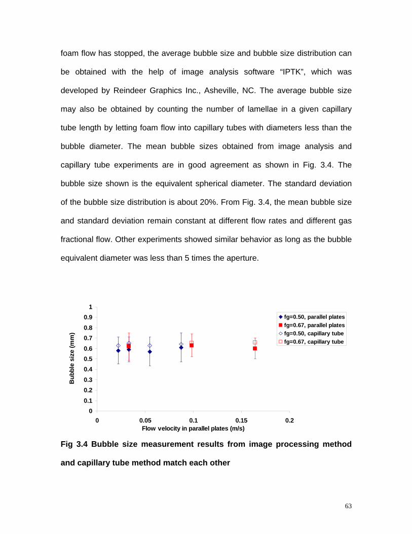
foam flow has stopped, the average bubble size and bubble size distribution can
be obtained with the help of image analysis software “IPTK”, which was
developed by Reindeer Graphics Inc., Asheville, NC. The average bubble size
may also be obtained by counting the number of lamellae in a given capillary
tube length by letting foam flow into capillary tubes with diameters less than the
bubble diameter. The mean bubble sizes obtained from image analysis and
capillary tube experiments are in good agreement as shown in Fig. 3.4. The
bubble size shown is the equivalent spherical diameter. The standard deviation
of the bubble size distribution is about 20%. From Fig. 3.4, the mean bubble size
and standard deviation remain constant at different flow rates and different gas
fractional flow. Other experiments showed similar behavior as long as the bubble
equivalent diameter was less than 5 times the aperture.
00.10.20.30.40.50.60.70.80.9
1
0 0.05 0.1 0.15 0.2Flow velocity in parallel plates (m/s)
Bub
ble
size
(mm
)
fg=0.50, parallel platesfg=0.67, parallel platesfg=0.50, capillary tubefg=0.67, capillary tube
Fig 3.4 Bubble size measurement results from image processing method
and capillary tube method match each other
63

3.4 Foam apparent viscosity in homogeneous fracture experiment
results
Experiments were conducted to investigate the effects of flow rate, bubble size,
gas fractional flow, and aperture on the apparent viscosity of foam flowing in
uniform fractures. From the experiments, the most important variable affecting
foam viscosity in a homogeneous fracture system is foam texture. Foam of finer
texture has more lamellae per unit length and, as a result, greater resistance to
flow. The foam bubbles in our experiments are individual bubbles because the
aperture is smaller than the equivalent diameter of the bubbles. No aggregation
or coalescence of bubbles was observed.
Results for a homogeneous fracture with an aperture of 0.2mm are shown in Fig.
3.5 ~ Fig. 3.8. The data fit the theory (based on contributions from liquid and
bubble deformation without the contribution from the surface tension gradient)
quite well at low flow rates. Because the theory is based on Hele-Shaw flow,
which is valid for creeping flow, the data begin to deviate from the theory when
the Reynolds number exceeds about 1~10, depending on bubble size and gas
fractional flow. Here the Reynolds number is defined as
liq
liqbUμ
ρ=Re (3.8)
64
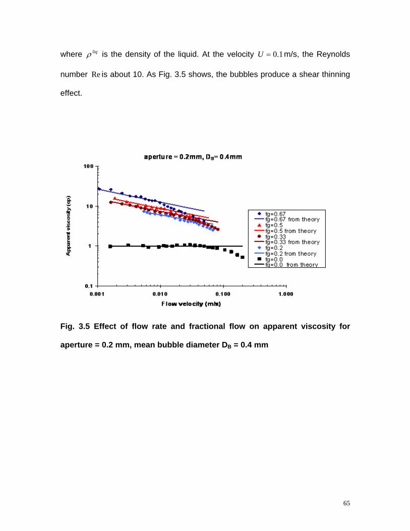
where is the density of the liquid. At the velocity liqρ 1.0=U m/s, the Reynolds
number is about 10. As Fig. 3.5 shows, the bubbles produce a shear thinning
effect.
Re
Fig. 3.5 Effect of flow rate and fractional flow on apparent viscosity for
aperture = 0.2 mm, mean bubble diameter DB = 0.4 mm B
65

Fig. 3.6 Effect of flow rate and fractional flow on apparent viscosity for
aperture = 0.2 mm, mean bubble diameter DB = 0.6 mm B
Fig. 3.7 Effect of flow rate and fractional flow on apparent viscosity for
aperture = 0.2 mm, mean bubble diameter DB = 0.8 mm B
66

Fig. 3.8 Effect of flow rate and fractional flow on apparent viscosity for
aperture = 0.2 mm, mean bubble diameter DB = 1.0 mm B
Fig. 3.5 ~ Fig. 3.8 also shows the effect of gas fractional flow on apparent
viscosity. With the increase of gas fractional flow or foam quality, the number of
lamellae per unit length or number of bubbles per unit area increases, which
causes apparent viscosity proportional to the half power of gas fractional flow in
equation (3.6).
67
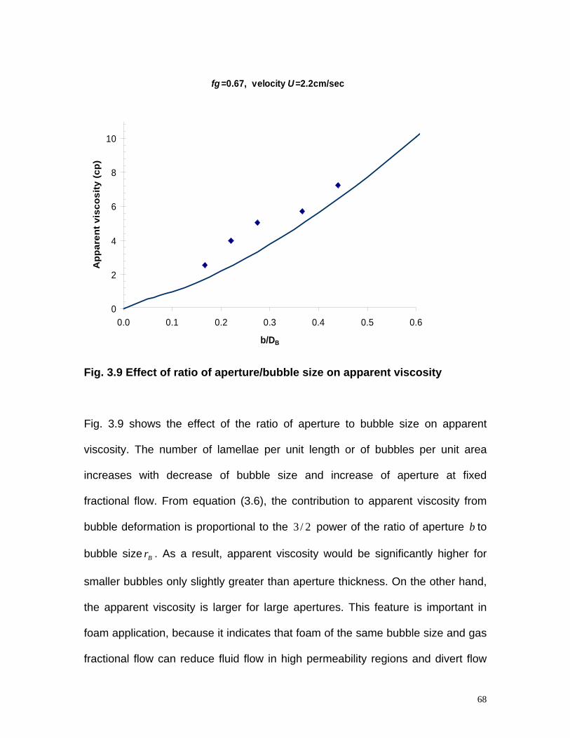
fg =0.67, velocity U =2.2cm/sec
0
2
4
6
8
10
0.0 0.1 0.2 0.3 0.4 0.5 0.6
b/DB
App
aren
t vis
cosi
ty (c
p)
Fig. 3.9 Effect of ratio of aperture/bubble size on apparent viscosity
Fig. 3.9 shows the effect of the ratio of aperture to bubble size on apparent
viscosity. The number of lamellae per unit length or of bubbles per unit area
increases with decrease of bubble size and increase of aperture at fixed
fractional flow. From equation (3.6), the contribution to apparent viscosity from
bubble deformation is proportional to the power of the ratio of aperture to
bubble size . As a result, apparent viscosity would be significantly higher for
smaller bubbles only slightly greater than aperture thickness. On the other hand,
the apparent viscosity is larger for large apertures. This feature is important in
foam application, because it indicates that foam of the same bubble size and gas
fractional flow can reduce fluid flow in high permeability regions and divert flow
2/3 b
Br
68
into low permeability regions. Experiments were conducted to investigate the
effects of flow rate, bubble size, gas fractional flow, and aperture on the apparent
viscosity of foam flowing in uniform fractures. From the experiments, the most
important variable affecting foam viscosity in a homogeneous fracture system is
foam texture. Foam of finer texture has more lamellae per unit length and, as a
result, greater resistance to flow. The foam bubbles in our experiments are
individual bubbles because the aperture is smaller than the equivalent diameter
of the bubbles. No aggregation or coalescence of bubbles was observed.
3.5 Bulk foam apparent viscosity
Princen [1983] modeled the theory for rheology of foams and highly concentrated
emulsions. Hirasaki and Lawson [1985] developed the model to describe bulk
foam apparent viscosity in a capillary tube. But the theory can be applied only to
bubbles with the shape of pentagonal dodecahedrons, which are obtained only at
quite high gas fractional flow and all the bubbles in the system are closely-
packed.
Many semi-empirical expressions are available for describing the shear viscosity
of concentrated dispersions of hard spheres. The most widely used is the
functional form suggested by Krieger and Dougherty [1972].
Kr K /5.2)1( −−= φη (3.9)
69

Where rη is the relative viscosity, which is the ratio of the viscosity of emulsion to
the viscosity of water. φ is the volume fraction of emulsion in water. K is the
crowding factor and equal to the reciprocal of the dense random packing limit
volume fraction maxφ , at which rη diverges to infinity. For random close packing
of monodisperse hard spheres, they found maxφ = 0.64 and K =1.56.
Mooney [1951] developed another expression for the relative viscosity of
emulsions where the particles behave as rigid spheres.
]1
5.2exp[φφη
Kr −= (3.10)
The crowding factor K in the above two equations can be smaller when the
particles are not uniformly distributed or the particles are deformable because
these can cause an increase of the dense random packing limit volume fraction.
Pal [1992] studied the rheology of polymer-thickened emulsions and found the
increase of the viscosity ratio of continuous phase to dispersed phase enhances
the internal circulation effect which leads to a decrease in the relative viscosity.
He suggested the following equation.
]1
5.2exp[/1
φφη
KIK
r −= (3.11)
70

where is the factor which takes into account internal circulation effects and is
given by
IK
])/(1
)/(4.01[
dc
dcIK
ηηηη
++
= (3.12)
In the above equation, cη is the viscosity of the continuous phase and dη is the
viscosity of the dispersed phase. Pal [1992] also suggested a crowding factor
K = 1.04, which means the dense random packing limit volume fraction maxφ =
0.96.
The apparent viscosity for bulk foam flow in fractures was measured at different
aperture, flow velocity and bubble size as in Fig. 3.10. The experiment set-up is
the same as the experiment for individual lamellae except the frits with smller
pore size were used. The theory predictions from Krieger and Dougherty
equation, Mooney equation and Pal’s model are also plotted in Fig. 3.10. The
experimental measurement matches the prediction from Pal’s model. The highest
gas fractional flow in our bulk foam experiments is 0.67 because we found
bubbles began to coalesce for gas fractional flow over 0.67.
71
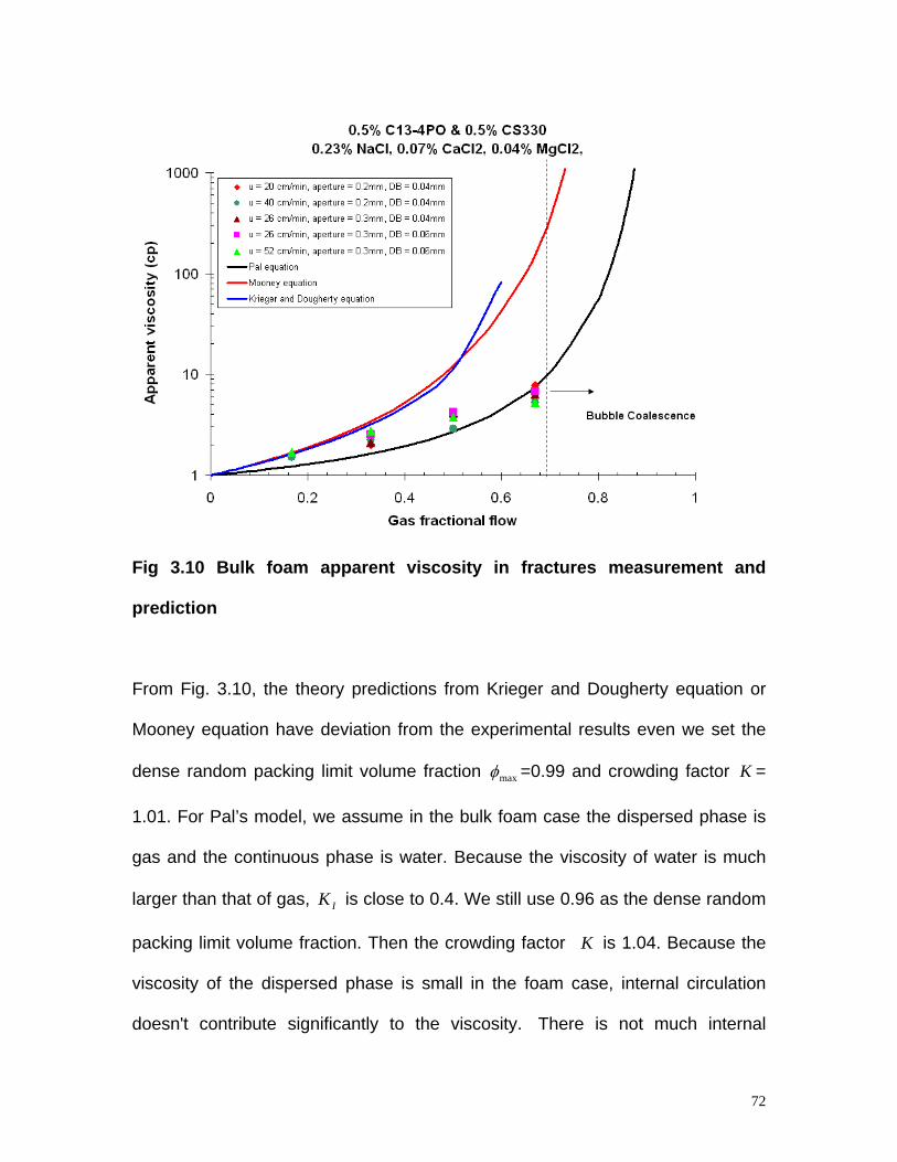
Fig 3.10 Bulk foam apparent viscosity in fractures measurement and
prediction
From Fig. 3.10, the theory predictions from Krieger and Dougherty equation or
Mooney equation have deviation from the experimental results even we set the
dense random packing limit volume fraction maxφ =0.99 and crowding factor K =
1.01. For Pal’s model, we assume in the bulk foam case the dispersed phase is
gas and the continuous phase is water. Because the viscosity of water is much
larger than that of gas, is close to 0.4. We still use 0.96 as the dense random
packing limit volume fraction. Then the crowding factor
IK
K is 1.04. Because the
viscosity of the dispersed phase is small in the foam case, internal circulation
doesn't contribute significantly to the viscosity. There is not much internal
72

circulation in the system because the surfactant films are coherent, which will
resist tangential flow at the interface. So from Pal's model the internal circulation
contribution is not important for foams where the dispersed phase is gas, i.e.,
that the model is consistent with our experiments.
One feature of the apparent viscosity prediction from Pal’s model is that the
bubble size doesn’t need to be uniform in a fracture only if the diameter of each
bubble is smaller than the aperture because the apparent viscosity is dependent
on the gas fractional flow only. From Pal [1992], the emulsions in his experiment
were polydisperse with respect to droplet size.
3.6 Contrary diversion effect
From Fig. 3.9, the foam has higher apparent viscosity in larger aperture region
than in smaller aperture region when the foam bubble size, gas fractional flow
are the same, which implies that foam can divert the fluid from the larger aperture
region to smaller aperture region. But at some condition, the foam apparent
viscosity in the thinner layer may be higher than that in thicker layer can cause
the contrary diversion, that is, the fluids is diverted from thinner layer to thicker
one and decrease the sweep efficiency. This may happen when the apertures in
a heterogeneous fracture system has a wide distribution and the foam bubble
size is less than some big apertures, which means the bulk foam exists in the big
aperture regions. As in Fig 3.11, the bulk foam apparent viscosity in big aperture
regions is less than the apparent viscosity of individual lamellae in some smaller
73
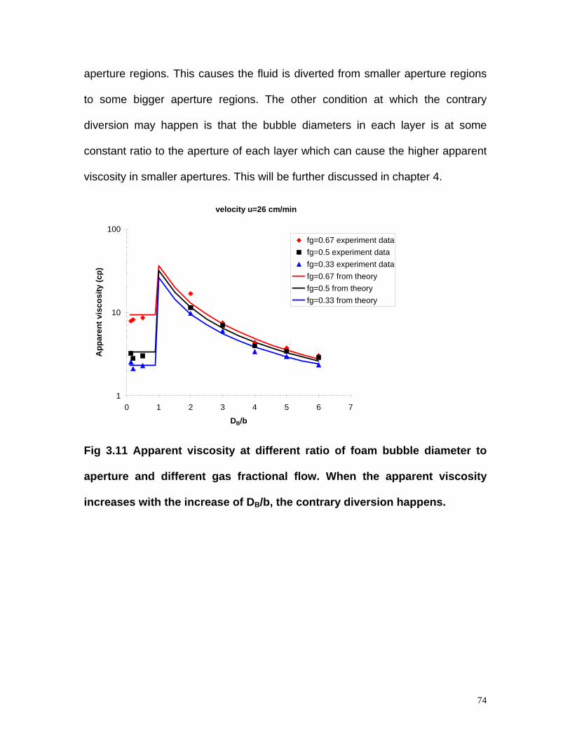
aperture regions. This causes the fluid is diverted from smaller aperture regions
to some bigger aperture regions. The other condition at which the contrary
diversion may happen is that the bubble diameters in each layer is at some
constant ratio to the aperture of each layer which can cause the higher apparent
viscosity in smaller apertures. This will be further discussed in chapter 4.
velocity u=26 cm/min
1
10
100
0 1 2 3 4 5 6 7
DB/b
App
aren
t vis
cosi
ty (c
p)
fg=0.67 experiment datafg=0.5 experiment datafg=0.33 experiment datafg=0.67 from theoryfg=0.5 from theoryfg=0.33 from theory
Fig 3.11 Apparent viscosity at different ratio of foam bubble diameter to
aperture and different gas fractional flow. When the apparent viscosity
increases with the increase of DB/b, the contrary diversion happens. B
74
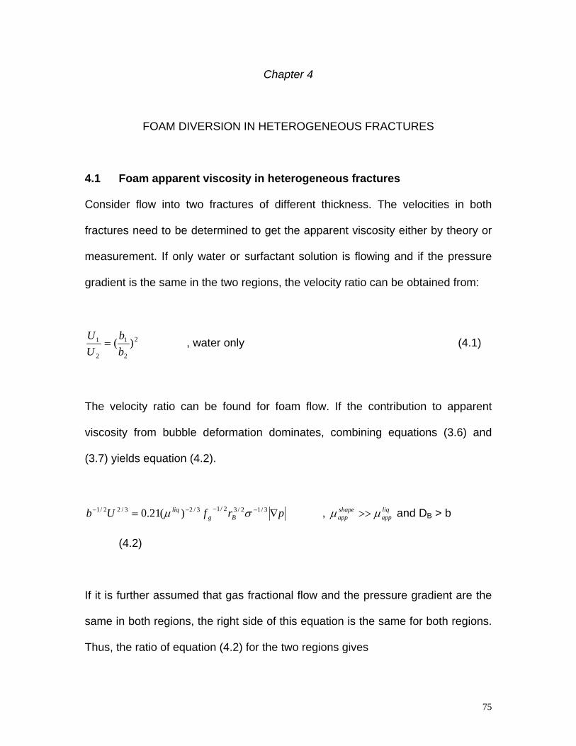
Chapter 4
FOAM DIVERSION IN HETEROGENEOUS FRACTURES
4.1 Foam apparent viscosity in heterogeneous fractures
Consider flow into two fractures of different thickness. The velocities in both
fractures need to be determined to get the apparent viscosity either by theory or
measurement. If only water or surfactant solution is flowing and if the pressure
gradient is the same in the two regions, the velocity ratio can be obtained from:
2
2
1
2
1 )(bb
UU
= , water only (4.1)
The velocity ratio can be found for foam flow. If the contribution to apparent
viscosity from bubble deformation dominates, combining equations (3.6) and
(3.7) yields equation (4.2).
prfUb Bgliq ∇= −−−− 3/12/32/13/23/22/1 )(21.0 σμ , and Dliq
appshapeapp μμ >> B > b
(4.2)
If it is further assumed that gas fractional flow and the pressure gradient are the
same in both regions, the right side of this equation is the same for both regions.
Thus, the ratio of equation (4.2) for the two regions gives
75
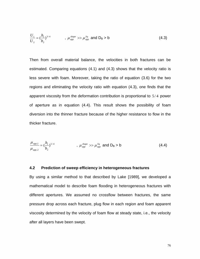
4/3
2
1
2
1 )(bb
UU
= , and Dliqapp
shapeapp μμ >> B > b (4.3)
Then from overall material balance, the velocities in both fractures can be
estimated. Comparing equations (4.1) and (4.3) shows that the velocity ratio is
less severe with foam. Moreover, taking the ratio of equation (3.6) for the two
regions and eliminating the velocity ratio with equation (4.3), one finds that the
apparent viscosity from the deformation contribution is proportional to power
of aperture as in equation (4.4). This result shows the possibility of foam
diversion into the thinner fracture because of the higher resistance to flow in the
thicker fracture.
4/5
4/5
2
1
2,
1, )(bb
app
app =μμ
, and Dliqapp
shapeapp μμ >> B > b (4.4)
4.2 Prediction of sweep efficiency in heterogeneous fractures
By using a similar method to that described by Lake [1989], we developed a
mathematical model to describe foam flooding in heterogeneous fractures with
different apertures. We assumed no crossflow between fractures, the same
pressure drop across each fracture, plug flow in each region and foam apparent
viscosity determined by the velocity of foam flow at steady state, i.e., the velocity
after all layers have been swept.
76
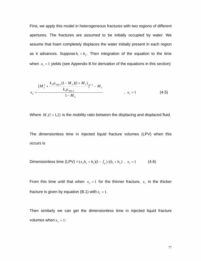
First, we apply this model in heterogeneous fractures with two regions of different
apertures. The fractures are assumed to be initially occupied by water. We
assume that foam completely displaces the water initially present in each region
as it advances. Suppose . Then integration of the equation to the time
when yields (see Appendix B for derivation of the equations in this section)
21 bb >
11 =x
2
22/1
2,1
121,222
2 1
])1)(1(
[
M
Mk
MMkM
x app
app
−
−+−
+
=μ
μ
, 11 =x (4.5)
Where is the mobility ratio between the displacing and displaced fluid. )2,1( =lM l
The dimensionless time in injected liquid fracture volumes (LPV) when this
occurs is
Dimensionless time (LPV) = )/()1)(( 21122 bbfbbx g +−+ , 11 =x (4.6)
From this time until that when 12 =x for the thinner fracture, in the thicker
fracture is given by equation (B.1) with
1v
11 =x .
Then similarly we can get the dimensionless time in injected liquid fracture
volumes when : 12 =x
77

Dimensionless time (LPV) = )/()1)(( 12211 bbfbbz g +−+ , 12 =x (4.7)
where exceeds 1 by the dimensionless length of a region of thickness
needed to hold the foam produced from fracture 1 up to that time.
1z 1b
]2
))(1(2
)1([12,2
1,212
1,2
2,11
app
app
app
app
kkMM
kk
zμ
μμμ +
−+
+= (4.8)
4.3 Fractures with log-normal distribution apertures
Normally there are more than two fractures. For multiple fractures, the key is to
get the number of fractures that have been swept at some FWR, the ratio of foam
to water being produced. The number N of fractures where foam has broken
through at some is given by FWR
∑∑+==
=LN
Nii
N
ii QQFWR
11/ (4.9)
where is the flow rate in the ith fracture and NiQ L is the total number of fractures
. Then by a derivation similar to that above for the two heterogeneous fractures,
the sweep efficiency and the dimensionless time can be obtained. There is a
difference when we calculated the sweep efficiency in multi-layer heterogeneous
fracture system from that in two layer heterogeneous fractures. Because the
foam enhanced sweep is used together with spontaneous imbibtion process to
78

recover residual oil in matrix, the matrix volume contacted by each fracture is
much larger than the volume of each fracture and more important than the
fracture volume. So in the calculation for the sweep efficiency, we assume each
fracture layer contacts the same volume of matrix. The dimensionless time is the
total fracture volumes of fluid injected.
Sweep efficiency =L
N
Nii
N
xNL
∑+=
+1 (4.10)
Dimensionless time =
∑
∑
=
=
L
L
N
ii
N
iii
b
bz
1
1 (4.11)
Olso [2001], Andres [2001], Baker, et. al. [2001], Wilson [1970] and Gale [1987]
have found that the fracture aperture distribution of reservoirs is approximately
log-normal. Such a log-normal aperture distribution can be described by the
function
2)]2/(1[ τerfC +
= (4.12)
where 2
)/ln(
N
bbσ
τ =
79
The function is the fraction of the samples that have aperture less than ,
i.e., the cumulative probability function. The parameter
)(bC b
b is the median or log-
mean aperture. The parameter is the variance of the distribution. If the log-
mean value
2Nσ
b and variance are known, different values of b can be obtained
and used in equation (4.10) and equation (4.11) to get the sweep efficiency and
dimensionless time.
2Nσ
4.4 Experimental methods
The fracture model used is shown in Fig. 4.1. It consists mainly of two parallel
glass plates. Changing the gasket thickness between the plates can change the
aperture of the fracture. The thick glass is from Lone Star Glass Company,
Houston, TX. It is borosilicate glass with 35.56 cm length and 20.32 cm width. Its
thickness is 6.35 ± 0.3 mm. The surface of the glass is polished. The thin glass is
Schott D-263 borosilicate glass from Precision Glass & Optics Company, Santa
Ana, CA. It is 25.4 cm long and 7.62 cm wide. It is 0.10 01.0± mm thick. It is not
quite long enough to span the flow area. The procedure for making the
heterogeneous fracture is: 1. Adhere the thin glass plate described above to half
of one of the thick glass plates by Norland optical adhesive; 2. Roll the thin glass
on the thick glass to remove any air and excess adhesive between them; 3. Cure
the adhesive by a high intensity ultraviolet lamp (Model Spectroline SB-100P) for
over 48 hours.
80
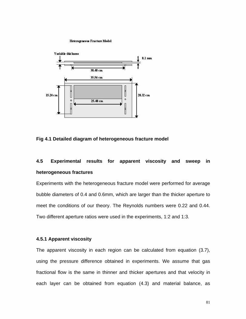
Fig 4.1 Detailed diagram of heterogeneous fracture model
4.5 Experimental results for apparent viscosity and sweep in
heterogeneous fractures
Experiments with the heterogeneous fracture model were performed for average
bubble diameters of 0.4 and 0.6mm, which are larger than the thicker aperture to
meet the conditions of our theory. The Reynolds numbers were 0.22 and 0.44.
Two different aperture ratios were used in the experiments, 1:2 and 1:3.
4.5.1 Apparent viscosity
The apparent viscosity in each region can be calculated from equation (3.7),
using the pressure difference obtained in experiments. We assume that gas
fractional flow is the same in thinner and thicker apertures and that velocity in
each layer can be obtained from equation (4.3) and material balance, as
81

indicated above. Also the apparent viscosity can be estimated from the sum of
equations (3.6) and (3.1). We consider first the case in which both regions of the
fracture are fully filled with foam, so that there are minimal lateral pressure
gradients and no cross flow. The theoretical and experimental results are
compared in Figs 4.2 and 4.3. For the range of experimental conditions listed at
low Reynolds’ number (less than 1) the apparent viscosity from measurement of
pressure difference fits well with that from theory prediction. This confirms that
the assumption of equal gas fractional flow is valid.
From Figs 4.2 and 4.3, we can see the effects of the aperture ratio on the
magnitude of diversion in heterogeneous fractures. The diversion depends on the
apparent viscosity difference between the two regions. If we ignore the
contribution of liquid to the total apparent viscosity, equation (4.4) predicts that
the apparent viscosity is proportional to the 5/4 power of aperture thickness. So
the apparent viscosity ratio is largest in Fig. 5.3, which is with 3:1 aperture ratio.
82
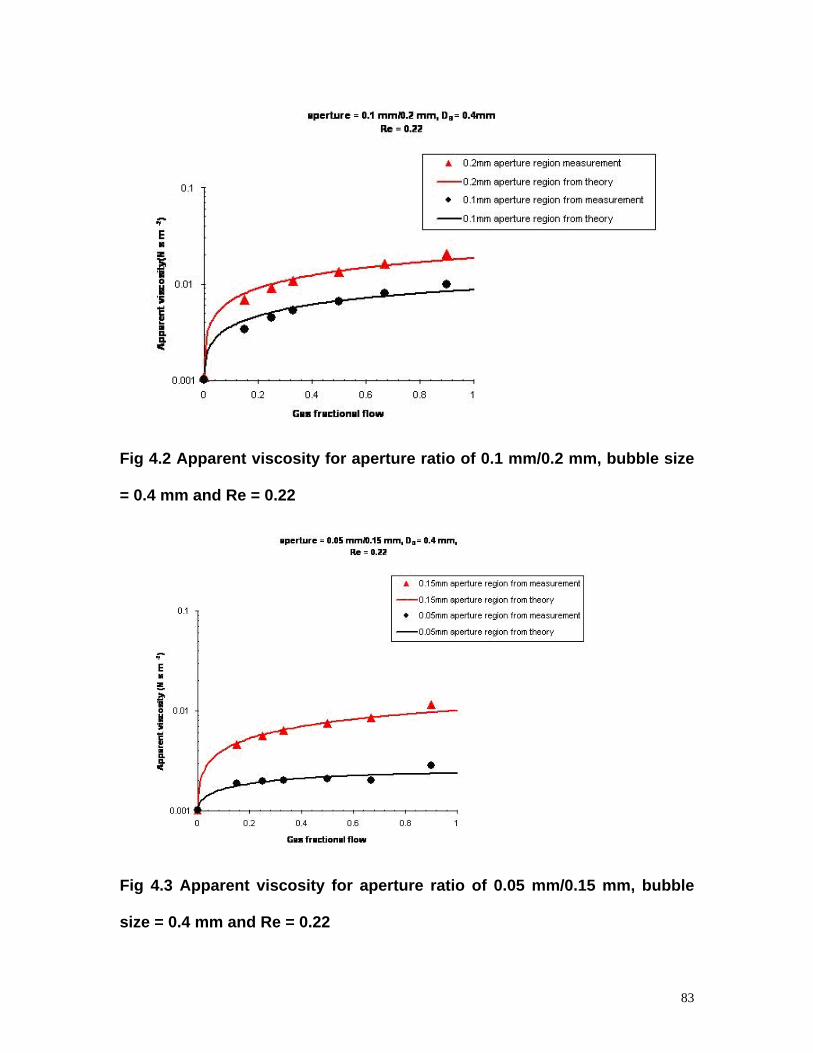
Fig 4.2 Apparent viscosity for aperture ratio of 0.1 mm/0.2 mm, bubble size
= 0.4 mm and Re = 0.22
Fig 4.3 Apparent viscosity for aperture ratio of 0.05 mm/0.15 mm, bubble
size = 0.4 mm and Re = 0.22
83

4.5.2 Sweep efficiency
Photographs were taken during experiments to investigate the sweep by foam
and surfactant solution in heterogeneous fractures. An example of
foam/surfactant solution sweep is shown in Fig. 4.5. For comparison, the picture
of sweep by surfactant solution alone is shown in Fig. 4.4. We use “fracture
volume” to measure the amount of injected foam or liquid needed for sweeping
the fractures. “Fracture volume” PV is defined as the volume of injected liquid
and gas or “foam” divided by volume of fractures. “Liquid fracture volume” LPV is
the volume of injected liquid divided by volume of fractures. The relationship
between fracture volume and liquid fracture volume is shown in equation (4.13).
(4.13) )1(*PVLPV gf−=
The injection of foam bubbles together with surfactant solution greatly improves
the sweep over the injection of surfactant solution only. From Fig. 4.4 for 0.05
mm/0.15 mm fracture, at Reynolds number 0.22, it takes about 6.6 fracture
volumes of surfactant solution to sweep the 0.05 mm aperture region, while
theory predicts that 7.0 fracture volumes are needed. With gas fractional flow 0.9
and bubble size at 0.4 mm in diameter, only 0.15 liquid fracture volume of
surfactant solution is needed, as shown in Fig. 4.5. The amount of surfactant
solution needed to sweep both regions is reduced by a factor of more than 40.
This large difference is partly the result of the higher apparent viscosity in the
84
thicker region and partly because less liquid is required to fill a given volume
when foam is used.
Experiments were also conducted for other gas fractional flows with aperture
ratios of 2 and 3. The results are shown in Fig. 4.6. It is easily seen that high gas
fractional flow can give better sweep efficiency, i.e., reduction in the amount of
surfactant solution required to sweep both portions of the heterogeneous
fracture. As might be expected, more surfactant solution is required for the
higher aperture ratio.
Fig. 4.7 shows the comparison between the theoretical predictions and
experimental results for foam/surfactant sweep in a heterogeneous fracture with
1:3 aperture ratio. Agreement is good. This validates the assumption of minimal
crossflow. It also indicates that the assumption of equal gas fractional flow in
different layers is reasonable for these conditions.
85
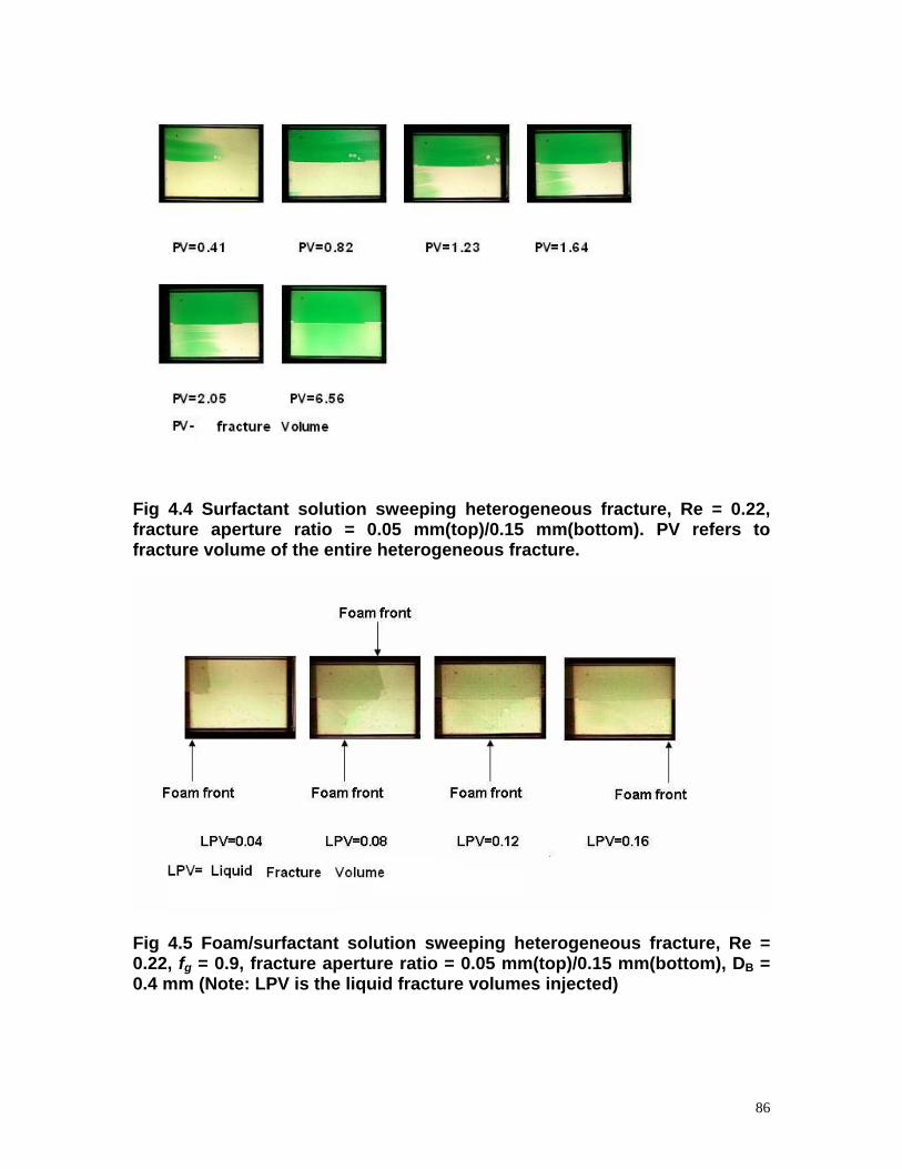
Fig 4.4 Surfactant solution sweeping heterogeneous fracture, Re = 0.22, fracture aperture ratio = 0.05 mm(top)/0.15 mm(bottom). PV refers to fracture volume of the entire heterogeneous fracture.
Fig 4.5 Foam/surfactant solution sweeping heterogeneous fracture, Re = 0.22, fg = 0.9, fracture aperture ratio = 0.05 mm(top)/0.15 mm(bottom), DB = 0.4 mm (Note: LPV is the liquid fracture volumes injected)
B
86
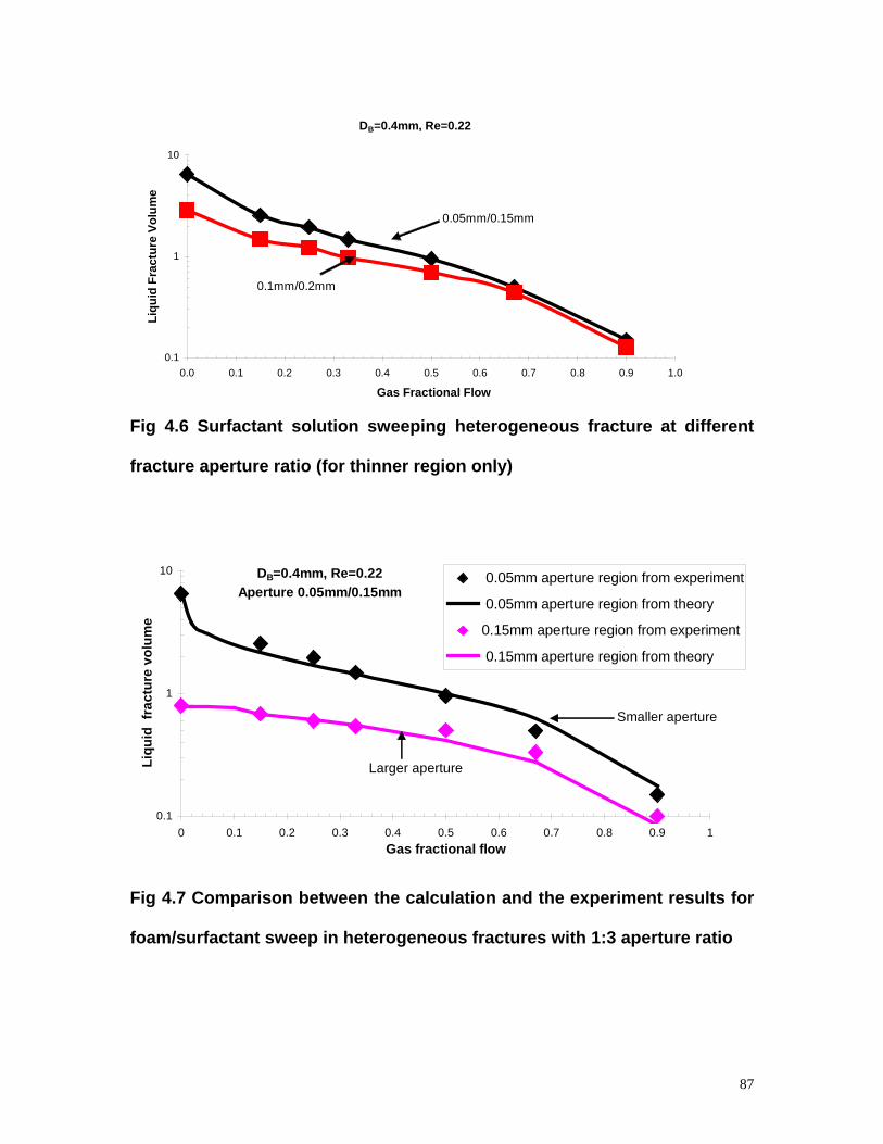
DB=0.4mm, Re=0.22
0.1
1
10
0.0 0.1 0.2 0.3 0.4 0.5 0.6 0.7 0.8 0.9 1.0
Gas Fractional Flow
Liqu
id F
ract
ure
Volu
me
0.05mm/0.15mm
0.1mm/0.2mm
Fig 4.6 Surfactant solution sweeping heterogeneous fracture at different
fracture aperture ratio (for thinner region only)
DB=0.4mm, Re=0.22Aperture 0.05mm/0.15mm
0.1
1
10
0 0.1 0.2 0.3 0.4 0.5 0.6 0.7 0.8 0.9 1Gas fractional flow
Liqu
id f
ract
ure
volu
me
0.05mm aperture region from experiment
0.05mm aperture region from theory
0.15mm aperture region from experiment
0.15mm aperture region from theory
Smaller aperture
Larger aperture
Fig 4.7 Comparison between the calculation and the experiment results for
foam/surfactant sweep in heterogeneous fractures with 1:3 aperture ratio
87

4.6 Sensitivity of sweep efficiency to foam bubble size in heterogeneous
fracture system
The fracture apertures in a fractured reservoir are believed to be distributed in
log-normal distribution [Baker, et al., 2001, Shang, et al, 2005, Olson, 2006,
Mantilla, 2006]. We consider a heterogeneous fracture system with 50 layers
having different apertures. The variance is 0.81, which is the most
heterogeneous fracture aperture distribution from literature [Baker, et al., 2001,
Shang, et al, 2005, Olson, 2006, Mantilla, 2006]. At different foam bubble size,
different apparent viscosity of foam is calculated in different fractures. Here we
studied the sweep efficiency sensitivity to bubble size in this heterogeneous
fracture system based on the assumptions that the pressure difference in
different fractures is the same and that the gas fractional flow in the different
fractures is the same.
2N
σ
Let’s first simplify the consideration to two fractures with different apertures to
study the mechanism of the effect of bubble size. Consider two fractures in a
heterogeneous fracture system filled with water with permeability ratio of
defined in equation (4.14). Fracture 1 is the thicker fracture while fracture 2 is the
thinner one.
12r
2
2
1
2
112 ⎟⎟
⎠
⎞⎜⎜⎝
⎛==
bb
kkr (4.14)
88

When the thinner fracture is swept, the hypothetical foam front in thicker fracture
from equation (4.8) is:
])2(
)1(2
)1([)(
12,1
1,212
1,2
2,11
app
app
app
appf
kkMM
kk
zμ
μμμ +
−+
+= , 12 =x (4.15)
If the fracture is swept by water, then 121 == MM and the above equation can
be changed to
21 /1
kkz w = (4.16)
Let p be the sweep improvement coefficient between the foam sweep and water
sweep.
fw pzz11
= (4.17)
If there is any improvement in sweep by foam over water, p is greater than 1.
]})2(
)1(2
)1([
)(1{
)(
2,1
1,212
1,2
2,1
2
1
1
1
app
app
app
appf
w
kkMM
kk
kk
zz
p
μμ
μμ +
−+
+== (4.18)
89

By algebraic manipulation and 1,
1app
wMμμ
= , 2,
2app
wMμμ
= because the displaced
fluid is water, the following equation describing the sweep improvement
coefficient in the heterogeneous system may be obtained:
⎥⎥⎦
⎤
⎢⎢⎣
⎡+−+
=
12121,1,
2, 1)11(
2
rr
p
app
w
app
app
μμ
μμ
(4.19)
where 2
112 k
kr = .
If foam sweep has improvement over water sweep, the value of
⎥⎥⎦
⎤
⎢⎢⎣
⎡+−+
12121,1,
2, 1)11(rrapp
w
app
app
μμ
μμ
needs to be smaller than 2.
From this, it is found that two factors affect the sweep by foam in heterogeneous
fractures with a given permeability ratio. The first one is the viscosity ratio of
foam in different fractures, and the second is the mobility ratio in the thicker
fracture.
4.6.1 Foam bubble size with some constant ratio (>1) to aperture.
When foam bubble sizes in different fractures are at a constant ratio to the
apertures of these fractures, i.e., Brb is constant, the lamellae bubbles per unit
length or number of bubbles per unit area in different fractures decreases with
the increase of aperture from equation (3.5). This may happen when the foam is
90

generated in each fracture in situ by some mechanism and few interconnections
exist between different fractures.
The TPV in these figures refers to the total fracture volume which is defined as
the total volume of injected liquid and gas or “foam” divided by volume of
fractures.
Fig 4.8 Sweep efficiency by foam with bubble size 2 times aperture in each
fracture
91
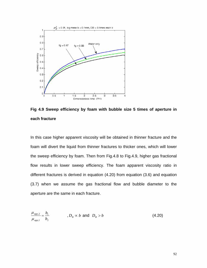
Fig 4.9 Sweep efficiency by foam with bubble size 5 times of aperture in
each fracture
In this case higher apparent viscosity will be obtained in thinner fracture and the
foam will divert the liquid from thinner fractures to thicker ones, which will lower
the sweep efficiency by foam. Then from Fig.4.8 to Fig.4.9, higher gas fractional
flow results in lower sweep efficiency. The foam apparent viscosity ratio in
different fractures is derived in equation (4.20) from equation (3.6) and equation
(3.7) when we assume the gas fractional flow and bubble diameter to the
aperture are the same in each fracture.
2
1
1,
2,
bb
app
app =μμ
, and (4.20) bDB ∝ bDB >
92
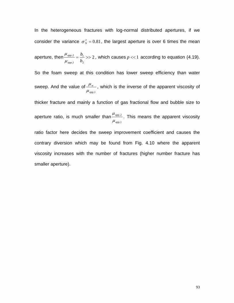
In the heterogeneous fractures with log-normal distributed apertures, if we
consider the variance , the largest aperture is over 6 times the mean
aperture, then
81.02 =Nσ
22
1
1,
2, >>=bb
app
app
μμ
, which causes 1<<p according to equation (4.19).
So the foam sweep at this condition has lower sweep efficiency than water
sweep. And the value of1,app
w
μμ , which is the inverse of the apparent viscosity of
thicker fracture and mainly a function of gas fractional flow and bubble size to
aperture ratio, is much smaller than1,
2,
app
app
μμ
. This means the apparent viscosity
ratio factor here decides the sweep improvement coefficient and causes the
contrary diversion which may be found from Fig. 4.10 where the apparent
viscosity increases with the number of fractures (higher number fracture has
smaller aperture).
93
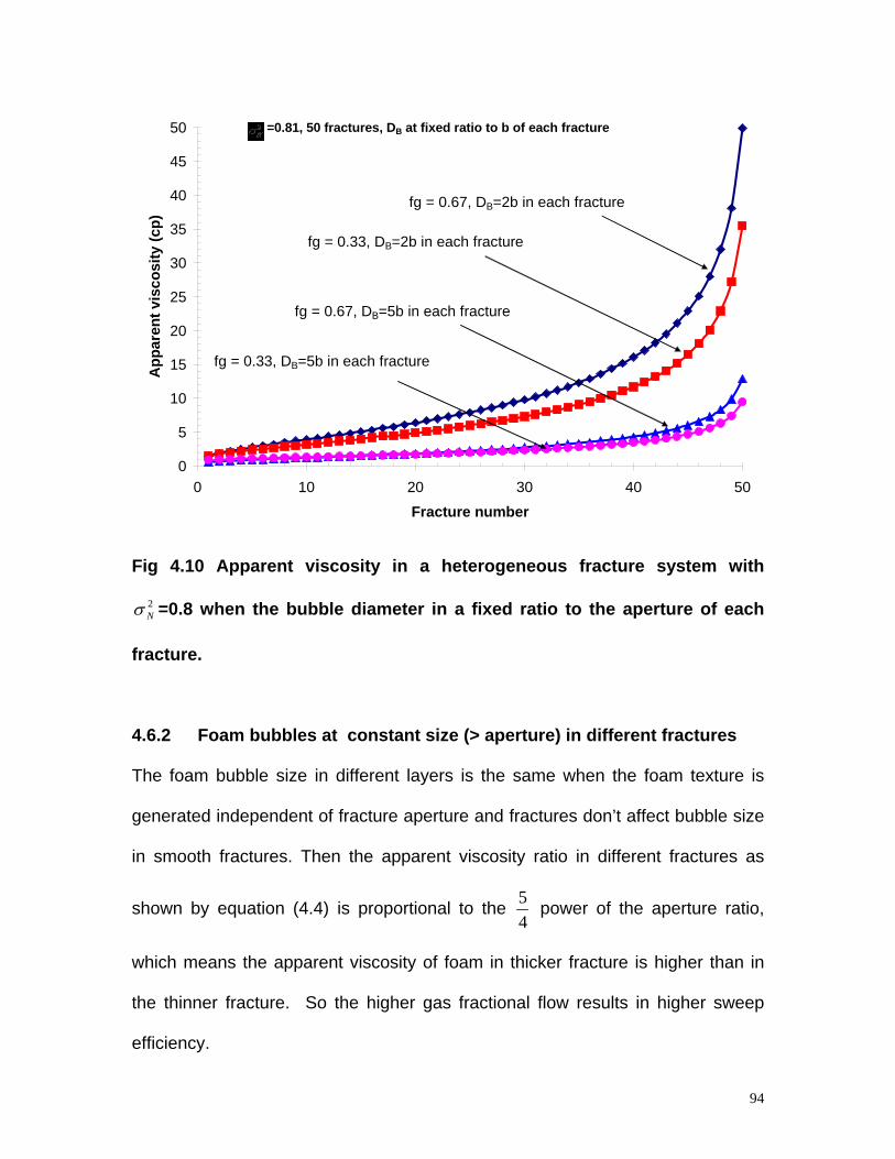
0
5
10
15
20
25
30
35
40
45
50
0 10 20 30 40 5
Fracture number
App
aren
t vis
cosi
ty (c
p)
=0.81, 50 fractures, DB at fixed ratio to b of each fracture
fg = 0.67, DB=2b in each fracture
fg = 0.33, DB=2b in each fracture
0
fg = 0.67, DB=5b in each fracture
fg = 0.33, DB=5b in each fracture
Fig 4.10 Apparent viscosity in a heterogeneous fracture system with
=0.8 when the bubble diameter in a fixed ratio to the aperture of each
fracture.
2Nσ
4.6.2 Foam bubbles at constant size (> aperture) in different fractures
The foam bubble size in different layers is the same when the foam texture is
generated independent of fracture aperture and fractures don’t affect bubble size
in smooth fractures. Then the apparent viscosity ratio in different fractures as
shown by equation (4.4) is proportional to the 45 power of the aperture ratio,
which means the apparent viscosity of foam in thicker fracture is higher than in
the thinner fracture. So the higher gas fractional flow results in higher sweep
efficiency.
94
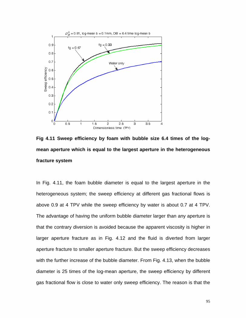
Fig 4.11 Sweep efficiency by foam with bubble size 6.4 times of the log-
mean aperture which is equal to the largest aperture in the heterogeneous
fracture system
In Fig. 4.11, the foam bubble diameter is equal to the largest aperture in the
heterogeneous system; the sweep efficiency at different gas fractional flows is
above 0.9 at 4 TPV while the sweep efficiency by water is about 0.7 at 4 TPV.
The advantage of having the uniform bubble diameter larger than any aperture is
that the contrary diversion is avoided because the apparent viscosity is higher in
larger aperture fracture as in Fig. 4.12 and the fluid is diverted from larger
aperture fracture to smaller aperture fracture. But the sweep efficiency decreases
with the further increase of the bubble diameter. From Fig. 4.13, when the bubble
diameter is 25 times of the log-mean aperture, the sweep efficiency by different
gas fractional flow is close to water only sweep efficiency. The reason is that the
95
apparent viscosity of foam is lower when the bubble diameter is larger than the
fracture aperture. If the bubble diameter is too big, the apparent viscosity can be
even lower than the viscosity of water. For the case when the bubble diameter is
larger than any aperture in the system, the foam with bubble diameter equal to
the largest aperture can supply the highest sweep efficiency because its
apparent viscosity is highest.
0
2
4
6
8
10
12
14
16
0 10 20 30 40 5Fracture Number
App
aren
t vis
cosi
ty (c
p)
=0.81, 50 fractures, DB= 6.4 times log-mean b
fg = 0.67
fg = 0.33
0
Fig 4.12 Apparent viscosity in a heterogeneous fracture system with
=0.81 when the bubble diameter is equal to the largest aperture in the
heterogeneous system.
2Nσ
96

Fig 4.13 Sweep efficiency by foam with bubble size 125 times of aperture
4.6.3 Foam bubbles at constant size (< aperture) in different layers
When the foam bubble diameter is less than any aperture in the heterogeneous
fracture system, bulk foam is obtained. For this case, 1,
2,
app
app
μμ
is a constant
because 1,appμ for bulk foam is determined only by gas fractional flow according
to equation (3.11). That is, the apparent viscosity is the same in each layer at the
same gas fractional flow, as shown in Fig. 4.15. The sweep efficiency is higher at
higher gas fractional flow because foam apparent viscosity is higher. From Fig.
4.14, the sweep efficiency by bulk foam is lower than for the case of individual
lamellae in each fracture with the bubble diameter is close to the largest aperture
(Fig. 4.11) because bulk foam doesn’t have any diversion effect.
97
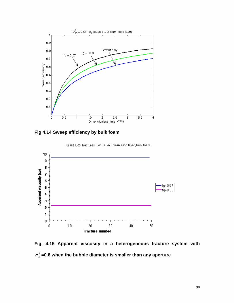
Fig 4.14 Sweep efficiency by bulk foam
Fig. 4.15 Apparent viscosity in a heterogeneous fracture system with
=0.8 when the bubble diameter is smaller than any aperture 2Nσ
98

4.6.4 Foam bubbles at constant size (> some apertures and < some
apertures ) in different layers
Because bubble size can affect the number of layers containing bulk foam and
1,appμ is related to gas fractional flow, the sweep improvement is related to bubble
size and gas fractional flow as in Fig. 4.16 and Fig. 4.18. From Fig. 4.17, we can
find the foam apparent viscosity appμ discontinuity when the foam bubble
diameter is equal to the aperture b because the model is switched from bulk
foam model to individual lamellae model. In this case, the foam apparent
viscosity
BD
appμ is less in largest apertures. Then as described in chapter 3, in
those cases where foam bubble diameter is only slightly greater than
aperture and bulk foam exists in some large aperture fractures, contrary
diversion effect can also be produced. With the increase of bubble size, we can
find from Fig. 4.17 and Fig. 4.19, the contrary diversion effect is less with the
increase of bubble size because fewer layers have bulk foam. Although the
highest apparent viscosity decreases with the increase of bubble size, the
decrease in the contrary diversion effect improves the sweep efficiency.
BD
b
99

Fig 4.16 sweep efficiency by foam with bubble size equal to log-mean
aperture
0
5
10
15
20
25
0 10 20 30 40 50
Fracture number
App
aren
t vis
cosi
ty (c
p)
fg =0.67
fg =0.33
=0.81, 50 fractures, DB= log-mean b
Fig 4.17 Apparent viscosity in a heterogeneous fracture system with
=0.8 when the bubble diameter is equal to the log-mean aperture 2Nσ
100
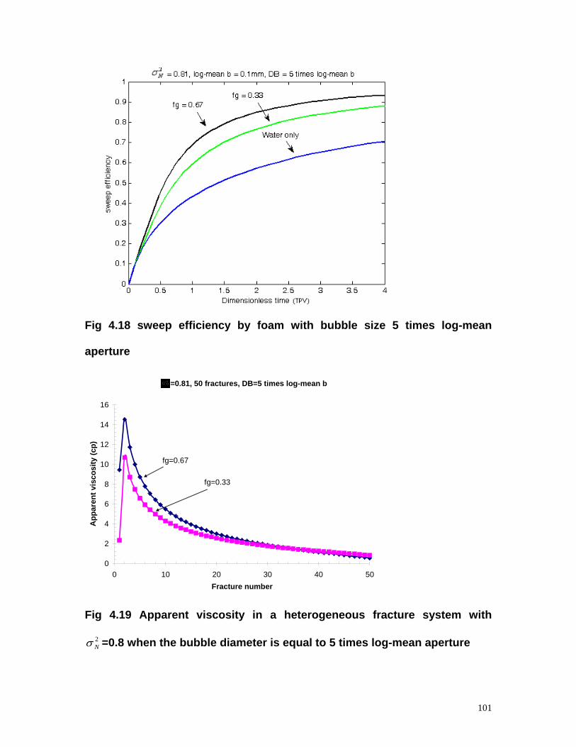
Fig 4.18 sweep efficiency by foam with bubble size 5 times log-mean
aperture
=0.81, 50 fractures, DB=5 times log-mean b
0
2
4
6
8
10
12
14
16
0 10 20 30 40 50Fracture number
App
aren
t vis
cosi
ty (c
p)
fg=0.67
fg=0.33
Fig 4.19 Apparent viscosity in a heterogeneous fracture system with
=0.8 when the bubble diameter is equal to 5 times log-mean aperture 2Nσ
101
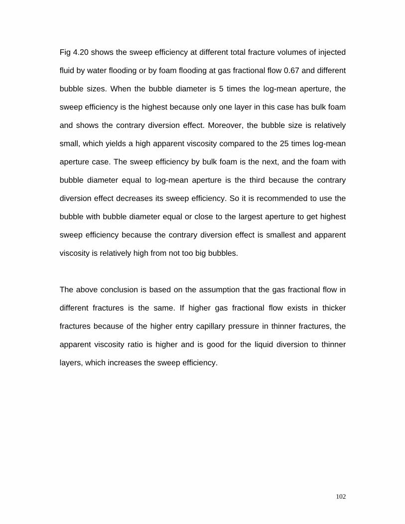
Fig 4.20 shows the sweep efficiency at different total fracture volumes of injected
fluid by water flooding or by foam flooding at gas fractional flow 0.67 and different
bubble sizes. When the bubble diameter is 5 times the log-mean aperture, the
sweep efficiency is the highest because only one layer in this case has bulk foam
and shows the contrary diversion effect. Moreover, the bubble size is relatively
small, which yields a high apparent viscosity compared to the 25 times log-mean
aperture case. The sweep efficiency by bulk foam is the next, and the foam with
bubble diameter equal to log-mean aperture is the third because the contrary
diversion effect decreases its sweep efficiency. So it is recommended to use the
bubble with bubble diameter equal or close to the largest aperture to get highest
sweep efficiency because the contrary diversion effect is smallest and apparent
viscosity is relatively high from not too big bubbles.
The above conclusion is based on the assumption that the gas fractional flow in
different fractures is the same. If higher gas fractional flow exists in thicker
fractures because of the higher entry capillary pressure in thinner fractures, the
apparent viscosity ratio is higher and is good for the liquid diversion to thinner
layers, which increases the sweep efficiency.
102
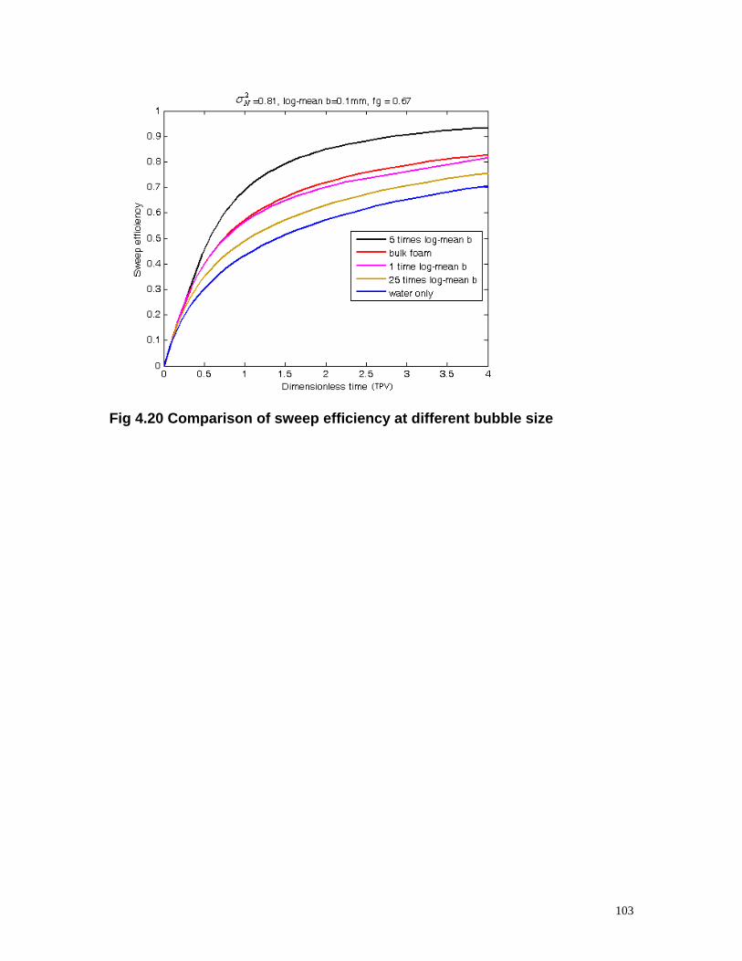
Fig 4.20 Comparison of sweep efficiency at different bubble size
103

Chapter 5
SURFACTANT EVALUATION FOR FOAM-AIDED ALKALINE/SURFACTANT
ENHANCED OIL RECOVERY PROCESS
5.1 Selection of surfactants
Selection of surfactants is crucial to foam-aided alkaline/surfactant enhanced oil
recovery process. The surfactant in this process should meet the requirements 1)
to get ultra-low interfacial tension and 2) generate strong foam. Traditionally, the
most commonly used surfactants for alkaline/surfactant flooding are sulfonated
hydrocarbons. Their advantages are [Salter, 1986] 1) they are very effective in
lowering interfacial tension; 2) they are inexpensive, especially petroleum
sulfonates; and 3) they are reported to be chemically stable. But the problem of
sulfonates is that they have poor hardness tolerance and salinity tolerance
[Green and Willhite, 1998].
Because of their known tolerance to divalent ions, exothylated (EO) and
propoxylated (PO) sulfates were evaluated by Gale et al. [1981], Osterloh and
Jante [1992], Wellington and Richardson [1995] and Aoudia et al. [1995].
Sulfates rather than sulfonates were evaluated in this research due to their easier
synthesis when ethoxylated or propoxylated and because the target application is
a low temperature carbonate reservoir where sulfate hydrolysis is not a problem.
104
Another important property of PO surfactants is that they decrease hydrophile-
lipophile balance (HLB) while not compromising solubility. In the
alkaline/surfactant EOR process, both natural surfactants and synthetic
surfactants exist. Natural surfactants are usually more hydrophobic than
synthetic surfactants. It is found that the closer the HLB of the added synthetic
surfactants are to the natural soap, the smaller influence water/oil ratio (WOR)
and surfactant concentration have on the process [Zhang et al., 2005]. The
decrease of HLB by increasing straight hydrocarbon chain length of the
surfactant will result in the precipitation of surfactants. The addition of PO groups
helps to overcome this dilemma [Minana-Perez et al., 1995]. Branching of the
hydrocarbon chain also opposes precipitation and formation of highly viscous
liquid crystalline phase.
From the work of Zhang et al. [2005], two surfactant formulations were
considered as candidates in alkaline/surfactant enhanced oil recovery process.
The surfactants involved are identified in Table 5.1.
The sources of CS330 and C13-4PO have been introduced in chapter 3. N67-
7PO is developed by Shell Chemical with Procter and Gamble and IOS is from
Shell’s Westhollow Technology Center, Houston, TX.
105

Trade name Structural name
CS-330 Sodium dodecyl 3EO sulfate
C13-4PO Ammonium iso-tridecyl 4PO sulfate
TC blend 1:1 blend weight ratio of C13-4PO and CS330
N67-7PO Ammonium C16-17 7PO sulfate
IOS Sodium C15-18 internal olefin sulfonate
NI blend 4:1 weight ratio of N67-7PO and IOS
Table 5.1 Surfactants used in the experiments for alkaline-surfactant EOR
process
Zhang et al. [2005] optimized the formulation by two steps: phase behavior tests
followed by interfacial tension measurements. For foam work, we tested the foam
strength and foam stability with the presence of residual oil of the optimized
surfactant formulation.
During the alkaline/surfactant EOR process, it is important to keep the surfactant
solution as one phase to assure that all the oil is contacted by a solution of the
proper composition and that no highly viscous phase forms. We made the
solutions with 3% N67-7PO&IOS at different mixing ratios of N67-7PO and IOS
at 1% Na2CO3 and different NaCl concentration. Fig. 5.1 shows the phase
behavior at ambient temperature of aqueous solutions containing 3% of mixtures
of N67-7PO and IOS as a function of added NaCl for a fixed 1% concentration of
106
Na2CO3. IOS exhibits precipitation above about 4% NaCl. In contrast, no
precipitation occurs and a surfactant-rich liquid phase less dense than brine
forms as NaCl content increases for solutions containing N67-7PO and its
mixtures having up to 75% IOS. The line is drawn for conditions where
separation of a second bulk phase was seen. The solutions appeared cloudy at
salinities slightly below the line, indicating that some small droplets of the new
phase were present. The phase transition occurs at higher salinities as IOS is
initially added to N67-7PO, reaching a maximum near 8% NaCl for a 1:1 blend.
For the 4:1 mixture of N67-7PO&IOS, it occurs at about 6% NaCl. For N67-7PO
alone, but not for the mixtures, some cloudiness was observed after several
months even at low salinities.
Fig. 5.2 shows behavior when CaCl2 is added to 0.5% mixtures of the two
surfactants with 2% NaCl present but no Na2CO3. A solid precipitate is observed
for IOS alone and the mixture containing 80% IOS for CaCl2 concentrations
exceeding about 0.1 and 0.25% respectively. Except when IOS content falls
below 10%, tolerance to calcium ions is about 1% for mixtures having higher
contents of N67-7PO. For these mixtures separation of a viscous, surfactant-rich
phase more dense than brine occurs at high concentrations of CaCl2.
107

3% N67-7PO&IOS, 1% Na2CO3
0%
1%
2%
3%
4%
5%
6%
7%
8%
9%
10%
N67-7PO
Con
cent
ratio
n of
NaC
l
Phase Separation
Precipitation
Clear
IOS 3:1 1:1 1:4 1:9
+
+
+
+
+ Cloudy after 9 months
Fig. 5.1 Aqueous phase behavior of N67-7PO&IOS blends, 1% Na2CO3 +
various NaCl
0.5% N67-7PO&IOS, 2% NaCl
0.0%
0.5%
1.0%
1.5%
2.0%
2.5%
N67-7PO
Con
cent
ratio
n of
CaC
l2
Phase Separation
Precipitation
Clear
IOS 4:1 2:1 1:1 1:2 1:4 1:9
Fig. 5.2 Aqueous phase behavior of N67-7PO&IOS blends, 1% Na2CO3 +
various CaCl2
108

5.2 Foam strength with different surfactants
From the description in chapter 4, foam can greatly improve the sweep efficiency
in fracture network. But the success of the foam sweep depends strongly on the
strength and stability of foam, which is related to the surfactant composition and
salinity. The surfactant composition and salinity in chapters 4 and 5 are from an
aquifer remediation project and were used in the fracture study because they had
been demonstrated to form strong foam in sand packs. The surfactant used in
the EOR process needs to be tested near the reservoir salinity. We tested the
strength of foam by coinjection of surfactant solution and air into a horizontal
sand pack initially filled with surfactant and brine at 2% NaCl and 1% Na2CO3 to
generate foam and measuring the pressure difference across the sand pack to
get the apparent viscosity of foam. The surfactants tested were various mixtures
of N67-7PO and IOS for total surfactant concentration of 0.5 wt% at the salinity
1% Na2CO3 and 2% NaCl. The sand pack is 1 foot long and its permeability is 40
darcy.
109

1 foot sand column, 40 darcy, 1% Na2CO3, 2% NaCl
0.1
1
10
100
1000
0.1 1 10 100 1000Superficial Velocity (ft/day)
App
aren
t vis
cosi
ty (c
p)fg=0.5,no N67-7POS,0.5% IOS
fg=0.5,0.05% C13-4PO&CS330(1:1)
fg=0.5,0.5% N67-7POS&IOS(1:1)
fg=0.5,0.5% N67-7POS&IOS(4:1)
fg=0.5,0.5% N67-7POS,no IOS
fg=0.0
0.2% N67-7PO&IOS(4:1), 0.5% polymer
Fig 5.3 Foam strength at different surfactant composition
1 foot sand column, 40 darcy
0.1
1
10
100
1000
0.1 1 10 100 1000Superficial Velocity (ft/day)
App
aren
t vis
cosi
ty (c
p)
fg=0.5,0.5% N67-7PO&IOS (4:1), 2% NaCl , 1%Na2CO3 fg=0.5,0.5% N67-7PO&IOS (4:1),0.5% NaCl ,1%Na2CO3 fg=0.5,0.5% N67-7PO,No IOS,1% NaCl , No Na2CO3
fg=0.5,no N67-7PO,0.5% IOS,1% Na2CO3,2% NaCl
fg=0.5,0.5%N67-7PO&IOS(1:1),1% Na2CO3,2% NaCl
fg=0.5, 0.5% N67-7PO, 1% Na2CO3
fg=0.5, 0.5% N67-7PO
Fig 5.4 Foam strength at different salinity
110

Fig. 5.3 shows the results of foam strength tests for different surfactant
compositions and different velocities at the same salinity. With total surfactant
concentration 0.5%, at mixing ratio N67-7PO with IOS at 1:1 to 4:1, the foam
apparent viscosity is almost the same as N67-7PO itself at concentration 0.5%.
The foam strength produced by the NI blend is weaker than that by the TC blend
at a lower concentration and the same salinity. The other finding is that IOS
alone is a strong foamer. At the superficial velocity around 1 ft/day, the apparent
viscosity of foam by IOS can be close to 900 cp. One reason may be that IOS is
hydrophilic, i.e., well below its optimal salinity with most oils at the conditions
studied. Such surfactants are generally good foamers. Fig. 5.4 indicates for the
mixture of N67-7PO and IOS, the foaming ability is not affected by different
salinity. So the conclusion is that the foaming ability of the mixture of N67-7PO
and IOS is limited by the foaming ability of N67-7PO. The reason may be that
N67-7PO is hydrophobic with a branched hydrophobe that prevents formation of
a compact surfactant monolayer.
Although from the above discussion, N67-7PO or NI blend is not a strong foamer
compared with IOS or TC blend, it can still get around 20~30 cp apparent
viscosity at low velocities typical of real reservoir conditions. From our study of
foam diversion in heterogeneous fractures in Chapter 4, when the foam apparent
viscosity is around 20 cp, we can obtain 20~40 times reduction in the liquid
volume required to sweep heterogeneous fractures with 1:2 or 1:3 fracture
aperture ratios. Then the foam by NI blend is strong enough to divert the
111

surfactant solution into the thinner fractures. And by the work of Zhang et. al.
[2005], at the salinity of 2% NaCl and 1% Na2CO3, which is close to the targeted
reservoir formation salinity, solution of the NI blend can get the ultra-low
interfacial tension with the reservoir crude oil. Although TC blend or IOS can
generate stronger foam, their optimum salinities are much higher than the
formation salinity. So NI blend can be used in alkaline-surfactant EOR process
with spontaneous imbibition in fractured oil reservoir to get both ultra-low
interfacial tension and foam mobility control.
But in forced convection oil displacement in matrix, the foam strength by NI blend
or N67-7PO is not enough at the salinity 2% NaCl and 1% Na2CO3 because the
foam in matrix is needed to displace viscous crude oil instead of water in
fractures. Polymer may be blended with NI blend to get NI/polymer foam which
has a close apparent viscosity to IOS foam at 20 ft/day as shown in Fig. 5.3.
5.3 Foam stability with the presence of residual oil
The foam was not only to be used in spontaneous imbibtion process in fractured
reservoir to divert surfactant solution into thinner apertures, but also to be used
as mobility control agent in forced convection alkaline-surfactant flooding
processes in reservoirs with few or no fractures. For the latter case, the foam
may contact crude oil not displaced by the alkaline/surfactant slug, which makes
the study of the foam stability with the presence of residual crude oil necessary.
The foam stability for different surfactants with the presence of residual oil was
112

tested in a short sand pack. A short sand pack is used to avoid the long periods
of time that would have been required to test various surfactants in the 1-ft long
sand pack. The set up for the experiment is shown in Fig. 5.5.
The porous medium consists of a 1.5 inch long and 0.5 inch diameter cylinder
packed with 50-mesh size sand. Pore volume for the short sand pack is about 5
ml. Foam is generated in the sand pack by co-injection of surfactant solution and
air. The surfactant is injected by an ISCO pump, and air is injected by an air flow
controller. Two pressure transducers measure the pressure drop across the
tubing and the injection pressure to the sand pack. Foam quality is measured by
passing foam from the tubing through an inverted burette containing an
IPA/water mixture, which breaks the foam. The ratio of the volume of air collected
to the amount of liquid displaced gives the quality of foam.
To test the foam stability in the presence of residual oil, first, the foam strength
without the presence of oil is measured for comparison at some constant gas
fractional flow. Second, the water-saturated pack is filled with hexadecane. Then
water is used to flush the sand pack to achieve residual oil saturation. Foam is
then generated at the same gas fractional flow. The steady state pressure
readings are recorded to compare the foam strength with or without residual oil in
the sand pack.
113
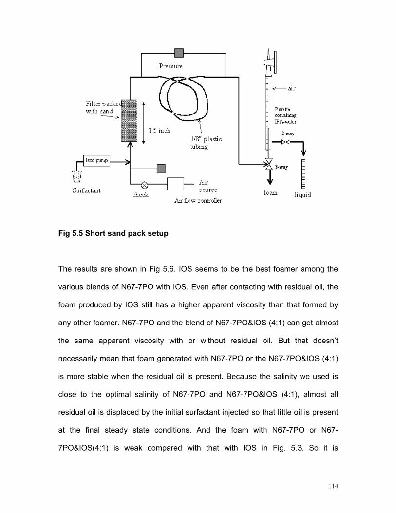
Fig 5.5 Short sand pack setup
The results are shown in Fig 5.6. IOS seems to be the best foamer among the
various blends of N67-7PO with IOS. Even after contacting with residual oil, the
foam produced by IOS still has a higher apparent viscosity than that formed by
any other foamer. N67-7PO and the blend of N67-7PO&IOS (4:1) can get almost
the same apparent viscosity with or without residual oil. But that doesn’t
necessarily mean that foam generated with N67-7PO or the N67-7PO&IOS (4:1)
is more stable when the residual oil is present. Because the salinity we used is
close to the optimal salinity of N67-7PO and N67-7PO&IOS (4:1), almost all
residual oil is displaced by the initial surfactant injected so that little oil is present
at the final steady state conditions. And the foam with N67-7PO or N67-
7PO&IOS(4:1) is weak compared with that with IOS in Fig. 5.3. So it is
114
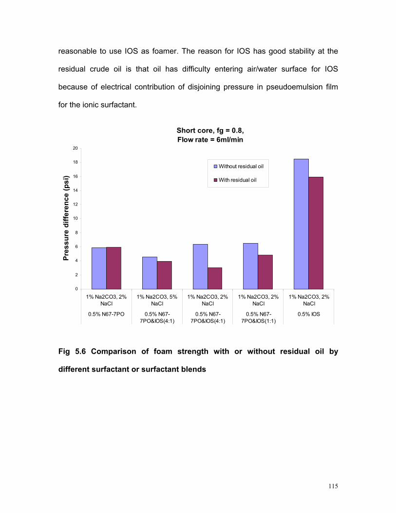
reasonable to use IOS as foamer. The reason for IOS has good stability at the
residual crude oil is that oil has difficulty entering air/water surface for IOS
because of electrical contribution of disjoining pressure in pseudoemulsion film
for the ionic surfactant.
Short core, fg = 0.8,Flow rate = 6ml/min
0
2
4
6
8
10
12
14
16
18
20
1% Na2CO3, 2%NaCl
1% Na2CO3, 5%NaCl
1% Na2CO3, 2%NaCl
1% Na2CO3, 2%NaCl
1% Na2CO3, 2%NaCl
0.5% N67-7PO 0.5% N67-7PO&IOS(4:1)
0.5% N67-7PO&IOS(4:1)
0.5% N67-7PO&IOS(1:1)
0.5% IOS
Pres
sure
diff
eren
ce (p
si)
Without residual oil
With residual oil
Fig 5.6 Comparison of foam strength with or without residual oil by
different surfactant or surfactant blends
115

116
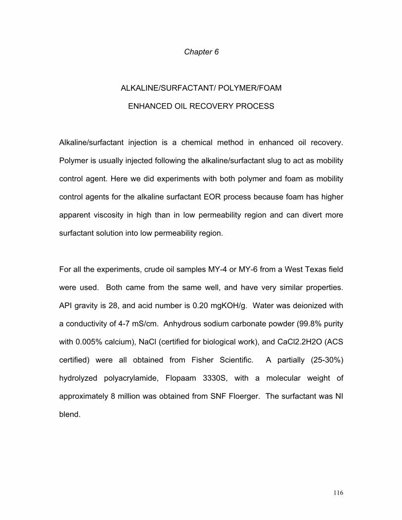
Chapter 6
ALKALINE/SURFACTANT/ POLYMER/FOAM
ENHANCED OIL RECOVERY PROCESS
Alkaline/surfactant injection is a chemical method in enhanced oil recovery.
Polymer is usually injected following the alkaline/surfactant slug to act as mobility
control agent. Here we did experiments with both polymer and foam as mobility
control agents for the alkaline surfactant EOR process because foam has higher
apparent viscosity in high than in low permeability region and can divert more
surfactant solution into low permeability region.
For all the experiments, crude oil samples MY-4 or MY-6 from a West Texas field
were used. Both came from the same well, and have very similar properties.
API gravity is 28, and acid number is 0.20 mgKOH/g. Water was deionized with
a conductivity of 4-7 mS/cm. Anhydrous sodium carbonate powder (99.8% purity
with 0.005% calcium), NaCl (certified for biological work), and CaCl2.2H2O (ACS
certified) were all obtained from Fisher Scientific. A partially (25-30%)
hydrolyzed polyacrylamide, Flopaam 3330S, with a molecular weight of
approximately 8 million was obtained from SNF Floerger. The surfactant was NI
blend.
116
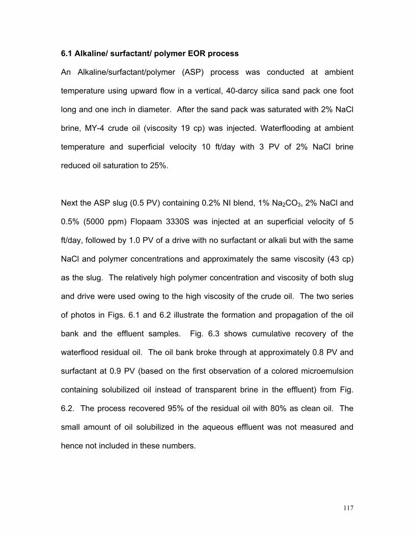
6.1 Alkaline/ surfactant/ polymer EOR process
An Alkaline/surfactant/polymer (ASP) process was conducted at ambient
temperature using upward flow in a vertical, 40-darcy silica sand pack one foot
long and one inch in diameter. After the sand pack was saturated with 2% NaCl
brine, MY-4 crude oil (viscosity 19 cp) was injected. Waterflooding at ambient
temperature and superficial velocity 10 ft/day with 3 PV of 2% NaCl brine
reduced oil saturation to 25%.
Next the ASP slug (0.5 PV) containing 0.2% NI blend, 1% Na2CO3, 2% NaCl and
0.5% (5000 ppm) Flopaam 3330S was injected at an superficial velocity of 5
ft/day, followed by 1.0 PV of a drive with no surfactant or alkali but with the same
NaCl and polymer concentrations and approximately the same viscosity (43 cp)
as the slug. The relatively high polymer concentration and viscosity of both slug
and drive were used owing to the high viscosity of the crude oil. The two series
of photos in Figs. 6.1 and 6.2 illustrate the formation and propagation of the oil
bank and the effluent samples. Fig. 6.3 shows cumulative recovery of the
waterflood residual oil. The oil bank broke through at approximately 0.8 PV and
surfactant at 0.9 PV (based on the first observation of a colored microemulsion
containing solubilized oil instead of transparent brine in the effluent) from Fig.
6.2. The process recovered 95% of the residual oil with 80% as clean oil. The
small amount of oil solubilized in the aqueous effluent was not measured and
hence not included in these numbers.
117
0 PV 0 .1 PV 0 .2 PV 0 .3 PV 0 .4 PV 0 .5 PV 0 .6 PV 0 .7 PV 0 .8 PV 1 .5 PV
Fig. 6.1 Photos showing behavior during ASP flood of silica sand pack
0.1 PV 0.2 PV 0.3 PV 0.4 PV 0.5 PV 0.6 PV 0.7 PV 0.8 PV 0.9 PV 1.0 PV 1.1 PV 1.2 PV 1.3 PV 1.4 PV 1.5 PV
Fig. 6.2 Effluents for different pore volume for ASP experiment
118

0
0.1
0.2
0.3
0.4
0.5
0.6
0.7
0.8
0.9
1
0 0.2 0.4 0.6 0.8 1 1.2 1.4 1.
Pore Volume
Oil
Rec
over
y
Surfactant Slug Polymer Drive
Surfactant Breakthrough
6
Fig. 6.3 Measured cumulative oil recovery for ASP flood in silica
sand pack.
0
0.5
1
1.5
2
2.5
3
3.5
0 0.2 0.4 0.6 0.8 1 1.2 1.4 1.6
Pore Volume
Pres
sure
diff
eren
ce (p
si)
Surfactant Slug
Polymer Drive
Surfactant Breakthrough
Fig. 6.4 Time-dependence of pressure drop during ASP flood in silica
sand pack.
119
Fig. 6.4 shows that the pressure drop across the sand pack increased steadily
during injection of the first pore volume of viscous slug and drive fluid, then
remained nearly constant at 3 psi. That is, no highly viscous phases or
emulsions developed.
Another ASP flood in a similar silica sand pack was made with the same
procedure and compositions except that NaCl content of the brine was 4%
instead of 2%. As Fig 6.5 shows, considerable oil traveled behind the oil
bank, which was much less distinct than in Fig. 6.1. Moreover, pressure
drop rose to 25 psia, nearly an order of magnitude greater than before.
The high pressure drop indicates that a highly viscous phase or emulsion
was present, presumably owing to separation of the surfactant slug into
polymer-rich and surfactant-rich phases at this salinity (shown in Fig. 6.6).
The pressure drop rose sharply as the concentrated polymer phase was
displaced by the polymer drive in Fig. 6.7.
120
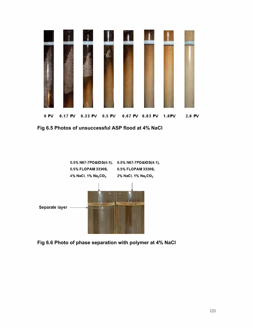
Fig 6.5 Photos of unsuccessful ASP flood at 4% NaCl
Fig 6.6 Photo of phase separation with polymer at 4% NaCl
121

Fig. 6.7 Time-dependence of pressure drop during unsuccessful ASP
flood
6.2 Foam drive possibility in alkaline/surfactant/polymer process
In normal alkaline/surfactant/polymer process, polymer is used as mobility control
agent to be injected together with surfactant and also as drive. However polymer
is expensive. We investigated the possibility of using foam to replace polymer as
drive.
The experiment was performed in a horizontal one-dimensional 1-foot long sand
pack. The sand pack’s permeability is 40 darcy. It was presaturated with a
polymer/surfactant solution to simulate a situation when residual crude oil
saturation was zero behind the surfactant/polymer slug. The polymer in this slug
is 0.5% FLOPAM 3330S. The surfactant is 0.5% N67-7PO&IOS (4:1). The
122

salinity is 2% NaCl and 1% Na2CO3. By measurement, the viscosity of the
polymer/surfactant solution is 43 cp at 24 C and shear rate 66 s-1.
The experiment was performed at constant pressure drop between 4.0 and 4.5
psi. The foam was generated in the sand pack by co-injection of surfactant
solution and air at gas fractional flow 0.67. We tried three different surfactants
using the same salinity as in the slug: 1% IOS, 0.5% CS330, 0.5% C13-
4PO&CS330 (1:1). The surfactant blend N67-7PO&IOS was not included
although it has good performance in displacing oil. As described as in chapter 5,
the foam produced by the blend of N67-7PO&IOS is weak. The experimental
results are shown in Fig. 6.8. About 0.1~0.2PV of co-injected fluid was needed to
get the pressure drop up to 4.5 psi. Then by changing the flow rate, the pressure
drop was kept between 4.0~4.5 psi. The foam produced by 1% IOS broke
through around 1 PV, 0.5% CS330 at 0.9 PV and 0.5% C13-4PO&CS330 (1:1) at
0.8PV. We also tried to use the foam generated by 1% N67-7PO&IOS (4:1) and
found the pressure drop never exceeded 1.5 psi before foam breakthrough.
123

fg = 0.67, pressure difference = 4.5psi 2% NaCl, 1% Na2CO3
Presaturated with 0.5% polymer, 0.4% N67-7PO, 0.1% IOS, 2% NaCl, 1% Na2CO3
0
20
40
60
80
100
120
0 0.1 0.2 0.3 0.4 0.5 0.6 0.7 0.8 0.9 1Pore Volume
Supe
rfic
ial V
eloc
ity (f
t/day
)
0.5% CS3300.5% C13-4PO&CS330 (1:1)1% IOS
foam breakthrough
0.1~0.2 PV injection is needed for pressure difference to increase to 4.5 psi.
Fig. 6.8 Foam sweep the sand pack presaturated with polymer/surfactant
Fig. 6.9 shows the apparent viscosity during the sweeping the sand pack by
foam. At the time of foam breakthrough, the apparent viscosity is about 40 cp for
0.5% CS330 and 200 cp for 1% IOS and 0.5% C13-4PO&CS330 (1:1). The
viscosity of the polymer/surfactant solution is 43 cp. If we assume the apparent
viscosity of the system at the foam breakthrough is equal to the foam apparent
viscosity, the latter is close to or higher than the viscosity of the
polymer/surfactant solution. But we did see the fingering at the interface of the
foam and polymer/surfactant. The reason may be that the foam front is not as
strong as the steady foam behind and the N67-7PO in the system may weaken
the foam front.
124

fg = 0.67, pressure difference = 4.5psi 2% NaCl, 1% Na2CO3
Presaturated with 0.5% polymer, 0.4% N67-7PO, 0.1% IOS
0
50
100
150
200
250
0 0.2 0.4 0.6 0.8 1 1.2Pore Volume
App
aren
t Vis
cosi
ty (c
p)
1% IOS
0.5% CS330
0.5% C13-4PO&CS330(1:1)
Fig. 6.9 Apparent viscosity during the sweeping the sand pack presaturated
with polymer/surfactant
The results in Fig. 6.8 show that it is possible to use foam instead of polymer as
drive in ASP process. And from the experiments to be described in the following
sections, 0.5% IOS and even 0.2% IOS is enough to generate strong foam to
displace oil and polymer. Although the cost of surfactant is comparable to
polymer at the same concentration, lower surfactant concentrations are possible.
Also less surfactant solution is required because a substantial portion of the drive
fluid would be the gas in the foam bubbles.
125

6.3 Foam drive in alkaline/surfactant/polymer process
To continue to investigate the possibility of using foam to replace polymer as
drive in ASP process, we did an experiment which involved crude oil. The
experiment was performed in a one dimensional sand pack in vertical position.
The sand pack is 1 foot long with 40 darcy permeability. The procedure for the
alkaline-surfactant-polymer-foam experiment is:
1. Fill the sand pack with CO2;
2. Fill the sand pack with water;
3. Fill the sand pack with crude oil;
4. Use brine to flood the sand pack at 10 ft/day superficial velocity until no oil
comes out;
5. Inject alkaline/NI blend/polymer solution into sand pack to displace oil for
0.5 PV at superficial velocity 5 ft/day;
6. Inject IOS/polymer solution as drive for 0.2 PV at superficial velocity 5
ft/day;
7. Co-inject IOS solution and air into sand pack as drive at gas fractional flow
0.67 and superficial velocity 20 ft/day.
The brine in this experiment contains 2% NaCl. The alkaline/surfactant/polymer
solution includes 1% Na2CO3 , 0.2% N67-7PO&IOS at 4:1 mixing ratio , 0.5%
polymer at 2% NaCl. The viscosity for the solution is 46.5 cp from measurement
by a viscometer at the shear rate 50 s-1. The crude oil is MY-4 and its viscosity is
19cp. The surfactant/polymer solution in step 6 is 0.5% IOS and 0.5% polymer at
126

2% NaCl. Its viscosity is 46.1cp from measurement. The reason that we include
step 6 is that we want to construct a barrier between NI blend and IOS because
from chapter 5 we found N67-7PO can make the foam weak. The co-injection of
air and surfactant solution is at gas fractional flow 0.67. The surfactant solution in
step 7 is 0.5% IOS at 2% NaCl and 1% Na2CO3. The residual saturation after
brine flooding is 25% from material balance calculation.
The ASPF displacement picture is shown in Fig. 6.10. From the picture, the oil
bank is pretty clear but there was a tail after the oil bank. The reason may be that
the injected oil for this experiment (but not others) crude oil contained some
viscous emulsion. But we can see that the shape of the tail didn’t change after
the foam drive began. This shows the foam drive forms a plug flow in the sand
pack. From Fig. 6.11, at around 1.5 PV, almost all the residual oil was recovered.
The big tail can also be found from the effluents shown in Fig. 6.12.
Fig. 6.13 shows the pressure history during the ASPF experiment. The first 0.7
PV is alkaline/surfactant/polymer slug and polymer drive injection. The pressure
difference during this time period gradually increases. When the air/surfactant co-
injection begins, the pressure difference decreases first and then increases up to
around 3 psi and stays there. That shows the steady foam forms.
127

Fig. 6.10 Photos showing behavior during ASPF flood of silica sand pack
Fig. 6.11 Recovery history for ASPF experiment
128

Fig. 6.12 Effluents for different pore volume for ASPF experiment
Fig. 6.13 Pressure history for ASPF experiment
The second ASPF experiment was performed for two reasons: first to test the
reproducibility of the ASPF experiment result, second to optimize the process by
using less surfactant slug. Different from the first ASPF experiment, the second
129
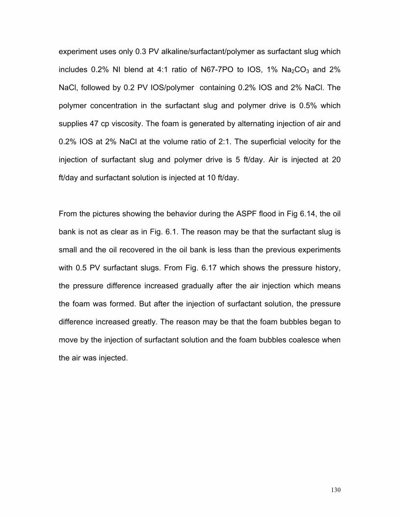
experiment uses only 0.3 PV alkaline/surfactant/polymer as surfactant slug which
includes 0.2% NI blend at 4:1 ratio of N67-7PO to IOS, 1% Na2CO3 and 2%
NaCl, followed by 0.2 PV IOS/polymer containing 0.2% IOS and 2% NaCl. The
polymer concentration in the surfactant slug and polymer drive is 0.5% which
supplies 47 cp viscosity. The foam is generated by alternating injection of air and
0.2% IOS at 2% NaCl at the volume ratio of 2:1. The superficial velocity for the
injection of surfactant slug and polymer drive is 5 ft/day. Air is injected at 20
ft/day and surfactant solution is injected at 10 ft/day.
From the pictures showing the behavior during the ASPF flood in Fig 6.14, the oil
bank is not as clear as in Fig. 6.1. The reason may be that the surfactant slug is
small and the oil recovered in the oil bank is less than the previous experiments
with 0.5 PV surfactant slugs. From Fig. 6.17 which shows the pressure history,
the pressure difference increased gradually after the air injection which means
the foam was formed. But after the injection of surfactant solution, the pressure
difference increased greatly. The reason may be that the foam bubbles began to
move by the injection of surfactant solution and the foam bubbles coalesce when
the air was injected.
130

Fig. 6.14 Photos showing behavior during ASPF flood of silica sand pack at
optimized condition
Fig. 6.15 Recovery history for ASPF experiment at optimized condition
131

Fig. 6.16 Effluents for different pore volume for ASPF experiment at
optimized condition
Fig. 6.17 Pressure history for ASPF experiment at optimized condition
The above two experiments give similar results: the recovery efficiency is above
90%, more than 70% of recovered oil is clean oil, and all the oil is recovered
within 1.6 total pore volume and most within 1.1 total pore volume. The
differences between the two experiments are that the surfactant slug in the
132
second experiment is 0.3 PV which is 0.2 PV less than in the first experiment,
and the foam in the second experiment is generated by surfactant/air alternate
injection while in the first one the foam is generated by co-injection of surfactant
solution and air. The 0.3 PV surfactant slug is enough to recover the residual oil
from the experiment. The pressure difference during the foam injection increases
up to 2 times of that during surfactant slug and polymer slug injection, which
shows the foam apparent viscosity is slightly greater than the viscosity of the
polymer.
6.4 Alkaline/surfactant/polymer/foam process
Although the foam drive is proven to be feasible in the previous experiments to
replace polymer drive, the unique advantage of foam in ASPF process is not fully
utilized if foam is only used as drive. The reason is that the entire alkaline
/surfactant slug is injected before the foam drive begins with the result that foam
has no effect on slug distribution among layers. The foam has higher apparent
viscosity in the high permeability region so foam with slug injection should be
able to divert more of the slug into low permeability region. Then foam can work
best in the heterogeneous system to get higher oil recovery by increasing the
sweep efficiency. We did two experiments to test the foam strength in two sand
packs with different permeability. From the description in chapter 6.1, the blend
of N67-7PO and IOS at 4:1 ratio at the salinity 1% Na2CO3 and 2% NaCl can get
ultra low interfacial tension between oil and water and displace the oil nearly
133
completely. But NI blend is a weak foamer. So we try to use NI blend with
polymer together as foamer.
The experiment for foam flooding to displace residual crude oil was performed in
a one dimensional vertical sand pack. The sand pack has 40 darcy permeability.
The procedure for doing the experiment is:
1. Fill the sand pack with CO2.
2. Fill the sand pack with brine at 2% NaCl.
3. Fill the sand pack with MY-6 crude oil at 10 ft/day.
4. Use brine (2% NaCl) to flood the sand pack at 10 ft/day until no oil comes
out.
5. Alternate the injection at 20 ft/day into the sand pack of 0.2% NI blend with
0.5% polymer at 1% Na2CO3 and 2% NaCl for 0.1 PV, and air for 0.1 PV.
Totally 0.6 PV of NI/polymer and air is injected.
6. Alternate the injection into the sand pack of 0.2% IOS at 1% Na2CO3 and
2% NaCl for 0.1 PV, and air for 0.1 PV. The superficial velocity is 20
ft/day.
6.4.1. 40 darcy sand pack
The pictures taken during the experiment are shown in Fig 6.18, and the
effluents’ pictures are shown in Fig 6.19. From measurement, the sand pack has
25% residual oil saturation after water flooding. The cumulative recovery
134

efficiency for the flooding is shown in Fig 6.20 and the pressure history is shown
in Fig 6.21.
Fig. 6.18 Pictures for the displacement of residual crude oil by polymer/foam in 40 darcy sand pack
Fig. 6.19 Pictures for effluents for polymer/foam flooding in 40 darcy sand
pack (Unit: PV)
135

Fig. 6.20 Recovery efficiency for polymer/foam flooding in 40 darcy sand
pack
Fig. 6.21 Pressure history for polymer/foam flooding in 40 darcy sand pack
136

Finally 94% of the residual crude oil was recovered by polymer/foam flooding.
Most of the crude oil was recovered between 1 and 1.6 total PV. The pressure
differences for this NI/polymer foam for the first 0.6 total PV and the IOS foam
drive after 0.6 total PV are close, which means that the apparent viscosities of
NI/polymer foam and IOS foam are close. In a foam displacing water experiment,
the NI/polymer foam apparent viscosity is 44 cp and the IOS foam apparent
viscosity is 81 cp. But in this displacing oil process, the IOS foam will contact
some N67-7PO in the NI/polymer foam and perhaps a little crude oil left after the
surfactant flooding, which may decrease the strength of the IOS foam. During the
experiment, the air (not bubble) breaks through around 0.9 PV. The reason for
early air breakthrough may be some air get into oil bank and even some distance
ahead of oil bank.
6.4.2 200 darcy sand pack In a 200 darcy sand pack, we performed a similar foam displacing oil experiment
using the same procedure as in 40 darcy sand pack. The pictures for the
displacement process, the effluents’ pictures, the accumulated recovery
efficiency and the pressure history are shown in Fig 6.22 to Fig 6.25.
The residual oil saturation after water flooding is 30% from measurement. Around
96% of the residual crude was recovered. The oil breakthrough at about 0.8 PV,
which is earlier than 1.0 PV in 40 darcy sand pack. The reason is that the
mobility ratio between the foam and the oil bank is smaller in 200 darcy sand
137

pack than in 40 darcy sand pack. The NI/polymer foam apparent viscosity in 200
darcy sand pack is 215 cp at 20 ft/day in the foam displacing brine experiment
described in section 5.2. The IOS foam in 200 darcy sand pack has the similar
strength to the NI/polymer foam because the measured pressure difference was
nearly the same (Fig. 6.25). The air breaks through the sand at around 0.7 PV
which is earlier than in 40 darcy sand pack. The reason may be that the air gets
into the oil bank and some distance ahead of oil bank. Because oil bank breaks
through earlier in 200 darcy sand pack than in 40 darcy sand pack, the air also
breaks through earlier.
Fig. 6.22 Pictures for the displacement of residual crude oil by
polymer/foam in 200 darcy sand pack
138
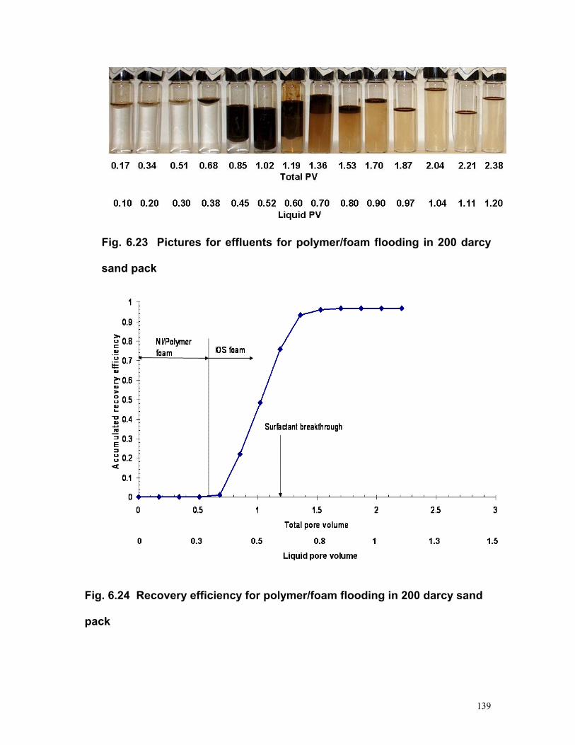
Fig. 6.23 Pictures for effluents for polymer/foam flooding in 200 darcy
sand pack
Fig. 6.24 Recovery efficiency for polymer/foam flooding in 200 darcy sand
pack
139
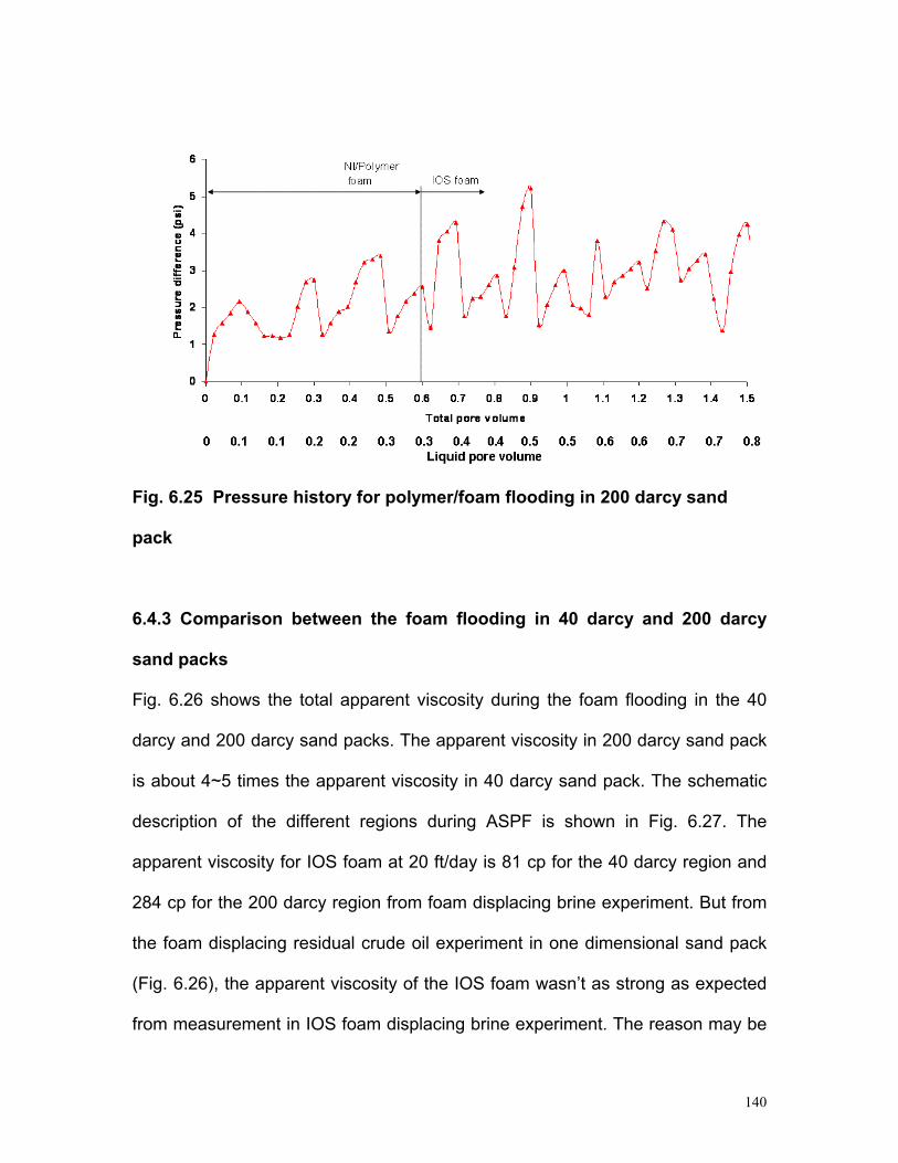
Fig. 6.25 Pressure history for polymer/foam flooding in 200 darcy sand
pack
6.4.3 Comparison between the foam flooding in 40 darcy and 200 darcy
sand packs
Fig. 6.26 shows the total apparent viscosity during the foam flooding in the 40
darcy and 200 darcy sand packs. The apparent viscosity in 200 darcy sand pack
is about 4~5 times the apparent viscosity in 40 darcy sand pack. The schematic
description of the different regions during ASPF is shown in Fig. 6.27. The
apparent viscosity for IOS foam at 20 ft/day is 81 cp for the 40 darcy region and
284 cp for the 200 darcy region from foam displacing brine experiment. But from
the foam displacing residual crude oil experiment in one dimensional sand pack
(Fig. 6.26), the apparent viscosity of the IOS foam wasn’t as strong as expected
from measurement in IOS foam displacing brine experiment. The reason may be
140

that the N67-7PO in the polymer/surfactant slug and a little crude oil left behind
surfactant slug make the IOS foam weaker. From the oil displacement
experiment, the apparent viscosity of the IOS foam is close to the apparent
viscosity of the NI/polymer foam because the pressure difference didn’t change
much before and after the polymer foam was displaced out of the sand pack.
Fig. 6.26 Apparent viscosity during the foam displacing oil for both 40
darcy and 200 darcy sand packs
The relative mobility of the foam is obtained by the pressure difference after the
foam has filled the sand pack from equation (6.1).
1−
∆=
Lp
uk foam
foamλ (6.1)
141
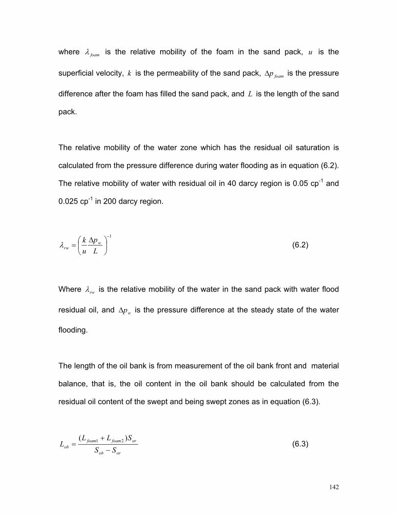
where foamλ is the relative mobility of the foam in the sand pack, u is the
superficial velocity, is the permeability of the sand pack, k foamp∆ is the pressure
difference after the foam has filled the sand pack, and is the length of the sand
pack.
L
The relative mobility of the water zone which has the residual oil saturation is
calculated from the pressure difference during water flooding as in equation (6.2).
The relative mobility of water with residual oil in 40 darcy region is 0.05 cp-1 and
0.025 cp-1 in 200 darcy region.
1−
∆
=Lp
uk w
rwλ (6.2)
Where rwλ is the relative mobility of the water in the sand pack with water flood
residual oil, and ∆ is the pressure difference at the steady state of the water
flooding.
wp
The length of the oil bank is from measurement of the oil bank front and material
balance, that is, the oil content in the oil bank should be calculated from the
residual oil content of the swept and being swept zones as in equation (6.3).
orob
orfoamfoamob SS
SLLL
−
+=
)( 21 (6.3)
142
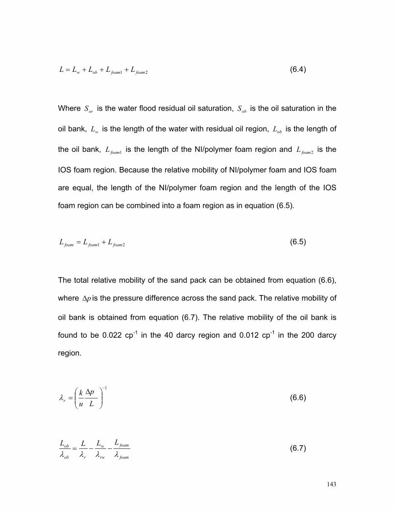
21 foamfoamobw LLLLL +++= (6.4)
Where is the water flood residual oil saturation, is the oil saturation in the
oil bank, is the length of the water with residual oil region, is the length of
the oil bank, is the length of the NI/polymer foam region and is the
IOS foam region. Because the relative mobility of NI/polymer foam and IOS foam
are equal, the length of the NI/polymer foam region and the length of the IOS
foam region can be combined into a foam region as in equation (6.5).
orS
L
obS
w obL
1foamL 2foamL
21 foamfoamfoam LLL += (6.5)
The total relative mobility of the sand pack can be obtained from equation (6.6),
where is the pressure difference across the sand pack. The relative mobility of
oil bank is obtained from equation (6.7). The relative mobility of the oil bank is
found to be 0.022 cp
p∆
-1 in the 40 darcy region and 0.012 cp-1 in the 200 darcy
region.
1−
∆=
Lp
uk
rλ (6.6)
foam
foam
rw
w
rob
ob LLLLλλλλ
−−= (6.7)
143

rwλ
obλ
1foamλ
Water region
Lw
Lob
Lfoam1
Lfoam2
L
2foamλ
Oil bank
NI/polymer foam
IOS foam
Fig. 6.27 Schematic description of the different regions during the ASPF
process in sand pack
From the above discussion, the relative mobilities of water and oil bank in 200
darcy sand pack are about half of those in 40 darcy sand pack and the foam
relative mobility in 40 darcy sand pack is 1/5 of that in 200 darcy sand pack. The
reason for the relative mobility difference of water and oil bank in the 40 darcy
and 200 darcy sand packs may be the residual oil saturation is different in the
two experiments. The relative mobility ratio in 200 sand pack is about 2~3 times
lower in 40 darcy sand pack. This may explain why the oil bank breaks through
earlier in 200 darcy sand pack. The results for the apparent viscosity and relative
mobility in the sand in the two experiments are summarized in Table 6.1.
144
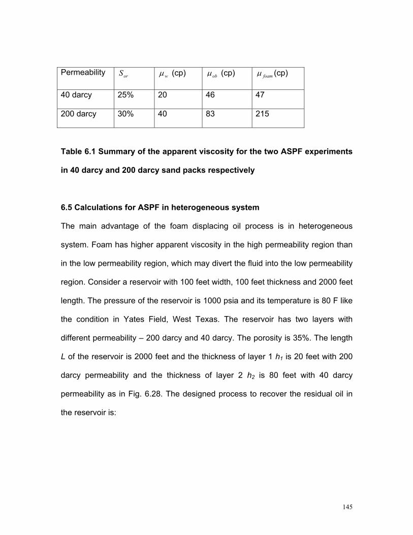
Permeability orS wµ (cp) obµ (cp) foamµ (cp)
40 darcy 25% 20 46 47
200 darcy 30% 40 83 215
Table 6.1 Summary of the apparent viscosity for the two ASPF experiments
in 40 darcy and 200 darcy sand packs respectively
6.5 Calculations for ASPF in heterogeneous system
The main advantage of the foam displacing oil process is in heterogeneous
system. Foam has higher apparent viscosity in the high permeability region than
in the low permeability region, which may divert the fluid into the low permeability
region. Consider a reservoir with 100 feet width, 100 feet thickness and 2000 feet
length. The pressure of the reservoir is 1000 psia and its temperature is 80 F like
the condition in Yates Field, West Texas. The reservoir has two layers with
different permeability – 200 darcy and 40 darcy. The porosity is 35%. The length
L of the reservoir is 2000 feet and the thickness of layer 1 h1 is 20 feet with 200
darcy permeability and the thickness of layer 2 h2 is 80 feet with 40 darcy
permeability as in Fig. 6.28. The designed process to recover the residual oil in
the reservoir is:
145

1. Alternate injecting NI blend/polymer and air at 20 ft/day in 0.1 PV
increment for total 0.6 PV. NI blend includes 0.2% N67-7PO and IOS at
4:1 ratio, 0.5% polymer, 2% NaCl and 1% Na2CO3.
2. Alternate injecting IOS and air in 0.1 PV increment to get IOS foam as
drive. IOS solution includes 0.2% IOS at 2% NaCl and 1% Na2CO3.
Fig. 6.28 Schematic of a reservoir with 2 layers at different permeability
From the result of experiment in section 6.3, the apparent viscosity of the crude
oil is 19 cp. When the residual oil saturation is 25%, the relative mobility of the
residual oil region is 0.05 cp-1 and the relative mobility of the oil bank is 0.022 cp-
1. The foam apparent viscosity is 215 cp in the 200 darcy layer and 46 cp in the
40 darcy layer.
The calculation can be made with the assumptions:
146
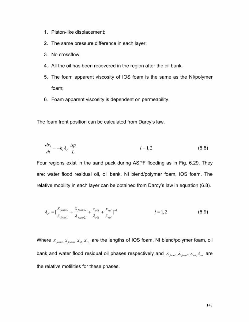
1. Piston-like displacement;
2. The same pressure difference in each layer;
3. No crossflow;
4. All the oil has been recovered in the region after the oil bank.
5. The foam apparent viscosity of IOS foam is the same as the NI/polymer
foam;
6. Foam apparent viscosity is dependent on permeability.
The foam front position can be calculated from Darcy’s law.
Lpk
dtdx
rlll ∆
−= λ 2,1=l (6.8)
Four regions exist in the sand pack during ASPF flooding as in Fig. 6.29. They
are: water flood residual oil, oil bank, NI blend/polymer foam, IOS foam. The
relative mobility in each layer can be obtained from Darcy’s law in equation (6.8).
1
2
2
1
1 ][ −+++=rol
rol
obl
obl
lfoam
lfoam
lfoam
lfoamrl
xxxxλλλλ
λ 2,1=l (6.9)
Where are the lengths of IOS foam, NI blend/polymer foam, oil
bank and water flood residual oil phases respectively and
roobfoamfoam xxxx ,,2,1
roobfaomfoam λλλλ ,,2,1 are
the relative motilities for these phases.
147

IOS foam
NI blend/Polymer foam Oil bank Water flood residual oil
Xro xob xfoam1 xfoam2
L
Fig. 6.29 schematic illustration of ASPF flooding
In this particular case, the relative mobility of IOS foam lfoam1λ is equal to that of
the NI blend/polymer foam lfoam2λ . Because all the oil after the oil bank has been
recovered, the oil bank length can be related to the length of the length of
foam ( by the material balance.
obx
)21 lfoamlfoam xx +
)()( 21
orlobl
orllfoamlfoamobl SS
Sxxx
−
+= 2,1=l (6.10)
where is the water flood residual oil saturation and is the oil saturation in
oil bank.
orlS oblS
Taking the ratio of the velocities in the two layers will eliminate time and pressure
drop since both layers experience the same p∆ . Then in two layers with different
permeability,
148
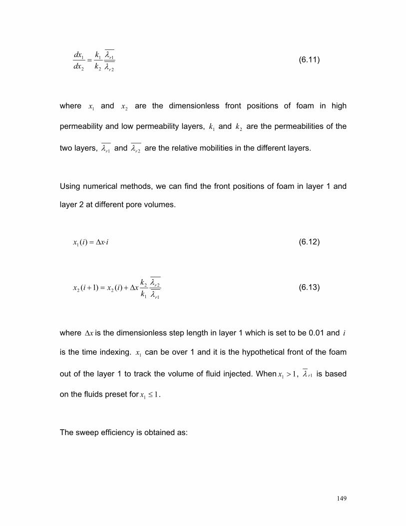
2
1
2
1
2
1
r
r
kk
dxdx
λλ
= (6.11)
where and are the dimensionless front positions of foam in high
permeability and low permeability layers, and k are the permeabilities of the
two layers,
1x 2x
1k 2
1rλ and 2rλ are the relative mobilities in the different layers.
Using numerical methods, we can find the front positions of foam in layer 1 and
layer 2 at different pore volumes.
ixix ⋅∆=)(1 (6.12)
1
2
1
222 )()1(
r
r
kkxixix
λλ
∆+=+ (6.13)
where is the dimensionless step length in layer 1 which is set to be 0.01 and i
is the time indexing. can be over 1 and it is the hypothetical front of the foam
out of the layer 1 to track the volume of fluid injected. When ,
x∆
1x
11 >x 1rλ is based
on the fluids preset for . 11 ≤x
The sweep efficiency is obtained as:
149

Sweep efficiency = 21
2211 )(hhhxhx
++ when 11 <x (6.14)
And Sweep efficiency = 21
221 )(hhhxh
++ when (6.15) 11 ≥x
The result is shown in Fig. 6.30 by the calculation with the above assumptions. It
shows that less than 1.06 total pore volume of foam is needed to sweep the
heterogeneous system while 1.36 pore volume of polymer is needed to get the
same sweep with ASP process. The foam breaks through layer 1 around 0.85
total pore volume and the polymer breaks through around 0.45 total pore volume.
The ASP process calculation is similar to that for ASPF process except that the
foam regions are replaced by surfactant slug and polymer drive regions, which
are both assumed to have an apparent viscosity of 46 cp. The most important
difference is that the polymer has the same apparent viscosity in different layers.
150

Fig. 6.30 Sweep efficiency of foam or polymer sweep in a heterogeneous
system with 5:1 permeability ratio and 1:4 thickness ratio
Because the foam is injected at gas fractional flow of 0.5, 0.53 PV of liquid
injection is needed, which includes 0.3 PV polymer-surfactant solution at 0.5%
polymer and 0.2% NI blend, and 0.23 PV 0.2% IOS solution. For a conventional
ASP process, 1.36 PV of liquid is needed which includes 0.3 PV polymer-
surfactant solution at 0.5% polymer and 0.2% NI blend, and 1.23 PV of polymer
solution at 0.5% concentration.
In each process, a total 0.3 PV NI blend was injected in the heterogeneous
system. By tracking the foam front of the IOS foam in ASPF or the polymer drive
front in ASP, there was 0.08 PV of NI blend/polymer solution flowing into layer1
and 0.22 PV into layer 2 in ASPF while there was 0.17 PV of NI blend/polymer
151
solution flowing into the higher permeability layer and 0.13 PV into the lower
permeability layer 2 with ASP. The foam diverted more surfactant solution from
high permeability layer to low permeability layer. 73% of NI blend solution flows
into layer 2 which contains 80% of the residual oil by ASPF process while only
43% of NI blend solution gets into layer 2 by ASP process. The diversion effect
by ASPF process is important because enough surfactant must be injected in
real reservoir to overcome the loss by the adsorption of surfactant. This example
here with permeability ratio 5 is not as severe as may be encountered in other
formations, where thief zone (high permeability region) could be an order of
magnitude or more greater than mean permeability. Then the ASPF process
could be even more beneficial.
Tables 6.1 and Table 6.2 list assumptions and results of calculations illustrating
the difference between revenue and chemical expenses for ASPF and ASP
processes in this reservoir. The cost of natural gas takes the largest part in the
whole cost of ASPF and the chemical cost is less than 10% of oil price. The price
of natural gas is the current market price. If the process is applied in a reservoir
where natural gas co-exists with crude oil, the cost can be greatly decreased. In
other words, the profit for the ASPF process can be higher than indicated.
Although it seems that the revenue minus expenses per bbl by ASPF or ASP
process is only about 16% saving, the advantage of ASPF is that more surfactant
solution is diverted into the low permeability layer to get the residual oil there
because in ASP process a larger surfactant slug is needed process to overcome
152
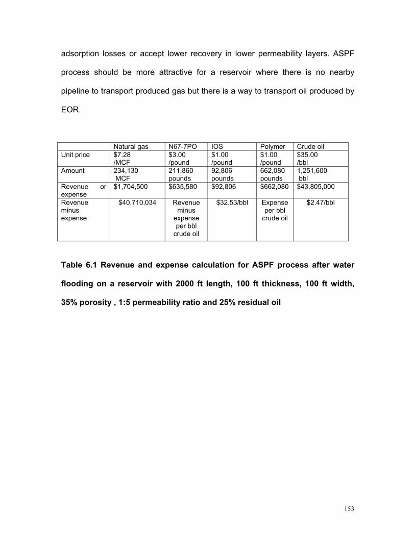
adsorption losses or accept lower recovery in lower permeability layers. ASPF
process should be more attractive for a reservoir where there is no nearby
pipeline to transport produced gas but there is a way to transport oil produced by
EOR.
Natural gas N67-7PO IOS Polymer Crude oil Unit price $7.28
/MCF $3.00 /pound
$1.00 /pound
$1.00 /pound
$35.00 /bbl
Amount 234,130 MCF
211,860 pounds
92,806 pounds
662,080 pounds
1,251,600 bbl
Revenue or expense
$1,704,500 $635,580 $92,806 $662,080 $43,805,000
Revenue minus expense
$40,710,034 Revenue minus
expense per bbl
crude oil
$32.53/bbl Expense per bbl
crude oil
$2.47/bbl
Table 6.1 Revenue and expense calculation for ASPF process after water
flooding on a reservoir with 2000 ft length, 100 ft thickness, 100 ft width,
35% porosity , 1:5 permeability ratio and 25% residual oil
153
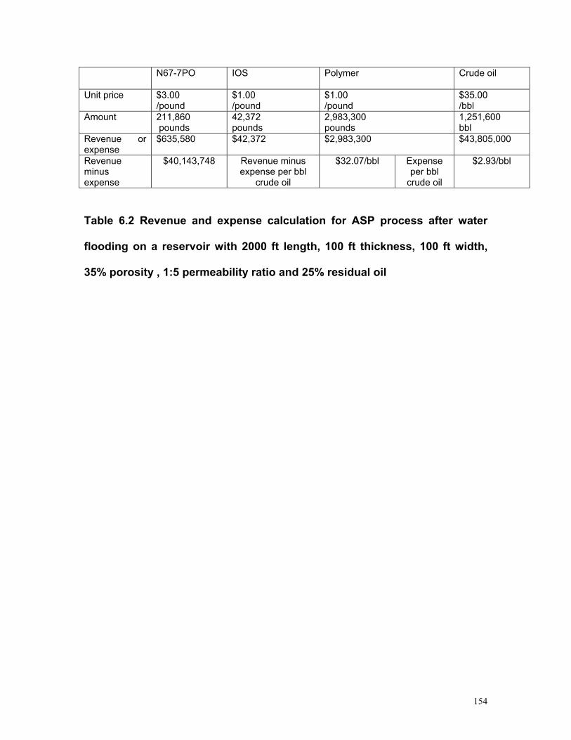
154
N67-7PO IOS Polymer Crude oil
Unit price $3.00 /pound
$1.00 /pound
$1.00 /pound
$35.00 /bbl
Amount 211,860 pounds
42,372 pounds
2,983,300 pounds
1,251,600 bbl
Revenue or expense
$635,580 $42,372
$2,983,300 $43,805,000
Revenue minus expense
$40,143,748 Revenue minus expense per bbl
crude oil
$32.07/bbl Expense per bbl
crude oil
$2.93/bbl
Table 6.2 Revenue and expense calculation for ASP process after water
flooding on a reservoir with 2000 ft length, 100 ft thickness, 100 ft width,
35% porosity , 1:5 permeability ratio and 25% residual oil

Chapter 7
CONCLUSIONS AND RECOMMENDATIONS
7.1 Conclusions
In this thesis, we studied foam flow in homogeneous fractures and found the
mechanisms than can affect foam apparent viscosity in fractures. The foam
diversion effect in heterogeneous fractures can be explained and predicted from
the mechanisms. Foam application in reservoirs without fractures was also
investigated and foam was found to be promising to work in alkaline/surfactant
processes to replace or supplement polymer as mobility control agent.
7.1.1 Foam flow in homogeneous fracture
For foam as individual bubbles, which have a diameter larger than the fracture
aperture, the apparent viscosity is the sum of two contributions: that resulting
from liquid between bubbles and that resulting from the resistance to deforming
the interface when a bubble passes through a fracture. The surface tension
gradient contribution does not appear to be significant in our experiments.
At conditions of sufficiently low Reynolds numbers and bubble sizes where no
coalescence occurs in homogeneous fracture, for the foam flow through a
smooth, uniform fracture, the foam texture (a measure of the bubble volume) is a
key parameter in determining , the number of lamellae per unit length, which is Ln
155

the main factor affecting the foam apparent viscosity in smooth uniform fractures
when the (undeformed) bubble diameter exceeds fracture aperture. Changes
which increase , e.g., higher gas fractional flow and larger ratios of
aperture thickness to bubble size, cause apparent viscosity to increase. The
aperture thickness effect is the basis for producing a more uniform sweep by the
use of foam.
Ln gf
For bulk foam at low to medium gas fractional flow, Pal’s equation can well
predict the apparent viscosity of bulk foam in fractures, i.e., when bubble
diameter is less than fracture aperture. From Pal’s equation, gas fractional flow
is the main factor to affect the apparent viscosity for bulk foam. gf
7.1.2 Foam diversion in heterogeneous fractures
We investigated different factors’ effects on sweep efficiency by foam in smooth
heterogeneous fractures and applied our theory to this situation assuming the
same in each portion of the fracture and no crossflow. Foam apparent
viscosity in each portion of a heterogeneous fracture can be calculated using the
theoretical result for a homogeneous fracture.
gf
Foam can greatly improve the sweep efficiency in a heterogeneous fracture
system if bubble size is the same and larger than the largest aperture in all
fractures. The amount of surfactant solution required is reduced substantially
156
both by foam’s ability to divert flow into smaller fractures and by the need for less
liquid to fill a given volume of fractures. Gas fractional flow, aperture ratio and
bubble size can greatly affect the sweep efficiency.
Agreement of theoretical predictions and experimental results was shown in
previous chapters and confirms validity of the theory’s assumptions of equal fg,
no crossflow and constant bubble size.
Dykstra-Parson’s model was applied in predicting the sweep efficiency by foam
in heterogeneous fracture system with log-normal distributed apertures. The
sweep efficiency was found to be greatly affected by the apparent viscosity ratio
in different fractures. If the foam apparent viscosity in the thicker fracture is larger
than that in the thinner fracture, foam can improve the sweep efficiency. But if the
foam apparent viscosity is lower in the larger aperture, e.g., when the bubble size
is at a fixed ratio to aperture in each layer or in many cases when bulk foam
exists in the large aperture fractures, contrary diversion may happen and the
sweep efficiency is decreased.
7.1.3 Surfactant evaluation
Two different surfactant blends were evaluated and NI blend was found to be the
better candidate in alkaline/surfactant EOR processes because it can get ultra-
low interfacial tension at its optimal salinity which is closer to the formation
salinity than TC blend. But from the foaming ability test, NI blend is much weaker
157

than TC blend. From our investigation, it was found that IOS by itself is a strong
foamer while N67-7PO is a weak foamer. The reason may be that N67-7PO is
quite hydrophobic, especially at optimal salinity. From the test of foam stability
with the presence of residual oil, NI blend can get almost the same strength with
or without residual oil while IOS foam is slightly weaker with residual oil than
without residual oil. But that doesn’t mean the foam by NI blend is more stable
with the presence of residual oil. The reason is that NI blend can displace almost
all the residual oil during the experiment. IOS can get much stronger foam than
NI blend even with the presence of residual oil. To try to simplify the alkaline
surfactant EOR process, from our surfactant evaluation, NI blend is a good
choice for displacing oil with optimal salinity close to formation brine salinity and
IOS is a good candidate as foamer.
7.1.4 Foam in alkaline/surfactant/ polymer/foam EOR process
In the conventional alkaline/surfactant/polymer (ASP) EOR process, polymer was
used as mobility control agent both in the displacement phase together with
alkaline and surfactant and in the subsequent drive phase. To save the
consumption of expensive polymer, we tried to use foam to replace polymer as
mobility control agent in the drive phase. We got a successful experiment by
using alkaline-surfactant-polymer-foam to displace residual crude oil in a one-
dimensional sand pack. That demonstrates the potential of using foam in ASP
EOR process to save the amount of polymer.
158

The biggest advantage of foam as mobility control agent over polymer is that
foam can have higher apparent viscosity in the higher permeability regions and
divert the alkaline/surfactant solution from high to low permeability regions. This
feature is especially beneficial to heterogeneous reservoirs where foam can
sweep a larger portion of the reservoir with less surfactant. Because NI blend
itself is a good surfactant blend for displacing oil but not a good foamer, N67-
7PO is used together with polymer to get low enough mobility ratio. It was found
that the foam with NI blend and polymer in 200 darcy sand pack is 4~5 times
stronger than in 40 darcy sand pack. Moreover, the ASPF process can recover
almost all the residual oil in less than 1.0 PV of injected liquid in either 40 darcy
or 200 darcy sand pack, which shows the possibility of using foam as mobility
control agent in the heterogeneous reservoir to recover residual crude oil.
7.2 Recommendations for future work
7.2.1 Foam flow in fractures
From previous description, it is found in our surfactant system that the foam
apparent viscosity in fractures results from two contributions – liquid between
bubbles and bubble deformation. But from Hirasaki and Lawson [1985], the foam
apparent viscosity in capillary tubes is from three contributions – liquid slugs,
bubble deformation and surface tension gradient. The reason that we didn’t
observe the surface tension gradient in fractures may be that in our surfactant
system the surfactant concentration is much above the CMC and the salinity is
higher than in the surfactant system used in capillary tube experiments, which
159

may cause the surfactant to be adsorbed and desorbed more rapidly. To
investigate if the contribution from surface tension gradient can appear in
fractures, other surfactant system should be tested in fractures.
Both in our work in fractures and the work by Hirasaki and Lawson [1985], there
is a common assumption that the fractures or capillary tubes are smooth. But
when the foam is used in reservoir, the fractures may have different roughness.
When the roughness is large enough, the foam bubbles may deform or even
break into smaller bubbles which may increase the apparent viscosity of foam.
This should be investigated to find the relationship of the roughness of the
fractures to the apparent viscosity of foam.
7.2.2 Surfactant
In the foam aided alkaline surfactant EOR process, the surfactant has two
functions – to get ultra-low interfacial tension and to stabilize foam. We tested
two different surfactant blends in our research – TC blend and NI blend. TC
blend can generate strong foam but it will get phase separation at low salinity. NI
blend can well displace oil but N67-7PO in NI blend makes the foam bubbles
unstable. Although we can use NI blend to displace oil and then use IOS to
generate foam as drive, the change of surfactants will make the process more
complicated. If a surfactant or surfactant blend can be found that can both
displace oil well at the suitable salinity and generate strong foam, the process will
be greatly improved and then foam can be more widely used in EOR process.
160
161
7.2.3 ASPF process
The alkaline-surfactant-polymer-foam process works well in 40 darcy and 200
darcy sand packs. It is recommended to develop the process in lower
permeability matrix, especially in reservoir cores. And the experiments by ASPF
process in two dimensional heterogeneous sand pack are recommended to study
the diversion effect by foam in heterogeneous system and find the foam apparent
viscosity change from one-dimensional to two-dimensional system in ASPF.

REFERENCES
Adams, W.T. and Schievelbein, V.H., "Surfactant flooding carbonate reservoirs," SPE/DOE preprint 12686 presented at 4th Symp. on EOR, Tulsa, Apr., 1984
Adibhatia, B., Sun, X., and Mohanty, K.K., “Numerical studies of oil production from initially oil-wet fracture blocks by surfactant brine imbibition,” SPE preprint 97687, presented at Intl. IORConf., Kuala Lumpur, Dec., 2005
Akers, R.J., “Foams”, Academic Press, 1975
Baker, R.O. , Telesford, A. , Wong, S. , Li, V. , Smith, G. , and Schoendorfer, H. , "AnIntegrated Fracture Characterization of a Heavy Oil Naturally Fractured carbonateReservoir", paper no. 2001-13, Prepared for Presentation at the Petroleum Society’sCanadian International Petroleum Conference held in Calgary, AB, Canada (June 12-14,2001).
Baker, T. , Celius, H.K. , Lie, T., Martinsen, H.A., Rasmussen, L. , and Vassenden, F. ,“Foam for Gas Mobility Control in the Snorre Field: the FAWAG Project”, SPE 56478,presnted at the 1999 SPE ATCE at Houston, TX (3-6 October 1999)
Basheva, E.S. , S. Stoyanov, N.D. Denkov, K. Kasuga, N. Satoh, and K. Tsujii, “FoamBoosting by Amphiphilic Molecules in the Presence of Silicone Oil”, Langmuir 2001, 17, 969-979
Basheva, E.S. , Stoyanov, S. , Denkov, N.D. , Kasuga, K. , Satoh, N. , and Tsujii, K. ,, “Roleof Bertaine as Foam Booster in the Presence of Silicone Oil Drops”, Langmuir 2000, 16, 1000-1013
162
Bernard, G.G. , and Holm, L.W. , “Effect of Foam on Permeability of Porous Media to Gas”,SPE Journal, September 1964, 267-274
Bertin, H.J. , "Foam Diversion Modeling Using a Bubble-Population Correlation", SPE 59366,presented at the 2000 SPE/DOE Improved Oil Recovery Symposium at Tulsa, OK (3-5 April2000)
Bertin, H.J. , Apaydin, O.G. , Castanier, L.M. , and Kovscek, A.R., "Foam Flow inHeterogeneous Porous Media: Effect of Cross Flow", Society of Petroleum EngineersJournal, 4 (2), 1999, 75-82.
Bretherton, F.P. , "The Motion of Long Bubbles in Tubes, Journal of Fluid Mechanics", 10(1961), 166-188.
Casteel, J.F. and Djabbarah, N.F , "Sweep Improvement in CO2 Flooding by Use of FoamingAgents", Society of Petroleum Engineers Reservoir Engineering, Nov 1988, 1186-1192.
Chang, H.L., Zhang, Z.Q., Wang, Q.M., Xu, Z.S., Guo, Z.D., Sun, H.Q., Cao, X.L., and Qiao, Q., "Advances in polymer flooding and alkaline/surfactant/polymer processes as developed and applied in the People's Republic of China," J. Petrol. Technol, 58(2), 84-89, Feb., 2006
Chen, H.L. et al, "Laboratory monitoring of surfactant imbibition with computerizedtomography," SPERE 4(1), 16 (2001)
163
Chen, H-L , Ke, M-J. , Chuang, T-K , and Flumerfeit, R.W. , "Experimental Studies ofCapillary Pressure Effects of Foams in Porous Media", SPE 20069, prepared for presentationat the 60th California Regional Meeting at Ventura, CA (April 4-6, 1990)
Cheng, L. , Reme, A. B. , Shan, D. , Coombe, D. A. , and Rossen, W. R. , "Simulating Foam Processes at High and Low Foam Qualities", Society of Petroleum Engineers, 59287,Presented at the SPE/DOE Improved Oil Recovery Symposium at Tulsa, OK (Apr 3-5, 2000).
Dalland, M. , and Hanssen, J. E. , “Enhanced Foams for Efficient Gas Influx Control”, SPE37217, presented at the 1997 SPE International Symposium at Houston, TX
Demin, Wang , Cheng Jiecheng, Yang Zhenyu, Li Qun, Wu Wenxiang, Yu Huiyu, "SuccessfulField Test of the First Ultra-Low Interfacial Tension Foam flood", Society of PetroleumEngineers, 72147, Presented at the SPE Asia Pacific Improved Oil Recovery Conference,Kuala Lumpur, Malaysia (Oct 8-9, 2001)
Detwiler, R.L. , Rajaram, H. , and Glass, R.J. , “Nonaqueous-Phase-Lquid Solution inVariable-Aperture fractures: Development of a Depth-Averaged Computational Model withComparison to a Physical Experiment”, Water Resources Research, Vol. 37, No. 12, Pages3115-3129, December 2001
Exerowa, D. , and Kruglyakov, P.M. , “Foam and Foam Films, Theory, Experiment,Application”, Elsevier, 1998
Falls, A.H. , Hirasaki, G.J., Patzek, T.W. , Gauglltz, D.A., Miller, D.D. , and Ratulowski, T.,“Development of a Mechanistic Foam Simulator: The Population Balance and Generation bySnap-Off”, SPERE 3, 884 (1988)
164

Falls, A.H. , Musters, J.J. , and Ratulowski, J. , “The Apparent Viscosity of Foams inHomogeneous Bead Packs”, SPE Reservoir Engineering, May 1989, 155-164
Falls, A.H., Thigpen, D.R., Nelson, R.C., Ciaston, J.W., Lawson, J.B., Good, P.A., Ueber,R.C., and Shahin, G.T., "A field test of cosurfactant-enhanced alkaline flooding," SPE/DOEpreprint 24117 for Symp. on EOR, Tulsa, Apr., 1992
Gale, J.E. , "Comparison of coupled fracture deformation and fluid models with directmeasurements of fracture pore structure and stress-flow properties." In: I.W. Farmer, J.J.K.Daemen, C.S. Desai, C.E. Glass and S.P. Neuman, (Eds.), Rock Mechanics: Proceedings ofthe 28th US Symposium. Tucson, Arizona. Rotterdam, Balkema, Rotterdam (1987),1213¯1222.
Garret, P.R. , “Defoaming, Theory and Industrial Applications”, Marcel Dekker Inc., 1993
Gauglitz, P.A. , Friedmann, F. , Kam, S.I. , and Rossen, W.R. , "Foam Generation in PorousMedia", SPE 75177, prepared for presentation at the SPE/DOE thirteenth Symposium onEOR at Tulsa, OK (13-17 April 2002)
Ghosh, O., "Liquid crystal to microemulsion transitions in anionic surfactant-oil-brinesystems," PhD Thesis, Rice University, 1985
165

Gillette, R. , "Characterizing the Viscosity of Foam Used in a Semiconductor Wafer CleaningSystem", Summer 2001 Intern Report
Hackett, J.L. and Miller, C.A., "Microemulsion to liquid crystal transition in two anionicsurfactant systems," SPERE 3, 791-800 (1988)
Hanssen, J. E. , “Foam as a Gas-blocking Agent in Petroleum Reservoirs I: EmpiricalObservations and Parametric Study”, Journal of Petroleum Science and Engineering, 10(1993) 117-133
Hassen, J.E. , Surguchev, L.M. , and Svorstol, I. , "SAG Injection in a North Sea StratifiedReservoir: Flow Experiment and Simulation", SPE 28847, presented at the EuropeanPetroleum Conference at London, UK (25-27 October 1994)
Heller, J.P. , and Kuntamukkula, M.S. , “Critical Review of the Foam Rheology Literature”,Ind. Eng. Chem. Res. 1987, 26, 318-325
Hirasaki, G.J. and Lawson, J.B , "Mechanisms of Foam Flow in Porous Media: ApparentViscosity in Smooth Capillaries", Society of Petroleum Engineers Journal, 25 (2), 1985, 176-190.
Hirasaki, G.J. , Jackson, R.E. , Jin, M. , Lawson, J.B. , Londergan, J. , Meinardus, H. , Miller,C.A. , Pope, G.A. , Szafranski, R. , and Tanzil, D. , "Field Demonstration of theSurfactant/Foam Process for Remediation of a Heterogeneous Aquifer Contaminated withDNAPL", in: Fiorenza, S. , Miller, C. A. , Oubre, C. L. , and Ward, C. H. (Eds.), NAPLRemoval: Surfactants, Foams, and Microemulsions, Lewis Publishers, 2000.
166
Hirasaki, G.J. , Zhang, D.L. , "Surface Chemistry of Oil Recovery From Fractured, Oil-Wet,Carbonate Formations", Society of Petroleum Engineers Journal, 9(2), 2004, 151-162.
Hirasaki, G.J. and Zhang, D.L., “Surface chemistry of oil recovery from fractured, oil-wet,carbonate formations,” SPEJ, 9(2), 151-162 (2004)
Hirasaki, G.J. et al, "Surfactant based enhanced oil recovery and foam mobility control,"Technical reports #4 (July, 2005) and #5 (Jan., 2006) to DOE for grant DE-FC26-03NT15406to Rice University
Huh, C., "Interfacial tensions and solubilizing ability of a microemulsion phase that coexistswith oil and brine," J. Colloid Interface Sci. 71, 408-426 (1979)
Jayanti, S. , Britton, L.N. , Dwarakanath, V. , Pope, G.A. , “Laboratory Evaluation of CustomDesigned Surfactants to Remediate NAPL Source Zones”, Paper, 2002
Kam, S.I. , and Rossen, W.R. , “A Model for Foam Generation in Homogeneous Media”,SPE77698, presented at the SPE ATCE at San Antonio, TX (29 September - 2 October 2002)
Khatib, Z.I. , Hirasaki, G.J. , and Falls, A.H. , , “Effects of Capillary Pressure on Coalescenceand Phase Mobilities in Foams Flowing through Porous Media”, SPE 15442, presented at the51st ATCE of SPE at New Orleans, LA (Oct 5-8, 1986)
167
Kibodeaux, K.R. , S.C. Zeilinger, and W.R. Rossen, "Sensitivity Study of Foam DiversionProcesses for Matrix Acidization", SPE 28550, presented at the 69th SPE ATCE at NewOrleans, LA (September 26-28, 1994)
Kovscek, A.R. and Radke, C.J. , "Fundamentals of Foam Transport in Porous Media", in: L.L.Schramm (Ed.), Foams: Fundamentals and Applications in the Petroleum Industry, AmericanChemical Society, Washington D.C., 1994, pp. 115-164.
Kovscek, A.R. , and Bertin, H.J. , "Estimation of Foam Mobility in Heterogeneous PorousMedia", Submitted to 2002 SPE/DOE Improved Oil Recovery Symposium, 2002
Kovscek, A.R. , and Radke, C.J. , "Pressure-driven Capillary Snap-off of Gas Bubbles at LowWetting-liquid Content", Colloids and Surfaces A: Physicochem. Eng. Aspects 212 (2003) 99-108
Kovscek, A.R. , and Radke, C.J. , “A Comprehensive Description of Transient Foam Flow inPorous Media”, Prepared for D.O.E./NIPER Symposium on Field Application of Foams for OilProduction, 1993
Kovscek, A.R. , and Radke, C.J. , “Gas Bubble Snap-Off under Pressure-Driven flow inConstricted Noncircular Capillaries”, Colloids and Surfaces, A: Physicochemical andEngineering Aspects 117 (1996) 55-76
Kovscek, A.R. , Tretheway, D.C. , Persoff, P. and Radke, C.J. , "Foam Flow through aTransparent Rough-Walled Rock Fracture", Journal of Petroleum Science and Engineering,13 (1995), 75-86.
168

Krieger, I.M. , "Rheology of Monodisperse Latices", Advances in Colloid and interfaceScience, 1972, 3, 111-136.
Lake, L.W. , "Enhanced Oil Recovery", Prentice Hall, New Jersey, 1989, 201-205.
Lawson, J.B. , and Hirasaki, G.J. , "Foam for Control of Injection Profiles", Report preparedfor the 1984 Reservoir Engineering/Research conference, 1984
Lawson, J.B. , Reisberg, J. , "Alternate Slugs of Gas and Dilute Surfactant for Mobility Controlduring Chemical Flooding", Society of Petroleum Engineers, 8839, Presented at SPE/DOEEnhanced Oil Recovery Symposium, Tulsa, OK (Apr 20-23, 1980).
Llave, F.M., Chung, F.T-H. , Louvier, R.W. , and Hudgins, D.A., "Foams as Mobility ControlAgents for Oil Recovery by Gas Displacement", SPE/DOE 20245, prepared for presentationat the SPE/DOE Seventh Symposium on EOR at Tulsa, OK ( April 22-25, 1990)
Mamun, C.K. , Rong, J.G. , Kam, S.I. , Liijestrand, H.M. , and Rossen, W.R. , "ExtendingFoam Technology from Improved Oil Recovery to Enviromental Remediation", SPE 77557,prepared for presentation at the SPE ATCE at San Antonio, TX (29 September-2 October2002)
Miller, C.A. and Qutubuddin, S., “Enhanced oil recovery with microemulsions,” in InterfacialPhenomena in Apolar Media, H.-F. Eicke and G.D. Parfitt (eds.), Marcel Dekker, New York,1987, 117-185
169
Miller, C.A., Ghosh, O., and Benton, W.J., "Behavior of dilute lamellar liquid crystallinephases," Colloids Surf. 19, 197 (1986)
Mooney, M.J. , "The Viscosity of a Concentrated Suspension of Spherical Particles", Journalof Colloid Science, 1951, 6, 162-170.
Mori, F., Lim, J.C., and Miller, C.A., "Equilibrium and dynamic behavior of a system containing a mixture of anionic and nonionic surfactants," Progr. Colloid Polym. Sci. 82, 114-121 (1990)
Myers, T.J. , and Radke, C.J. , “Transient Foam Displacement in the Presence of ResidualOil: Experiment and Simulation Using a Population-Balance Model”, Ind. Eng. Chem. Res.2000, 39, 2725-2741
Nelson, R.C., Lawson, J.B., Thigpen, D.R., and Stegemeier, G.L., “Cosurfactant-enhancedalkaline flooding,” SPE/DOE preprint 12672, presented at 4th Symp. On EOR, Tulsa, Apr.1984
Nelson, R.A. , "Geologic Analysis of Naturally Fractured Reservoirs", second ed., GulfProfessional Publishing, 2001.
Nguyen, Q.P. , Currie, P.K. , and Zitha, P.K.J. , "Effect of Capillary Cross-Flow onFoam–Induced Diversion in Layered Formations", Society of Petroleum Engineers, 82270,Presented at the SPE European Formation Damage Conference at Hague, Netherlands (May13-14, 2003).
170

Osterloh, W.T., and Jante Jr., M. J. , "Effects of Gas and Liquid Velocity on Steady StateFoam Flow at High Temperature", Society of Petroleum Engineers, 24179, Prepared forPresentation at the 1992 SPE/DOE Symposium on Enhanced Oil Recovery at Tulsa, OK(April 22-25, 1992).
Pal, R. , "Rheology of Polymer-thickened Emulsions", Journal of Rheology, 36(7), 1992
Palar, M. , Jasinski, R.J. , and Robert, J.A. , "A Experimental Study of Foam Flow throughBerea Sandstone with Applications to Foam Diversion in Matrix Acidizing", SPE 29678,prepared for presentation at the Western Regional Meeting at Bakersfield, CA (8-10 march1995)
Pope, G.A., Jackson, A., and Levitt, D., "Identification and evaluation of high-performanceEOR surfactants," SPE preprint 100089, presented at Symp. on IOR, Tulsa, Apr., 2006
Princen, H.M. , "Rheology of Foams and Highly Concentrated Emulsions, I. Elastic Propertiesand Yield Stress of a Cylindrical Model System", Journal of Colloid Interface Science (1983)91, No. 1 160-175.
Prud’homme, R.K. , and Khan, S.A. , “Foams, Theory, Measurements, and Applications”,Marcel Dekker Inc., 1995
Radke, C.J. , and Ransohoff, T.C. , "Mechanisms of Foam Generation in Glass Bead Packs",SPE 15441, prepared for presentation at the 61st ATCE at New Orleans, LA (October 5-8,1986)
171

Reed, R.L. and Healy, R.N., “Some physicochemical aspects of microemulsion flooding: areview,” in Improved Oil Recovery by Surfactant and Polymer Flooding, D.O. Shah and R.S.Schechter (eds.), Academic Press, New York, 1977, 383-437
Rossen, W.R. and Wang, M.W., "Modeling Foams for acid Diversion", Society of PetroleumEngineers, 24179, Society of Petroleum Engineers Journal, 6(4), 1999, 92-100.
Rossen, W.R. , "Snap-off in Constricted Tubes and Porous Media", Collids and Surfaces, A:Physicochemical and Engineering Aspects 166 (2000) 101-107
Scheibel, J.J., "The evolution of anionic surfactant technology to meet the requirements of the laundry detergent industry," J. Surfactants Detergents 7(4), 319-328 (2004)
Schramm, L.L. , ”Foams, Fundamentals and Applications in the Petroleum Industry”,American Chemical Society, 1994.
Seethepalli, A., Adibhatta, B., and Mohanty, K.K., “Physicochemical interactions duringsurfactant flooding of fractured carbonate reservoirs,” SPEJ 9(4), 411-418 (2004)
Siddiqui, S. , Talabani S. , Saleh, S.T. , and Islam, M.R. , "A Laboratory investigation of FoamFlow in Low Permeability Berea Sandstone Cores", Society of Petroleum Engineers, 37416,Prepared for Presentation at the 1997 SPE Production Operations Symposium at OklahomaCity, OK (March 9-11, 1997).
172

Singh, G. , Hirasaki, G.J. , and Miller, C.A. , “Dynamics of Foam Films in Constricted Pores”,AIChE Journal, Dec 1997, Vol. 43, No. 12, 3241-3252
Spinler, E.A. et al, "Enhancement of oil recovery using a low concentration of surfactant toimprove spontaneous and forced imbibition in chalk," SPE preprint 59290 for IOR Symp.,Tulsa, Apr., 2000
Standnes, D.C. and Austad, T., "Wettability alteration in carbonates: interaction between cationic surfactant and carboxylates as a key factor in wettability alteration from oil-wet to water-wet conditions," Colloids, Surf. A 216, 243-259 (2003)
Tanzil, D. , “Foam Generation and Propagation in Heterogeneous Porous Media”, Thesis forPh.D., 2001
Tanzil, D. , Hirasaki, G.J. , and Miller, C.A. , "Mobility of Foam in Heterogeneous Media:Flow Parallel and Perpendicular to Stratification", SPE 78601, presented at the 2000 SPEATCE at Dallas (1-4 October, 2000)
Tanzil, D., Hirasaki, G.J., and Miller, C.A., "Conditions for Foam Generation in HomogeneousPorous Media", SPE 75176, presented at SPE/DOE Thirteenth Symposium on EOR at Tulsa,OK (13-17 April 2002)
Vargo, J., Turner, J., Vergnani, B., Pitts, M., Wyatt, K. Surkalo, H., and Patterson, D.,"Alkaline-surfactant-polymer flooding of the Cambridge Minnelusa field," SPEREE 3(6), 552-558 (2000)
Wang, C. , Wang, B. , Cao, X. , and Li, H. , "Application and Design of Alkaline-Surfactant-Polymer System to Close Well Spacing Pilot Gudong Oilfield", SPE 38231, 1997
173
Wang, D. , Zhang, Z. , Cheng, C. , Yang, J. , Gao, S. , and Li, L. , "Pilot Tests ofAlkaline/Surfactant/Polymer Flooding in Daqing Oil Field", SPE Reservoir Engineering, Nov1997
Weaire, D. , and Hutzler, S. , “The Physics of Foams”, Oxford University Press, 1999
Wilson, C.R. , "An Investigation of Laminar Flow in Fractured Porous Rocks", Ph.D. Thesis,University of California, Berkeley, 1970
Wyatt, K., Pitts, M., and Surkalo, H., "Mature waterfloods renew oil production by alkaline-surfactant-polymer flooding," SPE preprint 78711 for SPE Eastern Regional Meeting, Lexington, KY, Oct., 2002.
Xie, X., Weiss, W.W., Tong, A., and Morrow, N.R., "Improved recovery from carbonatereservoirs by chemical stimulation," SPEJ 10(3), 276-285 (2005).
Yaghoobi, H. , Tsau, J.S. , and Heller, J.P. , "Improving CO2 Floods in HeterogeneousMedia", Society of Petroleum Engineers, 35403, Prepared for SPE/DOE Improved OilRecovery Symposium at Tulsa, OK (April 21-24, 1996)
Zerhboub, M. , Ben-Naceur, K. , Touboul, E. and Thomas, R. , "Matrix Acidizing: A NovelApproach to Foam Diversion", Society of Petroleum Engineers Production & Facilities, 9(2),1994, 121-126
Zhang, D.L., "Surfactant-enhanced oil recovery process for a fractured, oil-wet carbonatereservoir," PhD Thesis, Rice University, 2006
174

APPENDICES
APPENDIX A. DERIVATION FOR THE EQUIVALENT LAMELLAE PER UNIT
LENGTH Ln
Assuming that bubbles are distributed uniformly, the total number of bubbles
Nbubble in a rectangular area having length and width W is: L
2)()( LLLbubble LWnWnLnN =×= (A.1)
Then the total volume occupied by gas is:
233 )3/4()3/4( LBBbubblegas LWnrrNV ππ == (A.2)
However, the total volume occupied by gas is also given by:
ggas LWbfV = (A.3)
where b is the fracture thickness.
Combine the above two equations to obtain the number of equivalent lamellae
per unit length:
175

[ 2/13 )4/(3 BgL rbfn π= ] (A.4)
176

APPENDIX B. CALCULATION FOR THE SWEEP EFFICIENCY IN 2 LAYER
HETEROGENEOUS FRACTURES
Based on the assumptions listed at the beginning of Chapter 4, the calculation for
the sweep efficiency in 2 layer heterogeneous fractures was derived as below.
The foam front position in each fracture may be determined from Darcy’s law
Lpkvtx rellll /d/d ∆−== λ , =1, 2 (B.1)
l
where lv is the velocity in fracture l , and relλ is the average or composite
relative mobility in fracture defined by l
10,
10, )]1([]/)1(/[ −− −+=−+= lllappllapplrel xxxx µµλλλ for x < 1 (B.2) l
or 1,,−== lapplapprel µλλ for x > 1 l
where lapp,λ is the relative mobility of foam, is the relative mobility of water, 0λ
lapp,µ is the apparent viscosity of foam in fracture l and is the water viscosity . 0µ
Taking the ratio of the velocities in the two fractures will eliminate time and the
pressure drop since both regions experience the same p∆ . Thus before
breakthrough ( < 1), we have lx
177
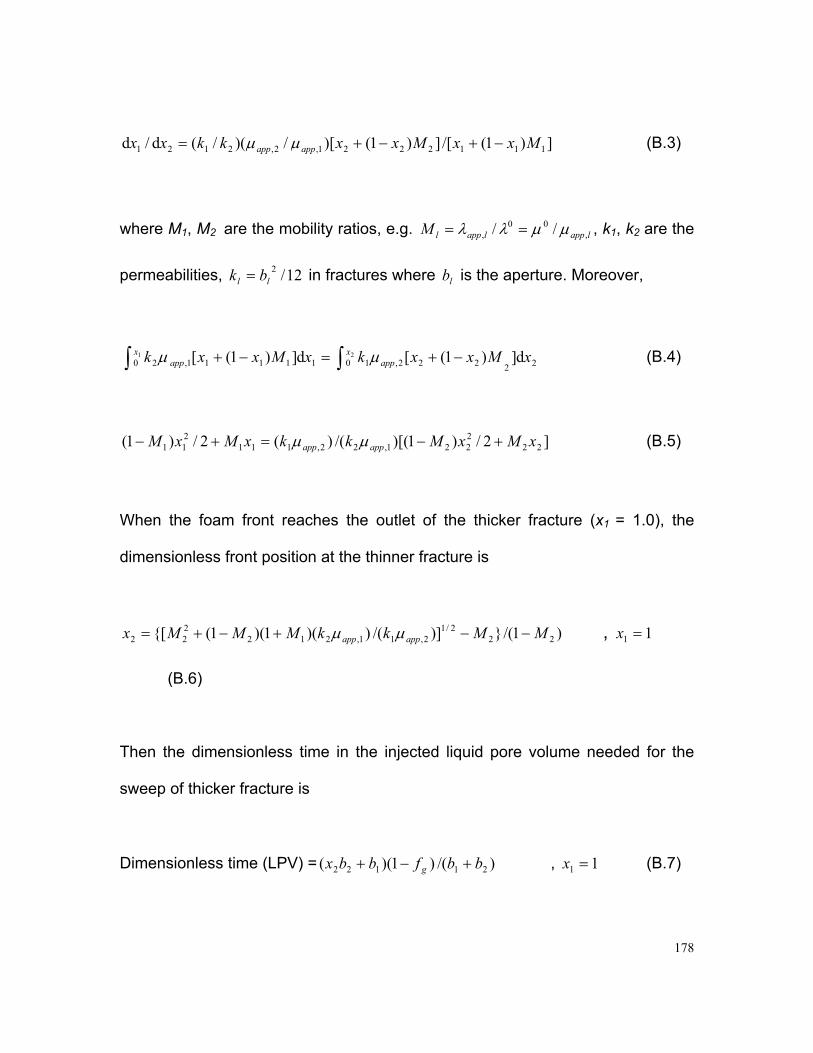
])1(/[])1()[/)(/(d/d 1112221,2,2121 MxxMxxkkxx appapp −+−+= µµ (B.3)
where M1, M2 are the mobility ratios, e.g. M , klapplappl ,00
, // µµλλ ==
lb
1, k2 are the
permeabilities, in fractures where is the aperture. Moreover, 12/2ll bk =
22222,1011111,20 d])1([d])1([ 21 xMxxkxMxxk appx
appx ∫∫ −+=−+ µµ (B.4)
]2/)1)[(/()(2/)1( 222221,22,111
211 xMxMkkxMxM appapp +−=+− µµ (B.5)
When the foam front reaches the outlet of the thicker fracture (x1 = 1.0), the
dimensionless front position at the thinner fracture is
)1/(})]/())(1)(1({[ 222/1
2,11,212222 MMkkMMMx appapp −−+−+= µµ , =x
(B.6)
11
Then the dimensionless time in the injected liquid pore volume needed for the
sweep of thicker fracture is
Dimensionless time (LPV) = ( )/()1)( 21122 bbfbbx g +−+ , (B.7)
11 =x
178

As the thinner fracture continues to be swept, the hypothetical dimensionless
front position in the thicker fracture (outside the fracture) can be obtained from 1z
])1()[/)(/(d/d 2221,2,2121 Mxxkkxz appapp −+= µµ (B.8)
That is, the product is the volume of foam produced from fracture 1
after foam breakthrough.
Lbwz )1( 1 −
∫∫ −+= 2
02
1
22221,2,211 1 d])1()[/)(/(dx
x appapp
zxMxxkkz µµ (B.9)
)](2/))()(1)[(/)(/(1 0222
202
2221,2,211
xxMxxMkkz appapp −+−−+= µµ (B.10)
Setting 0.12 =x
)]12,1k appµ
, and
, one finds )1/(}/())(1)(1({[ 222/
1,21222
02 MMkMMMx app −−+−+= µ
)]2/()1(2/)1)[(/(1 2,11,2121,22,11 appappappapp kkMMkkz µµµµ +−++= (B.11)
And the dimensionless time or the injected liquid pore volume needed to sweep
the thinner fracture is
Dimensionless time (LPV) = ( )/()1)( 12211 bbfbbz g +−+ , x (B.12) 12 =
179
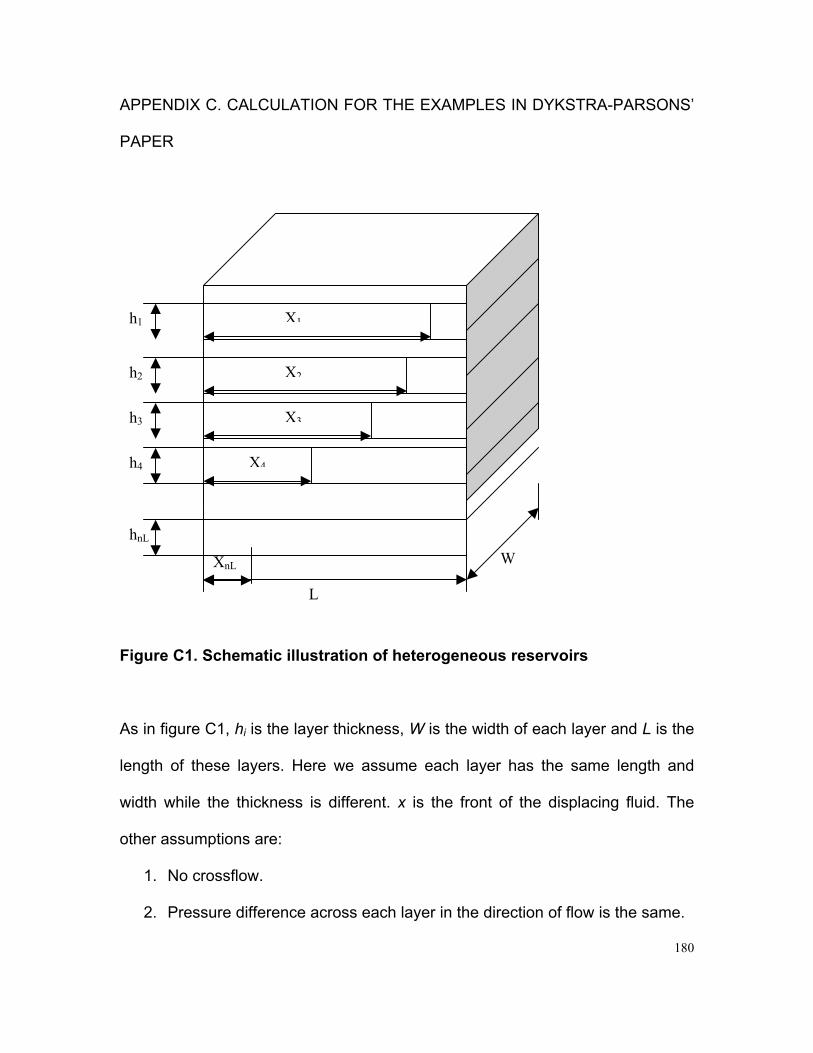
APPENDIX C. CALCULATION FOR THE EXAMPLES IN DYKSTRA-PARSONS’
PAPER
h4
h3
h2
h1
hnL
XnL
Figure C1. Schematic
As in figure C1, hi is th
length of these layers
width while the thickn
other assumptions are
1. No crossflow.
2. Pressure differe
X1
X2
X3
X4
L
W
illustration of heterogeneous reservoirs
e layer thickness, W is the width of each layer and L is the
. Here we assume each layer has the same length and
ess is different. x is the front of the displacing fluid. The
:
nce across each layer in the direction of flow is the same.
180
The number of break-through layer at some water oil ratio WOR was obtained by
∑
∑
+=
==Ln
nii
n
ii
Q
QWOR
1
1 (C.1)
Where is the total number of layers and is the number of layers water
breaks through. is the flow rate in layer i.
Ln n
iQ
whLpk
Q ii
ii
∆−=µ
(C.2)
iiiii xx 21 )1( µµµ −+= (C.3)
where x is the dimensionless front position between the displacing and
displaced fluid.
For the pressure difference over the entire length of the layerLp∆ is the same for
each layer, the equation to get WOR can be obtained.
181

[ ]∑
∑
+=
=
−+
=Ln
ni iiii
ii
n
i i
ii
xxhk
hk
WOR
1 21
1 1
)1( µµ
µ (C.4)
where 1µ is the apparent viscosity of water and 2µ is the apparent viscosity of
oil, x is the dimensionless front position of water. The equation for x is derived
as below:
[ ] wiii
ii
wiiii
i
wi
ii
SLp
mxxk
SLp
xxk
SLpk
dtdx
Φ∆∆
−+−=
Φ∆∆
−+−=
Φ∆∆
−=1
)1(/1
)1(1 1
21
µµµµ
(C.5)
Where is the porosity and Φ wS∆ is the water saturation difference between the
water and oil zone. Now we assume Φ and wS∆ keep the same in each layer.
is the mobility ratio in layer i and is obtained by im im
i
iim
1
2
µµ
= (C.6)
Before layer k breakthrough,
kkk
iii
k
i
i
k
i
k
mxxmxx
kk
dxdx
)1()1(
1
1
−+−+
=µµ (C.7)
182
iiiiikx
kkkkkix dxmxxkdxmxxk ik ])1([])1([ 1010 ∫∫ −+=−+ µµ (C.8)
]2
)1([
2)1( 2
1
12iii
i
ki
ikkkk
k xmxm
kk
xmxm
+−
=+−
µµ (C.9)
By setting 0.1=kx
i
i
ki
ik
kii
i m
m
kk
mmm
x−
−
+−
+
=1
)(
)1)(1(
2/1
1
1
2
µµ
(C.10)
ix in this equation is the water front for “slow layer” (not breakthrough). If the
thickness of a heterogeneous system is arranged from large layer to small layer,
the water front in all the layers with the layer number larger than k can be
obtained from equation (C.10).
After layer k breakthrough, we can use the similar method to find the hypothetical
front for “fast layer” (already breakthrough )
])1([1
1iii
k
i
i
k
i
k mxxkk
dxdx
−+=µµ (C.11)
183

∫∫ −+= i
i
k x
x iiiik
i
i
kx
k dxmxxkk
dx0
])1([1
1
1 µµ (C.12)
)]())((2
)1([1 0202
1
1iiiii
i
k
i
i
k xxmxxm
kk
xk
−+−−
+=µµ (C.13)
by setting and 0.1=ixi
i
ki
ik
kii
m
m
kk
mmm
xi −
−
+−
+
=1
)(
)1)(1(
2/1
1
1
2
0 µµ
])(2
)1(2
)1([1
1
11
1
ki
ik
ki
k
i
i
k
kkmm
kkx
k
µµµ
µ +−
++= (C.14)
At specific WOR, the number n can be found by the way of linear interpolation.
Then the water front in already breakthrough layer and not breakthrough layer
can be obtained from the equations (C.14) and (C.10). After finding the water
front, the sweep efficiency and dimensionless time at that WOR can be
calculated. The sweep efficiency can be shown as the percentage of the whole
volume that has been covered by displacing fluid. The dimensionless time is
shown as how much pore volume of displacing fluid is injected.
184
Sweep efficiency=
∑
∑∑
=
+==
+
L
L
n
ii
n
niii
n
ii
h
hxh
1
11 (C.15)
Dimensionless time =
∑
∑
=
=
L
L
n
ii
n
iii
h
hx
1
1 (C.16)
In Dykstra-Parsons’ paper, there are 8 examples for calculation of sweep
efficiency (coverage) for water flooding in oil fields at different permeability
variation and mobility ratiom . At the assumption of the 50 layers in the
examples is at equal thickness , we got similar results from the simulation to
those results in Dykstra-Parsons’ paper which is shown in Fig. C2. The water/oil
sweep has a constant mobility ratio and constant viscosity of water and oil
viscosity in each layer. The other assumption is the layers have log-normal
distributed permeability.
V
ih
Heterogeneity
The simulation was on the assumption that the permeability is in a lognormal
distribution. The lognormal permeability distribution can be described by the
function
185

+= )
2(1
21 τerfC (C.17)
where ν
τ)ln(kk
=
Comparison between calculation and D-P values
0
0.2
0.4
0.6
0.8
1
1.2
0.5 0.5 0.58 0.58 0.71 0.71 0.8 0.8
V
Cov
erag
e
CalculationD-P valueM=0.6 M=0.06
M=10
M=1
M=2.6
M=0.26
M=0.6M=0.06
Fig. C.2 Comparison of simulation results with Dykstra Parson's value
The function C is the fraction of the samples that have permeability less than
, i.e., cumulative probability function. The parameter
)(k
k k is the median
186

permeability or log-mean permeability. The parameter ν is the variance of the
distribution. We may divide the cumulative probability 100% by the layers number
and get the different values of C. If the log-mean value k and variance ν are
known, different values of can be obtained. k
Dykstra and Parsons defined a permeability variation V . The relationship
between V and ν is
2)]1[ln( V−=ν (C.18)
187


![(GJH &RJQLWLYH 6ROXWLRQV ZLWK 0LFURVRIW ,R7easdam.blob.core.windows.net/iotinaction...,r7 (gjh,r7 $]xuh 6skhuh26,r7:lqgrzv ,r7 /lqx[$]xuh,r7 (gjh &rpsdwleoh zlwk srsxodu rshudwlqj](https://img.pdfslide.us/doc/110x75/5f8df0458c541e24040c3752/gjh-rjqlwlyh-6roxwlrqv-zlwk-0lfurvriw-r7-gjhr7-xuh-6skhuh26r7lqgrzv.jpg)