ABSTRACT

Title of dissertation: CLASS NUMBERSOF REAL CYCLOTOMIC FIELDSOF CONDUCTOR pq

Eleni Agathocleous, Doctor of Philosophy, 2009

Dissertation directed by: Professor Lawrence WashingtonDepartment of Mathematics

The class numbers h+ of the real cyclotomic fields are very hard to compute.

Methods based on discriminant bounds become useless as the conductor of the field

grows and that is why other methods have been developed, which approach the

problem from different angles. In this thesis we extend a method of Schoof that was

designed for real cyclotomic fields of prime conductor to real cyclotomic fields of

conductor equal to the product of two distinct odd primes. Our method calculates

the index of a specific group of cyclotomic units in the full group of units of the field.

This index has h+ as a factor. We then remove from the index the extra factor that

does not come from h+ and so we have the order of h+. We apply our method to

real cyclotomic fields of conductor < 2000 and we test the divisibility of h+ by all

primes < 10000. Finally, we calculate the full order of the l-part of h+ for all odd

primes l < 10000.

CLASS NUMBERS OF REAL CYCLOTOMIC FIELDS OFCONDUCTOR pq

by

Eleni Agathocleous

Dissertation submitted to the Faculty of the Graduate School of theUniversity of Maryland, College Park in partial fulfillment

of the requirements for the degree ofDoctor of Philosophy

2009

Advisory Committee:Professor Lawrence Washington Chair/AdvisorAssociate Professor Harry TamvakisAssociate Professor Niranjan RamachandranProfessor Joel CohenProfessor William Gasarch

c© Copyright byEleni Agathocleous

2009

Acknowledgments

First and foremost I would like to thank my advisor, Professor Lawrence Wash-

ington, for his continuous guidance, support and excellent advice, for replying to

every single e-mail that I sent and for all the hours that he spent on the improve-

ment of this thesis. In every way, this document would not exist without him. I

would also like to thank Professors Harry Tamvakis, Niranjan Ramachandran, Joel

Cohen and William Gasarch for agreeing to serve on my committee.

I also wish to thank Haralambos Kafkarides for his continuous support and

encouragement, as well as my parents, Athos and Maro, my sister Nasia, and Maria-

Eleni. Finally I would like to thank all of my friends in College Park and in Wash-

ington DC and especially Christos Economides and Christina Aristidou, for all their

help and support and for making my stay here pleasant and fun!

ii

Table of Contents

0 Introduction 1

1 Extension of Schoof’s Methodto Real Cyclotomic Fields of Conductor pq 71.1 Schoof’s Method . . . . . . . . . . . . . . . . . . . . . . . . . . . . . 71.2 Finite Gorenstein Rings . . . . . . . . . . . . . . . . . . . . . . . . . 91.3 Extension of the Method to Real Cyclotomic Fields

of Conductor pq . . . . . . . . . . . . . . . . . . . . . . . . . . . . . . 121.3.1 Cyclotomic Units . . . . . . . . . . . . . . . . . . . . . . . . . 131.3.2 Leopoldt’s Cyclotomic Units and

the Decomposition of the Class Number of a Real Abelian Field 151.3.3 A New Cyclotomic Unit η . . . . . . . . . . . . . . . . . . . . 181.3.4 The module B= E/H = E/±ηZ[G] . . . . . . . . . . . . . . . . 26

2 The Computational Part and an Example 332.1 Reformulating Theorem 1.1 in terms of Polynomials . . . . . . . . . . 332.2 The Decomposition of the modules B[M ]⊥ . . . . . . . . . . . . . . . 352.3 Grobner Bases . . . . . . . . . . . . . . . . . . . . . . . . . . . . . . . 372.4 The Algorithm . . . . . . . . . . . . . . . . . . . . . . . . . . . . . . 42

2.4.1 Step 1 . . . . . . . . . . . . . . . . . . . . . . . . . . . . . . . 422.4.2 Step 2 . . . . . . . . . . . . . . . . . . . . . . . . . . . . . . . 432.4.3 Step 3 . . . . . . . . . . . . . . . . . . . . . . . . . . . . . . . 44

2.5 An Example . . . . . . . . . . . . . . . . . . . . . . . . . . . . . . . . 48

3 Tables and Discussion of the Results 55

4 Conclusion and Future Projects 59

Appendix 61

Bibliography 80

iii

Chapter 0

Introduction

Let Q(ζm) be the cyclotomic field of conductor m and denote by C its ideal

class group and by h = |C| its class number. In the same way let C+ and h+ denote

the ideal class group and class number of the maximal real subfield Q(ζm)+. The

natural map C+ −→ C is an injection [30, Theorem 4.14] and we have the well

known result h = h+ h−. The relative class number h− is easy to compute as there

is an explicit and easily computable formula for its order [30, Theorem 4.17]. Schoof

in [24] determined the structure and computed the order of h− for a large number of

cyclotomic fields of prime conductor. The number h+ however is extremely hard to

compute. The class number formula is not so useful as it requires that the units of

Q(ζm)+ be known. Methods that use the classical Minkowski bound become useless

as m grows, and other methods based on Odlyzko’s discriminant bounds (see [20]

and [21]) are only applicable to fields with small conductor. Masley in [19] computed

the class numbers for real abelian fields of conductor ≤ 100 and Van der Linden in

[29] was able to calculate the class number of a large collection of real abelian fields

of conductor ≤ 200. For fields of larger conductor however, the above methods can

not be effective. As a result, other methods and techniques were developed that

approach the problem from a different angle.

One of these methods is introduced by Schoof in [25] and is designed for real

1

cyclotomic fields of prime conductor. It is the goal of this thesis to extend his

method to real cyclotomic fields of conductor equal to the product of two distinct

odd primes. Schoof developed an algorithm that computes the order of the module

B=Units/(Cyclotomic Units), which is precisely equal to h+ in his case where the

conductor of the field is a prime number. In our case the order of B is h+, by

Sinnott’s formula that we give in Section 1.3, and therefore we could still work

with the same B as Schoof’s. The complicated structure of the group of cyclotomic

units however when the conductor is not prime, as we will see in 1.3.1, forces us to

provide a replacement for the group of cyclotomic units and therefore for B. Schoof

calculated the various l-parts of h+ by proving that the order of each l-part equals the

order of the finite module B[M ]⊥, M being some power of l. He then proved that the

various B[M ]⊥ are isomorphic to I/f<(η)<, where I is the augmentation ideal

of the group ring R = (Z/MZ)[G], G is the galois group of the extension Q(ζp)+/Q

and the maps f< ∈ HomR(E/±1, R) correspond to the frobenius elements of

unramified prime ideals < which split completely in the extension Q(ζp)+(ζ2M).

These maps are evaluated on η, which is a generator of the group of cyclotomic

units. To facilitate his calculations, he broke each module B[M ]⊥ into its Jordan-

Holder factors and expressed these factors in terms of polynomials so as to compute

their order. He applied his method to real cyclotomic fields of prime conductor p <

10000 and he calculated the l-part of h+ for the largest subgroup of Bl whose Jordan-

Holder factors have order < 80000. One of the great advantages of his method is

that it did not exclude the primes dividing the order of the extension, as opposed

to other methods that we discuss below. However, since he computed the order of

2

the largest subgroup of Bp whose Jordan-Holder factors have order less than 80000,

there is a slight probability that he did not get the full l-part of h+ but only part

of it.

Many of the other methods employ the well known Leopoldt’s decomposition

of the class number h+ of a real abelian field K, see [17], which derives from his

decomposition of the cyclotomic units into the product of the cyclotomic units of

all cyclic subfields Kξ of K. More specifically, we have that h+ = Q∏

χ hχ, where

the product runs over all non-trivial characters χ irreducible over the rationals, each

‘class number’ hχ is the index of the cyclotomic units of Kχ in its full group of units

Eχ and Q is some value which equals 1 in the case where the extension K/Q is cyclic

of prime order, but which is very hard to compute in the general case.

Gras and Gras in [12] used the above decomposition of cyclotomic units and

proved that for each cyclic subfield Kχ of K, there is a unit ε in the full group of

units Eχ of Kχ which is of the form ε = ηm, where η is a cyclotomic unit, and

ε has the property that m equals the order of the ‘class number’ of the specific

cyclic subfield Kχ. In the same paper we find a method that checks whether the

m-th root of a unit belongs to a subfield of K. This method has been employed by

Schoof in [25] and Hakkarainen in [13] and we use it here as well, in the third step

of our algorithm, modified however, in order to fit our case. In a different paper by

Gras, see [11], one can find some interesting results proved for a special case of real

abelian fields. Gras worked with cubic, cyclic extensions and proved that for any

Z ′-submodule F of the full group of units E there exists an element ω in the group

ring Z ′ = Z[G]/(1 + σ+ σ2) ∼= Z[ζ3] with the property that [E:F ] = NQ(√−3)/Q(ω).

3

This element ω is associated with the class number of these extensions and, together

with other facts proved in this article, Gras was able to calculate the class number

for cubic, cyclic extensions of conductor < 4000.

Recently in his thesis, Hakkarainen in [13] also used Leopoldt’s decomposition

to prove whether a prime l divides h+, and since he worked with arbitrary real

abelian fields K he could not draw exact conclusions about the l-part of h+ for the

primes that divide the degree of the extension K/Q. In order to prove the divisibility

of h+ by a prime l not dividing the degree, it sufficed to prove that l divides any of the

‘class numbers’ of the cyclic sub-extensions of K, since in Leopoldt’s decomposition

of the class number, any prime dividing h+ that does not divide the degree of the

extension can only come from the ‘class numbers’ of the cyclic sub-extensions. In

practice Hakkarainen checked the divisibility of h+ by all primes < 10000. He used

the method of Schwarz, see [27], in order to exclude the primes that do not divide h+

and used some ideas from van der Linden to search for units that are l-th powers in

the full group of units. Finally, he employed a method from [12] that we mentioned

above, to verify the divisibility of h+ by l. He applied his method to real abelian

number fields of conductor < 2000. In this thesis we apply our algorithm to the

fields of conductor pq that appear in Hakkarainen’s tables. We verify all the primes

that he obtained and we also complete his results in the sense that we verify the

divisibility of h+ by the exact power of those primes l < 10000 that also happen to

divide the degree of the extension.

There are also other methods that approach the problem of computing h+ in

different ways to the ones described above. Aoki, in [3], describes a method for

4

computing annihilators of the ideal class group. The method for the annihilators

of the plus part of the ideal class group that he describes in this paper involve

the construction of maps like the ones used in Schoof [25] for the description of

his modules whose order give the l-part of h+. The image of these maps in Aoki’s

paper, when applied on cyclotomic units give higher annihilators for the l-part of

h+. These ideas are based on the work of Thaine [28], as well as on the work of V.

Kolyvagin and K. Rubin. In another paper by Aoki and Fukuda [4], an algorithm

is introduced for the calculation again of the l-part of h+, but for odd primes not

dividing the degree of the extension.

Cornacchia in [7] studied a Galois module L introduced by Anderson in [2],

whose structure is related to both the circular units and the Stickelberger ideal.

Cornacchia studied this module for cyclotomic fields of prime conductor. He de-

composed Anderson’s module into its χ-components, where χ is a l-adic character

of the subgroup D of the galois group G with (|D|, l)=1 and then proved that

Ldualχ∼= (Z[G]χ/M)/Jχ, where Jχ is an ideal generated by homomorphisms repre-

senting maps from the group of l - units into Zχ[G]/M , where M is some sufficiently

large power of l. By applying his results with l = 2, he was able to calculate the

2-part of h+ for cyclotomic fields of prime conductor < 10000. Some of Cornacchia’s

ideas are also employed by Schoof in [25] that we have already discussed above.

In Chapter 1 that follows the introductory part of this thesis, we discuss in

more detail the method of Schoof. We stress the difficulties that arise when one

tries to apply it to cyclotomic fields of non-prime conductor and we show how to

generalize it in order to apply it to our case of cyclotomic fields of conductor pq. We

5

present a new unit and calculate the index of the subgroup that it generates, in the

full group of units. This group will replace the group of cyclotomic units that was

used for the fields of prime conductor. We then reformulate the main theorems of

Schoof in order to match our generalized case. In Chapter 2 we describe the results

of Chapter 1 in terms of polynomials so that we can perform our calculations, and

we give some basic facts about Grobner Bases since our polynomials are in two

variables. We then describe the three steps of the algorithm and give an example.

In Chapter 3 we present and discuss the tables with our results and in Chapter 4

we finish with the conclusion and future projects that can follow from this work.

6

Chapter 1

Extension of Schoof’s Method

to Real Cyclotomic Fields of Conductor pq

As was already explained in the introduction, the methods for calculating the

class number h+ of a real cyclotomic field which are based on discriminant bounds

become useless as the conductor of the field grows. That is why other techniques

were developed that approached the problem from a different angle. One of these is

Schoof’s method presented in [25], which focuses on the real cyclotomic fields Q(ζp)+

with prime conductor p. We will give a brief description of the method below so

that the reader can understand the changes one has to make in order to generalize it

to fields of non-prime conductor. A complete and formal description of our method

for real cyclotomic fields of conductor pq will start from Section 3, right after the

definition and some properties of finite Gorenstein Rings in Section 2, which we will

need to support the theoretical part of our method.

1.1 Schoof’s Method

For the fields Q(ζp)+ that Schoof focused on, we have that h+ = [E:H], where

E is the group of units of Q(ζp)+ and H is its subgroup of cyclotomic units. The

quotient B = E/H is a finite Z[G]-module, where G = Gal(Q(ζp)+/Q) is a cyclic

group of order (p − 1)/2 and we see that |B| = h+. Let l be any prime number.

7

As the order of B is the product of its l-parts, Schoof studied the modules B[M ]⊥

instead, where M is a power of l, since as we will see in the next section, for finite

Gorenstein rings R and any finite R-module A we have that

HomR(A,R) = A⊥ ∼= Adual = HomZ(A,Q/Z)

and therefore |A| = |Adual| = |A⊥|. Now, for each B[M ]⊥ Schoof found the order of

its simple Jordan-Holder factors since the product of those factors gives the order

of B[M ]⊥. First, he expressed the modules B[M ]⊥ in a way that facilitated the

calculations. For I, the augmentation ideal of the ring R = (Z/MZ)[G], he proved

that B[M ]⊥ ∼= I/f<(η)< where η is a generator of the group of cyclotomic units

H, f< is the frobenius group ring element that corresponds to an unramified prime

ideal < which splits completely in the extension Q(ζp)+(ζ2M)/Q, and < runs through

all such unramified prime ideals. Since he studied the l-parts of B he worked in Zl

and he used the isomorphism

Zl[G] ∼= Zl[x]/(x(p−1)/2 − 1)

where x ↔ σ : ζp + ζ−1p 7→ ζgp + ζ−gp , g a primitive root modulo p. The frobenius

maps he wrote as polynomials in the variable x. More specifically, for each fixed

l he wrote the order of G as mla with (m, l) = 1, so that the polynomial xm − 1

could be written as a product of irreducible polynomials φ in Zl[x]. This gave the

following isomorphism of Zl-algebras

Zl[G] ∼= Zl[x]/(x(p−1)/2 − 1) ∼= Zl[x]/((xla)m − 1) ∼=

∏φ Zl[x]/(φ(xl

a))

where the factors Zl[x]/(φ(xla)) are complete local Zl[G]-algebras with maximal

ideals (l, φ(x)) and residue fields isomorphic to F = Fl[x]/(φ(x)). The order of F

8

is lf , where f is the degree of φ. Using the above decomposition of the ring Zl[G],

one can write the l-part of any finite Zl[G]-module A as

A⊗ Zl ∼=∏φ

Aφ

where

Aφ = A⊗Zl[G] Zl[x]/(φ(xla

)).

As a finite module, A admits a Jordan-Holder filtration with simple factors, each of

which is isomorphic to some F . All these hold in particular for the module B=E/H

and the various B[M ]⊥ described above. A Jordan-Holder factor of B[M ]⊥ has

order lf and it corresponds to the unique subfield of Q(ζp)+ of degree equal to the

order of x in Fl[x]/(φ(x)). Schoof examined the divisibility of h+ by all primes <

80,000, for all cyclotomic fields of prime conductor p < 10,000, and calculated all

the Jordan-Holder factors of the various B[M ]⊥ which had order ≤ 80,000.

As we see above, one of the great advantages of Schoof’s Method, which will

also apply in our method as well, is that it does not exclude the primes dividing the

order of the group, in contrast to other methods that we have already discussed in

the introduction.

1.2 Finite Gorenstein Rings

In this section we give the definition and some basic properties of finite Goren-

stein rings that we will need later on. We follow Schoof [25].

Let R be a finite commutative ring and A any R-module. Define

A⊥ = HomR(A,R) and Adual = HomZ(A,Q/Z).

9

Both of these groups are R-modules.

Definition 1.1. The ring R is Gorenstein if the R-module Rdual is free of rank 1

over R.

Let R be a finite Gorenstein ring. For any M ∈ Z, any finite abelian group

G, and any irreducible polynomial g(x) ∈ R[x], we have that the rings Z/MZ,

(Z/MZ)[G] and R[x]/(g(x)) are finite Gorenstein rings.

In the next proposition we prove a fact that we already mentioned above and

which we will also use in the next chapter.

Proposition 1.1. Let R be a finite Gorenstein ring and let χ : R→ Q/Z denote a

generator of the R-module HomZ(R,Q/Z). Then, for every R-module A, the map

Φ : A⊥ → Adual : f 7→ χ · f is an isomorphism of R-modules.

Proof: For any R-module A we have the canonical isomorphism

HomR(A,HomZ(R,Q/Z)) ∼= HomZ(A,Q/Z).

We also have the R-isomorphism R ∼= HomZ(R,Q/Z) via the map that maps 1 to

χ. Hence A⊥ = HomR(A,R) ∼= HomZ(A,Q/Z) = Adual via the map Φ given in the

statement above. 2

We will also need the two propositions below. The first one shows that any

finite R-module is Jordan-Holder isomorphic to its dual, and together with Propo-

sition 1.1. above, justifies the use of the Jordan-Holder factors of B⊥ instead of B.

The idea of the second one we will use in the third step of our algorithm.

Proposition 1.2. Let R be a finite Gorenstein ring. Any finite R-module is Jordan-

Holder isomorphic to its dual.

10

Proof : Consider the exact sequence

0→ mA→ A→ A/mA→ 0.

Since the functor A → Adual from the category of finite Z/MZ-modules to itself is

exact, we apply it to the sequence above and we obtain the exact sequence

0→ (A/mA)dual → Adual → (mA)dual → 0.

We therefore have that

(A/mA)dual ∼= Adual/(mA)dual ∼= Adual[m] = a ∈ Adual : µa = 0 for all µ ∈ m.

This implies that

|A/mA| = |(A/mA)dual| = |Adual[m]|

and both are vector spaces over R/m. Hence, they have the same dimension and

therefore the same number of simple Jordan-Holder factors R/m. If mA = 0 then

we are done by the above. If A/mA = 0 then there are no Jordan-Holder factors

of R/m for A or for Adual. Now suppose A 6= mA 6= 0. We need the following

definition

Definition 1.2. If the simple factor modules of a composition series of a module

M are Q1, Q2, ..., Qn, we define

jh(M) = Q1 ⊕Q2 ⊕ ...⊕Qn

By induction, we may assume the proposition for all modules of order smaller

than |A|. In particular,

jh(mA) = jh((mA)dual) and jh(A/mA) = jh((A/mA)dual).

11

From the two exact sequences above and by [23, Lemma 7.86] we have that

jh(A) = jh(mA)⊕ jh(A/mA) and jh(Adual) = jh((A/mA)dual)⊕ jh(mAdual).

But since

jh(A/mA) = jh(Adual/mAdual) and jh(mA) = jh(mAdual).

we have that jh(A) = jh(Adual) and this complete the proof of the proposition. 2

Proposition 1.3. Let R be a finite Gorenstein ring and I an ideal of R. Suppose

there is an ideal J ⊂ R and a surjection g : R/J → I⊥ with the property that

AnnR(J) annihilates R/I. Then g is an isomorphism.

Proof: We have that |I| = |I⊥| ≤ |R/J | = |(R/J)⊥| = |AnnR(J)|. The last

equality follows from the fact that (R/J)⊥ is isomorphic to AnnR(J). Since AnnR(J)

⊂ I, we also have that |I| ≥ |AnnR(J)|, so that we must have equality everywhere,

and g is an isomorphism. 2

This concludes our brief introduction to finite Gorenstein rings. We continue

with the theoretical outline of our method.

1.3 Extension of the Method to Real Cyclotomic Fields

of Conductor pq

From our description of Schoof’s method in Section 1, one sees that the first

thing that needs to be considered is the group of units that will replace the group of

cyclotomic units that we have in the case of prime conductor. This subject will be

12

dealt with in 1.3.1. The second step will be to reformulate the main theorem which

describes the modules B[M ]⊥ in terms of the augmentation ideal and the frobenius

maps. This we will present in 1.3.2. In Chapter 2, we will describe everything in

terms of polynomials so that we can perform our calculations.

1.3.1 Cyclotomic Units

The group of cyclotomic units of the fields Q(ζm)+ for m not a prime number,

and therefore for the fields Q(ζpq)+, has a complicated structure. Sinnott in [26]

defined the cyclotomic units attached to an abelian field K as follows:

Definition 1.3. Let K be an abelian field and let Km = K ∩ Q(ζm). Let a be an

integer not divisible by m. The number NQ(ζm)/Km(1 − ζam) lies in K∗. Denote by

Dm the group generated in K∗ by −1 and all such elements NQ(ζm)/Km(1− ζam). The

circular units H are defined by H = E ∩ Dm, where E is the full group of units of

K.

In the same paper, Sinnott calculated their index in the full group of units to

be

[E : H] = 2bh+

where b = 0 if g = 1 and b = 2g−2 + 1− g if g ≥ 2 and g is the number of distinct

prime numbers of the conductor m.

Kucera and Conrad investigated the group of cyclotomic units described in

the definition above, for K being the cyclotomic field of conductor m. Kucera in

[14] found a basis for H and showed that every cyclotomic unit can be written as

13

a product of a root of unity and elements in that basis. Similarly, Conrad in [6]

constructed a basis B for H, with the property that Bd ⊂ Bm for d|m.

In the case where m is an odd prime power, the following units ξa together

with −1 were proven to form a system of independent generators for the group of

cyclotomic units of Q(ζm)+

ξa = ζ(1−a)/2m

1− ζam1− ζm

, 1 < a <1

2m, (a,m) = 1.

For a proof of this see for example [30, Lemma 8.1].

When m is not a prime power however, a set similar to the above does not

work since for example the unit (1− ζm) is not of that form or even worse, this set

might be of infinite index in the group of units and hence does not give full rank.

In this case, other sets of independent units were introduced which, even though

they do not generate the full group of cyclotomic units, they are of finite index in

the full group of units. See for example Ramachandra’s set of independent units in

[22] and Levesque’s system of independent units in [18], which is a generalization of

Ramachandra’s units with smaller index in the full group of units.

In earlier work, Leopoldt in [17] had also studied the group of cyclotomic units.

His approach was to decompose it into the product of the groups of cyclotomic units

that come from all cyclic subfields of the field in hand. The index of this product of

groups in the full group of units however contains a factor whose value is not always

known. We will explain Leopoldt’s decomposition of the cyclotomic units in more

detail below, since many of the methods for computing prime divisors of h+ adopt

this decomposition as it is less complicated to work with the cyclic subfields and

14

their units, instead of the whole field.

Finally, for a detailed presentation and comparison of the various groups of

cyclotomic units and their index in the full groups of units, for the special case of a

compositum of real quadratic fields, see [15].

1.3.2 Leopoldt’s Cyclotomic Units and

the Decomposition of the Class Number of a Real Abelian Field

Let ξ denote a rational character of G irreducible over Q and for each such

ξ 6= ξ0 let Ker(ξ) = α ∈ G|ξ(α) = ξ(1). Then the fields Kξ fixed by Ker(ξ)

are cyclic of conductor fξ and with cyclic galois group Gξ = G/Ker(ξ) of order

gξ. For each Dirichlet character χ let eχ = 1|G|∑

α∈G χ(α−1)α be its corresponding

idempotent and therefore denote by eξ =∑

χ∈[ξ] eχ the orthogonal idempotent of

the algebra Q[G] that corresponds to ξ, with equivalence class denoted by [ξ]. We

should also explain here that two characters ξ belong to the same equivalence class

if they generate the same cyclic subgroup.

Definition 1.4. A real unit ε is a ξ-unit if and only if ε2 ∈ Kξ and NKξ/L(ε2) = 1

for all proper subfields L of Kξ.

For each ξ 6= ξ0 let Eξ ⊂ Kξ be the group of proper ξ-units of Kξ. In other

words, Eξ is the set of ξ-units that lie in Kξ. Denote by Fξ the group generated by

the element θξ = ηγξξ , where ηξ and γξ are defined as follows:

For every automorphism α ∈ Gal(Q(ζfξ)+/Kξ) we choose an extension α ∈

15

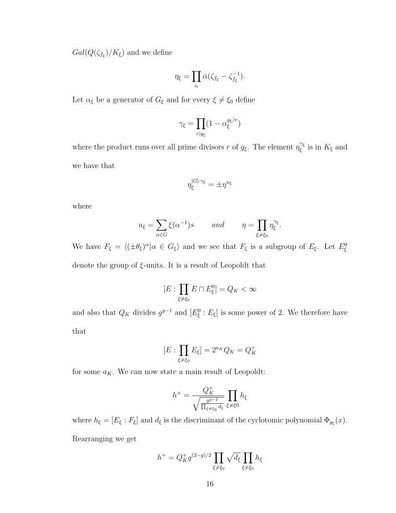
Gal(Q(ζfξ)/Kξ) and we define

ηξ =∏α

α(ζfξ − ζ−1fξ

).

Let αξ be a generator of Gξ and for every ξ 6= ξ0 define

γξ =∏r|gξ

(1− αgξ/rξ )

where the product runs over all prime divisors r of gξ. The element ηγξξ is in Kξ and

we have that

η|G|·γξξ = ±ηuξ

where

uξ =∑α∈G

ξ(α−1)s and η =∏ξ 6=ξ0

ηγξξ .

We have Fξ = 〈(±θξ)α|α ∈ Gξ〉 and we see that Fξ is a subgroup of Eξ. Let E0ξ

denote the group of ξ-units. It is a result of Leopoldt that

[E :∏ξ 6=ξ0

E ∩ E0ξ ] = QK <∞

and also that QK divides gg−1 and [E0ξ : Eξ] is some power of 2. We therefore have

that

[E :∏ξ 6=ξ0

Eξ] = 2aKQK = Q+K

for some aK . We can now state a main result of Leopoldt:

h+ =Q+K√gg−2∏ξ 6=ξ0

dξ

∏ξ 6=ξ0

hξ

where hξ = [Eξ : Fξ] and dξ is the discriminant of the cyclotomic polynomial Φgξ(x).

Rearranging we get

h+ = Q+Kg

(2−g)/2∏ξ 6=ξ0

√dξ∏ξ 6=ξ0

hξ

16

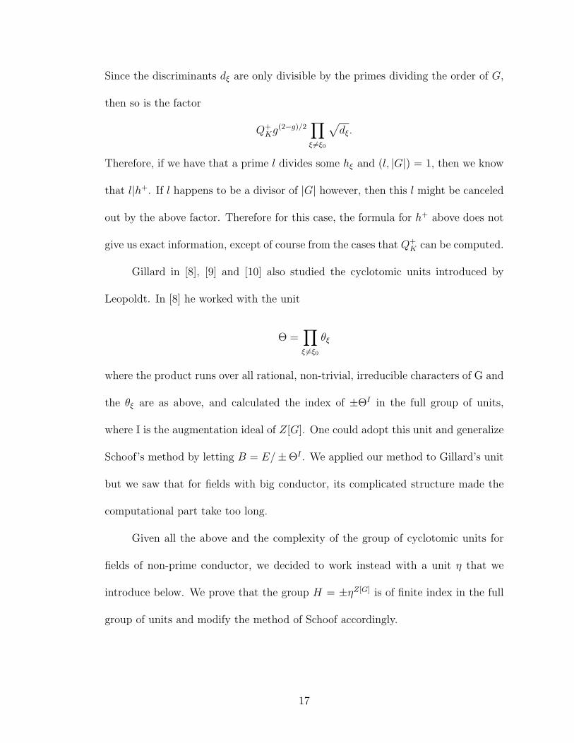
Since the discriminants dξ are only divisible by the primes dividing the order of G,

then so is the factor

Q+Kg

(2−g)/2∏ξ 6=ξ0

√dξ.

Therefore, if we have that a prime l divides some hξ and (l, |G|) = 1, then we know

that l|h+. If l happens to be a divisor of |G| however, then this l might be canceled

out by the above factor. Therefore for this case, the formula for h+ above does not

give us exact information, except of course from the cases that Q+K can be computed.

Gillard in [8], [9] and [10] also studied the cyclotomic units introduced by

Leopoldt. In [8] he worked with the unit

Θ =∏ξ 6=ξ0

θξ

where the product runs over all rational, non-trivial, irreducible characters of G and

the θξ are as above, and calculated the index of ±ΘI in the full group of units,

where I is the augmentation ideal of Z[G]. One could adopt this unit and generalize

Schoof’s method by letting B = E/±ΘI . We applied our method to Gillard’s unit

but we saw that for fields with big conductor, its complicated structure made the

computational part take too long.

Given all the above and the complexity of the group of cyclotomic units for

fields of non-prime conductor, we decided to work instead with a unit η that we

introduce below. We prove that the group H = ±ηZ[G] is of finite index in the full

group of units and modify the method of Schoof accordingly.

17

1.3.3 A New Cyclotomic Unit η

Let p and q be distinct odd primes. From now on, E will denote the group of

units of the real cyclotomic field Q(ζpq)+ and O its ring of integers. Without loss of

generality we will always assume that p < q. Choose and fix g and h, primitive roots

modulo p and q respectively. Denote by η(g,h) the following real unit of Q(ζpq)+:

η(g,h) = ζ−(p+q)pq (1− ζpqp+q)2 ζ

−g/2p

ζ−1/2p

(1− ζgp )

(1− ζp)ζ−h/2q

ζ−1/2q

(1− ζhq )

(1− ζq)

and by H(g,h) the group ±ηZ[G](g,h). We will usually omit the subscripts and just write

H and η since we will let ηα denote the unit η with the galois element α acting on it.

With this notation in mind, we are ready to prove a statement about the regulator

of the units ηαα∈G.

Proposition 1.4. Let E be the group of units of Q(ζpq)+ and H = ±ηZ[G] = ±ηZ[G]

(g,h)

as above, where g and h are any two fixed primitive roots modulo p and q respectively.

The index [E:H] is always finite and it equals:

[E : H] =2|G|−1h+

|G|·

∏χ=χp 6=1

1

2

[2(χ(q)−1−1)+(χ(g−1)−1)(q−1)

]·∏

χ=χq 6=1

1

2

[2(χ(p)−1−1)+(χ(h−1)−1)(p−1)

]where the characters χ in the first product are the even characters χp of conductor

p and those in the second product are the even characters χq of conductor q.

Proof : Define f by f(α) = log|ηα|. We see that∑

α f(α) = log|∏

α ηα| = 0.

Denote by χ an even Dirichlet character and note that for any root of unity ζ we

have that log|ζ i(1− ζj)| = log|1− ζj|, where i and j are arbitrary. The regulator R

18

of the units ηα is:

R = R(ηα)

= ±det(log|ηαβ|)α,β 6=1

= ±det(f(αβ))α,β 6=1

= ±det(f(βα−1))α,β 6=1 (by rearranging the rows)

= ± 1

|G|∏χ 6=1

∑β∈G

χ(β)f(β) (by [30, Lemma5.26(c)])

= ± 1

|G|∏χ 6=1

1

2

∑1≤β≤pq(β,pq)=1

χ(β)[log|1− ζβ(p+q)

pq |2 + log|1− ζgβp1− ζβp

|+ log|1− ζhβq1− ζβq

|]

(∗)

Before we continue with the proof of the proposition, we need the following

lemmas (the proofs are taken from [30]).

Lemma 1.1. For m|n ∈ Z+, if fχ does not divide (n/m) then

∑1≤b≤n,(b,n)=1

χ(b) log|1− ζbmn | = 0.

Proof: We need an a ≡ 1 mod n/m with (a, n)=1 and χ(a) 6= 1. If no such a

exists then for every a ≡ 1 mod(n/m), if (a, n)=1 then χ(a)=1. But this means that

the character χ : (Z/nZ)× → C× can be factored through (Z/(n/m)Z)×, therefore

fχ| (n/m), contradiction. Hence such a exists and since a ≡ 1 mod(n/m) we have

that ζbmn = ζabmn , hence

∑1≤b≤n(b,n)=1

χ(b) log|1− ζbmn | =∑

1≤b≤n(b,n)=1

χ(b) log|1− ζabmn | =

χ(a)−1 ·∑

ab(mod n)(ab,n)=1

χ(ab)log|1− ζabmn | = χ(a)−1 ·∑

1≤b≤n(b,n)=1

χ(b)log|1− ζbmn |.

19

Since χ(a)−1 6= 1, we have that

∑1≤b≤m(b,m)=1

χ(b) log|1− ζbmn | = 0,

as we wanted. 2

Lemma 1.2. Let n = mm′ with (m,m′) = 1 and assume fχ| m. Then

∑1≤b≤n,(b,n)=1

χ(b) log|1− ζbm′n | = φ(m′) ·∑

1≤a≤m,(a,m)=1

χ(a) log|1− ζam|.

Proof: Since fχ| m, χ factors through (Z/mZ)× and for every b with (b, n) =

1 there is a 0 ≤ c < m′ and an 1 ≤ a < m such that (a,m) = 1 and b = a + cm.

Conversely, for every a with (a,m) = 1 there are φ(m′) different choices for c such

that (b = a + cm, n) =1. Since ζbm′

n = ζbm we have that ζbm′

n depends only on a and

it is clear that χ also only depends on a. The lemma now follows. 2

Lemma 1.3. Let P,Q, g ∈ Z+ with fχ|P and g|P . Then

∑1≤b≤PQ,(b,g)=1

χ(b)log|1− ζbPQ| =∑

1≤a≤P,(a,g)=1

χ(a)log|1− ζaP |.

Proof: We can write b as b = a + cP for 1 ≤ a ≤ P and 0 ≤ c ≤ Q− 1. Then

(b, g) = 1 if and only if (a, g) = 1. Also, from the polynomial identity

1− xQ =∏

0≤c≤Q−1

(1− ζcPPQx)

we get the identity

1− ζaP = 1− (ζaPQ)Q = 1− ζaP =∏

0≤c≤Q−1

(1− ζa+cPPQ ).

Since the values of the character χ only depend on a, the lemma follows. 2

20

Lemma 1.4. Let n ∈ Z+ and assume fχ| n. Then

∑1≤b≤n(b,n)=1

χ(b) log|1− ζbn| =∏p|n

(1− χ(p))∑

1≤b≤n

χ(b)log|1− ζbn|.

Proof Let n =∏

i peii with ei ≥ 1 be the prime factorization of n. When we

expand the product∏

p|n(1− χ(p)), the right hand side equals

∑1≤b≤n(b,n)=1

χ(b) log|1− ζbn| −∑pi

χ(pi)∑

1≤b≤n

χ(b)log|1 − ζbn| +

∑pi 6=pj

χ(pipj)∑

1≤b≤m

χ(b)log|1− ζbn| − ...

We see that only those primes with (fχ, pi) = 1 appear in the sum above since

otherwise χ(pi) = 0. Therefore, we have that fχ| (n/pi) and by Lemma 1.3 above

with g =1, the sum becomes equal to

∑1≤b≤n

χ(b)log|1 − ζbn| −∑pi

∑1≤b≤mpi|b

χ(b)log|1 − ζbn| + ... =

∑1≤b≤n(b,n)=1

χ(b)log|1 − ζbn|. 2

We can now continue with the proof of Proposition 1.3.

For a character χ and the first summand in the brackets in (∗) above, we have

2∑

1≤β≤pq(β,pq)=1

χ(β) log|1− ζβ(p+q)pq | =

2χ(p+ q)−1∑

β(p+q) mod(pq)(β(p+q),pq)=1

χ(β(p+ q)) log|1− ζβ(p+q)pq |

= 2χ(p+ q)−1(1− χ(q))(1− χ(p))∑

1≤β≤pq

χ(β) log|1− ζβpq| (by Lemma 1.4).

21

To this sum, for characters of conductor p or q, we apply Lemma 1.3. The first sum

in (∗) now equals:

=

2χ(p+ q)−1

∑1≤β≤pq χ(β) log|1− ζβpq| , iffx = pq

2χ(q)−1(1− χ(q))∑

1≤α≤p χ(α) log|1− ζαp | , if fχ = p

2χ(p)−1(1− χ(p))∑

1≤α≤q χ(α) log|1− ζαq | , if fχ = q

For a character χ and the second summand we have

∑1≤β≤pq(β,pq)=1

χ(β)[log|1 ζgβp | − log |1− ζβp |

]

= χ(g)−1∑

gβ(mod pq)(β,pq)=1

χ(gβ)log|1− ζgβp | −∑

1≤β≤pq(β,pq)=1

χ(β)log|1 − ζβp |

= (χ(g−1)− 1)∑

1≤α≤pq(α,pq)=1

χ(α)log|1 − ζαp |.

If fχ = pq then

∑1≤α≤pq(α,pq)=1

χ(α)log|1 − ζαp | =∑

1≤α≤pq(α,pq)=1

χ(α)log|1 − ζqαpq | = 0 (by Lemma1.1).

Similarly, by applying Lemma 1.1 to the second summand for characters of conductor

q, we also get 0. For the characters of conductor p, we apply Lemma 1.2 to the second

summand. All of the above give the following:

=

0 , iffχ = pq

(χ(g−1)− 1)(q − 1)∑

1≤α≤p χ(α)log|1 − ζαp | , if fχ = p

0 , if fχ = q

Similarly, the third summand equals:

22

=

0 , iffχ = pq

0 , if fχ = p

(χ(h−1)− 1)(p− 1)∑

1≤α≤q χ(α)log|1 − ζαq | , if fχ = q

Putting all three together and denoting by χpq, χp and χq the characters of

conductor pq, p and q respectively, we have that

R = ± 1

|G|∏

χ=χpq 6=1

1

2· 2 χ(p+ q)−1

∑1≤β≤pq

χ(β) log|1− ζβpq|·

∏χ=χp 6=1

1

2

[2χ(q)−1 (1− χ(q)) + (χ(g−1)− 1)(q − 1)

] ∑1≤α≤p

χ(α)log|1− ζαp |·

∏χ=χq 6=1

1

2

[2χ(p)−1 (1− χ(p)) + (χ(h−1)− 1)(p− 1)

] ∑1≤α≤q

χ(α)log|1− ζαq |

The product over all characters of the term χ(p+ q)−1 will give ±1 since the value

of each χ is canceled out by that of χ. Therefore the above equals

= ± 1

|G|·∑

1≤β≤pq

χ(β) log|1− ζβpq|·

∏χ=χp 6=1

1

2

[2(χ(q)−11) + (χ(g−1)− 1)(q − 1)

] ∑1≤α≤p

χ(α)log|1− ζαp |·

∏χ=χq 6=1

1

2

[2(χ(p)−1 − 1) + (χ(h−1)− 1)(p− 1)

] ∑1≤α≤q

χ(α)log|1− ζαq |.

The L-series attached to each even character χ satisfies

L(1, χ) = −τ(χ)

fχ

∑1≤b≤fχ

χ(b)log|1 − ζbfχ|

therefore R is now equal to

R = ± 1

|G|∏

χ=χpq 6=1

(−fχ)

τ(χ)L(1, χ)·

23

∏χ=χp 6=1

1

2

[2(χ(q)−11) + (χ(g−1)− 1)(q − 1)

](−fχ)

τ(χ)L(1, χ)·

∏χ=χq 6=1

1

2

[2(χ(p)−1 − 1) + (χ(h−1)− 1)(p− 1)

](−fχ)

τ(χ)L(1, χ) =

± 1

|G|∏

16=χeven

τ(χ)L(1, χ)·

∏χ=χp 6=1

1

2

[2(1−χ(q))+(χ(g−1)−1)(q−1)

] ∏χ=χq 6=1

1

2

[2(1−χ(p))+(χ(h−1)−1)(p−1)

].

The class number formula for a real number field K of degree n, discriminant d,

class number h+ and regulator R+, is given by the formula

2|G|h+R+

2√|d|

=∏

1 6=χeven

L(1, χ).

By applying this formula to the above, we have that R is now equal to

R =2|G|−1h+R+

|G|·

∏χ=χp 6=1

1

2

[2(χ(q)−1−1)+(χ(g−1)−1)(q−1)

] ∏χ=χq 6=1

1

2

[2(χ(p)−1−1)+(χ(h−1)−1)(p−1)

].

Therefore,

R

R+=

2|G|−1h+

|G|·

∏χ=χp 6=1

1

2

[2(χ(q)−1−1)+(χ(g−1)−1)(q−1)

] ∏χ=χq 6=1

1

2

[2(χ(p)−1−1)+(χ(h−1)−1)(p−1)

].

So now, by [30, Lemma 4.15], we have that

[E : H] =R

R+=

2|G|−1h+

|G|·

∏χ=χp 6=1

1

2

[2(χ(q)−1−1)+(χ(g−1)−1)(q−1)

] ∏χ=χq 6=1

1

2

[2(χ(p)−1−1)+(χ(h−1)−1)(p−1)

]as desired.

24

To show that [E:H] is always finite it suffices to show that the regulator is

never zero. Assume it is zero. Then for some character of conductor p the sum

2(χ(q)−1 − 1) + (χ(g−1)− 1)(q − 1)

is zero or for some character of conductor q the sum

2(χ(p)−1 − 1) + (χ(h−1)− 1)(p− 1)

is zero. But

2(χ(q)−1 − 1) + (χ(g−1)− 1)(q − 1) = 0

⇔

2χ(q)−1 + (q − 1)χ(g)−1 = 2 + (q − 1)

which never happens as χ(g)−1 can never equal 1, since g is a primitive root. Simi-

larly for a character of conductor q. Therefore, the regulator is never zero and this

completes the proof of Proposition 1.3. 2

Denote by P the factor

2|G|−1

|G|·

∏χ=χp 6=1

[2(χ(q)−1−1)+(χ(g−1)−1)(q−1)

] ∏χ=χq 6=1

[2(χ(p)−1−1)+(χ(h−1)−1)(p−1)

]which appears in the index [E:H] in Proposition 1.3 above. We now have

[E : H] = P · h+.

One can take advantage of the fact that any choice of primitive roots g and h give a

finite index, and for each field Q(ζpq)+ one can choose the pair (g,h) with the prop-

erty that P(g,h) is divisible by the smallest number of distinct primes. Furthermore,

25

for the primes that appear in this P(g,h) one can can check to see if those primes

divide the greatest common divisor of all the P(g,h) for every pair of primitive roots

(g,h). In the case that a prime l does not divide the greatest common divisor, there

is some pair (g0, h0) for which l does not divide P(g0,h0). We can therefore repeat the

first part of our algorithm that we explain in the next chapter, for this pair (g0, h0)

and for this prime l. If l does not come up as a possible divisor for this pair of

primitive roots this means that it only divides P(g,h) for the initial choice of g and

h and not the class number. Hence, we do not need to consider this l in the next

steps of the algorithm. These facts are very useful in the computations described in

the next chapter, since they narrow down the number of primes that one needs to

check to see if they divide h+ and hence speed up the calculations.

In the remainder of this chapter we reformulate Schoof’s main theorem that

describes the module B = E/H in terms of the various B[M ]⊥.

1.3.4 The module B= E/H = E/±ηZ[G]

We denote by B be the Z[G]-module E/H, where H = ±ηZ[G] as above. From

Proposition 1.3 we have that the order of B is finite and equals the index [E : H].

Therefore, by generalizing Schoof, we can calculate its order and then multiply by

1/P in order to get h+, as desired.

Since H is of finite index in E we have that the map

26

Φ : Z[G]→ E

: α 7→ ηa

is a homomorphism whose image H is of finite index and therefore Z-isomorphic to

Z |G|−1. We have that H ∼= Z[G]/NG as Z[G]-modules, where NG is the norm of G.

Let M > 1 denote a power of a prime l. We let F = Q(ζpq)+(ζ2M) and ∆ =

Gal(F/Q(ζpq)+).

Lemma 1.5. The kernel of the natural map

j : E/EM → F ∗/F ∗M

is trivial if l odd and it has order two and is generated by −1 if l = 2.

Proof: Fix an embedding F ⊂ C. Then Q(ζpq)+ identifies with a subfield

of R. Suppose 0 < x ∈ E ⊂ R is in Kerj. Then x = yM , some y ∈ F ∗.

Since µM ⊂ F we may assume that y ∈ R and therefore conj(y)=y, where conj

is complex conjugation in ∆. Since ∆ commutative, s(y)=s(conj(y))=conj(s(y))

∀s ∈ ∆, therefore s(y)=±y ∀s ∈ ∆, since y and all its conjugates are real M -

th roots of x. If l 6= 2 then M is odd. Assume ∃s ∈ ∆ with s(y)=−y. Then

x=s(x)=s(yM)=(s(y))M=(−y)M=−x, contradiction. Therefore ∆ fixes y and hence

y ∈ (Q(ζpq)+)∗ and x ∈ EM . Since we took x > 0 we need to check for −1 as well.

Since M odd, (−1)M = −1 therefore −1 ∈ EM as well and in this case j is an

injection. If l = 2 we see that s(y2) = s(y)2 = y2 therefore y2 ∈ Q(ζpq)+∗. The

quadratic subextensions of F/Q(ζpq)+ are Q(ζpq)(i) and Q(ζpq)

+(ñ2) and hence

27

y2 = 2u2 or = ±u2, for some u ∈ E. If y2 = 2u2, then 2 = y2 v2, with v such that

vu =1, which can not happen since then (2) = (v)2 as ideals but 2 does not ramify

in Q(ζpq)+. So we can only have the second case where x=yM=(y2)2(k−1)

. For k ≥ 2

we have x = u2 and therefore x ∈ EM . When k = 1 we have x = y2 = ±u2, but

since x > 0 we still get x = u2 which implies that x ∈ EM . For −1, observe that −1

= ζM2M but −1 is not even a square in Q(ζpq)+ which means kerj = 〈−1〉 of order

two in this case. 2

Let Ω = Gal(F/Q). We have the following exact sequence of galois groups

0→ ∆→ Ω→ G→ 0.

Let < be any prime ideal of F of degree 1, ρ a prime ideal of Q(ζpq)+ and r a prime

number such that < | ρ | r. We have r ≡ ±1 mod(pq) and r ≡ 1 mod(2M). Let g

= |G| = (p−1)(q−1)2

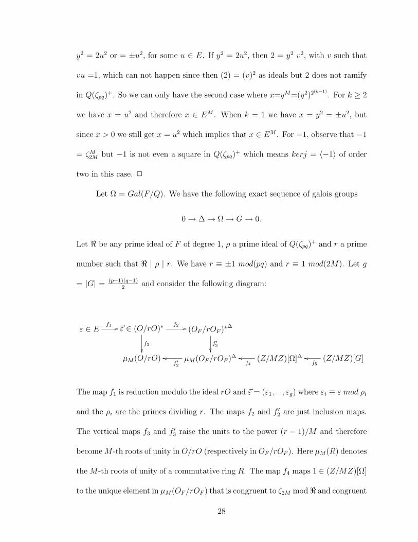
and consider the following diagram:

ε ∈ Ef1 // ~ε ∈ (O/rO)∗

f3

f2 // (OF/rOF )∗∆

f ′3

µM(O/rO) µM(OF/rOF )∆

f ′2

oo (Z/MZ)[Ω]∆f4

oo (Z/MZ)[G]f5

oo

The map f1 is reduction modulo the ideal rO and ~ε = (ε1, ..., εg) where εi ≡ ε mod ρi

and the ρi are the primes dividing r. The maps f2 and f ′2 are just inclusion maps.

The vertical maps f3 and f ′3 raise the units to the power (r − 1)/M and therefore

become M -th roots of unity in O/rO (respectively in OF/rOF ). Here µM(R) denotes

the M -th roots of unity of a commutative ring R. The map f4 maps 1 ∈ (Z/MZ)[Ω]

to the unique element in µM(OF/rOF ) that is congruent to ζ2M mod < and congruent

28

to 1 modulo all the other primes <′ that lie over r. There is such an ε ∈ E with

f ′3f2f1(ε) ≡ ζ2M(mod<) and f ′3f2f1(ε) ≡ 1(mod<′), by the Chinese Remainder

Theorem. Furthermore, since r splits completely in F , the orders of the two groups

are equal and therefore the map f4 is an isomorphism. Finally, the map f5 sends an

element g ∈ G ∼= Ω/∆ to the sum of its inverse images and once we fix an inverse

image g, this comes down to multiplying g by the ∆-norm =∑

s∈∆ s. The map f5

is an isomorphism since (Z/MZ)[Ω]∆ is fixed by ∆. Let f< = f−15 f−1

4 f ′3f2f1. Since

−1 = ζ2MM we have that f<(−1) = 0 and hence f< factors through the quotient

f< : E/± EM → (Z/MZ)[G].

Lemma 1.6. The maps f< correspond to the frobenius elements of the primes over

< in Gal(F ( M√E)/F ). Furthermore, every map in HomR(E/ ± EM , R) is of the

form f< for some < ∈ S where S denotes the set of unramified prime ideals < of

Q(ζpq)+(ζ2M) of degree 1 and R = (Z/MZ)[G].

Proof: Let µM denote the M -th roots of unity and once we choose a primitive

M -th root we have the isomorphism

HomZ(E/± EM , µM) ∼= HomZ(E/± EM , Z/MZ)

which is naturally isomorphic to HomZ(E/± EM , Q/Z). The group E/± EM is a

module over the group ring (Z/MZ)[G] = R, hence

HomZ(E/± EM , Q/Z) ∼= HomZ(E/± EM ⊗R R,Q/Z)

and the Adjoint Isomorphism Theorem gives

HomZ(E/± EM ⊗R R,Q/Z) ∼= HomR(E/± EM , HomZ(R,Q/Z)).

29

By Definition 1.1. we have that

HomZ(R,Q/Z) = Rdual ∼= R

and we have therefore shown that

HomZ(E/± EM , µM) ∼= HomR(E/± EM , R).

Now, from Lemma 1.5 above, we can identify the group E/± EM with a subgroup

of F ∗/F ∗M . Consider the extension F ( M√E)/F . Since < splits completely, we can

associate to it a uniquely determined element β in Gal(F ( M√E)/F ), namely the

frobenius automorphism corresponding to <, such that β( M√ε) ≡ ( M

√ε)r(mod <).

From our definition of f< above we have f<(ε) =∑

s∈G xss where xs is determined

by

s−1(ε)(r−1)/M ≡ ζxsM mod <.

The corresponding homomorphism in HomZ(E/±EM , Z/MZ) maps ε to x1. Since

β(ε)/ε is an M -th root of unity, we can write β( M√ε)/ M√ε ≡ ζx1

M mod < ⇔ ε(r−1)/M

≡ ζx1M mod <. Therefore every f< corresponds to the frobenius map of < in

Gal(F ( M√E)/F ). From Kummer Theory we have that

Gal(F (M√E)/F ) ∼= HomZ(E/± EM , µM)

and we showed above that HomZ(E/ ± EM , µM) ∼= HomR(E/ ± EM , R). By Ce-

botarev’s Density Theorem every element of HomR(E/± EM , R) is of the form f<

for some prime < of degree 1. This concludes the proof of the lemma. 2

Theorem 1.1. Let l and M be as above and let I denote the augmentation ideal of

30

R = (Z/MZ)[G]. We have B[M ]⊥ ∼= I/f<(η) : < ∈ S, where S denotes the set

of unramified prime ideals < of Q(ζpq)+(ζ2M) of degree 1.

Proof: Applying the Snake Lemma to the following diagram

0 −→ H/±1 −→ E/±1 −→ B −→ 0

↓M ↓M ↓M

0 −→ H/±1 −→ E/±1 −→ B −→ 0

yields the exact sequence of R-modules

0 −→ B[M ] −→ H/±HM −→ E/± EM .

Since Q/Z is an injective Z-module, the contravariant functor HomZ(−, Q/Z) is an

exact functor. Furthermore, from Proposition 1.1 we have that A⊥ ∼= Adual. From

both of the above, we therefore get the exact sequence

HomR(E/± EM , R) −→ HomR(H/±HM , R) −→ HomR(B[M ], R) −→ 0.

which gives the isomorphisms

HomR(B[M ], R) = B[M ]⊥ ∼= HomR(H/±HM , R)/HomR(E/± EM , R).

As we showed earlier,

H/±1 ∼= Z[G]/NG

and similarly here

(Z/MZ)[G]/NG∼= H/±HM ,

so the G-norm kills every R-homomorphism f : H/±HM → R. We see that

31

HomR(H/±HM , R) ∼= HomR(R/NG, R) ∼= AnnR(NG) ∼= I.

Furthermore, the map

HomR(E/± EM , R)→ HomR(H/±HM , R)→ I

is given by restriction and then evaluation on η. Therefore, by Lemma 1.6 we have

that

HomR(E/± EM , R) ∼= f<(η) : < ∈ S

where S denotes the set of unramified prime ideals < of Q(ζpq)+(ζ2M) of degree 1.

From all of the above we obtain

B[M ]⊥ ∼= I/f<(η) : < ∈ S,

as we wanted. 2

In the next chapter, we describe everything in terms of polynomials so that

we can perform our calculations, and then we give an example.

32

Chapter 2

The Computational Part and an Example

In this chapter we will use Theorem 1.1 and express B[M ]⊥ in terms of poly-

nomials, so that we can perform our calculations. In this chapter, l will denote an

odd prime.

2.1 Reformulating Theorem 1.1 in terms of Polynomials

Let l be a fixed odd prime, M > 1 some fixed power of l and G denotes the

galois group of Q(ζpq)+. The group G is of order (p− 1)(q − 1)/2 and we have the

isomorphisms

G ∼=(

(Z/pZ)? × (Z/qZ)?)/±1 ∼=

〈σ, τ : σ(p−1) = 1, τ (q−1) = 1, σ(p−1)/2τ (q−1)/2 = 1〉

where σ : ζp 7→ ζγp and τ : ζq 7→ ζδq with γ and δ being fixed primitive roots modulo

p and q respectively. The last of the three relations is the relation for complex

conjugation. The primitive roots γ and δ will be fixed throughout and will always

represent the generators of (Z/pZ)× and (Z/qZ)× respectively. We see that

Z[G] ∼= Z[x, y]/(xp−1 − 1, yq−1 − 1, x(p−1)/2y(q−1)/2 − 1)

via the map that sends σ to x and τ to y. Similarly,

(Z/MZ)[G] ∼= (Z/MZ)[x, y]/(xp−1 − 1, yq−1 − 1, x(p−1)/2y(q−1)/2 − 1).

33

Using this notation, the maps f< that were introduced in the previous chapter can

now be expressed as polynomials in the variables x and y as follows:

f<(x, y) =∑

1≤i≤p−1

∑1≤j≤(q−1)/2

logl(η(i,j)) · xi · yj

where

η(i,j) = ζ−γi

p ζ−δj

q (1− ζγip ζδj

q )2 ζ−gγi/2p

ζ−γi/2p

(1− ζgγip )

(1− ζγip )

ζ−hδj/2q

ζ−δj/2q

(1− ζhδjq )

(1− ζδjq ).

Here, logl denotes the discrete log which gives logl(η) = s where s ∈ Z/MZ is such

that η(r−1)/M ≡ ζsM mod <.

We note here that the second sum in the definition of f<(x, y) goes from 1 up

to (q − 1)/2 since we are in the real subfield of Q(ζpq).

Given the above, we can now reformulate Theorem 1.1 of the previous chapter

as follows:

Theorem 2.1. Let l be a fixed prime and let M > 1 be some fixed power of l.

Denote by R the ring

(Z/MZ)[x, y]/(xp−1 − 1, yq−1 − 1, x(p−1)/2y(q−1)/2 − 1)

and let B[M ]⊥ be as in Theorem 1.1. Then

B[M ]⊥ ∼= (x− 1, y − 1)/f<(x, y) : < ∈ S

where S = the degree 1 prime ideals of Q(ζpq)+(ζ2M).

Proof: From our polynomial description of Z[G] above, it follows that (x −

1, y−1) is the augmentation ideal of (Z/MZ)[G]. The result is now immediate from

Theorem 1.1. 2

34

We have now expressed the modules B[M ]⊥ in terms of polynomials. Another

step that is necessary for our calculating of their orders, especially for fields with

big conductors, is to find a way to break down these modules into smaller pieces.

This we handle in the next section.

2.2 The Decomposition of the modules B[M ]⊥

Let G denote the Galois group of the extension Q(ζpq)/Q. We can write Zl[G]

as follows: for the same fixed prime l as above, write p−1 = m1la1 and q−1 = m2l

a2

where la1||p− 1 and la2||q− 1. Since now l does not divide m1 and m2, we have that

Zl[G] ∼= Zl[x, y]/(xp−1 − 1, yq−1 − 1) ∼=

Zl[x, y]/((xla1 )m1 − 1, (yl

a2 )m2 − 1) ∼=

∏φx,φy

Zl[x, y]/(φx(xla1 ), φy(y

la2 )) ∼=

∏φx

Zl[x]/(φx(xla1 ))⊗

∏φy

Zl[y]/(φy(yla2 ))

where the product runs over all irreducible divisors φx of xm1 − 1 and φy of ym2 − 1.

We see that Zl[x]/(φx(xla1 )) and Zl[y]/(φy(y

la2 )) are complete local Zl[G]-algebras

with maximal ideals (l, φx(x)) and (l, φy(y)), respectively, and the orders of their

residue fields are lf1 and lf2 , where f1 = deg(φx(x)) and f2 = deg(φy(y)). Let ∆

denote the subgroup of G of order prime to l. From the decomposition of Zl[G]

above, we can write any finite Zl[G]-module A as a product of its φ-parts

Aφx,φy = A⊗Zl[G]

(Zl[x]/(φx(x

la1 ))⊗∏φy

Zl[y]/(φy(yla2 ))

).

35

The simple Jordan-Holder factors of each Aφx,φy over Zl[∆] are the same as those

over Zl[G] since we ‘removed’ the powers of x and y dividing the order of G.

All of the above about the module A also hold in particular for B, the var-

ious B[M ]⊥ and their φ-parts B[M ]⊥φx,φy . Therefore, when we want to find the

Jordan-Holder factors of B we can start by taking all combinations of degrees f1

and f2. Since x and y are non-zero elements in the corresponding residue fields[Zl[x]/(φx(x

la1 ))]/(l, φx(x)) and

[Zl[y]/(φy(y

la2 )]/(l, φy(y)), we must have that the

orders of x and y in the ring attached to φx and φy must divide (lf1−1) and (lf2−1)

respectively. Let d1 = gcd(p− 1, lf1 − 1) and d2 = gcd(q − 1, lf2 − 1) and let

Rd1,d2 = (Z/MZ)[x, y]/((xla1 )d1 − 1, (yl

a2 )d2 − 1).

Since the rings Rd1,d2 and Rφx,φy are direct summands of R, any map from their mod-

ules B[M ]d1,d2 and B[M ]φx,φy , respectively, to R will end up in these smaller rings.

Therefore we can refer to B[M ]⊥d1,d2 and B[M ]⊥φx,φy as Rd1,d2 and Rφx,φy modules,

respectively.

We see that, instead of going all the way down to the various B[M ]⊥φx,φy and

looking for the simple Jordan-Holder factors, one could evaluate directly the order

of the various Rd1,d2-modules

B[M ]⊥d1,d2∼= (x− 1, y − 1)/〈(xla1 )d1 − 1, (yl

a2 )d2 − 1, cnj, f<(x, y) : < ∈ S〉 (i)

where S is as in Theorem 2.1 and cnj denotes the conjugation relation

cnj = x(p−1)/2y(q−1)/2 − 1

as above. We have that (1± c)/2 are idempotents in (Z/MZ)[G] for M odd, where

36

c denotes complex conjugation. Therefore, the conjugation relation in the ideal

J = 〈(xla1 )d1 − 1, (yla2 )d2 − 1, cnj, f<(x, y) : < ∈ S〉 (ii)

from (i) above, makes B[M ]⊥d1,d2 a (Z/MZ)[G]-module. Note that here, the poly-

nomials f< are restrictions of the frobenius elements of Theorem 2.1 to this smaller

extension determined by the set of polynomials (xla1 )d1 − 1 and (yl

a2 )d2 − 1. They

are therefore of the form

f<(x, y) =∑

1≤i≤d1la1

∑1≤j≤d2la2

logl(∏

m≡imod(d1la1 )

n≡jmod(d2la2 )

η(m,n)) · xi · yj (iii).

2.3 Grobner Bases

Before we continue with the outline of the algorithm, one last thing that needs

to be discussed is the way we handle the appearance of two variables x and y in

our calculations of the ideals J defined in the previous section, in order to get

a description of the various B[M ]⊥d1,d2 and to also calculate their order. We use

the theory for Grobner Bases, which we present here by following [1]. As before,

d1 = gcd(p − 1, lf1 − 1) will be the order of x and d2 = gcd(q − 1, lf2 − 1) will be

the order of y in the ring Rd1,d2 , where f1 and f2 are the degrees of some irreducible

polynomials φx and φy respectively. Again, let B[M ]⊥d1,d2 be the corresponding

Rd1,d2-module and

J = 〈(xla1 )d1 − 1, (yla2 )d2 − 1, cnj, f<(x, y) : < ∈ S〉

the corresponding ideal. All the computations for the calculation of the frobenius

polynomials were performed in PARI and the computations for a basis for the ideal

37

J in MATHEMATICA, which allows the computations of bases for ideals whose

elements are polynomials in more than one variable and their coefficients are in any

ring (Z/MZ), not necessarily a field.

In this section, R = A[x, y] will denote a polynomial ring in two variables x

and y with coefficients in a Noetherian ring A. Hence R is Noetherian as well. This

R is not necessarily related to the various rings Rd1,d2 of the previous section. We

use R more generally. Because of the appearance of more than one variable in our

polynomials, we need to agree on the order of the variables and also find a way to

compare every element. We call a power product an element of the form xayb with

a, b non-negative integers and we denote by T 2 the set of all power products of the

polynomial ring Rd1,d2 defined in the previous section as

Rd1,d2 = (Z/MZ)[x, y]/((xla1 )d1 − 1, (yl

a2 )d2 − 1).

Following the definition of term order given in [1], we define a total order on T 2 as

follows:

Definition 2.1. By a term order on T 2 we mean a total order < on T 2 which

satisfies the following conditions:

(i) 1 < xayb for all 1 6= xayb ∈ T 2

(ii) If xa1yb1 < xa2yb2 then (xa1yb1)(xcyd) < (xa2yb2)(xcyd) for all (xcyd) ∈ T 2.

The type of term order that we use here is the lexicographical order on T 2

which we define below:

Definition 2.2. The lexicographical order on T 2 with x > y is defined as:

38

For (a1, b1), (a2, b2) with ai, bi positive integers, we define xa1yb1 < xa2yb2 if

and only if (a1 < a2 or (a1 = a2 and b1 < b2)). We therefore have

1 < y < y2 < y3 < ... < x < xy < xy2 < ... < x2 < ...

Now that we have chosen a term order on our polynomial ring, for each poly-

nomial

f = c1xa1yb1 + c2x

a2yb2 + ...+ cnxanybn

with ci 6= 0 in (Z/MZ) and xa1yb1 > xa2yb2 > ... > xanybn , we can define:

lp(f) = xa1yb1 , the leading power product of f ,

lc(f) = c1, the leading coefficient of f ,

lt(f) = c1xa1yb1 , the leading term of f .

Since the coefficients are not necessarily in a field, we need to ‘re-define’ divi-

sion.

Definition 2.3. Let G be a set of polynomials in R, G = g1, g2, ..., gn. We say

that f reduces to h modulo the set G in one step, denoted

fG // h ,

if and only if

h = f − (c1xa1yb1f1 + ...+ csx

asybsfs)

for c1, ..., cs ∈ R and with lp(f) = xaiybilp(fi) for all i such that ci 6= 0 and lt(f) =

c1xa1yb1lt(f1) + ...+ csx

asybslt(fs).

39

Definition 2.4. Let f , h and f1, f2, ..., fs be polynomials in R, with fi 6= 0 ∀ 1 ≤

i ≤ s, and let F = f1, f2, ..., fs. We say that f reduces to h modulo F , denoted

f F // h ,

if and only if there exist polynomials h1, ..., ht−1 ∈ R such that

f F // h1F // h2

F // ... F // ht−1F // h .

We note that if

fF // h ,

then f − h ∈ 〈f1, ..., fs〉.

We will now give the statement of a theorem ([1, Theorem 4.14]) which basi-

cally serves as the definition for a Grobner Basis. We need to state first that the

leading term ideal of an ideal V of a ring R, denoted by LT (V ), is defined as:

LT (V ) = 〈lt(v) : v ∈ V 〉.

Theorem 2.2. Let V be an ideal of R and let G = g1, ..., gn be a set of non-zero

polynomials in V . The following are equivalent:

(i) LT (G) = LT (V ).

(ii) For any polynomial f ∈ R we have

f ∈ V if and only if

fG // 0

(iii) For all f ∈ V , f = h1g1 + ...+ hngn for some polynomials h1, ..., hn ∈ R,

such that lp(f) = max1≤i≤n(lp(hi)lp(gi)). 2

40

Definition 2.5. A set G of non-zero polynomials contained in an ideal V of a ring

R is called a Grobner basis for V if and only if G satisfies any one of the three

equivalent conditions of Theorem 2.2 above. Obviously G is a Grobner basis for

〈G〉.

The Noetherian property of the ring R and Theorem 2.2 above, yield the

following Theorem ([1, Corollary 4.1.17]):

Theorem 2.3. Let J ⊆ R[x, y] be a non-zero ideal. Then J has a finite Grobner

Basis. 2

Denote by GJ a Grobner basis for our ideal J of the ring Rd1,d2 as above. We

see that the order of B[M ]⊥d1,d2 is the order of the quotient

(x− 1, y − 1)/ 〈GJ〉.

In the last step of the algorithm we will also need to compute the annihilator

of some ideal 〈GJ〉 over the finite ring Rd1,d2/Nd, where Nd is the polynomial in

Rd1,d2 representing the norm element. For this we follow a method outlined in [1,

Proposition 4.3.11] and we calculate the ideal quotient

T : 〈GJ〉 = f ∈ Rd1,d2/Nd : f〈GJ〉 ⊆ T

where T = 〈(xla1 )d1 − 1, (yla2 )d2 − 1, Nd〉. We therefore see that

Ann(Rd1,d2/Nd)(〈GJ〉) = T : 〈GJ〉.

We are now ready to describe the steps of the algorithm.

41

2.4 The Algorithm

2.4.1 Step 1

Fix distinct odd primes p and q and an odd prime l. The product pq is

the conductor of the field Q(ζpq)+ whose class number h+ we want to calculate

and M = l is the prime that we check to see if it divides h+. Factor xm1 − 1

and ym2 − 1 into irreducibles in Z/lZ where, as above, gcd(mi, l)=1 for i=1,2 and

m1la1 = p − 1 and m2l

a2 = q − 1. As before, let (f1, f2) be a pair of degrees

of irreducible polynomials φx, φy respectively, which appear in the factorization of

Z[G]. Let d1 = gcd(p − 1, lf1 − 1) and d2 = gcd(q − 1, lf2 − 1). For various primes

r with r ≡ ±1(mod pq) and r ≡ 1(mod 2l) we calculate the frobenius elements

f< as in (ii). Let J0 denote the zero ideal of Rd1,d2 together with the conjugation

relation cnj. We pick several frobenius polynomials f<i that we calculated above

and we let Ji = Ji−1 + (f<i). This ascending chain of ideals will computationally

stabilize at some ideal J l ⊆ (x− 1, y− 1) in Rd1,d2 . If J l happens to equal the whole

augmentation ideal (x − 1, y − 1) of Rd1,d2 , then the module B[l]d1,d2 is trivial. If

however, for some pair of degrees (f1, f2) we have a strict inclusion J l ⊂ (x−1, y−1)

then the corresponding B[l]⊥d1,d2 is not trivial, if J l has indeed stabilized at the correct

ideal J . Hence we believe that l divides the index [E:H].

As expected, in most cases the ideal J l is the whole augmentation ideal and

so we do not continue to steps 2 and 3 for this prime l. When we do get a non-

trivial quotient (x− 1, y − 1)/J l for some l however, we do not proceed to the next

step right away but we follow first the procedure outlined right after the proof of

42

Proposition 1.1.3. That is, for each prime l that appears in the factor P(g,h) for the

specific pair of (g, h) with which we run step 1, but does not appear in the greatest

common divisor of all the P(g,h), we run step 1 again with a pair of primitive roots

(g0, h0) for which l does not divide P(g0,h0). If l gives a non-trivial factor, then we

proceed to the next steps. We follow this procedure because it is computationally

much faster to run step 1 with the same pair of primitive roots (g, h) for all primes,

instead of trying to determine which pair is best for each prime and then running

the test. Furthermore, most primes will give a trivial factor anyway and therefore

it is not worth trying to find the best pair (g, h) for each one of them.

2.4.2 Step 2

In this step we repeat the procedure of step 1 but with higher powers of l, i.e.

for M = l2, l3, etc, and only for those primes which ‘passed’ step 1. The coefficients

of the frobenius polynomials f< now lie in (Z/MZ) and we have to make sure that

the primes r satisfy r ≡ 1(mod 2M) for the specific power M of l. As before, let

Rd1,d2 = (Z/MZ)[x, y]/((xla1 )d1−1, (yl

a2 )d2−1), and denote by IM its augmentation

ideal. As in Step 1, for each M we have that the sequence of ideals

J0 ⊂ J1 ⊂ ... ⊂ Ji ⊂ ...

will stabilize at some ideal JM and from the sequence of surjective maps

...→ IlM/JlM → IM/J

M → ...

we have that the orders of the modules IM/JM are non-decreasing. Since B[M ]⊥d1,d2

is finite and its order is bounded above by |Bd1,d2| which is finite and indepen-

43

dent of M , the orders of the quotients IM/JM will have to stabilize. We will have

that for some power M of l, |IlM/J lM | = |IM/JM | hence IlM/JlM ∼= IM/J

M .

Therefore M annihilates IlM/JlM and therefore it also annihilates its quotient(

IlM/JlM)/〈f<(x, y) : < ∈ S〉 ∼= B[lM ]⊥d1,d2 . This implies that M(B[lM ]duald1,d2

) =

0 which gives M(B[lM ]d1,d2) = 0 since as finite abelian groups, B[lM ]duald1,d2and

B[lM ]d1,d2 are isomorphic. Therefore B[Ml]d1,d2 = B[M ]d1,d2 and

|MBd1,d2| = |Bd1,d2/B[M ]d1,d2| = |Bd1,d2|/|B[Ml]d1,d2| = |lMBd1,d2|.

Therefore (MBd1,d2)/l(MBd1,d2) = 0 and by Nakayama’s Lemma, MBd1,d2 = 0.

Again, since Bd1,d2 and Bduald1,d2

are isomorphic as finite abelian groups, we obtain

MB⊥d1,d2 = 0.

2.4.3 Step 3

In the third and last step we determine the structure and hence the order of

the module B⊥d1,d2 , by showing that the surjective map

g : (x− 1, y − 1)/((xla1 )d1 − 1, (yl

a2 )d2 − 1, JM)→ B⊥d1,d2

is actually an isomorphism.

Let M be as in step 2, i.e. the power of l which annihilates B⊥d1,d2 . Consider

the exact sequence:

0 // B[M ]ψ′ // H/±HM // H/± EM // 0

Recall that the (Z/MZ)[G]-module H/ ± Hm is isomorphic to (Z/MZ)[G]/NG.

Furthermore, since M annihilates B⊥d1,d2∼= HomRd1,d2

(Bd1,d2 , Rd1,d2) that implies

44

that M also annihilates Bd1,d2 . Therefore, tensoring by Rd1,d2 we obtain the following

exact sequence of Rd1,d2-modules

0 // Bd1,d2ψ // Rd1,d2/Nd

// (H/± EM)d1,d2// 0 .

With the ideals IM , JM ⊆ Rd1,d2 as above, we have the exact sequence

0→ JM → IM → IM/JM → 0

which yields the following exact sequence of Rd1,d2-duals

0→ HomRd1,d2(IM/J

M , Rd1,d2)→ HomRd1,d2(IM , Rd1,d2)→

HomRd1,d2(JM , Rd1,d2)→ 0.

We need the following: For any ideal J ⊆ R, R some finite Gorenstein ring, du-

ality yields a surjection R ∼= HomR(R,R) → HomR(J,R). Therefore every R-

homomorphism from J to R is given by multiplication by some element of R and so

from the last exact sequence we have that

HomRd1,d2(IM , Rd1,d2)

∼= Rd1,d2/AnnRd1,d2 (IM) = Rd1,d2/Nd.

Therefore, the kernel of the map

HomRd1,d2(IM , Rd1,d2)→ HomRd1,d2

(JM , Rd1,d2)

is Ann(Rd1,d2/Nd)(JM) and we have that (IM/J

M)⊥ = HomRd1,d2(IM/J

M , Rd1,d2)∼=

Ann(Rd1,d2/Nd)(JM). From the surjection g : IM/J

M → B⊥d1,d2 that we established

from step 2 we have an injection

Ψ : Bd1,d2 → (IM/JM)⊥ ∼= Ann(Rd1,d2/Nd)(J

M).

45

Assume that AnnRd1,d2/(Nd)(JM) annihilates

(Rd1,d2/Nd

)/ψ(Bd1,d2). Then

AnnRd1,d2/Nd(JM) ⊆ ψ(Bd1,d2).

But now we have that

|AnnRd1,d2/Nd(JM)| ≤ |ψ(Bd1,d2)| = |Bd1,d2| = |Ψ(Bd1,d2)| ≤ |Ann(Rd1,d2/Nd)(J

M)|.

Therefore we have that the orders of IM/JM and B⊥d1,d2 are equal and hence g is an

isomorphism. From the second exact sequence above we have that

(Rd1,d2/Nd

)/ψ(Bd1,d2)

∼= (H/± EM)d1,d2 .

Hence, if we show that AnnRd1,d2/Nd(JM) annihilates (H/ ± EM)d1,d2 , we will have

proved that g is an isomorphism.

To find the annihilator AnnRd1,d2/Nd(JM) we find a Grobner basis GJM for the

ideal JM and then we calculate the ideal quotient as explained before step 1 above.

That is, we calculate the ideal quotient

T : 〈GJ〉 = f ∈ Rd1,d2/Nd : f〈GJ〉 ⊆ T

where T = 〈(xa1)d1 − 1, (ya2)d2 − 1, Nd〉. We therefore see that

AnnRd1,d2/Nd(〈GJ〉) = T : 〈GJ〉.

Then, we apply each generator h(x, y) of the annihilator to the unit ηd1,d2 , where

ηd1,d2 is the unit η with the ‘norm’ element (xp−1−1)(yq−1−1)

(xla1d1−1)(yl

a2d2−1)applied to it. If η

h(x,y)d1,d2

is an M -th power of a unit in E then we are done. To see whether it is an M -th

power we follow a method similar to the one in Gras and Gras [12] that we also

46

mentioned in the Introduction. We reformulate here the main proposition from [12]

in order to make it applicable to our case and we prove it again, only for the case

that l is odd since we only calculate the odd l-parts of h+.

We denote by ηhd the unit ηh(x,y)d1,d2

that we already described above and by Gd

the quotient of G containing the coset representatives of the embeddings in G, which

map ζp to ζgi

p and ζq to ζhi

q , for 1 ≤ i ≤ la1d1 and ≤ j ≤ la2d2.

Proposition 2.1. Let M be a fixed power of an odd prime l as above and consider

the polynomial

P (X) =∏a∈Gd

(X − (a(ηhd ))1/M)

where (a(ηhd ))1/M denotes the real M-th root of a(ηhd ). If P has coefficients in Z then

ηhd is an M-th power in Q(ζpq)+.

Proof: Let N be the largest power of l for which the unit (ηhd )1/N lies in

Q(ζpq)+. If M = N then we are done so we assume N < M . Then (ηhd )1/N is not

an element of (Q(ζpq)+)l and therefore by [16, Chapter VIII, Theorem 16] we have

that the polynomial

T (X) = XM/N − (ηhd )1/N

is irreducible in Q(ζpq)+. Since M/N ≥ 3, T (X) has at least one complex root.

Therefore (ηhd )1/M has at least one Galois conjugate that is not real. But P (X) ∈

Z[X] implies that the Galois conjugates are roots of P (X) which are real. Therefore

we have a contradiction. 2

47

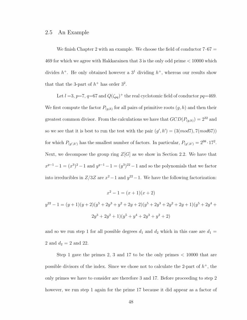
2.5 An Example

We finish Chapter 2 with an example. We choose the field of conductor 7·67 =

469 for which we agree with Hakkarainen that 3 is the only odd prime < 10000 which

divides h+. He only obtained however a 31 dividing h+, whereas our results show

that that the 3-part of h+ has order 32.

Let l =3, p=7, q=67 andQ(ζpq)+ the real cyclotomic field of conductor pq=469.

We first compute the factor P(g,h) for all pairs of primitive roots (g, h) and then their

greatest common divisor. From the calculations we have that GCD(P(g,h)) = 232 and

so we see that it is best to run the test with the pair (g′, h′) = (3(mod7), 7(mod67))

for which P(g′,h′) has the smallest number of factors. In particular, P(g′,h′) = 298 ·172.

Next, we decompose the group ring Z[G] as we show in Section 2.2. We have that

xp−1−1 = (x3)2−1 and yq−1−1 = (y3)22−1 and so the polynomials that we factor

into irreducibles in Z/3Z are x2−1 and y22−1. We have the following factorization:

x2 − 1 = (x+ 1)(x+ 2)

y22 − 1 = (y + 1)(y + 2)(y5 + 2y3 + y2 + 2y + 2)(y5 + 2y3 + 2y2 + 2y + 1)(y5 + 2y4 +

2y3 + 2y2 + 1)(y5 + y4 + 2y3 + y2 + 2)

and so we run step 1 for all possible degrees d1 and d2 which in this case are d1 =

2 and d2 = 2 and 22.

Step 1 gave the primes 2, 3 and 17 to be the only primes < 10000 that are

possible divisors of the index. Since we chose not to calculate the 2-part of h+, the

only primes we have to consider are therefore 3 and 17. Before proceeding to step 2

however, we run step 1 again for the prime 17 because it did appear as a factor of

48

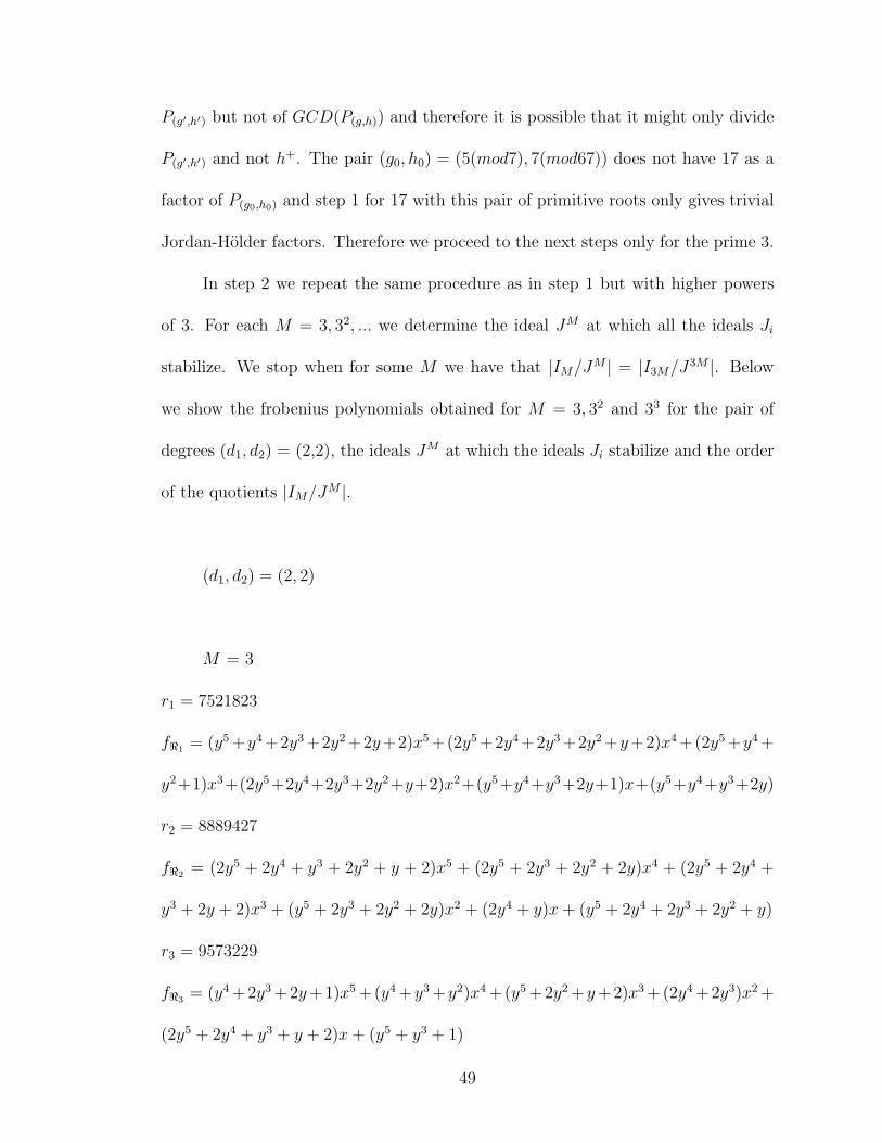
P(g′,h′) but not of GCD(P(g,h)) and therefore it is possible that it might only divide

P(g′,h′) and not h+. The pair (g0, h0) = (5(mod7), 7(mod67)) does not have 17 as a

factor of P(g0,h0) and step 1 for 17 with this pair of primitive roots only gives trivial

Jordan-Holder factors. Therefore we proceed to the next steps only for the prime 3.

In step 2 we repeat the same procedure as in step 1 but with higher powers

of 3. For each M = 3, 32, ... we determine the ideal JM at which all the ideals Ji

stabilize. We stop when for some M we have that |IM/JM | = |I3M/J3M |. Below

we show the frobenius polynomials obtained for M = 3, 32 and 33 for the pair of

degrees (d1, d2) = (2,2), the ideals JM at which the ideals Ji stabilize and the order

of the quotients |IM/JM |.

(d1, d2) = (2, 2)

M = 3

r1 = 7521823

f<1 = (y5 +y4 +2y3 +2y2 +2y+2)x5 +(2y5 +2y4 +2y3 +2y2 +y+2)x4 +(2y5 +y4 +

y2+1)x3+(2y5+2y4+2y3+2y2+y+2)x2+(y5+y4+y3+2y+1)x+(y5+y4+y3+2y)

r2 = 8889427

f<2 = (2y5 + 2y4 + y3 + 2y2 + y + 2)x5 + (2y5 + 2y3 + 2y2 + 2y)x4 + (2y5 + 2y4 +

y3 + 2y + 2)x3 + (y5 + 2y3 + 2y2 + 2y)x2 + (2y4 + y)x+ (y5 + 2y4 + 2y3 + 2y2 + y)

r3 = 9573229

f<3 = (y4 + 2y3 + 2y+ 1)x5 + (y4 +y3 +y2)x4 + (y5 + 2y2 +y+ 2)x3 + (2y4 + 2y3)x2 +

(2y5 + 2y4 + y3 + y + 2)x+ (y5 + y3 + 1)

49

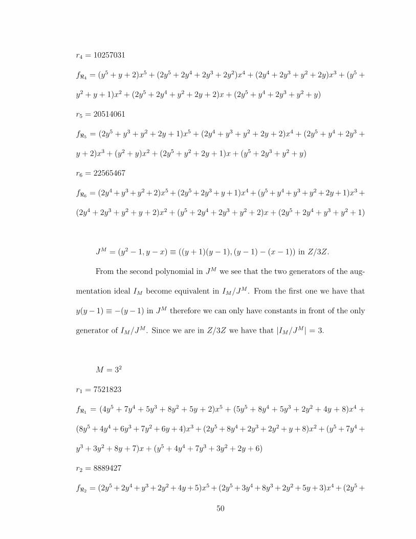
r4 = 10257031

f<4 = (y5 + y + 2)x5 + (2y5 + 2y4 + 2y3 + 2y2)x4 + (2y4 + 2y3 + y2 + 2y)x3 + (y5 +

y2 + y + 1)x2 + (2y5 + 2y4 + y2 + 2y + 2)x+ (2y5 + y4 + 2y3 + y2 + y)

r5 = 20514061

f<5 = (2y5 + y3 + y2 + 2y + 1)x5 + (2y4 + y3 + y2 + 2y + 2)x4 + (2y5 + y4 + 2y3 +

y + 2)x3 + (y2 + y)x2 + (2y5 + y2 + 2y + 1)x+ (y5 + 2y3 + y2 + y)

r6 = 22565467

f<6 = (2y4 + y3 + y2 + 2)x5 + (2y5 + 2y3 + y+ 1)x4 + (y5 + y4 + y3 + y2 + 2y+ 1)x3 +

(2y4 + 2y3 + y2 + y + 2)x2 + (y5 + 2y4 + 2y3 + y2 + 2)x+ (2y5 + 2y4 + y3 + y2 + 1)

JM = (y2 − 1, y − x) ≡ ((y + 1)(y − 1), (y − 1)− (x− 1)) in Z/3Z.

From the second polynomial in JM we see that the two generators of the aug-

mentation ideal IM become equivalent in IM/JM . From the first one we have that

y(y− 1) ≡ −(y− 1) in JM therefore we can only have constants in front of the only

generator of IM/JM . Since we are in Z/3Z we have that |IM/JM | = 3.

M = 32

r1 = 7521823

f<1 = (4y5 + 7y4 + 5y3 + 8y2 + 5y + 2)x5 + (5y5 + 8y4 + 5y3 + 2y2 + 4y + 8)x4 +

(8y5 + 4y4 + 6y3 + 7y2 + 6y+ 4)x3 + (2y5 + 8y4 + 2y3 + 2y2 + y+ 8)x2 + (y5 + 7y4 +

y3 + 3y2 + 8y + 7)x+ (y5 + 4y4 + 7y3 + 3y2 + 2y + 6)

r2 = 8889427

f<2 = (2y5 + 2y4 + y3 + 2y2 + 4y+ 5)x5 + (2y5 + 3y4 + 8y3 + 2y2 + 5y+ 3)x4 + (2y5 +

50

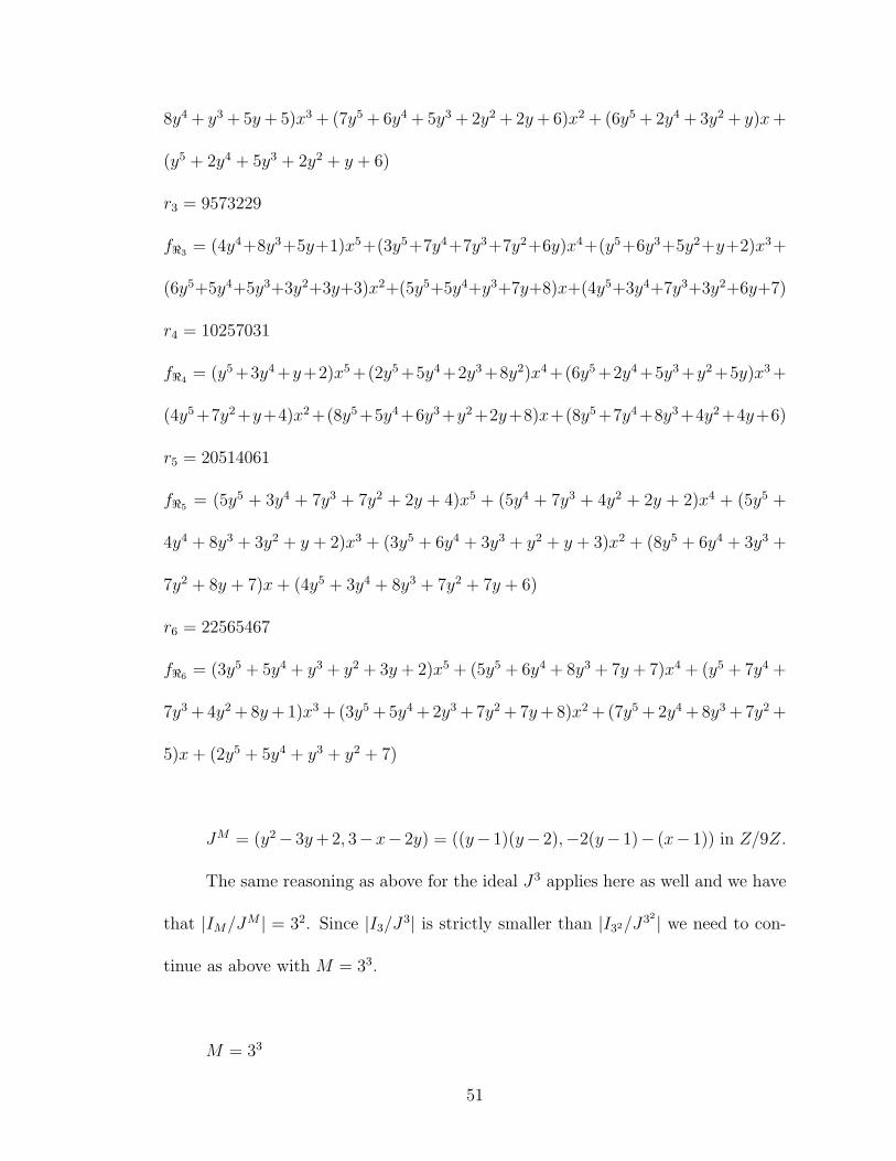
8y4 + y3 + 5y+ 5)x3 + (7y5 + 6y4 + 5y3 + 2y2 + 2y+ 6)x2 + (6y5 + 2y4 + 3y2 + y)x+

(y5 + 2y4 + 5y3 + 2y2 + y + 6)

r3 = 9573229

f<3 = (4y4+8y3+5y+1)x5+(3y5+7y4+7y3+7y2+6y)x4+(y5+6y3+5y2+y+2)x3+

(6y5+5y4+5y3+3y2+3y+3)x2+(5y5+5y4+y3+7y+8)x+(4y5+3y4+7y3+3y2+6y+7)

r4 = 10257031

f<4 = (y5 +3y4 +y+2)x5 +(2y5 +5y4 +2y3 +8y2)x4 +(6y5 +2y4 +5y3 +y2 +5y)x3 +

(4y5 +7y2 +y+4)x2 +(8y5 +5y4 +6y3 +y2 +2y+8)x+(8y5 +7y4 +8y3 +4y2 +4y+6)

r5 = 20514061

f<5 = (5y5 + 3y4 + 7y3 + 7y2 + 2y + 4)x5 + (5y4 + 7y3 + 4y2 + 2y + 2)x4 + (5y5 +

4y4 + 8y3 + 3y2 + y + 2)x3 + (3y5 + 6y4 + 3y3 + y2 + y + 3)x2 + (8y5 + 6y4 + 3y3 +

7y2 + 8y + 7)x+ (4y5 + 3y4 + 8y3 + 7y2 + 7y + 6)

r6 = 22565467

f<6 = (3y5 + 5y4 + y3 + y2 + 3y + 2)x5 + (5y5 + 6y4 + 8y3 + 7y + 7)x4 + (y5 + 7y4 +

7y3 + 4y2 + 8y+ 1)x3 + (3y5 + 5y4 + 2y3 + 7y2 + 7y+ 8)x2 + (7y5 + 2y4 + 8y3 + 7y2 +

5)x+ (2y5 + 5y4 + y3 + y2 + 7)

JM = (y2− 3y+ 2, 3−x− 2y) = ((y− 1)(y− 2),−2(y− 1)− (x− 1)) in Z/9Z.

The same reasoning as above for the ideal J3 applies here as well and we have

that |IM/JM | = 32. Since |I3/J3| is strictly smaller than |I32/J32| we need to con-

tinue as above with M = 33.

M = 33

51

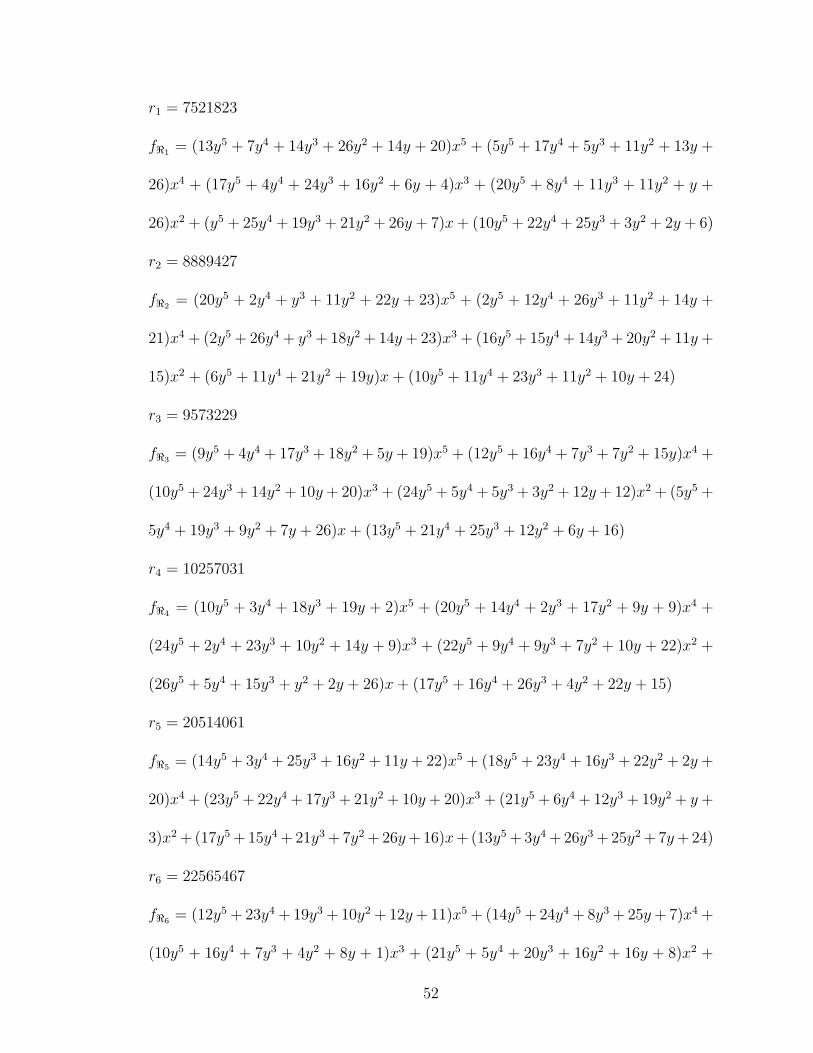
r1 = 7521823

f<1 = (13y5 + 7y4 + 14y3 + 26y2 + 14y + 20)x5 + (5y5 + 17y4 + 5y3 + 11y2 + 13y +

26)x4 + (17y5 + 4y4 + 24y3 + 16y2 + 6y + 4)x3 + (20y5 + 8y4 + 11y3 + 11y2 + y +

26)x2 + (y5 + 25y4 + 19y3 + 21y2 + 26y + 7)x+ (10y5 + 22y4 + 25y3 + 3y2 + 2y + 6)

r2 = 8889427

f<2 = (20y5 + 2y4 + y3 + 11y2 + 22y + 23)x5 + (2y5 + 12y4 + 26y3 + 11y2 + 14y +

21)x4 + (2y5 + 26y4 + y3 + 18y2 + 14y+ 23)x3 + (16y5 + 15y4 + 14y3 + 20y2 + 11y+

15)x2 + (6y5 + 11y4 + 21y2 + 19y)x+ (10y5 + 11y4 + 23y3 + 11y2 + 10y + 24)

r3 = 9573229

f<3 = (9y5 + 4y4 + 17y3 + 18y2 + 5y + 19)x5 + (12y5 + 16y4 + 7y3 + 7y2 + 15y)x4 +

(10y5 + 24y3 + 14y2 + 10y + 20)x3 + (24y5 + 5y4 + 5y3 + 3y2 + 12y + 12)x2 + (5y5 +

5y4 + 19y3 + 9y2 + 7y + 26)x+ (13y5 + 21y4 + 25y3 + 12y2 + 6y + 16)

r4 = 10257031

f<4 = (10y5 + 3y4 + 18y3 + 19y + 2)x5 + (20y5 + 14y4 + 2y3 + 17y2 + 9y + 9)x4 +

(24y5 + 2y4 + 23y3 + 10y2 + 14y + 9)x3 + (22y5 + 9y4 + 9y3 + 7y2 + 10y + 22)x2 +

(26y5 + 5y4 + 15y3 + y2 + 2y + 26)x+ (17y5 + 16y4 + 26y3 + 4y2 + 22y + 15)

r5 = 20514061

f<5 = (14y5 + 3y4 + 25y3 + 16y2 + 11y + 22)x5 + (18y5 + 23y4 + 16y3 + 22y2 + 2y +

20)x4 + (23y5 + 22y4 + 17y3 + 21y2 + 10y+ 20)x3 + (21y5 + 6y4 + 12y3 + 19y2 + y+

3)x2 + (17y5 + 15y4 + 21y3 + 7y2 + 26y+ 16)x+ (13y5 + 3y4 + 26y3 + 25y2 + 7y+ 24)

r6 = 22565467

f<6 = (12y5 + 23y4 + 19y3 + 10y2 + 12y+ 11)x5 + (14y5 + 24y4 + 8y3 + 25y+ 7)x4 +

(10y5 + 16y4 + 7y3 + 4y2 + 8y + 1)x3 + (21y5 + 5y4 + 20y3 + 16y2 + 16y + 8)x2 +

52

(25y5 + 2y4 + 8y3 + 16y2 + 5)x+ (20y5 + 14y4 + y3 + y2 + 16)

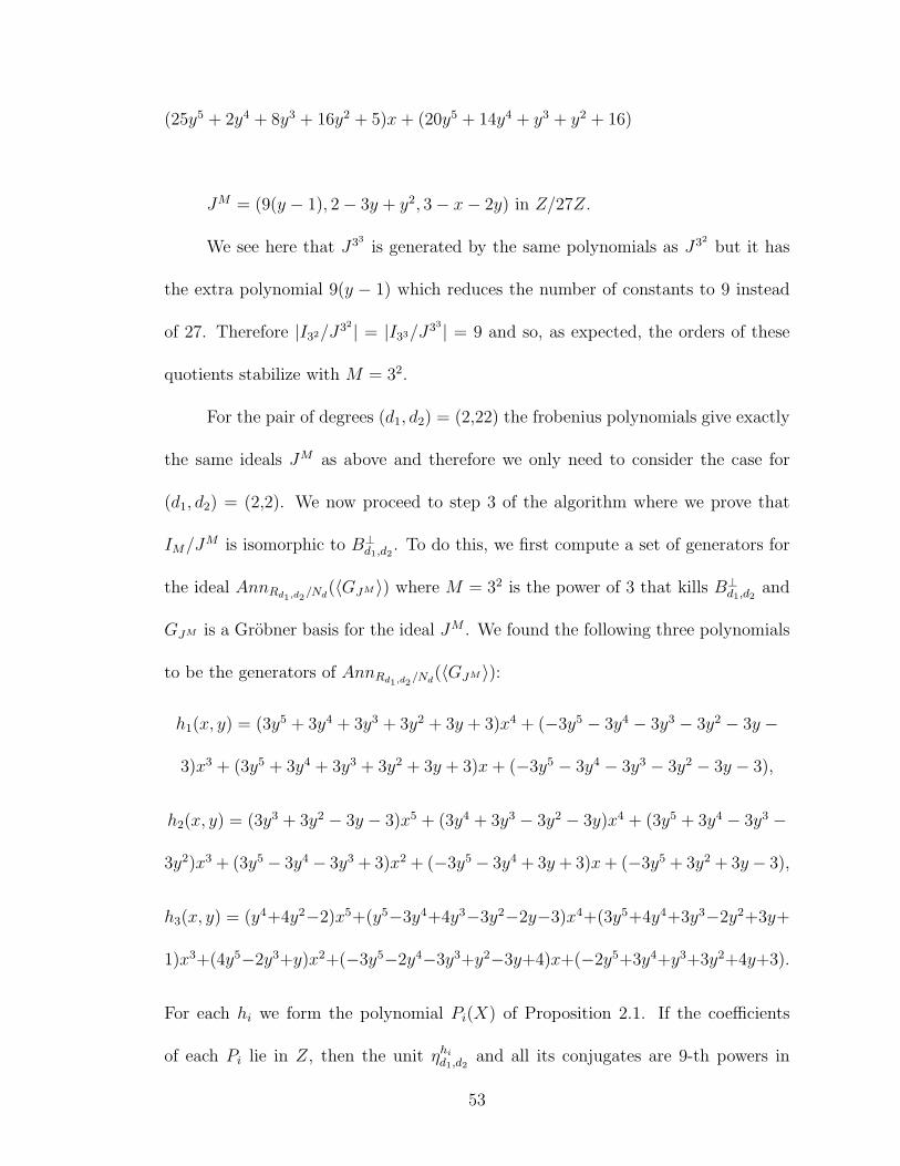
JM = (9(y − 1), 2− 3y + y2, 3− x− 2y) in Z/27Z.

We see here that J33is generated by the same polynomials as J32

but it has

the extra polynomial 9(y − 1) which reduces the number of constants to 9 instead

of 27. Therefore |I32/J32| = |I33/J33| = 9 and so, as expected, the orders of these

quotients stabilize with M = 32.

For the pair of degrees (d1, d2) = (2,22) the frobenius polynomials give exactly

the same ideals JM as above and therefore we only need to consider the case for

(d1, d2) = (2,2). We now proceed to step 3 of the algorithm where we prove that

IM/JM is isomorphic to B⊥d1,d2 . To do this, we first compute a set of generators for

the ideal AnnRd1,d2/Nd(〈GJM 〉) where M = 32 is the power of 3 that kills B⊥d1,d2 and

GJM is a Grobner basis for the ideal JM . We found the following three polynomials

to be the generators of AnnRd1,d2/Nd(〈GJM 〉):

h1(x, y) = (3y5 + 3y4 + 3y3 + 3y2 + 3y + 3)x4 + (−3y5 − 3y4 − 3y3 − 3y2 − 3y −

3)x3 + (3y5 + 3y4 + 3y3 + 3y2 + 3y + 3)x+ (−3y5 − 3y4 − 3y3 − 3y2 − 3y − 3),

h2(x, y) = (3y3 + 3y2 − 3y − 3)x5 + (3y4 + 3y3 − 3y2 − 3y)x4 + (3y5 + 3y4 − 3y3 −

3y2)x3 + (3y5 − 3y4 − 3y3 + 3)x2 + (−3y5 − 3y4 + 3y + 3)x+ (−3y5 + 3y2 + 3y− 3),

h3(x, y) = (y4+4y2−2)x5+(y5−3y4+4y3−3y2−2y−3)x4+(3y5+4y4+3y3−2y2+3y+

1)x3+(4y5−2y3+y)x2+(−3y5−2y4−3y3+y2−3y+4)x+(−2y5+3y4+y3+3y2+4y+3).

For each hi we form the polynomial Pi(X) of Proposition 2.1. If the coefficients

of each Pi lie in Z, then the unit ηhid1,d2 and all its conjugates are 9-th powers in

53

Q(ζpq)+ and we are done. The Pi were calculated with a precision of 2000. They are

big polynomials with very large integer coefficients and therefore we do not present

them here. The reader can find them in the Appendix. Since all the Pi have integer

coefficients this implies that 32 is the order of the 3-part of h+.

54

Chapter 3

Tables and Discussion of the Results

We present all our results in the Main Table below. For each field of conductor

pq we present the greatest common divisor of the P(g,h) for all pairs of primitive roots

(g, h), in the column GCD. Since we do not calculate the 2-part of h+, we leave out

the powers of 2 from the GCD. Therefore, if a ‘1’ appears in the column GCD for

some field, this means that no odd primes divide the greatest common divisor of the

various P(g,h). However, there are always powers of 2 in the GCD, as we see from

our calculations of the index [E : H] in chapter 1. In the column extra ‘nontrivial’

primes we present all the primes that step 1 gave to be possible divisors of h+,

besides the ones that already appear in the column GCD. The symbol h+ in the

fourth column, denotes the odd part of h+ for all primes l < 10000.

We have verified the results of Hakkarainen for the fields of conductor pq, for

the primes l that do not divide the degree of the extension. We mark with an

asterisk the fields whose class number we found to be divisible by a prime l which

also divides the degree of the extension. From those fields, there are three cases

where the primes that appear as possible divisors of h+ in Hakkarainen’s results,

i.e. divisors of a relative class number hχ, in our case they were only divisors of the

GCD and therefore not of h+. In other words, although these primes do divide the

index [E : H], we found that they come from GCD and not from h+. These are

55

the fields of conductor 11 · 43 where we found that 3 does not divide h+, the field of

conductor 7·211 where we found that 7 does not divide h+ and the field of conductor

17 · 103 where we found that 17 does not divide h+. For the field of conductor 7 · 67

we found that the 3-part of h+ is 32. Finally, for the fields of conductor 13 · 61 and

13 · 103 we found that 3 and 32 respectively are also divisors of h+.

The polynomials of the third step, which are used to prove that the unit α(ηhd )

is an M -th power in E by showing that their coefficients are in Z, were computed

with very high precision. That is why we get hundreds of decimals which are all 9’s

or all 0’s. We did not continue to prove rigorously that the coefficients are indeed

integers. However, to a very small number of fields with small polynomials we did

apply the method outlined in Schoof [25], which proves that the coefficients of these

polynomials are integers. This method requires that we round off the coefficients

of P (X) and then show that this new polynomial divides P (XM). This proved to

be too time consuming for large polynomials and this is why we did not apply it to

most of our fields.

56

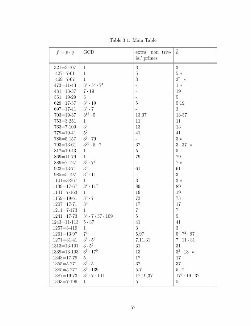
Table 3.1: Main Table

f = p · q GCD extra ‘non triv-ial’ primes

h+

321=3·107 1 3 3427=7·61 1 5 5 ∗469=7·67 1 3 32 ∗473=11·43 34 · 52 · 74 - 1 ∗481=13·37 7 · 19 - 19551=19·29 5 - 5629=17·37 34 · 19 5 5·19697=17·41 33 · 7 - 3703=19·37 316 · 5 13,37 13·37753=3·251 1 11 11763=7·109 34 13 13779=19·41 52 41 41785=5·157 32 · 79 - 3 ∗793=13·61 320 · 5 · 7 37 3 · 37 ∗817=19·43 1 5 5869=11·79 1 79 79889=7·127 34 · 72 - 7 ∗923=13·71 33 61 61985=5·197 33 · 11 - 31101=3·367 1 3 3 ∗1139=17·67 37 · 117 89 891141=7·163 1 19 191159=19·61 33 · 7 73 731207=17·71 32 17 171211=7·173 1 7 71241=17·73 34 · 7 · 37 · 109 5 51243=11·113 5 · 37 41 411257=3·419 1 3 31261=13·97 73 5,97 5 · 72 · 971271=31·41 33 · 56 7,11,31 7 · 11 · 311313=13·101 3 · 52 31 311339=13·103 37 · 175 13 32 · 13 ∗1343=17·79 5 17 171355=5·271 33 · 5 37 371385=5·277 32 · 139 5,7 5 · 71387=19·73 34 · 7 · 101 17,19,37 172 · 19 · 371393=7·199 1 5 5

57

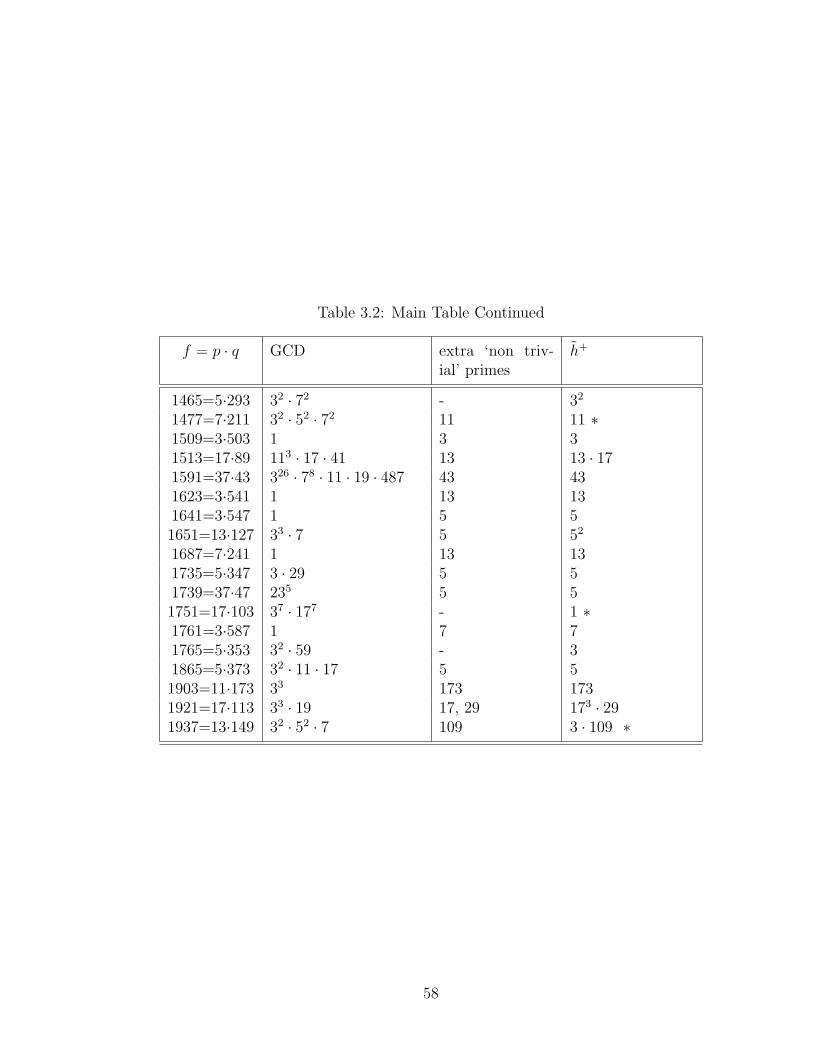
Table 3.2: Main Table Continued

f = p · q GCD extra ‘non triv-ial’ primes

h+

1465=5·293 32 · 72 - 32

1477=7·211 32 · 52 · 72 11 11 ∗1509=3·503 1 3 31513=17·89 113 · 17 · 41 13 13 · 171591=37·43 326 · 78 · 11 · 19 · 487 43 431623=3·541 1 13 131641=3·547 1 5 51651=13·127 33 · 7 5 52

1687=7·241 1 13 131735=5·347 3 · 29 5 51739=37·47 235 5 51751=17·103 37 · 177 - 1 ∗1761=3·587 1 7 71765=5·353 32 · 59 - 31865=5·373 32 · 11 · 17 5 51903=11·173 33 173 1731921=17·113 33 · 19 17, 29 173 · 291937=13·149 32 · 52 · 7 109 3 · 109 ∗

58

Chapter 4

Conclusion and Future Projects

In this thesis we studied the class number h+ of real cyclotomic fields. In

particular, we studied a pre-existing method introduced by Schoof [25] who calcu-

lated the l-part of h+ for cyclotomic fields of prime conductor, and we extended

this method to fields of conductor pq, p and q being distinct odd primes. We calcu-

lated the odd part of h+ for all odd primes less than 10000, for cyclotomic fields of

conductor < 2500. Our results verify the results of Hakkarainen [13] who studied

the divisibility of h+ by odd primes less than 10000, for fields of conductor < 2000.

Our results also complete his results in the sense that they give the full order of the

l-parts of h+ for each odd prime l < 10000, including the primes dividing the degree

of the field.

One can apply the second and third step of our algorithm to the prime l =

2 and therefore calculate the 2-part of h+ which we did not complete here, as well

as to primes l > 10000. For fields of conductor > 2000 the computations become

very time consuming. Therefore, if one is to calculate the l-parts of h+ for these

fields, one could set an upper bound to the degrees d1 and d2. Schoof in [25] for

example calculated the Jordan-Holder factors of order up to 80000. Furthermore,

one could apply our method to fields of conductor equal to the product of more than

two distinct odd primes, by adjusting accordingly the unit η and the description

59

of the galois group G in terms of polynomials. Of course we see that a larger

number of primes dividing the conductor implies a more complicated unit and more

variables. Therefore the calculations are expected to become very time consuming

as the conductor of the field grows.

One of the reasons that the primes that divide the degree of the field are

avoided in many methods for computing h+, lies in the difficulty of computing

the factor Q+K that we discussed in Subsection 1.3.1. Our method could help in

calculating this value, by applying the method to Leopoldt’s cyclotomic unit θξ

introduced in 1.3.1 for the cyclic subfield Kξ. We could do that for every ξ 6= ξ0 and

only for the primes that divide the order of the galois group since only those primes

appear in the index Q+K . We then divide this product with the product we find by

applying the method to our unit. The result is the order of Q+K .

60

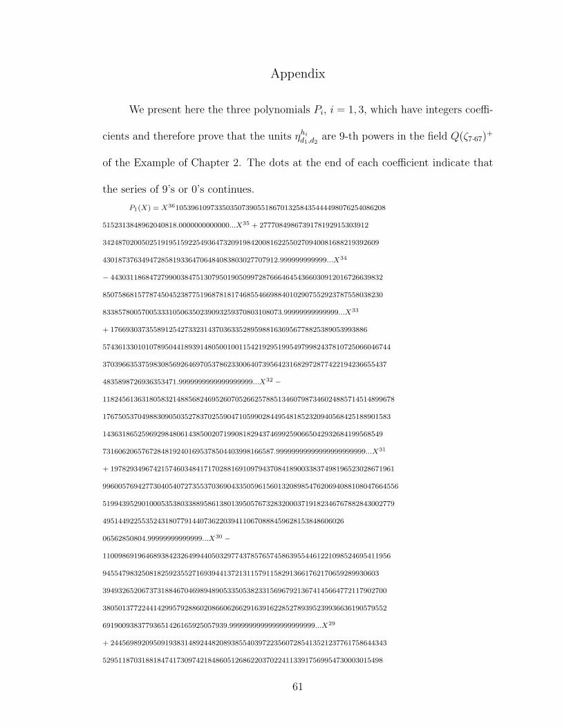
Appendix

We present here the three polynomials Pi, i = 1, 3, which have integers coeffi-

cients and therefore prove that the units ηhid1,d2 are 9-th powers in the field Q(ζ7·67)+

of the Example of Chapter 2. The dots at the end of each coefficient indicate that

the series of 9’s or 0’s continues.

P1(X) = X36105396109733503507390551867013258435444498076254086208

5152313848962040818.0000000000000...X35 + 2777084986739178192915303912

34248702005025191951592254936473209198420081622550270940081688219392609

430187376349472858193364706484083803027707912.999999999999...X34

− 4430311868472799003847513079501905099728766646454366030912016726639832

850758681577874504523877519687818174685546698840102907552923787558038230

8338578005700533310506350239093259370803108073.99999999999999...X33

+ 176693037355891254273323143703633528959881636956778825389053993886

57436133010107895044189391480500100115421929519954979982437810725066046744

3703966353759830856926469705378623300640739564231682972877422194236655437

4835898726936353471.9999999999999999999...X32 −

118245613631805832148856824695260705266257885134607987346024885714514899678

17675053704988309050352783702559047105990284495481852320940568425188901583

143631865259692984806143850020719908182943746992590665042932684199568549

73160620657672848192401695378504403998166587.99999999999999999999999...X31

+ 1978293496742157460348417170288169109794370841890033837498196523028671961

9960057694277304054072735537036904335059615601320898547620694088108047664556

519943952901000535380338895861380139505767328320003719182346767882843002779

49514492255352431807791440736220394110670888459628153848606026

06562850804.99999999999999...X30 −

11009869196468938423264994405032977437857657458639554461221098524695411956

94554798325081825923552716939441372131157911582913661762170659289930603

3949326520673731884670469894890533505382331569679213674145664772117902700

3805013772244142995792886020866062662916391622852789395239936636190579552

69190093837793651426165925057939.9999999999999999999999...X29

+ 24456989209509193831489244820893855403972235607285413521237761758644343

529511870318818474173097421848605126862203702241133917569954730003015498

61

22871951434808167003997676218121580379254248395187778623595659125887565

9144008994973509254995244645129122374274147428637264962970738335343754798

22052730106174422447999541680198098262634253583479514

62720834.99999999999999999999...X28 −

27436557356034724128817446413685197948411808135909544354956975329494

09658663429195537590532690585714627579052010736384406792449715211

830899443498069308081112093388139161566491176370470803796910045906

39062772914726090816222586097268188753238380117211292581206347558

8805233021652751637749047645330208638460261019340244710959505344578

950453410226765875375141682295733378024307.9999999999999999999999999...X27 +

1613833366410763456456079717682426881164960451134616497662425

9264664017926930928966218958385895844971621398414514983675560806018

314570324869426678376784580375358215022645037911552476248093144775954324

0428862589069909709277555574873995672921653833932239895

0227124445025992932357641918834159111777166513035099430412014766

182764644397830940824

106683696118474387368543296400134823122482

9066548852444606.999999999999999...X26 −

4635403380089426272687801176816126323523597073205882181607656464952

804237328200654528788008026512153298866596835293708740267998580

72192210761589694075573487972643504346241703333113864485939162487248273831860

101946569761033802036467623592502743899710074709

9533754932095601765376279

790241648911878694250657530670049416410336886981131314297229

45230283119643948817127450925446877388955069437370113489918117

67905811768733006359.9999999999999999999...X25 +

50899063110951250423796046159121202507656267532409988489050811463

3668686165594547366288881222528181685735138872258060202981093

13465302975573130916478674683007868313011051254351607975506640715533383343

9463881645430045092733661777763690407426317660215950141

7980859007538637711136389083127731633054913821014347446263744108364228

938341996620673770825795048143607897932141759534782075608277752455490052

5566788329116051179378877188854154366370240913982.9999999999999999999...X24

− 5398119935249082433570676523479132330706396424724716453378713669237

62

47684578873469918084975884240107478762014052873194824570226273509528589995

298560235552687177840055539914947106344057255369974108447567317902898711

21673876993955497181429163486515190178070

1884260717587061121123220763142136

612078227048756373203381588548524020344713102805265

6947959101722036031788094928

196109362903309473140516916736651107209084857400607372816

81540348609065189872660456078838341000851.99999999999999999...X23 +

1587941351618584928082215736422933903880348506182052121575672063010133646237408

6039506994372581193987977548485949847985276742253919923673987161991415

1228030864106147308003122046568701138254831477811456052865514162654009693504

980606118005902254701829510521608474316697043832153791320913553233218166470

4348082290350339134033668514840011488488585116727968877625432361852420907033

7467009917644006759327827471302311941205452430897201377019899265639133435283

55732851065392611791705437738111.999999999999999999999999...X22

− 83087122218775230881569900535282367086139781933961024325593142746271195267514266

7302213178988768845621139166972670629627810222471885420790416756024517602205804334383

1294353060113603717305450454418972365046857532083673885457186782895437001834674741075

4143169883114482532227890389324020008667373150266592813174260730037099326550952394634

3979801890071381051692711234928781981291000391126606555114817698981383873702198348255

7462695352294137620832434469873559275278736204041134595257381857660556853922

42779.99999999999999999...X21 +

1205841374755322595924322812088045424919065124905306616947104

1063886742879578899208050494297512731617808097296924069814495500854278233510344895142

4085950280575056471465529270459883269696545723520601534684131168038386245800686799119

0112742476174266890852695805631119302393352415233314761829102385133755011036605603310

6309116207947677551220525288298139562962055665768359229616434816293430473978921556963

7221027096729088288194492352386440023487629392426040745285416858879715928516944145821

616787877917806811948551742478033.999999999999...X20 −

3040884576862042046043610303235655081597195309990931270052265917959221685352680990765

2517334303901825409562744385301610459577321596488836654639629903420910182341741299532

2298632344544091654572463497840329480018757373008457903888104411793327864450578653552

3910279568734664825285659424900209732429592665434736754764847594601817045061053454860

0284277791760725769993082881364725224055442155485648191675600049962750481617329861903

63

9179331947200179844379632630563670740654848601563739493053638554498201286522977722157

3707035475082579.9999999999999999...X19 + 1917121787682851735092003419251040393260657

9976687109767673185665043316428571408373265130731585960504716418901631760956500847844

8006685227335908452359751739690697756445817385234799971309088239121436295656646452659

5315987002960658253514596884313472583135074775410859355587659180962871141232196112811

4854942361692352372785405175064365551231050979738127206689968883321965222941176791700

5168668340860477307592266966272649037191197406934134774079333467962530727583332113608

522364533511432634938575869311555547065109036992934

42644012173667.999999999999999999999...X18 −

2026763519321103866016748293034278165944217773244601197543323303320079351724021444

182230586040049633121202060270092694320291991686770046379835946549453291648234372395

3898267498925934914124958598650336595532473817022538170954066813999114377538517874638

8354788537965053917406982792063090785128654115342540310284672720683829695195304043524

3468944393302585074578321843293496794139160191788871081360341641210921293415253067061

3611962869152327845273253870042788690874315200401710962434664778746031530742529446119

81371725885087108568548335.9999999999999999...X17 +

535668941859072585978725512282002226721529589025692932829381547406837254997654566455

6733369503623674837069567594895489692631025192849018682143444185147188095486600433990

1512783580637695244327060782898715861562114856328077210148879050918309426104668240619

1765587050547231795199255905328775244072810392504786000177539364069462937527206950834

1648571840489820237816066540234578433382301812676272828956635596527874389809520643751

0783066623491115427083153881949555749222036155204794173896588485185399508900875954391

985314532366326054789.99999999999999999999...X16 −

101362433911685028852435019920245977154707329574475329291897016991484427435476188899

1341581683292456979783750358523191222712109880575581846295624373840529377868965489435

3872749172904383498710307472955063247838883594728141385608917207081812339740208863584

1634796680068903845422340879997902375702627749694838988861479080809384556957297984455

6739635216541074527296953954215013223906692782193168126440197594782655472201612260017

2435983819117816797928821206284212914103169415017789647384306194603474711104666363638

08090.000000000000000000000...X15 +

59721161492936066593669336726847798596152542824393514318260531323566263014608528553

3820862745600780461677453335369346831115705872080456411701101638721363076270707839997

9461985549170100998537836301395496168276005359879139732904573351143168424380286497852

0282418578000158173341313576081777769575212330285247504526715501731394326336712846927

64

1287616610431308988547037268886382074593335735196101110260858108857822229134241390551

5716045200034648821519607323899410448102243637549933727443919091

799902022.99999999999999999...X14 −

1113610351130300290327380245905294315608996406773211070182407690346722737417437822650

5581376969516733758033797611016662688342818601244749599603735274792480232845667477767

8320673164041804731985843785954703679893086224149797932634347939785113395674224084540

4901593248280426073360983635961852643280575115352181966288546208305682806313898540865

9649404222973993807032908539273358053799235496763254990471937672464477763112600843106

799821888406997427385751069157366824092226290873748090.00000000000000000...X13

+ 646560140218659873900705733490613975947171031564595272668076909052832422504604344399

9583918365280187321382085747412350109489511039299330855127348077579635640461755302728

6831394212028239664108296934702876679517643917484358837428132536173368675856897314816

6093640814734961610615656055084778916244608771637012492891259012718207209390103408941

7869806461575020788919526792490997005638316568582553405558286443739995057763421377144

557320465850068610815480247868670797.99999999999999...X12

− 5818605356870885651866318880487971181745757048428154704869932789216597

4592468912763190560401772463030057613859389834376371420574333526694489232236588312141

4107243309667631781906980338466665525816536947848620915128051809881114052757589925536

5773017849800094335336479055265970570482053435867938864400140303537358102762525334850

6864258375361041508804236879444315560570510433993164138575313115652973372991106924214

146821039862428287566917.999999999999999999...X11 +

131110925619705388917607834791319024281334448648125167732975040016527230382526955234

383044772374980740880898184992400037437056519675110896623013805802069350925794727590

8208964652833582150022332943197170314444376785285840218130285982077570145059511548370

1524539672478795402120441225835777151007663667852487522398081207980656307234974866238

77795931748923750913392181747378526651118473964838023986850

64422448767.9999999999999999999...X10 −

909474067895683378810285132078240966226505709872181887965916383224362761281040843599

1284930899248502883900529331500411005140487681461221775940751450313013077029791862847

775699652228749773857041129209691537236611805644260252702112118826954636958546475488

4228515684784752617935829078927541031863343968532462421221698251933620751848696033087

8166440270616746274345798028675702456027.9999999999999999999...X9

+ 176739211755797998563653104637832269737532689739418149012469637060044787235820915916

8806701272910401151753832346826633528549572056289126815494333222364195504377685384840

65

6270994579567105826186628630022334483776702764466446067465765073740430659624243721013

3995310945813119367215129500442393535731351514208374899864492110122831280776853109887

2232721956.999999999999999999...X8

− 652747573341726214791285102634632371912222692391215019088004368489628851249126099

2356410503251533197071320985431238900026379909638366238936828447318242566479079755298

4271003363630879810830587416416880997880556244386795556435694803174806463521568668685

0548631710603022252698451842868508226703884547724700749139

752145077.999999999999999999...X7 +

67440218376892859736435923592763108343171813693966563224332942809386172220

8202893128845163762850394102799060156012499261529400885644584178167369937304103710323

1925425582417118208469836230889537822530265640633892485649784491041654311559825288768

2284211202099582256077372425824895429369319.999999999999999999999...X6 −

1025126431787393766526278523671634301432741812966804454565977365590147800114067463154

3867085330526751988943702226653381050931226202182806548258736102222544935001492417398

0309116260824256363205432630135532227460183269861456311731966290752888

49723174311.9999999999999999999...X5 +

3895616738408948387452492067199750820294391411243785437186808708187635300231802548611

281189692541714510694226281725331463351163802375580021794381617821796918315782294349

12558645949697036075876480416022823514240493.99999999999999999...X4 −

1919477621972238921416569923816738286616270503347859689882716712002476643106377753236

33570272018099235441669175038352663602597330513694323800945953430986

68329951.9999999999...X3 +

2759195015225947121386622622817076298230828468678209042668958020865811100023772635242

23532988550611248013003.999999999999...X2 −

972511939164023729467624767604338173357709659432218631.99999999999999...X

+ 0.999999999999...

P2(X) = X36 +−105396109733503507390551867013258435444498076254086208515231384

8962040818.000000000000...X35 +

2777084986739178192915303912342487020050251919515922549364732091984200816

22550270940081688219392609430187376349472858193364706484083803027

707912.9999999999999...X34

− 44303118684727990038475130795019050997287666464543660309120167266398

328507586815778745045238775196878181746855466988401029075529237875580382

308338578005700533310506350239093259370803108073.9999999999...X33 +

66

176693037355891254273323143703633528959881636956778825389053993886

57436133010107895044189391480500100115421929519954979982437810725066

04674437039663537598308569264697053786233006407395642316829728774221942366

554374835898726936353471.99999999999999999999...X32 −

118245613631805832148856824695260705266257885134607987346024885714514899678

1767505370498830905035278370255904710599028449548185232094056842518890158314

3631865259692984806143850020719908182943746992590665042932684199568549731606

20657672848192401695378504403998166587.9999999999999999999...X31 +

1978293496742157460348417170288169109794370841890033837498196523028671961996

00576942773040540727355370369043350596156013208985476206940881080476645565199

4395290100053538033889586138013950576732832000371918234676788284300277949514492

25535243180779144073622039411067088845962815384860602606562850804.99999999999...X30 −

1100986919646893842326499440503297743785765745863955446122109852469541195694554798325081

82592355271693944137213115791158291366176217065928993060339493265206737318846704

698948905335053823315696792136741456647721179027003805013772244142995792886020866

06266291639162285278939523993663619057955269190093837793651426165925

057939.999999999999999999999...X29 +

2445698920950919383148924482089385540397223560728541352123776175864434352951187

03188184741730974218486051268622037022411339175699547300030154982287195143480816

7003997676218121580379254248395187778623595659125887565914400899497350925499524464

5129122374274147428637264962970738335343754798220527301061744224479995416801980982

6263425358347951462720834.999999999999999999...X28 −

2743655735603472412881744641368519794841180813590954435495697532949409658663

42919553759053269058571462757905201073638440679244971521183089944349806930808

1112093388139161566491176370470803796910045906390627729147260908162225860972

6818875323838011721129258120634755888052330216527516377490476453302086384

60261019340244710959505344578950453410226765875375141682295733378024

307.99999999999999999999...X27 +

16138333664107634564560797176824268811649604511346164976624259264664017926930

92896621895838589584497162139841451498367556080601831457032486942667837678458

037535821502264503791155247624809314477595432404288625890699097092775555748739

95672921653833932239895022712444502599293235764191883415911177716651303509943

041201476618276464439783094082410668369611847438736854329

64001348231224829066548852444606.999999999999999...X26 −

67

46354033800894262726878011768161263235235970732058821816076564649528042373

28200654528788008026512153298866596835293708740267998580721922107615896940

755734879726435043462417033331138644859391624872482738318601019465697610338

020364676235925027438997100747099533754932095601765376279790241648911878694

250657530670049416410336886981131314297229452302831196439488171274509254468

7738895506943737011348991811767905811768733006359.999999999999999...X25 +

508990631109512504237960461591212025076562675324099884890508114633668686165

594547366288881222528181685735138872258060202981093134653029755731309164786

746830078683130110512543516079755066407155333833439463881645430045092733661

7777636904074263176602159501417980859007538637711136389083127731633054913821

0143474462637441083642289383419966206737708257950481436078979321417595347820

756082777524554900525566788329116051179378877188854154366370240913982.99999

99999999999999...X24 −

539811993524908243357067652347913233070639642472471645337871366923747684578

87346991808497588424010747876201405287319482457022627350952858999529856023555

26871778400555399149471063440572553699741084475673179028987112167387699395549

718142916348651519017807018842607175870611211232207631421366120782270487563732

0338158854852402034471310280526569479591017220360317880949281961093629033094

7314051691673665110720908485740060737281681540348609065189872660456078838341

000851.9999999999999999999999999...X23 +

158794135161858492808221573642293390388034850618205212157567206301013364623740

86039506994372581193987977548485949847985276742253919923673987161991415122803

08641061473080031220465687011382548314778114560528655141626540096935049806061

1800590225470182951052160847431669704383215379132091355323321816647043480822

9035033913403366851484001148848858511672796887762543236185242090703374670099

176440067593278274713023119412054524308972013770198992656391334352835573285

1065392611791705437738111.999999999999999999999...X22 −

83087122218775230881569900535282367086139781933961024325593142746271195267514

266730221317898876884562113916697267062962781022247188542079041675602451760220

58043343831294353060113603717305450454418972365046857532083673885457186782895

437001834674741075414316988311448253222789038932402000866737315026659281317426

07300370993265509523946343979801890071381051692711234928781981291000391126606

55511481769898138387370219834825574626953522941376208324344698735592752787362

0404113459525738185766055685392242779.999999999999999999...X21 +

68

12058413747553225959243228120880454249190651249053066169471041063886742879578

89920805049429751273161780809729692406981449550085427823351034489514240859502

805750564714655292704598832696965457235206015346841311680383862458006867991190

11274247617426689085269580563111930239335241523331476182910238513375501103660

56033106309116207947677551220525288298139562962055665768359229616434816293430

47397892155696372210270967290882881944923523864400234876293924260407452854168

58879715928516944145821616787877917806811948551742478033.99999999999999...X20 −

30408845768620420460436103032356550815971953099909312700522659179592216853526

8099076525173343039018254095627443853016104595773215964888366546396299034209101

82341741299532229863234454409165457246349784032948001875737300845790388810441

179332786445057865355239102795687346648252856594249002097324295926654347367547

6484759460181704506105345486002842777917607257699930828813647252240554421554856

4819167560004996275048161732986190391793319472001798443796326305636707406548

486015637394930536385544982012865229777221573707035475082579.99999999

999999999999999999...X19 +

19171217876828517350920034192510403932606579976687109767673185665043316

42857140837326513073158596050471641890163176095650084784480066852273359084

523597517396906977564458173852347999713090882391214362956566464526595315987

002960658253514596884313472583135074775410859355587659180962871141232196112

81148549423616923523727854051750643655512310509797381272066899688833219652

2294117679170051686683408604773075922669662726490371911974069341347740793

3346796253072758333211360852236453351143263493857586931155554706510903699

293442644012173667.9999999999999...X18 −

20267635193211038660167482930342781659442177732446011975433233033200793517

240214441822305860400496331212020602700926943202919916867700463798359465494

53291648234372395389826749892593491412495859865033659553247381702253817095406

6813999114377538517874638835478853796505391740698279206309078512865411534254

0310284672720683829695195304043524346894439330258507457832184329349679413916

0191788871081360341641210921293415253067061361196286915232784527325387004278

8690874315200401710962434664778746031530742529446119813717258850871085685

48335.99999999999999999999...X17 +

5356689418590725859787255122820022267215295890256929328293815474068372549976

54566455673336950362367483706956759489548969263102519284901868214344418514718

809548660043399015127835806376952443270607828987158615621148563280772101488790

69

509183094261046682406191765587050547231795199255905328775244072810392504786000

17753936406946293752720695083416485718404898202378160665402345784333

823018126762728289566355965278743898095206437510783066623491115427083153881949555

7492220361552047941738965884851853995089008759543919853145323

66326054789.999999999999999999999...X16 −

101362433911685028852435019920245977154707329574475329291897016991484427435

4761888991341581683292456979783750358523191222712109880575581846295624373840

529377868965489435387274917290438349871030747295506324783888359472814138560

89172070818123397402088635841634796680068903845422340879997902375702627749

694838988861479080809384556957297984455673963521654107452729695395421501322

39066927821931681264401975947826554722016122600172435983819117816797928821

2062842129141031694150177896473843061946034747111046663

6363808090.0000000000000000...X15 +

5972116149293606659366933672684779859615254282439351431826053132356626301460

8528553382086274560078046167745333536934683111570587208045641170110163872136

30762707078399979461985549170100998537836301395496168276005359879139732904573

3511431684243802864978520282418578000158173341313576081777769575212330285247

504526715501731394326336712846927128761661043130898854703726888638207459333573

519610111026085810885782222913424139055157160452000346488215196073238994104

48102243637549933727443919091799902022.99999999999999...X14 −

1113610351130300290327380245905294315608996406773211070182407690346722737417437

8226505581376969516733758033797611016662688342818601244749599603735274792480232

84566747776783206731640418047319858437859547036798930862241497979326343479397851

13395674224084540490159324828042607336098363596185264328057511535218196628854620

830568280631389854086596494042229739938070329085392733580537992354967632549904

7193767246447776311260084310679982188840699742738575106915736682409222629087

3748090.000000000000000...X13 +

64656014021865987390070573349061397594717103156459527266807690905283242250460

434439995839183652801873213820857474123501094895110392993308551273480775796356

40461755302728683139421202823966410829693470287667951764391748435883742813253

617336867585689731481660936408147349616106156560550847789162446087716370124928

9125901271820720939010340894178698064615750207889195267924909970056383165685

825534055582864437399950577634213771445573204658500686108154802478686

70797.999999999999999999...X12 −

70

5818605356870885651866318880487971181745757048428154704869932789216597459

2468912763190560401772463030057613859389834376371420574333526694489232236588

31214141072433096676317819069803384666655258165369478486209151280518098811140

5275758992553657730178498000943353364790552659705704820534358679388644001403

035373581027625253348506864258375361041508804236879444315560570510433993164

1385753131156529733729911069242141468210398624282

87566917.999999999999999999...X11 +

13111092561970538891760783479131902428133444864812516773297504001652723038

25269552343830447723749807408808981849924000374370565196751108966230138058

020693509257947275908208964652833582150022332943197170314444376785285840218

13028598207757014505951154837015245396724787954021204412258357771510076636678

524875223980812079806563072349748662387779593174892375091339218174737852665

111847396483802398685064422448767.99999999999999999999...X10 −

909474067895683378810285132078240966226505709872181887965916383224362761281

0408435991284930899248502883900529331500411005140487681461221775940751450313

013077029791862847775699652228749773857041129209691537236611805644260252702112

118826954636958546475488422851568478475261793582907892754103186334396853246

24212216982519336207518486960330878166440270616746274345798028675

702456027.9999999999999999999...X9 +

176739211755797998563653104637832269737532689739418149012469637060

04478723582091591688067012729104011517538323468266335285495720562

8912681549433322236419550437768538484062709945795671058261866286300

2233448377670276446644606746576507374043065962424372101339953109458131

19367215129500442393535731351514208374899864492110122831280776853

1098872232721956.999999999999999999999999...X8 −

652747573341726214791285102634632371912222692391215019088004368489628851249

126099235641050325153319707132098543123890002637990963836623893682844

731824256647907975529842710033636308798108305874164168809978805562

44386795556435694803174806463521568668685054863171060302225269845184

2868508226703884547724700749139752145077.99999999999999...X7 +

674402183768928597364359235927631083431718136939665632243329428093

861722208202893128845163762850394102799060156012499261529400885644584178

16736993730410371032319254255824171182084698362308895378225302656406

33892485649784491041654311559825288768228421120209958225607737242582489

71

5429369319.999999999999999999999...X6 −

10251264317873937665262785236716343014327418129668044545659773655901478

0011406746315438670853305267519889437022266533810509312262021828065482587

361022225449350014924173980309116260824256363205432630135532227460183

26986145631173196629075288849723174311.999999999999999...X5 +

38956167384089483874524920671997508202943914112437854371868087081876353

00231802548611281189692541714510694226281725331463351163802375

580021794381617821796918315782294349125586459496970360758764

80416022823514240493.9999999999999999...X4 −

19194776219722389214165699238167382866162705033478596898827167120024766431

06377753236335702720180992354416691750383526636025973305136943238009459

5343098668329951.99999999999999...X3 +

275919501522594712138662262281707629823082846867820904266895802086581110

002377263524223532988550611248013003.9999999999999...X2 −

972511939164023729467624767604338173357709659432218631.999999999999999999...X

+ 0.9999999999999999999...

P3(X) = X36 − 24064643863891701293942210716949932222983552048522

126168830813231936.000000000000000...X35 +

159572628411472920456272921000946219399395333111605014428727076644555

94679063456989540349163206993251124052525816793245892240002895

6892.000000000000000000...X34 −

17802851874379630812595083381935420835809816421640693276771203723261722

1579148674766547414526363847556202832947133444465948533751431779566343

122929892951463362047963995790077790151397525717118485616080.00000...X33 +

5472934858782283870631192200195812179924079411531371317624535730539396143

980851281478916568214307265765012554080222169773949797242264731018705727

3357246060011493957955588912501618727775248173878751912081276142518967546

504836729530899664835405688433029595496316788546.000000000000000000...X32 −

27429260212073484922905824276732610776309185128535163584204511339613825006

998570541950823491140675220135291183038171099886297404125559639131185031359

1780453276645925186550732199778261661267153304024964811354198246345887888121

3962674474465871534713633881867438912899942283398726030182225837194

545135435810902879046.00000000000...X31 +

3436749880025446618719221480228908074773912334284399834769478658719362859793

72

513495092391799517212816981932343617347827608961981396536157704134277470844

50908017622831782029376204857488299657215216381706662441859953646046764538

5683575506970635035355667972258445687259796155700684747807284625623846403572

6014292317202018010391576410237185263578572088613233880408.0000000000000...X30 −

148701144412653390751853580028026067021417982803886402256388008019811289687

2945896387643883758778637976231355483060411652572044464098501492274662892883

04677749875358238546362795320804147929680994376940895569376766442576620346179

35382858938444407368847935381455580840082603345862365161818784025442398648393

244958706842220081441751793794329909743289632112580638058957031316841800676237

950657277727334.00000000000000...X29 +

1712453200066345501728486594550344967870556885583641004218783976497170041429591396

55804257508525776728459291433575592649138213888589711888751314206060910868809

548877737763125276661624121181201719756811210983058696919400305228448094305742

836841321475946750958652842735496170939701857813735424755441189878090245951489

780852754626051439009907405938307534245594163723560199206814980280355348721378

2025189545859517879483581225034092714927879.00000000000000000...X28 −

2248958577778145269557334434331897530603986718609941744273495427159945130191231

2600736142719164393152850417375716258317498342272174826355206866668309037979398

678859147968343657593298891222691267427010084867916751556890423227085284757679

1621892155496847272093337770277508877552376705939603313251738620226306675782200

73435986873613385118083704492688895825062096535216968747219172378453756208977272

483092388998914236355679190729779327294188999387586413012898894746506245037

596.0000000000000000000...X27 +

7862948876847468215711384076172546645636912731122535202112306348242066652189111879

4758642591014346665031201183058484033077956525017337848976798254547623148866294217

0982124331707475723472624687756833514848977121831624893170975460722345019903798061

07089984798271101234781693797699709134567974097589122847677342399867345920849952705

105485053347212953353704058226325634730936060257628908643581360106702821828028986

08040793651811186029579659364877886909360455223488396674163412921602770898837453340

2676565071216287.000000000000000...X26 −

1350205746703458720275916567882575268817717186741672384067111586290695666645415013

448637630220440410976114131308993658126632028805339744693099166462849706248624080

620016813133129669654317632493845312725843437786769161703595295013716719173650775

0250426276537615745957039360667063209990033431328767203502404064955651457727092490

73

274141410153288261598406483139571714337687310919263018951924098354068703786085820

40190214179701755809511917787238228389472677541939480906015124284705590526324810

95678160156745988896364129522634530194697163096030876618.0000000000000...X25 +

579777224309996847689204054340610259100271018987027284522652064685083570982232638

016604025717607565288310047643774578840842050898697063086780887549349953775940810

492161621544866669896024962675783555402649389566991694270987616096262537845497121

7077991310322306870743144972784349475235851240592429999574370530074710914103385110

6803636261642020913313697349761293432435274401786981252486112791937201768136904519

2638649590615542655487400028843817293342940181335202917884193914955509267165994896

5004138793338428495247514229793747409988503122595489971317715828120694928935820513

4558.0000000000000...X24 −

277550252803765601244769074448973127151272984492396807657236224311199527136308395755

73174366958405196862297123459814081644071641659581761060384921705578796802474341392

07855121371388107767396380134825393544075686544689351282101187634628524486928867676

84293677951173711150592202509159123002017352583036314612197480420388509038218589331

64461524231332797028074164524407498850318622343879501001555206259186601283281085972

16540901529523083022823456412441033201806108760527891765420784920496424787650798809

01653071032172684032279039906807813095064714663541293605912369829440583071769791815

3157355232544986.0000000000000000...X23 +

390143649073387235730548493511021548110061067034871641964756416270881091358221380832

029921259255481409327980168093660717325929757743062573096467778774883794427383817073

266565081956520153887093922636517654682090426360045420461457162335084979266691341870

1765879150498643168419468842524802971089634450090492671660328095557973987301374042

375517212176613245593232425357785057885274473086777141672741471233972019683863858247

8784480564050931481246622046785187955139951254532571846122588781897729619595358998

29598772264195793483073795009992467261755999740418278840753679857975653327267335921

4847503894314917624314279176816148205.00000000000000000000...X22 −

13876225330015935376747544290180634281430637976621153697906926415031623794004567927

99860272624304257019730728452172157572736098255459414130109890403427342828658177494

477533124377588951938127288201633705312806201137432234724744369301726594263063838284

81154505659159242373888017695610992545275438133563359871303660744232304016198614414

653966601298602122781655097705551091923790584176573823662673641738724517461487963035

865861861247180129906769176868374382414978297549540223825289698575508259045315449864

5173412841041199555519980097654463881218287222930643691345887740033254978717742424065

74

07654991644810234156860771509583971502065249980265584480.0000000000000000...X21 +

14491741657914959068663154018020450044187978343519792342150889767125700912424889797587

5620635690318028232112663083709056198809442465722512539651075019087403293182848103352

481540789449155877748437827708183129797219314958885658307922485352058854230191881450

476626590562240038257480389354546934446944665198761287483727655912121619607538055294

715177814296616475531864960286317477979610625006409327735506671042619426581751927131

494957259628261537554541741325474549663275032898935132626747461891632330967394244909

53575988027830872596008366582553542401088513251047255676152103333917600987139993492

8923341164975448809024702937533370789676483965481578548341434481719

920011.0000000000000000...X20 −

114352679944609717476743233736481473895507894115350273064979418098182134537627318

414594384514761245087659155406373732100982308971410767360687950605219456261865763

318495292872880842998288309175154707607241436306335589788327714290525029388134522

713472152418134796803722254873305059278323929015548431587189951343537215159981016

773228699240592482676832702393129600380164719374744010598371206838889219160915523

784156611966713560411485201731180865137579419041621690264615572380503340697583174

825219046526441358661877229452566022512623248987236980843585779101870555896330571

938314067083634178821101094126257943111067155545716798047169493153544235470309

51483348429993104772.0000000000000000...X19 +

225585987524393776546420131409326222831095342608396655459859894911167008348178912

9029719071512718673302412929630090919865719048577241643734908707317928118713054691

8396469843434520076725760282813853820469998865000310555893688418126440665526441600

47974717652662722190788541561670905074762815221063417750051135414597356199729990705

4491131283987422871168088819633768277597007568230186622375582880980149458037762886

448829700443549595092033913733874030231342299837885936549340393183130139244225512

3319890113364579430655351468134810901696223468127040088699868504942592205106333098

68380468653974480392700286597883348835144556861336815661427363374154278204892018

0594126601207.00000000000000000000...X18 −

600471526598053769498065254943793131139164393447946013569403157713431352830739574

056881010149310952846365049304434783019457630193943325289376052908256140964427078

677280827171116187253239385817741582520542911178642574948897180767417047034862019

9528223824567874699533366762721893609170446672732624699094199315930061354849059421

5232648246885193940726457851372675410244379032622824516311540723352339057674758625

393400172779118142486361979166221122179554307604148073986395664182647038692085655

75

7411331830561956105840210086096760096846511980245234161013564479876674580110

5488089104959751973772683058772195310389620174598530597736774240793374574252

15028622308091035.9999999999999999999...X17 +

3995882659161289574976283655965092664769417882361058576055097919292960238735561

37044180028018664559566833730582019678133387017630104013099316964851720930597133

2786172477747532474437905686265708214286233949678432948540139394437666097926142

436155799288259080011857981897141075566802624823022678899934166137809574164908

741047318194489636535420425241230038174961226093291719876788120767345066408394

04651492741744174456283107098702607085096375675707936727701295960381750323542

8239858642642695276205531947027416338547972071442562679121074490002371219524835

87387963410757223483841854264194623781963396009730857273866629590945081760245

752031639477842897727.0000000000000000000000000...X16 −

11345170267409904203104894935767267385754899962726697496014597725500351809048524

20855951365104715430492215342214765006514338065068984304261441962886189736867

8305815894811431090296481879608501725882675834172856066315233190011661233824

880306431288657964031034638544380063446705486170717574161912893899837100038724

010963594920550644267241825282152353941430384116308442125321790587329867110181

6054897833107538539501045821448301384606655155697975240478744083992600444777439

7083503769829544042305850684174664546412002076924950712806336777346332115050

88078437701069997296573973246881783664957627811577580358624414316400243201041

394494.000000000000000...X15 +

8518996424162506866024883506849190407865570997022262516668267983302834141355

0504605927964219199624986433918766835250825859101951657790100007480140930582

15742545509123337390440487569908464781809069048393975983222381947062201308408

61341551362406969752622205801275880015389635916663595495864135328688916368486

236136136024597988369984412520846413210720292684588641919609104933687006349897

0750603206304929532034717697248383139849711341287638567346106095690631122921570

48950590883511726934857758771346499430085786904529213481852896781290707778069

9423599535091912253516523322393115357882195044909377738481

244078.00000000000000000...X14 −

6617526418450892856227489921574334339243880570989269386027407499145997611668577849

169031485006297782783878916901137228909828528532672048502035861071251343615563

7191116515089601237974222406562407619397292142280291460275597450475335029710399

0151936769958893597876047859023718985656968481830410772968624774069098741754912

76

11981847756794336814006964101080970405346190097195076834892160159698938578317538

3545818601493660232060459023282829226031431740375747766686956172133306089838797

102702410076646187865122872758708797499143860472559885196620648793260396856055

32531358918455004291809678.00000000000000000000...X13 +

135950910228573910245619538874836757724129434703742980251640524686290438

49687190910106566810736138469299944677925259087555077072823685209240693495

33171256990223436128508889592104172634751807258962970953892289147951

041840556236296271908979094339057450536655275755253664584408608629768732

6273256454786887635240814008959490867319253797837752258243992095118589

058823916986286360160138005456224127923790439249845700166648985584881887

3498201680549243478973777799909570100930152946844606668809393645035265

162781620792864782979251953374472412681530488677527

507848559.0000000000000000...X12 −

819682964214547056992719404381478433216517867397217592888842541819738

3421930631537405530664112928360444295143238820890874345501927356279

104549424968641733506360614435320416250088610068526497896648229703

058833975370420792690477906601852466377835852252389814138738053247873898

8952261407516034963380826333272184084215692983448781500168773

06588277405601518715031927600118066268881867058589658136056201853

23475828461948932986603381403853320193036570744395517325423185716173750

68032735701572841282683726345354871394326133352260724

550.00000000000000000000...X11 +

18039996359875622074750259473617630015121159448366335189465888576

531209921878780710321634097656103116900207633013617750593959229294

140128409668505229687094689850988597771603821751724551018904075962

276139348734575844859596878183902403258351784503052021605531581835

034636535752228390519143617058075592003069286367312298498608291702

4020314627633505030162823097186207199624386908691633616682287574308

668857513936136532573186041030122111143197070322946861071693979695

67190755265055427297143907213005009.0000000000000000000000000

0000...X10 −

1826709568431134055022851310318244228561294212816748773074966236159

1620759224809370255549574734055395792506738539120251891359343215101

7556867633890062220130822624913169881187300170183075132444695325422

77

43398343874125218686745184727456110737834316587599164190994606672314

20539542341459048879969268862866629763823862499090486906465680275584

90849850397668176233056203356643784392642669785740382988649413207626

4879974602615545285650074835993990744447651962283240

162185754.0000000000000...X9 +

934790754788517523200027723516969196108830803194530898707998375460788

76388296426337963136027678778605331647811893649357350562978398

0708392957557583891307418419943979286186466748582153874566754799159392

135077190756324053691804293954204874886570994557662837791230775008441

778844094762927442961718650715964969267257604545044473958805026390856

438860003593643496438535426924438886676416539137094559111261598264225

23925418179154686830067072.00000000000000000000...X8 −

2361595681353187649946161741079783545380705670972524184483511159904302

5378251853638429086905536564790257457197179405304883063459004719056952

9316409624557903868473163185748366499539473766246877799221313811527088

75328457155341646952122807553578742901302728803085481806353863918963529

18344075902529418764122402119788631341207614685588444316464053783297900

861391398083956261719375335284102352400740068911378.00000000000000000

000000...X7 +

234619024918022407819044406857725286005352982321851960168659627957296

067390332512237669772542511405819426723199173295407744863882977938903

565054298665575864850334017149631346360724185916245017602528618692636

1801620407759429925135401068696246621450641497881148385638647926749455

8614093297461777483868596927850347315316694909197163371126496823488943

357397754906113307399190.000000000000000000000...X6 −

10368686785999052373406710480057299699540327576286864389173924398335246

12692979279383587520378194925820249721132859623765574344985168278037138

75000866700927409388914497761955224963787779926969327996570078664731685

48625042284205018838968762136056238145614092852567089057436010664406742

01151240363204687126807113262059301914234322318.00000000000000000000000

0000...X5 +

11455770258064085680548430098280112753544426213683459611830632141530478

67340179115626002999451528406917645606414783023283436666777807035522035

7174931784984325468963651309290530497650566633316049500107535513811311

78

0165264274999226693332970441833399650150964484640674774671604778017777

99807209.000000000000000000...X4 −

303938261488705611777211589894600794475486588216070620854915411559057677

05882985480768389614379272330878601274781701304575553531512717335598750

1711636860281715433251942908703130059510479530883969634078777703243030

3002327123228151024616.000000000000000000000000...X3 +

201598113255958759413512568540343156051128394080060599893944321983298200

566763074288176530377549538281618264399053278636173374319170533928252739

260450008802732629807452562042502502.00000000000000000000...X2 −

897993570702950544044491770018423201654711171188476646962493933305809252

599781219837593748.000000000000000000...X + 1.00000000000000000000000000...

79

Bibliography

[1] W. Adams, P. Loustaunau, An Introduction to Grobner Bases, American Math-ematical Society, USA , 1994.

[2] G. Anderson: Another Look at the Index Formulas of Cyclotomic NumberTheory, Journal of Number Theory 60 (1996), 142-164.

[3] M. Aoki: Notes on the Structure of the Ideal Class Groups of Abelian NumberFields, Proc. Japan Acad. 81, Ser. A (2005), 69-74.

[4] M. Aoki, T. Fukuda: An Algorithm for Computing p-Class Groups of AbelianNumber Fields, Algorithmic Number Theory, Lecture Notes in Comput. Sci.4076, Springer, Berlin (2006), 56-71.

[5] C. Batut, K. Belabas, D. Bernardi, H. Cohen, M. Olivier: User’s Guide toPARI-GP (version 2.3.0), Universite Bordeaux I, Bordeaux 2000.

[6] M. Conrad: Construction of Bases for the Group of Cyclotomic Units, Journalof Number Theory 81 (2000), 1-15.

[7] P. Cornacchia: Anderson’s Module for Cyclotomic Fields of Prime Conductor,Journal of Number Theory 67 (1997), 252-276.

[8] R. Gillard: Unites Cyclotomiques, Seminaire de Theorie des Nombres (1978),Grenoble.

[9] R. Gillard: Unites Elliptiques et Unites Cyclotomiques, Math. Ann. 243 (1979),181-189.

[10] R. Gillard: Unites Elliptiques et Groupes de Classes, Ann. Inst. Fourier 36(1986), 29-41.

[11] M-N. Gras: Methodes et algorithmes pour le calcul numerique du nombre declasses des unites des extensions cubiques cycliques de Q, Journal reine angew.Math. 277 (1975), 89-116.

[12] G. and M-N. Gras: Calcul du nombre de classes et des unites des extensionsabeliennes reelles de Q, Bulletin des Sciences Math. 101 (1977), 97-129.

[13] T. Hakkarainen: On the Computation of the Class Numbers of Real AbelianFields, Dissertation, University of Turku, 2007.

80

[14] R. Kucera: On Bases of the Stickelberger Ideal and of the Group of CircularUnits of a Cyclotomic Field, Journal of Number Theory 40 (1992), 284-316.

[15] R. Kucera: Different Groups of Circular Units of a Compositum of RealQuadratic Fields, Acta Arithmetica 67 (1994), no.2, 123-140.

[16] S. Lang, Algebra, Addison-Wesley Pub. Co., Reading, Mass., 1967.

[17] H. Leopoldt: Uber Einheitengruppe und Klassenzahl reeller abelscherZahlkorper, Abh. Deutsch. Akad. Wiss. Berlin. Kl. Math. Nat., 1953, no. 2(1954).

[18] C. Levesque: On Improving Ramachandra’s Unit Index, in Number Theory, R.A. Mollin (Ed), pp. 325-338, W. de Gruyter, Berlin, New York, 1990.

[19] J. Masley: Class Numbers of Real Cyclic Number Fields with Small Conductor,Compositio Mathematica 37 (1978), 297-319.

[20] A. Odlyzko: Lower Bounds for Discriminants of Number Fields, Acta Arith-metica 29 (1976), 275-297.

[21] A. Odlyzko: Lower Bounds for Discriminants of Number Fields II, TohokuMath. J. 29 (1977), 209-216.

[22] K. Ramachandra: On the Units of Cyclotomic Fields, Acta Arithmetica 12(1966), 165-173.

[23] J. Rotman, Advanced Modern Algebra, Prentice Hall, USA, 2002.

[24] R. Schoof: Minus Class Groups of the Fields of the l-th Roots of Unity, Math-ematics of Computation 67 (1998), 1225-1245.

[25] R. Schoof: Class Numbers of Real Cyclotomic Fields of Prime Conductor,Mathematics of Computation 72 (2003), 913-937.

[26] W. Sinnott: On the Stickelberger Ideal and the Circular Units of a CyclotomicField, Annals of Mathematics 108 (1978), 107-134.

[27] W. Schwarz: Uber die Klassenzahl abelscher Zahlkorper, PhD Thesis, Univer-sity of Saarbrucken (1995).

[28] F. Thaine: On the Ideal Class Groups of Real Abelian Number Fields, Annalsof Mathematics 128 (1988), 1-18.

81

[29] F. van der Linden: Class Number Computations of Real Abelian NumberFields, Mathematics of Computation 39 (1982), 693-707.

[30] L.C. Washington, Introduction to Cyclotomic Fields; second edition, Springer-Verlag, Berlin Heidenberg New York, 1997.

[31] Wolfram Research, Mathematica 6.0 for Linux x86, Champaign, Illinois 1988.

82