ABSTRACT

Title of Dissertation: COLLECTIVE ENTITY RESOLUTIONIN RELATIONAL DATA

Indrajit Bhattacharya, Doctor of Philosophy, 2006

Dissertation directed by: Dr. Lise GetoorDepartment of Computer Science

Many databases contain imprecise references to real-world entities. For exam-

ple, a social-network database records names of people. But different people can go

by the same name and there may be different observed names referring to the same

person. The goal of entity resolution is to determine the mapping from database

references to discovered real-world entities.

Traditional entity resolution approaches consider approximate matches be-

tween attributes of individual references, but this does not always work well. In

many domains, such as social networks and academic circles, the underlying entities

exhibit strong ties to each other, and as a result, their references often co-occur in

the data. In this dissertation, I focus on the use of such co-occurrence relationships

for jointly resolving entities. I refer to this problem as ‘collective entity resolution’.

First, I propose a relational clustering algorithm for iteratively discovering entities

by clustering references taking into account the clusters of co-occurring references.

Next, I propose a probabilistic generative model for collective resolution that finds

hidden group structures among the entities and uses the latent groups as evidence

for entity resolution. One of my contributions is an efficient unsupervised infer-

ence algorithm for this model using Gibbs Sampling techniques that discovers the

most likely number of entities. Both of these approaches improve performance over

attribute-only baselines in multiple real world and synthetic datasets. I also perform

a theoretical analysis of how the structural properties of the data affect collective

entity resolution and verify the predicted trends experimentally. In addition, I mo-

tivate the problem of query-time entity resolution. I propose an adaptive algorithm

that uses collective resolution for answering queries by recursively exploring and

resolving related references. This enables resolution at query-time, while preserv-

ing the performance benefits of collective resolution. Finally, as an application of

entity resolution in the domain of natural language processing, I study the sense dis-

ambiguation problem and propose models for collective sense disambiguation using

multiple languages that outperform other unsupervised approaches.

COLLECTIVE ENTITY RESOLUTION IN RELATIONAL DATA

by

Indrajit Bhattacharya

Dissertation submitted to the Faculty of the Graduate School of theUniversity of Maryland, College Park in partial fulfillment

of the requirements for the degree ofDoctor of Philosophy

2006

Advisory Committee:

Dr. Lise Getoor, Chair/AdvisorDr. Carol Espy-Wilson, Dean’s RepresentativeDr. Amol DeshpandeDr. Philip ResnikDr. Marie desJardins

c© Copyright by

Indrajit Bhattacharya

2006

Dedication

To my parents.

ii

Acknowledgments

First and foremost, I would like to sincerely thank my advisor Lise Getoor for

her help and support throughout my PhD experience. She gave me the opportunity

to work on research problems that are relevant, challenging and interesting. But,

more importantly, she introduced me to the world of research and has been a tutor

in all the different aspects of it — from picking a problem to writing a paper. I have

also learnt from her the importance of hard work and perseverance in the making of

a successful researcher. My pursuit of a PhD has not always been smooth-sailing,

and I would not have made it through, if it had not been for her patience and her

support. The door to her office has been open for me whenever I needed to talk.

I would like to thank my other committee members, Philip Resnik, Amol

Deshpande, Marie desJardins and Carol Espy-Wilson, for taking the time to review

my dissertation and for their help and suggestions for improving it. Philip and Amol,

in particular, have always been available for advice. I am thankful for their active

help during the job-hunting process and for counseling regarding career options in

general. I am also thankful for the opportunity to work with Yoshua Bengio during

the early years of my PhD. For the KDD Entity Resolution Challenge in the summer

of ’05 and for the research on query-based entity resolution that it inspired, I worked

in collaboration with my friend and fellow graduate student Louis Licamele. It has

been a pleasure working with him. I could always count on his optimism when

things looked bleak.

Among faculty members in the department, who have not been directly asso-

ciated with my dissertation, I will always remember and be thankful for the many

iii

hours that Bobby Bhattacharjee spent with me discussing research, career options,

and sometimes cricket to take a break from all those other things in life. I have also

benefited immensely from my interactions with Hanan Samet and Amitabh Varsh-

ney. Among graduate students I have collaborated with, Srinivsan Parthasarathy

introduced me to many interesting problems outside the domain of my dissertation.

He was the main inspiration for our work on peer-to-peer systems, for which we also

had Srinivas Kashyap in our team.

I have been fortunate to be a part of an excellent research group. I would like to

sincerely thank all the LINQS members — Rezarta Islamaj, Prithviraj Sen, Mustafa

Bilgic, Louis Licamele, Galileo Namata, Vivek Sehgal, Wontaek Tseo, John Park,

Hyunmo Kang and Elena Zheleva — for providing a wonderful working atmosphere,

from discussing research to reflecting on life over a cup of coffee. I would like to

specially thank the fellow residents of 3228 A.V. Williams Building — Rezarta,

Mustafa, Louis, Galileo, Vivek and also Nargess Memarsadeghi. It would have been

lonely in there without them.

I have come to know several excellent people in the department during the

course of my PhD. I will be always be thankful to Rajiv Gandhi for being a mentor

during the early years. Among others, Gutemberg Guerra-Filho, Vijay Gopalakrish-

nan, Srinivasan Parthasarathy, Arun Vasan, Arunesh Mishra and Gaurav Aggarwal

have always been good friends. When I needed company in A.V. Williams during

weekends, I could count on Kaushik Mitra and Sandeep Manocha.

Several staff members in the department have been exceptionally helpful.

Brenda Chick and Brad Plecs were always available for ready assistance, and Fatima

iv

Bangura and Felicia Chelliah will always be among the people I remember from my

PhD experience.

As I have learnt over the last six years, there is much to the PhD experi-

ence beyond research, and the quality of life outside had a direct impact on the

quality of research happening within the walls of the department. I have been for-

tunate to have several wonderful room-mates. Amit Roy-Chowdhury has been a

proverbial friend, philosopher and guide. I owe a lot to Ayush Gupta and Supratik

Datta, who have been my room-mates for the longest time. Beyond room-mates,

Kaushik Chakraborty, Sharmistha Acharya and Suddhasattwa Ghosh have been

friends through the highs and the lows.

Finally, there are those who can never be thanked enough, and it is useless to

try. It would have been impossible to be through it all without the support of my

parents.

v

Table of Contents

List of Tables ix

List of Figures x

1 Introduction 11.1 Data Integration and Entity Resolution . . . . . . . . . . . . . . . . . 11.2 Collective Entity Resolution Using Relationships . . . . . . . . . . . . 41.3 Collective Relational Clustering . . . . . . . . . . . . . . . . . . . . . 61.4 Probabilistic Model for Collective Entity Resolution . . . . . . . . . . 81.5 Entity Resolution for Queries . . . . . . . . . . . . . . . . . . . . . . 101.6 Applying Entity Resolution for Word Sense Disambiguation . . . . . 121.7 Terminology . . . . . . . . . . . . . . . . . . . . . . . . . . . . . . . . 141.8 Specific Contributions and Organization of the Dissertation . . . . . . 16

2 Relational Clustering for Collective Entity Resolution 192.1 Motivating Example for Entity Resolution Using Relationships . . . . 192.2 Entity Resolution Using Relationships: Problem Formulation . . . . . 232.3 Entity Resolution Approaches . . . . . . . . . . . . . . . . . . . . . . 25

2.3.1 Attribute-based Entity Resolution . . . . . . . . . . . . . . . . 262.3.2 Naive Relational Entity Resolution . . . . . . . . . . . . . . . 262.3.3 Collective Relational Entity Resolution . . . . . . . . . . . . . 28

2.4 Neighborhood Similarity Measures for Collective Resolution . . . . . 312.4.1 Common Neighbors . . . . . . . . . . . . . . . . . . . . . . . . 312.4.2 Jaccard Coefficient . . . . . . . . . . . . . . . . . . . . . . . . 322.4.3 Adamic/Adar Similarity . . . . . . . . . . . . . . . . . . . . . 332.4.4 Adar Similarity with Ambiguity Estimate . . . . . . . . . . . 342.4.5 Higher-Order Neighborhoods . . . . . . . . . . . . . . . . . . . 362.4.6 Negative Constraints From Relationships . . . . . . . . . . . . 37

2.5 Relational Clustering Algorithm . . . . . . . . . . . . . . . . . . . . . 382.5.1 Blocking to Find Potential Resolution Candidates . . . . . . . 382.5.2 Relational Bootstrapping . . . . . . . . . . . . . . . . . . . . . 402.5.3 Merging Clusters and Updating Similarities . . . . . . . . . . 432.5.4 Complexity Analysis . . . . . . . . . . . . . . . . . . . . . . . 44

2.6 Experimental Evaluation . . . . . . . . . . . . . . . . . . . . . . . . . 462.6.1 Evaluation on Bibliographic Data . . . . . . . . . . . . . . . . 46

2.6.1.1 Datasets . . . . . . . . . . . . . . . . . . . . . . . . . 472.6.1.2 Evaluation . . . . . . . . . . . . . . . . . . . . . . . 492.6.1.3 Experimental Details . . . . . . . . . . . . . . . . . . 502.6.1.4 Results . . . . . . . . . . . . . . . . . . . . . . . . . 512.6.1.5 Execution Time . . . . . . . . . . . . . . . . . . . . . 58

2.6.2 Experiments on Synthetic Data . . . . . . . . . . . . . . . . . 602.7 Conclusion . . . . . . . . . . . . . . . . . . . . . . . . . . . . . . . . . 64

vi

3 A Latent Dirichlet Model for Unsupervised Entity Resolution 663.1 A Motivating Example . . . . . . . . . . . . . . . . . . . . . . . . . . 663.2 LDA Model for Authors . . . . . . . . . . . . . . . . . . . . . . . . . 703.3 LDA Model for Author Resolution . . . . . . . . . . . . . . . . . . . 723.4 Inference using Gibbs Sampling . . . . . . . . . . . . . . . . . . . . . 743.5 Modeling Author Attributes . . . . . . . . . . . . . . . . . . . . . . . 763.6 Noise Model . . . . . . . . . . . . . . . . . . . . . . . . . . . . . . . 773.7 Determining Number of Entities . . . . . . . . . . . . . . . . . . . . . 78

3.7.1 Basic Inference With Gibbs Sampling . . . . . . . . . . . . . . 783.7.2 Relation to the Dirichlet Process . . . . . . . . . . . . . . . . 793.7.3 Block Assignment for Entity Resolution . . . . . . . . . . . . 81

3.8 Determining Model Parameters . . . . . . . . . . . . . . . . . . . . . 863.8.1 Number of Groups . . . . . . . . . . . . . . . . . . . . . . . . 873.8.2 Hyper-parameters . . . . . . . . . . . . . . . . . . . . . . . . . 873.8.3 Noise Model Parameters . . . . . . . . . . . . . . . . . . . . . 88

3.9 Algorithm Refinements . . . . . . . . . . . . . . . . . . . . . . . . . . 893.9.1 Bootstrapping Author Labels . . . . . . . . . . . . . . . . . . 893.9.2 Group Evidence for Author Self Loops . . . . . . . . . . . . . 89

3.10 Experimental Evaluation . . . . . . . . . . . . . . . . . . . . . . . . . 903.10.1 Results on Citation Data . . . . . . . . . . . . . . . . . . . . . 903.10.2 Properties of Collaborative Graphs . . . . . . . . . . . . . . . 953.10.3 Comparison With Collective Relational Clustering . . . . . . . 98

3.11 Conclusions . . . . . . . . . . . . . . . . . . . . . . . . . . . . . . . . 99

4 Entity Resolution for Queries 1014.1 Motivativation for Entity Resolution Queries . . . . . . . . . . . . . . 1014.2 Entity Resolution Queries: Formulation . . . . . . . . . . . . . . . . . 1044.3 Performance Dependencies in Relational Clustering . . . . . . . . . . 105

4.3.1 Performance Analysis of Attribute-based Resolution . . . . . . 1074.3.2 Characterizing Relations . . . . . . . . . . . . . . . . . . . . . 108

4.4 Two-Stage Query Processing . . . . . . . . . . . . . . . . . . . . . . . 1124.5 Adaptive Query Expansion . . . . . . . . . . . . . . . . . . . . . . . . 1174.6 Experimental Results . . . . . . . . . . . . . . . . . . . . . . . . . . . 119

4.6.1 Experiments on Real Data . . . . . . . . . . . . . . . . . . . . 1194.6.2 Experiments using Synthetic Data . . . . . . . . . . . . . . . . 127

4.7 Conclusions . . . . . . . . . . . . . . . . . . . . . . . . . . . . . . . . 129

5 Word Sense Disambiguation Using Bilingual Probabilistic Models 1315.1 Word Sense Disambiguation: Introduction and Related Work . . . . . 1315.2 Probabilistic Models for Parallel Corpora . . . . . . . . . . . . . . . 135

5.2.1 Notation . . . . . . . . . . . . . . . . . . . . . . . . . . . . . . 1355.2.2 The Sense Model . . . . . . . . . . . . . . . . . . . . . . . . . 1365.2.3 The Concept Model . . . . . . . . . . . . . . . . . . . . . . . 137

5.3 Constructing the Senses and Concepts . . . . . . . . . . . . . . . . . 1385.3.1 Building the Sense Model . . . . . . . . . . . . . . . . . . . . 139

vii

5.3.2 Building the Concept Model . . . . . . . . . . . . . . . . . . 1405.4 Learning the Model Parameters . . . . . . . . . . . . . . . . . . . . . 142

5.4.1 EM for the Sense Model . . . . . . . . . . . . . . . . . . . . . 1425.4.2 EM for the Concept Model . . . . . . . . . . . . . . . . . . . 1435.4.3 Initialization of Model Probabilities . . . . . . . . . . . . . . 143

5.5 Experimental Evaluation . . . . . . . . . . . . . . . . . . . . . . . . 1445.5.1 Evaluation with Senseval Data . . . . . . . . . . . . . . . . . 1455.5.2 Semantic Grouping of Spanish Senses . . . . . . . . . . . . . . 147

5.6 Model Analysis . . . . . . . . . . . . . . . . . . . . . . . . . . . . . . 149

6 Related Work 1526.1 Approximate Matching . . . . . . . . . . . . . . . . . . . . . . . . . . 1526.2 Theoretical Bounds for Cleaning . . . . . . . . . . . . . . . . . . . . . 1536.3 Efficiency Issues . . . . . . . . . . . . . . . . . . . . . . . . . . . . . . 1536.4 Probabilistic Models for Entity Resolution . . . . . . . . . . . . . . . 1556.5 Non-probabilistic Relational Approaches . . . . . . . . . . . . . . . . 1576.6 Group and Topic Modeling . . . . . . . . . . . . . . . . . . . . . . . . 1596.7 Queries . . . . . . . . . . . . . . . . . . . . . . . . . . . . . . . . . . . 1616.8 Data Cleaning Tools . . . . . . . . . . . . . . . . . . . . . . . . . . . 1616.9 Application Domains . . . . . . . . . . . . . . . . . . . . . . . . . . . 1626.10 Evaluation Metrics . . . . . . . . . . . . . . . . . . . . . . . . . . . . 162

7 Conclusions and Future Directions 164

A Synthetic Data Generation 169

Bibliography 175

viii

List of Tables

2.1 Performance of different algorithms on real datasets . . . . . . . . . . 51

2.2 Performance of neighborhood sim. measures on real datasets . . . . . 56

2.3 Execution times of different algorithms . . . . . . . . . . . . . . . . . 59

3.1 Performance of baselines using SoftTF-IDF . . . . . . . . . . . . . . . 93

3.2 Performance of LDA-ER on real datasets . . . . . . . . . . . . . . . . 94

3.3 Performance of LDA-ER over varying number of groups . . . . . . . . 95

3.4 Comparison of LDA-ER with relational clustering . . . . . . . . . . . 98

4.1 Resolution accuracy for queries using different algorithms . . . . . . . 123

4.2 Resolution accuracy using different adaptive expansion strategies . . . 125

4.3 Comparison between unconstrained and adaptive expansion . . . . . 126

5.1 Comparison with a baseline WSD model . . . . . . . . . . . . . . . . 146

5.2 Examples of Spanish concepts and senses . . . . . . . . . . . . . . . . 148

ix

List of Figures

2.1 References in the bibliographic example . . . . . . . . . . . . . . . . . 20

2.2 Example of (a) reference graph and (b) entity graph . . . . . . . . . . 22

2.3 Abstract representation of (a) reference graph and (b) entity graph . 24

2.4 The relational clustering algorithm . . . . . . . . . . . . . . . . . . . 39

2.5 Resolution performance over varying α on real datasets . . . . . . . . 54

2.6 Comparison of different relational similarity measures . . . . . . . . . 57

2.7 Execution time of CR with increasing references . . . . . . . . . . . . 60

2.8 Comparison of performance on synthetically generated data . . . . . 61

3.1 Illustration of author entities and collaboration groups . . . . . . . . 68

3.2 Plate representation for (a) author model and (b) reference model . . 71

3.3 Comparison of LDA-ER with baselines on synthetic data . . . . . . . 96

4.1 Illustration of (a) identifying relation and (b) ambiguous relation . . . 109

4.2 Construction of relevant set for a query . . . . . . . . . . . . . . . . . 114

4.3 Growth of relevant set size and query processing time . . . . . . . . . 120

4.4 Effect of identifying and ambiguous relations . . . . . . . . . . . . . . 127

4.5 Effect of using increasing levels of co-occurrence . . . . . . . . . . . . 128

5.1 Graphical representations of Sense and Concept models . . . . . . . . 136

5.2 Examples of Sense and Concept Models . . . . . . . . . . . . . . . . . 139

5.3 Comparison with Senseval2 WSD Systems . . . . . . . . . . . . . . . 147

A.1 The synthetic data generation algorithm . . . . . . . . . . . . . . . . 171

x

Chapter 1

Introduction

1.1 Data Integration and Entity Resolution

The phenomenal expansion of the world wide web, improved acquisition tech-

nology and increasing affordability of storage media have all contributed to an explo-

sive growth in the volume of publicly accessible data in digital form. This immense

volume of data, which was unimaginable a decade ago, brings with it new possibil-

ities for automated reasoning and knowledge discovery. As an illustration of how

large volumes of data can help, there have recent news reports of doctors using web

search technology for diagnosing complex symptoms in patients [84]. In this study,

doctors searched using patient symptoms without knowing the right diagnosis and

then selected the most relevant diagnosis from the top three results. This returned

the correct diagnosis for more than 50% of the patients studied. One of the biggest

hurdles for analyzing available data is that information is most often dispersed over

several data sources. It is often possible to make use of all the available data most

effectively if it is acquired (or indexed) and integrated into a central repository.

There are several information repositories, such as CiteSeer for computer science

publications, that automatically acquire data from different information sources us-

1

ing improved crawling technologies. However integration of the acquired data into a

consistent and coherent form is a more challenging problem. In the medical diagnosis

example, the doctors had to manually find the most relevant match for each query,

but completely manual curation is impossible in all but the smallest databases. As

a result, alongside automated acquisition, there has been an increasing dependence

on automated techniques for integrating the data and for maintaining quality of

information. While we have seen a surge in research interest in this area over the

last decade, the problems are expectedly quite daunting. Accuracy being critical in

many applications, there is need for further research in this area.

Entity resolution is an important component of data integration that comes

up frequently. In many databases, records refer to real-world entities, and as such

databases grow, there can many different records that refer to the same entity. For

example, a social network database can have different records with names ‘J. Doe’,

‘Jonathan Doe’ and ‘Jon Doe’ that refer to the same person. In the absence of

keys such as social security numbers, this duplication issue [52, 78] leads to several

different problems, such as redundant records, data inconsistencies, incorrectness

of computed statistics, and many others. From a knowledge discovery perspective,

mining data that has unresolved duplicates is very likely to yield patterns that are

both inaccurate and incomplete. This issue also comes up when integrating data

from different heterogeneous sources without shared keys and sometimes different

schemas as well [28]. Broadly, I call such database records references to real world

entities, and the entity resolution problem involves (a) finding the underlying enti-

ties in the domain and (b) tagging the references in the database with the entities

2

to which they correspond. Most often, these two problems cannot be solved inde-

pendently and need to be addressed at the same time.

In addition to databases, entity resolution is a common problem that comes

in different guises (and is given different names) in other computer science domains.

Examples include computer vision, where we need to figure out when features in two

different images refer to the same underlying object (the correspondence problem);

natural language processing where we would like to determine which noun phrases

refer to the same underlying entity (co-reference resolution); data fusion or conflation

in the geospatial domain, where spatial entities from different maps or images need

to be matched. The problem goes by different names even inside the database

community. Deduplication [52, 78] refers to problem of determining which records

or tuples within the same database or relational table correspond to the same real

world object. For data integration, approximate joins [28] are used for consolidating

information from multiple sources.

Entity resolution is a difficult problem and cannot be solved using exact

matches on tuple attributes, due to two main reasons that we discuss in greater

detail in Section 2.1. First, there is the identification problem, when different rep-

resentations arising from recording errors or abbreviations refer to the same entity.

In the earlier example, figuring out that ‘Jon Doe’ and ‘Jonathan Doe’ are the same

person is an instance of this problem. Failure in identification affects recall. The

second issue is disambiguation. It is possible that two records with name ‘J. Doe’,

the same address and the same age refer to two brothers and not to the same person.

This affects precision.

3

As I discuss in more detail in the chapter on related work (Chapter 6), the

study of entity resolution goes back a long way to Newcombe et al. [83] who in-

troduced the record linkage problem and Fellegi and Sunter [44] who formalized it.

Early approaches to entity resolution prescribed fuzzy attribute matches and many

sophisticated techniques have since been developed. However, approaches based

solely on attributes still cannot satisfactorily deal with the problem of false attribute

matches and, in general, it may be hard to improve precision and recall at the same

time using just attributes of individual records. The problem is compounded by the

lack of readily available training data. Preparing ground truth by manually tagging

pairs of references as matches or non-matches can be very painstaking, and typically,

labeled samples are sparse for most domains, if available at all. To get around this

issue, the focus has often been on developing unsupervised approaches for resolving

entities.

1.2 Collective Entity Resolution Using Relationships

In many domains, there may be additional information that we can use for re-

solving entities. The underlying entities often exhibit strong relational ties to certain

other entities. For instance, in social networks, people interact frequently with their

close friends, while in academic circles, researchers collaborate frequently with their

close associates. When such ties exist between entities, co-occurrences between the

references to these entities can be observed in the data. Names of colleagues co-occur

as author names in publications and names of friends are often found to co-occur in

4

emails. In the social network example, we may have records showing that ‘J. Doe’

communicates most with ‘D. Smith’ while ‘Jon Doe’ has frequent communications

with ‘Don Smith’. The goal is to make use of such relationships between references

to improve entity resolution performance. One way is to use the attributes of related

records as well when computing fuzzy matches. To compare the ‘J. Doe’ and ‘Jon

Doe’ references, we may also compare the names of their associates. While this may

lead to an improvement, it will not always work. For example, we do not want to

merge two person records simply because their friends have similar names.

The correct evidence to use for the ‘J. Doe’ and ‘Jon Doe’ references is whether

their best friends are in fact the same entity. This implies that in order to decide

about one reference, we need to know about the entities for some other references.

However, the problem is that we do not know the entities for these related records

either. So how can we use these relations then? I use the idea of collective entity

resolution, where the entities for related references need to be determined jointly

rather than independently.

Collective entity resolution using relations is a challenging problem for two

main reasons. This problem is an instance of collective clustering, where cluster

membership for any reference depends on cluster memberships of all related refer-

ences. Collective classification has been studied extensively in the machine learning

literature in recent years [25, 85, 62, 48, 64, 99]. But little work has been done for

collective clustering using relationships. In order for distance or similarity based ap-

proaches to work for this problem, the relationships need to be incorporated into the

similarity / distance measure. On the other hand, for model-based clustering to be

5

used, we need to come up with representations for relationships between the under-

lying entities or clusters. Aside from the modeling issues, the other huge challenge

is in terms of computation. The different clusters or entities cannot be determined

independently, but instead the space of joint cluster assignments for related refer-

ences needs to be explored. In contrast to attribute-based resolution, the database

cannot be cleaned with a single-pass approach anymore. It is necessary to resort to

iterative approaches, where each resolution that we make potentially provides new

evidence for determining the entities for other related references. Efficiency in han-

dling these dependencies is a key concern in designing algorithms for this problem.

The challenges for collective clustering are daunting, but there is the promise that

resolution accuracy can be significantly improved over traditional techniques.

In this dissertation, I first address the problem of collective entity resolution

using relationships and propose two novel approaches for solving it. The first is

a greedy agglomerative clustering approach called collective relational clustering

[8, 7, 9, 11, 10] and the second is a probabilistic generative model which I call

LDA-ER [12, 10].

1.3 Collective Relational Clustering

In essence, collective relational clustering is a hierarchical clustering algorithm,

where I start from an initial cluster assignment and then proceed by merging pairs

of clusters. This is similar to greedy agglomerative clustering with a key difference.

The similarity measure for cluster pairs accounts for relationships between different

6

references, and as a result of this, each merge operation affects similarities for re-

lated cluster pairs. In the social network example, suppose ‘J. Doe’ is known to be

friends with ‘D. Smith’ and ‘K. Zabrinsky’, while ‘Jon Doe’ has ‘Don Smith’ and

‘Kate Zabrinsky’ as friends. Then, if the relational clustering algorithm assigns the

two Zabrinsky references to the same cluster in some iteration, that increases the

similarity for the two ‘Smith’s and for the two ‘Doe’s, since they are now found to

be friends with the same person. The merge operations continue until the similarity

between the closest cluster pair drops below some threshold. The cluster similarity

measure combines attribute similarity of the clusters with their relational similar-

ity. The relational similarity is determined by the neighborhood of each cluster,

and I explore different ways for measuring shared neighborhood between clusters.

In parallel, I address the computational challenge arising from the dependencies by

efficiently finding the most similar cluster pair and updating similarities in each

iteration using novel indexing mechanisms.

The relational clustering algorithm has many attractive features. First, it is

simple to understand and the incremental evidence is easy to interpret. It is easily

customizable for specific domains by picking the best attribute similarity measures

for that domain. Due to the monotonicity of the process where clusters always

merge and also to the efficient implementation, it is quite fast. At the same time it

works very well in practice. However, it has a few short-comings as well. First, as

with traditional agglomerative clustering approaches, a similarity threshold needs

to be specified as a termination condition. Secondly, clusters are only merged in this

algorithm. Two clusters once merged can never split back to account for evidence

7

that might be found in some later iteration. This speeds up the algorithm but also

restricts the space of joint cluster assignments that it can explore. Also, different

merge sequences can lead to different resolution results. The second approach that

I propose is designed to deal with these specific issues.

1.4 Probabilistic Model for Collective Entity Resolution

The second approach that I propose for collective entity resolution using re-

lationships is a non-parametric probabilistic model. It is a probabilistic generative

model that describes how references for related entities might co-occur in the data.

It represents relationships between underlying entities using the novel idea of groups

of entities. References to entities that are members of the same group are more likely

to co-occur in the data. In the social network example, this captures the notion of

circles of friends. If the person entities ‘Jonathan Doe’, ‘Donald Smith’ and ‘Kather-

ine Zabrinsky’ are members of the same group of friends, then they are expected to

participate in conversations more frequently. This is similar to the idea of Latent

Dirichlet Allocation or LDA that is used for topic mixtures in document modeling

— hence the name LDA-ER. The critical difference with LDA is that the entities

are not observed directly. Instead, only the references to entities, for example the

names of the people, are observed in the data. The entities need to be determined

using the additional group evidence that is discovered from the co-occurrences.

The next challenge for the LDA-ER model is the design of tractable inference

algorithms. As in the LDA model, exactly inferring the groups and entities for the

8

observed references is intractable for LDA-ER. I propose an approximate inference

strategy based on Gibbs Sampling that infers the most likely group and entity for

each reference. Additionally, it automatically discovers the most likely number of

entities for the references without requiring any user specified threshold to be spec-

ified. This overcomes the first short-coming of the relational clustering approach,

namely that of threshold selection. In order to address the second issue — that of

clusters only being allowed to merge — I propose a sampling strategy for inference,

where a reference may be assigned to a new entity at any iteration of the algorithm

depending of current evidence. I also improve the computational complexity of the

inference algorithm by proposing an improved merge-split sampling strategy where

entities make random decisions to merge or split depending on available evidence.

In addition to non-parametric resolution of the references, as an interesting by-

product, the model returns hidden group structures among the underlying entities

that provide additional structural insight about the domain. However, these ben-

efits of LDA-ER come at a price — added computational overhead. Since it does

not take the greedy route of merging the closest clusters, but instead looks at all

the entities, each iteration is more expensive. Additionally, it is not possible to set

a worst-case upper-bound for the number of iterations, as with a greedy approach.

In summary, both of the proposed approaches for collective entity resolution

have their advantages and disadvantages. For domains where quick results are nec-

essary and termination thresholds can somehow be determined, the relational clus-

tering approach should be preferable. In other cases, where specifying a termination

threshold or an approximate number of entities apriori is difficult, LDA-ER should

9

be more useful. Also, in domains such as collaboration and social networks, where

discovery of hidden group structures is relevant, LDA-ER may be the preferred

approach.

1.5 Entity Resolution for Queries

The resolution approaches that I propose in the first part of this dissertation

are collective in nature — they resolve the references for an entire database as a

whole. This works well for offline cleaning, but is not very useful for processing

queries. Users query the web and different online databases everyday, and expect

to get answers that are entity resolved, either directly or indirectly. For example,

we may query the CiteSeer database of computer science publications looking for

books by ‘S Russell’. This query would be easy to answer if all author names in

CiteSeer were correctly mapped to their entities. But, unfortunately, this is not the

case. Going by CiteSeer records, Stuart Russell and Peter Norvig have written more

than 100 different books together [86]. Alternatively, in our social network example,

we may be searching different social network communities for a person named ‘Jon

Doe’. In this case, each online community may individually have records that are

clean. But query results that return records from all of them together may have

unresolved entities. Additionally, in both cases, it is not sufficient to simply return

records that match the query name, ‘S. Russell’ or ‘Jon Doe’ exactly. We need to

retrieve records with similar names as well, but, more importantly, partition the

records that are returned according to their entities.

10

In this thesis, I motivate the problem of query-time entity resolution and ap-

ply collective resolution techniques for the problem of answering queries [13]. The

biggest issue with this approach is the dependency structure of collective resolution.

In order to reason about the query records, it is necessary to reason about their

related records, which in turn require reasoning about their related records and so

on. I first formally analyze how accuracies for resolving different entities depend

on each other and on different structural characteristics of the data as a result of

collective resolution. Then I propose a two stage strategy for localizing collective res-

olution. First, the relevant records necessary for answering the query are extracted

by a recursive expansion process and then collective resolution is performed on the

extracted records only. Using formal analysis, I show that the recursive expansion

process can be terminated at reasonably small depths for accurately answering any

query; the returns fall off exponentially as neighbors that are further away are con-

sidered. However, the problem with this unconstrained expansion process is that it

may return too many records even at small depths that are impossible to resolve at

query time. I address this issue using an adaptive strategy that only considers the

most informative of the related records for answering any query. This significantly

reduces the number of records that need to be investigated at query time, but,

most importantly, does not compromise on the resolution accuracy for the query.

In summary, the adaptive expansion strategy enables query-time resolution while

preserving the performance benefits of collective resolution.

11

1.6 Applying Entity Resolution for Word Sense Disambiguation

As an application of entity resolution in the domain of natural language pro-

cessing, I consider the problem of word sense disambiguation and investigate how

collective entity resolution using relationships can be useful for this problem [14].

Words in natural language documents are often ambiguous in terms of their senses.

The identification and disambiguation issues that I mentioned in the context of en-

tity resolution are well studied in the area of linguistics as well. Identification is

necessary for the problem of synonymy, where different words can be used to refer

to the same sense. On the other hand, we also have polysemous words that can cor-

respond to multiple senses. Sense disambiguation deals with this second aspect of

the problem. Consider the word ‘bank’ in English. According to the WordNet sense

hierarchy, this word has 10 possible senses — financial institution, shore and re-

serve/stockpile being the three most common ones. Given two different occurrences

of the word ‘bank’ in a natural language corpus, we need to decide whether they

refer to the same sense or to different senses. This version of the problem is usually

referred to as sense discrimination [95]. For the sense disambiguation problem, sense

definitions are used from available sense hierarchies such as WordNet and then each

occurrence of an ambiguous word needs to be tagged with one of its possible senses.

Traditional approaches to sense disambiguation make use of the context around

a word. For example, the occurrence of ‘breeze’, ‘sand’ or ‘water’ is very likely

to suggest the shore sense of bank and ‘transaction’ would suggest the financial

institution sense. This is very similar to using attributes of a specific reference

12

to determine the corresponding entity. More recent approaches make use of co-

occurrence relationships in the form of translations. It is known that translations

can help disambiguate senses [22, 33, 34, 55, 91]. For example, when ‘bank’ is

translated in Spanish as ‘orilla’, it most likely to mean shore. Following Diab and

Resnik [38], I make use of parallel corpora where the same document is available in

multiple languages, for example in English and French as in the Canadian Hansards.

Then aligned translation threads spanning documents in multiple languages serve as

co-occurrence relations that we can use for resolving senses. As for entity resolution,

I explore the problem of collective sense disambiguation, where senses are resolved

for multiple languages simultaneously.

Despite the striking similarities with the entity resolution problem, the word

sense disambiguation problem has certain interesting features that set it apart. First,

we can make use of the sense definitions available for English words from the Word-

Net hierarchy. Effectively, these provide us with the domain entities for English

words and we do not need to discover them. While this simplifies part of the

problem, certain other aspects make it more challenging. Each translation thread

spans words from multiple languages, each of which has its own defined senses. In

essence, we can imagine this as an instance of multi-type entity resolution, where

the co-occurrence relations connect entities of multiple types, each of which can be

ambiguous. The other interesting aspect is the availability of the WordNet ontology

for English (and more recently some other languages as well). On one hand, this

provides sense definitions for words. On the other, it opens up possibilities for reso-

lution approaches that can make use of the information-rich hierarchy, for instance

13

in defining similarity measures between senses [89]. I propose two different proba-

bilistic generative models for collective sense disambiguation from translations. The

approach that I propose makes use of the WordNet structure to resolve senses in En-

glish and additionally to construct a semantic hierarchy for any secondary language

for which translations are available.

1.7 Terminology

Before moving on to the main chapters of the dissertation, I review the termi-

nology that I have established in this introductory chapter and will be using in the

rest of the dissertation:

• Entity: An entity is a real world object, such as a person, place, organization,

event, etc. that is easily recognized by a human being. Entities can also be

abstract, such as a sense in the context of linguistics. The entities may be

known for some domains. In others, they need to be discovered.

• Reference: A reference or a record is an observation or a mention of an entity,

such as names of persons or places. A tuple in a census database is an example

of a reference. In many cases, references need to be extracted from textual

documents. The mapping from references to entities is often uncertain.

• Attribute: An attribute is an observed property of an individual reference, for

example the recorded name, address or phone number of a person reference

in a social network database. Attributes of a reference are mostly derived

14

from corresponding attributes of the underlying entities. However, in many

applications we do not have attributes which serve as identifiers for entities

and this leads to uncertainty in the mapping from references to entities.

• Relationship: When multiple references are observed together, or in the

same context, that forms a co-occurrence relationship between those refer-

ences. For example, we have names of different people occurring in the same

email or names of researchers occurring as co-author names in publications.

When viewing the data as a graph, we alternatively use the term hyper-edge

to refer to a co-occurrence relationship that connects many reference nodes.

Co-occurrences usually happen as a result of ties or links between the under-

lying entities, such as a friendships between people. I sometimes use the term

relationship to refer to these ties between entities as well. But, unless explic-

itly mentioned, relationship will be used to mean a co-occurrence relationship

between multiple references.

• Group: A group is a collection of entities that have close ties between them-

selves. For example, we can have a group of friends or a group of colleagues

who inter-act frequently. Entities can belong to multiple groups at the same

time. Groups are only observed indirectly through co-occurrences that mostly

happen between references to entities that belong to the same group. The

observed co-occurrence relations in the data provide evidence for discovering

the group structures among the entities, and the group evidence in turn helps

in improved resolution of the references.

15

1.8 Specific Contributions and Organization of the Dissertation

The specific contributions of this dissertation are as follows:

1. In this dissertation, I define the problem of collective entity resolution us-

ing relationships between references. I introduce two different approaches for

unsupervised collective entity resolution. The relational clustering algorithm

combines attributes with relationships in a novel way to measure similari-

ties between clusters. The probabilistic LDA-ER model uses group structures

among underlying entities to resolve references. I propose novel inference al-

gorithms for this model using sampling approaches.

2. I perform extensive experiments on multiple real and synthetic datasets and

compare against various baselines to demonstrate that collective entity resolu-

tion significantly improves performance over traditional approaches that make

use of attributes of references. Using synthetically generated data, I also ex-

plore structural and other properties of datasets to investigate characteristics

that favor or adversely affect collective resolution.

3. I motivate the problem of query-time entity resolution where entities are re-

solved on the fly for answering queries over unresolved databases. I formally

analyze the dependencies arising from collective resolution and show the va-

lidity of a limited-depth recursive expansion process for answering queries. I

propose adaptive algorithms that identify the most informative related ref-

erences for resolving queries collectively. This enables query-time resolution

16

while preserving the performance benefits of collective resolution.

4. As an application of entity resolution in the domain of computational lin-

guistics, I investigate the problem of word sense disambiguation in natural

language documents. Using aligned translation threads from parallel texts,

I focus on collective sense resolution in multiple languages. I propose two

probabilistic models for word sense disambiguation using translations that

outperform existing unsupervised approaches for this problem.

There is a large body of related work on entity resolution, as I discuss in

Chapter 6. But this dissertation stands out in more ways than one. Though en-

tity resolution problem has been around for many years, my relational clustering

approach [8] is one of the first to make use of relationships for collective or joint

resolution. Since then, the use of relationships and even collective solutions for this

problem have gained in popularity, and both probabilistic and non-probabilistic ap-

proaches have been proposed by other researchers. Therefore, it is important to

appreciate the contributions and the novelty of this dissertation in the light of this

related research. The probabilistic model that I propose is one of the very few gener-

ative models for noisy and uncertain co-occurrence relations, and unlike most other

models, my learning algorithm is completely unsupervised. LDA-ER is also unique

in that it uses a group variable to model relationships between entities, thereby

avoiding expensive pair-wise relationship variables. The other approach based on

relational clustering is unique in that it poses collective relational entity resolution as

a distance/similarity-based clustering problem. The problem of collective clustering

17

has previously received little attention in the literature, and my proposed approach

of using similarity-measures that accommodate collective decisions is one of the first

solutions to be proposed. Unlike most other work on entity resolution, efficiency is a

key concern for all my approaches. This finally culminates in the formulation of the

query-time entity resolution problem. Looking beyond entity resolution, clustering

at query time in the presence of relationships has not been studied in the literature

to the best of my knowledge. Motivating this problem and proposing a working

solution for it also counts as a significant contribution of this dissertation.

The rest of the dissertation is organized as follows. The next two chapters,

Chapter 2 and Chapter 3, discuss the two approaches to collective entity resolution.

In Chapter 2, I first motivate the entity resolution problem using a bibliographic

example and formulate the problem. I also discuss different approaches based on

attributes and relationships that may be used to address the entity resolution prob-

lem before going into the details of the relational clustering algorithm. Next, in

Chapter 3, I describe and evaluate the probabilistic approach to collective entity

resolution. Then I move on to the problem of entity resolution for queries in Chap-

ter 4, where I first motivate the problem and then discuss, analyze and evaluate

algorithms for query-time entity resolution. Chapter 5 discusses the word sense dis-

ambiguation problem. I review related work in entity resolution in Chapter 6 and

then finally discuss potential future directions and conclude in Chapter 7.

18

Chapter 2

Relational Clustering for Collective Entity Resolution

In this chapter, I propose the first solution to the collective entity resolution

problem, which is based on a novel unsupervised relational clustering algorithm.

Before describing the proposed approach, I first present a more realistic motivating

example for entity resolution using the relations between references in Section 2.1

and formalize the relational entity resolution problem in Section 2.2. I explore

and compare different approaches for entity resolution and formulate collective re-

lational entity resolution as a clustering problem in Section 2.3. I propose novel

relational similarity measures for collective relational clustering in Section 2.4. I

discuss the clustering algorithm in further detail in Section 2.5. In Section 2.6,

I describe experimental results using the different similarity measures on multiple

real-world datasets. I also present detailed experiments on synthetically generated

data to identify data characteristics that indicate when collective resolution should

be favored over the more naive approaches and finally conclude in Section 2.7.

2.1 Motivating Example for Entity Resolution Using Relationships

I consider as our motivating example the problem of resolving the authors in a

database of academic publications similar to DBLP, CiteSeer or PubMed. Consider

19

W Wang A Ansari W Wang A Ansari

A AnsariW W Wang���������������������

���������������������

������������������������������������������������������������������

�������������������������������������������������������

A Mouse Immunity Model A Better Mouse Immunity Model

Autoimmunity in Biliary CirrhosisMeasuring Protien−bound Fluxetine

C ChenL Li W Wang

C Chen

Paper 2

Paper 4Paper 3

Paper 1

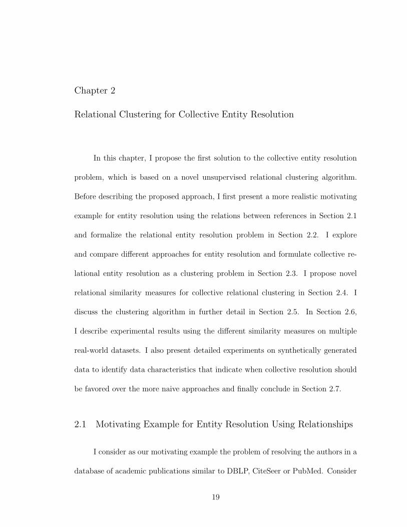
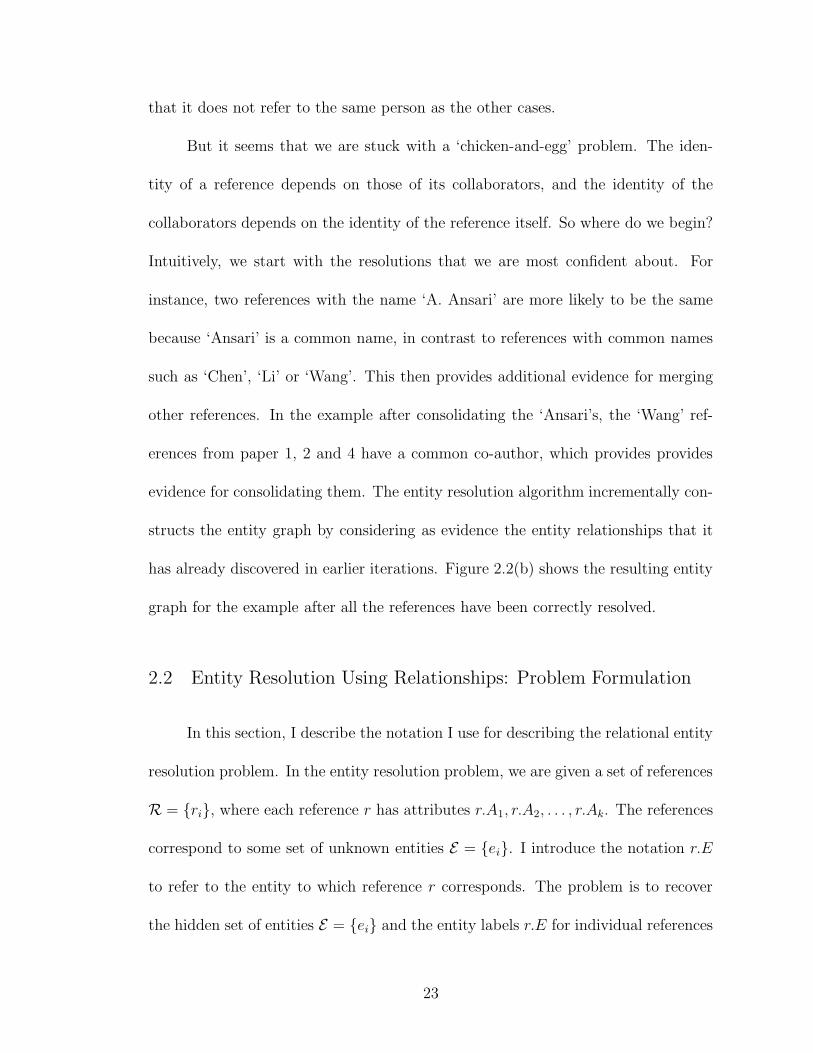
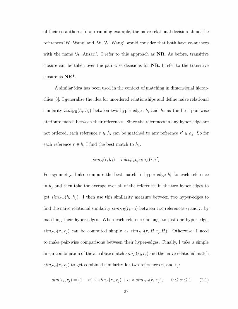
Figure 2.1: The references in different papers in the bibliographic example. Refer-ences to different entities are shaded differently.

the following set of four papers, which I will use as a running example:

1. W. Wang, C. Chen, A. Ansari, “A mouse immunity model”

2. W. Wang, A. Ansari, “A better mouse immunity model”

3. L. Li, C. Chen, W. Wang,“Measuring protein-bound fluxetine”

4. W. W. Wang, A. Ansari, “Autoimmunity in biliary cirrhosis”

Now imagine that we would like to find out, given these four papers, which

of these author names refer to the same author entities. This involves determining

whether paper 1 and paper 2 are written by the same author named Wang, or

whether they are different authors. We need to make similar decisions about the

Wang from paper 3 and the Wang from paper 4, and all pairwise combinations. We

need to answer similar questions about the other author names Ansari and Chen as

well.

In this example, it turns out there are six underlying author entities, Wang1

and Wang2, Chen1 and Chen2, Ansari and Li. The three references with the

20

name ‘A. Ansari’ correspond to author Ansari and the reference with name ‘L. Li’

to author Li. However, the two references with name ‘C. Chen’ map to two different

authors Chen1 and Chen2. Similarly, the four references with name ‘W. Wang’ or

‘W. W. Wang’ map to two different authors. The ‘Wang’ references from the first,

second, and fourth papers correspond to author Wang1, while that from the third

paper maps to a different author Wang2. This is shown pictorially in Figure 2.1,

where references which correspond to the same authors are shaded identically.

There are two different subproblems that are of interest in solving the entity

resolution problem. One is figuring out for any author entity the set of different

name references which may be used to refer to the author. I refer to this as the

identification problem. For example, for a real-world entity with the name ’Wei

Wei Wang’, her name may come up as ‘Wei Wang’, ‘Wei W. Wang’, ‘W. W. Wang’,

‘Wang, W. W.’ and so on. There may also be errors in the data entry process, so

that the name may be incorrectly recorded as ‘W. Wong’ or ‘We Wang’ etc.

In addition to the reconciliation of different looking names which refer to the

same underlying entity, a second aspect of entity resolution problem is distinguishing

references that have very similar and sometimes exactly the same name and yet refer

to different underlying entities. I refer to this as the disambiguation problem.

An example of this is determining that the ’W. Wang’ of paper 1 is distinct from

the ’W. Wang’ of paper 3. The extent of the disambiguation problem depends on

the domain. The problem can be exacerbated by the use of abbreviations; many

databases (for example PubMed) store only abbreviated names.

21

A Ansari

A AnsariW W Wang

W WangW Wang A Ansari

W Wang

C Chen

C Chen

L Li

(a)

Chen2

Wang2Li

Ansari

Chen1

Wang1

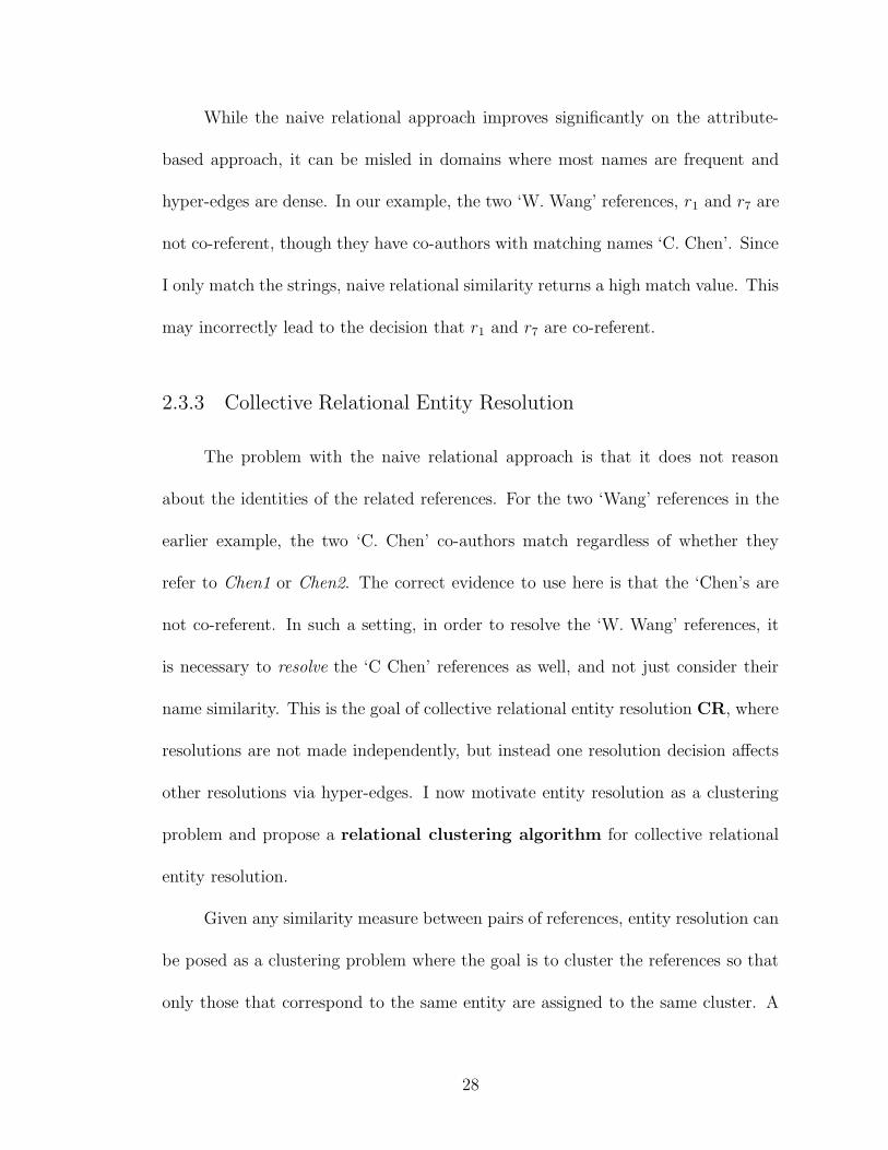
(b)

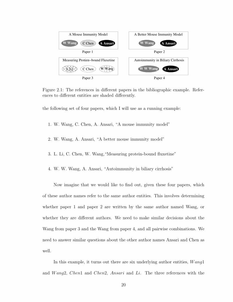
Figure 2.2: (a) The reference graph and (b) the entity graph for the author resolutionexample.

The aim is to make use of the relationships that hold among the observed

references to resolve them better, and to solve both the identification and disam-

biguation problem at the same time. As in the case of the census example, we can

represent the relationships as a graph where the vertices represent the author refer-

ences and the hyper-edges represent the co-authorship relations that hold between

them in the dataset. Figure 2.2(a) shows the reference graph for the bibliographic

example, where the nodes are the references and hyper-edges in the graph indicate

which references co-occur. Given this graph representation for the data, the goal is

to take the hyper-edges into account to better partition the references into entities.

Now, in addition to the similarity of the attributes of the references, I consider their

relationships as well. In terms of the graph representation, two references that have

similar attributes are more likely to be the same entity if their hyper-edges connect

to the same entities as well. To see how this can help, observe in Figure 2.1(a) that

the Wang references in papers 1, 2 and 4 collaborate with Ansari’s who correspond

to the same author. This makes it more likely that they are the same entity. In con-

trast, the ‘Wang’ from paper 3 collaborates with different authors, which suggests

22

that it does not refer to the same person as the other cases.

But it seems that we are stuck with a ‘chicken-and-egg’ problem. The iden-

tity of a reference depends on those of its collaborators, and the identity of the

collaborators depends on the identity of the reference itself. So where do we begin?

Intuitively, we start with the resolutions that we are most confident about. For

instance, two references with the name ‘A. Ansari’ are more likely to be the same

because ‘Ansari’ is a common name, in contrast to references with common names

such as ‘Chen’, ‘Li’ or ‘Wang’. This then provides additional evidence for merging

other references. In the example after consolidating the ‘Ansari’s, the ‘Wang’ ref-

erences from paper 1, 2 and 4 have a common co-author, which provides provides

evidence for consolidating them. The entity resolution algorithm incrementally con-

structs the entity graph by considering as evidence the entity relationships that it

has already discovered in earlier iterations. Figure 2.2(b) shows the resulting entity

graph for the example after all the references have been correctly resolved.

2.2 Entity Resolution Using Relationships: Problem Formulation

In this section, I describe the notation I use for describing the relational entity

resolution problem. In the entity resolution problem, we are given a set of references

R = {ri}, where each reference r has attributes r.A1, r.A2, . . . , r.Ak. The references

correspond to some set of unknown entities E = {ei}. I introduce the notation r.E

to refer to the entity to which reference r corresponds. The problem is to recover

the hidden set of entities E = {ei} and the entity labels r.E for individual references

23

h h

h h

1 2

43

r r

rrr

r

r

r

r

r1 2

3

4 5

6 7

8

9 10

(a)

r 2 r 4 r 10r 1 r 5 r 9

h3

h1

h4

h2

r 6 r 7

r 8

r 3

Wang1: Ansari:

Li:

Chen2:

Wang2:

Chen1:

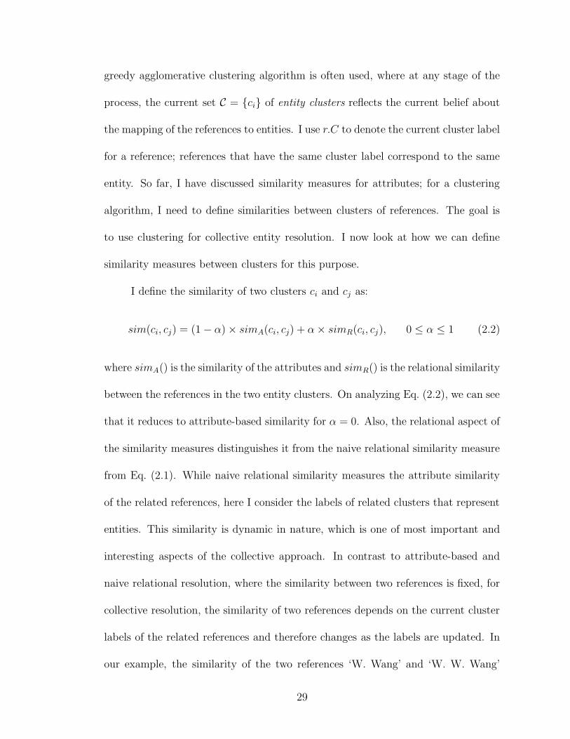
(b)

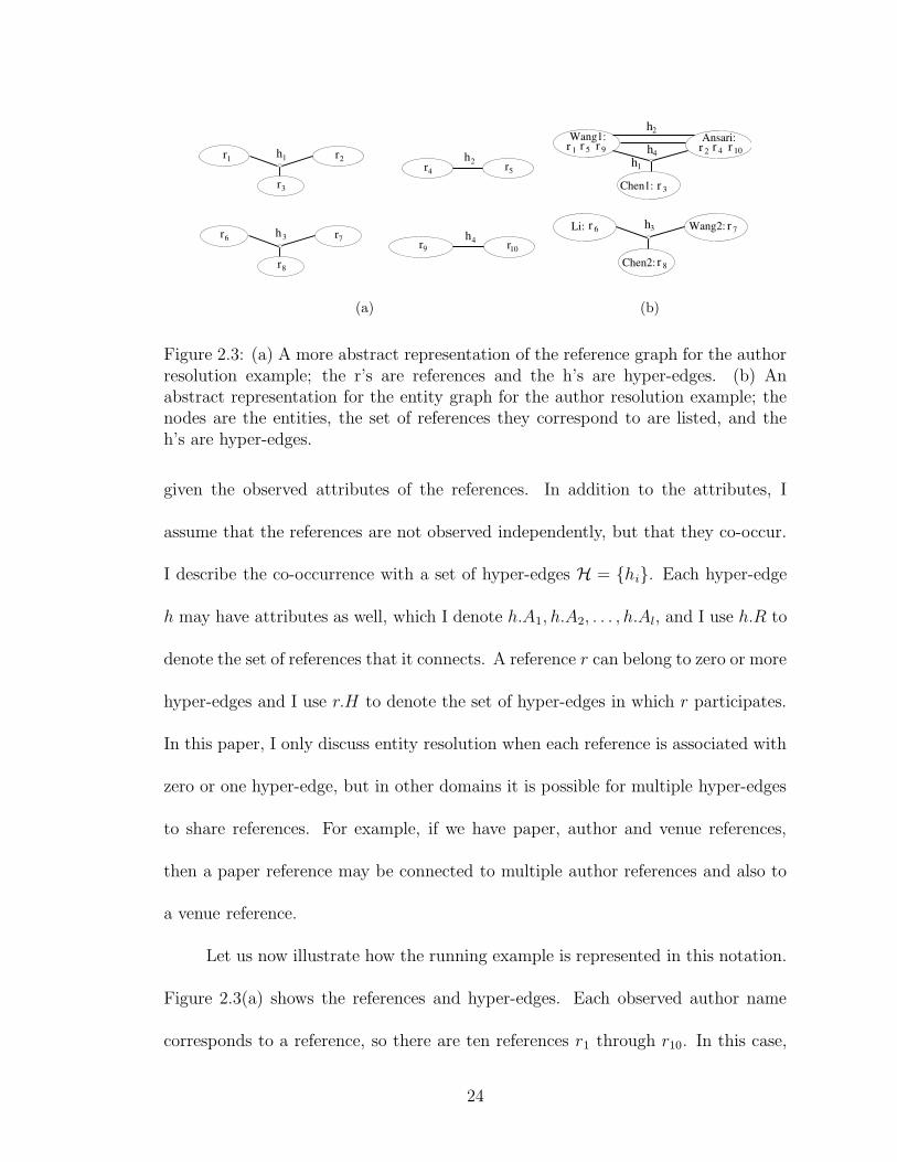
Figure 2.3: (a) A more abstract representation of the reference graph for the authorresolution example; the r’s are references and the h’s are hyper-edges. (b) Anabstract representation for the entity graph for the author resolution example; thenodes are the entities, the set of references they correspond to are listed, and theh’s are hyper-edges.

given the observed attributes of the references. In addition to the attributes, I

assume that the references are not observed independently, but that they co-occur.

I describe the co-occurrence with a set of hyper-edges H = {hi}. Each hyper-edge

h may have attributes as well, which I denote h.A1, h.A2, . . . , h.Al, and I use h.R to

denote the set of references that it connects. A reference r can belong to zero or more

hyper-edges and I use r.H to denote the set of hyper-edges in which r participates.

In this paper, I only discuss entity resolution when each reference is associated with

zero or one hyper-edge, but in other domains it is possible for multiple hyper-edges

to share references. For example, if we have paper, author and venue references,

then a paper reference may be connected to multiple author references and also to

a venue reference.

Let us now illustrate how the running example is represented in this notation.

Figure 2.3(a) shows the references and hyper-edges. Each observed author name

corresponds to a reference, so there are ten references r1 through r10. In this case,

24

the names are the only attributes of the references, so for example r1.A is “W.

Wang”, r2.A is “C. Chen” and r3.A is “A. Ansari”. The set of true entities E is

{Ansari, Wang1, Wang2, Chen1, Chen2, Li} as shown in Figure 2.3(b). References

r1, r5 and r9 correspond to Wang1, so that r1.E = r5.E = r9.E = Wang1. Similarly,

r2.E = r4.E = r10.E = Ansari and r3.E = Chen1 and so on. There are also the

hyper-edges H = {h1, h2, h3, h4}, one for each paper. The attributes of the hyper-

edges in this domain are the paper titles; for example, h1.A1=“A Mouse Immunity

Model”. The references r1 through r3 are associated with hyper-edge h1, since

they are the observed author references in the first paper. This is represented as

h1.R = {r1, r2, r3}. Also, this is the only hyper-edge that each of these references

participate in. So r1.H = r2.H = r3.H = {h1}. I similarly represent the hyper-edge

associations of the other references.

2.3 Entity Resolution Approaches

In this section, I compare and contrast existing entity resolution approaches. I

distinguish between attribute-based, naive relational and collective relational entity

resolution. While the attribute-based approach considers only the attributes of the

references to be matched, the naive relational approach considers attribute similar-

ities for related references as well. In contrast, the collective relational approach

resolves related references jointly. I consider each approach in detail one by one.

25

2.3.1 Attribute-based Entity Resolution

This is the traditional approach [44, 30] where similarity simA(ri, rj) is com-

puted for each pair of references ri, rj based on their attributes and only those pairs

that have similarity above some threshold are considered co-referent. I use the ab-

breviation A to refer to the attribute-based approach. Additionally, transitive

closure may be taken over the pair-wise decisions. I denote this approach as A*.

Several sophisticated similarity measures have been developed for names, and

popular TF-IDF schemes may be used for other textual attributes like keywords.

The measure that works best for each attribute can be used. Finally, a weighted

combination of the similarities over the different attributes for each reference can be

taken for the combined attribute similarity between two references. In our example,

the approach A may allow us to decide that the ‘W. Wang’ references (r1, r5) are

co-referent. I may also decide using A that ‘W. Wang’ and ‘W.W. Wang’ (r1, r9) are

co-referent, but not as confidently. However, as I have already discussed, attributes

are often insufficient for entity resolution, particularly for the disambiguation aspect

of the problem. In our example, A is almost certain to mark the two ‘W. Wang’

references (r1, r7) as co-referent, which is incorrect.

2.3.2 Naive Relational Entity Resolution

The simplest way to use relationships to resolve entities is to treat related

references as additional attributes for matching. For instance, to determine if two

author references in two different papers are co-referent, we can compare the names

26

of their co-authors. In our running example, the naive relational decision about the

references ‘W. Wang’ and ‘W. W. Wang’, would consider that both have co-authors

with the name ‘A. Ansari’. I refer to this approach as NR. As before, transitive

closure can be taken over the pair-wise decisions for NR. I refer to the transitive

closure as NR*.

A similar idea has been used in the context of matching in dimensional hierar-

chies [3]. I generalize the idea for unordered relationships and define naive relational

similarity simNR(hi, hj) between two hyper-edges hi and hj as the best pair-wise

attribute match between their references. Since the references in any hyper-edge are

not ordered, each reference r ∈ hi can be matched to any reference r′ ∈ hj. So for

each reference r ∈ hi I find the best match to hj:

simA(r, hj) = maxr′∈hjsimA(r, r′)

For symmetry, I also compute the best match to hyper-edge hi for each reference

in hj and then take the average over all of the references in the two hyper-edges to

get simNR(hi, hj). I then use this similarity measure between two hyper-edges to

find the naive relational similarity simNR(ri, rj) between two references ri and rj by

matching their hyper-edges. When each reference belongs to just one hyper-edge,

simNR(ri, rj) can be computed simply as simNR(ri.H, rj.H). Otherwise, I need

to make pair-wise comparisons between their hyper-edges. Finally, I take a simple

linear combination of the attribute match simA(ri, rj) and the naive relational match

simNR(ri, rj) to get combined similarity for two references ri and rj:

sim(ri, rj) = (1 − α) × simA(ri, rj) + α × simNR(ri, rj), 0 ≤ α ≤ 1 (2.1)

27

While the naive relational approach improves significantly on the attribute-

based approach, it can be misled in domains where most names are frequent and

hyper-edges are dense. In our example, the two ‘W. Wang’ references, r1 and r7 are

not co-referent, though they have co-authors with matching names ‘C. Chen’. Since

I only match the strings, naive relational similarity returns a high match value. This

may incorrectly lead to the decision that r1 and r7 are co-referent.

2.3.3 Collective Relational Entity Resolution

The problem with the naive relational approach is that it does not reason

about the identities of the related references. For the two ‘Wang’ references in the

earlier example, the two ‘C. Chen’ co-authors match regardless of whether they

refer to Chen1 or Chen2. The correct evidence to use here is that the ‘Chen’s are

not co-referent. In such a setting, in order to resolve the ‘W. Wang’ references, it

is necessary to resolve the ‘C Chen’ references as well, and not just consider their

name similarity. This is the goal of collective relational entity resolution CR, where

resolutions are not made independently, but instead one resolution decision affects

other resolutions via hyper-edges. I now motivate entity resolution as a clustering

problem and propose a relational clustering algorithm for collective relational

entity resolution.

Given any similarity measure between pairs of references, entity resolution can

be posed as a clustering problem where the goal is to cluster the references so that

only those that correspond to the same entity are assigned to the same cluster. A

28

greedy agglomerative clustering algorithm is often used, where at any stage of the

process, the current set C = {ci} of entity clusters reflects the current belief about

the mapping of the references to entities. I use r.C to denote the current cluster label

for a reference; references that have the same cluster label correspond to the same

entity. So far, I have discussed similarity measures for attributes; for a clustering

algorithm, I need to define similarities between clusters of references. The goal is

to use clustering for collective entity resolution. I now look at how we can define

similarity measures between clusters for this purpose.

I define the similarity of two clusters ci and cj as:

sim(ci, cj) = (1 − α) × simA(ci, cj) + α × simR(ci, cj), 0 ≤ α ≤ 1 (2.2)

where simA() is the similarity of the attributes and simR() is the relational similarity

between the references in the two entity clusters. On analyzing Eq. (2.2), we can see

that it reduces to attribute-based similarity for α = 0. Also, the relational aspect of

the similarity measures distinguishes it from the naive relational similarity measure

from Eq. (2.1). While naive relational similarity measures the attribute similarity

of the related references, here I consider the labels of related clusters that represent

entities. This similarity is dynamic in nature, which is one of most important and

interesting aspects of the collective approach. In contrast to attribute-based and

naive relational resolution, where the similarity between two references is fixed, for

collective resolution, the similarity of two references depends on the current cluster

labels of the related references and therefore changes as the labels are updated. In

our example, the similarity of the two references ‘W. Wang’ and ‘W. W. Wang’

29

increase once the Ansari references are given the same cluster label.

As I have mentioned earlier, similarity measures for attributes have been stud-

ied in great detail. The focus is on measuring relational similarity between two clus-

ters of references. The references in each cluster c are connected to other references

via hyper-edges. For collective entity resolution, relational similarity considers the

cluster labels of all these connected references. Recall that each reference r is as-

sociated with one or more hyper-edges in H. Therefore, the set of hyper-edges c.H

that I need to consider for an entity cluster c is defined as

c.H =⋃

r∈R∧r.C=c

{h | h ∈ H ∧ r ∈ h.R}

These hyper-edges connect c to other clusters. The relational similarity for two

clusters c1 and c2 needs to compare this connectivity pattern to other clusters for

c1 and c2.

For any cluster c, the set of other clusters to which c is connected via its

hyper-edge set c.H form the neighborhood Nbr(c) of cluster c:

Nbr(c) =⋃

h∈c.H,r∈h.R

{cj | cj = r.C}

This defines the neighborhood as a set of related clusters, but the neighborhood

can also be defined as a bag or multi-set, in which the multiplicity of the different

neighboring clusters is preserved. I will use NbrB(ci) to denote the bag of neighbor-

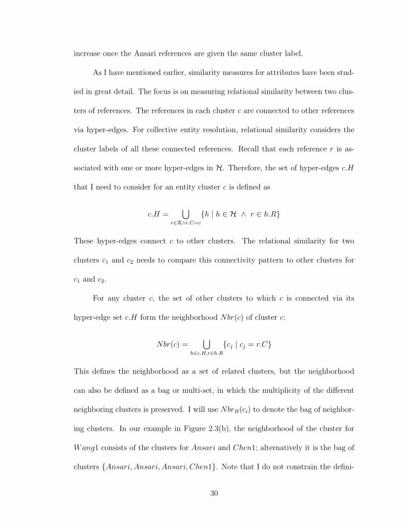
ing clusters. In our example in Figure 2.3(b), the neighborhood of the cluster for

Wang1 consists of the clusters for Ansari and Chen1; alternatively it is the bag of

clusters {Ansari, Ansari, Ansari, Chen1}. Note that I do not constrain the defini-

30

tion of the neighborhood of a cluster to exclude the cluster itself. In Section 2.4.6,

I discuss how such constraints can be handled when required by the domain.

For the relational similarity between two clusters, I look for commonness in

their neighborhoods. This can be done in many different ways, as I explore in the

following section.

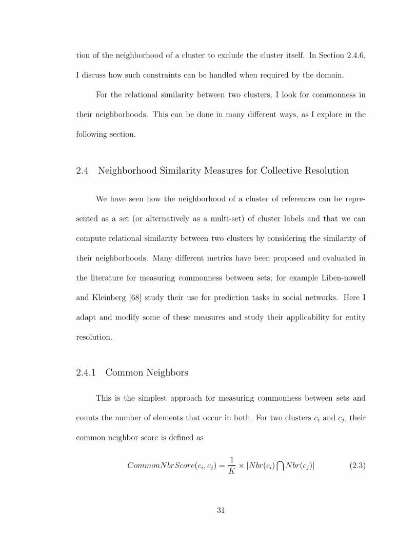
2.4 Neighborhood Similarity Measures for Collective Resolution

We have seen how the neighborhood of a cluster of references can be repre-

sented as a set (or alternatively as a multi-set) of cluster labels and that we can

compute relational similarity between two clusters by considering the similarity of

their neighborhoods. Many different metrics have been proposed and evaluated in

the literature for measuring commonness between sets; for example Liben-nowell

and Kleinberg [68] study their use for prediction tasks in social networks. Here I

adapt and modify some of these measures and study their applicability for entity

resolution.

2.4.1 Common Neighbors

This is the simplest approach for measuring commonness between sets and

counts the number of elements that occur in both. For two clusters ci and cj, their

common neighbor score is defined as

CommonNbrScore(ci, cj) =1

K× |Nbr(ci)

⋂

Nbr(cj)| (2.3)

31

where K is a large enough constant such that the measure is less than 1 for all

pairs of clusters. For two references ‘John Smith’ and ‘J. Smith’, where attribute

similarity is not very informative, this score measures the overlap in their connected

entities. The greater the number of common entities, the higher the possibility that

the two references refer to the same entity as well.

This definition ignores the frequency of connectivity to a neighbor. Suppose

‘John Smith’ has collaborated with the entity ‘J. Brown’ several times, while ‘J.

Smith’ has done so only once. To investigate if this information is relevant for

entity resolution, I also define a common neighbor score with frequencies that takes

into account multiple occurrences of common clusters in the neighborhoods:

CommonNbrScore + Fr(ci, cj) =1

K ′× |NbrB(ci)

⋂

NbrB(cj)| (2.4)

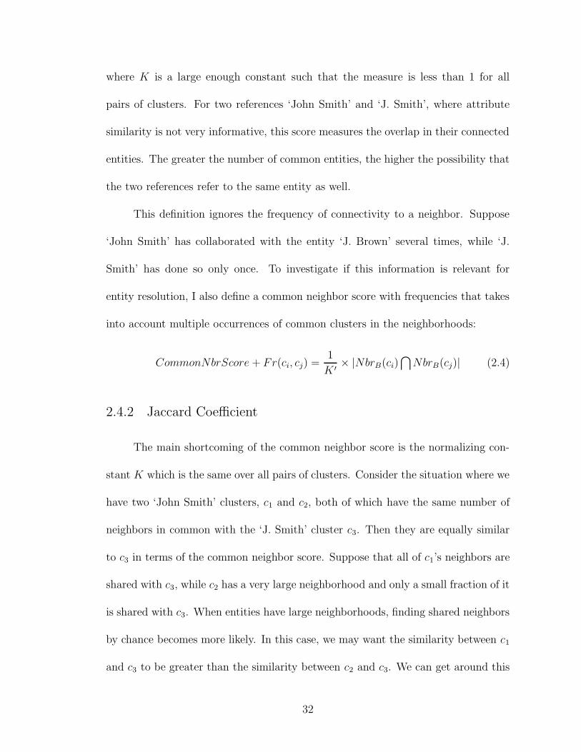
2.4.2 Jaccard Coefficient

The main shortcoming of the common neighbor score is the normalizing con-

stant K which is the same over all pairs of clusters. Consider the situation where we

have two ‘John Smith’ clusters, c1 and c2, both of which have the same number of

neighbors in common with the ‘J. Smith’ cluster c3. Then they are equally similar

to c3 in terms of the common neighbor score. Suppose that all of c1’s neighbors are

shared with c3, while c2 has a very large neighborhood and only a small fraction of it

is shared with c3. When entities have large neighborhoods, finding shared neighbors

by chance becomes more likely. In this case, we may want the similarity between c1

and c3 to be greater than the similarity between c2 and c3. We can get around this

32

issue by taking into account the size of neighborhood. This gives us the Jaccard

coefficient for two clusters:

JaccardCoeff(ci, cj) =|Nbr(ci)

⋂

Nbr(cj)|

|Nbr(ci)⋃

Nbr(cj)|(2.5)

As before, we may consider neighbor counts to define the Jaccard coefficient with

frequencies, JaccardCoeff + Fr(ci, cj), by using NbrB(ci) and NbrB(cj) in the

definition.

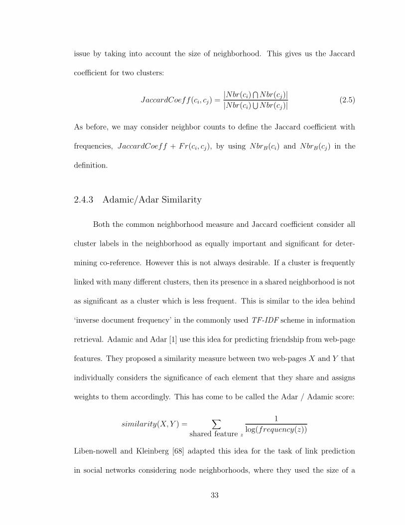
2.4.3 Adamic/Adar Similarity

Both the common neighborhood measure and Jaccard coefficient consider all

cluster labels in the neighborhood as equally important and significant for deter-

mining co-reference. However this is not always desirable. If a cluster is frequently

linked with many different clusters, then its presence in a shared neighborhood is not

as significant as a cluster which is less frequent. This is similar to the idea behind

‘inverse document frequency’ in the commonly used TF-IDF scheme in information

retrieval. Adamic and Adar [1] use this idea for predicting friendship from web-page

features. They proposed a similarity measure between two web-pages X and Y that

individually considers the significance of each element that they share and assigns

weights to them accordingly. This has come to be called the Adar / Adamic score:

similarity(X, Y ) =∑

shared feature z

1

log(frequency(z))

Liben-nowell and Kleinberg [68] adapted this idea for the task of link prediction

in social networks considering node neighborhoods, where they used the size of a

33

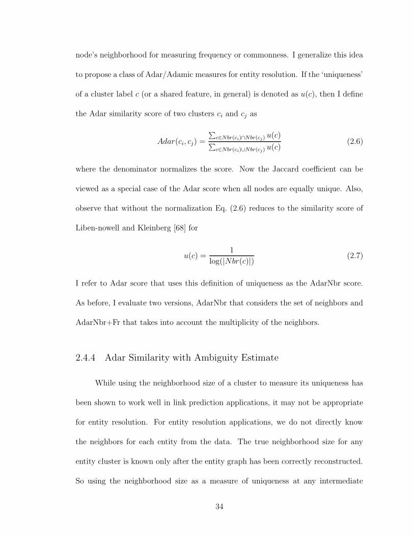
node’s neighborhood for measuring frequency or commonness. I generalize this idea

to propose a class of Adar/Adamic measures for entity resolution. If the ‘uniqueness’

of a cluster label c (or a shared feature, in general) is denoted as u(c), then I define

the Adar similarity score of two clusters ci and cj as

Adar(ci, cj) =

∑

c∈Nbr(ci)∩Nbr(cj) u(c)∑

c∈Nbr(ci)∪Nbr(cj) u(c)(2.6)

where the denominator normalizes the score. Now the Jaccard coefficient can be

viewed as a special case of the Adar score when all nodes are equally unique. Also,

observe that without the normalization Eq. (2.6) reduces to the similarity score of

Liben-nowell and Kleinberg [68] for

u(c) =1

log(|Nbr(c)|)(2.7)

I refer to Adar score that uses this definition of uniqueness as the AdarNbr score.

As before, I evaluate two versions, AdarNbr that considers the set of neighbors and

AdarNbr+Fr that takes into account the multiplicity of the neighbors.

2.4.4 Adar Similarity with Ambiguity Estimate

While using the neighborhood size of a cluster to measure its uniqueness has

been shown to work well in link prediction applications, it may not be appropriate

for entity resolution. For entity resolution applications, we do not directly know

the neighbors for each entity from the data. The true neighborhood size for any

entity cluster is known only after the entity graph has been correctly reconstructed.

So using the neighborhood size as a measure of uniqueness at any intermediate

34

stage of the resolution algorithm is incorrect, and is an overestimate of the actual

neighborhood size.

As an alternative, we can use a definition of uniqueness which incorporates

a notion of the ambiguity of the names found in the shared neighborhood. To

understand what this means, consider two references with name ‘A. Aho’. Since

‘Aho’ can be considered as an ‘uncommon’ name, they are very likely to be the

same person. In contrast, two other references with a common name such as ‘L. Li’

are less likely to be the same person. So I define the ambiguity Amb(r.Name) of a

reference name as the probability that multiple entities share that particular name.

Intuitively, clusters which share neighbors with uncommon names are more

likely to refer to the same entity and should be considered more similar. I define

the uniqueness of a cluster c as inversely proportional to the average ambiguity of

its references:

u(c) =1

Avgr∈c(Amb(r.Name))(2.8)

In general, this approach is not specific to names and can be used with any attribute

of the references. I refer to an Adar similarity score which uses this definition of

uniqueness as AdarName when applied to the set of neighbors and AdarName+Fr

to refer to the measure applied to the bag of neighbors.

The Adar-Name measure is defined in terms of the ambiguity of a reference’s

name. There are a number of ways to estimate the ambiguity of a name. One

scheme that works quite well in our domains is to estimate the probability that two

randomly picked references with Name = n correspond to different entities. For a

35

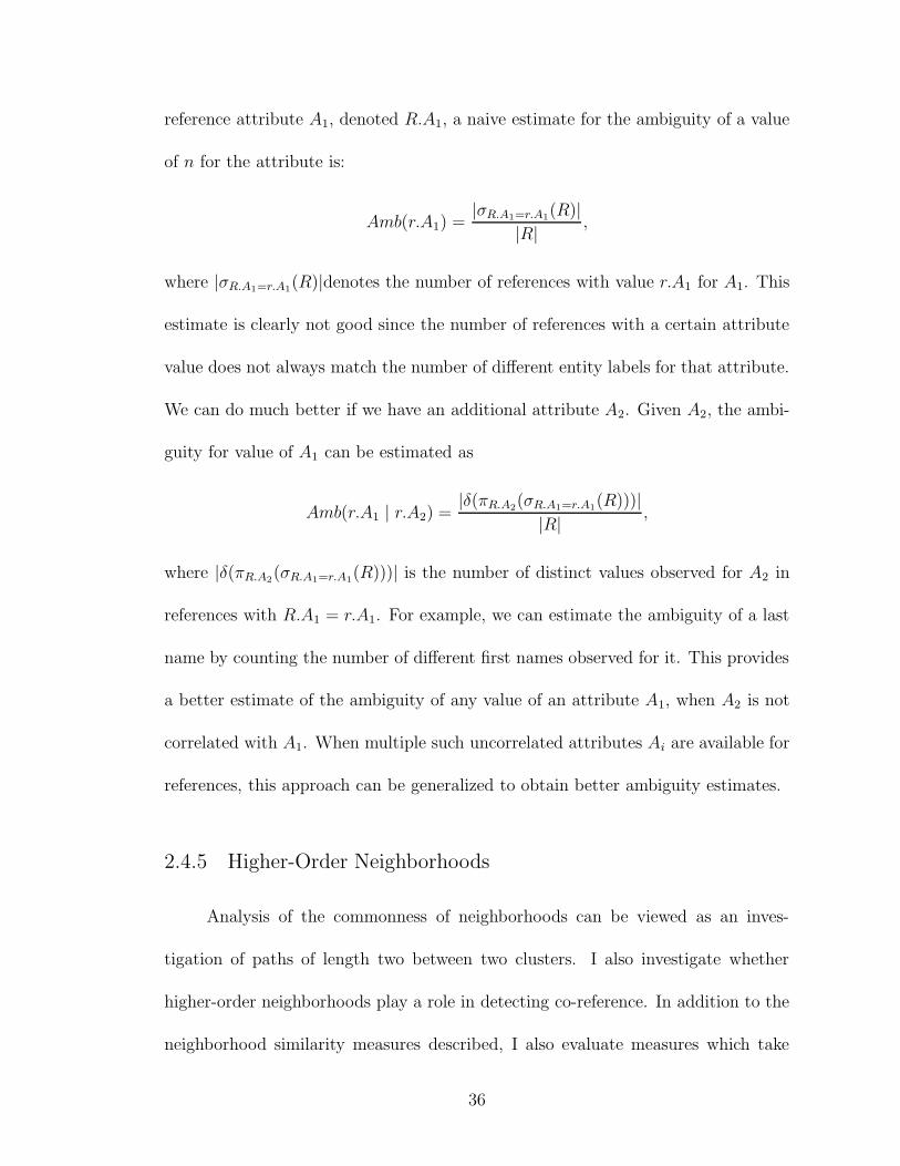
reference attribute A1, denoted R.A1, a naive estimate for the ambiguity of a value

of n for the attribute is:

Amb(r.A1) =|σR.A1=r.A1(R)|

|R|,

where |σR.A1=r.A1(R)|denotes the number of references with value r.A1 for A1. This

estimate is clearly not good since the number of references with a certain attribute

value does not always match the number of different entity labels for that attribute.

We can do much better if we have an additional attribute A2. Given A2, the ambi-

guity for value of A1 can be estimated as

Amb(r.A1 | r.A2) =|δ(πR.A2(σR.A1=r.A1(R)))|

|R|,

where |δ(πR.A2(σR.A1=r.A1(R)))| is the number of distinct values observed for A2 in

references with R.A1 = r.A1. For example, we can estimate the ambiguity of a last

name by counting the number of different first names observed for it. This provides

a better estimate of the ambiguity of any value of an attribute A1, when A2 is not

correlated with A1. When multiple such uncorrelated attributes Ai are available for

references, this approach can be generalized to obtain better ambiguity estimates.

2.4.5 Higher-Order Neighborhoods

Analysis of the commonness of neighborhoods can be viewed as an inves-

tigation of paths of length two between two clusters. I also investigate whether

higher-order neighborhoods play a role in detecting co-reference. In addition to the

neighborhood similarity measures described, I also evaluate measures which take

36

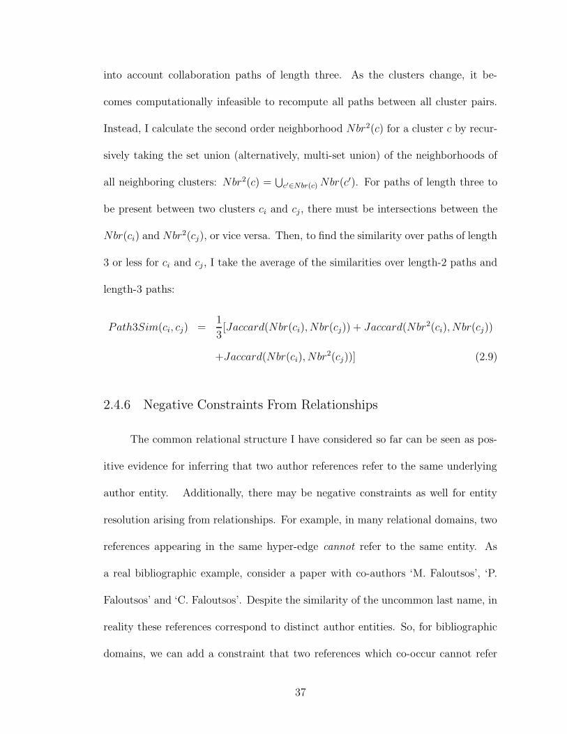
into account collaboration paths of length three. As the clusters change, it be-

comes computationally infeasible to recompute all paths between all cluster pairs.

Instead, I calculate the second order neighborhood Nbr2(c) for a cluster c by recur-

sively taking the set union (alternatively, multi-set union) of the neighborhoods of

all neighboring clusters: Nbr2(c) =⋃

c′∈Nbr(c) Nbr(c′). For paths of length three to

be present between two clusters ci and cj, there must be intersections between the

Nbr(ci) and Nbr2(cj), or vice versa. Then, to find the similarity over paths of length

3 or less for ci and cj, I take the average of the similarities over length-2 paths and

length-3 paths:

Path3Sim(ci, cj) =1

3[Jaccard(Nbr(ci), Nbr(cj)) + Jaccard(Nbr2(ci), Nbr(cj))

+Jaccard(Nbr(ci), Nbr2(cj))] (2.9)

2.4.6 Negative Constraints From Relationships

The common relational structure I have considered so far can be seen as pos-

itive evidence for inferring that two author references refer to the same underlying

author entity. Additionally, there may be negative constraints as well for entity

resolution arising from relationships. For example, in many relational domains, two

references appearing in the same hyper-edge cannot refer to the same entity. As

a real bibliographic example, consider a paper with co-authors ‘M. Faloutsos’, ‘P.

Faloutsos’ and ‘C. Faloutsos’. Despite the similarity of the uncommon last name, in

reality these references correspond to distinct author entities. So, for bibliographic

domains, we can add a constraint that two references which co-occur cannot refer

37

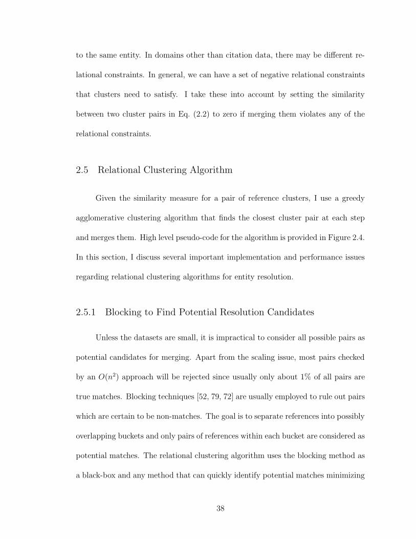
to the same entity. In domains other than citation data, there may be different re-

lational constraints. In general, we can have a set of negative relational constraints

that clusters need to satisfy. I take these into account by setting the similarity

between two cluster pairs in Eq. (2.2) to zero if merging them violates any of the

relational constraints.

2.5 Relational Clustering Algorithm

Given the similarity measure for a pair of reference clusters, I use a greedy

agglomerative clustering algorithm that finds the closest cluster pair at each step

and merges them. High level pseudo-code for the algorithm is provided in Figure 2.4.

In this section, I discuss several important implementation and performance issues

regarding relational clustering algorithms for entity resolution.

2.5.1 Blocking to Find Potential Resolution Candidates

Unless the datasets are small, it is impractical to consider all possible pairs as

potential candidates for merging. Apart from the scaling issue, most pairs checked

by an O(n2) approach will be rejected since usually only about 1% of all pairs are

true matches. Blocking techniques [52, 79, 72] are usually employed to rule out pairs

which are certain to be non-matches. The goal is to separate references into possibly

overlapping buckets and only pairs of references within each bucket are considered as

potential matches. The relational clustering algorithm uses the blocking method as

a black-box and any method that can quickly identify potential matches minimizing

38

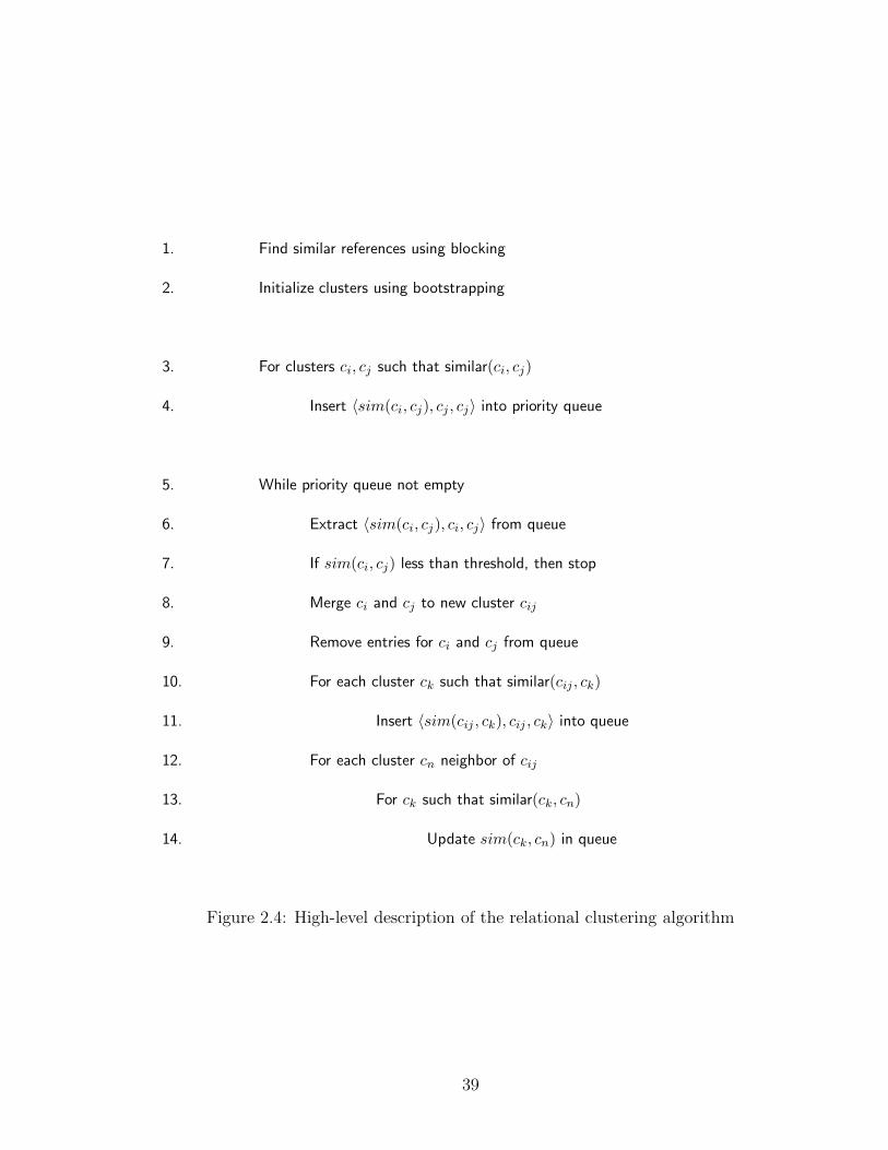
1. Find similar references using blocking

2. Initialize clusters using bootstrapping

3. For clusters ci, cj such that similar(ci, cj)

4. Insert 〈sim(ci, cj), cj , cj〉 into priority queue

5. While priority queue not empty

6. Extract 〈sim(ci, cj), ci, cj〉 from queue

7. If sim(ci, cj) less than threshold, then stop

8. Merge ci and cj to new cluster cij

9. Remove entries for ci and cj from queue

10. For each cluster ck such that similar(cij , ck)

11. Insert 〈sim(cij , ck), cij , ck〉 into queue

12. For each cluster cn neighbor of cij

13. For ck such that similar(ck, cn)

14. Update sim(ck, cn) in queue

Figure 2.4: High-level description of the relational clustering algorithm

39

false negatives can be used. I use a variant of an algorithm proposed by McCallum

et al. [72] that I briefly describe below.

The algorithm makes a single pass over the list of references and assigns them

to buckets using an attribute similarity measure. Each bucket has a representative

reference that is the most similar to all references currently in the bucket. For

assigning any reference, it is compared to the representative for each bucket. It is

assigned to all buckets for which the similarity is above a threshold. If no similar

bucket is found, a new bucket is created for this reference. A naive implementation

yields a O(n(b + f)) algorithm for n references and b buckets and when a reference

is assigned to at most f buckets. This can be improved by maintaining an inverted

index over buckets. For example, when dealing with names, for each character I

maintain the list of buckets storing last names starting with that character. Then

the buckets can be looked up in constant time for each reference leading to an O(nf)

algorithm.

2.5.2 Relational Bootstrapping

Each iteration of the relational clustering algorithm makes use of clustering

decisions made in previous iterations. This is achieved by measuring the shared

neighborhood for similar clusters, as explained in Subsection 2.3.3. But if we begin

with each reference in a distinct cluster, then initially there are no shared neigh-

bors for references that belong to different hyper-edges. So the initial iterations of

the algorithm have no relational evidence to depend on. As a result, the relational

40

component of the similarity between clusters would be zero and merges would occur

based on attribute similarity alone. Many of such initial merges can be inaccurate,

particularly for the references with ambiguous attribute values. To get around this,

we need to bootstrap the clustering algorithm such that each reference is not as-

signed to a distinct cluster. Specifically, if we are confident that some reference pair

is coreferent, then they should be assigned to the same initial cluster. However,

precision is crucial for the bootstrap process, since the algorithm cannot undo any

of these initial merge operations. Observe that this bootstrapping is not necessary

for approaches that are not collective. For such approaches, the decision for any ref-

erence pair is the same irrespective of the decisions for other pairs. So bootstrapping

does not have any effect on subsequent decisions. In this subsection, I describe the

bootstrapping scheme for relational clustering that makes use of the hyper-edges

for improved bootstrap performance. The basic idea is very similar to the naive

relational approach described in Subsection 2.3.2, with the difference that I use ex-

act matches instead of similarity for attributes. To determine if any two references

should be assigned to the same initial cluster, I check if their attributes match ex-

actly. For references with ambiguous attributes, I also check if the attributes of their

related references match. I now discuss this in greater detail.

The bootstrap scheme goes over each reference pair that is potentially coref-

erent (as determined by blocking) and determines if it is a bootstrap candidate.

First, consider the simple bootstrap scheme that looks only at the attributes of two

references. It determines which attribute values are ambiguous and which are not

using a data-based ambiguity estimate, as described in Subsection 2.4.4. References

41

with ambiguous attribute values are assigned to distinct clusters. Any reference pair

whose attribute values match and are not ambiguous is considered to be a bootstrap

candidate.

The problem with this simple approach is that it assigns all references with

ambiguous attributes to distinct clusters leading to poor recall in datasets with

high ambiguity. When hyper-edges are available, they can be used as evidence

for bootstrapping of ambiguous references. A pair of ambiguous references form a

bootstrap candidate if their hyper-edges match. Two hyper-edges h1 and h2 are said

to have a k-exact-match if there are at least k pairs of references (ri, rj), ri ∈ h1.R,

rj ∈ h2.R with exactly matching attributes, i.e. ri.A = rj.A. Two references r1 and

r2 are bootstrap candidates if any pair of their hyper-edges have a k-exact-match.

As a bibliographic example, two references with name ‘W. Wang’ will not be merged

during bootstrapping on the basis of the name alone. However, if the first Wang

reference has co-authors ‘A. Ansari’ and ‘C. Chen’, and the second Johnson has

coauthor ‘A. Ansari’, then they have a 1-exact-match and, depending on a threshold

for k, they would be merged. The value of k for the hyper-edge test depends on the

ambiguity of the domain. A higher value of k should be used for domains with high

ambiguity. Also, when matching hyper-edges, references with ambiguous attributes

are not considered for matches in high ambiguity domains. For example, ‘C. Chen’

may not be considered for a co-author match, since it is a common name.

Other attributes of the references, and also of the hyper-edges, when available,

can be used to further constrain bootstrap candidates. Two references are considered

only if these other attributes do not conflict. In the bibliographic domain, author

42

references from two different papers can be merged only if their languages and

correspondence addresses match.

After the bootstrap candidates are identified, the initial clusters are created

using the union-find approach so that any two references that are bootstrap can-

didates are assigned to the same initial cluster. In addition to improving accuracy

of the relational clustering algorithm, bootstrapping reduces execution time by sig-

nificantly lowering the initial number of clusters without finding the most similar

cluster-pairs or performing expensive similarity computations.

2.5.3 Merging Clusters and Updating Similarities

Once the similar clusters have been identified and bootstrapping has been per-

formed, the algorithm iteratively merges the most similar cluster pair and updates

similarities until the similarity drops below some specified threshold. This is shown

in lines 5-14 of Figure 2.4. The similarity update steps for related clusters in lines

12-14 are the key steps that distinguish collective relational clustering from a tra-

ditional agglomerative clustering algorithm. In order to perform the update steps

efficiently, indexes need to maintained for each cluster. In this section, I describe

the data structure that I maintain for this purpose.

In addition to its list of references, I maintain three additional lists with each

cluster. First, I maintain the list of similar clusters for each cluster. The second list

keeps track of all neighboring clusters. Finally, I keep track of all the queue entries

that involve this cluster. For a cluster that has a single reference r, the similar

43

clusters are those that contain references in the same bucket as r after blocking.

Also, the neighbors for this cluster are the clusters containing references that share

a hyper-edge with r. Then, as two clusters merge to form a new cluster, all of these

lists can be constructed locally for the new cluster from those of its parents. All of

the update operations from lines 9-14 can be performed efficiently using these lists.

For example, updates for related clusters are done by first accessing the neighbor

list and then traversing the similar list for each of them.

2.5.4 Complexity Analysis

Now that I have described each component of the relational clustering algo-

rithm, let us analyze its time complexity. First, I look at how the number of sim-

ilarity computations required in lines 3-4 of Figure 2.4 is reduced by the blocking

method. I consider the worst case scenario where the bootstrapping approach does

not reduce the number of clusters at all. We need to compare every pair of references

within each bucket. Suppose we have n references that are assigned to b buckets

with each reference being assigned to at most f buckets. Then using an optimistic

estimate, we have nf/b references in each bucket, leading to O((nf/b)2) compar-

isons per bucket and a total of O(n2f 2/b) comparisons. In all of this discussion, I

assume that the number of buckets is proportional to the number of references, i.e.,

b is O(n). Additionally, assuming that f is a small constant independent of n, we

have O(n) computations.

Now, let us look at the time taken by each iteration of the algorithm. To

44

analyze how many update/insert operations are required, I assume that for each

bucket that is affected by a merge operation, all the O((nf/b)2) computations need

to be redone. Then we need to find out how many buckets may be affected by a

merge operation. I say that two buckets are connected if any hyper-edge connects

two references in the two buckets. Then if any bucket is connected to k other buckets,

each merge operation leads to O(k(nf/b)2) update/insert operations. This is still

only O(k) operations when f is a constant independent of n and b is O(n). Using a

binary-heap implementation for the priority queue, the extract-max and each insert

and update operation take O(log q) time, where q is the number of entries in the

queue. So the total cost of each iteration of the algorithm is O(k log q).

Next, I count the total number of iterations that the algorithm may require.

In the worst case, the algorithm may have to exhaust the priority queue before the

similarity falls below the threshold. So we need to consider the number of merge

operations that are required to exhaust a queue that has q entries. If the merge tree

is perfectly balanced, then the size of each cluster is doubled by each merge operation

and as few as O(log q) merges are required. However, in the worst case, the merge

tree may be q deep requiring as many as O(q) merges. With each merge operation

requiring O(k log q) time, the total cost of the iterative process is O(qk log q).

Finally, in order to put a bound on the initial size q of the priority queue,

I again consider the worst case scenario where bootstrapping does not reduce the

number of initial clusters. This resulting in O(n2f 2/b) entries in the queue as shown

earlier. Since this is again O(n), the total cost of the algorithm can be bounded by

O(nk log n). The one cost that I have not considered so far is that of bootstrapping.

45

We can analyze the bootstrapping by considering it as a sequence of cluster merge

operations that do not require any updates or inserts to the priority queue. Then

the worst case analysis of the number of iterations accounts for the bootstrapping

as well.

To see how this compares against the attribute and naive relational baselines,

observe that they need to take a decision for each pair of references in a bucket.

This leads to a worst case analysis of O(n) using the same assumptions as before.

However, each similarity computation is more expensive for the naive relational

approach since it requires a pair-wise match to be computed between two hyper-

edges.

2.6 Experimental Evaluation

I evaluated the proposed relational entity resolution algorithm on several real-

world and synthetic datasets. I begin with a description of the experiments on real

bibliographic datasets.

2.6.1 Evaluation on Bibliographic Data

The real-world datasets describe publications in several different scientific re-

search areas. As in our running example, the goal is to use co-author relationships

in the papers to help discover the underlying author entities in the domain and map

the author references to the discovered author entities. I first describe the datasets

in more detail, and then describe the evaluation and results.

46

2.6.1.1 Datasets

CiteSeer: The CiteSeer dataset contains 1,504 machine learning documents with

2,892 author references to 1,165 author entities. For this dataset, the only attribute

information available is author name. The full last name is always given, and in

some cases the author’s full first name and middle name are given and other times

only the initials are given. The dataset was originally created by Giles et al. [49]

and the version which I use includes the author entity ground truth provided by

Aron Culotta and Andrew McCallum, University of Massachusetts, Amherst.

arXiv: The arXiv dataset describes high energy physics publications. It was orig-

inally used in KDD Cup 20031. It contains 29,555 papers with 58,515 references

to 9,200 authors. The attribute information available for this dataset is also just

the author name, with the same variations in form as described above. The author

entity ground truth for this data set was provided by David Jensen, University of

Massachusetts, Amherst.

BioBase: The third dataset, describing biology publications, is the Elsevier BioBase

dataset2 which was used in a recent IBM KDD-Challenge competition. It was cre-

ated by selecting all Elsevier publications on ‘Immunology and Infectious Diseases’

between years 1998 and 2001. It contains 156,156 publications with 831,991 author

references. Unlike arXiv and CiteSeer that have complete as well as initialed author

names, in BioBase, all of the first names and middle names are abbreviated. How-

1http://www.cs.cornell.edu/projects/kddcup/index.html2http://help.sciencedirect.com/robo/projects/sdhelp/about biobase.htm

47

ever the BioBase dataset has other attributes which I use for resolution including:

keywords, topic classification, language, country of correspondence and affiliation of

the corresponding author. There is a wide variety in the data with 20 languages, 136

countries, 1,282 topic classifications and 7,798 keywords. Entity labels are available

only for the top 100 author names with the highest number of references. I evaluate

entity resolution performance for BioBase over 10,595 references that have these 100

names, although the collective resolution algorithm requires resolving many of the

other references as well.

Ground truth was determined for all of these datasets by the owners using

a combination of automatic and manual strategies. The process is not completely

free from errors and I had to perform additional cleaning for some CiteSeer and

arXiv references in the course of the experiments. For BioBase, 97% of the labels

are estimated to be correct.

Despite the common underlying domain, these datasets vary in a number of

important ways. The most important difference is in the inherent uncertainty in

the name references. I introduce two measures, which I refer to as ambiguity (corre-

sponding to the disambiguation aspect of resolution) and dispersion (corresponding

to the identification aspect), to measure the uncertainty in the data. I consider a

name (last name and first initial) to be ambiguous if multiple entities share that

name. In CiteSeer dataset, only 3 out of 1185 names are ambiguous and the average

number of entities per ambiguous name is 2.33 (the maximum is 3). For arXiv,

374 of the 8737 names are ambiguous, and the average number of entities for these

ambiguous names is 2.41 (the maximum is 11). For BioBase, the ambiguity is much

48

higher — 84 of the 100 names are ambiguous. The number of entities for each name

ranges from 1 to 100 with an average of 32. I introduce dispersion as another mea-

sure of the inherent difficulty of the entity resolution problem for a domain. The

dispersion for an entity is the number of distinct observed names for each entity.

For CiteSeer, 202 out of the 1164 entities have multiple recorded names, the average

and maximum dispersion are 1.24 and 8 respectively. In contrast, 3083 out of 8967

entities for arXiv are dispersed over multiple names, and the average dispersion is

1.44 and the maximum is 10. Since I do not have complete ground truth for the

BioBase dataset, dispersion cannot be directly measured. Apart from the level of

uncertainty, BioBase differs significantly from the other two datasets in terms of its

hyper-edge structure. For BioBase, the number of author references per publication

ranges from 1 to 100 with the average being 5.3. In comparison, the averages are

1.92 and 1.98 respectively for CiteSeer and arXiv, the range being 1 to 10 for both.

2.6.1.2 Evaluation

I compare attribute-based entity resolution (A), naive relational entity reso-

lution (NR) that uses attributes of related references, and the proposed collective

relational entity resolution (CR). For the first two algorithms, I also consider vari-

ants which perform transitive closures over the pair-wise decisions (A* and NR*).

In order to measure the performance of the algorithms I consider the cor-

rectness of the pair-wise co-reference decisions over all references. I evaluate the

pair-wise decisions using the F1 measure, which is the harmonic mean of precision

49

and recall. For a fair comparison, I consider the best F1 for each of these algorithms

over all possible thresholds for determining matches.

2.6.1.3 Experimental Details

For comparing attributes, which is required for all of the algorithms, I use the

Soft TF-IDF similarity for names [30, 16] since it has been shown to perform well

for name-based entity resolution. Essentially, Soft TF-IDF augments the TF-IDF

similarity for matching token sets with approximate token matching using a sec-

ondary string similarity measure. Jaro-Winkler is reported to be the best secondary

similarity measure for Soft TF-IDF, but for completeness, I also experiment with

the Jaro and the Scaled Levenstein measures. Scaled Levenstein belongs to the edit-

distance family of similarity measures that assigns unit cost to each edit operation

and normalizes the result. Jaro and Jaro-Winkler do not belong to the edit-distance

family. The measure the number and order of common characters between strings.

Jaro-Winkler is a variant of Jaro that also considers the longest common prefix [30].

They are both well suited for short strings such as personal names. In the case of

BioBase, where I had other multi-valued attributes to make use of besides names, I

used TF-IDF similarity.

Since for CiteSeer and arXiv it is infeasible to consider all pairs as potential

duplicates, blocking is employed to extract the potential matches. This approach

retains ∼99% of the true duplicates for both CiteSeer and arXiv. I use bootstrapping

for the relational clustering algorithm (CR) for all three datasets. I use bootstrap

50

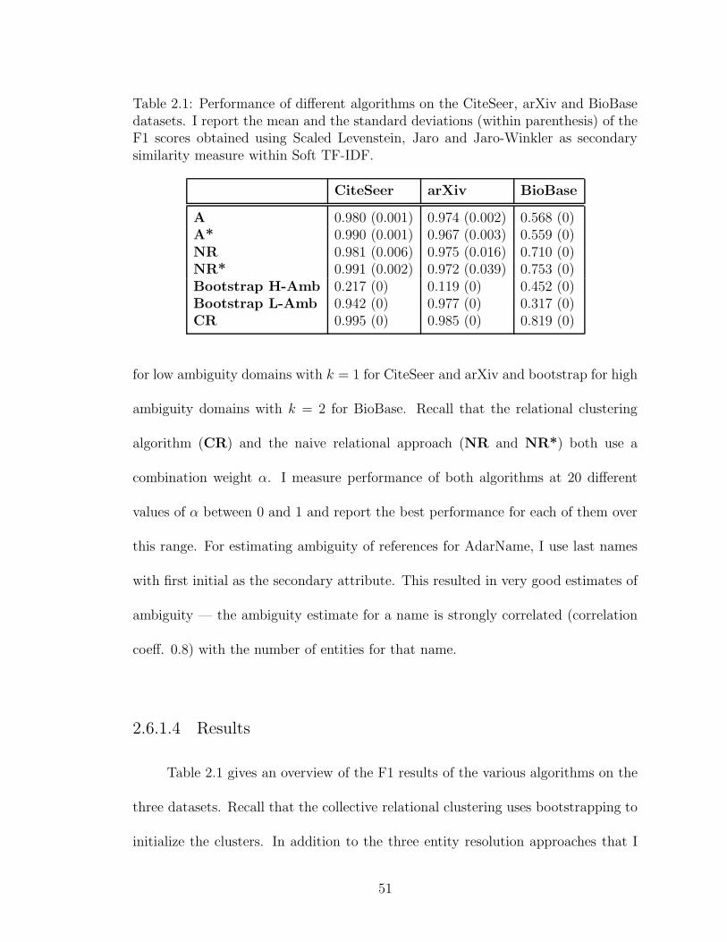
Table 2.1: Performance of different algorithms on the CiteSeer, arXiv and BioBasedatasets. I report the mean and the standard deviations (within parenthesis) of theF1 scores obtained using Scaled Levenstein, Jaro and Jaro-Winkler as secondarysimilarity measure within Soft TF-IDF.

CiteSeer arXiv BioBase

A 0.980 (0.001) 0.974 (0.002) 0.568 (0)A* 0.990 (0.001) 0.967 (0.003) 0.559 (0)NR 0.981 (0.006) 0.975 (0.016) 0.710 (0)NR* 0.991 (0.002) 0.972 (0.039) 0.753 (0)Bootstrap H-Amb 0.217 (0) 0.119 (0) 0.452 (0)Bootstrap L-Amb 0.942 (0) 0.977 (0) 0.317 (0)CR 0.995 (0) 0.985 (0) 0.819 (0)

for low ambiguity domains with k = 1 for CiteSeer and arXiv and bootstrap for high

ambiguity domains with k = 2 for BioBase. Recall that the relational clustering

algorithm (CR) and the naive relational approach (NR and NR*) both use a

combination weight α. I measure performance of both algorithms at 20 different

values of α between 0 and 1 and report the best performance for each of them over

this range. For estimating ambiguity of references for AdarName, I use last names

with first initial as the secondary attribute. This resulted in very good estimates of

ambiguity — the ambiguity estimate for a name is strongly correlated (correlation

coeff. 0.8) with the number of entities for that name.

2.6.1.4 Results

Table 2.1 gives an overview of the F1 results of the various algorithms on the

three datasets. Recall that the collective relational clustering uses bootstrapping to

initialize the clusters. In addition to the three entity resolution approaches that I

51

have discussed, I also include for comparison the two boot strapping approaches, one

for low ambiguity domains (Bootstrap L-Amb) that is used by CR for CiteSeer

and arXiv, and the other for high ambiguity data (Bootstrap H-Amb) that is

employed for BioBase. For CR, Table 2.1 records the performance for the best

neighborhood similarity measure, which is Jaccard for CiteSeer and arXiv, and

AdarName for BioBase. As mentioned earlier, there are several possible choices for

the secondary string metric used with the Soft TD-IDF similarity for comparing the

names. The results above are the averages using three choices — Scaled Levenstein,

Jaro and Jaro-Winkler, with the standard deviation shown in parenthesis.

First, note that the standard deviation in Table 2.1 measures sensitivity of

entity resolution performance in terms of the similarity measure used for names. We

can see that the results are not very sensitive to the secondary string metric choice.

In fact, for collective relational entity resolution (CR), the choice is irrelevant and

for the BioBase dataset, in which I have additional features besides the names, the

choice is also irrelevant. For the cases in which there were some small differences,

Scaled Levenstein was most often, but not always, the best.

Second, looking at the first line in Table 2.1, note the differences in per-

formance for attribute-based entity resolution (A) for the three datasets. The

attribute-based algorithm performs remarkably well for the CiteSeer database, and

its performance on the arXiv dataset is also respectable. This is in keeping with

our earlier observation about the ‘hardness’ of the datasets in terms of ambiguity

and dispersion. The CiteSeer dataset has very little ambiguity and arXiv is only

moderately more ambiguous. When datasets are not ambiguous, all dispersed en-

52

tities can be successfully identified simply by raising the discrimination threshold

for determining duplicates. This increases recall without generating false positives.

However, this is not possible when there is significant ambiguity in the data, as we

see in the case of BioBase. The performance of the bootstrapping algorithms high-

light the same trend. For CiteSeer and arXiv, the low ambiguity version (Bootstrap

L-Amb) performs almost as well as the attribute baseline. In a higher ambiguity

dataset such as BioBase, it performs many incorrect matches. The high ambiguity

bootstrap strategy (Bootstrap H-Amb), which is more cautious for ambiguous

references, performs poorly for CiteSeer and arXiv due to low recall but improves

performance over Bootstrap L-Amb for BioBase by increasing precision.

Next, observe that the naive relational entity resolution algorithm (NR) which

uses attributes of related references in its similarity calculations improves perfor-

mance over A only marginally for CiteSeer and arXiv, while the improvement is

quite significant in the case of BioBase. This suggests that while the attributes of

related entries can help in disambiguation in domains with high ambiguity, there

may not be much improvement for less ambiguous domains.

The table also shows that the effect of transitive closure on entity resolution

performance varies over the datasets. While it improves performance for both A

and NR for CiteSeer and arXiv, in the case of BioBase, it helps NR but not A. A

possible explanation is that transitive closure helps in domains with low ambiguity,

but it may result in false identifications in higher ambiguity domains.

Finally, note that across all three datasets, the collective relational entity

resolution algorithm (CR) performs the best. The gains for the less ambiguous

53

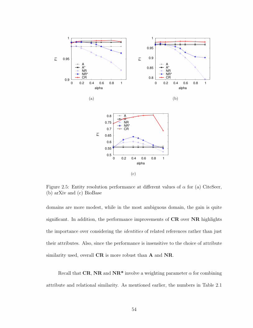
0.9

0.95

1

0 0.2 0.4 0.6 0.8 1

F1

alpha

AA*NRNR*CR

(a)

0.8

0.85

0.9

0.95

1

0 0.2 0.4 0.6 0.8 1

F1

alpha

AA*NRNR*CR

(b)

0.5

0.55

0.6

0.65

0.7

0.75

0.8

0 0.2 0.4 0.6 0.8 1

F1

alpha

AA*NRNR*CR

(c)

Figure 2.5: Entity resolution performance at different values of α for (a) CiteSeer,(b) arXiv and (c) BioBase

domains are more modest, while in the most ambiguous domain, the gain is quite

significant. In addition, the performance improvements of CR over NR highlights

the importance over considering the identities of related references rather than just

their attributes. Also, since the performance is insensitive to the choice of attribute

similarity used, overall CR is more robust than A and NR.

Recall that CR, NR and NR* involve a weighting parameter α for combining

attribute and relational similarity. As mentioned earlier, the numbers in Table 2.1

54

record the best performance over different values of α for each of these algorithms.

The best performance is not always achieved for the same value of α for different

datasets or for the 100 different reference names in BioBase. In Figure 2.5 we see how

the performance of the different algorithms changes over different values of α for the

three datasets. For BioBase, I plot the average performance over all 100 reference

names for a particular value of α. As a reference, I also show the performances of A

and A* which do not depend on α. We can make two interesting observations from

the plots. First, the relational clustering algorithm CR consistently outperforms the

naive relational baselines (NR) and (NR*) for all values of α for all three datasets.

Secondly, for CiteSeer and arXiv, the naive relational approach outperforms the

attribute-only baseline only marginally for small values of α and then its performance

drops significantly at higher values. It is more stable for BioBase but performs still

drops below the attribute-only baseline for high values of α. The performance of

CR is significantly more stable over varying α for all three datasets. This is another

validation of the usefulness of resolving related references instead of considering their

similarities.

Now I explore CR in more depth, by comparing the performance of the al-

gorithm using different graph-based similarity measures. Table 2.2 shows the per-

formance of the collective relational entity resolution with the different proposed

measures on the three datasets. There is little difference in performance on the

CiteSeer and arXiv datasets. The simplest measure, Common, correctly retrieves

almost all duplicates in CiteSeer. Recall that due to the ‘blocking’ approach, 100%

recall — and therefore an F1 score of 1.0 — is not attainable for these two datasets.

55

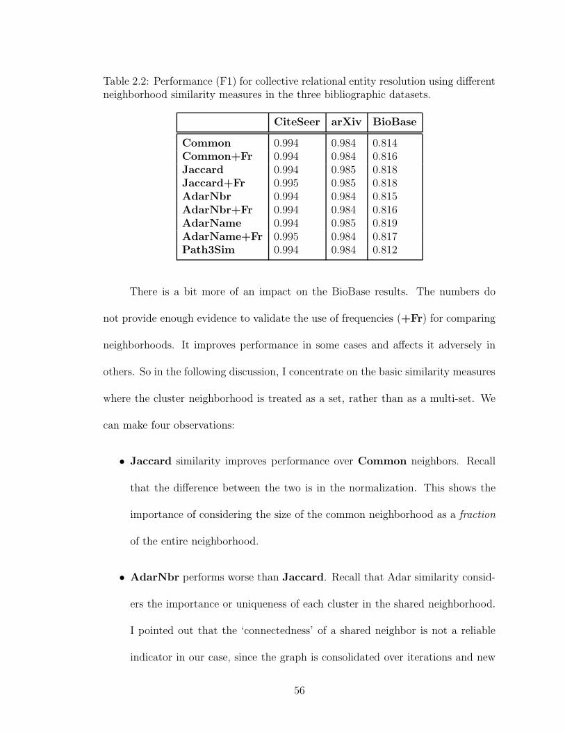
Table 2.2: Performance (F1) for collective relational entity resolution using differentneighborhood similarity measures in the three bibliographic datasets.

CiteSeer arXiv BioBase

Common 0.994 0.984 0.814Common+Fr 0.994 0.984 0.816Jaccard 0.994 0.985 0.818Jaccard+Fr 0.995 0.985 0.818AdarNbr 0.994 0.984 0.815AdarNbr+Fr 0.994 0.984 0.816AdarName 0.994 0.985 0.819AdarName+Fr 0.995 0.984 0.817Path3Sim 0.994 0.984 0.812

There is a bit more of an impact on the BioBase results. The numbers do

not provide enough evidence to validate the use of frequencies (+Fr) for comparing

neighborhoods. It improves performance in some cases and affects it adversely in

others. So in the following discussion, I concentrate on the basic similarity measures

where the cluster neighborhood is treated as a set, rather than as a multi-set. We

can make four observations:

• Jaccard similarity improves performance over Common neighbors. Recall

that the difference between the two is in the normalization. This shows the

importance of considering the size of the common neighborhood as a fraction

of the entire neighborhood.

• AdarNbr performs worse than Jaccard. Recall that Adar similarity consid-

ers the importance or uniqueness of each cluster in the shared neighborhood.

I pointed out that the ‘connectedness’ of a shared neighbor is not a reliable

indicator in our case, since the graph is consolidated over iterations and new

56

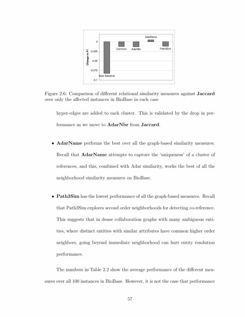
Best Baseline

Common AdarNbr

AdarName

Path3Sim

-0.1

-0.075

-0.05

-0.025

0

Cha

nge

in F

1

Figure 2.6: Comparison of different relational similarity measures against Jaccardover only the affected instances in BioBase in each case

hyper-edges are added to each cluster. This is validated by the drop in per-

formance as we move to AdarNbr from Jaccard.

• AdarName performs the best over all the graph-based similarity measures.

Recall that AdarName attempts to capture the ‘uniqueness’ of a cluster of

references, and this, combined with Adar similarity, works the best of all the

neighborhood similarity measures on BioBase.

• Path3Sim has the lowest performance of all the graph-based measures. Recall

that Path3Sim explores second order neighborhoods for detecting co-reference.

This suggests that in dense collaboration graphs with many ambiguous enti-

ties, where distinct entities with similar attributes have common higher order

neighbors, going beyond immediate neighborhood can hurt entity resolution

performance.

The numbers in Table 2.2 show the average performance of the different mea-

sures over all 100 instances in BioBase. However, it is not the case that performance

57

is affected for every instance by changing the similarity measure. For example, per-

formance changes in only 22 of the 100 instances when using Jaccard similarity

instead of AdarName similarity, as compared to 80 for Jaccard compared to the

baseline attribute-based similarity measure. In Figure 2.6, I compare the other

measures with Jaccard similarity by measuring the average change in F1-measure

over only the affected instances. We see the same trends as discussed above, but

difference between the measures become more pronounced.

2.6.1.5 Execution Time

As we have seen, the use of collective relational entity resolution improves

entity resolution performance over attribute-based baselines. However it is more

expensive computationally. Table 2.3 records the execution times in CPU seconds

of the baseline algorithms and CR on the three datasets. All execution times are

reported on a Dell Precision 870 server with 3.2GHz Intel Xeon processor and 3GB

of memory. Let us first consider the execution times for CiteSeer and arXiv. As

expected, CR takes more time than the baseline but it is still quite fast. It takes

less than 3 secs for the 2,982 references in CiteSeer and less than 5 minutes for the

58,515 references in arXiv. This is around 9 times as long as the baseline for CiteSeer

and 17 times for arXiv. Recall that the complexity of neighborhood similarity is

linear in the average connectivity between similar names. The average number of

neighbors per entity for CiteSeer is 2.15 and for arXiv it is 4.5. So this difference in

the degree of relational connectivity explains the difference in execution times for

the two datasets. Also, the available attribute for these two datasets is the author

58

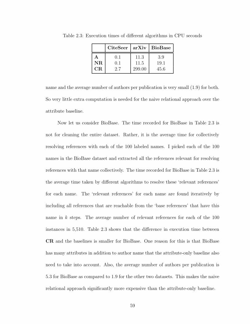
Table 2.3: Execution times of different algorithms in CPU seconds

CiteSeer arXiv BioBase

A 0.1 11.3 3.9NR 0.1 11.5 19.1CR 2.7 299.00 45.6

name and the average number of authors per publication is very small (1.9) for both.

So very little extra computation is needed for the naive relational approach over the

attribute baseline.

Now let us consider BioBase. The time recorded for BioBase in Table 2.3 is

not for cleaning the entire dataset. Rather, it is the average time for collectively

resolving references with each of the 100 labeled names. I picked each of the 100

names in the BioBase dataset and extracted all the references relevant for resolving

references with that name collectively. The time recorded for BioBase in Table 2.3 is

the average time taken by different algorithms to resolve these ‘relevant references’

for each name. The ‘relevant references’ for each name are found iteratively by

including all references that are reachable from the ‘base references’ that have this

name in k steps. The average number of relevant references for each of the 100

instances in 5,510. Table 2.3 shows that the difference in execution time between

CR and the baselines is smaller for BioBase. One reason for this is that BioBase

has many attributes in addition to author name that the attribute-only baseline also

need to take into account. Also, the average number of authors per publication is

5.3 for BioBase as compared to 1.9 for the other two datasets. This makes the naive

relational approach significantly more expensive than the attribute-only baseline.

59

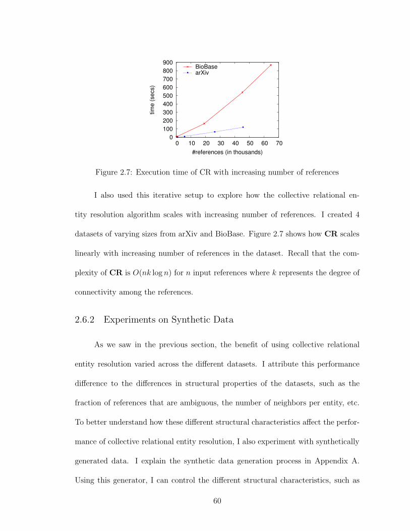
0 100 200 300 400 500 600 700 800 900

0 10 20 30 40 50 60 70tim

e (s

ecs)

#references (in thousands)

BioBasearXiv

Figure 2.7: Execution time of CR with increasing number of references

I also used this iterative setup to explore how the collective relational en-

tity resolution algorithm scales with increasing number of references. I created 4

datasets of varying sizes from arXiv and BioBase. Figure 2.7 shows how CR scales

linearly with increasing number of references in the dataset. Recall that the com-

plexity of CR is O(nk log n) for n input references where k represents the degree of

connectivity among the references.

2.6.2 Experiments on Synthetic Data

As we saw in the previous section, the benefit of using collective relational

entity resolution varied across the different datasets. I attribute this performance

difference to the differences in structural properties of the datasets, such as the

fraction of references that are ambiguous, the number of neighbors per entity, etc.

To better understand how these different structural characteristics affect the perfor-

mance of collective relational entity resolution, I also experiment with synthetically

generated data. I explain the synthetic data generation process in Appendix A.

Using this generator, I can control the different structural characteristics, such as

60

0.75

0.8

0.85

0.9

0.95

2.5 2.75 3 3.25 3.5 3.75

F1

avg #references / hyper-edge

AA*NRNR*CR

(a)

0.6

0.7

0.8

0.9

1

0.05 0.15 0.25 0.35 0.45

F1

Percentage of ambiguous attributes

AA*NRNR*CR

(b)

0.6

0.65

0.7

0.75

0.8

0.85

0.9

0.95

0 1 2 3 4 5 6 7 8

F1

avg #neighbors / entity

AA*NRNR*CR

(c)

Figure 2.8: Performance of different entity resolution algorithms on data syntheti-cally generated by varying different structural parameters such as (a) the averagesize of hyper-edges, (b) the percentage of ambiguous references and (c) the averagenumber of neighbors per entity. Standard deviations are shown using error bars.

the average number of references in each hyper-edge, the percentage of ambiguous

references in the data and the density of relationships among the underlying entities.

As I explain in Appendix A, the synthetic data generator is not tailored solely to

bibliographic data, but can model general relationships between entities, as in social

network data or email data.

I performed three sets of experiments on synthetically generated data. In all

of the experiments I consider average performance over 200 different runs. In the

61

first experiment, I studied the effect of the number of references in each hyper-edge.

The objective of this experiment is two-fold. Consider a collaborative graph, where

an entity e has many neighbors. If hyper-edges are small in size then two hyper-

edges involving a references r1 and r2 corresponding to e may not have any other

entities in common. Then it is not possible to identify r1 and r2 even using relational

similarity. Secondly, in ambiguous domains, a single shared neighbor may not be

enough to distinguish between two entities. In both cases, collective resolution is

expected to benefit from larger hyper-edge sizes. In each run for this experiment,

I first created an entity graph by adding 100 entities and 200 binary relationships.

Then I created different reference datasets, each with 500 hyper-edges. I varied pc

which led to different number of references in the edges. Figure 2.8(a) shows the

performance of the different entity resolution algorithms on these datasets. We see

that while the performances of the attribute baselines (A and A*) does not change,

the performance of CR improves with increasing number of references per hyper-

edge. Interestingly, performance of the naive relational approach (NR*) degrades

with increasing number of references. This demonstrates the importance of resolving

related names instead of considering their attribute similarities only.

In the second experiment, I varied the number of ambiguous references in the

data. Collective resolution is particularly useful for ambiguous references. It may

be possible to address the problem of identifying dispersed references for any entity

by using a smaller similarity threshold with the attribute-only baseline. In contrast,

disambiguation cannot be done using attributes but is often possible using relation-

ships. So I expected the collective resolution approach to show larger improvements

62

over the baseline for more ambiguous data. I created five sets of datasets, each with

100 entities, but with different ambiguous attribute probability pa. Then I added

200 binary relations between these entities and generated 500 hyper-edges with an

average of 2 references per hyper-edge. Figure 2.8(b) compares entity resolution

performance for the different algorithms on the datasets. As expected, the perfor-

mance of all algorithms drops with increasing percentage of ambiguous references.

However, the performance drop for CR is significantly slower than those for the

attribute and naive relational baselines since the entity relationships helps to make

the algorithm more robust. As a result, the gap between CR and the baselines

increases as the percentage of ambiguous references in the data increases.

In the final experiment, I explored the impact of varying the number of re-

lationships between the underlying entities. In the extreme situation, where there

are no relationships between entities, clearly no improvement can be obtained us-

ing collective resolution. At the other extreme, when all entities are connected to

each other, there is no pattern in the relationships that collective resolution can

exploit. The objective of this experiment was to explore how increased connectivity

among entities affects collective resolution. I first created a set of 100 entities. Then

I created different entity graph structures by adding different number of relations

between the entities. As before, I generated 500 hyper-edges (with an average of 2

references per hyper-edge) from each of these different entity-graphs and compared

performances of the different algorithms for the different datasets. The results are

shown in Figure 2.8(c). First note that, as expected, the performances of the at-

tribute baselines (A and A*) do not change significantly since they do not depend

63

on the relationships. The naive relational approaches (NR and NR*) degrade

in performance with higher neighborhood sizes, again highlighting the importance

of resolving related references. The performance of CR increases initially as the

number of relationships increases. However it peaks when the average number of

neighbors per entity is around 2 and then it starts falling off. In fact, it falls below

the attribute-baseline when the neighborhood size increases to 8. This is an inter-

esting result that shows that increasing number of relationships does not always

help collective entity resolution. As more relationships get added between entities,

relationship patterns between entities are less informative, and may actually hurt

performance. In this experiment, the probability of ambiguous attributes pa was 0.3.

We observe the same trend for other values of pa, the only change is the position of

the peak. The peak occurs earlier as pa is increased.

2.7 Conclusion

In summary, the relational clustering algorithm for collective entity resolution

using relations is a promising approach that improves resolution performance over

attribute-based and naive relational baselines. It has several nice properties in

that it is simple to understand and the incremental evidence in each iteration is

easy to interpret. It can be customized for different domains by using the attribute

similarity measure that works best. It is also fast, owing to efficient implementation;

it can resolve databases with 60,000 references in less than 5 minutes. All of these

features make it an attractive tool to use for domains that require fast resolution

64

with interpretable evidence.

On the other hand, this approach has certain limitations as well. For the

first limitation, recall that the similarity measure in Eqn. 2.2 involves a weighting

parameter α for combining attribute and relational similarity. It is not clear how the

optimal value for α should be chosen for each case and, for most of the comparisons, I

consider the best F1 score over all values of α. Figure 2.5 shows the performance for a

fixed value of α in contrast to a different optimal value for each case. It demonstrates

that there are significant performance improvements using CR for any value of α

over its entire range. Recall that the similarity measure uses only attributes when

α = 0 and only relations when α = 1. For CiteSeer and arXiv, performance does

not vary significantly with α. Since BioBase has much higher ambiguity in terms

of attributes (many references have exactly the same name and therefore mostly

the same countries, and all papers are from the same area), resolution performance

improves with increasing α.

Secondly, as with any clustering algorithm, determination of the termination

threshold is an issue. Note that this comes up for all of the baselines as well, and

here I report best accuracy over all thresholds. This is an area of ongoing research.

One other issue with the agglomerative clustering approach is that it is greedy in

terms of selecting clusters to merge and the final solution would be different for a

different merge sequence. Also, this approach is monotonic in that clusters only

merge. Two clusters once merged cannot split back later to account for any new

evidence that might be discovered. I address these issues with the probabilistic

generative model, which I describe in the next chapter.

65

Chapter 3

A Latent Dirichlet Model for Unsupervised Entity Resolution

In this chapter, I introduce a non-parametric probabilistic approach for solv-

ing the collective entity resolution, that addresses some of the limitations of the

relational clustering approach. This chapter is organized as follows. First, I present

a motivating example in Section 3.1. In Section 3.2, I first adapt the LDA model for

document authors and extend it for entity resolution in Section 3.3. The sampling

framework for inference is presented in Section 3.4. In Section 3.5 and Section 3.6, I

describe how entity attributes are modeled. Section 3.7 describes a novel algorithm

for determining the number of entities and in Section 3.8 and Section 3.9 I explore

parameter choices and algorithmic improvements . Finally, I present experimental

results on real and synthetic data in Section 3.10 and conclude in Section 3.11.

3.1 A Motivating Example

In this section, I introduce a concrete bibliographic example to explain the

entity resolution problem for authors and motivate the proposed approach. Consider

as an example six real paper citations P1 through P6 from CiteSeer:

• P1: “JOSTLE: Partitioning of Unstructured Meshes for Massively Parallel

Machines” C. Walshaw, M. Cross, M. G. Everett, S. Johnson

66

• P2: “Partitioning Mapping of Unstructured Meshes to Parallel Machine Topolo-

gies”, C. Walshaw, M. Cross, M. G. Everett, S. Johnson, K. McManus

• P3: “Dynamic Mesh Partitioning: A Unified Optimisation and Load-Balancing

Algorithm”, C. Walshaw, M. Cross, M. G. Everett

• P4: “Code Generation for Machines with Multiregister Operations”, Alfred

V. Aho, Stephen C. Johnson, Jefferey D. Ullman

• P5: “Deterministic Parsing of Ambiguous Grammars”, A. V. Aho, S. C. John-

son, J. D. Ullman

• P6: “Compilers: Principles, Techniques, and Tools”, A. Aho, R. Sethi, J.

Ullman

Each of the 6 papers has its own author references. For instance, the first paper

P1 has four references ‘C. Walshaw’, ‘M. Cross’, ‘M. G. Everett’ and ‘S. Johnson’.

In all we have 21 references in the 6 papers. The goal is to find out how many

different author entities these references correspond to and which reference maps to

which entity. Ground truth tells us that all of the Aho’s map to the same author

entity, as do the Everret’s and the Ullman’s. The interesting case here is that of

Johnson. The four Johnson references correspond to two Johnson entities: those in

papers P4 and P5 correspond to Stephen C. Johnson from Bell Labs, while those in

papers P1 and P2 map to Steve P. Johnson from University of Greenwich, London.

However, going by just the names of the references it is not clear why ‘Stephen C.

Johnson’ is not ‘S. Johnson’, when ‘Alfred V. Aho’ is the same as ‘A. Aho’. The

67

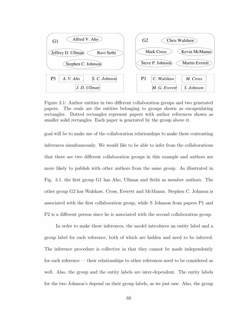
A. V. Aho S. C. Johnson

J. D. Ullman

G1 Alfred V. Aho

Jeffrey D. Ullman Ravi Sethi

Stephen C. Johnson

P5

S. Johnson

M. CrossC. Walshaw

M. G. Everett

G2 Chris Walshaw

Mark Cross Kevin McManus

Martin EverettSteve P. Johnson

P1

Figure 3.1: Author entities in two different collaboration groups and two generatedpapers. The ovals are the entities belonging to groups shown as encapsulatingrectangles. Dotted rectangles represent papers with author references shown assmaller solid rectangles. Each paper is generated by the group above it.

goal will be to make use of the collaboration relationships to make these contrasting

inferences simultaneously. We would like to be able to infer from the collaborations

that there are two different collaboration groups in this example and authors are

more likely to publish with other authors from the same group. As illustrated in

Fig. 3.1, the first group G1 has Aho, Ullman and Sethi as member authors. The

other group G2 has Walshaw, Cross, Everett and McManus. Stephen C. Johnson is

associated with the first collaboration group, while S Johnson from papers P1 and

P2 is a different person since he is associated with the second collaboration group.

In order to make these inferences, the model introduces an entity label and a

group label for each reference, both of which are hidden and need to be inferred.

The inference procedure is collective in that they cannot be made independently

for each reference — their relationships to other references need to be considered as

well. Also, the group and the entity labels are inter-dependent. The entity labels

for the two Johnson’s depend on their group labels, as we just saw. Also, the group

68

labels depend on the entity labels in turn. Sethi from paper P6 and Johnson from

paper P5 belong to the same group since they are tied by the identical entity labels

for the Aho’s and Ullman’s in the two papers. These two hidden variables are the

key distinctions of the model in comparison to some other recent ones that have been

proposed. Most other approaches introduce a decision variable for each potential

duplicate pair to infer whether or not they correspond to the same entity, while I

introduce two variables for each reference in the data. As data sizes grow, I believe

that this distinction has a significant impact.

It is interesting to note the role of papers P3 and P6 in this collective inference

for the Johnson’s though none of them contain a Johnson reference. They help to

reinforce our belief that there are two distinct tightly knit groups or communities

where member authors collaborate strongly with each other. Observe that frequent

collaborations between Walshaw and Aho, and Everett and Ullman for example

would have the opposite effect. Then we would think there is one collaboration

group, as opposed to two, and therefore all Johnson’s are more likely to be the same

author.

Not surprisingly, inferring the entity labels exactly turns out to be intractable.

For this model, I propose an effective Gibbs sampling approach for approximate

inference. Also, one critical aspect of the inference procedure is discovering the

likely number of entity labels, since the actual entities are hidden from us. I show

how the number of entities can be inferred as well.

Though I use the bibliographic domain of papers and authors, the model is

applicable in a straight-forward manner for other domains where noisy references to

69

person entities are observed together. Examples include names of people traveling

together on the same flight, names appearing together in the same email or groups of

people attending the same meeting. Furthermore, this approach can be generalized

to model other resolution problems. A very similar model may be used for word sense

resolution in natural language documents, where the references are word occurrences

and the senses are the entities to be resolved.

3.2 LDA Model for Authors

The idea of groups has been used for probabilistic modeling of natural lan-

guage documents. Most commonly, documents are viewed as bags of words and the

probabilistic approaches aim to represent the documents as mixtures over underly-

ing ‘topics’, which can be imagined as probabilistic groups of semantically related

words. This is very similar to the idea of modeling groups of underlying entities

allowing entities that belong to the same group to co-occur in the data.

The Latent Dirichlet Allocation (LDA) model was proposed by Blei et. al.

[21] as a mixture model for textual documents. In essense, it is a three level model

where each document (or, co-occurrence relation, in our terminology) is modeled

as a mixture over topics (or, groups, in our discussion) and then each word for

that document is generated in two steps, by first sampling a topic and then a word

from that topic. Though performing exact inference is not tractable in this model,

it is a popular approach for group modeling topics in machine learning literature.

Many authors have built on it since [93, 71] and efficient strategies for approximate

70

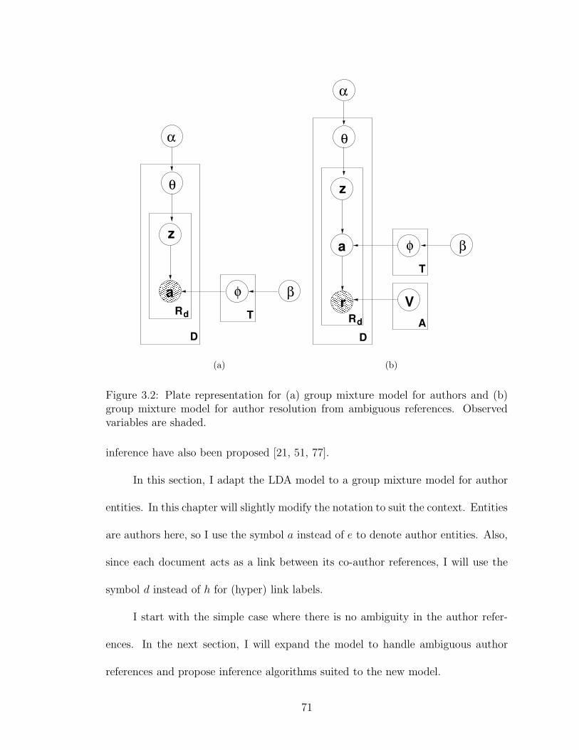
α

θ

βT

φ������������������������������

������������������������������

a

D

Rd

z

(a)

α

θ

Rd

βT

φ

������������

������������

a

r

z

AD

V

(b)

Figure 3.2: Plate representation for (a) group mixture model for authors and (b)group mixture model for author resolution from ambiguous references. Observedvariables are shaded.

inference have also been proposed [21, 51, 77].

In this section, I adapt the LDA model to a group mixture model for author

entities. In this chapter will slightly modify the notation to suit the context. Entities

are authors here, so I use the symbol a instead of e to denote author entities. Also,

since each document acts as a link between its co-author references, I will use the

symbol d instead of h for (hyper) link labels.

I start with the simple case where there is no ambiguity in the author refer-

ences. In the next section, I will expand the model to handle ambiguous author

references and propose inference algorithms suited to the new model.

71

Consider a collection of D documents and a set of A authors corresponding to

the authors of the documents. We have a set of R author references, {a1, . . . , aR}.

Each document can have multiple authors and for now, I assume the authors of each

document are observed. For an author reference ai, I use di to denote the document

in which it occurs. Further I introduce the notion of collaborative author groups.

These are groups of authors which tend to co-author together. I will assume that

there are T different groups. Each author reference ai has an associated group label

zi that takes values from 1 through T .

The probabilistic model is given using plate notation in Figure 3.2(a). The

probability distribution over authors for each group is represented as a multinomial

with parameters φj, so the probability P (a = i | z = j) of the ith author in the

database being chosen for the jth group is φji . We have T different multinomials,

one for each group. Each paper d is modeled as a mixture over the T groups.

The distribution used is again a multinomial with parameters θd, so the probability

Pd(z = j) of the jth group being chosen for document d is θdj . Each θd is drawn from

a Dirichlet distribution with hyperparameters α; similarly each φj is drawn from a

Dirichlet distribution with hyperparameters β.

3.3 LDA Model for Author Resolution

In the previous section, I assumed that the author identity can be determined

unambiguously from each author reference. However, when we are dealing with

author names, this is typically not the case. The same author may be represented

72

in a variety of ways: ‘Alfred V. Aho’, ‘Alfred Aho’, ‘AV Aho’, etc. There may be

mistakes due to typos or extraction errors. Finally, two ‘S. Johnson’s may not refer

to the same author entity. One may refer to ‘Stephen C. Johnson’ and another may

refer to ‘Steve P. Johnson’. The result is that we are no longer sure of the mapping

from the author reference to the author entity. We must resort to inference to

identify the true author for each reference.

To capture this, I will associate an attribute va with each author a. In addition,

I add an extra level to the model that probabilistically modifies the author attributes

Va to generate the references r = {r1, r2, . . . , rR}. Each reference is generated by

first sampling a group z and then an author entity a as before. Then, the author

reference r is generated from a by modifying the attribute va according to a noise

model N . I use a relatively sophisticated noise model that I explain in Section 3.6.

The probability of generating an author reference r from a particular author entity

is defined as P (r|va). The conditional probabilities for each reference are normalized

to sum to 1 over all author entities. It is the reference r that is observed, while the

entity a and group label z are hidden variables. The LDA-ER model is represented

in Figure 3.2(b).

Illustrating this in the context of our motivating example in Fig. 3.1, we have

already seen how the three author entities are chosen for paper P1. The attributes

va for the three authors are ‘Alfred V. Aho’, ‘Stephen C. Johnson’ and ‘Jeffrey D.

Ullman’. However the complete/correct names do not always appear in papers or

citations. In this case, the noise process modifies the attributes of the three selected

entities to generate ‘A. V. Aho’, ‘S. C. Johnson’ and ‘J. D. Ullman’ as the three

73

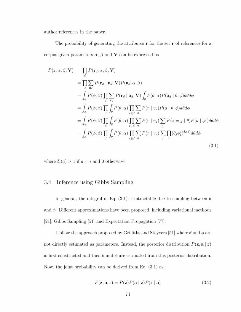
author references in the paper.

The probability of generating the attributes r for the set r of references for a

corpus given parameters α, β and V can be expressed as

P (r; α, β,V) =∏

d

P (rd; α, β,V)

=∏

d

∑

ad

P (rd | ad;V)P (ad; α, β)

=∫

φP (φ; β)

∏

d

∑

rd

P (rd | ad;V)∫

θP (θ; α)P (ad | θ, φ)dθdφ

=∫

φP (φ; β)

∏

d

∫

θP (θ; α)

∏

r∈d

∑

a

P (r | va)P (a | θ, φ)dθdφ

=∫

φP (φ; β)

∏

d

∫

θP (θ; α)

∏

r∈d

∑

a

P (r | va)∑

j

P (z = j | θ)P (a | φj)dθdφ

=∫

φP (φ; β)

∏

d

∫

θP (θ; α)

∏

r∈d

∑

a

P (r | va)∑

j

∏

i

(θjφji )

δi(a)dθdφ

(3.1)

where δi(a) is 1 if a = i and 0 otherwise.

3.4 Inference using Gibbs Sampling

In general, the integral in Eq. (3.1) is intractable due to coupling between θ

and φ. Different approximations have been proposed, including variational methods

[21], Gibbs Sampling [51] and Expectation Propagation [77].

I follow the approach proposed by Griffiths and Steyvers [51] where θ and φ are

not directly estimated as parameters. Instead, the posterior distribution P (z, a | r)

is first constructed and then θ and φ are estimated from this posterior distribution.

Now, the joint probability can be derived from Eq. (3.1) as:

P (z, a, r) = P (z)P (a | z)P (r | a) (3.2)

74

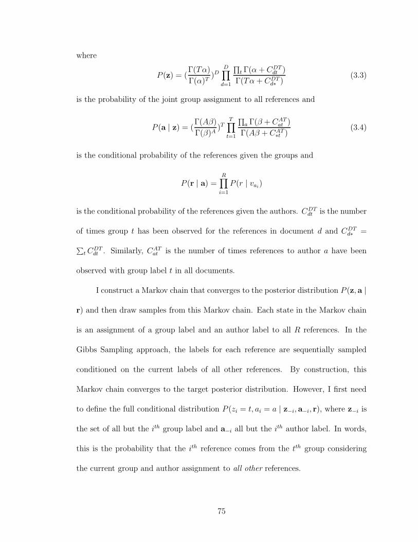
where

P (z) = (Γ(Tα)

Γ(α)T)D

D∏

d=1

∏

t Γ(α + CDTdt )

Γ(Tα + CDTd∗ )

(3.3)

is the probability of the joint group assignment to all references and

P (a | z) = (Γ(Aβ)

Γ(β)A)T

T∏

t=1

∏

a Γ(β + CATat )

Γ(Aβ + CAT∗t )

(3.4)

is the conditional probability of the references given the groups and

P (r | a) =R∏

i=1

P (r | vai)

is the conditional probability of the references given the authors. CDTdt is the number

of times group t has been observed for the references in document d and CDTd∗ =

∑

t CDTdt . Similarly, CAT

at is the number of times references to author a have been

observed with group label t in all documents.

I construct a Markov chain that converges to the posterior distribution P (z, a |

r) and then draw samples from this Markov chain. Each state in the Markov chain

is an assignment of a group label and an author label to all R references. In the

Gibbs Sampling approach, the labels for each reference are sequentially sampled

conditioned on the current labels of all other references. By construction, this

Markov chain converges to the target posterior distribution. However, I first need

to define the full conditional distribution P (zi = t, ai = a | z−i, a−i, r), where z−i is

the set of all but the ith group label and a−i all but the ith author label. In words,

this is the probability that the ith reference comes from the tth group considering

the current group and author assignment to all other references.

75

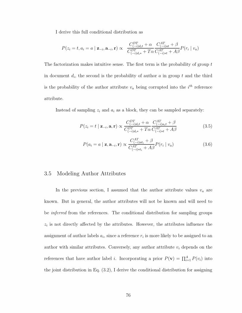
I derive this full conditional distribution as

P (zi = t, ai = a | z−i, a−i, r) ∝CDT

(−i)dit+ α

CDT(−i)di∗

+ Tα

CAT(−i)at + β

CAT(−i)∗t + Aβ

P (ri | va)

The factorization makes intuitive sense. The first term is the probability of group t

in document di, the second is the probability of author a in group t and the third

is the probability of the author attribute va being corrupted into the ith reference

attribute.

Instead of sampling zi and ai as a block, they can be sampled separately:

P (zi = t | z−i, a, r) ∝CDT

(−i)dit+ α

CDT(−i)di∗

+ Tα

CAT(−i)ait

+ β

CAT(−i)∗t + Aβ

(3.5)

P (ai = a | z, a−i, r) ∝CAT

(−i)ati+ β

CAT(−i)∗ti

+ AβP (ri | va) (3.6)

3.5 Modeling Author Attributes

In the previous section, I assumed that the author attribute values va are

known. But in general, the author attributes will not be known and will need to

be inferred from the references. The conditional distribution for sampling groups

zi is not directly affected by the attributes. However, the attributes influence the

assignment of author labels ai, since a reference ri is more likely to be assigned to an

author with similar attributes. Conversely, any author attribute vi depends on the

references that have author label i. Incorporating a prior P (v) =∏A

i=1 P (vi) into

the joint distribution in Eq. (3.2), I derive the conditional distribution for assigning

76

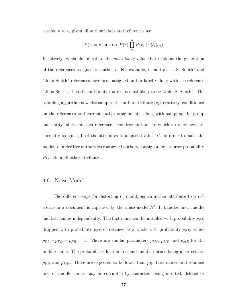
a value v to vi given all author labels and references as:

P (vi = v | a, r) ∝ P (v)R∏

j=1

P (rj | v)δi(aj)

Intuitively, vi should be set to the most likely value that explains the generation

of the references assigned to author i. For example, if multiple “J.S. Smith” and

“John Smith” references have been assigned author label i along with the reference

“Jhon Smth”, then the author attribute vi is most likely to be “John S. Smith”. The

sampling algorithm now also samples the author attributes vi iteratively, conditioned

on the references and current author assignments, along with sampling the group

and entity labels for each reference. For ‘free authors’ to which no references are

currently assigned, I set the attributes to a special value ‘?’. In order to make the

model to prefer free authors over assigned authors, I assign a higher prior probability

P (?) than all other attributes.

3.6 Noise Model

The different ways for distorting or modifying an author attribute to a ref-

erence in a document is captured by the noise model N . It handles first, middle

and last names independently. The first name can be initialed with probability pFI,

dropped with probability pFD or retained as a whole with probability pFR, where

pFI + pFD + pFR = 1. There are similar parameters pMI , pMD and pMR for the

middle name. The probabilities for the first and middle initials being incorrect are

pFIr and pMIr. These are expected to be lower than pR. Last names and retained

first or middle names may be corrupted by characters being inserted, deleted or

77

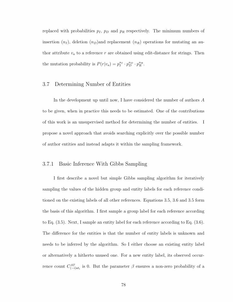
replaced with probabilities pI , pD and pR respectively. The minimum numbers of

insertion (nI), deletion (nD)and replacement (nR) operations for mutating an au-

thor attribute va to a reference r are obtained using edit-distance for strings. Then

the mutation probability is P (r|va) = pnI

I · pnD

D · pnR

R .

3.7 Determining Number of Entities

In the development up until now, I have considered the number of authors A

to be given, when in practice this needs to be estimated. One of the contributions

of this work is an unsupervised method for determining the number of entities. I

propose a novel approach that avoids searching explicitly over the possible number

of author entities and instead adapts it within the sampling framework.

3.7.1 Basic Inference With Gibbs Sampling

I first describe a novel but simple Gibbs sampling algorithm for iteratively

sampling the values of the hidden group and entity labels for each reference condi-

tioned on the existing labels of all other references. Equations 3.5, 3.6 and 3.5 form

the basis of this algorithm. I first sample a group label for each reference according

to Eq. (3.5). Next, I sample an entity label for each reference according to Eq. (3.6).

The difference for the entities is that the number of entity labels is unknown and

needs to be inferred by the algorithm. So I either choose an existing entity label

or alternatively a hitherto unused one. For a new entity label, its observed occur-

rence count CAT(−i)ati

is 0. But the parameter β ensures a non-zero probability of a

78

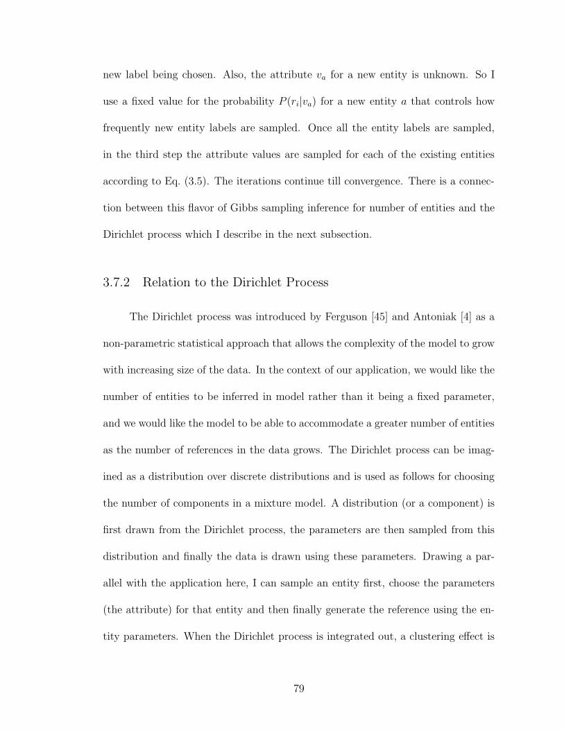
new label being chosen. Also, the attribute va for a new entity is unknown. So I

use a fixed value for the probability P (ri|va) for a new entity a that controls how

frequently new entity labels are sampled. Once all the entity labels are sampled,

in the third step the attribute values are sampled for each of the existing entities

according to Eq. (3.5). The iterations continue till convergence. There is a connec-

tion between this flavor of Gibbs sampling inference for number of entities and the

Dirichlet process which I describe in the next subsection.

3.7.2 Relation to the Dirichlet Process

The Dirichlet process was introduced by Ferguson [45] and Antoniak [4] as a

non-parametric statistical approach that allows the complexity of the model to grow

with increasing size of the data. In the context of our application, we would like the

number of entities to be inferred in model rather than it being a fixed parameter,

and we would like the model to be able to accommodate a greater number of entities

as the number of references in the data grows. The Dirichlet process can be imag-

ined as a distribution over discrete distributions and is used as follows for choosing

the number of components in a mixture model. A distribution (or a component) is

first drawn from the Dirichlet process, the parameters are then sampled from this

distribution and finally the data is drawn using these parameters. Drawing a par-

allel with the application here, I can sample an entity first, choose the parameters

(the attribute) for that entity and then finally generate the reference using the en-

tity parameters. When the Dirichlet process is integrated out, a clustering effect is

79

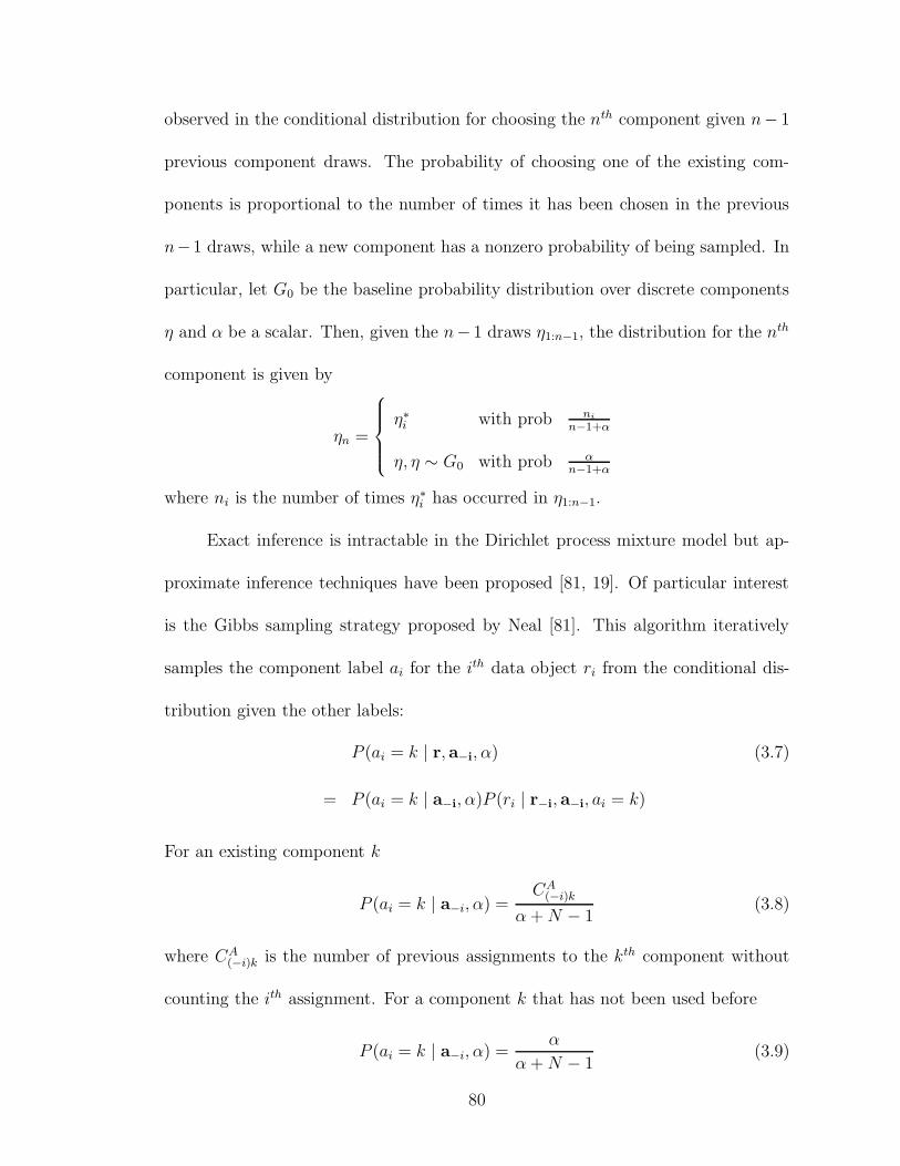
observed in the conditional distribution for choosing the nth component given n− 1

previous component draws. The probability of choosing one of the existing com-

ponents is proportional to the number of times it has been chosen in the previous

n−1 draws, while a new component has a nonzero probability of being sampled. In

particular, let G0 be the baseline probability distribution over discrete components

η and α be a scalar. Then, given the n− 1 draws η1:n−1, the distribution for the nth

component is given by

ηn =

η∗i with prob ni

n−1+α

η, η ∼ G0 with prob αn−1+α

where ni is the number of times η∗i has occurred in η1:n−1.

Exact inference is intractable in the Dirichlet process mixture model but ap-

proximate inference techniques have been proposed [81, 19]. Of particular interest

is the Gibbs sampling strategy proposed by Neal [81]. This algorithm iteratively

samples the component label ai for the ith data object ri from the conditional dis-

tribution given the other labels:

P (ai = k | r, a−i, α) (3.7)

= P (ai = k | a−i, α)P (ri | r−i, a−i, ai = k)

For an existing component k

P (ai = k | a−i, α) =CA

(−i)k

α + N − 1(3.8)

where CA(−i)k is the number of previous assignments to the kth component without

counting the ith assignment. For a component k that has not been used before

P (ai = k | a−i, α) =α

α + N − 1(3.9)

80

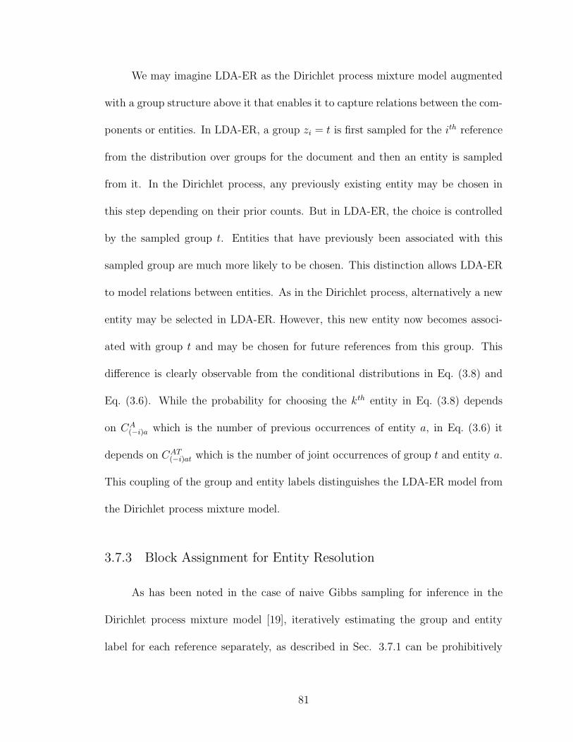
We may imagine LDA-ER as the Dirichlet process mixture model augmented

with a group structure above it that enables it to capture relations between the com-

ponents or entities. In LDA-ER, a group zi = t is first sampled for the ith reference

from the distribution over groups for the document and then an entity is sampled

from it. In the Dirichlet process, any previously existing entity may be chosen in

this step depending on their prior counts. But in LDA-ER, the choice is controlled

by the sampled group t. Entities that have previously been associated with this

sampled group are much more likely to be chosen. This distinction allows LDA-ER

to model relations between entities. As in the Dirichlet process, alternatively a new

entity may be selected in LDA-ER. However, this new entity now becomes associ-

ated with group t and may be chosen for future references from this group. This

difference is clearly observable from the conditional distributions in Eq. (3.8) and

Eq. (3.6). While the probability for choosing the kth entity in Eq. (3.8) depends

on CA(−i)a which is the number of previous occurrences of entity a, in Eq. (3.6) it

depends on CAT(−i)at which is the number of joint occurrences of group t and entity a.

This coupling of the group and entity labels distinguishes the LDA-ER model from

the Dirichlet process mixture model.

3.7.3 Block Assignment for Entity Resolution

As has been noted in the case of naive Gibbs sampling for inference in the

Dirichlet process mixture model [19], iteratively estimating the group and entity

label for each reference separately, as described in Sec. 3.7.1 can be prohibitively

81

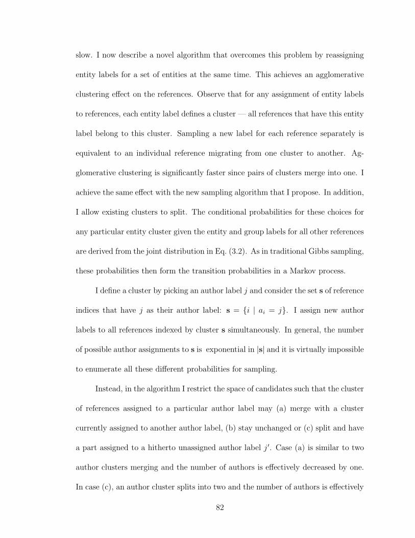
slow. I now describe a novel algorithm that overcomes this problem by reassigning

entity labels for a set of entities at the same time. This achieves an agglomerative

clustering effect on the references. Observe that for any assignment of entity labels

to references, each entity label defines a cluster — all references that have this entity

label belong to this cluster. Sampling a new label for each reference separately is

equivalent to an individual reference migrating from one cluster to another. Ag-

glomerative clustering is significantly faster since pairs of clusters merge into one. I

achieve the same effect with the new sampling algorithm that I propose. In addition,

I allow existing clusters to split. The conditional probabilities for these choices for

any particular entity cluster given the entity and group labels for all other references

are derived from the joint distribution in Eq. (3.2). As in traditional Gibbs sampling,

these probabilities then form the transition probabilities in a Markov process.

I define a cluster by picking an author label j and consider the set s of reference

indices that have j as their author label: s = {i | ai = j}. I assign new author

labels to all references indexed by cluster s simultaneously. In general, the number

of possible author assignments to s is exponential in |s| and it is virtually impossible

to enumerate all these different probabilities for sampling.

Instead, in the algorithm I restrict the space of candidates such that the cluster

of references assigned to a particular author label may (a) merge with a cluster

currently assigned to another author label, (b) stay unchanged or (c) split and have

a part assigned to a hitherto unassigned author label j ′. Case (a) is similar to two

author clusters merging and the number of authors is effectively decreased by one.

In case (c), an author cluster splits into two and the number of authors is effectively

82

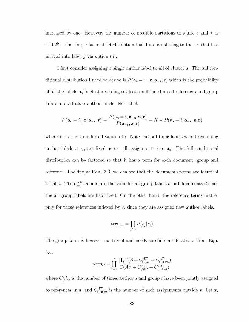
increased by one. However, the number of possible partitions of s into j and j ′ is

still 2|s|. The simple but restricted solution that I use is splitting to the set that last

merged into label j via option (a).

I first consider assigning a single author label to all of cluster s. The full con-

ditional distribution I need to derive is P (as = i | z, a−s, r) which is the probability

of all the labels as in cluster s being set to i conditioned on all references and group

labels and all other author labels. Note that

P (as = i | z, a−s, r) =P (as = i, a−s, z, r)

P (a−s, z, r)= K × P (as = i, a−s, z, r)

where K is the same for all values of i. Note that all topic labels z and remaining

author labels a−(s) are fixed across all assignments i to as. The full conditional

distribution can be factored so that it has a term for each document, group and

reference. Looking at Eqn. 3.3, we can see that the documents terms are identical

for all i. The CDTdt counts are the same for all group labels t and documents d since

the all group labels are held fixed. On the other hand, the reference terms matter

only for those references indexed by s, since they are assigned new author labels.

termR =∏

j∈s

P (rj|vi)

The group term is however nontrivial and needs careful consideration. From Eqn.

3.4,

termG =T∏

t=1

∏

a Γ(β + CAT(s)at + CAT

(−s)at)

Γ(Aβ + CAT(s)∗t + CAT

(−s)∗t)

where CAT(s)at is the number of times author a and group t have been jointly assigned

to references in s, and CAT(−s)at is the number of such assignments outside s. Let zs

83

be the set of groups currently assigned to the references indexed by s. For groups

t /∈ zs and authors a 6= i, the count C(s)ATat is 0 and the corresponding terms are

independent of the assignment i. Therefore

termG = K∏

t∈zs

Γ(β + CAT(s)it + CAT

(−s)it)

Γ(Aβ + CAT(s)∗t + CAT

(−s)∗t)

= K∏

t∈zs

(β + CAT(−s)it + CAT

(s)it − 1) . . . (β + CAT(−s)it)Γ(β + CAT

(−s)it)

(Aβ + CAT(−s)∗t + CAT

(s)∗t − 1) . . . (Aβ + CAT(−s)∗t)Γ(Aβ + CAT

(−s)∗t)

= K ′∏

t∈zs

(β + CAT(−s)it + CAT

(s)it − 1) . . . (β + CAT(−s)it)

(Aβ + CAT(−s)∗t + CAT

(s)∗t − 1) . . . (Aβ + CAT(−s)∗t)

Denoting

T (t, i) =

CAT(s)it∏

n=1

(β + CAT(−s)it + CAT

(s)it − n) (3.10)

T (t, ∗) =

CAT(s)∗t∏

n=1

(Aβ + CAT(−s)∗t + CAT

(s)∗t − n)

the group term can be written as

termG ∝∏

t∈zs

T (t, i)

T (t, ∗)

Putting everything together, the conditional distribution can be written as

P (as = i | z, a−s, r) ∝∏

t∈zs

T (t, i)

T (t, ∗)

∏

j∈s

P (rj | vi) (3.11)

An Interpretation of Block Assignment: Here I show how the terms in this

conditional probability can be rearranged so that the result makes intuitive sense.

Let j be an index into cluster s and tj be the group label for that reference. Also,

consider cluster s to be an ordered set and denote by s<j the set of elements in s

84

strictly before position j. Then I can rewrite Eq. (3.11) as

P (as = i | z, a−s, r) (3.12)

∝∏

j∈s

β + CAT(s<j)itj

+ CAT(−s)itj

Aβ + CAT(s<j)∗tj

+ CAT(−s)∗tj

P (rj|vi)

Here CAT(s<j)it

is the number of times author label i and group label t have occurred

jointly for just the references in s<j. I interpret this as follows. I assign author labels

to the references in cluster s in sequence. For each assignment, the second term is

the probability of the reference given the author and the first term is the probability

of the author label for the reference given its current group label, including the

assignments already made in the sequence as additional evidence. It must be stressed

that this ordering is introduced solely for interpretation purposes and the actual

probability is independent of the ordering. Note that Eq. (3.12) reduces to Eq. (3.6)

as expected when cluster s has a single element.

For the case when I partition cluster s into s1 and s2 and assign two different

author labels to them, the conditional probability looks very similar:

P (as1= i, as2

= i′ | z, a−s, r)

∝∏

t∈zs

T (t, i)T (t, i′)

T (t, ∗)

∏

j∈s1

P (rj | vi)∏

j∈s2

P (rj | vi′)

Observe that when one author label merges with another according to Eq. (3.11),

the attribute of the freed author j changes from vj to the free attribute ’?’. The dif-

ference in prior probabilities of the two attribute values leads to an additional term

in the merge probability in Eq. (3.11): P (?)/P (vj). Similarly, when splitting the

references assigned to author j between j and currently unassigned j ′, the attribute

85

of author j ′ changes to vj′ from ‘?’ and the split probability has the additional

term P (vj′)/P (?). Therefore, the higher the prior probability of ‘?’ relative to other

attributes, the higher will be the likelihood of a merge compared to a split.

Putting everything together, the entity resolution algorithm starts from an

initial assignment of authors and groups to all references and iterates over three steps

sequentially until convergence. First, it samples a group label for each reference.

This has complexity O(RT ) for R references and T group labels. Then for each

assigned author label, it samples the next author label for its current references.

This requires O(AS) operations for A author labels and a maximum of S potential

duplicates per author. Finally, it samples an attribute for each assigned author label,

requiring O(A) operations. For each round of sampling authors and attributes, I do

several iterations of group sampling to let the group labels stabilize for the current

author assignments. Note that all stages in an iteration are linear in the number

of references and author labels allowing the model to scale to large datasets as I

demonstrate in the experimental section.

3.8 Determining Model Parameters

I have described how the numbers of authors can be determined within the

sampling procedure. The remaining aspects of the model are the number of groups

and the Dirichlet hyper-parameters. Their choice affects performance in different

ways.

86

3.8.1 Number of Groups

I begin by observing that the choice of the number of groups is subjective and

not as critical as the number of entities. Relationships among the same set of entities

can be captured with different number of groups at different levels of resolution.

While it is possible to estimate the likely number of groups from the data, it is

an area of potential future research. Here I consider the effect of varying number

of groups on entity resolution. Recall that our guiding intuition is to assign the

same author label to sets of references when they are similar and have similar group

distributions. When the number of groups T is too small, misleading similarities in

group distributions are likely to be observed, leading to false positives. If T is too

high, references to the same author can get split over different groups, making false

negatives likely. In other words, lower T favors higher recall and lower precision,

while higher T leads to lower recall with higher precision.

3.8.2 Hyper-parameters

To appreciate the roles of α and β, note from Eq. (3.5) that when α = 0,

a reference is forced to pick a group label from the other references in the same

document. Similarly, when β = 0, a reference has to pick a group label from other

references to the same author, and also an author label from other references with

the same group label. In general, for low values of α and β, the model tends to

overfit the data. This is particularly undesirable for entity resolution, since I need

to estimate the number of authors and need to generalize from the current author

87

assignments. To get a feel for what values are appropriate, observe that Tα is the

number of pseudo reference counts added to each document. Since in most cases

documents will have one or two authors, I set Tα to be 0.25. Similarly, Aβ is the

number of pseudo references for each topic. I set β according to the number of

references in the dataset and the number of topics. A typical value for Aβ is 5.

3.8.3 Noise Model Parameters

I iteratively estimate the noise parameters from data in a unsupervised man-

ner. I start from an initial estimate that is typical of some datasets I explored. For

instance, first names are initialed and dropped with probabilities 0.75 and 0.001 (0.25

and 0.7 for middle names) and is incorrect with probability 0.0005 (0.001 for middle

names). Characters may be dropped, replaced or inserted, each with probability

0.0025. After every author sampling step, I re-estimate the probabilities looking

at each reference attribute and the attribute of the author it has been assigned to.

However, the estimates from the initial iterations may not be good. For example,

when all references are distinct entities, all corruption probabilities are estimated to

be 0. To prevent this, estimates are made to evolve slowly. A weighted combination

of the current probabilities and the new estimates yields the probabilities for the

next iteration. Typically, I retain current estimates with weight 0.9.

88

3.9 Algorithm Refinements

Unlike group labels, author labels for references are sampled from a restricted

space. Here I propose improvements for the sampling algorithm for inferring the

author labels.

3.9.1 Bootstrapping Author Labels

Initialization of author labels is an issue both for convergence time and qual-

ity. One option is to assign the same initial label to any two references that have

attributes v1 and v2, where either v1 = v2 or v1 is an initialed form of v2. How-

ever, for domains where last names repeat very frequently, like Chinese, Japanese

or Indian names, this can affect the initial accuracy quite adversely, from which it

is hard to recover. For the case of such common last names1, I propose an improved

bootstrapping scheme. I assign the same author label to pairs only when they have

document co-authors with the same initial author label. This improves bootstrap

accuracy significantly for one of the datasets that has frequently repeating names.

3.9.2 Group Evidence for Author Self Loops

Recall that Eq. (3.10) shows the group evidence for different transitions for

cluster s. CAT(−s)at is the number of references outside cluster s that have author label

a and group label t. For any group t, it is the group evidence for merging with the

cluster for author label a. However, if s is the cluster of references with author level

1http://en.wikipedia.org/wiki/List of most popular family names

89

j, then CAT(−s)jt will be 0 for all group labels t, since there are no references outside

cluster s with author label j. Therefore, cluster s has little affinity to itself when

considering group evidence and prefers merging with other clusters. Note however

that every cluster has higher attribute affinity to itself than to other clusters. I

introduce a scalar parameter that allows us to have additional control on the rate

of cluster merges. I consider a small fraction δ of CAT(s)jt as external group evidence

for j. The higher the value of δ, the stronger has to be the evidence to cause an

existing author label to merge with another label or to split into two.

3.10 Experimental Evaluation

I begin by evaluating the algorithm on two real citation datasets. I compare

the collaborative entity resolution model (LDA-ER) with the best attribute-based

models. Next, to gain further understanding of the conditions under which entity

resolution benefits from collaborative group information, I evaluate the proposed

model on a broad range of synthetic datasets with varying relational structure.

3.10.1 Results on Citation Data

I first perform experimental evaluations on two citation datasets, which I have

already introduced in Section 2.6. The first is the CiteSeer dataset containing ci-

tations to papers from four different areas in machine learning, originally created

by Giles et al. [49]. This has 2,892 references to 1,165 authors, contained in 1,504

documents. The second dataset is significantly larger; arXiv contains papers from

90

high energy physics used in KDD Cup 20032. This has 58,515 references to 9,200

authors, contained in 29,555 papers.

To evaluate the algorithms, I measure the performance of the models for de-

tecting duplicates in terms of precision, recall and F1 on pairwise duplicate decisions.

It is practically infeasible to consider all pairs, particularly for arXiv, so as others

have done, I employ a ‘blocking’ approach to extract the potential duplicates. This

approach retains ∼99% of the true duplicates for both datasets.

I use a simple scheme for attribute priors, where common last names are set to

be 10 times more likely than other last names, and the free attribute ‘?’ is 10 times

more likely than common names. When sampling group labels given the entity

assignments at each step, I iterate until the log-likelihood converges. Typically for

the first few steps, I perform 50 group sampling iterations for each author iteration.

Thereafter I proceed with 20 group iterations for each author iteration. The F1

converges in about 30 author iterations for CiteSeer and 50 author iterations for

arXiv. On a 3.2GHz Dell Precision 670 Intel Xeon server, this takes between 2.5

and 10 minutes for CiteSeer and between 2 and 12 hours for arXiv depending on the

number of groups. As discussed in Section 3.9.2, I use a small fraction (δ= 0.5%)

of group evidence for self probabilities.

As a baseline (A), I compare with the hybrid SoftTF-IDF measure [30] that

has been shown to outperform other unsupervised approaches for text-based entity

resolution. Essentially, it augments the TF-IDF similarity for matching token sets

with approximate token matching using a secondary string similarity measure. Jaro-

2http://www.cs.cornell.edu/projects/kddcup/index.html

91

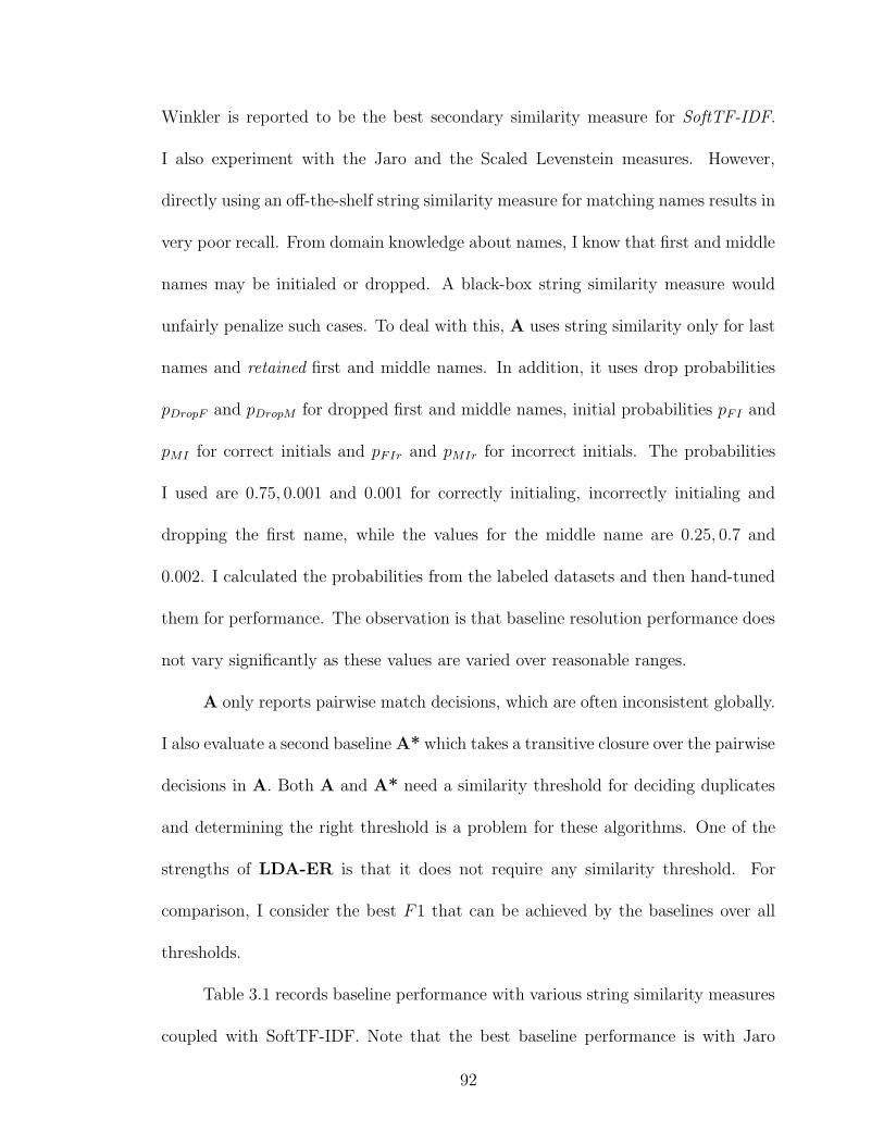
Winkler is reported to be the best secondary similarity measure for SoftTF-IDF.

I also experiment with the Jaro and the Scaled Levenstein measures. However,

directly using an off-the-shelf string similarity measure for matching names results in

very poor recall. From domain knowledge about names, I know that first and middle

names may be initialed or dropped. A black-box string similarity measure would

unfairly penalize such cases. To deal with this, A uses string similarity only for last

names and retained first and middle names. In addition, it uses drop probabilities

pDropF and pDropM for dropped first and middle names, initial probabilities pFI and

pMI for correct initials and pFIr and pMIr for incorrect initials. The probabilities

I used are 0.75, 0.001 and 0.001 for correctly initialing, incorrectly initialing and

dropping the first name, while the values for the middle name are 0.25, 0.7 and

0.002. I calculated the probabilities from the labeled datasets and then hand-tuned

them for performance. The observation is that baseline resolution performance does

not vary significantly as these values are varied over reasonable ranges.

A only reports pairwise match decisions, which are often inconsistent globally.

I also evaluate a second baseline A* which takes a transitive closure over the pairwise

decisions in A. Both A and A* need a similarity threshold for deciding duplicates

and determining the right threshold is a problem for these algorithms. One of the

strengths of LDA-ER is that it does not require any similarity threshold. For

comparison, I consider the best F1 that can be achieved by the baselines over all

thresholds.

Table 3.1 records baseline performance with various string similarity measures

coupled with SoftTF-IDF. Note that the best baseline performance is with Jaro

92

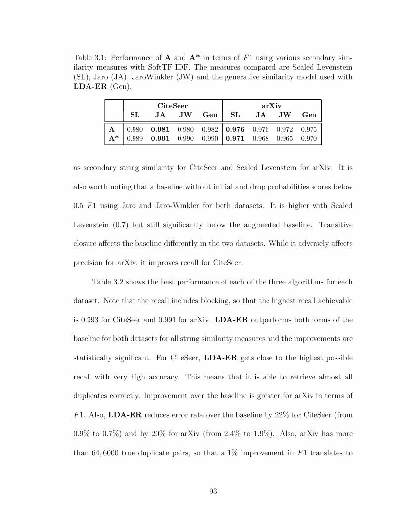
Table 3.1: Performance of A and A* in terms of F1 using various secondary sim-ilarity measures with SoftTF-IDF. The measures compared are Scaled Levenstein(SL), Jaro (JA), JaroWinkler (JW) and the generative similarity model used withLDA-ER (Gen).

CiteSeer arXiv

SL JA JW Gen SL JA JW Gen

A 0.980 0.981 0.980 0.982 0.976 0.976 0.972 0.975A* 0.989 0.991 0.990 0.990 0.971 0.968 0.965 0.970

as secondary string similarity for CiteSeer and Scaled Levenstein for arXiv. It is

also worth noting that a baseline without initial and drop probabilities scores below

0.5 F1 using Jaro and Jaro-Winkler for both datasets. It is higher with Scaled

Levenstein (0.7) but still significantly below the augmented baseline. Transitive

closure affects the baseline differently in the two datasets. While it adversely affects

precision for arXiv, it improves recall for CiteSeer.

Table 3.2 shows the best performance of each of the three algorithms for each

dataset. Note that the recall includes blocking, so that the highest recall achievable

is 0.993 for CiteSeer and 0.991 for arXiv. LDA-ER outperforms both forms of the

baseline for both datasets for all string similarity measures and the improvements are

statistically significant. For CiteSeer, LDA-ER gets close to the highest possible

recall with very high accuracy. This means that it is able to retrieve almost all

duplicates correctly. Improvement over the baseline is greater for arXiv in terms of

F1. Also, LDA-ER reduces error rate over the baseline by 22% for CiteSeer (from

0.9% to 0.7%) and by 20% for arXiv (from 2.4% to 1.9%). Also, arXiv has more

than 64, 6000 true duplicate pairs, so that a 1% improvement in F1 translates to

93

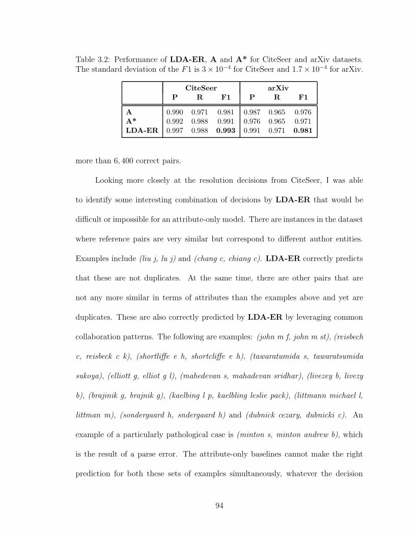
Table 3.2: Performance of LDA-ER, A and A* for CiteSeer and arXiv datasets.The standard deviation of the F1 is 3× 10−4 for CiteSeer and 1.7× 10−4 for arXiv.

CiteSeer arXiv

P R F1 P R F1

A 0.990 0.971 0.981 0.987 0.965 0.976A* 0.992 0.988 0.991 0.976 0.965 0.971LDA-ER 0.997 0.988 0.993 0.991 0.971 0.981

more than 6, 400 correct pairs.

Looking more closely at the resolution decisions from CiteSeer, I was able

to identify some interesting combination of decisions by LDA-ER that would be

difficult or impossible for an attribute-only model. There are instances in the dataset

where reference pairs are very similar but correspond to different author entities.

Examples include (liu j, lu j) and (chang c, chiang c). LDA-ER correctly predicts

that these are not duplicates. At the same time, there are other pairs that are

not any more similar in terms of attributes than the examples above and yet are

duplicates. These are also correctly predicted by LDA-ER by leveraging common

collaboration patterns. The following are examples: (john m f, john m st), (reisbech

c, reisbeck c k), (shortliffe e h, shortcliffe e h), (tawaratumida s, tawaratsumida

sukoya), (elliott g, elliot g l), (mahedevan s, mahadevan sridhar), (livezey b, livezy

b), (brajinik g, brajnik g), (kaelbing l p, kaelbling leslie pack), (littmann michael l,

littman m), (sondergaard h, sndergaard h) and (dubnick cezary, dubnicki c). An

example of a particularly pathological case is (minton s, minton andrew b), which

is the result of a parse error. The attribute-only baselines cannot make the right

prediction for both these sets of examples simultaneously, whatever the decision

94

Table 3.3: LDA-ER Performance over varying number of groups

CiteSeer arXiv

# Grps P R F1 P R F1

100 0.995 0.991 0.993 0.986 0.972 0.979200 0.997 0.988 0.993 0.988 0.972 0.980300 0.998 0.980 0.989 0.990 0.971 0.980400 0.999 0.980 0.989 0.990 0.970 0.980500 0.991 0.971 0.981

600 0.991 0.969 0.980

threshold, since they consider names alone.

I was also interested in exploring how the number of collaborative groups af-

fects the performance of the proposed entity resolution algorithm. Table 3.3 records

the performance of the group model on the two datasets with varying number of

groups. While I observe a general trend where precision improves and recall suffers

with more groups, note that the F1 is largely stable over a range of groups.

3.10.2 Properties of Collaborative Graphs

While the LDA-ER model shows improvement for both citation datasets, the

improvement is much more significant for the arXiv dataset. On investigating why

the model shows a larger improvement for arXiv than for CiteSeer, I found some

notable differences between the datasets. I call a reference ambiguous if there is more

than one author entity with that last name and first initial. There is a significant

difference in reference ambiguity between the two datasets — only 0.5% of the

references in CiteSeer are ambiguous while 9% of arXiv references are ambiguous.

A second difference is in the density of the author collaboration graph. The average

95

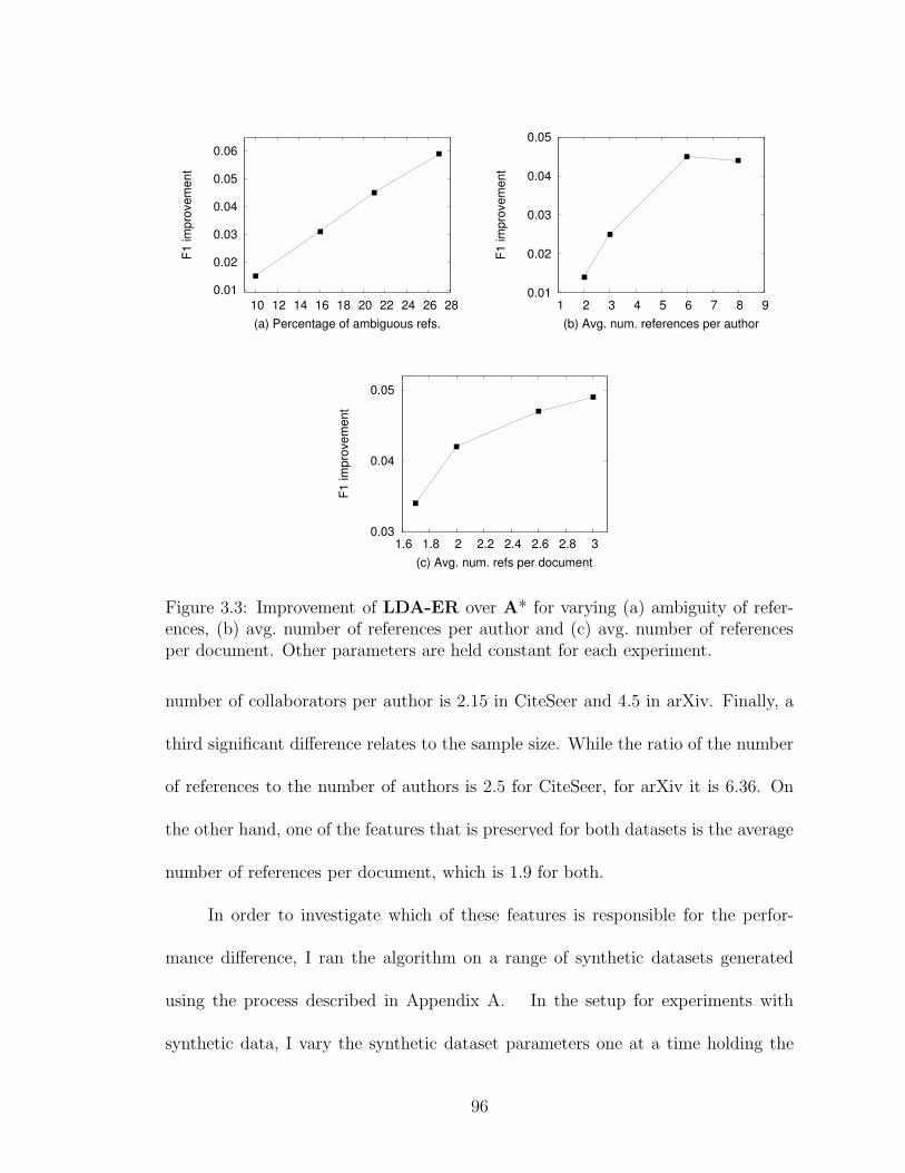
0.01

0.02

0.03

0.04

0.05

0.06

10 12 14 16 18 20 22 24 26 28

F1 im

prov

emen

t

(a) Percentage of ambiguous refs.

0.05

0.04

0.03

0.02

0.01 1 2 3 4 5 6 7 8 9

F1 im

prov

emen

t

(b) Avg. num. references per author

0.05

0.04

0.03 1.6 1.8 2 2.2 2.4 2.6 2.8 3

F1 im

prov

emen

t

(c) Avg. num. refs per document

Figure 3.3: Improvement of LDA-ER over A* for varying (a) ambiguity of refer-ences, (b) avg. number of references per author and (c) avg. number of referencesper document. Other parameters are held constant for each experiment.

number of collaborators per author is 2.15 in CiteSeer and 4.5 in arXiv. Finally, a

third significant difference relates to the sample size. While the ratio of the number

of references to the number of authors is 2.5 for CiteSeer, for arXiv it is 6.36. On

the other hand, one of the features that is preserved for both datasets is the average

number of references per document, which is 1.9 for both.

In order to investigate which of these features is responsible for the perfor-

mance difference, I ran the algorithm on a range of synthetic datasets generated

using the process described in Appendix A. In the setup for experiments with

synthetic data, I vary the synthetic dataset parameters one at a time holding the

96

others constant. The default values of the parameters are set to reflect the features

of the real datasets. The datasets have 1000 authors with an average of 4.5 collabo-

rators. I generate 3000 documents with an average of 2 references per document and

15% ambiguous references. I explore varying the fraction of ambiguous references,

the ratio of references to authors, the average number of collaborators and average

number of references per document. Since the results are averaged over different

datasets, I present only the improvement in F1 measure observed for the group

model over A*.

Figure 3.3 summarizes the trends that we observe. One significant improve-

ment trend is over varying ambiguity in the references. As shown in Figure 3.3(a),

it climbs sharply from 0.01 for 10% ambiguity (as in arXiv) to 0.06 for 27% refer-

ence ambiguity. Figure 3.3(b) shows that LDA-ER naturally benefits from higher

sample sizes for the author references. Figure 3.3(c) shows that LDA-ER benefits

from a greater number of authors per document. However, no statistically signifi-

cant trends emerged from the experiments with varying collaboration degree keeping

other factors like sample size fixed; some experiments showed larger improvements

with higher degree, however the results were not consistent. More thoroughly char-

acterizing properties of the collaborative graph structure that lead to improved

entity resolution is an interesting area for future work.

97

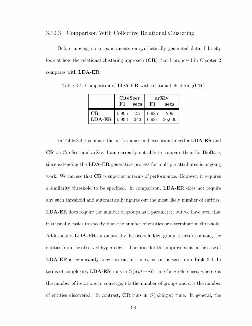
3.10.3 Comparison With Collective Relational Clustering

Before moving on to experiments on synthetically generated data, I briefly

look at how the relational clustering approach (CR) that I proposed in Chapter 2

compares with LDA-ER.

Table 3.4: Comparison of LDA-ER with relational clustering(CR)

CiteSeer arXivF1 secs F1 secs

CR 0.995 2.7 0.985 299LDA-ER 0.993 240 0.981 36,000

In Table 3.4, I compare the performance and execution times for LDA-ER and

CR on CiteSeer and arXiv. I am currently not able to compare them for BioBase,

since extending the LDA-ER generative process for multiple attributes is ongoing

work. We can see that CR is superior in terms of performance. However, it requires

a similarity threshold to be specified. In comparison, LDA-ER does not require

any such threshold and automatically figures out the most likely number of entities.

LDA-ER does require the number of groups as a parameter, but we have seen that

it is usually easier to specify than the number of entities or a termination threshold.

Additionally, LDA-ER automatically discovers hidden group structures among the

entities from the observed hyper-edges. The price for this improvement in the case of

LDA-ER is significantly longer execution times, as can be seen from Table 3.4. In

terms of complexity, LDA-ER runs in O(i(nt+a)) time for n references, where i is

the number of iterations to converge, t is the number of groups and a is the number

of entities discovered. In contrast, CR runs in O(nk log n) time. In general, the

98

inference algorithm for LDA-ER needs to go over many iterations before converging

and the hidden constants in the complexity are also high in comparison to CR, as

the execution times for CiteSeer and arXiv demonstrate.

So we can see that collective relational entity resolution (CR) and the prob-

abilistic generative model LDA-ER both have their strengths and weaknesses and

there is no clear winner in terms of performance. In domains where fast results are

needed and a termination threshold can be determined by alternative means, the

relational clustering approach may be the preferred choice. In other domains, where

a termination threshold is harder to specify, the non-parametric probabilistic model

may be more appropriate. Also, the hidden group structure discovered by LDA-ER

may be valuable in many domains such as social and collaborative networks.

3.11 Conclusions

In this chapter, I have developed a probabilistic generative model for collec-

tively resolving entities in relational data. There is a long history of work on entity

resolution. Recently, generative [67, 86] and discriminative [73, 98] probabilistic ap-

proaches have been proposed as well as non-probabilistic algorithms [60, 41]. The

proposed model differs from most of the above in that it is unsupervised, does not

assume the underlying entities to be known, does not make pairwise decisions and

explicitly models relations between entities using group membership. Unlike most

existing models, I do not introduce a decision variable for each potential duplicate

pair of references, but instead have an entity label for each reference. To model

99

collaborative relations between entities, I have introduced a group label for each

reference, so that entities coming from the same collaborative group are more likely

to be observed in a relation. For author resolution, this means that I model col-

laborative groups to explain co-authorship relations. The generative process in this

model may be viewed as an extension of the Dirichlet Process mixture model: the

group labels influence the choice of entities for each author reference in a paper.

Another contribution in my approach is an unsupervised Gibbs sampling algo-

rithm for collective entity resolution. It is unsupervised because I do not make use

of a labeled training set and it is collective because the resolution decisions depend

on each other through the group labels. Further, the number of entities is not fixed

in this model, and I have proposed a novel sampling strategy to estimate the most

likely number of entities given the references.

I have demonstrated the utility of the proposed model on two real-world ci-

tation datasets. Additionally, I have identified some of the conditions under which

these models are expected to provide greater benefit. Areas for future work include

extending the models to resolve multiple entity classes, handling multiple attributes

of different types and better characterization of collaborative graphs amenable to

these models. Though the improved sampling strategy addresses the computational

cost of the inference process to some extent, the execution times are orders of magni-

tude larger than the relational clustering approach. Designing algorithms for faster

inference that make this approach scalable to huge datasets is an obvious direction

of future research.

100

Chapter 4

Entity Resolution for Queries

Instead of collectively resolving all the references in a database, in this chapter

I investigate collective approaches for resolving entities on the fly for the purpose of

answering user queries over a database that has unresolved entity references. The

rest of this chapter is organized as follows. In Section 4.1, I motivate the problem

of resolving entities for answering queries, and in Section 4.2, I formulate the notion

of entity resolution queries. Section 4.3 investigates how the resolution performance

of related clusters depends recursively on each other as a result of this algorithm.

This motivates a recursive ‘expand and resolve’ strategy for processing queries. In

Section 4.4, I describe and analyze an unconstrained recursive strategy for extracting

the references relevant for collectively resolving a query. In Section 4.5, I present my

adaptive algorithm that extracts only the ‘most informative’ references for resolving

a given query. I present experimental results on real and synthetic data in Section 4.6

and finally conclude in Section 4.7.

4.1 Motivativation for Entity Resolution Queries

In spite of the widespread research interest and the practical nature of the

entity resolution problem, many publicly accessible databases remain unresolved,

101

or partially resolved, at best. The popular publication databases, CiteSeer and

PubMed, are representative examples. CiteSeer contains several records for the

same paper or author (going by CiteSeer records, Stuart Russell and Peter Norvig

have written more than 100 different books together [86]), while author names in

PubMed are not resolved at all. This is due to a variety of reasons, ranging from

rapid and often uncontrolled growth of the databases and the computational and

other expenses involved. Yet, millions of users access and query such databases ev-

eryday, mostly seeking information that, implicitly or explicitly, requires knowledge

of the resolved entities. The information gathered from such databases would be

significantly more useful or accurate if the entities were resolved.

Motivated by the abundance of such important and unresolved public databases,

I formulate the problem of query-time entity resolution. The goal is to enable users

to query an unresolved or partially resolved database and resolve the relevant enti-

ties on the fly. A user may access several databases everyday and he does not want

to clean every database that he queries. He only needs to resolve those entities that

matter for his query. For instance, when looking for all books by ‘Stuart Russell’ in

CiteSeer, it is not useful to resolve all other author references in CiteSeer. Also, the

resolution needs to be quick, even if it is not entirely accurate.

A possible solution for the query-time entity resolution problem that is both

quick and simple is to use attribute-based resolution. However, we have already seen

in Chapter 2 and Chapter 3 that collective resolution approaches can significantly

improve accuracy over attribute-only baselines. So the goal is to use collective reso-

lution using relationships for queries as well. But this added improvement comes at

102

a considerable computation cost arising from the dependencies. This added compu-

tational expense makes its application in query-time resolution challenging. Due to

its inter-dependent nature, the set of references that influence collective resolution

of a query may be very large. In this chapter, I first present a formal analysis of

how inter-dependence of different entity resolution decisions affect entity resolution

accuracy. This analysis motivates us to design a recursive resolution strategy for

query-centric entity resolution. I also present adaptive algorithms for extracting the

most relevant references for a query that enable us to resolve entities at query-time,

while preserving the gains of collective resolution.

My specific contributions in this chapter are as follows. First, I motivate and

formulate the problem of query-time entity resolution. The entity resolution strategy

that I use for query-time resolution is the collective relational clustering algorithm

(CR) introduced in Subsection 2.3.3. To the best of my knowledge, clustering

based on queries in the presence of relations has received little attention. I present

a structural analysis of how relational clustering affects entity resolution accuracy

and of the convergent nature of resolution performance for a recursive strategy for

resolving queries. I also formulate query-time clustering as a resource-constrained

problem and propose adaptive strategies for constructing the set of references that

influence a query. Finally, I present experimental results on large real-world and

synthetic datasets where this strategy enables collective resolution in seconds with

minimal loss in accuracy.

103

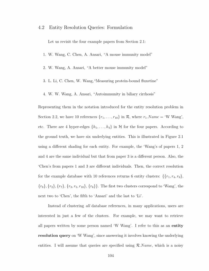
4.2 Entity Resolution Queries: Formulation

Let us revisit the four example papers from Section 2.1:

1. W. Wang, C. Chen, A. Ansari, “A mouse immunity model”

2. W. Wang, A. Ansari, “A better mouse immunity model”

3. L. Li, C. Chen, W. Wang,“Measuring protein-bound fluxetine”

4. W. W. Wang, A. Ansari, “Autoimmunity in biliary cirrhosis”

Representing them in the notation introduced for the entity resolution problem in

Section 2.2, we have 10 references {r1, . . . , r10} in R, where r1.Name = ‘W Wang’,

etc. There are 4 hyper-edges {h1, . . . , h4} in H for the four papers. According to

the ground truth, we have six underlying entities. This is illustrated in Figure 2.1

using a different shading for each entity. For example, the ‘Wang’s of papers 1, 2

and 4 are the same individual but that from paper 3 is a different person. Also, the

‘Chen’s from papers 1 and 3 are different individuals. Then, the correct resolution

for the example database with 10 references returns 6 entity clusters: {{r1, r4, r9},

{r8}, {r2}, {r7}, {r3, r5, r10}, {r6}}. The first two clusters correspond to ‘Wang’, the

next two to ‘Chen’, the fifth to ‘Ansari’ and the last to ‘Li’.

Instead of clustering all database references, in many applications, users are

interested in just a few of the clusters. For example, we may want to retrieve

all papers written by some person named ‘W Wang’. I refer to this as an entity

resolution query on ‘W Wang’, since answering it involves knowing the underlying

entities. I will assume that queries are specified using R.Name, which is a noisy

104

identifier for entities. Since names are ambiguous, treating them as identifiers leads

to undesirable results. For example, it would be incorrect to return the set {r1, r4, r8}

of all references with name ‘W Wang’ as the answer to the query. This answer does

not indicate that r8 is not the same person as the other two. Also, the answer

should include the paper by ‘W W Wang’ (r9), who is the same entity as the author

of the first paper. Therefore, the correct answer to the entity resolution query on

‘W Wang’ should be the partition {{r1, r4, r9}, {r8}}.

Different approaches introduces for the general entity resolution problem in

Section 2.3 — attribute-based, naive relational and collective relational resolution

— can also be used for entity resolution queries. The goal is to use the collective

relational entity resolution approach, since it significantly outperforms the other

two approaches in terms of entity resolution accuracy. But collective resolution

is more expensive computationally and execution time is a key issue for resolving

queries. Of the two collective relational entity resolution approaches that I have

proposed, collective relational clustering (Section 2.5) is significantly faster than the

probabilistic approach, and this is the algorithm that I adapt for resolving queries.

4.3 Performance Dependencies in Relational Clustering

The goal is to use the idea of collective resolution for queries. For collective

resolution, it is not sufficient to consider only the potential matches for the query in

the traditional fashion. For resolving the ‘W. Wang’ query, the traditional approach

simply considers the 4 references from the example that are similar in name —

105

the three ‘W. Wang’ references (r1, r4, r8) and the ‘W. W. Wang’ reference (r9).

In contrast, collective resolution benefits by additionally reasoning about the co-

author references, ‘Ansari’, ‘Chen’ and ‘Li’. As a result, entity resolution accuracy

for the query becomes dependent on the resolution accuracy of the related entities.

It is necessary to analyze the nature of this dependency in order to understand how

collective resolution affects performance for answering queries. In this section, I

identify the structural properties of the data that affect collective entity resolution

and formally analyze interdependent nature of the resolution performance. This

analysis also helps us to understand when relational clustering helps, when it has

an adverse effect and how it compares to traditional attribute-based resolution.

Recall that we are given a set of references R = {ri}. The references corre-

spond to an unobserved set of entities E . I assume that each reference ri corresponds

to a single entity from E , denoted as E(ri). An entity resolution algorithm partitions

the references into a set of clusters C = {ci} according to the underlying entities. The

accuracy of the resolution depends on how closely the partitioning of the references

into clusters corresponds to the underlying entities. I evaluate performance using

two different measures. The first measure is recall over each entity ei that measures

how many pairs of references that correspond to this entity ei are correctly assigned

to the same computed cluster. The second measure is precision for each computed

cluster ci measuring how many pairs of references assigned to this cluster ci truly

correspond to the same entity. These two measures depend on the attributes of the

references and also on the relationships between them, as I describe in the next two

subsections.

106

4.3.1 Performance Analysis of Attribute-based Resolution

First, I analyze how the reference attributes affect entity resolution perfor-

mance. Each reference ri has a set of attributes. I assume a similarity measure

that is defined over the domain of attributes. The traditional attribute-based clus-

tering approach considers only the pair-wise similarity between references based on

attribute values for resolving them. Two references ri, rj are said to be δ-similar if

their attribute similarity is at least δ. For attribute-based clustering, references are

assigned to the same cluster given some similarity threshold δ if they are δ-similar,

or, equivalently, if their attribute similarity is at least δ. In the example, for some

similarity measure defined over names and an appropriately determined similarity

threshold δ, the three ‘W. Wang’ references (r1, r4, r8) would be mapped to one

cluster c1 and the ‘W. W. Wang’ reference to a different cluster c2. In this case,

cluster c1 is not fully precise since the pairs (r1, r8) and (r4, r8) do not map to the

same entity. Also, one of the ‘Wang’ entities is not completely recalled since the

pairs (r1, r9) and (r4, r9) are missed.

In order to analyze how attribute-based resolution performs in general given

an arbitrary dataset, it is necessary to characterize the dataset in terms of two

probabilities defined on the attribute values of the references that it contains. The

first probability considers the ‘dissimilarity’ of attributes for references to the same

entity:

• attribute identification probability aI(δ): the probability that a randomly

chosen pair of references from the dataset that correspond to the same entity

107

are δ-similar to each other.

The second probability considers the similarity of attributes for references to differ-

ent entities:

• attribute ambiguity probability aA(δ): the probability that a randomly

chosen pair of references from the dataset that correspond to different entities

are δ-similar to each other.

The performance of the attribute-based clustering algorithm can be evaluated

using these two probabilities. Given a particular δ, the references pairs that are

correctly recalled for any domain entity e are those that are δ-similar. This is exactly

what aI(δ) denotes. Therefore the average recall for e is given by R(e, δ) = aI(δ).

On the other hand, the references that adversely affect precision for a particular δ

are those that are δ-similar to references to other entities. Therefore the average

precision for any computed cluster c is P (c, δ) = 1 − aA(δ). Alternatively, the

imprecision is given by I(c, δ) ≡ 1 − P (c, δ) = aA(δ).

4.3.2 Characterizing Relations

In addition to attributes, many domains have additional relational structure,

which I make use of for collective entity resolution. I now analyze how such relation-

ships affect entity resolution accuracy. As before, I use the relational structure in

the data as a set of co-occurrence relations H = {hj} over the references. In general,

references to any entity ei may co-occur frequently with references to a set of other

entities {ei1, . . . , eik}. These entities are called the neighbors N(ei) of entity ei.

108

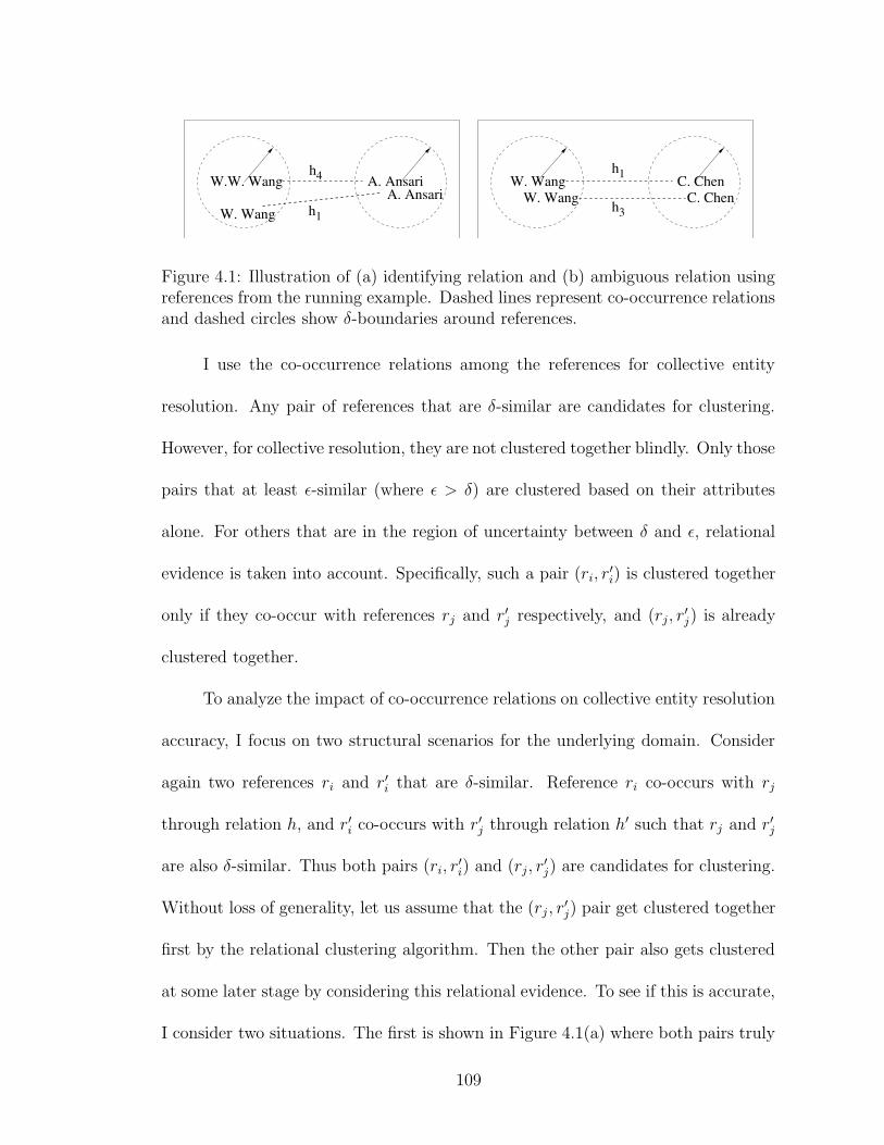
h4

h1

W.W. Wang

W. Wang

A. AnsariA. Ansari

h1

h3

W. Wang C. ChenW. Wang C. Chen

Figure 4.1: Illustration of (a) identifying relation and (b) ambiguous relation usingreferences from the running example. Dashed lines represent co-occurrence relationsand dashed circles show δ-boundaries around references.

I use the co-occurrence relations among the references for collective entity

resolution. Any pair of references that are δ-similar are candidates for clustering.

However, for collective resolution, they are not clustered together blindly. Only those

pairs that at least ε-similar (where ε > δ) are clustered based on their attributes

alone. For others that are in the region of uncertainty between δ and ε, relational

evidence is taken into account. Specifically, such a pair (ri, r′i) is clustered together

only if they co-occur with references rj and r′j respectively, and (rj, r′j) is already

clustered together.

To analyze the impact of co-occurrence relations on collective entity resolution

accuracy, I focus on two structural scenarios for the underlying domain. Consider

again two references ri and r′i that are δ-similar. Reference ri co-occurs with rj

through relation h, and r′i co-occurs with r′j through relation h′ such that rj and r′j

are also δ-similar. Thus both pairs (ri, r′i) and (rj, r

′j) are candidates for clustering.

Without loss of generality, let us assume that the (rj, r′j) pair get clustered together

first by the relational clustering algorithm. Then the other pair also gets clustered

at some later stage by considering this relational evidence. To see if this is accurate,

I consider two situations. The first is shown in Figure 4.1(a) where both pairs truly

109

correspond to the same entity. Then the collective resolution decision is correct and

h is an identifying relationship for reference ri. But now consider the second

scenario where (rj, r′j) do not correspond to the same entity, and neither does the

other pair (ri, r′i). This is illustrated in Figure 4.1(b). Then the decision to resolve

(rj, r′j) as coreferent is incorrect and the co-occurrence relation consequently leads

to the incorrect resolution of (ri, r′i) as well. This is the scenario when collective

resolution hurts accuracy, and h is an ambiguous relationship for ri.

In general, a reference ri can have a co-occurrence relation h that connects

multiple other references. Each of these other references in h can influence ri to be

resolved correctly or incorrectly. When co-occurrence relations connect more than

two references, the way the relational evidence is aggregated depends on the specific

relational similarity measure that is employed. Here, h an ambiguous relationship

for ri if the majority of the other references in h can lead to ri being incorrectly

clustered. Otherwise, h is called an identifying relationship for ri. Specifically, I

define:

• identifying relationship probability rI(δ): the probability that a randomly

chosen reference from the dataset has an identifying relationship

• ambiguous relationship probability rA(δ): the probability that a ran-

domly chosen reference from the dataset has an ambiguous relationship.

Having defined these two probabilities, I now analyze the performance of the

relational clustering algorithm. Let us first consider recall. Observe that the recall

for any entity e depends recursively on the recall of its neighbor entities N(e). A pair

110

of references for entity e is recalled correctly on the basis of attribute alone with

probability aI (the identifying attribute probability). Additionally, co-occurrence

relationships connect references to entity e with references to other entities from

N(e). If a reference pair from e is not recalled on the basis of attributes, it may

still be recalled correctly when one of them has an identifying relationship with a

neighbor entity, and that neighbor is recalled correctly. Denoting as R(e) the recall

for e and that of its neighbors as R(N(e)), we have:

R(e) = aI(ε) + (1 − aI(ε)) × rI(δ) × R(N(e)) (4.1)

On the other hand, a computed cluster c is imprecise on the basis of its attributes

alone with probability aA. In Subsection 2.3.3, I defined the neighbors for any cluster

as all the other clusters with which it shares co-occurrence relations. Aside from

the effect of attributes, a cluster can also imprecise when references have ambiguous

relationships and the neighbor clusters are imprecise. Formally, the imprecision

(1−precision) I(c) for any computed cluster c turns out to be:

I(c) = aA(ε) + (1 − aA(ε)) × rA(δ) × I(N(c)) (4.2)

Recall that any entity e can have multiple neighbors {eni }, and similarly, any

entity computed cluster c can have multiple neighbor clusters {cni }. To completely

analyze the dependence on neighbors, assume that references to entity e co-occur

with references to eni with probability pn

i . Also, fni denotes the fraction of co-

occurrence relations for cluster c that are shared with neighbor cni . Then recall and

111

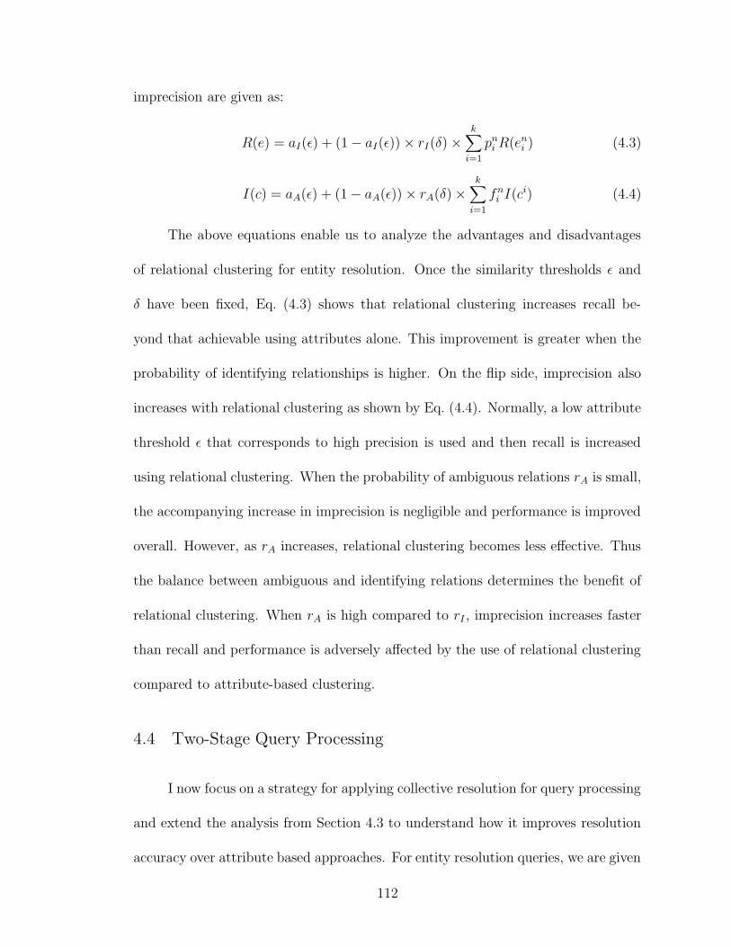
imprecision are given as:

R(e) = aI(ε) + (1 − aI(ε)) × rI(δ) ×k

∑

i=1

pni R(en

i ) (4.3)

I(c) = aA(ε) + (1 − aA(ε)) × rA(δ) ×k

∑

i=1

fni I(ci) (4.4)

The above equations enable us to analyze the advantages and disadvantages

of relational clustering for entity resolution. Once the similarity thresholds ε and

δ have been fixed, Eq. (4.3) shows that relational clustering increases recall be-

yond that achievable using attributes alone. This improvement is greater when the

probability of identifying relationships is higher. On the flip side, imprecision also

increases with relational clustering as shown by Eq. (4.4). Normally, a low attribute

threshold ε that corresponds to high precision is used and then recall is increased

using relational clustering. When the probability of ambiguous relations rA is small,

the accompanying increase in imprecision is negligible and performance is improved

overall. However, as rA increases, relational clustering becomes less effective. Thus

the balance between ambiguous and identifying relations determines the benefit of

relational clustering. When rA is high compared to rI , imprecision increases faster

than recall and performance is adversely affected by the use of relational clustering

compared to attribute-based clustering.

4.4 Two-Stage Query Processing

I now focus on a strategy for applying collective resolution for query processing

and extend the analysis from Section 4.3 to understand how it improves resolution

accuracy over attribute based approaches. For entity resolution queries, we are given

112

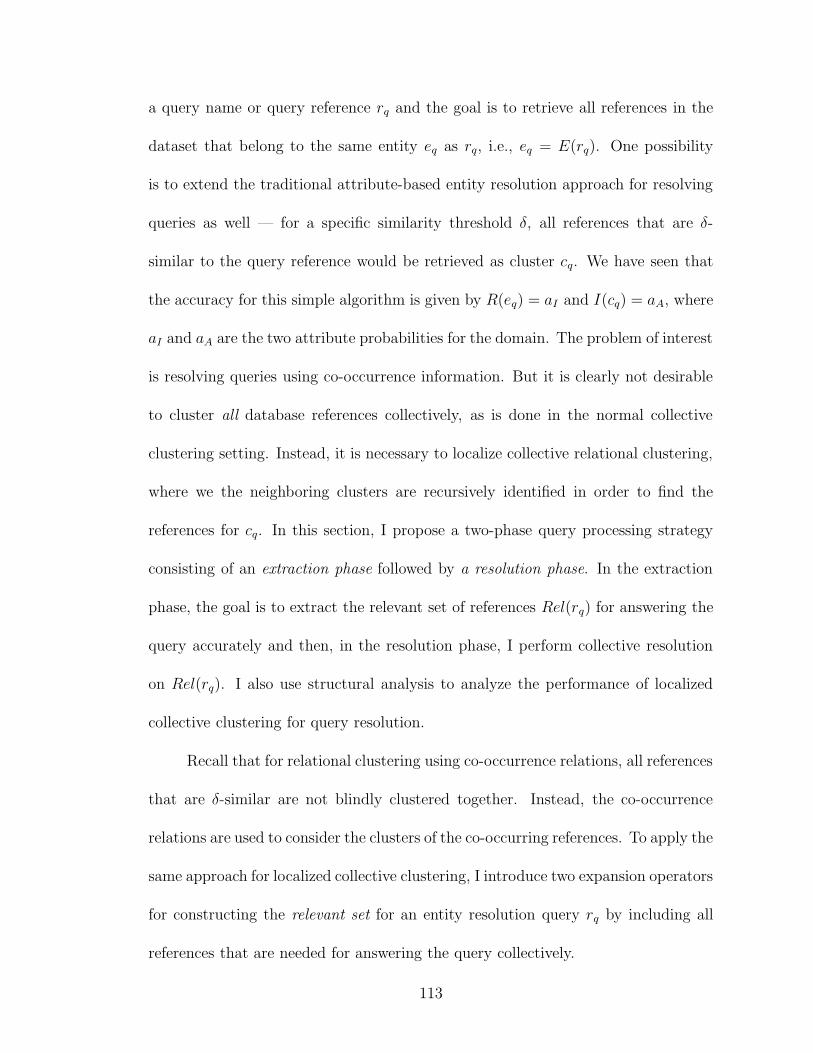
a query name or query reference rq and the goal is to retrieve all references in the

dataset that belong to the same entity eq as rq, i.e., eq = E(rq). One possibility

is to extend the traditional attribute-based entity resolution approach for resolving

queries as well — for a specific similarity threshold δ, all references that are δ-

similar to the query reference would be retrieved as cluster cq. We have seen that

the accuracy for this simple algorithm is given by R(eq) = aI and I(cq) = aA, where

aI and aA are the two attribute probabilities for the domain. The problem of interest

is resolving queries using co-occurrence information. But it is clearly not desirable

to cluster all database references collectively, as is done in the normal collective

clustering setting. Instead, it is necessary to localize collective relational clustering,

where we the neighboring clusters are recursively identified in order to find the

references for cq. In this section, I propose a two-phase query processing strategy

consisting of an extraction phase followed by a resolution phase. In the extraction

phase, the goal is to extract the relevant set of references Rel(rq) for answering the

query accurately and then, in the resolution phase, I perform collective resolution

on Rel(rq). I also use structural analysis to analyze the performance of localized

collective clustering for query resolution.

Recall that for relational clustering using co-occurrence relations, all references

that are δ-similar are not blindly clustered together. Instead, the co-occurrence

relations are used to consider the clusters of the co-occurring references. To apply the

same approach for localized collective clustering, I introduce two expansion operators

for constructing the relevant set for an entity resolution query rq by including all

references that are needed for answering the query collectively.

113

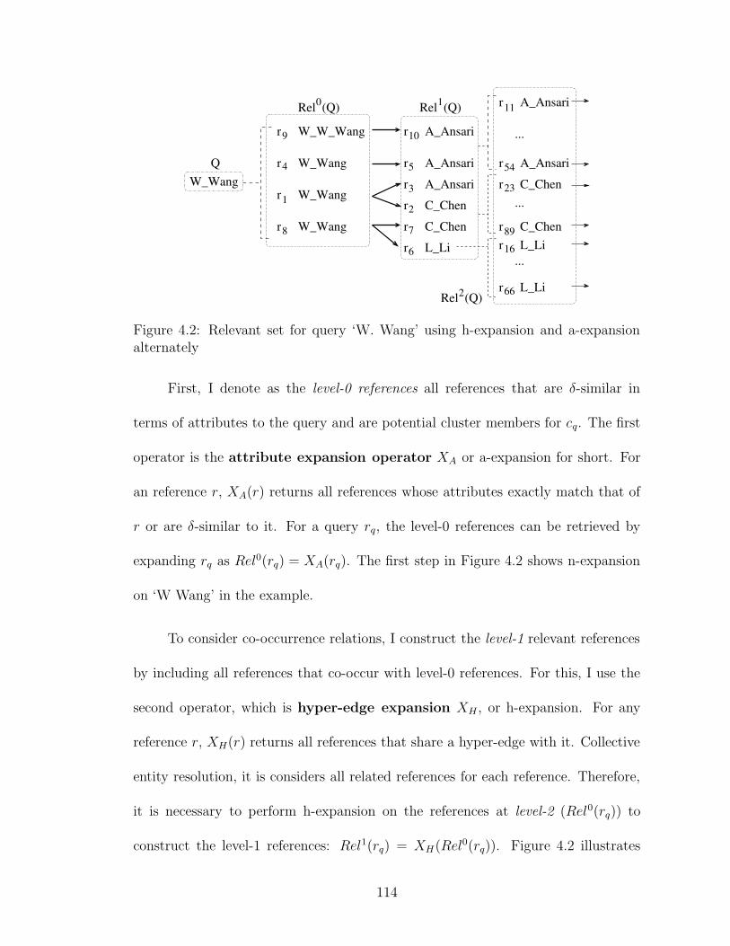
A_Ansarir

C_Chenr

L_Lir

L_Lir

C_Chenr

C_Chenr

L_Lir

A_Ansarir

A_Ansarir0Rel (Q) Rel (Q)1

Rel (Q)2

W_W_Wang

W_Wang

W_Wang

W_Wang

A_Ansari

C_Chen

r

r

r

r

r

r

r

A_Ansari

...

...

...

8

1

4

9 10

5

2

7

6

11

54

23

89

16

66

3W_WangQ

Figure 4.2: Relevant set for query ‘W. Wang’ using h-expansion and a-expansionalternately

First, I denote as the level-0 references all references that are δ-similar in

terms of attributes to the query and are potential cluster members for cq. The first

operator is the attribute expansion operator XA or a-expansion for short. For

an reference r, XA(r) returns all references whose attributes exactly match that of

r or are δ-similar to it. For a query rq, the level-0 references can be retrieved by

expanding rq as Rel0(rq) = XA(rq). The first step in Figure 4.2 shows n-expansion

on ‘W Wang’ in the example.

To consider co-occurrence relations, I construct the level-1 relevant references

by including all references that co-occur with level-0 references. For this, I use the

second operator, which is hyper-edge expansion XH , or h-expansion. For any

reference r, XH(r) returns all references that share a hyper-edge with it. Collective

entity resolution, it is considers all related references for each reference. Therefore,

it is necessary to perform h-expansion on the references at level-2 (Rel0(rq)) to

construct the level-1 references: Rel1(rq) = XH(Rel0(rq)). Figure 4.2 illustrates

114

this operation in the example.

To perform collective clustering for the query, the references at level-1 need to

be clustered as well. One option for level-1 references is attribute-based clustering

using a conservative ε-similarity to keep imprecision to a minimum. The analysis

technique from before is again useful for evaluating the performance for this ap-

proach. Expanding from Eq. (4.3), and using aI(ε) for the recall of each neighboring

entity for eq, the recall for the query entity is:

R(eq) = aI(ε) + (1 − aI(ε)) × rI(δ) ×k

∑

i=1

pni aI(ε)

Observing that∑k

i=1 pni = 1 allows us to simplify the above expression for recall:

R(eq) = aI(ε) + (1 − aI(ε)) × rI(δ) × aI(ε)

= aI(ε)[1 + (1 − aI(ε))rI(δ)]

Similarly, the imprecision for the computed cluster cq can be expressed as

I(cq) = aA(ε)[1 + (1 − aA(ε))rA(δ)]

So we can see that attribute-clustering of the the first level neighbors po-

tentially increases recall for the query entity eq, but imprecision goes up as well.

However, when the balance between rA and rI is favorable, the increase in impreci-

sion will be insignificant and much smaller than the corresponding increase in recall,

so that there is an overall performance improvement.

Is it possible to do better than this? We can go a step further and consider co-

occurrence relations for clustering the level-1 references as well. So, instead of con-

sidering ε-similarity for references in level-1 as before, I find all of their δ-similar ref-

115

erences, which I call level-2 (Rel2(rq)), using a-expansion: Rel2(rq) = XA(Rel1(rq)).

Then, to retrieve the second order neighbors, I consider level-3 references — those

that co-occur with level-2 references — using h-expansion on the em level-2 refer-

ences: Rel3(rq) = XH(Rel2(rq)). Then, as before, I cluster the level-3 references by

simply using ε-similarity of their attributes. In order to see how this affects accuracy

for the query, a few algebraic steps yield the following:

R(eq) = aI [1 + (1 − aI)rI + (1 − aI)2r2

I ]

I(cq) = aA[1 + (1 − aA)rA + (1 − aA)2r2A]

This recursive growth of the relevant set can be continued further. For-

mally, for a query rq, the expansion process alternates between a-expansion and

h-expansion:

Reli(rq) = XA(rq) for i = 0

XH(Reli−1(rq)) for odd i

XA(Reli−1(rq)) for even i

As I proceed recursively and consider higher order co-occurrences for localized

clustering, additional terms appear in the expressions for precision and recall, so

that for nth-order co-occurrences I get a geometric progression with n + 1 terms for

both. But this does not imply that this process needs to be continued to arbitrary

levels to get optimum benefit. The common ratio for the two geometric progressions

are (1−aI)rI and (1−aA)rA respectively. Both of these are significantly smaller than

1 and therefore the progressions converge very quickly with increasing co-occurrence

level. So the improvement in resolution accuracy for the query rq falls off quickly

116

with expansion depth, and the expansion process can be terminated at some cut-off

depth d∗:

Rel(rq) =d∗⋃

i=0

Reli(Q)

Also, the size of the relevant set can be significantly reduced by restricting

attribute expansion beyond level-0 to exact a-expansion X eA(r) that only considers

references with exactly the same attribute as r. Interestingly, it can be shown that

the restricted strategy that alternates between exact a-expansion and h-expansion

does not affect recall significantly.

4.5 Adaptive Query Expansion

The query expansion strategy from the previous section is unconstrained in

that it blindly expands all references in the current relevant set and also includes all

new references generated by an expansion operation. However, for many domains

the size of the relevant set resulting from such unconstrained expansion is prohibitive

for query-time resolution even for small expansion depths. Given the limited time

to process a query, one solution is to include the references that are most helpful

for resolving the query. To illustrate using the example from Figure 4.2, observe

that ‘Chen’ and ‘Li’ are significantly more common or ‘ambiguous’ names than

‘Ansari’ — even different ‘W. Wang’ entities are likely to have collaborators named

‘Chen’ or ‘Li’. Therefore, when h-expanding Rel0(rq) for ‘W. Wang’, ‘Ansari’ is more

informative than ‘Chen’ or ‘Li’. Similarly, when n-expanding Rel1(rq), we can choose

not to expand the name ‘A. Ansari’ any further, since two ‘A. Ansari’ references are

117

very likely to be coreferent. But more evidence is needed for the ‘Chen’s and ‘Li’s.

To describe this formally, the ambiguity of a name n is the probability that any two

references ri and rj in the database that have this name (ri.Name = rj.Name = n)

are not coreferent: Amb(n) = P (E(ri) 6= E(rj)). The goal of adaptive expansion is

to add less ambiguous references to the relevant set and, of the references currently

in the relevant set, expand the most ambiguous ones.

For adaptive hyper-edge expansion, upper-bound hmax is set on the num-

ber of new references that h-expansion at a particular level can generate. This can

be represented formally as |XH(Reli(rq))| ≤ hmax|Reli(rq)|. The value of hmax may

depend on depth i but it is small enough to rule out full h-expansion of the cur-

rent relevant set. Then, given hmax, the strategy is to choose the least ambiguous

references from XH(Reli(rq)), since they provide the most informative evidence for

resolving the references in Reli(rq). I sort the h-expanded references in increasing

order of ambiguity and select the first k from them, where k = hmax|Reli(rq)|.

Reliadapt(rq, hmax) = LeastAmb(k, XH(Reli−1adapt(rq))) (4.5)

The setting for adaptive attribute expansion is very similar. For some

positive number amax, exact a-expansion of Reli(rq) is allowed to include at most

amax|Reli(rq)| references. Note that now the selection preference needs to be flipped

— more ambiguous names need more evidence, so they are expanded first. So I

can sort XeA(Reli(rq)) in decreasing order of ambiguity and select the first k from

the sorted list, where k = amax|Reli(rq)|. But this could potentially retrieve only

references for the most ambiguous name, totally ignoring references with any other

118

name. To avoid this, I choose the top k ambiguous references from Reli(rq) before

expansion, and then expand the references so chosen.

Reliadapt(rq, nmax) = XeA(MostAmb(k, Reliadapt(rq))) (4.6)

Though this cannot directly control the number of new references added, µr × k is

a reasonable estimate, where µr is the average number of references per name.

The adaptive expansion scheme proposed in this section is crucially dependent

on the estimates of name ambiguity. For estimating ambiguity, I make use of the

strategy described in Subsection 2.4.4, where I estimate the ambiguity of one at-

tribute using a second attribute. This scheme worked quite well for us, as I illustrate

in the next section.

4.6 Experimental Results

For experimental evaluation of the query-time resolution strategies, I resorted

to both real and synthetically generated datasets. First, I describe the experiments

performed on real datasets and then I move on to experiments on synthetic data.

4.6.1 Experiments on Real Data

For real data, I used two citation datasets that I have already described in

Section 2.6. The first dataset, arXiv, contains papers from high energy physics and

was used in KDD Cup 20031. It has 58,515 references to 9,200 authors, contained

1http://www.cs.cornell.edu/projects/kddcup/index.html

119

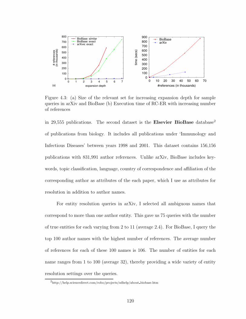
0

100

200

300

400

500

600

700

800

0 1 2 3 4 5 6 7

# re

fere

nces

(in th

ousa

nds)

expansion depth(a)

BioBase: similarBioBase: exactarXive: exact

0 100 200 300 400 500 600 700 800 900

0 10 20 30 40 50 60 70

time

(sec

s)

#references (in thousands)

BioBasearXiv

Figure 4.3: (a) Size of the relevant set for increasing expansion depth for samplequeries in arXiv and BioBase (b) Execution time of RC-ER with increasing numberof references

in 29,555 publications. The second dataset is the Elsevier BioBase database2

of publications from biology. It includes all publications under ‘Immunology and

Infectious Diseases’ between years 1998 and 2001. This dataset contains 156,156

publications with 831,991 author references. Unlike arXiv, BioBase includes key-

words, topic classification, language, country of correspondence and affiliation of the

corresponding author as attributes of the each paper, which I use as attributes for

resolution in addition to author names.

For entity resolution queries in arXiv, I selected all ambiguous names that

correspond to more than one author entity. This gave us 75 queries with the number

of true entities for each varying from 2 to 11 (average 2.4). For BioBase, I query the

top 100 author names with the highest number of references. The average number

of references for each of these 100 names is 106. The number of entities for each

name ranges from 1 to 100 (average 32), thereby providing a wide variety of entity

resolution settings over the queries.

2http://help.sciencedirect.com/robo/projects/sdhelp/about biobase.htm

120

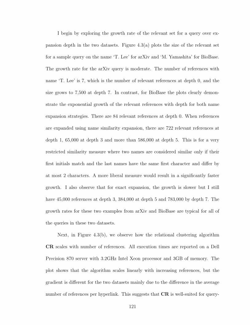
I begin by exploring the growth rate of the relevant set for a query over ex-

pansion depth in the two datasets. Figure 4.3(a) plots the size of the relevant set

for a sample query on the name ‘T. Lee’ for arXiv and ‘M. Yamashita’ for BioBase.

The growth rate for the arXiv query is moderate. The number of references with

name ‘T. Lee’ is 7, which is the number of relevant references at depth 0, and the

size grows to 7,500 at depth 7. In contrast, for BioBase the plots clearly demon-

strate the exponential growth of the relevant references with depth for both name

expansion strategies. There are 84 relevant references at depth 0. When references

are expanded using name similarity expansion, there are 722 relevant references at

depth 1, 65,000 at depth 3 and more than 586,000 at depth 5. This is for a very

restricted similarity measure where two names are considered similar only if their

first initials match and the last names have the same first character and differ by

at most 2 characters. A more liberal measure would result in a significantly faster

growth. I also observe that for exact expansion, the growth is slower but I still

have 45,000 references at depth 3, 384,000 at depth 5 and 783,000 by depth 7. The

growth rates for these two examples from arXiv and BioBase are typical for all of

the queries in these two datasets.

Next, in Figure 4.3(b), we observe how the relational clustering algorithm

CR scales with number of references. All execution times are reported on a Dell

Precision 870 server with 3.2GHz Intel Xeon processor and 3GB of memory. The

plot shows that the algorithm scales linearly with increasing references, but the

gradient is different for the two datasets mainly due to the difference in the average

number of references per hyperlink. This suggests that CR is well-suited for query-

121

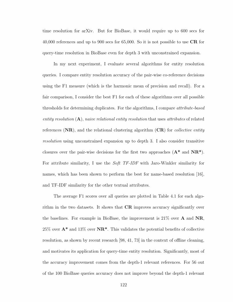
time resolution for arXiv. But for BioBase, it would require up to 600 secs for

40,000 references and up to 900 secs for 65,000. So it is not possible to use CR for

query-time resolution in BioBase even for depth 3 with unconstrained expansion.

In my next experiment, I evaluate several algorithms for entity resolution

queries. I compare entity resolution accuracy of the pair-wise co-reference decisions

using the F1 measure (which is the harmonic mean of precision and recall). For a

fair comparison, I consider the best F1 for each of these algorithms over all possible

thresholds for determining duplicates. For the algorithms, I compare attribute-based

entity resolution (A), naive relational entity resolution that uses attributes of related

references (NR), and the relational clustering algorithm (CR) for collective entity

resolution using unconstrained expansion up to depth 3. I also consider transitive

closures over the pair-wise decisions for the first two approaches (A* and NR*).

For attribute similarity, I use the Soft TF-IDF with Jaro-Winkler similarity for

names, which has been shown to perform the best for name-based resolution [16],

and TF-IDF similarity for the other textual attributes.

The average F1 scores over all queries are plotted in Table 4.1 for each algo-

rithm in the two datasets. It shows that CR improves accuracy significantly over

the baselines. For example in BioBase, the improvement is 21% over A and NR,

25% over A* and 13% over NR*. This validates the potential benefits of collective

resolution, as shown by recent research [98, 41, 73] in the context of offline cleaning,

and motivates its application for query-time entity resolution. Significantly, most of

the accuracy improvement comes from the depth-1 relevant references. For 56 out

of the 100 BioBase queries accuracy does not improve beyond the depth-1 relevant

122

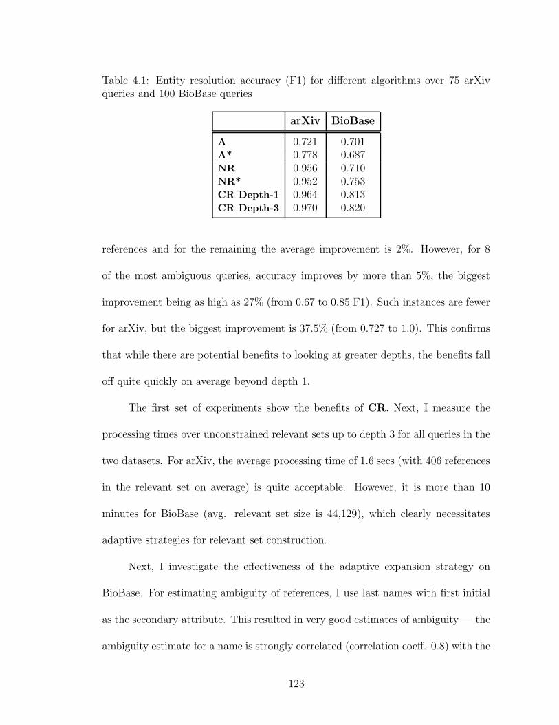
Table 4.1: Entity resolution accuracy (F1) for different algorithms over 75 arXivqueries and 100 BioBase queries

arXiv BioBase

A 0.721 0.701A* 0.778 0.687NR 0.956 0.710NR* 0.952 0.753CR Depth-1 0.964 0.813CR Depth-3 0.970 0.820

references and for the remaining the average improvement is 2%. However, for 8

of the most ambiguous queries, accuracy improves by more than 5%, the biggest

improvement being as high as 27% (from 0.67 to 0.85 F1). Such instances are fewer

for arXiv, but the biggest improvement is 37.5% (from 0.727 to 1.0). This confirms

that while there are potential benefits to looking at greater depths, the benefits fall

off quite quickly on average beyond depth 1.

The first set of experiments show the benefits of CR. Next, I measure the

processing times over unconstrained relevant sets up to depth 3 for all queries in the

two datasets. For arXiv, the average processing time of 1.6 secs (with 406 references

in the relevant set on average) is quite acceptable. However, it is more than 10

minutes for BioBase (avg. relevant set size is 44,129), which clearly necessitates

adaptive strategies for relevant set construction.

Next, I investigate the effectiveness of the adaptive expansion strategy on

BioBase. For estimating ambiguity of references, I use last names with first initial

as the secondary attribute. This resulted in very good estimates of ambiguity — the

ambiguity estimate for a name is strongly correlated (correlation coeff. 0.8) with the

123

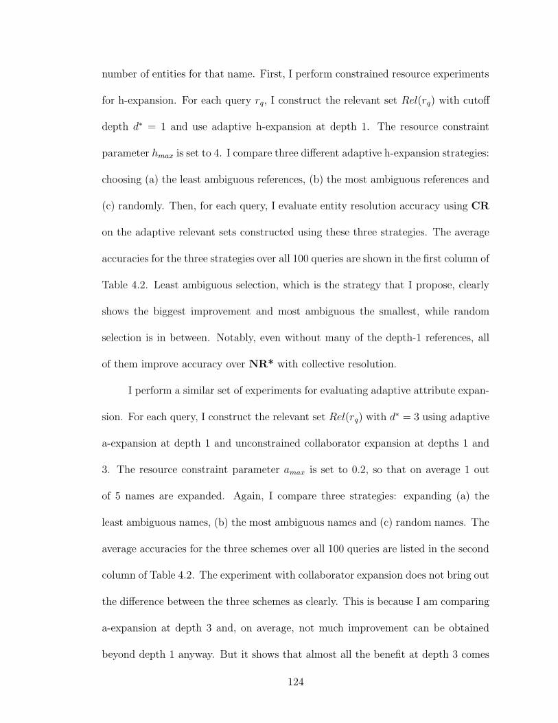
number of entities for that name. First, I perform constrained resource experiments

for h-expansion. For each query rq, I construct the relevant set Rel(rq) with cutoff

depth d∗ = 1 and use adaptive h-expansion at depth 1. The resource constraint

parameter hmax is set to 4. I compare three different adaptive h-expansion strategies:

choosing (a) the least ambiguous references, (b) the most ambiguous references and

(c) randomly. Then, for each query, I evaluate entity resolution accuracy using CR

on the adaptive relevant sets constructed using these three strategies. The average

accuracies for the three strategies over all 100 queries are shown in the first column of

Table 4.2. Least ambiguous selection, which is the strategy that I propose, clearly

shows the biggest improvement and most ambiguous the smallest, while random

selection is in between. Notably, even without many of the depth-1 references, all

of them improve accuracy over NR* with collective resolution.

I perform a similar set of experiments for evaluating adaptive attribute expan-

sion. For each query, I construct the relevant set Rel(rq) with d∗ = 3 using adaptive

a-expansion at depth 1 and unconstrained collaborator expansion at depths 1 and

3. The resource constraint parameter amax is set to 0.2, so that on average 1 out

of 5 names are expanded. Again, I compare three strategies: expanding (a) the

least ambiguous names, (b) the most ambiguous names and (c) random names. The

average accuracies for the three schemes over all 100 queries are listed in the second

column of Table 4.2. The experiment with collaborator expansion does not bring out

the difference between the three schemes as clearly. This is because I am comparing

a-expansion at depth 3 and, on average, not much improvement can be obtained

beyond depth 1 anyway. But it shows that almost all the benefit at depth 3 comes

124

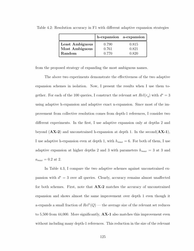
Table 4.2: Resolution accuracy in F1 with different adaptive expansion strategies

h-expansion a-expansion

Least Ambiguous 0.790 0.815Most Ambiguous 0.761 0.821Random 0.770 0.820

from the proposed strategy of expanding the most ambiguous names.

The above two experiments demonstrate the effectiveness of the two adaptive

expansion schemes in isolation. Now, I present the results when I use them to-

gether. For each of the 100 queries, I construct the relevant set Rel(rq) with d∗ = 3

using adaptive h-expansion and adaptive exact n-expansion. Since most of the im-

provement from collective resolution comes from depth-1 references, I consider two

different experiments. In the first, I use adaptive expansion only at depths 2 and

beyond (AX-2) and unconstrained h-expansion at depth 1. In the second(AX-1),

I use adaptive h-expansion even at depth 1, with hmax = 6. For both of them, I use

adaptive expansion at higher depths 2 and 3 with parameters hmax = 3 at 3 and

amax = 0.2 at 2.

In Table 4.3, I compare the two adaptive schemes against unconstrained ex-

pansion with d∗ = 3 over all queries. Clearly, accuracy remains almost unaffected

for both schemes. First, note that AX-2 matches the accuracy of unconstrained

expansion and shows almost the same improvement over depth 1 even though it

a-expands a small fraction of Rel1(Q) — the average size of the relevant set reduces

to 5,500 from 44,000. More significantly, AX-1 also matches this improvement even

without including many depth-1 references. This reduction in the size of the relevant

125

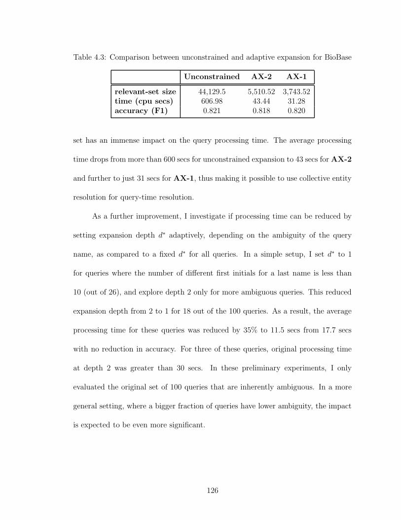
Table 4.3: Comparison between unconstrained and adaptive expansion for BioBase

Unconstrained AX-2 AX-1

relevant-set size 44,129.5 5,510.52 3,743.52time (cpu secs) 606.98 43.44 31.28accuracy (F1) 0.821 0.818 0.820

set has an immense impact on the query processing time. The average processing

time drops from more than 600 secs for unconstrained expansion to 43 secs for AX-2

and further to just 31 secs for AX-1, thus making it possible to use collective entity

resolution for query-time resolution.

As a further improvement, I investigate if processing time can be reduced by

setting expansion depth d∗ adaptively, depending on the ambiguity of the query

name, as compared to a fixed d∗ for all queries. In a simple setup, I set d∗ to 1

for queries where the number of different first initials for a last name is less than

10 (out of 26), and explore depth 2 only for more ambiguous queries. This reduced

expansion depth from 2 to 1 for 18 out of the 100 queries. As a result, the average

processing time for these queries was reduced by 35% to 11.5 secs from 17.7 secs

with no reduction in accuracy. For three of these queries, original processing time

at depth 2 was greater than 30 secs. In these preliminary experiments, I only

evaluated the original set of 100 queries that are inherently ambiguous. In a more

general setting, where a bigger fraction of queries have lower ambiguity, the impact

is expected to be even more significant.

126

0.2

0.3

0.4

0.5

0.6

0.7

0.8

0.9

1

0.5 0.6 0.7 0.8 0.9 1

Rec

all

Sim. Threshold

pR=0.2pR=0.5pR=1.0

0.65

0.7

0.75

0.8

0.85

0.9

0.95

1

0.5 0.6 0.7 0.8 0.9 1

Pre

cisi

on

Sim. Threshold

pRa=0.0pRa=0.3pRa=0.6

Figure 4.4: Effect of (a) identifying relations on recall and (b) ambiguous relationson precision for collective clustering

4.6.2 Experiments using Synthetic Data

I also experiment with synthetically generated data where I can control the

structural characteristics. For this purpose, I used the two-stage data generator

described in Appendix A to control the fraction of ambiguous and identifying rela-

tionships.

In the first set of experiments on synthetic data, I experiment with identifying

relationships. I generate 500 co-occurrence relations from the same 100 entities

with 200 entity-entity relationships using varying probability of co-occurrences pR =

0.2, 0.5, 1.0 in the data. The probability of ambiguous relationships is held fixed, so

that higher pR translates to higher probability of identifying co-occurrences in the

data. Figure 4.4(a) shows recall at different similarity thresholds for three different

co-occurrence probabilities. The results confirm that recall increases progressively

with more identifying relationships at all thresholds.

In my second experiment, I consider the effect of ambiguous relations on

precision of collective relational clustering. I add 200 binary relationships be-

127

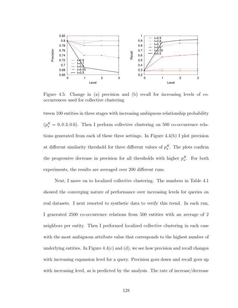
0.66

0.68

0.7

0.72

0.74

0.76

0.78

0.8

0.82

0 1 2 3

Pre

cisi

on

Level

t=0.9t=0.7t=0.6t=0.55t=0.5

0.2

0.3

0.4

0.5

0.6

0.7

0.8

0.9

1

0 1 2 3

Rec

all

Level

t=0.9t=0.8t=0.7t=0.6t=0.55t=0.5

Figure 4.5: Change in (a) precision and (b) recall for increasing levels of co-occurrences used for collective clustering

tween 100 entities in three stages with increasing ambiguous relationship probability

(pRa = 0, 0.3, 0.6). Then I perform collective clustering on 500 co-occurrence rela-

tions generated from each of these three settings. In Figure 4.4(b) I plot precision

at different similarity threshold for three different values of pRa . The plots confirm

the progressive decrease in precision for all thresholds with higher pRa . For both

experiments, the results are averaged over 200 different runs.

Next, I move on to localized collective clustering. The numbers in Table 4.1

showed the converging nature of performance over increasing levels for queries on

real datasets. I next resorted to synthetic data to verify this trend. In each run,

I generated 2500 co-occurrence relations from 500 entities with an average of 2

neighbors per entity. Then I performed localized collective clustering in each case

with the most ambiguous attribute value that corresponds to the highest number of

underlying entities. In Figure 4.4(c) and (d), we see how precision and recall changes

with increasing expansion level for a query. Precision goes down and recall goes up

with increasing level, as is predicted by the analysis. The rate of increase/decrease

128

depends on the structural properties. In other experiments, we have seen different

rates of change, but the trend remains the same. The analysis also showed that

precision and recall converges quickly depending on the structural properties. This

too is confirmed by the two plots where the curves flatten out by level 3.

As I have already discussed, an important issue with the collective relational

clustering algorithm is the determination of the termination threshold. Note that

this is an issue for all of the baselines as well, and here I report best accuracy over

all thresholds. This is an area of ongoing research. Preliminary experiments have

shown that the best threshold is query specific — setting the threshold depending

on the ambiguity of the query results in significantly better accuracy than a fixed

threshold for all queries. For an empirical evaluation, I cleaned the entire arXiv

dataset offline by running CR on all its references together and terminated at the

threshold that maximizes resolution accuracy over all references. This results in an

overall accuracy (F1) of 0.98. However, the average accuracy measured over the 75

queries in the test set is only 0.87. In comparison, recall that the best obtainable

accuracy when resolving the queries individually each with a different threshold is

0.97. This suggests that there may be potential benefits to localized cleaning over

its global counterpart in the offline setting.

4.7 Conclusions

In this chapter, I have motivated the problem of query-time entity resolution

for accessing unresolved third-party databases. The biggest issue in query-time res-

129

olution of entities is reducing the computational expense of collective resolution,

while maintaining its benefits in terms of resolution accuracy. I have motivated

query-time entity resolution as a constrained-resource problem and proposed an

adaptive strategy for extracting the set of most relevant references for collectively

resolving a query. I have formally analyzed the dependence of this approach on

structural and other characteristics of the data to show analytically why a recur-

sive expand-and-resolve strategy is feasible for this problem. I have demonstrated

that this adaptive strategy preserves the accuracy of unconstrained expansion while

dramatically reducing the number of relevant references, thereby enabling collective

resolution at query-time. I have also demonstrated how the same adaptive strategy

allows us to allocate resources depending on the ambiguity of the query, and reduces

processing time for less ambiguous queries by 35%. I have additionally performed

extensive experiments on real and synthetic data to validate the trends predicted by

the analysis. While I have presented results for bibliographic data, the techniques

are applicable in other relational domains. Interesting directions of future research

include exploring stronger coupling between the extraction and resolution phases of

query processing and investigating localized resolution for offline data cleaning as

well.

130

Chapter 5

Word Sense Disambiguation Using Bilingual Probabilistic Models

In this chapter, I look at a potential application of entity resolution in the do-

main of natural language processing and consider the related problem of word sense

disambiguation. The rest of the chapter is organized as follows. In Section 5.1, I

briefly introduce the word sense disambiguation problem and discuss related work.

In Section 5.2, I introduce the two probabilistic generative models for word sense

disambiguation and describe how I construct the structure of the models in Sec-

tion 5.3 and how the model parameters are trained in Section 5.4. I then discuss

experimental results in Section 5.5 and analyze the performance of the two models

in Section 5.6.

5.1 Word Sense Disambiguation: Introduction and Related Work

As mentioned in the introduction, the word sense disambiguation problem

closely resembles the general definition of entity resolution when the senses are

considered as entities and words in natural language documents as noisy observations

of the senses. However, it also presents some challenges that are unique to this

domain. Carefully constructed sense ontologies for languages, such as the WordNet

hierarchy for English, provide a valuable resource that approaches for solving this

131

problem should take into account. Also, parallel corpora have words from multiple

languages, all of which can be potentially ambiguous but the actual senses can differ

from one language to another. Models that I develop for multi-lingual word sense

disambiguation therefore need to resolve senses for different languages differently

but, at the same time, need to construct cross-lingual relationships between senses.

These are the challenges that I address in this chapter.

Word sense disambiguation (WSD) has been a central question in the compu-

tational linguistics community since its inception. WSD is fundamental to natural

language understanding and is a useful intermediate step for many other language

processing tasks [56]. Many recent approaches make use of ideas from statistical ma-

chine learning; the availability of shared sense definitions (e.g. WordNet [43]) and

recent international competitions [61] have enabled researchers to compare their

results. Supervised approaches [23, 105] typically outperform unsupervised ap-

proaches [2, 70, 69, 90, 104, 106], but often tend to be tuned to a specific corpus

and are constrained by scarcity of labeled data.

In an effort to overcome the difficulty of finding sense-labeled training data,

researchers have investigated unsupervised approaches for word sense disambigua-

tion. Yarowsky [104] makes use of a thesaurus to find the most predictive words

for each context. Yarowsky [106] proposes an iterative classification algorithm that

uses the idea of ‘one sense per collocation’ to sense-tag all occurrences of a word

starting from an initial set of labeled samples. Employing a similar idea, Mihalcea

[75] uses non-ambiguous words to iteratively determine classes for ambiguous words.

McCarthy et al. [74] make use of a thesaurus acquired from raw textual corpora and

132

WordNet similarity to automatically find the most prevalent sense for each word in

a document. Resnik [90] proposes a statistical measure of selectional preference of

predicates towards specific classes or senses.

It has been pointed out that the use of parallel corpora for sense tagging can

help with word sense disambiguation [22, 33, 34, 55, 91]. Brown et al. [22] use a

flip-flop algorithm to split English words French words into two classes (senses) to

have high mutual information through translations. Dagan and Itai [34] consider

the disambiguation problem of finding the right target word in machine translation

using a bilingual lexicon. They use statistics computed over corpora in the target

language to choose the most likely translations for syntactic tuples (related words)

in the source language. Ide [55] performs a statistical study of how the mapping

of words to senses varies between different languages. Resnik and Yarowsky [91]

suggest limiting sense distinctions to only those that are translated differently in

different languages and propose cross-linguistic measures of sense distinction.

The main inspiration for my work is Diab and Resnik [38], who use relational

structure in the form of translations for disambiguation and automatic sense tagging.

Bengio and Kermorvant [5] present a graphical model that is an attempt to proba-

bilistically formalize the main ideas of Diab and Resnik. Here I present two variants

of the probabilistic model by Bengio and Kermorvant that incorporate relational

structure to resolve senses. I also present empirical word sense disambiguation re-

sults which demonstrate the gain brought by this probabilistic relational approach,

even while using only the translated word to provide disambiguation information.

This is an instance where I do not make use of any attribute information for re-

133

solving entities. They are resolved based on relational structure alone. However,

the possible set of entity labels is provided to us in this case through the use of the

WordNet hierarchy.

The first generative model, the Sense Model, does not model groups of senses

explicitly. Instead, the senses in the two languages depend directly on each other

in this model. Specifically, the Sense Model clusters semantically related words

from the both languages into one set of senses, and translations are generated by

probabilistically choosing a sense and then words from the sense. I show that this

improves on the results of Diab and Resnik.

The next model, which I call the Concept Model, aims to improve on this by

modeling the senses of the two languages separately and by relating senses from the

two languages through a higher-level, semantically less precise concept. I use the

term concept to denote a group of related senses. The concept plays the same role

for word sense disambiguation as that of entity groups for resolution in Chapter 3.

The intuition is that not all of the senses that are possible for a word will be relevant

for a concept. In other words, the distribution over the senses of a word given a

concept can be expected to have a lower entropy than the distribution over the

senses of the word in the language as a whole. In this work, I look at translation

data as a resource for identification of semantic concepts. Improved performance

over the Sense Model validates the use of concepts in modeling translations.

For the rest of this chapter, for simplicity I will refer to the primary language

of the parallel document as English and to the secondary as Spanish.

134

5.2 Probabilistic Models for Parallel Corpora

I motivate the use of a probabilistic model by illustrating that disambigua-

tion using translations is possible even when a word has a unique translation. For

example, according to WordNet, the word prevention has two senses in English,

which may be abbreviated as hindrance (the act of hindering or obstruction) and

control (by prevention, e.g. the control of a disease). It has a single translation

in the corpus, that being prevencion. The first English sense, hindrance, also has

other words such as bar that occur in the corpus and all of these other words are

observed to be translated in Spanish as the word obstruccion. In addition, none

of these other words translate to prevencion. So it is not unreasonable to suppose

that the intended sense for prevention when translated as prevencion is different

from that of bar. Therefore, the intended sense is most likely to be control. At the

very heart of the reasoning is probabilistic analysis and independence assumptions.

The assumption is that senses and words have certain occurrence probabilities and

that the choice of the word can be made independently once the sense has been

decided. This is the flavor that I look to add to modeling parallel documents for

sense disambiguation. I formally describe the two generative models that use these

ideas in Subsection 5.2.2 and Subsection 5.2.3.

5.2.1 Notation

Throughout this chapter, I use uppercase letters to denote random variables

and lowercase letters to denote specific instances of the random variables. A trans-

135

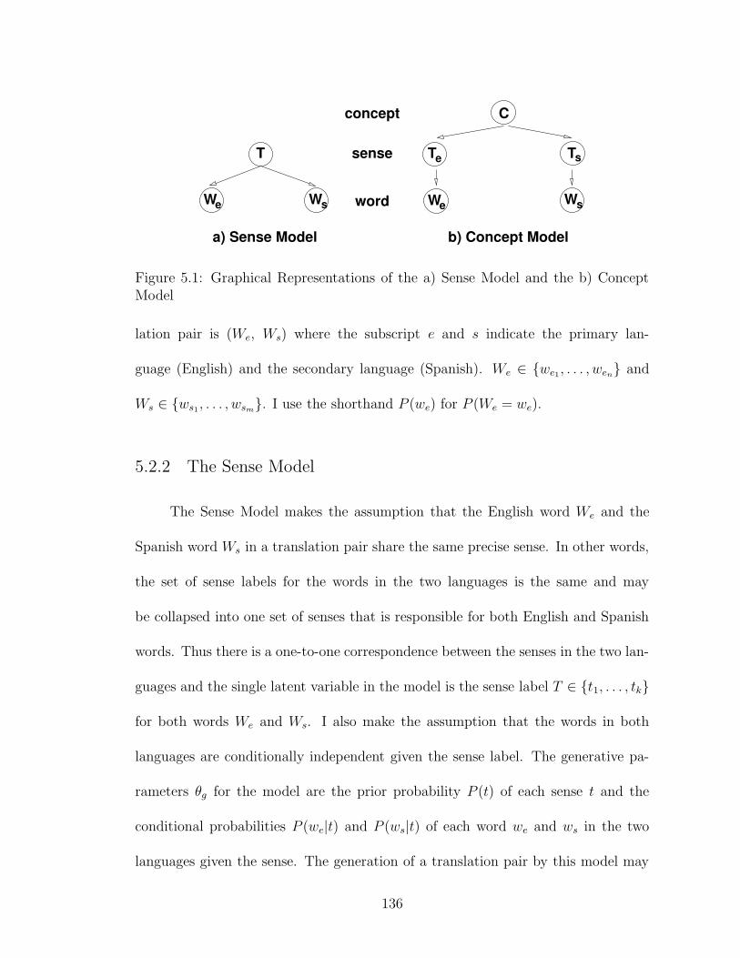
T

We Ws

Te Ts

C

WsWeword

concept

sense

b) Concept Modela) Sense Model

Figure 5.1: Graphical Representations of the a) Sense Model and the b) ConceptModel

lation pair is (We, Ws) where the subscript e and s indicate the primary lan-

guage (English) and the secondary language (Spanish). We ∈ {we1, . . . , wen} and

Ws ∈ {ws1, . . . , wsm}. I use the shorthand P (we) for P (We = we).

5.2.2 The Sense Model

The Sense Model makes the assumption that the English word We and the

Spanish word Ws in a translation pair share the same precise sense. In other words,

the set of sense labels for the words in the two languages is the same and may

be collapsed into one set of senses that is responsible for both English and Spanish

words. Thus there is a one-to-one correspondence between the senses in the two lan-

guages and the single latent variable in the model is the sense label T ∈ {t1, . . . , tk}

for both words We and Ws. I also make the assumption that the words in both

languages are conditionally independent given the sense label. The generative pa-

rameters θg for the model are the prior probability P (t) of each sense t and the

conditional probabilities P (we|t) and P (ws|t) of each word we and ws in the two

languages given the sense. The generation of a translation pair by this model may

136

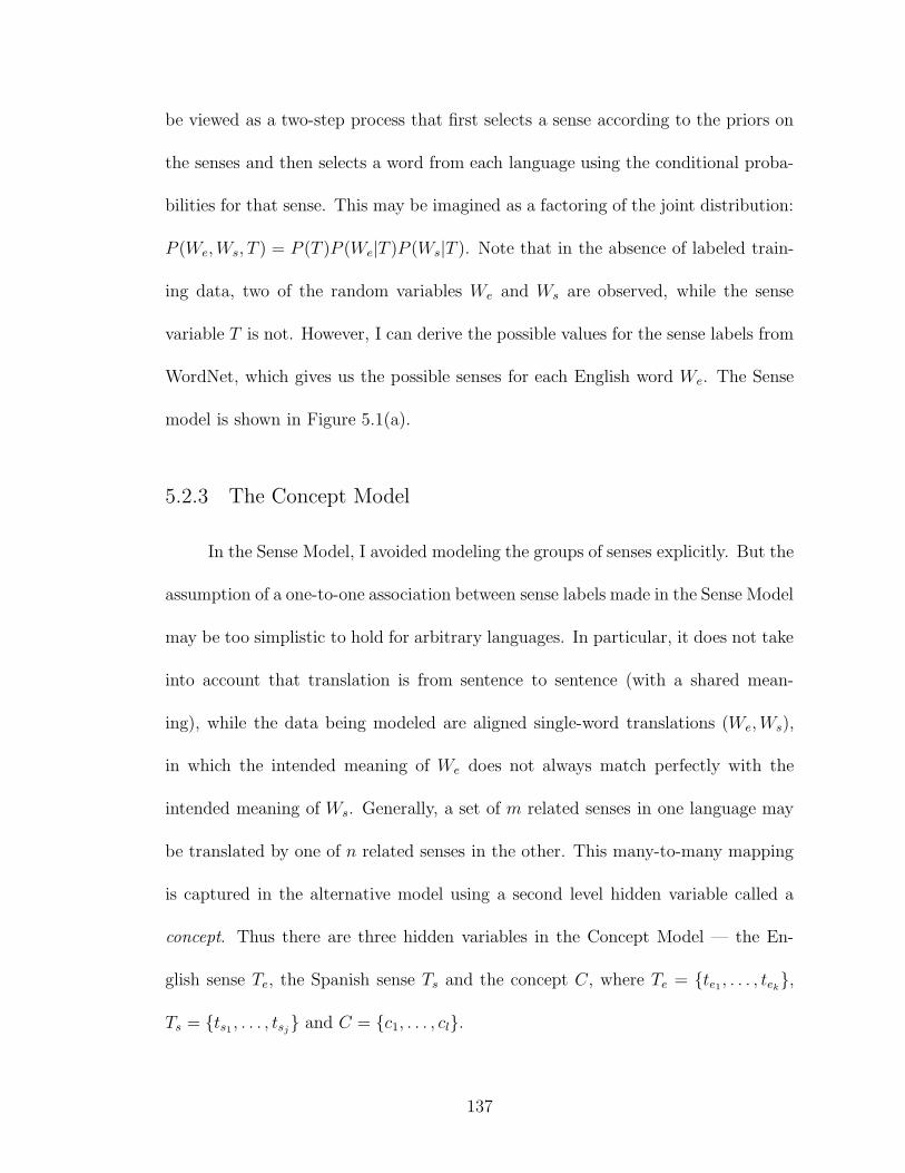
be viewed as a two-step process that first selects a sense according to the priors on

the senses and then selects a word from each language using the conditional proba-

bilities for that sense. This may be imagined as a factoring of the joint distribution:

P (We, Ws, T ) = P (T )P (We|T )P (Ws|T ). Note that in the absence of labeled train-

ing data, two of the random variables We and Ws are observed, while the sense

variable T is not. However, I can derive the possible values for the sense labels from

WordNet, which gives us the possible senses for each English word We. The Sense

model is shown in Figure 5.1(a).

5.2.3 The Concept Model

In the Sense Model, I avoided modeling the groups of senses explicitly. But the

assumption of a one-to-one association between sense labels made in the Sense Model

may be too simplistic to hold for arbitrary languages. In particular, it does not take

into account that translation is from sentence to sentence (with a shared mean-

ing), while the data being modeled are aligned single-word translations (We, Ws),

in which the intended meaning of We does not always match perfectly with the

intended meaning of Ws. Generally, a set of m related senses in one language may

be translated by one of n related senses in the other. This many-to-many mapping

is captured in the alternative model using a second level hidden variable called a

concept. Thus there are three hidden variables in the Concept Model — the En-

glish sense Te, the Spanish sense Ts and the concept C, where Te = {te1, . . . , tek},

Ts = {ts1 , . . . , tsj} and C = {c1, . . . , cl}.

137

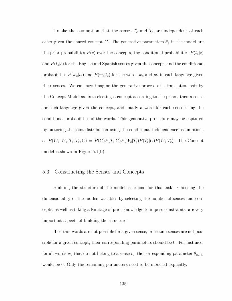
I make the assumption that the senses Te and Ts are independent of each

other given the shared concept C. The generative parameters θg in the model are

the prior probabilities P (c) over the concepts, the conditional probabilities P (te|c)

and P (ts|c) for the English and Spanish senses given the concept, and the conditional

probabilities P (we|te) and P (ws|ts) for the words we and ws in each language given

their senses. We can now imagine the generative process of a translation pair by

the Concept Model as first selecting a concept according to the priors, then a sense

for each language given the concept, and finally a word for each sense using the

conditional probabilities of the words. This generative procedure may be captured

by factoring the joint distribution using the conditional independence assumptions

as P (We, Ws, Te, Ts, C) = P (C)P (Te|C)P (We|Te)P (Ts|C)P (Ws|Ts). The Concept

model is shown in Figure 5.1(b).

5.3 Constructing the Senses and Concepts

Building the structure of the model is crucial for this task. Choosing the

dimensionality of the hidden variables by selecting the number of senses and con-

cepts, as well as taking advantage of prior knowledge to impose constraints, are very

important aspects of building the structure.

If certain words are not possible for a given sense, or certain senses are not pos-

sible for a given concept, their corresponding parameters should be 0. For instance,

for all words we that do not belong to a sense te, the corresponding parameter θwe|te

would be 0. Only the remaining parameters need to be modeled explicitly.

138

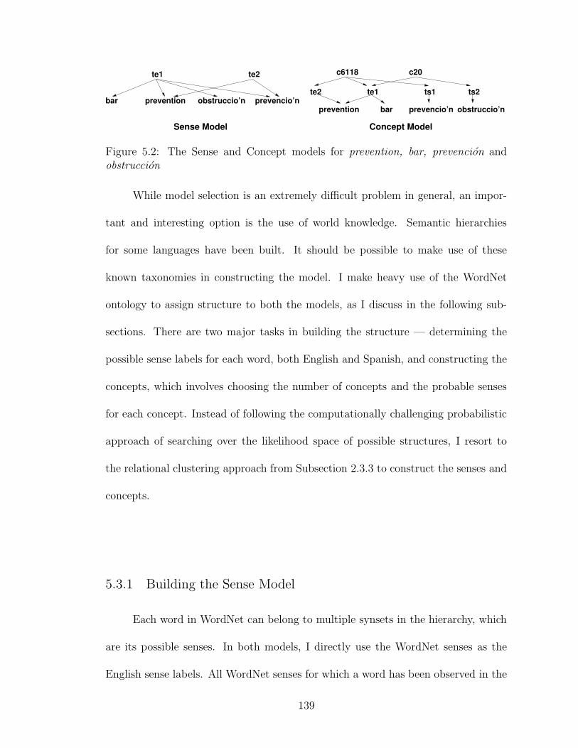
Concept Model

te2 ts1te1

barprevention

c6118

ts2

c20

prevencio’n obstruccio’n

Sense Model

bar prevention

te1 te2

prevencio’nobstruccio’n

Figure 5.2: The Sense and Concept models for prevention, bar, prevencion andobstruccion

While model selection is an extremely difficult problem in general, an impor-

tant and interesting option is the use of world knowledge. Semantic hierarchies

for some languages have been built. It should be possible to make use of these

known taxonomies in constructing the model. I make heavy use of the WordNet

ontology to assign structure to both the models, as I discuss in the following sub-

sections. There are two major tasks in building the structure — determining the

possible sense labels for each word, both English and Spanish, and constructing the

concepts, which involves choosing the number of concepts and the probable senses

for each concept. Instead of following the computationally challenging probabilistic

approach of searching over the likelihood space of possible structures, I resort to

the relational clustering approach from Subsection 2.3.3 to construct the senses and

concepts.

5.3.1 Building the Sense Model

Each word in WordNet can belong to multiple synsets in the hierarchy, which

are its possible senses. In both models, I directly use the WordNet senses as the

English sense labels. All WordNet senses for which a word has been observed in the

139

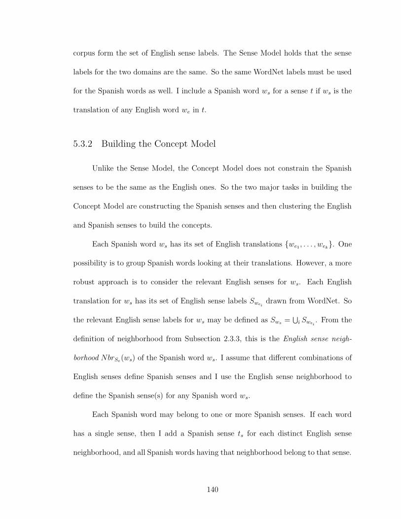
corpus form the set of English sense labels. The Sense Model holds that the sense

labels for the two domains are the same. So the same WordNet labels must be used

for the Spanish words as well. I include a Spanish word ws for a sense t if ws is the

translation of any English word we in t.

5.3.2 Building the Concept Model

Unlike the Sense Model, the Concept Model does not constrain the Spanish

senses to be the same as the English ones. So the two major tasks in building the

Concept Model are constructing the Spanish senses and then clustering the English

and Spanish senses to build the concepts.

Each Spanish word ws has its set of English translations {we1, . . . , wek}. One

possibility is to group Spanish words looking at their translations. However, a more

robust approach is to consider the relevant English senses for ws. Each English

translation for ws has its set of English sense labels Sweidrawn from WordNet. So

the relevant English sense labels for ws may be defined as Sws=

⋃

i Swei. From the

definition of neighborhood from Subsection 2.3.3, this is the English sense neigh-

borhood NbrSe(ws) of the Spanish word ws. I assume that different combinations of

English senses define Spanish senses and I use the English sense neighborhood to

define the Spanish sense(s) for any Spanish word ws.

Each Spanish word may belong to one or more Spanish senses. If each word

has a single sense, then I add a Spanish sense ts for each distinct English sense

neighborhood, and all Spanish words having that neighborhood belong to that sense.

140

Otherwise, each English neighborhood can be imagined to combine multiple Spanish

senses. So I split the neighborhoods into frequently occurring subgroups or sub-

neighborhoods. I identify sub-neighborhoods by intersecting pairs of neighborhoods

and each sub-neighborhood that occurs significantly many times is recognized to

represent a Spanish sense. I consider both ways of building Spanish senses. In

either case, a constructed Spanish sense ts comes with its neighborhood of English

senses, which I denote as NbrSe(ts).

Once I have the Spanish senses, I cluster them to form concepts. I use the

English sense neighborhood corresponding to each Spanish sense to define a measure

of similarity for a pair of Spanish senses. Following Subsection 2.3.3, I use the

neighborhood similarity measure. The specific measure that I use is the Jaccard

similarity, which is the most robust1. This similarity measure is then used to cluster

the Spanish senses. Two Spanish senses are considered to be similar if their similarity

measure is above a threshold. Then I take a transitive closure over these similarities

to construct clusters of similar Spanish senses.

Finally, I build the concepts from the Spanish sense clusters. Since a concept is

defined by a set of related English and Spanish senses, each Spanish sense cluster can

be taken to represent a concept. This is because the Spanish senses in a cluster are

grouped by similarity in their relations with English senses. So a concept is formed

by taking the Spanish senses from each cluster and their related English senses. The

1Another option would be to use a measure of similarity for English senses, proposed by

Resnik [89] for two synsets in a concept hierarchy like WordNet. The initial results with this

measure were not favorable.

141

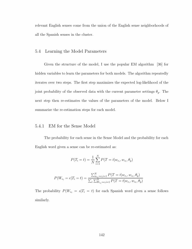
relevant English senses come from the union of the English sense neighborhoods of

all the Spanish senses in the cluster.

5.4 Learning the Model Parameters

Given the structure of the model, I use the popular EM algorithm [36] for

hidden variables to learn the parameters for both models. The algorithm repeatedly

iterates over two steps. The first step maximizes the expected log-likelihood of the

joint probability of the observed data with the current parameter settings θg. The

next step then re-estimates the values of the parameters of the model. Below I

summarize the re-estimation steps for each model.

5.4.1 EM for the Sense Model

The probability for each sense in the Sense Model and the probability for each

English word given a sense can be re-estimated as:

P (Ti = t) =1

N

N∑

i=1

P (T = t|wei, wsi

, θg)

P (Wei= e|Ti = t) =

∑Nwei

=e,i=1 P (T = t|wei, wsi

, θg)∑

e

∑NWei

=e,i=1 P (T = t|wei, wsi

, θg)

The probability P (Wsi= s|Ti = t) for each Spanish word given a sense follows

similarly.

142

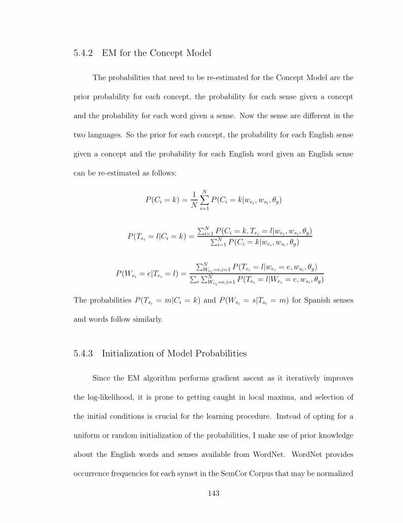
5.4.2 EM for the Concept Model

The probabilities that need to be re-estimated for the Concept Model are the

prior probability for each concept, the probability for each sense given a concept

and the probability for each word given a sense. Now the sense are different in the

two languages. So the prior for each concept, the probability for each English sense

given a concept and the probability for each English word given an English sense

can be re-estimated as follows:

P (Ci = k) =1

N

N∑

i=1

P (Ci = k|wei, wsi

, θg)

P (Tei= l|Ci = k) =

∑Ni=1 P (Ci = k, Tei

= l|wei, wsi

, θg)∑N

i=1 P (Ci = k|wei, wsi

, θg)

P (Wei= e|Tei

= l) =

∑NWei

=e,i=1 P (Tei= l|wei

= e, wsi, θg)

∑

e

∑NWei

=e,i=1 P (Tei= l|Wei

= e, wsi, θg)

The probabilities P (Tsi= m|Ci = k) and P (Wsi

= s|Tsi= m) for Spanish senses

and words follow similarly.

5.4.3 Initialization of Model Probabilities

Since the EM algorithm performs gradient ascent as it iteratively improves

the log-likelihood, it is prone to getting caught in local maxima, and selection of

the initial conditions is crucial for the learning procedure. Instead of opting for a

uniform or random initialization of the probabilities, I make use of prior knowledge

about the English words and senses available from WordNet. WordNet provides

occurrence frequencies for each synset in the SemCor Corpus that may be normalized

143

to derive probabilities Pwn(te) for each English sense te. For the Sense Model, these

probabilities form the initial priors over the senses, while all English (and Spanish)

words belonging to a sense are initially assumed to be equally likely. However,

initialization of the Concept Model using the same knowledge is non-trivial. Each

English sense te should have Pinit(te) = Pwn(te). But since each sense belongs to

multiple concepts, the constraint∑

te∈c P (te|c) = 1 also has to be satisfied for each

concept. Instead of going for an optimal assignment, I settle for a compromise. I

set Pinit(te|c) = Pwn(te) and P (c) =∑

te∈c Pwn(te). Subsequent normalization takes

care of the sum constraints. For a Spanish sense, I set P (ts) =∑

te∈NbrSe(ts) Pwn(te).

Once I have the Spanish sense probabilities, I follow the same procedure for setting

P (ts|c) for each concept. All the Spanish and English words for a sense are initially

set to be equally likely, as in the Sense Model.

5.5 Experimental Evaluation

Both the models are generative probabilistic models learned from parallel cor-

pora and are expected to fit the training and subsequent test data. A good fit should

be reflected in good prediction accuracy over a test set. The prediction task of in-

terest is the sense of an English word when its translation is provided. I estimate

the prediction accuracy and recall of the models on Senseval data.2 In addition, the

Concept Model learns a sense structure for the Spanish language. While it is hard

2Accuracy is the ratio of the number of correct predictions and the number of attempted

predictions. Recall is the ratio of the number of correct predictions and the size of the test set.

144

to objectively evaluate the quality of such a structure, I present some interesting

concepts that are learned as an indication of the potential of this approach.

5.5.1 Evaluation with Senseval Data

In the experiments with real data, I make use of the parallel corpora con-

structed by Diab and Resnik [38] for evaluation purposes. I chose to work on these

corpora in order to permit a direct comparison with their results. The sense-tagged

portion of the English corpus is comprised of the English “all-words” section of the

SENSEVAL-2 test data. The remainder of this corpus is constructed by adding the

Brown Corpus, the SENSEVAL-1 corpus, the SENSEVAL-2 English Lexical Sample

test, trial and training corpora and the Wall Street Journal sections 18-24 from the

Penn Treebank. This English corpus is translated into Spanish using two commer-

cially available MT systems: Globalink Pro 6.4 and Systran Professional Premium.

The GIZA++ implementation of the IBM statistical MT models was used to derive

the most-likely word-level alignments, and these define the English/Spanish word

co-occurrences. To take into account variability of translation, I combine the trans-

lations from the two systems for each English word, following in the footsteps of

Diab and Resnik [38]. For my experiments, I focus only on nouns, of which there

are 875 occurrences in the tagged data. The sense tags for the English domain

are derived from the WordNet 1.7 inventory. After pruning stopwords, I end up

with 16,186 English words, 31,862 Spanish words and 2,385,574 instances of 41,850

distinct translation pairs. The English words come from 20,361 WordNet senses.

145

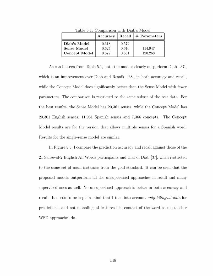
Table 5.1: Comparison with Diab’s Model

Accuracy Recall # Parameters

Diab’s Model 0.618 0.572 -Sense Model 0.624 0.616 154,947Concept Model 0.672 0.651 120,268

As can be seen from Table 5.1, both the models clearly outperform Diab [37],

which is an improvement over Diab and Resnik [38], in both accuracy and recall,

while the Concept Model does significantly better than the Sense Model with fewer

parameters. The comparison is restricted to the same subset of the test data. For

the best results, the Sense Model has 20,361 senses, while the Concept Model has

20,361 English senses, 11,961 Spanish senses and 7,366 concepts. The Concept

Model results are for the version that allows multiple senses for a Spanish word.

Results for the single-sense model are similar.

In Figure 5.3, I compare the prediction accuracy and recall against those of the

21 Senseval-2 English All Words participants and that of Diab [37], when restricted

to the same set of noun instances from the gold standard. It can be seen that the

proposed models outperform all the unsupervised approaches in recall and many

supervised ones as well. No unsupervised approach is better in both accuracy and

recall. It needs to be kept in mind that I take into account only bilingual data for

predictions, and not monolingual features like context of the word as most other

WSD approaches do.

146

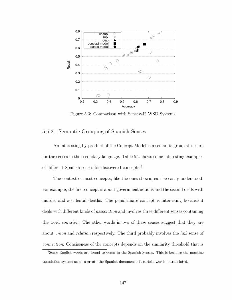
0

0.1

0.2

0.3

0.4

0.5

0.6

0.7

0.8

0.2 0.3 0.4 0.5 0.6 0.7 0.8 0.9

Rec

all

Accuracy

unsup.sup.diab

concept modelsense model

Figure 5.3: Comparison with Senseval2 WSD Systems

5.5.2 Semantic Grouping of Spanish Senses

An interesting by-product of the Concept Model is a semantic group structure

for the senses in the secondary language. Table 5.2 shows some interesting examples

of different Spanish senses for discovered concepts.3

The context of most concepts, like the ones shown, can be easily understood.

For example, the first concept is about government actions and the second deals with

murder and accidental deaths. The penultimate concept is interesting because it

deals with different kinds of association and involves three different senses containing

the word conexion. The other words in two of these senses suggest that they are

about union and relation respectively. The third probably involves the link sense of

connection. Conciseness of the concepts depends on the similarity threshold that is

3Some English words are found to occur in the Spanish Senses. This is because the machine

translation system used to create the Spanish document left certain words untranslated.

147

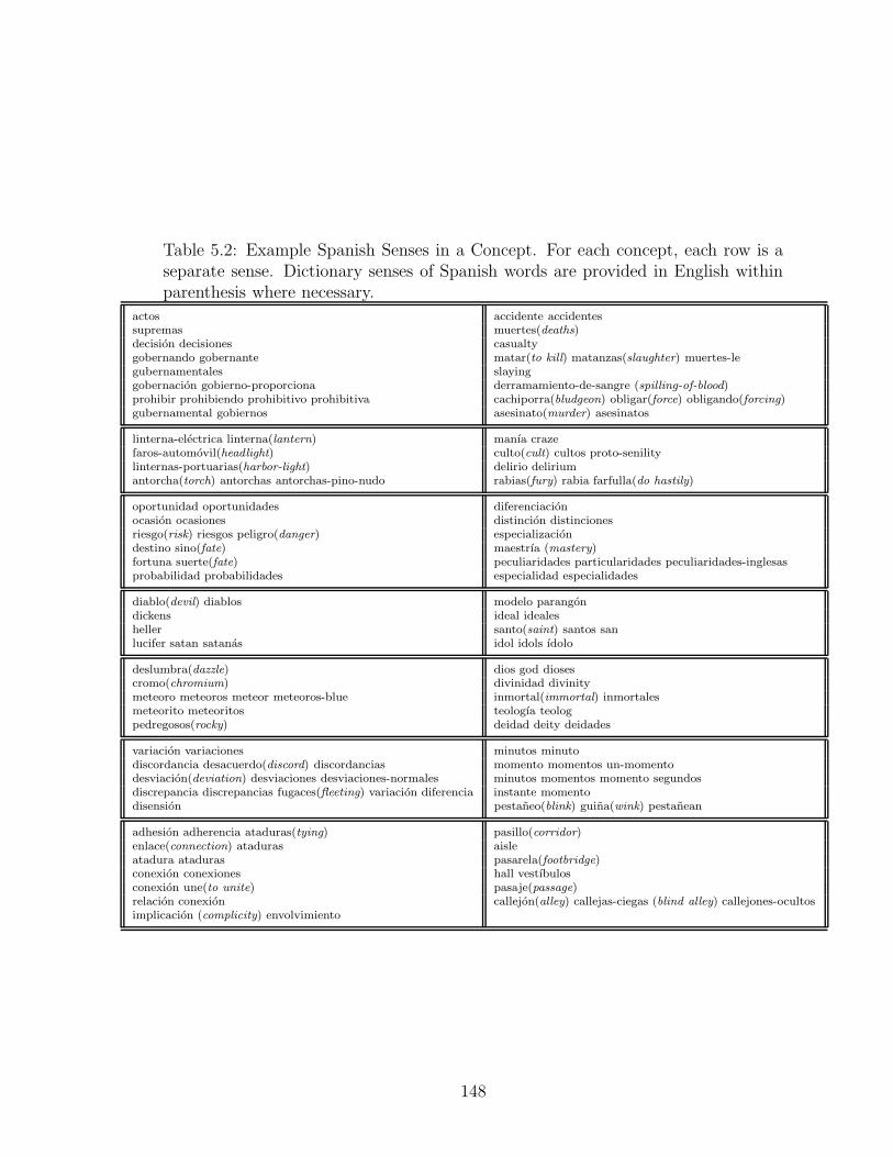
Table 5.2: Example Spanish Senses in a Concept. For each concept, each row is aseparate sense. Dictionary senses of Spanish words are provided in English withinparenthesis where necessary.

actos accidente accidentessupremas muertes(deaths)decision decisiones casualtygobernando gobernante matar(to kill) matanzas(slaughter) muertes-legubernamentales slayinggobernacion gobierno-proporciona derramamiento-de-sangre (spilling-of-blood)prohibir prohibiendo prohibitivo prohibitiva cachiporra(bludgeon) obligar(force) obligando(forcing)gubernamental gobiernos asesinato(murder) asesinatos

linterna-electrica linterna(lantern) manıa crazefaros-automovil(headlight) culto(cult) cultos proto-senilitylinternas-portuarias(harbor-light) delirio deliriumantorcha(torch) antorchas antorchas-pino-nudo rabias(fury) rabia farfulla(do hastily)

oportunidad oportunidades diferenciacionocasion ocasiones distincion distincionesriesgo(risk) riesgos peligro(danger) especializaciondestino sino(fate) maestrıa (mastery)fortuna suerte(fate) peculiaridades particularidades peculiaridades-inglesasprobabilidad probabilidades especialidad especialidades

diablo(devil) diablos modelo parangondickens ideal idealesheller santo(saint) santos sanlucifer satan satanas idol idols ıdolo

deslumbra(dazzle) dios god diosescromo(chromium) divinidad divinitymeteoro meteoros meteor meteoros-blue inmortal(immortal) inmortalesmeteorito meteoritos teologıa teologpedregosos(rocky) deidad deity deidades

variacion variaciones minutos minutodiscordancia desacuerdo(discord) discordancias momento momentos un-momentodesviacion(deviation) desviaciones desviaciones-normales minutos momentos momento segundosdiscrepancia discrepancias fugaces(fleeting) variacion diferencia instante momentodisension pestaneo(blink) guina(wink) pestanean

adhesion adherencia ataduras(tying) pasillo(corridor)enlace(connection) ataduras aisleatadura ataduras pasarela(footbridge)conexion conexiones hall vestıbulosconexion une(to unite) pasaje(passage)relacion conexion callejon(alley) callejas-ciegas (blind alley) callejones-ocultosimplicacion (complicity) envolvimiento

148

selected. Some may bring together loosely-related topics, which can be separated

by a higher threshold.

5.6 Model Analysis

In this section, I back up the experimental results with an in-depth analysis

of the performance of the two proposed models.

The Sense Model was motivated by Diab and Resnik [38] but the flavors of

the two are quite different. The most important distinction is that the Sense Model

is a probabilistic generative model for parallel corpora, where interaction between

different words stemming from the same sense comes into play, even if the words

are not related through translations, and this interdependence of the senses through

common words plays a role in sense disambiguation.

I started off with the discussions on semantic ambiguity with the intuition that

identification of semantic concepts in the corpus that relate multiple senses should

help disambiguate senses. The Sense Model falls short of this target since it only

brings together a single sense from each language. I will now revisit the motivating

example from Section 5.2 and see how concepts help in disambiguation by grouping

multiple related senses together.

For the Sense Model, P (prevention|te2) > P (prevention|te1) since it is the only

word that te2 can generate. However, this difference is compensated for by the higher

prior probability P (te1), which is strengthened by both the translation pairs. Since

the probability of joint occurrence is given by the product P (t)P (we|t)P (ws|t) for

149

any sense t, the model does not develop a clear preference for any of the two senses.

The critical difference in the Concept Model can be appreciated directly from

the corresponding joint probability P (c)P (te|c)P (we|te)P (ts|c)P (ws|ts), where c is

the relevant concept in the model. The preference for a particular instantiation

in the model is dependent not on the prior P (te) over a sense, but on the sense

conditional P (te|c). In the example, since <bar, obstruccion> can be generated

only through concept c20, P (te1|c20) is the only English sense conditional boosted

by it. <prevention, prevencion> is generated through a different concept c6118,

where the higher conditional P (prevention|te2) gradually strengthens one of the

possible instantiations for it, and the other one becomes increasingly unlikely as the

iterations progress. The inference is that only one sense of prevention is possible in

the context of the parallel corpus. The key factor in this disambiguation was that

two senses of prevention separated out in two different concepts.

The other significant difference between the models is in the constraints on

the parameters and the effect that they have on sense disambiguation. In the Sense

Model,∑

t P (t) = 1, while in the Concept Model,∑

te∈c P (te|c) = 1 separately for

each concept c. Now for two relevant senses for an English word, a slight difference

in their priors will tend to get ironed out when normalized over the entire set of

senses for the corpus. In contrast, if these two senses belong to the same concept in

the Concept Model, the difference in the sense conditionals will be highlighted since

the normalization occurs over a very small set of senses — the senses for only that

concept, which in the best possible scenario will contain only the two contending

senses, as in concept c118 of the example.

150

As can be seen from Table 5.1, the Concept Model not only outperforms the

Sense Model, it does so with significantly fewer parameters. This may be counter-

intuitive since Concept Model involves an extra concept variable. However, the

dissociation of Spanish and English senses can significantly reduce the parameter

space. Imagine two Spanish words that are associated with ten English senses and

accordingly each of them has a probability for belonging to each of these ten senses.

Aided with a concept variable, it is possible to model the same relationship by

creating a separate Spanish sense that contains these two words and relating this

Spanish sense with the ten English senses through a concept variable. Thus these

words now need to belong to only one sense as opposed to ten. Of course, now there

are new transition probabilities for each of the eleven senses from the new concept

node. The exact reduction in the parameter space will depend on the frequent sub-

neighborhoods discovered for the English sense neighborhoods of the Spanish words.

Longer and more frequent sub-neighborhoods will lead to larger reductions. It must

also be borne in mind that this reduction comes with the independence assumptions

made in the Concept Model.

It may be noted that predicting senses from translations need not necessarily

be an end result in itself. As I have already mentioned, lack of labeled data is a severe

hindrance for supervised approaches to word sense disambiguation. At the same

time, there is an abundance of bilingual documents and many more can potentially

be mined from the web. It should be possible using the proposed approach to

(noisily) assign sense tags to words in such documents, thus providing huge resources

of labeled data for supervised approaches to make use of.

151

Chapter 6

Related Work

In this chapter, I review related work on entity resolution and group / topic

models. I discusss related work for word sense dismabiguation in Section 5.1. The

entity resolution problem has been studied in many different areas under different

names — co-reference resolution, deduplication, object uncertainty, record linkage,

reference reconciliation, etc. Here I review some of the main work, but the review

is not exhaustive. Winkler [102] also provides a nice summary report.

6.1 Approximate Matching

The traditional approach to entity resolution looks at textual similarity in the

descriptions of the entities. For example, determining whether two citations refer

to the same paper depends on the similarity measure such as edit distance between

the two citation strings. There has been extensive work on defining approximate

string similarity measures [78, 80, 30, 27] that may be used for unsupervised entity

resolution. Cardie and Wagstaff [24] have posed noun phrase coreference in natural

language documents as an unsupervised clustering problem based on a similarity

measure that combines multiple linguistic features. Another approach is to use

adaptive supervised algorithms that learn string similarity measures from labeled

152

data [92, 15, 31, 100]. One of the difficulties in using a supervised method for

resolution is constructing a good training set that includes a representative collection

of positive and negative examples. Other approaches use active learning [94, 100],

where the user is asked to label ambiguous examples by the learner.

6.2 Theoretical Bounds for Cleaning

Cohen et al. [29] studies the theoretical problem of ‘hardening a soft database’

that has many co-referent entries. Hardening refers to the task of figuring out which

pairs of soft identifiers refer to the same real world object. Given the likelihood of

being co-referent for each soft pair and a probability distribution of possible hard

databases, hardening is defined as the optimization problem of finding the most

likely hard model given the soft facts. A cost is associated with each hard tuple

that is added to the database and for each co-reference decision made. They show

that this optimization problem is NP-hard even under strong restrictions. They

propose a greedy agglomerative clustering approach for an approximate solution.

This algorithm’s complexity is linear in the number of entries in the soft database.

6.3 Efficiency Issues

Given that solving the entity resolution problem optimally is computationally

expensive, an important focus is on efficiency issues in data cleaning, where the

goal is to come up with inexpensive algorithms for finding approximate solutions

to the problem. The key mechanisms for doing this involve computing the matches

153

efficiently and employing techniques commonly called ‘blocking’ to quickly find po-

tential duplicates and eliminate non-duplicates from consideration [52, 79, 72, 54].

The merge/purge problem was posed by Hernandez and Stolfo [52] with effi-

cient schemes to retrieve potential duplicates without resorting to quadratic com-

plexity. They use a ‘sorted neighborhood method’ where an appropriate key is

chosen for matching. Records are then sorted or grouped according to that key and

potential matches are identified using a sliding window technique. However, some

keys may be badly distorted so that their matches cannot be spanned by the window

and such cases will not be retrieved. The solution proposed is a multi-pass method

over different keys and then merging the results using transitive closure. Monge and

Elkan [79] combine the union find algorithm with a priority queue look-up to find

connected components in an undirected graph. McCallum et al. [72] propose the

use of canopies to first partition the data into overlapping clusters using a cheap

distance metric and then use a more accurate and expensive distance metric for

those data pairs that lie within the same canopy. Gravano et al. [50] propose

a sampling approach to quickly compute cosine similarity between tuples for fast

text-joins within an SQL framework. Chaudhuri et al. [27] use an error tolerant

index for data warehousing applications for probabilistically looking up a small set

of candidate reference tuples for matching against an incoming tuple. This is consid-

ered ‘probabilistically safe’ since the closest tuples in the database will be retrieved

with high probability. This is also efficient since only a small number of matches

needs to be performed. Swoosh [6] has recently been proposed as a generic entity

resolution framework that considers resolving and merging duplicates as a database

154

operator and the goal is to minimize the number of record-level and feature-level

operations.

6.4 Probabilistic Models for Entity Resolution

The groundwork for posing entity resolution as a probabilistic classification

problem was done by [44], who extend the ideas of [83] for labeling pairs of records

from two different files to be merged as “match” or “non-match” on the basis of

agreement among their different fields. Winkler [103] and more recently Ravikumar

and Cohen [88] have built upon this work.

Probabilistic models that take into account interaction between different entity

resolution decisions have been proposed for named entity recognition in natural

language processing and for citation matching. McCallum and Wellner [73] use

conditional random fields for noun coreference and use clique templates with tied

parameters to capture repeated relational structure. Singla and Domingos [98] use

the idea of merging evidence to allow the flow of reasoning between different pair-wise

decisions over multiple entity types. These two relational models are supervised

and require labeled data to train the parameters. Wellner and McCallum have also

extended their model for performing extraction and resolution jointly [101].

Availability of sufficient labeled data is often an issue for this problem and

unsupervised relational models have also been developed. Li et al. [67] address

the problem of disambiguating “entity mentions”, potentially of multiple types,

in the context of unstructured textual documents. They propose a probabilistic

155

generative model that captures a joint distribution over pairs of entities in terms

of co-mentions in documents. Pasula et al. [86] propose a generic probabilistic

relational model framework for the citation matching problem. Daume and Marcu

[35] have recently proposed an extension to Pasula et al.’s model, where the number

of clusters or entities is directly modeled by a Dirichlet Process and is similar in

spirit to ours. However, I propose a three level model where the selection of author

entities depends on the groups that they belong to. Milch et al. [76] propose a

more general approach to the identity uncertainty problem. They present a formal

generative language for defining probability distribution over worlds with unknown

objects and identity uncertainty. This can be seen as a probability distribution

over first order model structures with varying number of objects. They show that

the inference problem is decidable for a large class of these models and propose a

rejection sampling algorithm for estimating probabilities.

All of these probabilistic models have been shown to perform well in practice

and have the advantage that the match / non-match decisions do not depend on

any user specified threshold but are learned directly from data. However, this ben-

efit comes at a price. Inference in relational probabilistic models is an expensive

process. Exact inference is mostly intractable and approximate strategies such as

loopy belief propagation and monte carlo sampling strategies are employed. Even

these approximate strategies take several iterations to converge and extending such

approaches to large datasets is still an open problem.

156

6.5 Non-probabilistic Relational Approaches

Alternative approaches [3, 60, 41] consider relational structure of the entities

for data integration but avoid the complexity of probabilistic inference. By avoiding

a formal probabilistic model, these approaches can handle complex relationships

between different entities more easily and the resolution process is significantly faster

as well.

Kalshnikov et al. [60] enhance feature-based similarity between an ambiguous

reference and the many entity choices for it with relationship analysis between the

entities, such as affiliation and co-authorship. They propose a ‘content attraction

principle’ hypothesizing that an ambiguous reference will be more strongly connected

via such relationships to its true entity compared to other entity choices for it.

They translate this principle to a set of non-linear equations involving connection

strengths in the entity graph, which are solved to determine the entity choice for

each reference. This approach is useful for incremental data cleaning when the set

of entities currently in the database is known and an incoming reference needs to

be matched with one of these entities. In the more general setting that I consider,

the entities are not known and need to be discovered.

Ananthakrishna et al. [3] introduce relational deduplication in data warehouse

applications where there is a dimensional hierarchy over the relations. Using an

approach similar in spirit to our naive relational baseline, they augment the string

similarity measure between two tuples with the similarity between their foreign

key relations across the hierarchy which they call children sets. In the specific case,

157

where the relationships represent an ordered set as in a domain hierarchy, they show

how the similarity computation can be made more efficient. To avoid comparison

between all pairs of tuples in a relation, they propose a grouping strategy that makes

uses of the relational hierarchy.

The approach that is the most similar in spirit to relational clustering algo-

rithm is that of Dong et al. [41]. They collectively resolve entities of multiple types

by propagating relational evidence in a dependency graph, and demonstrate the

benefits of collective resolution in real datasets. Their approach creates a binary

decision node for each potential pair of duplicates, which can be expensive in large

datasets. One key strategy that they employ to propagate evidence is merging at-

tribute decision nodes. Specifically, for a pair of names such as ‘J. Smith’ and ‘John

Smith’, they create a single decision node in the dependency graph and multiple

entity pairs can share this decision. However, while ‘John Smith’ and ‘J. Smith’

may refer to the same individual for a particular mention of ‘J Smith’, it is quite

possible for another mention of ‘J. Smith’ to refer to ‘James Smith’. This approach

is useful for identifying many dispersed references for the same entity but not for

domains where disambiguation is important.

Neville et al. [82] explore different graph partition schemes for clustering in

graphs where the edge weights reflect attribute similarity between nodes. By vary-

ing the edge weights and edge existence probabilities conditioned on the cluster

labels, they compare algorithms that consider only attributes and those that com-

bine attribute and relational evidence. They report that spectral techniques for

partitioning [97] work better that other min-cut and k-clustering approaches but

158

combining attribute and relational information proves detrimental for clustering.

The SUBDUE system proposed by Jonyer et al. [59] is a scheme for conceptual

clustering of structured data. In addition to partitioning the data, conceptual clus-

tering also summarizes the clusters with conceptual descriptions of objects contained

in them. SUBDUE generates a hierarchical conceptual clustering by discovering sub-

structures in the data using the minimum description length principle. This helps

to compress the graph and represent conceptual structure as well.

Doan et al. [40] explore a profiler-based approach for tying up disjoint at-

tributes for sanity checks using domain knowledge. For example, on merging two

objects, (9, John Smith) and (John Smith, 120k) from two tables with schemas (age,

name) and (name, salary), we get a person whose age is 9 years and whose salary is

120K. This would be deemed an unlikely match by a profiler.

6.6 Group and Topic Modeling

Many models have been proposed over the last few years for discovering groups

or topics (in the context of documents) from co-occurrences. Hofmann [53] proposed

a probabilistic interpretation of latent semantic indexing (PLSI) as one of the first

topic mixture models for documents. Cohn and Hofmann [32] later accounted for

hyper-links to propose a joint model for words and links. Blei et al. [21] improved

Hofmann’s PLSI model by introducing a prior over topic mixtures in the Latent

Dirichlet Allocation (LDA) model. One way to accommodate variable number of

groups or mixture components is the Dirichlet Process mixture model [4]. An alter-

159

native approach that leads to the same formalism is to derive the limit of a finite

mixture model, where the number of components is taken to infinity [81]. Many

extensions of the Dirichlet process mixture model have since been proposed, such

as the hierarchical topic model [18], correlated topic models [20] and Pachinko Al-

location [66] to account for correlations between different components.

Recent approaches have been proposed to incorporate author entities into topic

models [93, 71]. Kubica et al. [63] have proposed a different style of generative

models for links using underlying groups of entities. But none of these component

mixture models account for uncertainty in the identity of the entities, though the

author-topic model [93] recognizes the problem of duplicate authors. The only other

mixture model approach to entity resolution, apart from ours, is that of Daume’

and Marcu [35] who use the Dirichlet Process mixture model for resolving entities.

However, they do not account for relationships among the entities.

Exact inference is known to be intractable for the topic/group mixture models

and different approximate inference strategies are resorted to. Hofmann [53] uses

annealed or tempered Expectation Maximization, while Blei et al. have proposed

variational approaches [19]. Others [81, 51, 93] have developed approximate infer-

ence algorithms using sampling strategies. Split-merge inference has been recently

proposed in the context of Metropolis-Hasting sampling by Jain and Neal [57, 58].

I have proposed similar ideas for the LDA-ER model in the context of Gibbs Sam-

pling inference.

160

6.7 Queries

Little work has been done in the literature for query-centric cleaning or re-

lational approaches for answering queries, where execution time is as important as

accuracy of resolution. Approaches have been proposed for localized evaluation of

Bayesian networks [42], but not for clustering problems. Recently, Chandel et al.

[26] have addressed efficiency issues in computing top-k entity matches against a

dictionary in the context of entity extraction from unstructured documents. They

process top-k searches in batches where speed-up is achieved by sharing computation

between different searches. Fuxman et al. [47] motivate the problem of answering

queries over databases that violate integrity constraints and address scalability is-

sues in resolving inconsistencies dynamically at query-time. However, the relational

aspect of the problem, which is the major scalability issue that I address, does not

come up in any of these settings.

6.8 Data Cleaning Tools

A number of frameworks and tools have also been developed for data cleaning.

Galhardas et al. [46] propose a framework for declarative data cleaning by extending

SQL with specialized operators for matching, clustering and merging. The WHIRL

system [28] integrates a logical query language for doing ‘soft’ text joins in databases

with efficient query processing. Potter’s Wheel [87], Active Atlas [100] and D-Dupe

[17] are some other data cleaning frameworks that involve user interaction.

161

6.9 Application Domains

Data cleaning and reference disambiguation approaches have been applied and

evaluated in a number of domains. The earliest application is on medical data [83].

Census data is an area where detection of duplicates poses a significant challenge

and Winkler [103] has successfully applied his research and other baselines to this

domain. A great deal of work has been done making use of bibliographic data

[54, 65, 72, 94, 86]. Almost without exception, the focus has been on the matching

of citations. Work in coreference resolution and disambiguating entity mentions in

natural language processing [73, 67] has been applied to text corpora and newswire

articles like the TREC corpus. There has been recent research on resolving entities

in email [39] and geospatial data [96]. For detailed evaluation of algorithm perfor-

mance, researchers have also resorted to synthetic [82] and semi-synthetic [3, 27]

datasets where various features of the data can be varied in a controlled fashion.

6.10 Evaluation Metrics

As has been pointed out by Sarawagi et al. [94], choice of a good evaluation

metric is an issue for entity resolution tasks. Mostly, resolution has been evaluated

as a pair-wise classification problem. Accuracy may not be the best metric to

use since datasets tend to be highly skewed in their distribution over duplicate

and non-duplicate pairs; often less than 1% of all pairs are duplicates. In such a

scenario, a trivial classifier that labels all pairs as non-duplicates would have 99%

accuracy. Though accuracy has been used by some researchers [103, 78, 27, 82],

most have used precision over the duplicate prediction and recall over the entire set

162

of duplicates. Observe that a classifier that indiscriminately labels all pairs as non-

duplicates will have high precision but zero recall. The two measures are usually

combined into one number by taking their harmonic mean. This is the so-called F1

measure. Another option that has been explored is weighted accuracy but this may

report high accuracy values even when precision is poor. Cohen et al. [30] rank all

candidate pairs by distance and evaluate the ranking. In addition to the maximum

F1 measure of the ranking, they consider the non-interpolated average precision and

interpolated precision at specific recall levels.

Some other approaches to this problem have posed it as a clustering task,

where references that correspond to the same entity are associated with the same

cluster. Performance measures that evaluate the qualities of the clusters generated

compared to the true clusters are more relevant in such cases. Monge and Elkan

[79] use a notion of cluster purity for evaluation. Each of the generated clusters

may either match a true cluster, be a subset of a true cluster or include references

from more than one cluster. They treat the first two cases as pure clusters while

the third category of clusters is deemed impure. They use the number of pure and

impure clusters generated as the evaluation metric. I have proposed an alternative

evaluation metric for this clustering task where I measure the diversity of each con-

structed cluster of entity references in terms of the number of references to different

real entities that it contains [8] and the dispersion of each entity over the number of

different clusters. I show that dispersion-diversity plots capture the quality of the

clusters directly and can be used to evaluate the trade-off in a fashion similar to

precision-recall curves.

163

Chapter 7

Conclusions and Future Directions

In this dissertation, I have defined the problem of collective relational entity

resolution. I have demonstrated it to be a powerful and promising approach that

combines attribute similarity with relational evidence and improves performance

over traditional approaches. I have introduced two different approaches for collective

entity resolution. The collective relational clustering approach combines attribute

similarity with relational similarity and performs greedy agglomerative clustering to

identify the underlying entities. While it is fast and intuitive in nature, performance

depends on the choice of a termination threshold. My second approach, a probabilis-

tic generative model for collective entity resolution, uses non-parametric Bayesian

estimation to obviate the need for any user-specified threshold. The novelty in my

model is the discovery of hidden group structures among the underlying entities for

collective entity resolution. For both models, I have focused on designing efficient

algorithms. Efficiency issues are addressed in the greedy relational clustering ap-

proach using indexed priority queues and indexes for keeping track of dependencies.

For my probabilistic model for collective resolution, I have proposed an improved

split-merge sampling algorithm for speeding up inference. Using extensive experi-

ments, I have demonstrated that both models improve resolution performance over

164

traditional approaches. I have also motivated the problem of query-time entity res-

olution for accessing unresolved third-party databases and have proposed adaptive

algorithms for performing collective resolution at query-time. As an application of

the entity resolution problem in natural language processing, I have studied the

problem of word sense disambiguation and demonstrated that my models for sense

disambiguation using translations improve performance over other unsupervised ap-

proaches.

There are many interesting avenues for future work. There are aspects in both

the relational clustering algorithm and the LDA-ER model that require further re-

search. In order for the relational clustering approach to be effective in practice, the

termination threshold needs to be specified. The obvious way to automate this is to

learn the threshold from labeled training examples. In this dissertation, I have fo-

cused on unsupervised approaches for entity resolution. But though manual tagging

of training samples is an expensive process, it is possible to collect small numbers of

labeled examples for training in most domains. Labeled examples can also be used

for learning the parameters of the similarity measure — the weight α for combining

relational and attribute similarity and also weights for different attributes that may

be available for each domain. I have performed some preliminary experiments in

this direction and found that even small amounts of labeled samples can be helpful.

Finding the right examples to label for optimal benefit might be an interesting direc-

tion for research. It will also be interesting to investigate merge sequences other than

the greedy approach and analyze the sensitivity of resolution performance to differ-

ent merge sequences, though preliminary experiments have shown that the greedy

165

strategy performs the best. The probabilistic generative model can be improved

to handle more general attributes and to account for the words in the documents

themselves. Currently, references in each paper are generated independently of each

other given the group distribution. Instead, we may associate a generation styles

with each paper that all references in the paper have to follow. For example, if

one name in a paper is abbreviated in a particular way, the other names are most

likely to be abbreviated following the same style. Additionally, there needs to be

further research in more efficient inference algorithms for component models such

as LDA-ER.

There are also several research direction for collective relational entity resolu-

tion in general. I have done preliminary work on extending my relational clustering

algorithm to handle multiple types of entities [9]. Most real applications involve

multiple entity types that relate to one another and further research needs to be

done for this problem. There are several domains that present significant and unique

challenges for collective entity resolution, such as handling spatial relationships in

geospatial data integration and modeling the temporal aspect of relationships for re-

solving name references in emails. Applying collective resolution for matching nodes

across ontologies also poses interesting challenges due to the hierarchical nature of

the relationships.

An important focus in this dissertation has been on efficiency issues and I

have proposed algorithms that scale nicely with the size of the data. But today it is

common for real datasets to have millions of records. This brings up many issues that

we have not addressed. For example, I have implicitly assumed that the datasets

166

fit in memory. Significant research needs to be done for collective cleaning to work

for web-scale datasets. An alternative to offline cleaning that I have explored in

this dissertation is that of resolving entities on the fly as and when required. Based

on my results, this seems to be a promising approach. Query processing time may

be improved further by caching and reusing computation between different queries.

Currently, my algorithm works in two distinct phases where the relevant references

are extracted in the first phase and then resolved in the second. Response times

may be improved by stronger coupling between the extraction and resolution phases,

where expansions are done only when available evidence is insufficient for resolution.

In all of my approaches, I have assumed that the references and relationships

have already been extracted and are available in a database. However, automated

extraction from unstructured data is a very challenging problem and is a subject of

ongoing research. Exploring joint models for extraction and resolution is another

promising direction.

To summarize, the entity resolution problem is attracting growing attention

to address the influx of structured and semi-structured data from a multitude of

heterogeneous sources. Accurate resolution is important for a variety of reasons

ranging from cost-effectiveness and reduction in data volume to accurate analysis

for critical applications. In the case of structured data, it is especially important

to look at entity resolution from a relational perspective. In this dissertation, I

have explored the entity resolution problem and have demonstrated that approaches

that consider relationships between different database records and make decisions

collectively for related records significantly improve performance over traditional

167

baselines. This dissertation is among the first to motivate and investigate the impact

of collective relational clustering for a critical data integration problem. Looking into

the future, as available data grows in volume and diversity, data analysis tasks get

more complex, and accuracy of information becomes more critical than ever before,

the significance and benefits of collective relational models for handling uncertainity

in real database applications will only become more obvious.

168

Appendix A

Synthetic Data Generation

In this appendix, I describe my approach for generating synthetic data that

I have used for validating and analyzing the different models and algorithms that

I have proposed in this dissertation. The synthetic data experiments are crucial

for understanding different aspects of the proposed approaches. While experiments

on real data are crucial for appreciating the impact of the approaches in real life

scenarios, they do not provide a complete picture. As we have seen, the three differ-

ent real datasets that we have used have varying characteristics, and performances

of the algorithms differ from one dataset to another. This naturally leads to the

following question — ‘How well will the algorithms perform on a new dataset?’. In

order to answer this question, I have analyzed the proposed approaches theoretically

to quantify their dependence on different data characteristics. I have then relied on

synthetic data to back up this analysis with empirical evidence.

Since I have proposed LDA-ER as a generative model for co-occurring ref-

erences in this dissertation, it is worthwhile to explain why I do not use it as the

synthetic data generator. First, while data generated using LDA-ER may be used

for validating the other approaches, it will not be very illuminating for analyzing

LDA-ER itself. Secondly, LDA-ER is not a ‘complete’ generative model, in that

169

it does not model all aspects of the data. Some of the data characteristics, such

as the number of references, the reference attributes, the number of co-occurrence

relations, the size of the co-occurrence relations, etc., are observed and LDA-ER

does not propose a generative model for these aspects. Also, LDA-ER does not

directly model the sizes of the collaborative groups or the ambiguities of the en-

tity attributes and relationships. All of these are important characteristics that the

generative process for synthetic data needs to handle.

The different characteristics of the data can be broadly divided into two cate-

gories — properties of the underlying entities and their relationships, and properties

of the generation process of the co-occurrence relationships. Examples from the

first category are the number of entities, the ambiguity of the entity attributes, the

number of relationships among the entities, etc, while the number of co-occurrence

relations in the data, the average size of the co-occurrence relations and the refer-

ence attributes are examples from the second category. Accordingly, the synthetic

data generation process has two stages. In the first stage, I create the collabora-

tion graph among the underlying entities and the entity attributes. In the second,

co-occurrence relations are generated from this collaboration graph. A high level

description of the generative process in shown in Figure A.1. Next I describe the

two stages of the generation process one by one.

The graph creation stage, in turn, has two sub-stages. First the domain entities

and their attributes are created and then relationships are added between them.

For creating entities, I control the number of entities and the ambiguity of their

attributes. I create N entities and their attributes one after another. For simplicity

170

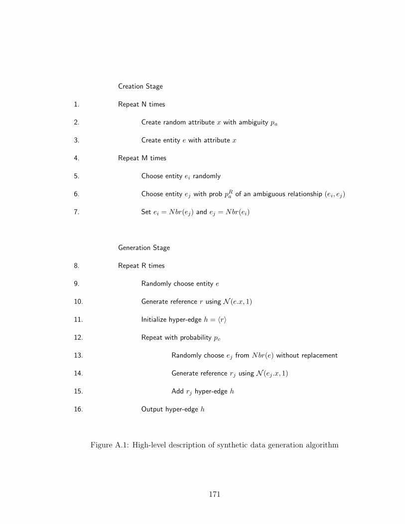
Creation Stage

1. Repeat N times

2. Create random attribute x with ambiguity pa

3. Create entity e with attribute x

4. Repeat M times

5. Choose entity ei randomly

6. Choose entity ej with prob pRa of an ambiguous relationship (ei, ej)

7. Set ei = Nbr(ej) and ej = Nbr(ei)

Generation Stage

8. Repeat R times

9. Randomly choose entity e

10. Generate reference r using N (e.x, 1)

11. Initialize hyper-edge h = 〈r〉

12. Repeat with probability pc

13. Randomly choose ej from Nbr(e) without replacement

14. Generate reference rj using N (ej .x, 1)

15. Add rj hyper-edge h

16. Output hyper-edge h

Figure A.1: High-level description of synthetic data generation algorithm

171

and without losing generality, each entity e has a single floating point attribute

e.x, instead of a character string. A parameter pa controls the ambiguity of the

entity attributes; with probability pa the attribute of a new entity is chosen from

values that are already in use by existing entities. Then M binary relationships are

added between the created entities. As with the attributes, there is a parameter

controlling the ambiguity of the relationships, as defined in Section 4.3. For each

binary relationship (ei, ej), first ei is chosen randomly and then ej is sampled so

that (ei, ej) is an ambiguous relationship with probability pRa .

Before describing the process of generating co-occurrence relationships from

the graph, let us consider in a little more detail the issue of attribute ambiguity.

What finally needs to be controlled is the ambiguity of the reference attributes.

While these depend on the entity attributes, they are not completely determined by

entities. Taking the example of names, two people who have names ‘John Michael

Smyth’ and ‘James Daniel Smith’ can still be ambiguous in terms of their observed

names in the data depending on the generation process of observed names. In other

words, attribute ambiguity of the references depends both on the separation between

entity attributes and the dispersion created by the generation process. I make the

assumption that for an entity e with attribute e.x, its references are generated from a

Gaussian distribution with mean x and variance 1.0. So, with very high probability,

any reference attribute generated from e.x will be in the range [e.x − 3, e.x + 3].

So this range in the attribute domain is considered to be ‘occupied’ by entity e.

Any entity has an ambiguous attribute if its occupied range intersects with that of

another entity.

172

Now I come to the generation of co-occurrence relationships from the entity

collaboration graph. In this stage, R co-occurrence relationships or hyper-edges are

generated, each with its own references. For each hyper-edge 〈ri, ri1, . . . , rik〉, two

aspects need to be controlled — how many references and which references should

be included in this hyper-edge. This is done as follows. First, I sample an entity

ei which serves the initiator entity for this hyper-edge. Then other entities eij for

this hyper-edge are repeatedly sampled (without replacement) from the neighbors

of the initiator entity ei. The size of the hyper-edge is determined using a parameter

pc. The sampling step for a hyper-edge is terminated with probability pc after each

selection eij. The process is also terminated when the neighbors of the initiator

entity are exhausted. Finally, references rij need to be generated from each of the

selected entities eij. This is done for each entity e by sampling from its Gaussian

distribution N (e.x, 1).

As we have seen, the data generation process controls different aspects of

the data that are useful for analyzing the models and algorithms proposed in this

dissertation. The synthetic data generation model is motivated by the domain of

academic collaborations, but is general enough to handle different kinds of relational

data. Essentially, it models any domain that has entities with potentially ambiguous

attributes, relationships between those entities, and hyper-edges of arbitrary arity

that contain noisy references to these entities. So this model can mimic different

kinds of noisy relational data, for example, email data, where names of different

people get mentioned in the same email, and product shopping data with noisy

descriptions of different products that people may buy together. In effect, this data

173

generator enables us to investigate the impact of collective relational approaches

to clustering in domains other than bibliographic data, and also for applications

beyond entity resolution.

174

Bibliography

[1] Lada Adamic and Eytan Adar. Friends and neighbors on the web. SocialNetworks, 25(3):211–230, July 2003.

[2] Eneko Agirre, Jordi Atserias, Lluis Padro, and German Rigau. Combiningsupervised and unsupervised lexical knowledge methods for word sense disam-biguation computers and the humanities. In Computers and the Humanities,Special Double Issue on SensEval. Eds. Martha Palmer and Adam Kilgarriff.34:1,2, 2000.

[3] Rohit Ananthakrishna, Surajit Chaudhuri, and Venkatesh Ganti. Eliminatingfuzzy duplicates in data warehouses. In Proceedings of the 28th InternationalConference on Very Large Databases (VLDB-2002), Hong Kong, China, 2002.

[4] Charles Antoniak. Mixtures of dirichlet processes with applications to bayesiannonparametric problems. The Annals of Statistics, 2:1152–1174, 1974.

[5] Yoshua Bengio and Christopher Kermorvant. Extracting hidden sense proba-bilities from bitexts. Technical report, TR 1231, Departement d’informatiqueet recherche operationnelle, Universite de Montreal, 2003.

[6] Omar Benjelloun, Hector Garcia-Molina, Qi Su, and Jennifer Widom. Swoosh:A generic approach to entity resolution. Technical report, Stanford University,March 2005.

[7] Indrajit Bhattacharya and Lise Getoor. Deduplication and group detectionusing links. In Proceedings of the 10th ACM SIGKDD Workshop on LinkAnalysis and Group Detection (LinkKDD-04), Seattle, WA, USA, 2004.

[8] Indrajit Bhattacharya and Lise Getoor. Iterative record linkage for cleaningand integration. In SIGMOD 2004 Workshop on Research Issues on DataMining and Knowledge Discovery, Paris, France, 2004.

[9] Indrajit Bhattacharya and Lise Getoor. Relational clustering for multi-typeentity resolution. In The 11th ACM SIGKDD Workshop on Multi RelationalData Mining (MRDM-05), Chicago, IL, USA, 2005.

[10] Indrajit Bhattacharya and Lise Getoor. Collective entity resolution in rela-tional data. IEEE Data Engineering Bulletin, Special Issue on Data Cleaning,pages 4–12, June 2006.

[11] Indrajit Bhattacharya and Lise Getoor. Entity Resolution in Graphs, chapterMining Graph Data (L. Holder and D. Cook, eds.). Wiley, 2006.

[12] Indrajit Bhattacharya and Lise Getoor. A latent dirichlet model for unsuper-vised entity resolution. In SIAM Conference on Data Mining (SIAM-SDM),Bethesda, MD, USA, 2006.

175

[13] Indrajit Bhattacharya and Lise Getoor. Query-time entity resolution. In ACMConference on Knowledge Discovery and Data Mining (KDD), Philadelphia,PA, USA, 2006.

[14] Indrajit Bhattacharya, Lise Getoor, and Yoshua Bengio. Unsupervised sensedisambiguation using bilingual probabilistic models. In Proceedings of The42nd Annual Meeting of the Association for Computational Linguistics (ACL),Barcelona, Spain, 2004.

[15] Mikhail Bilenko and Raymond Mooney. Adaptive duplicate detection us-ing learnable string similarity measures. In Proceedings of the Ninth ACMSIGKDD International Conference on Knowledge Discovery and Data Mining(KDD-2003), Washington DC, USA, 2003.

[16] Mikhail Bilenko, Raymond Mooney, William Cohen, Pradeep Ravikumar, andStephen Fienberg. Adaptive name matching in information integration. IEEEIntelligent Systems, 18(5):16–23, 2003.

[17] Mustafa Bilgic, Louis Licamele, Lise Getoor, and Ben Shneiderman. D-dupe:An interactive tool for entity resolution in social networks. In Visual AnalyticsScience and Technology (VAST), Baltimore, 2006.

[18] David Blei, Thomas Griffiths, Michael Jordan, and Josh Tenenbaum. Hier-archical topic models and the nested chinese restaurant process. In AdvancesIn Neural Information Processing Systems (NIPS), Vancouver, BC, Canada,2003.

[19] David Blei and Michael Jordan. Variational methods for the dirichlet process.In International Conference on Machine Learning (ICML), Banff, Alberta,Canada, 2004.

[20] David Blei and John Lafferty. Correlated topic models. In Advances in NeuralInformation Processing Systems, Vancouver, BC, Canada, 2006.

[21] David Blei, Andrew Ng, and Michael Jordan. Latent dirichlet allocation.Journal of Machine Learning Research, 3:951–991, Jan 2003.

[22] Peter Brown, Stephen Della Pietra, Vincent Della Pietra, and Robert Mer-cer. Word-sense disambiguation using statistical methods. In Meeting of theAssociation for Computational Linguistics, pages 264–270, 1991.

[23] Rebecca Bruce and Janyce Wiebe. A new approach to sense identification. InARPA Workshop on Human Language Technology, 1994.

[24] Claire Cardie and Kiri Wagstaff. Noun phrase coreference as clustering. InProceedings of the Joint SIGDAT Conference on Empirical Methods in NaturalLanguage Processing and Very Large Corpora (EMNLP), College Park, MD,USA, 1999.

176

[25] Soumen Chakrabarti, Byron Dom, and Piotr Indyk. Enhanced hypertextcategorization using hyperlinks. In Proceedings of the 1998 ACM SIGMODInternational Conference on Management of Data, 1998.

[26] Amit Chandel, P. C. Nagesh, and Sunita Sarawagi. Efficient batch top-ksearch for dictionary-based entity recognition. In Proceedings of the 22ndInternational Conference on Data Engineering (ICDE’06), Washington, DC,USA, 2006.

[27] Surajit Chaudhuri, Kris Ganjam, Venkatesh Ganti, and Rajeev Motwani. Ro-bust and efficient fuzzy match for online data cleaning. In Proceedings of the2003 ACM SIGMOD International Conference on Management of Data, SanDiego, CA, USA, 2003.

[28] William Cohen. Data integration using similarity joins and a word-based infor-mation representation language. ACM Transactions on Information Systems,18:288–321, 2000.

[29] William Cohen, Henry Kautz, and David McAllester. Hardening soft informa-tion sources. In Proceedings of the Sixth International Conference on Knowl-edge Discovery and Data Mining (KDD-2000), Boston, MA, USA, 2000.

[30] William Cohen, Pradeep Ravikumar, and Stephen Fienberg. A comparison ofstring distance metrics for name-matching tasks. In Proceedings of the IJCAI-2003 Workshop on Information Integration on the Web, Acapulco, Mexico,2003.

[31] William Cohen and Jacob Richman. Learning to match and cluster large high-dimensional data sets for data integration. In Proceedings of the Eighth ACMSIGKDD International Conference on Knowledge Discovery and Data Mining(KDD-2002), Edmonton, Alberta, CA, 2002.

[32] David Cohn and Thomas Hofmann. The missing link: A probabilistic modelof document content and hypertext connectivity. In Advances in Neural In-formation Processing Systems (NIPS), Vancouver, BC, Canada, 2001.

[33] Ido Dagan. Lexical disambiguation: Sources of information and their statisti-cal realization. In Meeting of the Association for Computational Linguistics,Berkeley, CA, USA, 1991.

[34] Ido Dagan and Alon Itai. Word sense disambiguation using a second languagemonolingual corpus. Computational Linguistics, 20(4):563–596, 1994.

[35] Hal Daume and Daniel Marcu. A bayesian model for supervised clustering withthe dirichlet process prior. Journal of Machine Learning Research, 6:1551–1577, Sep 2005.

177

[36] A. Dempster, N. Laird, and D. Rubin. Maximum likelihood from incompletedata via the EM algorithm. Journal of the Royal Statistical Society, B 39:1–38,1977.

[37] Mona Diab. Word Sense Disambiguation Within a Multilingual Framework.PhD thesis, University of Maryland, College Park, 2003.

[38] Mona Diab and Philip Resnik. An unsupervised method for word sense taggingusing parallel corpora. In Proceedings of the 40th Anniversary Meeting of theAssociation for Computational Linguistics (ACL-02), Philadelphia, PA, USA,2002.

[39] Christopher Diehl, Lise Getoor, and Galileo Namata. Name reference resolu-tion in organizational email archives. In SIAM Conference on Data Mining(SDM), Bethesda, MD, USA, 2006.

[40] AnHai Doan, Ying Lu, Yoonkyong Lee, and Jiawei Han. Object matchingfor data integration: A profile-based approach. In Proceedings of the IJCAIWorkshop on Information Integration on the W eb, Acapulco, MX, 2003.

[41] Xin Dong, Alon Halevy, and Jayant Madhavan. Reference reconciliation incomplex information spaces. In ACM SIGMOD International Conference onManagement of Data, Baltimore, MD, USA, 2005.

[42] Denise Draper and Steve Hanks. Localized partial evaluation of belief net-works. In Proceedings of the Annual Conference on Uncertainty in ArtificialIntelligence, Seattle, WA, USA, 1994.

[43] Christiane Fellbaum. WordNet: An Electronic Lexical Database. MIT Press,1998.

[44] I. Fellegi and A. Sunter. A theory for record linkage. Journal of the AmericanStatistical Association, 64:1183–1210, 1969.

[45] Thomas Ferguson. A bayesian analysis of some nonparametric problems. TheAnnals of Statistics, 1:209–230, 1973.

[46] Daniela Florescu, Eric Simon, and Dennis Shasha. An extensible frameworkfor data cleaning. In Proceedings of the 16th International Conference on DataEngine ering, San Diego, CA, USA, 2000.

[47] Ariel Fuxman, Elham Fazli, and Rene Miller. Conquer: Efficient managementof inconsistent databases. In Proceedings of the ACM SIGMOD InternationalConference on Management of Data, Baltimore, MD, USA, 2005.

[48] Lise Getoor, Nir Friedman, Daphne Koller, and Ben Taskar. Learning prob-abilistic models of link structure. Journal of Machine Learning Research,3:679–707, December 2002.

178

[49] C. Lee Giles, Kurt Bollacker, and Steve Lawrence. CiteSeer: An automaticcitation indexing system. In Proceedings of the Third ACM Conference onDigital Libraries, Pittsburgh, PA, USA, 1998.

[50] Luis Gravano, Panagiotis Ipeirotis, Nick Koudas, and Divesh Srivastava. Textjoins for data cleansing and integration in an rdbms. In 19th IEEE Interna-tional Conference on Data Engineering, Bangalore, India, 2003.

[51] Thomas Griffiths and Mark Steyvers. Finding scientific topics. In Proceedingsof the National Academy of Sciences, volume 101, pages 5228–5235, April2004.

[52] Mauricio Hernandez and Salvatore Stolfo. The merge/purge problem for largedatabases. In Proceedings of the 1995 ACM SIGMOD International Confer-ence on Management of Data (SIGMOD-95), San Jose, CA, USA, 1995.

[53] Thomas Hofmann. Probabilistic latent semantic analysis. In Proc. of Uncer-tainty in Artificial Intelligence, UAI’99, Stockholm, Sweden, 1999.

[54] Jeremy Hylton. Identifying and merging related bibliographic records. Mas-ter’s thesis, Department of Electrical Engineering and Computer Science,MIT, 1996.

[55] Nancy Ide. Cross-lingual sense determination: Can it work? In Computersand the Humanities: Special Issue on Senseval, 34:147-152, 2000.

[56] Nancy Ide and Jean Veronis. Word sense disambiguation: The state of theart. Computational Linguistics, 28(1):1–40, 1998.

[57] Sonia Jain and Radford Neal. A split-merge markov chain monte carlo pro-cedure for the dirichlet process mixture model. Technical report, Dept. ofStatistics, University of Toronto, 2000.

[58] Sonia Jain and Radford Neal. Splitting and merging components of a noncon-jugate dirichlet process mixture model. Technical report, Dept. of Statistics,University of Toronto, 2005.

[59] Istvan Jonyer, Lawrence Holder, and Diane Cook. Graph-based hierarchicalconceptual clustering. Journal of Machine Learning Research, 2(1-2):19–43,2001.

[60] Dmitri Kalashnikov, Sharad Mehrotra, and Zhaoqi Chen. Exploiting relation-ships for domain-independent data cleaning. In SIAM International Confer-ence on Data Mining (SIAM SDM), Newport Beach, CA, USA, April 21–232005.

[61] Adam Kilgarrif and Joseph Rosenzweig. Framework and results for englishsenseval. Computers and the Humanities, 34(1):15–48, 2000.

179

[62] Jon Kleinberg. Authoritative sources in n hyperlinked environment. Journalof the ACM, 46(5):604–632, 1999.

[63] Jeremy Kubica, Andrew Moore, Jeff Schneider, and Yiming Yang. Stochasticlink and group detection. In Proceedings of the Eighteenth National Conferenceon Artificial Intelligence (AAAI), Edmonton, Alberta, Canada, 2002.

[64] John Lafferty, Andrew McCallum, and Fernando Pereira. Conditional ran-dom fields: Probabilistic models for segmenting and labeling sequence data.In 18th International Conference on Machine Learning (ICML), Williams Col-lege, MA, USA, 2001.

[65] Steve Lawrence, Kurt Bollacker, and C. Lee Giles. Autonomous citationmatching. In Proceedings of the Third International Conference on Au-tonomous Agents, Seattle, WA, USA, 1999.

[66] Wei Li and Andrew McCallum. Pachinko allocation: Dag-structured mixturemodels of topic correlations. In International Conference on Machine Learning(ICML), Pittsburgh, PA, USA, 2006.

[67] Xin Li, Paul Morie, and Dan Roth. Semantic integration in text: From am-biguous names to identifiable entities. AI Magazine. Special Issue on SemanticIntegration, 2005.

[68] David Liben-Nowell and Jon Kleinberg. The link prediction problem for socialnetworks. In 12th International Conference on Information and KnowledgeManagement (CIKM), New Orleans, LA, USA, 2003.

[69] Dekang Lin. Word sense disambiguation with a similarity smoothed case li-brary. In Computers and the Humanities: Special Issue on Senseval, 34:147-152, 2000.

[70] Kenneth Litkowski. Senseval: The cl research experience. In Computers andthe Humanities, 34(1-2), pp. 153-8, 2000.

[71] Andrew McCallum, Andres Corrada-Emmanuel, and Xuerui Wang. Topicand role discovery in social networks. In International Joint Conference onArtificial Intelligence (IJCAI), Edinburgh, Scotland, 2005.

[72] Andrew McCallum, Kamal Nigam, and Lyle Ungar. Efficient clustering ofhigh-dimensional data sets with application to reference matching. In Pro-ceedings of the Sixth International Conference On Knowledge Discovery andData Mining (KDD-2000), Boston, MA, USA, 2000.

[73] Andrew McCallum and Ben Wellner. Conditional models of identity uncer-tainty with application to noun coreference. In Advances In Neural Informa-tion Processing Systems (NIPS), Vancouver, BC, Canada, 2004.

180

[74] Diana McCarthy, Rob Koeling, Julie Weeds, and John Carroll. Finding pre-dominant senses in untagged text. In Proceedings of the 42nd Annual Meetingof the Association for Computational Linguistics, Barcelona, Spain, 2004.

[75] Rada Mihalcea. The role of non-ambiguous words in natural language disam-biguation. In Proceedings of the Conference on Recent Advances in NaturalLanguage Processing, Borovetz, Bulgaria, 2003.

[76] Brian Milch, Bhaskara Marthi, David Sontag, Stuart Russell, Daniel L. Ong,and Andrey Kolobov. Blog: Probabilistic models with unknown objects. InInternational Joint Conference on Artificial Intelligence (IJCAI), Edinburgh,Scotland, 2005.

[77] Thomas Minka. Expectation propagation for approximate bayesian inference.In Proceedings of the 17th Conference in Uncertainty in Artificial Intelligence,2001.

[78] Alvaro Monge and Charles Elkan. The field matching problem: Algorithmsand applications. In Proceedings of the Second International Conference onKnowledge Discovery and Data Mining (KDD-96), Portland, OR, USA, 1996.

[79] Alvaro Monge and Charles Elkan. An efficient domain-independent algorithmfor detecting approximately duplicate database records. In Proceedings of theSIGMOD 1997 Workshop on Research Issues on Data Mining and KnowledgeDiscovery, Tuscon, AZ, USA, 1997.

[80] Gonzalo Navarro. A guided tour to approximate string matching. ACM Com-puting Surveys, 33(1):31–88, 2001.

[81] Radford Neal. Markov chain sampling methods for dirichlet process mixturemodels. Journal of Computational and Graphical Statistics, 9:249–265, 2000.

[82] Jennifer Neville, Micah Adler, and David Jensen. Clustering relational datausing attribute and link information. In Proceedings of the Text Mining andLink Analysis Workshop, Eighteenth International Joint Conference on Arti-ficial Intelligence (IJCAI), Acapulco, Mexico, 2003.

[83] H. Newcombe, J. Kennedy, S. Axford, and A. James. Automatic linkage ofvital records. Science, 130:954–959, 1959.

[84] BBC News. Google ’aids doctors’ diagnoses’.http://news.bbc.co.uk/2/hi/health/6132856.stm, 10 November 2006.

[85] Lawrence Page, Sergey Brin, Rajeev Motwani, and Terry Winograd. Thepagerank citation ranking: Bringing order to the web. Technical report, Stan-ford Digital Library Technologies Project, 1998.

181

[86] Hanna Pasula, Bhaskara Marthi, Brian Milch, Stuart Russell, and Ilya Sh-pitser. Identity uncertainty and citation matching. In Advances in NeuralInformation Processing Systems, Vancouver, BC, Canada, 2003.

[87] Vijayshankar Raman and Joseph M. Hellerstein. Potter’s wheel: An interac-tive data cleaning system. In Proceedings of the 27th International Conferenceon Very Large Databases (VLDB-2001), Rome, Italy, 2001.

[88] Pradeep Ravikumar and William Cohen. A hierarchical graphical model forrecord linkage. In Proceedings of the Conference on Uncertainty in ArtificialIntelligence (UAI), Banff, Alberta, Canada, July 2004.

[89] Philip Resnik. Using information content to evaluate semantic similarity ina taxonomy. In International Joint Conference on Artificial Intelligence (IJ-CAI), Montreal, Quebec, Canada, 1995.

[90] Philip Resnik. Selectional preference and sense disambiguation. In Proceedingsof ACL Siglex Workshop on Tagging Text with Lexical Semantics, Why, Whatand How?, Washington, DC, USA, 1997.

[91] Philip Resnik and David Yarowsky. Distinguishing systems and distinguish-ing senses: new evaluation methods for word sense disambiguation. NaturalLanguage Engineering, 5(2), 1999.

[92] Eric Ristad and Peter Yianilos. Learning string edit distance. IEEE Transac-tions on Pattern Analysis and Machine Intelligence, 20(5):522–532, 1998.

[93] Michal Rosen-Zvi, Tom Griffiths, Mark Steyvers, and Padhraic Smyth. Theauthor-topic model for authors and documents. In Proceedings of the Confer-ence on Uncertainty in Artificial Intelligence, Banff, Alberta, Canada, 2004.

[94] Sunita Sarawagi and Anuradha Bhamidipaty. Interactive deduplication usingactive learning. In Proceedings of the Eighth ACM SIGKDD InternationalConference on Knowledge Discovery and Data Mining (KDD-2002), Edmon-ton, Alberta, Canada, 2002.

[95] Hinrich Schutze. Automatic word sense discrimination. Computational Lin-guistics, 24(1):97–123, 1998.

[96] Vivek Sehgal, Lise Getoor, and Peter Viechnicki. Entity resolution in geospa-tial data integration. In ACM International Symposium on Advances in Geo-graphic Information Systems, Arlington, VA, USA, 2006.

[97] Jianbo Shi and Jitendra Malik. Normalized cuts and image segmentation.IEEE Transactions on Pattern Analysis and Machine Intelligence, 22(8):888–905, 2000.

182

[98] Parag Singla and Pedro Domingos. Multi-relational record linkage. In Pro-ceedings of 3rd Workshop on Multi-Relational Data Mining at ACM SIGKDD,Seattle, WA, USA, 2004.

[99] Ben Taskar, Abbeel Pieter, and Daphne Koller. Discriminative probabilisticmodels for relational data. In Uncertainty in Artificial Intelligence: Proceed-ings of the Eighteenth Conference (UAI), San Francisco, CA, USA, 2002.

[100] Sheila Tejada, Craig Knoblock, and Steven Minton. Learning object iden-tification rules for information integration. Information Systems Journal,26(8):635–656, 2001.

[101] Ben Wellner, Andrew McCallum, Fuchun Peng, and Michael Hay. An in-tegrated, conditional model of information extraction and coreference withapplication to citation matching. In Conference on Uncertainty in ArtificialIntelligence (UAI), Banff, Alberta, Canada, 2004.

[102] William Winkler. The state of record linkage and current research problems.Technical report, Statistical Research Division, U.S. Census Bureau, Wash-ington, DC, 1999.

[103] William Winkler. Methods for record linkage and Bayesian networks. Tech-nical report, Statistical Research Division, U.S. Census Bureau, Washington,DC, 2002.

[104] David Yarowsky. Word-sense disambiguation using statistical models of Ro-get’s categories trained on large corpora. In Proceedings of the InternationalConference on Computational Linguistics, Nantes, France, 1992.

[105] David Yarowsky. One sense per collocation. In Proceedings os the ARPAHuman Language Technology Workshop, Princeton, NJ, USA, 1993.

[106] David Yarowsky. Unsupervised word sense disambiguation rivaling supervisedmethods. In Meeting of the Association for Computational Linguistics, pages189–196, Cambridge, MA, USA, 1995.

183