Embed Size (px)
Citation preview


ABOUT JPGE
Journal of Petroleum and Gas Engineering (JPGE) is an open access journal that provides rapid publication (monthly) of articles in all areas of the subject such as Petroleum geology, reservoir simulation, enhanced oil recovery, Subsurface analysis, Drilling Technology etc. The Journal welcomes the submission of manuscripts that meet the general criteria of significance and scientific excellence. Papers will be published shortly after acceptance. All articles published in JPGE are peer-reviewed. Journal of Petroleum and Gas Engineering is published monthly (one volume per year) by Academic Journals.
Contact Us
Editorial Office: [email protected]
Help Desk: [email protected]
Website: http://www.academicjournals.org/journal/JPGE
Submit manuscript online http://ms.academicjournals.me/

Editors
Dr. Chuanbo Shen Department of Petroleum Geology, Faulty of Earth Resources, China University of Geosciences Wuhan, Hubei 430074, P. R. China. Dr. Amir Hossein Jalili Research project manager, Gas Science Department, Research Institute of Petroleum Industry (RIPI), Tehran Iran. Dr. Salima Baraka-Lokmane Senior Lecturer in Hydrogeology, University of Brighton, Cockcroft Building, Lewes Road, Brighton BN2 4GJ, UK. Abouzar Mirzaei-Paiaman Production Engineer Department of petroleum engineering, National Iranian South Oil Company (NISOC), Iran. Mobeen Fatemi Department of Chemical and Petroleum Engineering, Sharif University of Technology, Tehran, Iran.
Prof. Yu Bo Beijing Key Laboratory of Urban Oil and Gas Distribution, Technology Department of Oil and Gas Storage and Transportation, China University of Petroleum – Beijing Beijing, P. R. China, 102249.

Editorial Board
Dr. Haijian Shi Kal Krishnan Consulting Services, Inc., Oakland, CA Dr. G Suresh Kumar
Petroleum Engineering Program Department of Ocean Engineering Indian Institute of Technology – Madras Chennai 600 036 INDIA
BIOEDIT (www.bioedit.co.uk)

International Journal of Medicine and Medical Sciences
International Journal of Water Resources and Environmental Engineering
Table of Contents: Volume 5 Number 1 March 2014
ARTICLES
Research Articles Pressure transient analysis of multiple leakages in a natural gas 1 Pipeline Sunday O. Isehunwa, Sunday B. Ipinsokan and Oluwatoyin O. Akinsete A study of the effects of waste lubricating oil on the 9 physical/ chemical properties of soil and the possible Remedies Udonne J. D. and Onwuma H. O
Vol. 5(1), pp. 1-8, March, 2014
DOI 10.5897/JPGE 2013.0176 ISSN 2I41-2677
Copyright © 2014
Author(s) retain the copyright of this article
http://www.academicjournals.org/JPGE
Journal of Petroleum and Gas
Engineering
Full Length Research Paper
Pressure transient analysis of multiple leakages in a natural gas pipeline
Sunday O. Isehunwa*, Sunday B. Ipinsokan and Oluwatoyin O. Akinsete
Department of Petroleum Engineering, University of Ibadan, Ibadan, Nigeria.
Received 16 September, 2013; Accepted 31 December, 2013
Pipelines are principal devices for natural gas transportation which are amenable to operational challenges such as leakages. Several methods for predicting leakages in natural gas pipeline have been developed. Some of these techniques detect leakages after several hours while some are prone to false alarms or inaccurate predictions. This study developed a pressure transient analysis model for predicting gas pipeline leakages in real time. The method of characteristics was employed to solve the resultant non-linear gas flow equations without neglecting the inertia term as in previous studies. The system behaviour was simulated after discretizing the pipe length and the differences between observed and calculated variables were used to predict single and multiple leakages. Results were validated using field data.
Key words: Pipeline leakages, natural gas, pressure transient, analytical method, method of characteristics.
INTRODUCTION Pipeline networks are essential infrastructure in modern transportation of natural gas. Material defects, temperature and pressure changes, bad maintenance, corrosion, sabotage action, and other factors can lead to leaks with consequent economic, environmental, and safety implications. Therefore, leak detection and location methods are keys in the overall integrity management of pipeline systems. The efficiency of a leak detection system can be assessed using parameters such as leak sensitivity, location estimating accuracy, ease of operation, availability, false alarm rate, maintenance requirement and cost.
Pipeline leakages can be defined based on the magnitude of the leak flow and on the way the leak flow develops. Leak prediction or detection methods can be classified into hardware based methods, biological methods and software based methods. Eisler et al. (2012) grouped leak detection methods as internal-type
and external-type leak detection systems. External-type methods are used for routine surveillance of pipelines rather than continuous monitoring (Zhanget al., 2013). The external-type has reduced applicability in deep subsea conditions.
Acoustic monitoring techniques utilize acoustic detectors to predict the wave of noise which will be generated as the gas escapes from the pipeline (Barbagelata, 2011; Brodetsky and Savic, 1993; Klein, 1993). They are simple and accurate, and can predict relatively small leaks. However, a large number of acoustic sensors along the pipeline are required, which will increase the cost. If the leaks are too small to produce acoustic signals at levels substantially higher than the background noise, this technology will be useless (Walker, 2011; Sivathanu, 2003).
Optical monitoring methods can be classified as either passive or active (Reichardt et al., 1999). Active methods
*Corresponding author. E-mail: [email protected].
Author(s) agree that this article remain permanently open access under the terms of the Creative Commons Attribution
License 4.0 International License
2 J. Petroleum Gas Eng. involve the illumination of the area above the pipeline with a radiation source, usually a laser or a broad band source. Then the absorption or scattering caused by gas molecules above the surface is monitored using an array of sensors at specific wavelengths (Iseki et al., 2000; Spaeth and O‟Brien, 2003). In contrast to active methods, passive methods do not require a source. They detect the radiation emitted by the natural gas, or the background radiation serves directly. Optical monitoring techniques can be used for moving vehicles, aircraft, portable systems, or on site, and are able to monitor the pipeline over an extended range. Moreover, they have high spatial resolution and sensitivity under specific conditions. But for most optical methods, the implementation cost is high. High false alarm rate is another disadvantage.
Liquid sensing cables (Alaskan Department of Environmental Conservation [ADEC], 2000) are buried beneath or adjacent to pipelines and are designed to reflect changes in transmitted energy pulses as a result of impedance differentials induced by contact with hydrocarbon liquids. Safe energy pulses are continuously sent by a microprocessor through the cable. Advantages include relatively high accuracy in determining leak location, no modifications to existing pipeline, and easy software configuration and maintenance. Disadvantages include very high installation costs and extensive power and signal wiring requirements.
Sampling methods are mostly used to detect hydrocarbon gas leaks (Sperl, 1991). The sampling can be done by carrying a flame ionization detector along a pipeline or using a sensor tube buried in parallel to the pipeline. Very tiny leaks can be detected using these methods. The response time varies from several hours to days, and the cost of monitoring long pipelines is very high. The method does not function for exposed pipelines, and it is very expensive because the trace chemical needs to be added to the gas continuously.
Flow monitoring methods rely on pressure and/or flow signals at different sections of a pipeline. When the pipeline operates normally, there are some steady relationships among these signals. Changes in these relationships will indicate the occurrence of leaks. Volume balance is the most straightforward flow monitoring method. A leak alarm will be generated when the difference between upstream and downstream flow measurements changes by more than an established tolerance (Ellul, 1989). But because of the inherent flow dynamics and the superimposed noise, only relatively large leaks can be detected. Wang et al. (1993) formulated the pressure gradients by using the autoregressive (AR) model. Using this model, some improvement in the leak prediction capability could be achieved.
The magnetic flux leakage method periodically inspects the pipeline for damages using a „pig‟, which is launched at the inlet and retrieved at the outlet. The pig employs
the magnetic flux leakage (MFL) technique for assessing the condition of the pipe (Afzal and Udpa, 2002). This method is functional only for a seamless gas pipeline, and leaks cannot be detected continuously.
The Particle Filter (PF), proposed by Gordon et al. (1993) uses sequential Monte-Carlo methods to approximate the optimal filtering by representing the probability density function (PDF) with a swarm of particles. The method is able to handle any functional nonlinearity system or noise of any probability distribution hence it has attracted much attention (Bolviken et al., 2001; Doucet et al., 2000; Kitagawa, 1996).
The working principle of mass balance method for leak detection is straightforward. If a leak occurs, the mass balance equation presents a systematic deviation. Although simple and certainly reliable, the primary difficulty in implementing this principle in practice derives from the huge variations experienced by the line pack term. This effect implies a very long detection time. The principle is also very sensitive to arbitrary disturbances and dynamics of pipelines and may lead to false detections (Eisler et al., 2012; Eisler, 2011). Billmann and Isermann (1987) and Shields et al. (2001) have used a nonlinear state observer and a special correlation technique for leak detection. Other authors (Benkherouf and Allidina, 1988; Zhou and Frank, 1995; Zhao and Zhou, 2001) have developed similar techniques to predict and locate leaks, with an improved detection speed. Tiang (1997) used thermal methods.
In simulating transient flow of single-phase natural gas in pipelines, most of the previous investigators neglected the inertia term in the momentum equation. This renders the resulting set of partial differential equations linear. Numerical methods previously used to solve this system of partial differential equations include the method of characteristics (MOC) and a variety of explicit and implicit finite difference schemes (Wylie et al., 1971; Streeter and
Wylie, 1970; Liou, 1989; Wylie and Streeter, 1993; Bergant et al., 2001; Kim, 2005). Neglecting the inertia term in the momentum equation will definitely result in loss of accuracy of the simulation results. In order to compensate for the absence of the inertia term in the momentum equation, Yow introduced the concept of “inertia multiplier” to partially account for the effect of the inertia term in the momentum equation. Wylie et al. (1971) simulated transients in natural gas pipelines in accordance with the concept of “inertia multiplier” which sometimes yield very misleading results. This study used the MOC to linearize the nonlinear hydraulic equations, which was then solved analytically. THEORETICAL FRAMEWORK
It was assumed that temperature is constant because the heat lost to the environment as a result of work done is negligible; this assumption is valid for short pipelines. The flow of gas through the
pipeline was modelled under the following assumptions: 1. The flow is isothermal. 2. Axial molecular and eddy transport is negligible in comparison with the bulk transport. 3. Steady-state friction correlations are valid.
4. The pipe has a constant cross-sectional area over any increment .
The governing unsteady pipe flow equations can be expressed as:
gf
FFx
Pu
t
u
x
uc
t
P
2
2 (1)
By regrouping Equation 1, we have:
gf
FFx
Pu
x
uc
t
u
t
P
2
2 (2)
Or,
gf
FFx
Pu
x
uc
t
uP
2
2 (3)
Equation (3) can be represented as:
0
D
x
F
x
(4)
Isehunwa et al. 3 And
Ommu (5)
Where O
m is the mass flux at the inlet of pipeline which is the
product of the gas density and gas velocity is constant along the pipeline.
The one dimensional (Zhou and Adewumi, 1995) form of the momentum for gas flow in horizontal pipelines with spatially invariant temperature is given by Equation 6:
D
mf
x
P
x
u Og
2
22
(6)
For inclined or vertical natural gas pipeline with spatially invariant temperature distribution along pipeline, Equation 6 can be modified by introducing gravitational factor to give:
2
22 sin
2 c
Pg
D
mf
x
P
x
u Og
(7)
By substituting terms and solving, gas flow in inclined pipelines can be described by Equation 8:
For horizontal pipelines, and there is a discontinuity in the
(8)
second term of L.H.S. of Equation (8). The singularity at can
be removed by applying L‟Hopital‟s Rule:
(9)
Hence, substituting and Equation 9 into Equation 8 gives
for horizontal pipelines:
0ln 22
22
2
2
2
XPP
cm
A
P
P
f
DiO
i
O
g
(10)
Where O
P and i
P are the outlet and inlet pressure respectively as
shown in Figure 1 and X is the length of the pipe and discharge rate
Q. Equation 10 becomes:
0ln 22
222
2
2
2
XPP
cQ
A
P
P
f
DiO
i
O
g
(11)
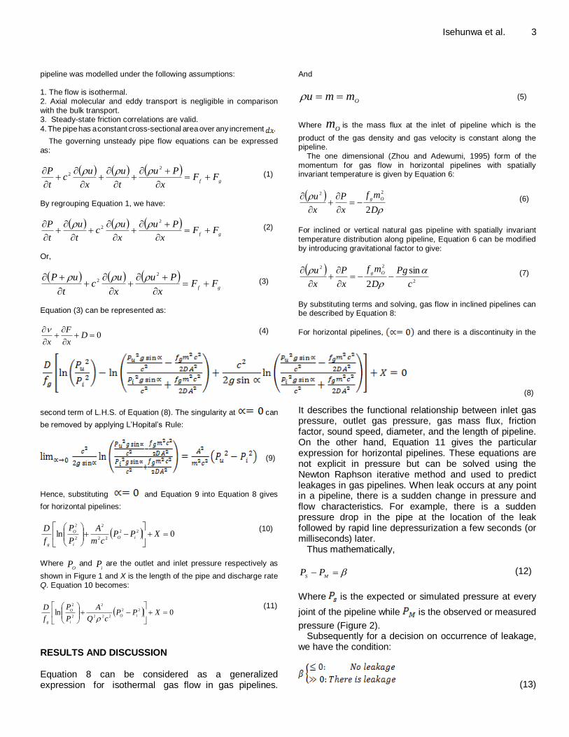
RESULTS AND DISCUSSION Equation 8 can be considered as a generalized expression for isothermal gas flow in gas pipelines.
It describes the functional relationship between inlet gas pressure, outlet gas pressure, gas mass flux, friction factor, sound speed, diameter, and the length of pipeline. On the other hand, Equation 11 gives the particular expression for horizontal pipelines. These equations are not explicit in pressure but can be solved using the Newton Raphson iterative method and used to predict leakages in gas pipelines. When leak occurs at any point in a pipeline, there is a sudden change in pressure and flow characteristics. For example, there is a sudden pressure drop in the pipe at the location of the leak followed by rapid line depressurization a few seconds (or milliseconds) later.
Thus mathematically,
MS
PP (12)
Where is the expected or simulated pressure at every
joint of the pipeline while is the observed or measured
pressure (Figure 2). Subsequently for a decision on occurrence of leakage,
we have the condition:
(13)
4 J. Petroleum Gas Eng.
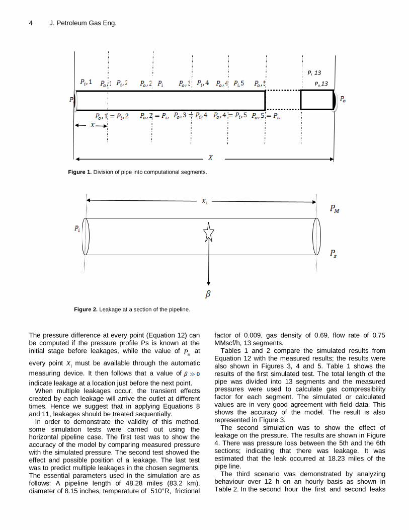
Figure 1: Division of pipe into computational segments
Q
6
3
5
,3
Po,13
Pi, 13
Figure 1. Division of pipe into computational segments.
Figure 2. Leakage at a section of the pipeline.
The pressure difference at every point (Equation 12) can be computed if the pressure profile Ps is known at the initial stage before leakages, while the value of
MP at
every point i
x must be available through the automatic
measuring device. It then follows that a value of
indicate leakage at a location just before the next point. When multiple leakages occur, the transient effects
created by each leakage will arrive the outlet at different times. Hence we suggest that in applying Equations 8 and 11, leakages should be treated sequentially.
In order to demonstrate the validity of this method, some simulation tests were carried out using the horizontal pipeline case. The first test was to show the accuracy of the model by comparing measured pressure with the simulated pressure. The second test showed the effect and possible position of a leakage. The last test was to predict multiple leakages in the chosen segments. The essential parameters used in the simulation are as follows: A pipeline length of 48.28 miles (83.2 km), diameter of 8.15 inches, temperature of 510°R, frictional
factor of 0.009, gas density of 0.69, flow rate of 0.75 MMscf/h, 13 segments.
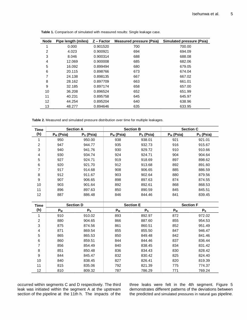
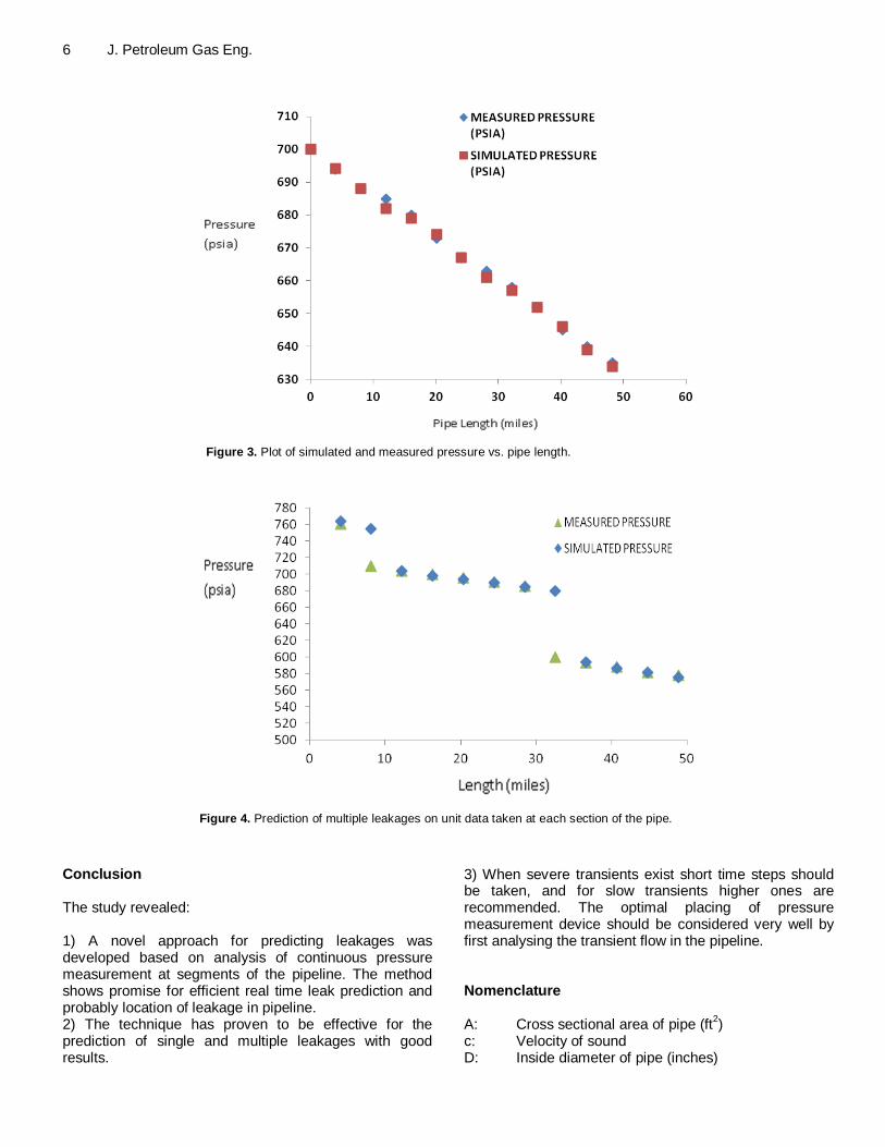
Tables 1 and 2 compare the simulated results from Equation 12 with the measured results; the results were also shown in Figures 3, 4 and 5. Table 1 shows the results of the first simulated test. The total length of the pipe was divided into 13 segments and the measured pressures were used to calculate gas compressibility factor for each segment. The simulated or calculated values are in very good agreement with field data. This shows the accuracy of the model. The result is also represented in Figure 3.
The second simulation was to show the effect of leakage on the pressure. The results are shown in Figure 4. There was pressure loss between the 5th and the 6th sections; indicating that there was leakage. It was estimated that the leak occurred at 18.23 miles of the pipe line.
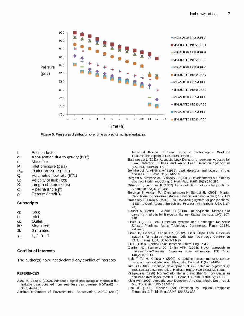
The third scenario was demonstrated by analyzing behaviour over 12 h on an hourly basis as shown in Table 2. In the second hour the first and second leaks
Isehunwa et al. 5
Table 1. Comparison of simulated with measured results: Single leakage case.
Node Pipe length (miles) Z – Factor Measured pressure (Psia) Simulated pressure (Psia)
1 0.000 0.901520 700 700.00
2 4.023 0.900921 694 694.09
3 8.046 0.900314 688 688.08
4 12.069 0.900008 685 682.06
5 16.092 0.899494 680 679.05
6 20.115 0.898766 673 674.04
7 24.138 0.898135 667 667.02
8 28.162 0.897709 663 661.01
9 32.185 0.897174 658 657.00
10 36.208 0.896524 652 651.99
11 40.231 0.895758 645 645.97
12 44.254 0.895204 640 638.96
13 48.277 0.894646 635 633.95
Table 2. Measured and simulated pressure distribution over time for multiple leakages.
Time (h)
Section A Section B Section C
PM (Psia) PS (Psia) PM (Psia) PS (Psia) PM (Psia) PS (Psia)
1 950 950.00 938 938.01 921 921.01
2 947 944.77 935 932.73 916 915.67
3 940 941.76 930 929.72 910 910.66
4 930 934.74 924 924.71 904 904.64
5 927 924.71 919 918.69 897 898.62
6 920 921.70 912 913.68 892 891.60
7 917 914.68 908 906.65 885 886.59
8 912 911.67 903 902.64 880 879.56
9 907 906.65 898 897.63 874 874.55
10 903 901.64 892 892.61 868 868.53
11 896 897.63 850 890.59 845 845.51
12 887 886.48 846 844.46 841 839.45
Time (h)
Section D Section E Section F
PM PS PM PS PM PS
1 910 910.02 893 892.97 872 972.02
2 880 904.65 866 887.60 855 954.53
3 875 874.56 861 860.51 852 951.49
4 871 869.54 855 855.50 847 946.47
5 865 865.53 850 849.48 842 841.46
6 860 859.51 844 844.46 837 836.44
7 856 854.49 840 838.45 834 831.42
8 851 850.48 836 834.43 830 828.42
9 844 845.47 832 830.42 825 824.40
10 840 838.45 827 826.41 820 819.39
11 815 835.06 792 821.39 775 774.37
12 810 809.32 787 786.29 771 769.24
occurred within segments C and D respectively. The third leak was initiated within the segment A at the upstream section of the pipeline at the 11th h. The impacts of the
three leaks were felt in the 4th segment. Figure 5 demonstrates different patterns of the deviations between the predicted and simulated pressures in natural gas pipeline.
6 J. Petroleum Gas Eng.
Figure 3. Plot of simulated and measured pressure vs. pipe length.
Figure 4. Prediction of multiple leakages on unit data taken at each section of the pipe.
Conclusion The study revealed: 1) A novel approach for predicting leakages was developed based on analysis of continuous pressure measurement at segments of the pipeline. The method shows promise for efficient real time leak prediction and probably location of leakage in pipeline. 2) The technique has proven to be effective for the prediction of single and multiple leakages with good results.
3) When severe transients exist short time steps should be taken, and for slow transients higher ones are recommended. The optimal placing of pressure measurement device should be considered very well by first analysing the transient flow in the pipeline. Nomenclature A: Cross sectional area of pipe (ft
2)
c: Velocity of sound D: Inside diameter of pipe (inches)
Isehunwa et al. 7
Time (h) Figure 5. Pressures distribution over time to predict multiple leakages.
f: Friction factor g: Acceleration due to gravity (ft/s
2)
m: Mass flux Pi: Inlet pressure (psia) PO: Outlet pressure (psia) Q: Volumetric flow rate (ft
3/s)
U: Velocity of fluid (ft/s) X: Length of pipe (miles) α: Pipeline angle (°) ρ: Density (ibm/ft
3).
Subscripts g: Gas; i: Inlet; u: Outlet; M: Measured; S: Simulated;
i : 1, 2, 3... 7.
Conflict of Interests The author(s) have not declared any conflict of interests. REFERENCES
Afzal M, Udpa S (2002). Advanced signal processing of magnetic flux
leakage data obtained from seamless gas pipeline. NDTandE Int.
35(7):449-457. Alaskan Department of Environmental Conservation, ADEC (2000).
Technical Review of Leak Detection Technologies, Crude-oil
Transmission Pipelines Research Report 1. Barbagelata L (2011). Accoustic Leak Detector Underwater Acoustic for
Leak Detection. Subsea and Arctic Leak Detection Symposium
(SALDS), Houston, TX. Benkherouf A, Allidina AY (1988). Leak detection and location in gas
pipelines. IEE Proc. 35(2):142-148.
Bergant A, Simpson AR, Vitkvsky JP (2001). Developments of Unsteady pipe flow friction modelling. J. Hydr. Res. IAHR 39(3):249-257.
Billmann L, Isermann R (1987). Leak detection methods for pipelines.
Automatica 23(3):381-385. Bolviken E, Acklam PJ, Christiphersen N, Stordal JM (2001). Monte-
Carlo filters for non-linear state estimation. Automatica 37(2):177-183.
Brodetsky E, Savic M (1993). Leak monitoring system for gas pipelines. IEEE Int. Conf. Acoust. Speech Sig. Process. Minneapolis, USA 3:17-20.
Doucet A, Godsill S, Ardrieu C (2000). On sequential Monte-Carlo sampling methods for Bayesian filtering. Statist. Comput. 10(3):197-208.
Eisler B (2011). Leak Detection systems and Challenges for Arctic Subsea Pipelines. Arctic Technology Conference, Paper 22134, February.
Eisler B, Genesis, Lanan GA (2012). Fiber Optic Leak Detection Systems for subsea Pipelines. Offshore Technology Conference (OTC), Texas, USA, 30 April-3 May.
Ellul I (1989). Pipeline Leak Detection. Chem. Eng. P. 461. Gordon NJ, Salmond DJ, Smith AFM (1993). Novel approach to
nonlinear/non-Gaussian Bayesian state estimation. IEE Proc.
140(2):107-113. Iseki T, Tai H, Kimura K (2000). A portable remote methane sensor
using a tunable diode laser. Meas. Sci. Technol. 11(6):594-602.
Kim SH (2005). Extensive development of leak detection algorithm by impulse response method. J. Hydraul. Eng. ASCE 131(3):201-208
Kitagawa G (1996). Monte-Carlo filter and smoother for non- Gaussian
nonlinear state space models. J. Comput. Graph. Statist. 5(1):1-25. Klein WR (1993). Acoustic Leak Detection. Am. Soc. Mech. Eng. Petrol.
Div. (Publication) PD 55:57-61.
Liou JC (1998). Pipeline Leak Detection by Impulse Response Extraction. J. Fluids Eng. ASME 120:833-838.
8 J. Petroleum Gas Eng. Reichardt TA, Einfield W, Kulp TJ (1999). Review of remote detection for
natural gas transmission pipeline leaks. Shields DN, Ashton SA, Daley S (2001). Design of nonlinear observers
for detecting faults in hydraulic sub-sea pipelines. Contr. Eng. Pract. 9(3):297-311.
Sivathanu Y (2003). Natural Gas Leak Detection in Pipelines.
Technology Status Report, En‟Urga Inc., West Lafayette, IN. Spaeth L, O‟Brien M (2003). An additional tool for integrity monitoring.
Pipeline Gas J. 230(3):41-43.
Sperl JL (1991). System pinpoints leaks on Point Arguello offshore line. Oil Gas J. 89(36):47-52.
Streeter VL, Wylie EB (1970). Natural Gas Pipeline Transients. Sot. Pet.
Eng. J. 75:357-364. Tiang X (1997). Non-isothermal long pipeline leak detection and location.
Atca Scientiarum Naturalium Universitis Pekinensis 33(5):574-580.
Walker I (2011). Leak Detection using Distributed Acoustic Sensing. Subsea and Arctic Leak Detection Symposium (SALDS), Houston, TX.
Wang G, Dong D, Fang C (1993). Leak detection for transport pipelines based on autoregressive modelling. IEEE Trans. Instrum. Meas. 42(1):68-71.
Wylie EB, Streeter VL (1993). Fluid Transients in Systems. Englewood Cliffs: Prentice-Hall.
Wylie EB, Stoner MA, Streeter VL (1971). Network System Transient
Calculation by Implicit Methods. SPEJ 3:356-362.
Zhang J, Hoffman A, Murphy K, Lewis J, Twomey M (2013). Review of
Pipeline Leak Detection Technologies. Pipeline Simulation Interest Group (PSIG). PSIG Annual Meeting, Prague, Czech Republic, Paper
PSIG 1303, 16-19 April. Zhao Q, Zhou DH (2001). Leak detection and location of gas pipelines
based on a strong tracking filter. Trans. Contr. Automat. Syst. Eng.
3(2):89-94. Zhou DH, Frank PM (1996). Strong tracking filtering of nonlinear time-
varying stochastic systems with colored noise with application to
parameter estimation and empirical robustness analysis. Int. J. Contr. 65(2):295-307.
Zhou J, Adewunmi MA (1995). The Development and Testing of a New
Flow Equation. Pipeline Simulation Interest Group 27th Annual Meeting Albuquerque, NM.
Vol. 5(1), pp. 9-14, March, 2014
DOI 10.5897/JPGE 2013.0163 ISSN 2I41-2677
Copyright © 2014
Author(s) retain the copyright of this article
http://www.academicjournals.org/JPGE
Journal of Petroleum and Gas
Engineering
Full Length Research Paper
A study of the effects of waste lubricating oil on the physical/ chemical properties of soil and the possible
remedies
Udonne J. D.* and Onwuma H. O
Department of Chemical and Polymer Engineering, Lagos State University, Lagos, Nigeria.
Received 20 May, 2013; Accepted 13 November, 2013
Waste oil management in Nigeria is not well supervised, hence the indiscriminate disposition into the soil drains and sometimes open water. This has attendant implications on soil and water quality. Need has arisen to evaluate the consequence of such mismanagement on the environment. This study was designed to evaluate the effects of waste oil on the physical and chemical properties of soil in Lagos, and the possible remedies. The soil analysis showed that waste lubricating oil adversely altered the physical and chemical properties of the soil. It resulted in increase in bulk density from 1.10 to 1.15 g/cm
3, organic carbon (2.15 to 3.05), moisture content and reduction in pH (6.5 to 6.0), porosity,
capillarity (8.10 to 0.04 cm/h), water holding capacity, phosphorus and potassium contents. However, application of remediation agents such as water hyacinth, organic waste (ground corn cobs) and Polyurethane foam to the contaminated soil sample reduced the waste oil concentration and this resulted in improvements in the physical and chemical properties of the soil. Key words: Waste oil, pollution, remediation, water hyacinth, reduce wear, environment.
INTRODUCTION Lubricating oils are viscous liquids product of petroleum composed of long-chain saturated hydrocarbons (base oil) and additives that are used for lubricating moving parts of engines and machines. It is usually produced by vacuum distillation of crude oil (Kalichevsky and Peter, 1960). It aids the reduction of frictional forces between contacting metal surfaces of the engines by creating a separating film between the metal surfaces of adjacent moving parts. This minimizes direct contact between them, thereby decreasing the heat caused by friction and reducing wear, thus protecting the engine. There are three major classes of lubricating oils, namely: lubricating greases, automotive oils and industrial lubricating oil. Waste oils are usually generated during servicing of
engines (Anoliefo and Vwioko, 2001; Ogbo et al., 2006). Waste lubricating oil having been contaminated with impurities in the course of usage and handling; contain Toxic and harmful substances such as benzene, lead, cadmium, polycyclic aromatic hydrocarbons (PAHs), zinc, arsenic, polychlorinated biphenyls (PCBs) etc. which are hazardous and detrimental to the soil and the surrounding environment.
Increase in demand for cars, heavy duty automobiles, generators etc. throughout the years, led to increase in demand for lubricating oils, and this eventually resulted in the generation of large volumes of waste oils worldwide. In Nigeria, waste oil irrespective of the type and source of collection, is sometimes dumped on vacant plots, farm
*Corresponding author. E-mail: [email protected]
Author(s) agree that this article remain permanently open access under the terms of the Creative Commons Attribution
License 4.0 International License
10 J. Petroleum Gas Eng. lands etc., causing harmful or toxic materials to percolate through the soil thus contaminating the soil and thereby changing the physical and chemical properties. Used oil is also sometimes dumped down drain, sewers, disrupting the operations at waste water treatment plants (Odegba and Sadiqi, 2002). Research has shown that the increased pollution incidents in the environment are more widespread than pollution with crude oil (Atuanya, 1980). In recognition of the danger of environmental pollution caused by the indiscriminate disposal of waste oils to individuals and nations, management of waste oil then became a critical course of concern to nations of the world.
METHODOLOGY
Sample preparation
Soil sample contaminated with waste oil were collected at depth of
(0 to 5 cm) from two different spots: in an auto-mechanic workshop in Lagos while the uncontaminated soil sample of the same quantity was collected at the same depth of (0-5cm) at about 5 meters away from the contaminated spot.
The two soil samples were put into two medium sized (15 cm3)
plastic containers and labeled „A‟ for the uncontaminated soil sample and „B‟ for the contaminated soil sample. Both samples were sieved and taken to “Lagos State Material Testing Laboratory,
Ojodu-Berger, Lagos for evaluation and analysis of the soil properties in the laboratory. The physical and chemical properties of both soil samples were then analyzed accordingly and various results obtained for the tested parameters.
The physical properties determined were: bulk density, soil capillarity, soil porosity, water holding capacity. The chemical properties determined were: soil pH, phosphorus content, potassium content and moisture content.
Methods of soil analysis
The soil samples were analyzed for both physical and chemical properties using various methods of analysis as discussed below.
The bulk density was determined according to ASTM 29. The soil porosity, soil capillarity and water holding capacity (WHC) were determined according to Akinsanmi (1975); soil pH was tested by means of a glass electrode pH meter by dipping the glass electrode
into 1:1 soil-water suspension; Exchangeable cations, Potassium (K+), was determined by using methods of “Udo and Ogunwale (1986),” whereby the ammonium acetate extract topsoil samples were subjected to flame photometry and atomic absorption spectrometer; available phosphorus was extracted by Bray 1 method (Bray and Kurtz, 1945) and analyzed colometrically; Organic carbon (c) was determined using the adapted (Walkley and Black, 1934) method. Bulk density
The bulk densities of the soil samples were determined according to ASTM C29. Apparatus used were: metal cylindrical container, weighing balance, vernier caliper. Soil capillarity
The soil capillarity was determined using Akinsanmi (1975) method.
Apparatus used were 2 long and wide glass tubes, cotton wool, dry soil samples, clock and ruler.
Procedure: The lower end of each tube was closed with a plug of
cotton wool. One tube was filled with dry uncontaminated soil and
the other with dry contaminated soil sample. The ends of the tubes were tapped gently on the bench to tightly pack the soils in both tubes such that the soil was not more tightly compressed in one tube than the other. The tubes were set in a trough containing water up to a depth of 5 cm. Each tube was supported with a clamp when necessary. After intervals of ten minutes, the rise of water in each tube above the level of water in the trough was then measured. The experiment was left for about 24 h and then examined for the rise of water level in both soil samples. Soil porosity and water holding capacity (WHC)
These were also determined according to Akinsanmi (1975). The various results were as shown in Table 1. Apparatus used were oven, two 100 cm
3 measuring cylinders, two funnels, cotton wool,
dry soil samples and stop clock.
Procedure: Equal volumes of both soil samples were completely
dried in an oven and placed in separate funnels plugged with cotton wool. The funnels were carefully tapped persistently on the bench until all visible air spaces were filled, and each funnel placed in the open end of each 100 cm
3 measuring cylinder. 50 cm
3 of water was
quickly poured into the funnel containing each soil sample. Using the stop clock, the time taken for the first drop of water to drip through into the measuring cylinder was noted in each case. Water was allowed to drain through the soil samples until no water dripped
into the measuring jars any longer. The volume of water which passed through was measured in each case. By subtraction, the volume of water retained was determined in each case. Soil pH
The soil pH was determined with the use of pH indicator (meter). Apparatus used were test tube, pH indicator, weighing balance, spatula, beaker.
Procedure: 5 g of the soil sample was weighed into 5 g of distilled
water in a test tube and vigorously stirred. The pH was obtained using a pH indicator and read after 3 s. It was cross-matched with the color scale. pH of 6.5 was obtained for the soil sample without oil while pH of 6.0 was obtained for the waste or used oil contaminated soil. Phosphorus content
This was determined by the Bray and Kutz method with the use of absorption spectrophotometer. Apparatus used were test tube, beaker, and absorption spectrophotometer. Reagents used were: Bray extractant consisting of 0.025 normal HCl and 0.03 normal NH4F.
Procedure: 1 g scoop of soil and 10 ml of extractant were mixed
together for 5 min. This was further shaken to give a blue color. The intensity of the blue color filtrate developed was treated with ammonium molybdate – hydrochloric acid solution and aminonaphthol – sulfonic acid solution. The color was measured using an absorption spectrophotometer at 640 nm. The result was calculated in ppm as shown in Table 2.
Potassium content
Apparatus used were: test tube, color scale, beaker, and spatula.
Udonne and Onwuma 11
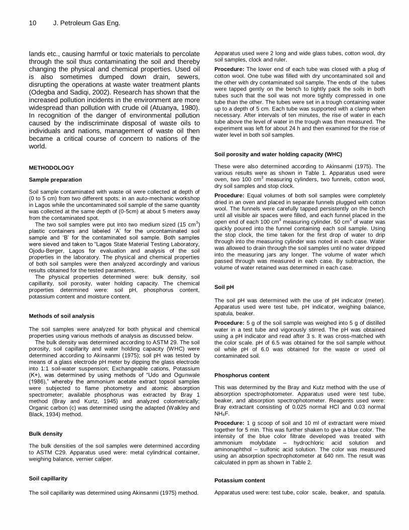
Table 1. Results of soil analysis showing effects of waste lubricating oil on the physical properties of soil.
Parameters Uncontaminated soil sample „A‟ Contaminated soil sample „B‟
Bulk density (g/cm3) 1.10 1.15
Soil capilarity (cm/h) 8.10 0.04
Soil porosity (ml) 110 80
Water holding capacity (WHC) (ml) 55.0 15.0
Table 2. Results of soil analysis showing the effects of waste lubricating oil on the chemical properties of soil.
Parameters Uncontaminated Soil Sample „A‟ Contaminated Soil Sample „B‟
Soil pH 6.5 6.0
Phosphorus content (ppm) 80 40
Potassium content (ppm) 98 60
Organic carbon 2.15 3.05
Moisture content (%) 3.5 9.9
Procedure: A test tube was placed into cavity of the thermoformed lining and filled with 0.7% nitric acid. Potassium test sticks were removed as required and then the container was resealed immediately. A test stick was dipped into the solution to be tested so that the reaction zone was completely moist. Excess liquid was shaken off. A test stick was placed into the test tube which was filled with 0.7% nitric acid and then left for one minute. The test tube
was removed and compared with the color scale. In the presence of potassium, the test paper turned yellow to orange red. Moisture content Apparatus used were: sampling can with lid, weighing balance, oven, and spatula. Procedure: The sampling cans were weighed with weighing
balance based on different samples to be tested. Each sampling can was filled with the soil sample and weighed. They were dried in oven for six (6) hours and weighed. Results obtained were as
recorded in Table 2. RESULTS AND DISCUSSION Results of the soil analysis on both soil samples indicate that the presence of waste lubricating oil in the soil altered the soil chemistry, and thus led to adverse effects on the physical and chemical properties of the soil.
The presence of waste or used lubricating oil in the soil altered the physical properties as explained below and shown in Table 1. The bulk density slightly increased with the presence of waste oil. While the bulk density in the control or uncontaminated soil sample was 1.10 g/cm
2,
that of waste oil contaminated soil was 1.15 g/cm3.
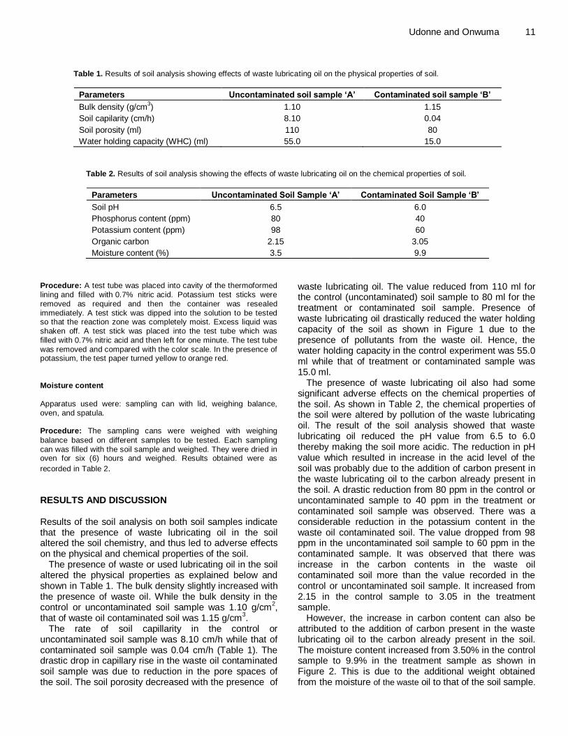
The rate of soil capillarity in the control or uncontaminated soil sample was 8.10 cm/h while that of contaminated soil sample was 0.04 cm/h (Table 1). The drastic drop in capillary rise in the waste oil contaminated soil sample was due to reduction in the pore spaces of the soil. The soil porosity decreased with the presence of
waste lubricating oil. The value reduced from 110 ml for the control (uncontaminated) soil sample to 80 ml for the treatment or contaminated soil sample. Presence of waste lubricating oil drastically reduced the water holding capacity of the soil as shown in Figure 1 due to the presence of pollutants from the waste oil. Hence, the water holding capacity in the control experiment was 55.0 ml while that of treatment or contaminated sample was 15.0 ml.
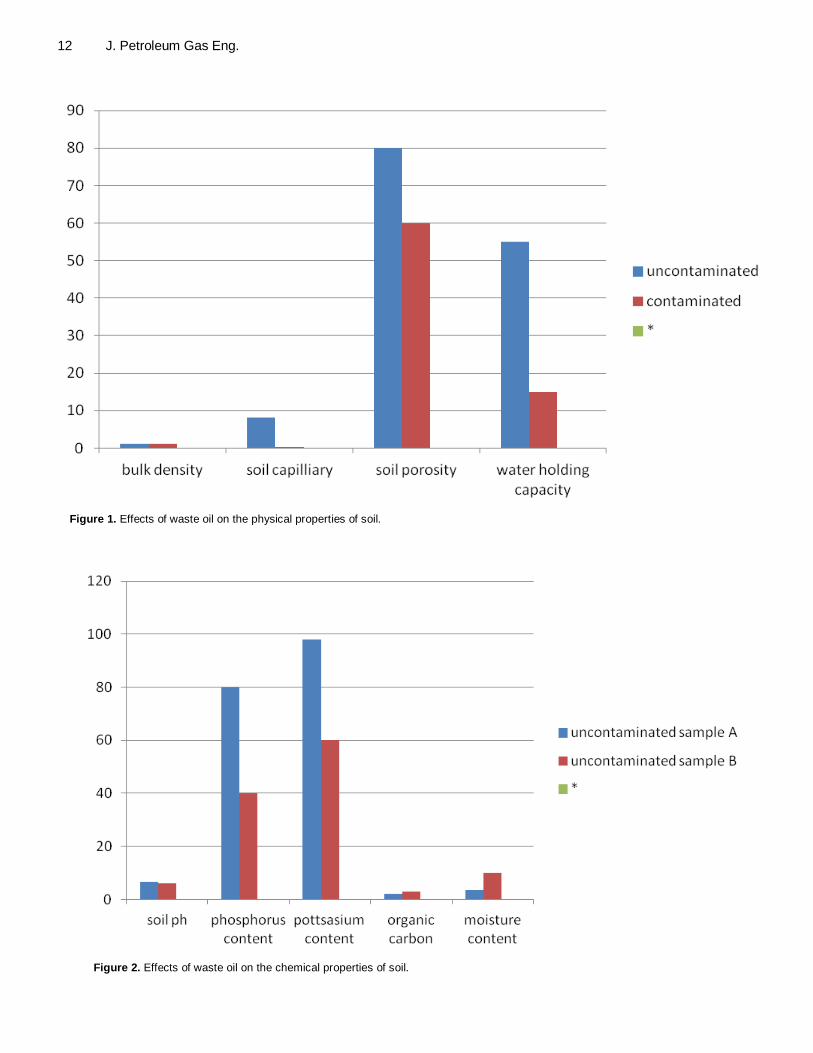
The presence of waste lubricating oil also had some significant adverse effects on the chemical properties of the soil. As shown in Table 2, the chemical properties of the soil were altered by pollution of the waste lubricating oil. The result of the soil analysis showed that waste lubricating oil reduced the pH value from 6.5 to 6.0 thereby making the soil more acidic. The reduction in pH value which resulted in increase in the acid level of the soil was probably due to the addition of carbon present in the waste lubricating oil to the carbon already present in the soil. A drastic reduction from 80 ppm in the control or uncontaminated sample to 40 ppm in the treatment or contaminated soil sample was observed. There was a considerable reduction in the potassium content in the waste oil contaminated soil. The value dropped from 98 ppm in the uncontaminated soil sample to 60 ppm in the contaminated sample. It was observed that there was increase in the carbon contents in the waste oil contaminated soil more than the value recorded in the control or uncontaminated soil sample. It increased from 2.15 in the control sample to 3.05 in the treatment sample.
However, the increase in carbon content can also be attributed to the addition of carbon present in the waste lubricating oil to the carbon already present in the soil. The moisture content increased from 3.50% in the control sample to 9.9% in the treatment sample as shown in Figure 2. This is due to the additional weight obtained from the moisture of the waste oil to that of the soil sample.
12 J. Petroleum Gas Eng.
Figure 1. Effects of waste oil on the physical properties of soil.
Figure 2. Effects of waste oil on the chemical properties of soil.
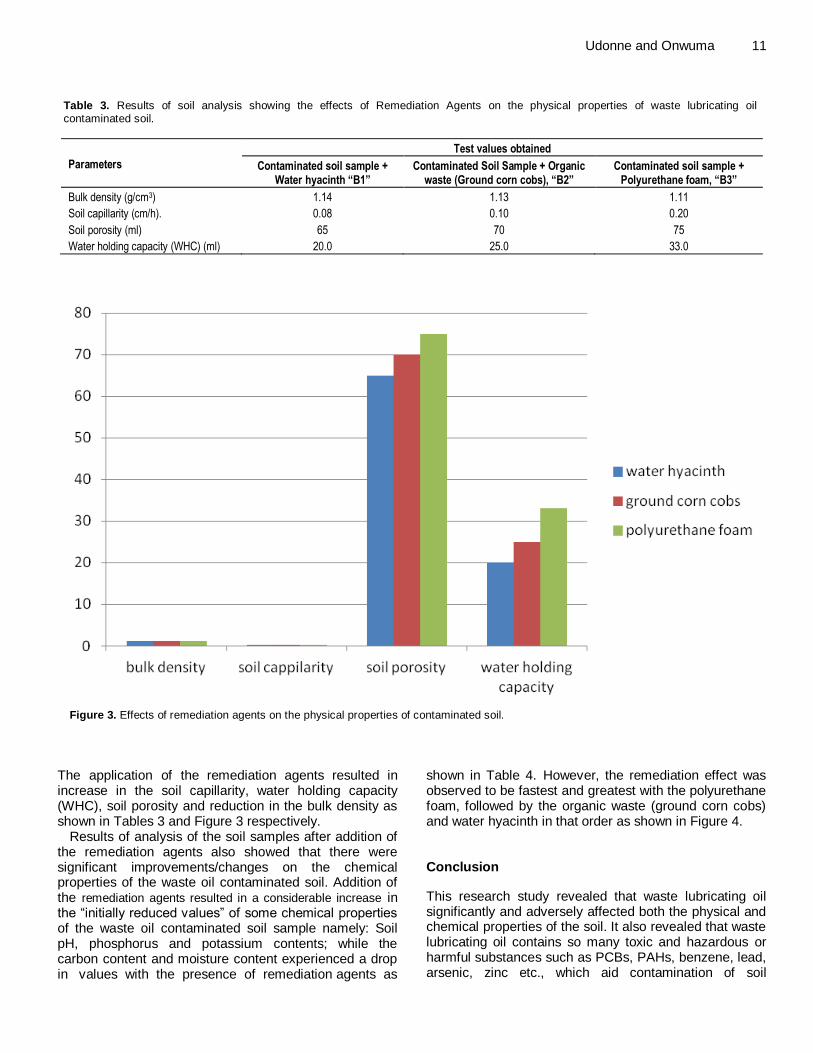
Udonne and Onwuma 11 Table 3. Results of soil analysis showing the effects of Remediation Agents on the physical properties of waste lubricating oil contaminated soil.
Parameters
Test values obtained
Contaminated soil sample + Water hyacinth “B1”
Contaminated Soil Sample + Organic waste (Ground corn cobs), “B2”
Contaminated soil sample + Polyurethane foam, “B3”
Bulk density (g/cm3) 1.14 1.13 1.11
Soil capillarity (cm/h). 0.08 0.10 0.20
Soil porosity (ml) 65 70 75
Water holding capacity (WHC) (ml) 20.0 25.0 33.0
Figure 3. Effects of remediation agents on the physical properties of contaminated soil.
The application of the remediation agents resulted in increase in the soil capillarity, water holding capacity (WHC), soil porosity and reduction in the bulk density as shown in Tables 3 and Figure 3 respectively.
Results of analysis of the soil samples after addition of the remediation agents also showed that there were significant improvements/changes on the chemical properties of the waste oil contaminated soil. Addition of the remediation agents resulted in a considerable increase in the “initially reduced values” of some chemical properties of the waste oil contaminated soil sample namely: Soil pH, phosphorus and potassium contents; while the carbon content and moisture content experienced a drop in values with the presence of remediation agents as
shown in Table 4. However, the remediation effect was observed to be fastest and greatest with the polyurethane foam, followed by the organic waste (ground corn cobs) and water hyacinth in that order as shown in Figure 4. Conclusion
This research study revealed that waste lubricating oil significantly and adversely affected both the physical and chemical properties of the soil. It also revealed that waste lubricating oil contains so many toxic and hazardous or harmful substances such as PCBs, PAHs, benzene, lead, arsenic, zinc etc., which aid contamination of soil
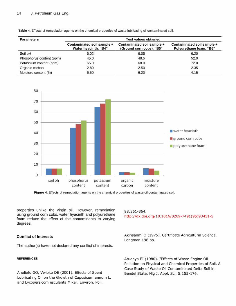
14 J. Petroleum Gas Eng. Table 4. Effects of remediation agents on the chemical properties of waste lubricating oil contaminated soil.
Parameters Test values obtained
Contaminated soil sample + Water hyacinth, “B4”
Contaminated soil sample + (Ground corn cobs), “B5”
Contaminated soil sample + Polyurethane foam, “B6”
Soil pH 6.02 6.05 6.20
Phosphorus content (ppm) 45.0 48.5 52.0
Potassium content (ppm) 65.0 68.0 72.0
Organic carbon 2.80 2.50 2.35
Moisture content (%) 6.50 6.20 4.15
Figure 4. Effects of remediation agents on the chemical properties of waste oil contaminated soil.
properties unlike the virgin oil. However, remediation using ground corn cobs, water hyacinth and polyurethane foam reduce the effect of the contaminants to varying degrees. Conflict of Interests The author(s) have not declared any conflict of interests. REFERENCES
Anoliefo GO, Vwioko DE (2001). Effects of Spent
Lubricating Oil on the Growth of Caposicum annum L.
and Lycopersicom esculenta Miker. Environ. Poll.
88:361-364.
http://dx.doi.org/10.1016/0269-7491(95)93451-5
Akinsanmi O (1975). Certificate Agricultural Science.
Longman 196 pp.
Atuanya EI (1980). "Effects of Waste Engine Oil
Pollution on Physical and Chemical Properties of Soil. A
Case Study of Waste Oil Contaminated Delta Soil in
Bendel State. Nig J. Appl. Sci. 5:155-176.

Atuanya EI (1980). Effects of Waste Engine Oil
Pollution on Physical and Chemical Properties of Soil.
Nig. J. Appl. Sci. 5:55-176.
Odjegba VI, Sadiqi AO (2002). Effects of Spent Engine
oil on the Growth Parameters, Chlorophyll and Protein
Levels of Amaranthus hybridus L. The
Environmentalist 22:23-28.
http://dx.doi.org/10.1023/A:1014515924037
Udom BE, Mbagwu JSC, Willie ES (2008). A journal on
"Physical Properties and Maize production in a Spent
oil Contaminated Soil Bioremediated with Legumes
and Organic Nutrients 7(1):33-40.