YITP-14-49

ABJ Wilson loops and Seiberg Duality

Shinji Hiranoa, Keita Niib and Masaki Shigemoric,d

aSchool of Physics and Center for Theoretical Physics

University of the Witwatersrand

WITS 2050, Johannesburg, South Africa

bDepartment of Physics

Nagoya University, Nagoya 464-8602, Japan

cYukawa Institute for Theoretical Physics

Kyoto University, Kyoto 606-8502, Japan

dHakubi Center, Kyoto University, Kyoto 606-8501, Japan

Abstract

We study supersymmetric Wilson loops in the N = 6 supersymmetric U(N1)k ×U(N2)−k Chern-Simons-matter (CSM) theory, the ABJ theory, at finite N1, N2 and k.

This generalizes our previous study on the ABJ partition function. First computing

the Wilson loops in the U(N1) × U(N2) lens space matrix model exactly, we perform

an analytic continuation, N2 to −N2, to obtain the Wilson loops in the ABJ theory

that is given in terms of a formal series and only valid in perturbation theory. Via

a Sommerfeld-Watson type transform, we provide a nonperturbative completion that

renders the formal series well-defined at all couplings. This is given by min(N1, N2)-

dimensional integrals that generalize the “mirror description” of the partition function

of the ABJM theory. Using our results, we find the maps between the Wilson loops in

the original and Seiberg dual theories and prove the duality. In our approach we can

explicitly see how the perturbative and nonperturbative contributions to the Wilson

loops are exchanged under the duality. The duality maps are further supported by

a heuristic yet very useful argument based on the brane configuration as well as an

alternative derivation based on that of Kapustin and Willett.

arX

iv:1

406.

4141

v2 [

hep-

th]

17

Sep

2014

1 Introduction

Duality is one of the most fascinating phenomena in quantum field theory. It provides

an alternative, often non-perturbative, understanding of the theory that is not accessible

in the original description. Seiberg duality [1], under which weakly coupled gauge theory

is mapped into strongly coupled one with different rank, and vice versa, is a prominent

example. Although the mapping of local operators under Seiberg duality is known to be

rather simple [1], the transformation properties of non-local operators, such as Wilson loops,

are more non-trivial and less studied.

By its strong-weak nature, any checks of Seiberg duality must involve a non-perturbative

approach. The localization method [2–4] is a powerful technique applicable to supersymmet-

ric field theory and reduces the infinite dimensional path integral of quantum field theory to

a finite integral which can be often regarded as a matrix model integral. This method allows

for exact computation of quantities such as partition function and Wilson loops at strong

coupling, and is an ideal tool for studying non-perturbative physics such as Seiberg duality.

Among various supersymmetric gauge theories calculable by the localization method, we

focus on the three-dimensional N = 6 supersymmetric U(N1)k × U(N2)−k Chern-Simons-

matter (CSM) theory, known as the ABJ theory [5], where k ∈ Z6=0 is the Chern-Simons level.

In the special case with N1 = N2, this theory is called the ABJM theory [6]. It is believed that

the U(N)k × U(N +M)−k ABJ theory gives the low-energy description of the system of N

M2-branes and M fractional M2-branes probing C4/Zk, and its holographic dual geometry is

AdS4×S7/Zk in M-theory or AdS4×CP3 in type IIA superstring [5,6]. It is also conjectured

that this theory has another dual description in terms of the N = 6 supersymmetric, parity-

violating version of the Vasiliev higher spin theory in four dimensions [7].

Applying the localization method to the ABJ(M) theory on S3 yields [8] the so-called

ABJ(M) matrix model, which has been extensively studied recently and led to much insight

into the non-perturbative effects in the theory. For instance, applying the standard large N

technique to the ABJ matrix model reproduced the N3/2 scaling of the free energy expected

from the gravity dual [4, 9, 10]. For the ABJM theory, the 1/N corrections were summed

to all orders using holomorphic anomaly equation at large ’t Hooft coupling λ = N/k in

the type IIA regime k � 1 and an Airy function behavior was found [11]. Furthermore,

the powerful Fermi gas approach was developed and reproduced the Airy function in the M-

theory regime (large N , finite k) [12]. Based on the Fermi gas approach, instanton corrections

were examined [13,14] and a cancellation mechanism between worldsheet and membrane (D2)

instantons was discovered. More recently, the Fermi gas approach was generalized to the

ABJ theory in [15] and further studied in [16]. In a different line of development, in [17],

the ABJ matrix model was rewritten in a form generalizing the “mirror description” for

the ABJM theory [18, 19]. This was achieved by starting with the U(N1) × U(N2) lens

space matrix model [20, 21] which is exactly computable and analytically continuing it by

sending N2 → −N2 to reach the ABJ matrix model. As a result, partition function was

written as a min(N1, N2)-dimensional contour integral and the residue it picks up can be

2

given an interpretation of perturbative or non-perturbative contribution, according to its k

dependence. Later, this mirror expression was reproduced in a more direct way in [22]. This

formulation is particularly suitable for studying the duality with the higher spin theory [7,23].

It was conjectured in [5] that the ABJ theory has Seiberg duality, which states that the

following two theories are equivalent:

U(N1)k × U(N2)−k = U(2N1 −N2 + k)k × U(N1)−k , (1.1)

where we assumed N1 ≤ N2. This duality can be understood in the brane realization of

the ABJ theory [5] as moving 5-branes past each other and creating/annihilating D3-branes

between them by the Hanany-Witten effect [24]. It is a special case of the Giveon-Kutasov

duality [25] for more general N = 2 CS-matter theories,1 which can be regarded as the three-

dimensional analog of the four-dimensional Seiberg duality [39]. The equality of the partition

function (up to a phase) between the dual theories in (1.1) was proven in [40], although one

mathematical relation was assumed. On the other hand, in the “mirror” framework of [17],

the equality of the dual partition function is more or less obvious [17, 22] and, moreover, it

was observed that the perturbative and non-perturbative contributions get exchanged into

each other under the duality.

Wilson loops are the only observables in pure CS theory [41] and, even in CS-matter

theory, they are very natural objects to consider. It is known that there are two basic

circular supersymmetric Wilson loops for the ABJ(M) theory on S3; the Wilson loop carrying

a non-trivial representation with respect to one of the two gauge groups preserves 16

of

supersymmetry [42–44] while an appropriate combination of 16-BPS Wilson loops for two

gauge groups preserves 12

of supersymmetry [45]. The bulk dual of the 12-BPS Wilson loop

is a fundamental string while the bulk dual of the 16-BPS Wilson loop is not completely

understood [42–44].2 By the localization method, these Wilson loops can be computed

using the ABJ(M) matrix model [8], and the techniques developed for partition function

to study non-perturbative effects can be generalized to Wilson loops, such as the large N

analysis [9,46,47], the Fermi gas approach [48], and the cancellation between worldsheet and

membrane instantons [49,50].

In this paper we study the 16

and 12-BPS Wilson loops and their Seiberg duality in the ABJ

theory, based on the approach developed in [17] for partition function. We mainly focus on

the representations with winding number n. Starting with Wilson loops in lens space matrix

model and analytically continuing it, we obtain a new expression for the supersymmetric

Wilson loops in the ABJ theory in terms of min(N1, N2)-dimensional contour integrals. As

an application and as a way to check the consistency of our formula, we study Seiberg

duality on the ABJ Wilson loops. The duality rule for Wilson loops is highly non-trivial

because they are non-local operators and not charged under the global symmetry. How to

find Given-Kutasov duality relations for Wilson loops in general N = 2 CS-matter theories,

1An incomplete list of related papers is [10,26–38].2See section 5 for more discussion.

3

of which the ABJ theory is a special case, was proposed in [51] based on quantum algebraic

relations. We derive the duality rule of the supersymmetric Wilson loops using our integral

expression and confirm that it is consistent with the proposal of [51]. We also discuss how

the perturbative and non-perturbative effects are mapped under Seiberg duality. Moreover,

we provide a heuristic explanation of the duality rule from the brane realization of the ABJ

theory. In an appropriate duality frame, the Wilson loop is interpreted as the position of

the branes and, carefully following how the Hanany-Witten effect acts on it, we reproduce

the correct duality rule.

This paper is organized as follows. In section 2, we present the main results of the

paper without proof: the integral expression for the 16-BPS and 1

2-BPS Wilson loops and the

their transformation rules under Seiberg duality. In section 3, we explain how to derive the

integral expression for the ABJ Wilson loops by analytically continuing the lens space ones.

In section 4, we first give a heuristic, brane picture for the Seiberg duality rule, and then

present a rigorous proof using the integral expression. Section 5 is devoted to a summary

and discussion. Appendices contain further detail of computations in the main text, as well

as a discussion of Wilson loops with general representation in Appendix C and an alternative

derivation of the Seiberg duality rule using the algebraic approach of [51] in Appendix F.

2 Main results

The Wilson loops we are concerned with are those preserving fractions of supersymmetries

in the N = 6 U(N1)k×U(N2)−k CSM theory, also known as the ABJ(M) theory, saturating

the Bogomol’nyi-Prasad-Sommerfield (BPS) bound. More specifically, we consider two types

of circular BPS Wilson loops on S3, one preserving a 16-th and the other preserving a half of

supersymmetries [42–45]. In the main text of this paper, we restrict ourselves to the Wilson

loops with winding number n, where n = 1 (or n = −1) corresponds to the fundamental

(or anti-fundamental) representation of U(N1) and/or U(N2) gauge groups, and the Wilson

loops in more general representations will be discussed in Appendix C.

The ABJ(M) theory consists of two 3d N = 2 vector multiplets (AAµ , σA, λA, λA, DA)

with A = 1, 2 which are the dimensional reduction of 4d N = 1 vector multiplets and four

bifundamental chiral multiplets, an SU(4)R vector, (CI , ψI , FI) with I = 1, · · · , 4 in the

representation (N1, N2) and their conjugates. The 16-BPS Wilson loops of our interest are

constructed as [42–44,52]

W I16(N1, N2;R)k :=

⟨TrRP exp

∫ (iA1

µxµ +

2π

k|x|M I

JCICJ

)ds

⟩, (2.1)

where the path of the loop specified by the vector xµ(s) is a circle, and the matrix M IJ is de-

termined by the supersymmetries preserved and one can choose it to beM = diag(−1,−1, 1, 1).

These are the Wilson loops on the first gauge group U(N1), but the W II16

(N1, N2;R)k, those

on the second gauge group U(N2), can be constructed similarly by replacing N1 → N2,

4

A1µ → A2

µ and CI → CI (CJ → CJ). The 12-BPS Wilson loop is constructed in [45] and can

be conveniently expressed in terms of the supergroup U(N1|N2) as

W 12(N1, N2;R)k :=

⟨TrRP exp

(i

∫Ads

)⟩, (2.2)

where R is a super-representation of U(N1|N2) and A is the super-connection

A =

A1µx

µ − i2πk|x|N I

JCICJ

√2πk|x|ψI ηI√

2πk|x|ηIψI A2

µxµ − i2π

k|x|N I

JCICJ

(2.3)

with the matrix N IJ = diag(−1, 1, 1, 1), the (super-)circular path (x1, x2) = (cos s, sin s),

and ηI = (eis/2,−ie−is/2)δ1I .As mentioned, we are concerned with Wilson loops with winding number n rather than in

generic representations in this paper. Focusing on this class of Wilson loops, the application

of the localization technique [3] for the 16-BPS Wilson loops with winding n reduces to the

finite dimensional integrals of the matrix model type [8]

W I16(N1, N2;n)k =

⟨N1∑j=1

enµj

⟩(2.4)

where the vev is with respect to the eigenvalue integrals

〈O〉 := NABJ

∫ N1∏i=1

dµi2π

N2∏a=1

dνa2π

∆sh(µ)2∆sh(ν)2

∆ch(µ, ν)2O e− 1

2gs(∑N1i=1 µ

2i−

∑N2a=1 ν

2a) (2.5)

with the shorthand notations for the one-loop determinant factors defined by

∆sh(µ) =∏

1≤i<j≤N1

(2 sinh

(µi − µj

2

)), ∆sh(ν) =

∏1≤a<b≤N2

(2 sinh

(νa − νb

2

))(2.6)

and

∆ch(µ, ν) =

N1∏i=1

N2∏a=1

(2 cosh

(µi − νa

2

)). (2.7)

The coupling constant3 gs is related to the CS level k by

gs :=2πi

k, (2.8)

while the factor NABJ in front is the normalization factor [4]

NABJ :=i−

κ2(N2

1−N22 )

N1!N2!, κ := sign k . (2.9)

3Note that this is not the physical string coupling constant. The physical string coupling constant of the

dual type IIA string theory in AdS4 × CP3 is (gs)physical ∼ N1/4k−5/4.

5

Meanwhile, the 12-BPS Wilson loop localizes to the supertrace [45]

W 12(N1, N2;R)k =

⟨strR

(eµi 0

0 −eνa)⟩

(2.10)

that yields, for the n winding Wilson loop, a linear combination of 16-BPS Wilson loops [48]

W 12(N1, N2;n)k =W I

16(N1, N2;n)k − (−1)nW II

16

(N1, N2;n)k . (2.11)

Note that the integral (2.5) is a well-defined Fresnel integral even for non-integral (but real)

k and thus gives a continuous function k, although in the physical ABJ theory the CS level

k is quantized to an integer.

We now present the results of our analysis of these matrix eigenvalue integrals.

2.1 The Wilson loops in ABJ theory

The 16-BPS Wilson loops are only on the first U(N1) or the second U(N2) gauge group.

Depending on whether N1 ≤ N2 or N1 ≥ N2, their formula takes rather different forms.

• The 16-BPS U(N1) Wilson loop with N1 ≤ N2 : In the case of N1 ≤ N2, introducing

the normalized Wilson loop W I16

(N1, N2;n)k,4 we find the 1

6-BPS Wilson loop with winding

number n on the first gauge group U(N1) to be

W I16(N1, N2;n)k :=

W I16

(N1, N2;n)k

W I16

(N1, N2; 0)k= q−

n2

2+n I(N1, N2;n)kI(N1, N2; 0)k

, (2.12)

where

q := e−gs = e−2πik (2.13)

and

I(N1, N2;n)k :=1

N1!

N1∑l=1

N1∏i=1

[−1

2πi

∫C

πdsisin(πsi)

]q−nsl+n(l−2)

N1∏i=1i 6=l

(qsi−sl−n)1(qsi−sl)1

(2.14)

×N1∏i=1

[(−1)M (qsi+1)M

(1 + qnδil) (−qsi+1+nδil)M

i−1∏j=1

(qsi−sj)1(−qsi−sj+nδil)1

N1∏j=i+1

(qsj−si)1(−qsj−si−nδil)1

]

with M := |N2 −N1| = N2 −N1 and the symbol (a)z := (a; q)z is a shorthand notation for

the q-Pochhammer symbol defined in Appendix A. The choice of the integration contour C

will be discussed in detail in Section 3.3. We note that the integral expression I(N1, N2; 0)kwithout winding agrees with that of the partition function in [17].5

4The normalization is essentially by the partition function.5The precise relation to the quantity Ψ defined in [17] is I(N1, N2; 0)k = N1Ψ(N1, N2)k.

6

• The 16-BPS U(N1) Wilson loop with N1 ≥ N2 : In the case of N1 ≥ N2 the formula

turns out to be slightly more involved and takes the form

W I16(N1, N2;n)k :=

W I16

(N1, N2;n)k

W I16

(N2, N1; 0)k= q−

n2

2+n I

(1)(N1, N2;n)k + I(2)(N1, N2;n)kI(2)(N1, N2; 0)k

(2.15)

that is only valid for |n| ≥ 1 as will be elaborated in the comments below6 and we defined

I(1)(N1, N2;n)k : =1

N2!

n−1∑c=0

N2∏a=1

[−1

2πi

∫C1[c]

πdsasin(πsa)

]qn(2c−M)

(q1−n)c (q1+n)M−1−c(q)c(q)M−1−c

N2∏a=1

(qsa+1)M2 (−qsa+1)M

×N2∏a=1

[(−qsa+1+c)1 (qsa+1+c−n)1(qsa+1+c)1 (−qsa+1+c−n)1

a−1∏b=1

(qsa−sb)1(−qsa−sb)1

N2∏b=a+1

(qsb−sa)1(−qsb−sa)1

], (2.16)

and

I(2)(N1, N2;n)k :=1

N2!

N2∑d=1

N2∏a=1

[−1

2πi

∫C2

πdsasin(πsa)

]q−nsd+n(d−M−2)

N2∏a=1a6=d

(qsa−sd−n)1(qsa−sd)1

(2.17)

×N2∏a=1

[ (qsa+1+nδad

)M

(1 + qnδad) (−qsa+1)M

a−1∏b=1

(qsa−sb)1(−qsa−sb+nδad)1

N2∏b=a+1

(qsb−sa)1(−qsb−sa−nδad)1

]

with M := |N2 − N1| = N1 − N2. Note that I(2)(N1, N2; 0)k = I(N2, N1; 0)k and the

normalization in (2.15) differs from that in (2.12) in that the ranks of the gauge groups N1

and N2 are exchanged. The choice of the integration contours C1 = {C1[c]} (c = 0, · · · , n−1)

and C2 will be discussed in detail in Section 3.3. We would, however, like to make a remark

concerning the contour C1[c]: There are subtleties in evaluating the integrals with the contour

C1[c]. In order to properly deal with them, we shall adopt the ε-prescription shifting the

parameter M → M + ε with ε > 0 and the contour is placed between sa = −1 − c and

−1− c− ε. Related comments will be made in Section 3.4 below (3.37) and Appendix D.

• The 16-BPS U(N2) Wilson loops : It follows from the definition and symmetry that

the 16-BPS Wilson loop on the second gauge group U(N2) with winding number n is related

to that on the first gauge group U(N1) in a simple manner:

W II16

(N1, N2;n)k = W I16(N2, N1;n)−k . (2.18)

• The 12-BPS Wilson loop : Meanwhile, the (normalized) 1

2-BPS Wilson loop is given

by a linear combination of two (normalized) 16-BPS Wilson loops, one on the first and the

6The expression (2.12), on the other hand, does not have this restriction.

7

other on the second gauge group, and turns out to take a rather simple form

W 12(N1, N2;n)k := W I

16(N1, N2;n)k − (−1)nW II

16

(N1, N2;n)k

=

(−1)n+1q

n2

2−n I

(1)(N2, N1;n)−kI(2)(N2, N1; 0)−k

for N1 ≤ N2

q−n2

2+n I

(1)(N1, N2;n)kI(2)(N1, N2; 0)k

for N1 ≥ N2 ,

(2.19)

where the two terms q−12n2+nI(2)(N1, N2;n)k and (−1)nq

12n2−nI(N2, N1;n)−k cancel out, as

we will show later in Section 3.5.

• Comments on the zero winding limit n → 0 : There are a few subtleties to be

addressed in the expressions I(1) in (2.16) and I(2) in (2.17). They are linked to the comments

made below (3.10) and (3.11) concerning the ranges of the summations and the discussions

in Appendix D. Here we focus on the subtlety in the range of the sum∑n−1

c=0 in (2.16). In

its original form, the sum over c is taken from 0 to M − 1 as derived in (B.37) in Appendix

B.2. However, when n ≥ 1, we can rewrite the sum (B.37) + (B.38), after passing it to the

integral representation discussed in Section 3.3, by the sum (2.16) + (2.17). In particular,

the upper limit M − 1 of the sum over c can be replaced by n − 1. For n < M this relies

on the fact that the factor (q1−n)c = 0 when n ≥ 1 and c ≥ n. Since the factor (q1−n)cdoes not vanish when n < 1, it implies that the n = 0 limit of (2.16) that violates the

bound n ≥ 1 would not coincide with (M times) the integral representation for the partition

function in [17]. In fact, (2.16) in the n = 0 limit simply vanishes, whereas (2.17) reduces to

(N2 times) the integral representation for the partition function.

• Comments on the bound on winding number n : We observe that the integrals

(2.14) and (2.17) diverge when |n| ≥ k2.7 As we will elaborate later, the contour C for the

integrals goes to imaginary infinity. For large imaginary sl and sc, the integrands become

asymptotically exp(2πnisl/k)/ sin(πsl) and exp(2πnisc/k)/ sin(πsc), respectively, that grow

exponentially when |n| > k2

and approach a constant when |n| = k2. This implies that 1

6-BPS

Wilson loops are only well-defined for |n| < k2. In the 1

2-BPS case, it might appear that

the Wilson loop is well-defined for all values of n, since the integral (2.16) converges for any

n. Note, however, first that since (2.16) is periodic under the shift n → n + k owing to

the properties, qk = 1 and (q1−n)c≥n = 0, the winding n is restricted to the range |n| ≤ k2.

Moreover, as indicated in (3.38), a closer inspection shows that the 12-BPS Wilson loop, in

the ABJM limit, diverges at the winding n = k2

due to the factor (1 + qn)−1 that comes from

the pole at sa = −1− c. This implies that in the case of k = 1, 2, the only allowed winding

is n = 0 and thus the 12-BPS Wilson loop does not exist.8

7We thank Nadav Drukker for discussions on this point. This is also in accord with the singularities at

k = 1, 2 observed in [48]. See more comments on the 12 -BPS case.

8We are indebted to Yasuyuki Hatsuda for discussions on this point, correcting our statements in the

previous version of this paper.

8

• Comments on the ABJM limit : In the ABJM limit the ranks of two gauge groups

are equal, i.e., N1 = N2 ⇐⇒ M = 0, and the two results (2.12) and (2.15) coincide as they

should. However, the way they coincide turns out to be very subtle. Naively, it may look

that I(1)(N1, N2;n)k vanishes and I(N1, N2;n)k and I(2)(N1, N2;n)k coincide in the ABJM

limit. However, a careful analysis of the ABJM limit reveals that limN1→N2 I(1)(N1, N2;n)k

remains finite, but the sum I(1)(N1, N2;n)k + I(2)(N1, N2;n)k coincides with I(N1, N2;n)k in

the limit. As will be elaborated in Section 3.4, this is rooted in the difference of the integration

contours C in (2.12) and C1, C2 in (2.15). Since C 6= C2, the integral I(2)(N1, N2;n)k differs

from I(N1, N2;n)k even in the ABJM limit, but this difference is canceled by I(1)(N1, N2;n)k.

Note that it is very important that limN1→N2 I(1)(N1, N2;n)k 6= 0, since the 1

2-BPS Wilson

loop (2.19) exists nonvanishing in the ABJM limit.

2.2 Seiberg duality of the Wilson loops

As we discussed in the introduction, the ABJ theory is conjectured to possess Seiberg duality

as given in (1.1). In our previous paper [17], we have explicitly checked that the partition

functions of a dual pair are equal to each other up to a phase factor. The precise form of the

phase factor was first conjectured by [40] and later derived in [31, 53]. The difference of the

phase factors in dual pairs is now understood as an anomaly in large gauge transformations

[54]. We would like to emphasize that not only does our formula for the partition function

in [17] confirm the proof in [40, 53] but it also allows us to understand how Seiberg duality

of the ABJ theory works in detail. In particular, it was observed explicitly in [17] that

the perturbative and nonperturbative contributions to the partition function are exchanged

under the duality. In Section 4 we will see the same property in the duality of Wilson loops.

• The duality map of 16-BPS Wilson loops : Using our formulas, we find the maps

between Wilson loops in the original and Seiberg dual theories:

W II16

(N1, N2;n)k = −W I16(N2, N1;n)k − 2(−1)n+1W II

16

(N2, N1;n)k , (2.20)

W I16(N1, N2;n)k = W II

16

(N2, N1;n)k (2.21)

for the 16-th BPS Wilson loops, and the rank of the dual gauge group is denoted by N2 =

2N1 −N2 + k.

• The duality map of 12-BPS Wilson loops : For the 1

2-BPS Wilson loops, the duality

map turns out to be very simple

W 12(N1, N2;n)k = (−1)nW 1

2(N2, N1;n)k . (2.22)

Note that these three relations are not independent, but one of them can be derived from the

other two. In the following sections, we will refer to (2.20), (2.21), and (2.22) as the 16-BPS

9

Wilson loop duality, the flavor Wilson loop duality, and the 12-BPS Wilson loop duality,

respectively.9

We will vindicate these maps by a heuristic yet very useful argument based on the brane

configuration in Section 4.1 and an alternative proof that is an application of the proof by

Kapustin and Willett [51] in Appendix F.

3 The derivation of the results

We follow the same strategy as that employed in the computation of the ABJ partition

function [17]. The outline of the derivation is as follows:

(1) We first compute Wilson loops in the U(N1) × U(N2) lens space matrix model, where

the Wilson loops are defined in analogy to those in the ABJ theory. The matrix integrals

are simply Gaussian and can be done exactly.

(2) We then analytically continue the rank of one of the gauge groups from N2 to −N2. This

maps the lens space matrix model to the ABJ matrix model [4, 9]. As in the case of the

partition function, the result so obtained is expressed in terms of formal series that is not

well-defined in the regime of the strong coupling we are concerned with and only sensible

as perturbative expansion with the generalized ζ-function (polylogarithm) regularization

assumed.

(3) Similar to the case of the partition function, we can render the formal series perfectly

well-defined by means of the Sommerfeld-Watson transform and the resultant expression is

given in terms of min(N1, N2)-dimensional integrals. This is a nonperturbative completion in

the sense that what renders the formal series well-defined is an inclusion of nonperturbative

contributions, as will be elaborated later.

3.1 The lens space Wilson loop

We define the (un-normalized) Wilson loop on the first gauge group U(N1) with n windings

in the lens space matrix model by

W Ilens(N1, N2;n)k :=

⟨N1∑j=1

enµj

⟩, (3.1)

where we have defined the expectation value of O by

〈O〉 := Nlens

∫ N1∏i=1

dµi2π

N2∏a=1

dνa2π

∆sh(µ)2∆sh(ν)2∆ch(µ, ν)2O e− 12gs

(∑N1i=1 µ

2i+

∑N2a=1 ν

2a) , (3.2)

9Under the duality the U(N1) sector is inert and can be regarded as a “flavor group.” The Wilson loops

in (2.21) are only on the U(N1) “flavor group,” hence the name, the flavor Wilson loop duality.

10

where the normalization constant Nlens is given by

Nlens =i−

κ2(N2

1+N22 )

N1!N2!. (3.3)

As will be shown in detail in Appendix B.1, the eigenvalue integrals are simply Gaussian and

can be carried out exactly. Introducing the normalized Wilson loop, the end result takes the

form

W Ilens(N1, N2;n)k :=

W Ilens(N1, N2;n)kW I

lens(N1, N2; 0)k= q−

n2

2+nS(N1, N2;n)kS(N1, N2; 0)k

, (3.4)

where the function S(N1, N2;n) is given by

S(N1, N2, n)k =1

N1!

N1∑l=1

∑1≤C1,··· ,CN1

q−2nCl+n(N+l−1)N1∏k,l=1k 6=l

(qCk−Cl−n

)1

(qCk−Cl)1(3.5)

×N1∏i=1

[(−q1+nδil

)Ci−1

(−q1−nδil

)N−Ci

(q)Ci−1(q)N−Ci

i−1∏j=1

(qCi−Cj

)1

(−qCi−Cj+nδil)1

N1∏j=i+1

(qCj−Ci

)1

(−qCj−Ci−nδil)1

],

where N = N1 + N2. We note that this is actually a finite sum: There is no contribution

from Ci > N , since the factor 1/(q)N−Ci =(q1−(Ci−N)

)Ci−N

for N − Ci < 0 vanishes. We

have deliberately rewritten the result in the form of an infinite sum that is suitable for the

analytic continuation in the next section.

3.2 The analytic continuation

The 16-BPS Wilson loop in ABJ theory can be obtained from the lens space Wilson loop (3.4)

by means of the analytic continuation N2 → −N2. A little care is needed for the analytic

continuation. Namely, the analytic continuation requires a regularization: We first replace

N2 by −N2 + ε and send ε → 0 in the end. As mentioned in Section 2.1, we need to treat

the cases N1 ≤ N2 and N1 ≥ N2 separately. We leave most of the computational details in

Appendix B.2.

• The 16-BPS U(N1) Wilson loop with N1 ≤ N2 : The function S(N1, N2;n)k in (3.5)

is continued as

S(N1,−N2 + ε, n)k = (ε ln q)N1 SABJ(N1, N2, n)k +O(εN1+1

), (3.6)

where we have defined

SABJ(N1, N2, n)k :=1

N1!

N1∑l=1

∑1≤C1,··· ,CN1

q−nCl+n(l−1)N1∏k,l=1k 6=l

(qCk−Cl−n

)1

(qCk−Cl)1(3.7)

×N1∏i=1

[(−1)Ci+M

(qCi)M

(1 + qnδil) (−qCi+nδil)M

i−1∏j=1

(qCi−Cj

)1

(−qCi−Cj+nδil)1

N1∏j=i+1

(qCj−Ci

)1

(−qCj−Ci−nδil)1

]

11

with M := |N2 − N1| = N2 − N1. Note that in contrast to the lens space case, there is

no truncation of summations and this sum is really an infinite sum. In fact, this is not a

convergent sum and becomes ill-defined for the value of q = e−2πi/k that is of our actual

interest. Thus this expression is at best a formal series and we shall render it well-defined on

the entire q-plane by means of a type of Sommerfeld-Watson transform in the next section.

Hence the analytic continuation yields an expression in terms of formal series

[W I

ABJ(N1, N2;n)k]naive

:= limε→0

W Ilens(N1,−N2 + ε;n)k = q−

n2

2+nS

ABJ(N1, N2;n)kSABJ(N1, N2; 0)k

(3.8)

for N1 ≤ N2. After implementing the generalized ζ-function (polylogarithm) regularization,

this result agrees with the final result (2.12) only in perturbative expansion in the coupling

constant gs(= − log q). Until Sommerfeld-Watson like transform is performed, this result is

not nonperturbatively complete.

• The 16-BPS U(N1) Wilson loop with N1 ≥ N2 : This case is slightly more involved

than the previous case. The analytic continuation of S(N1, N2;n)k consists of two terms

S(N1,−N2 + ε;n)k = (ε ln q)N2(SABJ(1) (N1, N2;n)k + SABJ

(2) (N1, N2;n)k)

+O(εN2+1

), (3.9)

where we have defined

SABJ(1) (N1, N2;n)k :=

1

N2!

n−1∑c=0

∑−c≤D1,··· ,DN2

qn(2c−M)(q1−n)c (q1+n)M−1−c

(q)c(q)M−1−c

N2∏a=1

(qDa)M

2 (−qDa)M(3.10)

×N2∏a=1

[(−1)Da

(−qDa+c

)1

(qDa+c−n

)1

(qDa+c)1 (−qDa+c−n)1

a−1∏b=1

(qDa−Db

)1

(−qDa−Db)1

N2∏b=a+1

(qDb−Da

)1

(−qDb−Da)1

],

SABJ(2) (N1, N2;n)k :=

1

N2!

N2∑d=1

∑1≤D1,··· ,Dd−1,Dd,··· ,DN2

−n+1≤Dd

q−nDd+n(d−M−1)N2∏a=1a6=d

(qDa−Dd−n

)1

(qDa−Dd)1(3.11)

×N2∏a=1

[(−1)Da

(qDa+nδad

)M

(1 + qnδad) (−qDa)M

a−1∏b=1

(qDa−Db

)1

(−qDa−Db+nδad)1

N2∏b=a+1

(qDb−Da

)1

(−qDb−Da−nδad)1

]

with M := |N2 − N1| = N1 − N2 and we replaced the sum∑M−1

c=0 by∑n−1

c=0 provided that

n > 0 in the first line of (3.10). See the remark below (2.17) for the explanation. The caveat

on convergence and well-definedness of the sum noted in the previous case applies to this

case as well. Note that when n = 0, (3.10) vanishes by definition.

An important remark is in order: In the first line of (3.10), we replaced the sum∑M−1c=0 by

∑n−1c=0 provided that n > 0 and extended the range of Da’s from

∑1≤D1,··· ,DN2

to∑−c≤D1,··· ,DN2

. In sync with this replacement and extension, we extended the range of Dd

from∑

1≤Dd to∑−n+1≤Dd in the first line of (3.11). As shown in Appendix D, the added

12

contributions conspire to cancel out in the sum SABJ(1) +SABJ

(2) , justifying the replacement and

extensions we have made in (3.10) and (3.11).

Similar to the previous case, the analytic continuation yields an expression in terms of

formal series[W I

ABJ(N1, N2;n)k]naive

:= limε→0

W Ilens(N1,−N2 + ε;n)k

= q−n2

2+nSABJ(1) (N1, N2;n)k + SABJ

(2) (N1, N2;n)k

SABJ(2) (N1, N2; 0)k

(3.12)

for N1 ≥ N2. Note that SABJ(1) (N1, N2; 0) = 0 as inferred from (3.10) and the denominator

SABJ(2) (N1, N2; 0) = SABJ(N2, N1; 0). Again this result is not complete as yet but agrees,

after the generalized ζ-function regularization, with the final result (2.15) in perturbative

expansion in the coupling constant gs(= − log q).

• The 16-BPS U(N2) Wilson loops : As stated in the summary of the main results, it

follows from the definition and symmetry that the Wilson loop on the second gauge group

U(N2) is obtained from that on the first gauge group U(N1) as[W II

ABJ(N1, N2;n)k]naive

=[W I

ABJ(N2, N1;n)−k]naive

. (3.13)

• The 12-BPS Wilson loop : The 1

2-BPS Wilson loop is given by a linear combination of

two 16-BPS Wilson loops, one on the first and the other on the second gauge group:[

W12ABJ(N1, N2;n)k

]naive

:= W IABJ(N1, N2;n)k − (−1)nW II

ABJ(N1, N2;n)k

= q−n2

2+nSABJ(1) (N1, N2;n)k

SABJ(2) (N1, N2; 0)k

(3.14)

forN1 ≥ N2 where we used the fact q−12n2+nSABJ

(2) (N1, N2;n)k = (−1)nq12n2−nSABJ(N2, N1;n)−k

that we will show in Section 3.5.

In the next subsection we discuss a nonperturbative completion of the above naive results

that were given in terms of the formal series SABJ, SABJ(1) and SABJ

(2) .

3.3 The integral representation – a nonperturbative completion

The analytic continuation in the previous section yielded tentative results for the ABJ Wil-

son loops that involve formal series (3.7), (3.10) and (3.11). These are non-convergent formal

series, since the summands do not vanish as Ci’s and Da’s run to infinity. If we are only inter-

ested in perturbative expansion in the coupling gs = − log q, implementing the generalized

ζ-function regularization

∞∑s=0

(−1)ssn =

{Li−n(−1) = (2n+1 − 1)ζ(−n) = −2n+1−1

n+1Bn+1 (for n ≥ 1) ,

1 + Li0(−1) = 12

= −B1 (for n = 0) ,(3.15)

13

where Lis(z) is the polylogarithm and Bn are the Bernoulli numbers, the formal series can

be rendered convergent as in the case of the partition function [17]. The ζ-function regular-

ized Wilson loops so obtained indeed reproduce the correct perturbative expansions in gs.

However, when q = e−gs is a root of unity with gs = 2πi/k that is the value we are actually

interested in and beyond the perturbative regime, the sums (3.7), (3.10) and (3.11) diverge

and require a nonperturbative completion.

Fortunately, as we have done so for the partition function [17], these problems can be

circumvented by introducing an integral representation similar to the Sommerfeld-Watson

transform:10 ∑1≤C1,··· ,CN1

N1∏i=1

(−1)Ci+1 (. . . ) −→N1∏i=1

[−1

2πi

∫C

πdsisin(πsi)

](. . . ) , (3.16)

∑1≤D1,··· ,DN2

N2∏a=1

(−1)Da+1 (. . . ) −→N2∏a=1

[−1

2πi

∫C

πdsasin(πsa)

](. . . ) , (3.17)

where Ci is replaced by si+1 and Da by sa+1. As we will see shortly, this is a transformation

that adds nonperturbative contributions missed in the formal series. Note, however, that this

is a prescription that lacks a first principle derivation and needs to be justified. In the case of

the partition function, this prescription has passed both perturbative and nonperturbative

checks. In particular, the latter has confirmed the equivalence of Seiberg dual pairs up to the

aforementioned phase factors [17]. More recently, a direct proof of this prescription for the

partition function was given by Honda by utilizing a generalization of Cauchy identity [22].

In the Wilson loop case, although we are missing a similar derivation, the proof of Seiberg

duality in Section 4 provides convincing evidence for this prescription.

The contour C of integration in (3.16) and (3.17) is chosen in order that (1) the per-

turbative expansion is correctly reproduced for small gs (corresponding to large k) and, (2)

as we decrease k continuously, the values of integrals remain continuous as functions of k.

These requirements yield the contour C parallel and left to the imaginary axis. To elaborate

on it, we look into the pole structure of integrands:

• The pole structure for n = 0 : It is illustrative to first review the pole structure for

the partition function, i.e., the n = 0 case. In this case, without loss of generality, we can

assume N1 ≤ N2.

It is very useful to classify the poles into two classes, perturbative (P) and nonperturbative

(NP) poles. We are interested in the summand in (3.7) with n = 0. By multiplying the factor∏N1

i=1 [−1/(2i sin(πsi))], this becomes the integrand with the replacement Ci → si + 1. The

P poles come from the factor∏N1

j=1 [(qsj+1)M/ sin(πsj)], whereas the NP poles are from the

factors∏N1

j=1 1/(−qsj+1)M and∏

j 6=i 1/(−qsj−si)1 for generic (real non-integral) values of k.

10We thank Yoichi Kazama and Tamiaki Yoneya for pointing out a similarity of this prescription to the

Sommerfeld-Watson transformation.

14

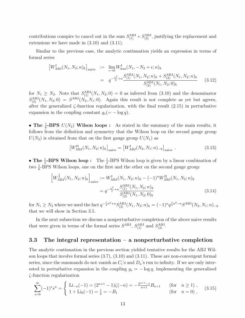
Hence the P poles are at

sj = . . . ,−M − 2,−M − 1; 0, 1, 2, . . . (3.18)

with the gap between sj = −M − 1 and 0 as shown in the left figures of Fig. 1. In (3.18),

we organized poles into groups separated by a semicolon to clarify this gap structure. In

the large k limit, these are the only poles. The contour C parallel to the imaginary axis can

be placed anywhere in the gap. Indeed, enclosing the contour with an infinite semi-circle

to the right in the complex sj plane, the residue integral reduces to the sum (3.7) with

the generalized ζ-function regularization (3.15) implemented automatically by the integral

formula

− 1

2πi

∫C

πds

sin(πs)sn = −2n+1 − 1

n+ 1Bn+1 (n ≥ 0) , (3.19)

and the perturbative expansion in gs is correctly reproduced. It should now be clear why

this class of poles are called P poles.

The NP poles are at

sj =k

2−M,

k

2− (M − 1), . . . ,

k

2− 1 mod k (3.20)

sj = si +k

2mod k (3.21)

This class of poles are called NP poles because k ∝ 1/gs and thus the residues are of order

exp(−1/gs). On the right panel of Fig. 1 shown is the case k = 3 and M = 2. Note that for

integer k as opposed to generic (non-integral) values of k, there are extra cancellations of

the zeros and poles in the factor∏N1

j=1 [(qsj+1)M/ sin(πsj)] since the zeros

sj = k −M,k − (M − 1), . . . , k − 1 mod k (3.22)

can coincide with some of the P poles in (3.18). More precisely, the gap between sj = −M−1

and 0 repeats itself periodically modulo k and thus the P poles for an integer k appear at

sj = 0, 1, . . . , k −M − 1 mod k . (3.23)

Now more important is the fact that for a given M < k as we decrease k continuously,

the NP poles on the positive real axis move to the left. For a sufficiently large k > 2M ,

the NP pole closest to the origin is at sj = k2−M > 0. As k is decreased from k > 2M to

k < 2M , this pole crosses the imaginary axis to the left. As we decrease k further, more NP

poles cross the imaginary axis. For the partition function to be continuous in k, these poles

should not cross the contour C and therefore we need to shift the contour C to the left so

as to avoid the crossing of these NP poles that invade into the real negative region. More

precisely, the contour C has to be placed between sj = −k2− 1 (> −M − 1) and k

2−M when

(M ≤) k < 2M . This is a prescription that needs to be justified. In [17] it was checked that

Seiberg duality holds with this contour prescription, vindicating our integral representation

as a nonperturbative completion.

15

Figure 1: The integration contour C for the partition function: (A) The left figure cor-

responds to the large k limit where only perturbative (P) poles indicated by red “+” are

present. (B) The right figure is an example of the finite k case (k = 3 and M = 2) where

nonperturbative (NP) poles indicated by blue “×” are also present. The green dotted line

corresponds to sj = si − k2

mod k with some si. Note that some of P poles and zeros of

integrands coalesce and cancel out for integer k.

• The pole structure for n > 0 and N1 ≤ N2 : It is straightforward to generalize the

contour prescription to the case of Wilson loops. In this case, however, we need to discuss

two cases N1 ≤ N2 and N1 > N2 separately. We start with the former that is simpler

than the latter. We are interested in the summand in (3.7). Again by multiplying the factor∏N1

i=1 [−1/(2i sin(πsi))], this becomes the integrand with the replacement Ci → si+1. For the

P poles the relevant factor is the same as in the partition function,∏N1

j=1 [(qsj+1)M/ sin(πsj)].

This yields the P poles for generic (non-integral) k at

sj = . . . ,−M − 2,−M − 1; 0, 1, 2, . . . . (3.24)

A similar remark on the integer k case applies to this case, and the gap between sj = −M−1

and 0 repeats itself periodically modulo k. This implies that the P poles for an integer k

appear at

sj = 0, 1, . . . , k −M − 1 mod k. (3.25)

For the NP poles the relevant factors are∏N1

j=1 1/(−qsj+1+nδjl)M and∏

j 6=i 1/(−qsj−si+nδjl)1where l runs from 1 to N1. The NP poles are thus at

sj =k

2−M − nδjl,

k

2− (M − 1)− nδjl, . . . ,

k

2− 1− nδjl mod k (3.26)

sj = si +k

2− nδjl mod k . (3.27)

Note that the NP poles are simply shifted by −nδjl as compared to those for the partition

function. Thus the pole structure differs from that of the partition function only for the

integration variable sl. As mentioned in the end of Section 2.1, the integral representation

for the sum (3.7) is only well-defined for |n| < k2. We thus restrict n in this range. In Fig. 2

16

shown are both P and NP poles as well as the contour C both for j 6= l and j = l. Similar

to the partition function, as we decrease k, NP poles on the positive real axis move to the

left. For j = l, in particular, when k becomes smaller than 2(M + n) (for n > 0), the NP

pole closest to the P pole at the origin crosses the imaginary axis. For Wilson loops to be

continuous as a function of k, similar to the partition function, the contour C has to be

placed between sl = min(−M − 1,−k2− 1− n) and max(0, k

2−M − n) for n > 0. Note that

the bound n < k2

ensures that sl = −M − 1 is left to sl = k2−M − n. For j 6= l the contour

is the same as that in the partition function. The pole structure and the integration contour

C in this case are shown in Figure 2.

Figure 2: The integration contour C for Wilson loops with N1 ≤ N2: Shown is the case,

k = 3, M = 2 and n = 1. (A) The left figure is for sj with j 6= l. The contour is placed

between sj = max(−M − 1,−k2− 1) and sj = min(0, k

2− M). (B) The right figure is

for sj with j = l and the contour is placed between sl = max(−M − 1,−k2− 1 − n) and

sl = min(0, k2−M − n). The green dotted line corresponds to sj = si − k

2− n mod k with

some si.

• The pole structure for n > 0 and N1 ≥ N2 : In this case we are interested in the

summands (3.10) and (3.11). Again by multiplying the factor∏N2

a=1 [−1/(2i sin(πsa))], these

summands become the integrands with the replacement Da → sa + 1. We first discuss the

pole structure of (3.10). This time the relevant factor for the P poles is different from the

previous cases,∏N2

a=1 [(qsa+1)M/ sin(πsa)× (qsa+1+c−n)1/(qsa+1+c)1] where c runs from 0 to

n− 1. This yields the P poles for generic k at

sa = . . . ,−M − 2,−M − 1; −1− c; 0, . . . ,−2− c+n; −c+n, . . . (3.28)

Note that there is an additional pole at sa = −1− c in the gap between sa = −M − 1 and

0 and a hole at sa = −1 − c + n. In the case of integer k, the gap, the additional point

sa = −1 − c and the hole sa = −1 − c + n repeat themselves modulo k and the P poles

appear at

sa = −1− c; 0, 1, . . . ,−2− c+ n; −c+ n, . . . , k −M − 1 mod k .

(3.29)

17

To be more precise, if c is small enough and the hole at sa = −1− c+ n falls into a gap, the

hole is absent.

For the NP poles the relevant factors are∏N2

a=1 1/(−qsa+1)M × (−qsa+1+c)1/(−qsa+1+c−n)1and

∏a6=b 1/(−qsa−sb)1. The NP poles are thus at

sa =k

2−M, . . . ,

k

2− 2− c; k

2− c, . . . , k

2− 1;

k

2+ (n− 1)− c mod k

(3.30)

sa = sb +k

2mod k . (3.31)

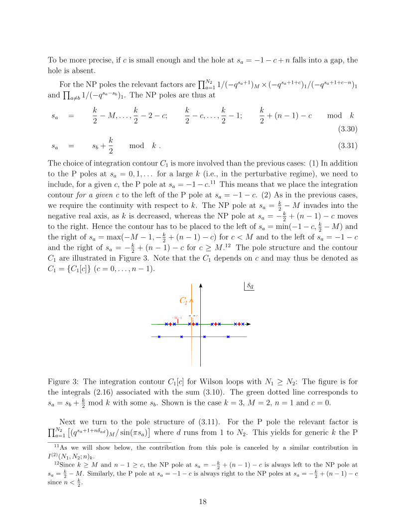
The choice of integration contour C1 is more involved than the previous cases: (1) In addition

to the P poles at sa = 0, 1, . . . for a large k (i.e., in the perturbative regime), we need to

include, for a given c, the P pole at sa = −1− c.11 This means that we place the integration

contour for a given c to the left of the P pole at sa = −1− c. (2) As in the previous cases,

we require the continuity with respect to k. The NP pole at sa = k2−M invades into the

negative real axis, as k is decreased, whereas the NP pole at sa = −k2

+ (n − 1) − c moves

to the right. Hence the contour has to be placed to the left of sa = min(−1− c, k2−M) and

the right of sa = max(−M − 1,−k2

+ (n− 1)− c) for c < M and to the left of sa = −1− cand the right of sa = −k

2+ (n − 1) − c for c ≥ M .12 The pole structure and the contour

C1 are illustrated in Figure 3. Note that the C1 depends on c and may thus be denoted as

C1 = {C1[c]} (c = 0, . . . , n− 1).

1

Figure 3: The integration contour C1[c] for Wilson loops with N1 ≥ N2: The figure is for

the integrals (2.16) associated with the sum (3.10). The green dotted line corresponds to

sa = sb + k2

mod k with some sb. Shown is the case k = 3, M = 2, n = 1 and c = 0.

Next we turn to the pole structure of (3.11). For the P pole the relevant factor is∏N2

a=1

[(qsa+1+nδad)M/ sin(πsa)

]where d runs from 1 to N2. This yields for generic k the P

11As we will show below, the contribution from this pole is canceled by a similar contribution in

I(2)(N1, N2;n)k.12Since k ≥ M and n − 1 ≥ c, the NP pole at sa = −k2 + (n − 1) − c is always left to the NP pole at

sa = k2 −M . Similarly, the P pole at sa = −1− c is always right to the NP poles at sa = −k2 + (n− 1)− c

since n < k2 .

18

poles at

sa = . . . ,−M − 2− nδad,−M − 1− nδad; −nδad, 1− nδad, . . . . (3.32)

Note that the P poles are shifted by −nδad as compared to those in the N1 < N2 case. For an

integer k the gap between sa = −M − 1− nδad and −nδad repeats itself periodically modulo

k and the P poles appear at

sa = −nδad, 1− nδad, . . . , k −M − 1− nδad mod k . (3.33)

It could happen that if the winding n is sufficiently large, k −M − 1− n becomes negative.

For the NP poles the relevant factors are∏N2

a=1 1/(−qsa+1)M and∏

a6=b 1/(−qsa−sb+nδad)1.The NP poles are thus at

sa =k

2−M,

k

2− (M − 1), . . . ,

k

2− 1 mod k (3.34)

sa = sb +k

2− nδad mod k . (3.35)

The choice of integration contour C2 is similar to theN1 ≤ N2 case except that the contour for

the variable sd is to the left of sd = min(−n, k2−M) and the right of sd = max(−M−1,−k

2−1)

and picks up, in particular, the residues from the P poles at sd = −1, . . . ,−n. The pole

structure and the contour C2 are illustrated in Figure 4.

2 2

Figure 4: The integration contour C2 for Wilson loops with N1 ≥ N2: (A) The left figure

is the pole structure and the contour for a 6= d. (B) The right figure is for a = d and the

contour is shifted by −n as compared to that in (A). The green dotted line corresponds to

sa = sb− k2−nδad mod k with some sb. The contours are the same. Shown is the case k = 3,

M = 2 and n = 1.

Again this is a prescription that lacks a first principle derivation. In the case of N1 ≤ N2,

similar to the partition function, for a large k, enclosing the contour with an infinite semi-

circle to the right in the complex sj plane, the residue integral reduces to the sum (3.7),

with the generalized ζ-function regularization (3.15) implemented automatically, and the

perturbative expansion in gs is correctly reproduced. In the case of N1 ≥ N2, however,

19

the way this prescription works is more subtle even for a large k. Each of the two integral

expressions (2.16) and (2.17) picks up extra perturbative contributions from the poles at

s = −1,−2, . . . ,−n. For 16-BPS Wilson loops these extra contributions cancel out in the sum

of (2.16) and (2.17), as shown in Appendix D, thereby reproducing the correct perturbative

expansion in gs.13 As the nonperturbative test, we show in the next section that Seiberg

duality holds with our prescription, where it becomes clear that the inclusion of the P poles

at s = −1,−2, . . . ,−n is necessary.

3.4 Remarks on the ABJM limit

As noted in Section 2.1, there are subtleties in taking the ABJM limit M → 0, in particular,

in the formula (2.16) for the case N1 ≥ N2. There are two points to be addressed; (1) the

agreement of the two formulae (2.12) and (2.15), and (2) the 12-BPS Wilson loop (2.19) in

the ABJM limit.

To address the first point, notice that the integrands of (2.14) and (2.17) in the limit

M → 0 become identical. However, as remarked before, the contours C and C2 are different.

Now since the factors∏N1

i=1[1/(−qsi+1+nδil)M ] in (2.14) and∏N2

a=1[1/(−qsa+1)M ] in (2.17) are

absent, there are no NP poles on the real axis. Hence the difference due to the contours C

and C2 only comes from the residues at the P poles sa = −1,−2, . . . ,−n in (2.17). Therefore,

in order for (2.12) and (2.15) to agree, these residues have to be canceled by (2.16). To see

it, we carefully take the M → 0 limit of (2.16):

I(1)(N1, N2;n)k =1

N2!

n−1∑c=0

N2∏a=1

[−1

2πi

∫C1[c]

πdsasin(πsa)

]qn(2c−M)

(q1−n)c (q1+n)M−1−c(q)c(q)M−1−c

N2∏a=1

(qsa+1)M2 (−qsa+1)M

×N2∏a=1

[(−qsa+1+c)1 (qsa+1+c−n)1(qsa+1+c)1 (−qsa+1+c−n)1

a−1∏b=1

(qsa−sb)1(−qsa−sb)1

N2∏b=a+1

(qsb−sa)1(−qsb−sa)1

], (3.36)

In particular, we focus on the factors near the P pole for a selected variable sd at sd = −1−cas M → 0+,

limsd→−1−c

(q1−n)c(q1+n)M−1−c

(q)c(q)M−1−c

(qsd+1)M(qsd+1+c)1

=q−nc(qn−c)M

(qn)1(q−c)c(q)M−1−clim

sd→−1−c

(qsd+1)M(qsd+1+c)1

=q−nc(qn−c)M

(qn)1

M→0+−→ q−nc

1− qn (3.37)

where we used (q1−n)c(q1+n)M−1−c = (−1)cq−nc+

12c(c+1)(qn−c)M/(q

n)1 and limε→0(qε−c)M/(q

ε)1 =

(q−c)c(q)M−1−c. Note that in the M → 0+ limit these factors vanish away from the P pole

sd = −1 − c, i.e., if the limit sd → −1 − c is not taken in the first line. Therefore, in the

ABJM limit the only contribution comes from the residues at the P poles sd = −1− c where

c = 0, . . . , n− 1.

13The perturbative equivalence of 16 -BPS Wilson loops of the lens space and ABJ matrix models, via the

analytic continuation, has been established and checked by direct perturbative calculations.

20

An important remark is in order: When c < M , the pole at sd = −1−c is clearly a simple

pole, since the factor (qsd+1+c)1 that appear in the first line of (3.37) is canceled by the same

factor in the q-Pochhammer symbol (qsd+1)M . However, when c ≥ M , it is subtle, because

there may not seem to be no apparent cancellation of these factors. Nevertheless, we treat

the pole at sd = −1− c as a simple pole. As it turns out, the proper way to deal with this

subtlety is to adopt an ε-prescription for the parameter M . Namely, M is always kept off an

integral value by the shift M → M + ε with ε > 0. The factor (qsd+1)M is always assumed

to be (qsd+1)M+ε with a non-integral index in our calculations and is defined by (A.3) for a

non-integral M + ε. With this prescription, the factor (qsd+1+c)1 is always canceled by the

same factor in (qsd+1)M+ε, making the pole at sd = −1 − c a simple pole. However, there

is one more subtlety in this prescription to be clarified. Namely, there appears a pole at

sd = −1 − c − ε even with this prescription when c ≥ M . If this pole were included within

the contour, the contribution (3.37) would have been canceled. In other words, it would have

been the same as treating the pole at sd = −1− c as a double pole. Thus our ε-prescription

involves a particular choice of the contour C1[c], i.e., to place it between sd = −1 − c and

−1− c− ε so as to avoid the latter pole. This is a very subtle point and so much of a detail

but is absolutely necessary for getting sensible results.

Without loss of generality, we can choose the index d to be 1, since the expression is

invariant under permutations of sa’s. This yields

I(1)(N,N ;n)k =1

2N−1(N − 1)!

n−1∑c=0

(−qn)c

1 + qn

N∏a=2

[−1

2πi

∫C1[c]

πdsasin(πsa)

](qsa+1+c)1 (qsa+1+c−n)1

(−qsa+1+c)1 (−qsa+1+c−n)1

×a−1∏b=2

(qsa−sb)1(−qsa−sb)1

N∏b=a+1

(qsb−sa)1(−qsb−sa)1

. (3.38)

As shown in Appendix D, this is exactly canceled out by the sum of residues in I(2)(N,N ;n)kat the P poles s1 = −1, . . . ,−n. Hence the formula (2.15) in the ABJM limit reduces

to I(2)(N,N ;n)k with the contour C2 being replaced by the contour C. This proves the

agreement of (2.12) and (2.15) in the ABJM limit. We also note that the formula (3.38),

when multiplied by q−12n2+n, yields the 1

2-BPS Wilson loop (2.19) in the ABJM limit (up to

a normalization). We now discuss more on the 12-BPS Wilson loop in the next subsection.

3.5 The 12-BPS Wilson loop

The 12-BPS Wilson loop is given by (2.19) that follows from the equality

q−12n2+nI(2)(N1, N2;n)k = (−1)nq

12n2−nI(N2, N1;n)−k , (3.39)

21

where N1 ≥ N2. In order to show this identity, we recall that

I(2)(N1, N2;n)k =1

N2!

N2∑d=1

N2∏a=1

[−1

2πi

∫C2

πdsasin(πsa)

]q−nsd+n(d−M−2)

N2∏a=1a6=d

(qsa−sd−n)1(qsa−sd)1

(3.40)

×N2∏a=1

[ (qsa+1+nδad

)M

(1 + qnδad) (−qsa+1)M

a−1∏b=1

(qsa−sb)1(−qsa−sb+nδad)1

N2∏b=a+1

(qsb−sa)1(−qsb−sa−nδad)1

]and

I(N2, N1;n)−k =1

N2!

N2∑d=1

N2∏a=1

[−1

2πi

∫C

πdsasin(πsa)

]qnsd−n(d−2)

N2∏a=1a6=d

(q−sa+sd+n)1(q−sa+sd)1

(3.41)

×N2∏a=1

[(−1)M (q−sa−1; q−1)M

(1 + q−nδad) (−q−sa−1−nδad ; q−1)M

a−1∏b=1

(q−sa+sb)1(−q−sa+sb−nδad)1

N2∏b=a+1

(q−sb+sa)1(−q−sb+sa+nδad)1

],

where M := |N2 −N1| = N1 −N2. In fact, it is straightforward to check that these two are

related, precisely as in (3.39), by the change of variables,

ta = −sa − 1−M − nδad , (3.42)

for a given d, where sa’s are the variables in the latter (3.41) and ta’s be identified with those

in the former (3.40). The contour C is placed in the intervals, −k2− 1 < sa < min(0, k

2−M)

for a 6= d and max(−M − 1,−k2− 1− n) < sd < min(0, k

2−M − n). By the above change of

variables, this becomes precisely the contour C2, where max(−M − 1,−k2− 1) < ta <

k2−M

for a 6= d and max(−M − 1− n,−k2− 1) < td < min(−n, k

2−M).14

This proves that the 12-BPS Wilson loop is given by q−

n2

2+nI(1)(N1, N2;n)k up to the

normalization.

4 Seiberg duality – derivations and a proof

There is a duality between two ABJ theories [5]. Schematically, when N2 > N1, the following

ABJ theories are equivalent:

U(N1)k × U(N2)−k = U(2N1 −N2 + k)k × U(N1)−k . (4.1)

The partition functions of the two theories agree up to a phase [17,40,53,54]. It was further

understood in [17] how the perturbative and nonperturbative contributions to the partition

function are exchanged under the duality map.

The Wilson loops, in contrast, are not invariant under the duality. The mapping rule

for 12-BPS Wilson loops in general representations in N = 2 CSM theories with a simple

14The −1 in (3.42) compensates the orientation flip of the contour.

22

gauge group has been studied by Kapustin and Willett [51]. These Wilson loops correspond

to 16-BPS Wilson loops in the ABJ theory. Our results are consistent with their rule and

slightly generalize it to the case where the flavor group is gauged. Similar to the case of the

partition function [17], our formulae for the Wilson loops allow us to understand an important

aspect of the duality, namely, how the perturbative and nonperturbative contributions are

exchanged under the duality map.

In this section we provide a proof of the duality map by analyzing our expressions (2.12),

(2.15) and (2.19) for the Wilson loops. To this end, let us recall our results for the duality

map of the Wilson loops, (2.20), (2.21), and (2.22).

• The 16-BPS Wilson loop duality :

W II16

(N1, N2;n)k = −W I16(N2, N1;n)k − 2(−1)n+1W II

16

(N2, N1;n)k , (4.2)

• The flavor Wilson loop duality :

W I16(N1, N2;n)k = W II

16

(N2, N1;n)k , (4.3)

• The 12-BPS Wilson loop duality :

W 12(N1, N2;n)k = (−1)nW 1

2(N2, N1;n)k , (4.4)

where we denoted the rank of the dual gauge group by N2 = 2N1 − N2 + k. These three

relations are not independent, but one of them can be derived from the other two by using

the relation between the 12- and 1

6-BPS Wilson loops

W 12(N1, N2;n)k = W I

16(N1, N2;n)k − (−1)nW II

16

(N1, N2;n)k . (4.5)

Before going into a rigorous technical proof, we provide a heuristic yet very useful and

intuitive way to understand how the Wilson loops would be mapped.

4.1 The brane picture – a heuristic derivation15

In Refs. [5,6], the brane realization of the ABJ(M) theory was proposed. The brane content

of this configuration is given by the following:

D3-brane : 0126

NS5-brane : 012345

(1, k) 5-brane : 012[37

]θ

[48

]θ

[59

]θ

(4.6)

15We thank Kazutoshi Ohta for explaining to us the brane picture in the work [55,56] and for very useful

discussions.

23

Here, x6 is periodically identified, and[37

]θ

means the direction on the 3-7 plane with an angle

θ with the x3 axis, where tan θ = k. For U(N1)k × U(N2)−k theory with N2 −N1 = M > 0,

there are N1 D3-branes between an NS5-brane and a (1, k) 5-brane, and N2 = N1 + M

D3-branes between the (1, k) and the NS5. This system realizes 3D supersymmetric field

theory that lives in the 012 directions and flows in the IR to the ABJ SCFT. Seiberg

duality corresponds to moving the NS5 and the (1, k) branes past each other and, during

the process, k D3-branes are created by the Hanany-Witten effect [24] while M D3-branes

are annihilated, in the end leaving D3-branes realizing the dual theory (4.1).

For our purpose, it is convenient to consider the following M-theory lift of the config-

uration (4.6), in which Wilson loops are geometrically realized [55, 56]. Assume that we

have non-trivial Wilson loop along e.g. x2, namely∫dx2A2 6= 0.16 If we T-dualize the

configuration (4.6) along x2 and further lift it to 11 dimensions, we obtain

M2 : 016

M5 : 012345

M5′ : 01[2A

]θ

[37

]θ

[48

]θ

[59

]θ

(4.7)

where “A” denotes the 11th direction. Note that the (1, k) 5-brane has lifted to an M5-

brane (denoted by M5′) that is tilted in four 2-planes with the same angle θ. In Figure 5, we

schematically described this configuration. Because M5′-branes are tilted in the x2-xA plane,

Figure 5: M-theory representation of ABJ theory with Wilson loops (presented

is the case with k = 3, N1 = 2, N2 = 4,M = 2). The left and right ends of the

configuration are identified. The position of the M2-branes in the x2 direction

corresponds to the Wilson loop. Among k places in which fractional M2-branes

can end, the occupied ones are denoted by • and the unoccupied ones by ◦.

there are only k places in which “fractional” M2-branes can stretch between M5′ and M5.

Note that only one fractional M2-brane can exist in one place because of the s-rule [55, 56].

M = N2 − N1 fractional M2-branes are distributed among these k places. On the other

hand, N1 “entire” M2-branes are going around the x6 direction and they do not have to sit

in these places but can be anywhere.

16The relation between the Wilson loop for ABJ theory on flat space and that for ABJ theory on S3 is

not clear. This is one of the reasons why the argument presented here is heuristic.

24

Because of the Wilson loop, different M2-branes are located at different positions along

the x2 direction. Let the x2 coordinate of the N1 M2-branes between M5 and M5′ be µj,

j = 1, . . . , N1, and that of the N2 = N1 +M M2-branes (both fractional and entire) between

M5′ and M5 be νa, a = 1, . . . , N2 (see Figure 5).17 Furthermore, let the x2 coordinate of the

k places in which fractional M2-branes can end be yα, α = 1, . . . , k. If the radius of the x2

direction is 2π, we have yα = 2παk

+ const and, for n ∈ Z,

k∑α=1

einyα ∝k∑

α=1

ei2πnα/k =

{0 (n 6= 0 mod k)

k (n = 0 mod k)(4.8)

As mentioned above, Seiberg duality corresponds to moving M5 and M5′ past each other.

In this process, M fractional M2-branes get annihilated, and k fractional M2-branes are

created, leaving N2 = N1 −M + k = 2N1 −N2 + k. The resulting configuration is shown in

Figure 6. Let the x2 coordinate of the N2 M2-branes (both fractional and entire) between

Figure 6: The Seiberg dual configuration of the configuration in Figure 5.

M5 and M5′ be µ1, . . . , µN2, and that of the N M2-branes between M5′ and M5 be ν1 . . . , νN1

(see Figure 6).

In the original configuration in Figure 5, among the k spots {1, . . . , k} at which frac-

tional M2-branes can end, let the occupied ones be O1, . . . , OM and the unoccupied ones be

U1, . . . , Uk−M . Of course, {O1, . . . , OM}+ {U1, . . . , Uk−M} = {1, . . . , k}. Clearly,

{ν1, . . . , νN2} = {µ1, . . . , µN1}+ {yO1, . . . , yOM}. (4.9)

In the dual theory, the position of the entire M2-branes are unchanged, while the occupied

and unoccupied spots for fractional M2-branes are interchanged. Therefore,

{µ1, . . . , µN2} = {µ1, . . . , µN1}+ {yU1

, . . . , yUk−M}= {µ1, . . . , µN1}+ {y1, . . . , yk} − {yO1

, . . . , yOM}, (4.10)

{ν1, . . . , νN1} = {µ1, . . . , µN1}. (4.11)

17 Note that there is no direct relation between the µ, ν here and the ones that appear in the ABJ matrix

model (2.4). In the computation of Wilson loops using localization [8], at saddle points, gauge fields (which

correspond to µ, ν here) vanish and Wilson loops get contribution only from auxiliary fields (which correspond

to µ, ν in the ABJ matrix model).

25

4.1.1 Fundamental representation

Now we want to use this picture to give a very heuristic explanation of Seiberg duality

(4.1). Consider the original configuration in Figure 5. The Wilson loop in the fundamental

representation simply measures the position of the M2-branes. Therefore, naively, we have18

W I16(N1, N2;n) ∼

N1∑j=1

einµj , (4.12)

W II16

(N1, N2;n)?∼

N2∑a=1

einνa =

N1∑j=1

einµj +M∑α=1

einyOα , (4.13)

where in the second equation we used (4.9). Actually, it turns out that, in order to reproduce

the explicit results obtained in the current paper, we must set νa → νa + π by hand so that

(4.13) is replaced by

W II16

(N1, N2;n) ∼N2∑a=1

ein(νa+π) = (−1)n

(N1∑j=1

einµj +M∑α=1

einyOα

). (4.14)

In the dual theory, using (4.10) and (4.11), we obtain

W I16(N2, N1;n) ∼ (−1)n

N2∑j=1

einµj = (−1)n

(N1∑j=1

einµj +k∑

α=1

einyα −M∑α=1

einyOα

)

= (−1)n

(N1∑j=1

einµj −M∑α=1

einyOα

), (4.15)

W II16

(N2, N1;n) ∼N1∑a=1

einνa =

N1∑j=1

einµj , (4.16)

where we introduced another ad hoc rule µj → µj + π just as we did in (4.14). Also, in

the second line of (4.15), we used (4.8), assuming that n 6= 0 mod k. Therefore, comparing

(4.12), (4.14) and (4.15), (4.16), we “derived” the following duality relations:

W I16(N1, N2;n) = W II

16

(N2, N1;n), (4.17)

W II16

(N1, N2;n) +W I16(N2, N1;n) = 2(−1)nW II

16

(N2, N1;n). (4.18)

This means that the 1/2-BPS Wilson loop defined by

W 12(N1, N2;n) := W I

16(N1, N2;n)− (−1)nW II

16

(N1, N2;n) (4.19)

18Note that this is very rough and heuristic; thus “∼”. In reality, νa is a variable to be integrated over

and is not localized at yα. Even if there is a sense in which they are localized at yα, we should sum over all

possible ways to distribute M fractional M2-branes over k positions.

26

is expected to have the following simple transformation rule:

W 12(N1, N2;n) = (−1)nW 1

2(N2, N1;n). (4.20)

Note that the above arguments are based on the identity (4.8) and are valid only for n 6= 0

mod k. We do not expect to get correct equations by setting n = 0 in the above duality

relations, as we commented in subsection 2.1.19

Although the ad hoc rule νa → νa + π, µj → µj + π was crucial to reproduce the

correct transformation rule for Wilson loops, its physical meaning is unclear. It is somewhat

reminiscent of the fact that, in the ABJ matrix model at large N1, N2 [9], the eigenvalue

distribution for U(N2) is offset relative to the U(N1) eigenvalue distribution on the complex

eigenvalue plane, but further investigations are left for future research. Since the arguments

given in this subsection are meant to be only heuristic, we simply accept the rule as a working

assumption and proceed. In passing, we note that, with the above ad-hoc rule, the 1/2-BPS

Wilson loop (4.19) can be understood simply as supertrace as follows:

W 12(N1, N2;n) ∼

∑j

einµj −∑a

einνa = trXn − trY n = strZn, (4.21)

where X = diag(eiµj), Y = diag(eiνa), and Z =

(X

Y

).

4.1.2 More general representations

The above heuristic method to guess the Seiberg duality relation can be generalized to more

general representations.20 For example, in the original U(N1)k × U(N2)−k theory, consider

19Actually, equations (4.17) and (4.20) still give correct equations if we set n = 0, but (4.18) does not.20For a U(N) representation with a Young diagram λ, the Wilson loop is Sλ(eiµ1 , . . . , eiµN ), where

Sλ(x1, . . . , xN ) is the Schur polynomial [45]. For example, S =∑i xi, S =

∑i≤j xixj , S =

∑i<j xixj .

27

the following 1/6-BPS Wilson loops:

W • ∼N1∑i≤j

ei(µi+µj) =1

2

(N1∑i=1

eiµi

)2

+1

2

N1∑i=1

e2iµi =:1

2(eiµ)2 +

1

2e2iµ

W • ∼N1∑i<j

ei(µi+µj) =1

2

(N1∑i=1

eiµi

)2

− 1

2

N1∑i=1

e2iµi =:1

2(eiµ)2 − 1

2e2iµ

W• ∼N2∑a≤b

ei(νa+νb) =1

2

(N2∑a=1

eiνa

)2

+1

2

N2∑a=1

e2iνa

=1

2

(N1∑i=1

eiµi +M∑α=1

eiyOα

)2

+1

2

(N1∑i=1

e2iµi +M∑α=1

e2iyOα

)=:

1

2(eiµ)2 +

1

2(eiyO)2 + eiµeiyO +

1

2e2iµ +

1

2e2iyO ,

W• ∼N2∑a<b

ei(νa+νb) =:1

2(eiµ)2 +

1

2(eiyO)2 + eiµeiyO − 1

2e2iµ − 1

2e2iyO ,

W ∼ −N1∑i=1

eiµiN2∑a=1

eiνa =: −(eiµ)2 − eiµeiyO ,

(4.22)

where WRR denotes the Wilson loop in the representations R and R for U(N1) and U(N2),

respectively, and “•” means the trivial representation. Also, in the last expression of each

line, we used a schematic notation, whose meaning is defined by the immediately preceding

expression. In the dual U(N2)k × U(N1)−k theory, we have

W • ∼1

2(eiµ)2 +

1

2(eiyO)2 − eiµeiyO +

1

2e2iµ − 1

2e2iyO ,

W • ∼1

2(eiµ)2 +

1

2(eiyO)2 − eiµeiyO − 1

2e2iµ +

1

2e2iyO ,

W• ∼ 1

2(eiµ)2 +

1

2e2iµ, W• ∼ 1

2(eiµ)2 − 1

2e2iµ,

W ∼ −(eiµ)2 + eiµeiyO .

(4.23)

The duality relation between W and W is readily found to be

W = SW , W =

W •

W •

W •

W •

W

, S =

0 0 1 0 0

0 0 0 1 0

0 1 3 1 2

1 0 1 3 2

0 0 −2 −2 −1

. (4.24)

The combinations that have simple transformation rule are

W1/2

:= W • +W• +W , W1/2

:= W • +W• +W , (4.25)

28

which transform as

W1/2

= W1/2, W

1/2= W

1/2. (4.26)

These are precisely the 1/2-BPS Wilson loops derived in [45].

Just as in (4.21), we can write these in terms of supertrace as follows:

W1/2

=1

2(strZ)2 +

1

2str(Z2) = str Z,

W1/2

=1

2(strZ)2 − 1

2str(Z2) = str Z.

(4.27)

Note that the right hand side is nothing but supertrace in the respective representations.

More generally, the 1/2-BPS Wilson loop for general representation R is given by21

W1/2R ∼ strR Z = PR(str(Zn)), (4.30)

where PR is a polynomial in str(Zn) (n = 1, . . . , |R|) obtained from the Schur polynomial.

Each term in the polynomial contains a product of |R| Z’s. The results from the previous

section, more specifically (4.20) and (4.21), say that str(Zn)→ (−1)n str(Zn) under duality.

Therefore, the transformation law for the general 1/2-BPS Wilson loop is

W1/2R → (−1)|R|W

1/2R . (4.31)

None of the above is a derivation of Seiberg duality for 1/6-BPS Wilson loops but is

merely a motivation for it. However, the fact that it predicts a simple duality law for 1/2-

BPS Wilson loops is evidence that the 1/6-BPS duality relation is also correct.

4.2 A rigorous derivation and proof

Since the mapping (4.3) for the flavor Wilson loop and (4.4) for the 12-BPS Wilson loop are

simple as compared to the mapping (4.2) for 16-BPS Wilson loops, it is the best strategy to

prove (4.3) and (4.4) and then infer (4.2) from them. In due course, we will also see manifestly

the exchange of perturbative and nonperturbative contributions under the duality.

21Note that the 1/2-BPS Wilson loops derived in [45] are

W1/2R = strR

(eµMM

−eνMM

)(4.28)

where µMM, νMM are the µ, ν that appear in matrix model (see footnote 17). Our ad hoc rule is to replace

this with

W1/2R = strR

(eiµ

eiν

)= strR Z (4.29)

where µ, ν are the positions of the M2-branes.

29

• The flavor Wilson loop duality : We first prove the flavor Wilson loop duality:

W I16(N1, N2;n)k = W II

16

(N2, N1;n)k = W I16(N1, N2;n)−k (4.32)

which amounts to the equality

q−n2

2+nI(N1, N2;n)kI(N1, N2; 0)k

=qn2

2−nI(N1, N2;n)−k

I(N1, N2; 0)−k. (4.33)

The basic idea for the proof is to show that (1) the integrands in the numerators are iden-

tical, i.e., they share exactly the same zeros and poles and the same asymptotics up to the

normalization, and (2) the contours are equivalent. The explicit forms of I(N1, N2;n)k and

I(N1, N2;n)−k are given by

I(N1, N2;n)k =1

N1!

N1∑l=1

N1∏i=1

[−1

2πi

∫C

πdsisin(πsi)

]q−nsl+n(l−2)

N1∏i=1i 6=l

(qsi−sl−n)1(qsi−sl)1

(4.34)

×N1∏i=1

[(−1)M (qsi+1)M

(1 + qnδil) (−qsi+1+nδil)M

i−1∏j=1

(qsi−sj)1(−qsi−sj+nδil)1

N1∏j=i+1

(qsj−si)1(−qsj−si−nδil)1

]

I(N1, N2;n)−k =1

N1!

N1∑l=1

N1∏i=1

[−1

2πi

∫C

πdsisin(πsi)

]qnsl−n(l+M−3)

N1∏i=1i 6=l

(q−si+sl+n)1(q−si+sl)1

(4.35)

×N1∏i=1

[(qsi+1)k−M

(1 + qnδil) (−qsi+1+nδil)k−M

i−1∏j=1

(q−si+sj)1(−q−si+sj−nδil)1

N1∏j=i+1

(q−sj+si)1(−q−sj+si+nδil)1

],

where M := |N2 − N1| = N2 − N1. At first glance the zeros and poles of (4.34) and (4.35)

differ in the M -dependence, since M is replaced by k−M in the latter. However, introducing

the dual variables in the latter

si = −si +k

2− 1− nδil , (4.36)

we can easily see that they actually agree. As simple as it may look, we stress that this is a

very important map and can be regarded as the duality transformation, as we now justify.

In terms of the original variables si, the poles of the integrand in (4.35) appear at

P : si = 0, 1, . . . ,M − 1 mod k , (4.37)

NP : si = −k2

+M − nδil, . . . ,k

2− 1− nδil mod k , (4.38)

(NP) : si = sj +k

2− nδil mod k . (4.39)

30

In terms of the dual variables si, these poles are mapped to

NP : si =k

2−M − nδil, . . . ,

k

2− 2− nδil,

k

2− 1− nδil mod k , (4.40)

P : si = 0, 1, . . . , k −M − 1 mod k , (4.41)

(NP) : si = sj +k

2− nδil mod k . (4.42)

These are precisely the same as the poles of the integrand in (4.34) and thus the two inte-

grands share exactly the same poles. We emphasize that the P and NP poles are exchanged

by the duality transformation (4.36). In terms of the original variables, the contour C is

placed in the intervals, max(M − k − 1,−k2− 1) < si < min(0,−k

2+ M) for i 6= l and

max(−M − 1,−k2− 1 − n) < sl < min(0,−k

2+ M − n). In terms of the dual variables,

this becomes the intervals, max(−k2− 1,−M − 1) < si < min(k

2− M, 0) for i 6= l and

max(−k2− 1,−M − 1 − n) < sl < min(k

2− M,−n). Hence, the contours C and C are

equivalent.22

Meanwhile, the zeros appear only from the factors (qsi−sj)1 and (qsi−sl−n)1 and do not

depend explicitly on M . It is easy to check that the zeros are invariant under the duality

transformation (4.36). Indeed, the factors that depend on the differences si − sj in (4.34)

and si − sj in (4.35) only differ from each other by the factor q2n(l−1) multiplying the latter.

It remains to find the asymptotics of the integrands. The asymptotics to be compared

with are those at si → i∞ in (4.34) and si → i∞ in (4.35), and for the factors that

depend on the differences of the variables we only need to care about the factor q2n(l−1).

Collecting various factors together and taking into account the orientations of the contours,

it is straightforward to find that the latter asymptotics is ikq−n2+2n times the former. Since

the factor ik is canceled by the same factor coming from the normalization, this completes

the proof of the equality (4.33).

• The 12-BPS Wilson loop duality : We next prove the duality for the 1

2-BPS Wilson

loop:

W 12(N1, N2;n)k = (−1)nW 1

2(N2, N1;n)k (4.43)

which from (2.19) amounts to the equality

qn2

2−nI(1)(N2, N1;n)−kI(2)(N2, N1; 0)−k

= −q−n

2

2+nI(1)(N2, N1;n)k

I(2)(N2, N1; 0)k. (4.44)

The explicit forms of I(1)(N2, N1;n)−k and I(1)(N2, N1;n)k are given by

I(1)(N2, N1;n)−k =1

N1!

n−1∑c=0

N1∏i=1

[−1

2πi

∫C1[c]

πdsisin(πsi)

]qn

(q1−n)c(q1+n)M−1−c

(q)c(q)M−1−c

N1∏i=1

(q−si−1; q−1)M2 (−q−si−1; q−1)M

×N1∏i=1

[(−q−si−1−c)1 (q−si−1−c−n)1(q−si−1−c)1 (−q−si−1−c−n)1

i−1∏j=1

(q−si+sj)1(−q−si+sj)1

N1∏j=i+1

(q−sj+si)1(−q−sj+si)1

], (4.45)

22The −1 in (4.36) compensates the orientation flip of the contour.

31

I(1)(N2, N1;n)k =1

N1!

n−1∑c=0

N1∏i=1

[−1

2πi

∫C1[c]

πdsisin(πsi)

]qn(2c+M) (q

1−n)c(q1+n)k−M−1−c

(q)c(q)k−M−1−c

N1∏i=1

(qsi+1)k−M2 (−qsi+1)k−M

×N1∏i=1

[(−qsi+1+c)1 (qsi+1+c−n)1(qsi+1+c)1 (−qsi+1+c−n)1

i−1∏j=1

(qsi−sj)1(−qsi−sj)1

N1∏j=i+1

(qsj−si)1(−qsj−si)1

]. (4.46)

Similar to the flavor Wilson loop duality, introducing the duality transformation in (4.45)

si = −si −k

2− 1 , (4.47)

it becomes evident that the two integrands share the same zeros and poles. In terms of the

original variables si, the poles of the integrand in (4.45) appear modulo k at

P : si = −1− c; 0, . . . ,−2− c+ n; −c+ n, . . . , k −M − 1 , (4.48)

NP : si =k

2−M, . . . ,

k

2− 2− c; k

2− c, . . . , k

2− 1;

k

2+ n− 1− c , (4.49)

(NP) : si = sj +k

2. (4.50)

In terms of the dual variables si, these poles are mapped, after shifting by +k, to

NP : si = −k2

+M, . . . ,k

2− 2− c; k

2− c, . . . , k

2− 1;

k

2+ n− 1− c , (4.51)

P : si = −1− c; 0, . . . ,−2− c+ n; −c+ n, . . . ,M − 1 , (4.52)

(NP) : si = sj +k

2, (4.53)

where c = (n−1)−c. Indeed, these are exactly the poles of the integrand in (4.46). We again

stress that the P and NP poles are exchanged by the duality transformation (4.47). The

contour C1 is placed in the interval, max(−M−1,−k2

+n−1−c) < si < min(−1−c, k2−M),

that is mapped to max(−k2

+ n− 1− c,−(k −M)− 1) < si < min(k2− (k −M),−1− c).23

Hence the contour in terms of the variables si is equivalent to C1.

to the left of sa = −1− c and the right of sa = −k2

+ (n− 1)− c for c ≥M

As for the zeros, similar to the flavor Wilson loop case, they appear only from the factors

that depend on the differences si − sj in (4.45) and si − sj in (4.46). In fact, these factors

are exactly the same in (4.45) and (4.46).

In order to examine the asymptotics, we first note that24

qn(2c+M) (q1−n)c(q

1+n)k−M−1−c(q)c(q)k−M−1−c

= qn(n−1)+n(M−c) limε→0

(qε)1(qn−c)k−M

(qn)1(qε−c)k−M

= −qn(n−1) (q1−n)c(q

1+n)M−1−c(q)c(q)M−1−c

. (4.55)

23More precisely speaking, these ranges are for c < M as discussed in Section 3.3, but for c ≥ M the

intervals are not conditional, −k2 + n− 1− c < si < −1− c and −k2 + n− 1− c < si < −1− c.24In the simplest case n = 1, only c = 0 gives a nonvanishing result in (4.55). The left hand side yields

qM (q2)k−M−1

(q)k−M−1= − 1−qM

1−q that equals the right hand side, − (q2)M−1

(q)M−1, with a minus sign. More generally, we

32

The asymptotics at si → i∞ in (4.45) and si → i∞ in (4.46) then differ only by the factor

−ikq−n2+2n and the factor ik is canceled by the same factor from the normalization. This

completes the proof of (4.44).

• The 16-BPS Wilson loop duality : Having proved the two of the duality maps (4.3)

and (4.4), the definition of the 12-BPS Wilson loop (4.5) implies the duality map (4.2) for

the 16-BPS Wilson loops: An easiest way to see it is to add (−1)n+1W I

16

(N1, N2;n)k to the

both sides of (4.2),

W 12(N1, N2;n) = −

(W I

16(N2, N1;n)k − (−1)nW I

16(N1, N2;n)k

)(4.56)

−2(−1)n+1(W II

16

(N2, N1;n)k −W I16(N1, N2;n)k

).

Using the flavor Wilson loop duality (4.3) and the relation (4.5), this yields the 12-BPS Wilson

loop duality,

W 12(N1, N2;n) = (−1)nW 1

2(N2, N1;n) . (4.57)

This thereby proves the 16-BPS Wilson loop duality (4.2).

4.3 The simplest example – the U(1)k × U(N)−k theory

It is illustrative to work out the simplest case, the duality between the U(1)k × U(N)−kand U(2 + k − N)k × U(1)−k ABJ theories, since the integral is one-dimensional and the

integration can be explicitly carried out. Apart from its simplicity, the U(1)k×U(N)−k may

also be relevant to the study of Vasiliev’s higher spin theory with U(1) symmetry in the ’t

Hooft limit, N, k → ∞ with N/k fixed [7]. Here we perform the integrals analytically and

explicitly check Seiberg duality for some small values of N , k and n. In this connection, in

the simplest case of N = 1, a check against the direct integral is provided for arbitrary k

and n in Appendix E.

find

limε→0

(qε)1(qn−c)k−M(qε−c)k−M

= limε→0

(qε)1(qc+1)k−M(qε−n+c+1)k−M

= limε→0

q−Mn (qε)1(1− qM−c) · · · (1− qM−c+n−1)

(1− q−c) · · · (q−ε)1 · · · (1− q−c+n−1)

= −q−nM limε→0

(qε)1(qn−c)M(qε−c)M

. (4.54)

33

4.3.1 The flavor Wilson loop

We first consider the duality of flavor Wilson loops that are 16-BPS Wilson loops on the

“flavor group” U(1). The 16-BPS flavor Wilson loops are given by

W I16(1, N ;n)k = q−

12n2+n I(1, N ;n)k

I(1, N ; 0)k, (4.58)

W II16

(N , 1;n)k = W I16(1, N ;n)−k = q

n2

2−n I(1, N ;n)−k

I(1, N ; 0)−k, (4.59)

where the dual gauge group N = 2 + k −N and the integral expression takes the form

I(1, N ;n)k =(−1)N−1q−n

1 + qn−1

2πi

∫C

πds

sin(πs)q−ns

(qs+1)N−1(−qs+1+n)N−1

. (4.60)

The function I(1, N ; 0)k appearing in the denominators is essentially the partition function

and has the following property under Seiberg duality [17,40]:

I(1, N ; 0)k = i−kI(1, N ; 0)−k . (4.61)

Meanwhile, the flavor Wilson loop duality is given by (2.21)

W I16(1, N ;n)k = W II

16

(N , 1;n)k (4.62)

that implies

I(1, N ;n)k = i−kqn2−2nI(1, N ;n)−k . (4.63)

This generalizes the relation (4.61) for the partition function, and we are going to check this

relation explicitly for some small values of N , k and n.

We first calculate the odd k case, since it is simpler than the even k case. The integrand

flips the sign under the shift of integration variable, s → s + k, in this case. Thanks to

this property, the integrals can be evaluated by considering the closed contour depicted in

Fig.7: Let us denote the original contour by C and the closed contour by C ′ that consists

of C + C1 + C2 + C3 where C2 is parallel to C and shifted by k. It is easy to see that there

are no contributions from the contours C1 and C3, and the integral along C2 is precisely the

same as that along the original contour C because the integrand only flips the sign under

the shift s → s + k. It is then clear that the integral along the closed contour C ′ is twice

that along C: ∫C

(· · · ) =1

2

∫C′

(· · · ) . (4.64)

Thus the integrals can be evaluated by residue calculations.

34

k

2� n � (N � 1)

k � N

k

2� n � 1

C

C1

C2

C3

Figure 7: The integration contour: Shown is a deformed contour where C2 is shifted to the

left from the vertical line running from s = 3k2−n−(N−1)+i∞−ε to 3k

2−n−(N−1)−i∞−ε,

exploiting the absence of poles on the strip between s = k −N and 3k2− n− (N − 1).

It is straightforward to carry out the calculation and we find that

I(1, N ;n)odd k =(−1)N−1q−n

2(1 + qn)

[k−N∑s=0

(−1)sq−ns(qs+1)N−1

(−qs+1+n)N−1(4.65)

+ik

2

N−1∑c=1

(−1)k+12

+cqn(n+c)N−1∏

b=1,b 6=c

(−qb−c−n)1(qb−c)1

],

where the first term is the contribution from the P poles at s = 0, 1, · · · , k − N , while the

second term is from the NP poles at s = k2− n− b, (b = 1, · · · , N − 1).

The even k case requires more considerations. In contrast to the odd k case, the integrand

is periodic under the shift s→ s+k. In addition, some of P and NP poles merge into double

poles, since k2

is an integer. We can, however, apply a similar trick as that used in [17, 57].

For an illustration of this trick, let us consider a generic integral of the form∫Cds f(s)

with f(s) being periodic under the shift s → s + k. The trick is instead to consider the

integrand g(s) = f(s)(s + a) with a being an arbitrary constant. This integrand shifts as

g(s+ k) = g(s) + kf(s) when s is shifted by k. Thus the integral∫C′dsg(s) along the closed

contour C ′ = C + C1 + C2 + C3 yields k∫Cdsf(s) provided that there are no contributions

from C1 and C3. This way the even k case can also be evaluated by residue calculations.

Note that the result does not depend on the choice of an arbitrary constant a.

In the following we only show the case when k2− (N − 1) − n > 0. The other case,

k2− (N − 1)−n < 0, however, can be easily derived in a similar manner. The poles encircled

35

by the contour appear at

s =

0, · · · , k

2−N − n (simple)

k2− (N − 1)− n, · · · , k

2− 1− n (double)

k2− n, · · · , k −N (simple)

. (4.66)

The residue evaluation then yields

I(1, N ;n)even k = −(−1)N−1q−n

1 + qn1

2k

[ ∑s=0,··· , k

2−N−n

k2−n,··· ,k−N

(−1)sq−ns(qs+1)N−1

(−qs+1+n)N−1(s+ a) (4.67)

+∑

b=1,··· ,N−1

lims→ k

2−b−n

d

ds

{(s−

(k

2− b− n

))2πq−ns

sinπs

(qs+1)N−1(−qs+1+n)N−1

(s+ a)

}],

where the first line is the contribution from simple poles and the second line from double

poles. These simple poles are a subgroup of P poles in (3.25), while the double poles are

composed of P and NP poles, i.e., those P poles in (3.25) coalescing NP poles in (3.26).

On the dual side, the integral I(1, N ;n)−odd k can be calculated similarly as

I(1, N ;n)−odd k =qn(N+1)

2(1 + qn)

[k−N∑s=0

(−1)sqns(qs+1)N−1

(−qs+1+n)N−1(4.68)

− ik

2

N−1∑b=1

(−1)k−12

+bq−n2−bn

N−1∏a=1,a 6=b

(−qa−b−n)1(qa−b)1

].

In the even k case we only show result for the case when k2− (N − 1)− n > 0:

I(1, N ;n)−even k =qn(N+1)

2k(1 + qn)

[ ∑s=0,··· , k

2−N−n

k2−n,··· ,k−N

(−1)sqns(qs+1)N−1

(−qN+1+n)N−1(s+ a) (4.69)

+∑

s= k2−N−n+1,··· , k

2−n−1

lims′→s

d

ds′

{π(s′ − s)2sin(πs′)

qns′ (qs

′+1)N−1(−qs′+1+n)N−1

(s′ + a)

}].

We have now collected necessary data to explicitly check the flavor Wilson loop duality.

36

• Numerical checks

Let us check (4.63) explicitly for the duality U(1)5×U(2)−5 = U(5)5×U(1)−5 with winding

n = 2. The results are

I(1, 2; 2)5 = (1.46 + 0.47i) + (0.90− 0.29i) + (0.45− 0.62i) + (−0.58i)︸ ︷︷ ︸P

+ (−0.73 + 1.01i)︸ ︷︷ ︸NP

, (4.70)

i−5I(1, 5; 2)−5 = (−0.73 + 1.01i)︸ ︷︷ ︸P

+ (1.46 + 0.47i) + (0.90− 0.29i) + (0.45− 0.62i) + (−0.58i)︸ ︷︷ ︸NP

. (4.71)

Both in the original and dual theories, the first line is the perturbative contribution, while the

second line is the nonperturbative contribution. We can explicitly see that the perturbative

and nonperturbative contributions are exchanged under Seiberg duality.

Next we consider the even k case, U(1)4×U(2)−4 = U(4)4×U(1)−4 with winding n = 1.

For the original theory we have

I(1, 2; 1)4 =i− 1

16

(4− 4i) + (3 + i)aπ

2π︸ ︷︷ ︸P+NP

+ (−1− i)(1 + a) +

(i

2− 1

2

)(2 + a)︸ ︷︷ ︸

P

(4.72)

=i− 1

16

[−2 +

2− 2i

π

], (4.73)

where the first term in the first line comes from the double pole at s = 0 and the rest are

from the simple P poles at s = 1, 2. Note that the a-dependence is canceled out, as it should.

For the dual theory we have

iI(1, 4, 1)−4 =i− 1

16

(4− 4i) + (3 + i)(−a′)π2π︸ ︷︷ ︸

P+NP

+ (−1− i)(1− a′) +

(i

2− 1

2

)(2− a′)︸ ︷︷ ︸

NP

(4.74)

=i− 1

16

[−2 +

2− 2i

π

], (4.75)

where the first term in the first line comes from the double pole at s = 0 and the rest are

from the simple NP poles at s = −1,−2. The a′-dependence is canceled out similar to the

previous case. However, we observe that the pole-by-pole maps agree if we identify a = −a′even though the constants a and a′ do not seem to carry any physical meaning. As indicated,

the P and NP poles are exchanged in the original (4.72) and dual (4.74) Wilson loops. These

examples provide evidence for the flavor Wilson loop duality (2.21).

37

4.3.2 The 12-BPS Wilson loop

We next turn to the 12-BPS Wilson loops with winding n (2.19)

W 12(1, N ;n)k = (−1)n+1q

n2

2−n I

(1)(N, 1;n)−kI(2)(N, 1; 0)−k

, (4.76)

W 12(N , 1;n)k = q−

n2

2+n I

(1)(N , 1;n)k

I(2)(N , 1; 0)k(4.77)

where the integral expression takes the form

I(1)(N, 1;n)k =n−1∑c=0

qn(2c−N+1) (q1−n)c(q

1+n)N−2−c(q)c(q)N−2−c

−1

2πi

∫C1[c]

πds

sin(πs)

(qs+1)N−12 (−qs+1)N−1

× (−qs+1+c)1 (qs+1+c+n)1(qs+1+c)1 (−qs+1+c+n)1

. (4.78)

The normalization factor has the relations I(2)(N, 1; 0)−k = (−1)N−1I(2)(N, 1; 0)k = I(1, N ; 0)kand obeys the duality relation

I(2)(N, 1; 0)−k = i−kI(2)(N , 1; 0)k . (4.79)

Meanwhile, the 12-BPS Wilson loop duality is given by (4.4)

W 12(1, N ;n)k = (−1)nW 1

2(N , 1;n)k (4.80)

that, together with (4.79), implies

I(1)(N, 1, n)−k = −i−kq−n2+2nI(1)(N , 1;n)k . (4.81)

This is the relation we are going to check explicitly for some small value of N , k and n.

Similar to the previous case, the integrand for odd k is anti-periodic under the shift

s → s + k, whereas it is periodic for even k. In the latter case, some of P and NP poles

merge into double poles. We can thus apply the same technique as that used in the previous

case to this case.

In the odd k case, the poles encircled by the contour appear at

P : s = −1− c; 0, 1, · · · ,−2− c+ n; −c+ n, · · · , k −N mod k (4.82)

NP : s =k

2− b+ nδb,1+c mod k (b = 1, · · · , N − 1) (4.83)

for I(1)(1, N ;n)−k and a given c and

P : s = −n+ c; 0, · · · , c− 1; c+ 2, · · · , N − 2 mod k (4.84)

NP : s =k

2− b− nδb,n−c mod k (b = 1, · · · , k −N + 1) (4.85)

38

for I(1)(N , 1;n)k and a given c = (n − 1) − c. As discussed, the change of the integration

variable, s = −s + k2− 1, precisely exchanges P and NP poles in the two theories. It is

straightforward to carry out the residue integrals and we find

I(1)(N, 1;n)±odd k

=1

2

n−1∑c=0

[(−2−c+n∑s=0

+k−N∑

s=−c+n

)(−1)sqn(2c−N+1) (q

1−n)c(q1+n)N−2−c

(q)c(q)N−2−c(4.86)

× (qs+1)N−12(−qs+1)N−1

(−qs+1+c)1(qs+1+c−n)1

(qs+1+c)1(−qs+1+c−n)1+ (−1)c+1qn(c−N+1) (qn−c)N−1(q

−n)1(−q−c)N−1(qn)1(−q−n)1

∓ikN−1∑b=1

(−1)k−12

+b−nδb,1+c qn(2c−N+1)(q1−n)c(q

1+n)N−2−c(q)c(q)N−2−c

∏N−1a=1 (−qa−b+n(δb,1+c−δa,1+c)+1)1

4∏N−1

a=1 (qa−b+n(δb,1+c−δa,1+c)+1)1

]

where q = e±2πik for ∓k with an abuse of notation. The first two lines are the contributions

from P poles and the last line is those from NP poles.

In the even k case we only show the case when k2> N − 1 + n. The other case can be

calculated in a similar manner. The poles encircled by the contour appear at

s =

−1− c; 0, · · · , k

2−N (simple)

k2− c+ n, · · · , k −N (simple)

k2− (N − 1), · · · ,−2− c− n; −c+ n, · · · , k

2− 1− c+ n (double)

. (4.87)

Similar to the previous case (4.67), we find that

I(1)(N, 1;n)even k

=−1

2k

n−1∑c=0

[ ∑s=0,··· , k

2−N

k2−c+n,··· ,k−N ;−1−c

(−1)sqn(2c−N+1) (q1−n)c(q

1+n)N−2−c(q)c(q)N−2−c

(qs+1)N−12(−qs+1)N−1

× (−qs+1+c)1(qs+1+c−n)1

(qs+1+c)1(−qs+1+c−n)1(s+ a) +

∑s= k

2−(N−1),··· ,−2−c+n−c+n,··· , k

2−1−c+n

lims′→s

d

ds′

{(s′ − s)2 π

sin πsqn(2c−N+1)

× (q1−n)c(q1+n)N−2−c

(q)c(q)N−2−c

(qs+1)N−12(−qs+1)N−1

(−qs+1+c)1(qs+1+c−n)1

(qs+1+c)1(−qs+1+c−n)1(s+ a)

}](4.88)

where a is an arbitrary constant.

39

• A numerical check

As an explicit check of (4.81), we consider the example, the duality U(1)5 × U(2)−5 =

U(5)5 × U(1)−5 with winding n = 2. For the original theory we have

I(1)(2, 1; 2)−5

=1

4

( ∑s=0,2,3,4

(−1)q2(q1−s)1

(−q1−s)1− 5iq2 +

2q(1− q)(1 + q)(1 + q2)

)(4.89)

= −1

4

[(1.80− 2.48i) + (−0.42 + 0.58i) + (0.42− 0.58i) + (−1.80 + 2.48i)︸ ︷︷ ︸

P

+ (2.93− 4.04i)︸ ︷︷ ︸NP

+ (−2.35i)︸ ︷︷ ︸P

](4.90)

where q = e−2πi5 . In (4.90) the first line is the contributions from P poles for c = 0 at

s = −1, 0, 2, 3, the first term in the second line from NP poles for c = 0 at s = k2

+ 1, and

the last term from the P pole for c = 1 at s = −2. For the dual theory we have

iI(1)(5, 1; 2)5

=i

4

(−(q3)22

(−q3)2(−q)2+ 5iq2

(−q3)3(q)3

+∑

b=0,1,3,4

5i(q3)22(q)2

(−1)b(q2−b)1(−q2−b)1

∏5a=0(−qa−b)1∏5a=1,a6=b(q

a−b)1

)(4.91)

= −1

4

[(2.93− 4.04i)︸ ︷︷ ︸

P

+ (−2.35i)︸ ︷︷ ︸NP

(4.92)

+ (1.80− 2.48i) + (−0.42 + 0.58i) + (+0.42− 0.58i) + (−1.80 + 2.48i)︸ ︷︷ ︸NP

].

The first term is the contributions from P poles for c = 1 at s = −2, the second term

from the NP pole for c = 0 at s = k2

+ 1, and the second line from NP poles for c = 1

at s = k2− b, (b = 0, 1, 3, 4). It is clear that in (4.90) and (4.92) the P and NP poles

are interchanged under the duality as expected. Thus this provides evidence for the 12-

BPS Wilson loop duality (4.4). By deduction, this result, combined with the flavor Wilson

loop duality between (4.70) and (4.71), also constitutes evidence for the 16-BPS Wilson loop

duality (4.2).

5 Summary and discussions

In the current paper, we discussed the Wilson loops of the ABJ theory and studied their

properties, generalizing the techniques developed in [17] for partition function. In more

detail, the objects of our interest were the circular 16- and 1

2-BPS Wilson loops with winding

40

number n in the U(N1)k × U(N2)−k ABJ theory on S3. By the localization technique,

the Wilson loop can be represented as an ordinary integral with N1 variables µi and N2

variables νa, corresponding to the eigenvalues of U(N1) and U(N2) adjoint matrices. Rather

than directly evaluating this ABJ matrix integral, we followed [17] and started instead with

the Wilson loop in the lens space matrix integral, which is related to the ABJ one by the

analytic continuation N2 → −N2. Because the lens space Wilson loop can be computed

exactly, by continuing it back to the ABJ theory by setting N2 → −N2, we arrived at an

infinite sum expression for the ABJ Wilson loop. Actually, this infinite sum is only formal

and does not converge. However, by means of a Sommerfeld-Watson transformation, we

turned it into a convergent integral of min(N1, N2) variables and successfully obtained the

“mirror” description of the ABJ Wilson loop, generalizing that for partition function. The

final expressions are given in (2.12) for the 16-BPS Wilson loop with N1 ≥ N2, in (2.15) for

the 16-BPS Wilson loop with N1 ≤ N2, and in (2.19) for the 1

2-BPS Wilson loop.

The ABJ theory is conjectured to possess a Seiberg-like duality given in (1.1). Based on

the integral expressions for the ABJ Wilson loops, we showed that the Wilson loops have

non-trivial transformation rule, given by (2.20)–(2.22). This result is consistent with the

result by Kapustin and Willett [51] and slightly generalize it to the case where the flavor

group is gauged. We also presented a heuristic explanation of the Seiberg-like duality based

on the brane construction of the ABJ theory, followed by a rigorous proof based on the

integral representation of Wilson loops. The brane picture is heuristic but quite powerful

and can be used to predict the duality rule for Wilson loops with general representations.

We also presented another derivation of the duality in Appendix F.

Our method to start from the lens space theory and analytically continue it to ABJ

theory involves subtleties associated with a Sommerfeld-Watson transformation to rewrite

a divergent sum in terms of a well-defined contour integral. In particular, this rewriting

has possible ambiguities in the choice of integration contours including the ε-prescription

for the parameter M . It is necessary to keep M slightly away from an integral value by

the shift M → M + ε with ε > 0 in the course of calculations. In sync with this shift the

contour C1[c] has to be placed between s = −1− c and −1− c− ε so as to avoid the pole at

s = −1− c− ε. Although the choice we made is well-motivated by the continuity in k and

necessary to obtain sensible results and Seiberg duality provides strong evidence in support

for it, a direct derivation is certainly desirable. The approaches taken in [15,22] presumably

provide promising directions for that purpose.

Actually, however, this weakness of our approach can be turned around and regarded as

its strength. The infinite sum we encounter in the intermediate stage can be understood as

giving a perturbative expansion of a gauge theory quantify which, by itself, is incomplete

and divergent. Rewriting it in terms of a finite contour integral can be thought of as sup-

plementing it with non-perturbative corrections to make it well-defined and complete; more

precisely, summing over P poles corresponds to summing up perturbative expansion and

including NP poles corresponds to adding non-perturbative corrections. We emphasize that

it is very rare that we can carry out this non-perturbative completion in non-trivial field

41

theories and ABJ Wilson loops provide explicit and highly non-trivial examples for it.

In [13], the partition function of ABJM theory was evaluated using the Fermi gas approach

in detail and a cancellation mechanism was found between non-perturbative contributions.

Namely, for certain values of k, the contribution from worldsheet instantons diverges but,

when that happens, the contribution from membrane instantons also diverges and they

cancel each other to produce a finite result. This was generalized to 1/2-BPS Wilson loops

in ABJM theory in [49] and to ABJ theory in [15, 16]. This phenomenon is reminiscent

of what is happening in our formulation, in which partition function and Wilson loops are

expressed as contour integrals. The integrals can be evaluated by summing over the residue

of P and NP poles, which are generically simple poles. As we change k continuously, at

some integral values of k, two such simple poles can collide and become a double pole. For

this to happen, the residue of each simple pole must diverge but their sum must remain

finite.25 It is reasonable to conjecture that this cancellation of residues is closely related to

the cancellation mechanism of [13]. We leave this fascinating possibility for future study.

We observed that the 16-BPS Wilson loop diverges for n ≥ k

2. Actually, because the

lens space Wilson loop (3.5) is invariant under n → n + k, we can define the analytically

continued 16-BPS ABJ Wilson loops to have this periodicity in n as n ∼= n + k. Then the

16-BPS ABJ Wilson loop is divergent only for n = k

2mod k, which can be checked in explicit

expressions such as (E.3). On the other hand, the 12-BPS Wilson loop is finite for all n. In

the type IIA bulk dual, in AdS4×CP3, the 12-BPS Wilson loop corresponds to a fundamental

string extending along AdS2 inside AdS4 and sitting at a point inside CP3 [42–44]. There is

no problem having n such fundamental strings, which must correspond to the 12-BPS Wilson

loop with arbitrary winding n. On the other hand, for generic n, the 16-BPS Wilson loop has

been argued to correspond to smearing the above fundamental string over CP1 ⊂ CP3 [42],

which seems a bit unnatural for an object as fundamental as a Wilson loop. However,

particularly for n = k2

mod k, there is a 16-BPS configuration in which a D2-brane is along

S1 ⊂ CP3 and carries fundamental string charge dissolved in worldvolume flux [42]. So, it is

tempting to conjecture that, for n 6= k2

mod k, there is some different configuration dual to

the 16-BPS Wilson loop which becomes the D2-brane configuration at n = k

2. The divergence

is presumably related to this phase transition. It would be interesting to actually find such

a brane configuration.

In [7], it was conjectured that the U(N1)k × U(N2)−k ABJ theory in the fixed N1, large

N2, k limit is dual to the N = 6 supersymmetric, parity-violating version of the Vasiliev

higher spin theory (where we assumed N1 � N2). Being based on N1-dimensional integral,

our formulation is particularly suited for studying this limit. So, it is very interesting to

use our results to evaluate Wilson loops in the higher spin limit and compare them with

predictions from the Vasiliev side. It is also interesting to see if our approach can be applied

to more general CSM theories with less supersymmetry, such as the necklace quiver [58].

25For example, consider 12ε (

1x+ε − 1

x−ε ) = 1x2−ε2 where ε→ 0.

42

Acknowledgments

We would like to thank Nadav Drukker, Masazumi Honda, Sanefumi Moriyama, Kazutoshi

Ohta and Kazumi Okuyama for useful discussions. MS thank the IPhT, CEA-Saclay for

hospitality where part of this work was done. SH would like to thank YITP, Nagoya Uni-

versity and KIAS for their hospitality where part of this work was done. The work of MS

was supported in part by Grant-in-Aid for Young Scientists (B) 24740159 from the Japan

Society for the Promotion of Science (JSPS).

A The q-analogs

The results in the main text are given in terms of q-Pochhammer symbols. In this appendix

we provide the definitions and some useful formulae and properties of related quantities.

Roughly, a q-analog is a generalization of a quantity to include a new parameter q, such that

it reduces to the original version in the q → 1 limit. In this appendix, we will summarize

definitions of various q-analogs and their properties relevant for the main text.

• q-number: For z ∈ C, the q-number of z is defined by

[z]q :=1− qz1− q , (A.1)

• q-Pochhammer symbol: For a ∈ C, n ∈ Z≥0, the q-Pochhammer symbol (a; q) is

defined by

(a; q)n :=n−1∏k=0

(1− aqk) = (1− a)(1− aq) · · · (1− aqn−1) =(a; q)∞

(aqn; q)∞. (A.2)

For z ∈ C, (a; q)z is defined by the last expression:

(a; q)z :=(a; q)∞

(aqz; q)∞=∞∏k=0

1− aqk1− aqz+k . (A.3)

This in particular means

(a; q)−z =1

(aq−z; q)z. (A.4)

For n ∈ Z≥0,

(a; q)−n =1

(aq−n; q)n=

1∏nk=1(1− a/qk)

. (A.5)

43

Note that the q → 1 limit of the q-Pochhammer symbol is not the usual Pochhammer

symbol but only up to factors of (1− q):

limq→1

(qa; q)n(1− q)n = a(a+ 1) . . . (a+ n− 1). (A.6)

We often omit the base q and simply write (a; q)ν as (a)ν .26

Some useful relations involving q-Pochhammer symbols are

(a)ν =(a)z

(aqν)z−ν= (a)z(aq

z)ν−z, (A.7)

(q)ν = (1− q)νΓq(ν + 1), (A.8)

(qµ)ν =(q)µ+ν−1(q)µ−1

= (1− q)ν Γq(µ+ ν)

Γq(µ), (A.9)

(aqµ)ν = (aqµ)z−µ(aqz)µ+ν−z =(aqµ)z

(aqµ+ν)z−ν=

(aqz)µ+ν−z(aqz)µ−z

, (A.10)

where µ, ν, z ∈ C and Γq(z) is the q-Gamma function defined below. For n ∈ Z, we have the

following formulae which “reverse” the order of the product in the q-Pochhammer symbol:

(aqz)n = (−a)nqzn+12n(n−1)(a−1q1−n−z)n, (A.11)

(±q−n)n = (∓1)nq−12n(n+1)(±q)n. (A.12)

If ν = n+ ε with |ε| � 1, the correction to this is of order O(ε):

(aqz)n+ε = (−a)nqzn+12n(n−1)(a−1q1−n−z)n(1 +O(ε)), a 6= 1. (A.13)

Here we assumed that a 6= 1 and a− 1� O(ε),

• q-factorials: For n ∈ Z≥0, the q-factorial is given by

[n]q! := [1]q[2]q · · · [n]q =(q)n

(1− q)n , [0]q! = 1, [n+ 1]q! = [n]q[n− 1]q! . (A.14)

• q-Gamma function: For z ∈ C, the q-Gamma function Γq(z) is defined by

Γq(z + 1) := (1− q)−z∞∏k=1

1− qk1− qz+k . (A.15)

The q-Gamma function satisfies the following relations:

Γq(z) = (1− q)1−z (q)∞(qz)∞

= (1− q)1−z(q)z−1, (A.16)

Γq(z + 1) = [z]qΓq(z), (A.17)

Γq(1) = Γq(2) = 1, Γq(n) = [n− 1]q! (n ≥ 1). (A.18)

26We will not use the symbol (a)ν to denote the usual Pochhammer symbol.

44

The behavior of Γq(z) near non-positive integers is

Γq(−n+ ε) =(−1)n+1(1− q)q 1

2n(n+1)

Γq(n+ 1) log q

1

ε+ · · · , Γq(n+ 1) = [n]q! , (A.19)

where n ∈ Z≥0, and ε→ 0. As q → 1, this reduces to the formula for the ordinary Γ(z),

Γ(−n+ ε) =(−1)n

Γ(n+ 1)

1

ε+ · · · , Γ(n+ 1) = n! . (A.20)

• q-Barnes G function: For z ∈ C, the q-Barnes G function is defined by [59]

G2(z + 1; q) := (1− q)− 12z(z−1)

∞∏k=1

[(1− qz+k1− qk

)k(1− qk)z

]. (A.21)

Some of its properties are

G2(1; q) = 1, G2(z + 1; q) = Γq(z)G2(z), (A.22)

G2(n; q) =n−1∏k=1

Γq(k) =n−2∏k=1

[k]q! = (1− q)− 12(n−1)(n−2)

n−2∏j=1

(q)j =n−2∏k=1

[k]n−k−1q , (A.23)∏1≤A<B≤n

(qA − qB) = q16n(n2−1)(1− q) 1

2n(n−1)G2(n+ 1; q). (A.24)

The behavior of G2(z; q) near non-positive integers is

G2(−n+ ε; q) =(−1)

12(n+1)(n+2)G2(n+ 2; q) (log q)n+1

q16n(n+1)(n+2)(1− q)n+1

εn+1 + · · · , (A.25)

where n ∈ Z≥0, and ε→ 0. As q → 1, this reduces to the formula for the ordinary G2(z),

G2(−n+ ε) = (−1)12n(n+1)G2(n+ 2)εn+1 + · · · . (A.26)

We note that the Vandermonde determinant can be expressed by the q-Barnes G-function

∆(N) :=∏

1≤A<B≤N

(qA − qB

)= q

16N(N2−1)(1− q) 1

2N(N−1)G2(N + 1; q) (A.27)

that follows from

∆(N + 1)

∆(N)= q

12N(N+1)

N∏l=1

(1− ql) = q12N(N+1)(1− q)NΓq(N + 1) . (A.28)

B The computational details

Some details of the calculations in the main text are given in this appendix. In particular,

we provide relevant details in the calculation of the Wilson loops in the lens space matrix

model and those of their analytic continuation to the Wilson loops in the ABJ(M) matrix

model. The analytic continuation presented here is a streamlined version of that given for

the partition function in [17].

45

B.1 The calculation of the lens space Wilson loop

We provide computational details of the derivation of (3.4). We first recall the definition of

the (un-normalized) Wilson loop in the lens space matrix model:

W Ilens(N1, N2;n)k :=

⟨N1∑j=1

enµj

⟩, (B.1)

where we have defined the expectation value of O by

〈O〉 := Nlens

∫ N1∏i=1

dµi2π

N2∏a=1

dνa2π

∆sh(µ)2∆sh(ν)2∆ch(µ, ν)2O e− 12gs

(∑N1i=1 µ

2i+

∑N2a=1 ν

2a) . (B.2)

The integrals (B.1) are actually Gaussian and can be performed exactly. To see it, it is

convenient to shift the eigenvalues as

µi → µi −iπ

2, νa → νa +

iπ

2. (B.3)

These yield

∆sh(µ)∆sh(ν)∆ch(µ, ν) = e−iπ2N1N2−N−1

2(∑j µj+

∑a νa)∆(µ, ν) , (B.4)

where N := N1 + N2. The Vandermonde determinant ∆(µ, ν) takes the following form and

can be expanded as

∆(µ, ν) :=∏j<k

(eµj − eµk)∏a<b

(eνa − eνb)∏j,a

(eµj − eνa)

=∑σ∈SN

(−1)σe∑N1j=1(σ(j)−1)µj+

∑N2a=1(σ(N1+a)−1)νa , (B.5)

where SN is the permutation group of length N and (−1)σ is the signature of an element

σ ∈ SN . Because each term in (B.5) is an exponential whose exponent is linear in µj, νa, the

integrals (B.2) are all Gaussian. To proceed, we define

W(j) :=

∫ N1∏i=1

dµi2π

N2∏a=1

dνa2π

∆sh(µ)2∆sh(ν)2∆ch(µ, ν)2enµje−1

2gs(∑N1i=1 µ

2i+

∑N2a=1 ν

2a) , (B.6)

so that W Ilens(N1, N2;n)k = Nlens

∑N1

j=1W(j). By using the expansion of the Vandermonde

determinants, this becomes

W(j) = i−2N1N2

∫ N1∏i=1

dµi2π

N2∏a=1

dνa2π

N1∏i=1

N2∏a=1

en(µj−iπ2 )−(N−1)(µi+νa)−π

2

4N∑

σ,τ∈SN

(−1)σ+τ (B.7)

× e∑N1A=1(σ(A)+τ(A)−2)µA+

∑N2B=1(σ(N1+B)+τ(N1+B)−2)νB− 1

2gs[∑N1i=1 µ

2i+

∑N2a=1 ν

2a−iπ(

∑N1i=1 µi−

∑N2a=1 νa)] .

46

It is then straightforward to perform the Gaussian integrals and find that

W(j) = (−1)N1N2eNπ2

8gs

( gs2π

)N2∑

σ,τ∈SN

(−1)σ+τe∑N1A=1

12gs

(gs(σ(A)+τ(A)+nδAj−N−1)+ iπ2 )

2

× e− iπn2 e∑NB=N1+1

12gs

(gs(σ(B)+τ(B)−N−1)− iπ2 )

2

=( gs

2π

)N2e−

gs6N(N+1)(N+2)+gs( 1

2n2−n−nN)

×∑

σ,τ∈SN

(−1)σ+τegs∑NA=1 σ(A)τ(A)+iπ

∑N1A=1(σ(A)+τ(A))+gsn(σ(j)+τ(j)) , (B.8)

where in the second equality we used i−2N1N2e−iπ2(N+1)(N1−N2+N) = 1 and

N∑A=1

σ(A) =N∑A=1

τ(A) =1

2N(N + 1) ,

N∑A=1

σ(A)2 =N∑A=1

τ(A)2 =1

6N(N + 1)(2N + 1) .

Notice that the sum over the permutation τ in (B.8) is the determinant of the Vandermonde

matrix

(xA)B :=

{ (−qσ(A)+nδAj

)B(A = 1, · · · , j, · · · , N1)(

q−σ(A))B

(A = N1 + 1, · · · , N), (B.9)

where we introduced q = e−gs . Thus (B.8) yields

W(j) = q−n2

2+n( gs

2π

)N2q−

13N(N2−1)

∑σ∈SN

(−1)σ+∑N1A=1 σ(A)q−nσ(j)

× (−1)N1(N1+1)

2

∏1≤A<B≤N1

(qσ(A)+nδAj − qσ(B)+nδBj

)(B.10)

×∏

N1+1≤A<B≤N

(qσ(A) − qσ(B)

) N1∏A=1

N∏B=N1+1

(qσ(B) + qσ(A)+nδAj

).

We now rewrite the sum over the permutation σ as the sum over the ways of partitioning N

numbers {1, 2, · · · , N} into two groups of ordered numbers {{C1, C2, · · · , CN1}, {D1, D2, · · · , DN2}}where C1 ≤ C2 ≤ · · · ≤ CN1 and D1 ≤ D2 ≤ · · · ≤ DN2 . In rewriting, we start with the

sequence of numbers {σ(1), σ(2), · · · , σ(N)} and then reorder it into

{D1, · · · , Da1 , C1, Da1+1, · · · , Da2 , C2, Da2+1, · · · , DaN1, CN1 , DaN1

+1, · · · , DN2} (B.11)

that is just a way of expressing {1, 2, · · · , N}. This obviously yields the sign (−1)σ. We

further reorder it into the partition

{C1, · · · , CN1 , D1, · · · , DN2} . (B.12)

We can find the sign picked up by this reordering as follows. We first move C1 farthest to

the left. This gives the sign (−1)C1−1. We next move C2 to the next to and the right of C1.

47

This gives the sign (−1)C2−2. In repeating this process, the move of Ci picks up the sign

(−1)Ci−i. Thus the sign picked up in the end of all the moves is

(−1)σ(−1)∑N1i=1 Ci−

12N1(N1+1) = (−1)σ+

∑N1A=1 σ(A)−

12N1(N1+1) . (B.13)

This is exactly the same sign factor as in (B.10) and thus canceled out. Hence we obtain

W(j) = (N1 − 1)!N2! q−n

2

2+n( gs

2π

)N2q−

13N(N2−1)

N1∑l=1

∑{N1,N2}

q−nCl (B.14)

×∏

1≤i<k≤N1

(qCi+nδil − qCk+nδkl

) ∏N1+1≤a<b≤N

(qDa − qDb

) N1∏i=1

N∏a=N1+1

(qCi+nδil + qDa

),

where {N1, N2} is the partition that we have just discussed. The factor (N1 − 1)!N2! arises

for a fixed l since there are so many numbers of the sequence that yield a given partition.

Note that, as anticipated from the definition of the Wilson loop, this is j-independent and

thus yields

W Ilens(N1, N2;n)k = i−

κ2(N2

1+N22 ) q−

n2

2+n( gs

2π

)N2q−

13N(N2−1)

N1∑l=1

∑{N1,N2}

q−nCl (B.15)

×∏

1≤i<k≤N1

(qCi+nδil − qCk+nδkl

) ∏N1+1≤a<b≤N

(qDa − qDb

) N1∏i=1

N∏a=N1+1

(qCi+nδil + qDa

).

This agrees with the partition function in [17] (up to the difference in normalizations) when

the winding n = 0. As we have done so for the partition function, using (A.27), we further

rewrite the Wilson loop (B.15) as a product of the q-Barnes G-function and a “generalization

of multiple q-hypergeometric function”:

W Ilens(N1, N2;n)k = i−

κ2(N2

1+N22 )q−

n2

2+n( gs

2π

)N2q−

N(N2−1)6

× (1− q)N(N−1)2 G2(N + 1; q)S(N1, N2;n)k , (B.16)

where the special function Sn(N1, N2) is defined by

S(N1, N2;n)k =

N1∑l=1

∑{N1,N2}

q−nCl∏

l<k≤N1

qCl+n − qCkqCl − qCk

∏1≤i<l

qCi − qCl+nqCi − qCl

×∏

Ci<Da

qCi+nδil + qDa

qCi − qDa∏

Ci>Da

qDa + qCi+nδil

qDa − qCi . (B.17)

We now define the normalized Wilson loop by W Ilens(N1, N2;n)k :=

WIlens(N1,N2;n)kWI

lens(N1,N2;0)kthat takes

the following simpler form

W Ilens(N1, N2;n)k = q−

n2

2+nS(N1, N2;n)kS(N1, N2; 0)k

. (B.18)

48

In the rest of this appendix we massage (B.17) into a more convenient form: Notice first that

once the set of Ci’s is selected out of the numbers {1, 2, · · · , N}, Da’s simply fill in the rest

of the numbers. Taking this fact into account, we can rewrite the special function (B.17) as

S(N1, N2;n)k =

N1∑l=1

∑1≤C1<···<CN1

≤N

q−nCl∏

l<k≤N1

qCl+n − qCkqCl − qCk

∏1≤i<l

qCi − qCl+nqCi − qCl

×∏

1≤a<C1

N1∏j=1

qa + qCj+nδjl

qa − qCjN1−1∏i=1

∏Ci<a<Ci+1

i∏j=1

qCj+nδjl + qa

qCj − qa

×

∏Ci<a<Ci+1

N1∏j=i+1

qa + qCj+nδjl

qa − qCj

∏CN1

<a≤N

N1∏j=1

qCj+nδjl + qa

qCj − qa (B.19)

=

N1∑l=1

∑1≤C1<···<CN1

≤N

q−2nCl+n(N+l−1)∏k 6=l

1− qCk−Cl−n1− qCk−Cl

×N1∏i=1

(N1−1∏j=i

(−qCj−Ci−nδil+1

)Cj+1−Cj−1

(qCj−Ci+1)Cj+1−Cj−1

i−1∏j=1

(−qCi−Cj+1+nδil+1

)Cj+1−Cj−1

(qCi−Cj+1+1)Cj+1−Cj−1

)

×N1∏i=1

((−qCi−C1+nδil+1)C1−1

(−qCN1

−Ci−nδil+1)N−CN1

(qCi−C1+1)C1−1(qCN1

−Ci+1)N−CN1

). (B.20)

In going from (B.19) to (B.20), we passed the expression

S(N1, N2;n)k =

N1∑l=1

∑1≤C1<···<CN1

≤N

q−nClN1∏

k=l+1

1− qCl−Ck+n1− qCl−Ck

l−1∏k=1

1− qCl−Ck+n1− qCl−Ck

×N1∏i=1

N1−1∏

j=i

Cj+1−Cj−1∏b=1

qCi−Cj−b+nδil + 1

qCi−Cj−b − 1

i−1∏j=1

Cj+1−Cj−1∏b=1

1 + qCi−Cj+1+b+nδil

1− qCi−Cj+1+b

×

N1∏j=1

C1−1∏b=1

1 + qCj−C1+b+nδjl

1− qCj−C1+b

N−CN1∏b=1

qCj−CN1−b+nδjl + 1

qCj−CN1−b − 1

. (B.21)

Note that we can extend the range of sums from 1 ≤ C1 < · · · < CN1 ≤ N to the

semi-infinite one 1 ≤ C1 < · · · < CN1 , since, by using (qα)−m = 1/ (qα−m)m, the factor

1/(qCN1

−Cj+1)N−CN1

=(qN−Cj+1

)CN1−N for CN1 > N vanishes when j = N1. By repeatedly

applying the formula (a)n = (a)m (aqm)n−m, we can simplify (B.20) to (3.5)

S(N1, N2;n)k =1

N1!

N1∑l=1

∑1≤C1,··· ,CN1

q−2nCl+n(N+l−1)∏k 6=l

1− qCk−Cl−n1− qCk−Cl (B.22)

×N1∏i=1

[(−q1+nδil

)Ci−1

(−q1−nδil

)N−Ci

(q)Ci−1(q)N−Ci

i−1∏j=1

(qCi−Cj

)1

(−qCi−Cj+nδil)1

N1∏j=i+1

(qCj−Ci

)1

(−qCj−Ci−nδil)1

].

49

We note that the summation over Ci’s is originally ordered,∑

1≤C1<···<CN1. However, the

summand in (B.22) is invariant under permutation of Ci’s, as the marked index l is summed

over, we have replaced∑

1≤C1<···<CN1by the unordered sum 1

N1!

∑1≤C1,··· ,CN1

.

B.2 Details of the analytic continuation

Having derived the lens space result, in particular, (B.22), here we provide the details of the

analytic continuation, N2 → −N2, to obtain the ABJ result:

S(N1, N2;n)kN2→−N2−→ SABJ(N1, N2;n)k . (B.23)

What we are going to do is simply to replace N2 in (B.22) by −N2 + ε and take the ε → 0

limit. The basic formula to use is

(q)−|z|+ε =∞∏k=0

1− qk+1

1− qε−|z|+k+1= − 1

ε ln q

|z|−2∏k=0

1

1− qk−|z|+1+O

(ε0)

= − 1

ε ln q (q1−|z|)|z|−1+O

(ε0)

= −(−1)|z|−1q12|z|(|z|−1)

ε ln q(q)|z|−1+O

(ε0), (B.24)

where we used (A.3) in the first equality. The nontrivial part is the denominator in the

factorN1∏i=1

(−q1+nδil

)Ci−1

(−q1−nδil

)N−Ci

(q)Ci−1(q)N−Ci(B.25)

in the second line of (B.22). However, we need to treat the two cases N1 ≤ N2 and N1 ≥ N2

separately, and the latter turns out to be more involved than the former.

B.2.1 The N1 ≤ N2 case

In this case it is straightforward to apply the formula (B.24). The denominator of (B.25)

yields

(q)Ci−1(q)N−Ci → (q)Ci−1(q)−M−Ci+ε = −(−1)M+Ci−1q12(M+Ci)(M+Ci−1)

ε ln q (qCi)M, (B.26)

where N = N1 + N2 and M := |N2 − N1| = N2 − N1 and we used (q)Ci−1/(q)M+Ci−1 =

1/(qCi)M . Meanwhile, we can rewrite the numerator of (B.25) after the analytic continuation

asN1∏i=1

(−q1+nδil

)Ci−1

(−q1−nδil

)−M−Ci

=

N1∏i=1

q(Ci+M)nδil+12(Ci+M)(Ci+M−1)

(1 + qnδil) (−qCi+nδil)M. (B.27)

Putting these together yields

N1∏i=1

(−q1+nδil

)Ci−1

(−q1−nδil

)N−Ci

(q)Ci−1(q)N−Ci→ (ε ln q)N1

N1∏i=1

(−1)Ci+Mq(Ci+M)nδil

(qCi)M

(1 + qnδil) (−qCi+nδil)M.

(B.28)

50

We thus find the analytic continuation (3.6)

S(N1,−N2 + ε;n)k ∼ (ε ln q)N1 SABJ(N1, N2;n)k , (B.29)

with the special function (3.7) for the ABJ theory

SABJ(N1, N2;n)k =1

N1!

N1∑l=1

∑1≤C1,··· ,CN1

q−2nCl+n(−M+l−1)∏k 6=l

1− qCk−Cl−n1− qCk−Cl (B.30)

×N1∏i=1

[(−1)Ci+M

q(Ci+M)nδil(qCi)M

(1 + qnδil) (−qCi+nδil)M

i−1∏j=1

(qCi−Cj

)1

(−qCi−Cj+nδil)1

N1∏j=i+1

(qCj−Ci

)1

(−qCj−Ci−nδil)1

].

B.2.2 The N1 ≥ N2 case

As mentioned, this case is more involved than the previous case. The major difference

stems from the fact that the factor (q)N−Ci in the denominator of (B.25), when analytically

continued to (q)N1−N2−Ci+ε, has the index N1−N2−Ci + ε = M −Ci + ε that is not always

negative in contrast to the previous case. This index becomes negative when Ci > M .

When the index is negative, the factor (q)M−Ci+ε is singular and of order ε−1 as in (B.24).

This means that the factor (B.25), when analytically continued, vanishes with some power

of ε. For the purpose of the analytic continuation, we are only concerned with the leading

vanishing term. In the previous case the leading vanishing term was of order εN1 as in (B.28).

To extract the leading vanishing term of the factor (B.25), we need to find in which

case the factor∏N1

i=1(q)M−Ci+ε is least singular. Now the summand in (B.24) is identically

zero whenever any of Ci’s coincide. In other words, it is only nonzero, when all of Ci’s are

different from each other. Thus we can focus on the case where none of Ci’s are equal.

Clearly, the factor∏N1

i=1(q)M−Ci+ε is least singular when M of Ci’s, being all different, take

values in {1, · · · ,M}. Since the order does not matter, without loss of generality, we can

choose {C1, C2, · · · , CM} = {1, 2, · · · ,M} by taking into account the combinatorial factor

N1CMM ! = N1!/N2!. This also implies that the leading vanishing term is of order εN1−M =

εN2 .

Having understood this point, the remaining task is to (1) plug {C1, C2, · · · , CM} =

{1, 2, · · · ,M} into (B.22) and (2) apply the formula (B.24) to the factors (q)M−Ci+ε with

Ci≥M+1 ≥ M + 1, while taking care of the sum over l by splitting the sum∑N1

l=1 into∑Ml=1 +

∑N1

l=M+1.

We first deal with the factorsN1∏i=1

(i−1∏j=1

(qCi−Cj

)1

(−qCi−Cj+nδil)1

N1∏j=i+1

(qCj−Ci

)1

(−qCj−Ci−nδil)1

)(B.31)

in the second line of (B.22). The factors with all the indices less than or equal to M yield

M∏i=1

(i−1∏j=1

(qi−j)1(−qi−j+nδil)1

M∏j=i+1

(qj−i)1(−qj−i−nδil)1

)=

M∏i=1

(q)i−1(q)M−i(−q1+nδil)i−1 (−q1−nδil)M−i

. (B.32)

51

The factors with one of the indices less than or equal to M and the other one greater than

M yield (∏N1

i=M+1

∏Mj=1

(qCi−j)1

(−qCi−j+nδil)1

)(∏Mi=1

∏N1

j=M+1

(qCj−i)1

(−qCj−i−nδil)1

)

=

∏N2

a=1

(qDa)2

M(−qDa+c)

1

(−qDa )2M (−qDa+c−n)1(l ≤M)∏N2

a=1

(qDa)2

M

(−qDa+nδad)M

(−qDa )M(l > M)

(B.33)

where we relabeled Da = Ca+M −M with a = 1, · · · , N2 and c = M − l for l ≤ M and

d = l −M for l > M . The factors with all the indices greater than M are trivially of a

similar form as (B.31). We next examine the factor in the first line of (B.22)

∏k 6=l

1− qCk−Cl−n1− qCk−Cl =

∏M

k=1k 6=l

1−qk−l−n1−qk−l

∏N1

k=M+11−qCk−l−n1−qCk−l (l ≤M)∏M

k=11−qk−Cl−n1−qk−Cl

∏N1k=M+1k 6=l

1−qCk−Cl−n1−qCk−Cl (l > M)

=

q−n(M−1−c) (q1−n)c(q1+n)M−1−c(q)c(q)M−1−c

∏N2

a=11−qDa+c−n1−qDa+c (l ≤M)

q−nM (qDd+n)M(qDd )M

∏N2a=1a6=d

1−qDa−Dd−n1−qDa−Dd (l > M)

.(B.34)

Finally, we look into the factor (B.25). The factors with i ≤ M are exactly the inverse of

(B.32) and canceled out, whereas the analytic continuation of the rest of the factors yields

N1∏i=M+1

(−q1+nδil

)Ci−1

(−q1−nδil

)M+ε−Ci

(q)Ci−1(q)M+ε−Ci∼ (ε ln q)N2

N2∏a=1

(−1)DaqnDaδa+M,l

(−qDa+nδa+M,l

)M

(1 + qnδa+M,l) (qDa)M.

(B.35)

Putting all factors together, we find the analytic continuation (3.9)

S(N1,−N2 + ε;n)k ∼ (ε ln q)N2(SABJ(1) (N1, N2;n)k + SABJ

(2) (N1, N2;n)k), (B.36)

where the special functions for the ABJ theory are given by

SABJ(1) (N1, N2;n)k =

1

N2!

M−1∑c=0

∑1≤D1,··· ,DN2

qn(2c−M)(q1−n)c (q1+n)M−1−c

(q)c(q)M−1−c

N2∏a=1

1− qDa+c−n1− qDa+c (B.37)

×N2∏a=1

[(−1)Da

(qDa)M

(−qDa+c

)M

2 (−qDa)M (−qDa+c−n)M

a−1∏b=1

(qDa−Db

)1

(−qDa−Db)1

N2∏b=a+1

(qDb−Da

)1

(−qDb−Da)1

]and

SABJ(2) (N1, N2;n)k =

1

N2!

N2∑d=1

∑1≤D1,··· ,DN2

q−nDd+n(d−M−1)N2∏a=1a6=d

(qDa−Dd−n

)1

(qDa−Dd)1(B.38)

×N2∏a=1

[(−1)Da

(qDa+nδad

)M

(1 + qnδad) (−qDa)M

a−1∏b=1

(qDa−Db

)1

(−qDa−Db+nδad)1

N2∏b=a+1

(qDb−Da

)1

(−qDb−Da−nδad)1

].

52

C Wilson loops in general representations

In this appendix, we present the expressions for Wilson loops in general representations. We

will be very brief in explaining how to derive these results, because it is similar to the one

for partition function (Ref. [17]) and for Wilson loops with winding number n (Appendix

B).

C.1 Lens space Wilson loops

Let us start with Wilson loops in the U(N1)× U(N2) lens space matrix model. In (3.1), we

considered representations with winding number n, but here we would like to consider general

representations. For the U(N1) representation with Young diagram λ, the Wilson loop can

be computed by inserting Sλ(eµ1 , . . . , eµN1 ) in the matrix integral, where Sλ(x1, . . . , xN1) is

the Schur polynomial for λ [45]. Because each term in the polynomial Sλ(eµ1 , . . . , eµN1 ) has

the form e∑j mjµj with mj ∈ Z, all we have to compute in principle is the matrix integral

with e∑j mjµj inserted. If the Wilson line carries a non-trivial representation for U(N2), we

must insert a similar factor also for νa.

Therefore, given {mj}N1j=1, {na}N2

a=1, the object of our interest here is the following matrix

integral:

W lens{m},{n}(N1, N2)k := 〈em·µ+n·ν〉

:= Nlens

∫ N1∏j=1

dµj2π

∫ N2∏a=1

dνa2π

∆sh(µ)2∆sh(ν)2∆ch(µ, ν)2e−1

2gs(∑j µ

2j+

∑a ν

2a)em·µ+n·ν , (C.1)

where m ·µ =∑

jmjµj, n · ν =∑

a naνa, with mj, na ∈ Z. By symmetry, it is clear that this

is invariant under mj ↔ ml and na ↔ nb. If m = n = 0, this reduces to partition function

while, for the case with a single winding number, e.g., mj = mδ1j, na = 0, this reduces to

the Wilson loop studied in the main text, (3.1), up to a factor:

W lens{m,0,... },{0,... }(N1, N2)k =

1

N1

W Ilens(N1, N2;m)k. (C.2)

By carrying out the Gauss integration and doing manipulations similar to (B.7)–(B.17),

53

we arrive at the following simple combinatorial expression:

W lens{m},{n}(N1, N2)k = i−

κ2(N2

1+N22 )( gs

2π

)N2q−

16N(N2−1)+

∑NA=1(−

P2A2

+PA)

× (1− q) 12N(N−1)G2(N + 1, q)S{m},{n}(N1, N2), (C.3)

S{m},{n}(N1, N2) :=∑

(N1,N2)

1

N1!

∑σ∈SN1

1

N2!

∑τ∈SN2

q−∑N1j=1mσ(j)Cj−

∑N2a=1 nσ(a)Da

×∏

Cj<Ck

qCj+mσ(j) − qCk+mσ(k)qCj − qCk

∏Da<Db

qDa+nτ(a) − qDb+nτ(b)qDa − qDb

×∏

Cj<Da

qCj+mσ(j) + qDa+nτ(a)

qCj − qDa∏

Da<Cj

qDa+nτ(a) + qCj+mσ(j)

qDa − qCj , (C.4)

where N := N1 + N2 and PA = (mj, na), A = 1, . . . , N . The symbol (N1, N2) denotes the

partition of the numbers (1, 2, · · · , N) into two groups N1 = (C1, C2, · · · , CN1) and N2 =

(D1, D2, · · · , DN2) where Ci’s and Da’s are ordered as C1 < · · · < CN1 and D1 < · · · < DN2 .

To proceed, let us focus on the case with na = 0, namely on the U(N1) Wilson loop

henceforth. In this case, we can rewrite the product in S in favor of the q-Pochhammer

symbol, just as we did in (B.19)–(B.22). After using various formulas for the q-Pochhammer

symbol in Appendix A, the final result can be written as

S{mj},{0}(N1, N2) =1

N1!

∑σ∈SN1

N1∏j=1

(−qN1+1−j−mσ(j))N2

(qj)N2

(−qj+mσ(j))−N1−N2

(qj)−N1−N2

N1∏j 6=k

1 + qk−j−mσ(j)

1− qk−j

×∑

1≤C1<···<CN1≤N1+N2

(−1)∑N1j=1(Cj−1)q

∑N1j=1(N1+N2−1−Cj)mσ(j)

×N1∏j=1

(qCj)−N1−N2

(−qCj+mσ(j))−N1−N2

N1∏j<k

(qCk−Cj+mσ(k)−mσ(j))1(qCk−Cj)1

(−qCk−Cj−mσ(j))1(−qCk−Cj+mσ(k))1(C.5)

In the above, we treated N2 as a continuous variable. To obtain an expression for integral

N2, let us shift N2 → N2 + ε with N2 ∈ Z where it is understood that ε will be taken to zero

at the end of computation. By extracting powers of ε from the q-Pochhammer symbols in

the first line of (C.5), we find, to leading order in small ε expansion,

S{mj},{0}(N1, N2 + ε) =(−1)N1N2(ε log q)N1∏N1

j=1(1 + qmj)

× 1

N1!

∑σ∈SN1

∑1≤C1<···<CN1

(−1)∑N1j=1(Cj−1)q−

∑N1j=1 Cjmσ(j)

×N1∏j=1

(qCj)−N1−N2−ε

(−qCj+mσ(j))−N1−N2−ε

N1∏j<k

(qCk−Cj+mσ(k)−mσ(j))1(qCk−Cj)1

(−qCk−Cj−mσ(j))1(−qCk−Cj+mσ(k))1. (C.6)

54

We will drop subleading terms in small ε expansion henceforth. For N2 ∈ Z>0, of course, the

factor εN1 in front of (C.6) must be canceled by the q-Pochhammer symbol (qCj)−N1−N2−ε,

because the original expression (C.4) was finite to begin with. This q-Pochhammer symbol

can be rewritten as (qCj)−N1−N2−ε = 1/(qCj−N1−N2−ε)N1+N2+ε ≈ 1/(qCj−N1−N2−ε)N1+N2 =

1/[(1 − qCj−N1−N2−ε) · · · (1 − qCj−1−ε)], where “≈” means up to subleading terms in powers

of ε. Indeed, for Cj ≤ N1 + N2, this always contains the factor 1/(1 − q−ε) = 1/(ε log q)

and, collecting contributions from C1, . . . , CN1 , we see that this completely cancels the εN1 .

Actually, this also means that, if Cj > N1 +N2, we have less powers of ε in the denominator

and, as a result, the summand vanishes as ε→ 0. Therefore, we are free to remove the upper

bound in the Cj-sum, as we have already done in (C.6).

In (C.6), summing over permutations σ ∈ SN1 acting on mj is the same as summing

over permutations acting on Cj (it is easy to show that, if we set j′ = σ(j), k′ = σ(k),

summing over j, k, σ is the same as summing over j′, k′, σ′ = σ−1, with Cj, Ck replaced by

Cσ′(j′), Cσ′(k′)). Therefore, we can relax the ordering constraint on Cj and forget about the

summation over permutations:

S{mj},{0}(N1, N2 + ε) =(−1)N1N2(ε log q)N1∏N1

j=1(1 + qmj)× 1

N1!

∞∑C1,...,CN1

=1

(−1)∑N1j=1(Cj−1)q−

∑N1j=1 Cjmj

×N1∏j=1

(qCj)−N(−qCj+mj)−N

N1∏j<k

(qCk−Cj+mk−mj)1(qCk−Cj)1

(−qCk−Cj−mj)1(−qCk−Cj+mk)1. (C.7)

Note that the sum over C1, . . . , CN1 is completely unconstrained, because the summand in

(C.6) vanishes if Cj = Ck with j 6= k. We can easily see that, upon setting mj = 0, this

reduces to the S function for the partition function [17]. We will refer to this as the unordered

formula. The formula (C.6) is referred to as the ordered formula.

C.2 Explicit expression for ABJ Wilson Loop (mj 6= 0, na = 0)

The ABJ Wilson loop is obtained by setting N2 → −N ′2 with N ′2 ∈ Z>0 in the above

expressions. More precisely, according [17], the formula for analytic continuation is

WABJ{m},{0}(N1, N

′2)k = lim

ε→0

[(2π)−N

′2

G2(N′2 + 1)

G2(−N ′2 + 1 + ε)W lens{m},{0}(N1,−N ′2 + ε)k

]. (C.8)

First, consider the case with N1 ≤ N ′2. Using the unordered expression (C.7), we straight-

forwardly obtain

S{mj},{0}(N1,−N ′2 + ε) =(−1)N1N ′2(ε log q)N1∏N1

j=1(1 + qmj)× 1

N1!

∑Cj≥1

(−1)∑j(Cj−1)q−

∑j Cjmj

×N1∏j=1

(qCj)N ′2−N1

(−qCj+mj)N ′2−N1

N1∏j<k

(qCk−Cj+mk−mj)1(qCk−Cj)1

(−qCk−Cj−mj)1(−qCk−Cj+mk)1(C.9)

55

We have the εN1 as a prefactor, which remains uncanceled by the q-Pochhammer. It is

not difficult to show that, when mj = mδ1j, this reduces to the formula (B.30), up to

normalization; namely, S{m,0,... },{0}(N1,−N ′2 + ε) = (1/N1)SABJ(N1, N

′2,m)k. The integral

representation is

S{mj},{0}(N1,−N ′2 + ε) =(−1)N1N ′2(ε log q)N1∏

j(1 + qmj)× 1

N1!

[N1∏j=1

−1

2πi

∫πdsj

sin(πsj)

]q−

∑j(sj+1)mj

×N1∏j=1

(qsj+1)M(−qsj+1+mj)M

N1∏j<k

(qsk−sj+mk−mj)1(qsk−sj)1

(−qsk−sj−mj)1(−qsk−sj+mk)1, (C.10)

where Cj ↔ sj +1 and M := N ′2−N1. Using the formula (C.8), the full expression including

the prefactors in (C.3) is

WABJ{mj},{0}(N1, N

′2)k = i−

κ2(N2

1+N′22 )(−1)

12N1(N1−1)

( gs2π

)N1+N′2

2

× (1− q) 12M(M−1) q

∑N1j=1(−

12µ2j+µj)G2(M + 1, q)

S{mj},{0}(N1,−N ′2 + ε)

(−1)N1N ′2 (ε ln q)N1. (C.11)

The case with N1 > N ′2 is more nontrivial as is the case for partition function [17]. In

this case, there are some powers of ε coming from (qCj)−(N1−N ′2) = (qCj)−M ′ = 1/(qCj−M′)M ′

in the summand, where we set M ′ := N1 − N ′2 > 0. One choice to get the most singular

contribution is

C1 = 1, C2 = 2, . . . , CM ′ = M ′,

CM ′+1 = M ′ + C ′1, . . . , CN1 = M ′ + C ′N2.

(C.12)

For this particular choice, by extracting powers of ε from the q-Pochhammer symbol, we can

show that (C.7) can be rewritten as

(−ε ln q)N′2

N1!∏N ′2

j=1(1 + qmM′+j)

∑C′j≥1

(−1)∑N′2j=1(C

′j−1)q

∑M′j=1(−2j+M ′)mj−

∑N′2j=1(C

′j+M

′)mM′+j

×∏N ′2

j=1(−qC′j+mM′+j)′M∏M ′−1

j=1 (q)j

∏1≤j<k≤M ′

(qk−j+mk−mj)1

M ′∏j=1

N ′2∏k=1

(qM′+C′k−j+mM′+k−mj)1

(−qM ′+C′k−j−mj)1(−qM ′+C′k−j+mM′+k)1

×∏

1≤j<k≤N ′2

(qC′k−C

′j+mM′+k−mM′+j)1(q

C′k−C′j)1

(−qC′k−C′j−mM′+j)1(−qC′k−C

′j+mM′+k)1

. (C.13)

The choice (C.12) is only one possibility and there are more; there are(N1

M ′

)ways to choose M ′

special Cj’s out of N1. Furthermore, there are M ′! ways to permute those M ′ special Cj’s. So,

in total, we have N1!N ′2!

ways. We should sum over all these choices. Or equivalently, as we have

seen in going between (C.6) and (C.7), we can fix the order of Cj’s to be C1 < C2 < · · · < CN1 ,

56

consider only (C.12), and sum over the permultations of mj. So, (C.5) can be expressed as

S{mj},{0}(N1,−N ′2 + ε)

=(−ε ln q)N

′2

N1!∏M ′−1

j=1 (q)j

∑σ∈SN1

q∑M′j=1(−2j+M ′)mσ(j)

∏1≤j<k≤M ′(q

k−j+mσ(k)−mσ(j))1∏N ′2j=1(1 + qmσ(M′+j))

×∑

1≤C′1<···<C′N′2

(−1)∑N′2j=1(C

′j−1)q−

∑N′2j=1(C

′j+M

′)mσ(M′+j)

×N ′2∏j=1

(−qC′j+mσ(M′+j))′MM ′∏j=1

N ′2∏k=1

(qM′+C′k−j+mσ(M′+k)−mσ(j))1

(−qM ′+C′k−j−mσ(j))1(−qM ′+C′k−j+mσ(M′+k))1

×∏

1≤j<k≤N ′2

(qC′k−C

′j+mσ(M′+k)−mσ(M′+j))1(q

C′k−C′j)1

(−qC′k−C′j−mσ(M′+j))1(−qC′k−C

′j+mσ(M′+k))1

. (C.14)

If we want to relax the ordering constraint and let C ′j’s run over all positive integers, then

the summation will be over SN1/SN ′2 , meaning that two permutations σ1, σ2 ∈ SN1 are

identified if {σ1(M ′ + 1), . . . , σ1(N1)N ′2} and {σ2(M ′ + 1), . . . , σ2(N1)N ′2} are permutations

of each other. One can show that, when mj = mδ1j, Eq. (C.14) reduces to (B.37) plus

(B.38), up to normalization. Namely, S{m,0,... },{0}(N1,−N ′2+ε) = (1/N1)[SABJ(1) (N1, N

′2,m)k+

SABJ(2) (N1, N

′2,m)k]. The integral representation is

S{mj},{0}(N1,−N ′2 + ε)

=(−ε ln q)N

′2

N1!∏M ′−1

j=1 (q)j

∑σ∈SN1

q∑M′j=1(−2j+M ′)mσ(j)

∏1≤j<k≤M ′(q

k−j+mσ(k)−mσ(j))1∏N ′2j=1(1 + qmσ(M′+j))

×

N ′2∏j=1

−1

2πi

∫πdsj

sin(πsj)

q−∑N′2j=1(sj+1+M ′)mσ(M′+j)

×N ′2∏j=1

(−qsj+1+mσ(M′+j))M ′M ′∏j=1

N ′2∏k=1

(qM′+sk+1−j+mσ(M′+k)−mσ(j))1

(−qM ′+sk+1−j−mσ(j))1(−qM ′+sk+1−j+mσ(M′+k))1

×∏

1≤j<k≤N ′2

(qsk−sj+mσ(M′+k)−mσ(M′+j))1(qsk−sj)1

(−qsk−sj−mσ(M′+j))1(−qsk−sj+mσ(M′+k))1. (C.15)

The full expression including the prefactors in (C.3) is

WABJ{mj},{0}(N1, N

′2)k = i−

κ2(N2

1+N′22 )(−1)

12(N ′2−1)N ′2

( gs2π

)N1+N′2

2

× q− 16M ′(M ′2−1)+

∑N1j=1(−

12µ2j+µj)(1− q) 1

2M ′(M ′−1)G2(M

′ + 1, q)S{mj},{0}(N1,−N ′2 + ε)

(−ε ln q)N′2

.

(C.16)

57

D The cancellation of residues at sa = −1,−2, · · · ,−nIn this appendix we show that, in our expression (2.15) for 1

6-BPS Wilson loops in the

N1 ≥ N2 case, the contributions from the P poles at sa = −1, · · · ,−n are absent. Namely,

these contributions are canceled between those from I(1)(N1, N2;n)k and I(2)(N1, N2;n)k.

This is necessary, in particular, for the 16-BPS Wilson loops (2.15) to correctly reproduce the

perturbative expansion in gs and also fills the gap of a proof that the two expressions (2.12)

and (2.15) agree in the ABJM limit N1 = N2.

We first recall the expressions of our interest:

I(1)(N1, N2;n)k :=1

N2!

n−1∑c=0

N2∏a=1

[−1

2πi

∫C1[c]

πdsasin(πsa)

]qn(2c−M)

(q1−n)c (q1+n)M−1−c(q)c(q)M−1−c

N2∏a=1

(qsa+1)M2 (−qsa+1)M

×N2∏a=1

[(−qsa+1+c)1 (qsa+1+c−n)1(qsa+1+c)1 (−qsa+1+c−n)1

a−1∏b=1

(qsa−sb)1(−qsa−sb)1

N2∏b=a+1

(qsb−sa)1(−qsb−sa)1

], (D.1)

and

I(2)(N1, N2;n)k :=1

N2!

N2∑d=1

N2∏a=1

[−1

2πi

∫C2

πdsasin(πsa)

]q−nsd+n(d−M−2)

N2∏a=1a6=d

(qsa−sd−n)1(qsa−sd)1

(D.2)

×N2∏a=1

[ (qsa+1+nδad

)M

(1 + qnδad) (−qsa+1)M

a−1∏b=1

(qsa−sb)1(−qsa−sb+nδad)1

N2∏b=a+1

(qsb−sa)1(−qsb−sa−nδad)1

].

In Section 3.3 we discussed the pole structures of the integrands and the integration contours

C1 and C2 in detail. The contour C1 for a given c is placed to the left of sa = min(−1−c, k2−

M) and the right of sa = max(−M − 1,−k2

+n− 1− c),27 whereas the contour C2 is placed,

for a 6= d, to the left of sa = min(0, k2−M) and the right of sa = max(−M − 1,−k

2− 1) and,

for a = d, to the left of sd = min(−n, k2−M) and the right of sd = max(−M −1,−k

2−1). In

particular, there are residues from the P poles at sd = −1− c, (c = 0, . . . , n− 1), for (D.1)

and sd = −1, · · · ,−n for (D.2). Recall (3.37) for generic (including non-integral) M

limsd→−1−c

(q1−n)c(q1+n)M−1−c

(q)c(q)M−1−c

(qsd+1)M(qsd+1+c)1

=q−nc(qn−c)M

(qn)1(q−c)c(q)M−1−clim

sd→−1−c

(qsd+1)M(qsd+1+c)1

=q−nc(qn−c)M

(qn)1(D.3)

where we used (q1−n)c(q1+n)M−1−c = (−1)cq−nc+

12c(c+1)(qn−c)M/(q

n)1, limε→0(qε−c)M/(q

ε)1 =

(q−c)c(q)M−1−c and (A.3). As remarked below (3.37) in Section 3.4, implicit in this calcula-

tion is the ε-prescription that always enables us to regard the P pole at sd = −1 − c as a

simple pole. Namely, the integer M is shifted to a non-integral value M + ε and the contour

C1[c] is placed between sd = −1− c and −1− c− ε so as to avoid the latter pole.

27A remark similar to footnote 23 applies.

58

This yields28

−2πiRessd=−1−c[I(1)(N1, N2;n)k

]=

(−1)c

N2!

N2∏a=1a6=d

[−1

2πi

∫C1[c]

πdsasin(πsa)

]qn(c−M)(qn−c)M(−q−c)M(−qn)1

×N2∏a=1a6=d

[(qsa+1)M (qsa+1+c)1 (qsa+1+c−n)1

2 (−qsa+1)M (−qsa+1+c)1 (−qsa+1+c−n)1(D.4)

×a−1∏b=1b 6=d

(qsa−sb)1(−qsa−sb)1

N2∏b=a+1b6=d

(qsb−sa)1(−qsb−sa)1

].

Similarly, it is straightforward to find that

−2πiRessd=−1−c[I(2)(N1, N2;n)k

]=

(−1)c+1

N2!

N2∏a=1a6=d

[−1

2πi

∫C2

πdsasin(πsa)

]qn(c−M) (qn−c)M(−qn)1 (−q−c)M

×N2∏a=1a6=d

[(qsa+1)M (qsa+1+c)1 (qsa+1+c−n)1

2 (−qsa+1)M (−qsa+1+c)1 (−qsa+1+c−n)1(D.5)

×a−1∏b=1b 6=d

(qsa−sb)1(−qsa−sb)1

N2∏b=a+1b6=d

(qsb−sa)1(−qsb−sa)1

].

Hence the sum of the two residues Ressd=−1−c[I(1)(N1, N2;n)k + I(2)(N1, N2;n)k

]exactly

cancels out. As c runs from 0 to n− 1, this implies the cancellation of the residues in (2.15)

at the P poles sd = −1, · · · ,−n, (d = 1, · · · , N2). More precisely, the cancellation requires

the equivalence of the contours C1 and C2. In this regard, note that the integrand of the

residue (D.4), in particular, does not have a pole at sa = −1− c and the contour C1 can thus

be shifted, past sa = −1− c, to the left of sa = min(0, k2−M) so that C1 becomes identical

to C2.

We would like to address the subtlety remarked below (3.10) and (3.11) concerning the

range, in particular, of the sum over c in (3.10) and (2.16). In its original form, the sum

over c ran from 0 to M − 1. When n is less than M , the sum simply terminates at c = n,

as the factors (D.3) vanish when c ≥ n. When n is greater than M , however, in order to

replace the upper limit M − 1 by n− 1, we need to show that the contribution from c = M

to n − 1 is absent in (2.15) and (3.12). Note that when c ≥ M in the first line of (D.3)

the factor (q)M−1−c in the denominator diverges. Thus, for c ≥ M , (D.3) might appear to

vanish. However, there are nonvanishing contributions coming from the poles at sd = −1− cas the second line of (D.3) indicates. This implies that the cancellation we have shown above

28With an abuse of notation, we denote the integrands of I(1)(N1, N2;n)k and I(2)(N1, N2;n)k by the same

symbols.

59

is all we need to ensure the absence of the contribution from c = M to n − 1 in (2.15) and

(3.12). The cancellation of the residues at sa = −1, . . . ,−n also justifies the extension of

the lower limits of the sum over Da’s in (3.10) and (3.11).

E The U(1)k × U(1)−k ABJM theory

As a simplest check of our prescriptions that lack first principle derivations, we compare the

result from the integral representation (2.12)–(2.14) with that from the direct calculation in

the case of the U(1)k × U(1)−k ABJM theory.

The direct integral of (2.4) yields

W I16(1, 1;n)k =

∫dµ

2π

dν

2π

enµe−1

2gs(µ2−ν2)

(2 cosh(µ−ν2

))2

=1

|k|q−

12n2+n

(1 + qn)2for |n| < k

2, (E.1)

where we used the Fourier transform of 1/ coshx

1

2 cosh x2

=

∫dp

2π

eixp2π

2 cosh p2

. (E.2)

As commented in Section 2.1, the restriction on winding number, |n| < k2, is necessary for the

convergence of integrals. Hence the direct calculation gives the normalized 16-BPS Wilson

loop

W I16(1, 1;n)k =

4q−12n2+n

(1 + qn)2. (E.3)

On the other hand, as calculated in Section 4.3, the result from our integral representation

yields29

I(1, 1;n)k =q−n

1 + qn

{12

∑k−1s=0(−1)sq−ns for odd k

− 12k

∑k−1s=0(−1)sq−ns(s+ a) for even k

=1

(1 + qn)2. (E.4)

Thus the normalized 16-BPS Wilson loop (2.12) indeed agrees with (E.3) providing evidence

for our prescriptions.

29For even k, since (−q−n)k = 1, the sum∑k−1s=0 (−q−n)s = 0 for an integer n. Meanwhile, this sum equals

1−q−nk

1+q−n =: f(n) for a non-integral n, To find the sum∑k−1s=0 (−q−n)ss for even k, we differentiate f(n) w.r.t.

n and then send n to an integral value.

60

F An alternative derivation of Seiberg duality

In this appendix we provide an alternative derivation of the duality transformations of ABJ

Wilson loops by following Kapustin and Willett [51]. In their approach Seiberg duality is

understood as an isomorphism of the algebras that BPS Wilson loops generate.

Before discussing the Wilson loops in the ABJ theory, we first give a brief sketch of

their construction of Wilson loop algebras and derivation of duality transformations for

generic three-dimensional supersymmetric gauge theories that admit localization. In order

to construct the Wilson loop algebras, we first define

Φ(t) =N∏j=1

(1 + txj)

= 1 + t

(N∑j=1

xj

)+ t2

(∑i<j

xixj

)+ · · ·+ tN

N∏j=1

xj

= 1 + t + t2 + t3 + · · ·+ tN

=:N∑i=0

tiφi (F.1)

and

Ψ(t) =∏j=1

(1− txj)−1

= 1 + tN∑j=1

xj + t2

(N∑j=1

x2j +∑i<j

xixj

)+ · · ·

= 1 + t + t2 + t3 + · · ·=:∑i=0

tiψi , (F.2)

where we denoted symmetric polynomials by the corresponding Young diagrams. Each

Young diagram corresponds to a specific representation of the Wilson loop. The variables

xi (i = 1, · · · , N) will be identified with the integration variables of the matrix models derived

from localization. The φi’s and ψi’s generate the ring of symmetric polynomials. Notice,

however, that Φ(−t)Ψ(t) = 1 by definition and thus the φi’s and ψi’s are not independent.

Next, to find the duality transformations for BPS Wilson loops, we construct an alge-

bra for a given theory from the ring of symmetric polynomials that quantum Wilson loops

generate. As it turns out, there is an isomorphism between the algebras for the original and

dual theories that can be regarded as the duality transformations. Here we only outline the

derivation of the duality transformations:

1. Using the matrix model obtained by localization, the invariance under the shift of an

61

integration variable yields the following identity:

〈p(x)〉 =⟨xM + a1x

M−1 + · · ·⟩

= 0 , (F.3)

where x is an integration variable and 〈· · · 〉 means vev of the matrix model. The

polynomial p(x) is at most of the M -th order in x, where M is a constant determined

by the rank and level of the gauge theory. This is a quantum constraint on the BPS

Wilson loops that the Wilson loop algebra is endowed with.

2. From the polynomial p(x) we construct the following quantities p(t) and Ψp(t):

p(t) := tMp(t−1) (F.4)

and

Ψp(t) := p(t)Ψ(t)|truncated atO(tM−N )

=M−N∑i=0

tiψpi (F.5)

= 1 + ( + a1)t+O(t2) .

In the algebra that Kapustin and Willett identify with a certain quotient of the ring,

the classical constraint Φ(−t)Ψ(t) = 1 is deformed to

Φ(−t)Ψp(t) = p(t) (F.6)

that the elements, φi’s and ψpi’s, of the algebra obey in quantum theory. The quantum

constraint (F.3) is crucial, and it is important that the left hand side of the constraint

(F.6) is truncated to a finite polynomial in t in contrast to the classical constraint

Φ(−t)Ψ(t) = 1.

3. Owing to the truncation in (F.5) and thus in (F.6), there exists an isomorphism under

the following transformations:

N ↔M −N , (F.7)

φi ↔ (−1)iψpi . (F.8)

That is, the quantum constraint (F.6) is invariant under these transformations. The

first transformation can be identified with the map of the ranks of the two gauge groups

in a dual pair and the second transformations with the maps of the BPS Wilson loops.

Thus the duality transformations of the Wilson loops can be extracted order by order

in t from (F.8). At O(t), for instance, we find for the fundamental representation

→ − ˜ − a1, (F.9)

where the tilde indicates that the Wilson loop is that in the dual theory.

62

F.1 ABJ Wilson loop duality

We now apply the above method to ABJ Wilson loops. The original theory is the U(N1)k×U(N2)−k ABJ theory and the dual theory is the U(N2)k × U(N1)−k theory with the dual

gauge group N2 = k+ 2N1−N2. In implementing the above procedure it is useful to regard

the original theory as the U(N2)−k Chern-Simons matter theory and the U(N1) part as flavor.

Let us first recall that the 16-BPS Wilson loop on the gauge group U(N2) with winding n is

given by the eigenvalue integrals

W II16

(N1, N2;n)k ∝∫ N1∏

i=1

dµi2π

N2∏a=1

dνa2π

∆sh(µ)2∆sh(ν)2

∆ch(µ, ν)2e−

12gs

(∑N1i=1 µ

2i−

∑N2a=1 ν

2a)

N2∑a=1

enνa , (F.10)

where we omitted the normalization factor as it is not relevant in the following discussion.

For later convenience, we introduce the following notations:

〈 . . . 〉µ :=

∫ N1∏j=1

dµj2π

∆sh(µ)2

∆ch(µ, ν)2e−

12gs

∑N1i=1 µ

2i ( . . . ) , (F.11)

〈 . . . 〉ν :=

∫ ∏ dνa2π

∆sh(ν)2

∆ch(µ, ν)2e+

12gs

∑N2a=1 ν

2a( . . . ) , (F.12)

〈 . . . 〉µ,ν :=

∫ N1∏j=1

dµj2π

N2∏a=1

dνa2π

∆sh(µ)2∆sh(ν)2

∆ch(µ, ν)2e−

12gs

(∑N1i=1 µ

2i−

∑N2a=1 ν

2a)( . . . ) . (F.13)

Note that in (F.11) only µi’s are integrated and νa’s are regarded as parameters of the theory.

In (F.12) the roles of µi’s and νa’s are interchanged. In this notation the 16-BPS Wilson loop

on the U(N2) is expressed as

W II16

(N1, N2;n)k ∝⟨

N2∑a=1

enνa

⟩µ,ν

. (F.14)

In the expression (F.12) we can regard the U(N1)k × U(N2)−k ABJ theory as the U(N2)

Chern-Simons matter theory at level −k with 2N1 hypermultiplets without Fayet-Iliopoulos

terms. From this viewpoint the flavor group is U(2N1) instead of U(N1). In (F.12), µi (i =

1, · · · , N1) can be thought of as mass parameters for the hypermultiplets. The Seiberg

dual is then the U(N2) Chern-Simons matter theory at level k with 2N1 hypermultiplets of

masses νa (a = 1, · · · , N1) without Fayet-Iliopoulos terms [25].30 These parameters are to be

integrated in the end.

30Precisely speaking, the ABJ theory has a superpotential, whereas the class of theories considered in the

Giveon-Kutasov duality [25] do not. Furthermore, the dual theories in the latter case have singlet meson fields

that together with dual quarks generate a superpotential. However, this difference can be safely disregarded

since the superpotential has no effect on the results of localization and only affects R-charges of the matter

fields.

63

In Step 1, to find (F.3) for the ABJ theory, we consider the following quantity:⟨enνa

N1∏i=1

(e−(µi−νa) + 1

)2⟩ν

. (F.15)

Integrals are invariant under shifts of integration variables. For our purpose, we consider, in

particular, the shift

νa → νa + 2πi , (F.16)

where a is a selected index but can be chosen arbitrarily. Note that the inserted factor∏N2

a=1

(e−(µl−νa) + 1

)2exactly cancels the poles that appear in the integrand (F.12) and allows

us to make the above shift keeping the range of integration intact. Under this shift (F.15)

becomes ⟨ekπi+kνaenνa

N1∏l=1

(e−(µl−νa) + 1

)2⟩ν

. (F.17)

Since this is identical to (F.15), we obtain the identity:⟨(1− ekπi+kνa) enνa

N1∏l=1

(e−(µl−νa) + 1

)2⟩ν

= 0 . (F.18)

This equation must hold for any representation of BPS Wilson loops and then yields the

operator identity

(1− (−1)kxk)

N1∏l=1

(xe−µl + 1

)2= 0 , (F.19)

where we introduced x = eνa . For later convenience, we rewrite this as

0 = p(x) :=(xk − (−1)k

) N1∏l=1

(x+ eµl)2 (F.20)

= xk+2N1 +

(2

N1∑i=1

eµi

)xk+2N1−1 +

(N1∑i=1

e2µi

)xk+2N1−2 + · · · . (F.21)

Note that this polynomial is at most of order O(xk+2N1).

In Step 2, we introduce the following quantities

p(t) = tk+2N1p(t−1)

=(1 + (−1)k+1tk

) [1 + t

(2

N1∑i=1

eµi

)+ t2

(N1∑i=1

e2µi + 4∑i<j

eµi+µj

)+O(t3)

](F.22)

64

and

Ψp(t) := p(t)Ψ(t) =∑i=1

tiψpi

= 1 + t

(+ 2

N1∑i=1

eµi

)+ t2

(+ 2

N1∑i=1

eµi +

N1∑i=1

e2µi + 4∑i<j

eµi+µj

)+O(t3)

+ (−1)k+1tk(

1 + t(

2∑

eµi +)

+O(t2)). (F.23)

The Wilson loop algebra is generated by φi and ψpi that are constrained by (F.6).

In Step 3, Seiberg duality of the Wilson loops is extracted from the transformation (F.8).

At O(t) we obtain

II → − ˜ I − 2∑i

eµi , (F.24)

where the subscripts I and II indicate that the Wilson loops are on the first and second

gauge group, respectively. In this example, the BPS Wilson loop of the original U(N2)−ktheory in the fundamental representation maps to minus that of the dual U(N2)k theory in

the fundamental representation shifted by a singlet that depends on the masses µi’s in the

dual theory.31

In order to find the duality maps for the ABJ theory, we need to integrate over the mass

parameters µi (i = 1, · · · , N1). The map (F.24) then becomes

II → − ˜ I − 2 ˜ II. (F.25)

In our notation this reads

W II16

(N1, N2; 1)k → −W I16(N2, N1; 1)k − 2W I

16(N2, N1; 1)k . (F.26)

This indeed agrees with (2.20).

We can run the same procedure for the flavor Wilson loops. Since the flavor group is

unchanged under Seiberg duality, we simply obtain the following map:

I → ˜ II (F.27)

which reads

W I16(N1, N2; 1)k → W II

16

(N2, N1; 1)k . (F.28)

This agrees with (2.21). Finally, the maps (F.26) and (F.28) imply that

W 12(N1, N2; 1)k → −W 1

2(N2, N1; 1)k . (F.29)

This agrees with (2.22). We have thus succeeded to reproduce Seiberg duality for the ABJ

Wilson loops with the winding n = 1.

31 In the k = 1 case it might look naively that there is an additional identity operator coming from the

O(tk) term that contributes to the duality map. However, the 16 -BPS Wilson loop with winding n is only

well-defined for n < k2 and thus the n = 1 fundamental Wilson loop is ill-defined for k = 1. This method is

therefore not applicable to the ABJ theory with k = 1. For the same reason the O(tk/2) terms in (F.23) are

meaningless because the 16 -BPS Wilson loops with winding n ≥ k

2 are involved at this order.

65

F.2 Wilson loop duality in more general representations

From the isomorphism of the Wilson loop algebras, we can also extract the duality transfor-

mations for the Wilson loops in higher dimensional representations in the ABJ theory. Here

we consider the Wilson loops that involve two boxes in Young diagrams corresponding to

the O(t2) terms in (F.23):

ψp2 = + 2∑i

eµi +∑i

e2µi + 4∑i<j

eµi+µj . (F.30)

Integrating over the mass parameters µi, we find the duality transformation of the antisym-

metric Wilson loop:

W• → W • + 2W + W n=2• + 4W• , (F.31)

where W n=2• is a fundamental Wilson loop with winding n = 2 and decomposed into

W n=2• = W• − W• . (F.32)

Using this relation, (F.31) yields

W• → W • + W• + 3W• + 2W . (F.33)

This agrees with the result from the heuristic derivation in the brane picture in Section 4.1.

For the flavor Wilson loops, we simply have

W • → W• , (F.34)

W • → W• . (F.35)

Lastly, we consider the Wilson loop that is on both gauge groups

W . (F.36)

The map of this Wilson loop is obtained from the duality transformation for the fundamental

Wilson loops:

W = I II → ˜ II

(− ˜ I − 2 ˜ II

)= −W − 2

(∑a

eνa)2

= −W − 2W• − 2W• , (F.37)

where integration over νa’s is implied. Combining (F.33), (F.35) and (F.37), we find the

map of the 12-BPS Wilson loop

W1/2 → W

1/2. (F.38)

This again agrees with the result in Section 4.1. Although it becomes increasingly cumber-

some, it is straightforward to generalize this procedure to more general higher dimensional

representations.

66

References

[1] N. Seiberg, “Electric - magnetic duality in supersymmetric nonAbelian gauge theories,”

Nucl. Phys. B 435, 129 (1995) [hep-th/9411149].

[2] E. Witten, “Topological Quantum Field Theory,” Commun. Math. Phys. 117, 353

(1988).

[3] V. Pestun, “Localization of gauge theory on a four-sphere and supersymmetric Wilson

loops,” Commun. Math. Phys. 313, 71 (2012) [arXiv:0712.2824 [hep-th]].

[4] M. Marino, “Lectures on localization and matrix models in supersymmetric Chern-

Simons-matter theories,” J. Phys. A A 44, 463001 (2011) [arXiv:1104.0783 [hep-th]].

[5] O. Aharony, O. Bergman and D. L. Jafferis, “Fractional M2-branes,” JHEP 0811, 043

(2008) [arXiv:0807.4924 [hep-th]].

[6] O. Aharony, O. Bergman, D. L. Jafferis and J. Maldacena, “N=6 superconformal Chern-

Simons-matter theories, M2-branes and their gravity duals,” JHEP 0810, 091 (2008)

[arXiv:0806.1218 [hep-th]].

[7] C. -M. Chang, S. Minwalla, T. Sharma and X. Yin, “ABJ Triality: from Higher Spin

Fields to Strings,” arXiv:1207.4485 [hep-th].

[8] A. Kapustin, B. Willett and I. Yaakov, “Exact Results for Wilson Loops in Supercon-

formal Chern-Simons Theories with Matter,” JHEP 1003, 089 (2010) [arXiv:0909.4559

[hep-th]].

[9] N. Drukker, M. Marino and P. Putrov, “From weak to strong coupling in ABJM theory,”

Commun. Math. Phys. 306, 511 (2011) [arXiv:1007.3837 [hep-th]].

[10] C. P. Herzog, I. R. Klebanov, S. S. Pufu and T. Tesileanu, “Multi-Matrix Models and

Tri-Sasaki Einstein Spaces,” Phys. Rev. D 83, 046001 (2011) [arXiv:1011.5487 [hep-th]].

[11] H. Fuji, S. Hirano and S. Moriyama, “Summing Up All Genus Free Energy of ABJM

Matrix Model,” JHEP 1108, 001 (2011) [arXiv:1106.4631 [hep-th]].

[12] M. Marino and P. Putrov, “ABJM theory as a Fermi gas,” J. Stat. Mech. 1203, P03001

(2012) [arXiv:1110.4066 [hep-th]].

[13] Y. Hatsuda, S. Moriyama and K. Okuyama, “Instanton Effects in ABJM Theory from

Fermi Gas Approach,” JHEP 1301, 158 (2013) [arXiv:1211.1251 [hep-th]].

[14] Y. Hatsuda, S. Moriyama and K. Okuyama, “Instanton Bound States in ABJM Theory,”

JHEP 1305, 054 (2013) [arXiv:1301.5184 [hep-th]].

67

[15] S. Matsumoto and S. Moriyama, “ABJ Fractional Brane from ABJM Wilson Loop,”

JHEP 1403, 079 (2014) [arXiv:1310.8051 [hep-th]].

[16] M. Honda and K. Okuyama, “Exact results on ABJ theory and the refined topological

string,” arXiv:1405.3653 [hep-th].

[17] H. Awata, S. Hirano and M. Shigemori, “The Partition Function of ABJ Theory,”

arXiv:1212.2966 [hep-th].

[18] F. Benini, C. Closset and S. Cremonesi, “Chiral flavors and M2-branes at toric CY4

singularities,” JHEP 1002, 036 (2010) [arXiv:0911.4127 [hep-th]].

[19] A. Kapustin, B. Willett and I. Yaakov, “Nonperturbative Tests of Three-Dimensional

Dualities,” JHEP 1010, 013 (2010) [arXiv:1003.5694 [hep-th]].

[20] M. Marino, “Chern-Simons theory, matrix integrals, and perturbative three manifold

invariants,” Commun. Math. Phys. 253, 25 (2004) [arXiv:hep-th/0207096].

[21] M. Aganagic, A. Klemm, M. Marino and C. Vafa, “Matrix model as a mirror of Chern-

Simons theory,” JHEP 0402, 010 (2004) [hep-th/0211098].

[22] M. Honda, “Direct derivation of “mirror” ABJ partition function,” JHEP 1312, 046

(2013) [arXiv:1310.3126 [hep-th]].

[23] S. Hirano, M. Honda, K. Okuyama and M. Shigemori, “ABJ theory in the higher spin

limit,” work in progress.

[24] A. Hanany and E. Witten, “Type IIB superstrings, BPS monopoles, and three-

dimensional gauge dynamics,” Nucl. Phys. B 492, 152 (1997) [hep-th/9611230].

[25] A. Giveon and D. Kutasov, “Seiberg Duality in Chern-Simons Theory,” Nucl. Phys. B

812, 1 (2009) [arXiv:0808.0360 [hep-th]].

[26] A. Hanany, D. Vegh and A. Zaffaroni, “Brane Tilings and M2 Branes,” JHEP 0903,

012 (2009) [arXiv:0809.1440 [hep-th]].

[27] A. Amariti, D. Forcella, L. Girardello and A. Mariotti, “3D Seiberg-like Dualities and

M2 Branes,” JHEP 1005, 025 (2010) [arXiv:0903.3222 [hep-th]].

[28] A. Armoni, A. Giveon, D. Israel and V. Niarchos, “Brane Dynamics and 3D Seiberg Du-

ality on the Domain Walls of 4D N=1 SYM,” JHEP 0907, 061 (2009) [arXiv:0905.3195

[hep-th]].

[29] J. Evslin and S. Kuperstein, “ABJ(M) and Fractional M2’s with Fractional M2 Charge,”

JHEP 0912, 016 (2009) [arXiv:0906.2703 [hep-th]].

68

[30] K. Jensen and A. Karch, “ABJM Mirrors and a Duality of Dualities,” JHEP 0909, 004

(2009) [arXiv:0906.3013 [hep-th]].

[31] F. Benini, C. Closset and S. Cremonesi, “Comments on 3d Seiberg-like dualities,” JHEP

1110, 075 (2011) [arXiv:1108.5373 [hep-th]].

[32] A. Amariti, C. Klare and M. Siani, “The Large N Limit of Toric Chern-Simons Matter

Theories and Their Duals,” JHEP 1210, 019 (2012) [arXiv:1111.1723 [hep-th]].

[33] C. Closset, “Seiberg duality for Chern-Simons quivers and D-brane mutations,” JHEP

1203, 056 (2012) [arXiv:1201.2432 [hep-th]].

[34] H. C. Kim, J. Kim da , S. Kim and K. Lee, “Vortices and 3 dimensional dualities,”

arXiv:1204.3895 [hep-th].

[35] D. Xie, “Three dimensional Seiberg-like duality and tropical cluster algebra,”

arXiv:1311.0889 [hep-th].

[36] S. Dwivedi and P. Ramadevi, “Is toric duality a Seiberg-like duality in (2 + 1)-d ?,”

JHEP 1407, 084 (2014) [arXiv:1401.2767 [hep-th]]. 39

[37] A. Amariti and D. Forcella, “Spin(7) duality for N = 1 CS-matter theories,” JHEP

1407, 082 (2014) [arXiv:1404.4052 [hep-th]].

[38] A. Amariti and C. Klare, “Chern-Simons and RG Flows: Contact with Dualities,”

arXiv:1405.2312 [hep-th].

[39] A. Giveon and D. Kutasov, “Brane dynamics and gauge theory,” Rev. Mod. Phys. 71,

983 (1999) [hep-th/9802067].

[40] A. Kapustin, B. Willett and I. Yaakov, “Tests of Seiberg-like Duality in Three Dimen-

sions,” arXiv:1012.4021 [hep-th].

[41] E. Witten, “Quantum Field Theory and the Jones Polynomial,” Commun. Math. Phys.

121, 351 (1989).

[42] N. Drukker, J. Plefka and D. Young, “Wilson loops in 3-dimensional N=6 supersym-

metric Chern-Simons Theory and their string theory duals,” JHEP 0811, 019 (2008)

[arXiv:0809.2787 [hep-th]].

[43] B. Chen and J. -B. Wu, “Supersymmetric Wilson Loops in N=6 Super Chern-Simons-

matter theory,” Nucl. Phys. B 825, 38 (2010) [arXiv:0809.2863 [hep-th]].

[44] S. -J. Rey, T. Suyama and S. Yamaguchi, “Wilson Loops in Superconformal Chern-

Simons Theory and Fundamental Strings in Anti-de Sitter Supergravity Dual,” JHEP

0903, 127 (2009) [arXiv:0809.3786 [hep-th]].

69

[45] N. Drukker and D. Trancanelli, “A Supermatrix model for N=6 super Chern-Simons-

matter theory,” JHEP 1002, 058 (2010) [arXiv:0912.3006 [hep-th]].

[46] M. Marino, P. Putrov, “Exact Results in ABJM Theory from Topological Strings,”

JHEP 1006, 011 (2010). [arXiv:0912.3074 [hep-th]].

[47] N. Drukker, M. Marino and P. Putrov, “Nonperturbative aspects of ABJM theory,”

JHEP 1111, 141 (2011) [arXiv:1103.4844 [hep-th]].

[48] A. Klemm, M. Marino, M. Schiereck and M. Soroush, “ABJM Wilson loops in the Fermi

gas approach,” arXiv:1207.0611 [hep-th].

[49] Y. Hatsuda, M. Honda, S. Moriyama and K. Okuyama, “ABJM Wilson Loops in Arbi-

trary Representations,” JHEP 1310, 168 (2013) [arXiv:1306.4297 [hep-th]].

[50] Y. Hatsuda, M. Marino, S. Moriyama and K. Okuyama, “Non-perturbative effects and

the refined topological string,” arXiv:1306.1734 [hep-th].

[51] A. Kapustin and B. Willett, “Wilson loops in supersymmetric Chern-Simons-matter

theories and duality,” arXiv:1302.2164 [hep-th].

[52] D. Berenstein and D. Trancanelli, “Three-dimensional N=6 SCFT’s and their membrane

dynamics,” Phys. Rev. D 78, 106009 (2008) [arXiv:0808.2503 [hep-th]].

[53] B. Willett and I. Yaakov, “N=2 Dualities and Z Extremization in Three Dimensions,”

arXiv:1104.0487 [hep-th].

[54] C. Closset, T. T. Dumitrescu, G. Festuccia, Z. Komargodski and N. Seiberg, “Com-

ments on Chern-Simons Contact Terms in Three Dimensions,” JHEP 1209, 091 (2012)

[arXiv:1206.5218 [hep-th]].

[55] T. Kitao, K. Ohta and N. Ohta, “Three-dimensional gauge dynamics from brane con-

figurations with (p,q) - five-brane,” Nucl. Phys. B 539, 79 (1999) [hep-th/9808111].

[56] K. Ohta and Y. Yoshida, “Non-Abelian Localization for Supersymmetric Yang-

Mills-Chern-Simons Theories on Seifert Manifold,” Phys. Rev. D 86, 105018 (2012)

[arXiv:1205.0046 [hep-th]].

[57] K. Okuyama, “A Note on the Partition Function of ABJM theory on S3,” Prog. Theor.

Phys. 127, 229 (2012) [arXiv:1110.3555 [hep-th]].

[58] M. Honda and S. Moriyama, “Instanton Effects in Orbifold ABJM Theory,”

arXiv:1404.0676 [hep-th].

[59] M. Nishizawa, “On a q-Analogue of the Multiple Gamma Functions,” Lett. Math. Phys.

37, 201 (1996) [arXiv:q-alg/9505086].

70